Robotics Toolbox For Matlab, Release 6
389 78 327KB
English Pages 81 Year 2001
Recommend Papers


File loading please wait...
Citation preview
Robotics
TOOLBOX for MATLAB
(Release 6)
0.6 z y
0.4
x
5.5
0.2
5 4.5
0
Puma 560
I11
4 −0.2
3.5
−0.4
3
−0.6
2.5
−0.8
2 4 4
2 −1
2
0
1
0
−2
−2
0.8
q3
0.6
−4
−4
q2
0.4
Peter I. Corke [email protected] http://www.cat.csiro.au/cmst/staff/pic/robot
April 2001
Peter I. Corke CSIRO Manufacturing Science and Technology Pinjarra Hills, AUSTRALIA. 2001 http://www.cat.csiro.au/cmst/staff/pic/robot
c CSIRO Manufacturing Science and Technology 2001. Please note that whilst CSIRO has taken care to ensure that all data included in this material is accurate, no warranties or assurances can be given about the accuracy of the contents of this publication. CSIRO Manufacturing Science and Technolgy makes no warranties, other than those required by law, and excludes all liability (including liability for negligence) in relation to the opinions, advice or information contained in this publication or for any consequences arising from the use of such opinion, advice or information. You should rely on your own independent professional advice before acting upon any opinion, advice or information contained in this publication.
3
1 Preface 1 Introduction This Toolbox provides many functions that are useful in robotics including such things as kinematics, dynamics, and trajectory generation. The Toolbox is useful for simulation as well as analyzing results from experiments with real robots. The Toolbox has been developed and used over the last few years to the point where I now rarely write ‘C’ code for these kinds of tasks. The Toolbox is based on a very general method of representing the kinematics and dynamics of serial-link manipulators. These parameters are encapsulated in Matlab objects. Robot objects can be created by the user for any serial-link manipulator and a number of examples are provided for well know robots such as the Puma 560 and the Stanford arm. The toolbox also provides functions for manipulating datatypes such as vectors, homogeneous transformations and unit-quaternions which are necessary to represent 3-dimensional position and orientation. The routines are generally written in a straightforward manner which allows for easy understanding, perhaps at the expense of computational efficiency. If you feel strongly about computational efficiency then you can rewrite the function to be more efficient compile the M-file using the Matlab compiler, or create a MEX version.
1.1 What’s new This release is more bug fixes and slight enhancements, fixing some of the problems introduced in release 5 which was the first one to use Matlab objects. 1. Added a tool transform to a robot object. 2. Added a joint coordinate offset feature, which means that the zero angle configuration of the robot can now be arbitrarily set. This offset is added to the user provided joint coordinates prior to any kinematic or dynamic operation, subtracted after inverse kinematics. 3. Greatly improved the plot function, adding 3D cylinders and markers to indicate joints, a shadow, ability to handle multiple views and multiple robots per figure. Graphical display options are now stored in the robot object. 4. Fixed many bugs in the quaternion functions.
1 INTRODUCTION
4
5. The ctraj() is now based on quaternion interpolation (implemented in trinterp()). 6. The manual is now available in PDF form instead of PostScript.
1.2 Contact The Toolbox home page is at http://www.cat.csiro.au/cmst/staff/pic/robot This page will always list the current released version number as well as bug fixes and new code in between major releases. A Mailing List is also available, subscriptions details are available off that web page.
1.3 How to obtain the toolbox The Robotics Toolbox is freely available from the MathWorks FTP server ftp.mathworks.com in the directory pub/contrib/misc/robot. It is best to download all files in that directory since the Toolbox functions are quite interdependent. The file robot.pdf is a comprehensive manual with a tutorial introduction and details of each Toolbox function. A menu-driven demonstration can be invoked by the function rtdemo.
1.4 MATLAB version issues The Toolbox works with MA TLAB version 6 and greater and has been tested on a Sun with version 6. The function fdyn() makes use of the new ‘@’ operator to access the integrand function, and will fail for older MA TLAB versions. The Toolbox does not function under MA TLAB v3.x or v4.x since those versions do not support objects. An older version of the toolbox, available from the Matlab4 ftp site is workable but lacks some features of this current toolbox release.
1.5 Acknowledgements I have corresponded with a great many people via email since the first release of this toolbox. Some have identified bugs and shortcomings in the documentation, and even better, some have provided bug fixes and even new modules. I would particularly like to thank Chris Clover of Iowa State University, Anders Robertsson and Jonas Sonnerfeldt of Lund Institute of Technology, Robert Biro and Gary McMurray of Georgia Institute of Technlogy, JeanLuc Nougaret of IRISA, Leon Zlajpah of Jozef Stefan Institute, University of Ljubljana, for their help.
1.6 Support, use in teaching, bug fixes, etc. I’m always happy to correspond with people who have found genuine bugs or deficiencies in the Toolbox, or who have suggestions about ways to improve its functionality. However I do draw the line at providing help for people with their assignments and homework!
1 INTRODUCTION
5
Many people are using the Toolbox for teaching and this is something that I would encourage. If you plan to duplicate the documentation for class use then every copy must include the front page. If you want to cite the Toolbox please use @ARTICLE{Corke96b, AUTHOR JOURNAL MONTH NUMBER PAGES TITLE VOLUME YEAR }
= = = = = = = =
{P.I. Corke}, {IEEE Robotics and Automation Magazine}, mar, {1}, {24-32}, {A Robotics Toolbox for {MATLAB}}, {3}, {1996}
which is also given in electronic form in the README file.
1.7 A note on kinematic conventions Many people are not aware that there are two quite different forms of Denavit-Hartenberg representation for serial-link manipulator kinematics: 1. Classical as per the original 1955 paper of Denavit and Hartenberg, and used in textbooks such as by Paul, Fu etal, or Spong and Vidyasagar. 2. Modified form as introduced by Craig in his text book. Both notations represent a joint as 2 translations (A and D) and 2 angles (α and θ). However the expressions for the link transform matrices are quite different. In short, you must know which kinematic convention your Denavit-Hartenberg parameters conform to. Unfortunately many sources in the literature do not specify this crucial piece of information, perhaps because the authors do not know different conventions exist, or they assume everybody uses the particular convention that they do. These issues are discussed further in Section 2. The toolbox has full support for the classical convention, and limited support for the modified convention (forward and inverse kinematics only). More complete support for the modified convention is on the TODO list for the toolbox.
1.8 Creating a new robot definition Let’s take a simple example like the two-link planar manipulator from Spong & Vidyasagar (Figure 3-6, p73) which has the following Denavit-Hartenberg link parameters Link 1 2
ai 1 1
αi 0 0
di 0 0
θi θ1 θ2
where we have set the link lengths to 1. Now we can create a pair of link objects:
1 INTRODUCTION
6
>> L1=link([0 1 0 0 0]) L1 = 0.000000
1.000000
0.000000
0.000000
R
0.000000
0.000000
R
>> L2=link([0 1 0 0 0]) L2 = 0.000000
1.000000
>> r=robot({L1 L2}) r = noname (2 axis, RR) grav = [0.00 0.00 9.81] alpha A theta 0.000000 1.000000 0.000000 1.000000 0.000000 0.000000
standard D&H parameters D R/P 0.000000 R 0.000000 R
>> The first few lines create link objects, one per robot link. The arguments to the link object can be found from >> help link . . LINK([alpha A theta D sigma]) . . which shows the order in which the link parameters must be passed (which is different to the column order of the table above). The fifth argument, sigma, is a flag that indicates whether the joint is revolute (sigma is zero) or primsmatic (sigma is non zero). The link objects are passed as a cell array to the robot() function which creates a robot object which is in turn passed to many of the other Toolbox functions. Note that the text that results from displaying a robot object’s value is garbled with MA TLAB 6.
7
2 Tutorial 2 Manipulator kinematics Kinematics is the study of motion without regard to the forces which cause it. Within kinematics one studies the position, velocity and acceleration, and all higher order derivatives of the position variables. The kinematics of manipulators involves the study of the geometric and time based properties of the motion, and in particular how the various links move with respect to one another and with time. Typical robots are serial-link manipulators comprising a set of bodies, called links, in a chain, connected by joints1 . Each joint has one degree of freedom, either translational or rotational. For a manipulator with n joints numbered from 1 to n, there are n 1 links, numbered from 0 to n. Link 0 is the base of the manipulator, generally fixed, and link n carries the end-effector. Joint i connects links i and i 1. A link may be considered as a rigid body defining the relationship between two neighbouring joint axes. A link can be specified by two numbers, the link length and link twist, which define the relative location of the two axes in space. The link parameters for the first and last links are meaningless, but are arbitrarily chosen to be 0. Joints may be described by two parameters. The link offset is the distance from one link to the next along the axis of the joint. The joint angle is the rotation of one link with respect to the next about the joint axis. To facilitate describing the location of each link we affix a coordinate frame to it — frame i is attached to link i. Denavit and Hartenberg[1] proposed a matrix method of systematically assigning coordinate systems to each link of an articulated chain. The axis of revolute joint i is aligned with zi 1 . The xi 1 axis is directed along the normal from zi 1 to zi and for intersecting axes is parallel to zi 1 zi . The link and joint parameters may be summarized as: link length
ai
link twist link offset
αi di
joint angle
θi
the offset distance between the zi 1 and zi axes along the xi axis; the angle from the zi 1 axis to the zi axis about the xi axis; the distance from the origin of frame i 1 to the xi axis along the zi 1 axis; the angle between the xi 1 and xi axes about the zi 1 axis.
For a revolute axis θi is the joint variable and di is constant, while for a prismatic joint di is variable, and θi is constant. In many of the formulations that follow we use generalized coordinates, qi , where θi for a revolute joint qi di for a prismatic joint 1 Parallel
ulators.
link and serial/parallel hybrid structures are possible, though much less common in industrial manip-
2 MANIPULATOR KINEMATICS
8
joint i
joint i−1
joint i+1
link i−1 link i Zi
Yi
Xi
T
ai−1
Ti−1
i
ai
Z i−1
Yi−1
X i−1
(a) Standard form joint i
joint i−1
joint i+1
link i−1 link i
Z i−1
Yi−1 a
Ti−1
X i−1
i−1
ai
Zi
Yi
X Ti
i
(b) Modified form Figure 1: Different forms of Denavit-Hartenberg notation. and generalized forces Qi
τi fi
for a revolute joint for a prismatic joint
The Denavit-Hartenberg (DH) representation results in a 4x4 homogeneous transformation matrix cos θi sin θi cos αi sin θi sin αi ai cos θi cos θi sin αi ai sin θi sin θi cos θi cos αi i 1 Ai (1) 0 sin αi cos αi di 0 0 0 1 representing each link’s coordinate frame with respect to the previous link’s coordinate system; that is 0 (2) Ti 0 Ti 1 i 1 Ai where 0 Ti is the homogeneous transformation describing the pose of coordinate frame i with respect to the world coordinate system 0. Two differing methodologies have been established for assigning coordinate frames, each of which allows some freedom in the actual coordinate frame attachment: 1. Frame i has its origin along the axis of joint i 4].
1, as described by Paul[2] and Lee[3,
2 MANIPULATOR KINEMATICS
9
2. Frame i has its origin along the axis of joint i, and is frequently referred to as ‘modified Denavit-Hartenberg’ (MDH) form[5]. This form is commonly used in literature dealing with manipulator dynamics. The link transform matrix for this form differs from (1). Figure 1 shows the notational differences between the two forms. Note that ai is always the length of link i, but is the displacement between the origins of frame i and frame i 1 in one convention, and frame i 1 and frame i in the other2. The Toolbox provides kinematic functions for both of these conventions — those for modified DH parameters are prefixed by ‘m’.
2.1 Forward and inverse kinematics For an n-axis rigid-link manipulator, the forward kinematic solution gives the coordinate frame, or pose, of the last link. It is obtained by repeated application of (2) 0
0
A1 1 A 2 K q
Tn
n 1
An
(3) (4)
which is the product of the coordinate frame transform matrices for each link. The pose of the end-effector has 6 degrees of freedom in Cartesian space, 3 in translation and 3 in rotation, so robot manipulators commonly have 6 joints or degrees of freedom to allow arbitrary end-effector pose. The overall manipulator transform 0 Tn is frequently written as Tn , or T6 for a 6-axis robot. The forward kinematic solution may be computed for any manipulator, irrespective of the number of joints or kinematic structure. Of more use in manipulator path planning is the inverse kinematic solution q
K
1
T
(5)
which gives the joint angles required to reach the specified end-effector position. In general this solution is non-unique, and for some classes of manipulator no closed-form solution exists. If the manipulator has more than 6 joints it is said to be redundant and the solution for joint angles is under-determined. If no solution can be determined for a particular manipulator pose that configuration is said to be singular. The singularity may be due to an alignment of axes reducing the effective degrees of freedom, or the point T being out of reach. The manipulator Jacobian matrix, Jθ , transforms velocities in joint space to velocities of the end-effector in Cartesian space. For an n-axis manipulator the end-effector Cartesian velocity is 0 tn
x˙n
0
x˙n
tn
Jθ q˙
(6)
Jθ q˙
(7)
in base or end-effector coordinates respectively and where x is the Cartesian velocity represented by a 6-vector. For a 6-axis manipulator the Jacobian is square and provided it is not singular can be inverted to solve for joint rates in terms of end-effector Cartesian rates. The Jacobian will not be invertible at a kinematic singularity, and in practice will be poorly 2 Many
and αi .
papers when tabulating the ‘modified’ kinematic parameters of manipulators list ai
1
and αi
1
not ai
3 MANIPULATOR RIGID-BODY DYNAMICS
10
conditioned in the vicinity of the singularity, resulting in high joint rates. A control scheme based on Cartesian rate control q˙ 0 Jθ 1 0 x˙n (8) was proposed by Whitney[6] and is known as resolved rate motion control. For two frames A and B related by A TB n o a p the Cartesian velocity in frame A may be transformed to frame B by B (9) x˙ B JA A x˙ where the Jacobian is given by Paul[7] as B
JA
f
A
TB
noaT 0
p
np op noaT
aT
(10)
3 Manipulator rigid-body dynamics Manipulator dynamics is concerned with the equations of motion, the way in which the manipulator moves in response to torques applied by the actuators, or external forces. The history and mathematics of the dynamics of serial-link manipulators is well covered by Paul[2] and Hollerbach[8]. There are two problems related to manipulator dynamics that are important to solve: inverse dynamics in which the manipulator’s equations of motion are solved for given motion to determine the generalized forces, discussed further in Section ??, and direct dynamics in which the equations of motion are integrated to determine the generalized coordinate response to applied generalized forces discussed further in Section 3.2. The equations of motion for an n-axis manipulator are given by Q
M q q¨
C q q˙ q˙
F q˙
Gq
(11)
where q q˙ q¨ M C F G Q
is the vector of generalized joint coordinates describing the pose of the manipulator is the vector of joint velocities; is the vector of joint accelerations is the symmetric joint-space inertia matrix, or manipulator inertia tensor describes Coriolis and centripetal effects — Centripetal torques are proportional to q˙2i , while the Coriolis torques are proportional to q˙i q˙ j describes viscous and Coulomb friction and is not generally considered part of the rigidbody dynamics is the gravity loading is the vector of generalized forces associated with the generalized coordinates q.
The equations may be derived via a number of techniques, including Lagrangian (energy based), Newton-Euler, d’Alembert[3, 9] or Kane’s[10] method. The earliest reported work was by Uicker[11] and Kahn[12] using the Lagrangian approach. Due to the enormous computational cost, O n4 , of this approach it was not possible to compute manipulator torque for real-time control. To achieve real-time performance many approaches were suggested, including table lookup[13] and approximation[14, 15]. The most common approximation was to ignore the velocity-dependent term C, since accurate positioning and high speed motion are exclusive in typical robot applications.
3 MANIPULATOR RIGID-BODY DYNAMICS
Method
Multiplications
Additions
Lagrangian[19]
5 3 n 32 21 n4 86 12 1 2 171 4 n 53 13 n 128 150n 48
25n4 66 13 n3 129 21 n2 42 13 n 96 131n 48
Recursive NE[19] Kane[10] Simplified RNE[22]
11
For N=6 Multiply Add 66,271 51,548
852 646 224
738 394 174
Table 1: Comparison of computational costs for inverse dynamics from various sources. The last entry is achieved by symbolic simplification using the software package ARM. Orin et al.[16] proposed an alternative approach based on the Newton-Euler (NE) equations of rigid-body motion applied to each link. Armstrong[17] then showed how recursion might be applied resulting in O n complexity. Luh et al.[18] provided a recursive formulation of the Newton-Euler equations with linear and angular velocities referred to link coordinate frames. They suggested a time improvement from 7 9s for the Lagrangian formulation to 4 5 ms, and thus it became practical to implement ‘on-line’. Hollerbach[19] showed how recursion could be applied to the Lagrangian form, and reduced the computation to within a factor of 3 of the recursive NE. Silver[20] showed the equivalence of the recursive Lagrangian and Newton-Euler forms, and that the difference in efficiency is due to the representation of angular velocity. “Kane’s equations” [10] provide another methodology for deriving the equations of motion for a specific manipulator. A number of ‘Z’ variables are introduced, which while not necessarily of physical significance, lead to a dynamics formulation with low computational burden. Wampler[21] discusses the computational costs of Kane’s method in some detail. The NE and Lagrange forms can be written generally in terms of the Denavit-Hartenberg parameters — however the specific formulations, such as Kane’s, can have lower computational cost for the specific manipulator. Whilst the recursive forms are computationally more efficient, the non-recursive forms compute the individual dynamic terms (M, C and G) directly. A comparison of computation costs is given in Table 1.
3.1 Recursive Newton-Euler formulation The recursive Newton-Euler (RNE) formulation[18] computes the inverse manipulator dynamics, that is, the joint torques required for a given set of joint angles, velocities and accelerations. The forward recursion propagates kinematic information — such as angular velocities, angular accelerations, linear accelerations — from the base reference frame (inertial frame) to the end-effector. The backward recursion propagates the forces and moments exerted on each link from the end-effector of the manipulator to the base reference frame3. Figure 2 shows the variables involved in the computation for one link. The notation of Hollerbach[19] and Walker and Orin [23] will be used in which the left superscript indicates the reference coordinate frame for the variable. The notation of Luh et al.[18] and later Lee[4, 3] is considerably less clear. 3 It
should be noted that using MDH notation with its different axis assignment conventions the Newton Euler formulation is expressed differently[5].
3 MANIPULATOR RIGID-BODY DYNAMICS
12
joint i
joint i−1
joint i+1
ni fi
n
_ _. v v i i
link i−1
f i+1 i+1
link i Zi
si
Yi Xi
N F i i
ai−1
Ti−1
T
ai
Z i−1
Yi−1
i
. ω ω i i v v. i i
p*
X i−1
Figure 2: Notation used for inverse dynamics, based on standard Denavit-Hartenberg notation. Outward recursion, 1 ωi
1
ωi
1
i 1˙ i 1 i 1
i 1 i 1 i 1
vi
1
v˙ i
1
ωi ωi
i 1˙ i 1 i 1
1 1
vi
1
v˙ i
1
ωi
z0 q˙ i
1
˙i ω
z0 q¨ i
1
Ri
i
Ri
i
ωi
1
ωi
1
i 1
i 1˙
i 1
pi
1
pi
1
i 1
Ri i v i
i 1
ωi
(13)
1
(14) i 1
1
ωi
i 1
1
pi
i 1 1
Ri i v˙ i
(15) (16)
˙i Ri ω
(17)
i 1
Ri z0 q˙ i
1
Ri z0 q¨ i
1
i 1
ωi
i i
fi
i
ni
i
Ri
1
Ri
1
1
ωi
1
i 1
v˙ i
i 1˙
ωi
i˙
i
i 1 1
˙i ω
pi i
si
i 1 i 1
pi
1
pi
1
(18) 2 i 1 ωi
1
i 1
Ri z0 q˙ i
mi v i ˙i Ji i ω
Ni
1
(19)
1
ωi
i
ωi
si
i
(20)
v˙ i
i˙
Fi
i
Inward recursion, n
ωi
vi
1
i 1
i
where
z0 q˙ i
i
i
Qi
ωi
i 1
vi
i
i
1 is translational R i i ωi
i 1
i
(12)
i 1
If axis i i 1
n.
1 is rotational
If axis i i 1
i
(21) i
ωi
J i ωi i
(22)
1.
i 1
fi
i 1
i 1
ni
1
(23)
Fi i 1
in T iR i 1 z0 i T if iR i 1 z0 i
Ri i pi
ii 1
fi
i 1
pi
if link i
1 is rotational
if link i
1 is translational
si
i
Fi
i
Ni
(24) (25)
3 MANIPULATOR RIGID-BODY DYNAMICS
i
i Ji si ωi ˙i ω vi v˙ i vi v˙ i ni fi Ni Fi Qi 1R i
is the link index, in the range 1 to n is the moment of inertia of link i about its COM is the position vector of the COM of link i with respect to frame i is the angular velocity of link i is the angular acceleration of link i is the linear velocity of frame i is the linear acceleration of frame i is the linear velocity of the COM of link i is the linear acceleration of the COM of link i is the moment exerted on link i by link i 1 is the force exerted on link i by link i 1 is the total moment at the COM of link i is the total force at the COM of link i is the force or torque exerted by the actuator at joint i is the orthonormal rotation matrix defining frame i orientation with respect to frame i 1. It is the upper 3 3 portion of the link transform matrix given in (1). i 1
i
ip i
Ri
Ri 1
cos θi sin θi 0 i 1
cos αi sin θi cos αi cos θi sin αi 1
Ri
i 1
Ri
sin αi sin θi sin αi cos θi cos αi
(26)
T
is the displacement from the origin of frame i i
z0
13
(27)
1 to frame i with respect to frame i.
ai di sin αi di cos αi
pi
It is the negative translational part of i 1 Ai 001 is a unit vector in Z direction, z0
(28)
1.
Note that the COM linear velocity given by equation (14) or (18) does not need to be computed since no other expression depends upon it. Boundary conditions are used to introduce the effect of gravity by setting the acceleration of the base link v˙0
g
(29)
where g is the gravity vector in the reference coordinate frame, generally acting in the negative Z direction, downward. Base velocity is generally zero v0
0
(30)
ω0 ˙0 ω
0 0
(31) (32)
At this stage the Toolbox only provides an implementation of this algorithm using the standard Denavit-Hartenberg conventions.
3.2 Direct dynamics Equation (11) may be used to compute the so-called inverse dynamics, that is, actuator torque as a function of manipulator state and is useful for on-line control. For simulation
REFERENCES
14
the direct, integral or forward dynamic formulation is required giving joint motion in terms of input torques. Walker and Orin[23] describe several methods for computing the forward dynamics, and all make use of an existing inverse dynamics solution. Using the RNE algorithm for inverse dynamics, the computational complexity of the forward dynamics using ‘Method 1’ is O n3 for an n-axis manipulator. Their other methods are increasingly more sophisticated but reduce the computational cost, though still O n3 . Featherstone[24] has described the “articulated-body method” for O n computation of forward dynamics, however for n 9 it is more expensive than the approach of Walker and Orin. Another O n approach for forward dynamics has been described by Lathrop[25].
3.3 Rigid-body inertial parameters Accurate model-based dynamic control of a manipulator requires knowledge of the rigidbody inertial parameters. Each link has ten independent inertial parameters: link mass, mi ; three first moments, which may be expressed as the COM location, si , with respect to some datum on the link or as a moment Si mi si ; six second moments, which represent the inertia of the link about a given axis, typically through the COM. The second moments may be expressed in matrix or tensor form as Jxx Jxy Jxz Jxy Jyy Jyz (33) J Jxz Jyz Jzz where the diagonal elements are the moments of inertia, and the off-diagonals are products of inertia. Only six of these nine elements are unique: three moments and three products of inertia. For any point in a rigid-body there is one set of axes known as the principal axes of inertia for which the off-diagonal terms, or products, are zero. These axes are given by the eigenvectors of the inertia matrix (33) and the eigenvalues are the principal moments of inertia. Frequently the products of inertia of the robot links are zero due to symmetry. A 6-axis manipulator rigid-body dynamic model thus entails 60 inertial parameters. There may be additional parameters per joint due to friction and motor armature inertia. Clearly, establishing numeric values for this number of parameters is a difficult task. Many parameters cannot be measured without dismantling the robot and performing careful experiments, though this approach was used by Armstrong et al.[26]. Most parameters could be derived from CAD models of the robots, but this information is often considered proprietary and not made available to researchers.
References [1] R. S. Hartenberg and J. Denavit, “A kinematic notation for lower pair mechanisms based on matrices,” Journal of Applied Mechanics, vol. 77, pp. 215–221, June 1955.
REFERENCES
15
[2] R. P. Paul, Robot Manipulators: Mathematics, Programming, and Control. Cambridge, Massachusetts: MIT Press, 1981. [3] K. S. Fu, R. C. Gonzalez, and C. S. G. Lee, Robotics. Control, Sensing, Vision and Intelligence. McGraw-Hill, 1987. [4] C. S. G. Lee, “Robot arm kinematics, dynamics and control,” IEEE Computer, vol. 15, pp. 62–80, Dec. 1982. [5] J. J. Craig, Introduction to Robotics. Addison Wesley, second ed., 1989. [6] D. Whitney and D. M. Gorinevskii, “The mathematics of coordinated control of prosthetic arms and manipulators,” ASME Journal of Dynamic Systems, Measurement and Control, vol. 20, no. 4, pp. 303–309, 1972. [7] R. P. Paul, B. Shimano, and G. E. Mayer, “Kinematic control equations for simple manipulators,” IEEE Trans. Syst. Man Cybern., vol. 11, pp. 449–455, June 1981. [8] J. M. Hollerbach, “Dynamics,” in Robot Motion - Planning and Control (M. Brady, J. M. Hollerbach, T. L. Johnson, T. Lozano-Perez, and M. T. Mason, eds.), pp. 51–71, MIT, 1982. [9] C. S. G. Lee, B. Lee, and R. Nigham, “Development of the generalized D’Alembert equations of motion for mechanical manipulators,” in Proc. 22nd CDC, (San Antonio, Texas), pp. 1205–1210, 1983. [10] T. Kane and D. Levinson, “The use of Kane’s dynamical equations in robotics,” Int. J. Robot. Res., vol. 2, pp. 3–21, Fall 1983. [11] J. Uicker, On the Dynamic Analysis of Spatial Linkages Using 4 by 4 Matrices. PhD thesis, Dept. Mechanical Engineering and Astronautical Sciences, NorthWestern University, 1965. [12] M. Kahn, “The near-minimum time control of open-loop articulated kinematic linkages,” Tech. Rep. AIM-106, Stanford University, 1969. [13] M. H. Raibert and B. K. P. Horn, “Manipulator control using the configuration space method,” The Industrial Robot, pp. 69–73, June 1978. [14] A. Bejczy, “Robot arm dynamics and control,” Tech. Rep. NASA-CR-136935, NASA JPL, Feb. 1974. [15] R. Paul, “Modelling, trajectory calculation and servoing of a computer controlled arm,” Tech. Rep. AIM-177, Stanford University, Artificial Intelligence Laboratory, 1972. [16] D. Orin, R. McGhee, M. Vukobratovic, and G. Hartoch, “Kinematics and kinetic analysis of open-chain linkages utilizing Newton-Euler methods,” Mathematical Biosciences. An International Journal, vol. 43, pp. 107–130, Feb. 1979. [17] W. Armstrong, “Recursive solution to the equations of motion of an n-link manipulator,” in Proc. 5th World Congress on Theory of Machines and Mechanisms, (Montreal), pp. 1343–1346, July 1979. [18] J. Y. S. Luh, M. W. Walker, and R. P. C. Paul, “On-line computational scheme for mechanical manipulators,” ASME Journal of Dynamic Systems, Measurement and Control, vol. 102, pp. 69–76, 1980.
REFERENCES
16
[19] J. Hollerbach, “A recursive Lagrangian formulation of manipulator dynamics and a comparative study of dynamics formulation complexity,” IEEE Trans. Syst. Man Cybern., vol. SMC-10, pp. 730–736, Nov. 1980. [20] W. M. Silver, “On the equivalance of Lagrangian and Newton-Euler dynamics for manipulators,” Int. J. Robot. Res., vol. 1, pp. 60–70, Summer 1982. [21] C. Wampler, Computer Methods in Manipulator Kinematics, Dynamics, and Control: a Comparative Study. PhD thesis, Stanford University, 1985. [22] J. J. Murray, Computational Robot Dynamics. PhD thesis, Carnegie-Mellon University, 1984. [23] M. W. Walker and D. E. Orin, “Efficient dynamic computer simulation of robotic mechanisms,” ASME Journal of Dynamic Systems, Measurement and Control, vol. 104, pp. 205–211, 1982. [24] R. Featherstone, Robot Dynamics Algorithms. Kluwer Academic Publishers, 1987. [25] R. Lathrop, “Constrained (closed-loop) robot simulation by local constraint propogation.,” in Proc. IEEE Int. Conf. Robotics and Automation, pp. 689–694, 1986. [26] B. Armstrong, O. Khatib, and J. Burdick, “The explicit dynamic model and inertial parameters of the Puma 560 arm,” in Proc. IEEE Int. Conf. Robotics and Automation, vol. 1, (Washington, USA), pp. 510–18, 1986.
1
2 Reference For an n-axis manipulator the following matrix naming and dimensional conventions apply. l q q qd qd qdd qdd robot T T Q M
Symbol
Dimensions link 1 n m n 1 n m n 1 n m n robot 4 4 4 4 m quaternion 1 6
v t d
3 1 m 1 6 1
Description manipulator link object joint coordinate vector m-point joint coordinate trajectory joint velocity vector m-point joint velocity trajectory joint acceleration vector m-point joint acceleration trajectory robot object homogeneous transform m-point homogeneous transform trajectory unit-quaternion object vector with elements of 0 or 1 corresponding to Cartesian DOF along X, Y, Z and around X, Y, Z. 1 if that Cartesian DOF belongs to the task space, else 0. Cartesian vector time vector differential motion vector
Object names are shown in bold typeface. A trajectory is represented by a matrix in which each row corresponds to one of m time steps. For a joint coordinate, velocity or acceleration trajectory the columns correspond to the robot axes. For homogeneous transform trajectories we use 3-dimensional matrices where the last index corresponds to the time step.
Units All angles are in radians. The choice of all other units is up to the user, and this choice will flow on to the units in which homogeneous transforms, Jacobians, inertias and torques are represented.
Robotics Toolbox Release 6
Peter Corke, April 2001
Introduction
2
Homogeneous Transforms
trnorm
Euler angle to homogeneous transform orientation and approach vector to homogeneous transform extract the 3 3 rotational submatrix from a homogeneous transform homogeneous transform for rotation about X-axis homogeneous transform for rotation about Y-axis homogeneous transform for rotation about Z-axis Roll/pitch/yaw angles to homogeneous transform homogeneous transform to Euler angles homogeneous transform to rotation submatrix homogeneous transform to roll/pitch/yaw angles set or extract the translational component of a homogeneous transform normalize a homogeneous transform
/ * inv norm plot q2tr qinterp unit
divide quaternion by quaternion or scalar multiply quaternion by a quaternion or vector invert a quaternion norm of a quaternion display a quaternion as a 3D rotation quaternion to homogeneous transform interpolate quaternions unitize a quaternion
diff2tr fkine ikine ikine560 jacob0 jacobn tr2diff tr2jac
differential motion vector to transform compute forward kinematics compute inverse kinematics compute inverse kinematics for Puma 560 like arm compute Jacobian in base coordinate frame compute Jacobian in end-effector coordinate frame homogeneous transform to differential motion vector homogeneous transform to Jacobian
accel cinertia coriolis friction ftrans gravload inertia itorque nofriction rne
compute forward dynamics compute Cartesian manipulator inertia matrix compute centripetal/coriolis torque joint friction transform force/moment compute gravity loading compute manipulator inertia matrix compute inertia torque remove friction from a robot object inverse dynamics
eul2tr oa2tr rot2tr rotx roty rotz rpy2tr tr2eul tr2rot tr2rpy transl
Quaternions
Kinematics
Dynamics
Robotics Toolbox Release 6
Peter Corke, April 2001
Introduction
3
Manipulator Models link puma560 puma560akb robot stanford twolink
construct a robot link object Puma 560 data Puma 560 data (modified Denavit-Hartenberg) construct a robot object Stanford arm data simple 2-link example
ctraj jtraj trinterp
Cartesian trajectory joint space trajectory interpolate homogeneous transforms
drivebot plot
drive a graphical robot plot/animate robot
manipblty rtdemo unit
compute manipulability toolbox demonstration unitize a vector
Trajectory Generation
Graphics
Other
Robotics Toolbox Release 6
Peter Corke, April 2001
accel
4
accel Purpose
Compute manipulator forward dynamics
Synopsis
qdd = accel(robot, q, qd, torque)
Description
Returns a vector of joint accelerations that result from applying the actuator torque to the manipulator robot with joint coordinates q and velocities qd.
Algorithm
Uses the method 1 of Walker and Orin to compute the forward dynamics. This form is useful for simulation of manipulator dynamics, in conjunction with a numerical integration function.
See Also
rne, robot, fdyn, ode45
References
M. W. Walker and D. E. Orin. Efficient dynamic computer simulation of robotic mechanisms. ASME Journal of Dynamic Systems, Measurement and Control, 104:205–211, 1982.
Robotics Toolbox Release 6
Peter Corke, April 2001
cinertia
5
cinertia Purpose
Compute the Cartesian (operational space) manipulator inertia matrix
Synopsis
M = cinertia(robot, q)
Description
cinertia computes the Cartesian, or operational space, inertia matrix. robot is a robot object that describes the manipulator dynamics and kinematics, and q is an n-element vector
of joint coordinates.
Algorithm
The Cartesian inertia matrix is calculated from the joint-space inertia matrix by Mx
Jq
T
MqJq
1
and relates Cartesian force/torque to Cartesian acceleration F
M x x¨
See Also
inertia, robot, rne
References
O. Khatib, “A unified approach for motion and force control of robot manipulators: the operational space formulation,” IEEE Trans. Robot. Autom., vol. 3, pp. 43–53, Feb. 1987.
Robotics Toolbox Release 6
Peter Corke, April 2001
coriolis
6
coriolis Purpose
Compute the manipulator Coriolis/centripetal torque components
Synopsis
tau c = coriolis(robot, q, qd)
Description
coriolis returns the joint torques due to rigid-body Coriolis and centripetal effects for the specified joint state q and velocity qd. robot is a robot object that describes the manipulator dynamics and kinematics.
If q and qd are row vectors, tau c is a row vector of joint torques. If q and qd are matrices, each row is interpreted as a joint state vector, and tau c is a matrix each row being the corresponding joint torques.
Algorithm
Evaluated from the equations of motion, using rne, with joint acceleration and gravitational acceleration set to zero, τ C q q˙ q˙ Joint friction is ignored in this calculation.
See Also
link, rne, itorque, gravload
References
M. W. Walker and D. E. Orin. Efficient dynamic computer simulation of robotic mechanisms. ASME Journal of Dynamic Systems, Measurement and Control, 104:205–211, 1982.
Robotics Toolbox Release 6
Peter Corke, April 2001
ctraj
7
ctraj Purpose
Compute a Cartesian trajectory between two points
Synopsis
TC = ctraj(T0, T1, m) TC = ctraj(T0, T1, r)
Description
ctraj returns a Cartesian trajectory (straight line motion) TC from the point represented by homogeneous transform T0 to T1. The number of points along the path is m or the length of the given vector r. For the second case r is a vector of distances along the path (in the range 0 to 1) for each point. The first case has the points equally spaced, but different spacing may be specified to achieve acceptable acceleration profile. TC is a 4 4 m matrix.
Examples
To create a Cartesian path with smooth acceleration we can use the jtraj function to create the path vector r with continuous derivitives. >> >> >> >> >>
T0 = transl([0 0 0]); T1 = transl([-1 2 1]); t= [0:0.056:10]; r = jtraj(0, 1, t); TC = ctraj(T0, T1, r); plot(t, transl(TC)); 2
1.5
1
0.5
0
−0.5
−1
0
1
2
3
4
5 Time (s)
6
7
8
9
10
See Also
trinterp, qinterp, transl
References
R. P. Paul, Robot Manipulators: Mathematics, Programming, and Control. Cambridge, Massachusetts: MIT Press, 1981.
Robotics Toolbox Release 6
Peter Corke, April 2001
diff2tr
8
diff2tr Purpose
Convert a differential motion vector to a homogeneous transform
Synopsis
delta = diff2tr(x)
Description
Returns a homogeneous transform representing differential translation and rotation corresponding to Cartesian velocity x v x v y v z ω x ωy ωz .
Algorithm
From mechanics we know that ˙ R
Sk Ω R
where R is an orthonormal rotation matrix and Sk Ω This can be generalized to T˙
0 ωz ωy
ωz 0 ωx
Sk Ω 000
P˙ 1
ωy ωx 0
T
for the rotational and translational case.
See Also
tr2diff
References
R. P. Paul. Robot Manipulators: Mathematics, Programming, and Control. MIT Press, Cambridge, Massachusetts, 1981.
Robotics Toolbox Release 6
Peter Corke, April 2001
drivebot
9
drivebot Purpose
Drive a graphical robot
Synopsis
drivebot(robot)
Description
Pops up a window with one slider for each joint. Operation of the sliders will drive the graphical robot on the screen. Very useful for gaining an understanding of joint limits and robot workspace. The joint coordinate state is kept with the graphical robot and can be obtained using the plot function. The initial value of joint coordinates is taken from the graphical robot.
Examples
To drive a graphical Puma 560 robot >> puma560 >> plot(p560,qz) >> drivebot(p560)
See Also
% define the robot % draw it % now drive it
plot
Robotics Toolbox Release 6
Peter Corke, April 2001
eul2tr
10
eul2tr Purpose
Convert Euler angles to a homogeneous transform
Synopsis
T = eul2tr([r p y]) T = eul2tr(r,p,y)
Description
eul2tr returns a homogeneous transformation for the specified Euler angles in radians.
These correspond to rotations about the Z, X, and Z axes respectively.
See Also
tr2eul, rpy2tr
References
R. P. Paul, Robot Manipulators: Mathematics, Programming, and Control. Cambridge, Massachusetts: MIT Press, 1981.
Robotics Toolbox Release 6
Peter Corke, April 2001
fdyn
11
fdyn Purpose
Integrate forward dynamics
Synopsis
[t q qd] = fdyn(robot, t0, t1) [t q qd] = fdyn(robot, t0, t1, torqfun) [t q qd] = fdyn(robot, t0, t1, torqfun, q0, qd0)
Description
fdyn integrates the manipulator equations of motion over the time interval t0 to t1 using M A TLAB ’s ode45 numerical integration function. It returns a time vector t, and matrices of manipulator joint state q and joint velocities qd. Manipulator kinematic and dynamic chacteristics are given by the robot object robot. These matrices have one row per time
step and one column per joint. Actuator torque may be specified by a user function tau = torqfun(t, q, qd)
where t is the current time, and q and qd] are the manipulator joint coordinate and velocity state respectively. Typically this would be used to implement some axis control scheme. If torqfun is not specified then zero torque is applied to the manipulator. Initial joint coordinates and velocities may be specified by the optional arguments q0 and qd0 respectively.
Algorithm
The joint acceleration is a function of joint coordinate and velocity given by q¨
Example
Mq
1
τ
C q q˙ q˙
Gq
F q˙
The following example shows how fdyn() can be used to simulate a robot and its controller. The manipulator is a Puma 560 with simple proportional and derivative controller. The simulation results are shown in the figure, and further gain tuning is clearly required. Note that high gains are required on joints 2 and 3 in order to counter the significant disturbance torque due to gravity. >> >> >> >> >> >> >> >>
puma560 % load Puma parameters t = [0:.056:5]’; % time vector q_dmd = jtraj(qz, qr,t); % create a path qt = [t q_dmd]; Pgain = [20 100 20 5 5 5]; % set gains Dgain = [-5 -10 -2 0 0 0]; global qt Pgain Dgain [tsim,q,qd] = fdyn(p560, 0, 5, ’taufunc’)
and the invoked function is
Robotics Toolbox Release 6
Peter Corke, April 2001
fdyn
12
% % taufunc.m % % user written function to compute joint torque as a function % of joint error. The desired path is passed in via the global % matrix qt. The controller implemented is PD with the proportional % and derivative gains given by the global variables Pgain and Dgain % respectively. % function tau = taufunc(t, q, qd) global Pgain Dgain qt;
% interpolate demanded angles for this time if t > qt(length(qt),1), % keep time in range t = qt(length(qt),1); end q_dmd = interp1(qt(:,1), qt(:,2:7), t); % compute error and joint torque e = q_dmd - q; tau = e * diag(Pgain) + qd * diag(Dgain)
Joint 1 (rad)
0.05
0
−0.05 0
0.5
1
1.5
2
2.5 Time (s)
3
3.5
4
4.5
5
0.5
1
1.5
2
2.5 Time (s)
3
3.5
4
4.5
5
0.5
1
1.5
2
2.5 Time (s)
3
3.5
4
4.5
5
Joint 2 (rad)
2 1 0 −1 0
Joint 3 (rad)
1 0 −1 −2 0
Results of fdyn() example. Simulated path shown as solid, and reference path as dashed.
Cautionary
The presence of friction in the dynamic model can prevent the integration from converging. The function nofriction can be used to return a friction-free robot object.
Robotics Toolbox Release 6
Peter Corke, April 2001
fdyn
13
See Also
accel, nofriction, rne, robot, ode45
References
M. W. Walker and D. E. Orin. Efficient dynamic computer simulation of robotic mechanisms. ASME Journal of Dynamic Systems, Measurement and Control, 104:205–211, 1982.
Robotics Toolbox Release 6
Peter Corke, April 2001
fkine
14
fkine Purpose
Forward robot kinematics for serial link manipulator
Synopsis
T = fkine(robot, q)
Description
fkine computes forward kinematics for the joint coordinate q giving a homogeneous transform for the location of the end-effector. robot is a robot object which contains a kinematic model in either standard or modified Denavit-Hartenberg notation. Note that the robot object can specify an arbitrary homogeneous transform for the base of the robot. If q is a vector it is interpreted as the generalized joint coordinates, and fkine returns a homogeneous transformation for the final link of the manipulator. If q is a matrix each row is interpreted as a joint state vector, and T is a 4 4 m matrix where m is the number of rows in q.
Cautionary
Note that the dimensional units for the last column of the T matrix will be the same as the dimensional units used in the robot object. The units can be whatever you choose (metres, inches, cubits or furlongs) but the choice will affect the numerical value of the elements in the last column of T. The Toolbox definitions puma560 and stanford all use SI units with dimensions in metres.
See Also
link, dh, mfkine
References
R. P. Paul. Robot Manipulators: Mathematics, Programming, and Control. MIT Press, Cambridge, Massachusetts, 1981. J. J. Craig, Introduction to Robotics. Addison Wesley, second ed., 1989.
Robotics Toolbox Release 6
Peter Corke, April 2001
friction
15
friction Purpose
Compute joint friction torque
Synopsis
tau f = friction(link, qd)
Description
friction computes the joint friction torque based on friction parameter data, if any, in the link object link. Friction is a function only of joint velocity qd If qd is a vector then tau f is a vector in which each element is the friction torque for the the corresponding element in qd.
Algorithm
The friction model is a fairly standard one comprising Coulomb friction Bi q˙ τi Fi t Bi q˙ τi
viscous friction and direction dependent θ˙ θ˙
0 0
See Also
link,nofriction
References
M. W. Walker and D. E. Orin. Efficient dynamic computer simulation of robotic mechanisms. ASME Journal of Dynamic Systems, Measurement and Control, 104:205–211, 1982.
Robotics Toolbox Release 6
Peter Corke, April 2001
ftrans
16
ftrans Purpose
Force transformation
Synopsis
F2 = ftrans(F, T)
Description
Transform the force vector F in the current coordinate frame to force vector F2 in the second coordinate frame. The second frame is related to the first by the homogeneous transform T. F2 and F are each 6-element vectors comprising force and moment components Fx Fy Fz Mx My Mz .
See Also
diff2tr
Robotics Toolbox Release 6
Peter Corke, April 2001
gravload
17
gravload Purpose
Compute the manipulator gravity torque components
Synopsis
tau g = gravload(robot, q) tau g = gravload(robot, q, grav)
Description
gravload computes the joint torque due to gravity for the manipulator in pose q. If q is a row vector, tau g returns a row vector of joint torques. If q is a matrix each row is interpreted as as a joint state vector, and tau g is a matrix in which each row is the gravity torque for the the corresponding row in q. The default gravity direction comes from the robot object but may be overridden by the optional grav argument.
See Also
robot, link, rne, itorque, coriolis
References
M. W. Walker and D. E. Orin. Efficient dynamic computer simulation of robotic mechanisms. ASME Journal of Dynamic Systems, Measurement and Control, 104:205–211, 1982.
Robotics Toolbox Release 6
Peter Corke, April 2001
ikine
18
ikine Purpose
Inverse manipulator kinematics
Synopsis
q = ikine(robot, T) q = ikine(robot, T, q0) q = ikine(robot, T, q0, M)
Description
ikine returns the joint coordinates for the manipulator described by the object robot whose endeffector homogeneous transform is given by T. Note that the robot’s base can be arbitrarily specified within the robot object. If T is a homogeneous transform then a row vector of joint coordinates is returned. If T is a homogeneous transform trajectory of size 4 4 m then q will be an n m matrix where each row is a vector of joint coordinates corresponding to the last subscript of T. The initial estimate of q for each time step is taken as the solution from the previous time step. The estimate for the first step in q0 if this is given else 0. Note that the inverse kinematic solution is generally not unique, and depends on the initial value q0 (which defaults to 0). For the case of a manipulator with fewer than 6 DOF it is not possible for the end-effector to satisfy the end-effector pose specified by an arbitrary homogeneous transform. This typically leads to nonconvergence in ikine. A solution is to specify a 6-element weighting vector, M, whose elements are 0 for those Cartesian DOF that are unconstrained and 1 otherwise. The elements correspond to translation along the X-, Y- and Z-axes and rotation about the X-, Y- and Z-axes. For example, a 5-axis manipulator may be incapable of independantly controlling rotation about the end-effector’s Z-axis. In this case M = [1 1 1 1 1 0] would enable a solution in which the end-effector adopted the pose T except for the end-effector rotation. The number of non-zero elements should equal the number of robot DOF.
Algorithm
The solution is computed iteratively using the pseudo-inverse of the manipulator Jacobian. q˙
J
q∆ F q
T
where ∆ returns the ‘difference’ between two transforms as a 6-element vector of displacements and rotations (see tr2diff).
Cautionary
Such a solution is completely general, though much less efficient than specific inverse kinematic solutions derived symbolically. This function will not work for robot objects that use the modified Denavit-Hartenberg conventions. This approach allows a solution to obtained at a singularity, but the joint coordinates within the null space are arbitrarily assigned. Note that the dimensional units used for the last column of the T matrix must agree with the dimensional units used in the robot definition. These units can be whatever you choose (metres, inches,
Robotics Toolbox Release 6
Peter Corke, April 2001
ikine
19
cubits or furlongs) but they must be consistent. The Toolbox definitions puma560 and stanford all use SI units with dimensions in metres.
See Also
fkine, tr2diff, jacob0, ikine560, robot
References
S. Chieaverini, L. Sciavicco, and B. Siciliano, “Control of robotic systems through singularities,” in Proc. Int. Workshop on Nonlinear and Adaptive Control: Issues in Robotics (C. C. de Wit, ed.), Springer-Verlag, 1991.
Robotics Toolbox Release 6
Peter Corke, April 2001
ikine560
20
ikine560 Purpose
Inverse manipulator kinematics for Puma 560 like arm
Synopsis
q = ikine560(robot, config)
Description
ikine560 returns the joint coordinates corresponding to the end-effector homogeneous transform T. It is computed using a symbolic solution appropriate for Puma 560 like robots, that is, all revolute 6DOF arms, with a spherical wrist. The use of a symbolic solution means that it executes over 50 times faster than ikine for a Puma 560 solution. A further advantage is that ikine560() allows control over the specific solution returned. config is a 3-element vector whose values are: config(1) config(2) config(3)
-1 or ’l’ 1 or ’u’ -1 or ’u’ 1 or ’d’ -1 or ’f’ 1 or ’n’
left-handed (lefty) solution †right-handed (righty) solution †elbow up solution elbow down solution †wrist flipped solution wrist not flipped solution
Cautionary
Note that the dimensional units used for the last column of the T matrix must agree with the dimensional units used in the robot object. These units can be whatever you choose (metres, inches, cubits or furlongs) but they must be consistent. The Toolbox definitions puma560 and stanford all use SI units with dimensions in metres.
See Also
fkine, ikine, robot
References
R. P. Paul and H. Zhang, “Computationally efficient kinematics for manipulators with spherical wrists,” Int. J. Robot. Res., vol. 5, no. 2, pp. 32–44, 1986.
Author
Robert Biro and Gary McMurray, Georgia Institute of Technology, [email protected]
Robotics Toolbox Release 6
Peter Corke, April 2001
inertia
21
inertia Purpose
Compute the manipulator joint-space inertia matrix
Synopsis
M = inertia(robot, q)
Description
inertia computes the joint-space inertia matrix which relates joint torque to joint acceleration τ
M q q¨
robot is a robot object that describes the manipulator dynamics and kinematics, and q is an nelement vector of joint state. For an n-axis manipulator M is an n n symmetric matrix. If q is a matrix each row is interpreted as a joint state vector, and I is an n the number of rows in q.
n
m matrix where m is
Note that if the robot contains motor inertia parameters then motor inertia, referred to the link reference frame, will be added to the diagonal of M.
Example
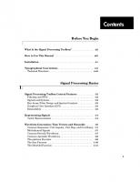
To show how the inertia ‘seen’ by the waist joint varies as a function of joint angles 2 and 3 the following code could be used.
>> >> >> >>
[q2,q3] = meshgrid(-pi:0.2:pi, -pi:0.2:pi); q = [zeros(length(q2(:)),1) q2(:) q3(:) zeros(length(q2(:)),3)]; I = inertia(p560, q); surfl(q2, q3, squeeze(I(1,1,:)));
5.5 5 4.5
I11
4 3.5 3 2.5 2 4 4
2 2
0 0
−2 q3
See Also
−2 −4
−4
q2
robot, rne, itorque, coriolis, gravload
Robotics Toolbox Release 6
Peter Corke, April 2001
inertia
References
22
M. W. Walker and D. E. Orin. Efficient dynamic computer simulation of robotic mechanisms. ASME Journal of Dynamic Systems, Measurement and Control, 104:205–211, 1982.
Robotics Toolbox Release 6
Peter Corke, April 2001
ishomog
23
ishomog Purpose
Test if argument is a homogeneous transformation
Synopsis
ishomog(x)
Description
Returns true if x is a 4
4 matrix.
Robotics Toolbox Release 6
Peter Corke, April 2001
itorque
24
itorque Purpose
Compute the manipulator inertia torque component
Synopsis
tau i = itorque(robot, q, qdd)
Description
itorque returns the joint torque due to inertia at the specified pose q and acceleration qdd which is given by τi M q q¨ If q and qdd are row vectors, itorque is a row vector of joint torques. If q and qdd are matrices, each row is interpreted as a joint state vector, and itorque is a matrix in which each row is the inertia torque for the corresponding rows of q and qdd. robot is a robot object that describes the kinematics and dynamics of the manipulator and drive. If robot contains motor inertia parameters then motor inertia, referred to the link reference frame, will be added to the diagonal of M and influence the inertia torque result.
See Also
robot, rne, coriolis, inertia, gravload
Robotics Toolbox Release 6
Peter Corke, April 2001
jacob0
25
jacob0 Purpose
Compute manipulator Jacobian in base coordinates
Synopsis
jacob0(robot, q)
Description
jacob0 returns a Jacobian matrix for the robot object robot in the pose q and as expressed in the base coordinate frame. The manipulator Jacobian matrix, 0 Jq , maps differential velocities in joint space, q, ˙ to Cartesian velocity of the end-effector expressed in the base coordinate frame. 0
For an n-axis manipulator the Jacobian is a 6
x˙
0
Jq q q˙
n matrix.
Cautionary
This function will not work for robot objects that use the modified Denavit-Hartenberg conventions.
See Also
jacobn, diff2tr, tr2diff, robot
References
R. P. Paul. Robot Manipulators: Mathematics, Programming, and Control. MIT Press, Cambridge, Massachusetts, 1981.
Robotics Toolbox Release 6
Peter Corke, April 2001
jacobn
26
jacobn Purpose
Compute manipulator Jacobian in end-effector coordinates
Synopsis
jacobn(robot, q)
Description
jacobn returns a Jacobian matrix for the robot object robot in the pose q and as expressed in the end-effector coordinate frame. The manipulator Jacobian matrix, 0 Jq , maps differential velocities in joint space, q, ˙ to Cartesian velocity of the end-effector expressed in the end-effector coordinate frame. n
n
x˙
Jq q q˙
The relationship between tool-tip forces and joint torques is given by τ For an n-axis manipulator the Jacobian is a 6
n
Jq q
n
F
n matrix.
Cautionary
This function will not work for robot objects that use the modified Denavit-Hartenberg conventions.
See Also
jacob0, diff2tr, tr2diff, robot
References
R. P. Paul. Robot Manipulators: Mathematics, Programming, and Control. MIT Press, Cambridge, Massachusetts, 1981.
Robotics Toolbox Release 6
Peter Corke, April 2001
jtraj
27
jtraj Purpose
Compute a joint space trajectory between two joint coordinate poses
Synopsis
[q [q [q [q
Description
jtraj returns a joint space trajectory q from joint coordinates q0 to q1. The number of points is n or the length of the given time vector t. A 7th order polynomial is used with default zero boundary conditions for velocity and acceleration.
qd qd qd qd
qdd] qdd] qdd] qdd]
= = = =
jtraj(q0, jtraj(q0, jtraj(q0, jtraj(q0,
q1, q1, q1, q1,
n) n, qd0, qd1) t) t, qd0, qd1)
Non-zero boundary velocities can be optionally specified as qd0 and qd1. The trajectory is a matrix, with one row per time step, and one column per joint. The function can optionally return a velocity and acceleration trajectories as qd and qdd respectively.
Robotics Toolbox Release 6
Peter Corke, April 2001
link
28
link Purpose
Link object
Synopsis
L = link L = link([alpha, a, theta, d]) L = link([alpha, a, theta, d, sigma]) L = link(dyn row) A = link(q) show(L)
Description
The link function constructs a link object. The object contains kinematic and dynamic parameters as well as actuator and transmission parameters. The first form returns a default object, while the second and third forms initialize the kinematic model based on Denavit and Hartenberg parameters. By default the standard Denavit and Hartenberg conventions are assumed but a flag (mdh) can be set if modified Denavit and Hartenberg conventions are required. The dynamic model can be initialized using the fourth form of the constructor where dyn row is a 1 20 matrix which is one row of the legacy dyn matrix. The second last form given above is not a constructor but a link method that returns the link transformation matrix for the given joint coordinate. The argument is given to the link object using parenthesis. The single argument is taken as the link variable q and substituted for θ or D for a revolute or prismatic link respectively. The Denavit and Hartenberg parameters describe the spatial relationship between this link and the previous one. The meaning of the fields for each model are summarized in the following table. alpha A theta D sigma
αi Ai θi Di σi
αi 1 Ai 1 θi Di σi
link twist angle link length link rotation angle link offset distance joint type; 0 for revolute, non-zero for prismatic
Since Matlab does not support the concept of public class variables methods have been written to allow link object parameters to be referenced (r) or assigned (a) as given by the following table
Robotics Toolbox Release 6
Peter Corke, April 2001
link
29
Method link.alpha link.A link.theta link.D link.sigma link.RP link.mdh
Operations r+a r+a r+a r+a r+a r r+a
Returns link twist angle link length link rotation angle link offset distance joint type; 0 for revolute, non-zero for prismatic joint type; ’R’ or ’P’ DH convention: 0 if standard, 1 if modified
link.I link.I
r a
link.m link.r
r+a r+a
3 3 symmetric inertia matrix assigned from a 3 3 matrix or a 6-element vector interpretted as Ixx Iyy Izz Ixy Iyz Ixz link mass 3 1 link COG vector
link.G link.Jm link.B link.Tc link.Tc
r+a r+a r+a r a
gear ratio motor inertia viscous friction Coulomb friction, 1 2 vector where τ τ Coulomb friction; for symmetric friction this is a scalar, for asymmetric friction it is a 2-element vector for positive and negative velocity
link.dh link.dyn link.qlim link.offset
r+a r+a r+a r+a
row of legacy DH matrix row of legacy DYN matrix joint coordinate limits, 2-vector joint coordinate offset (see discussion for robot object).
The default is for standard Denavit-Hartenberg conventions, zero friction, mass and inertias. The display method gives a one-line summary of the link’s kinematic parameters. The show method displays as many link parameters as have been initialized for that link.
Examples >> L = link([-pi/2, 0.02, 0, 0.15]) L = -1.570796 0.020000 0.000000 >> L.RP ans = R >> L.mdh ans = 0 >> L.G = 100; >> L.Tc = 5; >> L L = -1.570796 0.020000 0.000000
Robotics Toolbox Release 6
0.150000
R
0.150000
R
Peter Corke, April 2001
link
30
>> show(L) alpha = -1.5708 A = 0.02 theta = 0 D = 0.15 sigma = 0 mdh = 0 = 100 G Tc = 5 -5 >>
Algorithm
For the standard Denavit-Hartenberg conventions the homogeneous transform
i 1
Ai
cos θi sin θi 0 0
sin θi cosαi cos θi cosαi sin αi 0
sin θi sin αi cos θi sin αi cos αi 0
ai cos θi ai sin θi di 1
represents each link’s coordinate frame with respect to the previous link’s coordinate system. For a revolute joint θi is offset by For the modified Denavit-Hartenberg conventions it is instead
i 1
Ai
cos θi sin θi cos αi sin θi sin αi 0
1 1
sin θi cos θi cos αi cosθi sin αi 0
1 1
0 sin αi 1 cos αi 1 0
ai 1 di sin αi di cos αi 1
1 1
See Also
robot
References
R. P. Paul. Robot Manipulators: Mathematics, Programming, and Control. MIT Press, Cambridge, Massachusetts, 1981.
Robotics Toolbox Release 6
Peter Corke, April 2001
maniplty
31
maniplty Purpose
Manipulability measure
Synopsis
m = maniplty(robot, q) m = maniplty(robot, q, which)
Description
maniplty computes the scalar manipulability index for the manipulator at the given pose. Manipulability varies from 0 (bad) to 1 (good). robot is a robot object that contains kinematic and optionally dynamic parameters for the manipulator. Two measures are supported and are selected by the optional argument which can be either ’yoshikawa’ (default) or ’asada’. Yoshikawa’s manipulability measure is based purely on kinematic data, and gives an indication of how ‘far’ the manipulator is from singularities and thus able to move and exert forces uniformly in all directions. Asada’s manipulability measure utilizes manipulator dynamic data, and indicates how close the inertia ellipsoid is to spherical. If q is a vector maniplty returns a scalar manipulability index. If q is a matrix maniplty returns a column vector and each row is the manipulability index for the pose specified by the corresponding row of q.
Algorithm
Yoshikawa’s measure is based on the condition number of the manipulator Jacobian ηyoshi
JqJq
Asada’s measure is computed from the Cartesian inertia matrix Mx
Jq
T
MqJq
1
The Cartesian manipulator inertia ellipsoid is xM x x
1
and gives an indication of how well the manipulator can accelerate in each of the Cartesian directions. The scalar measure computed here is the ratio of the smallest/largest ellipsoid axes ηasada
min x max x
Ideally the ellipsoid would be spherical, giving a ratio of 1, but in practice will be less than 1.
See Also
jacob0, inertia,robot
References
T. Yoshikawa, “Analysis and control of robot manipulators with redundancy,” in Proc. 1st Int. Symp. Robotics Research, (Bretton Woods, NH), pp. 735–747, 1983.
Robotics Toolbox Release 6
Peter Corke, April 2001
nofriction
32
nofriction Purpose
Remove friction from robot object
Synopsis
robot2 = nofriction(robot)
Description
Return a new robot object that has no joint friction. The viscous and Coulomb friction values in the constituent links are set to zero. This is important for forward dynamics computation (fdyn()) where the presence of friction can prevent the numerical integration from converging.
See Also
link,friction,fdyn
Robotics Toolbox Release 6
Peter Corke, April 2001
oa2tr
33
oa2tr Purpose
Convert OA vectors to homogeneous transform
Synopsis
oa2tr(o, a)
Description
oa2tr returns a rotational homogeneous transformation specified in terms of the Cartesian orientation and approach vectors o and a respectively.
Algorithm T
oˆ
aˆ 0
oˆ 0
aˆ 0
0 1
where oˆ and aˆ are unit vectors corresponding to o and a respectively.
See Also
rpy2tr, eul2tr
Robotics Toolbox Release 6
Peter Corke, April 2001
puma560
34
puma560 Purpose
Create a Puma 560 robot object
Synopsis
puma560
Description
Creates the robot object p560 which describes the kinematic and dynamic characteristics of a Unimation Puma 560 manipulator. The kinematic conventions used are as per Paul and Zhang, and all quantities are in standard SI units. Also defines the joint coordinate vectors qz, qr and qstretch corresponding to the zero-angle, ready and fully extended poses respectively.
Details of coordinate frames used for the Puma 560 shown here in its zero angle pose.
See Also
robot, puma560akb, stanford
References
R. P. Paul and H. Zhang, “Computationally efficient kinematics for manipulators with spherical wrists,” Int. J. Robot. Res., vol. 5, no. 2, pp. 32–44, 1986. P. Corke and B. Armstrong-H´elouvry, “A search for consensus among model parameters reported for the PUMA 560 robot,” in Proc. IEEE Int. Conf. Robotics and Automation, (San Diego), pp. 1608– 1613, May 1994. P. Corke and B. Armstrong-H´elouvry, “A meta-study of PUMA 560 dynamics: A critical appraisal of literature data,” Robotica, vol. 13, no. 3, pp. 253–258, 1995.
Robotics Toolbox Release 6
Peter Corke, April 2001
puma560akb
35
puma560akb Purpose
Create a Puma 560 robot object
Synopsis
puma560akb
Description
Creates the robot object which describes the kinematic and dynamic characteristics of a Unimation Puma 560 manipulator. Craig’s modified Denavit-Hartenberg notation is used, with the particular kinematic conventions from Armstrong, Khatib and Burdick. All quantities are in standard SI units. Also defines the joint coordinate vectors qz, qr and qstretch corresponding to the zero-angle, ready and fully extended poses respectively.
See Also
robot, puma560, stanford
References
B. Armstrong, O. Khatib, and J. Burdick, “The explicit dynamic model and inertial parameters of the Puma 560 arm,” in Proc. IEEE Int. Conf. Robotics and Automation, vol. 1, (Washington, USA), pp. 510–18, 1986.
Robotics Toolbox Release 6
Peter Corke, April 2001
qinterp
36
qinterp Purpose
Interpolate unit-quaternions
Synopsis
QI = qinterp(Q1, Q2, r)
Description
Return a unit-quaternion that interpolates between Q1 and Q2 as r varies between 0 and 1 inclusively. This is a spherical linear interpolation (slerp) that can be interpreted as interpolation along a great circle arc on a sphere. If r is a vector, then a cell array of quaternions is returned corresponding to successive values of r.
Examples
A simple example
>> q1 = quaternion(rotx(0.3)) q1 = 0.98877 >> q2 = quaternion(roty(-0.5)) q2 = 0.96891 >> qinterp(q1, q2, 0) ans = 0.98877 >> qinterp(q1, q2, 1) ans = 0.96891 >> qinterp(q1, q2, 0.3) ans = 0.99159 >>
References
K. Shoemake, “Animating rotation with quaternion curves.,” in Proceedings of ACM SIGGRAPH, (San Francisco), pp. 245–254, The Singer Company, Link Flight Simulator Division, 1985.
Robotics Toolbox Release 6
Peter Corke, April 2001
quaternion
37
quaternion Purpose
Quaternion object
Synopsis
q q q q
Description
quaternion is the constructor for a quaternion object. The first form returns a new object with the same value as its argument. The second form initializes the quaternion to a rotation of theta about the vector v.
= = = =
quaternion(qq) quaternion(theta, v) quaternion([s vx vy vz]) quaternion(R)
The third form sets the four quaternion elements directly where s is the scalar component and [vx vy vz] the vector. The final method sets the quaternion to a rotation equivalent to the given 3 3 rotation matrix, or the rotation submatrix of a 4 4 homogeneous transform. Some operators are overloaded for the quaternion class q1 * q2 q * v q1 / q2 q j
double(q) inv(q) norm(q) plot(q) unit(q)
returns quaternion product or compounding returns a quaternion vector product, that is the vector v is rotated by the quaternion. v is a 3 3 vector returns q1 q2 1 returns q j where j is an integer exponent. For j 0 the result is obtained by repeated multiplication. For j 0 the final result is inverted. returns the quaternion coeffients as a 4-element row vector returns the quaterion inverse returns the quaterion magnitude displays a 3D plot showing the standard coordinate frame after rotation by q. returns the corresponding unit quaterion
Some public class variables methods are also available for reference only. method quaternion.d quaternion.s quaternion.v quaternion.t quaternion.r
Returns return 4-vector of quaternion elements return scalar component return vector component return equivalent homogeneous transformation matrix return equivalent orthonormal rotation matrix
Examples
Robotics Toolbox Release 6
Peter Corke, April 2001
quaternion
38
>> t = rotx(0.2) t = 1.0000 0 0 0 0.9801 -0.1987 0 0.1987 0.9801 0 0 0 >> q1 = quaternion(t) q1 = 0.995 >> q1.r ans = 1.0000 0 0
0 0.9801 0.1987
0 0 0 1.0000
0 -0.1987 0.9801
>> q2 = quaternion( roty(0.3) ) q2 = 0.98877 >> q1 * q2 ans = 0.98383 >> q1*q1 ans = 0.98007 >> q1ˆ2 ans = 0.98007 >> q1*inv(q1) ans = 1 >> q1/q1 ans = 1 >> q1/q2 ans = 0.98383 >> q1*q2ˆ-1 ans = 0.98383
Robotics Toolbox Release 6
Peter Corke, April 2001
quaternion
39
Cautionary
At the moment vectors or arrays of quaternions are not supported. You can however use cell arrays to hold a number of quaternions.
See Also
quaternion/plot
References
K. Shoemake, “Animating rotation with quaternion curves.,” in Proceedings of ACM SIGGRAPH, (San Francisco), pp. 245–254, The Singer Company, Link Flight Simulator Division, 1985.
Robotics Toolbox Release 6
Peter Corke, April 2001
quaternion/plot
40
quaternion/plot Purpose
Plot quaternion rotation
Synopsis
plot(Q)
Description
plot is overloaded for quaternion objects and displays a 3D plot which shows how the standard axes are transformed under that rotation.
Examples
A rotation of 0.3rad about the X axis. Clearly the X axis is invariant under this rotation.
>> q=quaternion(rotx(0.3)) q = 0.85303 >> plot(q)
1 Y 0.5
Z
Z
X 0
−0.5
−1 1 1
0.5 0.5
0 0 −0.5 Y
See Also
−0.5 −1
−1
X
quaternion
Robotics Toolbox Release 6
Peter Corke, April 2001
rne
41
rne Purpose
Compute inverse dynamics via recursive Newton-Euler formulation
Synopsis
tau = rne(robot, q, qd, qdd) tau = rne(robot, [q qd qdd]) tau = rne(robot, q, qd, qdd, grav) tau = rne(robot, [q qd qdd], grav) tau = rne(robot, q, qd, qdd, grav, fext) tau = rne(robot, [q qd qdd], grav, fext)
Description
rne computes the equations of motion in an efficient manner, giving joint torque as a function of joint position, velocity and acceleration. If q, qd and qdd are row vectors then tau is a row vector of joint torques. If q, qd and qdd are matrices then tau is a matrix in which each row is the joint torque for the corresponding rows of q, qd and qdd. Gravity direction is defined by the robot object but may be overridden by providing a gravity acceleration vector grav = [gx gy gz]. An external force/moment acting on the end of the manipulator may also be specified by a 6-element vector fext = [Fx Fy Fz Mx My Mz] in the end-effector coordinate frame. The torque computed may contain contributions due to armature inertia and joint friction if these are specified in the parameter matrix dyn. The MEX file version of this function is around 300 times faster than the M file.
Algorithm
Coumputes the joint torque τ
M q q¨
C q q˙ q˙
F q˙
Gq
where M is the manipulator inertia matrix, C is the Coriolis and centripetal torque, F the viscous and Coulomb friction, and G the gravity load.
Cautionary
This function will not work for robot objects that use the modified Denavit-Hartenberg conventions.
See Also
robot, fdyn, accel, gravload, inertia, friction
Limitations
A MEX file is currently only available for Sparc architecture.
Robotics Toolbox Release 6
Peter Corke, April 2001
rne
References
42
J. Y. S. Luh, M. W. Walker, and R. P. C. Paul. On-line computational scheme for mechanical manipulators. ASME Journal of Dynamic Systems, Measurement and Control, 102:69–76, 1980.
Robotics Toolbox Release 6
Peter Corke, April 2001
robot
43
robot Purpose
Robot object
Synopsis
r r r r r
Description
robot is the constructor for a robot object. The first form creates a default robot, and the second form returns a new robot object with the same value as its argument. The third form creates a robot from a cell array of link objects which define the robot’s kinematics and optionally dynamics. The fourth and fifth forms create a robot object from legacy DH and DYN format matrices.
= = = = =
robot robot(rr) robot(link ...) robot(DH ...) robot(DYN ...)
The last three forms all accept optional trailing string arguments which are taken in order as being robot name, manufacturer and comment. Since Matlab does not support the concept of public class variables methods have been written to allow robot object parameters to be referenced (r) or assigned (a) as given by the following table method robot.n robot.link robot.name robot.manuf robot.comment robot.gravity robot.mdh
Operation r r+a r+a r+a r+a r r
Returns number of joints cell array of link objects robot name string robot manufacturer string general comment string 3-element vector defining gravity direction DH convention: 0 if standard, 1 if modified. Determined from the link objects.
robot.base robot.tool robot.dh robot.dyn robot.q robot.qlim robot.islimit
r+a r+a r r r+a r+a r
robot.offset robot.plotopt robot.lineopt robot.shadowopt
r+a r+a r+a r+a
homogeneous transform defining base of robot homogeneous transform defining tool of robot legacy DH matrix legacy DYN matrix joint coordinates joint coordinate limits, n 2 matrix joint limit vector, for each joint set to -1, 0 or 1 depending if below low limit, OK, or greater than upper limit joint coordinate offsets options for plot() line style for robot graphical links line style for robot shadow links
Some of these operations at the robot level are actually wrappers around similarly named link object functions: offset, qlim, islimit.
Robotics Toolbox Release 6
Peter Corke, April 2001
robot
44
The offset vector is added to the user specified joint angles before any kinematic or dynamic function is invoked (it is actually implemented within the link object). Similarly it is subtracted after an operation such as inverse kinematics. The need for a joint offset vector arises because of the constraints of the Denavit-Hartenberg (or modified Denavit-Hartenberg) notation. The pose of the robot with zero joint angles is frequently some rather unusual (or even unachievable) pose. The joint coordinate offset provides a means to make an arbitrary pose correspond to the zero joint angle case. Default values for robot parameters are: robot.name robot.manuf robot.comment robot.gravity robot.offset robot.base robot.tool robot.lineopt robot.shadowopt
’noname’ ” ” 0 0 9 81 m s2 ones(n,1) eye(4,4) eye(4,4) ’Color’, ’black’, ’Linewidth’, 4 ’Color’, ’black’, ’Linewidth’, 1
The multiplication operator, *, is overloaded and the product of two robot objects is a robot which is the series connection of the multiplicands. Tool transforms of all but the last robot are ignored, base transform of all but the first robot are ignored. The plot() function is also overloaded and is used to provide a robot animation.
Examples >> L{1} = link([ pi/2 L = [1x1 link]
0
0
0])
>> L{2} = link([ 0 0 0.5 0]) L = [1x1 link] [1x1 link] >> r = robot(L) r = (2 axis, RR) grav = [0.00 0.00 9.81] standard D&H parameters alpha 1.570796 0.000000
A 0.000000 0.000000
theta 0.000000 0.500000
D 0.000000 0.000000
R/P R R
>>
Robotics Toolbox Release 6
Peter Corke, April 2001
robot
See Also
45
link,plot
Robotics Toolbox Release 6
Peter Corke, April 2001
robot/plot
46
robot/plot Purpose
Graphical robot animation
Synopsis
plot(robot, q) plot(robot, q, arguments...)
0.6 y
0.4
z x
0.2 0 −0.2
Puma 560
−0.4 −0.6 −0.8 −1 1 0.8 0.6 0.4
Description
plot is overloaded for robot objects and displays a graphical representation of the robot given the kinematic information in robot. The robot is represented by a simple stick figure polyline where line segments join the origins of the link coordinate frames. If q is a matrix representing a joint-space trajectory then an animation of the robot motion is shown.
GRAPHICAL ANNOTATIONS The basic stick figure robot can be annotated with shadow on the ‘floor’ XYZ wrist axes and labels, shown by 3 short orthogonal line segments which are colored: red (X or normal), green (Y or orientation) and blue (Z or approach). They can be optionally labelled XYZ or NOA. joints, these are 3D cylinders for revolute joints and boxes for prismatic joints the robot’s name All of these require some kind of dimension and this is determined using a simple heuristic from
Robotics Toolbox Release 6
Peter Corke, April 2001
robot/plot
47
the workspace dimensions. This dimension can be changed by setting the multiplicative scale factor using the mag option below. These various annotations do slow the rate at which animations will be rendered.
OPTIONS Options are specified by a variable length argument list comprising strings and numeric values. The allowed values are:
workspace w perspective ortho base, nobase wrist, nowrist name, noname shadow, noshadow joints, nojoints xyz noa mag scale erase, noerase loop, noloop
set the 3D plot bounds or workspace to the matrix [xmin xmax ymin ymax zmin zmax] show a perspective view show an orthogonal view control display of base, a line from the floor upto joint 0 control display of wrist axes control display of robot name near joint 0 control display of a ’shadow’ on the floor control display of joints, these are cylinders for revolute joints and boxes for prismatic joints wrist axis labels are X, Y, Z wrist axis labels are N, O, A annotation scale factor control erasure of robot after each change control whether animation is repeated endlessly
The options come from 3 sources and are processed in the order: 1. Cell array of options returned by the function PLOTBOTOPT if found on the user’s current path. 2. Cell array of options returned by the .plotopt method of the robot object. These are set by the .plotopt method. 3. List of arguments in the command line.
GETTING GRAPHICAL ROBOT STATE Each graphical robot has a unique tag set equal to the robot’s name. When plot is called it looks for all graphical objects with that name and moves them. The graphical robot holds a copy of the robot object as UserData. That copy contains the graphical handles of all the graphical sub-elements of the robot and also the current joint angle state. This state is used, and adjusted, by the drivebot function. The current joint angle state can be obtained by q = plot(robot). If multiple instances exist, that of the first one returned by findobj() is given.
Examples
To animate two Pumas moving in the same figure window.
>> >> >> >>
clf p560b = p560; p560b.name = ’Another Puma 560’; p560b.base = transl([-.05 0.5 0]);
Robotics Toolbox Release 6
% duplicate the robot % give it a unique name % move its base
Peter Corke, April 2001
robot/plot
>> >> >> >> >> >> >> >> >>
48
plot(p560, qr); % display it at ready position hold on plot(p560b, qr); % display it at ready position t = [0:0.056:10]; jt = jtraj(qr, qstretch, t); % trajectory to stretch pose for q = jt’, % for all points on the path plot(p560, q); plot(p560b, q); end
To show multiple views of the same robot. >> >> >> >> >> >>
clf figure plot(p560, qz); figure plot(p560, qz); plot(p560, qr);
% % % % %
create a new figure add a graphical robot create another figure add a graphical robot both robots should move
Now the two figures can be adjusted to give different viewpoints, for instance, plan and elevation.
Cautionary
plot() options are only processed on the first call when the graphical object is established, they are skipped on subsequent calls. Thus if you wish to change options, clear the figure before replotting.
See Also
drivebot, fkine, robot
Robotics Toolbox Release 6
Peter Corke, April 2001
rotvec
49
rotvec Purpose
Rotation about a vector
Synopsis
T = rotvec(v, theta)
Description
rotvec returns a homogeneous transformation representing a rotation of theta radians about the vector v.
See Also
rotx, roty, rotz
Robotics Toolbox Release 6
Peter Corke, April 2001
rotx,roty,rotz
50
rotx,roty,rotz Purpose
Rotation about X, Y or Z axis
Synopsis
T = rotx(theta) T = roty(theta) T = rotz(theta)
Description
Return a homogeneous transformation representing a rotation of theta radians about the X, Y or Z axes.
See Also
rotvec
Robotics Toolbox Release 6
Peter Corke, April 2001
rpy2tr
51
rpy2tr Purpose
Roll/pitch/yaw angles to homogeneous transform
Synopsis
T = rpy2tr([r p y]) T = rpy2tr(r,p,y)
Description
rpy2tr returns a homogeneous transformation for the specified roll/pitch/yaw angles in radians. These correspond to rotations about the Z, X, Y axes respectively.
See Also
tr2rpy, eul2tr
References
R. P. Paul, Robot Manipulators: Mathematics, Programming, and Control. sachusetts: MIT Press, 1981.
Robotics Toolbox Release 6
Cambridge, Mas-
Peter Corke, April 2001
rtdemo
52
rtdemo Purpose
Robot Toolbox demonstration
Synopsis
rtdemo
Description
This script provides demonstrations for most functions within the Robotics Toolbox.
Robotics Toolbox Release 6
Peter Corke, April 2001
stanford
53
stanford Purpose
Create a Stanford manipulator robot object
Synopsis
stanford
2
Z
1
0 y z
Stanford arm
x
−1
−2 2 1
2 1
0 0
−1 Y
−1 −2
−2
X
Description
Creates the robot object stan which describes the kinematic and dynamic characteristics of a Stanford manipulator. Specifies armature inertia and gear ratios. All quantities are in standard SI units.
See Also
robot, puma560
References
R. Paul, “Modeling, trajectory calculation and servoing of a computer controlled arm,” Tech. Rep. AIM-177, Stanford University, Artificial Intelligence Laboratory, 1972. R. P. Paul, Robot Manipulators: Mathematics, Programming, and Control. sachusetts: MIT Press, 1981.
Robotics Toolbox Release 6
Cambridge, Mas-
Peter Corke, April 2001
tr2diff
54
tr2diff Purpose
Convert a homogeneous transform to a differential motion vector
Synopsis
d = tr2diff(T) d = tr2diff(T1, T2)
Description
The first form of tr2diff returns a 6-element differential motion vector representing the incremental translation and rotation described by the homogeneous transform T. It is assumed that T is of the form 0 δz δy 0
δz 0 δx 0
δy δx 0 0
dx dy dz 0
The translational elements of d are assigned directly. The rotational elements are computed from the mean of the two values that appear in the skew-symmetric matrix. The second form of tr2diff returns a 6-element differential motion vector representing the displacement from T1 to T2, that is, T2 - T1. d
1 2 n1
n2
p2 p1 o1 o2
a1
a2
See Also
diff2tr, diff
References
R. P. Paul, Robot Manipulators: Mathematics, Programming, and Control. sachusetts: MIT Press, 1981.
Robotics Toolbox Release 6
Cambridge, Mas-
Peter Corke, April 2001
tr2eul
55
tr2eul Purpose
Convert a homogeneous transform to Euler angles
Synopsis
[a b c] = tr2eul(T)
Description
tr2eul returns a vector of Euler angles, in radians, corresponding to the rotational part of the homogeneous transform T.
See Also
eul2tr, tr2rpy
References
R. P. Paul, Robot Manipulators: Mathematics, Programming, and Control. sachusetts: MIT Press, 1981.
Robotics Toolbox Release 6
Cambridge, Mas-
Peter Corke, April 2001
tr2jac
56
tr2jac Purpose
Compute a Jacobian to map differential motion between frames
Synopsis
jac = tr2jac(T)
Description
tr2jac returns a 6 6 Jacobian matrix to map differential motions or velocities between frames related by the homogeneous transform T. If T represents a homogeneous transformation from frame A to frame B, A TB , then B
x˙
B
JA A x˙
where B JA is given by tr2jac(T).
See Also
tr2diff, diff2tr, diff
References
R. P. Paul, Robot Manipulators: Mathematics, Programming, and Control. sachusetts: MIT Press, 1981.
Robotics Toolbox Release 6
Cambridge, Mas-
Peter Corke, April 2001
tr2rpy
57
tr2rpy Purpose
Convert a homogeneous transform to roll/pitch/yaw angles
Synopsis
[a b c] = tr2rpy(T)
Description
tr2rpy returns a vector of roll/pitch/yaw angles, in radians, corresponding to the rotational part of the homogeneous transform T.
See Also
rpy2tr, tr2eul
References
R. P. Paul, Robot Manipulators: Mathematics, Programming, and Control. sachusetts: MIT Press, 1981.
Robotics Toolbox Release 6
Cambridge, Mas-
Peter Corke, April 2001
transl
58
transl Purpose
Translational transformation
Synopsis
T = T = v = xyz
Description
The first two forms return a homogeneous transformation representing a translation expressed as three scalar x, y and z, or a Cartesian vector v.
transl(x, y, z) transl(v) transl(T) = transl(TC)
The third form returns the translational part of a homogeneous transform as a 3-element column vector. The fourth form returns a matrix whose columns are the X, Y and Z columns of the 4 4 m Cartesian trajectory matrix TC.
See Also
ctraj, rotx, roty, rotz, rotvec
Robotics Toolbox Release 6
Peter Corke, April 2001
trinterp
59
trinterp Purpose
Interpolate homogeneous transforms
Synopsis
T = trinterp(T0, T1, r)
Description
trinterp interpolates between the two homogeneous transforms T0 and T1 as r varies between 0 and 1 inclusively. This is generally used for computing straight line or ‘Cartesian’ motion. Rotational interpolation is achieved using quaternion spherical linear interpolation.
Examples
Interpolation of homogeneous transformations.
>> t1=rotx(.2) t1 = 1.0000 0 0 0
0 0.9801 0.1987 0
0 -0.1987 0.9801 0
0 0 0 1.0000
>> t2=transl(1,4,5)*roty(0.3) t2 = 0.9553 0 -0.2955 0
0 1.0000 0 0
0.2955 0 0.9553 0
1.0000 4.0000 5.0000 1.0000
>> trinterp(t1,t2,0) % should be t1 ans = 1.0000 0 0 0
0 0.9801 0.1987 0
>> trinterp(t1,t2,1) ans = 0.9553 0 -0.2955 0
0 1.0000 0 0
0 -0.1987 0.9801 0
0 0 0 1.0000
% should be t2
0.2955 0 0.9553 0
Robotics Toolbox Release 6
1.0000 4.0000 5.0000 1.0000
Peter Corke, April 2001
trinterp
60
>> trinterp(t1,t2,0.5) % ’half way’ in between ans = 0.9887 0.0075 -0.1494 0
0.0075 0.9950 0.0998 0
0.1494 -0.0998 0.9837 0
0.5000 2.0000 2.5000 1.0000
>>
See Also
ctraj, qinterp
References
R. P. Paul, Robot Manipulators: Mathematics, Programming, and Control. sachusetts: MIT Press, 1981.
Robotics Toolbox Release 6
Cambridge, Mas-
Peter Corke, April 2001
trnorm
61
trnorm Purpose
Normalize a homogeneous transformation
Synopsis
TN = trnorm(T)
Description
Returns a normalized copy of the homogeneous transformation T. Finite word length arithmetic can lead to homogeneous transformations in which the rotational submatrix is not orthogonal, that is, det R 1.
Algorithm
Normalization is performed by orthogonalizing the rotation submatrix n
See Also
diff2tr, diff
References
J. Funda, “Quaternions and homogeneous transforms in robotics,” Master’s thesis, University of Pennsylvania, Apr. 1988.
Robotics Toolbox Release 6
o
a.
Peter Corke, April 2001
twolink
62
twolink Purpose
Load kinematic and dynamic data for a simple 2-link mechanism
Synopsis
twolink
2
1
Z
yz x 0 Simple two link −1
−2 2 1
2 1
0 0
−1 Y
Description
−1 −2
−2
X
Creates the robot object twolink which describes the kinematic and dynamic characteristics of a simple two-link planar manipulator. The manipulator operates in the vertical plane and for zero joint angles lies horizontally. Mass is assumed to be concentrated at the joints. All masses and lengths are unity.
See Also
dh, dyn, puma560, stanford
References
Fig 3-6 of “Robot Dynamics and Control” by M.W. Spong and M. Vidyasagar, 1989.
Robotics Toolbox Release 6
Peter Corke, April 2001
unit
63
unit Purpose
Unitize a vector
Synopsis
vn = unit(v)
Description
unit returns a unit vector aligned with v.
Algorithm vn
Robotics Toolbox Release 6
v v
Peter Corke, April 2001
dh (legacy)
64
dh (legacy) Purpose
Matrix representation of manipulator kinematics
Description
A dh matrix describes the kinematics of a manipulator in a general way using the standard DenavitHartenberg conventions. Each row represents one link of the manipulator and the columns are assigned according to the following table. Column 1 2 3 4 5
Symbol αi Ai θi Di σi
Description link twist angle link length link rotation angle link offset distance joint type; 0 for revolute, non-zero for prismatic
If the last column is not given, toolbox functions assume that the manipulator is all-revolute. For an n-axis manipulator dh is an n 4 or n 5 matrix. The first 5 columns of a dyn matrix contain the kinematic parameters and maybe used anywhere that a dh kinematic matrix is required — the dynamic data is ignored.
Lengths Ai and Di may be expressed in any unit, and this choice will flow on to the units in which homogeneous transforms and Jacobians are represented. All angles are in radians.
See Also
dyn,puma560,stanford,mdh
References
R. P. Paul, Robot Manipulators: Mathematics, Programming, and Control. sachusetts: MIT Press, 1981.
Robotics Toolbox Release 6
Cambridge, Mas-
Peter Corke, April 2001
dyn (legacy)
65
dyn (legacy) Purpose
Matrix representation of manipulator kinematics and dynamics
Description
A dyn matrix describes the kinematics and dynamics of a manipulator in a general way using the standard Denavit-Hartenberg conventions. Each row represents one link of the manipulator and the columns are assigned according to the following table. Column 1 2 3 4 5 6 7 8 9 10 11 12 13 14 15 16 17 18 19 20
Symbol α A θ D σ mass rx ry rz Ixx Iyy Izz Ixy Iyz Ixz Jm G B Tc+ Tc-
Description link twist angle link length link rotation angle link offset distance joint type; 0 for revolute, non-zero for prismatic mass of the link link COG with respect to the link coordinate frame
elements of link inertia tensor about the link COG
armature inertia reduction gear ratio; joint speed/link speed viscous friction, motor referred coulomb friction (positive rotation), motor referred coulomb friction (negative rotation), motor referred
For an n-axis manipulator, dyn is an n 20 matrix. The first 5 columns of a dyn matrix contain the kinematic parameters and maybe used anywhere that a dh kinematic matrix is required — the dynamic data is ignored.
All angles are in radians. The choice of all other units is up to the user, and this choice will flow on to the units in which homogeneous transforms, Jacobians, inertias and torques are represented.
See Also
dh
Robotics Toolbox Release 6
Peter Corke, April 2001