Automating manufacturing systems with PLCs [Version 4.7 ed.] 9780557344253, 0557344255
An in depth examination of manufacturing control systems using structured design methods. Topics include ladder logic an
157 34 4MB
English Pages 846 Year 2005
4. LOGICAL SENSORS 4.1......Page 3
7. KARNAUGH MAPS 7.1......Page 4
10. STRUCTURED LOGIC DESIGN 10.1......Page 5
14. PLC MEMORY 14.1......Page 6
16. ADVANCED LADDER LOGIC FUNCTIONS 16.1......Page 7
20. SEQUENTIAL FUNCTION CHARTS 20.1......Page 8
23. CONTINUOUS SENSORS 23.1......Page 9
25. CONTINUOUS CONTROL 25.1......Page 10
28. NETWORKING 28.1......Page 11
30. HUMAN MACHINE INTERFACES (HMI) 30.1......Page 12
33. SELECTING A PLC 33.1......Page 13
35. COMBINED GLOSSARY OF TERMS 35.1......Page 14
37. GNU Free Documentation License 37.1......Page 15
1.1 TODO LIST......Page 19
2.1.1 Ladder Logic......Page 20
2.1.2 Programming......Page 25
2.1.3 PLC Connections......Page 29
2.1.4 Ladder Logic Inputs......Page 30
2.1.5 Ladder Logic Outputs......Page 31
2.2 A CASE STUDY......Page 32
2.3 SUMMARY......Page 33
2.5 PRACTICE PROBLEM SOLUTIONS......Page 34
2.6 ASSIGNMENT PROBLEMS......Page 35
3.1 INTRODUCTION......Page 36
3.2 INPUTS AND OUTPUTS......Page 37
3.2.1 Inputs......Page 38
3.2.2 Output Modules......Page 42
3.3 RELAYS......Page 48
3.4 A CASE STUDY......Page 49
3.5 ELECTRICAL WIRING DIAGRAMS......Page 50
3.5.1 JIC Wiring Symbols......Page 52
3.7 PRACTICE PROBLEMS......Page 56
3.8 PRACTICE PROBLEM SOLUTIONS......Page 59
3.9 ASSIGNMENT PROBLEMS......Page 62
4.2 SENSOR WIRING......Page 64
4.2.1 Switches......Page 65
4.2.3 Sinking/Sourcing......Page 66
4.2.4 Solid State Relays......Page 73
4.3.2 Reed Switches......Page 74
4.3.3 Optical (Photoelectric) Sensors......Page 75
4.3.4 Capacitive Sensors......Page 82
4.3.5 Inductive Sensors......Page 86
4.3.7 Hall Effect......Page 88
4.4 SUMMARY......Page 89
4.5 PRACTICE PROBLEMS......Page 90
4.6 PRACTICE PROBLEM SOLUTIONS......Page 93
4.7 ASSIGNMENT PROBLEMS......Page 99
5.2 SOLENOIDS......Page 101
5.3 VALVES......Page 102
5.4 CYLINDERS......Page 104
5.5 HYDRAULICS......Page 106
5.6 PNEUMATICS......Page 108
5.7 MOTORS......Page 109
5.10 SUMMARY......Page 110
5.12 PRACTICE PROBLEM SOLUTIONS......Page 111
5.13 ASSIGNMENT PROBLEMS......Page 112
6.2 BOOLEAN ALGEBRA......Page 114
6.3 LOGIC DESIGN......Page 119
6.3.1 Boolean Algebra Techniques......Page 126
6.4.1 Complex Gate Forms......Page 127
6.4.2 Multiplexers......Page 128
6.5.1 Basic Logic Functions......Page 130
6.5.3 Motor Forward/Reverse......Page 131
6.5.4 A Burglar Alarm......Page 132
6.6 SUMMARY......Page 136
6.7 PRACTICE PROBLEMS......Page 137
6.8 PRACTICE PROBLEM SOLUTIONS......Page 140
6.9 ASSIGNMENT PROBLEMS......Page 150
7.1 INTRODUCTION......Page 153
7.2 SUMMARY......Page 156
7.3 PRACTICE PROBLEMS......Page 157
7.4 PRACTICE PROBLEM SOLUTIONS......Page 163
7.5 ASSIGNMENT PROBLEMS......Page 169
8.1 INTRODUCTION......Page 172
8.2 OPERATION SEQUENCE......Page 174
8.2.2 The Logic Scan......Page 175
8.4 MEMORY TYPES......Page 177
8.6 SUMMARY......Page 178
8.8 PRACTICE PROBLEM SOLUTIONS......Page 179
8.9 ASSIGNMENT PROBLEMS......Page 180
9.1 INTRODUCTION......Page 181
9.2 LATCHES......Page 182
9.3 TIMERS......Page 186
9.4 COUNTERS......Page 194
9.5 MASTER CONTROL RELAYS (MCRs)......Page 197
9.6 INTERNAL RELAYS......Page 199
9.7.1 Basic Counters And Timers......Page 200
9.7.2 More Timers And Counters......Page 201
9.7.3 Deadman Switch......Page 202
9.7.4 Conveyor......Page 203
9.7.5 Accept/Reject Sorting......Page 204
9.7.6 Shear Press......Page 206
9.8 SUMMARY......Page 207
9.9 PRACTICE PROBLEMS......Page 208
9.10 PRACTICE PROBLEM SOLUTIONS......Page 212
9.11 ASSIGNMENT PROBLEMS......Page 223
10.1 INTRODUCTION......Page 226
10.2 PROCESS SEQUENCE BITS......Page 227
10.3 TIMING DIAGRAMS......Page 231
10.6 PRACTICE PROBLEMS......Page 234
10.7 PRACTICE PROBLEM SOLUTIONS......Page 235
10.8 ASSIGNMENT PROBLEMS......Page 239
11.1 INTRODUCTION......Page 243
11.2 BLOCK LOGIC......Page 246
11.3 SEQUENCE BITS......Page 253
11.5 PRACTICE PROBLEMS......Page 257
11.6 PRACTICE PROBLEM SOLUTIONS......Page 258
11.7 ASSIGNMENT PROBLEMS......Page 268
12.1 INTRODUCTION......Page 271
12.1.1 State Diagram Example......Page 274
12.1.2.1 - Block Logic Conversion......Page 277
12.1.2.2 - State Equations......Page 286
12.1.2.3 - State-Transition Equations......Page 294
12.3 PRACTICE PROBLEMS......Page 299
12.4 PRACTICE PROBLEM SOLUTIONS......Page 304
12.5 ASSIGNMENT PROBLEMS......Page 319
13.1 INTRODUCTION......Page 326
13.2.1 Binary......Page 327
13.2.1.1 - Boolean Operations......Page 330
13.2.1.2 - Binary Mathematics......Page 331
13.2.2 Other Base Number Systems......Page 335
13.3.1 ASCII (American Standard Code for Information Interchange)......Page 336
13.3.2 Parity......Page 339
13.3.3 Checksums......Page 340
13.3.4 Gray Code......Page 341
13.5 PRACTICE PROBLEMS......Page 342
13.6 PRACTICE PROBLEM SOLUTIONS......Page 345
13.7 ASSIGNMENT PROBLEMS......Page 348
14.2 MEMORY ADDRESSES......Page 349
14.3 PROGRAM FILES......Page 350
14.4 DATA FILES......Page 351
14.4.1 User Bit Memory......Page 357
14.4.2 Timer Counter Memory......Page 358
14.4.3 PLC Status Bits (for PLC-5s and Micrologix)......Page 360
14.4.4 User Function Control Memory......Page 361
14.5 SUMMARY......Page 362
14.7 PRACTICE PROBLEM SOLUTIONS......Page 363
14.8 ASSIGNMENT PROBLEMS......Page 366
15.1 INTRODUCTION......Page 367
15.2.1 Move Functions......Page 369
15.2.2 Mathematical Functions......Page 371
15.2.3 Conversions......Page 376
15.2.4 Array Data Functions......Page 377
15.2.4.1 - Statistics......Page 378
15.2.4.2 - Block Operations......Page 379
15.3.1 Comparison of Values......Page 381
15.3.2 Boolean Functions......Page 387
15.4.1 Simple Calculation......Page 388
15.4.2 For-Next......Page 389
15.4.3 Series Calculation......Page 390
15.5 SUMMARY......Page 391
15.6 PRACTICE PROBLEMS......Page 392
15.7 PRACTICE PROBLEM SOLUTIONS......Page 394
15.8 ASSIGNMENT PROBLEMS......Page 400
16.2.1 Shift Registers......Page 402
16.2.2 Stacks......Page 404
16.2.3 Sequencers......Page 407
16.3.1 Branching and Looping......Page 410
16.3.2 Fault Detection and Interrupts......Page 415
16.4.1 Immediate I/O Instructions......Page 419
16.4.2 Block Transfer Functions......Page 421
16.5.1 State Diagrams......Page 423
16.6.1 If-Then......Page 427
16.6.2 Traffic Light......Page 428
16.7 SUMMARY......Page 429
16.8 PRACTICE PROBLEMS......Page 430
16.9 PRACTICE PROBLEM SOLUTIONS......Page 432
16.10 ASSIGNMENT PROBLEMS......Page 441
17.1 INTRODUCTION......Page 443
17.2 IEC 61131......Page 444
17.3 OPEN ARCHITECTURE CONTROLLERS......Page 445
17.7 ASSIGNMENT PROBLEMS......Page 446
18.2 THE IEC 61131 VERSION......Page 447
18.3 THE ALLEN-BRADLEY VERSION......Page 450
18.4 SUMMARY......Page 455
18.7 ASSIGNMENT PROBLEMS......Page 456
19.1 INTRODUCTION......Page 457
19.2 THE LANGUAGE......Page 458
19.3 SUMMARY......Page 475
19.6 ASSIGNMENT PROBLEMS......Page 476
20.1 INTRODUCTION......Page 477
20.3 SUMMARY......Page 492
20.4 PRACTICE PROBLEMS......Page 493
20.5 PRACTICE PROBLEM SOLUTIONS......Page 494
20.6 ASSIGNMENT PROBLEMS......Page 501
21.1 INTRODUCTION......Page 502
21.2 CREATING FUNCTION BLOCKS......Page 504
21.4 SUMMARY......Page 505
21.7 ASSIGNMENT PROBLEMS......Page 506
22.1 INTRODUCTION......Page 507
22.2 ANALOG INPUTS......Page 508
22.2.1 Analog Inputs With a PLC......Page 515
22.3 ANALOG OUTPUTS......Page 519
22.3.1 Analog Outputs With A PLC......Page 522
22.3.2 Pulse Width Modulation (PWM) Outputs......Page 524
22.3.3 Shielding......Page 526
22.5 SUMMARY......Page 528
22.6 PRACTICE PROBLEMS......Page 529
22.7 PRACTICE PROBLEM SOLUTIONS......Page 530
22.8 ASSIGNMENT PROBLEMS......Page 535
23.1 INTRODUCTION......Page 536
23.2 INDUSTRIAL SENSORS......Page 537
23.2.1.1 - Potentiometers......Page 538
23.2.2 Encoders......Page 539
23.2.3.1 - Potentiometers......Page 543
23.2.3.2 - Linear Variable Differential Transformers (LVDT)......Page 544
23.2.3.3 - Moire Fringes......Page 546
23.2.3.4 - Accelerometers......Page 547
23.2.4.1 - Strain Gages......Page 550
23.2.4.2 - Piezoelectric......Page 553
23.2.5 Liquids and Gases......Page 555
23.2.5.1 - Pressure......Page 556
23.2.5.2 - Venturi Valves......Page 557
23.2.5.3 - Coriolis Flow Meter......Page 558
23.2.5.6 - Vortex Flow Meter......Page 559
23.2.6 Temperature......Page 560
23.2.6.2 - Thermocouples......Page 561
23.2.6.3 - Thermistors......Page 563
23.2.7.1 - Light Dependant Resistors (LDR)......Page 565
23.2.8.2 - Conductivity......Page 566
23.3 INPUT ISSUES......Page 567
23.4 SENSOR GLOSSARY......Page 572
23.5 SUMMARY......Page 573
23.7 PRACTICE PROBLEMS......Page 574
23.8 PRACTICE PROBLEM SOLUTIONS......Page 575
23.9 ASSIGNMENT PROBLEMS......Page 577
24.2 ELECTRIC MOTORS......Page 579
24.2.1 Basic Brushed DC Motors......Page 581
24.2.2 AC Motors......Page 585
24.2.3 Brushless DC Motors......Page 593
24.2.4 Stepper Motors......Page 595
24.2.5 Wound Field Motors......Page 597
24.3 HYDRAULICS......Page 601
24.4 OTHER SYSTEMS......Page 602
24.6 PRACTICE PROBLEMS......Page 603
24.8 ASSIGNMENT PROBLEMS......Page 604
25.1 INTRODUCTION......Page 606
25.2 CONTROL OF LOGICAL ACTUATOR SYSTEMS......Page 609
25.3.1 Block Diagrams......Page 610
25.3.2 Feedback Control Systems......Page 611
25.3.3 Proportional Controllers......Page 613
25.3.4 PID Control Systems......Page 617
25.4.1 Oven Temperature Control......Page 619
25.4.2 Water Tank Level Control......Page 622
25.6 PRACTICE PROBLEMS......Page 625
25.7 PRACTICE PROBLEM SOLUTIONS......Page 626
25.8 ASSIGNMENT PROBLEMS......Page 631
26.1 INTRODUCTION......Page 633
26.4 SUMMARY......Page 639
26.7 ASSIGNMENT PROBLEMS......Page 640
27.1 INTRODUCTION......Page 642
27.2 SERIAL COMMUNICATIONS......Page 643
27.2.1 RS-232......Page 646
27.2.1.1 - ASCII Functions......Page 650
27.3 PARALLEL COMMUNICATIONS......Page 654
27.4.1 PLC Interface To a Robot......Page 655
27.6 PRACTICE PROBLEMS......Page 656
27.7 PRACTICE PROBLEM SOLUTIONS......Page 657
27.8 ASSIGNMENT PROBLEMS......Page 659
28.1 INTRODUCTION......Page 661
28.1.1 Topology......Page 662
28.1.2 OSI Network Model......Page 663
28.1.3 Networking Hardware......Page 665
28.1.4 Control Network Issues......Page 667
28.2.1 Devicenet......Page 668
28.2.2 CANbus......Page 672
28.2.3 Controlnet......Page 673
28.2.4 Ethernet......Page 674
28.2.6 Sercos......Page 675
28.3.1 Data Highway......Page 676
28.4 NETWORK COMPARISONS......Page 680
28.5.1 Devicenet......Page 682
28.7 PRACTICE PROBLEMS......Page 683
28.8 PRACTICE PROBLEM SOLUTIONS......Page 684
28.9 ASSIGNMENT PROBLEMS......Page 688
29.1 INTRODUCTION......Page 690
29.1.1 Computer Addresses......Page 691
29.1.3 Mail Transfer Protocols......Page 692
29.1.6 Novell......Page 693
29.1.8 HTML - Hyper Text Markup Language......Page 694
29.1.10 Encryption......Page 695
29.1.12 Clients and Servers......Page 696
29.1.16 ActiveX......Page 698
29.2.1 Remote Monitoring System......Page 699
29.6 ASSIGNMENT PROBLEMS......Page 700
30.1 INTRODUCTION......Page 701
30.2 HMI/MMI DESIGN......Page 702
30.4 SUMMARY......Page 703
30.7 ASSIGNMENT PROBLEMS......Page 704
31.2 ELECTRICAL WIRING DIAGRAMS......Page 705
31.2.1 Selecting Voltages......Page 712
31.2.2 Grounding......Page 713
31.2.3 Wiring......Page 716
31.2.4 Suppressors......Page 717
31.2.5 PLC Enclosures......Page 718
31.2.6 Wire and Cable Grouping......Page 720
31.3 FAIL-SAFE DESIGN......Page 721
31.4 SAFETY RULES SUMMARY......Page 722
31.9 ASSIGNMENT PROBLEMS......Page 724
32.1.1 Fail Safe Design......Page 726
32.2 DEBUGGING......Page 727
32.3 PROCESS MODELLING......Page 728
32.4.1 Developing a Program Structure......Page 733
32.4.2 Program Verification and Simulation......Page 736
32.5 DOCUMENTATION......Page 737
32.7 REFERENCES......Page 745
32.11 ASSIGNMENT PROBLEMS......Page 746
33.1 INTRODUCTION......Page 747
33.2 SPECIAL I/O MODULES......Page 752
33.3 SUMMARY......Page 755
33.6 ASSIGNMENT PROBLEMS......Page 756
34.1.1 General Functions......Page 757
34.1.2 Program Control......Page 759
34.1.3 Timers and Counters......Page 761
34.1.4 Compare......Page 766
34.1.5 Calculation and Conversion......Page 770
34.1.6 Logical......Page 776
34.1.7 Move......Page 777
34.1.8 File......Page 778
34.1.9 List......Page 783
34.1.10 Program Control......Page 786
34.1.11 Advanced Input/Output......Page 790
34.1.12 String......Page 793
34.2 DATA TYPES......Page 798
35.1 A......Page 805
35.2 B......Page 806
35.3 C......Page 809
35.4 D......Page 813
35.5 E......Page 815
35.6 F......Page 816
35.7 G......Page 817
35.9 I......Page 818
35.12 L......Page 820
35.13 M......Page 821
35.14 N......Page 823
35.15 O......Page 824
35.16 P......Page 825
35.18 R......Page 827
35.19 S......Page 829
35.20 T......Page 831
35.21 U......Page 832
35.23 W......Page 833
35.26 Z......Page 834
36.1 SUPPLIERS......Page 835
36.3 PLC/DISCRETE CONTROL REFERENCES......Page 836
37.2 APPLICABILITY AND DEFINITIONS......Page 840
37.3 VERBATIM COPYING......Page 841
37.5 MODIFICATIONS......Page 842
37.7 COLLECTIONS OF DOCUMENTS......Page 844
37.11 FUTURE REVISIONS OF THIS LICENSE......Page 845
37.12 How to use this License for your documents......Page 846
Recommend Papers


![Fundamentals of Modern Manufacturing: Materials, Processes and Systems. SI Version [7 ed.]
9781119767022, 1119767024](https://ebin.pub/img/200x200/fundamentals-of-modern-manufacturing-materials-processes-and-systems-si-version-7nbsped-9781119767022-1119767024.jpg)


![Design of Advanced Manufacturing Systems: Models for Capacity Planning in Advanced Manufacturing Systems [1 ed.]
1402029306, 9781402029301](https://ebin.pub/img/200x200/design-of-advanced-manufacturing-systems-models-for-capacity-planning-in-advanced-manufacturing-systems-1nbsped-1402029306-9781402029301.jpg)
![Automating manufacturing systems with PLCs [Version 4.7 ed.]
9780557344253, 0557344255](https://ebin.pub/img/200x200/automating-manufacturing-systems-with-plcs-version-47nbsped-9780557344253-0557344255.jpg)
File loading please wait...
Citation preview
FS = first scan
page 0
T1 = ST2 ⋅ A
A
ST1
T1
B
T3 = ST3 ⋅ ( C ⋅ B )
T3
T4 = ST2 ⋅ ( C + B )
T4
T2 ST2
ST2
T2 = ST1 ⋅ B
ST3
C*B
C+B
ST1 = ( ST1 + T1 ) ⋅ T2 + FS ST2 = ( ST2 + T2 + T3 ) ⋅ T1 ⋅ T4 ST3 = ( ST3 + T4 ⋅ T1 ) ⋅ T3
A T1
ST1
B
ST3
C
Automating Manufacturing Systems T2
ST2
B
with PLCs T3
C
T4
B
(Version 4.7, April 14, 2005) ST1
T2
ST1
T1 first scan T1
T4
ST2
ST2
Hugh Jack
T2 T3 T3
ST3 T4
ST3 T1
page 0
Copyright (c) 1993-2005 Hugh Jack ([email protected]).
Permission is granted to copy, distribute and/or modify this document under the terms of the GNU Free Documentation License, Version 1.2 or any later version published by the Free Software Foundation; with no Invariant Sections, no Front-Cover Texts, and no Back-Cover Texts. A copy of the license is included in the section entitled "GNU Free Documentation License".
This document is provided as-is with no warranty, implied or otherwise. There have been attempts to eliminate errors from this document, but there is no doubt that errors remain. As a result, the author does not assume any responsibility for errors and omissions, or damages resulting from the use of the information provided.
Additional materials and updates for this work will be available at http://claymore.engineer.gvsu.edu/~jackh/books.html
page i
1.1
2.
2.2 2.3 2.4 2.5 2.6
INTRODUCTION 2.1.1 Ladder Logic 2.1.2 Programming 2.1.3 PLC Connections 2.1.4 Ladder Logic Inputs 2.1.5 Ladder Logic Outputs A CASE STUDY SUMMARY PRACTICE PROBLEMS PRACTICE PROBLEM SOLUTIONS ASSIGNMENT PROBLEMS
2.1 2.1 2.6 2.10 2.11 2.12 2.13 2.14 2.15 2.15 2.16
PLC HARDWARE . . . . . . . . . . . . . . . . . . . . . . . . . . . . . . . . . . . . 3.1 3.1 3.2
3.3 3.4 3.5 3.6 3.7 3.8 3.9
4.
1.4
PROGRAMMABLE LOGIC CONTROLLERS . . . . . . . . . . . . . 2.1 2.1
3.
TODO LIST
INTRODUCTION INPUTS AND OUTPUTS 3.2.1 Inputs 3.2.2 Output Modules RELAYS A CASE STUDY ELECTRICAL WIRING DIAGRAMS 3.5.1 JIC Wiring Symbols SUMMARY PRACTICE PROBLEMS PRACTICE PROBLEM SOLUTIONS ASSIGNMENT PROBLEMS
3.1 3.2 3.3 3.7 3.13 3.14 3.15 3.17 3.21 3.21 3.24 3.27
LOGICAL SENSORS . . . . . . . . . . . . . . . . . . . . . . . . . . . . . . . . . . 4.1 4.1 4.2
4.3
INTRODUCTION SENSOR WIRING 4.2.1 Switches 4.2.2 Transistor Transistor Logic (TTL) 4.2.3 Sinking/Sourcing 4.2.4 Solid State Relays PRESENCE DETECTION 4.3.1 Contact Switches 4.3.2 Reed Switches 4.3.3 Optical (Photoelectric) Sensors 4.3.4 Capacitive Sensors 4.3.5 Inductive Sensors 4.3.6 Ultrasonic 4.3.7 Hall Effect
4.1 4.1 4.2 4.3 4.3 4.10 4.11 4.11 4.11 4.12 4.19 4.23 4.25 4.25
page ii
4.4 4.5 4.6 4.7
5.
INTRODUCTION SOLENOIDS VALVES CYLINDERS HYDRAULICS PNEUMATICS MOTORS COMPUTERS OTHERS SUMMARY PRACTICE PROBLEMS PRACTICE PROBLEM SOLUTIONS ASSIGNMENT PROBLEMS
5.1 5.1 5.2 5.4 5.6 5.8 5.9 5.10 5.10 5.10 5.11 5.11 5.12
BOOLEAN LOGIC DESIGN . . . . . . . . . . . . . . . . . . . . . . . . . . . . 6.1 6.1 6.2 6.3 6.4
6.5
6.6 6.7 6.8 6.9
7.
4.26 4.26 4.27 4.30 4.36
LOGICAL ACTUATORS . . . . . . . . . . . . . . . . . . . . . . . . . . . . . . 5.1 5.1 5.2 5.3 5.4 5.5 5.6 5.7 5.8 5.9 5.10 5.11 5.12 5.13
6.
4.3.8 Fluid Flow SUMMARY PRACTICE PROBLEMS PRACTICE PROBLEM SOLUTIONS ASSIGNMENT PROBLEMS
INTRODUCTION BOOLEAN ALGEBRA LOGIC DESIGN 6.3.1 Boolean Algebra Techniques COMMON LOGIC FORMS 6.4.1 Complex Gate Forms 6.4.2 Multiplexers SIMPLE DESIGN CASES 6.5.1 Basic Logic Functions 6.5.2 Car Safety System 6.5.3 Motor Forward/Reverse 6.5.4 A Burglar Alarm SUMMARY PRACTICE PROBLEMS PRACTICE PROBLEM SOLUTIONS ASSIGNMENT PROBLEMS
6.1 6.1 6.6 6.13 6.14 6.14 6.15 6.17 6.17 6.18 6.18 6.19 6.23 6.24 6.27 6.37
KARNAUGH MAPS . . . . . . . . . . . . . . . . . . . . . . . . . . . . . . . . . . 7.1 7.1 7.2 7.3
INTRODUCTION SUMMARY PRACTICE PROBLEMS
7.1 7.4 7.5
page iii
7.4 7.5
8.
8.3 8.4 8.5 8.6 8.7 8.8 8.9
INTRODUCTION OPERATION SEQUENCE 8.2.1 The Input and Output Scans 8.2.2 The Logic Scan PLC STATUS MEMORY TYPES SOFTWARE BASED PLCS SUMMARY PRACTICE PROBLEMS PRACTICE PROBLEM SOLUTIONS ASSIGNMENT PROBLEMS
8.1 8.3 8.4 8.4 8.6 8.6 8.7 8.7 8.8 8.8 8.9
LATCHES, TIMERS, COUNTERS AND MORE . . . . . . . . . . . . 9.1 9.1 9.2 9.3 9.4 9.5 9.6 9.7
9.8 9.9 9.10 9.11
10.
7.11 7.17
PLC OPERATION . . . . . . . . . . . . . . . . . . . . . . . . . . . . . . . . . . . . 8.1 8.1 8.2
9.
PRACTICE PROBLEM SOLUTIONS ASSIGNMENT PROBLEMS
INTRODUCTION LATCHES TIMERS COUNTERS MASTER CONTROL RELAYS (MCRs) INTERNAL RELAYS DESIGN CASES 9.7.1 Basic Counters And Timers 9.7.2 More Timers And Counters 9.7.3 Deadman Switch 9.7.4 Conveyor 9.7.5 Accept/Reject Sorting 9.7.6 Shear Press SUMMARY PRACTICE PROBLEMS PRACTICE PROBLEM SOLUTIONS ASSIGNMENT PROBLEMS
9.1 9.2 9.6 9.14 9.17 9.19 9.20 9.20 9.21 9.22 9.23 9.24 9.26 9.27 9.28 9.32 9.43
STRUCTURED LOGIC DESIGN . . . . . . . . . . . . . . . . . . . . . . . 10.1 10.1 10.2 10.3 10.4 10.5 10.6 10.7
INTRODUCTION PROCESS SEQUENCE BITS TIMING DIAGRAMS DESIGN CASES SUMMARY PRACTICE PROBLEMS PRACTICE PROBLEM SOLUTIONS
10.1 10.2 10.6 10.9 10.9 10.9 10.10
page iv
10.8
11.
INTRODUCTION BLOCK LOGIC SEQUENCE BITS SUMMARY PRACTICE PROBLEMS PRACTICE PROBLEM SOLUTIONS ASSIGNMENT PROBLEMS
11.1 11.4 11.11 11.15 11.15 11.16 11.26
STATE BASED DESIGN . . . . . . . . . . . . . . . . . . . . . . . . . . . . . . 12.1 12.1
12.2 12.3 12.4 12.5
13.
10.14
FLOWCHART BASED DESIGN . . . . . . . . . . . . . . . . . . . . . . . 11.1 11.1 11.2 11.3 11.4 11.5 11.6 11.7
12.
ASSIGNMENT PROBLEMS
INTRODUCTION 12.1.1 State Diagram Example 12.1.2 Conversion to Ladder Logic Block Logic Conversion State Equations State-Transition Equations SUMMARY PRACTICE PROBLEMS PRACTICE PROBLEM SOLUTIONS ASSIGNMENT PROBLEMS
12.1 12.4 12.7 12.7 12.16 12.24 12.29 12.29 12.34 12.49
NUMBERS AND DATA . . . . . . . . . . . . . . . . . . . . . . . . . . . . . . 13.1 13.1 13.2
13.3
INTRODUCTION 13.1 NUMERICAL VALUES 13.2 13.2.1 Binary 13.2 Boolean Operations 13.5 Binary Mathematics 13.6 13.2.2 Other Base Number Systems 13.10 13.2.3 BCD (Binary Coded Decimal) 13.11 DATA CHARACTERIZATION 13.11 13.3.1 ASCII (American Standard Code for Information Interchange)
13.11
13.4 13.5 13.6 13.7
14.
13.3.2 Parity 13.3.3 Checksums 13.3.4 Gray Code SUMMARY PRACTICE PROBLEMS PRACTICE PROBLEM SOLUTIONS ASSIGNMENT PROBLEMS
13.14 13.15 13.16 13.17 13.17 13.20 13.23
PLC MEMORY . . . . . . . . . . . . . . . . . . . . . . . . . . . . . . . . . . . . . . 14.1 14.1
INTRODUCTION
14.1
page v
14.2 14.3 14.4
14.5 14.6 14.7 14.8
15.
14.1 14.2 14.3 14.9 14.10 14.12 14.13 14.14 14.14 14.14 14.15 14.15 14.18
LADDER LOGIC FUNCTIONS . . . . . . . . . . . . . . . . . . . . . . . . 15.1 15.1 15.2
15.3
15.4
15.5 15.6 15.7 15.8
16.
MEMORY ADDRESSES PROGRAM FILES DATA FILES 14.4.1 User Bit Memory 14.4.2 Timer Counter Memory 14.4.3 PLC Status Bits (for PLC-5s and Micrologix) 14.4.4 User Function Control Memory 14.4.5 Integer Memory 14.4.6 Floating Point Memory SUMMARY PRACTICE PROBLEMS PRACTICE PROBLEM SOLUTIONS ASSIGNMENT PROBLEMS
INTRODUCTION DATA HANDLING 15.2.1 Move Functions 15.2.2 Mathematical Functions 15.2.3 Conversions 15.2.4 Array Data Functions Statistics Block Operations LOGICAL FUNCTIONS 15.3.1 Comparison of Values 15.3.2 Boolean Functions DESIGN CASES 15.4.1 Simple Calculation 15.4.2 For-Next 15.4.3 Series Calculation 15.4.4 Flashing Lights SUMMARY PRACTICE PROBLEMS PRACTICE PROBLEM SOLUTIONS ASSIGNMENT PROBLEMS
15.1 15.3 15.3 15.5 15.10 15.11 15.12 15.13 15.15 15.15 15.21 15.22 15.22 15.23 15.24 15.25 15.25 15.26 15.28 15.34
ADVANCED LADDER LOGIC FUNCTIONS . . . . . . . . . . . . . 16.1 16.1 16.2
16.3
INTRODUCTION LIST FUNCTIONS 16.2.1 Shift Registers 16.2.2 Stacks 16.2.3 Sequencers PROGRAM CONTROL 16.3.1 Branching and Looping
16.1 16.1 16.1 16.3 16.6 16.9 16.9
page vi
16.4
16.5 16.6
16.7 16.8 16.9 16.10
17.
17.1 17.2 17.3 17.4 17.4 17.4 17.4
INTRODUCTION THE IEC 61131 VERSION THE ALLEN-BRADLEY VERSION SUMMARY PRACTICE PROBLEMS PRACTICE PROBLEM SOLUTIONS ASSIGNMENT PROBLEMS
18.1 18.1 18.4 18.9 18.10 18.10 18.10
STRUCTURED TEXT PROGRAMMING . . . . . . . . . . . . . . . . 19.1 19.1 19.2 19.3 19.4 19.5 19.6
20.
INTRODUCTION IEC 61131 OPEN ARCHITECTURE CONTROLLERS SUMMARY PRACTICE PROBLEMS PRACTICE PROBLEM SOLUTIONS ASSIGNMENT PROBLEMS
INSTRUCTION LIST PROGRAMMING . . . . . . . . . . . . . . . . . 18.1 18.1 18.2 18.3 18.4 18.5 18.6 18.7
19.
16.14 16.18 16.18 16.20 16.22 16.22 16.26 16.26 16.27 16.28 16.29 16.31 16.40
OPEN CONTROLLERS . . . . . . . . . . . . . . . . . . . . . . . . . . . . . . . 17.1 17.1 17.2 17.3 17.4 17.5 17.6 17.7
18.
16.3.2 Fault Detection and Interrupts INPUT AND OUTPUT FUNCTIONS 16.4.1 Immediate I/O Instructions 16.4.2 Block Transfer Functions DESIGN TECHNIQUES 16.5.1 State Diagrams DESIGN CASES 16.6.1 If-Then 16.6.2 Traffic Light SUMMARY PRACTICE PROBLEMS PRACTICE PROBLEM SOLUTIONS ASSIGNMENT PROBLEMS
INTRODUCTION THE LANGUAGE SUMMARY PRACTICE PROBLEMS PRACTICE PROBLEM SOLUTIONS ASSIGNMENT PROBLEMS
19.1 19.2 19.19 19.20 19.20 19.20
SEQUENTIAL FUNCTION CHARTS . . . . . . . . . . . . . . . . . . . 20.1 20.1 20.2
INTRODUCTION A COMPARISON OF METHODS
20.1 20.16
page vii
20.3 20.4 20.5 20.6
21.
INTRODUCTION CREATING FUNCTION BLOCKS DESIGN CASE SUMMARY PRACTICE PROBLEMS PRACTICE PROBLEM SOLUTIONS ASSIGNMENT PROBLEMS
21.1 21.3 21.4 21.4 21.5 21.5 21.5
ANALOG INPUTS AND OUTPUTS . . . . . . . . . . . . . . . . . . . . 22.1 22.1 22.2 22.3
22.4 22.5 22.6 22.7 22.8
23.
20.16 20.17 20.18 20.25
FUNCTION BLOCK PROGRAMMING . . . . . . . . . . . . . . . . . . 21.1 21.1 21.2 21.3 21.4 21.5 21.6 21.7
22.
SUMMARY PRACTICE PROBLEMS PRACTICE PROBLEM SOLUTIONS ASSIGNMENT PROBLEMS
INTRODUCTION ANALOG INPUTS 22.2.1 Analog Inputs With a PLC ANALOG OUTPUTS 22.3.1 Analog Outputs With A PLC 22.3.2 Pulse Width Modulation (PWM) Outputs 22.3.3 Shielding DESIGN CASES 22.4.1 Process Monitor SUMMARY PRACTICE PROBLEMS PRACTICE PROBLEM SOLUTIONS ASSIGNMENT PROBLEMS
22.1 22.2 22.9 22.13 22.16 22.18 22.20 22.22 22.22 22.22 22.23 22.24 22.29
CONTINUOUS SENSORS . . . . . . . . . . . . . . . . . . . . . . . . . . . . 23.1 23.1 23.2
INTRODUCTION 23.1 INDUSTRIAL SENSORS 23.2 23.2.1 Angular Displacement 23.3 Potentiometers 23.3 23.2.2 Encoders 23.4 Tachometers 23.8 23.2.3 Linear Position 23.8 Potentiometers 23.8 Linear Variable Differential Transformers (LVDT)23.9 Moire Fringes 23.11 Accelerometers 23.12 23.2.4 Forces and Moments 23.15 Strain Gages 23.15 Piezoelectric 23.18
page viii
23.2.5
23.3 23.4 23.5 23.6 23.7 23.8 23.9
24.
23.20 23.21 23.22 23.23 23.24 23.24 23.24 23.25 23.25 23.25 23.26 23.26 23.28 23.30 23.30 23.30 23.31 23.31 23.31 23.32 23.32 23.37 23.38 23.39 23.39 23.40 23.42
CONTINUOUS ACTUATORS . . . . . . . . . . . . . . . . . . . . . . . . . 24.1 24.1 24.2
24.3 24.4 24.5 24.6 24.7 24.8
25.
Liquids and Gases Pressure Venturi Valves Coriolis Flow Meter Magnetic Flow Meter Ultrasonic Flow Meter Vortex Flow Meter Positive Displacement Meters Pitot Tubes 23.2.6 Temperature Resistive Temperature Detectors (RTDs) Thermocouples Thermistors Other Sensors 23.2.7 Light Light Dependant Resistors (LDR) 23.2.8 Chemical pH Conductivity 23.2.9 Others INPUT ISSUES SENSOR GLOSSARY SUMMARY REFERENCES PRACTICE PROBLEMS PRACTICE PROBLEM SOLUTIONS ASSIGNMENT PROBLEMS
INTRODUCTION ELECTRIC MOTORS 24.2.1 Basic Brushed DC Motors 24.2.2 AC Motors 24.2.3 Brushless DC Motors 24.2.4 Stepper Motors 24.2.5 Wound Field Motors HYDRAULICS OTHER SYSTEMS SUMMARY PRACTICE PROBLEMS PRACTICE PROBLEM SOLUTIONS ASSIGNMENT PROBLEMS
24.1 24.1 24.3 24.7 24.15 24.17 24.19 24.23 24.24 24.25 24.25 24.26 24.26
CONTINUOUS CONTROL . . . . . . . . . . . . . . . . . . . . . . . . . . . . 25.1 25.1
INTRODUCTION
25.1
page ix
25.2 25.3
25.4
25.5 25.6 25.7 25.8
26.
INTRODUCTION COMMERCIAL CONTROLLERS REFERENCES SUMMARY PRACTICE PROBLEMS PRACTICE PROBLEM SOLUTIONS ASSIGNMENT PROBLEMS
26.1 26.7 26.7 26.7 26.8 26.8 26.8
SERIAL COMMUNICATION . . . . . . . . . . . . . . . . . . . . . . . . . . 27.1 27.1 27.2
27.3 27.4 27.5 27.6 27.7 27.8
28.
25.4 25.5 25.5 25.6 25.8 25.12 25.14 25.14 25.17 25.20 25.20 25.21 25.26
FUZZY LOGIC . . . . . . . . . . . . . . . . . . . . . . . . . . . . . . . . . . . . . . 26.1 26.1 26.2 26.3 26.4 26.5 26.6 26.7
27.
CONTROL OF LOGICAL ACTUATOR SYSTEMS CONTROL OF CONTINUOUS ACTUATOR SYSTEMS 25.3.1 Block Diagrams 25.3.2 Feedback Control Systems 25.3.3 Proportional Controllers 25.3.4 PID Control Systems DESIGN CASES 25.4.1 Oven Temperature Control 25.4.2 Water Tank Level Control SUMMARY PRACTICE PROBLEMS PRACTICE PROBLEM SOLUTIONS ASSIGNMENT PROBLEMS
INTRODUCTION SERIAL COMMUNICATIONS 27.2.1 RS-232 ASCII Functions PARALLEL COMMUNICATIONS DESIGN CASES 27.4.1 PLC Interface To a Robot SUMMARY PRACTICE PROBLEMS PRACTICE PROBLEM SOLUTIONS ASSIGNMENT PROBLEMS
27.1 27.2 27.5 27.9 27.13 27.14 27.14 27.15 27.15 27.16 27.18
NETWORKING . . . . . . . . . . . . . . . . . . . . . . . . . . . . . . . . . . . . . 28.1 28.1
28.2
INTRODUCTION 28.1.1 Topology 28.1.2 OSI Network Model 28.1.3 Networking Hardware 28.1.4 Control Network Issues NETWORK STANDARDS 28.2.1 Devicenet
28.1 28.2 28.3 28.5 28.7 28.8 28.8
page x
28.3 28.4 28.5 28.6 28.7 28.8 28.9
29.
28.12 28.13 28.14 28.15 28.15 28.16 28.16 28.20 28.22 28.22 28.23 28.23 28.24 28.28
INTERNET . . . . . . . . . . . . . . . . . . . . . . . . . . . . . . . . . . . . . . . . . 29.1 29.1
29.2 29.3 29.4 29.5 29.6
30.
28.2.2 CANbus 28.2.3 Controlnet 28.2.4 Ethernet 28.2.5 Profibus 28.2.6 Sercos PROPRIETARY NETWORKS 28.3.1 Data Highway NETWORK COMPARISONS DESIGN CASES 28.5.1 Devicenet SUMMARY PRACTICE PROBLEMS PRACTICE PROBLEM SOLUTIONS ASSIGNMENT PROBLEMS
INTRODUCTION 29.1.1 Computer Addresses IPV6 29.1.2 Phone Lines 29.1.3 Mail Transfer Protocols 29.1.4 FTP - File Transfer Protocol 29.1.5 HTTP - Hypertext Transfer Protocol 29.1.6 Novell 29.1.7 Security Firewall IP Masquerading 29.1.8 HTML - Hyper Text Markup Language 29.1.9 URLs 29.1.10 Encryption 29.1.11 Compression 29.1.12 Clients and Servers 29.1.13 Java 29.1.14 Javascript 29.1.15 CGI 29.1.16 ActiveX 29.1.17 Graphics DESIGN CASES 29.2.1 Remote Monitoring System SUMMARY PRACTICE PROBLEMS PRACTICE PROBLEM SOLUTIONS ASSIGNMENT PROBLEMS
29.1 29.2 29.3 29.3 29.3 29.4 29.4 29.4 29.5 29.5 29.5 29.5 29.6 29.6 29.7 29.7 29.9 29.9 29.9 29.9 29.10 29.10 29.10 29.11 29.11 29.11 29.11
HUMAN MACHINE INTERFACES (HMI) . . . . . . . . . . . . . . . 30.1
page xi
30.1 30.2 30.3 30.4 30.5 30.6 30.7
31.
31.3 31.4 31.5 31.6 31.7 31.8 31.9
INTRODUCTION ELECTRICAL WIRING DIAGRAMS 31.2.1 Selecting Voltages 31.2.2 Grounding 31.2.3 Wiring 31.2.4 Suppressors 31.2.5 PLC Enclosures 31.2.6 Wire and Cable Grouping FAIL-SAFE DESIGN SAFETY RULES SUMMARY REFERENCES SUMMARY PRACTICE PROBLEMS PRACTICE PROBLEM SOLUTIONS ASSIGNMENT PROBLEMS
31.1 31.1 31.8 31.9 31.12 31.13 31.14 31.16 31.17 31.18 31.20 31.20 31.20 31.20 31.20
SOFTWARE ENGINEERING . . . . . . . . . . . . . . . . . . . . . . . . . . 32.1 32.1 32.2
32.3 32.4
32.5 32.6 32.7 32.8 32.9 32.10 32.11
33.
30.1 30.2 30.3 30.3 30.4 30.4 30.4
ELECTRICAL DESIGN AND CONSTRUCTION . . . . . . . . . . 31.1 31.1 31.2
32.
INTRODUCTION HMI/MMI DESIGN DESIGN CASES SUMMARY PRACTICE PROBLEMS PRACTICE PROBLEM SOLUTIONS ASSIGNMENT PROBLEMS
INTRODUCTION 32.1.1 Fail Safe Design DEBUGGING 32.2.1 Troubleshooting 32.2.2 Forcing PROCESS MODELLING PROGRAMMING FOR LARGE SYSTEMS 32.4.1 Developing a Program Structure 32.4.2 Program Verification and Simulation DOCUMENTATION COMMISIONING REFERENCES SUMMARY PRACTICE PROBLEMS PRACTICE PROBLEM SOLUTIONS ASSIGNMENT PROBLEMS
32.1 32.1 32.2 32.3 32.3 32.3 32.8 32.8 32.11 32.12 32.20 32.20 32.21 32.21 32.21 32.21
SELECTING A PLC . . . . . . . . . . . . . . . . . . . . . . . . . . . . . . . . . . 33.1
page xii
33.1 33.2 33.3 33.4 33.5 33.6
34.
33.1 33.6 33.9 33.10 33.10 33.10
FUNCTION REFERENCE . . . . . . . . . . . . . . . . . . . . . . . . . . . . . 34.1 34.1
34.2
35.
INTRODUCTION SPECIAL I/O MODULES SUMMARY PRACTICE PROBLEMS PRACTICE PROBLEM SOLUTIONS ASSIGNMENT PROBLEMS
FUNCTION DESCRIPTIONS 34.1.1 General Functions 34.1.2 Program Control 34.1.3 Timers and Counters 34.1.4 Compare 34.1.5 Calculation and Conversion 34.1.6 Logical 34.1.7 Move 34.1.8 File 34.1.9 List 34.1.10 Program Control 34.1.11 Advanced Input/Output 34.1.12 String DATA TYPES
34.1 34.1 34.3 34.5 34.10 34.14 34.20 34.21 34.22 34.27 34.30 34.34 34.37 34.42
COMBINED GLOSSARY OF TERMS . . . . . . . . . . . . . . . . . . . 35.1 35.1 35.2 35.3 35.4 35.5 35.6 35.7 35.8 35.9 35.10 35.11 35.12 35.13 35.14 35.15 35.16 35.17 35.18 35.19 35.20
A B C D E F G H I J K L M N O P Q R S T
35.1 35.2 35.5 35.9 35.11 35.12 35.13 35.14 35.14 35.16 35.16 35.16 35.17 35.19 35.20 35.21 35.23 35.23 35.25 35.27
page xiii
35.21 35.22 35.23 35.24 35.25 35.26
36.
35.28 35.29 35.29 35.30 35.30 35.30
PLC REFERENCES . . . . . . . . . . . . . . . . . . . . . . . . . . . . . . . . . . 36.1 36.1 36.2 36.3
37.
U V W X Y Z
SUPPLIERS PROFESSIONAL INTEREST GROUPS PLC/DISCRETE CONTROL REFERENCES
36.1 36.2 36.2
GNU Free Documentation License . . . . . . . . . . . . . . . . . . . . . . . 37.1 37.1 37.2 37.3 37.4 37.5 37.6 37.7 37.8 37.9 37.10 37.11 37.12
PREAMBLE APPLICABILITY AND DEFINITIONS VERBATIM COPYING COPYING IN QUANTITY MODIFICATIONS COMBINING DOCUMENTS COLLECTIONS OF DOCUMENTS AGGREGATION WITH INDEPENDENT WORKS TRANSLATION TERMINATION FUTURE REVISIONS OF THIS LICENSE How to use this License for your documents
37.1 37.1 37.2 37.3 37.3 37.5 37.5 37.6 37.6 37.6 37.6 37.7
plc wiring - 1.1
PREFACE Some sections are still in point form. The last major task of this book will be to write the preface to reflect the book contents and all of the features. Control systems apply artificial means to change the behavior of a system. The type of control problem often determines the type of control system that can be used. Each controller will be designed to meet a specific objective. The major types of control are shown in Figure 1.1.
CONTROL
CONTINUOUS
LINEAR
DISCRETE
NON_LINEAR
CONDITIONAL
e.g. MRAC e.g. PID
BOOLEAN
SEQUENTIAL EVENT BASED TEMPORAL
e.g. COUNTERS EXPERT SYSTEMS e.g. TIMERS
e.g. FUZZY LOGIC
Figure 1.1
Control Dichotomy
• Continuous - The values to be controlled change smoothly. e.g. the speed of a car. • Logical - The value to be controlled are easily described as on-off. e.g. the car motor is on-off. NOTE: all systems are continuous but they can be treated as logical for simplicity. e.g. “When I do this, that always happens!” For example, when the power is turned on, the press closes! • Linear - Can be described with a simple differential equation. This is the preferred starting point for simplicity, and a common approximation for real world problems. e.g. A car can be driving around a track and can pass same the same spot at a constant velocity. But, the longer the car runs, the mass decreases, and it travels faster, but requires less gas, etc. Basically, the math gets
plc wiring - 1.2
tougher, and the problem becomes non-linear. e.g. We are driving the perfect car with no friction, with no drag, and can predict how it will work perfectly. • Non-Linear - Not Linear. This is how the world works and the mathematics become much more complex. e.g. As rocket approaches sun, gravity increases, so control must change. • Sequential - A logical controller that will keep track of time and previous events. The difference between these control systems can be emphasized by considering a simple elevator. An elevator is a car that travels between floors, stopping at precise heights. There are certain logical constraints used for safety and convenience. The points below emphasize different types of control problems in the elevator. Logical: 1. The elevator must move towards a floor when a button is pushed. 2. The elevator must open a door when it is at a floor. 3. It must have the door closed before it moves. etc. Linear: 1. If the desired position changes to a new value, accelerate quickly towards the new position. 2. As the elevator approaches the correct position, slow down. Non-linear: 1 Accelerate slowly to start. 2. Decelerate as you approach the final position. 3. Allow faster motion while moving. 4. Compensate for cable stretch, and changing spring constant, etc. Logical and sequential control is preferred for system design. These systems are more stable, and often lower cost. Most continuous systems can be controlled logically. But, some times we will encounter a system that must be controlled continuously. When this occurs the control system design becomes more demanding. When improperly controlled, continuous systems may be unstable and become dangerous. When a system is well behaved we say it is self regulating. These systems don’t need to be closely monitored, and we use open loop control. An open loop controller will set a desired position for a system, but no sensors are used to verify the position. When a system must be constantly monitored and the control output adjusted we say it is closed loop. A cruise control in a car is an excellent example. This will monitor the actual speed of a car, and adjust the speed to meet a set target speed. Many control technologies are available for control. Early control systems relied upon mechanisms and electronics to build controlled. Most modern controllers use a com-
plc wiring - 1.3
puter to achieve control. The most flexible of these controllers is the PLC (Programmable Logic Controller).
Purpose • Most education focuses on continuous control systems. • In practice most contemporary control systems make use of computers. • Computer based control is inherently different than continuous systems. • The purpose of this book is to address discrete control systems using common control systems. • The objective is to prepare the reader to implement a control system from beginning to end, including planning and design of hardware and software. Audience Background • The intended reader should have a basic background in technology or engineering. A first course in electric circuits, including AC/DC circuits is useful for the reader, more advanced topics will be explained as necessary. Editorial notes and aids Sections labeled Aside: are for topics that would be of interest to one discipline, such as electrical or mechanical. Sections labeled Note: are for clarification, to provide hints, or to add explanation. Each chapter supports about 1-4 lecture hours depending upon students background and level in the curriculum. Topics are organized to allow students to start laboratory work earlier in the semester. sections begin with a topic list to help set thoughts. Objective given at the beginning of each chapter. Summary at the end of each chapter to give big picture. significant use of figures to emphasize physical implementations. worked examples and case studies. problems at ends of chapters with solutions. glossary. Platform
plc wiring - 1.4
This book supports Allen Bradley micrologix, PLC-5s, SLC500 series
1.1 TODO LIST - Finish writing chapters * - structured text chapter * - FBD chapter - fuzzy logic chapter * - internet chapter - hmi chapter - modify chapters * - add topic hierarchies to this chapter. split into basics, logic design techniques, new stuff, integration, professional design for curriculum design * - electrical wiring chapter - fix wiring and other issues in the implementation chapter - software chapter - improve P&ID section - appendices - complete list of instruction data types in appendix - small items - update serial IO slides - all chapters * - grammar and spelling check * - update powerpoint slides * - add a resources web page with links - links to software/hardware vendors, iec1131, etc. - pictures of hardware and controls cabinet
plc wiring - 2.1
2. PROGRAMMABLE LOGIC CONTROLLERS
Topics: • PLC History • Ladder Logic and Relays • PLC Programming • PLC Operation • An Example Objectives: • Know general PLC issues • To be able to write simple ladder logic programs • Understand the operation of a PLC
2.1 INTRODUCTION Control engineering has evolved over time. In the past humans were the main method for controlling a system. More recently electricity has been used for control and early electrical control was based on relays. These relays allow power to be switched on and off without a mechanical switch. It is common to use relays to make simple logical control decisions. The development of low cost computer has brought the most recent revolution, the Programmable Logic Controller (PLC). The advent of the PLC began in the 1970s, and has become the most common choice for manufacturing controls. PLCs have been gaining popularity on the factory floor and will probably remain predominant for some time to come. Most of this is because of the advantages they offer. • Cost effective for controlling complex systems. • Flexible and can be reapplied to control other systems quickly and easily. • Computational abilities allow more sophisticated control. • Trouble shooting aids make programming easier and reduce downtime. • Reliable components make these likely to operate for years before failure.
2.1.1 Ladder Logic Ladder logic is the main programming method used for PLCs. As mentioned before, ladder logic has been developed to mimic relay logic. The decision to use the relay
plc wiring - 2.2
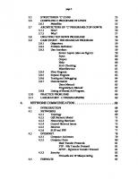
logic diagrams was a strategic one. By selecting ladder logic as the main programming method, the amount of retraining needed for engineers and tradespeople was greatly reduced. Modern control systems still include relays, but these are rarely used for logic. A relay is a simple device that uses a magnetic field to control a switch, as pictured in Figure 2.1. When a voltage is applied to the input coil, the resulting current creates a magnetic field. The magnetic field pulls a metal switch (or reed) towards it and the contacts touch, closing the switch. The contact that closes when the coil is energized is called normally open. The normally closed contacts touch when the input coil is not energized. Relays are normally drawn in schematic form using a circle to represent the input coil. The output contacts are shown with two parallel lines. Normally open contacts are shown as two lines, and will be open (non-conducting) when the input is not energized. Normally closed contacts are shown with two lines with a diagonal line through them. When the input coil is not energized the normally closed contacts will be closed (conducting).
plc wiring - 2.3
input coil
OR normally closed
normally open
OR
Figure 2.1
Simple Relay Layouts and Schematics
Relays are used to let one power source close a switch for another (often high current) power source, while keeping them isolated. An example of a relay in a simple control application is shown in Figure 2.2. In this system the first relay on the left is used as normally closed, and will allow current to flow until a voltage is applied to the input A. The second relay is normally open and will not allow current to flow until a voltage is applied to the input B. If current is flowing through the first two relays then current will flow through the coil in the third relay, and close the switch for output C. This circuit would normally be drawn in the ladder logic form. This can be read logically as C will be on if A is off and B is on.
plc wiring - 2.4
115VAC wall plug
relay logic
input B (normally open)
input A (normally closed)
A
B
output C (normally open)
C ladder logic
Figure 2.2
A Simple Relay Controller
The example in Figure 2.2 does not show the entire control system, but only the logic. When we consider a PLC there are inputs, outputs, and the logic. Figure 2.3 shows a more complete representation of the PLC. Here there are two inputs from push buttons. We can imagine the inputs as activating 24V DC relay coils in the PLC. This in turn drives an output relay that switches 115V AC, that will turn on a light. Note, in actual PLCs inputs are never relays, but outputs are often relays. The ladder logic in the PLC is actually a computer program that the user can enter and change. Notice that both of the input push buttons are normally open, but the ladder logic inside the PLC has one normally open contact, and one normally closed contact. Do not think that the ladder logic in the PLC needs to match the inputs or outputs. Many beginners will get caught trying to make the ladder logic match the input types.
plc wiring - 2.5
push buttons
power supply +24V com.
PLC inputs
ladder logic
A
B
C
outputs
115Vac AC power
light
neut.
Figure 2.3
A PLC Illustrated With Relays
Many relays also have multiple outputs (throws) and this allows an output relay to also be an input simultaneously. The circuit shown in Figure 2.4 is an example of this, it is called a seal in circuit. In this circuit the current can flow through either branch of the circuit, through the contacts labelled A or B. The input B will only be on when the output B is on. If B is off, and A is energized, then B will turn on. If B turns on then the input B will turn on, and keep output B on even if input A goes off. After B is turned on the output B will not turn off.
plc wiring - 2.6
A
B
B
Note: When A is pushed, the output B will turn on, and the input B will also turn on and keep B on permanently - until power is removed. Note: The line on the right is being left off intentionally and is implied in these diagrams.
Figure 2.4
A Seal-in Circuit
2.1.2 Programming The first PLCs were programmed with a technique that was based on relay logic wiring schematics. This eliminated the need to teach the electricians, technicians and engineers how to program a computer - but, this method has stuck and it is the most common technique for programming PLCs today. An example of ladder logic can be seen in Figure 2.5. To interpret this diagram imagine that the power is on the vertical line on the left hand side, we call this the hot rail. On the right hand side is the neutral rail. In the figure there are two rungs, and on each rung there are combinations of inputs (two vertical lines) and outputs (circles). If the inputs are opened or closed in the right combination the power can flow from the hot rail, through the inputs, to power the outputs, and finally to the neutral rail. An input can come from a sensor, switch, or any other type of sensor. An output will be some device outside the PLC that is switched on or off, such as lights or motors. In the top rung the contacts are normally open and normally closed. Which means if input A is on and input B is off, then power will flow through the output and activate it. Any other combination of input values will result in the output X being off.
plc wiring - 2.7
HOT
NEUTRAL A
B
C
D
G
E
F
H
INPUTS
X
Y
OUTPUTS
Note: Power needs to flow through some combination of the inputs (A,B,C,D,E,F,G,H) to turn on outputs (X,Y). Figure 2.5
A Simple Ladder Logic Diagram
The second rung of Figure 2.5 is more complex, there are actually multiple combinations of inputs that will result in the output Y turning on. On the left most part of the rung, power could flow through the top if C is off and D is on. Power could also (and simultaneously) flow through the bottom if both E and F are true. This would get power half way across the rung, and then if G or H is true the power will be delivered to output Y. In later chapters we will examine how to interpret and construct these diagrams. There are other methods for programming PLCs. One of the earliest techniques involved mnemonic instructions. These instructions can be derived directly from the ladder logic diagrams and entered into the PLC through a simple programming terminal. An example of mnemonics is shown in Figure 2.6. In this example the instructions are read one line at a time from top to bottom. The first line 00000 has the instruction LDN (input load and not) for input 00001. This will examine the input to the PLC and if it is off it will remember a 1 (or true), if it is on it will remember a 0 (or false). The next line uses an LD (input load) statement to look at the input. If the input is off it remembers a 0, if the input is on it remembers a 1 (note: this is the reverse of the LD). The AND statement recalls the last two numbers remembered and if the are both true the result is a 1, otherwise the result is a 0. This result now replaces the two numbers that were recalled, and there is only one number remembered. The process is repeated for lines 00003 and 00004, but when these are done there are now three numbers remembered. The oldest number is from the AND, the newer numbers are from the two LD instructions. The AND in line 00005 combines the results from the last LD instructions and now there are two numbers remembered. The OR instruction takes the two numbers now remaining and if either one is a 1 the result is a 1, otherwise the result is a 0. This result replaces the two numbers, and there is now a single
plc wiring - 2.8
number there. The last instruction is the ST (store output) that will look at the last value stored and if it is 1, the output will be turned on, if it is 0 the output will be turned off.
00000 00001 00002 00003 00004 00005 00006 00007 00008
LDN LD AND LD LD AND OR ST END
00001 00002 00003 00004
the mnemonic code is equivalent to the ladder logic below
00107 00001
00002
00003
00004
00107
END
Figure 2.6
An Example of a Mnemonic Program and Equivalent Ladder Logic
The ladder logic program in Figure 2.6, is equivalent to the mnemonic program. Even if you have programmed a PLC with ladder logic, it will be converted to mnemonic form before being used by the PLC. In the past mnemonic programming was the most common, but now it is uncommon for users to even see mnemonic programs. Sequential Function Charts (SFCs) have been developed to accommodate the programming of more advanced systems. These are similar to flowcharts, but much more powerful. The example seen in Figure 2.7 is doing two different things. To read the chart, start at the top where is says start. Below this there is the double horizontal line that says follow both paths. As a result the PLC will start to follow the branch on the left and right hand sides separately and simultaneously. On the left there are two functions the first one is the power up function. This function will run until it decides it is done, and the power down function will come after. On the right hand side is the flash function, this will run until it is done. These functions look unexplained, but each function, such as power up will be a small ladder logic program. This method is much different from flowcharts because it does not have to follow a single path through the flowchart.
plc wiring - 2.9
Start
power up
Execution follows multiple paths flash
power down
End
Figure 2.7
An Example of a Sequential Function Chart
Structured Text programming has been developed as a more modern programming language. It is quite similar to languages such as BASIC. A simple example is shown in Figure 2.8. This example uses a PLC memory location N7:0. This memory location is for an integer, as will be explained later in the book. The first line of the program sets the value to 0. The next line begins a loop, and will be where the loop returns to. The next line recalls the value in location N7:0, adds 1 to it and returns it to the same location. The next line checks to see if the loop should quit. If N7:0 is greater than or equal to 10, then the loop will quit, otherwise the computer will go back up to the REPEAT statement continue from there. Each time the program goes through this loop N7:0 will increase by 1 until the value reaches 10.
N7:0 := 0; REPEAT N7:0 := N7:0 + 1; UNTIL N7:0 >= 10 END_REPEAT;
Figure 2.8
An Example of a Structured Text Program
plc wiring - 2.10
2.1.3 PLC Connections When a process is controlled by a PLC it uses inputs from sensors to make decisions and update outputs to drive actuators, as shown in Figure 2.9. The process is a real process that will change over time. Actuators will drive the system to new states (or modes of operation). This means that the controller is limited by the sensors available, if an input is not available, the controller will have no way to detect a condition.
PROCESS
Connections to actuators
Feedback from sensors/switches PLC
Figure 2.9
The Separation of Controller and Process
The control loop is a continuous cycle of the PLC reading inputs, solving the ladder logic, and then changing the outputs. Like any computer this does not happen instantly. Figure 2.10 shows the basic operation cycle of a PLC. When power is turned on initially the PLC does a quick sanity check to ensure that the hardware is working properly. If there is a problem the PLC will halt and indicate there is an error. For example, if the PLC backup battery is low and power was lost, the memory will be corrupt and this will result in a fault. If the PLC passes the sanity check it will then scan (read) all the inputs. After the inputs values are stored in memory the ladder logic will be scanned (solved) using the stored values - not the current values. This is done to prevent logic problems when inputs change during the ladder logic scan. When the ladder logic scan is complete the outputs will be scanned (the output values will be changed). After this the system goes back to do a sanity check, and the loop continues indefinitely. Unlike normal computers, the entire program will be run every scan. Typical times for each of the stages is in the order of milliseconds.
plc wiring - 2.11
PLC program changes outputs by examining inputs THE CONTROL LOOP Read inputs
Figure 2.10
Set new outputs Power turned on Process changes and PLC pauses while it checks its own operation
The Scan Cycle of a PLC
2.1.4 Ladder Logic Inputs PLC inputs are easily represented in ladder logic. In Figure 2.11 there are three types of inputs shown. The first two are normally open and normally closed inputs, discussed previously. The IIT (Immediate InpuT) function allows inputs to be read after the input scan, while the ladder logic is being scanned. This allows ladder logic to examine input values more often than once every cycle.
x Normally open, an active input x will close the contact and allow power to flow. x Normally closed, power flows when the input x is not open. x IIT immediate inputs will take current values, not those from the previous input scan. (Note: this instruction is actually an output that will update the input table with the current input values. Other input contacts can now be used to examine the new values.) Figure 2.11
Ladder Logic Inputs
plc wiring - 2.12
2.1.5 Ladder Logic Outputs In ladder logic there are multiple types of outputs, but these are not consistently available on all PLCs. Some of the outputs will be externally connected to devices outside the PLC, but it is also possible to use internal memory locations in the PLC. Six types of outputs are shown in Figure 2.12. The first is a normal output, when energized the output will turn on, and energize an output. The circle with a diagonal line through is a normally on output. When energized the output will turn off. This type of output is not available on all PLC types. When initially energized the OSR (One Shot Relay) instruction will turn on for one scan, but then be off for all scans after, until it is turned off. The L (latch) and U (unlatch) instructions can be used to lock outputs on. When an L output is energized the output will turn on indefinitely, even when the output coil is deenergized. The output can only be turned off using a U output. The last instruction is the IOT (Immediate OutpuT) that will allow outputs to be updated without having to wait for the ladder logic scan to be completed.
When power is applied (on) the output x is activated for the left output, but turned off for the output on the right. x
x
An input transition on will cause the output x to go on for one scan (this is also known as a one shot relay) x OSR
plc wiring - 2.13
When the L coil is energized, x will be toggled on, it will stay on until the U coil is energized. This is like a flip-flop and stays set even when the PLC is turned off. x x L U Some PLCs will allow immediate outputs that do not wait for the program scan to end before setting an output. (Note: This instruction will only update the outputs using the output table, other instruction must change the individual outputs.) x IOT
Note: Outputs are also commonly shown using parentheses -( )- instead of the circle. This is because many of the programming systems are text based and circles cannot be drawn.
Figure 2.12
Ladder Logic Outputs
2.2 A CASE STUDY Problem: Try to develop (without looking at the solution) a relay based controller that will allow three switches in a room to control a single light.
plc wiring - 2.14
Solution: There are two possible approaches to this problem. The first assumes that any one of the switches on will turn on the light, but all three switches must be off for the light to be off. switch 1
light
switch 2 switch 3
The second solution assumes that each switch can turn the light on or off, regardless of the states of the other switches. This method is more complex and involves thinking through all of the possible combinations of switch positions. You might recognize this problem as an exclusive or problem. switch 1 switch 2 switch 3
light
switch 1 switch 2 switch 3 switch 1 switch 2 switch 3 switch 1 switch 2 switch 3
Note: It is important to get a clear understanding of how the controls are expected to work. In this example two radically different solutions were obtained based upon a simple difference in the operation.
2.3 SUMMARY • Normally open and closed contacts. • Relays and their relationship to ladder logic. • PLC outputs can be inputs, as shown by the seal in circuit. • Programming can be done with ladder logic, mnemonics, SFCs, and structured text. • There are multiple ways to write a PLC program.
plc wiring - 2.15
2.4 PRACTICE PROBLEMS 1. Give an example of where a PLC could be used. 2. Why would relays be used in place of PLCs? 3. Give a concise description of a PLC. 4. List the advantages of a PLC over relays. 5. A PLC can effectively replace a number of components. Give examples and discuss some good and bad applications of PLCs. 6. Explain why ladder logic outputs are coils? 7. In the figure below, will the power for the output on the first rung normally be on or off? Would the output on the second rung normally be on or off?
8. Write the mnemonic program for the Ladder Logic below. 100
201
101
2.5 PRACTICE PROBLEM SOLUTIONS 1. To control a conveyor system 2. For simple designs 3. A PLC is a computer based controller that uses inputs to monitor a process, and uses outputs to control a processusing a program.
plc wiring - 2.16
4. Less expensive for complex processes, debugging tools, reliable, flexible, easy to expend, etc. 5. A PLC could replace a few relays. In this case the relays might be easier to install and less expensive. To control a more complex system the controller might need timing, counting and other mathematical calculations. In this case a PLC would be a better choice. 6. The ladder logic outputs were modelled on relay logic diagrams. The output in a relay ladder diagram is a relay coil that switches a set of output contacts. 7. off, on 8. LD 100, LD 101, OR, ST 201
2.6 ASSIGNMENT PROBLEMS 1. Explain the trade-offs between relays and PLCs for control applications. 2. Develop a simple ladder logic program that will turn on an output X if inputs A and B, or input C is on.
plc wiring - 3.1
3. PLC HARDWARE
Topics: • PLC hardware configurations • Input and outputs types • Electrical wiring for inputs and outputs • Relays • Electrical Ladder Diagrams and JIC wiring symbols Objectives: • Be able to understand and design basic input and output wiring. • Be able to produce industrial wiring diagrams.
3.1 INTRODUCTION Many PLC configurations are available, even from a single vendor. But, in each of these there are common components and concepts. The most essential components are: Power Supply - This can be built into the PLC or be an external unit. Common voltage levels required by the PLC (with and without the power supply) are 24Vdc, 120Vac, 220Vac. CPU (Central Processing Unit) - This is a computer where ladder logic is stored and processed. I/O (Input/Output) - A number of input/output terminals must be provided so that the PLC can monitor the process and initiate actions. Indicator lights - These indicate the status of the PLC including power on, program running, and a fault. These are essential when diagnosing problems. The configuration of the PLC refers to the packaging of the components. Typical configurations are listed below from largest to smallest as shown in Figure 3.1. Rack - A rack is often large (up to 18” by 30” by 10”) and can hold multiple cards. When necessary, multiple racks can be connected together. These tend to be the highest cost, but also the most flexible and easy to maintain. Mini - These are similar in function to PLC racks, but about half the size. Shoebox - A compact, all-in-one unit (about the size of a shoebox) that has limited expansion capabilities. Lower cost, and compactness make these ideal for small applications. Micro - These units can be as small as a deck of cards. They tend to have fixed
plc wiring - 3.2
quantities of I/O and limited abilities, but costs will be the lowest. Software - A software based PLC requires a computer with an interface card, but allows the PLC to be connected to sensors and other PLCs across a network.
rack
mini
micro
Figure 3.1
Typical Configurations for PLC
3.2 INPUTS AND OUTPUTS Inputs to, and outputs from, a PLC are necessary to monitor and control a process. Both inputs and outputs can be categorized into two basic types: logical or continuous. Consider the example of a light bulb. If it can only be turned on or off, it is logical control. If the light can be dimmed to different levels, it is continuous. Continuous values seem more intuitive, but logical values are preferred because they allow more certainty, and simplify control. As a result most controls applications (and PLCs) use logical inputs and outputs for most applications. Hence, we will discuss logical I/O and leave continuous I/O for later. Outputs to actuators allow a PLC to cause something to happen in a process. A short list of popular actuators is given below in order of relative popularity. Solenoid Valves - logical outputs that can switch a hydraulic or pneumatic flow. Lights - logical outputs that can often be powered directly from PLC output boards. Motor Starters - motors often draw a large amount of current when started, so they require motor starters, which are basically large relays. Servo Motors - a continuous output from the PLC can command a variable speed or position.
plc wiring - 3.3
Outputs from PLCs are often relays, but they can also be solid state electronics such as transistors for DC outputs or Triacs for AC outputs. Continuous outputs require special output cards with digital to analog converters. Inputs come from sensors that translate physical phenomena into electrical signals. Typical examples of sensors are listed below in relative order of popularity. Proximity Switches - use inductance, capacitance or light to detect an object logically. Switches - mechanical mechanisms will open or close electrical contacts for a logical signal. Potentiometer - measures angular positions continuously, using resistance. LVDT (linear variable differential transformer) - measures linear displacement continuously using magnetic coupling. Inputs for a PLC come in a few basic varieties, the simplest are AC and DC inputs. Sourcing and sinking inputs are also popular. This output method dictates that a device does not supply any power. Instead, the device only switches current on or off, like a simple switch. Sinking - When active the output allows current to flow to a common ground. This is best selected when different voltages are supplied. Sourcing - When active, current flows from a supply, through the output device and to ground. This method is best used when all devices use a single supply voltage. This is also referred to as NPN (sinking) and PNP (sourcing). PNP is more popular. This will be covered in more detail in the chapter on sensors.
3.2.1 Inputs In smaller PLCs the inputs are normally built in and are specified when purchasing the PLC. For larger PLCs the inputs are purchased as modules, or cards, with 8 or 16 inputs of the same type on each card. For discussion purposes we will discuss all inputs as if they have been purchased as cards. The list below shows typical ranges for input voltages, and is roughly in order of popularity. 12-24 Vdc 100-120 Vac 10-60 Vdc 12-24 Vac/dc
plc wiring - 3.4
5 Vdc (TTL) 200-240 Vac 48 Vdc 24 Vac PLC input cards rarely supply power, this means that an external power supply is needed to supply power for the inputs and sensors. The example in Figure 3.2 shows how to connect an AC input card.
PLC Input Card 24V AC normally open push-button 24 V AC Hot Power Supply Neut.
00 01 02 03 04
normally open temperature switch
05 06 07 COM
I:013 Push Button 01
it is in rack 1 I/O Group 3
I:013 Temperature Sensor 03
Note: inputs are normally high impedance. This means that they will use very little current.
Figure 3.2
An AC Input Card and Ladder Logic
plc wiring - 3.5
In the example there are two inputs, one is a normally open push button, and the second is a temperature switch, or thermal relay. (NOTE: These symbols are standard and will be discussed in chapter 24.) Both of the switches are powered by the hot output of the 24Vac power supply - this is like the positive terminal on a DC supply. Power is supplied to the left side of both of the switches. When the switches are open there is no voltage passed to the input card. If either of the switches are closed power will be supplied to the input card. In this case inputs 1 and 3 are used - notice that the inputs start at 0. The input card compares these voltages to the common. If the input voltage is within a given tolerance range the inputs will switch on. Ladder logic is shown in the figure for the inputs. Here it uses Allen Bradley notation for PLC-5 racks. At the top is the location of the input card I:013 which indicates that the card is an Input card in rack 01 in slot 3. The input number on the card is shown below the contact as 01 and 03. Many beginners become confused about where connections are needed in the circuit above. The key word to remember is circuit, which means that there is a full loop that the voltage must be able to follow. In Figure 3.2 we can start following the circuit (loop) at the power supply. The path goes through the switches, through the input card, and back to the power supply where it flows back through to the start. In a full PLC implementation there will be many circuits that must each be complete. A second important concept is the common. Here the neutral on the power supply is the common, or reference voltage. In effect we have chosen this to be our 0V reference, and all other voltages are measured relative to it. If we had a second power supply, we would also need to connect the neutral so that both neutrals would be connected to the same common. Often common and ground will be confused. The common is a reference, or datum voltage that is used for 0V, but the ground is used to prevent shocks and damage to equipment. The ground is connected under a building to a metal pipe or grid in the ground. This is connected to the electrical system of a building, to the power outlets, where the metal cases of electrical equipment are connected. When power flows through the ground it is bad. Unfortunately many engineers, and manufacturers mix up ground and common. It is very common to find a power supply with the ground and common mislabeled.
Remember - Don’t mix up the ground and common. Don’t connect them together if the common of your device is connected to a common on another device.
One final concept that tends to trap beginners is that each input card is isolated. This means that if you have connected a common to only one card, then the other cards are not connected. When this happens the other cards will not work properly. You must connect a common for each of the output cards.
plc wiring - 3.6
There are many trade-offs when deciding which type of input cards to use. • DC voltages are usually lower, and therefore safer (i.e., 12-24V). • DC inputs are very fast, AC inputs require a longer on-time. For example, a 60Hz wave may require up to 1/60sec for reasonable recognition. • DC voltages can be connected to larger variety of electrical systems. • AC signals are more immune to noise than DC, so they are suited to long distances, and noisy (magnetic) environments. • AC power is easier and less expensive to supply to equipment. • AC signals are very common in many existing automation devices.
ASIDE: PLC inputs must convert a variety of logic levels to the 5Vdc logic levels used on the data bus. This can be done with circuits similar to those shown below. Basically the circuits condition the input to drive an optocoupler. This electrically isolates the external electrical circuitry from the internal circuitry. Other circuit components are used to guard against excess or reversed voltage polarity. +5V optocoupler
+
TTL
DC input COM
hot +5V AC input
optocoupler TTL
neut.
Figure 3.3
Aside: PLC Input Circuits
plc wiring - 3.7
3.2.2 Output Modules
WARNING - ALWAYS CHECK RATED VOLTAGES AND CURRENTS FOR PLC’s AND NEVER EXCEED!
As with input modules, output modules rarely supply any power, but instead act as switches. External power supplies are connected to the output card and the card will switch the power on or off for each output. Typical output voltages are listed below, and roughly ordered by popularity. 120 Vac 24 Vdc 12-48 Vac 12-48 Vdc 5Vdc (TTL) 230 Vac These cards typically have 8 to 16 outputs of the same type and can be purchased with different current ratings. A common choice when purchasing output cards is relays, transistors or triacs. Relays are the most flexible output devices. They are capable of switching both AC and DC outputs. But, they are slower (about 10ms switching is typical), they are bulkier, they cost more, and they will wear out after millions of cycles. Relay outputs are often called dry contacts. Transistors are limited to DC outputs, and Triacs are limited to AC outputs. Transistor and triac outputs are called switched outputs. - Dry contacts - a separate relay is dedicated to each output. This allows mixed voltages (AC or DC and voltage levels up to the maximum), as well as isolated outputs to protect other outputs and the PLC. Response times are often greater than 10ms. This method is the least sensitive to voltage variations and spikes. - Switched outputs - a voltage is supplied to the PLC card, and the card switches it to different outputs using solid state circuitry (transistors, triacs, etc.) Triacs are well suited to AC devices requiring less than 1A. Transistor outputs use NPN or PNP transistors up to 1A typically. Their response time is well under 1ms.
plc wiring - 3.8
ASIDE: PLC outputs must convert the 5Vdc logic levels on the PLC data bus to external voltage levels. This can be done with circuits similar to those shown below. Basically the circuits use an optocoupler to switch external circuitry. This electrically isolates the external electrical circuitry from the internal circuitry. Other circuit components are used to guard against excess or reversed voltage polarity. +V optocoupler TTL Sourcing DC output
optocoupler AC output
TTL
+V relay output AC/DC TTL
Figure 3.4
Note: Some AC outputs will also use zero voltage detection. This allows the output to be switched on when the voltage and current are effectively off, thus preventing surges.
Aside: PLC Output Circuits
Caution is required when building a system with both AC and DC outputs. If AC is
plc wiring - 3.9
accidentally connected to a DC transistor output it will only be on for the positive half of the cycle, and appear to be working with a diminished voltage. If DC is connected to an AC triac output it will turn on and appear to work, but you will not be able to turn it off without turning off the entire PLC.
ASIDE: A transistor is a semiconductor based device that can act as an adjustable valve. When switched off it will block current flow in both directions. While switched on it will allow current flow in one direction only. There is normally a loss of a couple of volts across the transistor. A triac is like two SCRs (or imagine transistors) connected together so that current can flow in both directions, which is good for AC current. One major difference for a triac is that if it has been switched on so that current flows, and then switched off, it will not turn off until the current stops flowing. This is fine with AC current because the current stops and reverses every 1/2 cycle, but this does not happen with DC current, and so the triac will remain on.
A major issue with outputs is mixed power sources. It is good practice to isolate all power supplies and keep their commons separate, but this is not always feasible. Some output modules, such as relays, allow each output to have its own common. Other output cards require that multiple, or all, outputs on each card share the same common. Each output card will be isolated from the rest, so each common will have to be connected. It is common for beginners to only connect the common to one card, and forget the other cards - then only one card seems to work! The output card shown in Figure 3.5 is an example of a 24Vdc output card that has a shared common. This type of output card would typically use transistors for the outputs.
plc wiring - 3.10
24 V DC Output Card
120 V AC Power Supply Neut.
00 01
Relay
02 03 Motor
04 05
24 V Lamp
06 07 COM in rack 01 I/O group 2
+24 V DC Power Supply COM
O:012 Motor 03 O:012
Lamp 07
Figure 3.5
An Example of a 24Vdc Output Card (Sinking)
In this example the outputs are connected to a low current light bulb (lamp) and a relay coil. Consider the circuit through the lamp, starting at the 24Vdc supply. When the output 07 is on, current can flow in 07 to the COM, thus completing the circuit, and allowing the light to turn on. If the output is off the current cannot flow, and the light will not turn on. The output 03 for the relay is connected in a similar way. When the output 03 is on, current will flow through the relay coil to close the contacts and supply 120Vac to the motor. Ladder logic for the outputs is shown in the bottom right of the figure. The notation is for an Allen Bradley PLC-5. The value at the top left of the outputs, O:012, indicates that the card is an output card, in rack 01, in slot 2 of the rack. To the bottom right of the outputs is the output number on the card 03 or 07. This card could have many different
plc wiring - 3.11
voltages applied from different sources, but all the power supplies would need a single shared common. The circuits in Figure 3.6 had the sequence of power supply, then device, then PLC card, then power supply. This requires that the output card have a common. Some output schemes reverse the device and PLC card, thereby replacing the common with a voltage input. The example in Figure 3.5 is repeated in Figure 3.6 for a voltage supply card.
24 V DC Output Card
Power Supply
V+
+24 V DC
COM
00 01
Relay
02
120 V AC Power Supply
03 04
Motor
05
Neut.
24 V lamp
06 07 in rack 01 I/O group 2
O:012 Motor 03 O:012
Lamp 07
Figure 3.6
An Example of a 24Vdc Output Card With a Voltage Input (Sourcing)
In this example the positive terminal of the 24Vdc supply is connected to the out-
plc wiring - 3.12
put card directly. When an output is on power will be supplied to that output. For example, if output 07 is on then the supply voltage will be output to the lamp. Current will flow through the lamp and back to the common on the power supply. The operation is very similar for the relay switching the motor. Notice that the ladder logic (shown in the bottom right of the figure) is identical to that in Figure 3.5. With this type of output card only one power supply can be used. We can also use relay outputs to switch the outputs. The example shown in Figure 3.5 and Figure 3.6 is repeated yet again in Figure 3.7 for relay output.
120 V AC/DC Output Card
24 V DC Power Supply
120 V AC Power Supply
00 01 02 03 Relay
04 05 06 07
Motor 24 V lamp
in rack 01 I/O group 2 O:012 Motor 03 O:012
Lamp 07
Figure 3.7
An Example of a Relay Output Card
plc wiring - 3.13
In this example the 24Vdc supply is connected directly to both relays (note that this requires 2 connections now, whereas the previous example only required one.) When an output is activated the output switches on and power is delivered to the output devices. This layout is more similar to Figure 3.6 with the outputs supplying voltage, but the relays could also be used to connect outputs to grounds, as in Figure 3.5. When using relay outputs it is possible to have each output isolated from the next. A relay output card could have AC and DC outputs beside each other.
3.3 RELAYS Although relays are rarely used for control logic, they are still essential for switching large power loads. Some important terminology for relays is given below. Contactor - Special relays for switching large current loads. Motor Starter - Basically a contactor in series with an overload relay to cut off when too much current is drawn. Arc Suppression - when any relay is opened or closed an arc will jump. This becomes a major problem with large relays. On relays switching AC this problem can be overcome by opening the relay when the voltage goes to zero (while crossing between negative and positive). When switching DC loads this problem can be minimized by blowing pressurized gas across during opening to suppress the arc formation. AC coils - If a normal relay coil is driven by AC power the contacts will vibrate open and closed at the frequency of the AC power. This problem is overcome by adding a shading pole to the relay. The most important consideration when selecting relays, or relay outputs on a PLC, is the rated current and voltage. If the rated voltage is exceeded, the contacts will wear out prematurely, or if the voltage is too high fire is possible. The rated current is the maximum current that should be used. When this is exceeded the device will become too hot, and it will fail sooner. The rated values are typically given for both AC and DC, although DC ratings are lower than AC. If the actual loads used are below the rated values the relays should work well indefinitely. If the values are exceeded a small amount the life of the relay will be shortened accordingly. Exceeding the values significantly may lead to immediate failure and permanent damage. • Rated Voltage - The suggested operation voltage for the coil. Lower levels can result in failure to operate, voltages above shorten life. • Rated Current - The maximum current before contact damage occurs (welding or melting).
plc wiring - 3.14
3.4 A CASE STUDY (Try the following case without looking at the solution in Figure 3.8.) An electrical layout is needed for a hydraulic press. The press uses a 24Vdc double actuated solenoid valve to advance and retract the press. This device has a single common and two input wires. Putting 24Vdc on one wire will cause the press to advance, putting 24Vdc on the second wire will cause it to retract. The press is driven by a large hydraulic pump that requires 220Vac rated at 20A, this should be running as long as the press is on. The press is outfitted with three push buttons, one is a NC stop button, the other is a NO manual retract button, and the third is a NO start automatic cycle button. There are limit switches at the top and bottom of the press travels that must also be connected.
SOLUTION 24VDC input card
24VDC output card solenoid O/0
I/0
advance
I/1
O/1
I/2
retract
I/3 I/4
O/2 relay for hydraulic pump com
Figure 3.8
-
+ 24VDC
com
Case Study for Press Wiring
The input and output cards were both selected to be 24Vdc so that they may share a single 24Vdc power supply. In this case the solenoid valve was wired directly to the output card, while the hydraulic pump was connected indirectly using a relay (only the coil is shown for simplicity). This decision was primarily made because the hydraulic pump
plc wiring - 3.15
requires more current than any PLC can handle, but a relay would be relatively easy to purchase and install for that load. All of the input switches are connected to the same supply and to the inputs.
3.5 ELECTRICAL WIRING DIAGRAMS When a controls cabinet is designed and constructed ladder diagrams are used to document the wiring. A basic wiring diagram is shown in Figure 3.9. In this example the system would be supplied with AC power (120Vac or 220Vac) on the left and right rails. The lines of these diagrams are numbered, and these numbers are typically used to number wires when building the electrical system. The switch before line 010 is a master disconnect for the power to the entire system. A fuse is used after the disconnect to limit the maximum current drawn by the system. Line 020 of the diagram is used to control power to the outputs of the system. The stop button is normally closed, while the start button is normally open. The branch, and output of the rung are CR1, which is a master control relay. The PLC receives power on line 30 of the diagram. The inputs to the PLC are all AC, and are shown on lines 040 to 070. Notice that Input I:0/0 is a set of contacts on the MCR CR1. The three other inputs are a normally open push button (line 050), a limit switch (060) and a normally closed push button (070). After line 080 the MCR CR1 can apply power to the outputs. These power the relay outputs of the PLC to control a red indicator light (040), a green indicator light (050), a solenoid (060), and another relay (080). The relay on line 080 switches a relay that turn on another device drill station.
plc wiring - 3.16
L1
N
010 stop
CR1
start
020
MCR CR1
L1
030
PLC
N 90-1
040
CR1
I:0/0
PB1
I:0/1
LS1
I:0/2
050 060
O:0/0 100-1
O:0/0 110-1
O:0/0 PB2
070
090
100
110 S1
120-1
120 CR2
ac com
080 CR1 090
90-1
035
100
100-1
050
110
110-1
060
120-1
070 Drill Station L1 N
CR2 130 Figure 3.9
L2 G
I:0/3 O:0/0
120
L1 R
A Ladder Wiring Diagram
plc wiring - 3.17
In the wiring diagram the choice of a normally close stop button and a normally open start button are intentional. Consider line 020 in the wiring diagram. If the stop button is pushed it will open the switch, and power will not be able to flow to the control relay and output power will shut off. If the stop button is damaged, say by a wire falling off, the power will also be lost and the system will shut down - safely. If the stop button used was normally open and this happened the system would continue to operate while the stop button was unable to shut down the power. Now consider the start button. If the button was damaged, say a wire was disconnected, it would be unable to start the system, thus leaving the system unstarted and safe. In summary, all buttons that stop a system should be normally closed, while all buttons that start a system should be normally open.
3.5.1 JIC Wiring Symbols To standardize electrical schematics, the Joint International Committee (JIC) symbols were developed, these are shown in Figure 3.10, Figure 3.11 and Figure 3.12.
plc wiring - 3.18
disconnect (3 phase AC)
circuit interrupter (3 phase AC)
normally closed limit switch
normally open limit switch
normally closed push-button
double pole push-button
mushroom head push-button
F
normally open push-button
breaker (3 phase AC)
thermal overload relay
liquid level normally open
Figure 3.10
fuse
motor (3 phase AC)
liquid level normally closed
JIC Schematic Symbols
vacuum pressure normally open
vacuum pressure normally closed
plc wiring - 3.19
temperature normally open
temperature normally closed
flow normally closed
flow normally open
R
relay contact normally open
relay contact normally closed
relay time delay on normally open
relay time delay on normally closed
indicator lamp
relay coil
relay time delay off normally open
relay time delay off normally closed
H1 H3 H2 H4
horn
buzzer
bell 2-H
solenoid
2-position hydraulic solenoid
normally open proximity switch
Figure 3.11
normally closed proximity switch
JIC Schematic Symbols
X1
X2
control transformer
Male connector
Female connector
plc wiring - 3.20
Tapped Resistor
Resistor
Variable Resistor (potentiometer) +
Rheostat (potentiometer)
Capacitor
Polarized Capacitor +
Variable Capacitor
Crystal
Thermocouple
Shielded Conductor
Common
Tapped Coil
Capacitor
Shielded
Coil or Inductor
Battery
Antenna
Grounded
Coil with magnetic core
Transformer Transformer magnetic core
Figure 3.12
JIC Schematic Symbols
plc wiring - 3.21
3.6 SUMMARY • PLC inputs condition AC or DC inputs to be detected by the logic of the PLC. • Outputs are transistors (DC), triacs (AC) or relays (AC and DC). • Input and output addresses are a function of the card location and input bit number. • Electrical system schematics are documented with diagrams that look like ladder logic.
3.7 PRACTICE PROBLEMS 1. Can a PLC input switch a relay coil to control a motor? 2. How do input and output cards act as an interface between the PLC and external devices? 3. What is the difference between wiring a sourcing and sinking output? 4. What is the difference between a motor starter and a contactor? 5. Is AC or DC easier to interrupt? 6. What can happen if the rated voltage on a device is exceeded? 7. What are the benefits of input/output modules? 8. (for electrical engineers) Explain the operation of AC input and output conditioning circuits. 9. What will happen if a DC output is switched by an AC output. 10. Explain why a stop button must be normally closed and a start button must be normally open. 11. For the circuit shown in the figure below, list the input and output addresses for the PLC. If switch A controls the light, switch B the motor, and C the solenoid, write a simple ladder logic
plc wiring - 3.22
program. 200 201
A 100
202
101
203 204
solenoid valve
205 206 207 com
102 103 104
+
B
C
105
24VDC 106 107
+ 12VDC
com
12. We have a PLC rack with a 24 VDC input card in slot 3, and a 120VAC output card in slot 2. The inputs are to be connected to 4 push buttons. The outputs are to drive a 120VAC lightbulb, a 240VAC motor, and a 24VDC operated hydraulic valve. Draw the electrical connections for the inputs and outputs. Show all other power supplies and other equipment/components required. 13. You are planning a project that will be controlled by a PLC. Before ordering parts you decide to plan the basic wiring and select appropriate input and output cards. The devices that we will use for inputs are 2 limit switches, a push button and a thermal switch. The output will be for a 24Vdc solenoid valve, a 110Vac light bulb, and a 220Vac 50HP motor. Sketch the basic wiring below including PLC cards. 14. Add three pushbuttons as inputs to the figure below. You must also select a power supply, and
plc wiring - 3.23
show all necessary wiring. 1 com 2 com 3 com 4 com 5 com
15. Three 120Vac outputs are to be connected to the output card below. Show the 120Vac source, and all wiring. V 00 01 02 03 04 05 06 07 16. Sketch the wiring for PLC outputs that are listed below. - a double acting hydraulic solenoid valve (with two coils) - a 24Vdc lamp - a 120 Vac high current lamp - a low current 12Vdc motor
plc wiring - 3.24
3.8 PRACTICE PROBLEM SOLUTIONS 1. no - a plc OUTPUT can switch a relay 2. input cards are connected to sensors to determine the state of the system. Output cards are connected to actuators that can drive the process. 3. sourcing outputs supply current that will pass through an electrical load to ground. Sinking inputs allow current to flow from the electrical load, to the common. 4. a motor starter typically has three phases 5. AC is easier, it has a zero crossing 6. it will lead to premature failure 7. by using separate modules, a PLC can be customized for different applications. If a single module fails, it can be replaced quickly, without having to replace the entire controller. 8. AC input conditioning circuits will rectify an AC input to a DC waveform with a ripple. This will be smoothed, and reduced to a reasonable voltage level to drive an optocoupler. An AC output circuit will switch an AC output with a triac, or a relay. 9. an AC output is a triac. When a triac output is turned off, it will not actually turn off until the AC voltage goes to 0V. Because DC voltages don’t go to 0V, it will never turn off. 10. If a NC stop button is damaged, the machine will act as if the stop button was pushed and shut down safely. If a NO start button is damaged the machine will not be able to start. 11. outputs: 200 - light 202 - motor 204 - solenoid inputs: 100 - switch A 102 - switch B 104 - switch C
100
200
102
202
104
210
plc wiring - 3.25
12.
0
0
1
1
2
2
3
3
4
4
5
5
6
6
7 com
+ 24VDC -
7 com
13.
+ 24VDC -
0
0
1
1
2
2
3
3
4
4
5
5
6
6
7
7
com
+ 24Vdc -
hot 220Vac neut.
hot 120Vac neut. Note: relays are used to reduce the total number of output cards
plc wiring - 3.26
14. 1
+
com
24Vdc -
2 com 3 com 4 com 5 com
15. hot
V 00 01 02 03 04 05 06 07
Load 1 Load 2 Load 3
120Vac neut.
plc wiring - 3.27
16.
relay output card + 00
power supply 24Vdc
-
01
02 hot 03
power supply 120Vac
neut. +
04
power supply 12Vdc
-
3.9 ASSIGNMENT PROBLEMS 1. Describe what could happen if a normally closed start button was used on a system, and the wires to the button were cut. 2. Describe what could happen if a normally open stop button was used on a system and the wires to the button were cut. 3. a) For the input and output cards below, add three output lights and three normally open push-
plc wiring - 3.28
button inputs. b) Redraw the outputs so that it uses a relay output card.
+ VDC
I:0/0
V
I:0/1
O:0/0
I:0/2
O:0/1
I:0/3
O:0/2
I:0/4
O:0/3
I:0/5
O:0/4
I:0/6
O:0/5
I:0/7
O:0/6
com
O:0/7
12VDC +
4. Draw an electrical wiring (ladder) diagram for PLC outputs that are listed below. - a solenoid controlled hydraulic valve - a 24Vdc lamp - a 120 Vac high current lamp - a low current 12Vdc motor 5. Draw an electrical ladder diagram for a PLC that has a PNP and an NPN sensor for inputs. The outputs are two small indicator lights. You should use proper symbols for all components. You must also include all safety devices including fuses, disconnects, MCRs, etc... 6. Draw an electrical wiring diagram for a PLC controlling a system with an NPN and PNP input sensor. The outputs include an indicator light and a relay to control a 20A motor load. Include ALL safety circuitry.
discrete sensors - 4.1
4. LOGICAL SENSORS
Topics: • Sensor wiring; switches, TTL, sourcing, sinking • Proximity detection; contact switches, photo-optics, capacitive, inductive and ultrasonic Objectives: • Understand the different types of sensor outputs. • Know the basic sensor types and understand application issues.
4.1 INTRODUCTION Sensors allow a PLC to detect the state of a process. Logical sensors can only detect a state that is either true or false. Examples of physical phenomena that are typically detected are listed below. • inductive proximity - is a metal object nearby? • capacitive proximity - is a dielectric object nearby? • optical presence - is an object breaking a light beam or reflecting light? • mechanical contact - is an object touching a switch? Recently, the cost of sensors has dropped and they have become commodity items, typically between $50 and $100. They are available in many forms from multiple vendors such as Allen-Bradley, Omron, Hyde Park and Tuurk. In applications sensors are interchangeable between PLC vendors, but each sensor will have specific interface requirements. This chapter will begin by examining the various electrical wiring techniques for sensors, and conclude with an examination of many popular sensor types.
4.2 SENSOR WIRING When a sensor detects a logical change it must signal that change to the PLC. This is typically done by switching a voltage or current on or off. In some cases the output of the sensor is used to switch a load directly, completely eliminating the PLC. Typical out-
discrete sensors - 4.2
puts from sensors (and inputs to PLCs) are listed below in relative popularity. Sinking/Sourcing - Switches current on or off. Plain Switches - Switches voltage on or off. Solid State Relays - These switch AC outputs. TTL (Transistor Transistor Logic) - Uses 0V and 5V to indicate logic levels.
4.2.1 Switches The simplest example of sensor outputs are switches and relays. A simple example is shown in Figure 4.1.
PLC Input Card 24V DC normally open push-button 24 Vdc Power Supply
+
00 01 02
-
03 V+ sensor
04 relay output
05 06
V-
07 COM
Figure 4.1
An Example of Switched Sensors
In the figure a NO contact switch is connected to input 01. A sensor with a relay output is also shown. The sensor must be powered separately, therefore the V+ and V- terminals are connected to the power supply. The output of the sensor will become active when a phenomenon has been detected. This means the internal switch (probably a relay) will be closed allowing current to flow and the positive voltage will be applied to input 06.
discrete sensors - 4.3
4.2.2 Transistor Transistor Logic (TTL) Transistor-Transistor Logic (TTL) is based on two voltage levels, 0V for false and 5V for true. The voltages can actually be slightly larger than 0V, or lower than 5V and still be detected correctly. This method is very susceptible to electrical noise on the factory floor, and should only be used when necessary. TTL outputs are common on electronic devices and computers, and will be necessary sometimes. When connecting to other devices simple circuits can be used to improve the signal, such as the Schmitt trigger in Figure 4.2.
Vi
Vo
Vi
Vo
Figure 4.2
A Schmitt Trigger
A Schmitt trigger will receive an input voltage between 0-5V and convert it to 0V or 5V. If the voltage is in an ambiguous range, about 1.5-3.5V it will be ignored. If a sensor has a TTL output the PLC must use a TTL input card to read the values. If the TTL sensor is being used for other applications it should be noted that the maximum current output is normally about 20mA.
4.2.3 Sinking/Sourcing Sinking sensors allow current to flow into the sensor to the voltage common, while sourcing sensors allow current to flow out of the sensor from a positive source. For both of these methods the emphasis is on current flow, not voltage. By using current flow, instead of voltage, many of the electrical noise problems are reduced. When discussing sourcing and sinking we are referring to the output of the sensor that is acting like a switch. In fact the output of the sensor is normally a transistor, that will act like a switch (with some voltage loss). A PNP transistor is used for the sourcing output, and an NPN transistor is used for the sinking input. When discussing these sensors the
discrete sensors - 4.4
term sourcing is often interchanged with PNP, and sinking with NPN. A simplified example of a sinking output sensor is shown in Figure 4.3. The sensor will have some part that deals with detection, this is on the left. The sensor needs a voltage supply to operate, so a voltage supply is needed for the sensor. If the sensor has detected some phenomenon then it will trigger the active line. The active line is directly connected to an NPN transistor. (Note: for an NPN transistor the arrow always points away from the center.) If the voltage to the transistor on the active line is 0V, then the transistor will not allow current to flow into the sensor. If the voltage on the active line becomes larger (say 12V) then the transistor will switch on and allow current to flow into the sensor to the common.
V+
V+ physical phenomenon
sensor output Sensor and Detector
NPN
current flows in when switched on
Active Line V-
V-
Aside: The sensor responds to a physical phenomenon. If the sensor is inactive (nothing detected) then the active line is low and the transistor is off, this is like an open switch. That means the NPN output will have no current in/out. When the sensor is active, it will make the active line high. This will turn on the transistor, and effectively close the switch. This will allow current to flow into the sensor to ground (hence sinking). The voltage on the NPN output will be pulled down to V-. Note: the voltage will always be 1-2V higher because of the transistor. When the sensor is off, the NPN output will float, and any digital circuitry needs to contain a pull-up resistor.
Figure 4.3
A Simplified NPN/Sinking Sensor
Sourcing sensors are the complement to sinking sensors. The sourcing sensors use a PNP transistor, as shown in Figure 4.4. (Note: PNP transistors are always drawn with the arrow pointing to the center.) When the sensor is inactive the active line stays at the V+
discrete sensors - 4.5
value, and the transistor stays switched off. When the sensor becomes active the active line will be made 0V, and the transistor will allow current to flow out of the sensor.
V+
V+ physical phenomenon Active Line
current flows out when switched on
Sensor and Detector
PNP sensor output V-
V-
Aside: The sensor responds to the physical phenomenon. If the sensor is inactive (nothing detected) then the active line is high and the transistor is off, this is like an open switch. That means the PNP output will have no current in/out. When the sensor is active, it will make the active line high. This will turn on the transistor, and effectively close the switch. This will allow current to flow from V+ through the sensor to the output (hence sourcing). The voltage on the PNP output will be pulled up to V+. Note: the voltage will always be 1-2V lower because of the transistor. When off, the PNP output will float, if used with digital circuitry a pull-down resistor will be needed.
Figure 4.4
A Simplified Sourcing/PNP Sensor
Most NPN/PNP sensors are capable of handling currents up to a few amps, and they can be used to switch loads directly. (Note: always check the documentation for rated voltages and currents.) An example using sourcing and sinking sensors to control lights is shown in Figure 4.5. (Note: This example could be for a motion detector that turns on lights in dark hallways.)
discrete sensors - 4.6
sensor
sensor
V+
V+
NPN
power supply
V-
V- (common)
V+
V+
PNP V-
power supply
sinking
sourcing
V- (common)
Note: remember to check the current and voltage ratings for the sensors.
Note: When marking power terminals, there will sometimes be two sets of markings. The more standard is V+ and COM, but sometimes you will see devices and power supplies without a COM (common), in this case assume the V- is the common.
Figure 4.5
Direct Control Using NPN/PNP Sensors
In the sinking system in Figure 4.5 the light has V+ applied to one side. The other side is connected to the NPN output of the sensor. When the sensor turns on the current will be able to flow through the light, into the output to V- common. (Note: Yes, the current will be allowed to flow into the output for an NPN sensor.) In the sourcing arrangement the light will turn on when the output becomes active, allowing current to flow from the V+, thought the sensor, the light and to V- (the common). At this point it is worth stating the obvious - The output of a sensor will be an input for a PLC. And, as we saw with the NPN sensor, this does not necessarily indicate where current is flowing. There are two viable approaches for connecting sensors to PLCs. The first is to always use PNP sensors and normal voltage input cards. The second option is to purchase input cards specifically designed for sourcing or sinking sensors. An example of a PLC card for sinking sensors is shown in Figure 4.6.
discrete sensors - 4.7
PLC Input Card for Sinking Sensors +V
current flow
Internal Card Electronics
+V NPN NPN sensor 00
01
PLC Data Bus
External Electrical
+V
power supply
-V
-V
Note: When a PLC input card does not have a common but it has a V+ instead, it can be used for NPN sensors. In this case the current will flow out of the card (sourcing) and we must switch it to ground.
ASIDE: This card is shown with 2 optocouplers (one for each output). Inside these devices the is an LED and a phototransistor, but no electrical connection. These devices are used to isolate two different electrical systems. In this case they protect the 5V digital levels of the PLC computer from the various external voltages and currents.
Figure 4.6
A PLC Input Card for Sinking Sensors
The dashed line in the figure represents the circuit, or current flow path when the sensor is active. This path enters the PLC input card first at a V+ terminal (Note: there is no common on this card) and flows through an optocoupler. This current will use light to turn on a phototransistor to tell the computer in the PLC the input current is flowing. The current then leaves the card at input 00 and passes through the sensor to V-. When the sensor is inactive the current will not flow, and the light in the optocoupler will be off. The optocoupler is used to help protect the PLC from electrical problems outside the PLC. The input cards for PNP sensors are similar to the NPN cards, as shown in Figure 4.7.
discrete sensors - 4.8
PLC Input Card for Sourcing Sensors 00
+V
Internal Card Electronics
PNP PNP sensor
current flow
-V 01 +V
power supply
-V com Note: When we have a PLC input card that has a common then we can use PNP sensors. In this case the current will flow into the card and then out the common to the power supply.
Figure 4.7
PLC Input Card for Sourcing Sensors
The current flow loop for an active sensor is shown with a dashed line. Following the path of the current we see that it begins at the V+, passes through the sensor, in the input 00, through the optocoupler, out the common and to the V-. Wiring is a major concern with PLC applications, so to reduce the total number of wires, two wire sensors have become popular. But, by integrating three wires worth of function into two, we now couple the power supply and sensing functions into one. Two wire sensors are shown in Figure 4.8.
discrete sensors - 4.9
+V PLC Input Card for Sourcing Sensors
two wire sensor
00 -V
01
+V
power supply
-V
com Note: These sensors require a certain leakage current to power the electronics. V+
PLC Input Card for Sinking Sensors
00 +V two wire sensor 01
-V
+V
power supply
-V
Figure 4.8
Two Wire Sensors
A two wire sensor can be used as either a sourcing or sinking input. In both of these arrangements the sensor will require a small amount of current to power the sensor, but when active it will allow more current to flow. This requires input cards that will allow a small amount of current to flow (called the leakage current), but also be able to detect when the current has exceeded a given value.
discrete sensors - 4.10
When purchasing sensors and input cards there are some important considerations. Most modern sensors have both PNP and NPN outputs, although if the choice is not available, PNP is the more popular choice. PLC cards can be confusing to buy, as each vendor refers to the cards differently. To avoid problems, look to see if the card is specifically for sinking or sourcing sensors, or look for a V+ (sinking) or COM (sourcing). Some vendors also sell cards that will allow you to have NPN and PNP inputs mixed on the same card. When drawing wiring diagrams the symbols in Figure 4.9 are used for sinking and sourcing proximity sensors. Notice that in the sinking sensor when the switch closes (moves up to the terminal) it contacts the common. Closing the switch in the sourcing sensor connects the output to the V+. On the physical sensor the wires are color coded as indicated in the diagram. The brown wire is positive, the blue wire is negative and the output is white for sinking and black for sourcing. The outside shape of the sensor may change for other devices, such as photo sensors which are often shown as round circles.
brown
V+ NPN (sinking)
NPN white
PNP (sourcing)
V+
blue
black
brown
blue
Figure 4.9
V-
PNP V-
Sourcing and Sinking Schematic Symbols
4.2.4 Solid State Relays Solid state relays switch AC currents. These are relatively inexpensive and are available for large loads. Some sensors and devices are available with these as outputs.
discrete sensors - 4.11
4.3 PRESENCE DETECTION There are two basic ways to detect object presence; contact and proximity. Contact implies that there is mechanical contact and a resulting force between the sensor and the object. Proximity indicates that the object is near, but contact is not required. The following sections examine different types of sensors for detecting object presence. These sensors account for a majority of the sensors used in applications.
4.3.1 Contact Switches Contact switches are available as normally open and normally closed. Their housings are reinforced so that they can take repeated mechanical forces. These often have rollers and wear pads for the point of contact. Lightweight contact switches can be purchased for less than a dollar, but heavy duty contact switches will have much higher costs. Examples of applications include motion limit switches and part present detectors.
4.3.2 Reed Switches Reed switches are very similar to relays, except a permanent magnet is used instead of a wire coil. When the magnet is far away the switch is open, but when the magnet is brought near the switch is closed as shown in Figure 4.10. These are very inexpensive an can be purchased for a few dollars. They are commonly used for safety screens and doors because they are harder to trick than other sensors.
Note: With this device the magnet is moved towards the reed switch. As it gets closer the switch will close. This allows proximity detection without contact, but requires that a separate magnet be attached to a moving part.
Figure 4.10
Reed Switch
discrete sensors - 4.12
4.3.3 Optical (Photoelectric) Sensors Light sensors have been used for almost a century - originally photocells were used for applications such as reading audio tracks on motion pictures. But modern optical sensors are much more sophisticated. Optical sensors require both a light source (emitter) and detector. Emitters will produce light beams in the visible and invisible spectrums using LEDs and laser diodes. Detectors are typically built with photodiodes or phototransistors. The emitter and detector are positioned so that an object will block or reflect a beam when present. A basic optical sensor is shown in Figure 4.11.
square wave smaller signal +V
+V lens
lens light
oscillator
amplifier demodulator detector and switching circuits
LED phototransistor
Figure 4.11
A Basic Optical Sensor
In the figure the light beam is generated on the left, focused through a lens. At the detector side the beam is focused on the detector with a second lens. If the beam is broken the detector will indicate an object is present. The oscillating light wave is used so that the sensor can filter out normal light in the room. The light from the emitter is turned on and off at a set frequency. When the detector receives the light it checks to make sure that it is at the same frequency. If light is being received at the right frequency then the beam is not broken. The frequency of oscillation is in the KHz range, and too fast to be noticed. A side effect of the frequency method is that the sensors can be used with lower power at longer distances. An emitter can be set up to point directly at a detector, this is known as opposed mode. When the beam is broken the part will be detected. This sensor needs two separate
discrete sensors - 4.13
components, as shown in Figure 4.12. This arrangement works well with opaque and reflective objects with the emitter and detector separated by distances of up to hundreds of feet.
emitter
Figure 4.12
object
detector
Opposed Mode Optical Sensor
Having the emitter and detector separate increases maintenance problems, and alignment is required. A preferred solution is to house the emitter and detector in one unit. But, this requires that light be reflected back as shown in Figure 4.13. These sensors are well suited to larger objects up to a few feet away.
reflector emitter
detector
reflector emitter object detector
Note: the reflector is constructed with polarizing screens oriented at 90 deg. angles. If the light is reflected back directly the light does not pass through the screen in front of the detector. The reflector is designed to rotate the phase of the light by 90 deg., so it will now pass through the screen in front of the detector.
Figure 4.13
Retroreflective Optical Sensor
discrete sensors - 4.14
In the figure, the emitter sends out a beam of light. If the light is returned from the reflector most of the light beam is returned to the detector. When an object interrupts the beam between the emitter and the reflector the beam is no longer reflected back to the detector, and the sensor becomes active. A potential problem with this sensor is that reflective objects could return a good beam. This problem is overcome by polarizing the light at the emitter (with a filter), and then using a polarized filter at the detector. The reflector uses small cubic reflectors and when the light is reflected the polarity is rotated by 90 degrees. If the light is reflected off the object the light will not be rotated by 90 degrees. So the polarizing filters on the emitter and detector are rotated by 90 degrees, as shown in Figure 4.14. The reflector is very similar to reflectors used on bicycles.
emitter have filters for emitted light rotated by 90 deg.
detector
emitter
object
reflector
light reflected with same polarity
light rotated by 90 deg. reflector
detector
Figure 4.14
Polarized Light in Retroreflective Sensors
For retroreflectors the reflectors are quite easy to align, but this method still requires two mounted components. A diffuse sensors is a single unit that does not use a reflector, but uses focused light as shown in Figure 4.15.
discrete sensors - 4.15
emitter object detector
Note: with diffuse reflection the light is scattered. This reduces the quantity of light returned. As a result the light needs to be amplified using lenses.
Figure 4.15
Diffuse Optical Sensor
Diffuse sensors use light focused over a given range, and a sensitivity adjustment is used to select a distance. These sensors are the easiest to set up, but they require well controlled conditions. For example if it is to pick up light and dark colored objects problems would result. When using opposed mode sensors the emitter and detector must be aligned so that the emitter beam and detector window overlap, as shown in Figure 4.16. Emitter beams normally have a cone shape with a small angle of divergence (a few degrees of less). Detectors also have a cone shaped volume of detection. Therefore when aligning opposed mode sensor care is required not just to point the emitter at the detector, but also the detector at the emitter. Another factor that must be considered with this and other sensors is that the light intensity decreases over distance, so the sensors will have a limit to separation distance.
discrete sensors - 4.16
effective beam effective detector angle
detector
emitter
effective beam angle
alignment is required
1 intensity ∝ ----2 r Figure 4.16
Beam Divergence and Alignment
If an object is smaller than the width of the light beam it will not be able to block the beam entirely when it is in front as shown in Figure 4.17. This will create difficulties in detection, or possibly stop detection altogether. Solutions to this problem are to use narrower beams, or wider objects. Fiber optic cables may be used with an opposed mode optical sensor to solve this problem, however the maximum effective distance is reduced to a couple feet.
emitter
detector object
the smaller beam width is good (but harder to align
Figure 4.17
The Relationship Between Beam Width and Object Size
Separated sensors can detect reflective parts using reflection as shown in Figure 4.18. The emitter and detector are positioned so that when a reflective surface is in position the light is returned to the detector. When the surface is not present the light does not return.
discrete sensors - 4.17
em er itt de
tec
to r
reflective surface
Figure 4.18
Detecting Reflecting Parts
Other types of optical sensors can also focus on a single point using beams that converge instead of diverge. The emitter beam is focused at a distance so that the light intensity is greatest at the focal distance. The detector can look at the point from another angle so that the two centerlines of the emitter and detector intersect at the point of interest. If an object is present before or after the focal point the detector will not see the reflected light. This technique can also be used to detect multiple points and ranges, as shown in Figure 4.20 where the net angle of refraction by the lens determines which detector is used. This type of approach, with many more detectors, is used for range sensing systems.
focal point emitter
detector
Figure 4.19
Point Detection Using Focused Optics
discrete sensors - 4.18
lens
distance 1
distance 2
emitter
lens detector 2 detector 1
Figure 4.20
Multiple Point Detection Using Optics
Some applications do not permit full sized photooptic sensors to be used. Fiber optics can be used to separate the emitters and detectors from the application. Some vendors also sell photosensors that have the phototransistors and LEDs separated from the electronics. Light curtains are an array of beams, set up as shown in Figure 4.21. If any of the beams are broken it indicates that somebody has entered a workcell and the machine needs to be shut down. This is an inexpensive replacement for some mechanical cages and barriers.
Figure 4.21
A Light Curtain
The optical reflectivity of objects varies from material to material as shown in Fig-
discrete sensors - 4.19
ure 4.22. These values show the percentage of incident light on a surface that is reflected. These values can be used for relative comparisons of materials and estimating changes in sensitivity settings for sensors.
Reflectivity nonshiny materials
Kodak white test card white paper kraft paper, cardboard lumber (pine, dry, clean) rough wood pallet beer foam opaque black nylon black neoprene black rubber tire wall
90% 80% 70% 75% 20% 70% 14% 4% 1.5%
shiny/transparent materials
clear plastic bottle translucent brown plastic bottle opaque white plastic unfinished aluminum straightened aluminum unfinished black anodized aluminum stainless steel microfinished stainless steel brushed
40% 60% 87% 140% 105% 115% 400% 120%
Note: For shiny and transparent materials the reflectivity can be higher than 100% because of the return of ambient light.
Figure 4.22
Table of Reflectivity Values for Different Materials [Banner Handbook of Photoelectric Sensing]
4.3.4 Capacitive Sensors Capacitive sensors are able to detect most materials at distances up to a few centimeters. Recall the basic relationship for capacitance.
discrete sensors - 4.20
Ak C = -----d
where,
C = capacitance (Farads) k = dielectric constant A = area of plates d = distance between plates (electrodes)
In the sensor the area of the plates and distance between them is fixed. But, the dielectric constant of the space around them will vary as different materials are brought near the sensor. An illustration of a capacitive sensor is shown in Figure 4.23. an oscillating field is used to determine the capacitance of the plates. When this changes beyond a selected sensitivity the sensor output is activated.
+V
electric field electrode
oscillator
electrode
detector
object
load switching
NOTE: For this sensor the proximity of any material near the electrodes will increase the capacitance. This will vary the magnitude of the oscillating signal and the detector will decide when this is great enough to determine proximity.
Figure 4.23
A Capacitive Sensor
These sensors work well for insulators (such as plastics) that tend to have high dielectric coefficients, thus increasing the capacitance. But, they also work well for metals because the conductive materials in the target appear as larger electrodes, thus increasing the capacitance as shown in Figure 4.24. In total the capacitance changes are normally in the order of pF.
discrete sensors - 4.21
electrode
metal
electrode
Figure 4.24
electrode
dielectric
electrode
Dielectrics and Metals Increase the Capacitance
The sensors are normally made with rings (not plates) in the configuration shown in Figure 4.25. In the figure the two inner metal rings are the capacitor electrodes, but a third outer ring is added to compensate for variations. Without the compensator ring the sensor would be very sensitive to dirt, oil and other contaminants that might stick to the sensor.
electrode compensating electrode
Figure 4.25
Note: the compensating electrode is used for negative feedback to make the sensor more resistant to variations, such as contaminations on the face of the sensor.
Electrode Arrangement for Capacitive Sensors
A table of dielectric properties is given in Figure 4.26. This table can be used for estimating the relative size and sensitivity of sensors. Also, consider a case where a pipe would carry different fluids. If their dielectric constants are not very close, a second sensor may be desired for the second fluid.
discrete sensors - 4.22
Material
Constant
Material
Constant
ABS resin pellet acetone acetyl bromide acrylic resin air alcohol, industrial alcohol, isopropyl ammonia aniline aqueous solutions ash (fly) bakelite barley powder benzene benzyl acetate butane cable sealing compound calcium carbonate carbon tetrachloride celluloid cellulose cement cement powder cereal charcoal chlorine, liquid coke corn ebonite epoxy resin ethanol ethyl bromide ethylene glycol flour FreonTM R22,R502 liq. gasoline glass glass, raw material glycerine
1.5-2.5 19.5 16.5 2.7-4.5 1.0 16-31 18.3 15-25 5.5-7.8 50-80 1.7 3.6 3.0-4.0 2.3 5 1.4 2.5 9.1 2.2 3.0 3.2-7.5 1.5-2.1 5-10 3-5 1.2-1.8 2.0 1.1-2.2 5-10 2.7-2.9 2.5-6 24 4.9 38.7 2.5-3.0 6.1 2.2 3.1-10 2.0-2.5 47
hexane hydrogen cyanide hydrogen peroxide isobutylamine lime, shell marble melamine resin methane liquid methanol mica, white milk, powdered nitrobenzene neoprene nylon oil, for transformer oil, paraffin oil, peanut oil, petroleum oil, soybean oil, turpentine paint paraffin paper paper, hard paper, oil saturated perspex petroleum phenol phenol resin polyacetal (Delrin TM) polyamide (nylon) polycarbonate polyester resin polyethylene polypropylene polystyrene polyvinyl chloride resin porcelain press board
1.9 95.4 84.2 4.5 1.2 8.0-8.5 4.7-10.2 1.7 33.6 4.5-9.6 3.5-4 36 6-9 4-5 2.2-2.4 2.2-4.8 3.0 2.1 2.9-3.5 2.2 5-8 1.9-2.5 1.6-2.6 4.5 4.0 3.2-3.5 2.0-2.2 9.9-15 4.9 3.6 2.5 2.9 2.8-8.1 2.3 2.0-2.3 3.0 2.8-3.1 4.4-7 2-5
discrete sensors - 4.23
Material
Constant
Material
Constant
quartz glass rubber salt sand shellac silicon dioxide silicone rubber silicone varnish styrene resin sugar sugar, granulated sulfur sulfuric acid
3.7 2.5-35 6.0 3-5 2.0-3.8 4.5 3.2-9.8 2.8-3.3 2.3-3.4 3.0 1.5-2.2 3.4 84
Teflon (TM), PCTFE Teflon (TM), PTFE toluene trichloroethylene urea resin urethane vaseline water wax wood, dry wood, pressed board wood, wet xylene
2.3-2.8 2.0 2.3 3.4 6.2-9.5 3.2 2.2-2.9 48-88 2.4-6.5 2-7 2.0-2.6 10-30 2.4
Figure 4.26
Dielectric Constants of Various Materials [Turck Proximity Sensors Guide]
The range and accuracy of these sensors are determined mainly by their size. Larger sensors can have diameters of a few centimeters. Smaller ones can be less than a centimeter across, and have smaller ranges, but more accuracy.
4.3.5 Inductive Sensors Inductive sensors use currents induced by magnetic fields to detect nearby metal objects. The inductive sensor uses a coil (an inductor) to generate a high frequency magnetic field as shown in Figure 4.27. If there is a metal object near the changing magnetic field, current will flow in the object. This resulting current flow sets up a new magnetic field that opposes the original magnetic field. The net effect is that it changes the inductance of the coil in the inductive sensor. By measuring the inductance the sensor can determine when a metal have been brought nearby. These sensors will detect any metals, when detecting multiple types of metal multiple sensors are often used.
discrete sensors - 4.24
metal
inductive coil +V
oscillator and level detector
output switching
Note: these work by setting up a high frequency field. If a target nears the field will induce eddy currents. These currents consume power because of resistance, so energy is in the field is lost, and the signal amplitude decreases. The detector examines filed magnitude to determine when it has decreased enough to switch.
Figure 4.27
Inductive Proximity Sensor
The sensors can detect objects a few centimeters away from the end. But, the direction to the object can be arbitrary as shown in Figure 4.28. The magnetic field of the unshielded sensor covers a larger volume around the head of the coil. By adding a shield (a metal jacket around the sides of the coil) the magnetic field becomes smaller, but also more directed. Shields will often be available for inductive sensors to improve their directionality and accuracy.
discrete sensors - 4.25
unshielded
shielded
Figure 4.28
Shielded and Unshielded Sensors
4.3.6 Ultrasonic An ultrasonic sensor emits a sound above the normal hearing threshold of 16KHz. The time that is required for the sound to travel to the target and reflect back is proportional to the distance to the target. The two common types of sensors are; electrostatic - uses capacitive effects. It has longer ranges and wider bandwidth, but is more sensitive to factors such as humidity. piezoelectric - based on charge displacement during strain in crystal lattices. These are rugged and inexpensive. These sensors can be very effective for applications such as fluid levels in tanks and crude distance measurement.
4.3.7 Hall Effect Hall effect switches are basically transistors that can be switched by magnetic fields. Their applications are very similar to reed switches, but because they are solid state they tend to be more rugged and resist vibration. Automated machines often use these to do initial calibration and detect end stops.
discrete sensors - 4.26
4.3.8 Fluid Flow We can also build more complex sensors out of simpler sensors. The example in Figure 4.29 shows a metal float in a tapered channel. As the fluid flow rate increases the pressure forces the float upwards. The tapered shape of the float ensures an equilibrium position proportional to flowrate. An inductive proximity sensor can be positioned so that it will detect when the float has reached a certain height, and the system has reached a given flowrate.
fluid flow out
metal float
inductive proximity sensor
fluid flow in As the fluid flow increases the float is forced higher. A proximity sensor can be used to detect when the float reaches a certain height.
Figure 4.29
Flow Rate Detection With an Inductive Proximity Switch
4.4 SUMMARY • Sourcing sensors allow current to flow out from the V+ supply. • Sinking sensors allow current to flow in to the V- supply. • Photo-optical sensors can use reflected beams (retroreflective), an emitter and detector (opposed mode) and reflected light (diffuse) to detect a part. • Capacitive sensors can detect metals and other materials. • Inductive sensors can detect metals. • Hall effect and reed switches can detect magnets. • Ultrasonic sensors use sound waves to detect parts up to meters away.
discrete sensors - 4.27
4.5 PRACTICE PROBLEMS 1. Given a clear plastic bottle, list 3 different types of sensors that could be used to detect it. 2. List 3 significant trade-offs between inductive, capacitive and photooptic sensors. 3. Why is a sinking output on a sensor not like a normal switch? 4. a) Sketch the connections needed for the PLC inputs and outputs below. The outputs include a 24Vdc light and a 120Vac light. The inputs are from 2 NO push buttons, and also from an optical sensor that has both PNP and NPN outputs. 24Vdc 24Vdc outputs inputs + V+ 0 24VDC 0 1 1
2
2
3
3 4 5
V+ optical NPN sensor PNP V-
4 5 6
6
7
7
com b) State why you used either the NPN or PNP output on the sensor.
5. Select a sensor to pick up a transparent plastic bottle from a manufacturer. Copy or print the specifications, and then draw a wiring diagram that shows how it will be wired to an appropriate PLC input card. 6. Sketch the wiring to connect a power supply and PNP sensor to the PLC input card shown
discrete sensors - 4.28
below. 00 01 02 + 24VDC -
03 04 05 06 07 COM
7. Sketch the wiring for inputs that include the following items. 3 normally open push buttons 1 thermal relay 3 sinking sensors 1 sourcing sensor 8. A PLC has eight 10-60Vdc inputs, and four relay outputs. It is to be connected to the following devices. Draw the required wiring. • Two inductive proximity sensors with sourcing and sinking outputs. • A NO run button and NC stop button. • A 120Vac light. • A 24Vdc solenoid.
discrete sensors - 4.29
I:0/0
I:0/0
I:0/1 I:0/2
I:0/1
I:0/3 I:0/4
I:0/2
I:0/5 I:0/6
I:0/3
I:0/7 com
9. Draw a ladder wiring diagram (as done in the lab) for a system that has two push-buttons and a sourcing/sinking proximity sensors for 10-60Vdc inputs and two 120Vac output lights. Don’t
discrete sensors - 4.30
forget to include hard-wired start and stop buttons with an MCR. L1
N
L1
PLC
I:0/0 I:0/1 I:0/2 I:0/3 com
N Vac O:0/0 O:0/1 O:0/2 O:0/3
4.6 PRACTICE PROBLEM SOLUTIONS 1. capacitive proximity, contact switch, photo-optic retroreflective/diffuse, ultrasonic 2. materials that can be sensed, environmental factors such as dirt, distance to object 3. the sinking output will pass only DC in a single direction, whereas a switch can pass AC and DC.
discrete sensors - 4.31
4. 24Vdc outputs V+
+ 24VDC -
24Vdc inputs 0
0
1
1
2
2
3
3 4
hot 120Vac neut.
V+ optical NPN sensor PNP V-
4 5
5
6
6
7
7
com
b) the PNP output was selected. because it will supply current, while the input card requires it. The dashed line indicates the current flow through the sensor and input card.
discrete sensors - 4.32
5. A transparent bottle can be picked up with a capacitive, ultrasonic, diffuse optical sensor. A particular model can be selected at a manufacturers web site (eg., www.banner.com, www.hydepark.com, www.ab.com, etc.) The figure below shows the sensor connected to a sourcing PLC input card - therefore the sensor must be sinking, NPN.
+ 24VDC -
V+ 0 1 2 3 4 5 6 7
discrete sensors - 4.33
6. 00 01 02 + 24VDC -
03 04 05 06 07 COM
discrete sensors - 4.34
7. 00 01 02 03 04
+ power 24Vdc supply -
05 06 07 COM V+ 00 01 02 03
+ power 24Vdc supply -
discrete sensors - 4.35
8.
power supply
+
I:0/0
O:0/0
-
I:0/1 -
V+ PNP VV+ PNP V-
I:0/2
O:0/1
I:0/3 I:0/4
O:0/2
I:0/5 I:0/6 I:0/7 com
+
O:0/3
power supply
120Vac power supply neut.
discrete sensors - 4.36
9. L1
N stop
start
C1 MCR
C1
L1
PLC
N
PB1 I:0/0
Vac L1
PB2 O:0/0
I:0/1
L2 PR1
O:0/1
I:0/2
O:0/2
I:0/3 C1 com
O:0/3
V+
V-
L1
N
4.7 ASSIGNMENT PROBLEMS 1. What type of sensor should be used if it is to detect small cosmetic case mirrors as they pass along a belt. Explain your choice. 2. Summarize the tradeoffs between capacitive, inductive and optical sensors. 3. a) Show the wiring for the following sensor, and circle the output that you are using, NPN or
discrete sensors - 4.37
PNP. Redraw the sensor using the correct symbol for the sourcing or sinking sensor chosen. 24Vdc inputs + V+ 24VDC 0 1 2 V+ optical NPN sensor PNP V-
3 4 5 6 7
4. A PLC has three NPN and two PNP sensors as inputs, and outputs to control a 24Vdc solenoid and a small 115Vac motor. Develop the required wiring for the inputs and outputs.
discrete actuators - 5.1
5. LOGICAL ACTUATORS
Topics: • Solenoids, valves and cylinders • Hydraulics and pneumatics • Other actuators Objectives: • Be aware of various actuators available.
5.1 INTRODUCTION Actuators Drive motions in mechanical systems. Most often this is by converting electrical energy into some form of mechanical motion.
5.2 SOLENOIDS Solenoids are the most common actuator components. The basic principle of operation is there is a moving ferrous core (a piston) that will move inside wire coil as shown in Figure 5.1. Normally the piston is held outside the coil by a spring. When a voltage is applied to the coil and current flows, the coil builds up a magnetic field that attracts the piston and pulls it into the center of the coil. The piston can be used to supply a linear force. Well known applications of these include pneumatic values and car door openers.
current off
Figure 5.1
A Solenoid
current on
discrete actuators - 5.2
As mentioned before, inductive devices can create voltage spikes and may need snubbers, although most industrial applications have low enough voltage and current ratings they can be connected directly to the PLC outputs. Most industrial solenoids will be powered by 24Vdc and draw a few hundred mA.
5.3 VALVES The flow of fluids and air can be controlled with solenoid controlled valves. An example of a solenoid controlled valve is shown in Figure 5.2. The solenoid is mounted on the side. When actuated it will drive the central spool left. The top of the valve body has two ports that will be connected to a device such as a hydraulic cylinder. The bottom of the valve body has a single pressure line in the center with two exhausts to the side. In the top drawing the power flows in through the center to the right hand cylinder port. The left hand cylinder port is allowed to exit through an exhaust port. In the bottom drawing the solenoid is in a new position and the pressure is now applied to the left hand port on the top, and the right hand port can exhaust. The symbols to the left of the figure show the schematic equivalent of the actual valve positions. Valves are also available that allow the valves to be blocked when unused.
solenoid
The solenoid has two positions and when actuated will change the direction that fluid flows to the device. The symbols shown here are commonly used to represent this type of valve.
exhaust out
power in
solenoid
power in Figure 5.2
exhaust out
A Solenoid Controlled 5 Ported, 4 Way 2 Position Valve
discrete actuators - 5.3
Valve types are listed below. In the standard terminology, the ’n-way’ designates the number of connections for inlets and outlets. In some cases there are redundant ports for exhausts. The normally open/closed designation indicates the valve condition when power is off. All of the valves listed are two position valve, but three position valves are also available. 2-way normally closed - these have one inlet, and one outlet. When unenergized, the valve is closed. When energized, the valve will open, allowing flow. These are used to permit flows. 2-way normally open - these have one inlet, and one outlet. When unenergized, the valve is open, allowing flow. When energized, the valve will close. These are used to stop flows. When system power is off, flow will be allowed. 3-way normally closed - these have inlet, outlet, and exhaust ports. When unenergized, the outlet port is connected to the exhaust port. When energized, the inlet is connected to the outlet port. These are used for single acting cylinders. 3-way normally open - these have inlet, outlet and exhaust ports. When unenergized, the inlet is connected to the outlet. Energizing the valve connects the outlet to the exhaust. These are used for single acting cylinders 3-way universal - these have three ports. One of the ports acts as an inlet or outlet, and is connected to one of the other two, when energized/unenergized. These can be used to divert flows, or select alternating sources. 4-way - These valves have four ports, two inlets and two outlets. Energizing the valve causes connection between the inlets and outlets to be reversed. These are used for double acting cylinders. Some of the ISO symbols for valves are shown in Figure 5.3. When using the symbols in drawings the connections are shown for the unenergized state. The arrows show the flow paths in different positions. The small triangles indicate an exhaust port.
Two way, two position normally closed
normally open
normally closed
normally open
Three way, two position
Four way, two position
discrete actuators - 5.4
Figure 5.3
ISO Valve Symbols
When selecting valves there are a number of details that should be considered, as listed below. pipe size - inlets and outlets are typically threaded to accept NPT (national pipe thread). flow rate - the maximum flow rate is often provided to hydraulic valves. operating pressure - a maximum operating pressure will be indicated. Some valves will also require a minimum pressure to operate. electrical - the solenoid coil will have a fixed supply voltage (AC or DC) and current. response time - this is the time for the valve to fully open/close. Typical times for valves range from 5ms to 150ms. enclosure - the housing for the valve will be rated as, type 1 or 2 - for indoor use, requires protection against splashes type 3 - for outdoor use, will resists some dirt and weathering type 3R or 3S or 4 - water and dirt tight type 4X - water and dirt tight, corrosion resistant
5.4 CYLINDERS A cylinder uses pressurized fluid or air to create a linear force/motion as shown in Figure 5.4. In the figure a fluid is pumped into one side of the cylinder under pressure, causing that side of the cylinder to expand, and advancing the piston. The fluid on the other side of the piston must be allowed to escape freely - if the incompressible fluid was trapped the cylinder could not advance. The force the cylinder can exert is proportional to the cross sectional area of the cylinder.
discrete actuators - 5.5
F advancing
Fluid pumped in at pressure P
Fluid flows out at low pressure
F retracting
Fluid flows out at low pressure
Fluid pumped in at pressure P
For Force: F P = --A
F = PA
where, P = the pressure of the hydraulic fluid A = the area of the piston F = the force available from the piston rod Figure 5.4
A Cross Section of a Hydraulic Cylinder
Single acting cylinders apply force when extending and typically use a spring to retract the cylinder. Double acting cylinders apply force in both direction.
discrete actuators - 5.6
single acting spring return cylinder
double acting cylinder
Figure 5.5
Schematic Symbols for Cylinders
Magnetic cylinders are often used that have a magnet on the piston head. When it moves to the limits of motion, reed switches will detect it.
5.5 HYDRAULICS Hydraulics use incompressible fluids to supply very large forces at slower speeds and limited ranges of motion. If the fluid flow rate is kept low enough, many of the effects predicted by Bernoulli’s equation can be avoided. The system uses hydraulic fluid (normally an oil) pressurized by a pump and passed through hoses and valves to drive cylinders. At the heart of the system is a pump that will give pressures up to hundreds or thousands of psi. These are delivered to a cylinder that converts it to a linear force and displacement.
discrete actuators - 5.7
Hydraulic systems normally contain the following components; 1. Hydraulic Fluid 2. An Oil Reservoir 3. A Pump to Move Oil, and Apply Pressure 4. Pressure Lines 5. Control Valves - to regulate fluid flow 6. Piston and Cylinder - to actuate external mechanisms The hydraulic fluid is often a noncorrosive oil chosen so that it lubricates the components. This is normally stored in a reservoir as shown in Figure 5.6. Fluid is drawn from the reservoir to a pump where it is pressurized. This is normally a geared pump so that it may deliver fluid at a high pressure at a constant flow rate. A flow regulator is normally placed at the high pressure outlet from the pump. If fluid is not flowing in other parts of the system this will allow fluid to recirculate back to the reservoir to reduce wear on the pump. The high pressure fluid is delivered to solenoid controlled vales that can switch fluid flow on or off. From the vales fluid will be delivered to the hydraulics at high pressure, or exhausted back to the reservoir.
air filter
fluid return
outlet tube
access hatch for cleaning refill oil filter
level gauge
baffle - isolates the outlet fluid from turbulence in the inlet
discrete actuators - 5.8
Figure 5.6
A Hydraulic Fluid Reservoir
Hydraulic systems can be very effective for high power applications, but the use of fluids, and high pressures can make this method awkward, messy, and noisy for other applications.
5.6 PNEUMATICS Pneumatic systems are very common, and have much in common with hydraulic systems with a few key differences. The reservoir is eliminated as there is no need to collect and store the air between uses in the system. Also because air is a gas it is compressible and regulators are not needed to recirculate flow. But, the compressibility also means that the systems are not as stiff or strong. Pneumatic systems respond very quickly, and are commonly used for low force applications in many locations on the factory floor. Some basic characteristics of pneumatic systems are, - stroke from a few millimeters to meters in length (longer strokes have more springiness - the actuators will give a bit - they are springy - pressures are typically up to 85psi above normal atmosphere - the weight of cylinders can be quite low - additional equipment is required for a pressurized air supply- linear and rotatory actuators are available. - dampers can be used to cushion impact at ends of cylinder travel. When designing pneumatic systems care must be taken to verify the operating location. In particular the elevation above sea level will result in a dramatically different air pressure. For example, at sea level the air pressure is about 14.7 psi, but at a height of 7,800 ft (Mexico City) the air pressure is 11.1 psi. Other operating environments, such as in submersibles, the air pressure might be higher than at sea level. Some symbols for pneumatic systems are shown in Figure 5.7. The flow control valve is used to restrict the flow, typically to slow motions. The shuttle valve allows flow in one direction, but blocks it in the other. The receiver tank allows pressurized air to be accumulated. The dryer and filter help remove dust and moisture from the air, prolonging the life of the valves and cylinders.
discrete actuators - 5.9
Flow control valve
Shuttle valve Receiver tank
Dryer
Filter
Pump
Pressure regulator
Figure 5.7
Pneumatics Components
5.7 MOTORS Motors are common actuators, but for logical control applications their properties are not that important. Typically logical control of motors consists of switching low current motors directly with a PLC, or for more powerful motors using a relay or motor starter. Motors will be discussed in greater detail in the chapter on continuous actuators.
discrete actuators - 5.10
5.8 COMPUTERS - More complex devices contain computers and digital logic. - to interface to these we use TTL logic, 0V=false, 5V=true - TTL outputs cards supply power and don’t need a separeate power supply - sensitive to electrical noise
5.9 OTHERS There are many other types of actuators including those on the brief list below. Heaters - The are often controlled with a relay and turned on and off to maintain a temperature within a range. Lights - Lights are used on almost all machines to indicate the machine state and provide feedback to the operator. most lights are low current and are connected directly to the PLC. Sirens/Horns - Sirens or horns can be useful for unattended or dangerous machines to make conditions well known. These can often be connected directly to the PLC.
5.10 SUMMARY • Solenoids can be used to convert an electric current to a limited linear motion. • Hydraulics and pneumatics use cylinders to convert fluid and gas flows to limited linear motions. • Solenoid valves can be used to redirect fluid and gas flows. • Pneumatics provides smaller forces at higher speeds, but is not stiff. Hydraulics provides large forces and is rigid, but at lower speeds. • Many other types of actuators can be used.
discrete actuators - 5.11
5.11 PRACTICE PROBLEMS 1. A piston is to be designed to exert an actuation force of 120 lbs on its extension stroke. The inside diameter of the cylinder is 2.0” and the ram diameter is 0.375”. What shop air pressure will be required to provide this actuation force? Use a safety factor of 1.3. 2. Draw a simple hydraulic system that will advance and retract a cylinder using PLC outputs. Sketches should include details from the PLC output card to the hydraulic cylinder. 3. Develop an electrical ladder diagram and pneumatic diagram for a PLC controlled system. The system includes the components listed below. The system should include all required safety and wiring considerations. a 3 phase 50 HP motor 1 NPN sensor 1 NO push button 1 NC limit switch 1 indicator light a doubly acting pneumatic cylinder
5.12 PRACTICE PROBLEM SOLUTIONS 1. A = pi*r^2 = 3.14159in^2, P=FS*(F/A)=1.3(120/3.14159)=49.7psi. Note, if the cylinder were retracting we would need to subtract the rod area from the piston area. Note: this air pressure is much higher than normally found in a shop, so it would not be practical, and a redesign would be needed. 2. cylinder V
+
00
-
24Vdc 01 02 03
pressure
sump
regulator release
pump
discrete actuators - 5.12
3.
ADD SOLUTION
5.13 ASSIGNMENT PROBLEMS 1. Draw a schematic symbol for a solenoid controlled pneumatic valve and explain how the valve operates. 2. We are to connect a PLC to detect boxes moving down an assembly line and divert larger boxes. The line is 12 inches wide and slanted so the boxes fall to one side as they travel by. One sensor will be mounted on the lower side of the conveyor to detect when a box is present. A second sensor will be mounted on the upper side of the conveyor to determine when a larger box is present. If the box is present, an output to a pneumatic solenoid will be actuated to divert the box. Your job is to select a PLC, sensors, and solenoid valve. Details are expected with a ladder wiring diagram. (Note: take advantage of manufacturers web sites.) 3. A PLC based system has 3 proximity sensors, a start button, and an E-stop as inputs. The system controls a pneumatic system with a solenoid controlled valve. It also controls a robot with a TTL output. Develop a complete wiring diagram including all safety elelemnts. 4. A system contains a pneumatic cylinder with two inductive proximity sensors that will detect when the cylinder is fully advanced or retracted. The cylinder is controlled by a solenoid controlled valve. Draw electrical and pneumatic schematics for a system. 5. Draw an electrical ladder wiring diagram for a PLC controlled system that contains 2 PNP sensors, a NO pushbutton, a NC limit switch, a contactor controlled AC motor and an indicator light. Include all safety circuitry.
discrete actuators - 5.13
plc boolean - 6.1
6. BOOLEAN LOGIC DESIGN
Topics: • Boolean algebra • Converting between Boolean algebra and logic gates and ladder logic • Logic examples Objectives: • Be able to simplify designs with Boolean algebra and Karnaugh maps
6.1 INTRODUCTION The process of converting control objectives into a ladder logic program requires structured thought. Boolean algebra provides the tools needed to analyze and design these systems.
6.2 BOOLEAN ALGEBRA Boolean algebra was developed in the 1800’s by James Bool, an Irish mathematician. It was found to be extremely useful for designing digital circuits, and it is still heavily used by electrical engineers and computer scientists. The techniques can model a logical system with a single equation. The equation can then be simplified and/or manipulated into new forms. The same techniques developed for circuit designers adapt very well to ladder logic programming. Boolean equations consist of variables and operations and look very similar to normal algebraic equations. The three basic operators are AND, OR and NOT; more complex operators include exclusive or (EOR), not and (NAND), not or (NOR). Small truth tables for these functions are shown in Figure 6.1. Each operator is shown in a simple equation with the variables A and B being used to calculate a value for X. Truth tables are a simple (but bulky) method for showing all of the possible combinations that will turn an output on or off.
plc boolean - 6.2
Note: By convention a false state is also called off or 0 (zero). A true state is also called on or 1. AND A B
OR A B
X
X = A⋅B A B 0 0 1 1
0 1 0 1
NOT A
X
X
X = A+B A B X
X = A A X
0 0 0 1
0 0 1 1
0 1
0 1 0 1
0 1 1 1
NAND A X B
NOR A B
X = A⋅B B A
X
X = A+B B X A
1 1 1 0
0 0 1 1
0 0 1 1
0 1 0 1
X
EOR A B
X
0 1 0 1
1 0
1 0 0 0
X
X = A⊕B B X A 0 0 1 1
0 1 0 1
0 1 1 0
Note: The symbols used in these equations, such as + for OR are not universal standards and some authors will use different notations. Note: The EOR function is available in gate form, but it is more often converted to its equivalent, as shown below. X = A⊕B = A⋅B+A⋅B
Figure 6.1
Boolean Operations with Truth Tables and Gates
In a Boolean equation the operators will be put in a more complex form as shown in Figure 6.2. The variable for these equations can only have a value of 0 for false, or 1 for
plc boolean - 6.3
true. The solution of the equation follows rules similar to normal algebra. Parts of the equation inside parenthesis are to be solved first. Operations are to be done in the sequence NOT, AND, OR. In the example the NOT function for C is done first, but the NOT over the first set of parentheses must wait until a single value is available. When there is a choice the AND operations are done before the OR operations. For the given set of variable values the result of the calculation is false.
given
X = (A + B ⋅ C) + A ⋅ (B + C)
assuming A=1, B=0, C=1 X = (1 + 0 ⋅ 1) + 1 ⋅ (0 + 1) X = (1 + 0) + 1 ⋅ (0 + 0) X = (1 ) + 1 ⋅ ( 0) X = 0+0 X = 0
Figure 6.2
A Boolean Equation
The equations can be manipulated using the basic axioms of Boolean shown in Figure 6.3. A few of the axioms (associative, distributive, commutative) behave like normal algebra, but the other axioms have subtle differences that must not be ignored.
plc boolean - 6.4
Idempotent A+A = A
A⋅A = A
Associative (A + B) + C = A + (B + C)
(A ⋅ B ) ⋅ C = A ⋅ (B ⋅ C)
Commutative A+B = B+A
A⋅B = B⋅A
Distributive A + ( B ⋅ C) = (A + B ) ⋅ (A + C )
A ⋅ (B + C) = (A ⋅ B) + (A ⋅ C)
A+0 = A
A+1 = 1
A⋅0 = 0
A⋅1 = A
Identity
Complement A+A = 1
(A ) = A
A⋅A = 0
1 = 0
DeMorgan’s (A + B) = A ⋅ B
(A ⋅ B ) = A + B
Duality interchange AND and OR operators, as well as all Universal, and Null sets. The resulting equation is equivalent to the original.
Figure 6.3
The Basic Axioms of Boolean Algebra
An example of equation manipulation is shown in Figure 6.4. The distributive axiom is applied to get equation (1). The idempotent axiom is used to get equation (2). Equation (3) is obtained by using the distributive axiom to move C outside the parentheses, but the identity axiom is used to deal with the lone C. The identity axiom is then used to simplify the contents of the parentheses to get equation (4). Finally the Identity axiom is
plc boolean - 6.5
used to get the final, simplified equation. Notice that using Boolean algebra has shown that 3 of the variables are entirely unneeded.
A = B ⋅ (C ⋅ (D + E + C) + F ⋅ C) A = B ⋅ (D ⋅ C + E ⋅ C + C ⋅ C + F ⋅ C)
(1)
A = B ⋅ (D ⋅ C + E ⋅ C + C + F ⋅ C)
(2)
A = B ⋅ C ⋅ (D + E + 1 + F)
(3)
A = B ⋅ C ⋅ (1)
(4)
A = B⋅C
(5)
Figure 6.4
Simplification of a Boolean Equation
Note: When simplifying Boolean algebra, OR operators have a lower priority, so they should be manipulated first. NOT operators have the highest priority, so they should be simplified last. Consider the example from before. X = (A + B ⋅ C) + A ⋅ (B + C) X = (A ) + (B ⋅ C) + A ⋅ (B + C ) X = (A) ⋅ (B ⋅ C) + A ⋅ (B + C) X = A ⋅ (B + C) + A ⋅ (B + C) X = A⋅B+A⋅C+A⋅B+A⋅C X = A ⋅ B + (A ⋅ C + A ⋅ C) + A ⋅ B
The higher priority operators are put in parenthases DeMorgan’s theorem is applied DeMorgan’s theorem is applied again The equation is expanded Terms with common terms are collected, here it is only NOT C
X = A ⋅ B + C ⋅ (A + A) + A ⋅ B
The redundant term is eliminated
X = A⋅B+C+A⋅B
A Boolean axiom is applied to simplify the equation further
plc boolean - 6.6
6.3 LOGIC DESIGN Design ideas can be converted to Boolean equations directly, or with other techniques discussed later. The Boolean equation form can then be simplified or rearranges, and then converted into ladder logic, or a circuit. If we can describe how a controller should work in words, we can often convert it directly to a Boolean equation, as shown in Figure 6.5. In the example a process description is given first. In actual applications this is obtained by talking to the designer of the mechanical part of the system. In many cases the system does not exist yet, making this a challenging task. The next step is to determine how the controller should work. In this case it is written out in a sentence first, and then converted to a Boolean expression. The Boolean expression may then be converted to a desired form. The first equation contains an EOR, which is not available in ladder logic, so the next line converts this to an equivalent expression (2) using ANDs, ORs and NOTs. The ladder logic developed is for the second equation. In the conversion the terms that are ANDed are in series. The terms that are ORed are in parallel branches, and terms that are NOTed use normally closed contacts. The last equation (3) is fully expanded and ladder logic for it is shown in Figure 6.6. This illustrates the same logical control function can be achieved with different, yet equivalent, ladder logic.
plc boolean - 6.7
Process Description: A heating oven with two bays can heat one ingot in each bay. When the heater is on it provides enough heat for two ingots. But, if only one ingot is present the oven may become too hot, so a fan is used to cool the oven when it passes a set temperature. Control Description: If the temperature is too high and there is an ingot in only one bay then turn on fan. Define Inputs and Outputs: B1 = bay 1 ingot present B2 = bay 2 ingot present F = fan T = temperature overheat sensor Boolean Equation: F = T ⋅ ( B1 ⊕ B2 ) F = T ⋅ ( B 1 ⋅ B 2 + B1 ⋅ B 2 )
(2)
F = B 1 ⋅ B2 ⋅ T + B 1 ⋅ B2 ⋅ T Ladder Logic for Equation (2): B1
B1
B2
(3) T
F
B2 Note: the result for conditional logic is a single step in the ladder
Warning: in spoken and written english OR and EOR are often not clearly defined. Consider the traffic directions "Go to main street then turn left or right." Does this or mean that you can drive either way, or that the person isn’t sure which way to go? Consider the expression "The cars are red or blue.", Does this mean that the cars can be either red or blue, or all of the cars are red, or all of the cars are blue. A good literal way to describe this condition is "one or the other, but not both".
Figure 6.5
Boolean Algebra Based Design of Ladder Logic
plc boolean - 6.8
Ladder Logic for Equation (3): B1
B1
Figure 6.6
B2
B2
T
F
T
Alternate Ladder Logic
Boolean algebra is often used in the design of digital circuits. Consider the example in Figure 6.7. In this case we are presented with a circuit that is built with inverters, nand, nor and, and gates. This figure can be converted into a boolean equation by starting at the left hand side and working right. Gates on the left hand side are solved first, so they are put inside parentheses to indicate priority. Inverters are represented by putting a NOT operator on a variable in the equation. This circuit can’t be directly converted to ladder logic because there are no equivalents to NAND and NOR gates. After the circuit is converted to a Boolean equation it is simplified, and then converted back into a (much simpler) circuit diagram and ladder logic.
plc boolean - 6.9
A B C X
B A C The circuit is converted to a Boolean equation and simplified. The most nested terms in the equation are on the left hand side of the diagram.
X = ( ( A ⋅ B ⋅ C ) + B) ⋅ B ⋅ ( A + C) X = (A + B + C + B ) ⋅ B ⋅ (A ⋅ C) X = A⋅B ⋅A ⋅C+B⋅B⋅A⋅C +C⋅B⋅A⋅C +B⋅B⋅A⋅C X = B⋅A ⋅C +B⋅A⋅C +0+B⋅A⋅C X = B⋅A ⋅C This simplified equation is converted back into a circuit and equivalent ladder logic.
B A C
X
B
Figure 6.7
A
C
X
Reverse Engineering of a Digital Circuit
To summarize, we will obtain Boolean equations from a verbal description or existing circuit or ladder diagram. The equation can be manipulated using the axioms of Boolean algebra. after simplification the equation can be converted back into ladder logic or a circuit diagram. Ladder logic (and circuits) can behave the same even though they are in different forms. When simplifying Boolean equations that are to be implemented in lad-
plc boolean - 6.10
der logic there are a few basic rules. 1. Eliminate NOTs that are for more than one variable. This normally includes replacing NAND and NOR functions with simpler ones using DeMorgan’s theorem. 2. Eliminate complex functions such as EORs with their equivalent. These principles are reinforced with another design that begins in Figure 6.8. Assume that the Boolean equation that describes the controller is already known. This equation can be converted into both a circuit diagram and ladder logic. The circuit diagram contains about two dollars worth of integrated circuits. If the design was mass produced the final cost for the entire controller would be under $50. The prototype of the controller would cost thousands of dollars. If implemented in ladder logic the cost for each controller would be approximately $500. Therefore a large number of circuit based controllers need to be produced before the break even occurs. This number is normally in the range of hundreds of units. There are some particular advantages of a PLC over digital circuits for the factory and some other applications. • the PLC will be more rugged, • the program can be changed easily • less skill is needed to maintain the equipment
plc boolean - 6.11
Given the controller equation; A = B ⋅ (C ⋅ (D + E + C) + F ⋅ C) The circuit is given below, and equivalent ladder logic is shown. D E C A F B D
C
X
The gates can be purchased for about $0.25 each in bulk. Inputs and outputs are typically 5V
E C X F
B
A
An inexpensive PLC is worth at least a few hundred dollars
C Consider the cost trade-off!
Figure 6.8
A Boolean Equation and Derived Circuit and Ladder Logic
The initial equation is not the simplest. It is possible to simplify the equation to the form seen in Figure 6.8. If you are a visual learner you may want to notice that some simplifications are obvious with ladder logic - consider the C on both branches of the ladder logic in Figure 6.9.
plc boolean - 6.12
A = B ⋅ C ⋅ (D + E + F ) D E F C B
A
D
C
B
A
E F
Figure 6.9
The Simplified Form of the Example
The equation can also be manipulated to other forms that are more routine but less efficient as shown in Figure 6.10. The equation shown is in disjunctive normal form - in simpler words this is ANDed terms ORed together. This is also an example of a canonical form - in simpler terms this means a standard form. This form is more important for digital logic, but it can also make some PLC programming issues easier. For example, when an equation is simplified, it may not look like the original design intention, and therefore becomes harder to rework without starting from the beginning.
plc boolean - 6.13
A = (B ⋅ C ⋅ D) + (B ⋅ C ⋅ E) + (B ⋅ C ⋅ F) B C D A E
F B
C
D
B
C
E
B
C
F
Figure 6.10
A
A Canonical Logic Form
6.3.1 Boolean Algebra Techniques There are some common Boolean algebra techniques that are used when simplifying equations. Recognizing these forms are important to simplifying Boolean Algebra with ease. These are itemized, with proofs in Figure 6.11.
plc boolean - 6.14
A + CA = A + C
proof:
A + CA ( A + C )( A + A) ( A + C )( 1) A+C
AB + A = A
proof:
AB + A AB + A1 A( B + 1 ) A(1) A
A + B + C = ABC
proof:
A+B+C (A + B) + C ( A + B )C ( AB )C ABC
Figure 6.11
Common Boolean Algebra Techniques
6.4 COMMON LOGIC FORMS Knowing a simple set of logic forms will support a designer when categorizing control problems. The following forms are provided to be used directly, or provide ideas when designing.
6.4.1 Complex Gate Forms In total there are 16 different possible types of 2-input logic gates. The simplest are AND and OR, the other gates we will refer to as complex to differentiate. The three popular complex gates that have been discussed before are NAND, NOR and EOR. All of these can be reduced to simpler forms with only ANDs and ORs that are suitable for ladder logic, as shown in Figure 6.12.
plc boolean - 6.15
NAND X = A⋅B
NOR X = A+B
X = A+B
X = A⋅B
A
EOR X = A⊕B X = A⋅B+A⋅B A B X
X A
B
X
B
Figure 6.12
Conversion of Complex Logic Functions
6.4.2 Multiplexers Multiplexers allow multiple devices to be connected to a single device. These are very popular for telephone systems. A telephone switch is used to determine which telephone will be connected to a limited number of lines to other telephone switches. This allows telephone calls to be made to somebody far away without a dedicated wire to the other telephone. In older telephone switch boards, operators physically connected wires by plugging them in. In modern computerized telephone switches the same thing is done, but to digital voice signals. In Figure 6.13 a multiplexer is shown that will take one of four inputs bits D1, D2, D3 or D4 and make it the output X, depending upon the values of the address bits, A1 and A2.
plc boolean - 6.16
D1
A1
A2
X
0 0 1 1
0 1 0 1
X=D1 X=D2 X=D3 X=D4
multiplexer X
D2 D3 D4
A1
Figure 6.13
A2
A Multiplexer
Ladder logic form the multiplexer can be seen in Figure 6.14.
A1
A2
D1
A1
A2
D2
A1
A2
D3
A1
A2
D4
Figure 6.14
A Multiplexer in Ladder Logic
X
plc boolean - 6.17
6.5 SIMPLE DESIGN CASES The following cases are presented to illustrate various combinatorial logic problems, and possible solutions. It is recommended that you try to satisfy the description before looking at the solution.
6.5.1 Basic Logic Functions Problem: Develop a program that will cause output D to go true when switch A and switch B are closed or when switch C is closed.
Solution: D = (A ⋅ B ) + C A
B
D
C
Figure 6.15
Sample Solution for Logic Case Study A
Problem: Develop a program that will cause output D to be on when push button A is on, or either B or C are on.
plc boolean - 6.18
Solution: D = A + (B ⊕ C) A
D
B
C
B
C
Figure 6.16
Sample Solution for Logic Case Study B
6.5.2 Car Safety System Problem: Develop Ladder Logic for a car door/seat belt safety system. When the car door is open, and the seatbelt is not done up, the ignition power must not be applied. If all is safe then the key will start the engine.
Solution: Door Open
Figure 6.17
Seat Belt
Key
Ignition
Solution to Car Safety System Case
6.5.3 Motor Forward/Reverse Problem: Design a motor controller that has a forward and a reverse button. The motor forward and reverse outputs will only be on when one of the buttons is pushed.
plc boolean - 6.19
When both buttons are pushed the motor will not work.
Solution: F = BF ⋅ BR
where, F = motor forward R = motor reverse BF = forward button BR = reverse button
R = BF ⋅ BR
BF
BR F
BF
BR R
Figure 6.18
Motor Forward, Reverse Case Study
6.5.4 A Burglar Alarm Consider the design of a burglar alarm for a house. When activated an alarm and lights will be activated to encourage the unwanted guest to leave. This alarm be activated if an unauthorized intruder is detected by window sensor and a motion detector. The window sensor is effectively a loop of wire that is a piece of thin metal foil that encircles the window. If the window is broken, the foil breaks breaking the conductor. This behaves like a normally closed switch. The motion sensor is designed so that when a person is detected the output will go on. As with any alarm an activate/deactivate switch is also needed. The basic operation of the alarm system, and the inputs and outputs of the controller are itemized in Figure 6.19.
plc boolean - 6.20
The inputs and outputs are chosen to be; A = Alarm and lights switch (1 = on) W = Window/Door sensor (1 = OK) M = Motion Sensor (0 = OK) S = Alarm Active switch (1 = on) The basic operation of the alarm can be described with rules. 1. If alarm is on, check sensors. 2. If window/door sensor is broken (turns off), sound alarm and turn on lights Note: As the engineer, it is your responsibility to define these items before starting the work. If you do not do this first you are guaranteed to produce a poor design. It is important to develop a good list of inputs and outputs, and give them simple names so that they are easy to refer to. Most companies will use wire numbering schemes on their diagrams.
Figure 6.19
Controller Requirements List for Alarm
The next step is to define the controller equation. In this case the controller has 3 different inputs, and a single output, so a truth table is a reasonable approach to formalizing the system. A Boolean equation can then be written using the truth table in Figure 6.20. Of the eight possible combinations of alarm inputs, only three lead to alarm conditions.
plc boolean - 6.21
Inputs S M
W
0 0 0 0 1 1 1 1
0 1 0 1 0 1 0 1
0 0 1 1 0 0 1 1
Output A 0 0 0 0 1 0 1 1
alarm off alarm on/no thief alarm on/thief detected
note the binary sequence Figure 6.20
Truth Table for the Alarm
The Boolean equation in Figure 6.21 is written by examining the truth table in Figure 6.20. There are three possible alarm conditions that can be represented by the conditions of all three inputs. For example take the last line in the truth table where when all three inputs are on the alarm should be one. This leads to the last term in the equation. The other two terms are developed the same way. After the equation has been written, it is simplified.
plc boolean - 6.22
A = ( S ⋅ M ⋅ W) + ( S ⋅ M ⋅ W ) + ( S ⋅ M ⋅ W ) ∴A = S ⋅ ( M ⋅ W + M ⋅ W + M ⋅ W ) ∴A = S ⋅ ( ( M ⋅ W + M ⋅ W ) + ( M ⋅ W + M ⋅ W ) ) ∴A = ( S ⋅ W ) + ( S ⋅ M ) = S ⋅ ( W + M ) W
W
(S*W) (S*W)+(S*M)
S
A
M
(S*M) M W
Figure 6.21
S
A
S
A Boolean Equation and Implementation for the Alarm
The equation and circuits shown in Figure can also be further simplified, as shown in Figure 6.22.
plc boolean - 6.23
W
W
(M+W)
S * (M+W) = (S*W)+(S*M)
M S
A M
S
A
W
Figure 6.22
The Simplest Circuit and Ladder Diagram
Aside: The alarm could also be implemented in programming languages. The program below is for a Basic Stamp II chip. (www.parallaxinc.com) w = 1; s = 2; m = 3; a = 4 input m; input w; input s output a loop: if (in2 = 1) and (in1 = 0 or in3 = 1) then on low a; goto loop ‘alarm off on: high a; goto loop ‘alarm on
Figure 6.23
Alarm Implementation Using A High Level Programming Language
6.6 SUMMARY • Logic can be represented with Boolean equations. • Boolean equations can be converted to (and from) ladder logic or digital circuits. • Boolean equations can be simplified. • Different controllers can behave the same way. • Common logic forms exist and can be used to understand logic.
plc boolean - 6.24
• Truth tables can represent all of the possible state of a system.
6.7 PRACTICE PROBLEMS 1. Is the ladder logic in the figure below for an AND or an OR gate?
2. Draw a ladder diagram that will cause output D to go true when switch A and switch B are closed or when switch C is closed. 3. Draw a ladder diagram that will cause output D to be on when push button A is on, or either B or C are on. 4. Design ladder logic for a car that considers the variables below to control the motor M. Also add a second output that uses any outputs not used for motor control. - doors opened/closed (D) - keys in ignition (K) - motor running (M) - transmission in park (P) - ignition start (I) 5. a) Explain why a stop button must be normally closed and a start button must be normally open. b) Consider a case where an input to a PLC is a normally closed stop button. The contact used in the ladder logic is normally open, as shown below. Why are they both not the same? (i.e., NC or NO) start
stop motor
motor
6. Make a simple ladder logic program that will turn on the outputs with the binary patterns when
plc boolean - 6.25
the corresponding buttons are pushed. OUTPUTS INPUTS H G
F E
1 1 1
0 1 0
1 0 0
1 0 1
D C
B A
0 0 0
0 0 1
1 0 1
1 1 1
Input X on Input Y on Input Z on
7. Convert the following Boolean equation to the simplest possible ladder logic. X = A ⋅ (A + A ⋅ B ) 8. Simplify the following boolean equations. a)
A ( B + AB )
b)
A ( B + AB )
c)
A ( B + AB )
d)
A ( B + AB )
9. Simplify the following Boolean equations, a) (A + B) ⋅ (A + B) b)
ABCD + ABCD + ABCD + ABCD
10. Simplify the Boolean expression below. ( ( A ⋅ B ) + ( B + A )) ⋅ C + ( B ⋅ C + B ⋅ C ) 11. Given the Boolean expression a) draw a digital circuit and b) a ladder diagram (do not simplify), c) simplify the expression. X = A ⋅ B ⋅ C + ( C + B) 12. Simplify the following Boolean equation and write corresponding ladder logic. Y = ( ABCD + ABCD + ABCD + ABCD ) + D 13. For the following Boolean equation, X = A + B ( A + CB + DAC ) + ABCD a) Write out the logic for the unsimplified equation.
plc boolean - 6.26
b) Simplify the equation. c) Write out the ladder logic for the simplified equation. 14. a) Write a Boolean equation for the following truth table. (Hint: do this by writing an expression for each line with a true output, and then ORing them together.) A B C D Result 0 0 0 0 0 0 0 0 1 1 1 1 1 1 1 1
0 1 0 1 0 1 0 1 0 1 0 1 0 1 0 1
0 0 1 1 0 0 1 1 0 0 1 1 0 0 1 1
0 0 0 0 1 1 1 1 0 0 0 0 1 1 1 1
1 0 0 1 0 1 0 1 1 0 0 1 0 0 1 1
b) Write the results in a) in a Boolean equation. c) Simplify the Boolean equation in b) 15. Simplify the following Boolean equation, and create the simplest ladder logic.
Y =
C A
+
A
+ ( BC ( A +
BC ) )
16. Simplify the following boolean equation with Boolean algebra and write the corresponding ladder logic. X = ( A + B ⋅ A ) + ( C + D + EC ) 17. Convert the following ladder logic to a Boolean equation. Then simplify it, and convert it back
plc boolean - 6.27
to simpler ladder logic. A
B
B
A
A
C
D
D
Y
D
18. a) Develop the Boolean expression for the circuit below. b) Simplify the Boolean expression. c) Draw a simpler circuit for the equation in b). A B C X
B A C
19. Given a system that is described with the following equation, X = A + (B ⋅ (A + C ) + C) + A ⋅ B ⋅ (D + E ) a) Simplify the equation using Boolean Algebra. b) Implement the original and then the simplified equation with a digital circuit. c) Implement the original and then the simplified equation in ladder logic. 20. Simplify the following and implement the original and simplified equations with gates and ladder logic. A + (B + C + D ) ⋅ (B + C) + A ⋅ B ⋅ (C + D )
6.8 PRACTICE PROBLEM SOLUTIONS 1. AND
plc boolean - 6.28
2. A
B
D
C
3. B
C
B
C
D
A
4. I
K
P
M
M K
D
B
where, B = the alarm that goes "Bing" to warn that the keys are still in the car. 5. a) If a NC stop button is damaged, the machine will act as if the stop button was pushed and shut down safely. If a NO start button is damaged the machine will not be able to start.) b) For the actual estop which is NC, when all is ok the power to the input is on, when there is a problem the power to the input is off. In the ladder logic an input that is on (indicating all is ok)
plc boolean - 6.29
will allow the rung to turn on the motor, otherwise an input that is off (indicating a stop) will break the rung and cut the power.) 6. H
X
Y
Z
X
G
Y
F
X
E
Z
ETC....
7. A
X
8. a) AB
b)
A+B
c) AB
d)
A+B
plc boolean - 6.30
9. a)
b)
( A + B ) ⋅ ( A + B ) = ( AB ) ( AB ) = 0
ABCD + ABCD + ABCD + ABCD = BCD + ABD = B ( CD + AD )
10. C 11. X = B ⋅ (A ⋅ C + C ) 12. Y = ( ABCD + ABCD + ABCD + ABCD ) + D Y = ( ABCD + ABCD + ABCD + ABCD )D Y = ( 0 + ABCD + 0 + 0 )D Y = ABCD A
B
C
D
plc boolean - 6.31
13. A
a) B
A
A
b)
X
C
B
D
A
C
B
C
D
A + DCB A
c) D
X C
B
plc boolean - 6.32
A
B
B
C
C
D C
A
B
D
A D B C
14.
ABCD + ABCD + ABCD + ABCD + ABCD + ABCD + ABCD + ABCD BCD + ACD + BCD + ABD + BCD + ACD + ABC BCD + CD ( A + A ) + CD ( B + B ) + ABD + ABC BCD + D ( C + AB ) + ABC
plc boolean - 6.33
15.
Y = C A + A + ( BC ( A + BC ) )
Y = C A + A + ( BC ( A + B + C ) )
Y = C A + ( A + ( BCABC ) ) Y = C A + ( A + 0 )
Y = C(A + (A + 1))
C
Y = C(A + ( 1) )
A
Y
Y = C(A + 0 ) Y = CA Y = C+A 16. X = ( A + B ⋅ A ) + ( C + D + EC )
X = ( A + B ⋅ A ) + ( C + D + EC ) OR
X = ( A + B ⋅ A ) ( C + D + EC )
X = A + B ⋅ A + CD ( E + C )
X = ( A ) ( B ⋅ A ) ( C + D + EC )
X = A + B + CDE
X = ( A ) ( B ⋅ A ) ( C + D + EC ) X = AB ( C + D + EC ) X = AB ( C + D + E )
X = AB ( CDE ) X = AB ( C + D + E )
plc boolean - 6.34
17. D
A Y
18. CAB C A B
X
A
B
C
X
plc boolean - 6.35
19. a)
X = A + (B ⋅ (A + C) + C ) + A ⋅ B ⋅ (D + E ) X = A + (B ⋅ A + B ⋅ C + C) + A ⋅ B ⋅ D + A ⋅ B ⋅ E X = A ⋅ (1 + B ⋅ D + B ⋅ E) + B ⋅ A + C ⋅ (B + 1) X = A+B⋅A+C
b)
ABCD E
X
X
plc boolean - 6.36
X
A
c)
B
A C C
A
B
D E X
A B
A
C
20. A + (B + C + D ) ⋅ (B + C) + A ⋅ B ⋅ (C + D ) A ⋅ (1 + B ⋅ (C + D) ) + (B + C + D ) ⋅ B + (B + C + D ) ⋅ C A + (C + D ) ⋅ B + C A+C⋅B+D⋅B+C A+D⋅B+C
plc boolean - 6.37
A+D⋅B+C A B C D B C C D A B
D B A C
6.9 ASSIGNMENT PROBLEMS 1. Simplify the following Boolean equation and implement it in ladder logic. X = A + BA + BC + D + C
2. Convert the following ladder logic to a Boolean equation. Simplify the equation using Boolean
plc boolean - 6.38
algebra, and then convert the simplified equation back to ladder logic. C
A
B
D X
B
A
D
D
3. Use Boolean equations to develop simplified ladder logic for the following truth table where A, B, C and D are inputs, and X and Y are outputs.
A
B
C
D
X
Y
0 0 0 0 0 0 0 0 1 1 1 1 1 1 1 1
0 0 0 0 1 1 1 1 0 0 0 0 1 1 1 1
0 0 1 1 0 0 1 1 0 0 1 1 0 0 1 1
0 1 0 1 0 1 0 1 0 1 0 1 0 1 0 1
0 1 0 1 0 0 0 0 0 1 0 1 0 1 0 1
0 0 0 0 0 1 1 1 0 0 0 0 0 1 1 1
plc boolean - 6.39
4. Convert the truth table below to a Boolean equation, and then simplify it. The output is X and the inputs are A, B, C and D. A
B
C
D
X
0 0 0 0 0 0 0 0 1 1 1 1 1 1 1 1
0 0 0 0 1 1 1 1 0 0 0 0 1 1 1 1
0 0 1 1 0 0 1 1 0 0 1 1 0 0 1 1
0 1 0 1 0 1 0 1 0 1 0 1 0 1 0 1
0 0 0 1 0 0 0 1 0 0 0 1 1 1 1 1
5. Simplify the following Boolean equation. Convert both the unsimplified and simplified equations to ladder logic. X = ( ABC ) ( A + BC )
plc karnaugh - 7.1
7. KARNAUGH MAPS
Topics: • Truth tables and Karnaugh maps Objectives: • Be able to simplify designs with Boolean algebra and Karnaugh maps
7.1 INTRODUCTION Karnaugh maps allow us to convert a truth table to a simplified Boolean expression without using Boolean Algebra. The truth table in Figure 7.1 is an extension of the previous burglar alarm example, an alarm quiet input has been added.
Given A, W, M, S as before Q = Alarm Quiet (0 = quiet) Step1: Draw the truth table S
M
W
Q
A
0 0 0 0 0 0 0 0 1 1 1 1 1 1 1 1
0 0 0 0 1 1 1 1 0 0 0 0 1 1 1 1
0 0 1 1 0 0 1 1 0 0 1 1 0 0 1 1
0 1 0 1 0 1 0 1 0 1 0 1 0 1 0 1
0 0 0 0 0 0 0 0 0 1 0 0 0 1 0 1
plc karnaugh - 7.2
Figure 7.1
Truth Table for a Burglar Alarm
Instead of converting this directly to a Boolean equation, it is put into a tabular form as shown in Figure 7.2. The rows and columns are chosen from the input variables. The decision of which variables to use for rows or columns can be arbitrary - the table will look different, but you will still get a similar solution. For both the rows and columns the variables are ordered to show the values of the bits using NOTs. The sequence is not binary, but it is organized so that only one of the bits changes at a time, so the sequence of bits is 00, 01, 11, 10 - this step is very important. Next the values from the truth table that are true are entered into the Karnaugh map. Zeros can also be entered, but are not necessary. In the example the three true values from the truth table have been entered in the table.
Step 2: Divide the input variables up. I choose SQ and MW Step 3: Draw a Karnaugh map based on the input variables
M W (=00) MW (=01) MW (=11) MW (=10) S Q (=00) SQ (=01) SQ (=11) SQ (=10)
1
1
1
Added for clarity Note: The inputs are arranged so that only one bit changes at a time for the Karnaugh map. In the example above notice that any adjacent location, even the top/bottom and left/right extremes follow this rule. This is done so that changes are visually grouped. If this pattern is not used then it is much more difficult to group the bits.
Figure 7.2
The Karnaugh Map
When bits have been entered into the Karnaugh map there should be some obvious patterns. These patterns typically have some sort of symmetry. In Figure 7.3 there are two patterns that have been circled. In this case one of the patterns is because there are two bits beside each other. The second pattern is harder to see because the bits in the left and right hand side columns are beside each other. (Note: Even though the table has a left and right hand column, the sides and top/bottom wrap around.) Some of the bits are used more than once, this will lead to some redundancy in the final equation, but it will also give a simpler
plc karnaugh - 7.3
expression. The patterns can then be converted into a Boolean equation. This is done by first observing that all of the patterns sit in the third row, therefore the expression will be ANDed with SQ. Next there are two patterns in the second row, one has M as the common term, the second has W as the common term. These can now be combined into the equation. Finally the equation is converted to ladder logic.
Step 4: Look for patterns in the map M is the common term MW SQ SQ SQ SQ
MW
MW
1
MW
1
all are in row SQ
1
W is the common term Step 5: Write the equation using the patterns A = S ⋅ Q ⋅ (M + W) Step 6: Convert the equation into ladder logic M
S
Q
A
W
Figure 7.3
Recognition of the Boolean Equation from the Karnaugh Map
Karnaugh maps are an alternative method to simplifying equations with Boolean algebra. It is well suited to visual learners, and is an excellent way to verify Boolean algebra calculations. The example shown was for four variables, thus giving two variables for the rows and two variables for the columns. More variables can also be used. If there were five input variables there could be three variables used for the rows or columns with the pattern 000, 001, 011, 010, 110, 111, 101, 100. If there is more than one output, a Karnaugh map is needed for each output.
plc karnaugh - 7.4
Aside: A method developed by David Luque Sacaluga uses a circular format for the table. A brief example is shown below for comparison. A
B
C
D
X
0 0 0 0 0 0 0 0 1 1 1 1 1 1 1 1
0 0 0 0 1 1 1 1 0 0 0 0 1 1 1 1
0 0 1 1 0 0 1 1 0 0 1 1 0 0 1 1
0 1 0 1 0 1 0 1 0 1 0 1 0 1 0 1
0 0 0 0 0 0 1 1 0 0 0 0 0 0 1 1
Convert the truth table to a circle using the Gray code for sequence. Bits that are true in the truth table are shaded in the circle. 1000 1001
0000 0001
1011 0011 1010
0010 0110
1110
0111
1111
0101
1101 1100
0100
Look for large groups of repeated patterns. 1. In this case ’B’ is true in the bottom half of the circle, so the equation becomes, X = B ⋅ (…) 2. There is left-right symmetry, with ’C’ as the common term, so the equation becomes X = B ⋅ C ⋅ ( …) 3. The equation covers all four values, so the final equation is, X = B⋅C
Figure 7.4
Aside: An Alternate Approach
7.2 SUMMARY • Karnaugh maps can be used to convert a truth table to a simplified Boolean equation.
plc karnaugh - 7.5
7.3 PRACTICE PROBLEMS 1. Setup the Karnaugh map for the truth table below. A B C D Result 0 1 0 1 0 1 0 1 0 1 0 1 0 1 0 1
0 0 1 1 0 0 1 1 0 0 1 1 0 0 1 1
0 0 0 0 1 1 1 1 0 0 0 0 1 1 1 1
0 0 0 0 0 0 0 0 1 1 1 1 1 1 1 1
0 0 0 1 1 1 1 1 0 0 1 1 0 0 1 1
2. Use a Karnaugh map to simplify the following truth table, and implement it in ladder logic. A
B
C
D
X
0 0 0 0 0 0 0 0 1 1 1 1 1 1 1 1
0 0 0 0 1 1 1 1 0 0 0 0 1 1 1 1
0 0 1 1 0 0 1 1 0 0 1 1 0 0 1 1
0 1 0 1 0 1 0 1 0 1 0 1 0 1 0 1
0 0 0 0 0 0 1 1 0 0 0 0 0 0 1 1
plc karnaugh - 7.6
3. Write the simplest Boolean equation for the Karnaugh map below, CD
CD
CD
CD
AB
1
0
0
1
AB
0
0
0
0
AB
0
0
0
0
AB
0
1
1
0
4. Given the truth table below find the most efficient ladder logic to implement it. Use a structured technique such as Boolean algebra or Karnaugh maps. A B C D
X Y
0 0 0 0 0 0 0 0 1 1 1 1 1 1 1 1
0 0 0 0 0 0 0 0 1 1 0 0 1 1 0 0
0 0 0 0 1 1 1 1 0 0 0 0 1 1 1 1
0 0 1 1 0 0 1 1 0 0 1 1 0 0 1 1
0 1 0 1 0 1 0 1 0 1 0 1 0 1 0 1
0 1 0 0 0 0 1 1 0 1 0 0 0 0 1 1
plc karnaugh - 7.7
5. Examine the truth table below and design the simplest ladder logic using a Karnaugh map. D
E
F
G
Y
0 0 0 0 0 0 0 0 1 1 1 1 1 1 1 1
0 0 0 0 1 1 1 1 0 0 0 0 1 1 1 1
0 0 1 1 0 0 1 1 0 0 1 1 0 0 1 1
0 1 0 1 0 1 0 1 0 1 0 1 0 1 0 1
0 0 0 0 0 1 0 1 0 1 0 1 0 1 0 1
6. Find the simplest Boolean equation for the Karnaugh map below without using Boolean algebra to simplify it. Draw the ladder logic. ABC ABC ABC ABC ABC ABC
ABC ABC
DE
1
1
0
1
0
0
0
0
DE
1
1
0
0
0
0
0
0
DE
1
1
0
0
0
0
0
0
DE
1
1
0
1
0
0
0
0
7. Given the following truth table for inputs A, B, C and D and output X. Convert it to simplified
plc karnaugh - 7.8
ladder logic using a Karnaugh map. A
B
C
D
X
0 0 0 0 0 0 0 0 1 1 1 1 1 1 1 1
0 0 0 0 1 1 1 1 0 0 0 0 1 1 1 1
0 0 1 1 0 0 1 1 0 0 1 1 0 0 1 1
0 1 0 1 0 1 0 1 0 1 0 1 0 1 0 1
0 0 0 0 0 1 0 1 0 0 0 0 1 1 1 1
8. Consider the following truth table. Convert it to a Karnaugh map and develop a simplified
plc karnaugh - 7.9
Boolean equation (without Boolean algebra). Draw the corresponding ladder logic. inputs
output
A
B
C
D
E
0 0 0 0 0 0 0 0 0 0 0 0 0 0 0 0 1 1 1 1 1 1 1 1 1 1 1 1 1 1 1 1
0 0 0 0 0 0 0 0 1 1 1 1 1 1 1 1 0 0 0 0 0 0 0 0 1 1 1 1 1 1 1 1
0 0 0 0 1 1 1 1 0 0 0 0 1 1 1 1 0 0 0 0 1 1 1 1 0 0 0 0 1 1 1 1
0 0 1 1 0 0 1 1 0 0 1 1 0 0 1 1 0 0 1 1 0 0 1 1 0 0 1 1 0 0 1 1
0 1 0 1 0 1 0 1 0 1 0 1 0 1 0 1 0 1 0 1 0 1 0 1 0 1 0 1 0 1 0 1
X
1 1
1 1
1
1
1 1 1 1
plc karnaugh - 7.10
9. Given the truth table below A B C D Z 0 0 0 0 0 0 0 0 1 0 0 0 1 0 0 0 0 1 1 0 0 0 0 0 1 1 0 0 1 1 1 0 1 0 1 1 0 1 1 1 0 1 0 0 0 1 1 0 1 0 0 1 1 0 0 0 1 1 1 0 0 1 0 0 1 1 1 1 0 1 1 1 0 1 1 1 1 1 1 1 a) find a Boolean algebra expression using a Karnaugh map. b) draw a ladder diagram using the truth table (not the Boolean expression). 10. Convert the following ladder logic to a Karnaugh map. A
C
A
B
X
D
11. a) Construct a truth table for the following problem. i) there are three buttons A, B, C. ii) the output is on if any two buttons are pushed. iii) if C is pressed the output will always turn on. b) Develop a Boolean expression. c) Develop a Boolean expression using a Karnaugh map. 12. Develop the simplest Boolean expression for the Karnaugh map below, a) graphically. b) by Boolean Algebra AB AB A B AB CD
1
1 1
CD
1
CD CD
1
1
plc karnaugh - 7.11
13. Consider the following boolean equation. X = ( A + BA )A + ( CD + CD + CD ) a) Can this Boolean equation be converted directly ladder logic. Explain your answer, and if necessary, make any changes required so that it may be converted to ladder logic. b) Write out ladder logic, based on the result in step a). c) Simplify the equation using Boolean algebra and write out new ladder logic. d) Write a Karnaugh map for the Boolean equation, and show how it can be used to obtain a simplified Boolean equation.
7.4 PRACTICE PROBLEM SOLUTIONS 1. AB
AB
AB
AB
1
1
1
1
CD
1
1
0
1
CD
0
0
0
1
CD
0
0
0
1
CD
2.
00 AB 01 11 10 B
00
CD 01 11
10
0 0 0 0
0 0 0 0
0 1 1 0
C
0 1 1 0
X = BC
X
plc karnaugh - 7.12
3. CD
CD
CD
CD
AB
1
0
0
1
AB
0
0
0
0
AB
0
0
0
0
AB
0
1
1
0
-For all, B is true
B ( AD + AD )
4. FOR X
00 AB 01 11 10
FOR Y 00
CD 01 11
0 0 1 1
0 0 1 1
10 00 AB 01 11 10
0 0 0 0
0 0 0 0
X = A⋅C
00
CD 01 11
0 0 0 0
1 0 0 1
10 0 1 1 0
0 1 1 0
Y = B⋅C⋅D+B⋅C
A
C
B
C
B
C
X D
Y
plc karnaugh - 7.13
5.
00 DE 01 11 10
00
FG 01 11
10
0 0 0 0
0 1 1 1
0 0 0 0
0 1 1 1
G
Y = G(E + D)
E
Y
D
6.
ABC ABC ABC ABC ABC ABC ABC ABC DE
1
1
0
1
0
0
0
0
DE
1
1
0
0
0
0
0
0
DE
1
1
0
0
0
0
0
0
DE
1
1
0
1
0
0
0
0
ABCE
AB A
B
A
B
output = AB + ABCE output
C
E
7. A
B X
D
B
plc karnaugh - 7.14
8. ABC ABC ABC ABC ABC ABC ABC ABC DE
0
0
0
0
0
1
0
0
DE
0
0
0
0
0
1
0
0
DE
0
1
1
1
0
1
1
0
DE
0
1
0
1
0
1
0
0
X = ABC + D ( ABC + ABC + EC ) A
B
C X
D
A
B
C
A
B
C
E
C
plc karnaugh - 7.15
9. AB
AB
AB
AB
1
0
0
1
CD
1
0
0
1
CD
0
0
0
0
CD
1
1
0
1
CD
Z=B*(C+D)+A B C D
A
B
C
D
A
B
C
D
A
B
C
D
A
B
C
D
A
B
C
D
A
B
C
D
A
B
C
D
Z
plc karnaugh - 7.16
10. A
B
C
D
X
0 0 0 0 0 0 0 0 1 1 1 1 1 1 1 1
0 0 0 0 1 1 1 1 0 0 0 0 1 1 1 1
0 0 1 1 0 0 1 1 0 0 1 1 0 0 1 1
0 1 0 1 0 1 0 1 0 1 0 1 0 1 0 1
0 0 0 0 0 0 1 1 0 0 1 0 0 0 1 0
A
B
C
out
0 0 0 0 1 1 1 1
0 0 1 1 0 0 1 1
0 1 0 1 0 1 0 1
0 1 0 1 0 1 1 1
CD
CD
CD
CD
AB
0
1
0
0
AB
0
1
0
0
AB
0
0
0
0
AB
1
1
0
0
AB
AB
AB
1
1
1
1
1
0
0
0
11. C+A⋅B
AB C C
plc karnaugh - 7.17
12. DA + ACD ABCD + ABCD + ABCD + ABCD + ABCD + ABCD ACD + ACD + ACD AD + ACD 13. a)
X = AB + A + ( C + D ) ( C + D ) ( C + D )
c)
X = A + B + CD CD
d)
CD
CD
CD
AB
1
1
1
1
AB
1
0
0
0
AB
1
1
1
1
AB
1
1
1
1
7.5 ASSIGNMENT PROBLEMS 1. Use the Karnaugh map below to create a simplified Boolean equation. Then use the equation to create ladder logic. AB
AB
AB
AB
1
1
1
1
CD
1
0
0
1
CD
0
0
0
1
CD
0
0
0
1
CD
plc karnaugh - 7.18
2. Use a Karnaugh map to develop simplified ladder logic for the following truth table where A, B, C and D are inputs, and X and Y are outputs.
A
B
C
D
X
Y
0 0 0 0 0 0 0 0 1 1 1 1 1 1 1 1
0 0 0 0 1 1 1 1 0 0 0 0 1 1 1 1
0 0 1 1 0 0 1 1 0 0 1 1 0 0 1 1
0 1 0 1 0 1 0 1 0 1 0 1 0 1 0 1
0 1 0 1 0 0 0 0 0 1 0 1 0 1 0 1
0 0 0 0 0 1 1 1 0 0 0 0 0 1 1 1
3. You are planning the basic layout for a control system with the criteria provided below. You need to plan the wiring for the input and output cards, and then write the ladder logic for the controller. You decide to use a Boolean logic design technique to design the ladder logic. AND, your design will be laid out on the design sheets found later in this book. • There are two inputs from PNP photoelectric sensors part and busy. • There is a NO cycle button, and NC stop button. • There are two outputs to indicator lights, the running light and the stopped light. • There is an output to a conveyor, that will drive a high current 120Vac motor. • The conveyor is to run when the part sensor is on and while the cycle button is pushed, but the busy sensor is off. If the stop button is pushed the conveyor will stop. • While the conveyor is running the running light will be on, otherwise the stopped light will be on.
plc karnaugh - 7.19
4. Convert the following truth table to simplified ladder logic using a Karnaugh map AND Boolean equations. The inputs are A, B, C and D and the output is X. A
B
C
D
X
0 0 0 0 0 0 0 0 1 1 1 1 1 1 1 1
0 0 0 0 1 1 1 1 0 0 0 0 1 1 1 1
0 0 1 1 0 0 1 1 0 0 1 1 0 0 1 1
0 1 0 1 0 1 0 1 0 1 0 1 0 1 0 1
1 1 0 0 1 1 0 0 1 0 1 0 1 0 1 0
plc operation - 8.1
8. PLC OPERATION Topics: • The computer structure of a PLC • The sanity check, input, output and logic scans • Status and memory types Objectives: • Understand the operation of a PLC.
8.1 INTRODUCTION For simple programming the relay model of the PLC is sufficient. As more complex functions are used the more complex VonNeuman model of the PLC must be used. A VonNeuman computer processes one instruction at a time. Most computers operate this way, although they appear to be doing many things at once. Consider the computer components shown in Figure 8.1.
Keyboard Input
256MB Memory Storage
Figure 8.1
SVGA Screen Output
686 CPU
Serial Mouse Input
30 GB Disk Storage
Simplified Personal Computer Architecture
Input is obtained from the keyboard and mouse, output is sent to the screen, and the disk and memory are used for both input and output for storage. (Note: the directions of these arrows are very important to engineers, always pay attention to indicate where information is flowing.) This figure can be redrawn as in Figure 8.2 to clarify the role of
plc operation - 8.2
inputs and outputs.
inputs
input circuits
Keyboard
output circuits
computer
outputs
Input Chip Graphics card
686 CPU Mouse
Monitor
Serial Input Chip Digital output chip
LED display
Disk Controller
Memory Chips Disk storage
Figure 8.2
An Input-Output Oriented Architecture
In this figure the data enters the left side through the inputs. (Note: most engineering diagrams have inputs on the left and outputs on the right.) It travels through buffering circuits before it enters the CPU. The CPU outputs data through other circuits. Memory and disks are used for storage of data that is not destined for output. If we look at a personal computer as a controller, it is controlling the user by outputting stimuli on the screen, and inputting responses from the mouse and the keyboard. A PLC is also a computer controlling a process. When fully integrated into an application the analogies become; inputs - the keyboard is analogous to a proximity switch input circuits - the serial input chip is like a 24Vdc input card computer - the 686 CPU is like a PLC CPU unit output circuits - a graphics card is like a triac output card outputs - a monitor is like a light storage - memory in PLCs is similar to memories in personal computers
plc operation - 8.3
It is also possible to implement a PLC using a normal Personal Computer, although this is not advisable. In the case of a PLC the inputs and outputs are designed to be more reliable and rugged for harsh production environments.
8.2 OPERATION SEQUENCE All PLCs have four basic stages of operations that are repeated many times per second. Initially when turned on the first time it will check it’s own hardware and software for faults. If there are no problems it will copy all the input and copy their values into memory, this is called the input scan. Using only the memory copy of the inputs the ladder logic program will be solved once, this is called the logic scan. While solving the ladder logic the output values are only changed in temporary memory. When the ladder scan is done the outputs will updated using the temporary values in memory, this is called the output scan. The PLC now restarts the process by starting a self check for faults. This process typically repeats 10 to 100 times per second as is shown in Figure 8.3.
Self input logic output test scan solve scan
0
Self input logic output test scan solve scan
Self input logic test scan solve
ranges from 20,000 thermal relay + 15 sec delay service mode reset button - assumed
b)
Legend button A button B motor thermal relay reset button state 1 state 2 state 3 lamp
I:001/01 I:001/02 O:000/03 I:001/03 I:001/04 - assumed B3:0/0 B3:0/1 B3:0/2 O:000/07
plc states - 12.39
first scan
MCR
L
U
U
state 1
state 2
state 3
MCR state 2
motor
state 3
light
state 1
button A
button B
MCR
L
U
MCR
state 2
state 1
plc states - 12.40
state 2
MCR
TON T4:0 base 1 preset 15 T4:0/DN
thermal relay
L
U
state 1
state 2
CTU C5:0 preset 20000 C5:0/DN
L
U
U
MCR
state 3
state 2
state 1
plc states - 12.41
state 3
reset button ??
MCR
L
U
state 1
state 3
RES counter
MCR
c)
S0 = ( S0 + S1 ( delay ( 15 ) + thermal ) )S0 ( buttonA + buttonB ) S1 = ( S1 + S0 ( buttonA + buttonB ) )S1 ( delay ( 15 ) + thermal )S3 ( counter ) S3 = ( S3 + S2 ( counter ) )S3 ( reset ) motor = S1 light = S3
plc states - 12.42
7. a) block logic method
door closed (state 3) remote OR button OR bottom limit door closing (state 2) remote OR button
light sensor
door opened (state 1)
remote OR button
door opening (state 4)
remote OR button OR top limit
plc states - 12.43
first scan
L
U
U
U
state 1
state 2
state 3
state 4
state 2
close door
state 4
open door
state 2
TOF T4:0 preset 300s
state 4 T4:0/DN
garage light
state 1 MCR
remote U button L
MCR
state 1
state 2
plc states - 12.44
state 2 MCR remote U button L
state 2
state 3
bottom limit light beam U
L
state 2
state 4
MCR state 3 MCR
remote U button L
MCR
state 3
state 4
plc states - 12.45
state 4 MCR remote U button L top limit MCR
state 2
state 3
plc states - 12.46
b) state-transition equations
door closed (state 3) remote OR button OR bottom limit door closing (state 2)
remote OR button
remote OR button
light sensor
door opened (state 1)
door opening (state 4)
remote OR button OR top limit
using the previous state diagram. ST1 = state 1 ST2 = state 2 ST3 = state 3 ST4 = state 4 FS = first scan ST1 = ( ST1 + T5 ) ⋅ T1 ST2 = ( ST2 + T1 ) ⋅ T2 ⋅ T3 ST3 = ( ST3 + T2 ) ⋅ T4 ST4 = ( ST4 + T3 + T4 ) ⋅ T5
T1 = state 1 to state 2 T2 = state 2 to state 3 T3 = state 2 to state 4 T4 = state 3 to state 4 T5 = state 4 to state 1 T1 = ST1 ⋅ ( remote + button ) T2 = ST2 ⋅ ( remote + button + bottomlimit ) T3 = ST2 ⋅ ( remote + button ) T4 = ST3 ⋅ ( lighbeam ) T5 = ST4 ⋅ ( remote + button + toplimit ) + FS
plc states - 12.47
ST1
remote
T1
button ST2
remote
T2
button
bottom limit ST3
remote
T3
button ST3
light beam
T4
ST4
remote
T5
button
top limit first scan
plc states - 12.48
T1
ST1
ST1
T5 T2
T3
ST2
ST2
T1
T4
ST3
ST3
T2
T5
ST4
ST4
T3
T4 ST2
close doo
ST4
open doo
ST2
TOF T4:0 preset 300s
ST4 T4:0/DN
garage light
plc states - 12.49
12.5 ASSIGNMENT PROBLEMS 1. Describe the difference between the block logic, delayed update, and transition equation methods for converting state diagrams to ladder logic. 2. Write the ladder logic for the state diagram below using the block logic method. FS
A ST1 ST2 B
D
C ST3
3. Convert the following state diagram to ladder logic using the block logic method. Give the stop button higher priority.
ST0: idle
ST1: 1 on
A
B
STOP STOP D + STOP
ST2: 2 on ST3: 3 on
C
plc states - 12.50
4. Convert the following state diagram to ladder logic using the delayed update method. part
FS
active
part idle
jam reset fault
5. Use equations to develop ladder logic for the state diagram below using the delayed update method. Be sure to deal with the priority problems. FS STA
D+E
E
STD
A
STB
E
B
C STC
plc states - 12.51
6. Implement the State-Transition equations.in the figure below with ladder logic. T4 D
T5 B
STA
STC
A
C T3
STB
T2
T1 first scan (FS) T1 = FS
STA = ( STA + T2 ) ⋅ T5
T2 = STB ⋅ A
STB = ( STB + T5 + T4 + T1 ) ⋅ T2 ⋅ T3
T3 = STB ⋅ C
STC = ( STC + T3 ⋅ T2 ) ⋅ T4
T4 = STC ⋅ D T5 = STA ⋅ B 7. Write ladder logic to implement the state diagram below using state transition equations. FS
A STA
B
STB
STC
C C
8. Convert the following state diagram to ladder logic using a) an equation based method, b) a
plc states - 12.52
method that is not based on equations.
FS
START
STB 5s delay
STA RESET STOP
DONE STE
STC STD FAULT
LIMIT
9. The state diagram below is for a simple elevator controller. a) Develop a ladder logic program that implements it with Boolean equations. b) Develop the ladder logic using the block logic technique. c) Develop the ladder logic using the delayed update method. move up
up_request FS
down_request
pause up
door_closed
up_request idle
at_floor
down_request move down
door_closed
at_floor
pause down
10. Write ladder logic for the state diagram below a) using an equation based method. b) without
plc states - 12.53
using an equation based method. OFFHOOK
OFFHOOK
IDLE
OFFHOOK FS CONNECTED
OFFHOOK
DIALING ANSWERED RINGING
DIALED
11. For the state diagram for the traffic light example, add a 15 second green light timer and speed up signal for an emergency vehicle. A strobe light mounted on fire trucks will cause the lights to change so that the truck doesn’t need to stop. Modify the state diagram to include this option. Implement the new state diagram with ladder logic. 12. Design a program with a state diagram for a hydraulic press that will advance when two palm buttons are pushed. Top and bottom limit switches are used to reverse the advance and stop after a retract. At any time the hands removed from the palm button will stop an advance and retract the press. Include start and stop buttons to put the press in and out of an active mode. 13. In dangerous processes it is common to use two palm buttons that require a operator to use both hands to start a process (this keeps hands out of presses, etc.). To develop this there are two inputs (P1 and P2) that must both be turned on within 0.25s of each other before a machine cycle may begin. Develop ladder logic with a state diagram to control a process that has a start (START) and stop (STOP) button for the power. After the power is on the palm buttons (P1 and P2) may be used as described above to start a cycle. The cycle will consist of turning on an output (MOVE) for 2 seconds. After the press has been cycled 1000 times the press power should turn off and an output (LIGHT) should go on.
plc states - 12.54
14. Use a state diagram to design a parking gate controller. light
keycard entry
gate
cars enter/leave
car detector
- the gate will be raised by one output and lowered by another. If the gate gets stuck an over current detector will make a PLC input true. If this is the case the gate should reverse and the light should be turned on indefinitely. - if a valid keycard is entered a PLC input will be true. The gate is to rise and stay open for 10 seconds. - when a car is over the car detector a PLC input will go true. The gate is to open while this detector is active. If it is active for more that 30 seconds the light should also turn on until the gate closes.
15. This morning you received a call from Mr. Ian M. Daasprate at the Old Fashioned Widget Company. In the past when they built a new machine they would used punched paper cards for control, but their supplier of punched paper readers went out of business in 1972 and they have decided to try using PLCs this time. He explains that the machine will dip wooden parts in varnish for 2 seconds, and then apply heat for 5 minutes to dry the coat, after this they are manually removed from the machine, and a new part is put in. They are also considering a premium line of parts that would call for a dip time of 30 seconds, and a drying time of 10 minutes. He then refers you to the project manager, Ann Nooyed. You call Ann and she explains how the machine should operate. There should be start and stop buttons. The start button will be pressed when the new part has been loaded, and is ready to be coated. A light should be mounted to indicate when the machine is in operation. The part is mounted on a wheel that is rotated by a motor. To dip the part, the motor is turned on until a switch is closed. To remove the part from the dipping bath the motor is turned on until a second switch is closed. If the motor to rotate the wheel is on for more that 10 seconds before hitting a switch, the machine should be turned off, and a fault light turned on. The fault condition will be cleared by manually setting the machine back to its initial state, and hitting the start button twice. If the part has been dipped and dried properly, then a done light should be lit. To select a premium product you will use an input switch that needs to be pushed before the start button is pushed. She closes by saying she will be going on vacation and you need to have it done before she returns. You hang up the phone and, after a bit of thought, decide to use the following outputs and inputs,
plc states - 12.55
INPUTS I/1 - start push button I/2 - stop button I/3 - premium part push button I/4 - switch - part is in bath on wheel I/5 - switch - part is out of bath on wheel
OUTPUTS O/1 - start button O/2 - in operation O/3 - fault light O/4 - part done light O/5 - motor on O/6 - heater power supply
a) Draw a state diagram for the process. b) List the variables needed to indicate when each state is on, and list any timers and counters used. c) Write a Boolean expression for each transition in the state diagram. d) Do a simple wiring diagram for the PLC. e) Write the ladder logic for the state that involves moving the part into the dipping bath. 16. Design ladder logic with a state diagram for the following process description. a) A toggle start switch (TS1) and a limit switch on a safety gate (LS1) must both be on before a solenoid (SOL1) can be energized to extend a stamping cylinder to the top of a part. Should a part detect sensor (PS1) also be considered? Explain your answer. b) While the stamping solenoid is energized, it must remain energized until a limit switch (LS2) is activated. This second limit switch indicates the end of a stroke. At this point the solenoid should be de-energized, thus retracting the cylinder. c) When the cylinder is fully retracted a limit switch (LS3) is activated. The cycle may not begin again until this limit switch is active. This is one way to ensure that a new part is present, is there another? d) A cycle counter should also be included to allow counts of parts produced. When this value exceeds some variable amount (from 1 to 5000) the machine should shut down, and a job done light lit up. e) A safety check should be included. If the cylinder solenoid has been on for more than 5 seconds, it suggests that the cylinder is jammed, or the machine has a fault. If this is the case the machine should be shut down, and a maintenance light turned on. f) Implement the ladder diagram on a PLC in the laboratory. g) Fully document the ladder logic and prepare a short report - This should be of use to another engineer that will be maintaining the system.
plc numbers - 13.1
13. NUMBERS AND DATA
Topics: • Number bases; binary, octal, decimal, hexadecimal • Binary calculations; 2s compliments, addition, subtraction and Boolean operations • Encoded values; BCD and ASCII • Error detection; parity, gray code and checksums Objectives: • To be familiar with binary, octal and hexadecimal numbering systems. • To be able to convert between different numbering systems. • To understand 2s compliment negative numbers. • To be able to convert ASCII and BCD values. • To be aware of basic error detection techniques.
13.1 INTRODUCTION Base 10 (decimal) numbers developed naturally because the original developers (probably) had ten fingers, or 10 digits. Now consider logical systems that only have wires that can be on or off. When counting with a wire the only digits are 0 and 1, giving a base 2 numbering system. Numbering systems for computers are often based on base 2 numbers, but base 4, 8, 16 and 32 are commonly used. A list of numbering systems is give in Figure 13.1. An example of counting in these different numbering systems is shown in Figure 13.2.
Figure 13.1
Base
Name
Data Unit
2 8 10 16
Binary Octal Decimal Hexadecimal
Bit Nibble Digit Byte
Numbering Systems
plc numbers - 13.2
decimal
binary
octal
hexadecimal
0 1 2 3 4 5 6 7 8 9 10 11 12 13 14 15 16 17 18 19 20
0 1 10 11 100 101 110 111 1000 1001 1010 1011 1100 1101 1110 1111 10000 10001 10010 10011 10100
0 1 2 3 4 5 6 7 10 11 12 13 14 15 16 17 20 21 22 23 24
0 1 2 3 4 5 6 7 8 9 a b c d e f 10 11 12 13 14
Figure 13.2
Note: As with all numbering systems most significant digits are at left, least significant digits are at right.
Numbers in Decimal, Binary, Octal and Hexadecimal
The effect of changing the base of a number does not change the actual value, only how it is written. The basic rules of mathematics still apply, but many beginners will feel disoriented. This chapter will cover basic topics that are needed to use more complex programming instructions later in the book. These will include the basic number systems, conversion between different number bases, and some data oriented topics.
13.2 NUMERICAL VALUES
13.2.1 Binary Binary numbers are the most fundamental numbering system in all computers. A single binary digit (a bit) corresponds to the condition of a single wire. If the voltage on the wire is true the bit value is 1. If the voltage is off the bit value is 0. If two or more wires are used then each new wire adds another significant digit. Each binary number will have an equivalent digital value. Figure 13.3 shows how to convert a binary number to a decimal equivalent. Consider the digits, starting at the right. The least significant digit is 1, and
plc numbers - 13.3
is in the 0th position. To convert this to a decimal equivalent the number base (2) is raised to the position of the digit, and multiplied by the digit. In this case the least significant digit is a trivial conversion. Consider the most significant digit, with a value of 1 in the 6th position. This is converted by the number base to the exponent 6 and multiplying by the digit value of 1. This method can also be used for converting the other number system to decimal.
26 = 64
25 = 32
24 = 16
23 = 8
22 = 4
21 = 2
20 = 1
1110001 1(26) = 1(25) = 1(24) = 0(23) = 0(22) = 0(21) = 1(20) =
64 32 16 0 0 0 1 113
Figure 13.3
Conversion of a Binary Number to a Decimal Number
Decimal numbers can be converted to binary numbers using division, as shown in Figure 13.4. This technique begins by dividing the decimal number by the base of the new number. The fraction after the decimal gives the least significant digit of the new number when it is multiplied by the number base. The whole part of the number is now divided again. This process continues until the whole number is zero. This method will also work for conversion to other number bases.
plc numbers - 13.4
start with decimal number 932
for binary (base 2)
932 --------- = 466.0 2
2(0.0) = 0
466 --------- = 233.0 2
2(0.0) = 0
233 --------- = 116.5 2
2(0.5) = 1
116 --------- = 58.0 2
2(0.0) = 0
58 ------ = 29.0 2
2(0.0) = 0
29 ------ = 14.5 2
2(0.5) = 1
14 ------ = 7.0 2
2(0.0) = 0
7 --- = 3.5 2
2(0.5) = 1
3 --- = 1.5 2
2(0.5) = 1
1 --- = 0.5 2
2(0.5) = 1
done
1110100100
multiply places after decimal by division base, in this case it is 2 because of the binary.
* This method works for other number bases also, the divisor and multipliers should be changed to the new number bases.
Figure 13.4
Conversion from Decimal to Binary
Most scientific calculators will convert between number bases. But, it is important to understand the conversions between number bases. And, when used frequently enough the conversions can be done in your head. Binary numbers come in three basic forms - a bit, a byte and a word. A bit is a single binary digit, a byte is eight binary digits, and a word is 16 digits. Words and bytes are
plc numbers - 13.5
shown in Figure 13.5. Notice that on both numbers the least significant digit is on the right hand side of the numbers. And, in the word there are two bytes, and the right hand one is the least significant byte.
BYTE MSB
WORD
LSB
MSB
LSB
0110 1011 0100 0010
0110 1011
most significant byte Figure 13.5
least significant byte
Bytes and Words
Binary numbers can also represent fractions, as shown in Figure 13.6. The conversion to and from binary is identical to the previous techniques, except that for values to the right of the decimal the equivalents are fractions.
binary: 101.011 2
1(2 ) = 4
1
0(2 ) = 0
0
1(2 ) = 1
–1
0(2 ) = 0
–2 1 1 ( 2 ) = --4
–3 1 1 ( 2 ) = --8
1 1 = 4 + 0 + 1 + 0 + --- + --- = 5.375 decimal 4 8
Figure 13.6
A Binary Decimal Number
13.2.1.1 - Boolean Operations In the next chapter you will learn that entire blocks of inputs and outputs can be used as a single binary number (typically a word). Each bit of the number would correspond to an output or input as shown in Figure 13.7.
plc numbers - 13.6
There are three motors M1, M2 and M3 represented with three bits in a binary number. When any bit is on the corresponding motor is on. 100 = Motor 1 is the only one on 111 = All three motors are on in total there are 2n or 23 possible combinations of motors on.
Figure 13.7
Motor Outputs Represented with a Binary Number
We can then manipulate the inputs or outputs using Boolean operations. Boolean algebra has been discussed before for variables with single values, but it is the same for multiple bits. Common operations that use multiple bits in numbers are shown in Figure 13.8. These operations compare only one bit at a time in the number, except the shift instructions that move all the bits one place left or right.
Name
Example
Result
AND OR NOT EOR NAND shift left shift right etc.
0010 * 1010 0010 + 1010 0010 0010 eor 1010 0010 * 1010 111000 111000
0010 1010 1101 1000 1101 110001 (other results are possible) 011100 (other results are possible)
Figure 13.8
Boolean Operations on Binary Numbers
13.2.1.2 - Binary Mathematics Negative numbers are a particular problem with binary numbers. As a result there are three common numbering systems used as shown in Figure 13.9. Unsigned binary numbers are common, but they can only be used for positive values. Both signed and 2s compliment numbers allow positive and negative values, but the maximum positive values is reduced by half. 2s compliment numbers are very popular because the hardware and software to add and subtract is simpler and faster. All three types of numbers will be found in PLCs.
plc numbers - 13.7
Type
Description
Range for Byte
unsigned
binary numbers can only have positive values.
0 to 255
signed
the most significant bit (MSB) of the binary number -127 to 127 is used to indicate positive/negative. negative numbers are represented by complimenting -128 to 127 the binary number and then adding 1.
2s compliment
Figure 13.9
Binary (Integer) Number Types
Examples of signed binary numbers are shown in Figure 13.10. These numbers use the most significant bit to indicate when a number is negative.
decimal 2 1 0 -0 -1 -2
binary byte 00000010 00000001 00000000 10000000 10000001 10000010
Note: there are two zeros
Figure 13.10 Signed Binary Numbers An example of 2s compliment numbers are shown in Figure 13.11. Basically, if the number is positive, it will be a regular binary number. If the number is to be negative, we start the positive number, compliment it (reverse all the bits), then add 1. Basically when these numbers are negative, then the most significant bit is set. To convert from a negative 2s compliment number, subtract 1, and then invert the number.
plc numbers - 13.8
decimal 2 1 0 -1 -2
binary byte
METHOD FOR MAKING A NEGATIVE NUMBER
00000010 00000001 00000000 11111111 11111110
1. write the binary number for the positive for -30 we write 30 = 00011110 2. Invert (compliment) the number 00011110 becomes 11100001 3. Add 1 11100001 + 00000001 = 11100010
Figure 13.11 2s Compliment Numbers Using 2s compliments for negative numbers eliminates the redundant zeros of signed binaries, and makes the hardware and software easier to implement. As a result most of the integer operations in a PLC will do addition and subtraction using 2s compliment numbers. When adding 2s compliment numbers, we don’t need to pay special attention to negative values. And, if we want to subtract one number from another, we apply the twos compliment to the value to be subtracted, and then apply it to the other value. Figure 13.12 shows the addition of numbers using 2s compliment numbers. The three operations result in zero, positive and negative values. Notice that in all three operation the top number is positive, while the bottom operation is negative (this is easy to see because the MSB of the numbers is set). All three of the additions are using bytes, this is important for considering the results of the calculations. In the left and right hand calculations the additions result in a 9th bit - when dealing with 8 bit numbers we call this bit the carry C. If the calculation started with a positive and negative value, and ended up with a carry bit, there is no problem, and the carry bit should be ignored. If doing the calculation on a calculator you will see the carry bit, but when using a PLC you must look elsewhere to find it.
plc numbers - 13.9
00000001 = 1 + 11111111 = -1
00000001 = 1 + 11111110 = -2
00000010 = 2 + 11111111 = -1
C+00000000 = 0
11111111 = -1
C+00000001 = 1
ignore the carry bits
Note: Normally the carry bit is ignored during the operation, but some additional logic is required to make sure that the number has not overflowed and moved outside of the range of the numbers. Here the 2s compliment byte can have values from -128 to 127.
Figure 13.12 Adding 2s Compliment Numbers The integers have limited value ranges, for example a 16 bit word ranges from 32,768 to 32,767. In some cases calculations will give results outside this range, and the Overflow O bit will be set. (Note: an overflow condition is a major error, and the PLC will probably halt when this happens.) For an addition operation the Overflow bit will be set when the sign of both numbers is the same, but the sign of the result is opposite. When the signs of the numbers are opposite an overflow cannot occur. This can be seen in Figure 13.13 where the numbers two of the three calculations are outside the range. When this happens the result goes from positive to negative, or the other way.
01111111 = 127 + 00000011 = 3 10000010 = -126 C=0 O = 1 (error)
10000001 = -127 + 11111111 = -1
10000001 = -127 + 11111110 = -2
10000000 = -128 C=1 O = 0 (no error)
01111111 = 127 C=1 O = 1 (error)
Note: If an overflow bit is set this indicates that a calculation is outside and acceptable range. When this error occurs the PLC will halt. Do not ignore the limitations of the numbers.
Figure 13.13 Carry and Overflow Bits These bits also apply to multiplication and division operations. In addition the PLC will also have bits to indicate when the result of an operation is zero Z and negative N.
plc numbers - 13.10
13.2.2 Other Base Number Systems Other number bases are typically converted to and from binary for storage and mathematical operations. Hexadecimal numbers are popular for representing binary values because they are quite compact compared to binary. (Note: large binary numbers with a long string of 1s and 0s are next to impossible to read.) Octal numbers are also popular for inputs and outputs because they work in counts of eight; inputs and outputs are in counts of eight. An example of conversion to, and from, hexadecimal is shown in Figure 13.14 and Figure 13.15. Note that both of these conversions are identical to the methods used for binary numbers, and the same techniques extend to octal numbers also.
163 = 4096
162 = 256 161 = 16 160 = 1 f8a3 15(163) = 61440 8(162) = 2048 10(161) = 160 3(160) = 3 63651
Figure 13.14 Conversion of a Hexadecimal Number to a Decimal Number
5724 ------------ = 357.75 16
16(0.75) = 12 ’c’
357 --------- = 22.3125 16
16(0.3125) = 5
22 ------ = 1.375 16
16(0.375) = 6
1 ------ = 0.0625 16
16(0.0625) = 1
Figure 13.15 Conversion from Decimal to Hexadecimal
165c
plc numbers - 13.11
13.2.3 BCD (Binary Coded Decimal) Binary Coded Decimal (BCD) numbers use four binary bits (a nibble) for each digit. (Note: this is not a base number system, but it only represents decimal digits.) This means that one byte can hold two digits from 00 to 99, whereas in binary it could hold from 0 to 255. A separate bit must be assigned for negative numbers. This method is very popular when numbers are to be output or input to the computer. An example of a BCD number is shown in Figure 13.16. In the example there are four digits, therefore 16 bits are required. Note that the most significant digit and bits are both on the left hand side. The BCD number is the binary equivalent of each digit.
1263 0001 0010 0110 0011
decimal
BCD
Note: this example shows four digits in two bytes. The hex values would also be 1263.
Figure 13.16 A BCD Encoded Number Most PLCs store BCD numbers in words, allowing values between 0000 and 9999. They also provide functions to convert to and from BCD. It is also possible to calculations with BCD numbers, but this is uncommon, and when necessary most PLCs have functions to do the calculations. But, when doing calculations you should probably avoid BCD and use integer mathematics instead. Try to be aware when your numbers are BCD values and convert them to integer or binary value before doing any calculations.
13.3 DATA CHARACTERIZATION
13.3.1 ASCII (American Standard Code for Information Interchange) When dealing with non-numerical values or data we can use plain text characters and strings. Each character is given a unique identifier and we can use these to store and interpret data. The ASCII (American Standard Code for Information Interchange) is a very common character encryption system is shown in Figure 13.17 and Figure 13.18. The table includes the basic written characters, as well as some special characters, and some control codes. Each one is given a unique number. Consider the letter A, it is readily recognized by most computers world-wide when they see the number 65.
decimal
hexadecimal
binary
ASCII
decimal
hexadecimal
binary
ASCII
plc numbers - 13.12
0 1 2 3 4 5 6 7 8 9 10 11 12 13 14 15 16 17 18 19 20 21 22 23 24 25 26 27 28 29 30 31
0 1 2 3 4 5 6 7 8 9 A B C D E F 10 11 12 13 14 15 16 17 18 19 1A 1B 1C 1D 1E 1F
00000000 00000001 00000010 00000011 00000100 00000101 00000110 00000111 00001000 00001001 00001010 00001011 00001100 00001101 00001110 00001111 00010000 00010001 00010010 00010011 00010100 00010101 00010110 00010111 00011000 00011001 00011010 00011011 00011100 00011101 00011110 00011111
NUL SOH STX ETX EOT ENQ ACK BEL BS HT LF VT FF CR S0 S1 DLE DC1 DC2 DC3 DC4 NAK SYN ETB CAN EM SUB ESC FS GS RS US
32 33 34 35 36 37 38 39 40 41 42 43 44 45 46 47 48 49 50 51 52 53 54 55 56 57 58 59 60 61 62 63
20 21 22 23 24 25 26 27 28 29 2A 2B 2C 2D 2E 2F 30 31 32 33 34 35 36 37 38 39 3A 3B 3C 3D 3E 3F
00100000 00100001 00100010 00100011 00100100 00100101 00100110 00100111 00101000 00101001 00101010 00101011 00101100 00101101 00101110 00101111 00110000 00110001 00110010 00110011 00110100 00110101 00110110 00110111 00111000 00111001 00111010 00111011 00111100 00111101 00111110 00111111
space ! “ # $ % & ‘ ( ) * + , . / 0 1 2 3 4 5 6 7 8 9 : ; < = > ?
Figure 13.17 ASCII Character Table
decimal
hexadecimal
binary
ASCII
decimal
hexadecimal
binary
ASCII
plc numbers - 13.13
64 65 66 67 68 69 70 71 72 73 74 75 76 77 78 79 80 81 82 83 84 85 86 87 88 89 90 91 92 93 94 95
40 41 42 43 44 45 46 47 48 49 4A 4B 4C 4D 4E 4F 50 51 52 53 54 55 56 57 58 59 5A 5B 5C 5D 5E 5F
01000000 01000001 01000010 01000011 01000100 01000101 01000110 01000111 01001000 01001001 01001010 01001011 01001100 01001101 01001110 01001111 01010000 01010001 01010010 01010011 01010100 01010101 01010110 01010111 01011000 01011001 01011010 01011011 01011100 01011101 01011110 01011111
@ A B C D E F G H I J K L M N O P Q R S T U V W X Y Z [ yen ] ^ _
96 97 98 99 100 101 102 103 104 105 106 107 108 109 110 111 112 113 114 115 116 117 118 119 120 121 122 123 124 125 126 127
60 61 62 63 64 65 66 67 68 69 6A 6B 6C 6D 6E 6F 70 71 72 73 74 75 76 77 78 79 7A 7B 7C 7D 7E 7F
01100000 01100001 01100010 01100011 01100100 01100101 01100110 01100111 01101000 01101001 01101010 01101011 01101100 01101101 01101110 01101111 01110000 01110001 01110010 01110011 01110100 01110101 01110110 01110111 01111000 01111001 01111010 01111011 01111100 01111101 01111110 01111111
‘ a b c d e f g h i j k l m n o p q r s t u v w x y z { | } r arr. l arr.
Figure 13.18 ASCII Character Table This table has the codes from 0 to 127, but there are more extensive tables that contain special graphics symbols, international characters, etc. It is best to use the basic codes, as they are supported widely, and should suffice for all controls tasks.
plc numbers - 13.14
An example of a string of characters encoded in ASCII is shown in Figure 13.19.
e.g. The sequence of numbers below will convert to A
W
e A space W e e space T e s t
e
T
e
s
t
65 32 87 101 101 32 84 101 115 116
Figure 13.19 A String of Characters Encoded in ASCII When the characters are organized into a string to be transmitted and LF and/or CR code are often put at the end to indicate the end of a line. When stored in a computer an ASCII value of zero is used to end the string.
13.3.2 Parity Errors often occur when data is transmitted or stored. This is very important when transmitting data in noisy factories, over phone lines, etc. Parity bits can be added to data as a simple check of transmitted data for errors. If the data contains error it can be retransmitted, or ignored. A parity bit is normally a 9th bit added onto an 8 bit byte. When the data is encoded the number of true bits are counted. The parity bit is then set to indicate if there are an even or odd number of true bits. When the byte is decoded the parity bit is checked to make sure it that there are an even or odd number of data bits true. If the parity bit is not satisfied, then the byte is judged to be in error. There are two types of parity, even or odd. These are both based upon an even or odd number of data bits being true. The odd parity bit is true if there are an odd number of bits on in a binary number. On the other hand the Even parity is set if there are an even number of true bits. This is illustrated in Figure 13.20.
plc numbers - 13.15
data bits
parity bit
Odd Parity
10101110 10111000
1 0
Even Parity
00101010 10111101
0 1
Figure 13.20 Parity Bits on a Byte Parity bits are normally suitable for single bytes, but are not reliable for data with a number of bits.
Note: Control systems perform important tasks that can be dangerous in certain circumstances. If an error occurs there could be serious consequences. As a result error detection methods are very important for control system. When error detection occurs the system should either be robust enough to recover from the error, or the system should fail-safe. If you ignore these design concepts you will eventually cause an accident.
13.3.3 Checksums Parity bits are suitable for a few bits of data, but checksums are better for larger data transmissions. These are simply an algebraic sum of all of the data transmitted. Before data is transmitted the numeric values of all of the bytes are added. This sum is then transmitted with the data. At the receiving end the data values are summed again, and the total is compared to the checksum. If they match the data is accepted as good. An example of this method is shown in Figure 13.21.
plc numbers - 13.16
DATA 124 43 255 9 27 47 CHECKSUM 505
Figure 13.21 A Checksum Checksums are very common in data transmission, but these are also hidden from the average user. If you plan to transmit data to or from a PLC you will need to consider parity and checksum values to verify the data. Small errors in data can have major consequences in received data. Consider an oven temperature transmitted as a binary integer (1023d = 0000 0100 0000 0000b). If a single bit were to be changed, and was not detected the temperature might become (0000 0110 0000 0000b = 1535d) This small change would dramatically change the process.
13.3.4 Gray Code Parity bits and checksums are for checking data that may have any value. Gray code is used for checking data that must follow a binary sequence. This is common for devices such as angular encoders. The concept is that as the binary number counts up or down, only one bit changes at a time. Thus making it easier to detect erroneous bit changes. An example of a gray code sequence is shown in Figure 13.22. Notice that only one bit changes from one number to the next. If more than a single bit changes between numbers, then an error can be detected.
ASIDE: When the signal level in a wire rises or drops, it induces a magnetic pulse that excites a signal in other nearby lines. This phenomenon is known as cross-talk. This signal is often too small to be noticed, but several simultaneous changes, coupled with background noise could result in erroneous values.
plc numbers - 13.17
decimal
gray code
0 1 2 3 4 5 6 7 8 9 10 11 12 13 14 15
0000 0001 0011 0010 0110 0111 0101 0100 1100 1101 1111 1110 1010 1011 1001 1000
Figure 13.22 Gray Code for a Nibble
13.4 SUMMARY • Binary, octal, decimal and hexadecimal numbers were all discussed. • 2s compliments allow negative binary numbers. • BCD numbers encode digits in nibbles. • ASCII values are numerical equivalents for common alphanumeric characters. • Gray code, parity bits and checksums can be used for error detection.
13.5 PRACTICE PROBLEMS 1. Why are binary, octal and hexadecimal used for computer applications? 2. Is a word is 3 nibbles? 3. What are the specific purpose for Gray code and parity? 4. Convert the following numbers to/from binary
plc numbers - 13.18
a) from base 10: 54,321
b) from base 2: 110000101101
5. Convert the BCD number below to a decimal number,
0110 0010 0111 1001 6. Convert the following binary number to a BCD number,
0100 1011 7. Convert the following binary number to a Hexadecimal value,
0100 1011
8. Convert the following binary number to a octal,
0100 1011
9. Convert the decimal value below to a binary byte, and then determine the odd parity bit, 97 10. Convert the following from binary to decimal, hexadecimal, BCD and octal. a)
101101
c)
10000000001
b)
11011011
d)
0010110110101
plc numbers - 13.19
11. Convert the following from decimal to binary, hexadecimal, BCD and octal. a)
1
c)
20456
b)
17
d)
-10
12. Convert the following from hexadecimal to binary, decimal, BCD and octal. a)
1
c)
ABC
b)
17
d)
-A
13. Convert the following from BCD to binary, decimal, hexadecimal and octal. a)
1001
c)
0011 0110 0001
b)
1001 0011
d)
0000 0101 0111 0100
14. Convert the following from octal to binary, decimal, hexadecimal and BCD. a)
7
c)
777
b)
17
d)
32634
15. a) Represent the decimal value thumb wheel input, 3532, as a Binary Coded Decimal (BCD) and a Hexadecimal Value (without using a calculator). i) BCD ii) Hexadecimal b) What is the corresponding decimal value of the BCD value, 1001111010011011? 16. Add/subtract/multiply/divide the following numbers. a) binary 101101101 + 01010101111011
i) octal 123 - 777
b) hexadecimal 101 + ABC
j) 2s complement bytes 10111011 + 00000011
c) octal 123 + 777
k) 2s complement bytes 00111011 + 00000011
d) binary 110110111 - 0101111
l) binary 101101101 * 10101
e) hexadecimal ABC - 123
m) octal 123 * 777
f) octal 777 - 123
n) octal 777 / 123
g) binary 0101111 - 110110111
o) binary 101101101 / 10101
h) hexadecimal 123-ABC
p) hexadecimal ABC / 123
plc numbers - 13.20
17. Do the following operations with 8 bit bytes, and indicate the condition of the overflow and carry bits. a) 10111011 + 00000011 d) 110110111 - 01011111 b) 00111011 + 00000011
e) 01101011 + 01111011
c) 11011011 + 11011111
f) 10110110 - 11101110
18. Consider the three BCD numbers listed below. 1001 0110 0101 0001 0010 0100 0011 1000 0100 0011 0101 0001 a) Convert these numbers to their decimal values. b) Convert the decimal values to binary. c) Calculate a checksum for all three binary numbers. d) What would the even parity bits be for the binary words found in b). 19. Is the 2nd bit set in the hexadecimal value F49? 20. Explain where grey code occurs when creating Karnaugh maps. 21. Convert the decimal number 1000 to a binary number, and then to hexadecimal.
13.6 PRACTICE PROBLEM SOLUTIONS 1. base 2, 4, 8, and 16 numbers translate more naturally to the numbers stored in the computer. 2. no, it is four nibbles 3. Both of these are coding schemes designed to increase immunity to noise. A parity bit can be used to check for a changed bit in a byte. Gray code can be used to check for a value error in a stream of continuous values. 4. a) 1101 0100 0011 0001, b) 3117 5. 6279 6. 0111 0101 7. 4B 8. 113
plc numbers - 13.21
9. 1100001 odd parity bit = 1 10. binary
101101
11011011
BCD
0100 0101
0010 0001 1001 0001 0000 0010 0101
0001 0100 0110 0001
decimal hex octal
45 2D 55
219 5D 333
1461 5B5 2665
decimal
1
17
20456
-10
BCD binary hex octal
0001 1 1 1
0001 0111 10001 11 21
0010 0000 0100 0101 0110 0100 1111 1110 1000 4FE8 47750
-0001 0000 1111 1111 1111 0110 FFF6 177766
hex
1
17
ABC
-A
BCD binary decimal octal
0001 1 1 1
0010 0011 10111 23 27
0010 0111 0100 1000 0000 1010 1011 1100 2748 5274
-0001 0000 1111 1111 1111 0110 -10 177766
BCD
1001
1001 0011
0011 0110 0001
0000 0101 0111 0100
binary decimal
1001 9 9 11
101 1101 93 5D 135
1 0110 1001 361 169 551
10 0011 1110 0574 23E 1076
10000000001 1025 401 2001
0010110110101
11.
12.
13.
hex octal
plc numbers - 13.22
14. octal
7
17
777
32634
binary decimal
111 7 7 0111
1111 15 F 0001 0101
1 1111 1111 511 1FF 0101 0001 0001
0011 0101 1001 1100 13724 359C 0001 0011 0111 0010 0100
hex BCD
15. a) 3532 = 0011 0101 0011 0010 = DCC, b0 the number is not a valid BCD 16.
a) 0001 0110 1110 1000
i) -654
b) BBD
j) 0000 0001 0111 1010
c) 1122
k) 0000 0000 0011 1110
d) 0000 0001 1000 1000
l) 0001 1101 1111 0001
e) 999
m) 122655
f) 654
n) 6
g) 1111 1110 0111 1000
o) 0000 0000 0001 0001
h) -999
p) 9
17. a) 10111011 + 00000011=1011 1110
d) 110110111 - 01011111=0101 1000+C+O
b) 00111011 + 00000011=0011 1110
e) 01101011 + 01111011=1110 0110
c) 11011011 + 11011111=1011 1010+C+O
f) 10110110 - 11101110=1100 1000
18. a) 9651, 2438, 4351, b) 0010 0101 1011 0011, 0000 1001 1000 0110, 0001 0000 1111 1111, c) 16440, d) 1, 0, 0 19. The binary value is 1111 0100 1001, so the second bit is 0 20. when selecting the sequence of bit changes for Karnaugh maps, only one bit is changed at a time. This is the same method used for grey code number sequences. By using the code the bits in the map are naturally grouped.
plc numbers - 13.23
21. 1000 10 = 1111101000 2 = 3e8 16
13.7 ASSIGNMENT PROBLEMS 1. Why are hexadecimal numbers useful when working with PLCs?
plc memory - 14.1
14. PLC MEMORY Topics: • PLC-5 memory types; program and data • Data types; output, input, status, bit, timer, counter, integer, floating point, etc. • Memory addresses; words, bits, data files, expressions, literal values and indirect. Objectives: • To know the basic memory types available • To be able to use addresses for locations in memory
14.1 INTRODUCTION Advanced ladder logic functions allow controllers to perform calculations, make decisions and do other complex tasks. Timers and counters are examples of ladder logic functions. They are more complex than basic input contacts and output coils and they rely upon data stored in the memory of the PLC. The memory of the PLC is organized to hold different types of programs and data.
14.2 MEMORY ADDRESSES The memory in a PLC is organized by data type as shown in Figure 14.1. There are two fundamental types of memory used in Allen-Bradley PLCs - Program and Data memory. Memory is organized into blocks of up to 1000 elements in an array called a file. The Program file holds programs, such as ladder logic. There are eight Data files defined by default, but additional data files can be added if they are needed.
plc memory - 14.2
Program Files 2
3
999
These are a collection of up to 1000 slots to store up to 1000 programs. The main program will be stored in program file 2. SFC programs must be in file 1, and file 0 is used for program and password information. All other program files from 3 to 999 can be used for subroutines.
Figure 14.1
Data Files O0
Outputs
I1
Inputs
S2
Status
B3
Bits
T4
Timers
C5
Counters
R6
Control
N7
Integer
F8
Float
This is where the variable data is stored that the PLC programs operate on. This is quite complicated, so a detailed explanation follows.
PLC Memory
14.3 PROGRAM FILES In a PLC-5 the first three program files, from 0 to 2, are defined by default. File 0 contains system information and should not be changed, and file 1 is reserved for SFCs. File 2 is available for user programs and the PLC will run the program in file 2 by default. Other program files can be added from file 3 to 999. Typical reasons for creating other
plc memory - 14.3
programs are for subroutines. When a user creates a ladder logic program with programming software, it is converted to a mnemonic-like form, and then transferred to the PLC, where it is stored in a program file. The contents of the program memory cannot be changed while the PLC is running. If, while a program was running, it was overwritten with a new program, serious problems could arise.
14.4 DATA FILES Data files are used for storing different information types, as shown in Figure 14.2. These locations are numbered from 0 to 999. The letter in front of the number indicates the data type. For example, F8: is read as floating point numbers in data file 8. Numbers are not given for O: and I:, but they are implied to be O0: and I1:. The number that follows the : is the location number. Each file may contain from 0 to 999 locations that may store values. For the input I: and output O: files the locations are converted to physical locations on the PLC using rack and slot numbers. The addresses that can be used will depend upon the hardware configuration. The status S2: file is more complex and is discussed later. The other memory locations are simply slots to store data in. For example, F8:35 would indicate the 36th value in the 8th data file which is floating point numbers.
Rack I/O slot number in rack Interface to outside world
Fixed types of Data files
O:000 I:nnn S2:nnn B3:nnn T4:nnn C5:nnn R6:nnn N7:nnn F8:nnn
outputs inputs processor status bits in words timers counters control words integer numbers floating point numbers
Other files 9-999 can be created and used. The user defined data files can have different data types.
Figure 14.2
Data Files for an Allen Bradley PLC-5
plc memory - 14.4
Only the first three data files are fixed O:, I: and S2:, all of the other data files can be moved. It is also reasonable to have multiple data files with the same data type. For example, there could be two files for integer numbers N7: and N10:. The length of the data files can be from 0 up to 999 as shown in Figure 14.3. But, these files are often made smaller to save memory.
T4:0 T4:1
T4:999 Figure 14.3
Locations in a Data File
Figure 14.2 shows the default data files for a PLC-5. There are many additional data types, a full list is shown in Figure 14.4. Some of the data types are complex and contain multiple data values, including BT, C, MG, PD, R, SC, and T. Recall that timers require integers for the accumulator and preset, and TT, DN and EN bits are required. Other data types are based on single bits, 8 bit bytes and 16 bit words.
plc memory - 14.5
Type
Length (words)
A - ASCII B - bit BT - block transfer C - counter D - BCD F - floating point MG - message N - integer (signed, unsigned, 2s compliment, BCD) PD - PID controller R - control SC - SFC status ST - ASCII string T - timer
1/2 1/16 6 3 1 2 56 1 82 3 3 42 3
NOTE: Memory is a general term that refers to both files and locations. The term file is specific to PLC manufacturers and is not widely recognized elsewhere.
Figure 14.4
Allen-Bradley Data Types
When using data files and functions we need to ask for information with an address. The simplest data addresses are data bits (we have used these for basic inputs and outputs already). An example of Address bits is shown in Figure 14.5. Memory bits are normally indicated with a forward slash followed by a bit number /n. The first example is from an input card I:000, the third input is indicated with the bit address /02. The second example is for a counter C5: done bit /DN. This could also be replaced with C5:4/15 to get equivalent results. The DN notation, and others like it are used to simplify the task of programming. The example B3/4 will get the fourth bit in bit memory B3. For bit memory the slash is not needed, because the data type is already bits.
plc memory - 14.6
bit - individual bits in accessed - this is like addressing a single output as a data bit. I:000/02 - the third input bit from input card I:000 C5:4/DN - the DN bit of a counter B3/4 - the fourth bit in bit memory NOTE: Some bit addresses, especially inputs and outputs are addressed using octal. This often leads to careless errors and mistakes. For example if you want the 11th output bit, or bit 10, you would need to use 12 in octal to address it properly. 1st 00
2nd 3rd 4th 5th 6th 7th 8th 9th 10th 11th 12th 13th 14th 15th 16th 01 02 03 04 05 06 07 10 11 12 13 14 15 16 17
Figure 14.5
Bit Level Addressing
Entire words can be addressed as shown in Figure 14.6. These values will normally be assumed to be 2s compliment, but some functions may assume otherwise. The first example shows a simple integer memory value. The next example gets up to inputs (from card 0 in rack zero) as a single word. The last two examples are more complex and they access the accumulator and preset values for a timer. Here a ’.’ is used as the ’/’ was used for bit memory to indicate it is an integer. The first two examples don’t need the ’.’ because they are both integer value types. Other types of word addressing are possible, including floating point numbers.
integer word - 16 bits can be manipulated as an integer. N7:8 - the 9th value from integer memory I:000 - an integer with all input values from an input card T4:7.ACC - the accumulator value for a timer T4:7.PRE - the preset value for a timer
Figure 14.6
Integer Word Addressing
Data values do not always need to be stored in memory, they can be define literally. Figure 14.7 shows an example of two different data values. The first is an integer, the second is a real number. Hexadecimal numbers can be indicated by following the number with H, a leading zero is also needed when the first digit is A, B, C, D, E or F. A binary number is indicated by adding a B to the end of the number.
plc memory - 14.7
literal data value - a data value can be provided without storing it in memory. 8 - an integer 8.5 - a floating point number 08FH - a hexadecimal value 8F 01101101B - a binary number 01101101
Figure 14.7
Literal Data Values
Sometimes we will want to refer to an array of values, as shown in Figure 14.8. This data type is indicated by beginning the number with a pound or hash sign ’#’. The first example describes an array of floating point numbers staring in file 8 at location 5. The second example is for an array of integers in file 7 starting at location 0. The length of the array is determined elsewhere.
file - the first location of an array of data values. #F8:5 - indicates a group of values starting at F8:5 #N7:0 - indicates a group of values starting at N7:0 Figure 14.8
File Addressing
Indirect addressing is a method for allowing a variable in a data address, as shown in Figure 14.9. The indirect (variable) part of the address is shown between brackets ’[’ and ’]’. If a PLC is looking at an address and it finds an indirect address it will look in the specified memory location, and put that number in place of the indirect address. Consider the first example below I:000/[N7:2], if the value in the integer memory location N7:2 is 45, then the address becomes I:000/45. The other examples are very similar. This type of technique is very useful when making programs that can be adapted for different recipes by changing a data value in one memory location the program can follow a new set of data.
plc memory - 14.8
indirect - another memory location can be used in the description of a location. I:000/[N7:2] -If N7:2 location contains 5 this will become I:000/05 I:[N7:1]/03 -If the integer memory location contains 2 this will become I:002/03 #I:[N7:1] -If the integer memory location contains 2 the file will start at I:002 N[N7:0]:8 - If the number in N7:0 is 10 the data address becomes N10:8
Figure 14.9
Indirect Addressing
Expressions allow addresses and functions to be typed in and interpreted when the program is run. The example in Figure 14.10 will get a floating point number from file 8, location 3, perform a sine transformation, and then add 1.3. The text string is not interpreted until the PLC is running, and if there is an error, it may not occur until the program is running - so use this function cautiously.
expression - a text string that describes a complex operation. “sin(F8:3) + 1.3” - a simple calculation Figure 14.10 Expression Data Values These data types and addressing modes will be discussed more as applicable functions are presented later in this chapter and book. Floating point numbers, expressions and indirect addressing may not be available on older or lower cost PLCs. Figure 14.11 shows a simple example ladder logic with functions. The basic operation is such that while input A is true the functions will be performed. The first statement will move (MOV) the literal value of 130 into integer memory N7:0. The next move function will copy the value from N7:0 to N7:1. The third statement will add integers value in N7:0 and N7:1 and store the results in N7:2.
plc memory - 14.9
A
MOV source 130 destination N7:0 MOV source N7:0 destination N7:1 ADD sourceA N7:0 sourceB N7:1 destination N7:2
Figure 14.11 An Example of Ladder Logic Functions
14.4.1 User Bit Memory Individual data bits can be accessed in the bit memory. These can be very useful when keeping track of internal states that do not directly relate to an output or input. The bit memory can be accessed with individual bits or with integer words. Examples of bit addresses are shown in Figure 14.12. The single blackened bit is in the third word B3:2 and it is the 4th bit 03, so it can be addressed with B3:2/03. Overall, it is the 35th bit, so it could also be addressed with B3/35.
plc memory - 14.10
15
0
B3:0 B3:1 This bit is B3:2/3 or B3/35. (2) * 16 + (3) = (35)
B3:2 B3:3 B3:4 B3:5 B3:6 B3:7 Other Examples: B3:0/0 = B3/0 B3:0/10 = B3/10 B3:1/0 = B3/16 B3:1/5 = B3/21 B3:2/0 = B3/32 etc...
Figure 14.12 Bit Memory This method can also be used to access bits in integer memory also.
14.4.2 Timer Counter Memory Previous chapters have discussed the operation of timers and counters. The ability to address their memory directly allows some powerful tools. Recall that by default timers are stored in the T4: file. The bits and words for timers are; EN - timer enabled bit (bit 15) TT - timer timing bit (bit 14) DN - timer done bit (bit 13) PRE - preset word ACC - accumulated time word Counter are stored in the C5: file and they have the following bits and words.
plc memory - 14.11
CU - count up bit (bit 15) CD - count down bit (bit 14) DN - counter done bit (bit 13) OV - overflow bit (bit 12) UN - underflow bit (bit 11) PRE - preset word ACC - accumulated count word As discussed before we can access timer and counter bits and words using the proper notation. Examples of these are shown in Figure 14.13. The bit values can only be read, and should not be changed. The presets and accumulators can be read and overwritten.
Words T4:0.PRE - the preset value for timer T4:0 T4:0.ACC - the accumulated value for timer T4:0 C5:0.PRE - the preset value for counter C5:0 C5:0.ACC - the accumulated value for counter C5:0 Bits T4:0/EN - indicates when the input to timer T4:0 is true T4:0/TT - indicates when the timer T4:0 is counting T4:0/DN - indicates when timer T4:0 has reached the maximum C5:0/CU - indicates when the count up instruction is true for C5:0 C5:0/CD - indicates when the count down instruction is true for C5:0 C5:0/DN - indicates when the counter C5:0 has reached the preset C5:0/OV - indicates when the counter C5:0 has reached the maximum value (32767) C5:0/UN - indicates when the counter C5:0 has reached the minimum value (-32768)
Figure 14.13 Examples of Timer and Counter Addresses Consider the simple ladder logic example in Figure 14.14. It shows the use of a timer timing TT bit to seal on the timer when a door input has gone true. While the timer is counting, the bit will stay true and keep the timer counting. When it reaches the 10 second delay the TT bit will turn off. The next line of ladder logic will turn on a light while the timer is counting for the first 10 seconds.
plc memory - 14.12
DOOR
TON T4:0 delay 10s
T4:0/TT
T4:0/TT
LIGHT
Figure 14.14 Door Light Example
14.4.3 PLC Status Bits (for PLC-5s and Micrologix) Status memory allows a program to check the PLC operation, and also make some changes. A selected list of status bits is shown in Figure 14.15 for Allen-Bradley Micrologic and PLC-5 PLCs. More complete lists are available in the manuals. For example the first four bits S2:0/x indicate the results of calculations, including carry, overflow, zero and negative/sign. The S2:1/15 will be true once when the PLC is turned on - this is the first scan bit. The time for the last scan will be stored in S2:8. The date and clock can be stored and read from locations S2:18 to S2:23.
plc memory - 14.13
S2:0/0 carry in math operation S2:0/1 overflow in math operation S2:0/2 zero in math operation S2:0/3 sign in math operation S2:1/15 first scan of program file S2:8 the scan time (ms) S2:18 year S2:19 month S2:20 day S2:21 hour S2:22 minute S2:23 second S2:28 watchdog setpoint S2:29 fault routine file number S2:30 STI (selectable timed interrupt) setpoint S2:31 STI file number S2:46-S2:54,S2:55-S2:56 PII (Programmable Input Interrupt) settings S2:55 STI last scan time (ms) S2:77 communication scan time (ms)
Figure 14.15 Status Bits and Words for Micrologix and PLC-5s The other status words allow more complex control of the PLC. The watchdog timer allows a time to be set in S2:28 so that if the PLC scan time is too long the PLC will give a fault condition - this is very important for dangerous processes. When a fault occurs the program number in S2:29 will run. For example, if you have a divide by zero fault, you can run a program that recovers from the error, if there is no program the PLC will halt. The locations from S2:30 to S2:55 are used for interrupts. Interrupts can be used to run programs at fixed time intervals, or when inputs change.
14.4.4 User Function Control Memory Simple ladder logic functions can complete operations in a single scan of ladder logic. Other functions such as timers and counters will require multiple ladder logic scans to finish. While timers and counters have their own memory for control, a generic type of control memory is defined for other function. This memory contains the bits and words in Figure 14.16. Any given function will only use some of the values. The meaning of particular bits and words will be described later when discussing specific functions.
plc memory - 14.14
EN - enable bit (bit 15) EU - enable unload (bit 14) DN - done bit (bit 13) EM - empty bit (bit 12) ER - error bit (bit 11) UL - unload bit (bit 10) IN - inhibit bit (bit 9) FD - found bit (bit 8) LEN - length word POS - position word
Figure 14.16 Bits and Words for Control Memory
14.4.5 Integer Memory Integer memory is 16 bit words that are normally used as 2s compliment numbers that can store data values from -32768 to +32767. When decimal fractions are supplied they are rounded to the nearest number. These values are normally stored in N7:xx by default, but new blocks of integer memory are often created in other locations such as N9:xx. Integer memory can also be used for bits.
14.4.6 Floating Point Memory Floating point memory is available in newer and higher cost PLCs, it is not available on the Micrologix. This memory stores real numbers in 4 words, with 7 digits of accuracy over a range from +/-1.1754944e-38 to +/-3.4028237e38. Floating point memory is stored in F8:xx by default, but other floating point numbers can be stored in other locations. Bit level access is not permitted (or useful) for these numbers.
14.5 SUMMARY • Program files store users programs in files 2 - 999. • Data files are available to users and will be 0-999 locations long. • Default data types on a PLC-5 include Output (O0:), Input (I1:), Status (S2:), Bit (B3:), Timer (T4:), Counter (C5:), Control (R6:), Integer (N7:) and Float (F8:). • Other memory types include Block Transfer (BT), ASCII (A), ASCII String (ST), BCD (D), Message (MG), PID Control (PD), SFC Status (SC).
plc memory - 14.15
• In memory locations a ’/’ indicates a bit, ’.’ indicates a word. • Indirect addresses will substitute memory values between ’[’, ’]’. • Files are like arrays and are indicated with ’#’. • Expressions allow equations to be typed in. • Literal values for binary and hexadecimal values are followed by B and H.
14.6 PRACTICE PROBLEMS 1. Can PLC outputs can be set with Bytes instead of bits? 2. How many types of memory can a PLC-5 have? 3. What are the default program memory locations? 4. How many types of number bases are used in PLC memory? 5. How are timer and counter memory similar? 6. What types of memory cannot be changed? 7. Develop Ladder Logic for a car door/seat belt safety system. When the car door is open, or the seatbelt is not done up, a buzzer will sound for 5 seconds if the key has been switched on. A cabin light will be switched on when the door is open and stay on for 10 seconds after it is closed, unless a key has started the ignition power. 8. Look at the manuals for the status memory in your PLC and find the first scan location 9. Write ladder logic for the following problem description. When button A is pressed a value of 1001 will be stored in N7:0. When button B is pressed a value of -345 will be stored in N7:1, when it is not pressed a value of 99 will be stored in N7:1. When button C is pressed N7:0 and N7:1 will be added, and the result will be stored in N7:2. 10. Using the status memory locations, write a program that will flash a light for the first 15 seconds after it has been turned on. The light should flash once a second. 11. How many words are required for timer and counter memory?
14.7 PRACTICE PROBLEM SOLUTIONS 1. yes, for example the output word would be addressed as O:000 2. There are 13 different memory types, 10 of these can be defined by the user for data files
plc memory - 14.16
between 3 and 999. 3. Program files 0 and 1 are reserved for system functions. File 2 is the default ladder logic program, and files 3 to 999 can be used for other programs. 4. binary, octal, BCD, 2s compliment, signed binary, floating point, bits, hexadecimal 5. both are similar. The timer and counter memories both use words for the accumulator and presets, and they use bits to track the status of the functions. These bits are somewhat different, but parallel in function. 6. Inputs cannot be changed by the program, and some of the status bits/words cannot be changed by the user. 7. Inputs
Outputs
door open seat belt connected key on
buzzer light
key on
door open
TON Timer T4:0 Delay 5s
seat belt connected T4:0/TT
buzzer door open TOF Timer T4:1 Delay 10s T4:1/DN
key on light
8. S2:1/14 for micrologix, S2:1/15 for PLC-5.
plc memory - 14.17
9. A
MOV Source 1001 Dest N7:0
B
MOV Source -345 Dest N7:1
B
MOV Source 99 Dest N7:1
C
ADD Source A N7:0 Source B N7:1 Dest N7:2
plc memory - 14.18
10.
first scan
RTF T4:1 delay 15 s
T4:1/DN
RTO T4:2 delay 0.5 s
T4:2/DN
RTO T4:3 delay 0.5 s
T4:3/DN
T4:2
T4:3/DN
T4:3
T4:2/DN T4:1/DN
RES
RES
O/1
11. three memory words are used for a timer or a counter.
14.8 ASSIGNMENT PROBLEMS 1. Briefly list and describe the different methods for addressing values (e.g., word, bit, literal, etc.). 2. Could timer ‘T’ and counter ‘C’ memory types be replaced with control ‘R’ memory types? Explain your answer.
plc basic functions - 15.1
15. LADDER LOGIC FUNCTIONS Topics: • Functions for data handling, mathematics, conversions, array operations, statistics, comparison and Boolean operations. • Design examples Objectives: • To understand basic functions that allow calculations and comparisons • To understand array functions using memory files
15.1 INTRODUCTION Ladder logic input contacts and output coils allow simple logical decisions. Functions extend basic ladder logic to allow other types of control. For example, the addition of timers and counters allowed event based control. A longer list of functions is shown in Figure 15.1. Combinatorial Logic and Event functions have already been covered. This chapter will discuss Data Handling and Numerical Logic. The next chapter will cover Lists and Program Control and some of the Input and Output functions. Remaining functions will be discussed in later chapters.
plc basic functions - 15.2
Combinatorial Logic - relay contacts and coils Events - timer instructions - counter instructions Data Handling - moves - mathematics - conversions Numerical Logic - boolean operations - comparisons Lists - shift registers/stacks - sequencers Program Control - branching/looping - immediate inputs/outputs - fault/interrupt detection Input and Output - PID - communications - high speed counters - ASCII string functions
Figure 15.1
Basic PLC Function Categories
Most of the functions will use PLC memory locations to get values, store values and track function status. Most function will normally become active when the input is true. But, some functions, such as TOF timers, can remain active when the input is off. Other functions will only operate when the input goes from false to true, this is known as positive edge triggered. Consider a counter that only counts when the input goes from false to true, the length of time the input is true does not change the function behavior. A negative edge triggered function would be triggered when the input goes from true to false. Most functions are not edge triggered: unless stated assume functions are not edge triggered.
plc basic functions - 15.3
NOTE: I do not draw functions exactly as they appear in manuals and programming software. This helps save space and makes the instructions somewhat easier to read. All of the necessary information is given.
15.2 DATA HANDLING
15.2.1 Move Functions There are two basic types of move functions; MOV(value,destination) - moves a value to a memory location MVM(value,mask,destination) - moves a value to a memory location, but with a mask to select specific bits. The simple MOV will take a value from one location in memory and place it in another memory location. Examples of the basic MOV are given in Figure 15.2. When A is true the MOV function moves a floating point number from the source to the destination address. The data in the source address is left unchanged. When B is true the floating point number in the source will be converted to an integer and stored in the destination address in integer memory. The floating point number will be rounded up or down to the nearest integer. When C is true the integer value of 123 will be placed in the integer file N7:23.
plc basic functions - 15.4
A
MOV Source F8:07 Destination F8:23
B
MOV Source F8:07 Destination N7:23
C
MOV Source 123 Destination N7:23
NOTE: when a function changes a value, except for inputs and outputs, the value is changed immediately. Consider Figure 15.2, if A, B and C are all true, then the value in F8:23 will change before the next instruction starts. This is different than the input and output scans that only happen before and after the logic scan.
Figure 15.2
Examples of the MOV Function
A more complex example of move functions is given in Figure 15.3. When A becomes true the first move statement will move the value of 130 into N7:0. And, the second move statement will move the value of -9385 from N7:1 to N7:2. (Note: The number is shown as negative because we are using 2s compliment.) For the simple MOVs the binary values are not needed, but for the MVM statement the binary values are essential. The statement moves the binary bits from N7:3 to N7:5, but only those bits that are also on in the mask N7:4, other bits in the destination will be left untouched. Notice that the first bit N7:5/0 is true in the destination address before and after, but it is not true in the mask. The MVM function is very useful for applications where individual binary bits are to be manipulated, but they are less useful when dealing with actual number values.
plc basic functions - 15.5
A
MOV source 130 dest N7:0 MOV source N7:1 dest N7:2 MVM source N7:3 mask N7:4 dest N7:5
MVM source N7:3 mask N7:4 dest N7:6 binary N7:0 N7:1 N7:2 N7:3 N7:4 N7:5 N7:6
before
0000000000000000 1101101101010111 1000000000000000 0101100010111011 0010101010101010 0000000000000001 1101110111111111
after
decimal
binary
0 -9385 -32768 22715 10922 1
0000000010000010 1101101101010111 1101101101010111 1101100010111011 0010101010101010 0000100010101011 1101110111111111
becomes
decimal 130 -9385 -9385 -10053 10922 2219
NOTE: the concept of a mask is very useful, and it will be used in other functions. Masks allow instructions to change a couple of bits in a binary number without having to change the entire number. You might want to do this when you are using bits in a number to represent states, modes, status, etc.
Figure 15.3
Example of the MOV and MVM Statement with Binary Values
15.2.2 Mathematical Functions Mathematical functions will retrieve one or more values, perform an operation and
plc basic functions - 15.6
store the result in memory. Figure 15.4 shows an ADD function that will retrieve values from N7:4 and F8:35, convert them both to the type of the destination address, add the floating point numbers, and store the result in F8:36. The function has two sources labelled source A and source B. In the case of ADD functions the sequence can change, but this is not true for other operations such as subtraction and division. A list of other simple arithmetic function follows. Some of the functions, such as the negative function are unary, so there is only one source.
A
ADD source A N7:04 source B F8:35 destination F8:36
ADD(value,value,destination) - add two values SUB(value,value,destination) - subtract MUL(value,value,destination) - multiply DIV(value,value,destination) - divide NEG(value,destination) - reverse sign from positive/negative CLR(value) - clear the memory location NOTE: To save space the function types are shown in the shortened notation above. For example the function ADD(value, value, destination) requires two source values and will store it in a destination. It will use this notation in a few places to reduce the bulk of the function descriptions.
Figure 15.4
Arithmetic Functions
An application of the arithmetic function is shown in Figure 15.5. Most of the operations provide the results we would expect. The second ADD function retrieves a value from N7:3, adds 1 and overwrites the source - this is normally known as an increment operation. The first DIV statement divides the integer 25 by 10, the result is rounded to the nearest integer, in this case 3, and the result is stored in N7:6. The NEG instruction takes the new value of -10, not the original value of 0, from N7:4 inverts the sign and stores it in N7:7.
plc basic functions - 15.7
ADD source A N7:0 source B N7:1 dest. N7:2 ADD source A 1 source B N7:3 dest. N7:3 SUB source A N7:1 source B N7:2 dest. N7:4 MULT source A N7:0 source B N7:1 dest. N7:5 DIV source A N7:1 source B N7:0 dest. N7:6 NEG source A N7:4 dest. N7:7 CLR dest. N7:8 DIV source A F8:1 source B F8:0 dest. F8:2
addr.
before
after
N7:0 N7:1 N7:2 N7:3 N7:4 N7:5 N7:6 N7:7 N7:8
10 25 0 0 0 0 0 0 100
10 25 35 1 -10 250 3 10 0
F8:0 F8:1 F8:2 F8:3
10.0 25.0 0 0
10.0 25.0 2.5 2.5
Note: recall, integer values are limited to ranges between 32768 and 32767, and there are no fractions.
DIV source A N7:1 source B N7:0 dest. F8:3 Figure 15.5
Arithmetic Function Example
A list of more advanced functions are given in Figure 15.6. This list includes basic trigonometry functions, exponents, logarithms and a square root function. The last function CPT will accept an expression and perform a complex calculation.
plc basic functions - 15.8
ACS(value,destination) - inverse cosine COS(value,destination) - cosine ASN(value,destination) - inverse sine SIN(value,destination) - sine ATN(value,destination) - inverse tangent TAN(value,destination) - tangent XPY(value,value,destination) - X to the power of Y LN(value,destination) - natural log LOG(value,destination) - base 10 log SQR(value,destination) - square root CPT(destination,expression) - does a calculation
Figure 15.6
Advanced Mathematical Functions
Figure 15.7 shows an example where an equation has been converted to ladder logic. The first step in the conversion is to convert the variables in the equation to unused memory locations in the PLC. The equation can then be converted using the most nested calculations in the equation, such as the LN function. In this case the results of the LN function are stored in another memory location, to be recalled later. The other operations are implemented in a similar manner. (Note: This equation could have been implemented in other forms, using fewer memory locations.)
plc basic functions - 15.9
given A =
C
ln B + e acos ( D )
assign A = F8:0 B = F8:1 C = F8:2 D = F8:3 LN SourceA F8:1 Dest. F8:4 XPY SourceA 2.718 SourceB F8:2 Dest F8:5 ACS SourceA F8:3 Dest. F8:6 MUL SourceA F8:5 SourceB F8:6 Dest F8:7 ADD SourceA F8:4 SourceB F8:7 Dest F8:7 SQR SourceA F8:7 Dest. F8:0
Figure 15.7
An Equation in Ladder Logic
The same equation in Figure 15.7 could have been implemented with a CPT function as shown in Figure 15.8. The equation uses the same memory locations chosen in Figure 15.7. The expression is typed directly into the PLC programming software.
plc basic functions - 15.10
A
Figure 15.8
CPT Dest. F8:0 Expression SQR(LN(F8:1)+XPY(2.718,F8:2)*ACS(F8:3))
Calculations with a Compute Function
Math functions can result in status flags such as overflow, carry, etc. care must be taken to avoid problems such as overflows. These problems are less common when using floating point numbers. Integers are more prone to these problems because they are limited to the range from -32768 to 32767.
15.2.3 Conversions Ladder logic conversion functions are listed in Figure 15.9. The example function will retrieve a BCD number from the D type (BCD) memory and convert it to a floating point number that will be stored in F8:2. The other function will convert from 2s compliment binary to BCD, and between radians and degrees.
A
FRD Source A D10:5 Dest. F8:2
TOD(value,destination) - convert from BCD to binary FRD(value,destination) - convert from binary to BCD DEG(value,destination) - convert from radians to degrees RAD(value,destination) - convert from degrees to radians
Figure 15.9
Conversion Functions
Examples of the conversion functions are given in Figure 15.10. The functions load in a source value, do the conversion, and store the results. The TOD conversion to BCD could result in an overflow error.
plc basic functions - 15.11
FRD Source A D9:1 Dest. N7:0 TOD Source A N7:1 Dest. D9:0 DEG Source A F8:0 Dest. F8:2 RAD Source A F8:1 Dest. F8:3 Addr.
Before
after
N7:0 N7:1 F8:0 F8:1 F8:2 F8:3 D9:0 D9:1
0 548 3.141 45 0 0 0000 0000 0000 0000 0001 0111 1001 0011
1793 548 3.141 45 180 0.785 0000 0101 0100 1000 0001 0111 1001 0011
these are shown in binary BCD form
Figure 15.10 Conversion Example
15.2.4 Array Data Functions Arrays allow us to store multiple data values. In a PLC this will be a sequential series of numbers in integer, floating point, or other memory. For example, assume we are measuring and storing the weight of a bag of chips in floating point memory starting at #F8:20 (Note the ’#’ for a data file). We could read a weight value every 10 minutes, and once every hour find the average of the six weights. This section will focus on techniques that manipulate groups of data organized in arrays, also called blocks in the manuals.
plc basic functions - 15.12
15.2.4.1 - Statistics Functions are available that allow statistical calculations. These functions are listed in Figure 15.11. When A becomes true the average (AVE) conversion will start at memory location F8:0 and average a total of 4 values. The control word R6:1 is used to keep track of the progress of the operation, and to determine when the operation is complete. This operation, and the others, are edge triggered. The operation may require multiple scans to be completed. When the operation is done the average will be stored in F8:4 and the R6:1/DN bit will be turned on.
A
AVE File #F8:0 Dest F8:4 Control R6:1 length 4 position 0
AVE(start value,destination,control,length) - average of values STD(start value,destination,control,length) - standard deviation of values SRT(start value,control,length) - sort a list of values
Figure 15.11 Statistic Functions Examples of the statistical functions are given in Figure 15.12 for an array of data that starts at F8:0 and is 4 values long. When done the average will be stored in F8:4, and the standard deviation will be stored in F8:5. The set of values will also be sorted in ascending order from F8:0 to F8:3. Each of the function should have their own control memory to prevent overlap. It is not a good idea to activate the sort and the other calculations at the same time, as the sort may move values during the calculation, resulting in incorrect calculations.
plc basic functions - 15.13
A
AVE File #F8:0 Dest F8:4 Control R6:1 length 4 position 0
B
STD File #F8:0 Dest F8:5 Control R6:2 length 4 position 0
C
SRT File #F8:0 Control R6:3 length 4 position 0
Addr.
before
after A after B
F8:0 F8:1 F8:2 F8:3 F8:4 F8:5
3 1 2 4 0 0
3 1 2 4 2.5 0
3 1 2 4 2.5 1.29
after C 1 2 3 4 2.5 1.29
Figure 15.12 Statistical Calculations
ASIDE: These function will allow a real-time calculation of SPC data for control limits, etc. The only PLC function missing is a random function that would allow random sample times.
15.2.4.2 - Block Operations A basic block function is shown in Figure 15.13. This COP (copy) function will
plc basic functions - 15.14
copy an array of 10 values starting at N7:50 to N7:40. The FAL function will perform mathematical operations using an expression string, and the FSC function will allow two arrays to be compared using an expression. The FLL function will fill a block of memory with a single value.
A
COP Source #N7:50 Dest #N7:40 Length 10
COP(start value,destination,length) - copies a block of values FAL(control,length,mode,destination,expression) - will perform basic math operations to multiple values. FSC(control,length,mode,expression) - will do a comparison to multiple values FLL(value,destination,length) - copies a single value to a block of memory
Figure 15.13 Block Operation Functions Figure 15.14 shows an example of the FAL function with different addressing modes. The first FAL function will do the following calculations N7:5=N7:0+5, N7:6=N7:1+5, N7:7=N7:2+5, N8:7=N7:3+5, N7:9=N7:4+5. The second FAL statement does not have a file ’#’ sign in front of the expression value, so the calculations will be N7:5=N7:0+5, N7:6=N7:0+5, N7:7=N7:0+5, N8:7=N7:0+5, N7:9=N7:0+5. With a mode of 2 the instruction will do two of the calculations when there is a positive edge from B (i.e., a transition from false to true). The result of the last FAL statement will be N7:5=N7:0+5, N7:5=N7:1+5, N7:5=N7:2+5, N7:5=N7:3+5, N7:5=N7:4+5. The last operation would seem to be useless, but notice that the mode is incremental. This mode will do one calculation for each positive transition of C. The all mode will perform all five calculations in a single scan whenever there is a positive edge on the input. It is also possible to put in a number that will indicate the number of calculations per scan. The calculation time can be long for large arrays and trying to do all of the calculations in one scan may lead to a watchdog time-out fault.
plc basic functions - 15.15
A
B
C
FAL Control R6:0 length 5 position 0 Mode all Destination #N7:5 Expression #N7:0 + 5
file to file
FAL Control R6:1 length 5 position 0 Mode 2 Destination #N7:5 Expression N7:0 + 5
element to file file to element
FAL Control R6:2 length 5 position 0 Mode incremental Destination N7:5 Expression #N7:0 + 5
file to element
Figure 15.14 File Algebra Example
15.3 LOGICAL FUNCTIONS
15.3.1 Comparison of Values Comparison functions are shown in Figure 15.15. Previous function blocks were outputs, these replace input contacts. The example shows an EQU (equal) function that compares two floating point numbers. If the numbers are equal, the output bit B3:5/1 is true, otherwise it is false. Other types of equality functions are also listed.
plc basic functions - 15.16
EQU A F8:01 B F8:02
B3:5 01
EQU(value,value) - equal NEQ(value,value) - not equal LES(value,value) - less than LEQ(value,value) - less than or equal GRT(value,value) - greater than GEQ(value,value) - greater than or equal CMP(expression) - compares two values for equality MEQ(value,mask,threshold) - compare for equality using a mask LIM(low limit,value,high limit) - check for a value between limits
Figure 15.15 Comparison Functions The example in Figure 15.16 shows the six basic comparison functions. To the right of the figure are examples of the comparison operations.
plc basic functions - 15.17
EQU A N7:03 B N7:02 NEQ A N7:03 B N7:02 LES A N7:03 B N7:02 LEQ A N7:03 B N7:02 GRT A N7:03 B N7:02 GEQ A N7:03 B N7:02
O:012 00 O:012 01 O:012 02 O:012
O:012/0=0 O:012/1=1 N7:3=5 O:012/2=0 N7:2=3 O:012/3=0 O:012/4=1 O:012/5=1
O:012/0=1 O:012/1=0 N7:3=3 O:012/2=0 N7:2=3 O:012/3=1 O:012/4=0 O:012/5=1
03 O:012 04 O:012 05
O:012/0=0 O:012/1=1 N7:3=1 O:012/2=1 N7:2=3 O:012/3=1 O:012/4=0 O:012/5=0
Figure 15.16 Comparison Function Examples The ladder logic in Figure 15.16 is recreated in Figure 15.17 with the CMP function that allows text expressions.
plc basic functions - 15.18
CMP expression N7:03 = N7:02 CMP expression N7:03 N7:02
O:012 00 O:012 01
CMP expression N7:03 < N7:02
O:012
CMP expression N7:03 N7:02 CMP expression N7:03 >= N7:02
02
03 O:012 04 O:012 05
Figure 15.17 Equivalent Statements Using CMP Statements Expressions can also be used to do more complex comparisons, as shown in Figure 15.18. The expression will determine if F8:1 is between F8:0 and F8:2.
CMP expression (F8:1 > F8:0) & (F8:1 < F8:2)
O:012 04
Figure 15.18 A More Complex Comparison Expression The LIM and MEQ functions are shown in Figure 15.19. The first three functions will compare a test value to high and low limits. If the high limit is above the low limit and the test value is between or equal to one limit, then it will be true. If the low limit is above
plc basic functions - 15.19
the high limit then the function is only true for test values outside the range. The masked equal will compare the bits of two numbers, but only those bits that are true in the mask.
LIM low limit N7:0 test value N7:1 high limit N7:2
N7:5/0
LIM low limit N7:2 test value N7:1 high limit N7:0
N7:5/1
LIM low limit N7:2 test value N7:3 high limit N7:0
N7:5/2
MEQ source N7:0 mask N7:1 compare N7:2
N7:5/3
MEQ source N7:0 mask N7:1 compare N7:4
N7:5/4
Addr.
before (decimal) before (binary)
N7:0 N7:1 N7:2 N7:3 N7:4 N7:5
1 5 11 15 0
0000000000000001 0000000000000101 0000000000001011 0000000000001111 0000000000001000 0000000000000000
Figure 15.19 Complex Comparison Functions
after (binary) 0000000000000001 0000000000000101 0000000000001011 0000000000001111 0000000000001000 0000000000001101
plc basic functions - 15.20
Figure 15.20 shows a numberline that helps determine when the LIM function will be true.
high limit
low limit
low limit
high limit
Figure 15.20 A Number Line for the LIM Function File to file comparisons are also permitted using the FSC instruction shown in Figure 15.21. The instruction uses the control word R6:0. It will interpret the expression 10 times, doing two comparisons per logic scan (the Mode is 2). The comparisons will be F8:10C, C>... will insert string B into A at position C converts an integer to BCD converts A from integer to real will compare A