Understanding Forest Disturbance and Spatial Pattern: Remote Sensing and GIS Approaches [1 ed.] 9780849334252, 9781420005189, 084933425X
Remote sensing and GIS are increasingly used as tools for monitoring and managing forests. Remotely sensed and GIS data
295 108 4MB
English Pages 269 Year 2006
Recommend Papers
![Sampling methods, remote sensing and GIS multiresource forest inventory [1 ed.]
3540325719, 9783540325710, 9783540325727](https://ebin.pub/img/200x200/sampling-methods-remote-sensing-and-gis-multiresource-forest-inventory-1nbsped-3540325719-9783540325710-9783540325727.jpg)
![Spatial Techniques for Soil Erosion Estimation: Remote Sensing and GIS Approach (SpringerBriefs in GIS) [1st ed. 2018]
9783319742861, 9783319742854, 3319742868](https://ebin.pub/img/200x200/spatial-techniques-for-soil-erosion-estimation-remote-sensing-and-gis-approach-springerbriefs-in-gis-1st-ed-2018-9783319742861-9783319742854-3319742868.jpg)


![Remote Sensing and GIS Technologies for Monitoring and Prediction of Disasters [1st Edition.]
9783642098154, 3642098150](https://ebin.pub/img/200x200/remote-sensing-and-gis-technologies-for-monitoring-and-prediction-of-disasters-1st-edition-9783642098154-3642098150.jpg)
![Understanding Forest Disturbance and Spatial Pattern: Remote Sensing and GIS Approaches [1 ed.]
9780849334252, 9781420005189, 084933425X](https://ebin.pub/img/200x200/understanding-forest-disturbance-and-spatial-pattern-remote-sensing-and-gis-approaches-1nbsped-9780849334252-9781420005189-084933425x.jpg)
- Author / Uploaded
- Michael A. Wulder
- Steven E. Franklin
- Similar Topics
- Biology
- Plants: Agriculture and Forestry
File loading please wait...
Citation preview
Understanding Forest Disturbance and Spatial Pattern Remote Sensing and GIS Approaches
Understanding Forest Disturbance and Spatial Pattern Remote Sensing and GIS Approaches Edited by
Michael A. Wulder Steven E. Franklin
Boca Raton London New York
CRC is an imprint of the Taylor & Francis Group, an informa business
CRC Press Taylor & Francis Group 6000 Broken Sound Parkway NW, Suite 300 Boca Raton, FL 33487-2742 © 2007 by Taylor & Francis Group, LLC CRC Press is an imprint of Taylor & Francis Group, an Informa business No claim to original U.S. Government works Printed in the United States of America on acid-free paper 10 9 8 7 6 5 4 3 2 1 International Standard Book Number-10: 0-8493-3425-X (Hardcover) International Standard Book Number-13: 978-0-8493-3425-2 (Hardcover) This book contains information obtained from authentic and highly regarded sources. Reprinted material is quoted with permission, and sources are indicated. A wide variety of references are listed. Reasonable efforts have been made to publish reliable data and information, but the author and the publisher cannot assume responsibility for the validity of all materials or for the consequences of their use. No part of this book may be reprinted, reproduced, transmitted, or utilized in any form by any electronic, mechanical, or other means, now known or hereafter invented, including photocopying, microfilming, and recording, or in any information storage or retrieval system, without written permission from the publishers. For permission to photocopy or use material electronically from this work, please access www. copyright.com (http://www.copyright.com/) or contact the Copyright Clearance Center, Inc. (CCC) 222 Rosewood Drive, Danvers, MA 01923, 978-750-8400. CCC is a not-for-profit organization that provides licenses and registration for a variety of users. For organizations that have been granted a photocopy license by the CCC, a separate system of payment has been arranged. Trademark Notice: Product or corporate names may be trademarks or registered trademarks, and are used only for identification and explanation without intent to infringe. Library of Congress Cataloging-in-Publication Data Wulder, Michael A. Understanding forest disturbance and spatial pattern : remote sensing and GIS approaches / author / editors, Michael Wulder and Steven E. Franklin. p. cm. Includes bibliographical references and index. ISBN 0-8493-3425-X (alk. paper) 1. Forests and forestry--Remote sensing. 2. Geographic information systems. I. Franklin, Steven E. II. Title. SD387.R4W85 2006 634.9--dc22 Visit the Taylor & Francis Web site at http://www.taylorandfrancis.com and the CRC Press Web site at http://www.crcpress.com
2006007999
To Yoka and John M.A.W.
For Barb S.E.F.
Preface This book was conceived as a contribution to the increasingly urgent need in the scientific and resource management communities to develop greater understanding of forest disturbance as a means to aid in the resolution of complex forest management planning issues worldwide. It is our view that, in the past decade, the capability to use remotely sensed data for the generation of forest disturbance products is increasingly well understood and, consequently, more widely available. The “howto” questions that have preoccupied geospatial analysts and practicing resource management professionals are now less critical. Rather, clarification is sought on the wider ecological meaning of the spatial patterns associated with disturbance and what can and should be done with the copious and diverse information that is generated by remote sensing and geographical information system (GIS) approaches. In addition, questions are emerging regarding how forest practices should be changed (if at all) to accommodate the new perspectives generated by geospatial technologies. For example, the use of landscape metrics to characterize landscape pattern from remotely sensed map products enables unprecedented opportunities for improved forest management and sustainable stewardship. Landscape metrics provide a synoptic and systematic means to understand the implications of disturbance processes, including issues such as altered habitat and forest fragmentation. However, the appropriate application and insightful interpretation of landscape metrics are only in their infancy, as are the emerging disciplines of landscape ecology and conservation biology, both of which owe a portion of their growth and potential to developments in the fields of remote sensing and GIS. We perceived an opportunity to present in this book a sequence of topics that would take the reader from a general biological or landscape ecological context of forest disturbance, to remote sensing and GIS technological approaches, through to pattern description and analysis, with compelling applied examples of integration and synthesis. The chapters for this volume were invited, peer reviewed, revised, and edited; the authors and reviewers adhered to the strictest standards and highest quality criteria in this process. The issues discussed here address both natural and humancaused forest change and include factors such as biological components, monitoring approaches, scale, and pattern analysis. In this book, our goal was to consider forest disturbance and spatial pattern from an ecological point of view within the context of structure, function, pattern, and change. Remotely sensed and GIS data are now the data sources of choice for those whose responsibility it is to capture, document, and understand landscape pattern and forest disturbance. A discussion of the concepts of pattern characterization, which is an area of research and application we expect will continue to grow in importance and significance to resource managers, highlights the challenges in this emerging area of research, and although significant progress has been made, clearly much remains to be done. We conclude this book with a final
chapter in which we provide a summary and description of the thematic issues related to detection and mapping of forest disturbances with remotely sensed and GIS data. Over the course of the book, we attempt to illustrate how the elements presented from ecological underpinnings, data considerations, change detection method, and pattern analysis, combine as a problem-solving, information-generating approach. It is our hope that the materials presented will stimulate discussion and provide guidance for those who are interested, or faced with similar challenges, in capturing and characterizing forest disturbance and pattern.
ACKNOWLEDGMENTS We acknowledge the important financial and administrative support from the Canadian Forest Service, the University of Saskatchewan, and the Natural Sciences and Engineering Research Council of Canada, without which this book would not have been possible. Sincere thanks are likewise extended to the many authors and reviewers for their enthusiastic participation in this project. Any contribution that this volume will make in advancing the understanding of spatial pattern and forest disturbance through remote sensing and GIS approaches is largely a result of their effort and commitment. A special thank you is offered to Jill Jurgensen and the staff and editors at Taylor & Francis for their superb assistance in bringing the source manuscript to fruition in this book publication. David Seemann and Joanne White of the Canadian Forest Service are thanked for support and assistance with the production of the book manuscript. To our many collaborators and colleagues, we are appreciative and indebted for your insights and constructive engagement on so many aspects of research, development, and communications. Finally, and especially, to our families, we express our sincere thanks for love, understanding, and continued support. Michael A. Wulder Victoria, British Columbia Steven E. Franklin Saskatoon, Saskatchewan
About the Editors Michael A. Wulder received his B.Sc. (1995) degree from the University of Calgary and his M.E.S. (1996) and Ph.D. (1998) degrees from the Faculty of Environmental Studies at the University of Waterloo. On graduation, Dr. Wulder joined the Canadian Forest Service, Pacific Forestry Centre, in Victoria, British Columbia, as a Research Scientist. He has served on the executive committee of the Canadian Remote Sensing Society since 2003, was co-chair of the 22nd Canadian Symposium on Remote Sensing in 2000, and co-edited the ensuing special issue of the Canadian Journal of Remote Sensing (December 2001). He has also co-chaired international workshops on light detection and ranging (LIDAR) remote sensing of forests in Canada and Australia (which also resulted in a special issue of the Canadian Journal of Remote Sensing in October 2003). In 2000, he assumed the lead role in the Land Cover component of the Earth Observation for Sustainable Development of forests program, funded by the Canadian Space Agency and the Canadian Forest Service. A land cover map of the forested area of Canada is nearing completion based on this effort. Dr. Wulder’s research interests focus on the application of remote sensing and GIS technologies to address issues of forest structure and function. Dr. Wulder’s major research publications include the book Remote Sensing of Forest Environments: Concepts and Case Studies (2003, KAP) and a forthcoming book entitled Monitoring of Large Area Forest Cover and Dynamics (2007, Taylor and Francis). He has produced more than 60 refereed articles in leading journals from the fields of remote sensing, forestry, environmental science, and geographical information systems. Dr. Wulder is an adjunct professor in the Department of Geography at the University of Victoria and the Department of Forest Resources Management of the University of British Columbia.
Steven E. Franklin received his B.E.S. (1980), M.A. (1982), and Ph.D. (1985) degrees from the Faculty of Environmental Studies at the University of Waterloo following earlier studies in the School of Forestry at Lakehead University in Thunder Bay, Ontario. Dr. Franklin taught remote sensing and geographical information system courses at Memorial University of Newfoundland (1985–1988) and the University of Calgary (1988–2003) before joining the University of Saskatchewan in 2003 as Vice-President Research and Professor of Geography. He has served as associate editor of both the Canadian Journal of Forest Research (2000–2003) and the Canadian Journal of Remote Sensing (1991–1996) and has served on the editorial board of the journal Computers and Geosciences (1993–1996). Dr. Franklin is a Fellow of the Canadian Aeronautics and Space Institute and has served on the executive of the Canadian Remote Sensing Society, including two years as chair. His major publications include more than 100 journal articles in a wide range of remote sensing and environmental journals and the books Remote Sensing for Sustainable Forest Management (2001, Lewis/CRC) and Remote Sensing of Forest Environments: Concepts and Case Studies (2003, KAP). Dr. Franklin has supervised more than 30 graduate students and postdoctoral fellows in an environmental remote sensing research program, with applications in forest ecology and wildlife management, largely funded by the Natural Sciences and Engineering Research Council of Canada.
Contributors Eric Arsenault Canadian Forest Service (Northern Forestry Centre) Natural Resources Canada Edmonton, Alberta, Canada Matthew Betts Greater Fundy Ecosystem Research Group University of New Brunswick Fredericton, New Brunswick, Canada Tom Bobbe USDA Forest Service Remote Sensing Applications Center Salt Lake City, Utah Mike Bobbitt Department of Forest Resources University of Idaho Moscow, Idaho Jess Clark USDA Forest Service Remote Sensing Applications Center Salt Lake City, Utah Warren B. Cohen USDA Forest Service Pacific Northwest Research Station Corvallis, Oregon Nicholas C. Coops Department of Forest Resource Management University of British Columbia Vancouver, British Columbia, Canada
Steven E. Franklin Department of Geography University of Saskatchewan Saskatoon, Saskatchewan, Canada Sarah E. Gergel Department of Forest Sciences and Centre for Applied Conservation Research University of British Columbia Vancouver, British Columbia, Canada Ronald J. Hall Canadian Forest Service (Northern Forestry Centre) Natural Resources Canada Edmonton, Alberta, Canada Sean Healey USDA Forest Service Rocky Mountain Research Station Ogden, Utah Andrew Hudak USDA Forest Service Rocky Mountain Research Station Moscow, Idaho Robert Kennedy USDA Forest Service Pacific Northwest Research Station Corvallis, Oregon Michael B. Lavigne Canadian Forest Service (Atlantic Forestry Centre) Natural Resources Canada Fredericton, New Brunswick, Canada
Leigh Lentile Department of Forest Resources University of Idaho Moscow, Idaho Julia Linke Department of Geography University of Calgary Calgary, Alberta, Canada Jennifer Miller Department of Geology and Geography West Virginia University Morgantown, West Virginia Penelope Morgan Department of Forest Resources University of Idaho Moscow, Idaho John Rogan Graduate School of Geography Clark University Worcester, Massachusetts
Rob Skakun Canadian Forest Service (Northern Forestry Centre) Natural Resources Canada Edmonton, Alberta, Canada Joanne C. White Canadian Forest Service (Pacific Forestry Centre) Natural Resources Canada Victoria, British Columbia, Canada Michael A. Wulder Canadian Forest Service (Pacific Forestry Centre) Natural Resources Canada Victoria, British Columbia, Canada Yang Zhiqiang Department of Forest Science Oregon State University Corvallis, Oregon
Contents Chapter 1
Introduction: Structure, Function, and Change of Forest Landscapes ................................................................................1
Julia Linke, Matthew G. Betts, Michael B. Lavigne, and Steven E. Franklin Chapter 2
Identifying and Describing Forest Disturbance and Spatial Pattern: Data Selection Issues and Methodological Implications ........................................................................................31
Nicholas C. Coops, Michael A. Wulder, and Joanne C. White Chapter 3
Remotely Sensed Data in the Mapping of Forest Harvest Patterns .................................................................................63
Sean P. Healey, Warren B. Cohen, Yang Zhiqiang, and Robert E. Kennedy Chapter 4
Remotely Sensed Data in the Mapping of Insect Defoliation ..........85
Ronald J. Hall, Robert S. Skakun, and Eric J. Arsenault Chapter 5
Using Remote Sensing to Map and Monitor Fire Damage in Forest Ecosystems .......................................................................113
Jess Clark and Thomas Bobbe Chapter 6
Integrating GIS and Remotely Sensed Data for Mapping Forest Disturbance and Change.......................................................133
John Rogan and Jennifer Miller Chapter 7
New Directions in Landscape Pattern Analysis and Linkages with Remote Sensing .......................................................................173
Sarah E. Gergel Chapter 8
Characterizing Stand-Replacing Harvest and Fire Disturbance Patches in a Forested Landscape: A Case Study from Cooney Ridge, Montana ..................................................................209
Andrew T. Hudak, Penelope Morgan, Mike Bobbitt, and Leigh Lentile
Chapter 9
Conclusion: Understanding Forest Disturbance and Spatial Pattern, Information Needs, and New Approaches .............233
Michael A. Wulder and Steven E. Franklin Index......................................................................................................................243
1
Introduction: Structure, Function, and Change of Forest Landscapes Julia Linke, Matthew G. Betts, Michael B. Lavigne, and Steven E. Franklin
CONTENTS Introduction................................................................................................................1 Landscape Ecology....................................................................................................5 Landscape Structure, Function, and Change.................................................5 Forest Management .......................................................................................6 Scale...........................................................................................................................7 Spatial Scale ..................................................................................................8 Temporal Scale ..............................................................................................9 Research Design and Interpretation ............................................................10 Processes Generate Patterns ....................................................................................10 Forest Stand Dynamics................................................................................11 Effects of Disturbance on Stand Dynamics and Landscapes .....................14 Patterns Generate Processes ....................................................................................16 Impacts of Patterns on Ecological Processes..............................................16 Fragmentation, Connectivity, and Isolation ................................................18 Predictive Modeling of Species Occurrence Using Geospatial Data .........20 Landscape Metrics .......................................................................................21 Conclusion ...............................................................................................................22 Acknowledgments....................................................................................................22 References................................................................................................................22
INTRODUCTION Forests are inherently dynamic in space and time. Their composition and distribution can change not only through continuous, subtle, and slow forest development and succession, but also through discontinuous, occasional, and sudden natural disturbances (Botkin, 1990; Oliver and Larson, 1996; Spies, 1997). In addition to natural processes, human activities and disturbances are the source of much contemporary forest change (Houghton, 1994; Meyer and Turner, 1994; Riitters et al., 2002). Such 1
2
Understanding Forest Disturbance and Spatial Pattern
land cover change is widely considered the primary cause of biodiversity decline and species endangerment (Hansen et al., 2001). Monitoring natural and humancaused land cover and forest changes, disturbance processes, and spatial pattern is relevant for the conservation of forest landscapes and their inhabitants (Balmford et al., 2003). In recent years, international political momentum dedicated to conservation of biodiversity and sustainable development has increased (Table 1.1). Biodiversity conservation and sustainable forest management require the collection of new kinds of forest and land cover information to complement traditional forest databases, model outputs, and field observations. Remote sensing and geographical information systems (GISs) have emerged as key geospatial tools — together with models of all kinds and descriptions — to satisfy increasing information needs of resource managers (Franklin, 2001). But, these are more than tools — they represent essentially new approaches to forest disturbance and spatial pattern mapping and analysis because they enable new ways of viewing disturbances and landscapes, which in turn influence our understanding and management practices. Critical developments in the use of remote sensing and GIS approaches include the ability to map biophysical (e.g., Iverson et al., 1989), biochemical (e.g., Roberts et al., 2003), and disturbance (e.g., Gong and Xu, 2003) characteristics of forest landscapes over a wide range of spatial scales and time intervals (Quattrochi and Pellier, 1991; Turner et al., 2003). This introductory chapter provides a brief landscape ecological foundation for the importance of detecting and monitoring forest disturbances and changes in forest landscape patterns. We discuss monitoring and scale considerations and then describe basic stand and landscape dynamics of interest to resource managers. We introduce landscape metrics, which are then more completely reviewed by Gergel (Chapter 7, this volume). We emphasize a developing understanding of pattern/process reciprocity in forested landscapes, which is then highlighted by several case studies of different disturbance patterns in widely differing forest environments. Immediately following this introduction is background material on pertinent remote sensing and GIS data selection, methods, and applications issues in support of forest pattern analysis and change detection (Chapter 2). This material leads naturally to the suite of illustrative examples of remote sensing and GIS approaches in forest harvest pattern detection (Chapter 3), forest insect defoliation mapping (Chapter 4), monitoring fire disturbance (Chapter 5), and the role of GIS in forest disturbance and change mapping (Chapter 6). Subsequent chapters in this book present specific aspects of spatial pattern analysis, including remote sensing considerations (Chapter 7) and a detailed remote sensing/GIS/pattern analysis case study (Chapter 8) designed to aid in understanding critical resource management issues. Each of these chapters has been selected as a representative perspective on developing remote sensing and GIS approaches, which are increasingly recognized, in combination with field data and modeling methods, as the only feasible way to monitor landscape change over large areas with sufficient spatial detail to allow comparison of resultant patterns of different management or natural disturbance regimes.
1992, United Nations Environment Programme
1994, Inter-Governmental Organization of Forestry Agencies 1994, Council of Europe
1997, United Nations Framework Convention on Climate Change
The Montreal Process
Pan-European Biological and Landscape Diversity Strategy
Kyoto Protocol
Initiation Year and Organization
Convention on Biological Diversity (CBD)
Program International treaty to pursue the conservation of biological diversity, the sustainable use of its components, and the fair and equitable sharing of the benefits arising out of the utilization of genetic resources, including by appropriate access to genetic resources and by appropriate transfer of relevant technologies, taking into account all rights over those resources and to technologies, and by appropriate funding A working group for the development of criteria and indicators that provide member countries with a common definition of what characterizes sustainable management of temperate and boreal forests The principal aim of the strategy is to find a consistent response to the decline of biological and landscape diversity in Europe and to ensure the sustainability of the natural environment Convention on Climate Change sets an overall framework for intergovernmental efforts to tackle the challenge posed by climate change with the Kyoto Protocol committing parties to individual, legally binding targets to limit or reduce their greenhouse emissions
Vision
Continued.
http://www.coe.int/t/e/Cultural_ Co-operation/Environment/Nature_ and_biological_diversity/Biodiversity/ default.asp#TopOfPage http://unfccc.int/2860.php
http://www.mpci.org/home_e.html
http://www.biodiv.org/default.shtml
Web Site Address
TABLE 1.1 Selected National Programs on the Conservation of Biological Diversity and Sustainable Management of Earth Resources Developed Since the Rio Earth Summit, the United Nations Conference on Environment and Development (UNCED), in 1992
Introduction: Structure, Function, and Change of Forest Landscapes 3
2001, DIVERSITAS, International GeosphereBiosphere Programme (IGBP), International Human Dimensions Programme on Global Environmental Change (IHDP), World Climate Research Programme (WCRP) 2001, United Nations
Earth System Science Partnership (ESSP)
Millennium Ecosystem Assessment (MA)
1999, Canadian Forest Service and Canadian Space Agency
Initiation Year and Organization
Earth Observation for Sustainable Development of Forests (EOSD)
Program
International work program designed to meet the needs of decision makers and the public for scientific information concerning the consequences of ecosystem change for human well-being and options for responding to those changes
Research and applications program to develop a forest measuring and monitoring system that responds to key policy drivers related to climate change and to report on sustainable forest development of Canada’s forest both nationally and internationally; space-based earth observation technologies are used to create products for forest inventory, forest carbon accounting, monitoring sustainable development, and landscape management The ESSP brings together researchers from diverse fields and from across the globe to undertake an integrated study of the Earth system: its structure and functioning; the changes occurring to the system; and the implications of those changes for global sustainability
Vision
http://www.millenniumassessment.org// en/index.aspx
http://www.essp.org/
http://eosd.cfs.nrcan.gc.ca/
Web Site Address
TABLE 1.1 (Continued) Selected National Programs on the Conservation of Biological Diversity and Sustainable Management of Earth Resources Developed Since the Rio Earth Summit, the United Nations Conference on Environment and Development (UNCED), in 1992
4 Understanding Forest Disturbance and Spatial Pattern
Introduction: Structure, Function, and Change of Forest Landscapes
5
LANDSCAPE ECOLOGY The traditional focus of forest ecology, management, and planning has been primarily on separate landscape elements such as homogeneous forest stands or habitat patches. The importance of interactions among different elements in a landscape was noted in the early 1980s (Forman, 1981), coincident with the need for forest management strategies to consider landscape structure as a requirement for longterm conservation of biodiversity (Noss, 1983; Risser et al., 1984). It has since become generally accepted that the structure of the landscape influences the ecological processes and functions that are operating within it (Haines-Young and Chopping, 1996). The discipline of landscape ecology is now widely recognized as a distinct perspective in resource management and ecological science. The central goal of landscape ecology is the investigation of the reciprocal effects and interactions of landscape patterns and ecological processes (Turner, 1989). Fundamental to such investigation is the awareness that landscape observation is scale dependent, spatially and temporally, with different landscape patterns and processes discernible from different points of view and time that are specific to the organism (e.g., trees vs. earthworms) or the abiotic process (e.g., carbon gas fluxes) under study (Perera and Euler, 2000). A brief overview of general scale considerations is included in this introductory section; Coops et al. (Chapter 2, this volume) present concrete spatial data selection issues related to scale.
LANDSCAPE STRUCTURE, FUNCTION,
AND
CHANGE
When studying the ecology of landscapes, at least three basic elements must be considered and understood: structure, function, and change (Forman, 1995; M. Turner, 1989). Landscape structure generally refers to the distribution of energy, material, and species. The spatial relationships of landscape elements are characterized as landscape pattern in two ways (McGarigal and Marks, 1995; Remmel and Csillag, 2003). First, the simple number and amount of different spatial elements within a landscape is generally defined as landscape composition, and this measure is generally considered to be spatially implicit. Second, the arrangement, position, shape, and orientation of spatial elements within a landscape are generally defined as landscape configuration, which is a spatially explicit measure. Within the framework of this book, this meaning of landscape pattern is used to ensure that both the amount and arrangement of spatial elements of interest are included. In contrast, some studies equate landscape pattern strictly with configuration and treat composition as a second landscape characteristic unrelated to pattern (e.g., Martin and McComb, 2002; Miller et al., 2004). A landscape can be defined as a spatially complex, heterogeneous mosaic in which homogeneous spatial elements or patches are repeated in similar form over an area bounded by the spatial scale at which ecological processes occur (Urban et al., 1987). For example, juvenile dispersal distance has been used to estimate the spatial extent of landscapes in forest birds (Villard et al., 1995); in another example, a third-order watershed could be the appropriate landscape for consideration of water flow and quality (Betts et al., 2002). Mosaic patterns exist at all spatial scales from
6
Understanding Forest Disturbance and Spatial Pattern
submicroscopic to the planet and universe and the type, size, shape, boundary, and arrangement of landscape elements across this mosaic influence a variety of ecological functions. Landscape function generally refers to the flow of energy, materials, and species and the interactions between the mosaic elements (Forman, 1995). Examples range from fundamental abiotic processes, such as cycling of water, carbon, and minerals (Waring and Running, 1998), to biotic processes, including forest succession (Oliver and Larson, 1996), and the dispersal and gene flow of wildlife (e.g., Hansson, 1991). Such biotic and abiotic flows are determined by the landscape structures present, and in turn, landscape structure is created and changed by these flows. The main processes or flows generating landscape structure formation and landscape change over time can be considered as natural and anthropogenic disturbances (e.g., wildfire, insect infestation, harvesting); biotic processes (e.g., succession, birth, death, and dispersal); and environmental conditions (e.g., soil quality, terrain, climate) (Levin, 1978). An overview of some of these processes in the forest environment is presented in a subsequent section of this chapter and in later chapters discussing specific disturbance processes.
FOREST MANAGEMENT The goals of forest management have expanded in recent decades to include values leading to the implementation of different strategies based on concepts of sustained yield, multiple use, and more recently, ecosystem management. Ecosystem management includes the balancing ecological and social (economic and noneconomic) forest values in the context of increasing population growth, resource use, pollution, and the rate and extent of ecosystem alteration (Kimmins, 2004). Concepts of natural disturbance emulation encompass the idea of trying to arrange changes in forests due to human disturbance to more closely approximate those induced by natural processes (Attiwill, 1994; Hunter, 1990). This is an acknowledgment of disturbances as one of the fundamental processes and drivers of landscape structure and functioning at all spatial and temporal scales in the field of landscape ecology (Turner, 1987). Principles of landscape ecology help to make this forest management approach a viable management option by providing a higher-level context for forest management practices (Crow and Perera, 2004). Emulating natural disturbance aims to guide local forest management by mimicking the natural range of spatial and temporal variation in landscape- and standlevel forest landscape structures created by past natural disturbances in the given location (Bergeron et al., 1999; Hunter, 1999; Kimmins, 2004). The presettlement landscape allowing for natural dynamism is thought to be the ideal condition against which contemporary landscape diversity and composition ought to be evaluated (Noss, 1983; Seymour and Hunter, 1999). The natural disturbance approach builds on the underlying assumption that forest ecosystems, long-term forest stability, and biodiversity will be sustained if the forest structures created by natural disturbances are maintained since they reflect the same conditions under which these ecosystems have evolved (Bunnell, 1995; Engelmark et al., 1993; Hunter, 1990). For example, Hudak et al. (Chapter 8, this volume) provide a case study perspective of forest
Introduction: Structure, Function, and Change of Forest Landscapes
7
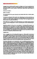
harvest and fire disturbance patterns in an area where both disturbances are known to have occurred. Consideration of the ecological effects of spatial patterns created by forest harvesting is important for the management regime (Franklin and Forman, 1987), and the patterns and processes in landscapes created by natural disturbances generally display greater variation in time and space than traditional silviculture and forest management (Seymour et al., 2002). Disturbance regimes can be described by a variety of characteristics; however, the main components include magnitude, timing, and spatial distribution (Seymour and Hunter, 1999), and each of these will have an impact on the stand- (or patch-) and landscape-level of the forest ecosystem. Magnitude generally describes the intensity or the physical force of the disturbance or the severity of the effect of the disturbance on the landscape element or organism (Seymour and Hunter, 1999; Turner et al., 2001). Timing of a disturbance mainly specifies the frequency, which is often expressed not only as the return interval between disturbances, but also as the duration and seasonality of a disturbance type (Seymour and Hunter, 1999). The spatial distribution of a disturbance refers to the extent, shape, and arrangement of disturbance patches (Seymour and Hunter, 1999). A review by Seymour et al. (2002) of disturbance regimes in northeastern North America contrasts the differences in aspects of these three main characteristics (magnitude, timing, and spatial distribution) by comparing wildfire with pathogens and insect herbivory. In the investigated cases, wildfires were of stand-replacing magnitude, with a return interval of 806 to 9000 years and a disturbance patch size distribution ranging between 2 and more than 80,000 ha, while pathogens and insect herbivory disturbance was of a magnitude to create smaller canopy gaps, with a return interval and patch size distribution ranging between 50 and 200 years and between 0.0004 and 0.1135 ha, respectively (Seymour et al., 2002; Figure 1.1). While the natural disturbance approach may be an ecologically sound premise, its constraints and limitations also need to be considered. Some issues to address in the future include (a) society’s reluctance to accept this paradigm in ecosystems that experience disturbances that are very large, severe, and frequent; (b) whether past disturbance regime effects will be rendered inapplicable in the future due to longterm climatic variation, invasion of nonnative species, air pollution, human-induced climate change (Kimmins, 2004); and (c) the difficulty in obtaining and interpreting historic disturbance data for adequate conclusions about the natural disturbance characteristics (Appleton and Keeton, 1999).
SCALE Every organism is an “observer” of the environment, and every observer looks at the world through a filter, imposing a perceptual bias that influences the recognition of natural systems (Levin, 1992). Science, in general, can be seen as a product of the way the world is seen, constrained by the space and time within which humans inhabit the world (Church, 1996). There is little doubt that ecologists’ perceptions have been revolutionized through availability of satellite imagery; for example:
8
Contiguous area disturbed and regenerated - ha
Understanding Forest Disturbance and Spatial Pattern
10000
Area = 10−8.2 ∗Interval3.74
1000 100
Severe fire and wind
10 1 0.1
0.001 0.0001
Natural canopy gaps
10 100 1000 10000 Interval between disturbances (at the same point on the landscape) - years
FIGURE 1.1 Boundaries of natural variation in studies of disturbance in northeastern North American forests. The hand-fitted diagonal boundary line defines the upper limits on these disturbance parameters in combination, all of which fall in the lower right of the diagram. Upper limits of the area and return interval of severe fires and windstorms were truncated at 104 Ha and 104 years, respectively. (Adapted from Seymour et al., 2002.)
• •
“Images from satellites have revolutionized our perception and approaches to understanding landscapes and regions” (Forman, 1995: p. 35) “More than any other factor, it was this perspective provided by satellite imagery that changed the … manager’s views about the main threats to the panda’s survival” (Mackinnon and de Wulf, 1994, p. 130)
Scale is a strong determinant of viewing, and interpreting the environment and the interest in scale-related research is rapidly increasing (Schneider, 1994). Scale is often understood simply as dimensions of time and space, but has been defined in various more complex ways; for example, Church (1996) considered scale as a relative measure set by the resolution of measurements. Schneider (1994, p.3) defined scale as “the resolution within the range of a measured quantity.” Common to all scientific definitions of scale, however, is a recognition of the temporal and spatial dimensions (Lillesand and Kiefer, 2000; Wiens, 1989).
SPATIAL SCALE In ecology, spatial scale is usually considered as the product of grain and extent (Forman, 1995; Wiens, 1989), which, in remote sensing, relate to resolution (pixel size) and area of coverage, respectively (Lillesand and Kiefer, 2000). A remote sensing scientist will typically define spatial scale as a proportion, a ratio of length on a map to actual length. Small scale, therefore, suggests that a large area is covered; in other words, the difference between actual and mapping size is great (coarse
Introduction: Structure, Function, and Change of Forest Landscapes
9
spatial detail). An ecologist’s typical definition of spatial scale is the level or degree of spatial resolution and spatial extent perceived or considered. Ecologists understand a small-scale study to encompass a small area with fine spatial detail. Overall extent and grain define the upper and lower limits of resolution of a study; they are analogous to the overall size of a sieve and its mesh size (Wiens, 1989). The spatial scale at which measurements or observations are taken influences the recognition of spatial patterns and underlying processes of the environment and of the organisms under study (Wiens, 1989); this has been called intrinsic scale, which may determine the type of spatial patterns observed. “The intrinsic scale is a property of the ecological process of interest, for example, tree fall, competition, stomatal control, or microclimate feedbacks, and it is governed in part by the size of the individual organisms (or events) and in part by the range of their interactions with their environment” (Malingreau and Belward, 1992, p. 2291). Others (e.g., Hunsaker et al., 2001) have been keen to understand the uncertainty associated with spatial data at different scales. Remotely sensed imagery is an optimal way to collect spatial data across multiple nested or hierarchical scales; imagery can provide synoptic coverage over large areas, enabling investigations at the landscape scale, or more detailed imagery can be collected representing smaller areas, most practically through some form of sampling framework. As always, limitations exist in the quantities of spatial resolution and area of coverage that can be obtained. Spatial resolution of imagery depends on the sensor spectral sensitivity, and the instantaneous field of view, while the area of coverage depends on the satellite or airborne altitude (swath width) and the instrument total field of view (Lillesand and Kiefer, 2000; Richards and Jia, 1999). Landsat satellites typically cover an area of 185 × 185 km with a sensor spatial resolution or pixel size of 30 × 30 m for most of the spectral bands; other satellites carrying Advanced Very High Resolution Radiometer (AVHHR) sensors cover an area of 2394 × 2394 km with a spatial resolution of approximately 1.1 km. More details on these fundamental concepts are presented in Chapter 2 of this volume.
TEMPORAL SCALE Temporal scale refers to the frequency with which an observation is made (Lillesand and Kiefer, 2000), but similar to the spatial scale, it is made up of two components; the temporal resolution and the temporal extent. The key to temporal scale is change over time, and this pattern or trend may change with hours, days, months, years, or centuries. Depending on the research question and the object under study, the temporal scale of the investigation can be very different. For each source of imagery, the temporal resolution — a sensor-specific component of scale — must be quantified. Satellites passing frequently over the same area translates into a higher temporal resolution for a given sensor package; for example, the temporal resolution is 24 days for Indian Resource Satellite (IRS)–P2 satellites (Richards and Jia, 1999), but 1 day for satellites carrying the AVHRR (Malingreau and Belward, 1992). In addition, the original start of data collection for different sensor packages determines the maximum possible temporal extent of any earth observation study. Operable satellites launched many years ago translate into a higher temporal extent; for example, the
10
Understanding Forest Disturbance and Spatial Pattern
IRS-P2 satellite was launched in October 1994 (Richards and Jia, 1999), while AVHRR satellites were launched in several National Oceanic and Atmospheric Administration series between June 1979 and May 1991. Clearly, the ability to monitor frequent landscape changes at the temporal scale desired (e.g., daily) may be limited by the temporal resolution and extent of a given satellite platform.
RESEARCH DESIGN
AND INTERPRETATION
Understanding the effect of scale on the detection and understanding of patterns and causal mechanisms is one step toward the development of common ecological theories within scales (Wiens, 1989). There is no single proper scale at which all sampling ought to be undertaken (Levin, 1992; Wiens, 1989), and there are no simple rules to select automatically the appropriate scales of attention (Meentemeyer, 1989). Ecological structure, function, and change are dependent on spatial and temporal scale (Turner, 1989). The identification of the appropriate scale to use will depend on the organism or phenomenon under investigation. A species- or phenomenoncentered approach, with recognition of its intrinsic scale to the identification of structure, is most relevant in the research design and analysis of forest landscapes. Arbitrary scale choices can be avoided by analyzing the variance of measurements across many scales using techniques such as the nearest neighbor method (Davis et al., 2000), semivariance analysis (Meisel and Turner, 1998), and several other univariate (spatial correlograms and spectral analysis) and multivariate methods (Mantel test and Mantel correlogram; Legendre and Fortin, 1989). Statistical approaches are typically based on the observation that variance increases as transitions are approached in hierarchical systems (O’Neill et al., 1986). Peaks of unusually high variance indicate scales at which the between-group differences are especially large, which suggest the representation of the scale of natural aggregation or patchiness of vegetation (Greig-Smith, 1952) or organisms; this is sometimes referred to as the boundary of a scale domain (Wiens, 1989). A method of identifying the appropriate scale of remotely sensed imagery uses a high spatial resolution image characterized statistically and then subsequently collapsed to successively coarser spatial resolutions while calculating local variance (Woodcock and Strahler, 1987). The image resolution at which local variance is highest can be deemed the appropriate remote sensing scale in relation to the structural components of the ground.
PROCESSES GENERATE PATTERNS Remote sensing of terrestrial ecosystems in support of resource management involves identifying ecosystems and their biological, ecological, and physical characteristics (Franklin, 2001). The definition of an ecosystem and the relevant characteristics vary with the resource managed and the issue under consideration. Therefore, the expectations that ecologists might have of remote sensing will vary; for example, species composition and the physical arrangement of the vegetation can be remotely sensed and used to describe or infer ecosystem attributes using straightforward methods and readily available data. Advances in remote sensing technology continue to expand the capacity to monitor changes of interest in ecosystems and
Introduction: Structure, Function, and Change of Forest Landscapes
11
resource management (Wulder et al., 2004). Forest ecosystems change over time because the trees must grow to survive, due to competition among trees, interactions among trophic levels, and large-scale disturbances. Certain aspects of the current state of ecosystem dynamism can be inferred from individual, remotely sensed images, and other aspects can only be assessed using a time series of images. In this section, we provide ecological background on the remote sensing of ecosystem attributes with special attention to the dynamic nature of these ecosystem attributes, the landscape structure, and composition.
FOREST STAND DYNAMICS Current understanding of patterns and processes of stand development have been fully described by Oliver and Larson (1996). Their synthesis is useful as a basis for understanding the potential contributions of remote sensing. Disturbance, meaning the death of trees that frees growing space, is fundamentally important for stand development. Oliver and Larson (1996) distinguished between autogenic and allogenic forms of disturbance; autogenic processes cause death of individual trees for reasons that are particular to the tree and ecosystem, and allogenic forms of disturbance arise outside of the affected trees or ecosystem. For ease of explaining the processes involved in stand dynamics and the stand structures that result, Oliver and Larson first described long-term stand development following a major disturbance, including autogenic processes responsible for death of trees, and then incorporated the impacts allogenic forms of disturbance imposed on this underlying pattern of stand development. Oliver and Larson pointed out that stand development has been investigated from two perspectives, one based on describing stand structures and the other based on understanding stand developmental processes. The latter approach has great value to resource management because it leads to greater capacity for predicting changes to stands over time. Individual remotely sensed images may be well suited to the stand structural approach to understanding stand dynamics, while stand development typically requires multitemporal resolution imagery. Ecological knowledge must be used to interpret the remotely sensed images to ensure maximum information extraction occurs from available remotely sensed data (Graetz, 1990). Forest ecosystems pass through four stages during the course of stand development (Figure 1.2). The period immediately following a major disturbance is the stand initiation stage. During this stage, the important process in stand dynamics is the establishment of a cohort of vegetation. New vegetation becomes established when the preexisting vegetation is killed; the number of species and the number of plants that establish themselves and grow to fill the unoccupied growing space depends on the ecoclimatic zone, site capacity to supply essential materials (nutrients and water), and the relative amount of growing space that is made available and the manner in which it is made available. The period of recruitment ends when the community of trees first comes to fully occupy the available growing space. At this time, the ecosystem enters the stem exclusion stage. Competition among established trees is the dominant process affecting ecosystem development and structure during the stem exclusion stage. Inherent differences among species affect the course of competition and consequently the stand structures that develop. Virtually no growing
12
Understanding Forest Disturbance and Spatial Pattern
Species A dominates
Species B, C & D dominates
Species B dominates
Tree heights
b c d d c c d
a
Time since disturbance Disturbance
“Stand initiation” stage
“Understory reinitiation” stage
“Stem exclusion” stage
“Old growth” stage
b b b
c c
b
c
c
a c c
a
a
b
c
c
c
d
b
b
d
c
d
d
c
d d
d
c
c c
d
c
FIGURE 1.2 Schematic stages of stand development following major disturbances. All trees forming the forest start soon after the disturbance; however, the dominant tree type changes as stem number decreases and vertical stratification of species progresses. The height attained and the time lapsed during each stage vary with species, disturbance, and site. (Adapted from Oliver and Larson, 1996.)
space becomes available for the establishment of additional trees as the result of density-dependent mortality (competition). At about the time that the height growth of successful competitors becomes negligible, these trees begin losing their ability to maintain their “grip” on the growing space. This diminished capacity might be abetted by disease or the activities of insects commonly found in the ecosystem and eventually some trees die. Species that have been less successful in competing in previous years may now expand to fill the vacated growing space and consequently come to dominate the overstory. However, if some of the growing space that comes available is captured by
Introduction: Structure, Function, and Change of Forest Landscapes
13
a ground story, particularly a ground story that includes advanced regeneration of some tree species, then the stand enters the understory reinitiation stage. Stand structure becomes increasingly complex with the onset of the understory reinitiation stage; the advanced regeneration does not have sufficient growing space to form a lower strata of the canopy. Consequently, the ecosystem remains dominated by the cohort of trees that were established after the initial disturbance. At a later time in stand development, the autogenic processes release growing space in sufficiently large areas to cause patches to return to the stand initiation stage, and as a result the ecosystem enters the old-growth stage. With the release of growing space in these patches, advanced growth is released, and other regeneration mechanisms operate to cause a new cohort of trees to become established. The establishment of patches of vegetation of new cohorts continues until all of the original cohort has been replaced, and at this time an old-growth stand exists. In nature, this stage of development is seldom achieved because in many parts of the globe large-scale disturbances return the entire ecosystem to the stand initiation stage. Other forests are influenced by gap-replacing disturbance, and there continues to be considerable debate about the historical frequency of gap versus stand-replacing disturbances. One possible valuable application of remote sensing would be to test some of the assumptions about the frequency and extent of gap versus stand-replacing forest disturbances (Wulder et al., 2004). Oliver and Larson (1996) presented that it is more common for a variety of tree species ranging from pioneers to long-lived, shade-tolerant species to become established during the stand initiation stage (known as initial floristics) than for later seral stage species to become established after early seral stage species have occupied the site, modified the environment, and lived a substantial portion of their life cycle (relay floristics). This is in contrast to ideas of early ecologists, who imagined that stand development involved a succession of stand cover types. Moreover, Oliver and Larson (1996) show that forest ecosystems commonly develop a stratified mixed stand structure during the stand initiation and stem exclusion stages. In stratified mixed stands, the pioneer species grow most rapidly in the years immediately following a disturbance and dominate the overstory in the years immediately following the disturbance. Species with inherently slow initial height growth but capable of surviving in shade, albeit with even slower growth rates, sort themselves into lower strata during the early years of the stem exclusion stage. Species that initially dominate the upper stratum are usually shorter lived than the more tolerant species in lower strata, and hence eventually the lower strata are freed from suppression and dominate the overstory. The difference between the initial floristic pattern of stand establishment and the relay floristic pattern has practical significance when interpreting the pattern of stand development of stratified mixed stands. In the past, stratified mixed stands have been sometimes misinterpreted to be uneven-aged stands, whereas in reality members of all strata became established in response to the same disturbance. This distinction is particularly important when devising silvicultural interventions to maintain or promote particular stand structures. Site characteristics such as microclimate and soil conditions vary spatially, affecting the mix of species that becomes established in the various ecosystems that make up a landscape. During the stand initiation stage, site characteristics can be viewed as environmental “sieves” through which species must pass to become
14
Understanding Forest Disturbance and Spatial Pattern
established. For example, species vary in their capacity to tolerate drought, grow on nutrient-poor soils, become established on cold sites, withstand exposure, and survive in shade. Many remotely sensed images only contain information about the uppermost canopy layer and not about lower strata and the ground story, but knowledge of ecological habits of the tree species and of the stand development patterns operating in the region can be used to better interpret current stages in stand development of the observed ecosystems and their future stand structures. Some promising new image data types with three-dimensional capabilities (e.g., light detection and ranging, LIDAR) are described by Coops et al. (Chapter 2, this volume).
EFFECTS
OF
DISTURBANCE
ON
STAND DYNAMICS
AND
LANDSCAPES
Fire, windthrow, insect attack, and harvesting are examples of allogenic disturbances. Each type of disturbance has a different impact on ecosystems and landscapes, thereby having diverse effects on the stand structure created, the species that can become established in the growing space made available by the disturbance, and changes to the soil and site conditions necessary for tree growth. The frequency and spatial extent of major disturbances affect the proportion of a landscape in each stage of stand development at any point in time. Remote sensing provides data for monitoring disturbances and documenting their effects on each ecosystem in a landscape. These data can provide a means to monitor the subsequent stand development for much larger numbers of ecosystems than could be measured by field surveys. The type and severity of disturbance affects the success that can be achieved by each regeneration strategy. For example, forest fires commonly consume the forest floor, thereby eliminating advanced regeneration and therefore some species such as balsam fir, which rely on advanced growth to become established after disturbance and are prevented from being a future part of the ecosystem after fire. Clark and Bobbe (Chapter 5, this volume) provide background and an example of using remote sensing for portraying fire impacts, and Hudak et al. (Chapter 8, this volume) include fire disturbance in the presented case study. A contrasting example on the role of disturbance in favoring particular regeneration strategies is what happens when the disturbance removes selected species from the overstory but does not eliminate the ground story, such as occurs with outbreaks of defoliating insects (Seymour, 1992; Figure 1.3). In these instances, species regenerating from advanced growth might have an advantage in acquiring the growing space made available, and species that are intolerant of shade might be limited in their capacity to regenerate. Hall et al. (Chapter 4, this volume) develop an approach useful in mapping insect disturbance using remote sensing. Disturbances can create atypical stand structures in ecosystems that had been in the stem exclusion or understory reinitiation stages at the time of disturbance. These relatively young stands would typically have complete overstories of trees belonging to one cohort if only allogenic processes were in play, but after a major disturbance that does not completely eliminate the original cohort, these stands will have more than one cohort visible from above. Such disturbed stands will exhibit greater spatial variability in stand structure than undisturbed stands. It is possible that these disturbed stands will have structure commonly associated with old-growth stands, and these structures might mislead some into believing that they are stable, old-growth
15
Introduction: Structure, Function, and Change of Forest Landscapes
Virgin stand ca. 1860 Red spruce Balsam fir Large, old red spruce dominate the overstory of the multi-aged stand after enduring long periods of suppression on lower strata. Earlier developmental stages are illustrated by the smaller (and probably younger) spruces A, B, and C B in the present stand. Firs generally occupy sub-canopy strata. Removal in1960 1890 sawlog harvests “umbrella” spruce C
A
Typical post-harvest structure ca. 1890
C
A
Repeated sawlog harvests remove old spruce. Residual overstory now consists of previously suppressed, unmerchantable spruces and firs. Advance seedlings and saplings begin to devolop in gaps created by harvesting.
B
Before spruce budworm outbreak ca. 1910
A C B
Many residual firs respond vigorously, and now dominate the overstory. Residual spruces also respond; some trees over 15 cm dbh are removed for pulpwood during early 1900s. Advance regeneration forms dense, virtually continuous lower stratum with an irregular structure corresponding to the tree heights when released.
After spruce budworm outbreak ca. 1925
C A
All mature firs (and some spruces) killed by budworm outbreak ca. 1913–1919. Many advance fir saplings also succumb; some survive but suffer severe dieback of their terminal shoots.
B
Second-growth stand ca. 1970 C B
After recovery, stand quickly returns to stem exclusion stage, as the sapling advance regeneration develops vigorously. Where remnant spruces B and C (from the original old-growth stand) do not blow down or succumb to bark beetles, they now dominate the overstory. Where budwormcaused mortality and logging removed the overstory completely, stand has very even-aged structure, with fir generally dominant over spruce.
FIGURE 1.3 Development of typical spruce-fir stand after logging and budworm attack circa 1860–1970. (Adapted from Seymour 1992.)
16
Understanding Forest Disturbance and Spatial Pattern
ecosystems. Disturbance can also change the capacity of a site to supply the nutrients and water required for establishment and growth. These effects can increase or decrease growth, and the impact on growth might vary over time. For example, fire can release nutrients held in recalcitrant organic matter, thereby increasing plant growth immediately after the fire, but fire also decreases the total stock of nitrogen existing on the site, which may decrease long-term potential productivity. A disturbance affecting a large area can reduce the number of tree species that can disperse seeds onto the disturbed areas. Dispersal distance varies among species depending on mode of dispersal, seed size, and special appendages on seeds that facilitate dispersal. Therefore, species such as trembling aspen with very light seeds that can disperse in wind for great distances can disperse seeds onto large disturbed areas, whereas species with heavy seeds and no wings or other appendages to facilitate dispersal can only disperse a short distance from their site of origin (Burns and Honkala, 1990). In some circumstances, species with restricted dispersal distances maintain a presence in stands that become established because variations in the severity of the disturbance leave islands of living trees throughout the disturbed area to serve as seed sources. For example, small patches of burned or lightly burned forest are sometimes found scattered across a burned landscape, and seeds from species such as white spruce can disperse from these refugia into the surrounding disturbed area. Large-scale disturbance is an integral part of numerous landscapes affecting the species found and the distribution of land area among stages of development. As a consequence, large-area forest fires affect virtually all of the boreal forest of central Canada on a regular basis (Stocks et al., 2003). Only tree species that are adapted to regenerate after fire are found in this region. Moreover, most stands are in the stem exclusion stage or early in the understory reinitiation stages because the fire frequency precludes many stands reaching the old-growth stage. Similarly, widespread outbreaks of spruce budworm in the spruce-fir forests of eastern North America profoundly affect stand development and the landscape (Baskerville, 1975). Spruce budworm outbreaks occur at 30-year intervals, and in northern New Brunswick there were two age classes of ecosystems existing at the beginning of the outbreak: 30-year-old forest stands originating from the immediately previous outbreak and 60-year-old stands originating from the outbreak before the last one (Figure 1.4). There is widespread mortality in the 60-year-old stands, causing those ecosystems to return to the stand initiation stage. In the 30-year-old stands, the effect of spruce budworm mortality is to thin stands and shift species composition to a higher percentage of spruce and birch and a lower percentage of balsam fir, although balsam fir usually continues to be the largest proportion of these stands. In this manner, disturbance has largely determined the landscape characteristics and significantly affected stand development of most stands in the region.
PATTERNS GENERATE PROCESSES IMPACTS
OF
PATTERNS
ON
ECOLOGICAL PROCESSES
Just as physical and ecological processes generate landscape structure, landscape structure influences physical and ecological processes. Specifically, landscape pattern
Introduction: Structure, Function, and Change of Forest Landscapes
17
1875 Budworm outbreak
1885
1912 Budworm outbreak
1924
1949 Budworm outbreak
1959 Unsprayed
Sprayed
Unsprayed
Sprayed
1972
FIGURE 1.4 Natural succession in the Green River fir-spruce-birch forest. The two columns represent two sequences both beginning in 1875 but with differing initial conditions. The blackened tops represent disfiguration by intensive budworm feeding. The hatched cones represent white spruce trees, the unshaded cones are firs, and the rounded trees are hardwoods. (Adapted from Baskerville, 1975.)
has been found to affect rates of wind and water erosion, intensity of natural disturbances (Foster, 1988), plant and animal movement (Beier and Noss, 1998), survival (Doherty and Grubb, 2002), and reproduction (Robinson et al., 1995). Here, a brief review is provided of the components of landscape pattern that have been shown to exert a strong influence on ecological processes. Such patterns are considered priorities for measurement in remote sensing (Gergel, Chapter 7, this volume).
18
Understanding Forest Disturbance and Spatial Pattern
All landscapes are characterized by degrees of heterogeneity (patchiness) at different scales; differing substrates (soils, bedrock), natural disturbances (fire, insect outbreaks), and human activity (forestry, road building) all create patchiness across a landscape. The “patch-corridor-matrix” model (Forman, 1995) has become a central component of landscape ecology in theory and in practice: 1. A patch is a homogenous area that differs from its surroundings (Forman, 1995). A woodlot surrounded by farmland and a wetland immersed in upland habitat are examples of patches. Patch shape often correlates with the intensity of human activity. Intense human activity often results in simpler, less-convoluted patch shape 2. Corridors are a form of patch in that they differ from the surrounding areas. However, they are usually identified as strips that aid in flows between patches (Lindenmayer, 1994). Corridors fulfill a number of roles, including facilitating animal dispersal, wildlife habitat, preventing soil and wind erosion, and aiding in integrated pest management (Barrett and Bohlen, 1991). A riparian buffer strip might serve as a corridor for forest songbirds (Machtans et al., 1996) or a kilometers-wide forested strip could serve as a corridor for cougar (Beier, 1995). The life history traits of each species determine the characteristics of corridor habitat 3. The matrix is the most extensive component of the landscape, is highly connected, and controls regional dynamics (Forman, 1995). For instance, in the Canadian prairies, small woodlot patches occur in a matrix of natural grassland or agricultural development The landscape structures briefly described above (patches, corridors, and matrix) influence, and are influenced by, landscape flows. These flows include diverse elements such as wildlife (Lindenmayer and Nix, 1993), soil and nutrients (Stanley and Arp, 1998), and water (Campbell, 1970). For example, Haddad (1999) demonstrated that pine plantations impede the movement of butterflies between patches of early successional forest. One of the central principles of landscape ecology is that all ecosystems are interrelated, with movement or flow rate dropping sharply with distance but more gradually between ecosystems of the same type (Forman, 1995). Thus, a very heterogeneous landscape (with many patch types) is marked by a relatively low degree of movement (flow) and a large amount of resistance.
FRAGMENTATION, CONNECTIVITY,
AND ISOLATION
Fragmentation is the “breaking apart” of habitat. This can occur as a result of natural processes such as forest fires or anthropogenic disturbances such as road building or timber harvesting. Different views exist about definitions regarding “habitat loss” and “fragmentation.” Wilcove et al. (1986) suggested that fragmentation is a combination of habitat loss and isolation; however, recently the emerging consensus is that habitat loss and fragmentation should be described separately (Andrén, 1994; Fahrig, 1998, 2002; Mazerolle and Villard, 1999). Fragmentation is often defined
Introduction: Structure, Function, and Change of Forest Landscapes
A
19
B
FIGURE 1.5 Unfragmented (A) versus fragmented (B) landscapes with the same amount of habitat present in each landscape.
purely as the breaking apart of habitat and does not always imply habitat loss. For instance, holding habitat area constant, a landscape can either be fragmented (i.e., many patches) or unfragmented (i.e., one patch) (Figure 1.5). While habitat loss and fragmentation are often confounded in real landscapes (i.e., they occur together), we emphasize that it is important to determine which of these is ecologically important; if populations respond to habitat fragmentation, land managers may be able to design landscapes that mitigate risks. Landscape fragmentation effects may be grouped into a few major categories, including edge, patch size, and distance between patches (connectivity) (Schmiegelow and Mönkkönen, 2002). For example, edges are the result of vegetation boundaries in the landscape and may result from (a) enduring features (soils, drainage, slope); (b) natural disturbances; or (c) human activities such as forest harvesting or farm development. An edge effect may be caused by differences in moisture, temperature, and light that occur along the boundary between different adjacent patch types (Saunders et al., 1991). A number of studies have reported increased rates of predation at forest edges (Paten, 1994); however, this appears to be context dependent (Batáry and Báldi, 2004). Many organisms are affected by the size of favorable habitat patches. Such species are termed area sensitive (Freemark and Collins, 1992). Robbins et al. (1989) found that “area” was one of the most significant habitat features for many neotropical migrant bird species. Area sensitivity has also been observed for amphibians (Hager, 1998). Although some debate exists about the area sensitivity of plants, a number of published studies reported lower genetic diversity and higher rates of extinction in smaller populations (Bell et al., 1991; Damman and Cain, 1998). In some cases, fragmented landscapes have been shown to exhibit the same characteristics as those observed in island archipelagos by MacArthur and Wilson (1967). Isolation of habitat seems to compound the effect of small patch size on the ability of some species to persist and recolonize. These findings can be understood better if placed in the context of the concept of metapopulations. The metapopulation concept requires that population dynamics be studied beyond the scale of local populations. “Equilibrium,” rather than occurring in a single, local population, might
20
Understanding Forest Disturbance and Spatial Pattern
occur as a result of a number of interconnected subpopulations that are distributed across a region (Husband and Barrett, 1996). Population dynamics are the result of a series of local extinctions and recolonizations in habitat patches (Levins, 1970). If the subpopulation of one patch becomes extinct, then it may eventually be recolonized by dispersers from a subpopulation that exists in a neighboring patch. This is the “rescue effect”; for a species to spread or persist, individuals must colonize unoccupied habitat patches at least as frequently as populations become extinct (Hanski and Ovaskainen, 2000). As fragmentation progresses, the distance between patches (isolation) of mature forest increases. This distance limits the ability of organisms to disperse and colonize new habitat patches. It is important to note that, in addition to the studies briefly described above indicating a significant influence of landscape pattern on species distributions, there are many studies that reveal only weak or nonexistent landscape pattern effects (Delin and Andrén, 1999; Game and Peterken, 1984; McGarigal and McComb, 1995; Schmiegelow et al., 1997; Simberloff and Gotelli, 1984). Indeed, the majority of evidence indicates that it is habitat loss rather than fragmentation per se that is the most important influence on species occurrence, reproduction, and survival (Fahrig, 2003). This appears particularly to be the case in forest mosaics (for reviews, see Bender et al., 1998; Mönkkönen and Reunanen, 1999). This idea reinforces the notion that it is important for remote sensing to provide accurate classifications of landscape composition in addition to input data to analyses of landscape configuration. Andrén (1994) proposed that landscape configuration is only important below a threshold in the proportion of suitable habitat at the landscape scale. Only at low levels of habitat are patches small and isolated enough to result in patch size effects or restrictions in movement (Gardner et al., 1991). This results in multiplicative impacts of fragmentation on habitat loss. A number of theoretical studies supported this “fragmentation threshold” hypothesis (Fahrig, 1998; Hill and Caswell, 1999; Wiegand et al., 2005; With and King, 1999), but it has rarely been demonstrated in nature (Trzcinski et al., 1999). However, this may be because “suitable habitat” has rarely been defined according to the requirements of individual species.
PREDICTIVE MODELING OF SPECIES OCCURRENCE USING GEOSPATIAL DATA To determine rates of change in the amount and pattern of habitat at any spatial scale, it is clearly necessary to have accurate definitions of habitat for different species. Remotely sensed data have been used extensively to develop habitat models; these are inexpensive to develop in comparison to models based on detailed vegetation data collected in the field (Osborne et al., 2001; Vernier et al., 2002) and provide an opportunity to generate predictions about species distributions over large spatial extents at relatively fine resolutions (Betts et al., 2006; Gibson et al., 2004; Linke et al., 2005). Such models are usually probabilistic in nature, but a wide range of modeling techniques are available, including classification trees, neural networks, generalized linear models, generalized additive models, and spatial interpolators (Segurado and Araujo, 2004). Models have been developed to cover aspects as diverse as biogeography, conservation biology, climate change research, habitat or species management (Guisan and Zimmermann, 2000), and vegetation mapping (J.
Introduction: Structure, Function, and Change of Forest Landscapes
21
F. Franklin, 1995). As the resolution of remotely sensed data improves, the range of potential applications is likely to increase (Coops et al., Chapter 2, this volume; Wulder et al., 2004).
LANDSCAPE METRICS To study the effects of landscape structure on ecological processes, it is necessary to develop methods to quantify spatial patterns into measurable variables before links to ecological processes can be determined (Frohn, 1998). Landscape metrics, or indices, have been developed to meet this need (Diaz, 1996). Early landscape metric studies presented only a few metrics, typically dominance (the degree to which certain kinds of landscape patches or classes predominate in the landscape), contagion (the extent to which similar patches are clumped together), and shape (the form of an area or a patch as determined by the variation of its border) (Forman, 1995; O’Neill et al., 1988). Today, an extensive array or suite of landscape metrics and indices exists (Elkie et al., 1999; McGarigal and Marks, 1995). The suite of available landscape metrics can be considered to include specific measures of area, edge, shape, core (or interior) area, nearest neighbor/diversity/richness/evenness, interspersion/juxtaposition, contagion/configuration, and connectivity/circuitry (Gergel, Chapter 7, this volume; McGarigal et al., 2000). The large number of metrics that have been developed to describe and quantify spatial structure often appears to be overwhelming, and the question of metric redundancy has frequently arisen. Initially, use of metrics that have known ecological relevance and application should be considered. However, some standard approaches have been employed to deal with the issues of redundancy and number of metrics for a given application. For example, Riitters et al. (1995) used a factor analysis to reduce to a few components more than 50 specific landscape metrics applied to 85 maps of land use and cover in the United States. Recent studies have concluded that it is possible to identify a parsimonious suite of metrics using principal components analysis to characterize much of the spatial patterns existing in a boreal forest landscape subject to many common disturbance processes (S. Cushman, personal communication, April and October, 2002; Linke and Franklin, in press). In addition to the issue of appropriate metric selection, there are several other factors known potentially to influence the interpretation and use of landscape metrics (Haines-Young and Chopping, 1996), including, for example, metric uniqueness, sensitivity, abrupt versus continuous edges, statistical quantification, study area extent, and scale or resolution. Another important characteristic of landscape metrics to consider is their actual behavior over a wide range of landscape structures; the instance of nonlinear landscape metric behavior over scale is briefly mentioned here: 1. Hargis et al. (1998) investigated the relationships between six landscape metrics and the proportion of two landcover types across simulated landscapes, also controlling for the size and shape of patches. Most metrics were linearly associated at the lower landcover proportion range but had nonlinear associations at higher proportions, which limits their direct comparability across different regions
22
Understanding Forest Disturbance and Spatial Pattern
2. Such nonlinear metric behavior was also found in simulated landscapes in a study of dispersal success on fractal landscapes (With and King, 1999) and in a study specifically designed to detect metric behavior under controlled conditions (Neel et al., 2004) An awareness of all of these interpretational effects and metric behavioral limitations must be embedded in any landscape quantification attempt. A detailed discussion of spatial pattern analysis using landscape metrics is presented by Gergel in Chapter 7.
CONCLUSION Understanding forest disturbance and spatial pattern is increasingly recognized as essential to effective and sustainable forest management in many forest environments around the world. We hope that this introduction has provided some insight into the challenges that are further elaborated in later chapters; the developing appetite in landscape ecology and conservation biology for spatial data and models that work with complex phenomena; the relationships between pattern and process, process and pattern; the specific details of remotely sensed and GIS data selection; the importance of scale; the myriad issues in fire and insect, forest harvesting, and other disturbance monitoring; and the emerging role of landscape metrics and modeling landscapes. The literature and practice of forest disturbance and spatial pattern using remote sensing and GIS approaches are diverse and increasing at an astonishing rate as new perspectives and insights take hold. We expect this presentation will be useful to those involved in this interesting and exciting endeavor, in the implementation and continued development of remote sensing and GIS approaches, and in their application to forest ecosystems and processes. We anticipate progress in these areas will help shape future directions in the important work of forest resource mapping, monitoring, and management.
ACKNOWLEDGMENTS The support of the Canadian Forest Service and the Natural Sciences and Engineering Research Council of Canada is gratefully acknowledged. We acknowledge the careful review and many helpful suggestions to improve this chapter provided during the review process.
REFERENCES Andrén, H. (1994). Effects of habitat fragmentation on birds and mammals in landscapes with different proportions of suitable habitat: a review. Oikos, 71, 355–366. Appleton, G.H. and Keeton, W.S. (1999). Applications of historic range of variability concepts to biodiversity conservation. In R.K. Baydack, H. Champa III, and J.B. Haufler (Eds.), Practical Approaches to the Conservation of Biological Diversity (pp. 71–86). Island Press, Washington, DC 313p.
Introduction: Structure, Function, and Change of Forest Landscapes
23
Attiwill, P.M. (1994). The disturbance of forest ecosystems: the ecological basis for conservative management. Forest Ecology and Management, 63, 247–300. Balmford, A., Green, R.E., and Jenkins, M. (2003). Measuring the changing state of nature. Trends in Ecology and Evolution, 18(7), 326–330. Barrett, G. and Bohlen, P. (1991). Landscape ecology. In W. Hudson (Ed.), Landscape Linkages and Biodiversity (pp. 149–161). Island Press, Washington, DC. 194p. Baskerville, G.L. (1975). Spruce budworm: super silviculturist. The Forestry Chronicle, August, 138–140. Batáry, P. and Báldi, A. (2004). Evidence of an edge effect on avian nest success. Conservation Biology, 18, 389–400. Beier, P. (1995). Dispersal of juvenile cougars in fragmented habitat. Journal of Wildlife Management, 59, 41–67. Beier, P. and Noss, R.F. (1998). Do habitat corridors provide connectivity? Conservation Biology, 12, 1241–1252. Bell, G., Martin, J., and Schoen, D. (1991). The ecology and genetics of fitness in forest plants III. Environmental variance in natural populations of Impatiens pallida. Journal of Ecology, 79, 697–713. Bender, D.J., Contreras, T.A., and Fahrig, L. (1998). Habitat loss and population decline: a meta-analysis of the patch size effect. Ecology, 79, 517–533. Bergeron, Y., Harvey, B., Leduc, A., and Gauthier, S. (1999). Forest management guidelines based on natural disturbance dynamics: stand and forest-level considerations. Forestry Chronicle, 75, 49–54. Betts, M., Forbes, G., and Knox, J. (2002). A landscape ecological approach to private woodlot planning in New Brunswick. Natural Areas Journal, 22, 311–317. Betts, M.G., Diamond, A.W., Forbes, G.J., Villard, M.-A., and Gunn, J. (2006). The importance of spatial autocorrelation, extent and resolution in predicting forest bird occurrence. Ecological Modelling, 191, 197–224. Botkin, D.B. (1990). Discordant Harmonies: A New Ecology for the Twenty-First Century. Oxford University Press, New York. 244p. Bunnell, F.L. (1995). Forest-dwelling vertebrate faunas and natural fire regimes in British Columbia: patterns and implications for conservation. Conservation Biology, 9, 636–644. Burns, R.M. and Honkala, B.H. (1990). Silvics of North America. Volume 2, Hardwoods. U.S. Department of Agriculture, Forest Service, Washington, DC. Agriculture Handbook 654. 877p. Campbell, C. (1970). Ecological implications of riparian vegetation management. Journal of Soil and Water Conservation, 2, 49–52. Church, M. (1996). Space, time and the mountain — how do we order what we see? The scientific nature of geomorphology. Proceedings of the 27th Binghamton Symposium in geomorphology (pp. 147–170). Edited by Rhoads, B.L. and C.E. Thorn. John Wiley & Sons, New York. Crow, T.R. and Perera, A.H. (2004). Emulating natural landscape disturbance in forest management — an introduction. Landscape Ecology, 19, 231–233. Damman, H. and Cain, M. (1998). Population growth and viability analyses of the clonal woodland herb, Asarum canadense. Ecology, 86, 13–26. Davis, J.H., Howe, R.W., and Davis, G.J. (2000). A multi-scale spatial analysis method for point data. Landscape Ecology, 15, 99–114. Diaz, N.M (1996). Landscape metrics. A new tool for forest ecologists. Journal of Forestry, 94(12), 12–16. Delin, A.E. and Andrén, H. (1999). Effects of habitat fragmentation on Eurasian red squirrel (Sciurus vulgaris) in a forest landscape. Landscape Ecology, 14, 67–72.
24
Understanding Forest Disturbance and Spatial Pattern
Doherty, P.F. and Grubb, T.C. (2002). Survivorship of permanent-resident birds in a fragmented forested landscape. Ecology, 83, 844–857. Elkie, P.C., Rempel, R.S., and Carr, A.P. (1999). Patch Analyst User’s Manual: A Tool for Quantifying Landscape Structure. Ministry of Natural Resources, Northwest Science and technology, Thunder Bay, ON, Canada. NWST Technical Manual TM002. 22p. Engelmark, O., Bradshaw, R., and Bergeron, Y. (1993). Disturbance dynamics in boreal forests: introduction. Journal of Vegetation Science, 4, 730–732. Fahrig, L. (1998). When does fragmentation of breeding habitat affect population survival? Ecological Modelling, 105, 273–292. Fahrig, L. (2002). Effect of habitat fragmentation on the extinction threshold: a synthesis. Ecological Applications, 12, 346–353. Fahrig, L. (2003). Effects of habitat fragmentation on biodiversity. Annual Reviews of Ecology and Systematics, 34, 487–515. Forman, R.T.T. (1981). Interaction among landscape elements: a core of landscape ecology. In S.P. Tjallingii and A.A. de Veer (Eds.), Perspectives in Landscape Ecology (pp. 35–48). PUDOC, Wageningen, Netherlands. 344p. Forman, R.T.T. (1995). Land Mosaics, the Ecology of Landscapes and Regions. Cambridge University Press, Cambridge, U.K. 632p. Foster, D.R. (1988). Species and stand response to catastrophic wind in central New England. U.S.A. Journal of Ecology, 80, 753–772. Franklin, J.F. (1995). Predictive vegetation mapping: geographic modelling of biospatial patterns in relation to environmental gradients. Progress in Physical Geography, 19, 474–499. Franklin, J.F. and Forman, R.T.T. (1987). Creating landscape patterns by forest cutting: ecological consequences and principles. Landscape Ecology, 1, 5–18. Franklin, S. E. (2001). Remote Sensing for Sustainable Forest Management, Lewis Publishers/CRC Press, Boca Raton, FL. 407p. Freemark, K. and Collins, B. (1992). Landscape ecology of birds breeding in temperate forest fragments. In J. Hagan and D. Johnson (Eds.), Ecology and Conservation of Neotropical Migrant Landbirds (pp. 443–454). Smithsonian Institution Press, Washington, DC. 609p. Frohn, R.C. (1998). Remote Sensing for Landscape Ecology: New Metric Indicators for Monitoring, Modeling, and Assessment of Ecosystems. Lewis Publishers, New York. 99p. Game, M. and Peterken, G. (1984). Nature reserve selection strategies in the woodlands of central Lincolnshire, England. Biological Conservation, 29, 157–181. Gardner, R.H., Turner, M.G., O’Neill, R.V., and Lavorel, S. (1991). Simulation of scaledependent effects of landscape boundaries on species persistence and dispersal. In M.M. Holland, P.G. Risser, and R.J. Naiman (Eds.), Ecotones: The Role of Landscape Boundaries in the Management and Restoration of Changing Environments (pp. 76–89). Chapman and Hall, New York. 142p. Gibson, L.A., Wilson, B.A., Cahill, D.M., and Hill, J. (2004). Spatial prediction of rufous bristlebird habitat in a coastal heathland: a GIS-based approach. Journal of Applied Ecology, 41, 213–223. Gong, P. and B. Xu, B.(2003). Remote sensing of forests over time: change types, methods, and opportunities. In M.A. Wulder and S. E. Franklin (Eds.), Remote Sensing of Forest Environments: Concepts and Case Studies (pp. 301–333). Kluwer Academic Publishers, Norwell, MA. 519p.
Introduction: Structure, Function, and Change of Forest Landscapes
25
Graetz, R.D. (1990). Remote sensing of terrestrial ecosystem structure: An ecologist’s pragmatic view. In R.J. Hobbs and H.A. Mooney (Eds.), Remote Sensing of Biosphere Functioning (pp. 5–30). Springer-Verlag, New York. 312p. Greig-Smith, P. (1952). The use of random and contiguous quadrats in the study of the structure of plant communities. Annals of Botany, 16, 293–316. Guisan, A. and Zimmermann, N.E. (2000). Predictive habitat distribution models in ecology. Ecological Modelling, 135, 147–186. Haddad, N.M. (1999). Corridor and distance effects on interpatch movements: a landscape experiment with butterflies. Ecological Applications, 9, 612–622. Hager, H.A. (1998). Area-sensitivity of reptiles and amphibians: are there indicator species for habitat fragmentation? Ecoscience, 5, 139–147. Hansen, A.J., Neilson, R.P., Dale, V.H., Flather, C.H., Iverson, L.R., Currie, D.J., Shafer, S., Cook, R., and Bartlein, P.J. (2001). Global change in forests: responses of species, communities, and biomes. Bioscience, 51, 765–779. Hanski, I. and Ovaskainen, O. (2000). The metapopulation capacity of a fragmented landscape. Nature, 404, 755–758. Hansson, L. (1991). Dispersal and connectivity in metapopulations. Biological Journal of the Linnean Society, 42, 89–103. Haines-Young, R. and Chopping, M. (1996). Quantifying landscape structure: a review of landscape indices and their application to forested landscapes. Progress in Physical Geography, 20, 418–445. Hargis, C.D., Bissonette, J.A., and David, J.L. (1998). The behaviour of landscape metrics commonly used in the study of habitat fragmentation. Landscape Ecology, 13, 167–186. Hill, M.F. and Caswell, H. (1999). Habitat fragmentation and extinction thresholds on fractal landscapes. Ecology Letters, 2, 121–127. Houghton, R.A. (1994). The worldwide extent of land-use change. Bioscience, 44, 305–313. Hunsaker, C., Goodchild, M., Friedl, M., and Case, E., (Eds.), (2001). Spatial Uncertainty in Ecology: Implications for Remote Sensing and GIS Applications. Springer-Verlag, New York. 402p. Hunter, M.L., Jr. (1990). Wildlife, Forests, and Forestry: Principles of Managing Forests for Biological Diversity. Prentice-Hall, Englewood Cliffs, NJ. 370p. Hunter, M.L., Jr. (1999). Maintaining Biodiversity in Forest Ecosystems. Cambridge University Press, Cambridge, U.K. 698p. Husband, B.C. and Barrett, S.C.H. (1996). A metapopulation perspective in plant biology. Journal of Ecology, 84, 461–469. Iverson, L.R., Graham, R.L., and Cook, E. A. (1989). Applications of satellite remote sensing to forested ecosystems. Landscape Ecology, 3, 131–143. Kimmins, J.P.H. (2004). Emulating natural forest disturbance: what does this mean? In A.H. Perera, L.J. Buse, and M.G. Weber (Eds.), Emulating Natural Forest Landscape Disturbances: Concepts and Applications (pp. 8–28). Columbia University Press, New York. 315p. Legendre, P. and Fortin, M.J. (1989). Spatial pattern and ecological analysis. Vegetatio, 80, 107–138. Levin, S.A. (1978). Pattern formation in ecological communities. In J.S. Steele (Ed.), Spatial Pattern in Plankton Communities (pp. 433–465). Plenum Press, New York. 482p. Levin, S.A. (1992). The problem of patterns and scale in ecology. Ecology, 73, 1943–1967. Levins, R. (1970). Extinction. In M. Gerstenhaber (Ed.), Some Mathematical Questions in Biology (pp. 77–107). American Mathematical Society, Providence, RI.
26
Understanding Forest Disturbance and Spatial Pattern
Lillesand, T.M. and Kiefer, R.W. (2000). Remote Sensing and Image Interpretation. 4th ed. John Wiley & Sons, New York. 724p. Lindenmayer, D. (1994). Wildlife corridors and the mitigation of logging impacts on fauna in wood-production forests in south-eastern Australia: a review. Wildlife Research, 21, 323–340. Lindenmayer, D. and Nix, H. (1993). Ecological principles for the design of wildlife corridors. Conservation Biology, 7, 627–630. Linke, J. and Franklin, S.E. (In press). Interpretation of landscape metric gradients based on satellite image classification of land cover. Canadian Journal of Remote Sensing. Linke, J., Franklin, S.E., Huettmann, F., and Stenhouse, G. (2005). Seismic cutlines, changing landscape metrics and grizzly bear landscape use in Alberta. Landscape Ecology, 20, 811–826. Machtans, C., Villard, M.-A., and Hannon, S. (1996). Use of riparian buffer strips as movement corridors by forest birds. Conservation Biology, 10, 1366–1379. Mackinnon, J. and de Wulf, R. (1994). Designing protected areas for giant pandas in China. In R.I. Miller (Ed.). Mapping the Diversity of Nature (pp.127–142). Chapman and Hall, London. Malingreau, J.P. and Belward, A.S. (1992). Scale considerations in vegetation using AVHRR data. International Journal of Remote Sensing, 13, 2289–2307. Martin, K.J. and McComb, W.C. (2002). Small mammal habitat associations at patch and landscape scales in Oregon. Forest Science, 48, 255–264. Mazerolle, M. and Villard, M-A. (1999). Patch characteristics and landscape context as predators of species presence and abundance: a review. Ecoscience, 6, 117–124. MacArthur, R. and Wilson, E.O. (1967). The Theory of Island Biogeography. Princeton University, Princeton, NJ. 203p. McGarigal, K. and Marks, B.J. (1995). FRAGSTATS. Spatial Pattern Analysis Program for Quantifying Landscape Structure. Reference Manual. Forest Science Department Oregon State University, Corvallis, OR. 122p. McGarigal, K. and McComb, W. (1995). Relationships between landscape structure and breeding birds in the Oregon coast range. Ecological Monographs, 65, 235–260. McGarigal, K., Cushman, S., and Stafford, S. (2000). Multivariate Statistics for Wildlife and Ecology Research. Springer-Verlag, New York. 283p. Meentemeyer, V. (1989). Geographical perspectives of space, time, and scale. Landscape Ecology, 3, 163–173. Meisel, J.E. and Turner, M.G. (1998). Scale detection in real and artificial landscapes using semivariance analysis. Landscape Ecology, 13, 347–362. Meyer, W.B. and Turner, B.L. II. (1994). Changes in Land Use and Land Cover: A Global Perspective. Cambridge University Press, Cambridge, U.K. 537p. Miller, J.R., Dixon, M.D., and Turner, M.G. (2004). Response of avian communities in largeriver floodplains to environmental variation at multiple scales. Ecological Applications, 14, 1394–1410. Mönkkönen, M. and Reunanen, P. (1999). On critical thresholds in landscape connectivity: a management perspective. Oikos, 84, 302–305. Neel, M., McGarigal, K., and Cushmann, S.A. (2004). Behaviour of class-level landscape metrics across gradients of class aggregation and area. Landscape Ecology, 19, 435–455. Noss, R.F. (1983). A regional landscape approach to maintain diversity. BioScience, 33, 700–706. Oliver, C.D. and Larson, B.C. (1996). Forest Stand Dynamics. John Wiley & Sons, New York. 520p.
Introduction: Structure, Function, and Change of Forest Landscapes
27
O’Neill, R.V., DeAngelis, D.L., Waide, J.B., and Allen, T.F.H. (1986). A Hierarchical Concept of Ecosystems. Princeton University Press, Princeton, NJ. 253p. O’Neill, R.V., Krummel, J.R., Gardner, R.H., Sugihara, G., Jackson, B., DeAngelis, D.L., Milne, B.T., Turner, M.G., Zygmunt, B., Christensen, S.W., Dale, V.H., and Graham, R.L. (1988). Indices of landscape pattern. Landscape Ecology, 1, 153–162. Osborne, P.E., Alonso, J.C., and Bryant, R.G. (2001). Modelling landscape-scale habitat use using GIS and remote sensing: a case study with Great Bustards. Journal of Applied Ecology, 38, 458–471. Paten, P.W.C. (1994). The effect of edge on avian nest success: how strong is the evidence? Conservation Biology, 8, 17–26. Perera, A.H. and Euler, D.L. (2000). Landscape ecology in forest management: An introduction. In A.H. Perera, D.L. Euler, and I.D. Thompson (Eds.), Ecology of a Managed Terrestrial Landscape: Patterns and Processes of Forest Landscapes in Ontario (pp. 3–11). UBC Press, Vancouver, BC, Canada. 336p. Quattrochi, D.A. and Pellier, R.E. (1991). Remote sensing for analysis of landscapes: an introduction. In M.G. Turner and R.H. Gardner (Eds.), Quantitative Methods in Landscape Ecology: The Analysis and Interpretation of Landscape Heterogeneity (pp. 51–76). Springer-Verlag, New York. 536p. Remmel, T.K. and Csillag, F. (2003). When are two landscape pattern indices significantly different? Journal of Geographical Systems, 5, 331–351. Richards, J.A. and Jia, X. (1999). Remote Sensing Digital Image Analysis. Springer, New York. 363p. Riitters, K.H., O’Neill, R.V., Hunsaker, C.T., Wickham, J.D., Yankee, D.H., Timmins, S.P.,Jones, K.B., and Jackson, B.L. (1995). A factor analysis of landscape pattern and structure metrics. Landscape Ecology, 10, 23–39. Riitters, K.H., Wickham, J.D., O’Neill, R.V., Jones, K.B., Smith, E.R., Coulston, J.W., Wade, T.G., and Smith, J.H. (2002). Fragmentation of continental United States forests. Ecosystems, 5, 815–822. Risser, P.G., Karr, J.R., and Forman, R.T.T. (1984). Landscape ecology: directions and approaches. Illinois Natural History Survey Special Publication No. 2. Illinois Natural History Survey, Champaign, IL. 18p. Robbins, C.S., Dawson, D., and Dowell, B. (1989). Habitat area requirements of breeding forest birds of the Middle Atlantic States. Wildlife Monographs, 103, 1–34. Roberts, D.A., Keller M., and Soares, J.V. (2003). Studies of land-cover, land-use, and biophysical properties of vegetation in the Large Scale Biosphere Atmosphere experiment in Amazonia. Remote Sensing of Environment, 87, 377–388. Robinson, S.K., Thompson, F.R., Donovan, T.M., Whitehead, D.R., and Faaborg, J. (1995). Regional forest fragmentation and the nesting success of migratory birds. Science, 267, 1987–1989. Saunders, D., Hobbs, R., and Margules, C. (1991). Biological consequences of ecosystem fragmentation: a review. Conservation Biology, 5, 18–32. Schmiegelow, F.K.A., Machtans, C., and Hannon, S. (1997). Are boreal birds resilient to forest fragmentation? An experimental study of short-term community responses. Ecology, 78, 1914–1932. Schmiegelow, F.K.A. and Mönkkönen, M. (2002). Habitat loss and fragmentation in dynamic landscapes: avian perspectives from the boreal forest. Ecological Applications, 12, 375–389. Schneider, D.C. (1994). Quantitative Ecology, Spatial and Temporal Scaling. Academic Press, New York. 395p.
28
Understanding Forest Disturbance and Spatial Pattern
Segurado, P. and Araujo, M.G. (2004). An evaluation of methods for modelling species distributions. Journal of Biogeography, 31, 1555–1568. Seymour, R.S. (1992). The red spruce — balsam fir forest of Maine: evolution of silvicultural practice in response to stand development patterns and disturbances. In M.J. Kelty, B.C. Larson, and O.D. Oliver (Eds.), The Ecology and Silviculture of Mixed-Species Forests (pp. 217–244). Kluwer Academic Publishers, Dordrecht, Netherlands. 287p. Seymour, R.S. and Hunter, M.L., Jr. (1999). Principles of ecological forestry. In M.L. Hunter Jr. (Ed.), Maintaining Biodiversity in Forest Ecosystems (pp. 22–64). Cambridge University Press, Cambridge, U.K. 698p. Seymour, R.S., White, A.S., and deMaynadier, P.G. (2002). Natural disturbance regimes in northeastern North America — evaluating silvicultural systems using natural scales and frequencies. Forest Ecology and Management, 155, 357–367. Simberloff, D. and Gotelli, N. (1984). Effects of insularisation on plant species richness in the prairie-forest ecotone. Biological Conservation, 29, 27–46. Spies, T.A. (1997). Forest stand structure, composition and function. In K.A. Kohm and J.F. Franklin (Eds.), Creating a Forestry for the 21st Century, the Science of Ecosystem Management (pp. 11–30). Island Press, London. Stanley, B. and Arp, P. (1998). Timber Harvesting of Forested Watershed: Impacts on Stream Discharge. Faculty of Forestry and Environmental Management, Fredericton, NB, Canada. Stocks, B.J., Mason, J.A., Todd, J.B., Bosch, E.M., Wotton, B.M., Amiro, B.D., Flannigan, M.D., Hirsch, K.G., Logan, K.A., Martell, D.L., and Skinner, W.R. (2003). Large forest fires in Canada, 1959–1997. Journal of Geophysical Research. Atmospheres. 108 (D1) 8149, doi:10.1029/2001JD000484. Trzcinski, M.K., Fahrig, L., and Merriam, G. (1999). Independent effects of forest cover and fragmentation on the distribution of forest breeding birds. Ecological Applications, 9, 586–593. Turner, M.G. (1987). Landscape Heterogeneity and Disturbance. Springer Verlag, New York. 241 p. Turner, M.G. (1989). Landscape ecology: the effect of pattern on process. Annual Review of Ecology and Systematics, 20, 171–197. Turner, M.G., Gardner, R.H., and O’Neill, R.V. (2001). Landscape Ecology in Theory and Practice — Pattern and Process. Springer-Verlag, New York. 352p. Turner, W., Spector, S., Gardiner, N., Fladeland, M., Sterling, E., and Steininger, M. (2003). Remote sensing for biodiversity science and conservation. Trends in Ecology and Evolution, 18, 306–314. Urban, D.L., O’Neill, R.V., and Shugart, H.H., Jr. (1987). Landscape ecology. A hierarchical perspective can help scientists understand spatial patterns. BioScience, 3, 119–127. Vernier, P., Schmiegelow, F.K.A., and Cumming, S. (2002). Modeling bird abundance from forest inventory data in the boreal mixed-wood forests of Canada. In J.M. Scott, P.J. Heglund, M.L. Morrison, J.B. Haufler, M.G. Raphael, W.A. Wall, and F.B. Sampson (Eds.), Predicting Species Occurrences, Issues of Accuracy and Scale (pp. 271–280). Island Press, Washington, DC. 868p. Villard, M.-A., Merriam, G., and Maurer, B.A. (1995). Dynamics in subdividing populations of neotropical migratory birds in a fragmented temperate forest. Ecology, 76, 27–40. Waring, R.H. and Running, S.W. (1998). Forest Ecosystems. Analysis at Multiple Scales. 2nd ed. Academic Press, San Diego, CA. 370p. Wiegand, T., Revilla, E., and Moloney, K.A. (2005). Effects of habitat loss and fragmentation on population dynamics. Conservation Biology, 19, 108–121.
Introduction: Structure, Function, and Change of Forest Landscapes
29
Wiens, J.A. (1989). Spatial scaling in ecology. Functional Ecology, 3, 385–397. Wilcove, D.S., McLellan, C.H., and Dobson, A.P. (1986). Habitat fragmentation in temperate zones. In M.E. Soule (Ed.), Conservation Biology: The Science of Scarcity and Diversity (pp. 237–256). Sinauer Assoc., Sunderland, MA. With, K.A. and King, A.W. (1999). Extinction thresholds for species in fractal landscapes. Conservation Biology, 13, 314–326. Woodcock, C.E. and Strahler, A.H. (1987). The factor of scale in remote sensing. Remote Sensing of Environment, 21, 311–332. Wulder, M.A., Hall, R.J., Coops, N., and Franklin, S.E. (2004). High spatial detail remotelysensed data for ecosystem characterization. Bioscience, 54(6), 511–521.
2
Identifying and Describing Forest Disturbance and Spatial Pattern: Data Selection Issues and Methodological Implications Nicholas C. Coops, Michael A. Wulder, and Joanne C. White
CONTENTS Introduction..............................................................................................................32 Background ..............................................................................................................32 Selection of Remotely Sensed Imagery ..................................................................33 Spatial Resolution........................................................................................34 Temporal Resolution....................................................................................37 Spectral Resolution......................................................................................38 Radiometric Resolution ...............................................................................39 Resolution Interactions and Implications....................................................40 Radiometric and Geometric Processing ..................................................................41 Radiometric Processing ...............................................................................42 Geometric Correction and Image Coregistration ........................................43 Methodologies for Disturbance Mapping ...............................................................44 Image Algebra..............................................................................................46 Image Regression or Correlation ................................................................47 Statistical Techniques ..................................................................................48 Image Classification ....................................................................................50 GIS Approaches ...........................................................................................51
31
32
Understanding Forest Disturbance and Spatial Pattern
Operational Considerations .....................................................................................51 Conclusions..............................................................................................................54 References................................................................................................................55
INTRODUCTION An increasing number of remotely sensed data sources are available for detecting and characterizing forest disturbance and spatial pattern. As the information that is extracted from remotely sensed data is often a function of image characteristics, matching the appropriate data source to the disturbance target of interest requires knowledge of these image characteristics. Furthermore, an understanding of the implications of the dependencies between imagery selected, disturbance of interest, and change detection approach followed is required to facilitate the selection of an appropriate data source. The method used to capture the disturbance information must also be considered within the context that not all methods inherently support all data sources and vice versa. The goals of this chapter are to identify the key issues for consideration during the data selection process; highlight how these issues have an impact on the successful detection and characterization of forest disturbance and spatial pattern; and finally review the range of methods available for detecting forest disturbances and emphasize the link between these methods and the selection of an appropriate data source.
BACKGROUND Observations of ecological disturbances have been acquired since remote sensing technologies first became available (Cohen and Goward, 2004). Since the invention of photography, it was apparent that images captured from the air provided important information on the spatial patterns on the Earth’s surface (Colwell, 1960) and quickly became critical for resource managers. As early as the 1910s, for example, barely a decade after the first aerial remote sensing platforms were developed, the synoptic view afforded by aerial sensors benefited a number of disciplines, including forestry and ecology (Spurr, 1948). During the 1920s, improved camera systems for producing vertical aerial photographs with minimal distortion were developed (Thompson and Gruner, 1980). As a result, the U.S. Department of Agriculture systematically began to photograph agricultural lands throughout the United States in the 1930s (Rango et al., 2002). By 1950, aerial photography was a standard tool for resource managers concerned with mapping land cover and land use change (Goward and Williams, 1997). Aerial coverage has continued to the present day to provide an invaluable resource to examine the dynamics of spatial pattern (Goslee et al., 2003; Rango et al., 2002). Space-based remote sensing of the Earth’s surface began from Explorer 6 in 1959 and the Television Infra Red Observation Satellite (TIROS) National Oceanic and Atmospheric Administration (NOAA) series of satellites began in 1960 (Goward and Williams, 1997). Since then, imagery from the Advanced Very High Resolution Radiometer (AVHRR) and more recently from the Moderate Resolution Imaging
Identifying and Describing Forest Disturbance and Spatial Pattern
33
Spectroradiometer (MODIS) sensors on TERRA and AQUA has made routine mapping of global vegetation possible (Cohen et al., 2002; Running et al., 1999). However, these systems are principally designed for global coverage with low spatial resolution (approximately 1 to 5 km), which is generally too coarse for monitoring localized or regional disturbance events (Cohen et al., 2002). Imagery at much finer spatial scales, at around 80 m, has been available since the launch of Landsat-1 in 1972 (Cohen and Goward, 2004). Since then, a family of Landsat satellites have orbited the Earth, with many other similar successful satellite programs initiated by other countries, including France, India, Japan, and Russia (Stoney, 2004). Successful launches of both commercial and government satellite programs over the past five years (and those planned for the next five years) have resulted in a large increase in the number of available satellite-based imaging sensors. In 2005, there were expected to be up to 30 satellites with spatial resolutions ranging from 0.3 m to 2.5 km (Stoney, 2004). As of the writing of this chapter, Landsat-5 is experiencing some technical difficulties, and Landsat-7 is not operating as envisioned, with a scan line corrector problem requiring the production of mosaicked image products. The status of the Landsat sensors, both operationally and politically, is changing rapidly. While continuity of the collection of Landsat-like data is enshrined as public policy, the continuity of the actual Landsat sensor program is currently not clear. Efforts are under way to ensure some form of data collection of Landsat-like data. The actual sensor, timing, and mechanisms for this to happen are currently not known. Current information can be found at http://landsat.usgs.gov/.
SELECTION OF REMOTELY SENSED IMAGERY As discussed by Linke et al. (Chapter 1, this volume), mapping and monitoring landscape disturbance is highly scale dependent — both spatially and temporally. As a result, the landscape patterns and processes that are discernible from any particular remotely sensed image source are dependent on the target of interest (e.g., single tree versus stand-replacing disturbance) and the spatial, spectral, radiometric, and temporal characteristics of the image source (Perera and Euler, 2000; Turner, 1989). These image characteristics must be considered during the data selection process along with the methods and techniques that may be used to detect the change. In addition, the information requirements of the end user must be considered. For example, an end user interested in the total area disturbed by fire in a single year may be satisfied with a simple binary classification indicating areas of fire and no fire. Conversely, an end user interested in forest succession following a fire event may require more detailed information on fire extent, as well as species composition and abundance, to monitor the pattern of forest succession over time. Image characteristics will dictate which image source is most appropriate for the given information need. The characteristics of a remotely sensed image are often collectively referred to as the image resolution and relate to the size of individual pixels or picture elements, the overall spatial extent of the image, the time interval of acquisition, the level of detail or discrimination the sensor is capable of providing, the region(s)
34
Understanding Forest Disturbance and Spatial Pattern
of the electromagnetic spectrum in which the sensor collects data, and the bit depth of the sensor. Each of these image characteristics and the interactions between these image characteristics, are addressed in the following sections. In addition, the implications of these characteristics for data selection, in the context of forest disturbance, are discussed.
SPATIAL RESOLUTION The spatial resolution of a remotely sensed scene provides an indication of the size of the minimum area that can be resolved by a detector at an instant in time (Strahler et al., 1986; Woodcock and Strahler, 1987). In the case of aerial photography, the spatial resolution is based on the film speed or size of the silver halide crystal (Nelson et al., 2001). In the case of digital sensors, an instrument that has a spatial resolution of 30 m is technically able to resolve any 30 m by 30 m area on the landscape as one single reflectance response. The information content of a pixel is tied to the relationship between the spatial resolution and the size of the objects of interest on the Earth’s surface. If trees are the objects of interest and a sensor with a 30-m spatial resolution is used, then many objects (trees) per pixel can be expected, which limits the utility of the data for characterizing the individual trees. However, if forest stands are the objects of interest and an image source with a 30-m pixel is used, a number of pixels will represent each forest stand, resulting in an improved potential for characterization of stand-level attributes. This relationship between pixels and objects was fully characterized by Woodcock and Strahler (1987). The area that is covered by a single remotely sensed image (spatial extent or image footprint) is principally a function of the sensor swath width or field of view (Lillesand and Kiefer, 2000; Richards and Jia, 1999). Instruments with a low spatial resolution typically have the capacity to capture larger areas. For example, Landsat Thematic Mapper (TM; considered a medium spatial resolution sensor) images have a spatial extent of 185 by 185 km with a spatial resolution of 30 m (for most of its spectral bands). Conversely, the NOAA AVHHR sensor has a much larger swath width and subsequently covers a greater area (2394 by 2394 km) with a spatial resolution of between 1.1 and 6 km (Richards and Jia, 1999), with the range in spatial resolution due to off-nadir (i.e., not directly beneath the sensor, but at an angle) scanning during data capture. The generalized description of spatial resolution indicates an expectation of the nature of the information that is captured (Woodcock and Strahler, 1987). High spatial resolution data may provide detailed information on objects as finite as individual trees, streams, or buildings; however, the image footprint or spatial extent is also typically limited (e.g., 10 by 10 km), often precluding use of this data for large area studies for both feasibility and cost reasons (Wulder, Hall, et al., 2004). Historically, medium spatial resolution sensors (such as Landsat TM and SPOT multispectral imagery) have provided the optimal resolution for characterizing large areas with comprehensive coverage while maintaining an ability to describe landscape-level phenomena, such as land cover change and regional disturbance (Franklin and Wulder, 2002; Woodcock et al., 2001). Further, the nature of the patterns identified from high spatial resolution data differs from those captured from lower
Identifying and Describing Forest Disturbance and Spatial Pattern
35
spatial resolution data (e.g., trees vs. stands). Gergel (Chapter 7, this volume) addresses issues related to the investigation of high spatial resolution data with landscape pattern metrics. Traditional trends in landscape pattern metrics found when analyzing Landsat or lower spatial resolution data will not necessarily be found when analyzing higher spatial resolution data as the patterns represent different surface or vegetation characteristics. Figure 2.1 provides an example of how the information content of a remotely sensed image can vary with spatial resolution. Figure 2.1A is a Landsat-7 Enhanced Thematic Mapper Plus (ETM +) multispectral image representing an area of approximately 8 km2. With the 30-m spatial resolution of the ETM+ data, broad-scale features such as forest stands, harvest blocks, and roads are discernible. A subarea representing approximately 0.5 km2 is shown in Figure 2.1B and Figure 2.1C. Panel B is a portion of a multispectral QuickBird image with a spatial resolution of 2.44 m. At this spatial resolution, individual trees can be identified. In the Figure 2.1C, a portion of a digital aerial photograph with a 0.30-m pixel is shown; individual trees can be resolved with greater detail than in the QuickBird image, and furthermore, the attributes associated with these individual trees can be characterized. For example, trees damaged by mountain pine beetle appear red in the digital photo (note that the same area of red-attack damage is also present in the QuickBird image). LIDAR (light detection and ranging) data represent the three-dimensional structure of the surface or vegetation canopy. LIDAR systems emit a pulse of laser infrared radiation and measure the time (and therefore distance) it takes for the pulse to reach and then be reflected by the surface (Lefsky and Cohen, 2003). LIDAR data are typically collected as single points or profiles; therefore, the land surface is sampled rather than fully imaged, resulting in noncontiguous data. Most airborne systems have a point spacing between 1 to 5 m depending on the system configuration and flying altitude and speed, which may be customized to meet user needs (Lim et al., 2003). These points are in turn processed to represent ground and canopy elevation surfaces. When selecting a data source for forest disturbance mapping, spatial resolution will be a key decision. Table 2.1 outlines the optimal applications associated with different spatial resolutions. Generally, broad-scale phenomena (covering large areas, for which general trends are of interest) are best characterized by low spatial resolution imagery (e.g., for monitoring trends in vegetation cover across North America). Conversely, high spatial resolution data are more appropriate for investigating disturbances that require a greater level of spatial detail, such as tree-level disturbances. For example, Figure 2.1 demonstrates that high spatial resolution data such as QuickBird or aerial photography would be required to capture tree-level damage caused by the mountain pine beetle. The spatial extent of data sources must also be considered in conjunction with data costs. Low spatial resolution data sources typically cover larger spatial extents and are less expensive; therefore, the per unit cost for these data sources is less than medium- or high-resolution data sources. Conversely, high spatial resolution data sources generally have smaller spatial extents and higher per unit costs. In addition, high spatial resolution data also present additional challenges for project logistics; image files tend to be large and cumbersome to store, manipulate, and
36
Understanding Forest Disturbance and Spatial Pattern
A
B
C
FIGURE 2.1 (See color insert following page 146.) Illustration of differing information content for three images with differing spatial resolution located near Merritt, British Columbia, Canada. Panel A is an approximately 8 km2 area of 30-m spatial resolution Landsat 7 ETM+ multispectral imagery (Path 46/Row 25) collected on August 11, 2001. The 0.05-km2 focus area in Panel A is represented in Panels B and C. Panel B is 2.4-m spatial resolution QuickBird multispectral imagery collected on July 17, 2004. Panel C is a digital ortho-image with a spatial resolution of 30 cm collected on August 22, 2003.
Identifying and Describing Forest Disturbance and Spatial Pattern
37
TABLE 2.1 Relationship Between Scale and Spatial Resolution in Satellite-Based Land Cover Mapping Programs Spatial resolution Low Medium High
Nature of suitable forest disturbance targets Disturbances that occur over hundreds or thousands of meters (small scale); detectable with sensors such as GOES, NOAA AVHRR, MODIS, SPOT VEGETATION Disturbances that occur over tens or hundreds of meters (medium scale); detectable with sensors such as Landsat, SPOT, IRS, JERS, ERS, Radarsat, and Shuttle platforms Disturbances that occur over scales of centimeters to meters (large scale); detectable with aerial remote sensing platforms (e.g., photography), IKONOS, QuickBird
Source: Adapted from Franklin and Wulder, 2002.
process. Furthermore, the increased spectral variability of high spatial resolution imagery can confound many commonly used image classification methods (Wulder et al., 2004). Careful thought must therefore be given to the information need and the spatial resolution as higher spatial resolution data will not necessarily provide better information.
TEMPORAL RESOLUTION The temporal resolution provides an indication of the time it takes for a sensor to return to the same location on the Earth’s surface. The revisit time is a function of the satellite orbit, image footprint, and the capacity of the sensor to image off nadir. The timing of image acquisition should be linked to the target of interest. Some disturbance agents may have specific biowindows (e.g., fire, defoliating or phloemfeeding insects) during which imagery must be collected to capture the required information (Wulder, Dymond, et al., 2004), while other disturbances may be less specific (e.g., harvest). For ongoing programs designed to monitor forest change before and after a disturbance event, the acquisition of images should occur in the same season over a series of years (known as anniversary dates). Anniversary dates are critical to ensure that the spectral responses of the vegetation remain relatively consistent over successive years (Lunetta et al., 2004). In addition, a reduction in image quality may also occur due to nonoptimal sun angles and reduced illumination conditions; as a result, off-year imagery is typically preferred over off-season imagery for remote sensing mapping applications (Wulder, Franklin, et al. 2004). For some applications, however, the capacity to incorporate temporal resolution can be advantageous. For example, analysis of vegetation at both leaf-on and leaf-off times can provide important information on the pattern of understory vegetation and nondeciduous canopy condition (Dymond et al., 2002). Temporal resolution of airborne sensors is less critical as, in many cases, image collection is undertaken on demand, often coincident with insect outbreaks or fires (Stone et al., 2001).
38
Understanding Forest Disturbance and Spatial Pattern
FIGURE 2.2 Comparison of spatial resolution and image footprint of current medium spatial resolution satellites (satellites and sensors listed in more detail in Table 2.2).
There are often trade-offs between image spatial and temporal resolution that have implications for data selection. Generally, high spatial resolution imagery has a smaller footprint (or image) size, and it takes longer for the satellite to revisit a location on the Earth’s surface at nadir than broader scale imagery. However, many high-resolution sensors have the capacity to tilt or position the sensor at an angle, thereby allowing locations on adjacent swaths to be acquired. This results in satellites such as IKONOS and QuickBird (with short revisit times, varying from 1 to 3.5 days depending on latitude of target location); however, images acquired will be off nadir. Medium-resolution satellites such as Landsat revisit the same location once every 16 days. The relationship between spatial resolution and footprint (or image) size for other medium spatial resolution systems is presented in Figure 2.2.
SPECTRAL RESOLUTION Spectral resolution provides an indication of the number and the width of the spectral wavelengths captured by a particular sensor The spectral resolution of standard black-and-white aerial photography is known as panchromatic and spans the complete visible portion of the electromagnetic spectrum, along with some portion of the near-infrared spectral wavelengths, with a single image band or channel. Sensors with more bands and narrower spectral widths are described as having an increased spectral resolution. Currently, most operational remote sensing systems have a small number of broad spectral channels: Landsat ETM+ data have seven spectral bands in the reflective portion of the electromagnetic spectrum and one band in the thermalinfrared region. Hyperspectral data (e.g., instruments with more than 200 narrow spectral bands) are becoming more widely available (Vane and Goetz, 1993), both on space-borne (such as the HYPERION sensor on the EO-1 [Earth Observer-1] platform) and airborne platforms such as HyMap (Cocks et al., 1998), CASI [Compact Airborne Spectographic Imager] (Anger et al., 1994), and the NASA AVIIS [Advanced Airborne Visible/Infrared Imaging Spectrometer] (Vane et al., 1993). The width and locations of these bands along the electromagnetic spectrum determine their suitability for forest disturbance applications. For example, a subtle spectral response, such as foliage discoloration, might manifest in a very specific region of
Identifying and Describing Forest Disturbance and Spatial Pattern
39
the electromagnetic spectrum and may therefore be more effectively detected with a hyperspectral instrument, whereas a dramatic change, such clearcutting, is discernible in a wide range of spectral wavelengths. Remote sensing imagery is often categorized as either active or passive. Passive, or optical, remotely sensed data are collected by sensors sensitive to light in the 400- to 2500-nm region of the electromagnetic spectrum (encompassing the visible, near-infrared, shortwave, mid- and long-infrared regions of the spectrum), which includes detection of reflected light and temperature (such as weather or meteorological satellites). Passive remotely sensed data are the type most commonly used for vegetation studies and forest disturbance applications; Examples include aerial photography, Landsat, SPOT, IKONOS, and QuickBird. Active remote sensing systems are characterized as those that emit energy, in one form or another, and then measure the return rate or amount of that energy back to the instrument. These active sensors can therefore operate under expanded meteorological conditions as the sun’s illumination is not required. Microwave and LIDAR systems are examples of active sensors that provide the energy illuminating the surface and record the backscattered radiation from the target (Lefsky and Cohen, 2003). The most common implementation for microwave sensors is synthetic aperture radar, which utilizes microwave wavelengths of 1 mm to 1 m, about 2000 to 2 million times the wavelength of green light (500 nm) (Lefsky and Cohen, 2003). The choice of active versus passive systems for forest disturbance mapping will depend on the information need. Since active sensors can operate regardless of weather, they may be most effectively used in areas where there is perpetual cloud cover (e.g., tropical rain forests). Terrestrial LIDAR sensors typically capture a single spectral band, often between 900 and 1064 nm (Lefsky and Cohen, 2003). New disturbance mapping opportunities are enabled through the repeated collection of LIDAR data representing differing time periods, such as monitoring of forest gap dynamics and growth (St-Onge and Vepakomma, 2004).
RADIOMETRIC RESOLUTION Radiometric resolution provides an indication of the actual information content of an image and is often interpreted as the number of intensity levels that a sensor can use to record a given signal (Lillesand and Kiefer, 2000). The finer the radiometric resolution of a sensor, the more sensitive it is to detecting small differences in reflected or emitted energy. Thus, if a sensor uses 8 bits to record data, there would be 28 = 256 digital values available, ranging from 0 to 255. However, if only 4 bits were used, then only 24 = 16 values ranging from 0 to 15 would be available, resulting in reduced radiometric resolution. Most low- and medium-resolution remotely sensed data commercially available are 8 bit. High-resolution data such as QuickBird are 11 bit. In terms of data selection for forest disturbance, radiometric resolution is the least critical of all of the image characteristics considered in this chapter as the sensors available for mapping of land cover and dynamics typically have a minimum of 8 bits. Given the option, it is usually better to use data with greater radiometric resolution; generally, users should receive data in the original bit format and not data that have been resampled to a lower radiometric resolution.
40
Understanding Forest Disturbance and Spatial Pattern
RESOLUTION INTERACTIONS
AND IMPLICATIONS
The variety of remote sensors onboard the array of satellites operated by public and private agencies that are currently orbiting the Earth and collecting data at various spatial, temporal, radiometric, and spectral resolutions renders the compilation of an exhaustive list of remote sensing systems difficult. For a comprehensive listing of remote sensing instruments and missions, refer to the work of Glackin and Peltzer (1999) as well as to sources on the Internet, which provide additional details on existing and planned remote sensing systems (e.g., Stoney, 2004). Relevant attributes of the most common systems are summarized in Table 2.2, and an indication of commonly used sensors with a range of spatial and spectral characteristics is provided in Figure 2.3. When selecting an appropriate image source to capture forest disturbance information, the information needs of the end users must guide the selection of data with consideration of spatial, spectral, and temporal resolutions. Logistical issues, such as metadata, data storage, file manipulation, and data costs must also factor into the decision. Once the relative merits of spatial, temporal, spectral, and radiometric properties have been considered relative to the target and information need, an appropriate data
TABLE 2.2 Characteristics of Select Low, Medium, and High Spatial Resolution Sensors Sensor
NOAA 17 (AVHRR) SPOT 4 (VEGETATION) Terra (MODIS)
Landsat-5 (TM) Landsat-7 (ETM+) SPOT 2 (HRV) SPOT 4 (HRVIR) SPOT 5 (HRG) IRS (RESOURCESAT-1) Terra (ASTER) EO-1 (HYPERION)
Orbview-3 QuickBird-2 IKONOS
Footprint (km2)
Spatial Resolution (m) (*)
Low Resolution Sensors 2940 1100 2250 1000 2330 500
Spectral Resolution (nm)
500–1250 430–1750 366–14385
Medium Resolution Sensors 185 30 185 30 (MS/SWIR); 15 (pan) 60 20 (MS); 10 (pan) 60 20 60 10 (MS); 20 (SWIR) 141 23.5 60 15 37 30
450–2350 450–2350 500–890 500–1750 500–1730 520–1700 530–1165 433–2350
High Resolution Sensors 8 4 (MS); 1 (pan) 16.5 2.44 (MS); 0.6 (pan) 13.8 4 (MS); 1 (pan)
450–900 450–900 450–850
* MS = multispectral, SWIR = shortwave infrared, pan = panchromatic.
41
Identifying and Describing Forest Disturbance and Spatial Pattern
Wavelength (µm) B G R NIR Spatial 0.4− 0.5− 0.6− 0.7− 0.8− 0.9− 1.0− Resolution 0.5 0.6 0.7 0.8 0.9 1.0 1.1 (m) 2 nm width depending on application (Anger et al., 1994) Hyperion collects 220 bands of spectral data over the 400 to 2500 nm spectral range.
FIGURE 2.3 Spatial resolution and approximate spectral resolution of multispectral sensors commonly used for vegetation mapping. Shaded blocks represent different spectral bands. Blocks of narrower width tend to indicate a sensor with greater spectral sensitivity. a CASI channels programmable in size; > 2 nm width depending on application (Anger et al., 1994). b Hyperion collects 220 bands of spectral data over the spectral range of 400 to 2500 nm.
source may be selected. Following data selection, a series of preprocessing steps is typically required to prepare the data for further analysis. The preprocessing requirements are particularly necessary when multiple dates of imagery are used to characterize forest disturbance or change events in general. Radiometric and geometric processing methods are addressed in the following section.
RADIOMETRIC AND GEOMETRIC PROCESSING Success in disturbance identification is dependent on robust radiometric and geometric preprocessing (Lu et al., 2004; Trietz and Rogan, 2004). Once the most appropriate remotely sensed imagery has been selected to monitor the disturbance and its spatial pattern, detection of this variation either spatially or temporally is only possible if changes in the phenomena of interest result in detectable changes in radiance, emittance, or backscatter (Smits and Annoni, 2000). Thus, it is critical that the change in signal is attributable to a real change in the land surface rather than a change in nonsurface factors such as atmospheric conditions, imaging and viewing conditions, or sensor degradation (Hame, 1988); radiometric processing is applied to image data to minimize the impacts of these factors on subsequent image analysis procedures. Similarly, the geometric matching of two or more scenes must be accurate, as image misregistration can have a large influence on the change detection results (Smits and Annoni, 2000). The following sections detail those processing steps required to prepare the imagery for further analysis.
42
Understanding Forest Disturbance and Spatial Pattern
RADIOMETRIC PROCESSING Data, as acquired by a remote sensing instrument, are affected by many sources of radiometric error and therefore require some form of radiometric processing prior to the application of image analysis techniques used to extract disturbance information (Peddle et al., 2003). A critical requirement for successful detection of disturbance and time series analysis is the correct derivation of the true change in radiometric response over time. In many portions of the electromagnetic spectrum, the atmosphere has a significant impact on the signal sensed by satellite or airborne sensors due to scattering and absorption by gas and aerosols (Song et al., 2001). Approaches to radiometric correction are typically described as absolute or relative (or a mixture of both). Absolute methods involve extracting the reflectance of a target at the Earth’s surface and require detailed information regarding the actual atmospheric conditions at time of overpass, such as water vapor content and aerosol optical thickness, to adjust the imagery using radiative transfer theory (Peddle et al., 2003). A limitation to absolute atmospheric correction methods is the requirement for detailed atmospheric data that are rarely routinely available at the location or time of satellite overpass, especially when the analysis is retrospective. Relative radiometric correction methods are designed to reduce atmospheric effects and variability between multiple images by using common features in the two images that have invariant spectral properties (Chen et al., 2005). The choice of whether to use an absolute or relative radiometric correction method depends on many factors; refer to the work of Chen et al. (2005) and Song et al. (2001) for a more detailed discussion on the relative merits of each approach. It should be noted that some analysis methods have been developed using specific data types (e.g., ground surface reflectance); therefore, if the user intends to implement these methods, he or she must ensure that the data are corrected to the appropriate level. The topics included in this chapter cover fundamental radiometric considerations: conversion of raw image values or digital numbers (DNs) to radiance; conversion of radiance values to reflectance; and normalizing imagery to minimize the impact of different atmospheric or illumination conditions. A more thorough and detailed discussion of radiometric processing considerations is provided by Peddle et al. (2003) and Hall et al. (1991). The methods described here, although generic in the sequence of steps that must be followed to complete the correction, are somewhat specific to Landsat products due to the long history of Landsat data usage. Research and methods for the radiometric processing of other sensors are becoming increasingly available (e.g., Pagnutti et al., 2003; Wu et al., 2005). Conversion of the sensor signal to surface reflectance requires that the raw DNs be first converted to radiance and then to reflectance. Conversion to at-satellite radiance (also known as top of atmosphere, TOA) is required if imagery from different sensors is to be compared (e.g., Landsat TM and ETM+) and is achieved using the following equation (Markham and Barker, 1986): Radi = DN i × Gaini + Offseti
(2.1)
Identifying and Describing Forest Disturbance and Spatial Pattern
43
where i is the band number for i = 1, 2, 3, 4, 5, 7 ; Radi is the TOA radiance of band i; DN i is the DN of band i; Gaini is the gain of band i; and Offseti is the offset of band i. Gains and offsets are provided in the header file for the imagery, or standard parameters specific to the sensor of interest are available from a variety of sources (e.g., Ekstrand, 1996; Huang et al., 2002; Markham and Barker, 1986). The radiance values are then converted to reflectance using the following equation (Huang et al., 2002): Re fi = ( Radi × π × d 2 ) / ( ESUN i × sin(θ))
(2.2)
where i is the band number for i = 1, 2, 3, 4, 5, 7; Re fi is the TOA reflectance of band i; Radi is the TOA radiance of band i; d is the Earth-Sun distance in astronomical units; ESUN i is the mean solar exoatmospheric irradiance of band i; and θ is the Sun elevation angle. The Earth-Sun distance d can be determined by a lookup table based on the Julian day when the data were acquired (Irish, 2000). The mean solar exoatmospheric irradiances for Landsat-7 ETM+ bands are provided in Irish (2000), with information for other sensors also available (e.g., Pagnutti et al. 2003; Tuominen and Pekkarinen, 2005). The Sun elevation angle θ either can be found in the raw data header file or calculated based on the time and date of data acquisition. This conversion to TOA reflectance is necessary to correct for variation caused by solar illumination differences as well as cross-sensor differences in spectral bands. When multiple images are used for change detection, disparities between the different image dates may persist (even after conversion to TOA reflectance) as a result of different atmospheric conditions and viewing and illumination geometries. To reduce these disparities, images undergo a normalization step (Du et al., 2002; Heo and Fitzhugh, 2000; McGovern et al. 2002; Yang and Lo, 2000). A number of variations on the normalization technique exist; however, most require use of a set of reference sites that appear over the entire image sequence. The sites, also known as pseudoinvariant features (Schott et al., 1988), are generally well-defined spatial objects in the scene that are interpreted as spectrally homogeneous and stable over time (Furby and Campbell, 2001). Both light and dark features can be used and often include lakes, mature even-age forest, dunes, and roads. Equations are then derived for all spectral channels to ensure these spectral features remain consistent over a temporal sequence of images (Yang and Lo, 2000).
GEOMETRIC CORRECTION
AND IMAGE
COREGISTRATION
In its raw state, satellite imagery contains spatial distortions that are a function of the acquisition system (e.g., factors associated with the sensor platform such as viewing angle, orbit, altitude, and velocity) or a function of external factors (e.g., effects of the Earth’s curvature, relief displacement, and deformations resulting from map projections). Some of these distortions are systematic and are routinely corrected by the data vendor before the data are distributed. Other distortions are more
44
Understanding Forest Disturbance and Spatial Pattern
difficult to fix and require the use of models or mathematical functions (Toutin, 2003). The term geometric correction refers to the processes used to correct spatial distortions; geometric correction is required to align remotely sensed imagery with other data sources and to combine multiple images, to either mosaic multiple images over large areas or coregister multiple images collected over the same location at different times. Geometric misregistration of images can be a significant source of error, and minimizing this error is a time-consuming task when undertaking change detection or data fusion methods (Dai and Khorram, 1998). Typically, a desirable target for geometric registration is an error of less than half a pixel. This ensures that misregistration does not introduce error into change detection results (Dai and Khorram, 1998; Igbokwe, 1999). It has been noted, however, that a misregistration, often reported as a root mean square error, of less than one pixel can be difficult to obtain (Gong and Xu, 2003). Generally, all geometric correction methods require the collection of ground control points (GCPs), which are points concurrently identified from a corrected source (e.g., basemap, corrected image) and an uncorrected image source. The differences in the X and Y positions of these points between these two sources are used to compensate for spatial distortions in the uncorrected image. In the case of orthorectification, the Z position (or elevation) is also used for the correction. A summary of geometric correction methods are provided in Table 2.3, while a more detailed treatment of methods is provided by Toutin (2003, 2004). Geometric correction methods typically take one of two forms: parametric or nonparametric. Nonparametric methods are considered suitable for low-resolution imagery, while parametric methods are necessary for high-resolution imagery. In the context of mapping forest disturbance, geometric correction is critical if a change detection approach is used and if the resulting disturbance information is to be integrated into other spatial databases.
METHODOLOGIES FOR DISTURBANCE MAPPING Once appropriate radiometric and geometric corrections have been applied, the image data are ready for analysis. The overriding objective when detecting landscape change and disturbances is to compare data from a series of points in time by (a) controlling all extrinsic factors caused by differences in variables that are not of interest and (b) assessing the real changes caused by the variable of interest (Lu et al., 2004). Therefore, as discussed in the previous section, minimizing and removing factors such as atmospheric attenuation and scattering, illumination, viewing distortion, and poor coregistration is critical to ensure the observed change is real. A wide variety of detection algorithms and time series approaches have been developed to detect change and disturbances in imagery, and selecting and implementing the most appropriate method is an important process in change detection studies. A number of current reviews exist (Coppin et al., 2004; Gong and Xu, 2003; Lu et al., 2004). Singh (1989) defined 11 categories of change detection techniques that can broadly be grouped into five distinct approaches: (a) image algebra (differencing, subtraction, or ratioing) of two or more images; (b) regression or correlation, in which a model is developed that predicts or compares spectral responses of a series of images; (c)
3D parametric functions
3D rational functions
3D polynomial functions
2D polynomial functions
Source: Modified after Toutin, 2004.
Parametric
Nonparametric
Method
Description
Models the distortion of the platform, the Earth, and the cartographic projection
Methods commonly applied when a classic geometric correction is done Do not require any a priori information about the sensor and therefore do not reflect the source of distortions in the image First-order polynomials correct for translation in both axes, a rotation, scaling in both axes, and an obliquity Second-order polynomials additionally correct for torsion and convexity in both axes Third-order polynomial corrects for additional distortions, which do not necessarily correspond to any physical reality of the image acquisition system; third-order polynomial functions introduce errors in the relative pixel positioning in ortho-images An extension of 2D methods and the method typically used when a traditional orthorectification is complete Used when the parameters of the acquisition system are unknown Used to approximate a model previously determined with a rigorous 3D parametric function or to determine (via leastsquares adjustment) the coefficients of the polynomial function
TABLE 2.3 Summary of Geometric Correction Methods
Have similar issues as 3D polynomial functions Should not be used with raw data or large-size images Use with small, georeferenced, or geocoded images Best choice among nonparametric methods Depends on sensor, platform Most suitable method for high-resolution imagery
Limitations similar to 2D polynomials (see above) Most suitable for small images
Limited to images with few or small distortions Most suitable for nadir viewing imagery, covering small areas, over flat terrain Not recommended when precise geometric positioning is required Not suitable for multisource/multiformat data integration and in high relief areas Requires numerous, regularly distributed GCPs Sensitive to error, not robust or consistent Correct locally at GCP locations only
Suitable applications/limitations
Identifying and Describing Forest Disturbance and Spatial Pattern 45
46
Understanding Forest Disturbance and Spatial Pattern
statistical techniques such as the tasseled cap transformation (TCT) and principal component analysis (PCA) that computes statistical components, which are then compared for temporal changes; (d) classification comparisons, by which images are classified separately, and the resulting classifications are compared; and (e) the increasing use of tools that analyze images and other data sets within a geographical information system (GIS). Each of these methods is discussed in detail in the following sections.
IMAGE ALGEBRA The use of simple algebraic operations to assess levels of change and disturbance through a time series of images is a commonly applied, relatively easy, and straightforward technique. The approaches all have the common characteristic of selecting either constant or dynamic thresholds to determine through time when and if a change has occurred. In this category of methods, two aspects are critical for the change detection results: selecting suitable image bands or vegetation indices and selecting suitable thresholds to identify the changed areas (Lu et al., 2004). The most commonly applied index is the normalized difference vegetation index (NDVI), which is the normalized ratio of the near-infrared and red regions of the spectrum (Eq. 2.3).
NDVI =
( NIR− R ) ( NIR+ R )
(2.3)
where R is the reflectance in the red, and NIR is the reflectance in the near infrared. In the near-infrared region of the spectrum, within-leaf scattering is high, and as a result, reflected radiation from the canopy is also high. Conversely, in the red component of the spectrum, high absorption by pigments results in low radiation reflection. Consequently, changes in vegetation amount and cover, as well as the photosynthetic capacity of the vegetation, are typically positively related to an increase in the difference between near-infrared and red radiation (Peterson and Running, 1989; Price and Bausch, 1995). A number of additional indices are based on theory similar to NDVI, such as the enhanced vegetation index (EVI) (Eq. 2.4) and specialty indices that incorporate the shortwave and mid-infrared spectral regions (such as the NDVIc [NDVI fire index]) (Eq. 2.5) and the normalized burn ratio (NBR) (Clark and Bobbe, Chapter 5, this volume; Hudak et al., Chapter 8, this volume; Key and Benson, 2005) (Eq. 2.6). NIR − R NIR + C1R − C 2 B + L
(2.4)
( SWIR − SWIRmin ) ( NIR − R ) * [1 − ( SWIRmax − SWIRmin ) ( NIR + R )
(2.5)
EVI = G *
NDVIc =
Identifying and Describing Forest Disturbance and Spatial Pattern
NBR =
( NIR − SWIR ) ( NIR + SWIR )
47
(2.6)
where B is the reflectance in the blue; R is the reflectance in the red; NIR is the reflectance in the near infrared; SWIR is the reflectance in the shortwave or midinfrared spectral channels; and G, C1, C2, and L are user-specified constants. At the broad scale, Potter et al. (2003) utilized a sequence of long-term AVHRR monthly spectral vegetation indices from 1982 to 1999 to identify major global disturbance events. Monthly vegetation indices were compared to a derived 18-year longterm average. The majority of the disturbance events (predominantly fire related) occurred in tropical savannah, scrubland, or boreal forest ecosystems. The analysis concluded that nearly 9 Pg of carbon have been lost from the terrestrial ecosystem to the atmosphere as a result of large-scale ecosystem disturbances. At the landscape scale, Nelson (1983) used the difference of the near-infrared spectral channels from Landsat MSS to delineate areas of gypsy moth defoliation. Lyon et al. (1998) undertook a comparison of seven spectral indices from three different dates to detect land cover change and concluded that changes in NDVI provided the best detection of vegetation change. In addition to using Landsat data, imagery from other sensors can be incorporated. For example, Stow et al. (1990) found that ratioing red and near-infrared bands of a Landsat MSS–SPOT high-resolution visible image (HRV) multitemporal pairs produced substantially higher change detection accuracy (about 10% better) than ratioing similar bands of a Landsat MSS–Landsat TM multitemporal pair (Lu et al., 2004).
IMAGE REGRESSION
OR
CORRELATION
More advanced methods of change detection can include the use of geometric models, spectral mixture models, and biophysical parameter models. In these approaches, multidate change is computed from physically based parameters such as leaf area index or biomass values, which are in turn computed from reflectance values. These transformed variables are preferred over simple vegetation indices for facilitating the interpretation of change and the extraction of vegetation information (Hall et al., Chapter 4, this volume; Lu et al., 2004). Adams et al. (1995) applied spectral linear unmixing approaches to extract spectral end-members, including healthy vegetation, nonphotosynthetic vegetation, exposed soil, and shade, and then analyzed changes in these spectral members as surrogates for land cover change. Rogan et al. (2002) applied a similar approach using Landsat imagery. Within a biophysical model framework, combinations of spectral bands as well as other data such as climate can be used to assess disturbance and land cover change. For example, monitoring phenological patterns of vegetation and its subsequent change is possible using a range of techniques, including measures of similarity (Coops and Walker, 1996), Fourier analysis (Andres et al., 1994), wavelet theory (Meyer, 1990), and harmonic analysis (Jakubauskas et al., 2001). Bennett (1979) provided a mathematical overview of spatial time series analysis. With these techniques, the emphasis is not only on temporal change but also on the shape characteristics of the temporal change. Lambin and Strahler (1994) used three
48
Understanding Forest Disturbance and Spatial Pattern
indicators — vegetation indices, land surface temperature, and spatial structure derived from AVHRR — to detect land cover change. Lawrence and Ripple (1999) utilized eight Landsat TM scenes to monitor changes in vegetation through time using fitted statistical models between each date to assess changes in overall vegetation cover. A key advantage of using these profile-based techniques that link with other data sets such as climate is that the full variation in the phenological cycle is resolved as data are collected throughout the growing season. As a result, changes linked to seasonality can be separated from other land cover changes and disturbances. A disadvantage is that typically only coarse spatial resolution imagery has a high enough temporal frequency to develop the necessary temporal profiles. This limits the change categories that can be detected and monitored (Coppin et al., 2004), although some research has taken place using time series to monitor ecosystem disturbances at finer spatial resolutions (e.g., Coops et al., 1999; Rogan et al., 2002; Sawaya et al., 2003).
STATISTICAL TECHNIQUES Rather than a simple ratio of spectral channels, more refined transformations of the input spectral bands have been promoted as a technique to extract information about vegetation disturbance. One advantage of statistical approaches is that they reduce data redundancy between bands and emphasize different information in derived components (Lu et al., 2004). The most commonly applied techniques are based on PCA and the TCT (Crist and Cicone, 1984). Although the use of principal components to derive multitemporal change can be difficult to ascertain without a detailed understanding of the eigen structure of the data, the link between vegetative change and TCT has been shown to be generally more robust (Collins and Woodcock, 1996; Coppin et al., 2004). Simplistically, the TCT are guided and scaled PCA, which transform the Landsat bands into channels of known characteristics; soil brightness, vegetation greenness, and soil/vegetation wetness. Changes in these components over time can therefore reflect changes in the vegetation characteristics. Cohen et al. (1998) contrasted the brightness and greenness components of a TCT output to assess changes in forest biomass in the Pacific Northwest of the United States from 1976 to 1991 and found harvest activity was detected in over 90% of the known clearcuts. As the wetness component contrasts the sum of the visible and near-infrared bands with the longer infrared bands to estimate vegetation or soil moisture, it has been used with success to detect forest disturbances through time. The difference between wetness indices calculated for multiple dates (known as the enhanced wetness difference index) has been used to discriminate partial harvesting with a per-pixel accuracy of approximately 71% (Franklin et al., 2000). This technique has also been applied by Skakun et al. (2003) to detect red-attack damage caused by mountain pine beetle (Dentroctonus ponderosa Hopkins) in stands of lodgepole pine (Pinus contorta). Skakun et al. (2003) used multitemporal Landsat ETM+ imagery that was corrected and processed using the TCT to obtain wetness components that were differenced to reveal spatial patterns of insect attack. Classification accuracy of red-attack damage based on this method ranged from 67% to 78%. In Figure 2.4, the use of TCT wetness to map mountain pine beetle red-attack
Identifying and Describing Forest Disturbance and Spatial Pattern
49
A
B 0 0–5 5–10 10–15 15–20 20–25 25–30 30–35 35–40 40–45 45–50 50–55 C
0 0.1–1 1.1–2 2.1–3 3.1–4 4.1–5 5.1–6
FIGURE 2.4 (See color insert following page 146.) Illustration of TCT wetness difference image with pixel-level insect infestation locations noted in yellow. Spatial information layers can be developed from the pixel-based infestation locations, such as Panel B, showing the pixel-based disturbance information aggregated as a proportion on a per hectare basis, and Panel C, in which the pixel-based disturbance is summed as an area estimate in hectares on a forest inventory polygon basis.
50
Understanding Forest Disturbance and Spatial Pattern
damage is presented. Pixel-based locations of insect attack are a single example of the types of information products that can be generated using this, or other, types of pixel-based change detection approaches. The Landsat pixel-based insect attack can be generalized to represent 1-Ha grid cells or forest inventory polygons. These grid or polygon representations of red-attack damage enable the pixel-based information to be ingested by models or to be incorporated into forest inventory databases. Coppin and Bauer (1994) also examined changes in forest cover through use of the TCT components as well as simple vegetation indices (such as NDVI) and found that changes identified the most important forest canopy change features, and that these can be adequately expressed as a normalized difference. One key advantage of the TCT method over other statistical methods such as PCA, and as highlighted through these studies, is that the transformations are independent of the image scenes, while PCA is dependent on the image scenes (Lu et al., 2004).
IMAGE CLASSIFICATION As an alternative to monitoring changes in the spectral response of vegetation before and after a disturbance event, another common technique of monitoring vegetation disturbance and pattern is to categorize all pixels in an image automatically into a series of land cover classes or themes and then compare the size and extent of the classes. This process of image classification can be either guided by human interpretation (known as supervised classification) or based principally on the statistical distribution of the spectral classes in the image (known as unsupervised classification). Image classification formed the basis of research investigating the differences in the structure and function of anthropogenic versus natural disturbance regimes (Tinker et al., 1998). Although natural processes (such as fire and windthrow) alter forest pattern, the landscape patterns produced by these processes is generally different from disturbances due to forest harvesting and associated road building. A single Landsat scene was used to classify a number of vegetation land cover and disturbance types. Several landscape pattern metrics were derived for the landscape as a whole and for the forest cover classes, and the relative effects of clearcutting and road building on the pattern of each watershed were examined. At both the landscape and cover class scales, clearcutting and road building resulted in increased fragmentation as represented by a distinct suite of landscape structural changes (Mladenoff et al., 1993; Tinker et al., 1998; White and Mladenoff, 1994). A similar approach was adopted by Bresee et al. (2004), who utilized six images acquired from 1972 to 2001. A supervised classification was used to classify the six dominant land cover types in the area, including two disturbance classes, nonforested bare ground, and regenerating forest or shrub. Changes in the size and degree of fragmentation of each of the natural and disturbed land cover classes were then assessed over the 27-year period. Results indicated that changes in management objectives and natural disturbances have had a clear influence on landscape patterns and composition in the region throughout the past 30 years. The presence and temporal variability of windthrow events, disease outbreaks, and changes in stumpage value all greatly influenced the composition and structure of the forest stands (Bresee et al., 2004).
Identifying and Describing Forest Disturbance and Spatial Pattern
51
Cohen et al. (2002) compared over 50 Landsat scenes in the Pacific Northwest to monitor changes in disturbance patterns due to harvesting and fire over the past 30 years. An unsupervised classification approach was used to label pixels as disturbed, undisturbed, or confused. A trajectory for each pixel was then determined through time to provide overall maps of disturbance of the area. The historical imagery and mapping of spectral classes representing forest disturbance indicated that harvest rates were lowest in the early 1970s, peaked in the late 1980s, and then decreased again in the mid-1990s. By comparing managed and natural disturbance regimes through time, an understanding can be developed on the relative impact of management regimes on ecosystems (Cohen et al., 2002). The comparison of two image classifications representing different dates to find change does need to be undertaken with care as the accuracy of each of the individual classifications effectively limit the accuracy of the final change layer (Fuller et al., 2003). For instance, if two classifications were to be used to find a 17% change with 75% reliability, both source classifications would require an accuracy of approximately 97% (Fuller et al., 2003).
GIS APPROACHES The significant development of GIS and its widespread adoption in natural resource management, coupled with developments in modeling of terrain and climate, have resulted in the development and implementation of models that integrate remote sensing observations with other spatial data sets (Rogan and Miller, Chapter 5, this volume). The advantage of using GIS within a change detection analysis is the capacity to incorporate a range of data sources into each change detection application. Lo and Shipman (1990) used overlay techniques to detect urban development using multitemporal aerial photography and to map quantitatively, changes in land use. With the availability of different types of satellite imagery and the capacity to digitize and analyze maps, these GIS functions offer convenient tools for land use and land cover change detection studies (Lu et al., 2004), especially when the change detection involves long period or multiscale land cover change analysis (Petit and Lambin, 2001). This type of change detection, with its ability to combine multisource data sets, is the focus of ongoing research into the integration of GIS and remote sensing techniques for better implementation of change detection analyses.
OPERATIONAL CONSIDERATIONS While the capability to monitor both vegetation disturbance and vegetation succession has been demonstrated with satellite and airborne image data sets (Foody et al., 1996), it is critical to recognize that disturbances not resulting in complete stand replacement (such as selective thinning) and successional processes that involve a slow change in species composition can be difficult to detect and classify (Table 2.4). Forest disturbance can be characterized by type (e.g., phenological, fire, disease, etc.); duration (e.g., days, months, years); spatial extent (e.g., tree, stand, watershed); rate (e.g., slow, medium, fast); and magnitude (e.g., small, medium, large) of the
52
Understanding Forest Disturbance and Spatial Pattern
TABLE 2.4 Major Types of Forest Change, Their Duration, Spatial Extent, Rate (on a Daily Basis), and Magnitude Type of change Phenological Regeneration Climatic adaptation Wind throw/flooding Fire Disease Insect attack Mortality Pollution Silviculture (thinning/pruning) Clearcutting Plantation
Time lapse (duration)
Spatial extent
Disturbance severity
Rate
Days to months Days to decades Years Minutes to hours Minutes to days Days to years Days to years Days to years Years Days
All levels Individual–stand All levels Individual–stand All levels All levels All levels All levels Stand–watershed Stand–watershed
Medium Small Small Large Large Small to large Small to large Large Small to large Large
Medium Slow Slow Medium to fast Fast Slow to medium Slow to fast Slow to fast Slow Fast
Days Days to decades
Stand–watershed Stand–watershed
Large Small
Fast Fast
Source: After Gong, P. and Xu, B., in M.A. Wulder and S.E. Franklin (Eds.), Remote Sensing of Forest Environments: Concepts and Case Studies (pp. 301–333), Kluwer Academic Publishers, Norwell, MA, 2003.
disturbance. The interactions of these elements for a given disturbance combine to suggest the type of imagery that should be selected, the date range over which the images should span, and the area of coverage required. The type of change (as identified in Table 2.4) has an influence on likelihood of detection using remote sensing image-based change detection procedures. Stand replacement disturbances (such as wildfire, clearcut logging) are more likely to be detected due to both their large visible extents and large change in vegetation structure and function (Cohen et al., 2002). In Figure 2.5, a relationship between the severity (or magnitude) and the accuracy that may be expected is portrayed. The notion is that subtle changes are more difficult to detect and map than dramatic changes. For instance, the removal of 10% of the stand volume to a partial harvest is more difficult to detect and map than a 40-Ha clearcut, resulting in lower mapped attribute accuracy or a lower detection likelihood. As a result, the expected accuracy when mapping changes in forest structure through partial harvesting is lower than when mapping clearcutting. The theory is supported through selected references included with Figure 2.5. The size (extent) of the disturbance also has an impact on the detectability as a function of the relationship between the spatial resolution and the objects of interest. Following any classification or feature identification, some form of accuracy assessment is recommended, and requisite statistics for accuracy estimates should be calculated (Stehman and Czaplewski, 1998). It is important that independent training and validation data sets are used for the assessment of accuracy (Stehman,
Identifying and Describing Forest Disturbance and Spatial Pattern
Description Non-Stand Replacement Disturbance
Reference
Defoliation
42–58%
Heikkila et al., 2002
Partial cut
55–80%
Wilson and Sader, 2002
Partial cut
55–70%
Franklin et al., 2000
Partial cut
55–80%
Jin and Sader, 2005
Wildire
74–98%
Clearcut, wildfire Stand Replacing Disturbance
Accuracy Level
88%
Wildfire
76%
Clearcut
79–96%
Clearcut
>90%
53
Wright Parmenter et al., 2003 Cohen et al., 2002 Miller and Yool, 2002 Wilson and Sader, 2002 Cohen et al., 1998
FIGURE 2.5 A theoretical representation of the increase in accuracy and decrease in confidence intervals (assuming equal sample sizes) associated with forest disturbance detection as disturbances on the forest landscape become more severe (e.g., increase in size) or more contiguous. Disturbances that are small and heterogeneous over the landscape, such as defoliation or partial harvesting, are generally more difficult to detect with remotely sensed data (depending on the spatial resolution of the data). Furthermore, the spectral variability associated with these disturbances is greater, making repeat detection of these non-standreplacing disturbances less probable (i.e., the precision of these estimates is low). Conversely, larger and more spatially contiguous disturbances are generally mapped with greater consistency and greater accuracy, hence the narrowing of the confidence intervals for these standreplacing disturbances.
54
Understanding Forest Disturbance and Spatial Pattern
1997). The data types that are commonly used are field and air photographs, other forms of purpose-collected data, and questioning or participation of knowledgeable stakeholders. The types of errors that emerge are characterized as either commission (falsely mapped changes) or omission (missed changes). The use of nonindependent data will typically yield a biased accuracy assessment (Rochon et al., 2003). Alternatively, if there is a lack of other independent observations with which to assess the accuracy of the output, statistical methods such as bootstrapping can help ensure that an unbiased estimate of the accuracy is developed. It is also acknowledged that the collection and use of training and validation data that reflect landscape changes can be problematic due to logistical and cost reasons. When mapping a single attribute of landscape disturbance, the collection of training and validation data are simplified by the number of classes under consideration; in this case, categorical transitions are from nondisturbed forest to some preidentified disturbance state, such as a harvest or insect attack. Analyses that are capturing a more broad range of changes require training and validation data that represent the full range of categorical transitions that are occurring or are expected to occur. The accuracy assessment of the results of remote sensing change detection applications can be problematic due to the nature of the validation as it can be based on the process or the resultant products. The type, magnitude, and extent of the change (as presented in Table 2.4 and Figure 2.5) combine to influence the efficacy of the change detection approach. The nature of the change detection approach and the types of data used can also influence the ability of the analyst to capture the changes and the portrayal of the accuracy results. Operational limitations to validation are acknowledged, leading to an understanding that there is not a single best practice for the training and accuracy assessment of change detection results (Stehman et al., 2003).
CONCLUSIONS In summary, when developing and applying remotely sensed time series data to assess forest change and disturbance, users should consider a range of important issues: •
•
Ensure the temporal and spatial scale of the disturbance phenomena monitored is well matched to the spatial, temporal, radiometric, and spectral resolution of the chosen remotely sensed imagery. In addition, ensure the data source can provide the information that the end user requires (e.g., a simple binary map showing disturbance areas versus a more complex product). Effective preprocessing is critical to successful forest disturbance detection and mapping. Once the imagery has been selected, it is crucial that the imagery is (or has been) calibrated to ensure that an observed change in signal is attributable to “true” change in the land surface rather than a change due to nonsurface factors such as different atmospheric conditions, imaging and viewing conditions, or sensor degradation. If multiple images are used (e.g., time series), then the images must be spatially aligned
Identifying and Describing Forest Disturbance and Spatial Pattern
•
•
•
55
precisely. High-quality geometric matching of the images is important to ensure that spurious change detection results do not occur. A variety of image-processing techniques exists to analyze change and detect disturbance regimes in remotely sensed observations. The method should be considered at the data selection stage, as not all data support all methods and vice versa. Select the most appropriate method (e.g., established or new spectral indices, statistical-based methods, image classification, or modeling) based on the desired outcome and level of complexity associated with the information needs of the end user. The increased use of GIS coupled with developments in modeling of terrain and climate have resulted in increasing interest in integrating changes in the spectral response with other spatial data sets within processbased modeling approaches. These models are providing useful information at regional and continental scales on ecological, hydrological, and physiological processes. Finally, some description or documentation of the accuracy of the disturbance or change mapping is required to provide users with an understanding of the reliability or limitations of the products produced. The description of the results of the change procedure can be heuristic or systematic and quantitative. The user can take the accuracy description and use this to guide the confidence placed on the change product for a given application.
REFERENCES Adams, J. B., Sabol, D., Kapos, V., Filho, R.A., Roberts, D.A., Smith, M.O., Gillespie, and A.R. (1995). Classification of multispectral images based on fractions of endmembers: application to land-cover change in the Brazilian Amazon. Remote Sensing of Environment, 52, 137–154. Andres, L., Salas W.A., and Skole, D. (1994). Fourier analysis of multi-temporal AVHRR data applied to land cover classification. International Journal of Remote Sensing 15, 1115–1121. Anger, C., Mah, S., and Babey, S. (1994). Technological enhancements to the compact airborne spectrographic imager (CASI). First International Airborne Remote Sensing Conference and Exhibition (Vol. 2, pp. 205–213). Altarum Airborne Conferences, Ann Arbor, MI, U.S.A. Bennett, R.J. (1979). Spatial Time Series. Pion, London, U.K. 674p. Bresee, M., Le Moine, J., Mather, S., Crow, T., Brosofske, K., Chen, J., Crow, T.R., and Radmacher, J. (2004). Disturbance and landscape dynamics in the Chequamegon National Forest Wisconsin, USA, from 1972 to 2001. Landscape Ecology, 19, 291–309. Chen, X., Vierling, L., and Deering, D. (2005). A simple and effective radiometric correction method to improve landscape change detection across sensors and across time. Remote Sensing of Environment, 98, 63–79. Cocks, T., Jenssen, R., Stewart, A., Wilson, I., and Shields, T. (1998). The HyMap™ Airborne Hyperspectral Sensor: the system, calibration and performance. In M. Schaepman, D. Schläpfer, and K.I. Itten (Eds.), Proceedings of the First EARSeL Workshop on Imaging Spectroscopy (pp. 37–43). October 6–8, 1998, Zurich. EARSeL, Paris, France.
56
Understanding Forest Disturbance and Spatial Pattern
Cohen, W.B., Fiorella, M., Gray, J., Helmer, E., and Anderson., K. (1998). An efficient and accurate method for mapping forest clearcuts in the Pacific Northwest using Landsat imagery. Photogrammetric Engineering and Remote Sensing, 64, 293–300. Cohen, W.B., and Goward, S.N. (2004). Landsat’s role in ecological applications of remote sensing. BioScience, 54, 535–545. Cohen, W.B., Spies, T.A., Alig, R.J., Oetter, D.R., Maiersperger T.K., and Fiorella, M. (2002). Characterizing 23 years (1972–1995) of stand replacement disturbance in western Oregon forests with Landsat imagery. Ecosystems, 5, 122–137. Coops, N.C., Bi, H., Barnett, P., and Ryan, P. (1999) Prediction of mean and current volume increments of a eucalypt forest using historical Landsat MSS data. Journal of Sustainable Forestry, 9, 149–168. Coops, N.C., and Walker, P.A. (1996). The use of the Gower metric statistic to compare temporal profiles from AVHRR data: a forestry and an agriculture application. International Journal of Remote Sensing, 17, 3531–3537. Collins, J.B., and Woodcock, C.E. (1996). An assessment of several linear change detection techniques for mapping forest mortality using multitemporal Landsat TM data. Remote Sensing of Environment, 56, 66–77. Colwell, R. N. (1960). Manual of Photographic Interpretation. American Society of Photogrammetry, Bethesda, MD. 868p. Coppin, P., Jonckherre, I., Nackaerts, K., and Muys, B. (2004). Digital change detection methods in ecosystem monitoring: a review. International Journal of Remote Sensing, 25, 1565–1596. Coppin, P.R. and Bauer, M.E. (1994). Processing of multitemporal Landsat TM imagery to optimize extraction of forest cover change features. IEEE Geoscience and Remote Sensing, 60, 287–298. Crist, E.P. and Cicone, R.C. (1984). A physically-based transformation of Thematic Mapper data — the TM tasseled cap. IEEE Transactions on Geoscience and Remote Sensing, 22, 256–263. Dai, X. and Khorram, S. (1998). The effects of image misregistration on the accuracy of remotely sensing change detection. IEEE Transactions on Geoscience and Remote Sensing, 36, 1566–1577. Du, Y., Teillet, P.M., and Cihlar, J. 2002. Radiometric normalizations of multitemporal highresolution satellite images with quality control for land cover change detection. Remote Sensing of Environment, 82, 123–134. Dymond, C.C., Mladenoff, D.J., and Radeloff, V.C. (2002). Phenological differences in tasseled cap indices improve deciduous forest classification. Remote Sensing of Environment, 80, 460–472. Ekstrand, S. (1996). Landsat TM-based forest damage assessment: correction for topographic effects. Photogrammetric Engineering and Remote Sensing, 62, 151–161. Foody, G.M., Palubinskas, G., Lucas, R.M., Curran, P.J., and Honzak, M. (1996). Identifying terrestrial carbon sinks: classification of successional stages in regenerating tropical forest from Landsat TM data. Remote Sensing of Environment, 55, 205–216. Franklin, S.E., Moskal, L.M., Lavigne M.B., and Pugh, K. (2000). Interpretation and classification of partially harvested forest stands in the Fundy model forest using multitemporal Landsat TM digital data. Canadian Journal of Remote Sensing, 26, 318–333. Franklin, S.E. and Wulder, M.A. (2002). Remote sensing methods in medium spatial resolution satellite data land cover classification of large areas. Progress in Physical Geography, 26, 173–205.
Identifying and Describing Forest Disturbance and Spatial Pattern
57
Fuller, R.M., Smith, G.M., and Devereux, B.J. (2003). The characterisation and measurement of land cover change through remote sensing: problems in operational applications? International Journal of Applied Earth Observation, 4, 243–253. Furby, S.L. and Campbell, N.A. (2001). Calibrating images from different dates to “like value” digital counts. Remote Sensing of Environment, 77, 1–11. Glackin, D.L. and Peltzer, G.R. (1999). Civil, Commercial, and International Remote Sensing Systems and Geoprocessing. The Aerospace Press, El Segundo, CA. 89p. Gong, P. and Xu, B. (2003). Remote sensing of forests over time: change types, methods, and opportunities. In M.A. Wulder and S.E. Franklin (Eds.), Remote Sensing of Forest Environments: Concepts and Case Studies (pp. 301–333). Kluwer Academic Publishers, Norwell, MA. 519p. Goslee, S.C., Havstad, K.M., Peters, D.P., Rango, A. and Schlesinger, W.H. (2003). Highresolution images reveal rate and pattern of shrub encroachment over six decades in New Mexico, U.S.A. Journal of Arid Environments, 54, 755–767. Goward, S.N. and Williams, D.L. (1997). Landsat and earth system science: development of terrestrial monitoring. Photogrammetric Engineering and Remote Sensing, 63, 887–900. Hall, F., Strebel, D., Nickeson, J., and Goetz, S. (1991). Radiometric rectification: toward a common radiometric response among multidate, multisensor images. Remote Sensing of Environment, 35, 11–27. Hame, T.H. (1988). Interpretation of forest changes from satellite scanner imagery. In Satellite Imageries for Forest Inventory and Monitoring Experiences, Methods, Perspectives (pp. 31–42). Department of Forest Mensuration and Management, University of Helsinki, Helsinki, Finland. Research Notes No. 21. Heikkila, J., Nevalainen, S, and Tokola, T. (2002). Estimating defoliation in boreal coniferous forests by combining Landsat TM, aerial photographs and field data. Forest Ecology and Management, 156, 9–23. Heo, J. and Fitzhugh, T.W. (2000). A standardized radiometric normalization method for change detection using remotely sensed imagery. Photogrammetric Engineering and Remote Sensing, 66, 173–182. Huang, C., Wylie, B., Homer, C., Yang, L., and Zylstra, G. (2002). Derivation of a tasseled cap transformation based on Landsat 7 at-satellite reflectance. International Journal of Remote Sensing, 23, 1741–1748. Igbokwe, J.I. (1999). Geometrical processing of multi-sensoral multi-temporal satellite images for change detection studies. International Journal of Remote Sensing, 20, 1141–1148. Irish, R.R. (2000). Landsat-7 science data user’s handbook. Retrieved from http://ltpwww. gsfc.nasa.gov/IAS/handbook/handbook_toc.html. National Aeronautics and Space Administration (last accessed April, 2006). Jakubauskas, M.E., Legates, D.R., and Kastens, J.H. (2001). Harmonic analysis of time-series AVHRR NDVI data. Photogrammetric Engineering and Remote Sensing, 67, 461–471. Jin, S. and Sader, S. (2005). Comparison of time series tasseled cap wetness and the normalized difference moisture index in detecting forest disturbances. Remote Sensing of Environment, 94, 364–372. Key, C.H. and Benson, N.C. (2005). Landscape assessment: ground measure of severity, the composite burn index; and remote sensing of severity, the normalized burn ratio. In D.C. Lutes, R.E. Keane, J.F. Caratti, C.H. Key, N.C. Benson, and L.J. Gangi (Eds.), FIREMON: Fire Effects Monitoring and Inventory System (in press). USDA Forest Service, Fort Collins, CO, U.S.A.
58
Understanding Forest Disturbance and Spatial Pattern
Lambin, E.F. and Strahler, A.H. (1994). Indicators of land-cover change for change vector analysis in multitemporal space at coarse spatial scales. International Journal of Remote Sensing, 15, 2099–2119. Lawrence, R.L. and Ripple, W.J. (1999). Calculating change curves for multitemporal satellite imagery: Mount St. Helens 1980–1995. Remote Sensing of Environment, 67, 309–319. Lefsky, M.A. and Cohen, W.B. (2003). Selection of remotely sensed data. In M.A. Wulder and S.E. Franklin (Eds.), Methods and Applications for Remote Sensing: Concepts and Case Studies (pp. 113–46). Kluwer Academic Publishers, Norwell, MA. 519p. Lillesand, T.M. and Kiefer, R.W. (2000). Remote Sensing and Image Interpretation. 4th ed. John Wiley and Sons, New York. 736p. Lim, K., Treitz, P., Wulder, M., St-Onge, B., and Flood. M. (2003). LiDAR remote sensing of forest structure. Progress in Physical Geography, 27, 88–106. Lo, C.P. and Shipman, R.L. (1990). A GIS approach to land-use change dynamics detection. Photogrammetric Engineering and Remote Sensing, 56, 1483–1491. Lu, D., Mausel, P., Bronzdizio, E., and Moran, E. (2004). Change detection techniques. International Journal of Remote Sensing, 25, 2365–2407. Lunetta, R.S., Johnson, D.M., Lyon, J.G., and Crotwell, J. (2004). Impacts of imagery temporal frequency on land-cover change detection monitoring. Remote Sensing of Environment, 89, 444–454. Lyon, J.G., Yuan, D., Lunetta, R.S., and Elvidge, C.D. (1998). A change detection experiment using vegetation indices. Photogrammetric Engineering and Remote Sensing, 64, 143–150. Markham, B.L. and Barker, J.L. (1986). Landsat MSS and TM post-calibration dynamic ranges, exoatmospheric reflectances and at-satellite temperatures. EOSAT Landsat Technical Notes, 1, 3–8. McGovern, E.A., Holden, N.M., Ward, S.M., and Collins, J.F. (2002). The radiometric normalization of multitemporal Thematic Mapper imagery of the midlands of Ireland — a case study. International Journal of Remote Sensing, 23, 751–766. Meyer, Y. (1990). Ondelettes et opérateurs: I. Actualités Mathématiques. Hermann, Paris. 215p. Miller, J., and Yool, S. (2002). Mapping forest post-fire canopy consumption in several overstorey types using multi-temporal Landsat TM and ETM data. Remote Sensing of Environment, 82, 481–496. Mladenoff, D.J., White, M.A., Pastor, J., and Crow, T.R. (1993). Comparing spatial pattern in unaltered old-growth and disturbed forest landscapes. Ecological Applications, 3, 294–306. Nelson, R.F. (1983). Detecting forest canopy change due to insect activity using Landsat MSS. Photogrammetric Engineering and Remote Sensing, 49, 1303–1314. Nelson, T., Wulder, M., and Niemann, K.O. (2001). Spatial resolution implications of digitising aerial photography for environmental applications. Journal of Imaging Science, 49, 223–232. Pagnutti, M., Ryan, R.E., Kelly, M., Holekamp, M.,K., Zanoni, V., Thome, K., and Schiller, S. (2003). Radiometric characterization of IKONOS multispectral imagery. Remote Sensing of Environment, 99, 53–68. Peddle, D.R., Teillet, P.M., and Wulder, M.A. (2003). Radiometric image processing. In M.A. Wulder and S.E. Franklin (Eds.), Remote Sensing of Forest Environments: Concepts and Case Studies (pp. 181–208). Kluwer Academic Publishers, Norwell, MA. 519p.
Identifying and Describing Forest Disturbance and Spatial Pattern
59
Perera, A.H. and Euler, D.L. (2000). Landscape ecology in forest management: An introduction. In A. H. Perera, D. L. Euler, and I. D. Thompson (Eds.), Ecology of a Managed Landscape: Patterns and Processes of Forest Landscapes in Ontario (pp. 3–11). University of British Columbia Press, Vancouver, BC, Canada. 346p. Peterson, D.L. and Running, S.W. (1989). Applications in forest science and management. In G. Asrar (Ed.), Theory and Application of Optical Remote Sensing (pp. 429–473). John Wiley and Sons, New York. 734p. Petit, C.C. and Lambin, E.F. (2001). Integration of multi-source remote sensing data for land cover change detection. International Journal of Geographical Information Science, 15, 785–803. Potter, C., Tan, P.-N., Steinbach, M., Klooster, S., Kumar, V., Myneni, R., and Genovese, V. (2003). Major disturbance events in terrestrial ecosystems detected using global satellite data sets. Global Change Biology, 9, 1005–1021. Price, J.C. and Bausch, W.C. (1995). Leaf area index estimation from visible and near-infrared reflectance data. Remote Sensing of Environment, 52, 55–75. Rango, A., Goslee, S., Herrick, J, Chopping, M., Havstad, K., Huenneke, L., Gibbens, R, Beck, R and McNeely, R. (2002). Remote sensing documentation of historic rangeland remediation treatments in southern New Mexico. Journal of Arid Environments, 50, 549–572. Richards, J.A. and Jia, X. (1999). Remote Sensing Digital Image Analysis: An Introduction. Springer, Berlin. 363p. Rochon, G.L., Johannsen, C., Landgrebe, D., Engel, B., Harbor, J., Majumder S., and Biehl, L. (2003). Remote sensing as a tool for achieving and monitoring progress toward sustainability. Clean Technologies and Environmental Policy, 5, 310–316. Rogan, J., Franklin, J., and Roberts, D.A. (2002). A comparison of methods for monitoring multitemporal vegetation change using Thematic Mapper imagery. Remote Sensing of Environment, 80, 143–156. Running, S.W., Baldocchi, D., Turner, D., Gower, S.T., Bakwin, P., and Hibbard, K. (1999). A global terrestrial monitoring network integrating tower fluxes, flask sampling, ecosystem modeling and EOS satellite data. Remote Sensing of Environment, 70, 108–127. Sawaya, K.E., Olmanson, L.G., Heinert, N.J., Brezonik, P.L., and Bauer, M.E. 2003. Extending satellite remote sensing to local scales: land and water resource monitoring using high-resolution imagery. Remote Sensing of Environment, 30, 144–156. Schott, J., Salvaggio, C., and Volchok, W. (1988). Radiometric scene normalization using pseudoinvariant features. Remote Sensing of Environment, 26, 1–16. Singh, A. (1989). Digital change detection techniques using remotely-sensed data. International Journal of Remote Sensing 10, 989–1003. Skakun, R.S., Wulder, M.A., and Franklin, S.E. (2003). Sensitivity of the thematic mapper enhanced wetness difference index to detect mountain pine beetle red-attack damage. Remote Sensing of Environment, 86, 433–443. Smits, P.C. and Annoni, A. (2000). Towards specification-driven change detection. IEEE Transactions on Geoscience and Remote Sensing, 38, 1484–1488. Stehman, S.V. (1997). Selecting and interpreting measures of thematic classification accuracy. Remote Sensing of Environment, 62, 77–89. Stehman, S.V. and Czaplewski, R.L. (1998). Design and analysis for thematic map accuracy assessment: fundamental principles. Remote Sensing of Environment, 64, 331–344. Stehman, S.V., Sohl, T.L., and Loveland, T.R. (2003). Statistical sampling to characterize recent United States land-cover change. Remote Sensing of Environment, 86, 517–529.
60
Understanding Forest Disturbance and Spatial Pattern
Song, C., Woodcock, C.E., Seto, K.C., Lenney, M.P., and Macomber, S.A. (2001). Classification and change detection using Landsat TM data: when and how to correct atmospheric effects. Remote Sensing of Environment, 75, 230–244. Spurr, S. (1948). Aerial Photographs in Forestry. Ronald Press Company, New York. 340p. Stone, C., Kile, G., Old, K., and Coops, N.C. (2001). Forest health monitoring in Australia: national and regional commitments and operational realities. Ecosystem Health, 7, 48–58. Stoney, W.E. (2004). ASPRS Guide to Land Imaging Satellites. Mitretek Systems. Accessed April 22, 2005 from http://www.asprs.org/news/satellites/satellites.html. St-Onge, B. and Vepakomma, U. (2004). Assessing forest gap dynamics and growth using multi-temporal laser-scanner data. In M. Thies, B. Koch, H. Spiecker, and H. Weinacker (Eds.), Proceedings of the ISPRS Working Group VIII/2. Laser-Scanners for Forest and Landscape Assessment (Vol. 36, Part 8/W2, pp. 1682–1750). Freiburg, Germany, October 3–6, 2004. International Archives of Photogrammetry, Remote Sensing and Spatial Information Sciences. Available at http://www.isprs.org/commission 8/workshop_laser_forest/ST-ONGE.pdf. Stow, D.A., Collins, D., and Mckinsey, D. (1990). Land use change detection based on multidate imagery from different satellite sensor systems. Geocarto International, 5, 3–12. Strahler, A.H., Woodcock, C.E. and Smith, J.A. (1986). On the nature of models in remote sensing. Remote Sensing of Environment,. 20, 121–139. Thompson, M.M. and Gruner, H. (1980). Foundations in photogrammetry. In C.C.Slama, C. Theurer, and S.W. Henriksen (Eds.), Manual of Photogrammetry (pp. l–36). American Society of Photogrammetry, Falls Church, VA. 1056p. Tinker, D.B., Resor, C.A.C., Beauvais, G.P., Kipfmueller, K.F., Fernandes, C.I., and Baker, W.L. (1998). Watershed analysis of forest fragmentation by clearcuts and roads in a Wyoming forest. Landscape Ecology, 13, 149–165. Toutin, T. (2003). Geometric correction of remotely sensed images. In M.A. Wulder and S.E. Franklin (Eds.), Remote Sensing of Forest Environments: Concepts and Case Studies (pp. 143–180). Kluwer Academic Publishers, Norwell, MA. 519p. Toutin, T. (2004). Geometric processing of remote sensing images: models, algorithms, and methods. International Journal of Remote Sensing, 25, 1893–1924. Trietz, P. and Rogan, J. (2004). Remote sensing for mapping and monitoring land-cover and land-use change — an introduction. Progress in Planning, 61, 269–279. Tuominen, S. and Pekkarinen, A. (2005). A. Local radiometric correction of digital aerial photographs for multi-source forest inventory. Remote Sensing of Environment, 89, 72–82. Turner, M.G. (1989). Landscape ecology: the effect of pattern on process. Annual Review of Ecology and Systematics 20, 171–197. Vane, G. and Goetz, A.F.H. (1993). Terrestrial imaging spectrometry: current status, future trends. Remote Sensing of Environment, 44, 117–126. Vane, G., Green, R., Chrien, T., Enmark, H., Hansen, E., and Porter, W. (1993). The airborne visible/infrared imaging spectrometer (AVIRIS). Remote Sensing of Environment, 44, 127–143. White, M.A. and Mladenoff, D.J. (1994). Old growth forest landscape transitions from preEuropean settlement to present. Landscape Ecology, 9, 191–205. Wilson, E.H. and Sader, S.A. (2002). Detection of forest harvest type using multiple dates of Landsat TM imagery. Remote Sensing of Environment, 80, 385–396. Woodcock, C.E., Macomber, S.A., Pax-Lenney, M., and Cohen, W.B. (2001). Monitoring large areas for forest change using Landsat: generalization across space, time, and Landsat sensors. Remote Sensing of Environment, 78, 194–203.
Identifying and Describing Forest Disturbance and Spatial Pattern
61
Woodcock, C.E. and Strahler, A.H. (1987). The factor of scale in remote sensing. Remote Sensing of Environment, 21, 311–332. Wright Parmenter, A., Hansen, A., Kennedy, R., Cohen, W., Langer, U., Lawrence, R., Maxwell, B., Gallant, A., and Aspinall, R. (2003). Land use and land cover change in the greater Yellowstone ecosystem: 1975–1995. Ecological Applications, 13, 687–703. Wu, J., Wang, D., and Bauer, M.E. (2005). Image-based atmospheric correction of QuickBird imagery of Minnesota cropland. Remote Sensing of Environment, 99, 315–325. Wulder, M., Hall, R., Coops, N., and Franklin, S. (2004). High spatial resolution remotely sensed data for ecosystem characterization. BioScience, 54, 1–11. Wulder, M.A., Dymond, C.C., and Erickson, B. (2004). Detection and Monitoring of the Mountain Pine Beetle. Natural Resources Canada, Canadian Forest Service, Pacific Forestry Centre, Victoria, BC, Canada. Information Report BC-X-398. 28p. Wulder, M.A., Franklin, S., and White, J. (2004). Sensitivity of hyperclustering and labeling land cover classes to Landsat image acquisition date. International Journal of Remote Sensing, 25, 5337–5344. Yang, X, and Lo, C.P. (2000). Relative radiometric normalization performance for change detection from multi-date satellite images. Photogrammetric Engineering and Remote Sensing, 66, 967–981.
3
Remotely Sensed Data in the Mapping of Forest Harvest Patterns Sean P. Healey, Warren B. Cohen, Yang Zhiqiang, and Robert E. Kennedy
CONTENTS Introduction..............................................................................................................63 Silvicultural Options................................................................................................64 Regeneration Harvest...................................................................................64 Thinning.......................................................................................................66 Salvage .........................................................................................................67 Data Considerations for Harvest Detection ............................................................67 Spatial Properties .........................................................................................68 Temporal Properties.....................................................................................69 Spectral Properties .......................................................................................70 Harvest Metrics........................................................................................................73 Case Study in Harvest Detection: Stand-Replacing Harvests in the Pacific Northwest (United States).........................................................................75 Background and Methods............................................................................75 Results and Analyses ...................................................................................78 Conclusions..............................................................................................................79 References................................................................................................................79
INTRODUCTION The economic value of the timber, paper, and fuel products extracted from forests has made forest harvesting one of the primary agents of forest disturbance globally. In addition to economic importance, forest harvests can have significant ecological consequences. Harvest levels have in some cases been observed to significantly affect wildlife habitat (Curtis and Taylor, 2004; Richards et al., 2002) and influence biogeochemical (Cohen et al., 1996; Hassett and Zak, 2005) and hydrological (Swank et al., 2001) cycles. This chapter summarizes a range of forest harvest practices by way of creating a framework for understanding data and method considerations specific to forest harvest detection. There are several thorough reviews of digital 63
64
Understanding Forest Disturbance and Spatial Pattern
change detection methodology (Coppin et al., 2004; Gong and Xu, 2003; Singh, 1989). With those works as background, the focus here is on how the physical characteristics of various silvicultural operations influence data and method considerations in the change detection process. A case study involving detection of standreplacing harvests in the Pacific Northwest of the United States of America is used to illustrate the process of selecting data and methods to address a particular set of analytical and mapping needs.
SILVICULTURAL OPTIONS Silviculture is the science of manipulating ecological processes with a goal of shaping the structure of a forest stand to meet management goals. Harvesting, in addition to often yielding merchantable forest products, is a primary tool in this manipulation. The term harvest is used here to represent the cutting of any trees, even if that cutting does not produce salable products. In this section, harvests are broken into three different kinds of cuts: regeneration harvest, thinning, and salvage. This organization of harvest operations is based on silvicultural intent; regeneration harvest is intended to stimulate growth of a new cohort of trees, thinning is intended to stimulate growth of existing trees, and salvage is regeneration neutral, focusing mainly on extracting dead or dying trees that would otherwise become unusable. Salvage harvests have also on occasion been classified as a type of thinning when undertaken to remove suppressed trees proactively (e.g., Smith et al., 1997). However, only salvage that follows another disturbance is discussed in this chapter. Although it is true that most remotely sensed data are fundamentally quantitative and not always suited to identifying silvicultural distinctions based on long-term intentions, there are nevertheless good reasons for becoming familiar with silvicultural theory. First, the management records often used as reference data in harvest mapping projects are likely to describe harvests in silvicultural terms (e.g., Franklin et al., 2000). Also, awareness of typical harvest strategies, some of which include a number of stand entries, can facilitate interpretation of the spectral data. This is particularly true if certain assumptions based on forest type and ownership can be used to predict likely harvest strategies in a given region. This section describes differences between regeneration, thinning, and salvage cuts and discusses the role of these harvest types within specific silvicultural systems.
REGENERATION HARVEST Regeneration harvest (often called stand-replacing harvest) involves the removal of trees with the intention of stimulating the development of a new cohort of trees. In silvicultural systems using even-age stands, regeneration harvests can take the form of a clearcut, where all trees are removed, or a retention harvest, where some trees are allowed to survive for a variable length of time into the next rotation (Figure 3.1). Clearcuts are often chosen by industrial forest landowners because they are simple to administer and because they create exposed conditions that favor a large group of commercially important shade-intolerant species (Oliver, 1981). There are several reasons that a landowner may temporarily retain trees in what otherwise
Remotely Sensed Data in the Mapping of Forest Harvest Patterns
65
Clearcut Regeneration Harvest
Seed Tree Retention Regeneration Harvest
Mechanical hinning
FIGURE 3.1 (See color insert following page 146.) Common harvest practices represented in color orthophotos and tasseled cap-transformed (Crist and Cicone, 1984) Landsat data. Both sets of images were acquired in 2002 and show closed-canopy coniferous forests in central Washington State.
would be a clearcut: as a seed source, to moderate microclimatic conditions for the new cohort in a “shelterwood” capacity, or simply to diversify the structure of the succeeding stand for wildlife or aesthetic purposes (British Columbia Ministry of Forests, 2003). Trees in these systems may be left in densities and spatial distributions that are as various as the reasons for leaving them. The confusing aspect of retention cuts from the point of view of the remote sensing analyst is that even if retained trees are left in detectable densities, their sometimes gradual removal can occur at a stage when the rest of the stand is growing vigorously. Related to even-age regeneration harvests are conversion cuts. Cutting all or most of the trees in a stand for the purpose of changing to a nonforest land use is not technically a silvicultural treatment, so it has no place in established silvicultural systems. Nevertheless, forest conversion is common throughout the world, particularly in the tropics, where shifting agricultural systems are employed (Achard et al., 2002). Losses of forest are also common on the forest/urban interface (Kline et al., 2004). While initially indistinguishable from even-age regeneration harvests, con-
66
Understanding Forest Disturbance and Spatial Pattern
version cuts become identifiable over time as they fail to show a spectral signature consistent with forest recovery. Some regeneration harvests are designed to create a multiage stand structure. Often called selective harvests, these cuts take out at least enough canopy and understory trees to stimulate regeneration of a new cohort. The intensity of removal can vary depending on the growth properties of the new trees, the preharvest structure of the stand, and both long- and short-term economic concerns. The management of multiage forests is considerably more complex than even-age forest management, primarily because competition must be managed between cohorts as well as within cohorts. Commitment to this more complex management by industrial forest owners is not common (Maguire, 2005); in practice, true selection harvests typically occur in places where, perhaps for wildlife or aesthetic reasons, uneven stand structure is a goal in itself.
THINNING The silvicultural distinction between partial regeneration harvest and thinning is that regeneration harvest is intended to stimulate the growth of a new cohort of trees, whereas thinning is not. Smith et al. (1997) outlined four distinct approaches to thinning that are summarized here: low thinning, crown thinning, selective thinning, and geometric thinning. Low thinning involves the removal of trees below a chosen size. Usually, this means removing trees from suppressed and intermediate crown classes to benefit trees in co-dominant and dominant positions. This system is traditionally most common when suppressed trees are merchantable, often as firewood (Smith et al., 1997). A considerable amount of attention has recently been given to this type of thinning as a means to reduce forest fuels in fire-prone landscapes in the American west (Brown et al., 2004; Fight, 2004), although other types of thinning have also been considered (Fiedler, 2004). Low thinning has likewise been considered as a way to remove the less-vigorous trees that are particularly vulnerable to insect attack (Oliver and Larson, 1996). Recent forest legislation makes thinning that reduces forest health risks, a management priority (Healthy Forests Restoration Act, 2003), so low thinning may occur on public lands with increasing frequency. As opposed to low thinning, which eliminates trees with growth rates that have already been suppressed, crown thinning involves the harvest of trees in the upper canopy classes to favor more vigorous or better-formed competitors. This practice is much more common than low thinning on industrial forest land for at least two reasons. First, the products of crown thinning are more often merchantable than the by-products of low thinning. Second, since it is large, vigorous trees that are removed, more of the site’s resources are released to remaining trees, resulting in larger gains in the annual increment of the “crop” trees (Smith et al., 1997). Thinning of dense young stands also falls into this category, although the trees cut in these cases typically have limited commercial value. Such density management thins are common not only in intensively managed plantations, but also in naturally regenerated stands (Doruska and Nolen, 1999; Wilson and Oliver, 2000). Smith et al. (1997) suggested that this type of thinning makes most sense on poor sites where the limitation of a critical resource prevents structural differentiation of the canopy into distinct strata.
Remotely Sensed Data in the Mapping of Forest Harvest Patterns
67
The third type of thinning, selective thinning, may appear quite similar to crown thinning in that both involve the thinning only of trees in the upper strata. The difference between the two approaches lies in the selection of trees to be left. Crown thinning involves cutting co-dominants to favor dominant trees, whereas in selective thinning dominants are cut to favor promising trees in co-dominant or subordinate crown positions. A practice that may resemble either harvest type involves the removal of trees with more regard for species than canopy class. This practice is used in the tropics in places where only a few trees per hectare may be merchantable. Geometric thinning is the removal or destruction of all trees in a regular pattern, usually in lines or nonlinear strips (Figure 3.1). This type of thinning is most often used as an expeditious way to reduce density in intensively managed young plantations, although it is also used in older, less-intensively managed stands where growth has stagnated and canopy differentiation has not occurred (Smith et al., 1997). In practice, it is common for more than one of the above thinning systems to be combined because of multiple management goals or the relatively high cost of each entry. Thus, the possibility of significant removals from all canopy classes should be allowed in the measurement of thinning activities.
SALVAGE Salvage cuts are used to extract wood products from stands that have been injured by insects, fire, disease, or some other disturbance. Salvage harvests are often aggressively pursued by industrial forest landowners because of their need to recover the economic value of the dead trees. However, salvage is less common by public agencies, which are often charged to manage forests for both economic and noneconomic values. Accessibility also influences the likelihood of salvage cuts; trees have a finite window of merchantability after mortality, and there often is not enough time to extend the infrastructure necessary for salvage. Salvage cuts are different from the other types of harvest in that the harvested trees’ photosynthetic contribution to canopy reflectance has either ended or been diminished prior to removal. This makes it difficult to detect a salvage thinning as an event separate from the initial disturbance. While new forest roads in a stand following a disturbance may be an indication of harvesting, many salvage operations are conducted by helicopter (Donovan, 2004), and others use existing road networks. Because of the fundamental difficulty in separating salvage cuts from the mortality resulting from the disturbances that precede them, salvage cuts are not considered in the following sections.
DATA CONSIDERATIONS FOR HARVEST DETECTION Coops et al. (Chapter 2, this volume) describe major issues involved with using remotely sensed data to detect forest disturbances. With Chapter 2 as background, this section focuses on considerations of remotely sensed data that are specific to the detection and characterization of harvests. As described in the preceding section, harvest types vary in tangible ways, including: the stratum of the canopy that is removed, the vigor of remaining trees, the expected response of the understory, and
68
Understanding Forest Disturbance and Spatial Pattern
the patchiness of removal. Since all of these factors can influence the reflective properties of a stand, this section makes use of previously described silvicultural distinctions as a framework for understanding the spatial, temporal, and spectral resolution issues surrounding the remote detection of harvest.
SPATIAL PROPERTIES The spatial resolution required of the data supporting harvest mapping depends largely on the dimensions of the forest changes to be mapped. Woodcock and Strahler (1987) suggested that spatial resolution should approximately match the spatial scale of the features of interest. If cells are much larger than the features to be detected, the spectral signal of the features will be averaged with and perhaps lost in the “noise” of spectrally dissimilar neighboring areas (Lefsky and Cohen, 2003). If spatial resolution is significantly finer than features of interest, cell values will display the reflective properties not of the features themselves but of their physical components, resulting in unnecessary within-feature spectral variation. The most commonly used remotely sensed data for harvest mapping have come from sensors such as Landsat and SPOT (Système pour l’Observation de la Terre) that have functional resolutions of 10–100 m (e.g., Alves et al., 1999; Cohen et al., 2002; Franklin et al., 2000; Heikkonen and Varjö, 2004; Jin and Sader, 2005; Sader et al., 2003; Saksa et al., 2003; Varjö, 1996; Woodcock et al., 2001). SAR (synthetic aperture radar) data have also been resampled to this resolution for harvest mapping (Ranson et al., 2003). This grain size is fine enough in relation to the size of most harvest units that the ratio of boundary pixels influenced by exterior conditions is relatively small compared to the number of interior pixels. However, this resolution does not allow identification of individual or small groups of trees that have been either cut or retained through the harvest process. While the presence of these trees may be inferred through modeling (e.g., Collins and Woodcock, 1996; Healey et al., 2006), the spatial averaging that occurs in the Landsat/SPOT range of resolution precludes explicit mapping of the removal and retention patterns that distinguish the various harvest practices described in this chapter. A variety of sensors, including digital frame camera platforms such as Airborne Data Acquisition and Registration (ADAR) and satellite-based systems like IKONOS and QuickBird have the ability to detect removal of large individual trees (Clark et al., 2004; Read et al., 2003). Although high-resolution sensors have been little used in regional harvest detection, they represent a potential means to better distinguish cuts that target co-dominant trees (i.e., crown thinning and selective harvest) from those that target typically broader dominant trees (i.e., selective thinning and highgrading) and those that remove no canopy trees (low thinning). The low thinning that is obscured from passive optical systems by the overstory could potentially be directly measured with canopy-penetrating technologies such as interferometric synthetic aperture radar and laser altimetry (LIDAR). However, to our knowledge, no work on this approach has been published, however. Coarser spatial resolution data, including data from the AVHRR (advanced very high resolution radiometer) and MODIS (moderate resolution imaging spectroradiometer) platforms, have been used to map land cover changes across large areas
Remotely Sensed Data in the Mapping of Forest Harvest Patterns
69
(Lambin and Ehrlich, 1997), but individual disturbances can be difficult to isolate at that scale (Ehrlich et al., 1997). Zhan et al. (2002), using 250-m MODIS data, were able to detect large-scale natural disturbances such as fire and flooding with relatively high accuracy. They found mapping of small-scale harvests, however, to be more problematic. Potter et al. (2005) used time series of 8-km AVHRR data to identify sudden decreases in fraction of photosynthetically active radiation over 20 years in the Pacific Northwest. According to finer-scale maps produced with Landsat data, these events roughly corresponded to large wildfires and periods of accelerated harvests. For calibrating global carbon models, the purpose and scale for which it was designed, this algorithm produced satisfactorily detailed information about harvest levels. For mapping individual harvests, however, the majority of harvest detection projects have used medium spatial resolution data (e.g., Landsat). Although the silvicultural distinctions that may be possible through the use of high spatial resolution imagery (e.g., IKONOS) would communicate a good deal about managerial intentions and the likely future stand development, the tradeoff discussed in Chapter 2 of this volume between spatial resolution and spatial extent, has thus far limited the role of such data in harvest detection.
TEMPORAL PROPERTIES The element of change in harvest mapping places particular emphasis on the temporal dimensions of the source data set. The remeasurement frequency must match the duration of the harvest signal, and measurements must be available that cover the time period of interest. Before discussing issues of temporal resolution, the relatively straightforward issue of temporal extent is mentioned. If digital source data is required for a period prior to the mid-1990s, the choice of platforms includes CORONA (operational from 1959 to 1972), Landsat (launched in 1972), AVHRR (launched in 1978), and SPOT (launched in 1987). This is not to suggest, however, that harvest detection must limit itself to historical data sources as it moves forward. For example, several harvest-mapping programs have successfully bridged the spectral and spatial differences between Landsat Multi-Spectral Scanner (MSS) and Landsat Thematic Mapper (TM imagery) (Alves et al., 1999; Cohen et al., 2002; Lunetta et al., 1998; Woodcock et al., 2001). Rigina (2003) combined declassified CORONA panchromatic high-resolution imagery from 1964 with both Landsat and Indian Remote Sensing 1C panchromatic imagery from 1996 to study forest decline and disturbance in Russia. The same objectives could also be accomplished with digitized historical aerial photos. Further cross-platform efforts should be expected as the constellation of remote sensing platforms evolves. For the sake of simplicity, comparative discussions of temporal resolution in this section assume a Landsat-like data source of medium spatial and spectral resolution. A distinction must be made between the temporal resolution of a particular sensor (i.e., potential overpass frequency) and the temporal resolution of the data set assembled for a harvest detection project. While it may be beneficial to possess a temporally dense sample of remotely sensed data, particularly to the extent that it allows separation of harvest and phenological change (Coppin et al., 2004),
70
Understanding Forest Disturbance and Spatial Pattern
the cost of acquiring and coregistering imagery can strictly limit the number of dates considered (e.g., Lunetta et al., 1998). There are also cases in which very high temporal resolution can be counterproductive. If a harvest is carried out over months or years as a series of light removals, the spectral signal of what in aggregate may be a significant harvest could be rendered imperceptible when spread out over several monitoring periods. This scenario is most likely in areas where shelterwood retention harvests are common. More common, though, is the concern that if the monitoring interval is too long, harvest signal will be lost or diluted because of postharvest canopy regrowth. This regrowth can take the form of regeneration of desired species and their competitors in the case of regeneration harvests, or it can take the form of canopy expansion in trees remaining after a thinning. Regeneration harvests generally produce a spectral signal that may be long-lasting (i.e., several years) but is also dynamic. Although the trees that regenerate following these harvests often grow quickly because of newly abundant site resources, the time required for this regeneration to appear and then the rate at which it grows can be highly variable across a landscape (Yang, 2004). Ecosystem productivity may play a role in how quickly harvest signal decays (Healey et al., 2005) and so may ownership-dependent variables such as pre- and postharvest site preparation. A survey of some of the many projects focused on detection of clearcuts (Banner and Ahern, 1995; Cohen et al., 2002; Hayes and Sader, 2001; Masek, 2005; Saksa et al., 2003) revealed remeasurement intervals ranging between 2 and 14 years. As a general rule, if harvest is to be mapped in terms of intensity and not just occurrence, fairly high temporal resolution will be required to minimize the degenerative effects of growth on the harvest signal. Although no study based solely on remotely sensed data has characterized harvests according to the silvicultural framework outlined, a few have partial harvests as a separate class. Franklin et al. (2000), working in New Brunswick, and Fischer and Levien (2001) in California were able to map harvests with fairly high accuracies into broad categories of intensity using Landsat TM data separated by five years. Working in Maine, Jin and Sader (2005) found that while five-year monitoring intervals produced clearcut maps nearly as accurate as those using two-year intervals, annual or biennial imagery was preferable for characterizing less-intensive harvests. Healey et al. (2006) used two-year intervals in Washington to produce continuous estimates of cover loss and basal area removal. In choosing the remeasurement frequency for a harvest-mapping project, consideration should be given to the stability of the harvest signal in relation to the level of detail required by the change detection process (recall Figure 2.5). Signal decay is influenced both by regional harvest practices and local revegetation rates. If fine distinctions between harvest levels are to be mapped or if light removals must be detected, then more frequent data collection will be needed.
SPECTRAL PROPERTIES For the detection of harvests, the ideal remotely sensed data will sample the areas of the electromagnetic spectrum that best separate the forest canopy from whatever mix of soil and vegetation is exposed when trees are removed. The better the contrast
71
Remotely Sensed Data in the Mapping of Forest Harvest Patterns
.6 Reflectance
Soil Maple Pinion pine 0 400
700 B1 B2 B3
1000 B4
1300
1600
B5 Wavelength (µm)
1900
2200 B7
FIGURE 3.2 Reflectance patterns of three physical components of a study scene. (Adapted from Lefsky, M.A. and Cohen, W.B., in M. Wulder and S. Franklin, Eds., Methods and Applications for Remote Sensing: Concepts and Case Studies (pp. 13–46), Kluwer Academic Publishers, Norwell, MA, 2003, with kind permission of Springer Science and Business Media.) Wavelengths measured by the Landsat TM bands (B1-B5, B7) are also shown.
in reflectance between disturbed and undisturbed forest, the more easily canopy removal can be measured. Factors that influence the spectral contrast between canopy and background include species composition, soil properties, shadow patterns, and canopy density. The ability to predict wavelengths at which reflectance from canopy and background are most different can help not only in the choice of satellite, but also in targeting useful bands. Figure 3.2 presents end member reflectances of soil, conifer needles, and deciduous leaves from a local spectral library (modified from Lefsky and Cohen, 2003). For simplicity, if these three elements were the only reflective components of a scene, then the general response in any spectral region could be predicted for a given harvest practice. Since the three components in Figure 3.2 differ little at the 400to 530-nm range, a relatively slight response would be expected if a harvest was to realign their relative weights in the composite spectral response. Alternately, a substantial signal would be observed in the 1600-nm region if a harvest removed the conifer component, leaving an equal mix of hardwoods and soil reflectance. If the background were made up purely of soil, then the harvest signal at this range would be even more pronounced. Familiarity with the spectral effects of the harvest practices to be encountered can inform the choice of the spectral characteristics of a project’s source data. The above scenario is, of course, a simplification of the factors affecting reflectance. Factors like logging slash, skid trails, herbaceous composition, species shifts, and shadow can make the interpretation process more complex (Danson and Curran, 1993; Franklin et al., 2000; Nilson et al., 2001; Olsson, 1994). A number of harvest mapping projects have focused on the contrast between reflectance in the visible range (particularly in the red), which is strongly absorbed by vegetation, and the near infrared, which is not (e.g., Banner and Lynham, 1981; Hayes and Sader, 2001; Miller et al., 1978; Singh, 1989; Zhan et al., 2002). The majority of these studies utilized transformations such as the normalized difference vegetation index to accentuate the red/near-infrared contrast.
72
Understanding Forest Disturbance and Spatial Pattern
Strong evidence has emerged that the shortwave infrared (SWIR) portion of the spectrum contains information that greatly improves characterization of changes in forest structure (Skole and Tucker, 1993; Cohen and Goward, 2004; Collins and Woodcock, 1996; Lu et al., 2004; Skakun et al., 2003; Williams and Nelson, 1986). As can be seen in Figure 3.2, significant separation exists between soil and vegetation reflectance in the SWIR range (B5 and B7), so reducing the fractional contribution of vegetation through harvest should result in higher reflectance in this range. This is generally the case, while visible reflectance typically also increases, and near-infrared reflectance decreases (Franklin et al., 2000). Figure 3.3a illustrates this pattern as observed in a study of partial harvest in Washington (Healey et al., 2006). The similarity between these data and results from Finland presented by Olsson (1994) suggest a relatively consistent response among regions. The wetness index of the tasseled cap transformation (Crist and Cicone, 1984), which is a contrast between the sum of the visible/near-infrared bands and the sum of the SWIR bands, is commonly used with Landsat data to amplify the changes in SWIR in harvest detection (Cohen and Goward, 2004; Franklin et al., 2000). Healey et al. (2006) found a strong relationship between wetness change and degree of basal area removal (Figure 3.3b). Although the wetness transformation is orthogonal to the other tasseled cap indices (Crist and Cicone, 1984), the results presented in Figure 3.3b clearly suggest a strong negative correlation between brightness and wetness in forest change space. This putative correlation was used by Healey et al. (2005) to reduce tasseled cap space to a single axis called the disturbance index, which is oriented in the presumed direction of increasing canopy removal. Jin and Sader (2005) mapped harvests using the normalized difference moisture index (NDMI), which contrasts near infrared and SWIR. NDMI-derived maps were similar in accuracy to maps produced with tasseled cap wetness, and NDMI can be used with sensors for which no tasseled cap transformation has been developed. The above studies were carried out with sensors of low-to-medium spectral resolution. Little use has thus far been made of hyperspectral imagery to map harvests. Likewise, although a number of groups are currently investigating the potential for using LIDAR in harvest detection, little has been published in this area (Lefsky and Cohen, 2003). A good deal of work has been done with SAR in the microwave portion of the spectrum to detect clearcuts and conversion cuts. Intensity of backscattering in this range can be significantly different in forests and clearings, and this difference can be used to map canopy openings (Drieman, 1994; Ranson et al., 2003; Saatchi et al., 1997; Yatabe and Leckie, 1995). Coherence of the return signal phase between two dates can also be used to identify harvests (Antikidis et al., 1998; Smith and Askne, 1997, 2001; Wegmüller and Werner, 1995), although care must be taken in image acquisition because radar imagery can be sensitive to seasonal (Cihlar et al., 1992) and weather differences (Smith and Askne, 2001). Texture images have also been derived from SAR data and have been used to aid in the identification of clearcuts (Luckman et al., 1998; Sanden and Hoekman, 1999). Measurements of partial harvests have not yet been made with SAR, however with different wavelengths of microwave energy able to penetrate to different depths of the canopy (Jet Propulsion Laboratory, 1986; Treuhaft et al., 2004), there exists the
73
Remotely Sensed Data in the Mapping of Forest Harvest Patterns
Change in reflectance
0.2
A
B5 (1.55–1.75) B7 (2.08–2.35)
0.15 0.1
B3 (.63−.69) B2 (.52−.60) B1 (.45−.52)
0.05 0
B4 (.76−.90)
−0.05 0
Change in tasseled cap value
0.2
0.1
0.2
0.3 0.4 0.5 0.6 0.7 0.8 Fraction of basal area removed
0.9
1
B
0.15
Brightness
0.1 0.05 0 −0.05 Greenness −0.1 −0.15 Wetness
−0.2 0
0.1
0.2
0.3 0.4 0.5 0.6 0.7 Fraction of basal area removed
0.8
0.9
1
FIGURE 3.3 Changes in Landsat reflectance values (a) and tasseled cap indices (b) associated with a range of basal area removals in central Washington. Basal area removal was inferred from stump data combined with harvest permit records. Digital counts of Landsat imagery corresponding to pre- and postharvest conditions were converted to ground reflectance units using the COST model described by Chavez (1996). Tasseled cap values were calculated using coefficients described by Crist and Cicone (1984). Landsat bands are displayed with associated wavelengths (in micrometers).
possibility of directly monitoring understory removals in stands in which the overstory is unaltered.
HARVEST METRICS Coppin et al. (2004) suggested that any approach to digital change detection includes both a change extraction algorithm and a set of rules for separating or labeling meaningful levels of change. These authors described ten categories of change extraction routines, the most common of which were postclassification comparison (delta classification), multidate composite analysis, univariate image differencing, image ratioing, and change vector analysis. Milne (1988), Singh (1989), and Coops et al. (Chapter 2, this volume) also discussed and categorized methods for detecting
74
Understanding Forest Disturbance and Spatial Pattern
ecological change. The use of any of these processes depends on the identification of a measurement variable that is specifically relevant to the type of change studied. Considerable variation exists in how harvests are labeled. The first section of this chapter described a hierarchy of harvest types based on silvicultural principles. However, vernacular usage of many silvicultural terms is sometimes inconsistent. Since the mapping process requires the identification of an attribute that is at least internally consistent, care should be taken in choosing a harvest measure that is both useful and unambiguous. This section focuses on how the effects of harvest may be conceptualized in a mapping context. It should be emphasized that all of the harvest variables to be discussed can be mapped with a range of levels of precision, depending on the quality of the supporting data and the ability of the chosen change extraction algorithm to identify necessary distinctions. Levels of precision may include simple detection of the presence/absence of harvest activity, classification of harvests into two or more categories, or estimating harvest effects as a continuous variable. There are at least three ways that the changes resulting from harvest may be mapped: in terms of the general intensity of canopy removal; as a change in a particular biophysical variable (e.g., biomass, cover, density); or by silvicultural harvest type. The majority of published harvest detection studies identified harvests that remove most of the canopy; these harvests are alternately called forest cutovers (Hall et al., 1989), clearcuts (Banner and Ahern, 1995), and stand-replacing harvests (Cohen et al., 2002). Such studies typically create a binary map identifying cuts from specific time periods. Many such efforts lack either the reference data or the image spatial resolution to ensure a consistent silvicultural definition of the cuts that are mapped. However, any retention harvests that may be loosely classified as clearings are likely to resemble clearcuts in terms of percentage canopy removal. Thus, in practice, the attribute of interest in these maps is general canopy reduction. As a broad measure of harvest level, this attribute has value both in the monitoring of industrial management activities (Sader and Winne, 1992) and as an element of large-scale ecological processes (Cohen et al., 1996). More specific quantification of the canopy removal resulting from harvest requires a more precise framework for describing the canopy. Potentially appropriate variables may include leaf area index, canopy cover, volume, basal area, and biomass. A variety of studies have shown these variables to be appropriate for characterization with remotely sensed data under certain conditions (Franklin, 2001; Hall et al., 1998; Lu et al., 2004; Mallinis et al., 2004; Steininger, 2000). Healey et al. (2006) estimated the changes in basal area and canopy cover over a range of harvest intensities using Landsat imagery, sample plots, and historical aerial photos. In addition to increasing the precision with which harvests can be labeled, modeling changes in specific biophysical variables expresses harvest in terms that may be of direct use in updating stand inventory information. Another way to describe harvest is by silvicultural practice. As mentioned, limitations in the horizontal and vertical spatial resolution of many types of remotely sensed data realistically preclude direct monitoring of many of the silvicultural distinctions between harvest types. However, Franklin et al. (2000) and Sader et al. (2003) used harvest records to enable distinction between clearcuts and partial cuts.
Remotely Sensed Data in the Mapping of Forest Harvest Patterns
75
In both studies, “clearcut” classes met the silvicultural definition of a clearcut, while all other harvests, including practices such as geometric harvesting and selective thinning, were grouped into the “partial cut” class. The advantage of considering harvests in silvicultural terms, particularly if individual partial cut practices can be identified, is that different practices may reflect different managerial priorities and create a richer context from which to project future developments. As partial harvests become more common because of efforts to reduce fuel loads (Brown et al., 2004) and as a result of changing forest practice laws (Sader et al., 2003), the need for more nuanced harvest information will increase. Different metrics of forest removal have the ability to emphasize different structural or silvicultural elements of harvest. Therefore, the decision of how to label and differentiate harvest types should be based on monitoring needs and should be integrated into the design of the overall change detection approach.
CASE STUDY IN HARVEST DETECTION: STAND-REPLACING HARVESTS IN THE PACIFIC NORTHWEST (UNITED STATES) BACKGROUND
AND
METHODS
The Northwest Forest Plan (the plan) was a 1994 amendment to the management plans of federal forestlands within the range of the spotted owl (Strix occidentalis caurina) in California, Oregon, and Washington. The aim of this plan was to balance the maintenance and restoration of older forest ecosystems with a predictable and sustainable level of harvest. Effectiveness monitoring was an important component of the plan, and separate monitoring programs were established to assess, among other plan outcomes, trends in old-growth forest ecosystems, habitat of spotted owls and marbled murrelets (Brachyramphus marmoratus), and the socioeconomic status of people in timber-dependent towns. Although a system of remeasured inventory plots has provided regionwide estimates of the net loss or gain of different forest types in the region, a spatially explicit record of significant disturbances was needed to assess changes to older forests and to owl habitat (Lint, 2005; Moeur et al., 2005). Furthermore, historical context was desired regarding harvest rates both before and after the plan was enacted. The monitoring strategy designed to meet these needs included the mapping of stand-replacing harvests and fires in Oregon and Washington from 1972 to 2002 in approximately four-year intervals using composite analysis with Landsat MSS, TM, and Enhanced Thematic Mapper Plus (ETM +) data. Change detection in California was approached differently (Levien et al., 2002) and is not discussed here. Methods used in Oregon and Washington were chosen in consideration of project needs. Landsat imagery was used as it satisfied the need for historical data and because its moderate spatial resolution struck a balance between a large study area (14.5 million Ha; see Figure 3.4) and the need for accurate spatial referencing of disturbances. Also, the spectral resolution of the Landsat satellites, particularly TM and ETM+, which provide SWIR information, has been useful in several vegetation mapping projects in the region (Cohen and Goward, 2004). The mapping interval minimized
76
Understanding Forest Disturbance and Spatial Pattern
Washington
Fires
Harvests 1972–1977 1977–1984
Oregon
1984–1988 1988–1992 1992–1996 1996–2000 2000–2002
FIGURE 3.4 (See color insert following page 146.) Map of stand-replacing harvests and fires within the range of the northern spotted owl in Oregon and Washington from 1972 to 2002.
image acquisition and processing costs while offering sufficient temporal resolution for the detection of clearings in the Pacific Northwest (Cohen et al., 1998). The stand-replacing harvest attribute (the detection of fires is not discussed here) met the study’s need to identify cuttings that removed all or nearly all of a stand’s trees. It should be noted that, silvicultural definitions notwithstanding, the standreplacing designation used here does not apply to gradual shelterwood cuts that leave a large percentage of resident trees. In fact, harvests leaving a large canopy component (partial harvests) were intentionally excluded from the map. The identification and labeling of harvested pixels was accomplished through the use of composite analysis, a process by which a multitemporal “stack” of image data is classified to identify relevant changes. Accurate cross-date spatial coregistration is essential in this process (Coppin and Bauer, 1996), and an automated tie-point program (Kennedy and Cohen, 2003) was used to carefully coregister imagery. Other data preparation, detailed by Healey et al. (in review) included masking out nonforest areas using a land cover layer prepared for the plan area (Weyermann and Fassnacht, 2000) and subsetting Landsat images along general ecosystem boundaries to reduce ecological variation in the spectral signal. Composite analysis was chosen because it was judged to be an accurate and efficient means of isolating pixels displaying multitemporal spectral signatures consistent with stand-replacing harvest (Cohen and Fiorella, 1998). Supervised classification, by which spectral properties of disturbed and undisturbed pixels are identified in advance, was chosen for this analysis. An informal study (Figure 3.5) indicated that such a process, when used with a maximum likelihood classifier, is more efficient at isolating clearcut pixels than
77
Remotely Sensed Data in the Mapping of Forest Harvest Patterns
60 50
Kappa
40 30 Unsupervised classification Supervised classification
20 10 0 0
20
40
60 Minutes
80
100
120
FIGURE 3.5 Pilot study of efficiency of composite analysis using unsupervised and supervised classification to detect stand-replacing harvests. Both approaches were applied in a 500,000-Ha study area in central Washington to create maps identifying stand-replacing harvests over two 4-year intervals using tasseled cap-transformed Landsat TM data. Resulting maps were evaluated against the Landsat imagery, allowing iterative adjustment of classification parameters (indicated by individual points). Kappa accuracy of successive maps was measured against hand-digitized disturbance maps and plotted over processing time. Reported times do not reflect preprocessing procedures that were common to both approaches.
unsupervised classification. Unsupervised classification relies on analyst interpretation of feature space clusters and can be time consuming when clusters are not well aligned with the boundaries of desired classes. Prior to composite analysis, the tasseled cap transformation was performed on the Landsat data for data reduction and feature emphasis (see Data Considerations section). A further transformation, called the disturbance index (DI), was performed on the tasseled cap indices to produce a single band per image/date. This index quantifies the degree to which a pixel fits a profile that is presumed to match the position of clearcuts in tasseled cap space. Specifically, pixels with high tasseled cap brightness and low tasseled cap greenness and wetness values have high DI values. Details of the transformation can be found in the work of Healey et al. (2005). Pixels that move suddenly from low to high DI values are identified by the classifier as having been disturbed. Composite analysis in different regions has shown DItransformed imagery to produce results comparable to tasseled cap-transformed data (Healey et al., 2005). Further, reduction to a single band allows visualization of multitemporal imagery in a single computer monitor. Figure 3.6 shows a three-date display of DI imagery that can be interpreted using additive color logic to identify the timing of each harvest. This ready identification of the date of each clearing facilitated the selection of training polygons for supervised composite analysis. Postprocessing of the Oregon and Washington disturbance map included the mosaicking of all of the mapped segments together and the removal of all mapped cuts
78
Understanding Forest Disturbance and Spatial Pattern
FIGURE 3.6 (See color insert following page 146.) Three dates of DI as viewed in a typical red-green-blue (RGB) monitor. The first date (1988) is plotted in the red color gun, the second (1992) in the green, and the third (1996) in the blue. Using the assumption that DI is high in disturbed areas, additive color logic can be used to interpret this multitemporal image. Cyancolored areas are high in both the second and third dates, suggesting a disturbance between the first and second dates. Blue pixels have a high DI only in the third date, indicating the occurrence of a disturbance between the second and third dates. Reddish colors indicate stands disturbed prior to the first date that are becoming revegetated by the second and third dates.
and “islands” of retained trees that were less than 2 Ha in size. The latter measure was intended to remove small areas of error introduced by spatial misregistration.
RESULTS
AND
ANALYSES
The map that was created through this process (Figure 3.4) displayed stand-replacing harvests larger than 2 Ha and identified the time period in which they occurred. Map error was assessed at approximately 2500 randomly selected points through a sampling strategy described by Cohen et al. (2002). Error rates (88.9% overall accuracy with a kappa coefficient of 0.83), reported by Healey et al. (2006), were acceptable for the analyses described in the next paragraph. In general, the earlier dates, which were mapped with lower spatial resolution Landsat MSS data, were less accurate than TM-mapped dates. On the pixel level, most errors resulted from either spatial misregistration or confusion of partial harvests with stand-replacing harvests. Three types of analyses were performed with the map in support of the plan’s vegetation monitoring program. First, the map was considered in conjunction with a variety of geographical information system layers to identify harvest trends over ecological provinces, ownership categories, and federal land use designations. Figure 3.7 shows harvest trends by ownership. Notable in the graph is the dramatic reduction in harvest on federal Forest Service and Bureau of Land Management lands during the time that has coincided with the Northwest Forest Plan (Moeur et al., 2005). The second type of analysis focused on the average size of harvest units for each
79
Remotely Sensed Data in the Mapping of Forest Harvest Patterns
Annual harvest (HA/YR)
50000 40000 30000 20000 10000 0 1972– 1977
1977– 1984
1984– 1988
Forest service
1988– 1991 Period BLM
1991– 1995 State
1995– 2000
2000– 2002
Private
FIGURE 3.7 Annual area of stand-replacing harvest by major forestland owners in the Oregon portion of the Northwest Forest Plan area.
ownership over time; in general, stand-replacing harvests on private land were larger than those on public land over all time periods (Healey et al., in review). Finally, the map was combined with circa 1996 maps of older forests and owl and murrelet habitat to identify recent changes in those resources. Summaries of these analyses can be found in the work of Moeur et al. (2005) and Lint (2005).
CONCLUSIONS Forest harvests can be measured in several ways. A large number of projects have focused on mapping clearcut-like operations that remove a majority of trees. Harvests can also be mapped according to silvicultural labels or as changes in specific biophysical variables. Each of these metrics can be mapped with a range of specificity, demanding more or less spatial, temporal, and spectral resolution of the supporting remotely sensed data set. Independent of the choice of detection algorithm, familiarity with expected harvest practices can facilitate interpretation of remotely sensed data for harvest mapping.
REFERENCES Achard, F., Eva, H.D., Stibig, H.-J., Mayaux, P., Gallego, J., Richards, T., & Malingreau, JP. (2002). Determination of deforestation rates of the world’s humid tropical forests. Science, 297, 999–1002. Alves, D.S., Pereira, J.L.G., de Souza, C.L., Soares, J.V., and Yamaguchi, F. (1999). Characterizing landscape changes in central Rondonia using Landsat TM imagery. International Journal of Remote Sensing, 20, 2877–2882.
80
Understanding Forest Disturbance and Spatial Pattern
Antikidis, E., Arino, O., Laur, H., and Arnaud, A. (1998). Deforestation evaluation by synergetic use of ERS SAR coherence and ATSR hot spots: the Indonesian fire event of 1997. Earth Observation Quarterly, 59, 34–38. Banner, A.V. and Ahern, F.J. (1995). Forest clearcut mapping using airborne C-band SAR and simulated RADARSAT imagery. Canadian Journal of Remote Sensing, 21, 124–137. Banner, A.V. and Lynham, T. (1981). Multitemporal analysis of Landsat data for forest cut over mapping — a trial of two procedures. Proceedings of the Seventh Canadian Symposium on Remote Sensing (pp. 233–240). Canadian Remote Sensing Society, Winnipeg, MB, Canada. British Columbia, Ministry of Forests, Forest Practices Branch. (2003). Silvicultural Systems Handbook for British Columbia. Forest Practices Branch, BC Ministry of Forests, Victoria, BC, Canada. 208p. Brown, R.T., Agee, J.K., and Franklin, J.F. (2004). Forest restoration and fire: principles in the context of place. Conservation-Biology, 18, 903–912. Chavez, P.S. (1996). Image-based atmospheric corrections — revisited and improved. Photogrammetric Engineering and Remote Sensing, 62, 1025–1036. Cihlar, J., Pultz, T.J., and Gray, A.L. (1992). Change detection with synthetic aperture radar. International Journal of Remote Sensing, 55, 153–162. Clark, D.B., Castro, C.S., Alvarado, L.D.A., and Read, J.M. (2004). Quantifying mortality of tropical rain forest trees using high-spatial-resolution satellite data. Ecology Letters, 7, 52–59. Cohen, W.B. and Fiorella, M. (1998). Comparison of methods for detecting conifer forest change with Thematic Mapper imagery. In R.S. Lunetta and C.D. Elvidge (Eds.), Remote Sensing Change Detection: Environmental Monitoring Methods and Applications (pp. 89–102). Ann Arbor Press, Chelsea, MI. 318p. Cohen, W.B., Fiorella, M., Gray, J., Helmer, E., and Anderson, K. (1998). An efficient and accurate method for mapping forest clearcuts in the Pacific Northwest using Landsat Imagery. Photogrammetric Engineering and Remote Sensing, 64, 293–300. Cohen, W.B. and Goward, S.N. (2004). Landsat’s role in ecological applications of remote sensing. Bioscience, 54, 535–545. Cohen, W.B., Harmon, M.E., Wallin, D.O., and Fiorella, M. (1996). Two decades of carbon flux from forests of the Pacific Northwest: estimates from a new modeling strategy. Bioscience, 46, 836–844. Cohen, W.B., Spies, T.A., Alig, R.J., Oetter, D.R., Maiersperger, T.K., and Fiorella, M. (2002). Characterizing 23 years (1972–1995) of stand-replacing disturbance in western Oregon forest with Landsat imagery. Ecosystems, 5, 122–137. Collins, J.B. and Woodcock, C.E. (1996). An assessment of several linear change detection techniques for mapping forest mortality using multitemporal Landsat TM data. Remote Sensing of Environment, 56, 66–77. Coppin, P.R. and Bauer, M.E. (1996). Digital change detection in forest ecosystems with remote sensing imagery. Remote Sensing Reviews, 13, 207–234. Coppin, P., Jonckheere, I., Nackaerts, K., Muys, B., and Lambin, E. (2004). Digital change detection methods in ecosystem monitoring: a review. International Journal of Remote Sensing, 25, 1565–1596. Crist, E.P. and Cicone, R.C. (1984). A physically-based transformation of Thematic Mapper data — the TM Tasseled Cap. IEEE Transactions on Geoscience and Remote Sensing, 22, 256–263. Curtis, J.M.R. and Taylor, E.B. (2004). The genetic structure of coastal giant salamanders (Dicamptodon tenebrosus) in a managed forest. Biological Conservation, 115, 45–54.
Remotely Sensed Data in the Mapping of Forest Harvest Patterns
81
Danson, P.M., and Curran, P.J., (1993). Factors affecting the remotely sensed response of coniferous forest plantations. Remote Sensing of Environment, 43, 55–65. Donovan, G.H. (2004). Consumer willingness to pay a price premium for standing-dead Alaska yellow cedar. Forest Products Journal, 54, 38–42. Doruska, P.F. and Nolen, W.R., Jr. (1999). Use of stand density index to schedule thinnings in loblolly pine plantations: a spreadsheet approach. Southern Journal of Applied Forestry, 23, 21–29. Drieman, J.A. (1994). Forest cover typing and clearcut mapping in Newfoundland with Cband SAR. Canadian Journal of Remote Sensing, 20, 11–16. Ehrlich, D., Lambin, E.F., and Malingreau, J.P. (1997). Biomass burning and broad-scale land-cover changes in Western Africa. Remote Sensing of Environment, 61, 201–209. Fiedler, C.E. (2004). A Strategic Assessment of Crown Fire Hazard in Montana: Potential Effectiveness and Costs of Hazard Reduction Treatments. U.S. Department of Agriculture, Forest Service, Pacific Northwest Research Station, Portland, OR. General Technical Report PNW 622. 48p. Fight, R.D. (2004). Thinning and Prescribed Fire and Projected Trends in Wood Product Potential, Financial Return, and Fire Hazard in New Mexico. U.S. Department of Agriculture, Forest Service, Pacific Northwest Research Station, Portland, OR. General Technical Report PNW 605. 48p. Fischer, C.S. and Levien, L.M. (2001). Monitoring California’s Hardwood Rangelands Using Remotely Sensed Data. In: Standiford, R.B., McCreary, D., Purcell, K.L. (Eds.) Proceedings of the Fifth Symposium on Oak Woodlands: Oaks in California’s Changing Landscape, October 22–25. pp 603–615. Gen. Tech. Report PSW-GTR-184. Albany, CA: PSW Research Station, Forest Service, Dept. Agriculture. 846p. Franklin, S.E. (2001). Remote Sensing for Sustainable Forest Management. CRC Press/Lewis Publishers, Boca Raton. 407p. Franklin, S.E., Moskal, L.M., Lavigne, M.B., and Pugh, K. (2000). Interpretation and classification of partially harvested forest stands in the Fundy Model Forest using multitemporal Landsat TM. Canadian Journal of Remote Sensing, 26, 318–333. Gong, P. and Xu, B. (2003). Remote sensing of forests over time: change types, methods, and opportunities. In M. Wulder and S. Franklin (Eds.), Methods and Applications for Remote Sensing: Concepts and Case Studies (pp. 301–333). Kluwer Academic Publishers, Norwell, MA. 519p. Hall, R.J., Franklin, S.E., and Gerylo, G.R. (1998). Estimation of stand volume from high resolution multispectral imagery. Proceedings 20th Canadian Symposium on Remote Sensing (pp. 191–196). Canadian Aeronautics and Space Institute, Ottawa, ON, Canada. Hall, R.J., Kruger, A.R., Scheffer, J., Titus, S.J., and Moore, W.C. (1989). A statistical evaluation of Landsat TM and MSS for mapping forest cutovers. Forest Chronicle, 65, 441–449. Hassett, J.E. and Zak, D.R. (2005). Aspen harvest intensity decreases microbial biomass, extracellular enzyme activity, and soil nitrogen cycling. Soil Science of America, 69, 227–235. Hayes, D.J. and Sader, S.A. (2001). Comparison of change-detection techniques for monitoring tropical forest clearing and vegetation regrowth in a time series. Photogrammetric Engineering and Remote Sensing, 67, 1067–1075. Healey, S.P., Cohen, W.B., Moeur, M., Spies, T.A., Whitley, M.G., Lefsky, M.A., and Pflugemacher, D. (In review). Evidence from the Landsat Satellite record that different harvest practices have created fundamental differences between Federal and private forests in the Pacific Northwest of the United States. J. Forestry.
82
Understanding Forest Disturbance and Spatial Pattern
Healey, S.P., Cohen, W.B., Yang, Z., and Krankina, O.N. (2005). Comparison of tasseled capbased Landsat data structures for use in forest disturbance detection. Remote Sensing Environment, 97, 301–310. Healey, S.P., Cohen, W.B., Yang, Z., and Pierce, D.J. (2006). Application of two regressionbased methods to estimate the effects of partial harvest on forest structure using Landsat data. Remote Sensing of Environment, 101, 115–126. Healthy Forests Restoration Act. (2003). Public Law No: 108-148. 29. Retrieved from: http://resourcescommittee.house.gov/issues/ffh/hfra_publaw.pdf on Jan. 1, 2006. Heikkonen, J. and Varjö, J. (2004). Forest change detection applying Landsat Thematic Mapper difference features: a comparison of different classifiers in boreal forest conditions. Forest Science, 50, 579–588. Jet Propulsion Laboratory. (1986). Shuttle Imaging Radar-C Science Plan. Jet Propulsion Laboratory, Pasadena, CA. JPL Publication 86-29. Jin, S.M. and Sader, S.A. (2005). Comparison of time series tasseled cap wetness and the normalized difference moisture index in detecting forest disturbances. Remote Sensing of Environment, 94, 364–372. Kennedy, R.E. and Cohen, W.B. (2003). Automated designation of tie-points for image-toimage coregistration. International Journal of Remote Sensing, 24, 3467–3490. Kline, J.D., Azuma, D.L., and Alig, R.J. (2004). Population growth, urban expansion, and private forestry in western Oregon. Forest Science, 50, 33–43. Lambin, E.F. and Ehrlich, D. (1997). Land-cover changes in sub-Saharan Africa (1982–1991): application of a change index based on remotely sensed surface temperature and vegetation indices at a continental scale. Remote Sensing of Environment, 61, 181–200. Lefsky, M.A. and Cohen, W.B. (2003). Selection of remotely sensed data. In M. Wulder and S. Franklin (Eds.), Methods and Applications for Remote Sensing: Concepts and Case Studies (pp. 13–46). Kluwer Academic Publishers, Norwell, MA. 519p. Levien, L., Fischer, C., Roffers, P., Maurizi, B., and Suero, J. (2002). Monitoring Land Cover Changes in California. California Land Cover Mapping and Monitoring Program. Northeastern California Project Area. USDA Forest Service and California Department of Forestry and Fire Protection Cooperative Monitoring Program. 171p. State of California, Resources Agency, Department of Forestry and Fire Protection, Sacramento, CA. Lint, J. (2005). Northwest Forest Plan — The First 10 Years (1994–2003): Status and Trends of Northern Spotted Owl Populations and Habitat. U.S. Department of Agriculture, Forest Service, Pacific Northwest Research Station, Portland, OR. Gen. Tech. Rep. PNW-GTR-648. 176p. Lu, D., Mausel, P., Brondizio, E., and Moran, E. (2004). Relationships between forest stand parameters and Landsat TM spectral responses in the Brazilian Amazon basin. Forest Ecology and Management, 198, 149–167. Luckman, A., Baker, J., Honzak, M., and Lucas, R. (1998). Tropical forest biomass density estimation using JERS-1 SAR: seasonal variation, confidence limits, and application to image mosaics. Remote Sensing of Environment, 63, 126–139. Lunetta, R.S., Lyon, J.G., Guindon, B., and Elvidge, C.D. (1998). North American landscape characterization: “triplicate” data sets and data fusion products. In R.S. Lunetta and C.D. Elvidge (Eds.), Remote Sensing Change Detection: Environmental Monitoring Methods and Applications (pp. 41–52). Ann Arbor Press, Chelsea, MI. 318p. Maguire, D. (2005). Uneven-aged management: panacea, viable alternative, or component of a grander strategy? Journal of Forestry, 103, 73–74. Mallinis, G., Koutsias, N., Makras, A. and Karteris, M. (2004). Forest parameters estimation in a European Mediterranean landscape using remotely sensed data. Forest Science, 50, 450–460.
Remotely Sensed Data in the Mapping of Forest Harvest Patterns
83
Masek, J. (2005). LEDAPS Disturbance Index: Algorithm Description v.1. Algorithm Description for LEDAPS disturbance products. Retrieved from http://ledaps.nascom.nasa. gov/ledaps/docs1.html on Jan. 1, 2006. Miller, L.D., Nualchawee, K., and Tom, K. (1978). Analysis of the Dynamics of Shifting Cultivation in the Tropic Forest of Northern Thailand Using Landscape Modeling and Classification of Landsat Imagery. NASA Goddard Space Flight Center, Greenbelt, MD. Technical Memorandum No. 79545. Milne, A.K. (1988). Change detection analysis using Landsat imagery: a review of methodology. Proceedings of IGARSS’88 Symposium (pp. 541–544). Edinburgh, Scotland. ESA, Noordwijk, The Netherlands. ESA SP-284. Moeur, M., Spies, T.A., Hemstrom, M., Martin, J.R., Alegria, J., Browning, J., Cissel, J., Cohen, W.B., Demeo, T.E., Healey, S., and Warbington, R. (2005). Northwest Forest Plan — The First 10 Years (1994–2003): Status and Trend of Late-Successional and Old-Growth Forest. U.S. Department of Agriculture, Forest Service, Pacific Northwest Research Station, Portland, OR. Gen. Tech. Rep. PNW-GTR-646. 142p. Nilson, T., Olsson, H., Anniste, J., Lükk, T., and Praks, J. (2001). Thinning-caused change in reflectance of ground vegetation in boreal forest. International Journal of Remote Sensing, 22, 2763–2776. Oliver, C.D. (1981). Forest development in North America following major disturbance. Forest Ecology and Management, 3, 153–168. Oliver, C.D. and Larson, B.G. (1996). Forest Stand Dynamics. John Wiley and Sons, New York. 537p. Olsson, H. (1994). Changes in satellite-measured reflectances caused by thinning cuttings in boreal forest. Remote Sensing of Environment, 50, 221–230. Potter, C., Tan, P.N., Kumar, V., Kucharik, C., Klooster, S., Genovese, V., Cohen, W., and Healey S. (2005). Recent history of large-scale ecosystem disturbances in North America derived from the AVHRR satellite record. Ecosystems, 8, 808–824. Ranson, K., Kovacs, K., Sun, G., and Kharuk, V. (2003). Disturbance recognition in the boreal forest using radar and Landsat-7. Canadian Journal of Remote Sensing, 29, 271–285. Read, J.M., Clark, D.B., Venticinque, E.M., and Moreira, M.P. (2003). Application of merged 1-m and 4-m resolution satellite data to research and management in tropical forests. Journal of Applied Ecology, 40, 592–600. Richards, W.H., Wallin, D.O., and Schumaker, N.H. (2002). An analysis of late-seral forest connectivity in Western Oregon, U.S.A. Conservation Biology, 16, 1409–1421. Rigina, O. (2003). Detection of boreal forest decline with high-resolution panchromatic satellite imagery. International Journal of Remote Sensing, 24, 1895–1912. Saatchi, S., Soares, J.B., and Alves, M. (1997). Mapping deforestation and land use in Amazon rainforest by using SIR-C imagery. Remote Sensing of Environment, 59, 191–202. Sader, S.A., Bertrand, M., and Wilson, E.H. (2003). Satellite change detection of forest harvest patterns on an industrial forest landscape. Forest Science, 49, 341–353. Sader, S.A. and Winne, J.C. (1992). RGB-NDVI colour composites for visualizing forest change dynamics. International Journal of Remote Sensing, 13, 3055–3067. Saksa, T., Uuttera, J., Kolström, T., Lehikionen, M., Pekkarinen, A., and Sarvi, V. (2003). Clear-cut detection in boreal forest aided by remote sensing. Scandinavian Journal of Forest Research, 18, 537–546. Sanden, J.J. van-der, and Hoekman, D.H. (1999). Potential of airborne radar to support the assessment of land cover in a tropical rain forest environment. Remote Sensing of Environment, 68, 26–40. Singh, A. (1989). Digital change detection techniques using remotely sensed data. International Journal of Remote Sensing, 10, 989–1001
84
Understanding Forest Disturbance and Spatial Pattern
Skakun, R.S., Wulder, M.A., and Franklin, S.E. (2003). Sensitivity of Thematic Mapper enhanced wetness difference index to detect mountain pine beetle red-attack damage. Remote Sensing of Environment, 86, 433–443. Skole, D., and Tucker, C. (1993). Tropical deforestation and habitat fragmentation in the Amazon: satellite data from 1978 to 1988. Science, 260, 1905–1910. Smith, D.M., Larson, B.C., Kelty, M.J., and Ashton, P.M.S. (1997). The Practice of Silviculture: Applied Forest Ecology. 6th ed. John Wiley and Sons, New York. 537p. Smith, G. and Askne, J. (1997). Use of ERS SAR interferometry for monitoring clear-cutting of forests. Proceedings of IGARSS’97 Symposium, Remote Sensing — A Scientific Vision for Sustainable Development (pp. 793–796). Singapore, August 3–8, 1997. IEEE, Piscataway, NJ. Smith, G. and Askne, J. (2001). Clear-cut detection using ERS interferometry. International Journal of Remote Sensing, 22, 3651–3664. Steininger, M.K. (2000). Satellite estimation of tropical secondary forest above-ground biomass: data from Brazil and Bolivia. International Journal of Remote Sensing, 21, 1139–1157. Swank, W.T., Vose, J.M., Elliott, K.J., Brooks, R.T., and Lust, N. (2001). Long-term hydrologic and water quality responses following commercial clearcutting of mixed hardwoods on a southern Appalachian catchment. Forest Ecology and Management, 143, 163–178. Treuhaft, R.N., Law, B.E., and Asner, G.P. (2004). Forest attributes from radar interferometric structure and its fusion with optical remote sensing. BioScience, 54, 561–571. Varjö, J. (1996). Controlling continuously updated forest data by satellite remote sensing. International Journal of Remote Sensing, 17, 43–67. Wegmüller, U. and Werner, C.L. (1995). SAR interferometric signatures of forest. IEEE Transactions on Geoscience and Remote Sensing, 33, 1153–1161. Weyermann, D. and Fassnacht, K. (2000). The interagency vegetation mapping project: estimating certain forest characteristics using Landsat TM data and forest inventory plot data. In J.D. Greer (Ed.), Remote Sensing and Geospatial Technologies for the New Millennium. Proceedings of the Eight Forest Service Remote Sensing Applications Conference (CD-ROM). Mira CD-ROM Publishing, St. Louis, MO. 11p. Williams, D.L. and Nelson, R.F. (1986). Use of remotely sensed data for assessing forest stand conditions in the eastern United States. IEEE Transactions on Geoscience and Remote Sensing, 24, 130–138. Wilson, J.S. and Oliver, C.D. (2000). Stability and density management in Douglas-fir plantations. Canadian Journal of Forest Research, 30, 910–920. Woodcock, C.E., Macomber, S.A., Pax-Lenney, M., and Cohen, W.B. (2001). Monitoring large areas for forest change using Landsat: generalization across space, time and Landsat sensors. Remote Sensing of Environment, 78, 194–203. Woodcock, C.E. and Strahler, A.H. (1987). The factor of scale in remote sensing. Remote Sensing of Environment, 21, 311–332. Yang, Z. (2004). Early forest succession following clearcuts in western Oregon: patterns and abiotic controls. Ph.D. dissertation. Oregon State University, Department of Forest Science, Corvallis, OR. 101p. Yatabe, S.M. and Leckie, D.C. (1995). Clearcut and forest-type discrimination in satellite SAR imagery. Canadian Journal of Remote Sensing, 21, 455–467. Zhan, X., Sohlberg, R., Townshend, J.R.G., DiMiceli, C., Carroll, M., Eastman, J.C., Hansen, M.R.S., and DeFries, R.S. (2002). Detection of land cover changes using MODIS 250m data. Remote Sensing of Environment, 83, 336–350.
4
Remotely Sensed Data in the Mapping of Insect Defoliation Ronald J. Hall, Robert S. Skakun, and Eric J. Arsenault
CONTENTS Introduction..............................................................................................................86 Major Insect Defoliators in North America ............................................................87 Aspen Defoliators: Forest Tent Caterpillar and Large Aspen Tortrix ........87 Gypsy Moth .................................................................................................89 Spruce Budworm .........................................................................................89 Hemlock Looper ..........................................................................................92 Jack Pine Budworm.....................................................................................92 Discussion: Linking Biology with Technology ..........................................93 Assessment of Insect Defoliation............................................................................94 Aerial Survey to Assess Insect Defoliation.................................................94 Remote Sensing to Assess Insect Defoliation.............................................95 Case Study: Remote Sensing of Aspen Defoliation ...............................................98 Introduction..................................................................................................98 Methods: How Is Annual Monitoring of Defoliation Patterns Achieved? ..................................................................................................99 Study Area..........................................................................................99 Aerial and Field Data Collection.......................................................99 Satellite Remotely Sensed Data.......................................................100 Determining Leaf Area Index for before and after Defoliation Time Periods............................................................................................101 Satellite Mapping of Aspen Defoliation ...................................................102 Results: Refinement of Sketch Map Survey Area ....................................103 Summary ................................................................................................................105 Acknowledgments..................................................................................................107 References..............................................................................................................107
85
86
Understanding Forest Disturbance and Spatial Pattern
INTRODUCTION There is an increasing need by government agencies and industry to map and monitor the area, severity, and spatial location of insect defoliation consistently to report and assess its impact on forest health and productivity. Information about pest activity is used to prescribe appropriate pest management practices and to measure the sustainability of forest ecosystems from timber supply and nontimber value perspectives (P. J. Hall and Moody, 1994; R. J. Hall et al., 2003; MacLean, 1990; Simpson and Coy, 1999). Damage from insect defoliation will (a) have an impact on trees and stands by causing timber volume changes due to mortality and growth loss; (b) influence host–pest interactions, including predisposition to secondary host infection; and (c) cause direct changes to stand dynamics (Alfaro, 1988; Coulson and Witter, 1984; Ives and Wong, 1988; Kulman, 1976). Aerial sketch mapping has been the most frequently used technique to map insect defoliation of North American forests (Ciesla, 2000; Harris and Dawson, 1979; Simpson and Coy, 1999). While the value of long-standing records is without question, there are limitations regarding the extent that aerial surveys can be used to relate defoliated area (the mapped quantity) to impact (the quantity of growth and wood volume loss) (MacLean, 1990). The questions of when, where, and how much damage remain fundamental to forest health concerns. Of interest is determining the role that remote sensing may play in providing answers to some of these questions. Insect defoliation affects the morphological and physiological characteristics of trees, and it is these characteristics that govern how trees absorb and reflect light (Murtha, 1982). The remote sensing approach has been to relate differences in spectral response to chlorosis (yellowing), foliage reddening, or foliage reduction over time, assuming that these differences can be interpreted, classified, or correlated to damage caused by insect activity (Franklin, 2001; R. J. Hall et al., 1983). Remote sensing data has long been explored for detecting and mapping insect defoliation; variable success has been reported (Dottavio and Williams, 1983; Franklin, 2001; Franklin and Raske, 1994; R. J. Hall et al., 2003; Heikkilä et al., 2002; Leckie and Ostaff, 1988; Radeloff et al., 1999; Riley, 1989; Royle and Lathrop, 1997). The range of remote sensing applications has included detecting and mapping defoliation, characterizing patterns of disturbance, modeling and predicting outbreak patterns, and providing data to pest management decision support systems. The possibility of forecasting the susceptibility and vulnerability of forested areas to insect defoliation has also been reported as a tool to provide mitigation options to forest managers (Luther et al., 1997). These applications were intended to produce information products that support pest management planning, impact studies, and regional or national reporting. A difficult challenge has been the use of visual or optical estimates of defoliation severity to define a spectral basis for damage class limits that can be mapped from the remote sensing image. This is an important problem requiring resolution if consistent detection and mapping is to be achieved (R. J. Hall et al., 2003). As a result, despite past research and apparent high potential for use of remote sensing to map insect defoliation, it remains a technology that has seen relatively little operational use (D. J. Peterson et al., 1999).
Remotely Sensed Data in the Mapping of Insect Defoliation
87
Successful use of remote sensing for entomological studies requires integrating knowledge about the insect pest, forest host, and remotely sensed image. Reliance on the remotely sensed image alone is insufficient because what is observed is the manifestation of damage rather than the causal agent itself. Knowledge of insect pest biology and its manifestation of damage can be related to species host phenology, stand composition, and structure to understand its damage impact. In turn, this knowledge is fundamental for remote sensing with respect to defining spectral regions appropriate for damage assessment, determining sensor spatial resolution requirements, identifying the optimum timing for data acquisition, and selecting or developing image-processing methods for mapping pest damage. What are the major defoliators in North America from which this integrative framework could be employed? Based on a review of forest health reports in Canada and the continental United States, six insect pests are considered among the major defoliators of deciduous and coniferous forests of North America. These insect pests include aspen defoliators such as the forest tent caterpillar (Malacosoma disstria Hubner) and large aspen tortrix (Choristoneura conflictana Wlk.); gypsy moth (Lymantria dispar L.); spruce budworm (Choristoneura fumiferana [Clem.] in the east and Choristoneura occidentalis Freeman in the west); eastern hemlock looper (Lambdina fiscellaria fiscellaria [Guen.]); and jack pine budworm (Choristoneura pinus pinus Freeman) (Hall et al., 1998; Simpson and Coy, 1999; U. S. Department of Agriculture [USDA], 2004). Many of these pests can cause periodic outbreaks over large areas that can culminate in extensive replacement of forest stands (Volney and Fleming, 2000). This chapter has been written within the context of these major North American defoliators. The purposes of this chapter are to: 1. Compare the general biological characteristics of six insect defoliators, their damage patterns, and the timing of defoliation damage 2. Summarize defoliation mapping methods, including aerial sketch map surveys, and which remotely sensed data and methods have been applied to these six insect defoliators 3. Present a case study for mapping and monitoring aspen defoliation over a multitemporal sequence of four image dates
MAJOR INSECT DEFOLIATORS IN NORTH AMERICA The following sections include, for select major insect defoliators in North America, brief biological descriptions in relation to defoliation damage, timing, and remotely sensed image acquisition considerations.
ASPEN DEFOLIATORS: FOREST TENT CATERPILLAR AND LARGE ASPEN TORTRIX The forest tent caterpillar and large aspen tortrix are the most serious insect defoliators of trembling aspen in North America (Figure 4.1a). These defoliators have affected large areas of forests in Canada and the continental United States, with a
88
Understanding Forest Disturbance and Spatial Pattern
FIGURE 4.1 (See color insert following page 146.) Patterns of moderate-to-severe insect defoliation from 1999 to 2003 in Canada and the continental United States.
notable peak in 2001 that approached 25 million Ha (Figure 4.1a; USDA, 2004). Damage is caused during larval feeding, which begins when the leaves emerge in the spring and lasts until the end of June or early July depending on the defoliator (Table 4.1). Trembling aspen tends to refoliate during late July depending on the duration and severity of defoliation. The ideal time for observing the actual severity of defoliation is when the largest amount of foliage has been consumed. This would be near the culmination of larval feeding, which occurs approximately from mid-
Remotely Sensed Data in the Mapping of Insect Defoliation
89
June to early July. This confines the time period when remote sensing imagery should be acquired. If the severity of defoliation is known to be severe based on field surveys or prior aerial survey knowledge, then it may be possible to obtain after-defoliation imagery earlier in June during the larval feeding period under the assumption that both before- and after-defoliation imagery would be acquired since the intensity of defoliation would be sufficiently persistent and dramatic to permit a wider time window to be used (R. J. Hall et al., 1983). While there was some reported success at interpreting and classifying the presence or absence of severe aspen defoliation from multidate Landsat images (R. J. Hall et al., 1983, 1984), more recent work has resulted in greater sensitivity to defoliation severity levels through detection of differences in leaf area index (LAI) between pre- and postoutbreak images (R. J. Hall et al., 2003).
GYPSY MOTH In 1869, gypsy moth was introduced into the Boston area from France for experimental crossbreeding with silkworms (Leatherman et al., 1995). Some escaped, and without natural enemies, they have become the most important defoliator of trees in the eastern United States (Herms and Shetlar, 2002). The gypsy moth was observed in eastern Canada in 1981 as a primary defoliator of red oak, although it has also defoliated white birch, red maple, and eastern white pine (Hall et al., 1998). During 1999 to 2001, it was a more significant defoliator in the United States compared to Canada, but its area of damage was more similar in 2003 (Figure 4.1b). Gypsy moth larvae emerge in late April to early May and begin feeding immediately, although the major defoliation damage occurs from older, larger larvae during early to midJune (Table 4.1). Because this pest has such a wide host base that includes deciduous and coniferous species, its detection and mapping by remote sensing can be challenging. As a result, a multitude of remote sensing techniques, including band ratios, supervised and unsupervised classifications, image differencing, and change vector analysis, to name a few, has been employed in gypsy moth studies (Hurley et al., 2004; Joria et al., 1991; Muchoney and Haack, 1994; Townsend et al., 2004). While refoliation in deciduous stands is often considered a bounding condition on image selection windows, Hurley et al. (2004) used three dates of image ratios representing before-defoliation, after-defoliation, and refoliation time periods to increase circumstantial evidence in the detection of gypsy moth defoliation events.
SPRUCE BUDWORM The eastern and western spruce budworms differ little in biology and are among the most destructive defoliators in North America (MacLean, 1990; Volney, 1985). The total area of defoliation in Canada and the United States has been relatively similar, within the range of 2 to 4 million Ha per year (Figure 4.1c). Duration of outbreaks appears to vary, but its damage pattern frequently includes current-year and older foliage and results in growth loss, top kill, and vast areas of mortality, especially if severe defoliation is repeated over several years (MacLean, 1990; Ostaff and MacLean, 1989). Larval feeding begins with emergence of the overwintering second
Overwinters in egg bands
Laid from midJune to early July; hatches in 2 weeks during early to late July
Overwintering egg mass on many substrates, emergence in late April to early May
Aspen defoliator: large aspen tortrix
Gypsy moth
Egg stage
Aspen defoliator: forest tent caterpillar
Species
5 instars, overwinters as second instar under bark scales; emerges when buds start to swell 6 instars female, 5 instars male; emerge in spring; feeds May to June
5 instars, emerges in spring, feeds 5–6 weeks to early July
Larval stage
7–14 days following pupal stage in midJune to early July
Late spring or early summer
Early to midsummer, typically July, approximately 2 weeks
Late July to early August
Adult stage
Early to midJune; adults emerge in 10 days
Mid- to late July; adults emerge in 10 days
Pupal stage
Largely a deciduous defoliator, may feed on conifers
Aspen foliage
Aspen foliage
Feeding preference
TABLE 4.1 Comparative Biology of Six Major Deciduous and Coniferous Defoliators
Nealis and Erb (1993); Jobin (1995); Leatherman et al. (1995)
No apparent preference for specific habitat conditions although overmature, suppressed, diseased trees, drought increase hazard
Many hosts: alder, aspen, birch, oak, tamarack, willow
Ives and Wong (1988); E. B. Peterson and Peterson (1992); Cerezke and Volney (1995)
References
Furniss and Carolin (1977); Ives and Wong (1988); E. B. Peterson and Peterson (1992)
No apparent preference although moisture stress and environmental conditions may increase damage
Optimal habitat
Trembling aspen
Trembling aspen, other deciduous species
Preferred hosts
90 Understanding Forest Disturbance and Spatial Pattern
July–August
Overwintering egg laid from August to October
August – September, emerging 6–10 days after deposit
Spruce budworm
Hemlock looper
Jack pine budworm
7 instars, spring to early July, second instar overwinters
6 instars, fumiferana: overwintering larvae emerges as 2nd instar in late April – May occidentalis: emerges in spring, feeds to late June Emerges in May/June, 4 instars through to August Male staminate flowers, young foliage
Young foliage
September to October
August to September in the soil/litter, bark crevices, moss on bark Early to mid-July on branches July to August; deposit eggs
Male flowers, young foliage
fumiferana: late June to July; mainly adult dispersal occidentalis: emerges 10 days following pupation
fumiferana: June occidentalis: late June to early July
Jack pine, Scots pine, red pine, lodgepole pine
Eastern hemlock, balsam fir, white spruce, many others
Many hosts: fumiferana: balsam fir, white spruce, black spruce occidentalis: Douglas fir, grand fir, white fir, subalpine fir Stressed trees, climatic factors leading to decreased vigor of forest stands Overstocked, overmature stands on poorquality sites
Warm temperatures, dry sites, dense uneven-aged mature stands
Fellin and Dewey (1982); Martineau (1984); Ives and Wong (1988); Ostaff and MacLean (1989); Shepherd et al. (1995) Coulson and Witter (1984); Martineau (1984); Raske et al. (1995) Kulman et al. (1963); Ives and Wong (1988); Cadogan (1995)
Remotely Sensed Data in the Mapping of Insect Defoliation 91
92
Understanding Forest Disturbance and Spatial Pattern
instar larvae in the spring until feeding culmination in June (Table 4.1). Spruce budworm can defoliate several host tree species depending on its location and is compounded by current and cumulative defoliation conditions, which complicates detection by remote sensing. During the latter stages of larval feeding, the needles turn reddish brown, which is an indicator of current defoliation, but the detection window is narrow relative to other insect pests, which restricts the time period when remotely sensed imagery could be acquired. Research has instead focused on the reflectance characteristics of cumulative defoliation (Leckie et al., 1988). As a result, there has been greater relative success at detection of cumulative damage even without the use of multidate imagery (Franklin and Raske, 1994).
HEMLOCK LOOPER The distribution of eastern hemlock looper extends from Alberta to Newfoundland in Canada and then south to Georgia in the eastern United States (MacLean and Ebert, 1999). While periodic large outbreaks have occurred in North America, the trend from 1999 to 2003 suggests it is a more significant pest in Canada (Figure 4.1d). The principal host is balsam fir, but other tree species become susceptible in high populations as the looper is an aggressive feeder that will consume foliage of all age classes (MacLean and Ebert, 1999; Raske et al., 1995). Emerging larvae in the spring feed on new needles, while later instars will feed on both new and old foliage; feeding is generally completed by late July (Table 4.1). Because the looper is a wasteful feeder, the residual foliage tends to get caught with the silken threads, and the desiccation of the damaged needles gives the trees their characteristic redbrown color. It is at this stage of damage that remote sensing studies tend to be focused (Franklin, 1989). Significant correlations have been reported between percentage defoliation and spectral reflectance values, particularly in the near- (r = − 0.78, p =.0001) and middle-infrared (r = −0.63, p =.0001) portions of the spectrum, suggesting that discrimination among light, moderate, and severe classes of defoliation was possible from single-date Landsat Thematic Mapper (TM) data (Luther et al., 1991). Outbreaks of this pest can affect large areas, such as the 1998–2000 event that defoliated over 400,000 Ha and was detected and mapped from 1-km coarse spatial resolution multitemporal SPOT (Système pour l’Observation de la Terre) Vegetation data (Fraser and Latifovic, 2005).
JACK PINE BUDWORM The jack pine budworm is considered the most important defoliator of jack pine in Canada and the lake states of the United States (Cadogan, 1995). Previous reports suggested outbreak patterns occur every 6 to 10 years (Volney and McCullough, 1994), when large areas can be damaged, and 1999–2003 trends suggest defoliation is currently at endemic levels (Figure 4.1e). Jack pine budworm overwinters as a second instar larva and emerges in late May soon after male cones open and new, young needles emerge (Table 4.1). The budworm larvae migrate to the tops and outer crown of trees due to their preference for male flower clusters and young foliage (Howse, 1984). Defoliation spreads from the top of the tree downward (Moody,
Remotely Sensed Data in the Mapping of Insect Defoliation
93
1986). Only the basal portion of the needle is eaten, while the rest becomes entangled in a mass of silk and larval excrement, which changes to a reddish color that becomes an indicator of defoliation severity (Volney, 1988). The red discoloration is likely the stage at which the greatest spectral change occurs, and as such, the timing for the mapping of defoliation is critical because peak coloration occurs during a short period from late June to early July (Howse, 1984). Wind and rain remove the red needles, resulting in exposed branches and top kill if severe defoliation was sustained. While the degree of top kill sustained in a stand is an indicator of defoliation severity (Hall et al., 1998), attempts to detect top kill on multidate satellite imagery proved difficult (R. J. Hall et al., 1995). The short time period during which the red discoloration is visible on trees remains the most appropriate time period for remote sensing observation (Leckie et al., 2005; Radeloff et al., 1999), but this does result in a very narrow window for acquiring cloud-free satellite images.
DISCUSSION: LINKING BIOLOGY
WITH
TECHNOLOGY
From the reviews of the biology and manifestation of damage caused by these forest pests (Table 4.1) and examples of remote sensing studies that have been undertaken, two issues appear fundamental to the successful use of remote sensing to map insect defoliation: the spectral and spatial characterization of defoliation and the timing of image acquisition. First, a remote sensing spectral basis for damage class limits (e.g., light, moderate, and severe) is required to achieve consistent detection and mapping of defoliation severity. Field and aerial surveys tend to rate areas defoliated into categories that remote sensing studies have attempted to emulate. Broad damage class limits are not conducive for consistent defoliation mapping because they may not correspond to differences in spectral response values that are spectrally or statistically separable on the image. The two factors that drive the spectral response of a sensor include its radiometric resolution and the range of sensitivity to the electromagnetic spectrum. Thus, remote sensing observations from airborne or satellite sensors are over a more continuous scale of spectral responses that can potentially capture a finer scale of defoliation levels than the broad classes that are typically used (Franklin, 2001; R. J. Hall et al., 2003). Defoliation tends to result in either physical loss of leaf area or leaf color change, which results in physical differences in spectral response when compared to predefoliation images. Several consecutive years of defoliation, however, tend to result in physiological weakening, top kill, and mortality for some defoliators. Understanding the role these factors may play in the resulting spectral responses recorded in the image is important to successful use of remote sensing for mapping defoliation. In addition to the spectral observations of defoliation, the size of the outbreak area must also be large enough to be detectable with the airborne or satellite sensor employed. The spatial resolution of the sensor and the areal coverage of an image are also important considerations in the selection of the appropriate sensor. As a result, with both sensor spectral and spatial resolution considerations, the remote sensing of a defoliation problem is more complex than a simple change in foliage condition. Second, the timing of image data acquisition should coincide with the period when spectral changes resulting from defoliation are most observable; for
94
Understanding Forest Disturbance and Spatial Pattern
many defoliators, this time period is often relatively short. Hardwoods, for example, tend to respond to defoliation by a second leaf flush in late spring or early summer (Radeloff et al., 1999). Red needles on conifers tend to be washed and blown away by rain and wind, leaving a predominantly green tree with only a reduction in needle leaf area that may or may not be detectable by remote sensing. Timing of data acquisition is notably one of the most difficult to achieve with satellite remote sensing because of the need for cloud-free conditions during the suitable range of dates for image acquisition. Most remote sensing studies tend to rely on pre- and postoutbreak images to detect spectral response differences resulting from insect defoliation. In the case of the gypsy moth, an additional image taken during the refoliation period was used to increase evidence of the forest pest (Hurley et al., 2004). In general, the greater the number of images required, the greater the likelihood that remote sensing, particularly from satellite platforms, will fail due to the decreasing likelihood of finding cloud-free images. There are, however, 29 remote sensing satellites in orbit and 34 planned, of which 70% will offer a spatial resolution of 2 to 36 m with a range of spectral configurations (Stoney, 2004). As the number of these remote sensing satellite sensors increases, the likelihood of obtaining a cloud-free image during the narrow time periods when spectral changes are at its maximum will increase. The opportunities to acquire imagery ranging from high (e.g., submeter pixel size) to low spatial resolution (e.g., 1-km pixel size) are obviously increasing at an unprecedented rate that should help ensure that future image data will be available during the narrow time periods necessary to capture damage from pest defoliation. This section has outlined the biology of these forest pests, their manifestation of damage, and how it influences the timing of remote sensing image acquisition. Logical questions that follow include: What has been the primary method used in defoliation surveys? Which remote sensing methods have been employed in mapping defoliation?
ASSESSMENT OF INSECT DEFOLIATION AERIAL SURVEY
TO
ASSESS INSECT DEFOLIATION
Aerial sketch mapping is the process of a trained observer delineating damaged areas viewed from an aircraft onto a map. It is the most frequently used method to collect information on the location, intensity, and area affected by forest pests (Ciesla, 2000). These data are used in support of pest management and provincial and national reporting on the status of forest pests (e.g., Alberta Sustainable Resource Development, 2003; Hall et al., 1998; Simpson and Coy, 1999; USDA, 2004). Such surveys are quick and timely as they are undertaken when pest damage is most observable and are considered cost-effective because of the large areas that can be observed rapidly (Ciesla, 2000). Notably, the accuracy of such surveys has been questioned due to the subjectivity of observer ratings, the ability to detect defoliated areas, and the determination of the exact locations of observed defoliation on the map (Ciesla, 2000; MacLean and MacKinnon, 1996). Variable weather conditions affect visibility and aircraft stability, which can influence sketch map
Remotely Sensed Data in the Mapping of Insect Defoliation
95
accuracy (MacLean and MacKinnon, 1996). Further, the damage label assigned to a delineated polygon is typically only an expression of the predominant level of damage since other levels of damage severity may occur within a polygon that has been mapped as moderate or severe. Aerial sketch map surveys are also impaired by the lack of time to record details, and the maps produced are not spatially precise because inclusions of large nondamaged areas and nonsusceptible land cover types result in overestimates of the actual area damaged (Harris and Dawson, 1979). In Canada, most forest health surveys conducted by provincial agencies tend to be focused on managed lands, and thus areas outside jurisdictional interest are not generally mapped for pest activity. Despite these compromising issues, aerial sketch map surveys remain in prevalent use. Perhaps the motivators for the continual use of aerial sketch map surveys is that the method guarantees data acquisition, it maintains the continuity of longterm records on a national scale, and efforts are under way to improve the consistency and quality of conditions under which these surveys are undertaken. In particular, training and education (British Columbia Ministry of Forests, 2005), survey standards (USDA, 1999), and technological innovations such as digital capture systems based on global positioning system technology combined with geographic information systems and portable computers (Ciesla, 2000; USDA, 2003) are in use to improve the quality and consistency of these products. In particular, moving toward digital capture of sketch map surveys greatly improves the efficiency of map production and helps to reduce transfer errors because the delineated line work can be accomplished immediately instead of requiring manual digitization processes after the aerial survey flights are completed. Given these method refinements and how these survey results have been used in reporting, there is the likelihood that these surveys will continue in the near future. Aerial surveys provide information on the causal agent of forest damage and their approximate location. While inventory data are sometimes used to obtain more realistic areas of defoliation, this practice is not common. Remote sensing can complement this information by generating more spatially precise and detailed defoliation maps from which its impact on the forest resource could be determined. A review of the remote sensing methods that have been used for insect defoliation illustrates the degree that they have been successful in obtaining information of operational relevance (i.e., used by those in forest management).
REMOTE SENSING
TO
ASSESS INSECT DEFOLIATION
Selected remote sensing studies were compiled to identify trends in sensor, image data, image preprocessing, analysis method, and type of insect defoliation data that were used to assess the six insect defoliators covered in this chapter (Table 4.2). Studies ranged from 1984 to 2004, of which Landsat TM, Enhanced Thematic Mapper Plus (ETM+), and SPOT data were most frequently employed in insect defoliation studies. More than half of the studies employed two or more dates of image data, representing before- and after-defoliation time periods. Timing of image acquisition coincident with the period when the manifestation of damage is most visually obvious remains the most important criterion for image selection. Some
Gypsy moth
Aspen defoliators
Insect Trembling aspen Trembling aspen Oak Oak
Oak
Oak
Alberta
Michigan
Virginia
Ohio
Maryland Pennsylvania
Species
Alberta
Study area
Landsat TM, ETM+ Landsat ETM+
SPOT HRV-XS SPOT HRV-XS
Landsat TM, SPOT
Landsat TM
Landsat MSS
Sensor1
Early June, Late June, Late July Aug. 4, 1999, Aug. 22, 2000, July 24, 2001
Multi-date: June 6/1977, June 8/1988 July 21, 1999, July 19, 2001 June 29, 1988 June 27, 1988 June 15, 1987 July 4, 1988
Image data: Single vs. multidate
AC, Tasselled Cap transformation, change vector analysis
Continuous
AC, modeling of changes in LAI No AC, supervised and unsupervised Principle components, image differencing, spectral temporal change classn., Post-classn. change detection AC, Infrared simple ratio and image differencing
Continuous via frass deposition
Class data
Class data
Class data
Class data
Analysis method2
Damage classification: class or continuous
No AC1
TABLE 4.2 Sample of Remote Sensing Studies Applied to the Six Insect Defoliators
Townsend et al. 2004
Hurley et al. 2004
Muchoney and Haack 1994
Joria et al. 1991
Hall et al. 2003
Hall et al. 1984
Reference
96 Understanding Forest Disturbance and Spatial Pattern
Jack pine
Northern Wisconsin
Quebec
Jack pine
Balsam fir, eastern hemlock
Newfoundland
Wisconsin
Balsam fir
Newfoundland
Jack pine
Balsam fir White spruce Balsam fir
Quebec
Saskatchewan
Balsam fir
Newfoundland
Landsat TM
Landsat TM
Landsat TM
SPOT Vegetation
Landsat TM
SPOT HRV MLA
Landsat TM
SPOT HRV MLA
June 14, 1987, May 10, 1992, Aug 1, 1993
10-day composites: June 1-10 to 2130 July 20, 1984, Aug. 11, 1986, Aug. 30, 1987 June 21, 1984
Aug. 6, 1990
Aug. 29, 1987
July 22, 1986
Aug. 27, 1991
No AC, supervised classification AC, spectral mixture analysis
AC, unsupervised classification
No AC, supervised classification No AC, correlation and Discriminant analysis AC, multiple logistic regression
No AC, vegetation indices, discriminant function AC, image segmentation
Continuous budworm population numbers
Class data
Class data
Class data
Class data
Class data
Class data
Class data
Hopkins et al. 1988 Radeloff et al. 1999
Hall et al. 1995
Fraser and Latifovic in press
Luther et al. 1991
Franklin 1989
Franklin and Raske 1994 Chalifoux et al. 1998
Landsat MSS, Landsat Multispectral Scanner; Landsat TM, Landsat 4 or 5 Thematic Mapper; Landsat ETM+, Landsat 7 Enhanced Thematic Mapper Plus; SPOT, Satellite Pour l’Observation de la Terre; SPOT HRV-XS, SPOT High Resolution Visible, Multispectral; SPOT HRV MLA, SPOT High Resolution Visible, Multispectral Linear Array. 2 AC, atmospheric correction procedures were employed.
1
Jack pine budworm
Hemlock looper
Spruce budworm
Remotely Sensed Data in the Mapping of Insect Defoliation 97
98
Understanding Forest Disturbance and Spatial Pattern
studies of insect pests, such as spruce budworm and hemlock looper, that result in foliage color change were reported with single-date images. In terms of atmospheric preprocessing, only half of the studies employed atmospheric correction or image normalization procedures, but most of the more recent studies after 1998 employed such procedures. This observation may be reflective of the developing science by which change detection studies now recommend image preprocessing procedures such as radiometric and atmospheric correction, geometric rectification, and topographic normalization processes be performed prior to analysis (Lu et al., 2004). Remote sensing methods employed in defoliation studies range from classification to modeling, and there appears to be no consistent approach for mapping (Table 4.2). Given the range of damage patterns, from physical loss of foliage to a change in foliage color, this finding was not unexpected. Image band ratios, transformations such as principle components and tasseled cap, image differencing, and various image classification approaches comprise the most frequently used approaches for mapping defoliation. Particularly promising results were reported from spectral mixture analysis, discriminant analysis, multiple logistic regression, and modeling changes in leaf area (Table 4.2). The type of information needed, however, is a driver for selection of method. Clearly, there are opportunities for developing more standardized procedures. To select the appropriate scale and image-processing method, the user requires a clear understanding of the problem and the information needed in relation to the biology and damage caused by the forest pest. Refer to Chapter 2, this volume, on scale and image-processing methods for additional details on image processing and spatial data modeling for capturing disturbances. Only 3 of the 14 studies reviewed employed continuous estimates of insect defoliation damage (Table 4.2). Aerial sketch map surveys or ground ocular assessments are typically subjective, which results in relatively broad classes of defoliation damage that are frequently used in remote sensing studies. Defining the spectral basis for these broad damage limits will remain a problem until more continuous estimates of defoliation damage become available. To illustrate many of the fundamental concepts and trends summarized in this chapter, the following case study shows the integration of biological knowledge with remote sensing methods to map and monitor aspen defoliation.
CASE STUDY: REMOTE SENSING OF ASPEN DEFOLIATION INTRODUCTION Trembling aspen is the most widely distributed North American tree species (Perala, 1990) and, from ecological and commercial perspectives, the most important deciduous tree species in the North American boreal forest (Hogg et al., 2002; E. B. Peterson and Peterson, 1992). Its geographic distribution extends from Atlantic Canada to the Pacific coast of Alaska and as far south as Mexico (E. B. Peterson and Peterson, 1992). Repeated defoliation by insects, in combination with drought, severe early spring freeze-thaw events, and fungal pathogens has caused reduced
Remotely Sensed Data in the Mapping of Insect Defoliation
99
growth and dieback of aspen in different parts of North America (Brandt et al., 2003; Hogg et al., 2002). In northern Alberta, Canada, an outbreak of large aspen tortrix defoliation was recorded by aerial sketch map surveys during the late 1990s and early 2000s, followed by collapse in 2004. This case study demonstrates how a four-year (2001 — 2004) time series of Landsat TM images can be used to map trembling aspen defoliation patterns by monitoring changes in LAI at the approximate same time of year through comparison with the preoutbreak year (1999). LAI is considered a fundamental biophysical measure of the forest canopy due to its governing role in many ecophysiological processes, such as canopy light interception, evapotranspiration, and photosynthesis (Running et al., 1989). In turn, defoliation and dieback influence the tree’s vegetative biomass, which can be monitored by satellite mapping of changes in leaf area.
METHODS: HOW IS ANNUAL MONITORING PATTERNS ACHIEVED?
OF
DEFOLIATION
Study Area The study area was located near the town of High Level in north central Alberta situated at 58.5°N, 116.2°W. The species occurring in the study area depended on moisture and site conditions and were characterized by pure and mixed stands of trembling aspen, balsam poplar, and white spruce. The study area was selected in part because of reported outbreaks of large aspen tortrix, which had been severely defoliating many trembling aspen stands (R. J. Hall et al., 2003). The area was also part of a long-term research project called CIPHA (Climate Change Impacts on Productivity and Health of Aspen) that was initiated in 2000 to monitor changes in aspen health as a result of changes in climate in combination with insect defoliation (Hogg et al., 2005). Aerial and Field Data Collection Aerial sketch maps are produced annually by an experienced provincial forest health surveyor, who delineates polygons onto a 1:250,000 topographic map while flying in a fixed-wing Cessna 210 aircraft at an elevation range of 900 to 1200 m above sea level at a speed of 270 to 300 km/hr (Maximchuk, 2005). These maps were obtained from the province for the 1999, 2001, 2002, 2003, and 2004 survey years. Each manually sketched polygon was assigned a defoliation severity rating of nillight (70%) as defined in the Alberta Land and Forest Service Aerial Survey Manual (Alberta Sustainable Resource Development, 2002). Larger areas of defoliation may include a combination of light, moderate, and severe defoliation but are labeled by the most frequently occurring or dominant severity rating for that area. Since aerial sketch maps generally provide an overview of defoliation extent and severity, they were useful in identifying where to locate field plots and to provide a general level of validation over the landscape.
100
Understanding Forest Disturbance and Spatial Pattern
Field plots were located within the strata defined by the aerial sketch map survey (Figure 4.2, Method 1a). Estimates of defoliation were based on mean defoliation ratings of 10 to 20 randomly selected trees per plot during the peak defoliation period of 22–25 June 2001. Defoliation of individual trees was visually estimated with the aid of binoculars to 10% classes (Michaelian et al., 2001) (Figure 4.2, Method 1b). Ten optical LAI-2000 measurements were taken in each selected plot (Figure 4.2, Method 2) and averaged for validating the estimation of LAI on the 2001 image. Given that it was not feasible to measure LAI in the field for each year of the time series, an indicator of how well LAI could be estimated on the image was derived through validating results from one of the image years. The optical LAI-2000 measurements were also validated by comparison with up to ten litter traps that were established in each sample plot (R. J. Hall et al., 2003). The geographic location of each plot was recorded with the aid of a Trimble Pro-XR global positioning satellite receiver, which had data subsequently differentially corrected to within 5 m of its true location with local base station data. Satellite Remotely Sensed Data Landsat TM and ETM+ image data (Table 4.3) were acquired to map the peak occurrence of aspen defoliation from 2001 to 2004, and a 1999 image was used as the predefoliation image (Figure 4.2, Method 3). The image selection criteria were defined by (a) an image acquisition date of early June to early July to capture the outbreak stage of defoliation prior to refoliation of trembling aspen that tends to occur during later July (Table 4.1); (b) a nondefoliated image to associate changes in spectral response from healthy deciduous stand conditions to defoliated stand conditions; and (c) a relatively cloud-free overlap region between the images. Relating the period of peak defoliation at a particular stage of vegetative phenology to the timing of image acquisition is the most important criterion when selecting images. While no cloud-free Landsat image was available from mid- to late June over the area of interest, there was a relatively consistent time series available in early July that was deemed acceptable (Table 4.3). The Landsat images were processed to retrieve top-of-atmosphere directional reflectance (Figure 4.2, Method 3a). The Landsat data corresponded to Level 1G at sensor radiance systematic corrected data that was processed using the PGS processor by Radarsat International. Radiometric calibration was performed using information provided in the image header files. An iterative dense dark vegetation atmospheric correction approach was applied to all scenes in this study using information extracted from selected dense dark vegetation pixels across various spectral wavelengths to determine the contribution of aerosols influencing the pixel radiances recorded at the satellite sensor. The 6S radiative transfer code (Vermote et al., 1997) was used iteratively to determine an estimate of surface reflectance given top-of-atmosphere reflectance and an estimate of aerosol optical depth. This approach provided a systematic and repeatable method for both radiometric calibration and atmospheric correction of multitemporal Landsat imagery as these factors are essential to produce precise estimates of LAI based on the broadband spectral vegetation indices that were used (Fernandes et al., 2003). All the images
101
Remotely Sensed Data in the Mapping of Insect Defoliation
1. Aspen Defoliation 2. Optical LAI Measurements (deciduous and mixedwood plots) Hemispherical photography
LI-COR LAI-2000
1a. Establish field plots in deciduous and mixedwood defoliated stands. 1b. Rate defoliation severity in the field by a percent estimate.
3. Acquire Before (T1) and After-Defoliation (T1, T3, ....) Satellite Images 4. Infrared Simple Ratio (ISR) ISR =
3a. Atmospheric correction to surface reflectance (ρ) 3b. Orthorectification
ρNear-infrared ρMid-infrared
5. Model LAI 5a. Generate LAI models using LAI data collected in method 2: optical LAI = f(ISR) 6. Model Percent Defoliation 5b. Apply LAI models to images stratified by deciduous and mixedwood land cover: 0
3
6a. Develop % defoliation model using defoliation estimates collected in method 1b: % defoliation = f(% change in LAI relative to T1 LAI)
6 6b. Apply % defoliation model to images and classify by nil to light, moderate, and severe defoliation levels: Nil to light 70%
FIGURE 4.2 (See color insert following page 146.) Method flowchart to generate a time series of aspen defoliation maps based on changes in LAI recorded between pre- and postdefoliation satellite images.
were then georeferenced to the Lambert conformal conic projection using a nearestneighbor, first-order transformation (Figure 4.2, Method 3b).
DETERMINING LEAF AREA INDEX TIME PERIODS
FOR BEFORE AND AFTER
DEFOLIATION
To determine the change in leaf area attributable to defoliation, a model that relates an image ratio or vegetation index to leaf area was needed for each image date so that differences resulting from defoliation could be computed. Studies suggested that the infrared simple ratio (ISR) (computed as Landsat ETM+ band 4/Landsat ETM+ band 5) was a more robust indicator of LAI (Fernandes et al., 2003) than
102
Understanding Forest Disturbance and Spatial Pattern
TABLE 4.3 Landsat TM and ETM+ Image Data for the Case Study for Mapping Aspen Defoliation Induced by Insect Activity Path
Row
Sensor
Year
46 46 47 47 46
19 19 19 19 19
ETM+ ETM+ TM TM TM
1999 2001 2002 2003 2004
Day July July July July July
21 10 12 15 10
Aspen defoliator Noninfestation year Large aspen tortrix Large aspen tortrix Large aspen tortrix Forest tent caterpillar
the simple ratio or reduced simple ratio reported in earlier studies (Chen et al., 2002). The ISR was computed for each of the 2001, 2002, 2003, and 2004 image dates (Figure 4.2, Method 4). Structural regressions between Landsat reflectance measurements based on the ISR and in situ optical LAI measurements were applied to each image date (Fernandes et al., 2003) (Figure 4.2, Method 5a). Validation of LAI estimates from the 2001 image was undertaken through comparison with field-based optical LAI-2000 measurements (Figure 4.2, Method 2). Model results were within a maximum absolute error of 1 LAI unit with a root-mean-square deviation of 0.37 LAI unit, a remarkable result considering it was originally developed for national applications (R. J. Hall et al., 2003). The ISR model was subsequently applied to each image date to produce an LAI image within the deciduous and mixed wood land cover types for each of the 2001, 2002, 2003, and 2004 image dates (Figure 4.2, Method 5b). Classified land cover for this region from the Earth Observation for Sustainable Development of forests program (Wulder et al., 2003) in collaboration with the Alberta Ground Cover Characterization project was used to stratify the images into deciduous and mixed wood cover types to ensure regions designated as coniferous, shrub, agriculture, or other nonsusceptible species types would not be modeled. The overall accuracy of land cover maps produced by the Alberta Ground Cover Characterization project is targeted at 80%.
SATELLITE MAPPING
OF
ASPEN DEFOLIATION
Because changes in LAI attributable to defoliation should be relative to the amount of LAI present before defoliation, the percentage change in LAI from 2001 to 2004 was computed relative to LAI in 1999. A model to estimate percentage defoliation as a function of change in LAI was derived based on percentage defoliation values measured in the field (Figure 4.2, Method 6a). This model was an exponential function with an R2 of 0.77 (R. J. Hall et al., 2003). While this model was originally generated for descriptive purposes, additional field and image data could be used in an operational program to define better the relationship between percentage defoliation and percentage change in LAI relative to the before-defoliation year. This percentage defoliation model was subsequently applied to the defoliation images for
Remotely Sensed Data in the Mapping of Insect Defoliation
103
2001, 2002, 2003, and 2004. A median filter was employed on the resulting defoliation raster maps to remove isolated single pixels and to preserve homogeneous areas of pixels that more likely represent areas of aspen defoliation. A visual assessment of the image models within the aerial sketch-mapped areas suggested that most of these isolated pixels were located outside the delineated defoliated areas. The image models were then classified into the three broad defoliation severity classes (70%) to produce a thematic map depicting the patterns of defoliation severity for each image year.
RESULTS: REFINEMENT
OF
SKETCH MAP SURVEY AREA
The aerial sketch map surveys provide a broad indicator of the annual areal extent of aspen defoliation. These surveys overestimate the actual area of damage because they include areas not susceptible to aspen defoliation, such as conifer forest, agricultural lands, and water bodies. Within the study area selected for this case study, the deciduous and mixed wood land covers were approximately 232,000 Ha and 302,000 Ha, respectively, which amounted to an approximate 530,000 Ha of forested land that was potentially susceptible to aspen defoliation. The total defoliated area derived from aerial sketch mapping was nil in 1999, but the area increased to more than 350,000 Ha annually between 2001 and 2003, followed by a reduction to 90,000 Ha in 2004 due to the collapse of the large aspen tortrix outbreak. Intersecting the deciduous and mixed wood land cover with the aerial sketch maps excluded areas not subject to defoliation. The resulting area of susceptible forest was approximately 70,000 Ha for deciduous forest and 95,000 Ha for mixed wood forest from 2001 to 2003. The susceptible area obtained in 2004 was approximately 19,000 Ha for deciduous forest and 37,000 Ha for mixed wood forest. Once the amount of susceptible area was determined, it was simpler to isolate the defoliated forest within it. Translating the percentage reduction in leaf area from the satellite images to percentage defoliation resulted in a much smaller area of defoliation within each of the deciduous and mixed wood land cover types (Figure 4.3). Aspen defoliation in the deciduous land cover was approximately 20,000 to 30,000 Ha from 2001 to 2003 and less than 10,000 Ha in 2004 (Figure 4.3a). The yearly pattern of defoliation was markedly different between the deciduous (Figure 4.3a) and mixed wood (Figure 4.3b) land cover types, which was attributed to increased complexity of the mixed wood stands due to the conifer component. The large decrease in defoliated area observed in 2004 was consistent with the reported collapse of defoliation from the aerial sketch map surveys. While the accuracy of the smaller areas is difficult to validate, we can at least compare the general trends reported from the aerial sketch map survey with that derived from the remote sensing mapping of defoliation. There was a similar trend in the patterns of defoliation mapped from the remote sensing time series compared to that mapped from the aerial surveys (Figure 4.4). The similarity in these yearly trends is a strong indicator that the remote sensing approach does provide a reasonable representation of the actual trends as represented in the aerial sketch map data over the four-year time period. The key difference in these results is that the aerial survey sketch maps represent the total areal extent of
104
Understanding Forest Disturbance and Spatial Pattern
70% Total
Hectares (in thousands)
40 30 20 10 0 2001
2003
2002
2004
Year (a) 70% Total
Hectares (in thousands)
40 30 20 10 0 2001
2002
2003
2004
Year (b)
FIGURE 4.3 Area (hectares) impacted by light to nil (70%) defoliation for (a) deciduous and (b) mixed wood stands.
40 20 % Change
0 −20 −40 −60 −80
Remote sensing defoliation Aerial survey sketch map
−100 2001
2002
2003
2004
Year
FIGURE 4.4 Percentage change of total defoliation mapped from 2001 for remote sensing defoliation and aerial survey sketch maps.
Remotely Sensed Data in the Mapping of Insect Defoliation
105
defoliation, whereas the remote sensing derivation is closer to representing the net areal extent that appears to have sustained defoliation. A compilation of the remote sensing defoliation maps from 2001 to 2004 for a subsection of the study area is illustrated in Figure 4.5. The sketch maps and image composites provide a visual comparison of the results derived from aerial survey and remote sensing. The image enhancement distinguishes areas of aspen defoliation by a grayish color tone, with healthy deciduous and mixed wood stands depicted by light and dark orange tones, respectively. By comparing the defoliated areas on the images to the defoliation sketch maps, it was obvious where the remote sensing estimates more precisely defined the location of defoliation activities. The sketch maps, however, do provide a useful framework for associating the remote sensing patterns to the general areas of insect infestation. While the remote sensing changes in leaf area did identify areas of greatest change, without ancillary information it would be difficult to identify the cause of the change; an integration of both methods therefore appears best. The aerial sketch map would identify the causal agent and the general region where this activity is taking place, and remote sensing of disturbance caused by defoliation (Figure 4.2) would provide the mechanism for more precise mapping of the actual areas of defoliation.
SUMMARY One of the major natural disturbances on forest landscapes is caused by insect defoliators. While aerial and ground surveys are the means by which these disturbances are typically recorded, there has been considerable interest to explore the advantages of using remote sensing to help meet the information needs of government and industry. These advantages include achieving more consistent and precise mapping of pest activities for reporting and assessing impacts on sustainability of forest ecosystems. A conceptual model for more successful use of remote sensing was proposed through the integration of pest, host, and remote sensing knowledge. A table of comparative biology and damage patterns for six major defoliators summarized information about the manifestation of damage and the timing for which these activities occur relative to host tree phenology. This information is required to define the spectral basis for pest damage and timing of image acquisition relative to the causal agent. A review of remote sensing studies undertaken specifically to detect and map defoliation from the six pests revealed that a wide range of data and methods of analysis have been employed. A case study example with a comprehensive methods flowchart was assembled to illustrate the model application for mapping and monitoring of aspen defoliation over a four-year time series. A challenge is how to move forward toward an operational defoliation mapping program that uses remote sensing. While aerial surveys are subjective and not spatially precise, sketch maps do provide a strong advantage in that data acquisition is guaranteed. An approach to improve on these surveys is to develop an integrated program since the use of remote sensing alone for detection is more difficult than its use for mapping. Due to the large regions over which insect pests may occur, the selection of remotely sensed imagery is best undertaken within the framework of
106
Understanding Forest Disturbance and Spatial Pattern
2001
2002
2003
2004
Remote sensing defoliation: Aerial survey sketch map:
Nil to light 70%
N 0
5 10 15 20 Kilometers
FIGURE 4.5 (See color insert following page 146.) A subset of the study area illustrating the pattern of insect activity from 2001 to 2004. The aspen defoliation mapped by remote sensing provides a more realistic estimate of the severity and extent of forest damage than the aerial survey sketch maps. Image composites consist of Landsat band 4 as red, band 5 as blue, and band 3 as green using an adaptive stretch enhancement.
Remotely Sensed Data in the Mapping of Insect Defoliation
107
aerial surveys. These surveys provide information on the likely causal agent and the general location of pest defoliators to focus the image selection and acquisition activities. Subsequent analysis of remotely sensed images provides more precise mapping of the location and severity of the insect defoliation event.
ACKNOWLEDGMENTS Processing of the Landsat images in the case study to surface reflectance by C. Butson, of the Canadian Forest Service, is greatly appreciated. We are grateful to R. Lay, who assisted in the search and organization of the literature. Jim Ellenwood, Program Manager of Remote Sensing and Image Analysis for the Forest Health Technology Enterprise Team, United States Department of Agriculture — Forest Service, provided linkages to information sources. Review of the insect biology section by Dr. J. Volney of the Canadian Forest Service of Natural Resources Canada is appreciated.
REFERENCES Alberta Sustainable Resource Development. (2002). Forest Health Aerial Survey Summary. Alberta Sustainable Resource Development, Forest Management Branch, Land and Forest Division, Edmonton, AB, Canada. Retrieved May 2004 from http://www3.gov.ab.ca/srd/forests/health/data_standards.html. Alberta Sustainable Resource Development. (2003). 2003 Annual Report: Forest Health in Alberta. Department of Sustainable Resource Development, Public Lands and Forests Division, Forest Management Branch, Forest Health Section, Edmonton, AB, Canada. Alfaro, R.I. (1988). Pest damage in forestry and its assessment. Northwest Environ. J., 4, 279–300. Brandt, J.P., Cerezke, H.F., Mallett, K.I., Volney, W.J.A., & Weber, J.D. (2003). Factors affecting trembling aspen (Populus tremuloides Michx.) health in the boreal forest of Alberta, Saskatchewan, and Manitoba, Canada. Forest Ecology and Management, 178, 287–300. British Columbia Ministry of Forests. (2005). Aerial Overview Surveys Training Program. British Columbia Ministry of Forests, Forest Practices Branch. Retrieved April 21, 2005, from http://www.for.gov.bc.ca/pscripts/hfd/mtc/course.asp?courseid=32. Cadogan, B.L. (1995). Jack pine budworm, Choristoneura pinus. In J.A. Armstrong and W.G.H. Ives (Eds.), Forest Insect Pests in Canada (pp.123–126). Natural Resources Canada, Canadian Forest Service, Ottawa, ON, Canada. Cerezke, H.F. and Volney, W.J.A. (1995). Forest insect pests in the Northwest region. In Forest insects pests in Canada. Edited by J.A. Armstrong and W.G.H. Ives. Science and Sustainable Development Directorate, Canadian Forest Service, Natural Resources Canada, Ottawa, Ontario. pp. 59–72. Chalifoux, S., Cavayas, F., and Gray, J.T. (1998). Map-guided approach for the automatic detection on Landsat TM images of forest stands damaged spruce budworm. Photogrammetric Engineering and Remote Sensing, 64, 629–635. Chen, J.M., Pavlic, G., Brown, L., Cihlar, J., Leblanc, S.G., White, H.P., Hall, R.J., Peddle, D., King, D.J., Trofymow, J.A., Swift, E., Van der Sanden, J., and Pellikka. P. (2002). Validation of Canada-wide leaf area index maps using ground measurements and high and moderate resolution satellite imagery. Remote Sensing of Environment, 80, 165–184.
108
Understanding Forest Disturbance and Spatial Pattern
Ciesla, W.M. (2000). Remote Sensing in Forest Health Protection. USDA Forest Service, FHTET Rep. 00-03. 266p. Coulson, R.N. and Witter, R.A. (1984). Forest Entomology: Ecology and Management. John Wiley and Sons, Toronto, ON, Canada. 669p. Dottavio, C.L. and Williams, D.L. (1983). Satellite technology: an improved means for monitoring forest insect defoliation. Journal of Forestry, 81, 30–35. Fellin, D.G., and Dewey, J.E. (1982). Western spruce budworm. Forest Service, States Department of Agriculture, Forest Insect and Disease Leaflet, 53, 10p. Fernandes, R.A., Butson, C.B., Leblanc, S.G., and Latifovic, R. (2003). Landsat-5 TM and Landsat-7 ETM+ based accuracy assessment of leaf area index products for Canada derived from SPOT-4 Vegetation data. Canadian Journal of Remote Sensing, 29, 241–258. Franklin, S.E. (1989). Classification of hemlock looper defoliation using SPOT HRV imagery. Canadian Journal of Remote Sensing, 15, 178–182. Franklin, S.E. (2001). Remote Sensing for Sustainable Forest Management. Lewis Publishers, Boca Raton, FL. 407p. Franklin, S.E. and Raske, A.G. (1994). Satellite remote sensing of spruce budworm forest defoliation in western Newfoundland. Canadian Journal of Remote Sensing, 20, 37–48. Fraser, R.H. and Latifovic, R. (2005). Mapping insect-induced tree defoliation and mortality using coarse spatial resolution satellite imagery. International Journal of Remote Sensing, 26, 193–200. Furniss, R.L. and Carolin, V.M. (1977). Western Forest Insects. USDA For. Serv. Misc. Publ. No. 1339. Hall, P.J., Bowers, W.W., and Hirvonen, H. (1998). Forest Insect and Disease Conditions in Canada. Natural Resources Canada, Canadian Forest Service, Ottawa, ON, Canada. 72p. Hall, P.J. and Moody, B.H. (1994). Forest Depletions Caused by Insects and Diseases in Canada, 1982 — 1987. Natural Resources Canada, Canadian Forest Service, Ottawa, ON, Canada. Information Report ST-X-8. 14p. Hall, R.J., Crown, P.H., and Titus, S.J. (1984). Change detection methodology for aspen defoliation with Landsat MSS digital data. Canadian Journal of Remote Sensing, 10, 135–142. Hall, R.J., Crown, P.H., Titus, S.J., and Volney, W.J.A. (1995). Evaluation of Landsat Thematic Mapper data for mapping top kill caused by jack pine budworm defoliation. Canadian Journal of Remote Sensing, 21, 388–399. Hall, R.J., Fernandes, R.A., Butson, C., Hogg, E.H., Brandt, J.P., Case, B.S., and Leblanc, S.G. (2003). Relating aspen defoliation with changes in leaf area from field and satellite remote sensing perspectives. Canadian Journal of Remote Sensing, 2, 299–313. Hall, R.J., Still, G.N., and Crown, P.H. (1983). Mapping the distribution of aspen defoliation using LANDSAT color composites. Canadian Journal of Remote Sensing, 9, 86–91. Hall, R.J., Volney, W.J.A., and Wang, Y. (1998). Using GIS to associate forest stand characteristics with top kill resulting from defoliation by the jack pine budworm. Canadian Journal of Forest Research, 28, 1317–1327. Harris, J.W.E. and Dawson, A.F. (1979). Evaluation of Aerial Forest Pest Damage Survey Techniques in British Columbia. Canadian Forest Service, Pacific Forestry Centre, Victoria, BC, Canada. Information Report BC-X-198. 22p. Heikkilä, J., Nevalainen, S., and Tokola, T. (2002). Estimating defoliation in boreal coniferous forests by combining Landsat TM, aerial photographs and field data. Forest Ecology and Management, 158, 9–23.
Remotely Sensed Data in the Mapping of Insect Defoliation
109
Herms, D.A. and Shetlar, D.J. (2002). Assessing options for managing gypsy moth. The Ohio State University Extension Factsheet, HYG-2175–02. Retrieved April 10, 2005, from http://ohioline.osu.edu/hyg-fact/2000/pdf/2175.pdf. Hogg, E.H., Brandt, J.P., and Kochtubajda, B. (2002). Growth and dieback of aspen forests in northwestern Alberta, Canada, in relation to climate and insects. Canadian Journal of Forest Research, 32, 823–832. Hogg, E.H., Brandt, J.P., and Kochtubajda, B. (2005). Factors affecting interannual variation in growth of western Canadian aspen forests during 1951 — 2000. Canadian Journal of Forest Research, 35, 610–622. Hopins, P.F., MacLean, A.L., and Lillesand, T.M. (1988). Assessment of Thematic Mapper imagery for forestry applications under Lake States conditions. Photogrammetric Engineering and Remote Sensing, 54, 61–68. Howse, G.M. (1984). Insect pests of jack pine: biology, damage and control. Proceedings Jack Pine Symposium (pp. 131–138). Environment Canada, Canadian Forest Service, Great Lakes Forestry Research Centre, Sault Ste. Marie, ON, Canada. Canada-Ontario Joint Forest Research. Committee Proceedings 0-P-12. Hurley, A., Watts, D., Burke, B., and Richards, C. (2004). Identifying gypsy moth defoliation in Ohio using Landsat data. Environmental and Engineering Geoscience, 10, 321–328. Ives, W.G.H. and Wong, H.R. (1988). Tree and shrub insects of the prairie provinces. Canadian Forest Service, Northern Forestry Center, Edmonton, Alberta, Canada. Information Report NOR-X-292. 327p. Jobin, L. (1995). Gypsy moth, Lymantria dispar. Forest insect pests in Canada. Edited by Armstrong, J.A., and W.G.H. Ives. Natural Resources Canada, Can. For. Serv., Science and Sustainable Development Directorate, Ottawa, Canada. pp. 134–139. Joria, P., Ahearn, S., and Connor, M. (1991). A comparison of the SPOT HRV and Landsat Thematic Mapper for detecting gypsy moth defoliation in Michigan. Photogrammetric Engineering and Remote Sensing, 57, 1605-1612. Kulman, H.M. (1976). Effects of insect defoliation on growth and mortality of trees. Annual Review of Entomology, 16, 289–324. Kulman, H.M., Hodson, A.C., and Duncan, D.P. (1963). Distribution and effects of jack pine budworm defoliation. Forest Science, 9, 146–156. Leatherman, D.A., Farmer, D.S., and Hill, D.S. (1995). Gypsy Moth. Colorado State University, Fort Collins, CO. Trees and Shrubs, Cooperative Extension Newsletter, Number 5.539. Leckie, D.G., Cloney, E., and Joyce, S.P. (2005). Automated detection and mapping of crown discolouration caused by jack pine budworm with 2.5-m resolution multispectral imagery. International Journal of Applied Earth Observations and Geoinformation, 7, 61–77. Leckie, D.G. and Ostaff, D.G. (1988). Classification of airborne multispectral scanner data for mapping current defoliation caused by the spruce budworm. Forest Science, 34, 259–275. Leckie, D.G., Teillet, P.M., Fedosejevs, G., and Ostaff, D.P. (1988). Reflectance characteristics of cumulative defoliation of balsam fir. Canadian Journal of Forest Research, 18, 1008–1016. Lu, D., Mausel, P., Brondizio, E., and Moran, E. (2004). Change detection techniques. International Journal of Remote Sensing, 25, 2365–2407. Luther, J.E., Franklin S.E., and Hudak, J. (1991). Satellite remote sensing of current-year defoliation by forest pests in western Newfoundland. In S.E. Franklin, M.D. Thompson, and F.J. Ahern (Eds.), Proceedings of the 14th Canadian Symposium on Remote Sensing (pp. 192–198) May 6–10, 1991, Calgary, Alberta. Canadian Remote Sensing Society, Ottawa, ON, Canada.
110
Understanding Forest Disturbance and Spatial Pattern
Luther, J.E., Franklin, S.E., Hudak, J., and Meades, J.P. (1997). Forecasting the susceptibility and vulnerability of balsam fir stands to insect defoliation with Landsat Thematic Mapper data. Remote Sensing of Environment, 59, 77–91. MacLean, D.A. (1990). Impact of forest pests and fire on stand growth and timber yield: implications for forest management planning. Canadian Journal of Forest Research, 20, 391–404. MacLean, D.A. and Ebert, P. (1999). The impact of hemlock looper [Lambdina fiscellaria fiscellaria (Guen.)] on balsam fir and spruce in New Brunswick, Canada. Forest Ecology and Management, 120, 77–87. MacLean, D.A. and MacKinnon, W. (1996). Accuracy of aerial sketch-mapping estimates of defoliation. Canadian Journal of Forest Research, 26, 2099–2108. Martineau, R. (1984). Insects harmful to forest trees. Multiscience Pub. Ltd., Montreal, Que. 261pp. Maximchuk, M. (2005). Personal communications. September 1. Michaelian, M., Brandt, J.P., and Hogg, E.H. (2001). Climate Change Impacts on the Productivity and Health of Aspen (CIPHA): Methods Manual. Natural Resources Canada, Canadian Forest Service, Northern Forestry Centre, Edmonton, AB, Canada. Unpublished report. 42p. Moody, B.H. (1986). The Jack Pine Budworm History Of Outbreaks, Damage and FIDS Sampling and Prediction System in the Prairie Provinces. Jack Pine Budworm Information Exchange (pp. 15–22). Manitoba Department of Natural Resources, Winnipeg, MB, Canada. Muchoney, D.M. and Haack, B.N. (1994). Change detection for monitoring forest defoliation. Photogrammetric Engineering and Remote Sensing, 60, 1243–1251. Murtha, P.A. (1982). Detection and analysis of vegetation stresses. Remote Sensing for Resource Management (pp. 141–158). Soil Conservation Society of America, Ankeny, IA. Nealis, V.G. and Erb, S. (1993). A sourcebook for management of the gypsy moth. Forestry Canada, Great Lakes Forestry Centre, Sault Ste. Marie, Ont. 48pp. Ostaff, D.P. and MacLean, D.P. (1989). Spruce budworm populations, defoliation and changes in stand condition during an uncontrolled spruce budworm outbreak on Cape Breton Island, Nova Scotia. Canadian Journal of Forest Research, 19, 1077–1086. Perala, D.A. (1990). Populus tremuloides Michx. — quaking aspen. In R.M. Burns and B.H. Honkala (Eds.), Silvics of North America. Vol. 2. Hardwoods (pp. 555–569). U.S. Department of Agriculture Handbook. Rand Corporation, Santa Monica, CA. 654p. Peterson, D.J., Resetar, S., Brower, J., and Diver, R. (1999). Forest Monitoring and Remote Sensing: A Survey of Accomplishments and Opportunities for the Future. RAND Science and Technology Policy Institute, Washington, DC. Report MR-111.0-OSTP. Peterson, E.B. and. Peterson, N.M. (1992). Ecology, Management, and Use of Aspen and Balsam Poplar in the Prairie Provinces. Forestry Canada, Northwest Region, Northern Forestry Centre, Edmonton, AB, Canada. Special Report 1. 252p. Radeloff, V.C., Mladenoff, D.J., and Boyce, M.S. (1999). Detecting jack pine budworm defoliation using spectral mixture analysis: separating effects from determinants. Remote Sensing of Environment, 69, 156–169. Raske, A.G., West, R.J., and Retnakaran, A. (1995). Hemlock looper, Lambdina fiscellaria. In J.A. Armstrong and W.G.H. Ives (Eds.), Forest Insect Pests in Canada (pp. 141–147). Natural Resources Canada, Canadian Forest Service, Ottawa, ON, Canada. Riley, J.R. (1989). Remote sensing in entomology. Annual Review of Entomology, 34, 247–271. Royle, D.D. and Lathrop, R.G. (1997). Monitoring hemlock forest health in New Jersey using Landsat TM data and change detection techniques. Forest Science, 43, 327–335.
Remotely Sensed Data in the Mapping of Insect Defoliation
111
Running, S.W., Nemani, R.R., Peterson, D.L., Band, L.E., Potts, D.F., Pierce, L.L., and Spanner, M.A. (1989). Mapping regional forest evapotranspiration and photosynthesis by coupling satellite data with ecosystem simulation. Ecology, 70, 1090–1101. Shepherd, R.F., Gray, T.G., and Harvey, G.T. (1995). Geographical distribution of Choristoneura species (Lepitoptera: Tortricidae) feeding on abies, picea, and pseudotsuga in western Canada and Alaska. Canadian Entomologist, 127, 813–830. Simpson, R. and Coy, D. (1999). An Ecological Atlas of Forest Insect Defoliation in Canada 1980–1996. Natural Resources Canada. Canadian Forest Service, Atlantic Forestry Centre, Fredericton, NB, Canada. Information Report M-X-206E. 15p. Stoney, W.E. (2004). ASPRS Guide to Land Imaging Satellites. Mitretek Systems. Retrieved April 22, 2005, from http://www.asprs.org/news/satellites/satellites.html. Townsend, P.A., Eshleman, K.N., and Welcker, C. (2004). Remote sensing of gypsy moth defoliation to assess variations in stream nitrogen concentrations. Ecological Applications, 14, 504–516. United States Department of Agriculture. (1999). Aerial Survey Standards. United States Department of Agriculture–Forest Service in conjunction with State and Private Forestry Forest Health Protection. Retrieved April 20, 2005, from http://www.fs.fed.us/foresthealth/publications/id/standards_1099.pdf. 7p. United States Department of Agriculture. (2003). Aerial Survey GIS Handbook: Sketchmaps to Digital Geographic Information. United States Department of Agriculture–Forest Service in conjunction with State and Private Forestry Forest Health Protection. Retrieved April 20, 2005, from http://www.fs.fed.us/foresthealth/publications/id/gishandbook.pdf. 74p. United States Department of Agriculture. (2004). Forest Insect and Disease Conditions in the United States 2003. United States Department of Agriculture, Forest Service, Forest Health Protection, Washington, DC. 142p. Vermote, E.F., Tanré, D., Deuzé, J.L., Herman, M., and Morcrette, J.J. (1997). Second simulation of the satellite signal in the solar spectrum: an overview. IEEE Transactions on Geoscience and Remote Sensing, 35, 675–686. Volney, W.J.A. (1985). Comparative population biologies of North American spruce budworms. In C.J. Sanders, R.W. Stark, E.J. Mullins, and J. Murphy (Eds.), Recent Advances in Spruce Budworms Research. Proceedings of the CANUSA Spruce Budworms Research Symposium (pp. 71–84). Canadian Forestry Service and United States Department of Agriculture–Forest Service, Ottawa, ON, Canada. Volney, W.J.A. (1988). Analysis of historic jack pine budworm outbreaks in the Prairie Provinces of Canada. Canadian Journal of Forest Research, 1, 1152–1158. Volney, W.J.A. and Fleming, R.A. (2000). Climate change and impacts of boreal forest insects. Agriculture, Ecosystems and Environment, 82, 283–294. Volney, W.J.A. and McCullough, D.G. (1994). Jack pine budworm population behaviour in northwestern Wisconsin. Canadian Journal of Forest Research, 24, 502–510. Wulder, M.A., Dechka, J., Gillis, M., Luther, J., Hall, R.J., Beaudoin, A., and Franklin, S.E. (2003). Operational mapping of the land cover of the forested area of Canada with Landsat data: EOSD land cover program. The Forestry Chronicle, 79, 1075–1083.
5
Using Remote Sensing to Map and Monitor Fire Damage in Forest Ecosystems Jess Clark and Thomas Bobbe
CONTENTS Introduction............................................................................................................113 Active and Postfire Mapping Efforts.....................................................................115 Active Fire Detection.................................................................................115 Broad Scale ......................................................................................115 Local Scale.......................................................................................116 Postfire Mapping........................................................................................117 Broad Scale ......................................................................................117 Local Scale.......................................................................................118 Burn Patterns and Severity ....................................................................................118 Emergency Assessment..............................................................................119 Extended Assessment ................................................................................119 Common Burn-Mapping Approaches ...................................................................120 Kauth-Thomas Transform..........................................................................120 Principal Components Analysis.................................................................120 Neural Networks and Object-Oriented Classification...............................121 Normalized Difference Vegetation Index ..................................................121 Normalized Burn Ratio .............................................................................122 Rationale for the Use of the Normalized Burn Ratio...............................123 Burn Mapping Case Study: The Willow Fire .......................................................124 Conclusions............................................................................................................124 References..............................................................................................................128
INTRODUCTION Each year, wildfires burn millions of hectares all over the world, with estimates suggesting that fires annually burn an area half the size of China (The Nature
113
114
Understanding Forest Disturbance and Spatial Pattern
Conservancy, 2004). Although widely characterized as detrimental to the environment, fire can be a critical ecosystem component. For example, frequent lowintensity fires consumed much of the understory and downed woody debris, allowing old-growth forests to flourish. Ecologists theorize that some species adapted to fire, using it as a mechanism for seeding and further distribution. In Australia, one example is the eucalyptus tree, easily the most dominant species on that continent. The eucalyptus trees “amalgamated hundreds of species which were ideally predisposed to survive in an environment of increasing fire” (Pyne, 1991, p. 27). In some cases, this adaptation to fire was essential, especially in Australia, where fire is commonplace. “Fire had touched other continents, but it branded Australia” (Pyne, 1991, p. 66). Early settlers in Australia used fire as a hunting tool, hunting along the fire front as frightened animals were flushed out of their habitats. European explorers reported that the Aborigine peoples in Australia used fire so often they would walk around with “fire sticks” (Pyne, 1991, p. 85) to create fire whenever they needed, whether for meals, hunting, or warmth. These human-caused fires facilitated a fire-adapted environment dependent on frequent low-intensity fires that maintained healthy vegetation conditions. When European settlers came to Australia and displaced Aborigines and their frequent fires, they reported rapid modification of vegetation structure and composition. Instead of grasses they had originally likened to English parks, they cited a thickening of scrub, enough eventually to close off open forests. The management practice of excluding fire from ecosystems where possible created significant fuel loads throughout Australia, therefore increasing the risk of catastrophic fire. “By the 1890s the consequences of removing Aboriginal fire became inescapable. By the 1980s, they required restitution” (Pyne, 1991, p. 133). Prescribed fire is now a frequently used practice in Australia. Several other examples throughout the world have been noted regarding the effects of the removal of fire from fire-adapted ecosystems. In North America, the landscape was accustomed to frequent fire, nearly all naturally caused. Repeated fires created open forests and cleared much of the dense understory. With the arrival of Anglo-European settlers, natural fires became a hindrance. Fire suppression in the United States began in the early 1900s after large wildfires destroyed millions of hectares of forest, burned many homes, and killed many people. Like Australia, by the 1980s the consequences of removing natural fire from the landscape created dangerous fuel buildup. Prescribed fires and other forest-thinning projects in the United States are now frequently used to control the fuel buildup created from suppression for so many years. In the Mediterranean also, historically fire was not trusted. People made every attempt to suppress and remove fire from the ecological cycle. Fire was not socially acceptable and was shunned as often as possible. Pyne (1997) writes that “Freeburning fire was the prerogative of free-ranging peoples, groups who wandered outside the fixed social order or who, by their mobility, threatened to destabilize that order and the landscape on which it depended” (p. 91). The social perception of fire during the late 1970s was such that, “In most Mediterranean countries, anyone considering the possibility that fire could be beneficial was in danger of being regarded as a pyromaniac and jeopardizing his professional career” (Naveh, 1990,
Using Remote Sensing to Map and Monitor Fire Damage
115
p. 2). This aversion to fire, natural or human caused, resulted in the Mediterranean region seeing more frequent fires and increasingly more devastation from those fires (Stocks and Trollope, 1992). Naveh (1990) wrote that it was not until 1989, that H. Biswell, an ecologist and forester, proved that fire could be used through prescribed burning for effective vegetation management. In situations throughout the world, suppression of natural fire drastically altered the composition and structure of vegetation that relied on frequent fires. Many land managers learned through difficult lessons that fire is an essential part of the ecosystem. As more people relocate near or in forested land, anthropogenic causes (e.g., arson, campfires, etc.) result in more wildfires. The juxtaposition of human life, property, and wildlands creates a need for accurate mapping of fire activity and its impacts. This chapter focuses on remote sensing technologies used to create accurate maps of burn scars and severity. Many band ratios, algorithms, and methods have been studied to meet these ends. This chapter discusses a number of commonly used methods, including KT (Kauth-Thomas), PCA (principal components analysis), neural networks and object-oriented classification, NDVI (normalized difference vegetation index), and NBR/dNBR (normalized burn ratio/differenced normalized burn ratio). Following the discussion of methods, the rationale for using the NBR/dNBR is made, and the results of an operational example are presented. The institutions and processes for making various stages of pre-, during, and postfire maps available to fire managers is also presented.
ACTIVE AND POSTFIRE MAPPING EFFORTS The effects and degree of disturbance on ecosystems by fire can typically be assessed during two stages of fire activity: active and postfire. A variety of tools is available to measure fire effects. These tools are typically available at broad (national or continental) and local (fire incident) scales. Active fire detection technology is used by wildland fire managers as a tool to assist strategic firefighting and planning and as a land management tool. Mapping of burn condition after a fire is often used to quantify the impacts of the fire on a variety of environmental variables, such as soil condition, property damage, and water quality.
ACTIVE FIRE DETECTION Active fire detection and mapping efforts play an important role in wildland fire suppression efforts. Fire detection technology allows managers and scientists to monitor the intensity, duration, and progression of active fires. This information is used for strategic and tactical planning and management of wildland fire suppression resources. Active fires are mapped at broad and local scales. Broad Scale The application of remote sensing systems to map actively burning lands has been the subject of many studies as there is a significant need to identify and characterize
116
Understanding Forest Disturbance and Spatial Pattern
active fires. At a broad scale, a number of satellite remote sensing systems are currently used to map active fires. Satellite remote sensing systems that provide broad-scale imagery typically provide excellent temporal resolution but lack sufficiently fine spatial resolution. Two common satellite remote sensing systems used in broad-scale active fire detection are AVHRR (Advanced Very High Resolution Radiometer) and GOES (Geostationary Operational Environmental Satellites), both operated by the U.S. National Oceanic and Atmospheric Administration. Originally launched as weather monitoring instruments, AVHRR and GOES are utilized by scientists to map fires. The Hazard Mapping System, used for both AVHRR and GOES, is an integrated system that combines automated fire detection algorithms with human interpretation to identify fire activity and smoke with multiple sensors (McNamara et al., 2002). The automated fire detection algorithms used with these sensors are quite robust considering the capabilities of the individual sensors. For example, Li et al. (2000) compared the results of AVHRR 1-km fire detection algorithms compared to burn areas delineated from conventional aerial surveillance and satellite-based techniques. These results indicate that the AVHRR-based algorithms sufficiently detected active fires, at the expense of increasing the number of false detections, which is caused by AVHRR’s low saturation threshold in its thermal bands, causing warm land features to be detected as fire. Feltz et al. (2003) reported on validation efforts for the wildfire automated biomass burning algorithm used with GOES imagery. The GOES sensor, with a spatial resolution of 4 km, consistently detects active large fire locations, especially in equatorial regions of the world. Due to higher satellite view angles, more errors occur when detecting active fires away from the equator (i.e., boreal regions). Another satellite sensor used frequently to map active fires is MODIS (MODerate resolution Imaging Spectroradiometer) aboard NASA’s (National Aeronautic and Space Administration) Terra and Aqua satellites, launched in 1999 and 2002, respectively. The MODIS system extends the fire detection and mapping capabilities of AVHRR and GOES and provides improved fire detection and mapping capabilities. In addition, MODIS was developed to create integrated measurements of the land, water, and atmosphere, including bands tailored to fire monitoring (Justice et al., 2002; Kaufman et al., 1998). The U.S. Department of Agriculture (USDA) Forest Service, in conjunction with NASA and the University of Maryland, uses MODIS data to create Web-based interactive maps showing active fire locations (http://activefiremaps.fs.fed.us and http://rapidfire.sci.gsfc.nasa.gov). This provides scientists, wildland fire managers, and the public a frequently updated, synoptic view of the fire situation at a broad scale. This information is used by wildland fire managers and the public and is useful in areas with large wilderness areas, such as Alaska and northern Canada. Local Scale Where more detail is needed, a different suite of remote sensing tools is available. One of the resources available to local wildland fire managers is the use of airborne thermal infrared fire-mapping systems. The process of extracting data from these systems is referred to as infrared interpretation. Wildland fire managers can task
Using Remote Sensing to Map and Monitor Fire Damage
117
airplanes with high spatial resolution thermal infrared sensors to image the fire to record actively burning locations. These data can be rapidly transferred back to the wildland fire suppression teams by transmitting the digital images to receiving stations on the ground or by manual transfer methods. Airborne thermal infrared mapping systems create highly accurate maps of active fire fronts and potential dangers. This technology allows fire managers to focus energies quickly on the most sensitive areas. After fires are contained, the focus of mapping efforts shifts from active fire detection to burn scar mapping and capture of postfire effects.
POSTFIRE MAPPING There is a significant need for accurate postfire data sets describing fire location, size, and severity. Resource managers frequently use maps of cumulative burns throughout their land base to update inventory and create management plans. Another postfire information need is burn severity maps. As fires burn in varying levels of severity throughout the burn scar, rehabilitation managers need to focus efforts on the most severely burned locations. For both needs, remote sensing technology allows scientists quick access to the required information. Broad Scale Satellite instruments available for broad-scale mapping have been used extensively for burn scar mapping. Burn scar data are utilized for several applications, including aerosol emission estimates, carbon cycle modeling, hazard assessment, resource management, and policy creation. In Spain, Vazquez et al. (2001) created burn scar maps showing fire sizes using images captured by the IRS (Indian Remote Sensing) satellite Wide Field Sensor and Linear Imaging Self-Scanner sensors. SPOT (Système pour l’Observation de la Terra) VGT (Vegetation) has also been utilized to map burn scars in Australia (Graetz et al., 2003) and Africa (Brivio et al., 2003). Fraser et al. (2000) and Fraser et al. (2003) used SPOT VGT multitemporal data to create a procedure for continental-scale mapping of boreal forests in Canada. Amiro and Chen (2003) not only used SPOT VGT imagery to map burn scars, but also used the imagery to determine historical burn scar age across Canadian boreal forests. MODIS is also regularly utilized to make broad-scale maps of burned areas (Martin et al., 2002; Justice et al., 2002; Roy et al., 2003), as well as AVHRR (Al-Rawi et al., 2001; Barbosa et al., 1998; Domenikiotis et al., 2003; Fernandez et al., 1997; Kasischke and French, 1995). In addition to coarse spatial resolution sensors, relatively fine spatial resolution Landsat data have been used to create general fire disturbance maps over large areas (Bowman et al., 2002; Koutsias and Karteris, 2000; Kramber, 1992; Sa et al., 2003; Zarriello et al., 1995). Burn scar mapping using low-to-moderate spatial resolution imagery is useful to evaluate the location and extent of burned areas and to update resource inventories. For example, during the summer of 2004, wildfires burned more than 4.4 million Ha in Alaska and the Yukon Territory. Many of the fires were in rugged, remote, inaccessible areas. At a regional and national scale, fire and resource managers used moderate-to-coarse spatial resolution remotely sensed data to map the burn scars
118
Understanding Forest Disturbance and Spatial Pattern
and update forest inventories. The imagery and methods used to create burn scar maps also assist in the monitoring of aerosols present in the air, the creation of carbon models, in making geologic hazard assessments, such as landslide potential, and in the creation of policy and management strategies. Local Scale When greater detail about a burn scar is desired, another suite of sensors is required to assess fire effects. Analysts use postfire imagery to estimate burn severity in terms of soil and vegetation. One method for creating these maps is the use of aerial photography. Aerial photography (digital or emulsion-coated film) provides excellent spatial resolution and results in detailed images of burned areas. These images are increasingly acquired and delivered in a digital format, which requires some imageprocessing skills, such as the ability to georeference and terrain correct the images (Bobbe et al., 2001). Because aerial photography usually covers a relatively small area, many photographs are acquired, requiring subsequent correction and mosaicking. The raster images can be added as a spatial layer into a geographical information system (GIS) to depict postfire condition accurately and to overlay with other GIS layers. Many cameras used for aerial photography can also acquire imagery using a color-infrared band combination. Instead of the typical red-green-blue acquisition, many cameras now include the NIR (near-infrared) band in place of the blue band. The NIR band is especially sensitive to vegetation health, making it possible for analysts to efficiently locate areas stressed by fire or other disturbances, such as insect infestation (Hall et al., Chapter 4, this volume). Typically, using aerial photography as part of a GIS for fire mapping is only feasible on smaller ( 15% ±15% canopy change +16 to +40% canopy change +41 to 100% canopy change Shrub/grass increase > 15% Change in developed areas
Little or no change Moderate increase in vegetation Large increase in vegetation Nonvegetation change
158
Understanding Forest Disturbance and Spatial Pattern
ment planning, fire and timber management, and species habitat assessment and for updating existing land cover maps at a low cost per unit area cost (approximately $0.01/Ha) (Levien et al., 1999, 2002). Landsat imagery that has been geometrically rectified, radiometrically normalized, and subset into processing areas is ready for input into the change-mapping process (Levien et al., 1999). A concurrent process involves preparing and mosaicking ancillary data layers, including vegetation maps based on California Vegetation (CALVEG) vegetation categories, fire history perimeters, and timber plantation/harvest information. Ancillary data are used both as a masking tool and as a means for stratification to label the change classes and implement the sampling design for field data collection. Image features are then extracted from the Landsat (E)TM data using texture (Band 4) and multitemporal Kauth-Thomas routines. An unsupervised classification is applied to each per-scene change image by CALVEG lifeform category, resulting in 50 change classes per lifeform. Each change class is labeled according to its level of change based on a gradient of change from large decreases in vegetation to large increases in vegetation. The final product from Phase I is a change map containing a gradient of classes that ranges from large decreases in vegetation to large increases in vegetation. The goal of Phase II is to make a land cover change map representing discrete changes in forest and shrub cover. The change map legend is shown in Table 6.4; it describes three discrete categories of forest canopy cover decrease and two classes of canopy increase. Further, a shrub cover increase and shrub decrease class is used, along with change in developed (urban) areas and no change (±15% canopy change) categories. The ±15% no change class was designed to reduce the confusion between phenological changes and postdisturbance increase classes by allowing for minor increases/decreases in vegetation abundance. Ground reference data are obtained by estimating forest canopy cover change within a five-year time frame using two sets of aerial photographs and in situ information. To calibrate canopy cover estimates from air photos, photo-interpreted canopy cover measurements are compared with those measured in the field. The result of this analysis is a calibration/validation data set portraying classes of canopy cover change, which are then used in the change-mapping process. An example of the Phase II change map for a pilot study region in southern California is shown in Figure 6.4. A general map accuracy assessment is performed on the land cover change maps. Final products from Phase II include the land cover change map derived from the classifier featuring discrete canopy cover change classes and the GIS database identifying the locations of vegetation change with cause information for coniferous forest, hardwood rangeland, shrub cover, and urban areas. This product is then made available to various national resource agencies for ecosystem management activities (Levien et al., 1999). Related products can be found at: http://www.fs.fed.us/r5/spf/about/fhp-change.shtml.
CONCLUSIONS AND FUTURE DIRECTIONS “The mapping and measurements of small to medium scale changes over large areas requires levels of precision in mapping which are near impossible to achieve with
INYO
SAN DIEGO IMPERIAL
RIVERSIDE
Pilot area
SAN BERNARDINO
Lakes/reservoirs Roads
Shrub/grass decrease < 15% Change in developed areas
Shrub/grass increase >15%
+41 to +100% CC
FIGURE 6.4 (See color insert following page 146.) Case study example of LCMMP map product in Southern California.
ORANGE
LOS ANGELES
KERN
TULARE
VENTURA
KINGS
SANTA BARBARA
SAN LUIS OBISPO
MONTEREY
SAN BENITO FRESNO
SANTA SANTA MERCED CRUZ CLARA MADERA
+16 to + 40% CC
+15 to –15% CC (no change)
–16 to –40% CC
–41 to –70% CC
–71 to –100% CC (canopy cover)
Integrating GIS and Remotely Sensed Data 159
160
Understanding Forest Disturbance and Spatial Pattern
satellite image classifications alone” (Fuller et al., 2003, p. 252). In response to the potentially confounding effects forest disturbances have on single-date mapping applications and the confusion caused by landscape heterogeneity on disturbance mapping applications, recent research has focused on strategies to reduce map confusion using new methods or additional data (Rogan et al., 2003). Advances in GISystems and GIS data availability, quality, and type in combination with advances in GIScience research can potentially mitigate the current challenges of large-area monitoring and detailed investigations of subtle forest modifications — two chief impediments to in-depth understanding of the scale and pace of forest change. Smith et al. (2003) stated that digital remotely sensed imagery is soon likely to be a standard instrument in the repertoire of the professional forest manager because the nexus of technology and need has finally occurred. Ustin et al. (2004, p. 689), however, held that “after 30 years of remote sensing, we are still struggling to understand how to interpret the information content in images.” To integrate better GIS and remotely sensed data and technology with the needs of forest management, we present some important research themes for the near future: 1. Future developments should include expert systems that make better use of multisensor approaches and context-based interpretation schemes (Davis et al., 1991; Fuller et al., 2003). 2. GIS intelligence (e.g., object and analysis models) should be used to automate the forest change/disturbance classification process. In return, GIS objects can be extracted from a remotely sensed image to update the GIS database (Ehlers et al., 2003). 3. Single research methodologies do not suffice for a complete analysis of forest cover change. Instead, a sequence of methodologies is needed that integrates disciplinary components over a range of spatial and temporal scales (S. E. Franklin and Wulder, 2002). 4. Representation of land cover as continuous fields of various biophysical variables for accurate detection of forest degradation (Lambin, 1999). 5. Increased data integration requires further investigation into data accuracy (Ahlqvist, 2004; Fuller et al., 2003). While there are some outstanding issues to address, data products developed through the integration of remote sensing and GIS enable the capture and representation of disturbance over a range of scales with predictable results. These disturbance products are suitable for further analysis to better inform landscape level dynamics, patterns, and resultant implications.
ACKNOWLEDGMENTS We wish to thank Dr. Mike Wulder and Dr. Steven Franklin, the editors of this book, for their insightful comments and direction while we were preparing this chapter. We also acknowledge the collaboration and advice of Lisa Fischer (U.S. Forest Service, California) and helpful comments from Dr. Tim Warner (West Virginia University), Tim Currie, Steven McCauley, Zachary Christman, Rima Wahab-Twibell (Clark Uni-
Integrating GIS and Remotely Sensed Data
161
versity), and Massachusetts Forest Monitoring Project (MAFoMP) student researchers (see: http://www.clarku.edu/departments/hero/research/forestchange.htm).
REFERENCES Ahlqvist, O. (2004). A parameterized representation of uncertain conceptual spaces. Transactions in GIS, 8, 493–514. Aspinall, R. (2002). A land-cover data infrastructure for measurement, modeling, and analysis of land-cover change dynamics. Photogrammetric Engineering and Remote Sensing, 68, 1101–1105. Attiwill, P.M. (1994). The disturbance of forest ecosystems: the ecological basis for conservative management. Forest Ecology and Management, 63, 247–300. Austin, M.P. and Smith, T.M. (1989). A new model for the continuum concept. Vegetatio, 83, 35–47. Bailey, R.G. (1983). Delineation of ecosystem regions. Environmental Management, 7, 365–373. Baker, W.L. (1989). A review of models of landscape change. Landscape Ecology, 2, 111–133. Bergen, K.M., Brown, D.G., Rutherford, J.F., and Gustafson, E.J. (2005). Change detection with heterogeneous data using ecoregional stratification, statistical summaries and a land allocation algorithm. Remote Sensing of Environment, 97, 434–446. Bolstad, P.V. and Stowe, T. (1994). An evaluation of DEM accuracy: elevation, slope, and aspect. Photogrammetric Engineering and Remote Sensing, 60, 1327–1332. Bonneau, L.R., Shields, K.S., and Civco, D.L. (1999). Using satellite images to classify and analyze the health of hemlock forests infested by the hemlock woolly adelgid. Biological Invasions, 1, 255–267. Borak, J. and Strahler, A. (1999). Feature selection and land cover classification of a MODISlike data set for a semi-arid environment. International Journal of Remote Sensing, 20, 919–938. Bricker, O.P. and Ruggiero, M.A. (1998). Toward a national program for monitoring environmental resources. Ecological Applications, 8, 326–329. Brivio, P.A., Colombo, R., Maggi, M., and Tomasoni, R. (2002) Integration of remote sensing data and GIS for accurate mapping of flooded areas. International Journal of Remote Sensing, 23, 429–441. Brown, J.F., Loveland, T., Merchant, J., Reed, B., and Ohlen, D. (1993). Using multisource data in global land characterization: Concepts, requirements, and methods. Photogrammetric Engineering and Remote Sensing, 59, 977–987. Cablk, M.E., Kjerfve, B., Michener, W.K., and Jensen, J.R. (1994). Impacts of Hurricane Hugo on a coastal forest: assessment using Landsat TM data. Geocarto International, 2, 15–24. Carbonell, J.G., Michalski, R.S., and Mitchell, T.M. (Eds.). (1983). An Overview of Machine Learning: An Artificial Intelligence Approach, Vol. 1. Tioga Publishing Co., Palo Alto, CA. 122p. Carpenter, G.A., Gopal, S., Macomber, S., Martens, S., Woodcock, C.E., and Franklin, J. (1999). A neural network method for efficient vegetation mapping. Remote Sensing of Environment, 70, 326–338. Chafer, C.J., Noonan, M., and Mcnaught, E. (2004). The post-fire measurement of fire severity and intensity in the Christmas 2001 Sydney wildfires. International Journal of Wildland Fire, 13(2): 227–240. Chen, K. (2002). An approach to linking remotely sensed data and areal census data. International Journal of Remote Sensing, 23, 37–48.
162
Understanding Forest Disturbance and Spatial Pattern
Chuvieco, E. and Congalton, R.G. (1988). Mapping and inventory of forest fires from digital processing of TM data. Geocarto International, 4, 41–53. Cibula, W. and Nyquist, M. (1987). Use of topographic and climatological models in a geographic data base to improve Landsat MSS classification for Olympic National Park. Photogrammetric Engineering and Remote Sensing, 53, 67–75. Ciesla, W.M., Dull, C.W., and Acciavatti, R.E. (1989). Interpretation of SPOT-1 color composites for mapping defoliation of hardwood forests by gypsy moth. Photogrammetric Engineering and Remote Sensing, 55, 1465–1470. Coates, D. (1997). Windthrow damage 2 years after partial cutting at the Date Creek Silvicultural Systems Study in the interior cedar-hemlock forests of northwestern British Columbia. Canadian Journal of Forest Research, 27, 1695–1701. Cochrane, M.A. and Souza, C.M. (1998). Linear mixing model classification of burned forests in the eastern Amazon. International Journal of Remote Sensing, 19, 3433–3440. Collins, J.B. and Woodcock, C.E. (1996). An assessment of several linear change detection techniques for mapping forest mortality using multitemporal Landsat TM data. Remote Sensing of Environment, 56, 66–77. Comber, A.J., Law, A.N., and Lishman, J. (2004). Application of knowledge for automated land cover change monitoring. International Journal of Remote Sensing, 25, 3177–3192. Congalton, R.G., Birch, K., Jones, R., and Schriever, J. (2002). Evaluating remotely sensed techniques for mapping riparian vegetation. Computers and Electronics in Agriculture, 37, 113–126. Conway, J., Eva, H., and D’Souza, G. (1996). Comparison of the detection of deforested areas using the ERS-1 ATSR and the NOAA-11 AVHRR with reference to ERS-1 SAR data: A case study in the Brazillian Amazon. International Journal of Remote Sensing, 17, 3419–3440. Coppin, P., Jonckheere, I., Nackaerts, K., Muys, B., and Lambin, E. (2004). Digital change detection methods in ecosystem monitoring: A review. International Journal of Remote Sensing, 25, 1565–1596. Coppin, P.R. and Bauer, M.E. (1996). Digital change detection in forest ecosystems with remote sensing imagery. Remote Sensing Reviews, 13, 207–234. Coulter, L., Stow, D., Hope, A., O’Leary, J., Turner, D., Longmire, P., Peterson, S., and Kaiser, J. (2000). Comparison of high resolution imagery for efficient generation of GIS vegetation layers. Photogrammetric Engineering and Remote Sensing, 66, 1329–1335. Davis, F.W., Quattrochi, D.A., Ridd, M.K., Lam, N.S.-N., Walsh, S.J., Michaelsen, J.C., Franklin, J., Stow, D.A., Johannsen, C.J., and Johnston, C.A. (1991). Environmental analysis using integrated GIS and remotely sensed data: some research needs and priorities. Photogrammetric Engineering and Remote Sensing, 57, 689–697. Dobson, J.E. (1993). A conceptual framework for integrating remote sensing, GIS, and geography. Photogrammetric Engineering and Remote Sensing, 59, 1491–1496. Eastman, J.R., Van Fossen, M.E., and Solarzano, L.A. (2005). Transition potential modeling for land cover change. In D. Maguire, M. Goodchild and M. Batty (Eds.), GIS, Spatial Analysis and Modeling. ESRI Press, Redlands, CA. 413p. Ehlers, M., Gahler, M., and Janowsky, R. (2003). Automated analysis of ultra high resolution remote sensing data for biotope type mapping: new possibilities and challenges. ISPRS Journal of Photogrammetry and Remote Sensing, 57, 315–326. Ekstrand, S.P. (1990). Detection of moderate damage on Norway Spruce using Landsat TM and digital stand data. IEEE Transactions on Geoscience and Remote Sensing, 28, 685–692.
Integrating GIS and Remotely Sensed Data
163
Emch, M., Quinn, J., Petersen, M., and Alexander, M. (2005). Forest cover change in the Toledo District, Belize from 1975 to 1999: a remote sensing approach. The Professional Geographer, 57, 256–267. Florinsky, I.V. (1998). Combined analysis of digital terrain models and remotely sensed data in landscape investigations. Progress in Physical Geography, 22, 33–60. Foody, G.M. (2002). Status of land cover classification accuracy assessment. Remote Sensing of Environment, 80, 185–201. Foster, D., Motzkin, G., and Slater,B. (1998). Land-use history as long-term broad-scale disturbance: regional forest dynamics in central New England. Ecosystems, 1, 96–119. Frank, T.D. (1988). Mapping dominant vegetation communities in the Colorado Rocky Mountain front range with Landsat Thematic Mapper and digital terrain data. Photogrammetric Engineering and Remote Sensing, 54, 1727–1734. Franklin, J. (1995). Predictive vegetation mapping: geographic modeling of biospatial patterns in relation to environmental gradients. Progress in Physical Geography, 19, 474–499. Franklin, J., Logan, T.L., Woodcock, C.E., and Strahler, A. (1986). Coniferous forest classification and inventory using Landsat and digital terrain data. IEEE Transactions on Geoscience and Remote Sensing, 24, 139–149. Franklin, S.E., Moskal, L.M., Lavigne, M.B., and Pugh, K. 2000, Interpretation and classification of partially harvested forest stands in the Fundy model forest using multitemporal Landsat TM digital data. Canadian Journal of Remote Sensing 26(4):318–333. Franklin, J., Phinn, S.R., Woodcock, C.E., and Rogan, J. (2003). Rationale and conceptual framework for classification approaches to assess forest resources and properties. In M.A. Wulder and S.E. Franklin (Eds.), Methods and Applications for Remote Sensing of Forests: Concepts and Case Studies (pp. 279–300). Kluwer Academic Publishers, Dordrecht, The Netherlands. 519p. Franklin, J., Woodcock, C.E., and Warbington, R. (2000). Digital vegetation maps of forest lands in California integrating satellite imagery, GIS modeling, and field data in support of resource management. Photogrammetric Engineering and Remote Sensing, 66, 1209–1217. Franklin, S.E. (2001). Remote Sensing for Sustainable Forest Management. Lewis Publishers, Boca Raton, FL. 407p. Franklin, S.E. and Raske, A.G. (1994). Satellite remote sensing of spruce budworm forest defoliation in western Newfoundland. Canadian Journal of Remote Sensing, 20, 37–48. Franklin, S.E. and Wulder, M.A. (2002). Remote sensing methods in medium spatial resolution satellite data land cover classification of large areas. Progress in Physical Geography, 26, 173–205. Franklin, S.E., Wulder, M.A., Skakun, R., and Carroll, A. (2003). Mountain pine beetle redattack forest damage classification using stratified Landsat TM data in British Columbia. Photogrammetric Engineering and Remote Sensing, 69, 283–288. Friedl, M., Brodley, C., and Strahler, A. (1999). Maximizing land cover classification accuracies produced by decision trees at continental to global scales. IEEE Transactions on Geoscience and Remote Sensing, 37, 969–977. Fuller, R.M., Smith, G.M., and Devereux, B.J. (2003). The characterization and measurement of land cover change through remote sensing: problems in operational applications? International Journal of Applied Earth Observation and Geoinformation, 4, 243–253. Gahegan, M. (2003). Is inductive machine learning just another wild goose (or might it lay the golden egg)? International Journal of Geographical Information Science, 17, 69–92.
164
Understanding Forest Disturbance and Spatial Pattern
Gahegan, M. and Ehlers, M. (2000). A framework for the modelling of uncertainty between remote sensing and geographic information systems. ISPRS Journal of Photogrammetry and Remote Sensing, 55, 176–188. Gahegan, M. and Flack, J. (1999). The integration of scene understanding within a geographic information system: a prototype approach for agricultural applications. Transactions in GIS, 3, 31–49. Gemmell, F. and Varjo, J. (1999). Utility of reflectance model inversion versus two spectral indices for estimating biophysical characteristics in boreal forest test site. Remote Sensing of Environment, 68, 95–111. Gemmell, F., Varjo, J., Strandstrom, M., and Kuusk, A. (2002). Comparison of measured boreal forest characteristics with estimates from TM data and limited ancillary information using reflectance model inversion. Remote Sensing of Environment, 81, 365–377. Gong, P. and Xu, B. (2003). Remote sensing of forests over time: change types, methods, and opportunities. In M.A. Wulder and S.E. Franklin (Eds.), Methods and Applications for Remote Sensing of Forests: Concepts and Case Studies (pp. 301–333). Kluwer Academic Publishers, Dordrecht, The Netherlands. 519p. Gopal, S., Woodcock, C.E., and Strahler, A. (1999). Fuzzy neural network classification of global land cover from a 1° AVHRR data set. Remote Sensing of Environment, 67, 230–243. Guisan, A. and Zimmerman, N. (2000). Predictive habitat distribution models in ecology. Ecological Modelling, 135, 147–186. Hansen, M.C., DeFries, R.S., Townshend, J.R.G., and Sohlberg, R. (2000). Global land cover classification at 1 km spatial resolution using a classification tree approach. International Journal of Remote Sensing, 21, 1331–1364. Hansen, M.C., Dubayah, R., and DeFries, R.S. (1996). Classification trees: an alternative to traditional land cover classifiers. International Journal of Remote Sensing, 17, 1075–1081. Hansen, M.C. and Reed, B.C. (2000). A comparison of the IGBP DISCover and University of Maryland Global Land Cover Products. International Journal of Remote Sensing, 21, 1365–1374. Heikkonen, J. (2004). Forest change detection applying Landsat Thematic Mapper difference features: a comparison of different classifiers in Boreal forest conditions. Forest Science, 50, 579–588. Herrmann, K., Rock, B.N., Ammer, U., and Paley, H.N. (1988). Preliminary assessment of airborne spectrometer and airborne thematic mapper data acquired for forest decline areas in the Federal Republic of Germany. Remote Sensing of Environment, 24, 129–149. Hinton, J. (1999). Image classification and analysis using integrated GIS. In P. Atkinson and N. Tate (Eds.), Advances in Remote Sensing and GIS Analysis (pp.207–239). John Wiley and Sons, Chichester, U.K. Holmes, K.W., Chadwick, O.A., and Kyriakidis, P.C. (2000). Error in a USGS 30-meter digital elevation model and its impact on terrain modeling. Journal of Hydrology, 233, 154–173. Homer, C. and Gallant, A. (2001). Partitioning the Conterminous United States into Mapping Zones for Landsat TM Land Cover Mapping. USGS Draft White paper. Retrieved from http://landcover.usgs.gov. June 2004. Huang, C., Homer, C., and Yang, L. (2003). Regional forest land-cover characterizations using medium spatial resolution satellite data. In M.A. Wulder and S.E. Franklin (Eds.), Methods and Applications for Remote Sensing of Forests: Concepts and Case Studies (pp. 389–410). Kluwer Academic Publishers, Dordrecht, The Netherlands. 519p. Huang, X. and Jensen, J.R. (1997). A machine-learning approach to automated knowledgebase building for remote sensing image analysis with GIS data. Photogrammetric Engineering and Remote Sensing, 63, 1185–1194.
Integrating GIS and Remotely Sensed Data
165
Huggard, D., Klenner, W., and Vyse, A., (1999). Windthrow following four harvest treatments in an engelmann spruce-subalpine fir forest in southern interior British Columbia, Canada. Canadian Journal of Forest Research, 29, 1547–1556. Hunter, G. and Goodchild, M.F. (1997). Modeling the uncertainty of slope and aspect estimates derived from spatial databases. Geographical Analysis, 29, 35–49. Hutchinson, C.F. (1982). Technique for combining Landsat and ancillary data for digital classification improvement. Photogrammetric Engineering and Remote Sensing, 48, 123–130. Irland, L.C. (1998). Ice storm 1998 and the forests of the Northeast: A preliminary assessment. Journal of Forestry, 96, 32–40. Jacobberger-Jellison, P.A. (1994). Detection of post-drought environmental conditions in the Tombouctou region. International Journal of Remote Sensing, 15, 3138–3197. Jensen, J.R. (2005). Digital Image Processing. Prentice Hall, Upper Saddle River, NJ. 526p. Johnson, R.D. (1994). Change vector analysis for disaster assessment: a case study of hurricane Andrew. Geocarto International, 1, 41–45. Joria, P.E., Ahearn, S.C., and Connor, M. (1991). A comparison of the SPOT and Landsat Thematic Mapper satellite systems for detecting gypsy moth defoliation in Michigan. Photogrammetric Engineering and Remote Sensing, 57, 1605–1612. Kasischke, E.S., Goetz, S., Hansen, M.C., Ozdogan, M., Rogan, J., Ustin, S., and Woodcock, C.E. (2004). Temperate and Boreal Forests. In S. Ustin (Ed.), Manual of Remote Sensing. Vol. 4: Remote Sensing for Natural Resource Management and Environmental Monitoring. John Wiley and Sons, New York. 848p. Key, C.H. and Benson, N.C. (2002). Measuring and remote sensing of burn severity. In J.L. Coffelt and R.K. Livingston (Eds.), U.S. Geological Survey Wildland Fire Workshop. Los Alamos, NM, October 31–November 3, 2000. USGS Open-File Report 02-11. 55p. U.S. Department of The Interior, USGS, Denver, CO. Khorram, S., Brockhaus, J., Bruck, R., and Campbell, M. (1990). Modeling and multitemporal evaluation of forest decline with Landsat TM digital data. IEEE Transactions on Geoscience and Remote Sensing, 28, 745–749. Kittredge, D.B., Finley, A.O., and Foster, D.R. (2003). Timber harvesting as ongoing disturbance in a landscape of diverse ownership. Forest Ecology and Management, 180, 425–442. Lamar, W.R., McGraw, J.B. and Warner, T.A. (2005). Multitemporal censusing of a population of eastern hemlock (Tsuga canadensis L.) from remotely sensed imagery using an automated segmentation and reconciliation procedure. Remote Sensing of Environment, 95, 133–143. Lambin, E.F. (1999). Monitoring forest degradation in tropical regions by remote sensing: some methodological issues. Global Ecology and Biogeography Letters, 8, 191–198. Lawrence, R.L., and Wright, A. (2001). Rule-based classification systems using classification and regression tree (CART) analysis. Photogrammetric Engineering and Remote Sensing, 67(10), 1137–1142. Lees, B. (1996). Sampling strategies for machine learning using GIS. In M.F. Goodchild, L. Steyart, B. Parks, M. Crane, C. Johnston, D. Maidment, and S. Glendinning (Eds.), GIS and Environmental Modelling: Progress and Research Issues (pp. 39–42). GIS World, Ft. Collins, CO. Lees, B.G. and Ritman, K. (1991). Decision-tree and rule-induction approach to integration of remotely sensed and GIS data in mapping vegetation in disturbed or hilly environments. Environmental Management, 15, 823–831. Levien, L., Fischer, C., Roffers, P., Maurizi, B., Suero, J., Fischer, C., and Huang, X. (1999). A Machine Learning Approach to Change Detection Using Multi-scale Imagery. ASPRS Annual Conference, Portland, OR. (American Society for Photogrammetry and Remote Sensing, Bethesda, MD.)
166
Understanding Forest Disturbance and Spatial Pattern
Levien, L.M., Fischer, C., Roffers, P., Maurizi, B., and Suero, J. (2002). Monitoring Land Cover Changes in California: Northeastern California Project Area. State of California, Resources Agency, Department of Forestry and Fire Protection, Sacramento, CA, 171p. URL: http://frap.cdf.ca.gov/projects/land_cover/monitoring/pdfs/north eastern_ca_report.pdf (accessed May 26, 2006). Lim, K., Treitz, P., Wulder, M., St-Onge, B., and Flood M. (2003). LiDAR remote sensing of forest structure. Progress in Physical Geography, 27, 88–106. Lindemann, J.D. and Baker, W.L. (2002). Using GIS to analyze a severe forest blowdown in the southern Rocky Mountains. International Journal of Geographic Information Science, 16, 377–399. Liu, J., Zhuang, D., Luo, D., and Xiao, X. (2003). Land-cover classification of China based on integrated analysis of AVHRR imagery and geo-spatial data. International Journal of Remote Sensing, 24, 2485–2500. Loveland, T.R., Sohl, T.L., Stehman, S.V., Gallant, A.L., Sayler, K.L., and Napton, D.E. (2002). A strategy for estimating the rates of recent United States land-cover changes. Photogrammetric Engineering and Remote Sensing, 68, 1091–1100. Luther, J.E., Franklin, S.E., Hudak, J., and Meades, J.P. (1997). Forecasting the susceptibility and vulnerability of balsam fir stands to insect defoliation with Landsat Thematic Mapper data. Remote Sensing of Environment, 59, 77–91. Macomber, S.A. and Woodcock, C.E. (1994). Mapping and monitoring conifer mortality using remote sensing in the Lake Tahoe Basin. Remote Sensing of Environment, 50, 255–266. Malerba, D., Esposito, F., Lanza, A., and Lisi, F.A. (2001). Machine learning for information extraction from topographic maps. In H.J. Miller and J. Han (Eds.), Geographic Data Mining and Knowledge Discovery (pp.291–314). Taylor and Francis, New York. McCullagh, P. and Nelder, J. (1989). Generalized Linear Models. Chapman and Hall, London, U.K. 511p. McIver, D.K. and Friedl, M.A. (2002). Using prior probabilities in decision-tree classification of remotely sensed data. Remote Sensing of Environment, 81, 253–261. McIver, D. and Wheaton, E., (2005). Tomorrow’s forests: adapting to a changing climate. Climatic Change, 70, 273–282. Medler, M. and Yool, S.R. (1997). Improving Thematic Mapper based classification of wildfire induced vegetation mortality. Geocarto International, 12, 49–58. Mertens, B., Forni, E., and Lambin, E.F. (2001). Prediction of the impact of logging activities on forestcover: a case-study in the East province of Cameroon. Journal of Environmental Management, 62, 21–36. Millward, A.A., and Kraft, C.E. (2004). Physical influences of landscape on a large-extent ecological disturbance: the northeastern North American ice storm of 1998. Landscape Ecology, 19(1): 99–111. Mladenoff, D.J. (2005). The promise of landscape modeling: successes, failures, and evolution. In J.A. Wiens, L. Fahrig, B. Milne, P. Dennis, R. Hobbs, J. Nassauer, and M. Moss (Eds.), Issues and Perspectives in Landscape Ecology. Cambridge University Press, Cambridge, U.K. 390p. Moore, I., Grayson, R., and Ladson, A. (1991). Digital terrain modelling: a review of hydrological, geomorphological, and biological applications. Hydrological Processes, 5, 3–30. Morisette, J.T., Khorram, S., and Mace, T. (1999). Land-cover change detection enhanced with generalized linear models. International Journal of Remote Sensing, 20, 2703–2721. Muchoney, D. and Williamson, J. (2001). A Gaussian adaptive resonance theory neural network classification algorithm applied to supervised land cover mapping using multitemporal vegetation index data. IEEE Transactions on Geoscience and Remote Sensing, 39, 1969–1977.
Integrating GIS and Remotely Sensed Data
167
National Center for Geographic Information and Analysis. (2005). Retrieved from: http://www.ncgia.ucsb.edu. Website: Retrieved June 2004. Nelson, R.F. (1983). Detecting forest canopy change due to insect activity using Landsat MSS. Photogrammetric Engineering and Remote Sensing, 49, 1303–1314. Nepstad, D.A., Veríssimo, A., Alencar, A., Nobre, C., and Lima, E. (1999). Large-scale impoverishment of Amazonian forests by logging and fire. Nature, 398, 505–508. Nilson, T., Olsson, H., Anniste, J., Lükk, T., and Praks, J. (2001). Thinning-caused change in reflectance of ground vegetation in boreal forest. International Journal of Remote Sensing, 22, 2763–2776. Olsson, H. (1995). Reflectance calibration of Thematic Mapper data for forest change detection. International Journal of Remote Sensing, 50, 221–230. Olthof, I., King, D., and Lautenschlager, R.A. (2004). Mapping deciduous storm damage using Landsat and environmental data. Remote Sensing of Environment, 89, 484–496. Pan, D., Domon, D., Marceau, D., and Bouchard, A. (2001). Spatial pattern of coniferous and deciduous forest patches in an eastern North America agricultural landscape: the influence of land use and physical attributes. Landscape Ecology, 16, 99–110. Parmenter, A.W., Hansen, A., Kennedy, R.E., Cohen, W., Langer, U., Lawrence, R., Maxwell, B., Gallant, A., and Aspinall, R. (2003). Land use and land cover change in the greater Yellowstone ecosystem. Ecological Applications, 13(3), 687–703. Pellikka, P., Seed, E.D., and King, D.J. (2000). Modelling deciduous forest ice storm damage using aerial CIR imagery and hemispheric photography. Canadian Journal of Remote Sensing, 36, 394–405. Perlitsch, S. (1995). Terrain Shape Classification of Digital Elevation Models Using Eigenvectors and Fourier Transforms. Ph.D. dissertation, SUNY-Syracuse, Syracuse, NY. Peters, A.J., Reed, B.C., Eve, M.D., and Havstad, K.M. (1993). Satellite assessment of drought impact on native plant communities of southeastern New Mexico, U.S.A. Journal of Arid Environments, 24, 305–319. Peterson, S.H., and Stow, D.A. (2003). Using multiple image endmember spectral mixture analysis to study chaparral regrowth in southern California. International Journal of Remote Sensing, 24(22), 4481–4504. Pontius, R.G., Jr. (2002). Statistical methods to partition effects of quantity and location during comparison of categorical maps at multiples resolutions. Photogrammetric Engineering and Remote sensing, 68, 1041–1049. Powell, R.L., Matzke, N., de Souza, C., Jr., Clark, M., Numata, I., Hess, L.L., and Roberts, D.A. (2004). Sources of error in accuracy assessment of thematic land-cover maps in the Brazilian Amazon. Remote Sensing of Environment, 90, 221–234. Pyne, S.J., Andrews, P.L., and Laven, R.D. (1996). Introduction to Wildland Fire. John Wiley and Sons, New York. 808p. Quinlan, J.R. (1993). C4.5: Programs for Machine Learning. Morgan Kaufman, San Mateo, CA. Raclot, D., Colin, F., and Puech, C. (2005). Updating land cover classification using a rulebased decision system. International Journal of Remote Sensing, 26, 1309–1321. Radeloff, V.C., Mladenoff, D.J., and Boyce, M.S. (1999). Detecting jack pine budworm defoliation using spectral mixture analysis: separating effects from determinants. Remote Sensing of Environment, 69, 156–169. Ramsey, R.D., Falconer, A., and Jensen, J.R. (1995). The relationship between NOAAAVHRR NDVI and ecoregions in Utah. Remote Sensing of Environment, 53, 188–198. Raza, A. and Kaiz, R. (2001). An object-oriented approach for modeling urban land-use changes. URISA Journal, 14, 37–55.
168
Understanding Forest Disturbance and Spatial Pattern
Riano, D., Chuvieco, E., Ustin, S., Zomer, R., Dennison, P., Roberts, D., and Salas, J. (2002). Assessment of vegetation regeneration after fire through multitemporal analysis of AVIRIS images in the Santa Monica Mountains. Remote Sensing of Environment, 79:60–71. Ricchetti, E. (2000). Multispectral satellite image and ancillary data integration for geological classification. Photogrammetric Engineering and Remote Sensing, 66, 429–436. Rogan, J. and Chen, D. (2004). Remote sensing technology for mapping and monitoring land cover and land use change. Progress in Planning, 61, 301–325. Rogan, J. and Franklin, J. (2001). Mapping wildfire burn severity in southern California forests and shrublands using enhanced Thematic Mapper imagery. Geocarto International, 16, 89–99. Rogan, J., Miller, J., Stow, D., Franklin, J., Levien, L., and Fischer, C. (2003). Land cover change mapping in California using classification trees with Landsat TM and ancillary data. Photogrammetric Engineering and Remote Sensing, 69, 793–804. Rogan, J. and Yool, S.R. (2001). Mapping fire-induced vegetation depletion in the Peloncillo Mountains, Arizona and New Mexico. International Journal of Remote Sensing, 22, 3101–3121. Rohde, W.G. and Moore, H.J. (1974). Forest defoliation assessment with satellite imagery. Proceedings of the Ninth International Symposium on Remote Sensing of Environment, Ann Arbor, MI, April. 15–19. Environmental Research Institute of Michigan, Ann Arbor, MI. Roy, D.P., Giglio, L., Kendall, J.D., and Justice, C.O. (1999). A multitemporal active-fire based burn scar detection algorithm. International Journal of Remote Sensing, 20, 1031–1038. Sader, S.A., Bertrand, M., and Wilson, E.H. (2003). Satellite change detection patterns on an industrial forest landscape. Forest Science, 49, 341–353. Saksa, T., Uuttera, J., Kolström, T., Lehikoinen, M., Pekkarinen, A., and Sarvi, V. (2003). Clearcut detection in boreal forest aided by remote sensing. Scandinavian Journal of Forest Research, 18, 537–546. Satterwhite, M., Rice, W., and Shipman, J. (1984). Using landform and vegetation factors to improve the interpretation of LANDSAT imagery. Photogrammetric Engineering and Remote Sensing, 50, 83–91. Saveliex, A.A. and Dobrinin, D.V. (2002). The use of Kohonen’s neural nets for the detection of land-cover transitions. In L. Bruzzone and P. Smits (Eds.), First Annual Workshop on the Analysis of Multi-temporal Remote Sensing Images. World Scientific Publishing Co. 440p. Hackensack, NJ: (p. 148–155) Schwarz, M. and Zimmerman, N. (2005). GLM-based forest continuous fields- an optimization based on MODIS data for complex topographic terrain. Remote Sensing of Environment, 95, 428–443. Senoo, T., Kobayashi, F., Tanaka, S., and Sugimura, T. (1990). Improvement of forest type classification by SPOT HRV with 20 m mesh DTM. International Journal of Remote Sensing, 11, 1011–1022. Seto, K., Woodcock, C.E., Song, C., Huang, X., Lu, J., and Kaufmann, R. (2002). Monitoring land-use change in the Pearl River Delta using Landsat TM. International Journal of Remote Sensing, 21, 1985–2004. Shasby, M. and Carneggie, D. (1986). Vegetation and terrain mapping in Alaska using Landsat MSS and digital terrain data. Photogrammetric Engineering and Remote Sensing, 52, 779–787. Siqueira, P., Chapman, B., Saatchji, S., and Freeman, A., 1997, Amazon Rainforest visualization/classification enabled by supercomputers (ARVORES). Proceedings of the International Geoscience and Remote Sensing Symposium (IGARSS’97), Singapore, 3–8 August, 1997, volume 1, pp. 104–106, IEEE, Piscataway NJ.
Integrating GIS and Remotely Sensed Data
169
Siqueira, P., Chapman, B., and McGarragh, G. (2003). The coregistration, calibration and interpretation of the multiseason JERS-1 SAR data over South America. Remote Sensing of Environment, 87, 389–403. Siqueira, P., Hensley, S. Shaffer, S., Hess, L., McGarragh, G., Chapman, B. and Freeman, A. (2000). A continental scale mosaic of the Amazon Basin using JERS-1 SAR. IEEE Transactions on Geosciences and Remote Sensing, 38, 2638–2644. Skakun, R., Franklin, S.E., and Wulder, M.A. (2003). Sensitivity of the EWDI to mountain pine beetle red-attack damage. Remote Sensing of Environment, 30, 433–443. Skidmore, A. (1989). A comparison of techniques for calculating gradient and aspect from a gridded digital elevation model. International Journal of Geographical Information Science, 3, 323–334. Skidmore, A.K. and Turner, B.J. (1988). Forest mapping accuracies are improved using a supervised nonparametric classifier with SPOT data. Photogrammetric Engineering and Remote Sensing, 54, 1415–1421. Smith, A.M.S., Wooster, M.J., Drake, N.A.,. Dipotso, F.M., Falkowski, M.J., and Hudak, A.T. (2005). Testing the potential of multi-spectral remote sensing for retrospectively estimating fire severity in African Savannahs. Remote Sensing of Environment, 97, 92–115. Smith, J., Lin, T., and Ranson, K. (1980). The Lambertian assumption and Landsat data. Photogrammetric Engineering and Remote Sensing, 46, 1183–1189. Smith, J.L., Clutter, M., Keefer, B., and Ma, Z. (2003). The future of digital remote sensing for production forestry organizations. Forest Science, 49(3), 455–456. Song, M. and Civco, D. (2004). Road extraction using SVM and image segmentation. Photogrammetric Engineering and Remote Sensing, 70, 1365–1372. Souza, C.M. and Barreto, P. (2000). An alternative approach for detecting and monitoring selectively logged forests in the Amazon. International Journal of Remote Sensing, 21, 173–179. Souza, C.M., Roberts, D.A., and Cochrane, M.A. (2005). Combining spectral and spatial information to map canopy damage from selective logging and forest fires. Remote Sensing of Environment, 98, 329–343. Steyaert, L.T. (1996). Status of land data for environmental modeling and challenges for geographic information systems in land characterization. In M.F. Goodchild, L. Steyart, B. Parks, M. Crane, C. Johnston, D. Maidment, and S. Glendinning (Eds.), GIS and Environmental Modelling: Progress and Research Issues (pp. 17–27). GIS World, Ft. Collins, CO. 504p. Stoms, D. (1996). Validating large-area land cover databases with maplets. Geocarto International, 11, 87–95. Stow, D. (1999). Reducing misregistration effects for pixel-level analysis of landcover change. International Journal of Remote Sensing, 20, 2477–2483. Strahler, A. (1980). The use of prior probabilities in maximum likelihood classification of remote sensing data. Remote Sensing of Environment, 10, 135–163. Strahler, A., Logan, T.L., and Bryant, N.A. (1978). Improving forest classification accuracy from Landsat by incorporating topographic data. Twelfth International Symposium on Remote Sensing of Environment (pp. 927–942). Ann Arbor, MI. Talbot, S.S. and Markon, C.J. (1986). Vegetation mapping of Nowitna National Wildlife Refuge, Alaska using Landsat MSS Digital Data. Photogrammetric Engineering and Remote Sensing, 52, 791–799. Trietz, P. and Howarth, P. (2000). Integrating spectral, spatial and terrain variables for forest ecosystem classification. Photogrammetric Engineering and Remote Sensing, 66(3), 305–317.
170
Understanding Forest Disturbance and Spatial Pattern
Treitz, P. and Rogan, J. (2004). Remote sensing for mapping and monitoring land cover and land use change: an introduction. Progress in Planning, 61, 269–279. Turner, B.L., II, Skole, D., Sanderson, S., Fischer, G., Fresco, L.O., and Leemans, R. (1999). Land-Use and Land-Cover Change Science/Research Plan. International GeosphereBiosphere Programme, Stockholm, Sweden. IGBP Report No. 35 and HDP Report No. 7. Turner, B.L., II. (2002). Toward integrated land-change science: advances in 1.5 decades of sustained international research on land-use and land-cover change. In W. Steffen, J. Jäger, D. Carson, and C. Bradshaw (Eds.), Challenges of a Changing Earth: Proceedings of the Global Change Open Science Conference (pp. 21–26). Amsterdam, The Netherlands, July 10–13, 2001. Springer-Verlag, Heidelberg, Germany. Ustin, S., Zarco-Tejada, P.J., Jacquemoud, S., and Asner, G.P. (2004). Remote sensing of the environment: state of the science and new directions. In S. Ustin (Ed.), Manual of Remote Sensing Volume 4: Remote Sensing for Natural Resource Management and Environmental Monitoring. John Wiley and Sons, New York. 848p. Van Niel, K., Laffan, S., and Lees, B. (2004). Effect of error in the DEM on environmental variables for predictive vegetation modelling. Journal of Vegetation Science, 15, 747–756. Varjo, J. (1997). Change detection and controlling forest information using multitemporal Landsat TM imagery. Acta Forestalia Fennica, 258, 1–64. Vigilante, T., Bowman, D.M.J.S., Fisher, R., Russell-Smith, J., and Yates, C., (2004). Contemporary landscape burning patterns in the far North Kimberly region of north-west Australia: human influences and environmental determinants. Journal of Biogeography, 31, 1317–1333. Vogelmann, J.E., Sohl, T.L., Campbell, P.V., and Shaw, D.M. (1998). Regional land cover characterization using LANDSAT Thematic Mapper data and ancillary data sources. Environmental Monitoring and Assessment, 51, 415–428. Warner, T.A., Levandowski, D.W., Bell, R., and Cetin, H. (1994). Rule-based geobotanical classification of topographic, aeromagnetic and remotely sensed vegetation community data. Remote Sensing of Environment, 50, 41–51. White, J., Ryan, K., Key, C., and Running, S. (1996). Remote Sensing of forest fire severity and vegetation recovery. International Journal of Wildland Fire, 6, 125–136. White, J.C., Wulder, M.A., Brooks, D., Reich, R., and Wheate, R.D. (2005). Detection of red attack stage mountain pine beetle infestation with high spatial resolution satellite imagery. Remote Sensing of Environment, 96, 340–351. Williams, D.L. and Nelson, R.F. (1986). Use of remotely sensed data for assessing forest stand conditions in the Eastern United States. IEEE Transactions on Geoscience and Remote Sensing, 24, 130–138. Wilson, E.H. and Sader, S.A. (2002). Detection of forest harvest type using multiple dates of Landsat TM imagery. Remote Sensing of Environment, 80, 385–396. Wilson, J.P. and Gallant, J.C. (1998). Terrain-based approaches to environmental resource evaluation. In S.N. Lane, K.S. Richards, and J.H. Chandler (Eds.), Landform Monitoring, Modelling and Analysis (pp. 219–240). John Wiley and Sons, Chichester, U.K. Woodcock, C.E. (2002). Uncertainty in remote sensing. In G. Foody and P. Foody (Eds.), Uncertainty in Remote Sensing and GIS (pp. 19–24). John Wiley and Sons, New York. Wulder, M. (1998). Optical remote sensing techniques for the assessment of forest inventory and biophysical parameters. Progress in Physical Geography, 22, 449–476. Wulder, M.A., Franklin, S.E., White, J., Cranny, M., and Dechka, J. (2004). Inclusion of topographic attributes in an unsupervised classification of satellite imagery. Canadian Journal of Remote Sensing, 30, 137–149.
Integrating GIS and Remotely Sensed Data
171
Wulder, M.A., Skakun, R., Franklin, S.E., and White, J. (2005). Enhancing forest inventories with mountain pine beetle infestation information. Forestry Chronicle, 81, 149–159. Yool, S.R., Eckhardt, D., Estes, J., and Cosentino, M. (1985). Describing the brushfire hazard in Southern California. Annals of the Association of American Geographers, 75, 417–430. Zhan, X., Sohlberg, R., Townshend, J.R.G., DiMiceli, C., Carroll, M., Eastman, J.C., Hansen, M.C., and DeFries, R.S. (2002). Detection of land cover changes using MODIS 250 meter data. Remote Sensing of Environment, 83, 336–350.
7
New Directions in Landscape Pattern Analysis and Linkages with Remote Sensing Sarah E. Gergel
CONTENTS Introduction............................................................................................................174 How Do We Measure Spatial Pattern?..................................................................175 Importance of Grain, Minimum Mapping Unit, Extent, and Classification Scheme .............................................................................175 Grain.................................................................................................175 Minimum Mapping Unit..................................................................179 Extent ...............................................................................................180 Classification Scheme ......................................................................181 Spatially Implicit versus Spatially Explicit Measures of Pattern .............181 Neighbor Rules, Patch Definition, and Landscape Connectivity .............182 Tools of the Trade......................................................................................183 New Concepts of Fragmentation...............................................................185 Additional Measures of Fragmentation.....................................................187 Edges and Ecotones...................................................................................190 Important Considerations for Pattern Analysis of Forest Disturbance.................191 Avoid Redundant Metrics..........................................................................191 Context Needed when Quantifying Disturbance Patterns ........................192 Why the Interplay between Pattern Analysis in “Real” and “Artificial” Landscapes Is Essential...........................................................................193 Neutral Landscape Models ........................................................................194 Challenges and Opportunities ...............................................................................196 Accuracy Assessment of Landscape Metrics ............................................197 Pattern Analysis Using High Spatial Resolution Imagery........................199 Linear Landscape Metrics .........................................................................201 Conclusions............................................................................................................202 Acknowledgments..................................................................................................203 References..............................................................................................................203 173
174
Understanding Forest Disturbance and Spatial Pattern
INTRODUCTION Spatial patterning in forests and landscapes has long been of interest to ecologists, foresters, and managers. From the “natural” forces that shape landscapes (such as fire and insect outbreaks) to the cultural and anthropogenic forces that shape landscapes (road building, urbanization, and harvesting), the quantification of these patterns has been a major focus of much of ecological and management-related research. Many of the reasons for such interest in the quantification of spatial pattern have been elaborated on in previous chapters in this volume. The technological and conceptual advances in remote sensing have shaped the way landscape ecologists (the inventors of pattern analysis techniques discussed here) conduct research. It is likely that the discipline of remote sensing will continue to wield this important influence. In this chapter, the interplay between remote sensing and pattern analysis (using landscape metrics or landscape pattern indices) is emphasized in an attempt not only to provide context for how pattern analysis is currently conducted but also to explore the ways in which pattern analysis might develop in the future. The study of spatial pattern has progressed rapidly in only a matter of decades, from the early days of spatial analysis (the 1970s) when paper maps were simply overlaid with overheads and plasticine layers of other maps, to the automated routines of geographical information system (GIS) and image analysis software that can generate hundreds of landscape pattern indices (LPIs) in minutes. The discipline of remote sensing and related advances and techniques to a large extent can be credited for the ability to ask questions about spatial pattern at broad scales. The ability to ask questions at the broader scales on large landscapes (tens of thousands of kilometers) as opposed to the fine, plot-level scale of traditional ecology and routine field sampling was a major advance in spawning the discipline of landscape ecology. The fact that such databases as Landsat are familiar to, and routinely used by, those in a wide variety of environmental sciences is a major contribution to the environmental sciences. However, as pattern analysis software and imagery become more widely available, the potential for misuse of these tools and data are nontrivial. Interestingly, the latest advances in remote sensing techniques not only allow the analysis of these broad regions of interest to landscape ecology, but also are now producing fine-scale, submeter resolution data sources (e.g., using IKONOS, QuickBird). This fine scale was until recently the purview of field-sampling programs and the mainstay of traditional field ecology, forestry professionals, and field managers (Wulder, Hall, et al., 2004). Because of this new convergence of spatial scales, it is useful to assess the philosophy and lessons learned from spatial pattern analysis within the context of the future directions of remote sensing that will include these finer spatial resolution sources of data. While aerial photos and GIS also largely helped shape ecological research and management, spatial pattern analysis was largely driven by a “Landsat view” of the world, given its ubiquitous and extensive coverage and compatibility with raster-based LPI techniques. The goals of this chapter are to examine the linkages between remote sensing and spatial pattern analysis and how they might both evolve to assist in the assessment of landscape change. First, the basic concepts of pattern analysis are discussed. This discussion also examines pattern analysis within the context of our
175
New Directions in Landscape Pattern Analysis and Linkages
prevailing conceptual notions of fragmentation, which have advanced considerably over time, as well as discusses issues of relevance to quantifying natural levels of variability in fragmentation and disturbance in forested ecosystems. While maintaining a focus on raster data, several questions are posed that could benefit pattern analysis greatly through more collaborative work between remote sensing scientists and landscape ecologists.
HOW DO WE MEASURE SPATIAL PATTERN? Before delving into the implications of new remote sensing techniques for pattern analysis, a review of some of the major concepts in pattern analysis is warranted. Readers familiar with the tools of pattern analysis from the perspective of landscape ecology might consider skipping to the next section. Those interested in “hands-on” experience with pattern analysis software (using pre-prepared data sets and free software) may benefit from examining the work of Cardille and Turner (2001) and Greenberg et al. (2001).
IMPORTANCE OF GRAIN, MINIMUM MAPPING UNIT, EXTENT, CLASSIFICATION SCHEME
AND
For those relatively new to pattern analysis using landscape metrics or landscape pattern indices (Table 7.1), the primary goal is often to use a classified map and ask such basic questions as: How many cover types are on this map? What proportion of the map is occupied by old forest? Which forest types are fragmented and dispersed? Which cover types are highly connected? How many remnant forest patches are there? How many burned forest patches are there? Interestingly (or unfortunately), the answers to the above questions are very much influenced by the grain, minimum mapping unit (MMU), extent, and classification scheme used to create the map. Furthermore, not only can quantitatively different answers be obtained, but also qualitatively different answers may be obtained using the exact same map with different grain, extent, and classification scheme. Similarly, changes through time in one location (i.e., the results from an analysis of change detection) may be erroneous if the maps that are compared differ in any of these aspects. This is a nontrivial point that is important to consider not only in one’s own analysis but also in interpreting the results of others. Examples of the impact of these decisions are numerous, and a few generalities are relayed here. Grain Grain size is one aspect of scale and in the context of raster maps is typically analogous to the pixel size on a regularly partitioned square tessellation (or the
Total edge (TE), edge length (EL), inner edge length
Area-weighted mean patch size (AWMPS)
Mean patch size (MPS)
Number of patches (NP)
Total core area (TCA)
Proportion pi
Metric
j =1
∑ aij
j =1
∑
n
⎛ 1 ⎞ aijc ⎜ ⎝ 10, 000 ⎟⎠
NP
i =1
∑ ai
S
2 i
where Si is the size of the largest patch Variety of methods possible (areal and linear)
∑S AWMPS =
MPS =
i = NP
aijc = core area (m2) of patch ij based on specified edge depths (m) NP = total number of patches in the landscape
TCA =
(100) A where aij = area (m2) of patch ij, and A = total landscape area (m2)
pi =
n
Equation
Higher values indicate more edge habitat, more fragmentation
Larger values indicates less fragmentation; also termed Sav size
Higher values indicate more fragmentation; also termed total clusters Low values indicate high levels of fragmentation
The sum of the core areas of each patch of the corresponding patch type (divided by 10,000 to convert to hectares)
Proportion of landscape occupied by class i; also termed PLAND in Fragstats S
Indicates
Gardner (2001); McGarigal et al. (2002)
Gardner (2001)
McGarigal et al. (2002)
McGarigal et al. (2002)
McGarigal et al. (2002)
Turner et al. (2001)
Reference
TABLE 7.1 Summary of Commonly Used Landscape Metrics and More Recently Developed Ones Discussed in This Chapter
176 Understanding Forest Disturbance and Spatial Pattern
2
(100)
M=
# edges
∑ p ⎤⎥ ⎡⎢1 − ∑ ( p a ) ⎥⎥⎦ ⎢⎣ 1 ⎤ ⎥ N ⎥⎦
−1
# forest pixels # total pixels
⎡ PC = ⎢1 − ⎢ ⎣⎢
where AT is total area of landscape EMS = AT(1 – LD)
i =1
∑
⎡ ai ⎤ ⎢ T⎥ ⎢⎣ A ⎥⎦
ai
pi
A
NP i − NP
i =1
∑4
LD = 1 −
MSI =
j =1
i = NP
LPI =
n
max(aij )
A1 AWMPS 100
Higher values indicate more fragmentation
Higher values are correlated with higher simulated dispersal success
Note: EMS =
Higher values indicate more fragmentation
Higher values indicate greater complexity of shapes
LPI is the percentage of the landscape comprised by the largest patch; larger values indicate less fragmentation
Matheron (1970), with equation from Jeanjean and Achard (1997)
Schumaker (1996)
Jaeger (2000)
Jaeger (2000)
Saura (2002)
McGarigal et al. (2002)
Calculations may vary depending on the software used and input specifications. This table is by no means exhaustive; a more comprehensive summary of metrics is available in the work of McGarigal et al. (2002), and the behavior is summarized in the work of Neel et al. (2004).
Matheron fragmentation index
Patch cohesion (PC)
Effective mesh size (EMS)
Landscape division (LD)
Mean shape index (MSI)
Largest patch index (LPI)
New Directions in Landscape Pattern Analysis and Linkages 177
178
Understanding Forest Disturbance and Spatial Pattern
spatial resolution of the image data source). Earlier studies suggested that changes in landscape pattern indices due to scale changes may not be extremely problematic. For example, aerial photography used to create raster maps of varying pixels size (4-, 12-, 28-, to 80-m cell sizes) suggested that in some situations the effects of changing scale were not dramatic (Wickham and Riitters, 1995). Another early study found that while pattern indices were sensitive to change in grain, estimating landscape pattern indices at different scales was fairly feasible using aggregation algorithms (Benson and MacKenzie, 1995). Recent work suggests more serious complications than initially identified, with increases in grain size generally leading to the loss of the most rare or fragmented classes on a map. Interestingly, it is precisely such cover classes that are often of concern to conservation (rare habitat) or management (small patchy disturbances). This loss of the rarest classes is then accompanied by an increase in the most dominant cover classes. With increasing grain, the complexity of patches will likely decrease as the edges between classes will be underestimated (Turner et al., 2001). A comparison of SPOT (Systeme Pour l’Observation de la Terre) multispectral high-resolution visible, Landsat Thematic Mapper (TM) and National Oceanic and Atmospheric Administration Advanced Very High Resolution Radiometer (AVHRR) suggested that indices such as landscape division and the largest patch index may be less sensitive to this type of scale change (Saura, 2004), whereas the number of patches, edge length, and mean patch size were quite sensitive to varying resolution and should not be compared among maps with varying resolution (Saura, 2004). Another fragmentation metric, patch cohesion, while sensitive to resolution at low proportions of remaining habitat, is less sensitive at higher proportions. Incidentally, because the metric is less sensitive to changes in spatial pattern (aggregation) at high proportions, it is less useful for quantifying habitat fragmentation (Saura, 2004). Thus, different metrics might respond quite markedly to changes in grain. Due to the diversity of responses of metrics to changes in grain, studies have attempted to create scaling laws for translation of the results of a pattern analysis across scales, using both “real” and “simulated” landscapes (Shen et al., 2004; Wu, 2004). Shen et al. (2004) found several general groupings of pattern indices according to their scaling behavior and suggest the following groupings: • • •
Type I showed predictable behavior with simple scaling functions such as power laws or linear functions Type II exhibited stair-step response patterns and were essentially not predictable Type III showed unpredictable and erratic responses to scale changes
Other work has even attempted to use less-spatial, coarser-scale forest inventory (stand attribute data) data to predict the values of pattern indices at finer scales (Cumming and Vernier, 2002; Kleinn, 2000). Despite this work, reliable, well-tested, universal scaling laws, which are transportable among different regions, currently do not exist. As noted by Saura (2004), most of the studies that examine the impact of changing grain cell size do so by “coarsening up” of an existing image (with
New Directions in Landscape Pattern Analysis and Linkages
179
exceptions, including Benson and MacKenzie, 1995 and Saura, 2004). Such artificial coarsening is important as scaling laws using artificially coarsened data (in contrast to spatial data from a coarser spatial resolution sensor) may be subject to the influence of significant aggregation errors due to the assumptions used for grouping pixels. For example, a majority rule filter may result in a more fragmented pattern (on the coarser version) than the pattern on an image derived from a coarser scale sensor (Saura, 2004). Differences in fragmentation metrics from maps created through aggregation (via majority rules) versus metrics from coarser-grained sensors suggest that the values for number of patches, mean patch size, and edge length may suggest a higher level of fragmentation in a landscape with cells that have been aggregated (Saura, 2004). The loss of information and errors resulting from the aggregation of fine-scale data into coarser scales have been well examined, with a useful overview provided by Turner et al. (2001). A variety of equations which are helpful in reducing the errors in the resulting areal estimates of cover types exist and there are rules that can be followed to ensure that the value of proportion is maintained even over several aggregations (Turner et al., 2001). Nonetheless, even when comparing images at different scales that have not been artificially coarsened but are derived from different sensors, some important issues must be considered. An early study compared SPOT Landsat TM and AVHRR imagery classified into two classes using the near-infrared band to distinguish land and water (Benson and MacKenzie, 1995), with a high resultant accuracy (92% accuracy for water and 99% for land). As the pixel size changed from 20 m to 1.1 km, percentage water decreased by 44% (Benson and MacKenzie, 1995). Thus, the areal estimates obtained for cover classes obtained from different resolution sensors may also vary and must be accounted for when examining changes in pattern indices. Minimum Mapping Unit A related issue often confused with grain cell size is that of MMU. This is often referred to as the size of the smallest area that will be mapped as a distinct area. Often, a MMU is implemented in the postclassification phase as small remnant patches (below some minimum size) are removed through use of a majority (modal) filter or other technique. The rationale is to remove the speckled “salt-and-pepper” apparent in an image. In practice, this idea is often confused with grain (by nonremote sensing scientists) due to a failure to recognize that the MMU is used “post hoc” in a classification scheme. Maps with the same grain and extent but differing MMUs can have quite different resulting landscape metrics (Langford et al., 2006; Saura, 2002). Rare and fragmented cover types may be lost when using an increased MMU, along with a concomitant increase in the most dominant cover classes (Saura, 2002). The implications of this procedure are directly relevant for any study that examines patch sizes because the smallest patches are assumed to be errors in this context and thus are removed from the image. Thus, simple measures of fragmentation such as the total number of patches and mean patch size should always be viewed with caution, with some explicit discussion of the grain and MMU implemented on the map from which the pattern indices are drawn.
180
Understanding Forest Disturbance and Spatial Pattern
Fragmentation metrics such as landscape division and related indices have been suggested for use when comparing fragmentation among images with different MMUs (Saura, 2002). It has been suggested that mean shape index in particular should not be used when comparing maps with different MMUs (or even a different patch size distribution) as it is most sensitive to MMU, while an area-weighted mean shape index is robust. However, the ideal situation would use images with identical MMUs. The frequency with which MMUs are used in the postprocessing of spatial data, and the fact that MMUs may differ among cover classes, combined with the frequency of use of patch level statistics for pattern analysis suggest that this issue should always be explicitly mentioned in any pattern analysis. Extent The spatial extent of an image, or the total area of an image, can have an impact on the results of a pattern analysis. An increase in the spatial extent examined often leads to an increase in the number of cover types observed (Turner et al., 2001). Smaller extents can lead to the truncation of the largest patch as well as changes in the shape of many other patches, so metrics of patch shape need to be used with caution in smaller maps. Furthermore, truncation of the map can lead to consistent, if not great, overestimation of the number of habitat patches as connections among adjacent patches near the edge of the map are severed (envision a large irregularly shaped patch near the edge of a landscape). One key heuristic is to avoid undertaking a pattern analysis on maps of less than 100 by 100 cells. Another heuristic is that the map extent should be two to five times greater than the size of the largest patch on the landscape (O’Neill et al., 1996). Extent does not necessarily co-vary with grain, but often the use of an extremely broad extent also results in the use of coarser grain data, so in practice, issues of extent and grain must often be considered simultaneously. Not only is map extent important in terms of its absolute area, but also the logic or rationale used in demarcating landscape boundaries is quite important. In one multiscale analysis of land cover pattern, the use of arbitrary rectangular boundaries was compared to the results from landscapes demarcated using watershed boundaries (Cain et al., 1997). According to the pattern indices, landscapes defined by watershed boundaries were more homogeneous within, than landscapes defined by arbitrary rectangles (Cain et al., 1997). This was logically surmised to be related to the geophysical controls exerted over the region. Quantifying natural levels of variability in ecosystems (Landres et al., 1999) remains an important challenge for applied and basic research. Given the clear importance of the watershed as a management unit, characterizing heterogeneity and quantifying landscape patterns over the scale of watersheds should be encouraged further as an extent more appropriate than randomly demarcated landscapes that are estranged from the geophysical template on which the landscape developed. While there will rarely be one prescriptive “right” scale over which to conduct a pattern analysis, depending on the questions under consideration, certain scales (grain, MMU, and extents) are likely more appropriate than others. As such, careful consideration should always be given to these choices and assumptions.
181
New Directions in Landscape Pattern Analysis and Linkages
Classification Scheme It is important for any pattern analysis to discuss the origins and rationale used to create the classification used before that image is used in any pattern analysis. From the standpoint of end users of remotely sensed imagery, the classification scheme is among the most important variables to consider to interpret remotely sensed data and the resulting pattern analysis appropriately. Many end users have little control over this aspect as it is “predetermined” from the standpoint of most end users who are not remote sensing scientists. The preprocessing of the data into some predefined classification scheme affects every metric of pattern that is derived from an image. The rationale behind the classification scheme is among the important variables most ignored and not addressed directly in the translation of imagery to the final end user. Ultimately, problems arise when classification schemes developed for one application are used carte blanche by others for a different application. It is not uncommon for simpler classification schemes (i.e., fewer categories) to have a higher classification accuracy. Extreme examples might include classifications depicting only land and water with accuracies exceeding 95% (Benson and MacKenzie, 1995), or a habitat versus nonhabitat classification scheme. Because the proportions of different cover classes can have an impact on all derived metrics, it is quite conceivable that the impact of classification errors on class proportion and thus many pattern indices could be reduced through the use of simpler classification schemes. An important caveat remains that a simpler classification scheme, if created through the use of a majority rules filter, could induce aggregation errors.
SPATIALLY IMPLICIT
VERSUS
SPATIALLY EXPLICIT MEASURES
OF
PATTERN
Spatially explicit measures of pattern yield information about the location of a class or patch in the landscape. In contrast, spatially implicit, or nonspatial, measures include such metrics as “percentage cover” or “total area” of a land cover class or pi (the proportion of the landscape in class i). Such measures give no indication of where in the landscape such cover classes occur; the importance of this distinction cannot be overstated. Spatially implicit measures are straightforward to measure and are often used in the calculation of other metrics. Ecological or management-related questions that can rely on spatially implicit measures of land cover are simpler than those that require spatially explicit landscape metrics of configuration (Gergel, 2005). Also, nonspatial measures are the easiest to rectify with the most basic types of classification accuracy assessments used for remotely sensed imagery. Landscape pattern indices of configuration are those that yield information on the location of pixels and land cover classes relative to each other. It is important to remember that pi is often used directly in the calculation of several metrics configurations and thus can covertly or overtly govern much of the “behavior” of these spatially explicit metrics. The simple fact that some metrics appear to be tightly linked to proportion both through correlations (Neel et al., 2004) and the fact that pi is often used directly in the formulae for many metrics (Turner et al., 2001) makes several metrics of configuration potentially problematic for use in assessing fragmentation. Correlation coefficients between many metrics and proportion may
182
Understanding Forest Disturbance and Spatial Pattern
exceed 0.90, and correlations between many metrics and level of aggregation may exceed 0.80 (Neel et al., 2004). Interestingly, an important dilemma in empirical field studies of organismal response to fragmentation is controlling for and distinguishing the impact of fragmentation from the independent effects of habitat loss (or proportion) (Fahrig, 2003; Harrison and Bruna, 1999). This distinction is also important in the realm of watershed management that attempts to link land cover change to changes in water quality (Gergel, 2005). Given the close linkages between proportion and configuration pattern indices, it is not surprising that dissecting the independent effects of habitat loss (a nonspatial process) from habitat fragmentation (an inherently spatially explicit process) has been quite difficult. Such questions are among the core of our understanding for quantitatively linking pattern and process. Thus, metrics that are strongly related to aggregation but independent of class area are the most robust and useful metrics to quantify fragmentation (Neel et al., 2004).
NEIGHBOR RULES, PATCH DEFINITION,
AND
LANDSCAPE CONNECTIVITY
Questions regarding spatial configuration often involve calculating the total number of patches, mean patch size, or total amount of edge in a landscape. All of these metrics require information about how individual pixels are located relative to their “neighbors,” and all require some assumptions on how to determine what a neighbor actually is. Neighbor rules refer to the definition one uses to determine pixel and patch connectivity. For example, when two pixels of the same class share a flat edge and are considered part of the same patch; this is referred to as the four-neighbor rule. The eight-neighbor rule is used when two pixels of the same class share at least one corner and are considered connected and part of the same patch. Not surprisingly, estimates of landscape change can vary drastically depending on the neighbor rule (Gardner, 2001). No comparisons of landscape fragmentation through time should ever be reported without explicit mention of the neighbor rule used in the analysis. For example, a landscape could appear to become more fragmented in 2000 (as compared to 1980) simply because a four-neighbor rule for defining connectivity was used in 2000 and an eight-neighbor rule was used in 1980. The choice of neighbor rule is often more of an art than a science but should always be governed by the questions under consideration. Movement patterns of insects, for example, vary by flying ability (Driscoll and Weir, 2005) and habitat (Ross et al., 2005; Schooley and Wiens, 2004), whereas movement patterns of plants may depend on the dispersal agent (e.g., birds, cattle, or seed rain) (Arrieta and Suarez, 2005). In practice, an eight-neighbor rule is often used to define hydrologically connected landscapes and to define the connectivity among adjacent wetlands. Eight-neighbor rules are commonly used when defining adjacencies for good dispersers (e.g., birds) or for processes such as fire that can jump as they spread across a landscape. Connectivity for organisms and processes that disperse poorly (unable to cross gaps or travel far distances) are often mapped using four-neighbor rules. Last, any discussion of connectivity should distinguish between structural connectivity and functional connectivity. Structural connectivity (which pixels are adjacent to others) is easily quantified, down to several significant digits, using the variety
New Directions in Landscape Pattern Analysis and Linkages
183
of software packages described next. Functional connectivity is in fact more important and more relevant to management and conservation. Functional connectivity may be dynamic and variable for any process or organism and is much more difficult to quantify and map. For example, the gap-crossing ability of flying insects may render patches several pixels away as functionally “connected” when individuals are able to traverse 100 m of generally inhospitable habitat to reach the next suitable patch of habitat. The spread of fire might also be looked at in this context as the ability to “jump” from one fire-prone area to the next and is influenced by the direction and slope of spread (e.g., up- or downslope) and may change due to changing wind speed and direction. Understanding these mechanisms that influence how structural connectivity translates into functional connectivity for the spread of insects, pathogens, fire, and the like, is key to translating static landscape patterns into the dynamic landscape processes that are ultimately of interest.
TOOLS
OF THE
TRADE
Once the above issues regarding the input data set and goals of the analysis and questions are formalized, there exist a variety of software packages to perform the pattern analysis. Among the most widely used and known is Fragstats (McGarigal et al., 2002), originally released to the public in 1995 as part of research conducted by the U.S. Department of Agriculture Forest Service and has since become the industry standard. This software exemplifies not only the enormous utility that can be derived from such software, but also can easily lead the uninformed user to make some beginner’s mistakes. Some of these common mistakes include: 1. Not providing a clear rationale or theoretical reason for why the metrics were chosen (Gustafson, 1998). At a minimum, this involves a hypothesis for the expected direction of change in a metric. Ideally, this involves a likely explanation for the ecological reasons and mechanisms causing this change. 2. Including results from too many metrics. Many metrics are highly correlated, so the presentation of more than a defined small set is rarely warranted. Techniques such as principal components analysis can help reduce the redundancy of metrics. 3. Not considering and matching the scale of analysis to the scale of the question at hand (Gustafson, 1998). If possible, one should try to conduct the analysis at different scales. The importance of these points cannot be emphasized enough. Neglect of these points has substantially limited our ability to link pattern metrics with process, the ultimate goal of pattern analysis. In addition to Fragstats, other freely available software has been developed, and these packages vary in their utility for research versus direct management applications (Table 7.2). Along with conducting pattern analyses on an image, several programs include the ability to create simulated maps, the importance of which is discussed in the Real and Artificial Landscapes section. Furthermore, at http://www.csiss.org/ clearinghouse/ a wide variety of additional
184
Understanding Forest Disturbance and Spatial Pattern
TABLE 7.2 Additional Freely Available Software Packages for Calculation of Landscape Metrics or Landscape Pattern Indices (LPIs) Software
Description
Apack 2.17
Similar in many respects to Fragstats but generally faster. The program originated as a linkage to the Landis forest disturbance model. Apack has since been redesigned by others with a specific emphasis on handling thousands of larger data sets in a computationally efficient manner and can now take advantage of multiple processors. The software requires an Erdas GIS or ASCII text format for input files. Emphasizes the diversity of ways to calculate and analyze fractals. The software can be used to explore the concepts of self-similarity, random growth processes, and stochastic renormalization. Exercises have been developed for ClaraT that examine self-affine functions and linkages to time series analysis (Milne et al. 1999). The Landscape Ecological Analysis Package was designed for management-related purposes, such as the monitoring of spatial patterns through time in response to differing management and policy options. The program was designed for use with spatial fire regime simulators and interfaces with Fragstats, ArcView, Arc/Info, Erdas are in various stages of development. Calculates landscape metrics but was originally designed for the creation of simulated, highly controllable replicated maps, primarily for research purposes. Fragmentation and proportion can be varied independently using two simple parameters. The software includes area-weighted metrics and the option for lacunarity analysis, but does not overwhelm the user with an enormous number of pattern indices. Educational materials have been developed to assist users (Gardner 1999, 2001). Runs in a PC Windows environment and computes several landscape pattern indices related to edges, number, size, and shape of the patterns and others. Raster output can be saved as images easily importable to other programs. The program also generates realistic simulated maps using algorithms different from Rule. The relative abundance of cover classes and fragmentation can be varied independently and systematically controlled. Simulations are generally rapid, only a few seconds for an 800 × 800 map.
ClaraT
Leap II
Rule
Simmap 2.0
Reference Mladenoff and DeZonia (1999)
Milne et al. (1999)
Perera et al. (1997)
Gardner (1999)
Saura and Martinez-Millan (2000)
New Directions in Landscape Pattern Analysis and Linkages
185
programs may be found. Selection of an appropriate program can be determined by the specific concern, with discipline-specific programs for spatial questions related to crime hot spots, mining, epidemiology, and diverse social science applications. There are also extensions created to work within a GIS platform to conduct spatial analyses. The major (nontrivial) benefit of such extensions is that they avoid the creation and export of ASCII grids or text files from the GIS for import into a separate self-contained program. This is important as files are often huge and unwieldy. This can become quite problematic when multiple landscapes are analyzed, particularly if one does not have access to automated code for repeated analyses of many maps. Researchers in such a situation may particularly benefit from programs such as the Patch Analyst ArcView Extension (Rempel and Carr, 2003), or r.le (Baker and Cai, 1992), which is essentially a series of commands written for GRASS GIS (open source GIS software).
NEW CONCEPTS
OF
FRAGMENTATION
Traditional ways of viewing and measuring habitat fragmentation have largely been influenced by the Island Biogeography perspective (MacArthur and Wilson, 1967), in which habitat fragments are seen as islands within an inhospitable matrix. The pioneer of plant ecology John Curtis’s classic map of landscape change through time in Cadiz Township, Wisconsin (Figure 7.1), represents this quintessential view of habitat fragmentation from this island perspective. As this perspective has been so influential in shaping conservationists’ view of reserves and reserve design (Diamond, 1976), it is not surprising that many of the most widely used metrics for assessing habitat fragmentation include the numbers of patches and mean patch size, as the relevance of such metrics for a “Curtis-style” fragmented landscape is fairly obvious (Figure 7.1). The aforementioned problem of dissecting the independent effects of nonspatial habitat loss from spatially explicit habitat fragmentation is also evident from such a map. However, in other parts of the world, habitat fragmentation is occurring at different rates and through different causes, leading to a variety of fragmented landscapes that do not fit this island model. Several types and phases of habitat fragmentation have been identified (Forman, 1995; Jaeger, 2000; McIntyre and Hobbs, 1999). One specific typology of landscape fragmentation introduced the idea of variegated landscapes (McIntyre and Hobbs, 1999) that occur along a continuum from intact to variegated, fragmented, and relictual landscapes (Figure 7.2a). The concept of a variegated landscape may be more relevant in largely intact landscapes, typical of many regions of Canada, for example. Deforestation is among the most widely quantified of the different land cover conversion processes. Thus, it has become clear that land cover conversion is often not uniform or random but tends to be clustered (Lepers et al., 2005), often in highly productive areas and often at the edge of forested areas and along roads. Another useful categorization therefore includes four main types of fragmentation that occur as a result of different spatial processes: linear, insular, diffuse, and massive fragmentation (Jeanjean et al., 1995). Figure 7.2b shows additional phases of fragmentation that have been identified,
186
Understanding Forest Disturbance and Spatial Pattern
1831
1882
1902
1950
FIGURE 7.1 Classic example of habitat fragmentation from Cadiz Township, Wisconsin, by John Curtis as a result of European settlement. The dark shaded areas represent intact habitat, with clear patterns of habitat fragmentation of remaining patches from 1831 to 1882 to 1902 to 1950. (Originally from Curtis, J., in W. L. Thomas (Ed.), Man’s Role in Changing the Face of the Earth, University of Chicago Press, Chicago, 1956.)
including perforation and incision by linear agents such as roads, as well as dissection, dissipation, shrinkage, and attrition (Forman, 1995; Jaeger, 2000) (Figure 7.2b). Rather than debate specific terminology of the classifications, note several points of interest (Figure 7.2). First, note the very different dominant patterns occurring in early versus later stages of the process, as well as the diversity of causes (e.g., linear vs. more diffuse). It is likely that not all metrics behave consistently across all phases of fragmentation or are useful in all types of landscapes. Thus, it is important to distinguish among landscape pattern indices that are useful in the early versus later stages of fragmentation, as well as those more or less sensitive to linear drivers of fragmentation. The basic landscape pattern indices of use in an island-type landscape (e.g., number of patches, mean patch size) might not always be of use in other situations. “Perforated” landscapes might respond particularly well to different metrics of fragmentation, such as lacunarity, that attempt to address the “holiness” of landscapes. These distinctions are quite relevant to consider depending on whether one’s focal class of interest is widely dissected across the landscape or makes up the background matrix of the landscape. As important as determining the correct metric to describe the structural connectivity of a landscape, it ultimately is more important to appropriately represent the functional connectivity of a landscape throughout the process of fragmentation of the landscape as the point at which a
187
New Directions in Landscape Pattern Analysis and Linkages
A
Intact
Variegated
Fragmented
Relictual
Destroyed habitat
Habitat Fragmentation Phases 1. Perforation
2. Incision
3. Dissection
4. Dissipation
5. Shrinkage
6. Attrition
FIGURE 7.2 Classification of landscapes according to various stages of fragmentation. Panel A shows a scheme proposed by McIntyre and Hobbs (1999) that includes four general categories based on the degree of fragmentation. Panel B presents the phases of the fragmentation process (from Jaeger, 2000, and modified and extended after Forman, 1995, p. 407, Figure 12.1). Note the initial and ending patterns are similar to the original patterns in the classic Curtis example, but the intermediary causes and patterns are quite distinct: the first phases of fragmentation are driven largely by linear disturbances as well as the perforated landscape patterns.
landscape becomes functionally fragmented varies greatly by process or organism (Neel et al., 2004).
ADDITIONAL MEASURES
OF
FRAGMENTATION
New landscape metrics are under continuous development. This is driven in part by a need to better quantify functional connectivity of landscapes (as some metrics are
188
Understanding Forest Disturbance and Spatial Pattern
better correlated with dispersal success Schumaker, 1996). Due to the extreme importance of the measuring forest fragmentation (and its inverse, habitat connectivity) and given that a variety of new metrics have been proposed to improve on traditional metrics of connectivity, several of the recent new ideas in measuring habitat fragmentation are discussed next. This discussion includes several indices not routinely calculated by all software packages (Table 7.1). As a result, they may not be as familiar in the literature. This list is certainly not exhaustive, however, discussed are several new metrics that may be particularly suited to address questions previously unanswerable by the “standard metrics.” This idea is revisited at the end of this chapter within the context of new approaches and new metrics needed for fine-scale pattern analysis. Three recent LPIs, landscape division, effective mesh size, and splitting index, have been devised by Jaeger (2000) in an attempt to better link fragmentation indices to ecological processes of interest. Very loosely, these three metrics are meant to relate to the likelihood of two organisms finding each other (or not) on a given landscape. Landscape division is the probability that two random locations are both situated in the cover class of interest. While all three are closely related, they are different in their interpretation and behavior. In a comparison of these three newer metrics to a suite of more commonly used LPIs, many traditional LPIs were deemed useful for distinguishing only certain phases of fragmentation but not others (Jaeger, 2000), whereas, the new proposed metrics were useful for all phases of fragmentation. Furthermore, a comparison that involved degree of landscape division, splitting index, effective mesh size (as well as two road density measures), found that only these three new metrics responded consistently to increasing fragmentation. Metrics such as number of patches and average patch size were inconsistent (Jaeger, 2000) and should be replaced by effective mesh size. Effective mesh size is also recommended when one must compare among landscapes of differing extent. As a result of this work, useful criteria for evaluating the utility of fragmentation metrics have been proposed and include intuitive interpretation, low sensitivity to extremely small patches, monotonous changes to different stage of fragmentation, and mathematical simplicity (Jaeger, 2000). Lacunarity (Mandelbrot, 1983) is a measure of texture and has been used within the context of quantifying landscape-level patterns (Plotnick et al., 1993). Lacunarity refers to the “holiness” or “gappiness” of a landscape. Lower lacunarity occurs for patterns that contain similar gap sizes, whereas higher lacunarity occurs in landscapes with a wider range of gap sizes (Plotnick et al., 1993). Unlike measures such as contagion (O’Neill et al., 1988), which is merely a fine-scale measure of texture, lacunarity allows the examination of multiscale texture (Plotnick et al., 1993). This is important as fragmentation can occur at finer as well as broader scales. Lacunarity is the result of a moving window (or gliding box) analysis described further in the work of Plotnick et al. (1993) and Gardner (1999). A lacunarity analysis can provide information about the overall portion of the map occupied by the cover class of interest, the contagion at a given scale, the scale at which map patterns are random, and the scales over which the landscape exhibits self-similar patterns (Plotnick et al., 1993). It is important to remember that lacunarity is a scale-dependent measure; therefore, both high and low values can be observed on the same landscape when measured at different scales. As such, a measurement of lacunarity at one scale, or
189
New Directions in Landscape Pattern Analysis and Linkages
the use of one single value, is generally not extremely useful. Instead, the power of lacunarity is the information provided by measurements made at different scales (Plotnick et al., 1993). Furthermore, in contrast to many other neighborhood analysis techniques, measurements made at multiple scales are not sensitive to map edges. However, lower lacunarity values (as the box size increases) are likely to be detected (Plotnick et al., 1993). Lacunarity is also reliable for use on sparse maps, which may make it useful to consider further in fragmentation studies. This metric deserves more examination for variegated landscape patterns and for perforating agents of landscape change, as in Figure 7.2b. Interestingly, the Matheron index (Matheron, 1970), essentially a core/perimeter ratio, deserves mention as it has been used by the remote sensing community for quite some time but has not been used at all in the landscape ecology literature. Some interesting work showing the behavior of the Matheron index (Matheron, 1970) is reproduced here in Figure 7.3 (Achard et al., 2001). In this case, the index was calculated for every 9 × 9 pixel block on a coarse spatial resolution map (AVHRR image). Note that the range of fragmentation is greatest at 50% forest cover. Thus, the behavior of fragmentation indices must be evaluated within the context of the remaining proportion of habitat on the landscape in case of mathematical artifacts related to correlations with pi, as well as due to the diversity of conceptualizations of the phases of fragmentation previously discussed.
120 Sratum 4 Forest Fragmentation (AVHRR)
100 Sratum 2
Sratum 1 80
60
40
20 Sratum 3 0 0
20
40
60
80
100
Forest cover percentage (AVHRR)
FIGURE 7.3 Relationship between percentage cover of forest versus one measure of forest fragmentation (Achard et al., 2001). The amount of fragmentation varies with proportion of forests, as does the variability in fragmentation values. Shown here is the Matheron index (Matheron, 1970) of fragmentation.
190
EDGES
Understanding Forest Disturbance and Spatial Pattern AND
ECOTONES
An ecotone is an area where the majority of the variables (species or environmental factors) show the highest rates of change (Burrough, 1986). Some have further distinguished an edge as referring to only sharper changes, while using the term boundary to refer to both sharp and more gradual changes (Fagan et al., 2003). Both sharp edges and gradual boundaries can influence the exchange of materials or indicate that a flux of material or energy is occurring in an area. Edges are quite important ecologically given the increased diversity, disturbance, microclimate conditions, exotic species, and other effects often observed at edges. Defining edges is also critical to defining patches and thus defining our view of habitat fragmentation. In most metric calculation packages, edge can be quantified in a variety of ways using different specific algorithms (e.g., Rule vs. Fragstats Algorithms) and reported in different units, such as the length of linear edge (kilometers) or total area of edge habitat (hectares). Edges are also, unfortunately, among the most misclassified portions of a landscape image. Classification errors can be due to a variety of factors, but mixed pixels (where the field of view includes more than one cover type) (Hlavka and Livingston, 1997) are particularly problematic. Edge errors become more important as the landscape becomes more fragmented with many edges between cover classes. This is particularly ironic as such landscapes are precisely those landscapes which a fragmentation analysis is of most interest to managers, conservation biologists, etc. One option uses “area-weighted” and “core area” metrics. Such metrics help mitigate edge problem as they essentially “ignore” the portions of the landscape where classification errors are highest. The legitimacy and implications of this approach, which ignores the “edgey” areas of the landscape that are often of most interest in a fragmentation analysis, are troubling and deserving of more attention. Thus, when characterizing forest fragmentation, edge-related forest fragmentation measures might be particularly problematic. As such, special consideration should be paid to the study of edges through all phases of a pattern analysis research, from classification to specifications made when using Fragstats. Many of the advancements in edge detection have occurred outside the realm of the standard software packages for pattern analysis. One group of edge detection algorithms requires evenly spaced data, thus rendering them useful for remotely sensed imagery, and is based on wombling (Womble, 1951). Briefly, on a grid, a wombling algorithm essentially compares a point to its four nearest neighbors by calculating the first partial derivative of a variable in the four cardinal directions (Fortin, 1994). A wombling “surface” is formed that describes the magnitude of the rates of change observed for given variables; the surface is level when the rate of change is zero (or very low) and inclined when the variable shows a higher rate of change. A boundary or ecotone is defined as those areas where wombling values are high (above some chosen threshold) (Fortin, 1994). Values can also be averaged among several variables to obtain a wombling surface for a combination of variables. Such techniques, however, will almost always detect a gradient of some sort. Therefore, significance tests are essential in determining if the observed rates of change are different from what might be observed at random. Interestingly, testing for
New Directions in Landscape Pattern Analysis and Linkages
191
significance using a simple null random pattern will lead to a conservative test compared to the use of a null pattern with spatial autocorrelation. Boundaries detected for different types of vegetation structure in deciduous forest in Quebec using wombling yielded interesting results (Fortin, 1997). Delineated boundaries were compared using trees only, shrubs only, as well as trees and shrubs combined and involved comparisons using densities, percentage cover, and presence/absence data (Fortin, 1997). Overlap among boundaries was determined using an overlap statistic: Os. In many cases, similar boundaries were found regardless of whether density, percentage cover, or presence/absence was used. One useful aspect of this work for remote sensing is that boundaries detected using tree percentage cover corresponded well to boundaries defined using densities, possibly fortuitous for ground validation, for which swiftly and easily collected measurements are desirable (Fortin, 1997). The generality of this, especially when applied to new high spatial resolution imagery sources, would be interesting to test.
IMPORTANT CONSIDERATIONS FOR PATTERN ANALYSIS OF FOREST DISTURBANCE AVOID REDUNDANT METRICS While a seemingly amazing array of landscape metrics is possible to calculate, it is clear that many are quite highly correlated and thus redundant (Griffith et al., 2000; Neel et al., 2004; Riitters et al., 1995). As such, the number of metrics reported in any study will generally need to be reduced substantively from the entire set output from the software. The number of metrics can be reduced through the careful selection of a small set of metrics clearly related to a specific hypothesis (Langford et al., 2006) or reduced in number via principal components analysis, factor analysis, or other multivariate reduction techniques (Cain et al., 1997; Cardille et al., 2005; Cumming and Vernier, 2002; Imbernon and Branthomme, 2001; Riitters et al., 1995). There have been several indications that there may be four or five distinct dimensions that can measured on a landscape using landscape metrics (Cain et al., 1997; Cumming and Vernier, 2002; Li and Reynolds, 1995; Riitters et al., 1995). These general groupings may even be robust to changes in grain (Griffith et al., 2000). One factor analysis (Cain et al., 1997) found fairly consistent relationships across different data sets. Primarily, the “texture factor” was the most important in all data sets and could explain the majority of variance regardless of spatial resolution and other factors (Cain et al., 1997). This analysis suggested four general groupings for metrics. The first group of metrics included texture variables such as land cover dominance and contagion. The second group included patch shape and compaction, and this grouping was not particularly robust. A third group included fractal estimators of perimeter complexity, and the fourth group included only the number of classes. Even fewer groupings of LPIs may be necessary (Neel et al., 2004). A thorough analysis of Fragstats output calculated from a variety of simulated replicate landscapes yielded three general behavioral groupings of metrics: those that are closely correlated with proportion or areal measures (or composition), a second group
192
Understanding Forest Disturbance and Spatial Pattern
closely tied to the spatial autocorrelation (or configuration), and a last group with less-predictable behavior (including unstable, nonlinear, threshold responses) in response to proportion and autocorrelation (Neel et al., 2004). The second class of metrics, those that respond to aggregation independent of proportion, are among the best suited for assessing habitat fragmentation. A detailed table with class-level LPIs, associated behavioral groupings, and correlations with proportion and autocorrelation is presented in the work of Neel et al. (2004). Examination of this table by all readers is highly recommended. Furthermore, the nonlinear behavior of many metrics suggests linear analytical techniques may be inappropriate (Neel et al., 2004). Unless there is an ecological or geophysical reason to calculate many metrics, there is little need for it (Cain et al., 1997). Thus, it is generally appropriate to examine the correlations among any metrics one might consider using and then only report a limited number of metrics.
CONTEXT NEEDED
WHEN
QUANTIFYING DISTURBANCE PATTERNS
Characterizing fragmentation and natural disturbance regimes invariably requires some measure of central tendency to describe a situation. However, in many cases the distribution of pattern metrics is nonnormal, possibly log-normal, rendering mean values problematic for adequately summarizing pattern. Examining the distribution of patch sizes will generally be much more illuminating than only examining the mean patch size. For example, mean fire size, as determined by a “mean patch size” metric for burned areas or the average size of patches estimated by Fragstats, might not actually ever occur on a landscape. Instead, median values or, preferably, a frequency distribution, are better suited for describing actual patterns. Furthermore, the sensitivity of any measure of central tendency to the characteristics of the input data (such as grain and extent) should also be addressed explicitly before patterns can be accurately quantified. However, few researchers have the time or capability to fully address patterns in such detail in every study. Furthermore, when examining the distribution of patch sizes, small patches can be quite important to quantify as in some cases the distribution of patch sizes is dominated by many very small patches. For example, one study examined the statistical distribution of patch sizes for burn scars in tropical savannah using Landsat Multi-Spectral Scanner (MSS) and ponds in the Arctic using ERS-1 synthetic aperture radar images (Hlavka and Livingston, 1997), two very fragmented cover types. They determined that 24,776 of 27,698 ponds were less than 0.0028 km2 and 472 of 477 total burn scars were less than 8 km2. Last, their comparison of the distribution of burn scars between AVHRR and Landsat revealed three types of distortion with the coarse spatial resolution imagery (Hlavka and Livingston, 1997). The study stressed that while patches smaller than a pixel cannot be detected, patches of equal size to a pixel might likely be detected in neighboring pixels (Hlavka and Livingston, 1997). Clearly, the possibility of small patches approaching the size of the MMU or grain size of the image must be carefully considered. Other features of the map itself will greatly influence the perceived patch size distribution as truncation of the map effectively limits the size of the largest patch, while the resolution and MMU will have an impact on the smallest patch size visible.
193
New Directions in Landscape Pattern Analysis and Linkages
Patch size distributions of fragmented cover classes can be modeled with theoretical distributions (Hlavka and Livingston, 1997), and these distributions are not necessarily normally distributed. An analysis of patch size distributions that compared the fit of a Pareto (power) distribution and an exponential distribution resulted in r2 values ranging from 79 to 99% for these distributions (Hlavka and Livingston, 1997). Comparing mean values of patch sizes, particularly from distributions that are not the same, is potentially extremely problematic. This could be a problem for other LPIs as well. For example, some results suggest that mean shape index in particular should not be used when comparing maps with different patch size distributions (Saura, 2002). Diverse tools are needed to adequately describe the natural and unnatural range of variability in landscape pattern and provide the context for the results (Cumming and Vernier, 2002; Cushman and Wallin, 2000; Kemper et al., 2000; Staus et al., 2002; Tinker et al., 2003). In addition to empirical data from individual studies attempting to characterize natural and anthropogenic sources of variability in landscape disturbance, two sources of information are essential if landscape ecologists and others want truly to understand the broader context in which their particular landscape patterns reside. Next, a brief overview of these two additional approaches is provided. These approaches can aid specifically in the aforementioned problems of varying patch size distributions among different landscapes, interactions between proportion and arrangement, and the impact of grain, extent, and MMU.
WHY THE INTERPLAY BETWEEN PATTERN ANALYSIS “ARTIFICIAL” LANDSCAPES IS ESSENTIAL
IN
“REAL”
AND
While diverse definitions of spatial heterogeneity abound, there is generally no agreed-on quantitative definition of landscape heterogeneity. As a result, teasing out variability in pattern caused by natural versus anthropogenic forces still remains problematic (as discussed in Chapter 8, this volume). Ultimately, most pattern analyses fundamentally ask questions about the causes and consequences of spatial heterogeneity. An important goal of pattern analysis should be to quantify landscape patterns rigorously to determine which landscapes are outside or approaching the limits of their natural range of variability. Certainly, a more quantitative definition of landscape heterogeneity might be useful for comparing among different landscapes and asking: Which landscapes are more heterogeneous than others? How did this heterogeneity arise? What portion of the heterogeneity is due to human causes versus natural sources of variability? Simply comparing among a few landscapes or contrasting one landscape over multiple time periods might indeed detect differences, but whether the changes observed are ecologically or statistically significant is generally unknowable with small sample sizes. Meaningful interpretation of the actual relevance of an LPI is difficult without some context for its actual range and variability in the real world. An obvious example might be examining 20 years of landscape change using the available archive of Landsat images in a region where the dominant organism lives well beyond 20 years. This might not provide the entire view of natural levels of variation across such a landscape.
194
Understanding Forest Disturbance and Spatial Pattern
Thus, new ways of quantifying the range in metrics that move beyond comparing two or three landscapes are needed. Such methods would use a multitude of replicated landscapes that span the possible range of variation due to natural sources as well as the possible range of variation due to anthropogenic causes. The first of these databases, called META-LAND, has been developed in the United States (Cardille et al., 2005), originating in the agriculture-dominated midwestern regions of the United States but rapidly growing to include new areas, including Canada, starting with British Columbia (Gergel et al., in preparation). This system offers the unprecedented ability to select from the full range of natural variability actually seen in landscapes. With such databases, pattern analysis of one landscape through time will have the necessary context to determine if the changes actually seen are out of the ordinary. Furthermore, metric behavior on “real landscapes” cannot be understood until there is also an understanding of how landscape metrics behave on artificially created maps with only controlled sources of variability.
NEUTRAL LANDSCAPE MODELS An essential key to understanding the behavior of landscape metrics is to understand and interpret their behavior in highly controlled situations on landscapes that have been designed (and replicated) to vary in explicit ways, an experimental design largely unobtainable in the field (Langford et al., 2006; Neel et al., 2004; Saura and MartinezMillan, 2000). These simulated maps have been termed neutral landscape models (NLMs) (Gardner et al., 1987) and spatial stochastic models (Fortin et al., 2003). Such simulated maps are an important complement to the use of classified imagery for evaluating LPIs for a variety of important reasons. So-called real landscapes — maps and classified remotely sensed imagery — have errors. Some of these errors are unknown, unquantifiable, and biased. Patterns seen in real landscapes may be biased due to natural sources of variability or postprocessing and data collection methods. For example, anisotropy can have an impact on the value and range of variability seen in LPIs, and one may not even be aware of the magnitude and direction of such a bias in an image. Creating artificial landscapes enables control of such sources of bias, creating highly controlled replicate landscapes that are difficult to find in the real world. NLMs enable one to ask many of the questions posed in this chapter while controlling for the sources of variability that are not of interest and explicitly manipulating the sources of variability that are of interest (e.g., pi and aggregation; see Figure 7.4). Neutral landscape models may also be quite useful for the above-mentioned “chicken-and-egg” problem by which the amount of cover class affects the resulting fragmentation metric derived from a landscape, and the measured area of a land cover class can be impacted by the fragmentation patterns seen on the ground. Major advances in realism have been made in the latest generation of neutral landscape models (Table 7.2) using fractal midpoint displacement algorithms (Gardner et al., 1987) and the modified random clusters method (Saura and MartinezMillan, 2000). The realism of artificial maps is improving such that, in a recent survey involving over 100 map experts, the respondents were unable to discern synthetic maps from actual maps (Hargrove et al., 2002). Thus, quite realistic,
195
New Directions in Landscape Pattern Analysis and Linkages
Simulated Landscapes (Neutral Landscapes)
20% Habitat
40% Habitat
60% Habitat
Fragmented
Clumped
FIGURE 7.4 Several examples of simulated neutral landscapes showing the range of habitat proportions as well as fragmentation that can be systematically manipulated. Both can be varied independently in programs such as Rule (Gardner, 1999) and SimMap (Saura and Martinez-Millan, 2000). The ability to distinguish the effects of habitat loss independently from the changes due to habitat fragmentation is a crucial challenge in pattern analysis and can be aided by the use of simulated maps. These landscapes were originally used in the work of Langford et al., 2006.
multiple-category maps are possible with independently controllable categories such as clumpiness and proportion (Gardner, 1999; Remmel and Csillag, 2003) as both have an impact on the expected values and the variance in LPIs on simulated maps (Gardner, 1999). Landscapes with linear, noodlelike features and nonstationary anisotropy (Gardner, 1999; Hargrove et al., 2002) have also been created. To the author’s knowledge, all of the current options for simulated maps (and all reported data on their behavior) are based solely on rectangular landscapes, the boundaries of which bear little resemblance to the shapes of natural physiographic, ecoregional, watershed-level, or geomorphic boundaries often seen in actual landscapes, aside from agricultural fields.
196
Understanding Forest Disturbance and Spatial Pattern
NLMs have been fundamental to the development of a vast array of theory in landscape ecology (With and King, 1997). While simulated maps may seem only useful in the realm of theory and of little value for management and on-the-ground decision making, it has become apparent that to generate a full range of behaviors from landscapes, improvements in NLMs are essential. For example, if the behavior of a new (or existing) landscape pattern index has only been evaluated in one location, its behavior remains largely unknown. Further, if the expected value and variance of a metric is not known, there is really no basis on which to decide what constitutes significant landscape change (or significant difference) (Csillag and Boots, 2005; Remmel and Csillag, 2003). Instead, an LPI should be evaluated relative to some underlying statistical distribution of the LPI (Fortin et al., 2003), which is difficult to quantify when N = 1 or N = 2 landscapes. Thus, simulating the probability distribution of an LPI, ideally over a range of proportions and magnitudes of autocorrelation (Fortin et al., 2003), is an essential part of devising a rigorous statistical test to detect statistically significant landscape change. In general, the statistical distribution over which most metrics occur is not well understood except in the case of random landscapes. Despite this, LPI values are often compared among landscapes without reference to any underlying distribution. The goal of creating better spatial models for null hypothesis testing is not lost on other disciplines (Goovaerts and Jacquez, 2005). Efforts are under way from organizations such as the U.S. National Cancer Institute to fund research into neutral models for use in pattern recognition for health and epidemiological purposes. Interestingly, this was motivated in part by a need to address the problems and bias toward false positives that can be created by unrealistic and oversimplified null hypotheses such as complete spatial randomness. It is likely that expansion of new and improved neutral spatial model software will continue as it is explored in disciplines beyond that of landscape ecology. In summary, it is clear that comparing any two LPIs devoid of any context for the probability distribution from which they arise is nonilluminating and may border on nonsensical. However, it is also important to point out that there are benefits and disadvantages to comparing the value of an LPI to a probability distribution derived from images of actual landscapes (the real world) versus a probability distribution derived from simulated maps. Probability distributions derived from real maps are fraught with unknown and unquantifiable errors and biases. Simulated maps benefit from the ability to span the entire theoretical (and likely wider) range of possible values consistently for a given LPI through systematic control and replication. However, the ecological significance of an LPI value that falls within or outside the theoretical distribution may be harder to determine as the simulated probability distribution may span a much greater range of variability than actually observed for an LPI on real landscapes. Thus, statistically significant and ecologically significant differences in LPIs must both be addressed.
CHALLENGES AND OPPORTUNITIES A variety of future challenges faces the users and creators of spatial data used in pattern analysis. These challenges span the range of purely conceptual to entirely
New Directions in Landscape Pattern Analysis and Linkages
197
technical, as well as challenges that will involve both. Due to the earlier assertion that changes in the discipline of remote sensing science have been the driving force behind the development of landscape pattern analysis, the focus here is on issues that appear promising for active collaboration between the two disciplines and that yield practical benefits to those using pattern analysis for decision making.
ACCURACY ASSESSMENT
OF
LANDSCAPE METRICS
As any map typically contains error, any analysis derived from that map will also contain errors. There are diverse potential causes of errors in an image that can lead to over- or underestimation of the areal amounts of different cover classes (Achard et al., 2001). These causes of errors include data compositing procedures, data resampling or rescaling, classification techniques, training sites, and number of classes used (Wulder, Boots, et al., 2004). For example, errors as high as 40–50% have been reported for areal estimates of burns (Setzer and Pereira, 1991). One of the primary ways in which errors in a map might be related to errors in landscape metrics is through inaccuracies in the classification. However, research on the accuracy of landscape metrics is generally sparse (Langford et al., 2006). Early work suggested little need for concern regarding the impact of classification accuracy upon resulting landscape metrics. Wickham et al. (1997) suggested that if differences in land cover composition were roughly 5% greater than the misclassification rate, it could be assumed that the calculated differences between LPIs were not due to misclassification. Recent work has reported mixed conclusions about the severity of the issue (Brown et al., 2000; Hess and Bay, 1997; Shao et al., 2001; Wickham et al., 1997). Of the limited number of studies that have explicitly addressed the impact of classification error on propagation of errors to metrics, the ability to generalize the findings remains limited. Furthermore, caution should be exercised as studies based on “real maps” have inherent biases and trends. Often these maps have also been subjected to a MMU correction as well. Thus, extrapolation of any quantitative prediction of metric error from these studies is problematic. The results only apply to a given range of maps and structural types of landscapes as examined in the studies. Issues related to map accuracy and the relationship to errors in landscape metrics is particularly wellsuited to the aforementioned combined approaches of “bulk” pattern analysis and neutral landscape models that are necessary to have large sample sizes of replicate landscapes that truly span the diversity of landscape proportions and structure. As a consequence, these same studies could be built upon by spanning a greater range of proportions, spatial autocorrelation, and fragmentation. Intuitively, it may be thought that a more accurately classified map would result in more accurate landscape metrics. In one of the more systematic attempts to compare map classification accuracy and landscape metrics accuracy using thousands of simulated maps, replicated with systematically controlled proportions and aggregation of land cover), it was found that percentage error of the metrics did not relate well to the percentage classification error on the same map (Langford et al., 2006). The study focused on the landscape metrics routinely used to quantify habitat fragmentation, and the impact on other metrics remains to be examined.
198
Understanding Forest Disturbance and Spatial Pattern
As mentioned, errors in the areal extent of different cover classes on a classified image are often greater as the landscape becomes more fragmented with many edges between cover classes (Roesch et al., 1995). Pattern (as measured using spatial autocorrelation) was seen early in the remote sensing literature as having an impact on accuracy assessment (Congalton, 1988). This is particularly troubling as it is precisely in such fragmented landscapes that one is most likely interested in conducting a pattern analysis for management or conservation purposes. The problem of inaccuracies in landscape metrics when measured across multiple scales might also be exacerbated by the fragmented structure of landscapes. For example, several studies have examined the correlations between fine-scale data sources and coarser scale data sets (Jeanjean and Achard, 1997). Interestingly, the correlations between deforestation measured using Landsat TM and coarser-scale AVHRR data sources were different depending on the degree of fragmentation (Jeanjean and Achard, 1997). In landscapes with high levels of fragmentation r2 = 0.36 and areas with lower levels of fragmentation yielded r2 values of 0.85. Thus, the discrepancy (or errors) among the two data sets were clearly of greater concern in the fragmented situation, whereas agreement among the different data sources (thus corroborating the accuracy of both) was higher when the landscape was largely intact. Such errors in the areal measures of cover classes and the extent to which these errors translate into metric errors remain to be determined. The recurring (and somewhat circular) chicken-and-egg problem between proportional areal measures and fragmentation measures is troubling. It is clear that the proportion of the landscape occupied by a cover class has an enormous impact on any resulting configuration metrics that may be calculated for that landscape. However, the original landscape structure, particularly when fragmented, can have an impact on the resulting areal proportion measures on an image. Neutral landscape models can help with this problem through an attempt to control for these factors separately or a priori, but it is clear this circularity must be addressed. Because we are aware that classification errors are generally higher at patch edges, core area metrics may be useful in some instances (where the patch edges are ignored and only the core area of the patches are used by Fragstats to calculate metrics). Given the importance of edges to a variety of management and conservation concerns (e.g., negative edge effects), this solution may not be feasible for all applications. Accuracy assessment of imagery is an important research issue and practical challenge for both map users and producers. While specifics are routinely debated, there nonetheless exists an entire body of literature, accepted methods, jargon, and tools associated with accuracy assessment (Foody, 2002). There exists no such parallel for accuracy assessment of landscape metrics. In addition, much of the traditional, standardized ways of addressing accuracy assessment of imagery are generally nonspatial and of limited value for directly assessing the validity of any pattern analysis. User and producer errors do not give any indication of where in the landscape errors exist. In addition, reporting overall accuracies of land cover classifications (Cain et al., 1997) rather than per class estimates, is problematic, especially for rare cover classes, as the low number of reference points renders the confusion matrix problematic (Langford et al., 1996). In one example, “background” matrix cells had both producer’s and user’s accuracy exceeding 99%, while the more
New Directions in Landscape Pattern Analysis and Linkages
199
rare fire class had producer’s and user’s accuracies of just over 12% and 7%, respectively, with a resulting overall accuracy exceeding 99%. This is particularly problematic when the rare cover types (e.g., remaining habitat, small patchy disturbances) are those classes subject to a pattern analysis. Few studies have examined errors in landscape metrics, and each has resulted in different conclusions. From the few studies that do exist, there is limited ability to generalize to the broad range of applications undertaken with pattern analysis, much less to make any quantitative predictions regarding the nature or magnitude of errors in landscape metrics that may be a result of errors in base maps. The limited results that exist, however, suggest that much more research, and more systematic research, is needed to answer this question (Langford et al., 2006). This oversight in research, the lack of our ability to assess the direction and magnitude of errors in landscape metrics, could have potentially serious consequences for research, management, and policy as there is likely error of unknown magnitude in the results of every pattern analysis ever conducted (Langford et al., 2006). Furthermore, our assessments of natural levels of variability in landscape pattern could be unduly influenced by the variability in metrics simply caused by error. This will inhibit our ability to prescribe management treatments (i.e., based on some ideal number or size of burns) or to quantify unnatural levels of insect outbreak at the landscape scale.
PATTERN ANALYSIS USING HIGH SPATIAL RESOLUTION IMAGERY The vast majority of published research involving landscape pattern analysis has used Landsat TM data. Reliable, repeat availability (since the 1970s) at low prices (or free) has rendered it the true “workhorse” of landscape ecology. The importance of the repeated imagery, allowing the tracking of changes over time, has revolutionized the way ecology, global ecology, and many other disciplines see the world. Thus, most of our ideas about landscape pattern analysis are derived from a Landsat view of the world. Questions such as “How has landscape X changed through time?” are often implicitly asking, “How have the land cover classes associated with 30 × 30 m pixels changed through time?” Issues with the continuity of the Landsat series of satellites are not explored further here (some details may be found in Chapter 2 of this volume). New high spatial resolution sensors are under development and deployment, resulting in data made available more cheaply and readily (e.g., QuickBird, IKONOS). Thus, scientists have an unprecedented opportunity to envision landscape patterns composed of meter and even submeter size pixels. The new research questions empowered by such approaches are numerous, as are the new challenges (Wulder, Hall, et al., 2004). The obvious challenge will be reconcilation with the common Landsat view of the world: many cover types per pixel versus the highresolution perspective with many pixels per cover type. The major errors in landscape metrics previously discussed (mixed pixels at edges of cover types) may become less relevant as newer problems arise (e.g., finer scale patterns and problems associated with shading and structure of the understory). Are current metrics and approaches relevant for pattern analysis on finer-resolution imagery? How does clumpiness (spatial autocorrelation) vary with scale as
200
Understanding Forest Disturbance and Spatial Pattern
we move from a worldview with many objects per pixel to one with many pixels per object? An interesting first attempt at linking pattern metrics with fine-scale measurements was in tropical forests in Sabah, Malaysia (Marsden et al., 2002). The goal was to quantify fine-scale structure of understory vegetation at a scale relevant to a foraging animal. Lateral photographs of the understory vegetation were converted to black-and-white images, scanned, and then read into Fragstats for a pattern analysis (Marsden et al., 2002). Findings of the study included that density measures were intercorrelated (such as mean patch size and number of patches), and complexity measures (shape and fractal dimension) were also intercorrelated. However, the shape measures were not significantly correlated with the complexity measures (Marsden et al., 2002). This study suggested that pattern metrics traditionally used at broader spatial scales may also be useful for vegetation at fine scales. It also suggested that a coherent set of metrics can be used to measure shape consistently, while a different set may be useful for measuring complexity. More important, the work suggested that these measures of shape and complexity are quantifying distinct, uncorrelated aspects of vegetation structure. Furthermore, as finer-scale data are often used as “truth” for accuracy assessment of a coarser-scale image (Achard et al., 2001; Lepers et al., 2005), it is important to revisit some of the potential issues with this approach. Correlations between a fine- and coarse-scale image may be influenced by fragmentation levels (Jeanjean and Achard, 1997). Recall, the results of regression analysis of percentage cover measured at a fine resolution (e.g., Landsat TM) versus percentage cover measured at a more coarse spatial resolution (e.g., AVHRR) differed in fragmented and continuous landscapes (Achard et al., 2001). It was suggested that it may be useful to control for the effect of this variable (fragmentation) on the variance in the parameter of interest (area in forest cover) (Achard et al., 2001) by selecting sites based on several strata that account for the relationship between percentage deforestation and forest fragmentation. Referring again to their results in Figure 7.3, it is suggested that a selection of ground truth sites occur in each of four strata: first stratum is low proportion of forest (