Scale in Remote Sensing and GIS 156670104X, 9781566701044
The recent emergence and widespread use of remote sensing and geographic information systems (GIS) has prompted new inte
286 68 146MB
English Pages 446 [447] Year 1997
Cover
Title
Copyright
Dedication
Preface
Contents
Introduction: Scale, Multiscaling, Remote Sensing, and GIS
Chapter 1 Multiscale Nature of Spatial Data in Scaling Up Environmental Models
Chapter 2 Scale Dependence of NDVI and Its Relationship to Mountainous Terrain
Chapter 3 Understanding the Scale and Resolution Effects in Remote Sensing and GIS
Chapter 4 Multiresolution Covariation Among Landsat and AVHRR Vegetation Indices
Chapter 5 Multiscaling Analysis in Distributed Modeling and Remote Sensing: An Application Using Soil Moisture
Chapter 6 Examining the Effects of Sensor Resolution and Sub-Pixel Heterogeneity on Spectral Vegetation Indices: Implications for Biophysical Modeling
Chapter 7 Multiscale Vegetation Data for the Mountains of Southern California: Spatial and Categorical Resolution
Chapter 8 The Use of Remotely Sensed Surface Temperatures from an Aircraft-Based Thermal Infrared Multispectral Scanner (TIMS) to Estimate the Spatial and Temporal Variability of Latent Heat Fluxes and Thermal Response Numbers from a White Pine (Pinus strobus L.) Plantation
Chapter 9 Scaling Predicted Pine Forest Hydrology and Productivity Across the Southern United States
Chapter 10 Modeling Effects of Spatial Pattern, Drought, and Grazing on Rates of Rangeland Degradation: A Combined Markov and Cellular Automaton Approach
Chapter 11 Scaling Land Cover Heterogeneity for Global Atmosphere–Biosphere Models
Chapter 12 Quadtrees: Hierarchical Multiresolution Data Structures for Analysis of Digital Images
Chapter 13 Statistical Models for Multiple-Scaled Analysis
Chapter 14 Image Characterization and Modeling System (ICAMS): A Geographic Information System for the Characterization and Modeling of Multiscale Remote Sensing Data
Chapter 15 Approaches to Scaling of Geo-Spatial Data
Chapter 16 Multifractals and Resolution Dependence of Remotely Sensed Data: GSI to GIS
Epilog
Index
Recommend Papers


![Recent Advances in Remote Sensing and GIS in Sub-Sahara Africa [1 ed.]
9781617615122, 9781617610035](https://ebin.pub/img/200x200/recent-advances-in-remote-sensing-and-gis-in-sub-sahara-africa-1nbsped-9781617615122-9781617610035.jpg)

![Spatial Techniques for Soil Erosion Estimation: Remote Sensing and GIS Approach (SpringerBriefs in GIS) [1st ed. 2018]
9783319742861, 9783319742854, 3319742868](https://ebin.pub/img/200x200/spatial-techniques-for-soil-erosion-estimation-remote-sensing-and-gis-approach-springerbriefs-in-gis-1st-ed-2018-9783319742861-9783319742854-3319742868.jpg)

![Remote Sensing and GIS Technologies for Monitoring and Prediction of Disasters [1st Edition.]
9783642098154, 3642098150](https://ebin.pub/img/200x200/remote-sensing-and-gis-technologies-for-monitoring-and-prediction-of-disasters-1st-edition-9783642098154-3642098150.jpg)


- Author / Uploaded
- Dale A. Quattrochi
- Michael F. Goodchild
- Similar Topics
- Technique
- Electronics: Signal Processing
File loading please wait...
Citation preview
Scale in Remote Sensing and GIS Edited by
Dale A. Quattrochi
National Aeronautics and Space Administration Huntsville, Alabama and
Michael F. Goodchild
University of California Santa Barbara, California
CRC Press is an imprint of the Taylor & Francis Group, an informa business
Cover: Color composite image of processed Landsat Thematic Mapper image recorded September 14, I 989
over the central Amazon River approximately 50 km upstream from the town of Obidos and 650 km downstream from the town of Manaus. The record flood of 1989 has receded approximately 2 m, the floodplain is draining, and flow is from left to right (west to east) in the main channel which is 4 to 6 km wide. The color of the main channel (red) indicates relatively high suspended-sediment concentrations in the water. The dark blue color indicates relatively clear water, and blue-green indicates tropical forest. Image processing completed by L. A. K . Mertes, De partment of Geography, University of California, Santa Barbara. Raw image provided by R. Almeida Filho of INPE, Brazil. Cover design: Denise Craig First published 1997 by Lewis Publishers Published 2021 by CRC Press Tay lor & Francis Group 6000 Broken Sound Parkway NW, Suite 300 Boca Raton, FL 33487-2742 © 1997 by Taylor & Franc is Group, LLC CRC Press is an imprint of Tay lor & Francis Group, an Informa business No claim to ori g inal U.S . Government works TSBN 13: 978- 1-56670-1 04-4 (hbk) DOT: 10.1201 /9780203740 170
This book conta ins infonnation obtained from authentic and highly regarded sources. Reasonable efforts have been made to publish reliable data and information, but the author and publisher cannot assume responsibility for the validity of all materials or the consequences of their use. The authors and publishers have attempted to trace the copyright holders of a ll material reproduced in this publication and apologize to copyright holders if permission to publish in this form has not been obtained. If any copyright material has not been acknowledged please write and let us know so we may rectify in any future reprint. Except as permitted under U.S. Copyright Law, no part of this book may be reprinted, reproduced, transmitted, or utilized in any form by any electronic, mechanical, or other means, now known or hereafter invented, including photocopy ing, microfilming, and recording, or in any information storage or retrieval system, without written permission from the publishers. For permi ssion to photocopy or use material electronically from this work, please access www. copyright.corn (http://www.copyri ght.com/) or contact the Copyright Clearance Center, lnc. (CCC), 222 Rosewood Drive, Danvcrs, MA 0 1923, 978-750-8400. CCC is a not-for-profit organization that provides licenses and registration for users. For organi zations that have been granted a photocopy license by the CCC, a separate system of payment has been arranged.
Trademark Notice: Product or corporate names may be trademarks or registered trademarks, and are used on ly for identification and explanation without intent to infringe.
Visit the Taylor & Francis Web site at http://www.taylorandfrancis.com and the CRC Press Web site at http://www.crcpress.com Library of Congress Card Number
96-27 156
Library of Congress Cataloging-in-Publication Data Scale in remote sensing and GIS / edited by Dale A. Quattrochi and Michael F. Goodchild p. cm. Includes bibliographical references and index. ISBN 1-56670-104-X I. Geographic information systems. 2. Remote sensing. I. Quattrochi, Dale A. II . Goodc hild, Michael F. G70.2 12.S28 1996 62 l .36'78-- λγ), can be related to the order of singularity γthat characterizes this threshold, ελ > λγ, by: normalup erPnormalrleft-parenthesi epsilonSubscriptlamdaBaselinegreater-thanlamdaSuperscriptgam aBaselineright-parenthesi almost-equalslamdaSuperscriptminuscleft-parenthesi gam aright-parenthesi
(1) where the codimension function, c(γ), describes the sparseness of the field intensities ( Schertzer and Lovejoy, 1987 ). The significance of Eq. 1 for geography is 5 immediately obvious, since is essentially a map resolution (rather than the “scale” of the map, the ratio of distance on the map to distance in reality). If ελ represents a density of interest (such as forest cover, cloud cover, etc.) then Eq. 1 precisely determines how the histograms of the density vary with map resolution. Changing resolution can drastically change the statistical properties; only the codimension function will remain the same (see Figure 1 ). 4
λ
An
K(q),
equivalent description may be made
which is defined
in terms of the moment
scaling function,
as:
lamdaSuperscriptup erKleft-parenthesi qright-parenthesi Baselinealmost-equals eftpoint gangle psilonSubscriptlamdaSuperscriptqBaselinerightpoint gangle
(2) This gives the scaling behavior of each moment q of the field. 6 In real systems with finite inner and outer scaling cutoffs, the multiscaling behavior (different scaling exponents for each moment) will only be observed over some finite range of scales. These however
can
be
quite large;
in the
case
of the
atmosphere,
noted above, it
can
4
When the codimension is smaller than the dimension of the space in which the process is observed, it has a geometric interpretation as the difference between the dimension of space and the fractal dimension of the geometric subset described by the singularity value. 5 More precisely it is the square root of the ratio of the area (in 2 dimensions) of the region represented to the area of the smallest structure represented. 6 Note that there is a growing realization (e.g., Mandelbrot, 1995) that the “codimension” formalism (given here) for multifractals is indispensable. The codimension formalism is related to the still popular dimension formalism ( Halsey et al. 1986 ) by f(α) = D c, α = d γ, τ = (q 1 )D K(q), where D is the dimension of the space in which the process is observed. In particular, the codimension formalism avoids the paradox of negative (“latent”) fractal dimensions, has the advantage that it gives an intrinsic -
characterization of the process, independent of D, and spaces (0 → ∞).
can
-
be
applied
-
to
-
infinite dimensional probability
Table 1
Multifractal Parameters and Multiscaling Ranges Determined for
Field Radiation fields
Rain
Rivers Turbulent velocity
Clouds Microwaveb1 Ocean colorbh Rain Radar reflectivity1 Raingauge, horizontal Raingauge, time series1 Daily streamflow' Wind (tunnel, time)' Wind atmos.
Temperatures
Turbulent scalars
Measuring networks Surfaces
(time)k Wind atmos. (horizontal)1 Wind atmos. (vertical)m Climatological Temperatures Temperature (atmos., time)" Temperature, atmos. (hor.)s Pollution (Seveso)1 Oxygen concentration"" Salinity"" Temperature, oceans Plankton concentration"" Cloud liquid water (hor.)u Density of stations" Sea Ice (radar)x Ocean surface (0.95 pm)r
Topography30 Astrophysics Solid Earth
Physiology
Rock fracture surfacesab Galactic luminoscitybb
Seismicity* Geomagnetic field63 Low frequency speech"
Variety of Geophysical Fields
C,
H
1.35 1.35
0.15
0.3-0.4b 0.3-0.5b
2.0
0.05
0.15
4000 km 2000 km 7m-> 200 km
0.30
0.0
30 m -> 64 km
0.20
0.0 0.0-0.1 -0.1 ± .1 .33 .33 0.33 ± .03 0.6±.1n 0.2403 0.30 .33 ± ,03s2
Type Clouds, Visible, Infra red3
a
1.35 1.35 0.5-0.7 1.45 ± .3
0.10
.45-60
Range of scales 160 m 10 km
-»
->
50 km -» 4000 km 8 minutes -» 16 days" 1 month -» 30 years
1.30
0.2 ± .1 0.06
1.45
0.07
1.35+.07 1.85 ±.05 1.6°2 1.20
0.068 + .01
1.25 ± .06
0.04 ± .01
1.2
0.8
-0.2
1.6
0.06 0.06
.2 ± .3
10 m -» 16 km
1.6
.1 ± .2
10
1.6
0.06
.33
.076 ± .01
0.05°2 0.04
1 ms -» 1 s 1 ms -» 1 s 12 m -> 12 km 50 m -> 14 km
400 —> 40,000 years 0.1 s -4 1000 s 12 m
12 km
30
5 km
m ->
m -»
16 km
10 m -> 16 km
1.6
0.06
.0 ± .3
10 m -4 16 km
2.00 ± .01
0.07 ± .01v
0.28 ± .03v
5m-» 330 km
0.8
0.3
0.0
1.85 ± .05
0.01 ± .01 0.25
-.15 ± .05
1.8+.1
0.06 ± .01
1.5
0.30
0.5 ± .02 0.80
1.2 ±0.4
1.3 ±0.1 1.35 0.09
1.1
1.1
1.9 2.0
0.1
0.35
0.0
0.0 0.7 -0.35
200 km -» 20000 km
50
m ->
25 km
1 m -t 50 m 50 m ->
10,000 km
50 pm -> 5 cm 0.1 -» 100°
2 km -» 1000 km 400 m -» 100 km 0.1 s -> 1000 s
(Tessier et al., 1993b; see also Lovejoy and Schertzer, 1993). The value of H depends slightly on the wavelength band used. b1At 19, 21, 37 GHz (Lavallee et al., 1993a), the value of H depends slightly
a
b
0
1
h
on
the wavelength band used.
et al., 1993b). Tessier et al. (1993b) and Ladoy et al. (1993) obtain similar values for the global network and Nimes respectively (for 12 hour, 24 hour resolution, respectively). Other similar values were obtained in Reunion and Dedougou (Hubert et al., 1993). Nguyen et al. (1993) find a slighly larger a, smaller C, in various locations near Montreal. Using a very large data base, Olsson et al. (1995) find similar values in Lund, Sweden, over periods of 8 minutes to 1 week.
(Tessier
(Tessier et al., 1996c), 50 rivers. (Schmitt et al., 1992a), note that the theoretical (Kolmogorov) value of H is 1/3. k (Schmitt et al., 1994). ' (Chigirinskaya et al., 1994). (Lazarev et al., 1994), radiosondes. H was first estimated using Jimspheres, by Endlich and Mancuso (1968), and confirmed by Adelfang (1971), and Schertzer and Lovejoy (1985a). The theoretical (Bogliano-Obhukov) value of H is 3/5. o2(Schmitt et al., 1995). ^(Lovejoy and Schertzer, 1986), analysis of hemispheric temperatures and ice core paleotemperatures. p (Schmitt et al., 1992b), the theoretical value for H is 1/3 if it is approximated as a passive scalar. (Chigirinskaya et al., 1994). s2The theoretical value (passive scalar approximation) is 1/3. 1 (Salvadori et al., 1993). (Brosamlen, 1993).The value a 2 may be an artifact of the measuring device which poorly estimates the low density region. Davis et al. (1994) obtained similar values for H, C, with a smaller data set. The theoretical value (passive scalar approximation) is 1/3. Using the global meteorological measuring network, considering the station density as a multifractal (Tessier, 1993; Tessier et al., 1994a). Synthetic aperture radar, 10, 30 cm wavelengths, all polarizations (Falco et al., 1995). v (Tessier et al., 1993c). “Deadman’s Butte, Wyoming, 50 to 25 km, France, 1 to 1000 km (Lavallee et al., 1993b), present paper, etopo 5:10 km to planetary scale, unpublished analysis. ab(Schmittbuhl et al., 1995). “’(Garrido, et al.). “(Hooge, 1993; Hooge et al., 1994). “(Hooge et al., 1995). " (Larnder et al., 1992). ®(Tessier et al., 1996a). hhParameters are for eight visible channels, Tessier et al., 1996b. '
i
m "
s
u
v
w
x
=
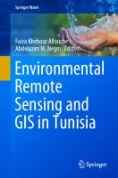
Figure
cover
A schematic illustration of a multifractal field analyzed over a scale ratio λ, with two scaling thresholds λγ1 and λγ2, corresponding to two orders of singularity: γ2 > γ1.
1
nine
to ten
orders of
magnitude (from planetary
scales
to
the viscous
dissipation
scale). These
scaling exponent functions
allow a complete characterization of the statistics nevertheless somewhat difficult to handle, as they They an infinite of hierarchy parameters (i.e., an arbitrary convex function). We represent wish to find an expression for one (or both) of these functions that will enable us to describe the scaling in a fairly simple form, with a small number of parameters. In order to do this, we note that many geophysical systems involve turbulence, which has long been regarded as arising from cascade processes (Richardson, 1922). of the field.
Explicit
are
cascade models have been developed ( Novikov and Stewart, 1964 ; Mandelbrot, et al., 1978 ; Schertzer and Lovejoy, 1987 ), where a quantity energy flux (for atmospheric turbulence) is injected at large scales and
1974 ; Frisch such
as
cascades
smaller and smaller scales via multiplicative modulations (see Figure 2 ). quite general conditions involving scaling non-linear cascade-like dynamics
to
Under
(even in the absence of strictly hydrodynamic turbulence), due to the existence of stable attractive generators of multifractal processes, cascade processes such as this are believed to result in “universal” multifractals 7 (Schertzer and Lovejoy. 1987), where the
K(q)
function is
given by
7
Note, however, the recent debate about strong vs. weak universality ( Schertzer and Lovejoy. 1995 b, 1996; She and Waymire, 1995). The She-Leveque model based on a cascade of eddies postulates a recursive scaling relation between different sets of eddies, and filamentary structures for the highest order This corresponds to a weak version of universality, with an implicit assumption of an upper the singularities. The strong universality discussed here has no explicit assumptions about structures in the system, and has no intrinsic maximum order of singularity.
singularities.
bound
on
Figure
2
A schematic illustration of a multifractal field
being produced by
a
multiplicative
cascade (Schertzer and Lovejoy, 1987 ). up er K left-parenthesi q right-parenthesi equals StartFraction up er C 1 Over alpha minus 1 EndFraction left-parenthesi q Superscript alpha Baseline minus q right-parenthesi com a lpha not-equals 1 up er K left-parenthesi q right-parenthesi equals up er C 1 times q times log times q com a lpha equals 1
(3)
C1 is the codimension of the mean of the field, characterizing the of the mean value of the field, and the Levy index α characterizes the sparseness of degree multifractality (Schertzer and Lovejoy, 1987 ). As a → 0, K(q) becomes linear and we obtain the monofractal β-model (Novikov and Stewart, 1964 ; Yaglom,
where 0
0, while H < 0 acts as a differentiation, in effect “roughening” the field more and more for decreasing H. in Plate 11 the images on The parameter C1 also has a fairly obvious meaning the right have a much larger C1, resulting in most of the normalized field having a fairly small value, with a few large spikes. As α is decreased, the field (again, a normalized field) changes from one that has more symmetric deviations from the mean to one that is fairly high-valued with a few large downward deviations. This is most noticeable in the images with a lower C1. .
,
—
,
Linear Generalized Scale Invariance The second step in describing and hence modeling geophysical fields is the determination of the anisotropy present in the system. Although most systems exhibit statistical scale invariance over various ranges, a priori this scale invariance should 8
actually a lognormal.
This is
misnomer
—
due to
divergence
of moments, the distribution will
only be approximately
9 This is true for “bare” cascade quantities. For the observed “dressed” quantities, Eq. 6 will break down below a critical value of q and trivial scaling will result ( Naud et al., 1996 ). From the data analysis point
of view,
we
*
plates
Color
restore the bare scaling by fractionally follow numbered page 168.
differentiating by
order H or
higher.
not be
to be isotropic (the multifractals, or fractals, will not be “selfsimilar"). Indeed, the only reason that isotropy is often implicitly assumed is that
expected
anisotropic nature of most geophysical systems is usually hidden through the of isotropic analysis techniques. For example, the Fourier power spectrum of a field is defined to include an angular integration in Fourier space that tends to “wash out” (by integrating out) all but the most severe anisotropies; nevertheless, as we show below, these do play an important part in determining the texture and morphology the
use
of the fields. The only scaling anisotropy usually considered in the literature is “self-affine” scaling, in which anisotropy is confined to fixed coordinate axes: this is an insufficient generalization for most applications. The framework of generalized scale invariance (GSI) was developed to describe much more general scaling anisotropies. It extends the idea of scale invariance, where the small-scale and large-scale structures and behaviors
are
related
by
a
scale-changing operator that depends only
on
the scale ratio, to include more complicated scale-dependent changes of behavior and structure, such as differential stratification and rotation. We therefore regard our systems in terms of GSI, restricting ourselves to the linear case (where the anisotropies are statistically independent of position; they depend only upon the scale ratio). To develop the framework of GSI, we need several components. The first of these is the scale changing operator, Tλ. Scale-invariance requires that the statistical properties of a field are changed in a power-law way with an isotropic change in scale λ of space, such as zooming. Tλ is the rule relating the statistical properties at one scale to another. Since the properties only depend on the scale ratio λ and not actual sizes,
Tλmust
have
semi-group properties;
in
particular
it admits
a
generator
G such that: up er T Subscript lamda Baseline equals lamda Superscript negative up er G
(7) In the
of linear GSI, G is a matrix: the identity matrix for the isotropic case (see Figure 3 ), but a more general one for the case of self-affinity or more general anisotropies (Figure 4 ). We also require a family of balls that cover the space and are acted upon by the case
scale
changing operator (these balls define the topology of the space), as well as a way to define what we mean by scale (these requirements are described in detail in Schertzer and Lovejoy, 1985b ). In many physical cases there is no overall stratification (e.g., if we study horizontal and not vertical cross-sections of the atmosphere, earth
or
oceans).
It therefore suffices for
a
definition of scale
to use
the “obvious”
one, i.e., the square root of the area of these balls. In the isotropic case the balls are in fact circles, indicating no preferred direction at any scale. In the anisotropic case, if a scale exists at which the system is isotropic, we call this scale the spheroscale. The family of balls obtained from acting upon it with Tλ will be ellipses, and the G matrix together with the size of the spheroscale will define our system. If no such scale exists, it may be necessary to define a somewhat more complicated family of balls; one such family is of fourth-order closed polynomial balls (Pecknold et al., 1996 ) (see Figure 5 ).
Figure 3
A schematic illustration of the shape of the mean structures as functions of scale in self-similar scaling (G = 1 more precisely, the family of “balls,” see text).
We may decompose G into quaternion-like elements (Lovejoy and Schertzer 1985 ; Schertzer and Lovejoy 1985b ) : G
=
d1 +eI
+fJ
+
cK
where
1equalsStar 2By2Matrix1stRow1stColumn12ndColumn02ndRow1stColumn02ndColumn1EndMatrixup erIequalsStar 2By2Matrix1stRow1stColumn02ndColumn egative12ndRow1stColumn12ndColumn0EndMatrixup erJequalsStar 2By2Matrix1stRow1stColumn02ndColumn12ndRow1stColumn12ndColumn0EndMatrixup erKequalsStar 2By2Matrix1stRow1stColumn12ndColumn02ndRow1stColumn02ndColumn egative1EndMatrix
(8)
A fundamental parameter for the description of the overall type of present in the system will be given by
anisotropy
a squared equals c squared plus f squared minus e squared
(9) In the
case that a2 < 0, we say that the system is rotation dominant: as the scale the balls rotate through an infinite angle of rotation (although for a finite changes, total scale ratio, only a finite amount of rotation is possible). If a2 > 0, we call the system stratification dominant: in a like manner, an indefinitely large “stretching” of the unit ball is permitted, but the total amount of rotation never exceeds π/2. Thus, an analysis of the anisotropies of our system involves determining the parameters c, d,f, and e, along with the spheroscale (or other family of balls). This
determines the scaling anisotropy of the system in the approximation of linear GSI. For cases involving position-dependent anisotropy, the linear GSI approx-
completely
Figure 4
Top: Self-affine scaling with G
reopsre-steicntalinog 0 ver= ca of
atmosphere. The shape of the balls models the average eddy shape; the flattening of the large balls models the fact that the atmosphere is increasingly stratified at large scale, and the small-scale vertically oriented balls correspond to “convective” type eddies or “rain shafts.” The value 5/9 is that obtained from observations and theoretical arguments concerning the stratification of the horizontal wind (Schertzer and Lovejoy, 1985a). Bottom: More complex anisotropy (horizontal crosssection),
the
with G
=
1.This shows the rotational effects of off-diagonal elements.
imation may be made over subregions of the system, as in the section, Cloud Radiances, below. Of course, this applies only to positive scalar fields; for problems involving continuum mechanics, an extension to vector and tensor multifractal fields is necessary (Schertzer and Lovejoy, 1995a).
Data Analysis A full analysis for all the relevant parameters involves several techniques. Because of its sensitivity to scaling (and possible breaks thereof) and also because of its greater familiarity to geophysicists, one of the most basic analysis tools that we use to examine the scaling behavior of a system is a measurement of the power |k| where k is the wave spectrum. The power spectrum, E(k), at wave number k vector, is defined as the ensemble average of the angular integral of the square of =
Figure
5
Fourth order polynomial balls, showing non-elliptical contours: on the left is a convex stratification dominant example, with a ; on the right is a rotation dominant 1 example showing highly non-convex shapes, with
the Fourier transformed field. In
an
isotropic scaling system we can express
the E(k)
as:
up er E left-parenthesis k right-parenthesis tilde k Superscript negative beta
(10) This parameter, the “spectral slope,” β, is useful for describing as well as simulating the process and is related to the moment scaling function by (Monin and Yaglom, 1975 ; Lavallée et al., 1993b ) beta equals 1 minus upper K left-parenthesis 2 right-parenthesis plus 2 upper H
(11) where K(q) is the moment scaling function for the conservative process and H is the degree of non-conservation of the mean of the process. Thus, given the universal parameters α and C1 we may determine K(2) from Eq. 3 and hence the exponent H from the measured spectral slope. To estimate α and C1, it is often convenient to use a double trace moment technique (Lavallée, 1991 ; Lavallée et al., 1992 ). The field ε is renormalized by first raising its values at the finest resolution to the power η and then integrating (or degrading or dressing) up to a scale λ. This renormalized field will then be described by its own moment scaling function, K(q, η). The relation between K(q, η) and the usual statistical scaling exponent K(q) is (Halsey, 1989; Lavallée et al., 1992 ): up er K left-parenthesis q comma eta right-parenthesis equals up er K left-parenthesis q eta right-parenthesis minus q up er K left-parenthesis eta right-parenthesis
(12) For the
case
where the process is
a
universal multifractal
we
have:
up er K left-parenthesis q comma eta right-parenthesis equals eta Superscript alpha Baseline up er K left-parenthesis q right-parenthesis equals eta Superscript alpha Baseline dot StartFraction up er C 1 Over alpha minus 1 EndFraction left-parenthesis q Superscript alpha Baseline minus q right-parenthesis
(13) The scaling exponent in this case has two components: one depends on the universal parameter α only while the second is K(q), the usual scaling exponent. By isolating the first component we can determine the value of the parameter α directly and then deduce C1. By plotting K(q, η) vs. η on a double logarithmic plot, we find the value of α from the slope of the line. Using this estimate of α and the value of q, we can deduce the value of C1 from the intercept of the line with η = 1. It must be noted, however, that in the case where β > 1, (i.e., where H > 0; see Eq. 3 and note that K(2) > 0) we cannot be dealing with a conserved process, and estimates of α and C1 will be inaccurate. 10 The field must be fractionally differentiated in order to yield a conserved process (i.e., it must be filtered by kH in Fourier space in order to remove the effect of the fractional integration k-H) and to obtain stable and accurate estimates of the multifractal parameters α and C1 (see Lavallée et al., 1993b ; Naud et al., 1996). In this case, however, to avoid technical complications with Fourier techniques (arising from the necessity of zero-padding our field and the associated numerical “ringing” this causes), the fractional differentiation in Fourier space was avoided. Instead, the modulus of the gradient of the our
taken, having approximately the effect of a fractional differentiation of long as H < 1, this is adequate for using the double trace moment (Lavallée et al., 1993b ). Strictly speaking the scaling exponents are determined from an ensemble average.
fields
was
order 1. As
It is necessary to have a large number of independent measurements of the field because of intermittency and the extreme variability of multifractal fields. Certain orders of singularity, corresponding to very high field values, may in fact have a codimension larger than the dimension of space, and will almost surely not appear in any given realization/example of the field. Nevertheless, these values will appear in a sufficiently large number of realizations and can be statistically important, even
dominating
the
higher
order statistical moments. 11
Simulation Once the multifractal parameters of the fields have been measured, we wish to simulate the type of geophysical field being studied, producing realizations of a stochastic anisotropic multifractal process. It should be emphasized that the aim of this is not to produce a facsimile of the fields analyzed; rather, it is to produce fields (each one a realization of the simulation process) of the same “type,” i.e., with the as the measured field (given by at all scales and intensitites same statistics —
—
Specifically, there will be trivial scaling (K 0) for all q below a critical (usually low) value. They will in fact generally cause a divergence of the high order moments of the field ( Schertzer and Lovejoy, 1985 a, 1987), associated with a non-classical form of self-organized criticality ( Schertzer and Lovejoy, 1996). Thus, in order to obtain a full characterization of a field’s multifractal parameters, we require a sufficiently large number of independent observations, so that the singularities corresponding to this critical moment of divergence qD will appear. 10
11
=
see Eq. 1 ). c(γ), which determines the probability distribution of field values Since we use the framework of linear GSI, the anisotropic characteristics of the data will also be reproduced; this leads to realistic texture and morphology. In order to produce realizations that correspond to the measured parameters of our data, the —
of simulating continuous universal multifractal cascades was used and Lovejoy, 1987 ; Wilson et al., 1991 ; Pecknold et al., 1993 ). This Schertzer ( simulation technique consists of generating an independent identically distributed
technique
12
Lévy noise, with a Lévy index corresponding to the universal parameter α, and performing a fractional integration using an appropriate power-law filter function to produce a log-divergent generator (the logarithm of the field). This generator is then exponentiated, and the resulting multifractal field may then be “H-filtered” (i.e., fractionally integrated or differentiated by the order H to produce a non-conservative field, as explained above), in effect causing a scale-invariant “smoothing” or “roughening," respectively, of the field. For fields exhibiting scaling anisotropy, the filter function is modified to take into account non-isotropic notions of scale implied by the GSI parameters of the system being modeled. A graphical representation of the simulation procedure may be found in Plate 13 * This type of simulation was performed for all the data types analyzed, using the universal multifractal and GSI parameters determined. We may note that space/time realizations can be made by further modifications of the filter to ensure that causality is respected; see Marsan .
et
al. (1996) ; Tessier
et
al. (1996).
Data and Results
Landscape Topography It has been known for almost half a century that topography has a power law spectrum over a wide range of scales (Venig-Meinesz, 1951), indicating scaling of at least the second-order moment. Indeed, topography has been a frequent subject of study by fractal analyses (see e.g., Goodchild, 1980 ; Aviles et al., 1987 ; Okubo and Aki, 1987 ; Turcotte, 1989 ; De Cola, 1990 ). However, since topography is better described as a scale-invariant field, rather than a scale-invariant geometric set of points, a priori there will be no unique fractal dimension for topography. Rather, each set exceeding a different altitude threshold will have its own fractal dimension, decreasing with increasing altitude threshold: it will be a multifractal field. Multifractal analyses of topography (Lovejoy and Schertzer, 1990 ; Lavallée et al., 1993b ; Lovejoy et al., 1995 ) have convincingly confirmed this in several regions of the world. To illustrate this, we analyzed the power spectra and the universal multifractal parameters of landscape topography. The power spectrum analysis used 20 contig-uous 512 × 512 sections of U.S. topography data, from the area near latitude 40° N, and longitude 110° W, at a spacing of 3 arc seconds, corresponding to approxi12
Lévy distributions
are
the result of the
generalized central limit case, corresponding
variables; the Gaussian is the familiar special *
Color
plates
follow numbered page 168.
theorem for the 2,
to α =
sum
of i.i.d. random
90-m resolution. An example of the data is shown in Plate 14* The power spectrum of all 20 of these realizations of this data is shown in Figure 6 ; we note that this shows excellent scaling of E(k) over the whole range of 2.5 orders of 1.91, in close agreement with the magnitude. The spectral slope is given byβ 13 approximate value of β ≈2 noted in the literature (Venig-Meinesz, 1951; Bell,
mately
.
=
1975 ).
Figure 6
The power spectrum for 20 realizations of topography data. The spectral slope determined by linear regression is β = 1.91. Note the slight curvature at the large wavenumber end is probably associated with noise at the highest resolution of the data (corresponding to 2 x 9 m).
determined the spectral slope, it remains to find the multifractal parameters C1. Because of the strong variability and intermittency of multifractal fields, analysis of data, as mentioned above in Data Analysis, is best performed on a large number of independent realizations. Indeed, because scaling is a statistical symmetry, on any individual realization the scaling is necessarily broken; the values obtained for α, C1 and H will only be statistical estimates. Additionally, in order to estimate α, it is necessary to have good statistics for the lower order singularities of the field. 14 This can lead to difficulties, particularly in topography data. Regions of low gradient are generally sampled at a much lower resolution than highly variable areas, and this, in conjunction with quantization difficulties (this dataset, for example,
Having α
and
has altitude measured erroneous
exactly
zero
only to the nearest meter) can result in large areas with an gradient. Although the scaling for high q >̃ 0.3 were unaffected
(since they are insensitive to the low gradients), the estimate of α is sensitive the low q scaling and such artificially zero gradients, which can cause a significant decrease in the estimate of the parameter α (here, from the true value of α ≈ 1.7 to to
13
In Lovejoy and Schertzer(1995) itis shown how the value β intermittency corrections to a basic β 2 law. 14 This is because α is the order of nonanalyticity of K(q) at are dominated by the frequent low values of the gradients. * Color plates follow numbered page 168.
=
1.91 can be accounted for via multifractal
=
q
=
0 (see
Eq. 3) and
the q ≈ 0 statistics
about 1.35). In analyzing our dataset at the nominal 90-m resolution, it was noticed that up to 20% of our field was exactly zero gradient; accordingly, a 2048 × 2048 section was taken and coarse-grained to 256 × 256, giving a scale range of about 0.7 to 120 km. The data
are currently being analyzed using a Fourier filtering technique to sidestep the problems given by such low gradients. Preliminary results correspond to those given here, and indicate that the need for coarse-graining will be obviated, allowing for the use of the entire scaling range of data.
An example of the multiscaling of the data is noted in Figure 7 : the trace moment of the mean of various moments of the field (the trace moment is the average over the realizations of the η moments of the field, degraded to a scale ratio λ and then the q-th moment summed) shows excellent scaling (power-law behavior) of each moment over the entire range of data.
Figure
7
Scaling of the with q
=
trace of the moments of topography 1.5. λ = 1 corresponds to 180 km.
data, for
3 different moments
η,
analysis (defined in Data Analysis) of the data yielded C1 0.07 + 0.01; the logK(q,η) vs. logη curve is shown in Figure 8 A comparison of the moment scaling function of one section of the field with the theoretical K(q) curve (see Eq. 3 ) is shown in Figure 9 The value A double trace moment
the values α
=
1.70 ± 0.05 and
=
.
.
for α is slightly lower than that found in a study of the topography of Deadman’s Butte (α ≈ 1.9, from Lavallée et al., 1993b ), but identical to that found from estimates of the universal multifractal parameters of the topography of France (see Table 1 ). These were for a single realization in each case. Analysis of data of the entire continental U.S. at 90-m resolution is proceeding. Together with the spectral slope, the parameters measured via double trace moment yield a value of H 0.52 ± 0.05, in close agreement with previously found values, as well as with theoretical arguments based on dimensional analysis (Lovejoy et al., 1995 ). We may note that this =
Figure 8
Graph of the double trace moment, logK(q,η) vs. logη, for q fit gives α = 1.70, and its intercept gives C1 = 0.07.
Figure 9
Comparison of theoretical moment scaling function with parameters determined from the double trace moment, with the measured scaling moment function of a degraded 256 × 256 section of topography data. The experimentally determined values are given by the circles. The curve is the theoretical value from Eq. 3 , using α = 1.70 and C1 = 0.07. This clearly shows that the field is multifractal: a monofractal field would have a linear K(q) function.
multifractal behavior rules
=
1.5. The slope of the
the popular self-affine surface models, since they are and thus have linear K(q) curves. fundamentally monoscaling found the universal multifractal Having parameters of our topography data, one of the sections was chosen for an analysis of its GSI parameters. It is pictured in out
Plate 14 * together with its spectral energy density, which shows the anisotropies in the system. In an isotropic system, the Fourier transform would have circular symmetry, rather than the roughly elliptical ones actually observed. This analysis was performed using the scale invariant generator (SIG) technique described in Lewis (1994) In SIG, an initial guess of the generator G is used to relate neighboring scales, and an error function based on the actual 2-D spectral density and the .
2-D spectral density is defined, and a minimization over the GSI parameter space is performed to find the best fitting parameters c,f, and e. Here it was found that c 0.15,f= -0.10, and e 0.41, giving a rotation dominant system (a2 -0.14), with expected errors of roughly ±0.05 on c and f and ±0.1 on e, which is a less well-estimated parameter (Lewis, 1994 ). Several examples, simulated using the values for multifractal and GSI parameters measured here but with different random seeds, are found in Figure 10 The difference between the realizations illustrates that any given examples using the same parameters have only the same statistics. A comparison of the 3-D ray-tracing representations of the realizations
theoretically expected =
=
=
.
with that of the dataset reveals some resemblance at the larger scales. However, the flat regions that are seen at the smaller scales are not in general present in the simulated examples. It is suspected that this is caused by the erroneous areas of exactly zero gradient present in the data. Finally, not unexpectedly, the simulated realizations do not show river networks; algorithms to estimate the latter from the realizations exist and could perhaps yield even more visually realistic results. Cloud Radiances The multifractal nature of clouds must be taken into account when
modeling
the weather and climate (not to mention when dealing with their tendency to obscure surface phenomena in satellite imaging), and thus a good understanding of the statistical nature of cloud fields is important from a meteorological perspective. Beyond the importance of characterizing the basic variability via α, C1 and H, GSI provides the attractive possibility of obtaining a quantitative
their effects
on
basis for cloud classification, which is currently performed primarily by qualitative visual observation (or by operator assisted pattern recognition algorithms) on satellite data. This quantification may be regarded as a scaling extension of previous approaches involving measures of roughness and texture determined at a unique range of scales. In contrast, GSI gives a measure of the latter arbitrarily large range of scales. To illustrate this possibility, a set of analyses were performed on a series of visible channel satellite cloud images. These images were taken by the NOAA-9 satellite off the coast of Florida, longitude 70 West and latitude 27.5 North, during February 1986. The images analyzed were 512 × 512 pixel AVHRR channel 1, visible light images with wavelength 0.5 to 0.7 ηm. The range of scales was 1.1 to 560 km. These images were previously isotropically analyzed (Tessier et al., 1993 ) and shown to have good scaling, and universal multifractal parameters given by α 1.13
scale,
or over a narrow
over an
=
* Color
plates
follow numbered page 168.
Figure
10 Four realizations of simulated landscape topography, using the parameters measured for the dataset α = 1.7, C1 = 0.07, H = 0.5, using different random seeds and incorporating anisotrophy using GSI parameters c = 0.15, f = -0.10, e = 0.4. They are
visualized with ray-tracing techniques.
0.09 ± 0.10, and H 0.4 ± 0.2. An example of the scaling of the (isotropic) power spectrum of one of these images is given in Figure 11 The image, * along with its spectral power density, is seen in Plate 15 In a general cloud scene is an indication that we are various cloud types coexist; this dealing with non-linear
±
0.20, C1
=
=
.
.
(position-dependent) GSI. We therefore extracted from the original twelve images sixteen 256 × 256 pixel sub-images with fairly homogeneous cloud types (as determined 15 by a professional meteorologist ) and analyzed their GSI parameters, working
15 *
Dr. A. Bellon, McGill Weather Radar Observatory. plates follow numbered page 168.
Color
to different linear approximations GSI. The results are shown in Table 2 Although considering the number of parameters measured, namely η, c,f, e, and the spheroscale, this is a small sample, we still see a clear clustering of parameters by cloud type; for example, the cumulus cases are all rotation dominant (a2 < 0),
under the
hypothesis that various cloud types correspond
to
.
Figure 11 The power spectrum of
a visible light cloud radiance field, wavelength 0.5 to 0.7 μm, range of scales 1.1 to 560 km. The spectral slope determined by linear regression is β = 1.77.
Table 2
Parameters of 16 subsections of NOAA-9 AVHRR channel 1 cloud radiance data, arranged by cloud type, giving p, β, the slope of the power spectrum, the GSI parameter a, and the size of the spheroscale. The parameter a is accurate to within ± 0.05 and i2 = -1. The mesoscale convective complexes (MCC) were selfselfsimilar similar (isotropic) to within statistical error, so that any scale may be taken as a
spheroscale
Stratification dominant clouds Cloud type
Spheroscale (km)
P
Cirrus Cirrus Cirrus Altocumulus Stratus
6.3 10
1.57 1.88 1.68
0.10 0.65 0.25 0.05 0.05
1.65 1.60 1.84
0.05 0.15 0.25
1.91
0.10
2.9 14 9.4 9.4
1.88
0.25
7.6
1.92 1.77
Stratus Stratus Stratus Altostratus Nimbostratus
4.7
0.8 7.0
Rotation dominant/isotropic clouds Cloud type Cumulus Cumulus Cumulus Stratus MCC MCC
Spheroscale ( km)
p 1.04 1.21 1.04 1.79
0.19/ 0.05/ 0.28/ 0.0
1.56 1.83
0.0 0.0
34
31 28 2.3 any any
with a comparatively large spheroscale. 16 Likewise, both examples of a mesoscale convective complex were nearly isotropic, while in general the cirrus clouds were more
strongly
stratification dominant than the stratus clouds
(a2
was
larger).
Simulated
of cumulus and stratus types of cloud using some of the parameters given in Table 2 and the values for α, C1 and H given above may be seen in Plates 16 and 17 * We may note that, comparing the simulated cumulus to the example
examples .
16
Recall that the spheroscale is a scale at which structures are isotropic, and it need not exist. However, in all the cloud cases examined it was determined that a spheroscale could be approximately found at the scale indicated in Table 2, evidenced by the existence of a circular iso-energy contour in the 2-D
spectral
energy
*
plates
Color
density. follow numbered page 168.
given, and likewise comparing the example of stratus cloud to that simulated, the general structures correspond rather well. Certain of the structures evident in the actual data are not present in the simulated examples. This is to be expected, since given realization, actual
or simulated, will not be identical to another. This large between different realizations of the same process is highlighted by the differences between the simulated clouds of each type, which were created using the same parameters. Still, the simulated cumulus consists, as does the real cumulus, of clusters of fairly small clouds arranged in bands. Likewise, the stratus example
any
variability
is
a
scale complex consisting of a few fairly large, stratified structures, which also be noted in the simulated stratus. It is obvious that the large parameter
large
can
space involved in GSI requires that a large number of images of varying cloud types be analyzed to draw further conclusions. It is also true that a complete classification and modeling scheme using GSI may have to take into account the properties of these cloud radiance fields not just in the visible spectrum, but also in the infrared, as indeed was necessary for qualitative visual classification. This is particularly true as regards the distinction between the lower altitude water clouds, such as cumulus and stratus, and the higher altitude ice clouds, cirrus. Currently, techniques are being developed for the analysis and modeling of vector multifractals for
better
(Schertzer
and
Lovejoy, 1995a),
which should
provide
of the interrelations between different parts of the cloud radiance spectrum, as well as to provide more visually realistic simulated clouds. Indeed, it is naϊve to expect a scalar multifractal framework (such as that presented here) to be completely adequate for studying clouds; the effect of the vector wind field is frequently apparent (e.g., in cyclones). The extension of linear GSI to nonlinear GSI may also allow for a greater ability to realistically describe these fields, allowing different types of basic anisotropy for different regions of the field. A further application of the modeling of cloud systems currently being undertaken is the simulation of radiative transfer in multifractal clouds (for a 2-D version, a
understanding
Davis et al., 1992 ; Naud et al., 1996; in 3-D, see Stanway et al., 1996 ). A 3dimensional anisotropic cloud liquid water field is generated using the measured multifractal parameters (by the process described in Simulation), with a stratification in the vertical direction with respect to the horizontal (see Figure 12 for an image of the simulated cloud, and Figure 13 for the radiation field). Photons are then forward scattered through the cloud, using an isotropic phase function, with the intensity being estimated at the detector using spherical harmonics to help smooth see
out the
high-frequency
Monte Carlo noise. The resultant radiation fields may then
be compared with satellite data. We are convinced that explicit cloud and radiation models of this type are essential for understanding cloud/radiation interactions (see also Davis et al., 1990 ; Gabriel et al., 1990 ; Lovejoy et al., 1990 ; Davis, 1992 ; Lovejoy and Schertzer, 1995; Naud et al., 1996 for more on radiative transfer in fractal and multifractal clouds).
Aeromagnetic Anomaly The magnetic field of the Earth is a superposition of the main field internal to the planet, of fields arising from electrical currents flowing in the ionized upper
Figure
12 Three-dimensional multifractal cloud simulation, using universal multifractal parameters measured from satellite data. Only regions exceeding a minimum liquid water density are shown, the gray scale is proportional to the log of the density. The parameters are α = 1.35, C1 = 0.10, H = 0.40, and the vertical stratification is characterized by Hz = 0.55 (close to that for the wind field).
Figure
13 The results of Monte Carlo scattering of 150 000 000 photons through the cloud in Figure 12 with the mean optical thickness at the vertical as 1.0, seen from above. The sun was incident at 0.0 radians, with the results smoothed to partially remove the high-frequency Monte Carlo noise. Note that more realistic clouds would have highly forward-peaked phase functions.
atmosphere, and of fields induced by currents flowing within the Earth's crust. We analyzed airborne data of (the modules) of these magnetic fields, with the (transient)
atmospheric effects statistically removed (by a complex set of pre-processing filterING 17 operations ). Seven data sets from varying regions of Canada were analyzed for their multifractal parameters. The aeromagnetic fields, whose properties are discussed in depth in Pecknold et al. (1996) were obtained on 256 × 256 (maximum) sized square grids which were coarse grained to 128 × 128 over an approximately 200 × 200 km area, yielding a maximum resolution of ~1.6 km (see Plate 18 * for an example). The coarse graining was performed to eliminate significant artifacts at the highest frequencies, due most likely to the limited resolution of the measuring ,
device, oversampling, or noise. Additionally, as can be seen from the power spectrum of the data (Figure 14), a fairly sharp break in the scaling occurs at about 10 km. This is believed to be caused by a high-pass filter used in the pre-processing to remove the transients as mentioned above. Below we study the multifractal behavior only over the range of scales in the high frequency regime.
Figure 14 The power spectrum of seven aeromagnetic anomaly fields. The spectral slope for high frequencies is β ≈ 2.0; for low frequencies β 0.53. The relative flatness of the low frequency regime is believed to be an artifact of the data pre-processing to =
remove
transients.
The universal multifractal parameters of the aeromagnetic field were measured ( Pecknold et al., 1996 ) as α ≈ 1.9 + 0.1, Cl ≈ 0.10 ± 0.02, and H 0.70. An analysis of the GSI parameters for one of the datasets was performed (latitude 87° W, longitude 50° N) yielding values of c 0.05,f= 0.10, e 0.22, a rotation dominant system. In this dataset, however, no spheroscale appears to exist (this is confirmed by statistical analysis). We may see this by looking at the spectral energy density in Plate 18 *: the shapes of the balls describing the anisotropy in this dataset are somewhat rhomboid-like (this may be seen best towards the center of the image, since the larger spectral density contours, corresponding to small-scale structures, =
=
17 *
Using proprietary software. Color plates follow numbered
page 168.
=
was found to be reasonably well described by a family balls, as described in Pecknold et al. (1996) ; the simple quadratic family of ellipses is insufficient to describe this system. The aeromagnetic field was simulated using the GSI and universal multifractal parameters measured for this dataset, and this is also shown in Plate 18 The general structure is seen to are
fairly noisy). The system
of fourth order
polynomial
.
be
quite
similar to that of the dataset.
Sea Ice
Finally,
the radar
reflectivity
of
sea
ice
was
examined. Recent work has shown
scaling of synthetic aperture radar reflectivity fields of sea ice over almost three orders of magnitude (Falco et al., 1996 ), and found multifractal statistics over the range of ∼12 m to 6 km. These multifractal parameters and the GSI parameters of two different scenes of SAR reflectivity fields from sea ice, in several wavelength and polarization combinations, were estimated. The fields were 512 × 512 pixels, with
m. The measurements were by the Jet Propulsion Laboratory operating simultaneously at the C band (5.6 cm) and L band (25 cm) wavelength ranges, transmitting and receiving from separate antennas in three linear polarization combinations: HH, VV, HV, where the symbols represent horizontal (H) and vertical (V) polarizations in the transmitted and received beams respectively. a
resolution of 12.5
airborne SAR
The data images were taken from an altitude of 9 km over the Beaufort Sea (76° N 165° W) in March 1988 (Drinkwater et al., 1991 ). One of the images analyzed is shown in Plate 19 * In the image, ridges, lees and ice types of various ages can be identified. The scaling of the power spectrum of this example is shown in Figure 15 giving a spectral slope of β 0.83. In some cases, the scaling of the power spectrum is affected by the large anisotropies present in the system. The universal -
.
=
,
multifractal parameters for sea ice were given by α 1.85 ± 0.05, C1 = 0.01 ± 0.01, and H -0.05 to -0.15, with only the value of H varying with polarization and =
=
wavelength. The GSI parameters were not very sensitive to the polarizations, but did vary from scene to scene. In the case of our image, the parameters were found to be c 0.21,f= 0.0, and e 0.0. This field was also analyzed for its unit ball, and it was found that it was best described, as in the case of the aeromagnetic anomaly dataset, by fourth order polynomials. In fact, the original aim of extending the simplest case =
=
of linear GSI, described
by elliptical families of balls, to the families of quartic balls, provide description of the ridges, fissures and lees present in SAR ice images (Pecknold et al., 1996 ). These structures do not seem to be adequately modeled by the framework of linear GSI with a spheroscale, since they have pronounced was to
a
Fourier space isolines (corresponding to the balls; see e.g., sea ice field made using the parameters given above
nonconvex
Figure
5
above).
A simulated
is found in Plate 20 * We note that the large scale structures, in particular the floes and fissures, are not reproduced, although some degree of clustering into larger scale structures may be noted, as well as certain aspects of the texture. We suspect that .
*
Color
plates follow numbered
page 168.
Figure 15 The power spectrum of a sea ice radar reflectivity field. The spectral slope determined by linear regression is β 0.83. =
use
of tensor, rather than scalar, multifractals may lead to significant improvement largely by stress and strain tensors.
since the ice field is determined
Summary The quest for more realistic ways to represent and model geographical and geophysical systems, together with the fact that most remotely sensed fields exhibit scaling over the physically significant ranges, has led to the recognition that multifractals fundamental theoretical tool. The framework of scalar universal multifractals, together with linear generalized scale invariance, permits fairly realistic of the statistical properties and of the visual characteristics of many both modeling geographically and geophysically significant fields. It does this with only six basic are a
describing the infinity of fractal dimensions, and another three anisotropy (and therefore texture and morphology) over the entire describing scaling range. We have a relatively simple yet surprisingly realistic description of the field and of its aggregation/resolution dependent properties over arbitrarily exponents
—
three
the
—
—
wide ranges of scales. In
comparison, standard modeling techniques start from non-linear deterministic partial differential equations and then seek to
approximate integrate these
over a numerically manageable range of scales, typically only about orders of magnitude. They necessarily make unrealistic homogeneity assumptions about the unresolved scales which can in fact result in a feedback of large uncontrollable errors on the resolved scales. 18 Even when this is accomplished they still give no information about how the results can be extended to smaller (or larger) scales. The main extensions of the multifractal framework which will be necessary
two
18 These assumptions go under the general rubric of “parameterization”; the existence of self-organized critical (small scale) fluctuations generally predicted by multifractal cascade theory indicates that such deterministic parameterizations cannot generally succeed.
universality full non-linear classes), (position independent) without leaving the general (position dependent) version. In short, it is easy more multifractal framework to introduce parameters and increase scaling
are
from scalar to vector and tensor multifractals
(and their
and from linear GSI
more
complex
to a
—
—
realism. Further work is still necessary to obtain a more accurate and comprehensive picture of the place of universal multifractals and GSI in the study of geographical and geophysical systems. For example, the analysis of GSI parameters of clouds to determine the relationship between this anisotropic parameterization and the cloud classification is ongoing. Likewise, the problem of recognition of sea ice may be examined by relating its anisotropies to its morphology, and an analysis of aeromagnetic anomalies may provide some clues as to the underlying structure and composition of the Earth’s crust. More complete analysis of available topography data will also be performed.
Currently, the entire continental U.S. at a resolution of 3" of arc is being analyzed for scaling and for its multifractal parameters. Preliminary estimates of the topography of the Earth at a resolution of 5' are also continuing, and show consistency with the results obtained thus far for smaller data sets. Finally, new methods are being developed for analysis and modeling, such as techniques for analyzing and simulating multifractal fields on a sphere, a necessity in conjunction with the extension of global data (see Plate 21 * for an example of simulated topography on the sphere, Tan et al., 1996 ). Additionally, methods dealing with vector and tensor fields (“Lie cascades,” Schertzer and Lovejoy, 1995a) promise to provide further insight into the more complicated physics that underlies the
systems that
observe. The present
of multifractal
modeling, dealing quantities, are insufficient to deal with interrelated fields such as the multiple channel satellite-imaged radiance fields. Likewise, dealing with vector fields such as velocity fields we
techniques
do with scalar fields and cascades of scalar
they completely as
cloud also suggests the need for further developments in the modeling of multifractals. Thus, this framework of Lie cascades provides hope for yet more realistic and accurate modeling of the world around us.
References
Adelfang
,
S. I. , On the relation between wind shears
10 , 138 , 1971
over
various intervals J. Atmos. Sci. , .
.
Aviles , C. A. , Scholz , C. H. , and Boatwright , J. , Fractal analysis applied to characteristic segments of San Andreas fault , J. Geophys. Res. , 92 , 331 , 1987 Bak , P. , Tang, C. , and Weiessenfeld , K. , Self-organized criticality: An explanation of 1/f noise , .
Phys.
Rev. Lett. , 59 , 381 , 1987
.
topography Deep Sea Res. 22 883 analysis of cloud liquid water over the range 5m unified scaling model M.Sc. thesis, McGill University
Bell , T. H. , Statistical features of
sea
floor
,
,
,
Brosamlen , G. , Multifractal new
* Color
plates
test of the
follow numbered page 168.
,
,
,
1975
.
to 330km: a
1993
.
Lovejoy S. Lazarev A. and Ordanovich A. Unified multifractal atmospheric dynamics tested in the tropics part 1: horizontal scaling and selforganized criticality Nonlin. Processes Geophys. ( 1 ), 105 1994 A. Lovejoy S. and Schertzer D. Supercomputer simulation of radiative transfer inside multifractal cloud models in I.R.S. 92 Arkin A. Lenoble C., and Gelyn J. F., Eds., Deepak Hampton, VA 112 1992 A. Lovejoy S. Gabriel P. Schertzer D. and Austin G. L. Discrete angle radiative
Chigirinskaya
Y. , Schertzer , D. ,
,
,
,
,
,
.
Davis ,
,
,
,
,
,
,
,
,
,
,
,
,
,
transfer. Part III: numerical results Res. , 95 , 11729 , 1990
.
,
,
,
.
,
,
,
,
,
,
Davis ,
,
on
,
,
,
homogeneous and fractal clouds J. Geophys. ,
.
Davis , A. , Marshak , A. Wiscombe , W. ,
,
and Cahalan , R. , Multifractalcharacterization of
nonstationarity and intermittency in geophysical fields: observed, retrieved J.
Res. , 99 , 8055 1994
Geophys. Transport University 1992
,
Davis , A. , Radiation
or
simulated.
.
in Scale Invariant
Optical
Media Ph. D. thesis, McGill ,
.
,
Davis , F. and Simonett , D. S. , GIS and remote
sensing Geographic Information Systems Longman Scientific and ,
,
D. J. , Goodchild , M. F. and Rhind , D. W. , Eds., Technical Press , Harlow, UK 1991 , 191
Maguire
,
.
,
De Cola , L. and Lam , N.
Introduction to fractals in geography, in Fractals in Geography, De Cola , L. and Lam , N. , Eds., Prentice Hall , Englewood Cliffs, NJ , 1993 ,
.
De Cola , L. , Fractal
analysis
of
classified LANDSAT
a
Drinkwater, M. R. , Kwok , R. , Winnebrenner, D. P., and SAR observations of Endlich , R. M. , and Mancuso , R. L. , with
severe
Falco , T. , Francis , F. ,
preprint, 1990 Rignot E. Multifrequency polarimetric
scene ,
.
,
ice , J.
,
Geophys. Res. 96 20679 Objective Analysis of environmental
sea
,
,
,
1991 conditions associated
thunderstorms and tornadoes Mon. Weather Rev. , 96 , 342 , 1968 .
Lovejoy
,
S. , Schertzer, D.
invariance and universal multifractals in
.
Kerman , B. , and Drinkwater, M. , Scale
,
ice
sea
synthetic aperature
radar
reflectivity
fields , IEEE Trans, Geosci. Remote Sensing , 34 , 906 , 1996 Frisch , U. P. Sulem , P. L. and Nelkin , M. A simple dynamical model of intermittency in fully developed turbulence , J. Fluid Mech. 87 719 , 1978 .
,
,
,
.
,
Gabriel , P., Lovejoy , S. , Davis , A. , Schertzer , D. and Austin , G. L. , Discrete angle radiative transfer. Part II: renormalization approach to scaling clouds , J. Geophys. Res. , 95 , 11717 , 1990 .
Garrido , P. , in
Lovejoy S. and Schertzer D. the large scale structure of the ,
,
,
,
Multifractal processes and self-organized universe , Physica A , 225 , 294 , 1996
criticality
.
Goodchild , M. F. , Fractals and the accuracy of 1980
geographical
measures , Math. Geol. , 12 , 85
,
.
P. Generalized dimensions of strange attractors Phys. Rev. Lett., A 97 227 1983 Halsey T. C. Multifractality, scaling and diffusive growth in Fractals Physical Origin and Properties Pietronero L. Ed., Plenum Press New York 1989 Halsey T. C. Jensen M. H. Kadanoff L. P. Procaccia I. and Shraiman B. Fractal measures and their singularities: the characterization of strange sets Phys. Rev. A 33 1141
Grassberger
,
,
,
,
,
,
,
,
,
,
,
,
,
,
,
.
.
,
,
,
,
,
1986
,
,
,
,
,
,
.
Hentschel , H. G. E. and Procaccia , I. , The infinite number of
generalized
dimensions of
fractals and strange attractors , Physica D , 8 , 435 , 1983 C. , Earthquakes as a Space-Time Multifractal Process M.Sc. thesis, McGill University, 1993 .
Hooge
,
.
.
Hooge C. Lovejoy S. Schertzer D. Pecknold S. Malouin J.-F. and Schmitt F. Multifractal phase transitions: the origin of self-organized criticality in earthquakes Nonlin. Processes Geophys. 1 ( 2 ), 191 197 1994 ,
,
,
,
,
,
,
,
,
,
,
,
.
-
,
,
.
Hubert , P. , Tessier, Y. , Desurosne , I.
Ladoy P., Lovejoy ,
S. , Schertzer , D. , Carbonnel , J. P., Violette , S. ,
,
and Schmitt , F. , Multifractals and extreme rainfall events
,
Res. Let. , 20 ( 10 ), 931 , 1993 Kapteyn , J. C. , Skew frequency curves in
.
Geophys.
.
1903
biology and
statistics , Publ. Astron. Lab.
Groningen
,
.
Ladoy P. Schmitt F. Schertzer D. and Lovejoy S. Analyse multifractale de la variabilité temporelle des observations pluviometrique à Nimes Comptes Rendus de l'Académie des Sciences de Paris II ( 317 ), 775 1993 Lamder C. Desaulnier-Soucy N. Lovejoy S. and Schertzer D. Evidence for universal multifractal behaviour in human speech International Journal of Chaos and Bifurcation 2 ( 3 ), 715 1992 ,
,
,
,
,
,
,
,
.
,
,
,
.
,
,
,
,
,
,
,
,
.
.
,
Lavallée , D.
,
Multifractal
,
Lavallée , D.
,
and Simulation of Turbulent Fields , Ph.D.
techniques: Analysis
thesis, McGill University 1991
.
Jourdan , D. , Gautier, C. , and
Hooge
C. , Universal multifractal
,
properties of Exposition,
microwave satellite data , ASPRS/ACSM 1993, Annual Convention and New Orleans , 1993 a.
Lavallée , D. , Lovejoy , S. , Schertzer , D. , and Ladoy , P. , Nonlinear variability and landscape topography: analysis and simulation in Fractals in Geography, De Cola L. and Lam , ,
,
N. , Eds., Prentice-Hall , Englewood Cliffs, NJ , 1993 b, 171 Lavallée , D. , Lovejoy , S. , Schertzer , D. , and Schmitt , F. , On the determination of universal .
multifractal parameters in turbulence ,
Topological Aspects of the Dynamics of Fluids Zalslavsky G. Eds., Kluwer Boston 1992
and Plasmas , Moffat , K. , Tabor, M. and 463
,
,
,
,
,
.
Lazarev , A. , Schertzer , D. ,
Lovejoy S. and Chigirinskaya Y. Unified multifractal atmospheric dynamics tropics part II: vertical scaling and generalized scale invariance Nonlin. Processes Geophys. 1 115 1994 Lewis G. The Scale Invariant Generator Technique and Scaling Anisotropy in Geophysics M.Sc. thesis, McGill University 1994 Lovejoy S. Gabriel P. Davis A. Schertzer D. and Austin G. L. Discrete angle radiative transfer. Part I: scaling and similarity, universality and diffusion J. Geophys. Res. ,
,
,
,
tested in the
.
,
,
,
.
,
,
,
.
,
,
,
,
,
,
,
,
,
,
,
,
95 , 11699 , 1990
,
.
Lovejoy S. Lavallée D. Schertzer D. and Ladoy P. The 1½ law and multifractal topography: theory and analysis Nonlin. Process. Geophys. 2 16 1995 Lovejoy S. and Schertzer D. Generalized scale invariance in the atmosphere and fractal ,
,
,
,
,
,
,
,
,
,
,
,
,
.
,
,
models of rain , Water Resour. Res. , 21 ( 8 ), 1233 , 1985 Lovejoy, S. and Schertzer, D. , How bright is the coast of Brittany? , in Fractals in Geoscience .
and Remote
Sensing
Wilkinson , G. ,
,
Kanellopoulos
,
I. and
Mégier
,
J. , Eds., Office
for Official Publications of the European Communities , Luxembourg 1 , 1995 , 102 Lovejoy, S. and Schertzer, D. , Our multifractal atmosphere: a unique laboratory for non-linear .
.
dynamics Phys. Can. 46 62 1990 Lovejoy S. and Schertzer D. Scale invariance in climatological temperatures and plateau Ann. Geophys. 4B 401 1986 ,
,
,
,
.
Mandelbrot , B. B. , How
.
,
,
,
,
long
,
,
the
spectral
.
is the coastline of Britain? Statistical
dimension , Science , 155 , 636 , 1967
self-similarity and fractional
.
Mandelbrot , B. B. , Intermittent turbulence in self-similar cascades: moments and dimension of the carrier, J. Fluid Mech. , 62 , 331
divergence ,
1974
of
high
.
Mandelbrot , B. B. , Negative dimensions and Hölders, multifractals and their Hölder spectra, and the role of lateral preasymptotics in science , J. Fourier Anal. Appl. (Kahane Special Issue), 1995 .
Mandelbrot , B. B. , Stochastic models for the Earth’s relief, the shape and the fractal dimension of the coastlines, and the number-area rule for islands , Proc. Nat. Acad. Sci. U.S.A. , 72 , 3825 , 1975
.
Marsan , D. , Schertzer, D. , and and
Lovejoy
S. Causal
,
space-time multifractal processes: predictability Geophys. Res. (in press), 1996 Causal space-time multifractal modelling of rain
,
of rain fields , J.
forecasting
Marsan , D. , Schertzer, D. and
.
,
Lovejoy S. J. Geophys Res. (in press), 1996 Meneveau C. and Sreenivasan K. R. Simple multifractal cascade model for fully developed turbulence Phys. Rev. Lett. 59 ( 13), 1424 1987 Monin A. S. and Yaglom A. M. Statistical Fluid Mechanios MIT Press Boston 1975 Naud C. Schertzer D. and Lovejoy S. Fractional integration and radiative transfer in multifractal atmospheres in Stochastic Models in Geosystems Molchanov S. and Woyczynski W. Eds., Springer-Verlag New York 1996 239 Nguyen V. T. V. Pandley G. R. and Rousselle J. Estimation of missing short-duration rainfalls using data measured at longer time scales in 6th International Conference on Urban Storm Drainage Marsalek J. and Tomo H. C. Eds., Niagara Falls Ontario, ,
,
,
,
,
,
,
,
,
,
,
.
,
,
,
.
,
,
,
,
,
,
,
,
,
,
,
,
,
.
,
,
,
,
,
,
,
.
,
,
,
,
,
Canada , 1993
170
,
,
.
Novikov , E. A. and Stewart R. ,
Intermittency of turbulence and spectrum of fluctuations in energy-dissipation Izv. Akad. Nauk. SSSR. Ser. Geofiz. 3 408 1964 O’Brien L. Introducing Quantitative Geography: Measurement, Methods, and Generalised Linear Models Routledge London; New York 1992 Okubo P. G. and Aki K. Fractal geometry in the San Andreas fault system J. Geophys. ,
,
,
,
,
.
,
,
,
,
,
,
,
Res. , 92 , 345 , 1987 Olsson , J. ,
Niemczynowicz behavior of
2 ( 1 ), 23 , 1995
.
J. , and Berndtsson R. , Limits and characteristics of the multifractal
,
,
rainfall time series Nonlin. Processes
high-resolution
a
.
Geophys.
,
.
Parisi , G. and Frisch U. A multifractal model of ,
in
.
,
,
intermittency in Turbulence and Predictability Dynamics Ghil M. Benzi R. ,
,
Fluid
Geophysical
Dynamics
and Climate
,
,
,
,
and Parisi , G. , Eds., North Holland , Amsterdam , 1985 , 84 Pecknold , S. , Lovejoy, S. , and Schertzer , D. , The morphology and texture of .
anisotropic using generalized scale invariance in Stochastic Models in Geosystems Molchanov S. and Woyczynski W. Eds., Springer-Verlag New York 1996 269 Pecknold S. Lovejoy S. Schertzer D. and Hooge C. Universal multifractals and anisotropic scale invariance in aeromagnetic fields Geophys. Int. J. (in preparation), 1996 Pecknold S. Lovejoy S. Schertzer D. Hooge C. and Malouin J.-F. The simulation of universal multifractals in Cellular Automata: Prospects in Astrophysical Applications, Lejeune A. and Perdang J. Eds., World Scientific Singapore 1993 228 multifractals
,
,
,
,
,
,
,
,
,
,
,
,
,
,
,
,
,
.
,
,
.
,
,
,
,
,
,
,
,
,
,
,
,
,
,
Perrin , J. , Les Atomes , NRF-Gallimard , Paris , 1913
Richardson , L. F. , Weather Prediction by Numerical Process , 1922 , Republished by Dover New York 1965 ,
Richardson , L. F. , The Gen.
Syst.
Schertzer, D. and
problem
of
,
contiguity:
Yearb. , 6 , 139 , 1961
Lovejoy
,
an
,
.
,
.
Cambridge University
Press ,
.
appendix
of statistics of deadly
quarrels
,
.
S. The dimension and intermittency of atmospheric dynamics , ,
Turbulent Shear Flows 4 , University of Karlsruhe , Karlsruhe , FRG, 1983
Springer-Verlag
,
.
Schertzer, D. and
Lovejoy, S. , The dimension and intermittency of atmospheric dynamics , Turbulent Shear Flows 4 , Launder, B. , Ed., Springer 1985 a, 7 Schertzer , D. and Lovejoy , S. , Generalised scale invariance in turbulent phenomena , Physico-Chem. ,
Hydrodynam.
J. , 6 , 623 1985 b. ,
.
Lovejoy S. Physical modeling and analysis of rain and clouds by anisotropic multiplicative processes J. Geophys. Res., D 8( 8), 9693 1987 Schertzer D. and Lovejoy S. Generalized scale invariance and multiplicative processes in the atmosphere PAGEOPH 130 57 1989 Schertzer D. and Lovejoy S. Nonlinear geodynamical variability: multiple singularities, universality and observables Non-Linear Variability in Geophysics: Scaling and Schertzer , D. and
,
,
of
scaling
.
,
,
,
,
,
,
,
,
,
,
.
,
,
,
Fractals , Schertzer , D. and Lovejoy , S. , Eds., Kluwer , Boston , 1991 a, 41 Schertzer , D. and Lovejoy , S. , Scaling nonlinear variability in geodynamics in Nonlinear .
,
in
Variability
and Fractals , Schertzer, D. and
Geophysics: Scaling
Lovejoy S., Eds., ,
Kluwer Academic Publishers , Dordrecht , 41 , 1991 b. Schertzer , D. and
Lovejoy S., Multifractal generation of self-organized criticality in Proceedings of the Second IFIP Working Conference on Fractals in the Natural and ,
,
Applied Sciences
Novak , M. M. , Ed., North Holland , Amsterdam , 1994 , 325
,
.
Schertzer , D. and Lovejoy , S. , From scalar cascades to Lie cascades: joint multifractal
analysis of rain and cloud processes in Space/Time Variability and Interdependance for Various Hydrological Processes Feddes R. A. Ed., Cambridge University Press New ,
,
,
,
,
York , 1995 a. Schertzer, D.
and S. Lovejoy Standard and advanced multifractal techniques for remote sensing in Fractals in Geoscience and Remote Sensing edited by Wilkinson I. K. G. Mégier J. Eds., Office for Official Publications of the European Communities Luxembourg 1995 b, 11 Schertzer D. and Lovejoy S. The multifractal phase transition route to self-organized criticality, Phys. Rep. (in press), 1996 Schertzer D. and Lovejoy S. Universal multifractals do exist! J. Appl. Meteorol. (in press), ,
,
,
,
,
,
.
,
,
,
,
,
,
.
,
,
,
,
,
,
,
,
1996 b. Schertzer, D. , Lovejoy , S. , Lavallée , D. , and Schmitt , F. , Universal hard multifractal turbulence: theory and observation , in Nonlinear Dynamics of Structures , Sagdeev, R. Z. , Frisch , U. , Moiseev, A. S. , and Erokhin , A. , Eds., World Scientific , 213
Singapore
,
1991 ,
.
Schmitt , F. , Lavallée , D. , Schertzer, D. , and
project
climate data
.
Lovejoy S. Empirical determination of universal velocity fields Phys. Rev. Let. 68 305 1992 a. Multifractal analysis of the Greenland ice-core ,
multifractal exponents in turbulent Schmitt , F. , Lovejoy, S. , and Schertzer, D.
,
.
,
Res. Let. , 22 , 1689 , 1995
Geophys.
,
,
,
.
Schmitt , F., Lovejoy, S. , Schertzer , D. , Lavallée , D. , and Hooge , C. , First estimates of multifractal indices for velocity and temperature fields Comptes Rendus de .
1'Académie des Sciences de Paris serie II , 314 , 749 , 1992 b. ,
Schmitt , F. , Schertzer, D.
,
Lovejoy S. and Brunet Y. Estimation of universal multifractal ,
,
,
,
atmospheric turbulent velocity data Fractals 3 568 1994 She Z.-S. and Waymire E. C. Quantized energy cascade and log-poisson statistics in fully developed turbulence Phys. Rev. Lett. 74 (2 ), 262 1995 Stanway J. D. Lovejoy S. and Pecknold S. Monte Carlo simulation of radiative transfer in multifractal clouds (in preparation), 1996 indices for
,
,
,
,
,
,
,
.
Lovejoy
,
.
,
.
and area ,
Length, shape
Tan , J. , Pecknold , S. ,
,
,
,
Steinhaus , H. ,
,
,
,
,
,
,
Colloq.
Math. , III
,
1 , 1954
.
S. , Schertzer, D. , and Malouin , J. F. , Simulations of continuous
multifractal processes on the sphere , (in preparation), 1996 Tessier, Y. , Multifractal Objective Analysis, Rain and Clouds Ph. D., McGill University , 1993 Tessier, Y. , Claerdebout , M. , Lovejoy , S. , Novak , R. , Roff, J. , Ingram , G. , Bourget , E. , and Schertzer , D. , Universal multifractal analysis of plankton and related physical variables .
.
gathered during the
CHASE
experiment
.
J. Map. Ecol. , (in
.
preparation),
1996 a.
Tessier, Y. , Lataille , S. , cover,
Tessier , Y. ,
Lovejoy
,
S. , and Schertzer, D. , Multifractal
in EGS XX General
Lovejoy
Assembly Hamburg, Germany ,
S. , and Schertzer, D.
,
for rain and clouds J.
,
of the
analysis
vegetation
1995 b.
,
Universal Multifractals: theory and observations
Meteorol. , 32 ( 2 ), 223 , 1993 b.
Appl. Lovejoy S. and Schertzer D. Multifractal analysis and simulation of the global raingage network J. Appl. Meteorol. 33 1572 1994 Y. Lovejoy S. Schertzer D. Hubert P. and Pecknold S. Multifractal analysis and modeling of rainfall and river flows and scaling transfer functions J. Geophys. Res. (in press), 1996 c. Y., Lovejoy S., Schertzer D. Lavallée D. and Kerman B. Universal multifractal indices for the ocean surface at far red wavelengths Geophys. Res. Let. 20 1167 .
Tessier , Y. ,
,
,
,
,
.
Tessier ,
,
,
,
,
,
,
.
,
,
,
,
,
,
,
Tessier ,
,
,
,
,
,
,
,
,
.
,
,
,
1993 c. Tessier, Y. , Lovejoy S. Schertzer D. , and Claerdeboudt, M. , Scale invariant algorithms for remote sensing of ocean colour Int. J. Remote Sensing (in preparation), 1996 b. .
,
,
,
,
Lovejoy S. Hubert P. Schertzer D. and Pecknold S. Multifractal analysis and modeling of Rainfall and river flows and scaling, causal transfer functions J. Geophys. Res. (in press), 1996 c. Tessier Y. Schertzer D. and Lovejoy S. The multifractal global raingage network: analysis and simulations J. Appl. Meteorol 32 ( 12 ), 1572 1994 Turcotte D. L. Fractals in geology and geophysics Pageoph 131 171 1989 Venig-Meinesz F. A. (1951), A remarkable feature of the Earth’s topography Proc. K. Ned. Tessier , Y. ,
,
,
,
,
,
,
,
,
,
,
,
,
,
,
,
,
,,
,
,
.
,
,
,
,
,
.
,
,
,
Akad. Wet. Ser. B Phys. Sci. 54 212 1991 Wilson , J. , Schertzer, D. , and Lovejoy , S. Physically based modelling by multiplicative cascade processes in Non-Linear Variability in Geophysics: Scaling and Fractals ,
,
,
.
,
,
,
Schertzer, D. and
Yaglom
,
S. , Eds., Kluwer Boston , 185 , 1991 the fluctuation in energy dissipation of the
Lovejoy
A. M. , The influence
on
,
,
characteristics in the inertial interval Sov. ,
Phys.
.
shape of turbulent
Dokl. , 2 , 26 , 1996
.
Epilog Scale is
confusing concept, often misunderstood, and meaning different things the context and disciplinary perspective. In this book we have tried to reconcile, or at least elucidate, some of the more obvious conceptions of scale; its attributes, its characteristics, and its ambiguities. We do not claim by any stretch of the imagination to have resolved the “scale issue,” particularly with regard to the integration of remote sensing with GIS, or an IGIS. In fact, it was not our original intent to do so, as has been indicated in the Preface. Hopefully, however, we have depending
a
on
a framework that can be used to further illuminate the role of scale within IGIS as a basic dimension of what we now identify as digital geographic data. The sixteen chapters have examined scale as a foundation for relating data obtained through remote sensing with data obtained and manipulated through assimilation and analysis in a GIS environment. Although the process is still far from perfect, with modern geographic information technologies, we believe we can now integrate
presented an
data our
across
scales in ways that are more rigorous, robust, and more of the processes operating in the Earth system.
compatible
with
understanding A
theme of the book has been multiscaling. Multiscale approaches, or entail an even higher order of dimensionality in scale; rather than cope with the effects of forcing a single scale, multiscaling proposes that two or more scales be related together in a common database design and analytic framework, providing a cohesive cascade of data scales. As we have seen, multiscaling can pervade many types of data and analytical processes, from purely descriptive to purely statistical and theoretical, including the theoretical framework for multiscaling presented in Chapter 16 Hence, the integration and analytical interrelationships common
multiscaling,
.
afforded
multiscaled data exacerbate the seemingly simple problems we are confronted with in dealing with data obtained at matching or similar scales. We hope this book has provided insight into some analytical and processing methods than can be employed to better understand how data collected at different scales and from different sources (e.g., remote sensing, maps) can be meshed together to assist in addressing complex space, time, geographic, and environmental questions.
by
Instead of just
being
a
treatise that focuses
examining the difficulties associated with data, we hope this is a proactive book
only
on
defining, describing,
and
scaling and the analysis of multiple scaled as opposed to just a “how to” book
—
—
DOI: 10.1201/9780203740170-18
Scale in Remote Sensing and GIS
presenting
a
litany
of
problems
that need to be addressed. Above all, it and useful.
intent to make this book informative It is in the nature of scientific than
was our
—
inquiry
that research often
yields
more
questions
Although number of chapters in this book have examined process–scale interrelationships, they leave us with the sense that we still know far too little about how geographic and environmental processes and their dynamics are manifested at different scales. Questions of scale are paramount to understanding Earth processes and how these processes are reflected in geographic pattern and form on the landscape. For example, which processes are invariant with scale so that it is irrelevant what scale of observation is used, particularly as observed through answers.
a
sensing? Which processes are scale-dependent, so that the multiscaled approach and the IGIS structure become truly useful approaches to successfully understanding their dynamics, linkages, and basic dimensions? Resolutions to these questions and many others are critical if we are to make effective use of the rich
remote
variety of
sensing sources that are becoming available, with their wide ranges and temporal resolutions, and if we are to make good decisions balance these factors in future generations of sensors. How should we
of remote
spatial, spectral,
about how to handle these data? How should And more importantly, how do
process these data to achieve
meaningful results? of these data, particularly in combination with other non-remotely sensed data within a GIS framework? Answers to these questions are likely to come more quickly if scale is recognized we
we
make
sense
generic issue, with associated theory, tools, and techniques that can be of simultaneous value to a large number of disciplines. We hope this book has contributed to this notion of a “science of scale,” by stressing the universality of the scale issue. In the future, we like to think that courses might be offered on scale, perhaps as part of a broader program in geographic information science, or within programs in statistics or environmental science. Such courses might emphasize generic theoretical frameworks, common analytic techniques, and basic tools. They might even raise some of the broader implications of scale that are missing from this book as a
—
implications for decision-making, for example, or the development of environmental policy. Above all, they would be based on the assertion, supported by much of the content of this book, that scale is a fundamental and inescapable dimension of geographic data.
Index
A Absorbed
Bernoulli
photosynthetically
active radiation
(APAR), 180
Adaptive dynamic interpolation, 342 Advanced very high resolution radiometer (AVHRR), 75 123 302 ,
,
Aeromagnetic anomalies, 387 389 Aeromagnetic field, 364 386 Aggregating fine scale models, 115 Aggregation, 15 classification hierarchy and, 23 composition of, 77 ,
,
experiment,
219
Bernoulli random process, 216 Bernoulli trials, 216 Between-band correlations, 274 Biophysical models, 114 125 ,
Biophysical processes, Box-counting method, Boxplots, 37
29 319
Break distance, 319
Breakpoints,
302
fractional,
Brownian motion,
318
C
data, 13 16 ,
features filtered
during,
18
Calibration, 116
methods, 13 19
California, 79
pixel, 16 problem,
Canopy
,
362
/resolution
dependence,
388
routines, 303 of slope angle, 38
Cartographic scale,
average method, 18 zonal, 361
,
radiation
Arc/Info™, 299
319
Cellular automata, 344 Cellular automaton models, 212 227 ,
,
Climate, 380 Cloud(s) ,
76
classification,
380
radiances, 373 380 384 simulated, 384 ,
,
,
Characteristic scale, 29 76 Chesapeake Bay, 79
Average 15
,
368
Central limit theorem, 82
Astrophysics, 366 Atmospheric model, 122 Atmospheric radiance, 173 Autocorrelation, spatial, 62 method,
,
,
lengths, 336 Cell-counting method,
Anisotropy, 363 370 371 372 APAR, see Absorbed photosynthetically active ,
13 14 23 361
Cave
315 ,
remotely sensed,
Cantor set, 314 Cascade processes, 95 Cattle grazing, 213
using
Algorithms,
surface temperatures, 183
18
value, 275 AVHRR, see Advanced very high resolution radiometer
,
stratus, 383
Coastlines, 326 332 ,
Codimension, 365 375 Coefficient of variation (CV), 34 35 42 Commutative operations, 77 ,
,
B Baltimore/Washington, Bathymetry, 329
79
Compass method, 324 Complexity, spatial, 73 Conditional expectation,
283
,
Scale in Remote Sensing and GIS
Conditionally positive
definite function, 282
Conflation, 80
Contouring,
281
224
,
low, 220
Correlation between
frequency, 216 high, 219 regime,
slope
and
NDVIdif,
49
return
216
interval, 216 219 ,
values, 78
Correspondence analysis, 286
E
Covariance, 277 278 ,
Hydrologic Laboratory, problem, 339
Coweeta Crease
172
Earth
Observing System (EOS), 296 Laboratory Applications
Earth Resources
Cross-level fallacies, 61
Cross-variogram,
Software (ELAS) module TRADE, 174
287
Cubic convolution method, 303
Ecological fallacy,
CV,
ELAS,
see
Coefficient of variation
see
61
,
361
Earth Resources
Applications TRADE
D
Emergent properties concept,
14
Environmental models, multiscale nature of
Data
aggregation, 13 16 analysis, 378 exploration, 82 layers, 274
spatial data in scaling up, 13 26 aggregation methods, 15 16 forecasting scale tendency by fractals, 19 geographic scale, 23 multiple scales of spatial data, 16 19 -
,
effects of
management, 77 models, 273 281 volume, 75 Datasets, management of, 77
-
-
Erosion
fluvial, 343
parallel retreat, 344 Error, propagation of, 131
222 225 228 ,
DEM, see Digital elevation model Desertification, 211 autogenic vs. allogenic factors in, 212
spatial pattern
effects on, 225
studying, vegetation dynamics during, 212 Diagonalization, near, 288 of temoral scales for
213
ESTAR, 98
Evapotranspiration 171 Expected NDVI, 36 Exponential models, 347 Exponent of similarity, 324 ,
Extent, 13 Extreme fluctuations, 364
Differential stratification, 371 Differentiation, 370
Digital elevation 33
model (DEM), 14
,
16
F ,
124
,
Fast Fourier transform
Digital orthophotoquads (DOQ), Digital terrain data, 311
78
Distance measures, 37 Distributed water and energy balance model, 98 Divider method, 324 Domain, 13 Dominant value method, 15 16 18 DOQ, see Digital orthophotoquads ,
,
Double trace moment, 374 378 ,
Downwasting model,
343
Drought effects, 216 220 221 222 228 ,
,
,
22
,
,
,
-
-
-
Dead-ice topography, 343 Degradation potential, 220 probability, 217 221 process,
-
resolution, 14 15 22 23 scale definition, 13 14 EOS, see Earth Observing System Erdas/IMAGINE, 300
,
use
Laboratory
Software module
,
filtering method, 340 FD, see Fractal dimension FIFE, see First ISLSCP Field Experiment Filter, 289 First ISLSCP Field Experiment (FIFE), 114 120 Fissures, 387 Floes, 387 Fluvial erosion, 343 Fluxes, partitioning of latent and sensible heat, ,
171 Forest canopy temperatures calibrated, 173
remotely sensed, 171 spatial distribution of,
172
Index
Fourier transforms, 309 Fourth order
FPAR,
polynomial,
Geomorphological models, 343 Geomorphological processes, 343 Geo-spatial data, approaches to scaling,
387
Fraction of absorbed
see
,
,
,
-
-
Fractal(s), 97 297 309 312 362 , 364
analysis,
309 360
basic concepts of fractal geometry, 312 314 characterization of linear and volumetric
active radiation
photosynthetically ,
296 297
elements of terrain, 332 337 of terrain simulation algorithms, -
,
clouds, 384
development
dimension (FD), 19 20 34 35 278 290 297 ,
,
,
,
,
337 342 -
,
,
313 364
fractal characterization of terrain surfaces,
,
method, 63 67 58 ,
326 331 -
,
parameters, 319 semivariance-based, 13 20
improving existing geomorphological models,
sets, 362 surface measurement
methods for
343 345 -
,
algorithms, 301 photosynthetically
Fraction of absorbed
radiation (FPAR), 117 Fractional Brownian motion, 318
,
estimating
fractal dimension,
315 326 -
active
box-counting method, 319 323 comparison of three commonly -
125
used
methods, 325 326 variogram method, 315 319 walking divider method, 324 325 GIS, see Geographic information systems Glacier National Park (GNP), 28 30 Global atmosphere-biosphere models, scaling -
Fractional differentiation, 375 Fractional dimension, 313
-
-
Functional classification, 170
,
G
land cover
heterogeneity for, 231 246 procedures for aggregating land cover heterogeneity for test data in
Gamma value, 319
GCM,
see
General circulation model
General circulation model (GCM), 169 Generalizations, 74 361
Africa, 236 241 -
land
,
Generalized scale invariance (GSI), 363 371 376 ,
,
heterogeneity in global atmosphere-biosphere models,
cover
,
379
234 236 -
Generator, 371
remote
Geographic
information systems (GIS), 13 27 57 93 297 ,
,
remote
of
vegetation heterogeneity,
-
methods to determine land cover
sensing and, 107
heterogeneity from remotely
sensed
data, 233 234 -
,
map, 227
sensors to
273
detect land cover
heterogeneity.
232 233 -
time series, 227
Geographic
information systems, understanding scale and resolution effects in remote
sensing and, 57 72 analyzing effects of scale, 63
Grazing ,
-
70
-
64 65 -
local variance method, 65
228
-
120
Ground scene model, 121
GSI, GVI,
65 67
see
see
Generalized scale invariance Greenness
of scale and resolution, 58 59 scale-related issues, 60 63 ecological fallacy problem, 61
meanings
,
spatial pattern efects under, 223 Greenness vegetation index (GVI),
fractal method, 67 70
geographic variance method, analysis method,
GNP, see Glacier National Park Grain, use of for resolution, 14 effects of, 216 221
-
texture
sensing
232 234
,
,
-based modeling, data, 213 228
packages,
-
effects of
vegetation index
-
-
modifiable areal unit
problem, optimum spatial resolution for remotely sensed imagery, 62 63 problem of inferring spatial processes across 60 61 -
-
scales, 61 62 Geographic scale, 13 23 Geographic variance, 58 63 64 -
,
,
,
H Hausdorff-Besicovich dimension, 313
Heterogeneity, degrees of, Hierarchical models, 226
Histogram, 299 Homogeneity degrees of, 274 scale, 362
274
I ICAMS,
Landforms, 329
Image characterization and modeling
see
Landscape
system IGIS,
see
Integrated
behaviors, 212
GIS
Image
complexity, 297 composition, 217 configuration, 225 dynamics, 217 ecology, pattern and
characterization, 29 classification, 32 303 ,
data, scaling effects in, 119 display and output, 299
filtering, 303 input, 299 Image characterization
,
,
measures,
and
modeling system
-
developmental objectives
and system
design,
299 300
,
220
patterns, 213 processes, 213 structure, 29 Latent heat flux measurements, 170
-
example applications,
300 303
image characterization methods, 301 specialized functions, 303 scale, remote sensing, GIS, and fractal analysis, 296 299 Independent cut method, 338
-
-
302
-
Integrated GIS (IGIS), Intergraph™, 299
Leaf
area index (LAI), 115 125 Length-of-path method, 324 ,
Lie cascades, 389 Linear GSI, 372 373 384 388 -
,
,
regression models, 42 Linearly independent functions, Linear
282
Little Washita, 95
Indicator transform, 285 Individualistic fallacy, 61
Local variance, 58 63 65 Localized interaction, 214 217 226 ,
,
362
,
Logarithmic models, 347 Log-normal distributions, LogNormality, 285
Internet, 300
Interpolation, 76 281 282 Inversion of operations, 77 ,
process, 28
indices, 217 222 224 227
(ICAMS), 295 307
functions and
Landsat thematic mapper, 74 Landsat-TM, 301
,
,
363
LOWTRAN6, 173
Isarithm, 68 301 ,
M J
Magnetic field,
Jornada Basin, 211
384
Map scale, 13 58 336
JAVA, 300
,
,
,
214 225
Markov-cellular
,
approach,
216
Markov-cellular automaton model (M-CA), 213 215 227 ,
K Konza Prairie
Long Term Ecological Reserve (KPLTER), 124 KPLTER, see Konza Prairie Long Term Ecological Reserve Kriging, 76 estimator, 283 variance, 284
Markov-Gauss process, 340 Markov model, 213 214 ,
Markov process, 212 Mass
wasting,
342
Mathematica, 78 MAUP, see Modifiable areal unit problem MC, see Moran’s coefficient M-CA,
see
Markov-cellular automaton model
Mean, 299 local variance, 34 window variance, 42
L LAI,
see
Measurement scale, 59
Leaf area index
Lake Charles, Louisiana, 301
Measuring networks,
Lake-rich landscapes, 343 Land
Median, 299 Mesoscale convective
complex, Midpoint displacement, 338
characterization, 85 surface energy balance /water interface, 303
366
modeling,
127
382 383 -
Minimum variance unbiased estimator, 283 Mode, 299
,
simulation, 375 376
Model(s)
-
aggregating fine scale, 115 atmospheric, 122
zonal
,
exponential, 347 121
scene,
347
-
-
retreat, 343
landscape-based vegetation
digital vegetation map for mountains of southern California,
stand-based
148 152 -
N NASA,
347
state-and-transition, 212 Modifiable areal unit problem (MAUP), 23 60 78 Modified Markov process, 340 ,
,
MODIS, 123
see
115
Monofractal, 97 Monomials, 282 Moran’s coefficient (MC), 34 35 Moran’s I index of spatial autocorrelation, 42 ,
Morphology,
376
Mountain front
sinuosity,
337
Multifractal(s), 297 314 362 analysis, 364 behavior, 379 386 ,
,
Space
Administration National Aeronautics and Space Administration
(NASA), 295 296 spatial data infrastructure (NSDI), Nearest neighborhood method, 303 Near-infrared analysis, 303 -
Needle temperatures, 172 Negative definiteness, 278
Neighborhood configurations,
,
388
,
Normalized difference
,
77 346
analysis,
parameters, 386 phase transitions, 364 processes, 368 375
linear
,
,
vegetation
index (NDVI),
125 299 ,
303
regression
models of, 42
Normalized difference
,
dependence
,
Multifractals, resolution dependence and, 361 394
vegetation index, scale of and relationship to
mountainous terrain, 27 55 -
background,
-
373 375
28 30 -
methods, 32 38 digital image processing, 32 33
-
-
results, 376 388 -
aeromagnetic anomaly,
-
digital terrain analysis, 33 34 image block statistics, 35 scaling NDVI and landcover types,
384 387 -
-
cloud radiances, 380 384 -
landscape topography,
376 380 -
ice, 387 388 generalized scale invariance, 363 364 linear generalized scale invariance, 370 373 -
-
-
multifractals and -
123
,
corrected version of, 28 expected, 36
universal, 374 389 Multifractality, 77 95 , 363
364 370
,
Normalization, 78
modeling, 389 natural examples of,
sea
215 227
,
,
analysis,
84
effect, 214 223 rules, 226 Nonlinear transformation, 285 Normality, 283 285
clouds, 384 fields, 365 370
data and
National Aeronautics and
National
expansions,
scaling,
database for
California, 152
issues involved with, 94
spherical,
data
maps
for Palomar Mountain area, 153 162
self-affine surface, 379 sensor, 122
Moment
363
-
Poisson-Brown, 338 pure nugget, 283 radiation, 384 scale-based, 341
scaling
-
background, 142 146 case study, 146 162 comparisons of two digital vegetation
Markov, 213 M-CA, 227
parallel
361
,
-
hierarchical, 226
logarithmic,
,
,
cellular automaton, 212 227 downwasting, 343
ground
aggregation problem,
Multiscale, 95 96 365 378 behavior, 365 data, 296 Multiscale vegetation data, for mountains of southern California, 141 168
universality,
statistical methods, 36 38 -
objectives,
27 28 -
results and discussion, 38 50 boxplots, 38 -41 -
cover
type control, 46 49 -
36
discussion of models, 49 50
comparison
-
distance measures, 46 model results, 42 -45
study NDVI,
-
see
vs.
-
206
growth measurements, 204 hydrologic validation, 203 input data, 202 203 PnET-IIS predicted vs. measured hydrology,
Normalized difference vegetation
-
index
NSDI,
predicted growth, 205
forest
area, 30 31
see
of PnET-IIS
measured forest
National spatial data infrastructure
204 205 -
Nth cell method, 15 18
regional modeling, 206
summary
,
stand-level modeling, 191 195 -
hydrology, stand description,
192 194 -
O Objects,
identification of, 73
Observational scale, 58 Operational scale, 14 23 ,
192
summary of stand-level
hydrology,
,
59
aggregation, 16 coarser aggregated,
classification level and, 23
-
195
49
dominant, 17 19
Plants, functional groups of, 213
major, 20 matching of,
Pleistocene
,
16
Point
resolution of polygonal areal units and, Operations, composition of, 77 Optimum resolution, 362 Orthophoto quad imagery, 75
22
glaciation, value(s), 274
30
average of, 275 variation of, 276
variogram,
279
Poisson-Brown
Polygonal
primary model,
338
areal units, resolution of, 22
Positive definiteness, 278 280 ,
P
Potential direct solar insolation, 33 Power law, 362 364
Parallel retreat
,
erosion, 344 model, 343 Partial transformations, 115 Partitioning, 116
Power spectrum, 342 373 381 ,
,
Principal components analysis (PCA), Propagation of error, 131 Proportional effect, 364
Patch scale, 211
286 303 ,
Pure nugget model, 283 Pyramid, 74
Pattern
descriptors, 28 recognition algorithms,
380
variables, 42 PCA, see Principal components analysis
plane-filling curves, 333 Penman-Monteith equation, 175
Q Quadtrees,
247 271 -
hierarchical partitioning of variance,
Peano
,
253 257
176
-
Phase function, 384
multiresolution Haar
Physiographic provinces, 328 Physiology, 366 Pine forest hydrology and productivity, scaling predicted, across southern United States, 187 209
ecosystem-level forest modeling, 195 202 data aggregation, 200 202 PnET-IIS predicted hydrology, 198 PnET-IIS predicted vs. measured forest growth, 198 200 site description, 196 198 summary of ecosystem modeling, 202 -
-
nested analysis of variance, 255 257 pyramids and quadtrees, 248 252 -
-
basic concepts of heirarchical data structures for images, 248 250
properties
-
-
-
-
remote
sensing image analysis using quadtrees, 257 266 -
adjusting mapping
units to local
variability,
261
multi-tilling
191
testing and validation, 189 regional-scale forest modeling, 202
gray-scale image quadtrees,
for
toward further
189
model structure, 189
of
250 252
-
-
representation,
253 255
-
-
model scales, 188
194
Pixel
sampling, 258 260 applications of HQ-decomposition with implications -
environmental research, 262 266
model
-
-
206
Quaternion, 372
for
R
data sources, 97 99 -
ESTAR, 98 Radar
reflectivity,
387
soil moisture
modeling, 98 multiscaling analysis, 99 103
Radial Basis Function, 282 Radiation
-
modeled fields, 103 scaling and multiscaling
Regional Atmospheric Modeling System
Random additions, successive, 339 Random field, 76
19
geographic
one-pixel, 18 polygonal areal units,
22
relationship between operational scale and,
Random walk techniques, 324
14
of, 211 230 drought effects, 221 222 effects of pattern on process, 225 226 grazing effects, 222 224 limitations of Markov-cellular model, rates
spatial,
59
studies of, 14 of grain for, 14 Richardson technique, 324 Rivers, 366 380 use
-
-
-
,
Rotation, 371 372
-
,
Roughening, 370 Roughness, 380
226 227 -
description,
scale and, 23
of
Rangeland degradation, modeling effects of spatial pattern, drought, and grazing
213 217 -
cellular automaton model, 214 effects of drought, 216
S
effects of grazing, 216 217 functional groups, 213
Sample variance, 280 Sampling unit, 29 Satellite imaging, 380
-
Markov-cellular automaton model, 214 216
Scalar universal
-
Markov model, 213 214 scaling with multiple-scale data, 226
Scale(s),
-
simulation
experiment, 217 219 characterization of landscape dynamics, -
217 218
spatial pattern,
217
simulation conditions, 219
spatial pattern effects,
,
of action, 59 -based model, 341
cartographic,
dependence,
225
of GIS data in Markov-cellular
multifractals, 388
225 295
13 14 23 ,
,
,
361
characteristic, 29 definitions of, 58
-
use
-
identification of, 15
Random fractals, 297 Random funtion, 277
effects of
96 97
,
see
on
properties,
Renormalized field, 374 Resolution(s), 13 23 aggregation of grids to, 15 approaching dominant operational scales,
model, 122 Rain, 366
model
99
ESTAR fields, 101 102
fields, 366 models, 384 Radiative transfer in clouds, 384
RAMS,
-
-
29 59 ,
,
86 341 ,
factor, 96
modeling,
227 228 -
geographic, 13 homogeneity, 362 388 importance of, 1 3 independence, 342 ,
Recursive subdivision, 338
-
Regional Atmospheric Modeling System (RAMS), 170 Regional variation, 274 Regression models, 37
invariance, 118, 345, 363, 370
Remote
invariant
field, 376
geometric
sensing, 213 228 data, scaling issues, 117 GIS-based modeling and, 107 images, analysis of, 299 scaling effects in, 94 Remote sensing, multiscaling analysis in distributed modeling and, 93 ,
-
set, 376
generator (SIG), 380
map, 13 58 measurement, 59 multiple, 226 228 ,
,
observational, 58
operational, 112
14 15 23 ,
,
,
59
classification level and, 23
dominant, 17 matching of, 16
,
resolution of polygonal perceptions of, 3 5 prediction at, 104 problems of, 5 6
areal units and, 22
-
,
,
-
,
spatial, 227 Scaling, 93 362 ,
,
364 373 380
,
,
,
anisotropy, 371 behavior, 365 effects, in image data, 119 exponent, 97 362 issues, 94 117 ,
,
,
96
,
,
-
Standard deviation
fractals and fractal dimension, 290 291 -
Sea ice radar reflectivity field, recognition of, 389
heterogeneity, homogeneity, and scale, 274 interpolation of spatial data, 281 286
364
-
deterministic methods, 281 estimation variances, 284
simulated, 387 universal multifractal parameters for, 387 Second order stationary, 277 278 ,
Self-affinity,
297 363 371 ,
non-linear transforms, 285 286 regression methods, 283 284 -
-
-
surface models, 379
-
Self-organized criticality, 363 364 Self-similarity, 290 312 371 Semi-group, 371
noise removal, 289
,
spatial intervariable correlation, 286 spatial variability, 275 281 empirical form, 275 277 frequency distributions, 277 modeling variability, 280 281 non-point data, 279 280
-
,
,
Semivariance-based fractal dimension, 20 engineering, 122
Sensor model, 122 Shrublands, 211 SIG, see Scale invariant generator
-
-
-
theoretical models, 277 279 time and space, 275 -
Simple averaging, 303 Simple scaling, 96
Statistical
Simulation, 376 384 cumulus clouds, 384 217 218 226 ,
Soil
moisture, 94
312
Sub-pixel biophysical attributes,
modeling, 98 scaling exponents, 101 resources, heterogeneity of,
of land surface, 121 variability, 49 Surface fluxes, spatial distribution of, 170 SVIs, see Spectral vegetation indices
211
potential, 33
Solid earth, 366
Space/time realizations, Sparseness, 363 365 Spatial autocorrelation,
self-similarity,
Stratification dominant clouds, 383 Stratification dominant system, 372 Stratus clouds, 383 Stream networks, 333 Structural classification, landcover type, 170
,
,
376
Symmetries,
363
,
15
16 19 62 76
,
,
,
,
T
Moran’s I index of, 42
statistics, 299
Spatial configurations,
Temperature, 217 218 223 ,
288
-
Sensor electrical
Solar radiation
282
smoothing, 288 289 combination, 289 interpolation, 288 289
373
experiment,
-
software, 285
,
fractals, 313
scaling,
340
,
Statistical models, for multiple-scaled analysis, 273 293
Scope, 76 see
,
Standard deviation (SD), 34 35 42 State-and-transition model, 212
up, 13 21 Scene simulation, 121
SD,
,
,
ratio, 372
simple,
Spatial correlation, 275 280 Spatial dependence, 277 Spatial distribution, of surface fluxes, 170 Spatial heterogeneity, 225 295 Spatial pattern effects, 221 225 228 Spatial resolution, 59 361 Spatial scales, 211 227 Spatial variability, 273 274 Spectral response, 80 Spectral synthesis method, 340 Spectral vegetation indices (SVIs), 118 Spherical models, 347 Spheroscale, 371 382 386 Square-square recursive subdivision method,
,
173 303 366 ,
Tensor fields, 389
,
Terrain
Universal multifractal, 363 , 374 , 376 , 378 , 380
derivatives and, 28 features, 311
Universal parameters, 374
simulation, 337 surfaces, 326
V
Texture, 376 380
Variability, maximum,
,
58 63
analysis,
,
65
,
,
measures, 299 301 Thematic mapper (TM), 74 Thermal-infrared analysis, 303 Thermal infrared multispectral of
remotely
,
scanner
(TIMS),
sensed surface
temperatures from aircraft-based, 169
-
185 -
estimating evapotranspiration, 175 176 micrometeorological instrumentation, 174 study area, 172 173 techniques for obtaining remotely sensed -
-
surface temperatures, 173 174 thermal response number, 174 175
,
,
choice of valid, 283 estimator for, 280
results and discussion, 176
-
182
-
spatial
multifractals, 384 multifractals and, 389
tensor
dynamics, 213 220 illustration of, 221
-
179
Time, charactreistics of, 74 TIMS, see Thermal infrared multispectral TM, see Thematic mapper TOA, see Top of atmosphere Top of atmosphere (TOA), 122
use
of NDVI to assess, 32
Vegetation indices, examining effects of sensor resolution and sub-pixel heterogeneity
Thermal response number (TRN), 170 Thin-Plate Spline, 282
327
212 ,
-
177
landscape-scale,
spatial pattern effects on, 225 226 productivity within alpine environment, 31
latent heat flux estimates, 180 181
thermocouple temperatures, white pine, 182 Thermal remote sensing, 170
Vector
,
diurnal surface energy fluxes, 179 forest canopy stomata resistance, 179 180
coweeta
forest canopy temperature heterogeneity, 176
modeling of, 278 point value, 278
Vegetated/non-vegetated boundaries, 303 Vegetation
-
-
on
spectral, 113 139 -
background, 114 121 biophysical modeling using remotely sensed -
scanner
data, 117 119 -
first ISLSCP field
experiment, 120 121 scaling biophysical models, 114 117 scaling of image data, 119 120 remote sensing scene simulation modeling, -
-
-
data, 389
121 128 -
profiles, 326 Topological dimension,
biophysical modeling, 125 128 data and study site, 123 124 model description, 121 123 simulation scenarios, 123 -
313
Transition
-
-
probabilities,
214 219 223 ,
,
simulation results, 128 133
rules, 214 215 217 ,
-
,
Trend surface, 283 342
propagation of error in
,
Triangular prism methods,
301
Trigonometric series, 342 TRN, see Thermal response number Turbulent scalars, 366 Turbulent
,
,
method, 315
methods, 172 176
Topography,
geographic, 58 63 64 local, 58 63 65 Variation, of point values, 276 Variogram(s), 278 301 309 ,
,
use
67
Variance, 76 299
velocity,
land surface process
models, 131 133 relationships among multiresolution NDVI -
and LAI and FPAR, 128 131 -
Vegetation indices,
multiresolution covariation
among landset and AVHRR, 73 91
366
-
U Universal behavior, 364
Universality,
363
analysis,
80 88 -
cross-sensor
covariation, 85 88
multiresolution 82 85 -
-
analysis
of landsat data,
multiresolution analysis, 74 78 composition of aggregation with other -
operators, 77 78
White
-
multiresolution covariation, 78
multiresolution variance, 76 77 area and data sources, 78 80 -
study
Weierstrass-Mandelbrot random fractal function, 341
pine
canopy, 172
Within-band correlations, 274 World Wide Web, 300
-
Visualization, 78 von Koch Snowflake, 313
Y Yardstick method, 324
W Wavelets, 309 Weather, 380
Z Zonal
aggregation,
361