The Analysis of Biological Data: Solutions Manual [First ed.] 9780981519401
This is the solutions manual for all problems that are not in the book.
285 106 1MB
English Pages 44 Year 2008
Recommend Papers
![The Analysis of Biological Data [2, 1 ed.]
0981519407, 9780981519401](https://ebin.pub/img/200x200/the-analysis-of-biological-data-2-1nbsped-0981519407-9780981519401.jpg)
![The Analysis of Biological Data [3 ed.]
9781319226299](https://ebin.pub/img/200x200/the-analysis-of-biological-data-3nbsped-9781319226299.jpg)


![Instructor’s Solutions Manual for Econometric Analysis of Cross Section and Panel Data [Second ed.]](https://ebin.pub/img/200x200/instructors-solutions-manual-for-econometric-analysis-of-cross-section-and-panel-data-secondnbsped.jpg)
![Exploratory Data Analysis Using R (Instructor Solution Manual, Solutions) [1 ed.]
9781498730235, 149873023X](https://ebin.pub/img/200x200/exploratory-data-analysis-using-r-instructor-solution-manual-solutions-1nbsped-9781498730235-149873023x.jpg)
![Introduction to Data Science: Data Analysis and Prediction Algorithms with R (Instructor Solution Manual, Solutions) [1 ed.]
0367357984, 9780367357986](https://ebin.pub/img/200x200/introduction-to-data-science-data-analysis-and-prediction-algorithms-with-r-instructor-solution-manual-solutions-1nbsped-0367357984-9780367357986.jpg)
![The Analysis of Biological Data: Solutions Manual [First ed.]
9780981519401](https://ebin.pub/img/200x200/the-analysis-of-biological-data-solutions-manual-firstnbsped-9780981519401.jpg)
File loading please wait...
Citation preview
The Analysis of Biological Data - Whitlock and Schluter Solutions to assignment problems - PLEASE DO NOT POST Chapter 1 10. (a) Discrete (b) Continuous (c) Continuous (d) Discrete (e) Continuous 11. Observational study. The researcher has no control over which women have miscarriages and which lose their fetus from other causes. 12. (a) numerical, discrete (the variable, if not the partners) (b) numerical , continuous (c) categorical, ordinal (d) numerical, continuous (e) categorical, ordinal (f) numerical, continuous (g) categorical, nominal (h) numerical, discrete (i) categorical, nominal (j). numerical, continuous 13. (a) Observational study: the individual fish were not assigned to subspecies by the researcher. (b) Subspecies of fish and wavelength of maximum sensitivity. (c) The explanatory variable is the subspecies, the response variable is the wavelength of maximum retina sensitivity. 14. (a) No. The 500 households selected to receive the survey might be a random sample, but the low completion rate (< 20%) makes the sample a volunteer sample. (b) Volunteer bias Those who volunteer to respond to a survey on recycling might have different opinions of the program than those who did not respond. 15. (a) Omitting cell phones could bias a sample. If younger individuals are more likely to use a cell phone, omitting cell phones would bias the sample towards older individuals. (b) Equal chance of being selected. 16. (a) The population of interest is coastal Californian population of piñon pine trees. (b) A single plot was randomly sampled, but trees were not randomly sampled. The multiple trees within the same plot might not be independent, if they are related, of similar age, or share the same environment. 17. The 60 samples are not a random sample. The 6 dives measured on each bird are not independent. The six dive results measured from each bird are likely to be more similar than dive results obtained from six different birds sampled randomly from the population.
Chapter 2 14. (a) Between 12 and 13 mm. (b) Approximately 50% of the finches are at the modal beak width. (c) Changing the widths of intervals or “bins” of the histogram can alter its shape. Draw several histograms with the data, using wider and narrower intervals, is needed to determine whether a second peak is present. (d) Bimodal. 15. (a) Touching the first segment of the hind leg led to the greatest response. Touching the thorax or distal portions of any of the legs resulted in the lowest response. (b) Map. 16. (a) Frequency table. (b) A single variable (number of convictions). (c) 21. (d) 265 of 395 (the fraction 0.67) had no convictions. (e)
Histogram − it is the easiest way to visualize the frequency distribution for a numerical variable. (The cumulative frequency distribution is also an appropriate graph). (f) Skewed (right) and unimodal (mode is 0 convictions). There are no outliers. (g) The sample was six schools near the research office ⎯ not a random sample of British boys or any other population. 17. (a) This is a contingency table. (b)
(c) Categorical, ordered. Groups should be arranged by increasing income. (d) The relative frequency of conviction decrease as available income increases.
(e) The mosaic plot made it easier to see the pattern. Whereas the table gives the frequencies, the graph visualizes the association between the variables. 18. (a)
(b) Histogram: it visualizes the frequencies of each spermatophore mass interval very clearly. (c) The main part of the distribution is fairly symmetric with a mode of 0.06−0.07. There is an extreme measurement at large spermatophore mass. (d) Outlier. 19. (a) Both variables are continuous numeric variables. (b) Scatter plot. (c) The relationship is positive but non-linear. As temperature increases the fusion frequency increases. (d) The 20 measurements are not a random sample because each fish was measured several times and the multiple measurements were all combined. 20. (a) Line graph. (b) The steepness of each segment tells us the net increase in the number of endangered species added in a given year (it is not exactly the total number added, because some species might have been removed from the list in a given year). (c) The net number of endangered species has been increasing steadily over time, but has tapered off toward the most recent dates. 21. (a) Histogram. (b) The bars of a histogram should not have gaps between them. (A lesser problem is that it is not clear what the ticks on the x-axis refer to.) (c) The variation in protein similarity is the most interesting feature: some proteins are nearly identical between humans and puffer fish, while others are nearly completely dissimilar. (d) Skewed left. (e) The mode is 70% similarity (presumably the interval the number “70” represents is 67.5−72.5). 22. (a) Cumulative frequency distribution. (b) The y-axis indicates the quantile of the variable indicated on the x-axis (annual percent change in human population). The quantile is the fraction of observations less than or equal to the value on the x-axis. (c) Approximately 10% of the countries had negative change in population size. (d) The 0.10 quantile is approximately 0 growth, the 0.50 quantile is 1.5% growth, and the 0.90 quantile is 3% growth.
(e) The 60th percentile is approximately 1.75% growth. 23. (a) Scatter plot.
(b) Number of fruits previously produced, because we wish to use it to predict photosynthetic capacity. (c) Negative association: photosynthetic capacity reduced in trees that produced many fruits previously. 24. (a) Grouped histograms. Explanatory variable: genotype at PTC gene. Response variable: Taste sensitivity score. Genotype is categorical variable, taste sensitivity is numerical. (b). Scatter plot. Explanatory variable: migratory activity of parents. Response variable: migratory activity of offspring. Both variables are numerical. (c) Grouped cumulative frequency distributions. Explanatory variable: year of study. Response variable: density of fine roots. Root density is numerical. While year is a numerical variable, strictly speaking, it is used as a categorical variable in this figure to define the three groups of measurements. (c) Grouped bar graph. Explanatory variable: HIV status. Response variable: needle sharing. Both variables are categorical. 25. (a) Percentage of adults with BMI greater than 25 increased steadily from 1995 to 2002 then it dropped slightly and became steady after 2002. (b) While cute, the figure does not help the eye visualize the association between year and the percentage of adults with BMI greater than 25. (c) Line graph.
26. (a) Contingency table.
Eggs eaten No eggs eaten Total
No sneaker 61 389 450
One sneaker 18 17 35
Two or more sneakers 16 4 20
Total 95 410 505
(b) Mosaic plot. (A grouped bar plot might also be effective.)
Chapter 3 10. (a) 5.5 (in log10 units). (b) 0.26 recruits (in log10 units). (c) 39/39 = 1.0 (100%). 11. (a) Box plot: (Grouped histogram or grouped cumulative frequency distribution are also valid.)
(b) V1a enhanced group has a higher mean (86%) than control (58%). (c) Control group has the higher standard deviation (29.8%) than V1a enhanced group (12.9%). 12. (a) Histogram shows a sharply right-skewed frequency distribution of ages, with the mode at a young age. There might be a second, low peak at intermediate ages.
(b) Median appears to be between 0 and 5 million years ago (mya), whereas mean is between 5 and 10 mya. The mean is greater than the median because the distribution is right-skewed: the large values influence the mean more than the median. (c) Mean (8.66 mya) is indeed greater than the median (3.51 mya). (d) First quartile: 1.105 mya; third quartile: 17.61 mya; interquartile range: 16.50 mya. (e) Box plot:
13. (a) Median: 8.0 (the value of the 64th sorted observation). (b) First quartile: 3 prey species. Third quartile: 17 prey species. Interquartile range: 14 prey species. (c) No, because we don't have the numbers in the "more than 20" class.. 14. (a) This is a histogram. (b) Mean: approximately 1000 yards/minute. The frequency distribution is fairly symmetric, so the mean should lie near the middle. (c) Median: approximately 900 yards/minute. The frequency distribution is fairly symmetric, so the median should lie near the middle, close to the mean. (d) Mode: 1000−1100 yards/minute (the most frequently occurring interval in a frequency distribution) (e) Standard deviation (s): approximately 200 yards/minute. Based on the fact that if the distribution is roughly bell-shaped (normal distribution) then about 95% of the observations will lie between the mean minus 2s and the mean plus 2s. From the histogram we observe that 600 to 1400 yards/min should include about 95% of the frequency distribution, so (1400 − 600)/4 = 200 yards/min. This is a very rough calculation! 15. (a) The mean should be k times larger. (b) The standard deviation should be k times larger. (c) The median should be k times larger. (d) The interquartile range should be k times larger. (e) The coefficient of variation will not change. (f) The variance will be k2 times larger. 16. (a) There are not many observations, so it is difficult to say what the full distribution would look like. Nevertheless, the point on the far left suggests that the distribution is strongly left-skewed or perhaps has an outlier. The mean will be sensitive to the extreme observation, whereas the median will not be affected. In this case the median is a better description of where the majority of the data are located. (b) The standard deviation is sensitive to extreme observations, whereas the interquartile is less affected. In this case the interquartile range gives a better description of the spread of the bulk of the data.
17. (a) The frequency distributions are all right-skewed: The whiskers and span from median to third quartile are greater than those on the opposite side of the box, and there are multiple extreme values of actual survival times. (b) The distributions for predictions of 6−24 months are broader (higher spread) than those for predictions of 1−4 months, as indicated by a larger interquartile range. (c) Median actual survival times increased slightly with increasing predicted survival times between 1 to 6 months, but did not increase further for longer predicted survival times. Predicted survival times tend to be over-optimistic: beyond predictions of about 2 months, median actual survival times are consistently less than predicted times. (d) The means will be greater than the medians because the distributions are right-skewed, and so might be closer to the predicted survival times. 18. (a) Females had slightly higher mean LRS (1.7 recruits) than males (1.5 recruits). (b) Every recruit must have both a father and a mother, so it is not easy to see why male and female LRS should differ. One possibility is that females live longer than males. Another possibility is that some females in the study mated with other males that were not part of the sample. (c) Females had slightly higher variance in LRS (4.3 recruits2) than males (3.5 recruits2).
Chapter 4 8. (a) SE = 6.7 / 4620 = 0.10. In women, 4.6 / 6228 = 0.06. (b) Standard deviation, because it describes the spread of the distribution of the variable itself. In contrast, the standard error describes the spread of the sampling distribution of the sample mean. (c) The standard error, because it describes the spread of the distribution of sample means. If the standard error is small, then the sample mean is likely close to the population mean (low uncertainty). (d) The study did not actually measure number of sexual partners, but merely reported the number that respondents claimed. Perhaps men exaggerate their numbers or women underestimate theirs. Another possibility is that men obtain partners also from women not included in the survey (e.g., prostitutes or women living outside Britain). 9. (a) False. (b) True. (c) True. (d) True. 10. No (the true mean and the sample confidence limits are all constants, so there is no probability involved). The correct interpretation is that in 95% of random samples, the 95% confidence interval calculated will contain the population mean. 11. (a) A histogram or cumulative frequency distribution. (b) 8.3 genes. (c) 0.7 genes. (d) The spread of the sampling distribution of the mean number of genes regulated. (e) That we have a random sample of the total population of regulatory genes. 12. (a) Using the 2SE method, 6.9 < µ < 9.8 genes.
(b) The interval between 6.9 and 9.8 represents the most plausible values for the population mean. In roughly 95% of random samples from the population, when we compute the 95% confidence interval the interval will include the true population mean. 13. (a) False (b) True. (c) False. (d) False.
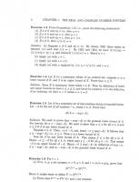
Chapter 5 17. (a) No, some plants are tall with green pods, so "tall" and "green pods" are not mutually exclusive. (b) 1200/1600 were tall, 1200/1600 were green. If independent, Pr[tall and green] = Pr[tall] × Pr[green] = 3/4 × 3/4 = 9/16, or 900 out of 1600. There were 900 out of 1600, so it appears that green and tall are independent. 18. (a) There are four kings, so Pr[draw king] = 4/52 = 1/13 (b) Pr[spade face card] = 3/52 (J, Q, K of spades = 3; 52 total) (c) Pr[card without number] = A, K, Q, J of any suit = 16 /52. (d) Pr[red] = 0.5 (13 diamonds, 13 hearts, 26 total). Pr[ace] = 4/52 = 1/13. Pr[red ace] = 2/52 = 1/26. There are red aces, so these are not mutually exclusive. Pr[red ace] = Pr[red] × Pr[ace], so they are independent. (e) Mutually exclusive events include red or black; Jack or number; spade or diamond (and many others). (f) Pr[red king] = 2/52 = 1/26. Pr[face card hearts] = 3/52. No, these events are not mutually exclusive: the king of hearts is a red king and a face card in hearts. No, these events are not independent. This is easily shown by example: Pr[king hearts] = 1/52; this is not equal to Pr[red king] × Pr[face card hearts] = 6 / 2704. 19. (a) If you pick any nucleotide from the first region, there is a 25% probability that you will pick the same nucleotide from the second region, as all nucleotides have the same probability there. Therefore, the odds that a random draw of one nucleotide from each region will match is 0.25. (b) For a codon from the first region to match a codon from the second region, this is equivalent to three independent draws occurring, each one matched in the two regions. If the probability of one matching is 0.25, then the probability of three in a row matching is 1/43 = 0.015625. 20. (a) Pr[rain on random day in Vancouver] = (0.25 × 0.58) + (0.25 × 0.38) + (0.25 × 0.25) + (0.25 × 0.53) = 0.435. (b) Pr[winter| raining] = Pr[raining| winter] × Pr[winter] / Pr[raining] = 0.58 × 0.25 / 0.435 = 0.333
21. (a) (b) Pr["Yes"] = (0.5 × 0.5) + (0.5 × 0.2) = 0.35 22. Pr[10 adenines in a row], if nucleotides are random in sequence and only draw 10, = 0.2510 = 9.54 × 10⁻⁷. 23. Imagine that the order of expression of eight genes is 1 to 8. What is the probability that these eight genes would end up in this order on a chromosome if distributed randomly? There is a 1/8 chance that gene 1 will be first. If this is true, there is a 1/7 chance that gene 2 is second. If both of these are true, there is a 1/6 chance that gene 3 is third, and so on. Overall, the product of the independent probabilities is 2.48 × 10⁻⁵. This is an acceptable answer. However, the sequence of genes would be in the same order as their expression starting at either the first or the eight gene, so we should multiply this by two to get 4.96 × 10⁻⁵. 24. Pr[all land on chromosome A] = 0.18= 1 × 10⁻⁸. There are ten different chromosomes that they could all land on, so 10 different ways to end up on the same chromosome. 10 × 10-8=10-7. 25. (a)
Overall probability of survival = (0.3 × 0.8) + (0.2 × 0.3) + (0.5 × 0.1) = 0.35 (b) Pr[Survival | lands] = 0.35. (c) Pr[Survival] = Pr[Survival | lands] × Pr[lands] = 0.35 × 0.8 = 0.28 26. (a) Pr[drawn pebble is white] = 2/5 (b) Pr[drawn pebble is white | first drawn is black] = 1/2 (c) Pr[three draws with replacement are white] = 0.43 = 0.064 (d) Pr[three sequential draws without replacement white] = 0 (there are only two white pebbles in the bag!]
(e) Drawing with replacement means that each event is independent. This is not true when drawing without replacement. 27. There are two ways to get blackjack. The first card is an ace (4/52) and the second card is a 10, J, Q, or K (16/51), or the first card is 10, J, Q or K (16/52) and the second card is an ace (4/51). In either case, the probability is 0.024. Since there are two routes, the overall probability is 0.048. 28. (a) Pr[3 randomly chosen people have different birthdates]. We imagine the first person draws a birthdate at random. The second person then has 364/365 probability of not choosing the same as the first. The third person has 363/365 of not choosing either of the other dates. Therefore, the probability that none of the three share a birthdate is 364/365 × 363/365 = 0.992. (b) Pr[10 randomly chosen people have different birthdates]? Using the logic from a, we calculate this as (364 × 363 × 362 × 361 × 360 × 359 × 358 × 357 × 356 / 3659) = 0.883. (c) If birth rates are higher at certain times of the year, this would reduce the probability that 10 randomly chosen people have different birthdates. As a thought experiment, imagine that all of the births took place in April. Then, the 10 people would have only 30 days to choose from, vastly increasing the odds that at least two birthdates would be shared. 29. Pr[five wins] = 0.55 = 0.03125. So, great generals do approximately as well as expected by chance (but slightly worse). 30. Imagine the cards being dealt one at a time. The probability that you can still have a royal flush after the first card is dealt is 20/52, because there are 20 cards in the deck of 52 cards that can be a part of a royal flush. If the first card dealt makes the royal flush possible, then there are 4 other cards of the remaining 51 in the deck that could be dealt for the second card and still leave a royal flush possible. (Only 4, because the second card has to match the suit of the first card.) For the third, fourth, and fifth cards, there are 3 out of 50, 2 out of 49, and 1 out of 48 left in the deck, assuming all previous cards leave the royal flush possible. Therefore the probability of a royal flush is 20 4 3 2 1 × × × × = 1.54 × 10 −6 . 52 51 50 49 48 31. Pr[at least one false alarm in 10 mammograms] = 0.5 = 1 - Pr[no false alarms in 10 tests]. Pr[no false alarms in 10] = Pr[no false alarm in 1 test]10 = 0.5. Pr[no false alarm in 1 test] = 0.51/10 Pr[no false alarm in one test] = 0.933 Pr[false alarm] = 1-Pr[no false alarm] = 0.067
Chapter 6 11. (a) Alternative hypothesis (b) Null hypothesis (c) Alternative hypothesis (d) Null hypothesis (e) Alternative hypothesis 12. (a) H0: Cigarette smoking has no effect on lung cancer. HA: Cigarette smoking affects the risk of lung cancer.
(b) H0: GM crop and non-GM crop suffer equal amounts of herbivore damage. HA: GM crop and non-GM crop suffer different amounts of herbivore damage. (c) H0: Industrial effluents do not affect fish densities. HA: Industrial effluents affect fish densities. (d) H0: Municipal safe-injection sites have no influence on the rate of HIV transmission. HA: Municipal safe-injection sites influence the rate of HIV transmission. 13. Statement (c) is true. 14. Statement (a) is true. 15. (a) H0: Males from the two populations have the same probability of being chosen (i.e., p = 0.5, where p is the probability that a female chooses the male from her own population). HA: Females choose one type of male over the other (i.e., p ≠ 0.5). (b) Because either outcome, that females prefer their own males (p > 0.5) or that females prefer the other males (p < 0.5), is possible. (c) P = 2 × (Pr[12] + Pr[13] + … Pr[18]) = 0.238. (d) P is the chance, if the null hypothesis is true, that 12 or more females out 18 choose their own males, or that 6 or fewer would do so. (e) The estimate of p, the proportion of females choosing their own males is 12/18 = 0.67. (Note that the estimate of the parameter differs from the null hypothesis that the proportion is 0.5). 16. (a) The smaller, 60-subject study. (b) The larger, 100-subject study. (c) Both studies have the same probability of a Type-I error. (d) Two-tailed (it is not inconceivable that COX-2 would reduce the risk of cardiac arrest). 17. The study probably reported a P-value of 0.01. The correct interpretation is that under the null hypothesis, the probability is 0.01 of obtaining a sex ratio as different (or more different) from the continental average as that observed. 18. (a) The test should be two-tailed. It is not inconceivable that snakes would choose the cooler site. (b) H0: Snakes have no temperature preference in resting sites. HA: Snakes prefer one temperature over the other. (c) The P-value would be 2 × 0.03 = 0.06.
Chapter 7 13. (a) The best estimate for heroin contact is 7/50 = 0.14. (b) The 95% confidence interval is: 0.07 < p < 0.27. (c) If estimated proportion is the true proportion, we can calculate the probability of getting exactly 7 bills with heroin out of a sample of 50. ⎛ 50⎞ Pr[7] = ⎜ ⎟ 0.14 7 (1− 0.14) 43 = 0.161. ⎝ 7⎠ 14. (a) 5 out of 12 notice the gorilla (5/12) = 0.417 (b) The 95% confidence interval (calculated using the Agresti-Coull approximation): p' = 7 / 16 = 0.4375, so the confidence interval is: 0.194 < p < 0.681.
(c) The best estimate of the students who fail to notice the gorilla is 7/12, or 0.583. 15. (a) 109 of 200 had injured themselves = 0.545. p’=111/204 = 0.544, so the confidence interval is: 0.476 < p < 0.612. (b) It is not clear whether the shoppers were selected randomly or were self-selected. Those who had sustained injury may have been more likely to take time to tell their tale of horror than those who had not. 16. (a) 1856 out of 5743 amphibian species are vulnerable, or 0.323. (b) This is not a sample: these are all of the known amphibian species. Because there is no sample of the population, the interpretation of the confidence interval makes no sense, so standard confidence interval calculations are not warranted. 17. (a) We expect the mean proportion of red alleles to be 0.5. (b) The standard deviation of the proportion of red-eyed alleles is
(0.5)(1− 0.5)
= 0.088 . 32 (c) If 0.6 of the alleles are for red eyes, 0.4 must be for brown eyes (alleles must be one type or the other). ⎛ 32⎞ (d) Pr[16 of 32 are red] = Pr[16] = ⎜ ⎟ 0.516 (1− 0.5)16 = 0.14. ⎝ 16⎠ (e) Pr[# red > 30] = Pr[30] + Pr[31] + Pr[32] = 1.23 × 10⁻⁷. 18. (a) 9 out of 32 brown = 0.28. Confidence interval: 0.16 < p < 0.46. 26 out of 32 brown = 0.81. p' = 0.78. Confidence interval: 0.64 < p < 0.91. (b) These confidence intervals do not overlap. 95% of the samples taken would result in a confidence interval containing the actual proportion of brown in the source population. With many sampled populations, some (ca. 5%) should have proportions where the 95% confidence interval does not include the actual proportion. 19. p = 10 / 200 = 0.05. p' = 12/ 204 = 0.06. Confidence interval: 0.03 < p < 0.09. 20. (a) 4 correct out of 10 = 0.4. Expected success rate = 1 /5 = 0.2 (b) Using the binomial test for the null hypothesis that the receiver had a probability of success of 1/5, we must calculate the probability of obtaining 4, 5, 6 . . . 10 correct results, and sum these together. For a two-tailed test, we must multiply the sum by 2. For four successes, Pr[4] = ⎛10⎞ 4 6 ⎜ ⎟ 0.2 (1− 0.2) = 0.088. ⎝ 4⎠ # successes 4 5 6 7 8 9 10 sum
Probability 0.088080384 0.026424115 0.005505024 0.000786432 0.000073728 0.000004096 0.000000102 0.120873882
For the two-tailed test, p = 0.24. (Even for a one-tailed test, p = 0.12). This does not meet the 0.05 cut-off for significance, so we would not reject the null hypothesis of that the probability of success was 0.2. (c) As the number of trials increases, the standard error of the estimated proportion declines (as the number of trials is in the denominator). In other words, the precision of the estimate of the proportion improves. With larger sample sizes, smaller proportional differences can be detected. 21. (a) 6101 / 9821 butter-side down = 0.621. Confidence interval: 0.612 < p < 0.631. (b) The 95% confidence interval for p exclude 0.5, so it is not very likely that the true value is 0.5. 22. 2832 / 67410 = 0.042 infections. p' = 0.042. For the 99% confidence interval, Z = 2.58, so the confidence interval is: 0.040 < p < 0.044. (b) With a smaller sample size, the confidence interval will most likely be wider. We divide by the square-root of n + 4 to find the width of the confidence interval, so as n declines, the quotient increases, and so the confidence interval grows larger. 23. (a) On average 0.25 of 12 peas should be wrinkled, or 3. (b) The standard deviation of the proportion of wrinkled pea plants is the standard error, or 0.125. (c) The variance is the square of the standard deviation, or 0.015625 ⎛12⎞ (d) Pr[2 wrinkled peas] = Pr[2] = ⎜ ⎟ 0.25 2 (1− 0.25)10 = 0.23. ⎝ 2⎠
Chapter 8 11. (a) The number of flowers in a square meter plot should be Poisson distributed. (b) Number of heads out of 10 flips of a coin should be binomially distributed. (c) Bombs per city block should be Poisson distributed. (d) Daily hits on a website should be Poisson distributed. (e) Elephant attacks on humans in Serengeti should be Poisson distributed. (f) Red flowers in sets of 100 in a field of multiple types of flowers is binomially distributed. 12. The probabilities that bound the test statistic are given below, along with the precise values calculated by Excel.
1 4 2 10
4.12 1.02 9.5 12.4
P from Statistical Table A P < 0.05 P > 0.05 P < 0.025 P > 0.05
1
2.48
P > 0.05
χ
df
2
P from computer 0.042379 0.906748 0.008652 0.259177 0.115302
13. (a) Null hypothesis: windows will kill the same number of birds per time period at any angle. Alternate hypothesis: windows angled towards the ground will kill a different number of birds per time period than windows at the vertical.
(b) 30 / 53 were killed by windows at the vertical, or 0.566. (c) We can use a goodness of fit test for the null hypothesis. (d) The null hypothesis implies windows at each angle should kill 33% of the birds. window angle 0 (vertical) 20 40 total
obs deaths 30 15 8 53
exp deaths 17.67 17.67 17.67
(Observed − Expected) 2 Expected 8.6 0.4 5.3 14.3
We had three categories, no estimated parameters, so df= 2. χ2 =14.3 > 13.92, the critical value for P = 0.001, so window angle does influence bird mortality (P < 0.001). (e) Windows might be more or less likely to cause harm depending on location as well as angle, so assigning windows to different angles and changing them daily at random was important to ensure that it was angle, not some other factor, that was being tested. 14. The mean is 0.61 deaths per regiment-year. We must combine categories to avoid expected numbers of deaths per regiment year less than 1. number of deaths 0 1 2 3+
(Observed − Expected) 2 Observed 109 65 22 4
Expected 108.67 66.29 20.22 4.82
Expected 0.00 0.03 0.16 0.11 2 χ =0.32
We have four categories, one estimated parameter (the mean), so two degrees of freedom. Our test statistic is less than 5.99, the critical value for P = 0.05, so it appears that death by horse was randomly distributed among Prussian regiments. 15. (a) Null hypothesis: the probability of giving birth on a weekend is 2/7. Alternative hypothesis: the probability of giving birth on a weekend is not 2/7. (b) There are several approaches that could be used to test this hypothesis. You could calculate the probability of observing 216 weekend births out of 932 total using the binomial distribution. However, the calculations would be tedious for such large numbers, as you would need to sum the probabilities of 0 to 216 weekend births. As an alternative, you could use a goodness of fit test to calculate the test statistic and compare it to the chi-square distribution. This is approximate, and in some cases the data may violate assumptions for the test (although not in this particular case), but it is simple and fast to calculate. (c) We use the goodness of fit test to test whether the distribution of births fits the null hypothesis of 2/7 on the weekend and 5/7 on weekdays.
(Observed − Expected) 2 weekday weekend
observed 716 216 932
expected 665.71 266.29
Expected 3.80 9.50 2 χ =13.30
There are two categories, no estimated parameters, so one degree of freedom. We can reject the null hypothesis that the probability of giving birth is constant on each day of the week with P < 0.001. 16. Plots with more than 3 truffles had to be combined with plots with three truffles to avoid expected frequencies of less than 1.
(Observed − Expected) 2 0 1 2 3+
Observed 203 39 18 28 288
Expected 158.1 94.8 28.5 6.7
Expected 12.8 32.9 3.8 68.4
χ2 = 117.9. There are four categories, one estimated parameter, so 2 df. P < 0.001. The truffles are clumped. (There are more plots with high and low numbers of truffles than expected by the Poisson distribution, and too few with the mean number.) 17. (a) The mean number of males per outcrop is the average, or 22 males / 22 outcrops = 1 male per outcrop. The standard error is the standard deviation (here, 0.62 males), divided by the squareroot of the sample size, or 0.13. (b) To test if the distribution fits the binomial, first we must estimate the chance that a fish is male. There are 132 fish, and 22 are male, or 1/6. Next, we calculate the probability of each number of male fish out of six fish, from 0 to 6 (we need to calculate the probabilities for events even if they do not appear). For instance, to calculate the probability of zero males, we use: ⎛ 6⎞ Pr[0] = ⎜ ⎟ 0.17 0(1− 0.17) 6 = 0.33. ⎝ 0⎠ We then calculate the expected number of outcrops for each number of males, combining categories if the expectation is less than one. Because the expected values ere not high enough, we combined the categories at the higher end. (Observed − Expected) 2 Observed Binomial Expected Expected males females frequency proportion frequency 0 1 2+
6 5 4 or less
4 14
0.3349 0.4019
7.37 8.84
1.54 3.01
4
0.2632
5.79
0.55
We have three categories, one parameter estimated, so df = 3-1-1=1. χ2 = 5.1, and the critical 2 value is χ 0.05,1 = 3.84 so P y] 1- 0.15866=-.84134 0.12100 0.04006 1- 0.15866=-.84134
Pr[Y < y] 0.15866 1-0.12100 = 0.87900 1-0.04006 = 0.95994 0.15866
18. B corresponds to n = 1: it is the most dispersed and bimodal. A corresponds to n = 2: it has more central tendency. C is based on n = 8. As the sample size grows, the SE will decrease (since we are dividing by the square root of n), so we can assign the sample size based on the decreasing standard deviation.
19. We wish to test whether bees distinguish between flowers with crab spiders or not. Our null hypothesis is that bees do not distinguish between the two, so p = 0.5, the expected number of flowers with spiders that bees choose is 16.5, and the standard deviation is n p (1− p) = 33(0.5)(0.5) = 2.87 . What is the probability of observing 24 trials where bees choose flowers with the spider? We convert this to a standard normal deviate: (24 - 16.5) / 2.87 = 2.61. A proportion 0.00453 of the null distribution is above this point; multiplied by two we get the P-value: P = 0.009. So, bees do not choose at random: they are more likely to choose flowers with crab spiders than expected by chance. 20. Mean -5 10 -55 12
s
y 5 -5.2 30 8.0 20 -61.0 3 12.5
SE 20
Z20
1.118 -0.18 6.708 -0.30 4.472 -1.34 0.671 0.67
Pr(Y < Y ) 0.43 0.38 0.08 0.78
SE50
Z50 0.707 4.243 2.828 0.424
Pr(Y < Y ) -0.28 -0.47 -2.12 1.18
0.39 0.32 0.02 0.88
Chapter 11 11. The standard error is SE = s / n = 0.66 / 14.7 mm.
6 = 0.269. t 0.05(2),5 = 2.57, so the 95% CI is 13.3 to
12. (a) The researchers had separate samples, so the standard deviations might have differed between them by chance. Also, the researchers might have had different sample sizes, so even if the standard deviation had been the same the standard error would differ. (b) The researcher with the smaller confidence interval probably had the larger sample size, as both the SE and the critical t value decrease as the sample size increases. (c) We cannot know that the difference was due to the sample size. By chance, the larger sample may have had a much higher sample standard deviation, causing it to have a broader confidence interval. 13. (a) On average, 88.2% of the time southern hemisphere dolphins swim clockwise. (b) The standard error is 2.86%, the df = 7, critical t 0.05(2),7 df = 2.36, so the confidence interval is 88.2 ± 2.86(2.36) or 81.4 < µ < 95.0%. (c) For the 99% confidence interval, we use the same calculation, but with t 0.01(2),7 df = 3.5, so the interval is: 78.2% < µ < 98.2%. (d) The standard deviation of clockwise swimming is 8.1%. (e) The median value for the percentage of clockwise swimming is the average of the 4th and 5th values, or 87.1%. (f) To test the null that µ0 = 0.5, we calculate t = (88.2 - 50) / 2.86 = 13.4. For 7 df, 13.4 > 7.06, the critical value for P = 0.0002. We reject the null hypothesis, P < 0.0002.
14. The mean mating index is -51.46, the standard deviation is 24.57, and the standard error is 8.19. Testing the null that there is no assortative mating by size (µ0=0), calculate t = -51.46 / 8.19 = 6.29. There are 8 df, so P < 0.002 since tcrit = 4.5 for α(2) = 0.002. We reject the null hypothesis that there is no assortative mating based on size in sticklebacks. 15. Mean weight is 10.01 µg, s = 0.2 µg, and since n = 30, SE = 0.2 / 30 = 0.037 µg. We test whether the mean sampled weight, 10.01 µg, differs from the expected weight of 10 µg. t = (10.01 - 10.0) / 0.037 = 0.27. This is less than tcrit for α(2) = 0.05 for 29 df, so we do not reject the null hypothesis that the balance is accurate. 16. Mean = 0.47, expected mean = 0.5, s = 0 .13, SE = 0.058. t = (0.47 - 0.5) / 0.058 = -0.52. This is less than tcrit for α(2) = 0.05 for 4 df, so we do not reject the null hypothesis that there is no preference in the maze when the temperature is equalized. 17. (a) Mean relatedness = -0.05, s = 0.45, SE = 0.20. The critical value for t0.05(2),4 df = 2.78, so the 95% confidence interval is -0.05 ± 0.2 (2.78), or -0.61 < µ < 0.51. (b) We calculate t: t = (-0.05 - 0) / 0.2 = -0.25. This is closer to zero than tcrit for α(2) = 0.05 for 4 df, so we do not reject the hypothesis that the unhelpful subordinates have a relatedness of zero.
Chapter 12 15. The difference in white blood cell count is 1.87, with the more promiscuous species having the higher count. (b) 0.10 < µd < 3.62. (c) The null hypothesis that there is no difference means that µ0 = 0, so t = 1.87 / 0.52 = 3.56 > α(2)0.01, 8 df, so P < 0.01. We reject the null hypothesis: promiscuous primates have higher white blood cell counts. 16. (a) We need to use Welch's t-test as the variances appear to differ with the diet. (b) For Welch's t, we need the difference in the means (2.05 - 1.54 = 0.51), with standard error of the difference = 0.0604. The null difference in means is zero. t = 8.3. The calculated degrees of freedom are 26. We can reject the null hypothesis that the diets do not lead to a difference in eye stalk length, P < 0.0002. 17. (a) Two sample t-test: The difference in means is 19.9 - 17.5 = 2.4. The null difference in means is zero. The pooled sample variance is 8.46, so the standard error of the difference between two means is 1.05. t = 2.4 / 1.05 = 2.29, with 29 df. The critical value for α(2) = 0.05 = 2.05, so P < 0 .05. We reject the null hypothesis that the copulation times are equal for the two circadian rhythm mutations. (b) We will assume that the copulation time data are normally distributed, as otherwise it is not possible to use the F-test for equal variance. F (3.37)2/(2.47)2 = 11.36 / 6.10 = 1.86, with 13, 16 df. The critical value for α(1) = 0.05 is between 2.35 and 2.42, so we do not reject the null hypothesis of equal variances. 18. Two-sample t-test: t = 3.86, df = 44, P < 0.001. Reject the null hypothesis; males are more aggressive when mated with a neighboring female.
19. (a) The mean difference is 1.83 species, with more downstream of where a tributary enters on average. There are twelve pairs of data, so we use 11 df in finding t for the confidence interval. The value for t0.05(2), 11 = 2.20. The standard error of the difference is 0.96, so the confidence interval is 1.83 + 2.2 × 0.96, or -0.28 < µd < 3.94. (b) We use the paired t-test, t = 1.83 / 0.96 = 1.91. This is less than the critical value for α(2) = 0.05 = 2.2, so we do not reject the null hypothesis that tributaries have no effect on electric fish species diversity. (c) We had to assume that the species counts were normally distributed. 20. (a) two-sample t-test: The null hypothesis is that the relatedness does not differ between helpers and non-helpers. The observed difference in relatedness is 0.32, with a standard error of 0.26. t = 0.32 / 0.26 = 1.25, which is closer to zero than the critical value for 11 df, so we do not reject the null hypothesis. (b) The 95% confidence interval for the difference in mean relatedness is 0.32+ 0.26 (the SE) × 2.2 (from t distribution) gives: -0.24 < µ1 - µ2 < 0.88. 21. (a) two-sample t-test: The difference is (1.51 - 0.87) = 0.64, the null hypothesis is that the difference is zero, and the SE of the difference is 0.16. t = 0.64 / 0.16 = 4.0, so we reject the null hypothesis that there is not a difference (P < 0.01). (b) The estimated difference is 0.64. The standard error is 0.16. 22. (a) The standard error is the standard deviation divided by the square-root of the sample size. To calculate the standard deviation from the standard error, multiply by the square root of the sample size: SD baby = 1.69; SD adult = 2.91. (b) two sample t-test: the difference in mean conductivity is 2.0, SE = 1.34. The null hypothesis is that there is no difference, so (µ1 - µ2)0 = 0. t = 2.0 / 1.34 = 1.50, with 12 df. We cannot reject the null hypothesis that the conductivity does not differ between adult and baby dolphin blubber. (P > 0.05). 23. (a) The mean change in oxygen consumption was 31.78 ml O2 kg–1. (b) For the 99% confidence interval, we need the standard error of the difference (2.31) and the t0.01(2), 9 = 3.25. The confidence interval is: 24.3 < µd < 39.3. (c) t = 31.78 / 2.31 = 13.78, which is greater than t0.0002(2), 9 = 6.01, so P < 0.0002. There is clearly a difference in oxygen consumption during feeding dives. 24. (a) two-sample t-test: The mean difference is 2.9, the difference under the null hypothesis is 0, the SE is 0.454, and df = 28, so t = 6.39, P < 0.002. The toughness varies depending on the direction. (b) This is a test of finger nail toughness for this one volunteer, but it does not test the relative toughness of fingernails in the population as a whole. You would want to do this on a random sample of humans, taking several samples from each person and using them to calculate mean toughness in each direction for that person. Since each sample from a different person is not independent, you should use a paired t-test to compare the differences in toughness in each direction, treating the difference for each person as a single data point. 25. No, this is not a valid statement. Drug X had some effect on chilblains and drug Y did not have a statistically significant effect. However, this did not mean that drug Y had no effect, which is the implication of concluding that drug X is better than drug Y based strictly on the two independent tests. To conclude that drug X is more effective, it is necessary to compare the mean effect of
drug X and the mean effect of drug Y in a two-sample t-test (assuming that the assumptions are met).
Chapter 13 16. (a) We will use the Mann-Whitney U test for this. There are no ties for the PHA response, so assigning ranks is easy. R1 = 146, n1 = 10, n2 = 10, so U1 = 9, U2 = 91, and U = 91. The critical value for α = 0.01 for 10, 10 is 84, so P < 0.01. (b) The Mann-Whitney U test : R1 = 132, n1 = 10, n2 = 10, so U1 = 23, U2 = 77, and U = 77. The critical value for α = 0.05 for 10, 10 is 77, so P = 0.05. (c) We assumed that the shapes of the two distributions were similar, which is supported by looking at the histograms for each group. 17. (a) The null hypothesis is that the median number of sexual partners is not different for biologists vs. sports majors. The alternate hypothesis is that the median number of sexual partners differs between the two groups. U is the larger of U1 and U2, or 8500.5. For this sample size, it is 2U − n1n 2 appropriate to use the Z statistic: Z = = 4.02: The probability above Z= 4.02 n1n 2 ( n1 + n 2 + 1) /3 is 0.00003, which we double to account for the other tail, so P = 0.00006. We reject the null hypothesis. (b) The distributions are roughly the same shape, so the assumptions for the Mann-Whitney U test are appropriate. (c) There are a number of questions that might be asked about the design. Were the sex ratios the same in the two groups? Sexual behavior (and the reporting of it) might well differ between the sexes. It would be useful to have the survey taken under conditions guaranteeing anonymity, to increase accuracy of the answers. 18. (a) A log-transform could make the data normally distributed, allowing use of a 2-sample t-test. Alternatively, a Mann-Whitney U could be used if the data are still highly skewed after transformation. (b) The variances are similar and the distributions are perhaps not too skewed after log transformation, so a t-test on the log-transformed data is reasonable. Average for non-territorial log GnRH: -0.359 (SD 0.397). Average for territorial log GnRH: 0.460 (SD 0.542). s2p = 0.218; SE X1-X2 = 0.282. t = 2.90, df = 9. P < 0.02, so reject the null hypothesis that the hormone levels are equal in the two groups. (c) The 95% confidence interval for the difference in mean GnRH = 0.816 + 0.283 * 2.26 (from tα(2) = 0.05 for 9 df) = 0.18 < µT − µ NT < to 1.45. 19. Histogram of differences in species number for climbing and non-climbing clades.
We will use a sign test to see if more the climbing clade has more species more often than would be expected by chance. There are 48 clades, 10 of which have more species in the non-climbing ⎛ 48 ⎛ 48⎞ 48−x x ⎞ clade, 38 have more in the climbing clade. P = 2⎜ ∑ ⎜ ⎟ 0.5 0.5 ⎟ = 0.00006 . Clades with ⎝ x =38⎝ x ⎠ ⎠ climbing vines have more species than expected by chance. 20. (a) Both distributions are roughly normal (not too skewed, probably), but the variance for the Kokanee is much greater than for the sockeye. Therefore, we could use Welch's t-test. The variance increases as the mean increases, so the log transformation might help. (b) With a log transformation, the standard errors are roughly equal, so we can use a two-sample t-test. t = 12.1, df = 33, P < 0.0001. We can reject the null hypothesis that these two have the same skin color. 21. The log-transformed data are approximately normal with roughly equal standard deviations, so we can use a two-sample t-test. s2p = 1.56; SE X1-X2 = 0.250. t = 5.30, with 162 df. P < 0.00002. Yes, babies differ in their exposure to smoke. (b) If we back-transform the numbers, we see means of 3.53 to 13.20, for a ratio of 3.7 times more exposure in the less-strict households. (c) This is an observational study. (Babies were not assigned randomly to smoking or nonsmoking households.) 22. (a) This distribution is skewed left, so the one-sample t-test is not appropriate. We can use the sign test instead. (b) 13 of the 15 samples have positive correlations, so we can calculate the probability of 13 of 15, 14 of 15, and 15 of 15 under the null hypothesis that positive and negative correlations are ⎛15 ⎞ equally likely using the binomial distribution: Pr[13] = ⎜⎜ ⎟⎟0.515 = 0.0032. Summing the ⎝13 ⎠ probabilities for 13, 14, 15 together, then multiplying by 2 (two-tailed test), we find that P = 0.0074, so we can reject the null hypothesis. 23. The distribution is left skewed, and has both positive and negative values. Therefore, we're back ⎛ 36 ⎛ 36⎞ ⎞ to a sign test. 21 of the 36 showed an increase in biomass. P = 2⎜ ∑ ⎜ ⎟ 0.5 36−x 0.5 x ⎟ = 0.41. We ⎝ x =21⎝ x ⎠ ⎠ do not see a change in biomass using the data in this way.
24. These differences are not normally distributed. With a sign test: 9 of 10 females preferred the ⎛ 10 ⎛10⎞ ⎞ redder finch. P = 2⎜ ∑ ⎜ ⎟ 0.510−x 0.5 x ⎟ = 0.02 Females, on average, prefer red males. ⎝ x =9 ⎝ x ⎠ ⎠
Chapter 14 13. The study should have a control group receiving a placebo treatment. Without it we cannot estimate the effect of the treatment. 14. Replication; balance (same numbers of treated and untreated eyes); blocking (treated and untreated eyes were paired); control (untreated eyes; sham surgery or transplant from a blind cave fish would have provided a more complete control); randomization (eye to be treated was chosen randomly on each fish). Ironically, blinding was not used. 15. (a) Increase bias (subjects having different ethnic backgrounds might be assigned to different treatments, introducing a confounding variable). No likely effect on sampling error. (b) Reduce sampling error. No effect on bias. (c) No direct effect on either bias or sampling error (but will affect decisions about sample size that will in turn affect sampling error). (d) Reduce sampling error (blocking). No effect on bias. (e) Increase bias (sample not a random sample). No clear effect on sampling error. (f) Increase bias (if effect is compared to a general population rather than a proper control group). No likely effect on sampling error. (g) Decrease sampling error. No effect on bias. (h) Increase bias (expectations might affect response to treatment). No effect on sampling error. 16. (a) Blocking. (b) Reduce sampling error (by eliminating the effect of date on the response variable). 17. 81 birds. This is a paired design, so use the sample size formula for paired t-test in Quick Formula Summary. n = 8(0.159 / 0.05)2 = 80.9, round up to 81. 18. (a) Orringer et al. used blocking in a paired design, where both treatments were applied to each subject, whereas Seaton et al. used a completely randomized design, applying two treatments to separate subjects. (b) If there is variation from subject to subject in the number of facial lesions, as a result of other factors such as age, sex, or physiology. This variation will make it more difficult to detect a treatment effect in the completely randomized design in which different treatments are applied to separate groups of subjects. The paired design eliminates the subject-to-subject variation, increasing the power of the test of treatment effect. (c) There might be “contamination”, whereby laser treatment to one side of the face affects the number of lesions on the other side of the face (e.g., by changing general hormonal or immune function). 19. Experimental studies randomly assign treatments to experimental units, reducing bias by breaking associations between confounding variables and the explanatory variable. This allows the causal relationship between the explanatory and response variables to be assessed. Random assignment is not possible in observational studies, and therefore they can never completely eliminate the effects of confounding factors.
20. (a) Yes: The diclofenac gel treatment was the control for the leech treatment. (b) Experimental study: treatments were (randomly) assigned to patients by the researchers. (c) This is a completely randomized design: the two treatments were applied to separate groups of patients. (d) The study was not double-blind: patients were aware of the treatment given them. This might have influenced their expectations of the benefits of treatment, and so their responses and the outcome of the experiment. 21. (a) The same individual could be tested with both the right and left hands (paired or block design) (b) If there was substantial variation between individuals in their reaction times. The paired design would eliminate this source of sampling error on the estimate of reaction times. (c) You would need to know the σ, the standard deviation in response time within each population. You would also need to specify the desired width of the confidence interval. 22. (a) No control group. (b) The control was not simultaneous⎯time is a confounding variable. (c) Treatments were not assigned randomly to patients. Sex is a confounding variable. (d) This study failed to include blinding (best is double blind, in which neither patients nor clinician knows which subjects received which treatment). 23. (a) Observational study: the researchers did not assign eviction or non-eviction to females. (b) Power is maximized with a balanced design. Imbalance of sample size reduces power. (c) The imbalance in sample size would increase the width of the confidence interval compared to a balanced design. (d) Let’s use the square root of the pooled sample variance, 28.4 = 5.33 to estimate σ. n = 8 (5.33 / 3)2 = 25.25, or 26 individuals in each group. 24. A factorial design. By including all combinations of treatments, it allows the measurement of the effects of each variable (age and diet restriction) separately, and the effects of their interaction.
Chapter 15 12. (a) ANOVA. (b) Try transforming the data to better meet the assumptions of normality and equal variances. If this fails, use the Kruskal-Wallis test if the distributions have equal shape. (c) ANOVA is appropriate if sample size is large enough (appealing to the Central Limit Theorem). (d) Tukey-Kramer test of all pairs of means. 13. (a) The two main assumptions of ANOVA might not be met. The variances are unequal in the two groups, and the data do not appear to be normally distributed in all the groups. (b) The main assumption of the Kruskal-Wallis test might not be met: the distributions do not appear to have the same shape. [Faced with this situation, most researchers would apply both methods, report the results from both, and go with the findings if they give the same answer] 14. (a) The figure below shows the proportion of flies that took a second blood meal from cows in the two groups.
(b) ANOVA assumes that the measurements in the two populations are normally distributed with equal variance. These assumptions do not appear to be met in the present data. In flies given a first blood meal from a cow, the measurements do not appear to be normally distributed and the variance is low compared with flies given a first blood meal from a lizard. (c) The data are proportions, so the arcsine square root transformation is the logical first choice for a transformation. The two panels on the right of the figure above show the proportions after transformation. This has indeed largely fixed the problem: the data appear more normal and the variances are similar in the two groups. (d) H0: The means of the two treatment groups are the same (µ1 = µ2). HA: The means of the two treatment groups are different (µ1 ≠ µ2). You can use either a two-sample t-test or ANOVA. The ANOVA results are: Source of variation Sum of squares df Mean squares F-ratio P Groups (First blood meal) 1.258154 1 1.258154 56.34 0.00001 Error 0.245619 11 0.022329 Total 1.503773 12 The critical value F0.05(1),1,11 = 4.84. Since F > 4.84, P < 0.05, reject H0. First blood meal affects the mean proportion of flies taking their second blood meal from cows. 15. (a) A large sample size makes ANOVA more robust to departures from the assumption of normality. In addition, a large sample size increases the power of the test. (b) A balanced design makes ANOVA more robust to departures from the assumption of equal variances. In addition, a balanced design increases the power of the test compared with an unbalanced design having the same total sample size. 16. Show the data. 17. (a) Group i 6 6 3
Group j 1 3 1
Yi − Y j
23.26 12.60 10.67
SE q 7.13 3.26 7.45 1.69 7.13 1.50
q0.05, k , N − k
2.47 2.47 2.47
Conclusion Reject H0 Do not reject H0 Do not reject H0
(b) These are unplanned comparisons − we are searching for differences between groups rather than testing a specific difference between two groups identified as crucial prior to seeing the data. (c) This would result in a probability of making at least one Type 1 error greater than α = 0.05 during the course of testing all pairs of means. (d) 0.05. 18. (a) SEY is a measure of the precision of the estimate of the mean: it is the standard deviation of the sampling distribution of the mean. (b) H0: Mouse strains in the population do not differ in the mean number of minutes spent in the open. HA: Mouse strains in the population differ in the mean number of minutes spent in the open. Source of variation Sum of squares df Mean squares F-ratio P Groups (Strain) 5.4087 3 1.8029 14.66 0.00001 Error 2.9515 24 0.1230 Total 8.3602 27 The critical value F0.05(1),3,24 = 3.01. Since F > 3.01, P < 0.05, reject H0. Conclude that mouse strains in the population vary in the mean number of minutes spent in the open. (c) Random-effects ANOVA: the four inbred strains were picked at random from a population of strains. (d) Variance among groups: sA2 = 0.240. Variance within groups, MSerror = 0.120. (e) Repeatability = 0.66. (f) The fraction of total variance that is among groups. 19. (a) The data indicate that the assumption of equal variance within all populations is violated. Some treatments have much higher variance than others. The assumption that the measurements are normally distributed within populations might also be violated for some groups (e.g., larva + adult treatment). (b) The Kruskal-Wallace test, when used to test differences between means, assumes that the frequency distributions are the same in the different groups. This assumption is clearly violated, so we cannot conclude that the means are different. All we can conclude from the Kruskal-Wallis result is that the distributions are different, but not necessarily their means or medians. 20. The answer is (b). a) It is never possible to conclude that a difference does not exist, only that it was not detected. (b) Correct: while the study did not detect a difference, an undetected difference may nonetheless be present. (c) The P-value gives no indication of the size of the difference between groups. (c) A larger sample size would increase power to detect a difference if one was present. Nevertheless, it is possible that there is no difference among age groups. 21. (a) Source of variation Groups (specimens)
Sum of squares 0.015788
df 24
Mean squares 0.000658
F-ratio 3.96
P 0.0005
Error 0.004150 25 0.000166 Total 0.019938 49 Statistical Table D shows that the critical value F0.05(1),24,25 is between 1.94 and 2.03 (actual value is 1.96). Since the observed F-ratio is greater, P < 0.05. (b) The mean squares for error are the estimate for the variance within groups for head width: 0.00017. (b) s2A = (0.000658 − 0.000166)/ 2 = 0.000246. (c) The repeatability is 0.000246 / (0.000246 + 0.000166) or 0.597. This is slightly less than the repeatability of the femur measurement, indicating that head size has a higher proportion of its total variation attributable to measurement error. 22. (a) Planned comparison. (b) Y1 − Y2 = 8.90 − 6.08 = 2.82. MSerror= 0.2935, df = 13, SE = 0.328, t0.05(2),13 = 2.16, 2.11 < µ1 − µ2 < 3.53. (c) H0: Habitat types do not differ in mean cone size (µ1 = µ2 = µ3). HA: Habitat types differ in mean cone size (at least one µi is different). Source of variation Sum of squares df Mean squares F-ratio P Groups (Habitat type) 29.404 2 14.7020 50.09 3.81, P < 0.05, reject H0. Conclude that mean cone size differs between habitat types. 23. (a) No, the sample sizes in the different groups are unequal, so the design is not balanced. (b) The sham-treatment is the main control for the marrow treatment: the mice are subjected to the same handling but don’t receive the enhanced marrow. The untreated mice provide a baseline measurement, allowing the researchers to determine the effect of the sham surgery. (c) Sample mean Y Group Standard deviation s Enhanced 211.11 116.67 Sham-treated 560.00 219.09 Untreated 666.67 206.60 (d) The standard deviations are not equal, the sample size is small, and the design is unbalanced. ANOVA is not robust to the violation of equal standard deviations under these conditions. (e) A log transformation may overcome this. After transforming, the differences in the standard deviations are less extreme: Group Enhanced Sham-treated Untreated
Sample mean Y 5.22 6.27 6.45
Standard deviation s 0.54 0.38 0.36
(f) H0: Mean dilution is equal among treatments (µ1 = µ2 = µ3)
HA: Mean dilution differs among treatments (at least one µi is different) Source of variation Sum of squares df Mean squares F-ratio P Groups (Treatment) 6.6196 2 3.3098 15.78 0.0001 Error 3.5660 17 0.2098 Total 10.1856 19 The critical value F0.05(1),2,17 = 3.59. Since F > 3.59, P < 0.05, reject H0. Conclude that mean dilution differs between treatments. (g) Use the Tukey-Kramer method. 24. (a) Source of variation Sum of squares df Mean squares Groups (specimens) 11.322 33 0.343 Error 1.566 34 0.046 Total 12.888 67 s2A = (0.343 - 0.046)/ 2 = 0.149. The repeatability is 0.149/ (0.149 + 0.046) or 0.76. (b) Repeatability measures the fraction of the total variance in measurements of running speed that is between lizards, rather than variation between measurements made at separate times on the same lizard.
Chapter 16 12. (a) There is a negative linear relationship between telomere length and chronicity, but it is not strong. (b) −0.43. (c) −0.66 < ρ < −0.13. (d) It is the range of most plausible values for the parameter ρ. If you were to repeatedly and randomly sample individuals from the same population and compute the 95% confidence interval each time, 19 out of 20 of the intervals are expected to include the population correlation ρ. (e) Assume random sampling, and that the two variables have a bivariate normal distribution in the population. (f) (Answers may vary) The scatter plot suggests that the relationship between telomere length and chronicity might be mildly non-linear, which would violate the assumption of bivariate normality. 13. (a)
(b) r = 0.82 (c) H0: There is no correlation between second language proficiency and grey matter density (ρ = 0). HA: There is a correlation between second language proficiency and grey matter density (ρ ≠ 0). r = 0.82, SE = 0.13, t = 6.37, df = 20, P = 0.000003 t0.05(2),20 = 2.09. Since t is greater than t0.05(2),20, P > 0.05. Reject H0. Conclude that second language proficiency and grey matter density are correlated.
(d) Random sampling and a bivariate distribution of gray matter density and language proficiency in the population. (e) No, because there appears to be two outlying observations, which violates the assumption of bivariate normality. (f) No, correlation alone does not imply causation. Perhaps individuals with high grey matter densities are able to achieve a high proficiency in a second language. An experiment would be necessary to test whether proficiency affects grey matter. 12. (a) 95%: −0.006 < ρ < 0.68 99%: −0.14 < ρ < 0.75 (b) 95%: −0.53 < ρ < 0.15 99%: −0.61 < ρ < 0.26 13. (a) The assumption of bivariate normality is violated: there is an outlier. (b) Using a rank correlation would be appropriate. (c) H0: The population rank correlation is zero (ρS = 0) HA: The population rank correlation is not zero (ρS ≠ 0) rS = −0.30. P = 0.053. rS (0.05(2),41) = 0.308. Since rS is not greater than or equal to rS (0.05(2),41), P > 0.05, do not reject H0. Conclude that we cannot reject the null hypothesis of zero correlation. (d) Random sample, and that there's a linear relationship between the ranks of the two variables. 14. (a) butterfly: r = 0.35 SEr = 0.26; bird: r = 0.61 SEr = 0.22; plants: r = 0.41 SEr = 0.25 (b) butterfly: −0.20 < ρ < 0.73; bird: 0.14 < ρ < 0.85; plants: −0.13 < ρ < 0.76 15. −0.35 < ρ < 0.81. 16. (a) r = −0.86. (b)
(c) The relationship is non-linear. (d) A transformation of one or both variables (e.g., the log transformation) to make the relationship linear is the first step. If transformations fail to remedy the problem, a nonparametric correlation is the next option. 17. (a) r = 0.86 (b) SE = 0.18 (c) The standard error is the standard deviation of the sampling distribution of r.
(d) H0: There is no correlation between increase in slow-wave sleep and increase in performance (ρ = 0). HA: There is a correlation between increase in slow-wave sleep and increase in performance (ρ ≠ 0). $n.df:
t = 4.84, df = 8, P = 0.0013. t0.05(2),8 = 2.31. Since t is greater than t0.05(2),8, P > 0.05. Reject H0. Conclude that is a positive correlation between increase in slow-wave sleep and increase in performance. (e) This is an observational study [note: the original study also included an experiment]. The researchers did not assign subjects to different values of slow wave sleep increase. 18. (a) Measurement error tends to reduce the estimated correlation between variables. (b) Take multiple measurements on each subject, then average them. (c) Repeatability (Chapter 15). 19. (a)
(b) The assumption of bivariate normally is violated. For example, the frequency distribution of each variable is skewed right, and there is much more scatter for large values than for small values of both variables. (c) Transformation of one or both variables. The log transformation is always a good one to try when variables are right-skewed and values are greater than zero. The arcsine transformation is also an obvious on to try on the variable “percent left handed”, because it can be converted to a fraction by dividing by 100 (don’t forget the square root step). (d) A log transformation of both variables yielded a satisfactory outcome:
A log transformation of homicide rate and an arcsine transformation of percent left handed (after dividing by 100) also gave a satisfactory outcome (though the log appeared slightly better). (e) H0: There is no correlation between homicide rate and percent left-handed individuals (ρ = 0). HA: There is a correlation between homicide rate and percent left-handed individuals (ρ ≠ 0).
Results using the log-log transformation: r = 0.88, SE = 0.19, t = 4.59, df = 6, P = 0.0037 t0.05(2),6 = 2.45. Since t is greater than t0.05(2),6, P > 0.05. Reject H0. Conclude that homicide rate and percent left-handed individuals in societies are correlated. Results using log transformation of homicide and arcsine of percent left-handed: r = 0.87, SE = 0.20, t = 4.29, df = 6, P = 0.0051 t0.05(2),6 = 2.45. Since t is greater than t0.05(2),6, P > 0.05. Reject H0. Conclude that homicide rate and percent left-handed individuals in societies are correlated. 20. (a) The data clearly have an outlier, and so do not fit the assumption of bivariate normal.
(b) (Answers may vary). A log-transformation of distance improves matters considerably. A log transformation of recruitment helps matters a bit more, but not hugely, and might raise some additional problems (higher scatter at one end of the distribution than the other, but hard to tell because of small sample size) (c) Log transformation of distance only: r = 0.81, SE = 0.24. Log transformation of both variables: r = 0.72, SE = 0.29. (d) Log transformation of distance only: 0.24 < ρ < 0.96 Log transformation of both variables: 0.02 < ρ < 0.94 21. (a) r = 0.55, SE = 0.15 (b) 0.15 < ρ < 0.79 (c) Random sampling and a bivariate normal distribution of percent receptors blocked and rating of “high”. (d) A lower correlation is expected (closer to zero) when there is a smaller range of values for the variables even when the relationship between the variables is otherwise the same. This could explain the results of the second team of researchers despite using the same population and sample size. 22. Association between treatment (a categorical variable with two groups) is measured by the difference between the means of the two groups rather than with a correlation coefficient. The difference is tested with a two-sample t test (or ANOVA). H0: Mean growth rate is the same in the two CO2 groups (µ1 = µ2) HA: Mean growth rate differs between the two CO2 groups (µ1 ≠ µ2) X 1 = 1.66 (Normal), X 2 = 1.53 (High), SE X 1 − X 2 = 0.237, t = 0.54, df = 12, P = 0.60. t0.05(2),12 = 2.18. Since t is not greater than or equal to t0.05(2),12, P > 0.05. Do not reject H0. Conclude that the null hypothesis of no difference between the means of the two groups is not rejected by these data.
Chapter 17 13. (a) The variance in Y is not equal for all X, but increases with increasing X. (b) The relationship between X and Y is not linear. (c) The residuals are not normally distributed. (d) The residuals are not normally distributed, and the variance in Y is not the same for all X, because of the outlier. 14. (a) The number of added nutrients should be the explanatory variable (X), as this was controlled by the experimenters. The response variable of interest (Y) is the number of plant species supported.
(b) b = −3.34 (3.34 species are lost for each nutrient added), SE = 1.10. (c) R2 = 0.54 (d) H0: There is no treatment effect (β = 0) HA: There is a treatment effect (β ≠ 0) t = −3.04, df = 8, P = 0.016, t0.05(2),8 = 2.31. Since t > 2.31, P < 0.05. Reject H0. Conclude that adding more nutrients reduces the number of plant species supported. 15. (a)
(b) Y = 0.152 + 0.028X (c) %Nitrogen per earthworm species. (d) Yˆ = 0.294. (e) SE = 0.0096. (f) 0.009 < β < 0.048 16. (a) The equation is a power function, which can be made linear by taking the log of each side: log(R) = log(α) + β log(M). β is now the slope of a linear relationship between ln mass (X) and ln basal metabolic rate (Y). After taking logs and applying the usual formulas we get b = 0.74. (b) The formula for the line is calculated as: Y = −4.05 + 0.74 X , where X is ln mass and Y is ln basal metabolic rate:
(c) SE = 0.042, t0.05(2),15 = 2.13, 0.65 < β < 0.83 17. H0: The slope of the relationship between ln metabolic rate and ln mass is 0.75 (β = 0.75) HA: H0: The slope of the relationship between ln metabolic rate and ln mass is not 0.75 (β ≠ 0.75) t = (b − β0)/SE = −0.20, df = 15, P = 0.84, t0.05(2),15 = 2.13. Since t < 2.13, P > 0.05. Do not reject. Conclude that the slope of the linear relationship (exponent of the power function) is not significantly different from 0.75. 18. (a) b = 0.798 (b) b = 0.771 (c) Regression toward the mean. 19. (a) b = 0.0025, SE = 0.00045. (b) H0: There is no relationship between fleck duration and relative growth (β = 0) HA: There is a relationship between fleck duration and relative growth (β ≠ 0) t = 5.64, df = 19, P = 0.00002. t0.05(2),19 = 2.09. Since t > 2.09, P < 0.05. Reject H0. Conclude that there is a (positive) relationship between fleck duration and growth. (c) 0.0012 < β < 0.0038 (d) Assume that there is a normal distribution of Y values for each X, of which we have a random sample. Assume that the relationship is linear. Assume that the variance in Y is the same at every X. (e) Scatter plot and then residual plot. 20. (a) Group Mean Standard deviation Breeding males 0.336 0.027 Breeding females 0.317 0.059 Molting females 0.303 0.067
n 9 9 6
(b) H0: Mean slope is the same in the three groups (µ1 = µ2 = µ3) HA: Mean slope is not the same in the three groups (at least one of the µi is different) Source of variation Sum of squares df Mean squares F-ratio P Groups 0.00394 2 0.00197 0.734 0.49 Error 0.05636 21 0.00268 Total 0.06030 23 F0.05(1),2,21 = 3.47. Since F < 3.47, P > 0.05. Do not reject. Conclude that the slopes are not significantly different among penguin groups.
21. (a) Relative horn size (mm2) 0.074 0.079 0.019 0.017 0.085 0.081 0.011 0.023 0.005 0.007 0.004 −0.002 −0.065 −0.065 −0.014 −0.014 −0.132 −0.143 −0.177
Relative wing Predicted relative mass (µ g) wing mass (µ g) Residuals −42.8 −9.9 −32.9 −21.7 −10.6 −11.1 −18.8 −2.6 −16.2 −16.0 −2.4 −13.6 −12.8 −11.4 −1.4 11.6 22.5 −10.9 7.6 9.2 −1.6 1.6 4.8 −3.2 3.7 4.5 −0.8 1.1 2.2 −1.1 −0.8 −0.7 −0.1 0.1 −2.9 −3.0 12.1 8.5 3.6 20.1 8.5 11.6 21.2 1.7 19.5 22.2 1.7 20.5 20.1 17.4 2.7 12.5 18.8 −6.3 7.0 23.3 −16.3
(b)
(c) The scatter plot and residual plot show that X and Y are not linearly related, violating a core assumption of linear regression. (d) Try a transformation to make the relationship linear. If that fails, resort to nonlinear regression. 22. (a) The relationship between the days survived and spores produced is non-linear. Square root transformed number of spores rises with increasing host longevity but then appears to decline at the longest host lifespans. (b) A quadratic curve.
23. If we extrapolate from the regression based non-human primates, the human glia-neuron ratio is somewhat higher than that predicted for a brain of its mass, but not by much. On this basis, the metabolic demands of the human brain are not much greater than that of other primates, once we take brain size into account. But the extrapolation is risky: we can’t be sure that the relationship between glia-neuron ratio and brain mass in non-human primates is linear beyond the range of the data. In the scatter plot, the relationship between the two variables appears slightly curved even within the range of the non-human primate data. As a result, it isn’t possible to draw a firm conclusion. 24. (a) To make the distribution of residuals more normal, to make the variance of Y (and of the residuals) equal for all values of X, and to make a non-linear relationship linear. It is often effective when the variable is a count. (b) The researcher assigned the doses of DEET to subjects. (c) Source of variation Sum of squares df Mean squares F-ratio Regression 9.97315 1 9.97315 22.58 Residual 22.08375 50 0.4417 Total 32.05690 51 (d) H0: The slope of the relationship between DEET dose and number of bites is zero (β = 0) HA: The slope of the relationship between DEET dose and number of bites is not zero (β ≠ 0) F = 22.58, df = 1,50, P =0.00002. ; F0.05(1),1,50 = 4.03. Since F > 4.03, P < 0.05. Reject H0. Conclude that the slope is significantly different from zero. (e) R2 = 0.31. It is the fraction of the variation in number of bites (square root transformed) that is “explained” by X. 25. The slope is close to 1. (b) The inner pair of lines show the confidence bands. They give the most plausible range of values for the mean Y (actual year of birth) corresponding to each X (estimated year of birth). (c) The outer lines show the prediction interval. This gives the most plausible range of values for a single Y measurement (actual year of birth) corresponding to each X (estimated year of birth).
Chapter 18 8. (a) It measures whether the full linear model that include the term WORKERTYPE is a significantly better fit to the data than a model lacking the term (but including all other terms). (b) It measures whether the full linear model that include the BLOCK term is a significantly better fit to the data than a model lacking the term (but including all other terms). (c) It should be retained because it was part of the design, and because it might still improve the ability to detect an effect of the factor of interest. (d) The residuals are the difference between the observed values and the values predicted by the model. (e) The residuals are plotted along the Y-axis. The predicted values from the model are plotted along the X axis. 9. (a) BRAINSIZE = CONSTANT + SPECIES + MASS + SPECIES*MASS
(b) SPECIES*MASS represents the interaction between the effects of SPECIES and the effects of MASS. (c) This F-ratio measures whether the full linear model that include the interaction term in the linear model is a significantly better fit to the data than a model lacking the term (but including all other terms). (d) H0: There is no interaction between the effects of species and body mass on brain size. (Or, equivalently, the linear regressions of brain size on body mass in the two species have equal slopes). HA: There is an interaction between the effects of species and body mass on brain size (Or, equivalently, the linear regressions of brain size on body mass in the two species do not have equal slopes). (e) We are unable to reject the null hypothesis of no interaction between species and body mass on brain size. (Or, equivalently, we are unable to reject the null hypothesis of equal regression slopes of brain size on body mass in the two species). (f) Assume that there is no interaction, drop the interaction term from the model, and then proceed to test for differences between species in brain size after controlling for body mass. 10. The predicted values lie along two parallel regression lines, one for each species.
11. (a) The authors probably began by testing the null hypothesis of no interaction between MATURATION and EXPLOITATION. Being unable to reject the null hypothesis or no interaction, they assumed that none was present, and then dropped the interaction term from their general linear model. (b) That the response variable (CV, coefficient of variation of population size) has a normal distribution with equal variance in every combination of maturation age and exploitation group. That we have a random sample of values of CV from each combination [this assumption also covers the assumption that species data are independent⎯see Interleaf 11]. That the relationship between CV and age of maturation is linear and has the same slope in both exploitation groups. (c) Yes. The P-value for the EXPLOITATION term is small (P = 0.005). 12. (a) Numbers at the right of plot indicate family numbers. (Standard error bars could be added to this plot). The non-parallel lines in the interaction plot suggests an interaction is present between morning glory species and family (the effect of morning glory species on development time is not the same in all families).
(b) TIME = CONSTANT + SPECIES + FAMILY + SPECIES*FAMILY. TIME is the development time in days, CONSTANT is the grand mean of development time, SPECIES is the morning glory species fed to the beetles, FAMILY is the family that the beetle belongs to, and SPECIES*FAMILY is the interaction between FAMILY and SPECIES. (c) SPECIES is a fixed effect and FAMILY is a random effect. The morning glory species are repeatable groups of direct interest. They are not a random sample of morning glory species. In contrast, the families were randomly sampled from a population of families. They are not repeatable (a future study of the same population would not use the same families) nor of direct interest. (e) That TIME is normally distributed with equal variance for all combinations of SPECIES and FAMILY. That the individuals in each combination of SPECIES and FAMILY are a random sample. (f) Each F-ratio measures whether the full linear model that include the corresponding term in the linear model is a significantly better fit to the data than a model lacking the term (but including all other terms) 13. (a) Factorial design. (b) OFFSPRING = CONSTANT + FEMALEORIGIN + MALEORIGIN + FEMALEORIGIN*MALEORIGIN. (c) The main effect of female’s origin (FEMALEORIGIN) and the interaction between male’s origin and female’s origin (FEMALEORIGIN*MALEORIGIN). The main effect of male’s origin (MALEORIGIN) appears to be small because the mean percentage of offspring is similar in the two groups when averaged over the two groups of females.
Chapter 19 16. −0.88 < ρ < −0.58 17. B is a randomized data set because there is little or no relationship between the two variables, whereas A shows a positive relationship. Since randomization tends to break up associations, it is more likely that A is the data and B is a randomization. 18. (a) No. The assumption of a normal distribution is violated. (b) 1. Confidence interval based on the t-distribution might be appropriate after transformation. 2. Bootstrap. (c) 1. Randomization test. 2. Mann-Whitney U-test. 19. (a) The sampling distribution of sample median biomass ratio.
(b) 0.134. (c) 1.3 < population median < 1.8 20. The distribution includes outliers and the trimmed mean is an objective way to increase the precision of the estimate. For the light data, the 5% trimmed mean drops the three smallest and three largest values, and the 5% trimmed mean is 28.8274. Bootstrapping is an excellent way to calculate the uncertainty of the trimmed mean. The results of 1000 bootstrap replicate estimates of the trimmed mean are shown in the following histogram. Of the bootstrap estimates, 2.5% were below 24.8254, 5% were below 24.8260, 95% were below 24.8285, and 97.5% were below 24.8288. (a) 24.8254 < µ < 24.8288. (b) Yes. 21. (a) The null distribution for the variance/mean ratio. (b) H0: The variance/mean ratio equals that expected according to the random placement of compensatory mutations. HA: The variance/mean ratio does not equal that expected according to the random placement of compensatory mutations. None of the simulated values for the variance/mean ratio were as large or larger than the observed ratio of 2.64. Hence, P = 2 × 0/10,000. (In this case we say that P < 0.0001 rather than that P = 0.) Since P < 0.05, reject H0. Conclude that compensatory mutations are clumped.
Chapter 20 9. (a) 540 generations (b) 220 < number of generations < 1160 (c) This interval is like a 95% confidence interval. It describes the most plausible values of the number of generations since the origin of the huntingtin mutation. 10. (a) Binomial distribution. ⎛ 68 ⎞ 55 (b) L[p | 13 labile] = ⎜⎜ ⎟⎟ p 13 (1 − p ) . This measures the probability of getting 13 gender-labile ⎝ 13 ⎠ individuals in a sample of 68 if the data given that the proportion of gender-labile individuals in the population is p. (c) We assume that we have a random sample of shrubs. Each individual shrub had the same probability of being sampled and sampling of individuals was independent. ⎡⎛ 68 ⎞⎤ (d) ln L[p | 13labile] = ln ⎢⎜⎜ ⎟⎟⎥ + 13 ln[ p ] + 55 ln[1 − p ] ⎣⎝ 13 ⎠⎦ (e) –8.93 11. (a) 0.019 (b) 0.11 < p < 0.30 12. (a) H0: The fraction of patients improving p is 0.5 HA: The fraction of patients improving p is not 0.5
G = 2 (–1.9 – (–4.5)) = 5.2. χ 02.05,1 = 3.84 . Since G > 3.84, P < 0.05 (exact P = 0.023). Reject H0. More patients improve than deteriorate. (b) 0.52 < p < 0.84 13. (a)
(b) 0.87 (c) 0.76 < p < 0.95. 14. (a) H0: The proportion of mated females chosen by the wasps is 0.5. HA: The proportion of mated females chosen by the wasps is not 0.5. The Expected frequency is 16 for both categories. ⎡ Observedi ⎤ ⎛ ⎡ 23 ⎤ ⎡ 9 ⎤⎞ (b) G = 2∑ Observedi ln ⎢ ⎥ = 2⎜⎜ 23ln ⎢ ⎥ + 9ln ⎢ ⎥ ⎟⎟ = 6.34 ⎣ 16 ⎦ ⎣16 ⎦ ⎠ ⎝ ⎣ Expectedi ⎦ (c) The critical value is χ 02.05,1 = 3.84 with 1 df. The observed G >3.84, so P < 0.05 Exact P = 0.012). Reject H0. The wasps prefer the mated females. (d) The value of the G-statistic here is the same as the statistic calculated using the log-likelihood ratio test. This is no coincidence: the G-test is a log-likelihood test. 15. (a)
(b) 0.87 (c) 0.77 < p < 0.95 16. (a) 0.85 (b) 0.77 < p < 0.91. There is almost complete overlap with the confidence interval for males.
17. H0: Infants have no preference for direct or indirect gaze (p = 0.5) HA: Infants prefer one gaze type over the other (p ≠ 0.5) The maximum likelihood estimate for p is pˆ = 0.88 (this can be obtained by using a spreadsheet to find the peak in the likelihood curve, or by simply calculating pˆ = 15/17. The log-likelihood of p = 0.5 is −6.87, and that of p = 0.88 is −1.25. G = 2*(−1.25−(−6.87)) = 11.24. χ 02.05,1 = 3.84 . Since G > 3.84, P < 0.05 (exact P = 0.0008). Reject H0. Infants prefer the direct gaze over indirect gaze. 18. (a) 0.04 (b) −142.98 (c) 0.02 < λ < 0.06
Chapter 21 8. (a) A low fail-safe number indicates that even a small publication bias would change the conclusion. Therefore, we should not be confident in the results of the meta-analysis. (b) A large fail-safe number suggests that it would take an improbably large publication bias to change the conclusions. In this case we should be confident in the results. 9. Meta-analysis has potentially greater objectivity; it can provide a quantitative measure of the overall or average effect; it has more power than vote-counting; it can evaluate publication bias. 10. (a) Odds ratio. (b) Standardized mean difference. (c) Correlation coefficient. (d) Odds ratio. (e) Standardized mean difference. 11. (a) Moderator variable (b) “Continent” is potentially a confounding variable. If so, then the estimate of the effect of alien vs. native predators might be biased. (c) By combining multiple studies of different type, meta-analysis introduces “study type” as a variable whose association with study outcome can be measured. 12. Chance; real differences between study systems; some studies have biased protocols