Support Water-Management Decision-Making Under Climate Change Conditions 1606920332, 9781606920336, 9781607412045

Citation preview

SUPPORT WATER-MANAGEMENT DECISION-MAKING UNDER CLIMATE CHANGE CONDITIONS

No part of this digital document may be reproduced, stored in a retrieval system or transmitted in any form or by any means. The publisher has taken reasonable care in the preparation of this digital document, but makes no expressed or implied warranty of any kind and assumes no responsibility for any errors or omissions. No liability is assumed for incidental or consequential damages in connection with or arising out of information contained herein. This digital document is sold with the clear understanding that the publisher is not engaged in rendering legal, medical or any other professional services.

SUPPORT WATER-MANAGEMENT DECISION-MAKING UNDER CLIMATE CHANGE CONDITIONS

ANGEL UTSET SUASTEGUI

Nova Science Publishers, Inc. New York

Copyright © 2009 by Nova Science Publishers, Inc.

All rights reserved. No part of this book may be reproduced, stored in a retrieval system or transmitted in any form or by any means: electronic, electrostatic, magnetic, tape, mechanical photocopying, recording or otherwise without the written permission of the Publisher. For permission to use material from this book please contact us: Telephone 631-231-7269; Fax 631-231-8175 Web Site: http://www.novapublishers.com NOTICE TO THE READER The Publisher has taken reasonable care in the preparation of this book, but makes no expressed or implied warranty of any kind and assumes no responsibility for any errors or omissions. No liability is assumed for incidental or consequential damages in connection with or arising out of information contained in this book. The Publisher shall not be liable for any special, consequential, or exemplary damages resulting, in whole or in part, from the readers’ use of, or reliance upon, this material. Independent verification should be sought for any data, advice or recommendations contained in this book. In addition, no responsibility is assumed by the publisher for any injury and/or damage to persons or property arising from any methods, products, instructions, ideas or otherwise contained in this publication. This publication is designed to provide accurate and authoritative information with regard to the subject matter covered herein. It is sold with the clear understanding that the Publisher is not engaged in rendering legal or any other professional services. If legal or any other expert assistance is required, the services of a competent person should be sought. FROM A DECLARATION OF PARTICIPANTS JOINTLY ADOPTED BY A COMMITTEE OF THE AMERICAN BAR ASSOCIATION AND A COMMITTEE OF PUBLISHERS. LIBRARY OF CONGRESS CATALOGING-IN-PUBLICATION DATA Suasteguiá, Angel Utset. Introducing modelling tools to support water-management decision-making under climate change conditions / Angel Utset Suasteguiá. p. cm. ISBN 978-1-60741-204-5 (E-Book) 1. Irrigation--Management--Data processing. 2. Irrigation--Management--Mathematical models. 3. Climatic changes--Data processing. 4. Climatic changes--Mathematical models. I. Title. TC812.S829 2009 333.91'3--dc22 2008041993

Published by Nova Science Publishers, Inc. New York

CONTENTS Preface Chapter 1

vii Climate Change, Agriculture and Water Resources in the Mediterranean Region

1

Chapter 2

Climate Scenarios, Seasonal Forecasts and Downscaling Issues 11

Chapter 3

Simulating Crop-Growth and Crop Water-Use

17

Chapter 4

Applying Climate and Crop-Growth Simulation Tools to Support Agricultural Decision-Making

35

References

67

Index

81

PREFACE According to climate change assessments, less precipitations and higher temperatures can be expected in the Iberian Peninsula and other Mediterranean zones. Besides, an increment in droughts and other extreme events can be expected as well. Such climatic conditions require an effort to optimize irrigation technologies and to improve water management efficiency. There are currently available water-use and crop-growth simulation models, which can be combined to climate scenarios and weather generators in order to recommend, through many simulations, the most reliable irrigation management. The Preliminary Assessment of the Impacts in Spain due to the Effects of Climate Change and the National Plan for Adaptation to Climate Change recommend the use of such simulation tools in Spanish climate-change impact assessments. Those tools, however, have not been used yet to support irrigation decision-making in our country. In that sense, the EU-funded proposal AGRIDEMA, leaded by Spain, has been addressed to introduce such tools, connecting the tools “providers” from Universities and high-level research centres, with their “users”, located in agricultural technological or applied-research centres. AGRIDEMA comprised courses and Pilot Applications of the tools. Local researchers knew in the AGRIDEMA courses how to access to GCM data and seasonal forecasts, they receive also basic knowledge on weather generators, statistical and dynamical downscaling; as well as on available crop models as DSSAT, WOFOST, CROPSYST, SWAP and others. About 20 pilot assessments have been conducted in several European countries during AGRIDEMA, applying the modelling tools in particular cases. The AGRIDEMA results are commented, mentioning particularly the Pilot Assessments that were held in Spain and in the Mediterranean area. Furthermore, several “users” opinion regarding the available climate and crop-growth

viii

Angel Utset Suastegui

simulation tools are also pointed out. Those opinions can be used as important feedback by the tools “developers”. An illustrative example on how modelling tools can help to manage Sugarbeet irrigation under present and future climate conditions in Spain is also shown. Several future research directions are pointed out, as followed from the shown example and the AGRIDEMA results. Those research directions agree with the actions recommended in the Spanish National Plan for Adaptation to Climate Change, as well as in the European and international guidelines. Stakeholder will adopt climate-change mitigation options only if they realize the reliability of such options on their specific cases. To achieve this, the “users” of the modelling tools must develop local demonstration proposals, aimed to model calibration and validation, etc. Particularly, some demonstration proposals should be aimed to recommend productive and efficient irrigation water managements under the adverse climate conditions that Spanish farmers will eventually face in the next years.

Chapter 1

CLIMATE CHANGE, AGRICULTURE AND WATER RESOURCES IN THE MEDITERRANEAN REGION The last IPCC (2007) report pointed out clearly the climate variability observed in the last decades, very probably due to the higher concentration of CO2 and other gases emissions related to human activity. Particularly, the increment in the frequency of extreme event, as droughts and flooding, has been considered also as a climate-change consequence. Despite that temperature rising could be expected all over the world, rainfall changes are different according to the regions. Northern regions might expect increment in yearly rainfall, while total precipitation in other zones, as the Mediterranean regions, could be significantly lower during the second half of the 20 century (IPCC, 2007). Climate change will bring important consequences to agriculture, perhaps the man activity most dependants on meteorological conditions. According to IPCC (2007), general yield changes, freezing-loosing reductions, increment in crop and livestock damages due to higher temperature and other adverse and positive changes can be expected in the future. Those consequences will be different according to the regions. The IPCC Working Group II, aimed to assess Climate Change Impacts, Adaptation and Vulnerabilities on natural managed and human systems; reported significant changes on several physical and biological systems in Europe from 1970 to 2004. Most of those changes are consistent with the expected response to temperature rising and cannot explained by natural variability (IPCC, 2007). According to the IPCC Working Group II, Climate Change is expected to magnify regional differences in Europe’s natural resources and assets. In Southern Europe,

2

Angel Utset Suastegui

climate change is projected to worsen conditions (high temperatures and drought) in a region already vulnerable to climate variability, and to reduce water availability, hydropower potential, summer tourism and, in general, crop productivity (IPCC, 2007). One of the main achievements of the IPCC (2007) fourth assessment is its confirmation, through new data and documentary proves, of many previsions that had been already made in the previous IPCC assessments. For instance, the IPCC (2001) report already pointed out the Climate-Change related risks on European and World agriculture. Olesen and Bindi (2002) studied the climate change impact to European agriculture, considering several regions within Europe. According to them, Mediterranean agriculture will be the most affected, due to precipitation reduction in the zone, which will bring lesser water availability. Water scarcity, combined to higher transpiration rates due to temperature increments, will mean a challenge for irrigated agriculture in Southern Europe. Those conclusions agree with the IPCC (2007) last report. Despite rainfall changes are less confident than temperature rising at the global scale, many of the modelling assessments included in the IPCC (2007) report coincided in predicting less rainfall in the Mediterranean region. Besides long-term climate-change effects, its related climate variability and the increment in extreme-events frequency (IPCC, 2007) can mean important constraints to agriculture. The higher mean temperature of 2003 summer is a good example of that. Such warm summer brought many agricultural loosing, particularly in France (Seguin et al., 2004). The European Commission is aware about the Climate Change risks that can be expected in Europe. The European Environmental Agency released a Technical Report aimed to point out the vulnerability and adaptation to Climate Change in Europe (EEA, 2006). The report indicates that Southern Europe, the Mediterranean and central European regions are the most vulnerable to Climate Change. Considering vulnerabilities by issues, the EEA (2006) technical report considered that Climate Change and increased CO2 atmospheric concentration could bring a beneficial impact on Northern European agriculture, through longer growing season and increasing plan productivity. However, in the South and parts of Eastern Europe the impacts are likely to be negative (EEA, 2006). The EEA (2006) report gives special attention to water resources availability in Southern Europe as one of the most important Climate-Change expected risks. The report remarks the importance of adopting concrete measures and policies on National and EU Adaptation plans to Climate Change, although it is a relative new issue.

Climate Change, Agriculture and Water Resources…

3

Due to the importance of water resources management under Climate Change conditions, the European Environmental Agency released recently a Technical Report addressed to this issue (EEA, 2007). Two main impacts are recognized in the report: Flooding risks in Northern and Central Europe, as well as water scarcity in Southern countries. According to EEA (2007), several adaptation measures have been taken regarding flooding, but few have been addressed to water scarcity. Furthermore, three priorities are pointed out in the EEA (2007) report. The top priority for adaptation in the water sector should be to reduce the vulnerabilities of people and societies to shifts in hydro-meteorological trends, increased climate variability and extreme events. A second priority is to protect and restore ecosystems that provide water resources services. The third priority should be to close the gap between water supply and demand by enhancing actions that reduce demands (EEA, 2007). The report also recognize the need of research on climate-change impacts in water sector, as well as the interactions among European, national and local decision-making levels. Besides the EEA (2006) and (2007) reports, the European Commission is preparing a “Green Book” regarding Climate Change to be released late 2007. The first draft (EC, 2007) of such “Green Book” identifies also the Mediterranean region as the most risky zone within Europe, due to the combination of temperature rising with precipitation reductions. Concerning the future of European agriculture, the Green Book points out that Climate Change would be one of several challenges, as world-trade globalisation and rural population decrement. Furthermore, the Common Agricultural Policy and several other EU policies and directives can effectively influence in climate-change adaptation issues, as water use efficiency and pollution risks (EC, 2007).

1.1 THE SPANISH CLIMATE-CHANGE ADAPTATION PLAN Additionally to the EU concerns, the Spanish government and the National institutions are also ready to introduce Climate-Change adaptation actions, taking into account that Spain is one of the most risky countries within Europe. The huge assessment comprised in the Preliminary Evaluation of Climate Change effects in Spain (Moreno, 2005), including the risks of Spanish agriculture (Minguez et al., 2005), has been an important guidelines to develop Climate-change adaptation strategies at the country level. In general, the Minguez et al. (2005) assessments agree with the IPCC (2007) and the EEA (2006) reports. They all point out that the increase in CO2 concentration and air temperature, as well as changes in seasonal rainfall, would

4

Angel Utset Suastegui

have counteracting and non-uniform effects. The positive effect of CO2 on photosynthetic rates can be compensated by greater temperatures and less precipitation. They also agree that while milder winter temperatures will allow higher crop growth rates if water is sufficiently available, higher summer temperatures can increase evaporative demand and hence irrigation requirements. As highlighted in all the above-cited reports, Minguez et al. (2005) indicated that he expected increase in extreme weather years will difficult crop management and will require more analysis of agricultural systems sustainability. Minguez et al. (2005) also pointed out that crop simulation models using climate data from Regional Climate Models are nowadays the most efficient tools for impact analysis, as they are able to quantify the non-linear effects of climate change. Furthermore, they indicate the need of identifying regions with different impacts in order to recommend the corresponding adaptation measures. According to Minguez et al. (2005), short term adaptation strategies can rely on simple management practices such as changes in sowing dates and cultivars. Nevertheless, in the long term, adaptation of cropping systems to future climate conditions is required. Implications on vegetable crops, fruit orchards, olive groves and vineyards should specifically addressed to assess adaptation at minimum cost (Minguez et al., 2005). Minguez et al. (2005) summarizes that one of the main constraints of Spanish agriculture will be related to water availability for summer-crops agriculture, due to the expected rainfall decrement combined with the temperature rising, particularly in the summer. Furthermore, drought frequency and intensity will be higher in the near future, since it has been observed already from the last 30 years (IPCC, 2007). Along with the IPCC (2007) and the EEA (2006) and (2007) reports, Minguez et al. (2005) point out that weather variability could be the most critical issue in the coming years. The stability and sustainability of Spanish agroecosystems is affected by interannual and seasonal variations in rainfall, water availability for irrigation, the greater or smaller frequency of frost in springtime and the storms that have especial impact on the fruit and vegetable sector. Furthermore, Minguez et al. (2005) indicated also that improving water management efficiency should be a priority. Minguez et al. (2005) pointed out particularly the influence of the CAP in crop sequences of both dry farming and in irrigation systems. Crop choices are not always the best in agronomic terms, especially in relation to climate and soil, so the sustainability of these agricultural systems is questionable. The progressive reduction of EU subsidies is beginning to affect management decisions, as can be seen in the restructuring and changing geographic distributions of olive groves

Climate Change, Agriculture and Water Resources…

5

and vineyards. Therefore, CAP and other European and national policies should be taken into account. Following the conclusions of the Preliminary Evaluation of Climate Change effects in Spain (Moreno, 2005), the Spanish Climate-Change Office has prepared the National Plan for Adaptation to Climate Change (PNACC, 2006). The Plan comprises action guidelines for the hydraulic resources, the agricultural sector and several other sectors that can be potentially affected by Climate Change. The PNACC (2006) includes also a Workplan and a Timetable. The first task is to develop Spanish-based Climate-Change scenarios that can be used further for impact assessments at each involved sector. Developing such regional data base was defined as a priority in the EEA (2006) report. The first version of the Spanish Climate-Change scenarios has been already provided by the National Institute of Meteorology (Brunet et al., 2007). Furthermore, due to its extreme importance, assessing Climate-Change effects on the hydraulic resources in Spain is the second commitment included in the PNACC (2006). Regarding crop agriculture, the PNACC comprises the following guidelines: • • • • •

Mapping climate change effects on Spanish agricultural zones. Developing crop models to simulate radiation interception, water and nitrogen balances and yields. Evaluating irrigation demands according to different scenarios. Providing general recommendations for short-term agricultural management under climate change conditions. Identifying long term adaptation strategies, particularly in fruits, olives and vineyards.

1.2 CLIMATE CHANGE AND SPANISH IRRIGATED AGRICULTURE: THE CHALLENGE Irrigation is largely the main water user in most countries. Worldwide agricultural production in irrigated area is, in average, more than twice the production in rainfed zones, despite that irrigated area is lesser than 25% of the total agricultural area. The increment of world population and their feeding needs point toward an efficient agriculture and therefore irrigation is an absolute need. Irrigated agricultural land means approximately 350 million ha in the world. Irrigated areas are responsible for approximately 40% of the global food production (Smedema et al., 2000).

6

Angel Utset Suastegui

According to EUROSTAT data, irrigated area comprised 14 807 980 ha in the EU-25 during 2003. It meant 9.5% of the total EU agricultural area. The irrigated area corresponding to the EU Mediterranean countries (i.e. Spain, Italy, France and Greece) is more than 80% of the total EU-25 irrigated area. Particularly, Spanish irrigated area is 30% of the total EU-25 area, which makes Spain as the country with the largest irrigated area in the EU. Irrigated area is about 20% of the total cropped area in Spain, which means more than twice the average EU ratio. Despite their location corresponds to the temperate climate area, solar radiation rates in Mediterranean countries are relatively high. This radiation conditions could lead to higher crop transpiration rates and hence suitable agricultural productions. However, water availability constraints in Mediterranean agriculture are higher than those found in other places of the world. Therefore, rainfed production in those countries of common crops is usually lower than that found, for instance, in Northern Europe. Table 1: Relevant crops in Spain, according to reported rainfed, irrigated and total cropped area (MAPA, 2004) Crop Barley Olives Wheat Vineyards Fruits Sunflower Maize Oats Vegetables Alfalfa Rye Potato Sugarbeet

Rainfed (ha) 2807592 2056532 2024930 1009407 987169 699105 96872 462888 28897 49441 104789 28466 17101

Irrigated (ha) 303281 383050 195711 163390 271201 87727 464569 33439 396866 191239 3283 72635 82733

Total % of Total % Irrigated 3110873 21.3 9.7 2439582 16.7 15.7 2220641 15.2 8.8 1172797 8.0 13.9 1258370 7.6 28.3 786832 5.4 11.1 561441 3.8 82.7 496327 3.4 6.7 425763 2.9 93.2 240680 1.6 79.5 108072 0.7 3.0 101101 0.7 71.8 99834 0.7 82.9

Table 1 shows the most relevant crops in Spain, according to the Ministry of Agriculture report (MAPA, 2004). Table 1 shows also the total cropped area, as well as the corresponding rainfed and irrigated area. Moreover, the Table depicts the percent of each crop area, regarding the total agricultural area; as well as the percent of irrigated area of each crop, respecting the total crop area. As can be seen in the Table, rainfed cereals as Barley and wheat are the most important

Climate Change, Agriculture and Water Resources…

7

crops in Spain, although olives and vineyards represent an important cropped area as well. Maize shows the largest irrigation area, followed by vegetables and olives. Irrigated cereals mean also an important percent of the total Spanish irrigated area. Vegetables, Sugarbeet, Maize, Alfalfa and Potatoes are mainly irrigated crops in Spain, since more than 70% of their cropped area is under irrigation. Irrigated agriculture in Spain and most of the Mediterranean area was introduced since ancient times and it has been improved through the long farmer’ experience. Crops yields under irrigation are indeed quite high. However, irrigation techniques have been kept in the same way for centuries in many Mediterranean countries. Inefficient flooding irrigation systems, for instance, is still the most commonly found in many areas of Spain (Neira et al., 2005) and other Mediterranean countries. Irrigation is expensive, but assures the farmer productions and keeps rural population in the countryside. It has been shown that farm profitability in Europe is lower than that reported in industrial or technical business. If farming is not profitable then existing farmers will cease their activities, and young people may not be attracted into agriculture. This will mean the long-term decline of the industry and of rural areas. Actually, one of the most important constraints that face European countryside is its continuous depopulation. Most farms are small businesses, often family-run. They are an important local employer in many rural regions and major players in the rural world. Farmers play a positive role in the maintenance of the countryside and the environment by working for secure and profitable futures for themselves and their families. Therefore, to keep good living standards in the European countryside is an important concern of EU authorities, as well as national governs. A quite large irrigation modernisation is being conducted in Spain (Beceiro, 2003), aimed to replace flooding by sprinkler and other more-efficient techniques with governmental aids. The Spanish program aimed to introduce new engineering irrigation infrastructures in the national agriculture, Plan Nacional de Regadíos (MAPA, 2005), is carried out by the Spanish Ministry of Agriculture. The program has been recently revised and its goals comprised not only to increment irrigated areas, but to significantly improve water savings and to avoid groundwater pollution. This kind of effort is in accordance with the Lisbon Strategy and the goals of the EU Commission of Agriculture, addressed to improve farmer’s income, to make more competitive their agricultural production and to meet the EU environmental requirements (EU, 2005; Fischer, 2005). Irrigation modernisations efforts have been made in non-European Mediterranean countries also, as Egypt. However, there is still a big difference in

8

Angel Utset Suastegui

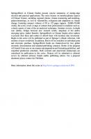
irrigated agricultural production between European and non-European Mediterranean countries. As can be seen in Figure 1, shown below, rainfed crop production, as wheat, is similar in all the compared countries. However, the yields of a usually irrigated crop, as maize, are much larger in European countries than in non-European Mediterranean countries. The above information is a national average; therefore it includes also non-irrigated maize, as well as irrigated wheat. Nevertheless, the figure depicts clearly the mean yields at each country. Maize yields of the European and non-European Mediterranean countries show a considerable difference. This could be mainly due to the large new engineering irrigation infrastructures, which have been available in European Mediterranean countries since the last 20 years.

10 9 8

Yield (T/ha)

7 6 Wheat

5

Maize

4 3 2 1 0 Egypt

Italy

Morocco

Siria

Spain

Figure 1: Average yields in 2004 in several Mediterranean countries, according to FAOSTAT data.

Furthermore, Figure 2 depicts the absolute difference in Maize yields (in T/ha) and production (in BT) between Spain and Egypt from 1990 to 2004, following the same FAOSTAT (2005) data. Despite total Egyptian production is higher than that of Spain, the Spanish yields are not only higher than the corresponding Egyptian yields, but their yield differences have been linearly incremented during the last 15 years. The yield differences between Spain and the European Mediterranean countries as compared to Non-European Mediterranean countries can be due to many reasons, but indeed the new engineering irrigation infrastructures that has

Climate Change, Agriculture and Water Resources…

9

been introduced in the European Mediterranean countries, as Spain, during the last 20 years (MAPA, 2005) has a notable influence in this yearly yield increment. Despite the infrastructures investments in Spain and other European countries, irrigation is still very expensive at the world scale. Water could be not enough under the future-enhanced droughts conditions, particularly considering third-world population rise. However, irrigation must not only been kept, but also enlarged in order to feed the foreseen world population. This contradiction has been pointed out as important concern during the 19th Congress of the International Commission on Irrigation and Drainage (ICID), held in Beijing recently. The ICI Congress focused on the theme of "Use of Water and Land for Food Security and Environmental Sustainability" and they pointed out that: the key to increase future food production lies in expansion of irrigated and drained lands where potential exists; in better water and land management in existing irrigated and drained areas; and in increase in water use efficiency and land productivity, in the Beijing ICID declaration.

1990

1995

2000

2004

4

Absolute difference

3

2

y = 0.7237x - 0.2666 R2 = 0.9101

1

0

-1

-2

-3

Prod-Dif

Yield-Dif

Figure 2: Absolute differences between Egyptian and Spanish Maize productions (in BT) and yields (in T/ha).

Climate change will impose a new challenge to Spanish and Mediterranean irrigation areas. Improving irrigation efficiency is an imperative, although it has been recognized that much water can still be saved in Spanish irrigation systems (Playan and Mateos, 2005). Some climate-change impact assessments have estimated that CO2 rising will significantly reduce the crop water requirements

10

Angel Utset Suastegui

(Guereña et al., 2001; Villalobos and Fereres, 2004). However, such positive “fertilizing effect” of CO2 rising seems to have been overestimated according to the FACE results (Craft-Brandner and Salvucci, 2004; Aisnworth and Long., 2005). Hence, Spanish irrigated agriculture might be affordable in the future only by reducing the water consumes. Furthermore, the globalisation of the world market and the “cost recovering principle” included in the EU Water Framework Directive (2000/60/EC) would lead to prices reductions in the future, while incrementing water costs. Several examples can be pointed out on the challenge that climate change, combined with WFD and other future policies, could bring to the affordability of irrigated agriculture in Spain. Perhaps the most updated situation concerns Sugarbeet cropping. The EU Commission of Agriculture has proposed a reform to current EU sugar production conditions, which has been strongly rejected by Spanish sugar-beet farmers and producers, as well as those from other countries. The reform implies a substantial reduction of current EU prices. Sugar-beet is mainly an irrigated crop in Spain and other Mediterranean countries; hence the production costs are relatively high due to irrigation. Farmers who use groundwater to irrigate sugar beet are the ones facing the highest problem, due to the increment of oil costs. Furthermore, drought conditions, as that found during 2005 in Spain, can be strengthen in the near future, due to global change. Therefore, farmers need to reduce irrigation costs while cropping Sugarbeet under these new prices and climate conditions. They need help in order to find a reliable irrigation management. This is particularly important in those farms where irrigation modernisation or any irrigation investment in new technologies is expected, due to the amortization of the investment costs.

Chapter 2

CLIMATE SCENARIOS, SEASONAL FORECASTS AND DOWNSCALING ISSUES Complex Models regarding general atmospheric circulation (GCM) have been developed to predict the future earth climate. Those models are able to simulate the energy and mass exchanges between the atmosphere and the earth surface, according to several man-due scenarios of greenhouse gases emissions (IPCC, 2007). The HadCM3 model, developed by the United-Kingdom Meteorological Office, and the German ECHAM4 model were considered in the IPCC (2007) report, among other non-European GCM’s. On the other hand, seasonal time-scale climate predictions are now made routinely at a number of operational meteorological centers around the world, using comprehensive coupled models of the atmosphere, oceans, and land surface (Stockdale et al. 1998; Mason et al. 1999; Kanamitsu et al. 2002; Alves et al. 2002; Palmer et al., 2004). Particularly, GCM were integrated over 4-month time scales with prescribed observed sea surface temperatures (SSTs) within the PROVOST project (Palmer et al., 2004). Single model and multi-model ensembles were treated as potential forecasts. A key result was that probability scores based on the full multi-model ensemble were generally higher than those from any of the single-model ensembles (Palmer et al., 2004). Based on PROVOST results, the Development of a European Multi-model Ensemble System for Seasonal to Inter-annual Prediction project (DEMETER) was conceived, and funded under the European Union 5th Framework Environment Programme (Palmer et al., 2004). The principal aim of DEMETER was to advance the concept of multi-model ensemble prediction by installing a number of state-of-the-art global coupled ocean–atmosphere models on a single supercomputer, and to produce a series of 6-month multi-model ensemble

12

Angel Utset Suastegui

hindcasts with common archiving and common diagnostic software. As a result of DEMETER, real-time multi-model ensemble seasonal global predictions are now routinely made at the European Centre for Medium-Range Weather Forecasts (ECMWF). Palmer et al. (2004) showed some DEMETER applications. Results indicate that the multi-model ensemble is a viable pragmatic approach to the problem of representing model uncertainty in seasonal-to-inter-annual prediction, and will lead to a more reliable forecasting system than that based on any one single model (Palmer et al., 2004). On the other hand, Doblas-Reyes et al. (2006), pointed out the potential of DEMETER predictions of seasonal climate fluctuations to crop yield forecasting and other agricultural applications. They recommend a probabilistic approach at all stages of the forecasting process. The ENSEMBLES EU-funded proposal (Hewitt, 2005) is an important recent effort to improve the skill of seasonal forecasts and to make them available to stakeholders. The ENSEMBLES proposal uses the collective expertise of 66 institutes to produce a reliable quantitative risk assessment of long-term climate change and its impacts. Particular emphasis is given to probable future changes in climate extremes, including storminess, intense rainfall, prolonged drought, and potential climate ‘shocks’ such as failure of the Gulf Stream. To focus on the practical concerns of stakeholders and policy makers, ENSEMBLES considers impacts on timeframes ranging from seasonal to decadal and longer, at global, regional, and local spatial scales. Several useful tools to assess climate-change impacts on agriculture have been developed during the last years. GCM are among such tools. However, GCM estimations of temperature, precipitation and other meteorological variables are usually made for large areas. For instance, Guereña et al. (2001) showed that those estimations are not very useful to Spanish agricultural climate-change impact assessments, due to the notable topographical changes within the Peninsula for relative small distances. Therefore, a “downscaling” of GCM outputs is absolutely needed before using their estimations for agricultural applications. Wilby and Wigley (2001) summarized the available downscaling techniques; which can be classified as statistical, dynamical and weather generators. A dynamical downscaling method is to apply numerical regional climate models at high resolution over the region of interest. Regional models have been used in several climate impact studies for many regions of the world, including parts of North America, Asia, Europe, Australia and Southern Africa (e.g Giorgi and Mearns, 1999; Kattenberg et al., 1996; Mearns et al., 1997). The regional climate models obtain sub-grid scale estimates (sometimes down to 25 km resolution) and

Climate Scenarios, Seasonal Forecasts and Downscaling Issues

13

are able to account for important local forcing factors, such as surface type and elevation. Particularly, the regional climate model RegCM was originally developed at the National Center for Atmospheric Research (NCAR), USA and has been mostly applied to studies of regional climate and seasonal predictability around the world. It is further developed by the Physics of Weather and Climate group at the Abdus Salam International Centre for Theoretical Physics (ICTP) in Trieste, Italy. The PRUDENCE Regional Models Experiment has been developed in Europe under the EU Framework Research Program (Christensen and Christensen, 2007). PRUDENCE project provides a series of high-resolution regional climate change scenarios for a large range of climatic variables for Europe for the period 2071-2100 using four high resolution GCMs and eight RCMs. Wilby and Wigley (2001) classified statistical downscaling in regression methods and weather-pattern approaches. The regression method uses statistical linear or non-linear relationships between sub-grid scale parameters and coarse resolution predictor variables. Wilby and Wigley (2001) included Artificial Neural Network within the regression-type statistical downscaling. On the other hand, weather-pattern based approaches involve grouping meteorological data according to a given classification scheme. Classification procedures include principal components, canonical correlation analyses, fuzzy rules, correlationbased pattern recognition techniques and analogue procedures; among others (Wilby and Wigley, 2001). Theoretically, dynamical downscaling methods are better than simple statistical methods since they are based on physical laws. However, statistical downscaling method are less computational exigent and can give good results if the relationships between predictand and predictors are stationary (Wilby and Wigley, 2001).

2.1 WEATHER GENERATORS Weather generators have been very used in agriculture climate-change impact assessments (Hoogenboom, 2000; Sivakumar, 2001). A weather generator produces synthetic daily time series of climatic variables statistically equivalent to the recorded historical series, as well as daily site-specific climate scenarios that could be based on regional GCM results (Semenov and Jamieson, 2001). The weather generator usually mimics correctly the mean values of the climatic variables, although underestimates their variability (Mavromatis and Jones, 1998; Semenov and Jamieson, 2001; Wilby and Wigley, 2001). Different weather

14

Angel Utset Suastegui

generators are available, but according to Wilby and Wigley (2001), the US-made and the UK-made WGEN and LARS-WG are the most widely used. LARS-WG is a stochastic weather generator which can be used for the simulation of weather data at a single site (Racsko et al, 1991; Semenov et al, 1998; Semenov and Brooks, 1999; Semenov and Barrow, 2002), under both current and future climate conditions. These data are in the form of daily timeseries for a suite of climate variables, namely, precipitation, maximum and minimum temperature and solar radiation. According to Semenov and Barrow (2002), stochastic weather generators were originally developed for two main purposes: 1. To provide a means of simulating synthetic weather time-series with statistical characteristics corresponding to the observed statistics at a site, but which were long enough to be used in an assessment of risk in hydrological or agricultural applications. 2. To provide a means of extending the simulation of weather time-series to unobserved locations, through the interpolation of the weather generator parameters obtained from running the models at neighbouring sites. A stochastic weather generator is not a predictive tool, but simply a mean to generate time-series of synthetic weather statistically ‘identical’ to the observations. A stochastic weather generator, however, can serve as a computationally inexpensive tool to produce multiple-year climate change scenarios at the daily time scale which incorporate changes in both mean climate and in climate variability (Semenov and Barrow, 1997). The LARS-WG weather generator focused to overcome the limitations of the Markov chain model of precipitation occurrence (Richardson and Wright, 1984). This widely used method of modelling precipitation occurrence (which generally considers two precipitation states, wet or dry, and considers conditions on the previous day only) is not always able to correctly simulate the maximum dry spell length. LARS-WG follows a ‘series’ approach, in which the simulation of dry and wet spell length is the first step in the weather generation process. The most recent version of LARS-WG (version 3.0 for Windows 9x/NT/2000/XP) has undergone a complete redevelopment in order to produce a robust model capable of generating synthetic weather data for a wide range of climates (Semenov and Barrow, 2002). LARS-WG has been compared with another widely-used stochastic weather generator, which uses the Markov chain approach (WGEN; Richardson, 1985; Richardson and Wright, 1984), at a number

Climate Scenarios, Seasonal Forecasts and Downscaling Issues

15

of sites representing diverse climates and has been shown to perform at least as well as, if not better than, WGEN at each of these sites (Semenov et al, 1998).

Chapter 3

SIMULATING CROP-GROWTH AND CROP WATER-USE On the other hand, many crop simulation models have been appeared in the last 20 years. Those models are able to estimate crop water-use and growth under any weather and cop management conditions. Those models, combined with downscaled GCM scenarios, can be a reliable approach to support decisionmaking under climate change conditions (Hoogenboom, 2000). Despite many models are available, Mechanistic models i.e. those based in the physical laws of the soil-water-plant-atmosphere continuum, are the most suitable to climatechange impact assessments (Eatherall, 1997), since the laws are, in principle, valid for al climatic conditions. According to Tubiello and Ewert (2002), more than 40 assessments of climate-change impact on agriculture have been published up to now. They pointed out that generally models provided accurate results, compared to actual data. The most used models in such assessments are DSSAT (Jones et al., 2003) and those developed in Wageningen (Van Ittersum et al., 2003). As pointed out above, modelling tools appeared in the eighties, due to computer availability, aimed to simulate crop growth and final yields. Numerous crop growth models have been developed since them. The models can use weather data input, such as short term weather forecast, a season’s forecasted weather or climate scenarios to estimate potential or actual growth, development or yield. Historical-production records are useful for assessing the impacts of climate variability on crop yields, but cannot reveal crop response under alternative management strategies, which can be done through modelling simulations. Bastiaansen et al. (2004) provided an update revision of the modelling applications to irrigation assessments. They pointed out the opportunities lying in

18

Angel Utset Suastegui

such modelling approaches to irrigation and drainage assessments, with more than 40 examples. The simulation examples comprises assessing irrigation supply needs, as well as irrigation designing, scheduling, management and performance; salt-affected soils due to irrigation, groundwater recharge and estimating soil losses, among others. Models have been usually classified as empirical, functional and mechanistics (Connolly, 1998; Bastiaansen et al., 2004). Mechanistic models, i.e. those based in the physical laws of the soil-water-plan-atmosphere are more suitable to assess climate-change effects on agriculture than empirical models (Eatherall, 1997; Hoogenboom, 2000), since the theoretical mechanistic-model backgrounds is still valid under these new conditions. According to Bastiaansen et al. (2004), concerning suitability to describe irrigation and drainage processes, models can be classified as bucket, pseudo-dynamics, Richards-equation based, SVAT models, multidimensional and crop-production models. However, at the plot and field scale only the bucket, the crop-oriented models and those based on the Richards equation have been significantly used. The Richards equation describes the vertical movement of water within the soil profile and its solutions can, at least theoretically, provide the water distribution under certain initial and border conditions (Kutilek and Nielsen, 1994). Therefore, concerning irrigation studies at field and plot scales, the most important mechanistic modelling approaches are those mainly aimed to simulate crop-growth and those addressed to physically-based simulation of soil-water movement, through numerical solutions of the Richards equation. These models have been called agrohydrological models, because they combine agricultural and hydrological issues (Van Dam, 2000).

3.1 CROP-GROWTH ORIENTED SIMULATION MODELS According to Stockle et al. (2003), the initial crop-growth simulation models, mainly theoretical approaches, appeared in the 1970s (de Wit et al., 1970; Arkin et al., 1976). Applications oriented models appeared during the 1980s (Wilkerson et al., 1983; Swaney et al., 1983). Models such as SUCROS and others associated with the Dutch ‘School of de Wit’ (Bouman et al., 1996); as well as those produced in the US as the CERES (Ritchie, 1998) and CROPGRO (Boote et al., 1998) families of models had a significant impact on the crop modelling community (Stockle et al., 2003). As pointed out by Brisson et al (2003), the rest of the crop-growth simulating models, although different; generally follow similar

Simulating Crop-Growth and Crop Water-Use

19

guidelines than the originally produced models. Alexandrov (2002) provided a complete summary of the crop models that have been used in Europe.

3.1.1 The DSSAT Models and the “Cascade Approach” The Decision Support System for Agrotechnology Transfer (DSSAT) was originally developed by an international network of scientists, cooperating in the International Benchmark Sites Network for Agrotechnology Transfer project (IBSNAT, 1993; Tsuji et al., 1998; Uehara, 1998; Jones et al., 1998), to facilitate the application of crop models in a systems approach to agronomic research (Jones et al., 2003). DSSAT is a microcomputer software package that contains crop-soil simulation models, data bases for weather, soil, and crops, and strategy evaluation programs integrated with a ‘shell’ program which is the main user interface (Jones et al., 1998). DSSAT originally comprises the CERES models for maize (Jones and Kiniry, 1986) and wheat (Ritchie and Otter, 1985), as well as the SOYGRO soybean (Wilkerson et al., 1983) and PNUTGRO peanut (Boote et al., 1986) models, among others (Jones et al., 2003). The decision to make these models compatible led to the design of the DSSAT and the ultimate development of compatible models for additional crops, such as potato, rice, dry beans, sunflower, and sugarcane (Hoogenboom et al., 1994; Jones et al., 1998; Hoogenboom et al., 1999; Jones et al., 2003). According to Hoogenboom et al. (1999), the DSSAT Cropping System Model (CSM) simulates growth and development of a crop over time, as well as the soil water, carbon and nitrogen processes and management practices. The CSM main components are: • • •

A main driver program, which controls timing for each simulation, A Land unit module, which manages all simulation processes which affect a unit of land Primary modules that individually simulate the various processes that affect the land unit including weather, plant growth, soil processes, soilplant-atmosphere interface and management practices.

Collectively, these components simulate the changes over time in the soil and plants that occur on a single land unit in response to weather and management practices.

20

Angel Utset Suastegui

DSSAT has a module format. Each module has six operational steps, (run initialization, season initialization, rate calculations, integration, daily output, and summary output). The main program controls the timing of events: the start and stop of simulation, beginning and end of crop season, as well as daily time loops (Hoogenboom et al., 1999). Ritchie (1998) provided the background of DSSAT models regarding simulation of soil-water movement and crop water-use. The DSSAT simulation of the soil water balance depends on the capability of water from rainfall or irrigation to enter soil through the surface and be stored in the soil reserve. The “cascading approach” as used in DSSAT is explained by Ritchie (1998). Drainage from a layer takes place only when the soil water content at a given depth is between field saturation and the drained upper limit. The Priestley-Taylor (1972) equation for potential evapotranspiration is used in DSSAT. Calculation of potential evaporation requires an approximation of daytime temperature and the soil-plant reflection coefficient (albedo) for solar radiation. For the approximation of the daytime temperature a weighted mean of the daily maximum and minimum air temperatures is used. The combined crop and soil albedo is calculated from the model estimate of leaf area index and the input bare soil albedo (Ritchie, 1998). The root water absorption in DSSAT is calculated using a law of the limiting approach whereby the soil resistance, the root resistance, or the atmospheric demand dominates the flow rate of water into the roots. The flow rates are calculated using assumptions of water movement to a single root and that the roots are uniformly distributed within a layer (Ritchie, 1998). The potential transpiration and biomass production rates are reduced by multiplying their potential rates by a soil water deficit factor calculated from the ratio of the potential uptake to the potential transpiration. A second water deficit factor is calculated to account for water deficit effects on plant physiological processes that are more sensitive than the stomata controlled processes of transpiration and biomass production (Ritchie, 1998). The DSSAT models have been indeed the most used simulation tools in agricultural climate-effect assessments (Tubiello and Ewert, 2002) and crop water balance studies (e.g. Eitzinger et al., 2002). They were calibrated and validated at many agricultural regions of the world (Hoogenboom, 2000). DSSAT models have been intensively used also in the framework of the CLIMAG activities aimed to mitigate and estimate agricultural climate-risks (Adiku et al., 2007; Meza, 2007; Singh et al., 2007).

Simulating Crop-Growth and Crop Water-Use

21

3.1.2 The Wageningen Models Van Ittersum et al. (2003) provided a complete summary of the family of models made in Wageningen, The Netherlands, during the last 30 years. According to Tubiello and Ewert (2002), these Dutch models have been the most widely used, after DSSAT models, in agricultural climate-risk assessments. As pointed out by Van Ittersum et al. (2003), the Wageningen group has a long tradition in developing and applying crop models in its agroecological research program, based on the pioneering work of C.T. de Wit. In the 1960s and 1970s the main aim of these modelling activities was to obtain understanding at the crop scale based on the underlying processes. De Wit and co-workers at the Department of Theoretical Production Ecology of Wageningen University, and the DLO Research Institute for Agrobiology and Soil Fertility developed the model BACROS and evaluated components of the model (such as canopy photosynthesis) with especially designed equipment and field experiments (De Wit et al., 1978; Goudriaan, 1977; Van Keulen, 1975; Penning de Vries et al., 1974). These modelling approaches have served as the basis and inspiration for modelling groups around the world (Stockle et al., 2003). In the 1980s a wide range of scientists in Wageningen became involved in the development and application of crop models. The generic crop model SUCROS for the potential production situation was developed (Van Keulen et al., 1982; Van Laar et al., 1997), which formed the basis of most recent Wageningen crop models such as WOFOST (Van Keulen and Wolf, 1986), MACROS (Penning de Vries et al., 1989), and ORYZA (Bouman et al., 2001). In the 1990s the Wageningen group focused more on applications in research, agronomic practice and policy making (Van Ittersum et al., 2003). Crop modelling in Wageningen for potential production situations follows the photosynthesis approach in the SUCROS family of models (Van Ittersum et al., 2003). LINTUL (Light INTerception and UtiLisation) models use the linear relationship between biomass production and the amount of radiation intercepted (captured) by the crop canopy (Monteith, 1981), which has been found for many crop species, grown under well-watered conditions and ample nutrient supply, in the absence of pests, diseases and weeds. This relationship sets a finite limit on yield potential (Sinclair, 1994), which thus can be modelled without going into detailed descriptions of the processes of photosynthesis and respiration. Spitters and Schapendonk (1990) developed the model LINTUL with a module for the calculation of crop growth based on the LUE concept. In the photosynthesis approach in SUCROS (Simple and Universal CROp growth Simulator) models, the daily rate of canopy CO2 assimilation is calculated

22

Angel Utset Suastegui

from daily incoming radiation, temperature and leaf area index (LAI). The model contains a set of subroutines that calculate the daily totals by integrating instantaneous rates of leaf CO2 assimilation (Goudriaan and Van Laar, 1994; Van Laar et al., 1997). Particularly, the model WOFOST (WOrld FOod STudies) simulates crop production potentials as dictated by environmental conditions (soils, climate), crop characteristics and crop management (irrigation, fertiliser application) (Van Diepen et al., 1989). The model has been continuously modified, and applied for many different purposes (e.g. De Koning and Van Diepen, 1992). WOFOST uses the SUCROS approach for potential production conditions. WOFOST permits dynamic simulation of phenological development from emergence till maturity on the basis of crop genetic properties and environmental conditions. The cultivar-specific values of thermal time assimilate conversion coefficients, maximum rooting depth, daily root development rate and partitioning fractions are important inputs. Dry matter accumulation is estimated by the rate of gross CO2 assimilation of the canopy. This rate depends on the radiation energy intercepted by the canopy, which is a function of incoming radiation and of crop leaf area. Simulated growth processes and phenological development are regulated by temperature (e.g. the maximum rate of photosynthesis), radiation and atmospheric CO2 content and limited by availability of water. Root extension is computed in a simple way, the initial and the maximum rooting depth as determined by the crop and by the soil and the maximum daily increase in rooting depth being specified prior to the simulation. The daily increase in rooting depth is equal to the maximum daily increase unless maximum rooting depth is reached. The Ritchie (1972) equation is used to separate the evaporation and transpiration terms from the evapotranspiration. The potential biomass production rate is assumed to decrease in the same proportion as the transpiration so that the actual amount of biomass produced on a given day and consequently during whole season can be calculated. WOFOST has been used by the European Union’s Joint Research Centre (JRC) to develop a system for regional crop state monitoring and yield forecasting for the whole European Union (Van Ittersum et al., 2003). The system comprises winter wheat, grain maize, barley, rice, sugar beet, potatoes, field beans, soybean, winter oil seed rape and sunflower. This system, called crop growth monitoring system (CGMS), generates region-specific indicators of the agricultural season conditions in the current year, on a semi-real time basis. This has been realised by simulating yields from weather and soil data, which serve as crop production indicators. This model output is qualitative in the sense that it is based on comparison of quantified indicators of the current year with those of the past. It

Simulating Crop-Growth and Crop Water-Use

23

provides information on whether in the current season a given crop deviates from the ‘normal’ growing pattern in terms of biomass and phenological development. These crop indicators are used in combination with regression techniques as a basis for quantitative regional yield prediction for the various crops. The system is operational for the EU and has been installed in various non-EU countries. According to Van Ittersum et al. (2003), despite that Wageningen has a strong tradition in crop modelling, which has yielded a rich variety in crop modelling approaches and modules; there has not been a strong drive towards integration of research efforts, particularly not for implementation and application purposes.

3.1.3 Other Available Crop-Oriented Models As pointed out above, besides DSSAT and the Wageningen models, several other models have been developed during the last years, aimed to estimate crop development and yields under different agricultural management conditions. Some of these models have been developed and tested in Europe. Numerous models are now available, with different objectives, and many new models are still appearing. Actually, there is no universal model and it is necessary to adapt system definition, simulated processes and model formalisations to specific environments or to new problems (Van Ittersum et al., 2003). To efficiently manage irrigation systems has been one of the most important issues considered in simulation models since they appear. Particularly, the European Society of Agronomy (ESA), has a special session dedicated to such modelling tools. Besides, special numbers of the European Journal of Agronomy have been dedicated to promote such models. The CROPSYST model (Stockle et al., 2003), the French model STICS (Brisson et al., 2003) and the Australian model APSIM (Keating et al., 2003) are examples of such other models. Other available European model is the Czech model PERUN (Dubrovsky et al., 2002, 2003). The model is a computer Windows-based system for probabilistic crop yield forecasting. The system comprises all parts of the process: (1) Preparation of input parameters for crop model simulation, (2) launching the crop model simulation, (3) statistical and graphical analysis of the crop model output, (4) crop yield forecast. The weather data series are calculated by the stochastic weather generator Met&Roll (Dubrovsky, 1999) with parameters that are derived from the observed series. The synthetic weather series coherently extends the available observed series and fit the weather forecast. Wind speed and humidity were added to the standard set of four surface weather characteristics

24

Angel Utset Suastegui

generated by Met& Roll to meet the input data requirements. These two variables are generated separately by nearest neighbours re-sampling. To prepare the weather data for seasonal crop yield forecasting, the weather generator may now generate the synthetic series which coherently follows the observed series at any day of the year. The crop yield forecast made by PERUN is based on the WOFOST crop model simulations run with weather series consisting of observed series till DAY1 coherently followed up by synthetic weather series since DAY. The simulation is repeated n times (new synthetic weather series are stochastically generated for each simulation) and the probabilistic forecasts are then issued in terms of the average and standard deviation of the model crop yields obtained in the n simulations. The synthetic part of the weather series is prepared by a two step.

3.2 AGROHYDROLOGICAL MODELS Agrohydrological or water-oriented models were significantly developed during the last years (Bastiaansen et al., 2004). The models SWAP (Van Dam et al., 1997), DRAINMOD (Kandil et al., 1995), WAVE (Vanclooster et al., 1994), ISAREG (Teixeira and Pereira, 1992) and HYDRUS (Šimunek et al., 1998) can be considered as agrohydrological models, among others. The unsaturated zone, i.e. the zone between the soil surface and the groundwater, is a complicated system governed by highly non-linear processes and interactions. Flow processes can alternatively be described by means of physical-mathematical models. According to Bastiaansen et al. (2004), unsaturated-zone models can be used to simulate the timing of irrigations and irrigation depths, drain spacing and drain depth, and system behaviour and response. The models have increased our understanding of irrigation and drainage processes in the context of soil–plant–atmosphere systems. Progress in modelling can be attributed to merging separated theories of infiltration, plant growth, evapotranspiration and flow to drain pipes into a single numerical code (Bastiaansen et al., 2004). According to Van Ittersum et al. (2003) agrohydrological models are more suitable to irrigation and water-use assessments than crop-growth oriented models, although both approaches have been used.

Simulating Crop-Growth and Crop Water-Use

25

3.2.1 Constraints of Crop-Oriented Models Regarding the Simulation of Soil Water-Movement and Crop Water-Use Actually, water moves not only down within the soil, but also lateral and even upward, depending on the potential gradients (Kutilek and Nielsen, 1994). Transport phenomena, as water movement into the soil, are driven by potential gradients that depend on gravity, water extraction by roots and water that enters or leaves the profile from top or bottom, causing different soil water suctions in the different layers. The cascade approach could be appropriate on sandy soils or if the objective is to calculate the amount of water available to the crop over longer periods of time. However, this approach could fail in soils with significant clay and silt content and if the objective is to calculate daily soil-water profiles, as needed in irrigation assessments. A Richards-based approach might be more appropriate in those cases (Van Ittersum et al., 2003). Several researchers have pointed out the DSSAT limitations regarding soilwater simulations, due to the use of the cascade approach in such simulations (Gabrielle et al., 1995; Maraux et al., 1998; Mastrorilli et al., 2003). According to Ritchie (1998), there is definitely a need to have better DSSAT simulations of the water balance in very poorly drained conditions where oxygen stresses will impact plant growth. Some attempts to improve DSSAT in that concern have been made already (Yang et al., 2004). Particularly, since the cascade approach is unable to simulate upward water movement due to capillary rising, DSSAT yield predictions significantly depart from actual yields under heavy rain conditions (Rosenzweig et al., 2002). Particularly, Utset et al. (2006) showed that capillary rising can be an important component of maize water balance, when maize is cropped nearby river and channels, where shallower water tables can be found. Extreme rainfall conditions will be more frequent in the near future, due to climate change (IPCC, 2007). As pointed out by Rosenzweig et al. (2002), yield loses in the US due to heavy rainfall could be very important in the future and the modelling-based climate-risk assessments should take them into account. Utset et al. (2006) results also showed that water excess could significantly affect crop production. Figure 3 depicts the maize relative transpiration (ratio between actual and maximum transpiration) as simulated during dry years through SWAP by Utset et al. (2006). RT is depicted in Figure 3 as a function of Total Water Supply (TWS), considering a water table at a 2-m depth. The line shows the obtained regression. As can be seen in the figure, higher TWS gives raise to a reduction in RT rather than to further increments. Since the Feddes et al. (1978)

26

Angel Utset Suastegui

root water-uptake function, included in SWAP, is able to account on water-excess effects on crop water use, the Utset et al. (2006) simulations can estimate the extreme rainfall effect also, whereas other models are unable to evaluate that consequence. Utset et al. (2006) simulation results indicate that precipitation excess could bring a negative effect in flooded irrigated maize, if relatively shallow water tables are found.

1.00 0.99

Relative Transpiration

0.98 0.97 0.96 0.95 0.94 0.93 0.92 0.91 250

350

450

550

650

750

850

950

1050

1150

1250

TWS (mm)

Figure 3: Simulated Maize relative transpirations as a function of Total Water Supply in dry years, considering a shallower water-table at 2-m depth (after Utset et al., 2006).

3.2.2 SWAP Model: Generalities Feddes et al. (1978) developed the agrohydrological model SWATR (Soil Water Actual Transpiration Rate) to describe transient water flow in cultivated soils with various soil layers and under the influence of groundwater. The model was further developed to accommodate more boundary conditions (Belmans et al., 1983), crop growth (Kabat et al., 1992), shrinkage and swelling of clay soils (Oostindie and Bronswijk, 1992), and salt transport (Van den Broek et al., 1994). More recently, the model SWAP (Van Dam et al., 1997) was released as a result of a combination of SWATR with WOFOST (Van Keulen and Wolf, 1986). Several improved versions of SWAP were released; the most updated includes also the solute-leaching simulation model PEARL (Kroes, 2001). SWAP is a computer model that simulates transport of water, solutes and heat in variably saturated top soils. The program is designed for integrated modelling

Simulating Crop-Growth and Crop Water-Use

27

of the Soil-Atmosphere-Plant System. Transport processes at field scale level and during whole growing seasons are considered. System boundary conditions at the top are defined by the soil surface with or without a crop and the atmospheric conditions. The lateral boundary simulates the interaction with surface water systems. The bottom boundary is located in the unsaturated zone or in the upper part of the groundwater and describes the interaction with local or regional groundwater. Van Dam (2000) provides a detail description of the SWAP theoretical background. SWAP solves Richards’s equation numerically, subject to specified initial and boundary conditions and the soil hydraulic functions. The maximum root water extraction rate, integrated over the rooting depth, is equal to the potential transpiration rate, which is governed by atmospheric conditions. The potential root water extraction rate at a certain depth may be determined by the root length density, at this depth as fraction of the total root length density. Stresses due to dry or wet conditions and/or high salinity concentrations may reduce The potential root water extraction rate. The water stress in SWAP is described by the function proposed by Feddes et al. (1978), which comprises a coefficient that takes values between zero and one. Under conditions wetter than a certain “anaerobiosis point” (h1) water uptake by roots is zero, as well as the coefficient α. Likewise, under conditions drier than “wilting point” (h4), α is also zero. Water uptake by the roots is assumed to be maximal when the soil water pressure-head is between h2 and h3 and hence α-value is one in that case. The values of α decrease linearly with h for h values lower than h4 but larger than h3. According to Leenhardt et al. (1995), the Feddes et al. (1978) root water-uptake model has the advantage that not only considers the crop transpiration reduction due to lower soil-water contents, but also takes in account the negative effect of water excess in the soil root zone. Utset et al. (2000) showed that the Feddes et al. (1978) model fits better to actual data, obtained in tropical conditions, than the model provided by Van Genuchten et al. (1987). This SWAP feature could be very important, since flooding could be regionally more severe in the future (IPCC, 2000, Rosenzweig et al., 2002; Utset et al., 2006). For salinity stress the response function of Maas and Hoffman (1977) is used in SWAP (Van Dam, 2000), as this function has been calibrated for many crops. Besides calculating crop yields through the WOFOST module, a simpler approach to calculate yield reduction as function of growing stage can be used in SWAP (Doorenbos and Kassam, 1979; Smith, 1992). The ratio between actual to potential transpirations is known as “Relative transpiration ratio” (Van Dam, 2000). The relative transpiration reductions can be related to the effects of water

28

Angel Utset Suastegui

stress (De Wit et al., 1978; Van Dam 2000). The relative yield of the entire growing season is calculated as product of the relative yields of each growing stage. Two different types of irrigation can be specified in SWAP (Kroes et al., 2002). Either a fixed irrigation can be specified, or an irrigation schedule can be calculated for a specific crop according to a number of criteria. A combination of fixed and calculated irrigations is also possible. An example of this is a fixed irrigation (preparation of the seed bed) before planting and calculated irrigations based on soil moisture conditions after planting. Fixed irrigations can be applied the whole year. Irrigation scheduling can only be active during a cropping period. The irrigation type can be specified as a sprinkling or surface irrigation. In case of sprinkling irrigation, interception will be calculated (Kroes et al., 2002).

3.2.3 SWAP Model: The Simple Approach to Estimate Crop Water-Use Kroes and Van Dam (2003) described the SWAP performance. According to them, the simple SWAP crop-growth approach represents a green canopy that intercepts precipitation, transpires and shades the ground. Leaf area index, crop height and rooting depth must be specified as functions of the development stage. SWAP simulates crop growing on a daily basis. The development stage (DVS) at a given day j depends on the development stage at the previous day and the daily temperature, according to:

DVS j = DVS j −1 +

Teff Tsum

[1.]

where Tsum is the required temperature sum and Teff is the effective daily temperature, calculated from mean daily air temperature minus a minimum starting temperature (3 ºC). DVS reaches 1 at anthesis and 2 at maturity, according to the temperature sums at these two stages. Van Dam (2000) provided the theoretical SWAP background. SWAP solves the Richards equation numerically, subject to specified initial and boundary conditions and the hydraulic functions of the soil. The maximum root water extraction rate (Sp) at a depth z, considering a uniform root-length density distribution, can be calculated from:

Simulating Crop-Growth and Crop Water-Use

Sp ( z ) =

Tp Droot

29

[2.]

Where Droot is the root density fraction, integrated over the rooting length density at this depth and Tp is the potential transpiration rate, which is subject to atmospheric conditions. Actual root water uptake can be estimated through:

Sa( z ) = α Sp( z )

[3.]

The α values range from zero (no root-water uptake) to one (maximum wateruptake, no stress) according to the Feddes et al. (1978) function. These values change according to actual soil water-content, but the function is crop-dependent (Van Dam, 2000). Utset et al. (2000) showed that the original parameters of the Feddes et al. (1978) model can be used to simulate potato water-use in conditions that are very different from those existing where the model was originally applied. Therefore, the parameters applied to sugarbeet in the Netherlands have been used in this assessment. The potential reference evapotranspiration (ETP) is calculated in SWAP by the Penman-Monteith approach, although the user may introduce other ETP calculations (Van Dam, 2000). In addition, the crop coefficients Kc must be introduced to convert reference ETP on maximum crop evapotranspiration. SWAP first of all separates the potential plant transpiration rate Tp and potential soil evaporation rate Ep and then calculates the reduction of potential plant transpiration and soil evaporation rates. The soil evaporative component can be separated from the total evapotranspiration calculated by the equation:

Ev = ETP e − m. I

[4.]

where m is a crop-dependent coefficient and I is the Leaf Area Index. The transpirative component is therefore calculated from the difference between the total evapotranspiration and the evaporative component. Ritchie (1972) and Feddes (1978) used m = 0.39 for common crops. Secondly, actual transpiration is calculated considering the root water uptake reduction due to water stress, using equation [2]. Actual soil evaporation can be calculated from the Maximum Darcy flow at the soil surface, which depends on actual soil water content and hydraulic conductivity, although several other

30

Angel Utset Suastegui

options for calculating actual soil evaporation are implemented in SWAP (Van Dam, 2000). The simple SWAP crop-growth approach does not estimate the crop yield. However, the user can define yield response factors (Doorenbos and Kassam, 1979; Smith, 1992) for various growing stages as functions of the development stage. During each growing stage k, the actual yield Ya,k (kg ha-1) relative to the potential yield Yp,k (kg ha-1) during the said growing stage is calculated by:

1−

Ya , k Yp , k

⎛ T = K y , k ⎜1 − a , k ⎜ T p,k ⎝

⎞ ⎟ ⎟ ⎠

[5.]

where Ya,k and Yp,k are the actual and potential yields for the period k, Ta,k and Tp,k are the actual and potential crop transpiration, respectively, and Ky,k is a coefficient which depends on the crop and on the crop growing period k. Final relative yields, i.e. the ratio between Ya and Yp, are calculated as the product of the relative yields of each growing stage k. In SWAP, irrigations may be prescribed at fixed times or scheduled in accordance with certain criteria. According to Kroes and Van Dam (2003), the irrigation scheduling criteria applied in SWAP are similar to those found in CROPWAT (Smith, 1992), IRSIS (Raes et al., 1988) and others. SWAP can therefore be used to select the irrigation management that maximizes crop yield, minimizes irrigation costs, optimally distributes a limited water supply or optimizes production from a limited irrigation system capacity (Kroes and Van Dam, 2003).

3.2.4 HYDRUS Model An important modelling approach, aimed to simulate water and solute transport through the soil vadose zone is the model HYDRUS-1D (Šimunek et al., 2005). The model consists of the HYDRUS computer program, and the HYDRUS1D interactive graphics-based user interface. According to Šimunek et al. (2005), the HYDRUS program numerically solves the Richards equation for saturated-unsaturated water flow and convection-dispersion type equations for heat and solute transport. The water flow equation incorporates a sink term to account for water uptake by plant roots, as well as in SWAP (see equation 1). The heat transport equation considers movement by conduction as well as convection with flowing water. Salinity is also considered through the Maas and Hoffman

Simulating Crop-Growth and Crop Water-Use

31

(1977) function and the simulation of crop water uptake follows a similar approach than the SWAP model. The HYDRUS-1D code may be used to analyze water and solute movement in unsaturated, partially saturated, or fully saturated porous media. The flow region itself may be composed of non-uniform soils (Šimunek et al., 2005). Flow and transport can occur in the vertical, horizontal, or in a generally inclined direction. The water flow part of the model considers prescribed head and flux boundaries, as well as boundaries controlled by atmospheric conditions, free drainage, or flow to horizontal drains (Šimunek et al., 2005). The source code was developed and tested on a Pentium 4 PC using the Microsoft's Fortran PowerStation compiler. Several extensions of the MS Fortran beyond the ANSI standard were used to enable communication with graphic based user-friendly interface (Šimunek et al., 2005). HYDRUS1D comprises an interactive graphics-based user-friendly interface for the MS Windows environment. The HYDRUS1D interface is directly connected to the HYDRUS computational programs. Besides, the HYDRUS program come with several utility programs that make easier the data input process. HYDRUS1D can be considered as a one-dimensional version of the HYDRUS-2D code. This updated modelling release is aimed to simulate water, heat and solute movement in two-dimensional variably saturated media (Šimunek et al., 1998), while incorporating various features of earlier related codes such as SUMATRA (van Genuchten, 1978), WORM (Van Genuchten, 1987), HYDRUS 3.0 (Kool and van Genuchten, 1991), SWMI_ST (Šimunek, 1992), and HYDRUS 5.0 (Vogel et al., 1996). Indeed, to be able to simulate soil water-movement and crop water-uptake in two dimensions open new possibilities that perhaps make HYDRUS2D the most important currently available model in this concern (Van Genuchten and Šimunek, 2005).

3.2.5 Agrohydrological Models Constraints Many models comparisons have pointed out that despite mechanistic model yield more accurate and sounder simulations; they require many input parameters that are not always easy to measure or to estimate (Leenhardt et al., 1995; Connolly, 1998; Bastiaansen et al., 2004). Sensitivity analysis of SWAP outputs showed that the simulated water balance are most sensitive to the crop coefficients used for calculating potential transpiration and to the soil hydraulic properties (Van Dam, 2000). This agrees with other analysis made with similar agrohydrological modelling approaches, based on Richards’ equation (Clemente

32

Angel Utset Suastegui

et al., 1994; Leenhardt et al., 1995). Unfortunately, the soil hydraulic properties use to show high spatial variability (Warrick and Nielsen, 1980; Van Genuchten, 1994; Leenhardt et al., 1995). Therefore, the SWAP dependence on these properties can be seen as one of the highest constraints when using such modelling approach (Van Genuchten, 1994; Leenhardt et al., 1995; Van Dam, 2000).

3.2.6 Simple Crop Water-Use Simulation Models. CROPWAT Very often availability of model input data (especially soil input data) is a serious limitation for applications of complex crop water balance models as to be used for irrigation scheduling. This is especially a problem in poor agricultural regions, where input data generation might be a serious cost factor. The limitation on input data quality can lead to the situation that simple models or methods may perform better than the complex models. That is why for all SIRDEM experimental sites the performance of a simple approach will be tested as an alternative option. The test will result in defining limitations and potentials of both simple and complex approaches. CROPWAT is a free-distributed code from the Food and Agriculture Organization (FAO) and can be downloaded from the FAO web (http://www.fao.org/landandwater/aglw/cropwat.stm). It is meant as a practical tool to help agro-meteorologists, agronomists and irrigation engineers to carry out standard calculations for evapotranspiration and crop water use studies, and more specifically the design and management of irrigation schemes. CROPWAT allows the development of recommendations for improved irrigation practices, the planning of irrigation schedules under varying water supply conditions, and the assessment of production under rainfed conditions or deficit irrigation. It simulates crop water-requirements on a monthly, 10-days period or daily basis with a simplified soil water balance (cascade approach). Actually, the cascade approach can yield same results than the physically-based approach, based on numerical solutions of Richards’s equation, as shown by Eitzinger et al. (2004).

Simulating Crop-Growth and Crop Water-Use

33

3.3 MODELS CALIBRATION, VALIDATION AND INTER-MODEL COMPARISONS Since SWAP simulates the soil-water balance; the model outputs include deep drainage, capillary rising and runoff also. The model itself can provide irrigation recommendations, based on the simulated soil water contents and crop evapotranspiration. All these capabilities can be used at the field level to integrate a general farm water-management, trying to help farmers to control water more efficiently and to improve the environmental and economic performance of irrigation systems. SWAP is specifically oriented to water management, but comprises the WOFOST also, which make SWAP able to simulate crop-growth as well. Nevertheless, SWAP simulation outputs should be compared to other similar modelling approach. As shown by Eitzinger et al. (2004); Tardieu (2005) and others, several model approaches can yield the same results. Particularly, DSSAT models have been used for irrigation and crop water-use assessments in Spain (Guereña et al., 2001; Villalobos and Fereres, 2004) and overseas (Hoogenboom, 2000). Therefore, a prior model comparison should be made before selecting the model that can be used to irrigation decision-making. Such comparison should include, at least, some internationally used model as those of DSSAT, based on the “Cascade approach”; as well as an agrohydrological model.

Chapter 4

APPLYING CLIMATE AND CROP-GROWTH SIMULATION TOOLS TO SUPPORT AGRICULTURAL DECISION-MAKING Despite the manifold papers addressed to estimate climate-change and climate-variability effects on agriculture, appeared in the last years, few cases can be referred where such tools have been effectively used to provide recommendations to farmers and stakeholders. Some of the current actions regarding such applications are outlined below.

4.1 PREVIOUS EXPERIENCE Probably, the most important contributions to the use of the available simulation tools to support agricultural decision-making are CLIMAG (Climate Prediction and Agriculture) activities. The CLIMAG workshops were held in Geneva 1999 and 2005, sponsored by WMO and IRI (Sivakumar, 2001; Sivakumar and Hansen, 2007). The CLIMAG proceedings remain as significant guidelines for using such tools in future studies. However, the assessments of climate-impacts on agriculture made in the framework of CLIMAG were only specially-funding applications. The CLIMAG assessments did not yield to sustainable applications of the simulation tools in the targeted countries. One of the most important successful applications of climate information, combined to crop-growth simulation models, have been made in Australia (Meinke et al, 2001; Hammer et al., 2001; Meinke et al., 2006). Rainfall and many other meteorological variables strongly depend on El Niño behaviour. Since

36

Angel Utset Suastegui

ENSO occurrence can be forecasted several months in advance, this information can be used to support agricultural decision-making, through crop-growth modelling exercises (Hammer et al., 2001). A “participatory process” (Meinke et al., 2001) comprising researchers, stakeholders and extension facilities has been pointed out as a way to provide sustainable and sounder support to Australian agriculture. Another important application of climate information and crop-growth models can be found in the South East Climate Consortium (SECC), as described by Hoogenboom (2007). Seasonal forecasts at the county level, using ENSO phases, are combined with DSSAT modelling results in order to provide estimations of final yields, water and fertilizer requirements and several other outputs very useful to farmers. The forecast and the whole system are only reliable in El Niño years, although current researches aim to enlarge the system reliability to other years (Baigorria, 2007). El Niño signal is not very strong over Europe, which limits the applicability of ENSO-based forecasts. Marletto et al. (2005) showed that WOFOST simulations of winter wheat yields, based on the available seasonal forecasts, departed significantly from the recorded data. However, using spatial and temporal aggregated data, as usually done by JRC when providing recommendations to the EU Commission of Agriculture, might be not the right approach to capture the relationships between weather variables and crop growing. Hansen et al. (2006) provided an insight view of current advances and challenges while translating climate forecasts into reliable agricultural decisionmaking. They describe several methods used up to now to spatially and temporal downscale the forecasts, recommending methods comparisons and evaluations at local scales. Likewise, Alexandrov (2007) provided an update revision of current state on applying climate scenarios and seasonal forecasts to support agricultural decision-making. Alexandrov (2007) points out that improved climate prediction techniques are growing faster and finding more applications; hence close contacts between climate forecasters, agrometeorologists, agricultural research and extension agencies in developing appropriate products for the user community are needed. Furthermore, feedbacks from end users are essential identifying the opportunities for agricultural applications (Alexandrov, 2007).

Applying Climate and Crop-Growth Simulation Tools…

37

4.2 THE ROLE OF LOCAL AGRICULTURAL RESEARCH AND EXTENSION SERVICES As pointed out above, negative climate-variability impacts could be reduced by following adaptation options, which can be obtained from crop-model simulations combined with climate scenarios. The usefulness of such simulation tools has been proved in manifold papers, usually produced in Universities or similar centres. However, despite of the considerable public concern about climate change, European stakeholders and farmers are not yet using these scientific results for agricultural decision-making. Actually, the most reliable climatechange mitigation options depend on each specific situation. While experts and researchers at high-level centres in Europe and other places (“developers”) have established significant Know-How and produced relevant of the above-cited tools for such climate-impacts studies; practical experts at local agricultural-research or extension centres as well as agricultural advisers (“users”), those who should apply these tools for agricultural decision-making, are often not aware about the available tools or their access to such tools is quite limited due to several reasons, as financial issues or lack of user-friendly design of tools. A connection is needed between the “developers” and “users”, to improve decision making by better implementing the climate and crop-growth simulation model tools. Furthermore, feedback from low end-users to the tool-provider researchers is a prerequisite for improving these tools for their practical use e.g. by providing background information, setting up the actual input data needs, fitting time and spatial scales as required by specific applications and other similar issues. In that context AGRIDEMA, a Specific Support Action (SSA), has been funded by the EU Sixth Framework Program from January 2005 to June 2007. The SSA aims to promote a research network, linking European modelling toolproviders and developers with the potential users of their research results (Utset et al., 2007a). AGRIDEMA general objective is to establish initial contacts and to conduct primary collaborations between “developers” and potential “users”, basically researchers and experts at agricultural services.

4.3 THE AGRIDEMA PROPOSAL. GENERAL DESCRIPTION AGRIDEMA comprises the following specific objectives:

38

Angel Utset Suastegui 1. To identify European human resources that developed, improved and tested simulating tools such as GCM, seasonal forecasts, regional downscaling techniques and agricultural-impact simulation models; inviting them to participate in the SSA proposal activities for implementing their tools and Know-How. 2. To identify and to invite attending the SSA activities to potential users of the European-provided modelling tools. 3. To conduct short courses, where the invited “developers” will present the particularities of their developed or validated tools to the invited “users”. 4. To perform pilot collaborations between “developers” and “users”. 5. To disseminate the obtained results and to build up a wider consortium, comprising both, the “developers” of the simulating tools and the potential “users” of such tools (e.g. experts from regional agriculturaloriented research centres, advisers and farmers).

According to these objectives, several tasks or “work packages” were scheduled. The tasks can be seen in Figure 1. Following the AGRIDEMA timetable, three Workpackages were finished during the 1st period, i.e. “Identifying and Contacting developers”, “Identifying and contacting users” and “Courses on climate and crop-growth modelling tools”.

4.3.1 Identifying and Contacting Developers The AGRIDEMA consortium created an initial list of which developers should be contacted. The list was based mainly the partners experience and previous contact. The use of European-made simulation tools was encouraged. The following Table shows the simulation tools that were contacted by the AGRIDEMA consortium, as well as the corresponding European institution and relevant person. Several work agreements were achieved between the AGRIDEMA consortium and most of the contacted “developers”, pointing out the “developers” participation in the AGRIDEMA courses, as well as their future support of the “Pilot Assessments” to be conducted by the “users” in the framework of AGRIDEMA.

Applying Climate and Crop-Growth Simulation Tools…

39

Table 2: Models, institutions and “developers” included in the AGRIDEMA activities. Model REGCM3 LARS-WG, SIRIUS Met&Roll Statistical downscaling DEMETER LAPS SWAP WOFOST PERUN ROIMPEL CROPSYST STICS DSSAT

Institution ICTP, Italy Rothamsted Experimental Station, UK Inst. Atmos. Physics, Czech Republic BOKU, Austria

Contact J. Pal M. Semenov M. Dubrovsky H. Formayer

ECMWF, UK Agrometeorological Institute Novi Sad, Serbia Wageningen Agricultural University, The Netherlands Wageningen Agricultural University, The Netherlands Mendel University Brno, Czech Republic Romanian Foundation on Global Change, Romania ISCI, Italy INRA, France University of Madrid, Spain

F. Doblas-Reyes D. Michailovic J. Kroes K. Van Diepen M. Trnka C. Simota M. Donatelli F. Ruget A. Iglesias

4.3.2 Identifying and Contacting Users Mediterranean countries could face the highest negative consequences of global warming within Europe, through water-shortage and crop-water requirements increments. Besides, since climate-change and extreme events effects could be more serious in countries with less-developed agriculture, the EU associated countries from Central and Eastern Europe, with relative reduced technological capacities, would be more affected than Northern-European countries. Therefore, AGRIDEMA focuses on “users” coming from Southern, Central and Eastern Europe, as well as from the countries of the Mediterranean area. The members of the AGRIDEMA consortium released a call to “users” applicants since April 2005. Relevant institutions were contacted, according to

40

Angel Utset Suastegui

AGRIDEMA partner’s experience, as well as official centres depending on the Countries’ Ministries of Agriculture or similar institutions. The call was published also using all the available means, including email lists and internet facilities. As pointed out by the three AGRIDEMA partners during their first meeting, the basic criteria for selecting the “users” institutions to be involved in the proposal were: i.

To be able to communicate in English and to be able to work with data management software (Windows, Excel, etc.). ii. To be involved with local agricultural decision-making, advising and farming. iii. To be aware about the potential benefits of agricultural decision modelling tools, being able to identify which agricultural management options should be change and how to optimise management and reduce climate risk of local agricultural production. iv. To have available data for the training course and for the potential conducting the SSA pilot assessments (crop growth and yields, meteorological variables, soil properties, irrigation and crop management scheduling, etc).

Additionally, users conducting PhD studies in the same subjects of AGRIDEMA activities will be especially considered for invitation.

4.3.3 The AGRIDEMA Courses on Climate and Crop-Growth Simulation Tools The Courses were held in Vienna in November-December 2005, as scheduled in the proposal. Since many applications to the AGRIDEMA courses were received from “users” out of the targeted countries, the AGRIDEMA partners decided to include these applicants also without any course fee, if they were able to support their trips and lodging expenses. Finally, 44 “users” were present in total, from more than 15 different countries. Sixteen “users” were fully supported by AGRIDEMA and other eight were partially supported by the SSA. A picture showing all the participants in the AGRIDEMA courses is depicted in Figure 2. Institutions from several countries decided to support additional participants in AGRIDEMA courses. Particularly, the participation of five Spanish researchers was supported by the INIA AC05-008 complementary action. Besides, several students and researchers from BOKU, Austria, were in the courses too.

Applying Climate and Crop-Growth Simulation Tools…

41

The AGRIDEMA web page (www.agridema.com) shows all the details of Courses held in Vienna; as the lectures program, time schedule, invited developers, participant users, etc. The courses on Climate tools comprise lectures on climate change scenarios, dynamical and statistical downscaling, as well as weather generators. The details and work-performance of quite known cropgrowth models as SIRIUS, DSSAT, CROPSYST and WOFOST; among others, were shown too.

4.3.4 The Agridema Pilot Assessments The AGRIDEMA pilot assessments were basically applications conducted by some of the “users” that attended the AGRIDEMA courses on climate and cropgrowth simulation tools that were held in Vienna ending 2005. Assessments were made using existing data and were addressed to relevant issues concerning climate risks and agricultural decision-making in their respective countries and institutions. The following issues were considered in the Assessments propositions: • •

• •

Local modelling comparisons and validations using available data will be encouraged as the agreement subjects. All the collaborations must identify clearly the potential benefits of these modelling applications for local agricultural decision-making. Particularly, those applications which include farmers from regional medium and small enterprises, as potential users of the tested tools, will be better considered for funding. Educational outputs, such as Ph. D. studies connected to the work agreements are highly desirable. Only original and different propositions can be supported.

The selection of the pilot assessments was based on the propositions that the “users” made at the end of the AGRIDEMA courses. The selection was geographically made. The AGRIDEMA consortium partners considered the available budget and the agreements among them during their first meeting. Eight assessments were selected in the Mediterranean area, although only six were funded (those not leaded by ITACyL). Five assessments were conducted in Central Europe and three in Eastern Europe. The SSA coordinator gave priority to cooperation and exchange among the Mediterranean “users”, as well as funding dissemination activities, rather than to support ITACyL researches that have other

42

Angel Utset Suastegui

funding possibilities. Furthermore, ITACyL received additional funds from the Spanish government to strength the cooperation with the Spanish institutions working in AGRIDEMA Pilot Assessments (Complementary Action CGL200626211-E) as well as with the Mediterranean countries involved (International Complementary Action PCI2005-A7-0105). The Pilot assessments were conducted from March to October 2006. The AGRIDEMA support was based on agreements to be signed between each “user” conducting Pilot assessments and the corresponding partner of the AGRIDEMA consortium. The Pilot assessments information can be seen in the AGRIDEMA web page: www.agridema.org. The complete lists of the funded AGRIDEMA Pilot assessments can be seen below. Table 3: Pilot Assessments conducted in the framework of AGRIDEMA Mediterranean area (under the responsibility of the Spanish partner) Title Full irrigation estimates and palliative measurements for coping with climate change in vineyard and peach orchards in Spain: a past tendency towards a future perspective Optimizing irrigation water management on the global change context in a Mediterranean region Estimating climate-change effects on Sugarbeet irrigation efficiency in the Spanish Northern Plateau Adaptations of irrigated cropping systems of Southern Italy as affected by climate change at field/farm scale Assessment of the Impact of Climate Change on Water Productivity in Rainfed Wheat Systems in the Mediterranean region Assessment of the Impact of Climate Change on Water Productivity in Irrigated potatoes in the Southern Mediterranean region Estimation of water availability for annual crops at Tree – Crop ecosystems

*Conducting a Ph D in this issue

Presenter Name

Institution

Jordi Marsal

IRTA, Spain

Jose A. Rodriguez* Blanca del Rio

DAP, Andalusia, Spain ITACyL, Spain

Domenico Ventrella

CRA-ISA, Italy

Fatema Mosseddaq

IAV Hassan II, Morocco

Mahmoud Medany

CLAC, Egypt

Dimos Anastasiou

NAGREF, FDA, Greece

Applying Climate and Crop-Growth Simulation Tools…

43

Table 3: Continued Central Europe (under the responsibility of the Austrian partner) Presenter Name

Title Modelling of the maize production and the impact of climate change on maize yields in Croatia Irrigation in different Climate conditions using crop models Introducing crop modeling tools into a Serbian crop production

Visnja Vucetic

Determination of the water demand and use of various crops in the region Lake Neusiedl and Seewinkel

Ildikó Dobi Gerhard Kubu

Modelling of crop yields in the present and future climatic conditions in WIELKOPOLSKA REGION (POLAND) with and without irrigation management practices

Jacek Leśny

Blaz Kurnik Branislava Lalić

Institution Meteorological Service of Croatia EARS (Met. Office, Slovenia) University of Novi Sad, Novi Sad, Serbia and Montenegro Hungarian Meteorological Service; Univ. of Natural Resources and Appl. Life Sciences, BOKU Agricultural University of Poznań

Eastern Europe (under the responsibility of the Bulgarian partner) Title Impact of climate factors on grain yield of spring barley in Latvia Climate variability and change over the Balkan peninsula and related impacts on crops Complex assessment the efficiency of adaptation of agricultural ecosystems to climate change in the European part of Russia based on integration with European crop models

Presenter Name Jelena Korolova* Stanislava Radeva Vladimir Romanenkov

Institution Latvia University of Agriculture (LUA) NIMH, Bulgaria All-Russian Institute for Agrochemistry

*Conducting a Ph D in this issue

The reports of the AGRIDEMA Pilot assessments, which can be downloaded from the AGRIDEMA web, comprise an excellent collection of many different applications from several European and Mediterranean countries, all of them addressed to local potential climate-risks. The strategic AGRIDEMA goal, which

44

Angel Utset Suastegui

aims to promote a research network, linking European modelling tool-providers and developers with the potential users of their research results, has been already partially fulfilled.

4.4 THE AGRIDEMA PILOT-ASSESSMENTS RESULTS According to the AGRIDEMA goals, the Pilot assessments should comprise the two following tasks: 1. Downscaling the provided GCM-outputs and/or seasonal-forecasts. 2. Simulating impacts (such as crop growth and yield, drought stress level etc.) under the locally-obtained climate scenarios, evaluating several management options, which might mitigate the probable climate impact. Scientific quality of the assessments is quite variable, which can be expected from the wide irregularity of AGRIDEMA applicants. Furthermore, the applicability of the obtained results varies among the assessments as well. Generally, those assessments conducted by researchers located in agricultural stations are closer to stakeholder goals, but unclear regarding climate analysis. Objectives were too ambitious sometimes and could not be fulfilled with a simple application. Moreover, the use of the climate and crop modelling tools shown in the AGRIDEMA courses was mainly related to the user’ previous experience and not to the tool reliability for the expected goal. Comparisons between modelling tools were not conducted in most of the cases. In spite of all the above, the AGRIDEMA results constitutes perhaps the most important collection of independent climate-change agricultural assessments that have been made in Europe. The table shows the climate and crop-growth simulation tools that have been used in the AGRIDEMA pilot assessments. The downscaling method is clearly identified in all the reports. However, the GCM data source is not always pointed out. In some cases, the assessment was very simple due to the lack of data or relevant knowledge on the crop model. As can be concluded from the Table, the most used GCM outputs were the Canadian CCCMa (4 times) and HADCM3 (3 times). The ECHAM and CSIRO GCM outputs were used in one assessment, where a GCM output comparison was performed. The LARS-WG appeared in 8 of the AGRIDEMA pilot assessment, which makes this weather generator as the most frequently used climate-tool in the framework of AGRIDEMA. According to Wilby and Wigley (2001), LARS-

Applying Climate and Crop-Growth Simulation Tools…

45

WG is one of the most used weather generators. The AGRIDEMA results confirm this conclusion. The Met&Roll weather generator was found in 3 assessments, including one comparison with LARS-WG. The Regional ReGCM3 model was used in 2 assessments and the MAGICC model in one. Table 4: Climate and crop-growth tools used in the AGRIDEMA Pilot assessments Assessment Conductor Jordi Marsal Jose A. Rodriguez Blanca del Río Domenico Ventrella Fatema Mosseddaq Mahmoud Medany Dimos Anastasiou Visnja Vucetic Blaz Kurnik

Institution

CLIMATE

CROP

IRTA, Spain DAP, Andalusia, Spain ITACyL, Spain

CCMA -LARS CCMA -LARS CCMA -LARS

CROPSYST DSSAT SWAP

CRA-ISA, Italy

CGM-LARS

SWAP

IAV Hassan II, Morocco CLAC, Egypt NAGREF, FDA, Greece Meteorological Service of Croatia EARS (Met. Office, Slovenia)

MAGICC CCMA -LARS ECHAM4-CSIROHADCM3-M&R REGCM3-LARS

DSSAT DSSAT SWAP DSSAT CROPSYST

Regarding the crop models considered in the Pilot assessments, the Wageningen model WOFOST was the most used, but in its SWAP (3 times) and PERUN (3 times) versions. DSSAT models were employed in 4 Pilot Assessments, while CROPSYST was used 3 times, ROIMPEL was considered 2 times and SIRIUS was used in one assessment, which performed a model comparison with PERUN. The frequency of using crop models in the AGRIDEMA Pilot assessments is similar to that found in climate-change impact assessments all over the world, reported by Tubiello and Ewert (2002) as well as in Europe, as pointed out by Alexandrov (2002). An important AGRIDEMA conclusion is that DSSAT, SWAP-WOFOST and CROPSYST are the most relevant crop-growth simulation models that are being used in Europe for climate-change risk assessments. Furthermore, SWAP has been the most used agrohydrological model within the AGRIDEMA Pilot assessments.

46

Angel Utset Suastegui

4.5 A PILOT ASSESSMENT EXAMPLE: MANAGING SUGARBEET IRRIGATION IN THE SPANISH NORTHERN PLATEAU UNDER PRESENT AND FUTURE CLIMATE CONDITIONS Castilla y Leon, with 94 000 km2, is the largest Spanish Autonomic Community and one of the major administrative regions of Europe. Castilla y Leon is basically a large plateau, with an important agricultural production. The region involves more than 20% of the cultivated area of Spain, 22.7% of grassland area and 31.9% of the cereals-cropping area. Even though Castilla and Leon comprises only 6% of Spanish population, they mean about 12% of the reported farm-workers in Spain, almost twice the country mean (7.7%) and higher than the European mean (9.0%). Castilla y León is, after Andalusia, the Spanish Autonomic Community with higher irrigation surface. According to the last Ministry of Agriculture report (MAPA, 2004), Castilla y León irrigated-agriculture produces 57% of Sugarbeet, 38% of maize and 30% of potatoes of the whole country. The investment in irrigation infrastructures in Castilla y León is the second highest in Spain. However, such investment must be joined to applied researches aimed to improve water-management efficiency, particularly in eventual prices diminishing or severe droughts. The recent reform of the European Sugar Market (EC Council Regulation 318/2006) will bring important reductions on the Sugarbeet prices. Irrigation means about 35% of the total Sugarbeet production costs in Northern Spain. Sugarbeet water requirements will be higher in the future, according to ClimateChange predictions, while water availability will diminish in the Castilla y León zone. Furthermore, EU Water Framework Directive (EC Directive 2000/60), through its “recovering costs” principle, will very probably increment the water prices. The combination of all these factors could yield that Sugarbeet becomes an unaffordable crop in Castilla y León in the near future. According to the above, an AGRIDEMA Pilot assessment was conducted in order to calibrate and validate the SWAP model for Sugarbeet water-use simulations, as well as to estimate Climate Change effects on water use efficiency, considering a typical irrigation management. Utset et al. (2007b) provided the calibration and validation of the SWAP model. The assessment was conducted at Valladolid, Northern Spain (41º39’N, 4º43’W). The regional climate is Mediterranean Semiarid with an annual average precipitation of 531 mm.

Applying Climate and Crop-Growth Simulation Tools…

47

According to the local soil map (JCYL, 1987), Sugarbeet is cropped mainly in Cambisols and Fluvisols.

4.5.1 SWAP Calibration and Validation. The Assessment Data The SWAP calibration comprised data of experiments addressed to study water-shortage effects on sugarbeet growth, made during 1992, 1993, 1994 and 1995 in a clayey Fluvisol and in a Cambisol (Velicia, 1998). The water-stress effect on sugarbeet yields depends on the growing period (Brown et al., 1987; Groves and Bailey, 1994; Fabeiro et al., 2003). Accordingly, water shortages were applied at the beginning and end of sugarbeet development. Four irrigation start and end dates were considered (Velicia, 1998), based on non-restrictive irrigation management with typical considerations (Morillo, 1993; Allen et al., 1998), which provides all the sugarbeet water requirements from seeding to harvest. Four plots were dedicated to each irrigation design at each soil type. The plots were separated from each other by at least 20 m in other to avoid water redistribution among them. Sugarbeet roots can reach up to 2 m in length (Brown et al., 1987; Velicia, 1998). The root distribution in depth depends on soil and moisture conditions. However, according to Velicia (1998), about 60% of the roots is usually found in the first 30 cm, whereas 90% could be found at depths shallower than 90 cm. Therefore, a non-linear root distribution was assumed. Potential evapotranspiration was calculated by the Penman-Monteith approach, using meteorological data available from stations at distances of 1.2 and 2.3 km from the plots. Maximum crop evapotranspiration was calculated considering the Kc coefficients estimated for the zone (Morillo, 1993). Daily temperature values were also recorded. The SWAP FCS stage was considered as the date when sugarbeet covers soil completely under non-restrictive irrigation water-management conditions (Velicia, 1998). The maturity date was assumed as the harvest. The sugarbeet (Ramona cultivar) germination date was May 15 and the average harvest date was October 15. The said dates were considered for computing the temperature sums at FCS and maturity and can be considered as typical dates for spring-sown sugarbeet (Morillo, 1993). The irrigation water applied at each plot was measured weekly. Final sugarbeet yields were measured at each plot. The leaf area index (LAI) was measured monthly at each plot. The length and width of all the green leaves on each plant in 1-m rows were measured. LAI was

48

Angel Utset Suastegui

indirectly estimated according to a regression equation obtained from previous studies (Velicia, 1998). Root lengths and weights were also measured (Velicia, 1998) from three randomly selected plants, removed entirely from the ground at each plot on a monthly basis. Soil water content was measured weekly by a neutron probe (Velicia, 1998). The actual crop evapotranspiration was estimated by water balance (Allen et al., 1998). The actual crop transpiration was separated from total evapotranspiration considering the experimentally-measured LAI values (Ritchie, 1998). Final yields were measured and total crop transpiration was computed as the cumulative sum; the Ky coefficients (Doorenbos and Kassam, 1979; Kroes and Van Dam, 2003) were then calculated. The hydraulic properties of the soil were estimated from the physical soil data taken at each plot (Velicia, 1998) through a pedotransfer function (Shaap et al., 2001). SWAP simulations were performed at each plot, considering the parameters obtained in the calibration and free drainage at the bottom of the 1-m soil layer. A regression between relative yields and actual yields was conducted in order to find which maximum yield adapted better to the experimental conditions. An independent data set was used for SWAP validations. Two sugarbeet plots, corresponding to a Cambisol (Plot Z) and a Fluvisol (Plot A), were selected in the Valladolid area. The plots were separated from each other by a distance of approximately 15 km. Sugarbeet was seeded in the two plots in March 2005. Emergence dates were April 5 (A) and April 25 (Z). Undisturbed soil samples were taken at 20-40 cm depth in ten randomly-selected sites within each plot. The soil water retention curves were determined at each sample through a sand-kaolin box and a Richard membrane (Klute, 1986). The saturated hydraulic conductivity of each sample of soil was measured in a laboratory permeameter. The soil field capacity and the wilting point were considered as the water contents at 33 and 1500 kPa, respectively. The parameters of the Van Genuchten model for the soil-water characteristic curve were estimated through the RETC code (Van Genuchten et al., 1991). Access tubes were placed at the same places where soil samples were taken at each plot. Soil water contents were measured weekly during July and August 2005 at 0-20, 20-40 and 40-60 cm depths by a Trime TDR [IMKO Micromodultechnick GmbH]. Actual crop evapotranspiration was computed using the balance method from the measured water contents and neglecting any possible capillary rising, runoff and/or percolation. Daily precipitation, global radiation, maximum and minimum temperature, wind speed and relative humidity values were recorded at two agrometeorological stations located near the selected plots.

Applying Climate and Crop-Growth Simulation Tools…

49

Irrigation was applied traditionally in a way similar to that used by farmers to manage sugarbeet water applications at each plot. The irrigation water supply at each plot was measured through a water counter. Sixteen irrigations were applied on the Z Plot from June to August, comprising a total water application of 508 mm. Likewise, 556 mm of water were applied by irrigation on the A plot in the same period over eighteen irrigations. Precipitations are scarce in the Mediterranean summer. Accordingly, the total rainfall recorded was 41 mm on the Z Plot and 25 mm on the A Plot during the 2005 sugarbeet cropping season. Actual SWAP simulations were conducted using the measured soil and meteorological data and considering the model calibration performed. Free drainage at the bottom of the 1-m simulated soil layer was considered, which is consistent with the soil descriptions (JCYL, 1987). Correlation and determination coefficients between simulated and estimated actual evapotranspirations were calculated, as well as the same coefficients between the SWAP-simulated actual evapotranspirations and the sugarbeet water requirements, calculated from Penman-Monteith computations of the reference evapotranspiration and the sugarbeet coefficients in use, as provided by Morillo (1993). Furthermore, Root Mean Square Errors (RMSE) were calculated between the simulated ETC and the water-balance estimated ETC, as well as between the simulated ETC and the maximum ETC, estimated from weather data. The RMSE has been considered as the most effective method of comparing simulated and actual values in evaluation model performance (Willmott et al., 1985; Timsina and Humphreys, 2006). The normalized RMSEn is used to compare modelling performances and can be calculated as:

⎡ −1 n 2⎤ ⎢n ∑ (Pi − Oi ) ⎥ i =1 ⎦ RMSEn = ⎣ n n −1 ∑ Oi

0.5

[6.]

i =1

where Pi and Oi are the predicted and observed values, respectively, and n is the number of observations.

50

Angel Utset Suastegui

4.5.2 SWAP Calibration. The Results Table 5 summarizes the calibration results; comparing the experimentallyobtained temperature sums at FCS and maturity, as well as the LAI and Ky values at several development stages with the corresponding values of the original SWAP calibration for Northern Europe. Table 5: Average temperature sums, Leaf Area Index, Root Lengths and Root Length Densities; as well as KC and Ky coefficients as function of development stages (DVS) under Mediterranean conditions and those values originally considered in the SWAP calibration provided for Northern Europe (after Utset et al., 2007b). Function Temperature Sum (ºC)

Anthesis Maturity Leaf Area Index LAI

Locally-obtained

SWAP original

1141 2008

365 1622

DVS 0.55 0.75 0.77 0.80 0.89 0.92 0.98 1.00 1.01 1.02 1.02 1.08 1.10 1.15 1.16 1.17 1.22 1.28 1.79 1.85 1.88

LAI 0.4 0.6 0.6 0.9 1.2 1.6 2.1 1.7 2.1 3.1 2.4 3.2 2.7 3.3 3.2 2.5 2.3 5.5 3.8 4.9 3.5

DVS 0.56 0.74 1.00 1.27 1.52 1.76

LAI 0.13 0.44 1.47 4.48 5.04 4.69

Applying Climate and Crop-Growth Simulation Tools…

51

Table 5: Continued Function Root Length (cm) RL

Root Length Density (RLD) as a function of Relative Root Length (RRL)

Crop Coefficients KC

Locally-obtained DVS RL 0.55 46 0.75 71 0.77 81 0.80 77 0.89 81 0.92 72 0.98 115 1.00 95 1.01 81 1.02 104 1.02 107 1.08 112 1.10 125 1.15 118 1.16 107 1.17 129 1.22 131 1.28 125 1.79 123 1.85 135 1.88 126 RRL RLD 0.25 0.60 0.70 0.90 1.00 1.00 DVS KC 0.40 0.4 0.50 0.5 0.60 0.7 0.80 1.0 1.80 1.1 2.00 0.9

SWAP original DVS RL 0.56 58 0.74 70 1.00 87 1.27 118 1.52 120 1.76 120

RRL 0.0 1.0

RLD 1.0 1.0

DVS 0.0 2.0

KC 1.0 1.0

52

Angel Utset Suastegui Table 5: Continued Function Yield response factors Ky

Locally-obtained DVS Ky 0.33 1.00 0.80 1.50 1.00 1.50 1.50 1.00 2.00 0.90

SWAP original DVS Ky 0.0 1.0 2.0 1.0

Average FCS, i.e. maximum foliar development, corresponds to 71 days after germination in the irrigation managements that provide all the sugarbeet water requirements (Velicia, 1998). Therefore, development stage (DVS) reaches one at that date. The temperature sum at this development stage is 1141 ºC, which is much higher than the 365 ºC originally considered in SWAP. Indeed, average temperatures in Southern Europe after May are higher than the temperatures usually recorded in the Netherlands and other sites of Northern Europe, where SWAP has been previously calibrated. However, temperature sums from germination to FCS similar to those shown in Table 5 for Mediterranean conditions have been found in France (Durr and Mary, 1998) and the UK (Werker and Jaggard, 1997). Furthermore, the difference between the temperature sums at FCS and maturity is lower under Mediterranean conditions than in Northern Europe, which indicates a faster growing rate during summer. Estrada (2001) pointed out the influence of direct sun radiation on sugarbeet growing while cropped under Mediterranean conditions with unlimited water supply. Such direct radiation influence could determine that the temperature sums needed for sugarbeet maturation under Mediterranean conditions is lower than that required in Northern Europe. The experimentally-measured Leaf Area Indexes are also shown in Figure 4 as a function of the DVS calculated from the temperature sums shown in Table 5. The original SWAP values are included in the figure as a continuous line. Furthermore, Figure 4 also shows the measured and SWAP-original sugarbeet root-lengths as functions of the crop DVS. As the figure shows, the sugarbeet LAI development under Mediterranean conditions follows a pattern similar to that measured in Northern Europe. Therefore, the original function included in SWAP could be considered as still valid in a warmer environment. The sugarbeet leaf area and root lengths show faster growing rates and higher averages in Mediterranean conditions than those anticipated in the original SWAP

Applying Climate and Crop-Growth Simulation Tools…

53

functions, particularly before FCS. This is in accordance with the temperature sum differences shown in Table 5. Measured LAI

SWAP LAI

Measured RL

SWAP RL

6

160

120

LAI

4

100

3

80 60

2

40 1

Root length (cm)

140

5

20

0

0 0

0.2

0.4

0.6

0.8

1

1.2

1.4

1.6

1.8

2

DVS

Figure 4: Measured sugarbeet Leaf Area Indexes (LAI) and Root Lengths (RL), as functions of the crop development stages (DVS). The continuous and dashed line shows the respective SWAP original functions (after Utset et al. 2007b). 160 140

Root length (cm)

120 100 80 60 40 20 0 0.00

0.20

0.40

0.60

0.80

1.00

1.20

1.40

1.60

1.80

2.00

DVS

Figure 5. Measured Sugarbeet root lengths under several water managements as function of the crop development stages (DVS). The continuous line shows the SWAP original function (after Utset et al. 2007b).

Figure 5 compares the experimentally-measured sugarbeet root-lengths with those originally considered in SWAP as functions of the crop development stages.

54

Angel Utset Suastegui

The SWAP function might slightly underestimate the sugarbeet root development as grown under Mediterranean conditions. However, the measured values behave in a way that is similar to the original SWAP function. Furthermore, there is a considerable dispersion of the measured values, which can be due to the different soil types considered. Kc

Ky 1.6

1.2 1.0

0.8

0.6 0.4

Ky coefficient

Kc coefficient

1.2 0.8

0.4 0.2 0.0

0.0 0.0

0.2

0.4

0.6

0.8

1.0

1.2

1.4

1.6

1.8

2.0

2.2

DVS

Figure 6: Sugarbeet Crop (KC) and yield factor (Ky) coefficients considered for SWAP simulations under Mediterranean conditions, as functions of the crop development stages (DVS) (after Utset et al. 2007b). 110 100

Yields (T/ha)

90 80 70 60 50 40 30 20 0.40

0.50

0.60

0.70

0.80

0.90

1.00

Relative yields

Figure 7: Experimentally obtained sugarbeet yields vs. SWAP simulated relative yields. The dashed and the solid lines show the regressions considering all the data and fittingreduced data, respectively (after Utset et al., 2007b).

Applying Climate and Crop-Growth Simulation Tools…

55

Likewise, Figure 6 depicts the Mediterranean-considered and the SWAPoriginal KC and Ky coefficients as functions of the development stages. Unlike the original SWAP value, which sets the same KC coefficient for all the sugarbeet crop development, we consider a variable KC. Velicia (1998) showed that sugarbeet water requirements are lower than the maximum reference evapotranspiration during the initial growing period. However, sugarbeet water needs increase significantly after completing foliar development and starting the root-growing period (Velicia, 1998), which might be considered for a DVS of around 0.8. Crop water needs are reduced close to maturity. Furthermore, the relationships between sugarbeet transpiration and root yield should not be considered as linear, as originally in SWAP. A reduction of actual sugarbeet transpiration regarding its potential transpiration may imply no serious yield reduction during initial leaf development, but such a reduction has significant consequences on final yields at the beginning of the root growing period (Velicia, 1998). The Ky coefficient, as well as the relative importance of water shortage in Mediterranean sugarbeet yields, can be linearly reduced after the initial rootgrowing period (Velicia, 1998). Figure 7 depicts the relationship between the measured yields and the simulated relative yields, as well as the corresponding regression line. The data in Figure 10 comprise all the pairs of simulated-actual yields, regardless of water managements or soil types. As shown in Figure 7, lower actual yields start notably at the 1:1 line, while yields of above 50 t/ha generally correlate well with the simulated relative yields. Indeed, SWAP only takes into account the yield reductions due to water shortage. However, final yields rely on many other issues besides water availability, such as weed infections, diseases or nutrient deficiency. Furthermore, relative yields are always estimated as one if irrigation water is sufficient, whereas actual yields are variable. That is why the dispersion shown in Figure 10 is higher around the highest simulated relative yields. The correlation coefficient between simulated relative yields and the actual sugarbeet yields was 0.71. According to the regression obtained, the average maximum yield to be used in equation [5] should be 87.5 t/ha. The regression is statistically significant at the 99% probability level and explains more than 50% of the yield variability. However, the simulated relative yields are not normally distributed, since they are skewed to their highest value. Therefore, statistical comparisons between simulated relative yields and actual yields are limited. Despite this, the relatively high correlation coefficient and the level of statistical regression confidence would allow this simple SWAP approach to simulate water management effects on sugarbeet yields.

56

Angel Utset Suastegui

The average sugarbeet yield corresponding to simulated relative yields higher than 0.95 was 90.8 t/ha. Taking into account both results, a potential maximum yield for sugarbeet of around 89 t/ha can be used in SWAP simulations to estimate the effects of water availability on the final yields during crop seasons.

4.5.3 SWAP Validation: The Results The soil water contents at the average depth of 0-60 cm in the Cambisol and Fluvisol plots, measured during the sugarbeet irrigation season, are shown in Figure 8. The water contents are generally close to the field capacity, shown in the figure by a dashed line. Water contents much higher than the field capacity would indicate an excess of water in the root zone and eventual water percolation. Furthermore, water contents much lower than the field capacity would indicate potential water excess and inefficient irrigation management. The results shown in Figure 8 indicate that, despite their non-technical approach, farmers usually know how to manage irrigation in an acceptable way (Utset et al., 2006). Cambisol (Z Plot)

Fluvisol (A Plot)

35

Water content (cm3/cm3)

30 25 20 15 10 5 0 28-6

8-7

18-7

28-7

7-8

17-8

27-8

Date

Figure 8: Average soil-water contents at the 0-60 cm depth in the Cambisol and Fluvisol plots during the 2005 Sugarbeet irrigation season. The dashed lines show the corresponding Field Capacities (after Utset et al., 2007b).

However, water contents are higher than the field capacity at the earlier stages of sugarbeet development, when the sugarbeet roots are not long enough and crop water use is lower. The results suggest that water application might be excessive at this stage. The difference between the measured soil water contents and the

Applying Climate and Crop-Growth Simulation Tools…

57

field capacity is higher in the Fluvisol, where clay contents are higher and water moves slowly across the soil profile. Figure 9 shows the actual SWAP-simulated sugarbeet evapotranspiration, the maximum sugarbeet evapotranspiration, calculated using the Penman-Monteith reference evapotranspiration and the KC coefficients shown in Table 5, as well as the actual crop evapotranspiration estimated from water balance and the water content measurements shown in Figure 8. The evapotranspiration values given in Figure 9 comprise both the Cambisol and the Fluvisol data and were calculated on a weekly basis. Measured ETc

ETc max (PM)

Simulated ETc

90 80 70

ET (mm)

60 50 40 30 20 10 0 30-6

10-7

20-7

30-7

9-8

19-8

29-8

Date

Figure 9: SWAP-simulated sugarbeet actual evapotranspiration (Simulated ETc), sugarbeet maximum evapotranspiration calculated from the Penman-Monteith reference evapotranspiration (ETc Penman-Monteith) and actual evapotranspiration estimated by water balance from the measured soil water contents (after Utset et al., 2007b).

As shown in the figure, simulations can follow the temporal changes of both measured ETC values and those computed from reference evapotranspirations. The measured ETC values are higher than the simulated and maximum rates computed from weather data at the beginning of the irrigation season. The water balance was calculated neglecting the percolation and capillary rising components of the balance. However, at these earlier sugarbeet stages, irrigation excess might yield to significant water loss by percolation, which is in accordance with the water contents being higher than the field capacity for the same period, as shown in Figure 8. The simulated evapotranspirations are lower than the maximum, as expected.

58

Angel Utset Suastegui

All the computed evapotranspirations indicate that sugarbeet water use at the end of the cropping season is lower than at the beginning of the root growing period, as pointed out by Velicia (1998). 90 80

Simulated ETc (mm)

70 60 50 40 30 20 10 0 0

10

20

30

40

50

60

70

80

90

Water-balance measured ETc (mm)

Figure 10A: Simulated and water-balance measured ETc. The dashed line shows the 1:1 relationships. 40

Simulated - Observed (mm)

35 30 25 20 15 10 5 0 0

10

20

30

40

50

60

70

80

90

Water-balance measured ET C (mm)

Figure 10B: Absolute differences vs. Water-balance measured ETc Figure 10: Comparison between water-balance measured and SWAP-simulated ETc (A) as well as absolute differences between water-balance measured and SWAP-simulated as functions of water-balance measured evapotranspirations (B) (after Utset et al., 2007b).

Applying Climate and Crop-Growth Simulation Tools…

59

The correlation coefficient between the actual SWAP-simulated evapotranspiration and the maximum weather-dependent sugarbeet evapotranspiration was 0.81; whereas the correlation coefficient between the simulated and actual estimated water-balance evapotranspirations was 0.75. Figure 9 also shows that simulated ETC values correlate better with the maximum evapotranspiration than with the measured ETC. In practice, irrigation management at both plots was able to keep soil water contents above field capacity throughout the sugarbeet growing season. Therefore, actual crop evapotranspiration must be close to the highest possible maximum, since water requirements were mainly satisfied. This can explain the good ratios between the SWAP simulations and the weather-based maximum ETC. However, ETC calculations by water balance were made ignoring any eventual percolation. However, water loss by percolation seems to be significant at the beginning of the irrigation season, since the water contents measured during the said period were higher than the field capacity, as shown in Figure 8. SWAP estimates that all the components of the water balance and the simulated evapotranspirations do not comprise percolation. This could explain the relatively lower correlation between SWAP-estimated and measured ETC. Figure 10A shows the ratios between sugarbeet evapotranspirations estimated by water balance and the SWAP-simulated evapotranspirations. As the figure shows, simulated and field-measured evapotranspirations are close to the 1:1 line, particularly for the lower rates of the measured ETc. As indicated below, sugarbeet ETC could be overestimated by water-balance estimations. Figure 10B shows the absolute differences between ETC values simulated by SWAP and the ETC estimated by water balance. Absolute differences depend on the measured ETC values. Differences are much higher for the water-balance measured ETC that is higher than 30 mm. This value is higher than the Readily Available Water usually computed for sugarbeet (Morillo, 1993). Therefore, actual sugarbeet evapotranspiration could hardly reach such high values (Allen et al., 1998). Despite these differences, the regression line between simulated and waterbalance measured ETc has a gradient of 1.14. The regression is statistically significant at the 99% confidence level. Simulated ETc values can explain up to 56.8% of the variability of water-balance ETc estimates. Furthermore, Table 6 shows the summary statistics of the water-balance measured ETc, the SWAP simulated ETc and the paired differences. As shown in the Table, both ETc data can be considered as distributed normally. According to a t-test for difference between means, considering non-equal variances, there is no statistical difference between the water-balance measured and the SWAP simulated sugarbeet ETc at

60

Angel Utset Suastegui

the 95% confidence level. The same result was achieved by comparing the probability distributions of the water-balance measured and the SWAP simulated ETc values through a Kolmogorov-Smirnov test. However, according to a variance-comparison F-test, the water-balance measured ETc is significantly more variable than the SWAP simulated ETc at the 95% confidence level. Table 6: Summary statistics of the water-balance measured and SWAP simulated sugarbeet evapotranspirations (after Utset et al., 2007b).

Mean Standard deviation Minimum Maximum Skewness Kurtosis

Water-balance ETc 35.1 19.4 11.1 83.5 1.311 1.015

Simulated ETc 26.5 12.8 10.9 54.8 0.937 -0.192

Difference 11.9 9.9 0.0 36.6 1.035 0.163

Calculations of normalized RMSE, as computed by equation [6], yielded 1.8 and 2.3 when comparing SWAP-simulated ETC with weather-based maximum ETC and water-balance based ETC. According to Timsina and Humphreys (2006), the values for normalized RMSE can be considered as relatively high, indicating unreliable modelling performance. Considering only simulated and observed pairs with the water-balance measured ETC below 30 mm yields a normalised RMSE of 0.9, almost three times lower than considering the higher ETC values. According to the simulations, actual sugarbeet evapotranspiration was close to maximum evapotranspiration throughout the crop season. Furthermore, the irrigation managements at both plots were enough to keep the soil water content above the field capacity, as pointed out above. Accordingly, the simulated relative yields were 0.98 at the A plot and 0.92 at the Z plot. This means that the yields obtained with the said irrigation managements are close to the maximum, i.e. 87 and 82 t/ha on the A and Z plots, respectively. However, the simulated water loss due to percolation was relatively high: approximately 10% of the irrigation water applied. This over-irrigation could be useful in the case of saline soils. However, soil salinisation is not a main concern in the Duero basin (JCYL, 1987). The results indicate that sugarbeet irrigation management can still be improved in the area, as pointed out by Playan and Mateos (2005) and many others.

Applying Climate and Crop-Growth Simulation Tools…

61

4.5.4 Simulating Current and Future Sugarbeet Water-Use The baseline 1960-1990 and the 2010-2040 Climate Change scenarios were taken from the CGCM2 model outputs, provided by the Canadian Centre for Climate Modelling and Analysis (Flato et al., 2000; Flato and Boer, 2001). The IPCC SRES A2 scenario for greenhouse gases emissions (IPCC, 2001) was considered. Despite other global circulation models, CGCM2 provides free internet access to daily simulation data in a text format. Hence, this model is more suitable for simple agricultural applications anywhere. According to Merrit et al (2006), results considering CGCM2 are similar than those obtained through other general circulation models. A historical meteorological series of Valladolid (41.7º N, 4.85º W), comprising daily data from 1970 to 2005 of maximum and minimum temperatures, sunshine hours and precipitation; was used in combination with the LARS-WG weather generator (Semenov and Barrow, 2002) to generate 100 realizations of local weather corresponding to 2025, approximately. The weather generator realizations were perturbed according to the CGCM2 results corresponding to the study site, i.e., Northeast of Iberian Peninsula. The relative change in wet and dry series lengths, as affected by global change, was done following the approach recommended by Semenov and Barrow (2002), based on the daily CGCM2 outputs for each ten-year range. The relative changes in temperature standard deviations, as well as relative changes in mean temperature, precipitation amount and solar radiation were obtained from the CGCM2 daily estimations, as suggested by Semenov and Barrow (2002). Besides, 100 realizations were also obtained, without perturbing the weather generators. Such data was representative of current climate conditions, for the 1970-2005 period. The Priestley and Taylor (1972) equation for computing the maximum evapotranspiration was used instead of the recommended PenmanMonteith approach. Penman-Monteith computations involve meteorological variables that are not included in GCM and downscaling assessments. The Priestely and Taylor approach, however, needs only maximum and minimum temperatures, as well as global radiation. Those variables can be obtained from GCM and are usually considered in the available weather generators. Besides, many crop-growths oriented models, as DSSAT, uses this approach to compute evapotranspiration (Ritchie, 1998) and most of the studies addressed to estimate climate-change effects on Spanish agriculture (Guereña et al., 2001; Minguez et al., 2005). Furthermore, according to Utset et al. (2004), both approaches are statistically equivalent when considered to simulate water managements through SWAP.

62

Angel Utset Suastegui

Both climate data, representing current and 2025 climate conditions, were used as input in the SWAP model, considering the sugarbeet calibration parameters described above and shown by Utset et al. (2007b). A typical irrigation management, as conducted by farmers in the zone (Utset et al., 2007b) was considered. The soil hydraulic properties estimated for a Cambisol at Valladolid province were used in SWAP simulations. Figure 11 depicts the average components of the simulated water balance in the sugarbeet plot, according to the irrigation management considered, for the current and the 2025 climate conditions. 450 400

water balance (mm)

350 300 250

2005 2025

200 150 100 50 0 ETmax

ETact

BF

Ef Rain

Figure 11: Water balance components in a sugarbeet irrigated plot at current and 2025 climate conditions.

The water balance analysis comprises the Priestley and Taylor maximum evapotranspiration, as well as the simulated sugarbeet actual evapotranspiration, the simulated bottom flux under the 1-m soil layer considered for simulations and the effective rain. As can be seen in the figure, the considered irrigation management is able to cover the sugarbeet irrigation management at current conditions, since the crop actual evapotranspiration is almost equal to the maximum evapotranspiration. The irrigation water-management was correct from the crop water-use point of view, since soil water contents were over or close to field capacity as can be seen in Figure 8. However, water use efficiency is low, since the simulated bottom flux is very large. The considered irrigation management could still be improved, changing the irrigation frequency and the water depth in order to minimize water looses keeping soil water contents close to filed capacity. Playan and Mateos

Applying Climate and Crop-Growth Simulation Tools…

63

(2005) pointed out also that despite irrigation managements in Spain are generally able to fulfil crop water requirements; water use efficiency can still be largely improved. The maximum evapotranspiration in 2025 is higher and the effective rain is lower than in current conditions, which agrees with the Climate Change assessments. However, the considered irrigation management is still able to fulfil the sugarbeet water requirements, in average. Accordingly, the water use efficiency is higher since the water looses by percolation are lower. Besides the average results shown in Figure 11, Figure 12 depicts the simulated actual sugarbeet evapotranspiration under the irrigation period for the current and the 2025 climate conditions. 20 18

Sugarbeet ETc (mm)

16 14 12

2005 2025

10 8 6 4 2 0 18-5

7-6

27-6

17-7

6-8

26-8

15-9

5-10

25-10

Date

Figure 12: Sugarbeet actual evapotranspiration (ETc) during the crop irrigation period at current and 2025 climate conditions. Vertical bars indicate ETc variability.

The sugarbeet actual evapotranspirations in 2025 are higher, or at least similar, than the corresponding evapotranspiration in the current climate conditions, as expected. Furthermore, the variability of actual evapotranspiration is also very high in 2025. It means that the considered water management might be not enough to satisfy the sugarbeet water requirements in several years around 2025. The success probability of the considered water management is much higher under current conditions. Weather variability has been internationally estimated as the most important climate-change risk in agriculture (Katz and Brown, 1992; Mearns et al., 1996; Riha et al., 1996; Rosenzweig et al., 2002). The European approach and the Spanish assessments agree also with these

64

Angel Utset Suastegui

estimates (Minguez et al., 2005; EC, 2007). Our results indicated also that the enhancement of weather variability around 2025, associated to Climate Change, could significantly affect the reliability of the currently considered sugarbeet irrigation-management. Furthermore, Figure 13 shows the simulated water flux (positive downwards) under the whole irrigation campaign. 70

Bottom flux (mm)

50

30

2005 2025

10

18-5 -10

7-6

27-6

17-7

6-8

26-8

15-9

5-10

25-10

-30

-50

Date

Figure 13: Bottom water flux (positive downwards) during the crop irrigation period at current and 2025 climate conditions. Vertical bars indicate ETc variability.

As shown in Figure 11, average water looses in 2025 are lower than in current conditions. Sugarbeet maximum evapotranspirations will be higher in the future and hence the crop will use some of the water that is currently percolating. This relative increment of the water-use efficiency of the current irrigation management would be more evident during the first crop growing stages, as well as during the tuber formation period. However, in the same way than the actual evapotranspiration shown in Figure 12, the water loosing variability will be much higher in the future. The variability is extremely large during the first crop-growing phases. Rainfall variability and temperature extremes are expected one of the most important consequences of Climate Change for the first half of the XXI century (IPCC, 2007; EC, 2007). It would have a significant effect in the water-use efficiency of the currently considered irrigation water managements.

Applying Climate and Crop-Growth Simulation Tools…

65

INTRODUCING CLIMATE AND CROP-GROWTH SIMULATION TOOL TO SUPPORT AGRICULTURAL DECISION-MAKING: THE “USERS” POINT OF VIEW “Users” and “Developers” were invited to the final AGRIDEMA workshop, which was held in Valladolid, Spain, middle 2007. The results of the assessments report were presented, focusing on the “users” points of view regarding the limitations of the available climate and crop-growth modeling tools. Hence, the “developers” received a feedback on how to improve the corresponding tools. Furthermore, the “developers” also pointed out the current development of the tools. Some representatives of farmer organizations, insurance companies and policy makers were also present. AGRIDEMA interactions between “Users” and “developers” yielded some interesting results. Regarding the GCM outputs, “users” complained on the data format and the time scale. Only the Canadian CCCMa model provides daily data in an easily-converted format, through a Web service. This became such model as the most used in the AGRIDEMA framework. Besides, “Users” request to the national meteorological services to provide statistical (and/or) dynamical downscaled data of the most relevant GCM and emission scenarios. Such data can be used at each country in climate-change agricultural applications. Some of the “Users” and particularly the farmer representatives argue about the utility of RCM data, since the 2070-2100 seems to be extremely far for practical medium-term assessments. Farmers are mainly interested on seasonal or short-term applications. Furthermore, market prices, CAP, WFD and European or national policies can significantly influence farmer decision, besides of climate conditions. Particularly, CAP cross-compliance and the rural development funds can be an important instrument to introduce and evaluate climate-change adaptation measures in the European agriculture. Concerning the weather generators, “Users” from the Mediterranean region pointed out that the main current approach, based on generating the variables needed for Priestly and Taylor evapotranspiration approach might not be useful. The Penman-Monteith approach has been largely recognized as the most adequate in dry conditions. “Users” took note about the facilities provided through the EU proposal ENSEMBLES. The availability of downscaled data from seasonal forecast and decadal scenarios could be an important encouragement for climaterisk agricultural assessments. According to the AGRIDEMA results, DSSAT, WOFOST and CROPSYST are the most relevant crop-growth simulation models that are being used in

66

Angel Utset Suastegui

Europe for climate-change risk assessments. The utility of crop models to support agricultural decision-making has been recognized. However, the “cascade approach” considered in many models to simulate soil water balance might be not adequate. This approach ignores capillary rising, which might be important in rainfed or deficit irrigation crop systems. The AGRIDEMA participants strongly encouraged Universities and Educational politicians to held courses of current climate and crop-growth simulation tools. These tools are still unknown by most of their potential “Users”, which has been considered as the main current limitation to introduce them in practice. Besides, they encourage also conducting demonstration proposals, addressed to calibrate and validate the simulation tools in several farm conditions. FP7 cooperation program aims to increase private investment rates in R+D in Europe. The demonstration proposals, funded by FP7, could count on farmers and agribusiness since they are interested in adopting reliable measures in order to reduce climate risks. The participation of agricultural applied-research or extension services in those proposals is crucial.

REFERENCES Adiku, S.G.K, Mawunya, F. D., Jones J.W., et al. (2007). Can ENSO help in agricultural decision making in Ghana?. Sivakumar, M.V.K., Hansen, J. (Eds.) Climate Prediction and Agriculture, Adavances and Challenges Proceedings of the START/WMO International Workshop held in Geneva, Switzerland, 11-13 May 2005, Washington D.C. USA, International START Secretariat, 205-212. Ainsworth, E.A. & Long, S.P. (2005). What have we learned from 15 years of free-air CO2 enrichment (FACE)?. A meta-analytic review of the responses of photosynthesis, canopy properties and plant production to rising CO2. New Phytologist 165, 351-372. Alexandrov, V. (2002). Summarizing Crop Growth Simulation Models in Europe with Potential for Operational Assessment of Crop Status and Yield Prognosis. In: Dunkel, Z., V.Alexandrov, Z. Gat, R. Guerreiro, A. Kleschenko and Y. Ozalp (eds.), Report of the RA VI Working Group on Agricultural Meteorology. CAgM Report No.89, WMO/TD No.1113, Geneva, Switzerland, 119-214. Alexandrov, V. (2007). Current Climate Forecasting as a Helping Tool for Agricultural Decision Making. AGRIDEMA, FP6-EC contract No 003944, Deliver 8, 11. Allen, R., Pereira, L.A., Raes, D., et al. (1998). Crop Evapotranspiration. FAO Irrigation and Drainage Paper 56, Rome, 293. Alves, O., Wang, G., Zhong, A., et al. (2002). POAMA: Bureau of Meteorology operational coupled model seasonal forecast system. Proc. ECMWF Workshop on the Role of the Upper Ocean in Medium and Extended Range Forecasting, Reading, United Kingdom, ECMWF, 22–32.

68

Angel Utset Suastegui

Arkin, G.F., Vanderlip, R.L. & Ritchie, J.T. (1976). A dynamic grain sorghum growth model. Trans. ASAE 19, 622-626, 630. Baigorria, G.A. (2007). When there is no El Niño: Approaches for crop yield forecasting Bastiaansen, W.G.M., Allen, R.G., Droogers, P., et al. Inserting man’s irrigation and drainage wisdom into soil water flow models and bringing it back out: How far we progressed?. In R.A. Feddes, G.H. de Rooij & J.C. Van Dam (eds). Unsaturated-zone modelling: Progress, challenges and applications. Kluwer Academic Publishers, Wageningen. Beceiro, M.S. (2003). Legal considerations of the 2001 National Hydrological Plan. Water Int. 28 (3), 303–312. Belmans, C., Wesseling, J. & Feddes, R.A. (1983). Simulation function of the water balance of a cropped soil: SWATRE. J. Hydrol., 63:271-286. Boote, K.J., Jones, J.W., Hoogenboom, G., et al. (1998). The CROPGRO model for grain legumes. In: Tsuji, G.Y., Hoogenboom, G., Thornton, P.K. (Eds.), Understanding Options for Agricultural Production. Kluwer Academic Publishers, Dordrecht, The Netherlands, 99-128. Boote, K.J., Jones, J.W., Mishoe, J.W., et al. (1986). Modeling growth and yield of groundnut. Agrometeorology of Groundnut: Proceedings of an International Symposium, ICRISAT Sahelian Center, Niamey, Niger. 21-26 Aug, 1985, ICRISAT, Patancheru, A.P. 502 324, India, 243-254. Bouman, B.A.M., Kropff, M.J., Tuong, T.P., et al. (2001). ORYZA2000: Modeling Lowland Rice (ISBN 971-22-0171-6). International Rice Research Institute/Wageningen University and Research Centre, Los Banos (Philippines)/ Wageningen, 235. Bouman, B.A.M., van Keulen, H., van Laar, H.H., et al. (1996). The ‘School of de Wit’ crop growth simulation models: a pedigree and historical overview. Agric. Syst. 52, 171-198. Brown, K.F., Messem, A.B., Dunham, R., et al. (1987). Effect of drought on growth and water use of Sugarbeet. J. Agric. Sci. 109:421-435. Brunet, M., Casado, M.J., de Castro, M., et al. (2007). Generación de Escenarios Regionalizados de Cambio Climático para España. Instituto Nacional de Meteorología, Ministerio de Medio Ambiente, Madrid, 145. Christensen, J.H. & Christensen, O.B. (2007). A summary of the PRUDENCE model projections of changes in European climate by the end of this century. Climatic Change, 81: 7-30. Clemente, R., De Jong, R., Hayhoe, H., et al. (1994). Testing and comparison of three unsaturated soil water flow models. Agric. Water Manag. 25: 135-152.

References

69

Connolly, R.D. (1998). Modelling effects of soil structure on the water balance of soil-crop systems: A review. Soil Till. Res. 48:1-19. Craft-Brandner, S.J. & Salvucci, M.E. (2004). Analyzing the impact of high temperature and CO2 on net photosynthesis: biochemical mechanisms, models and genomics. Field Crop. Res. 90:75-85. De Koning, G.H.J. & Van Diepen, C.A. (1992). Crop production potential of rural areas within the European communities. IV. Potential, water-limited and actual crop production. Working document W68, Netherlands Scientific Council for Government Policy, The Hague, The Netherlands, 83. de Wit, C.T., Brouwer, R. & Penning de Vries, F.W.T. (1970). The simulation of photosynthetic systems. In: Setlik, I. (Ed.), Prediction and measurement of photosynthetic productivity. Proceeding IBP/PP Technical Meeting Trebon 1969. Pudoc, Wageningen, The Netherlands, 47-50. de Wit, C.T., et al. (1978). Simulation of Assimilation, Respiration and Transpiration of Crops (Simulation Monographs). Pudoc, Wageningen, The Netherlands, 141. Doblas-Reyes, F.J., Hagedorn, R. & T.N. Palmer. (2006). Developments in dynamical seasonal forecasting relevant to agricultural management. Climate Res. 33:19-26. Doorenbos, J. & Kassan, A.H. (1979). Efectos del agua sobre el rendimiento de los cultivos. Roma, FAO, (Estudios FAO: Riego y Drenaje). 33. Dubrovsky M., Zalud Z., Eitzinger J., et al. (2003). PERUN system and its application for assessing the crop yield potential of the Czech Republic. XXVIII General Assembly of EGS, 6-11 April 2003; Nice, France. Dubrovsky M., Zalud Z., Trnka M., et al. (2002). PERUN - The System for the Crop Yield Forecasting. in: XIV Czecho-Slovak Bioclimatological conference, 2-4. September 2002, Lednice, Czech Rep. Dubrovsky, (1999). Met&Roll: The weather generator for crop growth modelling. In: Proc. International Symposium Modelling Cropping Systems, 21-23 June 1999, Lleida, Spain, p.291-292 Durr, C. & Mary, B. (1998). Effects of nutrient supply on pre-emergence growth and nutrient absorption in Wheat (Triticum aestivum L.) and Sugarbeet (Beta vulgaris L.). Annals of Botany, 81:665-672. Eatherall, A. (1997). Modelling climate impacts on ecosystems using linked models and a GIS. Climatic Change 35: 17-34. Eitzinger, J., Stastna, M., Zalud, Z., et al. (2002). A simulation study of the effect of soil water balance and water stress on winter wheat production under different climate change scenarios. Agric. Water Manage. 2003. 61:195-217.

70

Angel Utset Suastegui

Eitzinger, J., Trnka, M., Hosch, J., et al. (2004). Comparison of CERES, WOFOST and SWAP models in simulating soil water content during growing season under different soil conditions. Ecological Modelling. 171:223-246. Estrada, M. Influencia de la radiación solar sobre el desarrollo y la producción de la remolacha azucarera. Ph D. Dissertation, University of Leon, 189. European Commission (EC). 2007. Green Paper from the Commission to the Council, the European Parliament, the European Economic and Social Committee and the Committee of the Regions. Adapting to Climate Change in Europe – Options for EU Action. COM(2007) 354, Brussels, 27. European Environment Agency (EEA). 2006. Vulnerability and adaptation to climate change in Europe. EEA Technical Report No 7/2005. EEA, Copenhagen, 84. European Environment Agency (EEA). 2007. Climate change and Water adaptation issues. EEA Technical Report No 2/2007. EEA, Copenhagen, 114. Fabeiro, C., Martín de Santa Olalla, F., López, R., et al. (2003). Production and quality of the sugar beet (Beta vulgaris L.) cultivated under controlled deficit irrigation conditions in a semi-arid climate. Agric. Water Manag. 62:21-227. Feddes, R. A.., Kowalik, P. & Zaradny, H. (1978). Simulation of field water use and crop yield. PUDOC, Wageningen, Simulation Monographs, 189. Fischer M. B. 2005. Rural development and the Lisbon Strategy. SPEECH/05/22. European Parliament Agricultural Committee. Brussels. Flato, G.M. & Boer, G.J. (2001) Warming Asymmetry in Climate Change Simulations. Geophys. Res. Lett., 28, 195-198. Flato, G.M., Boer, G.J., Lee, W.G., et al. (2000). The Canadian Centre for Climate Modelling and Analysis Global Coupled Model and its Climate. Climate Dynamics, 16, 451-467. Gabrielle, B., Menasseri, S. & Houot, S. (1995). Analysis and field evaluation of the Ceres models water balance component. Soil Sci. Soc. Am. J. 59:1403:1412. Giorgi, F. & Mearns, L.O. (1999). Introduction to special section: Regional climate modeling revisited. Journal of Geophysical Research, 14(D6): 63356352. Goudriaan, J. (1977). Crop Micrometeorology: A Simulation Study. Simulation Monographs. Pudoc, Wageningen, The Netherlands, 257. Goudriaan, J. & Van Laar, H.H. (1994). Modelling potential crop growth processes. Textbook with exercises. In: Current issues in Production Ecology, vol. 2. Kluwer Academic Publishers, Dordrecht, The Netherlands, 238. Groves, S.J. & Bailey, R.J. (1994). Strategies for the sub-optimal irrigation for sugar beet. Aspects Appl. Biol., 201–207.

References

71

Guereña, A., Ruiz-Ramos, M., Díaz-Ambrona, C.H., et al. (2001). Assessment of climate change and agriculture in Spain using climate models. Agron. J. 93:237-249. Hammer, G.L., Hansen, J.W., Philips, J.G., et al. (2001). Advances in application of climate prediction in agriculture. Agricultural Systems. 70:515-553. Hansen, J.W., Challinor, A., Ines, A., et al. (2006). Translating climate forecasts into agricultural terms: advances and challenges. Climate Res. 33:27-41. Hewitt, C.D. (2005): The ENSEMBLES Project: Providing ensemble-based predictions of climate changes and their impacts. EGGS newsletter, 13, 22-25. Hoogenboom, G. (2000). Contribution of agrometeorology to the simulation of crop production and its applications. Agric. For. Meteorol. 103:137-157. Hoogenboom, G., Fraisse, C.W., Jones, J.W., et al. (2007). Climate-based agricultural risk management tools for Florida, Georgia and Alabama, USA. Sivakumar, M.V.K., Hansen, J. (Eds.) Climate Prediction and Agriculture, Adavances and Challenges Proceedings of the START/WMO International Workshop held in Geneva, Switzerland, 11-13 May 2005, Washington D.C. USA, International START Secretariat, 273-278. Hoogenboom, G., Jones, J.W., Wilkens, P.W., et al. (1994). Crop models. In: Tsuji, G.Y., Uehara, G., Balas, S. (Eds.), DSSAT Version 3, vol. 2. University of Hawaii, Honolulu, HI, 95-244. Hoogenboom, G., Wilkens, P.W., Thornton, P.K., et al. (1999). Decision support system for agrotechnology transfer v3.5. In: Hoogenboom, G.,Wilkens, P.W., Tsuji, G.Y. (Eds.), DSSAT version 3, vol. 4 (ISBN 1-886684-04-9). University of Hawaii, Honolulu, HI, 1-36. International Benchmark Sites Network for Agrotechnology Transfer. (1993). The IBSNAT Decade. Department of Agronomy and Soil Science, College of Tropical Agriculture and Human Resources, University of Hawaii, Honoluly, Hawaii. IPCC (2007) Summary for Policymakers. In: Climate Change 2007: The Physical Science Basis. Contribution of Working Group I to the Fourth Assessment Report of the Intergovernmental Panel on Climate Change [Solomon, S., D. Qin, M. Manning, Z. Chen, M. Marquis, K.B. Averyt, M.Tignor and H.L. Miller (eds.)]. Cambridge University Press, Cambridge, United Kingdom and New York, NY, USA. IPCC (2001). Impacts, Adaptations and mitigation of climate change: ScientificTechnical analysis. Cambridge University Press, 879. Jones, C.A. & Kiniry, J.R. (1986). CERES-Maize: A Simulation Model of Maize Growth and Development. Texas A&M University Press, College Station, Texas.

72

Angel Utset Suastegui

Jones, J. W., Tsuji, G.Y, Hoogenboom G., et al. (1998). Decision support system for agrotechnology transfer: DSSAT v3. En: G. Tsuji, G. Hoogenboom and P. Thornton (Eds), Understanding options for agricultural production, Kluwer Academic Publishers, Dordrecht, 157-178. Jones, J.W., Hoogenboom, G., Porter, C.H., et al. (2003). The DSSAT cropping system model. Eur. J. Agron. 18:235-265. Junta de Castilla y León (JCYL), Consejería de Medio Ambiente & Ordenación del Territorio (1987). Mapa de suelos de Castilla y León. Dirección General de Urbanismo y Calidad Ambiental, Valladolid, 98. Kabat, P., Van dem Broek, B & Feddes, R. (1992). SWACROP: A water management and crop production simulation models. ICID Bulletin 41 (2):6184. Kanamitsu, M. & Coauthors (2002). NCEP dynamical seasonal forecast system 2000. Bull. Amer. Meteor. Soc., 83, 1019–1037. Kandil, H.M., Skaggs, R.W. & Abdel-Dayem, S.A. (1995). DRAINMOD-S: water management model for irrigated arid lands, crop yield and applications Irrigation and Drainage systems 9:239-258. Kattenberg, A., F. Giorgi, H. Grassl, G.A. et al. (1996). Climate models projections of future climate. In: Climate Change 1995. The Science of Climate Change. Contribution of Working Group I to the Second Assessment Report of the Intergovernmental Panel on Climate Change. [Houghton, J.T., L.G.M. Filho, B.A. Callander, N. Harris, A. Kattenberg, and K. Maskell (eds.)]. Cambridge University Press, Cambridge, 285-357. Katz, R. & Brown, B. (1992). Extreme events in a changing climate: variability is more important than averages. Climate Change. 21. 289-302. Keating, B.A., Carberry, P.S., Hammer, G.L., et al. (2003). An overview of APSIM, a model designed for farming systems simulation. Eur. J. Agron., 18, 267-288. Klute, A. (1986). Methods of Soil Analysis. Part 1. Agronomy Monograph. Series No 9 (2nd Edition). ASA and SSSA, Madison, Wiscosin. Kool, J.B. & Th. van Genuchten, M. (1991). HYDRUS - One-dimensional variably saturated flow and transport model, including hysteresis and root water uptake, Version 3.3, Research Report No. 124, U. S. Salinity Laboratory, USDA, ARS, Riverside, CA. Kroes, J.C., Van Dam, J., Huygen, J., et al. (2002). User’s guide of SWAP, version 2.0. Report 81, Wageningen University, 138. Kroes, J.G. & Van Dam, J.C. (2003). Reference Manual SWAP version 3.0.3. Alterra-rapport 773, ISSN 1566-7197, 211.

References

73

Kroes, J.P. (2001). Summary on the Swap model. COST ACTION 718 “Meteorological Applications for Agriculture”. Report of WG2 group. Kutilek, M. & Nielsen, D. (1994). Soil Hydrology. Cremlingen-Destedt, Catena Verlag, 370. Leenhardt, D., Voltz, M. & Rambal, S. (1995). A survey of several agroclimatic soil water balance models with reference to their spatial application. Eur. J. Agron. 4 (1), 1-14. Maas, E.V. & G.J. Hoffman, (1977). Crop salt tolerance-current assessment. J. Irrig. and Drainage Div., 103: 115-134. Maraux, F. & Lafolie, F. (1998). Modeling soil water balance of a maize-sorghum sequence. Soil Sci. Soc. Am. J. 62:75-82. Marletto, V., Zinoniu, F., Criscuolo, L., et al. (2005). Evaluation of downscaled DEMETER multi-model ensemble seasonal hindcasts in a northern Italy by means of a model of wheat growth and soil water balance. Tellus, 57:488497. Mason, S.J., Goddard, L., Graham, N.E., et al. (1999). The IRI seasonal climate prediction system and the 1997/98 El Niño event. Bull. Amer. Meteor. Soc., 80, 1853–1873. Mastrorilli, M., Katerji, N. & Nouna, B.B. (2003). Using the CERES-MAIZE model in a semi-arid Mediterranean environment. Validation of three revised versions. Eur. J. Agron. 19:125-134. Mavromatis, T. & Jones, P.D. (1998). Comparison of climate scenario construction methodologies for impact assessment studies. Agric. For. Meteor. 91:51-67. Mearns, L.O., Rosenzweig, C. & Goldberg, R. (1996). The effect of changes in daily and interannual climatic variability on CERES-Wheat: A sensitivity study. Climatol. Change 32:257-292. Mearns, L.O., Rosenzweig, C. & Goldberg, R. (1997). Mean and variance change in climate scenarios: methods, agricultural applications, and measures of uncertainty. Climatic Change, 35, 367-396. Meinke, H., Baethgen, W.E., Carberry, P.S., et al. (2001). Increasing profits and reducing risks in crop production using participatory systems simulation approaches. Agricultural Systems. 70:493-513. Meinke, H., Nelson, R., Kokic, P., et al. (2006). Actionable climate knowledge: from analysis to synthesis. Climate Res. 33:101-110. Merritt, W.S., Younes, A., Barton, M., et al. (2006). Hydrologic response to scenarios of climate change in sub watersheds of the Okanagan basin, British Columbia. J. Hydrol. 326:79-108.

74

Angel Utset Suastegui

Meza, J. (2007). Use of ENSO Driven Climatic Information for Optimum Irrigation Under Drought Conditions: Preliminary Assessment Based on Model Results. Sivakumar, M.V.K., Hansen, J. (Eds.) Climate Prediction and Agriculture, Adavances and Challenges Proceedings of the START/WMO International Workshop held in Geneva, Switzerland, 11-13 May 2005, Washington D.C. USA, International START Secretariat, 79-88. Mínguez, M.I.T., Ruíz, A. & Estrada, A. (2005). Impacts on the Agrarian Sector. In. Moreno J. M. (Ed) A Preliminary General Assessment of the Impacts in Spain Due to the Effects of Climate Change. ECCE Project - Final Report. Spanish Ministry of Environment – University of Castilla La Mancha, Madrid, 30. Ministerio de Agricultura y Pesca (MAPA) (2004). Anuario de Estadística Agroalimentaria. http://www.mapa.es/es/estadistica/pags/anuario/Anu_04/indice.asp?parte=7& capitulo=34 Ministerio de Agricultura y Pesca (MAPA) (2005). Plan Nacional de Regadíos. http://www.mapa.es/es/desarrollo/pags/pnr/principal.htm Monteith, J.L. (1981). Evaporation and surface temperature. Quarterly J. Royal Soc., 107, 1-27. Moreno J. M. (Ed). (2005). A Preliminary General Assessment of the Impacts in Spain Due to the Effects of Climate Change. ECCE Project - Final Report. Spanish Ministry of Environment – University of Castilla La Mancha, Madrid, 786. Morillo, R. (1998). Necesidades hídricas de la remolacha. En Morillo, R. (Eds) El riego de la remolacha azucarera en Castilla y León. AIMCRA - Caja Duero, Zamora, 190. Neira, X.X., Alvarez, C.J., Cuesta, T.S., et al. (2005). Evaluation of water-use in traditional irrigation: An application to the Lemos Valley irrigation district, northwest of Spain. Agricultural Water Management 75:137–151. Oficina Española de Cambio Climático (2006). Plan Nacional de Adaptación al Cambio Climático (PNACC). S. G. para la Prevención de la Contaminación y del Cambio Climático. Ministerio de Medio Ambiente, Madrid, 59. Olesen, J.E. & Bindi, B. (2002). Consequences of climate change for European agricultural productivity, land use and policy. European J. Agronomy. 16:239-262. Oostindie, K. & Bronswijk, J.J.B. (1992). FLOCR - a simulation model for the calculation of water balance, cracking and surface subsidence of clay soils. Report 47, Alterra Green World Research, Wageningen.

References

75

Palmer, T.N., Alessandri, A., Andersen, U., et al. Development of a european multimodel ensemble system for seasonal-to-interannual prediction (DEMETER). American Meteorological Society, 853-872. Penning de Vries, F.W.T., Brunsting, A.H.M. & Van Laar, H.H. (1974). Products, requirements and efficiency of biosynthesis: a quantitative approach. Journal of Theoretical Biology 45, 339-377. Penning de Vries, F.W.T., Jansen, D.M., Ten berge, HF.M., et al. (1989). Simulation of eco-physiological processes of growth of several annual crops. Simulation Monographs, PUDOC-IRRI, Wageningen, the Netherlands. Playan, E. & Mateos, L. (2005). Modernization and optimization of irrigation systems to increase water productivity. Agric. Water Manag. 80:100-116. Priestley, C.H.B. & Taylor, R.J. (1972). On the assessment of the surface heat flux and evapotranspiration using large-scale parameters. Mon Weather Rev 100: 81-92. Rackso, P., Szeidl, L. & Semenov, M. (1991). A serial approach to local stochastic weather models. Ecological modelling. 57:27-41. Raes, D., Lemmens, H. van Aelst, P., et al (1988). IRSIS (Irrigation Scheduling Information System), reference manual. Laboratory of Land Management, K.U. Leuven, Belgium. Richardson, C. & Wright, D. (1984). WGEN: A model for generating daily weather variables. USDA-ARS ARS-8.80. Richardson, C.W. (1985). Weather simulation for crop management models. TRANSACTION of the ASAE 28(5):1602-1606. Riha, S.J., Wilks, D.S. & Simoens, P. (1996). Impact of temperature and precipitation variability on crop model predictions. Climatic Change 32:293311. Ritchie J. & Otler, S.(1985). Description and performance of CERES wheat: a user-oriented wheat yield model. En: W. Willis (Ed) ARS. Wheat yield Project. U.S. Dept. of Agric. Res. Serv. ARS-38, 217. Ritchie, J.T. (1972). Model for predicting evaporation from a row crop with an incomplete cover. Water Res. 8: 1204-1212. Ritchie, J.T. (1998). Soil water balance and plant water stress. In: G. Tsuji, G. Hoogenboom and P. Thornton (Eds), Understanding options for agricultural production, Kluwer Academic Publishers, Dordrecht, 41-54. Rosenzweig, C.; Tubiello, F.N.; Goldberg, R.; et al. (2002). Increased crop damage in the US from excess precipitation under climate change. Global Environmental Change. 12:197-202.

76

Angel Utset Suastegui

Schaap, M.G., Leij, F.J., van Genuchten, M.Th. (2001). Rosetta: a computer program for estimating soil hydraulic parameters with hierarchical pedotransfer functions. J. Hydrol. 251:163– 176. Seguin, B., Baculat, B., Baret, F., et al. An overview of the consequences of the 2003 summer for agriculture in France. In Jacobsen, S.E., Jensen C. R. & J.R. Porter (Eds) Proceedings of VIII Congress of the European Society of Agronomy. KVL, Copenhagen, 355-356. Semenov, M.A. & Barrow, E.M. (1997). Use of a stochastic weather generator in the development of climate change scenarios. Climatic Change 35: 397-414. Semenov, M.A. & Brooks, R.J. (1999). Spatial interpolation of the LARS-WG stochastic weather generator in Great Britain. Climate Research 11: 137-148. Semenov, M.A. & Jamieson, P.D. (2001). Using weather generators in crop modelling. In Sivakumar, M.V.K. (Ed.) Climate Prediction and Agriculture, Proceedings of the START/WMO International Workshop held in Geneva, Switzerland, 27-29 September 1999, Washington D.C. USA, International START Secretariat, 322. Semenov, M.A. & Barrow, E.M. (2002). LARS-WG. A stochastic weather generator for use in climate impact studies. User Manual. Rothamstead Research, Hertfordshire, 27 pp. Semenov, M.A. & Barrow, E.M. (2002). LARS-WG. A stochastic weather generator for use in climate impact studies. User Manual. Rothamstead Research, Hertfordshire, 27. Semenov, M.A., Brooks, R.J., Barrow, E.M., et al. (1998). Comparison of the WGEN and LARS-WG stochastic weather generators in diverse climates. Climate Research. 10:95-107. Simunek, J., Sejna, M. & Van Genucheten, M.T. (1998). The HYDRUS-1D software package for simulating the one-dimensional movement of water, heat and multiple solutes in a variable-saturated media: version 2.0. International Ground Water modelling Center, Colorado School of Mines, Golden, Report No. IGWMC-TPS-70. Šimunek, J., Vogel, T. & Th. van Genuchten, M.. (1992). The SWMS_2D code for simulating water flow and solute transport in two-dimensional variably saturated media, Version 1.1, Research Report No. 126, U. S. Salinity Laboratory, USDA, ARS, Riverside, CA. Šimůnek, J., van Genuchten, M. Th. & Šejna, M. (2005). The HYDRUS-1D Software Package for Simulating the One-Dimensional Movement of Water, Heat, and Multiple Solutes in Variably-Saturated Media. Department of Environmental Sciences University Of California Riverside, Riverside, California, 270.

References

77

Sinclair, T.R. (1994). Limits to crop yield? In: Boote, K.J., Bennett, J.M., Sinclair, T.R., Paulsen, G.M. (Eds.), Physiology and Determination of Crop Yield. ASA, CSS Singh, K.K., Raji, D., Kaushik, S., et al. (2007). Application of Seasonal Climate Forecast for Sustainable Agricultural Production in Telangana sub-division of Andhra Pradesh, India. Sivakumar, M.V.K., Hansen, J. (Eds.) Climate Prediction and Agriculture, Adavances and Challenges Proceedings of the START/WMO International Workshop held in Geneva, Switzerland, 11-13 May 2005, Washington D.C. USA, International START Secretariat, pp 111128. Sivakumar, M.V.K. (Ed.) Climate Prediction and Agriculture, Proceedings of the START/WMO International Workshop held in Geneva, Switzerland, 27-29 September 1999, Washington D.C. USA, International START Secretariat, 322 pp. Sivakumar, M.V.K. & J. Hansen (Eds). (2007). Climate Prediction and Agriculture, Adavances and Challenges Proceedings of the START/WMO International Workshop held in Geneva, Switzerland, 11-13 May 2005, Washington D.C. USA, International START Secretariat, 288. Smedema, L.K., Abdel-Dayem, S. & Ochs, W.J., (2000). Drainage and agricultural development. Irrigation and Drainage Systems, 14 (3), 223-235. Smith, M. (1992). CROPWAT, a computer program for irrigation planning and management. FAO Irrigation and Drainage Paper 46, Rome, 60. Spitters, C.J.T. & Schapendonk, A.H.C.M. (1990). Evaluation of breeding strategies for drought tolerance in potato by means of crop growth simulation. Plant and Soil 123, 193-203. Stockdale, T.N., Anderson, D.L.T., Alves, J.O.S. et al. (1998). Global seasonal rainfall forecasts using a coupled ocean–atmosphere model. Nature, 392, 370–373. Stockle, C.O., Donatelli, M. & Nelson, R. (2003). CropSyst, a cropping systems simulation model. Eur. J. Agron. 18:289-307. Swaney, D.P., Jones, J.W., Boggess, W.G., et al. (1983). Real-time irrigation decision analysis using simulation. Trans. ASAE 26, 562-568. Tardieu, F. (2005). Crop simulation models as a research and a dryland farming tool. In Proceedings of InterDrought-II Congress, Roma. Teixeira, J.L. & Pereira, L.S. (1992). ISAREG: an irrigation scheduling simulation model. ICID Bulletin 41:29-48. Timsina, J. & Humphreys, E. (2006). Performance of CERES-Rice and CERESWheat models in rice–wheat systems: A review. Agric. Syst. 90:5-31.

78

Angel Utset Suastegui

Tsuji, G. Hoogenboom & Thornton, P. (1998). Understanding options for agricultural production, Kluwer Academic Publishers, Dordrecht. Tubiello, F.N. & Ewert, F. (2002). Simulating the effects of elevated CO2 on crops: approaches and applications for climate change. European J. Agron. 18:57-74. Uehara, G. (1998). Synthesis. In: Tsuji, G.Y., Hoogenboom, G., Thornton, P.K. (Eds.), Understanding Options For Agricultural Production. Kluwer Academic Publishers, Dordrecht, The Netherlands, 389-392. using Global and Regional Circulation Models. In Proceedings of II International Workshop on Climate Change and its impact on agriculture, Viçosa, Brasil. Utset, A., Eitzinger, J. & Alexandrov, V. (2007). AGRIDEMA: An EU-funded effort to promote the use of climate and crop simulation models in agricultural decision-making. Sivakumar, M.V.K., Hansen, J. (Eds.) Climate Prediction and Agriculture, Advances and Challenges Proceedings of the START/WMO International Workshop held in Geneva, Switzerland, 11-13 May 2005, Washington D.C. USA, International START Secretariat, pp 259264. Utset, A., Farre, I., Martínez-Cob, A., et al. (2004). Comparing Penman–Monteith and Priestley–Taylor approaches as reference-evapotranspiration inputs for modeling maize water-use under Mediterranean conditions. Agric. Water Manag. 66:205-219. Utset, A., Martínez-Cob, A., Farré, I., et al. (2006). Simulating the effects of extreme dry and wet years on the water use of flooding-irrigated maize in a Mediterranean landplane. Agric. Water Manag. 85:77-84. Utset, A., Ruiz, M., Garcia, J., et al. (2000). A SWACROP-based potato root water-uptake function as determined under tropical conditions. Potato Research 43:19-29. Utset, A., Velicia, H., del Rio, B., et al. (2007). Calibrating and validating an agrohydrological model to simulate sugarbeet water use under Mediterranean conditions. Agric. Water Manag. (in press) Van Dam, J.C., Huygen, J., Wesseling, J.G., et al. (1997). Theory of SWAP version 2.0. Report 71. Technical Document 45, Wageningen, 167. Van Dam, J.C. (2000). Field-scale water flow and solute transport. SWAP model concepts, parameter estimation and case studies. Doctoral Thesis, Wageningen University. ISBN 90-5808-256-3, 167. Van den Broek, B.J., van Dam, J.C., Elbers, J.A., et al. (1994). SWAP 1993, input instructions manual. Report 45, Subdep. Water Resources, Wageningen University.

References

79

Van Diepen, C., Rappoldt, C., Wolf, J. Et al. (1989). CWFS. Crop growth simulation model WOFOST documentation version 4.1 Staff Working paper SOW-88-01. Centre for World Food Studies, Amsterdam. Van Genuchten, M. (1978). Calculating the unsaturated hydraulic conductivity with a new closed form analytical model. Research Report 78 WR 08 Dept. of Civil Eng., Princeton, New Jersey, 63. Van Genuchten, M. (1994). New issues and challenges in soil physics research. In Proceedings of 15th World Congress of Soil Science. Volume 1: Inaugural and state of the art conferences, Acapulco, México. Van Genuchten, M. Th. & Šimůnek, J.. Advanced modelling of water flow and contaminant transport in the vadose zone and groundwater. Department of Earth Sciences, Utrecht University, The Netherlands, 165. Van Genuchten, M. Th., (1987). A numerical model for water and solute movement in and below the root zone. Res. Report, US Salinity Lab., Riverside, CA. Van Genuchten, M., Leij, F. & Yates, S. (1991). The RETC Code for quantitying the hydraulic functions of unsaturated soils. EPA/600/2-91/065. Van Ittersum, M.K., Leffelaar, P.A., van Keulen, H., et al. (2003). On approaches and applications of the Wageningen crop models. Eur. J. Agron. 18:201-234. Van Keulen, H. (1975). Simulation of water use and herbage growth in arid regions. Simulation Monographs. Pudoc, Wageningen, The Netherlands, 184. Van Keulen, H., (1982). Crop production under semi-arid conditions, as determined by nitrogen and moisture availability. In: Penning de Vries, F.W.T., Van Laar, H.H. (Eds.), Simulation of Plant Growth and Crop Production. Simulation Monographs. Pudoc, Wageningen, The Netherlands, 234-249. Van Keulen, H. & Wolf, J. (1986). Modelling of agricultural production: weather, soils and crops. Pudoc Wageningen Simulation Monographs. Van Laar, H.H., Goudriaan, J. Van Keulen, H. (1997). SUCROS97: Simulation of crop growth for potential and water-limited production situations. Quantitative Approaches in Systems Analysis, No. 14. C.T. de Wit Graduate School for Production Ecology and Resource Conservation, Wageningen, The Netherlands, 52. Vanclooster, M., Viane, P. & Diels, J. (1994). WAVE: a mathematical model for simulating water and agrochemicals in the soil and vadose environment. Reference and User’s Manual (release 2.0). Katholieke Universiteit Leuven, Leuven. Velicia, H. (1998). Efecto del estrés hídrico sobre la producción y calidad de la remolacha azucarera (Beta vulgaris L.) de siembra primaveral en diferentes

80

Angel Utset Suastegui

momentos del cultivo en las condiciones de la Cuenca del Duero. PhD Dissertation, Agricultural Eng. Dept., Higher School of Agronomy, Polytechnic University of Madrid, 284. Villalobos, F.J. & Fereres, E. (2004). Climate change effects on crop water requirements in Southern Spain. II. Contrasting meteorological and agronomic viewpoints. In Jacobsen, S.E., Jensen C. R. & J.R. Porter (Eds) Proceedings of VIII Congress of the European Society of Agronomy. KVL, Copenhagen, 349-350. Vogel, T., Huang, K., Zhang, R. et al. (1996). The HYDRUS code for simulating one-dimensional water flow, solute transport, and heat movement in variablysaturated media, Version 5.0, Research Report No 140, U.S. Salinity laboratory, USDA, ARS, Riverside, CA. Warrick, A. & Nielsen D.R. (1980). Spatial variability of soil physical properties in the field. In: D. Hillel (ed.) Applications of Soil Physics Academic Press, New York, 319-314. Werker, A. R. & Jaggard, K.W. (1997). Modelling asymmetrical growth curves that rise and then fall: applications to foliage dynamics of sugarbeet (Beta vulgaris L.). Annals of Botany, 79:657-665. Wilby, R.L. & Wigley, T.M.L. Down-scaling general circulation issues in climate prediction. In Sivakumar, M.V.K. (Ed.) Climate Prediction and Agriculture, Proceedings of the START/WMO International Workshop held in Geneva, Switzerland, 27-29 September 1999, Washington D.C. USA, International START Secretariat. 39-68. Wilkerson, G.G., Mishoe, J.W., Jones, J.W., et al. (1983). Within-season decision making for pest control in soybeans. ASAE Paper No. 83-4044, St. Joseph, MI. Willmott, C.J., Ackleson, S.G., Davis, R.E., et al. (1985). Statistics for the evaluation and comparison of models. J. Geophys. Res. 90 (C5), 8995–9005. Yang, H.S., Dobermann, A., Lindquist, J.L., et al. (2004). Hybrid-maize A maize simulation model that combines two crop modeling approaches. Field Crop Res. 87:131-154.

INDEX # 2D, 31, 76

A absorption, 20, 69 access, vii, 37, 61 adaptation, 2, 3, 4, 5, 37, 43, 65, 70 administrative, 46 Africa, 12 age, 41, 42 agricultural, vii, 2, 4, 5, 6, 7, 8, 12, 14, 18, 20, 21, 22, 23, 32, 35, 36, 37, 38, 40, 41, 43, 44, 46, 61, 65, 66, 67, 69, 71, 72, 73, 74, 75, 77, 78, 79 agricultural sector, 5 agriculture, 1, 2, 3, 4, 5, 6, 7, 10, 12, 13, 17, 18, 35, 36, 39, 46, 61, 63, 65, 71, 76, 78 AGRIDEMA, vii, 37, 38, 39, 40, 41, 42, 43, 44, 45, 46, 65, 66, 67, 78 agrochemicals, 79 air, 3, 20, 28, 67 Alabama, 71 alternative, 17, 32 amortization, 10 Amsterdam, 79 application, 19, 21, 22, 23, 36, 44, 49, 56, 69, 71, 73, 74 applied research, 46

arid, 72, 79 ARS, 72, 75, 76, 80 Asia, 12 assessment, 2, 3, 12, 14, 29, 32, 43, 44, 45, 46, 73, 75 assets, 1 assimilation, 21, 22 assumptions, 20 atmosphere, 11, 17, 18, 19, 24, 77 attention, 2 Australia, 12, 35 Austria, 39, 40 availability, 2, 4, 6, 17, 22, 32, 42, 46, 55, 56, 65, 79

B BAC, 21 background information, 37 barley, 22, 43 Beijing, 9 Belgium, 75 benefits, 40, 41 biochemical, 69 biological, 1 biological systems, 1 biomass, 20, 21, 22, 23 biosynthesis, 75 boundary conditions, 26, 27, 28 breeding, 77

82

Index

Britain, 76 British, 73 British Columbia, 73 Brno, 39 Brussels, 70 Bulgaria, 43 business, 7

C calibration, viii, 46, 47, 48, 49, 50, 62 California, 76 CAP, 4, 65 capacity, 30, 48, 56, 57, 59, 60, 62 capillary, 25, 33, 48, 57, 66 carbon, 19 Central Europe, 3, 41, 43 cereals, 6, 46 CERES, 18, 19, 70, 71, 73, 75, 77 channels, 25 circulation, 11, 61, 80 classification, 13 classified, 12, 13, 18 clay, 25, 26, 57, 74 climate change, iv, vii, 2, 4, 5, 10, 12, 13, 14, 17, 25, 37, 41, 42, 43, 69, 70, 71, 73, 74, 75, 76, 78 climate extremes, 12 Climatic change, iv CO2, 1, 2, 3, 9, 21, 22, 67, 69, 78 codes, 31 College Station, 71 Colorado, 76 Columbia, 73 communication, 31 communities, 69 community, 18, 36 compiler, 31 complementary, 40 compliance, 65 components, 13, 19, 21, 57, 59, 62 computer, 17, 23, 26, 30, 76, 77 computing, 47, 61 concentration, 1, 2, 3 concrete, 2

conduction, 30 conductivity, 29, 48, 79 confidence, 55, 59 Congress, iv, 9, 76, 77, 79, 80 constraints, 2, 4, 6, 7, 32 construction, 73 contaminant, 79 control, 33, 80 controlled, 20, 31, 70 convection, 30 conversion, 22 Copenhagen, 70, 76, 80 correlation, 13, 55, 59 correlation coefficient, 55, 59 costs, 10, 30, 46 cracking, 74 Croatia, 43, 45 crop models, vii, 5, 19, 21, 43, 45, 66, 79 crop production, 8, 22, 25, 43, 69, 71, 72, 73 crops, 4, 6, 19, 23, 27, 29, 42, 43, 75, 78, 79 CSS, 77 current limit, 66 Czech Republic, 39, 69

D Darcy, 29 data base, 5, 19 data generation, 32 data set, 48 decision making, 37, 67, 80 decisions, 4 deficiency, 55 deficit, 20, 32, 66, 70 definition, 23 demand, 3, 4, 20, 43 density, 27, 28, 29 deviation, 24, 60 diagnostic, 12 directives, 3 diseases, 21, 55 dispersion, 30, 54, 55 disseminate, 38 distribution, 18, 28, 47 division, 77

Index draft, 3 drainage, 18, 24, 31, 33, 48, 49, 68 drought, 2, 4, 10, 12, 44, 68, 74, 77 droughts, vii, 1, 9, 46 dry, 4, 14, 19, 25, 26, 27, 61, 65, 78

E earth, 11 Earth Science, 79 Eastern Europe, 2, 39, 41, 43 economic, 33 economic performance, 33 ecosystems, 3, 42, 43, 69 Egypt, 7, 8, 42, 45 Egyptian, 8, 9 electronic, iv electrostatic, iv email, 40 emission, 65 encouragement, 65 end-users, 37 energy, 11, 22 engineering, 7, 8 English, 40 environment, 7, 31, 52, 73, 79 environmental, 7, 22, 33 environmental conditions, 22 EPA, 79 equipment, 21 ESA, 23 estimating, 18, 76 EU, vii, 2, 3, 4, 6, 7, 10, 12, 13, 23, 36, 37, 39, 46, 65, 70, 78 Europe, 1, 2, 3, 6, 7, 12, 19, 23, 36, 37, 39, 41, 43, 44, 45, 46, 50, 52, 66, 67, 70 European, vii, viii, 2, 3, 5, 7, 8, 9, 11, 22, 23, 37, 38, 39, 43, 46, 63, 65, 68, 69, 70, 74, 76, 78, 80 European Commission, 2, 3, 70 European Environment Agency (EEA), 2, 3, 4, 5, 70 European Parliament, 70 European Union, 11, 22 EUROSTAT, 6

83

evaporation, 20, 22, 29, 75 evapotranspiration, 20, 22, 24, 29, 32, 33, 47, 48, 49, 55, 57, 59, 60, 61, 62, 63, 64, 65, 75, 78 experimental condition, 48 expert, iv expertise, 12 experts, 37, 38 extraction, 25, 27, 28

F failure, 12 family, 7, 21 FAO, 32, 67, 69, 77 farm, 7, 33, 42, 46, 66 farmers, viii, 7, 10, 33, 35, 36, 37, 38, 41, 49, 56, 62, 66 farming, 4, 7, 40, 72, 77 farms, 7, 10 FD, 65 FDA, 42, 45 fee, 40 feedback, viii, 37, 65 feeding, 5 fertiliser, 22 fertilizer, 36 flooding, 1, 3, 7, 27, 78 flow, 20, 24, 26, 29, 30, 31, 68, 72, 76, 78, 79, 80 flow rate, 20 fluctuations, 12 focusing, 65 food, 5, 9 food production, 5, 9 forecasting, 12, 22, 23, 68, 69 Fortran, 31 France, 2, 6, 39, 52, 69, 76 freezing, 1 frost, 4 fruits, 5 funding, 35, 41 funds, 42, 65 futures, 7

84

Index

G gases, 1, 11, 61 generation, 14, 32 generators, vii, 12, 13, 14, 41, 45, 61, 65, 76 genetic, 22 Geneva, 35, 67, 71, 74, 76, 77, 78, 80 genomics, 69 Georgia, 71 germination, 47, 52 GIS, 69 global warming, 39 goals, 7, 44 government, 3, 42 grain, 22, 43, 68 grassland, 46 gravity, 25 Great Britain, 76 Greece, 6, 42, 45 greenhouse, 11, 61 greenhouse gas, 11, 61 greenhouse gases, 11, 61 groundwater, 7, 10, 18, 24, 26, 27, 79 grouping, 13 groups, 21 growth, vii, 4, 17, 18, 19, 21, 22, 24, 25, 26, 28, 30, 33, 35, 36, 37, 38, 40, 41, 44, 45, 47, 65, 66, 68, 69, 70, 73, 75, 77, 79, 80 growth rate, 4 guidelines, viii, 3, 5, 19, 35

H harvest, 47 Hawaii, 71 head, 31 heat, 26, 30, 31, 75, 76, 80 height, 28 high resolution, 12 high temperature, 2, 69 high-level, vii, 37 human, 1, 38 human activity, 1 human resources, 38

humidity, 23, 48 Hungarian, 43 hydro, 3 hydrological, 14, 18 hydropower, 2 hysteresis, 72

I Iberian Peninsula, vii, 61 impact analysis, 4 impact assessment, vii, 5, 9, 12, 13, 17, 45, 73 implementation, 23 income, 7 India, 68, 77 indicators, 22 industrial, 7 industry, 7 infections, 55 Information System, 75 injury, iv insight, 36 inspiration, 21 institutions, 3, 39, 40, 41, 42 insurance, 65 insurance companies, 65 integration, 20, 23, 43 intensity, 4 interaction, 27 interactions, 3, 24, 65 interface, 19, 30, 31 Intergovernmental Panel on Climate Change (IPCC), 1, 2, 3, 4, 11, 25, 27, 61, 64, 71, 72 international, viii, 19 internet, 40, 61 investment, 10, 46, 66 investment rate, 66 irrigation, vii, viii, 4, 5, 7, 8, 9, 10, 17, 18, 20, 22, 23, 24, 25, 28, 30, 32, 33, 40, 42, 43, 46, 47, 49, 52, 55, 56, 57, 59, 60, 62, 63, 64, 66, 68, 70, 74, 75, 77 Italy, 6, 13, 39, 42, 45, 73

Index

J January, 37

K Kolmogorov, 60

L land, 5, 9, 11, 19, 74 land use, 74 large-scale, 75 Latvia, 43 law, 20 laws, 13, 17, 18 leaching, 26 lead, 6, 10, 12, 32 legumes, 68 limitation, 32, 66 limitations, 14, 25, 32, 65 linear, 13, 21, 55 Lisbon Strategy, 7, 70 livestock, 1 living standard, 7 living standards, 7 location, 6 long-term, 2, 7, 12 losses, 18 lying, 17

85

market prices, 65 Markov, 14 Markov chain, 14 mathematical, 24, 79 maturation, 52 measurement, 69 measures, 2, 3, 4, 65, 66, 73 mechanical, iv media, 31, 76, 80 Mediterranean, v, vii, 1, 2, 3, 6, 7, 8, 9, 10, 39, 41, 42, 43, 46, 49, 50, 52, 54, 55, 65, 73, 78 Mediterranean countries, 6, 7, 8, 10, 39, 42, 43 Mendel, 39 meteorological, 1, 3, 11, 12, 13, 35, 40, 47, 49, 61, 65, 80 Microsoft, 31 Ministry of Environment, 74 missions, 1, 11, 61 modeling, 43, 65, 70, 78, 80 models, iv, vii, 4, 5, 11, 12, 14, 17, 18, 19, 20, 21, 23, 24, 26, 31, 32, 33, 35, 36, 38, 41, 43, 45, 61, 65, 68, 69, 70, 71, 72, 73, 75, 77, 78, 79, 80 modernisation, 7, 10 modules, 19, 23 moisture, 28, 47, 79 Montenegro, 43 Morocco, 42, 45 movement, 18, 20, 25, 30, 31, 76, 79, 80 MS, 31 multidimensional, 18

M

N

Madison, 72 magnetic, iv maintenance, 7 maize, 8, 19, 22, 25, 43, 46, 73, 78, 80 management, iv, vii, 3, 4, 5, 9, 10, 17, 18, 19, 22, 23, 30, 32, 33, 40, 42, 43, 44, 46, 47, 55, 56, 59, 60, 62, 63, 64, 69, 71, 72, 75, 77 management practices, 4, 19, 43 manifold, 35, 37 market, 10, 65

national, 3, 5, 7, 8, 65 natural, 1 natural resources, 1 negative consequences, 39 Netherlands, 21, 29, 39, 52, 68, 69, 70, 75, 78, 79 network, 19, 37, 44 New Jersey, 79 New York, iii, iv, 71, 80 Nielsen, 18, 25, 32, 73, 80

86

Index

Niger, 68 nitrogen, 5, 19, 79 non-linear, 4, 13, 24, 47 non-uniform, 4, 31 normal, 23 North America, 12 Northeast, 61 NSE, 12 nutrient, 21, 55, 69

O observations, 14, 49 oceans, 11 oil, 10, 22 oils, 22, 31 olive, 4 olives, 5, 7 optimization, 75 organizations, 65 oxygen, 25

P palliative, 42 paper, 79 Paper, 67, 70, 77, 80 parameter, 78 parameter estimation, 78 Parliament, 70 pattern recognition, 13 pedigree, 68 percolation, 48, 56, 57, 59, 60, 63 performance, 18, 28, 32, 33, 41, 49, 60, 75 pest control, 80 pests, 21 Philippines, 68 photosynthesis, 21, 22, 67, 69 photosynthetic, 4, 69 photosynthetic systems, 69 physical properties, 80 physics, 79 physiological, 20, 75 planning, 32, 77

plants, 19, 48 play, 7 policy makers, 12, 65 policy making, 21 politicians, 66 pollution, 3, 7 poor, 32 population, 3, 5, 7, 9, 46 porous, 31 porous media, 31 potato, 19, 29, 77, 78 potatoes, 22, 42, 46 pragmatic, 12 precipitation, 1, 2, 3, 4, 12, 14, 26, 28, 46, 48, 61, 75 predictability, 13 prediction, 11, 12, 23, 36, 71, 73, 75, 80 predictor variables, 13 predictors, 13 preparation, iv, 28 pressure, 27 prices, 10, 46, 65 priorities, 3 private, 66 private investment, 66 probability, 11, 55, 60, 63 probability distribution, 60 probe, 48 procedures, 13 producers, 10 production, 5, 6, 7, 8, 9, 10, 17, 18, 20, 21, 22, 25, 30, 32, 40, 43, 46, 67, 69, 71, 72, 73, 75, 78, 79 production costs, 10, 46 productivity, 2, 9, 69, 74, 75 profitability, 7 profits, 73 program, 7, 19, 20, 21, 26, 30, 31, 41, 66, 76, 77 progressive, 4 promote, 23, 37, 44, 78 property, iv pseudo, 18 public, 37

Index

R RA, 67 radiation, 5, 6, 14, 20, 21, 22, 48, 52, 61 rain, 22, 25, 62, 63 rainfall, 1, 2, 3, 4, 12, 20, 25, 26, 49, 77 range, 13, 14, 21, 29, 61 rape, 22 real time, 12, 22 recognition, 13 redevelopment, 14 redistribution, 47 reduction, 2, 4, 10, 25, 27, 29, 55 reflection, 20 regional, 1, 5, 12, 13, 22, 27, 38, 41, 46 regression, 13, 23, 25, 48, 55, 59 regression equation, 48 regression line, 55, 59 regression method, 13 regressions, 54 relationship, 21, 55 relationships, 13, 36, 55, 58 reliability, viii, 36, 44, 64 research, vii, viii, 3, 19, 21, 23, 36, 37, 38, 44, 66, 77, 79 researchers, vii, 25, 36, 37, 40, 44 resistance, 20 resolution, 12, 13 resources, 1, 2, 3, 5, 38 respiration, 21 restructuring, 4 retention, 48 rice, 19, 22, 77 risk, 12, 14, 21, 25, 40, 45, 63, 65, 66, 71 risk assessment, 12, 21, 25, 45, 66 risk management, 71 risks, 2, 3, 20, 41, 43, 66, 73 RLD, 51 Romania, 39 Rome, 67, 77 ROS, 21 runoff, 33, 48 rural, 3, 7, 65, 69 rural areas, 7, 69 rural development, 65

87

rural population, 3, 7 Russia, 43 Russian, 43

S SAE, 80 saline, 60 salinity, 27 salt, 18, 26, 73 sample, 48 sampling, 24 sand, 48 saturation, 20 savings, 7 scaling, 80 scarcity, 2, 3 scheduling, 18, 28, 30, 32, 40, 77 scientific, 37 scientists, 19, 21 scores, 11 seasonal variations, 4 seed, 22, 28 seeding, 47 selecting, 33, 40 semi-arid, 70, 73, 79 sensitivity, 73 Serbia, 39, 43 series, 11, 13, 14, 23, 24, 61 services, iv, 3, 37, 65, 66 shocks, 12 shortage, 39, 47, 55 short-term, 5, 65 simulation, vii, viii, 4, 14, 17, 18, 19, 20, 22, 23, 24, 26, 31, 33, 35, 37, 38, 41, 44, 45, 61, 65, 66, 68, 69, 71, 72, 73, 74, 75, 77, 78, 79, 80 simulations, vii, 17, 24, 25, 26, 31, 36, 37, 46, 48, 49, 54, 56, 57, 59, 60, 62 sites, 14, 15, 32, 48, 52 Slovenia, 43, 45 software, 12, 19, 40, 76 soil, 4, 17, 18, 19, 20, 22, 24, 25, 26, 27, 28, 29, 30, 31, 32, 33, 40, 47, 48, 49, 54, 55,

88 56, 57, 59, 60, 62, 66, 68, 69, 70, 73, 76, 79, 80 soils, 18, 22, 25, 26, 31, 60, 74, 79 solar, 6, 14, 20, 61, 70 solutions, 18, 32 soybean, 19, 22 soybeans, 80 Spain, vii, 3, 5, 6, 7, 8, 9, 10, 33, 39, 42, 45, 46, 63, 65, 69, 71, 74, 80 spatial, 12, 32, 36, 37, 73 species, 21 speed, 23, 48 stability, 4 stages, 12, 28, 30, 50, 53, 54, 55, 56, 57, 64 stakeholder, 44 stakeholders, 12, 35, 36, 37 standard deviation, 24, 61 standards, 7 statistics, 14, 59, 60 stochastic, 14, 23, 75, 76 storms, 4 strategic, 43 strategies, 3, 4, 5, 17, 77 strength, 42 stress, 27, 28, 29, 44, 47, 69, 75 stress level, 44 students, 40 subsidies, 4 sugar, 10, 22, 70 sugar beet, 10, 22, 70 sugarcane, 19 summer, 2, 4, 49, 52, 76 sunflower, 19, 22 supply, 3, 18, 21, 30, 32, 49, 52, 69 surface water, 27 sustainability, 4 swelling, 26 Switzerland, 67, 71, 74, 76, 77, 78, 80 synthesis, 73 synthetic, 13, 14, 23, 24 systems, 1, 4, 7, 9, 19, 23, 24, 27, 33, 42, 66, 69, 72, 73, 75, 77

Index

T Tc, 63 technological, vii, 39 temperature, 1, 2, 3, 4, 12, 14, 20, 22, 28, 47, 48, 50, 52, 53, 61, 64, 69, 74, 75 temporal, 36, 57 Texas, 71 theoretical, 18, 27, 28 thermal, 22 time, 11, 12, 13, 14, 19, 20, 22, 25, 37, 41, 65, 77 time series, 13 timetable, 38 timing, 19, 20, 24 tolerance, 73, 77 tourism, 2 trade, 3 tradition, 21, 23 training, 40 transfer, 71, 72 transpiration, 2, 6, 20, 22, 25, 27, 29, 30, 31, 48, 55 transport, 26, 30, 31, 72, 76, 78, 79, 80 two-dimensional, 31, 76

U uncertainty, 12, 73 uniform, 4, 28, 31 United Kingdom (UK), 14, 39, 52, 67, 71 USDA, 72, 75, 76, 80 users, vii, 36, 37, 38, 39, 40, 41, 44, 65

V validation, viii, 46 values, 13, 22, 27, 29, 47, 48, 49, 50, 52, 54, 57, 59, 60 variability, 1, 2, 3, 4, 13, 14, 17, 32, 35, 37, 43, 55, 59, 63, 64, 72, 73, 75, 80 variable, 44, 55, 60, 76 variables, 12, 13, 14, 24, 35, 36, 40, 61, 65, 75 variance, 60, 73

Index vegetables, 7 vineyard, 42 Vineyards, 6 vulnerability, 2

W Washington, 67, 71, 74, 76, 77, 78, 80 water, iv, vii, viii, 2, 3, 4, 5, 6, 7, 9, 17, 18, 19, 20, 22, 24, 25, 26, 27, 28, 29, 30, 31, 32, 33, 36, 39, 42, 43, 46, 47, 48, 49, 52, 53, 55, 56, 57, 58, 59, 60, 61, 62, 63, 64, 66, 68, 69, 70, 72, 73, 74, 75, 76, 78, 79, 80 water absorption, 20 water resources, 2, 3

89

water table, 25 watersheds, 73 web, 32, 41, 42, 43 wet, 14, 27, 61, 78 wheat, 6, 8, 19, 22, 36, 69, 73, 75, 77 wind, 48 winter, 4, 22, 36, 69 wisdom, 68 workers, 21, 46

Y yield, 1, 8, 12, 17, 21, 22, 23, 24, 25, 27, 30, 31, 32, 33, 35, 43, 44, 46, 48, 54, 55, 56, 57, 68, 69, 70, 72, 75, 77