Introduction to Mathematics With Maple 9789812389312, 98-1-238-931-8
The principal aim of this book is to introduce university level mathematics - both algebra and calculus. The text is sui
332 18 17MB
English Pages 544 Year 2004
Cover Page......Page 1
Title Page......Page 4
ISBN 9812389318......Page 5
Preface......Page 8
Outline of the book......Page 9
Notes on notation......Page 11
Exercises......Page 13
Acknowledgments......Page 14
Contents (with page links)......Page 16
1.1 Our aims......Page 22
1.2.2 Starting Maple......Page 25
1.2.3 Worksheets in Maple......Page 26
1.2.4 Entering commands into Maple......Page 27
1.2.6 Using previous results......Page 29
1.3.1 Help......Page 30
1.3.2 Error messages......Page 31
1.4.1 Basic mathematical operators......Page 32
1.4.3 Performing calculations......Page 33
1.4.4 Exact versus floating point numbers......Page 34
1.5.1 Assigning variables and giving names......Page 39
1.5.2 Useful inbuilt functions......Page 41
1.5.2.1 expand()......Page 42
1.5.2.3 simplify()......Page 43
1.5.2.4 normal()......Page 44
1.5.2.6 sort()......Page 45
1.5.2.7 combine()......Page 46
1.6 Examples of the use of Maple......Page 47
2.1 Sets......Page 54
2.1.1 Union, intersection and difference of sets......Page 56
2.1.2 Sets in Maple......Page 59
2.1.2.1 Expression sequences, lists......Page 60
2.1.3 Families of sets......Page 63
2.1.5 Some common sets......Page 64
2.2 Correct and incorrect reasoning......Page 66
2.3 Propositions and their combinations......Page 68
2.4 Indirect proof......Page 72
2.5 Comments and supplements......Page 74
2.5.1 Divisibility: An example of an axiomatic theory......Page 77
3.1 Relations......Page 84
3.2 Functions......Page 89
3.3.1 Library of functions......Page 96
3.3.2 Defining functions in Maple......Page 98
3.3.3 Boolean functions......Page 101
3.3.4 Graphs of functions in Maple......Page 102
3.4 Composition of functions......Page 110
3.5 Bijections......Page 111
3.6 Inverse functions......Page 112
3.7 Comments......Page 116
4.1 Fields......Page 118
4.2 Order axioms......Page 121
4.3 Absolute value......Page 126
4.4 Using Maple for solving inequalities......Page 129
4.5 Inductive sets......Page 133
4.6 The least upper bound axiom......Page 135
4.7 Operation with real valued functions......Page 141
4.8 Supplement. Peano axioms. Dedekind cuts......Page 142
Order......Page 145
Addition......Page 146
When is a cut a rational number?......Page 147
Summary of Peano's axioms......Page 148
5.1 Inductive reasoning......Page 150
5.2 Aim high!......Page 156
5.3 Notation for sums and products......Page 157
5.3.1 Sums in Maple......Page 162
5.3.2 Products in Maple......Page 164
5.4 Sequences......Page 166
5.5 Inductive definitions......Page 167
5.6 The binomial theorem......Page 170
5.7 Roots and powers with rational exponents......Page 173
5.8 Some important inequalities......Page 178
5.9 Complete induction......Page 182
5.10 Proof of the recursion theorem......Page 185
5.11 Comments......Page 187
6.1 Polynomial functions......Page 188
6.2 Algebraic viewpoint......Page 190
6.3 Long division algorithm......Page 196
6.4 Roots of polynomials......Page 199
6.5 The Taylor polynomial......Page 201
6.6 Factorization......Page 205
7.1 Field extensions......Page 212
7.2 Complex numbers......Page 215
7.2.1 Absolute value of a complex number......Page 217
7.2.2 Square root of a complex number......Page 218
7.2.4 Geometric representation of complex numbers. Trigonometric form of a complex number......Page 220
7.2.5 The binomial equation......Page 223
8.1 General remarks......Page 228
8.2 Maple commands solve and fsolve......Page 230
8.3 Algebraic equations......Page 234
Rational roots......Page 235
Multiple roots......Page 238
Real roots......Page 239
The concept of an algebraic solution......Page 240
Quadratic equations......Page 241
Cubic equations......Page 242
8.3.1 Equations of higher orders and fsolve......Page 246
8.4 Linear equations in several unknowns......Page 249
9.1 Equivalent sets......Page 252
10.1 The concept of a limit......Page 260
10.2 Basic theorems......Page 270
10.3 Limits of sequences in Maple......Page 276
10.4 Monotonic sequences......Page 278
10.5 Infinite limits......Page 284
10.6 Subsequences......Page 288
10.7 Existence theorems......Page 289
10.8 Comments and supplements......Page 296
11.1 Definition of convergence......Page 300
11.2 Basic theorems......Page 306
11.3 Maple and infinite series......Page 310
11.4 Absolute and conditional convergence......Page 311
11.5 Rearrangements......Page 316
11.6 Convergence tests......Page 318
11.7 Power series......Page 321
11.8.1 More convergence tests......Page 324
11.8.2 Rearrangements revisited......Page 327
11.8.3 Multiplication of series......Page 328
11.8.4 Concluding comments......Page 330
12.1 Limits......Page 334
12.1.1 Limits of functions in Maple......Page 340
12.2 The Cauchy definition......Page 343
12.3 Infinite limits......Page 350
12.4 Continuity at a point......Page 353
12.5 Continuity of functions on closed bounded intervals......Page 359
12.6 Comments and supplements......Page 374
13.1 Introduction......Page 378
13.2 Basic theorems on derivatives......Page 383
The chain rule......Page 385
Derivative of the inverse function......Page 387
13.3 Significance of the sign of derivative......Page 390
13.4 Higher derivatives......Page 401
13.4.1 Higher derivatives in Maple......Page 402
13.4.2 Significance of the second derivative......Page 403
13.5 Mean value theorems......Page 409
13.6 The Bernoulli-I'Hospital rule......Page 412
13.7 Taylor's formula......Page 415
13.8 Differentiation of power series......Page 419
13.9 Comments and supplements......Page 422
14.1 Introduction......Page 428
14.2 The exponential function......Page 429
14.3 The logarithm......Page 432
14.4 The general power......Page 436
14.5 Trigonometric functions......Page 439
The school definition......Page 444
14.6 Inverses to trigonometric functions.......Page 446
14.7 Hyperbolic functions......Page 451
15.1 Intuitive description of the integral......Page 452
A tentative attempt at definition of the integral......Page 454
15.2 The definition of the integral......Page 459
15.2.1 Integration in Maple......Page 464
15.3 Basic theorems......Page 466
15.4 Bolzano-Cauchy principle......Page 471
15.5 Antiderivates and areas......Page 476
15.6 Introduction to the fundamental theorem of calculus......Page 478
15.7 The fundamental theorem of calculus......Page 479
Direct integration......Page 482
15.8 Consequences of the fundamental theorem......Page 490
15.9 Remainder in the Taylor formula......Page 498
15.10 The indefinite integral......Page 502
15.11 Integrals over unbounded intervals......Page 509
15.12 Interchange of limit and integration......Page 513
15.13 Comments and supplements......Page 519
A.1.1 Introduction......Page 522
A.1.2 The conditional statement......Page 523
A.1.3 The while statement......Page 525
A.2 Examples......Page 527
References......Page 532
Index of Maple commands used in this book (with page links)......Page 534
Index (with page links)......Page 540
Recommend Papers


![Informal Introduction to Stochastic Processes with Maple [2013 ed.]
1461440564, 9781461440567](https://ebin.pub/img/200x200/informal-introduction-to-stochastic-processes-with-maple-2013nbsped-1461440564-9781461440567.jpg)
![An Introduction to Modern Mathematical Computing: With Maple™ [1 ed.]
1461401216, 9781461401216](https://ebin.pub/img/200x200/an-introduction-to-modern-mathematical-computing-with-maple-1nbsped-1461401216-9781461401216-i-3434405.jpg)
![An Introduction to Modern Mathematical Computing: With Maple™ [1 ed.]
1461401216, 9781461401216](https://ebin.pub/img/200x200/an-introduction-to-modern-mathematical-computing-with-maple-1nbsped-1461401216-9781461401216.jpg)


- Author / Uploaded
- Pamela W. Adams
- K. Smith
- Rudolf Vyborny
- Similar Topics
- Computers
- Software: Systems: scientific computing
File loading please wait...
Citation preview
IflTRODUCTIOII TO
MATtlFMATIC5 WITH
This page intentionally left blank
InTRODUCTlOn TO
M A T t l f MAT10
N E W JERSEY * L O N O O N
-
SINGAPORE * B E l J l N G
S H A N G H A I * HONG KONG
TAIPEI * C H E N N A I
Published by
zyxwvutsr zyxwv zyxwv zyxw
World Scientific Publishing Co. Pte. Ltd. 5 Toh Tuck Link, Singapore 596224
USA ofice: Suite 202, 1060 Main Street, River Edge, NJ 07661
UK ofice: 57 Shelton Street, Covent Garden, London WCZH 9HE
British Library Cataloguing-in-PublicationData A catalogue record for this book is available from the British Library.
zyxwvutsr
INTRODUCTION TO MATHEMATICS WITH MAPLE Copyright 0 2004 by World Scientific Publishing Co. Pte. Ltd.
All rights reserved. This book, or parts thereoJ may not be reproduced in any form or by any means, electronic or mechanical, includingphotocopying, recording or any information storage and retrieval system now known or to be invented, without written permission from the Publisher.
For photocopying of material in this volume, please pay a copying fee through the Copyright Clearance Center, Inc., 222 Rosewood Drive, Danvers, MA 01923, USA. In this case permission to photocopy is not required from the publisher.
ISBN 98 1-238-931-8 ISBN 98 1-256-009-2 (pbk)
Printed by FuIsland Offset Printing (S) Pte Ltd, Singapore
To Narelle, Helen and Aia for their understanding and support while we were writing this book.
This page intentionally left blank
Preface
zy
I attempted mathematics, and even went during the summer of 1828 with a private tutor to Barmouth, but I got on very slowly. The work was repugnant to me, chiefly from my not being able to see any meaning in the early steps in algebra. This impatience was very foolish, and in after years I have deeply regretted that I did not proceed far enough at least to understand something of the great leading principles of mathematics, for men thus endowed seem to have an extra sense. Charles Darwin, Autobiography (1876)
zyx
Charles Darwin wasn’t the last biologist to regret not knowing more about mathematics. Perhaps if he had started his university education at the beginning of the 21St century, instead of in 1828, and had been able to profit from using a computer algebra package, he would have found the material less forbidding. This book is about pure mathematics. Our aim is to equip the readers with understanding and sufficiently deep knowledge to enable them to use it in solving problems. We also hope that this book will help readers develop an appreciation of the intrinsic beauty of the subject! We have said that this book is about mathematics. However, we make extensive use of the computer algebra package Maple in our discussion. Many books teach pure mathematics without any reference to computers, whereas other books concentrate too heavily on computing, without explaining substantial mathematical theory. We aim for a better balance: we present material which requires deep thinking and understanding, but we also fully encourage our readers to use Maple to remove some of the laborious computations, and to experiment. To this end we include a large number of Maple examples.
zyxw
vii
viii
zyxwvutsr zyx Introduction to Mathematics with Maple
Most of the mathematical material in this book is explained in a fairly traditional manner (of course, apart from the use of Maple!). However, we depart from the traditional presentation of integral by presenting the Kurzweil-Henstock theory in Chapter 15.
Outline of the book
There are fifteen chapters. Each starts with a short abstract describing the content and aim of the chapter. In Chapter 1, “Introduction”, we explain the scope and guiding philosophy of the present book, and we make clear its logical structure and the role which Maple plays in the book. It is our aim to equip the readers with sufficiently deep knowledge of the material presented so they can use it in solving problems, and appreciate its inner beauty. In Chapter 2, “Sets”, we review set theoretic terminology and notation and provide the essential parts of set theory needed for use elsewhere in the book. The development here is not strictly axiomatic-that would require, by itself, a book nearly as large as this one-but gives only the most important parts of the theory. Later we discuss mathematical reasoning, and the importance of rigorous proofs in mathematics. In Chapter 3, “Functions”, we introduce relations, functions and various notations connected with functions, and study some basic concepts intimately related to functions. In Chapter 4, “Real Numbers)’, we introduce real numbers on an axiomatic basis, solve inequalities, introduce the absolute value and discuss the least upper bound axiom. In the concluding section we outline an alternative development of the real number system, starting from Peano’s axioms for natural numbers. In Chapter 5, “Mathematical Induction”, we study proof by induction and prove some important inequalities, particularly the arithmeticgeometric mean inequality. In order to employ induction for defining new objects we prove the so-called recursion theorems. Basic properties of powers with rational exponents are also established in this chapter. In Chapter 6, “Polynomials”, we introduce polynomials. Polynomial functions have always been important, if for nothing else than because, in the past, they were the only functions which could be readily evaluated. In this chapter we define polynomials as algebraic entities rather than func-
Preface
zyxwv z ix
zyxwv zyxw zyx zyxw
tions and establish the long division algorithm in an abstract setting. We also look briefly at zeros of polynomials and prove the Taylor Theorem for polynomials in a generality which cannot be obtained by using methods of calculus. In Chapter 7, “Complex Numbers”, we introduce complex numbers, that is, numbers of the form a bz where the number z satisfies z2 = -1. Mathematicians were led to complex numbers in their efforts of solving algebraic equations, that is, of the form a,xn un-lxn-’ a0 = 0, with the arc real numbers and n a positive integer (this problem is perhaps more widely known as finding the zeros of a polynomial). Our introduction follows the same idea although in a modern mathematical setting. Complex numbers now play important roles in physics, hydrodynamics, electromagnetic theory and electrical engineering, as well as pure mathematics. In Chapter 8, “Solving Equations”, we discuss the existence and uniqueness of solutions to various equations and show how to use Maple to find solutions. We deal mainly with polynomial equations in one unknown, but include some basic facts about systems of linear equations. In Chapter 9, “Sets Revisited”, we introduce the concept of equivalence for sets and study countable sets. We also briefly discuss the axiom of choice. In Chapter 10, “Limits of Sequences”, we introduce the idea of the limit of a sequence and prove basic theorems on limits. The concept of a limit is central to subsequent chapters of this book. The later sections are devoted to the general principle of convergence and more advanced concepts of limits superior and limits inferior of a sequence. In Chapter 11, “Series”, we introduce infinite series and prove some basic convergence theorems. We also introduce power series-a very powerful tool in analysis. In Chapter 12, “Limits and Continuity of Functions”, we define limits of functions in terms of limits of sequences. With a function f continuous on an interval we associate the intuitive idea of the graph f being drawn without lifting the pencil from the drawing paper. The mathematical treatment of continuity starts with the definition of a function continuous at a point; this definition is given here in terms of a limit of a function at a point. We develop the theory of limits of functions, study continuous functions, and particularly functions continuous on closed bounded intervals. At the end of the chapter we touch upon the concept of limit superior and inferior of a function. In Chapter 13, “Derivatives”, we start with the informal description
+
+
+ +
X
zyxw zyx zyxwvutsrqp Introduction to Mathematics with Maple
of a derivative as a rate of change. This concept is extremely important in science and applications. In this chapter we introduce derivatives as limits, establish their properties and use them in studying deeper properties of functions and their graphs. We also extend the Taylor Theorem from polynomials to power series and explore it for applications. In Chapter 14, “Elementary Functions”, we lay the proper foundations for the exponential and logarithmic functions, and for trigonometric functions and their inverses. We calculate derivatives of these functions and use these for establishing important properties of these functions. In Chapter 15, “Integrals”, we present the theory of integration introduced by the contemporary Czech mathematician J. Kurzweil. Sometimes it is referred to as Kurzweil-Henstock theory. Our presentation generally follows Lee and Vfbornf (2000, Chapter 2). The Appendix contains some examples of Maple programs. Finally, the book concludes with a list of References, an Index of Maple commands used in the book, and a general Index.
zyxw
Notes on notation Throughout the book there are a number of ways in which the reader’s attention is drawn to particular points. Theorems, lemmas’ and corollaries are placed inside rectangular boxes with double lines, as in Theorem 0.1 (For illustrative purposes only!) This theorem is referred to only in the Preface, and can safely be ignored when reading the rest of the book. Note that these are set in slanting font, instead of the upright font used in the bulk of the book. Definitions are set in the normal font, and are placed within rectangular boxes, outlined by a single line and with rounded corners, as in Defintion 0.1 (What is mathematics?) There are almost as many definitions of what mathematics is as there are professional mathematicians living at the time. ‘A lemma is sometimes known as an auxiliary theorem. It does not have the same level of significance as a theorem, and is usually proved separately to simplify the proof of the related theorem(s).
Preface
zyxw zy xi
The number before the decimal point in all of the above is the number of the chapter: numbers following the decimal point label the different theorems, definitions, examples, etc., and are numbered consecutively (and separately) within each chapter. Corollaries are labeled by the number of the chapter, followed by the number of the theorem to which the corollary belongs then followed by the number of the individual corollary for that theorem, as in
zyxwvu zyx
Corollary 0.1.1 (Also for illustrative purposes only!) Since Theorem 0.1 is referred to only in the Preface, any of its corollaries can also be ignored when reading the rest of the book.
Corollary 0.1.2 (Second corollary for Theorem 0.1) j u s t as helpful as the first corollary for the theorem!
This is
Corollaries are set in the same font as theorems and lemmas. Most of the theorems, lemmas and corollaries in this book are provided with proofs. All proofs commence with the word “Proof.” flush with the left margin. Since the words of a proof are set in the same font as the rest of the book, a special symbol is used to mark the end of a proof and the resumption of the main text. Instead of saying that a proof is complete, or words to that effect, we shall place the symbol 0 at the end of the proof, and flush with the right margin, as follows:
zyx zy zyx
Proof. This is not really a proof. Its main purpose is to illustrate the occurrence of a small hollow square, flush with the right margin, to indicate the end of a proof. 0 Up to about the middle of the 20th century it was customary to use the letters ‘q.e.d.’ instead of 0,q.e.d. being an abbreviation for quod erut demonstrundum, which, translated from Latin, means which was to be proved. To assist the reader, there are a number of Remarks scattered throughout the book. These relate to the immediately preceding text. There are also Examples of various kinds, used to illustrate a concept by providing a (usually simple) case which can show the main distinguishing points of a concept. Remarks and Examples are set in sans serif font, like this, to help distinguish them.
xii
zyxwvutsr zyxwv Introduction to Mathematics with Maple
zyxw
Remark 0.1 The first book published on calculus was Sir Isaac Newton's Philosophiae Naturalis Principia Mathernatica (Latin for The Mathematical Principles of Natural Philosophy), commonly referred to simply as Principia. As might be expected from the title, this was in Latin. We shall avoid the use of languages other than English in this book.
Since they use a different font, and have additional spacing above and below, it is obvious where the end of a Remark or an Example occurs, and no special symbol is needed t o mark the return to the main text.
Scissors in the margin Obviously, we must build on some previous knowledge of our readers. Chapter 1 and Chapter 2 summarise such prerequisites. Chapter 1 contains also a brief introduction to Maple. Starting with Chapter 3 we have tried to make sure that all proofs are in a strict logical order. On a few occasions we relax the logical requirements in order to illustrate some point or to help the reader place the material in a wider context. All such instances are clearly marked in the margin (see the outer margin of this page), the
z zyx
beginning by scissors pointing into the book, the end by scissors opening outwards. The idea here is to indicate readers can skip over these sections if they desire strict logical purity. For instance, we might use trigonometric functions before they are properly introduced,2 but then this example will be scissored.
Exercises
There are exercises to help readers to master the material presented. We hope readers will attempt as many as possible. Mathematics is learned by doing, rather than just reading. Some of the exercises are challenging, and these are marked in the margin by the symbol 0. We do not expect that readers will make an effort to solve all these challenging problems, but should attempt at least some. Exercises containing fairly important additional information, not included in the main body of text, are marked by 0. We recommend that these should be read even if no attempt is made to solve them. 2Rather late in Chapter 14
*
*
zyxwv zyxwv Preface
xiii
zyxwv zyxwvu
Acknowledgments
The authors wish to gratefully acknowledge the support of Waterloo Maple Inc, who provided us with copies of Maple version 7 software. We thank the Mathematics Department at The University of Queensland for its support and resourcing. We also thank those students we have taught over many years, who, by their questions, have helped us improve our teaching. Our greatest debt is to our wives. As a small token of our love and appreciation we dedicate this book to them.
Peter Adams K e n Smith Rudolf Vy’borny’
The University of Queensland, February 2004.
This page intentionally left blank
zy zyxwvut Contents
zyxwvut
Preface
vii
1. Introduction 1.1 1.2
1.3
1.4
1.5
1.6
1
Ouraims . . . . . . . . . . . . . . . . . . . . . . . . . . . Introducing Maple . . . . . . . . . . . . . . . . . . . . . . 1.2.1 What is Maple? . . . . . . . . . . . . . . . . . . . . . 1.2.2 Starting Maple . . . . . . . . . . . . . . . . . . . . . 1.2.3 Worksheets in Maple . . . . . . . . . . . . . . . . . . 1.2.4 Entering commands into Maple . . . . . . . . . . . . 1.2.5 Stopping Maple . . . . . . . . . . . . . . . . . . . . . 1.2.6 Using previous results . . . . . . . . . . . . . . . . . 1.2.7 Summary . . . . . . . . . . . . . . . . . . . . . . . . Help and error messages with Maple . . . . . . . . . . . . 1.3.1 Help . . . . . . . . . . . . . . . . . . . . . . . . . . . 1.3.2 Error messages . . . . . . . . . . . . . . . . . . . . . Arithmetic in Maple . . . . . . . . . . . . . . . . . . . . . 1.4.1 Basic mathematical operators . . . . . . . . . . . . . 1.4.2 Special mathematical constants . . . . . . . . . . . . 1.4.3 Performing calculations . . . . . . . . . . . . . . . . . 1.4.4 Exact versus floating point numbers . . . . . . . . . Algebra in Maple . . . . . . . . . . . . . . . . . . . . . . . 1.5.1 Assigning variables and giving names . . . . . . . . . 1.5.2 Useful inbuilt functions . . . . . . . . . . . . . . . . . Examples of the use of Maple . . . . . . . . . . . . . . . .
2 . Sets
1 4 4 4 5 6 8 8 9 9 9 10 11 11 12 12 13 18 18 20 26
33 xv
xvi
zyxwvutsr zyxwvu zyx zyxwvu Introduction to Mathematics with Maple
2.1
2.2 2.3 2.4 2.5
Sets . . . . . . . . . . . . . . . . . . . . . . . . . . . . . . 2.1.1 Union, intersection and difference of sets . . . . . . . 2.1.2 Sets in Maple . . . . . . . . . . . . . . . . . . . . . . 2.1.3 Families of sets . . . . . . . . . . . . . . . . . . . . . 2.1.4 Cartesian product of sets . . . . . . . . . . . . . . . . 2.1.5 Some common sets . . . . . . . . . . . . . . . . . . . Correct and incorrect reasoning . . . . . . . . . . . . . . . Propositions and their combinations . . . . . . . . . . . . Indirect proof . . . . . . . . . . . . . . . . . . . . . . . . . Comments and supplements . . . . . . . . . . . . . . . . . 2.5.1 Divisibility: An example of an axiomatic theory . . .
3. Functions 3.1 3.2 3.3
3.4 3.5 3.6 3.7
63
Relations . . . . . . . . . . . . . . . . . . . . . . . . . . . 63 Functions . . . . . . . . . . . . . . . . . . . . . . . . . . . 68 Functions in Maple . . . . . . . . . . . . . . . . . . . . . . 75 3.3.1 Library of functions . . . . . . . . . . . . . . . . . . . 75 3.3:2 Defining functions in Maple . . . . . . . . . . . . . . 77 3.3.3 Boolean functions . . . . . . . . . . . . . . . . . . . . 80 3.3.4 Graphs of functions in Maple . . . . . . . . . . . . . 81 Composition of functions . . . . . . . . . . . . . . . . . . . 89 Bijections . . . . . . . . . . . . . . . . . . . . . . . . . . . 90 Inverse functions . . . . . . . . . . . . . . . . . . . . . . . 91 Comments . . . . . . . . . . . . . . . . . . . . . . . . . . . 95
4 . Real Numbers 4.1 4.2 4.3 4.4 4.5 4.6 4.7 4.8
97
Fields . . . . . . . . . . . . . . . . . . . . . . . . . . . . . Order axioms . . . . . . . . . . . . . . . . . . . . . . . . . Absolute value . . . . . . . . . . . . . . . . . . . . . . . . Using Maple for solving inequalities . . . . . . . . . . . . . Inductive sets . . . . . . . . . . . . . . . . . . . . . . . . . The least upper bound axiom . . . . . . . . . . . . . . . . Operation with real valued functions . . . . . . . . . . . . Supplement. Peano axioms. Dedekind cuts . . . . . . . .
5 . Mathematical Induction 5.1 5.2
33 35 38 42 43 43 45 47 51 53 56
Inductive reasoning . . . . . . . . . . . . . . . . . Aimhigh! . . . . . . . . . . . . . . . . . . . . . .
97 100 105 108 112 114 120 121 129
..... .....
129 135
zyxwv z zyxw
zyxwv zyxwv Contents
xvii
Notation for sums and products . . . . . . . . . . . . . . . 5.3.1 Sums in Maple . . . . . . . . . . . . . . . . . . . . . 5.3.2 Products in Maple . . . . . . . . . . . . . . . . . . . 5.4 Sequences . . . . . . . . . . . . . . . . . . . . . . . . . . . 5.5 Inductive definitions . . . . . . . . . . . . . . . . . . . . . 5.6 The binomial theorem . . . . . . . . . . . . . . . . . . . .
5.3
5.7 5.8 5.9 5.10 5.11
Roots and powers with rational exponents . . . . . . . . . Some important inequalities . . . . . . . . . . . . . . . . . Complete induction . . . . . . . . . . . . . . . . . . . . . . Proof of the recursion theorem . . . . . . . . . . . . . . . Comments . . . . . . . . . . . . . . . . . . . . . . . . . . .
6 . Polynomials 6.1 Polynomial functions . . . . . . . . . . . . . . . . . . . . . 6.2 Algebraic viewpoint . . . . . . . . . . . . . . . . . . . . . 6.3 Long division algorithm . . . . . . . . . . . . . . . . . . 6.4 Roots of polynomials . . . . . . . . . . . . . . . . . . . . . 6.5 The Taylor polynomial . . . . . . . . . . . . . . . . . . . . 6.6 Factorization . . . . . . . . . . . . . . . . . . . . . . . . .
136 141 143 145 146 149 152 157 161 164 166 167
.
167 169 175 178 180 184
7. Complex Numbers 7.1 Field extensions . . . . . . . . . . . . . . . . . . . . . . . . 7.2 Complex numbers . . . . . . . . . . . . . . . . . . . . . . . 7.2.1 Absolute value of a complex number . . . . . . . . . 7.2.2 Square root of a complex number . . . . . . . . . . . 7.2.3 Maple and complex numbers . . . . . . . . . . . . . . 7.2.4 Geometric representation of complex numbers. Trigonometric form of a complex number . . . . . . . 7.2.5 The binomial equation . . . . . . . . . . . . . . . . .
199 202
8. Solving Equations
207
9 . Sets Revisited
191 194 196 197 199
zyxw
General remarks . . . . . . . . . . . . . . . . . . . . . . . Maple commands solve and f solve . . . . . . . . . . Algebraic equations . . . . . . . . . . . . . . . . . . . . . . 8.3.1 Equations of higher orders and f solve . . . . . . 8.4 Linear equations in several unknowns . . . . . . . . . .
8.1 8.2 8.3
191
207
. . 209
213
. . 225 . . 228 231
xviii
zyx zyxwvutsr zyxwv Introduction to Mathematics with Maple
9.1
Equivalent sets
........................
231
239
10. Limits of Sequences 10.1 10.2 10.3 10.4 10.5 10.6 10.7 10.8
.................... .................... Limits of sequences in Maple . . . . . . . . . . . . . . . . Monotonic sequences . . . . . . . . . . . . . . . . . . . . . Infinite limits . . . . . . . . . . . . . . . . . . . . . . . . . Subsequences . . . . . . . . . . . . . . . . . . . . . . . . . Existence theorems . . . . . . . . . . . . . . . . . . . . . . Comments and supplements . . . . . . . . . . . . . . . . . The concept of a limit Basic theorems . . . .
11. Series 11.1 11.2 11.3 11.4 11.5 11.6 11.7 11.8
279
Definition of convergence . . . . . . . . . . . . . . . . . . Basic theorems . . . . . . . . . . . . . . . . . . . . . . . . Muple and infinite series . . . . . . . . . . . . . . . . . . Absolute and conditional convergence . . . . . . . . . . Rearrangements . . . . . . . . . . . . . . . . . . . . . . . . Convergence tests . . . . . . . . . . . . . . . . . . . . . . . Power series . . . . . . . . . . . . . . . . . . . . . . . . . . Comments and supplements . . . . . . . . . . . . . . . . 11.8.1 More convergence tests. . . . . . . . . . . . . . . . 11.8.2 Rearrangements revisited . . . . . . . . . . . . . . . 11.8.3 Multiplication of series. . . . . . . . . . . . . . . . . 11.8.4 Concluding comments . . . . . . . . . . . . . . . .
. 279 285
. 289
.
. . . . .
12. Limits and Continuity of Functions
290 295 297 300 303 303 306 307 309 313
12.1 Limits . . . . . . . . . . . . . . . . . . . . . . . . . . . . . 12.1.1 Limits of functions in Maple . . . . . . . . . . . . . . 12.2 The Cauchy definition . . . . . . . . . . . . . . . . . . . . 12.3 Infinite limits . . . . . . . . . . . . . . . . . . . . . . . . . 12.4 Continuity at a point . . . . . . . . . . . . . . . . . . . . . 12.5 Continuity of functions on closed bounded intervals . . . . 12.6 Comments and supplements . . . . . . . . . . . . . . . . . 13. Derivatives
13.1 Introduction . . . . . . . . . . . . . . 13.2 Basic theorems on derivatives . . .
239 249 255 257 263 267 268 275
313 319 322 329 332 338 353 357
............ .............
357 362
zyxwv z zyx
zyxw
Contents
13.3 Significance of the sign of derivative. . . . . . . . . . . . . 13.4 Higher derivatives . . . . . . . . . . . . . . . . . . . . . . . 13.4.1 Higher derivatives in Maple . . . . . . . . . . . . . . 13.4.2 Significance of the second derivative . . . . . . . . . 13.5 Mean value theorems . . . . . . . . . . . . . . . . . . . . . 13.6 The Bernoulli-1’Hospital rule . . . . . . . . . . . . . . . . 13.7 Taylor’s formula . . . . . . . . . . . . . . . . . . . . . . . . 13.8 Differentiation of power series . . . . . . . . . . . . . . . . 13.9 Comments and supplements . . . . . . . . . . . . . . . . . 14. Elementary Functions 14.1 14.2 14.3 14.4 14.5 14.6 14.7
369 380 381 382 388 391 394 398 401
407
Introduction . . . . . . . . . . . . . . . . . . . . . . . . . . 407 The exponential function . . . . . . . . . . . . . . . . . . . 408 The logarithm . . . . . . . . . . . . . . . . . . . . . . . . . 411 The general power . . . . . . . . . . . . . . . . . . . . . . 415 Trigonometric functions . . . . . . . . . . . . . . . . . . . 418 Inverses to trigonometric functions. . . . . . . . . . . . . . 425 430 Hyperbolic functions . . . . . . . . . . . . . . . . . . . . .
15. Integrals
Appendix A
z
431
15.1 Intuitive description of the integral . . . . . . . . . . . . . 15.2 The definition of the integral . . . . . . . . . . . . . . . . 15.2.1 Integration in Maple . . . . . . . . . . . . . . . . . . 15.3 Basic theorems . . . . . . . . . . . . . . . . . . . . . . . . 15.4 Bolzano-Cauchy principle . . . . . . . . . . . . . . . . . . 15.5 Antiderivates and areas . . . . . . . . . . . . . . . . . . . 15.6 Introduction to the fundamental theorem of calculus . . . 15.7 The fundamental theorem of calculus . . . . . . . . . . . . 15.8 Consequences of the fundamental theorem . . . . . . . . . 15.9 Remainder in the Taylor formula . . . . . . . . . . . . . . 15.10 The indefinite integral . . . . . . . . . . . . . . . . . . . . 15.11 Integrals over unbounded intervals . . . . . . . . . . . . . 15.12 Interchange of limit and integration . . . . . . . . . . . . . 15.13 Comments and supplements . . . . . . . . . . . . . . . . .
A.l
xix
Muple Programming
Some Maple programs A.l.l Introduction . . .
.................... ....................
431 438 443 445
450 455 457 458 469 477 481 488 492 498
501 501 501
xx
zyxwvutsrq zyxw zyx zyxwvu
zyxwv Introduction to Mathematics with Maple
A .1.2 The conditional statement . . . . . . . . . . . . . . . 502
A.2
A.1.3 The while statement . . . . . . . . . . . . . . . . . . 504 Examples . . . . . . . . . . . . . . . . . . . . . . . . . . . 506
References
511
Index of Maple commands used an this book
513
Index
519
Chapter 1
zyx
Introduction
zyxwv zyx
In this chapter we explain the scope and guiding philosophy of the present book, we try to make clear its logical structure and the role which Maple plays in the book. We also wish to orientate the readers on the logical structure which forms the basis of this book.
1.1
Our aims
Mathematics can be compared to a cathedral. We wish to visit a small part of this cathedral of human ideas of quantities and space. We wish to learn how mathematics can be built. Mathematics spans a very wide spectrum, from the simple arithmetic operations a pupil learns in primary school to the sophisticated and difficult research which only a specialist can understand after years of long and hard postgraduate study. We place ourselves somewhere higher up in the lower half of this spectrum. This can also be roughly described as where University mathematics starts. In natural sciences the criterion of validity of a theory is experiment and practice. Mathematics is very different. Experiment and practice are insufficient for establishing mathematical truth. Mathematics is deductive, the only means of ascertaining the validity of a statement is logic. However, the chain of logical arguments cannot be extended indefinitely: inevitably there comes a point where we have to accept some basic propositions without proofs. The ancient Greeks called these foundation stones axioms, accepted their validity without questioning and developed all their mathematics therefrom. In modern mathematics we also use axioms but we have a different viewpoint. The axiomatic method is discussed later in section 2.5. Ideally, teaching of mathematics would start with the axioms, however, this is hopelessly
zyxw
1
2
zyxwvutsrq zyxw zyxw Introduction to Mathematics with Maple
impractical at any level of instruction. We begin our serious work in Chapter 3. New concepts are introduced by rigorous definitions and theorems are proved. We believe that in our exposition, set theoretical language and notation is not only convenient but desirable. This poses a problem in that set theory should be established axiomatically and we are in no position to do so here. So we patched it up; Chapter 2 contains all that the reader needs, but not at a rigorous level. Hence scissors in the margin1 appear only after Chapter 2. We hope that at some later stage the reader will fill in this gap but we also give a warning not to do so now: axiomatic set theory is more difficult than anything we do here. We shall aid our computations by a computer program called Maple. This program is supposed to be user friendly, the name can be thought of as an acronym for MAthematics and PLEasure, or MAthematical Programming LanguagE. The truth is that Maple was developed at the University of Waterloo in Canada, and the creators of Maple wanted to give it a name with a distinctive Canadian flavour. Ever since computers were invented they have been very powerful instruments for solving problems which required large scale numerical calculations. However, in the the last decades there were programs invented that can manipulate a variety of symbolic expressions and operate on them. These programs have various names; we shall call them computer algebra systems. For instance, such a program can provide you with a partial quotient and remainder of division of two polynomials. Maple, if properly asked, will tell you that x6 1 divided by x2 + x 1 is x4 - x3 x - 1 with remainder 2. It can also give you an approximation of
zyx zyxwv zyx zyxwv +
+
+
1- x 2 1 i-2 2
+
by a polynomial of fourth degree as 1- 2x2 2x4. Maple is one of the computer algebra systems; others include MACSYMA, MuMath, MATLAB, and Mathematica. Maple is now widely used in engineering, education and research; clearly its knowledge is useful. This book is not about Maple, however when we arrive at some point where Maple can be usefully employed we show the reader how to do it. We hope that after readers finish reading this book it will be easy for them to adjust to another computer algebra system, if they need to. Some very basic facts about how to use Maple are explained in the rest of this Chapter. Maple ‘knows’ more mathlThe notation of using scissors in the margin is explained in the preface.
Introduction
zyxw z 3
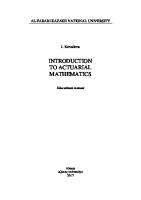
ematics than we can ever hope of managing, but this is not always an advantage. It is like having a servant who is better educated than oneself. It can give us an answer in terms of more advanced mathematics than we know. When we encounter this we shall show how to overcome it. Clearly, we cannot use Maple when building our theory; this would be circuitous. Hence readers should understand that scissors are applied automatically whenever Maple appears. Maple has proved itself as a very powerful tool; it helped solved research problems which were intractable by paper and pencil manipulation. However, computer algebra systems are only human inventions and can fail. As an example we present a graph of the function f , where f(x) = z sin7x, as produced by Maple (see Figure 1.1).
zyxwvu +
~
~~
Fig. 1.1 Graph of x
~~
+ sin 72
The graph, because of its irregularity, is clearly wrong. Here it is easy to spot the error, but on another occasion it can be more insidious. It is therefore necessary to be careful and critical when looking at output from a computer algebra system. Results are not necessarily correct simply
4
zyxwvutsrq zyxw zyx Introduction to Mathematics with Maple
because they come from the computer. The use of computer in mathematics does not free anybody from the need of thinking.
1.2 1.2.1
Introducing Maple What is Maple?
Maple is a powerful mathematical computer program, designed to perform a wide variety of mathematical calculations and operations. It can do simple calculations, matrix operations, graphing, and even symbolic manipulations, such as finding the derivative or integral of a function. It can also solve a variety of equations such as finding zeros of a polynomial or to solve linear as well as some nonlinear systems of equations.
Maple is a mathematical computer program, designed to perform a variety of mathematical calculations and operations on symbolic as we11 as numeric entities. 1.2.2
Starting Maple
We presume that the readers can handle basic tasks on a computer, be it their own PC or a large computer at an educational institution with a Unix operating system. In particular, we presume that the readers know how to handle files and directories and do some simple editing of a file. The differences between Maple use on a P C or on a Unix or Linux machine are minimal and we shall comment only on the essential ones. Before you can start Maple you must be sure that Maple is installed on your machine. At a large educational institution this will be almost automatic, for your home PC you can obtain Maple from a scientific software supplier or from Waterloo Maple at
zyx zy
http://www.maplesoft.com/sales/student_iro.html.
Once the P C has has finished booting, you can begin your Maple session. To start Maple, use the mouse to point at the Maple for Windows icon, and double click the left-hand mouse button. Alternatively, on a Unix or Linux machine you give the command maple after you login.2
2There is also the command maple, which will open Maple on a Unix machine without the graphical interface. We do not recommend to use it because of the limited display. However it can be useful, for example, if you are connected to a Unix machine through
zyxw zy zyxwvut zyxwvu
zyx zyxw zy
Introduction
5
When Maple starts, a window appears with a number of menus at the top (such as File, Edit, Format, and so on). Near the top left-hand side of the screen is the Maple prompt, which is a > character, followed by a flashing cursor, which is a I character.
To run Maple, double click the left-hand mouse button on the Maple for Windows icon. On a Unix or Linux machine give the command xmaple. 1.2.3
Worksheets in Maple
An important concept in Maple is that of a worksheet. During a Maple session, the computer screen will display your commands (and comments), together with Maple output, graphs and other pictures. All of this material is collectively called a worksheet. Usually, when you use Maple, you will be wanting to enter a new set of commands. By default, Maple opens an empty worksheet as soon as you run the program. Any commands you enter will be executed, thus forming your worksheet. When you have finished using Maple, you will be given the option of saving your worksheet to a file. Sometimes you will not need to do this, and will not save a copy of the worksheet. However, if you have not finished your work, or if you wish to use the results at a later date, you may decide to save the worksheet to a floppy or hard disk on your computer. Save files from Maple in the usual way; note that the standard filename extension for a Maple worksheet file is .mw or .mws. If a worksheet has already been saved during a previous Maple session then you can load a copy of that worksheet into Maple. That is, rather than starting a new worksheet, you can reload an existing worksheet, and modify it as required. To load an existing worksheet, you first need to know the name of the worksheet, and where it has been saved (for example, on a floppy disk, or on the PC network). Next, use the File menu, near the top of the screen, and seIect the Open menu option. Again this is done in the standard way. Once the existing worksheet has been loaded, you can modify and execute commands, add comments, and perform your choice of Maple operations. Of course, when you have finished you may choose to save the modified a modem. Most often in such a case the graphics are not available anyhow. If you use Linux then xmaple can be applied only if Xwindows is being used.
6
zyxwvutsrqp zyxw zyxw Introduction to Mathematics with Maple
worksheet so you can use it again.
A Maple worksheet is the name given to the text and graphics from a Maple session. Maple opens a new, empty worksheet by default, but you can load an existing worksheet using the File menu. You will be asked if you wish to save your current worksheet before you exit Maple.
zy zyxw
1.2.4 Entering commands into Maple
Whether you are creating a new worksheet, or reloading an existing one, you will probably want to enter some new commands into your worksheet. Whenever Maple displays the flashing I cursor, it is waiting for you to type a command. You can use menu items to get Maple to do the things you want, but you will also often need to enter your commands as text. This is done by typing your desired command, and (almost always!) ending the command with a semicolon (;) or a colon ( :). Press the Enter (or Return) key to execute the command. If you end the command with a semicolon, then Maple performs the command, and displays the result. If you end the command with a colon, then Maple performs the command, but no result is displayed. The colon is useful for intermediate calculations, but most of the time you will use a semicolon. Sometimes you might forget the semicolon or colon, and press the enter key. Nothing will happen, until you enter a semicolon (on the next line). ~
~
Most Maple commands end with a semicolon or colon, followed by the enter key. Don’t forget! But if you do forget, type the semicolon or colon on the next line. Using arithmetic in Maple is discussed in detail in Section 1.4, but the following examples should be fairly clear. For example, you might wish to evaluate the sum 1+3 5. Your Maple session will appear as the following:
+
1+3+5;
z
Introduction
9
z zyxw 7
zyx zy ~~~
zyxwvutsrqponmlkj
The command entered into Maple is 1+3+5; (note the semicolon!), and the answer from Maple is 9. Maple displays your command near the lefthand side of the screen, and the result is displayed in the centre. When using Maple commands, please note the following points: 0
0 0
0
0
0
Maple is case sensitive. Most of the in-built Maple functions are in lowercase letters. Be careful to choose the correct case for your commands! Maple usually ignores spaces in your input commands. Be careful to spell the commands correctly, and use the required punctuation. Be particularly careful to use the correct brackets, in the correct places. If you make any mistakes while typing your command, use the backspace key to correct the error. You can also highlight something and remove it by using Cut from the Edit menu. Sometimes, a command you type may take a long time to execute. You can interrupt execution (and return to the Maple prompt) by typing Control-C, sometim.eswritten C t r l - C , (that is, you press the c o n t r o l key, at the same time as pressing the C key).
Note that you can enter multiple commands on the same line, provided you use a semicolon or colon at the end of each command. For example, to evaluate 1 3 5, 21° and 64 x 123, enter the following commands. Note the use of * for multiplication and for exponentiation.
+ +
>
1+3+5; 2-10; 64*123;
9 1024
7872
8
zyxwvutsrqp zyxw zyx Introduction to Mathematics with Maple
If you forgot the semicolon and hit the enter key, you can complete the command on the next line by typing semicolon and the enter key there.
64
1.2.5
z
zyx zy zyxwvu
Stopping Maple
When you have finished, you can quit Maple in a number of ways. The easiest is to select the Exit command in the File menu.
I 1.2.6
To exit Maple, select Exit from the File menu!
Using previous results
I
Often, you will want to use the results of immediately previous calculations in subsequent calculations. The percentage character % refers to the previous result, two %% refers to the second-last result, and %%% refers to the third last result. In older versions of Maple the double quote character 'I is used instead of %.To find out which of the % or It to use on your machine type ?ditto at the Maple prompt. To evaluate 24, then 24 x 5 , then 24 x 5 + 2 4 :
16
80
96
zyxw zyxwv
zy zyxwv zyxwvut zyxwv zyxw Introduction
9
Type %, %% and %%% to use the results of the three most recent calculations.
Sometimes, you will need to use many previous results, not just the last three. This can be done via the history function. You can use the help command to learn more about the history command. Using help is discussed in detail in Section 1.3, but typing ?history will give you the required informat ion.
1.2.7
Summary
In summary:
0
0
0
double click on the Maple for Windows icon or give the command xmaple type your commands, ended with a semicolon or colon make sure the syntax, spelling and punctuation are correct exit using Exit from the File menu
1.3 Help and error messages with Maple 1.3.1
Help
Maple contains a great deal of on-line help. This can be accessed via the help command, usually entered as the question mark ? character.
Use the ? command for helpful information. Use ?name for help on the command name.
You can use the ? command in a number of ways. The following table summarises the more common uses (some of which will only become important after you have used Maple more extensively).
10
zyxwvutsr zyxwvu zyxw zyx zyxwv Introduction to Mathematics with Maple
Command ~~
?
?name
Help Topic General help Help on the topic name, or list all topics which begin with name An index of available help topics Standard library functions Basic data types Maple expressions Maple statements
zyxwv
?index ?library ?datatypes ?expressions ?st at ement s
Other useful help information can be accessed via the commands info, usage, related. These commands all give more information about a specified function. A very convenient way of using help is to open the Help menu by clicking on Help located in the upper right corner of the screen. If you know exactly the name you are looking for choose Topic Search otherwise use Full Text Search from the Help menu.
1.3.2
zyxwvu Error messages
When Maple encounters an error, it usually displays an error message. These error messages are intended to be helpful: please read them, and think about what is being said. The following examples show some error messages from Maple. In each case, the message is reasonably simple to understand. In the first case, we have tried to divide by 0, which is (of course) impossible. In the second case, the expression which has been entered is not valid: we have missed out a number or a variable. >
1/0;
Error, numeric exception: division by zero.
>
3*4+;
Error,
’;’
unexpected.
Note that in this case, the Maple input cursor will be positioned in the command you entered, at the place where Maple thinks the error occurred. In the next two examples we failed to type * to indicate multiplication. The results are surprising.
z zyxw zyxwvu Introduction
>
11
(3+2)4;
Error, unexpected number
>
4(3+2);
zyxwv zyxwv 4
In the first instance Maple gave the correct error message. However, in the second example Maple gave a wrong answer and did not issue an error message. The moral of this is simple, always try to enter your command precisely and carefully. A wrong input can return a wrong result without any warning.
Pay attention to the error messages! Maple tries to make them meaningful, often with a pointer to the location of the problem.
1.4
1.4.1
Arithmetic in Maple
Basic mathematical operators
As many of the previous examples have shown, Maple can be used for arithmetical calculations, and supports all of the usual mathematical operations. Furthermore, Maple follows the usual rules regarding order of calculations. For example, multiplication is evaluated before addition, and so on. The following table summarises many of the common arithmetical operations. Mat hematical Operation
Description Addition Subtraction Multiplication Division Exponentiation Factorial Square root
Mathematical example 1+3+5 9-5-3
Result 9 1 10 4 32
zyxw zy
2 x 5
8/2 25
usage 1+3+5 9-5-3 2*5 8/2 2-5 5! sqrt (25)
5! J25
120 5
12
zyxw zyxwvutsrq Introduction to Mathematics with Maple
zyx zyxwvutsr
1.4.2 Special mathematical constants
Maple also knows a number of useful mathematical constants, which can be used in your calculations. Two of the most important ones are shown in the following table. Note the capital letter in P i .
zyxwvut I
I Mathematical I name 7i-
1
e
I
Description Area of the unit circle Exponential constant
Maple usage
1 Approximate 1
Pi
I exp(1) I
value 3.141592 2.7182818
I
~~
Maple supports all of the common mathematical operations, and special mathematical constants. 1.4.3 Performing calculations When performing calculations, you must be sure to: 0
0
0
0
0
zyx
include suitable brackets. For example, when using sqrt, whatever you want to take the square root of must be enclosed in round brackets. match up your opening and closing brackets. For example, sqrt (4)+5 is not the same as sqrt (4+5). always use an asterisk character * for multiplication. To evaluate 2x&, you must enter 2*x*sqrt (4*x). ensure that you have entered your expressions with appropriate precedence. For example, 4*3+5 is different to 4* (3+5). When in doubt, use brackets. enter divisions correctly, using a / character. To evaluate -I-6 , you would enter (2*5+6) /(3*2). 3x2
Always put the multiplication sign in! Always use brackets for function arguments! Be careful with precedence rules in calculations! Ensure that your brackets match up, and are correctly located!
zyxwv
Consider the following Maple session. Note that if a # character appears anywhere in a line, then the rest of the line is regarded as a comment by
zyxw zyxwvuts zyxwvu Introduction
13
Maple, and is ignored. You should use comments to make your calculations more readable.
> > > >
zyx
# F o r g e t t i n g b r a c k e t s around f u n c t i o n arguments # g i v e s an e r r o r # Try t o f i n d t h e square r o o t of 4
s q r t 4;
Error, unexpected number.
> >
# The argument of t h e square r o o t f u n c t i o n
>
# Evaluate t h e square r o o t of 4
>
sqrt(4);
# needs t o be placed i n parentheses
2
> >
# Evaluate ( t h e square r o o t of 4)+5;
sqrt(4)+5; 7
>
# Evaluate t h e square r o o t of (4+5)
>
sqrt(4+5);
3 > >
# Evaluate (2*5+6) divided by (3*2)
(2*5+6) / (3*2) ;
1.4.4 Exact versus floating point numbers The Muple session given in the previous section shows that Maple evaluates 8 (2 * 6 6)/(3 * 2) to -, rather than to 2.66667. This is important. Muple 3 will (within the limitations of the current version of the software) give you the exact result rather than an approximation. The number of digits may be large but Muple will produce all the digits.
+
14
zyxwvutsrq zyxw zyx Introduction t o Mathematics with Maple
>
(9^9)^9;
1966270504755529136180759085269121 1628310345094421476692731541553\ 7966391196809 Note the backslash at the end of the line telling you that the number continues on the next line. If you want an approximation you must ask for it. One way to do this is to type the numbers in your command with decimal points. Any number which contains a decimal point is called in Maple a floating point number, FP number for short. The name refers to the way in which these numbers are stored and handled by Maple.3 For sake of brevity we shall refer to numbers without decimal points as exact numbers. For example, integers and fractions are exact numbers. So are fi and T . If only exact numbers enter a computation, Maple will produce an exact result. It is important 1 to realize that for Maple, - and .1 are distinct entities, not because of 10 their appearance, but because of the way they are treated by Maple. If you enter .1 into Maple you give tacitly some instructions which are absent 1 when entering -. Here is our first example with FP numbers. 10
zyxwv zyx
>
zyxwv
I . ~ + s q r(3.0) t ;
2.732050808 It is sufficient to write >
l + s q r t (3.0) ;
2.732050808 ~~
~
3Neither here nor anywhere else do we attempt t o explain the internal workings of Maple.
zy zyxw zyxwvu Introduction
However
1.0
15
+&
produces a correct result but not the one you wanted. You can control the precision of the decimal output via the D i g i t s command (note: capital D!), which allows you to view and set the number of significant figures: >
Digits;
10 >
s q r t (132.); 11.48912529
>
Digits:=20; s q r t ( 1 3 2 . ) ;
Digits
:= 20
11.489125293076057320
zyxw
Use D i g i t s to custamise the number of significant figures given in the answer to a calculation. The next two examples show why exact arithmetic is preferable. In the first example we set digits to three. This is not essential; a similar thing can happen with any number of digits. >
Digits:=3: 1/(22-7*sqrt (2)-7*sqrt (3)) ; 1 22 - 7 f i - 7 fi
16
zyxwvutsrq zyx zyxwvu
zyxwvu
Introduction to Mathematics with Maple
>
1/(22-7*sqrt (2.0)-7*sqrt (3.0)) ;
Error,'divisionby zero
We did not ask for division by zero, however, within the precision of three decimals the denominator is approximately equal to zero and this causes Maple to issue an error message. If the above number appeared somewhere in a long calculation the process would stop. This would not happen with exact arithmetic. Increasing the number of digits helps, but the result using Maple's default precision of ten digits is correct only to seven digits. >
Digits :4 0 :1/ (22-7*sqrt (2.0)-7*sqrt (3.0)) ; -41.92768397
-41.92768468330373949420182744528363166911107461864767765
In the next example one would expect that after taking the root and exponentiation the original number would be returned: however, calculation with floating point numbers is not exact! >
27.0'(1/8); 1.509803648
26.99999993
The imperfection of the last two examples is not some fault in Maple's design, it is instead inherent in the nature of approximate calculations. We would encounter the same phenomena if we performed the calculations with paper and pencil. If all of the entries in a calculation are exact, you can still obtain a decimal point approximation, using the evalf 0 function. Evalf stands
zyx
zyxw z
zyxwv
Introduction
17
for EVALuate with Floating point arithmetic. The first argument to the evalf () function must be the calculation you want to be evaluated. Optionally, a second argument tells Maple how many significant digits are required. >
evalf ( s q r t (132) ;
11.48912529 > >
# Evaluate t h e square r o o t with 30 s i g n i f i c a n t d i g i t s .
evalf ( s q r t (132) ,301 ;
11.4891252930760573197012229364 >
sqrt(l32);
> > >
# Recall t h a t
% g i v e s t h e r e s u l t of
# t h e most r e c e n t l y e n t e r e d computation.
evalf(%);
11.48912529
You can use the c o n v e r t 0 function to convert a FP number to an exact fraction. More generally, you can use convert () to convert numbers or expressions to many different formats (such as binary, hexadecimal, and so on). Type ?convert; for more information on this useful command.
>
# Give P i t o 20 s i g n i f i c a n t d i g i t s ,
> >
# and w r i t e t h e r e s u l t as an exact f r a c t i o n . convert (evalf(Pi,2O) , f r a c t i o n ) ;
103993 33102 Use evalf () t o produce a floating point result. Use c o n v e r t 0 t o convert from one format t o another.
18
zyxwvutsrq zyxw zyxwv Introduction to Mathematics with Maple
Algebra in Maple
1.5
zyx zyxwv zyx
In the previous examples, Maple has largely been used as a calculator: an expression is entered, and Maple calculates an answer. However, Maple is much more powerful than this. You can use any letters or combinations of letters (except for system constants such as P i ) as variables, and you can then manipulate algebraic expressions in many ways. For example, you can find sums and products, expand and factorise expressions, and so on.
1.5.1
Assigning variables and giving names
The assignment operator := is used to assign values to variables. Then whenever you use that variable, Maple will replace it with the expression or value which has been assigned to the variable. This allows interim results to be calculated, and then used in subsequent calculations. ~~~
> > >
# Assign the values 5-2 and (3'3)/4 # to the variables a1 and a2
a1 :=5^2; a2 :=3^3/4;
a1 : = 2 5
27 4
a2 := -
> >
# Look at the values of a1 and a2
al; a2;
25
27 4
-
> >
# Use the values of a1 and a2
al*a2;
675 4
Introduction
zyxw z 19
zyxwvu zyxwvu zyx
Here are two more examples with assigning algebraic expressions rather than numbers. >
u:=2*x+4;
u:=2~+4
3x+6 ~
>
v:=x-2-1;
v : = x 2 -1 >
z:=x-I; z:=x-l
x2 - 1
When a value is assigned to a variable, this value remains assigned until it is explicitly cleared. You must remember this: if you have assigned a value to a variable, each time you use that variable in a subsequent expression, the assigned value will be substituted into the expression. To clear the values of variables, you can use the restart command, which completely clears all variables (having the same result as if you exit Maple, then started it again). To clear the values of individual variables, you assign the variable its own name, with the right-hand side enclosed in single quotes. It is a good habit to begin a second worksheet with the restart command, otherwise the variables from the previous worksheet would be still assigned. ~
> >
~
~
~
~~
~~~
Assign a value t o the variable a2 a2:=27/4;
#
~~
~
20
zyxwvutsrqp zyxwvu zyxw
z
Introduction to Mathematics with Maple
27 a2 := -
4
> > >
zyxw
# Clear t h e variable a2, # f o r g e t t i n g its current value.
a2:=’a2’; a2 := a2
zyx
The assignment operator can be used to name almost any object which Maple recognizes. This can save a lot of typing by recalling the object by its assigned name either alone or as an argument of a command. >
p :=Pin3+5! ;
zyxw zyx
p := T 3 >
eq: =xA2+5=p;
eq := x2 >
p01y:=xn5+x+1;
+ 120
+ 5 = r3+ 120
poly := x5 >
+x + 1
f a c t o r (poly) ; 2.(
+ + 1)(2
- x2
+ 1)
Use := to assign values to variables. Use r e s t a r t to clear the values of all variables. Clear an individual variable by assigning the variable’s name to it, for example, x I : = ’ x l ’ ; . Use the assignment operator := to name mathematical objects.
1.5.2
Useful inbuilt functions
Maple provides you with a large number of very useful inbuilt functions. These can be used to manipulate expressions which you have defined. There is a command simplify. However, simplification can mean one thing on one occasion and something altogether different on another. Which is simpler,
zyxw z
zyx zyxwv zyxwvu zyxw Introduction
+
21
+
x4 - 1 or (x 1)(x - 1)(x2 l)? Maple simplifies only when there cannot be any doubt: x is undoubtedly simpler than II: 0. Therefore the decision how to manipulate is often left with the user: Maple provides a range of options: expand, factor, normal, collect, sort and combine.
+
1.5.2.1 expand ()
The expando function is used to distribute products over sums: > >
Define A=x^2-1 and B=x^2+1 A:=x^2-1; B:=x^2+1; #
A := x2 - 1
B := x2 + 1
> >
## Evaluate A*B
A*B;
( x2 - 1 )( x2
> >
+ 1)
Expand the previous result expand(%);
#
x4 - 1 > >
Expand (x-2-1) (~^2+1)-(~-1)^2 expand((x"2-1)*(x'2+1)-(x-l~^2);
#
x4 - 2 - x2 + 2 2 > # E x p a d (x+Y+z)-2- (x-y-Z) -2 > expand((x+y+z)^2-(x-y-z)^2);
4xy+4xz > >
Expand (1+2x)^6 expand((l+2*x)^6) ;
#
22
zyxwvutsrqp zyxw zyx Introduction to Mathematics with Maple
zyxwvu zyx zy
1.5.2.2 factor()
The factor0 function is used to factor a polynomial with integer, rational or algebraic number coefficients. factor0 is often used to reduce complicated expressions to a more manageable size. > >
# Assign xn2-1 to
f, in other words name xn2-1 as f
f:=x^2-1;
f :z2-l > >
# Factorise f
factor(f);
(2-l)(z+l) > >
# Factorise xn4-xn2+2x-2
factor(xn4-xn2+2*x-2) ; ( z - 1 ) (z3
+z2
+2)
1.5.2.3 simplify() The simplify() function is used to write a complicated expression in a simpler form. Often Maple leaves the expression unchanged and leaves the decision how to proceed with the user. > >
# Assign (sin x)^2 + (cos x1-2 to T T:=sin(x)^2+cos (x)^2;
T >
simplify(T) ;
:= sin( z ) 2
+ cos( x
) ~
Introduction
zyxwz 23
zyxw z 1
Note that the Maple command sin(x)-2 is evaluated as (sin(x))^2 and not as sin( (x) -2). Here Maple follows the standard rules of precedence in evaluating functions before applying other mathematical operations. If you are in any doubt, insert additional parentheses to avoid possible errors. > >
#
> >
#
>
c-CI;
> >
# Simplify the previous result
Assign (x+1)^3 to C C:=(x+1)^3;
Assign (x-1)^3 to Cl C1:=(~-1)^3;
simplify(%) ;
6x2+2
1.5.2.4 normal() The normal (1 function is used to write expressions in normalised form; that is, a numerator over a common denominator:
22-1 x(2-1)
24
zyxwvutsrqp zyxw
zyxwvut zy zyxw Introduction t o Mathematics with Maple
> # Normalise l/(x-I) + x/(x-1)^2 > normal(i/(x-I) + x/(x-I)^2) ;
22-1
1.5.2.5 collect () The collect() function is used to collect coefficients of like powers of a specified variable; this variable must be indicated, otherwise Maple does not know what to collect. In the following example, the final expression has been collected into coefficients of the variable x: > >
zyxwv
# Define f as (x+(x-y)^2)^2
f :=(x+(x-y)-2)-2;
f >
:= (x
- y)2)2
expand(f);
x2 + 2 x3 - 4 x2 y + 2 x y2 >
+(x
+ x4 - 4 x3 y + 6 x2y2 - 4 x y3 + y4
collect (%,XI ;
x4 + ( 2 - 4 y ) x3 + ( -4 y
+ 1 + 6 y2 ) x2 + ( 2 y2 - 4Y3 ) X
Y4
1.5.2.6 sort() The sort (1 function is used to sort the terms of an expression into descending order of power of a specified variable. > >
# Assign xA5-3x^3+x^7 to f
f:=x-5-3*x-3+xn7;
f :=x5-3x3+x7 >
sort(f,x);
zy zyxw
zyxw zyxwvu zyxw zyxwvu 25
zyxw zyx
Introduction
x7+x5-3x3
> >
x^3y+x^4y^4+~^2+~^6y^2 to g g:=xn3*y+x*4*y^4+xn2+xn6*yA2; # Assign
g := x3 y
>
sort(g,y);
x4 y4
+ x4 y4 + x2 + x6
y2
+ x6 y2 + x3 y + x2
1.5.2.7 combine()
The combine command reduces a given expression into a single term, if possible, or transforms it into a more compact form. Sometimes, similarly as with simplify, it leaves the original expression unchanged, leaving the user with the option to try another command. The following examples illustrate the use of combine. >
combine(sqrt (12) *sqrt (3)) ;
6 >
combine(sqrt(3+sqrt(5))*sqrt(3-~qrt(S)));
>
expand(%); 2
zyxw
cos(2 x)
The combine command reduces integer powers of sin and cos into linear expressions in terms of sin and cos of multiple arguments. The result is often more extensive than the original expression.
26
zyxwvutsrqp zyxw zyxw
zy zyxwvut zyxwvu Introduction t o Mathematics with Maple
1 5 - COS(32) 16 16 combine(cos(x)n2+sin(x)n3) ;
- C O S ( ~2)
>
1 2
- cos(2 z)
+
+ -85
COS(Z)
+ -21 - -41 sin(3 z) + -43 sin(z)
1.5.2.8 subs() The subs command makes a substitution, it can be used to substitute a value or an expression. It does not simplify the result, it leaves it to the user to choose an appropriate command for further processing. >
subs(x=l,sqrt(xn2+ll*x+24)) ;
J36 >
simplify(%) ; 6
>
~~b~(~=t-3,~^2+6*~+1);
(t - 3)2 + 6 t - 17 >
expand(%);
t2 - 8
combine(), expand(), factor(), simplify(), normal 0,collect (>, sort () and subs ()
are all useful for manipulating mat hematical expressions.
Examples of the use of Maple
1.6
Example 1.1 (simplify; rationalize; factor) some quite complicated expressions
>
simplify(sqrt (2*sqrt (221)+3O)) ;
a+Im
Maple can simplify
zyxw zyx zyxwvu zyx zyx Introduction
27
On some similar occasions Muple does not simplify, the reason being that there is another command more appropriate: for example, rationalize is one such command.
1
zyx zyx
2 + f i
>
rationalize (%I;
2-fi
~~
zyxwvu
Another example of the same kind is:
>
>
simplify(2*a-2+5*a*b+2*bn2);
factor(%);
2 a2
+ 5 a b + 2 b2
(2a
+ b) (a + 2b)
Example 1.2 (solve) Maple can solve equations for you. The basic command is solve. We shall learn more about solving equations and the command solve in Chapter 8, but here is a simple example.
1 eq:=-+x+l >
1 =1 2-1
solve(eq);
La,1 + J z We trust that the readers do not need Muple to solve such simple equations, the next example is more sophisticated. We use Maple to solve a Diophantine equation, this means that the solution must be in integers.
Example 1.3 (Diophantine equation)
An example of a Diophantine
equation is
1 2 3 4 5 6 7 ~- 7 6 5 4 3 2 1 ~= 1357924680. The command for solving a Diophantine equation is isolve.
28
zyxwvutsrq zyxw zyx
zyxwvu Introduction t o Mathematics with Maple
>
isolve(l234567*x-765432l*y=l357924680); ( X = 4484627
+ 7654321-Nl , y = 723149 + 1234567-Nl }
The entry -Nl indicates an arbitrary integer, there are infinitely many solutions. The amount of work with pencil and paper t o find this solution would be considerable. Maple’s answer is instantane~us.~ It is easy t o see that the Diophantine equation 3 x - 2 y = nl where n is a given integer, has a solution (among infinitely many others) x = n, y = n. Maple’s answer is not very he1pfuI:
>
zyxwv z zyxw
isolve (3*x-2*y=n);
( x = - N l , n = 3 _ N l -2-N2, y = - N 2 )
This means that if we choose x arbitrarily and y also then - 2 y , which is correct but not helpful. What can we do with 12345673: 7654321y = n? As we might expect, blind use of isolve will
n = 3x
+
not help.
>
isolve (1234567*~-765432l*y=n) ;
(x = -Nl, y = -N2, n = 1234567-Nl
-
7654321-N2)
However we can solve the equation
>
isolve (1234567*~-765432l*v=l) ; (U = 661375
and then clearly
x
+ 1234567-Nl , u = 4100528 + 7654321-Nl }
= un and y = u n
*Maple will even tell you how long it took t o solve an equation or to execute another command. See time in the Help file.
Introduction
zyxwz 29
zyxw zyxwv zyx zyxwv
We have seen that Maple can save a lot of tedious work. However, even in a situation when Maple is unable to solve the problem directly, it can be used with advantage. At the beginning of this chapter we said that Maple can divide poly1 by x2 x 1. There are two nomials: we mentioned dividing x6 commands, rem to give the remainder and quo to give the quotient. The following Maple session shows how to use these commands. Note that three entries in brackets are required in both commands.
+
>
+ +
rem(x^6+1 ,xn2+x+1,x) ; 2
>
quo(xn6+l,xn2+x+l,x);
x4 - x3 -l-x - 1
zyx zyx
The third argument in both commands is important as the next example shows. >
rern(u^2+~^2,~-2*v,u) ;
5 v2
>
rem(u^2+vA2,u-2*v,v) ;
5 4
- u2
Maple can also find the remainder and quotient for division of integers. The commands are irem and iquo. >
irem(987654,13) ; 5
>
iquo(987654,13) ;
75973
30
zyxw zyx zyxwvutsrq Introduction to Mathematics with Maple
So far all the commands we have used were available directly on the command line. These commands reside in the main part of Maple called the kernel. More specialized or not very frequently used commands are grouped in packages. This helps with efficiency and speed of Maple. The list of packages can be obtained by first clicking on Help (located in the upper right corner of the screen) and choosing Topic Search from the menu which opens. In the dialog window which then appears fill in packages and click OK. Another window opens and there you can click on index,package. There are literally dozens of packages. In this section we shall use only two, the number theory package and the finance package. To obtain the list of commands available in a package issue a command with(package) . For instance, if we issue a command with(geometry1 Maple will produce a long list of various commands relating to geometry, and make these commands available. The first command in the list is Apollonius. Using Help will tell us how to use this command to solve the problem of finding a circle which is tangent to three given circles, a problem formulated and solved by Apollonius from Perge in third century BC. In a similar fashion we can employ any command from the above list after the command with(geometry) has been issued. If we know the name of the command and the package we can use the command on the command line. For instance, we can find all positive divisors of a number using the number theory package numtheory and the command numtheory [divisors], or the number of positive divisors using the command numtheoryCtau1 (note the use of [ and I).
z
>
numtheory[divisors] (144) ; (1, 2, 3, 4, 6, 8, 9, 12, 16, 18, 24, 36, 48, 72, 144)
>
numtheory [tau] ( 144); 15 ~
Alternatively, we can activate the command >
with(numtheory, divisors) ;
[divisors] and then use the short form of the command thus >
divisors (144) ;
Introduction
zyxwz 31
zyx zyxw zyxwv zyxw
(1, 2, 3, 4, 6, 8, 9, 12, 16, 18, 24, 36, 48, 72, 144)
Mathematics for finance is contained in the finance package.
Example 1.4 (Mortgage) A 35 year-old man is confident t h a t he can save $12,000 a year. He wishes to buy a house and stop payments a t 55, when he plans to retire. The current interest rate is 6%. In order to find out how much he can borrow he uses the command annuity from the finance package. From a mathematical point of view, mortgage and annuity are the same. A
company advances the money for the mortgage and the consumer pays back installments; in an annuity, in contrast, the individual makes a down payment and receives regular income from a finance institution.
>
w i t h ( f inance,annuity) ;
[annuity] >
a~nuity(12000,0.06,20);
137639.0546 This amount seems insufficient for a house of the desired standard and quality. The man decides to extend the life of the mortgage to see what happens. ~
~~
>
~~
~
~-
annuity(12000,0.06,30);
165177.9738 This is a sufficient amount. However, paying the mortgage for ten more years is not an attractive idea. To see by how much the installments must be increased for a mortgage of $165,000, use the following commands.
>
solve(annuity(x, .06,20)=165000);
14385.45190 Clearly, as long as it is affordable, it is far better to increase the cash payments rather than to increase the life of the mortgage. The Help file contains details of how to adapt the annuity for a more realistic situation of monthly or fortnightly payments.
32
zyxwvutsrq zyx zyxwvu
zyxwv zyxw Introduction to Mathematics with Maple
Exercises
@ Exercise 1.6.1
The command time(X) will tell you how much time (in seconds) was needed by Maple to execute X. Assign a, b, c to be 2100750,3100550,and 101ootrespectively. Solve the Diophantine equation ax by = c. Determine how much time was needed. [Hint: On the authors' machine using Maple 7 it was .039 sec].
+
+ x4 + 1.
Exercise 1.6.2
Use Maple to factorize xl'
Exercise 1.6.3
Find the quotient and remainder for
(1) 987654321, 123456789; (2) 100000, 17. Exercise 1.6.4
(1) (2)
Find the quotient and the remainder for the polynomials
+ 52 + 7) x4 + 1; X2O + 1, x9 + 2x + 7. X1O
Exercise 1.6.5 What are the monthly installments for a mortgage of $200,000 over a period of 40 years a t interest rate of 6.5%?
zyx zy
Chapter 2
Sets
zyx zyxw
In this chapter we review set theoretic terminology and notation. Later we discuss mathematical reasoning.
2.1
Sets
The word set as used in mathematics means a collection of objects. It is customary to denote sets by capital letters like M , M I , etc., below. At this stage the concept of a set is best illuminated by examples, so we list a few sets and name them for ease of reference. Table 2.1
Some examples of sets
M I , the set of all rational numbers greater than 1; Mz, the set of all positive even integers; M3, the set of all buildings on the St Lucia campus of the the M5, the M6, the M7, the M4,
University of Queensland; set of all readers of this book; set of all persons who praise this book; set of all persons who condemn this book; set of all even numbers between 1 and 5.
In these examples we have used the word ‘all’ to make it doubly clear that, for instance, every rational number greater than 1 belongs to M I . But usually, in mathematics, if someone mentions the set of rational numbers greater than 1 he or she means the set of all such numbers, and this is 33
34
zyxwvutsrq zyxw
zyxwv z zyx Introduction to Mathematics with Maple
automatically understood. Thus with a similar understanding we would say that M2 is the set of positive even integers. If an object x belongs to the set M , we say that x is an element of M or that x lies in M , and we denote this by writing x E M . If z is not an element of M we write z @ M . A set M is defined by specifying which elements lie in M . One way of describing a set is to list its elements, separated by commas, and enclose them in braces (curly brackets); for example, M7 = {2,4}, M2 ={2,4,6,8 ,... }. It is worth pointing out that the elements in a set can be other sets. Thus the set A = (2, {x,y}} has two elements; one is the number 2, and the other is a set with two elements, x and y. These could be some mathematical entities, or they could be sets, whose elements are other sets, whose elements . .. . Furthermore, the order in which the elements are listed inside {. . . } is irrelevant; thus M7 = {4,2} is the same set as Ad7 defined in Table 2.1. Also, any repetition of elements is ignored, so that we could equally well write M7 = {4,4,2,2,2,4,2,4}. The essential part of the definition of M7 is that both 2 and 4 must lie inside {. . .}, and nothing else is allowed there. A finite set has only a finite number of elements. Thus M3 and M4 are finite, whereas M I and M2 are infinite (that is, they are not finite). Two sets M and N are considered to be equal if they consist of the same elements. If all elements of a set A belong to a set B then we say that A is a part of B , or that A is a subset of B. This is denoted by A c B. Obviously A c A always. The relation A c B is often referred to as an inclusion. Thus in the above list it is obvious that Ad2 c M I . If all people were honest and rational it would be also true that M5 C M4 and M6 C M4; but in the world as it is this is not certain. If A c B and A is not equal to B we say that A is a proper subset of B. This relation between A and B is denoted by A 2 B. It is also convenient to introduce the empty set. This is a set which has no elements, and we regard it as a finite set. The symbol 8 is used to denote the empty set. We could also write 8 = {}. At the first encounter the empty set may look a little strange but the introduction of the empty set has advantages; for example, in the above list M4, M5 and M6 need not contain any elements at all.' The introduction of the empty set allows us to talk freely about M4, Ms and M6 without worrying whether or not they
zyxwv zy
zyxw zyxw
lBut since you have read this footnote i t seems that M4 contains at least one element.
zyxwv z zyxw
zyx zyxwvu zyxwv z zyx zyx Sets
35
contain an element. We also agree that @ c M for any set M . If M c N and N c M then clearly M and N consist of the same elements and hence M = N . In particular cases later, where we prove that M = N we often do so by showing that M c N and N c M . We now introduce some further notation. If P is a certain property then the set of all elements having the property P is denoted by {x; x has property P } ; for example,
M2 = {x; x is a positive even integer},
M7 = {x; x E M 2 , 1 < x < 5).
2.1.1
Union, intersection and diflerence of sets
Given two sets M and N we can define a new set, denoted by M U N , consisting of all elements belonging to either M or N (or both). The set M U N is called the union of M and N (see Figure 2.l), and clearly M U N =N UM.
MuN
Fig. 2.1 Union of two sets
We define another new set by taking elements common to both M and N ; these form a set called the intersection of M and N which is denoted by M n N (see Figure 2.2). Clearly M n N = N n M . Using the notation
36
zyxwvutsrq zyxw zyx zyxw zyx Introduction t o Mathematics with Maple
introduced above we have M U N = {x; x E M or x E N } and M n N = {x; x E M and x E N } . If M n N = 8 then we say that M and N are
disjoint.
Fig. 2.2 Intersection of two sets
zy zyx
Yet another set which can be formed from two sets is the difference. If M and N are sets then the difference M \ N is, by definition, the set of elements lying in M but not in N , that is, M \ N = {x; x E M , x 6 N } . This is illustrated in Figure 2.3. It is clear that M \ N # N \ M , unless M = N , in which case M \ N = 8.
Fig. 2.3 Difference of two sets
zyxwvu z zyxwvu zyx zyx
z zyx z zyx zyxwv 37
Sets
Given three sets L , M and N we can form two new sets A = ( L u M ) u N and B = L u ( M U N ) . For example, for B we form first the union M U N = Q and then use Q to form L U Q. It is easy to see that each of the new sets A,B consists of those elements belonging to at least one of the sets L , M , N . Hence ( L U M ) U N = L U ( M U N ) and we write simply L U M U N . The same convention is used for intersections; for example, the intersection of four sets A,B,C , D may be denoted simply by A n B n C n D. The corresponding ideas for 5 sets, or 25, or any finite number, presents no new difficulties but some compact notation is needed. Thus A1 n A2 n
nAi, 4
A3
nA4 is denoted by
seven sets
B1,
B2,
i=l . . . , B7. The
u
u 7
and in the same way,
Bi is the union of the
i=l
notation is extended to refer to an infinite
00
number of sets so that
Ci is the set of those elements contained in at
i=l
00
least one of the sets C1 i
C2?C,,
(7 Dk is the set of those elements
. , . and
k=l
contained in all the sets Dk,k = 1, 2, 3,
. . . . For example, if Ci is the set
u 00
of positive proper fractions with denominator i then the union
Ci is the
i=l
set of rational numbers between 0 and 1. And if Dk is the set of integers less 00
than or equal to I% then the intersection
0Dk consists of the set of negative
k=l
nDk 00
integers, together with 0 and 1, that is,
= (1, 0,-1, -2, -3,
. . .}.
k= 1
Exercises
Exercise 2.1.1
Use the definitions AUB={x; xEAorxEB},
AnB={x; xEAandxEB},
A\B = { x ; x E A, x
4 B},
to prove ( A nB ) U ( A \ B ) = A . The set of subsets of A is called the power set of A . For example, the power set of (1, 2 ) is {{}, {I}, {2}, (1, 2)}. Use Maple to create the power set of (1, 2 , 3, a, b, M } . [Hint: Use Help to find the command combinat [powerset J .]
@ Exercise 2.1.2
38
zyxwvutsrq zyx zyxwvu zyxwvu zyxwv
zyxwvu zy Introduction to Mathematics with Maple
2.1.2
Sets in Maple
Notation for sets in Maple is the same as in set theory. The empty set is denoted by {I (the common mathematical symbol for the empty set, 8, cannot be entered from the keyboard). Instead of the symbols U, n, \ we write union, intersect, minus, respectively. Hence
A >
B:={23,29,31,37,41,43,47,53,59,61,67,71};
zyxwvu B
>
:= (19, 25, 31, 37, 43, 49, 55)
:= (23, 29, 31, 37, 41, 43, 47, 53, 59, 61, 67, 71)
A union B;
(19, 23, 25, 29, 31, 37, 41, 43, 47, 49, 53, 55, 59, 61, 67, 71) >
A intersect
B; {31,37, 43)
>
A minus
B; { 19, 25,49, 55)
> B minus A ; (23, 29, 41, 47, 53, 59, 61, 67, 71) >
({a,b} union {x});
({1,2,x} minus {I});
Sets
z zyxwvu 39
z zyxw zyxwvu zyxw
In ordinary life there is no distinction between 1 and 1.0. We know that
Maple makes a distinction, consequently >
({I}intersect
{I-o});
({I} union (1.0));
0
2.1.2.1
Expression sequences, lasts
An expression is a basic entity in Maple; roughly speaking, it is a string of characters which can be entered into Maple. An expression sequence is an ordered n-tuple of expressions separated by commas. For instance j o h , I, Kai !Hy%, set, x+l/x, 1, 1 is an expression sequence. An expression sequence enclosed in square brackets constitutes a list. Order and repetition of expressions in lists or expression sequences do matter: [I, 21 , [2, 13 and [I, 2, 11 are all distinct. Sets, lists and expression sequences are all similar: the difference lies in the way Maple handles them. You can make an intersection of two sets but not of two lists. You can combine two lists into a new list in which the first element of the second list follows the last element of the first list. The following are some examples of using sets, lists and expression sequences in Maple.
zyxwv zyxw
>
# First we name a few sets, lists and
> > >
# expression sequences. A:={a,b,c}; B:={john,3! ,x!,Kathy}; C := [x,y ,z , z ,z] ;Z :=I, a, I,b;
A
:= { a , b, c}
40
zyxw zyxwvutsrq zyxw zyxw zyxw zyxw zyxw zyxwvu Introduction to Mathematics with Maple
B
:= (6,x!,john,
Kathy}
c := [x,y, 2 , 2 , 21 Z := 1, a , 1, b
> >
#
>
convert(A,list) ;convert(C,set);
> > >
#
> >
# the nops command counts the number of elements
> >
# the command convert changes a set into a list
or vice-versa
enclosing an expression sequence in appropriate symbols converts the sequence to a list or set, # respectively. #
in a list or a set, but cannot be applied to an expression sequence. nops (B) ;nops (C) ; # #
4 5
z zyxwvu zyxwvut Sets
#
41
the n-th element can be extracted from a
# list or an expression sequence by # attaching [n] to the list
zyxwv zyxwv
or expression sequence, respectively. Note that a set does not have an n-th element. # Maple will return a result, giving what it thinks # is the n-th element, and this need not agree # with what you might guess is the n-th element. AC21 ;B[11 ;Z[31;
##
#
b
6 1
The command op(2,A) has the same effect as A[2]. # However, the op command is more powerful # and more flexible. # It can extract all elements, or some chosen ## elements from a list or a set. ## Some examples on the use of op follow. op(2. .4,C); op(B); [op(A), op(3. .4,B)1;
#
zyx zyxw zyxw
6 , x!,john, Kathy
[a, b, c, john, Kathy] >
The command seq can be used to generate > # an expression sequence according to some formula. > seq(i-3 ,i=2..5) ;seq(nA2+n+7 ,n=O..3) ; #
8, 27, 64, 125
42
zyxwvutsrqp zyxw zyx
zyxw zyxwvu zyxw Introduction to Mathematics with Maple
7, 9, 13, 19
>
{seq(nn2+n+7,n=l. .30)}intersect{seq(nn2+n+ll,n=1. -30)); (13)
Exercises Combine the lists L = [l,3,5] and M = [I,2,3,4] into Exercise 2.1.3 a single list using the op command.
zyx zyxwvu zyxwv zyxwvu
Exercise 2.1.4 Find the number of distinct elements in a list by first converting it to a set.
Exercise 2.1.5 Find the number of elements in the power set of A, where A has 17 elements. [Hint: See Exercise 2.1.2. Use nops!]
2.1.3
Families of sets
Instead of saying that A is a set of sets we prefer to say that A is a system or a family of sets. Later we shall encounter situations where to each element l of a set L there is associated a set CZ. In such a situation we say that the family of sets Cl is indexed by the set L. It is natural to denote this indexed family by {Cl;l E L } . If {Cl;l E L } is an indexed family then by Cl we understand the union of the family Cl, that is, the set of all
u
1EL
elements belonging to at least one set Cl. Similarly, the intersection A1 is by definition the set of all elements
n
IEL
belonging to every set Al. A family of sets can be indexed by any set, not necessarily by a subset of positive integers. If, for instance, A1 is the set of points on the straight line between the points (1, 0) and ( I , 1) in the plane and L is the set of real numbers between 0 and 1 then Al is the interior
u
1EL
of the square with vertices (0, 0), (1, 0), (1, 1) and (0, 1).
2.1.4
z zyxwv zyxw
zyxwvut zyxw zy Sets
Cartesian product of sets
43
If A and B are sets then the set of ordered pairs of elements, (a, b),2 the first from A and the second from B , is called the Cartesian product of A and B and denoted by A x B. Expressing this in symbols, we have A x B = { ( a , b ) ; a E A , b E B}. Two ordered pairs ( a , b) and (c, d) are
defined to be equal if and only if a = c and b = d. It is natural to define A XB x C as the set of ordered triplets (a, b, c) with a E A , b E B and c E C. One would perhaps expect that A x B x C = ( A x B ) x C = A x ( B x C). However this is not strictly correct since ( A x B ) x C is a set of pairs of things in which the first thing is a pair of elements and the second thing is a single element; ( ( a , b), c) is its typical member, whereas a typical member of A x B x C is a triplet ( a , b, c). In this book we shall not make this fine distinction between ( A x B ) x C or A x ( B x C) and A x B x C. In the same way the idea of a Cartesian product of four or any finite number of sets should be clear. For A x A we write A 2 , and for A x A x - - - x A with n factors we write An. Warning: Realise that A x B generally is not equal to B x A .
zy
2.1.5
Some common sets
We assume that the reader is, at least on an intuitive basis, familiar with real numbers. The theory of real numbers (including, for example, the definition of integers, rationals, etc.) is systematically reviewed in Chapter 4. For ease of reference we name here some subsets of reals as follows. The set of all real numbers will be denoted consistently by R.
zyx zyxw zy
N is the set of natural numbers, N = (1, 2, 3, . . .}; NO is the set of non-negative integers, No = ( 0 , 1, 2, 3, . . . }; Z is the set of integers, Z= ( 0 , 1, -1, 2, -2, 3, -3, . . .};
{Q
Q= E; p
Z,q E N};3 P is the set of positive reals, P = {x; x E R, x > 0 ) .
Q is the set of rationals,
E
2Using set notation, the ordered pair (a, b) can be written (a, b) = (a,( a , b} }. In fact this equation can be used t o define an ordered pair. 3A more precise formulation of the definition of Q, using terminology introduced so far, would read Q = { ( p , q ) ; p E Z,q E N}
44
zyxwvutsr zyxw zyxw zyxwvu Introduction to Mathematics with Maple
Exercises
zyxwv z
Exercise 2.1.6 Give examples of sets M , N , P , Q such that A4 and neither P c Q nor Q c P.
Mi,
z
For the sets listed in Table 2.1 show that M I U M3nM4=O.
Exercise 2.1.7
cN
M2
=
Exercise 2.1.8 In this exercise A, B , C are arbitrary sets. Discover which of the following relations are correct. Prove the correct ones and give examples (strictly, counter-examples) to show that the others are false.
(1) A n ( B u C ) = ( A n B ) u ( A n C ) ; (2) ( A u B ) n C =( A n C ) u ( B u C ) ; (3) A u ( B n C ) = ( A u B ) n ( A u C ) ;
z zyxwv
(4) A U A = A , A n A = A ; ( 5 ) ( A n C ) u B =( A u B ) n ( C u B ) . Exercise 2.1.9
Let An = {x; x E
N, x a multiple of n}, B1 = (2;x E
u n u Bz,nB1. 00
R,x < l } , L = {x : x E Iw, x > O}. Find
00
An,
n=2
Exercise 2.1.10
@ Exercise 2.1.11
An,
n=2
EL
EL
What can you say about the sets A, B if AUB = AnB? Prove that
(1) ( A \ B ) n C = ( A n C ) \ ( B n C ) ; ( 2 ) ( A\ B ) u ( A \ C ) = A \ ( B n C ) ; (3) ( A \ B ) n ( A \ C ) = A \ ( B u C ) .
@ Exercise 2.1.12
Parts (2) and (3) of Exercise 2.1.11 can be generalized to families of sets. Prove that, if L is an index set, Al a family indexed by L , and X is any set, then
(These relations are known as de Morgan’s Rules.)
zyxwv z zyxw zyxwvu zyxwv
zyxwvu zyxwvuts zyx Sets
@ Exercise 2.1.13
Let A1 and
€31
45
be two families of sets indexed by a set
L. Prove that
U A E \ U B l c U(Al\Bl).
1EL
1EL
1EL
Also show by an example that the inclusion cannot, in general, be replaced by equality.
2.2
Correct and incorrect reasoning
The ability to reason correctly is essential in mathematics. Care is often needed, as the following fallacious argument shows. Let b be an arbitrary real number, and let c be the same number, that is, c = b. Multiply this equation by c and subtract b2, giving
that is, (C
+ b)(c - b) = b(c
-
b),
(2.1)
and hence, dividing by c - b we have
and therefore c = 0. We appear to have proved that an arbitrary real number c must be zero. As this is absurd we must look for an explanation. The error occurred when passing from Equation (2.1) to Equation (2.2), and involved an incorrect application of the following theorem. If yx = xx and z # 0 then y = 2. We applied this for x = c - b and overlooked the fact that c - b = 0. Consider the previous theorem again. It is of the form: ‘If ... then . . . ’. The part of the sentence starting with ‘If’ is called the hypothesis (or assumption(s) or condition(s)) and the phrase starting with ‘then’ is called the conclusion (or assertion(s)). The moral of the above example is that when applying a theorem one must make sure that the hypothesis is satisfied. Sometimes a mathematical theorem is not expressed in the form ‘ I f . .. then ...’, but even with such a variation of form the hypothesis can be identified. For example the theorem
zyxw
46
zyxw zyx zyxwvutsrq zyxwv zyxwvutsr zyx Introduction t o Mathematics with Maple
T: The product of two consecutive integers is divisible by two.
can be rephrased to exhibit the hypothesis and the conclusion more clearly as
T:If n is an integer then the number n(n + 1) is divisible by 2.
zyx zyxw
If the conclusion and the hypothesis are interchanged a new theorem is obtained, which is called the conuerse of the original theorem. The theorems P and C below are converses of each other.
P: If a right-angled triangle has hypotenuse c and other sides a , b then a2 + b2 = c2. C: If the sides of a triangle a, b, c satisfy a2 b2 = c2 then the triangle
+
is right-angled and c is its hypotenuse.
The converse is different in content from the original theorem. In the above example it happens that both theorems are true. The next example is different.
E: If an integer is divisible by six then it is an even number. S: If an integer is even then it is divisible by six. Clearly S says something quite different from E; moreover S is false while E is true. Summary: A piece of mathematical knowledge is usually stated in the form of a theorem, which has a hypothesis and a conclusion. If these are interchanged a new theorem is obtained. It is wrong to assume that the converse holds simply because the original theorem did. If one suspects that the converse is true and wishes to use it, then one must prove it. Actually, the converses of many important theorems are true. In such cases instead of stating the two separate theorems we use the phrase ‘if and only if’, and thus combine both theorems into one statement. For example, P and C together read
PC: The triangle with sides a , b, c is right-angled with hypotenuse c if and only if a2 b2 = c2.
+
The abbreviation ‘iff’ is sometimes used for ‘if and only if’.
zy zyxwvu zyxwvu
zyxwv zyxwvu zyxw Sets
Exercises
Exercise 2.2.1
47
State the following theorems in the form ‘ I f . . . then
(1) The diagonals of a rhombus are perpendicular. (2) Every algebraic equation of degree one or higher has a solution. (3) Every two positive integers have a greatest common divisor. (4) Grandfather’s knee pains whenever it rains. Exercise 2.2.2 false.
Give an example of a valid theorem whose converse is
Exercise 2.2.3 Give an example of a true theorem with a true converse. Use the phrase ‘if and only if’ to combine both theorems into one statement.
2.3
Propositions and their combinations
What has been said in the last section is really only a vague introduction to certain ideas. We now consider them more carefully. The typical structure of a theorem has already been mentioned: ‘If something, then some other things’. But what are the ‘things’ in question? The first point is that they cannot be any phrase or sentence (in English) like (Hooray!’, (HOWare you?’, ‘Go home!’, ‘The colour seven is tropical.’ They must be capable of being true or false (but not both). We shall call such sentences propositions. If A and B are propositions, then each may be true or false, and there are four possible cases in relation to the truth of both (see Table 2.2). Table 2.2 Truth and falsity of propositions
I. 11. 111. IV.
A A A A
is true, and so is B ; is true, but B is not; is not true, but B is; is not true, and neither is B.
Consider the following example.
48
zyxwvutsrq zyxw zyxw zyxwvut Introduction t o Mathematics with Maple
zy zyxwv
A: John, the engineering student, achieved top grades. B: John, the engineering student, has passed the year.
In this example case I1 cannot occur. If A and B are propositions, and case I1 does not occur, we say that A implies B , or that B follows f r o m A , and we denote this by A + B. Such a relation between two propositions is called an implication. We may express the implication A + B in other words by saying If A, then B; here A is the hypothesis and B is the conclusion. The reader will remember from Section 2.2 that when A B then B need not imply A . In our example, if John has all top grades he passes (so A + B ) , but if he passes he need not have all top grades, so B + A is not true. By forming an implication A + B we combine two propositions A and B into a new one; i f A then B. This new proposition is true if case I1 in Table 2.2 does not occur. After having made precise the meaning of the implication A + B , it is time to reflect and realize that in ordinary life many people do not understand implication the way mathematicians do. For example, our interpretation of A + B means that for a false proposition A the implication A + B is true no matter what proposition B is. This is clear, since if A is a false proposition and B is any proposition, the case I1 does not occur (neither does I). Consequently, i f 3 is less than 1 then all numbers are equal is a true implication, and so is if 3 is less than 1 then not all numbers are equal. Implication is an example of combining two propositions into a new one. There are many ways of forming new propositions. The negation of a proposition C is a proposition which is true if C is false and false if C is true. The negation of C is usually denoted by not C or 1C. For example, if D is the proposition the number six is even then 1 D is the number six is not even. The success of many proofs hinges upon a correct formulation of the proposition 7 C corresponding to a given C. For instance, if C means every blonde girl has a handsome suitor then 4’means it is not true that every blonde girl has a handsome suitor or, in other words, there is at least one blonde girl who either has n o suitor or her suitor is not handsome. Given two propositions A and B we can form a new proposition A and B. For example, if A is 16 is even and B is 16 is positive then A and B means 16 is even and positive. We shall agree that the proposition A and B is true if both propositions A and B are true. We denote the proposition A and B by A A B. The last combination of two propositions A and B we consider is A or
zyxwv z zyxwvu zyx 49
Sets
B. It is taken to mean that a t least one of the propositions A and B holds, that is to say case IV in Table 2.2 does not occur. Instead of A or B we may sometimes say either A or B. We denote the proposition A or B by AVB. Again, in ordinary life, some people may understand the proposition A or B differentl~.~(They would say ‘either A or B or both’ to cover the meaning of our ‘ A or B’.) If A is three is greater than zero and B is three is equal to zero then A V B is three is greater than or equal to zero and is a true proposition. Clearly, in this example, case I1 occurs, case IV does not occur, and A or B is true (by our convention). If A J B and B + A we say that A and B are equivalent and denote this by writing A H B. Using the terminology from Section 2.2 we say that A holds if and only if B’holds. The relation A e B is called equivalence. The truth of the implication A + B is often proved by showing that 4 3 + -A since both implications mean that case I1 of Table 2.2 does not occur. Similarly, the equivalence A H B is often proved by proving both A + B and 1 A + 1 B . for concise and convenient In this book we shall use the signs 3 or recordings of many theorems and mathematical statements. For instance we can state the theorem from Section 2.2 like this: For real numbers x, y, z the implication
zyxwv zyxwvu zyx
zyxwv zyxw (zy = z z and x
# 0) J y = z
(2.3)
holds (that is, the implication is true). Another example of this kind is
x > 1J
X
> 0.
(2.4)
This certainly looks like a true implication. Unfortunately, there is a snag in (2.4). Strictly speaking x > 1 is not a proposition (in terms of our earlier definition); this is because it is not possible to decide whether or not z > 1 is true unless we know what x actually is. In order to circumvent this difficulty we specify the precise meaning of (2.4). We shall say that (2.4) (or a similar ‘implication’, for example, (2.3) ) holds (is true) if it becomes a true implication after substitution of an arbitrary real number into (2.4) (or numbers z, y, z into (2.3) ). Sometimes in statements like (2.3) or (2.4) we shall substitute only natural *As in the question ‘Would you like tea or coffee?’ The implication here is ‘. . . t e a or coffee but not both’. In mathematical logic this is known as the exclusive or, but will not be used in this book.
50
zyxwvutsrqp zyxwvu zyxw zyxw Introduction t o Mathematics with Maple
zyxw zyxwv zyxwv
numbers or elements of a certain set, but it will be clear from the context what substitutions are envisaged. Now we are in a better position to appreciate the convention that false A
+
any B.
If we substitute either x = 1/2 or x = -1 into (2.4) then the hypothesis is false and the conclusion is true in the first case and false in the second. The implication, however, stays always true. Exercises
zy
Exercise 2.3.1 Let A be 2 is odd and B be 3 is odd. Decide whether or not the following implications hold. (1) A + B; (2) 1 A 3 4 3 ; (3) A +
+;
(4) B
3 A;
Exercise 2.3.2
In implication (2.3) in the text substitute
(1) x = 1, y = z = 2; (2) x = 2, y = 2, z = 3; (3) x = 0, y = 3, z = 9; and verify that the resulting implication is true in each case.
@ Exercise 2.3.3
z
Prove that ( A @ B ) if and only if ( B H A).
*
Exercise 2.3.4 Prove that for positive numbers a and b, ( u 5 b) (u2 5 b2) by showing ( u 5 b) + (u2 5 b2) and l ( u 5 b) 3 i ( u 2 5 b2). (Inequalities are systematically treated in Chapter 4, Section 4.2.) Exercise 2.3.5 Explain why the word ‘implication’appears in quotation marks in one place on page 49. Exercise 2.3.6
Verify that the following implications are correct.
(1) A 3 (AVB); ( 2 ) ’ ( A A B ) (1A) V (1B); (3) [ ( A B ) A ( B C ) ]+ ( A H C ) ;
*
Exercise 2.3.7
*
*
If M , N are sets prove
z zyxwv zyxwvu zyxwv zyxwv Sets
(1) ( M \ N ) U N = N H M c N ; (2) M U N C N H M C N ; (3) ( M \ N ) U ( N \ M ) = 0 M = N .
*
51
zyxw zyx
Exercise 2.3.8 If A and B are propositions state the negation of A V B and A + B. (Example: the negation of A A B is 1 A V 1B.)
Exercise 2.3.9 Decide which of the following propositions are true and which are false. Also state, in words, the negations of these propositions.
(1) There is an integer x such that for all integers y the equation xy = y holds. (2) For all integers y there is an integer x such that the equation x y = y holds. (3) For all integers y there is an integer x such that the equation x y = y2 holds. (4) There is an integer x such that for all integers y the equation xy = y2 holds. 2.4
Indirect proof
+ B and B is false then only case IV in Table 2.2 is possible (since I1 is ruled out by the truth of A + B ) and consequently A is false. If someone says ‘If I were rich I would buy a new house’, there is a clear implication that the person is not rich. By the same reasoning, if 1 A implies something false then 1 A is false, that is, A is true. This is used in proofs, since quite often the simplest way of proving that proposition A holds is to show that 1 A implies something manifestly wrong. This is known as indirect prooj In philosophical debate the method of indirect proof is known as reductio ad absurdum. A defence lawyer can show the innocence of the accused by showing that the assumption that the accused committed the crime leads to the inescapable conclusion that the accused was at two distant places at the same time-obviously an untenable proposition. The next example is a classic example of an indirect proof and goes back to the ancient Greeks. The argument appears in one of Euclid’s books (written approximately 300 B.C.). We briefly summarise the prerequisites for the proof. A prime is an integer greater than or equal to 2 which has no divisors except 1 and itself. A theorem from elementary number theory says that every positive integer greater than or equal to 2 is divisible by some prime (possibly itself). If A
52
zyxwvutsrqpo zyxw zyx
zyxwvu zyxwv Introduction to Mathematics with Maple
Now we prove: There are infinitely m a n y primes. For an indirect proof we assume the contrary. Then we can list all the primes as p l , pa, p3, . . . , p n . Now consider the integer formed by multiplying these together and adding 1: N = p l -pa .p3 - - - - p n 1; this is divisible by some prime, that is, one of the pi. Consequently 1 is divisible by pi since 1 = N - p l - p2 p3 - - .* p n and both N and p l - p2 - p3 . - - p n are divisible by pi (to make this rigorous we would also need to show that if a and b are divisible by p i , then so is a - b). However, the proposition that 1 is divisible by a prime (greater than 1) is obviously absurd. We have reached our goal: the theorem in italics has been proved. We have just given a simple example of a short indirect proof. In mathematics, however, we often encounter situations where an indirect proof requires a number of fairly difficult steps and students are apt to start worrying in the middle of the proof because things look a little strange. If this happens they should realise that in an indirect proof ‘the stranger, the better’ for as soon as we reach real absurdity we have attained our goal (of course, assuming that we didn’t make any errors).
+ -
Exercises
Exercise 2.4.1
Prove that each of the following numbers is not rational.
Exercise 2.4.2
Prove that every prime other than 2 is odd.
Exercise 2.4.3 Prove that for every prime p integer n such that either p = 6n - 1 or p = 6n Exercise 2.4.4 irrational.
Prove that if a E
Q,b
E
zyx 2 5 there exists a positive
+ 1.
Q,b #
0 then a
+ b J Z is
Sets
2.5
z zyxwv zyxw 53
zyxwvu zyxw zyxw zyxw Comments and supplements
The concept of a set was not introduced precisely in Section 2.1, it was only illustrated by examples. Now we give an example showing the inadequacy of such a simple intuitive approach. If z is an object then by {x} we denote the set consisting of one element x. A set having only one element is called a singleton. If X is a set we may ask whether or not { X } E X . Clearly, if X = 8 then { X } X because nothing is in X . On the other hand it seems that the family F of all singletons has the property that { F } E F because { F } is a singleton. Now define a set Y by Y = { { X } ; { X } f- X } . This seems innocent enough. Unfortunately we have a paradox on our hands. Neither { Y } E Y nor { Y } 4 Y . Indeed, if { Y }E Y then { Y } 4 Y by the defining property of the set Y . On the other hand, if { Y } Y then again, by the definition of Y , we have { Y }E Y . In either case we have both { Y }E Y and { Y } Y , which is absurd. This example is a slight modification of a famous paradox, the so-called Russell’s Purudox, named after its inventor, the British mathematician, logician and philosopher Bertrand Russell. Any reasonable theory must be free of any paradox. How are we to get rid of the paradoxes of set theory? (There are others besides Russell’s.) Perhaps we may say dogmatically that constructions like the set of all singletons or the set of all sets are not legitimate in set theory. When using a property defining a set it is safe to consider only subsets of a set which we know (like the reals) or which can be constructed from known sets (like the Cartesian product R x R) . Any mathematical discipline should be based on an already established branch of mathematics or founded axiomatically. Since set theory is most basic we have no choice but to build it axiomatically. An axiomatically based discipline starts with a few basic propositions axioms-which are not questioned for truth or validity, and develops from these axioms by logical means. Some may feel that axioms must be simple and self-evident. However, what is obvious and simple to a mathematician who has absorbed a great deal of knowledge accumulated over more than two millennia need not be obvious or simple to everybody. The question of the truth of axioms in the modern interpretation of axiomatic theories simply does not arise. Firstly, circular definition must be avoided. Consequently the primitive terms in the axiomatic system cannot be defined. If we set up an axiomatic system, say for set theory, then we simply agree to call the objects which satisfy the axioms sets. It can be objected that
4
4
4
54
zyxwvutsrqp zyxw Introduction t o Mathematics with Maple
with such an interpretation axiomatic mathematics becomes a meaningless game. Mathematics, because of its applicability to other sciences, engineering and its prominence in the history of human thought, is certainly not meaningless. It may be a puzzle why mathematics is at all applicable but this is a rather philosophical question which we will leave aside.5 To leave the primitive terms undefined has its advantage in that the undefined terms are capable of having several meanings. Imagine that we have proved some theorems on divisibility of integers as logical consequences of a few basic axioms. Then these theorems are applicable to any objects which satisfy the axioms. This actually happens with objects called Gaussian integers, and also polynomials with real or rational coefficients. We show this in Subsection 2.5.1 An example of an axiomatic theory which does not require any prerequisites is presented in Eves (1981, Lecture Thirty Five). The desire for an easy verification that a certain set of objects satisfies a list of axioms leads to the requirement of having as few axioms as possiblewithin reasonable limits: we don’t want to have so few axioms that the system is too weak to do any significant amount of mathematics. If none of the axioms (or parts of the axioms) is deducible from any of the others, the system of axioms is called independent. A fundamentally important requirement of any system of axioms is its consistency. A system of axioms is consistent if it is impossible to prove from it two propositions contradicting one another, for example, A and 1 A . An inconsistent system is obviously useless for any serious study. Most mathematicians now agree that in principle the only requirement a set of axioms must satisfy is consistency. An interesting application of sets and axiomatic ideas was developed by the economist Kenneth Arrow. He was interested in the way the preferences of individual members in a society could be combined to produce an overall preference for that society. For example, how do the individual preferences of people for breakfast cereal or clothes styles relate to the cereals or clothes styles most in demand in society. This is of considerable interest to economists and manufacturers. Arrow became famous, and received a Nobel Prize in Economics in 1972, in part for this work. It was realised that his work had much wider implications than just economics-it applies
zyxwvu zy
5The interested reader is referred to a famous paper by Eugene P. Wigner: The Unreasonable Effectiveness of Mathematics in the Natural Sciences, Communications in Pure and Applied Mathematics, vol. XI11 (1960), pp. 1-14; or the book Mathematics and Science, edited by Ronald E. Mickens, World Scientific Publishing, 1990. The contributors to this book discuss aspects of Wigner’s paper.
z
Sets
55
to any area in which individual preferences need to be combined in some way. In elections, voters (usually) have an order of preference for the candidates. The system of axioms set out by Arrow can be interpreted as a bare minimum statement for a voting system to be regarded as ‘democratic’. Arrow proved that the axioms he set out were, in fact, inconsistent, implying that the goal of finding a truly ‘democratic’ voting system is impossible. His work, which is quite easy to follow, is set out in Arrow (1963). Other people have tried, without success, to find other axioms for a ‘democratic’ voting system. Some of these, with proofs of inconsistency, can be found in Kelly (1978). The first scientific discipline which was axiomatized was geometry about 300 B.C. by Euclid. The geometry he created (or, rather, put on an axiomatic basis) is now called Euclidean geometry. The critical study of the foundations of Euclidean geometry was undertaken towards the end of the 1gth century, shortly after discoveries of other geometries. It was found that Euclid used tacitly some propositions unwarranted by his axioms. Euclid’s axioms were then augmented and Euclidean geometry perfected. Since their introduction no-one seriously doubted the consistency of the axioms of Euclidean geometry. It was, however, only later, in the 20th century that consistency was proved by the American mathematician of Polish origin, A. Tarski, and then only for a section of Euclidean geometry called ‘elementary Euclidean geometry’. The history of Euclidean geometry seemingly offers a way out of the problems besetting set theory. Set theory ought to be developed from a system of axioms which prevent the occurrence of the paradoxes. This was actually done in the first half of the 20th century. Among the axioms of set theory is one which prohibits constructions like the one in Russell’s paradox. Then we should aim at proving consistency for the axioms of set theory. Unfortunately, such efforts are doomed to failure. An Austrian mathematician, K. Godel, proved that the consistency of the generally accepted axioms of set theory cannot be proved by mathematical means.6 This creates a problem, in that we do not have an entirely satisfactory philosophy for the foundation of mathematics. The foundation of mathematics is not as rock solid as the layperson believes. We may add that there is one somewhat controversial axiom in set
zy
zyx z
zyxw zyxwv
6Actually Godel proved more than this. He showed that if the axioms of set theory are consistent, then it is possible t o formulate a proposition A such that neither A nor - A can be proved by mathematical means. ‘The axioms are consistent’ is one such proposition. These propositions are called undecidable.
56
zyxwvutsrqp zyxw zyxwvu zyx Introduction to Mathematics with Maple
theory - the axiom of choice mentioned in Chapter 9. It leads to rather surprising results, some of which are contradicted by our i n t ~ i t i o n .When ~ the foundations of mathematics are studied there is also a need for an analysis of the logical means used in deriving conclusions. Mathematicians are more divided on which arguments are permissible and which are not, rather than which system of axioms should be used. Not all mathematicians are prepared, for example, to accept an unrestricted use of indirect proof. Set theoretical language plays only an auxiliary, but convenient, role in the mathematics considered here: much of the mathematics in this book was in existence long before set theory was born. Here we leave axiomatics and set theory. The interested reader is referred to Halmos (1974).
2.5.1
zyxwvu zyxwv zyx zy
Divisibility: A n example of an axiomatic theory
This subsection requires more mathematical maturity than the rest of this chapter and uses some concepts explained only later in the book. Skipping this subsection will not affect understanding of the rest of the book. A set R is called a ring if, for every two elements x E R and y E R there is associated a sum x y E R and a product xy E R such that the axioms in Table 2.3 are satisfied. The set of even integers as well as the set of numbers of the form 9m+15n with rn,n E Z form a ring. The sum and product of even integers is even. The axioms from Table 2.3 are obviously satisfied for even integers, as they are for numbers of the form 9 m 15n. A ring R is called Euclidean if it has the following properties:
zyxwvu +
+
zyxwv
(1) if x # 0 and y # 0 then xy # 0; (2) for every element T E R with T # 0, there is a positive integer N ( T )
such that
(a) N(xy) 2 N ( z ) if x # 0 and y # 0; (b) for every two elements x, y with y such that
and either
T
= 0 or
#
0 there are q and
T
in R
N ( T )< N(y).
7There are no problems about independence and consistency of the axiom of choice, however. Godel showed that the axiom of choice is consistent with the other axioms of set theory, and Cohen proved that it is independent of the other axioms.
zyxwv zyxw zyx
zyx 57
Sets
zyxwvuts zyxwv zyxwv zyxwv Table 2.3 Ring axioms
:X + Y = Y + X :x (y Z) = (X y) z A3 : There is an element 0 E R such that 0 x = x for all
A1
A2
+ +
+ +
+
Mi : X Y = Y X M2 : x(?/z)= (XY)Z
x in R
every element x E R there exists an element (-2) E R such that (-x) x = 0. D : x(y Z) = xy
A4 : For
+ +
+ XZ.
zyxwv
The integers form a Euclidean ring: q, r are the quotient and the remainder, respectively, by division of x by y; N is the absolute value, N ( r ) = Irl. Polynomials with rational coefficients also form a Euclidean ring. q and r can be found by the long division algorithm (see Section 6.3). For N we take the degree of the polynomial.* In a ringg x is divisible by y if there is q E R such that x = qy. If x is divisible by y we say that y is a divisor of 2.l' The greatest common divisor d of two elements 2, y is defined as a common divisor (that is x = m d and y = n d for some m, n in the ring) which is divisible by any other common divisor of x, y. For example, in Z the numbers -4 and 4 are the greatest common divisors of 8 and 12. If d is a divisor and D the greatest common divisor of two elements in iZ then D = m d for some integer m and consequently 1 0 12 Id[. In Z the greatest common divisor of two elements has the largest absolute value among all common divisors. The set of all greatest common divisors of a and b is denoted by gcd(a, b). It is common but perhaps a little confusing to write d = gcd(a, b) instead of d E gcd(a, b). If z = 0 or y = 0 then the greatest
z
zy
8Another example of a Euclidean ring is the Gaussian integers: these are numbers of the form a bz with a, b E Z and z2 = -1. Here i t is less obvious what q, T in (2.5) should be. Let x = a zb, y = c zd, x/y = Q zp. Denote by q1 and 42 the nearest integer to Q and p, respectively. Then la - q1 I 5 1/2 and - q2 I 5 1/2. Set q = q1+ zq2 and T = x - qy with T = T I + z T ~ .We define N ( x ) = )xI2,that is N ( a + z b ) = a2 b2 and have N ( T )= IrI2 = Iy(q1 - a ) y(q2 5 lyI2(f f ) < IyI2 = N(y). Consequently the Gaussian integers form a Euclidean ring. 'Not necessarily a Euclidean ring. "0 is divisible by any element of R and no element distinct from 0 is divisible by 0.
+
+
+
+
+
+
+
58
zyxwvutsrqpo zyxw zyx
zyx zyxw zy zyx zyxwv zyxwv Introduction to Mathematics with Maple
common divisor of x, y is 0. Otherwise two greatest common divisors differ by at most a factor which is a divisor of 1. Indeed, if d, D are two greatest common divisors of x and y then d = m D and D = nd for some m, n E R. Consequently m n = 1 and m, n are divisors of 1. In Zthe divisors of 1 are 1 and -1. In the ring of polynomials with rational coefficients the divisors of 1 are all rational numbers distinct from 0.
Theorem 2.1 Two elements x, y in a Euclidean ring always have a greatest common divisor.
Proof. The Theorem is obvious if x or y is zero. We may assume for the rest of the proof that x # 0 and y # 0. Consider the sets
M = (mx + n y : m E R , n E R } , P = { N ( w ) : w E M , w # o}. P is a nonempty set of positive integers and has its smallest element N ( d ) (see Theorem 4.10). Let w E R be arbitrary. Since R is Euclidean we have w = dq+r and either r = 0 or N ( r ) < N ( d ) . However, the last inequality is impossible since N ( d ) is the smallest element of P . Consequently r = 0 and d is a divisor of x and y because both of these elements are in M . Every common divisor of z and y divides any element of M , and in particular d. Hence d is the greatest common divisor. 0 The proof just given is a good example of an existence proof characteristic of modern mathematics. The existence of a mathematical object is established without any laborious process of actually constructing the object. We now show a constructive and effective way of finding the greatest common divisor. This can be done by the so-called Euclid’s algorithm. If y # 0 then we can find qo and r1 such that
If
r1 = 0
then gcd(x, y) = y. If
r1
# 0 then again
7-2 # 0 we continue the process and obtain elements r1, 7-2, r3 . . . and the corresponding natural numbers N(r1) > N(r2) > N ( r 3 ) > .... The process must end after at
If r2 = 0 then it is easy to see that gcd(x, y) = T I . If
zyxwvu zyxwvut zyxw 59
Sets
zy z zyxwv
most N(r1) steps when we obtain
It can be shown by mathematical induction (see Chapter 5) that r n = gcd(z, 3 ) . Let us illustrate the Euclid algorithm by a simple example in Z. Start with x = 133 and y = 119.
133 = 119 X 1 -I- 14,
119 = 14 x 8
+ 7,
14=7~2. gcd(133,llg) = 7
Maple can be employed to do the computations in the Euclid algorithm. The command for finding the remainder of division of integers z by y, as we know, is irem(x,y). Let us find gcd(215441,149017)by using MupZe.ll >
irem(2I5441,149017);
66424 >
irem(149017,66424) ;
zyxwvut zyxwvu 16169
> >
# We can now use t h e same Maple command repeatedly # t o evaluate t h e successive remainders,
# and use t h e s e as t h e d i v i s o r i n t h e next s t e p
>
irem(%%,%> ;
1748
"The command irem(%%,%> ; below need not be retyped, you can use the menu of Edit to copy and paste.
60
zyxw zyxw zyxwvutsrq
zyxw zyxwvu zy zyx Introduction to Mathematics with Maple
437
>
irem(%%,%) ;
0
Using Maple and the Euclid algorithm we found that 437 is the greatest common divisor of 215441 and 149017. One can do even better: Maple has an inbuilt facility for determining the greatest common divisor. The command is igcd if we are working in iZ and gcd if we are working in the ring of polynomials with rational coefficients. For example ~
~~
~~
a
>
~
igcd(215441,149017) ;
437 >
gcd(x-2-5*~+6,~-2-4*~+4) ;
2-2
1
zyxwv zyxwv
Exercises
Exercise 2.5.1 Define the greatest common divisor ofn elements. Show that, in a Euclidean ring, n elements always have a greatest common divisor.
Exercise 2.5.2 R is a ring, w E R, z E R,h E R with gcd(w, h) = 1. Show that gcd(w, z ) = gcd(w hz, z ) . Prove this and apply it to finding a greatest common divisor of the following polynomials:
+
+
+ +
+ +
(1) xlo0 ax2 bx 1, ax2 bx 1; (2) 2 6 x5 3x4 - 6x3 - 8x2 - 22 - 3, x2 - 2 2 - 3.
+ +
zyxwvu z zyxwv zyxwvut zyxwv zyxw
zyxw z 61
Sets
Exercise 2.5.3
Use Maple to find the greatest common divisors oE
(1) 108, 144; (2) 1234567, 7654321; (3) 5xs - 2x7 x6 5 x 5
+ +
+ 2x4 - x3 + x2
-
-
1,
x5 - x4
+ x2
-
1.
This page intentionally left blank
Chapter 3
Functions
zy
zyxw
In this chapter we introduce relations, functions and various notations connected with functions, and study some basic concepts intimately related to functions.
3.1
zyxwvut zy zyxwvu zyx
Relations
In mathematics it is customary to define new concepts by using set theory. To say that two things are related is really the same as saying that the ordered pair ( a , b) has some property. This, in turn, can be expressed by saying that the pair ( a , b) belongs to some set. We define:
[ Definition 3.1 (Relation)
A relation is a set of ordered pairs.
1
This means that if A and B are sets then a relation is a part of the Cartesian product A x B. If a set R is a relation and ( a , b) E R then the elements a and b are related; we also denote this by writing aRb. For example, if related means that the first person is the father of the second person then this relation consists of all pairs of the form (father, daughter) or (father, son). Another example of a relation is the set C = { (1, 2), (2, 3), . . . , (11, 12), (12, 1)). This relation can be interpreted by saying that m and n are related (rncn)if n is the hour immediately following m on the face of a 12 hour clock. We define the domain of the relation R to be the set of all first elements of pairs in R. Denoting by domR the domain of R we have
domR = { a ; (a, b) E R } . The range of R is denoted by rgR and is the set of all second elements of 63
64
zyxwvutsrq zyxw zyxwvut Introduction to Mathematics with Maple
z zyxwv zy zyxw
pairs in R, so
r g R = { b ; (a, b) E R ) .
For the relation father-offspring the domain is the set of fathers, the range is the set of daughters and sons. For the 'clock' relation C clearly d o m C = r g C = (1, 2, ..., 12). We can often draw the graph of the relation R as in the diagram below. The graph of R consists of all points P with first coordinate x and second coordinate y such that P z (2, y) E R. The domain and the range of a relation is schematically indicated in Figure 3.1.
" f range R
0
I
zyxwvutsrqponmlkjih /
domain R
X
Fig. 3.1 Graph of a relation
The graphs of
are shown in Figures 3.2 to 3.4, respectively. The graph of a relation can cover a whole area, as in relations R2 and R3. Note that the boundary is included in R2 but not included in R3.
Fzlnctions zyxwvutsrqponmlkjihgfedcbaZYXWVU 65 zyxwvu
n
zyxwvutsrqponmlkjihgfedcbaZYXW
zyxw zyxw
Fig. 3.2 Graph of R1
Fig. 3.3 Graph of R2
The graph of a relation or a geometric picture generally is a telling guide; it helps understanding, and often motivates a proof of a theorem or construction of a counterexample. We shall use geometry freely to motivate or illuminate our theory. For this we presume that the reader is familiar with elementary geometry, including basic analytical geometry. However, we wish to emphasise that our theory itself is independent of any geometry and can stand on its own feet without any support of graphical illustrations. Our ability to draw a graph is restricted by the unavoidable imperfection of the
66
zyxw zyxwvutsrq Introduction to Mathematics with Maple
Y
I
zyxw zyxw X
Fig. 3.4 Graph of
R3
drawing instruments. It is perhaps not clear from Figure 3.4 that the points lying on the parabola y = x2 do not belong to the graph of R3. The next example is far more serious. Let R4 = ((2, y ) ; either x or y is rational}. Here the imperfection of the drawing instruments makes it impossible to draw the graph of R4, Either we will blacken the whole plane or the graph of R4 will be very incomplete. Obviously R4 cannot be graphed. We can define a number of properties of relations. 0 0
0
zyx
A relation R is said to be reflexive if xRx for every x E dom R. A relation R is said to be symmetric if x R y implies y R x for all x E dom R and y E rg R. A relation R is said to be transitive if x R y and y R a imply x R z . A relation which is reflexive, symmetric and transitive is called an equivalence relation, or simply an equivalence.
zyxwv zyx zyxw zy
Example 3.1
Let Mk = {(x,y ) ; x E
Z,y
E Z, x - y divisible by
k}
for
zyxwv z zyxwvuts zyxwvut zyxwv zyxwvu
zyxw 67
Functions
k
N. Then
the relation Mk is reflexive, symmetric and transitive. (Prove this!) The equivalence Mk is often called congruence modulo k, and the y mod k (read x congruent to y modulo k) is used instead of notation 2 E
=
XMky.
The ‘clock’ relation is not symmetric, nor reflexive, nor transitive. Examples of relations which are symmetric, reflexive or transitive are given in Exercises 3.1.1-3.1.6. If R is an equivalence relation on A and a E A then the set K = { b ; aRb) is called an equivalence class and a is a representative of K . Note that K depends on a; we can emphasise this by writing K , instead of K . Two equivalence classes K , and Kb are either identical or disjoint. For congruence modulo 3 it is easy to see that K1 = K4 and K1 n K2 = 8.
zyxwv
Remark 3.1
zy
Sometimes all elements in an equivalence class are identified, in other words elements in an equivalence class are considered equal. If this sounds too abstract, it is not. We are used from primary school to equations 2 4 6 like - = - = - . This is based on identification of elements in an
7
14
21
equivalence class. A common fraction p / q is just a pair of integers, say ( p , q). If two pairs of integers ( p , q ) and (r, s) with q # 0, s # 0 are defined to be equivalent if p s - qr = 0, then the pairs (2,7) (4,14) (3,21); this is the above equation of common fractions. Similarly, in arithmetic mod 3 we write 1 = 4 = 7 = ....
=
=
Exercises Exercise 3.1.1 Graph the following relations from R into R and decide which relations are (a) symmetric, (b) reflexive, or (c) transitive.
If the relation is symmetric or reflexive, how is this shown by the graph? Exercise 3.1.2 Let dom R = { 1, 2, 3, . . . , 12), and aRb if a and b differ by 6. Write this relation as a set of pairs, and describe the relation using the face of a clock.
68
zyxwvutsrq zyxw zyxwv Introduction to Mathematics with Maple
zyx zyx zyxwvu zyxwvu zyxw zy
Exercise 3.1.3
Define separate relations which are:
(1) reflexive, but not symmetric or transitive; (2) symmetric, but not reflexive or transitive; (3) transitive, but not symmetric or reflexive.
@ Exercise 3.1.4
sets such that A =
uA
Let be a set and B1 with 1 E L a family of disjoint B1. Define a relation on A by declaring aRb if a and
1EL
b lie in the same Bl. Show that this relation is an equivalence.
Define a relation S for subsets of R by S = { ( A , B ) ; A c R, B c R, ( A \ B ) U ( B \A) is finite). Prove that S is an equivalence relation, and the family of finite subsets of R is one equivalence class. Exercise 3.1.5
@ Exercise 3.1.6
Define a relation R with dom R = Zand rg R = (Z\{O}) as follows: (m,n)R(r,s) if m s = nr. Prove that R is an equivalence. This equivalence relation is a starting point for defining rational numbers in a terms of integers. The fraction - simply denotes the equivalence class h 2 4 -2 -4 containing the pair (a, b); clearly - = - = - = - = . . . 3 6 -3 -6
3.2
Functions
The concept of a function is the mathematical abstraction of the notion of dependence in ordinary life. The price of a commodity depends on its quality, the average daily temperature depends on the date, the area of a square depends on the length of its side. Using mathematical terminology we say, for example, that the area of a square is a function of the length of its side. A reasonably good description is to say that a function is a rule which associates with every element of a set, called the domain of a function, a uniquely determined element y called the value of the function. In one of the examples above the rule associates with each date a number equal to the average temperature on that date. However some doubts may arise as to what is meant by the word ‘rule’. In this book we define functions using set-theoretical language.
zyxw z zy zyxw Functions
Definition 3.2 (Function)
69
zy
A function is a relation F such that
[(z, y) E F and
(2,z )
E F]
+y =x
for all x E d o m F and y, z E r g F .
A function, then, is a set of ordered pairs such that no distinct pairs have the same first element. If F is a function and ( 2 , y) E F then y is the element associated with x by the rule for F . In the above ex-
z zyxwvu
ample, if there are only two qualities of a merchandise, good and bad, for which the prices are $20 and $10, respectively, the function is simply {(good, $20), (bad, $10)). Functions are usually denoted by letters f, g, h , . . . or F, G, H , . . .. Sometimes letters of the Greek alphabet such as 4, +, . . . are also used. Suffices are employed too. For example, we may denote the function { ( x , x / ( l n x 2 )); x E R} by fn. Since a function is a relation it is automatically clear what is d o m f , rgf and the graph of f . Definition 3.2 ensures that every line parallel to the y-axis intersects the graph of f in at most one point. Not every relation is a function; the relation fatherRdaughter is not a function because there is (at least one) father who has two daughters. The ‘clock’ relation C is a function because it does not contain two distinct pairs with the same first element. The relation R1 from the preceding section is not a function because the line x = 0 intersects the graph of R1 in two distinct points (see Figure 3.2). Iff is a function and ( 2 , y) E f then y is denoted by f ( x ) (read f of 2 ) . The symbol f ( x ) is called the function value or the value of the function at x. The range of f is simply the set of all function values. It is important to make a clear distinction between f , which is a set of pairs, and f ( x ) ,which is an element of rg f.’ It is possible to encounter in the literature expressions like ‘the function x2’. This is a drastic and undesirable abbreviation for { ( x , x 2 ) ; x E R}; undesirable because it confuses function with function value. We shall try to avoid such abuse of terminology. Instead of writing f = { ( x ,3); x E D } we shall often write
+
f:x++y, X E D .
(Read: ‘ x goes to y’ or ‘f sends x to y’.) IThis can be illustrated by reference t o using a computer or programmable calculator t o evaluate some expression. The computer program is the function, while the output displayed when the program is run with a particular value of z as input is the function value. There is a major difference between the program and the output of the program.
70
zyxwvutsr zyxw zyx zyxw zy zyxwvut zyxwv zy Introduction t o Mathematics with Maple
The notation f : x H f(x) is also used, for instance, h : x I-+ x / ( 1 + x). In a situation like this it is understood that the domain of f is the largest subset of R for which f(x) makes sense. For h it is R \ {-1). If there is no need to name a function we may even write x H y to describe a function, for example, x w x / ( I + x). The notation f : A I-+ B is used to indicate that domf = A and rgf c B. This notation is convenient in theoretical discussions, but it has the disadvantage that it does not explicitly describe the values of f. For instance, f : R 4 P means that f is defined and positive for all real x,but otherwise f can be arbitrary. It is often convenient t o display the function pairs in a table, particularly if we wish to draw the graph of the function. The table for the clock function C is given below.
zyxwvu Table 3.1 The clock function
x
1 2 3 4 5 6 ’ 7 8 9 1 0 1 1 1 2
C(x) 2
3
5
4
7
6
8
9
10
11
12
1
If dom f is infinite (or simply very large) we may fill in only a few values for x. Such an incomplete table for h : x I-+ x / ( 1 + x) is given in Table 3.2.
+
Table 3.2 The function h : x H x/( 1 z)
x
-3
-2
-3/2
-4/3
-1/2
-1/4
0
1
2
h(x) 3/2
2
3
4
-1
-1/3
0
1/2
2/3 J
The graph of a function usually conveys a good idea of what the function is like. To graph a relatively simple function (by hand) might be laborious, involving a considerable amount of calculation. This is where Maple is of great help. Not only does it carry out the required calculations, but it also has excellent graphical capabilities. We deal with graphs in Maple in Subsection 3.3.4. Figure 3.5 shows the graph of h obtained by Maple. Two functions are equal if they are equal as sets, that is, if they consist of the same elements (ordered pairs). Equal functions have the same domain
Functions
zyxwz 71
zyxwv
/
1""""'"' 4 X
~~
zyxw
zyxwvutsrqponmlkjihgfedcbaZYXWVUTSRQPONMLKJ X
Fig. 3.5 Graph of l f x
zyxwv zyxwvu z
and associate the same y with the same x. Of course, they then also have the same range.
Example 3.2 Denote by a!(z)the area of a square whose side has length x. Using the arrow notation for functions we can write QI : x t+ x 2 , x E P. Note that a! is not the same as s : x I-+ x 2 because s is tacitly defined on all of R (doms = R). So far, the letter z has been used for the first element of a pair belonging to a function. Other letters may be used freely; for example for h above
72
zyxwvutsrq zyx
zyxwv zyx zyxw zyxw
Introduction t o Mathematics with Maple
and a from Example 3.2 we could equally write:
h : t H t / ( t + 1); h = {(w,
V/(W
+ I));v E R - {-I}};
zyxwvu zyx zy a!:yHy2, YEP; a!
= {(s, s2); s E
ED}.
Example 3.3 The function x H x is perhaps the simplest function. It is called the identity and we denote it by id. In other words id : x H x or id(x) = x. By idA we denote the function {(x, x) : x E A } . This notation is used by other authors too but it is by no means standard. It is perhaps a little strange that there is a standard notation for many functions (like sin, cos, log) but not for the very often occurring function id.
Example 3.4 For a set A the characteristic function 1~of A is defined by l ~ ( x = ) 1 if x E A and l ~ ( x = ) 0 if x @ A. In terms of ordered pairs 1~= {(x, 1); x E A } U {(x, 0); x @ A } . If we do not specify otherwise we shall assume automatically that dom1A = R. However, in mathematics one often encounters a situation in which there is some general set X I fixed during a discourse, like R in our case, and then it is understood that dom1A = X . Clearly, l ~ ( z = ) 1 for every x E R. We can also write lw : x H 1. The function l p is sometimes called the Heaviside function in honour of the British mathematician and physicist Oliver Heaviside, who used it when applying mathematics to solve problems in electrical circuit theory. The function l g is called the zero function; clearly 1 0 : x H 0. It is customary to denote 1 0 by 0; however, one should realize that 1 0 and the number 0 are different objects. The context will (usually) make it clear when 0 is the number zero (see Axiom A3 in Table 4.1 in Chapter 4) and when it is used for the zero function. There is an intimate connection between sets and characteristic functions: see Exercise 4.7.1 and the comments at the end of this chapter. If f is a function then we define f(A)and f-l(B) by
Obviously f(A) = (9;(2,y) E f and x E A } . The set f(A)is called the image of A under f , and f - l ( B ) is called the pre-image of B. Some properties of the symbols f ( A ) and f-l(B) are established in Exercise 3.2.5. x2 then Clearly rg f = f(dom f ) and dom f = f-l(rg f). If s : x
zyxw z zyxwvu
zyx zyxwv zyxw zyx zyx zy zyxwv Functions
73
s({-1, 1, 2}) = {1,4}, s-1({1}) = (1, -l}, s-l({-l}) = 8. There is some harmless ambiguity in this notation. The symbol f ( N ) may denote the value of f at N E domf or it may denote the image of N under f for a set N . Usually it is clear from the context what N is. If f : D H V and A c D then the function f l (read ~ f restricted to A ) is defined by
f l ~
is called the restriction of f to A. Obviously, always f l C ~ f and d o r n f l ~= A . Perhaps we should have written dom(flA) but on occasions like this we shall omit the parentheses, since there is little fear of confusion about the meaning. The function a from Example 3.2 is a restriction of s : x H x2 to P. If g is a restriction of f to some set B , g = ~ J Bthen , f is called the extension of g from B to D. The function s is the extension of cu to R. Given f and B , the function f l is~ uniquely determined. However for a given g and D there may be several extensions of g from domg to D x2.1p(x) are both extensions of a from P to R. For instance, s and h : x It is a slight abuse of notation to denote by the same symbol a function and its restriction or a function and its extension. However we may resort to it in order to conform with widely used notation. For example, there is often no such distinction as we emphasised made between a and s above. Other words are used with the same meaning as the word ‘function’. We may occasionally use the word ‘map’ or ‘mapping’ instead of the word ‘function’, particularly if either dom f or rg f is not a subset of R. Some authors use the word ‘function’ only if the range is a set of numbers. The terms operator, functional, transformation, transform are also used for some functions. We may occasionally use the word ‘operator’ for a function whose domain is a set of functions. For example, if c E R, f : R + R and g : x H f(x - c ) then T : f g is called the translation operator. Similarly the function f ++ f ( is ~ called the restriction operator.
Exercises Exercise 3.2.1 Let f : R graphs off and g if
-+
R. Describe the relation between the
74
zyxw zyxwvutsr Introduction to Mathematics with Maple
zyxw zy zy z zyxwv zyxw zyxw zyxwvu zyxw
Sketch the graphs for f = 1 p and f (x) = x2.
Use the results of Exercise 3.2.1 to graph x
Exercise 3.2.2 52 3.
+
@ Exercise
I--+
2x2 +
The function signum is defined by
3.2.3
sgn : z
where A denotes {z; x E R, x
Hl
p
- 1~
< 0). Graph the function sgn.
Let f be defined as follows: if x is irrational then Exercise 3.2.4 P f(x) = 0; if x = - with p E Z,q E N and p , q relatively prime, then
f
(F)
q
a. Determine the values f ( l ) ,f(-l), f(.5), f(Jz),and graph 1
=
the corresponding points. graphed .)
@ Exercise 3.2.5 X , and B, (1) A1 (2) B1
B1, B2,
(You should realise that f itself cannot be
Let f : X I-+ Y ; A, A l , A2, A1 for 1 E L be subsets of B1 for 1 E L be subsets of Y . Prove:
c A2 =$ f(A1) c f(A2); c B2 +-f-l(B1) c f-l(B2);
give an example showing that equality need not hold; (5) f ( A i ) \ f(A2) c f(A1 need not hold;
(8) f - l ( B l \
B2)
\ A2); give an example showing that equality
= f-l(B1)
\ f-l(B2);
zyxwv zyxw zyxwv zyx zyxwv
zyxwv zy zyxwvu zyx 75
Functions
*
(9) f(f-l(B)) B; f(f-l(B)) = B B c f(X); (10) f-l(f(A))3 A; give an example showing that A can be a proper subset of f-l(f(A)).
(11) A1 c A (12) B c y
* f(A(A1)= f(A1); * (f(A)-l(B)= A n f-l(B).
Exercise 3.2.6 Let rg f = (0, 11. Show that there is a set A such that f(z)= ~ A ( z )for every z E d o m f . [Hint: A = f-1(1).] 3.3 3.3.1
Functions in Maple
Library of functions
Maple includes hundreds of mathemat,:al functions. The notation ldr unctions in Maple is similar to that used before for functions: these functions operate on one or more arguments, which are passed to the function in parentheses. The arguments to the functions usually specify the point at which the function should be evaluated. Some of the more common functions are shown in Table 3.3. If you want to use a function you must know the name of the function and then you can ask Maple for help. You might wonder why the common logarithm (logarithm to base 10) is not in the above table. The reason is simply because mathematicians rarely use it, and in these days of cheap pocket calculators for all sorts of specialised uses, and fairly cheap computers, a negligible number of other people use logarithm tables. The command ? l o g will tell you all you need about the common logarithm in Maple. The following session illustrates use of the common logarithm.
In( 100) In( 10) In( 100) -In( lo)
zyx zyxwvut Introduction to Mathematics with Maple
76
zy zy
Table 3.3 Some Maple library functions Mathematical name Description Absolute value Square root Exponential Function Natural logarithm Trigonomet ric function Trigonometric function Trigonometric function Maximum of two or more numbers Minimum of two or more numbers The greatest integer not exceeding x The smallest integer not preceding x
>
Maple usage abs (x) 1
sqrt(x) exp (x) log(x) or h ( x ) sin(x) cos (XI tdx) max (x y z )
zyx zyx zyx zyxwvut )
zyx
m i n h ,y z ) floor (x) ceil (x)
2
ln(2)
+ ln(5) ~
~~~~~~
There is an obvious error on the second last line, but we can blame only ourselves for it because we did not take into account the fact that the first command simplify (%%%) produces a result, namely 2, which now becomes the most recent result for the next command. The commands should have been
zyxw zyxwvu zy Functions
77
> simplify(%%%) ;simplify(%%%) ;simplify(%%%) ; Now the best way to recover is
zyx zyxw zyxwvuts zy zyx .3010299957
3.3.2
Defining functions in Maple
In Maple you can define your own functions. This allows you to evaluate functions at various points, without having to retype the function value. The following example shows how to define a function f (x) = x2 1, and how to find the value of this function at x = 2 and at x = 5. The notation is similar to the one we employed for defining functions: for H, in the Maple definition of the function, type -> as a hyphen followed by a greater-than sign.
+
> >
zyxwv
(x) = x-2 + 1 f:=x->x^2 + 1;
# Define f
f :=x+x2+1 >
>
f a t 2 and 5 f(2); f(5);
# Evaluate
5 26
In the next example, the variable a is assigned the value 3, then the function f (2)= ux2 is defined, and finally f ( 2 ) is evaluated.
78
zyxw zyxwvutsrq
zyxw zyxwvu zyxwvu zyxw Introduction to Mathematics with Maple
a := 3
>
f :=x->asx12;
12
As shown above, when you want to evaluate a function at a particular point, first define the function (say f ) , and then specify the required point in parentheses (for example, f (2)). More generally, you can place variables or expressions in the parentheses, and Maple will evaluate the function with respect to those variables or expressions. Look carefully at the following example: > >
Define f (x) = x+2 f:=x->x+2;
#
f :=x+x+2 > >
# Define g(x) = x-2 g:=x->xn2-2*x+1;
-
2x + I
g := x + x2 - 2 x + 1
x2-2x+l
zyxwz
zyxw zyxw zyx zyxw
Functions
79
( x + 2 ) (x2- 2 x + 1)
( x2 - 2 x + 1 ) 2
+2
In a similar way, you can define functions of two or more variables. Note the slightly different way of typing such functions, as shown below. > >
#
Define f (x,y) = sqrt(xA2+yn2)
f := (x,y) ->sqrt (x^2+y^2) ;
f
:= ( x,y )
-+
sqrt( x 2
+ Y2 )
5 > >
# Define g(x,y,z) = (x^2+~^2+~^2)/(X+y+Z) g: =(x, y,z) -> (x-2+y-2+zn2)/ (x+y+z) ;
Use := and -> to define functions. For example: f(x) = x2 1 is defined by f :=x->x^2+1; f(z,y) = x2 y2 is defined by f := (x ,y)->xA2+y^2.
+
+
80
zyxw zyx zyxwvutsrq zyxwvut Introduction to Mathematics with Maple
3.3.3
Boolean functions
zyxwvu zy
We call a function a Boolean function if its domain of definition is a set of propositions and its range has either two elements, namely true and false, or three elements, namely true, false and fail2 We shall tacitly assume that if the value of a Boolean function at P is true then, indeed, P is a true propostion. A Boolean function is realized in Maple by the command is. For instance >
is (Pi5/2); is (x>O) ;
true
false
FAIL
The last answer is natural, nobody can decide whether x is positive or not unless it is known what x actually represents. We now define two functions which we shall use in selecting elements from a list. > big: =x->is (x>2) ;sqbig:=x->is (xL2>2);
< x) := x -+ is(2 < x 2 )
big := x
+ is(2
sqbig We have seen earlier in Subsection 2.1.2.1 how to select elements from a list by using the op command, however very often it is needed to select the elements by some property rather than by their position in the list. Let us consider the list >
L:=[Pi,-l,sqrt(3),-2,
L
zyx
0.5,1/31;
:= [7r, -1,
a,-2,
.5,
-131
from which we wish to create a list of elements greater than 2. The command is select and we use the function big defined above. >
select (big,L) ; [TI
Similarly, we can create a list of elements with squares greater than 2. >
select (sqbig,L) ;
2Sometimes 0, 1 are used instead of false and true. Fail is used in Maple; on other occasions the word undecided is sometimes more appropriate.
zyxw z zyx zyxwvu zyx Functions
81
Other properties can also be used for selection or removal. For instance, for removal of rationals from L, we first define a function >
rat:=x->is(x,rational) ;
zy
rat := x -+is(x, rational) and then use the command remove . >
remove (rat ,L);
zyxwv a,
.51 Note that for Maple the floating point number .5 is not rational. If you do not like .5 in the list you can remove it manually, for example >
Cop(1,L) ,op(3,L)1;
a1
[r,
Exercises
Exercise 3.3.1 Which of the following numbers are prime: 1979, 7919, 1317237’ [Hint: is (x ,prime)]
Exercise 3.3.2 Find all complete squares between 100 and 200. [Hint: Make a list L of these integers, define sq:=x->is(sqrt(x) ,integer) and select (sq,L) .] Exercise 3.3.3 Find all primes between 5000 and 5100. [Hint: Use the methods of the two previous Exercises.] 3.3.4
Graphs of functions in Maple
Maple provides great power and flexibility in graphing various types of functions. The form of the command for graphing a function is plot (name,range,options);
(3.1)
The name and range are always compulsory. The word ‘range’ is used here as in common English meaning the limits (for the first coordinate) within which the graph will be displayed. It should not be confused with range of a function. The ‘name’ can be a general expression for a function value. This function value can be entered directly, as x2 - 3z is, or symbolically as sin(x) is, below. The alternative for the ‘name’ in (3.1) can be a name of a function, like sin. We deal first with ‘name’= function value. There is
a2
zyxwvutsrqp zyxw zyx zy Introduction t o Mathematics with Maple
a great number of options, which are all listed in the help file. The ones which are most likely to be needed by readers are explained as we go along. > >
zyxw zyxwvu
p1ot(xA2-3*x,x=-l. .4) ;plot(sin(x) ,x=-Pi..Pi);
The graphs of these two functions are shown in Figures 3.6 and 3.7. Note that the scales on the x- and y-axes are different. We shall see later how to force Maple to produce the same scales.
Fig. 3.6 Graph of y
= x2 - 32
The alternative for ‘name’=symbol of a function is perhaps more logically consistent, since we graph functions. It also saves typing if the function value is given by a long expression. The difference in ‘range’ in (3.1) is now in that the form x=a. .b must not be used, but just the limits in the form a. .b. We will illustrate this by an example with a function which we define our selves.
>
# First define the desired function
>
f :=x->x+l/(x-1) -2;
Functions
0.:
z zyxw 83
zyxwvutsrqpon
zyx zyxwv zyxw
Fig. 3.7 Graph of sinx
f
:=x-+x+-
1
(x - 1)2
Then p l o t the function; > plot (f ,-infinity. .infinity) ; >
#
The graph, shown in Figure 3.8, is reasonably good but, as must be expected with the infinite range of x, looks a little rough. The use of the infinite range is generally not recommended. It can, however, serve as a guide where to have a closer look at the graph. In our example it is near the dip in the curve. We now restrict the range of x to the interval where we expect the dip to occur. >
>
Restrict the range of x for the plot of the function plot(f,3/2..4); #
The portion of the graph restricted to 1.5 5 x 5 4 is shown in Figure 3.9.
84
zyxwvutsrqp zyxw zyx Introduction t o Mathematics with Maple
infinity
zyxwvutsrqpon infiiity
zyxw zyxwv 1
Fig. 3.8 Graph of x
+A - unrestricted range (x 1 y -
2.5
1.5
Fig. 3.9 Graph of x
3
3.5
I
4
+ (x -11 ) 2 -* restricted horizontal range ~
zyxw zy
zyxwvu zyx zyxw zy zyx Functions
85
If we specify the range of x as -1..5, Maple will not be able to cope3 because f takes very large values near x = 1. One possible way to help Maple to produce a good graph is to limit the range of the y values as well, for instance between 0 and 6. Note that the range of values for x must also be given, and must precede the range of values for y. As with other computer programs, Maple does just what you ask it to. The command p l o t (f , O . .6) will plot the function f for x between 0 and 6 and will not restrict the range of y. >
p l o t ( f ,-I. .5,0..6);
The result of restricting x to the range between -1 and 5 and y to the range between 0 and 6 is shown in Figure 3.10.
Fig. 3.10 Graph of x
1 +both ranges restricted (x 1 ) 2 ' *
-
+
The graph of S : x H x sin 7x, which was shown in Section 1.1 (see page 3) was not satisfactory. In order to obtain a good graph we can either limit the range of x or use the option numpoints to increase the number of points used to plot the graph. By default Muple uses 50 points, and it 3Try it on your machine.
86
zyxw zyx zyxwvutsrqp Introduction to Mathematics with Maple
zy
joins successive points by a straight line. In most cases this is satisfactory. But with functions with a large number of maxima and mimima within the range, more points are needed. With 150 points the graph is fine.
zyxwvu
>
# F i r s t d e f i n e t h e f u n c t i o n t o be graphed
>
S :=x->x+sin(7*x) ;
> >
# Now p l o t t h e f u n c t i o n :
> >
# and t h e second time over t h e o r i g i n a l range # but using more p o i n t s
>
p l o t ( S , - 5 . .5) ;plot(S,-20. .20,numpoints=i50);
# f i r s t with a r e s t r i c t e d range,
The results of these two graphs are shown in Figures 3.11 and 3.12, respectively.
zyxw
Fig. 3.11 Graph of x
+ sin 72: restricted range for x
Functions
zyxwz 87
zyxw zyxwv
Fig. 3.12 Graph of x
+ sin 72: additional points included
zyxwvu
Maple adjusts the scales on each axis to fit the picture. This sometimes results in an undesirable distortion as in the next graph of sinx. >
plot(sin,O. .Pi);
This is shown in Figure 3.13. The option scaling=CONSTRAINED ensures the same scale in both directions. The result of this is shown in Figure 3.14. >
zyxwvu
plot (sin,-Pi. .Pi,scaling=CONSTRAINED); _______~~ ~
It is possible to include multiple plots on the same set of axis by using set notation, so that all the function to be plotted are enclosed within braces { and 3. Try plot({sin(x) , c o s ( x ) ,sin(2x)),x=-4. .4) ;.
88
zyxwvutsrq zyxw zyx Introduction to Mathematics with Maple
Fig. 3.13 Graph of sinz over the interval [0, 7r]
Fig. 3.14 Graph of sinz using option scaling=CONSTRAINED
zyxwv zyxwvu
zyx zyxwvu zyxwvu zy zyxw z Functions
Exercises
Exercise 3.3.4
89
Graph the following functions:
+
x3 x - 2; H x3 - 32; 2 3 - 3x2 - 1. (5) x (3) x (4) x
H
Exercise 3.3.5 picture:
(1) x (2) x 3.4
In each case, graph each group of three functions in one
+
x H (x - 2)2, x H -(x 2)2; H cos x, x H cos(x/2),x H cos 22. H
22,
Composition of functions
If f and g are two functions then the composition of f and g , denoted by f o g (read f circle g) is defined by
The domain of f o g is the set of all x E dom g for which g(x) E dom f . In particular dom f o g = dom g if rg g c dom f . Generally f o g # g o f ; see Exercise 3.4.1. The same function can be expressed as a composition of two functions in many different ways; see Exercise 3.4.2. It is easy to see that
and we shall denote this double composition simply by f o g o h.
Exercises Exercise 3.4.1
Find f o g and g o f i f
(1) f : u H u 2 , g : x w x + l ; (2) f = C(1, 3), (2, 4511, 9 = ((1, 21, ( 0 , 0 ) ) .
What are domf o g and domg o f in (2)?
90
zyxwvutsrqp zyxw zyxwv
zyxwvu zyx zyxw zyx zyxwv Introduction to Mathematics with Maple
Exercise 3.4.2 A given function can generally be expressed as a composition of two functions in many different ways. Let
h : x H x2 + 22,
f :y
g :x
y2 - 1, x + 1,
F : y~ y 2 + 4 y + 3 , G : x H x - 1.
Show that h = f 3.5
og =F o
G.
Bijections
A function f is said to be one-to-one (or injective) if
for every
XI, 2 2 E
dom f . An equivalent implication is
f(x1) = f(x2)
A function f is said to be Example 3.5
* x1 = x2.
zyxw
one-to-one o n a set S if
fls is one-to-one.
In a theatre, associate with each visitor the chair sat on. This association defines a function which is one-to-one: each chair has a t most one visitor sitting on it.
Example 3.6 The function h : x I+ x / ( 1 + x) is also one-to-one. Indeed, if--x2 then it follows easily by removing fractions that x1 = x2. 1+x1 1+x2
zy
If f(C) = D then we say that f maps C onto D , or that f : C H D is surjective. If the theatre in Example 3.5 is sold-out, then the function defined by the association between people and seats is surjective. Y is called a bzjection of X onto Y if it is one-to-one A function F : X and onto (or it is both injective and surjective). A bijection F : X H Y is sometimes described as a one-to-one correspondence between X and Y . The function of Example 3.5 is a bijection of the audience onto the set of chairs in the theatre. The function h from Example 3.6 is a bijection of X R\{-1} ontoR\{l}. Indeed, if y # 1 there is an x such that -= yand x+l X for no x is -= 1. For given X and Y there can be several bijections of x+1
zyxw zy zyxwvut zy zyxwvu zy zyx zyx Functions
91
X onto Y . For instance, the identity function, the clock function C shown in Table 3.1 and the mapping from one number to the number diametrically opposite on the face of the clock are all bijections of (1, 2, 3, itself.
. . . , 12) onto
Exercises
Exercise 3.5.1 Prove that f : x H A x 3 &(u3- w3) u - w = (u - w)A with A > 0.1
+
3.6
+ x is one-to-one.
[Hint:
Inverse functions
If S is a relation then the relation S-1 = ((9, x); (2, y) E S } is called the inverse relation to S or simply the inverse of S . Since the point ( u ,w) is the mirror image of (w, u) across the line y = x, the graph of S-1 is simply the mirror image of the graph of S across this same line, y = x. Every function, as a relation, has an inverse: however this inverse relation need not be a function. If, for a function, the inverse relation f-1 is a function then it is called the inverse function to f or simply the inverse of f . The inverse function f-1 exists if and only if
that is, if f is one-to-one. The domain of f becomes the range of f-1, and similarly rg f = dom f-1. These results are illustrated in Figure 3.15. As a concrete example, if H : x H 22 then H-1 exists and
H-1
= ((2334;
x E R},
= {(y,Y/2>; Y E R l , = { (x,4 2 ) ;
x
E R}.
In other words, H-1 : x x/2. Viewing the inverse function as a set of (reversed) pairs is useful in graphing. The graph of f-1 can be obtained in Maple by the command
zyxwvu
note the presence of [ and I in the command! In Figure 3.16 the graph of the inverse to x I-+ &x3 x was obtained in this way. It follows from the definition of an inverse that f-1 (f(x)) = x for every z E dom f and f (f-1 (y) ) = y for every y E dom f-1 = rg f . This can also
+
92
zyxwvutsrq zyx zyxwvuts Introduction to Mathematics with Maple
Y
zyxw zyxwv
............
............
zyx z zy
Fig. 3.15 Graph of a one-to-one function
be written in the form f-10 f = idA and f o f-1 = idB where A = domf and B = r g f . For finding the inverse of f we simply solve the equation
with respect to x. If there is a unique solution to (3.2)then it is f-l(y). Since we know that it is irrelevant whether x or y or u is used in the notation f-1 : y H f-l(y) we can, after (3.2)has been solved, write x instead of y and y instead of x. This is illustrated in Figure 3.17.
Example 3.7
Let G : x ~ l / x x~:{x;O
zyx
zy zyxw zyxwvu zyx zyxw zyxwvu Functions
g(O>;g(l>;g(l.l>;g(-2);g(3);
95
+ x - y = 0, x)
0
.9216989942 1.
z zyxw
- 1.594562117
zyxw
2.088730145
It is important to realize that g is only an approximation to f-1. This happens because the command f solve gives only the numerical solution. For instance, g(f (sqrt (%Pi))) ; gives 2.506628274 instead o f
6.
Exercises Exercise 3.6.1
rg f and
f-1.
Exercise 3.6.2 Exercise 3.6.3
3.7
1 Let f : z H -. Prove that f is one-to-one and find 2-x
Use Maple to graph the inverse to f : x Find and graph the inverse o f f : x
H
H
x/(l
x5/(l
+ x4).
+ 1x1).
Comments
In our approach we derived the concept of a function from that of a set. It may be argued that the concept of a function is more fundamental than that of a set and should be used as the most primitive notion. It is, indeed, possible to choose the idea of a function as the most basic for all mathematics; such a procedure was conceived by the great mathematician
96
zyxwvutsrq zyx
zyxwvu Introduction t o Mathematics with Maple
John von Neumann in the early 1920s. Naturally if we choose functions as the foundation stone their theory has to be established on an axiomatic basis. We cannot a priori exclude the possibility that mathematics built on functions would then be distinct from the one based on sets. This does not seem to be the case: set theory and the rest of mathematics as we know it can be recaptured from von Neumann’s theory via characteristic functions, that is, functions whose range is ( 0 , 1). The fact that functions can be used instead of sets for the foundation of mathematics is interesting but little known, and at our level of sophistication no mathematician would be inclined to adopt it.
zyx zy
Chapter 4
Real Numbers
In this chapter we introduce real numbers on an axiomatic basis, solve inequalities, introduce the absolute value and discuss the least upper bound axiom. In the concluding section we outline an alternative development of the real number system.
z zyxwvutz
4.1
Fields
Real numbers satisfy three groups of axioms-field axioms, order axioms and the least upper bound axiom. We discuss each group separately. A set F together with two functions (x,y) x y, (x,y) xy from F x F into F is called a field if the axioms in Table 4.1 are satisfied for all x, y, z in F .
+
Table 4.1 Field axioms ~~
A1
Mi
:X + Y = Y + X
:X ~ = Z J X
A z : X+(Y+Z)=(Z+Y)+Z M2 : x(~z) = (XY)Z A3 : There is an element 0 E F M3 : There is an element 1 E F , 1 # 0, such that lx = x for such that 0 x = z for all x in F all x in F ; A4 : For every element x E M 4 : For every element x E F , x # 0, there exists an elF there exists an element ement x-l E F such that (-x) E F such that (-x) x-lx = 1; x = 0. D : x(y z ) = xy xz.
+
+
+
+
97
98
zyx zyxwvutsrq zyxwv zyxwv Introduction to Mathematics with Maple
+
The functions (x, y) I-+ x y and (2, y) I-+ xy are called addition and multiplication, respectively; x + y is the sum of x and y, xy is the product of x and y. Axioms A1-A4 deal with addition, while axioms M1-M4 deal with multiplication. Axioms A1 and M1 are called the commutative laws; axioms A2 and M2 are called the associative laws; axioms A3 and M3 state the existence of a unit element under addition and multiplication, respectively, which does not change x; axioms A4 and M4 state the existence of an inwerse element under addition and multiplication, respectively, to produce the respective unit element. Note that the unit element under addition, commonly called the zero element, does not have an inverse under multiplication. In more usual language, division by zero is forbidden. Axiom D is called the distributive law. In Chapter 2 we defined a ring as a set with addition and multiplication satisfying axioms A1-A4, MI, Ma and D. Hence every field is a ring, and a ring in which axioms M3 and M4 are satisfied is a field. It follows easily that the element 0 from axiom A3 is uniquely determined. Indeed, let z be such that x = x x for every x. Setting x = 0 gives
zyx +
o=z+o =O+z
by axiom A l ,
-
by axiom AS.
--z
zyxwvu zyx
A similar argument shows that there is exactly one element 1 and that -x and x - l are uniquely determined by x. We shall not dwell on such simple consequences of these axioms and hope that the 'usual rules' concerning addition and multiplication are known to the reader from elementary -1 arithmetic or algebra (for example, -(-a) = a , a.0 = 0, (a-') = a, (-1)a = -a, a2 - b2 = ( a b)(a - b), etc.). Derivation of some of these rules are to be found in the Exercises at the end of this section. Because of axiom A2 we write a b c instead of either a ( b c) or ( a b) c; similarly abc denotes either a(bc) or (ab)c. Many other conventions are used, for example, a - b and a bc are abbreviations for a (4 and )a (bc), respectively. A centred dot is sometimes used to indicate multiplication, as in a - b which means the same a as ab. The fraction - or a / b is simply ab-' and a b-' denotes a (b-'). b We trust that the reader is familiar with these and similar conventions from elementary algebra, including the rules for precedence of various operations. In cases where there is the possibility of ambiguity in this book, parentheses
+
+ +
+
+ +
+ +
+
+
+
+
zyxw z
zyxwv zyxwv zyxw zyxwv Real Numbers
99
will be inserted, or a centred dot used, to clarify the precise meaning. There are many fields. If we accept reals as known then we may exhibit the rationals also as a field. The structure of a field can be very different from that of the reals or rationals. For example, there exist fields with finitely many elements and these are important, not only theoretically but also in application. Let F = { z , u>, where z # u and addition and multiplication satisfy z z = z , u u = z , z u = u z = u,z z = z , uu = u, uz = zu = z . It is very easy to check that F is a field, with z = 0, u = 1. Note that there are no other elements in this field. The addition and multiplication tables for this field, which is known as G F ( 2 ) ,are shown in the following table.
+
+
+
+
Table 4.2 Addition and multiplication in Add Mu1tiply + 0 1 0 0 1 1 1 0 0 1
+
It may be thought that any area of mathematics which contained 1 1 = 0 as a basic rule was of little use. However this field is, possibly, more frequently used in the modern world than any other. Every time a computer carries out a parity check G F ( 2 )is invoked. Axiom M3 guarantees that any field must contain at least two elements, 0 and 1. Exercises In Exercises 4.1.1-4.1.3, a , b, c , d , z denote elements of a fixed field F . These Exercises are stated as theorems: your task is to prove them.
+
@ Exercise 4.1.1
T h e equation a x = b is uniquely solvable for x. T h e equation ax = b is uniquely solvable for x i f a # 0.
@ Exercise 4.1.2
zyxwvut
(1) a . O = O - a = O ; (2) -(-a) = a ; (3) (a-l)-' = a; (4) (-1)u = -u; ( 5 ) -U (-b) = -(a
+
+ b);
100
zyxwvutsr zyxw zyxwvu
zyxwvut zyxwv z zyxwvu zy Introduction to Mathematics with Maple
(-a)b = a(-b) = -(ab); (-a)(-b) = ab; a c ace --=bd bd’ a c ad+bc (9) - + - = b d bd ’ (6) (7) (8)
-*
(11) a-l
#o.
@ Exercise 4.1.3 (1) If ab = 0 then either a = 0 or b = 0; (2) a + c = b + c + a = b ; (3) ac = bc and c # 0 imply a = b.
@ Exercise 4.1.4
Let K be a set containing a t least two distinct elements. Assume that addition and multiplication on K satisfy axioms Al, A2, MI, M2, D and the following: A5 : For every a, b E K the M5 : For every a , b E K , a # 0, equation a i- x = b has a the equation ax = b has a solution. solution. Prove that K is a field. This means that the axioms A3, A4 and M3, M4 can be replaced by A5 and M5, respectively, and the definition of a field retains the same meaning. [Hint: First solve the equation a x = a, denote it by z and show that z b = b for every b E K . Show similarly that the solution to ax = a with a # 0 is the multiplication unit. The existence of (-a) and a - l is obtained by solving the equation x a = 0 or ax = 1 respectively. It is obvious that A5 and M5 are satisfied in any field.]
+
+
+
4.2
Order axioms
zy
A field F is ordered if the axioms in Table 4.3 are satisfied for all a, b, c in F . If a < b we say that a is less (or smaller) than b; if b < a we may also
write a > b and say that a is greater than b. The sign of inequality points towards the smaller element. The statement ‘a < b or a = b’ is recorded as a 5 b. The inequality a < b is called strict inequality to distinguish it from the inequality a 5 b. If 0 < a , then a is said to be positive, and negative if a < 0. The inequalities a 5 b and b 5 c are shortened to a 5 b 5 c and a similar convention is used if either or both of the inequalities is strict. Some easy consequences of the axioms are stated in the next Theorem.
zyxw zyxw zyx
Real Numbers
101
zyxw zyxw zyxw zyxwv Table 4.3 Order axioms
01 : There is a relation < on F such that exactly one of the following possibilities occurs: 0 2 0 3 0 4
a 0.
Proof.
zyxwv zyxw
Each of the parts of the theorem is proved separately.
+
(i) Using 0 3 with c = -(a b) gives -b = u - ( a b) < b - ( a b) = -a. (ii) If c < 0 then by (i) 0 < -c and it follows by by (i) bc < ac. (iii) Successive applications of 0 3 give
+
+
u+c 0, - > 0. Consequently 0 < - - = - and a b a b ab 1 1 - 1 1 -=a< b - = -. b ab ab a
-
zyx
Theorem 4.1 can advantageously be used to describe the set of x E F satisfying a given inequality. Consider, for instance, X
2-4
> 1.
(4.2)
Solving (4.2) means finding all x satisfying (4.2). This inequality only makes sense if x # 4. For x # 4 we have (x - 4)2 > 0 and it follows that (4.2) is satisfied if and only if
x2 - 4~ = X(X - 4) > (X - 4)2 = x2 - 82 + 1 6 , 42
> 16,
zyxw zyxwv x>4.
Thus x satisfies (4.2) if and only if x > 4. Maple can be used with advantage to solve inequalities. We deal with this in Section 4.4.
Example 4.1
We wish t o solve
x2
+ 6 > 52.
(4.3)
zyxwvuts
We rewrite the inequality in an equivalent form
(x - 2)(x - 3) > 0.
We distinguish two cases: (a) x > 2;
(4.4)
z zyxwvu zyxw zyxwvuts zyxwvuts zyx 103
Real Numbers
(b) x < 2; (for x = 2 the inequality is obviously false).
In case (a) we find by dividing by x - 2, that is, multiplying by -that Inequality (4.4) is satisfied if and only if
x -3 > 0
2-2
and it is not satisfied for
2 0 and z < 0 separately.] (4) (z + l)(2x - 1) > 0; (5) ( 5 -~2 ) ( 3 + ~ 1) 5 0; (2) 22
J:
X + l
solve (xA2>a,{x}) ;
This is an incomprehensible result but if we help Maple by making an assumption on a we get the correct answer: lThis was true at the time of writing this book. Later versions of Maple may be more powerful.
112
zyx zyxwvutsrq zyxwvu zyxw
zyx
Introduction to Mathematics with Maple
>
solve (xn2>a,{x)) assuming a>O;
{-x < -&}, {x < - 6 1
Unfortunately the command assuming does not help in the next example. >
solve(xn2>a,{x}) assuming a 1a n d m < n-1; sincern E S i t follows that n-1-m 2 1. 0 This last inequality shows that m + 1 E S.
+
We are now in a position to start building the theory of natural numbers; however we shall not pursue this, but simply leave some indications in the exercises how this theory can be established in our framework. We proved Theorems 4.5 and 4.6 because they are very important for some fundamental results of the next section (especially Theorem 4.10: The Well Ordering Principle). The German mathematician L. Kronecker once remarked “God made the natural numbers, everything else is the work of man”. This reflects two things. Firstly, the natural numbers are fundamental; we cannot explain
114
zyxwvutsrq zyx Introduction to Mathematics with Maple
zy zyxw zyx zyxw zy zyxwv
what they are. Secondly, after accepting natural numbers (for example, on an axiomatic basis), the negative integers, the rationals and the real numbers themselves can be defined and their respective theories built on the foundation of the theory of natural numbers. The axiomatic theory of natural numbers was established by the Italian mathematician G . Peano and the development indicated above is presented in Landau (1951) and Youse (1972). In this book we have chosen a different starting point, namely the axiomatic system for the reals, created for us by previous generations of mathematicians. However, we briefly outline the Peano approach in Section 4.8. Having defined N we can define Z and Q as
Z=NU{O}U{z; -xEN},
Q = {z;
Recall that we also set
z = ab-l,
a
E
z,b E N}.
zy
No = N U (0) and P = {z; J: > 0 ) .
Exercises
Exercise 4.5.1 Prove: k E N and m E N imply k [Hint: Use mathematical induction.]
+ m E N.
Exercise 4.5.2 Prove: k E N and m E N imply k m E N. [Hint: Use mathematical induction.] Exercise 4.5.3
Prove: k E Z and m E Zimply k
Exercise 4.5.4 Prove: n E N + n 5 n2. [Hint: Use Theorem 4.6.1
4.6
The least upper bound axiom
We start with a definition.
+ m E Z and k m E Z.
zyxwvu zyxw zyx
Real Numbers
115
2
&finition 4.2 (Bounded sets in ordered fields) A set S in ordered field F is said to be bounded above if there exists K E F such that
zy zyxwvu zyxwvu zyx zyxwvu
for all x E S. S is said to be bounded below if there exists k such that
for all II: E S . S is said to be bounded if it is bounded above and bounded below. The element K is called an upper bound for S and k is called a lower bound for S . Clearly, set S is bounded if and only if there exists K1 such that
for all x E S . The ‘if’ part is obvious with K = K1 and k = -K1. For the ‘only if’ part choose K1 = Max( IK I Ikl).
Example 4.2
+ +
n2 5n 3 n c N } . n2+n+I’
Let S =
M is bounded above since
n2+5n+3 n2+n+I
Example 5.3
+
+ + +
+
+ + +
Of course, 2 n 1 is never even. It is not likely that somebody would make such a blunder as asserting that 2 n 1 is even for some particular n E N, but example 5.3 clearly demonstrates the necessity of step 1. The particular starting value in the first step need not always be 1 as the next example shows. See also exercises 5.1.8, 5.1.9 and 5.1.10.
+
132
zyxwvutsrq zyx zyxwv Introduction to Mathematics with Maple
zyxwv zyxwv zyx zyx
Example 5.4
We wish t o prove that the equation 2x+5y=n
(5.3)
has a solution for every n E N, n 2 4 such that x and y belong to No. An everyday interpretation of (5.3) is that any amount of whole dollars of a t least $4 can be paid with a mixture of $2 and $5 notes (or coins). Step 1: For n = 4 Equation (5.3) has a solution x = 2, y = 0 , and both x and y belong t o No. Step 2: Assume that (5.3) has a solution X O , yo in non-negative integers for a particular value of n and consider the equation
zyxw zyxwv
+ 5y = n + 1. (5.4) If yo 2 1 then it is easy t o check that + 3, yo - 1) is a solution of (5.4) and both zo+ 3 and yo 1 are non-negative integers. If, on the other hand, yo = 0, then 2x0 = n 2 4, and so n must be even. Consequently xo 2 2, leading to xo - 2 2 0 , yo + 1 > 0 and (20 - 2, yo + 1) satisfy (5.4) and both 2x
(20
-
belong t o
No.
We now wish to emphasize the phrase any natural number in step 2.
Example 5.5 We 'prove' by induction that all natural numbers are equal. Let S be the set containing 1and all natural numbers n such that n = n 1. Clearly 1E S by the definition of S. Now let n E S, that is, n = n 1. Then n + 2 = (n+ 1)+ 1= n+ 1, and consequently (n+ 1) E S. So, by the Principle
+
+
of Mathematical Induction, S = N,and this, in turn, implies that n = n for every n E N,and so all natural numbers are equal.
+1
+
The error was that the inference from n to n 1 was incorrect: if n E S then either n = n 1 or n = 1. However, if n = 1 there is no way of showing that n 1= 2 E S. Another amusing example with a similar twist is given in Exercise 5.1.12.
+
+
Exercises Exercise 5.1.1 integer n.
Show that nI3 - n is divisible by 13 for every positive
Exercise 5.1.2 Prove that if p is a prime then for every positive integer n. Exercise 5.1.3
np -n
is divisible by p
Prove the following formulae by mathematical induction:
zyxw z zyxw
Mathematical Induction
133
+ + 32 + - - .+ n2 = n(n + I)(%+ 1) . (2) i 3+ 23 + s3+ - . + n3 = [ n ( n ; : ) ] 2 ; ’ n(n + 1)(6n3 + 9n2 + n - 1) (3) l 4+ z4 + 34 + - - - + n4 = 30 n2(n+ 1 ) ~ ( 2 + n ~2 n - 1). (4) 1 5 + 2 5 + 3 5 + - + n = (1) l 2 22
zy 9
zyxwvu
7
zyxwvu zyx 12 n ( 2 n - 1 ) ( 2 n 1) (an - 1)2= 7 3 1 ) ( 2 n 1) . 2 n ( n =
+
+ + s2+ . - + + + ( 6 ) 22 + 42 + 62 + - - - + 3 (7) l3 + 33 + s3+ . - -+ (272 - q3= n 2 ( 2 n 2 - 1 ) ; (8) 23 + + 63 + - - - + (2n)3 = 2 n 2 ( n + 112; n(n + l ) ( n+ 2 ) . ( 9 ) I . 2 + 2 - 3 + 3 - 4 + - . . + n(n + 1) = 3 (5) l2 32
9
7
(10) 1.2.3+2-3.4+3-4-5+.
- -+n(n+l)(n+2)
=
n(n
+ l ) ( n+ 2 ) ( n + 3 ) . 7
4 (11) Suggest a generalisation of (9) and (lo), and then prove the sug-
gested formula, by using induction. Exercise 5.1.4 Derive formulae (5)-(8) in the previous Exercise from formulae (1) and (2). [Hint: l2 2’ - - - ( 2 n ) 2 = l2 32 - - .( 2 n - 1)2 4(12 22 - - - n2).]
+ + +
@ Exercise 5.1.5
+ +
If a l , a2,
+
+ + +
. . . , an are real numbers then
zyxwv zyx zyxw z
Prove this by using mathematical induction.
Exercise 5.1.6 Prove, by mathematical induction, for x E R (1 2) (1 2 2 ) (1 2 4 ) - * - (1 22”) = 1 2 2’ x3 * - + 2 2 ” + ’ - 1 , where the right hand side contains all powers of x up to the highest shown.
+
+
Exercise 5.1.7 (1-;)
+
+
+ + + +
Let k be a natural number. Prove that for every n E
(1-5>
(l-;)...(l-;)
+
> I - n(n2k 1) .
N
134
zyxwvutsr zyx zyxwv Introduction to Mathematics with Maple
zyxwvu zy zyxwv zyx zyxwvu zyxwvu
@ Exercise 5.1.8
The formula
is valid for n = 1, 2 , 3, 4, 5 but not for n = 6. Construct a formula valid for the first million natural numbers but not valid for all n E N.
@ Exercise 5.1.9
Let
IM c Z with the following properties:
(1) M contains an integer r ; (2) k E M implies k 1 E M .
+
Then M contains all integers greater than or equal to r, M = {x; x Z, x 2 r } . Prove this.
E
Exercise 5.1.10 Use induction to decide for what values of n E N the inequality n 12 < n2 is correct.
+
Exercise 5.1.11
Ifm E
N,m > 1 then n 5 mn. Prove this.
@ Exercise 5.1.12
This puzzle is attributed to the Hungarian born American mathematician G. Polya.
Theorem: If a finite set of blonde girls contains one girl with blue eyes then all girls in the set have blue eyes. The ‘proof’proceeds by induction on the number of girls in the set. The statement is obviously true if the set contains only one girl. Consider now a set of k 1 blonde girls { G I , G2, . . . , Gk+l}, and assume that at least one of them, say GI, has blue eyes. Now taking the set { G I , Ga, . . . , Gk}, and using the induction hypothesis, we deduce that all the girls in this set have blue eyes. Taking now the set (G2, Gs,. . . , Gk+1}, which has only k elements and contains a girl with blue eyes, namely G2, the induction hypothesis ensures that all these girls, including Gk+l, have blue eyes. Combining this with the earlier result we see that all k 1 girls have blue eyes, which completes the proof. Explain this paradox, that is, find the logical error on the above ‘proof’.
+
+
@ Exercise 5.1.13
Prove: if n E numbers q and r such that
No and rn E N then there exist unique
n=mq+r,
OLr
# Evaluate t h e sum of i from 1 t o 10
>
sum(i,i=l..lO);
55
> >
# Evaluate t h e sum of i n 2 + i from 1 to 5
sum(in2+i,i=l. .5);
70 Recall that Maple gives exact solutions. Often when using the s u m 0 command, you will need to use either evalf (1 to obtain a floating point result, or a decimal point somewhere in the sum. In the following examples, s u m 0 is being used on fractions. >
# Evaluate t h e sum of l / i from 1 t o 50
>
s u m ( l / i , i = l . .50);
13943237577224054960759 3099044504245996706400 > > >
# Use e v a l f ( ) t o e v a l u a t e t h e same sum # giving a decimal r e s u l t
evalf ( s u m ( l / i , i = l . .50));
4.499205338 > > > >
# Use a decimal p o i n t t o e v a l u a t e # t h e sum of l / i from 1 t o 100,000
# g i v i n g a decimal r e s u l t
s u m ( l . / i , i = i . .100000);
142
zyxwvutsrq zyx Introduction to Mathematics with Maple
zyxwvu zyxwvutsrqp zyxwvut 12.09014612
Rather than specifying numbers as the range for summation, you can also use variables. In the following examples, the indefinite sum is calculated for i = 1 . .. N ) . > >
# Evaluate the sum of i from I to
N
sum(i,i=l. .N);
1
- (N
2
+ q2- -21 N - -21
The above result is not in the form you will find quoted in textbooks or other reference works such as Gradshtein and Ryzhik (1996), so we try to simplify it. >
simplify(%) ;
-1N 2 + 21N 2 _
> > >
zyx _
_
~
~
Evaluate the sum of i-2 from 1 to N # in simplified form simplify(sum(in2,i=l. .N)); #
zyxw
1 1 1 3 N 3 + 5N 2 +
s
Maple honours our convention on void sums (5.27), at least in cases where the second index is 1 less than the first index. For instance
0
0
zyxw zyxwvut Mathematical Induction
143
zyxwvu zyxwvu zyx zyxwvut zyxwv
Maple can sum elements of a list. This enables evaluation of sums which would be difficult to form. The next few lines of Maple show how to evaluate a sum of numbers of the form l / p where p runs through the first 100 primes. > L:=[seq(ithprime(k) ,k=l..loo)] : >
evalf(sum(l/L[i]
,i=I..iOO));
2.106342121
5.3.2
Products in Maple
The product0 function can be used t o calculate products. Its usage is very similar to that of the sum() function described above. > # Evaluate the product of l+l/i^2 from 1 to 10 > product (1+1/in2,i=l. .lo) ;
2200962205 658409472 Now turn this result into a decimal number. >
evalf(%); 3.342847117
> >
# Evaluate the product of (i+l)/(i-l) product((i+l)/(i-1) ,i=2..20) ;
from 2 to 20
210 > > > >
Evaluate the product of (i+l)/(i-l) for i ranging from 2 to N and reduce it # to what Maple thinks is the simplest form simplify(product((i+l)/(i-1) ,i=2..N));
# #
1 -N(N+l) 2
zyxwvutsr zyxw zyxwvut z
zyxwvutsrqpo zyx zyxw
144
Introduction to Mathematics with Maple
Muple can produce sums and products which would not be so easy to
produce otherwise. Assume we want to sum terms of the form aiajak where i, j , k are all distinct and run from 1 to 4. Subscripts are created in Muple by brackets: ai is entered into Muple as a[il . The first step is to produce a list of all possible combinations of three elements from { 1, 2, 3, 4). We use the combinatorics package called combinat and the command is choose. >
chs :=combinat[choose] (4,3);
chs := [[1,2,31, [I, 2,41, [I, 3,41, [ 2 , 3 , 4 1 1 The second element in the third list [1,3,4]can be recalled by >
chs[31 [2];
3 The required sum is now easily created >
sum(product (a[chs [i] [j]1 ,j=1.. 3 ) ,i=l . .4) ;
zy
Exercises
@ Exercise 5.3.1
i=l
n
Prove, by induction, for n E
N,q E R
n
i= 1
n
i=l
C qi = qn+l - 1 .
(3) (q - 1)
i=l
Exercise 5.3.2 notation. Exercise 5.3.3
Rewrite the formulae in Exercise 5.1.3 using the Let ai, bi be real numbers for i = 1, 2, 3, n
(1) 0 5 ai
n
< bi f o r i = 1, 2, ..., n implies n a i < r l [ b i ; i=l n
i=l n
(2) 0
5 ai 5 bi for i = 1, 2, . . . , n implies
n n ai 5
i=l
bi ;
i=l
. . . , n. Prove
z zyxwvu
zyxwv zyxw zyxwv zyxw zyxwvu zyx Mathematical Induction
n
(3)
n
k=l n
2
(4) ‘\ x a i )
c
145
n
=
i=l
aiaj;
i, j = l
Prove that among n real numbers a l l a2, . . . , an there is a largest and a smallest. The largest number is denoted by Max(a1, a2, . . . , an) and the smallest by Min(a1, a2, . . . , an).
@ Exercise 5.3.4
Let a l l 132, . . . , a, be real numbers, and bl, b2, . . . , bn Exercise 5.3.5 be positive real numbers. Prove that Min
(EL
a2
b1’&”’’
”> bn
ai+aa+-*.+an b,+b2+...+bn
[Hint: Start with n = 2. Let the minimum on the left-hand side be a l / b l . Derive the inequality alb2 albl I a2bl albl from which the left-hand inequality follows. Then use induction to prove the left-hand inequality. The argument for the other inequality is similar.]
+
0 Exercise 5.3.6 n
n
+
Show that n
[Hint: (1) Use (5.19) and (5.25). (2) Simplify the double sum in (1) by using Exercise 5.3.1 (3).] 5.4
Sequences
zyxw
A function whose domain is N is called a
sequence. Letters a, b, 2, y, z , u are often used to denote sequences. The function value of a sequence u at n is called the nth t e r n of the sequence and is denoted by un. However, we may occasionally use the notation u(n) also. Displaying the first few terms often gives a good idea of the behaviour of the sequence although one must realize that the first few terms alone do not determine the sequence.
zyx zyxwvutsrq
zyxwv zyxw zyxwvuts
146
Introduction to Mathematics with Maple
Exercises
Exercise 5.4.1 For a given k define two different sequences which have the same first k terms. 5.5
Inductive definitions
Sequences can often be defined inductively. For example, the arithmetic sequence with first term c and difference d can be so defined, by setting a1 = c and a,+l = a, d for n E N. Using the last relation successively for n = 1, 2, 3, . . . we obtain
+
a2=a1+d=c+dl a3 = a2 a4
+d = c+ 2d,
= a3 + d = C + 3 d ,
There seems to be no difficulty in finding a, for every n E N. Is it really certain that a, is defined for every n? The answer is ‘yes’, in this case. However this process of defining a sequence has some similarity with inductive reasoning discussed in Section 5.1 and we saw there that such a process needed to be made quite specific in mathematics. Consider the following. 99
zy
- and define f(1) = 1, f ( [ ( n+ l ) a ]+ 1) 100 f ( n ) + 1. Setting n successively t o 1, 2, 3, . . . we obtain
Example 5.6
Let
Q
=
f(2)=f([g] f(3) = f
(
f(4)=f([3
+1) = f ( l ) + l = 2 ,
+ 1) = f(2) 4- 1 = 3 +1) = f ( 3 ) + 1 = 4 ,
=
zyx
7
...There seems t o be no difficulty in finding f ( n ) successively for every n E However this time there is no sequence f such that
z N.
Mathematical Induction
and
z zyxw 147
zyxwvu zyxwvut zyxwvu zyxwv zyxw
for every n E N. Indeed, for n = 100 we have L(n to f(lO0) = f(lO0) 1. This is clearly impossible.
+
+ 1)aJ+ 1= 100, leading
Something more is needed to define a sequence than just checking that there is no difficulty in calculating the first few (or the first few billion) terms of the sequence. The solution is found in the Recursion Theorem.
zyxwvuts
Theorem 5.2 (Recursion Theorem) Let S be a set, a E S and g : S 4S. Then there exists a unique sequence f such that
f(1) = a ,
and
f(n + 1) = g(f(nN-
Proof. Here we prove only the uniqueness and postpone the proof of existence to Section 5.9 at the end of this chapter. Let F satisfy
Define M = {n; n E N and F(n) = f ( n ) } ;clearly 1 E M . Assume now that n E M . Then F(n 1) = g(F(n))= g(f(n))= f ( n 1). This means that n 1 E M . Consequently A4 = N, f ( n ) = F(n) for every n E N and therefore f = F .
+
+
+
zyxwv zyx
We now use the Recursion Theorem to define the arithmetic sequence. It is sufficient to take g : x H x d and f(1) = a1 = c. Theorems concerned with sequences defined inductively (recursively) are usually proved by mathematical induction. It is also possible to start with earlier or later terms than with n = 1. For instance, if a E R, n E No then we define an recursively as follows: a0 = 1, an+l = a . an.
+
148
zyxwvutsrq zyxwv zyxwv zyxwvu zyxwv zyxw zyxw zyxw Introduction to Mathematics with Maple
Theorem 5.3 (i) (ii) (iii) (iv) (v)
If a E R, b E R,
n E No,m E No then
anbn = (ab)"; anam = an+m; (am)n = amn;
0 5 a < b + an < b"; m < n, a > 1 am < an.
*
This theorem is elementary and we leave the proof, generalised to the case where m E Z, n E Z as Exercises 5.5.1, 5.5.5 and 5.5.7. As a guide, here we prove item (ii) by induction.
Proof. The statement is true for n = 0 and arbitrary m. Assume (ii) and consider an+' -am. By the recursive definition an+' = a - a n and by the induction hypothesis anam = an+m. Consequently an+' . am = a . an - am = a . an+m = an+m+l. 0
zyxwvu 1, 1, 2, 3, 5, 8, 13, 21, . . .
The sequence f is well defined and is called the Fibonacci sequence after the mathematician who first investigated it. It occurs in a wide range of seemingly unrelated areas, such as the arrangements of branches on a tree, the size of breeding populations of animals and in efficient procedures for sorting large amounts of data. However Theorem 5.2 is not directly applicable to this definition, and the required modification is stated in Exercise 5.5.4. If a similar recursive definition is needed relating more than two previous terms in the sequence, this will also need to be justified. Exercise 5.5.4 can serve as a guide to more general recursive definitions. A very general recursion theorem is proved later as Theorem 5.13.
Exercises
@ Exercise 5.5.1 For a # 0 , a E R and a # 0 , b # 0 , m E Z and n E Zprove: (I) an+m = anam; (2) (am)n= anm; (3) (ab)n = anbn.
n E N define a+
=
( u - ' ) ~ .For
zyxw zyxwv zyz Mathematical Induction
149
Exercise 5.5.2 Define the geometric sequence (progression) inductively and prove the formula for the nth term and for the sum of n terms.
@ Exercise 5.5.3
Prove that n
(1) an - b" = ( a - b)
zyxwv
an-'bk-l
;
zyxwv zyxwvu zyxwv k=l
2n
k=O
for n E N and a , b elements of a field.
Exercise 5.5.4 Let S be a set and g : S x S -+ S . Then there exists exactlyone sequence f such that f ( 1 ) = a E S, f ( 2 ) = b E S and f(n+2)= g ( f ( n ) f, ( n + 1) ) for n E N. Prove the uniqueness o f f .
@ Exercise 5.5.5
nE
N and 0 5 a < b imply an < b". Prove this.
@ Exercise 5.5.6
nE
N and a < b imply a2n+1 < b2n+1. Prove this.
@ Exercise 5.5.7
mE
Z,n E Z,n > m and a > 1 imply am < an. Prove
@ Exercise 5.5.8
-n
E
@ Exercise 5.5.9
m E
this.
Prove this.
N and 0 5 a < b imply bn < an. Prove this.
zyxw
Z,n E Z,n > m and 0 < a < 1 imply am > an.
2 1 . Show that xn is not = -3 1 x, defined for all n, and explain why this does not contradict Theorem 5.2! [Hint: Search for S.]
Exercise 5.5.10
5.6
Let
x1 =
--, xn+l
+
The binomial theorem
nt n! ( r e 2 finition 5.1 (Factorial and Binomial Coefficient)
nz. n
n factorial) is defined for n E NO by n! =
Consequently we have
i=l
O! = 1, l! = 1, 2! = 2, 3! = 1 2 3 = 6 , etc. The binomial coefficient
)
(read ' n by k' or ' n choose k ' ) is defined by
n!
150
zyxw zyxwv zyxwv
zyxw zyx zyxwvutsr zyx Introduction to Mathematics with Maple
It is a matter of simple calculation to check that
(L) + (Ic
1> (L 1:) =
. The last relation enables us to calculate
successively as shown in the following table. 1
1
1
1
1
3
1
1
2
4
5
1
3
4
6
10
(5.29)
1
10
1
5
1
Each number in this table is the sum of the two numbers which are situated to the left and the right in the row directly above it. The triangular table (5.29) is called Pascal's Triangle, and the kth element in the nth row is
(L I:) .
is an integer for n, k E
The Pascal triangle shows that
No
with k 5 n.
Theorem 5.4 (Newton's Binomial Theorem) ments of a ring and n E N then
If a , b are ele-
zyxwv (a
+ b)" =
2 (L)
x a"-'b'.
(5.30)
k=O
Remark 5.1 A ring need not contain all the natural numbers: for instance the ring of even numbers does not. In such a ring the product nu may not be defined for a in the ring and n E N . Usually multiplication by a natural number means repeated addition: by analogy we define
nxa
def
=
zyxw
a+a+...a Y
n summands
for a in a ring and n E N. For the proof of the Newton Theorem we also need the identity n x a m x a = (n m) x a.
+
+
Proof. The theorem is obviously true if n = 1. Assume (5.30) and consider ( a
+ b)"+l.
(a
zyxw
zyxwvu zyxwv Mathematical Induction
+ b)""
=
(a
+ b)(a+ b)"
Two easy consequences of (5.30) are 2n =
and 0=
(&)
= 2n-1
k=O
(3
is produced in Maple by binomial (n,k) .
zyx
Prove the following formulae for the binomial coeffi-
Exercise 5.6.1 cients:
k=O
(5.32)
zyxwvu
The binomial coefficient
(1)
(5.31)
7
g(-l)k(;).
k=O
N
zyz
zyxw zyxwvutsrqponm
2 (;) k=O
Exercises
151
where N =
IT]
n+l
;
152
zyxwvutsrq zyxw zyxw
zyxw zyxwv zyxw zyx
Introduction to Mathematics with Maple
[Hint: (1) Add (5.31) and (5.32). (2) Expand ( 1 + ~ )and ~ " (l+x)"(l+x)" and compare the coefficient of x".] Exercise 5.6.2
For integers k , n, 0 5 k 5 n prove n+l
j=k
[Hint: Use induction on m = n - k.] Exercise 5.6.3
For natural numbers k, n, k 5 n prove (1
@ Exercise 5.6.4
+
q
k
k2
n
n2
< 1+ - + - . n
Define the polynomial coefficients
zyxwvut
and prove the polynomial theorem r
r
for ai in some ring.
@ Exercise 5.6.5 [Hint:(l
Prove: 0
+ h)" < 1+
5.7
zyxw zyx + h)" < 1+ 2"h.
(1
and use (5.31).] k=O
Exercise 5.6.6
< h < 1, n E N implies
Prove: ( a
+ b)5 = a5 + b5
mod 5
Roots and powers with rational exponents
zyxw
A basic result of this section is the following: Theorem 5.5 I f a > 0 , a E R, n E positive number x such that xn = a.
N then there exists exactly one
zyxw z zy zyxw zyxw Mathematical Induction
zy zyx 153
The number x from Theorem 5.5 5.2 (nth root of a ) For n = 2 it is is called the nth root of a and is denoted by $. customary to write fi instead of fi.For a = 0 we set fi = 0.
zyxw zyx
For the proof of Theorem 5.5 we need the following Lemma.
Lemma 5.1
Let a
> 0, n E N,J: > 0.
(i) if zn < a there exists y E R such that x < y, y n < a. (ii) if a < xn there exists z E R such that 0 < z < x, a < zn.
Proof. (i) We find h with 0 < h < 1such that ~ ~ ( l t 0. Show that the positive formal L-series have the properties of positive elements mentioned on page 103 and conclude that formal L-series constitute an ordered field. Show that this field lacks the Archimedean property. [Hint: For A ( X ) = 1+ O X . . . +OX" - - - and n E N prove (1,A ( X ) ) > n.]
+
+
+-
zyx zyx
Let S be a non-empty set and 5 the set of functions f : S +-+ R. Define (f g)(z) = f(z) g(z) and (f - g)(z) = f(z)- g(z). Show that with these definitions5 becomes a ring which has a multiplicative unit. Show that if S contains at least two distinct elements then 5 is not an integral domain.
@ Exercise 6.2.11
6.3
+
+
Long division algorithm
The next theorem describes so-called long division. We have already used it in Section 1.5.2 and readers have probably encountered it many times before, however, most likely only for F = R and without a proper proof. ~
Theorem 6.1 If P ( X ) ,H ( X ) are polynomials over a field F and H ( X ) is not the zero polynomial then there exist polynomials Q ( X ) E F [ X ]and R ( X ) E F [ X ]such that
P ( X >= H ( X ) Q ( X )+ R ( X )
zyx (6.16)
and either deg R ( X ) < deg H ( X ) or R ( X ) is the zero polynomial. The polynomials Q ( X ) ,R ( X ) are uniquely determined.
Proof. First we prove uniqueness. If besides Q ( X ) and R ( X ) there are Q 1 ( X ) and R 1 ( X ) with the same properties then
H ( X ) [ Q ( X) Q l ( X ) ]= R l ( X ) - R ( X ) .
(6.17)
If Q ( X )- Q1 ( X )were not the zero polynomial then neither would R1 ( X )R ( X ) be and by (6.10) and (6.12)
176
zyx zyxwvutsrq zyx Introduction to Mathematics with Maple
This contradicts (6.17) and consequently Q(X) = Q1 (X) and then R(X) =
R1 (X).
zyxw z z
Now we prove existence. Let
with pn # 0 and hm # 0. If rn > n or P ( X ) = 0 then the theorem is true, with Q(X) = 0 and R(X) = P(X). In the remaining case we proceed by complete induction. The assertion is true if degP(X) = 0 with R(X) = 0 and Q(X) = poh;' = P(X)/H(X). Let us now consider the polynomial p(X) = P(X) - pnhklXn-mH(X). The polynomial p(X) has been chosen so that degp(X) < degP(X) or possibly p(X) = 0. In the latter case R(X) = 0 and Q(X) = anhmlXn-m. In the former case either by induction hypothesis or because degp(X) > degH(X) there exist polynomials G(X) and R(X) such that p(X) = H(X)G(X) R(X) with degR(X) < degH(X) or R(X) = 0. It follows that P(X) = 0 H(X)[pnh,lXn-m G(X)] R(X), as required.
+
+
+
zyxw
Maple can find the polynomials Q(X) and R(X). The commands are quo(P(X) ,H(X) ,X) for the quotient and rem(P(X1 ,H(X) ,X) for the remainder. Maple works in the field which is implied by the coefficients, this means, in the smallest field which contains the coefficients of P(X) and H(X). If, for example, P ( X ) and H(X) have integer coefficients then Q(X) and R(X) are found in Q[X]. In the following example the field is formed by numbers of the form a b& with a, b E Q.
+
-31J z - -91+ -31x >
rem(Xn2+sqrt(2)*X+sqrt (2) ,3*X+l,X);
2
-3 h + g
1
One can obtain both the remainder and the quotient by one command by adding an additional fourth argument, either q or r. However this argument must be enclosed in ' '. For instance
Polynomials
4
zyxw 177
zyxw
x+1 or
zyxw zyxw zy
zyx zy
The capitalized commands Quo and Rem work the same way, but the coefficients can belong to the field of equivalence classes mod p , where p is a prime. This is illustrated in the next example. >
Quo(x~10,6*~-1,x,’r’)mod 7;r; 62’
+ x8 + 6z7+ x6 + 6 x 5 + z4+ 6z3+ z2 + 6 z + 1 1
For polynomials of zero degree the Quo command can be used to find the multiplicative inverse of an element in the field of integers mod p . The next example shows how to find the multiplicative inverse of 91 mod 97.5 irem is then used to check the result. >
Quo(l,9l,X) mod 97;
5 0 f course, there is no remainder.
178
zyxwvutsrq zyxwvu
zyxw zyxwvu zyxwvu zyx Introduction to Mathematics with Maple
16
>
irem(l6*91,97);
1
Exercises
@ Exercise 6.3.1
If F is replaced by Z in Theorem 6.1 then polynomials Q ( X ) and R ( X ) need not exist. Consider the following example: P ( X ) = X 2 + 1 and H ( X ) = 2 X . However, polynomials in Z[X] lie also in Q [ X ]and the theorem can be applied to Q [ X ] .Obviously, the required polynomials do not have integer coefficients. Prove all these assertions.
@ Exercise 6.3.2
Prove that numbers of the form a and b E Q form a field. [Hint: Only Axiom M4 is not obvious.]
+b
zy
d with a E Q
Exercise 6.3.3 Let M be the ring of equivalence classes modulo 4. (See Exercise 6.2.4.) Considering P ( X ) = 2 X 2 , Q l ( X ) = X and Q z ( X ) = 3X show that Equation (6.16) is satisfied with two distinct polynomials Q ( X ).
+
+ +
I f H ( X ) = X" h,-lX"-' - - ho and F is merely an integral domain then the assertion of Theorem 6.1 remains valid. Prove it!
@ Exercise 6.3.4
Exercise 6.3.5 Quo command. 6.4
Find the multiplicative inverse of 2 mod 101 using the
Roots of polynomials
If F is a field, P ( X ) E F [ X ]then a belonging to some field containing F is a root of the polynomial P ( X ) or of its associated function P if P ( a ) = 0. A root of P ( X ) or of P is also called a zero of P ( X ) or of P , respectively. Theorem 6.1 is often used for H ( X ) = X -a, in which case Equation (6.16) reads
+
P ( X ) = ( X - a ) Q ( X ) P(u).
(6.19)
zyxw z zyxw
zyxwvut z zyx Polynomials
179
It follows that if a is a zero of P ( X ) then X - a divides P ( X ) . From this we have
Theorem 6.2 If F is a field then the polynomial P ( X ) E F [ X ]of degree n has at most n distinct roots in any field which contains F .
Proof. We proceed by induction. The theorem is obviously correct for polynomials of degree zero, If P ( X ) of degree n has no roots then there is nothing more to prove. If it has a root a then by Equation (6.19) we have P ( X ) = ( X - a ) Q ( X ) ,where Q ( X ) is of degree n - 1. By the induction hypothesis Q ( X ) has at most n - 1 roots and consequently P ( X ) has at most n roots. 0
zyxwv zyxwv
If M is merely a ring then P ( X ) E M [ X ]of degree n can have more roots than n: one such example is given in Exercise 6.4.1. Obviously a polynomial of degree n can have fewer than n roots, for example, the polynomial of the second degree X2-2X+1 has only one root. If P ( X ) = ( X - a ) " Q ( X ) with Q ( a ) # 0 we say that a is a root of P ( X ) of multiplicity k . For k = 2 the root is called a double root, for k = 1 the root is simple. It can be shown that for any polynomial in F [ X ]of degree at least one there exists a field F 3 F in which the polynomial has a root. The proof cannot be given here but we shall make some remarks concerning this result about field extensions in Chapter 7. Theorem 6.2 has the following very important consequence. ~~
Theorem 6.3
~
If F is a field and P ( X ) E F [ X ]is of the form
P ( X )= p , x n
+ ... + p o
+
and has n 1 distinct roots then p i = 0 for i = 0 , 1 , . . . ,n. I f F has infinitely many elements and P and Q are two polynomial functions with P ( z )= Q(z) for everyz E F then they have the same coefficients.
Proof.
zyxwv
P ( X ) - Q ( X ) must be the zero polynomial.
0
Exercises
@ Exercise 6.4.1 This exercise uses the notation of Exercise 6.2.11. Let A c S , A # S and assume that A has infinitely many elements. Show that the polynomial with B c A.]
ls\AX
E
g [ X ]has infinitely many roots. [Hint: X = 1~
180
zyxwvutsrq zyxw
zyxw zyxwvu Introduction to Mathematics with Maple
Exercise 6.4.2 Show that if F is finite then there exists a polynomial which is not the zero polynomial and for which every element in F is a root. 6.5
The Taylor polynomial
In this section we explore Equation (6.19) further. The coefficients of Q ( X ) = qn-lXn-' +...+qo and the value P ( a ) in Equation (6.19) can be easily obtained by comparing the coefficients.
(6.20) P i = -aql Po = -aqo
+ qo + P(a).
One finds qn-1 from the first equation. qn-2 can be found from the second equation, and by continuing with this process we can find all qk and also P(a). The whole computation can be arranged in the following array, known as Horner's scheme. Firstly, we write all coefficients of P ( X ) in the first row. It is important to write all coefficients, even the zero ones. Then we leave one row empty and copy p n in the first column of the third row.
With this done we multiply each element of the third row by a , place it in the next column in the row above, add up the elements in that column (by using equations (6.20) in the form qn-2 = pn-1 aqn-l, etc.) and successively fill in the whole array.
+
Pn
Pn-1
aqn-1
Pn-2
aq,-2
. . . P l Po ... aq1 aqo
(6.21)
We can divide Q ( X )by X - a , the quotient again by X - a and by continuing this process we form the following scheme.
Polynomials
zyxwv 181
z zyxw (6.22)
The coefficients of Q k ( x ) , which we denote by qk,a, can be obtained by continuation of the Horner scheme.
(6.23)
...
Finally, by working backwards through the schemes (6.22) and (6.23), we express P ( X ) as a sum of powers of X - a.
The right hand side of this equation is called the Taylor polynomial or the Taylor expansion of P ( X ) around the point X = a. In the scheme (6.23) we have g l , n - l = 92,n-2 = - - * - 9n-1,1 = Qn,o = 4n = P n . To illustrate the procedure we expand X4 4 X 2 3 X 2 in powers of X - 2 with the coefficients lying in the field of integers mod 5.
+
+ +
182
zyxwvutsrq Introduction to Mathematics with Maple
1 0 4 3 2 2 4 1 3 1 2 3 4 0 2 3 2 1 4 1 1 2 2 1 1 3
zyxwvuts zyxwvu zyx z 2 1 3
As a result we have x4+4x2+3x
+ 2 = (X
- 2)
+ 3(X - 2)2 + 3 ( X - 2)3+ (X - 2)4.
The coefficients qk can be determined in other ways than by the scheme k (6.23). One can write Xk = ((X - a ) a ) and use the binomial theorem (Theorem 5.4). Such a procedure might be advantageous if the degree of P(X) is very small. Collecting the absolute terms leads to the result qo = P ( u ) which we already know, collecting the coefficients of X - a leads to
+
We can take some inspiration from this formula and define a derivative of a polynomial (derivatives are treated from a calculus point of view in detail in Chapter 13) by
The formula for
q1
then becomes q1 = D P ( a ) .
The following formulae are rather important.
zyxwz zyxwvu zy zyxw z Polynomials
183
Equation (6.26) follows easily from the definition of derivative. To prove (6.27) we write
+ + ( X - a)2W1(X- a ) , P 2 ( X ) = P'(a) + ( D P z ( a ) ) ( X- A ) + ( X - u ) ~ W ~ -( X a),
P l ( X ) = P I ( u ) ( D P l ( a ) ) ( X- A )
where we abbreviated by W1 and W2 some polynomials whose form is unimportant for the proof. It follows that
P l ( X ) P 2 ( X )= P1(a)P2(a)
+ [ P 2 ( 4 D P 1 ( 4+ P1(a)DP2(a)]( X - a ) + ( X - a ) 2 W ( x- a ) ,
where we again denoted by W some polynomial. From this equation the formula (6.27) follows. Using induction it follows from (6.27) that D ( X c ) = ~ k ( X - c ) ~ - ' .This can also be verified directly from (6.25). Defining D k P ( X )Ef D ( D k - l P ( X ) )and applying D successively to Equation (6.25) and then substituting X = a we obtain
zyx
D 2 P ( a )= 2 1- 4 2 , D 3 P ( a )= 3 - 2 - 1 43, *
(6.28)
D"P(a) = n! qn. From these equations it is easy to find the coefficients q k . Some caution is needed: generally speaking, all coefficients of q k in (6.28) are distinct from zero6 only if F contains N. This, of course, happens in the most important cases when F = Q or R. The Taylor formula then takes the form
(6.29) The importance of this equation lies in the fact that it gives explicit formulae for the coefficients of powers of X - a. In practice, however, the process is sometimes reversed: one finds D k P ( a )as q k by using the scheme (6.23). If one has a computer and Maple available everything becomes easy. The command taylor(P(X) ,X=a,n)
zyxwv
6For example n! = 0 mod p if n 2 p .
184
zyxwvutsrq zyxw zyxw
zyx zyxw z zyxw Introduction to Mathematics with Maple
produces expansion (6.24) with the coefficients q k evaluated. It does that even if the coefficients of P ( X ) contain some parameters. It is advisable, as we mentioned earlier, to add the command convert. Hence the complete command is then taylor(P(X) ,X=a,n):convert(%,polynom) ;.
Exercises
Exercise 6.5.1 of x3for a = -1.
Use the binomial theorem to find the Taylor expansion
Exercise 6.5.2 polynomials
Find the Taylor expansion at a = -2 for the following
(1) P ( X ) =
x5;
(2) P ( X ) = x5
+ 2x4 + 3 x 2 + 2x + 1.
Decide in each cme which formula is more convenient to use, (6.23) or (6.29). Exercise 6.5.3
Use Maple to find the Taylor expansion of X 2 at a =
2b/3. 6.6
Factorization
In this section we shall assume that F always denotes a field. If not stated otherwise every polynomial is automatically assumed to belong to F [ X ]. In Section 2.5.1 we established some results on divisibility in a Euclidean ring and applied it to polynomials with rational coefficients. Since F [ X ]is also a Euclidean7 ring these results remain valid. We recapitulate some of them. The polynomial P ( X ) is a multiple of H ( X ) and H ( X ) is called a divisor of P ( X ) if there exists a polynomial Q ( X ) such that (6.30) The word factor is often used instead of divisor. If H ( X ) is a divisor of P ( X ) then we also say that H ( X ) divides P ( X ) ,or that P ( X ) is divisible by H ( X ) . If the polynomial D ( X ) is a divisor of both PI ( X ) and P 2 ( X ) it is called a common divisor: if every other common divisor divides D ( X ) then D ( X ) is called the greatest common divisor of P l ( X ) and P 2 ( X ) . For ~
7With N ( r ) equal to the degree of the polynomial.
zyxw z zyxwv Polynomials
185
any two polynomials P l ( X ) # 0 and P 2 ( X ) in F [ X ]the greatest common divisor always exists. It is the polynomial of the smallest degree which is of the form
zyxwvutsr zyxwv zyxw zyxw zyxw zyxwvu
with H l ( X ) and H 2 ( X ) in F [ X ] .The greatest common divisor is uniquely determined in the following sense: if D l ( X ) and D 2 ( X ) are two greatest common divisors of the same two polynomials then there exists an element in c E F such that D1 ( X ) = c D 2 ( X ) . A polynomial P ( X ) of degree n 2 1 is called reducible over (in) F if there exists a polynomial H ( X ) E F [ X ]of degree greater than zero but less than n such that Equation (6.30) holds. A polynomial P ( X ) of degree n 2 1 is irreducible over F if Equation (6.30) implies that d e g H ( X ) is either n or 0. It is important to realize that the concept of being reducible or irreducible depends not only on the polynomial P ( X ) but also on the field in question. For example, X 2 - 2 = ( X - &)(X &) is reducible in R [ X ] ,but it is left as an exercise to prove indirectly that it is irreducible in Q [ X ] .It follows from the definition that every polynomial of degree one is irreducible over F [XI. Our aim is to show that any polynomial can be decomposed into a product of irreducible polynomials and that such a decomposition is in a certain sense unique. To this purpose we first list some properties of irreducible polynomials.
+
(a) If P ( X ) is irreducible in F [ X ]and 0 # c E F then c P ( X ) is irreducible. (b) If H ( X ) is a divisor of an irreducible P ( X ) then either N ( X ) is of zero degree or H ( X ) = c P ( X ) for some nonzero element of F. (c) If (6.30) holds, and P ( X ) is divisible by some irreducible polynomial D ( X ) ,then D ( X ) is a divisor of either H ( X ) or Q ( X ) . If D ( X ) does not divide H ( X ) then the greatest common divisor of D ( X ) and H ( X ) is 1 and by (6.31) we have
+
1= D ( X ) A ( X ) H ( X ) B ( X ) for some A ( X ) and B ( X ) . Multiplying by Q ( X ) gives
186
zyxwvutsrq zyx zyx
zyxw
Introduction to Mathematics with Maple
The right hand side is divisible by D ( X ), and so then is Q ( X ). (d) If P ( X ) = Q l ( X ) Q 2 ( X ) Q n ( X ) and P ( X ) is divisible by an irreducible F ( X ) then F (X ) is a divisor of one of the Qi ( X ). This follows by an easy induction from (c). (e) Every polynomial of degree at least 1 is divisible by some irreducible polynomial. The statement is true for polynomials of degree 1. We proceed by complete induction. If the polynomial is not irreducible then it is a product of two polynomials of smaller degree and by the induction hypothesis one of these is divisible by an irreducible polynomial and consequently so is the original polynomial itself. 6
.
If d e g P ( X ) > 0 then by (e) we have P ( X ) = P I ( X ) Q l ( X )with an irreducible P l ( X ) . If Q l ( X ) is not of zero degree, then again Q l ( X ) is divisible by some irreducible polynomial, by continuing with this process we must finally arrive at a polynomial of zero degree and we have
P ( X ) = P1 ( X ) P 2 ( X ) P l ( X ) . * * *
(6.32)
zyxwvu zyxw zyxwvu
where all the polynomials Pi ( X ) are irreducible.
Theorem 6.4 For every polynomial P ( X ) E F [ X ] of degree at least one there exist polynomials P i ( X ) , i = 1, 2, . . . , I , irreducible over &"XI, such that (6.32) holds. If
P ( X ) = Q l ( X ) Q 2 ( X ). * . Q m ( X )
(6.33)
is another representation of P ( X ) with all Q i ( X )irreducible over F [ X ] then m = 1 and, with appropriate renumbering (if necessary), there are non-zero ci E F such that P i ( X ) = c i Q i ( X ) for i = 1, 2, . . . , 1.
An informal way of stating the theorem in an easy to remember form is: the decomposition of a polynomial into irreducible factors is unique.
Proof. The proof is inductive. The theorem is true if P ( X ) is of degree one, because such polynomials are irreducible. Let us now assume that the theorem is true for all polynomials of degree less than n and let P ( X ) be of degree n. Since P l ( X ) divides P ( X ) it must, by (d), divide one of the Q i ( X ) . Renumbering it Q l ( X ) (if required, and the others correspondingly), we have Q l ( X ) = c l P l ( X ) with a non-zero c1 because Q l ( X ) is irreducible over F [ X ]and P ( X ) is of positive degree. Substituting this
z zyxwv zyxwv
zyx zyxwv z 187
Polynomials
into Equation (6.32) we obtain
P 1 ( X ) P 2 ( X ). . . f i ( X ) = c I P I ( X ) Q ~ ( X ...Qm(X)) It follows that
P 2 ( X )-
*
- e ( X )= (ciQ2(X)) - Q m ( X ) * *
Since the polynomials in this equation are of degree less than n the theorem can be applied: it follows that I - 1 = rn - 1, consequently I = m and also
P 2 ( X ) = c2Q2(X), - .. , 4 ( X ) = czQz(X).
0
Remark 6.1
The theorem does not assert that the polynomials P i ( X ) are distinct. If we require that the leading coefficients in all polynomials are 1and group together identical polynomials, the factorization takes the form
P ( X ) = .(PI (X))"' ( P . ( X ) ) n z
* *
- (PS(X))"".
The polynomials P i ( X ) ,the natural numbers ni and F , are uniquely determined,
(6.34)
c, a non-zero element of
In Theorem 6.4 we established the existence and uniqueness of the decomposition of a polynomial into irreducible factors. Actual finding of the factors can be quite difficult, even in (?[XI. Merely to decide whether or not a polynomial is irreducible can also be quite difficult. Muple can be of great help with these tasks. The command to use is f a c t o r ( P ( X ) , option) ; A shorter name can be given for P ( X ) using the assignment operator. If o p t i o n is left out Muple tries to factorize the polynomial in the smallest field which contains the coefficients. For option we discuss here three possibilities.
zy
One types in the word real. The polynomial is then factored in R [ X ] ; A number or a list of numbers or a set of numbers is inserted for option. The number or each number in the list or set should be a root of a polynomial with rational coefficients, for example The factorization is carried out in the smallest field which contains the given number or all the numbers in the list or set, respectively. Similar to (b) but the numbers are given with RootOf. For example, instead of fi as in (b) the option is RootOf ( z 2- 2).
a,m.
The following session illustrates the use of f a c t o r .
188
zyx zyxwvutsrq zyxwvut
zyxw zyxw zyxw zyx
Introduction to Mathematics with Maple
> >
# to save typing we name the polynomial; p:=xn4+5*x-3+5*x+1:
> >
#
then we try to factor it; factor(p1;
x4
+ 5 x3 + 5 x + 1
Muple returned the polynomial to be factored. This means that the polynomial is irreducible over the rationals. Now we try to factor the polynomial in the smallest field which contains square roots of the first few primes. First we produce a list of these roots, the Maple command ithprime produces what it promises, the i-th prime. >
L:=[seq(sqrt(ithprime(i)) yi=l..5)1;
> >
#
Then we try to factor again; factor(p,L);
4
(2 x2 + 5 x
+ fih
x + 2) (2 x2
+ 5x
-
dii h x + 2)
We were lucky and found a factorization. A natural question arises as to how many primes should we include in the list. It is hard to guess; it is, however, not advisable to make the list too long. It can take a long time or Muple can refuse t o do it, because the task is just too big. Finally, we factor the polynomial over the reals. >
factor(p,real);
(x+ 5.179201362) (x+ .1930799616) (x2- .3722813232 x + .9999999999) Two things should be noted. Firstly, the factorization uses floating point approximations and is not exact: it is not an exact factorization in
z zyxwv
zyxwv zyxwvu zyxw zyxw Polynomials
189
zyxwv
the smallest possible subfield of reals. Secondly, the polynomial
2x2
+ 52 + f i h x + 2
can be factorized by solving the quadratic equation and a complete exact factorization in the smallest possible subfield of reals obtained. >
-5-1
solve (2*xn2+5*x+1in(1/2) *3-(1/2)*x+2) ;
4 4
4
JLZGZYZ, 54
----1
4
f i f i - 14 J 4 2 a
Denoting the first root as a and the second as b we then have p = (x - a)(x - b)(2x2
+ 5x - f i h x + 2).
The capitalized command F a c t o r works similarly: it factorizes a polynomial in the field of polynomials with coefficients integers modulo a prime. >
Factor(x^4+1) mod 101;
(x2
+ 10) (x2 + 91)
We are unable to prove it here but it is an interesting fact that the polynomial X4 1 is reducible in the field of integers mod p for every prime p and is irreducible over Q.
+
zyx
Exercises
Exercise 6.6.1 Let F be a field and Pl(X), P2(X) two polynomials in F I X ] o f degree n and m respectively. Assume that the greatest common divisor of PI( X ) and P2(X) is o f the form (6.31). Prove that the polynomials H I (X) and H2 ( X ) can be so chosen that deg H1 (X) 0 these are 6(Definition 5.2) and -fi:for a < 0 these are and For an imaginary number Q! = a zb with b # 0 there are also two square roots: one is given by Equation (7.17) and the other is -P.
z m -za.
+
~
~~
~~~
~~
~~
~
We deliberately avoided the use of the symbol f i for the square root of the complex number a , although this symbol is commonly used. Readers are warned that the rules which govern operations with square roots of positive reals as given in Theorem 5.6 are not valid for complex numbers. Some counter-examples are given in Exercises 7.2.4 and 7.2.5.
Remark 7.1
Exercises Give an example showing that the equation fifi = Exercise 7.2.4 is false if z , w are complex numbers. [Hint: Choose z = w = -1.1
J.w
zyxwvu zyxwvuts zyxw z z zyxwv zyxw 199
Cornpl ex Nurnbers
Exercise 7.2.5
7.2.3
Show that the equation
8;
- = - is false for z = -1.
zyxw zy z
Maple and complex numbers
Maple uses the letter I for 2. The arithmetic of complex number in Maple brings nothing new. Readers must not forget the operator * when entering a complex number, for instance 1 32 must be typed as 1+3*1.To obtain Z enter conjugate (2). For instance, conjugate ( (4+6*1)/ (1-1) ) ; yields 1 51. The absolute value of a complex number z is entered into Maple as abs (z), for instance abs (l+I) ; gives f i . If the square root of a complex number is relatively simple expression then Maple provides the exact answer. For instance, sqrt (2*I); returns 1 I and sqrt (24-10*1); gives 5 - I. Quite often Maple returns the question, e. g. sqrt (4+I); gives only d m . In such a case we have two options. We can use a floating point approximation, sqrt (4.0+1)yields 2.015329455 .24809839341. Or if we insist on obtaining an exact result we use the command evalc (sqrt (4+I) 1. The command evalc simplifies a complicated complex number to the standard form a + bz. We can also use Example A.2 in Appendix A which provides a Maple program which calculates the exact value of the square root of a complex number according to the formula (7.17).
+
+
+
+
7.2.4
Geometric representation of complex numbers. Trigonometric f o m of a complex number
A complex number a = a1 +za2 is represented in the plane with coordinate axis 2, y as a segment with the initial point at the origin and end point ( a l , a2). The length of this segment is lal. The sum a+/3 with /3 = bl+zb2 is then represented by the diagonal of the parallelogram constructed with sides a and /3; see Figure 7.1. The plane in which the complex numbers are depicted is often referred to as the complex plane or the Gaussian plane or the Argand diagram. A very useful representation of complex numbers is achieved with the help of trigonometric functions. They are rigorously defined and their properties established in Chapter 14. In this and the next subsection we rely on readers’ knowledge of trigonometric functions from their previous work. With the notation as in Figure 7.2 we have
*
200
zyxwvutsrqp zyxw zyx Introduction to Mathematics with Maple
Y
0
zyx zyxw X
zyxwv zyxwvu z zyxwv
Fig. 7.1 Sum of two complex numbers
z = IxI(cosq5
+ zsinq5).
(7.18)
For z # 0 the angle q5 is determined up to an integer multiple of 27r: it is uniquely determined by Equation (7.18) if it is additionally required that --T < 4 5 T and then it is called the argument of x. In Muple we have argument ( z ) . The inequalities 0 5 4 < 27r together with Equation (7.18) also uniquely determine 6.If w = Iwl(cos$ zsin$) then we obtain for the product
+
+ zsin$)(cos$ + zsinq), = ~ z ~ ~ w ~ ( c o-ssin4sin$ ~ c o s ~ + zcos+sin$ + zsin4cos$),
zw = IzIIwI(cosq5
= lzllwl (cos(6
+ $) +
2 sin($
+ $)I.
The absolute value of the product of two complex numbers is the product of absolute values. The sum of the arguments can be used as the angle which
Complex Numbers
zyxw 201
Y
z I I
zyx zyxwvut
I I
I
I I
I I I
zy
Izl sin+
I
I I
zyxwv I I I I I
I I
I I
I
0
Fig. 7.2 Trigonometric form of a complex number
zy z zyxwvuts
is subtended by the representation of the product and the real axis.8 This is illustrated in Figure 7.3, where for sake of simplicity we took Izl = IwI = 1. For z = w we have
zyxw
and by simple induction, for n E N,
zn = 1x1” ( cos(n4)
+ z sin(n4)).
(7.19)
This equation is called Moivre’s formula. 8 0 n e has to be careful not t o say that that the argument of the product is the sum of the arguments of the factors: it is, however, if the sum lies in the interval ] - 7r, 7r].
202
zyxwvutsrq zyxwvu
zy Introduction to Mathematics with Maple
Y
0
0
/
.
I
zyx zyx
zyxwvutsrqponmlkjihgfedcbaZ 1
O I
X
zyxw zyxwv zyxwv zyxw Fig. 7.3 Multiplication of complex numbers
Exercises
Use Equations (7.18), (7.19) and the Binomial Theorem Exercise 7.2.6 to express sin 54 in terms of sin 4 and cos 4.
Exercise 7.2.7 Express sin4 4 in terms of cos 2 4 and cos44. [Hint: Set z = cos 4 + z sin4 and then calculate ( z + 2)* in two different ways. The Maple command (combine( (sin(x))4) ; can also be used.] 7.2.5
The binomial equation
zyxwvu
The equation of the form
xn = a
(7.20)
with n E N is called the binomial equation. In this subsection we assume a # 0, since the case a = 0 is trivial. Let us try Maple for a = 1 and some n, say n = 3 and n = 10. >
solve (x13=1);
z
z zyxw
zyx zyxwv Complex Numbers
203
1 1 1 1 1,--+-I&,----I& 2 2 2 2 This is a nice result, but unfortunately for larger n Maple provide a complicated answer.
-/ 4
4
/W,/W /W,J
zyxw zyxw zy
%1:=J C f i
dCT5
%2 := The result is complicated but can be simplified by using the command evalc. One way to do it is to to put the solutions in a list first, say, L:=Csolve(x^(lO)-l,x)J and employ seq(evalc(L[i]),i=i. .lo). Fortunately there is a simple way of dealing with the binomial equation for any n. The key is the Moivre formula (7.19). We use it for z = Izl(cos ++z sin 4) and write a = lal(cos a z sin a ) with 0 5 a < 27r. Equation (7.20) is satisfied if and only if
+
m
1x1 = cos n$ = cos a sin n4 = sin a.
(7.21) (7.22) (7.23)
The last two equations in turn are satisfied if and only if 1
4 = -(a n
+ 2k7r),
(7.24)
for some integer k . Obviously not all these values of 4 can be distinct: by the uniqueness of the trigonometric representation they will be if
05a
+ 2k7~< 2nn.
(7.25)
204
zyxwvutsrqp zyxw zyx Introduction to Mathematics with Maple
zy zy zyxwv zy zyxwv
This leads to the condition
(7.26)
Consequently k = 0, 1, 2, xk =
. . . , n - 1. Now all the numbers
+n2k7r + sin
(COS CY
"")> n
are distinct and therefore they represent all solutions to Equation (7.20). For a = 1 they are denoted &k and by Moivre's formula &k = E ! . We shall call ~1 the nth primitive root of unity. In the Gaussian plane the numbers &k are equidistantly placed on the unit circle: &k+l is obtained by rotating &k by an angle 27r/n. The solutions to Equation (7.20) are called nth roots of a and are denoted by @. There are n roots and in order to give a well defined meaning to the symbolg some choice must be made. In order to avoid confusion or even a mistake the following convention is made: whenever a choice f o r the symbol fi is made that choice must be kept consistently during a calculation or a particular investigation. It is possible to derive some rules for computation with fi.One such obvious rule is ( fi)" =a for any complex a. Some other rules are left for Exercises 7.2.10-7.2.12. One must be aware that if some choice is made for the symbol fi this choice might be inconsistent with previous definitions, in particular with Definition 5.2. This is undesirable and it is best to avoid the use of the symbol for a complex a as much as possible. We explained it because this notation is commonly used and because it helps to understand what Maple does with nth roots of a. For instance, we agreed on Page 154 that would be -2/3 but if you ask Maple root [31(-1) ; or root [31(-8/27) ; the answers 2 are (-1) and - (- 1) ; Maple simplifies what can be simplified but leaves 3 the choice of (-1)t = to the readers. However, if we use the floating point approximations with the root command, Maple will made a choice for us! It finds the floating point approximation of the root for which the argument has the smallest absolute value and for which the imaginary part is non-negative. The following Maple worksheet illustrates this; Maple's choice might surprise you.
G
G
v v
'For n = 2 we write simply
f i instead
of
G.
zy zyxwvu zyxw zyxwv
zyxwvu zyxwvut zyxw 205
Complex Numbers
The choice is up to us. >
root [31(-1 .O) ; .5000000001+ 3660254037 I
fi.
The number 3660254037 is a floating point approximation to We 2 did not get the answer -1.000 because this root has the maximal argument and Maple chooses the approximation with the smallest argument.
>
(-1+1)-3; 24-21
but > root [3] (2.0+2.O*I); 1.366025404
+ .3660254037 I
This is an example where @ # a , as shown by Maple.
Exercises
zyxw
Exercise 7.2.8 Show that Equations (7.22) and (7.23) are satisfied if and only if (7.24)i holds. [Hint: multiply Equation (7.22) by COSQ and Equation (7.23) by sina! and add.] Exercise 7.2.9
Solve Equation (7.20) for
(1) a = 1 and n = 8;
(2) a = -1 and n = 4; (3) a = -2 22 and n = 3.
+
Exercise 7.2.10 tion (7.20) then
Prove: If a
# 0 and fi is a fixed solution to Equa-
is the set of all solutions to Equation (7.20), provided ~1 denotes the nth primitive root of unity. [Hint: All the numbers in the set are solutions to Equation (7.20) and are distinct.] Exercise 7.2.11 Prove: If a , b are complex numbers, n E N and the choice of value for each of f i l and is fixed and if ~1 denotes the nth primitive root of unity then there exists a Ic E N such that fiG = ~
206
E;
zyx
zyx zyxwvutsrq zyxw
zyxwvuts zyxwv zy zyxwv zy z Introduction to Mathematics with Maple
m.[Hint: Both numbers f i Gand m are solutions to the equation
xn - ab = 0. Use the previous exercise.]
@ Exercise 7.2.12
Prove: If a , b are complex numbers, n E N and the choice of value for each of G, is fixed then it is possible to define && in such a way that f i G = Consider the case of a = b = 2. [Hint: x = f i G satisfies Equation (7.20).]
m.
%(
Chapter 8
zy zyxw
Solving Equations
In this chapter we discuss existence and uniqueness of solutions to various equations and show how to use Maple t o find solutions. We deal mainly with polynomial equations in one unknown and add only some basic facts about systems of linear equations.
8.1
zy
zyxwv zyxwv zyxw zyxw
General remarks
Given a function f , solving the equation'
f (4= 0
(8.1)
means finding all x in dom f which satisfy Equation (8.1). Any x which satisfies Equation (8.1) is called a solution of Equation (8.1). In this chapter we assume that dom f is always part of R or C and it will be clear from the context which set is meant. Solving an equation like (8.1) usually consists of a chain of implications, starting with the equation itself and ending with an equation (or equations) of the form x = a. For instance: 1
x+l
1 += 0 =2 x + 2 + x + 1 = 0, x+2 =2 22 + 3 = 0 ,
(8.2)
3 j x = -2'
For greater clarity we printed the implication signs, but implications are always understood automatically. It is a good habit always to check the solution by substituting the found value back into the original equation. This
zyxwv
'A more complicated equation of the form F ( z ) = G(z) can be reduced to the form given by taking f = F - G. 207
208
zyxwvutsrq zyxw z zyxwv zyxwv zyx Introduction to Mathematics with Maple
is not a mere verification of the calculations, it has a far more fundamental reason. Solving an equation starts with an assumption that the equation is satisfied for some x, in other words, it is assumed that a solution exists. If it does not then the chain of implication can lead to a wrong result.2 Consider the following example3
zyxw
x - 1= J i T Z , x2 - 22 + 1 = 1 - 22, x2 = 0, x = 0.
(8-3)
Substituting 0 in the original equation gives -1 = 1. The conclusion is clear and easy: the original equation had no solution. It is preferable to use equivalences rather than implications. It is then possible to conclude that the value found in the last equation is indeed a solution. The verification is not necessary from the logical point of view but it is still useful for checking the calculations. It is not always possible to employ equivalences and this was the case in Equations (8.3): the second equation does not imply the first. If we do not use equivalences then the found value(s) need not be a solution and we must perform the check. Let us illustrate it by one more example.
zyx
x - 1 = dG%, x2 - 2 2
+ 1 = 5 - 22,
x2 = 4, x = 2 or x = -2.
(8.4)
Back substitution shows that 2 is a solution and -2 is not.
Exercises Exercise 8.1.1
Solve the following equations
x +-(I) 2-1 X
X t l
X
(2)
x +-=-
2-1
x+l
-
4x-2 22-1;
92-7
22-1'
zyxwv
2Remember, a false proposition can lead t o anything. means the square root of a 31n this book unless otherwise stated the symbol non-negative number y: if y contains an unknown or unknowns then the search is for quantities which make y non-negative.
zyxwv zyxw zyx zyxwv
zyxw z zyxwv zyxwvu Solving Equations
Exercise 8.1.2 Equations (8.3).
(
Solve the equation z - 1 = &?%. d x- 1)2 = a - 2 d a . I
209
[Hint: Mimic
Maple commands solve and fsolve
8.2
Maple can efficiently solve practically any equation. There are two commands: solve provides an exact solution and fsolve gives a numerical solution. Although generally speaking it is better to obtain an exact solution, for some equations this might take too long and for some equations it might even be impossible. Moreover, sometimes f solve gives a more useful result than solve. For example, it is usually preferable to use f solve on an equation like z2 z - 1 = 0 rather than solve it exactly. An exact solution can be converted to a floating point result by the command evalf. The following Maple session illustrates t h k 4
+
-1.618033989, .6180339887 >
solve (xA2+x-i=0); 1 1 --+-fil -1- -1 - f i 2 2 2 2
>
evalf(%); .6180339890, -1.618033989
Both commands have some options and sometimes it is important to employ these options. The structure for solve is
solve (equation,unknown), or if there are several equations and several unknowns
solve(equations, unknowns). The structure for f solve is
f solve (equation, unknown, range). 4Note that the Maple floatign point results differ in low decimal places. This is a natural result of computational inaccuracies.
210
zyx zyxwvutsrq zyxwv Introduction to Mathematics with Maple
z zy zy
The options unknown or unknowns identify the unknown or unknowns for which the equation should be solved. If there is only one unknown in the equation, this option can be omitted. However, if there are several unknowns or equations they should be entered as sets, for instance with { and 1 around them. The range could be given as a. .b, where a, b are real numbers, or could be - i n f i n i t y , i n f i n i t y . If the option range is given as above, Maple will find a solution5 although there might be many solutions in that range. The range can also be given by the word complex. In this case, fsolve searches for a complex solution. If the equation is a polynomial equation then f solve will find all real solutions, or all complex solutions if the option complex is given. There is additional useful and important information on solve and f solve in Help.
Example 8.1 >
zyx zyx
Now we use Maple for solving (8.3) and (8.4).
Eq:=x-l=sqrt(l-2*~);
Eq := x - 1 = JTZG >
solve(Eq,x) ;
Maple correctly did not return any result: there is no result t o be obtained. As we know, the equation has no solution. >
eqn:=x-i=sqrt (5-2*~);
eqn := x - 1 = JTTEi >
solve(eqn,x) ; 2
This is very pleasing: Maple returned the correct answer and omitted the spurious 'solution' x=-2. Maple can also check the solution.
>
x:=2;eqn;
x := 2 1=1 Maple has its own command eval for checking. >
eval(eqn,x=2) ;
51f there is one.
Solving Equations
z zyxw 21 1
zyxwv zyxwvu 1=1
Example 8.2
An agent offers an annuity of 12 years duration with yearly payments of $10 000 for $103 000. We wish t o compare this offer with other investments and therefore want t o know the interest rate. In order t o find it we use fsolve and annuity.6
>
with(f inance) ;
>
fsolve(annuity(1OOOO,x, i2)=1O3OOO) ; -1.781236788 ~~
~
An interest rate of -178% is clearly wrong. We shall look for an explanation shortly, but first we try t o employ options with fsolve. We know that the rate of interest must be positive and less then loo%, hence we try
.02432202661
zy
Why was the first result wrong? The explanation lies in the formula for annuity.
>
annuity(IOOOO,x,12); 1 10000 - J:
10000 J:(l+J:)12
So the equation to be solved reads l O ( 1 +z)l2- 10 = 103x(1+ x ) 1 2 . This is a polynomial equation and f solve will provide all real solutions. >
fso~ve~10*(l+x)~(~2)-l~-103*x*(l+x~n(12)) ;
-1.781236788, O . , .02432202661 ‘The finance package was introduced in Example 1.4.
212
zyxw zyx zyxwvutsrq Introduction to Mathematics with Maple
The discrepancy has disappeared. The annuity problem leads to a polynomial equation with three real solutions. The first attempt picked up the negative root of the polynomial equation, and this root was not the solution of the original problem. The second attempt was successful. The moral of this story is that we should always use the options with fsolve, provided we are certain in what range the desired solution lies.
zyx
Example 8.3 This example was used by mathematicians to tease lay people. It is not difficult but it requires a numerical solution.
zyx zyxwvu zyxwv 0
Fig. 8.1 Grazing goat
A goat is tied up a t the circumference of a circular meadow of radius one. How long should the rope be which allows the goat to graze an area of half the circle? Figure 8.1 shows half of the circular yard, with the goat tied a t the angle x. Using the notation from this figure we immediately recognize that the angle x = n/4 produces rope that is too long and that the angle x = n/3 produces rope which is too short. The length of the required rope is 2cosx and the area the goat can graze is 42 cos2 x n - 22 - sin(n - 22)
+
> >
fso~ve(x*2*(cos (~))-2+Pi/2-~-(1/2)*sin(2*x) = Pi/4,x,Pi/4. .Pi/3) ;
,95284’78647 >
X:=(%); X := .9528478647
>
*
2*cos(X);
1.158728473
z zyxw zyx zyxwvu 213
Solving Equations
The value for the length o f the rope looks about right: however t o be sure we found the right result, we calculate the area which the goat cannot graze and compare it with the area of the half-circle, which is 7r/2.
>
Pi-4*X*(cos(X)) ^2-2*((Pi-2*X)*(I/2)-(I/2)*sin(Pi-2*X))
;
1.570796326
>
evalf ( P i / 2 ) ;
1.570796327 This shows that we obtained the correct answer.
8.3
Algebraic equations
An equation of the form
P(.) = 0 ,
(8.5)
where P is a polynomial, is called algebraic. The degree of P and the coefficients of P are also the degree of the equation and the coefficients of the equation, respectively. We shall consider only equations with complex coefficient^.^ A zero of P is obviously a solution to (8.5) and is also called a root of Equation (8.5). From ancient times mathematicians tried to solve algebraic equations and it was only the German mathematician K. F. Gauss at the end of the eighteenth century who proved that algebraic equations always have solutions.
*
Theorem 8.1 (The Fundamental Theorem of Algebra) An algebraic equation with complex coefficients and of degree at least one always has a solution within the field of complex numbers. We shall not prove the theorem here, since it requires too much preparation. A proof accessible with our level of knowledge can be found in Kurosh (1980, pp. 142-151). The name is slightly misleading: a better name would be “The Fundamental Theorem of algebra of complex numbers”, but this name is still not perfect. There were many proofs given, however all of them use the concept of continuity, which will be considered in Chapter 12, and of completeness of reals. These parts of mathematics are not considered to belong to algebra. 7This, of course, includes also the real and the rational coefficients.
zyx
214
zyxwvutsrq zyxw zyx zy z
zyxwvu Introduction to Mathematics with Maple
An important consequence of the Fundamental Theorem of Algebra is that the only irreducible polynomials in C[X] are linear. Indeed, if P ( X ) E C[X] is of degree at least two then it has a root, say a , and is therefore divisible by X - a. Hence it is not irreducible. Writing P ( z ) as a product of its irreducible, that is linear, factors we have
Not all xi need be distinct, however it follows that an algebraic equation of nth degree has n complex roots, provided each root is counted as many times as its multiplicity. Multiplying through on the right hand side of Equation (8.6) and comparing coefficients leads to the so-called Vieta's formulae'
z zy zyxw
The polynomials on the right hand sides of Equations (8.7) are called elementary symmetric polynomials. The so-called fundamental theorem on symmetric polynomials states that any symmetric polynomial, that is a polynomial which is not changed by a permutation of indeterminates, can by expressed as a polynomial in elementary symmetric polynomials. We do not have much use for this otherwise important theorem, so we do not prove it. However, we illustrate it by a simple example. If W = ( 2 1 - ~ 2 then it is easy to see that W = a12 - 21-22.
Rational roots
)
~
It is clear (for instance from the Vieta formula for a n ) that if the equation P ( x ) = 0 has an integer root xi then zi divides a n . The next example shows how to use this for finding an integer root.
Example 8.4 > >
First we define the polynomial
zyx
f:=y->y^6+ 2*y^5 + 435*yn4 + 11025*~^3 - 37125*yn2 - 253125*y + 759375;
8Readers are probably familiar with these for n = 2, when P(x)= x 2 + p z p = -(21 2 2 ) , q = 2122.
+
+ q and
zyxw
zyxwvu zyxw z zyxwvutsr zyxw zyxw Solving Equations
f := y + y6 + 2 y5
215
+ 435 y4 + 11025y3 - 37125 y2 - 253125 y + 759375
Next we use the Maple command divisors t o find the positive divisors of the absolute term. For that we need the number theory package. We must not use letter D to denote the divisors, since it is protected. Maple provides the set of divisors, which we put into a list we call podi (for positive divisors).
>
with(numtheory, divisors) ;
> podi :=convert (divisors (759375),list) ; podi := [l,3, 5, 9, 15, 25, 27, 45, 75, 81, 125, 135, 225, 243, 375, 405, 625, 675, 1125,1215, 1875, 2025, 3125, 3375, 5625, 6075, 9375, 10125, 16875, 28125, 30375, 50625, 84375,151875,253125, 7593751 The next step is to create a list of all divisors.
zyx zyx zyxw
> di:=[op(podi) ,op(-podi)] ; This gives a long list di, from which we select those z for which f(z)= 0. The procedure for selecting elements from a list according to a given condition was discussed in Subsection 3.3.3 on page 80.
> good:=x->is(f (x)=O) ;
good := x -+ is(f(x) = 0)
>
select (good,di) ;
[3, -51
Since there are very many very large entries in di t o do this work with pen and paper would be almost forbidding, but with Maple it was easy.
Rational roots can be found similarly. Let ~ ( 2= ) aOzn
+ u1xn-l + . + an. *
*
(8.8)
If p and q are relatively prime integers and p/q is a zero of Q then p divides an and q divides ao. Indeed, we have
Since p and q are relatively prime, p divides an. It follows similarly that q divides ao. Therefore the rational zeros of Q can be found among fractions of the form divisor of an divisor of a0
(8.9)
216
zyx zyxwvutsrq zyxw Introduction to Mathematics with Maple
+
(See also Exercises 8.3.2-8.3.5.) If Q(x) = 4x2 4z - 3 we have to check 12 possibilities to find that -3/2 and 1 / 2 are the rational roots. Obviously, for a polynomial of higher degree with large coefficients the computer is needed. The next example shows the use of Maple for finding rational roots. The method we employ is not recommended when using mere pen and paper, but with Maple it is easier to implement. We make a substitution x = y/uo and seek the integer roots of u;-lQ(y). For justification see Exercise 8.3.1.
zyxwv zy zyxwv zyxwvu
Example 8.5 222 - 35. >
+
zyx
Let us now find the rational roots of Q ( x ) = 6 x 3 - 17x2
Q:=x->6*xn3-17*xn2+22*x-35;
Q := II: + 6 x3 - 17 x 2
+ 22 x - 35
>
x :=y/6 :36*Q (XI ;
> > >
~:~~->~n3-17*~n2+132*~~1260~ with(numtheory,divisors): L:=convert (divisors(l260) ,list) :div:=[op(L) ,op(-L)I :
>
good:=t->is(P(t)=O) :
>
select(good,div) ;
y3 - 17y2
+ 1329 - 1260
zyx
P has a root 14, consequently, the rational root of Q is 7 / 3 .
Maple has a ready-made command for finding rational roots of polynomials. It is roots,and Maple answers with a list of pairs [root, multiplicity]. If there are no rational roots Maple returns an empty list. We now compare roots with our previous results.
“3, 11, [ - 5 , 111 >
roots(P(t1);
zy zyxw zyxwv zyxwvu 217
Solving Equations
Multiple roots
It is important that solving of an algebraic equation can always be reduced to solving another algebraic equation with simple roots. Let k be a positive integer and
zyxwvu
with Q ( u ) # 0. Then by Equation (6.27)
D P ( x ) = k ( x - U)"'&(X)
+ ( X - u)'DQ(x) = ( X - u)"-'F(x),
(8.11)
with F ( a ) = kQ(a) # 0. Consequently a is a root of D P ( x ) of multiplicity k - 1. A root of P of multiplicity k is a root of multiplicity k - 1 of the greatest common divisor of P and D P . Thus P ( x ) divided by the greatest common divisor will have only simple roots. > P:=X->X^~-X^~+X^~-X^~-X^~-X^~+X+~;
zyxwvu +
x7 - x5 x6 - x4 - x3 - x 2 + x + 1 To investigate the multiplicity of roots of P , we look at9
P
>
:= x
4
gcd(P(x) ,D(P) (x));
+
x3 x 2 - x - 1 This polynomial is of degree three, so P must have three multiple roots. To find whether or not some have multiplicity greater than two, we again look for the greatest common divisor of this polynomial and its derivative > gcd(%,3*~^2+2*~-1); x+l -1 is a triple root of P and it is easy to conclude that 1 is a double root.
We could also find by inspection that 1 was a root of P , and use the Taylor polynomial to determine its multiplicity. >
taylor(P(x) ,x=l,8) :convert(%,polynom);
+
+
+
+
+
16 ( x - 1)2 40 ( x - 1)3 44 ( x - 1)4 26 ( x - 1)5 8 ( x - 1)6 ( x - 1)7
+
x5 3x4 -1 is now an obvious root >
+ 4x3 + 4x2 + 3 2 + 1
taylor(%,x=-l,6) :convert(%,polynom);
gThe command D(P)
(XI
in Maple produces the derivative of P(x>.
218
zyxw zyx zy
zyxwvutsrq zyxwv Introduction t o Mathematics with Maple
+
+
+ +
2 (z 113 - 2 (z 114 (J: As before we obtained that -1 is a triple root.
115
Real roots In this subsection we consider only polynomials with real coefficients. If a is an imaginary root of P then so is a. Indeed
zyxwvu z zyx zyxwvu
since Ei = ai because the coefficients are real. This leads to
Theorem 8.2 If a is a root of multiplicity k of an algebraic equation with real coefficients then so is 6. The number of imaginary roots of an equation with real coefficients is even.
Proof. We have just seen that the theorem is true for k = 1. We proceed by complete induction. If P has an imaginary root a then P ( x ) = (x2 (a 6)x aii)Q(x),with Q having a as a root of multiplicity smaller than that of P. By the induction hypothesis the multiplicity of 6 for Q is the 0 same as that of a and the assertion follows.
+
+
Mathematicians throughout the ages found many theorems which help to determine the number of real roots of a given polynomial and isolate them in separate intervals. The best known are the theorems of BudanFourier, Sturm and the so called rule of Descartes. The interested reader is referred to Kurosh (1980). Maple has a tool for an application of the Sturm Theorem. We shall not discuss these matters here, but mention a Maple command realroot. It responds with a list of intervals each containing just one root, selects in some reasonable way the length of these intervals and sometimes returns an interval [a,a] which indicates that a is a root. Multiplicity of roots is not taken into account. >
realroot (x^6+x^5-xA2+1);
"-1, -11, 1-27 -111
zy
zyxwvut zyxwv zyxwv Solving Equations
219
This means the polynomial has a root -1 and a real root in the interval [-2,-11. If there are no real roots the command returns an empty list.
> r e a l r o o t (xn4+I) ;
The concept of an algebraic solution
By an algebraic solution of an algebraic equation we understand formulae for the roots which use only the coefficients of the equation and only operations of addition, subtraction, multiplication, division and extraction of integer roots. This is a useful description but it is not precise enough. We shall say that we found an algebraic solution to the equation
with complex coefficientslO or that the equation is solvable in radicals if we define a finite chain of binomial equations
...
zyxwvu zyx zy zyxwv
with the following properties:
(1) the numbers mi, i = 1,..,k are positive integers; (2) A1 is an element of a field F which is an extension of Q by the
coefficients of (AE); (3) Ai for i = 2, . . . , k is an element of the smallest field which contains F and the roots of previous binomial equations; (4) all the roots of Equation (AE) lie in the smallest field which contains F and roots of the binomial equations (A1)-(Ak).
Example 8.6
Consider the equation (x3 - a)2
+ 2 = 0. We see that the
"The concept of an algebraic solution to an equations with coefficients in an arbitrary field can be defined rather similarly but we shall not do it here.
220
zyxwvutsrqp zyxw zyx Introduction to Mathematics with Maple
required chain of binomial equations is
It might be plausible to think that every algebraic equation is solvable in radicals: the equation was formed from the roots of the equation using addition, subtraction, multiplication, division and taking powers so it should be possible by using only addition, subtraction, multiplication, division and by extracting roots from complex numbers to untangle the equation and get back to the roots of the equation. Mathematicians for a long time held this false belief. It was the Italian mathematician Paulo Ruffini who lived in the second half of the eighteenth and first half of the nineteenth century who proved that there are equations of the fifth degree which cannot be solved algebraically. This was followed by important works of N.H. Abel and E. Galois. Today we have a theory, called the Galois theory (interested readers are referred for example to Hadlock (1978): however we add a warning that at this stage they might not be sufficiently equipped to handle it) by which it is possible to decide whether or not a given algebraic equation can be solved algebraically. The impossibility of solving an equation in radicals should not be confused with the existence of the solution. By the Fundamental Theorem of Algebra the solution always exists no matter whether or not a solution in radicals can be found. Solving an equation algebraically means finding the chain of Equations (A1)-(Ak); that is, finding the roots of the equation by using very special equations, namely the binomial equations. From this point of view it would be surprising if every algebraic equation was solvable in radicals. Obviously it is easy to be wise after the event. Equations of degree up to four are always solvable in radicals, other equations might or might not be algebraically solvable. Maple is fantastic in this regard: if there is a solution in radicals, Maple will find it." Quadratic equations
zy z zyxwvu
In this section we show that the 'usual' formula for the quadratic equation with which the readers are probably familiar from school is valid for a quadratic equation with complex coefficients. Rewriting the equation x 2
+
l1Within
reasonable limits of your computer capabilities.
zyxwv zyxw
zyxw z zyxwvuts zyx zyx Solving Equations
221
px + q = 0 in the form (x+ P-)2
1 = -D with D = p 2 - 4q we see immediately 2 4 that if D = 0 the equation has a double root 3 and if D > 0 then the 2 roots are
-P 1 2 +1? fand i ---a. 2 2 2
zyxwv zyxwv (8.12)
fiis understood in the sense of Definition 5.2, the square root of a positive real number. However, the Formulae (8.12) also hold if D is negative. The symbol then means Finally, if D is imaginary, we know that there are two complex numbers which squared equal to D. We denote one of them12 @ and the formulae (8.12) still hold. It is customary to choose fias p in Equation (7.17). For example, the roots of the equation x2 222 3 are z and -32, the roots of the equation x2 - 2x 1- 2 2 are 2 z and -2. It is useful to know by heart the Formulae (8.12) for the solution but Maple provides the solution instantly, also for an equation of the form ax2 bz c = 0. However, for an equation with numerical coefficients the formulae for the solution should not be used but the command s o l v e applied directly to the given equation.
zm.
+ +
+
+
+ +
Cubic equations Scipione del Ferro, who lived between 1496 and 1526, was the first to solve the general cubic equation. H. Cardano published formulae for the solution in his book Ars Mugnu in 1545 and the formulae for the solution are now often referred to as the Cardano formulae. Solving the cubic equation was undoubtedly a great intellectual achievement but the Cardano formulae themselves have little practical value. Often they give the solution in a rather complicated form and in case of an irreducible equation with real coefficients and three real roots the formulae involve cube roots of complex numbers and an effort to simplify them leads back to solving the equation. For this reason this case is called cusus irreducibilis (Latin for “the irreducible case”). Let us consider a cubic equation in more detail. An equation xn + a l X n - l 121t does not matter which.
+ + a, * *
’
=0
(8.13)
222
zyxw zyx zyxwvutsrqp zyxw
zyxwv zyxwv Introduction to Mathematics with Maple
zyx
can be rewritten in the form
+):
n
+ terms of degree less than n = 0. After the substitution y = x + a1/n, Equation (8.13) takes the form (x
In particular, for cubic equations, only the cubic x3
+ px + q = 0
needs to be solved. >
ceq:=xn3+p*x+q=0 ;
(8.14)
ceq := x3 + p z + q = o The Maple command solve can now provide the Cardano formulae, not in the original form, but Maple's form has an advantage. The Cardano formulae require the (possibly imaginary) cube root of 12p3 81q2; the correct choice of root has to be made. In the Maple formulae, this root can be chosen arbitrarily out of three possible values. However the same value must be kept throughout the formulae. The result is valid only for p # 0, but this is no obstacle since for p = 0 the equation is binomial.
+
>
Sol:=[solve(ceq,x)] ;
+
+
%1:= -108 q 12 J12p3 81 q2 For p = 3 and q = -4 the equation has an obvious root 1. But if we substitute p and q into the previous Maple result, we get: >
p:=3;q:=-4;Sol[l] ; p := 3 q := -4
zyx
6 16 (432 + 12 d m ) ( ' I 3 ) - (432 + 12 di%%)(1/3)
z zyxw zyxwvu zyxw
>
simplify(%) ;
+ &)(2/3) - 1 + &)(1/3)
(2 (2
>
rationalize (%); ((2
>
+ &)(2/3)
- 1) (2
+ &)(2/3)
(-2
+ 6)
simplify(%) ;
+ a)
+
+
zy zy 223
Solving Equations
((2 &)(2/3) - 1) (2 &)(2/3) (-2 We still cannot obtain 1. Of course, our approach was clumsy. Applying solve directly to the equation with numeric coefficients immediately gives the correct answer. >
solve (x^3+3*x-4=0,x) ;
1 1 1 1 1,--+-Ifi,----Ifi 2 2 2 2 If x1,x 2 , x 3 are roots of the equation then ( x 1 - ~ 2 ) ~ ( - ~x 31) 2 ( x 2 - ~ 3 ) is called the discriminant of the equation. By the fundamental theorem on symmetric polynomials (see page 214) the discriminant can be expressed in terms of the coefficients. This is a laborious task and we let Maple do it for us. We use the command simplify in a new way, specifying eqs as a list of equations, which Muple should use in expressing SP in a new form, thus simplify (PS,eqs) ;
zyx
> >
eqns := [x [ll +x [2]+x [31=0,x [l] *x [2]+x [l] *X [3]+X [2]*X [3] =p,-x[ll*x[2]*x[ 3]=qI;
+ +
+
disc := ( 2 1 - ~ > simplify(disc,eqns) ;
zyxw
+ 2 2 x3 == P, - 2 1 2 2 x 3 = Q] w)-2* (x [21-x [31)“2;
eqns := [XI 2 2 x3 = 0 , xi x 2 xi ~3 > disc : = (x [l] -x [2] ) ^2*(x [I] -x
2 (XI) -~~
~
3 ( 2 )2 -~~
3
)
~
-4p3 - 27q2
If p , Q are real then the equation has three real roots if and only if the discriminant is positive, however the Cardano formulae then contains complex numbers (in a rather complicated way). But solve might also give the roots in a complex form. Consider the equation
224
zyxwvutsrqp zyxw zyx
zyxwvu zyx zyxw zyx Introduction to Mathematics with Maple
>
Eq:=x^3-3*~+1=0;
EQ := x3 - 3 z + 1 = 0
zyx
Looking at the graph or evaluating the discriminant -4p3 - 27q2 = 81 shows that this equation has three real roots. However >
solve(Eq,x) ;
1 2 -%1+ 2 (-4 4 I &i)(1/3) ’ 1 1 -- % 1 51 I & ( s1 % l - (-4 4 (-4 4I fi)(1/3) 1 1 1 1 -- % 1 - -I %14 (-4 4I4)(1/3) 2 (-4
+
+
+
+
2
+ 4 I &)(1/3) 2
+ 4 I &)(ll3)1
One way to proceed is to use f solve. > fsolve(Eq,x) ;
, .3472963553,1.532088886
- 1.879385242
If we want an exact solution we use the command evalc similarly as we did in Subsection 7.2.5 with the binomial equation. > L:=[solve(Eq)l :seq(simplify(evalc(L[i])) ,i=l. . 3 ) ; 2 2 2 2 2 2 cos(-- T ) , -cos(- n) - &sin(- n),-cos(- T ) &isin(- T ) 9 9 9 9 9 For an irreducible cubic equation it is almost invariably better to use f solve rather than solve, not only in the case of three real roots. On the other hand if the equation is reducible in the field implied by the coefficients, solve will find all roots in a neat form even if all roots are real.
+
>
solve (8*xn3-6*x+sqrt (2)) ;
1
1
1
1
- 4- l h + p ,- z l h - z & ,
zy zyx 1 ,Jz
The case of an irreducible cubic equation with three real roots is called cusus irreducibilis. The Cardano formulae (or solve) express the roots
zyxw zy
zyxw
zyxwvu zyx zyxw Solving Equations
225
in a complicated form involving imaginary numbers and it can be shown that no amount of algebraic manipulation can simplify it to the standard form a bz. It is therefore very pleasing that with Muple you can obtain satisfactory result by using evalc together with solve. However Muple does not always do it ‘algebraically’: note that in the previous example trigonometric functions were used.
+
Equations of higher orders and fsolve
8.3.1
Although equations of fourth order can be solved algebraically and equations of order five or higher, generally speaking, cannot, we recommend, unless the equation has a strikingly simple form, to use f solve rather than solve. For comparison consider the next equation which can be solved algebraically (by solve). >
solve (~-5+x+i);
zyxwv zy
1
1
1
1
1
2
--+-I&,----I&,--%l-2 2 2 2 6 3 (100 1 -1% l + 12 (100
+
3 12 &%)(1/3)
+
1 3 12 r n ) ( 1 / 3 )
+
1 12 r n ) ( 1 / 3 )
2 3
(100
12
(100
3
(100
+ 12
rn)(1/3)
+
12 &3)(1/3) f solve (x^5+x+i) ;
%1:= (100
>
+ 12 4%)(1/3) 2 -
-
-1% l +
1
+ 3’
- ,7548776662
>
fsolve (xA5+x+i,x, complex) ;
-. 7548776662,
+
-.5000000000 - .8660254038 I , -.5000000000 .8660254038 I, .8774388331- .7448617666 I , .8774388331+ .7448617666 I Although we recommend using f s o l v e for solving equations of degree higher than three, even with the aid of a computer, numerical calculations can have problems of their own. The next example illustrates this.
226
zyxwvutsrqp zyxw
zyxwvu zyx zyxw zyxw Introduction to Mathematics with Maple
>
Digits:=5;
Digits := 5
>
badpol:=expand( (x-1.0001)n2*(x-1.0002)n2*(x-l.0003)n2) ;
+
>
+
badpol := x6 - 6.0012 x5 15.006 x4 - 20.012 x3 $15.012 x2 - 6.0060 x 1.0012 f solve (badpol) ; l., l., l., l., l., 1.0012
The results says that the polynomial has a root of multiplicity 5 (which it does not) and the error for the last root is fairly large. This was caused by the number of digits used and rounding of all numbers to 5 digits. However similar phenomena can occur with any number of digits. It shows that the analysis of rounding errors can be important, but a lot of deep mathematics is needed for that. To see the reason why we obtained such an unsatisfactory result we graph the polynomial. >
plot(badpol,x=0..2, scaling=CONSTRAINED); iI
X
zyxw zyxwv
zyxw z zyxwvu
zyx zyxwvut zyxw Solving Equations
227
We see that the graph is almost indistinguishable from the x axis between 0.6 and 1.4 and therefore to locate the zeros is difficult. By increasing the number of digits we obtain a perfect result.
>
restart;
> Digits:=30;
Digits := 30 > badpol:=expand((x-l.OOOl)~2*(x-l.OOO2)^2*(x-l.OOO3)^2);
+
>
+
badpol := x6 - 6.0012 x5 15.00600058 x4 - 20.012002320144 x3 15.0120034804320193 x2 - 6.00600232043203860132 x + 1.001200580144019301320036 f solve (badpol) ;
1.00010000000000000000000000000,1.00010000000000000000000000000, 1.00020000000000000000000000000,1.00020000000000000000000000000, 1.00030000000000000000000000000,1.00030000000000000000000000000 ~~
It should be realized that increasing the number of digits may not always be a viable option and, when the numbers come from experimental data, could be meaningless.
Exercises )
zyxw
Exercise 8.3.1 Prove: A rational root of a polynomial with integer coefficients and leading coefficient 1 is an integer. [Hint: q divides 1.1
Exercise 8.3.2 Test the numbers of the form (8.9) to find the rational roots of 2x6 x5 - 9x4 - 6x3 - 5x2 - 72 6 and then compare your results with that obtained by the Maple command roots. [Hint: Make a list L of divisors of 2 and a list K of positive divisors of 6. Then Cseq(op(L) /K [il ,i=l . .nops(K) ) 1 is the list to be tested.]
+
+
Exercise 8.3.3 Let S be a polynomial with integer coefficients, a a rational root of S and S(x) = (x - a)H(x). Show that H has integer coefficients. [Hint: Compare coefficients!] 1 Exercise 8.3.4 Use notation as in the previous exercise with a = p / q and p , q relatively prime. Prove that p - q and p q divide S( 1) and S (- l),
+
228
zyxwvutsrqp zyxwvu zyxw zyxwvu zyxw
z zyx z
Introduction to Mathematics with Maple
+ q.]
respectively. [Hint: q S ( 1 ) = ( q - p ) H ( l ) . Similarly for p
Exercise 8.3.5 Use the previous exercise t o find the rational roots of S ( x ) = 6 x 5 l l x 4 - x3 5 x - 6 .
+
+
Exercise 8.3.6 2x3 + 2x2 + 1.
+
Find the multiple roots of P ( x ) = x g 2x7
n;!?,
+ 2x5 + x4 +
+
Use f s o l v e on the equations ( x - j ) 10/11 = 0 , Exercise 8.3.7 n%P,(x- j ) + 1.1 = 0. Increase the number of Digits to 30 and repeat. 8.4
Linear equations in several unknowns
zy
Linear equations in several unknowns are important because many problems in Science and engineering lead ultimately to solving large systems of linear equations. For instance, in shipbuilding, equations with over 40000 unknowns were encountered. The branch of mathematics which deals with linear equations is linear algebra and Maple has two useful packages, linalg and Linear Algebra. This section is not meant even as a modest introduction to linear algebra or to these packages. It is a simple guide on how to solve small systems with exact coefficients. We start with a simple example which exhibits the behavior of linear systems. Consider the system
(8.15) (8.16) Subtracting the first equation from the second gives ( c - l ) y = b and if c # 1 , y is uniquely determined as y = b / ( c - 1 ) and x is then uniquely determined from the first equation x = - b / ( l - c ) . It is easy to check that the found values are indeed a solution. So we have
The first case: The system has a unique solution. If c = 1 and b have
# 0 then
the second equations contradicts the first. So we
The second case: The system has no solution. And if c = 1 and b = 0 then the second equation is superfluous: we can choose y arbitrarily and x = - y is a solution. So we have
Solving Equations
zyxw z
zyxw 229
The third case: The system has infinitely m a n y solutions and some of the unknowns can be chosen arbitrarily.
These three cases are typical for linear systems no matter how large the number of unknowns. Linear sytems have another feature: the solution always lies in the same field as the coefficients. We now look at some examples. The first one would require a lot of work with pen and paper, but using Maple the only work needed is to type the equations correctly.
zyxw zyx
zyxwvut z zyx
eqs := 2 ~ + 3 ~ + 4 ~ + 5 =~ 1 +, 26 ~~3 ~ + 4 ~ + 5 ~ + 6 wv = + -2, 3 2 + 4 y + 5 2 6~ + V 2~ = 3 , 4 ~ 5 y + 6 2 u 2 v 3 w = -4, 5 x 6 y z 2~ 3 v 4 w = 5 , 6 ~ y 2 2 3~ 4 v 5 w = - 6 ) {X
>
+
+ +
+ + + + + + +
+ + +
+ + + + +
so1ve(eqs,{x,y,z,u,v,w}) ;
w = - 10 z = - -32 u = -8 V = - -6 21’ 21 , 7’ 7 Returning to our introductory example > eql :={x+y=O ,x+c*y=b} ;
{
,
-25 y = - 38 x = -1 21’ 21
eql : = { x + y = O , x + c y = b }
>
solve(eqi,{x,y});
b b i Y = - x = --1 c’ -l+c
+
Maple returned the answer only for the ‘general’ case. This shows that even in simple examples when symbolic solution is obtained, caution is needed. > >
restart; equations:={x+y+z=l,x+y+a*z=l,x+b*y+z=l}; equations := {x
>
+ y + z = 1, x + b y + z = 1 , x + y + a z = l }
solve(equations,{x,y,z});
230
zyxwvutsrq zyxw zyx zyxwvut zyxw Introduction to Mathematics with Maple
(a: = 1 , z = 0, y = 0)
zyxwv zyxwv zyxw zyx
Maple again provided the solution in the general case. Unfortunately, in this example, it did not give any hint as to which values of a, b are exceptional. However, subtracting the first equation from the second and from the third leads to ( b- l ) y = 0, (a - 1)z = 0. If b = 1 and a # OI3 then z = 0, x = -y, and y can be chosen arbitrarily. This illustrates two facts: Maple did not provide a complete solutions for all possible values of a and b and in the third case some unknowns can be chosen but the system might determine which unknowns cannot be chosen. In this example z cannot be chosen but z or y can. Finally, if a = b = 1 any two unknowns can be chosen, say x , y and the third one is then uniquely determined, z = 1-x- y.
Exercises
Exercise 8.4.1
Use Maple to solve the systems
+
+
+ +
+ +
13The case a = 1 and b # 0 is similar.
+
+
+
zy
(1) x - z = 0 , y - u = 0, -x z - 2) = 0, -y u - UI = 0, -2 0,-u+w=o; (2) 2 - z + w = o , y - u + w = o , x - y + v - w = o , y - z + w = 0 , x - u + 2) = 0; (3) x y z = 1, ax by cz = d , a2x b2y c2z = d2.
2,
=
Chapter 9
zyx
Sets Revisited
In this chapter we introduce the concept of equivalence for sets and study countable sets. We also discuss briefly the axiom of choice.
9.1
zyxwvu zyxwvu
Equivalent sets
Two finite sets A and B have the same number of elements if there exists a bijection of A onto B. We can count the visitors in a sold-out theatre by counting the seats. The concept of equivalence for sets is an extension of the concept of two sets having the same number of elements, generalised to infinite sets.
zyx zyxwvu zyxwvu zyxwvu -
Definition 9.1 A set A is said to be equivalent to a set B if there exists a bijection of A onto B; we then write A B. Example 9.1 (a) The set
-
N and the set of even positive integers are equivalent.
n H 2n is a bijection of N onto (2, 4, 6, . . .}. (b) Z N. Let f : n H 2n for n > 0, and f : n
Indeed,
+
H -2n 1 for n 5 0. Then f is obviously onto and it is easy t o check that it is one-to-one. Hence it is a bijection of Zonto N.
(c) 10, I[-10, m[. The required bijection is 2
-
1
I-+
- - 1. X
We observe that the relation A B is reflexive, symmetric and transitive, and thus it is an equivalence relation. Reflexivity follows from the use of the function idA, which provides a bijection of A onto itself. If the function f is a bijection of A onto B then it has an inverse and f-1 is a bijection of B onto A , so A B + B A . Finally, i f f and g are bijections
-
-
231
z
232
zyxwvutsrq zyx zyxwvu zyx zyx zyxwvu zyxwv Introduction to Mathematics with Maple
of B onto C and of A onto B , respectively, then f 0 g is a bijection of A onto C, so ( A B,B C) + A C. In view of the symmetry property we may put A B into words as ‘the sets A and B are equivalent’. Displaying the first few terms of a sequence often gives a good insight into the behaviour of the sequence. For example, for the sequence from Example 9.1 (b) we have N
N
N
N
zyxw
0, 1, -1, 2, -2, 3, -3,
...
(9.1)
Etom this it is clear that each n E Zappears in a uniquely determined place in (9.1), which means that this sequence is a bijection of N onto Z. A set A is said to be enumerable if it is equivalent to N,that is, if there exists a bijection of N onto A; this bijection is called an enumeration of A . The set of even positive integers and Z are both enumerable by Example 9.1. A set is called countable if it is finite or enumerable. Note that ‘countable’ in mathematics differs from the meaning this word may have in other contexts. Warning: Some authors use the words ‘enumerable’ and ‘countable’ with slightly different meanings. Also the word ‘denumerable’ is sometimes used instead of ‘countable’. Theorem 9.1
The range of a sequence is countable.
Let the sequence be n H un. We list the members
and cross out all repetitions when ‘moving along the sequence (9.2) from left to right’. We are then left with either a finite sequence or we obtain an enumeration of rgu. The formal proof is as follows.
Proof.
zyx zyxwv
The theorem is obvious if r g u is finite. Define
n1
= 1, and if
. . . , n k have been defined let n k + 1 be the smallest integer n such that U n $ { un, , un,, . . . , unk }. Then the sequence k t+ U n k is an enumer-
n l , 722,
ation of rgu.
0
It is worth noting that in the course of this proof we have tacitly used the recursion theorem (Theorem 5.13) and the well ordering principle (Theorem 4.10).
zyxwvut zyxw
zyxwv zyxwvu zyxwvu zyxwvu zyxwv z z zyxw zyxw Sets Revisited
Theorem 9.2 sequence.
233
A non-empty countable set is the range of some
Proof. If A is enumerable then A is the range of its enumeration. If A is finite then A = { a l , a2, . . . , U N } for some N . In this case define a, = U N for n > N . Then n I+ a, is a sequence and A is its range. 0
Theorem 9.3 countable.
I f A is countable and f : A
H
B is onto, then B is
If A is finite then so is B. If A is enumerable let u be the enumeration of A. The function f o u is a sequence and its range is B . Hence B is countable by Theorem 9.1. 0
Proof.
Theorem 9.4
If B
c A and A is countable then so is B.
This is rather intuitive: a subset of a countable set is countable.
Proof. If B = 0 or B = A there is nothing to prove. Otherwise choose some element b E B. Now consider the identity function on B , idB, and let h be the extension of this to A such that h ( ~=) 6 for x E A \ B. Clearly h : A I-+ B is onto, and hence B is countable by Theorem 9.3. 0
Theorem 9.5
N x N is countable.
~
We can arrange the elements of
N x N into an infinite table.
234
zyxwvutsrq zyxw zyx zyx Introduction to Mathematics with Maple
By following the arrows we can arrange the elements of N x N into a sequence
zyxwvu zyxwv zyxw zyxw zyx
and this sequence enumerates N x N. For a reader who feels uncomfortable with this proof, because we have not explicitly defined the enumeration, we give another proof. However, a formal proof based on the above ideas can also be given.
Proof. Let u : (n, k) H 2n-1(2k-1). By Example 5.7 and Exercise 5.9.6 u is one-to-one and onto N. Consequently u-1 is an enumeration of N x N. 0
u 00
Let Ak be countable for every k
Theorem 9.6
E
N. Then
Ak
k=l
is countable.
A simple memory aid for Theorem 9.6 is: a countable union of countable sets is countable.
zyx
Proof. Without loss of generality we can assume that each Ak is nonempty. By Theorem 9.2 each Ak is the range of some sequence, say
ak: m + + a k ( m ) .
Let w be an enumeration of N x N,w : n H (m, k ) . Then n I-+ ak(m)maps
u 00
N onto
Ak, and by Theorem 9.1 this set is countable.
0
k=l
Theorem 9.7
Proof. onto
For k E
The set Q is countable.
N
Ak, the set Ak
define
Ak
=
(f;
mE
z}.
Since m
++
is countable by Theorem 9.3. Since Q =
m
- maps k00
u
z
Ak, we
k=l
see that Q is countable by Theorem 9.5.
Theorem 9.8
10, 1[ is not countable.
0
zyxw zy
zyxwv zyxwv zyxwvut zyxwvu zyx zyx Sets Revisited
235
The method of proof used here is known as Cantor's diagonal process (or Cantor's diagonalization process), and is often used on other occasions (see, for example, Exercise 9.1.6). The proof uses decimal fractions for real numbers, as expounded in Example 5.8.
Proof. Assume 10, I[ is countable, then 10, 1[is a range of some sequence a : n H a,. With each a, we associate its decimal fraction 0.aya;a:. . . (here n is an upper suffix, not the index of some power). We now define a sequence b, by b, = 5 if a: # 5 and b, = 1 if a: = 5 . This process is illustrated in the following diagram where a+ # b l , a; # b2, a: # b3, . . . , a%# bi, . . . , are marked, showing the reason for the adjective "diagonal". 1 1 1 1 1 a1 = 0.#1a2a3a4a5.. .ai1 . . .
a2 = 0.a1#2a3a4a5.. 2 2 2 2 2 . ai2 . . .
a3 = O . a ~ a ~ & a. .~.a: a ~. . . a4 = ~ . a4 ,4a ~ 4 a4~4g t. ~ .aat ,. . .
Let B have
= SUP
{ Bn; B
bl -- 10
b2 b3 ++lo2 lo3
+
.
a
,.
+&}. 10,
For m > n we
b7n .. .+ lom '
-lo
zy
B 5 Bn+ 9 5 10 1" < Bn+--.1 From It follows from these inequalities that 10" the definition of B it is obvious that B, 5 B , and so the decimal fraction
236
zyx zyxwvutsrq zyxwv Introduction to Mathematics with Maple
zyxw z zyxwvu zyx
associated with B is 0.blb2b3.. .; for the definition of decimal fraction see Example 5.8. It is also easy to see that 0 < B < 1. The decimal fraction for B differs in at least one place from the decimal fraction for any a,. Consequently B # a, for every n E N, contradicting the assumption that 0 the range of a was 30, l[. An obvious consequence of Theorem 9.8 is that R is not countable. Any x-a interval ] a , b[ is not countable either because b : x I--+ -is a bijection of b-a ] a , b[ onto 10, I[. Also the set of irrationals, that is, R \ Q is not countable: if it were then R would be countable as the union of R \ Q and Q. Theorem 9.8 shows that there is at least one infinite set which is ‘larger’ than the set of natural numbers. The next theorem describes enumerable sets as the smallest infinite sets, or, in other words, that the natural numbers are equivalent to any of the smallest infinite sets.
I/ Theorem
9.9
Every infinite set contains an enumerable part.
l
Proof. [First attempt] Let A be infinite, and choose a1 E A . The set A \ { a l } is non-empty (it is even infinite) and we can choose a2 E A \ { a l } . Continuing with this process indefinitely we select
zyxw
zyx
Then B = { a l , a2, a3, . . .} c A and n H a, is an enumeration of B.
0
The phrase “continuing with this process indefinitely” in the above ‘proof’ looks suspect. Can the proof be made impeccable by replacing the offending phrase by a reference to one of the recursion theorems? The trouble is that we have no function g as in Theorem 5.2 or gn as in Theorem 5.13 at our disposal, and since the theorem we are trying to prove refers to “every infinite set” there seems little hope of devising such functions. Arguments such as those used in the above ‘proof’ had been freely used in mathematics until it was realised that their acceptance hinges on the validity of the following statement-which has come to be known as the axiom of choice.
Axiom of Choice If S is a family of non-empty sets then there exists a function G such that G ( S )E S for every S E S.
Sets Revisited
zyxw zz 237
The great German mathematician David Hilbert compared the family S and the function G to a group of societies each selecting its president. From this point of view the axiom of choice is very plausible. However, the difficulty with its acceptance in mathematics lies in its great generality: it asserts the existence of G, for any infinite family of sets S, and, furthermore, each of the sets S in the family may also be infinite. We now return to the proof of Theorem 9.9: this time, using the axiom of choice, we can provide an impeccable proof.
zyxw
Proof. From the axiom of choice there exists a function G which associates with every non-empty subset B c A an element G ( B )E B . We now define
zyxw zyxwv
and inductively, for n E N,
The sequences n H An and n an are uniquely determined by the recursion theorem. To see this we define f , S and g in Theorem 5.13 as follows:
Now a, becomes the first element in the couple f ( n )and n enumeration of a part of A .
an is an
0
Exercises
3
Exercise 9.1.1 below.
Define a bijection for each of the pairs o f sets given
z
238
zyxwvutsrq zyxwv zyxw
zyxwv zyxwv zyxw zyxw zyxwvu zyx Introduction to Mathematics with Maple
N,No
(1) (3)
(0,4 R; [o, 13, 30, I[;
(5) (7)
@
Exercise 9.1.2
zx z,N;
(2) (4) (6) (8)
[o, 13, [3,71; [a, bl, [d, el;
Z x Z,Z; Q x Q, N.
Prove that ifA is not countable and B is countable then
A \ B is not countable. Exercise 9.1.3
Show that the following sets are countable:
(1) { a + b&; a E Q, b E Q}; (2) {x: x 2 + p x + q = o ; p E Q , q E Q } .
I f n E N and A l , A2, A S , . . . , A, are countable, then the set A1 x A2 x A3 x - - x A, is also countable. Prove this.
0 Exercise 9.1.4
0 Exercise 9.1.5
countable, then so is
I f L is countable and for every 1 E L the set A1 is A1 . Prove this slight generalisation o f Theorem 9.5.
u
IEL
0 Exercise 9.1.6
Use the diagonalization process from Theorem 9.8 to prove the following theorem. Let S be the set o f all sequences having (0, 1) as their ranges. Then S is not countable.
0 Exercise 9.1.7
Let S be the set o f real numbers in 10, I[ such that their decimal fractions do not contain the digit 7. Show that S is not countable. [Hint: Most of the work has already been done in the proof of Theorem 9.81.
0 Exercise 9.1.8
Prove, without using the axiom of choice, that the set B = {x; x irrational, 0 < x < 1) has an enumerable part. 1
0 Exercise 9.1.9 1,
n E N}.]
zyxw
The range of the sequence
1 2 1 2 3 1 2 3 4 1 2 3 4
2’5’3’ 3’ 3’ 4’4’4’4’5’5’5’5’- -
contains all rationals between 0 and 1. Use this sequence t o define a bijection Q onto N.
Chapter 10
zyx
Limits of Sequences
In the early sections of this chapter we introduce the idea of the limit of a sequence and prove basic theorems on limits. The concept of a limit is central to subsequent chapters of this book. The later sections are devoted to the general principle of convergence and more advanced concepts of limits superior and limits inferior of a sequence.
10.1
The concept of a limit
If we observe the behaviour of several sequences, for example
zy (10.1) (10.2) (10.3) (10.4)
we see that as n becomes larger the terms of each sequence approach a certain number: for Sequences (10.1)' (10.2) and (10.4) it is 0, for (10.3) it is 1. In Sequences ( l O . l ) , (10.2), (10.3) and (10.4) there is a clear pattern in this approach. In the next example the terms of the sequence approach a certain number quite irregularly. The following table is a record of an experiment: casting of two dice and noting as a success whenever the sum is 7. The columns headed n in Table 10.1 indicate the number of throws, and the other columns gives the values of s / n where s is the number of 239
240
zyxwvutsr zyxw zyx zyxwvu Introduction to Mathematics with Maple
successes in n trials.
Table 10.1 Results from throwing two dice n
1000000 1000001 1000002 1000003 1000004 1000005 1000006 1000007 1000008 1000009 1000010 1000011 1000012 1000013 1000014 1000015
n
.166553 .166552833 .166552667 .1665525 .166552334 .166552167 .166553001 .166553834 .166553668 .166553501 .166553334 .166553168 .166553001 .166552835 .166552668 .166553502
1000016 1000017 1000018 1000019 1000020 1000021 1000022 1000023 1000024 1000025 1000026 1000027 1000028 1000029 1000030
.166553335 .166553169 ,166553002 .166552835 .166552669 .166552502 .166552336 .166552169 .166552003 .166551836 .16655167 .166551503 .166551337 .16655117 ,166552003
zyxwvu zyx zyxw zyz
There is no discernible pattern this time but (assuming the dice are unbiased) the terms of the sequence of values of s / n approach the number .16666.. . = 1/6. What is characteristic is that after one million terms, all subsequent terms of the sequence are approximately equal t o .1666.. . within three decimal places. If we required higher accuracy we would have to keep casting the dice longer but the same phenomenon would occur; after casting the dice sufficiently often the terms of the sequence will be approximately equal t o 1/6 within the required accuracy. This leads us to:
Tentative temporary definition. The sequence n I+ zn has a limit 1 if, for any prescribed accuracy, there exists N such that for n > N , the terms x, are approximately equal t o 1. In the example of casting two dice for accuracy to three decimal places the number N was one million. In Sequences (10.1) and (10.2) the limit is clearly zero and for accuracy of k decimal places the number N would be
zyxwvutsrqponml k zyx
zyxwv zyxw z zyxwvuts Limits of Sequences
-
241
2 lok. For Sequence (10.3) the limit is again zero but it is not so obvious
what N should be. Since that
’
-I- ( - ‘ ) n 2n
1
+ (-1)”+’ 5
1
3 it is clear
will be approximately equal to zero to k decimal places if
n > 2.1Ok. Hence 2.10kwill do for N . Perhaps this N is unnecessarily large but that is of no importance; the tentative definition requires existence of some number N (with the required property) and soon as some N is found, the job is done. It is undesirable and often would be inconvenient to use a decimal fraction to measure accuracy. It is simpler to use a positive number, say E , and say that xn is approximately equal to I within E if
\ Definition 10.1 (Limit of a sequence) A sequence n H xn E CC is said t o have a limit I if for every positive E there exists a real number N such that
/
whenever n > N . If the sequence n H xn has a limit I we write lim = I
n+m
or
xn
-+
I.
A sequence which has a limit is called convergent. A sequence which is not convergent is called divergent. Definition 10.1 is often referred to as the E-N definition of the limit. The phrases “the sequence converges to 1” or the “sequence approaches I” are used with the same meaning as “the sequence has a limit 1 ” . The arrow in the notation xn -+ l indicating that I is the limit of the sequence x must not be confused with the arrow indicating the functional dependence as in n H x n . Hence n H I defines a sequence with every term equal to I , whereas xn -+ l states that I is the limit of the sequence n H 2,. Example 10.1 The sequence n H xn = c has a limit c. Since Ixn -cc( = 0 for every n we can choose any number for N , for instance N = 1, and 0 = lxn - I1 whenever n
>N.
0. The set N n+l 4.8 and consequently there exists N E N such that I/E < N . If n > N then 1 1 1 0 < -< - < E . This proves that lim -- 0. n+l N 12-00 n 1
+
1
Theorem 10.1
Every sequence has a t most one limit.
~~
I'
Proof.
-11
'I
Assume, contrary to what we want to prove, that the sequence > 0. Choose E = $1L - Z I . Then by the definition of the limit there exist numbers N1, N2 such that lxn - LI < E whenever n > N1 and Ixn - lI < E whenever n > N2. Let N = Max(N1,N2). If n > N then x has two distinct limits l , L , with IL - lI
This is manifestly wrong and we reached a contradiction.
0
We now make some important comments concerning the definition of a limit. (Definition 10.1
( A ) The number N from the definition depends on E : this is sometimes emphasised by writing N ( E ) .Generally, the smaller the value of E, the larger the value of N . (B) If n H xn has a limit l then there are many N such that Ixn - lI < E for n > N . As soon as we have a suitable N , then, for example, N + 1, N + 13 and 2N are also suitable: any number greater than N is suitable. (C) The meaning of Definition 10.1 is not changed if, instead of permitting N to be any real number we restrict it to N E N. (D) The symbol lim xn is to be understood as an indivisible quantity. n-00 It simply denotes the limit of the sequence x and does not introduce the symbol 00 in itself. In particular 00 does not denote a number. (E) The definition makes it possible to check whether or not a number 1 is the limit of a specified sequence. It provides no assistance with finding the value of 1. If we can guess what the limit should be then we can use the definition to prove that our guess was correct, or show that our guess was incorrect. Obviously this might be difficult or not feasible. It is, however, possible to prove powerful theorems
zyxw zyxwvu zyxwv z
zyxw zyxw zyxwvu zyx Limits of Sequences
243
concerning limits from the definition, and then to use these theorems to find limits. Some such theorems are given in the next section. (F) Consider now a real sequence x , that is, a sequence whose terms are real numbers Xn. Since the inequality Ixn - 11 < E is equivalent by Theorem 4.4 to
all terms of the sequence with an index greater than N lie in the interval 31 - E , 1 E [ . This means that outside this interval can lie only terms of the sequence with n 5 N , which are finitely many. If the terms xn are graphed as points on the number line then they cluster near 1 in the interval 11 - E , 1 E [ (see Figure 10.1).
+
+
Fig. 10.1 Limit of a real sequence For a complex sequence x , that is, a sequence xn E C for all n, the inequality lxn - 11 < E means that the distance between xn and I is less than E . Geometrically this means that, in the complex plane, xn lies in the circle centered at I and of radius E . If the sequence has a limit 1 the points xn in the complex plane cluster near 1 in the circle centered at 1 and of radius E , see Figure 10.2, where the terms of the sequence starting with 2 5 lie within the circle. It goes without saying that the letter n in the symbol lim Xn = I n-+m can be replaced by any other letter without altering the meaning. Thus lim Xn = lim xk = lim Xm. n+m
k+m
m-mo
Sometimes lim xn is abbreviated to limx,. We shall not do n+m that in this book. If several letters are involved in the formula for xn, confusion can arise. It is not clear what is the mean-
zyxwv i). (5 + i) + +
ing of lim ( n lim
n-+m
=1
n+2
(J> The notation xn
It is left as an exercise to show that
'
-+ 1
2
n
has the same disadvantage " as abbreviatinc u
244
zy
zyxwvutsrqp zyxw Introduction to Mathematics with Maple
Complex plane
zyxw zyxwv
0
Fig. 10.2 Limit of a complex sequence
lim
xn
n+co
in l / n
to lim xn. However, if no confusion can arise, as for example
--+
0, we shall use this notation for its convenience.
(K) It is easy to see by comparing the definitions that xn --+I if and only if Ixn - I1 -+ 0. In particular, for I = 0, we have that Xn -+ 0 if and only if
Ixnl -+
0.
Let a be a sequence of complex numbers and members of both sequences
bn = an+l.
Listing a few
(10.5)
and bl = a2, a3,
a4,. . .
(10.6)
shows that the sequence b is obtained from a by omitting the first term and renumbering.
zyxwv zyxw z zyxwvuts zyxwvu zyxw zyxwvu zz Limits of Sequences
245
Theorem 10.2 With the notation above lim n+m if lirn bn exists and then both limits are equal.
an
exists if and only
n+m
Proof.
Since the wording of the theorem includes 'if and only if' the proof comes in two parts. I. If lim an = 1 then for every E > 0 there exists N such that Ian - 11 < E n-mo
> N. Since bn = an+l, it follows that Jbn - I1 < E for n > N. 11. If lim bn = 1 then for every E > 0 there exists Nl such thatlb, - I1 < E n+m for n > N1. This means that Ian - 11 < E for n > N 1 + 1. 0 for n
zyxwv
The sequence b is obtained from a by omitting the first term. It is clear, by using Theorem 10.2 repeatedly, that omission or change of finite number of terms affects neither the existence nor the value of the limit. Because of this we extend convergence, divergence and limits to functions defined not on all of N but only on N \ A , where A is a finite set and we also call such functions sequences. For instance, if a n = l / ( n - 5 ) we would say that lim l/(n- 5) = 0 although the function a is not defined for n = 5 . n+m
zyxwv
The Sequence (10.3) is convergent t o 1, that is, 1 1 lim -- 1. Consider that -. Since lirn -= 0,
Example 10.3 n
12-00
n 4- 1
by Example 10.2, for every
n > N . Consequently
for n
'I=
InP1
E
> 0 there exists N
such that 0
N.
In Example 10.3 we used our knowledge of one sequence to establish the limit of another sequence. The same idea is contained in the next theorem.
Theorem 10.3 Assume that 5, E R and X n -+ I , yn + 1 and there is an N1 such that
Yn
E R for all n E N. If
xn L zn L Yn for n
Proof.
(10.7)
> N1 then Zn is convergent to 1. For every E > 0 there exist 1-&
N2
and N3 such that
< x, < l + &
(10.8)
246
zyxw zyx zyxwvutsrq zyxwvu
for n
Introduction to Mathematics with Maple
zyxwvu zyxw
> N2 and
for n > N3. Let N = Max(N1, Nz, N3). If n > N then all Inequalities (10.7), (10.8) and (10.9) hold. Consequently
and this implies
IZn
- ZI
< E.
zyxwvuts 0
We shall call Theorem 10.3 the Squeeze Principle. This is quite intuitive: zn is squeezed between xn and Yn, and as xn and gn approach I , so does zn -
Example 10.4
n
1
dm
To prove it we use the Squeeze principle but estimate
first. We
k=l have
and
Now we set
zyxwvu
Application of the Squeeze Principle completes the proof.
Example 10.5 that for every k E
1 n
Since lim - = 0 it follows from the Squeeze Principle n-mo
1
N,n-oo lim - = 0. nk
The Squeeze Principle dealt with real sequences. It has, however, an important consequence for complex sequences.
zyxw zyxwvu zyxwv z zyxwv zyxwvuts zyxwvu zyxw zyx Limits of Sequences
247
zyxw
Corollary 10.3.1 Let z be a complex sequence and y a real sequence. If IZn - 11 < Yn for n E N and lim Yn = O then lirn Zn = 1. n+w
Proof. Since 0 5 IZn - 11 < lim IZn - 11 = 0 and by (K) lim
n+m
Example 10.6
zyxw
zn
Let z 2 k - 1 = 1-
terms of the sequence are
1
the Squeeze Principle implies that
Yn
n+m
n4m
= 1.
0
1 Ic -I5, z 2 k = -for k E N.The first few k
3 3 7 4 1 5 5
2’2, 4’2’;’
$7
16’p - ’
It is not difficult to see that zk + 1. We prove it. Since l z 2 k - l - 11 = 1 1 2 - Iz2k - 11 = - we can, in applying the corollary, choose yk = - (since 2k
’
k
k
by Exercise 5.1.11 we have 2‘ 2 k ) and then I z ~- 11 5 yk for every k E Obviously y k --+ 0 and it follows from Corollary 10.3.1 that Z k + 1.
N.
Theorem 10.4 Assume that z is a complex sequence and 1 a complex number with Xn = %Zn, Yn = %Zn, p = % I and q = 91, Then zn
=I
(10.10)
lim
xn
=p
(10.11)
lim
yn
= 4.
(10.12)
lim
n+m
if and only if n-co
n+co
Proof. I. Assume (10.10). Since (10.13) and the right hand side of (10.13) approaches zero by (K) we can apply Corollary 10.3.1 again and we have Equation (10.11). The proof of Equation (10.12) is similar. 11. For e > 0 there are numbers N 1 , N 2 such that lxn - pl < e/2 and gn - 4)< e/2 for n > N1 and n > N 2 , respectively. Hence ~
l A formal proof is similar t o the one given in Example 10.2.
248
zyxwvutsrq zyxw zyx zyxwvu zyxwvu zy zy zyxwv Introduction to Mathematics with Maple
0
This proves (10.10).
Not every sequence has a limit. For instance the sequence n I-+ (-l)nis divergent. Assume, for an indirect proof, that ( - l ) n-+ 1. Then for E = 1 there exists a number N such that l(-l)n- ZI < 1 for all n > N . Choose a natural number k with k > N.Then I(-l)'"
-
ZI < 1
and
I(-l>"+'- ZI
< 1.
Consequently 2=
I(-ly - z + z - (-1)"+'1
5 I(-ly - ZI + I(-l)"+' - ZI < 2.
This contradiction completes the proof that the sequence has no limit.
Exercises Exercise 10.1.1
Prove that
zyxwvu C
(1) lim - = O for every c E C; n+oo n 1 ( 2 ) lim n+W = O; n2 2 (3) lim -= 0.
fi
+
zyxwvu
n-m n 3
+n
[Hint: For (1) mimic the proof of Example 10.2.
Use that the set n2+2
2
n3-1-n
n
{ fi;n E N} is not bounded for ( 2 ) . For (3) show that -< - and apply the Squeeze principle.]
4n+ 1 Write down 2n 1 the first eight members of the sequence a. Find N1 such that lan - 21 < l o 3 for n > N l . For E > 0 find N such that lan - 21 < E for n > N. [Hint: Simplify Ian - 21 .]
Exercise 10.1.2
Let
~
~
4n+1 2n
= -1 and ~2~ =
-.
+
Exercise 10.1.3 Let a1 = 100 and an++'= (a1- n)an for n E N. Write down the first five terms of the sequence. Find the limit. Exercise 10.1.4
Show that the sequence with terms 1 , 2 , 3 , 1 , 2 , 3 , 1 , 2 , 3 ,...
has no limit.
zyxwv zyxwvu zyxwv zyxwvu
zyxwv zyxw zyxwv zyx Limits of Sequences
@ Exercise 10.1.5 unchanged if
249
Prove that the meaning of Definition 10.1 remains
(1) the inequality n > N is replaced by n 2 N ; (2) the inequality lx, - ZI < E is replaced by lx, - Z I 5 E ; (3) for some positive EO the requirement that E is positive is replaced by the requirement that 0 < E 5 E O .
0 Exercise 10.1.6
Prove: If 1 E R and for every k E N there exists N such that LIOkxnJ= l l O k l ] for n > N then x, + 1. Is the converse true?
@ Exercise 10.1.7 inequality la1 < E
Let a E (C have the property that for every E > 0 the is true. Prove that a = 0. [Hint: For an indirect proof
choose 2~ = la1 .]
@ Exercise 10.1.8 Let x be a sequence with the property that for every E > 0 there exists a number N such that Ix, - I [ < E , for n > N and some I E .R. Prove that xn = I for n > N . This shows the importance of the order in which E and N appear in Definition 10.1. [Hint: Use the previous exercise.]
10.2
z zyxw z
Basic theorems
Definition 10.2 bounded above on a s e t S if the set f ( s ) is bounded, bounded below, bounded above, respectively. The function f is said to be bounded if it is bounded ~
~~
This means that a complex sequence x is bounded if and only if there exists a number K such that
Theorem 10.5
Every convergent sequence is bounded.
Proof. Let xn + 1. For > N . It follows that
n
E
= 1 there exists
N such that Ixn
- I1
< 1, for
250
zyxwvutsrqp zyxw zyx zyxwvut zyxwvu Introduction to Mathematics with Maple
for n > N . Let S1 = { x ; n > N } and S2 = { x ; n 5 N } . The set S1 is bounded by (10.14) and S2 is bounded because it is finite. Consequently, rgx = S1 U S2 is bounded. 0
z zyxwvu zyx zyxwvu xn
(iv) if m # 0 then - --+ Yn
-.1
m
An important special case of (iii) is Y n = c for every n E N. This yields cx, --+ CZ. By taking c = -1 we obtain -xn + -I and then it follows from (ii)that xn - Y n -+ 1 - m. By taking Y n = xn it follows from (iii) t h a t x: --+ Z 2 and by simple induction that xk -+ Z k for k E N. For x, = 1 it follows from (iv) t h a t l / y n --+l/m. It follows similarly from (iii) and (iv) t h a t y i k --+ m-IC,provided m # 0.
Remark 10.1
Proof.
(i) by (K) of Section 10.1 I X n - I [ -+ 0 and since follows from Corollary 10.3.1 that IZnl --+ 111. (ii) For 7 > 0 there exists Nl and N2 such that
IIXnI
- 1111
5
-ZI
it
>N
=
IXn
and
for n > N1 and n > N2, respectively. Consequently, for n Max(N1, N2) l(x,
+ Y n ) - (1 + m)l IIxn - + IYn - ml < 27 -
(10.17)
&
> 0, choose 7 = - and for this particular r] find iV1 and 2 N2 as above. Then for n > N we have from (10.17) that
Now take
E
This proves (ii).
zyxwv 0
zyxwv zyxw z zyxwv
zyxw zyx zy zyxwvut Limits of Sequences
Remark 10.2
251
We now pause and reflect on the proof completed thus far. Starting with (10.15) and (10.16) we finish with (10.17). This inequality is almost the one required by the definition of lim (2, Yn) = I m, except n-mo
+
+
that we have there 27 instead of 7. The fact that we used 7 instead of E is irrelevant, it was an arbitrary positive number. Only a simple adjustment was then needed to remove the factor 2. In a situation like this when we succeed in showing that there is N such that
for al! n > N and some fixed of Xn + L as completed.
M (independent of n) we shall regard the proof
We now return to the rest of the proof of Theorem 10.6.
Proof. (iii) Since xn --+ I the sequence x is bounded by Theorem 10.5, that is there is a K such that Ixnl 5 K for all n E N. Now, we have obviously that
and it follows that
For E > 0 we can find N1 and N2 such that (10.15) and (10.16) hold for n > N1 and n > N2, respectively. If n > N = Max( Nl , N2) then
In view of Remark 10.2 this proves (iii). 1 1 (iv) It suffices to prove that - --+ - because as soon as this is esYn
tablished (iv) follows by applying (iii) to Y n replaced by m
1
-. Let us Yn
choose E = - then there exists N such that (10.16) holds for n > N . 2 Consequently
for n
> N . In particular
Yn
# 0. It follows that 1
2
252
zyxwv
zyxw zyx zyxwvutsrqp zyxwvu Introduction to Mathematics with Maple
for n
>N.
Now we have
By Remark 10.1 and (K) of Section 10.1
z
and by Corollary 10.3.1 1
- --+
1
-.
m
Yn
0
zy zyx
Theorem 10.6 is important in itself for the further development of the theory but it is also a powerful tool for calculating limits. Example 10.7
lim 72-00
I + ; 4- ?
n2+4n-7
2n2 - n + 1
Example 10.8
=
lim n-oo
7
+ -$
2-$
-1imn+m(l+?-$)
-1
-
-
limnjOO (2 -
We wish t o find
1 - 2 -l-3 - 4
lim
-1
N.
= -1.
zyxw
+m
< Yn,
with X n ,
Yn
E R and 1
Nl and n > N2, respectively. For n from these inequalities
> N = Max(N1, N2) we obtain
0
A memory aid for Theorem 10.7 is: Inequality between limits implies a similar inequality ultimately for the terms of the sequences. Corollary 10.7.1 for n > N .
Proof.
If ym
-+
m > 0 then there exists N such that Y n > 0
It suffices to take x , = 1 = 0 for every n in Theorem 10.7.
Corollary 10.7.2 < m for n > N .
If xn
z
-+
0
1 < m then there exists N such that
X n
Proof.
zyxwvu zyxwvu It suffices to take Y n = m for every n in Theorem 10.7.
Theorem 10.8 for n E N then 1
If xn I m.
+ 1,
yn
-+
m with
Xn,
Y n E Iw and if xn
0
IYn
Proof. If m < 1 then by Theorem 10.7 (with the roles of x n and Y n interchanged) Y n < xn for some n E N,contrary to our assumption. 0 Taking Y n
=m
yields
Corollary 10.8.1
If X n
+1
and X
n
5 m then 1 5 m.
The next two examples illustrate the role of strict and non-strict inequalities in Theorems 10.7 and 10.8. Example 10.9 If X n = 0 and Y n = - l / n then 1 5 m since 1 = m = 0. However it is not true t h a t xn 5 Y n for sufficiently large n; we even have yn < xn for all n E N.
254
zyxwvutsrqp zyxw zyxw z
zyxwvuts zyxwvutsrqp
Introduction to Mathematics with Maple
If xn = - l / n and Y n = l / n then xn However the inequality I < m is false since I = m = 0.
Example 10.10
Exercises Exercise 10.2.1
< yn
for all n E N.
zyxwv Find the following limits
+ + +
1000n3- 2n 1 n-* 1 10n 5- loon3 17' -_ (3n 2)2 - (n I ) ~ (3) lim 72-00 (3n 2)3 (n 1)3 1+2+3+-+n (4) lim 2 n-oo n+2
( 2 ) lim
+
(
+ + +
-'>
@ Exercise 10.2.2
Prove: For every c E Iw there are sequences xn + c with xn E Q, Y n 4 Q. [Hint: Consider LncJ/n and LncJZ1/ ( n f i ) . ]
C,
yn
+
Exercise 10.2.3
zyx zyx
Prove that
[Hint: Use the inequalities LkxJ 5 kx, k x - 1 principle.]
@ Exercise 10.2.4
If X
n +
< [kxj and the Squeeze
Xn+1 + 1. Prove this. Also give I # 0 then X n
examples of convergent sequences n I--+ xn such that (1)
Xn+1
X n
diverges; (ii)
Xn+l +c#1. X n
Exercise 10.2.5 Give examples of divergent sequences x and y such that (i) x y is convergent; and (ii) x y is convergent.
+
Exercise 10.2.6
For A > 0, B > 0 and q E N prove
k=O
zyxwv zyxw z zyxwv Limits of Sequences
zyx zyxwvut
@ Exercise 10.2.7 show that
Using the previous exercise and the Squeeze principle 5, + 1
for q E -+
> 0 =+
6+ 4 q
N.
@ Exercise 10.2.8 x,
255
1 and r E Q.
@ Exercise 10.2.9
4
'I if
Find the following limits
(1) n+m lim
(diFTi - d z ) ;
(a) lim
f-7
n+w
zy z
Use the previous exercise to prove that x:
8n2-1
'
zyxw
[Hint: If you are finding some exercises difficult, we will show how to use Maple to solve them in the next Section.]
Exercise 10.2.10 Prove: If x, y are real sequences with zn + 1 and y, --+ m then Max(z,, y,) + Max(l, m) and Min(z,, yn) + Min(1, m). [Hint: use either Definition 10.1 or the identity Max(a, b) = i(a+b+la-bl).]
10.3 Limits of sequences in Maple
Maple can find limits of sequences quickly and efficiently even if the limit is hard to find otherwise. Simply, instead of writing lim f(n) we issue n+w the command limit (f (n) ,n=inf inity). On most occasions this would be sufficient but the command is incomplete: we have to tell Maple that n (or m or whatever notation we use) is a positive integer. This can be done
256
zyxwvutsrqp zyxw zyx zyxwv
zyxwvu zyxw Introduction to Mathematics with Maple
either with assume or assuming. We illustrate both possibilities. We wish to calculate lim (n 4- ‘I2 and lim ~
n-oo
3n2
71-00
(d-
-
>
assume(n: :posint) ;
>
limit ( ( (n+2)-2)/ (3*n-2),n=infinity) ;
d m ) .
1 -
3 limit (sqrt(nn2+2*n+3)-sqrt (nn2+n-i),n=infinity);
>
1 2
-
n := n
It is a good habit to clear the assigned variable if it is not needed any more. For calculating just one limit it is more convenient to use assuming. In the next example we need a cubic root. The command to use for odd roots is surd, since using fractional exponents can bring in complex roots which are undesirable. Now we calculate the limit from Exercise 10.2.9 part (ix). ~
>
limit(m+surd(l-mn3,3),m=infinity)
~~
assuming m::posint;
0 > limit ( (k-2)* (k+surd( l-k^3,3) ) ,k=inf inity) assuming k::posint;
1 3 Neglecting the assuming part of the command can lead to incorrect results. For instance lim sin(n.n) = 0 but n+oo
~
>
~
~~
~~~
limit (sin(n*Pi) ,n=infinity); -l..l
This result does not look right. We have to accept that we ask a wrong question and got a wrong answer.
zyxw zyxwvu zyxw z
Limits of Sequences
Exercises Exercise 10.3.1
zy 257
Use Maple to evaluate the limits in Exercise 10.2.9.
@ Exercise 10.3.2
What happens if you use Maple to solve Exercise 10.2.3. [Hint: Maple cannot solve this problem directly.] 3n Exercise 10.3.3 Let x, = and yn = q n 3 + 6 n 2 f 8 n 2n 1 q n 3 n2 - 9. Find lim MaX(X,, yn).
+
+
n-cc
10.4 Monotonic sequences
zy zyxwv zyxw zyxwvu z
We shall assume in this section that all functions (and sequences) are real valued Definition 10.3 tion f is said to be increasing on a set S if for every 51, x2 E S 21
5 x 2 =+ f ( X 1 )
I f(x2).
(10.19)
f is said to be increasing if it is increasing on dom f . By replacing the implication (10.19) by 21
< 5 2 =+ f (21) < f ( 2 2 )
we obtain the definition of a strictly increasing f (on S ) , and by reversing the inequality f ( X I ) f (x2) or f (x1) < f(x2) we obtain the definition
N we have
for n
>N.
Remark 10.3
0 If n H x , is decreasing and bounded below then
Remark 10.4 For an increasing sequence n H xn with limit 1 we shall write xn 7 1 , and similarly if xn decreases with limit 1 we shall write xn -1 1.
zyx
Although Theorems 10.9 and 10.10 sound theoretical their application often enables us to find limits.
Example 10.11 We show for b E CC that bn -+ 0 if lbl < 1. We define xn = lbl". Obviously xn+1 = I b l X n , hence the sequence n I-+ X n is decreasing, it is also bounded below by zero so it has a limit, say 1. Passing t o the limit in the previous equation gives 1 = IbJl. Consequently 1 = 0 and lbln .1 0. By (K) of Section 10.1 it follows that bn -+ 0.
Remark 10.5 If IcI > 1 then n H cn cannot be bounded. If it were then lcnl 1 1 and the same argument as in Example 10.11 would show that cn + 0, which is clearly impossible.
Example 10.12
for a
> 0.
We show that
The case a = 1 is obvious.
zyxwv zyxw z zyxwvut zyxw zyxw
zyxw zyxwvu Limits of Sequences
259
fi
Consider first a > 1. The sequence n -+ is decreasing and bounded -1 c. Then 1 5 c 5 and from below by 1. Hence it is convergent, consequently 1 5 cn 5 a. This means that the sequence n + cn is bounded so clearly c = 1. and therefore IcI 5 1. Hence we have IcI 5 15 c 5 If 0 < a < 1 then 1/u = b > 1. By Equation (5.33) and by what we have
fi
fi,
z zyxwv
just proved result.
fi
--j
1. By Remark 10.1 we have
=
1 - -+ 1, proving the
b v
The use of the existence assertion from Theorem 10.9 or Theorem 10.10 in Examples 10.11 and 10.12 is essential. Consider the sequence n H (-l)n and denote its limit I . Since ( -l)n+l = -( -1)" we obtain by passage to the limit that I = -I, that is I = 0. This conclusion is false since the sequence in question has no limit. The sequence n H (1
Example 10.13
+
i)n
is convergent and its limit
is denoted by e. This number plays an important part in mathematical analysis. We first prove that the sequence is bounded. By the binomial theorem
(1
+
;)n
=
2 (;)$ k=Q
=
l+nL n + L(12!
+L(l-;) n!
i)+ $ A) :) +... (l-;)...(l-G) (1-
(1-
1 2!
1 3!
< 1+ 1+ - + - + For n
(1
> 2 we have n! > 2n-1
+ ;J
* *
1 +n!
(10.21) '
and consequently
1 < 1 + 1+ + . . . + -1
2!
n!
1 1 < 1 + 1 + ~ +22- + " ' + -2"-1
< 3 (10.22)
We next prove that the sequence is increasing. In the arithmetic-geometric mean inequality (Theorem 5.10)
(10.23)
260
zyxwvutsr zyxw zyx Introduction to Mathematics with Maple
z zyxwv n+l
n+l
(10.24)
Example 10.14
Let yn = 1
1 1 1 + 1+ + - + - - - -. 2! 3! n!
The sequence
Yn
is obviously increasing and by (10.22) it is also bounded. Thus it has a limit,
zy
Y n E, say. We are going to show that E = e. Firstly, we have from (10.21), on using Theorem 10.8, that e 5 E. let us now estimate
(1 -
A)
(1 -
;)
... (1 -
+)
from below. Using Bernoulli’s inequality (Theorem 5.9) we have
zyxwvutsr r-1
for r, n E N, 1 < r
c n
since
1
21--
r(r - 1) n
5 n. Hence
n, we have Ym
= yn
1 + (n +1 I)! +-+...+(n + 2)! ~
1 m!
1
1
1
1
I Yn + -7 - yn + -. n!n+l I-= n!n
z zyxw zyxw zyxw
Limits of Sequences
261
zy zyxwvuts
1 This shows that Y n - is an upper bound for ym with m n!n 1 therefore e 5 yn -. Combining these results yields
+
> n and
zyxw zyxwvut + n!n
1 1+1+ 2!
1 +3!
1
+
-
e
m
+
-
n"
L e, then (1 +
-$) L $. n
Use the Squeeze principle and Example 10.12.1 Exercise 10.4.4
+ + +
Find the following limits
5" j n 5n+1' 2n 3" (3) lim 12-00 3n 5n'
(2) lim
zyxwvutsrqpon
n-+m
[Hint: Divide by the dominating term.] Exercise 10.4.5
Find the following limits
zyxwv zyxwvut zyxw z
Limits of Sequences
263
zyxw zyxwvu zyxw
(3) lim q 2 n + 5 n + 13,; n-+m
(4) Iim
n+m
qi7-F
[Hint: For (2)-(4) use the Squeeze principle.]
@ Exercise 10.4.6
Let a
> 0,
51
= 1, X n + l
( 2 &
=
2
X n
+:n)
. Prove
that lim x , exists and equals &. [Hint: x,+1 by the arithmeticn+m geometric mean inequality. Show that the sequence is decreasing after the second term, then pass to the limit in the defining equation.]
@ Exercise 10.4.7
Prove that nan -+ 0 for la1 < 1. [Hint: Use the method of Example 10.11. Let x , = nlaln. Then xn+l/x, = ( n l)lal/n and consequently the sequence n ++ xn is decreasing.]
+
Let p E N. Prove that nPun -+ 0 for la1 < 1. [Hint: use a similar procedure to that used in the previous exercise.]
@ Exercise 10.4.8 Exercise 10.4.9
x,
-+
10.5
Prove that if x ,
> 0 for n E N and %+'--+ 1 < 1 then
0. [Hint: x,+1 < 2, for large n, if x , Infinite limits
X n
+L
then L = 1L.I
zyxw
In this section we shall consider only real sequences. Consider the first few terms of the following sequences. TL H a,
:
1, 2, 4,8, 16, . . . ;
3 5 7 n ~ b , :1 , 4 , -, 16, -, 36, -, . . . ; 2 2 2
(10.26) (10.27)
nHc,:
1 , 2 , 1 , 2 , 1 , 2, . . . ;
(10.28)
n-d,:
1,2,1,3,1,4,1, ...;
(10.29)
None of these sequences has a limit but (10.26) and (10.27) behave quite differently compared with (10.28) or (10.29). It is natural to say that the terms of sequences (10.26) and (10.27) increase without limit. We would not say that about (10.29) although this sequence, too, is obviously unbounded.
264
zyxwvutsrq zyxw zyx zy
zyxwv zy
Introduction to Mathematics with Maple
Gefinition 10.4 (Positive infinite limits) A sequence x is s a i d 2 have the infinite limit +00 (or just 00) if for every K there exists N such that xn
for all n ,Xn
> N . If
>K
x has the infinite limit
(10.30) 00
+ 00.
we write lim xn = 00 or n-mo
zy
The limit in the sense of Definition 10.1 is sometimes called finite, particularly if one wants to emphasize that the limit is not infinite. Sequence (10.26) has the infinite limit 00 since an = 2n-1 2 n. For a given K it is sufficient to set N = K . Sequence (10.27) also has limit 00, for we have bn 2 n / 2 and it is sufficient t o choose N = 2K. Sequence (10.28) is bounded and therefore cannot have an infinite limit. We know that it has no finite limit either. Sequence (10.29) is unbounded but has no limit either because all odd terms are eaual 1. \
/
Definition 10.5 (Negative infinite limits) A sequence x is said to have the infinite Eimit -00 (or just -00) if for every k there exists N such that Xn
N . If x has the infinite limit Or X n + -03.
(10.31) -00
we write lim x n = -00 n-cc
Instead of saying that a sequence has limit 00 (or -00) we may occasionally say that the sequence diverges to 00 (or -00). Obviously lim (-n) = -00 whereas the sequence n H (-1)"n has no n+m limit, finite or infinite. We emphasize again that we have not introduced any infinite numbers. The statement lim x n = 00 or -00 refers to the behaviour of the sequence n+oo 00
x and the symbol
itself has no meaning of its own. Perhaps we should add that in mathematics infinite numbers are indeed introduced and used advantageously, but very little, if anything could be gained by introducing them here and now. There is some similarity between the definitions of finite and infinite limits. Some theorems concerning finite limits can be extended to infinite
zyxw zyxwvu zyxw zy
Limits of Sequences
265
limits but not all can and care is needed. For instance, changing finitely many terms of the sequence affects neither the existence nor the value of the limit. Also a sequence can have at most one limit, finite or infinite. The next theorem is the analog of the Squeeze principle.
zyxwv zyxwvu zyxwvu zyx
Theorem 10.11 If xn 2 Y n for n E N and Y n then xn 4OC) (yn + -00) also.
+= 00
(xn +
-00)
Proof. Let K be given. There exists N such that Y n > K for n > N. It follows from the assumption that x n > K for n > N , which proves that xn += 00. The proof for xn --OO is similar. 0 --f
Theorem 10.12 Yn
If xn
+= 00 (-00)
and Y n is bounded, then xn
+
+= 00 (-00)-
Proof. There exists M such that lynl < M for all n E N. Since xn -+ 00 for an arbitrary K there exists N such that 2, > K A4 for n > N. Consequently X n Yn > K M - lYnl > K for n > N . The proof for xn + -00 is similar. 0
+
+
+
If n
+ Yn is not bounded (for instance if Y n + -00) then the conclusion of Theorem 10.12 need not hold. Let 2, = 2n, Y n = a - 272, Z n = -371, un = -n, wn = -(2 (-l)n)n. Then xn += 00 and all the other sequences diverge to -00, while
+
Xn Xn
Xn
xn
I
Theorem 10.13 infinite).
+ Yn
+ zn +
+
a,
+ -00,
U n += +00
+ w,
has no limit, finite or infinite.
(10.32) (10.33) (10.34) (10.35)
zy
Every monotonic sequence has a limit (finite or
Proof. It suffices to consider an increasing sequence n I+ xn. If it is bounded then it has a finite limit by Theorem 10.10. If it is not bounded then for every K there exists N E N such that X N > K . Since n + xn is increasing it follows that xn > K for n > N . 0
266
zyxwvutsr zyxwvu
zyxwv z zyxw zyxw Introduction to Mathematics with Maple
Exercises
@ Exercise 10.5.1 unchanged if
Prove that the meaning of Definition 10.4 remains
(1) the inequality n > N is replaced by n 2 N ; (2) it is additionally required that N E Ni
(3) it is additionally required that K E N; (4) the inequality X n > K is replaced by xn 2 K ; (5) it is additionally required that for some fixed number a (for example,
a=O)K>a.
zy
Some of the following exercises are stated as theorems. The task is to prove them.
@ Exercise 10.5.2 If xn + 00 and Y n + c and c > 0 then X n Y n c < 0 then X n Y n + -00. Exercise 10.5.3 and
Give examples o f x , and yn such that xn
-+
-+ 00,
00.
If
Yn +0
(1) X n Y n 00; ( 2 ) for a given a E R it is true that xnyn + a. ( 3 ) the sequence n -+ xnyn has no limit, finite or infinite. +
@ Exercise 10.5.4
Prove: if zn + 00 or X n + -00
@ Exercise 10.5.5
Prove: if Ixnl +.
then 1xn1 -+
00.
1
00
then - + 0. Xn
zyxw zyxwvut
@ Exercise 10.5.6 Exercise 10.5.7 (1) lim
n2
Prove: if a
00.
Find the following limits
+ 3n - 10000
n+Jn 1 - 2 (2) lim n-00 n2 1On - 1' n-mc
> 1 then an -+
7
+
(3) for Q
2 O evaluate
lim n"
12-00
Exercise 10.5.8
If xn
> 0 and f i + 1 > 1 then xn
Exercise 10.5.9
If xn
> 0 and xn+l I > 1 then xn -+
Xn
-+
00.
zyx + 00.
zyxwv zyxwvu zyxwv zyxwv zyxwv
zyxwvuts zyxwvu zyxwvu zyxwvutsr zy 267
Limits of Sequences
10.6
If k
Subsequences
I-+ n k is a strictly increasing sequence of natural numbers, that is E N and n k < n k + l , then the sequence k H X n , is called a subsequence of the sequence n H xn. If we list the terms of the sequence
nk
(10.36)
we obtain a record of the terms of a subsequence by omitting some members in (10.36). For instance
are terms of a subsequence of (10.36). It is intuitive that if xn approaches a number then so does xnk. This leads to
I
Theorem 10.14 If a complex sequence x has a limit 1 then any subsequence k I-+ xnk also has the limit 1.
Proof.
For
k > N then
E:
nk
> 0 there exists N such that 2 k > N and therefore
1xn - 11
< E for
n
l
> N . If
Ixn, - ZI < E .
This proves that lim
Xn,
n-ca
= 1.
0
One can prove similarly that if a sequence diverges to 00 (or to -00) the so does every subsequence. Theorem 10.14 can often be used conveniently for proving that a given sequence is not convergent by finding two subsequences with distinct limits. For instance the sequence n H 1 ( - l ) nhas two subsequences k 1 (-1)2k -+ 2 and k H 1 (-1)2k+1-+ 0 and is therefore divergent.
+
+
zyxwv
Example 10.15
Since for n
+
23
268
zyxwvutsrq zyxw zyx
zy zy zy z zy
Introduction to Mathematics with Maple
the sequence is decreasing after the third term. It is also obviously bounded below, hence convergent. Let the limit be a. The subsequence k I-+ has by Theorem 10.14 the same limit. By Remark 10.1, Exercise 10.2.7 and
'a
6 = ( 'm)-+ 2
Example 10.12 we have
so we have a = a2. Moreover a - 2 1since
a2 and also
=
fifi -+a,
fi 2 1. Consequently a = 1.
Exercises
@ Exercise 10.6.1
Use the method of Example 10.15 to show that
(1) an -+O for 0 < a < 1; (2) VZ --+1 for o < b;
0 Exercise 10.6.2
Find lim
n+oo
the Squeeze principle.]
0 Exercise 10.6.3 we have (1 +
a>
10.7
zyxw zyxwv
(fi- 1)".
[Hint: Use Example 10.15 and
Prove that lim n (fi - 1) = 00. [Hint: For K E N n-oo
n
+ eK
< n for large n. It follows then K < n ( fi - l).]
Existence theorems
Monotonic sequences3 have the nice property that they always have limits. With a sequence n I-+ xn E R bounded below we can associate an increasing sequence n I+ a n as follows:
Similarly, if the sequence is bounded above, there is a decreasing sequence
zyxw (10.38)
an
L xn I Pn
3Monotonic sequences are automatically assumed to be real.
(10.39)
zyxw zyxwvu zyxwv z
zyxwv zyxw zyxw Limits of Sequences
for every n E N. We define: lim
as lim inf xn and lim
an
n-mc
269
n-oo
n-mo
Pn as lim sup xn. n-oo
These are called respectively the limit inferior and limit superior of the sequence n H 2,. Clearly lim inf zn 5 lim SUP xn.
zyxwvu n-oo
We say that limsupx, = n-oo
00
above. We say limsupz, = n-mo
n+oo
if
Xn E
-00
Iw and
the sequence is not bounded
if lim xn =
-00.
x3n-1 = 0,
23n
n+cc
We employ similar
conventions for the limit inferior.
Example 10.16 have that
for every
Let x3,-2
n and consequently a
= 1,
= -1,
liminf xn = -1 n+oo
Example 10.17
If Zn
liminf n-oo
2,
n E N. We
p = 1, hence
and
limsupx, = 1 n-oo
T
liminf xn = 1. Similarly if xn n-oo
= -1 for
1 then clearly a n =
Xn,
pn
=
I , limsupz,
=
n+oo
I 1 then a n = I , pn = xn and again limsupx,
=
n-oo
= 1.
. The following Table 10.2 4121 1 displays z n , a n and pn for the first few n. It is left as an exercise t o show that limsupx, = 1, liminfz, = -1. Example 10.18
n-oo
Let xn = (-l)n+l
n-oo
+
270
zyxwvutsr zyxw zyxwv zyx zyx Introduction to Mathematics with Maple
Theorem 10.15
zyxwv
A real bounded sequence n
and only if
xn
I-+
has a limit if
lim sup xn = lim inf xn n-00
and then
n-m
zyxwvutsrqp
lim sup x n = lim inf Xn = lim 12-00
Proof.
n+co
Xn
n-oo
.
Again we separate the proof into two parts.
I. If lim
xn
n-oo
= 1 then for every
E:
> 0 there exists N such that
for n > N . Consequently
This proves that
11. If limsup xn
=
n+ca
Principle since
liminf zn = 1 then lim n-oo
an
n-oo
5 xn 5 pn.
xn
= 1 by the Squeeze
0
Remark 10.6 Theorem 10.15 can be extended t o any real sequence. In other words, the Theorem remains valid if the word bounded is omitted. For instance, liminf x n = 00 if and only if lim x n = 00. n+m
A
71-00
sequence is said to be a Cuuchy sequence or simply Cuuchy if for
every E
> 0 there exists N such that lzn
-x,1
N and m > N . The limit of a sequence can be described informally as a number to which members of the sequence are ultimately approximately equal within a prescribed accuracy. A Cauchy sequence has the property that ultimately the members of the sequence are approximately equal to each other within any prescribed accuracy. It is fairly
zyxwv zyxwvu zyxwv z zy zyx
zyxwvu zyxwvu Limits of Sequences
271
obvious that a convergent sequence is Cauchy. Indeed, if x, every E there exists N such that k1.
- 11
&
N.
Now we have
lx, - zmI 5 Ix, - 11 + lxm - 11 < - + - = E , for n > N and m yielding ~~
> N.
&
&
2
2
--+
I then for
zyxw
The converse is also true, and is proved below,
~~
Theorem 10.16 (Bolzano-Cauchy) A sequence with complex terms is convergent if and only if it is Cauchy.
l
Proof. We need to prove the if part. Let n H x, be a Cauchy sequence. We first assume that xn are real. There exists a natural N such that
for n and m greater than N . Choose a particular m rn = N 1) then
+
>n
(for instance
for n > N . This means that all terms of the sequence with TI > N are bounded by the (fixed) number Ixml 1. Since the finite set of those xn with n 5 N is also bounded, say Ixnl < K for n 5 N , we have
+
for all n and hence the sequence is bounded. This allows us to make use of Theorem 10.15. Assume for an indirect proof that = lim inf x, x n --roo
Set
E
=
< lim sup x,
-
= 1.
X,--rOO
( d - i ) / 2 . Since xn is Cauchy there exists N1 such that
for n > N1 and m > N1. In (10.41) we keep m fixed and run n through k , k 1,.. .. We obtain
+
272
zyxwvutsrq zyxw zyx zyx Introduction to Mathematics with Maple
zyxwvuts zyxw
By the definition of limit superior and by Corollary 10.8.1 on preservation of inequalities it follows
i- E 5 xm. 1- E is a lower bound
zyxw z
for xm for m > N1 and therefore
n. For every E > 0 there exists N such that 2-N+1 2-n+1 + 0. Consequently for n > N and m > N we have
n1 such that xn2 E [a2,bz]. Continuing with this process we obtain a sequence of nested intervals [ a k , b k ]
274
zyxw zyx zyxwvutsrq zyxwvu zyxwvut zyxw zyx Introduction to Mathematics with Maple
such that bk - a k = ( B - A)/2-"' and X n k E [ a k , b k ] . By the Nested Intervals Lemma there exists c E [ak, bk] for all k E N and then C
(bk - a k )
5 ak 5 xn, 5 bk 5 c
The Squeeze principle implies lim
Xn,
k-mo
+
(bk - a k ) .
= c. This completes the proof for
real x. For a bounded complex x with un = 9222, and V n = 3 Z n we have that the sequence n H un is also bounded. By what we have already proved there is a convergent subsequence, Unk + &. Similarly, the bounded sequence k H V n , has a convergent subsequence vnkj + ij. By Theorem 10.4 it follows that
zy
zyxw
--3
0
Remark 10.8 Although we did not mention it explicitly we used the Recursion Theorem 5.2 in defining the sequence of intervals [an, bn]. Exercises
+
Exercise 10.7.1 Let x1 = 1, xn+l = -1 x i / 2 . Prove that n H xn is Cauchy and zn 3 1 [Hint: Calculate 2 2 , x3. Use induction to prove that 2 3 5 xn 5 2 2 . Then show that Ixn+1 - x n I 5 glxn - x n - i I , for n 2 3. Deduce lXn+1-xn) 5 7n-181-n. Thenuse Izn-Xn+lI+".+/~m-xm-11 5 7n-182-n to prove that it is Cauchy. The limit I must satisfy I = -1+Z2/2.]
a.
Exercise 10.7.2 Prove that for real sequences n X n 5 Yn for all n E N
H
xn, n
H
Y n with
(10.43)
(10.44) Give an example such that lim inf Y n n+oo
[Hint: If limsupy, =
00
{yn, Y n + l , . . .} and use pn 5 ( - I ) ~xn, = yn/2.]
set Y n = 1
+
n+m
there is nothing to prove. Otherwise set
n+m
SUP
< lim sup xn. pn
=
pn. Similarly for liminf. For the example
zyxwv zyxwvu zyxw z zyxwv zyxw zyxwvu Limits of Sequences
@
Exercise 10.7.3 that
Let n H
xn
275
be convergent and n I+
Yn
bounded. Prove
zyx zy zyx
State and prove a similar theorem for limit inferior. [Hint: Let xn -+ 1. For n > N obtain I - E Yn 5 xn Yn 5 1 E Yn then pass to the limit
+
superior .]
@ Exercise 10.7.4 liminf n-w
xn
+ +
Prove that for bounded sequences
+ lim inf n+oo
+
Yn
lim inf
lim inf Xn
n-ca
lim sup ( x n n-mo
n-00
+
Yn)
+ lim sup n+oo
Yn
5 lim sup xn + lim sup Yn. (10.45) n+oo
n-00
Give examples showing that all inequalities may be strict. [Hint: For lim sup obtain sup { x k y k ; Ic 2 n } 5 sup { x k ; Ic 2 n} sup { y k ; k 2 n } then pass
+
+
to the limit as n --+ 00. For an example set
Xn
= -Yn =
(- I)n-I
Let x1 = 1, 52 = 2 and xn+1 = -/., Prove that the sequence x is Cauchy and find its limit. [Hint: 1 5 xn 5 2, IXn+l xnl = f i ( d ~f i ) - ' I x n - Xn-11 I Ixn - x n - l I / f i ) x n + 1 f i = X n J G = ' * . = 2.1
Q) Exercise 10.7.5
+
@ Exercise 10.7.6 1
n]O,-[. 00
cE
n=l
n
1
zyxw 3
Intervals 0,-
,n
E
N are nested but there
Similarly, intervals [n,oo[are also nested but
n
is no
00
[n,00[=
0.
n=l
Why this does not contradict Theorem 10.17.
@ Exercise 10.7.7
Prove: If n I-+ xn is a bounded sequence and m is not the limit of this sequence then there exists a number 1 # r n and a subsequence converging to 1. [Hint: There is a positive number a and a subsequence n I-+ xnj such that lxnj - ml 2 a. Set y j = x n j , by the Bolzano-Weierstrass Theorem there is a subsequence y j k --+ 1 and 11 - ml 2
4 10.8
Comments and supplements
A number X is said to be an accumulation point of a sequence if there exists a subsequence converging to A. If there is a subsequence with an
276
zyxwvutsrq zyxwvu zyxw zyx zyxwv Introduction to Mathematics with Maple
zyxwv
infinite limit, for instance 00, we say also that 00 is an accumulation point of the sequence. For a bounded sequence it is clear that the set of all accumulation point is also bounded. Moreover, using the notation (10.37), (10.38) and(10.39) we have a n k 5 x n k 5 o n k . It follows from Theorem 10.8 that for any accumulation point X
zyx zyx
lim inf xn 5 X 5 lim sup xn. 12-00
(10.46)
72-00
We now show that lim sup x n is the largest accumulation point by defining n-mo
N there is a j n such that
a subsequence converging to it. For every n E an -
1
- < ~ j , ,5 an. n
By the definition of limit superior and Theorem 10.8 clearly xjn
lim SUP x n . n-00
zyx
Similarly the limit inferior is the smallest accumulation point. By the Bolzano-Weierstrass Theorem every bounded sequence has an accumulation point and if it has only one then it is convergent by Theorem 10.15. If a sequence, not necessarily bounded, has only one accumulation point then it has a limit.4 A sequence can have many accumulation points; the sequence with the following terms
1,
1 1 2 1 2 3 1 2 3 4
5’3’ 3’ 4’4’4’5’ 5’p ” $7
has any number between 0 and 1 as an accumulation point. The introduction of infinite limits superior and inferior enables simple formulation of some theorems, for instance, a sequence has a limit if and only i f its limit inferior and limit superior are equal. Exercise 10.8.4 asks for the proof of the following theorem: If 27.1 > 0 for all n E N then lim inf n-co
% 5 lim inf xn n-oo
zyxw %+I 65 lim sup 6 5 lim sup -. n400 12-00
(10.47)
Xn
In inequalities like these we interpret the symbol oo as larger than any real number and --oo as smaller than any real number. If, for instance ~ 2 n - 1= 1 and ~ 2 = , n then, with this convention, we may write
0 = liminf n-co
Xn+1 zn+l< liminf 6= 1 = limsup 6< limsup -= oo. Xn n+oo
4 P ~ ~ ~ ioc, b lory
n-mo
-00.
n+oo
Xn
zyxwv zyxw zyxwvu zyxwv zyx zyxwvu zyxw Limits of Sequences
Exercises
277
@ Exercise 10.8.1
Define a sequence for which all real numbers are accumulation points. [Hint: 1/2, -1/2,1/3, -1/3,2/3, -2/3,4/3, -4/3,5/3, -5/3, 1/4,-1/4,3/4, . . . ,11/4, -11/4,. . . ]
0 Exercise 10.8.2
Prove: If yn
-+Y
2 0 and n
-+
xn is bounded then
zyxw zyxw
lim SUP Ynxn 5 Y lim SUP xn. n-oo
n+oo
State a similar theorem for liminf. [Hint: xnyn 5 YnPn. Consider separately Y = 0.1
0 Exercise 10.8.3
Prove:
lim inf x n 5 lim inf n+co
21
n+co
+ + + ~2
Xn
n
5 limsup
21
+ + + ~2
n
n+oo
+ c:’”
+
. * *
(x:
+
Xn
5 lim sup xn. n-oo
[Hint:(l/(n p ) ) xk I ( l / ( n p ) ) xk pPn), let P -+ 00 using Exercises 10.7.3 and 10.7.4 as well as Theorem 10.15. Then let n -+ m.]
0Exercise 10.8.4
Prove Inequalities (10.47).
This page intentionally left blank
Chapter 11
Series
zyxw zyx zy zy zy zyx z zyxw
In this chapter we introduce infinite series and prove some basic convergence theorems. We also introduce power series-a very powerful tool in analysis.
11.1
Definition of convergence
Study of the behaviour of the terms of a sequence when they are successively added leads to infinite series. For an arbitrary sequence n H an E C we can form another sequence by successive additions as follows:
sn = a1
+ a2 + - - + an = z *
n
a i
(11.1)
i=l
To indicate that we consider n I-+
sn
rather than n H an we write
c
ai.
(11.2)
The symbol (11.2) is just an abbreviation for the sequence n Sn, with sn as in (11.1). We shall call (11.2) a “series” or an “infinite series”; an is the nth term of (11.2); Sn is the nth partial sum of (11.2). It is usually clear from the context what the partial sums for a series 1 like (11.2) are. On the other hand, if ai = - for some positive integer k ka 279
280
zyxw zyxwvutsrq zyxw zyx zyxwvu zyxwv zyxw zyxw Introduction to Mathematics with Maple
and every natural number i then sn =
However the symbol
1
1
k-a is ambiguous. On occasions like this we would
k-2 rather than
write
1
+ - + ... +-k” k k2
k - i . The letter i in (11.2) can be replaced
a
by another letter without altering the meaning of the symbol; for example we can write aj or arc instead of ai. For instance, the geometric series, that is the sequence n I+ sn where S n = 1 q q2 - - - qn-’, is denoted by qa-’.
+ + + +
De finition 11.1 (Convergence) convergent to a sum S if
The series (11.2) is said to
2
n
lim
n+ca
Cai= S.
(11.3)
i=l
The notation 00
zyxw
Cai=S i=l
(11.4)
is used as an abbreviation for series (11.2) to be convergent to a sum
S Obviously, by Theorem 10.1 a series can have at most one sum, so we may speak of ‘the sum’ rather than ‘a sum’. The phrases ‘the series is convergent to the sum S’, ‘the series has the sum S’ and ‘the series converges to S’, or variants of these, are used interchangeably. Equation (11.3) has, of course, the same meaning as1 lim sn = S.
n-cc
The notation and terminology for infinite series comes from the times when the theory was rather vague, but the notation has persisted ever since. The usage of the term sum2 is a bit unfortunate because the sum of a series is not the usual sum, but the limit of the sequence of partial sums. Instead lWith sn given by (11.1). 21t comes from times when the sum of a series was not well defined but regarded vaguely, intuitively and imprecisely as a sum of infinitely many terms of the series.
z zyxwv zyxwvu
zyxw
zyxwv zyxwvut 281
Series
of (11.2) or (11.4) the following suggestive notation is often used:
+ a2 + + - - .
(11.5)
+ a2 + a3 + ... = S.
(11.6)
a1
or
a1
a3
The notations of (11.5) and (11.6) have the advantage of being rather indicative of the terms of the series: for instance one gets a better impression of the series
zy (11.7)
by writing
1 -+1+ 3
-1+ - +1 - + -1+ - +1 - + -1 + . .1. 32
22
33
32
34
42
1
35
rather than (11.7). When using (11.6) one has to realize that the same symbol, namely
zyxw
zyxw zyxwvu
has two different meanings-it
c n
n
H
ak and also lim
k=l
n+ca
c ca
use the symbol
denotes the sequence of partial sums
n
ak. Perhaps we should add that most authors
k=l
ak instead of our symbol
c
Uk,
which, of course, has
k=l
the same disadvantage as (11.5), namely denoting the series and its sum by the same symbol. Since a series is nothing but the sequence of its partial sums, many definitions for sequences carry over to series. For example, a series is called divergent, divergent t o 00 (or -00) according to whether the sequence of its partial sums diverges, diverges to 00 (or -00) respectively. Similarlyas with sequences-the change of finitely many terms of a series does not affect its convergence or divergence, but changes the sum in the obvious way. In particular, the series
282
zyxwvutsrqp zyxw zyxw Introduction to Mathematics with Maple
converges if and only if, for N E
N
z zyx zyxwv zyxw zy
does, and then
or better still
(11.8)
00
By analogy with the finite sum we shall often write
ui instead of
i=N+1
00
i=l
Example 11.1
It is an immediate consequence of Definition 11.1and the result of Example 10.14 that 1 1+1+ 2!
Example 11.2
1 ++ -1 + * * . =e. 3! 4!
The geometric series Cq2-l converges t o
Indeed, sn = 1 + q + - . . + q n - '
=
for q
#
1 1-if lql < 1.
1 and lim sn = r 1 i since n+oo
00
lim qn = 0 for lql
n-ws
< 1 by Example 10.13. Consequently C qi-' i= 1
Example 11.3
=
&
z
Let us consider the series
1 1.3
1 + 3 1. 5 + +..-. 5.7
- -
We need some useful expression for the partial sum Sn
=
1 1.3
+ 3 1. 5
- -
By using the identity
+
s
e
e
+
1 (2n - 1)(2n
+ I)
'
1 (2k-l)(2k$l) we obtain
s,=-1 ( l - - +1- - - + 1 . . .1+ - - 2 3 3 5
1 2n-1
1 1 )=-2n+1 2
1 2(2n+1)'
zyxwvu z zyxwvuts zyx Series
Since sn
4
4 we have
m
1 (2k - 1)(2k k=l
c
Example 11.4 z
> 0.
zyx zyx zyxw 283
+ 1)
1 --
2
Let ao.ala2a3... be the decimal fraction for z E We know from Example 5.8 that
a.
IR,
a1 + . .. + an < z < a0 + a1 + ...+ an + 1 +10
10n -
10
10n
10n
It follows from the Squeeze Principle and Example 10.13 that n
ai 5 = z,
i=O
that is
(11.9) Consequently, if a0 . ula2as.s. is the decimal fraction for z, then z is the sum of the series (11.9). For z > 0 it is customary, in contrast t o what we have done in Example 5.8 to call a0 . alaza3.. . the decimal fraction for z if (11.9) holds, where a0 E No, and ai E {0,1,2.. ., 9 } for i E N. Every real z can then be represented by a decimal fraction, however this representation is no longer unique. For example, if z > 0 and z = a0 . a1a2a3.. .aN999. ' . with aN < 9, then also z = a0 .a1u2a3.. .GNOOO.. where G N = aN 1. This is obvious because
zyxwv +
+
-aN + 10N
c -=alv.
k=N+1 10k
10N
zy zy
Similar comments apply with appropriate changes made to binary and ternary fractions and obvious modifications should be made for negative reals, for 4 . instance the decimal expansion for -- IS -1.33333.. . .
3
Example 11.5
and sn + 00.
1 1 +++. . Jz&
The series 1
is divergent t o
00.
We have
284
zyxwvutsrqp zyxw zyx Introduction to Mathematics with Maple
zyxw zyxw zyxw
We shall see in the next section that sums of series share many properties, but not all, with ordinary sums (that is sums over a finite number of terms). For example, it is not permissible to remove (infinitely many) parentheses in a series. To see this, consider the series
(I - 1)+ (1- 1)
+ . - ..
All the terms of this series are zero, hence the series converges to zero. By removing parentheses we obtain the series 1- 1 +1 - 1 + - . .
with partial sums s1 = 1, s2 = 0 , s3 = 1, .. ., s2k = 0 , s2k+l = 1, which is clearly divergent. On the other hand, inserting parentheses into a convergent series is permissible, because this amounts to a selection of a subsequence of partial sums, and we know that every subsequence converges to the same limit as the original sequence.
Exercises. Exercise 11.1.1 Decide which of the following series are convergent and which are divergent, and find the sums of the convergent series. (1)
1 * 1'2 2.3 3.4 1 1 1 * (3) -+-+-+... 1 . 4 4 . 7 7.10 1 1 1 +-+.... (4) 1-2.3 2.3.4 3'4.5 1 2 +-+ 4...' (5) 1000 1001 1003
(2)
1 1 -+-+-+...
++-
(6) (7) x
+ C ( +' $G
@ Exercise 11.1.2
-
~)
zyx zyxwvutsr
with x
> 0.
Prove that if an = zn - xn+1 and lim xn = I then
the series C an is convergent and
n+cc
00
C an = XQ - 1. n=O
zyxwv zyxwvu zyxwv zyxw 285
Series
@ Exercise 11.1.3
The series
1 - (1- 1) - (1- 1) - - . *
converges to I. By inserting parentheses differently we obtain the series
zyx z zyxwvutsrq (1- 1)
+ (1 - 1)+
* . -
which converges to zero. Explain this seeming paradox.
@ Exercise 11.1.4 then
ak k=l
If
Cak
and
C bk
5
ak
5
bk
for k E N
bk.
Prove this result, and show that if in addition that
k=l
00
a,
converge, and
00
00
< b, for some m E IV then
00
ak
1, a E Q.
We have
zyxw
1 1 =I+-+-+...+2" 3" 1 - I + - + - + .1 .. 3" 5" 1 1 < 1 + 2" -4"+ - . .
1
zyxw zyxwvu
-+
(24" 1 1 1 -(1+ ( 2 n - 1)" 2" 2" 1 1
+ + + -+ 2"
1 1 ++ . . -+ 7 ) 3"
-Sn
(271)"
I 1 + -2"S 2 n . L
Consequently, for a
> 1 we have
2"-1
5
2"-1 -
1'
( 11.10)
Since ~ 2 n - l 5 ~ 2 it n follows from (11.10) that the sequence of partial sums is bounded and the series converges by Theorem 11.3.
Example 11.9
The series
cE, 1
which is called the harmonic series,
diverges. We will prove this indirectly, by assuming the contrary. Let
0°1 k=l
-= k
288
zyxw zyxwvutsrqp zyxwv z
zyxw z
Introduction to Mathematics with Maple 1
0
0
also converges; let
k=l
zyxwvutsr
are bounded above by S, hence this series 2k-1
S. The partial sums of
4
1
-= T . Then, and by Theorem 11.1, 2k - 1
1 s=1 + -1 + -1 + ... = 1 + -1 + -1 + ...+ ?1 ( l +-1 + -1 + ...) = T + -s.
2
3
3
5
2
3
2
Consequently, S = 27'. On the other hand,
zyxw zyx zyxwv zyxwv
S = l + -1+ -1+ . . . = I + - 1 + - +1 . . . + - +1 - +1- . .1. 3 5 2 4 6 2 3 1 1 1 < 1 + - + - +..-+ 1 + -1 5 3 5 3
+ + ... = 2T
(11.11)
which is a contradiction.
Theorem 11.4 (Comparison test) If 0 5 a k 5 the convergence of C bk implies the convergence of ~
bk
for k E N,then
Cak.
_ _ _ _ _ _ ~
/I
Proof. If C bk converges, then its partial sums are bounded. This implies that the partial sums of C a k are also bounded, which in turn implies that C a k converges. 0
Remark 11.3 divergence of
The conclusion of Theorem 11.4 can be rephrased as the of bk.
ak implies the divergence
Example 11.10
The series
1
72" diverges for a 5 1, a E Q. For a = 1
this was established in Example 11.9.
For a
divergence follows from the comparison test.
n
and
Exercises Use the comparison test to prove the convergence or divergence of the following series.
Exercise 11.2.1
1
zyxwv z zyxwv zyxw Series
289
z zyxwv zyxwvu zyx
@ Exercise 11.2.2
Give examples of series C U k such that
(1) ak + 0 and the series diverges; ( 2 ) the partial sums are bounded and the series diverges; ( 3 ) the partial sums are bounded, ak 4 0 and the series diverges.
0@
Exercise 11.2.3
> 0, b, > 0
If a,
for n E N and lim n-00
5 =L > 0 b,
prove that the series a k and C bk either both converge or both diverge. What conclusion can be drawn if L = O? [Hint: There exists N E N such that ILlb,/2 < a, < 31LIbn/2. Use the comparison test. If L = 0 then convergence of C b, implies that of C a, but C b, might diverge and C a, converge.] 11.3
zy
Maple and infinite series
For a few series it is easy to find the sum. Generally speaking, however, it is difficult to find a sum of an infinite series exactly and on many occasions only a numerical approximation of the sum can be found. Maple can find sums of many series almost instantly. For instance the sum of 00
c 1
1
+ l)(n + 2 ) . . . (n+ 10)
(n
can be found by the same method as in Example 11.3 but would require far more work. Finding the sum of an infinite series in Maple is very similar to finding a sum of finitely many terms. For example >
sum(l/product((n+i),i=l. .lO),n=l..20);
>
715357 23363003664000 sum(i/product ((n+i) ,i=i . .IO> ,n=i. .infinity) ; 1 32659200
Maple can find sums of infinite series for which we have not yet developed enough theory. For instance >
sum( I/n^2,n=I. . infinity) ;
290
zyxwvutsrq zyxw zyx zy zyxw Introduction to Mathematics with Maple
zyxwvu 1 6
- 7r2
In other situations we can even obtain a result hard to understand. For example
Mup2e returned the result in terms of the hypergeometric function but we need not to go into the study of this function: we can obtain a numerical approximation easily with the evalf command.
1.279585302
Exercises
zyxwv 00
Exercise 11.3.1
Find the sum of the series
from the first
i=l
principles and by Maple.
Exercise 11.3.2
Find
O01
to fifteen decimal places.
[Hint:
i=l
Digits=l5;evalf(sum(l/nA3,n=l..infinity)).]
11.4
Absolute and conditional convergence
Theorem 10.16, the so-called Bolzano-Cauchy convergence principle, leads to
zyxwvu zyxwv zyxwvu z zyxwvu zyxwv zyxwvu 291
Series
Theorem 11.5 The series a k converges i f and only if for every positive E , there exists an N such that
zyxwvu z (11.12)
I
Ik=n+l
for every natural number p and n > N .
Remark 11.4 Theorem 11.5 is also referred to as the Bolzano-Cauchy Theorem, or as the general principle of convergence. Proof.
Condition (11.12) is equivalent to the partial sums forming a Cauchy sequence. Hence, the sequence of partial sums converges if and only if (11.12) is satisfied. 0
I/
Corollary 11.5.1 I f a k converges, then for every positive number E there exists an M such that for n > M
l
This result was proved directly from the definition of convergence in Exercise 11.1.7 part (ii). Here we provide another proof.
Proof.
There exists an M such that
for n E N, p E
zyxwvu N,n > M . By taking limits as p
Example 11.11 1
C k . Clearly
00
we obtain
W e prove again t h e divergence of the harmonic series
1 k=n+l
-+
1
292
zyxwvutsrqp zyxw zyx zy z zyxw zyxw Introduction to Mathematics with Maple
Consequently, the Bolzano-Cauchy condition is not satisfied for p = n and the series must diverge.
=
$
and
zyxw zyx
Theorem 11.6 (Leibniz test) If a 1 2 a 2 2 a3 2 series C ( - - - ~ > ~ - l u k converges if and only i f a k -+ 0.
A series x(-l)k-'ak with
Uk
series.
Proof. 11. Let
E
-
2 0 then the
2 0 for every k E N is called an alternating
I. The 'only if' part is an immediate consequence of Theorem 1 1 . 3 .
s, = C L = l ( - l ) k - l a k . The sequence n I-+ s2, is increasing and the sequence n I--+ s2,-1 is decreasing. Indeed we have a 2 n + l - c 1 2 ~ + 2 2 0 and consequently s2,+2 = ~ 2 , (a2,+1 - a2,+2) 2 s2,. Similarly, -a2, a2,+1 L 0 and san+l = ~ 2 ~ --1a2n mn+l 5 s2,-1. Moreover, ~ 2 ~ 4 -=1 s2, U 2 n t l L S 2 n . Thus
+
+
+
+
zyxw
+ I ] and s2,+1 - SZ, = The bounded closed intervals [ s ~ ~ , s ~are~ nested a2,+1 -+ 0. By Theorem 6.7.3 there exists an S E [Q,, sa,+l] for every n E N. Since an -+ 0 for every positive E , there exists an N such that 0 5 a 2 ~ + 1< E . I f rn > 2N 1 then
+
Remark 11.5 The sum of an alternating series with decreasing terms is trapped between ~ 2 ,and s2,-1 for every n E N. Consequently, the error made in replacing S by a partial sum, that is S - s,, does not exceed in absolute value the first omitted term, and has the same sign. Example 11.12
Since n-"
-1 0 for a > 0, the series
I - - +1- - - +1 . . . 1 2" 3" 4" converges for a
> 0, a E Q.
Using Remark 11.5 with a = 1 yields
z zyxwvu zyxwvuts zyxwv 293
Series
zyxwvut c c
or, with a, = 2 and
c 100
n=l
n = 100 1
< "
(-l)n+ln2 -
1 Theorem 11.7
(-l)n+l-
1
100
5
n2
n=l
1
(-ly+l-
n=l
I f C lak I converges, then so does
n2
zyx zy
1 +-1012
C ak .
l
Proof. By the Bolzano-Cauchy Theorem, for every positive E there exists an N such that
k=n+l for n E
N,p
E
N and n > N .
Since
I
Ik=n+l the series
k=n+l
ak converges, by the Bolzano-Cauchy Theorem.
zy 0
For series with real terms there is another proof of Theorem 11.7 which employs an idea often used on other occasions.
Proof.
Let
a+
-
IC-
Iakl +ak 2
-
ak
=
lakl-ak 2
so that a: = ak if ak 2 0 and a; = -ak if a k 5 0. Then 0 5 a: 5 lakl, 0 _< a; _< l a k l , and then the convergence of C l a k l implies the convergence of C a: and C a;. This in turn implies convergence of C ak, by Remark 11.1, since ak = a;Z - a;. 0
zy
D 11.2 (Absolute and Conditional Convergence) If the series lakl converges, then C ak is said to be absolutely convergent. A convergent series which does not converge absolutely is said to be conditionally convergent.
Remark 11.6
The alternative proof of Theorem 11.7 shows t h a t for a conditionally convergent series ak with real terms, both of the series a: and x u ; are divergent.
C
C
294
zyxwvutsrqp zyx zyxw zyxw zyx zyxwv Introduction to Mathematics with Maple
Example 11.13
(-1)LtJ
The series
Let
Q!
(-
is the series
zyxwv z z 1
k2
E
Q. The series
> 0 and the series
Example 11.12 for a
Ic2
- converges by Example 11.8.
converges absolutely because
Example 11.14
1
- that
1 ( - l ) k + lconverges ~ by
1diverges for a 5 1, by Example ka
l)k+l
-is only conditionally convergent for 0 < a 5
11.13. Consequently 1.
Ica
Absolutely convergent series have some properties in common with finite sums which are not shared by conditionally convergent series. One such property is considered in the next section.
Exercises.
zyxw
Exercise 11.4.1 Test for the absolute or the conditional convergence of the following series 1
2
600 - 1100
+ - -3- + . . . -4
1600 2100 2 3 4 5 (2) -- -+---+...* 2 a - 1 3&-1 4&-1 5&-1
@ Exercise 11.4.2
I f u, are terms of a bounded sequence and ukbk converges absolutely. verges absolutely, prove that
Exercise 11.4.3 does too.
@ Exercise 11.4.4
If
converges absolutely prove that
con-
k+lak
Ic
Prove that if CUEand chi are convergent then [Hint: lakbk) 5 1/2(u; b;)]
C ukbk converges absolutely. @ Exercise 11.4.5
C bk
+
Prove that the series
1 - -1+ - -1- + 1 ---1 + - -1- + -1- - +1- - .1. . 1 2 2 4 3 8 4 16 5 32
1 6
zyxw zy
zyxw zyxwv zyx zy zy zyxw zy Series
295
has unbounded partial sums and therefore diverges. Does this contradict the Leibnitz test? If not, why not?
Exercise 11.4.6
The series 1 l 5 - 1 E!+1
1 ---
1 1 +- -++.. *-1 q3+1
that is, the series whose terms are given by
1
a2k-1 =
diverges and
-1
I7G-i-1
a k -+0.
a2k =
IW+l
Prove this, and explain why this example does not n 1 1 n 2 contradict the Leibniz test. [Hint: - ?) = k=2 f i - l k = 2 A- 1.l
x(-
zyxwvu
11.5
Rearrangements
nk is a bijection of N onto itself, then the series Can,is called a C a k . The rearranged series contains all the terms of the original series and no other terms, but contains them in different order.
If k
I-+
rearrangement of
Theorem 11.8 Every rearrangement of an absolutely convergent series converges absolutely and has the same sum. Proof. The idea of the proof is simple. If we go far enough, partial sums of both series will have a lot of terms in common, namely the first N , and the sum of all other terms in which they differ would be small by the BolzanoCauchy Theorem. The formal proof is as follows: We write E k , ak = S N 00 00 1 and c a k = S . Given E > 0, choose N so that lakl < - E ; then
C
IS - SNI
< + E . Now there exists an mo such that (721,.
and then
2
k=N+1
k=l
(121,
. . , n m }2 (1,. . . ,N }
for all m 2 mo
. . . , nm} = (1,. . . , N , u l , .. . ,UK} for some K 2 0 where ui m
are distinct integers all greater than N . Writing om =
an,, we have k=l
N
K
k=l
k=l
zyxwvutsr zyxwvuts Introduction to Mathematics with Maple
296
so
zyxwv zyxw zyxwvu zyxw zyxwv
and hence
for all m
2 mo, that
Example 11.15
is o m
+S
The series
as m + 00.
x-
(- 1)"1 ,fi
0
converges conditionally by Ex-
ample 11.14. We now show that its rear;angement
(11.13) diverges. We have
zyxwvuts zyxw
Consequently the partial sums of (11.13) are not bounded and the series must diverge.
Exercises.
@ Exercise 11.5.1
(++I
1 . Show that the series . k O0
Let S =
k=l
1 - +1 - - 1- + -1+ - 1- - +1 - +1. . . 1 1 + -1 - - + 3 2 5 7 4 9 11 6 1 3
(11.14)
1 - -1 - -1 + -1 - -1 - -1 + -1 - -1 - - 1 + -1- . . . 2 4 3 6 8 5 10 1 2 7
(11.15)
and
zyxw z zyxwvu zyxw
zyxw zyx zyxw Series
2s
is,
c (-
-)
297
converge and have sums and respectively. [Hint: For the series in (11.14) show that the series S can be written in either of the forms
s=
O 0 1 - 1 2k-1 2k
k=l
k=l
1 4k-3
’
1 4k-2
+--4 k1- 1
a)
’
and from the first of these
1 2
k=l
Now add the last two series. For the series in (11.15) proceed in a similar fashion. Do not forget to prove the convergence of all the series involved in whatever procedure you use. ] 11.6
Convergence tests
Since the sum of a series cannot often be found it is important to have criteria of convergence which will allow us to establish at least that the sum exists. If we know that a series converges we can than perform operations which will help in evaluation of the sum. In this section we prove two simple theorems which are based on comparison of a given series with the geometric series. In Section 11.8 we consider several finer tests of convergence.
zyxwvu zyxwv
Theorem 11.9 (Ratio or d’Alembert’s Test) N and a q such that
If there exists an
%+I 1-+4_ N then the series diverges. Condition (11.16) or (11.17) is satisfied if lim n+m/
1
% an
=
Z < 1 or if
298
zyxw zyxwvutsrq zyxwv zyxw
zyx zyxw Introduction to Mathematics with Maple
=I
> 1, respectively. Hence we have
Corollary 11.9.1 (d’Alembert’s Limit Test) then
If
C an converges absolutely if 1 < 1and diverges if I > 1.
zyxw
This corollary follows in a straightforward way from Theorem 11.9, so here we prove the theorem.
Proof.
zyxwv zy
We may assume that N E N and obtain successively from (11.16)
By an easy induction, l a ~ + k I 5 ( a ~ l q ~ We . now have that the series C l a ~ + k l converges by Theorem 11.4-the comparison test. Hence C a k converges absolutely. If (11.17) holds, then 0 < l a ~ 5 I laN+ll 5 l a ~ + a l and it is not true that a, --+ 0. The series diverges by Theorem 11.2. 0
Example 11.16
For the series C n x n we have
zyxwv
By Corollary 11.9.1 this series converges for 1x1 < 1 and diverges for 1x1 > 1. For 1x1 = 1the series obviously diverges. Perhaps it is worth mentioning that for 1x1 = 1Theorem 11.9 is still applicable, whereas Corollary 11.9.1 is not.
z, 1
with cy E Q converges for a > 1 and Example 11.17 The series diverges for a 5 1(see Examples 11.8 and 11.10). an+l
lim -= 1 regardless of a.
n-m
a,
This shows that no conclusion can be drawn regarding the convergence or divergence of the series C a n from
zyxw z z zyx 1 zyxwvu zyxwv zyxwv zyxwvu Series
299
Theorem 11.10 (Root Test or Cauchy’s Test) an N such that
l 1
If there exists
(11.18)
for n 2 N ,then C a n converges absolutely; if
m 2 1
zyxwv
for n 2 N , then
(11.19)
Can diverges.
= I , then the series Corollary 11.10.1 If limn-,m converges absolutely for I < 1 and diverges for I > 1.
C an
Remark 11.7
As with d’Alembert’s limit test, no conclusion can be drawn regarding convergence or divergence if I = 1. The series from Example 11.17 illustrates this again. We now give the proof of Theorem 11.10.
Proof.
Again we may assume that N E N. If (11.18) holds then Ian1 5 qn 00
for n 2 N . Since q
< 1,the series
lakl
converges by the comparison test
k=N
(Theorem 11.3). If (11.19) holds, then Ian1 2 1for n 2 N , and consequently + 0 is false and the series diverges by Theorem 11.2. 0
an
Example 11.18
The series
1 1 1 1 1 1+-+-+-+-+-+..3 2 32 22 33 is obviously convergent as a sum of two geometric series. Since 1
?k
i/an is
1
2-5 for n odd and 3-5 for n even, we can apply Theorem 11.10 to assert convergence. On the other hand, as an+l/an > 1 for an even n and an+l/an < 1 for an odd n, Theorem 11.9 is not applicable.
Inequalities (10.47) actually show that whenever Corollary 11.9.1 is applicable, so is Corollary 11.10.1. Moreover, in Corollary 11.9.1, the lim can be replaced by limsup for the convergence and by liminf for divergence test. Similar comments apply to Corollary 2.
300
zyxwvutsr zyxw zyx zyxwvu Introduction t o Mathematics with Maple
Exercises
Exercise 11.6.1
11.7
Test the following series for convergence:
Power series
zy
We encountered the series C n x n in Example 11.16. Series of the form
C Cnxn are called power series. A power series represents a function
(11.20)
n=O
The domain of this function is the set of all x for which the series converges-the so-called domain of convergence. For the power series from Example 11.16 the domain of convergence was the unit disc in the complex plane. The next theorem says, roughly speaking, that the domain of convergence of any power series is always a disc in the complex plane. Power series are, after polynomials, the simplest functions of a complex variable. In complex analysis many theorems on polynomials are extended to power series. However this goes far beyond the framework of this book.
zyxw zy
zyxwv zyxw zyxwv zyxw Series
Theorem 11.11 (Circle of convergence) C anxn there are only three possibilities: (i) (ii) (iii)
301
For a power series
it converges only for x = 0; it converges absolutely for all x E @; there exists a positive p such that the series converges absolutely for 1x1 < p and diverges for 1x1 > p.
zyxwv zy zy \
Definition 11.3 (Radius of Convergence) The number p defined in Theorem 11.11is called the radius of convergence of the series C c n x n . It is customary to say that p = 0 in case (i) and that p = 00 in case (iii) .
Proof.
Let
S = {x; there exists K such that IcnxnI 5 K for every n E N).
Obviously 0 E S and if there is no other element in S then the series diverges by Theorem 11.2 for all x # 0, this is case (i). Let p = s u p s , if S is bounded. Let now x be arbitrary if S is unbounded and 1x1 < p if S is bounded. In either case it is possible to choose T E S with 1x1 < r and we select such r. Then we obtain
zyxw
The series C cnxn now converges absolutely, by the comparison test. Hence we established convergence in cases (ii) and (iii). If 1x1 > p the series cannot converge because the sequence n I-+ Cnxn is unbounded. 0 Remark 11.8
Nothing can be asserted concerning the behaviour of the
power series for
1x1 = p. The series C n x n diverges for all complex x with
1x1 = p
= 1, the series
1x1 = p = 1, the series
c,i -xn
converges absolutely for all complex
x with
C(-l)n+lconverges conditionally for both x = 1 n
and x = -1 and the series
X2n
converges conditionally for
x
= -1 and
diverges for x = 1. The convergence or divergence of a given power series for complex x with 1x1 = p is a rather delicate matter which we shall not attempt t o solve.
z
302
zyxwvutsrq zyx zyxw zyx zyxwv zyxwvut zyxw zyxwv zy Introduction to Mathematics with Maple
The series of the form
(11.21)
are also called power series, 20 is the centre of this power series. All statements for series (1) lead immediately to similar statements for series (11.21) via the substitution y = x-XO. For instance, the analogue of Theorem 11.11 says that the series (11.21) converges for x = xo only, or for all x, or there is a positive p such that (11.21) converges for 1x - zol < p and diverges for Iz - xol > p. The number p is then the radius of convergence of (11.21).
Exercises. Exercise 11.7.1 Find the radius of convergence p of the following power series, and investigate the convergence for x = f p .
@ Exercise 11.7.2
I f lim J C n / C n + 1 J exists, prove that the radius of n-co convergence o f (11.20) is this limit. (Show that this is also true for lim Icn/cn+l I = 0 or oa). Give an example o f a power series with posn-co itive (and finite) radius of convergence for which lim ( C n / C n + l ( does not n+m exist .
0@
Exercise 11.7.3
Let limsup n+co
vergence p is given by: (1) p =
a1
i f O < a , a~ R;
(2) p = O if a! = 00; (3) p = 00 if a = 0.
= a.
Prove that the radius of con-
zyxwv z
zyx zyxw zyx zyx zyxwv Series
303
This theorem was originally proved by A. L. Cauchy and then forgotten until it was re-discovered by another French mathematician, J. Hadamard. The theorem became rather important afterwards.
@ Exercise 11.7.4 and
Using the previous result show that the series kCkXk have the same radius of convergence.
@ Exercise 11.7.5
CkXk
If there exists K E R and m E N such that lcnl 5 Kn" for all n E N, prove that the radius of convergence of (11.20) is a t least 1. Prove also that the radius of convergence of the series C nmxn is 1. [Hint: The radius of convergence of the last series is 1 by Exercise 11.7.2; for the first part use the the comparison test.] 11.8
Comments and supplements
To find the sum of an infinite series in a simple closed form is often difficult or impossible. In Sections 11.1 and 11.2 we found sums of only a few series. It can be shown that
1 + -1+ - +1. . . 22 32
lr2
=-
6
(1 1.22)
and that
1 +1 -1 + ... =log2 1-2 3 4
zyxw zyxwv zyxwv (11.23)
However, this cannot be done by merely finding the limit of the partial sums; more theory is needed before we can attempt to establish (11.22) and (11.23). (Perhaps we should mention that so far we have not even defined lr or the function x I-+ logx.) We have already pointed out that in cases where it is difficult or impossible to find the sum of a series it is important to establish that the series converges. The tests we have so far, namely the root and ratio tests, are rather crude, and many other tests for convergence exist. These tests are based on comparison with another series known to be convergent. The slower the convergence of this latter series, the finer the test derived. We mention here a few more tests. 11.8.1
M o r e convergence tests.
For series with non-negative and decreasing terms the following theorem is rather strong but has a simple elementary proof.
zyxw zyx zyxwvutsrq zyxwvutsrqponml k j i h gfed zyx zy zyxwvut zyxwvu Introduction t o Mathematics with Maple
304 Ti
11
Theorem 11.12 (Cauchy's condensation test) If a1 2 a2 2 Pa2i a3 2 - - - 2 0 , then the series C ai converges if and only i f does.
Proof. I. Assume
2ia2i converges. We obviously have
i=O
Consequently the partial sums of verges.
Cai are bounded 00
11. Assume
zyxwv and this series con-
C ai converges and put C ai = S. Then i=l
2 a1 + f
C 2aa2i i=2
k+l
22
C 2aa2i. i=O
Consequently the partial sums of verges.
22a2i are bounded and this series con-
We consider again En-" for a E Q (Examples 11.8, 11.9 and 11.10). Applying Cauchy's condensation test yields the result that C n-" converges if and only if 2n(1-")does. This latter series converges
Example 11.19
if and only if 2l-" < 1, that is, if and only if a! > 1.
zyxwv z
zyx zyxw zyxwvu zyxwvu zyxwv Series
Theorem 11.13 (Raabe’s test)
305
Let an
> 0. If there exists an
r > 1 and N E N such that
n ( 3 - 1 )
>_r
(11.24)
%+I
for all n > N , then the series exists an N1 E N such that
Cui is convergent.
If, however, there
(11.25)
n(-&l) N1 then Cui is divergent. Proof.
zyxwv
It follows from (11.24) that nun
2 (r + n)an+l > ( n + l ) a n + l ,
and
Hence the sequence n H nun is strictly decreasing after its Nth term and it is also bounded below. Consequently it converges, which by the result of Exercise 11.1.2 implies the convergence of the series
zyxwvu
Since T - 1 > 0 it follows from (11.26) by the Comparison Test that the series C a k + l also converges. Turning our attention to divergence, we see that Inequality (11.25) implies that nun 5 (n l)an+l and consequently ( N l ) a ~ + 5 l nun for n 2 N . It follows that there is a c such that 0 < c < nun for all n. By comparing x a k with a multiple of the harmonic series we see that the former series diverges. 0
+
Corollary 11.13.1
C ai
+
If an
> 0 and
converges. If this limit is less than 1 then this series diverges. ~
We know from Example 11.8 that the series
C l / n 2 converges.
The
306
zyxw zyx zyxwvutsr Introduction to Mathematics with Maple
ratio test is not conclusive for this series. On the other hand,
zy zyxw zyxw zyxwvu z = 2 t -1> 2
n(-&-+n[(+)2-l]
n
and Raabe's test yields convergence. Theorem 11.13can, of course, be used for testing absolute convergence of a series; if however n(la,l/la,+ll- 1) 5 1, then it follows only that ai is not absolutely convergent. For instance converges but n(la,/a,+ll - 1) = ,,GI/(,,GI) 5 1. We had only one test for non-absolute (conditional) convergence, namely the Leibniz test. We note that this test requires the terms to alternate in sign and to decrease in absolute value. There are many more general tests, and we refer the interested reader to Knopp (1956) for Abel's, Dirichlet's and Dedekind's tests.
c(-l)"+'/&
11.8.2
c
+
Rearrangements revisited.
We know from Section 11.5 that absolutely convergent series can be rearranged and the sum is not altered. We also had examples showing that a rearrangement of a conditionally convergent series may diverge or have a different sum. There is a famous theorem due to the German mathematician B. Riemann which states that a conditionally convergent series with >g real terms can be rearranged to have any sum. Theorem 11.14 (Riemann's gence) If A,ai E R and the series Cui converges conditionally, then there exists a rearrangement a,, such that Czl ant = A. There
Xi
We shall not prove this theorem, but indicate the main idea of the proof instead. We add up the positive terms of the series until we first exceed A; hence we have a,, anz . . . a,, > A. This can be done because the series of positive terms diverges to 03. Then we add successively negative terms until the sum is smaller than A for the first time. Thus
+
an,
+ +
+ anz + . .. + an, > A >
an1
+ anz + .. . + a,, + an,,, + ... + u n s .
Then we add positive terms to exceed A again, and by continuing with this process of jumping up and down over A we obtain the required rearrangement.
zyxwv z zyx
zyxw zyxw zyx Series
307
For series with complex terms the Riemann Theorem is not valid. This is clear from the following: If an, bn E R, C an converges absolutely and C bn converges conditionally then the series C(an zbn) converges conditionally but by Theorem 11.8 the real part of the rearranged series will have the same sum as the real part of the original series. On the other hand we have the following corollary to the Riemann Theorem.
+
Corollary 11.14.1 (Rearrangement of series with complex terms) I f an, bn E R and the series C ( a n zbn) converges conditionally to S then there is a rearrangement of the series which either has a sum distinct from S or diverges. zyxwvutsrqponmlkjihgfedcbaZYXWVUTSRQPONM
+
~~
~~~
Proof. One of the series C an, C bn must be only conditionally convergent, hence by Riemann’s Theorem can be rearranged to a different sum. If we apply the same rearrangement to C(an zbn) then the rearranged series cannot have S as its sum.
zyxw zyx zy +
11.8.3
Multiplication of series.
Infinite series which converge absolutely can be multiplied together. More precisely, we have the following theorem. Theorem 11.15 (Multiplication of series) If ai and bi converge absolutely, (rn,n) H k is a bijection from N x N onto N,and d k = anbm then the series d k converges absolutely and
(2%) n=l
( m=l F b m )
= Fk =dl k -
(11.27)
Remark 11.9 The content of this theorem is easy to remember: one multiplies the series C a n and Cb, by multiplying each term of the first series by every term of the second series and then arranges the series with terms anbm arbitrarily.
Example 11.20
If we multiply the series 1
+ x + x2 + - - -
arrange the resulting series by increasing powers of
(1 +x+x2
+ --)(l+x+x2 + - )
with itself and
x we obtain
l + x + x + x 2 +x2 +x2 + - . = 1+2x+3x2+=
308
zyxwvutsrq zyx Introduction to Mathematics with Maple
for 1x1
< 1.Consequently
zyx
zyxw
1 1 + 2 x + 3 x 2 + - - = zyxwvutsrqponmlkjihgfedcbaZYXWVUT ~
(1 - x)2'
It is often convenient to arrange the product series in the following form 00
+ (azh
ck = albl k=l
a1b2) 4- (Qbi 4- aab2 4- aib3) 4-
+
*
- . *
+ +
The series C cj with cj = ajbl aj-lb2 - - - albj is sometimes called the Cauchy product of the series C a n and C bm. In Example 11.20 the Cauchy product of C xk-' with itself was C k x k - l .
Example 11.21 itself is
(- 1)"+1
The Cauchy product of the series =
Jn
C cn where
2
1
2
J a d m 2-n + l
for 0
5 k < n - 1, and
1, therefore lim cn does not exist and the series C c n n+ca
must diverge. This example shows that the Cauchy product of two conditionally convergent series may diverge. The so called Merten's Theorem asserts that the Cauchy product of an absolutely convergent series with a conditionally convergent series is convergent and has the obvious sum. For the proof see Stromberg (1981) or Knopp (1956).
After these remarks and examples we turn to the proof of Theorem 11.15.
Proof.
Let A =
00
00
n=l
n=l
C Ian] and B = C Ibnl. Consider a sum ldll
+ Id21 + + * * *
where each dk above is of the form anbm. Let N be the maximum of these n and M be the maximum of such m. Then clearly
3By 2ab
z
zyxwvu
This series diverges, indeed3 consequently lcnl
with
5 a2 + b2
zyxw Series
zyxwv z 309
The partial sums of C ldkl are bounded and hence C d k converges absolutely. To find the sum of C d k it is sufficient to find a sum of a particular rearrangement. Consider
zyxwvu zyxwvu zy zyxw
Letting n -+
00
completes the proof of Equation (11.27).
0
We were led to infinite series by successive addition of terms of a sequence. Successive multiplication leads to infinite products. An example of an infinite product is in Exercise 11.8.3. Some other examples of successive operations on the terms of a sequence and the taking of limits are in Exercises 11.8.4 and 11.8.5.
11.8.4
Concluding comments
In conclusion we add a few historical comments. It was already Archimedes who realized that the sum of a series must be defined and not be left as (intuitively) obvious. His definition anticipated the modern one given by Cauchy one and a half millennia later. Archimedes considered only (simple) series with positive terms but for these his definition was equivalent t o Definition 11.1. Johann Bernoulli (1667-1748) is often credited with the divergence of the harmonic series; his proof is close to ours given in Example 11.9. The first who realized that the harmonic series diverges was most likely Nicole Oresme (1323-1382). He employed the inequality we used in Example 11.11. Oresme found the sum of 3 - +4. . . -1 + -2+ - +
(11.29) 2 4 8 1 6 by the following clever trick. He calculated the area T of the infinite tower in Figure 11.1 in two different ways. The areas of rectangles resting one on another 1 1 and leaning on the y-axis with top right hand corners at4 (1,l),( 2,2), (4’3) 1 1 are 1, - - - . - . Consequently 2’ 4
4The first rectangle is shaded in Figure 11.1
zy
310
zyxw zyxwvutsrq Introduction to Mathematics with Maple
Fig. 11.1 Oresme’s tower
zyx z
On the other hand the areas of the ‘ ~ t e p sabove ’ ~ the intervals [2-”, 2-”+’] are n2-n; hence the area of T is also 1 2 3 4 T=-+-+-+-+-.. 2 4 8 1 6 Consequently 1 + -2 + -3 + -4+ 2 4 8 1 6
-
.
... = 2 .
For us to find the sum of the series in (11.29) is easy, it suffices to put IC = 1/2 in Example 11.20 (and multiply by 1/2). This example illustrates two points: the intellectual power of the mathematicians of the distant past and that the wisdom accumulated in mathematical theories makes problems easier to solve. The history of infinite series is interesting, unfortunately we have to leave it now. 5The second step is shaded differently in Figure 11.1
zyxwvu zyxwvu
zyxw zyxwv zyx zyxwvu zy 31 1
Series
Exercises.
Exercise 11.8.1
For which values of a is the series
a(a - l ) ( a- 2). . . (a - k k!
convergent? The symbol for a E R, k E
+ 1)
N.
Exercise 11.8.2
Using Raabe’s test prove the convergence of ( 2 n - 1) .-
@ Exercise 11.8.3
Prove that
n-mo
@ Exercise 11.8.4
1
Let
zy
zyxwv i=l
a1 =
2,
a2 =
2
+ -2’1
a3 =
2
1 + 7, - - . Give 2+-
2
a recursive definition of an. Prove that lim an exists and find it. (The n-+m sequence n H an is an example of a continued fraction. Continued fractions play an important part in number theory and numerical analysis.) Exercise 11.8.5
Let
Give a recursive definition of xn. Prove that lim xn exists and find it. n-cc
This page intentionally left blank
z zyxwv Chapter 12
Limits and Continuity of Functions
Limits of functions are defined in terms of limits of sequences. With a function f continuous on an interval we associate the intuitive idea of the graph f being drawn without lifting the pencil from the drawing paper. Mathematical treatment of continuity starts with the definition of a function continuous at a point; this definition is given here in terms of a limit of a function at a point. In this chapter we shall develop the theory of limits of functions, study continuous functions, and particularly functions continuous on closed bounded intervals. At the end of the chapter we touch upon the concept of limit superior and inferior of a function.
12.1
Limits
zyxwvu zyxw
Looking at the graph of f : x
X
- x) (Figure 12.1), it is natural to 1x1 say that the function value approaches 1 as x approaches 0 from the right. Formally we define:
w
-(l
zyxwvu zyx zyxw zy zyx
efinition 12.1 A function f , with domf c R, is said to have a limit 1 at 2 from the right if for every sequence n xn for which 2, + 2 and x, > 5 it follows that f(xn) + 1. If f has a limit 1 at 2 from the right, we write limf(x) = 1. Xla:
(
Definition 12.2 If the condition xn > 2 is replaced by xn < 2 one obtains the definition of the limit of f a t 2 from the left. The limit of f at 2 from the left is denoted by limf(x).
Remark 12.1
xt2
The symbols x J, 2 and x 313
J
2 can be read as “x decreases
314
zyxwvutsrq zyx zyxwvut zyxwvu zyxw Introduction to Mathematics with Maple
to k” and “ x increases t o 2” , respectively.
-1
-1.5
zyxwvuts -0.5
-0.5
-
zyxwv zyxw X
Fig. 12.1 Graph of f(z)= -(1
-x)
1x1
Example 12.1 We now prove, according to Definition 12.1, the limit from the beginning of this section; that is, X
lim -(I XlO
If
Xn +
0 and xn
X
>
1x1 Xn
0 then -(1
lxn I
Xn
lim-(1 - x ) = -1 because -(1 x t o 1x1 lxnl xn - 1 + -1 if xn 4 0.
-x) =
1.
- xn) =
- xn)
= xn
(1 - xn) -
+
1 for xn
1. Similarly,
0 such that f(x) = g(x) for 0 < 1x - 21 < A then lim f(x) = 1 implies that limAg(x) = 1. This is clear
zyxwv zyxwv zyx zyx x+x
2-2
from the definition of a limit.
The Squeeze Principle (see Theorem 10.3) is also valid for limits of functions.
If there exists S > 0 such that
Theorem 12.4
g(z> L f(x) 5
for O
(12.1)
< Ix - ?I < S and lim g(z) = lim h ( z ) = 1 then f has a limit at X-Kt
x+x
2-2
2 and lim f(z)= 1.
Since the formulation of the theorem involves inequalities, the functions g, f, h are automatically assumed to be real valued.
Proof. The proof follows the same pattern as the proof of Theorem 12.3. If x, -+ 2 and x, # 2 then there exists N such that 0 < Ix, - 21 < 6 for n > N . Consequently g(xn) 5 for n f (x,)
f(%) L h(xn)
> N and it follows from the Squeeze Principle for sequences that --f
1. That in turn implies that lim f (x) = 1. 242
Example 12.7
We wish t o calculate lim
y Y W -1
x+o
22
0
. In order t o apply
the theorem we note that, by Exercises 5.8.5 and 5.8.6 with x replaced by 3x2 and n = 10,
ConsequentIy 3
10y/-
1qiT-32-l < -3 22 - 10'
zy
Now simple application of Theorem 12.4 shows that the limit is 3/10.
Remark 12.8
Theorem 12.4 remains valid if
+
(a) the inequality 0 < lx - 5 1 < S is replaced by 5 < x < x S (x - b < x < 2), and limit is replaced by limit from the right (limit from the left) ;
z zyxw zyxw zyxwvut zyxwv
zyxwvut zyx zyx zyxw zyxwv 319
Limits and Continuity of Fzlnctions
(b) one assumes the existence of K (k)such that inequality (12.1) is valid for x > K (x < k) and limits are replaced everywhere by limits at +oo
(-4.
There is a simple relation between the limit at +oo and the limit from the right at 0.
Theorem 12.5
We have
lim f(x) = 1 if and only if
l i m f ( l / y ) = 1. YlO
z++m
Proof. I. Assume that lim f(x) = I and let yn > 0 and yn z++m
+oo by Exercise 10.5.5 and therefore f(l/y,)
--+
-+
0. Then l/y, --+
I ; that is, limf(l/y) = 1. Y10
11. Assume limf(l/y) = 2 and let x n
4
+oo. Then there exists n such
Y10
that x, > 0 for n > N . For n > N set yn = l/xn. Then yn -+ 0 again by Exercise 10.5.5 and consequently f(l/y,) -+ 1. However f(l/y,) = f(xn) and hence f(xn) -+ 2 which proves z lim 4 t m f(s)= 1. 0
12.1.1
Limits of functions in Maple
Using Maple for evaluating limits is easy. The form of the command is limit (fvalue,x=relevantpoint ,direction) ; fvalue stands for the value of the function for which the limit is sought, relevantpoint can be infinity or -infinity as well as some numerical value, direction can be left, right or complex. If the limit is in the real domain in the sense of Definition 12.3, two-sided so to speak, then direction should be omitted. The following examples illustrate some possibilities. >
limit(2*x+floor (-x) ,x=3,right) ; 2
>
limit(x/abs(x) ,x=O,left);
-1
320
zyxwvutsrq zyxwvu zyxw zyx Introduction to Mathematics with Maple
1 >
zyx
l i m i t ( x + s q r t (xn2-3*x) ,x=-inf i n i t y ) ;
3 2
Sometimes Maple needs a little help >
l i m i t ( l / f loor (x) ,x=inf i n i t y ) ;
lim X+OO
1
floor(x) 0.
Now there is an obvious question: is this limit exactly O? Since
o < - - 1, it follows from the Squeeze Principle that, indeed, the limit is exactly 0.
Exercises Exercise 12.1.1 and by Maple.
Find the following limits by paper and pencil method
+ +
2x2 - 32 1 . x2-4 ’ 2x2 - 32 1 . (2) lim x-2 x2-4 ’ 2x3 - 2x2 ix - 1. (3) lim x+l x 3 - X Q - 3 x - 3 ’ (1) lim z-1
(4) lim x-1
X2-&
&-1’
z zyxw zyxw zyxwv 321
Limits and Continuity of Functions
(5)
(x
lim
(6) lim
lim x+o
(8) lim
zyxwvu zyx
7
Ye2-1. 7
22
ym-qi=%* x
2-0
ª9)
,
7
JiT7-1.
240
(7)
+ l)d2 -x 22-1
x+-1
+2 2
7
+ + (x + 1)5
lim
2)5
+
+ . . . + ( x + 1000)5 -
x5 10020 (10) lim x (&?Ti - x); X-++oO
7
x++oO
Exercise 12.1.2
Use the Squeeze principle to prove:
zyxwvutsr
(1) lim Ll/xjx = 1; 2-0
(2)
+
x2 1 lim -= -1;
x+-m
(3) lim
IzllxJ
lVE2-1.
x+o
7
X
(4) lirn x Iq(x), x+o
zyxw z zyxw zyxw zy
[Hint: For (3) use Exercise 5.8.5; for (4) use I z l ~ ( z ) 5 I The following exercises are stated as theorems-the them.
3
Exercise 12.1.3
If a
# 0 and ij
= a2
Izl.]
task is to prove
+ b then x+x lim f ( a z + b) = 1 if and
only if limAf ( y ) = 1. Is this statement true if limits are replaced everywhere Y+Y
by limits from the right? From the left? [Hint: No, but remains true if a > 0.1
3
Exercise 12.1.4
What happens if a
9 Exercise 12.1.5
If a > 0 then
< O?
Exercise 12.1.6
+ b) = 1 @ y++m lim
f ( y ) = 1.
lim f(x) = I @ lirn f(-y) = 1. 2++oO
@
lim f ( a x
X++m
lim f(z)= I
x+x
y--’-m
@
lirn f(2
h+O
+ h ) = I.
State similar
theorems for the limit from the right and for the limit from the left.
322
zyx zyxw zyxwvu
zyxwvutsrq zyxwv zyxwvut zyx zyx Introduction t o Mathematics with Maple
@ Exercise 12.1.7
limf(x) = lim f ( 2 zlx
t++m
+ $.1
@ Exercise 12.1.8 If lim f(x) = 0 and there are positive 6 and M such x+c that 1g(x)l 5 M for O < Ix - cI < 6 then lim f(x)g(x) = 0. x-c 12.2
zyx zy
The Cauchy definition
The great advantage of Definition 12.3 is that the theory of limits of sequences carries over easily to limits of functions. Sometimes it is a little inconvenient to prove that f(z) -+ l for every sequence n I--+ xn with x, -+2 and xn # 2. This inconvenience is often overcome by using Theorem 12.6 below, which is similar to the E-N definition of a limit of a sequence. If 2,1 E R and E , S are positive numbers then we call the set
an epsilon-delta box centred at ( 2 , l ) (or briefly, an E-6 box: see Figure 12.3). This €4box is the interior of a rectangle with vertices at (2 f 6,l f E ) . Theorem 12.6 below states that f has a limit 1 at 2 if for every E > 0 there exists 6 > 0 such that the graph of f near the point ( 2 , l ) with the possible exception of ( 2 ,f(2))lies in the €4box centred on ( 2 , l ) (see Figure 12.3). The graph of f enters the E-S box at the left vertical side and leaves it at the right vertical sight of the box. This happens for every positive & no matter how small E is.
The function f has a limit 1 at 2 if and only if for Theorem 12.6 every E > 0 there exists 6 > 0 such that 0 < 132 - 21
< 6 * If(.)
- lI < E .
(12.2)
Proof. I. Let E > 0 and assume there exists 6 > 0 such that the implication (12.2) holds. Let z n + 2 and x n # k , then there exists N such that 0 < n1. - 21 < S, and consequently - 11 < E for n > N . This proves f(xn) --+1 and hence limAf(x) = 1. x-x 11. Assume f has limit I but that it is not true that for every E > 0 there exists 6 such that the implication (12.2) holds. This means there exists EO > 0 for which there is no suitable 6, and in particular 6 = 1/n for n E N is not suitable. In other words, for every n E N there exists a number Z n
If(?)
z zyxw zyxwvu zyxwv zy Limits and Continuity of Functions
323
such that 0 < lxn - 21 < 1/n but I f ( x n ) - I1 2 EO. Now we have a sequence n H xn such that xn # ? and xn + ? by the Squeeze principle,2 but the sequence n H f(zn)does not converge to I . Hence I is not the limit of f at 2 , a contradiction, and so there must exist a 6 for every E such that the implication (12.2) holds. 0
zyx
zyxwv zyxwv zyxwvuts Fig. 12.3 Interpretation of Theorem 12.6
zyxw
Remark 12.9 The interpretation of Theorem 12.6 with the E-S box makes sense only if domf c R and I E R. However the theorem itself is valid in the complex domain as well.
Remark 12.10
Theorem 12.6 remains valid for the limit from the right and the limit from the left if the inequality 0 < Ix - 21 < S is replaced by the inequality 2 < x < 2 S and 2 - 6 < x < 2, respectively.
+
Remark 12.11 The modification of Theorem 12.6 for limits a t +oo or -oo reads: f has a limit I a t +oo or --oo if and only if for every E > 0 there exists K or Ic such that
respectively. More precisely by Corollary 10.3.1.
zyxwvutsrq zyxw zyx zyxwv zyxwvu zyxwvu zyx zyx zyxw Introduction t o Mathematics with Maple
324
As an illustration of Theorem 12.6 we prove t h a t lim z3=
Example 12.8
x-+-1
+
-1. In this case f(z)- I = x3 1 and we rewrite this expression in a more convenient3form: (x+l- 1)3 1 = (x+ 1)3-3(x+ 1)2+3(x+1). Consequently 1z3 11 5 I z 11(1z 112 312 11 3). Therefore, if Iz 11 < 1 then 1z3 11 5 712 11. For E > 0 we can choose S = Min(~/7,1)and we have 1 < 6 +-1.3 115 7s < &.
+ + +
+ +
+
+ + + +
+
zyxwvut +
Some authors use the implication (12.2) as the definition of a limit of
f at 2. More precisely they say: ‘f has a limit 1 by definition if for every
positive E there exists a positive S such that implication (12.2) holds.’ Such a definition is often referred to as Cauchy’s definition of the limit. Often it is also called the ~ - 6definition of the limit. Definition 12.3 is named after the German mathematician Heine. Theorem 12.6, in conjunction with Remark 12.10, makes the following theorem fairly obvious.
I( Theorem 12.7
Let I be an open interval and f : I t-+ R has a limit at 2 if and only if lim f(z)= lim f(z)and then lim f(z)= lim f(z)= XcTX
xt?
XlX
1
xi?
lim f(z). 2-2
Proof. I. If lim f(x) = I then for every E > 0 there exists S > 0 such that 5-2
that is,
and consequently limf(z) = 1. The proof that limf(x) = I is similar. xtx
XlX
11. If limf(z) = limf(x) = 1 then for every E > 0 there exists 61 > 0 and Xt?
62
X@
> 0 such that i - s1 < x < 2
* If(.)
- 11 < &,
(12.3)
- 11 < E ,
(12.4)
and
2 0 and 62 > 0 such that
L
l+k
O 0 such that g(x) > I when 0 < IJ: - 21 < A.
Corollary 12.8.1
Particularly important cases of this corollary are I = 0 or k = 0; if the limit of f is positive at 2 then f is positive near 2 too (but not necessarily at 2 itself).
326
zyxwvutsrq zyxw zyxwv zyxwv
zyxwv zyxwvu Introduction to Mathematics with Maple
Theorem 12.9 If lim f(x) = I and limg(z) = k andifthere exists X+2 x+x a positive u such that
f (4 I 9(4
(12.7)
for O < Iz - 21 < u,then I 5 k.
Proof. Assume contrary to what we want to prove that I > k. Then by Theorem 12.8 (with the roles of f and g interchanged) f(z)> g(z) for 0 < Iz - 21 < A for some A > 0. Hence (12.7) does not hold if 0 0 < Iz - 21 < Min(a, A), and this is a clear contradiction. Analogues of Theorems 12.8 and 12.9 as well as Corollary 12.8.1 are valid for limits from the right, from the left, at +oo and at -00. Proofs of these are left for the exercises. Bounded monotonic sequences always have limits. A similar theorem is valid for functions. The Cauchy definition is a convenient tool for the proof.
zyxwvu
Theorem 12.10 (Limits of monotonic functions) I f f :]a,b[~+R is monotonic and bounded then
exist.
Proof. We shall assume that f is increasing: if it is not, the theorem for an increasing function can be applied to -f. We prove that the first limit is equal to
I = inf {f(x);x € ] a ,b [ } . The proof that lim f(z)= sup {f(x);z € ] a ,b [ } xtb
is very similar. Let E > 0. By the definition of the greatest lower bound there exists 2 € ] a ,b[ such that
zyxwv zyxw zyxwvu zyxwvut zyxw
zyxwvu zyxwvu zyxw zyx 327
Limits and Continuity of Functions
For g = a
+ 6 we now have, by monotonicity of f, 1 I f(z)I f(z)< I +
for all 11: with a
E,
< J: < a + S.
0
A monotonic function, although having limits from right and left, need not have a limit. For example limsgn(z) = -1 and limsgn(z) = 1. Conse-
xto 210 quently there is no limit at 0. There is also an analogue to Theorem 12.6 for limits at
The function f has a limit I at
Theorem 12.11
+00
or
-00:
00,
lim f(x) = 1,
x++OO
if and only if for every
> 0 there exists K such that x > K
E
+
lf(4- 4 < E . Proof.
By Theorem 12.5 lim
= 1 if and only if limf(l/y) =
f(11:)
1.
Y10
X-++OO
This latter equation holds if and only if for every E > 0 there exists 6 > 0 such that 0 K + - 11 < E .
).(fI
Remark 12.12 if for every
E
For the limit a t
-00
we have
lim f(z)= I if and only
X+--oo
> 0 there exists k
such that
x Ic/al.]
K
z++m
+ f(z)< g(x).
State and prove an analogous theorem for the limit at -w.
@ Exercise 12.2.5
If lim f(x) = I then there exists 6 x+x
+
> 0 such that f is
bounded on ( 2 - S,2 6). State and prove similar theorems for the limits from the right, from the left and for limits a t +w or -GO.
@ Exercise 12.2.6
Theorem 12.9 remains valid if x --+ k is replaced by x 2 or by x 2 and the inequalities 0 < Ix - 21 < o by 2 - o < x < 2 or by 2 < x < 2 CT respectively.
+
@ Exercise 12.2.7
If lim f(z)= I , z++m
lim g(x) = k and if there exists X++W
K such that
then 1
5 k.
0 Exercise 12.2.8
If x E Q let x = p / q with p E Z and q E N and p and q relatively prime (the only positive integer dividing both is 1). Define
z zyx zyxwvu zyxwv zyxw zyxwv zyxwvu Limits and Continuity of Functions
329
f as follows: f(x) = I/q if x E Q and f(x) = O if x lim f(x) = 0 for 2 E Q. x+x
12.3
#
Q. Prove that
zyx zy
Infinite limits
Functions, like sequences, may have infinite limits. The following definition covers the possibilities of a function having +oo or -00 as a limit.
1
/Definition 12.5
If in the definitions of a limit from the right at x, limit from the left at 2, limit at 2, limit at +00 or limit at -00, the 1etter.Z denoting a real number is replaced by the symbol +00 or --oo one obtains the definition of an infinite limit. Iff has a limit +00 from the right at 2 , from the left at 2 , at 2 , at $00 or at -00, we write limf(x) = +00, limf(x) = +00, lim f(x) = +00, lim f(x) = +00 512
xT2
x++OO
245
or lim f(x) = +00, respectively. A similar notation is used for the X+--oo
.infinite limit
-00.
zyx
Typical behaviour of functions which have infinite limits at 2 is sketched in Figure 12.4. For the function f shown lim f(x) = -00,
lirn f(x) = +00, 5-+-OO
2-00
lim f(x) = 00,
x+o
while
Limits from Definitions 12.1-12.4 are sometimes called finite limits, particularly if one wants to emphasize that the limit in question is not an infinite limit.
Example 12.9
Clearly lirn x = +00, x++00
1 1 lim- = +oo, lim- = -00, 210 x xto x or infinite.
zyxwvu
lim x = X+--oo
-00,
lim x2 = +00,
2+-m
1 1 lim - = +00 but lim - does not exist, finite 2-0 x
x+o 2 2
Many theorems concerning finite limits can be extended to infinite limits, but not all can and care is needed. For instance, if limAf(z) = +00 then lim af(z) = +oo if a X+?
> 0 and lim- a f ( x ) =
x+x -00
if a
< 0 and ob-
2-2
viously lim*uf(z) = 0 if a = 0. Some extensions of Theorem 12.3 are x+x
discussed in Exercises 12.3.3, 12.3.5 and 12.3.7. Generally speaking, no
330
zyxwvut zyxwvu zyx Introduction to Mathematics with Maple
- 8 - 6 4 - 2
zyxwv zyxwvutsrqponml zyxw zyxw zy -
4
2
6
8 1 0 1 2
zy
Fig. 12.4 Behaviour of functions with infinite limits
+
conclusion can be made concerning limA(f(x) g(z)) if lim f(z)= +oo 2-2
2-2
and limAg ( x ) = -m. For questions of this kind see Exercises 12.3.4, 12.3.6 2-2
and 12.3.7. An analogue of the Cauchy definition for infinite limits is the following:
Theorem 12.12 Let rg f c R. Then limAf(x) = +m if and only 2-2 if for any K there exists 6 > 0 such that 0
K.
(12.8)
Proof. I. Take any K and assume that there exists 6 > 0 such that (12.8) holds. Let x, # 2 and x, -+ 2, then there exists N such that 0 < Iz, - 21 < 6 for n > N . By (12.8), f(xn) > K for n > N . This proves that lim f(z)= +oo. 2-2 11. Assume lim- f(x) = +oo but that for some KOthere does not exist 6 > 0 2-2 such that (12.8) holds. Then for every n E N there exists a number x, such that 0 < lx, - 21 < l / n but f(xn) 5 KO. Then x, # 2 and x, -+ ? but
zyxw zyxw
z zyxw zyxw zyxwvu zyxwvutsrqpon
zyxwvu zyxwv z Limits and Continuity of Functions
331
f(xn) -+ +oo is false. Consequently lim- f(x) = +oo is false, which is a x+x contradict ion. 0
Remark 12.13
Theorem 12.12 remains valid for the limit from the right and for the limit from the left if the inequality 0 < Ix - 51 < S is replaced by 2 - 6 < x < 5 and by 2 < x < 5 S respectively.
+
Remark 12.14
f 5g
It is an immediate consequence of Theorem 12.12 that if and limAf(z)= +oo then lim-g(x) = +oo. This remains valid for x+x
x+x
limits from the right, from the left, and limits a t +oo and We have lim (22 -
Example 12.10
x++oO
1.J)
=
+GO.
-00.
It follows from the
definition of the floor function that x 2 1x1 and therefore 22 - 1.J result then follows from Example 12.9 and Remark 12.14.
Exercises
(1) lim
-
Find the following limits.
1
x 1 ~ x2 2’
(2) lim
1
- a
X T d w 2
- 2’
2x+1 st-1 23 + 1’
(4) lim (5)
lim xn,
n E N;
X+-oO
1
(6) lim -
lim - n E N ; 210 x n ’ x3 1 (7) lim x++oO x2 52 - 7’ x3 1 (8) lim x+-m 2 2 + 52 - 7 ’ ZTO 2 n ’
+
(9)
The
zyxwv zyxwv zyxwvutsrqpo zyxwv
Exercise 12.3.1
(3)
2 x.
+
+
332
zyxwvutsrq zyxwvu zyx zyxwv zyxwv zy z zyxw Introduction to Mathematics with Maple 1
@ Exercise 12.3.2
Prove: lim -= 0 5-2
f (2)
* x+x lim lf(z)I = +oo. Also prove
this for lim and lim. [Hint: Use Exercise 10.5.5.1 xtx
xlx
@ Exercise 12.3.3
Prove: If lim f (x) = +oo and g is bounded below on xtx
some interval ( 2 - 6, 2 ) then lim(f (x) g(x)) = +a. Deduce that lim(f(z) g(x)) = +oo if lim f(z)=
+
+
xtz
XTX
ztx
+oo and limg(z) = I or +oo. xf2
@ Exercise 12.3.4
Let F be an arbitrary function with dom F = (-00,2). Find functions f and g such that limf(z) = +oo, limg(z) = --oo and
f
+ g = F.
-00,
XT2
XTX
+ g(z)) can be any number, +oo, or xtx 1 or need not exist at all. [Hint: 2f(x) = IF(x)I + F ( z ) + -g(x) = x-x Deduce that lim(f(x)
F ( 4 - f(4.1
@ Exercise 12.3.5
Prove: If lim f(z)= +oo and there are positive m and XTX
6 such that 2
-6
< x < 2 + g(x) 2 m then limj(x)g(x) = +oo. xt2
@ Exercise 12.3.6
Let F be an arbitrary function with dom F = (Loo, 2 ) . Find f and g such that lim f(x) = +oo, limg(x) = 0 and f g = F. What XTa:
XTj;.
can you say about limf(z)g(z)? [Hint: f(z)= IF(4I + 1 9 ( 4 = F(4 X t2 2 - X
fo'
The limit need not exist but if it does, it can equal anything.]
@ Exercise 12.3.7
Prove: I f f is bounded on some interval 2 - 6 < x
and limg(x) = +oo then lim-f (4 = 0, and if moreover f(x) xtx XTX 9 ( 4 g(x) 2 - 6 < x < 2 then lim= +m. XTX
>0
0 there exists S > 0 such that
Ix - 21 < S 3 If(x) - f(?)I
< E.
(12.9)
It is a detail but an important one: the inequality 0 < Ix - 21 from Theorem 12.6 is now omitted. The Corollary remains valid if the word continuity is replaced by continuity from the left or continuity from the right and the inequality Ix - 21 < 6 by 2 - 6 < x 5 2 or by 2 5 x 5 2 6, respectively.
+
zy
f is continuous or continuous from the right or continuous from the left at ? i f and only i f for every xn + 2 or xn + 2, xn 2 2 or 2, + 2, 2, I ?, respectively, it is true that f(2n) + f(2). Corollary 12.2.1 (to Definitions 12.1 and 12.2)
The only if part is not entirely obvious since now 2, = 2 for some n is possible. However the above Corollary can be proved using the Cauchy definition of continuity and the method of part I1 of the proof of Theorem 12.6. The next Corollary which is a counterpart of Theorem 12.3 is very useful for an instant recognition of whether or not a given function
z zyxw zyx
Limits and Continuity of Functions
zy 335
is continuous at some point. This helps in graphing functions in Maple. To obtain a correct graph of a function with a discontinuity use the option discont=true. The following Maple session illustrates this. > >
plot(signum(x-1) ,x=-1. .3); plot(signum(x-1) ,x=-1. .3,discont=true);
I
zyx zyxwv Fig. 12.5 Muple plotting discontinuities
Corollary 12.3.1 (to Theorem 12.3) Iff and g are continuous (continuous from the right, continuous from the left) at 5 then so are the functions
336
zyxwvutsrq zyxw
zyxwvu zyxw zyxw zy zy zy zyxwv zyxwvut Introduction to Mathematics with Maple
Corollary 12.8.2 (to Theorem 12.8) Let rg f c R and rg g c R. Iff and g are continuous at 3 and f(2) < g(3) then there exists a positive A such that
f (4< d-4
when Iz - 31 < A.
Remark 12.15 Important consequences of this Corollary are the cases g are constant. For instance, if f(2) < A4 or g(2) > 0 then f(x) < M or g(z) > 0, respectively, for Iz - 31 < A. Similar statements hold for continuity from the right and from the left, for instance if f is continuous from the right a t 3 and f(2)< M then there is a A > 0 such that f(x) < A4 for 2 5 x < ? + A . when f or
A very important tool for establishing continuity is the next theorem on the continuity of composite functions. It says that a composition of two continuous functions is continuous. More precisely, we have If g is continuous at 2 and f is continuous at Theorem 12.13 ij = g(2) then f o g is continuous at 3.
Proof. Let x, --+ 3. By Corollary 12.2.1 and continuity of g at 3 we have that y, = g(x,) --+ g(3), by the same Corollary and continuity of f at ij we also have that y, --+ f ( i j ) . In other words if 3, -+ 3 then 0 f o g(x,) -+ f o g(3). This, by Corollary 12.2.1, proves the theorem. A polynomial P is continuous everywhere and the square root function is continuous a t every ij > 0. Hence the function x :H is continuous a t every 3 for which P ( 2 ) > 0.
Example 12.12
Remark 12.16
,/m
Theorem 12.13 is important and has a simple wording and a simple proof. In contrast t o theorems about continuity considered so far it is NOT valid if continuity is replaced by continuity from the right or left throughout: see Exercise 12.4.7. Also, in contrast t o previously stated theorems and corollaries it does not translate directly to limits: see Exercise 12.4.8.
zy zyxw zyxw zyxwvu
zyxwv zyxwvu zyx zyxwv zyx Limits and Continuity of Functions
Exercises
337
@ Exercise 12.4.1
I t follows from Theorem 12.3 that a polynomial is continuous at every point y E R. Give a direct E - &proof. [Hint: P ( x ) P ( y ) = q(x,y)(x - y) with q(z,y) bounded for 1x - yI < 1, say by K . Then, given E > 0, choose S = e/K.]
@ Exercise 12.4.2
Why are the functions f1, f2 and f3 with f i ( x ) = x3/1x1, f2(x) = x3/1x1 and f i ( 0 ) = 1, f3(x) = ~1x1all distinct? Show that if removable singularities are cleared off then all three become equal. [Hint: All differ at 0 and two functions are equal if and only if they have the same domain of definition and have the same values for the same x. All three are equal for x # 0 and f3 is continuous at 0.1
Exercise 12.4.3 Decide which of the followingfunctions have removable singularities at 0.
Prove the statements in the next three Exercises.
@ Exercise 12.4.4
The function x H xlq(x) is continuous only at 0.
@ Exercise 12.4.5
The function 1~ is discontinuous everywhere. (It is called the Dirichlet 's function.)
Exercise 12.4.6 Let p , q denote relatively prime positive integers, with p < q. For x = p / q let f(x) = l/q, f(0) = f(1) = 1 and f(x) = 0 for all other x E [0, I]. This function is continuous at all irrational points and discontinuous at all rational points of [0,1]. [Hint: If 2 is rational then by Exercise 4.6.6 there is a sequence n H xn # Q with xn 4 2 and f ( x n ) = 0. On the other hand, if 2 is irrational, for any E > 0 there are only finitely many rational points p / q with l / q 2 E . Consequently, there is a S > 0 such that the set { 2 ;Ix - 21 < S} does not contain any of these points. For Ix - 21 < 6 either f(x) = 0 or 0 < f(x) = f ( p / q ) < l/q < E.]
zyxwvu zyx zyxwvut zy zy zyxw zy zyxwv
Introduction to Mathematics with Maple
338
@ Exercise 12.4.7
Both of the ffoorfunction and g : x H - x 2 are continuous from the right at 0 and a t g(0) = 0 but f o g is not continuous from the right at 0. Show this. Give an example of F, G continuous from the left a t G(l) and 1, respectively, such that F o G is not continuous from the left at 1. [Hint: f o g is -1 on [0,1[ and f o g(0) = 0. F ( x ) = 1x1,G ( x ) = 2 - x.]
0@
The direct translation of Theorem 12.13 into limits is Exercise 12.4.8 false. Show that if lim g(x) = 6 and lim- f (y) = I then lim- f o g(z) need 1 ’ 2
Y +Y
2 ’ 2
not be 1. [Hint: f (x)= [xl- 1x1,g(x) = 0, lim f o g ( x ) = 0, lim f (y) = 1.1
zyxwv zy x+2
12.5
Y-+O
Continuity
Definition 12.7 A function interval [a,b] if it is continuous at every point c such that a < c < b, continuous
This definition can be rephrased by saying that f is continuous on [a,b] if it is continuous from the left at every point c E ] U , b] and continuous from the right at every point c E [a,b[. When drawing a graph of a function f continuous on [a,b] with f ( a ) < 0 and f ( b ) > 0 one has to cross the x-axis or lift the pencil from the paper. This leads to the following theorem.
-
Theorem 12.14 I f f : [a,b] R is continuous with f ( a ) < 0 and f ( b ) > 0 then there exists a point c € ] a ,b[ such that f (c) = 0.
Proof. and
We denote [a,b] by [ao,bo] and consider the intervals [a,
[ a + bT , b]. I f f
(T)
=
$1
0 the proof ends, otherwise one of the
intervals will have the property that f is negative at the left end point and positive at the right end point. We denote this interval [ a l ,bl] and continue the process. Either we find a point c with f(c) = 0 in a finite number of steps, or we have constructed a sequence of intervals [a,, b,] b-a such that [a,, bn] 3 [a,+l, &+I], and b, - a, = -+. 0. By the Nested 2, Intervals Lemma (Theorem 10.17) there exists a number c such that a, 1 c
zyxw zyx zyxwvu Limits and Continuity of Functions
and
and
339
zyxwvu zyxwv zyxwvu bn
1c. By construction
f (bn) > 0.
(12.11)
zy
By taking limits as n 4 00 in (12.11) and (12.10) we have f(c) 5 0 and 0 f(c) 2 0,and consequently f(c) = 0. Remark 12.17
Despite its plausibility, Theorem 12.14 does require a proof. We have t o realize that intuition and the concept of continuity do not fully agree; for example there are continuous functions which behave so badly they cannot be graphed. Moreover, Theorem 12.14 has to be proved as a matter of principle: we are obliged t o prove it from the definition of continuity (and its established consequences) and not rely on drawings or our feelings.
The idea of the proof can be used to find the point c approximately. If we want to find c with an error not exceeding E , we find n so large that bn - an < E and then the approximate value ?i = (an bn)/2 differs from c by less than E . This can be easily programmed on a computer, and the method has the advantage that we have good control over the error. See Example A.3 in the Appendix.
+
zyx + +
Example 12.13 For f : x H x5 x 1 we have f(-1) = -1 and f(0) = 1. Since f is continuous by Example 12.8, the equation x5 x 1 has a solution in the interval [-1,0]. Since f is obviously strictly increasing this is
+ +
the only solution.
Example 12.14
Every cubic equation
f(x) = x3 + ax2 + bx + c = o with a,b,c E R has a t least one real solution. Since
zyxwv lim ( I + -x a+ > + x -
2+--00
there exists k
for
2C)=l, 3
< 0 such that
x 5 k , and consequently
f ( k ) < -k3 1 < 0. 2
340
zyxw zyx zyxwvutsrq zyxw zyxw zyxw zyxwvu zyxwv zyxw Introduction to Mathematics with Maple
Similarly there exists K
> 0 such that
1
f ( K ) > 5K3 > 0.
By Theorem 12.14 there exists c E [k,K ] such that f(c) = 0.
The following generalization of Theorem 12.14 is often used.
Theorem 12.15 (The Intermediate Value Theorem) Iff : [a,b]I+ R is continuous and a lies between f(a) and f ( b ) then there exists a point c E [a,b] such that f ( c ) = a.
Proof. If f ( a ) = f ( b ) then a = f ( a ) and the theorem is obvious. If f ( a ) < f ( b ) we define F : x H f(x) - a. Clearly F is continuous, F ( a ) < 0 and F(b) > 0. Therefore by Theorem 12.14 there exists a number c such that F(c) = 0; that is, f(c) - a = 0. If f ( a ) > f ( b ) one can apply the 0 already established result on -f. Example 12.15
The equation
has a solution in [1,2]. Indeed f(1) < 0 and f(2) value theorem applies with a = 0.
> 0 and the Intermediate
The intermediate value theorem plays an important role in our next theorem on continuity of the inverse function. We have: Theorem 12.16 interval I then
Iff is strictly increasing and continuous on an
(i) the inverse f-1 is strictly increasing on f(1); (ii) f(1)is an interval; (iii) f-1 is continuous on f(1). Remark 12.18
The theorem remains valid if the phrase strictly increasing
is replaced everywhere by strictly decreasing.
Y1 = f(f-l(Y1))
2 y2 = f ( f - l ( Y 2 ) ) ,
which is a contradiction. This proves (i).
zyxwv zyxw zyxwvu zyxwvu z Limits and Continuity of Functions
34 1
For every n E N let bn = b if b, the right-hand end-point of I , belongs to I . Otherwise let bn t b if I is bounded from above and bn + 00 if I is not bounded above. Define a, similarly at the left of I . Then by the intermediate value theorem each [f(an, f ( b n ) ] is a part of f ( I ) and moreover
is an interval.
V
/I
zy I I
I I
I
I
I I
I
zyxwv
zyxw zyx I
0
I I I
U = X - &
I
X
Fig. 12.6 Continuity of the inverse from the left.
To prove (iii) we denote by ij a point of f ( I ) which is not a left-hand end point of f ( I ) and ij = f(2), that is 2 = f-l(ij) . For a positive E let 6 = f(2 - e ) - f(2). (See Figure 12.6, which is provided for illustration, not as a proof.) For @ - 6 < y 5 ij we have, by the monotonicity of f-1, that
The continuity from the right can be proved similarly.
0
342
zyxwvutsrq zyxw zyx zyxwvu zyx zyx zyxw zy z Introduction to Mathematics with Maple
zy
By Exercise 5.5.6 the function x I+ x n ,for an odd n E N, is strictly increasing on R. Obviously it is continuous everywhere. Hence the inverse function x H x; is continuous everywhere where it is defined, and that is on R. An alternative notation commonly used is x i = f i . In Maple it is necessary to use surd(x) , but the other two symbols can have different meanings in Maple.
Example 12.16
The theorem asserts that f ( I ) is an interval and if I is bounded and closed then so is f ( 1 ) . However, if I is bounded but not closed, the set f ( I ) need not be bounded. The function x H 1/x2, x ~ ] 0 , 1has ] as the inverse y H l/a, y E [l,m[. The original function had bounded domain but the domain of the inverse was unbounded. Exercise 12.5.5 shows the importance of the assumption that the domain o f f was an interval. The next few theorems extend local properties of functions to global properties. Typical of these theorems is Theorem 12.18, proof of which establishes boundedness of the function, a global property, from continuity of the function at every point, a local property. An important tool for the proofs is the Cousin Lemma below. A finite sequence of points t k , k = 0 , 1 , . . . ,n forms a division T of an interval [a,b] if
u = to The intervals
[ t k , t1,+1]
< ti < t 2 < - . . < t ,
= b.
(12.14)
are called subintervals of the division. If there is an [ t k - l , t ~ ,for ] k = 1,. . . ,n then we call
X I , in every subinterval
a tagged division of [a,b]. The points XI, are called tags, and X I , tags the interval [tk-l ,t k ] . We shall denote the tagged division 12.15 with dividing points T = { t o , t l , . . . , t n } and tags X = { X l , X 2,..., X,} by T X . A function is called a gauge if it is positive everywhere where it is defined. If 6 is a gauge on [a,b] then the tagged division T X is called &fine if
X I , - XI,) < tlc-1 < t k < Xk
+6(Xk)
for all
k = 1 , 2 , . . . ,n. (12.16)
In proofs, a gauge is often used to control the size of subintervals of a tagged division. Of course, any other letter can be used in place of 6 but use of this letter is traditional and a gauge usually enters a proof from some related E-6 definition. We are now ready for4 4Lemma means an auxiliary theorem. History of mathematics knows a number of examples where a lemma becomes so important that it gains a status of a Theorem.
zyxw zyx zy zyx 343
Limits and Continuity of Functions
zy zyxw zyxwv zyzz
Theorem 12.17 (The Cousin Lemma) For every gauge 6 there is a 6-fine tagged division of a closed bounded interval [a,b].
Proof. We proceed indirectly. If there is no 6-fine tagged division of [a,b] then there is no 6-fine tagged division of one of the intervals [a,( a b)/2], [(a b)/2, b]. If it were then merging these two tagged divisions together would define a 6-fine tagged division of [a, b]. Denote this interval [al,bl] and continue the process indefinitely. We obtain a sequence of nested closed bounded intervals [a,,b,] and none has a &-fine tagged division. Since b, - a, = (b - a)/2-, --+ 0 there is a point c E [a,, b,] for every N. For E = S(c) > 0 there is rn E N such that b, - a, < S(c). Consequently
+
+
c - S(C) < a,
< b, < c + 6 ( ~ ) .
This means that a , 5 c 5 b, is a &fine tagged division of [a,, b,], 0 contradicting the definition of [a,, b,] . Cousin’s Lemma looks obvious, but see Exercise 12.5.6. The first application of Cousin’s Lemma is:
Theorem 12.18 (Continuous functions are bounded) I f f is continuous on a closed and bounded interval [a,b] then the function f is bounded on [a,b].
If1
is continuous on [a,b]. By Remark 12.15 there is a positive 6 such that lf(x)I < If(X)l 1 for Ix - XI < 6. Let T X be a &fine tagged division 12.15 and A4 = 1 Max(f(X1), f(X2), . . . f(X,)). If x E [a,b] then for some natural k the point x lies in the subinterval [ t k - l , t k ] and consequently Ix - X k I < 6. It follows that
Proof. By Corollary 12.3.1 the function
+
+
We emphasized that [a,b]was bounded and closed. The importance of this assumption is illuminated in Exercise 12.5.7. The next theorem says that a continuous f attains its maximum and minimum on [a,b]. This is so here.
344
zyxwvutsrq zyxw zy
zyxw zyxw z zyxwv Introduction to Mathematics with Maple
Theorem 12.19 (Weierstrass on extreme values) I f f is continuous on [a,b] then there exist c, d in this interval such that
f(c) I f(x) L f ( 4
for all x in [a,b].
Proof. We denote by m = inf {f(x);x E [a,b ] ) . For every natural n there is a point x, such that f(xn) < m l/n. By the Bolzano-Weierstrass Theorem there is a convergent subsequence, say xn, + c as k + 00. By Corollary 12.2.1 we obtain f(xnk) + f(c) and by Theorem 12.4 that f(x,,) --+ m. Hence f(c) = m, and by Definition of the greatest lower bound f(x) 2 m = f(c). The proof for d is similar or one can apply the already established part of the theorem to -f. 0
+
zyxw zyxwv z zy
This Weierstrass Theorem is theoretical in its character. However we shall see in the next chapter that the mere knowledge of the existence of, say, a maximum value, enables to find this extremum. The next theorem shows that continuous functions can be well approximated by some simple functions. We shall call a function Z piecewise linear on [a,b] if there is a division D such that 1 is linear on all intervals [xk-l,xk] for k = 1 , 2 , . . . x,. 5 Theorem 12.20 I f f : [a, b] H R is continuous on a bounded and closed interval [a,b] then for every positive E there exists a piecewise linear function I such that, for all x E [a,b],
If(.)
Proof.
).(fI
- l(x)I
< E.
By continuity, for every X E [a,b] we find S = S ( X ) such that < ~ / for 2 Ix -XI < S ( X ) . Let
- f(X)l
be a 6-fine tagged division of [a, b] and I the piecewise linear function which agrees with f at all the points xk (see Figure 12.7). If x E [xz-l,xk]then f(x) lies in the interval J k = ] f ( X k )- ~ / 2 f(Xk) , ~ / 2 and [ so does Z(x) because it lies between f(xk) and f(xk+l). Consequently If(.) - Z(x)I is 0 less then the length of J k , which is E .
+
51t is a consequence of the definition that a piecewise linear function 2 is continuous on [a,b].
zyx zyxwvut 345
Limits and Continuity of Functions
Y
zyxwv zyxwvu
zy zyxw zyxwv If I
(xk-1)
i I I
I
f (xk+l)
I I
I I
0
xk-1
xk
xk+l
2
Fig. 12.7 A detail of a piecewise linear approximation.
A graph of a linear approximation to a function is depicted in Figure 12.8. It was made with Maple: for making such graphs see Exercise 12.5.11.
Fig. 12.8 Piecewise linear approximation The theorem has a practical application in Maple. When making a plot of a continuous function, the picture on the screen is a graph of a linear approximation to the function. It has a large number of subintervals, so large that the eye sees a continuous curve rather than a polygonal line. If f is continuous at a point y E [a,b] then for every E > 0 there exists
346
a
zyxw zyxwvutsrq zyxwvuts zyxwv zyxw zyx Introduction to Mathematics with Maple
S > 0 such that
This S depends generally speaking on y (and also E). For instance for the function f : x H x2 a suitable 6 satisfying the implication 12.17 is 60 = - Iyl. This is easy to prove.
d w
The implication 12.17 does not determine 6 uniquely: any positive number smaller than 60 can be used as a S in 12.17. In particular
zyxwv zyx zyxwvuts zyxwvu E
S1 = 2 d W
&
&qF+
= 60
Iyl
Now if y is restricted to the interval [0,1] then
61 L E / ( 2 d X ) = 6
and so this 6 can be used in implication (12.17). We have found something important: 6 is the same for all y. As a consequence, with S = 6 the implication 12.17 holds for all y in [0, 1].6
12.8 We shall say that a function f is a set S if for every positive E there exists a positive S such 12.17 holds for all x , y E S.
T h e S in Definition 12.8 may (and usually does) depend Remark 12.19 on E , but does not depend on x (or y).
Theorem 12.21 (Uniform continuity) A function continuous on a closed bounded interval K is uniformly continuous on K .
Proof.
By continuity of f at X for every q there exists &(X)such that It - XI < 6. Then
If(t)- f ( X ) l < q/2 for (lu - XI
< S1 and Iw - X I < 6,)
+ If(u) - f(w)I
< q.
Let 62 be chosen so that the above implication holds for 61 and q replaced by 6 2 and &/2, respectively. By Cousin’s Lemma there is a tagged division “Not
merely for one particular y as before.
zyxw zyx zyxwvut
zyxwv zyxw Limits and Continuity of Functions
347
zyx zyx
T X which is &-fine. Define 1 6 = -Min(&(Xk); k = 1,.. .n) 2
If Iu-wI of 6
< 6 and u, w belongs to the same subinterval of T then by definition
If(.)
- f(4I
0 then there exists a polynomial P such that
If(.>
-
W I < ?5
(12.18)
for all x E [a, b].
zyxw
The main idea of the proof consists in showing that if f can be approximated by a polynomial on some interval that it can also be approximated by a polynomial on a slightly larger interval. For the proof we also need a polynomial approximation U of a function which is 1 on a part of the interval and 0 on another part of [a, b]. We state this as a lemma.
Lemma 12.1 I f a < c - Ic a polynomial U such that
< c 5 b then for every q~ > 0 there exists
l - ~ < U ( x ) < l for a L x < c - k
(12.19)
O L U ( x ) < l for c - k < x < c
(12.20)
5 U ( z ) < v for c 5 x 5 b
(12.21)
0
Proof. We denote I = b - a and d = c - k/2. First we find a polynomial p which is between 0 and 1/2 on [a, d] and between 1/2 and 1 on [d, b].
348
zyx zyxwvutsrq zyx zyxwv zyx zy Introduction to Mathematics with Maple
This is easy
p(x) =
51 + z1( x - d).
Then we define
zyxwvu zyxw U ( 4 = (1- [P(41n)2n
with some n E N which we choose suitably later. Obviously
(12.22)
0 5 U ( x )5 1
for a I x I b. Employing the Bernoulli inequality, from Equation (5.36), where n is replaced by 2n, gives
U(J:) for a 5 x
1 - [2p(z)ln L 1 - [2P(C - k)ln
c - k. On the other hand we have for c 5 x
(12.23)
Ib
Since both 2p(c-k) < 1 and 2p(c) > 1 it follows that both [2p(c-k)ln and [ 2 p ( ~ ) ] ---+ ~ 0. We can therefore find n E N such that
+=
0
1
Equations (12.19), (12.20) and (12.21) now follow from Equations (12.22), (12.23) and (12.24), respectively. 0 We now proceed with the proof proper of the Weierstrass theorem.
zyxw
For a given E > 0 let S, be the set of all t exists a polynomial P, with the property that
Proof.
5 b such that there
for a 5 J: 5 t. By continuity of f at a there exists t o such that
for a 5 x 5 to. Consequently f can be approximated by a constant f ( a ) on [a,to] and S, # 8. Let s = sup S,. Clearly a < s 5 b. By continuity of
z zyxw zyx zyxwvu 349
Limits and Continuity of Functions
zyxwvu zyxw zyxw zyx
f at s there is S > 0 such that
(12.26)
+
for s - S 5 x 5 s 6 and x 5 b. By the definition of the least upper bound there is a c with s - 6 < c 5 s and s E SE.This means there is a polynomial P, satisfying Equation (12.25) for a 5 z 5 c. Let m = Max{lf(z) - PE(x)(;a 5z
5 c}
and M so large that
zyxwvu
for all x E [a, b]. We apply the lemma for c - k = s - 6 to find the function U with 0 < 7 < 1so small that
(12.27)
2E
Mq- P(4I
’ u’v =
- uv’
212
-
zyxwvu
Exercises
Exercise 13.2.4 Use theorems of this section to calculate the following derivatives and then check your results by Maple. 1.
3.
(=)I;
(
3x+7 )I. x + 1)2 ’
(22 +
@ Exercise 13.2.5 Theorem 13.4.1
zyxwv +
Prove that (f(aa: b))’ = af’(ax
+ b).
[Hint: Use
@ Exercise 13.2.6
Theorem 13.4 is not valid if the derivative is replaced by right-hand (or left-hand) derivative. Give an example of this. [Hint: g(x) = -2, f(x) = 1x1 at x = 0.1
@ Exercise 13.2.7
Prove that Theorem 13.4 remains valid if the derivative is replaced by right-hand (or left-hand) derivative, provided g is strictly increasing (decreasing).
Derivative of the inverse function Now we study the derivative of the inverse function. We consider a function f strictly monotonic on some interval I. Figure 13.2 provides a good motivation. The tangent to the graph of f at (x,f(x)) forms an acute angle a with the x-axis. Hence the tangent to the graph of f-1 at (f(x),x) = (y, f-l(y)) subtends an angle a with the y-axis and the angle 7r/2 - a with the z-axis. It follows that
4
z
Derivatives
zyxwz 367
zyx zy zyxwv zyxwv zyxw Fig. 13.2 Derivative of the inverse
We state this as
%(
1 Theorem 13.6 (Derivative of the inverse function)
I f f is strictly monotonic and f has a derivative f’(x) # 0 a t an interior point x of the interval I then the inverse function has the derivative fLl(y) at the point y = f(z)and 1
fXY)=f ‘b)
1)
(13.18)
*
The above formula is easily remembered as dY-- 1 dx
dx dY
with the understanding that y denotes f(x).
(13.19)
368
zyxwvu zyxw zyxwvutsrq zyxwv zyxwv zyx
zyx
Introduction to Mathematics with Maple
+
h) - f-l(y). By the Theorem on the Proof. Define k ( h ) = f-l(y continuity of the inverse, k is continuous a t 0 with k ( 0 ) = 0. Denote y = f(x) then x = f-l(y) and we obtain successively:
f-l(Y + h) = x + k ( h ) , Y +h =f ( x
(13.20)
+W)),
+
(13.21)
(13.22)
h = f(z k ( h ) )- f ( x ) .
By Theorem 13.1
with V continuous at 0. Substituting for h from Equation (13.22) gives (13.24) Using Equation (13.20) for k ( h ) leads to
0
Taking limit as h -+ 0 proves Equation (13.18).
zyxwv zyxw
A more detailed and careful examination of the proof will show that if f’(x) = 0 then f i l ( y ) = f o o with the sign valid for a strictly increasing f and - sign for a strictly decreasing f .
+
Example 13.7 Let f ( x ) = xm with m E N. Then f is increasing, for m odd on all of R and for m even on [ O , o o [ . The inverse’ f-l(y) = yl/m has the derivative
1 dyh --yn1 fl_,(y) = - -dy mxm--l m
1-1
.
(13.25)
We know t h a t the formula (xn)’ = nxn-l holds for n E Z. Equation (13.25) extends it t o n of the form l/rn with m E N. We now use the chain rule t o extend it for any rational m = p / q , p E Z and q E N.
(
zyxwvu
(x”)‘ = (x”p)’
‘For even m we tacitly understand that f is restricted to [0,m[.
zyxw zy zyxwvu zyxwv zyxw zyx zyx zyxwv Derivatives
369
Exercises
@ Exercise 13.2.8
The validity of Theorem 13.6 can be extended to endpoints of I = [a,b]. 14 for instance, f is strictly increasing and f $ ( a ) # 0, then (f-1); exists at c = f ( a ) and
+
zyxwv
Prove it. [Hint: Define F ( z ) = f(z)for z 2 a and F ( z ) = f ( a ) f:(a)(z a ) for x < a. Show that Theorem 13.6 can be applied to F and prove (f-1):
(4= P-d;
(c1.1
@ Exercise 13.2.9
Prove: I f f is strictly increasing on I and f'(c) = +oo for an interior point c E I then for d = f(c) the derivative fLl(d) = 0 13.3
Significance of the sign of derivative.
If a function has a positive derivative then the tangent forms an acute angle with the z-axis and it is plausible that then the function increases, locally at a point or in an interval. We shall prove both theorems in this regard. We start with the case of the derivative having a constant sign on an interval. Theorem 13.7 (On the sign of the derivative) Assume that a function f is continuous on the interval I and denote by I" the set of interior points of I . Then (i) (ii) (iii) (iv) (v)
f'(z)2 O in I" +- f f'(z) 5 0 in I" + f f'(z) = O in I" + f f'(z) > 0 in I" + f f'(z) < 0 in I" +- f
is increasing in I ; is decreasing in I . is constant in I ; is strictly increasing in I ; is strictly decreasing in I ;
This theorem remains valid if f' is replaced by f : (or fi) Remark 13.5 everywhere. It is this more general version which we prove.
Proof. We prove first (i) indirectly. So assume that fi(z)2 0 in I' and that there are points z1 < 2 2 with f(z1) > f(z2). It is easy to explicitly define a linear function Z with the following properties; see Figure 13.3. (a) Z'(x)
< 0 for all 2,
370
zyx zyxwvutsrq Introduction t o Mathematics with Maple
I I
I I
I
Fig. 13.3 A function which does not increase from
I I I
I I
zyxwvut
zyxwvu zyxw zyxwvu zyx zyxwv 21
to
x2
e
Let S = {x; f(x) - Z(x) > 0, XI 5 x 5 22) and = sup {S}. Since f(x2) Z(x2) < 0 by continuity of f -1 there is a positive S such that f(x) -Z(x) < 0 for x2 - 6 < x 5 2 2 . Consequently < 22. Using (b) and continuity of f - Z it follows similarly that > z1. By the definition of the greatest lower bound, for every n E N,there is xn with l/n > X n 2 5 and xn E S . Passing to the limit as n + 00 in the inequality f(xn) - Z(zn) > 0 leads to f(
fsolve(D(p) (x)=O);
-1.527525232, -1.354006401, 1.354006401, 1.527525232 Since we were dealing with a polynomial, f s o l v e found all solutions t o
zyxwv z zyxwvu Derivatives
373
p(x) = 0 automatically. In more general situations, additional care is needed to find all solutions. Example 13.9
The problem consists of finding a rectangle of largest area cut from a metal plate with the lower left hand corner removed; see Figure 13.6. We seek the maximum value of A(x) = (d-x)(w-1+x) on the interval [0,1].
zy zy zyxw
Fig. 13.6 A rectangular plate
+
+
The derivative A’(x) = d - w 1- 22 is positive for x < c = (d - w 1)/2 and negative for c > x. If 0 < c < 1then the largest value of A is attained a t c and the dimensions of the largest rectangle are d - c and w - 1 c. If c < 0 then A’(x) < 0 on [0,1], the function is strictly decreasing and A attains its maximum value a t the left end-point of [0,1] and the dimensions of the largest rectangle are d and w - 1. Similarly, if c > 1 then A has the largest value for x = 1. We needed the zero of A but the zero in itself was of secondary importance, the crucial importance was the sign of the derivative.
+
zyxwvu zy
Example 13.10 > > >
Find intervals of monotonicity of the following function.
restart;
f :=~->100/(401*~^3-899*~^2+600*~) ;
f
>
:= x + 100
D(f)(x);
-100
>
1
zyxw
401 x3 - 899 x2
+
+ 600 x
1203 x2 - 1798 x 600 (401 x3 - 899 x 2 600 x ) ~
L:=[solve(D(f) (x)=O,x)] ;
+
374
zyxwvut zyxw zyx zyxw
zyx zyxw
Introduction to Mathematics with Maple
L := [--899
1203
-
1 -
1 +-&ail 1203 1203 899
1203 m'
.5029588776, .9916379636
b=-
899 + L 1203 1203
d m
zy
f is discontinuous a t 0, hence Theorem 13.7 cannot be applied t o any interval containing zero. We are left with the intervals ] - w,O[ and 30, a ] , [a,b] and [b,w[. Near 0 the derivative is negative, by continuity it is negative on ] - 00, O[ and ]O,a[. Hence f is strictly decreasing on these intervals. For large x the derivative is obviously also negative, hence f strictly decreases on [b, w[. On the remaining interval f strictly increases. Our result is confirmed by the graph >
zyxwvu
plot(f(x),x=-1. .2,y=-2. .2); 2-
local maximum
Y
1-
0.5
1
1.5
2
zyxwvu X
zyxw
1-
-
+
Fig. 13.7 Graph of f(x) = 100/(401x3 - 8 9 9 ~ ' 6002)
zyxw z zyxw zy zyx zyxw
Derivatives
375
We observe from the graph in Figure 13.7 that at x = &/3 the function is larger than at nearby points although obviously f is larger still for z positive and close to 0. We say that f has a local maximum at a / 3 . More precisely
finition 13.2 A function f : I H R is said to have a 1 0 2 maximum at c, an interior point of I , if there exists a positive 6 such that, for 0 < Ix - cI < S,
f ( 4 I f(c)*
(13.29)
z zyxw zyxwv
If this inequality is strict then the maximum is also strict. If inequality (13.29) is reversed then f has a local minimum and if the reversed inequality is strict then f has a strict local minimum.
The common name for a local maximum or a local minimum is a local extremum. The function x H (x 1x1)(2 - x) has a local minimum at 0, the function x I--+ x2(x - 1) has a strict local maximum at 0.
+
1) Theorem 13.8
I f f has a local extremum a t c and f'(c) exists then
1
Proof. For definiteness let us assume f has a local maximum. Then, since f(x)-f(c) 5 0 to the right of c, it follows that f i ( c ) 5 0. Similarly f:(c) 2 0. Since the derivative exists f'(c) = f i ( c ) = fL(c) and consequently f'(c) = 0. a
It is important to be aware that the converse of Theorem 13.8 is false. The function x I+ x3 has derivative 0 at x = 0 but is strictly increasing on R and therefore cannot have a local extremum at 0. The next Theorem guarantees the existence of a local extremum. Theorem 13.9
I f f is continuous a t c and
f'W > 0
(13.30)
f'(4 < 0
(13.31)
on some interval ] a ,c[ and
on some interval ] c , b [ then f has a strict local maximum at c. If reversed inequalities hold in (13.30) and (13.31) then f has a strict local minimum a t c.
376
zyxwvutsrq zyx zyx Introduction to Mathematics with Maple
This Theorem is easily remembered as: If f' changes sign at c then it has a local extremum at c.
z zyxwv zyxwvu
Proof. By Theorem 13.7 and by inequality (13.30), the function f increases to the left of c. Hence it is smaller to the left of c than it is at c. Similarly, f decreases to the right of c so it is smaller there than at c. The proof for the local minimum is similar, or we can apply the already proved 0 part of the theorem to -f. Example 13.11 Let f(x) = (1 - x2)l0x2O. It is clear without any differentiation that f has strict local minima a t - l , O , 1. However there are other extrema. Since
and f' changes sign a t both x = -1/dand x = l / f i the function has strict local maxima a t these points.
zyxwvuts zyx
Many practical problems in applications require finding the largest or the smallest value of a given function on a given interval. Obviously, the largest or the smallest value is either a local extremum or the value of the function at one of the ends of the interval. The next example shows how to use Maple in such a situation.
Example 13.12
We wish t o find the largest and smallest value of the function below, on the interval [0,2].
>
>
f , defined
restart;
f:=x->15/(l+abs(x-l))+xn2+2*~-1; 1
f
:= x + 15
g := -15
I
1
+ Ix - 11 + x 2 + 2 x - 1
abs(1, x - 1) +22+2 (1 Ix - 11)2
+
zyxw
abs(1, x - 1) denotes sgn(x - 1). The reason why Maple uses this alternative notation need not concern us. However we note that f is not differentiable a t
x = 1. >
L :=solve (g ,x) ;
Derivatives
z zyxwv 377
zyxwvu zyxwvuts zyxwv zyxw zyx
For better understanding we convert these numbers t o decimal fractions.
>
L1 :=evalf (1);
Ll
:= 1.674571001, -1.583911177
Now we put together the end-points, the points where the derivative does not exist (there is just one) and zeros of the derivative which lie in [0,2].
>
K:=O,I,2,Ll[l];
K
:= 0,
1, 2, 1.674571001
We evaluate the function f a t these points, using the Muple command map to map the set { K } onto the set {Kl}. >
Kl:=map(f,{K});
13 29 K l := (17, 14.11084811, 2, 2)
z
In order to apply max and min we convert K 1 t o an expression sequence.
13 29 K2 := 17, 14.11084811, 2 ' 2
17
17 is the value of f a t x = 1, 13/2 is attained a t 0. We had better check it: >
is(i7=f (1)); is(13/2=f (0));
true true
378
zyxw zyxwvutsrq Introduction to Mathematics with Maple
z zyx zyxwv
We succeeded, and have found the maximum and minimum values. However, when using a computer algebra system, it is always advisable to check the results. A small typing error can cause an enormous error in the final result. Moreover, it is easy to overlook some subtle feature of Maple, for instance t h a t solve or fsolve did not find all solutions to Of(.) = 0. Here the easiest check is to plot f.
>
plot(f
,o..2);
16-
14-
12-
10-
................................................... 0
0.2
0.4
0.6
0.8
1
1.2
1.4
1.6
1.8
2
zyx
Fig. 13.8 Graph of the function f
zyxw
If the derivative is 0 at some point then the function might or might not have a local extremum at that point. We get a more definite answer if the derivative is positive. A function f is said to be increasing at a point c if there is a S > 0 such that f ( c - h) < f(c) and
f ( c + h) > f ( c ) ,
(13.32)
for 0 < h < 6. If the inequalities (13.32) for f are reversed the function is said to be decreasing at c.
z zyxwvuts
zyxw z zyxwv zy Derivatives
379
~
Theorem 13.10 If Df(c) > 0 or Df(c) c or decreasing at c, respectively.
< 0 then f is increasing a t
with D(0) = Df(c) and D continuous at 0. If Df(c) > 0 then by Remark 12.15 we have D ( h ) > 0 for Ihl < 6. Consequently Equations 13.32 hold. The proof is entirely similar if Df(c) < 0. The derivative of a function has the intermediate property even if it is not continuous.
Theorem 13.11 I f f ‘ exists on an open interval I then it has the intermediate value property.
zyx zy
Proof. For sake of definiteness let f’(s1)< L < f‘(22) with 2 1 < 2 2 . Define an auxiliary function F : z H Lx - f(2). On the interval [XI,221 the function F attains its maximum, say at c. By Theorem 13.10 F is increasing at x1 and decreasing at 2 2 . Consequently c # 2 1 and c # 2 2 and the maximum at c is local. By Theorem 13.8 we have F’(c) = 0 and consequently f’(c) = L. 0 This Theorem is not valid for one-sided derivatives, For f(z)= 1x1 we have f i ( 1 ) = 1, f;(-1) = -1 but fi(2)is never zero on ]0,1[.
Ezercises Exercise 13.3.1 Find the local maxima and minima of [Hint: The answer is -1,O, 1.1
@ Exercise 13.3.2
v m .
zyxw
Prove that if a continuous f has only one local minimum a t c on an interval I and no local maximum then f (c) is the smallest value o f f on I . [Hint: Indirect proof, assume that f(d) < f(c) and find a local maximum between c and d.]
@ Exercise 13.3.3
The previous exercise is particulaxly useful if I is either infinite or open. Find the minimum value of 2 1/x2 on 10, cm[.
+
380
zyxwvutsrq zyxw zyx zyxwv z Introduction to Mathematics with Maple
@ Exercise 13.3.4 Prove: If a continuous f has local minima at a and b, b > a, then it has at least one local maximum at some point c € ] a ,b[ If
zy zyx
further, f has no local minimum inside ] a ,b[ then f attains its largest value at c. Show also that the assumption that f continuous is essential.
@ Exercise 13.3.5
I f f is increasing on I with rgg c I then g and f have the same extrema (local or otherwise). Prove it.
og
Exercise 13.3.6 A truck travels between Sydney and Brisbane, a distance of 700km, at the uniform speed of x km per hour and does not exceed the speed limit of lOOkm per hour. Assuming that the consumption of diesel for 1OOkm is given by a bx2 of litres, that the cost of the crew is c dollars per hour and the cost of diesel per litre is $0.74. For what c is the limit speed of 100km/hour the most economical?
+
Exercise 13.3.7 Among all circular cones of surface area S find the one which has the largest volume. Exercise 13.3.8 Find the circular cone of largest volume inscribed in a sphere of radius R.
@ Exercise 13.3.9
Use Theorem 13.7 to prove: I f f ' is constant on some open interval I then f is linear on I .
13.4
Higher derivatives
zyx
If a function f has a derivative at every point of an interval I then the function x H f'(z) is denoted naturally as f '. If this function has a derivative at x then it is called the second derivative of f at x and is denoted by f"(x) or D2f(x). The second derivative can again have a derivative, the third derivative, denoted by f "'. The nth derivative f(") is defined inductively
(13.34)
zyxw
The notation with D2 = D D or generally D" is also used. For instance
(x7)" = 7 (x6)' = 42x5 = D2x7,
zyxw
zy zyxw zyxwvu Derivataves
or if f(x) = (1
+ x)"
with m E
D ( 1 + x)" = m(1 D2(1
+ x)"
38 1
Q then
+ x)m-l,
= m(m - 1)(1+ 2 y 2
(13.35) (13.36) (13.37)
+
+ 1)(1+ x ) ~ - " . = m(m - 1) - ( m- n + 1).
P ( 1 x)" = m(m - 1 ) . - (m - n
(13.38)
For x = 0 we obtain f'"'(0) The Leibniz formula for the nth derivative of the product reads
zyxwvu zyxwvu zyxwvu zyxwvu (13.39)
In this formula u(O),the zero derivative of u,is to be understood as u itself. Similarly do)= w. This convention is not only used here but generally throughout calculus. The proof of Equation (13.39) is by induction, and is similar to the proof of the binomial theorem 5.4 and is left to the readers as an exercise. 13.4.1
> >
Higher derivatives in Maple
restart;
f:=x->x^3;
f :=x-+x3
>
D(f)(x);
3 x2 >
Df :=unapply(%,x);
Df : = x + 3 x 2 >
D(Df)(-2); - 12
>
diff ( x 6 3 , x , x ) ;
- 12
382
zyxwv zyx zyxwvutsrq zyxwvu Introduction to Mathematics with Maple
zyxwvu zyxwv
If we have to differentiate many times it is convenient to produce a sequence of x's first. >
dnu:=seq(x,k=l. .ll):diff(x"(lOO),dnu);
5653408585997652480000z8' > dnum:=seq(x,k=l. .100):diff(I/(l+x),d~:subs(x=O,%);
9332621544394415268169923885626670049071596826438162146859\ 2963895217599993229915608941463976156518286253697920827223\ 758251185210916864000000000000000000000000 By Equation (13.38), for m = -1 this number is equal to confirmed: >
loo!; this is easily
%/loo!; 1
13.4.2
Significance of the second derivative
zy
Applying Theorems 13.9 and 13.10 to the second derivative gives
Theorem 13.12 Assume f'(c) = 0. If f"(c) > 0 then f has a strict local minimum at c, if f"(c) < O then f has a strict local maximum at C.
This theorem deals with the second derivative at a point. We are now going to study the behaviour of a function if the second derivative is of a definite sign on some interval. A function f is said to be convex on an interval I if
(13.40) for 21 < x2 < 5 3 in I . If the inequality in Equation (13.40) is strict the function is strictly convex. f is said to be concave or strictly concave on I if -f is convex or strictly convex, respectively. The terms concave up (upwards) and concave down (downwards) are used by some authors instead of convex and concave. Equivalent forms of inequality (13.40) are
Derivatives
zyxwv z 383
zy zyxw zy z
The geometrical meaning of Equation (13.40) is: The point ( 2 2 , f ( x 2 ) ) lies below the straight line joining ( 2 1 , f(x1)) with ( 2 2 , f(zz)), whereas Equation (13.42) indicates that the slope of the line joining (XI , f ( 2 1 ) ) to ( 2 3 , f ( 2 3 ) ) is smaller than the slope of the line joining ( 2 3 , f ( x 3 ) ) to ( 2 2 , f ( ~ 2 ) ) . This means that the difference quotients are monotonically increasing. The next theorem extends this monotonicity to the derivative.
Theorem 13.13 A function differentiable on an open interval I is convex if and only if f ’ is increasing on I . I t is strictly convex if and only if f ’ is strictly increasing on I .
zyxwv zy zy
Corollary 13.13.1 A function differentiable on an open interval I is concave if and only i f f ‘ is decreasing on I . I t is strictly concave if and only i f f ’ is strictly decreasing on I . Proof.
Let f be convex. Sending 2 2
-+ z1
in inequality (13.42) gives
(13.43)
Taking the limit again in inequality (13.42), this time as 22
-+ 2 3 ,
leads to
(13.44)
Combining Inequalities (13.43) and (13.44) leads to f’(x1) _< f ’ ( 2 3 ) . Since 2 1 and x 3 were arbitrary, subject only to the condition 21 < 3 3 , we have proved the monotonicity of f If f is not convex then there are three points 21 < 2 2 < 2 3 such that inequality (13.40) is false. In other words
’.
(13.45) We denote
384
zyxwvutsrq zyxw zyx
zyxw zyxw zyx zyxw zyx
Introduction to Mathematics with Maple
and chose an auxiliary function
From inequality (13.45) we obtain F(x1)= 0 < F(x2), consequently, by Theorem 13.7, there is a point J12 between x1 and 2 2 such that f’(J12) > Q. Reasoning similarly leads to J23 between 22 and x3 for which f’(C23) < Q. This proves f‘ is not increasing. If f is strictly convex then f’ is still increasing, if it were not strictly increasing it would be constant on some subinterval of I , and then f would be linear on this subinterval by Exercise 13.3.9, hence not strictly convex. If f is strictly increasing but not strictly convex then F defined in Equation (13.46) would be zero at 21, x2, 2 3 and would have local extrema in 3x1, 22 [ and 1x2,x3 [. At these points F’(x)= 0 and consequently at these points f‘ would be equal to Q. So, f‘ would not be strictly increasing. 0 This Theorem, together with Theorem 13.7, leads to the next Theorem, which is easier to apply. ~~
Assume that f” exists on an open interval I .
Theorem 13.14 Then (i) f”(x)
(ii) (iii) (iv) (v)
2 O in I” + f
f”(x) 5 O f”(x) = O f”(x) > O f”(x) < O
in in in in
I” =+ f I” + f I” =+ f I” 3 f
is convex in I ; is concave in I ; is linear on I ; is strictly convex in I ; is strictly concave in I .
Example 13.13 > >
restart; f :=x->(4l*x^3-119*x)--(l/3);
f
:= x + (41 x3 - 119 x)(’/~)
2 (123x2 - 119)’ 82 x -9 (41 x3 - 119 x)(5/3) (41 x3 - 119 x ) ( 2 / 3 ) +
+
238 123 x’ 119 f2 := -9 (41 x3 - 119 x)(5/3)
zyxw z zy
zyx
Derivatives
385
zyxw zyxwv zyxw zyxw zy
The numerator is positive, so the sign is determined by the denominator. To find where the derivative is positive and where it is negative we find the zeros of the denominator.
>
~:=[so~ve(4i*x~3-i~~*x=O,x)l;
L := [O, We denote
>
a:=L[3] ;b:=L[21 ;
1 1 -&mi, -41 dam] 41
1 a := -- &35 41 1 b : = -dB% 41
f is convex on 10, b[ and 3 - 00, u [ and concave on the two remaining intervals. The graph is shown in Figure 13.9. When plotting f the command surd must be used rather than a fractional exponent because cube roots of negative numbers are involved. > >
restart; plot(surd(41*xn3-119*~,3) ,X -2.
-2);
A function f is said to have an inflection point at c if f‘ has a strict local extremum at c. An immediate consequence of this definition is
Theorem 13.15 f”(c) = 0.
Iff has an inflection at c and f”(c) exists then
An inflection point is of significance for the graph of f since the graph of f attaches itself tightly to the tangent at the inflection point: the graph crosses the tangent from one side to the other. If, for instance, f‘ has a strict local maximum at c then, for some positive 6, the function
has a positive derivative for c - 6 < x < c and also for c Consequently F is strictly increasing and
F ( z ) < 0 = F ( c ) for x < c, F ( z ) > 0 for x > c.
zy
< x < c+6 .
(13.47) (13.48)
386
zyxwvutsr Introduction to Mathematics with Maple
zyx zyxw zyx
Fig. 13.9 Convexity, concavity
f
c-s
C
C + 6
t.
zyx zyx
Fig. 13.10 An inflection point a t x = c
Inequality (13.47) means that the graph of f lies first below the tangent and then by inequality (13.48) above the tangent. Similarly, if f ' has a strict
zyxw z zyxwvu zyxwv zy zyxwvu
zyxw zyxwvu zyxwvu Derivatives
387
local minimum, then the graph crosses from above to below the tangent. If f”(c) = 0 then f might have an inflection point at c but need not. (x4)” = 4 . 3 is~zero ~ at x = 0 but there is no inflection. The next Theorem guarantees the existence of an inflection point. Theorem 13.16 tion point at c.
If f’’(c) = 0 and f”‘(c)
# 0 then f
has an inffec-
Proof. This is an immediate consequence of the definition of an inflection point and Theorem 13.12. 0
+
Example 13.14 The function f : x H 72 x3 has the second derivative equal to zero at x = 0, the third derivative f”’(0) = 6. Consequently f has an inflection point at IL: = 0 by Theorem 13.16.
Exercises Exercise 13.4.1 Find intervals where the given functions are convex and where they are concave.
+
I . f (x) = 3x5 - lox3 6 x - 7, 2. g(z) = (x - 3)6 - 32 4, 3. h(x) = x3/(x2 1).
+
+
@ Exercise 13.4.2
Prove: I f f is convex, but not strictly convex, on an interval I , then there is a subinterval of I on which f is linear.
Exercise 13.4.3 Find a and b such that f : x inflection point at x = 1.
H
2ax3
+ bx2 has an
@ Exercise 13.4.4
Prove: A differentiable function has an inflection between two consecutive local extrema.
@ Exercise 13.4.5 The function f : x H ZIZI has an inflection point a t x = 0, however it is not true that f”(0) = 0. Why? [Hint: Consider f ’ ( x ) for x > 0 and for x < 0.1 @ Exercise 13.4.6
Prove: f is convex on [a, b] if and only iff; exists on [a, b] and is increasing.
or
fL
388
zyxwvutsrq zyxwvu
13.5
Introduction to Mathematics with Maple
Mean value theorems
Figure 13.11suggests that there is a point (c, f ( c ) )on the graph off where the tangent is parallel to the line joining the end-points, that is (13.49)
I I I
a
01
c
b
zy zyxwvut zyxwvutsrq zy zyxwv zyxwv Fig. 13.11 The mean value theorem
We state this as
1
Theorem 13.17 (The Lagrange mean value theorem) I f f : [a,b] I-+ R is continuous on [a,b] and differentiable for a < IC < b then there exists a point c E [a,b] such that Equation (13.49) holds.
Figure 13.12 exhibits the same phenomenon for a parametrically given curve {[f(t),g ( t ) ] ;a 5 t 5 b } . We state this as
Derivatives
zyxw zy z 389
zyxwvu
Theorem 13.18 (The Cauchy mean value theorem) I f f : [a, b] H R and g : [a, b] H R are continuous on [a, b] and differentiable for a < t < b then there exists a point c with a < c < b such that
zyx
The Lagrange mean value theorem is a special case of the Cauchy mean value theorem for g ( s ) = x. It suffices to prove the Cauchy theorem. The term mean value theorems is not really appropriate; the emphasis should lie on the increment of the function or functions, not on the mean value c, but in English-speaking mathematics the terminology is firmly established. If g’(z) # 0 for a < x < b then it follows from (13.50) that2 g(b) - g(a) # 0 and Equation (13.50) takes a more convenient form
zyxw (13.51)
Formulae (13.49), (13.50) and (13.51) are often written in a different but equivalent form. One writes x and x+ h instead of a and b. Then c becomes x O h with 0 < 0 < 1. Equation (13.51) then becomes
+
(13.52)
The advantage in using the notation with 0 is that for negative h, equations like (13.52) hold without any need to change the inequality for 0. The numbers c or 0 are not uniquely determined, for instance, for constant f the number c can be any number in [a, b] and 0 any number in ]0,1[. The dependence of 0 on f , x and h in the Lagrange mean value theorem is studied in Exercises 13.5.1 and 13.5.2. The importance of the mean value theorem comes from the fact that it allows conclusions to be made about the function from knowledge of the derivative, even if nothing more is known about 0 than 0 < O < 1. For the proof of the Cauchy theorem we denote
2By choosing f(s)= s.
390
zyxw zyx zyxwvutsrq Introduction to Mathematics with Maple
0
zyxw
zyx zy zy zyxwvu zyx Fig. 13.12 The Cauchy mean value theorem
Readers familiar with analytic geometry will recognize that IF(x)l is twice the area of a triangle with vertices ( f ( a ) ,g(a)), (f(z), g(x)), ( f ( b ) , g ( b ) ) .
Proof. F is zero at the ends of the interval [a, b]. By Weierstrass’ theorem 12.22 the function F attains its extrema in [a, b]. Since F ( a ) = F(b) = 0 either the maximum or the minimum is attained at an interior point c. By Theorem 13.8 the derivative F’(c) = 0 and this is equivalent to Equation (13.50). 0 Exercises
@ Exercise 13.5.1
Show: If f ( t ) = t2 then 0 from the Lagrange mean value theorem is 1/2, independent of x.
0@
Exercise 13.5.2 Find 0 from the Lagrange mean value theorem if f ( t ) = t 3 . Show that 0 --+ 1/2 as h + 0.
@ Exercise 13.5.3
The Lagrange mean value theorem becomes false i f f fails to be differentiable at one point. [Hint: f(x) = 1x1, [a, b] = [-1,ll.l
zyxw z zyxwvu zyxwv Derivatives
391
zyxwv zyxw zyx zyxwv
@ Exercise 13.5.4
Prove: Between two real zeros of a differentiable function there is a zero of the derivative.
@ Exercise 13.5.5
For complex valued functions the mean value theorems are false. Consider the following counterexample to the Lagrange theorem: f (x)= x3 - x 2(x3 - z2) and [a, b] = [0,1].
+
13.6
The Bernoulli-1’Hospital rule
Theorems for calculating limits by means of derivatives are known as 1’Hospital rules. However they were discovered by J. Bernoulli who communicated them to Marquis I’Hospital, who promptly published them under his own name. Their importance for practical evaluation of limits is diminished when limits can be found easily by Maple. However, we need the rule in the next section. We first make a remark indicating that the rule is plausible.
Remark 13.6
If f ( a ) = g(a) = 0 then
zyxwv h
provided f’(a), g’(a) exist and g’(a) # 0. If we try to apply this result to f i - 1 and g(x) = for a = 1 we encounter a difficulty: g’(1) does not exist. However the limit can be calculated as
f(x) =
(13.54) with the result that
lim
x+1-
fi-1 ~
3 2-15
= lim -
v m
= 0.
In the above we have two variants. In the first the required limit is equal to the ratio of the derivatives a t the point in question. In the second the limit is equal t o the limit of the ratio of the derivatives a t that point. It is a rather subtle, but significant, point t o recognise that these two procedures are distinct. The combination of these two methods is important for extending the rule t o the case where the first few derivatives of f and g are zero a t the point. The following theorem describes the general situation.
zyxwvutsrq zyxw zyxw
zyxw zyxwvuts zyxwvu Introduction to Mathematics with Maple
392
Theorem 13.19 Let I be an interval, a an interior point of I and f : I R and g : I H R. If n is a non-negative integer, f(”) and g(n) are continuous at a, = f(,)(a) = 0,
(13.55)
g(a) = g’(a) = - - - = g(,)(a) = 0,
(13.56)
f ( a ) = f’(a) =
* * *
and EITHER (i) lim x-a
f(n+l) (x)
g(n+l)(2)
OR (ii) both f
=I
(a)and gn+l ( a ) # 0 exist
then
f (4 lirn 9(x)
(13.57)
x-a
I
exists and is equal to 1 or to
fgn+l(a) ,+l (4 respectively. ’
Proof. We commence the proof of (i) for3 n = 0. Using the Cauchy mean value theorem gives
zyxwvu
for some O with 0 < 0 < 1. Let h, -+ 0 then4 Oh, + 0 and by assumption (i) and the definition of a limit, f’(a+Oh,)/g’(a+Oh,) -+ 1. Consequently lim x+a
fo = 1. We proceed by induction now. 9(4
(13.59) by assumption and by what we have already established. Since
f (4= lim f” (4 -
zyxwvu zyxwv zyx lim
x+a
g(x)
5-a
g”(z)
)
by the induction hypothesis, we now have (i). 3f(0) and g(O)
are understood as f and 9,respectively.
40depends on n but this dependence has no influence on the proof.
(13.60)
zyxw zz zyxwv zyxw Derivatives
393
For (ii), we have by (i) that Equation (13.60) is true and by Equa0 tion (13.53) applied to f n and g n in place of f and g we obtain (ii).
The next Theorem has a very similar proof. It says, roughly speaking, that the derivative cannot have “jump discontinuities”.
Theorem 13.20 I f f : I H R is continuous a t an interior point of intervd I and lim f’(x) = I then f is differentiable at a and f’(a)= 1. x-+a
Proof.
By the Lagrange mean value theorem
zyx zyxwv
with 0 < 0 < 1. If h n -+ 0 then Oh, -+ 0 and the right hand side tends (by assumption) to 1. Consequently, the left hand side has also limit I and 0 this means that the derivative exists and is 1 . The derivative can exist at a even if lim f’(z)does not. For instance, if f(z)= x2saw(1/z) for derivative at 0.
2
#
x4a
0 and f ( 0 ) = 0 then f has a discontinuous
The Bernoulli-1’Hospital rule can also be applied in situation when g ( x ) -+ 00. For sake of completeness we state the next theorem in which the symbol Lim stands consistently throughout the theorem for any of lim x-a or lim or lim or lim or lim . xTa
xJa
x+m
Theorem 13.21
x+-m
f ‘(4 If Lirn = I then g‘(4 f (4-1 Lim 9(4
if EITHER
Lim f(z)= Lim g ( x ) = 0 OR Lim 1g(z)1= 00
~~
This theorem remains true if I denotes
00
or
-00.
394
zyxwvutsrq zyxw zyx
zyxw z zyxwvu zyx zyxwv zyxwv Introduction to Mathematics with Maple
Exercises
Exercise 13.6.1 in Exercise 12.1.1.
Use the methods of this section to evaluate the limits
@ Exercise 13.6.2
Reckless application of the Bernoulli-I’Hospital rule can lead t o wrong results. For instance, lim ((x2 2)/(3x3 - 1)) =
+
x+1
lim(2x/9z2) = 2/9 but clearly lim ((z2
x-1
x+l
+ 2)/(3z3 - 1)) = 3/2.
Where
is the mistake.
0@
Exercise 13.6.3 Show that Theorem 13.20 can be extended t o one-sided limits and one-sided derivatives .
0@
Exercise 13.6.4 The Bernoulli-1’Hospital rule can be extended to onesided derivatives. Prove: If g is monotonic, limf(z) = limg(z) = 0 and xla
limf:(z)/g$(z) xla
xla
= l or limfL(x)/gl(x) = l then limf(x)/g(x) = 1. [Hint: xla
xla
For the proof and discussion of theorems of this type see Vyborny and Nester (1989).]
13.7
Taylor’s formula
Often it is convenient and sometimes even necessary to approximate a given function by another function, which is simpler or has better properties. It is easy to work with polynomials, which have many simple good properties. For example, they have derivatives of all orders and their function values can be computed by multiplication and addition only. Even computers can handle polynomials better than most other functions: Maple finds all zeros of a polynomial by f solve, but need not do so for a more complicated function. We have already encountered polynomial approximation in Weierstrass’ Theorem 12.22 which deals with a uniform approximation of a continuous function on an interval. However, the theorem does not really give any means of finding this approximation effectively and constructively. Our study in this section will deal with a different approximation. It is constructive and effective, but approximates the given function only5near a given point. We encountered Taylor polynomial before in Section 6.5. If f is a poly-
zyxw
‘However, generally speaking, and given some luck, the approximation can be good everywhere.
zyxw zyxwv zyxw Derivatives
395
nomial of degree n then
zyxw zyx zy zy zy zy
is a polynomial equal to f for all x. If f is n times differentiable at a then T, can always be formed, regardless of whether or not f is a polynomial. It is natural to expect that T, would be a good approximation of f and then the estimate of
would determine how good the approximation is. In the last chapter of this book we shall derive powerful but reasonably simple estimates of &+I. In this section we shall be satisfied with the next Theorem 13.22, which says that Rn is of an order of magnitude smaller than (z - a),. We illustrate the nature of approximation by plotting some graphs in Maple. Let as recall that the command6 taylor (f (x) ,x=a, k) :convert (% ,polynom) ; produces the Taylor polynomial for f of degree k and it can be then used for plotting. The following lines of Maple code produce the first eight approximations, t G t 8 , for the function defined below. > >
restart; F:=x->l/sqrt(l+x);
> > >
k:=l; while k = o for i > N since 22ih~ is an integerlo
1 (ii) g N ( x -k h N ) - g N ( z ) = - ' 4' (iii)
Using this we have
The right-hand side goes to infinity as N exist.
zy
+ 00.
A finite derivative cannot
Exercises
0 Exercise 13.9.1
C
O 0 1 -gn(z) i=k+l 2n
0 Exercise
Prove that F is continuous. [Hint: Choose k such that k
< &/3. Then use continuity of
13.9.2 Bolzano function.
C 2n1
-gn(x).]
1
Use Maple to plot the third approximation to the
'OThe function saw has period 1 and hence saw(u
+ m) = saw(u) for m E N.
%
This page intentionally left blank
Chapter 14
Elementary Functions
zy
zy
In this chapter we lay the proper foundations for the exponential and logarithmic functions, for trigonometric functions and their inverses. We calculate derivatives of these functions and use this for establishing important properties of these functions.
14.1 Introduction We have already mentioned that some theorems from the previous chapter are valid for differentiation in the complex domain. Specifically, this is so for Theorem 13.1 and 13.2, for basic rules of differentiation in Theorems 13.3, 13.5 and for the chain rule, Theorem 13.4. In contrast, Theorem 13.7 makes no sense in the complex domain since the concept of an increasing function applies only to functions which have real values. However, part (iii) of Theorem 13.7 can be extended as follows.
zyxwvu zyxw zyxwvu z zyx zyxw
zyxwv zyxw
For a E C and R > 0 denote by S the disc { z ; lz - a1 < R } or the whole complex plane C. I f f’(z) = 0 for d l z E S then f is constant in S .
Theorem 14.1
+
Proof. For t E [0,1] let 2 = tzl (1 - t)z2. If z1 and z2 are in S so is 2. Let F : t I--+ f(Z), F l ( t ) = %ZF(t) and f 2 ( t ) = Q F ( t ) . Then F’(t) = f’(Z)(z1 - 2 2 ) = 0.
Consequently F i ( t ) = Fi(t) = 0. By (iii) of Theorem 13.7 both F1 and F2 are constant in [0,1],hence f(z1) = f(z2) and f is constant in S. 0 An easy consequence of this Theorem is: f : C H C is a polynomial of degree at most n if and only if f(n+l)(z) = 0 for z E C. 407
408
zyxwvutsr zyxw zyx Introduction t o Mathematics with Maple
zyxwv
14.2
The exponential function
A natural question to ask is: Is there a function which is not changed by differentiation? An obvious and uninteresting answer is, yes, the zero function. Hence a better question is: Does a function E exist such that E’ = E and E’(a) # 0 for some a? The answer is contained in the next theorem.
zyxw
Theorem 14.2
The equation
E’(x)= E(x)
(14.1)
has a solution exp : C H C satisfying the condition exp(0) = 1. The function exp has the following properties (i) exp(1) = e. (ii) For z , y E C exp(z
+ Y) = exp(z) exP(Y)-
(14.2)
(iii) exp(x) # 0 for all x E C. (iv) The restriction of exp to R is strictly increasing and for a nonnegative integer n
zyxw zyxw
If E is any solution to Equation (14.1) in C then there is a constant c such that E(x) = cexp(x). The graph of exp is shown in Figure 14.1
Proof. If exp existed then all derivatives at 0 would be exp(0) = 1 and the Maclaurin expansion of exp would be x2 x3 1 + x + -+ -+ * - . 2! 3!
Xn +n!
+ a * .
.
This series converges by the ratio test, Corollary 11.9.1, for all complex x, it therefore defines a function, say E. Obviously E(0) = 0 and by Theorem 13.25 x x2 xn-l E’(x) = 1 + 2 -2! + 3 - 3! - . - + n - n ! + - . .= E(+
+
E has the defining property of exp, so we call it exp and we have a very
Elementary finctions
zyxw 409
zyxw zyx zyxw zyxw zyxw zyxw zyx 1 -
0
Fig. 14.1 The exponential function
important expansion
x2 x3 Xn exp(x)= l + x + - + - + - - - + - + - - * . 2! 3! n!
(14.4)
(i) is obvious from the definition of e, that is, by Examples 10.13 and 10.14. To prove (ii) consider H : x H exp(x u)exp(-x). We have that H’(x) = 0, consequently H(x) = H ( 0 ) = exp(u). Hence we have that exp(x+u) exp(-x) = exp(u). Since x and u are arbitrary complex numbers we can set z = z u and -x = y. Then u = z x and Equation (14.2) follows. By (ii) we have exp(z)exp(-x) = exp(0) = 1, hence (iii). exp(0) = 1 by (ii) and by the intermediate value theorem exp(x) > 0 for all x E R. Since exp(x)’ = exp(z) > 0 the function exp is increasing.
+
+
+
410
zyxwvutsr zyxw zyx zyxwvu zyxwvuts Introduction to Mathematics with Maple
For x
> 0 we have
xn+l
exp(x)>l+x+-..+-
(n
+ l)!
,p+l
>-
+
(n l)!
and therefore
z
The second limit relation in (14.3) follows from the first since
zyxw 1
If E is a solution to Equation (14.1) in C then [E(z)/exp(z)]' = 0, consequently this function is constant and then E(x) = E(0)exp(x).
0
zyxwv
Equation (14.3) could also been proved using Theorem 13.19.
For f(x) = exp(-l/x2) with f(0) = 0, the derivatives = 0 for all k E N. Firstly
Example 14.1 f(')(O)
zyxwv (14.5)
It will be convenient t o consider
1
(14.6) Since, by Equation (14.4) with
x
replaced by 1/x2, we have
Consequently the limit in Equation (14.6) is zero. It follows from this equation with k = 1 and from Equation (14.6) that f'(0) = 0. For x # 0 the derivative f'(x) = 2exp(-l/x2)/x3 is of the form P(l/x)exp(-1/x2), where P is a polynomial. Simple induction shows that this is also true for any derivative f(")(z),By Equation (14.6) then lim fck)(x)= 0. It follows that f ( k ) ( 0 )= 0
zyxwvuts 2-0
for all k E N as asserted. This example is interesting because the Maclaurin series of f converges for all x, it is zero for all x and hence it is n o t equal t o f(x) for any x # 0.
z zy zy
zyxw zyxwvu zyxwvu zyxwvu zyxw Elementary f i n c t i o n s
411
It is customary to write e" instead of exp(s) for any x E C. This is
justified by the fact that for r E Q, er = exp(r). Proof of this is left to Exercise 14.2.2.
Exercises
@ Exercise 14.2.1
Prove: exp(x)exp(-2) = 1.
@ Exercise 14.2.2
Prove: exp(nx) = (exp(x))". Then use it repeatedly to show exp(r) = er for r E Q.
Exercise 14.2.3 For f(z)= x1"exp(x2) find f'104'(0) and f(1003)(0). [Hint: Use the expansion for exp(y) with y = z2.] Find local extrema, points of inflection, intervals of Exercise 14.2.4 convexity and concavity for f(x) = exp(-x2). Graph this function.
@ Exercise 14.2.5
For g ( x ) = (exp(z) - l)/x show that the discontinuity at x = 0 is removable and find the Maclaurin expansion of 9. Exercise 14.2.6
Find the following limits
1 (1) lim exp( -); xyo x exp(l/x) . (2) lim "10 1 exp( l/x) ' x 10-20exp(x) . (3) lim 2+m 2 3 2 2 - 102 200'
+
+
+
+
(4) 2+00 lim exp(ax) for a E R. [Hint: Consider three possibilities for u.]
14.3
The logarithm
We have seen that the restriction of x H exp(x) to R is strictly increasing on R. The inverse function to it exists and is called the natural logarithm or simply the logarithm and is denoted by In. The graph is shown in Figure 14.2. We summarise the properties of In in the next theorem.
412
zyxwvutsrq zyxw zyx Introduction to Mathematics with Maple
zyxw zy zyxwv Fig. 14.2 The graph of the logarithm
Theorem 14.3
The logarithm has the following properties
(i) it is defined on 10, oo[,is strictly increasing and maps 30, 00[ ontoR. , (iii) In 1 = O and In z
> 0 for x > 1; In x < 0 for 0 < z < 1; In e = 1.
(iv)
zyxwvuts
lim l n z X+OO
= 00,
lim l n z = -00.
2-0
(v) For every x
> 0 and y > 0
zyxwv + In y,
(14.7)
In - = l n z - lny.
(14.8)
ln(zy) = In z X
Y
Proof. (i) We already know that In is strictly increasing. By the inverse function theorem rgln = domexp = R.
z zyxw zy 413
Elementary Functions
(ii) By Theorem 13.6 on the derivative of the inverse function
,
zy zyx
(iii) exp(0) = 1 hence In 1 = 0; the inequalities for In x follow from the fact that In is increasing; exp(1) = e hence lne = 1. (iv) follows from (i). (v) Set x = exp(u) and y = exp(v). Then Inxy = In (exp(u) exp(w)) = In (exp(u
+ w)) = u + w = lnx + In y.
The second formula follows by writing x/y instead of x.
0
Example 14.2 (Logarithmic differentiation) Sometimes it is easier to evaluate Dln(f(x)) = f’(x)/f(x) rather than Df(x) and then find f’(x). For instance,
zyxw
1 1 In (f(x)) = - In (1 - x2) - - In (1 2 2
f’(4 - f(x)
X
-X
(1+x2)1
(1-22)
and after simplification
_. . I
f’(x) = -
+ x2)
2x (1 x2)di=?
+
Example 14.3 (Maclaurin series for the logarithm) derivative of ln(1 + x) to obtain the expansion
The function
We use the
zyxwvu x 2 x3 L(x) = x - - + - - ... 2 3
(14.10)
+
has, for 1x1 < 1, the same derivative as ln(1 x), and since L(0) = In 1 = 0 we have that lnx = L(x) for 1x1 < 1. In other words the right hand side of Equation (14.10) is the Maclaurin expansion of ln(1 x) for 1x1 < 1. We now show t h a t the expansion holds also for x = 1. Using the fact that in an
+
414
zyx zyxwvutsr zyxw zyxwv Introduction to Mathematics with Maple
alternating series with descending terms the remainder does not exceed the first omitted term, we have (for 5 > 0)
(14.11) Using continuity of In and sending x -+ 1 first and then n -+
00,
we have
(14.12)
zyxwvu z zyxw
This interesting series, called the Leibniz series, converges very slowly. To obtain In2 with accuracy of five decimal places we would have to add 100000 terms, a forbidding task. A better convergent series is obtained by replacing x with -x in Equation (14.10) and subtracting the resulting series.
(14.13)
To calculate In2 we would set x = -1/3. The remainder after the k-th nonzero term r k can be estimated as follows: Irk1
3-2k-1 3-2k+l 5 2 -2 k + 1 ( l + $ + . . . ) I
m.
A To achieve accuracy of five decimal places we need Irk1 5 0.5 rough estimate suggests k = 4 or 5 and a calculator or Maple would confirm t h a t k = 5 suffices. The series (14.13) was used in the past for calculating
logarithmic tables and although there is no need to have logarithmic tables now the series is still useful.
Exercises
+ + x2). [Hint:
Exercise 14.3.1 Find the Maclaurin expansion of ln( 1 x 1 x2 = (1 - x3)/(1 - 4 .1
+ +
@ Exercise 14.3.2 Exercise 14.3.3
Show that In is convex everywhere where it is defined. Find the following limits without using Maple.
zyxwv zyxwv zyxwvu
zyxw zyxwv zyxw 415
Elementary finctions
zyxwvutsrqp
(4) lim z+e
14.4
lnx - 1
-.x - e
The general power
If a > 0 and r E Q then
zyxw zyx ar = exp(r1na).
(14.14)
To prove this we define f(x) = xr exp(-r In x) for J: > 0. A simple calculation shows that f'(x) = 0 and therefore f(z)= f(1) for x > 0. Equation (14.14) follows by setting x = a and using Exercise 14.2.1. We now use Equation (14.14) to define the meaning of ar for a > 0 and any r E R. The symbol ar represents the exponential with base a and exponent r. With this definition, Theorem 5.8 becomes valid for r E R and s E R. The proofs are easy, as an example we prove part (v) of Theorem 5.8.
that is aras = exp(rIna)exp(slna)
= exp ( ( r
+ s) In a ) = ar+'.
For a = e we have et =exp(tIne) = exp(t), (et)' = exp(rln(et)) = exp(rt) = ert. For the In function the Equation (14.14) leads to lnar = ln(exp(r1na)) = r l n a . There are two functions naturally associated with Equation (14.14), p : x + + x r for x > 0, r E R; and
Ea :xI-+ ax for a > 0, x E R.
zy
416
zyxwvutsr zyx zyxw
zyxw zyxwv zyxw zyxw zyxwv zy
Introduction to Mathematics with Maple
We are familiar with p for a rational r and have already mentioned that the usual properties expressed in Theorem 5.8 extend to real r. We prove only the 'new' formula (a')' = rz'-l. Using the chain rule
zyxw
A consequence of this formula is that Equation (13.38)' namely Dn(I
+ x)"
= m(m - 1)
now holds for any real m, n E
- - - (m - n + 1)(1+ x
) ~ - ~ ,
(14.15)
N and x > - 1.
+
Example 14.4 (Maclaurin expansion of (1 x ) ~ )Using Equation (14.15) and the definition of binomial coefficients in (13.72) we are led t o
+ x)m
the following Maclaurin expansion of (1
(14.16)
+
and we want t o show that M ( x ) = (1 x ) ~ The . series on the right-hand side of (14.16) converges for 1x1 < 1 and diverges for 1x1 > 1 by the ratio test. Hence we assume 1x1 < 1 for the rest of this example. Differentiating M gives
The coefficient of x k equals rn
[("; '>
+
)I;:(
=m J;(
+ z ) M ' ( z )= rnM(z). Using this we have = (1 + q m - l [-mlM(z) + (1+ x ) M ' ( x ) ]= 0.
Consequently M satisfies (1
+
((1 2)-"M(z))' Hence (1
+ z)-"M(x)
= M ( 0 ) = 1, and finally
zyxw zyxw zyxwvut zyxw Elementary Functions
417
We now turn our attention to the function Ea. The graphs of E, for a = 5/9 and a = 9/5 are shown in Figure 14.3.
I
0
zyxwv zyxw zyxw zyxwv Fig. 14.3 The general exponential function
~
Theorem 14.4
~~
~~~~~~~~
The function x I-+ ax has the following properties
(i) (ax)'= ax In a (ii) It is strictly increasing for a > 1 and strictly decreasing for a < 1; (iii) it is convex.
Proof.
Employing the chain rule again (ax)'= [exp(zIn a)]' = exp(z In a ) In a = ax In a
The rest follows from (i) routinely.
0
The function inverse to E, is called logarithm with base a and denoted by log,. It exists for a > 0, a # 1. For a = 10 it is called the common
418
zyxw zyxwvutsrqp
zyxw zyx
Introduction to Mathematics with Maple
logarithm and denoted by log. Readers are most likely familiar with this function whose defining property is x = 10'ogx. To obtain a formula for log, we solve the equation y = ax with respect to x. Clearly lny = x l n a and consequently log, : t
In t In a
-.
The properties of the function log, are similar to and proved by the properties of In; see Exercises 14.4.3 and 14.4.4. Example 14.5 W e employ logarithmic differentiation t o find the derivative of X : x H xx. We have
z zyxwvu zy zyx zyx (14.17)
InX = x l n x , X' - = Inx 1,
+
(14.18)
X X' = xx((Inx+ 1).
(14.19)
Exercises
@ Exercise 14.4.1
Find the limit of (1
+ x ) ' / ~for x -+ 0. Compare with
Exercise 10.13.
Exercise 14.4.2
@ Exercise 14.4.3
Find the limit of x" as x -+ 0 and as x
-+
00.
If a > 0, b > 0, a # 1, b # 1, x > 0 prove log,z = -
@ Exercise 14.4.4
If x, y, a are positive, a log, xy = log, x
#
1, r E R, prove
+ log, Y,
X
log, - = log, x - log, Y, Y log, x' = r log, x.
Exercise 14.4.5 14.5
Find Dxfi.
Trigonometric functions
There was a good reason for restricting exp to R when dealing with logarithm. The function exp is not injective on C , indeed, it is periodic. A
z zyxw zyxw zyxw zyxwv zyxwv zyxw 419
Elementary Fbnctions
function f is said to be periodic with period p
# 0 if
+
(i) z E dom f + z p E dom f , (ii) f ( z p ) = f(x) for every x E dom f.
zyxwv zyxwvu zyx +
+
It is easy to see that if f is periodic then f(z mp) = f(z)for m E Z. The periodicity of exp is a part of the next theorem. In the rest of this section t denotes a real number.
Theorem 14.5 erties
The exponential function has the following prop-
(i) I exp(it)I = 1 for t E R. (ii) There exist a smallest positive number, which shall be called T, such that exp(z~/2)= 2. (iii) z H exp(z) is periodic with period 2x2. (iv) exp(2mz) = 1 if and only if z is an integer. (v) For t E R the function t H exp(zt) maps IR onto the unit circle in the complex plane.
Before we start proving the theorem we definelcost = %exp(it) and sin t = 53 exp(it). It follows from the expansion of exp that (14.20) (14.21) (sin t)‘ = cost
(14.22)
(cost)’ = - sint.
(14.23)
Proof. It follows from Equation (14.4) that exp(it) and exp(-it) are complex conjugates. Therefore
I exp(it)12 = I exp(it)(lexp(-it)(
= I exp(0)l = 1.
(ii) For t = 2 the series (14.20) alternates and the terms decrease. Consequently cos 2 < 1 - 2 16/24 < 0. There exists a to E [0,2] with cost0 = 0, by the intermediate value theorem. For 0 < t < 2 the derivative (cos t)’ = - sin t < 0, hence cost strictly decreases. Therefore, t o is uniquely determined and it is the smallest positive zero of of the function
+
‘Readers are most likely used to a different definition. However, later in this section we reconcile our definition with the ‘school’ definition.
420
zyxwvutsr zyx
zyxw zy zyx zy zyx zyxw
Introduction to Mathematics with Maple
cos. We denote it n/2. By Equation (14.22), the function sin increases on [O, n/2] and by (i) we have sinn/2 = 1. So we have exp(zn/2) = 2. It follows by successively using Equation (14.2) that exp(nz) = zz = -1 and exp(2nz) = (--l)(-I) = 1. (iii) now follows from Equation (14.2). (iv) Let x = %z, y = S z . Since
it follows that x = 0, since exp is increasing on R. For an integer n we have exp(2nnz) = exp(4nm/2) = 24n = 1. Since y = LyJ t with 0 5 t < 1, it suffices to show that exp(2tnz) = 1 implies t = 0. If exp(2tnz) = 1 then exp(tnz) = exp(-tnz) and since these are complex conjugates it follows that Sexp(tnz) = sin(tn) = 0. However sintn > 0 or 0 < t 5 1/2, for2 t > 1/2 also sintn = cos(t - n/2) > 0. The only possibility is t = 0. (v) Let u = a zb, IuI = 1.
+
+
(vl) Consider first the case a 2 0, b 2 0. Since cos is continuous and decreasing on [0, n/2] there exists t o with cos t o = a. Then
+
def
b = sinto > 0 and a zb = exp(zt0) = u. (v2) Let a < 0, b 2 0. By (vl) there exists tl with
+
Consequently u = exp(z(t1 n/2)). (v3) If b < 0 then by (vl) or (v2) there exists t 2 with -u = exp(zt2) and then u = exp(z(t2 n)).
+
Given a2
0
+ b2 = 1 we proved, in part (v), the existence of $ such that cos$ = a
zyxwvu zyxwvu sin$ = b
-n 0; for x
arctanx = arcsin
@ Exercise 14.6.3 Exercise 14.6.4
X ~
diT2
for
x E R.
Prove that: Darccot x = -l/(l Find f' for
zyx
< 0;
X
+ x2).
430
zyxwvutsr zyxw zyx zyxw zyxwv
zy zyxwvu Introduction to Mathematics with Maple
@ Exercise 14.6.5
0@
arctan x
- 1. x
Prove lim x+o
Exercise 14.6.6 By the previous Exercise 4 x arctan 1/5 E 4/5 M n/4. Set a = arctan 1/5 and ,O = 4 a - 7r/4. (It can be expected that ,O and tan ,O would be small, and the series for the arctan would converge quickly.) Show that tan @ = 1/239,7r/4 = 4 arctan 1/5 - arctan 1/239. To evaluate 7 ~ / 4to ten decimal places it suffices to take seven terms in the series for x = 1/5 and three terms for x = 1/239. Prove this and and confirm it numerically with Maple. 14.7
Hyperbolic functions
The following functions are often used in applications. From a purely mathematical point of view they offer nothing new, interestingly they display striking similarities with trigonometric functions, although in some formulae the sign and - are opposite to what they are in corresponding formulae for trigonometric functions. We have
+
ex - e-" 2 ' def ex e-" tanh = ex e-x' cosh2x sinh2 x = C O S def
def
cosh x =
sinhx =
+
+
ex
+ e-" 2
'
cosh2x - sinh2x = 1,
+
(sinhx)' = coshx, 1 (cosh 2) = sinh 2, (tanhz)' = -. cosh2x Maple knows hyperbolic functions. For instance >
~ ~ X ,
expand(sinh(2*x)) ; 2 sinh(x) cosh(x)
Exercises
zyxwv
Exercise 14.7.1 Show that sinh is strictly increasing on R and find an explicit formula for its inverse. Exercise 14.7.2
Find D
(-
cosh x sinh2 x
+ In (tanh
z))
.
zyx zy
Chapter 15
Integrals
In this chapter we shall present the theory of integration introduced by the contemporary Czech mathematician J. Kurzweil. Sometimes it is referred t o as Kurzweil-Henstockl theory. The first modern integration theory was developed by the German mathematician B. Riemann. His definition of an integral was similar but more innovative than the one developed previously by A. L. Cauchy. Riemann made a decisive steps forward by considering the totality of functions which can be integrated and building a systematic theory. Initially Riemann’s theory was a great success. Later it was found deficient in many aspects. However, unfortunate as it may be, it is this theory which is usually presented to first year classes and dealt with in books on calculus. Our presentation follows, in parts, Lee and Vfbornq (2000, Chapter 2).2
15.1
zyx zy zyxw zyxw zyxwv zyxwv
Intuitive description of the Integral
We considered tagged division of intervals in Section 12.5 of Chapter 12, particularly in Inequalities (12.15). Throughout this chapter T will be a set of dividing points of an interval [a, b] a = to
< tl
with(student1:
>
leftbox(x^3,x=0. .2);rightbox(x^3,x=O..2) ;
X
Fig. 15.2
X
Leftbox and a rightbox for a Riemann sum
zyxw z zyxw zy z
Integrals
435
For a monotonic function the middlesum lies between the leftsum and the rightsum and gives a better approximation. Increasing the number of intervals from four to ten improves the approximation. > rniddlebox(x^3,x=O. .2);middlebox(x'3,x=O.
.2,10) ;
6
4
2
0.2
0.4
0.6
zyxwvutsrq zyx 0.8
1
12
1.4
1.6
18
2
O'
02
04
X
06
08
1
12
14
18
IS
2
X
Fig. 15.3 Middleboxes for Riemann sums The command middlesum evaluates the Riemann sum. >
middlesum(x^3,x=O. .2,10);
>
evalf(%>;
3.980000000 The correct value is 4. Let us try a division with 100 subintervals. >
evalf (middlesum(x-3,x=O . .2,100) ) ;
3.999800000 In the next example we look at general tagged division with arbitrary tags.
436
zyxwvutsrq zyxw zyxwv zyxwvu zyxw zyxwvu Introduction to Mathematics with Maple
Example 15.2
If f(x) = x on [a,b] then the evaluation of R ( f ,T X ) is not
obvious and R depends on the tagged division T X . However, for a specially chosen XI say X = Y with
zyxw
it is easy to evaluate R ( f T , Y ) for any T .
R(fT , Y )= f
c
zyxw
2 i=l . 1
(t?- t?-l)
+ t;
=
(tf - ti 2
=
- (b2 - a2) ,
1 2
-
tf
+
2
* * *
- tn-2
2 + t; - tn-l)
z
We now show that if T is sufficiently fine then R(f,TX)-for any Xis arbitrarily close to (b2 - u2)/2. We estimate R ( f , T Y )- R ( f , T X ) = C:==,(yZ - &)(ti - t i - 1 ) . We define X = Max((ti - ti-& i = 1 , 2 , . . . , n ) , then clearly 1% - Xi1 5 X and
zy
If X is small then R ( f TX) , is close to R ( f T , Y ) = (b2 - u2)/2. As X becomes smaller the tagged division becomes finer and R ( f ,TX) approaches i ( b 2 - u 2 ) . Hence
[f
= [xdx
= Z1( b 2 - a2).
We shall try to obtain more insight into the approach of the Riemann sum to a limit by considering one more example.
Example 15.3
Let f(x) = 1-
[-
1x2] , and [a,b] = [-1, I]. Since f(x)
+
1
is 1except for x = 0, geometric intuition tells us that J-l f = 2. The Riemann sum R ( f , T X ) depends on whether or not 0 is a tag. We
zyxwv zyxwvu
zyxwv zyxw zy zyx 437
Integrals
distinguish three cases:
(i) X I , # 0; (ii) XI, = 0
no subinterval is tagged by zero;
3
Xi # O
only the interval [ t k - l ,
z zyx
i # k; t ~ ,is]tagged by zero;
for
(iii) X I , = XI,+^ = 0; zero tags two adjacent intervals. How can we ensure by one simple condition that
I R ( f , T X )- 21 < E . Define a gauge 6 on [-1,1] by
S(x) = 2
for
(15.1)
x#0
E
S(0) = 2
If the tagged division T X is S-fine then the length of the interval which is tagged 2 Equation (15.1) is satisfied. A tagged division is by zero is less than ~ / and sufficiently fine if it is 6-fine. This is the key for making our tentative definition of the integral precise.
Remark 15.1
zyx
In the above example it was convenient to have some intervals smaller than others. If one looks a t Figure 15.1 such a requirement is quite natural. When the function t o be integrated is unbounded the requirement that some intervals in the tagged division are substantially smaller than others becomes essential. We shall see this later in Example 15.4.
Exercises
@
zyxw &
With notation as in Example 15.2 if X < -show b-a that I R ( f , T X ) - $(b2 - a2)1 < E .
Exercise 15.1.1
zy
Exercise 15.1.2 Use Maple’s boxes for sin x on the interval [0, 27r]. Use the middlesum with 500 subintervals.
0 Exercise 15.1.3
Given E > 0, find, for the function f : x 1x1 - 1x1 and the interval [0, 101, a gauge S such that for every S-fine tagged division T X the inequality I%L(f, O X ) - 101 < E holds. [Hint: For an integer n let S(n)= e/22.]
438
zyxwvutsrq zyxw
z zyxwv zyxwv Introduction to Mathematics with Maple
15.2
The definition of the integral
When attempting to define the limit of Riemann sums it is easy to make precise that part of the informal statement concerning the smallness of R - I . We can say: The number I is the integral of f if for every positive E we have l R ( f , T X ) - I ( < E for all sufficiently fine tagged divisions T X . The difficulty lies in making precise the phrase suficiently fine. In Example 15.2 it was good enough to interpret the phrase T X is suficiently fine to mean that the length X of the largest subinterval [ti+l,ti] was smaller than & / ( b- a ) . This can be rephrased as: the tagged division & is 6-fine with 6 = . (See also Exercise 15.1.1). In Example 15.3 it 2(b - a) was convenient to require that some of the subintervals of a tagged division were substantially smaller than others and this was ensured by requiring that the tagged division was &fine, with the function 6 defined in that example. So we can say that in all our examples, sufficiently fine meant &fine with a suitable gauge 6. We shall abbreviate the saying that T X is &fine to T X 0 there exists S > 0 such that
< S then
x 5
456
zyxwvutsrqp zyxw zyxwvu zyx
zyxw zyxwv zyxw zyx Introduction to Mathematics with Maple
This proves A/,(w) = f(w) for a 5 w < b; similarly, one can show that A/_(w) = f ( w ) for a < w 5 b. It follows that A’(w) = f(w) and A is an antiderivative of f . Consequently A(w) = F(w) c. By setting x = a it follows that c = -F(a) and hence A(x) = F ( x ) - F ( a ) . In particular, for x = b we have
+
A(b) = F ( b ) - F ( a ) .
(15.25)
We have discovered a way to compute the area of the set
by (15.25), the difference of the values of an antiderivative to f at b and a.
Example 15.8
Consider the area of the set
s= {(x,y); 0 L x 5 1, x2 5 y 5 x}.
By the previous discussion the areas A1 and A2 of the sets { (2, y); 0 1, 0 5 y 5 x} and { (z, y); 0 5 x 5 1 , O I y 5 x2} are respectively
Al(v)
W2
=
-
2’
w3 A ~ ( w=)-
3’
=
5x5
1
57
1 A2(1) = 3’
1 6 A more detailed analysis of our discussion would show that we have actually proved the following theorem.
Obviously the area of S is
-.
zyx
Theorem 15.14 If it is at all possible to assign to every function f which is continuous and non-negative on [u,b],and which has an antiderivative F , and to every interval [u,w] c [a,b] a number AE(f) in such a way that (i) (ii) (iii) (iv)
A: 2 0; A: + A,”(f) = A r ( f ) for all a 5 u 5 w I w 5 b; A: = c(w - u) if f(x) = c for u 5 x 5 w; A: 5 A:(g) if f(x) 5 g ( x ) for u I x 5 w;
then A:(f)
= F(w) - F ( u ) . In particular, A:(f)
= F(b) - F ( a ) .
For any reasonable theory of area of planar sets, the area A: (f)of the set {(x,y); u 5 x 5 v, 0 5 y 5 f(x)} must satisfy the requirements (i)-(iv).
zyxw zy zyxw zyx zy zy Integrals
457
Our theorem asserts that AE(f)is uniquely determined and AE(f) = F ( v )F ( u ) , where F is any primitive of f . In other words: No matter how the
zyx
area of a planar set is defined, as long as requirements (i)-(iv) are satisfied we always have AE(f)= F ( v ) - F ( u ) . The theory which deals with the concepts of length, area and volume is measure theory. We shall not attempt to expound it and refer our readers to Lee and Vfbornf (2000). Theorem 15.14 is a kind of justification5 for evaluating areas by antider ivat ives.
15.6
zyx
Introduction to the fundamental theorem of calculus
s,"f
In Examples 15.1 and 15.1 and in Exercise 15.1.1 we found that was always the difference between the values of the antiderivative F of f at b and a. This is by no means so by chance. In Theorem 15.14 we found that the area of the set {(x,y); a 5 x 5 b, 0 5 y 5 f ( x ) } was the same difference. On the other hand, our intuition led us to believe that this area is All this indicates that
s,"f.
(15.26) where F is an antiderivative o f f . Equation (15.26) is often referred to as the Newton-Leibniz formula. The theorem which states that Formula (15.26) is valid for every function f possessing an antiderivative F is called the Fundamental Theorem of Calculus. We shall prove it in the next section. The difference F(b)- F ( a ) is often denoted by F(x)l: or FI:, or by [ F ( x ) ]
zy zyxw
Hence (15.26) can be rewritten in the form
Example 15.9
16
:.
laf = F(x)l:. b
By the Newton-Leibniz formula
xn dx
1 n+l
= -(bn+l
- an+l),
for
nE
N.
This result can also be established by using Maple.
Example 15.10
By the Fundamental Theorem of Calculus we have
(15.27) 5Provisional until readers become familiar with measure theory
458
zyxw zyxwvutsrqp zyxwvutsr zyxwvu
zyxwvuz zyxwvut Introduction to Mathematics with Maple
if either a < b < 0 or 0 < a < b. We know from Example 15.7 that the function f, defined by f(x) = 1/x2 for x # 0 and f(0) = 0 is not integrable on any interval containing zero.
15.7
The fundamental theorem of calculus
Theorem 15.15 (The Fundamental Theorem of Calculus.) Let F be an a antiderivative of f on [a,b]. Then f is (Kurzweil) integrable and
s,D
(15.28)
f = F(b) - F ( a ) .
We commence with a plan of the proof. For any tagged division T we have
c n
F(b) - F ( a ) =
( F ( t i )- F(t2-1)).
(15.29)
i=l
zyxw
We wish to show that R ( f T , X ) is close to F(b) - F ( a ) . We are going to do this by showing that F ( t i ) - F(ti-1) is very close to f ( X i ) ( t i - ti-1). For that we employ the relation F’(Xi) = f(Xi). However this need not hold for i = 1 or i = n. ( X i can be either a or b and F need not have a derivative at a or b ) . Therefore we split the sum (15.29) and R ( f ,T X ) into three summands and estimate the differences between them separately. We write
R ( f , T X )= f(Xl)(tl - a )
+
zyx
c
n-1
f ( X i ) ( t i- ti-1)
+ f(Xn)(b- tn-1)
i=2
and
F(b) - F ( a ) = F(t1) - F ( a )
+
c
n-1
[F(ti)- F(ti-1)I
+ F(b) - q n - 1 ) .
i=2
During the proof we shall consider only tagged divisions anchored at a and
b, that is, we shall have X1 = a and X n = b. We can always ensure this by demanding that the tagged division is 6-fine for some gauge.
zyxw zyxwv zyxwvu zy zyxwvu 459
Integrals
We denote
A5 =
C ( F ( t 2 )- F(t2-1)- f(Xi)(ti- ti-1))
*
r i=2 -l
zyxwv zyx
and b - y < t 5 b implies that
IF@) - F(t)I < E .
(15.32)
Since limf(a)(t - a ) = 0 and limf(b)(b - t ) = 0 there exists a positive tla
ttb
w such that
whenever a 5 t
< a + w , and
zyx zyx
whenever b - w < t 5 b. Since F’(x) = f(x) for x E ( a ,b) we can find a positive q = q(x) such that
and
whenever X - q(X) < u 5 X ties (15.34) and (15.33)
I w < X + q(X).
Combining Inequali-
460
zyxwvutsr zyxw zyx zyxwvu zyxw zy zyx zyx Introduction to Mathematics with Maple
Now define 6 by
&(a)= 6(b) = Min(y,w)
6(x) = Min ( ~ ( x (x ) , - a ) , ( b - 2)), for x E ( a ,b)
For the rest of the proof, let T X by &fine. (Recall from Remark 15.7 that (x- a ) and ( b - x) appear in the definition of 6 to anchor X1 at a and X, at b). Since tl - a < 6(X1) = &(a)I y we can use (15.31) with t = tl and we have
( F ( t 1 )- F ( u ) (= A1 < E .
(15.36)
Similarly
( F ( b )- F(tn-l)l = A2
Since tl - a
< E.
(15.37)
< & ( X I )5 w we can use (15.7) with t = tl and we have
Similarly
We can use (15.35) with X = X i , w = ti, and u = ti-1 and we obtain
JF(t2)- F(ti-1) - f(XZ)(tZ - t i 4 ) l
I &(ti
- ti-1)
Summing these inequalities for i = 2 , . . . ,n - 1, we have A5
< ~ ( -ba).
(15.40)
Combining (15.30) with (15.36), (15.37), (15.38), (15.39) and (15.40) gives
IR(f,T X ) - ( F ( b )- F(a))l < E ( 4 which completes the proof since E was arbitrary.
+b - a) 0
Remark 15.10 If F is continuous on [ q b ] and F’(x) = f(x) for all x E ] a ,b[ except possibly a finite set then f is integrable and s,” f = F(b) - F ( a ) . This follows immediately by dividing [a,b] into a finite number of intervals, where the Fundamental Theorem is applicable. It can be shown that (15.28) holds if there is a countable set S such that F’(x) = f(x) for every x E [a,b]-S and F is continuous on [a,b]. (See Exercise 15.7.6.)
z zyxwv zyxwv 46 1
Integrals
zyxwv zyxwv zyx s zyxw
Direct integration For evaluation of an integral of f we need a primitive of f . It is denoted by
J
f(x) d x. A primibiwe to a given function is not uniquely determined.
However, two primitives to the same function differ at most by a constant. Some authors write, for instance,
J
x d x = x2/2
+ C, emphasizing in this
way that the primitive to id is x H x2 or a function differing from it by a constant function. We prefer to regard equations involving primitives as equivalences: two functions are equivalent if they differ by a constant. Then we do not have to write C in the equations, but this requires some caution. The symbol f(x) d x denotes a primitive of f but not necessarily the same function at each occurrence. For instance, we have both
J J
(X
(x+ 1)2 + 1)dx = 2 '
(X
X2 + 1)dx = + X. 2
At many occasions the primitive can be easily obtained by reading a formula for differentiation backwards. Table 15.7 summarises such formulae, which we established earlier by differentiation. The formulae for interval ] - oo,O[)and
1
-are partly new. These are easily verified
GT-i
by differentiation. Extensive tables of primitives have been compiled (see, for example, Gradshtein and Ryzhik (1996)). Now, however, Maple will find the primitive with the command int (f (XI ,XI. Of course, there is no point in finding a primitive with Maple for evaluating an integral by the Fundamental Theorem. Maple will find the integral instantly. However if you want to have a primitive, Maple will find it for you on most occasions.6 Maple also omits the constant C as we do. Sometimes the primitive can be found by using Table 15.7 easily, so easily that it is not worth opening the computer. Here are some examples:
Example 15.11
it does not the primitive cannot be expressed by a simple formula anyhow.
462
zyxwvutsr zyxw zyxwvu zyxw zyx zyx
zyxw Introduction to Mathematics with Maple
Table 15.1 A short table of primitives
Range of validity; comments
xn+l
/ x n d x = n+l
n E Z, n # -1; x unrestricted for n 2 0; x # 0 for n < O X E P , a E R , a # -1
either x E] -00, O[ or x €10,00[ [exdx = ex
no restriction
/ a x d x = ax
I I
sinxdx =
-
acP,a#1 cosx
zyxwv
cos x dx = sin x
cos2 x
dx = tanx
s ' sin2 x
J
1
dx = cot x
dx = arcsinx dx = arctanx
1
no restriction
no restriction
any interval not containing (2k l ) r / 2 , k E Z
+
any interval not containing kr, k E Z x
€1
- 1,1[
no restriction no restriction for
+ sign;
] - 00, -I[ or 31, 00[ for
- sign
Example 15.12
z
zyxwv zyxwv
zyxwv zyx zyxw zyx zyx 463
Integrals
x + cos2x dx J sin2xd cos2 x = J sin2 dx= Jz J+ zd xz - tan x-cot x sin2 x cos2 x
1
x.
+
If F is the primitive of f on an interval [a, b] then x I--+ -F(Ax B ) is A the primitive of x H f(Ax + B) on the interval with endpoints Aa + B and Ab + B.7 Indeed, by the chain rule (iF(A2
+ B))‘ = ; F ( A X + B)A = AX + B ) .
Example 15.13
sin2xdx =
J1-czos2x
x dx=--
41 sin2x.
There is another simple formula very useful in direct integration, namely
valid on any interval on which f(x) # 0. If for instance f(x) lf(x)I = -f(x) and by the chain rule 1 [h(-f(x))]’ = -(-f’(x))
=
-f (4
< 0 then
f ‘(4 f (4-
Example 15.14
J
tanxdx=-
J
- sin x
-d x = lnlcosxl,
cosx sin2x cos2 x d x = J e d x + J - d x cos x 2 sin x cos x 2 cos x 2 sin x 1 1 = --In I cosxl - In I sinxl, 2 2
/ L d x = / sin 2x
+
+
J
X 2 2 - 4x
+5
dx=L/ 2x-4 dx 2 x2-445+5 d x + 7 / 1 (x - 2 ) 2 1 = - ln(x2 - 42 5) 7 arctan(x - 2). 2
+
+ +
We now illustrate the use of the F’undamental Theorem by several examples 7This is a simple special case of change of variables, but it is convenient to consider it here, before Theorem 15.17
464
zyxwvutsrqp zyxw zyxwv zyxwvu Introduction to Mathematics with Maple
Example 15.15
We have
zy zyxwvu zy
Just apply the Newton-Leibniz formula. Note that fi is not differentiable a t zero. In this example we can see how convenient it was t o assume in the theorem the existence of the derivative only in the open interval ] a ,b[. However, for the validity of the theorem it is essential that F is continuous on the closed
interval [a,b].
Example 15.16 Using the Fundamental Theorem gives an instant solution to Example 15.7. If the integral l i ( l / x 2 ) d x existed then (with 0 < E < 1)
l1
2
Jd’-$dx
fdx= 1 - 1. &
zyxwvut zyxwvu
For E -+ 0 the right hand side diverges to infinity - a contradiction.
Example 15.17 Let F be defined by F ( x ) = x2cos(n/x2)for x # 0 and F ( 0 ) = 0. By the Fundamental Theorem of Calculus F’ is integrable on [0,1] and F’ = -1. However IF’I is not integrable. For an indirect proof assume it is and define fi to be IF’( on 1/&[ (we denote this interval -]ai,bi[), and fi = 0 otherwise. Then
ll
]l/Jm,
Jd’ 1 Ibi 1 bi
bi
fi =
IF’[ 2
fi =
a,
For every n E
ai
N and every x
F’I = IF(bi)-F(ai)l
ai
=
1 -+: 2 + 1
1 2
2 -.
2
2 + 1
E [0,1] we have n
i=l
Consequent Iy
Since the right hand side of this inequality diverges as n --+ contradiction.
00
we have a
00
Example 15.18
Let f ( x ) =
CnXn
with radius of convergence r . Then
n=O 00
the function F defined by F ( x ) = n=O
CnXn+l . IS
n t l ‘
a primitive of
f by the
zyxw zyx z zyxw 465
Integrals
zyxwv zyxw zyx zyxwv
theorem on differentiation of power series (that is, Theorem 13.25). Hence by the Fundamental Theorem of Calculus 00
< a < /3 < r .
provided that -r
Example 15.19
for every
Using the previous example with f(x) = e - x 2 we obtain
x > 0.
The function
@(x)
=
Jdx
e-t2 dt plays an important role in probability and
areas of applied mathematics such as heat conduction. Equation (15.41) gives a meaningful expression for
0
Exercise 15.7.4
Show that
zyxwv zyxw zyxwvuts
if r > 0 and the series on the right hand side converges absolutely. [Hint: Use the same method as in Example 15.20.1
@ Exercise 15.7.5
Using the Fundamental Theorem of Calculus prove that f ( x ) = 1 / x is not integrable on [0,1]. Also give a simpler proof of Example 15.7. [Hint: J’,, f 2 JE1 2 - lne.]
@ Exercise 15.7.6
Prove that if
zyx
(i) F’(x) = f(x) for all x E [a,b] - S with countable S, and
(ii) F is continuous on [a,b]
then
[
f ( x ) d x = F(b) - F ( a ) . [Hint. Find q ( x ) as in (15.35) for x E
[a,b] - S and let q ( x ) = 1 otherwise. Let n I+ xn be an enumeration of S , define 6(xn) > 0 to be such that for I X - zn1 < 6(xn) we have IF(x) F(zn)l < ~ / and 2 If(xn)l ~ < ~ / and 2 let ~ 6(z) = 1 for x S. Define
4
zyxw z zyxwvuts zyxwv
zyxwvu zyxwvu Integrals
469
6(x) = Min(q(x),h(x)) and proceed as in the proof of the Fundamental Theorem of Calculus. ] 15.8
zyxw zyx
Consequences of the fundamental theorem
The rule for differentiation of a product and the chain rule lead to theorems on integration by parts and substitution. Theorem 15.16 (Integration by parts) If F and G are continuous on [a,b], F' = f and G' = g on [a,b] except on a finite setg then - F(u)G(u).
(15.42)
Proof. We have (FG)' = Fg+Gf except on a finite set, the function F G is continuous on [a, b] and by the Fundamental Theorem, Equation (15.42) follows. 0 Provided that one of the integrals in Equation (15.43) below exists we obtain useful formula
[
Fg = F(b)G(b)- F(a)G(a)-
[
fG.
(15.43)
The above formula is often rewritten in the easily remembered form (15.44) Ja
Ja
Example 15.21
The assumptions of the theorem alone do not guarantee the existence of either integral in Equation (15.43) as the following example shows. For F ( z ) = ~ ~ s i n z - ~ , G = ( z X) ~ C O S Z - ~for z # 0 and F ( 0 ) = G(0) = 0 neither Fg nor Gf exists because then both would exist by Equation (15.43) and so would their difference. However F ( z ) g ( z )- G ( z ) f (z) = 4z-l is not integrable. For F and G chosen as above, Equation (15.42) holds but Formula (15.43) does not make sense. Moreover this example also shows that the product of an integrable function f and a continuous function G need not be integrable.
$
Remark 15.11
so
We illustrate the use of integration by parts in three cases.
( i ) integrating a product in which one factor has a simple derivative and the other is not too difficult t o integrate, 91f one is prepared to use Exercise 15.7.6 this set can be countable.
z
470
zyxwvutsrq zyx
zyxw zyxwvu zyx zy zy zyx Introduction to Mathematics with Maple
(ii) by inventing a factor which is easy to integrate (this is actually a subcase of (i)), (iii) by integrating by parts we obtain an equation from which the integral can be found (sometimes to obtain such an equation one must integrate by parts twice).
Example 15.22 We illustrate (i) with the integral J: za l n z d z , Q! # -1, a E R. In applying Equation (15.44) we set u' = xa, v = Inz and have ta+l ta+l ta+l - 1 lx"lnxdx= a + l l n t - l s d x = - c U + l lnt - ( a 1)2 -
+
As a teaching tool, Maple has a command intparts in the student package. Besides the integral and the limits of integration, Maple also requires the factor to be differentiated, in other words the function v in Formula (15.44).
>
student[intparts] (Int(x^(alpha)*ln(x) ,x=l.. t ) , l n ( x ) ) ;
>
simplify(%);
The command intparts is useful in seeing how integration by parts works or as a practical introduction to integration by parts but a better insight into the method is obtained by working with pen and paper. If we want just the integral Maple would compute it instantly with the i n t o command. An example illustrating (ii) is
Example 15.23
arctan z d z = - -
n 1 - - -1n2.
We deal with the integral from Example 15.22 for a = -1
Example 15.24 to illustrate (iii)
1 2
consequently J = - In2 t.
zyxw z zyxw zyxw z
zyxwvut zyxw zyxwvu zyx 471
Integrals
Example 15.25 (Wallis' formula) By integration by parts we diminish k in the integral SI, = Jo5 sin'xdx. Such formulae are called reduction formulae. In Equation (15.44) we set u' = sin x, v = sin'-'
SI, = - sink-' x cos xl;l2
+ (k - 1)
1
x and have
TI2
z cos2x d x
This formula leads to an interesting limit for 7r, established by the British mathematician Wallis. For an even k = 2 n E N we have S2n =
2n-12n-3 l7r 2n - 1 -S2n-2= --. . . - 2n
2n
2n-2
22
since SO= 7r/2. Similarly
since S1 = 1. For z E [0,7r/2] we have 0 5 sinz sin2n+2x < - Sin2n+lz 5 sin2nz, and consequently This implies
5 1 and it follows that 5 S Z n + l 5 SZn.
S2n+2
and by the Squeeze principle
+
2n 2 Since --+ 1 we also have 2n+1
Equations (15.45) and (15.46) are the Wallis formulae. It follows from these formulae that lim f i S n = n+m
m.
Application of the chain rule leads to
472
zyxwvutsrq zyxw zyx
zyxwv zyxwv zyxwv z zyxwv
Introduction to Mathematics with Maple
Theorem 15.17 (Change of variables.)
If
(i) the function 4 : [a, b] H [A, B], (ii) 4 is continuous on [a, b], (iii) 4 has a derivative on ] a , b[; (iv) there is a function F , continuous on [A, B] with F’(z) = f(x) for x E ( A , B),
then
zyxwv ~~
The theorem is often referred to as integration by substitution.
The theorem as stated suggests that 4 ( a ) < 4 ( b ) . However, this is not guaranteed by the assumption of the theorem. Therefore we extend the definition of the integral first.
Remark 15.12
6efinition 15.3
If a = b we define
LUf= o and if b
(15.48)
< a we define
[f
= -/af
(15.49)
b
Most of what we learned about the integral extends easily to the case of b < a. For instance, integration by parts (15.43) is valid without any change, if b < a. On the other hand the formula
lf must be modified to
in order to be valid for any pair a , b.
) every t E ( a , b) and Proof. Noting that [F(4(t))]’= f ( 4 ( t ) ) @ ( tfor applying the Fundamental Theorem to the integral on the right-hand side
z zyxw zyxwvut 473
Integrals
zyxwvut zyxwv
of (15.47) we have
If $(t)= $(b) then both sides of Equation (15.47) are zero. If 4(a) < +(b) then by the Fundamental Theorem the left-hand side of (15.47) is F($(b))F ( ~ ( u )and ) both sides of Equation (15.47) are equal. If 4 ( a ) > 4(b) then
zyx z z zyxwvu zyxwv 0
the last equation holding by the Fundamental Theorem.
Equation (15.47) can be used in two different ways: to evaluate the integral on the left hand side by finding the value of the integral on the right hand side; or by going in the opposite direction. In either case, when making the substitution x = 4(t) one has to substitute not only 4(t) for x but also dx = +'(t)dt. This equation is easy to remember: it is obtained from dx - = #'(t),as if by multiplication by dt. When using Equation (15.47) from dt right to left an experienced mathematician recognizes the factor #(t)dt for substitution as dx; often an expert creates that factor by some manipulation of the integrand and achieves considerable simplification. Very important for the use of the theorem is to change not only the variables but also the limits of integration. If we wish to change variables x = 4(t)in the integral f we need to find a and b such that +(u) = a and 4(p) = b. This is easy if 4 has an inverse, since then, a = $ - ~ ( aand ) b = 4(p). The strength of this theorem lies in the fact that no assumption is made concerning the monotonicity of 4 or existence of 4-1. This is illustrated in Example 15.27.
zyxw :1
Example 15.26
The integral
+
l'
d
n
d x represents the area of a
quarter circle { (x, y); x2 y2 5 r 2 } .To apply the theorem we set x = $(t)= r sint with t E [-7r/2, 7r/2] and dx = r cos t d t. When x = 0 or x = r then t = 0 or t = n/2, and we have
l ' d m d x = r2
cos2t d t 7rr2
474
zyxwvutsrq zyxw zyx zyxw
zy zyxwv
Introduction to Mathematics with Maple
We have recaptured the geometric significance of r , for the second time. We originally defined 7r/2 as the smallest positive root of the equation cosz = 0.
Maple has a command changevar for changing variables. It resides in the student package. The structure of the command is as follows: changevar(equati0n defining the substitution, (Int(f(z), x = a..b), new variable) ;
We give two examples of changing variables in
> >
student [changevar] (x+sqrt (1+xn2)=t, Int(l/sqrt(l+xn2),x=0. .2),t);
lfi+2f dt
> >
student [changevar] (x=sin(t> , Int(sqrt ((i-x>/(i+x>>,x=O..1) ,t>;
sin(t)
+ 1 cos(t) d t
Maple will not easily simplify the integrand in the last example, but it is clear that the integrand is 1 - sint and so the integral can be easily evaluated. Part of the skill of using change of variables is anticipation of the form of the new integral and it is our belief that such an anticipation is acquired by working examples on change of variables with pen and paper. So we give two more examples working without Muple.
zyxw zy zyxwv zyxw s_,
tdt
we use Equa@Ti6 tion (15.47) from left to right. When making the substitution t2 16 = $(t)= x we recognize in t d t half of d x and we have
Example 15.27
L
In order to calculate
~t " z l 6
= z1 J 2 5 d x = &jZO 25 = 5 - 2&. 20 h
Note that $ is not monotonic on [-2,3].
+
zy z zy zyxwv zyxwv
zy zyxwvuts zy Integrals
Example 15.28 integral I =
?r
475
Using the substitution y = t a n x and d y =
dx leads to 1 8cos2x
dx
-in the cos2 x
+
The result is obviously wrong: an integral of a continuous positive function must be positive. We must look for an explanation. The function tan is discontinuous a t n/2, violating assumption (ii) in Theorem 15.47, so the theorem cannot be applied. The correct evaluation is as follows:
Jd
?r
dx l+8cos2x
=I
dx ?r dx 1 + 8 c 0 s ~ x + 1~+/8~c o s 2 x '
For the second integral we apply the substitution x = 7r - t, d x = -dt and have
dx
=-L12
dt 1+8cos2t
=1
dx 1+8cos2x'
Consequently ?r
dx l+8cos2x
dx '1+8cos2x
First we show thatlo
lim b-m/2
1 0
dx 1+8cos2x
Indeed
4 Now we evaluate (with b
dx
zyxw dx 1+8cos2z'
dx 5 ~ / -2 b. l+8cos2x
< 7r/2)
tan b
"If f f is integrable on [a, b] then lim tTb Section15.10
=1
(3)b
zyxwvu Jdb tan b
Jdt
f =
1
arctan
tan
f . We shall prove that later in
.
zyxw zyx zyxwvut zyxwvu zyxwv Introduction to Mathematics with Maple
476
zyx zyx
The limit of the right hand side for b t 7r/2 is 7r/6. Finally we have the result
dx
7 r 7 r
1+8cos2x
=2-=-
6
3'
It is interesting to compare our work in the last three examples with the ease with which Maple evaluates these integrals.
> restart; > int (sqrt(r-2-x-2),x=O..r) assuming r > O ; 1 4 int (x/sqrt(xA2+l6) ,x=-2. .3); -r27r
>
5 - 2 6 >
int(l/(l+8*(cos(x>)'2)
,x=O..Pi);
1 3
-7r
The last example on Maple use is particularly pleasing. Although mechanical use of change of variables could easily lead to a wrong result, Maple was sophisticated enough to avoid any mistake. Assumption (iv) in Theorem 15.17 is a little inconvenient. On some occasions we might like to change the variables because we do not know F but then it might be difficult to justify the use of (15.47).11 The next theorem does not have this weakness. However there is an additional assumption that 4 is monotonic.
zyxw
Theorem 15.18 (Monotonic change of variables) If we awume (i)-(iii) of Theorem 15.17 and if q5 is strictly monotonic then Formula (15.47) holds in the following sense: If one of the integrals appearing in (15.47) exists then so does the other and (15.47) is valid. For the proof we refer to Lee and Vfbornf (2000, Theorem 2.7.8).
Exercises Use integration by parts to evaluate the following inExercise 15.8.1 tegrals, with and without Maple. "Iff
is continuous on [a,b] then (iv) holds because of Corollary 15.21.1.
zyxwv zyxwv
zyxwvut zyxw zyx 477
Integrals
(1)
zexd x ;
X!
(2)
J
t3-tdt;
X !
(4)
J
0
rX
(5)
zyx zyxwv
zyxwvutsrqpon
{
tsintcostdt;
+
J, %d t , provided -5 < a < x < 5.
Exercise 15.8.2
(1)
SU(l+
+
x y o 0 dx, t = 1 x.
-1
sin x
15.9
Change the variables in the following integrals
d x, t = cos x assuming -n/2
< x < n/2;
Remainder in the Taylor formula
zy
The Peano form of the remainder in the Taylor formula says that the remainder is smaller than the last term by an order of magnitude. Sometimes a more precise estimate is needed. It is provided by the next theorem. Theorem 15.19 (Integral remainder) If f , f', . . . , f(") are continuous on an interval I with end-points a, b and f ( n + l ) exists on I except possibly a finite subset of I , then the function t H f("+')(t)(bt)"/n! is integrable on I and
lI)
f ( b ) = f(a)
+ f'(a)(b - a ) + - - - + f
( b - a)" n ( a ) T
+ %+l,
(15.50)
where
(15.51)
478
zyxwvutsr zyxw zyx zyxwv
zyxw zyxwv zyx zy Introduction to Mathematics with Maple
If one is prepared to use Exercise 15.7.6 then the excepRemark 15.13 tional set in the above theorem can be countable. Proof.
By induction. For n = 0 the result is just the Fundamental Theorem.12 For n = 1 we have
zyx
Employing integration by parts (15.44) with u = t - b and w' = f " we have
J" (ff ( s ) d s ) a
= J"(b - t ) f " ( t ) d t .
a
a
Turning to the induction hypothesis, by Equation (15.44) with u = f(n+l) and v(t) = ( b - t)("+')/(n l)!we have (the existence of the first integral is guaranteed by the induction hypothesis)
+
This means
Rn+l
= f ("+l)(U)
( b - a)"+' (n I)!
+
+ Rn+2.
Equation (15.50) is often given a different form
These ways of writing the formula have the advantage that they do not suggest that h is positive or that x > a. 12The case n = 1 is considered as motivation for the rest of the proof, from a strictly logical view this step is not needed.
zyxwv zyxwvut zyxw
zyx zy zyxwv zyxwv zyx Integrals
479
A particularly useful estimate of Rn+l follows from from the remainder formula (15.51) if f n + l is bounded on the interval [a, b]. If Ifn+'(x)l 5 M for x E [a, b] then (15.52)
We wish to approximate tan J: just by x. Using the Maple command taylor for obtaining the Taylor approximation gives
Example 15.29
>
taylor(tan(x) ,x=0,3);
x
+ 0(x3>
XI
This tells us that ltanx - 5 KJ2J3, for some constant K . This can be .001 or 1000. In concrete application a precise estimate of K can be important. We use Inequality (15.52).
>
t3:=diff (tan(x) ,x,x,x);
+
t3 := 2 (I + tan(z>2>2 4 tan(^)^ (1 + tan(x>2> >
simplify(%) ; 2
+ 8 tan(^)^ + 6 tan(^)^
We need some preliminary estimate of tan.
>
a:=0.01/l-(0.01n2)/2;
u := .0099500000 >
M:=2+8*a^2+6*an4;
M := 2.000792079 Finally
480
zyxw zyx zyxwvutsrq zyxwvut zyxwv Introduction to Mathematics with Maple
zyxwvu zyx zyx
for 1x1 5 .01. In the next example we wish to approximate exp(tanx)) by a polynomial of fifth degree.
>
taylor(exp(tan(x)) 13- x
,x=0,6);
37 + -21x2 + -21x3 + g3 x4 + x5 + O(x6) 120
+ tan(^)^)^ etan(z)+ 136 (1 + tan(^)^)^ etan(z) + 416 tan(^)^ (1 + tan(x)2)2etan(z)+ 1168tan(z)2(1 + tan(^)^)^ etan(z) + 480 tan(x) (1+ tan(^)^)^ etan(%)+ 40 (1+ tan(^)^)^ etan(z) + 32 tan(^)^ (1 + tan(x)2)etan(z)+ 496 tan(^)^ (1+ tan(x)2)2etan(z) + 720 tan(^)^ (1 + tan(^)^)^ etan(’)+ 260 tan(x)2 (1+ tan(^)^)^ etan(z) + 30 tan(x) (1 + tan(^)^)^ etan(z)+ (1 + tan(x)2)6etan(z)
t6 := 272 tan(x) (1
>
subs(tan(x)=a,t6);
185.0005512 e*0099 >
M: =evalf (%); M := 186.8504949
~~
-
for 1x1 5 0.01. Such The error is smaller than 10-12M/(6!) < .026 high accuracy is rarely needed but it was easy to achieve with MapZe.
Remark 15.14 (The Lagrange remainder) x E [a, b] then there exists a c € ] a ,b[ such that
If fn+’(x) exists for all
zyxw (15.53)
For n = 0 this formula reduces to the Lagrange mean value theorem and it is called the Lagrange remainder. This form is easy to remember: the remainder looks like the next term in the expansion but the derivative is evaluated a t a shifted point c. The Lagrange remainder is valid if f ( n + l ) exists on [a,b]. In proving it we assume, for sake of simplicity, that f ( n + l ) is bounded. Let rn, Ad be the greatest lower bound or the least upper bound of f ( n + l ) on [a, b]. Then
Integrats
zyxwv zy z zy 48 1
By the intermediate value property of the derivative there exists a c with
Exercises
zyxwv zyxwv zyxw zyxwv
Exercise 15.9.1 given intervals:
(I) sinx 1M x
+
(2) 1 xl+ x3 (3) cosx = 1
@
Find the accuracy of the following formulae on the
[-.rr/6,.rr/61;
=1-x
[o, 0.011;
[- 10-3,10-31.
Exercise 15.9.2 Give an example showing that the Lagrange remainder is not valid if f ( n + l ) fails to exist at one point of ]a, b[. [Hint: Go back to the mean value theorem.] 15.10
The indefinite integral
The function F(x) =
Lx.f
(15.54)
is called the indefinite integral of f , or simply the indefinite integral. We shall study its properties in this section. Whatever we say or prove about F applies with little or no change to F ( z ) = f . If T X is a tagged division
s,”
zyxw
then by T X I : we denote the tagged division
Lemma 15.1 Iff is integrable on [a, 61, a 5 c with the property that
< d 5 b and 6 a gauge
(15.55)
482
zyxwvutsrqp zyxwv zyxw zyxw
then,
Introduction to Mathematics with Maple
iP3 0x1: 0 let 61 5 6 and 62 5 6 be gauges such that
tagged divisions SY 0 find a gauge S such that
(15.58)
Obviously lim f(c)(t - c) = 0 and there exists w t.Lc
~ / for 2 c
< t < c = w.
Let c
> 0 such that f ( c ) ( t- c )
restart;
First we call the file with the read command then we use the procedure for finding the exact value of the square root
> >
read "Ourprocs.mII ;
>
compsqrt (-1) ;
-1 f i - z 1I f i 2
Other Maple objects can be saved the same way we saved compsqrt. Several functions, expressions or programs can be saved in a file. The structure of the command is save function, expression,
. . . , "myfi1e.m"
Note the comma after the words function and expression. The next Example illustrates the practical use of the idea in the proof of Theorem 12.15.
zyx
Example A.3 (Bisection method for finding roots) We halve the interval ( A , B ) to locate a zero of a given f within ten significant digits. 6Function, expression.
z zyxwv zyxw zyxwv zyxwvuts 509
Maple Programming
> bisect:=proc(f ,A,B) > local a,b,g; > > > > > > > > > > > > > > > > > > > > > > >
if O>evalf (f (A)) then g:=f else g:=-f end if; #
#now we make sure that f takes values #of opposite signs at the ends of the interval #
if evalf (g(B)) l do if O>evalf(g(a/2+b/2)) then a:=(1/2)*a b:=b; else b:=(l/2)*a+(1/2)*b; a:=a; end if; end do;
+(1/2)*b;
zyxwvu zyxwvu #
#it is easier to read it in decimal form,
#
(a+b) /2, evalf ( (a+b) /2) ; end if; end proc;
zyxwvu zy
bisect := proc(f, A, B ) locala, b, g; ifevalf(f(A)) < 0 theng := f e l s e g := -fend if; ifevalf(g(B)) < 0 thenError('f(A) * f ( B ) must be negative') else a :=A; b:= B ; while 1 < evalf (10000000000* b - 10000000000 * a) do if evalf ( g ( 1/2 * a 1/2 * b)) < 0 t h e n a := 1/2 * a 1/2 * b ; b := b else b := 1/2 * a 1/2 * b ; a := a end if end do; 1/2 * a 1/2 * b, evalf(l/2 * a 1/2 * b) end if end proc
+
+
+
+
+
510
zyxwvutsr zyx z
zyxwvuts z Introduction to Mathematics with Maple
An advantage of this method is that it always finds a zero. Other methods might become unstable if more than one zero of f is present in [A,B]. We now illustrate the use of the procedure on several examples. >
f:=x->x^3-3*x+l;
f :=x-+x3-3x+1 The polynomial has zeros in [-2, -11, [0,13 and [l,21. Let us see what happens for [-3,7] and [-2,5].
-258300740771, -1.879385242 137438953472
zyx zyxw
421 137386305 1.532088886 274877906944 ' The use of bisect is not restricted to polynomials. > f:=x->(1/2)*x-sin(x);
f := x
1 2
-+- x - sin(x)
>
bisect (f ,Pi/2,Pi) ;
>
41462209955 T , 1.895494267 68719476736 save bisect, "Bisect.mtt ;
zy zyxwvu References
zyxwv zyx zyxwv
Arrow, K. (1963). Social choice and individual values. New Haven: Yale University Press. Bartle, R. G. (2001). A modern theory of integration. Providence, Rhode Island: American Mathematical Society. Boas, R. P. (1972). A primer of real functions. The Mathematical Association of America. Eves, H. (1981). Great moments in mathematics (after 1650). Mathematical Association of America. Gradshtein, I., & Ryzhik, I. (1996). Table of integrals, series and products (computer file). Boston: Academic Press. Hadlock, C. R. (1978). Field theory and its classical problems. Mathematical Association of America. Halmos, P. R. (1974). Naive set theory. Springer. Kelly, J. (1978). Arrow impossibility theorems. New York: Academic Press. Knopp, K. (1956). Infinite sequences and series. New York: Dover. Kurosh, A. (1980). Higher algebra. Mir. Landau, E. (1951). Foundations of analysis. Chelsea. Lee, P. Y., & Vfbornf, R. (2000). The integral: An easy approach after Kurxweil and Henstock. Cambridge, UK: Cambridge University Press. Matsuoka, Y. (1961). An elementary proof of the formula l/k2 = 7r2/6. Amer. Math. Monthly, 68, 485-487. (Reprinted in Selected papers on calculus, The Mathematical Association of America) McCarthy, J. (1953). An everywhere continuous nowhere differentiable function. Amer. Math. Monthly, 60, 709. Spivak, M. (1967). Calculus. New York, Amsterdam: W.A. Benjamin, Inc. Stromberg, K. R. (1981). Foundations of analysis. Belmont, California: Wadsworth.
xE1
511
512
zyxwvuts zyxwv zyxw References
zyxwvu
Vyborny, R. (1987). Differentiation of power series. Amer. Math. Monthly, 94, 369-370. V$born$, R. (2001). Bolzano’s anniversary. The Australian Mathematical Society Gazette, 28, 177-183. Vyborny, R., & Nester, R. (1989). L’HGpital rule, a counterexample. Elemente der Mathematik, 44, 116-121. Youse, B. (1972). Introduction to real analysis. Boston: Allyn and Bacon.
zyx zyx zyx zyx
Index of Maple commands used in this book
The following table provides a brief description of the Maple commands used in this book, together with the pages on which they are described, and some of the pages on which they are used. Most of the commands in the following table are set in the type used for Maple commands throughout this book, such as collect. Any which are set in normal type, such as Exit, are not, strictly, Maple commands, but are provided here to assist in running a Muple session.
zyx
Table A.l: List of Maple commands used in this book Command
Description
abs (x) annuity
The absolute value of the number x Calculates quantities relating to annuities: requires the finance package to be loaded Calculates and graphs the eight circles which touch three specified circles: requires the geometry package to be loaded Make an assumption about a variable: holds for the remainder of the worksheet (or until restart) Make an assumption about a variable: holds only for the command it follows Evaluates the binomial coefficient The ceiling of x (the smallest integer not less than 2) Carry out a change of variables in an integral Collect similar terms together A collection of commands for solving problems in combinatorial theory: loaded by using the command with(combinat) Combine expressions into a single expression The complex conjugate B of a complex number z Continued on
Apollonius
assume
assuming binomial ceil (x) changevar collect combinat
combine conjugate
Pages 75 31
30
112
zyxw zyxwv 513
111
151 75, 118
474 24, 26 37
25, 26 199
next page
514
zyxwvutsrqp zyxwvu zyxwv Index of Maple commands
List of Maple commands (continued) Command
Description
Pages
zy zyxwvu zyxwv zyxwv
convert
Convert from one form to another
cos (x) dif f D(f ( a >
The trigonometric function cos x Differentiate a function Evaluates the derivative of the function f at x=a Set the number of digits used in calculations Find all the divisors of an integer: requires the numtheory package to be loaded The error function:
Digits divisors e r f (x) evalc
f solve
Changes a complex valued expression into the form a bz Evaluate an expression in numerical terms Exit from Maple session The base of natural logarithms: e = 2.7182818284.. . The exponential function ex Expand a n expression into individual terms Factorise a polynomial The same as f a c t o r except that calculations are carried out in a field modulo a prime p A collection of commands for financial calculations: loaded by using the command with (f inance ) The floor of z (the largest integer not greater than x) Find numerical solution(s) of an equation
geometry
A collection of commands for solving
evalf Exit exp(1)
exp (XI expand factor Fact o r
finance
f l o o r (x)
+
17, 17, 173, 184 75 36 1 359 15, 16 30, 215 465
199, 203
16, 17, 141 8 12
75 21, 25, 26 22, 26, 187 189
zyxwv 31
75,118
94, 209, 2 10 30
problems in geometry: loaded by using the command with (geometry) Continued on next page
zyxwvu zyxw zy
List of Maple commands (continued) Command
Description
int intersect intparts iquo
Integrate a function Intersection of two sets Carry out an integration by parts The quotient when one integer is divided by another The remainder when one integer is divided by another Test the value of a Boolean function Find integer solutions of equations Finds the ith prime number The logarithmic function In x The logarithmic function logx (the same as In x) The maximum of two or more real numbers Map elements of the set S into another set by the function f The minimum of two or more real numbers Difference of two sets Counts the number of items in a list or set Collects a sum of fractions over a common denominator A collection of commands for solving problems in number theory: loaded by using the command with(numtheory) Select one or more items from a list or set The value of 7r: 3.1415926535 . . . Plot a function Finds the sets comprising the power set of a given set: requires the combinat package to be loaded The product of a number of terms Quotient when one polynomial is divided by another Continued on
irem is isolve ithprime I n (x> log (XI
m i n h , y,z> minus nops normal numthe ory
OP
product QUO
Pages
443 38 470 29 29 80 27, 28 188 75 75
zyxw zyxwvu zyxw
max(x,y,z) map(f, s)
Pi plot powerset
z 515
Index of Maple commands
75 377
75 38 40 23, 26
30
41, 81 12 81 37
143 29, 176
next page
516
zyxwvutsrq zyxwvu zyxwv zyxwv Index of Maple commands
List of Maple commands (continued)
Command
Description
Pages
Quo
The same as quo except that calculations are carried out in a field modulo a prime p Rationalise a result with a complicated denominator Remainder when one polynomial is divided by another The same as rem except that calculations are carried out in a field modulo a prime p Remove one or more items from a set or a list Reset the Maple environment to its starting setting with no variables defined Finds rational roots of a polynomial Selects some elements from a list Used to generate an expression sequence Simplify a complicated expression
177
rationalize rem Rem remove restart roots select
27 29, 176 177 81 19 216 80 41 22,26, 142, 143 75 108, 209 24, 26 352
zyx zyxwvu
seq simplify s i n (x) solve sort spline
sqrt(x)
subs SUm
surd t d x ) tau taylor
The trigonometric function sin x Find a solution of an equation Sort a sequence of terms Approximate a function by straight lines or curves The square root function
Substitutes a value, or an expresseion, into another expression The sum of a series
11, 12, 13, 75, 26
zyx
Finds the real value of an odd root of a real number The trigonometric function tan z The number of factors of an integer Used to find the product of two polynomials, or a Taylor series
141, 143, 289 256
75 30 173, 183
Continued on next page
zyxwvu zyxwvu zyxw zyxwv 517
Index of Maple commands
List of Maple commands (continued) Command
Description
Pages
union with
Union of two sets The command with(newpackage1 loads the additional Maple commands available in the package newpackage Using worksheets in Maple
38 30
worksheets
zy
5, 6
This page intentionally left blank
zy zyxwv zyxwvu Index
zyxwvu
zyxwvutsrqponmlkjihgfe
!, 11 8 1, 72 'I,
0,xi
*,
Euclid, 55 field, 97
GF(2), 99, 192 order, 100 Peano, 121 ring, 57, 98
11 +, 11
-, 11 /, 11
backspace, 7 Barrow.1, 498 Bernoulli, 309 inequality, 157 rule, 390, 392 Bernoulli, J , 390 binomial coefficient, 400 Bolzano, 271, 273 function, 402 Bolzano-Cauchy principle, 451 bound lower, 115 upper, 115 bounded, 115 bounded above, 115 bounded below, 115
;, 6 :=, 18 ?, 9 #, 13
%, 8 -, 11 Abel, 220, 306, 467 abs, 76 algebra, 18 antiderivative, 455 a r c c o t , 427
zyxwv
Archimedes, 309, 498 arcsin, 425 arctan, 426 Argand, 199 arithmetical operators, 11 Arrow, Kenneth, 54 assigning variables, 18 axiom least upper bound, 114, 116 of choice, 236 axioms, 1, 53 GF(4), 193
zyx
Cantor, Georg diagonal process, 235 Cardano H., 221 Cartesian product, see sets, Cartesian product case sensitivity, 7 Cauchy, 270, 309 condensation test, 304 519
520
zyxwvutsrqp zyxw zyx zyxwv Introduction to Mathematics with Maple
convergence principle, 272 definition, 324 mean value theorem, 388 product, 308 Cavalieri, 498 ceil, 76 change of variables, 472, 476 characteristic function, 72 coefficient binomial, 400 Cohen, Paul, 56 comments, 13 complex number absolute value, 196 complex conjugate, 196 geometric representation, 199 imaginary, 196 imaginary part, 195 purely imaginary, 196 real part, 195 square root, 197 trigonometric form, 199 constants in Maple, 12 continuity at a point, 332 from the left, 333 from the right, 333 of the inverse, 340 on intervals, 338 uniform, 346 convergence uniform, 493 cos, 76 cosh, 430 cot, 427 Cousin lemma, 343 D’Alembert, 498 limit test, 298 test, 297 Darboux property, 355 de Morgan, Augustus, 44 decimal fraction, 162 Dedekind, 124, 306
Dedekind cut, 124 definition Cauchy, 324 derivative, 358 limit, 316 limit from the left, 313 limit from the right, 313 definitions Absolute and Conditional Convergence, 293 nth root of a, 153 degree of a polynomial, 171 Denjoy.A, 500 derivative definition, 358 from the left, 359 from the right, 359 Descartes R., 218 Dini, 401 derivate, 401 derivates, 401 Dirichlet, 306 divisor, 184 domain, 63
zyxw zyxw
e, 12 Euclid, 51, 55 Euler, 488 formulae, 421 Euler ’s integral, 488, 492 evalf 0 , 16 exact numbers, 13, 14 exp, 76 expression sequence, 39
Fermat, 498 Ferro del S., 221 field isomorphic, 171 floating point number, 14 floating point numbers, 13 floor, 76 formal power series, 169 formula
Index
reduction, 471 Wallis, 470 formulae Euler, 421 Fourier J., 218 fraction decimal, 162 function, 69 bijection, 90 decreasing, 257 increasing, 257 injective, 90 inverse, 91 one-to-one, 90 onto, 90 periodic, 419 step, 450 surjective, 90 uniformly continuous, 346 Functions in MupZe, 75
zyxwv z 521
inference, 131 infimum, 117 inflection, 385 integral, 438, 472 definition, 438 over unbounded intervals, 489 integral domain, 174 integration by parts, 468 by substitution, 472, 476 interrupting commands, 7 interval, 104 closed, 104 end points, 104 open, 104 isomorphic, 171 isomorphism, 171
zyxwvuts zyxwvu
Godel, Kurt, 55, 56 Galois, 220 Gamma, 492 function, 492 Gauss plane, 199 Gauss K. F, 213 greatest lower bound, 117
Kepler, 498 Kronecker, Leopold, 113 Kurzweil integrable, 438
Lagrange, 480 mean value theorem, 387, 480 remainder, 480, 481 Laplace, 495 integral, 495 Lebesgue, Henri, 498 axioms, 499 integration, 499 Leibniz, 498 formula, 380 series, 414 test, 292 Library of functions, 75 limit at infinity, 316 limit inferior, 353 limit superior, 353 list, 39 In, 76 local, 504 log, 76
zyxwvut zyxw
Hake, 484, 490 Hake ’ s theorem, 484, 490, 498, 499 Heaviside, Oliver, 72 help, 9 Henstock, R, 431 Hermite, C., 261 Hilbert, David, 237 Horner, 180
if statement, 502 increasing at a point, 378 induction hypothesis, 131 inequality arithmetic-geometric mean, 158 Bernoulli, 157
Map 1 e
522
zyxwvutsrqp zyxw zyx zyxwvu Introduction to Mathematics with Maple
zyxwvut zyxw zyx zyxw
commands, 513 integration, 443 Using convert0 , 17 collect0,24 diffo, 360 Digitso, 15 expando, 21 factor0, 22 int 0 , 443 normal 0 , 23 simplify(), 22 sort(), 24 Maclaurin, 400 max, 76 maximum local, 375 mean arithmetic, 158 geometric, 157 min, 76 minimum local, 375 Moivre, 201 multiple commands, 7
N, the
set of natural numbers,
43
No, the set of non-negative integers, 43 Newton, 498 binomial theorem, 150 Leibniz formula, 457 nops, 502 Oresme, 309
IF',
the set of positive real numbers, 43 Peano, 477 axiomatic approach, 166 axioms, 121, 127 remainder, 397 Peano, Giuseppe, 114 Perron.0, 500 pi, 12
Polya, G, 134 polynomial, 167, 170 unending, 169 polynomials multiplication, 170, 173 ring of, 170 previous results, 8 proc, 501 products in Maple, 143
Q , the set of rational numbers, 43 quitting Map'le, 8
R , the set of real numbers, 43 Raabe test, 304 radius of convergence, 301 range, 63 reducible, 185 relation, 63 inverse, 91 reflexive, 66 symmetric, 66 transitive, 66 Riemann integrable, 438 sum, 432 Riemann, Bernard, 306 ring isomorphic, 171 of polynomials, 170 root multiple, 217 primitive of unity, 204 rational, 214 Ruffini Paulo, 220 Russell, Bertrand, 53 scheme Horner, 180 semicolons, 6 sequence, 145 decreasing, 257
Index
Fibonacci, 148 increasing, 257 series formal power, 169 set countable, 232 sets Cartesian product, 43 countable, 232 difference, 36 enumerable, 232 intersection, 35 union, 35 sgn, 74 signum, 74 sin, 76 singleton, 53 sinh, 430 spaces, 7 sqrt, 11, 76 starting Maple, 4 statement if, 502 step function, 450 stopping Maple, 8 Stusm, 218 sums in Maple, 141
z zyxwv 523
Bolzano-Weierstrass, 273 dominated convergence, 497 greatest lower bound, 117 least upper bound, 124 monotone convergence, 495 square root, 198 Taylor, 477 The Intermediate Value Theorem, 340 Weierstrass, 344, 347
zyx zyxwvut
tagged division, 431 &fine, 342, 437 tan, 76 Tarski, Alfred, 55 Taylor, 400 polynomial, 180 Taylor expansion, 181 Taylor polynomial, 181 Taylor theorem, 477 test D’Alembert, 297 D’Alembert limit, 298 Leibniz, 292 Raabe, 304 root, 299 theorem binomial, 150 Bolzano-Cauchy, 271, 291, 354
Vieta, 214 von Neumann, John, 96 Wallis, 470 formula, 471 What is Maple?, 4
Z, the set of integers, 43 zero polynomial, 171