Electrical Equipment Handbook - Troubleshooting And Maintenance

Citation preview

Source: ELECTRICAL EQUIPMENT HANDBOOK

CHAPTER 1

FUNDAMENTALS OF ELECTRIC SYSTEMS

CAPACITORS Figure 1.1 illustrates a capacitor. It consists of two insulated conductors a and b. They carry equal and opposite charges ⫹q and ⫺q, respectively. All lines of force that originate on a terminate on b. The capacitor is characterized by the following parameters: ●

●

q, the magnitude of the charge on each conductor V, the potential difference between the conductors

The parameters q and V are proportional to each other in a capacitor, or q ⫽ CV, where C is the constant of proportionality. It is called the capacitance of the capacitor. The capacitance depends on the following parameters: ●

●

●

Shape of the conductors Relative position of the conductors Medium that separates the conductors The unit of capacitance is the coulomb/volt (C/V) or farad (F). Thus 1 F ⫽ 1 C/V

It is important to note that dV dq ᎏ ⫽C ᎏ dt dt but since dq ᎏ ⫽i dt Thus, dV i⫽C ᎏ dt This means that the current in a capacitor is proportional to the rate of change of the voltage with time.

1.1 Downloaded from Digital Engineering Library @ McGraw-Hill (www.digitalengineeringlibrary.com) Copyright © 2004 The McGraw-Hill Companies. All rights reserved. Any use is subject to the Terms of Use as given at the website.

FUNDAMENTALS OF ELECTRIC SYSTEMS

1.2

CHAPTER ONE

FIGURE 1.1 Two insulated conductors, totally isolated from their surroundings and carrying equal and opposite charges, form a capacitor.

In industry, the following submultiples of farad are used: ●

●

Microfarad (1 ␮F ⫽ 10⫺6 F) Picofarad (1 pF ⫽ 10⫺12 F)

Capacitors are very useful electric devices. They are used in the following applications: ●

To store energy in an electric field. The energy is stored between the conductors, which are normally called plates. The electric energy stored in the capacitor is given by 1 q2 UE ⫽ ᎏ ᎏ 2 C

●

●

●

●

To reduce voltage fluctuations in electronic power supplies To transmit pulsed signals To generate or detect electromagnetic oscillations at radio frequencies To provide electronic time delays

Figure 1.2 illustrates a parallel-plate capacitor in which the conductors are two parallel plates of area A separated by a distance d. If each plate is connected momentarily to the terminals of the battery, a charge ⫹q will appear on one plate and a charge ⫺q on the other. If d is relatively small, the electric field E between the plates will be uniform. The capacitance of a capacitor increases when a dielectric (insulation) is placed between the plates. The dielectric constant ␬ of a material is the ratio of the capacitance with

Downloaded from Digital Engineering Library @ McGraw-Hill (www.digitalengineeringlibrary.com) Copyright © 2004 The McGraw-Hill Companies. All rights reserved. Any use is subject to the Terms of Use as given at the website.

FUNDAMENTALS OF ELECTRIC SYSTEMS

FUNDAMENTALS OF ELECTRIC SYSTEMS

1.3

FIGURE 1.2 A parallel-plate capacitor with conductors (plates) of area A.

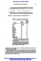
TABLE 1.1

Properties of Some Dielectrics*

Material

Dielectric constant

Dielectric strength,† kV/mm

Vacuum Air Water Paper Ruby mica Porcelain Fused quartz Pyrex glass Bakelite Polyethylene Amber Polystyrene Teflon Neoprene Transformer oil Titanium dioxide

1.00000 1.00054 78 3.5 5.4 6.5 3.8 4.5 4.8 2.3 2.7 2.6 2.1 6.9 4.5 100

∞ 0.8 — 14 160 4 8 13 12 50 90 25 60 12 12 6

*These properties are at approximately room temperature and for conditions such that the electric field E in the dielectric does not vary with time. † This is the maximum potential gradient that may exist in the dielectric without the occurrence of electrical breakdown. Dielectrics are often placed between conducting plates to permit a higher potential difference to be applied between them than would be possible with air as the dielectric.

dielectric to that without dielectric. Table 1.1 illustrates the dielectric constant and dielectric strength of various materials. The high dielectric strength of vacuum (∞, infinity) should be noted. It indicates that if two plates are separated by vacuum, the voltage difference between them can reach infinity without having flashover (arcing) between the plates. This important characteristic of vacuum has led to the development of vacuum circuit breakers, which have proved to have excellent performance in modern industry.

Downloaded from Digital Engineering Library @ McGraw-Hill (www.digitalengineeringlibrary.com) Copyright © 2004 The McGraw-Hill Companies. All rights reserved. Any use is subject to the Terms of Use as given at the website.

FUNDAMENTALS OF ELECTRIC SYSTEMS

1.4

CHAPTER ONE

CURRENT AND RESISTANCE The electric current i is established in a conductor when a net charge q passes through it in time t. Thus, the current is q i⫽ ᎏ t The units for the parameters are ●

●

●

i: amperes (A) q: coulombs (C) t: seconds (s)

The electric field exerts a force on the electrons to move them through the conductor. A positive charge moving in one direction has the same effect as a negative charge moving in the opposite direction. Thus, for simplicity we assume that all charge carriers are positive. We draw the current arrows in the direction that positive charges flow (Fig. 1.3). A conductor is characterized by its resistance (symbol ). It is defined as the voltage difference between two points divided by the current flowing through the conductor. Thus, V R⫽ ᎏ i where V is in volts, i is in amperes, and the resistance R is in ohms (abbreviated ⍀). The current, which is the flow of charge through a conductor, is often compared to the flow of water through a pipe. The water flow occurs due to the pressure difference between the inlet and outlet of a pipe. Similarly, the charge flows through the conductor due to the voltage difference. The resistivity ␳ is a characteristic of the conductor material. It is a measure of the resistance that the material has to the current. For example, the resistivity of copper is 1.7 ⫻ 10⫺8 ⍀⭈m; that of fused quartz is about 1016 ⍀⭈m. Table 1.2 lists some electrical properties of common metals. The temperature coefficient of resistivity ␣ is given by 1 d␳ ␣⫽ ᎏ ␳ ᎏ dT

FIGURE 1.3 Electrons drift in a direction opposite to the electric field in a conductor.

Downloaded from Digital Engineering Library @ McGraw-Hill (www.digitalengineeringlibrary.com) Copyright © 2004 The McGraw-Hill Companies. All rights reserved. Any use is subject to the Terms of Use as given at the website.

FUNDAMENTALS OF ELECTRIC SYSTEMS

FUNDAMENTALS OF ELECTRIC SYSTEMS

1.5

It represents the rate of variation of resistivity with temperature. Its units are 1/°C (or 1/°F). Conductivity (␴), is used more commonly than resistivity. It is the inverse of conductivity, given by 1 ␴⫽ ᎏ ␳ The units for conductivity are (⍀⭈m)⫺1. Across a resistor, the voltage and current have this relationship: V ⫽ iR The power dissipated across the resistor (conversion of electric energy to heat) is given by P ⫽ i2R or V2 P⫽ ᎏ R where P is in watts, i in amperes, V in volts, and R in ohms.

TABLE 1.2 Properties of Metals as Conductors

Metal

Resistivity (at 20°C), 10⫺8 ⍀⭈m

Temperature coefficient of resistivity ␣, per C° (⫻ 10⫺5)*

Silver Copper Aluminum Tungsten Nickel Iron Steel Manganin Carbon†

1.6 1.7 2.8 5.6 6.8 10 18 44 3500

380 390 390 450 600 500 300 1.0 ⫺50

*

This quantity, defined from 1 d␳ ␣⫽ ᎏ ␳ ᎏ dT

is the fractional change in resistivity d␳/␳ per unit change in temperature. It varies with temperature, the values here referring to 20°C. For copper (␣ ⫽ 3.9 ⫺3 ⫻ 10 /°C) the resistivity increases by 0.39 percent for a temperature increase of 1°C near 20°C. Note that ␣ for carbon is negative, which means that the resistivity decreases with increasing temperature. † Carbon, not strictly a metal, is included for comparison.

Downloaded from Digital Engineering Library @ McGraw-Hill (www.digitalengineeringlibrary.com) Copyright © 2004 The McGraw-Hill Companies. All rights reserved. Any use is subject to the Terms of Use as given at the website.

FUNDAMENTALS OF ELECTRIC SYSTEMS

1.6

CHAPTER ONE

FIGURE 1.4 Lines of B near a long, circular cylindrical wire. A current i, suggested by the central dot, emerges from the page.

THE MAGNETIC FIELD A magnetic field is defined as the space around a magnet or a current-carrying conductor. The magnetic field B is represented by lines of induction. Figure 1.4 illustrates the lines of induction of a magnetic field B near a long current-carrying conductor. The vector of the magnetic field is related to its lines of induction in this way: 1. The direction of B at any point is given by the tangent to the line of induction. 2. The number of lines of induction per unit cross-sectional area (perpendicular to the lines) is proportional to the magnitude of B. Magnetic field B is large if the lines are close together, and it is small if they are far apart. The flux ⌽B of magnetic field B is given by

冕

⌽B ⫽ B ⭈ dS The integral is taken over the surface for which ⌽B is defined. The magnetic field exerts a force on any charge moving through it. If q0 is a positive charge moving at a velocity v in a magnetic field B, the force F acting on the charge (Fig. 1.5) is given by F ⫽ q0v ⫻ B The magnitude of the force F is given by F ⫽ q0vB sin ␪ where ␪ is the angle between v and B.

Downloaded from Digital Engineering Library @ McGraw-Hill (www.digitalengineeringlibrary.com) Copyright © 2004 The McGraw-Hill Companies. All rights reserved. Any use is subject to the Terms of Use as given at the website.

FUNDAMENTALS OF ELECTRIC SYSTEMS

FUNDAMENTALS OF ELECTRIC SYSTEMS

1.7

The force F will always be at a right angle to the plane formed by v and B. Thus, it will always be a sideways force. The force will disappear in these cases: 1. If the charge stops moving 2. If v is parallel or antiparallel to the direction of B The force F has a maximum value if v is at a right angle to B (␪ ⫽ 90°). Figure 1.6 illustrates the force created on a positive and a negative electron moving in a magnetic field B pointing out of the plane of the figure (symbol 䉺). The unit of B is the tesla (T) or weber per square meter (Wb/m2). Thus 1N 1 tesla (T) ⫽ 1 weber/meter2 ⫽ ᎏ A⭈m

FIGURE 1.5 Illustration of F ⫽ q0 v ⫻ B. Test charge q0 is fired through the origin with velocity v.

The force acting on a current-carrying conductor placed at a right angle to a magnetic field B (Fig. 1.7) is given by F ⫽ ilB where l is the length of conductor placed in the magnetic field. Ampère’s Law Figure 1.8 illustrates a current-carrying conductor surrounded by small magnets. If there is no current in the conductor, all the magnets will be aligned with the horizontal component

FIGURE 1.6 A bubble chamber is a device for rendering visible, by means of small bubbles, the tracks of charged particles that pass through the chamber. The figure shows a photograph taken with such a chamber immersed in a magnetic field B and exposed to radiations from a large cyclotronlike accelerator. The curved υ at point P is formed by a positive and a negative electron, which deflect in opposite directions in the magnetic field. The spirals S are tracks of three low-energy electrons.

Downloaded from Digital Engineering Library @ McGraw-Hill (www.digitalengineeringlibrary.com) Copyright © 2004 The McGraw-Hill Companies. All rights reserved. Any use is subject to the Terms of Use as given at the website.

FUNDAMENTALS OF ELECTRIC SYSTEMS

1.8

CHAPTER ONE

FIGURE 1.7 A wire carrying a current i is placed at right angles to a magnetic field B. Only the drift velocity of the electrons, not their random motion, is suggested.

FIGURE 1.8 An array of compass needles near a central wire carrying a strong current. The black ends of the compass needles are their north poles. The central dot shows the current emerging from the page. As usual, the direction of the current is taken as the direction of flow of positive charge.

of the earth’s magnetic field. When a current flows through the conductor, the orientation of the magnets suggests that the lines of induction of the magnetic field form closed circles around the conductor. This observation is reinforced by the experiment shown in Fig. 1.9. It shows a current-carrying conductor passing through the center of a horizontal glass plate with iron filings on it. Ampère’s law states that

冖B ⭈ dl ⫽ ␮ i 0

where B is the magnetic field, l is the length of the circumference around the wire, i is the current, ␮0 is the permeability constant (␮0 ⫽ 4␲ ⫻ 10⫺7 T ⭈m/A). The integration is carried around the circumference. If the current in the conductor shown in Fig. 1.8 is reverse direction, all the compass needles change their direction as well. Thus, the direction of B near a current-carrying conductor is given by the right-hand-rule: If the current is grasped by the right hand and the thumb points in the direction of the current, the fingers will curl around the wire in the direction B.

Downloaded from Digital Engineering Library @ McGraw-Hill (www.digitalengineeringlibrary.com) Copyright © 2004 The McGraw-Hill Companies. All rights reserved. Any use is subject to the Terms of Use as given at the website.

FUNDAMENTALS OF ELECTRIC SYSTEMS

FUNDAMENTALS OF ELECTRIC SYSTEMS

1.9

FIGURE 1.9 Iron filings around a wire carrying a strong current.

Magnetic Field in a Solenoid A solenoid (an inductor) is a long, current-carrying conductor wound in a close-packed helix. Figure 1.10 shows a “solenoid” having widely spaced turns. The fields cancel between the wires. Inside the solenoid, B is parallel to the solenoid axis. Figure 1.11 shows the lines of B for a real solenoid. By applying Ampere’s law to this solenoid, we have B ⫽ ␮0 in where n is the number of turns per unit length. The flux ⌽B for the magnetic field B will become ⌽B ⫽ B ⭈ A

FARADAY’S LAW OF INDUCTION Faraday’s law of induction is one of the basic equations of electromagnetism. Figure 1.12 shows a coil connected to a galvanometer. If a bar magnet is pushed toward the coil, the galvanometer deflects. This indicates that a current has been induced in the coil. If the magnet is held stationary with respect to the coil, the galvanometer does not deflect. If the magnet is moved away from the coil, the galvanometer deflects in the opposite direction. This indicates that the current induced in the coil is in the opposite direction. Downloaded from Digital Engineering Library @ McGraw-Hill (www.digitalengineeringlibrary.com) Copyright © 2004 The McGraw-Hill Companies. All rights reserved. Any use is subject to the Terms of Use as given at the website.

FUNDAMENTALS OF ELECTRIC SYSTEMS

1.10

CHAPTER ONE

FIGURE 1.10 A loosely wound solenoid.

FIGURE 1.11 A solenoid of finite length. The right end, from which lines of B emerge, behaves as the north pole of a compass needle does. The left end behaves as the south pole.

Figure 1.13 shows another experiment in which when the switch S is closed, thus establishing a steady current in the right-hand coil, the galvanometer deflects momentarily. When the switch is opened, the galvanometer deflects again momentarily, but in the opposite direction. This experiment proves that a voltage known as an electromagnetic force (emf ) is induced in the left coil when the current in the right coil changes.

Downloaded from Digital Engineering Library @ McGraw-Hill (www.digitalengineeringlibrary.com) Copyright © 2004 The McGraw-Hill Companies. All rights reserved. Any use is subject to the Terms of Use as given at the website.

FUNDAMENTALS OF ELECTRIC SYSTEMS

FUNDAMENTALS OF ELECTRIC SYSTEMS

FIGURE 1.12 Galvanometer G deflects while the magnet is moving with respect to the coil. Only their relative motion counts.

1.11

FIGURE 1.13 Galvanometer G deflects momentarily when switch S is closed or opened. No motion is involved.

Faraday’s law of induction is given by d⌽ Ᏹ ⫽ ⫺N ᎏB dt where Ᏹ ⫽ emf for voltage N ⫽ number of turns in coil d⌽B/dt ⫽ rate of change of flux with time The minus sign will be explained by Lenz’ law.

LENZ’S LAW Lenz’s law states that the induced current will be in a direction that opposes the change that produced it. If a magnet is pushed toward a loop as shown in Fig. 1.14, an induced current will be established in the loop. Lenz’s law predicts that the current in the loop must be in a direction such that the flux established by it must oppose the change. Thus, the face of the loop toward the magnet must have the north pole. The north pole from the current loop and the north pole from the magnet will repel each other. The right-hand rule indicates that the magnetic field established by the loop should emerge from the right side of the loop. Thus, the induced current must be as shown. Lenz’s law can be explained as follows: When the magnet is pushed toward the loop, this “change” induces a current. The direction of this current should oppose the “push.” If the magnet is pulled away from the coil, the induced current will create the south pole on the right-hand face of the loop because this will oppose the “pull.” Thus, the current must be in the opposite direction to the one shown in Fig. 1.14 to make the right-hand face a south pole. Whether the magnet is pulled or pushed, its motion will always be opposed. The force that moves the magnet will always experience a resisting force. Thus, the force moving the magnet will always be required to do work. Figure 1.15 shows a rectangular loop of width l. One end of it has a uniform field B pointing at a right angle to the plane of the loop into the page (丢 indicates into the page and 䉺 out of the page). The flux enclosed by the loop is given by ⌽B ⫽ Blx

Downloaded from Digital Engineering Library @ McGraw-Hill (www.digitalengineeringlibrary.com) Copyright © 2004 The McGraw-Hill Companies. All rights reserved. Any use is subject to the Terms of Use as given at the website.

FUNDAMENTALS OF ELECTRIC SYSTEMS

1.12

CHAPTER ONE

FIGURE 1.14 If we move the magnet toward the loop, the induced current points as shown, setting up a magnetic field that opposes the motion of the magnet.

FIGURE 1.15 A rectangular loop is pulled out of a magnetic field with velocity v.

Faraday’s law states that the induced voltage or emf Ᏹ is given by d⌽ d dx Ᏹ ⫽ ⫺ ᎏB ⫽ ⫺ ᎏ (Blx) ⫽ ⫺Bl ᎏ ⫽ Blv dt dt dt where ⫺dx/dt is the velocity υ of the loop being pulled out of the magnetic field. The current induced in the loop is given by Blv Ᏹ i⫽ ᎏ ⫽ ᎏ R R where R is the loop resistance. From Lenz’s law, this current must be clockwise because it is opposing the change (the decrease in ⌽B). It establishes a magnetic field in the same direction as the external magnetic field within the loop. Forces F2 and F3 cancel each other because they are equal and in opposite directions. Force F1 is obtained from the equation (F ⫽ il ⫻ B) Downloaded from Digital Engineering Library @ McGraw-Hill (www.digitalengineeringlibrary.com) Copyright © 2004 The McGraw-Hill Companies. All rights reserved. Any use is subject to the Terms of Use as given at the website.

FUNDAMENTALS OF ELECTRIC SYSTEMS

FUNDAMENTALS OF ELECTRIC SYSTEMS

1.13

B2l2v F1 ⫽ ilB sin 90° ⫽ ᎏ R The force pulling the loop must do a steady work given by B2l 2v2 P ⫽ F1v ⫽ ᎏ R Figure 1.16 illustrates a rectangular loop of resistance R, width l, and length a being pulled at constant speed υ through a magnetic field B of thickness d. There is no flux ⌽B when the loop is not in the field. The flux ⌽B is Bla when the loop is entirely in the field. It is Blx when the loop is entering the field. The induced voltage or emf Ᏹ in the loop is given by

FIGURE 1.16 A rectangular loop is caused to move with a velocity v through a magnetic field. The position of the loop is measured by x, the distance between the effective left edge of field B and the right end of the loop.

d⌽B d⌽B d⌽B dx ᎏ ⫽ ⫺ᎏ Ᏹ ⫽ ⫺ᎏ ⫽ ⫺ᎏ v dt dx dt dx where d⌽B/dx is the slope of the curve shown in Fig. 1.17a. The voltage Ᏹ(x) is shown in Fig. 1.17b. Lenz’s law indicates that Ᏹ(x) is counterclockwise. There is no voltage induced in the coil when it is entirely in the magnetic field because the flux ⌽B through the coil does not change with time. Figure 1.17c shows the rate P of thermal energy generation in the loop, and P is given by Ᏹ2 P⫽ ᎏ R If a real magnetic field is considered, its strength will decrease from the center to the peripheries. Thus, the sharp bends and corners shown in Fig. 1.17 will be replaced by smooth curves. The voltage Ᏹ induced in this case will be given by Ᏹmax sin ␻t (a sine wave). This is exactly how ac voltage is induced in a real generator. Also note that the prime mover has to do significant work to rotate the generator rotor inside the stator.

INDUCTANCE When the current in a coil changes, an induced voltage appears in that same coil. This is called self-induction. The voltage (electromagnetic force) induced is called self-induced emf. It obeys Faraday’s law of induction as do any other induced emf’s. For a closedpacked coil (an inductor) we have N⌽B ⫽ Li where N ⫽ number of turns of coil ⌽B ⫽ flux i ⫽ current L ⫽ inductance of the device

Downloaded from Digital Engineering Library @ McGraw-Hill (www.digitalengineeringlibrary.com) Copyright © 2004 The McGraw-Hill Companies. All rights reserved. Any use is subject to the Terms of Use as given at the website.

FUNDAMENTALS OF ELECTRIC SYSTEMS

1.14

CHAPTER ONE

FIGURE 1.17 In practice the sharp corners would be rounded.

From Faraday’s law, we can write the induced voltage (emf) as di d(N⌽B) Ᏹ ⫽ ⫺ᎏ ⫽ ⫺L ᎏ dt dt This relationship can be used for inductors of all shapes and sizes. In an inductor (symbol ), L depends only on the geometry of the device. The unit of inductance is the henry (abbreviated H). It is given by 1 volt ⭈ second 1 henry (H) ⫽ ᎏᎏ ampere

V⭈s 冢ᎏ A 冣

In an inductor, energy is stored in a magnetic field. The amount of magnetic energy stored UB in the inductor is given by UB ⫽ 1⁄2 Li2 In summary, an inductor stores energy in a magnetic field, and the capacitor stores energy in an electric field. Downloaded from Digital Engineering Library @ McGraw-Hill (www.digitalengineeringlibrary.com) Copyright © 2004 The McGraw-Hill Companies. All rights reserved. Any use is subject to the Terms of Use as given at the website.

FUNDAMENTALS OF ELECTRIC SYSTEMS

FUNDAMENTALS OF ELECTRIC SYSTEMS

1.15

ALTERNATING CURRENT An alternating current (ac) in a circuit establishes a voltage (emf ) that varies with time as Ᏹ ⫽ Ᏹm sin ␻t where Ᏹm is the maximum emf and ␻ ⫽ 2␲␯, where ␯ is the frequency measured in hertz (Hz). This type of emf is established by an ac generator in a power plant. In North America, ␯ ⫽ 60 Hz. In western Europe and Australia it is 50 Hz. The symbol for a source of alternating emf is . This device is called an alternating-current generator or an ac generator. Alternating currents are essential for modern society. Power distribution systems, radio, television, satellite communication systems, computer systems, etc. would not exist without alternating voltages and currents. The alternating current in the circuit shown in Fig. 1.18 is given by i ⫽ im sin (␻t ⫺ ␪) where im ⫽ maximum amplitude of current ␻ ⫽ angular frequency of applied alternating voltage (or emf) ␪ ⫽ phase angle between alternating current and alternating voltage Let us consider each component of the circuit separately.

A Resistive Circuit Figure 1.19a shows an alternating voltage applied across a resistor. We can write the following equations: VR ⫽ Ᏹm sin ␻t and VR ⫽ iR R or Ᏹm iR ⫽ ᎏ sin ␻t R

FIGURE 1.18 A single-loop RCL circuit contains an ac generator. Voltages VR, VC , and VL are the timevarying potential differences across the resistor, the capacitor, and the inductor, respectively.

Downloaded from Digital Engineering Library @ McGraw-Hill (www.digitalengineeringlibrary.com) Copyright © 2004 The McGraw-Hill Companies. All rights reserved. Any use is subject to the Terms of Use as given at the website.

FUNDAMENTALS OF ELECTRIC SYSTEMS

1.16

CHAPTER ONE

VR

R iR

VR, iR (E = Em sin ␻t) (a)

VR 0

␲

2␲

␻t

␻ iR

(b)

iR,m(= Em/R)

VR ␻t

VR,m(= Em)

(c) FIGURE 1.19 (a) A single-loop resistive circuit containing an ac generator. (b) The current and the potential difference across the resistor are in phase (␪ ⫽ 0). (c) A phasor diagram shows the same thing. The arrows on the vertical axis are instantaneous values.

A comparison between the previous equations shows that the time-varying (instantaneous) quantities VR and iR are in phase. This means that they reach their maximum and minimum values at the same time. They also have the same angular frequency ␻. These facts are shown in Fig. 1.19b and c. Figure 1.19c illustrates a phasor diagram. It is another method used to describe the situation. The phasors in this diagram are represented by open arrows. They rotate counterclockwise with an angular frequency ␻ about the origin. The phasors have the following properties: 1. The length of the phasor is proportional to the maximum value of the alternating quantity described, that is, Ᏹm for VR and Ᏹm/R for iR. 2. The projection of the phasors on the vertical axis gives the instantaneous values of the alternating parameter (current or voltage) described. Thus, the arrows on the vertical axis represent the instantaneous values of VR and iR. Since VR and iR are in phase, their phasors lie along the same line (Fig. 1.19c).

A Capacitive Circuit Figure 1.20a illustrates an alternating voltage acting on a capacitor. We can write the following equations: Vc ⫽ Ᏹm sin ␻t and q Vc ⫽ ᎏ C

(definition of C)

Downloaded from Digital Engineering Library @ McGraw-Hill (www.digitalengineeringlibrary.com) Copyright © 2004 The McGraw-Hill Companies. All rights reserved. Any use is subject to the Terms of Use as given at the website.

FUNDAMENTALS OF ELECTRIC SYSTEMS

1.17

FUNDAMENTALS OF ELECTRIC SYSTEMS

VC

From these relationships, we have

C

q ⫽ ᏱmC sin ␻t or dq ic ⫽ ᎏ ⫽ ␻C Ᏹm cos ␻t dt

(E = Em sin ␻t) (a)

A comparison between these equations shows that the instantaneous values of Vc and ic are one-quarter cycle out of phase. This is illustrated in Fig. 1.20b. Voltage Vc lags ic; that is, as time passes, Vc reaches its maximum after ic does, by one-quarter cycle (90°). This is also shown clearly in the phasor diagram (Fig. 1.20c). Since the phasors rotate in counterclockwise direction, it is clear that phasor Vc,m lags behind phasor ic,m by one-quarter cycle. The reason for this lag is that the capacitor stores energy in its electric field. The current goes through it before the voltage is established across it. Since the current is given by

VC,iC

iC VC 0

␲

2␲

(b)

iC, m (= ␻CEm)

␻

iC VC ␻t

i ⫽ im sin (␻t ⫺ ␪) ␪ is the angle between Vc and ic. In this case, it is equal to ⫺90°. If we put this value of ␪ in the equation of current, we obtain i ⫽ im cos ␻t

␻t

VC, m (= Em)

(c) FIGURE 1.20 (a) A single-loop capacitive circuit containing an ac generator. (b) The potential difference across the capacitor lags the current by one-quarter cycle. (c) A phasor diagram shows the same thing. The arrows on the vertical axis are instantaneous values.

This equation is in agreement with the previous equation for current that we obtained, dq ic ⫽ ᎏ ⫽ ␻C Ᏹm cos ␻t dt where im ⫽ ␻CᏱm. Also ic is expressed as follows: Ᏹm ic ⫽ ᎏ xc cos ␻t and xc is called the capacitive reactance. Its unit is the ohm (⍀). Since the maximum value of Vc ⫽ Vc,m and the maximum value of ic ⫽ ic,m we can write Vc,m ⫽ ic,m xc Voltage Vc,m represents the maximum voltage established across the capacitor when the current is i.

Downloaded from Digital Engineering Library @ McGraw-Hill (www.digitalengineeringlibrary.com) Copyright © 2004 The McGraw-Hill Companies. All rights reserved. Any use is subject to the Terms of Use as given at the website.

FUNDAMENTALS OF ELECTRIC SYSTEMS

1.18

CHAPTER ONE

An Inductive Circuit Figure 1.21a shows a circuit containing an alternating voltage acting on an inductor. We can write the following equations: VL ⫽ Ᏹm sin ␻t and di VL ⫽ L ᎏ dt

(from definition of L)

From these equations, we have Ᏹm di ⫽ ᎏ sin ␻ dt L or Ᏹm cos ␻t iL ⫽ ∫di ⫽ ⫺ ᎏ ␻L A comparison between the instantaneous values of VL and iL shows that these parameters are out of phase by one-quarter cycle (90°). This is illustrated in Fig. 1.21b. It is clear that VL leads iL. This means that as time passes, VL reaches its maximum before iL does, by one-quarter cycle. VL L This fact is also shown in the phasor diagram of Fig. 1.21c. As the phasors rotate in the counterclockwise direction, it is clear (E = Em sin ␻t) that phasor VL,m leads (precedes) iL,m by one(a) quarter cycle. The phase angle ␪ by which VL leads iL in VL this case is ⫹90°. If this value is put in the VL, iL iL current equation 0

␲

2␲

␻t

i ⫽ im sin (␻t ⫺ ␪) we obtain

(b)

i ⫽ ⫺im cos ␻t ␻

This equation is in agreement with the previous equation of the current:

VL, m (= Em)

VL

Ᏹm iL ⫽ ∫di ⫽ ⫺ ᎏ cos ␻t ␻L

␻t iL

iL, m (- Em/vL) (c)

FIGURE 1.21 (a) A single-loop inductive circuit containing an ac generator. (b) The potential difference across the inductor leads the current by one-quarter cycle. (c) A phasor diagram shows the same thing. The arrows on the vertical axis are instantaneous values.

Again, for reasons of compactness of notation, we rewrite the equation as Ᏹm cos ␻t iL ⫽ ⫺ ᎏ XL where XL ⫽ ␻L

Downloaded from Digital Engineering Library @ McGraw-Hill (www.digitalengineeringlibrary.com) Copyright © 2004 The McGraw-Hill Companies. All rights reserved. Any use is subject to the Terms of Use as given at the website.

FUNDAMENTALS OF ELECTRIC SYSTEMS

1.19

FUNDAMENTALS OF ELECTRIC SYSTEMS

and XL is called the inductive reactance. As for the capacitive reactance, the unit for XL is the ohm. Since Ᏹm is the maximum value of VL (⫽ VL,m), we can write

iT iL

iR R

V

L

VL,m ⫽ iL,mXL This indicated that when any alternating current of amplitude im and angular frequency ␻ exists in an inductor, the maximum voltage difference across the inductor is given by

FIGURE 1.22 Circuit containing a resistor and an inductor.

VL,m ⫽ im XL

␻

Let us now examine the circuit shown in Fig. 1.22. Figure 1.23 illustrates the phasor diagram of the circuit. The total current is iT ⫽ iR ⫹ iL, and ␪ represents the angle between iT and the voltage V. It is called the phase angle of the system. An increase in the value of the inductance L will result in increasing the angle ␪. The power factor (abbreviation PF) is defined as PF ⫽ cos ␪

iR V

⍜

iL iT FIGURE 1.23 A phasor diagram of the circuit in Fig. 1.22.

It is a measure of the ratio of the magnitudes of iR/i T. The circuit shown in Fig. 1.22 shows that the load supplied by a power plant has two natures iR and iL. Equipment such as motors, welders, and fluorescent lights require both types of currents. However, equipment such as heaters and incandescent bulbs require the resistive current iR only. The power in the resistive part of the circuit is given by P ⫽ ViR

or

P ⫽ ViT cos ␪

This is the real power in the circuit. It is the energy dissipated by the resistor. This is the energy converted from electric power to heat. This power is also used to provide the mechanical power (torque ⫻ speed) in a motor. The unit of this power is watts (W) or megawatts (MW). The power in the inductor is given by Q ⫽ ViL

or

Q ⫽ ViT sin ␪

This is the reactive or inductive power in the circuit. It is the power stored in the inductor in the form of a magnetic field. This power is not consumed as the real power is. It returns to the system (power plant and transmission lines) every half-cycle. It is used to create the magnetic field in the windings of the motor. The main effects of reactive power on the system are as follows: 1. The transmission line losses between the power plant and the load are proportional to i T2 RT , where iT ⫽ iR ⫹ iL and RT is the resistance in the transmission lines. Therefore, iL is a contributor to transmission losses. 2. The transmission lines have a specific current rating. If the inductive current iL is high, the magnitude of iR will be limited to a lower value. This creates a problem for the utility because its revenue is mainly based on iR. Downloaded from Digital Engineering Library @ McGraw-Hill (www.digitalengineeringlibrary.com) Copyright © 2004 The McGraw-Hill Companies. All rights reserved. Any use is subject to the Terms of Use as given at the website.

FUNDAMENTALS OF ELECTRIC SYSTEMS

1.20

CHAPTER ONE

3. If an industry has large motors, it will require a high inductive current to magnetize these motors. This creates a localized reduction in voltage (a voltage dip) at the industry. The utility will not be able to correct for this voltage dip from the power plant. Capacitor banks are norFIGURE 1.24 Addition of capacitor banks at an mally installed at the industry to “correct” industry. the power factor. Figures 1.24 and 1.25 illustrate the correction in power factor. Angle ␪′ is smaller than ␪. Therefore, the new power factor (cos ␪′) is larger than the previous power factor (cos ␪). Most utilities charge a penalty when the power factor drops below 0.9 to 0.92. This penalty is charged to the industry even if the power factor drops once during the month below the limit specified by the utility. Most industries use the following methods to ensure that their power factor remains above the limit specified by the utility: a. The capacitor banks are sized to give the industry a margin above the limit specified by the utility. b. The induction motors at the industry are started in sequence. This is done to stagger the inrush current required by each motor. Note: The inrush current is the starting current of the induction motor. It is normally 6 to 8 times larger than the normal running current. The inrush current is mainly an inductive current. This is due to the fact that the mechanical energy (torque ⫻ speed) developed by the motor and the heat losses during the starting period of the motor are minimal (the real power provides the mechanical energy and heat losses in the motor). c. Use synchronous motors in conjunction with induction motors. A synchronous motor is supplied by ac power to its stator. It is also supplied by direct-current (dc) power to its rotor. The dc power allows the synchronous motor to deliver reactive (inductive) power. Therefore, a synchronous motor can operate at a leading power factor, as shown in Fig. 1.26. This allows the synchronous motors to correct the power factor at the industry by compensating for the lagging power factor generated by induction motors. The third form of power used is the apparent power. It is given by S ⫽ iTV

where iT ⫽ iR⫹iL

iT ␻ ⍜

FIGURE 1.25 Correction of power factor at an industry.

V

FIGURE 1.26 Phasor diagram of a synchronous motor.

Downloaded from Digital Engineering Library @ McGraw-Hill (www.digitalengineeringlibrary.com) Copyright © 2004 The McGraw-Hill Companies. All rights reserved. Any use is subject to the Terms of Use as given at the website.

FUNDAMENTALS OF ELECTRIC SYSTEMS

FUNDAMENTALS OF ELECTRIC SYSTEMS

1.21

The unit of this power is voltamperes (VA) or megavoltamperes (MVA). This power includes the combined effect of the real power and the reactive power. All electrical equipment such as transformers, motors, and generators are rated by their apparent power. This is so because the apparent power specifies the total power (real and reactive) requirement of equipment.

THREE-PHASE SYSTEMS Most of the transmission, distribution, and energy conversion systems having an apparent power higher than 10 kVA use three-phase circuits. The reason for this is that the power density (the ratio of power to weight) of a device is higher when it is a three-phase rather than a single-phase design. For example, the weight of a three-phase motor is lower than the weight of a single-phase motor having the same rating. The voltages of a three-phase system are normally given by va′a ⫽ Vm sin ␻t vb′b ⫽ Vm sin (␻t ⫺120°) vc′c ⫽ Vm sin (␻t ⫺240°) where Vm ⫽ Ᏹm. Figure 1.27 illustrates the variations of these voltages versus time. The phasors of these voltages are Va′a ⫽ V⬔0° Vb′b ⫽ V⬔⫺120° Vc′c ⫽ V⬔⫺240° where V is the root-mean-square (rms) value of the voltage.

FIGURE 1.27 A system of three voltages of equal magnitude, but displaced from each other by 120°.

Downloaded from Digital Engineering Library @ McGraw-Hill (www.digitalengineeringlibrary.com) Copyright © 2004 The McGraw-Hill Companies. All rights reserved. Any use is subject to the Terms of Use as given at the website.

FUNDAMENTALS OF ELECTRIC SYSTEMS

1.22

CHAPTER ONE

FIGURE 1.28 (a) Balanced three-phase phasor representation; (b) three-phase voltage source.

Figure 1.28a illustrates a graphical representation of the phasors. Figure 1.28b also shows the three voltage sources. When the three voltages are equal in magnitude, the system is called a three-phase balanced system. If the three voltages are unequal and/or the phase displacement is different from 120°, the system will be unbalanced. The phasor sum of the three voltages in a balanced system is zero. Three-Phase Connections The three-phase voltage sources are normally interconnected as a “wye” (Y) and a “delta” (⌬), as shown in Figs. 1.29a and b, respectively. Terminals a′, b′, and c′ join together in the wye connection to form the neutral point O. The system becomes a four-wire, three-phase system when a lead is brought out from point O. In the delta connection, terminals a and b′, b and c′, and c and a′ are joined to form the delta connection. In the wye connection (Fig. 1.29a), the voltages across the individual phases are identified as Va′a, Vb′b, and Vc′c. These are known as phase voltages. The voltages across the lines a, b, and c (or A, B, and C) are known as line voltages. The relationship between the line voltages and phase voltages is Vl ⫽ 兹3 苶Vp Figure 1.30 illustrates the relationships between all the phase voltages and line voltages. The line currents Il and phase currents Ip are the same in the wye connection. Thus, Il ⫽ Ip In the delta connection, the line voltages Vl are the same as the phase voltages Vp. Thus, Vl ⫽ Vp Figure 1.31 illustrates the phasors of the phase currents and line currents in the deltaconnected system. The relationship between the phase currents and line currents is given by Il ⫽ 兹3苶Ip

Downloaded from Digital Engineering Library @ McGraw-Hill (www.digitalengineeringlibrary.com) Copyright © 2004 The McGraw-Hill Companies. All rights reserved. Any use is subject to the Terms of Use as given at the website.

FUNDAMENTALS OF ELECTRIC SYSTEMS

FUNDAMENTALS OF ELECTRIC SYSTEMS

1.23

Power in Three-Phase Systems The average power in a single-phase ac circuit is given by PT ⫽ VpIp cos ␪p where ␪p is the power factor angle. The total power delivered in a balanced three-phase circuit is given by PT ⫽ 3 (Vp Ip cos ␪p) The total power expressed in terms of line voltages and currents for a wye or delta connection is PT ⫽ 兹3 苶 Vl Il cos ␪p

FIGURE 1.29 (a) Wye connection; (b) delta connection.

Downloaded from Digital Engineering Library @ McGraw-Hill (www.digitalengineeringlibrary.com) Copyright © 2004 The McGraw-Hill Companies. All rights reserved. Any use is subject to the Terms of Use as given at the website.

FUNDAMENTALS OF ELECTRIC SYSTEMS

1.24

CHAPTER ONE

FIGURE 1.30 Voltage phases for Y connection.

FIGURE 1.31 Current phasors for ⌬ connection.

Figure 1.32 illustrates a graphical representation of the instantaneous power in a threephase system. It is clear that the instantaneous power is constant and equal to 3 times the average power. This is an important feature for three-phase motors because the constant instantaneous power eliminates torque pulsations and resulting vibrations.

REFERENCES 1. D. Halliday and R. Resnick, Physics, Part Two, 3d ed., Wiley, Hoboken, N.J., 1978. 2. A. S. Nasar, Handbook of Electric Machines, McGraw-Hill, New York, 1987.

Downloaded from Digital Engineering Library @ McGraw-Hill (www.digitalengineeringlibrary.com) Copyright © 2004 The McGraw-Hill Companies. All rights reserved. Any use is subject to the Terms of Use as given at the website.

FUNDAMENTALS OF ELECTRIC SYSTEMS

FUNDAMENTALS OF ELECTRIC SYSTEMS

1.25

FIGURE 1.32 Power in a three-phase system.

Downloaded from Digital Engineering Library @ McGraw-Hill (www.digitalengineeringlibrary.com) Copyright © 2004 The McGraw-Hill Companies. All rights reserved. Any use is subject to the Terms of Use as given at the website.

FUNDAMENTALS OF ELECTRIC SYSTEMS

Downloaded from Digital Engineering Library @ McGraw-Hill (www.digitalengineeringlibrary.com) Copyright © 2004 The McGraw-Hill Companies. All rights reserved. Any use is subject to the Terms of Use as given at the website.

Source: ELECTRICAL EQUIPMENT HANDBOOK

CHAPTER 2

INTRODUCTION TO MACHINERY PRINCIPLES

ELECTRIC MACHINES AND TRANSFORMERS An electric machine is a device that can convert either mechanical energy to electric energy or electric energy to mechanical energy. Such a device is called a generator when it converts mechanical energy to electric energy. The device is called a motor when it converts electric energy to mechanical energy. Since an electric machine can convert power in either direction, such a machine can be used as either a generator or a motor. Thus, all motors and generators can be used to convert energy from one form to another, using the action of a magnetic field. A transformer is a device that converts ac electric energy at one voltage level to ac electric energy at another voltage level. Transformers operate on the same principles as generators and motors.

COMMON TERMS AND PRINCIPLES ␪ ⫽ angular position of an object. It is the angle at which it is oriented. It is measured from one arbitrary reference point (units: rad or deg). ␻ ⫽ angular velocity ⫽ d␪/dt. It is the rate of variation of angular position with time (units: rad/s or deg/s). fm ⫽ angular velocity, expressed in revolutions per second ⫽ ␻m/2␲. ␣ ⫽ angular acceleration ⫽ d␻/dt. It is the rate of variation of angular velocity with time (units: rad/s2). ␶ ⫽ torque ⫽ (force applied) ⫻ (perpendicular distance). Units are newton-meters (N⭈m) Newton’s law of rotation: ␶ ⫽ J␣ where J is the moment of inertia of the rotor (units: kg⭈m2). W ⫽ work ⫽ T␪, if T is constant (units: J). P ⫽ power ⫽ dW/dt. It is the rate of variation of work with time (units: W): P ⫽ T␻ 2.1 Downloaded from Digital Engineering Library @ McGraw-Hill (www.digitalengineeringlibrary.com) Copyright © 2004 The McGraw-Hill Companies. All rights reserved. Any use is subject to the Terms of Use as given at the website.

INTRODUCTION TO MACHINERY PRINCIPLES

2.2

CHAPTER TWO

THE MAGNETIC FIELD Energy is converted from one form to another in motors, generators, and transformers by the action of magnetic fields. These are the four basic principles that describe how magnetic fields are used in these devices:

Production of a Magnetic Field Ampere’s law is the basic law that governs the production of a magnetic field:

冖H ⭈ d l ⫽ I

net

where H is the magnetic field intensity produced by current Inet. Current I is measured in amperes and H in ampere-turns per meter. Figure 2.1 shows a rectangular core having a winding of N turns of wire wrapped on one leg of the core. If the core is made of ferromagnetic material (such as iron), most of the magnetic field produced by the current will remain inside the core. Ampere’s law becomes Hlc ⫽ Ni where lc is the mean path length of the core. The magnetic field intensity H is a measure of the “effort” that the current is putting out to establish a magnetic field. The material of the core affects the strength of the magnetic field flux produced in the core. The magnetic field intensity H is linked with the resulting magnetic flux density B within the material by B ⫽ ␮H where H ⫽ magnetic field intensity ␮ ⫽ magnetic permeability of material B ⫽ resulting magnetic flux density produced Thus, the actual magnetic flux density produced in a piece of material is given by the product of two terms:

FIGURE 2.1 A simple magnetic core.

Downloaded from Digital Engineering Library @ McGraw-Hill (www.digitalengineeringlibrary.com) Copyright © 2004 The McGraw-Hill Companies. All rights reserved. Any use is subject to the Terms of Use as given at the website.

INTRODUCTION TO MACHINERY PRINCIPLES

INTRODUCTION TO MACHINERY PRINCIPLES

H ␮

2.3

represents effort exerted by current to establish a magnetic field represents relative ease of establishing a magnetic field in a given material

In SI, the units are as follows: H ampere-turns per meter; ␮ henrys/meter (H/m); B webers/m2, known as teslas (T). And ␮0 is the permeability of free space. Its value is ␮0 ⫽ 4␲ ⫻ 10⫺7 H/m The relative permeability compares the magnetizability of materials. For example, in modern machines, the steels used in the cores have relative permeabilities of 2000 to 7000. Thus, for a given current, the flux established in a steel core is 2000 to 7000 times stronger than in a corresponding area of air (air has the same permeability as free space). Thus, the metals of the core in transformers, motors, and generators play an essential part in increasing and concentrating the magnetic flux in the device. The magnitude of the flux density is given by ␮Ni B ⫽ ␮H ⫽ ᎏ lc Thus, the total flux in the core in Fig. 2.1 is ␮NiA ␾ ⫽ BA ⫽ ᎏ lc where A is the cross-sectional area of the core.

MAGNETIC BEHAVIOR OF FERROMAGNETIC MATERIALS The magnetic permeability is defined by the equation B ⫽ ␮H The permeability of ferromagnetic materials is up to 6000 times higher than the permeability of free space. However, the permeability of ferromagnetic materials is not constant. Suppose we apply a direct current to the core shown in Fig. 2.1 (starting with 0 A and increasing the current). Figure 2.2a illustrates the variation of the flux produced in the core versus the magnetomotive force. This graph is known as the saturation curve or magnetization curve. At first, a slight increase in the current (magnetomotive force) results in a significant increase in the flux. However, at a certain point, a further increase in current results in no change in the flux. The region where the curve is flat is called the saturation region. The core has become saturated. The region where the flux changes rapidly is called the unsaturated region. The transition region between the unsaturated region and the saturated region is called the knee of the curve. Figure 2.2b illustrates the variation of magnetic flux density B with magnetizing intensity H. These are the equations: Ni H⫽ ᎏ lc ␾ B⫽ ᎏ A Downloaded from Digital Engineering Library @ McGraw-Hill (www.digitalengineeringlibrary.com) Copyright © 2004 The McGraw-Hill Companies. All rights reserved. Any use is subject to the Terms of Use as given at the website.

INTRODUCTION TO MACHINERY PRINCIPLES

2.4

CHAPTER TWO

It can easily be seen that the magnetizing intensity is directly proportional to the magnetomotive force, and the magnetic flux density is directly proportional to the flux. Therefore, the relationship between B and H has the same shape as the relationship between the flux and the magnetomotive force. The slope of flux-density versus the magnetizing intensity curve (Fig. 2.2c) is by definition the permeability of the core at that magnetizing intensity. The curve shows that in the unsaturated region the permeability is high and almost constant.

FIGURE 2.2 (a) Sketch of a dc magnetization curve for a ferromagnetic core. (b) The magnetization curve expressed in terms of flux density and magnetizing intensity. (c) A detailed magnetization curve for a typical piece of steel.

Downloaded from Digital Engineering Library @ McGraw-Hill (www.digitalengineeringlibrary.com) Copyright © 2004 The McGraw-Hill Companies. All rights reserved. Any use is subject to the Terms of Use as given at the website.

INTRODUCTION TO MACHINERY PRINCIPLES

INTRODUCTION TO MACHINERY PRINCIPLES

2.5

In the saturated region, the permeability drops to a very low value. Electric machines and transformers use ferromagnetic material for their cores because these materials produce much more flux than other materials. Table 2.1 lists the characteristics of soft magnetic materials including the Curie temperature (or Curie point) Tc. Above this temperature a ferromagnetic material becomes paramagnetic (weakly magnetized). Figure 2.3 shows several B-H curves of some soft magnetic materials. Permalloy, supermendur, and other nickel alloys have a relative permeability greater than 105. Only a few materials have this high permeability over a limited range of operation. The highest permeability ratio of good and poor magnetic materials over a typical operating range is 104.

Energy Losses in a Ferromagnetic Core If an alternating current (Fig. 2.4a) is applied to the core, the flux in the core will follow path ab (Fig. 2.4b). This graph is the saturation curve shown in Fig. 2.2. However, when the current drops, the flux follows a different path from the one it took when the current increased. When the current decreases, the flux follows path bcd. When the current increases again, the flux follows path bed. The amount of flux present in the core depends on the history of the flux in the core and the magnitude of the current applied to the windings of the core. The dependence on the history of the preceding flux and the resulting failure to retrace the flux path is called hysteresis. Path bcdeb shown in Fig. 2.4 is called a hysteresis loop. Notice that if a magnetomotive force is applied to the core and then removed, the flux will follow path abc. The flux does not return to zero when the magnetomotive force is removed. Instead, a magnetic field remains in the core. The magnetic field is known as the residual flux in the core. This is the technique used for producing permanent magnets. A magnetomotive force must be applied to the core in the opposite direction to return the flux to zero. This force is called the coercive magnetomotive force Ᏺc. To understand the cause of hysteresis, it is necessary to know the structure of the metal. There are many small regions within the metal called domains. The magnetic fields of all the atoms in each domain are pointing in the same direction. Thus, each domain within the metal acts as a small permanent magnet. These tiny domains are oriented randomly within the material. This is the reason that a piece of iron does not have a resultant flux (Fig. 2.5). When an external magnetic field is applied to the block of iron, all the domains will line up in the direction of the field. This switching to align all the fields increases the magnetic flux in the iron. This is the reason why iron has a much higher permeability than air. When all the atoms and domains of the iron line up with the external field, a further increase in the magnetomotive force will not be able to increase the flux. At this point, the iron has become saturated with flux. The core has reached the saturation region of the magnetization curve (Fig. 2.2). The cause of hysteresis is that when the external magnetic field is removed, the domains do not become completely random again. This is so because energy is required to turn the atoms in the domains. Originally, the external magnetic field provided energy to align the domains. When the field is removed, there is no source of energy to rotate the domains. The piece of iron has now become a permanent magnet. Some of the domains will remain aligned until an external source of energy is supplied to change them. A large mechanical shock and heating are examples of external energy that can change the alignment of the domains. This is the reason why permanent magnets lose their magnetism when hit with a hammer or heated.

Downloaded from Digital Engineering Library @ McGraw-Hill (www.digitalengineeringlibrary.com) Copyright © 2004 The McGraw-Hill Companies. All rights reserved. Any use is subject to the Terms of Use as given at the website.

Principal alloys

48% Ni 48% Ni 49% Ni Ni, Cu Ni, Mo Ni, Mo 50% Ni Si Si Si Si None 49% Co, V 49% Co, V 27% Co Carbonal power Mo, Ni Mg, Zn Mn, Zn Ni, Zn Ni, Al Mg, Mn

Trade name

48NI Monimax High Perm 49 Satmumetal Permalloy (sheet) Moly Permalloy (powder) Deltamax M-19 Silectron Oriented T Oriented M-5 Ingot iron Supermendur Vanadium Permendur Hyperco 27 Flake iron Ferrotron (powder) Ferrite Ferrite Ferrite Ferrite Ferrite

1.25 1.35 1.1 1.5 0.8 0.7 1.4 2.0 1.95 1.6 2.0 2.15 2.4 2.3 2.36 ⯝0.8 (Linear) 0.39 0.453 0.22 0.28 0.37

Saturation flux density, T

TABLE 2.1 Characteristics of Soft Magnetic Materials

80 6,360 80 32 400 15,900 25 40,000 8,000 175 11,900 55,000 15,900 12,700 70,000 5,200 (Linear) 1,115 1,590 2,000 6,360 2,000

H at Bsat, A/m

80,000 4,900 2,800 5–130 5–25 3,400 10,000 160 400 4,000

240,000 100,000 125 200,000 10,000 20,000 30,000

200,000 100,000

Amplitude permeability max. ␮m

13 6.3 318 143 30

26 80 8 92 198

8 28 40

1.6

4.0

Coercive force Hc, A/m

1.8⫻108

45 47 50 47 48 10.7 26 40 19 105–1015 1016 107 3⫻107 109

65 65 48 45 55

Electrical resistivity, ␮⍀⭈cm

135 190 500 500 210

932 925

746

732

499

398 454

398

Curie temperature, °C

INTRODUCTION TO MACHINERY PRINCIPLES

2.6

Downloaded from Digital Engineering Library @ McGraw-Hill (www.digitalengineeringlibrary.com) Copyright © 2004 The McGraw-Hill Companies. All rights reserved. Any use is subject to the Terms of Use as given at the website.

INTRODUCTION TO MACHINERY PRINCIPLES

INTRODUCTION TO MACHINERY PRINCIPLES

2.7

FIGURE 2.3 B-H curves of selected soft magnetic materials.

Energy is lost in all iron cores due to the fact that energy is required to turn the domains. The energy required to reorient the domains during each cycle of the alternating current is called the hysteresis loss in the iron core. The area enclosed in the hysteresis loop is directly proportional to the energy lost in a given ac cycle (Fig. 2.4).

FARADAY’S LAW—INDUCED VOLTAGE FROM A MAGNETIC FIELD CHANGING WITH TIME Faraday’s law states that if a flux passes through a turn of a coil of wire, a voltage will be induced in the turn of wire that is directly proportional to the rate of change of the flux with time. The equation is d␾ eind ⫽ ⫺ ᎏ dt where eind is the voltage induced in the turn of the coil and ␾ is the flux passing through it. If the coil has N turns and if a flux ␾ passes through them all, then the voltage induced across the whole coil is d␾ eind ⫽ ⫺N ᎏ dt where eind ⫽ voltage induced in coil N ⫽ number of turns of wire in coil ␾ ⫽ flux passing through coil

Downloaded from Digital Engineering Library @ McGraw-Hill (www.digitalengineeringlibrary.com) Copyright © 2004 The McGraw-Hill Companies. All rights reserved. Any use is subject to the Terms of Use as given at the website.

INTRODUCTION TO MACHINERY PRINCIPLES

FIGURE 2.4 The hysteresis loop traced out by the flux in a core when the current i(t) is applied to it.

FIGURE 2.5 (a) Magnetic domains oriented randomly. (b) Magnetic domains lined up in the presence of an external magnetic field.

2.8 Downloaded from Digital Engineering Library @ McGraw-Hill (www.digitalengineeringlibrary.com) Copyright © 2004 The McGraw-Hill Companies. All rights reserved. Any use is subject to the Terms of Use as given at the website.

INTRODUCTION TO MACHINERY PRINCIPLES

INTRODUCTION TO MACHINERY PRINCIPLES

2.9

Based on Faraday’s law, a flux changing with time induces a voltage within a ferromagnetic core in a similar manner as it would in a wire wrapped around the core. These voltages can generate swirls of current inside the core. They are similar to the eddies seen at the edges of a river. They are called eddy currents. Energy is dissipated by these flowing eddy currents. The lost energy heats the iron core. Eddy current losses are proportional to the length of the paths they follow within the core. For this reason, all ferromagnetic cores subjected to alternating fluxes are made of many small strips, or laminations. The strips are insulated on both sides to reduce the paths of the eddy currents. The strips are oriented in a parallel direction to the magnetic flux. The eddy current losses have the following characteristics: ●

●

They are proportional to the square of the lamination thickness. They are inversely proportional to the electrical resistivity of the material.

The thickness of the laminations is between 0.5 and 5 mm in power equipment and between 0.01 and 0.5 mm in electronic equipment. The volume of a material increases when it is laminated. The stacking factor is the ratio of the actual volume of the magnetic material to its total volume after it has been laminated. This is an important variable for accurately calculating the flux densities in magnetic materials. Table 2.2 lists the typical stacking factors for different lamination thicknesses. Since hysteresis losses and eddy current losses occur in the core, their sum is called core losses.

CORE LOSS VALUES Figure 2.6 shows the core loss data for M-15, which is a 3 percent silicon steel. This magnetic material is used in many transformers and small motors. Figure 2.7a and b shows the core loss data for a nickel alloy widely used in electronics equipment (48 NI) and a ferrite material, respectively.

PERMANENT MAGNETS Permanent magnets are a common excitation source for rotating machines. The performance of a permanent magnet depends on how the magnet is installed in the machine and whether it was magnetized before or after installation. Most permanent magnets, except for the new neodymium-iron-boron magnet, are not machinable. They must be used in the machine as obtained from the manufacturer. Table 2.3 lists the main characteristics of common permanent magnets. TABLE 2.2 Stacking Factors for Laminated Cores Lamination thickness, mm 0.0127 0.0254 0.0508 0.1–0.25 0.27–0.36

Stacking factor 0.50 0.75 0.85 0.90 0.95

Downloaded from Digital Engineering Library @ McGraw-Hill (www.digitalengineeringlibrary.com) Copyright © 2004 The McGraw-Hill Companies. All rights reserved. Any use is subject to the Terms of Use as given at the website.

INTRODUCTION TO MACHINERY PRINCIPLES

2.10

CHAPTER TWO

FIGURE 2.6 Core loss for nonoriented silicon steel 0.019-in-thick lamination. (Courtesy of Armco Steel Corporation.)

Figure 2.8 illustrates the demagnetization curve which is a portion of the hysteresis loop of alnico V. The coercive force Hc (the intersection of the curve with the horizontal H axis) represents the ability of the metal to withstand demagnetization from external magnetic sources. A second curve known as the energy product is often shown on this figure. It is the product of B and H plotted as a function of H. It represents the energy stored in the permanent magnet. Figure 2.9 illustrates the B-H characteristics of several alnico permanent magnets. The characteristics of several ferrite magnets are shown in Fig. 2.10. The neodymiumiron-boron (NdFeB) permanent magnets are superior to most permanent magnets.

Downloaded from Digital Engineering Library @ McGraw-Hill (www.digitalengineeringlibrary.com) Copyright © 2004 The McGraw-Hill Companies. All rights reserved. Any use is subject to the Terms of Use as given at the website.

INTRODUCTION TO MACHINERY PRINCIPLES

INTRODUCTION TO MACHINERY PRINCIPLES

2.11

FIGURE 2.7 (a) Core loss for typical 48 percent nickel alloy 4 mils thick. (Courtesy of Armco Steel Corporation.) (b) Core loss for Mn-Zn ferrites.

Downloaded from Digital Engineering Library @ McGraw-Hill (www.digitalengineeringlibrary.com) Copyright © 2004 The McGraw-Hill Companies. All rights reserved. Any use is subject to the Terms of Use as given at the website.

INTRODUCTION TO MACHINERY PRINCIPLES TABLE 2.3 Characteristics of Permanent Magnets

Type 1% Carbon steel 31Ⲑ2% Chrome steel 36% Cobalt steel Alnico I Alnico IV Alnico V Alnico VI Alnico VIII Cunife Cunico Vicalloy 2 Platinum-cobalt Barium ferrite-isotropic Oriented type A Oriented type B Strontium ferrite Oriented type A Oriented type B Rare earth—cobalt NdFeB

Residual flux density Br, G

Coercive force Hc, Oe

Maximum energy product, G⭈Oe ⫻ 106

9,000 9,500 9,300 7,000 5,500 12,500 10,500 7,800 5,600 3,400 9,050 6,200 2,200 3,850 3,300

50 65 230 440 730 640 790 1,650 570 710 415 4,100 1,825 2,000 3,000

0.18 0.29 0.94 1.4 1.3 5.25 3.8 5.0 1.75 0.85 2.3 8.2 1.0 3.5 2.6

4,000 3,550 8,600 11,200

2,220 3,150 8,000 8,500

3.7 3.0 18.0 30.0

Average recoil permeability

35 10 6.8 4.1 3.8 4.9 — 1.4 3.0 — 1.1 1.15 1.05 1.06 1.05 1.05 1.05 1.05

FIGURE 2.8 Demagnetization curve of alnico V.

2.12 Downloaded from Digital Engineering Library @ McGraw-Hill (www.digitalengineeringlibrary.com) Copyright © 2004 The McGraw-Hill Companies. All rights reserved. Any use is subject to the Terms of Use as given at the website.

INTRODUCTION TO MACHINERY PRINCIPLES

FIGURE 2.9 Demagnetization and energy product curves for alnicos I to VIII. Key: 1, alnico I; 2, alnico II; 3, alnico III; 4, alnico IV; 5, alnico V; 6, alnico VI; 7, alnico VII; 8, alnico VIII; 9, rare earth-cobalt.

FIGURE 2.10 Demagnetization and energy product curves for Indox ceramic magnets. Key: 1, Indox I; 2, Indox II; 3, Indox V; and 4, Indox VI-A.

2.13 Downloaded from Digital Engineering Library @ McGraw-Hill (www.digitalengineeringlibrary.com) Copyright © 2004 The McGraw-Hill Companies. All rights reserved. Any use is subject to the Terms of Use as given at the website.

INTRODUCTION TO MACHINERY PRINCIPLES

2.14

CHAPTER TWO

They also have a lower cost than samarium-cobalt (SmCo) magnets. Their machining characteristics, strength, and hardness are similar to those of iron and steel. Figure 2.11 shows a comparison of the NdFeB magnet characteristics with those of other common magnets. The energy product [product of B in gauss (G) and H in oersteds (Oe)] and the permeance ratio (ratio of B/H) are also shown on these figures. Permanent magnets are most efficient when operated at conditions that result in maximum energy product. The permeance ratios are useful in designing magnetic circuits. The flux density Bd and field intensity Hd are used to designate the coordinates of the demagnetization curve.

PRODUCTION OF INDUCED FORCE ON A WIRE A magnetic field induces a force on a current-carrying conductor within the field (Fig. 2.12). The force induced on the conductor is given by F ⫽ i (l ⫻ B) The direction of the force is given by the right-hand rule. If the index finger of the right hand points in the direction of vector l, and the middle finger points in the direction of the flux density vector B, the thumb will point in the direction of the resultant force on the wire. The magnitude of the force is F ⫽ ilB sin ␪ where ␪ is the angle between vector l and vector B.

FIGURE 2.11 Demagnetization curves of certain permanent magnets.

Downloaded from Digital Engineering Library @ McGraw-Hill (www.digitalengineeringlibrary.com) Copyright © 2004 The McGraw-Hill Companies. All rights reserved. Any use is subject to the Terms of Use as given at the website.

INTRODUCTION TO MACHINERY PRINCIPLES

INTRODUCTION TO MACHINERY PRINCIPLES

2.15

FIGURE 2.12 A current-carrying conductor in the presence of a magnetic field.

FIGURE 2.13 A conductor moving in the presence of a magnetic field.

INDUCED VOLTAGE ON A CONDUCTOR MOVING IN A MAGNETIC FIELD A magnetic field induces a voltage on a conductor moving in the field (Fig. 2.13). The induced voltage in the conductor is given by eind ⫽ (v ⫻ B) ⭈ l where v ⫽ velocity of conductor B ⫽ magnetic flux density l ⫽ length of conductor in magnetic field

REFERENCES 1. S. J. Chapman, Electric Machinery Fundamentals, 2d. ed., McGraw-Hill, New York, 1991. 2. A. S. Nasar, Handbook of Electric Machines, McGraw-Hill, New York, 1987.

Downloaded from Digital Engineering Library @ McGraw-Hill (www.digitalengineeringlibrary.com) Copyright © 2004 The McGraw-Hill Companies. All rights reserved. Any use is subject to the Terms of Use as given at the website.

INTRODUCTION TO MACHINERY PRINCIPLES

Downloaded from Digital Engineering Library @ McGraw-Hill (www.digitalengineeringlibrary.com) Copyright © 2004 The McGraw-Hill Companies. All rights reserved. Any use is subject to the Terms of Use as given at the website.

Source: ELECTRICAL EQUIPMENT HANDBOOK

CHAPTER 3

TRANSFORMERS

A transformer is a device that uses the action of a magnetic field to change ac electric energy at one voltage level to ac electric energy at another voltage level. It consists of a ferromagnetic core with two or more coils wrapped around it. The common magnetic flux within the core is the only connection between the coils. The source of ac electric power is connected to one of the transformer windings. The second winding supplies power to loads. The winding connected to the power source is called the primary winding or input winding. The winding connected to the loads is called the secondary winding or output winding.

IMPORTANCE OF TRANSFORMERS When a transformer steps up the voltage level of a circuit, it decreases the current because the power remains constant. Therefore, ac power can be generated at one central station. The voltage is stepped up for transmission over long distances at very low losses. The voltage is stepped down again for final use. Since the transmission losses are proportional to the square of the current, raising the voltage by a factor of 10 will reduce the transmission losses by a factor of 100. Also, when the voltage is increased by a factor of 10, the current is decreased by a factor of 10. This allows the use of much thinner conductors to transmit power. In modern power stations, power is generated at 12 to 25 kV. Transformers step up the voltage to 110 to 1000 kV for transmission over long distances at very low losses. Transformers then step it down to 12 to 34.5 kV for local distribution and then permit power to be used in homes and industry at 120 V.

TYPES AND CONSTRUCTION OF TRANSFORMERS The function of a transformer is to convert ac power from a voltage level to another voltage level at the same frequency. The core of a transformer is constructed from thin laminations electrically isolated from each other to reduce eddy current losses (Fig. 3.1). The primary and secondary windings are wrapped one on top of the other around the core with the low-voltage winding innermost. This arrangement serves two purposes: 1. The problem of insulating the high-voltage winding from the core is simplified. 2. It reduces the leakage flux compared to if the windings were separated by a distance on the core.

3.1 Downloaded from Digital Engineering Library @ McGraw-Hill (www.digitalengineeringlibrary.com) Copyright © 2004 The McGraw-Hill Companies. All rights reserved. Any use is subject to the Terms of Use as given at the website.

TRANSFORMERS

3.2

CHAPTER THREE

iP (t)

vP (t)

iS (t)

NP

NS

vS (t)

FIGURE 3.1 Core-form transformer construction.

The transformer that steps up the output of a generator to transmission levels (110⫹ kV) is called the unit transformer. The transformer that steps the voltage down from transmission levels to distribution levels (2.3–34.5 kV) is called a substation transformer. The transformer that steps down the distribution voltage to the final voltage at which the power is used (110, 208, 220 V, etc.) is called a distribution transformer. There are also two special-purpose transformers used with electric machinery and power systems. The first is used to sample a high voltage and produce a low secondary voltage proportional to it (potential transformers). The potential transformer is designed to handle only a very small current. A current transformer is designed to give a secondary current much smaller than its primary current.

THE IDEAL TRANSFORMER An ideal transformer does not have any losses (Fig. 3.2). The voltages and currents are related by these equations: NP υP(t) ᎏ ⫽ ᎏ ⫽a NS υS (t) NP iP (t) ⫽ NS iS (t) 1 iP (t) ᎏ ⫽ ᎏ iS (t) a The equations of the phasor quantities are VP ᎏ ⫽a VS

Downloaded from Digital Engineering Library @ McGraw-Hill (www.digitalengineeringlibrary.com) Copyright © 2004 The McGraw-Hill Companies. All rights reserved. Any use is subject to the Terms of Use as given at the website.

TRANSFORMERS

3.3

TRANSFORMERS

iP (t)

vP (t)

iS (t)

NS

NP

vS (t)

(a) iP (t)

NP NS

iS (t)

vP (t)

vS (t)

iP (t)

NP NS

iS (t)

vP (t)

vS (t) (b)

FIGURE 3.2 (a) Sketch of an ideal transformer. (b) Schematic symbols of a transformer.

1 IP ᎏ ⫽ ᎏ IS a The phase of angle VP is the same as the angle of VS, and the phase angle of IP is the same as the phase angle of IS. Power in an Ideal Transformer The power given to the transformer by the primary circuit is Pin ⫽ VP IP cos ␪P where ␪P is the angle between the primary voltage and current. The power supplied by the secondary side of the transformer to its loads is Pout ⫽ VS IS cos ␪S

Downloaded from Digital Engineering Library @ McGraw-Hill (www.digitalengineeringlibrary.com) Copyright © 2004 The McGraw-Hill Companies. All rights reserved. Any use is subject to the Terms of Use as given at the website.

TRANSFORMERS

3.4

CHAPTER THREE

where ␪S is the angle between the secondary voltage and current. An ideal transformer does not affect the voltage and power angle, ␪P ⫽ ␪S ⫽ ␪. The primary and secondary windings of an ideal transformer have the same power factor. The power out of a transformer is Pout ⫽ VSIS cos ␪S Applying the turns-ratio equations gives VP VS ⫽ ᎏ a

and

IS ⫽ aIP

so VP Pout ⫽ ᎏ aIP cos ␪ a Pout ⫽ VP IP cos ␪ ⫽ Pin Therefore, the output power of an ideal transformer is equal to its input power. The same relationship is applicable to the reactive power Q and apparent power S: Qin ⫽ VP IP sin ␪ ⫽ VS IS sin ␪ ⫽ Qout Sin ⫽ VP IP ⫽ VS IS ⫽ Sout

IMPEDANCE TRANSFORMATION THROUGH A TRANSFORMER The impedance of a device is defined as the ratio of the phasor voltage across it to the phasor current flowing through it. VL ZL ⫽ ᎏ IL Since a transformer changes the current and voltage levels, it also changes the impedance of an element. The impedance of the load shown in Fig. 3.3b is VS ZL ⫽ ᎏ IS The primary circuit apparent impedance is VP Z 'L⫽ ᎏ IP Since the primary voltage and current can be expressed as

Downloaded from Digital Engineering Library @ McGraw-Hill (www.digitalengineeringlibrary.com) Copyright © 2004 The McGraw-Hill Companies. All rights reserved. Any use is subject to the Terms of Use as given at the website.

TRANSFORMERS

TRANSFORMERS

VP ⫽ aVS

3.5

IS IP ⫽ ᎏ a

the apparent impedance of the primary is VS VP aVS Z 'L ⫽ ᎏ ⫽ ᎏ ⫽ a2 ᎏ IP IS /a IS Z 'L ⫽ a2ZL It is possible to match the magnitude of load impedance to a source impedance by simply selecting the proper turns ratio of a transformer.

ANALYSIS OF CIRCUITS CONTAINING IDEAL TRANSFORMERS The easiest way to analyze a circuit containing an ideal transformer is by replacing the portion of the circuit on one side of the transformer by an equivalent circuit with the same terminal characteristics. After substitution of the equivalent circuit, the new circuit (without a

FIGURE 3.3 (a) Definition of impedance. (b) Impedance scaling through a transformer.

Downloaded from Digital Engineering Library @ McGraw-Hill (www.digitalengineeringlibrary.com) Copyright © 2004 The McGraw-Hill Companies. All rights reserved. Any use is subject to the Terms of Use as given at the website.

TRANSFORMERS

3.6

CHAPTER THREE

transformer present) can be solved for its voltages and currents. The process of replacing one side of a transformer by its equivalent at the second side’s voltage level is known as reflecting or referring the first side of the transformer to the second side. The solution for circuits containing ideal transformers is shown in Example 3.1. EXAMPLE 3.1 A single-phase power system consists of a 480-V 60-Hz generator supplying a load Zload ⫽ 4 ⫹ j3 ⍀ through a transmission impedance Zline ⫽ 0.18 ⫹ j0.24 ⍀. Answer the following questions about this system.

1. If the power system is exactly as described above (Fig. 3.4a), what will be the voltage at the load? What will the transmission line losses be? 2. Suppose a 1:10 step-up transformer is placed at the generator end of the transmission line and a 10:1 step-down transformer is placed at the load end of the line (Fig. 3.4b). What will the load voltage be now? What will the transmission losses be now? Solution 1. Figure 3.4a shows the power system without transformers. Here IG ⫽ Iline ⫽ Iload. The line current in this system is given by V Iline ⫽ ᎏᎏ Zline ⫹ Zload 480 ⬔0° V ⫽ ᎏᎏᎏᎏ (0.18 ⍀ ⫹ j0.24 ⍀) ⫹ (4 ⍀⫹j3 ⍀) 480 ⬔0° ⫽ ᎏᎏ 4.18 ⫹ j3.24 480 ⬔0° ⫽ ᎏᎏ 5.29 ⬔37.8° ⫽ 90.8 ⬔ ⫺37.8° A Therefore the load voltage is Vload ⫽ Iline Zload ⫽ (90.8 ⬔ ⫺37.8° A)(4 ⍀ ⫹ j3 ⍀) ⫽ (90.8 ⬔ ⫺37.8° A)(5 ⬔ 36.9° ⍀) ⫽ 454 ⬔ ⫺ 0.9° V and the line losses are Ploss ⫽ (Iline)2 Rline ⫽ (90.8 A)2 (0.18 ⍀) ⫽ 1484 W 2. Figure 3.4b shows the power system with the transformers. To analyze this system, it is necessary to convert it to a common voltage level. This is done in two steps:

Downloaded from Digital Engineering Library @ McGraw-Hill (www.digitalengineeringlibrary.com) Copyright © 2004 The McGraw-Hill Companies. All rights reserved. Any use is subject to the Terms of Use as given at the website.

TRANSFORMERS

TRANSFORMERS

3.7

FIGURE 3.4 The power system of Example 3.1 (a) without and (b) with transformers at the ends of the transmission line.

a. Eliminate transformer T2 by referring the load over to the transmission line’s voltage level. b. Eliminate transformer T1 by referring the transmission line’s elements and the equivalent load at the transmission line’s voltage over to the source side. The value of the load’s impedance when reflected to the transmission system’s voltage is Z'load ⫽ a2Zload 10 2 ⫽ ᎏ (4 ⍀⫹j3 ⍀) 1

冢 冣

⫽ 400⫹j300 ⍀ The total impedance at the transmission line level is now Zeq ⫽ Z line ⫹ Z'load ⫽ 400.18 ⫹ j300.24 ⍀ ⫽ 500.3 ⬔36.88° ⍀ This equivalent circuit is shown in Fig. 3.5a. The total impedance at the transmission line level (Zline ⫹ Z'load) is now reflected in across T1 source’s voltage level: Z'eq ⫽ a 2Zeq ⫽ a 2 (Zline ⫹ Z'load) ⫽ ( 1⁄10)2 [(0.18 ⫹ j0.24) ⫹ (400 ⫹ j300)] ⍀

Downloaded from Digital Engineering Library @ McGraw-Hill (www.digitalengineeringlibrary.com) Copyright © 2004 The McGraw-Hill Companies. All rights reserved. Any use is subject to the Terms of Use as given at the website.

TRANSFORMERS

3.8

CHAPTER THREE

⫽ [(0.0018 ⫹ j0.0024) ⫹ (4 ⫹ j3)] ⍀ ⫽ 5.003 ⬔36.88° ⍀ Notice that Z″load ⫽ 4 ⫹ j3 ⍀ and Zline ⫽ 0.0018 ⫹ j0.0024 ⍀. The resulting equivalent circuit is shown in Fig. 3.5b. The generator’s current is 480 ⬔0° V IG ⫽ ᎏᎏ ⫽ 95.94 ⬔ ⫺36.88° A 5.003 ⬔36.88° ⍀ Knowing the current IG, we can now work back and find Iline and Iload. Working back through T1, we get NP1IG ⫽ NS1 Iline NP Iline ⫽ ᎏ1 IG NS1 ⫽ 1⁄10(95.94 ⬔ ⫺36.88° A) ⫽ 9.594 ⬔ ⫺36.88° A

FIGURE 3.5 (a) System with the load referred to the transmission system voltage level. (b) System with the load and transmission line referred to the generator’s voltage level.

Downloaded from Digital Engineering Library @ McGraw-Hill (www.digitalengineeringlibrary.com) Copyright © 2004 The McGraw-Hill Companies. All rights reserved. Any use is subject to the Terms of Use as given at the website.

TRANSFORMERS

TRANSFORMERS

3.9

Working back through T2 gives NP2 Iline ⫽ NS2 Iload NP2 Iload ⫽ ᎏ NS2 Iline 10 ⫽ ᎏ (9.594 ⬔ ⫺36.88° A) 1 ⫽ 95.94 ⬔ ⫺36.88° A It is now possible to answer the questions originally asked. The load voltage is given by Vload ⫽ Iload Zload ⫽ (95.94 ⬔ ⫺36.88° A)(5 ⬔ 36.87° ⍀) ⫽ 479.7 ⬔ ⫺0.01° V and the losses are given by Ploss ⫽ (Iline)2Rline ⫽ (9.594 A)2 (0.18 ⍀) ⫽ 16.7 W Notice that by stepping up the transmission voltage of the power system, the transmission losses have been reduced by a factor of 90. Also, the voltage at the load dropped significantly in the system with transformers compared to the system without transformers.

THEORY OF OPERATION OF REAL SINGLE-PHASE TRANSFORMERS Figure 3.6 illustrates a transformer consisting of two conductors wrapped around a transformer core. Faraday’s law describes the basis of transformer operation: d␭ eind ⫽ ᎏ dt where ␭ is the flux linkage in the coil across which the voltage is being induced. Flux linkage ␭ is the sum of the flux passing through each turn in the coil added over all coil turns: n

␭ ⫽ 冱 ␾i i⫽1

The total flux linkage through a coil is not N␾ (N is the number of turns). This is so because the flux passing through each turn of a coil is slightly different from the flux in the

Downloaded from Digital Engineering Library @ McGraw-Hill (www.digitalengineeringlibrary.com) Copyright © 2004 The McGraw-Hill Companies. All rights reserved. Any use is subject to the Terms of Use as given at the website.

TRANSFORMERS

3.10

CHAPTER THREE

iP (t)

vP (t)

NP

NS

vS (t)

FIGURE 3.6 Sketch of a real transformer with no load attached to its secondary.

neighboring turns. An average flux per turn is defined. If ␭ is the total flux linkage in all the turns of the coils, the average flux per turn is ␭ 苶 ␾⫽ ᎏ N where N is the number of turns. Faraday’s law can be written as 苶 d␾ eind ⫽ N ᎏ dt

THE VOLTAGE RATIO ACROSS A TRANSFORMER The average flux present in the primary winding of a transformer is

冕

1 苶 ⫽ ᎏ υP(t) dt ␾ NP The effect of this flux on the secondary coil of the transformer depends on how much of the flux reaches the secondary coil. Only a portion of the flux produced in the primary coil reaches the secondary coil. Some of the flux lines pass through the surrounding air instead of through the iron core (Fig. 3.7). The leakage flux is the portion of the flux that passes through one of the coils but not the other. The flux in the primary coil can be divided into two components: a mutual flux, which remains in the core and links both coils (windings), and a small leakage flux, which passes through the primary winding and returns through air, bypassing the secondary winding: ␾P ⫽ ␾M ⫹ ␾LP 苶

Downloaded from Digital Engineering Library @ McGraw-Hill (www.digitalengineeringlibrary.com) Copyright © 2004 The McGraw-Hill Companies. All rights reserved. Any use is subject to the Terms of Use as given at the website.

TRANSFORMERS

3.11

TRANSFORMERS

øM IS

IP

øLS

øLP

VS

VP

øM FIGURE 3.7 Mutual and leakage fluxes in a transformer core.

where 苶 ␾P ⫽ total average primary flux ␾M ⫽ flux component linking both primary and secondary coils ␾LP ⫽ primary leakage flux Similarly, the flux in the secondary winding is divided between the mutual and leakage fluxes which pass through the secondary winding and return through air, bypassing the primary winding: ␾S ⫽ ␾M ⫹ ␾LS 苶 where ␾ 苶S ⫽ total average secondary flux ␾M ⫽ flux component linking both primary and secondary coils ␾LS ⫽ secondary leakage flux The primary circuit can be expressed as d␾ 苶P υP (t) ⫽ NP ᎏ dt d␾LP d␾M ⫽ NP ᎏ ⫹ NP ᎏ dt dt The first term is eP(t), and the second is eLP(t). υP(t) ⫽ eP(t) ⫹ eLP(t)

Downloaded from Digital Engineering Library @ McGraw-Hill (www.digitalengineeringlibrary.com) Copyright © 2004 The McGraw-Hill Companies. All rights reserved. Any use is subject to the Terms of Use as given at the website.

TRANSFORMERS

3.12

CHAPTER THREE

The voltage in the secondary coil is expressed as d␾ 苶S υS(t) ⫽ NS ᎏ dt d␾M d␾LS ⫽ NS ᎏ ⫹ NS ᎏ dt dt ⫽ eS (t) ⫹ eLS (t) The mutual flux is eP(t) d␾M eS(t) ᎏ ⫽ ᎏ ⫽ ᎏ NP dt NS Therefore, eP(t) NP ᎏ ⫽ ᎏ ⫽a eS(t) NS This equation indicates that the ratio of the primary voltage caused by the mutual flux to the secondary voltage caused by the mutual flux is equal to the turns ratio of the transformer. In well-designed transformers, ␾M Ⰷ ␾LP and ␾M Ⰷ ␾LS; the ratio of the total voltage on the primary to the total voltage on the secondary is approximately

υP(t) NP ᎏ ≈ ᎏ ⫽a υS(t) NS

THE MAGNETIZING CURRENT IN A REAL TRANSFORMER When the ac power source is connected to a transformer, a current flows in the primary winding, even when the secondary winding is open-circuited. This is the current required to produce the flux in ferromagnetic core. It consists of these components: 1. The magnetization current im. The current required to produce the flux in the core of the transformer. 2. The core-loss current Ih ⫹ e. The current required to make up for the hysteresis and eddy current losses. Figure 3.8a illustrates the magnetization curve of a transformer core. The magnetization current can be determined if the flux in the core is known. If we assume that the leakage flux is negligible, the average flux in the core will be given by 1 ␾⫽ ᎏ 苶 NP

冕 υ (t) dt P

Downloaded from Digital Engineering Library @ McGraw-Hill (www.digitalengineeringlibrary.com) Copyright © 2004 The McGraw-Hill Companies. All rights reserved. Any use is subject to the Terms of Use as given at the website.

TRANSFORMERS

3.13

TRANSFORMERS

␾ , Wb

ᑠ, A • turns

(a)

␾ (t) and vP (t)

␾

vP (t) ␾ (t)

ᑠ = Ni

t

VM sin ␻t ␾ (t) = ␻N P im

(b)

t FIGURE 3.8 (a) The magnetization curve of the transformer core. (b) The magnetization current caused by the flux in the transformer core.

Downloaded from Digital Engineering Library @ McGraw-Hill (www.digitalengineeringlibrary.com) Copyright © 2004 The McGraw-Hill Companies. All rights reserved. Any use is subject to the Terms of Use as given at the website.

TRANSFORMERS

3.14

CHAPTER THREE

If the primary voltage is given by υP(t) ⫽ VM cos ␻t V, the resulting flux will be 1 苶⫽ ᎏ ␾ NP

冕V

M

cos ␻t dt

VM ⫽ ᎏ sin ␻t ␻NP

Wb

Figure 3.8b illustrates the variations of the current required to produce the flux in the core. The following observations can be made: 1. The magnetization current is not sinusoidal. It has a higher-frequency component due to magnetic saturation in the transformer core. 2. In the saturation region, a large increase in magnetizing current is required to provide a slight increase in the flux. 3. The fundamental component of the magnetization current lags the applied voltage by 90°. 4. The higher-frequency (harmonic) component of the magnetization current increases as the core is driven into saturation. The second component of the no-load current in the transformer is required to supply the core losses. The largest eddy current losses occur when the flux passes through 0 Wb because these losses are proportional to d␾/dt. The hysteresis losses are also the highest when the flux passes through zero. Therefore, the greatest core loss occurs when the flux goes through zero. Figure 3.9 illustrates the variations in the total current required to make up for core losses. The total no-load current is known as the excitation current. It is given by iex ⫽ im ⫹ ih ⫹ e Figure 3.10 illustrates the total excitation current in a transformer.

THE DOT CONVENTION Figure 3.11 illustrates a load supplied from a transformer. The dots on the windings of the transformer help to determine the polarity of the voltages and currents in the core without performing a physical examination. The dot convention states that a positive magnetomotive force Ᏺ is produced when the current flows into the dotted end of the winding. A negative magnetomotive force is produced when the current flows into the undotted end of the winding. Therefore, the magnetomotive forces will be subtracted if one current flows into the dotted end of a winding and the second flows out of the dotted end. The primary current shown in Fig. 3.11 produces a positive magnetomotive force ᏲP ⫽ NPiP. A negative magnetomotive force ᏲS ⫽ ⫺NSiS is produced by the secondary current. Therefore, the net magnetomotive force in the core is given by Ᏺnet ⫽ NPiP ⫺ NSiS In well-designed transformers, the net magnetomotive force is negligible. Therefore, NPiP ≈ NSiS

Downloaded from Digital Engineering Library @ McGraw-Hill (www.digitalengineeringlibrary.com) Copyright © 2004 The McGraw-Hill Companies. All rights reserved. Any use is subject to the Terms of Use as given at the website.

TRANSFORMERS

3.15

TRANSFORMERS

FIGURE 3.9 The core-loss current in a transformer.

iex

t vP (t)

FIGURE 3.10 The total excitation current in a transformer.

1 i N ᎏP ≈ ᎏS ⫽ ᎏ iS NP a The current then must flow into one dotted end and out of the other to eliminate the net magnetomotive force in the core.

THE EQUIVALENT CIRCUIT OF A TRANSFORMER Any accurate model of transformer behavior should show the losses that occur in real transformers. The major items that should be considered in such a model are 1. Copper losses. These are the resistive losses in the primary and secondary windings of the transformer. They are proportional to the square of the current in the windings. 2. Eddy current losses. These are the resistive heating losses in the core of the transformer. They are proportional to the square of the voltage applied to the transformer.

Downloaded from Digital Engineering Library @ McGraw-Hill (www.digitalengineeringlibrary.com) Copyright © 2004 The McGraw-Hill Companies. All rights reserved. Any use is subject to the Terms of Use as given at the website.

TRANSFORMERS

3.16

CHAPTER THREE

FIGURE 3.11 A real transformer with a load connected to its secondary.

3. Hysteresis losses. These are associated with the rearrangement of the magnetic domains in the core during each half-cycle. They are a nonlinear function of the voltage applied to the transformer. 4. Leakage flux. These fluxes ␾LP and ␾LS pass through only one winding, escaping the core. A self-inductance in the primary and secondary windings is associated with these escaped fluxes. The effects of these inductances must be included in any transformer model. The copper losses can be modeled by placing resistors RP and RS in the primary and secondary circuits, respectively. A voltage eLP is produced by the leakage flux in the primary windings ␾LP. It is given by d␾ LP eLP(t) ⫽ NP ᎏ dt Similarly, in the secondary windings, the voltage produced is d␾LS eLS(t) ⫽ NS ᎏ dt Since the leakage flux passes through air and air has a constant reluctance much higher than the reluctance of the core, the flux ␾LP is proportional to the current in the windings: ␾LP ⫽ (ᏼNP)iP ␾LS ⫽ (ᏼNS)iS where ᏼ ⫽ permeance of flux path NP ⫽ number of turns on primary coil NS ⫽ number of turns on secondary coil

Downloaded from Digital Engineering Library @ McGraw-Hill (www.digitalengineeringlibrary.com) Copyright © 2004 The McGraw-Hill Companies. All rights reserved. Any use is subject to the Terms of Use as given at the website.

TRANSFORMERS

TRANSFORMERS

3.17

By substituting these equations into the previous ones, we get d dip eLP(t) ⫽ NP ᎏ (ᏼNP) iP ⫽ NP2 ᏼ ᎏ dt dt di d eLS(t) ⫽ NS ᎏ (ᏼNS) iS ⫽ NS2 ᏼ ᎏS dt dt By lumping the constants together, we get di eLP(t) ⫽ LP ᎏP dt di eLS(t) ⫽ LS ᎏS dt where LP and LS are the self-inductances of the primary and secondary windings, respectively. Therefore, the leakage flux will be modeled as an inductor. The magnetization current Im is proportional (in the unsaturated region) to the voltage applied to the core but lags the applied voltage by 90°. Hence, it can be modeled as a reactance Xm connected across the primary voltage source. The core-loss current Ih ⫹ e is proportional to the voltage applied to the core and in phase with it. Hence, it can be modeled as a resistance Rc connected across the primary voltage source. Figure 3.12 illustrates the equivalent circuit of a real transformer. Although Fig. 3.12 represents an accurate model of a transformer, it is not a very useful one. The entire circuit is normally converted to an equivalent circuit at a single voltage level. This equivalent circuit is referred to its primary or secondary side (Fig. 3.13).

Approximate Equivalent Circuits of a Transformer In practical engineering applications, the exact transformer model is more complex than necessary in order to get good results. Since the excitation branch has a very small current compared to the load current of the transformers, a simplified equivalent circuit is produced.

FIGURE 3.12 The model of a real transformer.

Downloaded from Digital Engineering Library @ McGraw-Hill (www.digitalengineeringlibrary.com) Copyright © 2004 The McGraw-Hill Companies. All rights reserved. Any use is subject to the Terms of Use as given at the website.

TRANSFORMERS

3.18

CHAPTER THREE

IP

RP

VP

Rc

aIP

VP a

RP a2

j

XP a2

ja2 XS

a2RS

j XP

IS a

j Xm

aVS

(a) RS

Rc a2

j XS

j

Xm a2

IS

VS

(b) FIGURE 3.13 (a) The transformer model referred to its primary voltage level. (b) The transformer model referred to its secondary voltage level.

The excitation branch is moved to the front of the transformer, and the primary and secondary impedances are added, creating equivalent circuits (Fig. 3.14a and b). In some applications, the excitation branch is neglected entirely without causing serious error (Fig. 3.14c and d).

THE TRANSFORMER VOLTAGE REGULATION AND EFFICIENCY The transformer’s output voltage varies with the load even when the input voltage remains constant. This is due to the fact that a real transformer has impedances within it. The voltage regulation (VR) is used to compare the voltage variations in transformers. The fullload voltage regulation is a parameter that compares the transformer’s output voltage at no load with the output voltage at full load. It is given by VS,nl ⫺ VS,fl VR ⫽ ᎏᎏ ⫻ 100% VS,fl Since the secondary voltage at no load is given by V VS ⫽ ᎏP a

Downloaded from Digital Engineering Library @ McGraw-Hill (www.digitalengineeringlibrary.com) Copyright © 2004 The McGraw-Hill Companies. All rights reserved. Any use is subject to the Terms of Use as given at the website.

TRANSFORMERS

3.19

TRANSFORMERS

IP

Req

Rc

VP

IS a

j XeqP

P

aIP

VP a

aVS

j Xm

Req

Rc a2

j

Req = RP + a2 RS P

(a)

Xeq = XP +

a2

P

IP

Req

P

VP

j XeqP

j XeqS

S

Xm a2

VS

Req =

RP + RS a2

Xeq =

XP + XS a2

S

(b)

XS

S

IS a

aIP

aVS

Req

VP a

S

IS

j XeqS

IS

VS

(d)

(c)

FIGURE 3.14 Approximate transformer models: (a) Referred to the primary side; (b) referred to the secondary side; (c) with no excitation branch, referred to the primary side; (d) with no excitation branch, referred to the secondary side.

where a is the turns ratio of the transformer, then VP /a ⫺ VS,fl VR ⫽ ᎏᎏ ⫻ 100% VS,fl Most transformer applications limit the VR to a small value. In an ideal transformer VR ⫽ 0 percent.

The Transformer Phasor Diagram Figure 3.13 illustrates a simplified equivalent circuit for a transformer. The excitation branch (Rc and Xm) has a negligible effect on the voltage regulation of the transformer. The secondary voltage of the transformer depends on the magnitude of the series impedances within it and on the phase angle of the current flowing through it. The primary voltage of the transformer is given by V ᎏP ⫽ VS ⫹ ReqIS ⫹ jXeqIS a

Downloaded from Digital Engineering Library @ McGraw-Hill (www.digitalengineeringlibrary.com) Copyright © 2004 The McGraw-Hill Companies. All rights reserved. Any use is subject to the Terms of Use as given at the website.

TRANSFORMERS

3.20

CHAPTER THREE

VP a

␪

j Xeq IS

VS IS

Req IS

FIGURE 3.15 Phasor diagram of a transformer operating at a lagging power factor.

VP a j Xeq IS IS

VS Req IS (a) VP a j Xeq IS

IS Req IS VS (b) FIGURE 3.16 Phasor diagram of a transformer operating at (a) unity and (b) leading power factor.

Figure 3.15 illustrates a phasor diagram of a transformer operating at a lagging power factor. It is easy to notice that Vp /a ⬎ VS. Thus, the voltage regulation of a transformer with lagging loads is greater than zero. Figure 3.16a illustrates a phasor diagram of a transformer having a power factor of 1. The secondary voltage is again lower than the primary voltage. Thus, the voltage regulation is greater than zero. However, in this case, the voltage regulation is smaller than it was in the previous case (for a lagging current). The secondary voltage will actually be larger if the secondary current is leading (Fig. 3.16b). In this case, the transformer will have a negative voltage regulation.

Simplified Voltage Regulation Figure 3.17 illustrates a phasor diagram of a typical transformer operating with a lagging load. The primary voltage is given approximately by V ᎏP ⫽ VS ⫹ Req IS cos ␪ ⫹ XeqIS sin ␪ a

Downloaded from Digital Engineering Library @ McGraw-Hill (www.digitalengineeringlibrary.com) Copyright © 2004 The McGraw-Hill Companies. All rights reserved. Any use is subject to the Terms of Use as given at the website.

TRANSFORMERS

3.21

TRANSFORMERS

VP a Req IS cos ␪

␪

Xeq IS sin ␪

␪

␪

VS Req IS

j Xeq IS

IS VP ≈ VS + Req IS cos ␪ + Xeq IS sin ␪ a FIGURE 3.17 Derivation of the approximate equation VP /a.

The voltage regulation can be determined by using the VP /a term calculated from the equation above in the voltage regulation equation: VP /a ⫺ VS,fl VR ⫽ ᎏᎏ ⫻ 100% VS,fl

Transformer Efficiency The efficiency of a device is normally given by Pout ␩ ⫽ ᎏ ⫻ 100% Pin Pout ⫽ ᎏᎏ ⫻ 100% Pout⫹ Ploss Since the output power of the transformer is expressed by Pout ⫽ VS IS cos ␪ the efficiency of the transformer is given by VS IS cos ␪ ␩ ⫽ ᎏᎏᎏ ⫻ 100% PCu ⫹ Pcore ⫹ VS IS cos ␪ where PCu ⫽ copper losses and Pcore ⫽ core losses. Transformer Taps and Voltage Regulators Since the transformer’s output voltage varies with the load, most distribution transformers use taps in the windings to change the turns ratio of the transformer. Most applications have four taps with spacings of 2.5 percent of full voltage between them in addition to

Downloaded from Digital Engineering Library @ McGraw-Hill (www.digitalengineeringlibrary.com) Copyright © 2004 The McGraw-Hill Companies. All rights reserved. Any use is subject to the Terms of Use as given at the website.

TRANSFORMERS

3.22

CHAPTER THREE

the nominal setting. This arrangement permits a 5 percent adjustment above or below the nominal voltage rating of the transformer. The taps are adjusted normally when the transformer is deenergized. However, in some applications, the transformer output voltage varies significantly with the load. These variations could be caused by large line impedance (possibly due to long distance) between the generator and the load. Since normal loads require a steady voltage, these applications use a tap changing under load (TCUL) transformer or voltage regulator. This transformer has the ability to change the taps on power. A voltage regulator is a TCUL transformer that detects the voltage and changes the taps automatically to maintain constant system voltage.

THE AUTOTRANSFORMER In some applications, small adjustments in voltage are required. For example, the voltage may need to be increased from 110 to115 V or from 13.2 to 13.6 kV. These changes could be necessary to accommodate reductions in voltage that occur in power systems far from the generators. In these cases, it would be very expensive to have two full windings in the transformer. The autotransformer is used in these applications instead of the conventional transformer. Figure 3.18 illustrates a diagram of a step-up transformer. The two windings are arranged in a conventional manner in Fig. 3.18a. Figure 3.18b illustrates the connection of the two windings in an autotransformer. The two windings are now connected in series. The turns ratio of the autotransformer determines the relationship between the voltages on the first and second windings. The output voltage of the transformer is the sum of the voltages on the first and second windings. The first winding in the autotransformer is called the common winding. Its voltage appears on both sides of the transformer. The second winding is normally smaller than the first. It is called the series winding. Figure 3.19 illustrates a step-down autotransformer. The input voltage is the sum of the voltages on the series and common windings. The output voltage is only the voltage on the common winding. The terminology used for autotransformers is different from that for conventional common voltage transformers. The voltage on the common coil is VC and the common current IC is the current through the coil. The voltage on the series coil is called the series voltage IH ISE VSE IL

IP

NSE

IS

VH NC

VP

NP (= NC)

NS (= NSE)

(a)

VS

VL

VC IC

(b)

FIGURE 3.18 A transformer with its windings (a) connected in the conventional manner and (b) reconnected as an autotransformer.

Downloaded from Digital Engineering Library @ McGraw-Hill (www.digitalengineeringlibrary.com) Copyright © 2004 The McGraw-Hill Companies. All rights reserved. Any use is subject to the Terms of Use as given at the website.

TRANSFORMERS

TRANSFORMERS

3.23

FIGURE 3.19 A step-down connection.

VSE. The current in this coil is called the series current ISE. The current and voltage on the high-voltage side of the transformer are called IH and VH, respectively. The corresponding parameters on the low-voltage side are called IL and VL, respectively. From Fig. 3.18b, the voltages and currents in the coils are related by: VC NC ᎏ ⫽ ᎏ NSE VSE NCIC ⫽ NSEISE The voltages in the coils are given by VL ⫽ VC VH ⫽ VC ⫹ VSE The currents in the coils are given by IL ⫽ IC ⫹ ISE IH ⫽ ISE The ratio of low and high voltage is given by VL NC ᎏ ⫽ ᎏᎏ NSE ⫹ NC VH The ratio of low to high current is given by NSE ⫹ NC IL ᎏ ᎏ ⫽ ᎏ NC IH

THREE-PHASE TRANSFORMERS Most of the transformers used in power generation and distribution systems are three-phase. These transformers can be constructed from three single-phase transformers connected in a three-phase bank (Fig. 3.20). They can also be constructed by wrapping three sets of Downloaded from Digital Engineering Library @ McGraw-Hill (www.digitalengineeringlibrary.com) Copyright © 2004 The McGraw-Hill Companies. All rights reserved. Any use is subject to the Terms of Use as given at the website.

TRANSFORMERS

3.24

CHAPTER THREE

FIGURE 3.20 A three-phase transformer bank composed of independent transformers.

FIGURE 3.21 A three-phase transformer wound on a single three-legged core.

windings on a common core (Fig. 3.21). The second alternative is preferred because the transformer is cheaper, smaller, lighter, and slightly more efficient. Three-Phase Transformer Connections The primary and secondary phases of any three-phase transformer are independently connected as a wye (Y) or delta (⌬). The possible connections of a three-phase transformer are

Downloaded from Digital Engineering Library @ McGraw-Hill (www.digitalengineeringlibrary.com) Copyright © 2004 The McGraw-Hill Companies. All rights reserved. Any use is subject to the Terms of Use as given at the website.

TRANSFORMERS

TRANSFORMERS

1. 2. 3. 4.

3.25

Wye-wye (Y-Y) Wye-delta (Y-⌬) Delta-wye (⌬-Y) Delta-delta (⌬-⌬)

Figure 3.22 illustrates a Y-Y connection.

TRANSFORMER RATINGS Transformers have ratings for apparent power, voltage, current, and frequency.

Voltage and Frequency Ratings of a Transformer The voltage rating of a transformer is used to protect the winding insulation from failure due to high voltage applied to it. It also has a second purpose associated with the

FIGURE 3.22 Three-phase transformer Y-Y connections and wiring diagram.

Downloaded from Digital Engineering Library @ McGraw-Hill (www.digitalengineeringlibrary.com) Copyright © 2004 The McGraw-Hill Companies. All rights reserved. Any use is subject to the Terms of Use as given at the website.

TRANSFORMERS

3.26

CHAPTER THREE

magnetization current of the transformer. Figure 3.8a illustrates the magnetization curve of a transformer. When a voltage υ(t) ⫽ VM sin ␻t V is applied to the primary winding of the transformer, the flux will be VM ␾(t) ⫽ ⫺ ᎏ cos ␻t ␻NP A 5 percent increase in the applied voltage υ(t) will increase the flux in the core by 5 percent. However, in the saturation region, a 5 percent increase in flux requires a much larger increase in the magnetization current than 5 percent (Fig. 3.23). Thus, at a specified voltage, this high magnetization current starts to damage the insulation. The rated voltage is determined by the maximum acceptable magnetization current. Since the flux is proportional to V/␻, a transformer designed for 60-Hz operation can be operated on 50 Hz if the applied voltage is reduced by one-sixth. This is known as derating the transformer. Similarly, a transformer designed for 50-Hz operation can have 20 percent higher voltage when operated at 60 Hz if its insulation system can withstand the higher voltage.

FIGURE 3.23 The effect of the peak flux in a transformer core upon the required magnetization current.

Downloaded from Digital Engineering Library @ McGraw-Hill (www.digitalengineeringlibrary.com) Copyright © 2004 The McGraw-Hill Companies. All rights reserved. Any use is subject to the Terms of Use as given at the website.

TRANSFORMERS

TRANSFORMERS

3.27

Apparent Power Rating of a Transformer The apparent power rating of a transformer is used in conjunction with the voltage rating to determine the maximum allowable current in the transformer. Since the heat losses are proportional to i2R, the current must be limited to prevent a significant reduction in the life of the insulation due to overheating. If the transformer is operated at a lower frequency than normal (say, 50 Hz rather than 60 Hz) and its applied voltage is reduced as discussed above, its apparent power rating must be reduced by an equal amount. This is done to prevent overheating. Inrush Current The inrush current to the transformer is around 12 times the normal operating current. It usually lasts 8 to 10 cycles. The transformer and the power system connected to it must be able to withstand these high currents. Transformer Nameplate Figure 3.24 illustrates a typical nameplate for a distribution transformer. The information on the nameplate includes ●

●

Rated voltage Rated apparent power

FIGURE 3.24 A sample distribution transformer nameplate. Note the ratings listed: voltage, frequency, apparent power, and tap settings. (Courtesy of General Electric Company.)

Downloaded from Digital Engineering Library @ McGraw-Hill (www.digitalengineeringlibrary.com) Copyright © 2004 The McGraw-Hill Companies. All rights reserved. Any use is subject to the Terms of Use as given at the website.

TRANSFORMERS

3.28

CHAPTER THREE

FIGURE 3.25 Sketch of a current transformer.

●

●

●

●

●

●

Rated frequency Transformer impedance Voltage rating for each tap on the transformer Wiring schematic of the transformer Transformer type designation References to operating instructions

Instrument Transformers Potential transformers and current transformers are two special-purpose transformers used for taking measurements. Potential transformer is used to sample the voltage of a power system. It has high voltage on the primary side and low voltage on the secondary. Its power rating is low. These transformers are manufactured with different accuracy classes. Current transformer is used to sample the current in a line (Fig. 3.25). Its secondary winding is wrapped around a ferromagnetic ring while the single primary line goes through the center of the ring. A typical rating of a current transformer includes 600 : 5 and 1000 : 5. Extremely high voltages will appear across the secondary terminals of a current transformer if the terminals are open. The current transformer should always be kept shortcircuited to prevent dangerous high voltages from appearing at the secondary terminals.

REFERENCE 1. S. J. Chapman, Electric Machinery Fundamentals, 2d ed., McGraw-Hill, New York, 1991.

Downloaded from Digital Engineering Library @ McGraw-Hill (www.digitalengineeringlibrary.com) Copyright © 2004 The McGraw-Hill Companies. All rights reserved. Any use is subject to the Terms of Use as given at the website.

Source: ELECTRICAL EQUIPMENT HANDBOOK

CHAPTER 4

TRANSFORMER COMPONENTS AND MAINTENANCE

INTRODUCTION Electric power is generated most economically at 14 to 25 kV. System loads such as motors, lights, etc., require a voltage source of 440, 220, and 110 V. Transformers are needed to change the voltage level. They are also used for these reasons: 1. To reduce transmission losses between power plants and the load by stepping up the voltage. (When the voltage is stepped up, the current will be stepped down. This results in reduction of transmission losses which are proportional to the square of the current.) 2. Reduction in the diameter of the transmission line (amount of copper or aluminum) due to a reduction in the current flowing in the line. Typical transmission voltages are 13.2, 22, 66, 230, 345, and 500 kV. In general, the longer the distance, the higher the voltage used.

CLASSIFICATION OF TRANSFORMERS The two types of transformers are air-cooled (dry type) and oil-filled. The transformer rating increases with improved cooling methods. These are the typical ratings for various types of transformers:

Dry Transformers The two types of dry transformers are self-air-cooled and forced-air-cooled. The heat is removed by natural convection in self-air-cooled transformers. In forced-air-cooled, it is removed by blowers. The rating of dry-type transformers used to be limited to less than 1 MVA. However, modern technology pushed this rating to 20 MVA. This was mainly due to improvements in the quality of insulation and mechanisms of heat removal from the transformer. Oil-Immersed Transformers In this type of transformer, the windings and core are immersed in oil. The main types of oil-immersed transformers are 4.1 Downloaded from Digital Engineering Library @ McGraw-Hill (www.digitalengineeringlibrary.com) Copyright © 2004 The McGraw-Hill Companies. All rights reserved. Any use is subject to the Terms of Use as given at the website.

TRANSFORMER COMPONENTS AND MAINTENANCE

4.2 ●

●

●

CHAPTER FOUR

Oil-immersed self-cooled (heat is removed by natural convection of the oil through radiators) Oil-immersed cooled by forced air (heat is removed by blowers blowing air on radiators) Oil-immersed cooled by water (the oil is cooled by an oil-water heat exchanger)

The lowest rating of oil-type transformers is around 750 kVA. Since modern dry-type transformers are being manufactured up to a rating of 20 MVA, they are replacing oil-type transformers. The main reason is that oil-immersed transformers constitute a fire hazard, and they are very hard to maintain. Dry-type transformers are preferred in most industries. The rating of oil-immersed cooled-by-water transformers is normally higher than 100 MVA. However, they could be used for transformers having a rating as low as 10 MVA if the transformer is feeding a rectifier. Harmonics (deformation in the sine wave of current and voltage) are normally generated in this application, causing significant heat generation, that necessitate cooling through a heat exchanger. Most failures in transformers are caused by erosion of the insulating materials. Analysis of a transformer’s oil can provide trends and early warning signs of premature failure. Figure 4.1 illustrates a basic electric power system from the utility to the consumer.

MAIN COMPONENTS OF A POWER TRANSFORMER Figure 4.2 illustrates the outline drawing of a transformer. Figure 4.3 illustrates a cutaway view of an oil-filled transformer. The main components of the transformer are as follows: 1. Concrete base. This is to provide support for the transformer. It must be leveled and fire-resistant. 2. Core. It provides a route for the magnetic flux and supports the low-voltage and highvoltage windings. 3. Low-voltage winding. It has fewer turns compared with the high-voltage windings. Its conductor has a large diameter because it carries more current.

FIGURE 4.1 Basic electric power system.

Downloaded from Digital Engineering Library @ McGraw-Hill (www.digitalengineeringlibrary.com) Copyright © 2004 The McGraw-Hill Companies. All rights reserved. Any use is subject to the Terms of Use as given at the website.

TRANSFORMER COMPONENTS AND MAINTENANCE

TRANSFORMER COMPONENTS AND MAINTENANCE

4.3

Legend for Outline Drawing 1. 3 H. V. bushings; 69 kV, 350 kV B.I.L. 400 amps, C/W 1.50"-12 silver-plated stud. 2" usable thread length. LAPP Cat #B-88726-70. Internal bushing lead is drawlead connected. Shipping weight per bushing is 139 lb. 2. 3 L. V. bushings; 25 kV, 150 kV B.I.L. 2000 amps, C/W 1.50"-12 silver-plated stud. 2.5" usable thread length. LAPP Cat # B-88723-70. Internal lead is bottom connected. 3. 1 L. V. neutral bushings; 25 kV, 150 kV B.I.L. 2000 amps, C/W 1.50"-12 silver-plated stud. 2.5" usable thread length. LAPP Cat # B-88723-70. Internal lead is bottom connected. 4. 3 H. V. lightning arresters, 60 kV, 48 kV MCOV. Ohio brass polymer housed, station class PVN 314048-3001. Shipping weight of arrester is 53.6 lb. 5. H. V. lightning arrester supports C/W seismic bracing. Shipping weight of supports is 304 lb. 6. 3 L. V. lightning arresters, 9 kV, 7.65 kV MCOV. Ohio brass polymer housed, station class PVN 314008-3001. Shipping weight of arrester is 21.3 lb. 7. L. V. lightning arrester supports C/W seismic bracing. Shipping weight of supports is 138 lb. 8. Nitrogen preservation system, ABB Type RNB, in a hinged, lockable door compartment C/W regulators, cylinder pressure gauge, empty cylinder alarm switch, transformer tank pressure/vacuum gauge, high- & low-tank-pressure alarm switches & tank gas space sampling valve. Connected to a nitrogen cylinder. 9. Nitrogen cylinder. 10. Deenergized tap changer handle C/W position indicator & provision for padlocking. 11. Load tap changer, Reinhausen Type RMV-II, C/W Qualitrol Self-Sealing Pressure Relief Device #208-60U, C/W deflector, alarm contacts & semaphore, liquid level indicator C/W contacts, 11⁄2" NPT drain valve with sampler, dehydrating breather, vacuum interrupters and monitoring system. (See wiring diagram.) 12. 2 - 1" globe valves located approximately 6' below cover. 13. Ground connectors, Anderson # SW11-025-B. 14. 1" globe valve and plug. 15. 2 - Multiaxis impact recorders (one at each end). To be returned to Ferranti-Packard. 16. Magnetic liquid level indicator C/W contacts. (See wiring diagram.) FIGURE 4.2 Transformer outline drawing, Los Medanos Energy Center (Courtesy of VA Tech FerrantiPackard Transformers.)

Downloaded from Digital Engineering Library @ McGraw-Hill (www.digitalengineeringlibrary.com) Copyright © 2004 The McGraw-Hill Companies. All rights reserved. Any use is subject to the Terms of Use as given at the website.

TRANSFORMER COMPONENTS AND MAINTENANCE

4.4

CHAPTER FOUR

Legend for Outline Drawing (Cont.) 17. Rapid pressure rise relay C/W contacts. Located under oil. (See wiring diagram.) 18. 19. 20. 21. 22. 23. 24. 25. 26. 27. 28. 29. 30. 31. 32. 33. 34. 35. 36. 37. 38. 39. 40. 41. 42.

Pressure vacuum gauge C/W bleeder. C. T. outlet box for current transformer leads continued to control cabinet. Weatherproof control cabinet C/W LTC motor drive and C/W 7"⫻ 211⁄4 " opening(s) in bottom. Nameplate. Liquid temperature indicator C/W contacts. (See wiring diagram.) Winding temperature indicator C/W Contacts. (See wiring diagram.) Thermowell for liquid temperature indicator and winding temperature indicator. Qualitrol Self-Sealing Pressure Relief Device #208-60U C/W deflector, alarm contacts & semaphore. (See wiring diagram.) 2" NPT globe valve for draining C/W sampler. 2" NPT top filter press globe valve. 2"NPT globe valve located on tank cover for vacuum filling. 2" NPT globe valve (for F.P. Use). Copper-faced ground pads. 4 - Transformer lifting lugs, each C/W a 21⁄2 " dia. hole. Use slings with minimum leg length of 12 ft. 4 - Transformer jacking steps. Cover lifting lugs. Tank cover (welded on). 7 Detachable cooling radiators C/W shutoff valves, lifting lugs, 1" NPT top vent C/W brass plug and 1" NPT bottom drain plug. Shipping weight per radiator is 1336 lb. 9 Cooling fans C/W guards, 2 stages. (See wiring diagram.) Shipping weight per fan is 35 lb. Accessible core ground(s), inside box C/W 5-kV bushings. 2 - 18" dia. manholes. Safety harness anchor rod (for F.P. use). Slab base suitable for skidding and rolling in both directions. 2 sets of seismic radiator bracing per radiator bank (1 at top & 1 at bottom). Shipping weight per set is 41 lb.) Center of gravity—operation.

FIGURE 4.2 (Continued) Transformer outline drawing, Los Medanos Energy Center (Courtesy of VA Tech Ferranti-Packard Transformers.)

Downloaded from Digital Engineering Library @ McGraw-Hill (www.digitalengineeringlibrary.com) Copyright © 2004 The McGraw-Hill Companies. All rights reserved. Any use is subject to the Terms of Use as given at the website.

TRANSFORMER COMPONENTS AND MAINTENANCE

4.5

TRANSFORMER COMPONENTS AND MAINTENANCE

Legend for Outline Drawing (Cont.) 43. Center of gravity—shipping. 44. Warning plate—deenergized tap changer. 45. Bushing terminal connectors on HV, LV & neutral bushings are SEFCOR #SNFT-44-4B-SND (tin plated). 46. Liquid cover mark (⫹⫹⫹). 47. Thermal load gauge center. (See wiring diagram.) Notes: - [Bracketed] Items in legend are removed for shipping. - Oil is removed for shipping. Transformer rating data Oil-filled transformer 3-phase 60 Hz 55°/65°C rise Type: OA / FA / FA MVA: 18 / 24 / 30 H.V. - 67000 delta L.V. - 12470 wye Tank characteristics Tank strength: ±14.7 P.S.I. Tank size: 73 ⫻ 145 ⫻ 133-1/2" Paint: ANSI 70 gray

Estimaed mass of components Core & windings Tank & fittings Removable pads U.S. Gal. Liquid (trans) 4969 Liquid (rads) 492 Liquid (LTC) 280 Total liquid 5741 Total mass Shipping mass

44,855 lb 24,257 lb 9,353 lb 36,111 lb 3,574 lb 2,032 lb 41,717 lb 120,183 lb 72,000 lb

FIGURE 4.2 (Continued) Transformer outline drawing, Los Medanos Energy Center (Courtesy of VA Tech Ferranti-Packard Transformers.)

Downloaded from Digital Engineering Library @ McGraw-Hill (www.digitalengineeringlibrary.com) Copyright © 2004 The McGraw-Hill Companies. All rights reserved. Any use is subject to the Terms of Use as given at the website.

TRANSFORMER COMPONENTS AND MAINTENANCE

4.6

CHAPTER FOUR

Low-Voltage Bushing Hand Hole High-Voltage Bushing

Pressure Relief Device

Cover Lifting Eye

Lifting Lug Sealed Tank

Tank Bracing

Jacking Pads

Radiator Bracing

No-Load Tap Change

Core & Coil Assembly

Grounding Pad

FIGURE 4.3 Cutaway view of a power transformer.

4. High-voltage winding. It has a larger number of turns, and its conductor has a smaller diameter than the low-voltage winding conductor. The high-voltage winding is usually wound around the low-voltage winding (only cooling ducts and insulation separate the windings). This is done to minimize the voltage stress on the core insulation. 5. Tank. It houses the windings, core, and oil. It must be strong enough to withstand the gas pressures and electromagnetic forces that could develop when a fault occurs. 6. Oil. It is a good-quality mineral oil. It provides insulation between the windings, core, and transformer tank. It also removes the heat generated. The oil is specially refined, and it must be free from impurities such as water, inorganic acid, alkali, sulfur, and vegetable and mineral oil. Note: Some transformers use Askarel, which is nonflammable insulating and cooling medium, instead of insulating oil. It gives good fire protection, which is a significant advantage when the transformer is located inside a building. However, Askarel contains polychlorinated biphenals (PCBs). They have been linked to cancer-causing sub-

Downloaded from Digital Engineering Library @ McGraw-Hill (www.digitalengineeringlibrary.com) Copyright © 2004 The McGraw-Hill Companies. All rights reserved. Any use is subject to the Terms of Use as given at the website.

TRANSFORMER COMPONENTS AND MAINTENANCE

TRANSFORMER COMPONENTS AND MAINTENANCE

7. 8.

9. 10. 11.

12.

13. 14. 15.

16. 17.

4.7

stances. Therefore, they have been banned. Most industries are now in the process of replacing transformers containing Askarel with dry-type transformers or transformers containing mineral oil. Thermometer. It measures the oil temperature and initiates an alarm when the temperature exceeds the alarm set point. Low/high-voltage bushing. This ceramic bushing carries the low/high-voltage conductor and insulates it from the tank. The high-voltage bushing is usually filled with oil to enhance the heat removal capability. Low/High-voltage connection. It connects the low/high-voltage conductor to the circuit. Conservator tank. It contains oil and has the capability of absorbing the swell of the oil when it becomes hot. Gas detector relay. Electrical faults are characterized by the formation of gas. In the early stages of the fault, small quantities of gas are liberated. The amount of gas formed increases with time, and a violent explosion could occur. Most of the damage and expense can be saved if the fault can be discovered and corrected in its early stages. The gas detector relay detects gas buildup in the tank. Any gas generation inside the transformer passes through it. It has two parts. One part detects large rate of gas production which could be caused by a major fault (such as hydrogen, acetylene, and carbon monoxide). The second part detects the slow accumulation of air and gases which are released from the oil when it gets warm or from minor arcs. When the gas level reaches a predetermined amount, an alarm is annunciated. The relay has also the capability to trip the transformer in case of a serious fault which would result in a sudden rush of oil or gas through it. Explosion vent. It prevents the buildup of high pressure in the tank due to gas formation (caused by oil disintegration) when a fault occurs. A relief diaphragm at the end of the explosion vent ruptures when the gas pressure reaches a certain predetermined value, to relieve the pressure to atmosphere. Oil level. The oil level changes with the temperature of the oil. The core and winding must always be immersed in oil to ensure they are adequately cooled and insulated. Sight glass. It indicates oil level. Breather. This allows air movement to the conservator upon swell and shrinkage of the oil. It has a silica gel (air dryer) to remove moisture from the air entering the conservator tank. The transformer oil must be kept dry always. A water content of 8 parts per million (ppm) in the oil will reduce the dielectric strength to a dangerous level. Oxygen has also adverse consequences on the oil (it oxidizes it, resulting in the formation of sludge). Some transformers have a seal of inert gas (nitrogen) between the oil and atmosphere to prevent oxygen and moisture from reaching the oil. Radiator. It is a heat exchanger which cools the oil by natural circulation. Ground connection. The tank is connected to ground (earth) to ensure the safety of maintenance personnel.

Transformer Core The core is made from thousands of laminations of grain-oriented steel. The thickness of a lamination is around 12 mils. Each lamination is coated with a thin layer of insulating material. The windings have a circular cross section. They are normally concentric. The lowest-voltage winding is placed next to the core to reduce the voltage stress. There is a layer of insulation between the low-voltage winding and the core. There are also oil ducts

Downloaded from Digital Engineering Library @ McGraw-Hill (www.digitalengineeringlibrary.com) Copyright © 2004 The McGraw-Hill Companies. All rights reserved. Any use is subject to the Terms of Use as given at the website.

TRANSFORMER COMPONENTS AND MAINTENANCE

4.8

CHAPTER FOUR

and insulating barriers between the coils. The core is grounded at one point. The ground connection is normally accessible externally for test purposes.

Windings The windings must be able to withstand the large mechanical forces created by a short circuit. The winding insulation must be able to withstand the highest operating temperature without excessive degradation. The cooling fluid must be able to flow freely through spaces between the windings to remove the heat. The windings are arranged concentrically. The highest voltage is located on the outside.

Nitrogen Demand System Many transformers are equipped with an automatic nitrogen demand system. It regulates the pressure in the transformer during the thermal cycles of the oil (swell and shrinkage of the oil). Nitrogen is used as a buffer gas between the oil and the air. Its purpose is to keep outside air (containing water vapor) from contacting the oil. The water vapor has devastating effects on the oil. The dew point of nitrogen is less than ⫺50°C to ensure that it is very dry. Most units have an alarm indicating low nitrogen pressure in the cylinder.

Conservator Tank with Air Cell The conservator air cell preservation system is an expansion tank located above the main transformer tank. It provides a head of oil so that the transformer tank is filled always. The quality of oil in the transformer is preserved by sealing it from contaminants such as moisture and oxygen (Fig. 4.4). Air is drawn into the air cell (part 1) or expelled through the breather (part 2) as the oil level changes. The air cell prevents the transformer oil from coming in direct contact with atmospheric air. The air cell will inflate and deflate as the oil volume changes in the conservator tank.

FIGURE 4.4 Conservator tank with air cell.

Downloaded from Digital Engineering Library @ McGraw-Hill (www.digitalengineeringlibrary.com) Copyright © 2004 The McGraw-Hill Companies. All rights reserved. Any use is subject to the Terms of Use as given at the website.

TRANSFORMER COMPONENTS AND MAINTENANCE

TRANSFORMER COMPONENTS AND MAINTENANCE

4.9

Current Transformers Current transformers (CTs) are auxiliary transformers used normally for metering or operation of auxiliary equipment and relays. They could be located inside or outside the tank assembly.

Bushings A bushing is an insulated conductor passing through a cover of a piece of enclosed electrical equipment. The bushing carries the current through it and seals the opening against weather or oil pressure. It also supports the leads and provides protection against flashover due to overvoltage or heavy contamination (Fig. 4.5). A bushing has a voltage less than 35 kV and consists of a current-carrying conductor, an epoxy or porcelain insulator, and a mechanical assembly to hold it all together. It also has terminals on the top and bottom for connection. The bushing is filled with oil for cooling.

Tap Changers Many transformers have on-load or off-load tap changers. They change the effective number of the windings in the transformer to maintain the secondary voltage constant.

Insulation Figure 4.6 shows the main components of a power transformer and the major uses of Kraft paper. The winding insulation is normally made of paper. Cellulose board is also used as internal insulation in liquid-filled transformers. Cellulose insulation is impregnable with the insulating fluid of the transformer. This maintains a uniform dielectric stress throughout the transformer.

TYPES AND FEATURES OF INSULATION 1. Low-density calendered board, available in flat and formed parts in thickness up to 0.188 in. 2. Laminated low-density calendered board using dextrin resin. 3. High-density precompressed board designed for high mechanical strength and dimensional stability. The dimensional stability is important for the long life of the transformer. It ensures that the windings do not loosen over time. This insulation is used for space ducts in the transformer. 4. Laminated high-density boards using polyester resin. This material is typically used for clamping plates at each end of the transformer windings. It is completely impregnable with oil despite its high density. This ensures freedom from partial discharge. Aramid is another type of insulation used in power transformers. It is chemically similar to nylon. It is completely impregnable with oil. It is generally known as Nomex. It has high strength, and it can withstand an operating temperature of 170°C without deterioration (cellulose insulation can only withstand 105°C). However, Nomex is very expensive

Downloaded from Digital Engineering Library @ McGraw-Hill (www.digitalengineeringlibrary.com) Copyright © 2004 The McGraw-Hill Companies. All rights reserved. Any use is subject to the Terms of Use as given at the website.

TRANSFORMER COMPONENTS AND MAINTENANCE

4.10

CHAPTER FOUR

Top terminal

Expansion chamber Normal oil level filler plug

Through-type conductor Top porcelain

Oil-impregnated paper with foil equalizers

Support flange

Test tap bushing 1000-volt limit

Bottom tube

Spring assembly

Bottom washer Bottom terminal

FIGURE 4.5 Typical bushing construction.

Downloaded from Digital Engineering Library @ McGraw-Hill (www.digitalengineeringlibrary.com) Copyright © 2004 The McGraw-Hill Companies. All rights reserved. Any use is subject to the Terms of Use as given at the website.

TRANSFORMER COMPONENTS AND MAINTENANCE

TRANSFORMER COMPONENTS AND MAINTENANCE

Kraft paper providing turn to turn insulation of winding coil.

Conductor tap leads wrapped in paper insulation.

4.11

End rings using dense pressboard to aid in mechanical strength. Spaced to also provide for cooling of the inner winding(s).

Dense pressboard used for support.

FIGURE 4.6 Three-phase power transformer (75/125 MVA).

(about 10 times more than cellulose insulation). In general, Nomex is not cost-effective for use as a major insulation in a power transformer.

Reasons for Deterioration Insulation deteriorates due to the following: 1. 2. 3. 4.

Heat Contamination such as dirt, moisture, or oxygen Electrical stress Mechanical stress and strain

Insulation deterioration normally results in the loss of its mechanical properties. As the insulation weakens, it loses flexibility and becomes brittle. It would not be able to resist the mechanical stresses resulting from the magnetic forces, differential temperature expansion, and vibration. The insulation disintegrates, leading to electrical faults.

FORCES During normal operation, the axial and radial forces between the windings are moderate. These forces become severe during a short circuit. The transformer must be able to withstand fault conditions. This includes forces 10 times higher than normal. Figure 4.7 illustrates damaged top and bottom coils in a transformer.

CAUSE OF TRANSFORMER FAILURES Most transformers fail due to mechanical reasons. The windings are subjected to physical forces that operate in all directions. These forces can become astronomical under short-circuit conditions. For example, a 16-MVA transformer will develop a 500,000-lb vertical force

Downloaded from Digital Engineering Library @ McGraw-Hill (www.digitalengineeringlibrary.com) Copyright © 2004 The McGraw-Hill Companies. All rights reserved. Any use is subject to the Terms of Use as given at the website.

TRANSFORMER COMPONENTS AND MAINTENANCE

4.12

CHAPTER FOUR

FIGURE 4.7 (a) Examples of damage to top and bottom coils in a transformer; (b) bottom view of coil; (c) top view of coil.

and a hoop force (horizontal) of 3,000,000 lb. Therefore, the windings must be braced to withstand these forces. If the windings are not properly braced, physical movement occurs. Short circuit is developed, leading to transformer failure. Therefore, the root cause of electrical faults is mechanical in nature. When the Kraft paper is impregnable with a good, clean, dry oil, it becomes one of the best dielectrics known in industry. Water has devastating effects on Kraft paper. Most transformers fail due to the presence of water. The water that weakens the Kraft paper is the microscopic droplets formed by paper degradation and oil oxidation (Fig. 4.8). The water droplets are produced by the inner layers of paper and oil that is trapped between the coil (copper or aluminum) and the paper. The water acts as a solvent to dissolve and weaken the paper by destroying the fiber of the Kraft paper. This results in loosening the windings. The paper insulation will get abraded by the constant moving of the windings. A total failure is created by having a failure in an extremely small amount of the paper in the transformer. Adequate measures must be taken early, and promptly to protect the transformer. The water generated in the “innards of the transformer” that causes the destruction of the unit is significantly below the level of detection through oil test procedures and/or elec-

Downloaded from Digital Engineering Library @ McGraw-Hill (www.digitalengineeringlibrary.com) Copyright © 2004 The McGraw-Hill Companies. All rights reserved. Any use is subject to the Terms of Use as given at the website.

TRANSFORMER COMPONENTS AND MAINTENANCE

TRANSFORMER COMPONENTS AND MAINTENANCE

4.13

trical testing. Therefore, advanced deterioration would have already occurred by the time the evidence appeared in the test data. A suitable solution involves continuous dehydration of the transformer during normal operation. A less expensive solution involves servicing the transformer every 3 to 5 years. The amount of moisture in the paper of a transformer is expressed as percent moisture by dry weight (%M/dw). The aging factor is controlled by controlling the %M/dw. The upper limit of 0.5 %M/dw FIGURE 4.8 Water in microscopic droplets that should be specified when a transformer is cause the Kraft paper to dissolve from oil decay products. selected. If this limit is not specified, the moisture content could be as high as 1.5 to 2.0 %M/dw. Figure 4.9 illustrates the aging factor versus %M/dw. As shown, moisture weakens the Kraft paper. This weakening is measured and expressed by the aging factor (AF). Notice the significant increase of the AF with %M/dw. Figure 4.10 illustrates the significant decrease in transformer life expectancy with %M/dw. Most transformers fail at the bottom due to high %M/dw. This is caused by the fact that paper has up to 3000 times higher affinity for water than oil does at lower temperatures.

TRANSFORMER OIL The oil acts as insulation and a cooling medium for the transformer. The mineral oil used in transformers normally has these features: 1. 2. 3. 4. 5. 6.

It has a high flash point to minimize fire hazard. It is nonvolatile at operating temperatures to avoid evaporation losses. It has a low pour point. It remains as a liquid at the lowest ambient temperatures expected. It is stable and inert. It resists oxidation which increases acidity and formation of sludge.

Table 4.1 lists all the oil tests and when they are normally performed. The private industry usually performs the following tests only: dielectric breakdown, neutralization number (NN), interfacial tension (IFT), specific gravity, color, and visual exam. The remaining tests may be done when necessary. The visual examination consists of checking the color of the oil. The color varies from the clear (like water), with acidity of 0.01 to 0.03 mg KOH/g and interfacial tension of 30 to 45 dyn/cm; to black with acidity of 1.01 mg KOH/g and higher and interfacial tension of 6 to 9 dyn/cm. The acceptable conditions are clear to amber (acidity: 0.15 mg KOH/g; interfacial tension: 22 dyn/cm). Testing Transformer Insulating Oil The functions of the oil in the transformer are to

Downloaded from Digital Engineering Library @ McGraw-Hill (www.digitalengineeringlibrary.com) Copyright © 2004 The McGraw-Hill Companies. All rights reserved. Any use is subject to the Terms of Use as given at the website.

TRANSFORMER COMPONENTS AND MAINTENANCE

4.14

CHAPTER FOUR

FIGURE 4.9 Variation of aging factor with percent moisture divided by dry weight.

FIGURE 4.10 Variation of transformer life expectancy with percent moisture divided by dry weight.

Downloaded from Digital Engineering Library @ McGraw-Hill (www.digitalengineeringlibrary.com) Copyright © 2004 The McGraw-Hill Companies. All rights reserved. Any use is subject to the Terms of Use as given at the website.

TRANSFORMER COMPONENTS AND MAINTENANCE

4.15

TRANSFORMER COMPONENTS AND MAINTENANCE

TABLE 4.1 Insulating Oil Tests Available ASTM test method D877/D1816 D974 D924 D924 D971 D1500 D1298

D97 D1935 D92 D445 D2440

1. 2. 3. 4.

Test name

Units

Dielectric breakdown Neutralization number Power factor @ 100°C Power factor @ 25°C Interfacial tension Color Specific gravity PCB Water content Pour point Steam emulsion Flash point Viscosity Stability test Carbon content Metal particles Oxidation inhibitors Furans Degree of polymerization

kV mg KOH/g % % dyn/cm Scale 0.5 to 8.0 @15°C ppm ppm °C s °C °C

Used oil

New oil

♦ ♦

♦ ♦ ♦

♦ ♦ ♦ ♦ ♦ ♦ ♦

Aging analysis

♦ ♦ ♦ ♦ ♦ ♦ ♦ ♦ ♦ ♦ ♦ ♦

ppm (g/kg)

ppb Units Pv

Fault analysis

♦ ♦ ♦

Provide insulation Provide efficient cooling Protect the windings and core from chemical attack Prevent the buildup of sludge in the transformer

The condition of the oil in the transformer determines the transformer life. Annual testing is the minimum requirement to ensure acceptable dielectric strength for the oil. These are the benefits of annual testing: 1. It indicates the internal condition of the transformer. It detects the presence of sludge. The sludge must be purged before it can precipitate on the windings and other surfaces inside the transformer. 2. It indicates any deteriorating trends. The naphthenic insulating oils used in transformers today have been used for more than 50 years. The deteriorating trend of these oils is well known. Many data are available to permit the comparison between normal and abnormal oil. 3. It prevents a forced outage. Incipient problems are detected early. Corrective action is scheduled with minimal disruption. The tests that are required for transformer oil are listed in Table 4.2. The results of one test only cannot indicate the condition of the oil. The true condition of the oil is obtained by considering the combined results of the eight tests together (especially the first four tests). The ASTM D-877 (flat disk electrode) is the classical test for determining the dielectric strength of the oil. It will detect contaminants such as free water, dirt, or other conducting particles. However, it will not detect the presence of dissolved water, acid, or sludge.

Downloaded from Digital Engineering Library @ McGraw-Hill (www.digitalengineeringlibrary.com) Copyright © 2004 The McGraw-Hill Companies. All rights reserved. Any use is subject to the Terms of Use as given at the website.

TRANSFORMER COMPONENTS AND MAINTENANCE

4.16

CHAPTER FOUR

TABLE 4.2 The Eight Most Important ASTM Tests for In-Service Transformer Oil ASTM test method

Criteria for evaluating test results

D-877, Dielectric breakdown strength D-974, Neutralization (or acid) number (NN)

New oil should not break down at 30 kV or below Milligrams of potassium hydroxide required to neutralize 1 g of oil (0.03 or less of new oil) Dynes per centimeter (40 or higher for new oil) Compared against color index scale of 0.5 (new oil) to 8.0 worst case Specific gravity of new oil is approximately 0.875 Good oil is clear and sparkling, not cloudy

Free water present in oil

None/slight/moderate/heavy

Indicates deterioration and/or contamination of oil Reveals presence of moisture, resin varnishes, or other products of oxidation in oil, or of foreign contaminants such as motor oil or fuel oil

D-971, Interfacial tension (IFT) D-1524, Color D-1298, Specific gravity D-1524, Visual evaluation of transparency/opacity D-1698, Sediment D-924, Power factor

Power factor of new oil is 0.05 or less

Information provided by test

Acid present in oil

Sludge present in oil Marked change from one year to next indicates a problem Provides a quick check Cloudiness indicates presence of moisture or other contaminants

Note: For comparative purposes, specifications of new insulating oil can be obtained from ASTM D-3487-77, Standard Specifications for Mineral Insulating Oil in Electrical Apparatus, available from the American Society for Testing and Materials, 1916 Race St., Philadelphia, PA 19103.

Causes of Deterioration Oxygen, heat, and moisture have adverse effects on oil. Oxygen is derived from the air that entered the transformer and from the transformer oil. Oxygen is liberated in some cases by the effect of heat on cellulose insulation. The natural oxygen inhibitors in new insulating oil deplete gradually with time. Thus, the oxidation rate of the oil increases steadily while the oil is in service. Pure hydrocarbons do not oxidize easily under normal conditions. The American Society for Testing and Materials (ASTM) has established that oil oxidation results generally from a process that starts when oxygen combines with unstable hydrocarbon impurities. The metals in the transformer act as a catalyst for this combination. Acids, peroxides, alcohols, and ketones are the product of oxidation. The oxidation process results in continuous detrimental action on the insulating materials of the transformer. Sludge will eventually form. Greater damage will be caused by sludge formation. This is due to the inability of the sludge to circulate and remove the heat buildup. The most important tests of the eight ASTM tests listed in Table 4.2 are neutralization number (NN) and the D-971 for interfacial tension (IFT). This is so because these tests deal directly with the acid content and the presence of sludge. The two tests provide a quantitative description of the condition of the oil.

Downloaded from Digital Engineering Library @ McGraw-Hill (www.digitalengineeringlibrary.com) Copyright © 2004 The McGraw-Hill Companies. All rights reserved. Any use is subject to the Terms of Use as given at the website.

TRANSFORMER COMPONENTS AND MAINTENANCE

TRANSFORMER COMPONENTS AND MAINTENANCE

4.17

The Neutralization Number Test The NN test (ASTM D-974) determines the acid content of the oil. An oil sample of known quantity is titrated with the base potassium hydroxide (KOH) until the acid in the oil has been neutralized. The NN is expressed as the amount of KOH in milligrams required to neutralize 1 g of oil. A high NN indicates high acid content. The acid formation in the transformer begins as soon as the oil is placed in service. Figure 4.11 illustrates the increase of NN with time and temperature. Electromechanical vibration, mechanical shock, and especially heat will accelerate the normal deterioration of the oil. Even minute amounts of water will enhance the oxidation process and the formation of acids. The copper or copper alloys in the windings will act as a catalyst for this reaction. The Interfacial Tension Test The ASTM D-971 test for interfacial tension determines the concentration of sludge. In this test, a platinum ring is drawn through the interface between distilled water and the oil sample. A delicate balance (Cenco DuNuoy Tensiometer) is used to draw the ring. The test results are expressed in dynes per centimeter. This test gives good indication about the presence of oil decay products. The IFT of new oil is more than 40 dyn/cm. The IFT of badly deteriorating oil is less than 18 dyn/cm. The Myers Index Number

NN, mg KOH/gram of oil

A high IFT indicates that the oil is relatively sludge-free. Therefore, it will be purer than an oil with low IFT. Conversely, when the oil has a high acid content and bad deterioration, it

70°C

60°C