Solution manual of Walter Enders Time Series
563 55 2MB
English Pages 147
Recommend Papers


![Elements of Nonlinear Time Series Analysis and Forecasting (Instructor Res. n. 1 of 2, Solution Manual, Solutions) [1 ed.]
3319827707, 9783319827704](https://ebin.pub/img/200x200/elements-of-nonlinear-time-series-analysis-and-forecasting-instructor-res-n-1-of-2-solution-manual-solutions-1nbsped-3319827707-9783319827704.jpg)


File loading please wait...
Citation preview
INSTRUCTOR’S RESOURCE GUIDE TO ACCOMPANY
APPLIED ECONOMETRIC TIME SERIES (2nd edition) Walter Enders University of Alabama
Prepared by
Pin Chung American Reinsurance Company and Iowa State University
Walter Enders University of Alabama
Ling Shao University of Alabama
Jingan Yuan University of Alabama
PREFACE This Instructor’s Manual is designed to accompany the second edition of Walter Enders’ Applied Econometric Time Series (AETS). As in the first edition, the text instructs by induction. The method is to take a simple example and build towards more general models and econometric procedures. A large number of examples are included in the body of each chapter. Many of the mathematical proofs are performed in the text and detailed examples of each estimation procedure are provided. The approach is one of learning-by-doing. As such, the mathematical questions and the suggested estimations at the end of each chapter are important. In addition, it is useful to have students perform the type of semester project described at the end of this manual. One aim of this manual is to provide the answers to each of the mathematical problems. Many of these questions are answered in great detail. Our goal was not to provide the most mathematically elegant solution techniques. Sometimes a long and drawn-out answer provides more insight than a concise proof. This second aim is to provide sample programs that can be used to obtain the results reported in the ‘Questions and Exercises’ sections of AETS. Students should be encouraged to work through as many of these exercises as possible. In order to work through the exercises, it is necessary to have access to a statistical package such as EViews, Microfit, PC-GIVE, or RATS, SAS, SHAZAM or STATA. Matrix packages such as MATLAB, and GAUSS are not as convenient for univariate models. Some of these packages, such as EViews, allow you to perform most of the exercises using pull-down menus. Others, such as GAUSS, need to be programmed to perform relatively simple tasks. It is not possible to include programs for each of these packages within this small manual. There were several factors leading me to provide programs written for RATS and STATA. First, the RATS Programming Manual can be downloaded (at no charge) from www.estima.com/enders. The Programming Manual provides a complete discussion of many of the programming tasks used in time-series econometrics. STATA was included since it is a popular package that most would not consider to be a time-series package. Nevertheless, as shown below, STATA can produce almost all of the results obtained in the text. Adobe Acrobat allows you to copy a program from the *.pdf version of this manual and paste it directly into STATA or RATS. The languages used in RATS and STATA are relatively transparent. As such, users of other packages should be able to translate the programs provided here. As stated in the Preface of AETS, the text is certain to contain a number of errors. If the first edition is any guide, the number is embarrassingly large. I will keep a list of typos and corrections on my Web page: www.cba.ua.edu/~wenders. Moreover, time-series methods and techniques keep evolving very rapidly. I will try to keep you updated by posting research notes and clarifications on my Web page. I would be happy to post any useful programs or communications you might have; my e-mail address is [email protected].
CONTENTS 1. Difference Equations Lecture Suggestions Answers to Questions
1 2
2. Stationary Time-Series Models Lecture Suggestions Answers to Questions
17 20
3. Modeling Volatility Lecture Suggestions Answers to Questions
41 43
4. Models With Trend Lecture Suggestions Answers to Questions
59 60
5. Multiequation Time-Series Models Lecture Suggestions Answers to Questions
81 83
6. Cointegration and Error-Correction Models Lecture Suggestions Answers to Questions
107 110
7. Nonlinear Tine-Series Models Lecture Suggestions Answers to Questions
127 128
Semester Project
137
CHAPTER 1 DIFFERENCE EQUATIONS 1. Time-Series Models 2. Difference Equations and Their Solutions 3. Solution by Iteration 4. An Alternative Solution Methodology 5. The Cobweb Model 6. Solving Homogeneous Difference Equations 7. Particular Solutions for Deterministic Processes 8. The Method of Undetermined Coefficients 9. Lag Operators 10. Summary
1 6 9 14 17 22 30 33 38 41
Questions and Exercises
42
APPENDIX 1.1 Imaginary Roots and de Moivre’s Theorem APPENDIX 1.2 Characteristic Roots in Higher-Order Equations
44 46
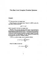
Lecture Suggestions Nearly all students will have some familiarity the concepts developed in the chapter. A first course in integral calculus makes reference to convergent versus divergent solutions. I draw the analogy between the particular solution to a difference equation and indefinite integrals. It is important to stress the distinction between convergent and divergent solutions. Be sure to emphasize the relationship between characteristic roots and the convergence or divergence of a sequence. Much of the current time-series literature focuses on the issue of unit roots. It is wise to introduce students to the properties of difference equations with unitary characteristic roots at this early stage in the course. Question 5 at the end of this chapter is designed to preview this important issue. The tools to emphasize are the method of undetermined coefficients and lag operators. Few students will have been exposed to these methods in other classes. I use overheads to show the students several data series and ask them to discuss the type of difference equation model that might capture the properties of each. The figure below shows three of the real exchange rate series used in Chapter 4. Some students see a tendency for the series to revert to a long-run mean value. The classroom discussion might center on the appropriate way to model the tendency for the levels to meander. At this stage, the precise models are not important. The objective is for students to conceptualize economic data in terms of difference equations.
Page 1: Difference Equations
Real Exchange Rates
(Panel.xls)
180
(1996 = 100)
160 140 120 100 80 60 1980 1983 1986 1989 1992 1995 1998 2001 U.S.
Canada
Germany
Answers to Questions 1. Consider the difference equation: yt = a0+ a1yt-1 with the initial condition y0. Jill solved the difference equation by iterating backwards: yt = a0 + a1yt-1 = a0 + a1[a0 + a1yt-2 ] = a0 + a0a1 + a0(a1)2 + .... + a0(a1)t-1 + (a1)ty0 Bill added the homogeneous and particular solutions to obtain: yt = a0/(1 - a1) + (a1)t[y0 - a0/(1 a1)]. A. Show that the two solutions are identical for a1 < 1. Answer: The key is to demonstrate: a0 + a0a1 + a0(a1)2 + .... + a0(a1)t-1 + (a1)ty0 = a0/(1 - a1) + (a1)t[y0 - a0/(1 - a1)] First, cancel (a1)ty0 from each side and then divide by a0. The two sides of the equation are identical if: 1 + a1 + (a1)2 + .... + (a1)t-1 = 1/(1 - a1) - (a1)t/(1 - a1) Page 2: Difference Equations
Now, multiply each side by (1 - a1) to obtain: (1 - a1)[1 + a1 + (a1)2 + .... + (a1)t-1] = 1 - (a1)t Multiply the two expressions in parentheses to obtain: 1 - (a1)t = 1 - (a1)t The two sides of the equation are identical. Hence, Jill and Bob obtained the identical answer. B. Show that for a1 = 1, Jill's solution is equivalent to: yt = a0t + y0. How would you use Bill's method to arrive at this same conclusion in the case a1 = 1. Answer: When a1 = 1, Jill's solution can be written as: yt = a0(10 + 11 + 12 + ... + 1t-1) + y0 = a0t + y0 To use Bill's method, find the homogeneous solution from the equation yt = yt-1. Clearly, the homogeneous solution is any arbitrary constant A. The key in finding the particular solution is to realize that the characteristic root is unity. In this instance, the particular solution has the form a0t. Adding the homogeneous and particular solutions, the general solution is yt = a0t + A To eliminate the arbitrary constant, impose the initial condition. The general solution must hold for all t including t = 0. Hence, at t = 0, y0 = a0t + A so that A = y0. Hence, Bill's method yields: yt = a0t + y0 2. The Cobweb model in section 5 assumed static price expectations. Consider an alternative formulation called adaptive expectations. Let the expected price in t (denoted by pt* ) be a weighted average of the price in t-1 and the price expectation of the previous period. Formally: pt* = αpt-1 + (1 - α) pt*−1
0 < α ≤ 1.
Clearly, when α = 1, the static and adaptive expectations schemes are equivalent. An interesting feature of this model is that it can be viewed as a difference equation expressing the expected price as a function of its own lagged value and the forcing variable pt-1.
Page 3: Difference Equations
A. Find the homogeneous solution for pt* Answer: Form the homogeneous equation pt* - (1 - α) pt*−1 = 0. The homogeneous solution is: pt* = A(1-α)t where A is an arbitrary constant and (1-α) is the characteristic root. B. Use lag operators to find the particular solution. Check your answer by substituting your answer into the original difference equation. Answer: The particular solution can be written as [ 1 - (1-α)L ] pt* = αpt-1 or
pt* = αpt-1/[ 1 - (1-α)L ] so that pt* = α[pt-1 + (1-α)pt-2 + (1-α)2pt-3 + ... ] To check the answer, substitute the particular solution into the original difference equation
α[pt-1 + (1-α)pt-2 + (1-α)2pt-3 + ... ] = αpt-1 + (1-α)α[pt-2 + (1-α)pt-3 + (1-α)2pt-4 + ... ] It should be clear that the equation holds as an identity. 3. Suppose that the money supply process has the form mt = m + ρmt-1 + εt where m is a constant and 0 < ρ < 1. A. Show that it is possible to express mt+n in terms of the known value mt and the sequence {εt+1, εt+2, ... , εt+n). Answer: One method is to use forward iteration. Updating the money supply process one period yields mt+1 = m + ρmt + εt+1. Update again to obtain mt+2 = m + ρmt+1 + εt+2 = m + ρ[m + ρmt + εt+1] + εt+2 = m + ρm + εt+2 + ρεt+1 + ρ2mt Repeating the process for mt+3 mt+3 = m + ρmt+2 + εt+3 Page 4: Difference Equations
= m + εt+3 + ρ[m + ρm + εt+2 + ρεt+1 + ρ2mt] For any period t+n, the solution is mt+n = m(1 + ρ + ρ2 + ρ3 + ... + ρn-1) + εt+n + ρεt+n-1 + ... + ρn-1εt+1 + ρnmt B. Suppose that all values of εt+i for i > 0 have a mean value of zero. Explain how you could use your result in part A to forecast the money supply n-periods into the future. Answer: The expectation of εt+1 through εt+n is equal to zero. Hence, the expectation of the money supply n periods into the future is m(1 + ρ + ρ2 + ρ3 + ... + ρn-1) + ρnmt As n → ∞, the forecast approaches m/(1-ρ). 4. Find the particular solutions for each of the following: i. yt = a1yt-1 + εt + β1εt-1 Answer: Assuming a1 < 1, you can use lag operators to write the equation as (1 - a1L)yt = εt + β1εt-1. Hence, yt = (εt + β1εt-1)/(1 - a1L). Now apply the expression (1 - a1L)-1 to each term in the numerator so that yt = εt + a1εt-1 + (a1)2εt-2 + (a1)3εt-3 + ... + β1[εt-1 + a1εt-2 + (a1)2εt-3 + ...] yt = εt + (a1+β1)εt-1 + a1(a1+β1)εt-2 + (a1)2(a1+β1)εt-3 + (a1)3(a1+β1)εt-4 + ... If a1 = 1, the improper form of the particular solution is: ∞
y t = b0 + ε t + (1+ β 1) ∑ ε t -i i=1
where: an initial condition is needed to eliminate the constant b0 and the non-convergent sequence. ii. yt = a1yt-1 + ε1t + βε2t Answer: Write the equation as yt = ε1t/(1-a1L) + βε2t/(1-a1L). Now, apply (1 - a1L)-1 to each term in the numerator so that Page 5: Difference Equations
yt = ε1t + a1ε1t-1 + (a1)2ε1t-2 + (a1)3ε1t-3 + ... + β[ε2t + a1ε2t-1 + (a1)2ε2t-2 + (a1)3ε2t-3 + ...] Alternatively, you can use the Method of Undetermined Coefficients and write the challenge solution in the form yt = Σciε1t-i + Σdiε2t-i where the coefficients satisfy: ci = (a1)i and di = β(a1)i. 5. The Unit Root Problem in time-series econometrics is concerned with characteristic roots that are equal to unity. In order to preview the issue: A. Find the homogeneous solution to each of the following. i) yt = a0 + 1.5yt-1 - 0.5yt-2 + εt Answer: The homogeneous equation is yt - 1.5yt-1 + .5yt-2 = 0. The homogeneous solution will take the form yt = Aαt. To form the characteristic equation, first substitute this challenge solution into the homogeneous equation to obtain Aαt -1.5Aαt-1 + 0.5Aαt-2 = 0 Next, divide by Aαt-2 to obtain the characteristic equation
α2 - 1.5α + 0.5 = 0 The two characteristic roots are α1 = 1, α2 = 0.5. The linear combination of the two homogeneous solutions is also a solution. Hence, letting A1 and A2 be two arbitrary constants, the complete homogeneous solution is A1 + A2(0.5)t ii) yt = a0 + yt-2 + εt Answer: The homogeneous equation is yt - yt-2 = 0. The homogeneous solution will take the form yt = Aαt. To form the characteristic equation, first substitute this challenge solution into the homogeneous equation to obtain Aαt - Aαt-2 = 0 Next, divide by Aαt-2 to obtain the characteristic equation α2 - 1 = 0. The two characteristic roots are α1 = 1, α2 = -1. The linear combination of the two homogeneous solutions is also a solution. Hence, letting A1 and A2 be two arbitrary constants, the complete homogeneous solution is Page 6: Difference Equations
A1 + A2(-1)t iii) yt = a0 + 2yt-1 - yt-2 + εt Answer: The homogeneous equation is yt -2yt-1 + yt-2 = 0. The homogeneous solution always takes the form yt = Aαt. To form the characteristic equation, first substitute this challenge solution into the homogeneous equation to obtain Aαt - 2Aαt-1 + Aαt-2 = 0 Next, divide by Aαt-2 to obtain the characteristic equation
α2 - 2α + 1 = 0 The two characteristic roots are α1 = 1, and α2 = 1; hence there is a repeated root. Thelinear combination of the two homogeneous solutions is also a solution. Letting A1 and A2 be two arbitrary constants, the complete homogeneous solution is A1 + A2t iv) yt = a0 + yt-1 + 0.25yt-2 - 0.25yt-3 + εt Answer: The homogeneous equation is yt - yt-1 - 0.25yt-2 + 0.25yt-3 = 0. The homogeneous solution always takes the form yt = Aαt. To form the characteristic equation, first substitute this challenge solution into the homogeneous equation to obtain Aαt - Aαt-1 -0.25Aαt-2 + 0.25Aαt-3 = 0 Next, divide by Aαt-3 to obtain the characteristic equation
α3 - α2 -0.25α + 0.25 = 0 The three characteristic roots are α1 = 1, α2 = 0.5, and α3 = -0.5. The linear combination of the three homogeneous solutions is also a solution. Hence, letting A1, A2 and A3 be three arbitrary constants, the complete homogeneous solution is A1 + A2(0.5)t + A3(-0.5)t B. Show that each of the backward-looking particular solutions is not convergent. i) yt = a0 + 1.5yt-1 - .5yt-2 + εt Answer: Using lag operators, write the equation as (1 - 1.5L + 0.5L2)yt = a0 + εt. Factoring the polynomial yields (1 - L)(1 - 0.5L)yt = a0 + εt. Although the expression (a0 + εt)/(1 - 0.5L) is convergent, (a0 + εt)/(1 - L) does not converge. Page 7: Difference Equations
ii) yt = a0 + yt-2 + εt Answer: Using lag operators, write the equation as (1 - L)(1 + L)yt = a0 + εt. It is clear that neither (a0 + εt)/(1 - L) nor (a0 + εt)/(1 + L) converges. iii) yt = a0 + 2yt-1 - yt-2 + εt Answer: Using lag operators, write the equation as (1 - L)(1 - L)yt = a0 + εt. Here there are two characteristic roots that equal unity. Dividing (a0 + εt) by either of the (1 - L) expressions does not lead to a convergent result. iv) yt = a0 + yt-1 + 0.25yt-2 - 0.25yt-3 + εt Answer: Using lag operators, write the equation as (1 - L)(1 - 0.5L)(1 + 0.5L)yt = a0 + εt. The expressions (a0 + εt)/(1 + 0.5L) and (a0 + εt)/(1 - 0.5L) are convergent, but the expression (a0 + εt)/(1 - L) is not convergent. C. Show that equation (i) can be written entirely in first-differences; i.e., ∆yt = a0 + .5∆yt-1 + εt. Find the particular solution for ∆yt. [HINT: Define y t* = ∆yt so that y t* = a0 - 0.5 y t*−1 + εt. Find the particular solution for y t* in terms of the {εt} sequence.] Answer: Subtract yt-1 from each side of yt = a0 + 1.5yt-1 - .5yt-2 + εt to obtain yt - yt-1 = a0 + 0.5yt-1 - .5yt-2 + εt so that ∆yt = a0 + 0.5yt-1 - 0.5yt-2 + εt = a0 + 0.5∆yt-1 + εt The particular solution for y t* = a0 + 0.5 y t*−1 + εt is given by y t* = (a0 + εt)/(1 - 0.5L) so that y t* = 2a0 + εt + 0.5εt-1 + 0.25εt-2 + 0.125εt-3 + .... D. Similarly transform the other equations into their first-difference form. Find the backwardlooking particular solution, if it exists, for the transformed equations. ii) yt = a0 + yt-2 + εt, Answer: Subtract yt-1 from each side to form yt - yt-1 = a0 - yt-1 + yt-2 + εt or ∆yt = a0 - ∆yt-1 + εt so that y t* = a0 - y t*−1 + εt Note that the first difference ∆yt has characteristic root that is equal to -1. The proper form of the backward-looking solution does not exist for this equation. If you attempt Page 8: Difference Equations
the challenge solution y t* = b0 + Σαiεt-i, you find b0 + α0εt + α1εt-1 + α2εt-2 + α3εt-3 + ... = a0 - b0 - α0εt-1 - α1εt-2 - α2εt-3 - ... + εt Matching coefficients on like terms yields b0 = a0 - b0 α0 = 1 α1 = -α0 and αi = (-1)i
⇒ b0 = a0/2 ⇒ α1 = -1
In Part E, students are asked to solve an equation of this form with a given initial condition. iii) yt = a0 + 2yt-1 - yt-2 + εt Answer: Subtract yt-1 from each side to obtain yt - yt-1 = a0 + yt-1 - yt-2 + εt so that ∆yt = a0 + ∆yt-1 + εt Using the definition of y t* it follows that y t* = a0 + y t*−1 + εt. Again, a proper form for the particular solution does not exist. The improper form is y t* = a0t + εt + εt-1 + εt-2 +... Notice that the second difference ∆2yt does have a convergent solution since ∆ y t* = a0 + εt iv) yt = a0 + yt-1 + 0.25yt-2 - 0.25yt-3 + εt Answer: Subtract yt-1 from each side and note that 0.25yt-2 - 0.25yt-3 = 0.25∆yt-2 so that ∆yt = a0 + 0.25∆yt-2 + εt or y t* = a0 + 0.25 y t*− 2 + εt Write the equation as (1 - 0.25L2) y t* = a0 + εt. Since (1 - 0.25L2) = (1 - 0.5L)(1 + 0.5L), it follows that y t* = (a0 + εt)/[(1 - 0.5L)(1 + 0.5L)] E. Given the initial condition y0, find the solution for: yt = a0 - yt-1 + εt. Page 9: Difference Equations
Answer: You can use iteration or the Method of Undetermined Coefficients to verify that the solution is t a i+t t t yt = ∑ (-1) ε i + (-1) y 0 + 0 [ 1 - (-1) ] 2 i=1 Using the iterative method, y1 = a0 + ε1 - y0 and y2 = a0 + ε2 - y1 so that y2 = a0 + ε2 - a0 - ε1 + y0 = ε2 - ε1 + y0 Since y3 = a0 + ε3 - y2, it follows that y3 = a0 + ε3 - ε2 + ε1 - y0. Continuing in this fashion yields y4 = a0 + ε4 - y3 = a0 + ε4 - a0 - ε3 + ε2 - ε1 + y0 = ε4 - ε3 + ε2 - ε1 + y0 To confirm the solution for yt note that (-1)i+t is positive for even values of (i+t) and negative for odd values of (i+t), (-1)t is positive for even values of t, and (a0/2)[1 - (-1)t] equals zero when t is even and a0 when t is odd. 6. A researcher estimated the following relationship for the inflation rate (πt):
πt = -.05 + 0.7πt-1 + 0.6πt-2 + εt A. Suppose that in periods 0 and 1, the inflation rate was 10% and 11%, respectively. Find the homogeneous, particular, and general solutions for the inflation rate. Answer: The homogeneous equation is πt - 0.7πt-1 - 0.6πt-2 = 0. Try the challenge solution πt = Aαt, so that the characteristic equation is Aαt - 0.7Aαt-1 - 0.6Aαt-2 = 0 or α2 - 0.7α - 0.6 = 0 The characteristic roots are: α1 = 1.2, α2 = -0.5. Thus, the homogeneous solution is
πt = A1(1.2)t + A2(-0.5)t The backward-looking particular solution is explosive. Try the challenge solution: πt = b + Σbiεt-i. For this to be a solution, it must satisfy b + b0εt + b1εt-1 + b2εt-2 + b3εt-3 + ... = -0.05 + 0.7(b + b0εt-1 + b1εt-2 + b2εt-3 + b3εt-4 + ...) + 0.6(b + b0εt-2 + b1εt-3 + b2εt-4 + b3εt-5 + ...) + εt Matching coefficients on like terms yields: Page 10: Difference Equations
b = -0.05 + 0.7b + 0.6b b0 = 1 b1 = 0.7b0 b2 = 0.7b1 + 0.6b0
⇒ b = 1/6 ⇒ b1 = 0.7 ⇒ b2 = 0.49 + 0.6 = 1.09
All successive values for bi satisfy the explosive difference equation bi = 0.7bi-1 + 0.6bi-2 If you continue in this fashion, the successive values of the bi are: b3 =1.183; b4 = 1.4821; b5 = 1.74727; b6 = 2.11235; b7 = 2.527007... Note that the forward-looking solution is not satisfactory here unless you are willing to assume perfect foresight. However, this is inconsistent with the presence of the error term. (After all, the regression would not have to be estimated if everyone had perfect foresight.) The point is that the forward-looking solution expresses the current inflation rate in terms of the future values of the {εt} sequence. If {εt} is assumed to be a white-noise process, it does not make economic sense to posit that the current inflation rate is determined by the future realizations of εt+i. Although the backward-looking particular solution is not convergent, imposing the initial conditions on the particular solution yields finite values for all πt (as long as t is finite). Consider the general solution
πt = 1/6 + εt + 0.7εt-1 + b2εt-2 + ... + bt-2ε2 + bt-1ε1 + btε0 + bt+1ε-1 + ... + A1(1.2)t + A2(-0.5)t For t = 0 and t = 1: 0.10 = 1/6 + ε0 + 0.7ε-1 + b2ε-2 + ... + A1 + A2 0.11 = 1/6 + ε1 + 0.7ε0 + b2ε-1 + ... + A1(1.2) + A2(-0.5) These last two equations define A1 and A2. Inserting the solutions for A1 and A2 into the general solution for πt eliminates the arbitrary constants.
Page 11: Difference Equations
B. Discuss the shape of the impulse response function. Given that the U.S. is not headed for runaway inflation, why do you believe that the researcher's equation is poorly estimated? Answer: The impulse response function is given by the {bi} sequence. The impact of an εt shock on the rate of inflation is 1. Only 70% of this initial effect remains for one period. After this one-time decay, the effect of the εt shock on πt+2, πt+3, ... explodes. You can see the impulse response function in the accompanying chart. The impulse responses imply that the inflation rate will grow exponentially. Given that there will not be runaway inflation, we would want to disregard the estimated model. 7. Consider the stochastic process: yt = a0 + a2yt-2 + εt. A. Find the homogeneous solution and determine the stability condition. Answer: The homogeneous solution has the form yt = Aαt. Form the characteristic equation by substitution of the challenge solution into the original equation, so that Aαt - a2Aαt-2 = 0 so that α2 = a2. The two characteristic roots are α1 = a 2 and α2 = - a 2 . The stability condition is for a2 to be less than unity in absolute value. B. Find the particular solution using the Method of Undetermined Coefficients. Answer: Try the challenge solution yt = b + Σbiεt-i. For this to be a solution, it must satisfy b + b0εt + b1εt-1 + b2εt-2 + b3εt-3 + ... = a0 + a2(b + b0εt-2 + b1εt-3 + b2εt-4 + b3εt-5 + ...) + εt Matching coefficients on like terms b = a0 + a2b Page 12: Difference Equations
⇒ b = a0/(1-a2)
b0 = 1 b1 = 0 b2 = a2b0 b3 = a2b1
⇒ b2 = a2 ⇒ b3 = 0 (since b1 = 0)
Continuing in this fashion, it follows that bi = (a2)i/2 if i is even and 0 if i is odd. 8. Consider the Cagan demand for money function in which: mt - pt = α - β[pt+1 - pt] A. Show that the backward-looking particular solution for pt is divergent. Answer: Using lag operators, rewrite the equation as βpt+1 - (1 + β)pt = α - mt. Combining terms yields [1 - (1 + 1/β)L]pt+1 = (α - mt)/β so that lagging by one period results in [1 - (1 + 1/β)L]pt = (α - mt-1)/β Since β is assumed to be positive, the expression (1 + 1/β) is greater than unity. Hence, the backward-looking solution for pt is divergent. B. Obtain the forward-looking particular solution for pt in terms of the {mt} sequence. In forming the general solution, why is it necessary to assume that the money market is in long-run equilibrium? Answer: Solving for βpt yields
βpt = [α - mt-1]/[1 - (1 + 1/β)L] The expression (-mt-1)/[1 - (1 + 1/β)L] can be obtained using Property 6 of lag operators. Let (1 + 1/β) correspond to the term a and apply Property 6 so that (-mt-1)/[1 - aL] = (aL)-1[(aL)0 + (aL)-1 + (aL)-2 + (aL)-3 + ... ]mt-1 = a-1[(aL)0 + (aL)-1 + (aL)-2 + (aL)-3 + ... ]mt = a-1[mt + a-1mt+1 + a-2mt+2 + a-3mt+3 + ... ] Since (1 + 1/β) = a, it follows that a-1 = β/(1+β). Also note that α/[1 - (1 + 1/β)L] = -αβ. Thus, the solution for pt is 1 pt = - α + 1+ β
β ∑ i= 0 1 + β ∞
i
mt+i
C. Find the impact multiplier. How does an increase in mt+2 affect pt? Provide an intuitive explanation of the shape of the entire impulse response function. Page 13: Difference Equations
Answer: The impact multiplier is the effect of mt on pt. As such ∂pt/∂mt = 1/(1+β). For any i, the effect of mt+i on pt is [1/(1+β)][β/(1+β)]i. Since [β/(1+β)]i decreases as i increases, future values of the money supply have a smaller effect on the current price level than the current value. Notice that a permanent increase in the money supply, such that ∆mt = ∆mt+1 = ... has a proportional effect on pt since [1/(1+β)]Σ[(β/(1+β)]i = 1. 9. For each of the following, verify that the posited solution satisfies the difference equation. The symbols c, c0, and a0 denote constants. Equation Solution A. yt - yt-1 = 0 yt = c B. yt - yt-1 = a0 yt = c + a0t C. yt - yt-2 = 0 yt = c + c0(-1)t D. yt - yt-2 = εt yt = c + c0(-1)t + εt + εt-2 + εt-4 + ... Answer: Substitute each posited solution into the original difference. A. Since yt = c and yt-1 = c, it immediately follows that c - c = 0. B. Since yt-1 = c + a0(t-1), it follows that c + a0t - c - a0(t-1) = a0. C. The issue is whether c + c0(-1)t - c - c0(-1)t-2 = 0? Since (-1)t = (-1)t-2, the posited solution is correct. D. Does c + c0(-1)t + εt + εt-2 + εt-4 + ... - c - c0(-1)t-2 - εt-2 - εt-4 - εt-6 - ... = εt? Since c0(-1)t = c0(-1)t-2, the posited solution is correct. 10. Part 1: For each of the following, determine whether {yt} represents a stable process. Determine whether the characteristic roots are real or imaginary and whether the real parts are positive or negative. A. yt - 1.2yt-1 + .2yt-2 B. yt - 1.2yt-1 + .4yt-2 C. yt - 1.2yt-1 - 1.2yt-2 D. yt + 1.2yt-1 E. yt - 0.7yt-1 - 0.25yt-2 + 0.175yt-3 = 0 [Hint: (x - 0.5)(x + 0.5)(x - 0.7) = x3- 0.7x2 - 0.25x + 0.175] Answers: A. The characteristic equation α2 - 1.2α + 0.2 = 0 has roots α1 = 1 and α2 = 0.2. The unit root means that the {yt} sequence is not convergent. B. The characteristic equation α2 - 1.2α + 0.4 = 0 has roots α1,α2 = 0.6 ± 0.2i. The roots are imaginary. The {yt} sequence exhibits damped wave-like oscillations. C. The characteristic equation α2 - 1.2α - 1.2 = 0 has roots α1 = 1.85 and α2 = -0.65. One of the roots is outside the unit circle so that the {yt} sequence is explosive. D. The characteristic equation α + 1.2 = 0 has the root α = -1.2. The {yt} sequence has explosive oscillations. E. The characteristic equation α3 - 0.7α2 - 0.25α + 0.175 = 0 has roots α1 = 0.7, α2 = 0.5 and α3 = -0.5. Although all roots are real, there are damped oscillations due to the presence of the Page 14: Difference Equations
term (-0.5)t. Part 2: Write each of the above equations using lag operators. Determine the characteristic roots of the inverse characteristic equation. Answers: Rewrite each using lag operators in order to obtain the inverse characteristic equation. A. (1 - 1.2L + 0.2L2)yt has the inverse characteristic equation 1 - 1.2L + 0.2L2 = 0. Solving this quadratic equation for the two values of L (called L1 and L2) yield the characteristic roots of the inverse characteristic equation. Here, L1 = 1.0 and L2 = 5.0. Since one root lies on the unit circle, the {yt} sequence is not convergent. Note that these roots are the reciprocals of the roots found in Part 1. B. (1 - 1.2L + 0.4L2)yt has the inverse characteristic equation 1 - 1.2L + 0.4L2 = 0. The roots are L1, L2 = 1.5 ± 0.5i. The roots of the inverse characteristic equation are outside the unit circle so that the {yt} sequence exhibits convergent wave-like oscillations. C. (1 - 1.2L - 1.2L2)yt has the inverse characteristic equation 1 - 1.2L - 1.2L2 = 0. The roots are -1.54 and 0.54. One of the inverse characteristic roots is inside the unit circle so that the {yt} sequence is explosive. D. The inverse characteristic equation (1 + 1.2L)yt has the inverse characteristic root: L = 1/1.2 = -0.8333. Since this inverse characteristic root is negative and lies inside the unit circle, the {yt} sequence has explosive oscillations. E. (1 - 0.7L - 0.25L2 + 0.175L3)yt has the inverse characteristic equation 1 - 0.7L - 0.25L2 + 0.175L3 = 0. Factoring yields the equivalent representation (1 - 0.5L)(1 + 0.5L)(1 - 0.7L) = 0. The inverse characteristic roots are 2.0, -2.0, and 1.0/0.7 = 1.429. All the inverse characteristic roots lie outside of the unit circle. 11. Consider the stochastic difference equation: yt = 0.8yt-1 + εt - 0.5εt-1. A. Suppose that the initial conditions are such that: y0 = 0 and ε0 = ε-1 = 0. Now suppose that ε1 = 1. Determine the values y1 through y5 by forward iteration. Answer: If we assume that all future values of {εt} = 0 we can find the solution. In essence, this is the method used to obtain the impulse response function. y1 = 1, y2 = 0.3, y3 = 0.24, y4 = 0.192, y5 = 0.1536 B. Find the homogeneous and particular solutions. Answer: The solution to the homogeneous equation yt - 0.8yt-1 = 0 is yt = A(0.8)t . Using lag operators, the particular solution is yt = (εt - 0.5εt-1)/(1 - 0.8L). If we apply 1/(10.8L) to εt and -0.5εt-1, we obtain yt = εt + 0.8εt-1 + (0.8)2εt-2 + (0.8)3εt-3 + ... -0.5[εt-1 + 0.8εt-2 + (0.8)2εt-3 + ... ] = εt + (0.8 - 0.5)εt-1 + 0.8(0.8 - 0.5)εt-2 + 0.82(0.8 - 0.5)εt-3 + ... Page 15: Difference Equations
yt = εt + 0.3εt-1 + 0.8(0.3)εt-2 + 0.82(0.3)εt-3 + ... C. Impose the initial conditions in order to obtain the general solution. Answer: Combining the homogeneous and particular solutions yields the general solution yt = εt + 0.3εt-1 + 0.8(0.3)εt-2 + 0.82(0.3)εt-3 + ... + A(0.8)t . Now impose the initial condition y0 = 0 and ε0 = ε-1 = 0 to obtain 0 = ε0 + 0.3ε-1 + 0.8(0.3)ε-2 + 0.82(0.3)ε-3 + ... + A. Hence A = -ε0 - 0.3ε-1 - 0.8(0.3)ε-2 - 0.82(0.3)ε-3 + ... Hence, A = 0 if the system began in initial equilibrium. Now substitute for A to obtain t -2
y t = ε t + 0.3 ∑ (0.8 ) ε t -i -1 i
i= 0
D. Trace out the time path of an εt shock on the entire time path of the {yt} sequence. Answer: ∂yt/∂εt = 1; ∂yt+1/∂εt = ∂yt/∂εt-1 = 0.3; ∂yt+2/∂εt = ∂yt/∂εt-2 = 0.3(0.8); ∂yt+3/∂εt = ∂yt/∂εt-3 = 0.3(0.8)2; and for i ≥ 1: ∂yt+i/∂εt = ∂yt/∂εt-i = 0.3(0.8)i-1 12. Use Equation (1.5) to determine the restrictions on α and β necessary to ensure that the {yt} process is stable. Answer: To determine stability, it is only necessary to examine the homogeneous portion of (1.5); i.e., yt - α(1+β)yt-1 + αβyt-2 = 0 where 0 < α < 1 and β > 0. In terms of the notation used in Figure 1.6, a1 = α(1+β) and a2 = -αβ. Given that α and β are positive, a1 > 0 and a2 < 0. Thus, the point labled α2 could correspond to α(1+β) units along the a1 axis and -αβ units along the a2 axis. The stability conditions for a second-order difference equation are: a1 + a2 < 1 a2 < 1 + a1 -a2 < 1 (since a2 < 0). Note that a1 + a2 = α(1+β) - αβ = α. Since 0 < α < 1, the first stability condition is always satisfied. To satisfy the second condition (i.e., a2 < 1 + a1), it is necessary to restrict the coefficients such that -αβ < 1 + α(1+β); simple manipulation yields: 0 < 1 + α + 2αβ. Since α and β are positive, the second stability condition necessarily holds. The third condition (i.e., -a2 < 1) is equivalent to αβ < 1 or β < 1/α. Hence, to ensure stability, it is necessary to restrict β to be less than 1/α. Page 16: Difference Equations
CHAPTER 2 STATIONARY TIME-SERIES MODELS 1. Stochastic Difference Equation Models 2. ARMA Models 3. Stationarity 4. Stationary Restrictions for an ARMA (p,q) Model 5. The Autocorrelation Function 6. The Partial Autocorrelation Function 7. Sample Autocorrelations of Stationary Series 8. Box–Jenkins Model Selection 9. Properties of Forecasts 10. A Model of the Producer Price Index 11. Seasonality 12. Summary and Conclusions
48 51 52 56 60 65 67 76 79 87 93 99
Questions and Exercises
100
Appendix 2.1:Estimation of an MA(1)Process Appendix 2.2:Model Selection Criteria
104 105
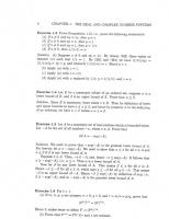
Lecture Suggestions I use Figure M2-1 to illustrate the effects of differencing and over-differencing. The first graph depicts 100 realizations of the unit root process yt = 1.5yt-1 - 0.5yt-2 + εt. If you examine the graph, it is clear there is no tendency for mean reversion. This non-stationary series has a unit root that can be eliminated by differencing. The second graph in the figure shows the firstdifference of the {yt} sequence: ∆yt = 0.5∆yt-1 + εt. The positive autocorrelation (ρ1 = 0.5) is reflected in the tendency for large (small) values of ∆yt to be followed by other large (small) values. It is simple to make the point that the {∆yt} sequence can be estimated using the BoxJenkins methodology. It is obvious to students that the ACF will reflect the positive autocorrelation. The third graph shows the second difference: ∆2yt = -0.5∆2yt-1 + εt - εt-1. Students are quick to understand the difficulties of estimating this over-differenced series. Due to the extreme volatility of the {∆2yt} series, the current value of ∆2yt is not helpful in predicting ∆2yt+1. The effects of logarithmic data transformations are often taken for granted. I use Figure M2-2 to illustrate the effects of the Box-Cox transformation. The first graph shows 100 realizations of the simulated AR(1) process: yt = 5 + 0.5yt-1 + εt. The {εt} series is precisely the same as that used in constructing the graphs in Figure M2-1. In fact, the only difference between Page 17: Stationary Models
Figure M2-1: The Effects of Differencing Non-stationary Sequence 5
The {yt} sequence was constructed as: yt = 1.5yt-1 - 0.5yt-2 + εt The unit root means that the sequence does not exhibit any tendency for mean reversion.
0
5
20
40
60
80
100
First-difference 1
The first-difference of the {yt} sequence is:
0.5
∆yt = 0.5∆yt-1 + εt
0
The first-difference of {∆yt} is a stationary AR(1) process such that a1 = 0.5.
0.5
1
0
20
40
60
80
100
Second-difference 1
The second-difference of the sequence is:
0.5
∆2yt = -0.5∆2yt-1 + εt - εt-1 0
The over-differenced {∆2yt} sequence has an invertible error term.
0.5
1
0
20
40
60
Page 18: Stationary Models
80
100
Figure M2-2: Box-Cox Transformations
yt = 5 + 0.5yt-1 + εt
λ = 0.5
12
6
10
4
8
0
50
100
2
0
50
Standard Deviation = 0.609
100
Standard Deviation = 0.193
Logarithmic Transformation: λ = 0
λ = -0.5
4
2
2
0
0
0
50
Standard Deviation = 0.061
100
0
50
100
Standard Deviation = 0.019
The first graph shows 100 realizations of a simulated AR(1) process; by construction, the standard deviation of the {yt} sequence is 0.609. The next three graphs show the results of BoxCox transformations using values of λ = 0.5, 0.0, and -0.5, respectively. You can see that decreasing λ acts to smooth the sequence.
Page 19: Stationary Models
the middle graph of Figure M2-1 and the first graph of Figure M2-2 involves the presence of the intercept term. The effects of a logarithmic transformation can be seen by comparing the two lefthand-side graphs of Figure M2-2. It should be clear that the logarithmic transformation smooths" the series. The natural tendency is for students to think smoothing is desirable. However, I point out that actual data (such as asset prices) can be quite volatile and that individuals may respond to the volatility of the data and not the logarithm of the data. Thus, there may be instances in which we do not want to reduce the variance actually present in the data. At this time, I mention that the material in Chapter 3 shows how to estimate the conditional variance of a series. Two Box-Cox transformations are shown in the right-hand-side graphs of Figure M2-2. Notice that decreasing λ reduces variability and that a small change in λ can have a pronounced effect on the variance.
Answers to Questions 1. In the coin-tossing example of Section 1, your winnings on the last four tosses (wt) can be denoted by wt = 1/4εt + 1/4εt-1 + 1/4εt-2 + 1/4εt-3 A. Find the expected value of your winnings. Find the expected value given that εt-3 = εt-2 = 1. Answers: Throughout the text, the term εt denotes a white-noise disturbance. The properties of the {εt} sequence are such that: i. Eεt = Eεt-1 = Eεt-2 = ... = 0, ii. Eεtεt-i = 0 for i ≠ 0, and iii. E(εt)2 = E(εt-i)2 = ... = σ2. Hence: Ewt = E(1/4εt + 1/4εt-1 + 1/4εt-2 + 1/4εt-3) Since the expectation of a sum is the sum of the expectations, it follows that Ewt = (1/4)(Eεt + Eεt-1 + Eεt-2 + Eεt-3) = 0. Given the information εt-3 = εt-2 = 1, the conditional expectation of wt is Et-2wt = E(wt εt-3 = εt-2 = 1) = (1/4)(Et-2εt + Et-2εt-1 + Et-2εt-2 + Et-2εt-3) so that Et-2wt = 0.25(0 + 0 + 1 + 1) = 0.5 B. Find var(wt). Find var(wt) conditional on εt-3 = εt-2 = 1. Answers: var(wt) = E(wt)2 - [E(wt)]2 so that var(wt) = E(1/4εt + 1/4εt-1 + 1/4εt-2 + 1/4εt-3)2 = (1/16)E[(εt)2 + 2εtεt-1 + 2 εtεt-2 + 2εtεt-3 + (εt-1)2 + 2εt-1εt-2 + 2εt-1εt-3 + (εt-2)2 + 2εt-2εt-3 + (εt-3)2] Since the expected values of all cross-products are zero, and it follows that: Page 20: Stationary Models
var(wt) = (1/16)4σ2 = 0.25σ2 Given the information εt-3 = εt-2 = 1, the conditional variance is var(wtεt-3 = εt-2 = 1) = Et-2(1/4εt + 1/4εt-1 + 1/4εt-2 + 1/4εt-3)2 - (Et-2wt)2 = (1/16)Et-2[ ε t2 + 2εtεt-1 + 2εtεt-2 + 2εtεt-3 + (εt-1)2 + 2εt-1εt-2 + 2εt-1εt-3 + (εt-2)2 + 2εt-2εt-3 + (εt-3)2] - (0.5)2 Since Et-2εt-2 = Et-2εt-3 = 1, it follows that var(wt εt-3 = εt-2 = 1) = (1/16)(σ2 + σ2 + 1 + 1 + 2) - 0.25, so that var(wt εt-3 = εt-2 = 1) = (1/8)σ2 C. Find: i. Cov(wt, wt-1) ii. Cov(wt, wt-2) iii. Cov(wt, wt-5) Answers: Using the same techniques as in Part B: i. Cov(wt, wt-1) = Ewtwt-1-E(wt)E(wt-1) = (1/16)E(εt + εt-1 + εt-2 + εt-3)(εt-1 + εt-2 + εt-3 + εt-4) = (1/16)E[(εt-1)2 + (εt-2)2 + (εt-3)2 + cross-product terms] Since the expected values of the cross-product terms are all zero Cov(wt, wt-1) = (1/16)3σ2 ii. Cov(wt, wt-2) = (1/16)E(εt + εt-1 + εt-2 + εt-3)(εt-2 + εt-3 + εt-4 + εt-5) = (1/16)E[(εt-2)2 + (εt-3)2 + cross-product terms] Since the expected values of the cross-product terms are all zero Cov(wt, wt-2) = (1/16)2σ2 iii. Cov(wt, wt-5) = (1/16)E(εt + εt-1 + εt-2 + εt-3)(εt-5 + εt-6 + εt-7 + εt-8) = (1/16)E[cross-product terms]. Hence: Cov(wt, wt-5) = 0 2. Substitute (2.10) into yt = a0 + a1yt-1 + εt. Show that the resulting equation is an identity. Answer: For (2.10) to be a solution, it must satisfy: a0[1 + a1 + a12 + ... + a1t-1] + a1ty0 + εt + a1εt-1 + a12εt-2 + ... + a1t-1ε1 = a0 + a1{a0[1 + a1 + a12 + ... + a1t-2] + a1t-1y0 + εt-1 + a1εt-2 + a12εt-3 + ...+ a1t-2ε1} + εt Notice that all terms cancel. Specifically: a0[1 + a1 + a12 + ... + a1t-1] ≡ a0 + a1{a0[1 + a1 + a12 + ... + a1t-2]} a1ty0 ≡ a1a1t-1y0 and: Page 21: Stationary Models
εt + a1εt-1 + a12εt-2 + ... + a1t-1ε1 = a1{ εt-1 + a1εt-2 + a12εt-3 + ... + a1t-2ε1} + εt A. Find the homogeneous solution to: yt = a0 + a1yt-1 + εt. Answer: Attempt a challenge solution of the form yt = Aαt. For this solution to solve the homogeneous equation it follows that α = a1 and A can be any arbitrary constant. B. Find the particular solution given that a1 < 1. Answer: Using lag operators, write the equation as (1 - a1L)yt = a0 + εt. Since a0/(1-a1L) = a0/(1-a1) and εt/(1-a1L) = εt + a1εt-1 + a12εt-2 + ... + a1t-1ε1 + a1tε0 + a1t+1ε-1 + ..., it follows that the particular solution is ∞
y t = a 0 / ( 1 - a1 ) + ∑ a1i ε t -i i= 0
C. Show how to obtain (2.10) by combining the homogeneous and particular solutions. Answer: Combining the homogeneous and particular solutions yields the general solution: ∞
t y t = a 0 / ( 1 - a1 ) + ∑ a1i ε t -i + A(a1 ) i= 0
so that when t = 0 ∞
y 0 = a 0 / ( 1 - a1 ) + ∑ a1i ε -i + A i= 0
Solve for A and substitute the answer into the general solution to obtain (2.10). 3. Consider the second-order autoregressive process yt = a0 + a2yt-2 + εt ,where a2 < 1. A. Find: i. Et-2yt ii. Et-1yt iii. Etyt+2 iv. Cov(yt, yt-1) v. Cov(yt, yt-2) vi. the partial autocorrelations φ11 and φ22 Answers: i) Et-2yt = Et-2(a0 + a2yt-2 + εt) = a0 + a2yt-2 ii) Et-1yt = Et-1(a0 + a2yt-2 + εt) = a0 + a2yt-2 Note the Et-1yt = Et-2yt since information obtained in period (t-1) does not help to predict the value of yt. iii) Etyt+2 can be obtained directly from the answer to Part i. Simply update the time index by two periods to obtain: Etyt+2 = a0 + a2yt Page 22: Stationary Models
The simplest way to answer Parts iv. and v. is to obtain the particular solution for yt. Students should be able to show: yt = a0/(1-a2) + εt + a2εt-2 + (a2)2εt-4 + (a2)3εt-6 + (a2)4εt-8 + ... iv) Cov(yt, yt-1) = E[(yt - Eyt)(yt-1 - Eyt-1)] = E[εt + a2εt-2 + (a2)2εt-4 + (a2)3εt-6 + (a2)4εt-8 + ...] [εt-1 + a2εt-3 + (a2)2εt-5 + (a2)3εt-7 + ...] so that Cov(yt, yt-1) = 0 v) Cov(yt, yt-2) = E[εt + a2εt-2 + (a2)2εt-4 + (a2)3εt-6 + ...] [εt-2 + a2εt-4 + (a2)2εt-6 + (a2)3εt-8 + ...] = a2E[(εt-2)2 + (a2)2(εt-4)2 + (a2)4(εt-6)2 + (a2)6(εt-8)2 + ... ] Given a2 < 1, the infinite summation Σ(a2)2i = 1/[1 - (a2)2] so that: cov(yt, yt-2) = a2σ2/[1 - (a2)2] vi). As shown in Part iv, the covariance between yt and yt-1 is zero. Hence, from (2.35), ρ1 = φ11 = 0. Given ρ1 = 0, (2.36) indicates that φ22 = ρ2. Given the answer to v and that var(yt) = var (yt-i) = ... = σ2/[1 - (a2)2], it follows that φ22 = cov(yt, yt-2)/var(yt) = {a2σ2/[1 - (a2)2]}/{σ2/[1 - (a2)2]} = a2 B. Find the impulse response function. Given yt-2, trace out the effects on an εt shock on the {yt} sequence. Answer: One way to answer the question is to use the particular solution for yt: yt = a0/(1-a2) + εt + a2εt-2 + (a2)2εt-4 + (a2)3εt-6 + (a2)4εt-8 + ... Hence: ∂yt/∂εt = 1. By the simple change of subscripts: ∂yt+1/∂εt = ∂yt/∂εt-1 = 0; ∂yt+2/∂εt = ∂yt/∂εt-2 = a2; ∂yt+3/∂εt = ∂yt/∂εt-3 = 0; ∂yt+4/∂εt = ∂yt/∂εt-4 = (a2)2 ... C. Determine the forecast function: Etyt+s. The forecast error et (s ) is the difference between yt+s and Etyt+s. Derive the correlogram of the { et (s ) } sequence. [Hint: Find Et et (s ) , Var [et (s )], and Et [et ( s )et ( s − j )] for j = 0 to s]. Answer: To find the forecast function, first find the general solution for yt in terms of y0. For a given value of y0, students should be able to show that if t is even, then: yt = a0[1 + a2 + (a2)2 + ... + (a2)t/2-1] + εt + a2εt-2 + (a2)2εt-4 + (a2)3εt-6 + ... + (a2)t/2y0 Page 23: Stationary Models
Hence: E0yt = a0[1 + a2 + (a2)2 + ... + (a2)t/2-1] + (a2)t/2y0. To find Etyt+2s, update the time subscripts such that Etyt+2s = a0[1 + a2 + (a2)2 + ... + (a2)s-1] + (a2)syt Generalizing the result from Part A above, note that for odd-period forecasts, Etyt+2s-1 = Etyt+2s-2. To find the forecast error, subtract Etyt+s from yt+s. For even values of s, we can let s = j/2 and form et (s ) = εt+s + a2εt+s-2 + (a2)2εt+s-4 + ... + (a2)s/2-1εt+2 The forecast error has a mean of zero since: Et[εt+s + a2εt+s-2 + (a2)2εt+s-4 + ... + (a2)s/2-1εt+2] = 0 Similarly, the variance is [1 + (a2)2 + (a2)4 + ... + (a2)s-2]σ2. The correlations between the forecast error for any period t+s and the forecast error for any odd period is zero. For even periods, we can begin by forming the covariance between et(2) and et(4) as: E[(εt+4 + a2εt+2)(εt+2)] = a2σ2 so that the correlation coefficient is a2/(1 + (a2)2)1/2. Similarly, the covariance between et(2) and et(6) as: E[(εt+6 + a2εt+4 + (a2)2εt+2)(εt+2)] = (a2)2σ2 so that the correlation coefficient is (a2)2/[1 + (a2)2 + (a2)4]1/2
4. Two different balls are drawn from a jar containing three balls numbered 1, 2, and 4. Let x = number on the first ball drawn and y = sum of the two balls drawn. A. Find the joint probability distribution for x and y; that is, find prob(x = 1, y = 3), prob(x = 1, y = 5), ... , and prob(x = 4, y = 6). Answer: Let x = number on the first ball; z = number on the second ball; and y = x + z. Consider the contingency table Summations x=1 x=2 x=4 z=1 y=3 y=5 z=2 y=3 y=6 z=4 y=5 y=6 Page 24: Stationary Models
Notice that the same outcome for x and z is not possible since two different balls are drawn from the jar. Thus, prob(x=1, y=2), prob(x=2, y=4), and prob(x=3, y=6) are all equal to zero. The remaining six outcomes are equally likely. The probabilities (x=1, y=3), (x=1, y=5), ... (x=4, y=6) all equal 1/6. B. Find each of the following: E(x), E(y), E(yx = 1), E(xy = 5), Var(xy = 5), and E(y2) Answers: Each outcome for x has a probability of 1/3. Thus: i) E(x) = (1/3)(1 + 2 + 4) = 7/3 ii) The expected value of y is the summation of each possible outcome for y multiplied by the probability of that outcome. Since each cell has a probability of 1/6, reading across the rows of the table yields: E(y) = (1/6)(3 + 5 + 3 + 6 + 5 + 6) = 14/3 iii) When x = 1, y can take on values 3 or 5. Hence: E(yx = 1) = 0.5(3) + 0.5(5) = 4.0 iv) When y = 5, x can take on values 1 or 4. Hence: E(xy =5) = 0.5(1 + 4) = 2.5 v) Var(xy = 5) = E(x2y = 5) - [E(xy =5)]2 = 0.5(12 + 42) - (2.5)2 = 8.5 - 6.25 = 2.25 Var(xy = 5) = 2.25 vi) The expected value of y2 is the summation of each possible squared outcome for y multiplied by the probability of that outcome. Hence: E(y2) = (1/3)(32 + 52 + 62) = 70/3 C. Consider the two functions: w1 = 3x2 and w2 = x-1. Find: E(w1 + w2) and E(w1 + w2y = 3). Answers: The expected value of a function of x [(i.e., F(x)] is equal to the value of the function evaluated at each possible realization of x multiplied by the probability of the associated realizations. Moreover, since the expectation of a sum is the sum of the expectations, E(w1 + w2) = E(3x2) + Ex-1 = 3(1/3)(12 + 22 + 42) + (1/3)(1 + 1/2 + 1/4) = 21 + 1.75/3. Hence: E(w1 + w2) = 21.5833 When y = 3, x can only take on the values 1 or 2. Hence, E(w1 + w2y = 3) = E(w1y = 3) + E(w2y = 3) = 3(1/2)(12 + 22) + (1/2)(1 + 1/2) =15/2 + 3/4 = 33/4. Hence: E(w1+ w2y = 3) = 33/4 D. How would your answers change if the balls were drawn with replacement? Answer: The contingency table changes since it is possible for x and z to take on the same values. The new contingency table becomes: Page 25: Stationary Models
z=1 z=2 z=4
x=1 y=2 y=3 y=5
Summations x=2 y=3 y=4 y=6
x=4 y=5 y=6 y=8
Each entry from (x=1, y=2) through (x=4, y=8) has a probability of 1/9. Part B becomes: i) E(x) = 1/3(1 + 2 + 4) = 7/3. ii) E(y) = (1/9)(2 + 3 + 5 + 3 + 4 + 6 + 5 + 6 + 8) = 42/9 = 14/3 iii) E(yx=1) = (1/3)(2 + 3 + 5) = 10/3. iv) E(xy=5) = (1/2)(1 + 4) = 2.5. v) Var(xy=5) = E(x2y=5) - [E(xy=5)]2 = (1/2)(1 + 42) - (2.5)2 = 17/2 - 6.25 = 2.25. vi). E(y2) = (1/9)[22 + 2(3)2 + 42 + 2(5)2 + 2(6)2 + 82] = 224/9. Note that the answer to Part C is unchanged. 5. The general solution to an n-th order difference equation requires n arbitrary constants. Consider the second-order equation: yt = a0 + 0.75yt-1 - 0.125yt-2 + εt. A. Find the homogeneous and particular solutions. Discuss the shape of the impulse response function. Answer: The homogeneous equation is yt = 0.75yt-1 - 0.125yt-2. Try the challenge solution yt = Aαt and obtain Aαt - 0.75Aαt-1 + 0.125Aαt-2 = 0 so that the characteristic equation is α2 - 0.75α + 0.125 = 0. The two characteristic roots are 0.5 and 0.25 and A can be any arbitrary constant. Since a linear combination of the two homogeneous solutions is also a solution, the complete form of the homogeneous solution is yt = A1(0.5)t + A2(0.25)t where A1 and A2 are arbitrary constants. The particular solution has the form yt = b0 + Σαiεt-i. The constant b0 can easily be found as b0 = a0(1 - 0.75 + 0.125) = 8a0/3. To find the αi substitute yt = Σαiεt-i into yt = 0.75yt-1 - 0.125yt-2 + εt to obtain:
α0εt + α1εt-1 + α2εt-2 + α3εt-3 + ... = 0.75(α0εt-1 + α1εt-2 + α2εt-3 + ...) - 0.125(α0εt-2 + α1εt-3 + α2εt-4 + ...) + εt Matching coefficients on like terms, it follows that: Page 26: Stationary Models
α0 = 1; α1 = 0.75; and all subsequent αi are such that αi = 0.75αi-1 - 0.125αi-2 For example, α2 = 0.4375, α3 = 0.2348, α4 = 0.1211, and α5 = 0.0615. The impulse responses are given by the coefficients of the particular solution. For example, ∂yt/∂εt = 1; ∂yt+1/∂εt = ∂yt/∂εt-1 = 0.75; ∂yt+2/∂εt = ∂yt/∂εt-2 = 0.4375. Since both characteristic roots are positive and less than unity, the impulse responses converge directly toward the long-run value yt = 8a0/3. B. Find the values of the initial conditions (i.e., y0 and y1) that ensure {yt} sequence is stationary (Note: A1 and A2 are the arbitrary constants in the homogeneous solution). Answer: The general solution is the sum of the homogeneous and particular solutions: yt = A1(0.5)t + A2(0.25)t + 8a0/3 + εt + 0.75εt-1 + 0.4375εt-2 + ... so that for periods 0 and 1: y0 = A1+ A2 + 8a0/3 + ε0 + 0.75ε-1 + 0.4375ε-2 + ... y1 = A1(0.5) + A2(0.25) + 8a0/3 + ε1 + 0.75ε0 + 0.4375ε-1 + ... The issue is to select y0 and y1 such that A1 = A2 = 0. If y0 = 8a0/3 + ε0 + 0.75ε-1 + 0.4375ε-2 + ... and y1 = 8a0/3 + ε1 + 0.75ε0 + 0.4375ε-1 + ... , then A1 = A2 = 0, so that the general solution is: yt = 8a0/3 + εt + 0.75εt-1 + 0.4375εt-2 + ... C. Given your answer to part B, derive the correlogram for the {yt} sequence. Answer: Given the initial conditions found in Part A, the Yule-Walker equations can be used to derive the correlogram. For simplicity, abstract from the constant a0 since it does not affect the autocorrelations. Hence, set a1 = 0.75 and a2 = -0.125, and use (2.28) and (2.29) to find the autocorrelations. Given that ρ0 = 1, it follows that ρ1 = 0.75 - 0.125ρ1 and ρ1 = 2/3 and ρs = 0.75ρs-1 -0.125ρs-2 For example, ρ2 = 0.375; ρ3 = 0.1979; ρ4 = 0.1012; ρ5 = 0.0512..... 6. Consider the second-order stochastic difference equation: yt = 1.5yt-1 - 0.5yt-2 + εt. A. Find the characteristic roots of the homogeneous equation. Answer: The homogeneous equation is yt - 1.5yt-1 + 0.5yt-2 = 0. If you try the challenge solution yt = Aαt, A and α must satisfy: Aαt - 1.5Aαt-1 + 0.5Aαt-2 = 0. Dividing by Aαt-2, the characteristic equation is α2 - 1.5α + 0.5 = 0. Thus, A can be any arbitrary constant and the characteristic roots, (i.e., α) can be 1 or 0.5. The homogeneous solution is: Page 27: Stationary Models
yt = A1 + A2(0.5)t B. Demonstrate that the roots of 1 - 1.5L + 0.5L2 are the reciprocals of your answer in Part A. Answer: To solve the inverse characteristic equation for L, form (1 - L)(1 - 0.5L) = 0. The solutions are L = 1 and L = 1/0.5 = 2. Hence, the two inverse characteristic roots are the reciprocals of characteristic roots found in Part A. Thus, the stability condition is for the characteristic roots to lie inside of the unit circle or for the roots of the inverse characteristic equation to lie outside of the unit circle. C. Given initial conditions for y0 and y1, find the solution for yt in terms of the current and past values of the {εt} sequence. Explain why it is not possible to obtain the backward looking solution for yt unless such initial conditions are given. Answer: One way to solve the problem is to use the initial conditions y0 and y1 and iterate forward. Since, y2 = 1.5y1 - 0.5y0 + ε2, and y3 = 1.5y2 - 0.5y1 + ε3, it follows that: y3 = ε3 + 1.5ε2 + 1.75y1 - 0.75y0. Similarly, y4 = 1.5y3 - 0.5y2 + ε4. Substituting for y3 and y2 yields: y4= ε4 + 1.5ε3 + 1.75ε2 + 1.875y1 - 0.875y0 Continuing in this fashion yields: y5 = ε5 + 1.5ε4 + 1.75ε3 + 1.875ε2 + 1.9375y1 - 0.9375y0 y6 = ε6 + 1.5ε5 + 1.75ε4 + 1.875ε3 + 1.9375ε2 + 1.96875y1 - 0.96875y0 The solution has the form: t -2
y t = ∑ α i ε t -i + α t -1 y1 + α t y 0 i= 0
where: α0 = 1, α1 = 1.5, αt = 1- αt-1, and the remaining coefficients αi solve the difference equation αi = 1.5αi-1 - 0.5αi-2. Since the coefficients will grow progressively larger, the backward particular solution will not be convergent. The initial conditions are necessary for yt to be finite for finite values of t. D. Find the forecast function for yt+s. Answer: First write the answer to Part C in terms of s rather than in terms of t: s -2
y s = ∑ α iε s-i + α s-1 y 1 + α s y 0 i =0
Then update by t periods to obtain: Page 28: Stationary Models
s-2
y t+s = ∑ α i ε t+s -i + α s -1 yt +1 + α s yt i= 0
For s > 1, forecasts conditioned on the information in t+1 and t can be made using Et+1yt+s = αs-1yt+1 + αsyt. E. Find: Eyt, Eyt+1, Var(yt), Var(yt+1), and Cov(yt+1, yt). Answers: The point is to illustrate that the {yt} sequence is not stationary. Consider: i. Eyt = αt-1y1 + αty0. Since αt-1 and αt are functions of time, the mean is not constant. ii. Eyt+1 = αty1 + αt+1y0. Note that Eyt+1 ≠ Eyt. iii. var(yt) = [1 + (α1)2 + (α2)2 + ... + (αt-2)2]σ2 iv. var(yt+1) = [1 + (α1)2 + (α2)2 + ... + (αt-1)2]σ2 so that var(yt+1) ≠ var(yt ). v. cov(yt+1, yt) = [α0α1 + α1α2 + ... + αt-3αt-2]σ2. 7. The file entitled SIM_2.XLS contains the simulated data sets used in this chapter. The first column contains the 100 values of the simulated AR(1) process used in Section 7. This first series is entitled Y1. The following programs will perform the tasks indicated in the text. Due to differences in data handling and rounding, your answers need only approximate those presented in the text. Sample Program for RATS Users all 100 open data a:\sim_2.xls data(format=xls,org=obs)
;* The first 3 lines read in the data set ;* Modify this if your data is not on drive a:
cor(partial=pacf,qstats,number=24,span=8) y1
;* calculates the ACF, PACF, and Q-
graph 1 # y1
;* plots the simulated series
statistics
boxjenk(ar=1) y1 / resids
;* estimates an AR(1) model and saves the ;* residuals in the series called resids
* The next 3 lines compute and display the AIC and SBC compute aic = %nobs*log(%rss) + 2*%nreg compute sbc = %nobs*log(%rss) + %nreg*log(%nobs) display 'aic = ' AIC 'sbc = ' sbc * Obtain the ACF, PACF, and Q-statistics of the residuals cor(partial=pacf,qstats,number=24,span=8,dfc=%nreg) resids Page 29: Stationary Models
* Now estimate the model with a MA term at lag 12 boxjenk(ar=1,ma=||12||) y1 / resids cor(partial=pacf,qstats,number=24,span=8,dfc=%nreg) resids compute aic = %nobs*log(%rss) + 2*%nreg compute sbc = %nobs*log(%rss) + %nreg*log(%nobs) display 'aic = ' AIC 'sbc = ' sbc
boxjenk(ar=2) y1 / resids boxjenk(ar=1,ma=1) y1 / resids
;* Estimates the AR(2) model ;* Estimates an ARMA(1, 1) model
Sample Program for STATA Users /*Note: All the code is written for STATA release 8.0. Since STATA cannot read datasets in the Excel format, please save the Excel datasets as text files and read them in using the line below, or you can use a program such as Stat/Transfer to translate the datasets from Excel's format to STATA's format */ clear cd "X:\New_data" /*Please change this line accordingly to wherever the dataset is saved*/ insheet using sim_2.txt tsset obs
/*declare this is a time series dataset*/
*A:plot the sequence against time line y1 obs *B:verify the first 12 coefficients of the ACF and PACF corrgram y1, lag(24) *C:estimate Model 1 reg y1 l.y1, noconstant /*the calculation of AIC and SBC makes use of the saved results after estimation commands such as -reg-, -arima-. type -ereturn list- to obtain a complete list of saved results after a particular estimation command*/ display "AIC = "=e(N)*ln(e(rss))+2*e(df_m) /*compute AIC of Model 1*/ display "SBC = "=e(N)*ln(e(rss))+e(df_m)*ln(e(N)) /*compute SBC of Model 1*/ predict resids, residuals /*calculate residuals after estimation and save it as a new variable called resids*/ corrgram resids, lag(24) /*verify Q stats of residuals of Model 1*/ Page 30: Stationary Models
/*Next, reestimate Model 1 using ARIMA command. the reason for doing so is to make the two models comparable because Model 2 cannot be estimated by linear regression*/ arima y1,ar(1) noconstant display "AIC = "=-2*e(ll)+2*e(k) display "SBC = "=-2*e(ll)+e(k)*ln(e(N)) predict resids1,residuals corrgram resids1, lag(24) /*verify Q stats of residuals of Model 1*/ /*Note: here the required matsize should be max(AR, MA+1)^2, which is 169(max(1,13)^2). But matsize for intercooled stata is initially set at 40, far below the required size. Refer to [R]matsize for details.*/ set matsize 800 arima y1,ar(1) ma(12) noconstant /*estimate Model 2*/ display "AIC = "=-2*e(ll)+2*e(k) display "SBC = "=-2*e(ll)+e(k)*ln(e(N)) /*Note: Since ARIMA in STATA estimates a model using a combination of BHHH and BFGS, it does not report the residual sum of squares which makes impossible the computation of AIC and SBC using the formula appropriate for a model estimated by OLS. However, AIC and SBC are still obtainable if we make use of the log likelihood function value. The final conclusion of which model is better remains unchanged*/ predict resids2, residuals corrgram resids2, lag(24) /*verify Q stats of residuals of Model 2*/ *D: estimate the series y1 as an AR(2) without an intercept reg y1 l.y1 l2.y1, noconstant *E:estimate the series y1 as an ARMA(1,1) without an intercept arima y1,ar(1) ma(1) noconstant 8. The second column in file entitled SIM_2. XLS contains the 100 values of the simulated ARMA(1, 1) process used in Section 7. This series is entitled Y2. The following programs will perform the tasks indicated in the text. Due to differences in data handling and rounding, your answers need only approximate those reported in the text. Sample Program for RATS Users all 100 open data a:\sim_2.xls data(format=xls,org=obs)
;* The first 3 lines read in the data set ;* Modify this if your data is not on drive a: Page 31: Stationary Models
cor(partial=pacf,qstats,number=24,span=8) y2 ;* calculates the ACF, PACF, and Q-statistics graph 1 ;* plots the simulated series # y2 *RATS contains a procedure to plot autocorrelation and partial autocorrelations. To use the *procedure use the following two program lines: source(noecho) c:\winrats\bjident.src ;* assuming RATS is in a directory called C:\WINRATS @bjident y2 boxjenk(ar=1) y2 / resids ;* estimates an AR(1) model and saves the residuals cor(number=24,partial=partial,qstats,span=8) resids / cors compute aic = %nobs*log(%rss) + 2*%nreg compute sbc = %nobs*log(%rss) + %nreg*log(%nobs) display 'aic = ' AIC 'sbc = ' sbc boxjenk(ar=2) y2 / resids ;* estimates an AR(2) model and saves the residuals cor(number=24,partial=partial,qstats,span=8) resids / cors compute aic = %nobs*log(%rss) + 2*%nreg compute sbc = %nobs*log(%rss) + %nreg*log(%nobs) display 'aic = ' AIC 'sbc = ' sbc *Continue to copy the statements used in Question 7. For the MA(2) use: boxjenk(ma=2) y2 / resids cor(number=24,partial=partial,qstats,span=8) resids / cors *To compare the MA(2) to the ARMA(1, 1) you need to be a bit careful. For a head-to-head *comparison, you need to estimate the models over the same sample period. The ARMA(1, 1) *uses 99 observations while the MA(2) uses all 100 observations. Use: boxjenk(ma=2) y2 2 100 resids ;* This instructs RATS to use only observations 2 – 100. boxjenk(ar=1,ma=1) y2 / resids cor(number=24,partial=partial,qstats,span=8) resids / cors compute aic = %nobs*log(%rss) + 2*%nreg compute sbc = %nobs*log(%rss) + %nreg*log(%nobs) display 'aic = ' AIC 'sbc = ' sbc
Sample Program for STATA Users clear Page 32: Stationary Models
cd "a:\New_data" /*Change if the dataset is saved elsewhere*/ insheet using sim_2.txt tsset obs /*declare this is a time series dataset*/ *A:plot the sequence against time line y2 obs /*verify the first 12 coefficients of the ACF and PACF*/ corrgram y2, lag(12) *B:estimate Model 1 reg y2 l.y2, noconstant /*compute AIC and SBC of Model 1(99 obs)*/ display "AIC = "=e(N)*ln(e(rss))+2*e(df_m) display "SBC = "=e(N)*ln(e(rss))+e(df_m)*ln(e(N)) /*compute AIC and SBC of Model 1(98 obs)*/ display "AIC*= "=(e(N)-1)*ln(e(rss))+2*e(df_m) display "SBC*= "=(e(N)-1)*ln(e(rss))+e(df_m)*ln(e(N)-1) predict resids1, residuals corrgram resids1, lag(24) /*Q stats of residuals of Model 1*/ arima y2,ar(1) ma(1) noconstant /*estimate Model 2*/ display "AIC = "=-2*e(ll)+2*e(k) display "SBC = "=-2*e(ll)+e(k)*ln(e(N)) predict resids2, residuals corrgram resids2, lag(24) /*verify Q stats of residuals of Model 2*/ reg y2 l.y2 l2.y2, noconstant /*estimate Model 3*/ display "AIC = "=e(N)*ln(e(rss))+2*e(df_m) display "SBC = "=e(N)*ln(e(rss))+e(df_m)*ln(e(N)) predict resids3, residuals corrgram resids3, lag(24) *C: estimate the process using a pure MA(2) model arima y2,ma(1 2) noconstant predict residsc, residuals corrgram residsc, lag(24) 9. The third column in SIM_2.XLS contains the 100 values of a AR(2) process; this series is entitled Y3. The following programs will perform the tasks indicated in the text. Due to differences in data handling and rounding, your answers need only approximate those reported in the text. Page 33: Stationary Models
Sample Program for RATS Users Use the first three lines from Question 7 or 8 to read in the data set. To graph the series use: cor(partial=pacf,qstats,number=24,span=8) y3 ;* calculates the ACF, PACF, and Q-statistics graph 1 ; # y3 ;* plots the simulated series boxjenk(ar=1) y3 / resids
;* estimates an AR(1) model and saves the residuals
boxjenk(ar=1,ma=1) y3 / resids ;* estimates an ARMA(1) model and saves the residuals cor(partial=pacf,qstats,number=24,span=8,dfc=%nreg) resids boxjenk(ar=2) y3 / resids ;* estimates an AR(2) model and saves the residuals cor(partial=pacf,qstats,number=24,span=8,dfc=%nreg) resids *To estimate the AR(2) model with the single MA coefficient at lag 16 use: boxjenk(ar=2,ma=||16||) y3 / resids Sample Program for STATA Users Use the first four lines from Question 7 or 8 to read in the data set. To graph the data use: *A:plot the sequence against time line y3 obs corrgram y3, lag(12) /*verify the first 12 coefficients of the ACF and PACF*/ *B:estimate the series as an AR(1) process reg y3 l.y3, noconstant display "AIC = "=e(N)*ln(e(rss))+2*e(df_m) /*compute AIC of the AR(1) model*/ display "SBC = "=e(N)*ln(e(rss))+e(df_m)*ln(e(N)) /*compute SBC of AR(1) model 1*/ predict residsb, residuals corrgram residsb, lag(24) /*verify Q stats of residuals of the AR(1) Model*/ *C:estimate the series as an ARMA(1,1) process arima y3,ar(1) ma(1) noconstant predict residsc, residuals corrgram residsc, lag(24) /*verify Q stats of residuals of the ARMA(1,1) model*/ *E:estimate the series as an AR(2) process Page 34: Stationary Models
reg y3 l.y3 l2.y3, noconstant display "AIC = "=e(N)*ln(e(rss))+2*e(df_m) /*compute AIC of the AR(2) model*/ display "SBC = "=e(N)*ln(e(rss))+e(df_m)*ln(e(N)) /*compute SBC of the AR(2) model*/ predict residse, residuals corrgram residse, lag(24) /*verify Q stats of residuals of the AR(2) model*/ set matsize 800 arima y3,ar(1 2) ma(16) noconstant
10. The text uses AIC = T ln(SSR) + 2 n . Suppose that the AIC from model (AIC1) is smaller than that for model 2 (AIC2). Hence, model 1 is selected over model 2. In fact, any monotonic transformation of the AIC will always lead to model 1 being selected over model 2. The issue is to show whether the various ways of reporting the AIC (and SBC) are monotonic transformations of each other. Consider the version reported by E-Views:
AIC = -2ln(L)/T + 2n/T where (as you can see from Appendix 2.1) lnL = -(T/2)ln(2π) – (T/2)lnσ2 – (2σ2)-1Σ(εt)2 Since -(T/2)ln(2π) is a constant, it can be ignored in calculating the formula (i.e., adding or subtracting is a monotonic transformation) since it will not affect the relative ranking of the two models. Also note that σ2 is calculated as Σ(εt)2/T. Note that this implies (σ2)-1Σ(εt)2 = T (i.e, a constant). Hence, a monotonic transformation of ln L is -(T/2) ln(Σ(εt)2/T) Hence, a monotonic transformation of AIC = -2ln(L)/T + 2n/T is ln(Σ(εt)2/T) + 2n/T or multiplying by T and adding ln(T)—two more monotonic transformations, we get AIC = T ln(SSR) + 2 n The argument is identical for the SBC and for the formula AIC = exp(2n/T) (SSR/T). 11. RATS users can enter the following code: cal 1960 1 4 all 2002:1 open data a:\quarterly.xls data(format=xls,org=obs)
;* The 4 lines read in the data set ;* The PPI is quarterly over the 1960:1 – 2002:1 period
Page 35: Stationary Models
dif ppi / dy log ppi / ly dif ly / dly
;* These 2 lines form the logarithmic change
*Figure 2.5 was created using: spg(hfi=1,vfi=3,hea='Figure 2.5') gra(hea='Panel a: The Producer Price Index: (1995 = 100)') 1 ; # ppi gra(hea='Panel b: First Difference of the PPI') 1 ; # dy gra(hea='Panel c: Logarithmic Difference of the PPI') 1 ; # dly spg(done) /*The next three lines estimate an ARMA(1, 1), ARMA(1, ||1,4||) and an AR(2) over the full sample period. To compare the three using the AIC or SBC, estimate all three over the same sample period. */ boxjenk(define=eq1,constant,ar=1,ma=1,dif=1) ly / resids boxjenk(define=eq1,constant,ar=1,ma=||1,4||,dif=1) ly / resids boxjenk(define=eq1,constant,ar=2,dif=1) ly / resids *To perform the 50 out-of-sample forecasts of the ARMA(1, 1), ARMA(1, ||1,4||) models, we *need to initialize two series to hold the 50 forecasts: set arma11 = 0. set arma114 = 0. *Now each model will be estimated fifty times using the sample period 2 through period 118 + i *(1989:3 = 2002:1-50). At the end, i = 50 so that the final period is 2001:4. At each estimation, *the 1-step-ahead forecast is made. The forecasts from the ARMA(1, 1) will be stored in arma11 *and those from the ARMA(1, ||1,4||) will be in arma114. do i = 1,50 boxjenk(define=eq1,constant,ar=1,ma=1,noprint) dly * 2002:1-51+i resids forecast 1 1 2002:1-50+i # eq1 arma11 boxjenk(define=eq1,constant,ar=1,ma=||1,4||,noprint) dly * 2002:1-51+i resids forecast 1 1 2002:1-50+i # eq1 arma114 end do i *Next create the two forecast errors as the actual value of dly minus the forecast set err11 1989:4 * = dly - arma11 Page 36: Stationary Models
set err114 1989:4 * = dly - arma114 *The summary statistics for the two series are given by: table 1989:4 * err11 table 1989:4 * err114 *For the Diebold-Mariano test, form (2.62) using the absolute values set d 1989:4 * = abs(err11) - abs(err114) *The mean value (i.e., d ) and the variance (i.e., γ0) can be obtained using: sta d ; com dbar = %mean ; dis dbar %variance /*You should find that d equals -4.99789e-05 and that the variance of dt is 6.94794e-06. For all practical purposes that autocorrelations of dt are zero. Hence, the desired statistic is: */ DM = -4.99789e-05/[0.00000694794/49)0.5] = -0.13273. * There is not a significant difference between the two forecasts. *For the Granger-Newbold test, form x and z using set x 1989:4 * = err11 + err114 set z 1989:4 * = err11 - err114 *Obtain the correlation coefficient using cross x z 1989:4 * 0 0 rxz *The correlation is -0.0767318. This is stored in rxz(1). Hence the Granger-Newbold statistic can be computed using: com den = (1-rxz(1)**2)/49 dis rxz(1)/(den**.5) *The value of -0.538 is not significant at any conventional level. Sample Program for STATA Users clear cd "a:\New_data" /*Please change this line accordingly if the dataset is saved elsewhere*/ insheet using quarterly.txt gen obs = _n /*obs is 1,2,...,_N, a new column vector created to act as a time variable*/ Page 37: Stationary Models
tsset obs /*declare this is a time series dataset*/ gen lppi=ln(ppi) gen dlppi=d.lppi /*make the data transformation*/ *A:estimate the series as an ARMA(1,1) process arima dlppi, ar(1) ma(1) predict resids1, residuals corrgram resids1, lag(12) /*verify Q stats of residuals of the ARMA(1,1) Model*/ arima dlppi, ar(1) ma(1 4) /*estimate the series as an ARMA(1,1 4) process*/ predict resids2, residuals corrgram resids2, lag(12) /*verify Q stats of residuals of the ARMA(1,1 4) Model*/ reg dlppi l.dlppi l2.dlppi /*estimate the series as an AR(2) process*/ display "AIC = "=e(N)*ln(e(rss))+2*e(df_m) /*compute AIC of the AR(2) model*/ display "SBC = "=e(N)*ln(e(rss))+e(df_m)*ln(e(N)) /*compute SBC of AR(2) model 1*/ predict resids3, residuals corrgram resids3, lag(12) /*verify Q stats of residuals of the AR(2) Model*/ *B:estimate the ARMA(1,1) model over the period 1960:Q1 to 1989:Q3 gen time = real(substr(descriptor,1,4) + substr(descriptor,6,1)) /*this line is to change the string variable "descriptor" in the original dataset to a numerical variable "time" to facilitate the following estimation over certain periods*/ arima dlppi if time 19893, residuals /*obtain the fifty one-step ahead forecast errors from the ARMA(1,1) model and save it to the new variable e1t*/ summ e1t *B:estimate the ARMA(1,1 4) model over the period 1960:Q1 to 1989:Q3 arima dlppi if time 19893, residuals /*obtain the fifty one-step ahead forecast errors from the ARMA(1,1 4) model*/ summ e2t *C:DM test using mean absolute error to compare the ARMA(1,1) to the ARMA(1,(1,4)) model gen yt=abs(e1t)-abs(e2t) if time > 19893 summ yt if time > 19893,detail display "DM Stat="=r(mean)/sqrt(r(Var)/(r(N)-1)) *D:Granger-Newbold test to compare the AR(2) model to the ARMA(1,1) model reg dlppi l.dlppi l2.dlppi if time 19893, residuals gen xt=e1t+e3t if time > 19893 gen zt=e1t-e3t if time > 19893 cor xt zt display "GN Stat="=r(rho)/sqrt((1-(r(rho))^2)/49) *D:Granger-Newbold test to compare the ARMA(1,1) model to the ARMA(1,(1,4)) model gen xt1=e1t+e2t if time > 19893 gen zt1=e1t-e2t if time > 19893 cor xt1 zt1 display "GN Stat="=r(rho)/sqrt((1-(r(rho))^2)/49) 12. RATS Users can use the following to obtain the results reported in Section 11. *The first 4 lines read in the data set cal 1960 1 4 all 2002:1 open data a:\quarterly.xls data(format=xls,org=obs) *Next create x as M1NSA, and make a number of transformations set x = m1nsa log x / lx dif lx / dlx dif(sdiffs=1) lx / slx dif(sdiffs=1,dif=1) lx / sdlx set growth = 100*dlx
;*Log transformation = lx ;* Difference of the log = dlx ; * First seasonal difference of the log = slx ;* First seasonal difference and regular difference of the log = sdlx ;* Equivalent to 100*log(x/x{1})
* Figures 2.7 was created with label growth x # 'Rate of Growth' 'M1 in Billions'
;* created the legend for the graph
gra(hea='Figure 2.7: The Level and Growth Rate of M1',overlay=line, $ patterns,key=below,nokbox,ovl='billions of $',vla='rate of growth') 2 ;# growth ; # x; *The AR(1) model with a seasonal MA(1) coefficient was estimated using: box(ar=1,sma=1,constant) sdlx / resids *The AR(1) model with a multiplicative seasonal AR(1) coefficient was estimated using: box(ar=1,sar=1,constant) sdlx / resids Page 39: Stationary Models
*The MA(1) model with a multiplicative seasonal MA(1) coefficient was estimated using: box(ma=1,sma=1,constant) sdlx / resids B. Now use DDNSA. Simply redefine x as ddnsa and make the indicated transformations: set x = ddnsa log x / lx dif lx / dlx dif(sdiffs=1) lx / slx dif(sdiffs=1,dif=1) lx / sdlx set growth = dlx
;* Equivalent to log(x/x{1})
*If you form the correlation of x, you should obtain the indicated values. The ACF and PACF of the growth rate (i.e., dlx) is given by cor(number=24,partial=partial,qstats,span=4) dlx / cors C. The correlations of the log(DDNSAt) – log(DDNSAt-4) is given by cor(number=12,partial=partial,qstats,span=4) slx D. Estimate the three models for sdlx over the same sample period. The first model has the lowest AIC and SBC. The residuals from this model show no sign of serial correlation. box(ar=1,sma=1,constant) sdlx 1962:3 * resids cor(number=24,partial=partial,qstats,span=4) resids / cors box(ar=1,sar=1,constant) sdlx 1962:3 * resids cor(number=24,partial=partial,qstats,span=4) resids / cors box(ma=1,sma=1,constant) sdlx 1962:3 * resids cor(number=24,partial=partial,qstats,span=4) resids / cors
Page 40: Stationary Models
CHAPTER 3 MODELING VOLATILITY 1. Economic Time Series: The Stylized Facts 2. ARCH Processes 3. ARCH and GARCH Estimates of Inflation 4. A GARCH Model of the PPI: An Example 5. A GARCH Model of Risk 6. The ARCH-M Model 7. Additional Properties of GARCH Processes 8. Maximum Likelihood Estimation of GARCH Models 9. Other Models of Conditional Variance 10. Estimating the NYSE Composite Index 11. Summary and Conclusions Questions and Exercises
108 112 120 123 127 129 132 138 140 143 150 151
Lecture Suggestions 1. I make an overhead transparency of Figure 3-7 to illustrate ARCH processes. As described on page 116 of the text, the upper-left-hand graph shows 100 serially uncorrelated and normally distributed disturbances representing the {vt} sequence. These disturbances were used to construct the {εt} sequence shown in the upper-right-hand graph. Each value of εt was constructed using the formula εt = vt[1 + 0.8(εt-1)2]. The lower two graphs show the interaction of the ARCH error term and the magnitude of the AR(1) coefficients. Increasing the magnitude of the AR(1) coefficient from 0.0, to 0.2, to 0.9, increased the volatility of the simulated {yt} sequence. For your convenience, a copy of the figure is reproduced below. 2. Instead of assigning Question 4 as a homework assignment, I use the three models to illustrate the properties of an ARCH-M process. Consider the following three models: Model 1: yt = 0.5yt-1 + εt Model 2: yt = εt - (εt-1)2 Model 3: yt = 0.5yt-1 + εt - (εt-1)2 Model 1 is a pure AR(1) process that is familiar to the students. Model 2 is a pure ARCH-M process. When the realized value of εt-1 is large in absolute value, the conditional expectation of yt is negative: Et-1yt = -(εt-1)2. Thus, Model 2 illustrates a simple process in which the conditional mean is
Page 41: Modeling Volatility
Figure 3.7: Simulated ARCH Processes ε t = ν t ⋅ 1 + 0.8 ⋅ (ε t−1)
White noise process vt 8
8
0
0
8
0
20
40
60
80
100
8
0
20
40
80
100
(b)
(a)
yt = 0.9yt-1 + εt
yt = 0.2yt-1 + εt 20
20
0
0
20
60
2
20 0
20
40
60
80
(c)
Page 42: Modeling Volatility
100
0
20
40
60
(d)
80
100
negatively related to the absolute value of the previous period's error term. Suppose that all values of εi for i ≤ 0 are zero. Now, if the next 5 values of the εt sequence are (1, -1, -2, 1, 1), yt has the time path shown in Figure 3M-1 (see the answer to Question 4 below). I use an overhead transparency of Figure 3M-1 to compare the path of the AR(1) and ARCH-M models. Model 3 combines the AR(1) model with the ARCH-M effect exhibited by Model 2. The dotted line shown in Figure 3M-1 shows how the AR(1) and ARCH-M effects interact.
Answers to Questions 1. Suppose that the {εt } sequence is the ARCH(q) process
εt = vt . [α0 +α1(εt-1)2 +...+ αq (εt-q)2]1/2 Show that Et −1ε t2 has the same form as the conditional variance of (3.1). Answer: Regardless of whether or not the actual regression residuals are used, the expected value of E(εt)2 is: Et-1(εt)2 = α0 + α1E(εt-1)2 + ... + αqE(εt-q)2 Now using (3.8), εt = vt . [α0 +α1(εt-1)2 +...+ αq (εt-q)2]1/2 so that: Et-1(εt) = Et-1[(vt)2 (α0 + α1 (εt-1)2 +...+ αq (εt-q)2)] = Et-1(vt)2 . Et-1[α0 + α1 (εt-1)2 +...+ αq (εt-q)2] = α0 + α1 (εt-1)2 +...+ αq (εt-q)2 2
Thus, using either (3.1) or (3.8): Et-1(εt)2 = α0 + α1(εt-1)2 +...+ αq (εt-q)2 2. Consider the ARCH-M model represented by equations (3.23) through (3.25). Recall that {εt} is a white noise disturbance; for simplicity let E(εt)2 = E(εt-1)2 = ... = 1. A. Find the unconditional mean: Eyt. How does a change in δ affect the mean? Using the example of section 6, show that changing β and δ from (-4, 4) to (-1, 1) preserves the mean of the {yt} sequence. Answer: Combine (3.23), (3.24) and (3.25) and take the expectation of the result to obtain: q .
Eyt = E (µt + εt) = E (β + δ ht + εt) = E [β + δ[α0 +
∑ α (ε i
2 t-i) ]
+ εt]
i =1
Since E(εt)2 = E(εt-1)2 = ... = 1, and Eεt = 0 it follows that: q
Eyt = β + δ.(α0 + ∑ αi) i =1
Increasing β has a 1:1 effect on the mean; the effect of a one-unit change in δ in Eyt is α0 + Page 43: Modeling Volatility
Σαi. It is straightforward to show that α0 + Σαi = 1. Since E(εt)2 = E[(vt)2ht] = 1 and E(vt)2 = 1, it follows that E(ht) = 1. Hence: Eht = E[α0 + Σαi (εt-i)2] = α0 + Σαi = 1. Given β = -4, δ = 4, the unconditional mean of yt is: Eyt = -4 + 4 (α0 + Σαi) = -4 + 4.1 = 0. Similarly, if β = -1 and δ = 1, then Eyt = 0. Hence, changing β and δ from (-4, 4) to (-1, 1) preserves the mean of the {yt} sequence. B. Show that the unconditional variance of yt when ht = α0 + α1 (εt-1)2 does not depend on β, δ, and α0. Answer: From Equation (3.23), yt = µt + εt so that the unconditional variance of yt is: Var(yt) = var(µt) + var(εt) + 2 Cov(µt,εt). Note that: Var(εt) = E(εt)2 - [E(εt)]2 = 1 - 02 = 1. Next, form cov(µt,εt) as: Cov(µt,εt) = = = = = =
E (µtεt) - E(µt) . E(εt) E [(β+δ.ht) . εt] - E (β+δ.ht) . 0 E {[β+δ . (α0 +α1(εt-12)] .εt} E [β.εt+δ . (α0 +α1(εt-1)2) εt] β.E(εt)+δ . E[(α0 +α1(εt-1)2 )εt] β.0+δ.0 = 0
Now, find Var(µt) as: Var(µt) = var(β+δ.ht) = δ2var(ht) = δ2var[α0 +α1(εt-1)2] = δ2(α1)2var[(εt-1)2]. Hence, the unconditional variance of yt does not depend on β and α0 since var(yt) = var(µt + εt) and cov(ut, εt) = 0. Thus: Var(yt) = 1 + δ2(α1)2 . var[(εt-1)2] However, as opposed to the assertion in the question, increasing the absolute value of δ increases var(yt). 3. Bollerslev proved that the ACF of the squared residuals resulting from the GARCH (p, q) process represented by (3.9) acts as an ARMA (m, p) process where m = max(p, q). You are to illustrate this result using the examples below. Page 44: Modeling Volatility
A. Consider the GARCH(1,2) process: ht = α0 + α1(εt-1)2 + α2 (εt-2)2 + β1 ht-1. Following the steps in the question, it is possible to write: (εt)2 = α0 + (α1 + β1) (εt-1)2 + α2 (εt-2)2 - β1ηt-1 + ηt where: ηt = (εt)2 - ht Show that ηt is serially uncorrelated and that the {(εt)2} sequence acts as an ARMA(2,1) process. Answer: Recall that: εt = vt ht where E(vt) = 0 and Var(vt) = 1. To show that ηt is serially uncorrelated, we need to prove Cov(ηt, ηs) = 0, for t≠s. By definition, ηt = (εt)2 - ht, and εt = vt ht so that:
ηt = (εt)2 - ht = (vt)2ht - ht = [(vt)2 - 1] ht. Since vt and ht are independent, it follows that: E(ηt) = E{[(vt)2 - 1] ht}= E [(vt)2-1]E(ht) = (1-1) . E(ht) = 0, ∀t. As such, cov(ηt,ηs) = E {[ηt-E(ηt)][ηs-E(ηs)]} = E (ηt.ηs) = E {[(vt)2-1]ht.[(vs)2-1]hs} cov(ηt, ηs) = E[(vt)2-1]E(ht).E[(vs)2-1]E(hs) = 0 Thus, ηt is serially uncorrelated. To show that the {(εt)2} sequence acts as an ARMA(2,1) process use the results that: E(ηt) = 0 and Cov (ηt,ηs) = 0, for t≠s. Since (εt)2 = α0 + (α1+β1) (εt-1)2 + α2 (εt-2)2 - β1ηt-1 + ηt, it is immediately clear that the {(εt)2} sequence acts as an ARMA(2,1) process with autoregressive coefficients (α1+β1), α2, a moving average coefficient -β1, and {ηt} as a white noise process. B. Consider the GARCH(2, 1) process: ht = α0 + α1(εt-1)2 + β1 ht-1 + β2 ht-2. Show that it is possible to add ηt to each side to obtain: (εt)2 = α0 + α1(εt-1)2 + β1 ht-1 + ηt + β2 ht-2. Show that adding and subtracting the terms β1(εt-1)2 and β2 (εt-2)2 to the right-hand-side of this equation yields an ARMA(2,2) process. Answer: Given the GARCH(2, 1) process, ht = α0 + α1(εt-1)2 + β1 ht-1 + β2 ht-2, it is possible Page 45: Modeling Volatility
to add ηt = (εt)2 - ht to each side to obtain: ht + [(εt)2 - ht] = α0 + α1(εt-1)2 + β1 ht-1 + β2ht-2 + (εt)2 - ht. Hence: (εt)2 = α0 + α1 (εt-1)2 + ηt + β1 ht-1 + β2 ht-2. Now, add and subtract the terms β1(εt-1) and β2(εt-2)2 to the right-hand-side of above equation yields: 2
(εt)2 = α0 + α1(εt-1)2 + ηt + β1ht-1 + β2ht-2 = α0 + α1(εt-1)2 + ηt + β1 ht-1 - β1(εt-1)2 + β1(εt-1)2 + β2ht-2 - β2(εt-2)2 + β2(εt-2)2 = α0 + α1(εt-1)2 + ηt - β1[(εt-1)2 - ht-1] + β1(εt-1)2 - β2 [(εt-2)2 - ht-2]+ β2(εt-2)2 (εt)2 = α0 + (α1 + β1)(εt-1)2 + β2(εt-2)2 + ηt - β1ηt-1 - β2ηt-2 Since {ηt} acts as a white noise process, the {(εt)2} sequence acts as an ARMA(2,2) process with AR coefficients (α1 + β1) andβ2 and MA coefficients (-β1), and (-β2). C. Provide an intuitive explanation of the statement: "The Lagrange Multiplier for ARCH errors test cannot be used to test the null of white noise squared residuals against an alternative of a specific GARCH(p,q) process." Answer: Every GARCH(p,q) process has a representation of ARMA(m,p) process for the ACF of the squared residuals, where m=max(p,q). So that the Lagrange Multiplier for ARCH errors test cannot be used to test the null of white noise squared residuals against an alternative of a specific GARCH(p,q) process. D. Sketch the proof of the general statement that the ACF of the squared residuals resulting from the GARCH(p,q) process represented by (3.9) acts as an ARMA(m,p) process where m=max(p,q). q
p
2
Answer: Consider the GARCH(p,q) process: ht = α0 + αi ∑ (εt-i) + ∑ βjht-j. i =1
Add the expression
(ε2t
- ht) to each side to give: p
q
2
2
(εt) = α0 + ∑ αi(εt-i) + ∑ βjht-j + (εt)2 - ht j =1
i =1
p
q
p
p
= α0 + ∑ αi(εt-i)2 + [ ∑ βj(εt-j)2 - ∑ βj(εt-j)2] + ∑ βjht-j + (εt)2 - ht j =1
i =1
q
p
j =1
j =1
p
= α0 + [ ∑ αi (εt-i)2 + ∑ βj(εt-j)2] - ∑ βj[(εt-j)2 - ht-j] + (εt)2 - ht i =1
j =1
2
j =1
= α0 + (α + β1)(εt-1) + (α2 + β2) (εt-2)2 + ... + (αm + βm)(εt-m )2 -β1ηt-1 - β2ηt-2 -...-βp ηt-p + ηt, Page 46: Modeling Volatility
j=1
where ηt ≡ (εt)2 - ht, m = max(p,q), αi ≡ 0 for i > q, and βj ≡ 0 for j > p. Hence: m
(εt)2 = α0 + ∑ (αk + βk)(εt-k)2 + ηt - β1ηt-1 - β2ηt-1 -β2ηt-2 -...- βp ηt-p, k =1
where m = max(p,q), αi ≡ 0 for i > q, βj ≡ 0 for j > p. Since ηt is serially uncorrelated the ACF of the squared residuals resulting from the GARCH(p, q) process acts as an ARMA(m, p) process where m = max(p, q). 4. Let y0 = 0 and let the first five realizations of the {εt} sequence be: (1,-1,-2, 1, 1). Plot each of the following sequences: Model 1: yt = 0.5yt-1+εt Model 2: yt = εt - (εt-1)2 Model 3: yt = 0.5yt-1 + εt - (εt-1)2 Answer: The time paths of the three models are shown in Figure 3M-1. Note that Model 3 contains autoregressive and ARCH-M effects. The effect of introducing the autoregressive term in going from Model 2 to Model 3 increases the volatility of the series. Similarly, the effect of introducing the ARCH-M effect in going from Model 1 to Model 3 is to increase the volatility of the series. The autoregressive coefficients and ARCH-M effects interact.
Page 47: Modeling Volatility
B. For each of the three models, calculate the sample mean and variance of {yt}. Answer: For Model 1, the realizations are: (1,-0.5,-2.25,-0.125, 0.9375). The sample mean of Model 1 is: (1/5) (1 - 0.5 - 2.25 -0.125 + 0.9375) = -0.1875, and the sample variance is: (1/5) [12 +(-0.5)2+(-2.25)2 +(-0.125)2+(0.9375)2] - (-0.1875)2 = 1.40625. For Model 2, the realizations are: (1,-2,-3,-3, 0). The sample mean of Model 2 is: (1/5) (1-2-3-3+0) = -1.4, and the sample variance is (1/5) [12 +(-2)2+(-3)2+(-3)2+0] - (-1.4)2 = 2.64. For Model 3, the realizations are: (1,-1.5,-3.75,-4.875, -2.4375). The sample mean is (1/5) (1-1.5-3.75-4.875-2.4375) = -2.3125 and the sample variance is: (1/5) [12+ (-1.5)2 + (3.75)2 + (-4.875)2 + (-2.4375)2] - (-2.3125)2 = 4.05625. Hence: Model Mean 1 -0.1875 2 -1.4 3 -2.3125
Variance 1.40625 2.64 4.05625
5. The file labeled ARCH.XLS contains the 100 realizations of the simulated {yt} sequence used to create the lower right-hand panel of Figure 3.10. The following program will reproduce the reported results. Sample Program for RATS Users: all 100 open data a:\arch.xls data(format=xls,org=obs) table / y
;* allocates space for 100 observations ;* opens the data set assumed to be on drive a:\
;* produces the summary statistics for the ARCH(1) series ;* ARCH(1) series labeled y
* Next, estimate an AR(1) model without an intercept and produce the ACF and PACF. boxjenk(ar=1) y / resids cor(partial=pacf,qstats,number=24,span=4,dfc=1) resids * Now, define sqresid as the squared residuals from the AR(1) model and construct the ACF * and PACF of these squared residuals. set sqresid = resids*resids cor(partial=pacf,qstats,number=24,span=4,dfc=1) sqresid Page 48: Modeling Volatility
linreg sqresid # constant sqresid{1}
;* estimate an AR(1) model of the squared residuals
compute trsq= %nobs*%rsquared cdf chisqr trsq 1
;* Calculate TR2 and its significance level
linreg sqresid # constant sqresid{1 to 4}
;* estimate an AR(4) model of the squared residuals.
nonlin b1 a0 a1 ;* prepares for a non-linear estimation b1 a0 and a1 frml regresid = y - b1*y{1} ;* defines the residual frml archvar = a0 + a1*regresid(t-1)**2 ;* defines the variance frml archlogl = (v=archvar(t)), -0.5*(log(v)+regresid(t)**2/v) ;* defines the likelihood boxjenk(ar=1) y ;* estimate an AR(1) in order to obtain an initial compute b1=%beta(1) ;* guess for the value of b1 and a0 compute a0=%seesq, a1=.3 ;* the initial guesses of a0 and a1 * Given the initial guesses and the definition of archlogl, the next line performs the non* linear estimation of b1, a0, and a1. maximize(method=bhhh,recursive,iterations=75) archlogl 3 *
Sample Programs for STATA Users clear cd "a:\New_data" /*Please change this line accordingly if the dataset is saved elsewhere*/ insheet using arch.txt summarize y gen obs = _n /*obs is 1,2,...,_N, a new column vector created to act as a time variable*/ tsset obs /*declare this is a time-series dataset*/ /*A:estimate the series using OLS*/ reg y l.y,noconstant predict resids,residuals corrgram resids,lag(24) /*B: obtain the ACF and PACF of the residuals*/ gen sqresid=resids^2 /*C:obtain the ACF and PACF of the squared residuals*/ corrgram sqresid,lag(24) /*D:estimate the squared residuals as an AR(1) process*/ reg sqresid l.sqresid scalar define lm = e(N)*e(r2) /*make use of the saved results after estimation to calculate test statistics*/ display "Lagrange Multiplier is: "=lm Page 49: Modeling Volatility
display "Prob-value is: "=chi2tail(e(df_m),lm) /*E:estimate the squared residuals as an ARCH(4) process*/ reg sqresid l.sqresid l2.sqresid l3.sqresid l4.sqresid /*F:simultaneously estimate the sequence and the ARCH(1) error process using ML estimation*/ arch y l.y, arch(1) noconstant 6. The file QUARTERLY.XLS contains the quarterly values of the U.S. Producer Price Index (PPI) that were used in Section 4. The following program will estimate the various GARCH models of the logarithmic change in the PPI. cal 1960 1 4 all 2002:1 open data a:\quarterly.xls data(format=xls,org=obs)
;* Sets the calendar dates to begin in 1960:Q1 ;* through 2002:Q1 ;* Change this line if the data is not on drive a:
* The next three lines form the inflation rate as the logarithmic change in the PPI dif ppi / dy log ppi / ly dif ly / dly *The next line estimate the ARMA(1, ||1,4||) model and stores the residuals in the series resids. The * following lines creates the correlations and Q-statistics of resids. boxjenk(define=eq1,constant,ar=1,ma=||1 , 4 ||) dly / resids cor(qstats,number=24,span=4) resids * Next, create the squared residuals. The correlations of the squared residuals and the Q-statistics are * obtained using set r2 = resids**2 cor(qstats,span=4,number=12) r2 * Estimate a linear regression in the form of (3.17) using four lags of the squared residuals lin r2 ; # constant r2{ 1 to 4} * Now use eight lags lin(nopri) r2 ; # constant r2{1 to 8} * To exclude lags 5 through 8 use: exc ; # r2{5 to 8} * The following block of instructions can be used to estimate the ARMA(1,(1,4)) model with * ARCH(4) errors. Additional details can be found in Chapter 1 of the Programming Manual. Page 50: Modeling Volatility
set u = 0.0 nonlin b0 b1 b2 b3 a0 a1 a2 a3 a4 frml e = dly - b0 - b1*dly{1} - b2*u{1} - b3*u{4} frml var = a0 + a1*e{1}**2 + a2*e{2}**2 + a3*e{3}**2 + a4*e{4}**2 frml L = (u = e), -.5*(log(var)+e(t)**2/var) boxjenk(noprint,constant,ar=1,ma=||1,4||) dly compute b0=%beta(1), b1=%beta(2), b2 = %beta(3) , b3 = %beta(4) compute a0=%seesq, a1=.1 , a2 = .1 , a3 = .6 , a4 = .1 maximize(iterations=75) L 6 *
* To constrain the coefficients in the ARCH(4) process to be 0.4, 0.3, 0.2 and 0.1, use set u = 0.0 nonlin b0 b1 b2 b3 a0 a1 frml e = dly - b0 - b1*dly{1} - b2*u{1} - b3*u{4} frml var = a0 + a1*(.4*e{1}**2 + .3*e{2}**2 + .2*e{3}**2 + .1*e{4}**2) frml L = (u = e), -.5*(log(var)+e(t)**2/var) boxjenk(noprint,constant,ar=1,ma=||1,4||) dly compute b0=%beta(1), b1=%beta(2), b2 = %beta(3) , b3 = %beta(4) compute a0=%seesq, a1=.1 , a2 = .1 , a3 = .6 , a4 = .1 maximize(iterations=75) L 6 * * To estimate the ARMA(1,(1,4)) with GARCH(1,1) errors, use set w = 0.0 set u = 0.0 nonlin b0 b1 b2 b3 a0 a1 a2 frml e = dly - b0 - b1*dly{1} - b2*u{1} - b3*u{4} frml var = a0 + a1*e{1}**2 + a2*w{1} frml L = (u = e), (w = var), -.5*(log(var)+e(t)**2/var) boxjenk(noprint,constant,ar=1,ma=||1,4||) dly compute b0=%beta(1), b1=%beta(2), b2 = %beta(3) , b3 = %beta(4) compute a0=%seesq, a1=.3 , a2 = .5 maximize(iterations=75) L 6 * *The residuals are contained in the series u. You can perform the appropriate diagnostics on this series. STATA Users can use the following program clear cd "a:\New_data" /*Please change this line accordingly if the dataset is saved elsewhere*/ insheet using quarterly.txt gen obs = _n /*obs is 1,2,...,_N, a new column vector created to act as a time variable*/ tsset obs Page 51: Modeling Volatility
gen piet=ln(ppi)-ln(l.ppi) /*A:estimate equation (3.16)*/ arima piet,ar(1) ma(1 4) predict resids,residuals corrgram resids,lag(24) /*obtain the ACF and PACF of the residuals*/ /*B:plot the ACF and PACF of the squared residuals*/ gen r2 = resids^2 corrgram r2,lag(12) ac r2,lag(12) pac r2,lag(12) reg r2 l.r2 reg r2 l.r2 l2.r2 l3.r2 l4.r2 /*estimate a linear regression in the form of (3.17) using four lags of the squared residuals*/ test l2.r2 l3.r2 l4.r2 /*test if an ARCH(1) model is adequate for characterizing the error process*/ quietly reg r2 l.r2 l2.r2 l3.r2 l4.r2 l5.r2 l6.r2 l7.r2 l8.r2 /*use eight lags*/ test l5.r2 l6.r2 l7.r2 l8.r2 /*test if an ARCH(4) model is necessary to characterize the error process*/ /*C:replicate the results for the various GARCH models in section 4*/ /*due to the different methods used in STATA to maximize the likelihood function and the possible difference in the initial values of the coefficients, the following regression results are slightly different from those in RATS*/ arch piet,ar(1) ma(1 4) arch(1/4) /*estimate piet using an ARMA(1,(1,4)) model assuming an ARCH(4) error process*/ /*constrain the coefficients in the ARCH(4) process to be 0.4,0.3,0.2,0.1*/ constrain define 1 (3/4)*[ARCH]l1.arch=[ARCH]l2.arch constrain define 2 (2/4)*[ARCH]l1.arch=[ARCH]l3.arch constrain define 3 (1/4)*[ARCH]l1.arch=[ARCH]l4.arch arch piet,ar(1) ma(1 4) arch(1/4) constraint(1/3) lincom [ARCH]l.arch/.4 /*recover the alpha parameter from the original specification. Any of the four arch parameters could be used to produce an identical estimate. It is equivalent to A1 in RATS.*/ arch piet,ar(1) ma(1 4) arch(1) garch(1) /*estimate piet using an ARMA(1,(1,4)) model assuming an GARCH(1,1) error*/ 7. The second series on the file ARCH.XLS contains 100 observations of a simulated ARCH-M Page 52: Modeling Volatility
process. The following programs will produce the indicated results. * The next three lines read in the 100 observations from the file. all 100 open data a:/arch.xls data(format=xls,org=obs) table / y_m
;* The second series on the file is called y_m. TABLE produces the desired ;* summary statistics.
* The following instruction produces the graph of the ARCH-M process graph(header='Simulated ARCH-M Process') 1 ; # y_m * To estimate the MA(||3,6||) process and save the residuals as resids, use: boxjenk(constant,ma=||3,6||) y_m / resids *The correlations of resids (and the Q-statistics) are given by cor(partial=pacf,qstats,number=24,span=8) resids * Now form the squared residuals and obtain the autocorrelations using set ressq = resids*resids ;* Form the squared residuals cor(partial=pacf,qstats,number=24,span=4) ressq * Perform the Lagrange multiplier test for ARCH(4) errors by regressing the squared error on its own * four lags. linreg ressq; # constant ressq{1 to 4} *To obtain the F-statistic use exclude ; # ressq{1 to 4} * Alternatively, to obtain TR2 use compute trsq = %nobs*%rsquared ;* Compute T*R2 and obtain the cumulative density cdf chisqr trsq 4 ;* of trsq as chi-square with 4 degrees of freedom. set u = 0.0 nonlin b0 b1 a0 a1 frml var = a0 + a1*u{1}**2 frml e = y_m - b0 - b1*var(t) frml L = (u = e), -.5*(log(var)+e**2/var) compute b0=.8, b1=.6 , a0=.2, a1=.7 maximize L 2 *
;* variance equation ;* mean equation ;* likelihood function ;* initial guesses
Sample Program for STATA Users clear Page 53: Modeling Volatility
cd "X:\New_data" /*Please change this line accordingly if the dataset is saved elsewhere*/ insheet using arch.txt summarize y_m gen obs = _n /*obs is 1,2,...,_N, a column vector that acts as a time variable*/ tsset obs /*declare this is a time series dataset*/ line y_m obs /*produce the graph of the ARCH-M process*/ /*estimate the MA(3,6) process and store the residuals in the new variable resids*/ set matsize 800 /*matsize is initially set at 40 but here it requires at least max(ar,ma+1)^2 or 49(max(0,6+1)^2). see [R]matsize for more detail*/ arima y_m,ma(3 6) predict resids,residuals corrgram resids,lag(24) gen ressq = resids^2 corrgram ressq,lag(24) /*perform the Lagrange Multiplier test for ARCH(4) errors*/ reg ressq l.ressq l2.ressq l3.ressq l4.ressq test l.ressq l2.ressq l3.ressq l4.ressq /*obtain the F-stat of the null hypothesis of no ARCH errors*/ display "LM stat ="=e(N)*e(r2) /*make use of the saved results after estimation to calculate test statistics*/ display "Prob-value is: "=chi2tail(e(df_m),e(N)*e(r2)) /*C,D:estimate y series as the ARCH-M process*/ arch y_m,archm arch(1) predict resids1,residuals corrgram resids1,lag(12) 8. Consider the ARCH(2) process: Et-1(εt)2 = α0 + α1(εt-1)2 + α2(εt-2)2. A. Suppose that the residuals come from the model yt = a0+a1yt-1+εt. Find the conditional and unconditional variance of {yt} in terms of the parameters a1, α0, α1, and α2. Answer: To find the conditional variance of {yt}, first note that the conditional mean of yt is: Et-1yt = Et-1(a0+a1yt-1+εt) = a0+a1.yt-1. The conditional variance of {yt} is: Var(yt|yt-1, yt-2,...) = = = =
Et-1[yt-Et-1(yt)]2 Et-1 [(a0+a1yt-1+εt) - (a0+a1yt)]2 = Et-1(εt)2 Et-1[α0 + α1(εt-1)2 + α2(εt-2)2] α0 + α1(εt-1)2 + α2(εt-2)2
To find the unconditional variance of {yt} find the particular solution for yt as: Page 54: Modeling Volatility
yt = a0/(1-a1) + εt + a1εt-1 + (a1)2εt-2 + ... Thus, the unconditional mean is: Eyt = a0/(1-a1). Using the solution for yt and Eyt, the unconditional variance of yt is: Var(yt) = E [yt-E(yt)]2 = E[εt + a1εt-1 + (a1)2εt-2 + (a1)3εt-3 + ... ]2 = σ2/[1 - (a1)2] Given that εt = vt. 2 2) ).
2 2 2 2 2 α 0 + α 1 ε t-1 + α 2 ε t- 2 , it follows that (εt) = v t [α0+α1(εt-1) + α2(εt-
Since Eεt = Evt = 0:
E(εt)2 = E (vt)2E[α0 + α1(εt-1)2+α2(εt-2)2] = α0+α1 E(εt-1)2 + α2 E(εt-2)2 Since the unconditional variance of εt is identical to that of εt-1 and εt-2, the unconditional variance is: E(εt)2 = α0 /(1-α1-α2) so that the unconditional variance of yt is: ∞
Var(yt) = ∑ (a1)2iVar(εt-i) = α0 /[(1-α1-α2)(1-(a1)2)]. i =0
B. Suppose that {yt} is an ARCH-M process such that the level of yt is positively related to its own conditional variance. For simplicity, let: yt = α0 + α1(εt-1)2 + α2(εt-2)2 + εt. Trace out the impulse response function of {yt} to an εt shock. You may assume that the system has been in long-run equilibrium (εt-2 = εt-1 = 0) but now ε1 = 1. Thus, the issue is to find the values of y1, y2, y3, and y4 given that ε2 = ε3 =...= 0. Answer: Iterating forward from the initial conditions: y1 = α0 + α1(ε0)2 + α2(ε-1)2 + ε1 = α0 + α1.02 + α2.02 + 1 = α0+1 y2 = α0 + α1(ε1)2 + α2(ε0)2 + ε2 = α0 + α1 + α2.02 + 0 = α0+α1 y3 = α0 + α1(ε2)2 + α2(ε1)2 + ε3 = α0 + α1.02 + α2.12 + 0 = α0+α2 y4 = α0 + α1(ε3)2 + α2(ε2)2 + ε4 = α0 + α1.02 + α2.02 + 0 = α0 y5 = α0 + α1(ε4)2 + α2(ε3)2 + ε5 = α0 + α1.02 + α2.02 + 0 = α0,.... Hence: dy1/dε1 = 1; dy2/dε1 = α1; dy3/dε1 = α2; and dyi/dε1 = 0 for i > 3. C. Use your answer to Part B to explain the following result. A student estimated {yt} as an MA(2) process and found the residuals to be serially uncorrelated. A second student estimated the same Page 55: Modeling Volatility
series as the ARCH-M process: yt = α0 + α1(εt-1)2 + α2(εt-2)2 + εt. Why might both estimates appear reasonable? How would you decide which is the better model? Answer: If α1 and α2 are positive, positive values of εt will be associated with positive values of yt, yt+1, and yt+2. Negative realizations of εt will be associated with positive values of yt+1 and yt+2. In any event, yt+1 and yt+2 will always appear to move together. However, there is no particular tendency for yt+1 and yt+3 to move together. The sequence may appear to be a MA process. Diagnostic checking of the squares of the residuals from the MA(2) model will indicate if there are ARCH-M effects. The point (see question 8d) is that an ARCH-M process may appear to be an MA process 9. This program produces the results for the NYSE data used in Section 10. Sample Program for RATS Users Instead of programming the maximum likelihood estimation, this section illustrates the GARCH.SRC procedure. You can download the procedure from www.estima.com. * To begin, the first four lines read in the data set NYSE.XLS. Note that the data set begins on January 3, 1995 and ends on August 30, 2002. The typical week has five observations. However, the market closes for events such as holidays and September 11, 2001. No attempt has been made to adjust the dates for such missing observations. As such, the data set contains 1938 observations; hence it appears to end on May 28, 2001. CAL(daily) 1995 1 3 all 2002:9:30 open data a:\nyse.xls data(org=obs,format=xls) *Create the summary statistics with tab * Create the logarithmic change in the NYSE Composite Index using the next two instructions. * The resulting variables is called rate. set x = composite; set rate = log(x)-log(x{1}) cor(qstats,number=24,span=4) rate
;* Obtain the ACF and Q-statistics of rate
* To obtain the two equations in (3.41) use box(constant,ma=1) rate ;* Estimate the MA(1) box(constant,ma=2) rate / resids ;* Estimate the MA(2) and save the residuals Page 56: Modeling Volatility
cor(qstats,number=24,span=4) resids set r2 = resids**2 cor(qstats,number=24,span=4) r2
;* Obtain the ACF of the residuals from the MA(2) ;* Create the squared residuals called r2. ;* Obtain the ACF of r2.
* The next two lines perform the LM test for ARCH errors be regressing the squares residual on * its own four lags. The F-statistic is produced by the EXCLUDE instruction lin r2 ; # constant r2{1 to 4} exclude ; # r2{1 to 4} * GARCH.SRC will estimate most GARCH-type models. Compile the procedure using source(noecho) c:\winrats\garch.src * Respectively, estimate MA(2)-GARCH(1,1) and the MA(1)-GARCH(1,1) models with @garch(mod=garch,ma=2,p=1,q=1,nointeractive) rate @garch(mod=garch,ma=1,p=1,q=1,nointeractive) rate * Estimate the IGARCH and ARCH-M models with @garch(mod=igarch,ma=1,p=1,q=1,nogra,nointeractive) rate @garch(mod=garch,ma=1,p=1,q=1,nointeractive,aim,term=none,iters=200) rate * Estimate the IGARCH model have the naormalized residuals in nres and the conditional * variance in cvar (as described on page 147, ht = cvar and nres = εt/(ht)0.5 @garch(mod=igarch,ma=1,p=1,q=1,nointeractive,nogra) rate / nres cvar cor(qstats,number=24,span=4) nres ;* Check for remaining serial correlation in nres set n2 = nres*nres ;* Square the normalized residuals lin n2 ; # constant n2{1 to 4} ;* LM test for remaining ARCH effects in the residuals * As on page 147, check for leverage effects by regressing n2 on the lagged normalized residuals. lin n2 ; # constant nres{1 to 3} * To perform the Engle-Ng test, create the indicator function set d1 = %if(nreso. B. yt = 1.1 yt-1 + εt Answer: As in Part A, iterate forward to obtain: y1 = 1.1 y0 + ε1, y2 = 1.1 y1 + ε2 = 1.1 (1.1 y0+ε1) + ε2 = 1.12 y0 + ε2 + 1.1 ε1, y3 = 1.1 y2 + ε3 = 1.1 (1.12 y0+ε2+1.1ε1) + ε3 = 1.13 y0 + ε3 + 1.1 ε2 + 1.12 ε1, y4 = 1.1 y3 + ε4 = 1.1 (1.13 y0+ε3+1.1ε2+1.12ε1) + ε4 = 1.14 y0 + ε4 + 1.1 ε3 + 1.12 ε2+1.13ε1, … yt = 1.1t y0 + εt + 1.1 εt-1 + 1.12εt-2 +...+ 1.1t-2ε2 + 1.1t-1 ε1. Update by s periods so that the solution for yt+s can be written as: yt+s = 1.1syt + εt+s + 1.1 εt+s-1 + 1.12εt+s-2 +...+ 1.1s-2εt+2 + 1.1s-1 εt+1. The forecast function is: Etyt+s = 1.1syt In contrast to part (a), the forecast function is not flat. As s increases, the forecast value will grow at the rate of 1.1. Note also that this process is not stationary since it explodes. C. yt = yt-1+1+εt Answer: Iterating forward: y1 = y0 +1+ε1, y2 = y1+1+ε2 = (y0 +1+ε1) + 1+ε2 = y0 +2+ε2+ε1, y3 = y2+1+ε3 = (y0 +2+ε2+ε1) +1+ε3 = y0 +3+ε3+ε2+ε1, y4 = y3+1+ε4 = (y0 +3+ε3+ε2+ε1) +1+ε4 = y0 +4+ε4+ε3+ε2+ε1, … t
yt = y0 + t + ∑ εi i =1
The solution for yt+s can be written as: s
yt+s = yt + s + ∑ εt+i. i =1
Taking the expectation, the forecast function is: Etyt+s = yt + s The mean change in yt is always the constant 1, is reflected in the forecast function. This is a random-walk plus drift model with drift term equal to 1. Page 61: Models With Trend
D. yt = yt-1+t+εt Answer: Using the same technique as in A through C. y1 = y2 = y3 = y4 = … yt =
y0 +1+ε1, y1+2+ε2 = (y0 +1+ε1) +2+ε2 = y0 +1+2+ε2+ε1, y2+3+ε3 = (y0 +1+2+ε2+ε1) +3+ε3 = y0 +1+2+3+ε3+ε2+ε1, y3+4+ε4 = (y0 +1+2+3+ε3+ε2+ε1) +4+ε4 = y0+1+2+3+4+ε4+ε3+ε2+ε1, y0 +(1+2+3 +...+ t) + (εt+εt-1 +...+ ε2+ε1).
The solution for yt+s can be written as: yt+s = yt+[(t+1)+(t+2)+...+(t+s)] + (εt+s+εt+s-1+...+εt+2+εt+1). The forecast function is: s (s + 1) 2 Note that the change in yt is positively related to t. As such, the slope of the forecast function is positively related to t. Et yt+s = yt+(t+1)+(t+2)+...+(t+s) = yt + s.t +
E. yt = µt + ηt + 0.5ηt-1, where: µt = µt-1+εt Answer: Given initial conditions for all stochastic terms: y1 y2 y3 y4 _ yt
= = = =
µ1 + η1 + 0.5η0 = µ0 + ε1 + η1 + 0.5η0, µ2+η2+0.5η1 = (µ1+ε2) +η2+0.5η1 = µ0+ε1+ε2+η2+0.5η1, µ3+η3+0.5η2 = (µ2+ε3) +η3+0.5η2 = µ0+ε1+ε2+ε3+η3+0.5η2, µ4+η4+0.5η3 = (µ3+ε4) +η4+0.5η3 = µ0+ε1+ε2+ε3+ε4+η4+0.5η3,
= µ0+ε1+ε2+...+εt-1+εt+ηt+0.5ηt-1.
In period zero, the value of y0 is given by: y0 = µ0+η0+0.5η-1 (assume that µ0, η0 and η-1 are known) so that we can write the model as: t
yt = (y0-η0-0.5η-1) + ∑ εi+ηt+0.5ηt-1. i =1
The solution for yt+s can be written as: s
yt+s = (yt-ηt-0.5ηt-1) +
∑
εt+i +ηt+s+0.5ηt+s-1.
i =1
Hence, the forecast function is: Etyt+1 = yt - 0.5ηt - 0.5ηt-1, s=1, Etyt+s = yt - ηt - 0.5ηt-1, s > 1. Page 62: Models With Trend
Here yt is a random-walk plus a stationary component that is a MA(1) process. F. yt = µt+ηt+0.5ηt-1, where µt = 0.5+µt-1+εt. Answer: y1 = µ1+η1+0.5η0 = 0.5+µ0+ε1 + η1+0.5η0, y2 = µ2+η2+0.5η1 = (0.5+µ1+ε2) + η2+0.5η1 = µ0+0.5.2+ε2+ε1+η2+0.5η1, y3 = µ3+η3+0.5η2 = (0.5+µ2+ε3) + η3+0.5η2 = µ0+0.5.3+ε3+ε2+ε1+η3+0.5η2, y4 = µ4+η4+0.5η3 = (0.5+µ3+ε4) + η4+0.5η3 = µ0+0.5.4+ε4+ε3+ε2+ε1+η4+0.5η3, … yt = µ0+0.5.t +
t
∑
εi+ηt+0.5ηt-1.
i =1
In period zero, the y0 is: y0 = µ 0+η0+0.5η-1. For given values of µ0,η0 and η-1: .
t
yt = (y0-η0-0.5η-1) + 0.5 t + ∑ εi+ηt+0.5ηt-1. i =1
Updating by s periods, the solution for yt+s can be written as: .
yt+s = (yt-ηt-0.5ηt-1) + 0.5 s +
s
∑
εt+i+ηt+s+0.5ηt+s-1.
i =1
Taking the conditional expectation, the forecast function is: Et yt+s = yt - 0.5ηt - 0.5ηt-1 +0.5, s=1 Et yt+s = yt - ηt - 0.5ηt-1 + 0.5.s , s > 1
Note that {yt} is a general trend plus irregular process. The change in the trend (i.e., ∆µt) consists of a stochastic component εt plus a deterministic component (i.e., change 0.5). The irregular component contains the stationary MA(1) process ηt+0.5ηt-1. Other properties of this model can be seen in Section 8. G. How can you make the models of Parts B and D stationary? Answer: For Part B, it is possible to subtract yt-1 from each side of yt = 1.1 yt-1 + εt to obtain: ∆yt = 0.1yt-1 + εt. To examine the properties of the {∆yt} sequence, add and subtract 0.1yt-2 to the right-hand side to obtain ∆yt = 0.1∆yt-1 + 0.1yt-2 + εt. Now add and subtract 0.1yt-3 to obtain: ∆yt = 0.1∆yt-1 + 0.1∆yt-2 + 0.1yt-3 + εt. Continuing in this fashion yields ∆yt = 0.1(∆yt-1 + ∆yt-2 + ∆yt-3 + ... ) + εt. Obviously, the first differences are not stationary. For Part D, write yt = yt-1 + t + εt as: ∆yt = t + εt. Now, simply detrend the ∆yt sequence to obtain a stationary sequence. Page 63: Models With Trend
H. Does model E have an ARIMA(p,1,q) representation? Answer: The model has an ARIMA(0,1,2) representation. Recall that: yt = µt+ηt+0.5ηt-1, where µt = µt-1+εt. Differencing once yields: ∆yt = εt + (1 - 0.5L - 0.5L2)ηt, where ∆yt is stationary. The {∆yt} sequence is stationary as: E(∆yt) = 0, Var(∆yt) = σ2 + 1.5ση2, and all autocorrelations are constant. The first order autocorrelation of ∆yt is:
ρ1 = Cov(∆yt,∆yt-1) / [
Var (∆ yt )
Var (∆ y t-1) ] = -0.25σ2η / (σ2 +1.5ση2)
The second order autocorrelation of ∆yt is:
ρ2 = Cov(∆yt,∆yt-2) /[
Var (∆ yt )
Var (∆ yt- 2) ] = -0.5ση2 / (σ2+1.5ση2)
The third order autocorrelation of ∆yt is:
ρ3 = Cov(∆yt,∆yt-3) /[
Var (∆ yt )
Var (∆ yt- 3) ] = -0 / (σ2 +1.5σ2η) = 0
and: ρ4 = ρ5 = ... = 0. Thus, the autocorrelation function of ∆yt has the same characteristics as an MA(2) process, hence, yt has an ARIMA(0,1,2) representation. 2. Given the initial condition y0, find the general solution and the forecast function for the following variants of the trend plus irregular model: A. yt = µt+vt where µt = µt-1+εt, vt = (1+β1L) ηt and Eεtηt = 0. Answer: Iterate from period zero forward to obtain: y1 = µ1+v1 = µ0+ε1+η1+β1η0, y2 = µ2+v2 = µ1+ε2+η2+β1η1 = µ0+ε2+ε1+η2+β1η1, y3 = µ3+v3 = µ2+ε3+η3+β1η2 = µ0+ε3+ε2+ε1+η3+β1η2, _ t
yt = µ0+ ∑ εi+ηt+β1ηt-1. i =1
Since y0 = µ0+v0 = µ0+η0+β1η-1, it follows that: t
yt = (y0-v0) + ∑ εi+ηt+β1ηt-1 i =1
Page 64: Models With Trend
Hence the general solution for yt is: t
yt = y0-η0-β1η-1 + ∑ εi+ηt+β1ηt-1 i =1
Next, update by s periods so that: s
yt+s = yt-ηt-β1ηt-1 + ∑ εt+i+ηt+s+ β1ηt+s-1 i =1
If we take the conditional expectation, the forecast function is: Etyt+s = yt-ηt-β1ηt-1+β1ηt for s=1 and Etyt+s = yt-ηt-β1ηt-1, s≥2.
B. yt = µt+vt where µt = µt-1+εt and vt = (1+β1L)ηt and the correlation between εt and ηt equals unity. Answer: The general solution and the forecast function are identical to those given in part A. The point is that the underlying model is not identified unless the correlation between the innovations is known. C. Find the ARIMA representation of each model. Answer: The first difference of the model from Part A is: ∆yt = εt + [1+(β1-1)L-β1L2]ηt. Given that Eεtηt = 0, it follows that E(∆yt) = 0 and: Var(∆yt) = σ2 + 2(β21-β1+1)σ2η, where σ2 ≡ Var(εt), σ2η ≡ Var(ηt). The first order autocorrelation of ∆yt is: ρ1 = Cov(∆yt,∆yt-1) / [ Var (∆ yt ) . Var (∆ y t-1) ] = -(1-β1)2σ2η / [σ2+2(β21-β1+1)σ2η] The second order autocorrelation of ∆yt is:
ρ2 = -β1σ2η / [σ2+2(β21-β1+1)σ2η] and all higher autocorrelations are zero. Hence, the model acts as an ARIMA(0, 1, 2) process such that:
ρ1 = -(1-β1)2σ2η / [σ2+2(β21-β1+1)σ2η] ρ2 = -β1σ2η / [σ2+2(β21-β1+1)σ2η] and ρi = 0 for i > 2. Difference the model of Part B to obtain: Page 65: Models With Trend
∆yt = εt + [1+(β1-1)L-β1L2]ηt. Given that Eεtηt = σσηand E(∆yt) = 0, Var(∆yt) = σ2+2(β21-β1+1)σ2η+2σση, where σ2 ≡ Var(εt), σ2η ≡ Var(ηt). The first order autocorrelation of ∆yt is:
ρ1 = [(β1-1)σση-(1-β1)2σ2η] /[σ2+2(β21-β1+1)σ2η+2σση] The second order autocorrelation of ∆yt is:
ρ2 = (-β1σση-β1σ2η) /[σ2+2(β21-β1+1)σ2η+2σση] and all higher autocorrelations are zero. Hence, the model acts as an ARIMA(0, 1, 2) process such that
ρ1 = [(β1-1)σση-(1-β1)2σ2η] /[σ2+2(β21-β1+1)σ2η+2σση] ρ2 = (-β1σση-β1σ2η) /[σ2+2(β21-β1+1)σ2η+2σση] and all ρi = 0 for i > 2. 3. The programming manual contains the program for RATS users. Even if you do not use RATS, the logic is virtually identical for any software package. Notice that John’s results (see part c) are similar to those reported from a standard t-table. Additional replications would improve the accuracy of his results. Sample Program for STATA Users clear set seed 12 /*this is to make the results reproducible*/ /*A:an experiment of tossing a coin and a tetrahedron*/ set obs 100 /*the two functions generate random integers in the interval [1,2] and [1,4] respectively. So their sum should be in [2,6]. The numbers are stored in the variable "num"*/ gen num = int(1+2*uniform()) + int(1+4*uniform()) table num set obs 1000 /*do the experiment using 1000 replications*/ gen num1=int(1+2*uniform())+int(1+4*uniform()) table num1 Page 66: Models With Trend
/*B:replicate the Monte Carlo results for the t-dist. of an autoregressive coefficient*/ capture program drop mc1 program mc1,rclass version 8.0 drop _all set obs 500 /*you may also change the sample size here, say 100*/ gen a0 = 2 gen epsilon = invnorm(uniform()) /*epsilon is a random variable distributed as N(0,1)*/ gen y = a0 + epsilon /*y is generated using the equation y = 2 + et*/ gen time = _n tsset time reg y l.y /*estimate the model under the alternative hypothesis*/ return scalar tdist1 = (_b[l.y]/_se[l.y]) /*obtain the t-stat of a single estimation*/ end /*run the program mc1 a thousand times to obtain the Monte Carlo critical values of the t-stat*/ simulate "mc1" tdist1 = r(tdist1), reps(1000) summarize tdist1, detail sort tdist1 display tdist1[50] " " tdist1[950] /*show the critical values at 10% significance level*/ display tdist1[25] " " tdist1[975] /*show the critical values at 5% significance level*/ display tdist1[5] " " tdist1[995] /*show the critical values at 1% significance level*/ /*C:perform another Monte Carlo experiment*/ capture program drop mc2 program mc2,rclass version 8.0 drop _all set obs 100 gen a0=2 gen ep = invnorm(uniform()) gen time = _n gen y = sum(a0) + sum(time) + sum(ep) /*y is generated using the equation y(t)=a0+y(t1)+a2*t+et where a0=2 and a2=1. To see the results using different values of a0 and a2, change 'gen a0=2' above to another value of a0 and change this line to gen y = sum(a0) + sum(a2*time) + sum(ep)*/ tsset time reg d.y l.y time return scalar tdist2 = (_b[l.y]/_se[l.y]) end simulate "mc2" tdist2 = r(tdist2), reps(2000) summarize tdist2, detail Page 67: Models With Trend
/*D:replicate Dickey-Fuller Tau-statistic(no constant or time trend)*/ capture program drop mc3 program mc3,rclass version 8.0 drop _all set obs 100 gen ep = invnorm(uniform()) gen time = _n gen y = sum(ep) /*y is generated using the equation y(t)=y(t-1)+ep*/ tsset time reg d.y l.y,noconstant return scalar tdist3 = (_b[l.y]/_se[l.y]) end simulate "mc3" tdist3 = r(tdist3), reps(2000) summarize tdist3, detail sort tdist3 display tdist3[20] " " tdist3[50] " " tdist3[100] " " tdist3[200] 4. The columns in the file labeled REAL.XLS contain the logarithm of the real exchange rates for Canada, Japan, Germany, and the U.K. The following program can be used to answer Question 4. Sample Program for RATS Users calendar 1973 2 12 allocate 1989:12 open data a:\real.xls data(format=xls,org=obs) / table
;* Set the calendar for monthly data beginning ;* with 1973:2 ;* It is assumed that the data is on drive a:\ ;* Create the sample statistics of each series
;* The following steps can be repeated for each real exchange rate series. dif rcan / drcan ;* Create the first-difference of the Canadian rate. * Now find the ACF of rcan and drcan cor rcan cor drcan * Notice the slow decay of the autocorrelations of rcan. This can be indicative of a unit root. * Perform the Dickey-Fuller tests lin drcan ; # constant rcan{1} lin drcan ; ;* Now use 12 lags # constant rcan{1} drcan{1 to 12} * Since neither have a trend, use the τµ statistic Page 68: Models With Trend
set trend = t ;* create a time trend lin drcan ; # constant rcan{1} drcan{1 to 12} ;* Now use 12 lags plus the time trend * Use the ττ statistic to test for a unit root Sample Program for STATA Users clear cd "x:\New_data" /*change this line to wherever the dataset is saved*/ insheet using real.txt gen obs = _n tsset obs /*declare this is a time series dataset*/ /*A:find the ACF and PACF*/ corrgram rcan,lag(12) /*ACF and PACF of the level of the real exchange rate*/ corrgram rger,lag(12) corrgram rjap,lag(12) corrgram ruk,lag(12) /*ACF and PACF of the first difference of the real exchange rate*/ corrgram d.rcan, lag(12) corrgram d.rger,lag(12) corrgram d.rjap,lag(12) corrgram d.ruk,lag(12) /*ACF and PACF of the detrended real exchange rate*/ reg rcan obs /*first regress the real exchange rate on trend*/ /*obtain the residual series, which is the detrended real exchange rate*/ predict residrcan,residuals corrgram residrcan, lag(12) reg rger obs predict residrger,residuals corrgram residrger, lag(12) reg rjap obs predict residrjap,residuals corrgram residrjap, lag(12) reg ruk obs predict residruk,residuals corrgram residruk, lag(12) /*C:DF and ADF tests of unit root*/ dfuller rcan /*Dicky-Fuller test for RCAN (No lags)*/ Page 69: Models With Trend
dfuller rcan, lags(12) /*Augmented Dicky-Fuller test for RCAN (12 lags)*/ dfuller rcan, lags(12) trend /*Augmented Dicky-Fuller test for RCAN (Trend + 12 lags)*/ dfuller rger dfuller rger, lags(12) dfuller rger, lags(12) trend dfuller rjap dfuller rjap, lags(12) dfuller rjap, lags(12) trend dfuller ruk dfuller ruk, lags(12) dfuller ruk, lags(12) trend 5. The seasonal unit root procedures can be downloaded from the Estima website www.estima.com. HEGYQNEW.SRC performs the Hylleberg, Engle, Granger, and Yoo (HEGY) unit root test on quarterly data. MHEGY.SRC performs the test using monthly data. cal 1960 1 4 ;* Read in the data set. The format is the same as that for Chapter 2 all 2002:1 open data a:\quarterly.xls data(format=xls,org=obs) log m1nsa / lm1
;* Call lm1 the log of the M1NSA series.
source(noecho) c:\winrats\myhegy.src ;* Compile the procedure * Now implement the procedure. The maximum number of lags in 8. The lag length is chosen by * removing lags that are not significant that the 5% level. @hegyqnew(signif=0.05,criterion=signlag,nlags=8) lm1 * Alternatively, you can make your own transformations as follows: dif lm1 / dlm1 ;* Difference lm1 dif(sdiffs=1) lm1 / d4lm1 ;* Create the seasonal difference set trend = t ;* Create a time trend set y1 = lm1+lm1{1}+lm1{2}+lm1{3} ; Create y1t set y2 = lm1-lm1{1}+lm1{2}-lm1{3} ;* Create y2t set y3 = lm1 - lm1{2} ;* Create y3t * Now regress the seasonal difference on a constant, trend, y1t-1, y2t-1, y3t-1, y3t-2, and various lags. * You can experiment with different lag lengths and by including the deterministic seasonal * dummy variables. Page 70: Models With Trend
lin d4lm1 # constant trend y1{1} y2{1} y3{1} y3{2} d4lm1{1 to 2} Program for STATA Users clear cd "x:\New_data" /*change this line to wherever the dataset is saved*/ insheet using quarterly.txt gen time = q(1960q1)+_n-1 /*the dataset starts from 1960Q1*/ tsset time,format(%tq) /*declare this is a quarterly timeseries dataset*/ gen yt = ln(m1nsa) /*form the four variables for quarterly data*/ gen y1t = l.yt + l2.yt + l3.yt + l4.yt gen y2t = l.yt - l2.yt + l3.yt - l4.yt gen y3t = l.yt - l3.yt gen y4t = l2.yt - l4.yt /*estimate the regression(Intercept + Seasonal dummies + time + no lags)*/ reg s4.yt time y1t y2t y3t y4t test y3t y4t /*determine whether there is a seasonal unit root in M1*/ /*use the package "hegy4" to perform the test for seasonal unit root in a quarterly timeseries. First search "seasonal unit root" in the range "all",then click to install the module "HEGY4"*/ hegy4 yt, lags(1/9) det(strend) /*estimate the regression(Intercept + Seasonal dummies + time + 9 lags)*/ 6. The second column in the file BREAK.XLS contains the simulated data used in Section 8. RATS PROGRAM FOR PARTS A and B The data set contains 100 simulated observations with a break occurring at t = 51. To replicate the results in section 8, perform the following: all 100 open data a:\break.xls data(format=xls,org=obs)
;* These three lines read in the data set
set trend = t
;* Creates a time trend
* The graph of the series shown in Figure 4.10 was created using graph 1 ; # y1 * The ACF is obtained using cor(method=yule) y1 Page 71: Models With Trend
dif y1 / dy1 ;* Difference y1 * The next three lines perform the Dickey-Fuller tests reported on the top of page 207. linreg dy1 ; # y1{1} linreg dy1 ; # constant y1{1} linreg dy1 ; # constant trend y1{1} * Next, create a dummy variable with a break occurring in period 51 set dummy = %if(t.ge.51,1,0) * Regress y1 on a constant, a trend and the dummy variable. Save the residuals as resids lin y1 / resids ; # constant trend dummy * Regress resids on its own first lag linreg resids ; # resids{1} Continuation for parts C through G graph 1 ; # y2 ;* Create the graph of y2 cor y2 dif y2 / dy2
;* Creates the ACF of y2. Note that the ACF shows little decay ;* Difference y2
* Now perform the Dickey-Fuller test. Diagnostic testing does not reveal the need for * any lagged changes. Nevertheless, the constant and trend do not appear to be significant. lin dy2 ; # constant trend y2{1} * Now estimate y2t = a0 + a2t + µ2DL and save the residuals as resids lin y2 / resids; # constant trend dummy * Regress resids on its first lag lin resids ; # resids{1} * The coefficient on the lagged residual is 0.965. The series seems to contain a unit root. * Instead create a pulse dummy called d2; d2 = 1 only in period 51 set d2 = %if(t.eq.51,1,0) * Regress y2 on a constant, a trend and d2 and save the residuals as resids lin y2 / resids; # constant trend d2 * Regress resids on its first lag lin resids ; # resids{1} * The coefficient on the lagged residual is 0.982. Hence, there is a unit root. Page 72: Models With Trend
Sample Program for Stata Users clear cd "x:\New_data" insheet using quarterly.txt gen obs = _n tsset obs /*A:replicate the result of section 9*/ gen lgdp=ln(gdp) /*estimate the logarithmic first difference of real gdp as an AR(2) process*/ reg d.lgdp l.(d.lgdp) l2.(d.lgdp) dfuller lgdp,trend lags(2) regress /*replicate the result of (4.45)*/ dfuller lgdp,lags(2) regress /*replicate the result of (4.46)*/ /*B:perform the Perron test to determine if real gdp is trend stationary with a break occuring in mid-1973*/ gen x=0 replace x=1 if _n>=55 /*generate a dummy variable x which takes the value 1 after 1973Q3*/ reg lgdp x obs predict resid,residuals dfuller resid,noconstant reg resid l.resid, noconstant predict resid1,residuals corrgram resid1,lag(12) 7. The file QUARTERLY.XLS contains the real GDP data that was used to estimate (4.45). A. The following program will replicate the results in Section 9. * The data set runs from 1960Q1 through 2002Q1. Read in the data with cal 1960 1 4 all 2002:1 open data a:\quarterly.xls data(format=xls,org=obs) set time = t set ly = log(gdp) dif ly / dly
; * Create a trend ; * Create ly as the log of GDP ; * Create the first difference of ly
* You can estimate (4.42) using lin dly; # constant time ly{1} dly{1 to 2} Page 73: Models With Trend
exc ; # time ly{1} exc ; # constant time ly{1}
;* Test for the drift using the φ3 statistic ;* Test for the constant and trend using φ2
* Estimate the model without the trend lin dly; # constant ly{1} dly{1 to 2} exc ; # constant ly{1}
;* Test for the drift using the φ1 statistic
B. Create the level and pulse dummies beginning with the fourth quarter of 1973 set level = %if(t.ge.1973:4,1,0) set pulse C. * RATS contains the procedures BNDECOMP.SRC and HPFILTER.SRC that allow you to perform the Beveridge-Nelson decomnposition and the HP filter. If you do not have the procedures, you can download them from the Estima website www.estima.com. You can perform the two decompositions using source(noecho) c:\winrats\bndecomp.src @bndecomp(log) gdp perm 1960:1 1970:1 2002:1 2 0 source(noecho) c:\winrats\hpfilter.src @hpfilter gdp / hp_rgdp Sample Program for STATA Users clear cd "x:\New_data" insheet using quarterly.txt gen obs = _n tsset obs /*A:replicate the result of section 9*/ gen lgdp=ln(gdp) /*estimate the logarithmic first difference of real gdp as an AR(2) process*/ reg d.lgdp l.(d.lgdp) l2.(d.lgdp) dfuller lgdp,trend lags(2) regress /*replicate the result of (4.45)*/ dfuller lgdp,lags(2) regress /*replicate the result of (4.46)*/ /*B:perform the Perron test to determine if real gdp is trend stationary with a break occuring in mid-1973*/ gen x=0 replace x=1 if _n>=55 /*generate a dummy variable x which takes the value 1 after 1973Q3*/ reg lgdp x obs predict resid,residuals Page 74: Models With Trend
dfuller resid,noconstant reg resid l.resid, noconstant predict resid1,residuals corrgram resid1,lag(12) 8. The file PANEL.XLS contains the real exchange rate series used to perform the panel unit root tests reported in Section 12. A. Replicate the results of Section 12. SAMPLE RATS PROGRAM cal 1980 1 4 ;* The first four lines read in the data set. The quarterly observations all 2002:2 ;* begin in 1980Q1 and end in 2002Q2. open data a:\panel.xls data(format=xls,org=obs) * To select lag lengths, you can begin with 8 lags and pare down the model by dropping a lag if * it is not significant at the 5% level. An automated way to do this is to use a do loop. Consider log australia / lx ; dif lx / dlx ;* Form the logarithmic change in the real Australian rate do i = 8,1,-1 ;* Use lag 8 through 1 in steps of -1 * Now, perform a augmented Dickey-Fuller test using lags 1 to i lin(noprint) dlx ; # dlx{1 to i} lx{1} constant dis i %tstats(i) %tstats(i+1) end do i
; Display the t-stat for lag i and for Dickey-Fuller test
*Now repeat for Canada log canada / lx ; dif lx / dlx do i = 8,1,-1 lin(noprint) dlx ; # dlx{1 to i} lx{1} constant dis i %tstats(i) %beta(i+1) %tstats(i+1) end do i * Repeat for each country for find the lag lengths reported in Table 4.8. * To find the common time effect, form the average value of the real rate set aver = (australia+canada+france+germany+japan+netherlands+UK+US)/8 * Subtract the time average from each rate. Since we are using logs, we can use the following * to create log of the modified Australian real rate set lx = log(australia/aver); dif lx / dlx * Repeat for each nation and perform the Dickey-Fuller test for each. For the Australian case do i = 8,1,-1 Page 75: Models With Trend
lin(noprint) dlx ; # dlx{1 to i} lx{1} constant dis i %tstats(i) %beta(i+1) %tstats(i+1) end do i B. If Germany and Canada are excluded from the sample, the evidence in favor of PPP is much stronger. However, the selection of the panel should be made on theoretical grounds. C. As in a standard unit root test, the power of a panel unit root test is decreased in the presence of a time trend that is not actually in the data generating process. Q9. The Programming Manual contains the complete answer Questions 9 for RATS users. Sample Program for STATA Users clear set seed 12 /*A:an experiment of tossing two tetrahedra*/ set obs 1000 /*there are 1000 trials of the experiment*/ gen num=int(1+4*uniform())+int(1+4*uniform()) table num /*B:show the downward bias for the first-order AR coefficient in sample of 100 and 50 observations*/ /*this is to replicate the results with a sample size of 100*/ capture program drop bias program define bias,rclass version 8.0 drop _all args alpha1 set obs 100 /*to see the results of a smaller sample size, just change the obs to 50*/ gen time = _n tsset time gen y=0 gen ep=invnorm(uniform()) forvalues i=1/100 { replace y=`alpha1'*y[`i']+ep[`i'+1] if (_n>`i') } reg y l.y return scalar discrep = `alpha1' - _b[l.y] end simulate "bias 0.2" discrep = r(discrep),reps(1000) summarize discrep simulate "bias 0.5" discrep = r(discrep),reps(1000) Page 76: Models With Trend
summarize discrep simulate "bias 0.9" discrep = r(discrep),reps(1000) summarize discrep simulate "bias 0.99" discrep = r(discrep),reps(1000) summarize discrep simulate "bias 0" discrep = r(discrep),reps(1000) summarize discrep /*C:Dickey-Fuller critical values(constant + time trend)*/ capture program drop dfcv program dfcv,rclass version 8.0 drop _all set obs 100 gen ep = invnorm(uniform()) gen y = sum(ep) gen time = _n tsset time reg d.y l.y time /*to obtain the DF critical values for a model with constant but no time trend, just drop the time variable here*/ return scalar contime = (_b[l.y]/_se[l.y]) end simulate "dfcv" contime = r(contime), reps(10000) sort contime /*show the critical values of the Tau(tau) statistic at 1%,2.5%,5%,10% significance levels*/ display contime[100] " " contime[250] " " contime[500] " " contime[1000] /*D:power of the DF test(Constant but No Time Trend)*/ capture program drop power program define power,rclass version 8.0 args alpha1 drop _all set obs 100 /*to see the results of a smaller sample size, just change the obs to 50*/ gen time = _n tsset time gen y=0 gen ep=invnorm(uniform()) scalar hits10=0 scalar hits5=0 scalar hits1=0 local i=1 while `i'`i') local i=`i'+1 } reg d.y l.y /*to obtain the power of the DF stat(Constant+Time Trend), just include "time" variable in this regression*/ if abs( _b[l.y]/_se[l.y])>2.58 { return scalar hits10 = hits10+1 } if abs( _b[l.y]/_se[l.y])>2.89 { return scalar hits5 = hits5+1 } if abs( _b[l.y]/_se[l.y])>3.51 { return scalar hits1 = hits1+1 } end simulate "power 0.8" hits10 = r(hits10) hits5 = r(hits5) hits1 = r(hits1),reps(1000) summarize hits10 display " when alpha1=0.8,the power of the test(10% significance level) = "=r(N) summarize hits5 display " when alpha1=0.8,the power of the test(5% significance level)= "=r(N) summarize hits1 display " when alpha1=0.8,the power of the test(1% significance level)= "=r(N) simulate "power 0.9" hits10 = r(hits10) hits5 = r(hits5) hits1 = r(hits1),reps(1000) summarize hits10 display " when alpha1=0.9,the power of the test(10% significance level) = "=r(N) summarize hits5 display " when alpha1=0.9,the power of the test(5% significance level)= "=r(N) summarize hits1 display " when alpha1=0.9,the power of the test(1% significance level)= "=r(N) simulate "power 0.95" hits10 = r(hits10) hits5 = r(hits5) hits1 = r(hits1),reps(1000) summarize hits10 display " when alpha1=0.95,the power of the test(10% significance level) = "=r(N) summarize hits5 display " when alpha1=0.95,the power of the test(5% significance level)= "=r(N) summarize hits1 display " when alpha1=0.95,the power of the test(1% significance level)= "=r(N) simulate "power 0.99" hits10 = r(hits10) hits5 = r(hits5) hits1 = r(hits1),reps(1000) summarize hits10 Page 78: Models With Trend
display " when alpha1=0.99,the power of the test(10% significance level) = "=r(N) summarize hits5 display " when alpha1=0.99,the power of the test(5% significance level)= "=r(N) summarize hits1 display " when alpha1=0.99,the power of the test(1% significance level)= "=r(N) 10. Section 7 of Chapter 4 of the Programming Manual contains a discussion of bootstrapping. In particular, Program 4.14 provides an example of bootstrapping regression coefficients. A. Use the data in MONEYDEM.XLS to estimate the logarithmic change in real GDP (dlrgdpt) as an AR(2) process. You should obtain dlrgdpt =0.005 + 0.0251dlrgdpt-1 + 0.136dlrgdpt-2 + εt As shown in the program, construct the 95% confidence interval for the AR(2) coefficient 0.0136. B. Follow the program to obtain the bootstrap 95% confidence interval for the coefficient. C. How would you modify the program so as to obtain the bootstrap 95% confidence interval for the AR(1) coefficient? Sample Program for STATA Users /*obtain the bootstrap 95% confidence interval for the AR(2) and AR(1) coefficients.*/ clear cd "X:\New_data" /*Please change the directory to wherever the dataset is saved*/ insheet using money_dem.txt gen obs = _n tsset obs gen lrgdp = ln(rgdp) gen dlrgdp = d.lrgdp reg dlrgdp l.dlrgdp l2.dlrgdp /*estimate dlrgdp as an AR(2) process*/ capture save moneydem,replace predict resids, residuals keep resids /*"resids" is the series from which the bootstrapped residuals are drawn */ capture save resids,replace scalar beta1hat = _b[L.dlrgdp] scalar beta2hat = _b[L2.dlrgdp] scalar beta0hat = _b[_cons] capture program drop bsbeta program define bsbeta,rclass version 8.0 use resids,clear Page 79: Models With Trend
gen rn = 4 + int((_N-4+1)*uniform()) /*the first three observations of dlrgdp are missing due to the first difference and the two lags of rgdp. Hence the sample is drawn in [4,_N] or [4,169]*/ gen estar = resids[rn] /*obtain the bootstrapped residuals*/ merge using moneydem tsset obs scalar ii = 2 + int((_N-2)*uniform()) /*the first observation of dlrgdp is missing due to the first difference of rgdp. Moreover, the upper bound should be _N-1 to ensure the second initial value is not missing. Hence "ii" is drawn in [2,_N) or [2,169)*/ gen ystar = dlrgdp[ii] replace ystar = dlrgdp[ii+1] if _n > 1 forvalues i = 1/167 { replace ystar = beta1hat*ystar[`i'+1] + beta2hat*ystar[`i'] + beta0hat + estar[`i'] if _n>`i'+1 } reg ystar l.ystar l2.ystar /*estimate the model using the bootstrapped sample*/ return scalar beta2star = _b[L2.ystar] return scalar beta1star = _b[L.ystar] end set seed 2001 simulate "bsbeta" beta2star = r(beta2star) beta1star = r(beta1star),reps(1000) summarize beta2star,detail sort beta2star display "90% confidence interval for beta2:" beta2star[50] " " beta2star[950] display "95% confidence interval for beta2:" beta2star[25] " " beta2star[975] display "95% confidence interval for beta2:" beta2star[5] " " beta2star[995] /*obtain the bootstrap 95% confidence interval for the AR(1) coefficient*/ quietly summarize beta1star,detail sort beta1star display "95% confidence interval for beta2:" beta1star[25] " " beta1star[975]
Page 80: Models With Trend
CHAPTER 5 MULTIEQUATION TIME-SERIES MODELS 1. 2. 3. 4. 5. 6. 7. 8. 9. 10. 11. 12. 13. 14.
Intervention Analysis Transfer Function Models Estimating a Transfer Function Limits to Structural Multivariate Estimation Introduction to VAR Analysis Estimation and Identification The Impulse Response Function Testing Hypotheses Example of a Simple VAR:Terrorism and Tourism in Spain Structural VARs Examples of Structural Decompositions The Blanchard–Quah Decomposition Decomposing Real and Nominal Exchange Rates: An Example Summary and Conclusions Questions and Exercises
240 247 257 261 264 269 272 281 287 291 295 301 307 310 311
Lecture Suggestions 1. Although many economists are skeptical of parsimonious intervention and transfer function models, it is wise not to skip Sections 1 through 3. These sections act as an introduction to VAR analysis. In a sense, VAR analysis can be viewed as a progression. Intervention analysis treats {yt} as stochastic and {zt} as a deterministic process. Transfer function allows {zt} to be stochastic, but assumes that there is no feedback from the {yt} sequence to the {zt} sequence. The notion of an autoregressive distributed lag (ADL) is also introduced here. Finally, VAR analysis treats all variables symmetrically. Use Section 4 to explain the limitations of intervention and transfer function analysis and to justify Sims' methodology. 2. You should emphasize the distinction between the VAR residuals and the structural innovations. Questions 4, 5, and 6 at the end of the chapter are especially important. I work through one of these questions in the classroom and assign the other two for homework. You might also make an overhead of Figure 5.7 in order to illustrate the effects of alternative orderings in a Choleski decomposition. A large-sized version of the figure is included here for your convenience.
Page 81: Multiequation Time-Series Models
Figure 5.7: Two Impulse Response Functions Model 1:
yt 0.7 0.2 yt−1 ut = ⋅ + 0.2 0.7 z z − t 1 t vt
Response to εzt shock
Response to εyt shock
1
1
0.5
0.5
0
0
10
0
20
0
5
(a)
Response to εyt shock
1
1
0.25
0.25
10
20
yt 0.7 −0.2 yt−1 ut = ⋅ + zt −0.2 0.7 zt−1 vt
Response to εzt shock
0
15
(b)
Model 2:
0.5
10
20
0.5
0
(c)
Legend: Solid line = {yt} sequence
10
(d)
Cross-hatch = {zt} sequence
Note: In all cases ut = 0.8vt + εyt and vt = εzt Page 82: Multiequation Time-Series Models
20
Answers to Questions 1. Consider three forms of the intervention variable: pulse: z1 = 1 and all other zi = 0 pure jump: z1 = z2 = ... = 1 and all other zi = 0 prolonged impulse: z1 = 1; z2 = 0.75; z3 = 0.5; z4 = 0.25; and all other values of zi = 0 A. Show how each of the following {yt} sequences responds to the three types of interventions: i) yt = 0.5yt-1 + zt + εt Answer: Using lag operators to solve for yt: yt = (zt + εt)/(1 - 0.5L) = (1 + 0.5L + 0.25L2 + 0.125L3 + ... )zt + εt/(1 - 0.5L) Note that dyt+i/dzt = dyt/dzt-i and that for a pure pulse, only z1 = 1. Hence: dyt/dzt = 1; dyt+1/dzt = dyt/dzt-1 = 0.5; dyt+2/dzt = dyt/dzt-2 = 0.25; ... . Thus, for t ≥ 1: dyt/dz1= (0.5)t-1 For the pure jump, z1 = z2 = ... = 1 and all other zi = 0 so that: dy1/dz1 = 1; dy2/dz1 = 1 + 0.5; dy3/dz1 = 1 + 0.5 + 0.25; ... . Thus, for the pure jump: dyt/dz1 = 1 + 0.5 + 0.52 + 0.53 + ... + 0.5t-1 Notice that as t →∞, the limiting value of the pure jump is: dyt/dz1 = 1/(1-0.5) = 2.0. For the prolonged impulse, use the solution for yt and treat: dz1 = 1; dz2/dz1 = 0.75; dz3/dz1 = 0.5; dz4/dz1 = 0.25 and all other values of dzi = 0. Thus, the impulse responses are: obtained as: dy1/dz1 = 1; dy2/dz1 = 1(0.75) + 0.5(1); dy3/dz1 = 1(0.5)+0.5(0.75) + 0.25(1); and for t ≥ 4: dyt/dz1 = 0.5t-1 + 0.75(0.5)t-2 + 0.5(0.5)t-3 + 0.25(0.5)t-4 ii) yt = -0.5yt-1 + zt + εt Answer: Use lag operators to write: (1 + 0.5L) yt = zt + εt. Explicitly solving for yt: yt = (zt + εt)/(1+0.5L) = zt + (-0.5)zt-1 + (-0.5)2zt-2 + (-0.5)3zt-3 + ... + (-0.5)izt-i + ... + εt/(1+0.5L) For the pulse intervention: z1 = 1 and all other zi = 0. Hence: Page 83: Multiequation Time-Series Models
dy1/dz1 = 1, dy2/dz1 = -0.5, dy3/dz1 = (-0.5)2, ... . Thus, for t ≥ 1: dyt/dz1 = (-0.5)t-1 For the pure jump: z1 = z2 = ... = 1. Hence: dy1/dz1 = 1, dy2/dz1 = 1 + (-0.5), dy3/dz1 = 1 + (-0.5) + (-0.5)2, ... . Thus, for t ≥ 1: dyt/dz1 = 1 + (-0.5) + (-0.5)2 + ... + (-0.5)t-1 For the prolonged impulse: z1 = 1; z2 = 0.75; z3 = 0.5; z4 = 0.25; and all other values of zi = 0. Hence: dy1/dz1 = 1, dy2/dz1 = 0.75 + (-0.5) ⋅ 1, dy3/dz1 = 0.5 + 0.75 ⋅ (-0.5)+ 1 ⋅ (-0.5)2, dy4/dz1 = 0.25 + 0.5 ⋅ (-0.5) + 0.75 (-0.5)2 + 1 (-0.5)3, dy5/dz1 = 0.25 ⋅ (-0.5) + 0.5 ⋅ (-0.5)2 + 0.75 ⋅ (-0.5)3 + (-0.5)4, ... . So that, for all t ≥ 4: dyt/dz1 = 0.25 (-0.5)t-4 + 0.5 ⋅ (-0.5)t-3 + 0.75 ⋅(-0.5)t-2 + 1 ⋅ (-0.5)t-1 iii) yt = 1.25yt-1 - 0.5yt-2 + zt + εt Answer:
iv) yt = yt-1 + zt + εt Answer: Write the solution for yt using (1-L)yt = zt + εt, so that given y0: yt = zt + zt-1 + zt-2 + zt-3 + ... + z1 + εt + ... + ε1 + y0 For the pulse, set z1 = 1 and all other zi = 0 so that: dy1/dz1 = 1, dy2/dz1 = 1, dy3/dz1 = 1, ... so that for all t ≥ 1: dyt/dz1 = 1 For the pure jump, set z1 = z2 = ... = 1 and all other zi = 0, so that: dy1/dz1 = 1, dy2/dz1 = 2, dy3/dz1 = 3, ... . Hence, for all t ≥ 1: dyt/dz1 = t For the prolonged impulse set z1 = 1; z2 = 0.75; z3 = 0.5; z4 = 0.25; and all other values of zi = 0 so that: Page 84: Multiequation Time-Series Models
dy1/dz1 = 1, dy2/dz1 = 0.75+1, dy3/dz1 = 0.5+0.75+1, dy4/dz1 = .25+0.5+0.75+1, ... and for all t ≥ 4: dyt/dz1 = 0.25+0.5+0.75+1 v) yt = 0.75yt-1 + 0.25yt-2 + zt + εt Answer: The time paths of the responses are given in the three figures below. The actual coefficients are derived in Part B.
B. Notice that the intervention models in iv) and v) have unit roots. Show that the intervention variable z1 = 1; z2 = -l; and all other values of zi = 0, has only a temporary effect on these two sequences. Answer: From the solution for yt in part iv), yt = zt + zt-1 + zt-2 + zt-3 + ... + z1 + εt + ... + ε1 + y0. Set z1 = 1 and z2 = -1 so that: dy1/dz1 = 1, dy2/dz1 = 1 -1 = 0, so that for all t ≥ 2: dyt/dz1 = 0 For the model in part v), yt = (zt + εt)/[(1-L)(1+0.25L)]. Abstracting from terms containing elements of the {εt} sequence, the improper form of the particular solution is: yt = (zt + zt-1 + zt-2 + ... )/(1+0.25L) = (1 - 0.25L + 0.252L2 - 0.253L3 + ... )zt + (1 - 0.25L + 0.252L2 - 0.253L3 + ... )zt-1 + (1 - 0.25L + 0.252L2 - 0.253L3 + ... )zt-2 + ... = zt + (1 - 0.25)zt-1 + (1 - 0.25 + 0.252)zt-2 + (1 - 0.25 + 0.252 - 0.253)zt-3 + ... To find the proper form of the solution, it is necessary to impose two initial conditions. However, from the improper form of the solution, it is clear that for z1 = 1 and z2 = -1: dy1/dz1 = 1, dy2/dz1 = -1 + 0.75 = -0.25, dy3/dz1 = 0 - 0.75 + (1 - 0.25 + 0.252), ... and: dyt/dz1 = (-0.25)t-1 for t ≥ 1. Hence, the long-run effect converges to zero. C. Show that an intervention variable will not have a permanent effect on a unit root process if all values of zi sum to zero. Answer: If yt has a single unit root, the model can be written in the form (1-L)A(L)yt = zt + εt. Page 85: Multiequation Time-Series Models
To sketch the proof, abstract from the {εt} sequence and consider the particular solution for yt. Since there is a single unit root, all characteristic roots of A(L) lie outside the unit circle and the expression A(L)yt is stationary. Now consider zt/(1-L) = zt + zt-1 + zt-2 + ... ; by assumption this sum is zero. Beginning from a given value of y0, the long-run effects of {zt} on A(L)yt (and on yt itself) must converge toward zero. D. Discuss the plausible models you might choose if the {yt} sequence is: i) stationary and you suspect that the intervention has a permanent effect on Eyt. Answer: The intervention variable {zt} might be a pure jump or gradually increasing (decreasing) process. ii) stationary and you suspect that the intervention has a growing and then a diminishing effect. Answer: The intervention variable {zt} might be a prolonged impulse process. iii) non-stationary and you suspect that the intervention has a permanent effect on the level of {yt}. Answer: Model {yt} as a unit root process and model the intervention variable {zt} as a pulse or gradually increasing (decreasing) process. iv) non-stationary and you suspect that the intervention has a temporary effect on the level of the {yt}. Answer: Model {yt} as a unit root process and model the intervention variable {zt} such that the values of zi sum to zero. v) non-stationary and you suspect that the intervention increases the trend growth of {yt}. Answer: Model {yt} as a unit root process and model the intervention variable {zt} as a pure jump or gradually increasing process. 2. Let the realized value of the {zt} sequence be such that z1 = 1 and all other values of zi = 0. A. Use equation (5.11) to trace out the effects of the {zt} sequence on the time path of yt. Answer: From (2.9) yt = a1yt-1 + c0zt + εt so that: yt = (c0zt + εt)/(1-a1L) = c0(1+a1L+a12L2+...+a1iLi+...) zt + εt/(1-a1L) = c0zt + c0a1zt-1 + c0a12zt-2 + ... + c0a1izt-i + ... + εt/(1 - a1L) Since z1 = 1 and all other values of zi = 0: dy1/dz1 = c0, dy2/dz1 = c0a1, dy3/dz1 = c0a12, and in general: dy1+i/dz1 = c0a1i B. Use equation (5.12) to trace out the effects of the {zt} sequence on the time paths of yt and ∆yt. Page 86: Multiequation Time-Series Models
Answer: Recall that: ∆yt = a1⋅∆yt-1 + c0zt + εt To trace out the effects of the {zt} sequence on the time path of ∆yt, let wt ≡ ∆yt, then write (2.10) as: wt = a1wt-1 + c0zt + εt. Since the form of the equation is identical to that in part A, it follows that: d(∆y1)/dz1 = c0, d(∆y2)/dz1 = c0a1, d(∆y3)/dz1 = c0a12, ..., and in general: d(∆y1+i)/dz1= c0a1i . To find the effects of the {zt} sequence on the time path of yt, write (2.10) as follows: yt - yt-1 = a1(yt-1-yt-2) + c0zt + εt, or yt - (1+a1)yt-1 + a1yt-2 = c0zt + εt, or [1-(1+a1)L + a1L2]yt = c0zt + εt. The improper form of the solution for yt is: yt = c0zt/[1-(1+a1)L+a1L2] + εt/[1-(1+a1)L+a1L2] = c0zt/[(1-L)(1-a1L)] + εt/[1-(1+a1)L+a1L2] = c0[1+(1+a1)L + (1+a1+a12)L2 + ... + (1+a1+a12+...+a1i)Li +...] zt + εt/[1-(1+a1)L+a1L2] = c0zt + c0(1+a1)zt-1 + c0(1+a1+a12)zt-2 +...+ c0(1+a1+a12+...+a1i)zt-i + ... + εt/[1-(1+a1)L+a1L2] Hence, dyt/dzt = c0, dyt/dzt-1 = dyt+1/dzt = c0(1+a1), dyt/dzt-2 = dyt+2/dzt = c0(1+a1+a12), and dyt/dzt-i = dyt+i/dzt = c0(1+a1+a12+...+a1i), ... . It follows that dy1/dz1 = c0, dy2/dz1 = c0(1+a1), dy3/dz1 = c0(1+a1+a12), ... and: dy1+i/dz1 = c0(1 + a1 + a12 + ... + a1i). C. Use (5.13) to trace out the effects of the {zt} sequence on the time patterns of yt and ∆yt. Answer: Write (2.11) as follows: yt-yt-1 = a1(yt-1-yt-2) + c0(zt-zt-1) + εt, or yt-(1+a1)yt-1+a1yt-2 = c0(zt-zt-1) + εt, or [1-(1+a1)L+a1L2]yt = c0 ⋅ (1-L)zt + εt. Solving for yt: yt = c0(1-L)zt/[1-(1+a1)L+a1L2] + εt/[1-(1+a1)L+a1L2] = c0(1-L)zt/[(1-L)(1-a1L)] + εt/[(1-L)(1-a1L)] = c0zt/(1-a1L) + εt/[(1-L)(1-a1L)] = c0[1+a1L+a12L2+...+a1iLi+...]zt + εt/[(1-L)(1-a1L)] = c0zt + c0a1zt-1 + c0a12zt-2 +...+ c0a1izt-i +...+ εt/[(1-L)(1-a1L)] Page 87: Multiequation Time-Series Models
Hence, dyt/dzt-i = dyt+i/dzt = c0a1i. Given that z1 = 1 and all other zi = 0: dy1/dz1 = c0, dy2/dz1 = c0a1, dy3/dz1 = c0a12, ... . Next, to find the effects of the {zt} sequence on the time path of ∆yt, rewrite (2.11) as: ∆yt = a1∆yt-1 + c0(1-L)zt + εt. Again, let ∆yt ≡ wt so that: (1-a1L)wt = c0(1-L)zt + εt. Solving for wt (i.e., ∆yt): wt = c0(1-L)zt/(1-a1L) + εt/(1-a1L) = c0[1+(a1-1)L+a1(a1-1)L2+a12(a1-1)L3+...+ai-1(a1-1)Li+...]zt + εt/(1-a1L) = c0zt+c0(a1-1)zt-1+c0a1(a1-1)zt-2+c0a12(a1-1)zt-3+... + c0a1i-1(a1-1)zt-i+...+ εt/(1-a1L). Hence, dwt/dzt = c0 and for i > 0, dwt/dzt-i = dwt+i/dzt = d∆yt+i/dzt = c0⋅a1i-1(a1-1). Thus: d∆yt+i/dzt = c0 a1i-1(a1-1). Given that z1 = 1 and all other values of zi = 0, it follows that: d∆y1/dz1 = c0, d∆y2/dz1 = c0(a1-1), d∆y3/dz1 = c0a1(a1-1),..., and: d∆y1+i/dz1 = c0a1i-1(a1-1). D. Would your answers to parts A through C change if {zt} was assumed to be a white noise process and you were asked to trace out the effects if a zt shock of the various {yt} sequences? Answer: The answers will not change if {zt} was assumed to be a white noise process. Since if we were interested to trace out the effects of a zt shock (which equals to unity), we only need to change the time index from 1 to t in parts A through C. E. Assume that {zt} is a white noise process with a variance equal to unity. (i) Use (5.11) to derive the cross-correlogram between {zt} and {yt}. Answer: From part A, we obtain: yt = c0zt + c0a1zt-1 + c0a12zt-2 +...+ c0a1izt-i +...+ εt/(1-a1L). Form the Yule-Walker equations by multiplying yt by each zt-i: ytzt = c0zt2 + c0a1zt-1zt + c0a12zt-2zt +...+ c0a1izt-izt +...+ εtzt/(1-a1L) ytzt-1 = c0zt⋅zt-1 + c0a1zt-12 + c0a12zt-2zt-1 +...+ c0a1izt-izt-1 +...+ εtzt-1/(1-a1L) ... ytzt-i = c0ztzt-i + c0a1zt-1zt-i + c0a12zt-2zt-i +...+ c0a1izt-i2 +...+ εtzt-i/(1-a1L ) Page 88: Multiequation Time-Series Models
... Since {zt} and {εt} are independent white noise disturbances, it follows that: Eytzt = c0 Eytzt-1 = c0a1 ... Eytzt-i = c0a1i. The cross-correlation between zt-i and yt is: ρyz(i) = cov(yt,zt-i)/(σyσz) = c0a1i/σy⋅1 = c0a1i/σy , where: σy = [(c02 + σ2)/(1-a12)]1/2, σ2 = var(εt). ii) Use (5.12) to derive the cross-correlogram between {zt} and {∆yt}. Answer: Again, let wt ≡ ∆yt, so that: wt = a1wt-1 + c0zt + εt, or wt = (c0zt + εt)/(1-a1L) = c0zt + c0a1zt-1 + c0a12zt-2 +...+ c0a1izt-i +...+ εt/(1-a1L) Form the Yule-Walker by multiplying yt by each zt-i and take expectations. Since {zt} and {εt} are independent: Ewtzt = c0, Ewtzt-1 = c0a1, and in general, Ewtzt-i = c0a1i. Hence, the cross-correlogram between {zt} and {∆yt} is given by:
ρ∆yz(i) ≡ cov (∆yt, zt-i)/(σ∆y⋅σz) = c0a1i/(σ∆y⋅1) = c0a1i/σ∆y, where: σ∆y = σw = [(c02 + σ2)/(1-a12)]1/2 Note that the pattern of the cross-correlogram is the same as that above, i.e.,
ρ∆yz(i) ≡ c0(a1)i/[(c02 + σ2)/(1-a12)]1/2 (iii) Use (5.13) to derive the cross-correlogram between {zt} and {∆yt}. Answer: Let wt ≡ ∆yt, and using lag operators to write: (1-a1L)wt = c0(1-L)zt + εt. In part C it was shown that: wt = c0zt + c0(a1-1)zt-1 + c0a1(a1-1)zt-2 +...+ c0a1i-1(a1-1)zt-i +...+ εt/(1-a1L). Forming the Yule-Walker equations and noting that {zt} and {εt} are Page 89: Multiequation Time-Series Models
independent white noise disturbances, it follows that: Ewtzt = E∆ytzt = c0 Ewtzt-1 = E∆ytzt-1 = c0(a1-1) Ewtzt-2 = E∆ytzt-2 = c0a1(a1-1) ... Ewtzt-i = E∆ytzt-i = c0a1i-1(a1-1). Hence, for i = 0, ρ∆yz(0) = c0/σ∆y and for i > 0, the cross-correlations are: ρ∆yz(i) ≡ cov(∆yt, zt-i)/(σ∆y⋅σz) = c0a1i-1(a1-1)/σ∆y , for i ≥1 where: σ∆y = σW = [2c02/(1+a1) + σ2/(1-a12)]1/2 (iv) Now suppose that zt is the random walk process zt = zt-1 + εzt. Trace out the effects of an εzt shock on the ∆yt sequence. Answer: Case (1): ∆yt = a1∆yt-1 + c0zt + εt. Since (1-L)zt = εzt, it follows that: ∆yt = a1∆yt-1 + c0εzt/(1-L) + εt or letting wt = ∆yt: (1-a1L)wt = c0εzt/(1-L) + εt. Solve for wt to obtain: wt = c0εzt /[(1-L)(1-a1L)] + εt/(1-a1L) The form of the impulse responses is identical to that in part B. Hence: i
d∆yt+i/dεzt = c0 ∑ a1j j=0
Case (2): ∆yt = a1∆yt-1 + c0∆zt + εt. Define wt = ∆yt and note that ∆zt = εzt. Hence: wt = a1wt-1 + c0εzt + εt . Notice the same pattern as in the part A, so that: dwt/dεzt = d∆yt/dεzt = c0 and for i > 0: d∆yt+i/dεzt = c0a1i 3. Consider the transfer function model: yt = 0.5 yt-1 + zt + εt where zt is the autoregressive process: zt = 0.5 zt-1 + εzt A. Derive the cross-correlation between the filtered {yt} sequence and the {εzt} sequence. Answer: Since zt = 0.5 zt-1 + εzt, we may write the {zt} sequence as: (1-0.5L)zt = εzt. In terms of the notation used in the text, D(L) ≡ (1-0.5L) and E(L) ≡ 1, so that D(L)zt = E(L)εzt. Also let A(L) = 0.5, C(L) = 1, and B(L) = 1, so that: yt = A(L)yt-1 + C(L)zt + B(L)εt. Here, the filtered value of yt (yft) is: Page 90: Multiequation Time-Series Models
yft = [D(L)/E(L)]yt = (1-0.5L)yt = 0.5 ⋅ (1-0.5L)yt-1 + (1-0.5L)zt + (1-0.5L)εt, so that: yft = 0.5yft-1 + εzt + (1-0.5L)εt. A simple way to obtain the cross-covariances is to multiply yft by the successive values of εzt-i. Since Eεtεzt-i = 0 for all t and i, it follows that: Eyftεzt = σ2εz Eyftεzt-1 = 0.5σ2εz Eyftεzt-2 = 0.52 σ2εz Eyftεzt-3 = 0.53 σ2εz, so that in compact form: Eyftεzt-i = 0.5i σ2εz. The cross-correlation between yft and εzt-i is defined as:ρyz(i) = Cov(yft, εzt-i)/(σyfσεz). Since Eyft = 0, Eεzt = 0, and var(yft) = (1+0.52+0.54+0.56+...)σ2εz + σ2, it follows that σyf = (4/3 σ2εz + σ2)1/2 . Hence, the cross-correlations between the filtered {yt} sequence and the {εzt} sequence are:
ρyz(i) = 0.5i σ2εz/[(4/3 σ2εz + σ2)1/2 ⋅ σεz] or: ρyz(i) = 0.5i ⋅ σεz/(4/3 σ2εz + σ2)1/2 B. Now suppose yt = 0.5 yt-1 + zt + 0.5 zt-1 + εt and zt = 0.5 zt-1 + εzt .Derive the cross-autocovariances between the filtered {yt} sequence and εzt. Show that the first two cross-autocovariances are proportional to the transfer function coefficients. Show that the cross-covariances decay at the rate 0.5. Answer: Since zt = 0.5 zt-1 + εzt, we can write (1-0.5L) zt = εzt. The filtered values of yt sequence (i.e., yft) are: yft = (1-0.5L) yt. Hence: yft = 0.5yft-1 + (1 + 0.5L)εzt + (1 - 0.5L) εt. You can obtain the Yule-Walker equations in precisely the same way as in part A above. For an alternative solution technique, obtain the moving average representation for yft as: (1-0.5L) yft = (1+0.5L) εzt + (1-0.5L) εt so that: yft = (1+0.5L)εzt/(1-0.5L) + εt = (1+L + 0.5L2 + 0.52L3 + 0.53L4 + 0.54L5 +...) εzt + εt = εzt + εzt-1 + 0.5 εzt-2 + 0.52 εzt-3 + 0.53 εzt-4 + 0.54 εzt-5 +... + εt. Now multiply by the successive values of εzt-i to obtain: yftεzt = εzt⋅εzt + εzt-1⋅εzt + 0.5εzt-2⋅εzt + 0.52εzt-3⋅εzt +...+ εt⋅εzt Page 91: Multiequation Time-Series Models
yftεzt-1 = εzt⋅εzt-1 + εzt-1⋅εzt-1 + 0.5εzt-2⋅εzt-1 + 0.52⋅εzt-3⋅εzt-1 + 0.53 εzt-4⋅εzt-1 +...+ εt⋅εzt-1 yftεzt-2 = εzt⋅εzt-2 + εzt-1⋅εzt-2 + 0.5 εzt-2⋅εzt-2 + 0.52⋅εzt-3⋅εzt-2 + 0.53 εzt-4⋅εzt-2 +...+ εt⋅εzt-2 yft εzt-3 = εzt⋅εzt-3 + εzt-1⋅εzt-3 + 0.5 εzt-2⋅εzt-3 + 0.52⋅εzt-3⋅εzt-3 + 0.53 εzt-4⋅εzt-3 +...+ εt⋅εzt-3 ... Now take the expected value of each of the above equations and note that {εt} and {εzt} are independent white noise disturbances. It follows that: Eyftεzt = σ2εz , Eyftεzt-1 = σ2εz , Eyftεzt-2 = 0.5 σ2εz , Eyftεzt-3 = 0.52 σ2εz ... Eyftεzt-i = 0.5i-1 σ2εz for all i ≥ 2 Clearly, the cross-autocovariances decay at the rate of 0.5. Since c0 = 1, it is obvious that the first two autocovariances are proportional to the transfer function coefficients. 4. Use (5.28) to find the appropriate second-order stochastic difference equation for yt. yt 0.8 0.2 yt1 e1t = + z t 0.2 0.8 z t1 e2t One way to answer the questions is to first transform the first-order VAR in the {yt} and {zt} sequences into a second-order difference equation for yt. Using (5.10), it follows that: yt = [(1-0.8L)e1t + 0.2e2t-1] /[(1-0.8L)(1-0.8L) - 0.04 L2]. Similarly, the solution for zt is: zt = [0.2 e1 t-1 + (1-0.8L)e2t] /[(1-0.8L)(1-0.8L) - 0.04 L2]. A. Determine whether the {yt} sequence is stationary. Answer: The inverse characteristic equation is: (1-0.8L)(1-0.8L) - 0.04 L2 = 0. The two roots of the inverse characteristic equation are 1 and 5/3. Although one root (5/3) is outside the unit circle, the other root (1) is on the unit circle, the sequence is not stationary. B. Discuss the shape of the impulse response function of yt to a one unit shock in e1t and to a one unit shock in e2t. Answer: Iterating backwards from t yields: yt = (1+0.8L + 0.8⋅0.6L2 + 0.8⋅0.62L3 + 0.8⋅0.63L4 + ...) e1t + (0.2L + 0.32L2 + 0.392L3 + 0.4352L4 + 0.46112L5 +...)e2t . Hence, dyt+1/de1t = dyt/de1t-1 = 0.8; dyt+1/de2t = dyt/de2t-1 = 0.2 Page 92: Multiequation Time-Series Models
dyt+2/de1t = dyt/de1t-2 = 0.8⋅0.6 = 0.48; dyt+2/de2t = dyt/de2t-2 = 0.32 dyt+3/de1t = dyt/de1t-3 = 0.8⋅0.62 = 0.288; dyt+3/de2t = dyt/de2t-3 = 0.392 3 dyt+4/de1t = dyt/de1t-4 = 0.8⋅0.6 = 0.1728; dyt+4/de2t = dyt/de2t-4 = 0.4352 ... C. Suppose e1t = εyt + 0.5 εzt and e2t = εzt. Discuss the shape of the impulse response function of yt to a one-unit shock in εyt. Repeat for a one-unit shock in εzt. Answer: The responses to εyt shocks are identical to those given in part B above. However, in response to a one-unit shock in εzt, εyt changes by 0.5 units. Hence, the response to an εzt shock is equal to that reported in part B plus 0.5 times the effect of an εyt shock on yt+i, i.e., dyt+1/dεzt = (0.8/2 + 0.2) = 0.6, dyt+2/dεzt = (0.48/2 + 0.32) = 0.56, dyt+3/dεzt = (0.288/2 + 0.392) = 0.536, dyt+4/dεzt = (0.1728/2 + 0.4352) = 0.5216
D. Suppose e1t = εyt and that e2t = 0.5εyt + εzt. Discuss the shape of the impulse response function of yt to a one-unit shock in εyt. Repeat for a one-unit shock in εzt. Answer: The responses to an εzt shock are identical to those given in part B above. However, in response to a one-unit shock in εyt, εzt changes by 0.5 units. Hence, the response to an εyt shock is equal to that reported in part B plus 0.5 times the effect of an εzt shock on yt+i, i.e., dyt+1/dεyt = (0.8 + 0.2/2) = 0.9, dyt+2/dεyt = (0.48 + 0.32/2) = 0.64 dyt+3/dεyt = (0.288 + 0.392/2) = 0.484, dyt+4/dεyt = (0.1728 + 0.4352/2) = 0.3904
E. Use your answers to C and D to explain why the ordering in Choleski decomposition is important. Answer: In essence, part C uses a Choleski decomposition such that the current value of yt does not have a contemporaneous effect on zt. In part D the current value of zt does not have a contemporaneous effect on yt. Both models show that the effect of a one unit shock of εyt will eventually die out (with different rates). However, the impulse responses of {yt} to an εzt shock are profoundly different. In C, the effects of εzt shocks eventually die out; in parts B and D, the effects of εzt shocks increase without bound. F. Using the notation in (5.27), find (A1)2 and (A1)3. Does (A1)n appear to approach zero (i.e., the null matrix)? Answer: 0.8 0.2 0.8 0.2 0.68 0.32 A1 A1 = = 0.2 0.8 0.2 0.8 0.32 0.68 and: Page 93: Multiequation Time-Series Models
0.8 0.2 0.68 0.32 0.608 0.392 3 A1 = = 0.2 0.8 0.32 0.68 0.392 0.608 The expression (A1)n does not approach zero as n increases. Instead (A1)n approaches: 0.5 0.5 n A1 = 0.5 0.5 Thus, for large n, A1(A1)n = (A1)n. To verify this result, note that: 0.8 0.2 0.5 0.5 0.5 0.5 = 0.2 0.8 0.5 0.5 0.5 0.5 5. Using the notation of (5.20) and (5.21) suppose: a10 = 0, a20 = 0, a11 = 0.8, a12 = 0.2, a21 = 0.4, and a22 = 0.1. A. Find the appropriate second-order stochastic difference equation for yt. Determine whether the {yt} sequence is stationary. Answer: Using the same technique as in question 4, the solutions for yt and zt are: yt = [(1-0.1L)e1t + 0.2Le2t ]/[(1-0.8L)(1-0.1L) - 0.08 L2] zt = [0.4Le1t + (1-0.8L)e2t ]/[(1-0.8L)(1-0.1L) - 0.08 L2] Notice that the inverse characteristic equation has a single root; i.e., (1-0.8L)(1-0.1L) - 0.08 L2 = 1 - 0.9L Hence, the solutions for yt and zt are: yt = [(1-0.1L)e1t + 0.2Le2t ]/(1 - 0.9L) zt = [0.4Le1t + (1-0.8L)e2t ]/(1 - 0.9L) Since the root of the inverse characteristic equation is 10/9, the sequence is stationary. B. Answer the parts B through F of Question 4 using these new values of the aij Part B: Discuss the shape of the impulse response function of yt to a one unit shock in e1t and to a one unit shock in e2t. Answer: Write the solution for yt in its moving-average form: yt = (1+0.8L + 0.8⋅0.9L2 + 0.8⋅0.92L3 + 0.8⋅0.93L4 +...) e1t + (0.2L + 0.2⋅0.9L2 + 0.2⋅0.92L3 + 0.2⋅0.93L4 +...) e2t . Hence the impulse responses are: dyt+1/de1t = dyt/de1t-1 = 0.8, dyt+2/de1t = dyt/de1t-2 = 0.8⋅0.9 = 0.72, dyt+3/de1t = dyt/de1t-3 = 0.8⋅0.92 = 0.648, dyt+4/de1t = dyt/de1t-4 = 0.8⋅0.93 = 0.5832, ... Page 94: Multiequation Time-Series Models
dyt+1/de2t = dyt/de2t-1 = 0.2 dyt+2/de2t = dyt/de2t-2 = 0.2⋅0.9 = 0.18 dyt+3/de2t = dyt/de2t-3 = 0.2⋅0.92 = 0.162 dyt+4/de2t = dyt/σe2t-4 = 0.2⋅0.93 = 0.1458
Part C. Suppose e1t = εyt + 0.5εzt and e2t = εzt. Discuss the shape of the impulse response function of yt to a one unit shock in εyt. Repeat for a one unit shock in εzt. Answer: The effects of an εyt are unchanged from the answer in part B. Here, the εzt shock induces a 0.5 change in e1t. Hence, the response to an εzt shock is equal to that reported in part B plus 0.5 times the effect of an e1t shock on yt+i: dyt+1/dεzt = (0.8/2 + 0.2) = 0.6, dyt+2/dεzt = (0.72/2 + 0.18) = 0.54 dyt+3/dεzt = (0.648/2 + 0.162) = 0.486 dyt+4/dεzt = (0.5832/2 + 0.1458) = 0.4374, .... Part D. Suppose e1t = εyt and e2t = 0.5εyt + εzt. Discuss the shape of the impulse response function of yt to a one unit shock in εyt. Repeat for a one unit shock in εzt. Answer: Now, the effects of an εzt are unchanged from the answer in part B. However, the εyt shock induces a 0.5 change in e2t. Hence, the response to an εyt shock is equal to that reported in part B plus 0.5 times the effect of an e2t shock on yt+i: dyt+1/dεyt = 0.9, dyt+2/dεyt = 0.81, and in general: dyt+i/dεyt = dyt/dεyt-i = (0.9)i Part E. Use your answers to parts C and D to explain why the ordering in a Choleski decomposition is important. Answer: A Choleski decomposition equates 100% of the 1-step ahead forecast error in one of the variables with a pure innovation in that variable. In part C, for example, e2t is equivalent to an innovation in εzt. The triangular structure means that an e2t shock has a contemporaneous effect on yt and zt but that an e1t shock has a contemporaneous effect only on yt. Since the VAR innovations cannot be identified, the restriction imposed by Choleski decomposition is not testable. Part D introduces the alternative Choleski decomposition. Obviously, the decay patterns present using the alternative decompositions are quite different. Part F. Using the notation in (5.19), find (A1)2 and (A1)3. Does (A1)n appear to approach zero (i.e., the null matrix) ? Answer: 0.8 0.2 0.8 0.2 0.72 0.18 A1 A1 = = 0.4 0.1 0.4 0.1 0.36 0.09 0.72 0.18 0.8 0.2 0.648 0.162 3 A1 = = 0.36 0.09 0.2 0.8 0.324 0.081 As opposed to the answer in question 4, here (A1)n does approach zero. Page 95: Multiequation Time-Series Models
C. How would the solution for yt change if a10 = 0.2? Answer: The new solution for yt is: yt = [0.18 + (1-0.1L)e1t + 0.2Le2t] /(1-0.9L) = 1.8 + [(1-0.1L) e1t + 0.2Le2t ]/(1-0.9L) Here, yt has a non-zero mean. However, the impulse responses are invariant to the non-zero intercept. 6. Suppose the residuals of a VAR are such that Var(e1) = 0.75, Var(e2) = 0.5 and Cov(e1t, e2t) = 0.25. A. Using (5.55)-(5.58) as guides, show that it is not possible to identify the structural VAR. Answer: Given that: 0.75 0.25 Σ= 0.25 0.5 it follows that: 0.0 1 b12 0.75 0.25 1 b21 var(ε 1) = 0.0 var(ε 2) b21 1 0.25 0.5 b12 1 Carry out the indicated multiplication to obtain: Var(ε1) 0 = 0 = Var(ε2)
= 0.75 + 0.5b12 + 0.5b212. 0.25 + 0.5b12 + 0.75b21 + 0.25b12b21. 0.25 + 0.5b12 + 0.75b21 + 0.25b12b21. = 0.5 + 0.5b21 + 0.75b221.
The second and third are identical. Hence, there are three independent equations to solve for the four unknowns b12, b21, Var(ε1), and Var(ε2). Without an additional restriction, it is not possible to identify the structural VAR. B. Using Choleski decomposition such that b12 = 0, find the identified values of b21, Var(ε1), and Var(ε2). Answer: If b12 = 0, the three independent equations in part A yield: Var(ε1) = 0.75 0 = 0.25 + 0.75b21, so that: b21 = -1/3. Var(ε2) = 0.5 + 0.5b21 + 0.75b221 = 5/12. C. Using Choleski decomposition such that b21 = 0, find the identified values of b12, Var(ε1), and Var(ε2). Answer: If b21 = 0, the three independent equations in part A yield: Page 96: Multiequation Time-Series Models
Var(ε2) = 0.5. 0 = 0.25 + 0.5b12, so that: b12 = -1/2. Var(ε1) = 0.75 + 0.5b12 + 0.5b212 , so that Var(ε1) = 5/8. D. Using a Sims-Bernanke decomposition such that b12 = 0.5, find the identified values of b21, Var(ε1), and Var(ε2). Answer: If b12 = 0.5, we find: Var(ε1) = 0.75 + 0.5⋅0.5 + 0.5⋅(0.5)2 = 1.125. 0 = 0.25 + 0.5⋅0.5 + 0.75b21 + 0.25⋅0.5b21, so that: b21 = -6/7. Var(ε2) = 0.5 + 0.5b21 + 0.75b221 , so that Var(ε2) = 61/98. E. Using a Sims-Bernanke decomposition such that b21 = 0.5, find the identified values of b12, Var(ε1), and Var(ε2). Answer: If b21 = 0.5, we find: Var(ε2) = 0.5 + 0.5⋅0.5 + 0.75⋅(0.5)2 = 0.9375. 0 = 0.25 + 0.5b12 + 0.75⋅0.5 + 0.25⋅0.5⋅b12 , so that: b12 = -1. Var(ε1) = 0.75 + 0.5b12 + 0.5b212 , so that Var(ε1) = 0.75 + 0.5⋅(-1) + 0.5⋅(-1)2 = 0.75. F. Suppose that the first three values of e1t are estimated to be 1, 0, -1 and that the first three values of e2t are estimated to be -1, 0, 1. Find the first three values of ε1t and ε2t using each of the decomposition in parts B through E. Answer: Given that the first three errors terms are: t 1 2 3
e1t 1.0 0.0 -1.0
e2t -1.0 0.0 1.0
then σ21 = 2/3, σ12 = σ21 = -2/3, and σ22 = 2/3 . Hence, the variance/covariance matrix is: 2/3 -2/3 Σ= so that -2/3 2/3 0.0 1 b12 2/3 - 2/3 1 b21 var(ε 1) = 0.0 var( ) 1 ε 2 b21 1 - 2/3 2/3 b12 Carry out the indicated multiplication to obtain: Var(ε1) = 2/3 - 4/3 b12 + 2/3 b212. 0 = -2/3 + 2/3 b12 + 2/3 b21 - 2/3 b12b21. Page 97: Multiequation Time-Series Models
0 = -2/3 + 2/3 b12 + 2/3 b21 - 2/3 b12b21. Var(ε2) = 2/3 -4/3 b21 + 2/3 b221. If b12 = 0, we find: Var(ε1) = 2/3. 0 = -2/3 + 2/3 b21, so that: b21 = 1. Var(ε2) = 2/3 - 4/3 b21 + 2/3 b221 so that Var(ε2) = 2/3 - 4/3 + 2/3 = 0. Using the notation of the text, each {ε1t} and {ε2t} sequence can be recovered as εt = Bet so that:
ε1t = e1t and ε2t = e1t + e2t . Thus, the identified structural shocks are: t ε1t 1 1.0 2 0.0 3 -1.0
ε2t 0.0 0.0 0.0
If b21 = 0, we find Var(ε2) = 2/3. 0 = -2/3 + 2/3 b12, so that: b12 = 1. Var(ε1) = 2/3 - 4/3 b12 + 2/3 b212, so that Var(ε1) = 0. Using the notation of the text, each {ε1t} and {ε2t} sequence can be recovered as εt = Bet so that:
ε1t = e1t + e2t and: ε2t = e2t . Thus, the identified structural shocks are: t 1 2 3 If b12 = 0.5, you can use the same logic to find: Page 98: Multiequation Time-Series Models
ε1t 0.0 0.0 0.0
ε2t -1.0 0.0 1.0
t 1 2 3
ε1t 0.5 0.0 -0.5
ε2t 0.0 0.0 0.0
t 1 2 3
ε1t 0.0 0.0 0.0
ε2t -0.5 0.0 0.5
If b21 = 0.5, you should find:
7. This set of exercises uses data from the file entitled QUARTELY.XLS. In Chapter 2 the logarithmic changes in the U.S. Producer Price Index and M1 (not seasonally adjusted) were both estimated using the Box-Jenkins method. Here, the goal is to model both simultaneously using a VAR. Program for RATS Users * The first four lines read in the data set cal 1960 1 4 all 4 2002:1 open data a:\quarterly.xls data(format=xls,org=obs) * Next, create the growth rate of the money supply (gm1) and the inflation rate (inf) set gm1 = log(m1nsa) - log(m1nsa{1}) set inf = log(ppi) - log(ppi{1}) seasonal seasons ; * Create the seasonal dummy variable * First estimate the VAR with 12 lags system 1 to 2 vars gm1 inf lags 1 to 12 det constant seasons{-2 to 0} end(system) estimate(outsigma=v,noprint,sigma) / 1 * Now use 8 lags. Be sure to begin the estimation in 1963Q2 so that the two systems are * estimated over the same sample period. system 1 to 2 vars gm1 inf lags 1 to 8 det constant seasons{-2 to 0} Page 99: Multiequation Time-Series Models
end(system) estimate(noprint) / 3 * Perform the likelihood ratio test ratio(degrees=16,mcorr=28) 63:2 * #12 #34
;* There are 16 degrees of freedom in that 4 lags of each ;* variable are eliminated from each equation. Each ;*equation in the 12-lag system has 28 regressors
* The test for 8 to 4 lags can be conducted using system 1 to 2 vars gm1 inf lags 1 to 8 det constant seasons{-2 to 0} end(system) estimate(noprint) / 1 system 1 to 2 vars gm1 inf lags 1 to 4 det constant seasons{-2 to 0} end(system) estimate(noprint) 62:2 * 3 ratio(degrees=16,mcorr=20) 62:2 * #12 #34
;* Estimate beginning with 1962Q2. Now the small ;* correction is 20 since the 8-lag equations contain 20 ;* regressors (8 lags of each variable plus the intercept ;* plus the three seasonals
* The 8-lag model including the seasonals and intercepts can be estimated using system 1 to 2 vars gm1 inf lags 1 to 8 det constant seasons{-2 to 0} end(system) estimate(outsigma=V,sigma) / 1 * The following can be used to produce the impulse responses and variance decompositions errors(impulses) 2 24 V #1;#2 *** To estimate the VAR in levels use set m1 = log(m1nsa) seasonal seasons set lp = log(ppi) system 1 to 2 Page 100: Multiequation Time-Series Models
vars m1 lp lags 1 to 12 det constant seasons{-2 to 0} end(system) estimate / 1 errors(impulses) 2 24 V #1;#2 Program for STATA Users clear cd "x:\New_data" /*change this line if the dataset is saved elsewhere*/ insheet using quarterly.txt gen obs = _n tsset obs /*declare this is a time series dataset*/ gen lm1nsa = ln(m1nsa) gen lppi = ln(ppi) gen mt = d.lm1nsa /*this is the rate of growth of the money supply*/ gen piet = d.lppi /*this is the inflation rate*/ /*generate three seasonal dummy variables*/ gen d1=0 quietly replace d1= 1 if match(descriptor,"*Q1") gen d2=0 quietly replace d2= 1 if match(descriptor,"*Q2") gen d3=0 quietly replace d3= 1 if match(descriptor,"*Q3") /*B:estimate the VARs*/ set matsize 800 quietly var mt piet,lags(1/12) exog(d1 d2 d3) scalar ldet12 = ln(e(detsig)) display ldet12 scalar numpar12 = e(tparms)/e(neqs) quietly var mt piet in 14/169,lags(1/8) exog(d1 d2 d3) scalar ldet8 = ln(e(detsig)) display ldet8 /*ii:estimate the VARs over the same period (1963Q2 - 2002Q1)using 12 and 8 lags respectively*/ /*iii:perform the likelihood ratio test for the null hypothesis of 8 lags*/ scalar lr8 = (e(T)-numpar12)*(ldet8-ldet12) display "likelihood ratio = "= lr8 Page 101: Multiequation Time-Series Models
display "the significance level of the likelihood ratio stat = "= chi2tail(e(neqs)*numpar12e(tparms), lr8) /*iv:estimate the VARs with 8 and 4 lags over the same sample period (1962Q2 - 2002Q1)*/ quietly var mt piet,lags(1/8) exog(d1 d2 d3) scalar ldet88 = ln(e(detsig)) display ldet88 scalar numpar8 = e(tparms)/e(neqs) quietly var mt piet in 10/169,lags(1/4) exog(d1 d2 d3) scalar ldet4 = ln(e(detsig)) display ldet4 /*perform the likelihood ratio test for the null hypothesis of 4 lags*/ scalar lr4 = (e(T)-numpar8)*(ldet4-ldet88) display "likelihood ratio = "= lr4 display "the significance level of the likelihood ratio stat = "= chi2tail(e(neqs)*numpar8e(tparms), lr4) /*v:determine whether the seasonal dummy variables belong in the model*/ quietly var mt piet,lags(1/8) scalar ldet80 = ln(e(detsig)) display ldet80 scalar lr80 = (e(T)-numpar8)*(ldet80-ldet88) display "likelihood ratio = "= lr80 display "the significance level of the likelihood ratio stat = "= chi2tail(e(neqs)*numpar8e(tparms), lr80) 8. The results of the Granger causality tests are F-Tests, Dependent Variable GM1 Variable F-Statistic GM1 13.5880 INF 2.7003
Signif 0.0000000 0.0085625
F-Tests, Dependent Variable INF Variable F-Statistic GM1 1.5226 INF 13.8415
Signif 0.1544934 0.0000000
The results indicate that gm1 Granger causes inf . At conventional significance levels, inf does not Granger cause gm1. The VAR treats seasonality using deterministic dummy variables. One issue might be the presence of a seasonal unit root in the M1NSA series. The 2-variable VAR omits the presence of other potentially important influences on the variables. The other examples in the text suggest that real GDP and interest rates can have important influences on the money supply and inflation. Page 102: Multiequation Time-Series Models
9. Most of Question 9 is answered in the Programming Manual. For part F, notice that dlrgdp shows no contemporaneous response to either dlrm2 or drs shocks. Hence, dlrgdp must be causally prior to dlrm2 and drs. Also notice that dlrm2 shows no contemporaneous response to drs. Hence, dlrm2 must be causally prior to drs. The scales in the figures are difficult to interpret because the variables have different units. Notice that real GDP and the money supply are expressed in logarithmic form while drs is the change in the short-term interest rate. As such, to compare the magnitudes of the various effects is it typical to standardize units so as to express the responses in terms of standard deviations. Program for STATA Users clear cd "x:\New_data" /*change this line if the dataset is saved elsewhere*/ insheet using money_dem.txt gen obs = _n tsset obs gen lrgdp = ln(rgdp) gen dlrgdp = d.lrgdp gen price = gdp/rgdp gen lrm2 = ln(m2/price) gen dlrm2 = d.lrm2 gen drs = d.tb3mo /*A:estimate a VAR with 12 lags of dlrgdp,dlrm2 and drs*/ set matsize 800 var dlrgdp dlrm2 drs, lags(1/12) scalar ldet12 = ln(e(detsig)) scalar numpar12 = e(tparms)/e(neqs) /*the results from the following formula for AIC and SBC are different from those reported in Stata*/ display "AIC ="= e(T)*ldet12 + 2*e(tparms) display "SBC ="= e(T)*ldet12 + e(tparms)*ln(e(T)) var dlrgdp dlrm2 drs in 14/169, lags(1/8) scalar ldet8 = ln(e(detsig)) display "AIC ="= e(T)*ldet8 + 2*e(tparms) display "SBC ="= e(T)*ldet8 + e(tparms)*ln(e(T)) /*c:perform the likelihood ratio test for the null hypothesis of 8 lags*/ scalar lr8 = (e(T)-numpar12)*(ldet8-ldet12) display "likelihood ratio = "= lr8 display "the significance level of the likelihood ratio stat = "= chi2tail(e(neqs)*numpar12e(tparms), lr8) Page 103: Multiequation Time-Series Models
/*D:show that drs is not block exogenous for dlrgdp and dlrm2*/ quietly var dlrgdp dlrm2 drs, lags(1/12) scalar ldet3d = ln(e(detsig)) scalar numpar3d = e(tparms)/e(neqs) quietly var dlrgdp dlrm2,lags(1/12) scalar ldet2d = ln(e(detsig)) scalar lrd = (e(T)-numpar3d)*(ldet2d-ldet3d) display "likelihood ratio = "= lrd display "the significance level of the likelihood ratio stat = "= chi2tail(e(tparms), lrd) /*E:Granger-causality test*/ quietly var dlrgdp dlrm2 drs, lags(1/12) vargranger /*F:impulse response functions*/ varirf set results1 varirf create var1, order(dlrgdp dlrm2 drs) step(13) replace set(results1) varirf ctable (var1 dlrgdp dlrgdp oirf) (var1 dlrgdp dlrm2 oirf) (var1 dlrgdp drs oirf) (var1 dlrm2 dlrgdp oirf) (var1 dlrm2 dlrm2 oirf) (var1 dlrm2 drs oirf) (var1 drs dlrgdp oirf) (var1 drs dlrm2 oirf) (var1 drs drs oirf),step(11) noci varirf cgraph (var1 dlrgdp dlrgdp oirf) (var1 dlrm2 dlrgdp oirf) (var1 drs dlrgdp oirf) (var1 dlrgdp dlrm2 oirf) (var1 dlrm2 dlrm2 oirf) (var1 drs dlrm2 oirf) (var1 dlrgdp drs oirf) (var1 dlrm2 drs oirf) (var1 drs drs oirf),lstep(0) ustep(11) cilines /*G:estimate a near-VAR*/ constraint 1 [dlrgdp]:l.dlrgdp l2.dlrgdp l3.dlrgdp l4.dlrgdp l5.dlrgdp l6.dlrgdp l7.dlrgdp l8.dlrgdp l9.dlrgdp l10.dlrgdp l11.dlrgdp l12.dlrgdp constraint 2 [dlrm2]:l.dlrgdp l2.dlrgdp l3.dlrgdp l4.dlrgdp l5.dlrgdp l6.dlrgdp l7.dlrgdp l8.dlrgdp l9.dlrgdp l10.dlrgdp l11.dlrgdp l12.dlrgdp var dlrgdp dlrm2 drs, lags(1/12) constraint(1 2)
10. Question 9 suggests that is appropriate to estimate three-variable twelve-lag VAR for dlrdgpt, dlrm2t and drst. Now suppose we want the contemporaneous relationships among the variables to be: emt 1 0 0 ε yt e = g ε yt 21 1 g 23 mt ert 0 0 1 ε rt where: ey, emt and ert are the regression residual from the dlrgdpt, dlrm2t and drst equations, and εyt, εmt and εrt are the pure shocks (i.e., the structural innovations) to dlrgdpt, dlrm2t and Page 104: Multiequation Time-Series Models
drst, respectively. A. Provide a plausible economic interpretation of this set of restrictions. Answer: The first restriction indicates that real GDP has a contemporaneous effect on the real money supply. The second indicates that real GDP is contemporaneously affected by all variables in the system. The third indicates that only the interest rate shocks have a contemporaneous effect on the interest rate. As it stands, this makes little economic sense. The programming manual actually uses e yt 1 0 0 ε yt e = g 1 g 23 ε mt mt 21 ert 0 0 1 ε rt In this way, the contemporaneous values of real GDP and the interest rate are unaffected by the other variables in the system. In contrast, the real money supply responds to all three variables. Notice that the system is overidentified. Sample Program for STATA Users clear cd "x:\New_data" insheet using money_dem.txt gen obs = _n tsset obs gen lrgdp = ln(rgdp) gen dlrgdp = d.lrgdp gen price = gdp/rgdp gen lrm2 = ln(m2/price) gen dlrm2 = d.lrm2 gen drs = d.tb3mo set matsize 800 matrix A = (1,0,0\.,1,.\0,0,1) /*define the matrix that shows the contemporaneous relationships among the variables*/ svar dlrgdp dlrm2 drs, aeq(A) lags(1/12) varirf set results1 varirf create var1,step(11) replace set(results1) varirf ctable (var1 drs dlrgdp oirf) (var1 drs dlrm2 oirf) (var1 drs drs oirf),step(12) noci varirf cgraph (var1 drs dlrgdp oirf) (var1 drs dlrm2 oirf) (var1 drs drs oirf),lstep(0) ustep(11) cilines
Page 105: Multiequation Time-Series Models
Page 106: Multiequation Time-Series Models
CHAPTER 6 COINTEGRATION AND ERROR-CORRECTION MODELS 1. 2. 3. 4. 5. 6. 7. 8. 9. 10. 11.
Linear Combinations of Integrated Variables Cointegration and Common Trends Cointegration and Error Correction Testing for Cointegration: The Engle–Granger Methodology Illustrating the Engle–Granger Methodology Cointegration and Purchasing Power Parity Characteristic Roots, Rank, and Cointegration Hypothesis Testing Illustrating the Johansen Methodology General-to-Specific Modeling Summary and Conclusions
319 325 328 335 339 344 347 354 362 366 372
Questions and Exercises
373
Appendix 6.1: Inference on a Cointegrating Vector Appendix 6.2: Characteristic Roots, Stability, and Rank
378 381
Lecture Suggestions Figure 6.1 and Worksheet 6.1 illustrate the concept of cointegration. Worksheet 6.2 illustrates spurious regressions. You can use Figures M6-1 and M6-2 below for further emphasis. The first two panels in Figure M6-1 show 100 realizations of two independent unit root processes. The {yt} and {zt} sequences were constructed as: yt = 0.1 + yt-1 + εyt and: zt = 0.2 + zt-1 + εzt where: εyt and εzt are independent white-noise disturbances. Two sets of one hundred random numbers were drawn to represent the {εyt} and {εzt} sequences. Using the initial values y0 = 0 and z0 = -5, the next 100 realizations of each were constructed using the formulas above. The drift terms impart a positive trend to each. Since each sequence tends to increase over time, the two appear to move together. The scatter plot in the third panel and the time plots in the fourth panel reflect this tendency. The spurious regression of yt on zt Page 107: Cointegration
Figure M6-1: A Spurious Regression yt = 0.1 + y t-1 + ε yt
zt = 0.2 + zt-1 + ε zt
20
20
10
10
0
0
10
0
20
40
60
80
10
100
0
20
40
60
80
100
Both sequences were simulated as independent unit root processes. Each has a positive drift so that the two sequences tend to increase over time. The relationship is spurious.
Scatter Plot of the two Sequences
15
The Spurious Relationship
20
y sequence
10 10 5 0 0
5
5
0
5 z sequence
10
15
The scatter plotcaptures the tendency of both series to increase over time. The regression of y on z yields: y = 0.68z + 1.63.
10
0
20
40
60
Transform the z sequence as: w = 0.68z + 1.63. The time paths of y and w seem to move together. However, the regression coefficients are meaningless.
The non-stationary error
2
1
0
1
2
0
20
40
60
80
100
The regression error-term y - 0.68z - 1.63 is non-stationary. Hence, all deviations from the estimated relationship are permanent; the regression is spurious.
Page 108: Cointegration
80
100
Figure M6-2: An Equilibrium Relationship yt = yt-1 + εyt
zt = zt-1 + εzt
4
4
2
2
0
0
2
2
4
0
20
40
60
80
4
100
0
20
40
60
80
100
The simulated {yt} and {zt} sequences are both random-walk plus noise processes. Each meanders without any tendency to return to a long-run mean value. The error terms are: εyt = εt + ηyt - ηyt-1 and εzt = εt + ηzt - ηzt-1. Since each has the same stochastic trend, the {yt} and {zt} series are cointegrated. Scatter Plot
y sequence
4
2
2
0
0
2
2
4
4
2
0 z sequence
The Transformed Sequence
4
2
4
4
0
20
40
60
80
100
{y} sequence {w} sequence
The scatter plot of zt and yt captures the tendency of both series to move together. The regression of yt on zt yields: yt = 0.889zt + 0.007.
Transform the zt sequence as: wt = 0.889zt + 0.007. The time paths of yt and wt move together as a result of the common stochastic trend.
The Stationary Error Process 1
0.5
The regression error-term yt - 0.889zt - 0.007 is stationary. Hence, all deviations from the estimated relationship are temporary. The variables are cointegrated
0
0.5
1
0
20
40
60
80
100
Page 109: Cointegration
appears to have a "good" fit. However, regression coefficients are meaningless. The problem is that the error-term is a unit-root process; all deviations from the regression line are permanent. In contrast, the simulated {yt} and {zt} sequences shown in Figure M6-2 are cointegrated. The two random-walk plus noise processes were simulated as: yt = yt-1 + εt + ηyt - ηyt-1 zt = zt-1 + εt + ηzt - ηzt-1 where: εt, ηyt, and ηzt are computer generated random numbers. The series have the same stochastic trend. The scatter plot in the third panel and the time plots in the fourth panel reflect the tendency of both to rise and fall together in response to the common {εt} shocks. The regression of yt on zt yields a stationary error process. Hence, all deviations from the regression line are temporary.
Answers to Questions 1. Let equations (6.14) and (6.15) contain intercept terms such that: yt = a10 + a11yt-1 + a12zt-1 + εyt
and
zt = a20 + a21yt-1 + a22zt-1 + εzt
A. Show that the solution for yt can be written as: yt = [ (1 - a22L)εyt + (1-a22)a10 + a12Lεzt + a12a20] / [ (1 - a11L)(1 - a22L) - a12a21L2 ] Answer: Use lag operators to rewrite the system as: (1 - a11L)yt - a12Lzt = a10 + εyt -a21Lyt + (1-a22L)zt = a20 + εzt Now write the system in matrix form as: (1 a11 L) a12 L y t a10 + ε yt = a 21 L (1 a 22 L) z t a 20 + ε zt Using Cramer's Rule or matrix inversion, we can obtain the solutions for yt as: (1 a 22 L)(a10 + ε y t ) + a12 L(a 20 + ε z t ) yt = (1 a11 L)(1 a 22 L) a12 a 21 L 2 Since (1 - a22L)a10 = (1-a22)a10, and a12La20 = a12a20, the solution for yt is verified. Page 110: Cointegration
B. Find the solution for zt. Answer: Use your answer to Part A and apply Cramer's Rule or matrix inversion to obtain: a 21 L(a10 + ε y t ) + ( 1 a11 L)(a20 + ε z t ) zt = (1 a11 L)(1 a 22 L) a12 a 21 L2 C. Suppose that yt and zt are CI(1, 1). Use the conditions in (6.19), (6.20), and (6.21) to write the error-correcting model. Compare your answer to (6.22) and (6.23). Show that the error-correction model contains an intercept term. Answer: Imposing the restrictions necessary to ensure that yt and zt are CI(1, 1), the equations for yt and zt can be written as: ∆yt = -[a12a21/(1-a22)]yt-1 + a21zt-1 + εyt + a10 ∆zt = a21yt-1 - (1 - a22)zt-1 + εzt + a20 Normalizing the cointegrating vector with respect to yt-1: ∆yt = αy(yt-1 - βzt-1) + εyt + a10 ∆zt = αz(yt-1 - βzt-1) + εzt + a20 where: αy = -a12a21/(1-a22); αz = a21; and β = (1-a22)/a21. Thus, the error-correcting equations for ∆yt and ∆zt each contain a drift term. Another way to answer the question is to note that the solutions for yt and zt obtained in Parts A and B contain the deterministic expressions [(1-a22)a10 + a12a20] and [a21a10 + (1-a11)a20], respectively. Since the denominator contains a characteristic root equal to unity, the solution for each contains a deterministic trend. D. Show that {yt} and {zt} have the same deterministic time trend (i.e., show that the slope coefficient of the time trends are identical). Answer: The constant in the numerator of the solution for yt is: [(1-a22)a10 + a12a20]. Since 1a22 = a12a21/(1-a11), this constant can be rewritten as: [a12/(1-a11)][a21a10 + (1-a11)a20]. Up to the expression [a12/(1-a11)], this deterministic numerator expression is the same as that in the solution for zt. Given that the denominators are identical, yt and zt can be said to have the same deterministic time trend. E. What is the condition such that the slope of the trend is zero? Show that this condition is such that the constant can be included in the cointegrating vector. Answer: The {yt} sequence does not have a slope if (1-a22)a10 + a12a20 = 0. Solving for a10 yields a10 = -a12a20/(1-a22). Using this relationship, the error-correction equation for ∆yt is: ∆yt = αy(yt-1 - βzt-1) + εyt - a12a20/(1-a22) = αy(yt-1 - βzt-1 + a20/a21) + εyt Since αz = a21, the error-correction model for ∆zt can be written as: Page 111: Cointegration
∆zt = αz(yt-1 - βzt-1 + a20/a21) + εzt. Thus, the normalized long-run equilibrium relationship is yt-1 - βzt-1 + a20/a21. The cointegrating vector has an intercept although the {∆yt} and {∆zt} sequences do not contain deterministic trends. 2. The data file COINT6.PRN contains the three simulated series used in sections 5 and 9. The following programs will reproduce the results. Sample Program for RATS Users all 100 open data a:coint6.prn ;* The data disk is in drive a:\ data(format=prn,org=obs) / y z w table ;* Produce summary statistics for y, z and w set dy = y - y(t-1) set dz = z - z(t-1) set dw = w - w(t-1)
;* Take first-differences
linreg dy # constant y{1} linreg dy # constant y{1} dy{1 to 4}
;* Perform Dickey-Fuller test ;* Perform Augmented Dickey-Fuller test
* Repeat the four lines above for z and w. Alternatively, you can use the procedure entitled * DFUNIT.SRC. To use DFUNIT.SRC, type the statements source c:\rats\dfunit.src ;* The procedure is assumed the dfunit.src procedure is in the :*RATS directory on drive c: dfunit(lags=4) / y linreg y / residy # constant z w
;* Estimate the long-run equilibrium relationship using y as ;* the left-hand-side variable. Save the residuals as "residy"
set dresidy = residy - residy{1} ;* Obtain first-difference of the residuals linreg dresidy ;* Perform the Dickey-Fuller test of the residuals # residy{1} linreg dresidy ;* Perform the Augmented Dickey-Fuller test # residy{1} dresidy{1 to 4} * Repeat the 7 lines above for z and w system 1 to 3 variables dy dz dw Page 112: Cointegration
;* Set up the system for the error-correction model
lags 1 to 2 ;* Use 2 lags of dy, dz, and dw det constant residy{1} ;* Include a constant and the error-correction term. You can end(system) ;* use the residuals from the other two equilibrium relations estimate(outsigma=vsigma) * Estimate the model. Vsigma is the variance/covariance matrix errors(impulses) 3 24 vsigma ;* Perform innovation accounting using the error-correction #1;#2;#3 ;* model
* To reproduce the results in Section 9, use the CATS procedure or the downloadable file * entitled johansen.src. Note that the Johansen procedure in RATS does not allow you to use * the variable name w. Redefine w using the following statement set x = w source c:\rats\johansen.src ;* It is assumed the johansen.src procedure is in the RATS directory on drive c:\ @johansen.src(lags=2) / #yzx Note that johansen.src may inappropriately add seasonal dummy variables to your model. Moreover, there is no simple way to choose the form of the intercept term. If you use RATS, your answers will be slightly different from those reported in the text. For example, the λmax and λtrace statistics will be reported as: lambda, lambda-max- and trace test 0.32496 0.13401 0.02536 38.51272 14.10061 2.51767 2.51767 16.61829 55.13101 Sample Program for STATA Users clear cd "x:\New_data" /*change this line if the dataset is saved elsewhere*/ insheet using coint6.txt summarize y z w gen obs = _n tsset obs /*A: reproduce the results in section 5*/ /*step 1: pretest the variables for their order of integration*/ reg d.y l.y /*D-F regression of unit root test(no lags)*/ reg d.z l.z reg d.w l.w reg d.y l.y l.(d.y) l2.(d.y) l3.(d.y) l4.(d.y) /*augmented D-F regression of unit root test(four lags)*/ reg d.z l.z l.(d.z) l2.(d.z) l3.(d.z) l4.(d.z) Page 113: Cointegration
reg d.w l.w l.(d.w) l2.(d.w) l3.(d.w) l4.(d.w) /*Note:the command DFULLER is able to carry out all the estimations above as long as the option 'regress' is included.*/ /*step 2: estimate the long-run equilibrium relationship*/ reg y z w predict eyt,resid /*save the residuals to the series named eyt*/ reg z y w predict ezt,resid reg w y z predict ewt,resid /*check if eyt,ezt,ewt are stationary*/ reg d.eyt l.eyt reg d.ezt l.ezt reg d.ewt l.ewt reg d.eyt l.eyt l.(d.eyt) l2.(d.eyt) l3.(d.eyt) l4.(d.eyt) reg d.ezt l.ezt l.(d.ezt) l2.(d.ezt) l3.(d.ezt) l4.(d.ezt) reg d.ewt l.ewt l.(d.ewt) l2.(d.ewt) l3.(d.ewt) l4.(d.ewt) /*step 3: estimate the error-correction model*/ var d.y d.z d.w,lags(1) exog(l.ewt) /*B: reproduce the results in section 9*/ /*Note: there are modules available to test for the number of cointegrating vectors in VARs and estimate the vector error correction models after one or more cointegrating vectors have been identified. They can be obtained by first searching "vector error correction model" in the range "search all" and then installing the package called "VECECM"*/ johans y z w,lags(2) nonormal standard johans y z w,lags(2) nonormal level(90) /*the above two lines test the number of cointegrating vectors using Johansen procedure with 95% and 90% Osterwald-Lenum critical values respectively. In accord with the results in the textbook, critical values of Case 1* with the assumption that the intercept term is in the cointegration equation are appropriate*/ 3. The file COINT_PPP.XLS contains quarterly values of German, Japanese, and Canadian wholesale prices and bilateral exchange rates with the United States. The file also contains the U.S. wholesale price level. The names on the individual series should be self-evident. For example, p_us is the U.S. price level and ex_g is the German exchange rate with the United States. All variables except the mark/dollar exchange rates run from 1973:Q4 to 2001:Q4 and all have been normalized to equal 100 in 1973:Q4. Page 114: Cointegration
A. Form the log of each variable. Estimate the long-run relationship between Canada and the United States as log(ex_ca) = 4.12 + 0.937 log(p_ca) – 0.830log(p_us) Do the point estimates of the slope coefficients seem to be consistent with long-run PPP? Answer: Although the point estimates seem to be consistent with long-run PPP, you need to be a bit careful. There is a natural tendency to think that 0.937 is approximately equal to unity and 0.830 is approximately equal to minus one. However, inference on the cointegrating is unwarranted since the residuals from the regression are serially correlated and prices are not necessarily weakly exogeneous. B. Since the residuals from the equilibrium regression contain a unit root, shocks to the real exchange rate never decay. Hence, long-run PPP fails. C. A RATS program that can perform the indicated tests is cal 1973 4 4 ;* The data set begins in 1973Q4 and ends in 2004Q4 all 2001:4 open data a:\coint_ppp.xls data(org=obs,format=xls) * Next, take the log of each variable log ex_g / lex_g ; log ex_ca / lex_ca ; log ex_j / lex_j log p_g / lp_g ; log p_j / lp_j ; log p_ca / lp_ca ; log p_us / lp_us * You should now test each for a unit root * The long-run relationship for the Canadian-U.S. rate can be obtained using lin lex_ca / resids ; # constant lp_ca lp_us * Now, test the residuals for a unit root dif resids / dr lin dr ; # resids{1} dr{1 to 3} * Similarly, PPP for the German-U.S. rate can be tested using lin lex_g / resids ; # constant lp_g lp_us dif resids / dr lin dr ; # resids{1} dr{1 to 4} Sample STATA Program clear cd "x:\New_data" /*change this line if the dataset is saved elsewhere*/ Page 115: Cointegration
insheet using coint_ppp.txt gen obs = _n tsset obs gen lex_ca = ln(ex_ca) gen lex_j = ln(ex_j) gen ex_g1 = real(ex_g) /*note:some observations in the original series of ex_g are denoted by the string "NA" so it is treated as a string variable. To perform estimation, however, ex_g needs to be changed to a numeric variable by the "real" function.*/ gen lex_g1 = ln(ex_g1) gen lp_ca = ln(p_ca) gen lp_j = ln(p_j) gen lp_g = ln(p_g) gen lp_us = ln(p_us) /*test if long-run PPP theory holds between Canada and US*/ reg d.lex_ca l.lex_ca l.(d.lex_ca) l2.(d.lex_ca) l3.(d.lex_ca) /*check if lex_ca is stationary*/ reg d.lp_ca l.lp_ca l.(d.lp_ca) l2.(d.lp_ca) l3.(d.lp_ca) /*check if lp_ca is stationary*/ reg d.lp_us l.lp_us l.(d.lp_us) l2.(d.lp_us) l3.(d.lp_us) /*check if lp_us is stationary*/ reg lex_ca lp_ca lp_us predict mu1,residuals reg d.mu1 l.mu1 l.(d.mu1) l2.(d.mu1) l3.(d.mu1) /* The other countries can be tested in the same way*/ 4. The second, fourth, and fifth columns of the file labeled INT_RATES.XLS contain the interest rates paid on U.S. 3-month, 3-year, and 10-year U.S. government securities. The data run from 1954:7 to 2002:12. These columns are labeled TBILL, r3, and r10, respectively. RATS PROGRAM cal 1954 7 12 ;* The data set runs from July 1954 to December 2002 all 2002:12 open data a:\int_rates.xls data(org=obs,format=xls) *To test each series for a unit root using dfunit.src source(noecho) c:\winrats\dfunit.src @dfunit(ttest,lags=12) tbill @dfunit(ttest,lags=12) r3 @dfunit(ttest,lags=12) r10 * The long-run relationship can be estimated using the T-bill rate as the ‘dependent’ variable. linreg tbill / resids ; * Save the residuals as resids # constant r3 r10 Page 116: Cointegration
* Perform the Engle-Granger test on resids diff resids / dresids ;* Obtain first-difference of the residuals linreg dresids ;* Perform the Dickey-Fuller test of the residuals # resids1{1} dresids1{1 to 9} * Repeat using the 10-year rate as the ‘dependent’ variable linreg r10 / resids10 # constant r3 tbill dif resids10 / dresids10 lin dresids10 ; # resids10{1} dresids10{1 to 4} ; * Note the lag length of 4 * Note that some would use 12 lags lin dresids10 ; # resids10{1} dresids10{1 to 12} * To estimate the error-correction model you need to difference the variables diff tbill / dtbill ; diff r3 / dr3 ; diff r10 / dr10 * Beginning with RATS 5.0, you can estimate the error-correction model as a system of equations. Note that the resisuals from part B (i.e., resids) are used as the error-correction terms system 1 to 3 variables dtbill dr3 dr10 lags 1 to 12 det resids{1} end(system) estimate(noftests,outsigma=v) / 1 * The multivariate AIC and SBC are calculated using compute aic = %nobs * %logdet + 2*(38*3) compute sbc = %nobs * %logdet + 38*3*log(%nobs) display 'aic = ' aic 'sbc = ' sbc * Now use only 6 lags system 1 to 3 variables dtbill dr3 dr10 lags 1 to 6 det constant resids{1} end(system) estimate(noprint,noftests,outsigma=v) 1955:8 * 4 Sample Program for STATA Users clear cd "x:\New_data" /*change this line if the dataset is saved elsewhere*/ insheet using int_rates.txt Page 117: Cointegration
gen obs = _n tsset obs /*A:examine whether the variables have unit roots*/ dfuller tbill,lags(12) display "estimated alpha1 ="=_b[l.tbill] display "AIC ="=e(N)*ln(e(rss))+2*e(df_m) dfuller tbill,lags(11) display "AIC ="=e(N)*ln(e(rss))+2*e(df_m) dfuller tbill,lags(10) display "AIC ="=e(N)*ln(e(rss))+2*e(df_m) dfuller tbill,lags(9) display "AIC ="=e(N)*ln(e(rss))+2*e(df_m) /*AIC is increasing as the lag length decreases*/ dfuller r3,lags(12) display "estimated alpha1 ="=_b[l.r3] dfuller r10,lags(12) display "estimated alpha1 ="=_b[l.r10] /*B:estimate the cointegrating relationships using the Engle-Granger procedure*/ reg tbill r3 r10 predict resid1,residuals dfuller resid1,lags(9) display "estimated coefficient: "=_b[l.resid1] /*C:use r10 as the dependent variable to redo Part B*/ reg r10 tbill r3 predict resid2,residuals dfuller resid2,lags(4) display "estimated coefficient: "=_b[l.resid2] dfuller resid2,lags(12) display "estimated coefficient: "=_b[l.resid2] /*D:estimate an error-correction model using 12 lags of each variable*/ set matsize 800 var d.tbill d.r3 d.r10,lags(1/12) exog(l.resid1) noconstant varlmar,mlag(12) /*check if the disturbances are not autocorrelated using LM test*/ /*obtain the three residual series and determine whether they appear to be white noise*/ predict residtb,equation(#1) residuals wntestb residtb,table wntestq residtb predict residr3,equation(#2) residuals wntestb residr3,table wntestq residr3 Page 118: Cointegration
predict residr10,equation(#3) residuals wntestb residr10,table wntestq residr10 /*E:estimate the model using Johansen procedure*/ /*Note: please install the package named "johans" first. It can be obtained by searching "johans" in the range "all"*/ johans tbill r3 r10,lags(12) nonormal standard /*Case 1* is the appropriate table for critical values in this model*/ 5. Suppose you estimate π to be: 0.6 - 0.5 0.2 0.1 π = 0.3 - 0.25 - 1.0 0.4 1.2 A. Show that the determinant of π is zero. Answer: Each element in row 1 is twice the corresponding element in row 2 (i.e., π1i = 2π2i) and half the corresponding element in row 3 (i.e., π1i = 0.5π3i). Since one row can be expressed as is a linear multiple of the another, the determinant must be zero. B. Show that two of the characteristic roots are zero and that the third is 0.75. Answer: Construct the determinant: 0.6 - λ 0.5 0.2 0.3 0.25 - λ 1.2
0.1 = 0.75 λ 2 - λ 3
1.0 0.4 - λ
The three values of λ such that the determinant is zero are obtained by solving the equation: λ2(λ - 0.75) = 0, so that: λ = 0, 0, and 0.75 C. Let β' = (3 -2.5 1) be the single cointegrating vector normalized with respect to x3. Find the (3 × 1) vector α such that π = αβ'. Answer: The problem is to select α = (α1 α2 α3)' such that π = (α1 α2 α3)'(3 -2.5 1). Hence,
α1 = π11/3 = π12/(-2.5) = π13/1 so that: α1 = 0.6/3 = -0.5/(-2.5) = 0.2/1 = 0.2. Repeating for α2 and α3 yields: α1 = 0.2; α2 = 0.3/3 = 0.1; α3 = 1.2/3 = 0.4 How would α change if you normalized β with respect to x1? Page 119: Cointegration
Answer: Normalizing with respect to x1 yields: β' = (1, -5/6, 1/3). All values of αi must be three times larger. Hence: α1 = 0.6; α2 = 0.3; α3 = 1.2 D. Describe how you could test the restriction β1 + β2 = 0. Answer: The appropriate method is discussed on page 395 of the text. Using the notation in the text, for r = 1 the appropriate test statistic is: * T [ ln (1 - λ*1 ) - ln (1 - λˆ1 ) ] Now suppose you estimate π to be: 0.8 0.4 0.0 π = 0.2 0.1 0.0 0.75 0.25 0.5 E. Show that the three characteristic roots are: 0.0, 0.5, and 0.9. Answer: Form the determinant 0.8 - λ 0.4 0.0 0.2 0.1 - λ 0.75
0.0 = - 0.45λ + 1.4 λ 2 - λ 3
0.25 0.5 - λ
Solving for the values of λ such that the determinant is zero yields: λ(λ - 1.4λ + 0.45) = 0 so that: λ = 0, 0.5, 0.9 2
F. Select β such that: 0.8 0.75 β = 0.4 0.25 0.0 0.5 Find the (3 × 2) matrix α such that π = αβ'. Answer: Here β is not normalized with respect to x1, x2 or x3. Nevertheless, it is possible to find α. Consider: 1 0 α = 0.25 0 0 1 It is straightforward to verify π = αβ'. 6. Suppose that x1t and x2t are integrated of orders 1 and 2, respectively. You are to sketch the proof Page 120: Cointegration
that any linear combination of x1t and x2t is integrated of order 2. Towards this end: A. Allow x1t and x2t to be the random walk processes: x1t = x1t-1 + ε1t
x2t = x2t-1 + ε2t
and
i) Given the initial conditions x10 and x20, show that the solution for x1t and x2t have the form x1t = x10 + Σε1t-i and x2t = x20 + Σε2t-i. Answer: Let the index of summation run from i = 0 to t-1 so that: x1t = ε1t + ε1t-1 + ... + ε11 + x10. This challenge solution must satisfy x1t = x1t-1 + ε1t. The issue is whether:
ε1t + ε1t-1 + ... + ε11 + x10 = ε1t-1 + ... + ε11 + x10 + ε1t. Clearly, the two sides are identical for all possible realizations of the {ε1t} sequence. The same argument applies to x2t. Hence the two solutions are: t -1
t -1
i= 0
i= 0
x1t = ∑ ε 1t -i + x10 and x 2t = ∑ ε 2 t -i + x20 ii) Show that the linear combination β1x1t + β2x2t will generally contain a stochastic trend. Answer: The linear combination β1x1t + β2x2t will contain the expression: t -1
t -1
i= 0
i= 0
β 1 ∑ ε 1t -i + β 2 ∑ ε 2t -i The sum of these two stochastic trends is also a stochastic trend. Simply define εt = β1ε1t + β2ε2t, so that the linear combination β1x1t + β2x2t contains the stochastic trend Σεt. iii) What assumption is necessary to ensure that x1t and x2t are CI(1, 1)? Answer: Suppose {ε1t} and {ε2t} are perfectly correlated such that ε2t = βε1t where β is a constant. Now, select values of β1 and β2 such that β1 + β2β = 0. The linear combination β1x1t + β2x2t does not contain a stochastic trend since: t -1
β 1 ∑ ε 1t -i + β 2 β i= 0
t -1
∑ε
1t -i
=0
i= 0
B. Now let x2t be integrated of order 2. Specifically, let ∆x2t = ∆x2t-1 + ε2t. Given initial conditions for x20 and x21, find the solution for x2t. [You may allow ε1t and ε2t to be perfectly correlated]. Answer: One simple way to find x2t is to define zt = ∆x2t so that zt = zt-1 + ε2t. Given the initial condition for z1 (= x21 - x20), the solution for zt is: zt = ε2t + ε2t-1 + ... + ε22 + z1 so that: x2t = x2t-1 + ε2t + ε2t-1 + ... + ε22 + x21 - x20. Now eliminate x2t-1 by iterating backwards: x2t = ε2t + ε2t-1 + ... + ε22 + x21 - x20 + (ε2t-1 + ε2t-2 + ... + ε22 + x21 - x20 + x2t-2). Page 121: Cointegration
= ε2t + 2ε2t-1 + ... + 2ε22 + 2(x21 - x20) + x2t-2 Continue to iterate backwards to obtain: x2t = ε2t + 2ε2t-1 + ... + 2ε22 + 2(x21 - x20) + [ε2t-2 + ε2t-3 + ... + ε22 + (x21 - x20) + x2t-3] = ε2t + 2ε2t-1 + 3εt-3 + ... + 3ε22 + 3(x21 - x20) + x2t-4 The solution is: x2 t = ε 2 t + 2 ε 2t -1 + 3 ε 2 t - 2 + 4 ε 2 t -3 + ...+ (t - 1) ε 22 + t x 21 - (t - 1) x 20 ii. Is there any linear combination of x1t and x2t that contains only a stochastic trend? Is there any linear combination of x1t and x2t that does not contain a stochastic trend? Answer: No. Rewrite the solution for x2t as: t -2
t -2
t -2
i= 0
i =0
i= 0
x2 t = ∑ ε 2 t -i + ∑ ε 2t -i-1 + ∑ ε 2 t -i -2 + ... + ε 22 + t x21 - (t - 1) x 20 Even if ε1t and ε2t are perfectly correlated, the linear combination of the two must contain the following expression: t -2
∑ε i= 0
t -2
2 t -i -1
+ ∑ε
2 t -i - 2
+ ... + ε
22
i=0
Thus, the linear combination contains a double summation of the {ε2t} sequence. No linear combination contains only a stochastic trend. The point is that all linear combinations are I(2). C. Provide an intuitive explanation for the statement: If x1t and x2t are integrated of orders d1 and d2 where d2 > d1, any linear combination of x1t and x2t is integrated of order d2. Answer: If x2t ~ I(d2), its solution will contain a d2-tuple summation of the {ε2t} sequence. However, the solution for x1t will contain only a d1-tuple summation. There is no linear combination of the two sequences that reduce the order of the summation in the solution for x2t. 7. The Programming Manual that accompanies this text contain a discussion of nonlinear least squares and maximum likelihood estimation. If you have not already done so, download the manual and programs from the Wiley website. A. Section 5.5 in Chapter 4 contains discussion of the problem of conducting inference on the parameters of a cointegrating vector. Execute Program 4.10. Why is it a problem that only 16.8% of the true values of β1 lie within a 95% confidence interval? B. How would you modify the program so as to generate the Engle-Granger critical values? The question is answered in the Programming Manual using RATS. Page 122: Cointegration
STATA Users can obtain the results for question 7 using: clear /*A:this is to rewrite program 4.10 in the program manual in stata*/ capture program drop coint program define coint,rclass version 8.0 drop _all args alpha1 alpha2 beta1 set obs 150 gen time = _n tsset time gen yt = invnorm(uniform()) gen xt = invnorm(uniform()) gen e1t = invnorm(uniform()) gen e2t = invnorm(uniform()) scalar success = 0 forvalues i=1/149 { replace yt =(1-`alpha1')*yt[`i'] + (`alpha1'*`beta1')*xt[`i'] + e1t[`i'+1] if (_n>`i') replace xt =(1-`alpha2'*`beta1')*xt[`i'] + `alpha2'*yt[`i'] + e2t[`i'+1] if (_n>`i') } reg yt xt in 51/150 if `beta1'>=(_b[xt]-1.96*_se[xt]) & `beta1' 0 gt = ρ 2 g t −1 if gt −1 ≤ 0 If ρ1 and ρ2 are both positive such that ρ2 > ρ1 , the positive gap is closed more quickly. C. It costs ten cents to transport between Alabama and Mississippi. Hence, a price discrepancy of less than ten cents will not be eliminated by arbitrage. However, fifty percent of any price gap exceeding ten cents will be eliminated within a period. Answer: A band-TAR specification is ρ1 g t −1 if gt −1 > 0.10 ∆gt = 0 if | gt −1 |< 0.10 ρ g if g < −0.10 1 t −1 t −1 Here, there is no change in the gap if gt-1 is less than $0.10. Adjustment occurs only if the absolute value of the gap exceeds $0.10. D. The value of pA, but not the value of pM, responds to a price gap. Answer: Here, there is no need to use a nonlinear mechanism since a linear specification can cature the dynamics. Consider ∆pAt = α1(pAt-1 - pMt-1) 2. Draw the phase diagram for each of the following processes A. The GAR model: yt = 1.5yt-1 – 0.5 yt3−1 + εt Answer: Note that we can reparameterize the model as the NLAR(1) process: yt = [1.5 0.5(yt-1)2]yt-1. As you should infer from Panel (a) of Figure M7.1, equilibrium positions (i.e., yt Page 128: Nonlinear Models
= yt-1) occur at -1, 0 and +1. However, 0 is not a stable point since [1.5 - 0.5(yt-1)2] exceeds 1 in the neighborhood of yt-1 = 0. Moreover, the absolute value of the slope exceeds 1 when | yt-1 | > 50.5. Hence, the system will converge to 1 beginning with values 0 < yt-1 < 50.5 and will converge to -1 beginning with values -50.5 < yt-1 < 0. B. The TAR model: yt = 1 + 0.5yt-1 + εt if yt-1 > 2 and yt = 0.5 + 0.75yt-1 + εt if yt-1 ≤ 2. Answer: Panel (b) of Figure M7.1 indicates a break in the slope of the phase diagram at yt-1 = 2. There is a single stable ‘equilibrium’ position at yt-1 = 2. However, there is more persistence when yt-1 < 2. C. The TAR model: yt = 1 + 0.5yt-1 + εt if yt-1 > 0 and yt = -1 + 0.5yt-1 + εt if yt-1 ≤ 0. Answer: Panel (c) of Figure M7.1 indicates that this model is discontinuous at the threshold. Equilibrium positions occur when yt-1 = +2 and yt-1 = –2. Since the degree of auroregressive decay is always 0.5, both of the equilibrium values of the skeleton are stable. D. The TAR model: yt = -1 + 0.5yt-1 + εt if yt-1 > 0 and yt = +1 + 0.5yt-1 + εt if yt-1 ≤ 0. Answer: Panel (d) of Figure M7.1 indicates that this model is discontinuous at the threshold of zero. There is no value satisfying the relation yt = yt-1; hence, there is not an attractor for this model. E. The LSTAR model: yt = 0.75yt-1 + 0.25yt-1/[ 1 + exp(-yt-1) ] + εt Answer: Panel (e) of Figure M7.1 indicates that this model acts like a unit root process for large values of yt-1. At the other extreme, only 75% of a highly negative value of yt-1 persists into the subsequent period. F. The ESTAR model: yt = 0.75yt-1 + 0.25yt-1[ 1 - exp(- yt2−1 ) ] + εt Answer: Panel (f) of Figure M7.1 indicates that this model acts like a unit root process when | yt-1 | is large. When yt-1 is near zero, only 75% of yt-1 persists into the subsequent period. 3. In the Markov switching model, let p1 denote the unconditional probability that the system is in regime one and let p2 denote the unconditional probability that the system is in regime two. As in the text, let pii denote the probability that the system remains in regime i. Prove the assertion p1 = (1 – p22)/(2 – p11 – p22) p2 = (1 – p11)/(2 – p11 – p22) Answer: Note that the probabilities are independent of time. Unconditional probability of being in regime 1 (p1) is given by: p1 = p1p11 + p2(1 – p22) Note p1 is expressed as a sum: p1p11 is the probability that the system is in regime 1 (p1) multiplied by the probability of remaining in state 1 and remains in regime 1 (p11) p2(1 – p22) is the probability that the system is in state 2 (p2) multiplied by the probability of switching to state 1 from state 2 (1 – p22) Since p2 = 1 – p1, we get p1 = (1 – p22)/(2 – p11 – p22) Page 129: Nonlinear Models
Figure M7.1: The Six Phase Diagrams 5
4
2 4
2
0
2
4 2
5
0
2
2
(a)
(b)
5
5
5
0
5
5
0
5
5
(c)
(d)
2
2
4
5
2
0
2
(e)
Page 130: Nonlinear Models
2
2
0
2
(f)
2
4. The file labeled LSTAR.XLS contains the 250 realizations of the series used in Section 5. Sample Program for RATS Users all 250 open data a:\lstar.xls data(format=xls,org=obs)
;* The first three lines read in the data set
* The correlations of {yt} can be obtained using cor(num=12,span=4,qstats) y lin y / resids; # constant y{1} cor(number=24,span=4,qstats) resids set r2 = resids**2 cor(number=24,span=4,qstats) r2
;* Estimate the linear model and save the residuals ;* as the series resids ;* Obtain the ACF of the residuals ;* Create the squared residuals ;* The residuals and squared residuals show no ;* serial correlation
* B. Perform the RESET rest. To perform the RESET test we need to regress the residuals on * the regressors and powers of the fitted values. Obtain the fitted values using prj fitted ; * The series fitted corresponds to { yˆ t }. Next, obtain the powers of { yˆ t }. set f2 = fitted**2; set f3 = fitted**3 ; set f4 = fitted**4 * Next, regress the residuals on a constant, yt-1 and powers of the fitted values lin resids ; # constant y{1} f2 f3 f4 exc ; # f2 f3 f4 ;* Test the exclusion of ( yˆ t )2, ( yˆ t )3 and ( yˆ t )4 ;* RATS users can also use the RESET.SRC procedure * Now do the test using only ( yˆ t )2 and ( yˆ t )3 lin resids ; # constant y{1} f2 f3 exc ; # f2 f3 ;* Again, you reject the null of linearity *D. Perform the LM test for LSTAR versus ESTAR adjustment. Let yt-1 be the delay * parameter set delay = y{1} * To determine if yt-2 should be the delay parameter, use: set delay = y{2} * Now, multiply yt-1 by the powers of delay parameter. set y1d = y{1}*delay set y1d2 = y{1}*delay**2 set y1d3 = y{1}*delay**3 * Regress resids on a constant, yt-1, (yt-1)2, (yt-1)3, and (yt-1)4 lin resids ; # constant y{1} y1d y1d2 y1d3 exc ; # y1d y1d2 y1d3
;* Perform the F-test to see if you can reject the null of linearity Page 131: Nonlinear Models
exc ; # y1d3
;* The t-test to see if you can reject the LSTAR in favor of the ;* ESTAR model
* Use nonlinear least squares to estimate gamma given that c = 4.4 com c = 4.4 nonlin a0 a1 b0 b1 gamma ;* Instruct RATS to estimate α0, α1, β0 β1 and γ given c * Next, create the LSTAR formula frml lstar y = a0 + a1*y{1} + (b0 + b1*y{1})/(1+exp(-gamma*(y{1}-c))) * Next are the initial guesses com a0 = 1.2, a1 = .5, b0 = 1. , b1 = -0.8, gamma = 20. nlls(frml=lstar,iterations=100) y 2 250 * Now iterate. As illustrated in Table 7.1, you can use the estimated value of γ = 3.83 to find * the estimates of α0, α1, β0 β1 and c. Use these estimated values to find an updated value of γ. */ E. If you estimate the process as a GAR process, you should find yt = 2.03 + 0.389yt-1 + 0.201yt-2 - 0.147 yt2−1 + εt (8.97) (6.97) (3.48) (-10.57) 2 To estimate the GAR model, form the variable yt −1 */ set y2 = y{1}**2 lin y / resids ; # constant y{1 to 2} y2 ; * Estimate the model and save the residuals 5. The file INDPROD_60.XLS contains the industrial production series used to estimate the TAR model in Section 6. Use the data to replicate the results reported in the text. Sample Program for RATS Users * The first four lines read in the data set. The sample runs from Jan. 1960 to June 2002 cal 1960 1 12 all 2002:6 open data a:\indpro_60.xls data(org=obs,format=xls) set y = 100*((indprod/indprod{1})-1)
; *Create the growth rate
* Estimate the growth rate as an AR(3) and save the residuals as resids lin y / resids; # constant y{1 to 3 } * Obtain the ACF of the residuals and the squared residuals cor(number=24,span=4,qstats) resids set r2 = resids**2 cor(number=24,span=4,qstats) r2
Page 132: Nonlinear Models
* To perform the RESET test, obtain the fitted values prj fitted * Regress the residuals of the AR(3) on a constant, yt-1 yt-2, yt-3 and powers of the fitted values set f2 = fitted**2; set f3 = fitted**3 ;set f4 = fitted**4 lin resids ; # constant y{1 to 3 } f2 f3 f4 exc ; # f2 f3 f4 ;* Obtain the F-statistic * Let d = 1 and suppose that the threshold is zero. Let flag denote the indicator variable. Set * flag =1 if yt-1 > 0 set flag = %if(y{1}