Semiparametric and Nonparametric Econometrics [1 ed.] 978-3-642-51850-8, 978-3-642-51848-5

Citation preview

Arnan Ullah (Editor)

Semiparametric and Nonparametric Econometrics With 12 Figures

Physica-Verlag Heidelberg

Editorial Board Wolfgang Franz, University Stuttgart, FRG Baldev Raj, Wilfrid Laurier University, Waterloo, Canada Andreas Worgotter, Institute for Advanced Studies, Vienna, Austria

Editor Aman UUah, Department of Economics, University of Western Ontario, London, Ontario, N6A 5C2, Canada

First published in "Empirical Economics" Vol. 13, No.3 and 4,1988

CIP-Kurztitelaufnahme der Deutschen Bibliothek Semiparametric and nonparametric econometrics / Aman Ullah (ed.) - Heidelberg: Physica-Verl. ; New York : Springer, 1989 (Studies in empirical economics)

NE: Ullah, Aman [Hrsg.j

ISBN 978-3-642-51850-8 DOI 10.1007/978-3-642-51848-5

ISBN 978-3-642-51848-5 (eBook)

This work is subject to copyright. All rights are reserved, whether the whole or part of the material is concerned, specifically the rights of translation, reprinting, reuse of illustrations, recitation, broadcasting, reproduction on microfilms or in other ways, and storage in data banks. Duplication of this publication or parts thereof is only permitted under the provisions of the German Copyright Law of September 9, 1965, in its version of June 24, 1985, and a copyright fee must always be paid. Violations fall under the prosecution act of the German Copyright Law. © Physica-Verlag Heidelberg 1989

Softcover reprint of the hardcover 1st edition 1989 The use of registered names, trademarks, etc. in this publication does not imply, even in the absence of a specific statement, that such names are exempt from the relevant protective laws and regulations and therefore free for general use. Printing: Kiliandruck, Grtinstadt Bookbinding: T. Gansert GmbH, Weinheim-Sulzbach 710017130-543210

Introduction

Over the last three decades much research in empirical and theoretical economics has been carried on under various assumptions. For example a parametric functional form of the regression model, the heteroskedasticity, and the autocorrelation is always assumed, usually linear. Also, the errors are assumed to follow certain parametric distributions, often normal. A disadvantage of parametric econometrics based on these assumptions is that it may not be robust to the slight data inconsistency with the particular parametric specification. Indeed any misspecification in the functional form may lead to erroneous conclusions. In view of these problems, recently there has been significant interest in 'the semiparametric/nonparametric approaches to econometrics. The semiparametric approach considers econometric models where one component has a parametric and the other, which is unknown, a nonparametric specification (Manski 1984 and Horowitz and Neumann 1987, among others). The purely nonparametric approach, on the other hand, does not specify any component of the model a priori. The main ingredient of this approach is the data based estimation of the unknown joint density due to Rosenblatt (1956). Since then, especially in the last decade, a vast amount of literature has appeared on nonparametric estimation in statistics journals. However, this literature is mostly highly technical and this may partly be the reason why very little is known about it in econometrics, although see Bierens (1987) and Ullah (1988). The focus of research in this volume is to develop the ways of making semiparametric and nonparametric techniques accessible to applied economists. With this in view the paper by Hartog and Bierens explore a nonparametric technique for estimating and testing an earning function with discrete explanatory variables. Raj and Siklos analyse the role of fiscal policy in S1. Louis model using parametric and nonparametric techniques. Then there are papers on the nonparametric kernel estimators and their applications. For example, Hong and Pagan look into the performances of nonparametric kernel estimators for regression coefficient and heteroskedasticity. They also compare the behaviour of nonparametric estimators with the Fourier Series estimators. Another interesting application is the forecasting of U.S. Hog supply. This is by Moschini et aI.

VI

Introduction

A systematic development of nonparametric procedure for estimation and testing is given in Ullah's paper. The important issue in the applications of nonparametric techniques is the selection of window-width. The Survey by Marron in this regard is extremely useful for the practioners as well as theoretical researchers. Scott also discusses this issue in his paper which deals with the analysis of income distribution by the histogram method. Finally there are two papers on semiparametric econometrics. The paper by Horowitz studies various semiparametric estimators for censored regression models, and the paper by Tiwari et al. provides the Bayesian flavour to the semiparametric prediction problems. The work on this volume was initiated after the first conference on semiparametric and nonparametric econometrics was held at the University of Western Ontario in May, 1987. Most of the contributors of this volume are the participants of this conference, though the papers contributed here are not necessarily the papers presented at the conference. I take this opportunity to thank all the contributors, discussants and reviewers without whose help this volume would not have taken the present form. I am also thankful to M. Parkin for his enthusiastic support to the conference and other activities related to nonparametric econometrics. It was also a pleasure to coordinate the work on this volume with B. Raj, co-editor of Empirical Economics. Arnan Ullah University of Western Ontario

References Bierens H (1987) Kernel estimation of regression function. In Bewley TF (ed) Advances in econometrics. Cambridge University Press, New York, pp 99-144 Horowitz J, Newmann GR (1987) Semiparametric estimation of employment duration models. Econometric Reviews 5 -40 Manski CF (1984) Adoptive estimation of nonlinear regression models. Econometric Reviews 3(2):149-194 Rosenblatt M (1956) Remarks on some nonparametric estimates of density function. Annals of Mathematical Statistics 27 :832-837 Ullah A (1988) Nonparametric estimation of econometric functions. Canadian Journal of Economics 21 :625-658

Contents

The Asymptotic Efficiency of Semiparametric Estimators for Censored linear Regression Models J. L. Horowitz . . . . . . . . . . . . . . . . . . . . . . . . . . . . . . . . . . . . . . . . . . .. Nonparametric Kernel Estimation Applied to Forecasting: An Evaluation Based on the Bootstrap G. Moschini, D. M. Prescott and T. Stengos . . . . . . . . . . . . . . . . . . . . . . . ..

19

Calibrating Histograms with Application to Economic Data D. W. Scott and H.-P. Schmitz. . . . . . . . . . . . . . . . . . . . . . . . . . . . . . . . ..

33

The Role of Fiscal Policy in the St. Louis Model: Nonparametric Estimates for a Small Open Economy B. Raj and P. L. Siklos . . . . . . . . . . . . . . . . . . . . . . . . . . . . . . . . . . . . . ..

47

Automatic Smoothing Parameter Selection: A Survey J. S. Marron. . . . . . . . . . . . . . . . . . . . . . . . . . . . . . . . . . . . . . . . . . . . ..

65

Bayes Prediction Density and Regression Estimation - A Semiparametric Approach R. C. Tiwari, S. R. Jammalamadaka and S. Chib . . . . . . . . . . . . . . . . . . . . ..

87

Nonparametric Estimation and Hypothesis Testing in Econometric Models A. Ullah . . . . . . . . . . . . . . . . . . . . . . . . . . . . . . . . . . . . . . . . . . . . . . ..

101

Some Simulation Studies of Nonparametric Estimators Y. Hong and A. Pagan . . . . . . . . . . . . . . . . . . . . . . . . . . . . . . . . . . . . . ..

129

Estimating a Hedonic Earnings Function with a Nonparametric Method J. Hartog and H. J. Bierens . . . . . . . . . . . . . . . . . . . . . . . . . . . . . . . . . . ..

145

The Asymptotic Efficiency of Semiparametric Estimators for Censored Linear Regression Models 1 By J. L. Horowitz 2

Abstract: This paper presents numerical comparisons of the asymptotic mean square estimation errors of semiparametric generalized least squares (SGLS), quantile, symmetrically censored least squares (SCLS), and tobit maximum likelihood estimators of the slope parameters of censored linear regression models with one explanatory variable. The results indicate that the SCLS estimator is less efficient than the other two semiparametric estimators. The SGLS estimator is more efficient than quantile estimators when the tails of the distribution of the random component of the model are not too thick and the probability of censoring is not too large. The most efficient semiparametric estimators usually have smaller mean square estimation errors than does the tobit estimator when the random component of the model is not normally distributed and the sample size is 500-1,000 or more.

1 Introduction There are a variety of economic models in which data on the dependent variable is censored. For example, observations of the durations of spells of employment or the lifetimes of capital goods may be censored by the termination of data acquisition, in which case the dependent variables of models aimed at explaining these durations are censored. In models of ｬ｡｢ｾｲ＠ supply, the quantity of labor supplied by an individual may be continuously distributed when positive but may have positive probability of being zero owing to the existence of comer-point solutions to the problem of choosing the quantity of labor that maximizes an individual's utility. Labor supply then follows a censored probability distribution.

I thank Herman J. Bierens for comments on an earlier draft of this paper. 2 Joel 1. Horowitz, Department of Economics, University of Iowa, Iowa City, IA 52242, USA.

2

J. L. Horowitz

A typical model of the relation between a censored dependent variable y and a vector of explanatory variables x is y = max (0, a

+ fix + u),

(1)

where a is a scalar constant, ｾ＠ is a vector of constant parameters, and u is random. The standard methods for estimating a and ｾＬ＠ including maximum likelihood (Amerniya 1973) and two-stage methods (Heckman 1976, 1977) require the distribution ofu to be specified a priori up to a finite set of constant parameters. Misspecification of this distribution causes the parameter estimates to be inconsistent. However, economic theory rarely gives guidance concerning the distribution of u, and the usual estimation techniques do not provide convenient methods for identifying the distribution from the data. Recently, a variety of distribution-free or semiparametric methods for estimating ｾ＠ and, in some cases either a or the distribution of u, have been developed (Duncan 1986; Fernandez 1986; Horowitz 1986, 1988; Powell 1984, 1986a, b). These methods require the distribution of u to satisfy regularity conditions, but it need not be known otherwise. Among these methods, three - quantile estimation (Powell 1984, 1986b), symmetrically censored least squares (SCLS) estimation (Powell 1986a) and serniparametric M estimation (Horowitz 1988) - yield estimators of ｾ＠ that are N 1/ 2 -consistent and asymptotically normal. These three methods permit the usual kinds of statistical inferences to be made while minimizing the possibility of obtaining inconsistent estimates of ｾ＠ due to misspecification of the distribution of u. None of the known N 1/ 2 -consistent semiparametric estimators achieves the asymptotic efficiency bound of Cosslett (1987). Intuition suggests that SCLS is likely to be less efficient than the other two, but precise information on the relative efficiencies of the different estimators is not available. In addition, limited empirical results (Horowitz and Neumann 1987) suggest that semiparametric estimation may entail a substantial loss of estimation efficiency relative to parametric maximum likelihood estimation. It is possible, therefore, that with samples of the sizes customarily encountered in applications, the use of semiparametric estimators causes a net increase in mean square estimation error relative to the use of a parametric estimator based on a misspecified model. However, precise information on the relative errors of parametric and semiparametric estimators is not available. Expressions for the asymptotic mean square estimation errors of the various estimators are available, but their complexity precludes analytic comparisons of estimation errors, even for very simple models. Consequently, it is necessary to use numerical experiments to obtain insight into the relative efficiencies of the estimators. This paper reports the results of a group of such experiments. The experiments consist of evaluating numerically the asymptotic variances of three semiparametric estimators of the slope parameter ｾ＠ in a variety of censored linear regression models with one ex-

The Asymptotic Efficiency of Semiparametric Estimators

3

planatory variable. The estimators considered are quantile estimators, semiparametric generalized least squares (SGLS) estimators (a special case of semiparametric M estimators), and SCLS estimators. The numerically determined variances of these estimators are compared with each other, with the Cosslett efficiency bound, and with an asymptotic approximation to the mean square estimation error of the maximum likelihood estimator of t3 based on correctly and erroneously specified distributions of the random error term u. The next section describes the estimators used in the paper. Section 3 describes the models on which the numerical experiments were based and presents the results. Section 4 presents the conclusions of this research.

2 Description of the Estimators It is assumed in the remainder of this paper that x and

of x, and that estimation of a and

t3 are scalars, u is independent

t3 is based on a simple random sample {Yn, Xn:

n = 1, ... , N} of the variables (y, x) in equation (1).

a) Quantile Estimators Let 0 be any number such that 0 < 0 < 1. Let l(A) denote the indicator of the event A. That is, l(A) = 1 if A occurs and 0 otherwise. In quantile estimation based on the 0 quantile, the estimators of a and

t3 satisfy

[aN(0),bN(0)]=argminN- 1 ｾ＠

N

n=l

po[Yn-max(O,a+bx n )],

(2)

where aN(O) and bN(O) are the estimators, and for any real z

Po(z) == [0 - l(z < O)]z.

(3)

This estimator can be understood intuitively as follows. Let Uo denote the 0 quantile of the distribution of u. Then max (0, Uo + a + Itt) is the 0 quantile of Y conditional on x. For any random variable z, Epo(z - is minimized over the parameter ｾ＠ by setting ｾ＠ equal to the 0 quantile of the distribution of z. Therefore, Epo [y - max (0,

n

4

1. 1. Horowitz

Ue +a + bx)] is minimized with respect to (a, b) at (a, b) = (ex, (3). Quantile estimation consists of minimizing the sample analogue of EPe [y - max (0, Ue + a + bx )]. Powell (1984, 1986b) has shown that subject to regularity conditions, bN (8) converges almost surely to (3 and aN(8) converges almost surely to ex + ue. Moreover, N 1/ 2 [aN(8) - ex - ue, bN (8) - (3]' is asymptotically bivariate normally distributed with mean zero and covariance matrix VQ(8) = w(8)D- 1 , where w(8) = 8(1 - 8)/[f(ue )]2,

(4)

f is the probability density function of u, D(8) = E[ 1(ex + Ue

+ {3x > O)X'X],

(5)

and X = (1, x). This paper is concerned exclusively with the ({3, (3) component of VQ (8) - that is, with the asymptotic variance of N 1/ 2 [b N (8) - (3].

b) The Semiparametric Generalized Least Squares Estimator If the cumulative distribution function of U were known, {3 could be estimated by nonlinear generalized least squares (NGLS). Moreover, an asymptotically equivalent estimator could be obtained by taking one Newton step from any N 1/ 2 -consistent estimator toward the NGLS estimator. When the cumulative distribution function of U is unknown, one might consider replacing it with a consistent estimator. The SGLS method consists, essentially, of carrying out one-step NGLS estimation after replacing the unknown distribution function with a consistent estimate. To define the SGLS estimator precisely, let F denote the unknown cumulative distribution function of u, and let bN be any N 1/ 2 -consistent estimator of (3. Given any scalar b, let FN (-, b) denote the Kaplan-Meier (1958) estimator of F based on y - bx. In other words, Y n - bx n is treated as an estimate of the censored but unobservable random variable Yn - (3x n , and FN (-, b) is the estimator of F that is obtained by applying the method of Kaplan and Meier (1958) to the sequence {Yn - bx n } (n = 1, .. .,N). Let F(·, b) denote the almost sure limit of FN (·, b) as N ｾ＠ 00. It follows from the strong consistency of the Kaplan-Meier estimator based on y - (3x that F(-, (3) = F(·). For each b, let Fb (·, b) = aF(·, b)/ab, and let F Nb (·, b) be the consistent estimator of F b (·, b) defined by

(6)

The Asymptotic Efficiency of Semiparametric Estimators

where {ob N } is a sequence satisfying ob N ｾ＠ 0 and IN1/ 2 ob N I ｾｯ＠ Y and x. define ｡ｾ＠ ix as the variance of y conditional on x. That is

00

f

｡ｾｬｸ］Ｒ＠

-(jx

asN ｾｏＮ＠

5

For each

00

u[1-F(u)]du+2j3x

f

-(jx

[l-F(u)]du

-{-(jxJ [I-F(U)]dU}2

(7)

Let ｳｾ＠ Ix be the estimate of ｡ｾ＠ Ix that is obtained by substituting bN and F N(-, bN) into equation (7) in place of 13 and F. For eachy. x. and scalar b. define tJ;(y. x. b. F) by

tJ;(y. x. b. F) =

ＨＱＯ｡ｾｬｸＩ＠

-l

{y -

(8)

[1 - F(u)]du } [1 - F(-bx)]x.

Let tJ;N be the function obtained from tJ; by repiacing F(·) with FN (-, bN ) and a;,lx with ｓｾｬｸＮ＠ Let H(·) denote the cumulative distribution function of y - {3x, and let H NO denote the empirical distribution function of y - bNX based on the simple random sample {Yn,x n }. For any h >0, define the setXh by Xh

= {x

(9)

: H(-j3x)>h}.

Let X Nh denote the set obtained from X h by replacing H with HN and 13 with bN . Finally, define A by

j

-X 2 [I-F(-j3X)]2 +x[I-F(-j3x)]

A- E -

2

J Fb(U.j3)du

-(jx

) I(xEXh ) ,

(10)

ayl x

where E denotes the expected value over the distribution of x. Let AN be the quantity obtained from (10) by replacing 13 with bN , F(·) with F N(-, bN ), F b(-, 13) with F NbC bN). a; Ix with ｳｾ＠ lx, and the expected value with the sample average. The SGLS estimator of 13, j3N, is given by N

j3N = bN -

Al:/ N- 1

1; tJ; N[Yn, x n , bN,FN(·, b N )] I(x n EXNh ).

n=l

(11)

J. L. Horowitz

6

The intercept ex is not identified in SGLS estimation because no centering constraint is imposed on F. The estimate of ex is subsumed in the location of the estimated distribution FN . Accordingly, this paper is concerned exclusively with comparing the asymptotic variances of the quantile and SGLS estimators ｯｦｾＮ＠ The SGLS estimator can be understood heuristically as follows. When b ］ｾＬ＠ the term in braces ({ }) in equation (8) is the expected value of Y conditional on x. Therefore, if the functions F(u, b) and a;\x were known, the generalized least squares estimator of ｾ＠ would solve

N- 1 ｾ＠

N

n=1

1/I[Yn,x n , b, F(-, b)] = O.

(12)

Subject to regularity conditions, an asymptotically equivalent estimator could be obtained by taking one Newton step from any N 1/ 2 -consistent estimator of ｾ＠ toward the solution of (12). The resulting estimator would be

ｾｎ＠

=b N -

(A1.J )-1 N- 1 ｾ＠

N

n=1

1/I[Yn, Xn, bN,F(-, b N )],

(13)

where AN is a consistent estimator of A* = Eyx a1/l[y, x, ｾＬｆＨＭ＠ ｾＩ｝Ｏ｡｢Ｎ＠ The SGLS estimator amounts to implementing this idea using consistent estimators for the unknown functions F(u, b) and a;\x' Apart from the factor l(x EXNh ), AN is a consistent estimator of A*. l(x E X Nh ) is included in AN and equation (11) because N 1/ 2 _ consistency of F N(U, bN) as an estimator of F(u) is guaranteed only if u is bounded away from Uo == inf {u: H(u) > O} (Breslow and Crowley 1974). Inclusion of l(x EXNh ) does not depend on in equation (11) and in AN implies that with probability 1, ｾｎ＠ values of F(u) or F N(U, b N) for which u fails to satisfy this requirement. Horowitz (1988) has shown that the SGLS estimator ｾｎ＠ converges almost surely to ｾＮ＠ Moreover, ｎＱＯＲＨｾ＠ ＭｾＩ＠ is asymptotically normally distributed with mean O. The expression for the asymptotic variance of ｎＱＯＲＨｾ＠ ＭｾＩ＠ is quite lengthy and requires additional notation. Let H* denote the sub distribution function of uncensored values ofy ＭｸｾＺ＠

H*(u) =E[I(y - ｾｸ＠

< u)l(y > 0)],

(14)

where the expectation is over the joint distribution of Y and x. Given any y, x, and u, define Ij(y, x, u) (i = 1, ... ,4) by

The Asymptotic Efficiency of Semiparametric Estimators

_ .. 1(y - (3x < u') - H(u') *, Il(y,xu)-F(u)J [(')2 dH(u)

ＢＱＨｹＭｾｸ＼ｵＧＩｉ＾ｏｈＪ＠

12(y, x, u) = -F(u)!

1(y - ｾｸ＠

X,

, dH(u)

[H(u')]2

13(y,x,u)=F(u)

14 (y,

(15a)

/lIu ]

u

7

< u)l(y > 0) - H*(u) [H(u)]

(15b)

(15c)

u) = -F(u)[I(y > 0) - H*(oo)].

(15d)

Let z be a random variable whose distribution is the same as that ofx in equation (1), and define D(y, x) by

D(y, x) =Ez

z[I-F(-I3z)]I(zEXh ) 2 0ylz

4

L

..

J Ij(y, x, u)du.

(16)

j=1 -(3z

Let Vs denote the asymptotic variance of ｎｉＯＲＨｾ＠ (1988) that

- ｾＩＮ＠

It follows from Horowitz

(17) where the expectation is over the joint distribution of y and x in equation (1). The t/J term in equation (17) represents the effects of sampling error in ｾｎ＠ when F is known, and the D term represents the effects of sampling error in FN .

c) The Symmetrically Censored Least Squares Estimator The SCLS estimator is given by

J. L. Horowitz

8

Heuristically, this estimator amounts to applying ordinary least squares to a data set in which Yn is replaced by the "symmetrically censored" variable min [Yn, 2(a + bx n )] if a + bXn > 0, and observation n is dropped otherwise. Powell (1986a) has shown that under regularity conditions, aN and b N converge almost surely to a and (3. Moreover, Nl/2(aN - a) and N l /2(b N - (3) are bivariate normally distributed with means of zero and covariance matrix VT = C- l DC- l , where

C=E[l(--a- {3x < u < a + {3x)X'X],

(20)

and D

=E {l(a + (3x > 0) min [u 2 ,(a + {3x?]X'X}.

(21)

d) Maximum Likelihood Estimation Suppose u in equation (1) is distributed as N(O, a2 ). Then the log-likelihood of the sample {Yn, xn} is N

logL(a,b,s2)= ＠ｾ 10g/(Yn,xn;a,b,i), n=l

(22)

where

l(y, x; a, b, S2) =(l/s)1/> (

y -a -bX) S

1 (y

> 0)

Y -a -bX) s 1(y = 0)

+ «I> (

(23)

and I/> and «1>, respectively, are the standard normal density and cumulative ､ｩｳｴｲｾｯｮ＠ functions. As is well known, the maximum likelihood estimators aN, bN and SN of a, (3 and a2 are strongly consistent, and Nl/2(aN - a), N l / 2(b N - (3) andNl / 2 (s1- 02) are asymptotically multivariate normally distributed with means of zero and a covariance matrix given by the inverse of the information matrix.

The Asymptotic Efficiency of Semiparametric Estimators

9

If u is not normally distributed, maximum likelihood estimation using the log likelihood function of (22) and (23) yields inconsistent parameter estimates. Therefore, E[N(b N - (3)2) ｾ＠ 00 as N -+ 00. To obtain an asymptotic approximation to the mean square estimation error when the distribution of u is misspecified, suppose that the true cumulative distribution of u is F(u; c? ,v), where v is a (possibly vector-valued) parameter, F is a continuous function of v for each u and c? , and F(u; c? ,0) =lP(uja). Let {vN: N = 1,2, ... } be a sequence of v values such that vN -+ 0 and N 1/ 2 VN =0(1) as N -+00. For eachN, let {Yn,x n } be sampled from equation (1) with u -F(u; c?, VN). Define (3N as the value of b obtained by maximizingE[log [(y, x;a, b, s2»), where [is as defined in (23) and the expectation is calculated under the assumption that u is distributed as F(u; c? , VN). Let VilP denote the «(3, (3) component of the inverse of the information matrix based on the log likelihood (22). Then it follows from Silvey (1959) that when bN is obtained by maximizing (22), N 1/ 2 (b N - (3) is asymptotically normally distributed with mean N 1/ 2 «(3N - (3) and variance VilP. Thus, the asymptotic mean square estimation error is

(24)

3 The Experiments and Their Results The experiments described in this section were carried out to compare V Q(8), Vs, V T and MSE for various values of 8 and specifications of the distribution of u. In computing MSE, it was assumed that (3 was estimated using the log likelihood function (23), even if the true distribution of u was not normal. This assumption reflects the situation in most applications, where the distribution of u is unknown and, therefore, the log likelihood function is misspecified unless, by accident, u has the assumed distribution. Thus, when the true distribution of u is non-normal, MSE indicates the error made by using a misspecified parametric model to estimate (3. When the true distribution of u is normal, the differences between MSE and VQ , Vs and V T indicate the losses of asymptotic efficiency entailed in using estimators that are robust against misspecification of the distribution of u.

10

J.1. Horowitz

a) Design The experiments are based on the model y = max (O,x + u).

(25)

This is the model of equation (l) with (l = 0 and {3 = 1. In each experiment,x has the beta (3, 3) distribution on the interval [-1 + ｾＬ＠ 1 + ｾ｝Ｌ＠ where the real number ｾ＠ varies among experiments to achieve different probabilities that y is censored. The distribution of u is a mixture of symmetrically truncated normals. That is, (26) where Nrlll, a2 ) denote the cumulative distribution function obtained by symmetrically truncating the normal (Il, a2 ) distribution at Il ± 4a, and 'Y is between 0 and 1. The values of the Il'S, a's and 'Y were selected to achieve different values of the variance, skewness, and kurtosis of the mixture. The mean of the distribution of u is 0 in all of the experiments. The normal distributions used in the mixtures are truncated to satisfy a regularity condition of Horowitz (1988) that requires the distribution of u to have bounded support. Table 1 shows the parameters of the distributions used in the experiments. Experiments 1-12 involve varying the kurtosis of Fwhile keeping the variance constant and the skewness equal to zero. For each value of the kurtosis, there are experiments with censoring probabilities of (roughly) 0.15,0.50, and 0.85. Experiments 13-21 together with 1-3 involve varying the variance of F while holding the kurtosis and skewness constant at O. At each value of the variance, there are experiments with censoring probabilities of approximately 0.15, 0.50, and 0.85. Experiments 22-24 involve a skewed distribution with nearly zero kurtosis. The number of experiments with skewed distributions is limited by the difficulty of creating skewed mixtures of normals with kurtosis close to O. In each experiment, the ({3, (3) components of VQ (8), Vs , V T , and MSE were computed numerically. MSE was evaluated using the asymptotic approximation (24).

The Asymptotic Efficiency of Semiparametric Estimators

11

Table 1. Parameters of the Distributions of X and U*

1.0 21.0

2

2

ITI

0.0

0.0

0.25

0.0

0.25

0.65

0.0

ＰＮｾＵ＠

0.0

0.250.25

IT"

p

5

ｾ＠ I

ＰＮｾＵ＠

c

0.0

0.0

0.50

0.0

').')

'),15

3

1.0

-0.65

0.0

ＰＮｾＵ＠

0.0

0.25

0.25

0.0

0.0

0.85

4

0.9615

0.0

0.0

0.20

0.0

1.50

0.25

0.0

3.0

0.50

5

0.9615

0.60

0.0

0.20

0.0

1.50

0.25

0.0

3.0

0.16

6

0.9615

-0.60

0.0

0.20

0.0

1.50

0.25

0.0

3.0

0.84

7

0.9260

0.0

0.0

0.15

0.0

1.50

0.25

0.0

6.0

0.50

8

0.9260

0.60

0.0

0.15

0.0

1.50

0.25

0.0

6.0

0.15

9

0.9260

-0.60

0.0

0.15

0.0

1.50

0.25

0.0

6.0

0.85

10

0.8621

0.0

0.0

0.05

0.0

1.50

0.25

0.0

12.0

0.50

11

0.8621

0.55

0.0

0.05

0.0

1.50

0.25

0.0

12.0

0.14

12

0.8621

-0.55

0.0

0.05

0.0

1.50

0.25

0.0

12.0

0.86

13

1.0

0.0

0.0

0.125

0.0

0.125

0.125

0.0

0.0

0.50

14

1.0

0.55

0.0

0.125

0.0

0.125

0.125

0.0

0.0

0.15

15

1.0

-0.55

0.0

0.125

0.0

0.1250.125

0.0

0.0

0.85

16

1.0

0.0

0.0

0.41

0.0

0.41

0.41

0.0

0.0

0.50

17

1.0

0.80

0.0

0.41

0.0

0.41

0.41

0.0

0.0

0.14

18

1.0

-0.80

0.0

0.41

0.0

0.41

0.41

0.0

0.0

0.86

19

1.0

0.0

0.0

1.0

0.0

1.0

1.0

0.0

0.0

0.50

20

1.0

1.10

0.0

1.0

0.0

1.0

1.0

0.0

0.0

0.15

0.0

0.85

21

1.0

-1.10

0.0

1.0

0.0

1.0

1.0

0.0

22

0.70

-0.10

-0.12

0.05

1.08

0.25

0.41

1.120.020.49

23

0.70

0.48

-0.12

0.05

1.08

0.25

0.41

1.12

'),02

0.15

24

0.70

-1.10

-0.12

0.05

1.08

0.25

0.41

1.12

0.02

0.85

Definitions of symbols: 'Y, Ll., Ill, ai, 1l2, and ｡ｾ＠ are as defined in Equation (26). a2 , S, and 1(, respectively, are the variance, skewness, and kurtosis of the distribution of u. Pc is the probability that y is censored.

*

12

J. L. Horowitz

b) The Relative Asymptotic Variances of the Three Semiparametric Estimators components of VQ (8), Vs and V T obtained in the experiThe values of the ＨｾＬＩ＠ ments are shown in Table 2. The table also shows the Cosslett asymptotic efficiency bound on the variance of N1/\b N ＭｾＩ＠ for each experiment. The asymptotic variances of the quantile estimators were computed for the 0.05,0.10, ... ,0.90, and 0.95 quantiles. However, only the variances corresponding to the 0.50 quantile (the least-absolutedeviations (LAD) estimator) and the most efficient quantile among those evaluated are reported. The results show, not surprisingly, that the asymptotic variances of all the estimators increase as the censoring probability increases and as the variance of u increases, other parameters remaining constant. In all but two experiments, the most efficient quantile is above the median. This result, which has been observed in other numerical experiments (Horowitz 1986), occurs because with left-censoring, there are more data available for quantile estimation at high quantiles than at low ones. None of the estimators achieves the Cosslett efficiency bound. The variance of the SGLS estimator is close to the bound when the distribution of u is normal or close to normal and there is little censoring. The asymptotic variances of the quantile and SCLS estimators are well above the Cosslett bound, as are those of the SGLS estimator when the distribution of u is far from normal or there is a high probability of censoring. The SCLS estimator is less efficient than SGLS in every experiment, and SCLS is less efficient than the most efficient quantile estimator in all but three experiments. The variance of the SCLS estimator exceeds that of the SGLS estimator by a factor of roughly 1.1 0 to over 1,000, depending on the experiment. The relative efficiency of SCLS decreases as the probability of censoring increases. None of these results is surprising. The SCLS estimator discards information by artificially censoring low values of y so as to symmetrize the distribution of y conditional on x. The probability that an observation is artificially censored and, therefore, the severity of the information loss increases as the probability of true censoring increases. The other semiparametric estimators do not sacrifice information in this way. The LAD estimator is either less efficient than the SGLS estimator or unidentified in 21 of the 24 experiments. Some of the differences between the variances of the two estimators are very large. For example, in experiment 3, the variance of the LAD estimator exceeds that of the SGLS estimator by approximately a factor of 79, and in experiment 18, the LAD variance exceeds the SGLS variance by more than a factor of 9,000. The efficiency of the LAD estimator in comparison with the SGLS estimator is lowest when the censoring probability is 0.85, but the efficiency of LAD also is low in several of the experiments with a censoring probability of 0.50. For example, in experiments 1, 16, and 19 the LAD variance is more than 5 times the SGLS variance.

13

The Asymptotic Efficiency of Semiparametric Estimators

Table 2. Asymptotic Variances of the Semiparametric Estimators of {3

Estimator and Variance Host Eff. Quantile

17.37

5.97

0.B5

IB.26

3.02

1.96

3.29

2.97

0.65

2.Bl

1. 93

3

25.26

19B4.20

26.55

0.95

4

3.91

14.66

5.6B

0.B5

15.3B

2.7B

5

1. B6

2.95

2.61

0.65

2.66

1. 71

6

135.96

894.44

28.02

0.95

7

4.16

11.64

5.34

0.80

6LS

LAOI

3.23 2

Exp't

1

Cosslett 81

SCLS

2727.3

1167.9 12.35

Bound

9.52

9.62 2.45

8

1. 73

2.34

2.11

0.65

9

172.72

714.04

35.12

0.90

10

4.56

4.54

3.20

0.75

5.90

1. 37

11

1. 03

0.97

0.91

0.60

1. 45

0.55

12

59.58

164.67

37.27

0.B5

13

1. 95

B.69

4. t)8

0.85

8.38

1. 82

14

1. 05

1. 90

1. 67

0.70

1. 57

1. 00

15

13.26

302.30

21. 79

0.95

16

4.94

29.03

8.02

0.80

31. 91

4.50

3.94

3.09

2.25 90B.6

187.9

364.2

1. 38 10.89

10.72

7.:5

17

3.22

4.67

0.55

18

52.81

4.94xl0 5

33.87

0.95

19

10.61

69.52

14.64

0.80

20

7.54

11.00

11.00

0.50

B.46

7.43 22.57

4.80

N.1. 2

74659. 86.69

13.14 9.B4

21

137.44

43.49

0.95

N.I2

22

9.76

14.00

13.23

0.90

N.A.3

3.01

23

4.5B

2.25

2.00

0.40

0.84

24

26.04

N. 12

23.84

0.95

N.A.3 N.A. 3

LAD is the least absolute deviations (0.50 quantile) estimator. sponding to the most efficient quantile estimator. 2 The estimator is not identified. 3 The SeLS estimator is inconsistent and was not evaluated.

(J

13.09

denotes the quantile corre-

14

J. L. Horowitz

The LAD estimator performs best in comparison to SGLS when the censoringprobability is 0.15. Among the experiments with this censoring probability, the LAD variance does not exceed the SGLS variance by more than a factor of 1.8. The ratio of the LAD variance to the SGLS variance decreases as the kurtosis of F increases if the other parameters of F and the censoring probability are held constant. This is to be expected since SGLS is basically a method of moments estimator and, therefore, is likely to be sensitive to outliers in the data. There are three experiments in which the variance of the LAD estimator is less than that of the SGLS estimator. In two of these (experiments 10 and 11), the kurtosis of F is 12, the highest kurtosis included in the experiments. In these experiments, however, the differences between the SGLS and LAD variances are less than 6 percent. The difference between the variances of the two estimators is more substantial in experiment 23, where F is skewed. In this experiment, the SGLS variance is approximately double the LAD variance. Now consider the most efficient quantile (MEQ) estimator. There are 15 experiments in which the MEQ variance exceeds the SGLS variance and 9 experiments in which the opposite is the case. The ratio of the MEQ variance to the SGLS variance tends to be highest when the censoring probability is 0.50 and lowest when the censoring probability is 0.85, other parameters remaining constant, but this pattern does not hold in all of the experiments. There are two sets of experiments (10-12 and 19-21) in which the highest ratio occurs with a censoring probability of 0.15 and two (13-15 and 22-24) in which the lowest ratio occurs with this censoring probability. There are 12 experiments (1-3 and 13-21) in whichFis normal. In 10 of these, the SGLS estimator is more efficient than the MEQ estimator. The ratio of the MEQ variance to the SGLS variance varies from 1.05 to 2.09 in these experiments. In experiments 18 and 21 F is normal and the MEQ variance is less than the SGLS variance. In both of these experiments, the probability of censoring is 0.85. The SGLS variance exceeds the MEQ variance by 56 percent in experiment 18 and by a factor of 3.16 in experiment 21. The ratio of the MEQ variance to the SGLS variance tends to decrease as the kurtosis of F increases, other parameters remaining constant. Experiment 12 is the only exception to this pattern. When the censoring probability is 0.15 or 0.50, the SGLS estimator is more efficient than the MEQ estimator through a kurtosis of 6 and less efficient at a kurtosis of 12. The SGLS estimator is less efficient than the MEQ estimator in all of the positive-kurtosis experiments with a censoring probability of 0.85. Depending on the experiment, the variance of the SGLS estimator exceeds the variance of the MEQ estimator by up to a factor of 5 when the censoring probability is 0.85. In experiments 22-24, where F is skewed, the SGLS variance is less than the MEQ variance when the censoring probability is 0.49 and larger than the MEQ variance

The Asymptotic Efficiency of Semiparametric Estimators

15

Table 3. Mean Square Estimation Errors of Semiparametric and Maximum Likelihood Estimators

E::p' t

ｂｾＱ＠

KSE of Kaximum LikelihoDd Estuator when N=500 N=1000 N=1500

3.23

1. 00

2.94

2

1. 96

1. 00

1. 91

1. 91

1. 91

3

25.26

1. 00

9.33

9.33

9.33

4

3.91

1.03

3.49

4.05

4.61

2.94

2.94

5

1. 96

1. 01

1.77

1. 79

1. 90

6

29.02

1. 11

16.51

22.31

29.11

7

4.16

1. 09

5.92

8.83

11. 74

8

1. 73

1. 01

1. 63

1. 70

1.77

9

35.12

1. 23

41.09

66.70

92.31

10

3.20

1. 21

26.03

48.93

71. 84

11

0.91

1. 03

1. 80

2.36

2.92

12

37.27

1. 46

136.58

244.58

352.59

13

1. 95

1. 00

1. 80

1. 80

1. 80

14

1. 05

1.00

1. 00

1. 00

1. 00

15

13.26

1. 00

7.3';;

7.33

7.33

16

4.94

1. 00

4.35

4.35

4.35

17

3.22

1. 00

3.06

3.06

3.06

33.87

1. 00

12.69

12.69

12.69

19

10.61

1. 00

9.43

9.43

9.43

20

7.54

1.00

7.35

7.35

7.35

21

43.49

1. 00

21. 02

21. 02

21. 02

22

9.76

1.16

19.03

31. 05

43.08 25.48 34.13

18

1

KSE of Kost Efficient Sellliparallletric EstimatDr

23

2.00

1. 22

10.54

18.01

24

23.94

0.89

21.44

27.79

(jN is

the almost sure limit of the maximum likelihood estimator of (j. The true value of (j is 1.0.

16

J. L. Horowitz

when the censoring probability is 0.15 or 0.85. The ratio of the MEQ variance to the SGLS variance is 1.36 when the censoring probability is 0.50, 0.44 when the censoring probability is 0.15, and 0.92 when the censoring probability is 0.85.

c) The Relative Asymptotic Mean Square Estimation Errors of Semiparametric and Quasi Maximum Likelihood Estimators Table 3 shows the mean square errors of the most efficient semiparametric estimator of (3 (that is, either SGLS or the most efficient quantile estimator) and the maximum likelihood estimator. The maximum likelihood estimator is based on the assumption that the distribution of u is normal, so it is inconsistent in experiments where u is not normally distributed. Accordingly, Table 3 includes the value of (3'N, the almost sure limit of the maximum likelihood estimator, for each experiment. In experiments 1-3 and 13-21 u is normally distributed, so the maximum likelihood estimator is more efficient than the most efficient semiparametric estimator. However, the differences between the mean square errors of the semiparametric and maximum likelihood estimators are very small (less than 15 percent) when the probability of censoring is 0.15 or 0.50. The mean square error of the most efficient semiparametric estimator exceeds that of the maximum likelihood estimator by roughly a factor of 2-3 when the probability of censoring is 0.85. In experiments 4-12 and 22-24, the d!stribution of u is non-normal, so the maximum likelihood estimators are based on a misspecified model. In all of these experiments except 5, 6 and 8, the mean square error of the maximum likelihood estimator exceeds that of the most efficient semiparametric estimator when the sample size is in the range 500-1,000 or above. In experiments 5 and 8, the mean square error of the most efficient semiparametric estimator is only slightly larger than that of the maximum likelihood estimator with sample sizes of 500-1,000. Not surprisingly, the ratio of the mean square error of the maximum likelihood estimator to that of the most efficient semiparametric estimator increases as the departure of u from normality increases. Thus, for example, with a sample size of 1,000, the maximum likemlOod estimator is either more accurate or only slightly less accurate than the most efficient semiparametric estimator in experiments 4-6, where the distribution of u has a kurtosis of 3. But in experiments 10-12, where the kurtosis is 12, the mean square error of the maximum likelihood estimator exceeds that of the most efficient semiparametric estimator by a factor of 2.6-15, depending on the probability of censoring.

The Asymptotic Efficiency of Semiparametric Estimators

17

4 Conclusions As is always the case with numerical experiments, it is not clear how far the results presented here can be generalized. However, certain patterns that may have some generality are present. First, the SCLS estimator is always less efficient than the SGLS estimator and' usually is less efficient than the most efficient quantile estimator. The loss of efficiency by SCLS tends to be quite large unless the probability of censoring is low. The SGLS estimator appears to be more efficient than the most efficient quantile estimator when the tails of the distribution of u are not too thick (that is, the kurtosis of the distribution of u is not too high) and the probability of censoring not too large. In the experiments with symmetric distributions of u, the variance of the SGLS estimator exceeds that of the most efficient quantile estimator only when the kurtosis of the distribution of u is 12 or the probability of censoring is 0.85. In the experiments with high kurtosis or high probability of censoring, however, the variance of the SGLS estimator can be several times the vari.ance of the most efficient.quantile estimator. The variance of the LAD estimator is usually larger than that of the most efficient quantile estimator and is especially large when the probability of censoring is high. Consequently, SGLS tends to be more efficient than LAD, regardless of the probability of censoring, when the tails of the distribution of u are not too thick. Only one skewed distribution of u is included in the experiments reported here, so it is not possible to reach conclusions concerning the effects of skewness on the relative efficiencies of SGLS and quantile estimators. With the skewed distribution, the most efficient quantile estimator is more efficient than the SGLS estimator when the censoring probability is 0.15 or 0.85, and the LAD estimator is more efficient than SGLS when the censoring probability is 0.15. These results suggest that skewness may have an important effect on the relative efficiencies of SGLS and quantile estimators. This effect might be a useful topic for future research. Finally, the mean square estimation error of the most efficient serniparametric estimator (among those considered in this paper) tends to be less than that of the maximum likelihood estimator when the latter estimator is based on a misspecified distribution of u and the sample size is in the range 500-1,000 or more. Even if the maximum likelihood estimator is based on a correctly specified model, the loss of efficiency due to the use of the most efficient semiparametric estimator is small unless the probability of censoring is high. These results are based on asymptotic approximations whose accuracy in finite samples is unknown. Nonetheless, they suggest that the use of semiparametric estimation'methods is likely to be advantageous with sample sizes in the range frequently encountered in applications.

18

J. 1. Horowitz: The Asymptotic Efficiency of Semiparametric Estimators

References Amemiya T (1973) Regression analysis when the dependent variable is truncated normal. Econometrica 41:997-1016 Breslow N, Crowley J (1974) A large sample study of the life table and product limit estimates under random censoring. The Annals of Statistics 2:437 -453 Cosslett SR (1987) Efficiency bounds for distribution-free estimators of the binary choice and the censored models. Econometrica 55 :559 -585 Duncan GM (1986) A Semiparametric censored regression estimator. Journal of Econometrics 32:5-34 Fernandez L (1986) Nonparametric maximum likelihood estimation of censored regression models. Journal of Econometrics 32:35-57 Heckman J (1976) The common structure of statistical models of truncation, sample selection, and limited dependent variables and a simple estimator. Annals of Economic and Social Measurement 5:475-492 Heckman J (1979) Sample selection bias as a specification error. Econometrica 47:53-162 Horowitz JL (1986) A distribution-free least squares estimator for censored linear regression models. Journal of Econometrics 32 :59 -84 Horowitz JL (1988) Semiparametric M estimation of censored linear regression models. Advances in Econometrics: Robust and Nonparametric Statistical Inference 7 (forthcoming) Horowitz JL, Neumann GR (1987) Semiparametric estimation of employment duration models. Econometric Reviews 6:5 -40 Kaplan EL, Meier P (1958) Nonparametric estimation from incomplete observations. Journal of the American Statistical Association 53:457-481 Powell JL (1986a) Symmetrically trimmed least squares estimation for tobit models_ Econometrica 54:1435-1460 Powell JL (1986b) Censored regression quantiles. Journal of Econometrics 32:143-155 Powell JL (1984) Least absolute deviations estimation for the censored regression model. Journal of Econometrics 25 :303-325 Silvey SD (1959) The lagrangian multiplier test. Annals of Mathematical Statistics 30:389-407

Nonparametric Kernel Estimation Applied to Forecasting: An Evaluation Based on the Bootstrap By G. Moschinil , D. M. Prescott2 and T. Stengos2

Abstract: The results reported in this paper lend support to the nonparametric approach to estimating regression functions. This conclusion is based on a comparison of two sets of eight quarterly forecasts of U.S. hog supply generated by a well specified parametric dynamic model and by nonparametric kernel estimation. Despite the relatively small sample size, the nonparametric point forecasts are found to be as accurate as the parametric forecasts according to the mean square error and mean absolute error criteria. Bootstrap resampling is used to estimate the distributions of the forecast errors. The results of this exercise favour the nonparametric forecasts, which are found to have a tighter distribution.

1 Introduction In recent years, econometricians have shown increasing interest in nonparametric approaches to estimation and statistical testing. Traditionally, the estimation of economic models and the testing of hypotheses has been conducted in the context of parametric, and frequently linear parametric models. Many critical assumptions are embodied in parametric specifications of economic models. While these assumptions add structure to the model and typically reduce the variance of parameter estimates, there is always the risk that the parameterization is inappropriate with the result that estimators will be biased and inferences invalid. Over the years, considerable advances have been made in the development of more flexible parametric models that impose fewer restrictions on the data, see for example, Lau (1986). However, as White (1980) has pointed out, all of these parametric models suffer from a number of statistical drawbacks. As Ullah (1987) has discussed, the nonparametric approach makes few assumptions about the structure of the data generating process under investigation. As such,

1 Giancarlo Moschini, Department of Economics, Iowa State University, USA. 2 David M. Prescott and Thanasis Stengos, Department of Economics, University of Guelph, Canada The authors are grateful to Aman Ullah for his very helpful comments on this paper. However, the authors remain responsible for any errors and limitations.

20

G. Moschini et al.

this approach to estimation and inference is less likely to suffer from specification error. In addition, nonparametric methods can focus directly on the issue at hand, obviating the need to estimate "nuisance" parameters. For example, it is not necessary to estimate derivatives in order to generate forecasts. Only direct estimates of the conditional mean are required. On the other hand, since less structure is supplied by the investigator, nonparametric methods place more emphasis on the information contained in the data themselves. Not surprisingly, for nonparametric methods to yield precise statistical inferences, larger data sets are typically required. The purpose of the present paper is to apply the nonparametric approach to the problems of regression estimation and forecasting. The method is illustrated with an application to a dynamic model of U.S. hog supply. Out-of-sample nonparametric forecasts are compared to those obtained from a linear parametric model. By conventional standards, the linear model gives an excellent representation of the hog supply process and therefore it provides a realistic benchmark against which the nonparametric model can be evaluated. The non parametric and parametric forecasts are evaluated on the basis of two criteria. First, eight quarterly out-of-sample point forecasts are compared to the actual levels of hog supply in the forecast period. Second, the distributions of the forecast errors are compared by bootstrapping the two alternative models. In the next section we describe the nonparametric methods that we used to estimate the model of hog supply and to generate the out-of-sample point forecasts. In Section 3 we present the results of estimating a conventional linear parametric model of hog supply. In Section 4, we compare the parametric and nonparametric forecasts and their standard errors, as computed by the bootstrap technique. The details of the bootstrap resampling procedures that we use to simulate the distributions of the OLS and nonparametric forecast errors are presented in the Appendix.

2 Nonparametric Estimation The notation in this section follows that of Ullah (1987). Let (Yt,Xil, ... , xip), i = 1, ... , n be the i-th independently and identically distributed observation from an absolutely continuous p + 1 variate distribution with density fey, Xl, •.• ,Xp) =fey, x). The conditional mean of y given x can be written as M(x) = E(y Ix). In parametric estimation, M(x) is typically assumed to be linear in x but, in the nonparametric approach, M(x) remains a general functional form. The conditional mean of y can be expressed as f(y,x) E(Ylx) =M(x) = fy fl(x) dy

(1)

Nonparametric Kernel Forecasting

21

where flex) is the marginal density of x. Investigators are frequently interested in estimating the first derivatives of M(x) with respect to Xj. This problem is considered by Ullah and Vinod (1987) and Rilstone and Ullah (1987). However, in the nonparametric framework it is not necessary to estimate these derivatives in order to compute forecasts. Forecasts are estimated directly by constructing an empirical counterpart to (1). Silverman (1986) discusses the use of nonpararnetric methods to the estimation of density functions. Consider first the estimation of the univariate density function f(z) using the random sample zl, ... , Zn. Let F(z) be the empirical cumulative distribution function defined as the proportion of the sample values that are less than or equal to z. An estimate of the density functionf(z) can be obtained from

F(z + h/2) - F(z - h/2)

A

fez) =

h

for small values of h, or

fez) = (hn)-l ｾ＠ n I (Z-zt) t=l h

(2)

A

where

I() = 1

if

=0

1

Z-Zt

1

2

z

2

--- U ::J

I

......, ....'"

.""'" ..,.

'"

...'"'"'"

'"...;

...

::J

e

ｾ＠

.....

'"

""> ｾ＠

...

>

U ::l

1

...'" .c

'tl

""

"" '"

'"

'" .,; II'>

N

0

'" .,;

...

...

'"

'"

'" ..;

.

'"

...'" ".'" ... ! " ｾ＠ ...

0

I

.....

.., .....'"

N

II'>

'"

C

'"

'"

...'"'" •

C

0

0 0

..... ..,

'"

::l

.

C

....'"

. ".'"

'" . ..,

...'"'"

...

'"

...

'"

!

....'"

::l

... ....e '" "> '"

e

....

'" >

..,"I .-C! o

,..

,.. +

'"

,..

FIGURE 1b

0

of,..,..

,..

+

,..

,..

+

oI

'"ｯｾ

I 0.0

Ｍ

,..

__ Ｍｾ 0.2

Ｍｾ

0.4

0.'

x

ｾ＠

__ Ｍｾ＠ 0.11

1.0

X

FI GURE 1 d

FI GURE 1c ,.. + ,.. ,.. of,..,.. ,..

,..

,..

,.. oI

ｾＬ＠

I

\

I

\

I

｣ｩ I ｾＭ0.0 Ｍ

__ Ｍ 0.2

ｾ 0.4ｾＯＭ

\

I

\

ｾＧ 0.' Ｋ Ｍ ｾＭ

0.'

ｾ＠ 1.0

X

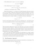
Fig. 1. Simulated regression setting. Solid curve is underlying regression. Residuals are Gaussian. Dashed curves are moving weighted averages, with Gaussian weights, represented at the bottom. Standard deviations in the weight functions are: Fig. 1b, 0.015; Fig. 1c, 0.04; Fig. 1d, 0.12

tions from too far away appear in the averages, with the effect of introducing some bias , or in other words features of the underlying curve that are actually present have been smoothed away. The very large amount of flexibility in nonparametric curve estimators, demonstrated by changing the window width in the example of Fig. 1, allows great payoffs, because these estimators do not arbitrarily impose structure on the data, which is always done by parametric estimators. To see how this is the case, think of doing a simple linear regression least squares fit of the data in Fig. 1. Of course, if the structure imparted by a parametric model is appropriate, then that model should certainly be used for inference, as the decreased flexibility allows for much firmer results, in terms

Smoothing Parameter Selection

67

of more powerful hypothesis test, and smaller confidence intervals. However it is in cases where no model readily suggests itself, or there may be some doubt as to the model, that nonparametric curve estimation really comes to the fore. See Silverman (1986) and HardIe (1988) for interesting collections of effective data analyses carried out by these methods. However there is a price to be paid for the great flexibility of nonparametric methods, which is that the smoothing parameter must be chosen. It is easy to see in Fig. I which window width is appropriate, because that is a simulation example, where the underlying curve is available, but for real data sets, when one has little idea of what the underlying curve is like, this issue clearly becomes more difficult. Most effective data analysis using non parametric curve estimators has been done by choosing the smoothing parameter by a trial and error approach consisting of looking at several different plots representing different amounts of smoothness. While this approach certainly allows one to learn a great deal about the set of data, it can never be used to convince a skeptic in the sense that a hypothesis test can. Hence there has been a search for methods which use the data in some objective, or "automatic" way to choose the smoothing parameter. This paper is a survey of currently available automatic smoothing parameter selection techniques. There are many settings in which smoothing type estimators have been proposed and studied. Attention will be focussed here on the two most widely studied, which are density and regression estimation, because the lessons seem to be about the same for all settings. These problems are formulated mathematically in Section 2. There are also many different types of estimators which have been proposed in each setting, see for example Prakasa Rao (1983), Silverman (1986), and HardIe (1988). However all of these have the property that, as with the moving average estimator in Fig. 1, their performance is crucially dependent on choice of a smoothing parameter. Here again the lessons seem to be about the same, so focus is put on just one type of estimator, that is kernel based methods. These estimators are chosen because they are simple, intuitively appealing, and best understood. The form of these are given in Section 2. Other important estimators, to which the ideas presented here also apply include histograms, the various types of splines, and those based on orthogonal series. To find out more about the intuitive and data analytic aspects of non parametric curve estimation, see Silverman (1986) for density estimation, and see Eubank (1988) and HardIe (1988) for regression (the former regression book requires more mathematical knowledge of the reader, and centers around smoothing splines, the latter is more applied in character, with the focus on kernel estimators). For an access to the rather large theoretical literature, the monograph by Prakasa Rao (1983) is recommended. Other monographs on curve estimation, some of which focus on some rather specialized topics, include Tapia and Thompson (1978), Wertz (1978), Devroye and Gyorfi (1984), Nadaraya (1983) and Devroye (1987). Survey papers have been written

J. S. Marron

68

on density estimation by Wegman (1972), Tarter and Kronmal (1976), Fryer (1977), Wertz and Schneider (1978) and Bean and Tsokos (1980). Collomb (1982, 1985) and Bierens (1987) provide surveys of nonparametric regression. See Ullah (1987) for discussion of both settings as well as others. Section 2 of this paper introduces notation. Section 3 discusses various possibilities for "the right amount of smoothing", and states an important asymptotic quantification of the smoothing problem. Section 4 introduces and discusses various methods for automatic bandwidth selection in the density estimation context. This is done for regression in Section 5. Section 6 discusses some hybrid methods and related topics.

2 Mathematical Formulation and Notation The density estimation problem is mathematically formulated as follows. Use independent identically distributed observations, Xl' ... , X n' from a probability density f(X), to estimate f(x). The kernel estimator of f. as proposed by Rosenblatt (1956) and Parzen (1962), is given by

ｦｾＨｸＩ＠

= n- 1 ｾ＠

n

Kh(x - Xi),

i=l

where K is often taken to be a symmetric probability density, and KhO = K(·jh)Jh. See Chapter 3 of Silverman (1986) for a good discussion of the intuition behind this estimator and its properties. The smoothing parameter in this estimator is h. often called the bandwidth or window width. Note that the estimator could have been dermed without h appearing as a separate parameter, however because the amount of smoothing is so crucial it is usually represented in this form. One way of formulating the nonparametric regression problem is to think of using Yi = m(xi) + fi'

i=I, ... ,n,

where the fi are mean zero errors, to estimate the regression curve, m(x). This setup is usually called "fixed design" regression. A widely studied alternative is "stochastic design" regression, in which the xi's are treated as random variables. While mathematical analysis of the two settings requires different techniques, the smoothing aspects tend to correspond very closely, so only the fixed design is explicitly formulated here. See Chapter 2 of Hardle (1988) for a formulation of the stochastic design regression

Smoothing Parameter Selection

69

problem. Kernel estimators in regression were introduced by Nadaraya (1964) and Watson (1964). One way to formulate them is as a weighted average of the form n

mh(x) = 1: Wi(x, h)Y;, ;=1

where the weights are defined by n

W;(x, h)=Kh(x-X;)/ 1: Kh(x-Xi ). ;=1

See Section 3.1 of HardIe (1988) for discussion of this estimator, and a number of other ways of formulating a kernel regression estimator. In both density and regression estimation, the choice of the kernel function, K, is of essentially negligible concern, compared to choice of the bandwidth h. This can be seen at an intuitive level by again considering Fig. 1. Note that if the shape of the weight functions appearing at the bottom is changed, the effect on the estimator will be far less than is caused by a change in window width. See Section 3.3.2 of Silverman (1986) and Section 4.5 of HardIe (1988) for a mathematical quantification and further discussion of this.

3 "Right" Answers The traditional method of assessing the performance of estimators which use an automatic smoothing parameter selector, is to consider some sort of error criterion. The usual criteria may be separated into two classes, global and pointwise. As most applications of curve estimation call for a picture of an entire curve, instead of its value at one particular point, only global measures will be discussed here. The most commonly considered global error criteria in density estimation are the Integrated Squared Error (Le. the L2 norm), ISE(h) = f [ih - 1]2. and its expected value, the Mean Integrated Squared Error MISE

=E(ISE(h ».

70

J. S. Marron

Related criteria are the Integrated Absolute Error (Le. the L 1 norm), IAE

=f

ｉｦｾ＠

- f I,

and its expected value, MIAE

=E(IAE(h»,

There are other possibilities such as weighted versions of the above, as well as the supremum norm, Hellinger distance, and the Kullback-Leibler distance. In regression, one can study the obvious regression analog of the above norms, and in addition there are other possibilities, such as the Average Squared Error, n

ASE(h)=n- 1 1; [mh(x;)-m(x;)]2,

;=1

and its expected value. MASE(h) =E(ASE(h».

For the rest of this paper, the minimizers of these criteria will be denoted by an h with the appropriate subscript, e.g. h M1SE ' An important question is how much difference is there between these various criteria. In Section 6 of their Chapter 5. Devroye and Gyorfi (1984) report that there can be a very substantial difference between h MISE and hMIAE in density estimation. However. this issue is far from clear, as Hall and Wand (1988) point out that, for several specific densities, the difference betweeen h AMISE and h AMIAE is very small. Given that there is an important difference between the squared error and the absolute error type criteria, there is no consensus on which should be taken as "the right answer". Devroye and Gyorfi (1984) point out a number of reasons for studying density estimation with absolute error methods. This has not gained wide acceptance though. one reason being that squared error criteria are much easier to work with from a technical point of view. The result of this is that all of the real theoretical breakthroughs in density estimation have come first from considering squared error criteria, then with much more work, the idea is extended to the absolute error case. The issue of the difference between the random criteria, such as ISE and IAE, and their expected values, such as MISE and MIAE, seems more clear. In particular it has been shown by Hall and Marron (1987a) that h ISE and h MISE do converge to each

Smoothing Parameter Selection

71

other asymptotically, but at a very slow rate, and may typically be expected to be quite far apart. Here again there is no consensus about which should be taken as "the right answer". ISE has the compelling advantage that minimizing it gives the smoothing parameter which is best, for the set of data at hand, as opposed to being best only with respect to the average over all possible data sets, as with MISE. However, acceptance of ISE as the "right answer" is controversial because ISE is random, and two different experimenters, whose data have the same underlying distributions, will have two different "right answers". TIlls type of reason is why statistical decision theory (see for example Ferguson 1967) is based on "risk" instead of on "loss". See Scott (1988) and Carter, Eagleson and Smith (1986) for further discussion ofthis issue. One advantage of MISE is that it allows a very clean asymptotic summary of the smoothing problem. In particular, for kernel density estimation, if K is a probability density andfhas two continuous derivatives, then as n ｾ＠ 00 and h ｾ＠ 0, with nh ｾ＠ 00, MISE(h) = AMISE(h) + o (AMISE(h », where

see for example (3.20) of Silverman (1986). Recall from Fig. 1, that too small a window width results in too much sample variability. Note that this is reflected by the first term (usually called the variance term) in AMISE becoming too large. On the other side, the fact that a too large window width gives too much bias, is reflected in the second term which gets large in that case. There is a tendency to think of h AMISE as being the same as h MISE , and this seems to be usually nearly true, but can be quite far off sometimes. Scott (1986) has shown that for the lognormal density AMISE and MISE will still be very far apart even for sample sizes as large as a million. See Dodge (l986) for related results concerning pointwise error criteria.

4 Density Estimation In this section most of the automatic bandwidth selectors proposed for kernel density estimation are presented and discussed. It should be noted that most of these have obvious analogs for other types of estimators as well.

J. S. Marron

72

4.1 Plug-in methods The essential idea here is to work with AMISE(h) and plug in an estimate of the only unknown part, which is f (f")2 . Variations on this idea have been proposed and studied by Woodroofe (1970), Scott, Tapia and Thompson (1977), Scott and Factor (1981), Krieger and Pickands (1981), and Sheather (1983, 1986). Most of the above authors consider the case of pointwise density estimation, but the essential ideas carryover to the global case. A drawback to this approach. is that estimation of f (f")2 requires specification of a smoothing parameter. The argument is usually given that the final estimator is less dependent on this secondary smoothing parameter, but this does not seem to have been very carefully investigated·. An interesting approach to the problem is given in Sheather (1986). A second weakness of the plug-in estimator is that it targets AMISE, which can be substantially different from MISE. A major strength of the plug-in selector is that, if strong enough smoothness assumptions are made, then it seems to have much better sample variability properties than many of the selectors in the rest of Section 4. see remark 4.6 of Hall and Marron (1987a). For plug-in estimators in the absolute error setting, see Hall and Wand (1989). Related results. which can be applied to pointwise absolute error bandwidths can be found in Hall and Wand (1988).

4.2 Psuedo Likelihood Cross-Validation Also called Kullback-Leibler cross-validation. this was proposed independently by Habbema. Hermans and van den Broek (1974) and by Duin (1976). The essential idea is to choose that value of h which maximizes the psuedo-likelihood, n

II !h(Xj ), j=l

However this has a trivial minimum at h = 0, so the cross-validation principle is invoked by replacing!h in each factor by the leave one out version,

Smoothing Parameter Selection

73

Another viewpoint on why the leave-one-out estimator is appropriate here is that the original criterion may be considered to be using the same observations to construct the estimator, as well as assess its performance. When the cross-validation principle (see Stone 1974) is used to attack this problem, we arrive at the modification based on using the leave-one-out estimator. Schuster and Gregory (1981) have shown that this selector is severely affected by the tail behavior of f Chow, Geman, and Wu (1983) demonstrated that if both the kernel and the density are compactly supported then the resulting density estimator will be consistent. The fact that this consistency can be very slow, and the selected bandwidth very poor, was demonstrated by Marron (1985), who proposed an efficient modification of the psuedo-likelihood based on some modifications studied by Hall (1982). Hall (1987a, b) has provided a nice characterization of the pseudo-likelihood type of cross-validation, by showing that it targets the bandwidth which minimizes the Kullback-Leibler distance between ih and f Hall goes on to explore the properties of this bandwidth, and concludes that it may sometimes be appropriate for using a kernel estimate in the discrimination problem, but is usually not appropriate for curve estimation. For this reason, psuedo-likelihood currently seems to be of less current interest than the other smoothing parameter selectors considered here.

43 Least Squares Cross-Validation This was proposed independently by Rudemo (1982a) and by Bowman (1984). The essential idea is to target ISE(h) = ｦｪｾ＠

-2

fihf+ ff2.

The first term of this expansion is available to the experimenter, and the last term is independent of h. Using a method of moments estimate of the second term results in the criterion.

which is then minimized to give a cross-validated smoothing parameter. The fact that the bandwidth chosen in this fashion is asymptotically correct for ISE, MISE, and AMISE has been demonstrated, under various assumptions, by Hall (1983, 1985), Stone (1984), Burman (1985) and Nolan and Pollard (1987) (see Stone

74

J. S. Marron

1985 for the histogram analog of this). Marron and Padgett (1987) have established the analogous result in the case of randomly censored data. A comparison to an im· proved version of the Kullback·Leibler cross-validation was done by Marron (1987a). The main strength of this bandwidth is that it is asymptotically correct under very weak smoothness assumptions on the underlying density. Stone (1984) uses assumptions so weak that there is no guarantee that fh will even be consistent, but the bandwidth is still doing as well as possible in the limit. This translates in a practical sense into a type of robustness. The plug-in selector is crucially dependent on AMISE being a good approximation of MISE, but least squares cross-validation still gives good asymptotic performance, even in situations where the MISE:::::: AMISE approximation is very bad. A drawback to least squares cross-validation is that the score function has a tendency towards having several local minima, with some spurious ones often quite far over on the side of undersmoothing. This does not seem to be only a small sample aberation, as Scott and Terrell (1987) noticed it in their simulation study even for very large samples. For this reason it is recommended that minimization be done by a grid search through a range of h's, instead of by some sort of computationally more efficient step·wise minimization algorithm (which will converge quite rapidly, but only to a local minimum). An unexplored possibility for approaching the local minimum problem is to select the bandwidth which is the largest value of h for which a local minimum occurs. Another major weakness of the least squares cross-validated smoothing parameter is that it is usually subject to a great deal of sample variability, in the sense that for different data sets from the same distributions, it will typically give much different answers. This has been quantified asymptotically by Hall and Marron (1987a), who show that the relative rate of convergence of the cross-va1i4ated bandwidth to either of hISE or h MISE is excruciatingly slow. It is interesting though that the noise level is of about the same order as the relative difference between h lSE and h MISE . This is the result referred to in Section 3, concerning the practical difference between random error criteria and their expected values. While the noise level of the cross-validated bandwidth is very large it is rather heartening that the same level exists for the difference between the two candidates for "optimal", in the sense that the exponents in the algebraic rate of convergence are the same. This leads one to suspect that the rate of convergence calculated by Hall and Marron (1987a) is in fact the best possible. This was shown, in a certain minimax sense, by Hall and Marron (1987b). To keep this in perspective though, note that the constant multiplier of the rate of convergence of the optimal bandwidths to each other is typically smaller than for cross-validation. Since the rates are so slow, it is these constants which are really important. See Marron (1987b) for further discussion. Recall that an attractive feature of the plug-in bandwidth selectors was their sample stability. These selectors have a faster rate of convergence to hAM ISE than the rate at which h lSE and h MISE come together. This does not contradict the above minimax

Smoothing Parameter Selection

7S

result because this faster rate requires much stronger smoothness assumptions. In settings of the type which drive the minimax result, the plug-in selectors will be subject to much more sample noise, and also h AMISE will be a very poor approximation to h MISE ·

A somewhat surprising fact about the least squares cross-validated bandwidth is that, although its goal is hISE , these two random variables are in fact negatively correlated! This means that for those data sets where h ISE is smaller than usual, the crossvalidated bandwidth tends to be bigger than usual, and vice versa. This phenomenon was first reported in Rudemo (1982a), and has been quantified theoretically by Hall and Marron (1987a). An intuitive explanation for it has also been provided by Rudemo, in terms of "clusterings" of the data. If the data set is such that there is more clustering than usual, note that h ISE will be larger than usual, because the spurious structure needs to be smoothed away, while cross-validation will pick a smaller bandwidth than usual because it sees the clustering as some fme structure that can only be resolved with a smaller window. On the other hand, if the data set has less clustering than usual, then hISE will be smaller than usual, so as to cut down on bias, while cross-validation sees no structure, and hence takes a bigger bandwidth. An interesting consequence of this negative correlation is that if one could find a stable "centerpoint", then (if ISE is accepted as the right answer) it would be tempting to use a bandwidth which is on the opposite side of this from h ev . A last drawback of least squares cross-validation is that it can be very expensive to compute, especially when the recommended grid search minimization algorithm is used. Two approaches to this problem are the Fast Fourier Transform approximation ideas described in Section 3.5 of Silverman (1986), and the Average Shifted Histogram approximation ideas described in Section 5.3 of Scott and Terrell (1987). HardIe, Marron and Wand (1988) have extended the least squares cross-validation idea to estimation of derivatives of a probability density.

4.4 Biased Cross-Validation This was proposed and studied by Scott and Terrell (1987). It is a hybrid combining aspects of both plug-in methods, and also least squares cross-validation. The essential idea is to minimize, by choice of h, the following estimate of AMISE(h),

Note that if the bandwidth used in the estimate of f (j"i were different from h, the bandwidth being assessed, then the selected bandwidth would be the same as the plug-

76

J.S.Marron

in bandwidth discussed in Section 4.1. The fact that the same h is used in the estimate of f (j"i is what makes biased cross-validation substantially different. Scott and Terrell (1987) show that the biased cross-validated bandwidth has sample variability with the same rate of convergence as least squares cross-validation, but with a typically much smaller constant coefficient. This is crucial as the rates are so slow that it is essentially the constant coefficients that determine performance of the selectors. Scott and Terrell (1987) also demonstrate the superior performance of biased cross-validation in some settings by simulation results. A drawback of biased cross-validation is that, like the plug-in, its effective performance requires much stronger smoothness assumptions than required for least squares cross-validation. It seems possible that in settings where biased cross-validation is better than least squares cross-validation, the plug-in will be better yet, and in settings where the plug-in is inferior to least squares cross-validation, biased crossvalidation will be as well, although this has not been investigated yet. Another weak point of biased cross-validation is that for very small samples, on the order of n = 25, Scott and Terrell (1987) report that the method may sometimes fail all together. in the sense that there is no minimum. This seems to be not as bad as the spurious local minima that occur for least squares cross-validation, because at least it is immediately clear that something funny is going on. Also unlike the spurious minima in least squares cross-validation, this problem seems to disappear rapidly with increasing sample size.

4.5 Oversmoothing

This idea has been proposed in Chapter 5, Section 6 of Devroye and Gyorfi (1984) and by Terrell and Scott (1985). The essential idea is to note that

h

AMISE

=(

f K2 )1/5 n- 1/5 2 (f x K)2 f (j"i .

The only part of this expression that is unvailable to the experimenter is f (f'i . If one could find a lower bound for this quantity, then by substituting the lower bound, one would obtain a bandwidth which is asymptotically larger (oversmoothed) than any of the squared error notions of "optimal" described above. For such a lower bound to exist, it turns out to be enough· that the scale of the f distribution is controlled, say by rescaling so that its variance is equal to one. Thus this oversmoothing idea can be reasonably implemented by rescaling through some estimate of the sample variance.

Smoothing Parameter Selection

77

The version of the oversmoothed bandwidth described here is that of Terrell and Scott, the Devroye and Gyorfi version is the L 1 analog of this idea. Terrell and Scott (1985) show that for unimodal densities, such as the Gaussian, the difference between the oversmoothed bandwidth and h AMISE is often surprisingly small. Another benefit of this is that it is very stable accross samples because the only place the data even enter are through the scale estimate, which has a fast parametric rate of convergence. Of course the oversmoothed bandwidth has the obvious drawback that it can be very inappropriate for multimodal data sets, which unfortunately are the ones that are most interesting when data is being analyzed by density estimation techniques. A possible application of the oversmoothed bandwidth, that has been suggested in some oral presentations given by David Scott, is that it can be used to provide an upper bound to the range of bandwidths considered by minimization based techniques such as the various types of cross-validation. The usefulness of this idea has not yet been investigated.

5 Regression Estimation Note that two of the ideas proposed above for density estimation, the plug-in selectors and biased cross-validation, can be directly carried over to the regression setting. Neither of these ideas has been investigated yet (although see Millier and Stadtmtiller 1987 for a local criterion based plug-in selector). In this section most of the automatic bandwidth selectors that have been considered for kernel regression estimation are presented and discussed. Again note that the ideas here have obvious analogs for other types of estimators as well.

5.1 Cross-Validation This was first considered in the nonparametric curve estimation context by Clark (1975) and Wahba and Wold (1975) for spline estimators. The essential idea is to use the fact that the regression function, m(x) is the best mean square predictor of a new observation taken at x. This suggests choosing the bandwidth which makes mh(x) a good predictor, or in other words taking the minimizer of the estimated prediction error, EPE(h) = n- 1 ｾ＠

n

;=1

[Y; - mh(Xj)]2.

78

J. S. Marron

This criterion has the same problem that was observed in Section 4.2, namely that it has a trivial minimum at h = O. As above this can be viewed as being caused by using the same data to both construct and assess the estimator, and a reasonable approach to this problem is provided by the cross-validation principle. Hence the cross-validated bandwidth is the one which minimizes the criterion obtained by replacing mh(Xj) by the obvious leave-one-out version. See Hardie and Marron (1985a) for a motivation of this criterion that is very similar in spirit to that for density estimation least squares cross-validation, as described in Section 4.3. The fact that the bandwidth chosen in this fashion is asymptotically correct was established by Rice (1984) in the fixed design context, and by Hardie and Marron (1985a) in the stochastic design setting. Hardie, Hall and Marron (1988) have shown that this method of bandwidth selection suffers from a large amount of sample variability, in a sense very similar to that described for the least squares cross-validated density estimation bandwidth in Section 4.3. In particular, the excruciatingly slow rate of convergence, and the negative correlation between the cross-validated and ASE optimal bandwidths are here also. See Marron (1987b) for further discussion. One thing that deserves further comment is that Rudemo has provided an intuitive explanation of the cause of the negative correlation in this setting, which is closely related to his intuition for density estimation, as described near the end of Section 4.3. TItis time focus on the lag-one serial correlation of the actual residuals (Le. on p(€j, €j+l))' Under the assumptions of independent errors, this will be zero on the average, but for any particular data set, the empirical value will typically be either positive or negative. Note that for data sets where the empirical serial correlation is positive, there will be a tendency for residuals to be positive in "clumps" (corresponding to the "clusters" described in Section 4.3). This clumping will require h ASE to be larger than usual, so as to smooth them away. Another effect is that cross-validation will feel there is some fine structure present, which can only be recovered by a smaller bandwidth. For those data sets with a negative empirical correlation, the residuals will tend to alternate between positive and negative. The effect of this is that the sample variability will be smaller than usual, so ASE can achieve a smaller value by taking a small bandwidth which eliminates bias. On the other hand, cross-validation does not sense any real structure, and hence selects a relatively large bandwidth. Methods of relating these ideas to bandwidth selection for derivatives of regression functions have been proposed by Rice (1986) and Milller, Stadtmilller and Schmitt (1987).

Smoothing Parameter Selection

79

5.2 Model Selection Methods There has been a great deal of attention to a problem very closely related to nonparametric smoothing parameter selection, which is often called "model selection". The basic problem can perhaps be best understood in the context of choosing the degree of a polynomial, for a least squares fit of a polynomial regression function, although the largest literature concerns choice of the order of an ARMA fit in time series analysis. To see that these problems are very similar to bandwidth selection, note that when too many terms are entered into a polynomial regression, the resulting curve will be too wiggly, much as for the small bandwidth curve in Fig. 1. On the other hand if too few terms are used, there will not be enough flexibility to recover all the features of the underlying curve, resulting in an estimate rather similar to the large bandwidth curve in Fig. 1. Given the close relationship between these problems, it is not surprising that there has been substantial cross-over between these two areas. The main benefit for nonparametric curve estimation has been motivation for a number of different bandwidth selectors. Rice (1984) has shown that the bandwidth selectors motivated by a number of these (based on the work of Akaike, Shibata and others), as well as the Generalized Cross Validation idea of Craven and Wahba (1979), all have the following structure. Choose the minimizer of a criterion of the form EPE(h) 1/I(h), where EPE(h) was defined in Section 5.1 above. The function 1/I(h) can be thought of as a correction factor, which has an effect similar to replacing the estimator by its leave-one-out version, as done by cross-validation, as described in Section 5.1 above. Rice (1984) shows that all of these bandwidths asymptotically come together, and also converge to h MASE , see U (1987) for a related result. HardIe and Marron (198Sb) show that extra care needs to be taken with these selectors when the design is not equally spaced, and the errors are not heteroscedastic. See Silverman (1985) for related discussion in the context of spline estimation. Deeper properties, concerning the sample variability of these bandwidths, have been investigated by Hardie, Hall and Marron (1988). It is shown there that, in a much deeper sense than that of Rice (1984), all of these bandwidths are asymptotically equivalent to each other and also to the cross-validated bandwidth discussed in Section 5.1. Hence all properties described for the cross-validated bandwidth apply to these as well.

80

J.S.Marron

5.3 Unbiased Risk Estimation This consists of yet another method of adjusting the estimated prediction error defined in Section 5.1. This essential idea was proposed by Mallows (1973) in the model selection context, and comes from considering the expected value of EPE(h). When this is done, it becomes apparent that the bias towards h too small can be corrected by minimizing a criterion of the form EPE(h) + 202 K(O)/nh,

where &2 is some estimate of the residual variance, a2 =E[ et]. There has been substantial work done on the non parametric estimation of a2 , see for example Kendall (1976). For more recent references, see Rudemo (1982b), Rice (1984), Gasser, Sroka and Jennen (1986) and Eagleson and Buckley (1987) for discussion of possible estimates of a2 . The results of Rice (1984) and HardIe, Hall and Marron (1988), described above, apply here to this type of selector as well. For an interesting connection to Stein shrinkage estimation see Li (1985). The main drawback to this type of selector is that it depends on an estimate of a2 , although this should not be too troubling, because there are estimates available with a fast parametric convergence rate, so the amount of noise in this estimation is at least asymptotically negligible. HardIe, Hall and Marron (1988) have demonstrated that, in a rather strong sense, the bandwidth selectors discussed in Section 5.2 are essentially equivalent to the unbiased risk estimator. The one important difference is that the latter uses an explicit estimate of a2 , while the former all essentially make use of the fact that EPE(h) provides an implicit estimate. An advantage of this selector over the selectors in Sections 5.1 and 5.2 is that it appears to handle settings in which reasonable values of the bandwidth are close to h =O. This happens typically when there is very small error variance, so not much local averaging needs to be done. It is immediately clear that cross-validation suffers in this type of context, but it can also be seen that the other selectors have similar problems. These issues have not been well investigated yet.

6 Extensions, Hybrids and Hopes for the Future There are many possibilities for modifying the above selectors, in the hopes of improving them. Also ideas from one setting may be used to generate ideas in the other. For example, the density estimation plug-in idea discussed in Section 4.1 has been

Smoothing Parameter Selection

81

adapted to regression by Miiller (1985) and Tsybakov (1987). Also biased cross-validation as discussed in Section 4.4 has an obvious regression analogue (on which David Scott reports he is currently working). Bhattacharya and Mack (1987) have studied a stochastic process that is closely related to the plug-in bandwidth selectors (they work explicitly with the nearest neighbor density estimator, but it appears that analogous ideas should hold for conventional kernel density and regression estimators as well). This gives a certain linear model, which is then used to give an improved bandwidth. It seems there may be room for improvement of this type of some of the other bandwidth selectors described above as well. Kappenman (1987) proposed a density estimation bandwidth selection method based on considering two estimates of f (f'')2. Mielniczuk and Vieu (1988)and Marron (1988) have shown that this bandwidth is not very useful in its present form, but it does provide a new set of ideas for finding bandwidth selection methods. For example, in Marron (1988) it is shown that a reasonable modification of J(appenman's bandwidth provides a new characterization of the least squares cross-validated bandwidth discussed in Section 4.3. Burman (1988) provides a detailed analysis and suggests improvement of v-fold cross-validation. The basic idea here is to replace the leave-one-out estimators by leaveseveral-out versions, and then assess the performance against each of the left out observations. This has the distinct advantage that it cuts down dramatically on the amount of computation required, at least if direct implementation is used (there seems to be less gain if an algorithm of one of the types described at the end of Section 4.3 is used). If too many observations are left out, then note that the selected smoothing parameter should be reasonably good, except that it will be appropriate for the wrong sample size (the size of the sample minus those left out). Burman provides a nice quantification of this, and goes on to use the quantification to provide an appropriate correction factor. Burman also provides similar results for another modification of cross-validation based on "repeated learning testing" methods. Another means of modifying cross-validation, and also a number of the other automatic bandwidth selectors, is through partitioning, as proposed by Marron (1987c). The basic idea here is to first partition the data into subsets. In density estimation this could be done randomly, while it may be more appropriate to take every k-th point in regression. Next construct the cross-validation score for each sample separately, and find the minimizer of the average of these score functions. When this is rescaled to adjust for the fact that the subset cross-validation scores are for much smaller sample sizes, the resulting bandwidth will often have, up to a point, much better sample stability than ordinary cross-validation. A drawback to this approach is that one must decide on the number of subsets to use, and this problem seems to closely parallel that of smoothing parameter selection. N. I. Fisher has pointed out (in personal correspondence) that partitioned crossvalidation seems subject to a certain inefficiency, caused by the fact that observations

82

J. S. Marron

are not allowed to "interact" with observations in the other subsets. He then proposed overcoming this problem by replacing the average over cross-validation scores for the partition subsets by an average of the scores over all possible subsets of a given size. Of course there are far too many subsets to actually calculate this score function, so an average over some randomly selected subsets should probably be implemented. TIlis idea has yet to be analyzed, although again the subsample size will clearly be an important issue. Wolfgang Hardie has proposed another possibility along these lines, for density estimation. The idea is to minimize a cross-validation score based on a subsample consisting of say every k-th order statistic, or perhaps of averages of blocks of k order statistics. The resulting sample would be much more stable with respect to the type of clusterings which drive Rudemo's intuition, regarding the noise in least-squares crossvalidation described near the end of Section 4.3. This idea has also not been investigated, and here again choice of k seems crucial.

7 Conclusions It should be clear from the above that the field of smoothing parameter selection is still in its infancy. While many methods have been proposed, none has emerged as clearly superior. There is still much comparison to be done, and many other possibilities to be investigated. The implications, in terms of actual data analysis, of what is knowJ;l currently about automatic methods of smoothing parameter selection, are that there is still no sure-fire replacement for the traditional trial and error method. This is where one plots several smooths, and then chooses one based on personal experience and opinion. Indeed none of these automatic methods should be used without some sort of verification of this type. Scott and Terrell (1987) have suggested the reasonable idea of looking at several automatically selected bandwidths, with the idea that they are probably acceptable when they agree, and there is at least a good indication that special care needs to be taken when they disagree. There are many things yet to be investigated in connection to this idea, especially in terms of how correlated all these automatically selected bandwidths are to each other. Also there is the issue of how many different bandwidths the user is willing to consider. Hopefully the field can at least be narrowed somewhat.

Acknowledgement: The author is grateful to a number of people who have pointed out oversights and inaccuracies in an earlier version of this paper.

Smoothing Parameter Selection

83

8 References Bean SJ Tsokos CP (1980) Developments in nonparametric density estimation. International Statistical Review 48:267-287 Bhattacharya PK, Mack KP (1987) Weak convergence of k·NN density and regression estimators with varying k and applications. Annals of Statistics 15 :976-994 Bierens HJ (1987) Kernel estimation of regression function. In: Bewley TF (ed) Advances in econometrics. Canbridge University Press, New York; pp 99-144 Bowman A (1984) An alternative method of cross-validation for the smoothing of density estimates. Biometrika 65 :521-528 Burman P (1985) A data dependent approach to density estimation. Zeitschrift ftir Wahrscheinlichkeitstheorie und verwandte Gebiete 69:609-628 Burman P (1988) Estimation of the optimal transformations using v-fold cross-validation and repeated learning testing methods. Unpublished manuscript Chow YS, Geman S, Wu LD (1983) Consistent cross-validated density estimation. Annals of Statistics 11 :25-- 38 Clark RM (1975) A calibration curve for radio carbon dates. Antiquity 49:251-266 Collomb G (1981) Estimation non parametrique de la regression: revue. International Statistical Review 49:75-93 Collomb G (1985) Nonparametric regressio: an up·to-date bibliography. Statistics 16:309-324 Craven P, Wahba G (1979) Smoothing noisy data with spline functions. Numerische Mathematik 31:377- 403 Devroye L, Gyarfi L (1984) Nonparametric density estimation: The Ll view. Wiley, New York Devroye L (1987) A course in density estimation. Birkhauser, Boston Dodge Y (1986) Some difficulties involving nonparametric estimation of a density function. Journal of Official Statistics 2:193-202 Duin RPW (1976) On the choice of smoothing parameters of Parzen estimators of probability density functions. IEEE Transactions on Computers C-25:1175-1179 Eagleson GK, Buckley MJ (1987) Estimating the variance in nonparametric regression. Unpublished manuscript Eubank R (1988) Spline smoothing and nonparametric regression. Wiley, New York Ferguson TS (1967) Mathematical statistics, a decision theoretic approach. Academic Press, New York Fryer MJ (1977) A review of some non-parametric methods of density estimation. Journal of the Instiute of Mathematics and its Applications 20:335-354 Gasser T, Sroka L, Jennen C (1986) Residuals variance and residual pattern in nonlinear regression. Biometrika 73:625-633 Habbema JDF, Hermans J, van den Broek K (1984) A stepwise discrimination analysis program using density estimation. Compstat 1974: Proceedings in Computational Statistics. Physica Verlag, Vienna, pp 101-110 HardIe W (1988) Applied nonparametric regression HardIe W, Marron JS (1985a) Optimal bandwidth selection in nonparametric regression function estimation. Annals of Statistics 12:1465-1481 HardIe W, Marron JS (1985b) Asymptotic nonequivalence of some bandwidth selectors in nonparametric regression. Biometrika 72:481-484 HardIe W, Hall P, Marron JS (1988) How far are automatically chosen regression smoothers from their optim urn? Journal of the American Statistical Association 83: 86-10 1, with discussion

84

J. S. Marron

Hardie W, Marron JS, Wand MP (1988) Bandwidth choice for density derivatives. Unpublished manuscript Hall P (1982) Cross-validation in density estimation. Biometrika 69:383-390 Hall P (1983) Large sample optimality of least square cross-validation in density estimation, Annals of Statistics 11 :1156- 1174 Hall P (1985) Asymptotic theory of minimum integrated square error for multivariate density estimation. Proceedings of the Sixth International Symposium on Multivariate Analysis at Pittsburgh,25-·29 Hall P (1987a) On the estimation of probability densities using compactly supported kernels. Journal of Multivariate Analysis 23:131-158 Hall P (1987b) On Kullback-Leibler loss and density estimation. Annals of Statistics 15 :1491-1519 Hall P, Marron JS (1987a) Extent to which least-squares cross-validation minimises integrated square error in nonparametric density estimation. Probability Theory and Related Fields 74:567- 581 Hall P, Marron JS (1987b) On the amount of noise inherent in bandwidth selection for a kernel density estimator. Annals of Statistics 15:163--181 Hall P Marron JS (1987c) Estimation of integrated squared density derivatives. Statistics and Probability Letters 6: 109 -115 Hall P, Wand M (1988) On the minimization of absolute distance in kernel density estimation. To appear in Statistics and Probability Letters Hall P, Wand M (1989) Minimizing L1 distance in nonparametric density estimation. To appear in Journal of Multivariate Analysis Kappenman RF (1987) A nonparametric data based univariate function estimate. Computational Statistics and Data Analysis 5 :1- 7 Kendall MS (1976) Time Series. Griffin, London Krieger AM, Pickands J (1981) Weak convergence and efficient density estimation at a point. Annals of Statistics 9 :1066 -1078 Li KC, Hwang J (1984) The data smoothing aspects of Stein estimates. Annals of Statistics 12: 887- 897 Li KC (1985) From Stein's unbiased risk estimates to the method of generalized cross-validation. Annals of Statistics 13 :1352--1377 Li KC (1987) Asymptotic optimality for Cp , CL, cross-validation and generalized cross-validation: discrete index set. Annals of Statistics 15 :958-975 Mallows CL (1973) Some comments on Cp , Technometrics 15:661-675 Marron JS (1985) An asymptotically efficient solution to the bandwidth problem of kernel density estimation. Annals of Statistics 13:1011-1023 Marron JS (1986) Will the art of smoothing ever become a science? Marron JS (ed) Function estimates. American Mathematical Society Series: Contemporary Mathematics 9 :169-178 Marron JS (1987a) A comparison of cross-validation techniques in density estimation. Annals of Statistics 15 :152- -162 Marron JS (1987b) What does optimal bandwidth selection mean for nonparametric regression estimation. Dodge Y (ed) Statistical data analysis based on the L 1 norm and related methods. North Holland, Amsterdam Marron JS (1987c) Partitioned cross-validation. North Carolina Institute of Statistics, Mimeo Series # 1721 Marron JS (1988) Improvement of a data based bandwidth selector. Unpublished manuscript Marron JS, Padgett WJ (1987) Asymptotically optimal bandwidth selection for kernel density estimators from randomly right-censored samples. Annals of Statistics 15: 1520-15 35

Smoothing Parameter Selection

85

Mielniczuk J, Vieu P (1988) Asymptotic suboptimality of one method of cross-validatory bandwidth choice in density estimation. Vnpublished manuscript MUller HG (1985) Empirical bandwidth choice for nonparametric kernel regression by means of pilot estimators. Statistics and Decisions, Supplement Issue No. 2:193-206 MUller HG, Stadtmilller V (1987) Variable bandwidth kernel estimators of regression curves. Annals of Statistics 15 :182--201 MUller HG, Stadtmilller V, Schmitt T (1987) Bandwidth choice and confidence intervals for derivatives of noisy data. Biometrika 74:743-749 Nadaraya EA (1964) On estimating regression. Theory of Probability and its Application 9:141142 Nolan D, Pollard D (1987) V-processes: rates of convergence. Annals of Statistics 15 :780-799 Parzen E (1962) On estimation of a probability density function and mode. Annals of Mathematical Statistics 33:1065-1076 Prakasa Rao BLS (1983) Nonparametric functional estimation. Academic Press, New York Rice J (1984) Bandwidth choice for nonparametric regression. Annals of Statistics 12:1215-1230 Rice J (1986) Bandwidth choice for differentiation. Journal of Multivariate Analysis 19:251-264 Rosenblatt M (1956) Remarks on some non-parametric estimates of a density function. Annals of Mathematical Statistics 27 :832-837 Rosenblatt M (1971) Curve estimates. Annals of Mathematical Statistics 42:1815-1842 Rudemo M (1982a) Empirical choice of histograms and kernel density estimators. Scandanavian Journal of Statistics 9 :65 --78 Rudemo M (1982b) Consistent choice of linear smoothing methods. Report 82-1, Department of Mathematics, Royal Danish Agricultural and Veterinary Vniversity, Copenhagen Schuster EA, Gregory CG (1981) On the nonconsistency of maximum likelihood nonparametric density estimators. Eddy WF (ed) Computer Science and Statistics: Proceedings of the 13th Symposium on the Interface. Springer, New York, pp 295-298 Scott DW (1985) Handouts for ASA short course in density estimation. Rice Vniversity Technical Report 776-331-86-2 Scott DW (1986) Choosing smoothing parameters for density estimators. .In: Allen DM (ed) Computer Science and Statistics: The Interface, pp 225-229 Scott DW (1988) Discussion of HardIe W, Hall P, Marron JS, How far are automatically chosen regression smoothers from their optimum? To appear Journal of the American Statistical Association Scott DW, Factor LE (1981) Monte Carlo study of three data-based nonparametric probability density estimators. Journal of the American Statistical Association 76:9-15 Scott DW. Tapia RA, Thompson JR (1977) Kernel density estimation revisited. Nonlinear Analysis, Theory, Methods and Applications 1:339--372 Scott DW, Terrell GR (1987) Biased and unbiased cross-validation in density estimation. Journal of the American Statistical Association 82:1131-1146 Sheather SJ (1983) A data-based algorithm for choosing the window width when estimating the density at a point. Computational Statistics and Data Analysis 1 :229-238 Sheather SJ (1986) An improved data-based algorithm for choosing the window width when estimating the density at a point Computational Statistics and Data Analysis 4:61-65 Silverman BW (1985) Some aspects of the spline smoothing approach to nonparametric regression curve fitting (with discussion). Journal of the Royal Statistical Society, Series B 46:1-52 Silverman BW (1986) Density estimation for statistics and data analysis. Chapman and Hall, New York Stone CJ (1984) An asymptotically optimal window selection rule for kernel density estimates. Annals of Statistics 12:1285-1297

86

J. S. Marron: Smoothing Parameter Selection

Stone CJ (1985) An asymptotically optimal histogram selection rule. Proceedings of the Berkeley Symposium in Honor of Jerzy Neyman and Jack Keifer Stone M (1974) Cross-validatory choice and assessment of statistical predictions. Journal of the Royal Statistical Society, Series B 36:111-147 Tapia RA, Thompson JR (1978) Nonparametric probability density estimation. The Johns Hopkins University Press, Baltimore Tarter ME, Kronmal RA (1976) An introduction to the implementation and theory of nonparametric density estimation. The American Statistician 30:105-112 Terrell GR, Scott DW (1985) Oversmoothed density estimates. Journal of the American Statistical Association 80 :209 -214 Tsybakov AB (1987) On the choice of the bandwidth in kernel nonparametric regression. Theory of Probability and Its Applications 32:142-148 Ullah A (1987) Nonparametric estimation of econometric functionals. Research Report 18. University of Western Ontario, to appear in Canadian Journal of Economics Wahba G, Wold S (1975) A completely automatic fench curve: fitting spline functions by crossvalidation. Communications in Statistics 4:1-17 Watson GS (1964) Smooth regression analysis. Sankhya, series A 26:359-372 Wegman EJ (1972) Nonparametric probability density estimation: I. a summary of the available methods. Technometrics 14:533-546 Wertz W (1978) Statistical density estimation: a survey. Angewandte Statistique und Okonometrie 13, Vandenhoeck und Ruprecht Wertz W, Schneider B (1979) Statistical density estimation: a bibliography. International Statistical Review 49 :75-93 Woodroofe M (1970) On choosing a delta sequence. Annals of Mathematical Statistics 41:16651671

Bayes Prediction Density and Regression Estimation A Semiparametric Approach By R. C. Tiwari l • S. R. Jammalamadaka 2 and S. Chib 3

Abstract: This paper is concerned with the Bayes estimation of an arbitrary multivariate density, f(x), x E Rk. Such an f(x) may be represented as a mixture of a given parametric family of densities {h(xlll)} with support in Rk, where II (in R d ) is chosen according to a mixing distribution G.

We consider the semiparametric Bayes approach in which G, in turn, is chosen according to a Dirichlet process prior with given parameter . We then specialize these results when f is expressed as a mixture of m ultivaria te normal densities ct>(x IJ.L, A) where J.L is the mean vector and A is the precision matrix. The results are finally applied to estimating a regression parameter.

1 Introduction In a recent paper, Ferguson (1983) presents a nonparametric Bayes procedure for estimating an arbitrary density f(x) on the real line. This paper extends the results of Ferguson to the multivariate case and considers the estimation of the predictive density as well as the regression parameter. Consider a k x 1 random vector X = (Y, X 2 , ... , X k )' where, in the regression context, Y may be regarded as the dependent variable and (X2 , ... , X k ) as the set of independent variables. We assume that X has an unknown density f(x), x E Rk. Such an f(x) may be represented as a mixture of a multivariate normal densities {¢(x 1t1, A)}, i.e., f(x) = J ¢(xlt1, A)dG 0 is the degrees of freedom and A is a s.p.d. matrix of order k. We use the notation X - MVtk(ll, A, v) to denote that X has the pdf given by (7).

90

R. C. Tiwari et al.

Let o{) be a finite non-null finitely additive measure on (R d , R d ). A random probability measure P on (R d , R d ) is a Dirichlet process with parameter a, and write P ED(a), if for every finite s and every measurable partition A 1, ... , As of R d , the random variables (P(A 1, ... , peAs)) have the Dirichlet distribution with parameters (a(Ad, ... ,a(As))(cf. Ferguson 1973). Let 00 represent the degenerate probability measure at a single point 8. Let G be the distribution function associated with the random probability measure P. Then, under D(a), G can expressed as (cf. Sethuraman and Tiwari 1982):

00

G = ｾ＠

i=l

(8)

PiOO" I

where (i) 8 1 , 8z , ... , are iid on (R d , Rd ) with the common distribution Go

=aO/M,

(ii) (P1, pz, ... ) and (8 1 , 8z , ... ) are independent, (iii) q1 =P1,QZ =Pz/(I-pd,Q3 =P3/(1-P1 -Pz), ... are iid Beta (1,M),M= a(R d ). More generally than (1), one may assume that the unknown density "'(x) is expressed as a mixture of a family of k-variate densities {h(xI8)}, with the mixing distribution G (on 8) in R d , i.e., "'(x)

=f h(xI8)dG(8).

(9)

If this mixing distribution G, is assumed to have a Dirichlet prior, then from (8)

00

"'(x)

= ｾ＠

p;h(xI8;).

(10)

;=1

Let xl, ... ,x n be a random sample from "'(x) given by (9). This is equivalent to first choosing 8 1 , ... , 8 n i.i.d. from Go (8), and then xi from hex l8 i ), i = 1, ... , n independently. Then the posterior distribution of G given xl, ... , X n is a mixture of Dirichlet processes (cf. Antoniak 1974)

(11)

Bayes Prediction Density

where dH(O 1, is

... ,

On Ix 1, ... , xn), the posterior density of 0 1 ,

.•• ,

91

On given Xl, ... , Xn ,

with the notation M(n) = M(M + 1) .,. (M + n - 1). From (11) we have

A

1 n

=-

ｾ＠ 0lh is the empirical measure of the observed 0 1 , •.. , On and Go n i=l I corresponds to the normalized Q-measure. Consequently we have the following:

where Gn(-)

Theorem 1: The Bayes estimator of lj;(x) under squared error loss function, lj;n(x) E[ lj;(X)IXl, ... , xn], is given by

M n lj;n(x) = M + n lj;o(x) + M + n lj;n(x)

=

A

(13)

where lj;o(x), the estimate of lj;(x) for no sample size, is given by lj;o(X)

=Elj;(x) =J h(xIO)dGo(O)

(14)

and

(15)

The nonparametric Bayes estimate of lj;(x) is, therefore, seen to be a weighted average of the prior guess lj;o(x) given in (14), and ｾｮＨｸＩ＠ given in (15). Two special cases of interest as M, the strength in the prior goes to zero and infinity, may be considered as in Ferguson (1983).

92

R. C. Tiwari et al.

In particular, as M ｾ＠

00,

the 8;'s are all distinct and the prediction density is given

by 1 n l/J*(x) = - L l/J(xlxj), n ;=1

(16)

where

l/J(xlx;) =

f hex j8)h(x;18)dG o(8) f h(x j I8)dG o(8)

is the Bayes prediction density of x given the one observation x;.

3 Results for Normal Mixtures In this section we specialize the results of the previous section by letting () = (fJ., A) and hex 18) be a multivariate normal density with mean fJ. and the precision matrix A. We also let Go be the joint prior distribution of (fJ., A) given by

(17) and

(18) Now, let the unknown density [(x), be a random mixture of a multivariate normal densities as in (1) i.e., [(x)

=f (x 1fJ., A)dG(fJ., A)

where ( ·1fJ., A) is the pdf in (5).

(19)

Bayes Prediction Density

93

In (19), consider the special choice of a Dirichlet process prior for G with parameter ex =MG o , where Go is the natural conjugate prior of (11, A) given by (17) and (18) namely the normal-Wishart. It is important to note that nothing prevents us from choosing an arbitrary measure Go, as the prior of (J.

Lemma 1: Let (11, A) have a joint normal-Wishart prior given by (17) and (18). Then the prior guess of the prediction density at x'/o(x), is given by (see equation (14»

b*

It (x)ex ( 1 + - - (x - 11*)'A*(x - 11*)

)-(k+V*-k*+I)/2

b* + 1

o

(20)

a k-variate MVt density with mean vector 11*, precision matrix ... ,xil + (Sl -21 l )h ... ,xp)whereas x + (s,-21,)h =(Xl, ""Xi, + (s,.-21,)h ... ,xp). For r = I we get (2.5). Further for r =2 we get various cross derivatives. In what follows we consider the nonparametric estimation of the partial derivatives of R(x) without specifying its form. This is done by first considering a nonparametric estimator of R(x) and then taking its partial derivatives. Before presenting these we note that the partial derivatives discussed above are not confined to the regression model (2.2). In fact, although not considered here explicitly, the extension to dynamic models with stationary variables and system models are straightforward. For example, for the first order autoregressive model the regression functionin (2.1) becomes E(yly-t> where y-l is the lagged value of the stationary variable y. Similarly for the system model y will be a vector of say q endogenous variables and E(y Ix) will be a vector regression function. We restrict ourselves to the model for the sake of simplicity in exposition. The extension of the results to the simultaneous equations models is discussed in Section 5.

(2.2)

3 Estimation and Testing of Hypothesis 3.1 Estimation of Regression Function First we consider the non parametric kernel estimation of the regression function R(x) in (2.2) or (2.1). This can be obtained by the following methods.

Estimation and Hypothesis Testing

105

a) Nadaraya (1964) and Watson (1964) Method We observe that R(x) depends on the unknown densities. Thus, using the data on p + 1 variables z =(y, x) we first note from Rosenblatt (1956) for p = 1 and Cacoullos (1966) for p > 1 that

7

(Zi-Z)

1 n In(y, x) = In(z) = nh q K -h- •

q =p

+1

(3.1)

and

(3.2)

where h, the window-width (also called the smoothing parameter or band-width), is a positive function of the sample size n which goes to zero as n ｾ＠ 00, K is a kernel or weight function such that J K(z )dz = I, and K I (x) = J K(z )dy. The kernel K determines the shape of the curves and the window width h determines their width. For details on the kernel density estimation, see Prakasa-Rao (1983), Silverman (1986) and mlah (1988). Substituting (3.1) and (3.2) into (2.1) it can easily be verified that

n In(y, x) Rn(x) =Rn = Jy I () dy = l: yjWj(x) In X

(3.3)

1

where

K1(T) Wj(x) = n

( x.-x ) l: K - , I

I

(3.4)

h

Rn is known as the Nadaraya (1964) and Watson (1964) type regression function estimator. Thus kernel nonparametric regression estimates the unknown R(x) be a weighted average of the observed values of yj, where the weight of the i-th observation depends on the distance Xj to x through the kernel K. Note that in (3.3) the difference between

106

A. Ullah

Xi and X is scaled by window width h surrounding the point x over which the data are

averaged. SubstitutingRn into (2.2) gives the nonparametric model:

(3.5) where e is the nonparametric residual. We observe that this nonparametric model (3.5) has been obtained without making assumptions about the functional form of the R(x).

b) The Least Squares Method The Nadaraya-Watson estimator Rn defined in (3.3) can be viewed as a weighted least squares (LS) estimator of R(x). This is because Rn is the value of R(x) for which the weighted squared error

(3.6)

is minimum. This is obtained by solving

as

n

aR(x) =2 t K

(x.7-x)(Yi-R(X»=O

(3.7)

or

n

t

(x.-x) Yi=R(X)t K(x.-x) K'7 ｾ＠ n

for R(x). The solution is identical with (3.3).

(3.8)

Estimation and Hypothesis Testing

107

c) Method of Moments

In (2.2), note that E(ulx) = 0 by construction. Thus for any kernel function of x we get the following moment condition.

EK (

T-x X

)

(3.9)

u=O

where Xo is a fixed point. A sample estimate of this is

O) 1 n 1 n (Xi-XO) -"L K (xi-X - - ui=-"LK - - (Yi-R(X))=O, nl

h

nl

h

(3.10)

and we would choose R(x) for which this holds. The solution will be the same as (3.3). We note that since Rn in (3.3) is a weighted average of the Yi it may be sensitive to fluctuations in the data. In such situations a robust family of estimators can be developed as a solution of R in

(3.11 )

where 1/In is a bounded function for all x satisfying some regularity conditions; see Collomb and Hardie (1986) and Hardie (1984). The choice of a family of bounded functions 1/1 x in (3.11) guarantees bounded influence and suggests more stable prediction properties. The unbounded influence function 1/1 Au) =u gives the classical Nadaraya-Watson estimator Rn(x). In the Nadaraya-Watson regression estimator, Rn, the window width h is the same under all the data points. An alternative is to consider

(3.12)

where hi denotes a sequence of positive numbers. The estimator (3.12) is known as the recursive regression estimator. The hi is assumed to satisfy ｾ＠ hf ｾ＠ 00 as n ｾ＠ 00. This

108

A. Ullah

estimator was first examined by Ahmad and lin (1976) and later by Greblicki and Krzyzak (1980), Devroye and Wagner (1980a), Gyorfi (1981), Krzyzak and Pawlak (1984) and Singh and Ullah (1986). For hi =h in (3.12) we get (3.3). An alternative estimator, which suppresses hiP from (3.12), is given as

Yi K (Xi - --X)

＠ｾ n -

Rn(x) =

hi

I

ｾｋ＠

n

( X-X )

I

hi

(3.13)

_i_

This estimator has been studied by Devroye and Wagner (1980a), Krzyzak and Pawlak (1984) and Greblicki and Pawlak (1987). Note that this estimator is obtained by simply replacing It by hi in (3.3). We note that the estimators Rn(x) and Rn(x) are recursive in the sense that when an additional data point becomes available it can be updated according to

(3.14)

(3.15)

where 'Yn = 'Yn-l + K

X -X) ,'Yo = O. When 'Yn in (3.15) is replaced by nhP then the (1:-

estimator Rn is very similar to the recursive estimator obtained by the method of stochastic approximation (see Revesz 1977). Note that un =Y n - Rn - I (x) on the right hand of Rn(x) can be considered as one-step-ahead prediction error and it has been used to update the recursive estimator of R(x) as each new data becomes available. The new information at time n comes in the form of Un and R is estimated by updating Rn_ l . The residuals U so generated can be called as nonparametric recursive residuals. Stone (1977) has considered a class of regression estimator (3.3) in which the weight function Wi (x) is the weight with the property that values of i where Xi is close to X get higher weight than those that are far from x. The weight function Wi is said to be a probability weight function if ｾ＠ Wt(x) = 1 and nonnegative if wi ｾ＠ O. The k-nearest neighbor weight estimator is a special case and it is

Estimation and Hypothesis Testing

ｒｾＨｸＩ＠

= ｾ＠

109

n

y7wi

(3.16)

1

where Wi = 11k, 1 .;;;; i';;;; k and Wi =0 elsewhere, and yt is the reordered data of y according to increasing values of the norm IIx i-X II. Note that x's in (2.2) are stochastic. However, if they are fixed "design" variables such as time and age then R(x) can be estimated by various nonparametric curve fitting procedures. Among the prominent methods are smoothing splines (Reinsch 1967); kernel estimator (Priestley and Chao 1972; Ahmad and Un 1984); and local regression (Stone 1977; Muller 1987). Silverman (1984) has shown that smoothing splines are essentially equivalent to kernel estimates with certain kernels if the Xi are equidistantly spaced, where some Sort of adaptation to local nonequidistance takes place if the Xj are not equidistancely spaced. In addition to above estimators, Johnston (1982) has considered the estimator of R(x) when 11 (x) is known. The properties of his estimator are discussed in HardIe and Kelly (1987). Finally, we note here that the regression estimators discussed above are under the assumption that Uj in (2.2) have the same variances and they are independent. However if V(u) = ｾ＠ is an n x n positive definite matrix either due to heteroskedasticity or serial correlation one could obtain the generalized least squares (GLS) estimator of R(x). For this, it is convenient to note that the least squares estimator in vector notation, corresponding to (3.6), is to minimize (y - LR(x))'K(y - LR(x)) =u'K 1/ 2K1/ 2u

(3.17)

with respect to R(x), where L = [1 ... 1]' and K = D(K 1 , ... , K n) is an n x n diagonal matrix with K j =K«xj - x)lh). This gives Rn = (L'KL)-1 L'Ky

(3.18)

which is equal to (3.3). In fact (3.18) can be calculated by the least squares regression of K1/2y on K1/2 L. Thus if V(u) = ｾ＠ then the GLS estimator of R(x) can be obtained by minimizing u'K 1/ 2 ｾＭＱ＠ K 1/2 u. This gives (3.19) For

ｾ＠

= I, (3.19) reduces to (3.18).

110

A. Ullah

Before turning to the estimation of partial derivatives we note that Rn is useful for nonparametric forecasting. Also. since Rn is the estimator of conditional expectation it provides a way out of specifying expectation variables appearing in various econometric variables, e.g., rational expectation models. For forecasting, see Ullah and Singh (1985) and Moschini et al. (1988).

3.2 Estimation of Partial Derivatives A consistent estimator of the response coefficient /3(x) (first derivative of R(x)) in (2.3) is simply _ /3(x)

R(x +h)-R(x -h) 2h .

(3.20)

=

But this is not operational since R(x ± h) is not known. An operational version is

(3.21)

where Rn(x) is the regression estimator given in (3.3) Similarly the estimators of the s-th order derivative of R(x) in (2.5) and the cross derivatives in (2.6) can be written by replacing R( ) with Rn( ). Thus, the estimator of /3(a) (x ) in (2.5) is

(3.22)

and that of cross derivatives, following (2.5), is

｢ｾ｡ＱＫ＠

... +ar)= ( _1 2h

)'1

1

+ ... +a r aｾ＠

11 =0

r ... ｾ＠ a (-ll1+ ... + lr ( S1 ) Ir=O 11

XR(X+(S1- 2/dh, ... x+(sr- 2Ir)h).

.••

(Sr) Ir

Estimation and Hypothesis Testing

III

The estimator (3.22) and its properties have been considered in Ahmad and Ullah (1987). For s = 1, (3.21) reduces to (3.20) and this has been considered in Rilstone (1987) and Rilstone and Ullah (1987). Ullah and Vinod (1988) proposed the estimator of (3(x) = 3R(x )/3x as an analytical derivative of Rn(x) in (3.3). Their estimator is

(3.23)

where wli =K' «Xi - X)/ h)/"L K(Xi - x)/h) and w2i =Wi(X) "L wli; Wi(X) is as in (3.4) and K'«Xi-X)/h)=3K«Xi-X)/h)/3xj. Numerically (3n(x)=b n(x). However in contrast to bn(x), the derivation of asymptotic properties as well as calculations of Bn(x) (especially of higher order derivatives) would be difficult. An alternative derivation of Pn(x) and its generalization for higher order derivatives can be obtained as below. Let us write from (2.1), usingfl (x) = f(x),

R(x)=

fyf(y, x)dy g(x) fleX) = f(x)

(3.24)

or R(x )f(x) =g(x). Differentiating it with respect to Xj we get s-th order derivative of R(x), (3(S) (x ), as a solution of

(3.25)

The estimator of fj 2. Another variant of nonparametric estimation is the Fourier method advocated by Gallant (1982). In this (1) is approximated by a quadratic polynomial in Xi and a linear combination of cosine and sine terms in Xi

=0iO

i

Yj

2

M

=(30 + (31Xj + {3zXj + L

('Yj cosjXj + OJ sinjxj) + Vj.

(7)

j=l

Table 1. Values of c to Construct Kernel in (6) 1=2

Co c1 c2 c3

1

1=4

1.5 -0.5

1=6

1.875 -1.25 0.125

1=8

2.1875 -2.1875 0.4375 -0.02083

134

Y. Hong and A. Pagan

The formulation has its origins in approximation theory where it is known that a Fourier series can approximate g(Xj) arbitrarily well over the range (0, 27T) (in fact to use this method data must be scaled to be in this range). For economic analysis the Fourier technique has the extra advantage that it also approximates derivatives of g(x;) with respect to Xj arbitrarily well, and this is important as these derivatives correspond to economic quantities of interest such as the marginal product. Provided M is chosen such that M 00 as N 00 and g(.) is sufficiently smooth, the estimator of g(x*) formed as the OLS predictions from (7) is consistent. Andrews (1988) shows that, if M is set to eN'". where e is a constant and 0 < r < 1, (Nl-r)1/2 (g(x*) - g(x*» is asymptotically normal. The choice of r is therefore akin to that of the bandwidth in kernel regression. If the problem of bias is ignored or eliminated by bias reducing methods N 2 /(q+4)(m* - m*) is asymptotically normal, and writing the normalizing factor as (N' Ni- j, where 4>i = t/li-E(t/ljl 11). Engle's (1982) ARCH model for example sets

｡ｾ＠

= ao

+

.f (lj4>;_j'

]=1

Pagan and Ullah (1988) advance an estimation strategy that seeks to avoid the The basic idea advanced in that paper was to replace ｡ｾ＠ by parameterization of ｡ｾＮ＠ 4>; = (t/li - E( t/ltl Fj))2 , and to then conSistently estimate {j and li by applying N with instruments constructed from Fj (including Xj as its own instrument). Of course instrument construction needs to be done carefully, since they must be as highly correlated with 4>; as possible. In fact, because E(4); I Fi ) = ｡ｾＬ＠ ｡ｾ＠ appeals as a good instrument, making it desirable to estimate ｡ｾ＠ for this purpose. An important facet of the IV strategy is that it only requires mj = E( t/lil Fj) to be estimated accurately; truncation of the instrument set to (say) = E(4); I Fj), where Fi E Fi, does not affect the consistency of the estimators of (j and li, although efficiency might be affected if ｡ｾ＠ has only a weak correlation with Ｔ＾ｾＮ＠ Overall, there is a trade-off between maximizing instrument correlation and restricting "Pi to be small enough to get estimates that are not "too noisy". Basically the N approach requires the computation of mj = E( t/ltl Fj) and some (although as noted above it is not crucial that the latter be accurate). estimate of As described earlier, mi might be linear in the members of ft Le., W;'Y, and this is a frequent assumption in VAR modeling. If so mi can be estimated as the predictions from the regression of t/li against Wj. However, in some instances it may be desirable to allow mt to be a non-linear function of Fi, and then it could be estimated in the same way as g(x*) was estimated earlier. Whichever wayan estimate for mj, mj, is generated, ｾ［＠ = (t/li - mti replaces and an instrument is used for ｾ［＠ . In Section 4 we use as instruments the non parametric estimate of the conditional variance of t/I j given "Pt. Now although neither mj nor is likely to be estimated very precisely unless dim (ft) is small or the number of observations is large, these quantities are only being used as "regressors" in (8), and so the N estimator of (j and li should be root-N consistent and asymptotically normal. To get this result, following Pagan and Ullah (1988) it is necessary to show that N- 1/ 2 r, ｚｩＨｾ［＠ - 4>h ｾ＠ 0, where Zi are the chosen instruments. When the conditional mean is parameterized as wt'Y this is true, as discussed in Pagan (1984) and exploited in tests for heteroskedasticity, but no general proof currently exists when 4>i is estimated nonparametrically, particular when t/li is a time series. An alternative estimator, if Fi = Fj , might be to regress Yi against Xi and as this would give a consistent estimator of li, {j, but the standard errors would need to be adjusted because of a "generated regressor" bias arising from the use of rather than Just as in the case when is constructed parametrically from Fi , Pagan (1984), the appropriate adjustment may be difficult to do directly, but is easily done with the IV procedure. Hence. estimation and inference is naturally performed within the N framework.

a;

a;

a;

a;

a;

a;

a; ,

at.

a;

at

136

Y. Hong and A. Pagan

The final issue to be addressed concerns which non parametric method should be used to construct mi and In Section 4 we employ both the kernel based approach and the Fourier method. Both are easy to apply and have advantages. It should be noted that for the Fourier technique, is estimated as the predictions obtained by fitting a Fourier approximation to (t/Ji - mi)2 , since E( t/Ji - mi)2 = is the basis of such a regression.

of.

of

of

3 Kernel and Fourier Estimation of a CES Production Function White (1980) set up a simulation experiment to evaluate the ability of flexible functional forms to adequately approximate unknown regression functions. He simulated data from a CES production function

(9) In our first experiment K was fixed at the value 1.71, log Li was distributed uniformly over [0,1], ui was Li.d. (0,0.01) and p was set to be -5. This gives an unknown functional relation betweenYi and Xi = L i . The variance of Uj was chosen so as to get an R2 of around 0.9 when (9) is fitted with both L j and K j • Our aim is to estimate the functional relation gj = (LiS + 2(1.71)- S r(1/S) at selected points L* = 1.284, 1.568, 1.852, 2.136, 2.420. A variety of estimators was applied. Because of the bias problem the kernel estimator was computed with jackknifing (c5 = 0.25, 0.5 and 0.75) as in (5) and higher order kernels (I =4, 6, 8) as in (6). The number of terms in the Fourier approximation (7) (M) was set to 2, making it independent of sample size. Three sample sizes N = 60, 100 and 200 were used and 500 replications performed. Fig. 1, 2 and 3 graph gj evaluated at the five points L * detailed above along with the average estimates provided by the standard kernel (I = 2), jack-knifing (c5 = 0.75), a higher-order kernel (l = 8) and Fourier series estimators; the values of c5 and I represented the choices with smallest average bias. The bias problem with standard kernel estimators is immediately apparent, but neither of the bias reducing procedures is particularly successful in samples of size 60, with noticable bias at the lower end of the grid. As the sample grows the higher order kernel approach improves but the jackknifed estimator does not. Of course for this set of parameters the relative magnitude of the bias is small: what is important is its resilience to an increase in sample size. With other parameter combinations the magnitude of the bias could probably be made much greater.

Nonparametric Estimator Simulation

137

0

'"

'":': 0

:':

'"0--'

Z 0

60

::>0

0--'

0

0:: CL

'"ｾ＠ 0

LEGEND

ｾ＠

• = True Value o = Standard Kernel o = Jacknifing Method o = Higher Order Kernel " = Fourier Approximation ｾ＠

ｾ＠

1.00

1.25

1.50

1.75

2.25

2.00

2.50

2.75

3.00

LABOR Fig. 1. Nonparametric Estimates of a CES Production Function

{N = 60}

o

ｾＬＭ＠

o

:':

'" z :3

o

F UO

::>0

0--'

o

8:

LEGEND • = True Value

o = Standard Kernel o = Jacknifing Method o = Higher Order Kernel " = Fourier Approximation 1.00

1.25

1.50

1.75

2.00

LABOR Fig. 2. Nonparametric Estimates of a CES Production Function {N = 100}

2.25

2.50

2.75

3.00

138

Y. Hong and A. Pagan

o

ｾＬＭ＠

..,

on

z":

o

i= Uo ｾＮＬ＠ 0":

o

If LEGEND

• = True Value

o = Standard Kernel o Jacknifing Methad a = Higher Order Kernel 6 Fourier Approximation

= = 3+-__ｾ＠ __ｾ＠ ____ｾ＠ __ｾ＠ __ｾ＠ __ｾ＠ ____ｾ＠ __ｾ＠ 1.00

1.25

1.50

1.75

2.00

2.25

2.50

2.75

3.00

LABOR

Fig. 3. Nonparametric Estimates of a CES Production Function {N = 200}

In contrast to the poor performance of the kernel estimators the Fourier method exhibits very small bias at all points in the L-space. In fact, simulations with N as low as 30 did not change this conclusion. Hence, for problems characterized by a single regressor in Xj, the Fourier estimator would seem to produce estimates of m* that are

Table 2. Average Estimates of gO for (9), Various Estimators, N = 60 L* = K* = 1.284

L* = K* = 1.852

L* = K* = 2.420

gO

1.0307

1.4867

1.9426

Fourier

1.0207

1.4758

1.9479

6 = 0 25 6=05 6 = 0.75

1.0000 0.9979 0.9964

1.4634 1.4713 1.4776

1.9303 1.9339 1.9364

1=2 1=4 1=6 1=8

1.0264 0.9871 0.9814 3.4396

1.4231 1.6257 1.4980 1.3363

1.8520 2.0040 1.9603 1.5865

Nonparametric Estimator Simulation

Table 3. Average Estimates of g(.) for (9), Various Estimators, N L*

=K* = 1.284

L*

= 100

=K* = 1.852

L*

=K* =2.420

g(.)

1.0307

1.4867

Fourier

1.0197

1.4777

1.9426 1.9336

6 =0.25 6 =0.5 6 =0.75

1.005 0.9989 0.9980

1.4680 1.4753 1.4805

1.9413 1.9446 1.9470

1 =2 1 =4 1 =6 1 =8

1.0225 0.9917 0.9950 1.0056

1.4317 1.6828 1.4701 1.5267

1.8735 1.9871 1.9456 1.8561

Table 4. Average Estimates of g(.) for (9), Various Estimators, N L*

=K* = 1.284

139

=200

L*=K*=1.852

L*

=K* =2.420

g(.)

1.0307

1.4867

1.9426

Fourier

1.0196

1.4747

1.9376

6 =0.25 6 =0.5 6 =0.75

1.000 0.9989 0.9991

1.4728 1.4789 1.4822

1.9498 1.9532 1.9556

1 =2 1=4 1 =6 1 =8

1.0176 0.9957 1.0053 1.0287

1.4421 1.5635 1.5706 1.5497

1.8939 1.9935 1.9862 1.9336

much closer to the true values than any of the kernel based procedures. Of course one might improve upon the kernel estimates by using variable bandwidths or selecting these by cross-validation: what the experiment emphasis is that bias is a potentially serious problem for kernel methods. When the complete production function is estimated, results are rather similar. In this instance log KI is distributed uniformly over [0, 1] and a grid of 25 points was taken corresponding to all bivariate combinations of the points (1.284,1.568,1.852, 2.136,2.420) for L * and K*. Tables 2, 3 and 4 show the average estimates of m* obtained for three of the combinations (L *, K*) = (1.284, 1.284), (1.852, 1.852) and (2.420, 2.420). A complete tabulation is available on request. Generally, the Fourier approximation does reasonably well, although it is noticeable that the bias does not reduce very much with the sample size and it may be that M should have been in-

140

Y. Hong and A. Pagan

creased. The basic kernel estimator (l = 2) is not dominated by the Fourier estimator as much as it was when Xj was a scalar, while the bias reduction methods perform well for large values of K and L but remain very poor at the left end of the grid. Indeed the best strategy might well be to stay with the raw kernel, as some of the higher-order kernel estimators (l> 2) are incredibly variable, with extreme outliers in a number of replications. These limited experiments emphasize the problem of asymptotic bias in the kernel estimator and, at least for a small number of conditioning variables, suggest that Fourier methods may well be the best way to approximate g(l What is very disappointing in the results is the relatively poor performance of methods that have been proposed to reduce the bias of standard kernel estimators. Perhaps these methods would work better in larger sample sizes, but it is obvious by comparing the first columns of Tables 2 and 4 that the improvement seems very slight, even when the sample size tripled. A much more detailed comparison between the estimators as well as investigation of other ways to reduce bias is therefore warranted.

4 Risk Estimation and ARCH Models In these experiments the parameter 0 in equation (8), with f3 = 0 and so Zj excluded, was estimated by nonparametric methods. The conditional variance of I/Ij, ｡ｾ＠ , followed variants of Engle's (1982) ARCH model, while I/Ij = 11 + rf>j. The density of the error term rf>j, conditional upon past information, was taken to be N(O, af}, with 0, the location parameter 11, and ｡ｾ＠ all being set to unity. Two experiments were performed, with ｡ｾ＠ being either an ARCH (1 ) or an ARCH (4) of the type used by Engle et al. (1987) when modeling the excess holding yield on U.S. Treasury Bills. 2 _

aj -

ｾｯ＠

ｾＱ＠

+

,/,2

(10)

'1'1-1

2 4 2

aj = ｾ＠

+ ｾＱ＠

ｾ＠

((5 - j)jl0)rf>j_j

(11)

j=1

Four estimators of 0 were considered. A) Estimate ｡ｾ＠ by a kernel estimator, with conditioning variables l/Ii-1, ... , I/Ii-r, r being the order of the ARCH process, and regress Yi against

of.

B) Replace ｡ｾ＠ in (8) by ｾ＠ = (I/Ii - pi, p. being the sample mean of I/Ii, and then do instrumental variables with 0; as instrument for ｾ［＠ .

Nonparametric Estimator Simulation

141

C) Fit the Fourier approximation to (7) withYi replaced by ¢;, take the predictions, -2 . f 2 d ·-2 ai ,as an estImator 0 ai, an regress Yi agamst ai . D) Fit the parameters ao, -2 . regress Y i agamst ai .

a1

in (10) and (11) and J1 using M.L.E., compute 5; and

Estimator D is meant to be a benchmark since it would be as efficient as any two-stage estimator could be, in that it exploits the fact that the conditional variance is generated by an ARCH process and the conditional density is normal. The Fourier approximation might be expected to be a good one when r = 1 since a; =ao + a1 (l/Ii-1 - J1)2 =ao + a11/17-1 - 2a1 J1l/1i-1 + a1J12 , and therefore the quadratic terms that lead the However, it will lose someFourier approximation are all that is needed to estimate thing owing to the addition of unnecessary trigonometric terms. Because of this feature M was varied with the sample size, being 1 for N =30, 2 for N =60, 100, and 3 for N = 200. In the case of equation (11) only the diagonal terms in the quadratic form derived from (l/Ii-1, l/Ii-2, l/Ii-3, l/Ii-4) were retained. Table 5 gives the mean and standard deviations (in parentheses) of the estimated (j from the four estimators for a1 =0.2 and 0.5, as in (10), and for sample sizes N = 60, 100 and 200. Table 6 gives comparable results when is from (11). The kernel based estimators do quite well in estimating (j, although it is noticeable that

a; .

a;

Table 5. Mean and Standard Deviation of Estimators of 5 in (8)

a;

aT = "'0 + "'1 1-1

Estimator A "'1

B

C

D

= 0.2

N=60

1.0728 (0.2392)

1.1223 (0.2578)

0.8749 (0.2459)

1.0235 (0.1827)

N= 100

1.0458 (0.1782)

1.0718 (0.1940)

0.8902 (0.2117)

1.0124 (0.1393)

N=200

1.0269 (0.1246)

1.0388 (0.1351)

0.9012 (0.1626)

1.0126 (0.0986)

N=60

1.2076 (0.2435)

1.1960 (0.2923)

0.8963 (0.2734)

1.0570 (0.2047)

N= 100

1.1589 (0.1984)

1.1433 (0.2630)

0.8939 (0.2599)

1.0364 (0.1748)

N=200

1.1223 (0.1600)

1.0901 (0.1882)

0.8606 (0.2341)

1.0305 (0.1304)

"'1

= 0.5

142

Y. Hong and A. Pagan

Table 6. Mean and Standard Deviation of Estimators of 6 in (8)

at

4

= ao

+ al L «5 - j)/10) rt>t-j j=l

Estimator A

C

B

D

al = 0.2

N=60

1.0497 (0.2818)

1.1176 (0.2943)

0.6978 (0.2027)

0.9954 (0.1914)

N= 100

1.0181 (0.2036)

1.0603 (0.2169)

0.7758 (0.1780)

1.0015 (0.1404)

N= 200

0.9980) (0.1378)

1.0274 (0.1418)

0.8521 (0.1302)

1.0048 (0.0930)

N=60

1.1686 (0.2793)

1.1442 (0.2927)

0.7016 (0.2023)

0.9991 (0.1847)

N= 100

1.1344 (0.2009)

1.0786 (0.2l35)

0.7648 (0.1892)

1.0074 (0.1420)

N=200

1.1008 (0.1460)

1.0346 (0.1553)

0.8234 (0.1649)

1.0157 (0.0975)

al = 0.5

there is a small sample bias which is declining only slowly and that this worsens as al rises. However, the move from a single (1/I;-d to four conditioning variables (1/1;-1, ···,1/1'-4) did not affect the performance of the estimator at all. This is to be expected from the theory, arising from the fact that the nonparametric estimators are effectively being averaged, and therefore root-N consistency should hold. It is hard to be certain if this prediction is correct or not, but the ratio of the standard error of § at N = 100 to that at N = 200 is generally around 1.2-1.3, so that the variance would be in ratio 1.4-1.7, compared to the theoretical requirement of 0. It is also noticeable that the benchmark estimator D gives good results and it is certainly more efficient than any of the kernel methods, although the efficiency loss might be acceptable given the greater robustness of the kernel procedures to specification errors in ｡ｾ＠ . Perhaps the most disappointing result from Tables 5 and 6 was the poor performance of the Fourier based estimator. When r = 4 this might be expected since a very large number of terms appear in the expansion. But the fact that (j is poorly estimated when r = 1, relative to that from the kernel and ARCH methods, when r = 1 is surprising, as it has already been noted that performance might have been expected to be good in this context, in that one is merely adding on superfluous trigonometric regressors in the first stage when estimating In fact, if the trigonometric terms are

at.

Nonparametric Estimator Simulation

143

dropped i.e. ｡ｾ＠ is estimated by regressing ｾ＠ against a constant, 1/1;-1 and 1/17-1, the average values of 8 for the three sample sizes were 1.0102,0.995 and 0.996 (a1 =0.2) and 1.1 079, 1.0922 and 1.0837 (a1 =0.5). Hence the bias stems directly from the addition of the Fourier terms. No simple explanation of this outcome could be found and it clearly will repay further study.

5 Conclusion This paper has tried to present some evidence upon the relative performance of kernel and Fourier based non parametric estimators. When estimating a conditional mean theoretical considerations point to an asymptotic bias problem for kernel methods, and this was borne out in our experiments with a production function. More disturbing however was the fact that some of the methods suggested to overcome this problem were not very effective, and in some instances the bias in the estimated mean could be worse than if no adjustment was made at all. The bias problem afflicting the kernel estimator was not present for the Fourier method and this must make it a strong candidate when the context requires the estimation of a conditional mean, If kernel methods are to be used better procedures for bias correction will need to be developed. In contrast to this outcome, when the non parametric estimators of a conditional variance were "averaged" by their employment in a regression to estimate the effects of risk, the kernel estimators were much superior to the Fourier ones. It is significant that, in this semi-nonparametric setting, the OLS estimator of the risk coefficient exhibits no asymptotic bias, even when the kernel method is used to generate a conditional variance for use as a proxy for the missing true variance. Hence, kernel procedures look attractive in this situation, although a wider range of specifications will need to be examined before one could confidently recommend them. Our experiments show that non parametric estimation may be a useful tool in econometric analysis, even in relatively small sample sizes. We have also found that there are differences in performance between the different non parametric estimators and it will be important to determine the most effective one in any particular case. Certainly a lot more needs to be done so as to attain a good understanding of the performance of various estimators before one is likely to see them in widespread application.

144

Y. Hong and A. Pagan: Nonparametric Estimator Simulation

References Andrews D (1988) Asymptotic normality of series estimators for various nonparametric and semiparametric models. Mimeo, Yale University Bartlett MS (1963) Statistical estimation of density functions. Sankhya A 25:145-154 Bierens H (1987) Kernel estimators of regression functions. Ch. 3 in Bewley T (ed) Advances in econometrics, ftfth world congress, vol I, pp 99-144 Chalfont JA, Gallant AR (1985) Estimating substitution elasticities with the Fourier cost function. Journal of Econometrics 28 :205 -222 Deaton A (1988) Agricultural pricing policies and demand patterns in thailand. Mimeo, Princeton University Eastwood BJ, Gallant AR (1987) Adaptive truncation rules for seminonparametric estimators that achieve asymptotic normality. Mimeo, North Carolina State University Engle RF (1982) Autoregressive conditional heteroscedasticity with estimates of the variance of United Kingdom inflation. Econometrica 50:987-1008 Engle RF, Lillien DM, Robins RP: Estimating time varying risk premia in the term structure: the ARCH-M model. Econometrica 55: 391-408 Gallant AR (1982) Unbiased determination of production technologies. Journal of Econometrics 20:285-323 Monahan JF (1981) Enumeration of elementary multi-indexes for multivariate Fourier series. Institute of Statistics Mimeograph Series No. 1338, North Carolina State University Nadaraya EA (1964) On estimating regression. Theory of Probability and its Applications 9:141142 Pagan AR (1984) Econometric issues in the analysis of regressions with generated regressors. International Economic Review 25:221-247 Pagan AR, Ullah A (1988) The econometric analysis of models with risk terms. Journal of Applied Econometrics 3:87-105 Pagan AR, Hong Y (1988) Non-parametric estimation and the risk premium. Rochester Center for Economic Research Working Paper no. 135, University of Rochester Rilstone P, Ullah A (1987) Non-parametric estimation of response coefftcients. Mimeo, University of Western Ontario Robinson P (1987) Root-N-consistent semiparametric regression. Discussion Paper No. R_9, London School of Economics Schucany WR, Sommers JP (1977) Improvement of Kernel type density estimators. Journal of the American Statistical Association 72:420-423 Singh RS, Ullah A (1985) Nonparametric time series·estimation of joint DGP, conditional DGP and vector autoregression. Econometric Theory 1:27-52 Watson GS (1964) Smooth regression analysis. Sankhya, Series A 26:359-372 White H (1980) Using least squares to approximate unknown regression functions. International Economic Review 21 :149-170

Estimating a Hedonic Earnings Function with a Nonparametric Method By J. Hartog 1 and H. J. Bierens 2

Abstract: In this paper we apply the nonparametric approach of Bierens and Hartog (1988) to estimating and testing an earnings function which emphasizes the simultaneous impact of supply characteristics (like education) and demand characteristics (like job level). The data support this emphasis and point to significant non-linearities. In particular, job level comes out as an important variable.

1 Introduction In this paper, we use the nonparametric econometric theory for specifying, estimating and testing regression models with discrete explanatory variables, developed in Bierens and Hartog (I 988) to estimating and testing an earnings function. The empirical application in Bierens and Hartog (1988) merely served as an illustration of the econometric theory. In the present paper the focus is on the empirical application and its consequence for the theory on earnings differentials. We take the theory of hedonic prices as our point of departure. An important extension of the present paper is to add job level as an explanatory variable and to demonstrate the important interaction with the other explanatory variables. This extension is in tune with earlier work (Hartog 1981, 1985, 1986a, b), stressing that allocation of workers to jobs, and hence, the demand side of the labor market, cannot be neglected in explaining earnings differentials. A typical feature of the explanatory variables in this earnings function is that they take on a finite number of values. In Bierens and Hartog (1988) it has been shown that such regression models take the form of a finite-order polynomial of a linear function

1 Joop Hartog, University of Amsterdam, Jodenbreestraat 23,1011 NH Amsterdam, The Netherlands. 2 Herman J. Bierens, Free University, De Boeleiaan 1105, 1081 HV Amsterdam, The Netherlands.

We gratefully acknowledge the comments of an anonymous referee.

146

J. Hartog and H. J. Bierens

of the regressors. Therefore we proposed a two-stage estimation procedure, where in the first stage the linear function involved is estimated by OLS and in the secondstage the polynomial involved is estimated by regression on orthogonal polynomials. Moreover, we proposed a number of tests for testing the order of the polynomial and the redundancy of explanatory variables. For convenience of the reader this econometric theory will be reviewed. The plan of the paper is as follows. In Section 2 we discuss our earnings function and the ideas behind it, and the data are described in Section 3. In Section 4 we show that regression models with discrete explanatory variables take the form of a polynomial of a linear combination of the regressors. Section 5 is devoted to estimation procedures and Section 6 deals with testing the regression function. In Section 7 we apply the approach involved to our earnings function, and in Section 8 our empirical findings are interpreted.

2 Allocation and the Earnings Function An earnings function specifies the relation between an individual's earnings in the labor market and relevant characteristics of the worker and the job. Generally, in a market interpretation, such an earnings function emerges from the interaction of supply and demand behavior. In this section, a particular specification of the market interpretation will be presented. Consider, as a start, the following simplified situation. All workers are identical in potential productivity and in preferences. Jobs differ in only one characteristic, the level of difficulty and complexity of the task to be performed, or job level, for short. Job levels are ranked. with level 1 the simplest and level J the most complex. Suppose, workers have a reservation wage for participating at all in the labor market, and have reservation wages wi that make them indifferent for work at any job level j, j = 1,2, ... 1. The reservation wages wi are identical for all individuals, and fixed, independent of any other variable in the model. An example of such reservation wages, or iso-utility wages, is given in Fig. 1. Now it is clear that if workers have unrestricted, costless access to all jobs, the observed wage ｾ｡ｴ･＠ at any job level j will equal wi. Any deviations would be corrected by supply movements between jobs. Which points in this set wi will be observed, depends on the conditions of the demand side. Suppose, all firms are identical, producing a homogeneous commodity, and all face the same choice of technology. The production process can be either organized with jobs of levell, or of 2, or of any other level j. Higher job levels put higher demands on the workers, but generate higher productivity, like an intellectual analogue of the speed of an assembly line. Suppose, the firm's options can be represented with iso-profit wages }.j(ll), i.e. wages paid to a worker in an organization with

Estimating a Hedonic Earnings Function with a Nonparametric Method

147

I"

I

-- /

/

/.

.,,,,," .""/ ,.I

/

.....- .,.....---

.

.,."...,."".,...

.... ..... ,,

/

//,ett-.: ..__ｾＭ＠

" ｾ＠ ｾ＠

I

-

-1-" I

....t'

---- ---

ｾＮＭ＠

.

"j (IT=a>O)

•

.1 2

"

5

6

7

job level

Fig. 1. Reservation wages and iso-profit points

jobs at level j that would all leave the same profit level II to the firm. In Fig. 1, an illustration is given for equivalence at a profit level II = O. If iso-profit wage lines (or rather, iso-profit points) were always parallel to the one at II = 0, all firms would select on organization with j = 3, as this would generate the highest profit. In fact, what the firm does is select the organization that realizes a point on the best iso-profit line compatible with the wage function, that was already derived to be equal to wi. The location of the iso-profit points will presumably be determined by other variables as well, like e.g. the number of workers hired, the volume of output and the number of firms in the market. For example, free entry of firms may adjust the location of isoprofit points to make II = 0 the only feasible (long-run) equilibrium. This may affect the optimal job level, but as long as firms are identical, only one organization cum job ｾ･ｶｬ＠ is selected (and only one wage-job level combination is observed), unless wi and )./ have equal distances at different j, i.e. have "parallel curves" over a range containing an optimum. The location of the iso-profit points may differ between firms, if firms differ in one or more characteristics: given supplies of other relevant inputs, input prices, product market characteristics in case of heterogeneous products, etc. It is conceivable that firms have, in the short run, a given organization, with given job levels. Then, if the maximum wage )./ that the firm can pay for this job level is higher than the reservation wage c.J, workers can be profitably hired at this job level; competition will drive

148

J. Hartog and H. J. Bierens

the wage level down to wi. If f.! < wi, workers are not observed at the job level, for the firm under consideration. Differences between firms, due to their different characteristics, may create a set of feasible job levels, with observed wage rates equal to the wages wi. The distribution of firms by shift characteristics will determine the observed allocation. This result is not really different if firms do have a choice as to the job level at which they operate. The situation becomes more complicated if the reservation wages wi are dependent on one or more endogenous variables. Suppose, for example, that firms' isoprofit wages f.! depend on the size of the firm, through economies of scale, and that individuals' reservation wages wi also depend on firm size, as they prefer work in smaller units, say, Then, realized wi curves are segments of curves conditional on different firm sizes. Now, the distribution of firms ,by size also determines the selection of observed wages among the conditional wi curves. With a given distribution of firm sizes, this generalizes the earlier rule that the demand side determines the selection of observed wages from an exogenous reservation wage structure. But if firm size is subject to choice by firms, there is full interaction between the selection and matching of characteristics and the wage structure; the firms' choice of scale will also depend on the wage structure, that is, on the preferences of the individuals. The distribution of firms by size becomes endogenous. An analogous argument can be developed by starting from the supply side. If individuals differ in levels of education, with a fixed level for any worker, and if the iso-profit line is completely fixed, independent of any endogenous variable, observed wages will always lie on this unique iso-profit line. In earlier work (Hartog 1986a, b), a short-run framework was assumed, with individuals' education levels and firms' job levels fixed. This allowed the interpretation of the estimated earnings function as revealing the demand price for education and the supply price for job level. Generally speaking, the theory outlined above leads to an earnings function that contains supply characteristics and demand characteristics simultaneously, and is not restricted a priori to either the first (like in the pure human capital model) or to the second set (like in pure segmentation models). Explicit models, specifying a utility and a profit structure and deriving the implied equilibrium earnings function are technically very complicated and only a few examples exist (Epple 1987). Rosen (1974) has suggested a method, for the case of characteristics that assume continuous values, to derive supply and demand functions, in a two-step procedure. First, estimate an earnings function relating wages to characteristics and next, compute the partial derivatives of the function to obtain marginal characteristics prices. Then, take these marginal prices at the sample points as the dependent variables for supply prices and demand prices for each characteristic, and relate these to explanatory variables. conditions for supply and demand functions apply. Then, the usual ｩ､･ｾｴｦ｣｡ｯｮ＠ Hartog (1986a) is in fact an application of this approach for discrete variables. Epple (1987) and Bartik (1987) have tecently demonstrated that OLS may not be the appropriate technique for estimating demand and supply functions.

Estimating a Hedonic Earnings Function with a Nonparametric Method

149

In this paper, we will not attempt to identify supply and demand functions. Rather, we will content ourselves with estimating the earnings function. From the outlined theory of job-worker matching and the associated theory of hedonic prices, we take the message that both supply and demand variables are relevant in explaining wages and that the resulting equilibrium earnings function may be quite complex. Essentially, the theory claims that we cannot expect marginal characteristics prices to be uniform throughout the labor market. This an important reason for preferring a semi-parametric method, in which the functional form is determined by the data rather than by the investigator. The method, developed by Bierens and first presented in Bierens and Hartog (1988) will be outlined in Sections 4, 5 and 6.

3 The Data The data are taken from the Dutch Wage Structure Survey 1979 (CBS 1979) collected by the national statistical office, CBS. The Wage Structure Survey (WSS) is a representative wage survey, where data on individual workers are taken from the administration of firms and institutions. In comparison to individual surveys, this allows a careful observation of earnings, using well-defined concepts. For privacy reasons however, the wages of top-level officials are not available; the cut-off level is a monthly wage of Dfl. 11,500,- , more than 4 times the median wage in the Netherlands, surpassed by less than 1% of the workers (CBS 1980, p. 312). Hence, the sample is truncated at the top; we did not attempt any correction. We used hourly earnings, found from dividing reported earnings per payment interval (week, month, etc.) by reported hours of work. The WSS contains some 700,000 observations, but CBS has agreed to compile a special data tape, created as a random sample from WSS. This sample contains 30,612 observations. Restricting the analysis to individuals who work full-time, have received their wage continuously (no interruptions due to illness, working short-time, etc.), worked at their present employer during the full year and for whom level of education is known, leaves 13,986 observations (the largest reductions in the number of observations are due to "working only part of the year", n = 9,811, and to missing observations on annual earnings, n = 3,526). From these 13,986 observations a random subsample of size 2,000 has been drawn, to meet the constraint on computer cost. Most of the explanatory variables used are rather conventional and need no explanation. Job level however, is a new variable, requiring elaboration. The scale used consists of 9 job levels; instructions about the assignment of jobs to job levels were included in the original survey. To quote the instruction: "The assignment should be as precise as possible on the basis of the activities performed, taking into account the necessary education or knowledge, the difficulty and the degree of responsibility. It is

150

J. Hartog and H. J. Bierens

not the actual education of the worker that determines the assignment to job level, but the education or knowledge that is required for the job. In practice, the distinction of workers by function, salary scale or rank that your firm may use, can provide guidance". A detailed description of the job levels can be found in Hartog (1986a). The point to be stressed here is the emphasis placed by the instruction, on required levels of education. That is precisely the emphasis needed for the present approach. The models stressing allocation effects assume that the demand side of the labor market is heterogeneous, and that the productivity of a worker depends on the nature of the job. This implies the potential existence of comparative advantage, where relative differences between individuals change with the type of employment. Detecting such effects reo quires measurement of the demand side and this can be done by a scale for job difficulty. Somewhat disturbingly, the instruction also refers to the salary scale as an auxiliary indicator of the job level. That seems to make the explanatory variable dependent on the variable that is to be explained. The problem is less serious than it may seem. First, the detailed instruction will in many cases enable to determine the job level without recourse to the salary scale. And second, the firm may indeed have constructed its salary structure precisely to express the dependence of earnings on the required capabilities of the worker, in line with the theory promoted above. In other words, the causality may very well run from job requirements to earnings, even though the grading instruction allows to use the information in reversed order.

4 Specification of the Earnings Function We shall estimate an earnings function relating the log of gross hourly wages (measured in 0.01 guilders) to the following six explanatory variables: X(l) = job

level, ranging from 1 to 9 (see Hartog 1986a for details):

1: lowest level, not even requiring limited specific training. 9: highest level, personnel with authority and responsibility for the whole firm, for example members of the board of directors.

Estimating a Hedonic Earnings Function with a Nonparametric Method

X(2)

151

=level of education, ranging from 1 to 7: 1: 2: 3: 4: 5: 6: 7:

X(3)=

basic lower vocational intermediate general intermediate vocational higher general higher vocational university

sex

1: male 2: female X

(4) = age

class 3 , ranging from 1 to 10:

1: age < 20 2: 20