Polynomial Optimization, Moments, and Applications (Springer Optimization and Its Applications, 206) 3031386582, 9783031386589
Polynomial optimization is a fascinating field of study that has revolutionized the way we approach nonlinear problems d
163 112 10MB
English Pages 280 [274] Year 2023
Preface
Acknowledgments
Contents
Contributors
Polynomial Optimization, Certificates of Positivity, and Christoffel Function
1 Introduction
2 Notation, Definitions and Preliminary Results
3 The Moment-SOS Hierarchy in Polynomial Optimization
3.1 A Moment-SOS Hierarchy of Lower Bounds
3.2 A Moment-SOS Hierarchy of Upper Bounds
4 The Christoffel-Darboux Kernel and Christoffel Functions
4.1 Christoffel-Darboux Kernel
4.2 Christoffel Function
4.3 Some Distinguishing Properties of the CF
5 CF, Optimization, and SOS-Certificates of Positivity
5.1 The CF to Compare the Hierarchies of Upper and Lower Bounds
5.2 The CF and Positive Polynomials
5.3 A Disintegration of the CF
5.4 Positive Polynomials and Equilibrium Measure
6 Conclusion
Appendix
References
Relative Entropy Methods in Constrained Polynomial and Signomial Optimization
1 Introduction
2 From Relative Entropy Programming to the SAGE Cone
2.1 Cones and Optimization
2.2 The Exponential Cone and the Relative Entropy Cone
2.3 The Basic AM/GM Idea
2.4 The SAGE Cone (Sums of Arithmetic-Geometric Exponentials)
3 Conditional Nonnegativity Over Convex Sets
4 The Circuit View for Unconstrained AM/GM Optimization
5 Sublinear Circuits
6 Irredundant Decompositions
7 Further Developments
References
Symmetries in Polynomial Optimization
1 Introduction
2 Preliminaries on the Moment-SOS Hierarchy in Polynomial Optimization and Semidefinite Programming
3 Using Representation Theory in SDPs for Sums-of-Squares
3.1 Basic Representation Theory
3.2 Representation Theory of Sn
3.3 Using Representation Theory to Simplify Semidefinite Formulations
4 Invariant Theory
4.1 Basics of Invariant Theory
4.2 Invariant Theory and Sums of Squares
4.3 Symmetric Sums of Squares
5 Miscellaneous Approaches
5.1 Orbit Spaces and Polynomial Optimization
5.2 Reduction Via Orbit Decomposition
5.3 Symmetries of Optimizers
References
Copositive Matrices, Sums of Squares and the Stability Number of a Graph
1 Introduction
1.1 Organization of the Chapter
1.1.1 Notation
2 Preliminaries on Polynomial Optimization, Nonnegative Polynomials and Sums of Squares
2.1 Sum-of-Squares Certificates for Nonnegativity
2.2 Approximation Hierarchies for Polynomial Optimization
2.3 Optimality Conditions and Finite Convergence
3 Sum-of-Squares Approximations for COPn
3.1 Cones Based on Pólya's Nonnegativity Certificate
3.2 Lasserre-Type Approximation Cones
3.3 Links Between the Various Approximation Cones for COPn
4 Exactness of Sum-of-Squares Approximations for COPn
4.1 Exactness of the Conic Approximations Kn(r)
4.2 Exactness of the Conic Approximations LAS(r)n
4.3 The Cone of 55 Copositive Matrices
5 The Stability Number of a Graph α(G)
5.1 The Hierarchy ζ(r)(G)
5.2 The Hierarchy (r)(G)
5.2.1 Some Key Ingredients for the Proof for Theorem 22
6 Concluding Remarks
References
Matrix Factorization Ranks Via Polynomial Optimization
1 Introduction and Motivation for Matrix Factorization Ranks
1.1 Applications of Nonnegative Factorization
1.2 Commonly Used Notation
1.3 On Computing the Nonnegative Rank
1.4 Other Factorization Ranks
2 Bounding Matrix Factorization Ranks
2.1 A Brief Introduction to Polynomial Optimization
2.2 Generalized Moment Problems
2.3 Constructing a Hierarchy of Lower Bounds for CP-Rank
2.4 A Note on Computing Hierarchies of SDPs
3 Exploiting Sparsity
3.1 An Abbreviated Introduction to Ideal Sparsity
3.2 Ideal Sparsity in Approximating CP-Rank
3.3 Advantages of the Sparse Hierarchy
4 Summary
References
Polynomial Optimization in Geometric Modeling
1 Geometric Modeling and Polynomials
2 Polynomial Optimization Problems and Convex Relaxations
2.1 Sum of Squares Relaxations
2.2 Moment Relaxations
2.3 Computing the Minimizers
3 Minimal Enclosing Ellipsoids of Semi-algebraic Sets
4 Parameterized Surfaces
4.1 Closest Point and Surface-Surface Intersection
4.2 Bounding Box and Enclosing Ellipsoid of Parametric Surfaces
5 Robots and Mechanisms
5.1 Direct Kinematic Problem
5.2 Bounding Box of Robot Workspace
5.3 Enclosing Ellipsoid of Robot Workspace
5.4 Trajectories of a Parallel Robot
6 Conclusion
References
Assessing Safety for Control Systems Using Sum-of-Squares Programming
1 Introduction
1.1 Organization
1.2 Notation
2 Safety in Control Systems
2.1 Relationship Between Invariance and Safety
2.2 Control Invariance for Continuous-Time Systems
2.2.1 Control Invariance with Set Representation
2.2.2 Control Invariance with Function Representation
2.3 Control Invariance for Discrete-Time Systems
2.4 Summary
3 Sum-of-Squares Programming
3.1 Sum-of-Squares Decomposition
3.2 Convex Optimisation for Safety
3.3 Safety for Continuous-Time Systems
3.4 Safety for Discrete-Time Systems
3.5 Summary
4 Safety for Linear Systems with Constrained Inputs
4.1 Unit Peak Input
4.2 Summary
5 Applications
5.1 Nonlinear Control Affine System
5.2 Linear System
6 Conclusion
Appendix
References
Polynomial Equations: Theory and Practice
1 Polynomial Equations in Optimization
2 Systems of Equations and Algebraic Varieties
3 Number of Solutions
3.1 Bézout's Theorem
3.2 Kushnirenko's Theorem
3.3 Bernstein's Theorem
4 Computational Methods
4.1 Normal Form Methods
4.2 Homotopy Continuation
5 Case Study: 27 Lines on the Clebsch Surface
References
Index
Recommend Papers


![Nonlinear Analysis and Global Optimization (Springer Optimization and Its Applications, 167) [1st ed. 2021]
3030617319, 9783030617318](https://ebin.pub/img/200x200/nonlinear-analysis-and-global-optimization-springer-optimization-and-its-applications-167-1st-ed-2021-3030617319-9783030617318.jpg)
![Introduction to Continuous Optimization (Springer Optimization and Its Applications, 172) [1st ed. 2021]
3030687112, 9783030687113](https://ebin.pub/img/200x200/introduction-to-continuous-optimization-springer-optimization-and-its-applications-172-1st-ed-2021-3030687112-9783030687113.jpg)


- Author / Uploaded
- Michal Kočvara (editor)
- Bernard Mourrain (editor)
- Cordian Riener (editor)
File loading please wait...
Citation preview
Springer Optimization and Its Applications 206
Michal Kočvara Bernard Mourrain Cordian Riener Editors
Polynomial Optimization, Moments, and Applications
Springer Optimization and Its Applications Volume 206
Series Editors Panos M. Pardalos My T. Thai
, University of Florida, Gainesville, FL, USA
, CSE Building, University of Florida, Gainesville, FL, USA
Advisory Editors Roman V. Belavkin, Faculty of Science and Technology, Middlesex University, London, UK John R. Birge, University of Chicago, Chicago, IL, USA Sergiy Butenko, Texas A&M University, College Station, TX, USA Vipin Kumar, Dept Comp Sci & Engg, University of Minnesota, Minneapolis, MN, USA Anna Nagurney, Isenberg School of Management, University of Massachusetts Amherst, Amherst, MA, USA Jun Pei, School of Management, Hefei University of Technology, Hefei, Anhui, China Oleg Prokopyev, Department of Industrial Engineering, University of Pittsburgh, Pittsburgh, PA, USA Steffen Rebennack, Karlsruhe Institute of Technology, Karlsruhe, BadenWürttemberg, Germany Mauricio Resende, Amazon (United States), Seattle, WA, USA Tamás Terlaky, Lehigh University, Bethlehem, PA, USA Van Vu, Department of Mathematics, Yale University, New Haven, CT, USA Michael N. Vrahatis, Mathematics Department, University of Patras, Patras, Greece Guoliang Xue, Ira A. Fulton School of Engineering, Arizona State University, Tempe, AZ, USA Yinyu Ye, Stanford University, Stanford, CA, USA Honorary Editor Ding-Zhu Du, University of Texas at Dallas, Richardson, TX, USA
Aims and Scope Optimization has continued to expand in all directions at an astonishing rate. New algorithmic and theoretical techniques are continually developing and the diffusion into other disciplines is proceeding at a rapid pace, with a spot light on machine learning, artificial intelligence, and quantum computing. Our knowledge of all aspects of the field has grown even more profound. At the same time, one of the most striking trends in optimization is the constantly increasing emphasis on the interdisciplinary nature of the field. Optimization has been a basic tool in areas not limited to applied mathematics, engineering, medicine, economics, computer science, operations research, and other sciences. The series Springer Optimization and Its Applications (SOIA) aims to publish state-of-the-art expository works (monographs, contributed volumes, textbooks, handbooks) that focus on theory, methods, and applications of optimization. Topics covered include, but are not limited to, nonlinear optimization, combinatorial optimization, continuous optimization, stochastic optimization, Bayesian optimization, optimal control, discrete optimization, multi-objective optimization, and more. New to the series portfolio include Works at the intersection of optimization and machine learning, artificial intelligence, and quantum computing. Volumes from this series are indexed by Web of Science, zbMATH, Mathematical Reviews, and SCOPUS.
Michal Koˇcvara . Bernard Mourrain . Cordian Riener Editors
Polynomial Optimization, Moments, and Applications
Editors Michal Koˇcvara University of Birmingham Birmingham, UK
Bernard Mourrain Aromath Inria at Université Côte d’Azur Sophia Antipolis, France
Cordian Riener UiT The Arctic University of Norway Tromsø, Norway
ISSN 1931-6828 ISSN 1931-6836 (electronic) Springer Optimization and Its Applications ISBN 978-3-031-38658-9 ISBN 978-3-031-38659-6 (eBook) https://doi.org/10.1007/978-3-031-38659-6 This work was supported by FP7 People: Marie-Curie Actions (POEMA, MCSA ITN, Grant N◦ 813211) © The Editor(s) (if applicable) and The Author(s), under exclusive license to Springer Nature Switzerland AG 2023 This work is subject to copyright. All rights are solely and exclusively licensed by the Publisher, whether the whole or part of the material is concerned, specifically the rights of translation, reprinting, reuse of illustrations, recitation, broadcasting, reproduction on microfilms or in any other physical way, and transmission or information storage and retrieval, electronic adaptation, computer software, or by similar or dissimilar methodology now known or hereafter developed. The use of general descriptive names, registered names, trademarks, service marks, etc. in this publication does not imply, even in the absence of a specific statement, that such names are exempt from the relevant protective laws and regulations and therefore free for general use. The publisher, the authors, and the editors are safe to assume that the advice and information in this book are believed to be true and accurate at the date of publication. Neither the publisher nor the authors or the editors give a warranty, expressed or implied, with respect to the material contained herein or for any errors or omissions that may have been made. The publisher remains neutral with regard to jurisdictional claims in published maps and institutional affiliations. This Springer imprint is published by the registered company Springer Nature Switzerland AG The registered company address is: Gewerbestrasse 11, 6330 Cham, Switzerland Paper in this product is recyclable.
Preface
Non-linear global optimization problems are at the heart of many technological challenges related to environment, infrastructure management, resource control, finance, and more. Mathematically speaking, they have the following simple form: .
inf f (x)
x∈S
(1)
where f , the objective function, is non-linear and S, the feasible set, can be described by equality or inequality constraints. The last few decades have witnessed a significant advancement in the methods used to address such computational problems, dealing with non-linearity and, at the same time, providing global solutions. Traditional optimization techniques rely on convergence processes towards a local optimum of the problem, meaning that their performance is greatly influenced by the initial point. As a result, no guarantee can be given on the quality of the output. In contrast, the new state-of-the-art approaches utilize the so-called moment method to solve Polynomial Optimization Problems (POP) globally. This method is based on exploiting semi-definite programming and computer algebra techniques. This set of techniques also enables computation of certificates for global optima, which is critical in many problems. The high-level reliability of this method is achieved through a strong interplay between convex geometry, numerical analysis, algebraic techniques to handle non-linearity, and certification. The core of the approach is to replace problem (1) with .
sup λ
(2)
s.t. λ ∈ R f (x) − λ ∈ pos(S) ,
v
vi
Preface
where .pos(S) is the set of functions positive on S. This is a convex cone of functions, since the sum of two positive functions on S is positive on S and .pos(S) is invariant by scaling by a positive scalar. The dual formulation reads as .
inf A(f )
(3)
s.t. A(1) = 1 A ∈ M(S) = pos(S)∨ , where .M(S) = pos(S)∨ , the cone dual to .pos(S), is the cone of measures supported on S. In many problems, the objective function f is a polynomial and one take for .pos(S) the convex cone of polynomials, which are positive on S. By RieszHaviland’s theorem, its dual cone .M(S) is the cone of Radon measures supported on S. As positive functions or polynomials are infinite-dimensional and difficult to characterize effectively, they are approximated by Sum of Squares of polynomials (SOS). These are represented by symmetric Positive Semi-definite (PSD) matrices. Similarly, polynomials in .pos(S) can be approximated by elements of truncated quadratic modules , which are sums of convex cones in finite-dimensional spaces. Since the cone of PSD matrices is self-dual, the dual problem involves cones of positive pseudo-moment sequences, which can be represented by the intersection of PSD cones. This leads to a hierarchy of so-called SOS-Moment relaxations, also known as Lasserre’s relaxation. Following this approach, solving the difficult problem (1) becomes solving a sequence of convex finite-dimensional problems with PSD matrices, i.e., semidefinite optimization problems (SDP). This approach has revolutionized the field of global optimization, going beyond the traditional paradigms of mathematical optimization by exploiting new advances in algebra and convex geometry. Specifically, over the last 4 years, active research at the intersection of algebra, geometry, and computer science has developed these approaches in the context of the European network POEMA (http://poema-network. eu/), resulting in significant scientific and technological advances. This research has stimulated the exchange of interdisciplinary and intersectoral knowledge between algebraists, geometers, computer scientists, and industrial actors facing real-world optimization problems. This book gathers eight high-quality chapters on these hot topics and presents aspects of the results of this research activity, making them accessible to a broad audience: . Chapter 1, authored by Jean B. Lasserre, establishes an unexpected connection between two seemingly disparate fields: polynomial optimization and real algebraic geometry on the one hand, and the theory of approximation and orthogonal polynomials on the other. . Chapter 2, written by Thorsten Theobald, provides an introduction into the concepts of relative entropy programming in the context of polynomial and signomial optimization.
Preface
vii
. In Chap. 3, Philippe Moustrou, Cordian Riener, and Hugues Verdure present techniques from representation theory and invariant theory and expose how these can be used algorithmically to leverage symmetries in polynomial optimization. . Chapter 4, by Luis Felipe Vargas and Monique Laurent, focuses on the cone of copositive matrices and explores the development and analysis of conic inner approximations, with a specific focus on the stable set problem. . Chapter 5, authored by Andries Steenkamp, delves into matrix factorization, the various notions of ranks associated with these factorizations, and the approximation of these ranks. . In Chap. 6, Soodeh Habibi, Michal Koˇcvara, and Bernard Mourrain demonstrate applications of polynomial optimization techniques to geometric modeling problems. . Chapter 7, written by Han Wang, Kostas Margellos, and Antonis Papachristodoulou, discusses the concept of safety for control systems in both continuous and discrete time forms. . Finally, Chap. 8, authored by Simon Telen, discusses the theory and algorithmic practice of solving polynomial equations. The selection of topics delivered by experts from various disciplines aims to provide a comprehensive overview of the cutting-edge research on algebraic and geometric optimization techniques and may be a valuable resource for researchers, practitioners, and graduate students interested in global optimization and its applications. Birmingham, UK Sophia Antipolis, France Tromsø, Norway
Michal Koˇcvara Bernard Mourrain Cordian Riener
Acknowledgments
The contributions presented in the book are closely related to the research activities, developed in the European Network POEMA, dedicated to polynomial and moment optimization. This project receives funding from the European Union’s Horizon 2020 research and innovation program under the Marie Sklodowska-Curie grant agreement N.◦ 813211 (POEMA). All these works would not have been possible without the valuable and efficient help of Thuy Linh Nguyen, whom we warmly thank.
ix
Contents
Polynomial Optimization, Certificates of Positivity, and Christoffel Function . . . . . . . . . . . . . . . . . . . . . . . . . . . . . . . . . . . . . . . . . . . . . . . . . . . . . . . . Jean B. Lasserre
1
Relative Entropy Methods in Constrained Polynomial and Signomial Optimization . . . . . . . . . . . . . . . . . . . . . . . . . . . . . . . . . . . . . . . . . . . . . . . . . . . . Thorsten Theobald
23
Symmetries in Polynomial Optimization . . . . . . . . . . . . . . . . . . . . . . . . . . . . . . . . . . . . . . Philippe Moustrou, Cordian Riener, and Hugues Verdure
53
Copositive Matrices, Sums of Squares and the Stability Number of a Graph. . . . . . . . . . . . . . . . . . . . . . . . . . . . . . . . . . . . . . . . . . . . . . . . . . . . . . . . . . . . . . . . . . . . . . . . . 113 Luis Felipe Vargas and Monique Laurent Matrix Factorization Ranks Via Polynomial Optimization . . . . . . . . . . . . . . . . . 153 Andries Steenkamp Polynomial Optimization in Geometric Modeling . . . . . . . . . . . . . . . . . . . . . . . . . . . . 181 Soodeh Habibi, Michal Koˇcvara, and Bernard Mourrain Assessing Safety for Control Systems Using Sum-of-Squares Programming . . . . . . . . . . . . . . . . . . . . . . . . . . . . . . . . . . . . . . . . . . . . . . . . . . . . . . . . . . . . . . . . . . . . . 207 Han Wang, Kostas Margellos, and Antonis Papachristodoulou Polynomial Equations: Theory and Practice . . . . . . . . . . . . . . . . . . . . . . . . . . . . . . . . . . 235 Simon Telen Index . . . . . . . . . . . . . . . . . . . . . . . . . . . . . . . . . . . . . . . . . . . . . . . . . . . . . . . . . . . . . . . . . . . . . . . . . . . . . . . 263
xi
Contributors
Soodeh Habibi School of Mathematics, University of Birmingham, Birmingham, UK Michal Koˇcvara School of Mathematics, University of Birmingham, Birmingham, UK Institute of Information Theory and Automation, Czech Academy of Sciences, Praha 8, Czech Republic Jean B. Lasserre LAAS-CNRS and Institute of Mathematics, Toulouse, France Monique Laurent Centrum Wiskunde & Informatica, Amsterdam, Netherlands Tilburg University, Tilburg, Netherlands Kostas Margellos Department of Engineering Science, University of Oxford, Oxford, UK Bernard Mourrain Inria at University Côte d’Azur, Sophia Antipolis, France Philippe Moustrou Institut de Mathématiques de Toulouse, Université Toulouse Jean Jaurès, Toulouse, France Antonis Papachristodoulou Department of Engineering Science, University of Oxford, Oxford, UK Cordian Riener Institutt for Matematikk og Statistikk, UiT – Norges arktiske universitet, Tromsø, Norway Andries Steenkamp Centrum Wiskunde & Informatica (CWI), Amsterdam, Netherlands Simon Telen Centrum Wiskunde & Informatica (CWI), Amsterdam, Netherlands Current: Max Planck Institute for Mathematics in the Sciences, Leipzig, Germany Thorsten Theobald Goethe-Universität, FB 12 – Institut für Mathematik, Frankfurt am Main, Germany
xiii
xiv
Contributors
Luis Felipe Vargas Centrum Wiskunde & Informatica (CWI), Amsterdam, Netherlands Hugues Verdure Institutt for Matematikk og Statistikk, UiT – Norges arktiske universitet, Tromsø, Norway Han Wang Department of Engineering Science, University of Oxford,Oxford, UK
Polynomial Optimization, Certificates of Positivity, and Christoffel Function Jean B. Lasserre
Abstract We briefly recall basics of the Moment-SOS hierarchy in polynomial optimization and the Christoffel-Darboux kernel (and the Christoffel function (CF)) in theory of approximation and orthogonal polynomials. We then (i) show a strong link between the CF and the SOS-based positive certificate at the core of the Moment-SOS hierarchy, and (ii) describe how the CD-kernel provides a simple interpretation of the SOS-hierarchy of lower bounds as searching for some signed polynomial density (while the SOS-hierarchy of upper bounds is searching for a positive (SOS) density). This link between the CF and positive certificates, in turn allows us (i) to establish a disintegration property of the CF much like for measures, and (ii) for certain sets, to relate the CF of their equilibrium measure with a certificate of positivity on the set, for constant polynomials.
1 Introduction In this chapter we describe (in our opinion, surprising) links between different fields, namely optimization—convex duality—certificates of positivity in real algebraic geometry on the one hand, and orthogonal polynomials—Christoffel function— approximation—equilibrium measures, on the other hand. More precisely, consider the polynomial optimization problem: P:
.
f ∗ = min {f (x) : x ∈ S } ,
(1)
J. B. Lasserre (O) LAAS-CNRS and Institute of Mathematics, Toulouse, France e-mail: [email protected] © The Author(s), under exclusive license to Springer Nature Switzerland AG 2023 M. Koˇcvara et al. (eds.), Polynomial Optimization, Moments, and Applications, Springer Optimization and Its Applications 206, https://doi.org/10.1007/978-3-031-38659-6_1
1
2
J. B. Lasserre
where f is a polynomial and .S is a basic semi-algebraic set.1 Importantly, .f ∗ in (1) is understood as the global minimum of .P and not a local minimum. As a polynomial optimization problem, .P is NP-hard in general. However, in the early 2000 the Moment-SOS hierarchy (SOS stands for “sum-of-squares”) has emerged as a new methodology for solving .P. Its distinguishing feature is (i) to exploit powerful certificates of positivity from real algebraic geometry (and dual results on the .S-moment problem) and (ii) combine them with the computational power of semidefinite programming in conic optimization, to obtain a hierarchy of (convex) semidefinite relaxations of .P of increasing size. The optimal values of such semidefinite relaxations provide a monotone non decreasing sequence of certified lower bounds which converges to the global minimum .f ∗ . In addition, finite convergence is generic and when there are finitely many global minimizers, they can be obtained (also generically) from the optimal solutions of the exact semidefinite relaxation, via a simple linear algebra routine. Moreover, this methodology is easily adapted to solve the Generalized Moment Problem (GMP) whose list of potential applications in mathematics, computer science, probability and statistics, quantum information, and many areas of engineering, is almost endless. For a detailed description of the methodology and an account of several of its applications, the interested reader is referred to e.g. the books [8, 9, 12] and the many references therein. Less known is another (still SOSbased) hierarchy but now with an associated monotone non increasing sequence of upper bounds which converges to .f ∗ . While very general in its underlying principle, its practical implementation requires the feasible set .S to have a “simple” geometry like a box, a simplex, an ellipsoid, a hypercube, or their image by an affine mapping, and recently, rates of its asymptotic convergence have been obtained in e.g. [4, 27– 29]. Crucial at each step t of the Moment-SOS hierarchy of lower bounds, is a dual pair of semidefinite programs associated with a dual pair .(Ct , Ct∗ ) of convex cones. By a duality result of Nesterov [23], the respective interiors of .Ct and .Ct∗ are in a simple one-to-one correspondence. In fact, its recent interpretation in [15, Lemma 3] states that every polynomial .p ∈ int(Ct ) has a distinguished SOS-based representation in terms of Christoffel functions associated with some momentsequence .φ p ∈ int(Ct∗ ). (In particular, every degree-2t SOS p in the interior of the convex cone .Σt of SOS of degree at most 2t, is the reciprocal of the Christoffel function of some linear functional .φ p ∈ Σt∗ .) In turn this duality result can be exploited to reveal additional properties of the CF. For instance we use it to obtain a disintegration property of the CF [15], very much in like for measures on a Cartesian product of Borel spaces. Also, for certain compact sets we can relate the CF of their equilibrium measure with a certain SOS-based representation of constant polynomials. Finally, we reveal an interpretation of the latter representation [16] related to what we call a generalized polynomial Pell equation (an equation which originates in algebraic number theory). 1A
basic semi-algebraic set in the intersection of finitely many sublevel sets of polynomials.
Polynomial Optimization, Certificates of Positivity, and Christoffel Function
3
So in this chapter we first briefly review basics of the moment-SOS hierarchies of lower and upper bounds. We next introduce the Christoffel-Darboux kernel (CDkernel) and the Christoffel function (CF) and describe some of their basic properties, which in our opinion are interesting on their own and should deserve more attention from the optimization community. We then describe our interpretation of Nesterov’s duality result to establish a strong link between the Christoffel functions and the SOS-based positivity certificate used in the Moment-SOS hierarchy. Conversely, we also describe how this duality result of convex analysis can be used to provide a disintegration property of the Christoffel function and a result on equilibrium measures of certain compact semi-algebraic sets. We hope that this brief account on links between seemingly distinct disciplines will raise curiosity from the optimization community.
2 Notation, Definitions and Preliminary Results Let .R[x] denote the ring of real polynomials in the variables .x = (x1 , . . . , xn ) and let .R[x]t ⊂ R[x] (resp. .Σ[x]t ⊂ R[x]) be its subset of polynomials of degree at n most t (resp. sum-of-squares (SOS)Σpolynomials of degree at most ) Let .Nt := (n+t2t). n {α ∈ N : |α| ≤ t} (where .|α| = i αi ) with cardinal .s(t) = n . Let .vt (x) = (xα )α∈Nn be the vector of monomials up to degree t. Then .p ∈ R[x]t reads t
x |→ p(x) = ,
.
∀x ∈ Rn ,
where .p ∈ Rs(t) is the vector of coefficients of p in the basis .(xα )α∈Nn . Given a closed set .X ⊂ Rn , denote by .M (X) (resp. .M (X)+ ) the space of finite signed Borel measures (resp. the convex cone of finite Borel measures) on .X. The support .supp(μ) of a Borel measure .μ on .Rn is the smallest closed set A such that n .μ(R \ A) = 0, and such a set A is unique. Riesz Linear Functional With any real sequence .φ = (φα )α∈Nn (in bold letter) is associated the Riesz linear functional .φ ∈ R[x]∗ (not in bold) defined by: p (=
Σ
.
pα xα )
|→
φ(p) :=
α∈N
Σ
pα φα = ,
∀p ∈ R[x] .
α∈N
n
n
A sequence .φ has a representing measure if there exists a Borel measure .φ ∈ f M (Rn )+ such that .φα = xα dφ for all .α ∈ Nn , in which case f φ(p) =
.
p dφ ,
∀p ∈ R[x] .
Given a sequence .φ = (φα )α∈Nn and a polynomial .g ∈ Σ R[x] (.x |→ g(x) := Σ n γ ), denote by .g · φ the new sequence .(g · φ) := g x α γ γ γ gγ φα+γ , .α ∈ N ,
4
J. B. Lasserre
with associated Riesz linear functional .g · φ ∈ R[x]∗ : g · φ(p) = φ(g p) ,
.
∀p ∈ R[x] .
Moment Matrix With .t ∈ N, the moment matrix .Mt (φ) associated with a real sequence .φ = (φα )α∈Nn is the real symmetric matrix .Mt (φ) with rows and columns indexed by .Nnt , and with entries Mt (φ)(α, β) := φ(xα+β ) = φα+β ,
α, β ∈ Nnt .
.
If .φ has a representing measure .φ then necessarily .Mt (φ) is positive semidefinite (denoted .Mt (φ) > 0 or .Mt (φ) > 0) for all t. But the converse is not true in general. Localizing Matrix Similarly, with .t ∈ N, the localizing matrix .Mt (g·φ) Σ associated with a real sequence .φ = (φα )α∈Nn and a polynomial .x |→ g(x) = γ gγ xγ , is the real symmetric matrix .Mt (g · φ) with rows and columns indexed by .Nnt , and with entries Σ α+β .Mt (g · φ)(α, β) := g · φ(x ) = φ(g xα+β ) = gγ φα+β+γ , α, β ∈ Nnt . γ
Equivalently, .Mt (g · φ) is the moment matrix of the sequence .g · φ. Orthonormal Polynomials Let .φ = (φα )α∈Nn be a real sequence such that .Mt (φ) is positive definite (denoted .Mt (φ) > 0) for all t. Then with .φ one may associate a family of orthonormal polynomials .(Pα )α∈Nn ⊂ R[x], i.e., which satisfy: φ(Pα · Pβ ) = δα=β ,
.
∀α, β ∈ Nn ,
(2)
where .δ• is the Kronecker symbol. One way to obtain the .Pα ’s is via certain determinants formed from entries of .Mt (φ), For instance, with .φ(1) = 1 and in dimension .n = 1, .P0 = 1 and [
φ0 φ1 .P1 = τ1 · det 1 x
]
⎡
⎤ φ0 φ1 φ2 P2 = τ2 · det ⎣ φ1 φ2 φ3 ⎦ , 1 x x2
etc.,
with .τk being a scalar that ensures .φ(Pk2 ) = 1, .k ∈ N. For more details the interested reader is referred to e.g. [5, 7]. Putinar’s Positivstellensatz Let .g0 := 1 and .G := {g0 , g1 , . . . , gm } ⊂ R[x] with tg := [deg(g)/2] for all .g ∈ G. Let
.
S := { x ∈ Rn : g(x) ≥ 0 ,
.
∀g ∈ G } ,
(3)
Polynomial Optimization, Certificates of Positivity, and Christoffel Function
5
and define the sets Q(G) = {
Σ
.
σg g ;
σg ∈ Σ[x] , ∀g ∈ G}.
(4)
σg g ;
deg(σg g) ≤ 2t , ∀g ∈ G} ,
(5)
g∈G
Qt (G) = {
Σ
g∈G
called respectively the quadratic module and the t-truncated quadratic module associated with G. Remark 1 With .R > 0, let .x |→ θ (x) := R − ||x||2 . The quadratic module .Q(G) ⊂ R[x] is said to be Archimedean if there exists .R > 0 such that .θ ∈ Q(G), in which case it provides an algebraic certificate that the set .S in (3) is compact. If one knows that .S ⊂ {x : ||x||2 ≤ R} for some R then it is a good idea to include the additional (but redundant) constraint .R − ||x||2 ≥ 0 in the definition (3) of .S, in which case the resulting associated quadratic module .Q(G) is Archimedean. Theorem 1 (Putinar [26]) Let .S be as in (3) and let .Q(G) be Archimedean. (i) If .p ∈ R[x] is strictly positive on .S then .p ∈ Q(G). (ii) A real sequence .φ = (φα )α∈Nn has a representing Borel measure on .S if and only if .Mt (g · φ) > 0 for all .t ∈ N, and all .g ∈ G. Theorem 1 is central to prove convergence of the Moment-SOS hierarchy of lower bounds on .f ∗ , described in Sect. 3.1. Another Positivstellensatz We next provide an alternative Positivstellensatz where the compact set .S is not required to be semi-algebraic. Given a real sequence .φ = (φα )α∈Nn , define the convex cones φ
Ct,s := { g ∈ R[x]t : Ms (g · φ) > 0 } ,
.
t ,s ∈ N.
(6)
φ
Let t be fixed. Observe that for each s, the convex cone .Ct,s is defined in terms of the single linear matrix inequality .Ms (g · φ) > 0, on the coefficients .(gα ) of s(t) of the coefficient vector .g ∈ R[x]t . It defines a spectrahedron in the space .R ( ) s(t) of .g ∈ R[x] (recall that .s(t) = n+t ). It is a closed convex cone. .g = (gα ) ∈ R t n Theorem 2 ([10]) Let .S ⊂ Rn be a compact set and let .φ be an arbitrary finite Borel measure on .Rn whose support is .S and with moments .φ = (φα )α∈Nn . Then .g ∈ R[x] is nonnegative on .S if and only if .Ms (g · φ) > 0 for all .s ∈ N. Theorem 2 is central to prove the convergence of the Moment-SOS hierarchy φ of upper bounds on .f ∗ , described in Sect. 3.2. With t fixed, .(Ct,s )s∈N provides φ a monotone non increasing sequence of convex cones .Ct,s , each being an outer approximation of the convex cone .Ct (S)+ of polynomials of degree at most t, nonnegative on .S = supp(φ).
6
J. B. Lasserre
n φ φ In addition, . ∞ for all s then by s=0 Ct,s = Ct (S)+ . Indeed if .g ∈ Ct,s f Theorem 2, .g ∈ Ct (S)+ . Conversely, if .g ∈ Ct (S)+ then . S p2 g dφ ≥ 0, for φ all .p ∈ R[x]s , that is, .Ms (g · φ) > 0, and as s was arbitrary, .g ∈ Ct,s for all s. Notice that Theorem 2 is a Nichtnegativstellensatz and applies to sets with are not necessarily semi-algebraic. However, if on the one hand the set .S is not required to be semi-algebraic, on the other hand one needs to know the moment sequence φ .φ to exploit numerically the convex cone .Ct,s . In addition, the set .S may also be non-compact. It is then enough to take a reference measure .φ on .S such that f |x | e i dφ < M for some .M > 0; see e.g. [10, 11]. In particular, one may then .supi approximate from above the convex cone .Ct (Rn )+ (resp. .C (Rn+ )+ ) of polynomials n n n 2 nonnegative on Σthe whole .R n(resp. .R+ ). (Just take .φ = exp(−||x|| )dx on .R (resp. .φ = exp(−2 i xi ) dx on .R+ .)
3 The Moment-SOS Hierarchy in Polynomial Optimization Consider the optimization problem .P in (1) where .f ∈ R[x], .S is the basic semialgebraic set described in (3), and .f ∗ in (1) is the global minimum of .P.
3.1 A Moment-SOS Hierarchy of Lower Bounds Assumption 1 The set S in (3) is compact and contained in the Euclidean ball of √ radius R. Therefore with no loss of generality we may and will assume that the quadratic polynomial x |→ θ (x) := R − ||x||2 is in G. Technically this implies that the quadratic module Q(G) is Archimedean; see Remark 1. For every g ∈ R[x], let tg := [deg(g)/2]. Define t0 := max[tf , maxg∈G tg ], and consider the sequence of semidefinite programs indexed by t ∈ N: ρt =
.
inf
φ∈R
s(2t)
{ φ(f ) : φ(1) = 1 ; Mt−tg (g · φ) > 0 , ∀g ∈ G } ,
t ≥ t0 .
(7)
For each t ≥ t0 , (7) is a semidefinite program and a convex relaxation of (1) so that ρt ≤ f ∗ for all t ≥ t0 . In addition, the sequence (ρt )t≥t0 is monotone non decreasing. The dual of (7) reads: ρt∗ = sup { λ : f − λ =
Σ
.
σg ,λ
g∈G
σg g ;
σg ∈ Σ[x]t−tg , ∀g ∈ G } .
(8)
Polynomial Optimization, Certificates of Positivity, and Christoffel Function
7
By weak duality between (7) and (8), ρt∗ ≤ ρt for all t ≥ t0 and in fact, under Assumption 1, there is no duality gap, i.e., ρt∗ = ρt for all t ≥ t0 ; see e.g. [9, 12]. KKT-Optimality Conditions In the context of problem P in (1) with feasible set S as in (3), for x ∈ S, let J (x) := {g ∈ G : g(x) = 0} identify the set of constraints that are active at x. Let x∗ ∈ S, and define CQ(x∗ ) :
.
the vectors (∇g(x∗ ))g∈J (x∗ ) are linearly independent.
(9)
In non linear programming, the celebrated first-order necessary Karush-KuhnTucker (KKT) optimality conditions state that if x∗ ∈ S is a local minimizer for P and CQ(x∗ ) holds, then there exists λ∗ = (λ∗g )g∈G ⊂ R+ such that ∇f (x∗ ) −
Σ
.
λ∗g ∇g(x∗ ) = 0 ;
λ∗g g(x∗ ) = 0 , ∀ g ∈ G .
g∈G
In addition if λ∗g > 0 whenever g(x∗ ) = 0, then strict complementarity is said to hold. Finally, the second-order sufficient optimality condition holds at x∗ if ⎛ uT ⎝∇ 2 f (x∗ ) −
Σ
.
⎞ λ∗g ∇ 2 g(x∗ ) ⎠ u > 0 ,
∀u (/= 0) ∈ ∇G(x∗ )⊥ ,
g∈G
where ∇G(x∗ )⊥ := {u ∈ Rn : uT ∇g(x∗ ) = 0 , ∀g ∈ J (x∗ ) }, and ∇ 2 h(x∗ ) denotes the Hessian of h evaluated at x∗ . Theorem 3 Let Assumption 1 hold with S as in (3), and consider the semidefinite program (7) and its dual (8). (i) ρt∗ = ρt for all t ≥ t0 . Moreover (7) has an optimal solution φ ∗ for every t ≥ t0 , and if S has a nonempty interior then (8) also has an optimal solution (σg∗ )g∈G . (ii) As t increases, ρt ↑ f ∗ and finite convergence takes place if (9), strict complementarity, and second-order sufficiency condition, hold at every global minimizer of P (a condition that holds true generically). (iii) Let s := maxg∈G tg . If rank(Mt (φ ∗ )) = rank(Mt−s (φ ∗ )) for some t, then ρt = f ∗ (i.e., finite convergence takes place) and from φ ∗ one may extract rank(Mt (φ ∗ )) global minimizers of P via a linear algebra subroutine. In Theorem 3(iii), the (flatness) condition on the ranks of Mt (φ ∗ ) and Mt−s (φ ∗ ), also holds generically (e.g. if the second-order sufficiency condition holds at every global minimizer); see e.g. [1, 2, 24]. In the recent work [2], the authors have provided the first degree-bound on the SOS weights in Putinar’s positivity certificate f ∈ Q(G), with a polynomial dependence on the degree of f and a constant related
8
J. B. Lasserre
to how far is f from having a zero in S. (The previous known bound of [25] has an exponential dependence.) As stated in (7), the standard Moment-SOS hierarchy does not scale well with the dimension. This is because it involves s(2t) moment variables φα and semidefinite matrices of size s(t). Fortunately, for large-scale polynomial optimization problems, sparsity and/or symmetries are often encountered and can be exploited to obtain alternative hierarchies with much better scaling properties. The interested reader is referred to the recent book [20] and the many references therein where various such techniques are described and illustrated. Also in [21] are described firstorder methods that exploit a constant trace property of matrices of the semidefinite program (7); they can provide an alternative to costly interior point methods for solving large-scale semidefinite relaxations.
3.2 A Moment-SOS Hierarchy of Upper Bounds In this section we now consider a hierarchy of upper bounds on the global minimum f ∗ of .P in (1) and where .S ⊂ Rn is a compact set with nonempty interior. Let .μ be a probability measure with support .S and with associated sequence of moments n .μ = (μα ) α∈N . Consider the sequence of optimization problems indexed by .t ∈ N: .
f τt = min {
.
f f σ dμ :
σ ∈Σ[x]t
S
σ dμ = 1 }.
(10)
S
τt∗ = sup { λ : Mt (f · μ) > λ Mt (μ)}
(11)
λ
It is straightforward to see that .τt ≥ f ∗ for all t. Indeed let .σ ∈ Σ[x]t be a feasible solution of (10). Then as .f ≥ f ∗ for all .x ∈ S, f f σ dμ ≥ f
.
S
∗
f
σ dμ = f ∗ . S
Moreover, .τt∗ ≤ τt for every t because from the definition of the localizing and moment matrices associated with .μ and f , f Mt (f · μ) > λ Mt (μ) ⇒ S
which in turn implies .λ ≤
f S
f f σ dμ ≥ λ
.
σ dμ ,
∀σ ∈ Σ[x]t ,
S
f σ dμ for all .σ feasible in (10), and therefore .λ ≤ τt .
Theorem 4 ([10]) Let .S ⊂ Rn be compact with nonempty interior and .τt and .τt∗ be as in (10) and (11) respectively. Then .τt = τt∗ for every t and .τt ↓ f ∗ as t increases. Moreover (10) (resp. (11)) has an optimal solution .σ ∗ ∈ Σ[x]t (resp. .λ∗ ) and .λ∗ is
Polynomial Optimization, Certificates of Positivity, and Christoffel Function
9
the smallest generalized eigenvalue of the pair of matrices .(Mt (f · μ), Mt (μ)) with associated eigenvector .σ ∗ . The proof of the convergence .τt ↓ f ∗ as t increases, is based on Theorem 2. The dual problem (11) has a single variable .λ and is a generalized eigenvalue problem associated with the pair of matrices .(Mt (f · μ), Mt (μ)). Therefore .τt can be computed by standard linear algebra routine with no optimization. See e.g. the discussion in [10, Section 4]. However the size of the involved matrices makes this technique quite difficult even for modest size problems. Nevertheless and fortunately, there is a variant [13] that reduces to computing generalized eigenvalues of related univariate Hankel moment matrices by using the pushforward (univariate) measure .#μ (on the real line) of .μ by f . That is, .#μ(B) = μ(f −1 (B)) for all .B ∈ B(R), and therefore f ∗ = inf { z : z ∈ f (S) } = inf { z : z ∈ supp(#μ) } .
.
Then letting .Ht (#μ) (resp. .Ht (z · #μ)) be the (univariate) Hankel moment matrix associated with .#μ (resp. .z · #μ), the sequence of scalars .(δt )t∈N defined by δt := sup{ λ : Ht (z · #μ) > λ Ht (#μ) } ,
.
t ∈ N,
(12)
λ
provides a monotone non-increasing sequence of upper bounds .(δt )t∈N that converges to .f ∗ . For more details, the interested reader is referred to [13, 28]. When comparing (12) with (11), the gain in the computational burden is striking. Indeed in (12) one has to compute ( ) generalized eigenvalues of Hankel matrices in (11). Recent works in [4, 27–29] have of size .t + 1 instead of size . n+t t proven nice rates for the convergence .δt ↓ f ∗ and .τt ↓ f ∗ , with an appropriate choice of the reference measure .μ on specific sets .S (e.g., sphere, box, simplex, etc.). Interestingly, the analysis makes use of sophisticated results about zeros of orthogonal polynomials, and a clever perturbation of the Christoffel-Darboux kernel.
4 The Christoffel-Darboux Kernel and Christoffel Functions In this section we briefly review basic properties of the Christoffel-Darboux (CD) kernel and Christoffel functions. For more details on these classical tools, the interested reader is referred to e.g. [18, 19] and the many references therein.
10
J. B. Lasserre
4.1 Christoffel-Darboux Kernel Let .S ⊂ Rn be compact with nonempty interior and let .μ ∈ M (S)+ be such that n .Mt (μ) > 0 for all .t ∈ N. Let .(Pα ) α∈N ⊂ R[x] be a family of polynomials that are orthonormal with respect to .μ, and view .R[x]t as a finite-dimensional vector subspace of the Hilbert space .L2 (S, μ). Then the kernel Σ
μ
(x, z) |→ Kt (x, z) :=
.
∀x, z ∈ Rn , t ∈ N ,
Pα (x) Pα (z) ,
(13)
α∈N
n t
is called the Christoffel-Darboux (CD) kernel associated with .μ. It has an important property, namely it reproduces .R[x]t . Indeed, for every .p ∈ R[x]t , f p(x) =
.
S
μ
∀x ∈ Rn ,
Kt (x, z) p(z) dμ(z) ,
(14)
μ
and for this reason, .(R[x]t , Kt ) is called a Reproducing Kernel Hilbert Space (RKHS). Then every .f ∈ L2 (S, μ) can be approximated by a sequence of polynomials .(fˆt )t∈N , where .fˆt ∈ R[x]t for every .t ∈ N, and x |→ fˆt (x) :=
f
μ
.
S
f (z) Kt (x, z) dμ(z) =
Σ (f
) f (z) Pα (z) dμ(z)
Pα (x) ,
S
α∈N
n t
so that .||f − fˆt ||L2 (S,μ) → 0 as t increases; see e.g. [19, Section 2, p. 13]. Interpreting the Reproducing Property Given .y ∈ Rn fixed, let .p ∈ R[x]t be the polynomial defined by μ
x |→ p(x) := Kt (y, x) ,
.
∀x ∈ Rn .
(15)
Then by the reproducing property (14), observe that f
f xα p(x) dμ(x) = yα =
.
S
xα δ{y} (dx) ,
∀α ∈ Nnt ,
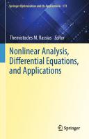
that is, viewing p as a signed density w.r.t. .μ, the signed measure .pdμ on .S, mimics the Dirac measure at .y, as long as only moments of order at most t are concerned. This is illustrated in Fig. 1 where .S = [−1, 1] and .dμ = 1[−1,1] (x)dx, t varies between 1 and 10, and .y = 0, 1/2, 1.
Polynomial Optimization, Certificates of Positivity, and Christoffel Function y=0
y = 0.5
11
y=1
6 4
100
CD−kernel
4
degree 2
5
2 50
10 15
0 0 0
−2 −1.0
−0.5
0.0
0.5
1.0
−1.0
−0.5
0.0 x
0.5
1.0
−1.0
−0.5
0.0
0.5
1.0
μ
Fig. 1 The signed measure .Kt (y, x)dx (with different values of t) mimics the Dirac measure at .y = 0 (left) .y = 0.5 (middle) and .y = 1 (right); reprinted from [19, p. 45] with permission. ©Cambridge University Press
4.2 Christoffel Function μ
With t.∈ N, the function .At : Rn → R+ associated with .μ, and defined by ⎤−1
⎡
⎥ ⎢Σ μ μ x |→ At (x) := Kt (x, x)−1 = ⎣ Pα (x)2 ⎦ n α∈Nt
.
,
∀x ∈ Rn ,
(16)
is called the (degree-t) Christoffel function (CF), and recalling that .Mt (μ) is nonsingular, it also turns out that
μ
At (x) =
.
[
vt (x)T Mt (μ)−1 vt (x)
]−1
,
∀x ∈ Rn .
(17)
The CF also has an equivalent and variational definition, namely: f μ
At (x) =
.
=
inf {
p∈R[x]t
p2 dμ : p(x) = 1 } ,
∀x ∈ Rn.
inf { : = 1 } ,
p∈R
s(t)
(18)
S
∀x ∈ Rn . (19)
In (19) the reader can easily recognize a convex quadratic programing problem which can be solved efficiently even for large dimensions. However solving (19) μ only provides the numerical value of .At at .x ∈ Rn , whereas in (17) one obtains the μ −1 coefficients of the polynomial .(At ) (but at the price of inverting .Mt (μ)).
12
J. B. Lasserre
The reader will also notice that from its definitions (16) or (17), the CF depends only on the finite sequence .μ2t = (μα )α∈Nn of moments of .μ, up to degree 2t, 2t and not on .μ itself. Indeed there are potentially many measures on .S with same μ moments up to degree 2t, and therefore indexing .At with .μ is not totally correct; μ2t therefore a more correct labelling would be .At . One reason for this labelling is that in theory of approximation, one is usually given a measure .μ on a compact set μ .S and one is interested in the sequence .(At )t∈N and its asymptotic properties. φ
Remark 2 In fact, one may also define the CD-kernel .Kt and the Christoffel φ function (CF) .At associated with a Riesz linear functional .φ ∈ R[x]∗ whose associated sequence .φ is such that .Mt (φ) > 0, no matter if .φ is a measure on .S or not. Indeed for fixed t, and letting .(Pα )α∈Nn be orthonormal w.r.t. .φ, the polynomial t
φ
(x, y) |→ Kt (x, y) :=
.
Σ
Pα (x) Pα (y) ,
∀x, y ∈ Rn ,
α∈N
n t
is well-defined, and all definitions (13)–(19) are still valid. But again, historically the CD-kernel was defined w.r.t. a given measure .μ on .S . Finally, one may use φ φ φ φ φ φ interchangeably the notations .Kt (resp. .At ) or .Kt (resp. .At ), or .Kt 2t (resp. .At 2t ) as in all cases, the resulting mathematical objet depends only on the finite moment sequence .φ 2t = (φα )α∈Nn of .φ. 2t
4.3 Some Distinguishing Properties of the CF φ
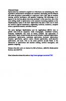
The CF .At associated with a Borel measure .φ on a compact .S ⊂ Rn , has an φ interesting and distinguishing feature. As t increases, .At (x) ↓ 0 exponentially fast for every .x /∈ S whereas its decrease is at most polynomial in t whenever φ .x ∈ S; see e.g. [19, Section 4.3, pp. 50–51]. In other words, .At identifies the support of .φ when t is sufficiently large. In addition, at least in dimension .n = 2 or .n = 3, one may visualize this property even for small t, as the resulting superlevel φ sets .S γ := { x : At (x) ≥ γ }, .γ ∈ R, capture the geometric shape of .S quite accurately; For instance in Fig. 2 are displayed several level sets .S γ associated with the empirical measure .φN supported on a cloud of N points that approximates the geometric shape obtained with the letters “C” and “D” of Christoffel and Darboux. In [17], the interested reader can find many other examples of 2D-clouds with nontrivial geometric shapes which are captured quite well with levels set .S γ associated with .φN , even for relatively low degree t. Another nice feature of the CF is its ability to approximate densities. Indeed let .φ and .μ be finite Borel measures on a compact set .S, and let .μ be such that uniformly μ on compact subsets of .int(S), .limt→∞ s(t) At = hμ , where .hμ is continuous and positive on .int(S) (and recall that .s(t) is the dimension of .R[x]t ). In addition suppose
Polynomial Optimization, Certificates of Positivity, and Christoffel Function
3930
3510
3930
2219760
830
60
830
60
13
3510
66 60 6 6
830
7360
180
66
180 68670
3930
7360
3510
393035
10
φ
Fig. 2 Level sets .S γ associated with .A10N for various values of .γ ; the red level set is obtained with .γ := s(10); reprinted from cover of [19, p. 45] with permission. ©Cambridge University Press
that .φ has continuous and positive density .fφ w.r.t. .μ. Then uniformly on compact subsets of .int(S) .
φ
lim s(t) At = fφ · hμ
t→∞
(see e.g. [19, Theorem 4.4.1]). So if the function .hμ is already known then one can approximate the density .fφ , uniformly on compact subsets of .int(S). Finally, another distinguishing property of the CF is its link with the so-called equilibrium measure of the compact set .S. The latter is a measure on .S (let us denote it by .λS ) which minimizes some Riesz energy functional if .n = 1 (invoking pluripotential theory and viewing .Rn as a subset of .Cn if .n > 1). For a detailed treatment see e.g. [3]. The measure .λS is known only for sets with specific geometry (e.g., an interval of the real line, the simplex, the unit sphere, the unit euclidean unit box). However under some condition,2 as t increases, the Borel measure .νt on .S
2 The
set .S is assumed to be regular and .(S, φ) possesses the Bernstein-Markov property; see e.g. [19, Section 4.4].
14
J. B. Lasserre φ
with density .1/s(t)At w.r.t. .φ, converges to .λS in the weak-.* topology of .M (S) (the Banach space of finite signed Borel measures on .S equipped with the total variation norm). That is: f f f h dφ = h dλS , ∀h ∈ C (S) . lim h dνt := lim t→∞ S t→∞ S s(t)Aφ S t where .C (S) is the space of continuous functions on .S; (see e.g. [19, Theorem 4.4.4]). In particular, the moments .νt,α , .α ∈ Nnt , converge to the moments of .λS .
5 CF, Optimization, and SOS-Certificates of Positivity 5.1 The CF to Compare the Hierarchies of Upper and Lower Bounds Recall the polynomial optimization problem .P in (1) with .S ⊂ Rn as in (3). Let .μ be a finite Borel (reference) measure whose support is exactly .S and with an associated sequence of orthonormal polynomials .(Pα )α∈Nn . Next, with .φ ∈ Rs(2t) and from the reproducing property (14), observe that ⎛ f ⎜ .φ(f ) = φ ⎝
=
⎞ Σ S
Σ
α∈N2t
⎟ Pα (x)Pα (y) f (y) dμ(y)⎠
n
f
φ(Pα )
Pα (y) f (y) dμ(y) S
α∈N2t n
f
=
f (y) S
Σ α∈N
f φ(Pα ) Pα (y) dμ(y) =
f (y) σφ (y) dμ(y) S
n 2t
where the degree-2t polynomial .y |→ σφ (y) := density w.r.t. .μ.
Σ
α∈N2t n
φ(Pα ) Pα (y), is a signed
Therefore in the semidefinite relaxations (7) of lower bounds on .f ∗ , one searches for a linear functional .φ ∈ R[x]∗2t which satisfies φ(1) = 1 ;
.
Mt (g · φ) > 0 ,
∀g ∈ G , (continued)
Polynomial Optimization, Certificates of Positivity, and Christoffel Function
15
f and which minimizes .φ(f ) = S f σφ dμ, where .σφ is a degree-2t polynomial signed density w.r.t. .μ, with coefficients .(σφ,α := φ(Pα ))α∈Nn . 2t
The reason why the semidefinite relaxations (7) can be exact (i.e., .ρt = f ∗ for some t), is that the signed probability measure .dνt = σφ dμ can mimic the Dirac measure at a global minimizer .ξ ∈ S and so .φ(f ) = f (ξ ); see Fig. 1. This is in contrast to the hierarchy of semidefinite relaxations (10) of upper bounds where one searches also for a polynomial probability density .σ dμ w.r.t. .μ, but as this density .σ is an SOS (hence positive), it cannot be a Dirac measure, and therefore the resulting convergence .τt ↓ f ∗ is necessarily asymptotic and not finite. For more details on a comparison between the Moment-SOS hierarchies of upper and lower bounds, the interest reader is referred to [14].
5.2 The CF and Positive Polynomials Of course, from its definition (17) the reciprocal .(At )−1 of the CF is an SOS of degree 2t. But we next reveal an even more interesting link with SOS polynomials. Observe that the .Qt (G) in (5) is a convex cone and its dual reads μ
Qt (G)∗ = { φ = (φα )α∈Nn : Mt−tg (g · φ) > 0 ,
.
2t
∀g ∈ G}.
(20)
A Duality Result of Nesterov Lemma 1 If .p ∈ int(Qt (G)) then there exists .φ ∈ int(Qt (G)∗ ) such that p=
Σ
.
g(x) vt−tg (x)T Mt−tg (g · φ)−1 vt−tg (x) ,
∀x ∈ Rn.
(21)
g∈G
=
Σ
g · (At−tg )−1 . g·φ
(22)
g∈G
In particular, for every SOS .p ∈ int(Σt [x]), .1/p is the CF of some linear functional φ ∗ s(2t) such that .M (φ) > 0. In addition, .φ ∈ Σ[x] , i.e., .1/p = At for some .φ ∈ R t 2t in the univariate case, .φ has a representing measure on .R. Equation (21) is from [23] while its interpretation (22) is from [15, Lemma 4]. Observe that (22) provides a distinguished representation of .p ∈ int(Qt (G)), and in view of its specific form, we propose to name (22) the Christoffel representation of
16
J. B. Lasserre
p ∈ int(Qt (G)), that is:
.
int(Qt (G)) = {
Σ
.
g · (At−tg )−1 : φ ∈ int(Qt (G)∗ ) } . g·φ
(23)
g∈G
Of course, an intriguing question is: What is the link between .φ ∈ int(Qt (G)∗ ) in (22) and the polynomial .p ∈ int(Qt (G))? A partial answer is provided in Sect. 5.4. A Numerical Procedure to Obtain the Christoffel Representation Consider the following optimization problems: P: .
P∗ :
Σ Σ inf { − log det(Mt−tg (g · φ)) : φ(p) = s(t − tg ) s(2t) φ∈R g∈G g∈G Mt−tg (g · φ) > 0 , ∀g ∈ G } . sup {
Qg >0
.
Σ
(24)
log det(Qg ) :
g∈G
p(x) =
Σ
g(x) vt−tg (x)T Qg vt−tg (x) ,
∀x ∈ Rn } .
(25)
g∈G
Both .P and .P∗ are convex optimization problems that can be solved by off-the-shelf software packages like e.g. CVX [6]. Theorem 5 Let .p ∈ int(Qt (G)). Then .P∗ is a dual of .P, that is, for every feasible solution .φ ∈ Rs(2t) of (24) and .(Qg )g∈G of (25), Σ .
log det(Qg ) ≤ −
g∈G
Σ
log det(Mt−tg (g · φ)) .
(26)
g∈G
Moreover, both .P and .P∗ have a unique optimal solution .φ ∗ and .(Q∗g )g∈G respectively, which satisfy Q∗g = Mt−tg (g · φ ∗ )−1 ,
.
∀g ∈ G ,
(27)
and which yields equality in (26). The proof which uses Lemma 2 in Appendix, mimics that of [15, Theorem 3] (where p was a constant polynomial) and is omitted.
Polynomial Optimization, Certificates of Positivity, and Christoffel Function
17
5.3 A Disintegration of the CF We next see how the above duality result, i.e., the Christoffel representation (22) of int(Qt (G)), can be used to in turn infer a disintegration property of the CF. So let μ n .At (x, y) be the CF of a Borel probability measure .μ on .S × Y , where .S ⊂ R and .Y ⊂ R are compact. It is well-known that .μ disintegrates into its marginal probability .φ on .S, and a conditional measure .μ(dy|x) ˆ on Y , given .x ∈ S, that is, .
f μ(A × B) =
μ(B|x) ˆ φ(dx) ,
.
∀A ∈ B(S) , B ∈ B(Y ) .
S∩A
Theorem 6 ([15]) Let .S ⊂ Rn (resp. .Y ⊂ R) be compact with nonempty interior, and let .μ be a Borel probability measure on .S × Y , with marginal .φ on .S. Then for every .t ∈ N, and .x ∈ S, there exists a probability measure .νx,t on .R such that φ
μ
ν
At (x, y) = At (x) · At x,t (y) ,
.
∀x ∈ Rn , y ∈ R .
(28)
The proof in [15, Theorem 5] heavily relies on the duality result of Lemma 1. In particular every degree-2t univariate SOS p in the interior of .Σ[y]t is the reciprocal of the Christoffel function of some Borel measure on .R.
5.4 Positive Polynomials and Equilibrium Measure This section is motivated by the following observation. Let .(Tn )n∈N (resp. .(Un )n∈N ) be the family of Chebyshev polynomials of the first kind (resp. second kind). They are orthogonal w.r.t. measures .(1 − x 2 )−1/2 dx and .(1 − x 2 )1/2 dx on .[−1, 1], respectively. (The Chebyshev measure .(1−x 2 )−1/2 dx/π is the equilibrium measure of the interval .[−1, 1].) They also satisfy the identity Tn (x) + (1 − x 2 ) Un−1 (x) = 1 ,
.
∀x ∈ R ,
n = 1, . . .
Equivalently, it is said that the triple .(Tn , (1 − x 2 ), Un ) is a solution to (polynomial) Pell’s equation for every .n ≥ 1. For more details on polynomial Pell’s equation (originally Pell’s equation is a topic in algebraic number theory), the interested reader is referred to [22, 30]. Next, letting .x |→ g(x) := (1 − x 2 ), and after normalization to pass to orthonormal polynomials, in summing up one obtains At (x)−1 + (1 − x 2 ) At−1 (x)−1 = 2t + 1 ,
.
φ
g·φ
∀x ∈ R , ∀t = 0, 1, . . .
(29)
Now, invoking Lemma 1, observe that (29) also states that .p ∈ int(Qt (G)) where G = {g} and p is the constant polynomial .x |→ p(x) = 2t + 1. In addition, it also means that if one solves .P in (24) with .p = s(t) + s(t − tg ) = 2t + 1 (recall
.
18
J. B. Lasserre
that .tg = 1), then its unique optimal solution .φ is just the vector of moments (up to degree 2t) of the equilibrium measure .φ = (1 − x 2 )−1/2 dx/π of the interval .S = [−1, 1]. So in Lemma 1 the linear functional .φp associated with the constant polynomial .p = 2t + 1 is simply the equilibrium measure of .S (denote it .λS ). The notion of equilibrium measure associated to a given set originates from logarithmic potential theory (working in .C in the univariate case to minimize some energy functional) and some generalizations have been obtained in the multivariate case via pluripotential theory in .Cn . In particular if .S ⊂ Rn ⊂ Cn is compact then the equilibrium measure .λS is equivalent to Lebesgue measure on compact subsets of .int(S). See e.g. Bedford and Taylor [3, Theorem 1.1] and [3, Theorem 1.2]. The Bernstein-Markov Property A measure with compact support .S satisfies the Bernstein-Markov property if there exists a sequence of positive numbers .(Mt )t∈N such that for all .t ∈ N and all .p ∈ R[x]t , .
sup |p(x)| (= ||p||S ) ≤ Mt · ||p||L2 (S,μ) , x∈S
and .limt→∞ log(Mt )/t = 0. So when it holds, the Bernstein-Markov property describes how the sup-norm and the .L2 (S, μ)-norm of polynomials relate when the degree increases. In [16] we have obtained the following result. Let .x |→ θ (x) := 1 − ||x||2 and possibly after an appropriate scaling, let .S in (3) be such that .θ ∈ Q1 (G) (so that n .S ⊂ [−1, 1] ); see Remark 1. Theorem 7 ([16]) Let .φ ∈ R[x]∗ (with .φ0 = 1) be such that .Mt (g · φ) > 0 for all g·φ .t ∈ N and all .g ∈ G, so that the Christoffel functions .At are all well defined. In addition, suppose that there exists .t0 ∈ N such that Σ .
s(t − tg ) =
g∈G
Σ
g · (At−tg )−1 , g·φ
∀t ≥ t0 .
(30)
g∈G
Then: (a) for every .t ≥ t0 , the finite moment sequence .φ ∗t := (φα )α∈Nn is the Σ 2t unique optimal solution of (24) (with p the constant polynomial .x |→ g∈G s(t − tg )). (b) .φ is a Borel measure on .S and the unique representing measure of .φ. Moreover, if .(S, g · φ) satisfies the Bernstein-Markov property for every .g ∈ G, then .φ is the equilibrium measure .λS and therefore the Christoffel polynomials g·λS −1 .(At )g∈G satisfy the generalized Pell’s equations: Σ .
g∈G
s(t − tg ) =
Σ g∈G
g · (At−tSg )−1 , g·λ
∀t ≥ t0 .
(31)
Polynomial Optimization, Certificates of Positivity, and Christoffel Function
19
Importantly, the representation of .S in (3) depends on the chosen set G of generators, which is not unique. Therefore if (30) holds for some set G, it may not hold for another set G. The prototype of .φ in Theorem 7 is the equilibrium measure of .S = [−1, 1], i.e., the Chebyshev measure .(1 − x 2 )−1/2 dx/π on .[−1, 1]. So Theorem 7 is a strong result which is likely to hold only for quite specific sets .S (and provided that a good set of generators is used). In [16] the author could prove that (30) also holds for the equilibrium measure .λS of the 2D-simplex, the 2D-unit unit box, the 2D-Euclidean unit ball, at least for .t = 1, 2, 3. However, if .θ ∈ Q1 (G) then as proved in [16, 21], .1 ∈ int(Qt (G)) for all t, and therefore (24) has always a unique optimal solution .φ ∗t . That is, for every .t ≥ t0 , (30) hold for some .φt ∈ R[x]∗2t which depends on t (whereas in (30) one considers moments up to degree 2t of the same .φ). Moreover, every accumulation point .φ of the sequence .(φ ∗t )t∈N has a representing measure .φ on .S. An interesting issue to investigate is the nature of .φ, in particular its relationship with the equilibrium measure .λS of .S. Finally, for general compact sets .S with nonempty interior, to .λS one may associate the polynomial pt∗ := Σ
.
Σ 1 g·λ g · (At−tSg )−1 g∈G s(t − tg ) g∈G
which is well-defined because the matrices .Mt−tg (g · λS ) are non singular. In Theorem 7 one has considered cases where .pt∗ is exactly the constant (equal to 1) polynomial (like for the Chebyshev measure on .S = [−1, 1]). We now consider the measures .(μt := pt∗ λS )t∈N , with respective densities .pt∗ w.r.t. .λS . Each .μt is a probability measure on .S because f .
pt∗ dλS = Σ
Σf 1 g·λ g · (At−tSg )−1 dλS g∈G s(t − tg ) g∈G
= Σ
Σ 1
g∈G s(t − tg ) g∈G
= Σ
Σ 1 s(t − tg ) = 1 . g∈G s(t − tg ) g∈G
Moreover, preceding as in the proof of Theorem 7 in [16], it follows that f .
lim
t→∞
α
x
pt∗ dλS
f =
xα dλS ,
∀α ∈ Nn .
As .S is compact it implies that the sequence of probability measures .(μt )t∈N ⊂ M (S)+ converges to .λS for the weak-.* topology of .M (S). In other words (and
20
J. B. Lasserre
in an informal language), the density .pt∗ of .μt w.r.t. .λS behaves like the constant (equal to 1) polynomial, which can be viewed as a weaker version of (31).
6 Conclusion SOS polynomials play a crucial role in the Moment-SOS hierarchies of upper and lower bounds through their use in certificates of positivity of real algebraic geometry. We have shown that they are also related to the Christoffel function in theory of approximation. Interestingly, the link is provided by interpreting a duality result in convex optimization applied to a certain convex cone of polynomials and its dual cone of pseudo-moments. It also turns out that in this cone, the constant polynomial is strongly related to the equilibrium measure of the semi-algebraic set associated with the convex cone. We hope that these interactions between different and seemingly disconnected fields will raise the curiosity of the optimization community and yield further developments. Acknowledgments Research supported by the AI Interdisciplinary Institute ANITI funding through the French program “Investing for the Future PI3A” under the grant agreement number ANR-19-PI3A-0004. This research is also part of the programme DesCartes and is supported by the National Research Foundation, Prime Minister’s Office, Singapore under its Campus for Research Excellence and Technological Enterprise (CREATE) programme. This research receives also funding from the European Union’s Horizon 2020 research and innovation programme under the Marie Sklodowska-Curie grant agreement N.◦ 813211 (POEMA).
Appendix Lemma 2 Let Sn be the space of real symmetric n × n matrices and let Sn++ ⊂ Sn be the convex cone of real n × n positive definite matrices Q (denoted Q > 0). Then n + log det(M) + log det(Q) ≤ ,
.
∀M , Q , ∈ Sn++ .
with equality if and only if Q = M−1 . Proof Consider the concave function { f : Sn → R ∪ {−∞}
.
Q |→ f (Q) =
log det(Q) if Q ∈ Sn++ , −∞ otherwise,
and let f ∗ be its (concave analogue) of Legendre-Fenchel conjugate, i.e., M |→ f ∗ (M) := inf n − f (Q) . Q∈S
.
(32)
Polynomial Optimization, Certificates of Positivity, and Christoffel Function
21
It turns out that {
∗
f (M) =
.
n + log det(M) (= n + f (M)) if M ∈ Sn++ , −∞ otherwise.
Hence the concave analogue of Legendre-Fenchel inequality states that f ∗ (M) + f (Q) ≤ ,
.
and yields (32).
∀M , Q ∈ Sn , u n
References 1. Baldi, L.: Représentations Effectives en Géométrie Algébrique Réelle et Optimisation Polynomiale. Thèse de Doctorat, Université Côte d’Azur, Nice (2022) 2. Baldi, L., Mourrain, B.: On the effective Putinar’s Positivstellensatz and moment approximation. Math. Program. 200, 71–103 (2022) 3. Bedford, E., Taylor, B.A.: The complex equilibrium measure of a symmetric convex set in Rn . Trans. Am. Math. Soc. 294, 705–717 (1986) 4. de Klerk, E., Laurent, M.: Convergence analysis of Lasserre hierarchy of upper bounds for polynomial optimization on the sphere. Math. Program. 193, 665–685 (2022) 5. Dunkl, C.F., Xu, Y.: Orthogonal Polynomials of Several Variables, 2nd edn. Cambridge University Press, Cambridge (2014) 6. Grant, M., Boyd, S.: CVX: Matlab Software for Disciplined Convex Programming, version 2.1 (2014). http://cvxr.com/cvx 7. Helton, J.W., Lasserre, J.B., Putinar, M.: Measures with zeros in the inverse of their moment matrix. Ann. Prob. 36, 1453–1471 (2008) 8. Henrion, D., Korda, M., Lasserre, J.B.: The Moment-SOS Hierarchy: Lectures in Probability, Statistics, Computational Geometry, Control and Nonlinear PDEs. World Scientific, Singapore (2022) 9. Lasserre, J.B.: Moments, Positive Polynomials and Their Applications. Imperial College Press, London (2009) 10. Lasserre, J.B.: A new look at nonnegativity on closed sets and polynomial optimization. SIAM J. Optim. 21, 864–885 (2011) 11. Lasserre, J.B.: The K-Moment problem for continuous linear functionals. Trans. Am. Math. Soc. 365, 2489–2504 (2013) 12. Lasserre, J.B.: Introduction to Polynomial and Semi-Algebraic Optimization. Cambridge University Press, Cambridge (2015) 13. Lasserre, J.B.: Connecting optimization with spectral analysis of tri-diagonal matrices. Math. Program. 190, 795–809 (2021) 14. Lasserre, J.B.: The Moment-SOS hierarchy and the Christoffel-Darboux kernel. Optim. Lett. 15, 1835–1845 (2021) 15. Lasserre, J.B.: A disintegration of the Christoffel function. C. R. Math. 360, 1071–1079 (2022) 16. Lasserre, J.B.: Pell’s equation, sum-of-squares and equilibrium measures of compact sets. C. R. Math. 361, 935–952 (2023) 17. Lasserre, J.B., Pauwels, E.: Sorting out typicality via the inverse moment matrix SOS polynomial. In: Lee, D.D., Sugiyama, M., Luxburg, U.V., Guyon, I., Garnett, R. (eds.) Advances in Neural Information Processing Systems, pp. 190–198. Curran Associates, Inc., Red Hook (2016)
22
J. B. Lasserre
18. Lasserre, J.B., Pauwels, E.: The empirical Christoffel function with applications in data analysis. Adv. Comput. Math. 45, 1439–1468 (2019) 19. Lasserre, J.B., Pauwels, E., Putinar, M.: The Christoffel-Darboux Kernel for Data Analysis. Cambridge Monographs on Applied and Computational Mathematics. Cambridge University Press, Cambridge (2022) 20. Magron, V., Wang, J.: Sparse Polynomial Optimization: Theory and Practice. World Scientific, Singapore (2023) 21. Mai, N.H.A., Lasserre, J.B., Magron, V., Wang, J.: Exploiting constant trace property in large scale polynomial optimization. ACM Trans. Math. Software 48(4), 1–39 (2022) 22. Mc Laughlin, J.: Multivariable-polynomial solutions to Pell’s equation and fundamental units in real quadratic fields. Pacific J. Math. 210, 335–348 (2002) 23. Nesterov, Y.: Squared functional systems and optimization problems. In: Frenk, H., Roos, K., Terlaky, T., Zhang, S. (eds.) High Performance Optimization, pp. 405–440. Applied Optimization Series, vol. 33, Springer, Boston (2000) 24. Nie, J.: Certifying convergence of Lasserre’s hierarchy via flat truncation. Math. Program. 142, 485–510 (2013) 25. Nie, J., Schweighofer, M.: On the complexity of Putinar’s Positivstellensatz. J. Complexity 23, 135–150 (2007) 26. Putinar, M.: Positive polynomials on compact semi-algebraic sets. Indiana Univ. Math. J. 42, 969–984 (1993) 27. Slot, L.: Sum-of-squares hierarchies for polynomial optimization and the Christoffel-Darboux kernel. SIAM J. Optim. 32, 2612–2635 (2022) 28. Slot, L., Laurent, M.: Near-optimal analysis of Lasserre’s univariate measure-based bounds for multivariate polynomial optimization. Math. Program. 188, 443–460 (2021) 29. Slot, L., Laurent, M.: Improved convergence analysis of Lasserre’s measure-based upper bounds for polynomial optimization on compact sets. Math. Program. 193, 831–871 (2022) 30. Webb, W.A., Yokota, H.: Polynomial Pell’s equation. Proc. Am. Math. Soc. 131, 993–1006 (2002)
Relative Entropy Methods in Constrained Polynomial and Signomial Optimization Thorsten Theobald
Abstract Relative entropy programs belong to the class of convex optimization problems. Within techniques based on the arithmetic-geometric mean inequality, they facilitate to compute nonnegativity certificates of polynomials and of signomials. While the initial focus was mostly on unconstrained certificates and unconstrained optimization, recently, Murray, Chandrasekaran and Wierman developed conditional techniques, which provide a natural extension to the case of convex constrained sets. This expository article gives an introduction into these concepts and explains the geometry of the resulting conditional SAGE cone. To this end, we deal with the sublinear circuits of a finite point set in .Rn , which generalize the simplicial circuits of the affine-linear matroid induced by a finite point set to a constrained setting.
1 Introduction Relative entropy programs provide a class of convex optimization problems [5]. They are concerned with optimizing linear functions over affine sections of the relative entropy cone } { xi n ≤ τi for all i , Krel = cl (x, y, τ ) ∈ Rn>0 × Rn>0 × Rn : xi ln yi
.
where .cl denotes the topological closure. Relative entropy programming contains as a subclass geometric programming and the special case .n = 1 of the relative entropy cone can be viewed as a reparametrization of the exponential cone. Beside applications in fields such as engineering and information theory, the last years have
T. Theobald (O) FB 12 – Institut für Mathematik, Goethe-Universität, Frankfurt am Main, Germany e-mail: [email protected] © The Author(s), under exclusive license to Springer Nature Switzerland AG 2023 M. Koˇcvara et al. (eds.), Polynomial Optimization, Moments, and Applications, Springer Optimization and Its Applications 206, https://doi.org/10.1007/978-3-031-38659-6_2
23
24
T. Theobald
shown an exciting and powerful application of relative entropy programming for optimization of polynomials and of signomials (i.e., exponential sums). Namely, within techniques based on the arithmetic-geometric mean inequality (AM/GM inequality), relative entropy programs facilitate to compute nonnegativity certificates of polynomials and of signomials. These techniques can also be combined with other nonnegativity certificates, such as sums of squares. A signomial, also known as exponential sum or exponential polynomial, is a sum of the form Σ cα exp() .f (x) = α∈T with real coefficients .cα and a finite ground support set .T ⊂ Rn . Here, . is the usual scalar product and we point out explicitly that the definition of a signomial also allows for negative or non-integer entries in the elements of .T. Exponential sums n can be seen as a generalization of polynomials: Σ when .Tα ⊂ N n, the transformation .xi = ln yi gives polynomial functions .y |→ α∈T cα y on .R>0 . For example, we have .f = 5 exp(2x1 + 3x2 ) − 3 exp(4x2 + x3 ) versus .p = 5y12 y23 − 3y24 y3 . When n n .T ⊂ N , a signomial f is nonnegative on .R if and only if its associated polynomial n p is nonnegative on .R+ , where .R+ denotes the set of nonnegative real numbers. Signomial optimization has additional modeling power compared to polynomial optimization. For example, the non-integer exponent . 12 is possible in signomial optimization, which corresponds to square roots. This leads to additional applications, for example, in chemical reaction networks [22], aircraft design optimization [38] or epidemiological models [31]. The following idea connects global nonnegativity certificates for polynomials and for signomials to the AM/GM inequality. This basic insight goes back to Reznick [34] and was further developed by Pantea, Koeppl, Craciun [32], Iliman and de Wolff [14] as well as Chandrasekaran andΣShah [4]. For support Σm points m m n .α0 , . . . , αm ∈ R and .λ = (λ1 , . . . , λm ) ∈ R+ with . λ = 1 and . i i=1 i=1 λi αi = α0 , the signomial m Σ .
λi exp() − exp()
i=1
is nonnegative on .Rn . This is a consequence of the weighted AM/GM inequality, see Sect. 2.3. During the early developments of AM/GM-based optimization of polynomials and signomials, most work concentrated on unconstrained certificates and unconstrained optimization. In the recent work [25], Murray, Chandrasekaran and Wierman presented an extension of the relative entropy methods to a conditional setting with a convex constrained set. In this situation, the constrained approach provides a much more suitable framework than earlier initial approaches of address-
Relative Entropy Methods in Constrained Polynomial and Signomial Optimization
25
ing constraints in AM/GM-based optimization based on a mix with a Krivine-type Positivstellensatz [4, 10]. The goal of this expository article is to offer an introduction into the relative entropy methods for unconstrained and for constrained polynomial and signomial optimization. The resulting cones are called the SAGE cone and the conditional SAGE cone, where SAGE is the acronym for Sums of Arithmetic-Geometric Exponentials. The geometry of the SAGE cone is governed by the simplicial circuits of the affine-linear matroid induced by the support .T [12, 24, 35]. In order to exhibit the geometry of the conditional SAGE cone, we spell out and study the sublinear circuits of a finite point set in .Rn , which generalize the simplicial circuits to a constrained setting [26]. Sublinear circuits of polyhedral sets have specifically been studied in [28]. Meanwhile, the conditional SAGE approaches has also been extended towards hierarchies and Positivstellensätze for conditional SAGE [36] and to additional nonconvex constraints [9].
2 From Relative Entropy Programming to the SAGE Cone We provide some background on relative entropy programming and explain the main concepts of the SAGE cone.
2.1 Cones and Optimization Conic optimization is concerned with optimization problems of the form .inf{cT x : Ax = b, x ∈ K} for a convex cone .K ⊂ Rn , where .A ∈ Rm×n , .b ∈ Rm and .c ∈ Rn . Usually, we assume that the cone K is closed, full-dimensional and pointed, where pointed means that K contains no lines. A closed, full-dimensional and pointed cone is called a proper cone. If a self-concordant barrier function for K is known, then conic optimization problems over K can be approached efficiently through interior point methods (see, e.g., [30]). Prominent special cases of conic programming are linear programming and semidefinite programming. Linear programming (LP) can be viewed as conic programming over the nonnegative cone .K = Rn+ . Linear programming arises in polynomial optimization, for example, in LP-relaxations via Handelman’s Theorem [13] or in the DSOS approach (diagonally dominant sums of squares [1]). Semidefinite programming (SDP) can be viewed as conic programming over the cone .S+ n of positive semidefinite symmetric .n × n-matrices. Semidefinite programming is ubiquitous in polynomial optimization through sums of squares. In particular, with respect to constrained optimization, semidefinite programming is tightly connected to Lasserre’s hierarchical relaxation and thus to Putinar’s Positivstellensatz and to moments (see, e.g., [17]). Recent developments on the
26
T. Theobald
use of semidefinite programming in polynomial optimization include the improved exploitation of sparsity, see [19, 37].
2.2 The Exponential Cone and the Relative Entropy Cone The exponential cone and the relative entropy cone are rather young cones within the development of convex optimization. The exponential cone is defined as the three-dimensional cone } { ( ) z2 z1 . ≤ .Kexp = cl z ∈ R × R+ × R>0 : exp z3 z3 In 2006, Nesterov gave a self-concordant barrier function [29], see also [6]. This enables efficient interior-point algorithms for approximating optimization problems over .Kexp . The exponential cone is depicted in Fig. 1. Remark 1 For any convex function .ϕ : R( →) R, the perspective function .ϕ˜ : R × ˜ y) = yϕ xy . The closure of the epigraph of the R>0 → R is defined as .ϕ(x, perspective function, .
{ ( )} x , cl (t, x, y) ∈ R × R × R>0 : t ≥ yϕ y
Fig. 1 The exponential cone
Relative Entropy Methods in Constrained Polynomial and Signomial Optimization
27
is known to be a closed convex cone. The exponential cone is exactly the cone which arises from this construction for the exponential function .ϕ : x |→ exp(x). The exponential cone is a non-symmetric cone, where ‘symmetric’ means that a cone is homogeneous and self-dual. Optimization over a Cartesian product of exponential cones contains as a special case the class of geometric programming, which has many applications in engineering [3]. Moreover, the exponential cone has applications, for example, in maximum likelihood estimation or logistic regression [20]. The dual of the exponential cone is ∗ .Kexp
} { ( ) e · s2 s3 ≤− , = cl s ∈ R0 → R, f (x) = x ln x,
.
see Fig. 2. The relative entropy function is defined as .D : R>0 × R>0 → R, .D(x, y) = x ln xy . It is a convex function in .z = (x, y), also called a jointly convex function in x and y. To see the joint convexity, observe that the Hessian of D evaluates to ( ∇ D(x, y) =
.
2
1 x
− y1
− y1 x y2
) .
The relativeΣentropy function can be extended to vectors .x, y ∈ Rn>0 by setting n xi .D(x, y) = i=1 xi ln yi . The relative entropy cone is defined as 1 Krel := cl {(x, y, τ ) ∈ R>0 × R>0 × R : D(x, y) ≤ τ } .
.
Here, the upper index “1” indicates that x, y and .τ are scalars. The relative entropy cone can be viewed as a reparametrization of the exponential cone, because of the Fig. 2 The negative entropy function
28
T. Theobald
equivalences x ln
.
( τ) y x ≤ τ ⇐⇒ exp − ≤ ⇐⇒ (−τ, y, x) ∈ Kexp . y x x
More generally, the relative entropy cone can be extended to triples of vectors by n ⊂ R3n as defining .Krel { } xi n ≤ τi for all i . Krel = cl (x, y, τ ) ∈ Rn>0 × Rn>0 × Rn : xi ln yi
.
This allows to model the n-variate relative entropy condition D((x1 , . . . , xn ), (y1 , . . . , yn )) :=
n Σ
.
xi ln
i=1
xi ≤t yi
as n ∃τ ∈ Rn with (x, y, τ ) ∈ Krel and 1T τ = t,
.
where .1 denotes the all-ones vector.
2.3 The Basic AM/GM Idea The following idea, going back to Reznick [34] and further developed in [4, 14, 32], connects global nonnegativity certificates for polynomials and for signomials to the AM/GM inequality. Consider support points .α0 ,Σ . . . , αm ∈ Rn such that Σm.α0 is a convex combination of .α1 , . . . , αm , that is, .α0 = m i=1 λi αi = α0 with . i=1 λi = 1 and .λ ∈ Rm + . Then the signomial m Σ .
λi exp() − exp()
(1)
i=1
is nonnegative on .Rn . Namely, we can use the following weighted AM/GM inequality, which can easily be derived from the strict convexity of the univariate function .x |→ − ln x on the domain .(0, ∞). Theorem 1 (Weighted Σ Arithmetic-Geometric Mean Inequality) For each .z ∈ Rn+ and .λ ∈ Rn+ with . ni=1 λi = 1, we have n Σ .
i=1
λ i zi ≥
n || i=1
ziλi .
Relative Entropy Methods in Constrained Polynomial and Signomial Optimization
29
The nonnegativity of (1) follows from the weighted AM/GM inequality through m Σ .
λi exp() ≥
i=1
m ||
(exp())λi = exp()
(2)
i=1
for all .x ∈ Rn . Clearly, sums of such exponential sums of the form (1) are nonnegative as well. We will see later how to generalize this core idea from the unconstrained setting to the constrained case with respect to a set X. For the class of signomials, we assume that an underlying finite ground support set .T ⊂ Rn is given. When considering subsets of the ground support, we usually employ the convention that .A refers to terms with positive coefficients and .B (or .β in case of single elements) refers to terms with possibly negative coefficients. Let f be a general signomial whose coefficients except at most one are positive, f (x) =
Σ
.
cα exp() + d exp() with cα > 0 and d ∈ R.
(3)
α∈A
Chandrasekaran and Shah [4] have given the following exact characterization of the nonnegativity of f in terms of the coefficients .(cα )α∈A and d. This insight establishes a fundamental connection from the nonnegativity of signomials (or polynomials) with at most one negative coefficient to the relative entropy function. Theorem f in (3) is nonnegative if and only if there exists .ν ∈ RA + Σ 2 The signomial Σ with . α∈A να α = ( α∈A να )β and .D(ν, ec) ≤ d, where D denotes the relative entropy function and e is Euler’s number. As revealed by the proof, a natural way to see why the relative entropy function occurs is through duality theory. For a function .g : Rn → R, the conjugate .g ∗ : Rn → R is defined by ( ) g ∗ (y) = sup y T x − g(x) .
.
x
The conjugate function of .g(x) = ex is .g ∗ (y) = y ln y − y on the domain .R+ , where we use the convention .0 · ln 0 := 0. Using standard computation rules from convex optimization, the conjugate function of g(x) =
n Σ
.
ci exi
i=1
is .D(y, ec), where .c := (c1 , . . . , cn )T .
with c1 , . . . , cn > 0
30
T. Theobald
Proof The nonnegativity of the signomial f Σ is equivalent to the nonnegativity of f (x) exp() and thus also equivalent to . α∈A cα exp( − ) ≥ −d Σ for all .x ∈ Rn . The function . α∈A cα exp( − ) is, as a sum of convex functions, convex as well. Its infimum can be formulated as the convex optimization problem
.
inf
.
Σ A
x∈R , t∈R n
cα tα s.t. exp() ≤ tα
∀α ∈ A,
α∈A
where the inequality constraints can also be written as . ≤ ln tα . The primal problem satisfies Slater’s condition from convex optimization, because a Slater point can be constructed by considering an arbitrary point .x ∈ Rn and choosing all .tα sufficiently large. For the Lagrange dual, we obtain, by reducing to the conjugate function together with the computation rules above, .
sup −D(ν, ec) s.t. A ν∈R+
Σ α∈A
να α = (
Σ
να )β.
α∈A
Due to Slater’s condition, we have strong duality and the dual optimum is attained. This shows the theorem. u n
Example We consider the Motzkin-type signomial .fδ = e4x+2y + e2x+4y + 1 + δe2x+2y with some parameter .δ ∈ R. In order to determine the smallest .δ such that .fδ is nonnegative, we can consider the signomial gδ (x) := fδ (x) e−2x−2y = e2x + e2y + e−2x−2y + δ.
.
Since .gδ has at most one negative term, we can formulate the nonnegativity of .gδ in terms of the relative entropy condition
.
inf δ ( ) ( ) ( ) 2 0 −2 ν1 + ν2 + ν3 = 0, 0 2 −2 ν1 ν2 ν3 + ν2 ln + ν3 ln ≤ δ, ν1 ln e·1 e·1 e·1 ν ∈ R3+ , δ ∈ R.
The minimal .δ satisfying this condition is .δ = −3 and .minx,y fδ=−3 = 0.
Relative Entropy Methods in Constrained Polynomial and Signomial Optimization
31
In the algorithmic access via conic optimization as described Σ above, it is essential that the vector .ν in Theorem 2 is not normalized to, say, . α∈A να = 1. Indeed, normalizing the vector .ν in that theorem gives a formulation of a nonnegativity condition which can be viewed as a slight generalization of the AM/GM consideration (2). Proposition 1 The signomial f in (3) is nonnegative if and only if there exists .λ ∈ A with . Σ λ α = β, .Σ R+ α α∈A λα = 1 and α∈A (
|| .
α∈A with λα >0
)λα
cα λα
≥ −d .
(4)
A satisfying (4), using the weighted AM/GM-inequality Proof If there exists .λ ∈ R+ with weights .(λα )α∈A gives Σ .
cα exp() ≥
α∈A
)λα || ( 1 || ( cα )λα cα exp ( = exp() λα λα
λα >0
λα >0
≥ −d exp() for all .x ∈ R. Hence, f is nonnegative. f is nonnegative, then, by Theorem 2, there exists .ν ∈ RA + with Σ Conversely, if Σ να ν ν for all . α ∈ A . α = ( )β and . D(ν, ec) ≤ d. Set . λ = α α α α∈A α∈A 1T ν and we can assume that .cα > 0 for all .α ∈ A. The convex univariate function ' .h : R>0 → R, .s |→ D(sλ, ec) has the derivative .h (s) = ln s + D(λ, c) and thus ∗ −D(λ,c) takes its minimum at .s = e with minimal value h(s ∗ ) = e−D(λ,c)
Σ
.
λα ln
α∈A
= −e−D(λ,c) = −
e−D(λ,c) λα = e−D(λ,c) (D(λ, c) − D(λ, c) − 1) e · cα ||
α∈A with λα >0
(
cα λα
)λα .
Hence, ∗
d ≥ D(ν, ec) ≥ h(s ) = −
.
|| α∈A with λα >0
(
cα λα
)λα . u n
32
T. Theobald
2.4 The SAGE Cone (Sums of Arithmetic-Geometric Exponentials) Building upon the AM/GM idea, Chandrasekaran and Shah [4] have introduced the following cones of nonnegative signomials. The elements of these cones admit a nonnegativity certificate based on the AM/GM inequality. For given .A and .β /∈ A, the AGE cone .CAGE (A, β) is defined as ⎧ ⎫ ⎨ ⎬ Σ cα e + de is nonnegative, c ∈ RA .CAGE (A, β) = f : f = . + ⎩ ⎭ α∈A Given a finite set .T ⊂ Rn , the SAGE cone .C(T ) is then defined as C(T ) :=
Σ
.
CAGE (T \ {β}, β).
β∈T
It consists of signomials which admit a decomposition as a sum of AGE signomials. The SAGE cone supports handling sparse signomials. A crucial property is that it allows cancellation-free representations. This was shown by Wang [35] in the polynomial setting and by Murray, Chandrasekaran and Wierman [24] in the signomial setting. Theorem 3 Let f be a signomial with support .T. If .f ∈ C(T' ) for some .T' ⊇ T, then .f ∈ C(T ). In words, if a signomial f supported on .T has a SAGE certificate with respect to some larger support set .T' , then the SAGE certificate also exists on the support set .T itself. Membership of a signomial to the SAGE cone can be formulated in terms of a relative entropy program. For disjoint .∅ /= A ⊂ Rn and .B ⊂ Rn , write C(A, B) :=
Σ
.
CAGE (A ∪ B \ {β}, β).
β∈B
Hence, signomials in .C(A, B) can Σonly have negative Σ coefficients within the subset B. It holds .C(A, B) = {f = α∈A cα e + β∈B cβ e ∈ C(A ∪ B) : cα ≥ 0 for α ∈ A}. This allows the following relative entropy formulation to decide whether a given signomial
.
f =
Σ
.
α∈A
cα exp() +
Σ
cβ exp()
β∈B
with .cα ≥ 0 for .α ∈ A and .cβ < 0 for .β ∈ B is contained in the SAGE cone.
(5)
Relative Entropy Methods in Constrained Polynomial and Signomial Optimization
33
Theorem 4 ([24]) The signomial f in (5) is contained in .C(A, B) if and only for A and .ν (β) ∈ RA such that every .β ∈ B there exist .c(β) ∈ R+ + Σ .
(β)
να α = (
Σ
α∈A α∈A D(ν (β) , e · c(β) ) ≤ cβ Σ (β) cα ≤ cα β∈B
(β)
να )β for β ∈ B, for β ∈ B, for α ∈ A.
For combining AM/GM-techniques for polynomials on .Rn and .Rn+ , Katthän, Naumann and the current author have developed the .S-cone [16]. AM/GM techniques can also be combined with sums of squares to hybrid methods, see [15]. Moreover, an implementation of the SAGE cone, called Sageopt was provided by Murray [23].
3 Conditional Nonnegativity Over Convex Sets Murray, Chandrasekaran and Wierman [25] generalized AM/GM optimization from the unconstrained setting to the constrained setting over a convex set .X ⊂ Rn . Denote by .σX (y) = sup{y T x : x ∈ X} the support function of X from classical convex geometry. .σX is a convex function .Rn → R+ ∪ {∞}. If X is polyhedral, then .σX is linear on every normal cone of X. The support function .σX arises naturally in optimization as the conjugate function of the indicator function 1X (x) =
.
{ 0 ∞
x ∈ X, otherwise
of a convex set X. We begin with the crucial insight that for a signomial with at most one negative term, the nonnegativity on X (“conditional nonnegativity”) can be formulated in terms of a relative entropy program involving also the support function of X. Let Σ cα exp() with .cα ≥ 0 for .α ∈ A. As short .T := A ∪ {β} and .f (x) = α∈T Σ T notation, for a given .ν ∈ R we write .Tν := α∈T ανα . Theorem 5 ([25]) The signomial f in (3) is nonnegative on X if and only if there Σ exists .ν ∈ RT \ {0} with . α∈T να = 0, .ν|A ≥ 0 and .σX (−Tν) + D(ν|A , ec|A ) ≤ cβ . Here, .ν|A denotes to the restriction of the vector .ν to the coordinates of .A. Proof Generalizing the idea of the Σ proof of Theorem 2, we now observe that f is nonnegative on X if and only if . α∈A cα exp( − ) ≥ −cβ for all .x ∈ X. The infimum of the left convex function can be formulated as the convex
34
T. Theobald
program .
inf
Σ A
x∈X, t∈R
cα tα s.t. exp() ≤ tα
∀α ∈ A.
α∈A
Strong duality holds, and the dual is .
max −(σX (−Tν) + D(ν|A , ec|A )) s.t. T ν∈R \{0}
Σ α∈T
να = 0, ν|A ≥ 0.
Hence, f is nonnegative if and only if this maximum is larger than or equal to −cβ . u n
.
It is useful to consider also the following alternative formulation of the characterization in Theorem 5. For .β ∈ T, set ⎧ ⎫ ⎨ ⎬ Σ να = 0 , .Nβ = ν ∈ RT : ν\β ≥ 0, ⎩ ⎭ α∈T where .ν\β refers to the vector .ν in which the component .β has been removed. The choice of the name N reflects that the coordinate .β is the only coordinate which may be negative. Corollary 1 The signomial f in (3) is nonnegative on X if and only if there exists ν ∈ Nβ \ {0} with .σX (−Tν) + D(ν|A , ec|A ) ≤ cβ .
.
The following theorem characterizes nonnegativity in terms of a normalized dual variable and thus generalizes Proposition 1. Theorem 6 ([26]) The signomial f in (3) is nonnegative on X if and only if there exists .λ ∈ Nβ with .λβ = −1 and || .
α∈A with λα >0
(
cα λα
)λα
≥ −cβ exp(σX (−Tλ)).
For given .A and .β /∈ A, define the conditional AGE cone .CX,AGE (A, β) as ⎧ ⎫ ⎨ ⎬ Σ . cα e + de nonnegative on X, c ∈ RA f : f = . + ⎩ ⎭ α∈A
(6)
Relative Entropy Methods in Constrained Polynomial and Signomial Optimization
The conditional SAGE cone is defined as Σ CX,AGE (T \ {β}, β). .CX (T ) = β∈T
35
(7)
These cones are abbreviated as the X-AGE cone and the X-SAGE cone. The result on cancellation-free representation from Theorem 3 also holds for the constrained situation. In the transition from the unconstrained optimization to the constrained optimization, the following key changeΣ in geometry and combinatorics takes place. Let f be a signomial of the form .f = α∈A cα e + de with .cα ≥ 0 for all .α ∈ A. If f is nonnegative over the set .X = Rn , then we have .β ∈ conv A. That is, the exponent vector of the term with negative coefficients lies in the convex hull of the exponent vectors of terms with positive coefficients, see Fig. 3. This property can get lost for other sets X. For example, for .X = R+ and .T = {(0), (1)}, the signomial .f : R → R, .f (x) = exp(x) − exp(0) is contained in .CX (T ). The left picture in Fig. 4 shows the graph of f and the right picture the support points. To characterize this change in geometry and combinatorics, recall that the recession cone .rec(X) of a convex set X is defined as .
rec(X) := {y : ∃x ∈ X such that x + λy ∈ X for all λ ≥ 0}.
For a given cone S, let .S ◦ := {y ∈ Rn : ≤ 0 for all x ∈ S} denote the polar cone of S. Observe that the polar cone and the dual cone are related through .S ◦ = −S ∗ . For .T := A ∪ {β} and a given convex set X, the inequality .σX (−Tν) < ∞ implies the weaker condition .β ∈ conv A + rec(X)◦ = conv A − rec(X)∗ , see Fig. 5. Fig. 3 In the case .X = Rn , the exponent vectors of terms with negative coefficients lie in the convex hull of the exponent vectors of terms with positive coefficients
Fig. 4 Left: The graph of the function .f (x) = exp(x) − exp(0). Right: The support point of the negative coefficient (visualized in blue) is not contained in the convex hull of the set of support points with positive coefficient (visualized in red)
36
T. Theobald
Fig. 5 The left picture visualizes the inequality .σX (−Tν) < ∞ in terms of the condition that is contained in the relative interior of .rec(X)◦ . The right picture shows the cone in which the term with negative coefficient has to lie. For example, the blue dot would be a possible support point for the negative coordinate .β
.−Tν
Membership to the conditional SAGE cone can now be formulated as a relative entropy program as well. For disjoint .∅ /= A ⊂ Rn and .B ⊂ Rn , write Σ
CX (A, B) :=
.
CX,AGE (A ∪ B \ {β}, β).
β∈B
It holds .CX (A, B) = } . cα ≥ 0 for α ∈ A .
}
f =
Σ
α∈A cα e
+
Σ
β∈B cβ e
∈ CX (A ∪ B) :
Theorem 7 ([25]) A signomial f =
Σ
.
α∈A
cα e +
Σ
cβ e
β∈B
with .cα ≥ 0 for .α ∈ A and .cβ < 0 for .β ∈ B is contained in .CX (A, B) if and only A and .ν (β) ∈ RA such that if for every .β ∈ B there exist .c(β) ∈ R+ + σX (−(A ∪ β)ν) + D(ν (β) , e · c(β) ) ≤ cβ for β ∈ B, Σ (β) . cα ≤ cα for α ∈ A. β∈B Since the formulations of the conditional SAGE approach use the support function, efficient numerical computation requires sets X for which the support function can be computed efficiently. A natural class where this is possible is provided by polyhedral sets X given by linear inequalities.
Relative Entropy Methods in Constrained Polynomial and Signomial Optimization
37
4 The Circuit View for Unconstrained AM/GM Optimization Revealing the structure of the SAGE cone and of the conditional SAGE cone relies on the decomposition of signomials into simpler signomials. In this section, we present the central ideas for the case of unconstrained AM/GM optimization. The decomposition property manifests itself on the level of the dual vector .ν in the entropy condition for nonnegativity. The linear (in-)equalities in the entropy condition offer a polyhedral view and an access through generators known as simplicial circuits. We begin with an example.
Example The nonnegative function .f = 7e0 + 3e2x + e3x + 3e3y − 9ex+y decomposes as f =
.
) 1( ) 1( 0 2e + 2e3x + 2e3y − 6ex+y + 12e0 + 6e2x + 4e3y − 12ex+y 2 2
into two non-proportional nonnegative AGE signomials. The support sets of f and the summands are depicted in Fig. 6.
Denote by .1 the all-ones vector and by .supp the support of a vector, i.e., the index set of its non-zero components. Definition 1 A nonzero vector .ν ∗ ∈ {ν ∈ RT : = 0} with .Tν ∗ = 0 is called a simplicial circuit if it is minimally supported and has exactly one negative component, named .(ν ∗ )− . Here, minimally supported means that there does not exist .ν ' ∈ RT \ {0} with .supp ν ' C supp ν ∗ , .0 α∈T
.
where .β := λ− . The SAGE cone admits the following decomposition as a Minkowski sum of .λ-witnessed AGE cones and of exponential monomials (i.e., signomials whose exponent vector .α has a single nonnegative entry). Theorem 8 For .A(T ) = / ∅, the SAGE cone decomposes as C(T ) =
Σ
.
C(T, λ) +
λ∈A(T )
Σ
R+ · exp().
α∈T
As a consequence, every signomial in the SAGE cone .C(T ) can be written as a non-negative sum of circuit-witnessed signomials and of exponential monomials. This was shown by Wang [35] in the polynomial setting and by Murray, Chandrasekaran, Wierman [24]. It reveals the two views on the SAGE cone. The first view comes from the definition of the SAGE cone in terms of AGE signomials. Equivalently, we can regard the SAGE cone as being non-negatively generated by the circuit-witnessed signomials and by exponential monomials. Remark 2 In the polynomial setting, a variety of works used the latter viewpoint in their definition of a cone for AM/GM optimization. Prominently, Iliman and de Wolff [14] have employed the notion of the cone of SONC polynomials (“Sums of Non-negative Circuit polynomial”). When considering polynomials over .Rn>0 , the exponential monomials from the signomial setting become ordinary monomials. In the adaption to polynomials over .Rn , which also has to take into account the signs in other orthants, the monomials become monomial squares. The dual SONC cone was studied in [11]. In order to give the idea for the decomposition in Theorem 8, we approach the situation from the linear condition within the relative entropy condition of Theorem 4. Lemma 1 (Decomposition Lemma) Let f =
Σ
.
cα exp() + cβ exp()
α∈A
be a signomial in .CAGE (A, β) and .ν satisfy the Σrelative entropy condition for f . If .ν can be written as a convex combination .ν = ki=1 θi ν (i) of non-proportional .ν (i) ∈ Nβ , then f has a decomposition into non-proportional signomials in .CAGE (A, β).
Relative Entropy Methods in Constrained Polynomial and Signomial Optimization
39
Before the proof, we illustrate the statement.
Example We adapt the earlier Example 4, taking .f = 2e0 + 3e2x + e3x + 3e3y − 9ex+y . Here, the dual vector .ν = (2, 3, 1, 3, −9) certifies the relative entropy condition. This specific situation is rather simple, because the coefficients sum to zero, which leads to a root at the origin. Writing 1 1 .ν = (2, 6, 0, 4, −12) + (2, 0, 2, 2, −6) gives the decomposition 2 2 f =
.
) ) 1( 1( 0 2e0 + 2e3x + 2e3y − 6ex+y . 2e + 6e2x + 4e3y − 12ex+y + 2 2
The first summand .ν ' := 12 (2, 6, 0, 4, −12) of .ν is a simplicial circuit, so that Lemma 1 does not apply on .ν ' . Indeed, the signomial . 21 (2e0 + 6e2x + 4e3y x+y ) cannot be decomposed into two non-proportional signomials, such .−12e that in these two signomials only the exponential monomial .12ex+y has a negative coefficient and only the exponential monomials .e0 , .6e2x and .4e3y can have a nonzero, positive coefficient. The same holds true for the second summand of .ν and the second summand of f .
Proof (of Lemma 1) Denote by .ν + := {α ∈ΣA : να > 0} the positive support of .ν and set .T = A ∪ {β}. For the given .f = α∈T cα exp(), construct vectors (i) for .1 ≤ i ≤ k by .c { (i) .cα
= (i)
(cα /να )να
if α ∈ ν +
0
otherwise
(i)
(i)
for all α ∈ T \ {β}
(i)
and by setting .cβ = D(ν\β , ec\β ). The coefficient vectors .c(i) define nonnegative Σ AGE signomials. It remains to show that . ki=1 θi c(i) ≤ c. For indices .α ∈ ν + , we have equality by construction, and for indices .α ∈ Σ (i) supp c \ supp ν, we have . ki=1 θi cα = 0 ≤ cα . Now consider the index .β. By (i) (i) construction, .να /cα = να /cα for .α ∈ T \ {β}, which gives k Σ .
i=1
(i)
(i)
θi D(ν\β , ec\β ) =
k Σ i=1
θi
Σ α∈A
(i)
να(i) ln
να
e · cα(i)
= D(ν\β , ec\β ).
40
T. Theobald
Hence, k Σ .
(i)
θi cβ
i=1
=
k Σ
(i)
(i)
θi D(ν\β , ec\β ) = D(ν\β , ec\β ) ≤ cβ .
i=1
u n
Example We consider circuits in the one-dimensional space .R. Let .T = {α1 , . . . , αm } ⊂ R. Then the simplicial circuits are recognized as the union of the edge generators of the polyhedral cones .Nβ for .β ∈ T. The set of normalized circuits can then be determined as λ =
.
αj − αi αk − αj ei − ej + ek αk − αi αk − αi
for i < j < k,
where .ei denotes the i-th unit vector in .Rm . Applying Theorem 8 gives a Minkowski decomposition of the univariate SAGE cone with ground set .T.
Using the circuit concept, membership in the SAGE cone can be also certified by a second-order cone program (see Averkov [2] in the polynomial setting, Magron, Wang [18] for a computational view and Naumann and the current author [27] for the extension of second-order representability to the primal and the dual .S-cone) or a power cone (Papp [33]). A principal question is whether further decompositions are possible by employing different negative terms. This will be treated in Sect. 6.
5 Sublinear Circuits In the previous sections, we have discussed the circuit concept for unconstrained AM/GM optimization and we have presented the framework of constrained AM/GM optimization. Strikingly, a generalized circuit concept can also be established for the case of constrained AM/GM optimization. These generalized circuits are called sublinear circuits and the setup is visualized in Fig. 7. Let .X ⊂ Rn be a convex set and .T ⊂ Rn be the finite ground support, where we assume that the functions .x |→ exp(), .α ∈ T, are linearly independent on X. We consider the conditional AGE cone .CX,AGE (A, β) and the conditional SAGE cone .CX (T ) as defined in (6) and (7). The primary goal of a circuit concept is to decompose signomials into simpler signomials and thus to decompose a cone
Relative Entropy Methods in Constrained Polynomial and Signomial Optimization
41
Fig. 7 The role of the sublinear circuits
under consideration. This will be an essential ingredient for studying the geometry of the conditional SAGE cone for a given set X and we will achieve a Minkowski decomposition. Further refinements will then yield irredundant decompositions, both for the unconstrained and the constrained case, and characterizations of the extreme rays. In [26], the following concept of sublinear circuits has been developed to resolve T : ν these \β ≥ 0, Σ questions. For .β ∈ T, recall the notion .Nβ = {ν ∈ R . = 0}. We consider the following generalization of the circuit notion from ν α α∈T Definition 1. Recall that the support function .σX is sublinear, that is, it satisfies n .σX (μ1 z2 + μ2 z2 ) ≤ μ1 σX (z1 ) + μ2 σX (z2 ) for .μ1 , μ2 > 0 and .z1 , z2 ∈ R . Definition 2 A non-zero vector .ν ∗ ∈ Nβ is called a sublinear circuit of .T with respect to X (for short, X-circuit) if 1. .σX (−Tν ∗ ) < ∞, 2. whenever a mapping .ν |→ σX (−Tν) is linear on a two-dimensional cone in .Nβ , then .ν ∗ is not in the relative interior of that cone. Denote by .AX (T ) the set of all normalized X-circuits of .T, i.e., circuits with entry −1 in the negative coordinate.
.
In more geometric terms, Definition 2 can be equivalently expressed as follows. For given .β ∈ T, consider the convex cone P := pos{(ν, σX (−Tν)) : ν ∈ Nβ , σX (−Tν) < ∞}
.
= {(ν, σX (−Tν)) : ν ∈ Nβ , σX (−Tν) < ∞} ∪ {0}, where .pos denotes the positive hull. This cone can be shown to be closed and pointed. Then a vector .ν ∗ ∈ Nβ is an X-circuit if and only if .(ν ∗ , σX (−Tν ∗ )) spans an extreme ray of P . For the case of polyhedral X, this characterization of X-circuits is straightforward to see and for non-polyhedral X, the convex-geometric details can be found in [26, Theorem 3.6]. As explained in the following, the structure of the sublinear circuits generalizes the structure of the affine-linear matroid which appears in the circuits of the unconstrained case.
42
T. Theobald
Example 1. Let .X = [−1, 1]2 and .T = {(0, 0)T , (1, 0)T , (0, 1)T }. Since X is compact, the condition .σX (−Tν) < ∞ is always satisfied. The set of normalized circuits is .AX (T ) = {(−1, 1, 0)T , (−1, 0, 1)T , (1, −1, 0)T , (0, −1, 1)T , T T T .(1, 0, −1) , (0, 1, −1) }. Namely, for .β = (0, 0) , the closed convex cone P = pos{(ν, σX (−Tν)) : ν(0,0) < 0, ν(1,0) ≥ 0, ν(0,1) ≥ 0}
.
= pos{(ν, σX ((−ν(1,0) , −ν(0,1) )T )) : ν(0,0) < 0, ν(1,0) ≥ 0, ν(0,1) ≥ 0} = pos{(ν, (−1, −1) · (ν(1,0) , ν(0,1) )T ) : ν(0,0) 0} denotes the positive support. Then f is nonnegative. Proof We show that (9) is satisfied if and only if there exists some .ν ∈ Nβ \ {0} such that the relative entropy condition in Corollary 1 is satisfied. Using .ν = sλ with some .s ≥ 0, we have .s = |νβ |. Hence, Σ
να + |νβ |σX (−Tλ) ecα α∈λ+ ) Σ( να , να ln = ec˜α +
D(ν\β , ec\β ) + σX (−Tν) =
.
να ln
(10)
α∈λ
Σ where we have used .|νβ | = α∈A : λα >0 να as well as the scaled coefficients .c˜α := cα exp(−σX (−Tλ)). Using the unconstrained version in Theorem 6, we know that there exists some .ν = sλ such that (10) is less than or equal to .cβ if and only if .
|| ( c˜α )λα ≥ −cβ . λα +
α∈λ
Relative Entropy Methods in Constrained Polynomial and Signomial Optimization
45
Since the left-hand side evaluates to .
|| ( cα )λα || || ( cα )λα exp(−σX (−T λ)), exp(−σX (−T λ))λα = λα λα + + + α∈λ
α∈λ
α∈λ
u n
the claim follows.
Σ Let the .λ-witnessed AGE cone .CX (T, λ) be defined as the set of signomials α∈T cα exp() with .cα ≥ 0 for α ∈ T \ {β} and which satisfy (9). By Lemma 3, the signomials in .CX (T, λ) are nonnegative X-AGE signomials. For polyhedral X, the conditional SAGE cone can be decomposed as a Minkowski sum with respect to the .λ-witnessed cones of the sublinear circuits.
.
Theorem 9 ([26]) For polyhedral X, the conditional SAGE cone decomposes as CX (T ) =
Σ
.
CX (T, λ) +
λ∈AX (T )
Σ
R+ · exp().
α∈T
Using the concept of sublinear circuits, the results on second-order representability and on power cone representability of the SAGE cone mentioned at the end of Sect. 4 can be generalized to the constrained case. If X is a polyhedron, then .CX (T ) is power cone representable. If in addition T .T X is rational, then .CX (T ) is second-order representable, see [26].
6 Irredundant Decompositions We consider irredundant decompositions both for the SAGE cone and for the conditional SAGE cone. We begin with the observation that, as a consequence of the definitions, simplicial circuits and sublinear circuits cannot be further decomposed on their supports. This raises the question whether a decomposition is possible on a larger support. Somewhat surprisingly, the answer is yes.
Example The signomial .f (x, y) = e0 + e3x + e3y − 3ex+y is globally nonnegative. On the ground set .T = {(0, 0)T , (3, 0)T , (0, 3)T , (1, 1)T }, the vector .ν = (1, 1, 1, −3)T is a simplicial circuit and thus f cannot be decomposed any further into non-proportional nonnegative signomials in the SAGE cone .C(T ). If the ground set .T also contains the point .(0, 1)T , then the exponential .ey (= e0·x+1·y ) is available and f can be decomposed into two (continued)
46
T. Theobald
non-proportional, nonnegative circuit signomials, ( f =
.
) ( ) 3 1 3 1 e3x + e3y + ey − 3ex+y + e0 + e3y − ey . 2 2 2 2
To see the nonnegativity of the summands, we can verify the condition in Proposition 1 through ( .
)1 ( )1 ( )1 3 1 1 1 1/2 6 3/2 2 · · = 3 3 · 3 6 · 3 2 = 3, 1/6 1/2 ( )2 ( )1 ( )2 ( )1 1 3 1/2 3 3 3 3 3 3 · = · = . 2/3 1/3 2 2 2 1 1/3
In [16], the concept of reduced simplicial circuits (for short, reduced circuits) has been introduced. Definition 3 A simplicial circuit .ν is reduced if the support points contain no additional element of .T in their convex hull. For the set of normalized reduced circuits on the ground set .T, we use the notation .A* (T ). See Fig. 8 for an illustration. The concept of reduced circuits provides an irredundant decomposition: Theorem 10 ([16]) For a finite support set T , we have C(T ) =
Σ
.
λ∈A* (T )
Fig. 8 Reduced circuits
C(T, λ) +
Σ α∈T
R+ · exp()
Relative Entropy Methods in Constrained Polynomial and Signomial Optimization * and Σ there is no proper subset .A C A (T ) such that .C(T ) = α∈T R+ · exp().
Σ
λ∈A C(T, λ)
47
+
Example Let .T = {(0, 0)T , (4, 0)T , (2, 4)T , (1, 1)T , (3, 1)T }. The convex hull of .T is a triangle. The points .(1, 1)T and .(3, 1)T are contained in the interior of the triangle. There are four simplicial circuits and all of them are two-dimensional. Two of them have the three vertices of .conv(T ) as outer vertices. Since the two simplicial circuits whose outer vertices are from .conv(T ) are not reduced, only the other two simplicial circuits are reduced.
Example For .T = {(0, 0)T , (3, 0)T , (0, 3)T , (1, 1)T , (0, 1)T }, we compute )T ( a decomposition of the non-reduced circuit .λ = 13 , 13 , 31 , −1, 0 . As initial step, we determine another simplicial circuit whose positive support is contained in the (positive or negative) support of the given simplicial circuit. For example, we can choose .λ' = ( 23 , 0, 31 , 0, −1)T . Then we determine the maximal .τ such that .λ − τ λ' is a simplicial circuit and the maximal .τ ' such that .λ' − τ ' λ is a simplicial circuit. The given circuit can be decomposed into these two newly computed circuits. In our situation, we obtain .τ = 12 and thus .ν := λ − τ λ' = (0, 13 , 16 , −1, 12 )T . Further, .τ ' = 0 and thus .ν ' := λ' −τ λ = ( 23 , 0, 13 , 0, −1)T . Using .ν and .ν ' , we observe the decomposition .λ = ν + 21 ν ' .
Reduced circuits provide an essential tool for studying the SAGE cone. In particular, they allow to characterize the extreme rays of the SAGE cone. Theorem 11 ([16]) The set .E(T ) of extreme rays of the SAGE cone .C(T ) with support .T is U
E(T ) =
.
λ∈A* (T ) β:=λ−
∪
⎧ ⎨Σ ⎩
⎫ ⎬ || ( cα )λα e : cα > 0 ∀α ∈ λ+ cα e − ⎭ λα + +
α∈λ
α∈λ
} U{ ce : c ∈ R+ . β∈T
Algebraic aspects of the boundary of the SAGE cone, such as the degree of the algebraic boundary, have been studied by Forsgård and de Wolff [12]. The
48
T. Theobald
reducibility concept and the irredundant decomposition in Theorem 10 can be generalized to the conditional SAGE cone. We start with an example.
Example Let .X = [0, ∞) and .T = {0, 1, 2}. (1) For .f = −e0 + e2x , choosing .ν = (−1, 0, 1)T works as a dual certificate to certify the nonnegativity through the entropy condition. Writing .ν = 1 1 T T 2 (−2, 2, 0) + 2 (0, −2, 2) gives the decomposition f =
.
1 1 (−2e0 + 2ex ) + (−2ex + 2e2x ). 2 2
(2) For .f = −ex + e2x , choosing .ν = (0, −1, 1)T works to certify the nonnegativity. Writing .ν = 12 (2, −4, 2)T + 21 (−2, 2, 0)T gives the decomposition f =
.
1 1 0 (2e − 4ex + 2e2x ) + (−2e0 + 2ex ). 2 2
Formally, reduced sublinear circuits are defined as follows. Definition 4 The reduced X-circuits of .T are the X-circuits .ν ∗ such that ∗ ∗ .(ν , σX (−Tν )) generates an extreme ray of .
pos
(}( ) } ) ν, σX (−Tν) : λ ∈ AX (T ) ∪ {(0, 1)} .
The set of normalized reduced X-circuits is denoted by .A*X (T ). The reduced sublinear circuits are sufficient to generate the full conditional SAGE cone in the following sense. For a polyhedral set X, this can be stated more simply as an irreducible Minkowski decomposition. Theorem 12 ([26]) For a finite support set .T, we have ( } }) Σ R+ · exp(). CX (T ) = cl conv CX (T, λ) : λ ∈ A*X (T ) + α∈T
.
For polyhedral X, the conditional SAGE cone decomposes as the finite Minkowski sum Σ Σ R+ · exp() .CX (T ) = CX (T, λ) + * λ∈AX (T ) α∈T
Relative Entropy Methods in Constrained Polynomial and Signomial Optimization
49
* and Σ there does not Σ exist a proper subset .A C AX (T ) such that .CX (T ) = R+ · exp(). CX (T, λ) + λ∈A α∈T
7 Further Developments Let us mention some further research directions on the SAGE cone and the conditional SAGE cone. Symmetry reduction for AM/GM-based optimization has been studied and also computationally evaluated by Moustrou, Naumann, Riener et al. [21]. Recently, extensions of the conditional SAGE approach towards hierarchies and Positivstellensätze [36] and to additional non-convex constraints [9] have been given. The latter work also compares the computations in the software system Sageopt [23] to semidefinite hierarchies based on sum of squares and moments. The combinatorial structure of the sublinear circuits is also rather open. For some results concerning polyhedral sets X see [28]. That work gives some necessary and sufficient conditions for an element .ν to be a (reduced) X-circuit and discusses distinguished classes, such as .X = Rn+ and .X = [−1, 1]n . Moreover, further understanding of the conditional SAGE cone, such as its algebraic boundary, through the sublinear circuits remains to be done. From the practical point of view, combining the conditional SAGE cone into hybrid techniques with other existing optimization techniques for nonnegativity certificates, such as sums of squares, appears to be a relevant task. Acknowledgments This expository article took its origin in the presentation material developed for a minicourse held at the Second POEMA (Polynomial Optimization, Efficiency Through Moments and Algebra) Learning Week, September 2021, Toulouse/hybrid. Thanks to Constantin Ickstadt, Nadine Defoßa as well as the anonymous reviewers for helpful comments.
References 1. Ahmadi, A.A., Majumdar, A.: DSOS and SDSOS optimization: more tractable alternatives to sum of squares and semidefinite optimization. SIAM J. Appl. Algebra Geom. 3(2), 193–230 (2019) 2. Averkov, G.: Optimal size of linear matrix inequalities in semidefinite approaches to polynomial optimization. SIAM J. Appl. Algebra Geom. 3(1), 128–151 (2019). https://doi.org/10. 1137/18M1201342 3. Boyd, S., Kim, S.J., Vandenberghe, L., Hassibi, A.: A tutorial on geometric programming. Optim. Eng. 8, 67–127 (2007) 4. Chandrasekaran, V., Shah, P.: Relative entropy relaxations for signomial optimization. SIAM J. Optim. 26(2), 1147–1173 (2016). https://doi.org/10.1137/140988978 5. Chandrasekaran, V., Shah, P.: Relative entropy optimization and its applications. Math. Program. A 161(1–2), 1–32 (2017). https://doi.org/10.1007/s10107-016-0998-2 6. Chares, R.: Cones and interior-point algorithms for structured convex optimization involving powers and exponentials. Ph.D. thesis, Université Catholique de Louvain (2009)
50
T. Theobald
7. Diamond, S., Boyd, S.: CVXPY: a Python-embedded modeling language for convex optimization. J. Mach. Learn. Res. 17(83), 1–5 (2016) 8. Domahidi, A., Chu, E., Boyd, S.: ECOS: an SOCP solver for embedded systems. In: Proceedings of European Control Conference 2013, Zürich, pp. 3071–3076. IEEE (2013) 9. Dressler, M., Murray, R.: Algebraic perspectives on signomial optimization. SIAM J. Appl. Algebra Geom. 6(4), 650–684 (2022) 10. Dressler, M., Iliman, S., de Wolff, T.: A Positivstellensatz for sums of nonnegative circuit polynomials. SIAM J. Appl. Algebra Geom. 1(1), 536–555 (2017) 11. Dressler, M., Naumann, H., Theobald, T.: The dual cone of sums of non-negative circuit polynomials. Adv. Geom. 21(2), 227–236 (2021) 12. Forsgård, J., de Wolff, T.: The algebraic boundary of the SONC cone. SIAM J. Appl. Algebra Geom. 6, 468–502 (2022) 13. Handelman, D.: Representing polynomials by positive linear functions on compact convex polyhedra. Pacific J. Math. 132(1), 35–62 (1988). http://projecteuclid.org/getRecord?id= euclid.pjm/1102689794 14. Iliman, S., de Wolff, T.: Amoebas, nonnegative polynomials and sums of squares supported on circuits. Res. Math. Sci. 3(paper no. 9) (2016). https://doi.org/10.1186/s40687-016-0052-2 15. Karaca, O., Darivianakis, G., Beuchat, P., Georghiou, A., Lygeros, J.: The REPOP toolbox: tackling polynomial optimization using relative entropy relaxations. In: 20th IFAC World Congress, IFAC PapersOnLine, vol. 50(1), pp. 11652–11657. Elsevier (2017). https://doi.org/ 10.1016/j.ifacol.2017.08.1669 16. Katthän, L., Naumann, H., Theobald, T.: A unified framework of SAGE and SONC polynomials and its duality theory. Math. Comput. 90, 1297–1322 (2021) 17. Lasserre, J.: Moments, Positive Polynomials and Their Applications. Imperial College Press, London (2010). https://doi.org/10.1142/p665 18. Magron, V., Wang, J.: SONC optimization and exact nonnegativity certificates via second-order cone programming. J. Symb. Comput. 115, 346–370 (2023) 19. Magron, V., Wang, J.: Sparse Polynomial Optimization: Theory and Practice. World Scientific, Singapore (2023) 20. MOSEK: MOSEK Modeling Cookbook 3.3.0. Online (2022). https://docs.mosek.com/ modeling-cookbook/index.html 21. Moustrou, P., Naumann, H., Riener, C., Theobald, T., Verdure, H.: Symmetry reduction in AM/GM-based optimization. SIAM J. Optim. 32, 765–785 (2022) 22. Müller, S., Feliu, E., Regensburger, G., Conradi, C., Shiu, A., Dickenstein, A.: Sign conditions for injectivity of generalized polynomial maps with applications to chemical reaction networks and real algebraic geometry. Found. Comp. Math. 16(1), 69–97 (2015). https://doi.org/10. 1007/s10208-014-9239-3 23. Murray, R.: Sageopt 0.5.3 (2020). https://doi.org/10.5281/ZENODO.4017991 24. Murray, R., Chandrasekaran, V., Wierman, A.: Newton polytopes and relative entropy optimization. Found. Comput. Math. 21, 1703–1737 (2021) 25. Murray, R., Chandrasekaran, V., Wierman, A.: Signomial and polynomial optimization via relative entropy and partial dualization. Math. Program. Comput. 13, 257–295 (2021). https:// doi.org/10.1007/s12532-020-00193-4 26. Murray, R., Naumann, H., Theobald, T.: Sublinear circuits and the constrained signomial nonnegativity problem. Math. Program. 198, 471–505 (2023) 27. Naumann, H., Theobald, T.: The S-cone and a primal-dual view on second-order representability. Beiträge Algebra Geom. (Special issue on the 50th anniversary of the journal) 62, 229–249 (2021) 28. Naumann, H., Theobald, T.: Sublinear circuits for polyhedral sets. Vietnam J. Math. (Special issue on the honor of Bernd Sturmfels) 50, 447–468 (2022) 29. Nesterov, Y.: Constructing self-concordant barriers for convex cones. CORE discussion paper no. 2006/30 (2006) 30. Nesterov, Y.: Lectures on Convex Optimization, 2nd edn. Springer, Berlin (2018)
Relative Entropy Methods in Constrained Polynomial and Signomial Optimization
51
31. Nowzari, C., Preciado, V.M., Pappas, G.J.: Optimal resource allocation for control of networked epidemic models. IEEE Trans. Control Netw. Syst. 4(2), 159–169 (2017) 32. Pantea, C., Koeppl, H., Craciun, G.: Global injectivity and multiple equilibria in uni- and bimolecular reaction networks. Discrete Contin. Dyn. Syst. B 17(6), 2153–2170 (2012). https:// doi.org/10.3934/dcdsb.2012.17.2153 33. Papp, D.: Duality of sum of nonnegative circuit polynomials and optimal SONC bounds. J. Symb. Comput. 114, 246–266 (2023) 34. Reznick, B.: Forms derived from the arithmetic-geometric inequality. Math. Annalen 283(3), 431–464 (1989) 35. Wang, J.: Nonnegative polynomials and circuit polynomials. SIAM J. Appl. Algebra Geom. 6(2), 111–133 (2022) 36. Wang, A.H., Jaini, P., Yu, Y., Poupart, P.: A Positivstellensatz for conditional SAGE signomials (2020). Preprint, arXiv:2003.03731 37. Wang, J., Magron, V., Lasserre, J.B., Mai, N.H.A.: CS-TSSOS: correlative and term sparsity for large-scale polynomial optimization. ACM Trans. Math. Softw. 48(4), 1–26 (2022) 38. York, M., Hoburg, W., Drela, M.: Turbofan engine sizing and tradeoff analysis via signomial programming. J. Aircraft 55(3), 988–1003 (2018). https://doi.org/10.2514/1.c034463
Symmetries in Polynomial Optimization Philippe Moustrou, Cordian Riener, and Hugues Verdure
Abstract This chapter investigates how symmetries can be used to reduce the computational complexity in polynomial optimization problems. A focus will be specifically given on the Moment-SOS hierarchy in polynomial optimization, where results from representation theory and invariant theory of groups can be used. In addition, symmetry reduction techniques which are more generally applicable are also presented.
1 Introduction Symmetry is a vast subject, significant in art and nature. Mathematics lies at its root, and it would be hard to find a better one on which to demonstrate the working of the mathematical intellect. Hermann Weyl
Polynomial optimization is concerned with optimization problems expressed by polynomial functions. Problems of this kind can arise in many different contexts, including engineering, finance, and computer science. Although these problems may be formulated in a rather elementary way, they are in fact challenging and solving such problems is known to be algorithmically hard in general. It is therefore beneficial to explore the algebraic and geometric structures underlying a given problem to design more efficient algorithms, and a kind of structure which is omnipresent in algebra and geometry is symmetry. In the language of algebra, symmetry is the invariance of an object or a property by some action of a group. The goal of the present chapter is to present techniques which allow to reduce the
P. Moustrou Institut de Mathématiques de Toulouse, Université Toulouse Jean Jaurès, Toulouse, France e-mail: [email protected] C. Riener (O) · H. Verdure Institutt for Matematikk og Statistikk, UiT - Norges arktiske universitet, Tromsø, Norway e-mail: [email protected]; [email protected] © The Author(s), under exclusive license to Springer Nature Switzerland AG 2023 M. Koˇcvara et al. (eds.), Polynomial Optimization, Moments, and Applications, Springer Optimization and Its Applications 206, https://doi.org/10.1007/978-3-031-38659-6_3
53
54
P. Moustrou et al.
complexity of an optimization problem with symmetry. Since it is impossible to give an exhaustive and detailed description of this vast domain, our goal here is to focus mainly on the Moment-SOS hierarchy in polynomial optimization and elaborate how the computation of such approximations can be simplified using results from representation theory and invariant theory of groups. In addition to these approaches we also mention some more general results, which allow to reduce the symmetry directly on the formulation of the polynomial optimization problem.
Overview We begin first with a short presentation of the basic Moment-SOS hierarchy in global polynomial optimization and semidefinite programming in the following Section. We do not give a very extended exposition of this topic but limit Sect. 2 to defining the concepts which are essential for this chapter. Section 3, which is devoted to the representation theory of (finite) groups, lays out a first set of tools allowing for reduction of complexity. We begin in Sect. 3.1 with a survey of the central ideas of representation theory from the point of view of symmetry reduction, where the main focus is on Schur’s Lemma and its consequences. Section 3.2 then gives a short collection of central combinatorial objects which are used to understand the representation theory of the symmetric group. Finally, Sect. 3.3 outlines how representation theory can be used to simplify semidefinite programs via block-diagonalization of matrices which are commuting with the group action. Building on representation theory we then turn to invariant theory in Sect. 4 which allows to closer study the specific situation of sums of squares which are invariant by a group. We begin with a basic tutorial on invariant theory in Sect. 4.1. Since this theory is easier in the particular situation of finite reflection groups, we put a special emphasis on these groups. Following this introduction we show in Sect. 4.2 how the algebraic relationship between polynomials and invariant polynomials can be used to gain additional understanding of the structure of invariant sums of squares. These general results are then exemplified in Sect. 4.3 for the case of symmetric sums of squares. Finally, Sect. 5 highlights some additional techniques for symmetry reduction: firstly, we overview in Sect. 5.1 how rewriting the polynomial optimization problem in terms of invariants and combining it with the semialgebraic description of the orbit space of the group action can be used. In Sect. 5.2, we show that even in situations where Schur’s Lemma from representation theory does not directly apply, one can already obtain good complexity reduction by structuring computations per orbit, and we illustrate this idea in the context of so-called SAGE certificates. We conclude, in Sect. 5.3 with some results guaranteeing the existence of structured optimizers in the context of polynomial optimization problems with symmetries.
Symmetries in Polynomial Optimization
55
2 Preliminaries on the Moment-SOS Hierarchy in Polynomial Optimization and Semidefinite Programming Given real polynomials .f, g1 , . . . , gm ∈ R[X1 , . . . , Xn ], a polynomial optimization problem is an optimization task of the following kind .
} { f ∗ = inf f (x) : g1 (x) ≥ 0, . . . , gm (x) ≥ 0 , x ∈ Rn .
(1)
As motivated above, the task of finding the optimal value of a such problems arises naturally in many applications. However, it is also known that this class of problems is algorithmically hard [50] and a given problem might be practically impossible to solve. One approach to overcome such challenges consists in relaxing the problem: instead of solving the original hard problem, one can relax the hard conditions and define a new problem, easier to solve, and whose solution might still be close to the solution of the original problem. This idea has produced striking new ways to approximate hard combinatorial problems, such as the Max-Cut problem [28]. One quite successful approach to relax polynomial optimization problems uses the connection of positive polynomials to moments and sums of squares of polynomials. We shortly outline this approach in the beginning since a big focus of this chapter deals with using symmetries in this setup. The overview we give here is short and a reader who is not familiar with the concepts is also advised to consult [43, 45] and in particular the original works by Lasserre [42] and Parrilo [53]. For simplifications we explain the main ideas only in the case of global optimization, i.e., when the additional polynomial constraints are trivial. In this case the problem we are interested to solve is to find } { f ∗ = inf f (x) : x ∈ Rn .
.
(2)
This problem is in general a non-convex optimization problem and it can be beneficial to slightly change perspective in order to obtain the following equivalent formulations which are in fact convex optimization problems. Firstly, one can associate to a point .x ∈ Rn the Dirac measure .δx which leads to the following reformulation of the problem: ∗
f = inf
.
{f
f f (x)dμ(x) :
} 1dμ(x) = 1 ,
(3)
where the infimum is considered over all probability measures .μ supported in .Rn . Since the Dirac measures .δx of every point are feasible solutions this reformulation clearly yields the same solution. Secondly, one can also reformulate in the following way: } { f ∗ = sup λ : f (x) − λ ≥ 0 ∀x ∈ Rn .
.
(4)
56
P. Moustrou et al.
It follows from results of Haviland [31] that both of the above presented reformulations are dual to each other. Even though the second formulation is equivalent from the algorithmic perspective, it points to the core of the algorithmic hardness of the polynomial optimization problem: it is algorithmically hard to test if a given polynomial .f ∈ R[X1 , . . . , Xn ] is non-negative, i.e., if .f (x) ≥ 0 for all n ∗ which are easier .x ∈ R . Therefore an approach to obtain approximations for .f to calculate consists in replacing this condition with one that is easier to check, but still ensures non-negativity. We say that a polynomial .f ∈ R[X1 , . . . , Xn ] is a sum of squares (SOS) if it can be written as .f = p12 + . . . + pl2 for some polynomials .p1 , . . . , pl ∈ R[X1 , . . . , Xn ]. Clearly every such polynomial is also non-negative and we can consider the problem f SOS = sup {λ : f (x) − λ is a SOS} .
(5)
.
Clearly we have .f SOS ≤ f ∗ , and as not every non-negative polynomial is a sum of squares, as was shown by Hilbert [34], this inequality will not be sharp in general. On the other hand, having a concrete decomposition into sums of squares provides an algebraic certificate of non-negativity. So one obtains an algebraically verifiable proof for the solution of the bound. This strengthening of the optimization problem gives, on the dual side, a relaxation of the moment formulation. The main feature which makes this approach also interesting for practical purposes comes from the fact that one can find a SOS-decomposition with the help of semidefinite programming. This was used by Lasserre [42] to define a hierarchy for polynomial optimization based on the sums of squares strengthening (5) and the corresponding relaxation of (3). In the context of polynomial optimization on compact semi algebraic sets this (under some additional assumptions) yields a converging sequence of approximations each of which can be obtained by a semidefinite program (see [43, 45] for more details on these hierarchies).
Semidefinite Programming Semidefinite programming (SDP) is an optimization paradigm which was developed in the 1970s as a generalization of linear programming. The main setup is to maximize/minimize a linear function over a convex set which is defined by the requirement that a certain matrix is positive semidefinite. We denote by .Symn (R) the set of all real symmetric .n×n matrices. Then a matrix n T .A ∈ Symn (R) is called positive semidefinite if .x Ax ≥ 0 for all .x ∈ R . In this case, we write .A > 0. Furthermore for .A, B ∈ Symn (R) we consider their scalar product = Tr(A · B).
.
(continued)
Symmetries in Polynomial Optimization
57
The set of all symmetric matrices .A ∈ Symn (R) which are positive semidefinite defines a convex cone inside .Symn (R). With these notations we can define what an SDP is. Definition 1 Let .C, A1 , . . . , Am ∈ Symn (R) be symmetric matrices and let ˙ a semidefinite program is an optimization problem of the form b ∈ Rm Then
.
y ∗ := inf . s.t. = bi , 1 ≤ i ≤ m , X > 0, where X ∈ Symn (R) . The feasible set L := {X ∈ Symn (R) : = bi , 1 ≤ i ≤ m , X > 0}
.
is a convex set. The main feature which spiked the interest in this class of optimization problems is that they are on the one hand practically solvable (see [52, 56] for more details) but on the other hand can be used to design good approximation of otherwise algorithmically hard optimization problems (see for example [78] for a detailed overview).
The Lovász Number of a Graph One example in which SDPs have proven to be especially powerful is in combinatorial optimization. In fact the seminal paper [46] in which Lovász introduced the parameter .ϑ defined below as the solution to a semidefinite program was one of the first instances where the formulation of SDPs arose. The combinatorial problem for which these notions were designed is related to the following parameters of a graph. Definition 2 Let .r = (V , E) be a finite graph. 1. A set .S ⊂ V is called independent, if no two elements in S are connected by an edge. Let .α(r) denote the cardinality of the largest independent set in .r. 2. For .k ∈ N a k-coloring of the vertices of .r is a distribution of k colors to the vertices of .r such that two neighbouring vertices obtain different colors. The number .χ (r) denotes the smallest k such that there is a k-coloring of the vertices in .r. (continued)
58
P. Moustrou et al.
Let .V = v1 , . . . , vn and .S ⊂ V be any independent vertex set. We consider the characteristic function .1S of S. Using this function, we can construct the following .n × n matrix M: Mi,j =
.
1 1S (vi )1S (vj ). |S|
It is clear that .M ∈ Symn (R). Furthermore, clearly .M > 0. Additionally, since .1S is the characteristic function of S and S consists only of vertices that do not share an edge, the following three properties of the matrix M hold: 1. .M Σi,j = 0 if .{vi , vj } ∈ E, 2. .Σvi ∈V Mi,j = 1, 3. . {vi ,vj }∈V ×V Mi,j = |S|. With these properties of M in mind, one defines the .ϑ-number of a graph .r. Definition 3 Let .r = (V , E) be a graph with vertex set .V = {v1 , v2 , . . . , vn }. Then the .ϑ-number of .r is defined as the solution to the following SDP: ϑ(r) = sup
{Σ i,j
.
Bi,j : B ∈ Symn (R), B > 0 Σ i Bi,i = 1, } Bi,j = 0 ∀(i, j ) ∈ E
(6)
Note that the above mentioned graph invariants are known to be hard to compute (see [25, 40]). On the other hand, the .ϑ-number is defined as the optimal solution of a semidefinite program and thus easier to calculate. In fact, Lovász could show the following remarkable relationship. Theorem 1 (Sandwich Theorem) With the notions defined above we have: α(r) ≤ ϑ(r) ≤ χ (r)
.
Furthermore, for the class of perfect graphs the .ϑ-number actually provides a sharp bound. Thus, in these cases, and as .α(r) is an integer, semidefinite programming yields polynomial time algorithms for computing these graph parameters.
Following Lovász’s work, various different SDP approximations of hard problems have been proposed, for instance in coding theory and sphere packing (see [3, 17, 18, 27, 44]).
Symmetries in Polynomial Optimization
59
Connecting SDPs with Sums of Squares In the context of polynomial optimization the relation to semidefinite approximations comes through the following observation originally due to Powers and Wörmann [54] that one can obtain a sums of squares decomposition of a given polynomial f via the so-called Gram Matrix method, which transfers this question into a semi-definite program. This connection is established in the following way: Let .p ∈ R[X1 , . . . , Xn ] be a polynomial of even degree With a slight abuse of notation we denote by .Y d a vector containing all (2d. n+d ) . monomials in the variables .X1 , . . . , Xn of degree at most d. Thus, every d polynomial .s = s(X) of degree d is uniquely determined by its coefficients relative to Y . Now assume that p decomposes into a form p=
.
Σ (sj (X))2
with polynomials sj of degree at most d.
j
Then with the above notation we can rewrite this as (Σ T) d d T .p = (Y ) sj sj Y , j
where now each .sj denotes the Σ coefficient vector of the polynomials .sj (X). T In this case the matrix .Q := j sj sj is positive semi-definite. Since by the so called Cholesky decomposition every positive semidefinite matrix Σ T for some .a ∈ Rn .A ∈ Symn (R) can be written in the form .A = a a j j j j we see that the above line of argument is indeed an equivalence and so the existence of a sum of squares decomposition of p follows by providing a feasible solution to a semi-definite program, i.e. we have Proposition 1 A polynomial .p ∈ R[X] of degree 2d is a sum of squares, if and only if there is a positive semi-definite matrix Q with p = Y T QY.
.
With this observation the formulation (5) can be directly transferred into the framework of semidefinite programming. This first approximation can already yield good bounds for the global optimum .f ∗ and in particular in the constraint case, it can be developed further to a hierarchy of SDP– approximations: for a given optimization problem in the form (2) which satisfies relatively general conditions on the feasible set K one can construct a hierarchy of growing SDP–approximations whose optimal solutions converge towards the optimal solution of the initial problem. This approach gives a relatively general method to approximate and in some cases solve the initial problem.
60
P. Moustrou et al.
Even though the Moment-SOS formulation described above yields a computational viable way to approximate the optimal solution, the dimension of the matrices in the resulting SDPs can grow fast with the problem size. This is why this approach is limited to small or medium size problems unless some specific characteristics are taken into account. The focus of this chapter is on presenting ways to overcome this bottleneck in the case when additional symmetry is present in the problem.
3 Using Representation Theory in SDPs for Sums-of-Squares Representation theory is a branch of mathematics that studies symmetries and their relation to algebraic structures. More concretely, it studies the ways in which groups can be represented as linear transformations of vector spaces by representing the elements of the groups as invertible matrices. In this way it becomes possible to examine the structure of the group using the tools of linear algebra, making easier the study of structural algebraic properties of the group. Representation theory has also proven to be a powerful tool to simplify computations, in the situation where a group action is assumed on a vector space of matrices. In this situation we can use representation theory to describe the set of matrices stabilized by the action in a simplified way, reducing the sizes of the matrices as well as the dimension of the matrix spaces. In turn, this allows to study other algebraic properties, such as positive semidefiniteness of the invariant matrices in a more efficient way. This computational aspect of representation theory gives rise to practical applications in many fields, including physics, chemistry, computer science, and engineering. For example, it can be used to study the behavior of particles in quantum mechanics and the properties of molecules in chemistry and many more (see for example [11, 30, 39, 73, 77]). In this section, we outline the basic ideas of representation theory and its use in particular in semidefinite programming, where representation theory has successfully served as a key for many fascinating applications (see [4, 74] for other tutorials on the topic). Our main focus here lies in the reduction of semidefinite optimization problems and sums of squares representations of invariant polynomials. We start by providing a basic introduction to representation theory. A comprehensive and approachable introduction to this topic can be found in Serre’s book [65]. Further readings on the subject can be found in [24, 38, 68, 70].
3.1 Basic Representation Theory We begin by introducing the central definitions of representation theory. Definition 4 Let G be a group. 1. A representation of G is a pair .(V , ρ), where V is a vector space over a field .K and .ρ : G → GL(V ) is a group homomorphism from G to the group of invertible
Symmetries in Polynomial Optimization
61
linear transformations of V . The degree of the representation is the dimension of the vector space V . 2. Two representations .(V , ρ) and .(V ' , ρ ' ) of the same group G are considered equivalent, or isomorphic, if there exists an isomorphism .φ : V → V ' such that ' −1 for all .g ∈ G. .ρ (g) = φρ(g)φ 3. Given a representation .(V , ρ), we can associate to it its character .χV : G → K, which is defined as χV (g) = Tr(ρ(g)).
.
Remark 1 A character of a group is a class function: it is constant on the conjugacy classes of G. If V is a finite-dimensional vector space, we can identify the image of G under .ρ as a matrix subgroup .M(G) of the invertible .n × n matrices with coefficients in .K by choosing a basis for V . We will denote the matrix corresponding to .g ∈ G as .M(g) and refer to the family .{M(g) | g ∈ G} as a matrix representation of G.
Examples of Representations To give a selection of examples, we consider the group .Sn of permutations of a set .S = {1, 2, . . . , n}. The group .Sn has several representations: 1. The trivial representation .V = C with .g(v) = v for all .g ∈ Sn and .v ∈ C. This trivial representation can analogously be defined for all groups. 2. The natural representation of .Sn on .Cn . In this representation, .Sn acts linearly on the n-dimensional space V =C =
.
n
n O
Cei .
i=1
For .g ∈ Sn , we define .g · ei = eg(i) and extend this to a linear map on V . With respect to the basis .e1 , . . . , en we obtain thus a matrix representation given by permutation matrices which are defined as .M(g) = (xij ) ∈ Cn×n with entries { 1, if g(i) = j .xij = δg(i),j = 0, else. (continued)
62
P. Moustrou et al.
3. A representation of .Sn on the polynomial ring .C[X1 , . . . , Xn ]. In this representation, we define g · Xi = Xg(i) for g ∈ Sn and i ∈ 1, . . . , n,
.
and extend it to a morphism of .C-algebras .C[X1 , · · · , Xn ] −→ C[X1 , · · · , Xn ]. In this case we write .f g for the image of a polynomial f under the action of .σ . This notation analogously applies to more general groups. 4. The regular representation, where .(Sn , ◦) acts on the vector space CSn =
O
.
Ces
s∈Sn
with formal symbols .es (.s ∈ Sn ) via .g(es ) = eg◦s . Also, this regular representation can analogously be defined for other finite groups.
The Notion of G-module Another way to define representations is to consider the linear action of a group G on a vector space V which gives V the structure of a G-module. A G-module is an abelian group M on which the action of G respects the abelian group structure on M. In the case when M is a vector space V , this just means that the group action is compatible with the operations on V . Given a vector space V that is a G-module, we can define a map .φ : G → GL(V ) that sends an element .g ∈ G to the linear map .v |→ gv on V . This map .φ is then a representation of G. Thus in the context of linear spaces, the notions of G-modules and representations of G are equivalent, and it can be more convenient to use the language of G-modules. In this case, we call a linear map φ:V →W
.
between two G-modules a G-homomorphism if φ(g(v)) = g(φ(v)) for all g ∈ G and v ∈ V .
.
The set of all G-homomorphisms between V and W is denoted by HomG (V , W ). Two G-modules are considered isomorphic (or equivalent) as G-modules if there exists a G-isomorphism from V to W .
.
Symmetries in Polynomial Optimization
63
Given a representation V , the set of all G-homomorphisms from V to itself is called the endomorphism algebra of V . It is denoted by .End(V ). If we have a matrix representation .M(G) of a group G, the endomorphism algebra corresponds to the commutant algebra .Com((M(G)). This is the set of all matrices commuting with the group action, i.e., .
Com(M(G)) := {T ∈ Cn×n such that T M(g) = M(g)T for all g ∈ G}.
When studying the action of a group G on a vector space V , it is important to consider subspaces that are closed under the action. Such a subspace is called a subrepresentation or G-submodule of V . If a representation V has a proper submodule, it is called reducible. If the only submodules of V are V and the zero subspace, the representation is called irreducible.
Decomposition of the Natural Representation of .Sn Consider the natural representation of .Sn on the n-dimensional vector space n .C . This representation is not irreducible. It has in fact two non-trivial subrepresentations, namely W1 = C · (e1 + e2 + . . . + en )
.
and
W2 = W1⊥
the orthogonal complement of .W1 for the usual inner product. Clearly, .W1 is irreducible since it is one-dimensional. Furthermore, also .W2 is in fact irreducible.
In the previous example, the vector space V is an orthogonal sum of irreducible representations. This is generally the case when the order of the group is not divisible by the characteristic of the ground field. In this case, a G-invariant inner product can be defined starting from any inner product . via G =
.
1 Σ . |G| g∈G
The existence of such a G–invariant scalar product is in fact the key to the following Theorem.
64
P. Moustrou et al.
Theorem 2 (Maschke’s Theorem) Let G be a finite group and consider a representation .(V , φ) defined over a field with a characteristic which is prime to .|G|. Then, for every subrepresentation W we have that the orthogonal complement of W with respect to .G is also a subrepresentation.
Remarks on Maschke’s Theorem As a consequence of Maschke’s Theorem, every reducible representation V can be decomposed as an orthogonal sum of irreducible representations. Note that such a decomposition is not necessarily unique. Indeed, if we consider a group G which acts trivially on a n-dimensional vector space, every onedimensional subspace is an irreducible subrepresentation. Furthermore, the assumption that the group is finite is not necessary and a G-invariant inner product also exists in the case of compact groups. So, a version of Maschke’s theorem also holds, for example, for compact groups, like .O(n).
A very central statement in representation theory, which is, in particular, the key to the symmetry reductions in the further sections, is the following statement which goes back to Schur. Theorem 3 (Schur’s Lemma) Let V and W be two irreducible G-modules of a group G. Every G-endomorphism from V to W is either zero or invertible. Furthermore, .End(V ) is a skew field over .K. In particular, if the ground field .K is algebraically closed, every G invariant endomorphism between V and V is a scalar multiple of the identity. Corollary 1 Let V be a complex irreducible G-module and .G be an invariant Hermitian form on V . Then .G is unique up to a real scalar multiple. One can define an inner product on the set of complex valued functions on a finite group G by =
.
1 Σ φ(g)ψ(g). |G| g∈G
Using Schur’s Lemma, one can show the following important property of irreducible characters. Theorem 4 Let G be a finite group and .K be algebraically closed. Then, for every pair of characters .(χi , χj ) corresponding to a pair of non-isomorphic irreducible representations we have = 0.
.
Symmetries in Polynomial Optimization
65
Moreover, the set of irreducible characters .{χi , i ∈ I } form an orthonormal basis for the .K-vector space of class functions of G. Recall that a class function on G is a function .G → K which is constant on the different conjugacy classes of G. Therefore, the following is a direct consequence. Corollary 2 Assume that G is finite. Then there exists a finite number of nonequivalent irreducible representations of G. If .K is algebraically closed, this number is equal to the number of conjugacy classes of G. Motivated by the notion of irreducible representations is the following notion of the isotypic decomposition of a representation. Here, isotypic means that we aim to decompose a representation V as a direct sum of subrepresentaions, where each summand is the direct sum of equivalent irreducible subrepresentations. Specifically, for a finite group G, suppose that .I = {W1 , W2 , . . . , Wk } are all the isomorphism classes of irreducible representations of G. Then the isotypic decomposition of V is a decomposition V =
mi k O O
.
Vij ,
i=1 j =1
where each .Vij is a subrepresentation of V that is equivalent to the irreducible representation .Wi . In other words, for each i, there exist G-isomorphisms φi,j : Wi → Vij , for all 1 ≤ j ≤ mi
.
The subspace Vi =
mi O
.
Vij
j =1
is called the isotypic component associated of type .Wi . Since there is a bijection between the set of characters and the set of isomorphism classes of representations, we can also index the isotypic components of a representation by the corresponding irreducible character. We then denote by .V χ the isotypic component of V associated to the irreducible representation of character .χ . The resulting isotypic decomposition of V V =
k O
.
Vi =
O
i=1
is unique up to the ordering of the direct sum.
χ
Vχ
66
P. Moustrou et al.
Computing an Isotypic Decomposition Using the characters of the irreducible representations, it is possible to calculate the isotypic decomposition as images of the projections πi : V −→ .
x |−→
dim Wi |G|
Σ
V g∈G χi (g)g
·x
(7)
where .χi is the character associated to the irreducible representation .Wi .
Combining the isotypic decomposition with Schur’s Lemma, we obtain the following consequences for representations defined over .C. Corollary 3 Let .V := m1 W1 ⊕ m2 W2 ⊕ . . . ⊕ mk Wk be a complete decomposition of a representation V over .C such that .dim Wi = di . Then we have: 1. .dim V = m O1 d1 + . . . mk dk , 2. .End V = ki=1 Cmi ×mi . 3. Let .χ be the character of V and .χi the character of .Wi then we have . = mi . 4. There is a basis of V such that a. The matrices of the corresponding matrix group .M(G) are of the form M(g) =
mi k O O
.
M (l) (g),
l=1 j =1
where .M (l) (G) is a matrix representation of G corresponding to .Wl . b. The corresponding commutant algebra is of the form
.
Com M(G) =
k O (Ni ⊗ Idl ), l=1
where .Nl ∈ Cml ×ml and .Idl denotes the identity in .Cdl ×dl . A basis for V as in the corollary above is called symmetry adapted basis. Given a matrix representation X of a representation V of a group G, Corollary 3 amounts to construct a basis of V such that the corresponding matrix representation has a particularly simple form. Specifically, we can decompose V into a direct sum of subrepresentations .Vl,β that are isomorphic to an irreducible representation .Wl of G, and the matrices of the representation will be block diagonal with blocks corresponding to these subrepresentations.
Symmetries in Polynomial Optimization
67
How to Construct a Symmetry Adapted Basis To construct such a basis, we consider a matrix representation .Y l corresponding to an irreducible representation .Wl of dimension .dl and define the map πα,β : V → V for each α, β = 1, . . . , dl ,
.
as ml Σ l Yβ,α (g −1 )M(g). |G|
πα,β =
.
g∈G
Here, .ml is the number of copies of .Wl that appear in the decomposition of V . It can be shown (see [65, Section 2.6]) that the map .π1,1 is a projection from V onto a subspace .Vl,1 isomorphic to .Wl , and .π1,β maps .Vl,1 onto .Vl,β , which is another subrepresentation of V isomorphic to .Wl . Thus we arrive at the announced decomposition and can use the maps to construct a symmetryadapted basis.
A representation that admits a very beautiful isotypic decomposition is the regular representation of a finite group G. Recall that this is defined on the vector space V reg =
O
.
Ceg ,
g∈G
via .ρ(g)(eh ) = eg·h for every .g, h ∈ G. Theorem 5 Let G be a finite group and .(V , ρ) isomorphic to the regular representation of G. Then, V =
O
.
(dim W )W,
W ∈I
and in particular, we have |G| = dim V =
Σ
.
W ∈I
(dim W )2 .
68
P. Moustrou et al.
Cyclic Permutation Matrices and the Associated Commutant Consider the cyclic group .C4 and let g be a generating element of this group, i.e., .C4 = {g 0 , g 1 , g 2 , g 3 }. The regular representation of this group is of dimension 4. It can be defined as a matrix representation via the cyclic permutation matrices given via ⎛
0 ⎜ 0 .g → | M reg (g) = ⎜ ⎝0 1
1 0 0 0
0 1 0 0
⎞ 0 0⎟ ⎟. 1⎠ 0
Furthermore, .C4 has 4 pairwisely non-isomorphic irreducible representations, each of which is one-dimensional and we get these representations via
.
ρj : G −→ C 2π i g |−→ e 4 j
for .0 < i < 3. With the projection defined above in (7) we obtain that the symmetry adapted basis B := {(1, 1, 1, 1), (1, i, −1, −i), (1, −1, 1, −1), (1, −i, −1, i)} .
.
With respect to this basis, the representation .V reg is given via the diagonal matrix ⎛ 1 ⎜ 0 .g → | X˜ reg (g) = ⎜ ⎝0 0
⎞ 0 0 0 i 0 0⎟ ⎟ 0 −1 0⎠ 0 0 −i
Now, consider a circulant matrix, i.e., a matrix of the from ⎛
α ⎜β .T := ⎜ ⎝γ δ
β γ δ α
γ δ α β
⎞ δ α⎟ ⎟. β⎠ γ (continued)
Symmetries in Polynomial Optimization
69
Clearly, this matrix commutes with the matrix representation .Xreg and doing the change of basis to the symmetry adapted basis we obtain ⎛
⎞ α+β +γ +δ 0 0 0 ⎜ ⎟ 0 α + iβ − γ − iδ 0 0 ⎟ .T˜ = ⎜ ⎝ ⎠ 0 0 α−β +γ −δ 0 0 0 0 α − iβ − γ + iδ More generally, for the cyclic group .Cn we see that this regular representation will contain n irreducible representations .ρ0 , . . . , ρn−1 , all of which are 1dimensional and given by ρj : g |→ e
.
2π i n j
,
and corresponding symmetric adapted bases is also known as the Fourierbasis.
Complex Irreducible Versus Real Irreducible The statements in Corollary 3 rely on the ground field to be algebraically closed. Therefore, a little bit of caution is necessary when working, for example, over the real numbers. Since this will be important for optimization we briefly highlight this situation. For a real irreducible representation .(V , ρ), there are two possible situations that lead to three different types (see [65, Section 13.2]): 1. If the complexification .V ⊗ C is also irreducible (type I), then representation can be directly transferred from .V ⊗ C to V and we can directly apply Corollary 3. 2. If the complexification .V ⊗ C is reducible, then it will decompose into two complex-conjugate irreducible G-submodules .V1 and .V2 . These submodules may be non-isomorphic (type II) or isomorphic (type III). If the complexification .V ⊗ C of a real G-module V has the isotypic decomposition V ⊗ C = V1 ⊕ · · · ⊕ V2l ⊕ V2l+1 ⊕ · · · ⊕ Vh ,
.
where each pair .(V2j −1 , V2j ) is complex conjugate (.1 ≤ j ≤ l) and V2l+1 , . . . , Vh are real, we can keep track of this decomposition in the real
.
(continued)
70
P. Moustrou et al.
representation, in the following way: consider a pair of complex conjugated G-modules .(V2j −1 , V2j ) with .d = dim V2j −1 . Then a basis .B2j −1 of .V2j −1 and the conjugated basis .B2j = B2j −1 of .V2j can be used to obtain a real basis of .V2j −1 ⊕ V2j by considering { } 1 ' ' 1 ' ' (b1 − b1 ), . . . , (bd − bd ) . b1 + b1 , . . . , bd + bd , i i where .bi ∈ B2j −1 and .bi' ∈ B2j −1 . Therefore, with a slight abuse of notation, we can translate the isotypic decomposition of .V ⊗ C above to a decomposition into real irreducible G representations via ) 1( V1 − V2 ⊕ · · · ⊕ (V2l−1 + V2l ) i ( ) 1 V2l−1 − V2l ⊕ V2l+1 ⊕ · · · ⊕ Vh. ⊕ i
V = (V1 + V2 ) ⊕
.
Note that in the case of a real irreducible representation W , also the structure of the corresponding endomorphism algebras differs from the complex case, depending on which of the three cases we are in. Indeed, in the case of nonalgebraically closed fields, the second statement in Schur’s Lemma 3 only yields that .End(W ) is isomorphic to a skew field. There are exactly three skew fields over .R, namely .R itself, .C, and the Quaternions .H, and these three cases exactly correspond to the types discussed above. Therefore, in the case of a real irreducible representation, we get that the endomorphism algebra is isomorphic to .R if it is of (type I), it is isomorphic to .C if we are of (type II) and it is isomorphic to .H in the case of (type III).
Real Symmetry Adapted Basis for Circulant Matrices We consider again the cyclic group .C4 acting linearly on .R4 by cyclically permuting coordinates. This representation is isomorphic to the regular representation, and we know a complex symmetry-adapted basis. If we denote by .b(1) , . . . , b(4) the basis elements of the symmetry-adapted basis given above, then the 4 real vectors } { 1 (1) .B := b , b(3) , b(2) + b(4) , (b(2) − b(4) ) i (continued)
Symmetries in Polynomial Optimization
71
yield a decomposition into real irreducible representations. The matrix T considered in the example above is then of the form ⎞ α+β +γ +δ 0 0 0 ⎟ ⎜ 0 α−β +γ −δ 0 0 ⎟. ⎜ .T B=⎝ 0 0 δ − β −α + γ ⎠ 0 0 α−γ δ−β ⎛
We thus see that the two non-real irreducible representations of .C4 give one real irreducible representation. We are in (type II) as these two complex irreducible representations are not isomorphic and therefore the corresponding endomorphism algebra decomposes into the blocks as above. Note that in the case of a symmetric circulant matrix we would have obtained the same diagonal form as in the complex case.
3.2 Representation Theory of Sn The representation theory of the symmetric group, which is of particular importance due to its historical significance and connections to combinatorics, is outlined here for future reference. It is known that the conjugacy classes of the symmetric group .Sn correspond one-to-one with partitions of n, which are non-decreasing sequences of positive integers that sum to n. A Young diagram, corresponding to a partition .λ = (λ1 , · · · , λk ) - n, is a collection of cells arranged in left-aligned rows, with .λ1 cells in the top row, .λ2 cells in the row below, and so on.
Example of a Young Diagram Consider the partition .(4, 3, 1) - 8. To this partition we associate the following Young diagram:
A Young tableau of shape .λ is obtained by filling the cells of the Young diagram of .λ with the integers 1 to n. Two tableaux are considered equivalent if their corresponding rows contain the same integers. Given a tableau T , its row-equivalent class .{T } can be visualized by removing the vertical lines separating the boxes in
72
P. Moustrou et al.
each row. Such a row equivalence class is also called a tabloid. We call the formal .Kvector space .Mλ which is spanned by all .λ-tabloids the partition module associated to .λ.
Example of Equivalent Young Tableaux Continuing with the above example and the partition .(4, 3, 1) - 8 we have, for example, the following two equivalent tableaux
We can represent the row equivalence class to which these two tableaux belong by {T1 } = {T2 } =
3 1 7 5 4 6 2 8
.
Combinatorics reveals further that the associated permutation module 8! M(4,3,1) is spanned by the . 4!·3! = 280 different tabloids.
.
Given a tableau T , we denote its columns by .C1 , · · · , Cc and consider the column stabilizer subgroup .CStabT ⊂ Sn defined by .
CStabT = SC1 × SC2 × · · · × SCc .
This setup of notations allows to define the following class of .Sn representations, which turn out to give a complete list of irreducible representations in the case .char(K) = 0. Definition 5 Let .λ - n be a partition. For a Young tableau T of shape .λ we define ET :=
Σ
.
sgn(σ ){σ T }.
σ ∈CStabT
Then, the Specht module .W λ ⊆ Mλ associated to .λ is the .K-vector space spanned by the .ET corresponding to all Young tableaux of shape .λ. A tableau is standard if every row and every column is filled in increasing order and it can be shown that the set of Young tabloids corresponding to standard Young tableaux is a minimal generating set of a Specht module. More importantly we have the following theorem:
Symmetries in Polynomial Optimization
73
Theorem 6 If .char(K) = 0 then the set .{W λ , λ - n} is the set of non-isomorphic irreducible representations of .Sn .
The Specht Modules of .S3 The Specht modules, and hence the irreducible representations of .S3 , are the following three. W (3) = < 1 2 3 >, / W (2,1) = 31 2 − 13 2 , 12 / 1 2 3 (1,1,1) W = 2 − 1 − 2 − 3
3
1
3 1 3 2
−
2 3 1
+
2 3 1
\
+
, 3 1 2
\ .
We further give the associated characters. These are constant on the 3 conjugacy classes of .S3 , namely .C1 = {Id}, .C2 = {(12), (13), (23)} and .C3 = {(123), (132)}. C1 C2 C3 1 1 χ(3) 1 . 0 −1 χ(2,1) 2 χ(1,1,1) 1 −1 1
This understanding of the irreducible representations allows us to examine the following example.
Diagonalization of a .S3 -invariant Gram Matrix We consider the permutation action of the group .S3 on .R3 and construct a Gram Matrix of the invariant scalar product. Since it is supposed to be .S3 invariant, we find S3 = α for j = 1..3, and S3 = β for j /= i.
.
(continued)
74
P. Moustrou et al.
The associated Gram matrix is therefore of the form ⎛
⎞ αββ . ⎝β α β ⎠ . ββα We further have seen that this representation decomposes into two irreducible ones, one of them being the trivial one, the other one being .W (2,1) . Thus, we find that, in this situation, the vectors .{e1 + e2 + e3 , e1 − e2 , e1 − e3 } form a symmetry adapted basis. Indeed, with respect to this basis, the Gram matrix is of the form ⎛
⎞ a + 2b 0 0 .⎝ 0 a − b 0 ⎠. 0 0 a−b
3.3 Using Representation Theory to Simplify Semidefinite Formulations We have seen that Schur’s Lemma allows for a block-diagonalization for matrices which commute with a given group action. Now assume that .(Rn , ρ) is an ndimensional representation of a finite group G. As we can always choose an orthonormal basis for .Rn with respect to a G-invariant scalar product, we can assume without loss of generality that the corresponding matrices are unitary, i.e. we have .M(g)M(g)T = Id for all .g ∈ G. Now this representation naturally carries over to a representation on .Symn (R) via Xg := M(g)XM(g)T ,
.
for X ∈ Symn (R) and g ∈ G.
A set .L ⊆ Symn (K) is called invariant with respect to G if for all .X ∈ L we have Xg ∈ L, for all g ∈ G. A linear functional . is G-invariant, if . = for all .g ∈ G and an SDP is G-invariant if both the cost function . as well as the feasible set .L are G-invariant.
.
Symmetries in Polynomial Optimization
75
Definition 6 For a given SDP we consider ∗ := inf yG s.t. = bi , 1 ≤ i ≤ m , . X = Xg for all g ∈ G, X > 0, where X ∈ Symn (R) . ∗ . Even more, we have the following. Clearly, .y ∗ ≤ yG ∗ = y∗. Theorem 7 If the original SDP is G-invariant then we have .yG
Proof For every feasible X and .g ∈ G the matrix .Xg is feasible. We have . = for every .g ∈ G. Since the feasible region is convex we have XG :=
.
1 Σ g X |G| g∈G
∗ = y∗. n is feasible with . = and .XG = XG for all .g ∈ G. Thus .yG u g
Notice that the additional condition we impose in the above formulation, namely that .X = Xg for all .g ∈ G clearly reduces the dimension of the space of possible solutions and therefore the number of free variables in the formulation. This first step of a reduction to orbits therefore reduces the intrinsic dimension of the problem. But in order to further simplify the formulation we also notice that Theorem 7 allows us to restrict to invariant matrices (i.e., the commutant of the associated matrix representation). By Schur’s Lemma we know that we can find a basis that blockdiagonalises the matrices in this space. Let .
Symn (R) = H1,1 ⊥H1,2 ⊥H1,mi ⊥H2,1 ⊥ · · · ⊥Hk,mk
be an orthogonal decomposition into irreducibles, and pick an orthonormal basis el,1,u for each .Hl,1 . Choose .φl,i : Hl,1 → Hl,i to obtain orthogonal bases
.
el,u,v = φl,i (el,1,v )
.
for each .Hl,u . This then gives us an orthonormal symmetry adapted basis. Now, for ever irreducible representation and every .(i, j ) ∈ {1, . . . , n}2 we can define zonal matrices .El (i, j ) with coefficients (El (i, j ))u,v :=
dl Σ
.
k (j ). el,u,h (i) · el,v,h
h=1
Σk These characterise invariant .X ∈ Symn (R) via .Xi,j = l=1 , for some .Ml ∈ Symml (R), 1 ≤ l ≤ k. Summing up we have provided:
76
P. Moustrou et al.
Theorem 8 A G-invariant SDP is equivalent to the following reduced SDP: inf s.t. = bi , 1 ≤ j, ≤ m , 1 ≤ i ≤ k, Σ . Xi,j = kl=1 , Ml > 0, where Ml ∈ Symml (R), 1 ≤ l ≤ k.
Some Remarks The main work that has to be done to obtain this nice form (i.e., the actual calculation of the zonal matrices) is far from trivial. However the possible reductions can make a difference that enables one to actually compute a given SDP which otherwise might be too big to be handled by a SDP-solver. Furthermore, in the context of semidefinite programming the issue with real irreducible representations versus complex irreducible representations can be easily avoided by replacing symmetric matrices with hermitian matrices. This is why the definition of the zonal matrices was given with the complex conjugate, which is necessary only in the case of a complex symmetry adapted basis.
We want to highlight this potential reduction of complexity by studying the example of the .ϑ-number introduced in Definition 3 for graphs with symmetry.
Symmetry Reduction for the .ϑ-number of a Cyclic Graph .Cn Consider a cyclic graph .Cn shown in the picture below for .n = 10.
(continued)
Symmetries in Polynomial Optimization
77
The .ϑ-number in this case is given by ϑ(Cn ) = sup
{Σ i,j
.
Bi,j : B ∈ Symn (R), B > 0 Σn i=1 Bi,i = 1, } Bi,j = 0 j ≡ i + 1 (mod n) .
(8)
We see that this SDP is invariant under the natural action of the cyclic group .Z/nZ. We get a symmetry adapted basis for the (complexification) of this representation through the Fourier basis, and a corresponding real decomposition. Then one obtains the following equivalent formulation for the SDP (8) { ϑ(Cn ) = sup n · x0 : (x0 , . . . , xL n2 ] ) ∈ R≥0 L n2 ]
Σ
j =0 L n2 ]
.
Σ
j =0
xj = 1,
(9)
} xj · cos( 2jnπ ) = 0
Through this formulation of the .ϑ-number as a linear program, it is possible to calculate the .ϑ-number directly. Indeed, we can deduce [46, Corollary 5] { ϑ(Ck ) =
.
n cos(π/k) 1+cos(π/k) k 2
for odd k, for even k.
Recall that our main objective is polynomial optimization. We now turn our attention to specific SDPs stemming from sums of squares approximations. Note that in this situation the action of a group G on .Rn also induces an action on the .R−vector space .R[X], as we have seen before and a matrix representation .M(G) for the space of polynomials of degree at most d. Thus, if .pg = p for all .g ∈ G we can define 1 Σ M(g)T QM(g), |G|
QG :=
.
g∈G
and will have p = (Y )T QG Y
.
78
P. Moustrou et al.
with the property that now .QG commutes with the matrix representation .M(G). Therefore the above methods for general SDPs can be used again to blockdiagonalize the matrix .QG and thus simplify the calculations. This was first explored in detail by Gatermann and Parillo [26] and several other authors [16, 21, 62]. We want to highlight this in the following example.
Symmetry Reduction of the SOS Decomposition of a Symmetric Quadratic Consider the homogeneous polynomial p=a·
n Σ
.
i=1
Xi2 + b ·
Σ
Xi Xj .
i 0) if .x Mx ≥ 0 for all .x ∈ R . n The set of .n×n positive semidefinite matrices is denoted by .S+ . The set of diagonal matrices with strictly positive diagonal entries is denoted by .Dn++ . We let .In , Jn (or simply .I, J ) denote the identity matrix and the all-ones matrix in .Sn . We denote by .R[x1 , x2 , . . . , xn ] the set of polynomials with real coefficients in n variables. Throughout we abbreviate .R[x1 , . . . , xnΣ ] by .R[x] when there is α no ambiguity. Any polynomial is of the form .p = α∈Nn pα x , where only finitely many coefficients .pα are nonzero. Then .|α| is the degree of the monomial α = x α1 · · · x αn and the degree of p, denoted .deg(p), is the maximum degree of .x n 1 its terms .pα x α with .pα /= 0. We denote by .R[x]r the set of polynomials of degree at most r. A form, also known as a homogeneous polynomial, is a polynomial in which all its terms have the same degree. Given a polynomial .f ∈ R[x] and a set .K ⊆ Rn , we say that f is nonnegative (or positive) on the set K if .f (x) ≥ 0 for all .x ∈ K, and we say that f is strictly positive on K if .f (x) > 0 for all .x ∈ K. Given a tuple Σof polynomials .h = (h1 , . . . , hl ), the ideal generated by h is defined as .I (h) := { li=1 qi hi : qi ∈ R[x]}. Its truncation Σ at degree r is defined as .I (h)r := { li=1 qi hi Σ : deg(qi hi ) ≤ r for Σ i ∈ [m]}. We will in particular consider the case when .h = ni=1 xi − 1 or .h = ni=1 xi2 − 1, n−1 that define the simplex .An and Then we use the Σnthe unit sphere .S , respectively. Σ shorthand notation .IAn := I ( i=1 xi −1) and .ISn−1 := I ( ni=1 xi2 −1). Finally, we Σ 2 let .Σ := { m i=1 qi : qi ∈ R[x]} denote the cone of sums of squares of polynomials, and, for an integer .r ∈ N, .Σr = Σ ∩ R[x]r is the subcone consisting of the sums of squares that have degree at most r.
Copositive Matrices, Sums of Squares and Stable Sets in Graphs
117
2 Preliminaries on Polynomial Optimization, Nonnegative Polynomials and Sums of Squares Polynomial optimization asks for minimizing a polynomial over a semialgebraic set. That is, given polynomials .f, g1 , . . . , gm , h1 , . . . , hl ∈ R[x], the task is to find (or approximate) the infimum of the following problem f ∗ = inf f (x),
.
x∈K
(4)
where { } K = x ∈ Rn : gi (x) ≥ 0 for i = 1, . . . , m and hi (x) = 0 for i = 1, . . . , l
.
(5) is a semialgebraic set. Problem (4) can be equivalently rewritten as f ∗ = sup{λ : f (x) − λ ≥ 0 for all x ∈ K}.
.
(6)
In view of this new formulation, finding lower bounds for a polynomial optimization problem amounts to finding certificates that certain polynomials are nonnegative on the semialgebraic set K.
2.1 Sum-of-Squares Certificates for Nonnegativity Testing whether a polynomial is nonnegative on a semialgebraic set is hard in general. Even testing whether a polynomial is globally nonnegative (nonnegative on .K = Rn ) is a hard task in general. An easy sufficient condition for a polynomial to be globally nonnegative is being a sum of squares. A polynomial .p ∈ R[x] is said to be a sum of squares if it can be written as a sum of squares of other polynomials, 2 for some .q , . . . , q ∈ R[x]. Hilbert [23, 24] showed that i.e., if .p = q12 + · · · + qm 1 m every nonnegative polynomial of degree 2d in n variables is a sum of squares in the following cases: .(2d, n)=.(2d, 1), .(2, n), or .(4, 2). Moreover, he showed that for any other pair .(2d, n) there exist nonnegative polynomials that are not sums of squares. The first explicit example of a nonnegative polynomial that is not a sum of squares was given by Motzkin [36] in 1967.
118
L. F. Vargas and M. Laurent
The Motzkin Polynomial Is Nonnegative, But Not a Sum of Squares The following polynomial in two variables is known as the Motzkin polynomial: h(x, y) = x 4 y 2 + x 2 y 4 − 3x 2 y 2 + 1.
.
(7)
The Motzkin polynomial is nonnegative in .R2 . This can be seen, e.g., by using the Arithmetic-Geometric Mean inequality, which gives .
x4y2 + x2y4 + 1 ≥ 3
/ 3
x4y2 · x2y4 · 1 = x2y2.
However, .h(x, y) cannot be written Σ as a sum of squares. This can be checked using “brute force”: assume .h = i qi2 and examine the coefficients on both sides (starting from the coefficients of the monomials .x 6 , y 6 , etc.; see, e.g., [47]). The Motzkin form is the homogenization of h, thus the homogeneous polynomial in three variables: m(x, y, z) = x 4 y 2 + x 2 y 4 − 3x 2 y 2 z2 + z6 .
.
(8)
Hence, the Motzkin form is nonnegative on .R3 and it cannot be written as a sum of squares.
In 1927 Artin [1] proved that any globally nonnegative polynomial Σ pi 2 f can be written as a sum of squares of rational functions, i.e., .f = i ( qi ) for some .pi , qi ∈ R[x], solving affirmatively Hilbert’s 17th problem. Equivalently, Artin’s result shows that for any nonnegative polynomial f there exists a polynomial q such that .q 2 f ∈ Σ. Such certificates are sometimes referred to as certificates “with denominator”. The following result shows that, when f is homogeneousΣand strictly positive on .Rn \ {0}, the denominator can be chosen to be a power of .( ni=1 xi2 ). Theorem 1 (Reznick [46]) Let .f ∈ R[x] be a homogeneous polynomial such that f (x) > 0 for all .x ∈ Rn \ {0}. Then the following holds:
.
n (Σ .
xi2
)r
f ∈Σ
for some r ∈ N.
(9)
i=1
Scheiderer [48] shows that the strict positivity condition can be omitted for .n = 3: any nonnegative form f in three variables admits a certificate as in (9). On the negative side, this is not the case for .n ≥ 4: there exist nonnegative forms in .n ≥ 4
Copositive Matrices, Sums of Squares and Stable Sets in Graphs
119
variables that do not admit a positivity certificate as in (9) (an example is given below).
Certificate for Nonnegativity of the Motzkin Polynomial Let .h(x, y) = x 4 y 2 + x 2 y 4 − 3x 2 y 2 + 1 be the Motzkin polynomial, which is nonnegative and not a sum of squares. However, (x 2 + y 2 )2 h(x, y) = x 2 y 2 (x 2 + y 2 + 1)(x 2 + y 2 − 2)2 + (x 2 − y 2 )2
.
is a sum of squares. This sum-of-squares certificate thus shows (again) that h is nonnegative on .R2 .
Σ A Nonnegative Polynomial f Such That .( ni=1 xi2 )r f ∈ / Σ For All .r ∈ N 2 6 Let .q(x, y, z, w) := m + w m, where m is the Motzkin form from (8). Clearly, q is nonnegative on .R4 , as m is nonnegative on .R3 . Assume that there exists .r ∈ N such that .(x 2 + y 2 + z2 + w 2 )r q ∈ Σ. Then, .p' := (x 2 + y 2 + z2 + 1)r q(x, y, z, 1) = (x 2 + y 2 + z2 + 1)r (m2 + m) is also a sum of squares. As .p' is a sum of squares, one can check that also its lowest degree homogeneous part is a sum of squares (see [31, Lemma 4]). However, the lowest degree homogeneous part of .p' is m, which is not a sum of squares. Hence this shows that .(x 2 + y 2 + z2 + w 2 )r q /∈ Σ for all .r ∈ N.
Next, we give some positivity certificates for polynomials on semialgebraic sets. The following result shows the existence of a positivity certificate for polynomials that are strictly positive on the nonnegative orthant .Rn+ . Theorem 2 (Pólya [43]) Let f be a homogeneous polynomial such that .f (x) > 0 for all .x ∈ Rn+ \ {0}. Then the following holds: n )r (Σ xi f has nonnegative coefficients
.
for some r ∈ N.
(10)
i=1
In addition, Castle, Powers, and Reznick [9] show that nonnegative polynomials on .Rn+ with finitely many zeros (satisfying some technical properties) also admit a certificate as in (10). Now we consider positivity certificates for polynomials restricted to compact semialgebraic sets. Let .g = {g1 , . . . , gm } and .h = {h1 , . . . , hl } be sets of polynomials and consider the semialgebraic set K defined as in (5). The quadratic
120
L. F. Vargas and M. Laurent
module generated by g, denoted by .M(g), is defined as M(g) :=
m {Σ
.
} σi gi : σi ∈ Σ for i = 0, 1, . . . , m, and g0 := 1 ,
(11)
i=0
and the preordering generated by g, denoted by .T(g), is defined as T(g) :=
{ Σ
.
J ⊆[m]
σJ
||
} gi : σJ ∈ Σ for J ⊆ {1, . . . m}, and g∅ := 1 .
(12)
i∈J
Observe that, if for a polynomial f we have f ∈ M(g) + I (h), .
(13)
or f ∈ T(g) + I (h),
(14)
.
then f is nonnegative on K. Moreover, if a polynomial admits a certificate as in (13), then it also admits a certificate as in (14), because .M(g) ⊆ T(g).
Example Consider the polynomial .p(x, y) = x 2 + y 2 − xy in two variables .x, y. We show that p is nonnegative on .R2+ in two different ways. The following identities hold: (x + y)p(x, y) = x 3 + y 3 ,
.
p(x, y) = (x − y)2 + xy, which both certify that p is nonnegative on .R2+ . The first identity is a certificate as in (10): .x 3 +y 3 has nonnegative coefficients. The second identity shows that .p ∈ T({x, y}), i.e., gives a certificate as in (14).
The following two theorems show that, under certain conditions on the semialgebraic set K (and on the tuples g and h defining it), every strictly positive polynomial admits certificates as in (13) or (14). Theorem 3 (Schmüdgen [49]) Let .K = {x ∈ Rn : gi (x) ≥ 0 for i ∈ [m], hj (x) = 0 for j ∈ [l]} be a compact semialgebraic set. Let .f ∈ R[x] such that .f (x) > 0 for all .x ∈ K. Then we have .f ∈ T(g) + I (h).
Copositive Matrices, Sums of Squares and Stable Sets in Graphs
121
We say that the sets of polynomials .g = {g1 , . . . , gm } and .h = {h1 , . . . , hl } satisfy the Archimedean condition if N−
n Σ
.
xi2 ∈ M(g) + I (h)
for some N ∈ N.
(15)
i=1
Note this implies that the associated set K is compact. We have the following result. Theorem 4 (Putinar [44]) Let .K = {x ∈ Rn : gi (x) ≥ 0 for i ∈ [m], hj (x) = 0 for j ∈ [l]} be a semialgebraic set. Assume the sets of polynomials .g = {g1 , . . . , gm } and .h = {h1 , . . . , hl } satisfy the Archimedean condition (15). Let .f ∈ R[x] be such that .f (x) > 0 for all .x ∈ K. Then we have .f ∈ M(g) + I (h). Note that positivity certificates for a polynomial f as in Theorems 3 and 4 involve a representation of the polynomial f “without denominators”.
2.2 Approximation Hierarchies for Polynomial Optimization Based on the result in Putinar’s theorem, Lasserre [27] proposed a hierarchy of approximations .(f (r) )r∈N for problem (4). Given an integer .r ∈ N, the quadratic module truncated at degree r (generated by the set .g = {g1 , . . . , gm }) is defined as M(g)r :=
m {Σ
.
} σi gi : σi ∈ Σr−deg(gi ) for i ∈ {0, 1, . . . , m}, and g0 = 1 ,
i=0
(16) and the parameter .f (r) as f (r) := sup{λ : f − λ ∈ M(g)r + I (h)r }.
.
(17)
Clearly, .f (r) ≤ f (r+1) ≤ f ∗ for all .r ∈ N. The hierarchy of parameters .f (r) is also known as Lasserre sum-of-squares hierarchy for problem (4).
Semidefinite Programming and Sums of Squares Consider a polynomial .p ∈ R[x]2d . The following observation was made in [10]: p ∈ Σ2d ⇐⇒ p = [x]Td M[x]d for some M > 0,
.
(18) (continued)
122
L. F. Vargas and M. Laurent
where .[x]d = (x α )|α|≤d denotes the vector of monomials with degree at most d. Σ 2 Indeed, if .p ∈ Σ2d then .p = m can write i=1 qi for some .qi ∈ R[x]d . We Σm 2 T .qi = [x] vi for an appropriate vector .vi . Then, we obtain .p = i=1 qi = Σmd Σm T T T T T [x]d ( i=1 vi vi )[x]d = [x]d M[x]d , where .M := i=1 vi vi is a positive semidefinite matrix. Σ T Conversely, assume .p = [x]Td M[x]d with .M > 0. Then .M = m i=1 vi vi Σm T 2 for some vectors .v1 , . . . , vm . Hence, .p = i=1 ([x]d vi ) is a sum of squares. So relation (18) shows that testing whether a given polynomial is a sum of squares can be modeled as a semidefinite program. There exist efficient algorithms for solving semidefinite programs (up to any arbitrary precision, and under some technical assumptions). See, e.g., [2, 11].
Under the Archimedean condition, by Putinar’s theorem, we have asymptotic convergence of the Lasserre hierarchy: .f (r) → f ∗ as .r → ∞. We say that finite convergence holds if .f (r) = f ∗ for some .r ∈ N. In general, finite convergence does not hold, as the following example shows.
A Polynomial Optimization Problem Without Finite Convergence Consider the problem .
min
x1 x2
x ∈ A3 , i.e., x1 ≥ 0, x2 ≥ 0, x3 ≥ 0, x1 + x2 + x3 = 1.
s.t.
We show that the Lasserre hierarchy for this problem does not have finite convergence. The optimal value is clearly 0 and is attained, for example, in .x = (0, 0, 1). Assume the Lasserre hierarchy has finite convergence. Then, x1 x2 = σ0 +
3 Σ
.
i=1
xi σi + q(
3 Σ
xi − 1),
(19)
i=1
for some .σi ∈ Σ for .i = 0, 1, 2, 3 and .q ∈ R[x]. For a scalar .t ∈ (0, 1) define the vector .ut := (t, 0, 1 − t) ∈ A3 . Now we evaluate Eq. (19) at .x + ut and obtain x1 x2 + tx2 = σ0 (x + ut ) + (x1 + t)σ1 (x + ut ) + x2 σ2 (x + ut )
.
+(x3 + 1 − t)σ3 (x + ut ) + q(x + ut )(x1 + x2 + x3 ). (continued)
Copositive Matrices, Sums of Squares and Stable Sets in Graphs
123
for any fixed .t ∈ (0, 1). We compare the coefficients of the polynomials in x at both sides of the above identity. Observe that there is no constant term in the left hand side, so .σ0 (ut ) + tσ1 (ut ) + (1 − t)σ3 (ut ) = 0, which implies .σi (ut ) = 0 for .i = 0, 1, 3 as .σi ∈ Σ and thus .σi (ut ) ≥ 0. Then, for .i = 0, 1, 3, the polynomial .σi (x + ut ) has no constant term, and thus it has no linear terms. Now, by comparing the coefficient of .x1 at both sides, we get .q(ut ) = 0. Finally, by comparing the coefficient of .x2 at both sides, we get .t = σ2 (ut ) for all .t ∈ (0, 1). This implies .σ2 (ut ) = t as polynomials in the variable t. This is a contradiction because .σ2 (ut ) is a sum of squares in t.
2.3 Optimality Conditions and Finite Convergence In this section we recall a result of Nie [39] that guarantees finite convergence of the Lasserre hierarchy (17) under some assumptions on the minimizers of problem (4). This result builds on a result of Marshall [34, 35]. Let u be a local minimizer of problem (4) and let .J (u) := {j ∈ [m] : gj (u) = 0} be the set of inequality constraints that are active at u. We say that the constraint qualification condition (abbreviated as CQC) holds at u if the set G(u) := {∇gj (u) : j ∈ J (u)} ∪ {∇hi (u) : i ∈ [l]}
.
is linearly independent. If CQC holds at u then there exist .λ1 , . . . , λl , μ1 , . . . , μm ∈ R satisfying ∇f (u) =
l Σ
.
λi ∇hi (u) +
Σ
μj ∇gj (u),
μj ≥ 0 for j ∈ J (u),
j ∈J (u)
i=1
μj = 0 for j ∈ [m] \ J (u). If we have .μj > 0 for all .j ∈ J (u), then we say that the strict complementarity condition (abbreviated as SCC) holds. The Lagrangian function .L(x) is defined as L(x) := f (x) −
l Σ
.
i=1
λi hi (x) −
Σ
μj gj (x).
j ∈J (u)
Another (second order) necessary condition for u to be a local minimizer is the following inequality v T ∇ 2 L(u)v ≥ 0 for all v ∈ G(u)⊥ .
.
(SONC)
124
L. F. Vargas and M. Laurent
If it happens that the inequality (SONC) is strict, i.e., if v T ∇ 2 L(u)v > 0 for all 0 /= v ∈ G(u)⊥ ,
.
(SOSC)
then one says that the second order sufficiency condition (SOSC) holds at u. We can now state the following result by Nie [39]. Theorem 5 (Nie [39]) Assume that the Archimedean condition (15) holds for the polynomial sets g and h in problem (4). If the constraint qualification condition (CQC), the strict complementarity condition (SCC), and the second order sufficiency condition (SOSC) hold at every global minimizer of (4), then the Lasserre hierarchy (17) has finite convergence, i.e., .f (r) = f ∗ for some .r ∈ N. Nie [39] uses Theorem 5 to show that finite convergence of Lasserre hierarchy (17) holds generically. Note that the conditions in the above theorem imply that problem (4) has finitely many minimizers. So this result may help to show finite convergence only when there are finitely many minimizers. It will be used later in this chapter (for the proof of Theorems 17 and 24).
3 Sum-of-Squares Approximations for COPn As mentioned in the Introduction, optimizing over the copositive cone is a hard problem, this motivates to design tractable conic inner approximations for it. One classical cone that is often used as inner relaxation of .COPn is the cone .SPNn , defined as SPNn := {M ∈ Sn : M = P + N where P > 0, N ≥ 0}.
.
(20)
In this section we explore several conic approximations for .COPn , strengthening SPNn , based on sums of squares of polynomials. They are inspired by the positivity certificates (9), (10), (13), and (14) introduced in Sect. 2.
.
3.1 Cones Based on Pólya’s Nonnegativity Certificate In view of relation (1), a matrix is copositive if the homogeneous polynomial .x T Mx is nonnegative on .Rn+ . Motivated by the nonnegativity certificate (10) in Pólya’s (r) theorem, de Klerk and Pasechnik [12] introduced the cones .Cn , defined as n )r { (Σ } Cn(r) := M ∈ Sn : xi x T Mx has nonnegative coefficients
.
i=1
(21)
Copositive Matrices, Sums of Squares and Stable Sets in Graphs (r)
125
(r+1)
for any .r ∈ N. Clearly, .Cn ⊆ Cn ⊆ COPn . By Pólya’s theorem (Theorem 2), U (r) the cones .Cn(r) cover the interior of .COPn , i.e., .int(COPn ) ⊆ r≥0 Cn . This T follows from the fact that .M ∈ int(COPn ) precisely when .x Mx > 0 for all (r) n .x ∈ R+ \{0}. The cones .Cn were introduced in [12] for approximating the stability number of a graph, as we will see in Sect. 5. In a similar way, in view of relation (3), a matrix is copositive if the homogeneous polynomial .(x ◦2 )T Mx ◦2 is globally nonnegative. Parrilo [41] introduced the cones (r) .Kn , that are defined by using certificate (9) as n )r { (Σ } Kn(r) := M ∈ Sn : xi2 (x ◦2 )T Mx ◦2 ∈ Σ .
.
(22)
i=1
U (r) Clearly, .Cn ⊆ Kn(r) ⊆ COPn , and thus .int(COPn ) ⊆ r≥0 Kn(r) . This inclusion also follows from Reznick’s theorem (Theorem 1). The following result by Peña, Vera and Zuluaga [54] gives information about the structure of the homogeneous polynomials f for which .f (x ◦2 ) is a sum of squares. As a byproduct, this gives the reformulation for the cones .Kn(r) from relation (24) below. Theorem 6 (Peña, Vera, Zuluaga [54]) Let .f ∈ R[x] be a homogeneous polynomial with degree d. Then the polynomial .f (x ◦2 ) is a sum of squares if and only if f admits a decomposition of the form Σ
f =
σS x S for some σS ∈ Σd−|S| .
.
(23)
S⊆[n],|S|≤d |S|≡d (mod 2)
In particular, for any .r ≥ 0, we have (r) .Kn
n )r (Σ = M∈S : xi x T Mx
{
n
Σ
=
i=1
} σS x S for some σS ∈ Σr+2−|S| .
(24)
S⊆[n],|S|≤r+2 |S|≡r (mod 2)
Alternatively, the cones .Kn(r) may be defined as n )r } { (Σ Σ Kn(r) = M ∈ Sn : xi x T Mx = σβ x β for some σβ ∈ Σr+2−|β| ,
.
i=1
β∈Nn |β|≤r+2
(25)
126
L. F. Vargas and M. Laurent
where, in (24), one replaces square-free monomials by arbitrary monomials. Based on this reformulation of the cones .Kn(r) , Peña et al. [54] introduced the cones .Qn(r) , defined as n )r { (Σ Qn(r) := M ∈ Sn : xi x T Mx =
} σβ x β for some σβ ∈ Σr+2−|β| .
Σ
.
β∈Nn |β|=r,r+2
i=1
(26) So .Qn(r) is a restrictive version of the formulation (25) for the cone .Kn(r) , in which the decomposition only allows sums of squares of degree 0 and 2. Then, we have Cn(r) ⊆ Qn(r) ⊆ Kn(r) ,
(27)
.
and thus int(COPn ) ⊆
U
.
Cn(r) ⊆
r≥0
U
Qn(r) ⊆
r≥0
U
Kn(r) .
(28)
r≥0
As an application of (24) we obtain the following characterization of the cones Kn(r) for .r = 0, 1. A matrix .M ∈ Sn belongs to .K(0) n if and only if
.
x T Mx = σ +
Σ
cij xi xj
.
1≤i 0 such that .P ≤ M. In other words, n K(0) n = {M ∈ S : M = P + N for some P > 0 and N ≥ 0} = SPNn . (30)
.
Copositive Matrices, Sums of Squares and Stable Sets in Graphs
127
(2) M belongs to the cone .K(1) n if and only if there exist symmetric matrices .P (i) for .i ∈ [n] satisfying the following conditions: (i) (ii) (iii) (iv)
P (i) > 0 for all .i ∈ [n], P (i)ii = Mii for all .i ∈ [n], .2P (i)ij + P (j )ii = 2Mij + Mii for all .i /= j ∈ [n], .P (i)j k +P (j )ik +P (k)ij ≤ Mij +Mik +Mj k for all distinct .i, j, k ∈ [n]. . .
Claim (1) and the “if” part in (2) in the above lemma were already proved by Parrilo in [41]. The “only if” part in (2) was proved by Bomze and de Klerk in [5]. A matrix P is said to be a .K(0) -certificate for M if .P > 0 and .P ≤ M. Now we show a result that relates the zeros of the form .x T Mx with the kernel of its (0) .K -certificates, which will be used later in the chapter. (0) n Lemma 2 ([31]) Let .M ∈ K(0) n and let P be a .K -certificate of M. If .x ∈ R+ and T .x Mx = 0, then .P x = 0 and .P [S] = M[S], where .S = {i ∈ [n] : xi > 0} is the support of x.
Proof Since P is a .K(0) -certificate there exists a matrix .N ≥ 0 such that .M = P + N. Hence, .0 = x T Mx = x T P x + x T Nx. Then .x T P x = 0 = x T Nx as .P > 0 and .N ≥ 0. This implies .P x = 0 since .P > 0. On the other hand, since .x T Nx = 0 and .N ≥ 0, we get .Nij = 0 for .i, j ∈ S. Hence, .M[S] = P [S], as .M = P + N.
3.2 Lasserre-Type Approximation Cones Recall the definitions (1) and (3) of the copositive cone. Clearly, in (1), the nonnegativity condition for .x T Mx can be restricted to the simplex .An and, in (3), the nonnegativity condition for .(x ◦2 )T Mx ◦2 can be restricted to the unit sphere n−1 . Based on these observations, one can now use the positivity certificate (13) or .S (14) to certify the nonnegativity on .An or .Sn−1 . This leads naturally to defining the following cones (as done in [32]): for an integer .r ∈ N, n { Σ (r) LASAn := M ∈ Sn : x T Mx = σ0 + σi xi
.
i=1
} + q for σ0 ∈ Σr , σi ∈ Σr−1 , q ∈ IAn , { (r) LASAn ,T = M ∈ Sn : x T Mx =
Σ
.
(31)
σS x S
S⊆[n],|S|≤r
} + q for σS ∈ Σr−|S| and q ∈ IAn ,
(32)
128
L. F. Vargas and M. Laurent
} { (r) LASSn−1 = M ∈ Sn : (x ◦2 )T Mx ◦2 = σ + q for some σ ∈ Σr , q ∈ ISn−1 .
.
(33) (r)
(r)
Clearly, we have .LASAn ⊆ LASAn ,T and, by Putinar’s theorem (Theorem 4), int(COPn ) ⊆
U
.
(r)
LASAn ,
int(COPn ) ⊆
r≥0
U
(r)
LASSn−1 .
(34)
r≥0
3.3 Links Between the Various Approximation Cones for COPn In this section, we link the various cones introduced in the previous sections. Theorem 7 ([32]) Let .r ≥ 2 and .n ≥ 1. Then the following holds. (r)
(r)
(2r)
LASAn ⊆ Kn(r−2) = LASAn ,T = LASSn−1 .
.
(35)
So, this result shows that membership in the cones .Kn(r) can be characterized via n n positivity certificates Σ on r.R+ or .R of Pólya- and Reznick-type (using a ’denominator’ of the form .( i xi ) for some .r ∈ N), or, alternatively, via ‘denominator-free’ positivity certificates on the simplex or the sphere of Schmüdgen- and Putinar-type. Theorem 7 was implicitly shown in [30, Corollary 3.9]. We now sketch the proof. (2r) First, the equality .Kn(r−2) = LASSn−1 follows from the following result. Theorem 8 (de Klerk, Laurent, Parrilo [13]) Let Σ f be a homogeneous polynomial of degree 2d and .r ∈ N. Then, we have .( ni=1 xi2 )r f ∈ Σ if and only if Σn 2 .f = σ + u( i=1 xi − 1) for some .σ ∈ Σ2r+2d and .u ∈ R[x]. In particular, for any .r ≥ 2, we have n )r−2 { (Σ } (2r) LASSn−1 = M ∈ Sn : xi2 (x ◦2 )T Mx ◦2 ∈ Σ = Kn(r−2) .
.
(36)
i=1
Next, the inclusion .LASAn ,T ⊆ LASSn−1 follows by replacing x by .x ◦2 in the (r)
(2r)
(r)
(r)
definition of .LASAn ,T . Indeed, if .M ∈ LASAn ,T , then x T Mx =
Σ
.
S⊆[n],|S|≤r
σS x S + q
n (Σ i=1
) xi − 1 for σS ∈ Σ|S|−r , q ∈ R[x].
Copositive Matrices, Sums of Squares and Stable Sets in Graphs
129
Then, by replacing x by .x ◦2 , we obtain ◦2 T
(x ) Mx
.
◦2
=
Σ
◦2
σS (x )
S⊆[n] |S|≤r
||
xi2
◦2
+ q(x )
n (Σ
i∈S
) xi2 − 1
i=1
for σS ∈ Σ|S|−r , q ∈ R[x], where the first summation is a sum of squares of degree at most 2r, thus showing (2r) that .M ∈ LASSn−1 . (r)
(r)
Finally, as the inclusion .LASAn ⊆ LASAn ,T is clear, it remains to show that (r)
Kn(r−2) ⊆ LASAn ,T in order to conclude the proof of Theorem 7. For this, we use the formulation (24) of the cones .Kn(r) . Let .M ∈ Kn(r−2) , then
.
n (Σ )r−2 xi x T Mx =
Σ
.
σS x S for some σS ∈ Σr−|S| .
S⊆[n],|S|≤r |S|≡r (mod 2)
i=1
Σ Σ Σ Σ Write . ni=1 xi = ( ni=1 xi − 1) + 1 and expand .( ni=1 xi )r as .1 + p( ni=1 xi − 1) for some .p ∈ R[x]. From this, setting .q = −px T Mx, we obtain x T Mx =
Σ
.
σS x S + q
S⊆[n],|S|≤r |S|≡r (mod 2)
n (Σ
) xi − 1 for some σS ∈ Σr+2−|S| , q ∈ R[x],
i=1 (r)
which shows .M ∈ LASAn ,T .
(r)
It is useful to note that, in the formulation (32) of .LASAn ,T , we could equivalently require a decomposition of the form Σ T .x Mx = σβ x β + q for some σβ ∈ Σr−|β| and q ∈ IAn , (37) β∈Nn ,|β|≤r
thus using arbitrary monomials .x β instead of square-free monomials .x S . This allows (r) to draw a parallel with the definitions of the cones .Cn (in (21)) and .Qn(r) (in (26)). Namely, using the same type of arguments as above, one can obtain the following (r) analogous reformulations for the cones .Cn and .Qn(r) : { Qn(r) = M ∈ Sn : x T Mx =
Σ
.
} σβ x β + q for σβ ∈ Σr+2−|β| and q ∈ IAn ,
β∈Nn |β|=r,r+2
(38)
130
L. F. Vargas and M. Laurent
Cn(r) = {M ∈ Sn : x T Mx =
Σ
cβ x β + q for cβ ≥ 0 and q ∈ IAn }.
.
(39)
β∈Nn
|β|=r+2
Seeing All Cones as Restrictive Schmüdgen-Type Representations of x T Mx (r) (r) (r) We illustrate how membership in the cones .LASAn , .LASAn ,T , .Cn , and .Qn(r) can also be viewed as ‘restrictive’ versions of membership in the cone .Kn(r−2) . (r) Indeed, as we saw above, .Kn(r−2) = LASAn ,T and thus a matrix M belongs to (r−2) .Kn if and only if the form .x T Mx has a decomposition of the form (37). (r) (r−2) Then, membership in the cones .LASAn , .Cn , and .Qn(r−2) corresponds to restricting to decompositions that allow only some terms in (37): .
.
σ0 + '
n Σ i=1
''
' xi σi + · · · + ' (r)
for cones LASAn
Σ
(r−2)
for cones Qn
β∈Nn ,|β|=r−2
'' x β σβ +
Σ
' x β cβ +
β∈Nn ,|β|=r
'
''
' (r−2)
for cones Cn
n Σ
xi − 1) i=1 ' '' ' ⎧ (r) ⎪ ⎪ ⎪LASAn ⎪ ⎨ for cones Q(r−2) ⎪ ⎪ n ⎪ ⎪ ⎩C(r−2) n q(
(40)
4 Exactness of Sum-of-Squares Approximations for COPn We have discussed several hierarchies of conic inner approximations for the copositive cone .COPn . In particular, we have seen that each of them covers the interior of .COPn . In this section, we investigate the question of deciding exactness of these hierarchies, where we say that a hierarchy of conic inner approximations is exact if it covers the full copositive cone .COPn .
4.1 Exactness of the Conic Approximations Kn(r) We first recall a result from [14], that shows equality in the inclusion .K(0) n ⊆ COPn for .n ≤ 4.
Copositive Matrices, Sums of Squares and Stable Sets in Graphs
131
Theorem 9 (Diananda [14]) For .n ≤ 4 we have COPn = {M ∈ Sn : M = P + N for some P > 0, N ≥ 0} = K(0) n (= SPNn ).
.
This result does not extend to matrix size .n ≥ 5. For instance, as we now see, the (0) Horn matrix H in (41) is copositive, but it does not belong to .K5 .
The Horn Matrix The Horn matrix ⎛
1 ⎜1 ⎜ ⎜ .H := ⎜−1 ⎜ ⎝−1 1
1 1 1 −1 −1
−1 1 1 1 −1
−1 −1 1 1 1
⎞ 1 −1⎟ ⎟ ⎟ −1⎟ ⎟ 1⎠ 1
(41)
is copositive. A direct way to show this is to observe that .H ∈ K(1) n . Parrilo [41] shows this latter fact by giving the following explicit sum of squares decomposition: 5 (Σ
) xi2 (x ◦2 )T H x ◦2 = x12 (x12 + x22 + x52 − x32 − x42 )2
i=1
+ x22 (x12 + x22 + x32 − x42 − x52 )2 + x32 (x22 + x32 + x42 − x52 − x12 )2 .
+ x42 (x32 + x42 + x52 − x12 − x22 )2
(42)
+ x52 (x12 + x42 + x52 − x22 − x32 )2 + 4x12 x22 x52 + 4x12 x22 x32 + 4x22 x32 x42 + 4x32 x42 x52 + 4x42 x52 x12 .
On the other hand, Hall and Newman [22] show that H does not belong to .SPN5 (0) (.= K5 ). We give a short proof of this fact, based on Lemma 2. Theorem 10 (Hall, Newman [22]) The Horn matrix H does not belong to .K(0) 5 . Hence, the inclusion .K(0) ⊆ COP is strict for any . n ≥ 5. n n
132
L. F. Vargas and M. Laurent (0)
Proof Assume, by way of contradiction, that .H ∈ K5 . Let P be a .K(0) -certificate for H , i.e., such that .P > 0 and .P ≤ H , and let .C1 , C2 , . . . , C5 denote the columns of P . Observe that .u1 = (1, 0, 1, 0, 0) and .u2 = (1, 0, 0, 1, 0) are zeros of the form T .x H x. Then, by Lemma 2, .P u1 = P u2 = 0. Hence, .C1 + C3 = C1 + C4 = 0, so that .C3 = C4 . Using an analogous argument we obtain that .C1 = C2 = . . . = C5 , which implies .P = tJ for some scalar .t ≥ 0, where J is the all-ones matrix. This leads to a contradiction since .P ≤ H . Next, we recall a result of Dickinson, Dür, Gijben and Hildebrand [15] that shows (1) exactness of the conic approximation .K5 for copositive matrices with an all-ones diagonal. Theorem 11 (Dickinson, Dür, Gijben, Hildebrand [15]) Let .M ∈ COP5 with (1) Mii = 1 for all .i ∈ [5]. Then .M ∈ K5 .
.
In contrast, the same authors show that the cone .COPn is never equal to a single cone .Kn(r) for .n ≥ 5. Theorem 12 (Dickinson, Dür, Gijben, Hildebrand [15]) For any .n ≥ 5 and .r ≥ 0, we have .COPn /= Kn(r) . Proof Let M be a copositive matrix that lies outside .K(0) n . Clearly, any positive diagonal scaling of M remains copositive, that is, .DMD ∈ COPn for any .D ∈ Dn++ . We will show that for any .r ≥ 0 there exists a diagonal matrix .D ∈ Dn++ such that .DMD /∈ Kn(r) . Fix .r ≥ 0 and assume, by way of contradiction, that .DMD ∈ Kn(r) for any Σ positive diagonal Σ matrix D. Then, for all scalars .d1 , d2 , . . . , dn > 0 the polynomial .( ni=1 xi2 )r ( ni,j =1 Mij di dj xi2 xj2 ) is a sum of squares. Equivalently, the Σ Σ polynomial .( ni=1 di−1 zi2 )r ( ni,j =1 Mij zi2 zj2 ) is a sum of squares in the variables √ di xi (.i = 1, . . . , n). Now we fix .d1 = 1 and we let .di → ∞ for .i = .zi = 2, . . . , n. Since the cone of sums of squares Σ of polynomials is closed (see, e.g., [29, Section 3.8]), the limit polynomial .(z12 )r ( ni,j =1 Mi,j zi2 zj2 ) is also a sum of squares Σ Σ 2 in the variables .z1 , . . . , zn . Say .(z12 )r ( ni,j =1 Mi,j zi2 zj2 ) = m k=1 qk . Then, for each k, we have .qk (z) = 0 whenever .z1 = 0.ΣHence, if .r ≥ 1, then .z1 can be factored out from .qk , and we obtain that .(z12 )r−1 ( ni,j =1 Mi,j zi2 zj2 ) is also a sum of squares. Σ After repeatedly using this argument we can conclude that . ni,j =1 Mi,j zi2 zj2 is a sum of squares, that is, .M ∈ K(0) n , leading to a contradiction. As was recalled earlier, sums of squares of polynomials can be expressed using semidefinite programming. Hence, the cone .Kn(r) is semidefinite representable, which means that membership in it can be modeled using semidefinite programming. In [4] it is shown that .COP5 is not semidefinite representable, which is thus a stronger result that implies Theorem 12. On the other hand, it was shown recently (r) in [51] that every .5 × 5 copositive matrix belongs to the cone .K5 for some .r ∈ N.
Copositive Matrices, Sums of Squares and Stable Sets in Graphs
133
Theorem 13 (Laurent, Vargas [32]; Schweighofer, Vargas [51]) We have U (r) COP5 = r≥0 K5 .
.
We will return to this result in Sect. 4.3, where we will give some hints on the strategy and tools that are used for the proof. It is known that the result from Theorem 13 does not extend to matrix size .n ≥ 6. To show this, we recall the following result. Proposition 1 ([31]) Let .M1 ∈ COPn and .M2 ∈ COPm be two copositive matrices. m T Assume .M1 ∈ / K(0) n and there exists .0 /= z ∈ R+ such that .z M2 z = 0. Then we have ( ) U (r) M1 0 ∈ COPn+m \ . Kn+m . (43) 0 M2 r∈N
Now we give explicit examples of copositive matrices of size .n ≥ 6 that do not belong to any of the cones .Kn(r) . U Examples of Copositive Matrices Outside . r≥0 Kn(r) Let .M1 = H be the Horn matrix, known to be copositive with .H ∈ / K(0) n . For the matrix .M2 we first consider the .1 × 1 matrix .M2 = 0 and, as a second ( ) 1 −1 example, we consider .M2 = ∈ COP2 . Then, as an application of −1 1 Proposition 1, we obtain ( .
H 0 0 0
) ∈ COP6 \
U r∈N
⎛ (r)
K6 ,
⎞ 0 U (r) ⎝ K7 . 1 −1 ⎠ ∈ COP7 \ 0 r∈N −1 1 H
(44)
The leftmost matrix in (44) is copositive, it has all its diagonal entries equal to 0 or 1, and it does not belong to any of the cones .K6(r) . Selecting for .M2 U the zero matrix of size .m ≥ 1 gives a matrix in .COPn \ r≥0 Kn(r) for any size .n ≥ 6. The rightmost matrix in (44) is copositive, it has all its diagonal (r) entries equal to 1, and it does not lie in any of the cones .K7 . More generally, 1 (mIm − Jm ), which is positive semidefinite if we select the matrix .M2 = m−1 U T with .e M2 e = 0, then we obtain a matrix in .COPn \ r≥0 Kn(r) with an allones diagonal for any size .n ≥ 7. In contrast, as mentioned in Theorem 11, (1) any copositive .5 × 5 matrix with an all-ones diagonal belongs to .K5 . The situation for the case of .6 × 6 copositive matrices remains open.
134
L. F. Vargas and M. Laurent
Question Is it true that any .6 × 6 copositive matrix with an all-ones diagonal belongs to (r) .K 6 for some .r ∈ N?
4.2 Exactness of the Conic Approximations LASA(r) n
We begin with the characterization of the matrix sizes n for which the hierarchy of (r) cones .LASAn is exact. (3)
Theorem 14 (Laurent, Vargas [32]) We have .COP2 = LASA2 , and the inclusion U (r) . r≥0 LASAn ⊆ COPn is strict for any .n ≥ 3. ( ) ac (3) Proof First, assume .M = ∈ COP2 , we show .M ∈ LASA2 . Note that .a, b ≥ cb √ T Mu ≥ 0 with .u = (1, 0), .(0, 1), and 0√and√.c ≥ − ab (using the fact that .u√ √ √ T 2 a)). Then we can write .x Mx .( b, √ 1 x2 , which, √ = ( √ax1 −2 bx2 ) +2(c+ ab)x modulo the ideal .IA2 , is equal to .( ax1 − bx2 ) (x1 + x2 ) + 2(c + ab)(x22 x1 + (3) x12 x2 ), thus showing .M ∈ LASA2 . For .n = 3, the matrix ⎛
⎞ 010 .M := ⎝1 0 0⎠ 000
(45)
is copositive (since nonnegative), but does not belong to any of the cones .LASA(r)3 . (r)
To see this, assume, by way of contradiction, that .M ∈ LASA3 for some .r ∈ N. Then the polynomial .x T Mx = 2x1 x2 has a decomposition as in (19). However, we showed in the related example (end of Sect. 2.2) that such a decomposition does not exist.
(r)
Some Differences Between the Cones .LASAn and .Kn(r) U U (r) By Theorems 7 and 14, we have . r LASAn ⊆ r Kn(r) , with equality if .n = 2. This inclusion is strict for any .n ≥ 3. Indeed, the matrix M in (45) is an example of a matrix that does not belong to any cone .LASA(r)3 while it (continued)
Copositive Matrices, Sums of Squares and Stable Sets in Graphs
(0)
135
(0)
belongs to the cone .K3 (because M is copositive and .COP3 = K3 , in view of Theorem 9). (1) Another example is the Horn Matrix H . As observed in (42), .H ∈ K5 (r) and it can be shown that .H ∈ / LASA5 for any r (see [32]). The proof exploits the structure of the (infinitely many) zeros of the form .x T H x in .A5 .
We just saw two examples of copositive matrices that do not belong to any cone (r) LASAn . In both cases, the structure of the infinitely many zeros plays a crucial role. We will now discuss some tools that can be used to show membership in some cone (r) T .LAS An in the case when the quadratic form .x Mx has finitely many zeros in .An . First, recall that, if a matrix M lies in the interior of the cone .COPn , then it (r) belongs to some cone .LASAn (see relation (34)). Therefore we now assume that M lies on the boundary of .COPn , denoted by .∂COPn . The next result shows that, if the quadratic form .x T Mx has finitely many zeros in .An and if these zeros satisfy an additional technical condition, then M belongs to some cone .LASA(r)n . .
Theorem 15 (Laurent, Vargas [32]) Let .M ∈ ∂COPn . Assume that the quadratic form .pM := x T Mx has finitely many zeros in .An and that, for every zero u of .pM U (r) in .An , we have .(Mu)i > 0 for all .i ∈ [n] \ Supp(u). Then, .M ∈ r≥0 LASAn and, U (r) moreover, .DMD ∈ r≥0 LASAn for all .D ∈ Dn++ . The proof of Theorem 15 relies on following an optimization approach, which enables using the result from Theorem 5 about finite convergence of the Lasserre hierarchy. For this, consider the following standard quadratic program .
min{x T Mx : x ∈ An }.
(46)
First, since .M ∈ ∂COPn the optimal value of problem (46) is zero and thus a vector .u ∈ An is a global minimizer of problem (46) if and only if u is a zero of .x T Mx. Next, observe that, as a direct consequence of the definitions, showing membership in some cone .LASA(r)n amounts to showing finite convergence of the Lasserre hierarchy for problem (46).
(r)
Linking Membership in .LASAn to Finite Convergence of Lasserre Hierarchy U (r) Assume .M ∈ ∂COPn . Then, .M ∈ r≥0 LASAn if and only if the Lasserre hierarchy (17) applied to problem (46) (for matrix M) has finite convergence.
136
L. F. Vargas and M. Laurent
Now, in order to study the finite convergence of the Lasserre hierarchy for problem (46), we will apply the result of Theorem 5 to the special case of problem (46). First, we observe that the Archimedean condition holds. For this, note that, for any .i ∈ [n], we have 1−xi = 1−
n Σ
.
k=1
xk +
Σ
xk ,
k∈[n]\{i}
1−xi2 =
(1 − xi )2 (1 + xi )2 (1+xi ). (1−xi )+ 2 2
Σ This implies .n − ni=1 xi2 ∈ M(x1 , . . . , xn ) + IAn , thus showing that the Archimedean condition holds. In [32] it is shown that the strict complementarity condition (SCC) holds at a global minimizer u of problem (46) if and only if .(Mu)i > 0 for all .i ∈ [n] \ Supp(u). It is also shown there that, if problem (46) has finitely many minimizers, then the second order sufficiency condition (SOSC) holds at each of them. These two facts (roughly) allow us to apply the result from Theorem 5 and to conclude the proof of Theorem 15. The exact technical details are summarized in the next result. Proposition 2 ([32]) Let .M ∈ ∂COPn and .D ∈ Dn++ . Assume the form .x T Mx has finitely many zeros in .An . Then the following holds. (i) (SCC) holds at a minimizer u of problem (46) (for M) if .(Mu)i > 0 for all .i ∈ [n] \ Supp(u). (ii) (SOSC) holds at every minimizer of problem (46) (for M). In addition, if the optimality conditions (SCC) and (SOSC) hold at every minimizer of problem (46) for the matrix M, then they also hold for every minimizer of problem (46) for the matrix DMD. The following example shows a copositive matrix M U for which the form .x T Mx has a unique zero in .An ; however M does not belong to . r≥0 Kn(r) , and thus it also U (r) does not belong to . r≥0 LASAn (in view of relation (35)). Hence, the condition on the support of the zeros in Theorem 15 cannot be omitted.
A Copositive Matrix with a Unique Zero, That Does Not Belong to Any Cone .Kn(r) Let .M1 be a matrix lying in .int(COPn ) \ K(0) n . Such a matrix exists for any .n ≥ 5. As an example for .M1 , one may take the Horn matrix H in (41), in which√we replace all entries 1 by t, where t is a given scalar such that .1 < t < 5 − 1 (see [31]). By Theorem 1 we have ⎛
⎞ 0 U (r) Kn+2 . .M := ⎝ 1 −1 ⎠ ∈ COPn+2 \ 0 r≥0 −1 1 M1
(47) (continued)
Copositive Matrices, Sums of Squares and Stable Sets in Graphs
137
Now we prove that the quadratic form .x T Mx has a unique zero in the simplex. For this, let .x ∈ An+2 such that .x T Mx = 0. As .M1 is strictly copositive and .y := (x1 , . . . , xn ) is a zero of the quadratic form .y T M1 y it follows that .x1 = . . . = xn = 0. Hence .(xn+1 , xn+2 ) is a zero of the quadratic form 2 2 .x n+1 − 2xn+1 xn+2 + xn+2 in the simplex .A2 and thus .xn+1 = xn+2 = 1/2. This shows that the only zero of the quadratic form .x T Mx in the simplex .An is .x = (0, 0, . . . , 0, 12 , 12 ), as desired.
4.3 The Cone of 5 × 5 Copositive Matrices In this section we return to the cone .COP5 , more specifically, to the result in U (r) Theorem 13 claiming that .COP5 = r K5 . Here we give a sketch of proof for (some of) the main arguments that are used to show this result. As a starting point, observe that it suffices to show that every .5 × 5 copositive matrix that lies on an extreme ray of .COP5 (for short, call such a matrix extreme) (r) belongs to some cone .K5 . Then, as a crucial ingredient, we use the fact that the extreme matrices in .COP5 have been fully characterized by Hildebrand [25]. Note that, if M is an extreme matrix in .COPn , then the same holds for all its positive diagonal scalings DMD where .D ∈ Dn++ . Hildebrand [25] introduced the following matrices T (ψ)
.
⎛
⎞ 1 − cos ψ4 cos(ψ4 + ψ5 ) cos(ψ2 + ψ3 ) − cos ψ3 ⎜ − cos ψ 1 − cos ψ5 cos(ψ5 + ψ1 ) cos(ψ3 + ψ4 )⎟ ⎜ ⎟ 4 ⎜ ⎟ = ⎜cos(ψ4 + ψ5 ) − cos ψ5 1 − cos ψ1 cos(ψ1 + ψ2 )⎟ , ⎜ ⎟ ⎝cos(ψ2 + ψ3 ) cos(ψ5 + ψ1 ) − cos ψ1 1 − cos ψ2 ⎠ − cos ψ3 cos(ψ3 + ψ4 ) cos(ψ1 + ψ2 ) − cos ψ2 1
where .ψ ∈ R5 , which he used to prove the following theorem. Theorem 16 (Hildebrand [25]) The extreme matrices M in .COP5 can be divided into the following three categories: (i) .M ∈ K(0) n , (ii) M is (up to row/column permutation) a positive diagonal scaling of the Horn matrix H ,
138
L. F. Vargas and M. Laurent
(iii) M is (up to row/column permutation) a positive diagonal scaling of a matrix .T (ψ) for some .ψ ∈ ψ, where the set .ψ is defined by 5 { } Σ ψ = ψ ∈ R5 : ψi < π, ψi > 0 for i ∈ [5] .
.
(48)
i=1
U As a direct consequence, in order to show equality .COP5 = r≥0 Kn(r) , it suffices to show that every positive diagonal scaling of the matrices .T (ψ) (.ψ ∈ ψ) and H lies in some cone .Kn(r) . It turns out that a different proof strategy is needed for the class of matrices .T (ψ) and for the Horn matrix H . The main reason lies in the fact that the form .x T Mx has finitely many zeros in the simplex when .M = T (ψ), but infinitely many zeros when .M = H . We will next discuss these two cases separately. Proof Strategy for the Matrices .T (ψ) Here we show that any positive diagonal scaling of a matrix .T (ψ) (with .ψ ∈ ψ) (r) belongs to some cone .K5 . We, in fact, show a stronger result, namely membership (r) in some cone .LASAn . For this, the strategy is to apply the result of Theorem 15 to the matrix .T (ψ). So we need to verify that the required conditions on the zeros of .x T T (ψ)x are satisfied. First, we recall a characterization of the (finitely many) zeros of .x T T (ψ)x, which follows from results in [25]. Lemma 3 ([25]) For any .ψ ∈ ψ, the zeros of the quadratic form .x T T (ψ)x in the simplex .A5 are the vectors .vi = ||uuii||1 for .i ∈ [5], where the .ui ’s are defined by ⎞ ⎛ ⎞ sin ψ5 sin(ψ3 + ψ4 ) ⎟ ⎜sin(ψ + ψ )⎟ ⎜ sin ψ ⎟ ⎜ ⎜ 4 5 ⎟ 3 ⎟ ⎜ ⎜ ⎟ .u1 = ⎜ 0 sin ψ4 ⎟, ⎟ , u2 = ⎜ ⎟ ⎜ ⎜ ⎟ ⎠ ⎝ ⎝ ⎠ 0 0 0 sin ψ4 ⎞ ⎛ ⎛ ⎛ ⎞ ⎞ 0 0 sin ψ2 ⎟ ⎜ sin ψ ⎜ ⎜ ⎟ ⎟ 0 0 ⎟ ⎜ ⎜ ⎜ ⎟ ⎟ 1 ⎟ ⎜ ⎜ ⎜ ⎟ ⎟ u3 = ⎜sin(ψ1 + ψ5 )⎟ , u4 = ⎜ sin ψ2 0 ⎟ , u5 = ⎜ ⎟. ⎟ ⎜ ⎜ ⎜ ⎟ ⎟ ⎝ sin ψ5 ⎝sin(ψ1 + ψ2 )⎠ ⎝ sin ψ3 ⎠ ⎠ 0 sin(ψ2 + ψ3 ) sin ψ1 ⎛
Then, it is straightforward to check that the conditions in Theorem 15 are satisfied and so we obtain the following result for the extreme matrices of type (iii) in Theorem 16. U Theorem 17 (Laurent, Vargas [32]) We have .DT (ψ)D ∈ r≥0 LASA(r)n for all 5 .D ∈ D++ and .ψ ∈ ψ.
Copositive Matrices, Sums of Squares and Stable Sets in Graphs
139
Proof Strategy for the Horn Matrix H As already mentioned, the above strategy cannot be applied to the positive diagonal scalings of H (extreme matrices of type (ii) in Theorem 16), because the form .x T H x has infinitely many zeros in .A5 ; e.g., any .x = ( 12 , 0, 2t , 1−t 2 , 0) with .t ∈ [0, 1] is a zero. In fact, as mentioned earlier, the Horn matrix H does not belong to any of the (r) cones .LASAn (see [32]). Then, another strategy should be applied for showing that (r)
all its positive diagonal scalings belong to some cone .K5 . U U (r) The starting point is to use the fact that . r Kn(r) = r LASSn−1 (recall Theorem 7) and to change variables. This enables us to rephrase the question of U whether all positive diagonal scalings of H belong to . r K5(r) as the question of deciding whether, for all positive scalars .d1 , . . . , d5 , the Σ form .(x ◦2 )T H x ◦2 can be written as a sum of squares modulo the ideal generated by . 5i=1 di xi2 −1. This latter question was recently answered in the affirmative by Schweighofer and Vargas [51]. Theorem 18 (Schweighofer, Vargas [51]) Let .d1 , d2 , . . . , d5 > 0 be positive real numbers. Then we have 5 ) ( Σ (x ◦2 )T H x ◦2 = σ + q 1 − di xi2 for some σ ∈ Σ and q ∈ R[x].
.
i=1
Therefore, .DH D ∈
U r
(r)
K5 for all .D ∈ D5++ .
The proof of this theorem uses the theory of pure states in real algebraic geometry (as described in [8]), combined with a characterization of the diagonal scalings of the Horn matrix that belong to the cone .K(1) n (given in [31]). The technical details go beyond the scope of this chapter, so we refer to [51] for details.
5 The Stability Number of a Graph α(G) In this section, we investigate a class of copositive matrices that arise naturally from graphs. Consider a graph .G = (V = [n], E), where .V = [n] is the set of vertices and E is the set of edges, consisting of the pairs of distinct vertices that are adjacent in G. A set .S ⊆ V is called stable (or independent) if it does not contain any edge of G. Then, the stability number of G, denoted by .α(G), is defined as the maximum cardinality of a stable set in G. Computing .α(G) is a well-known NPhard problem (see [26]), with many applications, e.g., in operations research, social networks analysis, and chemistry. There is a vast literature on this problem, dealing among other things with how to define linear and/or semidefinite approximations for .α(G) (see, e.g., [12, 28, 54] and further references therein).
140
L. F. Vargas and M. Laurent
Lasserre Hierarchy for .α(G) Via Polynomial Optimization on the Binary Cube The stability number of .G = ([n], E) can be formulated as a polynomial optimization problem on the binary cube .{0, 1}n : α(G) = max
{Σ
.
} xi : xi xj = 0 for {i, j } ∈ E, xi2 − xi = 0 for i ∈ V .
i∈V
(49) We can consider the Lasserre hierarchy (17) for problem (49) and obtain the following bounds { Σ Σ Σ las (r) (G) := min λ : λ − xi = σ + pij xi xj + qi (xi2 − xi ).
.
i∈V
{i,j }∈E
i∈V
}
for some σ ∈ Σ2r and pij , qi ∈ R[x]2r−2 .
(50) (51)
Clearly, we have .α(G) ≤ las (r) (G). Moreover, the bound is exact at order (α(G)) .r = α(G), that is, .α(G) = las (G) (see [28]). The proof is not difficult and exploits the fact that in the definition of these parameters one works modulo the ideal generated by the polynomials .xi2 − xi (.i ∈ V ) and the edge monomials .xi xj (.{i, j } ∈ E). At order .r = 1, the bound .las(1) (G) coincides with the parameter .ϑ(G) introduced in 1979 by Lovász in his seminal paper [33].
In this section we focus on the hierarchies of approximations that naturally arise when considering the following copositive reformulation for .α(G), given by de Klerk and Pasechnik [12]: α(G) = min{t : t (AG + I ) − J ∈ COPn }.
.
(52)
Here, .AG , I , and J are, respectively, the adjacency matrix of G (whose entries are all 0 except 1 at the positions corresponding to the edges of G), the identity, and the all-ones matrix. As a consequence, it follows from (52) that the following graph matrix MG := α(G)(I + AG ) − J
.
(53)
Copositive Matrices, Sums of Squares and Stable Sets in Graphs
141
belongs to .COPn . The copositive reformulation (52) for .α(G) can be seen as an application of the following quadratic formulation by Motzkin and Straus [37]: .
1 = min{x T (I + AG )x : x ∈ An }. α(G)
The Horn Matrix Coincides with the Graph Matrix of the Graph .C5 When .G = C5 is the 5-cycle, its adjacency matrix .AG is given by
AC5
.
⎛ 0 ⎜1 ⎜ ⎜ = ⎜0 ⎜ ⎝0 1
1 0 1 0 0
0 1 0 1 0
0 0 1 0 1
⎞ 1 0⎟ ⎟ ⎟ 0⎟ . ⎟ 1⎠ 0
As .α(C5 ) = 2, it follows that the graph matrix .MC5 = 2(I + AC5 ) − J of .C5 coincides with the Horn matrix H .
Based on the formulation (52), de Klerk and Pasechnik [12] proposed two hierarchies .ζ (r) (G) and .ϑ (r) (G) of upper bounds for .α(G), that are obtained by (r) replacing in (52) the cone .COPn by its subcones .Cn and .Kn(r) , respectively. In this section, we present several known results about these two hierarchies and related results for the graph matrices .MG . One of the central questions is whether the hierarchy .ϑ (r) (G) convergesU to .α(G) in finitely many steps or, equivalently, whether the matrix .MG belongs to . r Kn(r) , and what can be said about the minimum number of steps where finite convergence takes place.
5.1 The Hierarchy ζ (r) (G) As mentioned above, for an integer .r ≥ 0, the parameter .ζ (r) (G) is defined as ζ (r) (G) := min{t : t (AG + I ) − J ∈ Cn(r) }.
.
(54)
U (r) (r) (G) Since .int(COPn ) ⊆ r≥0 Cn , it follows directly that the parameters .ζ converge asymptotically to .α(G) as .r → ∞. Note that, if .G = Kn is a complete graph, then .α(G) = 1 and the matrix .I + AG − J is the zero matrix, thus (0) belonging trivially to the cone .Cn , so that .1 = α(Kn ) = ζ (0) (Kn ). However, finite convergence does not hold if G is not a complete graph.
142
L. F. Vargas and M. Laurent
Theorem 19 (de Klerk, Pasechnik [12]) Assume G is not a complete graph. Then, we have .ζ (r) (G) > α(G) for all .r ∈ N. (r)
By the definition of the cone .Cn , the parameter .ζ (r) (G) can be formulated as a linear program, Σ asking for the smallest scalar t for which all the coefficients of the polynomial .( ni=1 xi )r x T (t (I +AG )−J )x are nonnegative. The parameter .ζ (r) (G) is very well understood. Indeed, Peña, Vera and Zuluaga [42] give a closed-form expression for it in terms of .α(G). Theorem 20 (Peña, Vera, Zuluaga [42]) Write .r + 2 = uα(G) + v, where .u, v are nonnegative integers such that .v ≤ α(G) − 1. Then we have )r+2) ζ
.
(r)
(G) = )u) 2 , 2 α(G) + uv
where we set .ζ (r) (G) = ∞ if .r ≤ α(G) − 2 (since then the denominator in the above formula is equal to 0). So the above result shows that the bound .ζ (r) is useless for .r ≤ α(G) − 2. Another consequence is that after .r = α(G)2 − 1 steps we find .α(G) up to rounding. (See also [12] where this result is shown for .r = α(G)2 .) Corollary 1 ([42]) We have .Lζ (r) (G)] = α(G) if and only if .r ≥ α(G)2 − 1.
5.2 The Hierarchy ϑ (r) (G) We now consider the parameter .ϑ (r) (G), for .r ∈ N, defined as follows in [12]: ϑ (r) (G) := min{t : t (AG + I ) − J ∈ Kn(r) }.
.
(55)
(r)
Since .Cn ⊆ Kn(r) ⊆ COPn we have .α(G) ≤ ϑ (r) (G) ≤ ζ (r) (G) for any .r ≥ 0, and thus the parameters .ϑ (r) (G) converge asymptotically to .α(G) as .r → ∞. At order .r = 0, while the parameter .ζ (0) (G) = ∞ is useless, the parameter (0) .ϑ (G) provides a useful bound for .α(G). Indeed, it is shown in [12] that .ϑ (0) (G) coincides with the variation .ϑ ' (G) of the Lovász theta number .ϑ(G) (obtained by adding some nonnegativity constraints); so we have the inequalities .α(G) ≤ ϑ ' (G) = ϑ (0) (G) ≤ ϑ(G) (see [33, 50]). This connection in fact motivates the choice of the notation .ϑ (r) (G). For instance, if G is a perfect graph,1 then we have (0) (G) = α(G) (see [19] for a broad exposition). We also have .ϑ(C ) = .ϑ(G) = ϑ 5 1 A graph G is called perfect
if its clique number .ω(G) coincides with its chromatic number .χ(G), and the same holds for any induced subgraph .G' of G. Here .ω(G) denotes the maximum cardinality of a clique (a set of pairwise adjacent vertices) in G and .χ(G) is the minimum number of colors that are needed to color the vertices of G in such a way that adjacent vertices receive distinct colors.
Copositive Matrices, Sums of Squares and Stable Sets in Graphs
143
ϑ (0) (C5 ) (note that .C5 is not a perfect graph since .ω(C5 ) = 2 < χ (C5 ) = 3). But there exist graphs for which .α(G) = ϑ (0) (G) < ϑ(G) (see, e.g., [3]). In Theorem 19 we saw that the bounds .ζ (r) (G) are never exact. This raises naturally the question of whether the (stronger) bonds .ϑ (r) (G) may be exact. Recall the definition of the graph matrix .MG = α(G)(AG + I ) − J in (53), and define the associated polynomial .pG := (x ◦2 )T MG x ◦2 . Then, for any .r ∈ N, we have ϑ (r) (G) = α(G) ⇐⇒ MG ∈ Kn(r) ⇐⇒
n (Σ
.
xi2
)r
pG ∈ Σ.
i=1
As .MG is copositive the polynomial .pG is globally nonnegative. The point however is that .pG has zeros in .Rn \ {0}. In particular, every stable set .S ⊆ V of cardinality S .α(G) provides a zero .x = χ . Thus the question of whether .pG admits a positivity Σn certificate of the form .( I =1 xi2 )r pG ∈ Σ for some .r ∈ N (as in (9)) is nontrivial. In [12] it was in fact conjectured that such a certificate exists at order .r = α(G) − 1; in other words, that the parameter .ϑ (r) (G) is exact at order .r = α(G) − 1. Conjecture 1 (de Klerk and Pasechnik [12]) For any graph G, we have ϑ (α(G)−1) (G) = α(G), or, equivalently, we have .MG ∈ Kn(α(G)−1) .
.
Comparison of the Parameters .ϑ (r) (G) and .las (r) (G) At the beginning of Sect. 5 we introduced the parameters .las (r) (G). In [20] it is shown that, for any integer .r ≥ 1, a slight strengthening of the parameter (r) .las (G) (obtained by adding some nonnegativity constraints) is at least as good as the parameter .ϑ (r−1) (G). The bounds .las (r) (G) are known to converge to .α(G) in .α(G) steps, i.e., .las(α(G)) (G) = α(G). Thus Conjecture 1 asks whether a similar property holds for the parameters .ϑ (r) (G). While the finite convergence property for the Lasserre-type bounds is relatively easy to prove (by exploiting the fact that one works modulo the ideal generated by 2 .x − xi for .i ∈ V and .xi xj for .{i, j } ∈ E)), proving Conjecture 1 seems much i more challenging.
Conjecture 1 is known to hold for some graph classes. For instance, we saw above that it holds for perfect graphs (with .r = 0), but it also holds for odd cycles and their complements—that are not perfect (with .r = 1, see [12]). In [20] Conjecture 1 was shown to hold for all graphs G with .α(G) ≤ 8 (see also [42] for the case .α(G) ≤ 6). In fact, a stronger result is shown there: the proof relies on a technical construction
An induced subgraph .G' of G is any subgraph of G of the form .G' = G[U ], obtained by selecting a subset .U ⊆ V and keeping only the edges of G that are contained in U .
144
L. F. Vargas and M. Laurent
of matrices that permit to certify membership of .MG in the cones .Qn(r) (and thus in the cones .Kn(r) ). Theorem 21 (Gvozdenovi´c, Laurent [20]) Let G be a graph with .α(G) ≤ 8. Then we have .ϑ (α(G)−1) (G) = α(G), or, equivalently, .MG ∈ K(α(G)−1) . n Whether Conjecture 1 holds in general is still an open problem. However, a weaker form of it has been recently settled; namely finite convergence of the hierarchy (r) .ϑ to .α(G), or, equivalently, membership of the graph matrices .MG in U (G) (r) . r Kn . Theorem 22 (Schweighofer, Vargas [51]) For anyUgraph G, we have .ϑ (r) (G) = α(G) for some .r ∈ N. Equivalently, we have .MG ∈ r Kn(r) . In what follows we discuss some of the ingredients that are used for the proof of U U U (r) (r) this result. Here too, we will use the fact that . r LASAn ⊆ r Kn(r) = r LASSn−1 (recall Theorem 7) and so we will consider the quadratic form .x T MG x instead of the quartic form .pG = (x ◦2 )T MG x ◦2 . Whether the quadratic form .x T MG x has finitely many zeros in the simplex plays an important role. We will first discuss the case when there are finitely many zeros, in which case one can show a stronger result, U (r) namely membership of .MG in . r LASAn (see Theorem 24 below). As we will see in Corollary 2 below, whether the number of zeros of .x T MG x in .An is finite is directly related to the notion of critical edges in the graph G. We first introduce this graph notion.
Critical Edges Let .G = (V , E) be a graph. The edge .e ∈ E is critical is .α(G\e) = α(G)+1. Here .G \ e denotes the graph .(V , E \ {e}).
For example, for the above graph, the two dashed edges are its critical edges.
Copositive Matrices, Sums of Squares and Stable Sets in Graphs
145
Critical Graphs We say that G is critical if all its edges are critical. For example, odd cycles are critical graphs. The next figure shows the 5-cycle .C5 .
Acritical Graphs We say that G is acritical if it does not have critical edges. Every even cycle is acritical, as well as the Petersen graph. The next figure shows the 6-cycle .C6 and the Petersen graph.
We now explain the role played by the critical edges in the description of the zeros of the form .x T MG x in the simplex .An . First, note that, if S is a stable set of size .α(G), then .x = χ S /|S| is a zero. However, in general, there are more zeros. A characterization of the zeros was given in [30] (see also [18]). Theorem 23 ([30]) Let .x ∈ An with support .S := {i ∈ V : xi > 0} and let .V1 , V2 , . . . , Vk denote the connected components of .G[S], the subgraph of G T induced by the support S of x. Then x is a zero of the formΣ .x MG x if and only 1 if .k = α(G) and, for all .h ∈ [k], .Vh is a clique of G and . i∈Vh xi = α(G) . In addition, the edges that are contained in S are critical edges of G. In particular, we can characterize the graphs G for which the form .x T MG x has finitely many zeros in .An . Corollary 2 ([30]) Let G be a graph. The form .x T MG x has finitely many zeros in .An if and only if G is acritical (i.e., G has no critical edge). In that case, the zeros are the vectors of the form .χ S /|S|, where S is a stable set of size .α(G).
146
L. F. Vargas and M. Laurent
Zeros of the Form .x T MG x for the Cycles .C4 and .C5 The 4-cycle .C4 has vertex set .{1, 2, 3, 4} and edges .{1, 2}, .{2, 3}, .{3, 4}, and .{4, 1}. It has stability number .α(C4 ) = 2, it is acritical, and its maximum stable sets are the sets .{1, 3} and .{2, 4}. Then, in view of Corollary 2, the only zeros of the form .x T MC4 x in .A4 are .( 12 , 0, 12 , 0) and .(0, 12 , 0, 12 ). The 5-cycle .C5 has vertex set .{1, 2, 3, 4, 5} and edges .{1, 2}, .{2, 3}, .{3, 4}, .{4, 5}, and .{5, 1}. It has stability number .α(C5 ) = 2 and it is critical. Then, in view of Theorem 23, the form .x T MC5 x has infinitely many zeros in .A5 . For example, for any .t ∈ (0, 1), the point .xt = ( 12 , 0, 2t , 1−t 2 , 0) is a zero supported in the two cliques .{1} and .{3, 4} (indeed a critical edge). It can be checked that (up to symmetry) all zeros take the shape of .xt for .t ∈ [0, 1].
When G is an acritical graph one can show that its graph matrix .MG belongs to one of the cones .LASA(r)n , thus a stronger result than the result from Theorem 22. Theorem 24 (Laurent, Vargas [30]) Let G be an acritical graph. Then we have U (r) MG ∈ r≥0 LASAn .
.
(r)
As .LASAn ⊆ Kn(r) for any .r ∈ N, this result implies finite convergence of the hierarchy of bounds .ϑ (r) (G) to .α(G) for the class of acritical graphs. The proof of Theorem 24 relies on applying Theorem 5. By assumption, G is acritical, and thus the quadratic form .x T MG x has finitely many zeros in .An , as described in Corollary 2. Now it suffices to verify that the zeros satisfy the conditions of Theorem 5. We next give the (easy) details for the sake of concreteness. Lemma 4 ([30]) Let G be an acritical graph and let S be a stable set of size .α(G). Then, for .x = χ S /α(G), we have .(MG x)i > 0 for .i ∈ / S. Proof For a vertex .i ∈ V \ S, let .NS (i) denote the number of neighbours of i in S. We have .NS (i) ≥ 1 because .S ∪ {i} is not stable, as S is a stable set of size .α(G). Since G is acritical we must have .NS (i) ≥ 2. Indeed, if .NS (i) = 1 and .j ∈ S is the only neighbour of i in S, then .{i, j } is a critical edge, contradicting the assumption on G. Now we compute .(MG x)i : (MG x)i =
.
=
1 ((α(G) − 1)NS (i) − (α(G) − NS (i))) α(G) 1 (α(G)NS (i) − α(G)) > 0, α(G)
where the last inequality holds as .NS (i) ≥ 2. The above strategy does not extend for general graphs (having some critical edges) and also the result of Theorem 24 does not extend. For example, if .G = C5 is the
Copositive Matrices, Sums of Squares and Stable Sets in Graphs
147
5-cycle (whose edges are all critical), then .MG is the Horn matrix that does not belong to any of the cones .LASA(r)n (as we saw in Sect. 4.2). Hence another strategy U is needed to show membership of .MG in . r Kn(r) for general graphs. We now sketch some of the key ingredients that are used to show this result.
5.2.1
Some Key Ingredients for the Proof for Theorem 22
For studying Conjecture 1 and, in general, the membership of the graph matrices MG in the cones .Kn(r) , it turns out that the graph notion of isolated nodes plays a crucial role. A node i of a graph G is said to be an isolated node of G if i is not adjacent to any other node of G. Given a graph .G = (V , E) and a new node .i0 /∈ V , the graph .G ⊕ i0 is the graph .(V ∪ {i0 }, E) obtained by adding .i0 as an isolated node to G. The following result makes the link to Conjecture 1 clear. .
Theorem 25 (Gvozdenovi´c, Laurent [20]) Assume that, for any graph .G = ([n], E) and .r ∈ N, we have (r)
MG ∈ Kn(r) =⇒ MG⊕i0 ∈ Kn+1 .
.
(56)
Then Conjecture 1 holds. Moreover, it was conjectured in [20] that (56) holds for each .r ∈ N (which, if true, would thus imply Conjecture 1). However, this conjecture was disproved in [30].
Adding an Isolated Node May Not Preserve Membership in .K (r) Consider the 5-cycle .C5 , whose graph matrix coincides with the Hall matrix: (1) .MC5 = H . As we have seen earlier, .MC5 ∈ K 5 . In [30] it is shown that, if .G = C5 ⊕ i1 ⊕ · · · ⊕ i8 is the graph obtained by adding eight isolated nodes (1) to the 5-cycle, then .MG ∈ K13 , but, if we add one more isolated node .i0 to G (1) / K14 . (thus we add nine isolated nodes to .C5 ), then we have .MG⊕i0 ∈
Hence, one cannot rely on the result of Theorem 25 and a new strategy is needed for solving Conjecture 1. The following variation of Theorem 25 is shown in [31], which can serve as a U basis for proving a weaker form of Conjecture 1, namely membership of .MG in . r Kn(r) . Theorem 26 (Laurent, Vargas [31]) The following two assertions are equivalent. U U (r) (i) For any graph .G = ([n], E), .MG ∈ r≥0 Kn(r) implies .MG⊕i0 ∈ r≥0 Kn+1 . U (r) (ii) For any graph .G = ([n], E), we have .MG ∈ r≥0 Kn .
148
L. F. Vargas and M. Laurent
This result is used as a crucial ingredient in [51] for showing Theorem 22; namely, the authors of [51] show that Theorem 26 (i) holds. The starting point of their proof U U (r) is to use the fact that . r≥0 Kn(r) = r≥0 LASSn−1 (by Theorem 7) and then to show U (r) that membership of the graph matrices in . r≥0 LASSn−1 is preserved after adding Σ isolated nodes. Recall that .pG = (x ◦2 )T MG x ◦2 = i,j ∈V xi2 xj2 (MG )ij . Theorem 27 (Schweighofer, Vargas [51]) Let .G = ([n], E) be a graph. Assume Σ that .pG = σ0 + q( ni=1 xi2 − 1) for some .σ0 ∈ Σ and .q0 ∈ R[x1 , . . . , xn ]. Then Σn 2 2 .pG⊕i0 = σ1 + q1 (x + i=1 xi − 1) for some .σ1 ∈ Σ and .q1 ∈ R[xi0 , x1 , . . . , xn ]. i0 Here too, the proof of this theorem uses the theory of pure states in real algebraic geometry (as described in [8]). The technical details are too involved and thus go beyond the scope of this chapter, we refer to [51] for the full details. As explained above, this theorem implies Theorem 22. The result (and proof) of Theorem 27, however, does not give any explicit bound on the degree of .σ1 in terms of the degree of .σ0 . Hence one infer any information on the degree of a representation of Σn cannot 2 − 1). In other words, this result gives no information on the .pG in .Σ + I ( x i=1 i number of steps at which finite convergence of .ϑ (r) (G) to .α(G) takes place. Therefore, the status of Conjecture 1 remains widely open and its resolution likely requires new techniques. There is some evidence for its validity; for instance, Conjecture 1 holds for perfect graphs and for graphs G with .α(G) ≤ 8 (Theorem 25), and any graph matrix .MG belongs to some cone .Kn(r) (Theorem 22). These facts also make the search for a possible counterexample a rather difficult task.
6 Concluding Remarks In this chapter we have discussed several hierarchies of conic inner approximations for the copositive cone .COPn , motivated by various sum-of-squares certificates for positive polynomials on .Rn , .Rn+ , the simplex .An , and the unit sphere .Sn−1 . The (r) .Kn , originally defined as the sets of matrices main players are Parrilo’s conesΣ n M for which the polynomial .( i=1 xi2 )r (x ◦2 )T Mx ◦2 is a sum of squares of polynomials, thus having a certificate “with denominator” (for positivity on .Rn ). The question whether these cones cover the full copositive cone is completely settled: the answer is positive for .n ≤ 5 and negative for .n ≥ 6. The cones .Kn(r) also capture the class of copositive graph matrices, of the form .MG = α(G)(AG +I )−J for some graph G. The challenge in settling these questions lies in the fact that, for any copositive matrix lying on the border of .COPn , the associated form has (nontrivial) zeros (and thus is not strictly positive), so that the classical positivity certificates do not suffice to claim membership in the conic approximations, and thus other techniques are needed. A useful step is understanding the links to other certificates “without denominators” for positivity on the simplex or the sphere, which lead to the Lasserre-type
Copositive Matrices, Sums of Squares and Stable Sets in Graphs (r)
149
(r)
cones .LASAn and .LASSn−1 . Roughly speaking, the simplex-based cones form a weaker hierarchy, while the sphere-based cones provide an equivalent formulation for Parrilo’s cones (see Theorem 7 and relation (40) for the exact relationships). Membership in the simplex-based cones can be shown for some classes of copositive matrices, which thus implies membership in Parrilo’s cones. We recall Conjecture 1 that asks whether any graph matrix .MG belongs to the cone .Kn(r) of order .r = α(G) − 1, still widely open for graphs with .α(G) ≥ 9. The resolution of Conjecture 1 would offer an interesting result that is relevant to the intersection of combinatorial optimization (about the computation of .α(G)), matrix copositivity (membership of a class of structured copositive matrices in one of Parrilo’s approximation cones), and real algebraic geometry (a sum-of-squares representation result with an explicit degree bound for a polynomial with zeros). Matrix copositivity revolves around the question of deciding whether a quadratic form is nonnegative on .Rn+ . This fits, more generally, within the study of copositive tensors, thus going from quadratic forms to forms with degree .d ≥ 2. There is a wide literature on copositive tensors; we refer, e.g., to [40, 45, 53] and further references therein. The relationships between the various types of positivity certificates discussed in this chapter for the case .d = 2 extend to the case .d ≥ 2. (Note indeed that Theorems 6 and 8 hold for general homogeneous polynomials.) An interesting research direction may be to understand classes of structured symmetric tensors that are captured by some of the corresponding conic hierarchies. Acknowledgments This work is supported by the European Union’s Framework Programme for Research and Innovation Horizon 2020 under the Marie Skłodowska-Curie Actions Grant Agreement No. 813211 (POEMA).
References 1. Artin, E.: Über die Zerlegung definiter Funktionen in Quadrate. Abh. Math. Sem. Univ. Hamburg 5, 100–115 (1927). In: Lang, S., Tate, J. (eds.) Collected Papers. Addison-Wesley (1965). Reprinted by Springer, pp. 273–288 2. Ben-Tal, A., Nemirovski, A.: Lectures on Modern Convex Optimization - Analysis, Algorithms, and Engineering Applications. MPS-SIAM Series on Optimization (2001) 3. Best, M.R., Brouwer, A.E., MacWilliams, F.J., Odlyzko, A.M., Sloane, N.J.A.: Bounds for binary codes of length less than 25. IEEE Trans. Inf. Theory 24(1), 81–93 (1978) 4. Bodirsky, M., Kummer, M., Thom, A.: Spectrahedral Shadows and Completely Positive Maps on Real Closed Fields (2022). arXiv:2206.06312 5. Bomze, I., de Klerk, E.: Solving standard quadratic optimization problems via linear, semidefinite and copositive programming. J. Glob. Optim. 24, 163–185 (2002) 6. Bomze, I.M., Dür, M., de Klerk, E., Roos, C., Quist, A.J., Terlaky, T.: On copositive programming and standard quadratic optimization problems. J. Global Optim. 18(4), 301–320 (2000) 7. Burer, S.: On the copositive representation of binary and continuous nonconvex quadratic programs. Math. Program. A 120, 479–495 (2009) 8. Burgdorf, S., Scheiderer, C., Schweighofer, M.: Pure states, nonnegative polynomials and sums of squares. Comment. Math. Helv. 87(1), 113–140 (2012)
150
L. F. Vargas and M. Laurent
9. Castle, M., Powers, V., Reznick, B.: A quantitative Pólya‘s Theorem with zeros. J. Symbolic Comput. 44, 1285–1290 (2009) 10. Choi, M.D., Lam, T.Y., Reznick, B.: Sums of squares of real polynomials. In: K-Theory and Algebraic Geometry: Connections with Quadratic Forms and Division Algebras (Santa Barbara, CA, 1992). Proceedings of Symposia in Pure Mathematics, vol. 58, pp. 103–126. American Mathematical Society, Providence (1995) 11. de Klerk, E.: Aspects of Semidefinite Programming - Interior Point Algorithms and Selected Applications. Kluwer, New York (2002) 12. de Klerk, E., Pasechnik, D.: Approximation of the stability number of a graph via copositive programming. SIAM J. Optim. 12, 875–892 (2002) 13. de Klerk, E., Laurent, M., Parrilo, P.: On the equivalence of algebraic approaches to the minimization of forms on the simplex. In: Positive Polynomials in Control, vol. 312. LNCIS. Springer, Berlin (2005) 14. Diananda, P.: On non-negative forms in real variables some or all of which are non-negative. Math. Proc. Camb. Philos. Soc. 58(1), 17–25 (1962) 15. Dickinson, P.J.C., Dür, M., Gijben, L., Hildebrand, R.: Scaling relationship between the copositive cone and Parrilo’s first level approximation. Optim. Lett. 7(8), 1669–1679 (2013) 16. Dukanovic, I., Rendl, F.: Copositive programming motivated bounds on the clique and the chromatic number. Math. Program. 121, 249–268 (2010) 17. Dür, M.: Copositive Programming – A Survey. In: Diehl, M., Glineur, F., Jarlebring, E., Michiels, W. (eds.) Recent Advances in Optimization and Its Applications in Engineering, pp. 3–20. Springer, Berlin (2010). https://doi.org/10.1007/978-3-642-12598-01 18. Gibbons, L.E., Hearn, D.W., Pardalos, P.M., Ramana, M.V.: Continuous characterizations of the maximum clique problem. Math. Oper. Res. 22(3), 754–768 (1997) 19. Grötschel, M., Lovász, L., Schrijver, A.: Geometric Algorithms and Combinatorial Optimization. Algorithms and Combinatorics, vol. 2, 2nd edn. Springer, Berlin (1993) 20. Gvozdenovi´c, N., Laurent, M.: Semidefinite bounds for the stability number of a graph via sums of squares of polynomials. Math. Program. 110, 145–173 (2007) 21. Gvozdenovi´c, M., Laurent, M.: The operator ψ for the chromatic number of a graph. SIAM J. Optim. 19(2), 572–591 (2008) 22. Hall, M., Newman, M.: Copositive and completely positive quadratic forms. Math. Proc. Camb. Philos. Soc. 59(2), 329–339 (1963) 23. Hilbert, D.: Über die Darstellung definiter Formen als Summe von Formenquadraten. Math. Ann. 32, 342–350 (1888). See: Ges. Abh. 2, pp. 339–364. Springer, Berlin (1933). Reprinted by Chelsea, New York (1981) 24. Hilbert, D.: Über ternäre definite Formen, Acta. Math. 17, 169–197 (1893). See: Ges. Abh. 2, pp. 345–366. Springer, Berlin (1933). Reprinted by Chelsea, New York (1981) 25. Hildebrand, R.: The extreme rays of the 5 × 5 copositive cone. Linear Algebra Appl. 437(7), 1538–1547 (2012) 26. Karp, R.: Reducibility Among Combinatorial Problems, pp. 85–103. Plenum Press, New York (1972) 27. Lasserre, J.B.: Global optimization with polynomials and the problem of moments. SIAM J. Optim. 11, 796–817 (2001) 28. Laurent, M.: A comparison of the Sherali-Adams, Lovász-Schrijver and Lasserre relaxations for 0-1 programming. Math. Oper. Res. 28(3), 470–496 (2003) 29. Laurent, M.: Sums of squares, moment matrices and optimization over polynomials. In: Putinar, M., Sullivant, S. (eds.) IMA Volumes in Mathematics and Its Applications, vol. 149, pp. 157–270. Springer, New York (2009) 30. Laurent, M., Vargas, L.F.: Finite convergence of sum-of-squares hierarchies for the stability number of a graph. SIAM J. Optim. 32(2), 491–518 (2022)
Copositive Matrices, Sums of Squares and Stable Sets in Graphs
151
31. Laurent, M., Vargas, L.: Exactness of Parrilo’s conic approximations for copositive matrices and associated low order bounds for the stability number of a graph. Math. Oper. Res. 48(2), 1017–1043 (2023) 32. Laurent, M., Vargas, L.F.: On the exactness of sum-of-squares approximations for the cone of 5×5 copositive matrices. Linear Algebra Appl. 651, 26–50 (2022) 33. Lovász, L.: On the Shannon capacity of a graph. IEEE Trans. Inform. Theory 25, 1–7 (1979) 34. Marshall, M.: Representations of non-negative polynomials having finitely many zeros. Ann. Fac. Sci. Toulouse 15(3), 599–609 (2006) 35. Marshall, M.: Representation of non-negative polynomials, degree bounds and applications to optimization. Canad. J. Math. 61(1), 205–221 (2009) 36. Motzkin, T.S.: The arithmetic-geometric mean. In: Inequalities (Proceedings of a Symposium Wright-Patterson Air Force Base,Ohio), 1965, pp. 205–224. Academic, New York (1967) 37. Motzkin, T.S., Straus, E.G.: Maxima for graphs and a new proof of a theorem of Turán. Can. J. Math. 17, 533–540 (1965) 38. Murty, K.G., Kabadi, S.N.: Some NP-complete problems in quadratic and nonlinear programming. Math. Program. 39(2), 117–129 (1987) 39. Nie, J.: Optimality conditions and finite convergence of Lasserre’s hierarchy. Math. Program. 146(1–2), 97–121 (2012) 40. Nie, J., Yang, Z., Zhang, X.: A complete semidefinite algorithm for detecting copositive matrices and tensors. SIAM J. Optim. 28(4), 2902–2921 (2018) 41. Parrilo, P.A.: Structured Semidefinite Programs and Semialgebraic Geometry Methods in Robustness and Optimization. PhD thesis, California Institute of Technology (2000) 42. Peña, J., Vera, J., Zuluaga, L.F.: Computing the stability number of a graph via linear and semidefinite programming. SIAM J. Optim. 18(1), 87–105 (2007) 43. Pólya, G.: Über positive Daarstellung von Polynomen. Naturforsch. Ges. Zurich 73, 141–145 (1928) 44. Putinar, M.: Positive polynomials on compact semi-algebraic sets. Ind. Univ. Math. J. 42, 969–984 (1993) 45. Qi, L.: Symmetric nonnegative tensors and copositive tensors. Linear Algebra Appl. 439(1), 228–238 (2013) 46. Reznick, B.: Uniform denominators in Hilbert’s seventeenth problem. Math. Z. 220, 75–97 (1995) 47. Reznick, B.: Some concrete aspects of Hilbert’s 17th problem. In: Delzell, C.N., Madden, J.J. (eds.) Real Algebraic Geometry and Ordered Structures. Contemporary Mathematics, vol. 253, pp. 251–272 (2000) 48. Scheiderer, C.: Sums of squares on real algebraic surfaces. Manuscripta Math. 119, 395–410 (2006) 49. Schmüdgen, K.: The K-moment problem for compact semi-algebraic sets. Math. Ann. 289, 203–206 (1991) 50. Schrijver, A.: A comparison of the Delsarte and Lovász bounds. IEEE Trans. Inform. Theory 25, 425–429 (1979) 51. Schweighofer, M., Vargas, L.F.: Sum-of-squares certificates for copositivity via test states (2023). arXiv:2310.12853 52. Shaked-Monderer, N., Berman, A.: Copositive and Completely Positive Matrices. World Scientific Publishing Co. Pte. Ltd., Hackensack (2021) 53. Song, Y., Qi, L.: Necessary and sufficient conditions for copositive tensors. Linear Multilinear Algebra 63, 120–131 (2015) 54. Zuluaga, L.F., Vera, J., Peña, J.: LMI approximations for cones of positive semidefinite forms. SIAM J. Optim. 16, 1076–1091 (2006)
Matrix Factorization Ranks Via Polynomial Optimization Andries Steenkamp
Abstract In light of recent data science trends, new interest has fallen in alternative matrix factorizations. By this, we mean various ways of factorizing particular data matrices so that the factors have special properties and reveal insights into the original data. We are interested in the specialized ranks associated with these factorizations, but they are usually difficult to compute. In particular, we consider the nonnegative-, completely positive-, and separable ranks. We focus on a general tool for approximating factorization ranks, the moment hierarchy, a classical technique from polynomial optimization, further augmented by exploiting idealsparsity. Contrary to other examples of sparsity, the resulting sparse hierarchy yields equally strong, if not superior, bounds while potentially delivering a speed-up in computation.
1 Introduction and Motivation for Matrix Factorization Ranks We live in a digital world. Data drives decisions as a never-ending stream of information engulfs our lives. An essential tool for navigating the flood of information is the ability to distil large bodies of information into actionable knowledge. A practical example is nonnegative (NN) factorization, applied to data represented as a matrix. A NN factorization of an entry-wise nonnegative matrix .M ∈ Rm×n is a pair of +
This work is supported by the European Union’s Framework Programme for Research and Innovation Horizon 2020 under the Marie Skłodowska-Curie Actions Grant Agreement No. 813211 (POEMA). A. Steenkamp (O) Centrum Wiskunde & Informatica (CWI), Amsterdam, the Netherlands e-mail: [email protected] © The Author(s), under exclusive license to Springer Nature Switzerland AG 2023 M. Koˇcvara et al. (eds.), Polynomial Optimization, Moments, and Applications, Springer Optimization and Its Applications 206, https://doi.org/10.1007/978-3-031-38659-6_5
153
154
A. Steenkamp
nonnegative matrices .A ∈ Rm×r and .B ∈ Rr×n + + for some integer .r ∈ N such that: M = AB.
.
(1)
The primary object of interest is the inner dimension r of the factorization. One can always take .A = M and .B = I , where I is the identity matrix, hence getting .r = n. mn . In this case, one has managed to However, the interesting case is when .r < m+n express the .m × n values of M in terms of the .(m × r) + (r × n) values of A and B, and as a result, using less storage. The smallest integer r for which this is possible is called the nonnegative matrix factorization rank, or just the nonnegative rank for short, and is mathematically defined as follows, rank+ (M) := min{r ∈ N : M = AB for some A ∈ Rm×r and B ∈ Rr×n + + }.
.
(2)
It is not hard to see that the NN-rank is sandwiched between the classical rank and the size of the matrix, i.e., rank(M) ≤ rank+ (M) ≤ min{n, m}.
.
However, storage space efficiency is only part of the value of NN factorization. The true power of NN factorization comes from the fact that it is an easy-to-interpret linear dimensionality reduction technique. To understand what we mean by this, we first re-examine the relationship between the three matrices .M, A, and B in Eq. (1). Observe how the .j th column of M is given as a conic combination of the columns of A with weights given by the .j th column of B, i.e., M:,j =
r Σ
.
Bi,j A:,i .
(3)
i=1
Because all terms involved are nonnegative, zero entries in M force the corresponding entries of the factors to be zero. Formally, for any .k ∈ {1, 2, .., m} and .j ∈ {1, 2, .., n}, .Mk,j = 0 if and only if .Bi,j Ak,i = 0 for all .i ∈ {1, 2, .., r}. Having no cancellation among factors will be useful for interpreting applications of nonnegative factorization. We will explain this further in Sect. 1.1 with examples. Furthermore, observe that the nonnegative factorization needs not be unique. In fact, −1 for any non-singular, nonnegative matrix .P ∈ Rr×r + with nonnegative inverse .P one can produce another factorization M = (AP −1 )(P B).
.
An example of such a matrix P would be a permutation matrix.
(4)
Matrix Factorization Ranks Via Polynomial Optimization
155
Example of a Nonnegative Factorization Consider the following example of a .4 × 4 nonnegative matrix and its nonnegative factorization from which we can deduce that .rank+ (M) = 2, because .rank(M) = 2: ⎡
35 ⎢ 79 .M = ⎢ ⎣ 123 167
38 86 134 182
41 93 145 197
⎤ ⎤ ⎡ 12 44 [ ] ⎢ ⎥ 100 ⎥ ⎥ = ⎢ 3 4 ⎥ 9 10 11 12 = AB. 156 ⎦ ⎣ 5 6 ⎦ 13 14 15 16 78 212
1.1 Applications of Nonnegative Factorization Having introduced the nonnegative rank, we now justify its importance with three applications. What we present here is but a small fraction of the whole body of literature on nonnegative factorization. The interested reader is highly encouraged to read a recent monograph of Gillis [24] for an in-depth study of the nonnegative rank with many applications and further references. Alternatively, we invite the reader to try and conceive a few applications of their own. Image Processing When analyzing large amounts of images, it is natural to ask if the vast bulk of images are not just combinations of a few “basic images”. This raises two questions. First, how does one find or construct a set of basic images? Second, given this, hopefully small, set of basic images, how does one reproduce the original images? Lee and Seung answered both questions in [35], where they factorized a set of images of human faces into a set of typical facial features and nonnegative weights. Combining the weights and features, one approximately recovers the original faces. In this setting, the matrix M has as columns the vectorized gray-scale images of human faces, hence .Mi,j is the .ith pixel of the .j th face, with a value between 0 and 1, with 0 corresponding to black and 1 to white. Recalling the interpretation of (3), we can think of the columns of the matrix A as (vectorized) images of human facial features, like a mouth or pair of eyes. Hence, the .j th image .M:,j is a weighted sum of feature-images .A:,i (i ∈ [r]), where the (nonnegative) weight of feature .A:,i is given by entry .Bi,j of the matrix B. In contradistinction to other techniques like principle component analysis (PCA), which possibly gives factors with negative entries, NN factorization saves us from the task of interpreting notions like “negative pixels” or “image cancellations.” By “negative pixels,” we mean negative factor values, i.e., .Bi,j Ak,i < 0. This means that factor .Bi,j A:,i does not just add features but also possibly erases the features added by other factors .Bl,j A:,l , where .l /= i. A fun by-product of these image factorizations is that one can generate new images by multiplying the matrix A with
156
A. Steenkamp
new weights different from B. However, the resulting images are not guaranteed to look like faces for a poor choice of weights. Topic Recovery and Document Classification In text analysis, the matrix M is called the word occurrence matrix, and its entries .Mi,j are the number of times the .ith word occurs in the .j th document. This way of looking at a corpus of text is often called a “bag of words model,” the sequence is ignored, and only the quantity is considered. Since word count is always nonnegative, M is nonnegative and has some NN factors A and B. The columns of matrix A take the meaning of “topics”, and B gives the correct weights to recover M. Since there are no cancellations, we observe in the columns of A that certain sets of words tend to occur together, at least within the original set of documents. Moreover, we see how the documents (the columns of M) are composed from these base topics (the columns of A), with the importance of each topic given by the entries of B. One can hence use these learned topics to group or classify documents. Linear Extension Complexity This third application is different from the above two. First, we define the linear extension complexity, then we show how it relates to the nonnegative rank, and finally, we motivate its importance. The linear extension complexity of a polytope P is the smallest integer r for which P can be expressed as the linear image of an affine section of .Rr+ . Alternatively, the linear extension complexity can be defined as the smallest number of facets a higher dimensional polytope Q can have while still having P as a projection. In 1991 Yannakakis [43] proved that the linear extension complexity of P is equal to the nonnegative rank of the slack matrix associated with P . For a polytope P the slack matrix is .(di − ciT v)v∈V,i∈I , where .ci ∈ Rm , di ∈ R come from the hyperplane representation of .P = {x ∈ Rm : ciT x ≤ di (i ∈ I)}, and the vectors .v ∈ Rm come from the extremal point representation of .P = conv(V ). This link between nonnegative rank and linear extension complexity was instrumental in showing why many combinatorial problems, like the traveling salesman problem, could not be efficiently solved simply by lifting the associated problem polytope to higher dimensions in some clever way, see [22]. On the topic of lifting convex sets we refer the reader to the survey [21].
1.2 Commonly Used Notation We group here some notation used throughout the chapter. For any positive integer m ∈ N we denote by .[m] := {1, 2, . . . , m} the set consistingΣof the first m positive integers. For vectors .u, v ∈ Rm we denote by . := i∈[m] ui vi the vector inner-product of u and v. Similarly, for matrices .A, B ∈ Σ Rm×n we use the same notation to denote the Frobenius inner product . := i∈[m], j ∈[n] Ai,j Bi,j of A and B. We say that a square matrix .A ∈ Rm×m is positive semi-definite (PSD), denoted by .A > 0, if and only if .v T Av ≥ 0 for any choice of .v ∈ Rm . The set of all
.
Matrix Factorization Ranks Via Polynomial Optimization
157
PSD matrices of size .r ∈ N is denoted by .Sr+ := {A ∈ Rr×r : A > 0}. Analogous to real matrices that are PSD, there are complex square matrices that are Hermitian PSD. A complex matrix .A ∈ Cm×m is Hermitian PSD if and only if .v ∗ Av ≥ 0 for all .v ∈ Cm , where .v ∗ is the complex conjugate of v. For positive integer m, we denote by .Hm the set of all .m × m Hermitian matrices. By Σ[x] := {
Σ
.
σi : k ∈ N, σi = pi2 for some polynomial pi ∈ R[x]}
i∈[k]
we denote the set of all sums of squares of polynomials. If the variables .x = (x1 , x2 , . . . , xm ) are clear from the context we simply write .Σ.
1.3 On Computing the Nonnegative Rank Given the utility of computing nonnegative factorizations, it is natural to ask the following. Is it difficult to compute the nonnegative rank for a given data matrix .M ≥ 0? This was answered in the affirmative in 2009 by Vavasis [42]. Despite being NP-hard to solve, good approximations are sometimes quite accessible. In Sect. 2, we show a general technique for approximating the matrix factorization rank from below using tools from polynomial optimization. An alternative geometrically motivated approach is to look for a minimal rectangle cover for the support of M, see [25].Given a matrix .M ∈ Rn×m , one seeks the smallest set of rectangles, sets of the form .R := {{i, j } : i ∈ I ⊂ [n], j ∈ J ⊂ [n]}, such that for each nonzero entry .Mi,j /= 0, .{i, j } belongs to at least one of these rectangle. Finding the factorization rank does not necessarily give a factorization. The method we propose in Sect. 2 does not generally give a factorization, except in a particular case, which we consider in Sect. 2.3, where it is possible to recover the factors. For NN factorization, several algorithms exist that iteratively compute A and B given a guessed value r. However, these algorithms only give approximate factorizations, that is, .M ≈ AB, with respect to some norm. A sufficiently good approximate NN factorization also implies an upper bound on the NN rank. For practical problems, an approximation is often sufficient. For a detailed account of NN factorization, we refer the reader again to the book of Gillis [24].
1.4 Other Factorization Ranks Above, we looked at NN factorization and some of its applications in data analysis and optimization theory. However, there are many more matrix factorization ranks, each having its intricacies, applications, and interpretations. We list a few more examples of factorization ranks to link them to NN factorization and later state some results on some of them.
158
A. Steenkamp
Completely Positive Factorization This factorization is very similar to nonnegative factorization apart from the modification that .B = AT . Formally, an entry-wise nonnegative matrix .M ∈ Sm is completely positive (CP) if there exists a nonnegative matrix .A ∈ Rm×r + , for some integer .r ∈ N, such that: M = AAT .
(5)
.
Clearly, CP-matrices are doubly nonnegative, i.e., entry-wise nonnegative and positive semi-definite (PSD). However, these are not sufficient criteria for M to be CP, unless .m ≤ 4, see [2]. Consider the following (Example 2.9 from [2]) to see that this does not hold for .m ≥ 5.
Example of a Doubly Nonnegative Matrix That Is Not CP [2] ⎡
1 ⎢1 ⎢ ⎢ .M = ⎢ 0 ⎢ ⎣0 1
1 2 1 0 0
0 1 2 1 0
0 0 1 2 1
⎤ 1 0⎥ ⎥ ⎥ 0⎥. ⎥ 1⎦ 6
The nonnegativity is clear, the PSDness is checked via computing all the minors (or using a computer to check the eigenvalues). To see why the matrix is not CP, we refer to the explanation given in Berman and Shaked-Monderer’s monograph [2].
Just deciding if a given matrix is CP is already an NP-hard problem; see [15]. Because the completely positive factors A and .AT are the same, up to transposition, the CP factorization is often called a symmetric factorization. We will see another example shortly at the end of this section. Similar to nonnegative rank, there is a completely positive rank mathematically defined as the smallest inner dimension .r ∈ N for which a CP factorization of M exists, i.e. rankcp (M) := min{r ∈ N : M = AAT for some A ∈ Rm×r + }.
.
(6)
Clearly a matrix M is CP if and only if .rankcp (M) < ∞. Hence computing the CPrank can’t be any easier than deciding if M is CP. That being said, the complexity status of computing .rankcp (M) for a CP matrix M is unknown to the best of our knowledge. Some upper bounds are known for the CP-rank: first, .rankcp (M) ≤ m, ) ( when .m ≤ 4, and second, .rankcp (M) ≤ m+1 2 − 4 if .m ≥ 5, see [39]. In 1994 it was 2
conjectured by Drew, Johnson, and Loewy [17] that .rankcp (M) ≤ L m4 ], the bound
Matrix Factorization Ranks Via Polynomial Optimization
159
being only attained for CP matrices M that have complete bipartite support graphs. This conjecture was disproved by Bomze et al. [4, 5] two decades later, using several -7 specially constructed counter-examples. We show in Eq. (7) an example, namely .M 49 from [4], of size .m = 7, with .rankcp (M7 ) = 14 > L 4 ] = 12: ⎡
163 ⎢ 108 ⎢ ⎢ 27 ⎢ ⎢ .M7 = ⎢ 4 ⎢ ⎢ 4 ⎢ ⎣ 27 108
108 163 108 27 4 4 27
27 108 163 108 27 4 4
4 27 108 163 108 27 4
4 4 27 108 163 108 27
27 4 4 27 108 163 108
⎤ 108 27 ⎥ ⎥ 4 ⎥ ⎥ ⎥ 4 ⎥. ⎥ 27 ⎥ ⎥ 108 ⎦ 163
(7)
On the more applied side, CP matrices occur in the theory of block designs. We omit many details here, but essentially, block designs deal with arranging distinct objects into blocks in such a way that the objects occur with certain regularity within and among the blocks. There is a direct application of block design in designing experiments where researchers wish to prevent the differences between test subjects from obfuscating the differences in outcome due to treatment, see [29] for block designs in depth and see [38] for the link between block designs and CP matrices. From another perspective of applications, completely positive matrices are of great interest in optimization. In 2009, Burer [7] showed that any nonconvex quadratic program with binary and continuous variables could be reformulated as a linear program over the cone of completely positive matrices. This effectively meant that many NP-hard problems could now be viewed as linear programs with CP-membership constraints. This reformulation does not make the problems any easier to solve as the difficulty is now pushed into characterizing complete positivity. However, it does allow us to attack a large class of problems by understanding a unifying thread. For a thorough account of completely positive and copositive matrices, we refer the inquisitive reader to the monograph by Berman and Shaked-Monderer [38]. Separable Rank In the setting of quantum information theory, the state of some physical system is often characterized by a Hermitian PSD matrix .M ∈ Hm ⊗ Hm . These states are said to be separable if there exist vectors .a1 , . . . , ar , b1 , . . . , br ∈ Cm for which M=
r Σ
.
al al∗ ⊗ bl bl∗ ,
(8)
l=1
where .a ∗ denotes the complex conjugate of a, and .⊗ denotes the tensor product. We will not go into the details, but it suffices to think of separable states as fully explained by classical physics, in contradistinction, non-separable states, a.k.a. entangled states have special properties of interest in quantum physics. For rank-
160
A. Steenkamp
one states, i.e., if .rank(M) = 1, also called pure states, one can obtain a separable factorization by using singular value decomposition (SVD). Non-rank-one states are called mixed states, and deciding whether a mixed state M is separable is, in general, NP-hard, see [23, 28].
Example of an Entangled State [8] Consider the following mixed state of size .9 × 9, hence .m = 3. We have omitted showing zeros for readability, and we draw grid lines in order to highlight the block structure.
.
In [8] it is shown that M is entangled.
Analogously to other matrix ranks we considered thus far, there is also a notion of separable rank, see [14], sometimes called optimal ensemble cardinality [16], which we define for a separable matrix M as ranksep (M) = min{r ∈ N : M =
r Σ
.
al al∗ ⊗ bl bl∗ for some al and bl in Cm }.
l=1
(9) A possible interpretation of the separable rank is that it gives a sense of how complex a classical system is, with the convention being that an entangled state has infinite separable rank. To our knowledge, the complexity of computing the separable rank is still unknown. There are some crude bounds on the separable rank though rank(M) ≤ ranksep (M) ≤ rank(M)2 .
.
The left most inequality can be strict (see [16]) and the right most inequality follows from Caratheodory’s theorem [41]. In addition to the above definition, there are several other variations on this notion of separability. One variation is to look for factorizations of the form
Matrix Factorization Ranks Via Polynomial Optimization
161
Σr m M = l=1 Al ⊗ Bl , where .Al , Bl ∈ H are Hermitian PSD matrices. From this it is easy to define the associated mixed separable rank as the smallest r for which such a factorization is possible. When M is diagonal its mixed separable rank equals the nonnegative rank of an associated .m×m matrix consisting of the diagonal entries of M, see [13]. This shows that mixed separable rank is hard to compute.
.
Nonnegative Tensor Factorization Ranks Tensors, also called multi-way arrays, are natural generalizations of matrices commonly encountered in applied fields such as statistics, computer vision, and data science. Strictly speaking, tensor factorization ranks falls beyond the scope of this chapter, but given the similarities, we would be remiss not to include some remarks and references on the matter. Consider, for example, a three-way array .T ∈ Rn×m×p . Then, its tensor rank is the smallest number .r ∈ N of rank-one tensors (tensors of the form .a ⊗ b ⊗ c for some .a ∈ Rn , .b ∈ Rm , and .c ∈ Rp ) necessary to describe T , i.e. ranktensor (T ) = min{r ∈ N : T =
r Σ
.
al ⊗ bl ⊗ cl , al ∈ Rn , bl ∈ Rm , cl ∈ Rp }.
l=1
Similarly, one can define the nonnegative tensor rank by requiring the factors .al , bl , and .cl to be nonnegative. Moreover, one can define the symmetric tensor rank by requiring .n = m = p and the factors to be equal, i.e., .al = bl = cl for all .l ∈ [r]. An interesting effect of going to tensors is that some decompositions become unique [40]. See [9] for an applications-centric monograph on tensor factorization. For a mathematical survey, see Kolda and Bader [31]. Non-commutative Matrix Factorization Ranks We conclude this section with two more factorizations, often called noncommutative analogs of nonnegative- and CP factorizations. First is the positive semi-definite (PSD) factorization, where given a matrix .M ∈ Rm×n we look for + PSD matrices .A1 , . . . , Am , B1 , . . . , Bn ∈ Sr+ , for some .r ∈ N, such that the matrix M is described entry-wise as follows: .Mi,j = ∈ R for .i ∈ [m] and .j ∈ [n]. If the matrices .Ai and .Bj are diagonal for .i ∈ [m] and .j ∈ [n], then we recover a nonnegative factorization. Similar to nonnegative factorization, there is a substantial research interest in PSD-factorization, largely due to its many appealing geometric interpretations, including semi-definite representations of polyhedra. We refer the reader to the survey by Fawzi et al. [20] for further study of PSD-factorizations. Second, we have the symmetric analog of PSD-factorization, called a completely positive semi-definite (CPSD) factorization, which simply adds the requirement that .n = m and .Bi = Ai for all .i ∈ [m]. The associated definition of rank accompanying these two factorizations should be clear. We stop introducing matrix factorization ranks now and shift gears towards proving bounds.
162
A. Steenkamp
2 Bounding Matrix Factorization Ranks There are two modes of approximating factorization ranks. The first is from above, using heuristics to construct factorizations. The second is from below, via computing parameters, often combinatorial in nature, exploiting the support graph of the matrix M. The approach we follow falls in this latter category. We will explain the method applied to the CP-rank, though it should be clear what substitutions are needed to generalize it to the other factorization ranks we described in Sect. 1. In this section, we give the focal point of this chapter, the moment hierarchy. This is the core technique for approximating factorization ranks. In order to define the hierarchy, we start in Sect. 2.1 with polynomial optimization problems, which we feel is more natural than jumping straight into generalized moment problems considered in Sect. 2.2. Finally, we apply the tools built in Sect. 2.2 to the setting of CP-rank in Sect. 2.3. The significant results concerning the properties of the hierarchy, like convergence, flatness, and exactness, will be mentioned and explained as we proceed. See the works [26, 27] for a more fleshed-out exposition of the process we follow here.
2.1 A Brief Introduction to Polynomial Optimization We will be drawing heavily from the rich field of polynomial optimization, so it is only natural that we introduce some tools and notations in this regard. This small subsection is not an overview of the field. For that, we recommend the excellent works [33, 34]. We attempt to cover only the necessities needed to motivate the title and ease the reader into the more advanced machinery. Depending on the book’s other chapters and the reader’s background, some topics may be familiar, in which case, perusing this subsection will at least clarify the notation we use. Consider the following optimization problem: f min := inf f (x),
.
x∈K
(10)
where K := {x ∈ Rm : gi (x) ≥ 0 (i ∈ [p]) , hj (x) = 0 (j ∈ [q])},
.
(11)
and .f, g1 , . . . , gp , h1 , . . . , hq ∈ R[x] are polynomials in m variables .x1 , . . . , xm . The domain of optimization, K, is a basic closed semi-algebraic set. Problem (10) is called a polynomial optimization problem or a POP for short. POPs are versatile tools for modeling various problems. Clearly, linear and quadratic programs are instances of POPs. Furthermore, one can encode binary variables with polynomial constraints of the form .xi (xi − 1) = 0. Hence, many NP-hard problems can be reformulated as a POP, and, as such, POPs are generally hard to solve, see [33].
Matrix Factorization Ranks Via Polynomial Optimization
163
The moment approach to attacking a POP of the form (10) is as follows. We optimize the integral of the objective over probability measures that have support on K, i.e., we consider the following problem: f valPOP :=
inf
μ∈M (K)
.
f (x)dμ, f
(12) 1dμ = 1,
s.t.
where .M (K) is the set of all Borel measures supported on the set K. Problems (10) and (12) are equivalent in the sense that they have the same optimal values, i.e., .f min = valPOP . To see that .f min ≥ valPOP holds consider the Dirac delta measure .δx min supported at a minimizer .x min of problem (10). Then we have f POP .val ≤ f (x)dδx min = f (x min ) = f min . For the other inequality, .valPOP ≥ f min , simply observe f
f f (x)dμ ≥ f min
.
1dμ = f min .
The last equality comes from the fact that .μ is a probability measure. With the equivalence between POPs and this new problem (12) established, we can focus on solving the latter.
2.2 Generalized Moment Problems Problem (12) is a special instance of what is called a generalized moment problem (GMP), which is an even more versatile type of problem than a POP. Reformulating our optimization problem over measures does not give a clear advantage, as measures are difficult to handle. However, we will soon see in (16) how one can truncate the problem to create a hierarchy of semi-definite programs (SDP). Consider the following general form of GMP: val :=
.
inf
μ∈M (K)
{
f
f f0 (x)dμ :
} fi dμ = ai (i ∈ [N ]) ,
(13)
where.f0 , f1 , . . . , fN are polynomials. From the discussion in Sect. 2.1, we saw that POPs are a special class of GMPs with .N = 1 and .f1 = a1 = 1. In Sect. 2.3, we will show that the CP-rank can be reformulated as a GMP. Before we can start attacking the above GMP with the so-called moment method, we must first
164
A. Steenkamp
set some notation and basic definitions. Σ Let .Nm t be the set of all multi-indices m .α = (α1 , α2 , . . . , αm ) such that .|α| := α i=1 i ≤ t. If .t = ∞ we just write m m denote the truncated sequence of monomials .N . For .x = (x1 , x2 , . . . , xm ) ∈ R ( ) αm by .[x]t := x α α∈Nm , where .x α := x1α1 x2α2 · · · xm . For a measure .μ define its t moments to be the sequence of values, obtained when integrating the monomials w.r.t. the measure, i.e., f . x α dμ (α ∈ Nm ). Using moments, we can think of measures as linear functionals acting on the ring of polynomials. That is, for a measure .μ, we can define →R f α a linear map .L : R[x] α n by defining what it does to monomials: .L(x ) = x dμ for every .α ∈ N . Hence, Σ for any polynomial .f = α cα x α , we have f Σ Σ Σ f α α α .L(f ) = L( cα x ) = cα L(x ) = cα x dμ = f dμ. α
α
α
Denote the space of truncated linear functionals acting on the space of polynomials of degree at most t, i.e., on .R[x]t , by .R[x]∗t . Going in the opposite direction, i.e., from a linear functional .L ∈ R[x]∗ to a measure .μ, is not always possible. f When there does exists a measure .μ ∈ M (K) such that .L(x α ) = x α dμ for all m .α ∈ N , L is said to have a representing measure. We introduce some more concepts and notation to characterize the necessary conditions for measure representable functionals. Recall the definition of our semi-algebraic set K in Eq. (11): K := {x ∈ Rm : gi (x) ≥ 0 (i ∈ [p]) , hj (x) = 0 (j ∈ [q])}.
.
For .t ∈ N ∪ {∞} define the truncated quadratic module generated by .g := (g0 , g1 , g2 , . . . , gp ), with .g0 = 1, as {Σ p
M(g)2t :=
.
} σj gj : σj ∈ Σ, deg(σj gj ) ≤ 2t .
(14)
j =0
Here .Σ denotes the set of sums of squares of polynomials. In a similar vein we define the truncated ideal generated by .h := (h1 , h2 , . . . , hq ) as {Σ q
I(h)2t :=
.
} γj hj : γj ∈ R[x], deg(γj hj ) ≤ 2t .
j =1
When .t = ∞ we also just drop the subscript and write: .M(g) and .I(h).
(15)
Matrix Factorization Ranks Via Polynomial Optimization
165
A crucial observation (see [33]) is that if .L ∈ R[x]∗ has a representing measure .μ ∈ M (K) then .L ≥ 0 on .M(g) and .L = 0 on .I(h). Using this, we can define, for any .t ∈ N ∪ {∞}, the following sequence of parameters, ξt := min{L(f0 ) :L ∈ R[x]∗2t , L(fi ) = ai (i ∈ [N]), .
L ≥ 0 on M(g)2t ,
(16)
L = 0 on I(h)2t }. We call .ξ1 , ξ2 , . . . , ξ∞ a hierarchy as we clearly have for any .t ∈ N that, ξt ≤ ξt+1 ≤ ξ∞ ≤ val.
.
Exercise 1 Given a solution L to the problem associated with .ξt+1 construct a solution to the problem associated with .ξt .
Under mild assumptions, the bounds .ξt converge asymptotically to the optimum value .val as t goes to infinity. We state the well-known and widely used result here and refer to [12, 33] for a full exposition. Theorem 1 Assume problem (13) is feasible and the following Slater-type condition holds: there exist scalars z0 , z1 , . . . , zN ∈ R such that
N Σ
.
zi fi (x) > 0 for all x ∈ K.
i=0
Then (13) has an optimal solution .μ, which can be chosen to be a finite atomic Σ measure, i.e., .μ = j ∈J cj δx (j ) for some finite index set J , scalars .cj ≥ 0, and Σ 2 points .x (j ) ∈ K. If, in addition, .M(g) is Archimedean, i.e., .R − m i=1 xi ∈ M(g) for some scalar .R > 0, then we have .limt→∞ ξt = ξ∞ = val. Hence, the link between the GMP (13) and the hierarchy (16) is established. Earlier, we said that, for each t, problem (16) is an SDP. This fact may become apparent after the following characterizations. Firstly, observe that a polynomial .σ ∈ R[x]2t is a sum of squares, i.e. .σ ∈ Σ, if and only if there exists some matrix T .Mσ > 0 such that .σ (x) = [x]t Mσ [x]t . Having this in mind, we see that .L ≥ 0 on T T .Σ2t is equivalent to saying .L([x]t [x]t ) > 0, because .L(σ ) = L([x]t Mσ [x]t ) = T , and using the fact that the PSD cone is self-dual. Similarly, for any .σ ∈ Σ2t and .j ∈ [p] we have .L(gj σ ) = . Thus .L ≥ 0
166
A. Steenkamp
on .M(g)2t can be equivalently characterized by the PSD constraints: L(gj [x]t−dgj [x]Tt−dg ) > 0,
.
j
(17)
for .j = 0, 1, . . . , p, where .dgj := [deg(gj )/2]. Secondly, the ideal constraints L = 0 on .I(h)2t can be encoded as follows:
.
L(hj [x]2t−deg(hj ) ) = 0,
.
(18)
for each .j ∈ [q], where the vector equality should be understood entry-wise.
Exercise 2 Prove the above two claimed equivalences.
Using Eqs. (17) and (18) we can reformulate problem (16) as ξt = min{L(f ) :L ∈ R[x]∗2t , L(fi ) = ai (i ∈ [N ]), .
L(gj [x]t−dgj [x]Tt−dg ) > 0 (j = 0, 1, . . . , p),
(19)
j
L(hj [x]2t−deg(hj ) ) = 0 (j ∈ [q])}. For fixed level t, the program (19) is an SDP of size polynomial in m. It is known that SDPs are efficiently solvable under some technical conditions, see [36]. However, computing .val remains inefficient because the matrices describing (19) (m+t−d ) could be of size .maxj ∈[p] { t−d gj }, and hence soon grow beyond what most gj
currently available hardware can store in memory. In our experience the level t of the hierarchy is often quite small (1 to 5) for practical examples. Finite Convergence and Recovering Optimal Solutions Thus far in this section, we have seen how to get successive approximations of .val. We saw in the preceding Sect. 2.1 how GMPs relate to POPs, and soon in Sect. 2.3 we will see how GMPs relate to the CP-rank of a matrix. However, what was not shown is whether we can also recover an optimizer .x min . On another note, we said that the hierarchy quickly exceeds hardware capacity as the level increase, so it would be helpful if we had finite convergence, i.e., .ξt = ξ∞ for some .t < ∞. It turns out that there is a condition under which we solve both of these shortcomings mentioned above: finite convergence and the possibility of recovering an optimizer. Simply put, if a solution L to the hierarchy .ξt at level t satisfies the flatness condition (20), then the bound at that level is exact, i.e., .ξt = ξ∞ , and there is a way to extract a finite atomic solution to the GMP in Eq. (13). We formally state
Matrix Factorization Ranks Via Polynomial Optimization
167
the classical theorem due to Curto and Fialkow [10, 11], upon which we base these claims. Note that the original formulation by Curto and Fialkow was not in the context of GMPs. We refer the reader again to [12, 33] for a more cohesive view. Theorem 2 (Flatness Theorem [10, 11]) Consider the set K from (11) and define dK := max{1, [deg(gj )/2] : j ∈ [p]}. Let .t ∈ N such that .2t ≥ max{deg(fi ) : 0 ≤ i ≤ N } and .t ≥ dK . Assume .L ∈ R[x]∗2t is an optimal solution to the program (19) defining the parameter .ξt and it satisfies the following flatness condition:
.
rank L([x]s [x]Ts ) = rank L([x]s−dK [x]Ts−dK )
.
for some integer s such that dK ≤ s ≤ t.
(20)
Then equality .ξt = val holds and problem (13) has an optimal solution .μ which is finite atomic and supported on .r := rank L([x]s−dK [x]Ts−dK ) points in K. For the details on how to extract the atoms of the optimal measure when the flatness condition of Theorem 2 holds, we refer to [30, 34]. In the context of factorization, we will soon see that the convergence described in Theorems 1 and 2 is not towards the rank but instead another closely related convex parameter. Furthermore, for the cases of nonnegative- and CP factorization, the atoms we recover are exactly the columns of the factorization matrices. We now proceed to apply the above techniques to the task of approximating the completely positive rank.
2.3 Constructing a Hierarchy of Lower Bounds for CP-Rank With the moment hierarchy machinery in place, we return our attention to factorization ranks. In particular, we will construct a hierarchy of lower bounds for the CP-rank. It should be clear to the reader how to extend the contents of this section to the nonnegative and separable ranks. As for the other ranks discussed in Sect. 1, some technicalities will be required, which we omit for brevity and simply provide references where appropriate. Begin by recalling the definition of the CP-rank from Eq. (6), and note that we can equivalently express it as follows: rankcp (M) = min{r ∈ N : M =
r Σ
.
al alT for some a1 , a2 , . . . , ar ∈ Rm + }.
(21)
l=1
The above is sometimes called an atomic formulation because the factors .al (the columns of A in Eq. (6) formulation) can be thought of as the atoms of the factorization. Assuming we know that M is CP, we believe solving the optimization problem (21) is still hard, though, to the best of our knowledge, there is no proof of this claim. It is natural to ask if relaxing some constraints yields an easier problem.
168
A. Steenkamp
In this vein, Fawzi and Parrilo [19] introduced a natural “convexification” of the CP-rank: { } 1 T T τcp (M) := inf λ : M ∈ conv{xx T : x ∈ Rm + , M − xx > 0, M ≥ xx } . λ (22)
.
A similar parameter can be defined for the NN-rank [19] and the separable rank [27].
Exercise 3 Prove that .τcp (M) is a lower bound for .rankcp (M).
Because .τcp is a convex relaxation of the combinatorial parameter .rankcp , it is possibly strictly worse, i.e., .τcp (M) < rankcp (M) for some M. Furthermore, .τcp (M) does not appear any easier to compute than .rankcp (M), in part because we do not have an efficient characterization of the convex hull described in Eq. (22). However, not all is lost, as .τcp (M) can be reformulated as a GMP, τcp (M) =
{f inf
.
μ∈M(K M )
KM
f 1dμ :
KM
} xi xj dμ = Mij (i, j ∈ [m]), ,
(23)
where / K M := {x ∈ Rm : Mii xi − xi2 ≥ 0 (i ∈ [m]), .
Mij − xi xj ≥ 0 (i /= j ∈ [m]),
(24)
M − xx T > 0}. For a small proof using Theorem 1 see Lemma 2 of [32]. The idea of using a GMP to model CP matrices was already explored in the work of Nie [37]. √ The reader may wonder why the constraints .Mij −xi xj ≥ 0 and . Mii xi −xi2 ≥ 0 are preferred here over the equivalent and more intuitive constraints: .xi ≥ 0 and .Mij − xi xj ≥ 0 (for all .i, j ∈ [m]). This is because the former gives, for finite t, a larger truncated quadratic module, which in turn gives better bounds for the finite levels of the hierarchy. Both options are, of course, equivalent in the limit as t goes to infinity, see [26]. Note that the last constraint, .M − xx T > 0, is a polynomial matrix constraint. The idea behind this constraint is to encode that any CP factor .aa T of M is PSD less than M, i.e., .M − aa T > 0. We could equivalently have asked that .fv (x) := v T (M − xx T )v ≥ 0 for all .v ∈ Rn , or that the minors of .M − xx T be nonnegative. However the matrix formulation is computationally easier to implement as we will
Matrix Factorization Ranks Via Polynomial Optimization
169
see below. Several characterizations and supplementary references are considered for this constraint in [27]. Now we simply apply the techniques of Sect. 2.1 to construct a hierarchy of lower bounds for the above GMP (23) to obtain the following parameter for any .t ∈ N ∪ {∞}: ξt (M) := min{L(1) :L ∈ R[x]∗2t , cp
L(xx T ) = M, L([x]t [x]Tt ) > 0, / L(( Mii xi − xi2 )[x]t−1 [x]Tt−1 ) > 0 (i ∈ [m]),
.
(25)
L((Mij − xi xj )[x]t−1 [x]Tt−1 ) > 0 (i /= j ∈ [m]), L((M − xx T ) ⊗ [x]t−1 [x]Tt−1 ) > 0}. The basic idea for the construction of this hierarchy comes initially from [26]. The last constraint was added later in [27]. Using Theorem 1 we have the following chain of inequalities: cp
cp
cp
ξ1 (M) ≤ ξ2 (M) ≤ . . . ≤ ξ∞ (M) = τcp (M) ≤ rankcp (M).
.
Let us get some intuition for why this hierarchy works. Consider a CP factorization .a1 , . . . , ar ∈ Rm + of M with .r := rankcp (M). Define for each .i ∈ [r] the following evaluation linear functional .Lai that maps a polynomial .f (x) to its evaluation at the point .ai , i.e., Lai : R[x] E f (x) |→ f (ai ) ∈ R (i ∈ [r]).
.
Then .L˜ := rankcp (M).
Σ
i∈[r] Lai
˜ is feasible for the problem (25). Moreover, .L(1) = r =
Exercise 4 Show that .L˜ satisfies each of the constraints of problem (25).
One can think of the constraints in (25) as filters excluding solutions that are ˜ Of course, .L˜ is only feasible and not necessarily optimal. Hence dissimilar to .L. .ξt (M) ≤ rankcp (M) for every t, and in practice, the inequality is often strict. Σ The finite atomic measure .μ˜ := ri=1 δai supported on the atoms .a1 , . . . , ar is a ˜ representing measure of .L. With a hierarchy constructed, we can now compute some examples.
170
A. Steenkamp
2.4 A Note on Computing Hierarchies of SDPs We said before that, for a fixed .t ∈ N, problem (25) is an SDP, and we claimed that it could be computed efficiently. We now give some tips in implementing these problems using freely available software. Theory is often a poor substitute for hands-on experience when it comes to implementing code. Therefore, this small subsection is simply a snapshot of the quickly changing available tools. The reader is encouraged to play around with these tools should he/she seek a deeper understanding. At the end, we list a table of results so that the reader can get a feel for the power of these approximation hierarchies. Disclaimer, the procedure we describe here is based on the author’s experience and preferences and should not be seen as the only way to compute hierarchies. The core idea is to work inside the programming language Julia [3], within which there is a package called JuMP [18] specially designed as a high-level interface between several commonly used solvers and Julia. In particular, JuMP can interface with MOSEK [1], a powerful commercial interior-point solver. Though MOSEK requires a license to run, academic licenses are available free of charge at the time of writing this. To summarize, one installs Julia, imports JuMP, uses the JuMP syntax to formulate the desired SDP as a JuMP-model, and then one passes off the JuMPmodel to MOSEK to be solved. In broad strokes, this was the procedure followed in [26, 27, 32] to compute bounds for the NN-, CP-, and separable ranks. Some code is available as a package.1 Some Numerical Results for CP-Rank In [27], the hierarchy (25) was tested on several matrices with high CP-rank. See [4] -7 above in for the construction and definitions of these matrices. We already saw .M Eq. (7). We now list the bound at level .t = 3 of the hierarchy (25) for some of the other matrices in [4] (Table 1). Level .t = 3 was the highest that could be computed on the available hardware.
3 Exploiting Sparsity In this penultimate section, we explore sparsity, by which we mean the exploitation of zeros in the matrix M to obtain better bounds or faster computations. In particular, we will explore a special kind of sparsity called ideal sparsity, as defined in [32]. Recall in problem (16) that the ideal constraint in the SDP forces the measure to vanish on certain polynomials. In this section, we show how the zero entries in a matrix lead the measure vanish on particular monomials. Using this, we can replace the original measure by multiple measures, each with a smaller support
1 See
the code repository: https://github.com/JAndriesJ/ju-cp-rank.
Matrix Factorization Ranks Via Polynomial Optimization Table 1 Bounds for completely positive rank at level .t = 3
171 m2 4 ]
M
.rank(M)
m
.L
.M7
7 7 8 9
7 7 8 9
12 12 16 20
-7 .M -8 .M -9 .M
cp
.ξ3
(M)
11.4 10.5 14.5 18.4
.rankcp (M)
14 14 18 26
than the original one. The motivation behind this divide-and-conquer tactic is that the measures with smaller support lead to SDPs with smaller matrices and hence are easier to compute. Surprisingly, the sparse hierarchy, which we will define in (33), is also stronger than its dense analog (16), in contradistinction to other sparsity techniques where one often sacrifices the quality of the bounds in favor of computational benefits. We first begin with a general introduction to ideal sparsity for the GMP setting in Sect. 3.1. With the basic idea established, we apply ideal sparsity to CP-rank in Sect. 3.2 and construct a sparse analog to the hierarchy (25). Finally, we conclude this section with some results in Sect. 3.3 demonstrating the benefits of this sparse hierarchy over its dense analog.
3.1 An Abbreviated Introduction to Ideal Sparsity Let .V := [m], .E ⊆ {{i, j } ∈ V × V : i /= j }, and let .E := {{i, j } ∈ V × V : {i, j } ∈ / E, i /= j } be its complement. Suppose now that the semi-algebraic set from Eq. (11) is defined as follows KE := {x ∈ Rm : gi (x) ≥ 0 (i ∈ [p]) , xi xj = 0 ({i, j } ∈ E)}.
.
By definition, the ideal in Eq. (15) becomes IE,2t :=
{ Σ
.
} γij xi xj : γij ∈ R[x]2t−2 ⊆ R[x]2t .
(26)
{i,j }∈E
Observe that we have .KE ⊆ IE . We plan to partition .KE in a particular way to eliminate the need for ideal constraints in the subsequent levels of the hierarchy. Consider the undirected graph .G = (V , E) and denote its maximal cliques by .V1 , . . . , Vs . For each .k ∈ [s] define the following subset of .KE : .
-k := {x ∈ K : supp(x) ⊆ Vk } ⊆ K ⊆ Rm . K
(27)
172
A. Steenkamp
Here, .supp(x) = {i ∈ [m] : xi /= 0} denotes the support of .x ∈ Rm . Observe that -s cover the set .KE : -1 , . . . , K the sets .K -1 ∪ . . . ∪ K -s . KE = K
(28)
.
It is an easy exercise to see that if .x ∈ KE , then its support .supp(x) is a clique of -k , for the graph G, and thus it is contained in a maximal clique .Vk , so that .x ∈ K |V | k some .k ∈ [s]. Now define .Kk ⊆ R to be the projection of .Kk onto the subspace indexed by .Vk : -k } ⊆ R|Vk | . Kk := {y ∈ R|Vk | : (y, 0V \Vk ) ∈ K
(29)
.
We use the notation .(y, 0V \Vk ) to denote the vector of .Rn obtained from .y ∈ R|Vk | by padding it with zeros at all entries indexed by .V \ Vk . For an n-variate function |V | → R and a subset .U ⊆ V , we let .f |U | → R denote the function in .f : R |U : R the variables .x(U ) = {xi : i ∈ U }, which is obtained from f by setting to zero all the variables .xi indexed by .i ∈ V \ U . That is, .f|Vk (y) = f (y, 0V \Vk ) for .y ∈ R|Vk | . We may now define the following sparse analog of (13):
.
valsp :=
inf
s f {Σ
μk ∈M (Kk ),k∈[s]
f0 |Vk dμk :
k=1
s f Σ
} fi |Vk dμk = ai (i ∈ [N ]) .
k=1
(30) Proposition 1 ([32]) Problems (13) (using .KE ) and (30) are equivalent, i.e., their optimum values are equal: .val = valsp . Based on the reformulation (30) we can define the following ideal-sparse moment relaxation for problem (13): for any integer .t ∈ N ∪ {∞} isp
ξt .
:= inf
{Σ
s k=1 Lk (f0 |Vk )
: Lk ∈ R[x(Vk )]∗2t (k ∈ [s]), Σs k=1 Lk (fi |Vk ) = ai (i ∈ [N ]), }
(31)
Lk ≥ 0 on M(g|Vk )2t (k ∈ [s]) ,
where .g|Vk := (g0|Vk , g1|Vk , g2|Vk , . . . , gp|Vk ). Note that the ideal constraint are entirely captured by the fact that none of the measures .μk support any elements of the ideal. With two hierarchies converging to the same value, the obvious question is whether one converges faster. Surprisingly, the bounds for the sparse hierarchy (31) are at least as good as for the dense hierarchy (16). isp
Theorem 3 ([32]) For any integer .t ∈ N ∪ {∞}, we have .ξt ≤ ξt ≤ val. If, in addition .M(g) is Archimedian and the condition in Theorem 1 holds, then isp .limt→∞ ξt = val.
Matrix Factorization Ranks Via Polynomial Optimization
173
The advantage of (31) over (16) is twofold. Firstly, the sparse bounds are at least as good as the dense bounds. Secondly, there is potential for computation speed-up since each set .Vk can be much smaller than the whole set V . This holds despite there now being more variables and constraints overall. However, speed-up fails in cases where there are exponentially many (in n) maximal cliques, like when G is a complete graph with a perfect matching deleted. Observe that chordality need not be assumed on the cliques. However, we are required to find all maximal cliques. For an arbitrary graph, this could be difficult, but in the setting of factorization ranks, the graphs are often small, with around 5 to 15 vertices. Hence, one can compute the maximal cliques using algorithms like the one described in [6].
3.2 Ideal Sparsity in Approximating CP-Rank Return now to the completely positive rank. The rather abstractly defined ideal constraint in Sect. 3.1 will emerge naturally from the zeros in a matrix. Consider a CP matrix .M ∈ Sm + , assume .Mii > 0 for all .i ∈ [m]. If M is a CP matrix with .Mii = 0, then its .ith row and column are identically zero, and thus it can be removed without changing the CP-rank. Define the support graph .GM := (V , EM ) of M, with edge-set and non-edge-set respectively defined by: EM := {{i, j } : Mij /= 0, i, j ∈ V , i /= j },
.
E M := {{i, j } : Mij = 0, i, j ∈ V , i /= j }. If .GM is not connected, then M can be block-diagonalized using row and column permutations. It is immediately apparent that the CP-rank of a block diagonal matrix is the sum of the CP-ranks of its blocks. So we may assume that .GM is connected. Now we can modify the semi-algebraic set from Eq. (24) to read as follows isp
KM := {x ∈ Rm : .
√ Mii xi − xi2 ≥ 0 (i ∈ [m]), Mij − xi xj ≥ 0 ({i, j } ∈ EM ), xi xj = 0 ({i, j } ∈ E M ), M − xx T > 0}.
(32)
We have not introduced any new information. We have just explicitly encoded the fact that .Mij = 0 and .Mij − xi xj ≥ 0 imply .xi xj = 0 (because .x ≥ 0). In this form we can apply the results from Sects. 2.2, 2.3, 3.1 to define the following new
174
A. Steenkamp
hierarchy, cp,isp
ξt
(M) = min
s {Σ
Lk (1) : Lk ∈ R[x(Vk )]∗2t (k ∈ [s]),
k=1
Σ
Lk (xi xj ) = Mij (i, j ∈ V ),
k∈[s]:i,j ∈Vk .
Lk ([x(Vk )]t [x(Vk )]Tt ) > 0 (k ∈ [s]), / Lk (( Mii xi − xi2 )[x(Vk )]t−1 [x(Vk )]Tt−1 ) > 0 (i ∈ Vk , k ∈ [s]), Lk ((Mij − xi xj )[x(Vk )]t−1 [x(Vk )]Tt−1 ) > 0 (i /= j ∈ Vk , k ∈ [s]), Lk ((M − xx T ) ⊗ [x(Vk )]t−1 [x(Vk )]Tt−1 ) > 0, (k ∈ [s]). (33)
As a direct consequence of Theorem 3 we have the following relation: cp
cp,isp
ξt (M) ≤ ξt
.
(M) ≤ τcp (M).
Problem (33) looks cumbersome. However, it is ultimately just problem (25) with the single functional replaced by multiple functionals, each with support tailored to exclude polynomials in the ideal .IEM . Observe that, if, in problem (33), we replace the matrix .M − xx T by its principal submatrix indexed by .Vk , then one also gets a lower bound on .τcp (M), at most cp,isp cp,wisp .ξt (M), but potentially cheaper to compute. We let .ξt (M) denote the cp,isp parameter obtained in this way, by replacing in the definition of .ξt (M) the last constraint by Lk ((M[Vk ] − x(Vk )x(Vk )T ) ⊗ [x(Vk )]t−1 [x(Vk )]Tt−1 ) > 0 for k ∈ [s],
.
(34)
so that we have cp,wisp
ξt
.
cp,isp
(M) ≤ ξt
(M).
An Example of Maximal Cliques in the Support Graph of a Matrix To get some intuition into what the maximal cliques look like in the CP factorization setting, consider the following matrix and its associated support graph in Fig. 1.
Matrix Factorization Ranks Via Polynomial Optimization
175
Fig. 1 Example of a matrix and its support graph. This example has non-edges: .E M := {{1, 4}, {1, 6}, {2, 6}, {3, 4}, {3, 6}, {4, 5}}, and maximal cliques: .V1 := {1, 2, 3, 5, 7}, .V2 := {2, 4, 7}, .V3 := {5, 6, 7}, .V4 := {4, 6, 7}. Hence, if M is CP, then its factors can only be supported by one of these four cliques
3.3 Advantages of the Sparse Hierarchy In this subsection, we compare the dense and sparse hierarchies for approximating the CP-rank. The comparison is first made in terms of bounds and then in terms of computational speed-up. Better Bounds We now demonstrate some advantages of the sparse hierarchy (33) above its dense counterpart in (25). To this end consider one of the matrices from [5], namely, ⎡
91 ⎢ 0 ⎢ ⎢ ⎢ 0 ⎢ ⎢ 0 ⎢ ⎢ 19 ⎢ ⎢ - = ⎢ 24 .M ⎢ 24 ⎢ ⎢ 24 ⎢ ⎢ ⎢ 19 ⎢ ⎢ 24 ⎢ ⎣ 24 24
0 42 0 0 24 6 6 6 24 6 6 6
0 0 42 0 24 6 6 6 24 6 6 6
0 0 0 42 24 6 6 6 24 6 6 6
19 24 24 24 91 0 0 0 19 24 24 24
24 6 6 6 0 42 0 0 24 6 6 6
24 6 6 6 0 0 42 0 24 6 6 6
24 6 6 6 0 0 0 42 24 6 6 6
19 24 24 24 19 24 24 24 91 0 0 0
24 6 6 6 24 6 6 6 0 42 0 0
24 6 6 6 24 6 6 6 0 0 42 0
⎤ 24 6 ⎥ ⎥ ⎥ 6 ⎥ ⎥ 6 ⎥ ⎥ 24 ⎥ ⎥ 6 ⎥ ⎥. 6 ⎥ ⎥ 6 ⎥ ⎥ ⎥ 0 ⎥ ⎥ 0 ⎥ ⎥ 0 ⎦ 42
- = 37. At the first level .t = 1, we For this matrix we know that .rankcp (M) cp,isp cp (M) = 29.66 while the dense hierarchy gives .ξ1 (M) = 4.85. Going have .ξ1
176
A. Steenkamp
- = 29.66, but the sparse to higher levels does improve the dense bound to .ξ2 (M) bound does not seem to change. cp
cp,isp
cp
In [32], it was shown that the separation between .ξ1 (M) and .ξ1 (M) could be made arbitrarily big by taking matrices M of the form: ( ) (m + 1)Im Jm .M = ∈ S2m Jm (m + 1)Im and increasing m. Here .Im is the identity matrix, and .Jm is the all-ones matrix. This gap is motivated by the sparse hierarchy incorporating certain structural information that the dense hierarchy ignores. To understand what we mean, consider first the edge clique-cover number .c(G) of the graph G defined to be the minimal number of cliques needed to cover all edges of G. In Lemma 13 of [32] it is shown that cp,wisp
ξ1
.
(M) ≥ cfrac (GM ),
where .cfrac (G) is the fractional edge clique-cover number, the natural linear relaxation of .c(G): cfrac (G) := min
s {Σ
.
xk :
k=1
Σ
} xk ≥ 1 for {i, j } ∈ E .
k:{i,j }⊆Vk
Exercise 5 Compute the fractional and usual (integer) clique-cover number of .GM -.
Hence we have the following relations: cp,wisp
cp,wisp
(M) ≤ ξ2
cp,wisp
(M) ≤ . . . ≤ ξ∞
(M).
=
cfrac (GM ) ≤ ξ1
≤
≤
cp,isp
cp,isp
cp
ξ1 (M) ≤
cp
cp,isp
(M) ≤ . . . ≤ ξ∞
ξ2 (M)
(M) = τcp (M) ≤ rankcp (M)
=
(M) ≤ ξ2
≤
ξ1
≤
.
cp
≤ . . . ≤ ξ∞ (M).
Matrix Factorization Ranks Via Polynomial Optimization cp,wisp
177 cp
The weak sparse hierarchy .ξt and the dense hierarchies .ξt are incomparable, as there are examples where one outperforms the other and vice versa. Speed-Up in Computation We said before that the sparse hierarchy involves smaller SDPs than the dense version and, as a result, can be computed faster. To demonstrate this, the hierarchies are tested on a family of randomly generated CP-matrices ordered ascending in size and ascending in nonzero density. The nonzero density of a matrix M is the fraction of entries above the diagonal that are nonzero, hence for the identity matrix, it would be zero, and for a dense matrix with no zeros, it would be one. This parameter is crude in that it is oblivious to the structure of the support graph. Nonetheless, it suffices to show how the speedup is related to the sparsity in the matrix. Consider the following Fig. 2 taken from [32]. cp cp,isp cp,wisp The hierarchies .ξt,† , .ξt,† , and .ξt,† are slight modifications of the familiar cp
cp,isp
cp,wisp
parameters .ξt , .ξt , and .ξt described already. The exact definition is avoided here because there are several technicalities to consider that will only detract from the core message, which is that the sparse hierarchy is potentially much faster when there are many zeros in the matrix.
4 Summary Finally, we summarise this chapter. In Sect. 1, we introduced the reader to several factorization ranks and motivated their importance with applications and links to other branches of science. After building the general tools needed, we focused on approximating the CP-rank in Sect. 2. We then improved our approximation in Sect. 3 by including structural information about the matrix support graph before demonstrating the improvement with theoretical and numerical results. We hope to have convinced the reader of the generality and utility of polynomial optimization techniques in dealing with the difficult and pertinent problem of matrix factorization.
cp
cp,isp
cp,wisp
Fig. 2 Scatter plot of the computation times (in seconds) for the three hierarchies .ξ2,† (indicated by a red square), .ξ2,† (indicated by a yellow lozenge), .ξ2,† (indicated by a green circle) against matrix size and nonzero density for 850 random matrices. The matrices are arranged in ascending size (.n = 5, 6, 7, 8, 9) and then ascending nonzero density, ranging from the minimal density needed to have a connected support graph to a fully dense matrix. For each size and nonzero density ten examples were computed to account for different support graphs
178 A. Steenkamp
Matrix Factorization Ranks Via Polynomial Optimization
179
Acknowledgments We want to thank Prof. Dr. Monique Laurent for proofreading several drafts of this chapter and providing key insights when the author’s knowledge was lacking. We also thank the editors for the opportunity to consolidate and share our expertise on this fascinating topic.
References 1. Andersen, E.D., Andersen, K.D.: The MOSEK interior point optimizer for linear programming: an implementation of the homogeneous algorithm. In: Frenk, H., Roos, K., Terlaky, T., Zhang, S. (eds.) High Performance Optimization, pp. 197–232. Springer US, Boston (2000) 2. Berman, A., Shaked-Monderer, N.: Completely Positive Matrices. World Scientific, Singapore (2003) 3. Bezanson, J., Edelman, A., Karpinski, S., Shah, V.B.: Julia: a fresh approach to numerical computing. SIAM Rev. 59(1), 65–98 (2017) 4. Bomze, I.M., Schachinger, W., Ullrich, R.: From seven to eleven: completely positive matrices with high cp-rank. Linear Algebra Appl. 459, 208–221 (2014) 5. Bomze, I.M., Schachinger, W., Ullrich, R.: New lower bounds and asymptotics for the cp-rank. SIAM J. Matrix Anal. Appl. 36(1), 20–37 (2015) 6. Bron, C., Kerbosch, J.: Algorithm 457: finding all cliques of an undirected graph. Commun. ACM 16(9), 575–577 (1973) 7. Burer, S.: On the copositive representation of binary and continuous nonconvex quadratic programs. Math. Program. 120(2), 479–495 (2009) 8. Choi, M.-D.: Positive linear maps. In: Operator Algebras and Applications, vol. 38. Proc. Sympos. Pure Math., pp. 583–590 (1982) 9. Cichocki, A., Zdunek, R., Phan, A.H., Amari, S.-i.: Nonnegative Matrix and Tensor Factorizations: Applications to Exploratory Multi-Way Data Analysis and Blind Source Separation. Wiley Publishing, Hoboken (2009) 10. Curto, R.E., Fialkow, L.A.: Solution of the truncated complex moment problem for flat data. Am. Math. Soc. 119, 568 (1996) 11. Curto, R.E., Fialkow, L.A.: The truncated complex -moment problem. Trans. Am. Math. Soc. 352, 2825–2855 (2000) 12. de Klerk, E., Laurent, M.: A survey of semidefinite programming approaches to the generalized problem of moments and their error analysis. In: Araujo, C., Benkart, G., Praeger, C.E., Tanbay, B. (eds.) World Women in Mathematics 2018: Proceedings of the First World Meeting for Women in Mathematics (WM), pp. 17–56. Springer International Publishing, Cham (2019) 13. de las Cuevas, G., Netzer, T.: Mixed states in one spatial dimension: decompositions and correspondence with nonnegative matrices. J. Math. Phys. 61(4), 041901 (2020). https://doi. org/10.48550/arXiv.1907.03664 14. De las Cuevas, G., Drescher, T., Netzer, T.: Separability for mixed states with operator Schmidt rank two. Quantum 3, 203 (2019) 15. Dickinson, P.J.C., Gijben, L.: On the computational complexity of membership problems for the completely positive cone and its dual. Comput. Optim. Appl. 57, 403–415 (2014) 16. Divincenzo, D.P., Terhal, B.M., Thapliyal, A.V.: Optimal decompositions of barely separable states. J. Mod. Opt. 47(2–3), 377–385 (2000) 17. Drew, J.H., Johnson, C.R., Loewy, R.: Completely positive matrices associated with Mmatrices. Linear Multilinear Algebra 37, 303–310 (1994) 18. Dunning, I., Huchette, J., Lubin, M.: JuMP: a modeling language for mathematical optimization. SIAM Rev. 59, 295–320 (2017) 19. Fawzi, H., Parrilo, P.A.: Self-scaled bounds for atomic cone ranks: applications to nonnegative rank and cp-rank. Math. Program. 158(1), 417–465 (2016) 20. Fawzi, H., Gouveia, J., Parrilo, P.A., Robinson, R.Z., Thomas, R.R.: Positive semidefinite rank. Math. Program. 153(1), 133–177 (2015)
180
A. Steenkamp
21. Fawzi, H., Gouveia, J., Parrilo, P.A., Saunderson, J., Thomas, R.R.: Lifting for simplicity: concise descriptions of convex sets. SIAM Rev. 64(4), 866–918 (2022) 22. Fiorini, S., Massar, S., Pokutta, S., Tiwary, H.R., de Wolf, R.: Exponential lower bounds for polytopes in combinatorial optimization. J. ACM 62(2), 1–23 (2015) 23. Gharibian, S.: Strong NP-hardness of the quantum separability problem. Quantum Inf. Comput. 10, 343–360 (2010) 24. Gillis, N.: Nonnegative Matrix Factorization. Society for Industrial and Applied Mathematics, Philadelphia (2020) 25. Gillis, N., Glineur, F.: On the geometric interpretation of the nonnegative rank. Linear Algebra Appl. 437(11), 2685–2712 (2012) 26. Gribling, S., de Laat, D., Laurent, M.: Lower bounds on matrix factorization ranks via noncommutative polynomial optimization. Found. Comput. Math. 19, 1013–1070 (2019) 27. Gribling, S., Laurent, M., Steenkamp, A.: Bounding the separable rank via polynomial optimization. Linear Algebra Appl. 648, 1–55 (2022) 28. Gurvits, L.: Classical deterministic complexity of Edmonds’ problem and quantum entanglement. In: Proceedings of the Thirty-Fifth Annual ACM Symposium on Theory of Computing, STOC ’03, pp. 10–19. Association for Computing Machinery, New York (2003) 29. Hall, M.: Combinatorial Theory. Wiley, Hoboken (1988) 30. Henrion, D., Lasserre, J.-B.: Detecting global optimality and extracting solutions in GloptiPoly. In: Henrion, D., Garulli, A. (eds.) Positive Polynomials in Control, pp. 293–310. Springer, Berlin (2005) 31. Kolda, T.G., Bader, B.W.: Tensor decompositions and applications. SIAM Rev. 51(3), 455–500 (2009) 32. Korda, M., Laurent, M., Magron, V., Steenkamp, A.: Exploiting ideal-sparsity in the generalized moment problem with application to matrix factorization ranks. Math. Program. (2023) 33. Lasserre, J.B.: Moments, Positive Polynomials and Their Applications. Imperial College Press, Singapore (2009) 34. Laurent, M.: Sums of squares, moment matrices and optimization over polynomials. In: Putinar, M., Sullivant, S. (eds.) Emerging Applications of Algebraic Geometry, pp. 157–270. Springer, New York (2009) 35. Lee, D.D., Seung, H.S.: Learning the parts of objects by non-negative matrix factorization. Nature 401, 788–791 (1999) 36. Nesterov, Y., Nemirovskii, A.: Interior-Point Polynomial Algorithms in Convex Programming. Society for Industrial and Applied Mathematics, Philadelphia (1994) 37. Nie, J.: The A-truncated K-moment problem. Found. Comput. Math. 14(6), 1243–1276 (2014) 38. Shaked-Monderer, N., Berman, A.: Copositive and Completely Positive Matrices. World Scientific Publishing, Singapore (2021) 39. Shaked-Monderer, N., Bomze, I.M., Jarre, F., Schachinger, W.: On the cp-rank and minimal cp factorizations of a completely positive matrix. SIAM J. Matrix Anal. Appl. 34, 355–368 (2013) 40. Sidiropoulos, N.D., Bro, R.: On the uniqueness of multilinear decomposition of N-way arrays. J. Chemometrics 14(3), 229–239 (2000) 41. Uhlmann, A.: Entropy and optimal decompositions of states relative to a maximal commutative subalgebra. Open. Syst. Inf. Dyn. 5(3), 209–228 (1998) 42. Vavasis, S.A.: On the complexity of nonnegative matrix factorization. SIAM J. Optim. 20, 1364–1377 (2009) 43. Yannakakis, M.: Expressing combinatorial optimization problems by linear programs. In: STOC ’88 (1988)
Polynomial Optimization in Geometric Modeling Soodeh Habibi, Michal Koˇcvara, and Bernard Mourrain
Abstract In this chapter, we review applications of Polynomial Optimization techniques to Geometric Modeling problems. We present examples of topical problems in Geometric Modeling, illustrate their solution using Polynomial Optimization Tools, report some experimental results and analyse the behavior of the methods, showing what are their strengths and their limitations.
1 Geometric Modeling and Polynomials Geometric modeling aims at describing shapes of the real world by digital models. These digital models are used in many domains: visualization in scientific computing, rendering and animation, design and conception, manufacturing, numerical simulation, analysis of physics phenomena, mechanics, performance optimization . . . Most of the digital models used nowadays in Computer Aided Design (CAD) involve models based on spline representations, which are piecewise polynomial functions with global regularity properties [4]. Among them, the representation or approximation of shapes by meshes is certainly the most popular and corresponds to piecewise linear splines. Higher order splines allow to increase the accuracy of
S. Habibi () School of Mathematics, University of Birmingham, Birmingham, UK e-mail: [email protected] M. Koˇcvara School of Mathematics, University of Birmingham, Birmingham, UK Institute of Information Theory and Automation, Czech Academy of Sciences, Praha, Czech Republic e-mail: [email protected] B. Mourrain Inria at Université Côte d’Azur, Sophia Antipolis, France e-mail: [email protected] © The Author(s), under exclusive license to Springer Nature Switzerland AG 2023 M. Koˇcvara et al. (eds.), Polynomial Optimization, Moments, and Applications, Springer Optimization and Its Applications 206, https://doi.org/10.1007/978-3-031-38659-6_6
181
182
S. Habibi et al.
the representation and the efficiency to describe complex shapes. By increasing the degree of the polynomials of the representation, one needs less pieces and thus less data for the same level of approximation. The “unreasonable” power of polynomial approximation makes piecewise polynomial representations ubiquitous in Geometric Modeling. Standard digital representations of shapes correspond to the image of simple domains like triangles, squares, cubes by piecewise polynomial maps, which define so called patches. These patches are trimmed and assembled together to define the boundary surface or the volume of an object. Although piecewise polynomial models are very effective in representing complex shapes, they also require advanced methods and tools in practice. Many operations on shapes, such as patch intersections, distance computation, boundary volumes, etc., involve solving nonlinear and difficult problems [5]. In what follows, we illustrate how polynomial optimization methods can help solve these issues and discuss their practical performance. See also [9] for other examples of applications of polynomial optimization in geometric modeling.
2 Polynomial Optimization Problems and Convex Relaxations Polynomial Optimization Problems (POP) are problems of the form .
min f (x) x∈S
(1)
where S = {x ∈ Rn s.t.
.
gj (x) ≥ 0, j = 1, . . . , mI ,
hk (x) = 0, k = 1, . . . , mE }
is the semi-algebraic set defined by the sign constraints .g = (g1 , . . . , gmI ) and the equality constraints .h = (h1 , . . . , hmE ), for polynomial functions .f, gj , hk : Rn → R, j = 1, . . . , mI , k = 1, . . . , mE . Problem (1) is a special instance of nonlinear nonconvex optimization. In the following, we will discuss how these problems are translated into Semidefinite Programming (SDP) problems. There are various approaches to solving polynomial optimization problems, such as using a hierarchy of convex (semidefinite) relaxations to approximate (1). Such relaxations can be built using two methods: the SoS representation of nonnegative polynomials and the dual theory of moments. The general approach started with the work of Shor [14] and Nesterov [11]. Then, it was further developed by Lasserre [8] and Parrilo [12]. Here, we describe the two dual approaches to this development. Each will give additional complementary information about the problem.
Polynomial Optimization in Geometric Modeling
183
2.1 Sum of Squares Relaxations Sum-of-Squares (SoS) relaxation is a type of convex relaxation in which polynomial non-negativity constraints are replaced by SoS constraints which are more computationally tractable, and can be represented by semidefinite programs. This relaxation transforms nonlinear polynomial optimization problems into sequences of convex problems whose complexity is captured by a single degree parameter. To approximate the solutions of (1), it uses the following finite dimensional convex cones, also called truncated quadratic modules, Ql = {p = s0 +s1 g1 +smI gmI +t1 h1 +· · ·+tmE hmE , sj ∈ Σ22 l−dj , tk ∈ R[x]2 l−dk' },
.
where • .gj are the non-negativity polynomials of degree .dj and .hk are the equality polynomials of degree .dk' (we take .g0 = 1 and .d0 = 0 for notation convenience), Σ • .Σl2 = {p = i qi2 , qi ∈ R[x] l } is the convex cone of polynomials of degree 2 .≤ l, which are sums of squares, • .R[x]l is the vector space of polynomials ( of )degree .≤ l in the variables .x = (x1 , . . . , xn ). It is of dimension .s(l) = n+Ll] .We will denote the dual to .R[x]l n by .R[x]∗l . We verify that the truncated quadratic module .Ql is a convex cone since it is stable by scaling by a positive scalar and by addition. By construction, the polynomials in .Ql are non-negative on S. We approximate the solution of (1) by the solution of the following convex optimization problem: f ∧,l = sup λ
.
s.t. λ ∈ R
(2)
f (x) − λ ∈ Ql . For .l big enough, this problem is feasible. We check that if .f (x) − λ ∈ Ql then ∀x ∈ S, f (x) − λ ≥ 0 and .f ∗ ≥ λ. This shows that .f ∧,l ≤ f ∗ for all .l ∈ N. Under some conditions on .g, h (see e.g. [8]), we have .liml→∞ f ∧,l = f ∗ . The convex cones .Ql are tractable, since they involve sums of multiples of sum2 and multiples of linear spaces .R[x] of-squares cones .Σ2l 2l−dk' . Problem (2) is a tractable semidefinite program that can be solved by classical convex optimization techniques, such as interior point methods [3, 16].
.
184
S. Habibi et al.
Let .vj denote a basis of .R[x] 2 l−dj and .wk a basis of .R[x]2 l−dk' . Then (2) is 2
implemented as a semidefinite program of the form f ∧,l = sup λ
.
s.t. λ ∈ R, Aj > 0, Bk ∈ RNK f (x) − λ −
mI Σ
gj (x)vTj Aj vj −
j =1
mE Σ
hk (x)wTk Bk = 0 ,
k=1 d
where .Aj ∈ Rsj ×sj for .sj = s(l − 2j ) is positive semidefinite, i.e. .Aj > 0, if for any vector .v ∈ Rs×s .vT Aj v ≥ 0. The last polynomial constraint can be written as Σ .
cα (λ, A1 , . . . , AmI , B1 , . . . , BmE )xα = 0
|α|≤2 l
where .(xα )|α|≤2 l is the monomial basis of .R[x]l . It corresponds to a sequence of coefficient constraints .cα (λ, A, B) = 0, which are linear in .λ, A = (A1 , . . . , AmI ), B = (B1 , . . . , BmE ). We verify that .Ql ⊂ Ql+1 so that .(Ql ) is a hierarchy of nested convex finite dimensional cones.
Example of a Sum-of-Squares Relaxation
We consider the semi-algebraic set S defined by .
g = {1 − x, x − y 2 } h = {}
corresponding to the blue domain on the adjacent figure. The objective function is .f = x, corresponding to the vertical red line. (continued)
Polynomial Optimization in Geometric Modeling
185
We construct a SoS relaxation at order .l = 2. Here is how it can be constructed with the Julia packages MomentToolsa and DynamicPolynomials. > using MomentTools, DynamicPolynomials > X = @polyvar x y > M = SOS.Model(:inf, x, [], [1-x, x-y^2], X, 2) This gives a semidefinite program with three matrix variables .A0 ∈ R6×6 for 2 3×3 for .s ∈ Σ 2 , .A ∈ R3×3 for .s ∈ Σ 2 and no .B since .s0 ∈ Σ , .A1 ∈ R 1 2 2 k 4 2 1 .h = {}. There are 15 linear constraints corresponding to the coefficients of the 15 monomials of degree .≤ 4 in the variables .x, y.
a
https://github.com/AlgebraicGeometricModeling/MomentTools.jl.
2.2 Moment Relaxations The dual formulation of (2) is f ∨,l = inf A(f )
.
s.t. A(1) − 1 ∈ R∨ = {0}
(3)
A ∈ Ll := (Ql )∨ where Ll = (Ql )∨ = {A ∈ R[x]∗2l | ∀p ∈ Ql , A(p) ≥ 0}
.
is the dual cone of .Ql and .R∨ = {σ : R → R | ∀x ∈ R, σ (x) ≥ 0} = {0}. The elements .A ∈ Ll are linear functionals .A : R[x]2 l → R, represented in the dual basis .xα of .R[x]2 l by the coefficient vector .(Aα )|α|≤2 l . The coefficients α .Aα := A(x ) are called the pseudo-moments of .A. These coefficients correspond to the slack variables associated to the linear constraints .cα (λ, A, B) in (2). The constraint .A ∈ Ll translates into the conditions ∀s0 ∈ Σ22 l ,
.
A(s0 ) ≥ 0, .
(4)
∀sj ∈ Σ22 l−dj ,
A(gj sj ) ≥ 0 for j = 1, . . . , mI , .
(5)
∀tk ∈ R[x]2 l−dk' ,
A(hk tk ) = 0 for j = 1, . . . , mE .
(6)
186
S. Habibi et al.
The first two types of constraints (4), (5) correspond to semidefinite constraints H0 (A) > 0,
Hgj (A) > 0, for j = 1, . . . , mI ,
.
where • .H0 (A) = (A(xα+β ))|α|,|β|≤l is called the moment matrix of .A in degree .(l, l); • .Hgj (A) = (A(gj xα+β )) dj is called the localizing moment matrix of .A |α|,|β|≤l−
at .gj in degree .l −
dj 2
2
.
'
We denote by .H l,l (A) = (xα+β )|α|≤l,|β|≤l' the moment matrix of .A in degree ' .(l, l ). The third type of constraints (6) corresponds to linear constraints on .A of the form for |α| ≤ 2 l − dk' ,
A(hk xα ) = 0
.
k = 1, . . . , mE .
Therefore, (3) is also a tractable semidefinite program. As the evaluation .eξ : p ∈ R[x]2l |→ p(ξ ) at a point .ξ ∈ S is an element in .Ll such that .eξ (1) = 1, we have .f ∨,l ≤ f (ξ ) for .ξ ∈ S. This implies that f ∨,l ≤ inf f (ξ ) = f ∗ .
.
ξ ∈S
We verify that for .A ∈ Ll with .A(1) = 1 and .λ ∈ R such that .f − λ ∈ Ql , we have .A(f ) − λ ≥ 0 since .Ll = (Ql )∨ , so that .f ∧,l ≤ f ∨,l ≤ f ∗ . Under certain conditions on .g, h (see [8]), we also have .liml→∞ f ∨,l = f ∗ .
Example of a Moment Relaxation The moment relaxation at order .l = 2 for the previous example where .S = {(x, y) ∈ R2 | 1 − x ≥ 0, x − y 2 ≥ 0} and the objective function is .f = x is built as follows: > using MomentTools, DynamicPolynomials > X = @polyvar x y > M = MOM.Model(:inf, x, [], [1-x, x-y^2], X, 2) It is a convex optimization program on the moment sequence .A ∈ R15 with a linear objective function .A(f ) (as a function of .A) and with SDP constraints on moment matrices in .R6×6 , R3×3 , R3×3 .
Polynomial Optimization in Geometric Modeling
187
2.3 Computing the Minimizers The solution of the dual convex optimization problem (3) provides an optimal sequence of pseudo-moments .A∗ = (A∗α ), from which approximations of the optimizers of the non-linear optimization problem (1) can be recovered under some conditions. This can be done as follows. Assume that the set .{ξ1 , . . . , ξr } of ∗ minimizers of (1) is finite and Σrthat .A is numerically close to the moment sequence of a weighted sumΣ.μ = i=1 ωi δξi of Dirac measures .δξi at the minimizers, with .ωi > 0 and . ri=1 ωi = 1. This is the case for a sufficiently large order .l of the moment relaxation, by the convergence properties of the moment hierarchy [1, 8, 13]. 1. We form the moment matrix .H ∗ of .A∗ in degree .(l − 1, l). 2. We compute a Singular Value Decomposition (SVD) of .H ∗ = U SV T , where U and V are orthogonal matrices and S is diagonal, and deduce the numerical rank r of .H ∗ . Let .U [r] denote the first r columns of U . 3. We extract from .U [r] an invertible block .U0 of r rows corresponding to a monomial set .b = {b1 , . . . , br } of low degree. We compute the matrices .Ui corresponding to the rows associated to the monomials .xi · b in .U [r] . 4. We compute the common eigenvectors of .Mi = U0−1 Ui . We deduce the points .ξ1 , . . . , ξr , whose .j th coordinate is the eigenvalue of .Mj for the eigenvector associated to .ξi . For more details on the algorithm, see [7, 10]. Notice that in the construction of .H ∗ in step 1, we use the pseudo-moments of .A∗ up to degree .2 l − 1. We illustrate the behavior of this approach on different geometric problems, using the package MomentTools.1
Example of Minimizer Computation We continue with the previous example, and solve the moment relaxation at order .l = 2, using convex optimization tools from the Mosekb library, > using MomentTools, DynamicPolynomials, MosekTools > X = @polyvar x y > v, M = minimize(x, [], [1-x, x-y^2], X, 2, Mosek.Optimizer) we obtain .v = −6.371168130759666 · 10−10 . The moment matrix .H ∗ of the optimal pseudo-moment sequence .A∗ computed as > s = get_series(M)[1]; L1 = monomials(X, 0:2); (continued)
1 https://github.com/AlgebraicGeometricModeling/MomentTools.jl.
188
S. Habibi et al.
L2 = monomials(X, 0:1) > H = MultivariateSeries.hankel(s, L1, L2); is the following matrix (rounded with 2 decimal digits). ⎤T 1.0 0.0 −0.0 0.0 −0.0 0.0 ∗ .H = ⎣ 0.0 0.0 −0.0 0.0 −0.0 0.0 ⎦ . −0.0 −0.0 0.0 −0.0 0.0 −0.0 ⎡
The singular values of .H ∗ give a numerical rank .r = 1 and the extracted matrix .U [1] is [ ]T U [1] = −1.0 −0.0 0.0 −0.0 0.0 −0.0
.
with entries indexed by the monomials .[1, x, y, x 2 , x y, y 2 ]. We have .U0 = [1] indexed by .b = {1} and .U1 = [0.0] indexed by .x · b = {x}, .U2 = [0.0] indexed by .y · b = {y}. The eigenvector and eigenvalue computation of −1 −1 .M1 = U 0 U1 = [0.0] and .M2 = U0 U1 = [0.0] gives the unique minimizer .ξ = (0.0, 0.0). This minimizer computation can be done directly as follows: w, Xi = get_measure(M) which yields the following weight .ω and point .E for the approximation of .A∗ as a weighted sum of Dirac measures: [
]
ω = 1.0 ,
.
b
] 0.0 . E= −0.0 [
https://github.com/MOSEK/Mosek.jl.
Solution of linear semidefinite optimization problems resulting from SoS or Moment relaxations is often the bottleneck of the approach. With increasing order of the relaxation, the size of the SDP problem grows very quickly. While the “small” problems can be solved by general-purpose SDP solvers such as Mosek, larger problems are beyond their reach. It is therefore necessary to use an algorithm and software exploiting the particular structure of SoS relaxations. One of the features of these SDP problems is the very low rank of the solution (moment matrix). Loraine [6] is a new general-purpose interior-point SDP solver targeted to problems with low-rank data and low-rank solutions. It employs special treatment of low-rank data
Polynomial Optimization in Geometric Modeling
189
matrices and, in particular, an option to use a preconditioned iterative Krylov type method for the solution of the linear system. The used preconditioner is tailored to problems with low-rank solutions and proved to be rather efficient for these problems; for more details, see [6].
3 Minimal Enclosing Ellipsoids of Semi-algebraic Sets In this section, we consider another type of optimization problems, which appears in geometric modeling, namely computing the minimal ellipsoid enclosing a semialgebraic set. Let S be a semi-algebraic set defined as in Sect. 2: S = {x ∈ Rn s.t. gj (x) ≥ 0, j = 1, . . . , mI ,
hk (x) = 0, k = 1, . . . , mE } .
.
Let .ξi (x), i = 1, . . . , ν, be given polynomial functions. Define the set Sˆ = {η ∈ Rν s.t. ηi = ξi (x), i = 1, . . . , ν,
.
x ∈ S} .
This set typically represents a parametric subset of .Rn described by parameters x; see the next section. Assume that .Sˆ is bounded in .Rν . We are looking for a smallest-volume ˆ i.e., all feasible positions of (“minimal”) ellipsoid E that is enclosing the set .S, the .ν-dimensional point .ξ(x) = (ξ1 (x), . . . , ξν (x)). It is well-known that finding a minimal enclosing ellipsoid of a set of points .SP = {x(1) , . . . , x(m) } ⊂ Rν amounts to solving a semidefinite optimization problem; see, e.g., [2, 15]. Let us first recall this formulation. Assume that the convex hull of .SP has a nonempty interior. We consider an .n−dimensional ellipsoid represented by a strictly convex quadratic inequality with ν .D ∈ S , D > 0: E = {y ∈ Rν | (y − c)T D(y − c) ≤ 1} .
.
The volume of such an ellipsoid is 1
Vol(E) = (det(D))− 2 ,
.
so minimizing it amounts to maximizing .det(D) and, further, to maximizing log det(D), as D is assumed to be positive definite.
.
190
S. Habibi et al.
The minimal ellipsoid enclosing the set .SP can be computed from the solution of the following convex semidefinite optimization problem sup
.
log det(Z)
Z∈Sν , z∈Rν , γ ∈R
(7)
s.t. 1 − (x(i) )T Zx(i) + 2zT x(i) − γ ≥ 0, [ T] γ z > 0, z Z
i = 1, . . . , m ,
where .γ = cT Dc. Let .(Z ∗ , z∗ , γ ∗ ) be the solution of the above problem, then the minimal ellipsoid containing .SP is given by E = {y ∈ Rn | (y − c)T D(y − c) ≤ 1}
.
where .D = Z ∗ and .c = D −1 z∗ (see, e.g., [2, Prop. 4.9.2]). ˆ Now, to find the minimal enclosing ellipsoid of the semi-algebraic set .S, we generalize the above problem and solve, to global optimality, the following polynomial SDP problem sup
.
Z∈Sν , z∈Rν , γ ∈R, x∈Rn
log det(Z)
(8)
s.t. 1 − ξ(x)T Zξ(x) + 2zT ξ(x) − γ ≥ 0 , [ T] γ z > 0, z Z gj (x) ≥ 0,
j = 1, . . . , mI ,
hk (x) = 0,
k = 1, . . . , mE .
The relaxation of order .l reads as .
sup
Z∈Sν , z∈Rν , γ ∈R {σj }, {ψk }
log det(Z)
(9)
s.t. 1 − ξ(x)T Zξ(x) + 2zT ξ(x) − γ −
mI Σ j =1
σj (x)gj (x) −
[ T] γ z > 0, z Z
mE Σ k=1
ψk (x)hk (x) ∈ Σl2 ,
Polynomial Optimization in Geometric Modeling
σj ∈ Σ 2l−dj ,
191
j = 1, . . . , mI ,
2
ψk ∈ R[x]l−dk' ,
k = 1, . . . , mE .
To implement this convex program, we replace the objective function .log det(Z) by t for a point .(t, 1, Z) in the log-det cone: K = {(t, s, Z) ∈ R × R × Rν×ν | s log det(Z/s) ≥ t, Z > 0, s > 0}.
.
Using the fact that every SoS polynomial can be represented by a positive semidefinite matrix, we can rewrite (9) as the following convex SDP with linear matrix inequalities: .
log det(Z)
max
ν , z∈Rν , γ ∈R Z∈S ) (
l−dj s 2 Xj ∈S+
s l−dk'
, Yk ∈S
(
(10)
)
) ( ) ( s.t. 1 − ξ(x)T Zξ(x) + 2 zT ξ(x) − γ α
α
mI / mE / \ Σ \ Σ = Xj , Cαj + Yk , Dαk , j =0
for α = 0 ,
k=1
( ) ( ) − ξ(x)T Zξ(x) + 2 zT ξ(x) α
=
mI / Σ
α
\
Xj , Cαj +
j =0
mE / Σ
\ Yk , Dαk ,
for |α|≤l, α /= 0 ,
k=1
[ T] γ z > 0, z Z Xj > 0,
j = 0, . . . , mI ,
where .(π(x))α is the .α coefficient of the polynomial .π(x), . = trace(AT B) for j any matrices .A, B ∈ Rs×s , .Cα and .Dαk are matrices associated, respectively, with Σ j polynomials .gj (x) (.g0 (x) = 1) and .hk (x) via, .gj (x)vl (x)vl (x)T = α Cα xα and ) ( Σ n+l T k α . .hk (x)vl (x)vl (x) = α Dα x for some basis .vl of .R[x]l , of size .s(l) = n Denote by .ξ α ∈ Rν , .α : |α| ≤ l, vectors containing .α−coefficients of Σ polynomials .ξi (x), .i = 1, . . . , ν. Then .(ξ(x)ξ(x)T )α = ξ β ξ Tγ . β+γ =α
192
S. Habibi et al.
Theorem 1 The dual problem to (10) reads as inf
.
ψ∈Sν , λ∈Rd[l]
λ0 − log det(ψ) − ν ⎡
(11) ⎤
Σ
λα ξ Tα α:|α|≤2 ⎛l
λ0 ⎢ ⎥ ⎢ ⎥ ⎢ ⎞⎥ > 0 , ⎢ ⎥ Σ Σ ⎢ Σ ⎥ T ⎠⎦ ⎣ ⎝ λα ξ α ψ − λα ξβξγ
s.t.
α:|α|≤2 l
β+γ =α
α:|α|≤2 l
ψ > 0, Σ λα Cαj > 0,
j = 0, . . . , mI ,
α:|α|≤2 l
Σ
λα Dαk = 0,
k = 1, . . . , mE .
α:|α|≤2 l
Proof The Lagrangian function for (10) can be written as L(Z, z, γ , X, Y ; λ, E, Θ) = log det(Z) ( Σ λα 1|α=0 − (ξT Zξ)α + 2(zT ξ)α − γ|α=0 +
.
α:|α|≤2 l
−
mI / Σ
mE / \ Σ \) Xj , Cαj − Yk , Dαk
j =0
/
k=1
[
]\ Σ mI < > γ zT + E, + Θj , Xj z Z j =1
with .λ ∈ Rd[l] , .E ∈ Sν+1 , E > 0 and .Θ ∈ Sν , Θj > 0, leading to the following system of optimality conditions: Z −1 −
.
Σ
⎛ λα ⎝
α:|α|≤2 l
⎞
Σ
ξ β ξ Tγ ⎠ + E2:ν+1,2:ν+1 = 0
β+γ =α
Σ
λα ξ α + E2:ν+1,1 = 0
α:|α|≤2 l
λ0 − E1,1 = 0
(12)
Polynomial Optimization in Geometric Modeling
Σ
193
λα Cαj − Θj = 0,
α:|α|≤2 l
Σ
λα Dαk = 0,
j = 0, . . . , mI k = 1, . . . , mE .
α:|α|≤2 l
The Lagrangian dual to (10) reads as inf
.
sup
λ,E,Θ Z,z,γ ,X,Y
L(Z, z, γ , X, Y ; λ, E, Θ)
and, using (12), we get .
sup L(Z, z, γ , X, Y ; λ, E, Θ) = log det(Z) Z,z,γ
+λ0 −
Σ
/ λα Z,
\
Σ
ξ β ξ Tγ −
β+γ =α
α:|α|≤2 l
⎞ ⎛ mI / mE / \ Σ \ Σ λα ⎝ Xj , Cαj + Yk , Dαk ⎠
Σ
j =0
α:|α|≤2 l
k=1
mI < > > Σ < Θj , Xj + E2:ν+1,s:ν+1 , Z + j =1
/ = log det(Z)+λ0 −
Σ
⎛
⎞
Σ
λα ⎝
\
ξ β ξ Tγ ⎠ −E2:ν+1,2:ν+1 , Z
β+γ =α
α:|α|≤2 l
/ \ = log det(Z)+λ0 − Z −1 , Z = log det(Z)+λ0 −ν . Setting .ψ := Z −1 =
Σ
( λα
α:|α|≤2 l
)
Σ
β+γ =α
ξ β ξ Tγ
− E2:ν+1,2:ν+1 , we arrive at the
objective function of the dual problem. The condition .E > 0, together with the equalities (12), then leads to the constraints in the dual problem (11). n u The SDP formulation (11) corresponds to the following moment problem: .
inf
ψ∈Sν , A∈R[x]∗l
s.t.
A0 − log det(ψ) − ν ⎡
(13) ⎤
A(ξ )T
⎢ A0 ⎥ ⎣ ⎦>0 T A(ξ ) ψ − A(ξ ξ ) ψ > 0, Hgj (A) > 0, A(xα hk ) = 0,
j = 0, . . . , mI , |α| ≤ 2 l − dk' , k = 1, . . . , mE ,
194
S. Habibi et al.
where .A(ξ ) = [A(ξ1 (x)), . . . , A(ξν (x))], .A(ξ ξ T ) = (A(ξi (x)ξj (x)))1≤i,j ≤ν , .g0 = 1, .d0 = 0 and .Hgj (A) = (A(gj xα+β )) 2 l−dj . |α|,|β|≤
2
4 Parameterized Surfaces Most of the representations of shapes used in CAD are based on piecewise polynomial or rational parametrizations, namely the image of functions of the form 3 .σ : u ∈ D |→ (p1 (u), . . . , p3 (u)) ∈ R , where D is typically an interval, the unit 2 3 box in .R or the unit cube in .R and .pi are spline or piecewise polynomial functions or a ratio of two spline functions. For the sake of simplicity, hereafter the functions .pi will be polynomial functions. We illustrate the use of optimization tools on two types of problems involving surfaces parameterized by polynomials over the domain 2 .D = [0, 1] . These examples generalize easily to parametric volumes (Fig. 1).
4.1 Closest Point and Surface-Surface Intersection Given a point .A = (a1 , a2 , a3 ) ∈ R3 , finding the closest point to A on a parameterized surface .σ : (u1 , u2 ) ∈ D = [0, 1]2 |→ (p1 (u1 , u2 ), . . . , p3 (u1 , u2 )) can easily be stated as a minimization problem. This minimization problem is the problem (1) with f =
.
3 Σ (ai − xi )2 , i=1
{ g = uj , 1 − uj ,
} j = 1, 2 ,
h = {xi − pi (u1 , u2 ), Fig. 1 A teapot model composed on 20 patches of bicubic polynomial parametrizations
i = 1, . . . , 3} .
(14)
Polynomial Optimization in Geometric Modeling
195
Fig. 2 Closest points and intersection point for bicubic parametric surfaces
The objective function is a polynomial of degree 2. We have 3 equality constraints xi − pi (u1 , u2 ) = 0, .i = 1, . . . , 3 and 4 sign constraints .0 ≤ uj ≤ 1. This usually gives a single closest point, except for points on the medial axis of the surface as illustrated in Fig. 2. To detect if two surfaces given by the parametrizations .σ1 : u1 ∈ D |→ (p1,1 (u1 ), . . . , p1,3 (u1 )) ∈ R3 , .σ2 : u2 ∈ D |→ (p2,1 (u2 ), . . . , p2,3 (u2 )) ∈ R3 intersect, we use a slightly different formulation in order to get generically a single minimizer: We solve the optimization problem (1) with
.
f =||u1 − u2 ||2 , { } g = uk,j , 1 − uk,j , j = 1, 2, k = 1, 2 , { } h = p1,i (u1 ) − p2,i (u2 ), i = 1, . . . , 3 .
.
(15)
Example of Closest Point and Intersection Point Computation We illustrate in Fig. 2 the computation of the closest point based on the moment formulation (3) for the polynomial objective and constraints (14) (the two yellow points, which are the closest to the red point on the pink patch) for patches of degree 3 in .u1 and 3 in .u2 (called bi-cubic patches). We also show an intersection point (the green point on the intersection of the pink and blue patches) corresponding to the solution of (15). The orders of relaxation used for these computations are respectively .l = 3 and .l = 4.
4.2 Bounding Box and Enclosing Ellipsoid of Parametric Surfaces Computing simple minimal enclosing solids of a given shape is an important problem with many applications in animation, collision detection, simulation, robotics, etc.
196
S. Habibi et al.
Fig. 3 Closest points, intersection point and minimal enclosing ellipsoid for bicubic parametric surfaces
For minimal enclosing axis-aligned bounding boxes of parametric surfaces, this reduces to solving problems of the form (14), where the objective function is replaced by .±xi . For minimal enclosing ellipsoids, we need to solve the polynomial SDP (8) using SoS relaxations (10). Notice that (10) is not a standard (linear) SDP, due to the determinant function. It can be solved, for instance, by software Hypatia2 or Mosek using so called LogDetTriangular cones.
Example of Minimal Enclosing Ellipsoid Computation In Fig. 3, we present an example of a minimal enclosing ellipsoid for .p1 (u, v) = u + v, p2 (u, v) = 2u + u2 − uv + v 2 , p3 (u, v) = v + 12 u3 + 12 v 3 solved by MomentTools at relaxation level .l = 2, with Mosek convex optimizer: > > > > >
s = [u+v, 2*u+u^2-u*v+v^2, v+1/2*u^3+ 1/2*v^3] H = [x1-s[1], x2-s[2], x2-s[3]] G = [u-u^2, v-v^2] P = [x1, x2, x3] c, U, M = min_ellipsoid(P, H, G, X, 2, Mosek.Optimizer)
It returns the center c and the matrix U, which columns are the principal axes of the ellipsoid.
5 Robots and Mechanisms A parallel robot is defined by a fixed platform
2 https://github.com/chriscoey/Hypatia.jl.
Polynomial Optimization in Geometric Modeling
197
A = [A1 , . . . , A6 ] ⊂ R3×6 ,
.
and a moving platform with initial position B = [B1 , . . . , B6 ] ⊂ R3×6 ,
.
connected by extensible arms .Ai –.Bi . Figure 4 shows two examples of parallel robots. The robot on the right is known as the Stewart platform, and it is the geometry that we are considering in our numerical experiments. We represent the displacement of the moving platform by a rotation R of the orthogonal group .O(R3 ) and a translation .T ∈ R3 so that the position of the points of the moving platform is -i = RBi + T , B
.
i = 1, . . . , 6
with the length of the arms di = ||RBi + T − Ai ||2 , i = 1, . . . , 6.
.
The problem consists in analyzing the position of the moving platform under the constraints that the lengths of the arms are within some intervals: mi ≤ di ≤ Mi ,
.
i = 1, . . . , 6 .
Here is the parameterization of the rotation by unit quaternion:
Fig. 4 Parallel robots with a fixed platform (red platform), moving platform (blue platform) and extensible arms (yellow arms)
198
S. Habibi et al.
⎡ 2 ⎤ u1 + u22 − u23 − u24 −2u1 u4 + 2u2 u3 2u1 u3 + 2u2 u4 .R = ⎣ 2u1 u4 + 2u2 u3 u21 − u22 + u23 − u24 −2u1 u2 + 2u3 u4 ⎦ −2u1 u3 + 2u2 u4 2u1 u2 + 2u3 u4 u21 − u22 − u23 + u24
(16)
with .u21 + u22 + u23 + u24 = 1 and the translation .T = [x, y, z]. Then δi (u1 , u2 , u3 , u4 , x, y, z) = di2 = ||Bi ||2 + ||Ai ||2 + ||T ||2
.
+ 2RBi · T − 2RBi · Ai − 2T · Ai
(17)
is a polynomial function of .u = (u1 , . . . , u4 ) and .x, y, z of degree 2 in .u and total degree 3 (here .v · w stands for the standard inner product of vectors .v, w ∈ Rp ).
5.1 Direct Kinematic Problem The direct kinematic problem consists in finding the position of the moving platform such that a point C attached to the platform is at given point .X0 in the space. To solve this problem, we search for a position of the platform, which minimizes the norm of the translation T , solving the optimization problem (1) with f = ||T ||2 , { } g = δi − m2i , Mi2 − δi , i = 1, . . . , 6 , { h = (X0 )j − (RC + T )j , j = 1, . . . , 3 , } ||u||2 − 1 .
.
(18)
This is when we know the problem is feasible. If we are uncertain about the existence of a feasible solution, we reformulate the objective functions and the constraints to f = ||T ||2 + ρ||X0 − (RC + T )||2 , { } g = δi − m2i , Mi2 − δi , i = 1, . . . , 6 , } { h = ||u||2 − 1 ,
.
(19)
where .ρ is a penalty parameter (we choose .ρ = 1000 in our experiments). The minimizer of this problem yields the translation(s) .T new and rotation(s) .R new required to locate the new position of the platform. This position is calculated by new = R new B + T new for .i = 1, . . . , 6. .B i i
Polynomial Optimization in Geometric Modeling
199
Example of a Direct Kinematic Problem In Fig. 5, we illustrate the computational result of solving problem (1) for finding the new position of a Stewart platform. The values of the fixed platform .A0 and the initial position of the moving platform .B0 of this geometry are produced in Julia by > function pl(x,r) [r * cos(x), r * sin(x), 0] end > A0 = [pl(0,1), pl(pi/12,1),pl(2pi/3,1), pl(2pi/3+pi/12,1), pl(4pi/3,1), pl(4pi/3+pi/12,1)] > B0pre = [pl(5pi/3+pi/12,1/2), pl(pi,1/2), pl(pi/12+pi/3,1/2), pl(pi/3,1/2), pl(pi+pi/12,1/2), pl(5pi/3,1/2)] > Xi0 = [1, 0, 0, 0, 0, 0, 1] > R0 = Rotation(Xi0[1:4]\ldots); T0 = Xi0[5:7] > B0 = [R0*a + T0 for a in B0pre] where the function Rotation is the quaternion parametrization of rotations given in (16). In this numerical experiment, we consider the point C to be the centre of the moving platform and the point .X0 reached by the moving platform (shown in green in Fig. 5), to be > C = sum(b for b in B0)/length(B0) > X0 = [0.6,0.4,1] In addition, the upper bound and lower bound on the lengths are > D0 = norm.(B0-A0) > ub = D0 .+ 2.5 > lb = D0 .- 2.5 where D0 is the vector of the lengths of the robot arms in the initial position. We consider the objective function and constraints to be > f = nrm2(T) > g = []; for i in 1:6 g = [g; D1[i] - lb[i]^2; ub[i]^2 - D1[i]] end > h = [u1^2+u2^2+u3^2+u4^2-1] > h = [h; X0-(R*C+T)] We solve the moment relaxation of order .l = 3 by using Mosek convex optimizer: > > > >
using MomentTools, DynamicPolynomials, MosekTools X = @polyvar u1 u2 u3 u4 x y z v, M = minimize(f, h, g, X, 3, Mosek.Optimizer) w, Xi = get_measure(M) (continued)
200
S. Habibi et al.
Fig. 5 The new position of the platform is shown in violet such that the middle of the blue platform is at a given point in the space (the green point)
By selecting the minimizers Xi[:,i] with a big enough weight w[i], we obtain .T new and .R new needed to find the platform’s new position: > Sol = > for i if end > R_new > T_new
[] in 1:length(w) abs(w[i]) > 0.1
push!(Sol,Xi[:,i])
end
= Rotation(Sol[1][1:4]\ldots) = Sol[1][5:7]
and the new platform will be > B_new = [R_new *a + T_new for a in B0] which is demonstrated in violet in Fig. 5.
5.2 Bounding Box of Robot Workspace Let C be a point attached to the moving platform B; in our numerical experiments it is the center of the platform but it can be any other point. We will be looking for the axis-aligned bounding box problem of this point after all possible rotations and
Polynomial Optimization in Geometric Modeling
201
- = RC + T . The bounds can be obtained by solving translations, i.e., of the point .C the optimization problem (1) with -k = (RC + T )k , k = 1, 2, 3, f =±C { } g = δi − m2i , Mi2 − δi , i = 1, . . . , 6 , } { h = ||u||2 − 1 .
.
(20)
-k and three One needs to solve six optimization problems, three with objective .C with .−Ck , .k = 1, 2, 3, to find an interval for each coordinate of .C. By using these values, we obtain the extreme positions for different faces of the intended bounding box.
Example of Computing the Bounding Box In Fig. 6-left, we present the computational result of solving problem (1) to find the bounding box of a Stewart platform. The coordinates of the platform points for this robot are as mentioned in the previous example. We choose the upper bound and lower bound of the lengths to be > ub = D0 .+ 0.2 > lb = D0 .- 0.2 The constraints of this problem are > g = []; for i in 1:6 g = [g; D1[i]-lb[i]^2; ub[i]^2-D1[i]; B1[i][3]] end > h = [u1^2+u2^2+u3^2+u4^2-1] where > B1 = [R*a+T for a in B0] As we mentioned, to find the bounding box, we need to solve six optimization problems. If we consider > C_hat = R*C+T where C is the centre of the moving platform, the objective functions of these problems for .i = 1, . . . , 3 will be > f[i] = C_hat[i] We solve six moment relaxations by using Mosek software > for i in 1:3 (continued)
202
S. Habibi et al.
b[i], Mb[i] = minimize(f[i],h,g,X,l,opt) B[i], MB[i] = maximize(f[i],h,g,X,l,opt) end from which we deduce the bounding box shown in Fig. 6-left. These moment relaxations are of order .l = 3. Only to find b[3], we needed a higher order relaxation and we considered .l = 4. In order to find out if the order of relaxation is sufficient, we check whether .u21 + u22 + u23 + u24 is close enough to one at the solutions. In our numerical experiments to compute the minimum b[3] of the zcoordinate, with the relaxation order .l = 3, we find 4 approximate minimizers with the following norm for .u: > > > >
norm norm norm norm
sol sol sol sol
u: u: u: u:
0.9345868913061018 0.9796236439932896 0.6612425286297167 0.8916846004102044
Since these values are not close enough to 1, we increase the order of the relaxation and for .l = 4, we obtain 4 approximate minimizers with > > > >
norm norm norm norm
sol sol sol sol
u: u: u: u:
0.9973888649655355 0.9968397474090084 0.9971812563313878 0.9985517657681842
The relaxation at order .l = 4 gives a good enough approximation of the minimizers and of the minimum of z.
5.3 Enclosing Ellipsoid of Robot Workspace The minimal enclosing ellipsoid for all positions of point C from the above section can now be found by the same technique as in Sect. 4.2. The points .ξ(x) in (8) - as a function of .u1 , u2 , u3 , u4 , x, y, z as will now be replaced by the point .C, in problem (20). Figure 6-left presents a comparison of the bounding box and the minimal ellipsoid for the center point of the moving platform. The order of relaxation for computing the minimal ellipsoid is .l = 4 in this example.
Polynomial Optimization in Geometric Modeling
203
Fig. 6 On the left, we show a comparison of minimal enclosing ellipsoid and bounding box. The initial position and extreme position of the platform minimizing y is presented in the right
5.4 Trajectories of a Parallel Robot In this section, we analyse the trajectory of the point C attached to the platform .B, first when the first interval constraint is satisfied and the other five lengths have a fixed value in their length interval; secondly when the first two interval constraints are satisfied and the other four lengths have a fixed value. Case 1: Five Fixed Values In this case, the trajectory of the point C is the curve consisting of the possible positions of the C in the space. To obtain different positions of the platform under -1 , so we will have an interval for these constraints, we minimize and maximize .C extreme positions corresponding to the first coordinate. This means that we need to -1 and the additional constraints solve the problem (20) with objective .±C δi = δi0 ,
.
i = 2, . . . , 6 ,
in which .δ 0 = (d 0 )2 = ||B0 − A0 ||. Next, we sample the interval between these extreme values at intermediate values .μk , .k = 1, . . . , m and solve feasibility -1 − μk = 0 for .k = 1, . . . , m. problems with an additional equality constraint .C This minimization is done by solving problem (1) with f = 1, { } g = δ1 − m21 , M12 − δ1 , { -1 − μk , k = 1, . . . , m , h= C
.
(21)
204
S. Habibi et al.
δi − δi0 ,
i = 2, . . . , 6 , } ||u||2 − 1 .
The minimizers of these problems yield the displacements .(R, T ) and the positions -3 -2 , C of C in the space. The same computation is repeated for the other coordinates .C to get a better sampling of the trajectory. Case 2: Four Fixed Values We compute positions of C attached to the platform when the first two interval constraints are satisfied and the other four lengths have a fixed value. This traces out a surface of the positions of the point C. The problem is analogous to Case 1; only,we need to compute the interval for extreme positions corresponding to the first and second coordinates. Thus, we need to solve problem (1) with -k , k = 1, 2 , f =±C { } g = δi − m2i , Mi2 − δi , i = 1, 2 , { h = δi − δi0 , i = 3, . . . , 6 , } ||u||2 − 1 .
.
(22)
If we consider .μ and .γ to be values in the intervals obtained for the coordinates -1 and .C -2 , respectively, the final feasibility problem to solve should satisfy all the C -2 = γ . The final -1 = μ, C previous constraints and the additional constraints .C problem to solve is problem (1) with
.
f = 1, { } g = δi − m2i , Mi2 − δi , i = 1, 2 , { -2 − γ , ||u||2 − 1 , -1 − μ, C h= C
.
δi − δi0 ,
(23)
} i = 2, . . . , 6 .
As a result, we will have a set of points approximating a surface. We obtain these -1 and .C -2 and points by changing the constraints, choosing different values for .C solving the corresponding optimization problem. Figure 7 shows the computational result of solving problem (1) to find the trajectories of a Stewart platform for these two cases. The order of relaxation for these problems is .l = 3.
Polynomial Optimization in Geometric Modeling
205
Fig. 7 On the left, the trajectory of the center of the platform with 5 arm lengths fixed is shown. The trajectory of the center of the platform with 4 arm lengths fixed is shown in the right
6 Conclusion We have demonstrated how techniques of polynomial optimization can be used in the important area of geometric modeling. We focused on practical examples such as finding the bounding box or minimum enclosing ellipsoid for parametric surfaces or for a workspace of parallel robots. The limitations of our approach are typical for polynomial optimization, in particular, reliability of the numerical solutions of the resulting SDP problems and, sometimes, the necessity for higher order relaxations resulting in very large SDPs. The latter is, however, not too restrictive, given the small dimensions of the respective polynomial optimization problems. We thus believe that this technique will find further use, in particular, in robotics. Acknowledgments This work has been supported by European Union’s Horizon 2020 research and innovation programme under the Marie Skłodowska-Curie Actions, grant agreement 813211 (POEMA). The Julia package MomentTools.jl and Matlab package Loraine used in this chapter have been developed in the context of the POEMA project.
References 1. Baldi, L., Mourrain, B.: On the effective Putinar’s Positivstellensatz and moment approximation. Math. Program. A (2022). https://doi.org/10.1007/s10107-022-01877-6. https://hal. science/hal-03437328 2. Ben-Tal, A., Nemirovski, A.: Lectures on Modern Convex Optimization: Analysis, Algorithms, and Engineering Applications. Society for Industrial and Applied Mathematics, Philadelphia (2001) 3. De Klerk, E.: Aspects of Semidefinite Programming: Interior Point Algorithms and Selected Applications. Kluwer Academic Publishers, Dordrecht (2002)
206
S. Habibi et al.
4. Farin, G.E.: Curves and Surfaces for CAGD: A Practical Guide, 5th edn. Morgan Kaufmann Series in Computer Graphics and Geometric Modeling. Morgan Kaufmann, San Francisco (2001) 5. Farin, G., Hoschek, J., Kim, M.S.: Handbook of Computer Aided Geometric Design. Elsevier, Amsterdam (2002) 6. Habibi, S., Koˇcvara, M., Stingl, M.: Loraine—an interior-point solver for low-rank semidefinite programming. Optim. Methods Softw. (2023; in print) 7. Harmouch, J., Khalil, H., Mourrain, B.: Structured low rank decomposition of multivariate Hankel matrices. Linear Algebra Appl. (2017). https://doi.org/10.1016/j.laa.2017.04.015. https://hal.inria.fr/hal-01440063 8. Lasserre, J.B.: Global optimization with polynomials and the problem of moments. SIAM J. Optim. 11(3), 796–817 (2001) 9. Marschner, Z., Zhang, P., Palmer, D., Solomon, J.: Sum-of-squares geometry processing. ACM Trans. Graph. 40(6), 1–13 (2021). https://doi.org/10.1145/3478513.3480551 10. Mourrain, B.: Polynomial-exponential decomposition from moments. Found. Comput. Math. 18(6), 1435–1492 (2018). https://doi.org/10.1007/s10208-017-9372-x. https://hal.inria.fr/hal01367730 11. Nesterov, Y.: Squared functional systems and optimization problems. In: Frenk, H., Roos, K., Terlaky, T., Zhang, S. (eds.) High Performance Optimization, pp. 405–440. Springer, Boston (2000) 12. Parrilo, P.A.: Structured semidefinite programs and semialgebraic geometry methods in robustness and optimization. Ph.D. thesis, California Institute of Technology (2000) 13. Schweighofer, M.: Optimization of polynomials on compact semialgebraic sets. SIAM J. Optim. 15(3), 805–825. https://doi.org/10.1137/S1052623403431779. http://epubs.siam.org/ doi/10.1137/S1052623403431779 14. Shor, N.Z.: Quadratic optimization problems. Sov. J. Comput. Syst. Sci. 25, 1–11 (1987) 15. Todd, M.J.: Minimum-Volume Ellipsoids. Society for Industrial and Applied Mathematics, Philadelphia (2016) 16. Todd, M.J., Toh, K.C., Tütüncü, R.H.: On the Nesterov–Todd direction in semidefinite programming. SIAM J. Optim. 8(3), 769–796 (1998)
Assessing Safety for Control Systems Using Sum-of-Squares Programming Han Wang, Kostas Margellos, and Antonis Papachristodoulou
Abstract In this chapter we introduce the concept of safety for control systems in both continuous and discrete time form. Given a system and a safe set, we say the system is safe if the system state remains inside the safe set for all initial conditions starting from the initial set. Control invariance can be employed to verify safety and design safe controllers. To this end, for general polynomial systems with semialgebraic safe/initial sets, we show how Sum-of-Squares (SOS) programming can be used to construct invariant sets. For linear systems, evaluating invariance can be much more efficient by using ellipsoidal techniques and dealing with a series of SOS constraints. Following invariance analysis, safe control design and safety verification methods are proposed. We conclude this chapter by showing invariant set construction for both nonlinear and linear systems, and provide MATLAB code for reference.
1 Introduction The problem of establishing safety of a control system is a topic of significant research interest. Given a system, a predefined safe set and an initial set, safety requires that the system trajectories which start from an initial set stay inside the safe set over a defined time interval. Naturally, verifying safety for a given system and designing a safe control input under saturation constraints are important tasks. As the safe set is defined over a state space, the safety requirement can be formulated as a state constraint in a control verification or design program. Combined with a performance objective and a receding horizon, model predictive control (MPC) [7, 15, 21, 26] is a powerful technique for safe controller design with stability guarantees. However, there are two problems of interest: the first problem is analysis. Safety is a well-defined property like stability. Certifying safety for a given
H. Wang (O) · K. Margellos · A. Papachristodoulou Department of Engineering Science, University of Oxford, Oxford, UK e-mail: [email protected]; [email protected]; [email protected] © The Author(s), under exclusive license to Springer Nature Switzerland AG 2023 M. Koˇcvara et al. (eds.), Polynomial Optimization, Moments, and Applications, Springer Optimization and Its Applications 206, https://doi.org/10.1007/978-3-031-38659-6_7
207
208
H. Wang et al.
system, an initial set and a safe set through a converse theorem is of interest. The second problem is reducing computational complexity. Finding an online or offline method to design a safe control input with low computational complexity, even for high dimensional nonlinear systems is significant. For the first problem, reach-avoid games based on optimal control offer a direct interpretation of safety [18, 19, 30]. In such a formulation, the cost function is the value function that encodes the safe set. By computing the least worst value function achieved by the control input over a given time interval, we can certify safety. The super (or sub) zero-level set of the value function encodes all the states from which the system is safe over the time interval under consideration. The set consisting of these states is referred to as the viability kernel or invariance kernel of the safe set. Safety is therefore analyzed by the existence of the invariance kernel and an inclusion relationship between the kernel and the initial set. The corresponding optimal control input renders the system safe. Numerical computation for the value function is generally hard, and is obtained as the viscosity solution of a Hamilton-Jacobian-Isaac PDE [17, 20]. Interestingly, sets with similar properties as the invariance kernel of the safe set, referred as invariant sets, may not be unique. For some cases, finding an inner or outer approximation of the invariance kernel is sufficient for safety. The construction and approximation of these sets can be quite efficient using numerical methods. Construction and approximation methods for the invariance kernel can be summarized into three categories: the recursive method, optimisation and using neural networks. Proposed in the pioneering work [3, 4] the recursive method deals with discrete-time systems by backward state propagation from the safe set. Subsequent work ensures that the propagation could terminate with a finite recursion, and calculating the set intersection efficiently [1, 28, 34]. The main limitation of this method is that it is only applicable to discrete-time systems. The second method is using convex optimisation techniques to solve an algebraic geometry problem, i.e., finding a set of which the tangent cone at every point contains the system vector field [22]. For polynomial systems with semi-algebraic sets, the algebraic geometry problem can be relaxed and solved efficiently by sum-of-squares programming [2, 8, 12, 14, 23, 25, 31–33]. A SOS program is equivalent to a semi-definite program, which can be solved efficiently with interior-point methods [11]. As it is a convex programming problem, the SOS programming based method is efficiently implementable for invariant set construction. This method is also very scalable for different types of polynomial nonlinear systems. The last method emerged in recent years using deep learning [9, 16, 27]. The invariant set is parameterized by a neural network and data of system flows and derivation of invariant function is generated by an outside demonstrator using other control methods. Although more applicable to large scale nonlinear systems, the neural network based method currently lacks theoretical guarantees. Safety is a very critical property which requires rigorous guarantees for most applications.
Assessing Safety for Control Systems Using Sum-of-Squares Programming
209
1.1 Organization The organization of this chapter is as follows: Sect. 2 introduces safety in control systems, and reveals the relationship between invariance and safety. Section 3 shows the numerical methods using sum-of-squares programming for constructing invariant sets. Invariance for linear systems is discussed in Sect. 4. Applications of the proposed sum-of-squares techniques is elaborated in Sect. 5. Section 6 concludes the chapter.
1.2 Notation Rn denotes the space of n-dimensional real numbers. R+ , N+ denote the space of positive real and integer numbers, respectively. For a set X, X' is its complement, cl(X) is its closure.
2 Safety in Control Systems Consider a nonlinear system x † = f (x, u),
.
(1)
where .x(t) ∈ Rn is the n-dimensional state, and .u(t) ∈ U ⊂ Rm is the mdimensional control input, for any time instance t to be specified in the sequel. Here we use .x † to represent the state transition for both continuous and discrete time system. For continuous-time, we consider x(t) ˙ = f (x(t), u(t)),
.
and for discrete time x(t + 1) = f (x(t), u(t)).
.
For such a system, with a slight abuse of notation, .x(t, u, x0 ) denotes the state at time .t ≥ 0 (for discrete-time systems we also require t to be an integer), with inputs u starting from .x0 ∈ I, where .I ⊂ Rn is the initial set from which the system starts and is assumed to be non-empty. Here we assume that .x(t, u, x0 ) is unique for any .t ∈ L, where .L = [0, +∞) for continuous-time systems and .L = N+ for discrete time ones. To ease notation, in some occurrences we drop the dependence of u on time.
210
H. Wang et al.
Safety is a system-set property which models whether a dynamical system can stay within a set, .S ⊂ Rn . Such a set is usually determined by application requirements, such as collision avoidance in robotic applications. We assume that .S is non-empty and compact, and is the super zero-level set of a differentiable function n .s(x) : R → R, i.e. S := {x|s(x) ≥ 0}.
.
(2)
Only time-invariant safe sets are considered in this chapter. Naturally, we should have .I ⊆ S, such that system starts from the safe set. Definition 1 Consider system (1) and the safe set .S and initial set .I. The system is safe if for any .x0 ∈ I, .t ∈ T := [0, T ], there exists control input with .u(t) ∈ U such that .x(t, u, x0 ) ∈ S. Such a control input is called a safe control input. Given the definition of safety we present here two questions of interest. The first question is to verify safety for a given system, safe and initial sets.
Question 1 (Safety Verification) Given a dynamical system (1), control set U, initial set I and safe set .S, verify whether (1) is safe.
.
The second question is to design a safe control input.
Question 2 (Safe Control Input Design) Given a dynamical system (1), control set .U, initial set .I and safe set .S, design a safe control input.
These questions involve solving analysis and control synthesis problems under input and state constraints; one typical method is to formulate and solve an optimal control problem as follows: for any .(x, t), V (x, t) = max min s(ξ(τ )) u(·) τ ∈[t,T ]
.
subject to ξ † = f (ξ, u),
(3)
u(τ ) ∈ U, for all τ ∈ [t, T ], ξ(0) = x. The cost of the optimal control problem (3) involves choosing the control input .u(τ ) that maximizes the minimum value of .s(ξ ) over the time interval .T. This is because a larger .s(ξ ) implies “safer" since the safe set is defined over the super-level set of
Assessing Safety for Control Systems Using Sum-of-Squares Programming
211
s(ξ ). .V (x, t) : Rn × R+ → R is the value function of (3). Given x, if .V (x, 0) ≥ 0, we conclude that the system is safe starting from this state. It is now clear that the set
.
V := {x|V (x, 0) ≥ 0}
.
(4)
contains all the initial states .x0 from which (1) is safe. This is because for any x0 ∈ V and .t ∈ T, there exists .u ∈ U such that .s(x(t, u, x0 )) ≥ 0. The following statement based on .V provides an answer to Questions 1 and 2.
.
Answer to Questions 1 and 2 If .I ⊆ V, then system (1) is safe in .S. Moreover, the control input .u∗ (·) obtained from (3) renders the system safe.
If .I ⊆ V, we have that for any .x0 ∈ I, .V (x0 , 0) ≥ 0, safety is ensured. Conversely, .V is non-empty if the system is safe, since .I ⊆ V and .I is non-empty. The optimal control problem (3) is well-posed, but is hard to solve in practice as it is equivalent to solving a partial differential equation [17]. Our goal is to construct or approximate the set .V efficiently with alternative methods. We conclude and prove that, it .V is non-empty, then Properties of .V 1. .V ⊆ S. 2. If .T < ∞, then for all .t ∈ [0, T ], x0 ∈ V, there exists .u(t) ∈ U, such that .x(t, u, x0 ) ∈ S. 3. If .T → ∞ and .V is closed, then for all .t ≥ 0, x0 ∈ V, there exists .u(t) ∈ U, such that .x(t, u, x0 ) ∈ V.
The first two properties are straightforward following the aforementioned discussion. We formalize and prove the last property as it is the backbone of the analysis in the sequel. Lemma 1 Consider system (1), initial set .I, and safe set .S, with .T → ∞. For any (x, t), let .V (x, t) be the optimal value function of (3), and define .V as in (4). If .V is non-empty, then Property 3 holds.
.
Proof For any .x0 ∈ I, there always exists a trajectory starting from .x0 ∈ V and for any .t ≥ 0, .x(t, u, x0 ) ∈ S. Suppose that for one of the trajectories and for .T ≥ 0, we have .x(T , u, x0 ) ∈ S\V. Since .x(t, u, x0 ) is unique for any .t ≥ 0, we have
212
H. Wang et al.
that for any .τ ≥ 0, .x(T + τ, u, x0 ) = x(τ, u, x(T , u, x0 )) ∈ S. This indicates that x(T , u, x0 ) ∈ V, since the system is safe starting from .x(T , u, x0 ). For .τ → ∞ and ' .x(T + τ, u, x0 ) → V , we must have .x(T + τ, u, x0 ) ∈ cl(V) = V (since .V is closed), thus .x(T , u, x0 ) ∈ V. This leads to a contradiction. u n .
Property 2 is called invariance for a set with respect to a system. The existence of such a set reveals the safety property for a given system and safe set.
2.1 Relationship Between Invariance and Safety Definition 2 Consider system (1) and a set K. A set B ⊂ Rn is called a T invariance kernel of K if for any t ∈ [0, T ], x0 ∈ B, there exists u(t) ∈ U, such that x(t, u, x0 ) ∈ K. Note that V is the maximal T -invariance kernel for system (1) and safe set S. This is a corollary of Lemma 1, as one can see that any point exhibiting the invariance property will be within V. As we can see here, if a system is safe, then we can always construct a set V by solving the optimal control problem (3). The relationship between the existence of a T -invariance kernel B of S and safety is shown in the following converse theorem. Theorem 1 Consider system (1), initial set I, safe set S and time interval [0, T ]. If the system is safe, then there exists a T -invariance kernel B of S, such that I ⊆ B ⊆ S. Conversely, if there exists a T -invariance kernel B, such that I ⊆ B ⊆ S, then the system is safe. The same arguments hold for T → ∞ if S is closed. Proof We first consider T < ∞. For the sufficiency part of the proof suppose the system is safe, and for every B such that I ⊆ B ⊆ S, B is not a T -invariance kernel of S. Then there exists at least one x0 ∈ B and t ∈ T, such that x(t, u, x0 ) ∈ / S. Let B = I, this contradicts to the assumption that the system is initially safe. For the necessity part we have that for such a B, we have that for any x0 ∈ B and t ∈ T, x(t, u, x0 ) ∈ B ⊆ S. We now consider the case where T → ∞. The sufficiency follows the same arguments while the limit points are bypassed by the closeness of S. For the necessity part, consider a set B constructed by a collection of points B := {x(t, u, x0 )|t ≥ 0, x0 ∈ I, x(t, u, x0 ) ∈ S}. Then following the arguments in u n Lemma 1, we have that B is an invariance kernel of S, and hence B ∈ S. With Theorem 1 in hand, the safety verification problem is equivalent to an existence problem. By constructing a T -invariance kernel and the corresponding control input u, we solve the safety problem. Invariance introduced in Definition 2 is related to a safe set, as it requires that trajectories starting from the invariance kernel stay in the safe set. However, there is no safe set appearing in the third property. In fact, with T → ∞, every trajectory starting from V can stay within V for all time. We pay specific attention to the case T → ∞ since this commonly holds for general
Assessing Safety for Control Systems Using Sum-of-Squares Programming
213
nonlinear systems. The set V obtained by (3) is also called a control invariant set if it is non-empty. Definition 3 A set B is called a control invariant set for system (1) if for any x0 ∈ B, and t ≥ 0, there exists u(t) ∈ U such that x(t, u, x0 ) ∈ B. If B is a control invariant set sucht that B ⊆ S, then it is for sure a T -invariance kernel of S by definition. Control invariance is an isolated property for a set B compared with invariance kernel, which also depends on S. The existence of a control invariant set B also reveals safety. Theorem 2 Consider system (1), initial set I and safe set S. If there exists a control invariant set B such that I ⊆ B ⊆ S, then the system is safe. Conversely, if the system is safe, then there exists a control invariant set B such that I ⊆ B ⊆ S. Proof of Theorem 4 is analogous to that of Theorem 1.
2.2 Control Invariance for Continuous-Time Systems In this section we introduce and analyze control invariance for continuous-time systems. We first exploit conditions for control invariance with set representation, and give alternative conditions with function representation.
2.2.1
Control Invariance with Set Representation
Control invariance is closely related to the concept of tangent cone, which is defined in a point-wise manner over the set. Definition 4 Let .D be a compact set. The tangent cone of .D at x is the set } { dist(x + hz, D) n = 0, .℘D (x) = z ∈ R : lim inf h→0 h
(5)
dist(x, ℘) = inf ||x − y||,
(6)
where .
y∈℘
is a distance function and .|| · || denotes the Euclidian norm. The tangent cone to a set .D at x is shown in Fig. 1. We only illustrate the case of x ∈ ∂D since .℘D (x) = Rn if .x ∈ Int(D), and .℘D (x) = ∅ if .x ∈ D' . In the geometric sense, for a convex set .D, every vector .f (x, u) ∈ ℘D (x) points inside .D, or at least is tangent to the boundary curve of .D at x. The tangent cone clearly relates to control invariance. .
214
H. Wang et al.
Fig. 1 Tangent cone for a compact set .B at .x ∈ ∂B
Theorem 3 (Nagumo’s Theorem [22]) Consider a system .x˙ = f (x, u). Let .B be a compact and convex set. Then the set .B is a control invariant set for the system if and only if ∀x ∈ B, ∃u ∈ U, such that f (x, u) ∈ ℘B (x).
.
For continuous system dynamics, .f (x, u) is required to point inside the set .B only for .x ∈ ∂B. We note here that in Theorem 3, .B needs to be convex. One can construct a counter example involving a nonconvex set that is not control invariant even if it satisfies the requirement in Theorem 3. The tangent cone is defined point-wise in x. For special sets such as ellipsoidal control invariant or polyhedral control invariant sets, the tangent cone can be directly calculated. However, there is no explicit form for general compact sets .B. Verifying condition (5) and designing the control input are still challenging tasks.
2.2.2
Control Invariance with Function Representation
In this section we consider the invariance condition by the set representation of a set .B. Similarly to the definition of .S, suppose .B is the zero super-level set of a function .b(x) : Rn → R: B := {x|b(x) ≥ 0}.
.
Then the control invariance condition is summarized in the following theorem.
Assessing Safety for Control Systems Using Sum-of-Squares Programming
215
Theorem 4 Consider a system .x˙ = f (x, u) and a compact set .B described by the zero super-level set of a continuously differentiable function .b(x). Then .B is a control invariant set for the system if ∀x ∈ ∂B, ∃u ∈ U, such that
.
∂b(x) f (x, u) > 0. ∂x
(7)
Theorem 4 certifies control invariance by checking a Lyapunov-like derivative condition for every x on the boundary of the set .B. Expanding .b(x) at .x(t) with respect to t we have ˙ b(x(t + δt)) = b(x(t)) + b(x)| x=x(t) δt + o(x(t)),
.
where .o(x(t)) is a small residual term. If .b(x(t)) = 0 for .x(t) ∈ ∂B, then .b(x(t + ˙ ˙ δt)) > 0 if .b(x) > 0. We note here that .b(x) = ∂b(x) ∂x f (x, u) is necessary to be strictly positive to bypass the case .o(x(t)) < 0. Although condition (7) is only sufficient for control invariance and requires the function .b(x) to be continuously differentiable, it is easy to be checked numerically. For a given state .x(t) ∈ ∂B and function .b(x), checking .(7) can be done by solving a feasibility optimisation problem find u ∈ U .
subject to
∂b(x) f (x, u) > 0, ∀x ∈ ∂B. ∂x
Checking (7) for any .x ∈ ∂B is arduous as there are infinite conditions to check. We show how to deal with this using sum-of-squares programming in Sect. 3.
2.3 Control Invariance for Discrete-Time Systems The control invariance condition for discrete-time systems is slightly different from that for continuous-time systems. To check the control invariance of a given set .B, one needs to check the state transition for every .x ∈ B but not only .x ∈ ∂B. This is because for a discrete-time system .x(t + 1) = f (x(t), u(t)), there may be the case that .f (∂B, u) ∈ B, but .f (B, u) ∈ / B. The control invariance condition for discretetime systems is formalized in the following theorem, as a natural counterpart of the Nagumo’s Theorem 3. Theorem 5 Consider a system .x(t + 1) = f (x(t), u(t)) and a compact set .B defined by the zero super-level set of a function .b(x). Then .B is a control invariant
216
H. Wang et al.
set for the system if and only if ∀x ∈ B, ∃u ∈ U, such that b(f (x, u)) ≥ 0.
.
(8)
2.4 Summary In this section we revealed the relationship between invariance and safety. Given a safe set .S, initial set .I and system dynamics as in (1), safety is equivalent to the existence of a T -invariance kernel .B of the safe set .S. In the case where .T → ∞, safety is equivalent to control invariance of a set .B, where .I ⊆ B ⊆ S. Control invariance provides an easier way of verifying safety since it certifies a derivative condition for a compact subset of .B. On the contrary, T -invariance kernel is built on an inclusion relationship over trajectories, which is hard to be cast in an algebraic form. In the next section we introduce sum-of-squares programming, which is a powerful tool to analyze control invariance under safety, and design a safe control input.
3 Sum-of-Squares Programming Consider a polynomial optimisation problem min f (x)
x∈Rn .
subject to g(x) ≤ 0,
(9)
h(x) = 0, where .f (x) : Rn → R, .g(x) : Rn → R, .h(x) : Rn → R are polynomial functions. For convex .f (x), .g(x) and .h(x), (9) is a convex optimisation problem that can be solved efficiently. If any of these functions is non-convex, we can consider the following problem instead: max γ γ
.
(10)
subject to γ − f (x) ≤ 0, ∀x ∈ K := {x|g(x) ≤ 0, h(x) = 0} . Now the decision variable is .γ . The new constraint .γ − f (x) ≤ 0 is a nonpositivity constraint for a polynomial, and scales linearly in .γ . However, checking positivity of polynomials of degree higher than 4 is NP-hard. To deal with this issue, sum-ofsquares decomposition is proposed.
Assessing Safety for Control Systems Using Sum-of-Squares Programming
217
3.1 Sum-of-Squares Decomposition Definition 5 A polynomial f (x) is said to be a sum-of-squares polynomial if there exists polynomials fi (x), such that f (x) =
Σ
.
fi (x)2 .
(11)
i
We also call (11) a sum-of-squares decomposition for f (x). Clearly, if a function f (x) has a sum-of-squares decomposition, then it is non-negative for all x ∈ Rn . One question here is whether all positive polynomials admit a sum-of-squares decomposition - the answer is no. As an example, the Motzkin polynomial 1 + x 2 y 4 + x 4 y 2 − 3x 2 y 2 is nonnegative, but has no sum-of-squares decomposition. In the sequel, we use R[x] to denote the set of real polynomials in x, and Σ[x] to denote the set of sum-of-squares polynomials in x. Computing the sum-of-squares decomposition (11) can be efficient as it is equivalent to a positive semidefinite feasibility program. Lemma 2 Consider a polynomial f (x) of degree 2d in x ∈ Rn . Let z(x) be a vector of all monomials of degree less than or equal to d. Then f (x) admits a sumof-squares decomposition if and only if f (x) = z(x)T Qz(x), Q > 0.
.
(12)
In Lemma 2, z(x) is ( a user-defined monomial basis if d ( and n are ) ) fixed. ( In the ) n+d n+d n+d worst case, z(x) has components, and Q is a × d d d squared matrix. The necessity of Lemma 2 is natural from the definition of positive semi-definite matrix, considering the monomial z(x) as a vector of new variables zi . The sufficiency is shown by factorizing Q = LT L. Then z(x)T Qz(x) = (Lz(x))T Lz(x) = ||Lz(x)||22 ≥ 0. Given z(x), finding Q to decompose f (x) following (12) is a semi-definite program, which can be solved efficiently using interior point methods. Selecting the basis z(x) depends on the structure of f (x) to be decomposed. Going back n to n problem (10), γ should satisfy that the intersected set {x|γ − f (x) ≥ 0} K {x|γ − f (x) = 0} n is empty. Here the condition {x|γ − f (x) > 0} is expressed by {x|γ − f (x) ≥ 0} {x|γ − f (x) = 0}. The intersected set has a special structure: it is defined by a series of polynomial equality and inequality constraints. Definition 6 A set X ⊂ Rn is semi-algebraic if it can be represented using polynomial equality and inequality constraints. If there are only equality constraints, the set is algebraic. Three types of polynomials are defined based on a series of polynomials f1 (x), . . . , fm (x).
218
H. Wang et al.
Definition 7 The monoid generated by f1 (x), . . . , fm (x) is denoted by monoid(f1 (x), . . . , fm (x)) =
m ||
.
fi (x)ki , ki ∈ N,
i=1
where N is the set of non-negative integers. Definition 8 The ideal generated by polynomials f1 (x), . . . , fm (x) is denoted by ideal(f1 (x), . . . , fm (x)) =
m Σ
.
hi (x)fi (x),
i=1
where h1 (x), . . . , hm (x) are polynomials in x. Definition 9 The cone generated by polynomials f1 (x), . . . , fm (x) is denoted by
.
cone(f1 (x), . . . , fm (x)) =
r Σ
gi (x)ti (x),
i=1
where ti (x), . . . , tr (x) ∈ monoid(f1 (x), . . . , fm (x)), and g1 (x), . . . , gr (x) ∈ Σ[x]. The cone and ideal are closely related to the emptiness of semi-algebraic sets. Specifically, the ideal is related to algebraic sets. Lemma 3 .
− 1 ∈ t (x) + ideal(f1 (x), . . . , fm (x)) ⇔ {x ∈ Rn |fi (x) = 0, ∀i = 1, . . . , m} = ∅,
where t (x) ∈ Σ[x]. The cone is related to the sets defined by polynomial inequality constraints. Lemma 4 .
− 1 ∈ cone(f1 (x), . . . , fm (x)) ⇔ {x ∈ Rn |fi (x) ≥ 0, ∀i = 1, . . . , m} = ∅.
Lemmas 3 and 4 are known as Nullstellensatz. Based on these results, we have the main result of this section, called the Positivstellensatz theorem. Theorem 6 ([6, Theorem 4.4.2]) Let K be a semi-algebraic set, K := {x ∈ Rn |fi (x) ≥ 0, gj (x) = 0, hk (x) /= 0, ∀i = 1, . . . , m, j = 1, . . . , p, k = 1, . . . , q}. We have 0 ∈ cone(f1 (x), . . . , fm (x)) + ideal(g1 (x), . . . , gr (x)) .
+ monoid(h1 (x), . . . , hq (x)) ⇔ K = ∅.
(13)
Assessing Safety for Control Systems Using Sum-of-Squares Programming
219
The Positivstellensatz gives a necessary and sufficient condition to test whether a semi-algebraic set is empty or not. Testing whether 0 ∈ cone(f1 (x), . . . , fm (x)) + ideal(g1 (x), . . . , gr (x)) + monoid(h1 (x), . . . , hq (x)) can be done using sum-ofsquares programming. One thing worth mentioning here is the choice of polynomial multipliers h1 (x), . . . , hm (x) and sum-of-squares polynomial multipliers t1 (x), . . . , tr (x) in the cone and ideal. If there is no sum-of-squares decomposition for the Positivstellensatz condition, this does not necessarily imply that K = ∅, but can also be due to improperly chosen multipliers. In this case one can increase the degree of the multipliers and repeat the test (which is of non-decreasing accuracy) but this will result in a larger semidefinite programme. The following lemma gives relaxed conditions to test the emptyness of a semi-algebraic set. Lemma 5 (S-procedure) Suppose t (x) ∈ Σ[x], then f (x) − t (x)g(x) ∈ Σ[x] ⇒ f (x) ≥ 0, ∀x ∈ {x|g(x) ≥ 0}.
.
(14)
Suppose p(x) ∈ R[x], then f (x) − p(x)g(x) ∈ Σ[x] ⇒ f (x) ≥ 0, ∀x ∈ {x|g(x) = 0}.
.
(15)
Compared with Positivstellensatz, the S-procedure only gives a sufficient condition for the emptiness of a semi-algebraic set. However, a good feature is that there is no multiplier for f (x). This is especially useful when f (x) is a parameterized function to be constructed. We also highlight here that the S-procedure is sufficient and necessary for quadratic f (x) and g(x). In this case, t (x) degenerates into a positive scalar. Using Positivestellensatz for linear functions results in Farkas Lemma. Lemma 6 ([10, Farkas Lemma]) The set {x ∈ Rn |Ax + b ≥ 0, Cx + d = 0} is empty if and only if there exist λ ≥ 0 and μ such that λT A + μT C = 0, λT b + μT d = −1.
.
We have now shown the necessary basic results of sum-of-squares decomposition, and how to use it to characterize the emptiness of semi-algebraic sets. In the next part of this section we will leverage Theorem 6 and Lemma 5 to verify safety, as well as design a safe control input for polynomial systems over semi-algebraic sets.
3.2 Convex Optimisation for Safety We still separate our discussion into two parts, first on safety for continuoustime systems and then on safety for discrete-time systems. We restrict attention to polynomial control-affine systems and semi-algebraic safe/initial sets.
220
H. Wang et al.
3.3 Safety for Continuous-Time Systems Consider a polynomial control affine system x˙ = f (x) + g(x)u,
.
(16)
where .x(t) ∈ Rn is the state and .u(t) ∈ Rm is the control input. Here .f (x) : Rn → Rn and .g(x) : Rn → Rn × Rm are polynomial functions in x. The initial set .I and safe set .S are defined by the zero super-level sets of polynomial functions .h(x) and .s(x), respectively. To verify safety and design a safe control input for system (16), a control invariant set .B which satisfies .I ⊆ B ⊆ S is useful. Theorem 6 gives sufficient and necessary conditions to construct such a set, as well as the corresponding safe control input u. To do this, we use the function representation result in Sect. 2.2.2. Suppose .B is the zero super-level set of a polynomial function .b(x). Initial Condition The initial condition requires .x ∈ B for any .x ∈ I. Equivalently we have {x|h(x) ≥ 0, b(x) < 0} = ∅,
.
which can be re-written into a standard algebraic set condition {x| − b(x) ≥ 0, b(x) /= 0, h(x) ≥ 0} = ∅.
.
Given that .h(x), .b(x) are both polynomials, using Positivstellensatz we have σ0 (x) − σ1 (x)b(x) + b(x)2 + σ2 (x)h(x) = 0,
.
where .σ0 (x), σ1 (x), σ2 (x) ∈ Σ[x] are sum-of-squares multipliers. As .b(x) is an unknown polynomial to be determined, the bilinear term .σ1 (x)b(x) and .b(x)2 can not be transformed into a matrix semi-denifite problem. One way we follow here is to set .σ1 (x) = 1; then we have b(x) − s2 (x)h(x) = s0 (x) + b(x)2 ,
.
which is further relaxed to b(x) − σ2 (x)h(x) ∈ Σ[x].
.
(17)
Condition (17) can be cast into a sum-of-squares program with variables .b(x) ∈ R[x] and .σ2 (x) ∈ Σ[x]. We also remark here that (17) can also be derived from S-procedure, Lemma 5.
Assessing Safety for Control Systems Using Sum-of-Squares Programming
221
Safety Condition The safety condition requires .∀x ∈ B, .x ∈ S. Following the safe steps for the initial condition, we have the following sum-of-squares constraint .
− b(x) + σ1 (x)s(x) ∈ Σ[x],
(18)
where .σ1 (x) ∈ Σ[x]. Control Invariance Condition The last condition to be handled is the control invariance condition, given in (7). In function representation it is ∀x s.t. b(x) = 0, ∃u(x), such that
.
∂b(x) (f (x) + g(x)u(x)) > 0, ∂x
where .u(x) ∈ Rm [x] is a polynomial control input. In standard algebraic set form we have {x|b(x) = 0, −
.
∂b(x) (f (x) + g(x)u(x)) ≥ 0} = ∅. ∂x
Using Positivstellensatz we have ( ) ∂b(x) t (x)b(x) + σ4 (x) − (f (x) + g(x)u(x)) + σ3 (x) = 0, ∂x
.
where .t (x) ∈ R[x], .σ3 (x), σ4 (x) ∈ Σ[x], .σ3 (x) is a predefined small term. Following the same simplification steps as above, by letting .σ4 (x) = 1 we have .
∂b(x) (f (x) + g(x)u(x)) − t (x)b(x) + σ3 (x) ∈ Σ[x]. ∂x
(19)
∂b(x) ∂x
is a polynomial in x. Unlike (17) and (18), (19) has bilinearity in and .t (x)b(x) which cannot be removed easily. Summarizing (17)– (19), we have the following sum-of-squares program.
Here
.
∂b(x) . ∂x g(x)u(x)
find b(x), u(x), σ1 (x), σ2 (x), t (x) .
subject to (17), (18), (19)
(20)
b(x), u(x), t (x) ∈ R[x], σ1 (x), σ2 (x) ∈ Σ[x]. As noted already, the sum-of-squares program (20) can not be directly transformed into a semi-definite program due to the bilinearity in (19). A typical method to bypass this difficulty is to solve it iteratively by fixing part of the variables.
222
H. Wang et al.
Alternating Direction Methodology Let .bk (x), .uk (x) and .t k (x) be the solutions at the k-th iteration for .b(x), u(x), t (x). Utilizing the methodology of alternating direction algorithm, the sum-of-squares program (20) at the k-th iteration is divided into three programs: updating .b(x), updating .u(x) and updating .t (x). In each program, the other two variables are fixed polynomials. Updating .b(x) at the k-th iteration with fixed .u(x) = uk−1 (x), and .t (x) = we have the following feasibility optimisation problem
t k−1 (x)
find b(x) .
subject to (17), (18) ∂b(x) (f (x) + g(x)uk−1 (x)) − t k−1 (x)b(x) + σ3 (x) ∈ Σ[x]. ∂x
Updating .u(x) at the k-th iteration with fixed .b(x) = bk (x), .t (x) = t k−1 (x) we have the following feasibility optimisation problem find u(x) .
subject to
∂bk (x) (f (x) + g(x)u(x)) − t k−1 (x)bk (x) + σ3 (x) ∈ Σ[x]. ∂x
Updating .t (x) at the k-th iteration with fixed .b(x) = bk (x), .u(x) = uk (x) we have find t (x) .
subject to
∂bk (x) (f (x) + g(x)uk (x)) − t (x)bk (x) + σ3 (x) ∈ Σ[x]. ∂x
Solving the above three programs iteratively until convergence, we complete the safety synthesis. All the three programs are standard sum-of-squares programs, i.e., convex optimisation problems. There are several points we want to highlight here: • The iterative algorithm is not guaranteed to converge to a feasible solution. • Selection of monomial parameterization basis for .b(x), .u(x) and .t (x) influences the result. If the iterative algorithm does not converge, one can chose other polynomial basis, especially increase the degree of the monomial basis.
Assessing Safety for Control Systems Using Sum-of-Squares Programming
223
3.4 Safety for Discrete-Time Systems From the discussion in Sect. 2.3, safe control invariant set synthesis for discretetime system goes beyond just checking a condition at the boundary of the safe set. Consider a discrete-time control affine system x(t + 1) = f (x(t)) + g(x(t))u(t),
(21)
.
where .x(t) ∈ Rn and .u ∈ U. The initial and safe sets are constructed in the same way as those in the continuous-time case. Using the result of Theorem 5 yields the following SOS program: find b(x), u(x), σ1 (x), σ2 (x), σ3 (x) .
subject to (17), (18), σ1 (x), σ2 (x), σ3 (x) ∈ Σ[x]
(22)
b(f (x) + g(x)u(x)) − σ3 (x)b(x) + σ4 (x) ∈ Σ[x]. Beyond the bilinearity experienced in the continuous-time program case (20), unavoidable non-convexity occurs in the term .b(f (x) + g(x)u(x)), since .b(x) and .u(x) are both parameterized functions. The iterative algorithm cannot be used for this type of problems. To make computation efficient, a special form of control invariant sets, polyhedral sets, will be considered: b(x) = px + q,
(23)
.
where .p ∈ Rm × Rn , .q ∈ Rm and .b(x) : Rn → Rm is a vector function. Using the polyhedral invariant set, the SOS program is find b(x), u(x), σ1 (x), σ2 (x), σ3 (x) subject to − px − q + σ1 (x)h(x) ∈ Σ m [x], .
px + q − σ2 (x)s(x) ∈ Σ m [x],
(24)
pf (x) + pg(x)u(x) + q − σ3 (x)b(x) + σ4 (x) ∈ Σ [x], m
σ1 (x), σ2 (x) ∈ Σ[x], σ3 (x) ∈ Σ m [x]. Here .Σ m [x] is the set of m-dimensional SOS polynomial vectors. The alternative directional algorithm is now applicable to (24).
224
H. Wang et al.
3.5 Summary In this section we introduced sum-of-squares programming and its application to safety assessment. For polynomial systems with semi-algebraic initial and safe sets, invariance conditions proposed in Sect. 2 can be encoded as algebraic constraints in convex programs, and solved iteratively.
4 Safety for Linear Systems with Constrained Inputs In this section we pay special interest to continuous-time linear systems under unit peak input. The system dynamics are given by x˙ = Ax + Bu,
.
(25)
where .x(t) ∈ Rn denotes the state, and .u(x) ∈ Rm the control input, while the matrices .A ∈ Rn×n and .B ∈ Rn×m . Here we define u as feedback control input of state x. Define the compact semi-algebraic set .S := {x|s(x) ≥ 0} as the safe set. Throughout the paper, we assume that the system can be safely controlled within .S. For the sake of brevity, we assume the system is fully observable without state and output noise.
4.1 Unit Peak Input Unit peak input implies a constraint on the Euclidean norm. In the meaning of 2-norm, the control input u is bounded by .||u||22 ≤ umax , where .umax > 0 is a positive scalar. The system is assumed to be locally stabilizable around .x ∗ ∈ S. Among different types of invariance sets, we select the ellipsoidal invariance set as a candidate. Our choice stems from the fact that, if the system (25) is stabilizable (or locally stabilizable) with state feedback control law .u = kx, then there exists a quadratic Lyapunov function .V (x) = x T P x with .P > 0 [13, Theorem 4.17]. Then every sub-level set of .V (x) serves as an invariant set. Under this set-up, we use b(x) = −x T P x + l,
.
(26)
where P and l are parameters to be determined for a candidate function for the safe invariance set.
Assessing Safety for Control Systems Using Sum-of-Squares Programming
225
According to Theorem 2, .b(x) satisfies: ∂b(x) (Ax + Bu) ≥ 0, ∀ x such that b(x) = 0, . ∂x
∃u ∈ {u|||u||22 ≤ umax },
.
b(x) < 0, for any x such that s(x) < 0.
(27a) (27b)
To guarantee condition (27a) holds, we require that .
sup ||u||22 ≤umax
∂b(x) (Ax + Bu) ≥ 0, for any x such that b(x) = 0. ∂x
(28)
By (26), we have . ∂b(x) ∂x = 2P x. The maximizing u satisfies \ || || T || ∂b(x) || ∂b(x) T || B || , u = || B || · ||u||, ∂x ∂x
/ .
(29)
where . denotes the inner product operator. We directly have .u = −ζ B T P T x, where .ζ is a positive scaled scalar. Without control limitation, .ζ should be large enough to maximize . ∂b(x) ∂x Bu. Under the assumption that u is bounded, then .ζ is a function of both state x and matrix P . Condition (27a) turns out to be x T (−P A + ζ P BB T P T )x ≥ 0,
(30)
− P A − AT P + 2ζ P BB T P T > 0.
(31)
.
which is equivalent to .
We omit the boundary condition .b(x) = 0 since .B is convex and compact [5]. In fact, for a point y such that .b(y) /= 0, we can always find .x ∈ Rn and .t ∈ R, such that .x = ty and .b(x) = 0. We directly have that .x T (−P A + ζ P BB T P T )x ≥ 0 ⇔ y T (−P A + ζ P BB T P T )y ≥ 0. To overcome the bilinear term .ζ P BB T P T in (31), we propose the following conditions: .
− P A − AT P + 2ζ Pˆ > 0, . ] [ Pˆ P B > 0. B TP T I
Theorem 7 states that (32) is sufficient for (31).
(32a) (32b)
226
H. Wang et al.
Theorem 7 If there exist .ζ > 0, .P > 0 and .Pˆ satisfying (32) then P and .ζ satisfy (31). .
max l.
P ,Pˆ ,l,σ
subject to x T P x − l + σ s(x) ∈ Σ[x], . satisfying (32) .
max ζ '.
ζ ' ≥0,σ
subject to − ζ ' x T P BB T P T x − σ (−x T P x + l) + umax ∈ Σ[x],
(33a) (33b) (33c) (34a) (34b)
Here we use .Σ[x] to represent the set of sum-of-squares polynomials in x, and .σ ∈ Σ[x] to be a sum-of-squares multiplier. The programs (33) and (34) are computed iteratively following the alternating directional algorithm. Solving (33) requires to fix .ζ which is initialized to be a small constant. We remark that in (34) we use a new nonnegative decision variable .ζ ' instead of .ζ 2 to obtain a linear program. An alternative methods to overcome the bilinearity in (31) is to multiply .P −1 on both sides, which yields P −1 {−P A − AT P + 2ζ P BB T P T }P −1 > 0
.
⇐⇒ − AQ − QAT + 2ζ BB T > 0,
(35)
where .Q = P −1 . This new condition is a linear matrix inequality in Q and .ζ . Here the variables substitution leads to a necessary and sufficient condition since P is full rank.
4.2 Summary In this section we use ellipsoidal techniques to construct a control invariant set for a linear system with quadratic initial and safe sets, under unit peak input. Compared with general polynomial systems, the computation for linear systems is more efficient since the control invariant set is assumed to be an ellipsoid.
5 Applications In this section we show how to use the SOS parser SOSTOOLS [24] together with the SDP solver SeDuMi [29] to solve the proposed SOS programs for safe control invariant sets and controllers. Code in MATLAB is provided for reference. Two
Assessing Safety for Control Systems Using Sum-of-Squares Programming
227
types of systems are given for example, including a general polynomial control affine system (solving (20)) and a linear system (solving (33), (34)). Both of them are continuous-time systems.
5.1 Nonlinear Control Affine System Consider a system .
[ ] [ ] [ 2 ][ ] x˙1 x2 x1 + x2 + 1 u1 + , = x˙2 x1 + 13 x13 + x2 x22 + x1 + 1 u2
(36)
with unit peak input .u1 ∈ [−1.5, 1.5], .u2 ∈ [−1.5, 1.5]. The safe set is defined by a disc .S = {x|x12 + x22 − 3 ≤ 0}, and initial set defined by .I = {x|(x1 − 0.4)2 + (x2 − 0.4)2 − 0.16 ≤ 0}. .b(x) is parameterized by a forth-order polynomial, .u(x) is parameterized by a quadratic function. The synthesized control invariant set .B as a subset of .S, while enclosing .I as shown in Fig. 2.
Fig. 2 Control invariant set (inside the black curve) and safe control input. Vector field on .∂B points inside the set
228
H. Wang et al.
5.2 Linear System [
[ ] ] 0.8 0.7 11 Consider a linear system with .A = , .B = , and .−1 ≤ −0.4 −0.6 11 u ≤ 1. The safe set is the interior of a disc: .S := {x| − x12 − x22 + 1 ≥ 0}. Without a control input, the system’s dynamics are an unstable spiral; establishing safety starting from a closed safe set is therefore challenging. Figures 3 and 4 show the synthesized invariant set and value of control input. The control input 2 ≤ 1 for .x ∈ B. The sum-of-squares programs (33) and .u(x) satisfies .||u(x)|| 2 (34) are solved using SOSTOOLS [24] with SeDuMi v1.3.5 [29] as the SDP solver. By assuming .b(x) is an ellipsoidal and .u(x) is a linear input, the computation of the control invariant set for linear systems can be fairly efficient.
1.5
1
x
2
0.5
0
-0.5
-1
-1.5 -1.5
-1
-0.5
0
0.5
x1 Fig. 3 Ellipsoidal control invariant set for an unstable linear system
1
1.5
Assessing Safety for Control Systems Using Sum-of-Squares Programming
229
Fig. 4 Level sets of .||u||22 , .u = −ζ B T P T x
6 Conclusion In this chapter we demonstrate how to assess safety for control systems. The relationship between safety and invariance theory for both continuous and discrete-time systems is illustrated. For polynomial systems with semi-algebraic initial sets and safe sets, safety can be encoded into algebraic conditions, and synthesized by a sumof-squares program. For linear systems with quadratic initial/safe sets, ellipsoidal techniques can be applied for efficient computation. Numerical simulation of the introduced methodology is performed over a polynomial system and a linear system. A sample code in MATLAB is included.
230
H. Wang et al.
Appendix
Program Code with SOSTOOLS options.solver=’sedumi’; % you need to add SeDuMi into work path % Constructing the vector field pvar x1 x2; x = [x1;x2]; f = [ x2; +x1+x1^3/3+x2]; gx = [x1^2+x2+1; x2^2+x1+1]; limits = 1.5; % Define the safe set S >= 0 is safe bias = 0; S = -(x1-bias)^2-(x2-bias)^2+3; % Avoid a round region % Define the initial set I >= 0 I = -(x1-bias-0.4)^2-(x2-bias-0.4)^2+0.16; % Start from a round region % Initialize the SOSP prog = sosprogram(x); % The barrier function [prog,B] = sospolyvar(prog,monomials(x,0:4),’wscoeff’); % The multipliers [prog,sigma1] = sossosvar(prog,monomials(x,0:1)); [prog,sigma2] = sossosvar(prog,monomials(x,0:1)); [prog,sigma3] = sossosvar(prog,monomials(x,0:1)); % ============================= % Inequality constraints % Constraint 1: B(x) < 0 when S < 0 prog = sosineq(prog,-B+sigma1*S-0.001); % 0.001 is used for strict inequality % Constraint 2: B(x) >= 0 when I >= 0 prog = sosineq(prog,B-sigma2*I); % ============================= % Iterative procedure below, we interatively solve the problem, first find
(continued)
Assessing Safety for Control Systems Using Sum-of-Squares Programming
231
% a feasible control input % Initialize the control input SolU1 = 0; SolU2 = 0; % Initialize the barrier function g = [gx(1)*SolU1; gx(2)*SolU2]; prog_barrier = prog; expr = diff(B,x1)*(f(1,1)+g(1,1))+diff(B,x2)*(f(2,1)+g(2,1)); prog_barrier = sosineq(prog_barrier,expr); % Solve the problem prog_barrier = sossolve(prog_barrier,options); % Get the resulting invariant set SolB = sosgetsol(prog_barrier,B); clear prog_barrier % Initialize SolLambda1 = SolLambda2 = SolLambda3 = SolLambda4 = SolLambda5 =
the polynomial multiplier 0; 0; 0; 0; 0;
for i=1:20 % ============================ % First fix the multiplier, control input, solve for the invariant set % ============================ % Constraint 1: dB/dx*f(x)+alpha B > 0 when B = 0 g = [gx(1)*SolU1; gx(2)*SolU2]; prog_barrier = prog; expr = diff(B,x1)*(f(1,1)+g(1,1))+diff(B,x2)*(f(2,1)+g(2,1)) +SolLambda1*B; prog_barrier = sosineq(prog_barrier,expr); prog_barrier 2*B); prog_barrier 3*B); prog_barrier 4*B); prog_barrier 5*B);
= sosineq(prog_barrier,-SolU1+limits-SolLambda = sosineq(prog_barrier,SolU1+limits-SolLambda = sosineq(prog_barrier,-SolU2+limits-SolLambda = sosineq(prog_barrier,SolU2+limits-SolLambda
(continued)
232
H. Wang et al.
% Enlarge the area expr = B-sigma3*SolB; prog_barrier = sosineq(prog_barrier,expr); % Solve the problem prog_barrier = sossolve(prog_barrier,options); % Get the resulting invariant set SolB = sosgetsol(prog_barrier,B); % Delete the temporary variable clear prog_barrier; % ============================ % Then fix the invariant set, solve for the control input prog_u = sosprogram(x); [prog_u,u1] = sospolyvar(prog_u,monomials(x,0:3)); [prog_u,u2] = sospolyvar(prog_u,monomials(x,0:3)); g = [gx(1)*u1; gx(2)*u2]; expr = diff(SolB,x1)*(f(1,1)+g(1,1))+diff(SolB,x2)*(f(2,1) +g(2,1))+SolLambda1*SolB; prog_u = sosineq(prog_u,expr); % Control limits [prog_u,lambda2] = sospolyvar(prog_u,monomials(x,0:2)); [prog_u,lambda3] = sospolyvar(prog_u,monomials(x,0:2)); [prog_u,lambda4] = sospolyvar(prog_u,monomials(x,0:2)); [prog_u,lambda5] = sospolyvar(prog_u,monomials(x,0:2)); prog_u = sosineq(prog_u,-u1+limits-lambda2*SolB); prog_u = sosineq(prog_u,u1+limits-lambda3*SolB); prog_u = sosineq(prog_u,-u2+limits-lambda4*SolB); prog_u = sosineq(prog_u,u2+limits-lambda5*SolB); prog_u = sossolve(prog_u,options); % Get the control input SolU1 = sosgetsol(prog_u,u1); SolU2 = sosgetsol(prog_u,u2); % Get the multipliers SolLambda2 = sosgetsol(prog_u,lambda2); SolLambda3 = sosgetsol(prog_u,lambda3); SolLambda4 = sosgetsol(prog_u,lambda4); SolLambda5 = sosgetsol(prog_u,lambda5); % Delete the temporary variable clear prog_u; % ============================ % Then fix the invariant set, solve for the multipler lambda
(continued)
Assessing Safety for Control Systems Using Sum-of-Squares Programming
233
prog_lambda = sosprogram(x); [prog_lambda,lambda1] = sospolyvar(prog_lambda,monomials(x, 0:2)); g = [gx(1)*SolU1; gx(2)*SolU2]; expr = diff(SolB,x1)*(f(1,1)+g(1,1))+diff(SolB,x2)*(f(2,1)+ g(2,1))+lambda1*SolB; prog_lambda = sosineq(prog_lambda,expr); % Solve the problem prog_lambda = sossolve(prog_lambda,options); % Get the resulting polynomial multipler SolLambda1 = sosgetsol(prog_lambda,lambda1); % Delete the temproray variable clear prog_lambda; end
References 1. Anevlavis, T., Tabuada, P.: A simple hierarchy for computing controlled invariant sets. In: Proceedings of the 23rd International Conference on Hybrid Systems: Computation and Control, pp. 1–11 (2020) 2. August, E., Barahona, M.: Finding positively invariant sets and proving exponential stability of limit cycles using sum-of-squares decompositions (2022). arXiv preprint. arXiv:2208.11599 3. Bertsekas, D.: Infinite time reachability of state-space regions by using feedback control. IEEE Trans. Autom. Control 17(5), 604–613 (1972) 4. Bertsekas, D.P., Rhodes, I.B.: On the minimax reachability of target sets and target tubes. Automatica 7(2), 233–247 (1971) 5. Blanchini, F., Miani, S.: Set-Theoretic Methods in Control, vol. 78. Springer, Berlin (2008) 6. Bochnak, J., Coste, M., Roy, M.F.: Real Algebraic Geometry, vol. 36. Springer Science & Business Media, Berlin (2013) 7. Camacho, E.F., Alba, C.B.: Model Predictive Control. Springer Science & Business Media, Berlin (2013) 8. Clark, A.: A semi-algebraic framework for verification and synthesis of control barrier functions (2022). arXiv preprint. arXiv:2209.00081 9. Dawson, C., Gao, S., Fan, C.: Safe control with learned certificates: a survey of neural lyapunov, barrier, and contraction methods (2022). arXiv preprint. arXiv:2202.11762 10. Farkas, J.: Über die Theorie des einfachen Ungleichungen. J. Reine Angew. Mathematik 1902, 1–24 (1902) 11. Helmberg, C., Rendl, F., Vanderbei, R.J., Wolkowicz, H.: An interior-point method for semidefinite programming. SIAM J. Optim. 6(2), 342–361 (1996) 12. Iannelli, A., Marcos, A., Lowenberg, M.: Robust estimations of the region of attraction using invariant sets. J. Franklin Inst. 356(8), 4622–4647 (2019) 13. Khalil, H.K.: Nonlinear Systems, vol. 115, 3rd edn. Patience Hall, Hoboken (2002) 14. Korda, M., Henrion, D., Jones, C.N.: Convex computation of the maximum controlled invariant set for polynomial control systems. SIAM J. Control. Optim. 52(5), 2944–2969 (2014)
234
H. Wang et al.
15. Kouvaritakis, B., Cannon, M.: Model Predictive Control, vol. 38. Springer International Publishing, Switzerland (2016) 16. Lindemann, L., Robey, A., Jiang, L., Tu, S., Matni, N.: Learning robust output control barrier functions from safe expert demonstrations (2021). arXiv preprint. arXiv:2111.09971 17. Lygeros, J.: On reachability and minimum cost optimal control. Automatica 40(6), 917–927 (2004) 18. Lygeros, J., Tomlin, C., Sastry, S.: Controllers for reachability specifications for hybrid systems. Automatica 35(3), 349–370 (1999) 19. Margellos, K., Lygeros, J.: Hamilton–Jacobi formulation for reach–avoid differential games. IEEE Trans. Autom. Control 56(8), 1849–1861 (2011) 20. Mitchell, I.M., Bayen, A.M., Tomlin, C.J.: A time-dependent Hamilton-Jacobi formulation of reachable sets for continuous dynamic games. IEEE Trans. Autom. Control 50(7), 947–957 (2005) 21. Morari, M., Lee, J.H.: Model Predictive Control: Past, Present and Future. Comput. Chem. Eng. 23(4–5), 667–682 (1999) 22. Nagumo, M.: Über die Lage der Integralkurven gewöhnlicher Differentialgleichungen. Proc. Phys.-Math. Soc. Jpn., 3rd series 24, 551–559 (1942) 23. Oustry, A., Tacchi, M., Henrion, D.: Inner approximations of the maximal positively invariant set for polynomial dynamical systems. IEEE Control Syst. Lett. 3(3), 733–738 (2019) 24. Papachristodoulou, A., Anderson, J., Valmorbida, G., Prajna, S., Seiler, P., Parrilo, P.: Sostools version 3.00 sum of squares optimization toolbox for matlab (2013). arXiv preprint. arXiv:1310.4716 25. Prajna, S., Jadbabaie, A.: Safety verification of hybrid systems using barrier certificates. In: International Workshop on Hybrid Systems: Computation and Control, pp. 477–492. Springer, Berlin (2004) 26. Qin, S.J., Badgwell, T.A.: A survey of industrial model predictive control technology. Control. Eng. Pract. 11(7), 733–764 (2003) 27. Robey, A., Hu, H., Lindemann, L., Zhang, H., Dimarogonas, D.V., Tu, S., Matni, N.: Learning control barrier functions from expert demonstrations. In: 59th IEEE Conference on Decision and Control (CDC), pp. 3717–3724. IEEE (2020) 28. Rungger, M., Tabuada, P.: Computing robust controlled invariant sets of linear systems. IEEE Trans. Autom. Control 62(7), 3665–3670 (2017) 29. Sturm, J.F.: Using SeDuMi 1.02, a MATLAB toolbox for optimization over symmetric cones. Optim. Methods Softw. 11(1–4), 625–653 (1999) 30. Tomlin, C.J., Lygeros, J., Sastry, S.S.: A game theoretic approach to controller design for hybrid systems. Proc. IEEE 88(7), 949–970 (2000) 31. Wang, L., Han, D., Egerstedt, M.: Permissive barrier certificates for safe stabilization using sum-of-squares. In: 2018 Annual American Control Conference (ACC), pp. 585–590. IEEE (2018) 32. Wang, Z., Jungers, R.M., Ong, C.J.: Computation of the maximal invariant set of linear systems with quasi-smooth nonlinear constraints. In: 18th European Control Conference (ECC), pp. 3803–3808. IEEE (2019) 33. Wang, H., Margellos, K., Papachristodoulou, A.: Safety verification and controller synthesis for systems with input constraints (2022). arXiv preprint. arXiv:2204.09386 34. Wang, Z., Jungers, R.M., Ong, C.J.: Computation of invariant sets via immersion for discretetime nonlinear systems. Automatica 147, 110686 (2023)
Polynomial Equations: Theory and Practice Simon Telen
Abstract Solving polynomial equations is a subtask of polynomial optimization. This chapter introduces systems of such equations and the main approaches for solving them. We discuss critical point equations, algebraic varieties, and solution counts. The theory is illustrated by many examples using different software packages.
1 Polynomial Equations in Optimization Polynomial equations appear in many fields of science and engineering. Some examples are chemistry [18, 41], molecular biology [22], computer vision [31], economics and game theory [46, Chapter 6], topological data analysis [9], and partial differential equations [46, Chapter 10]. For an overview and more references, see [12, 13]. In the context of this book, polynomial equations arise from optimization problems. Let us consider the problem of minimizing a polynomial objective function k : h (x) = · · · = h (x) = 0} ⊂ Rk , .f (x1 , . . . , xk ) over the set .X = {x ∈ R 1 l where also .h1 , . . . , hl are polynomials in the k variables .x = (x1 , . . . , xk ). This is a polynomial optimization problem [34], often written as
.
min
f (x1 , . . . , xk ),
subject to
h1 (x1 , . . . , xk ) = · · · = hl (x1 , . . . , xk ) = 0.
x∈Rk
(1)
S. Telen (O) Centrum Wiskunde & Informatica (CWI), Amsterdam, The Netherlands Present Address: Max Planck Institute for Mathematics in the Sciences, Leipzig, Germany e-mail: [email protected] © The Author(s), under exclusive license to Springer Nature Switzerland AG 2023 M. Koˇcvara et al. (eds.), Polynomial Optimization, Moments, and Applications, Springer Optimization and Its Applications 206, https://doi.org/10.1007/978-3-031-38659-6_8
235
236
S. Telen
Introducing new variables .λ1 , . . . , λl we obtain the Lagrangian .L = f − λ1 h1 − · · · − λl hl , whose partial derivatives give the optimality conditions .
∂L ∂L = ··· = = h1 = · · · = hl = 0. ∂x1 ∂xk
(2)
A solution in .Rk is a candidate minimizer. Many methods for solving the equations (2), like those presented in Sect. 4, compute all complex solutions first and then select the real ones among them. The number of solutions over .C is typically finite. We present two examples of (1). First, we minimize the distance to algebraic varieties.
Example (Minimizing Euclidean Distance) Given a point .y = (y1 , . . . , yk ) ∈ Rk , we consider the squared Euclidean distance function 2 2 2 .f (x1 , . . . , xk ) = ||x − y|| = (x1 − y1 ) + · · · + (xk − yk ) . As above, X is 2 k ∗ the set .{x ∈ R | h1 = · · · = hl = 0}. The solution .x of the optimization problem (1) is x ∗ = arg min ||x − y||22 ,
(3)
.
x∈X
i.e. the point on X that is closest to y. The algebraic complexity of this problem is studied in [19]. For instance, let .k = 2, l = 1 and let X be the unit ball with respect to the 4-norm .||·||4 : .h = h1 = x14 + x24 − 1. We want to find the point on X closest to .y = (2, 1.4). In Mathematica [55], one solves (2) as follows: f = (x1 - 2)^2 + (x2 - 1.4)^2; h = x1^4 + x2^4 - 1; L = f - lambda*h; NSolve[{D[L, x1] == 0 && D[L, x2] == 0 && h == 0}, Reals]
This returns two critical points on X. One of them minimizes the distance to y, the other maximizes it. The minimizer is .x ∗ = (0.904944, 0.757564). If we delete the option Reals, the program returns 16 complex solutions.
Second, we set up a polynomial optimization problem from system identification.
Example (Parameter Estimation for System Identification) System identification is an engineering discipline that aims to construct models for dynamical systems from measured data. A model explains the relationship between input, output, and noise. It depends on a set of model parameters, (continued)
Polynomial Equations: Theory and Practice
237
which are selected to best fit the measured data. A discrete-time, single-input single-output linear time-invariant system with input sequence .u : Z → R, output sequence .y : Z → R and white noise sequence .e : Z → R is often modeled by A(q) y(t) =
.
C1 (q) B1 (q) e(t). u(t) + C2 (q) B2 (q)
(4)
Here .A, B1 , B2 , C1 , C2 ∈ C[q] are unknown polynomials of a fixed degree in the backward shift operator q, acting on .s : Z → R by .qs(t) = s(t − 1). The model parameters are the coefficients of these polynomials, which are to be estimated. Clearing denominators in (4) gives A(q)B2 (q)C2 (q)y(t) = B1 (q)C2 (q)u(t) + B2 (q)C1 (q)e(t).
.
(5)
Suppose we have measured .u(0), . . . , u(N), y(0), . . . , y(N ). Let .d = max(dA + dB2 + dC2 , dB1 + dC2 , dB2 + dC1 ), where .dA , dB1 , dB2 , dC1 , dC2 are the degrees of our polynomials. Writing (5) for .t = d, d + 1, . . . , N , we find algebraic relations among the coefficients of .A, B1 , B2 , C1 , C2 . The model parameters are estimated by solving .
min
o∈Rk
e(0)2 + . . . + e(N)2
subject to (5) is satisfied for t = d, . . . , N
where .o consists of .e(0), . . . , e(N ) and the coefficients of .A, B1 , B2 , C1 , C2 . We refer to [3, Section 1.1.1] for a worked-out example and more references.
More general versions of (1) add inequality constraints of the type .q1 (x) ≥ 0, . . . , ql' (x) ≥ 0, where .q1 , . . . , ql' are polynomials. Such problems can be handled using sums-of-squares relaxations [33]. This is discussed in other chapters. Our aim in this chapter is to introduce systems of polynomial equations in general, and methods for solving them. The reader is encouraged to try out these methods for polynomial optimization, for instance, in a Euclidean distance computation (3) or in system identification. Section 2 discusses solution sets to polynomial equations, also called algebraic varieties, and root finding over different fields. In Sect. 3, we present several classical upper bounds on the number of solutions. Section 4 is about normal form methods and homotopy continuation methods, which are two different important approaches to solving polynomial equations. Finally, Sect. 5 contains a case study in which we apply these methods to compute 27 lines on a cubic surface.
238
S. Telen
2 Systems of Equations and Algebraic Varieties Let K be a field with algebraic closure .K, e.g., .K = R and .K = C. The polynomial ring with n variables and coefficients in K is .R = K[x1 , . . . , xn ]. We abbreviate .x = (x1 , . . . , xn ) and use variable names .x, y, z rather than .x1 , x2 , x3 when n is n small. Elements of R are polynomials, which are functions .f : K → K of the form Σ Σ .f (x) = c(α1 ,...,αn ) x1α1 · · · xnαn = cα x α , α∈Nn
α∈Nn
with finitely many nonzero coefficients .cα ∈ K. A system of polynomial equations is f1 (x) = · · · = fs (x) = 0,
(6)
.
n
where .f1 , . . . , fs ∈ R. By a solution of (6), we mean a point .x ∈ K satisfying all of these s equations. Solving usually means finding coordinates for all solutions. This makes sense only when the set of solutions is finite, which typically happens when .s ≥ n. However, systems with infinitely many solutions can be ‘solved’ too, in an appropriate sense [44]. We point out that one is often mostly interested in solutions .x ∈ K n over the ground field K. The reason for allowing solutions over the algebraic closure .K is that many solution methods, like those discussed in Sect. 4, intrinsically compute all such solutions. For instance, (2) is a polynomial system with .n = s = k + l, and the field is .K = R. Here are some other examples.
Example (Univariate Polynomials (.n = 1) and Linear Equations) When n = s = 1, solving the polynomial system defined by .f = a0 + a1 x + · · · + ad x d ∈ K[x], with .ad /= 0, amounts to finding the roots of .f (x) = 0 in .K. These are the eigenvalues of the .d × d companion matrix
.
⎛ ⎜1 ⎜ Cf = ⎜ . ⎝ ..
.
−a0 /ad −a1 /ad .. .
⎞ ⎟ ⎟ ⎟ ⎠
(7)
1 −ad−1 /ad of f , whose characteristic polynomial is .det(x · id − Cf ) = ad−1 · f . Σn When .fi = j =1 aij xj − bi are given by affine-linear functions, (6) is a linear system of the form .Ax = b, with .A ∈ K s×n , .b ∈ K s .
Polynomial Equations: Theory and Practice
239
Fig. 1 Algebraic curves in the plane .(n = 2) and an algebraic surface .(n = 3). (a) Curves defined by .f, g from (8). (b) The Clebsch surface
This example shows that, after a trivial rewriting step, the univariate and affine-linear cases are reduced to a linear algebra problem. Here, we are mainly interested in the case where .n > 1, and some equations are of degree .> 1. Such systems require tools from nonlinear algebra [37]. We proceed with an example in two dimensions.
Example (Intersecting Two Curves in the Plane) Let .K = Q and .n = s = 2. We work in the ring .R = Q[x, y] and consider the system of equations .f (x, y) = g(x, y) = 0 where f = −7x − 9y − 10x 2 + 17xy + 10y 2 + 16x 2 y − 17xy 2 , .
g = 2x − 5y + 5x 2 + 5xy + 5y 2 − 6x 2 y − 6xy 2 .
(8)
Geometrically, we can think of .f (x, y) = 0 as defining a curve in the plane. This is the orange curve shown in Fig. 1a. The curve defined by .g(x, y) = 0 is shown in blue. The set of solutions of .f = g = 0 consists of points .(x, y) ∈ 2 Q satisfying .f (x, y) = g(x, y) = 0. These are the intersection points of the 2 two curves. There are seven such points in .Q , of which two lie in .Q2 . These are the points .(0, 0) and .(1, 1). Note that all seven solutions are real: replacing .Q by .K = R, we count as many solutions over K as over .K = C.
240
S. Telen
The set of solutions of the polynomial system (6) is called an affine variety. We n denote this by .VK (f1 , . . . , fs ) = {x ∈ K | f1 (x) = · · · = fs (x) = 0}, and replace .K by K in this notation to mean only the solutions over the ground field. Examples of affine varieties are the red curve .VK (f ) and the set of black dots .VK (f, g) in Fig. 1a. In the case of .VK (f ), Fig. 1a only shows the real part .VK (f ) ∩ R2 .
Example (Surfaces in .R3 ) Let .K = R and consider the affine variety .V = VC (f ) where f = 81(x 3 + y 3 + z3 )−189(x 2 y + x 2 z + y 2 x + y 2 z + xz2 + yz2 )+54xyz .
+ 126(xy + xz + yz)−9(x 2 + y 2 + z2 )−9(x + y + z) + 1. (9)
Its real part .VR (f ) is the surface shown in Fig. 1b. The variety V is called the Clebsch surface. It is a cubic surface because it is defined by an equation of degree three. We will revisit this surface in Sect. 5. Note that f is invariant under permutations of the variables, i.e., .f (x, y, z) = f (y, x, z) = f (z, y, x) = f (x, z, y) = f (z, x, y) = f (y, z, x). This reflects in the symmetries of the surface .VR (f ). Many polynomials from applications have similar symmetry properties. Exploiting this in computations is an active area of research, see for instance [28].
More pictures of real affine varieties can be found, for instance, in [15, Chapter 1, §2], or in the algebraic surfaces gallery hosted at https://homepage.univie.ac.at/ herwig.hauser/bildergalerie/gallery.html. We now briefly discuss commonly used fields K. In many engineering applications, the coefficients of .f1 , . . . , fs lie in .R or .C. Computations in such fields use floating point arithmetic, yielding approximate results. The required quality of the approximation depends on the application. Other fields also show up: polynomial systems in cryptography often use .K = Fq , see for instance [43]. Equations of many prominent algebraic varieties have integer coefficients, i.e., .K = Q. Examples are determinantal varieties (e.g., the variety of all .m × n matrices of rank .< min(m, n)), Grassmannians in their Plücker embedding [37, Chapter 5], discriminants and resultants [47, Sections 3.4, 5.2] and toric varieties obtained from monomial maps [48, Section 2.3]. In number theory, one is interested in studying rational points .VQ (f1 , . . . , fs ) ⊂ V (f1 , . . . , fs ) on varieties defined over .Q. Recent work in Q this direction for del Pezzo surfaces can be found in [17, 38]. Finally, in tropical geometry, coefficients come from valued fields such as the p-adic numbers .Qp or the Puiseux series .C{{t}} [35]. Solving over the field of Puiseux series is also relevant for homotopy continuation methods, see Sect. 4.2. We end the section with two examples highlighting the difference between .VK (f1 , . . . , fs ) and .VK (f1 , . . . , fs ).
Polynomial Equations: Theory and Practice
241
Example (Fermat’s Last Theorem) Let .k ∈ N \ {0} be a positive integer and consider the equation .f = x k + y k − 1 = 0. For any k, the variety .VQ (f ) 2
has infinitely many solutions in .Q . For .k = 1, 2, there are infinitely many rational solutions, i.e. solutions in .Q2 . For .k ≥ 3, the only solutions in .Q2 are .(1, 0), (0, 1) and, when k is even, .(−1, 0), (0, −1) [16].
2 2 Example (Computing √ Real Solutions) The √ variety .VC (x +2 y ) consists of the two lines .x + −1 · y = 0 and .x − −1 · y = 0 in .C . However, the real part .VR (x 2 + y 2 ) = {(0, 0)} has only one point. If we are interested only in this real solution, we may replace .x 2 + y 2 with the two polynomials .x, y, which have the property that .VR (x 2 + y 2 ) = VR (x, y) = VC (x, y). After this replacing step, an algorithm that computes all complex solutions will still recover only the interesting solutions. It turns out that such a ‘better’ set of equations can always be computed. The new polynomials generate the real radical ideal associated to the original equations [37, Sec. 6.3]. For recent computational progress, see [1]. A different approach for real root finding in bounded domains is subdivision, see [40].
3 Number of Solutions A univariate polynomial .f ∈ C[x] of degree d has at most d roots in .C. Moreover, d is the expected number of roots. We now formalize this. Consider the family F(d) = {a0 + a1 x + · · · + ad x d | (a0 , . . . , ad ) ∈ Cd+1 } = Cd+1
.
(10)
of polynomials of degree at most d. There is an affine variety .∇d ⊂ Cd+1 , such that all .f ∈ F(d) \ ∇d have precisely d roots in .C. Here .∇d = VC (Ad ), where .Ad is a polynomial in the coefficients .ai of .f ∈ F(d). Equations for small d are A1 = a1 ,
.
A2 = a2 · (a12 − 4 a0 a2 ), A3 = a3 · (a12 a22 − 4 a0 a23 − 4 a13 a3 + 18 a0 a1 a2 a3 − 27 a02 a32 ), A4 = a4 · (a12 a22 a32 − 4 a0 a23 a32 − 4 a13 a33 + 18 a0 a1 a2 a33 + · · · + 256 a03 a43 ).
242
S. Telen
- d is the discriminant for degree d polynomials. - d , where .A Notice that .Ad = ad · A Similar results exist for families of polynomial systems with .n > 1, which bound the number of isolated solutions from above by the expected number. This section states some of these results. It assumes that .K = K is algebraically closed.
3.1 Bézout’s Theorem Let .R = K[x] = K[x1 , . . . , xn ]. A monomial in R is a finite product of variables: Σ x α = x α1 · · · x αn , .α ∈ Nn . The degreeΣ of the monomial .x α is .deg(x α ) = ni=1 αi , and the degree of a polynomial .f = α cα x α is .deg(f ) = max{α : cα /=0} deg(x α ). We define the vector subspaces
.
Rd = {f ∈ R : deg(f ) ≤ d},
.
d ∈ N.
For an n-tuple of degrees .(d1 , . . . , dn ), we define the family of polynomial systems F(d1 , . . . , dn ) = Rd1 × · · · × Rdn .
.
That is, .F = (f1 , . . . , fn ) ∈ F(d1 , . . . , dn ) satisfies .deg(fi ) ≤ di , i = 1, . . . , n, and represents the polynomial system 0 with .s = n. We leave the fact that Σn .F (= n+di ) D .F(d1 , . . . , dn ) = K , with .D = i=1 n , as an exercise to the reader. Note that this is a natural generalization of (10). The set of solutions of .F = 0 is denoted by .VK (F ) = VK (f1 , . . . , fn ), and a point in .VK (F ) is isolated if it does not lie on a component of .VK (F ) with dimension .≥ 1. Theorem 1 (Bézout) For any .F = (f1 , . . . , fn ) ∈ F(d1 , . . . , dn ), the number of isolated solutions of .f1 = · · · = fn = 0, i.e., the number of isolated points in .VK (F ), is at most .d1 · · · dn . Moreover, there exists a proper subvariety D such that, when .F ∈ F(d , . . . , d ) \ ∇ .∇d1 ,...,dn C K 1 n d1 ,...,dn , .VK (F ) consists of exactly .d1 · · · dn isolated points. The proof of this theorem can be found in [21, Theorem III-71]. As in our univariate example, the variety .∇d1 ,...,dn can be described using discriminants and resultants. See, for instance, the discussion at the end of [47, Section 3.4.1]. Theorem 1 is an important result and gives an easy way to bound the number of isolated solutions of a system of n equations in n variables. The bound is almost always tight, in the sense that the only systems with fewer solutions lie in .∇d1 ,...,dn . Unfortunately, many systems coming from applications lie inside .∇d1 ,...,dn . Here is an example.
Example (A Planar Robot Arm) This example comes from robotics. Consider a planar robot arm whose shoulder is fixed at the origin .(0, 0) in (continued)
Polynomial Equations: Theory and Practice
243
the plane, and whose two arm segments have fixed lengths .L1 and .L2 . We determine the possible positions of the elbow .(x, y), given that the hand of the robot touches a given point .(a, b). The situation is illustrated in Fig. 2. The Pythagorean theorem gives the identities x 2 + y 2 − L21 = (a − x)2 + (b − y)2 − L22 = 0,
.
(11)
which is a system of .s = 2 equations in .n = 2 variables .x, y. The plane curves corresponding to these equations are shown in Fig. 2. Their intersection points are the possible configurations. Naturally, more complicated robots lead to more involved equations, see [54]. The system (11) with .K = C lies in .∇2,2 : the two real solutions seen in Fig. 2 are the only solutions over .C, and .2 < d1 · d2 = 4. However, the slightest perturbation of the equations introduces two extra solutions. For instance, replace the first equation with .x 2 + e · xy + y 2 − L21 = 0, for small .e. The resulting system lies in .F(2, 2) \ ∇2,2 . It has four complex solutions, two of which lie close to the intersection points in Fig. 2. The other two are large, see Remark 1.
Remark 1 Bézout’s theorem more naturally counts solutions in projective space PnK , and it accounts for solutions with multiplicity .> 1. More precisely, if .fi is a homogeneous polynomial in .n+1 variables of degree .di , and .f1 = · · · = fn = 0 has finitely many solutions in .PnK , the number of solutions (counted with multiplicity) is always .d1 · · · dn . We encourage the reader who is familiar with projective geometry to check that (11) defines two solutions at infinity, when each of the equations is viewed as an equation on .P2C by homogenizing. Introducing .e brings these solutions back into .C2 . Since they come from infinity, they have large coordinates.
.
Fig. 2 The two configurations of a robot arm are the intersection points of two circles
244
S. Telen
3.2 Kushnirenko’s Theorem An intuitive consequence of Theorem 1 is that random polynomial systems given by polynomials of fixed degree always have the same number of solutions. Looking at f and g from (8), we see that they do not look so random, in the sense that some monomials of degree .≤ 3 are missing. For instance, .x 3 and .y 3 do not appear. Having zero coefficients standing with some monomials in .F(d1 , . . . , dn ) is sometimes enough to conclude that the system lies in .∇d1 ,...,dn . That is, the system Σ is not random in the sense of Bézout’s theorem. The (monomial) support of .f = α cα x α is supp
(Σ
.
) cα x α = {α : cα /= 0} ⊂ Nn .
α
This subsection considers families of polynomial systems with fixed support. Let A ⊂ Nn be a finite subset of exponents of cardinality .|A|. We define
.
F(A) = { (f1 , . . . , fn ) ∈ R n : supp(fi ) ⊂ A, i = 1, . . . , n } = K n·|A| .
.
The next theorem expresses thef number of solutions for systems in this family in terms of the volume .Vol(A) = Conv(A) dα1 · · · dαn of the convex polytope { Conv(A) =
Σ
.
α∈A
λα · α : λα ≥ 0,
Σ
} λα = 1
⊂ Rn .
(12)
α∈A
The normalized volume .vol(A) is defined as .n! · Vol(A). Theorem 2 (Kushnirenko) For any .F = (f1 , . . . , fn ) ∈ F(A), the number of isolated solutions of .f1 = · · · = fn = 0 in .(K \ {0})n , i.e., the number of isolated points in .VK (F ) ∩ (K \ {0})n , is at most .vol(A). Moreover, there exists a proper subvariety .∇A C K n·|A| such that, when .F ∈ F(A) \ ∇A , .VK (F ) ∩ (K \ {0})n consists of .vol(A) isolated points. For a proof, see [32]. The theorem necessarily counts solutions in .(K \ {0})n ⊂ K n , as multiplying all equations with a monomial .x α may change the number of solutions in the coordinate hyperplanes (i.e., there may be new solutions with zerocoordinates). However, it does not change the normalized volume .vol(A). The statement can be adapted to count solutions in .K n , but becomes more involved [27]. We point out that, with the extra assumption that .0 ∈ A, one may replace .(K \ {0})n by .K n in Theorem 2. To compare Kushnirenko’s theorem with Bézout, note that .F(A) for A = {α ∈ Nn : deg(x α ) ≤ d}
.
(13)
is .F(d, . . . , d), and .d n = vol(A). Theorem 2 recovers Theorem 1 for .d1 = · · · = dn .
Polynomial Equations: Theory and Practice
245
Example (Back to Plane Curves) The polynomial system .f = g = 0 from (8) belongs to the family .F(A) with A = {(1, 0), (0, 1), (2, 0), (1, 1), (0, 2), (2, 1), (1, 2)}.
.
The convex hull .Conv(A) is a hexagon in .R2 , see Fig. 3. Its normalized volume is .vol(A) = n! · Vol(A) = 2! · 3 = 6. Theorem 2 predicts six solutions in .(Q \ {0})2 . These are six of the seven black dots seen in the left part of Fig. 1a: the solution .(0, 0) is not counted. We have a chain of inclusions .∇A ⊂ F(A) ⊂ ∇3,3 ⊂ F(3, 3) and .(f, g) ∈ F(A) \ ∇A .
Remark 2 The analog of Remark 1 for Theorem 2 is that .vol(A) counts solutions on the projective toric variety .XA associated with .A. It equals the degree of .XA in its |A|−1 embedding in .PK (after multiplying with a lattice index). A proof and examples are given in [48, Section 3.4]. When .A is as in (13), we have .XA = Pn . Remark 3 The convex polytope .Conv(supp(f )) is called the Newton polytope of f . Its importance goes beyond counting solutions: it is dual to the tropical hypersurface defined by f , which is a combinatorial shadow of .VK (f ) ∩ (K \ {0})n [35, Prop. 3.1.6].
3.3 Bernstein’s Theorem There is a generalization of Kushnirenko’s theorem which allows different supports for the polynomials .f1 , . . . , fn . We fix n finite subsets of exponents .A1 , . . . , An ⊂ Nn with respective cardinalities .|Ai |. These define the family of polynomial systems F(A1 , . . . , An ) = { (f1 , . . . , fn ) ∈ R n : supp(fi ) ⊂ Ai , i = 1, . . . , n } = K D ,
.
Fig. 3 The polytope in this example is a hexagon
.Conv(A)
246
S. Telen
where .D = |A1 | + · · · + |An |. The number of solutions is characterized by the mixed volume of .A1 , . . . , An , which we now define. The Minkowski sum .S + T of two sets .S, T ⊂ Rn is .{s + t : s ∈ S, t ∈ T }, where .s + t is the usual addition of vectors in .Rn . For a nonnegative real number .λ, the .λ-dilation of .S ⊂ Rn is n .λ · S = {λ · s : s ∈ S}, where .λ · s is the usual scalar multiplication in .R . Each of the supports .Ai gives a convex polytope .Conv(Ai ) as in (12). The function n →R .R ≥0 given by ≥0 (λ1 , . . . , λn ) − | → Vol( λ1 · Conv(A1 ) + · · · + λn · Conv(An ) )
(14)
.
is a homogeneous polynomial of degree n, meaning that all its monomials have degree n [14, Chapter 7, §4, Proposition 4.9]. The mixed volume .MV(A1 , . . . , An ) is the coefficient of the polynomial (14) standing with the monomial .λ1 · · · λn . Theorem 3 (Bernstein-Kushnirenko) For any .F = (f1 , . . . , fn ) ∈ F(A1 , . . . , An ), the number of isolated solutions of .f1 = · · · = fn = 0 in .(K \ {0})n , i.e., the number of isolated points in .VK (F ) ∩ (K \ {0})n , is at most .MV(A1 , . . . , An ). Moreover, there exists a proper subvariety .∇A1 ,...,An ⊂ K D such that, when n consists of precisely .F ∈ F(A1 , . . . , An ) \ ∇A1 ,...,An , .VK (F ) ∩ (K \ {0}) .MV(A1 , . . . , An ) isolated points. This theorem was originally proved by Bernstein for .K = C in [6]. The proof by Kushnirenko in [32] works for algebraically closed fields. Several alternative proofs were found by Khovanskii [30]. Theorem 3 is sometimes called the BKK theorem, after the aforementioned mathematicians. Like Kushnirenko’s theorem, Theorem 3 can be adapted to count roots in .K n rather than .(K \ {0})n [27], and if .0 ∈ Ai for all i, one may replace .(K \ {0})n by .K n . When .A1 = · · · = An = A, we have .F(A1 , . . . , An ) = F(A), and when n : deg(x α ) ≤ d }, we have .F(A , . . . , A ) = F(d , . . . , d ). .Ai = {α ∈ N i 1 n 1 n Hence, all families of polynomials we have seen before are of this form, and Theorem 3 generalizes Theorems 1 and 2. Note that, in particular, we have .MV(A, . . . , A) = vol(A).
Example (Mixed Areas) A useful formula for .n = 2 is .MV(A1 , A2 ) = Vol(A1 + A2 ) − Vol(A1 ) − Vol(A2 ). For instance, the following two polynomials appear in [47, Example 5.3.1]: f = a0 + a1 x 3 y + a2 xy 3 ,
.
g = b0 + b1 x 2 + b2 y 2 + b3 x 2 y 2 .
The system .f = g = 0 is a general member of the family .F(A1 , A2 ) = K 7 , where .A1 = {(0, 0), (3, 1), (1, 3)} and .A2 = {(0, 0), (2, 0), (0, 2), (2, 2)}. The Newton polygons, together with their Minkowski sum, are shown in (continued)
Polynomial Equations: Theory and Practice
247
Fig. 4. By applying the formula for .MV(A1 , A2 ) seen above, we find that the mixed volume for the system .f = g = 0 is the green area in the right part of Fig. 4, which is 12. Note that the Bézout bound (Theorem 1) is 16. and Theorem 2 also predicts 12 solutions, with .A = A1 ∪ A2 . Hence .F(A1 , A2 ) ⊂ F(A) ⊂ ∇4,4 ⊂ F(4, 4) and .F(A1 , A2 ) /⊂ ∇A .
Theorem 3 provides an upper bound on the number of isolated solutions to any system of polynomial equations with .n = s. Although it improves significantly on Bézout’s bound for many systems, it still often happens that the bound is not tight for systems in applications. That is, one often encounters systems .F ∈ ∇A1 ,...,An . Even more refined root counts exist, such as those based on Newton-Okounkov bodies [29]. In practice, with today’s computational methods (see Sect. 4), we often count solutions reliably by simply solving the system. Certification methods provide a proof for a lower bound on the number of solutions [11]. The actual number of solutions is implied if one can match this with a theoretical upper bound.
4 Computational Methods We give a brief introduction to two of the most important computational methods for solving polynomial equations. The first method uses normal forms, the second is based on homotopy continuation. We keep writing .F = (f1 , . . . , fs ) = 0 for the system we want to solve. We require .s ≥ n, and assume finitely many solutions over .K. All methods discussed here compute all solutions over .K, so we keep assuming that .K = K is algebraically closed. An important distinction between normal forms and homotopy continuation is that the former works over any field K, while the latter needs .K = C. If the coefficients are contained in a subfield (e.g. .R ⊂ C), a significant part of the computation in normal form algorithms can be done over this subfield. Also, homotopy continuation is most natural when .n = s, whereas
Fig. 4 The green area counts the solutions to equations with support in .P1 , P2
248
S. Telen
s > n is not so much a problem for normal forms. However, if .K = C and .n = s, continuation methods are extremely efficient and can compute millions of solutions.
.
4.1 Normal Form Methods Let .I = ⊂ R = K[x1 , . . . , xn ] be the ideal generated by our polynomials. For ease of exposition, we assume that I is radical, which is equivalent to all points in .VK (I ) = VK (f1 , . . . , fs ) having multiplicity one. In other words, the Jacobian matrix .(∂fi /∂xj ), evaluated at any of the points in .VK (I ), has rank n. Let us write .VK (I ) = {z1 , . . . , zδ } ⊂ K n for the set of solutions, and .R/I for the quotient ring obtained from R by the equivalence relation .f ∼ g ⇔ f − g ∈ I . The main observation behind normal form methods is that the coordinates of .zi are encoded in the eigenstructure of the K-linear endomorphisms .Mg : R/I → R/I given by .[f ] → | [g · f ], where .[f ] is the residue class of f in .R/I . We will now make this precise. First, we show that .dimK R/I = δ. We define .evi : R/I → K as .evi ([f ]) = f (zi ), and combine these to get ev = ( ev1 , . . . , evδ ) : R/I −→ K δ ,
.
given by
ev([f ])=( f (z1 ), . . . , f (zδ ) ).
By Hilbert’s Nullstellensatz [15, Chapter 4], a polynomial .f ∈ R belongs to I if and only if .f (zi ) = 0, i = 1, . . . , δ. In other words, the map .ev is injective. It is also surjective: there exist Lagrange polynomials .li ∈ R satisfying .li (zj ) = 1 if ev
i = j and .li (zj ) = 0 for .i /= j [47, Lemma 3.1.2]. We conclude that .R/I = K δ . The following statement makes our claim that the zeros .z1 , . . . , zδ are encoded in the eigenstructure of .Mg concrete.
.
Theorem 4 The left eigenvectors of the K-linear map .Mg are the evaluation functionals .evi , i = 1, . . . , δ. The eigenvalue corresponding to .evi is .g(zi ). Proof We have .(evi ◦ Mg )([f ]) = evi ([g · f ]) = g(zi )f (zi ) = g(zi ) · evi ([f ]), which shows that .evi is a left eigenvector with eigenvalue .g(zi ). Moreover, the δ .evi form a complete set of eigenvectors, since .ev : R/I → K is a K-linear u n isomorphism. We encourage the reader to check that the residue classes of the Lagrange polynomials .[li ] ∈ R/I form a complete set of right eigenvectors. We point out that, after choosing a basis of .R/I , the functional .evi is represented by a row vector .wiT of length .δ, and .Mg is a multiplication matrix of size .δ × δ. The eigenvalue relation in the proof of Theorem 4 reads more familiarly as .wiT Mg = g(zi ) · wiT . Theorem 4 suggests breaking up the task of computing .VK (I ) = {zi }δi=1 into two parts: (A) Compute multiplication matrices .Mg and (B) extract the coordinates of .zi from their eigenvectors or eigenvalues.
Polynomial Equations: Theory and Practice
249
For step (B), let .{[b1 ], . . . , [bδ ]} be a K-basis for .R/I , with .bj ∈ R. The vector .wi is explicitly given by .wi = (b1 (zi ), . . . , bδ (zi )). If the coordinate functions .x1 , . . . , xn are among the .bj , one reads the coordinates of .zi directly from the entries of .wi . If not, some more processing might be needed. Alternatively, one can choose .g = xj and read the j -th coordinates of the .zi from the eigenvalues of .Mxj . There are many things to say about these procedures, in particular about their efficiency and numerical stability. We refer the reader to [47, Remark 4.3.4] for references and more details, and do not elaborate on this here. We turn to step (A), which is where normal forms come into play. Suppose a basis .{[b1 ], . . . , [bδ ]} of .R/I is fixed. We identify .R/I with .B = spanK (b1 , . . . , bδ ) ⊂ R. For any .f ∈ R, there are unique constants .cj (f ) ∈ K such that f−
δ Σ
.
cj (f ) · bj ∈ I.
(15)
j =1
Σ These are the coefficients in the unique expansion of .[f ] = δj =1 cj (f ) · [bj ] in Σ our basis. The K-linear map .N : R → B which sends f to . δj =1 cj (f ) · bj is called a normal form. Its key property is that .N projects R onto B along I , meaning that .N ◦ N = N (.N|B is the identity), and .ker N = I . The multiplication map .Mg : B → B is simply given by .Mg (b) = N(g·b). More concretely, the i-th column of the matrix representation of .Mg contains the coefficients .cj (g · bi ), j = 1, . . . , δ of .N(g · bi ). Here is a familiar example.
Example (Normal Forms for .n = 1) Let .I = = be the ideal generated by the univariate polynomial .f ∈ K[x]. For general .ai , there are .δ = d roots with multiplicity one, hence I is radical. The dimension .dimK K[x]/I equals d, and a canonical choice of basis is d−1 ]}. Let us construct the matrix .M in this basis. That is, .{[1], [x], . . . , [x x we set .g = x. We compute the normal forms .N(x · x i−1 ): N(x i )=x i , i=1, . . . , d−1
.
and
N(x d )=−ad−1 (a0 +a1 x+· · ·+ad−1 x d−1 ).
One checks this by verifying that .x i − N(x i ) ∈ . The coefficients i i .cj (x ), j = 1, . . . , d of .N(x ) form the i-th column of the companion matrix .Cf in (7). Hence .Mx = Cf , and Theorem 4 confirms that the eigenvalues of .Cf are the roots of f .
Computing normal forms can be done using linear algebra on certain structured matrices, called Macaulay matrices. We illustrate this with an example from [49].
250
S. Telen
Example (Macaulay Matrices) Consider the ideal .I = ⊂ Q[x, y] given by .f = x 2 + y 2 − 2, g = 3x 2 − y 2 − 2. The variety .VQ (I ) = VQ (I ) consists of 4 points .{(−1, −1), (−1, 1), (1, −1), (1, 1)}, as predicted by Theorem 1. We construct a Macaulay matrix whose rows are indexed by .f, xf, yf, g, xg, yg, and whose columns are indexed by all monomials of degree .≤ 3:
f
⎡
x 3 x 2 y xy 2 y 3 x 2 y 2
1 1
xf ⎢ ⎢
1
x
y
xy
−2
⎤ ⎥ ⎥ ⎥ ⎥. ⎥ ⎥ ⎦
−2 1 1 −2 yf ⎢ 1 1 M= ⎢ g⎢ 3 −1 −2 ⎢ −2 xg⎣ 3 −1 −2 yg 3 −1
The first row reads .f = 1 · x 2 + 1 · y 2 − 2 · 1. A basis for .Q[x, y]/I is .{[1], [x], [y], [xy]}. These monomials index the last four columns. We now invert the leftmost .6 × 6 block and apply this inverse from the left to .M:
x 3 −x
˜ = M
⎡
x 3 x 2 y xy 2 y 3 x 2 y 2
x 2 y−y⎢ ⎢ xy 2 −x⎢ ⎢
1
x
y
−1
1 1
−1
1
y 3 −y ⎢ ⎢
1
x 2 −1 ⎣
1
y 2 −1
−1 1 −1
xy
−1 −1
⎤ ⎥ ⎥ ⎥ ⎥. ⎥ ⎥ ⎦
˜ are linear combinations of the rows of .M, representing The rows of .M polynomials in I . The first row reads .x 3 − 1 · x ∈ I . Comparing this with ˜ we can construct (15), we see that we have found that .N(x 3 ) = x. Using .M .Mx and .My :
[1]
⎡
[x] [x 2 ] [xy] [x 2 y]
0 [x] ⎢ ⎢1 Mx = [y] ⎣ 0 [xy] 0
1 0 0 0
0 0 0 1
⎤
0 0 ⎥ ⎥, 1 ⎦ 0
[1]
⎡
[y] [xy] [y 2 ] [xy 2 ]
0 [x] ⎢ ⎢0 My = [y] ⎣ 1 [xy] 0
0 0 0 1
1 0 0 0
The reader is encouraged to verify Theorem 4 for these matrices.
⎤ 0 1 ⎥ ⎥. 0 ⎦ 0
Polynomial Equations: Theory and Practice
251
Remark 4 The entries of a Macaulay matrix .M are the coefficients of the polynomials .f1 , . . . , fs . An immediate consequence of the fact that normal forms are computed using linear algebra on Macaulay matrices is that when the coefficients of .fi are contained in a subfield .K˜ ⊂ K, all computations in step .(A) can be done ˜ This assumes the polynomials g for which we want to compute .Mg have over .K. ˜ coefficients in .K. As illustrated in the example above, to compute the matrices .Mg it is sufficient to determine the restriction of the normal form .N : R → B to a finite-dimensional K-vector space .V ⊂ R, containing .g · B. The restriction .N|V : V → B is called a truncated normal form, see [50] and [47, Chapter 4]. The dimension of the space V counts the number of columns of the Macaulay matrix. Usually, one chooses the basis elements .bj of B to be monomials, and g to be a coordinate function .xi . The basis elements may arise as standard monomials from a Gröbner basis computation. We briefly discuss this important concept.
Gröbner Bases Gröbner bases are powerful tools for symbolic computation in algebraic geometry. A nice way to motivate their definition is by considering Euclidean division as a candidate for a normal form map. In the case .n = 1, this rewrites .g ∈ K[x] as g = q · f + r,
.
where
deg(r) < d.
(16)
Clearly .[g] = [r] in .K[x]/, and .N(g) = r since r ∈ B = spanK (1, x, . . . , x d−1 ).
.
To generalize this to .n > 1 variables, we fix a monomial order .= on R = K[x1 , . . . , xn ] and write .LT(f ) for the leading term of f with respect to .=. The reader who is unfamiliar with monomial orders can consult [15, Chapter 2, §2]. As above, let .I = ⊂ R be a radical ideal such that .|VK (I )| = δ < ∞. As basis elements .b1 , . . . , bδ of .B = R/I , we use the .δ .=–smallest monomials which are linearly independent modulo our ideal I . They are also called standard monomials. By [15, Chapter 9, §3, Theorem 3], there exists an algorithm which, for any input .g ∈ R, computes .q1 , . . . , qs , r ∈ R such that .
g=q1 · f1 + · · · +qs · fs +r,
.
where LT(fi ) does not divide any term of r, ∀i. (17) (continued)
252
S. Telen
This algorithm is called multivariate Euclidean division. Note how the condition “.LT(fi ) does not divide any term of r, for all i” generalizes .deg(r) < d in (16). From (17), it is clear that .[g] = [r]. However, we do not have .r ∈ B in general. Hence, unfortunately, sending g to its remainder r is usually not a normal form. . . but it is when .f1 , . . . , fs is a Gröbner basis! A set of polynomials .g1 , . . . , gk ∈ I forms a Gröbner basis of the ideal I if the leading terms .LT(g1 ), . . . , LT(gk ) generate the leading term ideal .. We point out that no finiteness of .VK (I ) or radicality of I is required for this definition. The remainder r in .g = q1 · g1 + · · · + qk · gk + r where .LT(fi ) does not divide any term of r, for all i, now satisfies .[g] = [r] and .r ∈ B. This justifies the following claim: Taking remainder upon Euclidean division by a Gröbner basis is a normal form.
Computing a Gröbner basis .g1 , . . . , gk from a set of input polynomials f1 , . . . , fs can be interpreted as Gaussian elimination on a Macaulay matrix [23]. Once this has been done, multiplication matrices are computed via taking remainder upon Euclidean division by .{g1 , . . . , gk }. On a sidenote, we point out that Gröbner bases are often used for the elimination of variables. For instance, if .g1 , . . . , gk form a Gröbner basis of an ideal I with respect to a lex monomial order for which .x1 ≺ x2 ≺ · · · ≺ xn , we have for .j = 1, . . . n that the j -th elimination ideal
.
Ij = I ∩ K[x1 , . . . , xj ] =
.
is generated by those elements of our Gröbner basis which involve only the first j variables, see [15, Chapter 3, §1, Theorem 2]. In our case, a consequence is that one of the .gi is univariate in .x1 , and its roots are the .x1 -coordinates of .z1 , . . . , zδ . The geometric counterpart of computing the j th elimination ideal is projection onto a j -dimensional coordinate space: the variety .VK (Ij ) ⊂ K j is obtained from .VK (I ) ⊂ K n by forgetting the final .n − j coordinates .(x1 , . . . , xn ) |→ (x1 , . . . , xj ) and taking the closure of the image. Here are two examples.
Example (The Projection of a Space Curve) Figure 5 shows a blue curve in .R3 defined by an ideal .I ⊂ R[x, y, z]. Its Gröbner basis with respect to the lex ordering .x ≺ y ≺ z contains .g1 ∈ R[x, y], which generates .I2 . The variety .VR (I2 ) = VR (g1 ) ⊂ R2 is the orange curve in the picture.
Polynomial Equations: Theory and Practice
253
Fig. 5 Gröbner bases can be used to compute the orange projection of the blue curve
Example (Smooth del Pezzo Surfaces) In [38], the authors study del Pezzo surfaces of degree 4 in .P4 with defining equations .x0 x1 − x2 x3 = a0 x02 + a1 x12 + a2 x22 + a3 x32 + a4 x42 = 0. We will substitute .x4 = 1 − x0 − x1 − x2 − x3 to reduce to the affine case. It is claimed that the smooth del Pezzo surfaces of this form are those for which the parameters .a0 , . . . , a4 lie outside the hypersurface .H = {a0 a1 a2 a3 a4 (a0 a1 − a2 a3 ) = 0}. This hypersurface is the projection of the variety 3 3 { Σ Σ ( )2 ai xi2 + a4 1 − xi (a, x) ∈ Q5 × Q4 : x0 x1 − x2 x3 =
.
i=0
i=0
} = 0 and rank(J ) < 2
onto .Q5 . Here J is the .2×4 Jacobian matrix of our two equations with respect to the four variables .x0 , x1 , x2 , x3 . The defining equation of H is computed in Macaulay2 [24] as follows: R = QQ[x_0..x_3,a_0..a_4] x_4 = 1-x_0-x_1-x_2-x_3 I = ideal( x_0*x_1-x_2*x_3 , a_0*x_0^2 + a_1*x_1^2 + ... + a_4* x_4^2 ) M = submatrix( transpose jacobian I , 0..3 ) radical eliminate( I+minors(2,M) , {x_0,x_1,x_2,x_3} )
The work behind the final command is a Gröbner basis computation.
Remark 5 In a numerical setting, it is better to use border bases or more general bases to avoid amplifying rounding errors. Border bases use basis elements .bi for B whose elements satisfy a connectedness property. See, for instance, [39] for details. They do not depend on a monomial order. For a summary and comparison between Gröbner bases and border bases, see [47, Sections 3.3.1, 3.3.2]. Nowadays, bases are selected adaptively by numerical linear algebra routines, such as QR decomposition
254
S. Telen
with optimal column pivoting or singular value decomposition. This often yields a significant improvement in terms of accuracy. See, for instance, Section 7.2 in [49].
4.2 Homotopy Continuation The goal of this subsection is to briefly introduce the method of homotopy continuation for solving polynomial systems. For more details, we refer to the textbook [45]. We set .K = C and .n = s. We think of .F = (f1 , . . . , fn ) ∈ R as an element of a family .F of polynomial systems. The reader can replace .F with any of the families seen in Sect. 3. A homotopy in .F with target system .F ∈ F and start system .G ∈ F is a continuous deformation of the map .G = (g1 , . . . , gn ) : Cn → Cn into F , in such a way that all systems obtained throughout the deformation are contained in .F. For instance, When .F ∈ F(d1 , . . . , dn ) as in Sect. 3.1 and G is any other system in .F(d1 , . . . , dn ), a homotopy is .H (x; t) = t · F (x) + (1 − t) · G(x), where t runs from 0 to 1. Indeed, for any fixed .t ∗ ∈ [0, 1], the degrees of the equations remain bounded by .(d1 , . . . , dn ), hence .H (x; t ∗ ) ∈ F(d1 , . . . , dn ). The method of homotopy continuation for solving the target system .f1 = · · · = fn = 0 assumes that a start system .g1 = · · · = gn = 0 can easily be solved. The idea is that transforming G continuously into F via a homotopy .H (x; t) in .F transforms the solutions of G continuously into those of F . Here is an example with .n = 1.
Example (.n = s = 1, F = F(3)) Let .f = −6 + 11x − 6x 2 + x 3 = (x − 1)(x − 2)(x − 3) be the Wilkinson polynomial of degree 3. We view 3 .f = 0 as a member of .F(3) and choose the start system .g = x − 1 = 0. The solutions of .g = 0, are the third roots of unity. The solutions of .H (x; t) = γ · t · f (x) + (1 − t) · g(x) travel from these roots to the integers .1, 2, 3 as t moves from 0 to 1. This is illustrated in Fig. 6. The random complex constant .γ is needed to avoid the discriminant, see below. This is known as the gamma trick.
More formally, if .H (x; t) = (h1 (x; t), . . . , hn (x; t)) is a homotopy with .t ∈ [0, 1], the solutions describe continuous paths .x(t) satisfying .H (x(t); t) = 0. Taking the derivative with respect to t gives the Davidenko differential equation .
dH (x(t), t) ∂H (x(t), t) = 0, = Jx · x(t) ˙ + ∂t dt
( with Jx =
∂hi ∂xj
) . i,j
(18)
Polynomial Equations: Theory and Practice
255
Fig. 6 The third roots of unity travel to .1, 2, 3 along continuous paths
Each start solution .x ∗ of .g1 = · · · = gn = 0 gives an initial value problem with x(0) = x ∗ , and the corresponding solution path .x(t) can be approximated using any numerical ODE method. This leads to a discretization of the solution path, see the black dots in Fig. 6. The solutions of .f1 = · · · = fn = 0 are obtained by evaluating the solution paths at .t = 1. The following are important practical remarks.
.
Predict and Correct Naively applying ODE methods for solving the Davidenko equation (18) is not the best we can do. Indeed, we have the extra information that the solution paths .x(t) satisfy the implicit equation .H (x(t), t) = 0. This is used to improve the accuracy of the ODE solver in each step. Given an approximation of .x(t ∗ ) at any fixed .t ∗ ∈ [0, 1) and a step size .0 < At a2 > b1 > b2 . This basis consists of 23 polynomials .g1 , . . . , g23 . > f := 81*(x^3 + y^3 + z^3) - 189*(x^2*y + x^2*z + x*y^2 + x*z^2 + y^2*z + y*z^2) + 54*x*y*z + 126*(x*y + x*z + y*z) - 9*(x^2 + y^2 + z^2) - 9*(x + y + z) + 1: > f := expand(subs({x = t*b[1] + a[1], y = t*b[2] + a[2], z = t*b[3] + a[3]}, f)): > f := subs({a[3] = -(7 + a[1] + 3*a[2])/5, b[3] = -(11 + 3*b[1] + 5*b[2])/7}, f): > ff := coeffs(f, t): > with(Groebner): > GB := Basis({ff}, grlex(a[1], a[2], b[1], b[2])); > nops(GB); ----> output: 23
The set of standard monomials is the first output of the command NormalSet. It consists of 27 elements, and the multiplication matrix with respect to .a1 in this basis is constructed using MultiplicationMatrix: > ns, rv := NormalSet(GB, grlex(a[1], a[2], b[1], b[2])): > nops(ns); ----> output: 27 > Ma1 := MultiplicationMatrix(a[1], ns, rv, GB, grlex(a[1], a[2], b[1], b[2])):
This is a matrix of size .27×27 whose eigenvectors reveal the solutions (Theorem 4). We now turn to julia and use msolve to compute the 27 lines on .{f = 0} as follows: using Oscar R,(a1,a2,b1,b2) = PolynomialRing(QQ,["a1","a2","b1","b2"]) I = ideal(R, [-189*b2*b1^2 - 189*b2^2*b1 + 27*(11 + 3*b1 + 5*b2)*b1^2 + ... A, B = msolve(I)
The output B contains 4 rational coordinates .(a1 , a2 , b1 , b2 ) of 27 lines which approximate the solutions. To see them in floating point format, use for instance [convert.(Float64,convert.(Rational{BigInt},b)) for b in B]
258
S. Telen
Fig. 7 Two views on the Clebsch surface with three of its 27 lines Fig. 8 The julia output when computing 27 lines on the Clebsch surface
We have drawn three of these lines on the Clebsch surface in Fig. 7 as an illustration. Other software systems supporting Gröbner bases are Macaulay2 [24], Magma [8], Mathematica [55] and Singular [25]. Homotopy continuation methods provide an alternative way to compute our 27 lines. Here we use the julia package HomotopyContinuation.jl [10]. using HomotopyContinuation @var x y z t a[1:3] b[1:3] f = 81*(x^3 + y^3 + z^3) - 189*(x^2*y + x^2*z + x*y^2 + x*z^2 + y^2*z + y*z^2) + 54*x*y*z + 126*(x*y + x*z + y*z) - 9*(x^2 + y^2 + z^2) - 9*(x + y + z) + 1 fab = subs(f, [x;y;z] => a+t*b) E, C = exponents_coefficients(fab,[t]) F = subs(C,[a[3];b[3]] => [-(7+a[1]+3*a[2])/5; -(11+3*b[1]+5*b[2])/7]) R = solve(F)
The output is shown in Fig. 8. There are 27 solutions, as expected. The last line indicates that a :polyhedral start system was used. In our terminology, this means that the system was solved using a homotopy in the family .F(A1 , . . . , A4 ) from Sect. 3.3. The number of tracked paths is 45, which is the mixed volume .MV(A1 , . . . , A4 ) of this family. The discrepancy .27 < 45 means that our system F lies in the discriminant .∇A1 ,...,A4 . The 18 ‘missing’ solutions are explained in [5, Section 3.3]. The output also tells us that all solutions have multiplicity one (this is the meaning of non-singular) and all of them are real. Other software implementing homotopy continuation are Bertini [2] and PHCpack [53]. Numerical normal form methods are used in Eigenvalue Solver.jl [4]. Acknowledgments This chapter is based on an introductory lecture given at the workshop Solving polynomial equations and applications organized at CWI, Amsterdam in October 2022. I thank Monique Laurent for involving me in this workshop, and all other speakers and attendants for
Polynomial Equations: Theory and Practice
259
making it a success. I was supported by a Veni grant from the Netherlands Organisation for Scientific Research (NWO).
References 1. Baldi, L., Mourrain, B.: Computing real radicals by moment optimization. In: Proceedings of the 2021 International Symposium on Symbolic and Algebraic Computation, pp. 43–50 (2021) 2. Bates, D.J., Sommese, A.J., Hauenstein, J.D., Wampler, C.W.: Numerically Solving Polynomial Systems with Bertini. SIAM, Philadelphia (2013) 3. Batselier, K.: A numerical linear algebra framework for solving problems with multivariate polynomials. PhD thesis, Faculty of Engineering, KU Leuven, Leuven (2013) 4. Bender, M.R., Telen, S.: Yet another eigenvalue algorithm for solving polynomial systems (2021). arXiv preprint. arXiv:2105.08472 5. Bender, M.R., Telen, S.: Toric eigenvalue methods for solving sparse polynomial systems. Math. Comput. 91(337), 2397–2429 (2022) 6. Bernstein, D.N.: The number of roots of a system of equations. Funct. Anal. Appl. 9(3), 183–185 (1975) 7. Berthomieu, J., Eder, C., Safey El Din, M.: msolve: a library for solving polynomial systems. In: Proceedings of the 2021 on International Symposium on Symbolic and Algebraic Computation, pp. 51–58 (2021) 8. Bosma, W., Cannon, J., Playoust, C.: The Magma algebra system. I. The user language. J. Symb. Comput. 24(3–4), 235–265 (1997). Computational algebra and number theory (London, 1993) 9. Breiding, P.: An algebraic geometry perspective on topological data analysis (2020). arXiv preprint. arXiv:2001.02098 10. Breiding, P., Timme, S.: HomotopyContinuation.jl: a package for homotopy continuation in Julia. In: International Congress on Mathematical Software, pp. 458–465. Springer, Berlin (2018) 11. Breiding, P., Rose, K., Timme, S.: Certifying zeros of polynomial systems using interval arithmetic (2020). arXiv preprint. arXiv:2011.05000 12. Breiding, P., Çelik, T.Ö., Duff, T., Heaton, A., Maraj, A., Sattelberger, A.-L., Venturello, L., Yürük, O.: Nonlinear algebra and applications (2021). arXiv preprint. arXiv:2103.16300 13. Cox, D.A.: Applications of Polynomial Systems, vol. 134 American Mathematical Society, Providence, (2020) 14. Cox, D.A., Little, J.B., O’Shea, D.: Using Algebraic Geometry, vol. 185. Springer Science & Business Media, Berlin (2006) 15. Cox, D.A., Little, J.B., O’Shea, D.: Ideals, Varieties, and Algorithms: An Introduction to Computational Algebraic Geometry and Commutative Algebra, corrected fourth edition. Springer Science & Business Media, Berlin (2018) 16. Darmon, H., Diamond, F., Taylor, R.: Fermat’s last theorem. Curr. Dev. Math. 1995(1), 1–154 (1995) 17. Desjardins, J., Winter, R.: Density of rational points on a family of del Pezzo surfaces of degree one. Adv. Math. 405, 108489 (2022) 18. Dickenstein, A.: Biochemical reaction networks: an invitation for algebraic geometers. In: Mathematical Congress of the Americas, vol. 656, pp. 65–83. Contemp. Math. (2016) 19. Draisma, J., Horobe¸t, E., Ottaviani, G., Sturmfels, B., Thomas, R.R.: The Euclidean distance degree of an algebraic variety. Found. Comput. Math. 16(1), 99–149 (2016) 20. Duff, T., Hill, C., Jensen, A., Lee, K., Leykin, A., Sommars, J.: Solving polynomial systems via homotopy continuation and monodromy. IMA J. Numer. Anal. 39(3), 1421–1446 (2019) 21. Eisenbud, D., Harris, J.: The Geometry of Schemes, vol. 197. Springer Science & Business Media, Berlin (2006)
260
S. Telen
22. Emiris, I.Z., Mourrain, B.: Computer algebra methods for studying and computing molecular conformations. Algorithmica 25(2), 372–402 (1999) 23. Faugère, J.-C.: A new efficient algorithm for computing Gröbner bases (F4). J. Pure Appl. Algebra 139(1–3), 61–88 (1999) 24. Grayson, D.R., Stillman, M.E.: Macaulay2, a software system for research in algebraic geometry. Available at http://www.math.uiuc.edu/Macaulay2/ 25. Greuel, G.-M., Pfister, G., Schönemann, H.: Singular—a computer algebra system for polynomial computations. In: Symbolic Computation and Automated Reasoning, pp. 227– 233. AK Peters/CRC Press, Natick (2001) 26. Huber, B., Sturmfels, B.: A polyhedral method for solving sparse polynomial systems. Math. Comput. 64(212), 1541–1555 (1995) 27. Huber, B., Sturmfels, B.: Bernstein’s theorem in affine space. Discret. Comput. Geom. 17(2), 137–141 (1997) 28. Hubert, E., Rodriguez Bazan, E.: Algorithms for fundamental invariants and equivariants. Math. Comput. 91(337), 2459–2488 (2022) 29. Kaveh, K., Khovanskii, A.G.: Newton-Okounkov bodies, semigroups of integral points, graded algebras and intersection theory. Ann. Math. 176, 925–978 (2012) 30. Khovanskii, A.G.: Newton polyhedra and the genus of complete intersections. Funct. Anal. Appl. 12(1), 38–46 (1978) 31. Kukelova, Z., Bujnak, M., Pajdla, T.: Automatic generator of minimal problem solvers. In: European Conference on Computer Vision, pp. 302–315. Springer, Berlin (2008) 32. Kushnirenko, A.G.: Newton polytopes and the Bézout theorem. Funct. Anal. Appl. 10(3), 233–235 (1976) 33. Lasserre, J.B.: Global optimization with polynomials and the problem of moments. SIAM J. Optim. 11(3), 796–817 (2001) 34. Laurent, M.: Sums of squares, moment matrices and optimization over polynomials. In: Emerging Applications of Algebraic Geometry, pp. 157–270. Springer, Berlin (2009) 35. Maclagan, D., Sturmfels, B.: Introduction to Tropical Geometry, vol. 161. American Mathematical Society, Providence (2021) 36. Maplesoft, a division of Waterloo Maple Inc.. Maple 37. Michałek, M., Sturmfels, B.: Invitation to Nonlinear Algebra, vol. 211. American Mathematical Society, Providence (2021) 38. Mitankin, V., Salgado, C.: Rational points on del Pezzo surfaces of degree four (2020). arXiv preprint. arXiv:2002.11539 39. Mourrain, B.: A new criterion for normal form algorithms. In: International Symposium on Applied Algebra, Algebraic Algorithms, and Error-Correcting Codes, pp. 430–442 (1999) 40. Mourrain, B., Pavone, J.P.: Subdivision methods for solving polynomial equations. J. Symb. Comput. 44(3), 292–306 (2009) 41. Müller, S., Feliu, E., Regensburger, G., Conradi, C., Shiu, A., Dickenstein, A.: Sign conditions for injectivity of generalized polynomial maps with applications to chemical reaction networks and real algebraic geometry. Found. Comput. Math. 16(1), 69–97 (2016) 42. Oscar – open source computer algebra research system, version 0.9.0 (2022) 43. Sala, M.: Gröbner bases, coding, and cryptography: a guide to the state-of-art. In: Gröbner Bases, Coding, and Cryptography, pp. 1–8. Springer, Berlin (2009) 44. Sommese, A.J., Verschelde, J., Wampler, C.W.: Numerical decomposition of the solution sets of polynomial systems into irreducible components. SIAM J. Numer. Anal. 38(6), 2022–2046 (2001) 45. Sommese, A.J., Wampler, C.W., et al.: The Numerical Solution of Systems of Polynomials Arising in Engineering and Science. World Scientific, Singapore (2005) 46. Sturmfels, B.: Solving Systems of Polynomial Equations. Number 97. American Mathematical Society, Providence (2002) 47. Telen, S.: Solving Systems of Polynomial Equations. PhD thesis, KU Leuven, Leuven (2020). Available at https://simontelen.webnode.page/publications/ 48. Telen, S.: Introduction to toric geometry (2022). arXiv preprint. arXiv:2203.01690
Polynomial Equations: Theory and Practice
261
49. Telen, S., Van Barel, M.: A stabilized normal form algorithm for generic systems of polynomial equations. J. Comput. Appl. Math. 342, 119–132 (2018) 50. Telen, S., Mourrain, B., Van Barel, M.: Solving polynomial systems via truncated normal forms. SIAM J. Matrix Anal. Appl. 39(3), 1421–1447 (2018) 51. Telen, S., Van Barel, M., Verschelde, J.: A robust numerical path tracking algorithm for polynomial homotopy continuation. SIAM J. Sci. Comput. 42(6), A3610–A3637 (2020) 52. Timme, S.: Mixed precision path tracking for polynomial homotopy continuation. Adv. Comput. Math. 47(5), 1–23 (2021) 53. Verschelde, J.: Algorithm 795: Phcpack: a general-purpose solver for polynomial systems by homotopy continuation. ACM Trans. Math. Softw. 25(2), 251–276 (1999) 54. Wampler, C.W., Sommese, A.J.: Numerical algebraic geometry and algebraic kinematics. Acta Numer. 20, 469–567 (2011) 55. Wolfram Research, Inc., Mathematica, Version 12.3. Champaign, IL (2022) https://www. wolfram.com/mathematica
Index
Symbols 58, 140, 142 of a cyclic graph .Cn , 76
.ϑ-number,
A AGE-function, 104
B Bézout’s theorem, 242 BKK theorem, 246 Bounding box, 196, 200
C Character character of a representation, 61 Clebsch surface, 256 Closest point, 194 Commutant algebra, 63 Completely positive factorization, 158 matrix, 158 rank (see CP-rank) semi-definite factorization, 161 Cone, 218 copositive (see Copositive cone) tangent (see Tangent cone) Cone of measures, vi Control invariant set, 213, 214, 216, 220, 223, 226, 227 Convex cone, vi
Copositive cone, 113, 124, 127, 137 matrix, 113, 125, 136 Covariant algebra, 88 CP-rank, 158, 162, 163, 166, 167, 170, 175
D Direct kinematic problem, 198 Discriminant, 256 Document classification, 156 Double nonnegative matrix, 158 Dynamical system, 209, 210
E Endomorphism algebra, 63
F Factorization completely positive (see Completely positive factorization) completely positive semi-definite (see Completely positive semi-definite factorization) nonnegative (see Nonnegative factorization) symmetric (see Symmetric factorization) Farkas lemma, 219 Finite convergence, 122, 123, 135, 144 Flatness condition, 7, 166 Frobenius inner product, 156
© The Author(s), under exclusive license to Springer Nature Switzerland AG 2023 M. Koˇcvara et al. (eds.), Polynomial Optimization, Moments, and Applications, Springer Optimization and Its Applications 206, https://doi.org/10.1007/978-3-031-38659-6
263
264 G Generalized moment problem, 2, 163 Geometric modeling, 181 Gram matrix .S3 -invariant, 73 method, 59 Gröbner basis, 251
H Harmonic polynomial, 89 Hilbert map, 99 Homomorphism G-homomorphism, 62 Homotopy continuation, 254 Horn matrix, 131, 133, 139 Hypatia, 196
I Ideal, 218 Ideal sparsity, 170 Interior point method, 8, 25, 170, 183, 217 Invariance property, 212 T -kernel, 212 Invariants basic, 87 polynomials, 82 primary, 85 ring, 83, 87 secondary, 85 semi-invariants, 83 theory, 82 Isotypic decomposition, 65, 83 computing, 66
J JuMP, 170
K Kushnirenko’s theorem, 244
L Lagrangian, 123, 192, 236 Linear extension complexity, 156 Localizing moment matrix, 4, 8, 186 Low-rank matrix, 188
Index M Macaulay matrix, 250 Maschke’s Theorem, 64 Matrix completely positive (see Completely positive matrix) copositive (see Copositive matrix) doubly nonnegative (see Double nonnegative matrix) polynomial, 81 symmetric positive semidefinite, vi zonal, 75 Mesh, 181 Minimal enclosing ellipsoid, 189, 202 Minimizing Euclidean Distance, 236 Module G-module, 62 permutation, 72 Specht (see Specht module) Moment, 164 approach, 163 hierarchy, 162, 187 matrix, 4, 9, 186, 187 method, 163 problem, 193 pseudo-moment, vi relaxation, 102, 172, 185–187 Moment-SOS hierarchy, 2, 5, 6, 8, 15, 54, 55 MomentTools, 185 Monoid, 218 MOSEK, 170, 187
N NN-rank, 154, 157, 168 Nonnegative factorization, 153, 155 matrix factorization rank (see NN-rank) rank (see NN-rank) Normal form, 248 Nullstellensatz, 218, 248 Numerical rank, 187
O Optimal control problem, 210 Optimality conditions, 7, 123, 136, 236 Orbit space, 99 formulation, 102
P Parallel robot, 196 Permutation matrices, 68
Index Polynomial equation, 235 Polynomial optimization problem (POP), 1, 14, 55, 117, 162, 182, 216, 235 Polynomial semidefinite program, 190 Positivstellensatz, 5, 218–221 Krivin-type, 25 Putinar, 4, 25 Principle component analysis, PCA, 155 Pseudo-moment, 185, 187
Q Quadratic module truncated (see Truncated quadratic module) Quantum information theory, 159
R Radon measure, vi Rank completely positive (see CP-rank) low (see Low-rank matrix) nonnegative (see NN-rank) numerical (see Numerical rank) separable (see Separable rank) tensor (see Tensor rank) Reflection group, 86 finite, 87 Relative entropy function, 27 programming, 23 Relaxation SOS-Moment relaxation, vi Representation, 60 character (see Character) irreducible, 63 isotypic decomposition (see Isotypic decomposition) matrix, 61 natural representation of .Sn , 61, 63 on the polynomial ring, 62 reducible, 63 regular, 62, 67, 88 subrepresentation, 63 theory, 60 theory of .Sn , 71 trivial, 61 Representing measure, 3, 15, 18, 164 Reynolds operator, 83 Riesz-Haviland’s theorem, vi
265 S Safe control input, 210 control system, 210 SAGE approximation, 104 cone, 32 function, 104 Schur’s Lemma, 64 consequences, 66 SeDuMi, 226 Semi-algebraic set, 2, 6, 108, 162, 164, 171, 173, 182, 189, 190, 217 Semidefinite optimization problem (SDP), vi, 163, 217 G-invariant, 74 Semidefinite program, see Semidefinite optimization problem (SDP) Semidefinite programming, 25, 55, 56, 121 Separable rank, 160 Signomial, 24, 29, 103 symmetric, 104 Singular value decomposition (SVD), 160, 187 Slack matrix, 156 variable, 185 Slater condition, 30, 165 SOSTOOLS, 226 Sparsity, 26, 170 ideal (see Ideal sparsity) Specht higher Specht polynomial, 95 module, 72 polynomial, 95 Spline, 181 Stability number of a graph, 139 Standard quadratic program, 135 Sum of Squares (SOS), vi, 3, 24, 59, 94, 117, 119, 121, 122, 124–126, 131, 139, 157, 164, 165, 183, 217, 223 Support graph, 173 Symmetric factorization, 158 polynomial, 84, 94 elementary, 84 Symmetry adapted basis, 66 construction, 67 real, 70 System identification, 236
266 T Tangent cone, 213 Tensor rank, 161 nonnegative (see Nonnegative tensor rank) symmetric, 161 Trajectory, 203 Truncated ideal, 164 linear functionals, 164 normal form, 251 quadratic module, vi, 5, 121, 164, 168, 183
Index W Word occurrence matrix, 156
Y Young diagram, 71 tableau, 71 tabloid, 72