ORDINARY DIFFERENTIAL EQUATIONS

Citation preview

9RDINARY DIFFERENTIAL EQUATIONS

Fritz John

1964- 1965 I

I

I

/

Table of Contents

I Chapter 1:

Local Existence Theorems

1.1

General Rerna.rks . . . . . . . . . . . . . . . . . . . . . . . . . . . . . . . . . . .

. l

1.2 1.- 3 1.4

Local Existence Proof by Picard Iteration......... First Order Systems . . . . . . . . • . . . . . . . . . . . . • . . . • . . . • . A Fixed Point Theorem ....................••.......

19 25

Chapter 2: 2.1 2. 2 2.3

9

Solutions in the Large

Global Solutions .•.•••••••.••.••..•.......••....•.. Euler Polygon Method • . • . . • • • • • . . • • • . . . . . . • • . . • . .. • . Continuous Dependence on Parameters ........•••.••.

Notes by

Michael Balch and Martin Braun

.--_.

courant Institute of Mathematical Sciences New York University

33 38

43

l

Chapter 1 Local Existence Theorem

·1.1:

General Remarks An ordinary differential equation is a functional relation

between an ·unknown function of one independent variable and its derivatives.

( In contrast to partial differentia:l e.quations

which involve derivatives with respect to several independent variables).

Thus F(x,y(x),y

(1)

(x), ••• ,y

(n)

(x)) = 0

shall denot·e the general differential equation of order n (where n we write y(n)(x) on occasion for d n y(x) ) . We shall often dx

want to pµt F = 0 into .. standard form; that is we should like to solve for the highest order derivative, thus

Y(n) = f ( X,Y,¥ (1) , ... ,y (n-1)) • How to achieve this is a question of application of the implicit function theorem.

The equation is called linear if it has the

given functions of x • In addition to single equations for one unknown function, we shall deal with systems of equations · for several unknown functions.

Thus i=l,.:.,n

2

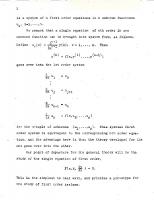
is a sys~em of n first order equations inn unknown functions ui, i=l, ... , n. We remark that a single equation

of nth order in one

unknown function can be brought into system form, as follows. cl V -1 . . . Define = OX V -1 y ( X) j V = l, .•• , . n. Then

goes over into the 1st order system .s!_u

dx

.£.._ u

dx

1

n

=

f ( X, u , • • • , U ) 2 n .

for then-tuple of unknowns

(u 1 , ... ,un).

This special first

order system is equivalent to the corresponding nth order equation, and the advantage here is that the theory developed for the one goes over into the other. Our point of departure for the general theory will be the study.of the single equation of first order,

F(x,y, ~~)

=

O.

This is the simplest to deal with, and provides a prototype for the study of fi~st order systems.

3

No general statements can be made about the equation in the form F

= o.

We put it into standard form by the implicit function

theorem of calculus, =

We ·supp~·se f to exist ( be. defined as a real function of its arguments) in som~ domain D of the xy plane.

The equation now

defines a direction field at every point (x,y) of D. we can find a function

y = y(x)

That is, if

defined in some x interval I,

that when substituted for yin y' = f(x,y) makes the equation an identity in x for x

~

I, the slope y' (x) a~ (x,y(x)) for x € I

must be given by f(x,y(x)).

Thus the direction field prescribes

the slope at each point of D for any·conceivable solution passing through ·that point.

We a~e led to expect that at-every point P

of D, we can find at least one such function y = y(x) satisfying these requirements, and passing through P.

Under the additional

stipulation of continuity for fin D, this will turn out to be the case.

These last remarks implicitly suggest that in order to

attach a label to. functions y £ C(I) satisfying y' = f(x,y) for x € I, we append to the differential equation a side condition of the ~orm y(x 0

)

= y 0 • Even so, we shall see that uniqueness is

not guaranteed without a further condition on f. We turn now to specific examples which highlight our introductory remarks, and hint at other cons.iderations of importance. We note that it will occasionally happen (as in our first few examples to follow) that we can solve an equation explicitly in terms of the given data.

In contrast to elementary courses in

4

t he subject, which deal amply with such special situations, our emphasis will be placed in developing other aspects of the general theory, whose study will often be sufficient for the purposes at hand.

The reader interested.in this very special and

often difficult question of explicit integration of a differential equation is referred to Ritt, Integration in Finite Terms, and to work of Liouville. We remind the reader that the general linear equation of first order,

~ = a(x)y + b(x) , where a and b.are given functions of x, say defined and continuous in

I= {xla ~ x ~ ~}, is an example of an equation that

can be solved expl~citly.

The function

y(x) = e

satisfies the equation in [a,~], and is that function for which X

0

€..

Thus the initial value problem

(a)

y' = a(x)y + b(x)

( b)

y(xo) = y 0

has an answer in every case.

X {; X

0

E

I I

If a and ~-are not. finite, we see

that solutions exist for all x.

This explicit solution is

obtained by two quadratures (integrations).

Another example of solution.by quadrature is given by the non-linear equation describing the motion of a simple pendulum, d 2y . : fl. + "'r"' dx2 .LJ

sin y = O

The solution by quadrature leads to an . elliptic :integral.

Again,

the solution by quadrature of the non-linear equation

_gives the Weierstrassj_-function as the inverse map of an elliptic integral function. For the non-linear Ricatti equation

l

= · A(x)y

2 + B(x)y + C(x) ,

where the coefficients depend on x, solution by quadrature is no longer possible in general.

An interesting result for this equa-·

tion is its equivalence with the general linear equation of second order. fined by

Thus, in terms of a new dependent variable z de-

y =

z' - -Az

, the equation goes over into z

Exercise 1.1.1 kinematics.

11

. A'

-

(

B + r ) z 1 + CAz = 0.

The Ric·atti equation is related to a proble_m in

The first order·system

6 dt

dx

=

& dt

= rx .. az

dz dt

=

PZ - ")'y

A. ay - ..,x

for the tri~le of unknown functions {x,y,z) in terms of a given triple of functions (a(t),~(t),r{t)), can be expressed by the single vector equation d dt £

where r

= (x, y, z) and

CD

=

CD )(

£ ,

= (a, t3, -y )°.

If r is the position vector -

•r

-----....

of a point Pin a rigid body rotating with angular velocity~ about a fixed origin, then the system above is just the familiar kinematical result for the instantaneous velocity of P. If .r, = .r,(t) is a solution, then 1~1 2 = c 2 = constant. Show that the new dependent variable A= A(t) defined by . ). = X

+ iy

C -

Z

,

which is a stereographic projection from the sphere of radius c onto the complex A-plane, satisfies a complex Ricat~i equation. (For a more complete discussion of the Ricatti equation, see Darboux, Theorie

~

Surfaces, Vol. I.).

The following examples illustrate what is to be expected for the manifold of solutions of a differential equation. · The non-linear equation (y 1 ) 2 + y 2 = - l is an example of a real . equation with no real solutions (the direction field defined by this equation is everywhere imaginary), regardless of side conditions imposed.

7

On the other hand, the equation (y 1 ) 2 + y 2 real direction fielo. only for

Iy I ~ . i,

= 1 detines a

and we can expect real .

solutions only for side conditions .of the form y(x0

IY0 1

~ 1.

y0

) =

,

The direction field

predict s at least 2 soluti ons pass ing through each point (x 0 ,y0 - co< x 0 < oo,

IY0 1

< l.

We see that functions yc(x)

),

= cos(x+c~.

'

where c is a constant, and z 1 : 1, z_ 1 = -~the envelopes Or ye.) satisfy the equation. But so does any continu,ously differentiable

combination

~(x) of the form (in say a~ x

cos(x-cr

a ~-

C

n,

m integers,

for ~(x) =

- 1Tn

Q

V

for

~

~

=

is similarly defined for x t f3 and x

+

~ C

X

X ~ C

1 = r+ l- 1 C

V

~

~! p),

m

+

1Tm ~

>

n

~

f3 0

- 1Tn if n even if n odd

M1T < X ~

t

f3 if m even if m odd

~ a •

Thus there exist

+1 - 1

infinitely many continuously differentiable solutions to the initial value problem ~

dx

(b)

=

8

that exist for all x, but which, when restricted to a small enough neighborhood of x 0 ,