Isolated Objects in Quadratic Gravity: From Action Principles to Observations (Springer Theses) 3031489934, 9783031489938
One of the main unanswered question of modern Physics is "How does gravity behave at small scales?". The aim o
125 15 5MB
English Pages 205 [197] Year 2024
Supervisor’s Foreword
Abstract
Contents
Acronyms
1 Introduction
1.1 Outline of the Thesis
1.2 Notes on Units and Adimensionalization
References
2 Quadratic Gravity
2.1 General Quadratic Gravity and Stelle's Action
2.1.1 Starobinski action and f left parenthesis upper R right parenthesisf(R) theories
2.1.2 Einstein-Weyl Gravity
2.2 Scale-Invariant Gravity
2.2.1 Scalar Sector and Einstein Frame Formulation
References
3 Analytical Approximations and Numerical Methods
3.1 Linear Regime and Linearized Equations of Motion
3.1.1 Non-vacuum Case
3.2 Series Expansion at Fixed Radius
3.2.1 Behavior Close to the Origin and Autonomous Dynamical System
3.3 Non-asymptotically Flat Solutions
3.4 Numerical Methods
3.4.1 Shooting Method
References
4 The Phase Diagram of Quadratic Gravity
4.1 The Phase Diagram of Einstein-Weyl Gravity
4.2 The Phase Diagram of Quadratic Gravity
4.3 Non-vacuum Solutions in the Phase Diagram
References
5 Solutions of Quadratic Gravity
5.1 Black Holes
5.2 Naked Singularities
5.2.1 Repulsive Naked Singularities
5.2.2 Attractive Naked Singularities
5.3 Wormholes
5.4 Compact Stars
5.5 Black Holes in Scale-Invariant Gravity
5.5.1 Quadratic Scale-Invariant Cosmology
References
6 Quasi-normal Modes and Stability of the Solutions
6.1 Numerical Methods for Quasi-normal Modes
6.2 Quasi-normal Modes of Solutions of Quadratic Gravity
6.2.1 Quasi-normal Modes of Black Holes in Quadratic Gravity
6.2.2 Quasi-normal Modes of Exotic Solutions in Einstein-Weyl Gravity
6.3 Quasi-normal Modes of Black Holes in Scale-Invariant Gravity
References
7 Semiclassical Quadratic Gravity and Black Hole Thermodynamics
7.1 Black Hole Thermodynamics and Semiclassical Gravity
7.1.1 Hawking Radiation and Black Hole Evaporation
7.1.2 The Path Integral Approach to Quantum Gravity and Black Hole Thermodynamics
7.1.3 Wald Entropy
7.2 Thermodynamics of Black Holes in Quadratic Gravity
7.3 Semiclassical Analysis of Black Holes in Scale-Invariant Gravity
7.3.1 Non-linear Stability and Transitions of Schwarzschild-de Sitter Solutions
References
8 Phenomenological Signatures of Quadratic Gravity
8.1 Shadow of Isolated Objects
8.2 Mass Definitions and Mass Discrepancies
References
9 Conclusions
Appendix A Tachyonic Black Holes
Appendix B Rotating Solutions and Newman-Janis Algorithm
Appendix Curriculum Vitae et Studiorum
Recommend Papers


- Author / Uploaded
- Samuele Silvervalle
File loading please wait...
Citation preview
Springer Theses Recognizing Outstanding Ph.D. Research
Samuele Silvervalle
Isolated Objects in Quadratic Gravity From Action Principles to Observations
Springer Theses Recognizing Outstanding Ph.D. Research
Aims and Scope The series “Springer Theses” brings together a selection of the very best Ph.D. theses from around the world and across the physical sciences. Nominated and endorsed by two recognized specialists, each published volume has been selected for its scientific excellence and the high impact of its contents for the pertinent field of research. For greater accessibility to non-specialists, the published versions include an extended introduction, as well as a foreword by the student’s supervisor explaining the special relevance of the work for the field. As a whole, the series will provide a valuable resource both for newcomers to the research fields described, and for other scientists seeking detailed background information on special questions. Finally, it provides an accredited documentation of the valuable contributions made by today’s younger generation of scientists.
Theses may be nominated for publication in this series by heads of department at internationally leading universities or institutes and should fulfill all of the following criteria . They must be written in good English. . The topic should fall within the confines of Chemistry, Physics, Earth Sciences, Engineering and related interdisciplinary fields such as Materials, Nanoscience, Chemical Engineering, Complex Systems and Biophysics. . The work reported in the thesis must represent a significant scientific advance. . If the thesis includes previously published material, permission to reproduce this must be gained from the respective copyright holder (a maximum 30% of the thesis should be a verbatim reproduction from the author’s previous publications). . They must have been examined and passed during the 12 months prior to nomination. . Each thesis should include a foreword by the supervisor outlining the significance of its content. . The theses should have a clearly defined structure including an introduction accessible to new PhD students and scientists not expert in the relevant field. Indexed by zbMATH.
Samuele Silvervalle
Isolated Objects in Quadratic Gravity From Action Principles to Observations Doctoral Thesis accepted by University of Trento, Trento, Italy
Author Dr. Samuele Silvervalle Department of Physics University of Trento Trento, Italy
Supervisor Prof. Massimiliano Rinaldi Department of Physics University of Trento Trento, Italy
Trento Institute for Fundamental Physics and Applications TIFPA-INFN Trento, Italy
Trento Institute for Fundamental Physics and Applications TIFPA-INFN Trento, Italy
ISSN 2190-5053 ISSN 2190-5061 (electronic) Springer Theses ISBN 978-3-031-48993-8 ISBN 978-3-031-48994-5 (eBook) https://doi.org/10.1007/978-3-031-48994-5 © The Editor(s) (if applicable) and The Author(s), under exclusive license to Springer Nature Switzerland AG 2024 This work is subject to copyright. All rights are solely and exclusively licensed by the Publisher, whether the whole or part of the material is concerned, specifically the rights of translation, reprinting, reuse of illustrations, recitation, broadcasting, reproduction on microfilms or in any other physical way, and transmission or information storage and retrieval, electronic adaptation, computer software, or by similar or dissimilar methodology now known or hereafter developed. The use of general descriptive names, registered names, trademarks, service marks, etc. in this publication does not imply, even in the absence of a specific statement, that such names are exempt from the relevant protective laws and regulations and therefore free for general use. The publisher, the authors, and the editors are safe to assume that the advice and information in this book are believed to be true and accurate at the date of publication. Neither the publisher nor the authors or the editors give a warranty, expressed or implied, with respect to the material contained herein or for any errors or omissions that may have been made. The publisher remains neutral with regard to jurisdictional claims in published maps and institutional affiliations. This Springer imprint is published by the registered company Springer Nature Switzerland AG The registered company address is: Gewerbestrasse 11, 6330 Cham, Switzerland Paper in this product is recyclable.
Everything we do is possible only thanks to all the people we have shared our lives with, but for this thesis I must give a special thanks to: Ilaria “Lalla” Torti, who always pushes me forward when I need it and bring me back to earth when I deserve it, all the people of the Trento branch of ADI, who have been companions in this city and comrades in academia, and Alfio Bonanno, who believed in me more than I did and has been a friend through all these years.
Supervisor’s Foreword
The thesis contains a comprehensive study of compact object solutions in quadratic gravity. As its main virtue, it presents the topic in an accessible way and complements the original results with published research, resulting in a coherent and broad review on the topic. In the last years, there has been a renewed interest in quadratic gravity theories, driven by the quest for well-motivated modifications of General Relativity able to explain a variety of phenomena, from dark energy to quantum effects. The branch of quadratic gravity considered in this work is renormalizable, and it is known to lead to a solid model of cosmic inflation. Nonetheless, compact objects in this context are much less known, due to highly non-linear equations of motion and delicate issues concerning their boundary conditions, even in the case of static and spherically symmetric spacetimes. This thesis largely contributes to fill this gap, by attacking the problem with both analytical and numerical tools. Vacuum and nonvacuum solutions are classified in terms of their geometry, their gravitational field at large distances and their behavior under small perturbations. Some of the results are discussed in a phenomenological perspective, opening the way to test the viability of these models in the future. Trento, Italy August 2023
Prof. Massimiliano Rinaldi
vii
Abstract
Quadratic curvature terms are commonly introduced in the action as first-order corrections of General Relativity, and, in this thesis, we investigated their impact on the most simple isolated objects, that are the static and spherically symmetric ones. Most of the work has been done in the context of Stelle’s theory of gravity, in which the most general quadratic contractions of curvature tensors are added to the action of General Relativity without a cosmological constant. We studied this theory’s possible static, spherically symmetric and asymptotically flat solutions with both analytical approximations and numerical methods. We found black holes with Schwarzschild and non-Schwarzschild nature, naked singularities which can have either an attractive or repulsive gravitational potential in the origin, non-symmetric wormholes which connects an asymptotically flat spacetime with an asymptotically singular one, and non-vacuum solutions modeled by perfect fluids with different equations of state. We described the general geometrical properties of these solutions and linked these short-scale behaviors to the values of the parameters which characterize the gravitational field at large distances. We studied linear perturbations of these solutions, finding that most are unstable, and presented a first attempt to picture the parameter space of stable solutions. We also studied the Thermodynamics of black holes and described their evaporation process: we found that either evaporation leads black holes to unstable configurations, or the predictions of quadratic gravity are unphysical. We also considered the possibility of generalizing Stelle’s theory by removing the dependence from the only mass-scale present by including a new dynamical scalar field, making the theory scale invariant. Having a more complex theory, we did not investigate exotic solutions but limited ourselves to the impact of the new additional degrees of freedom on known analytical solutions. It was already known that, in a cosmological setting, this theory admits a transition between two de Sitter configurations; we analyzed the same problem in the context of static and spherically symmetric solutions and found a transition between two Schwarzschild-de Sitter configurations. In order to do that, we studied both linear perturbations and the ix
x
Abstract
semiclassical approximation of the path integral formulation of Euclidean quantum gravity. At last, we tried to extract some phenomenological signatures of the exotic solutions. In particular, we investigated the shadow of an object on background freefalling light, and a possible way of determining the behavior close to the origin using mass measurements that rely on different physical processes. We show that whenever these measurements are applied to the case of compact stars, in principle it could be possible to distinguish solutions where different equations of state describe the fluid.
Contents
1 Introduction . . . . . . . . . . . . . . . . . . . . . . . . . . . . . . . . . . . . . . . . . . . . . . . . . . . 1.1 Outline of the Thesis . . . . . . . . . . . . . . . . . . . . . . . . . . . . . . . . . . . . . . . . 1.2 Notes on Units and Adimensionalization . . . . . . . . . . . . . . . . . . . . . . . References . . . . . . . . . . . . . . . . . . . . . . . . . . . . . . . . . . . . . . . . . . . . . . . . . . . . .
1 9 11 12
2 Quadratic Gravity . . . . . . . . . . . . . . . . . . . . . . . . . . . . . . . . . . . . . . . . . . . . . . 2.1 General Quadratic Gravity and Stelle’s Action . . . . . . . . . . . . . . . . . . 2.1.1 Starobinski Action and f (R) Theories . . . . . . . . . . . . . . . . . . 2.1.2 Einstein-Weyl Gravity . . . . . . . . . . . . . . . . . . . . . . . . . . . . . . . . 2.2 Scale-Invariant Gravity . . . . . . . . . . . . . . . . . . . . . . . . . . . . . . . . . . . . . . 2.2.1 Scalar Sector and Einstein Frame Formulation . . . . . . . . . . . References . . . . . . . . . . . . . . . . . . . . . . . . . . . . . . . . . . . . . . . . . . . . . . . . . . . . .
15 16 23 25 28 31 33
3 Analytical Approximations and Numerical Methods . . . . . . . . . . . . . . . 3.1 Linear Regime and Linearized Equations of Motion . . . . . . . . . . . . . 3.1.1 Non-vacuum Case . . . . . . . . . . . . . . . . . . . . . . . . . . . . . . . . . . . . 3.2 Series Expansion at Fixed Radius . . . . . . . . . . . . . . . . . . . . . . . . . . . . . 3.2.1 Behavior Close to the Origin and Autonomous Dynamical System . . . . . . . . . . . . . . . . . . . . . . . . . . . . . . . . . . . 3.3 Non-asymptotically Flat Solutions . . . . . . . . . . . . . . . . . . . . . . . . . . . . 3.4 Numerical Methods . . . . . . . . . . . . . . . . . . . . . . . . . . . . . . . . . . . . . . . . . 3.4.1 Shooting Method . . . . . . . . . . . . . . . . . . . . . . . . . . . . . . . . . . . . References . . . . . . . . . . . . . . . . . . . . . . . . . . . . . . . . . . . . . . . . . . . . . . . . . . . . .
35 36 38 41
4 The Phase Diagram of Quadratic Gravity . . . . . . . . . . . . . . . . . . . . . . . . 4.1 The Phase Diagram of Einstein-Weyl Gravity . . . . . . . . . . . . . . . . . . . 4.2 The Phase Diagram of Quadratic Gravity . . . . . . . . . . . . . . . . . . . . . . 4.3 Non-vacuum Solutions in the Phase Diagram . . . . . . . . . . . . . . . . . . . References . . . . . . . . . . . . . . . . . . . . . . . . . . . . . . . . . . . . . . . . . . . . . . . . . . . . .
55 56 60 65 68
45 47 49 49 54
xi
xii
Contents
5 Solutions of Quadratic Gravity . . . . . . . . . . . . . . . . . . . . . . . . . . . . . . . . . . 69 5.1 Black Holes . . . . . . . . . . . . . . . . . . . . . . . . . . . . . . . . . . . . . . . . . . . . . . . 71 5.2 Naked Singularities . . . . . . . . . . . . . . . . . . . . . . . . . . . . . . . . . . . . . . . . . 75 5.2.1 Repulsive Naked Singularities . . . . . . . . . . . . . . . . . . . . . . . . . 76 5.2.2 Attractive Naked Singularities . . . . . . . . . . . . . . . . . . . . . . . . . 80 5.3 Wormholes . . . . . . . . . . . . . . . . . . . . . . . . . . . . . . . . . . . . . . . . . . . . . . . . 83 5.4 Compact Stars . . . . . . . . . . . . . . . . . . . . . . . . . . . . . . . . . . . . . . . . . . . . . 90 5.5 Black Holes in Scale-Invariant Gravity . . . . . . . . . . . . . . . . . . . . . . . . 96 5.5.1 Quadratic Scale-Invariant Cosmology . . . . . . . . . . . . . . . . . . . 98 References . . . . . . . . . . . . . . . . . . . . . . . . . . . . . . . . . . . . . . . . . . . . . . . . . . . . . 100 6 Quasi-normal Modes and Stability of the Solutions . . . . . . . . . . . . . . . . 6.1 Numerical Methods for Quasi-normal Modes . . . . . . . . . . . . . . . . . . . 6.2 Quasi-normal Modes of Solutions of Quadratic Gravity . . . . . . . . . . 6.2.1 Quasi-normal Modes of Black Holes in Quadratic Gravity . . . . . . . . . . . . . . . . . . . . . . . . . . . . . . . . . . . . . . . . . . . . . 6.2.2 Quasi-normal Modes of Exotic Solutions in Einstein-Weyl Gravity . . . . . . . . . . . . . . . . . . . . . . . . . . . . . . 6.3 Quasi-normal Modes of Black Holes in Scale-Invariant Gravity . . . . . . . . . . . . . . . . . . . . . . . . . . . . . . . . . . . . . . . . . . . . . . . . . . . References . . . . . . . . . . . . . . . . . . . . . . . . . . . . . . . . . . . . . . . . . . . . . . . . . . . . . 7 Semiclassical Quadratic Gravity and Black Hole Thermodynamics . . . . . . . . . . . . . . . . . . . . . . . . . . . . . . . . . . . . . . . . . . . . . . . 7.1 Black Hole Thermodynamics and Semiclassical Gravity . . . . . . . . . 7.1.1 Hawking Radiation and Black Hole Evaporation . . . . . . . . . . 7.1.2 The Path Integral Approach to Quantum Gravity and Black Hole Thermodynamics . . . . . . . . . . . . . . . . . . . . . . 7.1.3 Wald Entropy . . . . . . . . . . . . . . . . . . . . . . . . . . . . . . . . . . . . . . . . 7.2 Thermodynamics of Black Holes in Quadratic Gravity . . . . . . . . . . . 7.3 Semiclassical Analysis of Black Holes in Scale-Invariant Gravity . . . . . . . . . . . . . . . . . . . . . . . . . . . . . . . . . . . . . . . . . . . . . . . . . . . 7.3.1 Non-linear Stability and Transitions of Schwarzschild-de Sitter Solutions . . . . . . . . . . . . . . . . . . . . References . . . . . . . . . . . . . . . . . . . . . . . . . . . . . . . . . . . . . . . . . . . . . . . . . . . . . 8 Phenomenological Signatures of Quadratic Gravity . . . . . . . . . . . . . . . . 8.1 Shadow of Isolated Objects . . . . . . . . . . . . . . . . . . . . . . . . . . . . . . . . . . 8.2 Mass Definitions and Mass Discrepancies . . . . . . . . . . . . . . . . . . . . . . References . . . . . . . . . . . . . . . . . . . . . . . . . . . . . . . . . . . . . . . . . . . . . . . . . . . . .
103 104 107 109 113 119 125 127 128 128 136 138 139 145 152 157 159 160 162 171
9 Conclusions . . . . . . . . . . . . . . . . . . . . . . . . . . . . . . . . . . . . . . . . . . . . . . . . . . . . 173 Appendix A: Tachyonic Black Holes . . . . . . . . . . . . . . . . . . . . . . . . . . . . . . . . . 179 Appendix B: Rotating Solutions and Newman-Janis Algorithm . . . . . . . . 185 Curriculum Vitae et Studiorum . . . . . . . . . . . . . . . . . . . . . . . . . . . . . . . . . . . . . 191
Acronyms
ADM BH CMB dS EH EW FLRW GR IR MTP No-sy PR QG RV SadS SdS SH SI SNS TOV UV WH
Arnowitt-Deser-Misner Black Hole Cosmic Microwave Background De Sitter Einstein-Hilbert Einstein-Weyl Friedman-Lemaître-Robertson-Walker General Relativity Infrared Massive Triple Point Non-symmetric Photon Ring Quadratic Gravity Rinaldi-Vanzo Schwarzschild-anti-de Sitter Schwarzschild-de Sitter Shadow Scale Invariant Schwarzschild-non-Schwarzschild Tolman-Oppenheimer-Volkoff Ultraviolet Wormhole
xiii
Chapter 1
Introduction
Gravity has always been the guiding light of Physics into field theories: it has been the first physical interaction described using a dynamical field (the concept itself of field was introduced in Physics in the eighteenth century in order to describe gravity [1]), the first to be described ab initio as a relativistic field theory [2], and it inspired gauge field theories [3], on which the Standard Model of Particle Physics is built. Nonetheless, it remains the only fundamental interaction on which a consensus on a Quantum Field Theory description is still lacking. Our understanding of the gravitational field changed dramatically in 1915 when Einstein’s proposed his theory of General Relativity [2], based on the simple and basic principles that the fundamental laws of Physics have to be the same in all reference frames, that the speed of light is independent of the choice of such frames, and that the gravitational and inertial mass are the same physical quantity. The main consequence of these principles is that the gravitational field is not a quantity defined in the spacetime, but is the structure of spacetime itself, and the gravitational interactions are given by its curvature. Supported by this solid theoretical foundation, and more than a century of experimental evidence, General Relativity proved itself as the current best explanation of the gravitational effects we observe in our universe. However, at very short distances and time intervals it predicts the appearance of singularities, in which physical quantities diverge and spacetime itself stops being a well-defined quantity; a microscopical description in the quantum regime then becomes necessary. The most common approach to quantum gravity exploits the conceptual solidity of General Relativity and the operational power of Quantum Field Theory, in the so-called covariant formulation of quantum gravity [4, 5]. In this context the fundamental objects of investigation are the quantum excitations of spacetime over a classical background, i.e., gravitons, and their scattering amplitudes, which are usually calculated using Feynman diagrams and perturbation theory. However, it was soon realized that to avoid divergent corrections is necessary to add different counterterms at each order in the perturbation theory, and the theory loses its predictivity being perturbatively non-renormalizable [6, 7]. To solve this issue a large number of approaches have been proposed: either to change our notion of renormalizability, © The Author(s), under exclusive license to Springer Nature Switzerland AG 2024 S. Silvervalle, Isolated Objects in Quadratic Gravity, Springer Theses, https://doi.org/10.1007/978-3-031-48994-5_1
1
2
1 Introduction
as done in the context of Asymptotic Safety in which a physical high energy behavior of gravity is guaranteed by non-perturbative effects [8, 9], to change the field content of the theory, as done in Supergravity in which the additional diagrams with the new particles remove the divergences [10, 11], to change our notion of quantum excitation, as in String Theories where the absence of point interactions renders the scattering amplitudes finite [12, 13], or to change our notion of spacetime, as in Causal Dynamical Triangulation where curvature emerges as the interlocking of flat spacetime simplices [14, 15]. Indeed, the search for a theory of quantum gravity has been, in all likelihood, the single topic that attracted the interest of the largest number of theoretical physicists in all of history. The aim of my Ph.D., however, was not to look for a fully consistent theory of quantum gravity, rather it was to understand what could be the most common predictions of these theories in an actual physical context. For this reason, we studied the most simple isolated objects, that are static, spherically symmetric and asymptotically flat, in some of the most common effective theories of quantum gravity, which are quadratic theories of gravity. General Relativity has as fundamental object of investigation the metric tensor .gμν (x), which defines (the norm) of any vector field .vμ (x) at any point of the spacetime .x as .||v(x)|| = gμν vμ vν (x). To parallel transport a vector field .vμ in the direction (of a second vector field .u ν , we introduce the covariant derivative ) ν μ ν μ μ ρ .u ∇ν v = u ∂ν v + Γ νρ v , where .Γ μνρ is an affine connection which is usually taken to be the Levi-Civita one, Γ μνρ =
.
) 1 μσ ( ∂ν gσρ + ∂ρ gνσ − ∂σ gνρ . g 2
(1.1)
This choice guarantees that the norms of vector fields do not change during the transport, thanks to .∇ρ gμν = 0, and that transporting a scalar field in the direction of .vμ and then in the direction of .u ν or the other way around has the same results, thanks to .Γ μνρ = Γ μρν . The dynamics of the spacetime can be completely extracted by its curvature, which can be quantified by the Riemann tensor . R ρσ μν [ .
] ∇μ , ∇ν vρ = R ρσ μν vσ ,
(1.2)
which can be expressed in terms of the Levi-Civita connection as .
ρ
ρ
R ρσ μν = ∂μ Γ ρνσ − ∂ν Γ ρμσ + Γ μλ Γ λνσ − Γ νλ Γ λμσ .
(1.3)
Other useful curvature tensors are the Ricci tensor . Rμν = R ρμρν and the Ricci scalar μν .R = g Rμν . Finally, as understood by Hilbert, Einstein’s theory of gravitation can be completely derived from a Lagrangian theory with an action defined as I
. EH
=
1 16π G
{
√ d4 x −g [R − 2Λ] + Imat ,
(1.4)
1 Introduction
3
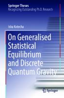
Fig. 1.1 Graviton-graviton scattering at tree level with one-loop and two-loop corrections, where we underlined the dependence from the constant .G of the interaction vertices
where .G is the Newton constant, .Λ is another constant relevant at cosmological scales and .Imat contains all the matter and radiation fields populating the spacetime. To give an intuitive understanding of why there is no consensus on a quantum version of (1.4), let us consider a small perturbation √ .h μν around the Minkowski metric .ημν = diag(−1, 1, 1, 1) as . gμν = ημν + Gh μν . Not considering the constant .Λ and the matter fields, the action (1.4) becomes { ] ] √ .I E H ∼ d4 x (∂h)2 + Gh(∂h)2 + Gh 2 (∂h)2 + ... , (1.5) where we considered having taken all possible covariant contractions of the metric and its derivatives. In a standard Quantum Field Theory description an interaction between two excitations, for example a graviton-graviton scattering, will have loop corrections in a perturbative expansion in the coupling constant .G, as can be seen pictorially in{Fig. 1.1. For a renormalizable theory, the divergent contributions of ∞ each loop .∼ 0 d4 k k 4 can be removed by regularizing the theory integrating only up to a scale .ΛU V , adding to the action a finite number of counterterms, and then finding a finite value when .ΛU V is taken to be infinite again. This is not the case for General Relativity, because the coupling constant .G has a dimension of inverse squared energy .[G] = E −2 , and to have the same dimension at every loop order, each diagram will have a dependence from the cutoff scale as .
) ) ( ( (G)tr ee + G 2 ΛU2 V 1−loop + G 3 ΛU4 V 2−loops + ...
(1.6)
Having a dependence from the cutoff different at any loop order, it is necessary to add a different counterterm at each order; in particular, it will be required to add terms with an increasing number of derivatives. The resulting picture is clear: either we add an infinite number of counterterms, or the limit .ΛU V → ∞ of the amplitude will be infinite; in any case, the theory is not renormalizable in the standard sense.
4
1 Introduction
Fig. 1.2 .β-decay of a neutron considering Fermi interaction, and considering the exchange of a − boson in the electroweak theory
.W
The standard approach to non-renormalizable theories which, nonetheless, are confirmed by low-energy experiments, is to consider them effective theories. For example, let us consider the Fermi model for .β-decay shown in Fig. 1.2. The fourpoint interaction has a coupling constant.G F of mass dimension.[G F ] = E −2 , and the same reasoning made for the graviton-graviton √ scattering can be applied. Nonetheless, we now know that at energies . E ∼ 1/ G √F the .β-decay can be described as the emission of a .W − boson with mass .m W ∼ 1/ G F in the context of the electroweak theory. The electroweak model, which has a dimensionless coupling constant .g ∗ is instead renormalizable, while for energy scales . E s. We then find as final expression for . V (r ) and .Y (r ) ( m s ) { e 2 − e−m 2 s ρ(s) + 3 p(s) e−m 2 r ∞ ds 4 π s 2 + (2 ρ(s) + 8π γ r 24 π γ m 2 s 0 0 ( ) { em 0 s − e−m 0 s e−m 0 r ∞ + 3 p(s)) − ds 4 π s 2 (ρ(s) − 3 p(s)) , r 48 π γ m 0 s 0 . ( ) { m 2 em 2 s − e−m 2 s e−m 2 r ∞ Y (r ) = − ds 4 π s 2 (2 ρ(s) + 3 p(s)) + r 48 π γ s 0 ( ) { m 0 em 0 s − e−m 0 s e−m 0 r ∞ − ds 4 π s 2 (ρ(s) − 3 p(s)) . r 48 π γ s 0 V (r ) = −
1 r
{
∞
ds 4 π s 2
(3.15)
40
3 Analytical Approximations and Numerical Methods
Using the definition .Y (r ) = r −2 (r W (r ))' we find .W (r ) as ( m s ) { ∞ e 2 − e−m 2 s e−m 2 r C 2 (1 + m 2 r ) ds 4 π s W (r ) = − + (2 ρ(s) + 3 p(s)) + r r 48 π γ m 2 s 0 . ( m s ) { ∞ e 0 − e−m 0 s e−m 0 r ds 4 π s 2 + (1 + m 0 r ) (ρ(s) − 3 p(s)) . r 48 π γ m 0 s 0
From the remaining equations of motion we can prove that .C = p(s) . We also note that the integral s 2 ρ(s)+3 8π γ {
∞
.
ds 4 π s 2 p(s)
{ ∞ (3.16) 0 ds 4 π
(3.17)
0
represents the total work of the system, that in our case is zero, and we get again as the final result e−m 2 r e−m 0 r 2M + 2 S2− + S0− r r r −m 2 r e−m 0 r 2M −e + S2 f (r ) = 1 − (1 + m 2 r ) − S0− (1 + m 0 r ) , r r r
h(r ) = 1 − .
(3.18)
with, however, an expression for the free parameters in terms of the stress-energy tensor properties { ∞ 1 ds 4 π s 2 ρ(s) 16π γ 0 { ∞ sinh (m 2 s) 1 = ds 4 π s 2 (2 ρ(s) + 3 p(s)) 16π γ 0 3 m2 s { ∞ sinh (m 0 s) 1 = ds 4 π s 2 (−ρ(s) + 3 p(s)) , 16π γ 0 3 m0 s
M= .
S2− S0−
(3.19)
where the definition of . M agrees with the one found solving the TolmanOppenheimer-Volkoff (TOV) equations in General Relativity, and the result agrees with the one found by Stelle in [1] with .ρ(s) = Mδ(s)/4π s 2 = Mδ 3 (x) and . p(s) = 0. While this result is valid only in the low energy density and pressure limit, it exhibits an extremely interesting feature: the presence of both the energy density and pressure in the expressions for . S2− and . S0− renders the gravitational potential sensitive to the physical nature of the fluid, namely to its equation of state. It is indeed manifest that fluids with a traceless stress-energy tensor will have no scalar Yukawa contribution, while to have a zero contribution from the tensor Yukawa term it is necessary to have either a negative energy density or a negative pressure, in agreement with the pure trace nature of the . R 2 term and the ghost nature of the .C μνρσ Cμνρσ term.
3.2 Series Expansion at Fixed Radius
41
3.2 Series Expansion at Fixed Radius While the linear theory is crucial to determine the asymptotic gravitational properties of the solutions, their specific physical nature can be categorized by analyzing their behavior close to the origin or a metric singularity (as an event horizon). As extensively explained in [2, 7], it is possible to use a variation of the Frobenius method to find the possible behaviors and to determine different families of solutions. Taking an expansion of the metric functions in the form h(r ) = (r − r0 )
t
[ N Σ
s
[ N Σ
n=0
.
f (r ) = (r − r0 )
] ) ( N +1 h t+n/∆ (r − r0 ) + O (r − r0 ) ∆ n ∆
] ) ( N +1 f s+n/∆ (r − r0 ) + O (r − r0 ) ∆ ,
(3.20)
n ∆
n=0
with .h 0 , f 0 /= 0, it is possible to solve the equations of motion order by order in .(r − r0 ). The lowest order equations are called indicial equations because, considering that .h 0 and . f 0 are different from zero by definition, they become equations for the indices .t and .s and determine their admissible values. The higher orders determine the number of the free parameters of the solution for a given set of indices instead. On the contrary, the choice of having whether .r0 = 0 or .r0 /= 0 and of the value of .∆ have to be chosen arbitrarily at the beginning of the calculation. Finally, it is possible to classify the solutions as .(s, t)r∆0 . At the present time, the known families are: where in the second column we made manifest the number of free parameters after imposing asymptotic flatness, a specific time parametrization, and a zero stressenergy tensor. In this thesis we did not analyze the last two families of solutions, being both particularly exotic and present only in a zero measure region of the parameter space, and we will not put any emphasis on the .(0, 0)r10 family, as it represents a generic point of the spacetime with no particular properties. (0, 0)10 family.
.
This family in the vacuum has the general form
.
( ( )) h(r ) = h 0 1 + h 2 r 2 + h 4 (h 2 , f 2 )r 4 + O r 6 ( ) f (r ) = 1 + f 2 r 2 + f 4 (h 2 , f 2 )r 4 + O r 6 ,
(3.21)
with free parameters .h 0 , h 2 and . f 2 , and includes all the solutions with regular curvature in the origin. As shown in [3], we can express all the non-zero terms of the μ ρ Riemann tensor on a local orthonormal frame . Rabcd = Rμνρσ ea ebν ec edσ as
42
3 Analytical Approximations and Numerical Methods
1 − f (r ) , r2 f ' (r ) =− , 2r ' f (r )h (r ) , = 2r h(r ) h(r ) f ' (r )h ' (r ) − f (r )h ' (r )2 + 2 f (r )h(r )h '' (r ) = , 4h(r )2
R yzyz = Rx yx y = Rx zx z .
Rt yt y = Rt zt z Rt xt x
(3.22)
where the other non-zero terms are related by symmetries and .t, x, y and .z are the coordinates in the orthonormal frame, and it can be shown that they are not divergent in the origin if and only if the metric behaves like (3.21). In the vacuum, this family’s only asymptotically Minkowski solution is the Minkowski spacetime itself, with .h 2 = f 2 = 0. In the context of compact stars, we want solutions that are regular everywhere, and then the metric in the origin will belong to the .(0, 0)10 family. Together with the stress-energy tensor, the metric functions will have the form ( ( )) h(r ) = h 0 1 + h 2 r 2 + h 4 (h 2 , f 2 , ρ0 , p0 )r 4 + O r 6 ( ) f (r ) = 1 + f 2 r 2 + f 4 (h 2 , f 2 , ρ0 , p0 )r 4 + O r 6 , . ( ) ρ(r ) = ρ0 + ρ2 (h 2 , f 2 , ρ0 , p0 )r 2 + O r 4 , ( ) p(r ) = p0 + p2 (h 2 , f 2 , ρ0 , p0 )r 2 + O r 4 ,
(3.23)
where the parameters .ρ0 and . p0 will be related by the equation of state of the fluid. (−1, −1)10 family.
.
This family has the general form
.
( ) ( ) 1 h(r ) = h −1 r −1 + + h 2 r 2 + h 3 ( f −1 , h 2 , f 2 )r 3 + O r 4 , f −1 ( ) −1 f (r ) = f −1r + 1 + f 2 r 2 + f 4 ( f −1 , h 2 , f 2 )r 3 + O r 4 ,
(3.24)
with free parameters .h −1 , f −1 , h 2 and . f 2 . The Schwarzschild metric is found setting h = f −1 = −r S and.h 2 = f 2 = 0, for which also all the terms. f n and.h n with.n > 2 are equal to zero. This family is singular in the origin, with the curvature invariants going as R 2 ∼ C( f −1 , h 2 , f 2 ) + O (r ) , R μν Rμν ∼ C( f −1 , h 2 , f 2 ) + O (r ) , . (3.25) ( −5 ) μνρσ −6 , Rμνρσ ∼ r + O r R
. −1
3.2 Series Expansion at Fixed Radius
43
where the constant .C goes to zero for the Schwarzschild metric. This family of solutions from parameter counting should be present in a zero-measure region of the parameter space, but, as we will see later, this is not the case. (−2, 2)10 family.
.
This family has the general form ( ) ( 6) f −1 3 2 4 5 , r + h 4 r + h 5 ( f −2 , f −1 , h 4 , f 0 , f 1 )r + O r h(r ) = h 2 r − f −2 . ) ( f (r ) = f −2 r −2 + f −1r −1 + f 0 + f 1r + f 2 ( f −2 , f −1 , h 4 , f 0 , f 1 )r 2 + O r 2 . (3.26) with free parameters .h 2 , f −2 , f −1 , h 4 , f 0 and . f 1 . The metric in the origin is extremely singular, with curvature invariants going as ( ) R 2 ∼ r −4 + O r −3 , ( ) . R μν Rμν ∼ r −8 + O r −7 , ( ) R μνρσ Rμνρσ ∼ r −8 + O r −7 .
(3.27)
While it is possible to find a combination of the free parameters for which the Ricci scalar is not diverging, namely the combination for which the solution is a solution of the equations of motion of the Einstein-Weyl sector of the theory, the squared Ricci tensor will always be singular as well as the Riemann tensor squared. This family has the total number of free parameters admissible by the equations, and therefore it is expected to represent a type of solution that populates a large area of the parameter space. (1, 1)1r0 family.
.
This family has the general form ( )) ( h(r ) = h 1 (r − r0 ) + h 2 ( f 1 , f 2 , r0 )(r − r0 )2 + O (r − r0 )3 , . ) ( f (r ) = f 1 (r − r0 ) + f 2 (r − r0 )2 + f 3 ( f 1 , f 2 , r0 )(r − r0 )3 + O (r − r0 )4 , (3.28) with free parameters.h 1 , f 1 , f 2 and.r0 . In this case, the Schwarzschild solution simply requires.h 1 = f 1 = 1/r0 and. f 2 = −1/r02 , and the curvature invariants are all regular at.r = r0 . The hypersurface defined by.r = r0 is then clearly an event horizon, and the 1 .(1, 1)r family is the family of black hole solutions. As previously said, black holes 0 are present only in the Einstein-Weyl sector of the theory, and the parameter . f 2 can be expressed in terms of . f 1 and .r0 . From the number of free parameters, it is already manifest that either an additional requirement forces the presence of a horizon or black holes will not be generic vacuum solutions, having only one free parameter after imposing asymptotic flatness and fixing the time parametrization. Thanks to
44
3 Analytical Approximations and Numerical Methods
the Corollary 2.1, this family of solutions is present only in the Einstein-Weyl sector of the theory. (1, 0)1r0 and .(1, 0)2r0 families.
.
These two families of solutions have the form ( ( )) h(r ) = h 0 1 + h 1 ( f 1 , r0 )(r − r0 ) + O (r − r0 )2 , . ( ) f (r ) = f 1 (r − r0 ) + f 2 ( f 1 , r0 )(r − r0 )2 + O (r − r0 )3 ,
(3.29)
with free parameters .h 0 , f 1 and .r0 for the .(1, 0)r10 family, and
.
( h(r ) = h 0 1 + h 1/2 (r − r0 )1/2 + h 1 (r − r0 ) + h 3/2 (h 1/2 , f 1 , h 1 , f 3/2 , r0 )(r − r0 )3/2 + ( )) + O (r − r0 )2 , ( ) f (r ) = f 1 (r − r0 ) + f 3/2 (r − r0 )3/2 + f 2 (h 1/2 , f 1 , h 1 , f 3/2 , r0 )(r − r0 )2 + O (r − r0 )5/2 ,
(3.30) with .h 0 , h 1/2 , f 1 , h 1 , f 3/2 and .r0 as free parameters for the .(1, 0)r20 family. While it is manifest that the .(1, 0)r10 family is a subset of the .(1, 0)r20 family, it is not trivial that it is not sufficient to require .h 1/2 = f 3/2 = 0 to derive one family from the other; an additional constraint can be derived by their interpretation as wormholes. Curvature invariants are regular at .r = r0 , and then it is sensible to expect the spacetime to continue after this point. Extending the spacetime to the region .r < r0 , we have the expansions
.
( )) ( h(r ) = h 0 1 + h˜ 1 ( f˜1 , r0 )(r0 − r ) + O (r0 − r )2 , ) ( f (r ) = f˜1 (r0 − r ) + f˜2 ( f˜1 , r0 )(r0 − r )2 + O (r0 − r )3 ,
(3.31)
for the .(1, 0)r10 family, and
.
( h(r ) = h 0 1 + h˜ 1/2 (r0 − r )1/2 + h˜ 1 (r0 − r ) + h˜ 3/2 (h˜ 1/2 , f˜1 , h˜ 1 , f˜3/2 , r0 )(r0 − r )3/2 + ( )) + O (r0 − r )2 , ( ) f (r ) = f˜1 (r0 − r ) + f˜3/2 (r0 − r )3/2 + f˜2 (h˜ 1/2 , f˜1 , h˜ 1 , f˜3/2 , r0 )(r0 − r )2 + O (r0 − r )5/2 ,
(3.32) for the .(1, 0)r20 family. However, the choice . f 1 = f˜1 leads to a spacetime with two time coordinates, and the choice . f 1 /= f˜1 leads to jumps in the curvature invariants. The only possible choice is then connecting one sheet of spacetime with .r > r0 to another sheet of spacetime with .r > r0 , and the solution is then interpreted as a wormhole. To express manifestly the wormhole nature, we can change the radial coordinate as 1 2 .r = r 0 + (3.33) ρ , 4 for which the metric of the two families looks like
3.2 Series Expansion at Fixed Radius
) ( 4) h1 2 dt 2 + .ds = h0 + ρ + O ρ 4 f1 + (
2
45
) ( 1 2 2 dΩ2 ( ) + r0 + ρ f2 2 4 4 ρ + O ρ 4 (3.34) dr 2
for the .(1, 0)r10 family, and (
) ( 3) h 1/2 h1 2 ρ+ ρ +O ρ ds = h 0 + dt 2 + 2 4 f1 + . ( )2 1 + r0 + ρ 2 dΩ2 , 4
dr 2
2
f 3/2 ρ 2
+
f2 2 ρ 4
( )+ + O ρ3
(3.35) for the .(1, 0)r20 family. Both metrics are manifestly well-behaved around .ρ = 0, and the second sheet of spacetime with .r > r0 is defined by the region .ρ < 0. While the metric in (3.34) is symmetric with respect to the transformation .ρ → −ρ, the one in (3.35) is not manifestly symmetric. The .(1, 0)r20 family is, however, really √ not symmetric because requiring a symmetry with . r − r0 = 21 |ρ| leads once again to jumps in the curvature invariants. The symmetry of the .(1, 0)r10 family, finally, adds the additional constraint on the free parameters of the solutions. Fixing a time parametrization and imposing asymptotic flatness then leads to only a single symmetric wormhole solution and to a large area of the parameter space populated by non-symmetric wormholes.
3.2.1 Behavior Close to the Origin and Autonomous Dynamical System We include here a parallel analysis done in Einstein-Weyl gravity to assess the behavior of the metric close to the origin. Let us consider a redefinition of the metric functions as η(r ) .h(r ) = ch e , f (r ) = c f eλ(r ) , (3.36) and, taking into consideration that for both the .(−1, −1)10 and the .(−2, 2)10 families the function . f (r ) diverges in the origin, approximate the Eq. (2.40) at leading order in .eλ(r ) (( )( ) ) 4 + r 4 + r η' (r ) η' (r ) + λ' (r ) + 2r η'' (r ) = 0, −8 + r (−4λ' (r ) + r (η' (r ) + λ' (r ))(λ' (r ) + η' (r )(−3 + r η' (r ) − 2r λ' (r ))) + −2r (−2 + r η' (r ))λ'' (r ) = 0. (3.37) With a redefinition of the independent variable .x = − ln(r ) and of the metric functions as.t (x) = η' (r ) and.s(x) = λ' (r ), the equations form the autonomous dynamical system
.
46
3 Analytical Approximations and Numerical Methods
−2s 2 t + s 2 − st 2 − 8s + t 3 − 3t 2 − 8 ds =− , dx 2(t − 2) . 1 dt = − (−st − 4s − t 2 − 2t − 4). dx 2
(3.38)
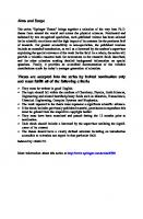
The functions .t (x) and .s(x) are expressed in terms of the original metric functions as r f ' (r ) r h ' (r ) , s= , .t = (3.39) h(r ) f (r ) and they clearly go to the leading exponents of a series expansion close to the origin in the limit .x → ∞. The dynamical system indeed has two fixed points, that are .(t, s) = (−1, −1) and .(2, −2), which correspond to the first exponents of the two non-trivial families of solutions close to the origin. The linear analysis shows that the fixed point .(−1, −1) has one attractive and one marginal direction, while the fixed point .(2, −2) has two attractive directions. The non-linear analysis shown in Fig. 3.1 confirms that the .(2, −2) fixed point is indeed attractive, while the .(−1, −1) one is attractive for only half of the perturbations. Together with confirming that the .(−1, −1)10 and the .(−2, 2)10 families are indeed favored as the behavior in the origin for solutions of the theory, the marginally stable nature of the .(−1, −1) fixed point opens the possibility of having logarithmic corrections to the .(−1, −1)10 family, which might solve the problem of the number of free parameters of the family that do not agree with the results of the phase diagram.
Fig. 3.1 Flow of the running exponents .t, s under the dynamical system (3.38); the arrows point in the direction of decreasing radius. The fixed point .(−1, −1) is in red, while the .(2, −2) is in blue, and the red/blue regions indicate the points that are attracted either to .(−1, −1) or .(2, −2)
3.3 Non-asymptotically Flat Solutions
47
3.3 Non-asymptotically Flat Solutions Having introduced in the previous section non-symmetric wormhole solutions, it becomes necessary to analyze the possibility of having non-asymptotically flat solutions. In this section we will focus on solutions which are asymptotically vanishing, that is where the metric goes as .h(r ) → 0 and . f (r ) → ∞ with .r → ∞, and then both the time and radial components of the metric goes to zero at large distances. To study this type of solution, we write the metric functions as
.
( ) h(r ) = ∊ h 1 (r ) 1 + ∊ h 2 (r ) + O(∊ 2 ) , 1 ( ), f (r ) = ∊ f 1 (r ) 1 + ∊ f 2 (r ) + O(∊ 2 )
(3.40)
( ) and expand the equations in powers of .∊ starting from .O ∊ −1 . Unfortunately, the equations are still not manageable and it is impossible to find a general solution. However, it has been discovered by Alessandro Zuccotti that the functions h 1 (r ) = C h r 2 e−ar , .
f 1 (r ) = C f r 2 e−ar ,
(3.41)
( ) with .a positive, solve the equations at order .O ∊ −1 . This specific form has been found realizing that the metric of non-symmetric wormholes at large distances satisfies with good approximation the equations ( ) 2 d h ' (r ) = 2, dr h(r ) r ( ' ) . d f (r ) 2 = − 2. dr f (r ) r
(3.42)
The expression (3.41), moreover, is in agreement at the first order with the one in (3.26) if expanded around a small radius. To go beyond the first order, it is convenient to consider the ansatz for the functions .h 2 (r ) and . f 2 (r ) .
h 2 (r ) = h˜ 2 (r )e−ar , f 2 (r ) = f˜2 (r )e−ar ,
(3.43)
where the expansion in .∊ is guaranteed to be well-defined at large distances thanks to the additional powers of .e−a r . The equations of motion at order .O(1) then become a system of third-order linear differential equations in .h˜ 2 (r ) and . f˜2 (r ). The solution can be found in a polynomial form
48
3 Analytical Approximations and Numerical Methods
.
h˜ 2 (r ) = h˜ 0 + h˜ 1 r + h˜ 2 r 2 + h˜ 3 r 3 , f˜2 (r ) = f˜0 + f˜1 r + f˜2 r 2 + f˜3 r 3 ,
(3.44)
where .h˜ 0 , . f˜0 and . f˜1 result to be other free parameters, and the other coefficients are completely determined by the six free parameters .(C f , C h , a, f˜0 , h˜ 0 , f˜1 ). Similarly, it is possible to continue the expansion as ( )) ( h(r ) = C h r 2 e−ar 1 + h˜ 2 (r )e−ar + h˜ 3 (r )e−2ar + O e−3ar , .
f (r ) = Cf
r 2 e−ar
1 ( )) , ( −ar ˜ 1 + f 2 (r )e + f˜3 (r )e−2ar + O e−3ar
(3.45)
where we changed the expansion in .∊ in an expansion in .e−ar , which however is) ( well-defined in the large radii limit. The functions .h˜ 3 (r ) and . f˜3 (r ) at order .O e−3ar can be found in a similar way as .h˜ 2 (r ) and . f˜2 (r ) in terms of six order polynomials, but with no other free parameters appearing. The total number of free parameters of these solutions then results to be six, the correct number needed to connect these solutions with the .(1, 0)r20 family. Although we do not discuss the convergence of this expansion, we believe that a certain convergence radius .r ∗ exists, such that for ∗ .r >> r , the solution is well approximated by (3.45). The solutions have a curvature singularity at spatial infinity, having curvature invariants going as ) ( R ∼ C(C f , a, f˜0 , h˜ 0 , f˜1 ) + O e−ar , ( 2ar ) e μν R Rμν ∼ O , . r6 ( 2ar ) e , R μνρσ Rμνρσ ∼ O r6
(3.46)
where the constant .C goes to zero in the Einstein-Weyl limit. Interestingly, if we look at the squared Weyl tensor, the divergent part of the squared Ricci and Riemann tensors compensate, and we get .C
μνρσ
( Cμνρσ ∼ 3
β R + m 22 α
)2
( )2 ( ) ( ) β + O e−ar = 3 C(C f , a, f˜0 , h˜ 0 , f˜1 ) + m 22 + O e−ar α
(3.47) which reduces to.3m 42 in the Einstein-Weyl limit. While it might be simply an interesting curiosity, we believe that it could be relevant for the application of the finite action principle [12], which is getting much attention in recent times for its applications in quadratic theories of gravity [13–15].
3.4 Numerical Methods
49
3.4 Numerical Methods Having shown in the previous sections the approximations used to describe the metric in various regimes, we present here the main numerical tools used to investigate the non-linear regime and the global structure of the solutions. Having as one of the main goals the study of isolated objects without a cosmological constant, all the solutions will be described at large distances by the weak field expansion shown in (3.5). To study the solutions qualitatively or to study the phase diagram of the theory, it is sufficient to integrate the equations using (3.5) as initial conditions at a large radius .x∞ . The integration has been done using the adaptive step size RungeKutta integrator DO2PDF developed by the N.A.G. group (see https://www.nag.com for details) with a tolerance of .10−12 for vacuum solutions and of .10−9 for nonvacuum solutions. The large radius has then been chosen as .x∞ = 18 in numerical units in order to have Yukawa corrections larger than the tolerance threshold. The solutions at the origin are classified in terms of the values of the running exponents (3.39) evaluated at a small radius .ro = 10−3 ; this is particularly useful for solutions without no metric singularity for .r > 0, and for the interior of black holes. To study solutions in greater detail, however, it is necessary to use a more refined method, described in the following paragraphs. The method described is also necessary to study black hole solutions, considering that they populate a zero-measure region of the parameter space and, therefore, cannot be analyzed using a simple initial value integration.
3.4.1 Shooting Method Choosing a specific type of solution to investigate means choosing one of the behaviors in Table 3.1 a priori, and then specifying an internal boundary. At the numerical level, choosing a specific type of solution to investigate then means solving a boundary value problem for a system of ordinary differential equations. To describe the general procedure, we can recast the equations of motion as a set of . N first-order ordinary differential equations with dependent variables.y and independent variable.x .
dy(x) = f(x, y1 , y2 , ..., y N ), dx
(3.48)
and impose Dirichlet boundary conditions at a certain point .x1 , characterized by .n 1 parameters .V j with . j = 1, ..., n 1 y(x1 ) = B1 (x1 , V1 , ..., Vn 1 );
.
(3.49)
we then impose Dirichlet boundary condition also at another point .x2 , characterized by .n 2 = N − n 1 parameters .Vk with .k = 1, ..., n 2 y(x2 ) = B2 (x2 , V1 , ..., Vn 2 ).
.
(3.50)
50
3 Analytical Approximations and Numerical Methods
Table 3.1 Families of solutions around finite and zero radii in quadratic gravity o Family .N of free parameters Interpretation .3 (→
.(0, 0)0
1 1
.(−2, 2)0
1
1 .(0, 0)r 0 1 .(1, 1)r 0 1 .(1, 0)r 0 2 .(1, 0)r 0 .(3/2, 1/2)r
2
3 .(4/3, 0)r 0
0) 1) .6 (→ 3) .6 (→ 3) .4 (→ 1) .3 (→ 0) .6 (→ 3) .3 (→ 0) .4 (→ 1)
Vacuum Naked singularity/Schwarzschild interior Naked singularity (Holdom star) Generic solution Black hole Symmetric wormhole Non-symmetric wormhole Unusual black hole Unusual wormhole
.4 (→
.(−1, −1)0
0
To solve this problem, the shooting method solves exactly (within the numerical integration accuracy) the equations and then makes the solution satisfy the boundary conditions, as opposed to the relaxation method in which the boundary conditions are satisfied by a solution which then is required to solve the differential equations. To implement the shooting method, we start by defining an . N -dimensional vector .V that can be thought as (
V1 .V = V2
)
where .V1 and .V2 are respectively an .n 1 and .n 2 -dimensional vectors with the parameters’ values defining the boundary conditions at .x1 and .x2 . We now define two distinct loading subroutine LOAD1(x1,v1,y) and LOAD2(x2,v2,y) that generate the starting vectors.B(x1 ) and.B(x2 ), and integrate the system (3.48) up to an intermediate point .x f from both boundaries, using a subroutine ODEINT(N,yi, yl,xi,xf,derivs), defining the vectors .y L (x f ) and .y R (x f ), where the subscripts . L and . R indicate if the integration has been done from left or right boundary. Finally, the subroutine SCORE(xf,yl,yr,f) define a discrepancy vector .F as F = y L (x f ) − y R (x f ).
.
Collecting everything in the subroutine subroutine FUNCV(N,v,f) call LOAD1(x1,v,yi) call ODEINT(N,yi,yl,x1,xf,derivs) call LOAD2(x2,v(n2+1),y) call ODEINT(N,yi,yr,x2,xf,derivs) call SCORE(xf,yl,yr,f) return end
3.4 Numerical Methods
51
the boundary value problem is reduced to a root-finding problem for the function F (V) defined by the subroutine FUNCV(N,v,f). Within the work made for this thesis, the subroutine ODEINT(N,yi,yl,xi,xf,derivs) has still been defined using the DO2PDF integrator, while, for the root-finding algorithm, it has been used the BROYDN subroutine found in the Fortran version of Numerical Recipes [16], which implements the Broyden’s method.
.
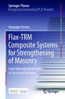
Shooting method for black holes. To study black hole solutions we impose, together with the boundary (3.5) at large distances, that the metric satisfies the boundary condition (3.28) at fourth order at a radius .rb = r H + 10−3 , where .r H is the radius at which the event horizon is located and is an external parameter. Having specified the value of .r H , the shooting method then finds the values of . M, S2− , f 1 and .h 1 for which the boundary value problem is solved with a precision of the root-finding algorithm of .10−6 (remember that thanks to the Corollary 2.1 black holes are present only in the Einstein-Weyl sector of the theory); the fitting radius .r f at which the two integrations are matched does not change the results and have been fixed at .r f = r H + 0.5 for optimal convergence. The family of black holes is found by varying the value of .r H , which is the only free parameter left. The series expansion (3.28) can then be extended to the other side of the horizon and be used as the initial value for an additional integration towards the origin. The metric at the origin is then classified using the running exponents (3.39). In Fig. 3.2, finally, we show how the numerical integration interpolates between the various analytical approximations for a non-Schwarzschild black hole.
Fig. 3.2 Analytical approximations and the shooting method for a non-Schwarzschild black hole; the non-linear solutions in solid lines interpolate between the asymptotic values (in dashed lines) and the series expansion at the horizon (in dotted lines), and at the end is fitted by another series expansion (in dotted-dashed lines) close to the origin
52
3 Analytical Approximations and Numerical Methods
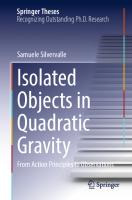
Shooting method for compact stars. In order to study compact star solutions the boundary (3.5) at large distances is imposed together with the conditions .ρ(r∞ ) = p(r∞ ) = 0, and the other boundary is fixed using the expansion (3.23) at fourth order at a small radius .ro = 10−3 . From the internal boundary the non-vacuum equations are integrated up to a radius . R∗ , which is an external parameter specified before the integration, while from the external boundary the vacuum equations of motion are solved up to the same radius. Matching the vacuum and non-vacuum equations of motion at the radius.r = R∗ fixes the star surface precisely at that radius. As in the case of black holes, the parameters . M, S2− , S0− , h 0 , ρ0 , p0 , h 2 and . f 2 are completely fixed by the integration and the radius . R∗ is the only free parameter of the solution, which can be varied to explore the family of solution. Each family is also specified by an equation of state . p = P(ρ), which, being an equation with dimensionful parameters, fixes the energy scales of the fluid. As we will discuss in more detail in Sect. 5.4, this will impose some restriction on either the free parameters of the action .α and .β or the parameters present in the equation of state. We also note that, in general, the equations of state of physical fluids assume that the energy density is always positive; the shooting method, however, will often produce negative values for the energy density in the integrations before convergence. We specify here that all the equations of state will be in terms of the energy density modulus, which guarantees a well-defined pres-
Fig. 3.3 Analytical approximations and the shooting method for a compact star; the non-linear solutions in solid lines interpolates between the asymptotic values (in dotted lines) and the series expansion at the origin (in dashed lines)
3.4 Numerical Methods
53
sure but can slow down the convergence process. In Fig. 3.3, finally, we show how the numerical integration interpolates between the various analytical approximations for a compact star with the polytropic equation of state. p = 0.2 ρ 2 in numerical units. Shooting method for wormholes. The general procedure for applying the shooting method to wormhole solutions is the same as the one for black holes, that is, a shooting method between the linearized expansion (3.5) at large distances and the series expansion (3.30) close to the metric singularity, and then a further integration with initial conditions set by the boundary at the metric singularity. Applying this method to wormholes, however, requires some additional care due to the presence of three free parameters and a divergent first derivative of the time component of the metric at the throat. We then present the procedure in the case of Einstein-Weyl gravity, where the presence of only two free parameters dramatically simplifies the discussion. The first point of caution is that it is much more convenient to fix the external parameters . M and . S2− to have
Fig. 3.4 Analytical approximations and the shooting method for wormholes, with the asymptotically flat patch in the top panel and the asymptotically vanishing in the bottom panel; the non-linear solutions in solid lines interpolates between the asymptotic values (in dashed lines) and the series expansion at the throat (in dotted lines), and at the end is fitted by the asymptotically vanishing metric at large distances in the second patch (in dotted-dashed lines)
54
3 Analytical Approximations and Numerical Methods
faster convergence in the codes. This required a previous parameter space analysis to find the area where an integration from large radii leads to a metric singularity at a finite radius. After this preliminary scan of the parameter space, using this external integration to formulate an educated guess for the parameters at the throat is also helpful. Having a divergent derivative of the time component of the metric, the integration from the throat is very sensitive to the specific values of the parameters, in particular to the throat radius and the parameter .b1/2 in (3.30). Nonetheless, taking into account these precautions, the shooting method results to be quite efficient also in this case, as can be seen in the example of a wormhole with . M = 0.6 and . S2− = −0.2 in Fig. 3.4.
References 1. Stelle KS (1978) Classical gravity with higher derivatives. Gen Rel Grav 9:353–371 2. Lü H, Perkins A, Pope C, Stelle K (2015) Spherically symmetric solutions in higher-derivative gravity. Phys Rev D 92(12):124019 3. Perkins A (2016) Static spherically symmetric solutions in higher derivativs gravity. PhD thesis, Imperial college 4. Bonanno A, Silveravalle S (2019) Characterizing black hole metrics in quadratic gravity. Phys Rev D 99(10):101501 5. Bonanno A, Silveravalle S (2021) The gravitational field of a star in quadratic gravity. J Cosmol Astropart Phys 08:050 6. Podolsky J, Svarc R, Pravda V, Pravdova A (2018) Explicit black hole solutions in higherderivative gravity. Phys Rev D 98(2):021502 7. Podolsky J, Svarc R, Pravda V, Pravdova A (2020) Black holes and other exact spherical solutions in quadratic gravity. Phys Rev D 101(2):024027 8. Svarc R, Podolsky J, Pravda V, Pravdova A (2018) Exact black holes in quadratic gravity with any cosmological constant. Phys Rev Lett 121(23):231104 9. Bonanno A, Silveravalle S, Zuccotti A (2022) Nonsymmetric wormholes and localized big rip singularities in Einstein-Weyl gravity. Phys Rev D 105(12):124059 10. Arnowitt RL, Deser S, Misner CW (2008) The dynamics of general relativity. Gen Rel Grav 40:1997–2027 11. Komar A (1959) Covariant conservation laws in general relativity. Phys Rev 113:934–936 12. Barrow JD, Tipler FJ (1988) Action principles in nature. Nature 331:31–34 13. Lehners J-L, Stelle KS (2019) A safe beginning for the universe? Phys Rev D 100(8):083540 14. Borissova JN, Eichhorn A (2021) Towards black-hole singularity-resolution in the Lorentzian gravitational path integral. Universe 7(3):48 15. Chojnacki J, Kwapisz J (2021) Finite action principle and Hoˇrava-Lifshitz gravity: Early universe, black holes, and wormholes. Phys Rev D 104(10):103504 16. Press WH, Teukolsky SA, Vetterling WT, Flannery BP (1992) Numerical recipes in FORTRAN: The art of scientific computing. Cambridge University Press
Chapter 4
The Phase Diagram of Quadratic Gravity
As extensively discussed in the previous chapter, there are many possible behaviors for the metric around the origin or a metric singularity in quadratic gravity. This large variety of short-scale behaviors is contrasted with the single, but very simple and physically intuitive, form of the metric at large distances. The weak field expansion at large distances is indeed characterized by the total mass and the strength of the interactions mediated by the additional massive modes, which characterize the gravitational interaction at large distances. It is then of fundamental relevance to understanding how these parameters affect the short-scale behavior of the solutions. To indicate the diagram in which different types of solutions are associated with specific regions of the parameter space, we borrowed the term “phase diagram” from classical Thermodynamics to highlight the fact that we are associating a “microscopical” property of solutions to the parameters describing their “global” external properties. This chapter is divided in three parts: – in the first section we will present the phase diagram of vacuum solutions in Einstein-Weyl gravity, which is the most informative two-dimensional reduction of the full quadratic theory. There will be four different types of solutions: black holes with Schwarzschild or non-Schwarzschild nature, naked singularities which are gravitationally repulsive in the origin, naked singularities which are gravitationally attractive in the origin and non-symmetric wormholes; we will show that black holes populate only a zero-measure region of the parameter space and that for large masses most of the solutions will be either wormholes if the Yukawa contribution to the gravitational potential is attractive, or repulsive naked singularities if the Yukawa contribution is repulsive; – in the second section we will present the main issues emerging in the evaluation of the phase diagram of vacuum solutions in the full quadratic theory, namely an inconsistency in the link between the linear and non-linear regimes in the case the masses of the two additional modes are different, and try to extract some physical information nonetheless. The families of solutions will be the same as in © The Author(s), under exclusive license to Springer Nature Switzerland AG 2024 S. Silvervalle, Isolated Objects in Quadratic Gravity, Springer Theses, https://doi.org/10.1007/978-3-031-48994-5_4
55
56
4 The Phase Diagram of Quadratic Gravity
Einstein-Weyl gravity and, in this case, also attractive naked singularities will have a relevant role in the region of the phase diagram with solutions with large masses; in particular repulsive singularities will be favored by a repulsive contribution of the massive tensor particle, attractive naked singularities by an attractive contribution of the massive scalar particle, and wormholes by a simultaneous attractive contribution of the tensor particle and a repulsive contribution of the scalar particle; – in the third section we will show the location of non-vacuum solutions in the phase diagram of vacuum solutions; in particular, in Einstein-Weyl gravity they will populate only the region where repulsive naked singularities are present, while in the full quadratic theory they will populate the surface which separates attractive and repulsive naked singularities. In all the cases considered, there will be two points in the phase diagrams which emerge as triple points for all the different types of solutions, of which one of them is Minkowski, and the other represents a solution with a small and positive mass; The results on the phase diagram of Einstein-Weyl gravity, both for vacuum and nonvacuum solutions, have been published in [1], while the ones on the phase diagram of the full quadratic theory have only been anticipated in [2], but not fully published yet.
4.1 The Phase Diagram of Einstein-Weyl Gravity The phase diagram of vacuum solutions of Einstein-Weyl gravity is depicted in Fig. 4.1. The parameter space is mapped by the values of the mass . M and the Yukawa charge . S2− , which characterize the gravitational potential at large distances; we will show here also the part of the phase diagram with . M < 0, and postpone to the following chapters the discussion on the possible phenomenological reductions of the diagram. To describe this diagram we will use the term “repulsive mass” for negative values of the parameter . M and attractive or repulsive Yukawa charge for negative or positive values of the parameters . S2− respectively; once specified the attractive or repulsive nature of the parameters we will use “large” and “small”, or similar terms, always referring to their modulus. The solutions will be characterized either by the presence of a metric singularity or by the value of the running exponents (3.39) t=
.
d log (h(r )) r h ' (r ) = , d log(r ) h(r )
s=
d log ( f (r )) r f ' (r ) = d log(r ) f (r )
(4.1)
at a small radius set to .ro = 10−3 . The integration of the equations has been done with a Fortran code as described in Sect. 3.4, and later cross-checked with a code written using the Wolfram Mathematica language by Alessandro Zuccotti. The phase diagram is divided into five main regions populated by three different types of solutions:
4.1 The Phase Diagram of Einstein-Weyl Gravity
57
Fig. 4.1 Phase diagram of vacuum solutions of the Einstein-Weyl theory; the dashed black line indicates Schwarzschild black holes, while the solid red and blue lines indicate non-Schwarzschild black holes
– Type I solutions: they are characterized by values of the running exponents between .−0.8 and .−1.4; – Type II solutions: they are characterized by values of the running exponent .t very close to 2 and of the running exponent .s very close to .−2; – Type III solutions: they are characterized by a metric singularity at a radius different from zero in which there is a zero of the function . f (r ) which is not a zero of the function .h(r ). We postpone to Chap. 5 a detailed description of these solutions; however, now we will sketch their main properties and the relation of their location in the phase diagram with the asymptotic parameters. Type I. The first type of solution seems to belong to the .(−1, −1)10 family; however, we have found relevant discrepancies from the expected value .t = s = −1 even at radii smaller than .ro = 10−3 . Moreover, these solutions cover an area of the phase diagram, while the number of free parameters of the .(−1, −1)10 family suggests that they should occupy a one-dimensional region. These considerations make evident that type I solutions should belong to some correction of the .(−1, −1)10 family, but with the same leading order. In [3] a non-Frobenius family that shares the same leading order of the .(−1, −1)10 family but with logarithmic corrections and with one additional free parameter has been found in the full quadratic theory, but in Einstein-Weyl gravity none of such family has been discovered. Sharing the leading behavior of .(−1, −1)10 solutions, however, we can still infer that they are naked sin-
58
4 The Phase Diagram of Quadratic Gravity
gularities with a repulsive gravitational force close to the origin, and we will refer to them as “repulsive naked singularities”. Indeed, they populate the area where both the mass and the Yukawa charge are repulsive, the area where the mass is repulsive and the Yukawa charge is attractive but with a repulsive mass larger than the attractive Yukawa charge, and the area where the mass is attractive and the Yukawa charge is repulsive but with a repulsive Yukawa charge larger than the attractive mass. Type II. The second type of solutions instead truly belong to the.(−2, 2)10 family, having found no relevant discrepancies from .(s, t) = (−2, 2) (except for the regions close to the transition with other families) and, in contrast with type I solutions, the area populated by these solutions agrees with the number of free parameters of the .(−2, 2)10 family. Belonging to this family, they also represent naked singularities, but with an attractive gravitational force close to the origin, and we will refer to them as “attractive naked singularities”. As opposed to their repulsive counterparts, they populate a region with an attractive mass and repulsive Yukawa charge but with a mass much larger than the Yukawa charge, a region with repulsive mass and attractive Yukawa charge but with a Yukawa charge much larger than the repulsive mass, and finally a small region with an attractive mass and an attractive Yukawa charge, but where both take small values. Type III. The third type of solutions, in principle, might belong to the .(1, 0)r10 or the .(1, 0)r20 families, but the number of the free parameters eliminates the possibility of having an area populated by .(1, 0)r10 solutions. Finally, the code which implements the shooting method with a .(1, 0)r20 boundary converges in all the regions shown populated by type III solutions in Fig. 4.1, confirming that this is indeed their behavior close to the metric singularity. We will refer to these solutions as either wormholes, nonsymmetric wormholes, or the contracted form no-sy WHs. They populated almost all the areas where both the mass and the Yukawa charge are attractive, with the exception of a region where both are small (occupied by type II solutions), a small region with attractive mass and repulsive Yukawa charge, but with small values of both parameters, and a region with repulsive mass and attractive Yukawa charge, but with the Yukawa charge being significantly larger than the repulsive mass. Black holes. Black holes populate only zero-measure regions of the phase diagram and then cannot be found by a simple scan of the parameter space, but it is necessary to use the shooting method. Schwarzschild black holes are shown in the dashed black line in Fig. 4.1, while non-Schwarzschild black holes are shown with the solid red and blue lines, where the two different colors indicate whether they have negative or positive Yukawa charge and will be useful in the discussion of Chaps. 6 and 7. Their
4.1 The Phase Diagram of Einstein-Weyl Gravity
59
specific location is on the lines which separate attractive naked singularities (type II) and non-symmetric wormholes (type III), and stressing the phase diagram analogy they represent the phase transition between the two different types of solutions. Being on this separation lines, Schwarzschild black holes always have an attractive mass and zero Yukawa charge, and non-Schwarzschild black holes have either an attractive mass and repulsive Yukawa charge, but both being small, an attractive mass and attractive Yukawa charge, but still both being small, or a repulsive mass and attractive Yukawa charge, but with no bounds for both of them and with a Yukawa charge always larger than the repulsive mass. Let us now focus on the most interesting part of the phase diagram from a phenomenological point of view, which is the one where solutions have a large attractive mass. The first point emerging is that black holes can have only Schwarzschild nature, they are present only in a zero-measure region of the parameter space and therefore are not expected to be the general vacuum solutions of Einstein-Weyl gravity, unless specific arguments are taken into account to require the existence of a horizon. For an attractive contribution of the Yukawa term in the asymptotic potential, the solutions will always be non-symmetric wormholes while, for a repulsive contribution, they will always be naked singularities; the main difference here is that for very small values of the repulsive Yukawa charge the naked singularity will be attractive and in the other cases it will be repulsive. Stressing a little bit more the phase diagram analysis, there are two “triple points” in the diagram, shown in detail in Fig. 4.2. The first corresponds to the Minkowski spacetime . M = 0, S2− = 0, while the second one, which we will call massive triple
Fig. 4.2 Triple points in the phase diagram of vacuum solutions of the Einstein-Weyl theory; the dashed black line indicates Schwarzschild black holes, while the solid red and blue lines indicate non-Schwarzschild black holes
60
4 The Phase Diagram of Quadratic Gravity
point from now on, is located at . M ≃ 0.623, S2− ≃ 0.102 in our numerical units. Both triple points are at the border of the areas populated by type I, type II, black hole, and wormhole solutions; moreover, the Minkowski one corresponds to the point where the horizon of Schwarzschild black holes goes to zero, while the massive triple point is where the horizon of non-Schwarzschild black holes goes to zero. Taking into account these properties, it seems that the Minkowski flat space is not unique as it is in General Relativity and could be not the only “true vacuum” of the theory; the presence of this massive triple point suggests that there might be a sort of ghost condensate vacuum, that might have relevant consequences on the study of quantum fluctuations.
4.2 The Phase Diagram of Quadratic Gravity Finding the phase diagram for the full quadratic theory was one of the objectives of this thesis. Unfortunately, as mentioned at the beginning of this chapter, an inconsistency in the link between the linear and non-linear regimes in the full theory appeared. In the weak field limit for the metric (3.5), two different Yukawa terms with two different masses are present; having two different masses results in an ill definition of the linear solution, opening possibilities as .
e−m 0 r e−m 2 r < r r2
(4.2)
for .m 0 > m 2 and .r large enough, which means having ( ) O (∊) < O ∊ 2 .
.
(4.3)
We specify here that even if in principle it could have been possible also to have a situation as e−m 2 r 1 . (4.4) < 2 r r for .r large enough, a term with no exponentials would be proportional only to the M parameter and then, being equal to a non-linear contraction of the Schwarzschild metric, will have a vanishing contribution to the Ricci tensor and will not appear in the equations of motion. Nonetheless, the ill behavior of the linearized metric with two exponentials persists. The most immediate consequence of this inconsistency is that, for .m 0 > m 2 , it is not possible to find a phase diagram where the section . S0− = 0 is equal to the phase diagram of Einstein-Weyl gravity. As a first step in the discussion, we present in Fig. 4.3 the phase diagram of the . R + R 2 theory, which is much simpler than the one of Einstein-Weyl gravity. Type I solutions, which are repulsive naked singularities, populate the majority of the area with a repulsive mass, with the exception of an attractive Yukawa charge larger than the repulsive mass, and are
.
4.2 The Phase Diagram of Quadratic Gravity
61
Fig. 4.3 Phase diagram of vacuum solutions of . R + R 2 gravity; the three types of solutions are the same as in Einstein-Weyl gravity and the dashed black line indicates Schwarzschild black holes
present only in a small portion of the area with an attractive mass and only if a much larger repulsive Yukawa charge is present. Type II solutions, which are attractive naked singularities, still populate the area with a repulsive mass and an attractive Yukawa charge but with a mass smaller than the Yukawa charge, and all the areas with an attractive mass and an attractive Yukawa charge. Type III solutions, which are nonsymmetric wormholes, instead populate almost all the area with an attractive mass and a repulsive Yukawa charge, in contrast to what happens in Einstein-Weyl gravity. In agreement with Theorem 2.1 there are only Schwarzschild black holes, which are on the . S0− = 0 line that is the intersection with the Einstein-Weyl theory. Also in this case, black holes appear only as transitions between wormholes and attractive naked singularities, and the only triple point of the diagram is the Minkowski spacetime. It is interesting to note that, as in Einstein-Weyl gravity, in the large mass limit half of the phase diagram is populated by non-symmetric wormholes, while in contrast to Einstein-Weyl gravity, the other half is populated by attractive naked singularities instead of repulsive ones. To understand how the scalar and tensor Yukawa terms interact one with the other, we can analyze the phase diagram of the full quadratic theory in the specific case .m 0 = m 2 where the linearized metric is well-defined, that we present in Fig. 4.4. To clarify the discussion, we superimposed the phase diagram of Einstein-Weyl gravity over the . S0− = 0 sector of the parameter space and the one of . R + R 2 gravity over the − . S2 = 0 sector, with a perfect agreement. Similarly to the previous cases, the three main volumes of the diagram are populated by the same types of solutions, namely attractive and repulsive naked singularities, and non-symmetric wormholes. Black holes are still present only in one-dimensional lines on the . S0− = 0 section of the surface which separate attractive naked singularities and non-symmetric wormholes. The phase diagram is then populated as follows:
62
4 The Phase Diagram of Quadratic Gravity
Fig. 4.4 Phase diagram of vacuum solutions of quadratic gravity in the case .m 0 = m 2 with superimposed the phase diagram of the Einstein-Weyl and the. R + R 2 sectors; the three types of solutions are the same of Einstein-Weyl gravity, the dashed black line indicates Schwarzschild black holes and the solid red and blue lines indicate the non-Schwarzschild ones
– Type I solutions are still the solutions more present in the area with a repulsive mass; in particular, they are more present whenever also the Yukawa charges have a repulsive contribution; for an attractive mass, they are present only if the tensor Yukawa charge . S2− is repulsive, while the scalar charge . S0− can be either attractive or repulsive but with an intensity always smaller than the tensor charge; – Type II solutions mainly populate the area where both the mass and the scalar charge are attractive, while for them to be repulsive they have to be contrasted by a stronger attractive contribution of the tensor Yukawa charge; as the mass increase, if the tensor charge is attractive the scalar charge has to be larger, while if the tensor charge is repulsive the scalar charge can be smaller;
4.2 The Phase Diagram of Quadratic Gravity
63
– Type III solutions mainly populate the area where both the mass and the tensor charge are attractive, but the scalar charge is repulsive, while for them to be repulsive they have to be compensated by a much stronger repulsive contribution of the scalar charge; as the mass increase, they can be present both for attractive and repulsive scalar and tensor Yukawa charges, especially in the regions where the repulsive scalar charge is larger than the repulsive tensor charge, or the attractive tensor charge is larger than the attractive scalar charge. To focus once again on the part of the phase diagram with a large attractive − − mass, repulsive naked singularities are present approximately ( − − ) when .−S2 ≲ S0 ≲ − − S2 , attractive naked singularities when . S0 ≲ min −S2 , S2 and non-symmetric wormholes whenever . S0− ≳ S2− . The triple points of the phase diagram of EinsteinWeyl gravity are now the intersections with the surface of zero scalar Yukawa charge of conjunction line of the surfaces that separate the three types of solutions; they still are the only points where the three generic vacuum solutions also meet with black holes. Regardless of the specific behavior of this phase diagram, we can track down some common behavior of the effects of the three asymptotic parameters, that is: – a repulsive mass . M < 0 will always favor repulsive naked singularities, and the values of the Yukawa charges have little effect; – with an attractive mass, a repulsive tensor charge . S2− > 0 favors repulsive naked singularities while an attractive tensor charge. S2− < 0 favors non-symmetric wormholes; – with an attractive mass, a repulsive scalar charge . S0− > 0 favors non-symmetric wormholes while an attractive scalar charge . S0− < 0 favors attractive naked singularities. From a physical point of view, we expect that changing the ratio between the two masses .m 0 and .m 2 , the Yukawa with a bigger mass should have less effect, and the phase diagram should become more similar to one of the two bi-dimensional cases Figs. 4.1 or 4.3; as an example, if we consider the case .m 2 >> m 0 we expect that varying the tensor charge . S2− will have little effect and the phase diagram will become the translation solid generated by the phase diagram 4.3 on the . S2− direction. Unfortunately, this is not the case: as we can see in Fig. 4.5, where we show the phase diagram in the case .m 0 = 23 m 2 , the tensor charge has less effect indeed, and the families of solutions are not influenced that much by the values of . S2− , but the phase diagram is not a translation of the one of . R + R 2 gravity. Moreover, the sector . S2− = 0 does not coincide anymore with the one of . R + R 2 gravity. The sector . S0− = 0, instead, still coincides with the Einstein-Weyl gravity phase diagram. In particular, what happens is that for an attractive scalar charge, repulsive and attractive naked singularities change their places in the phase diagram. Something similar happens in the case of .m 0 larger than .m 2 , as can be seen in Fig. 4.6, where we present the phase diagram in the case .m 0 = 23 m 2 . Here the values of the scalar charge . S0− have little effect on the families of solutions; still, we are not able to find the phase diagram of Einstein-Weyl gravity in the − 2 . S0 = 0 sector, while we find (approximately) the phase diagram of . R + R gravity
64
4 The Phase Diagram of Quadratic Gravity
Fig. 4.5 Phase diagram of vacuum solutions of quadratic gravity in the case .m 0 = 23 m 2 with superimposed the phase diagram of the Einstein-Weyl and . R + R 2 sectors
in the . S2− = 0 sector. The phase diagram, in this case, has a quite complicated structure that we believe is not particularly insightful to investigate deeply. As previously said at the beginning of this chapter, we believe these inconsistencies are due to the ill definition of the linear theory in the case of different masses. While having the phase diagram in the Einstein-Weyl, the . R + R 2 , and .m 0 = m 2 cases can shed light on the phase diagram of the full theory in the generic case, this ill-definition of the linearized theory has to be solved.
4.3 Non-vacuum Solutions in the Phase Diagram
65
Fig. 4.6 Phase diagram of vacuum solutions of quadratic gravity in the case .m 0 = 23 m 2 with superimposed the phase diagram of the Einstein-Weyl and . R + R 2 sectors
4.3 Non-vacuum Solutions in the Phase Diagram Leaving the safe place of General Relativity, where the only vacuum solution is the Schwarzschild metric and non-vacuum solutions also appear as Schwarzschild solutions outside their surface, it becomes a non-trivial and crucial point to understand which type of vacuum solutions describes the exterior of compact stars. We remember that while the vacuum solutions of General Relativity, i.e., with . Rμν = 0, are also vacuum solutions of quadratic gravity, ( ) the non-vacuum solutions of General Relativity, i.e., with . Rμν = 21 Tμν − 21 T gμν , are not solutions of quadratic gravity. For the same reason, we do not expect the non-vacuum solution of Einstein-Weyl
66
4 The Phase Diagram of Quadratic Gravity
gravity to be related to the ones of the full theory. Nonetheless, we will present both cases as they complete the discussion made in the previous sections. Einstein-Weyl gravity. The location of some families of non-vacuum solutions in Einstein-Weyl gravity is shown in Fig. 4.7; in particular, we present solutions generated by self-gravitating fluids with polytropic equations of state .
p = k0 ρ Γ ,
(4.5)
with different values of .k0 and .Γ. In particular, changing the polytropic exponent .Γ changes the shape of the relation between the . M and . S2− parameters while changing .k 0 , being related to the physical energy scales of the fluid, has a scaling effect on this relation. Nonetheless, there are some important common features: – the non-vacuum solutions are present only in the area populated by repulsive naked singularities; – as the star radius decreases, the solutions converge to the massive triple point of the phase diagram. The main qualitative difference is that the solutions with.Γ = 2, for which a vanishing central pressure is reached at a finite radius and with vanishing mass, also converge to the Minkowski triple point, while the solutions with .Γ = 4/3, 5/3, for which a
Fig. 4.7 Location of non-vacuum solutions on the phase diagram of Einstein-Weyl gravity; all the fluid equations of state have been modeled using polytropic equations, the dashed colored lines indicate e.o.s. with.Γ = 2 and different.k0 , while the solid and dotted black lines indicate e.o.s. with .Γ / = 2
4.3 Non-vacuum Solutions in the Phase Diagram
67
vanishing central pressure instead is reached in the large star radius limit and with a constant mass, seem to have a divergent value of the Yukawa charge. However, we have to note that for very large star radii, the integration becomes unstable because the weak field limit is not reliable anymore. The location of the non-vacuum solution in the phase diagram sheds new light on type I solutions that did not have a physical interpretation until now. They appear, in fact, as the external field of compact objects and are a candidate to be the generic observed solution in a quadratic theory of gravity. The second important aspect emerging from Fig. 4.7 is that the two triple points of vacuum solutions play a special role also for non-vacuum solutions. While the Minkowski flat space remains an attractive point for solutions that vanish for vanishing energy density (a property which is not valid for all the equations of state also in General Relativity), the massive triple point is an attractor for stars with a divergent central energy density independently of the equations of state of the fluid. Full quadratic theory. We show the location of non-vacuum solutions in quadratic gravity only in the specific case .m 0 = m 2 in Fig. 4.8. With respect to the Einstein-Weyl theory, there are one major difference and one major similarity: – in contrast to Einstein-Weyl gravity, non-vacuum solutions do not have a corresponding vacuum solution family, as they are constrained to the surface which separates attractive and repulsive naked singularities; – similarly as in Einstein-Weyl gravity, the solutions converge to the massive triple point of the phase diagram as the star radius decreases.
Fig. 4.8 Location of non-vacuum solutions on the phase diagram of quadratic gravity in the case = m 2 ; all the fluid equations of state have been modeled using polytropic equations, the dashed colored lines indicate e.o.s. with .Γ = 2 and different .k0 , while the solid and dotted black lines indicate e.o.s. with .Γ /= 2
.m 0
68
4 The Phase Diagram of Quadratic Gravity
The interpretation of repulsive naked singularities as the vacuum solutions representing the asymptotic field of a compact star has been quite short-lived, as now no family has this role. It is still interesting to note that the types of solutions present also in General Relativity, that is, black holes and compact stars, are present only in the surfaces that separate different solutions.
References 1. Silveravalle S, Zuccotti A (2023) The phase diagram of Einstein-Weyl gravity. Phys Rev D 107(6):064029 2. Silveravalle S (2022) The gravitational field of isolated objects in quadratic gravity. In: Nuovo Cimento Soc Ital Fis C (to be published) 3. Perkins A (2016) Static spherically symmetric solutions in higher derivativs gravity. PhD thesis, Imperial college
Chapter 5
Solutions of Quadratic Gravity
In the previous chapter, we showed how the asymptotic gravitational properties affect the metric in the short-scale regime. However, we just sketched the properties of the different solution types without going into detail. In this chapter, instead, we will try to give a complete overview of the global properties of the metric for various solutions of quadratic gravity, leaving some specific topics to the following chapters. These solutions are collected in Fig. 5.1 in the particular case of Einstein-Weyl gravity, where we also stressed the relevance of the Yukawa charges on the solutions setting the same mass . M for all the types of solutions. In the last subsection we will also present the specific properties of analytical solutions of General Relativity whenever they are considered as solutions of scale-invariant gravity. This chapter is divided in five parts: – in the first section we will present black hole solutions, with a focus on the nonSchwarzschild black holes present in quadratic gravity; we will show that it is possible to have black holes for which the Yukawa term in the potential is attractive and black holes for which it is repulsive, which have respectively a divergent and a vanishing metric in the origin. The most interesting characteristic of this type of black hole, however, is that the mass decreases and the surface gravity increases as the horizon radius increases, precisely the opposite of what happens in General Relativity; – in the second section we will describe the two types of naked singularities present in the theory, showing some generic metric forms, their causal structure and discussing the behavior of geodesics. Repulsive naked singularities present an infinite potential barrier that prevents geodesics from reaching it; nonetheless, this means also that outgoing geodesics will get to spatial infinity with an extreme amount of energy. Attractive naked singularity, on the contrary, can be reached by all ingoing geodesics; outgoing geodesics, instead, need an extreme amount of energy to escape the singularity;
© The Author(s), under exclusive license to Springer Nature Switzerland AG 2024 S. Silvervalle, Isolated Objects in Quadratic Gravity, Springer Theses, https://doi.org/10.1007/978-3-031-48994-5_5
69
70
5 Solutions of Quadratic Gravity
Fig. 5.1 Vacuum solutions in the case of Einstein-Weyl gravity with mass . M = 0.6. The Schwarzschild BH in dashed black has . S2− = 0, the non-Schwarzschild BH in orange has . S2− = 0.101, the type I solution in red has . S2− = 0.2, the type II solution in green has . S2− = 0.075, and the type III solution in dotted and solid blue has . S2− = −0.2
– in the third section we will describe non-symmetric wormholes, showing also in this case some generic metric forms, their causal structure and discussing the behavior of geodesics. We will show that these wormholes connect an asymptotically flat spacetime with another one that is asymptotically singular; geodesics will reach this singularity in a finite amount of proper time but in an infinite time for an external observer. We will also discuss that an infinite amount of energy is required to leave the singularity, and that these types of wormholes appear as a good example of black hole mimickers; – in the fourth section we will consider the case of non-vacuum solutions, where a perfect fluid with either a polytropic or a realistic equation of state is selfgravitating. We will show how the presence of the Weyl term in the action has a significant repulsive contribution to the gravitational interaction, opening the possibility of having standard fluids which can sustain compact stars with very large masses. In this section we will restore physical units using very unnatural values of .α and .β in (2.5), which, however, are helpful to illustrate more clearly the effects of the quadratic terms; – in the fifth section we will present the known analytical solutions of scale-invariant gravity, namely Schwarzschild, (anti-)de Sitter and Schwarzschild-(anti-) de Sitter; in particular, we will show that it is possible to have two Schwarzschild-de Sitter solutions, one with a zero scalar field and the other with a non-zero scalar field, which are also the only solutions present in the Einstein frame. We will also briefly present some results of the theory in a cosmological setting, namely a transition between two asymptotically de Sitter spacetimes, which motivated the analysis of a transition between the two Schwarzschild-de Sitter black holes. Black hole solutions have been presented for the first time in [1], and later investigated in [2, 3] and in [4] we completely characterized their metric; naked singularities have been studied in [2], and the asymptotically vanishing one have been investigated in detail in [5]; non-symmetric wormholes have been first presented in [2] and then we presented the global properties shown in this chapter in [6]; we studied compact stars in quadratic gravity for the first time in [6], and most of the results
5.1 Black Holes
71
shown in this chapter will be taken from that paper. Finally, black hole solutions in scale-invariant gravity have been studied in [7–9] and we review them in [10], while the cosmological case has been investigated in various paper, of which we point out [11–13].
5.1 Black Holes One of the first results of the study of solutions of quadratic gravity has been the discovery of a class of non-Schwarzschild black hole solutions [1] which, for the Corollary 2.1, are present only in the Einstein-Weyl sector of the theory. These solutions have an event horizon, described by the behavior of the .(1, 1)r10 family in Sect. 3.2, but have a non-zero value of the Yukawa charge . S2− in the asymptotic expansion (3.5) and then the two metric functions .h(r ) and . f (r ) are different one from the other. In terms of the sign of the Yukawa charge, we can define two different branches of non-Schwarzschild solutions: a Yukawa attractive and Yukawa repulsive branches that connect at a crossing point with the Schwarzschild solutions (which have zero Yukawa charge). As described in Sect. 3.4.1, we find black hole solutions specifying an event horizon radius and deriving all the other parameters using the shooting method technique. In Fig. 5.2 we finally show the parameters characterizing the black hole metrics in function of the horizon radius. At large distances We can immediately see from the top panels that Yukawa repulsive black holes are present only for small horizon radius and small positive masses, while Yukawa attractive black holes have unbounded horizon radii and unbounded negative masses. These properties already set some constraints on the presence of non-Schwarzschild black holes in our universe, as they are either large but gravitationally repulsive or small both in size and mass, and then they cannot model astrophysical black holes. Close to the horizon The parameters .h 1 and . f 1 in the middle panels, which are the values of the first derivatives of .h(r ) and . f (r ) at the horizon, show another striking difference from Schwarzschild black holes, namely that the strength of the gravitational interaction at the horizon increases for increasing horizon radius. To quantify this statement, we can consider the surface gravity at the horizon / κ=
.
I )I 1√ 1 μ ν ( = − (∇ K ) ∇μ K ν II h 1 f1, 2 2 r=r H
(5.1)
72
5 Solutions of Quadratic Gravity
Fig. 5.2 Parameters of black hole solutions in terms of the horizon radius; the black dashed line indicates Schwarzschild black holes, while the solid red and blue lines indicate the two branches of non-Schwarzschild black holes. In the top panels are shown the asymptotic field parameters, in the middle panels are shown the parameters that describe the metric close to the horizon, and in the bottom panels the running exponents which characterize the metric close to the origin
where . K μ is the timelike Killing field, which clearly increases as the horizon radius grows with the behavior of .h 1 and . f 1 shown in Fig. 5.2. This increase leads to an indefinite growth in the tidal forces that, as we will see later, is directly translated to the temperature. Nonetheless, the geometry close to the horizon will have no distinct differences from the one of a Schwarzschild metric, and there will be no qualitative differences in geodesics dynamics. Let us indeed consider a generic geodesic which, in a static spherically symmetric spacetime, can be defined as the integral line of the vector field .V μ with components
5.1 Black Holes
73
E dt = , dτ h(r ) / . ( E2 ) L2 dr r V = = ± f (r ) − 2 +∊ , dτ h(r ) r Vt =
(5.2)
dθ = 0, dτ . L dφ = 2, Vφ = dτ r Vθ =
with .∊ = −1 and .τ the proper time for a timelike geodesic, or .∊ = 0 and .τ an affine parameter for a null geodesic, and where we considered .θ = π/2 without loss of generality; the .± in front of the radial component indicate whether the geodesic is ingoing to smaller radii or outgoing to larger radii. Close to the horizon, the geodesic will behave as E dt ∼ , Vt = dτ h 1 (r − r H ) / f1 dr r V = ∼± E, dτ h 1 . (5.3) dθ = 0, Vθ = dτ L dφ Vφ = ∼ 2, dτ rH and then we recover the usual coordinate time and proper time behaviors close to the horizon / { rH dr h 1 rτ =0 − r H / , τ ∼− = f1 f1 E rτ =0 E h1 . { rH dr log(rt=0 − r H ) − log(r − r H ) t ∼− = lim = +∞, √ √ h 1 f 1 (r − r H ) r →r H h 1 f1 rt=0 (5.4) in which choosing a Schwarzschild metric has the only effect of setting .h 1 = f 1 = 1/r H . At the origin In the last panels we show the values of the running exponents (3.39) measured at r = 10−3 , which explicitly show that the two branches are indeed different in nature. While the properties at large distances and close to the horizon are physically different but follow a sort of continuity, there is clearly a transition between the .(−1, −1)10
. o
74
5 Solutions of Quadratic Gravity
Fig. 5.3 Metric of non-Schwarzschild black holes, with a Yukawa repulsive black hole in the left panel and a Yukawa attractive black hole in the right one; both are compared with a Schwarzschild metric with the same horizon radius Fig. 5.4 Penrose diagram for all the types of black hole solutions considered
and the .(−2, 2)10 families as we pass from the Yukawa attractive black holes to the Yukawa repulsive ones, which is faster as we evaluate the running exponents closer to the origin. These two possible behaviors at the origin, however, are not relevant in the context of geodesics dynamics, as the presence of the event horizon guarantees that all of them will reach the singularity. To conclude, the two branches of black holes have very qualitatively different behaviors, as shown manifestly in Fig. 5.3. All the general properties described above can be directly seen in this figure: for the Yukawa repulsive black hole we note the stronger attractive force at large distances, the weaker tidal forces close to the horizon, and the vanishing of the time component of the metric at the origin, and for the Yukawa attractive black hole the repulsive gravitational force at large distances, the strong and attractive force close to the horizon, and the divergence of the time component of the metric at the origin. While they have different metrics, and then different physical properties, having a single horizon and a singularity in the origin, all the three different types of black holes considered have the causal structure depicted in Fig. 5.4, with the singularity being the future endpoint of all the geodesics intersecting the event horizon. We also note that in [4] we found a class of non-Schwarzschild black holes in the case of .α < 0, that is a tachyonic mass .m 22 < 0; we will present this type of black holes in Appendix A.
5.2 Naked Singularities
75
5.2 Naked Singularities One of the most immediate results of the study of solutions of quadratic gravity is that naked singularities populate the majority of the parameter space. As previously said, the first type of naked singularities has a divergent time component of the metric at the origin, and it might coincide with a logarithmic correction of the .(−1, −1)10 family; nonetheless, the dominant contribution close to the origin will be given by the.r −1 terms in the metric. The second type of naked singularity has a vanishing time component of the metric close to the origin, and it truly coincides with the .(−2, 2)10 family of solutions. For both types of solutions, if we consider the .(−1, −1)10 as the leading order behavior of type I solutions, the Kretschmann scalar . R μνρσ Rμνρσ diverge, as .r −6 for type I and .r −8 for type II solutions; also for both solutions the tortoise coordinate { dr ∗ .r = (5.5) √ h(r ) f (r ) goes to zero as .r → 0, and therefore both types of solutions have the causal structure pictured in the Penrose diagram in Fig. 5.5. It is then manifest that these spacetimes represent naked singularities, having all the light cones intersecting the singular origin at a finite time. While they share the same causal structure, these two types of naked singularities have very different properties that will be described in detail in the following paragraphs.
Fig. 5.5 Penrose diagram for both types of naked singularities considered
76
5 Solutions of Quadratic Gravity
Fig. 5.6 Metric functions for a repulsive naked singularity with positive mass, in particular with .(M, S2− , S0− ) = (1, 1, −0.3) (on the left), and one with negative mass, in particular with − − .(M, S2 , S0 ) = (−1, −1, 0.3) (on the right)
5.2.1 Repulsive Naked Singularities From the analysis of the phase diagram in Fig. 4.4, they are linked with the presence of a repulsive gravitational force at large distances, i.e. to a negative mass . M < 0, or to an attractive gravitational force at large distances with a repulsive contribution of the Yukawa term associated with the spin-2 particle whenever it dominates over the contribution of the scalar particle. In other words, to have a repulsive naked singularity is necessary to have a relevant repulsive contribution of a tensor mode, whether massive or massless. In Fig. 5.6 there are two examples of this type of solution, one with positive and one with negative mass. In the second case is clear that the attractive contribution of a Yukawa term is not sufficient to contrast the repulsive contribution of a negative mass. In the first case, the repulsive contribution instead becomes relevant only close to the origin, giving rise to a minimum in the gravitational potential at some radius .r /= 0. To recall what was said in Chap. 4, this type of solution is characterized by a divergent behavior of the time component of the metric .gtt = −h(r ) and by a vanishing behavior of the radial component .grr = 1/ f (r ); from the Frobenius analysis collected in Table 5.1, the only family of solution which has this behavior at the origin is the .(−1, −1)10 family. Unfortunately, there are two main points of caution: the first is that the analysis of the running exponents (3.39) does not have .(−1, −1) as a result, but there are discrepancies of the order of some percentage points, the second is that the number of free parameters of that family suggests that these solutions should be present on a line only. Looking at the detail of the running exponents for two repulsive naked singularities in Fig. 5.7, it is clear that it is not a matter of how close to the origin the exponents are evaluated, but it is truly a deviation from the .(−1, −1)10 behavior. However, the Frobenius analysis and the dynamical system analysis confirm that the first exponents of a metric that diverges in the origin have to be .(−1, −1), and the corrections have to be of higher order. In [14] a family of logarithmic corrections of the Frobenius .(−1, −1)10 family exists. However, such a family has not been found in the Einstein-Weyl case where
5.2 Naked Singularities
77
Table 5.1 Impact of the free parameters on the solutions; the parameters are taken in units of the length scales discussed in section, .∆Mmax is the difference in the maximum mass of the stars, .∆Rmax and .∆ pc,max are the differences of the radius and central pressure for stars with mass equal to the maximum of General Relativity .α/α0
Theory
.∆Mmax /M⊙
.∆Rmax /km
.∆
pc,max /dyn cm −2
0.001
0.350
.−0.969..·1035
1
0.005
0.539
.−0.544..·1035
2
0.009
0.665
0.314..·1035
5
0.013
0.770
2.897..·1035
10
0.015
0.816
7.218..·1035
1/2
0.472
3.733
.−1.502..·1035
1
0.786
5.112
.−1.505..·1035
2
1.256
6.915
.−1.512..·1035
5
2.225
10.177
.−1.524..·1035
10
3.341
13.585
.−1.531..·1035
Full theory, .ξ = 0.5 1/2
0.477
3.489
.−1.488..·1035
1
0.791
4.549
.−1.481..·1035
2
1.258
5.849
.−1.480..·1035
5
2.209
8.004
.−1.484..·1035
10
3.292
10.030
.−1.490..·1035
Full theory, .ξ = 1.0 1/2
0.472
3.615
.−1.496..·1035
1
0.790
4.808
.−1.495..·1035
2
1.267
6.261
.−1.496..·1035
5
2.243
8.644
.−1.501..·1035
10
3.357
10.853
.−1.506..·1035
Full theory, .ξ = 1.5 1/2
0.474
3.668
.−1.499..·1035
1
0.787
4.936
.−1.450..·1035
2
1.264
6.512
.−1.504..·1035
5
2.247
9.140
.−1.511..·1035
10
3.374
11.608
.−1.517..·1035
.R
+
or .β/β0
1/2
.R
R2
+ Cμνρσ
C μνρσ
we still find numerically the same behavior. The possibility of logarithmic corrections can be seen in Fig. 5.8, where the log-linear plot of the functions.r h(r ) and.r f (r ) are shown. In contrast with a pure Frobenius family, where the functions should flatten to a constant, it is clear that they have a logarithmic behavior at small radii. While the actual behavior of the metric at the origin remains a problem to be solved, most of the relevant physical information can be extracted nonetheless. Let us consider the general geodesic defined by the integral lines of the vector (5.2); if we consider the .(−1, −1)10 as the first approximation of the metric, and a timelike radial geodesic with . L = 0, this vector takes the form
78
5 Solutions of Quadratic Gravity
Fig. 5.7 Trend of the running exponents .t (r ) and .s(r ) defined in (3.39) for a repulsive naked singularity with positive mass (on the left) and one with negative mass (on the right)
Fig. 5.8 Logarithmic corrections of the .(−1, −1)10 family for a repulsive naked singularity with positive mass (on the left) and one with negative mass (on the right)
E dt ∼ r, dτ h −1 / ) f −1 ( 2 dr ∼± Vr = E − h −1r −1 , dτ h −1 Vt =
.
(5.6)
dθ = 0, Vθ = dτ dφ = 0, Vφ = dτ which is clearly defined only up to .r = hE−12 . It is then manifest the repulsive nature of this singularity, as a massive particle with starting energy . E¯ at spatial infinity can reach only up to the limiting radius.rl = hE¯−12 , and at the same time a particle emitted at / . The particle emitted a radius .r¯ will reach spatial infinity with an energy . E i = hr−1 ¯ close to the singularity will then have a huge amount of energy, but, to reach the singularity, it is necessary to have an infinite amount of energy. It is clear that having logarithmic corrections, or simply having an exponent .t ∼ −1 does not change this property of the singularity. It is instead possible to reach the singularity for null
5.2 Naked Singularities
79
geodesics, for which the argument of the square root is always positive. It is also possible to evaluate the total proper time and coordinate time that is required to reach the singularity, which both result to be finite { τ =−
0
rτ =0
{
.
t =−
dr / ( 2 ) ∼− E f (r ) h(r)
0
rt=0
/ h(r )
{
/
0
rτ =0
{
E dr f (r )
(
E2 h(r)
) ∼−
/ h −1 dr = f −1 E
0
rt=0
h −1 rτ =0 , f −1 E
r dr r2 = √ t=0 . √ f −1 h −1 2 f −1 h −1
(5.7)
We can have an insight into the nature of the singularity by studying a congruence of infalling geodesics with tangent vector (5.2). Following the discussion in Chap. 4 of [15], we can define the vector field . Z μ , which represents the separation of points in nearby geodesics, that satisfies the equation .
d μ Z = B μν Z ν , dτ
(5.8)
where we have defined the deviation tensor .
Bμν = h ρμ h σν ∇ρ Vσ
(5.9)
with .h μν being the metric of either the hypersurface orthogonal to the geodesic in the timelike case or the surface transverse to the geodesic in the null case. For the timelike case it is not possible to reach the singularity, while for the null case the Eq. (5.8) close to the singularity can be rewritten in terms of the radial coordinate as ⎞⎛ t ⎞ ⎛ t ⎞ ⎛ t ⎞ ⎛ 0000 Z (r ) Z (r ) Z (r ) r ⎟ ⎜ Z r (r ) ⎟ ⎜0 0 0 0 ⎟ ⎜ Z r (r ) ⎟ d dτ d ⎜ (r ) Z ⎟⎜ ⎟, ⎟= ⎟∼⎜ ⎜ ⎜ (5.10) . 1 dr dτ ⎝ Z θ (r )⎠ dr ⎝ Z θ (r )⎠ ⎝0 0 r 0 ⎠ ⎝ Z θ (r )⎠ 1 φ φ φ Z (r ) Z (r ) Z (r ) 000 r with the geodesics keeping a constant distance in the time and radial directions and converging in the angular directions as . Z θ ∼ Z φ ∼ r → 0 purely for geometrical aspects (that is, they follow radial directions which converge to the origin), exactly as in the case of Minkowski space. The repulsive naked singularity, therefore, seems to have no physical problems for everything concerning ingoing geodesics, while its singular nature is present in the high energy of the outgoing geodesics.
80
5 Solutions of Quadratic Gravity
5.2.2 Attractive Naked Singularities The second type of naked singularities, as shown in Fig. 4.4, is associated with the presence of a positive mass and an attractive contribution of the Yukawa term associated with the scalar particle, whenever it dominates over the contribution of the tensor particle. However, it is possible to find this type of singularity also in the region of negative mass, but only if there is a strongly attractive contribution of the Yukawa term associated with the tensor particle. In other words, it is a type of solution that requires a strong attractive gravitational force. In Fig. 5.9 we show two examples of this type of solution, one with an attractive gravitational potential at large distances, on the left, and one with a repulsive gravitational potential at large distances, on the right. In the second case, the repulsive behavior at large distances and the attractive behavior close to the origin give rise to a potential barrier at some radius .r /= 0, which can be more and more accentuated as we get closer to the family of repulsive naked singularities. As previously said, this type of solution is characterized by both the time component of the metric .gtt = −h(r ) and the radial one .grr = 1/ f (r ) going to zero at the origin, and from the analysis done in Sect. 3.2 we expect it to coincide with the 1 .(−2, 2)0 Frobenius family of solutions. In contrast to what happens for repulsive naked singularities, the running exponents (3.39) converge precisely on the .(−2, 2) values, as can be seen in Fig. 5.10. As an additional cross-check, we can also perform an analysis similar to the one done for repulsive naked singularities, and study the behavior of the functions −2 .r h(r ) and .r 2 f (r ) close to the origin. We show as an example the behavior of such functions for the same two solutions in Fig. 5.11, where it is clear that there are no logarithmic corrections to the Frobenius family. It is however important to specify that, while the value of the .h 2 parameter on ( the)left and of the . f −2 parameter on the right are quite small, they are of order .O 10−2 and have to be considered as small parameter different from zero.
Fig. 5.9 Metric functions for an attractive naked singularity with positive mass, in particular with − − = (0.5, −0.1, −0.5) (on the left), and one with negative mass, in particular with = (−0.2, −0.5, −0.5) (on the right)
.(M, S2 , S0 ) − − .(M, S2 , S0 )
5.2 Naked Singularities
81
Fig. 5.10 Trend of the running exponents .t (r ) and .s(r ) defined in (3.39) for an attractive naked singularity with positive mass (on the left) and one with negative mass (on the right)
Fig. 5.11 No logarithmic corrections of the.(−2, 2)10 family for an attractive naked singularity with positive mass (on the left) and one with negative mass (on the right)
If we now look at the geodesic (5.2), there is no infinite potential barrier, and it can be extended up to the origin. In the case . L = 0 the geodesic takes the form E dt ∼ , dτ h2 r 2 / / . ( E2 ) 1 1 f −2 dr ∼ ± 2 f −2 + ∊ r2 ∼ ± 2 E , Vr = dτ r h2 r h2 Vt =
(5.11)
dθ = 0, dτ . dφ = 0, Vφ = dτ Vθ =
and there is no difference between a timelike and a null geodesic. From (5.11) we can then immediately evaluate the proper and coordinate time required to reach the singularity as
82
5 Solutions of Quadratic Gravity
{ τ =−
0
/
rτ =0
{
.
t =−
0
rt=0
f (r )
dr ( 2
{
E h(r )
+∊
) ∼−
/
0
rτ =0
E dr / ( 2 ) ∼− E h(r ) f (r ) h(r ) + ∊
{
h 2 r 2 dr = f −2 E
/
h 2 rτ3=0 , f −2 3E (5.12)
0
rt=0
dr rt=0 =√ , √ f −2 h 2 f −2 h 2
which are both finite. It is now possible also to solve the differential equation (5.8) for the deviation vector . Z μ of a congruence of geodesics both in the timelike and in the null cases. The null congruence follows the same equation as in (5.10), with different geodesics keeping a constant distance in the time and radial direction and converging on the angular directions for geometrical aspects. The timelike congruence instead has to satisfy the equation ⎛
⎛ t ⎞ ⎛ ⎞ 1 Z t (r ) Z (r ) √r r ⎜ r ⎟ ⎜ h 2 f−2 ⎟ dτ d ⎜ ⎜ Z θ (r ) ⎟ = d ⎜ Z θ (r ) ⎟ ∼ ⎜− r . ⎝ ⎠ dr dτ Z (r ) dr ⎝ Z (r )⎠ ⎝ 0 φ Z (r ) Z φ (r ) 0
√ 1 h 2 f −2 r − r1
0 0
⎞⎛
⎞ Z t (r ) ⎜ r ⎟ 0 0⎟ ⎟ ⎜ Z (r ) ⎟ , (5.13) 1 ⎠ ⎝ Z θ (r ) ⎠ 0 r Z φ (r ) 0 r1
00
which is solved by ⎧ t Z (r ) ∼ c1 + c2 log(r ), ⎪ ⎪ ⎪ ⎨ Z r (r ) ∼ −√h f (c + c log(r )) , 2 −2 1 2 μ .Z = θ θ ⎪ Z (r ) ∼ c r, ⎪ ⎪ ⎩ φ Z (r ) ∼ cφ r.
(5.14)
While on the angular directions geodesics converge, as usual simply for geometrical reasons, the behavior in the time and radial component is quite peculiar, with different points in the geodesics being separated by an infinite amount of time and an infinite radial distance. In other words, an object falling into an attractive naked singularity will undergo an extreme spaghettification process. While, at least for solutions with positive mass, geodesics can always reach the singularity, what has to be taken with care is how geodesics can leave the singularity. While the proper and coordinate time required to reach a specific (small) radius .r¯ is simply / τ∼
.
h 2 r¯ 3 , f −2 3E
t∼√
r¯ , f −2 h 2
(5.15)
as can be seen from (5.12), what is relevant is the time component of the vector .V μ in (5.11). From this component is indeed possible to extract the redshift of a photon emitted at radius .r and measured at infinity as
5.3 Wormholes
83
/ .
z=
1 h(r∞ ) 1 ∼√ , =√ h(r ) h(r ) h 2r
(5.16)
which clearly diverges as .r → 0. As we approach the singularity, the energy required to leave it gets larger and larger, and it becomes infinite precisely at the singularity. Exactly the opposite of what happens for repulsive naked singularities, we can conclude that the singularity cannot communicate with the surrounding spacetime, but all the infalling geodesics can experience the nature of the singularity.
5.3 Wormholes A large area of the phase diagram is populated by type III solutions for which the radial component of the metric diverges, while the time component is finite and different from zero. It is common practice to interpret this behavior as the presence of a wormhole solution [16–19] and, as already discussed in Sect. 3.2, we believe that this is the case also in quadratic gravity. From now on, we will refer to these solutions as non-symmetric wormholes or using the contracted forms, no-sy wormholes or nosy WHs. This type of solution seems to be favored by a positive mass and either a repulsive contribution of the massive scalar field or an attractive contribution of the massive tensor field. They are also present in the case of a repulsive negative mass, but in this case a very attractive massive tensor contribution and a very repulsive massive scalar contribution are required. In other words, type III solutions are favored by the competing contributions of the tensors and scalar fields. Due to the numerical expenses of implementing the shooting method for wormhole solutions, and for the sake of simplicity while presenting the results, we will specify the discussion on this type of solution to the case of the Einstein-Weyl theory. Thanks to this numerical method is indeed possible to confirm that type III solutions of the phase diagram in Fig. 4.1 truly belong to the .(1, 0)r20 family, as the shooting method implemented as stated in the third paragraph Sect. 3.4.1 converges in all and only in the area populated by wormhole solutions. Moreover, is it possible to show the relations between the asymptotic parameters and the property close to the throat; in Fig. 5.12 we then show the relation between the throat radius .r T and the parameter .h 0 , which can be linked to the redshift of a photon emitted at such distance and √ measured at infinity by .z (r T ) = 1/ h 0 , with the location of the solutions in the phase diagram. It is manifest from the left panel of Fig. 5.12 that the throat radius increases with an increasing mass; and in particular, as the Yukawa charge goes to zero, the throat radius approaches the mass-radius relation of the event horizon of the Schwarzschild metric .r H = 2 M. We note that the throat radius also increases as the Yukawa charge decreases, and then in the large mass limit where no-sy wormholes are present only for negative values of . S2− , the throat is always larger than the event horizon of a Schwarzschild black hole with the same mass. It is also important to note that as the gravitational parameters of a wormhole get closer to the ones of a
84
5 Solutions of Quadratic Gravity
Fig. 5.12 Trend of the two main throat parameters in the phase diagram of Einstein-Weyl gravity. In function of the gravitational parameters . M and . S2− we show the throat radius .r T in the left panel, and the redshift parameter .h 0 in the right panel
black hole, that is, in the phase diagram we get closer to either the Schwarzschild or non-Schwarzschild black hole lines, the parameter .h 0 gets closer to zero, and then the redshift of a photon emitted at the throat increases, and diverges in the limit of black holes. At the physical level, this means that the topological sphere defined by .r T becomes an infinite redshift surface in this limit or, in other words, it becomes indistinguishable from an event horizon. For large masses then, if the Yukawa charge is sufficiently small, no-sy wormholes are optimal black hole mimickers. As for single solutions, in Fig. 5.13 we present an example of a non-symmetric wormhole spacetime, both in function of the .r coordinate and of the .ρ coordinate defined in (3.33); in particular in function of this latter coordinate, the functions .h(ρ) and . f (ρ), as well as . gρρ (ρ) are smoothly matched from both the patches in .ρ = 0. The time component of the metric in this coordinate frame .h(ρ) is monotonic, meaning that an observer would feel a gravitational force always in the direction of decreasing .ρ. This corresponds to an attractive central force in the asymptotically flat patch and a repulsive central force in the second patch, considering as attractive or repulsive whether it attracts objects towards small or large values of the .r coordinate, respectively. The wormhole nature is manifest in the geodesic dynamics around the throat. Indeed, recalling the transformation (3.33), the radial component in (5.2) can be written in terms of .ρ as / ) dρ f (r ) ( E 2 L2 . (5.17) =± − 2 +∊ . dτ (r − r T ) h(r ) r If we consider the specific form of . f (r ) around the throat (3.30), Eq. (5.17) can be integrated, obtaining a smooth geodesic that goes from positive to negative .ρ. On the contrary, it is not possible to build a differentiable geodesic that goes from .r > r T to .r < r T with a metric as (3.32), confirming once again the interpretation
5.3 Wormholes
85
Fig. 5.13 Metric of a no-sy WH solution with . M = 0.5, . S2− = −0.3 and . S0− = 0: in the panels on the left the metric is in function of the .r -coordinate, while in the panels on the right is in function of the .ρ-coordinate; solid and dashed lines indicate whether we are in the asymptotically flat or in the asymptotically vanishing patch, respectively
of the .(1, 0)r20 as a wormhole solution family. It is trivial to see that geodesics will reach the throat in a finite amount of proper and coordinate time { τ =−
rT
rτ =0
.
/ f (r )
(
{
dr E2
h(r )
−
L2 r2
+∊
) ∼−
rT
rτ =0
dr ( 2
/ f 1 (r − r T )
E h0
−
L2 r T2
+∊
) =
(√ √ ) 2 rτ =0 − r T = / ( ), 2 2 f 1 Eh 0 − rL2 + ∊ T { rT { rT Edr Edr ∼ − t =− / ( / ( 2 ) 2 2 rt=0 rt=0 E h 1 (r − r T )3/2 f 1 Eh 0 − h(r ) f (r ) h(r) − Lr 2 + ∊ (√ √ ) 2E rt=0 − r T = / ( 2 ). 2 h 1 f 1 r T rt=0 Eh 0 − rL2 + ∊
L2 r T2
+∊
) =
T
(5.18) From geodesics dynamics close to the throat, it is also possible to infer that a freefalling object entering the wormhole throat from the asymptotically flat patch will always proceed until it reaches the surface .r → ∞ of the second patch. Taking into account that the radical argument in (5.17) has to be positive, and considering the 3 1 expansion . f (r ) = f 1 (r − r T ) + O((r − r T ) 2 ) and .h(r ) = h 0 + O((r − r T ) 2 ), for positive . f 1 and .h 0 we get the condition
86
5 Solutions of Quadratic Gravity
Fig. 5.14 Details of the metric in the asymptotically vanishing region of a no-sy WH solution with . M = 0.5, − − . S2 = −0.3 and . S0 = 0
.
E2 L2 > 2 − ∊. h0 rT
(5.19)
cannot vanish, indeed However this means that once entered the second patch, . dρ dτ we have E2 E2 L2 L2 > . > 2 − ∊ > 2 − ∊, (5.20) h(r ) h0 r rT since .h(r ) decreases in the asymptotically vanishing region. This means that a freefalling object will inevitably reach .ρ = −∞ since the gravitational force attracts it, and the angular momentum conservation contributes in the same direction. This behavior implies that the photon sphere (see e.g. [20]) of no-sy wormholes is always located in the asymptotically flat patch. Finally, we move our analysis to the asymptotic surface .ρ = −∞ in the second patch, which, as can be seen from Fig. 5.13, has both the time component of the metric .gtt = −h(r ) and the radial component of the metric .grr = 1/ f (r ) going to zero. A common behavior for the metric in this limit emerged during the calculations, namely all the solutions considered satisfy with good accuracy the relation ) h ' (r ) 2 2 → − 2, h(r ) r . ( ' ) ( ' )2 '' f (r ) f (r ) f (r ) 2 d = − → 2, dr f (r ) f (r ) f (r ) r d dr
(
h ' (r ) h(r )
)
h '' (r ) = − h(r )
(
(5.21)
at large distances in the second patch; this particular combination is shown in Fig. 5.14.
5.3 Wormholes
87
This asymptotic behavior can be analytically integrated and results in the approximation (3.41), which has been proven to be a solution of the first-order expansion of an asymptotically vanishing solution at large distances. We can then use this approximation of the metric to infer some properties of the spacetime in this limit. At first, it is possible to show that the asymptotic surface .r → ∞, .ρ → −∞ is located at a finite proper distance from the wormhole throat. Indeed, the proper radial distance is given by { ∞ dr .r˜max = (5.22) , √ f (r ) rT and this integral converges with . f (r ) interpolated between (3.30) and (3.41) as .r˜max
=
{ ∞
√
rT
√ { ∞/ 2 C f −ar a dr e 2 asy (2 + arasy ), C f r e− 2 r dr = r˜asy + ∼ r˜asy + f (r ) a2 rasy
(5.23) where .rasy is a radius at which the metric is well approximated by (3.41) and .r˜asy is its proper distance from the throat. This means that even the proper volume of the entire .ρ < 0 region is finite, as given by .V p
= 4π
{ ∞ rT
√ 8π C f − a r r2 2 + a 3 r 3 ), dr √ e 2 asy (48 + 24arasy + 6a 2 arasy ∼ Vasy + asy f (r ) a4
(5.24) where .Vasy is the proper volume closed inside the radius .rasy . Moreover, the proper time interval needed to fall into this surface is finite, as it goes as { .
∞
τs =
/
rτ =0
f (r )
(
dr E2 h(r )
−
L2 r2
+∊
) ∼ τasy
√ 2 C h C f −arasy 2 e (2 + 2arasy + a 2 rasy ), + Ea 3
(5.25) where .τasy is the proper time required to reach .rasy . However, for a distant observer in the asymptotically flat patch, a particle falls into the wormhole throat in a finite time interval, but the time needed to reach the surface .ρ → −∞ results divergent, as it is given by { .
t=
∞
rt=0
/ h(r )
f (r )
Edr ( 2
E h(r )
{ −
L2 r2
+∊
)∼
∞
rt=0
/ Cf dr → ∞. Ch
(5.26)
These peculiar properties are in agreement with the fact that the hypersurface defined by .r → ∞ is indeed singular, as seen by the behavior of the curvature invariants in (3.46) which, however, as said in Sect. 3.3, leave the Ricci scalar and squared Weyl tensor constant (3.47). We also note that, besides the singular nature of the curvature invariants, the fact that a timelike geodesic reaches an infinite radius in a finite proper time is a strong indication that the spacetime is geodesically incomplete.
88
5 Solutions of Quadratic Gravity
Fig. 5.15 Conformal diagram of a no-sy WH spacetime; the dotted lines indicate surfaces of constant time and radius
As it is clear that the hypersurface at .r → ∞ is a singular region, it is a new kind of singularity with unique physical properties. To begin with, the causal structure of this spacetime is radically different from the standard solutions of General Relativity. As shown in the conformal diagram of Fig. 5.15, we see that the causal structure of a no-sy WH is equivalent to the one of a maximally extended Minkowski with a singularity at the “internal” .J I+ and .J I− . This is not surprising, considering that the .t-.r sector of a no-sy wormhole spacetime is conformally equivalent to the Minkowski one after the coordinate transformation ds 2 = h(r )(−dt 2 + dr ∗2 ) + r 2 dΩ2 ,
.
(5.27)
where the tortoise coordinate goes to zero at the throat. The relevant information manifestly shown in Fig. 5.15, however, is that the singularity is at the edges of the causal structure. In other words, a distant observer can communicate with the singularity only in an infinite amount of time. Furthermore, recalling the definition 1 , of the redshift of a photon emitted at radius .r and measured at infinity .z(r ) = √h(r ) we see that the singularity is actually on an infinite redshift surface and, as for an event horizon, an infinite amount of energy is required to leave it. The singularity is therefore naked only in its infinite past section, and can be interpreted as the equivalent of a white hole singularity. The problem of dealing with naked singularities in no-sy wormhole spacetimes is then reduced to finding a collapse mechanism for generating such objects. We now consider the behavior of a congruence of infalling geodesics with tangent vector (5.2), where with infalling we mean that has a negative.V r in the asymptotically flat patch and a positive .V r in the asymptotically vanishing one. The first thing we want to highlight is that the expansion scalar θ = h μν Bμν
.
(5.28)
5.3 Wormholes
89
does not go to a negative infinite value at the singularity, as it happens in the Schwarzschild case, but it goes to a positive infinite value as in the limit of outgoing geodesics reaching spatial infinity in asymptotically flat solutions. However, the peculiar feature here is that the expansion scalar goes to infinity in a finite proper time. It is, in fact, possible to prove that the expansion scalar at large radii satisfies θ (τ ) >
.
1 , (τs − τ )α
(5.29)
with .0 < α < 1 and .τs being the proper time (or the affine parameter) at which the geodesic reaches the singularity, and then that it diverges in the limit .τ → τs . The second thing we want to highlight is the behavior of the deviation vector . Z μ . If we restrict ourselves to radial geodesics, using the definition of proper time (5.25) and the asymptotic expansion (3.41), we can solve the differential equations (5.8) close to the singular surface as ⎧ t t ⎪ ⎪ Z (r ) ∼ c r, ⎪ ⎨ Z r (r ) ∼ cr r, μ . Z = ⎪ Z θ (r ) ∼ cθ r, ⎪ ⎪ ⎩ φ Z (r ) ∼ cφ r,
⎧ t t ⎪ ⎪ Z (r ) ∼ c , ⎪ ⎨ Z r (r ) ∼ cr , Zμ = ⎪ Z θ (r ) ∼ cθ r, ⎪ ⎪ ⎩ φ Z (r ) ∼ cφ r,
(5.30)
in the timelike and null cases, respectively. While null geodesics diverge only for geometrical aspects, timelike geodesics experience extreme tidal forces in the radial and temporal directions that actually diverge as they get closer to the singularity. The presence of such disruption of timelike observers at a finite value of the proper time has a remarkable resemblance with the Big Rip cosmological scenario, where the expansion of the universe diverges in a finite amount of cosmological time. However, this Big Rip-like singularity is localized inside a topological sphere of radius .r = r T for an observer in the asymptotically flat patch, and has an “origin” in the topological sphere of radius .r = r T for an observer in the asymptotically vanishing one. With the information at our disposal, we can now have an insight into how observers perceive no-sy wormholes: – infalling observers coming from the asymptotic flat patch are attracted by the no-sy wormhole just as by other compact objects, but after they have reached the radius .r = r T they start to feel a repulsive force, and tidal forces in all directions: they are quickly pushed away to spatial infinity, and the tidal forces become so strong that can break all the binding energies and completely disrupt the observer in a finite amount of proper time, just like in the Big Rip cosmological scenario; however, in principle observers can always turn on a rocket and escape their fate; – distant observers in the asymptotically flat patch see an attractive object enclosed inside the topological sphere of radius .r = r T ; the object is smaller than its photon sphere, and the object will absorb the light emitted outside this sphere; however, particles can emit light from inside the object, but this emission is expected at
90
5 Solutions of Quadratic Gravity
extremely low frequencies: first of all photons are exponentially redshifted, and the temperature of a ball of gas is expected to decrease, as the volume increases as can be seen from (5.30); moreover, distant observers will never see the disruption of the infalling gas, that is instead perceived as “frozen” inside the object. In conclusion, we can interpret no-sy WHs as black hole mimickers with a “singularity by disruption” instead of a “singularity by compression” that, for this reason, is always avoidable.
5.4 Compact Stars We conclude our review of solutions of quadratic gravity with non-vacuum solutions or, using a more astrophysical term, compact stars. This name is guaranteed to have a physical sense by our choice of equations of state, which can be a simple, “scholastic”, polytropic model [21] Γ .p = k ρ , (5.31) where in particular we used .Γ = 2, 3, 4/3, 5/3 while studying the location of nonvacuum solutions in the phase diagram and only the case .Γ = 2 for the results shown in this section, and a realistic SLy equation of state [22, 23] in its analytical representation [24] ( )3 a1 + a2 log10 ρ + a3 log10 ρ a7 + a8 log10 ρ )] [ ( [ ( )] log10 p = + + exp a5 log10 ρ − a6 + 1 exp a9 a10 − log10 ρ + 1 . a11 + a12 log10 ρ a15 + a16 log10 ρ [ ( )] [ ( )] + + ; exp a13 a14 − log10 ρ + 1 exp a17 a17 − log10 ρ + 1 (5.32) we have to note, however, that in the analytical representation of the SLy equation of state the pressure and density are expressed respectively in .dyn/cm2 and .g/cm3 , and the .ai are numerical parameters that can be found in [24]. The analytical repis then consistent only in the range of energy densities of order resentation [ 4 ] (5.32) 16 . 10 –10 g/cm.3 , and it is clear that this sets a constraint on the scales of the solutions that can be described using such an equation of state. The choice of an equation of state indeed, fixing the energy scales of the fluid, renders necessary to make some clarifications on the units used. In particular, in the general quadratic theory, we have that the dimensionful and dimensionless energy densities relate as ρ
. df
≃ ρdl
1090 g/cm3 . α
(5.33)
Having the minimum dimensionless value fixed at .10−6 by the tolerance threshold of the root-finding algorithm, we have to choose values of .α not greater than .1080 .
5.4 Compact Stars
91
We believe that, having found most of the dimensionless values of the density in the [ ] range . 10−6 –100 , a value of .α of order .1074 might be optimal. For the evaluation of (5.32), and while showing the results, we will restore physical units fixing the length scale .l2 = 1/m 2 equal to the Sun Schwarzschild radius .rs,⊙ = 2 G M⊙ , in a similar, yet different, fashion to what has been done in [25]. We use the same units, i.e. the unit length equals to the Sun Schwarzschild radius, also for the . R + R 2 and General Relativity results, in order to have an explicit comparison with the . R + Cμνρσ C μνρσ and full quadratic cases. The numerical value for the parameter .α (or .β) is then actually of order .1074 , as required by the SLy equation of state. This value exceeds the .1060 laboratory limit obtained for the Yukawa correction to the gravitational potential [26, 27]. These values are also against “naturalness” principles, considering that )lead to minimal values of the masses .m 0 and .m 2 , which would be of order ( they −9 eV , and an extreme amount of fine-tuning is necessary. Nevertheless, we .O 10 opted to use these units for two reasons: – exaggerating the quantitative variations from General Relativity we are able to have a better understanding of the qualitative differences between the different theories; – most of the results that we will show in this section are sensitive only to the presence of two Yukawa terms in the potential, regardless of their fundamental origin, and then they could model different theories in which could be not necessary to have extremely large dimensionless numbers. At last, we specify that in this section we fixed the energy scale of the fluid in the case of the polytropic equation of state by fixing .k = 6.51185 · 10−17 cm.3 /g. To have a better understanding of the role of the two quadratic terms in the action, we will investigate both the case in which a single Yukawa is present, that is, in Starobinski’s . R + R 2 and Einstein-Weyl . R + C μνρσ Cμνρσ models, and the full quadratic theory. We believe that in this section can be instructive to study solutions with a ratio of the masses .ξ = m 0 /m 2 different from unity in order to try to have an insight into the relative weights of the two terms in the action. In Figs. 4.7 and 4.8 can be indeed seen that non-vacuum solutions in the full quadratic theory and its reductions are qualitatively different; at the physical level, this is understood as a coupling between the fluid and the massive modes of the gravitational theory. We then believe that it is more relevant to study the general theory, and use Starobinski’s and Einstein-Weyl models to have clear in mind the different roles of the two quadratic terms, taking into account the problems of using different masses ratios. Nonetheless, both from Figs. 4.7 and 4.8, and from Fig. 5.16, we can try to extrapolate the relation between the Yukawa charges . S2− and . S0− and compact stars. The scalar sector has somehow a predictable trend: it is always attractive, and the associated charge . S0− decreases as the value of .ξ is lowered. Here we have to remember that lower values of 2 μνρσ .ξ mean that the. R term is dominant with respect to the.C μνρσ C term in the action (2.5), or, from a particle point of view, the range of the massive scalar contribution to the gravitational interaction is larger than the massive tensorial one. The tensor sector, on the contrary, can be both attractive and repulsive, which, however, is something we have already seen for all the solutions considered. In particular, for values of .ξ > 1
92
5 Solutions of Quadratic Gravity
Fig. 5.16 . S2− and . S0− relation with the radius varying .ξ , and the reference . R + Cμνρσ C μνρσ and 2 . R + R solutions
the contribution is always repulsive and the precise value has very little impact on the associated charge . S2− , while for values .ξ < 1 it rapidly becomes attractive for most of the solutions. However, we have to remember that in this case the range of the scalar contribution is larger than the tensor one, and then we can associate the attractive behavior of the Weyl term to the presence of massive scalar particles outside the effective volume where the majority of the repulsive particles are present. As a final remark, we can differentiate the dependence of the solutions of the full quadratic theory from .ξ = m 0 /m 2 in three classes: • .m 0 > m 2 the two Yukawa terms are competing, one being attractive and the other repulsive, and the scalar charge is larger than the tensorial one; • .m 0 ∼ m 2 the two Yukawa terms are competing, one being attractive and the other repulsive, and the scalar charge is of the same order as the tensorial one; • .m 0 < m 2 the two Yukawa terms are both attractive, and the scalar charge is smaller than the tensorial one. Nonetheless, we specify one more time that the only completely consistent case is the one with .m 0 = m 2 , in which then the scalar sector is always attractive and the tensor is always repulsive. We move now to the analysis of explicit star structure, which we show in Fig. 5.17 in the case of General Relativity, Starobinski’s and Einstein-Weyl models, and in Fig. 5.18 in the full quadratic theory. In particular, we opted to show the behavior of the metric functions .h(r ) and . f (r ), the scalar curvature . R and the pressure for three stars with the same mass. From Fig. 5.17 it seems that the presence of the massive scalar results in a slight strengthening of gravity, with a deeper non-relativistic gravitational potential .φ(r ) ∝ (h(r ) − 1) and higher internal pressure. The massive spin-2 particle, on the contrary, leads to a major softening of the gravitational interaction, with much smaller internal pressure and non-relativistic gravitational potential. On the other hand, including both terms results in a decrease in radial distortion and scalar curvature. If, in the Einstein-Weyl case, we could relate this effect to the decrease in the fluid pressure and energy density, in the . R + R 2 case we have to connect this behavior with a specific property of the theory. From Fig. 5.18 we see that the full quadratic case is mainly affected by the presence of the Weyl term, with a global softening of gravity, that is less pronounced as the
5.4 Compact Stars
93
Fig. 5.17 Structure of three . M = M⊙ stars for GR, . R + R 2 , and . R + Cμνρσ C μνρσ theories; the dashed vertical lines in the top-right panel indicate the star surface in the . R + R 2 case. From left to right and top to bottom are: pressure, Ricci scalar, temporal component of the metric and radial component of the metric
Fig. 5.18 Structure of three . M = M⊙ stars with different values of .ξ , and the reference + Cμνρσ C μνρσ solution; the dashed vertical lines in the top-right panel indicate the star surfaces in the full quadratic cases. From left to right and top to bottom are: pressure, Ricci scalar, temporal component of the metric and radial component of the metric
.R
value of .ξ is lowered. Here we have to remember that lower values of .ξ mean that the . R 2 term is dominant with respect to the .Cμνρσ C μνρσ term in the action (2.6), or, from a particle point of view, the range of the massive scalar contribution to the gravitational interaction is larger than the massive tensorial one. The impact of the. R 2 term on the scalar curvature is also clearer, which is to increase the curvature outside the star and decrease it inside. The . R 2 term also contributes to smooth even more the radial component of the metric, decreasing the radial distortion. The behavior of the
94
5 Solutions of Quadratic Gravity
Fig. 5.19 Mass relations with radius and central pressure for GR, . R + R 2 and . R + Cμνρσ C μνρσ
Ricci scalar is better understood by looking at the trace of the equation of motion (2.10) .
(6β ☐ − 2γ ) R =
1 T 2
( =⇒
) 1 1 ☐ − 2 R = T, ξ2 2
(5.34)
where on the right we made everything dimensionless and introduced the parameter ξ . For higher values of .ξ , the Ricci scalar gets closer to its form in General Relativity . R ∝ −T , which is zero outside and large inside the star. For lower values of .ξ , instead, we have that the presence of the fluid has little effect on scalar curvature that gets closer to being determined by .☐R = 0 and then, having imposed regularity in the origin and asymptotic flatness, flattens out and gets closer to zero. Having a deeper gravitational potential, the flattening of the scalar curvature has to be driven by a more regular behavior of . f (r ), or in other words, by a decrease in the radial distortion. Having now a fluid sustaining our solution, it becomes crucial to understand in which way the properties of the fluid affect the global properties of the compact star. In Figs. 5.19 and 5.20 we show the asymptotic mass . M relations with the star radius and central pressure, for the restricted theories and for the full quadratic theory, respectively. In Fig. 5.19 the softening effect of the Weyl term is manifest, with the same pressure being able to sustain greater stellar masses, and with the same mass being bounded in larger volumes. We also note that this softening is quite impressive, with an increase in the maximum mass of a factor greater than 1.5. From both Figs. 5.19 and 5.20, we see that the . R 2 term does not always lead to a strengthening of gravity, but there is a trend inversion for higher masses, where the scalar contribution seems to weaken the gravitational interaction, resulting in an increase of the maximum mass. From Fig. 5.20, it also appears that there is a confirmation that the full quadratic theory is mainly affected by the Weyl term, with the scalar mode slightly modifying the parameters found in the . R + Cμνρσ C μνρσ theory. Even if a complete formal description of such effects has yet to be found, we can still associate these behaviors with the nature of the two massive modes. The Weyl term acts through a particle with negative energy states, therefore it is sensible to expect a repulsive contribution to gravity. The . R 2 term, instead, acts through a .
5.4 Compact Stars
95
Fig. 5.20 Mass relations with radius and central pressure varying .ξ , and the reference + Cμνρσ C μνρσ solutions
.R
massive scalar that has a more familiar role in gravity. In particular, we expect an attractive contribution to the interaction, but also an increase in stability, considering that the scalar field is also distributed outside the star. It is then sensible to have a strengthening of the gravitational interaction, but also a greater maximum mass. In all the previous discussions we left unchanged the mass of one of the massive modes or, in other words, the value of either .α or .β in the action (2.5). This approach is useful to emphasize the relative effects of the . R 2 and Weyl terms, but does not explain the global impact of the quadratic terms in detail. Here we want to give a flavor of the effects of the free parameters; while we are conscious that differences in the internal energy densities and pressures would have important consequences while using a realistic equation of state, we indeed limit ourselves to present the impact of the free parameters only at a qualitative level using the polytropic e.o.s. In Table 5.1 we show the variation of the maximum mass, the radius and central pressure for stars with mass equal to their maximum in General Relativity, similar to what has been done in [28]. The parameter .α (or .β for the . R + R 2 theory) is in units of the value .α0 (or .β0 ) for which the intrinsic length scale is equal to the Sun Schwarzschild radius. We confirm once again that the Weyl term has an impressive impact on the solutions, with both masses and radii increasing significantly as the value of .α is increased; the . R 2 term, instead, only slightly modifies the case of General Relativity and the Einstein-Weyl solutions. We also have a confirmation of the softening effect of the Weyl term, having a decrease in the central pressure, and of the trend inversion of the strengthening effect of the . R 2 term close to the maximum mass. We note, however, that the significant differences in the internal pressures for different values of.β might be much more relevant while considering a realistic equation of state. In conclusion, the variation of the free parameters of the theory does not change the behavior of the solutions of quadratic gravity but, as could be expected, has an impact only on the scales of the deviations from General Relativity.
96
5 Solutions of Quadratic Gravity
5.5 Black Holes in Scale-Invariant Gravity Having a more complex theory, we believe that the first step that can be done to understand the solutions of scale-invariant gravity is to analyze the behavior of the known, analytical solutions of General Relativity whenever they are considered as solutions of this theory. In this section we will not indulge in the properties of these solutions because they are common knowledge, having exactly the same geometrical structure as the solutions of General Relativity. The relevant discrepancies will be given by these solutions’ dynamical and thermodynamical aspects, which we postpone to the following chapters. Considering then the ansatz for the metric ds 2 = − f (r )dt 2 +
.
dr 2 + r 2 dΩ2 , f (r )
(5.35)
the known analytical solutions are the Schwarzschild metric
.
φ = 0, R = 0,
(5.36)
2M , f (r ) = 1 − r where . M is a free length parameter; there is also a Schwarzschild-anti-de Sitter solution φ = 0, R = − 4|Λ|, (5.37) . |Λ| 2 2M + r , f (r ) = 1 − r 3 where .Λ is a free negative cosmological constant, and we used its modulus to underline this fact; finally, there are two distinct Schwarzschild-de Sitter solutions φ = 0, .
R = 4Λu , Λu 2 2Mu − r , f (r ) = 1 − r 3 /
and φ=± .
(5.38)
8ξ Λs , λ
R = 4Λs , 2Ms Λs 2 f (r ) = 1 − − r , r 3
(5.39)
5.5 Black Holes in Scale-Invariant Gravity
97
where .Λu , .Λs , . Mu and . Ms are free parameters, and the cosmological constants are positive. We can clearly also find (anti-)de Sitter solutions, simply requiring the . M parameters to be zero; then there will be a single anti-de Sitter spacetime and two de Sitter spacetimes, of which one has a zero scalar field and the other a non-zero scalar field. If we look at the theory in the Einstein frame, not all these solutions have a counterpart: the Schwarzschild and Schwarzschild-anti-de Sitter solutions would require an ill-defined conformal transformation .g˜ μν = u(x)gμν with a nonpositive .u(x), which however is not a conformal map. In the Einstein frame the only solutions with constant curvature and scalar field are indeed two Schwarzschild-de Sitter solutions, namely ρ = ρ0 , ζ = 0, .
and
M S2 I , 16β 2Mu Λu 2 f (r ) = 1 − − r , r 3 Λu =
ρ = ρ0 , √ ζ = 6M S I arcsinh .
(/
( ) ξ2 1− , Ω Λs 2 2Ms − r , f (r ) = 1 − r 3 Λs =
(5.40)
) ξ , 12Ω
M S2 I 16β
(5.41)
where here only .ρ0 , . Mu and . Ms are free parameters. Scale invariance, however, is recovered if we remember that the effective Planck mass . M S I is a redundant parameter, and it is not fixed by any experiment. To fix a convention for the next chapters, we will refer to the horizon of Schwarzschild solutions as r = 2M,
(5.42)
. b
and to the horizon of Schwarzschild-anti-de Sitter as r
. b
s.t. rb − 2M +
|Λ| 3 r = 0. 3 b
(5.43)
For the Schwarzschild-de Sitter solution, instead, we remember that whenever the parameters satisfy the relation .9M 2 Λ < 1, the function . f (r ) has three real roots given by
98
5 Solutions of Quadratic Gravity
) ( 2 π +η , r = √ cos 3 Λ ) ( 2 π −η , .r c = √ cos 3 Λ (η) 2 , .r 0 = − √ cos 3 Λ
. b
(5.44) (5.45) (5.46)
√ where .cos η = 3M Λ. The first two are positive and represent the black hole and cosmological horizons, respectively, while the third will not be considered as it is in the region .r < 0. The main goal in our study of solutions in scale-invariant gravity will be looking for a transition between the two different Schwarzschild-de Sitter solutions. This is motivated by the results in a cosmological setting, which we will shortly present, and will be carried out both at a purely classical and dynamical level in Sect. 6.3 and at a semiclassical level in Sect. 7.3.
5.5.1 Quadratic Scale-Invariant Cosmology A transition between two cosmological de Sitter spacetimes is known to happen in scale-invariant gravity, as shown in [11, 13] in the simplified theory (2.56). By imposing the flat Friedmann-Lemaître-Robertson-Walker metric ds 2 = −dt 2 + a(t)2 δi j dx i dx j
.
(5.47)
in the equations of motion, is indeed possible to rewrite the equations of motion (2.57) as two second-order equations in the scalar field .φ and the Hubble parameter . H = a/a, ˙ namely φ¨ + 3H φ˙ − 12ξ φ H˙ − φ(24ξ H 2 − λφ 2 ) = 0, ( ) 1 φ2 36β 2H H¨ − H˙ 2 + 6H 2 H˙ − φ˙ 2 + 12ξ φ φ˙ H + (24ξ H 2 − λφ 2 ) = 0, 2 4 (5.48) where the .(˙) indicates a derivative with respect to the cosmological time coordinate .t. Despite the apparent complicate form, these equations can be reduced to four firstorder equations and studied with the means of dynamical system analysis. The result is that the system has two fixed points. The first, at .
/ .
Hu =
Λu , 3
φu = 0,
(5.49)
5.5 Black Holes in Scale-Invariant Gravity
99
Fig. 5.21 Cosmological evolution of the Hubble parameter . H (t), on the left, and the scalar field 2 , on the right, in terms of the cosmological time coordinate
.φ(t)
where .Λu is an arbitrary cosmological constant, while the second, at / .
Hs =
Λs , 3
/ φs =
8ξ Λs , λ
(5.50)
where .Λs is still arbitrary. A linear analysis of the two fixed points shows that the first one (5.49) is unstable, and the second one (5.50) is stable. Numerical integration not only confirms the stability and instability of the two points but shows explicitly that there is a transition between the unstable and the stable points, which we show in Fig. 5.21. It turns out that the evolution from the unstable to the stable point yields an inflationary phase, thoroughly studied in [13]. In particular, we can use (2.55) to relate the two cosmological constants of the two possible de Sitter solutions with zero and non-zero scalar field: ) ( ξ (1 + 12ξ ) Λs . .Λu = 1+ (5.51) 12βλ The interesting feature is that, at the stable fixed point, the scalar field has a nontrivial value and, as a result, a mass term is spontaneously generated and the scale invariance is spontaneously broken. Together with looking for a similar transition in the case of static and spherically symmetric configurations, one of our goals will be trying to understand whether the presence of black holes will increase the lifetime of the meta-stable phase, and then of inflation, or if it will speed up its decay.
100
5 Solutions of Quadratic Gravity
References 1. Lü H, Perkins A, Pope C, Stelle K (2015) Black holes in higher-derivative gravity. Phys Rev Lett 114(17):171601 2. L.u¨ H, Perkins A, Pope C, Stelle K (2015) Spherically symmetric solutions in higher-derivative gravity. Phys Rev D 92(12):124019 3. Goldstein K, Mashiyane JJ (2018) Ineffective higher derivative black hole hair. Phys Rev D 97(2):024015 4. Bonanno A, Silveravalle S (2019) Characterizing black hole metrics in quadratic gravity. Phys Rev D 99(10):101501 5. Holdom B, Ren J (2017) Not quite a black hole. Phys Rev D 95(8):084034 6. Bonanno A, Silveravalle S, Zuccotti A (2022) Nonsymmetric wormholes and localized big rip singularities in Einstein-Weyl gravity. Phys Rev D 105(12):124059 7. Calzà M, Rinaldi M, Sebastiani L (2018) A special class of solutions in . F(R)-gravity. Eur Phys J C 78(3):178 8. Cognola G, Rinaldi M, Vanzo L (2015) Scale-invariant rotating black holes in quadratic gravity. Entropy 17:5145–5156 9. Cognola G, Rinaldi M, Vanzo L, Zerbini S (2015) Thermodynamics of topological black holes in . R 2 gravity. Phys Rev D 91:104004 10. Boudet S, Bombacigno F, Olmo G, Porfírio P (2022) Quasinormal modes of schwarzschild black holes in projective invariant chern-simons modified gravity. J Cosmol Astropart Phys 2022:032 11. Rinaldi M, Vanzo L (2016) Inflation and reheating in theories with spontaneous scale invariance symmetry breaking. Phys Rev D 94(2):024009 12. Rinaldi M, Vanzo L, Zerbini S, Venturi G (2016) Inflationary quasiscale-invariant attractors. Phys Rev D 93:024040 13. Ghoshal A, Mukherjee D, Rinaldi M (2023) Inflation and primordial gravitational waves in scale-invariant quadratic gravity with Higgs. JHEP 05:023 14. Perkins A (2016) Static spherically symmetric solutions in higher derivative gravity. PhD thesis, Imperial College 15. Hawking SW, Ellis GFR (2011) The large scale structure of space-time. Cambridge monographs on mathematical physics. Cambridge University Press 16. Morris MS, Thorne KS (1988) Wormholes in space-time and their use for interstellar travel: a tool for teaching general relativity. Am J Phys 56:395–412 17. Morris MS, Thorne KS, Yurtsever U (1988) Wormholes, time machines, and the weak energy condition. Phys Rev Lett 61:1446–1449 18. Visser M (1989) Traversable wormholes: some simple examples. Phys Rev D 39:3182–3184 19. Hochberg D, Visser M (1997) Geometric structure of the generic static traversable wormhole throat. Phys Rev D 56:4745–4755 20. Claudel C-M, Virbhadra KS, Ellis GFR (2001) The geometry of photon surfaces. J Math Phys 42:818–838 21. Silbar RR, Reddy S (2004) Neutron stars for undergraduates. Am J Phys 72:892–905. [Erratum: Am J Phys 73:286 (2005)] 22. Chabanat E, Bonche P, Haensel P, Meyer J, Schaeffer R (1998) A Skyrme parametrization from subnuclear to neutron star densities. 2. Nuclei far from stablities. Nucl Phys A 635:231–256. [Erratum: Nucl Phys A 643:441–441 (1998)] 23. Douchin F, Haensel P (2001) A unified equation of state of dense matter and neutron star structure. Astron Astrophys 380:151 24. Haensel P, Potekhin AY (2004) Analytical representations of unified equations of state of neutron-star matter. Astron Astrophys 428:191–197 25. Sbisà F, Baqui PO, Miranda T, Jorás SE, Piattella OF (2020) Neutron star masses in. R 2 -gravity. Phys Dark Univ 27:100411
References
101
26. Kapner DJ, Cook TS, Adelberger EG, Gundlach JH, Heckel BR, Hoyle CD, Swanson HE (2007) Tests of the gravitational inverse-square law below the dark-energy length scale. Phys Rev Lett 98:021101 27. Giacchini BL (2017) Experimental limits on the free parameters of higher-derivative gravity. In: 14th Marcel Grossmann meeting on recent developments in theoretical and experimental general relativity, astrophysics, and relativistic field theories, vol 2, pp 1340–1345 28. Astashenok AV, Odintsov SD, de la Cruz-Dombriz A (2017) The realistic models of relativistic stars in . f (R) = R + α R 2 gravity. Class Quant Grav 34(20):205008
Chapter 6
Quasi-normal Modes and Stability of the Solutions
The stability of solutions against linear perturbations is one of the most important properties to investigate. An unstable solution in general will be in a time-evolving state and, if the time scales of this evolution are much shorter than the ones generally present in Astrophysics, the probability of detecting it could be effectively zero. The phase diagram of solutions of quadratic gravity and the knowledge of their global properties are then only the starting point for the analysis of these solutions in a physical context. In this chapter, we study the evolution of linear perturbations of quadratic gravity and scale-invariant gravity solutions, with a special focus on black hole solutions. This chapter is divided in three parts: – in the first section we present the general procedure used to integrate the equations governing the dynamics of linear perturbations, and we will discuss how it can be used both for assessing the stability of a solution and to recover the frequency of quasi-normal modes, that are the decaying oscillations of perturbations at large distances; – in the second section we apply this procedure to the solutions of Einstein-Weyl gravity: after presenting the equation of motion of tensor perturbation derived in [1], we first show that both Schwarzschild and non-Schwarzschild black holes in quadratic gravity need a minimum radius to be stable, which is precisely the radius at which the two families of solutions crosses each other; we also make a first exploratory study of the stability of exotic solutions, finding that all wormhole solutions are unstable, attractive naked singularities are stable, and repulsive naked singularities are stable only if the Yukawa charge is small; – in the third section we study the evolution of perturbations of the two Schwarzschild-de Sitter solutions present in scale-invariant gravity: we show using both analytical and numerical methods that Schwarzschild-de Sitter black holes with zero scalar field are always unstable, while Schwarzschild-de Sitter solutions with a non-zero value of the scalar field are always stable, in agreement with the results of the theory in a cosmological setting [2]. © The Author(s), under exclusive license to Springer Nature Switzerland AG 2024 S. Silvervalle, Isolated Objects in Quadratic Gravity, Springer Theses, https://doi.org/10.1007/978-3-031-48994-5_6
103
104
6 Quasi-normal Modes and Stability of the Solutions
The results on the stability of solutions of quadratic gravity presented in Sect. 6.2 are not part of any publication yet, while the results on the stability and instability of Schwarzschild-de Sitter black holes in scale-invariant gravity presented in Sect. 7.3, which we specify here that have been found by Simon Boudet, have been published in [3].
6.1 Numerical Methods for Quasi-normal Modes As just anticipated, in this section we briefly describe the method used to study perturbations in quadratic gravity and scale-invariant gravity; however, we will not refer to a specific form of the equations used, and the method presented can be applied to quadratic gravity as well as General Relativity or scale-invariant gravity. Linear perturbations are defined considering the ansatz for the metric g
. μν
= g¯ μν + ∊ h μν ,
(6.1)
where .g¯ μν is the background metric and .h μν is the perturbation, and the equations of motion are expanded at first order in .∊ G
. μν
( ) ( ) = G¯μν + ∊ Hμν + O ∊ 2 = ∊ Hμν + O ∊ 2 ,
(6.2)
where the last equality is given by the fact that the background metric satisfies the background equations of motion. The impressive result of the Regge-Wheeler-Zerilli equation [4, 5] was to reduce the tensor Eq. (6.2), in the case of a static and spherically symmetric background, to a scalar equation for a function .ϕ(r, t) in the form ( .
d2 d2 − dt 2 dr ∗ 2
) ϕ(r, t) + V (r )ϕ(r, t) = 0,
(6.3)
where .V (r ) is a potential determined by the theory in exam and the background metric, and .r ∗ is the tortoise coordinate, defined as usual as { dr ∗ (6.4) .r = . √ f (r )h(r ) Many methods to study the stability of the solutions consider the ansatz for the function .ϕ(r, t) = ψ(r )ei ω t (see for example [6]), to rewrite Eq. (6.3) as .
( ) d2 ψ(r ) − ω2 + V (r ) ψ(r ) = 0, dr ∗ 2
(6.5)
and to look for a positive or negative value of the imaginary part of .ω and assess whether the solution is stable or unstable. Our procedure instead directly tackles
6.1 Numerical Methods for Quasi-normal Modes
105
Fig. 6.1 Integration grid for the numerical evolution of the perturbation on light-cone coordinates; the black dots indicate the rhomboid of vertices . S, W, E and . N used for the integration
Eq. (6.3) using the light-cone coordinates .v = t + r ∗ and .u = t − r ∗ , in which the equation takes the form 4
.
d2 ϕ(u, v) + V (r )ϕ(u, v) = 0 dv du
(6.6)
which can be integrated numerically. As described in [6–10], the standard technique is to discretize the coordinates .u, v on a grid with step .h and dimension .n max × n max and performing the integration as ϕ(N ) = ϕ(W ) + ϕ(E) − ϕ(S) +
.
( ) h2 V (S)(ϕ(W ) + ϕ(E)) + O h 4 8
(6.7)
where the variable is evaluated in the points . S = (u, v), .W = (u + h, v), . E = (u + h, v) and . N = (u + h, v + h), as shown in Fig. 6.1. With suitable initial conditions, the integration can be carried on row after row, and the evolution of perturbation is known both in space and in time. There are indeed two fundamental pieces of information that can be extracted with this procedure: ∗ ∗ , with .r∞ large and fixed, gives us the time evolution of – setting .v − u = 2 r∞ perturbation at large distances, of which the frequencies are the quasi-normal modes of the solution; – setting .v + u = 2 t∞ , with .t∞ large and fixed, gives us the radial displacement of perturbations at large times, and the presence of large values of the perturbations at any point is the smoking-gun of the instability of the solution.
For this integration there are two main points of caution: the first one is numerical, and it is due to the fact that the theory predicts a potential with a dependence from the radial coordinate .r , but the integration is done using the tortoise coordinate .r ∗ , the second is more fundamental and it is the choice of the initial conditions. Regarding the
106
6 Quasi-normal Modes and Stability of the Solutions
first point, the inversion of the tortoise coordinate has been done simply by looking at the radius .r¯ (r ∗ ) which solves the equation { .
I I dr ∗I = 0. −r I √ f (r )h(r ) r=¯r (r ∗)
(6.8)
While it can be numerically expensive to invert the tortoise coordinate at each point of the grid, having a potential that depends only on the radius allows us to evaluate the potential at the beginning of the integration for all the possible values of .r ∗ which, being on a diagonal of the grid, will be .n max instead of .n max × n max , and consider its value at the point . S as .
V (S) = V (v, u) = V (v − u) = V (r ∗ ) = V (r ).
(6.9)
Regarding the second point of caution, the initial conditions have to be set differently depending on the solutions considered. On the .u = 0 axis the standard approach is to consider an initial Gaussian perturbation ϕ(v, 0) = e−
.
(v−v0 )2 2σ
,
(6.10)
which represents an initial “impulse” sent into the spacetime, of which, however, the specific form will not be relevant for the late time evolution. For black holes the second standard initial condition is to set to zero the perturbation on the .v = 0 axis (see as an example [11]). With this choice of the initial conditions, it is easy to see that the grid can be filled integrating row by row. The same initial condition can be used for wormholes but not for naked singularities, for which the tortoise coordinate is not defined in the range .(−∞, ∞) but in the range .(0, ∞). In this case we considered the initial conditions .ϕ(r ∗ = 0) = 0, as done for example in [12]. While the condition for black holes means setting to zero the perturbation close to the horizon, both the conditions for wormholes and naked singularities imply that we are setting to zero the perturbation close to the singularity. Even if it might be possible to have a non-zero perturbation at the singularity, we will consider only this case as in the most conservative approach the singularity is a point that does not belong to the spacetime, and then considering the perturbation exactly at the singularity has no physical meaning. In the subsequent discussion the perturbation is integrated using a modification of the previous Fortran codes, where the inversion of the tortoise coordinate is made using the N.A.G. subroutine C05ADF with the same precision of the integrator. To test the code, we performed some integrations in the case of General Relativity, in which the potential in (6.6) has to be taken to be the Regge-Wheeler one ( ( )) l(l + 1) 3 f (r ) h ' (r ) f ' (r ) . V (r ) = h(r ) − (6.11) + , r2 2r h(r ) f (r )
6.2 Quasi-normal Modes of Solutions of Quadratic Gravity
107
Fig. 6.2 Regge-Wheeler potential in terms of the tortoise coordinate and quasi-normal modes for a Schwarzschild black hole with horizon radius .r H = 1 for a perturbation of multipole .l = 2; in dashed black there are the numerical results, and in solid red the analytical ones
and the metric is the Schwarzschild one, which is .
h(r ) = f (r ) = 1 −
2M . r
(6.12)
We show in Fig. 6.2 both the potential and the quasi-normal modes for a perturbation of a Schwarzschild metric with horizon radius .r H = 1 and multipole .l = 2. This choice of multipole has been taken because it is the lowest multipole perturbation which cannot be removed with a choice of gauge. Both the potential and the quasinormal modes agree with the standard results in General Relativity; in particular, we compared the potential found using the shooting method with its analytical form and the power law tail of the quasi-normal modes with the expected analytical one φ(t, r∞ ) ∼ t −(2l+3) .
.
(6.13)
We believe then that we can use the code in quadratic gravity with sufficient trust in its results.
6.2 Quasi-normal Modes of Solutions of Quadratic Gravity The main obstacle that prevented the study of perturbations in quadratic gravity was the difficulty in finding an equation in the form of (6.3) for tensor perturbation in quadratic gravity. Nonetheless, such an equation was found at the end of 2022 by A. Held and J. Zang in [1]. The first step in the derivation is rewriting the action (2.5) in the Einstein frame, following [13], as { .I Stelle
=
[ ( )] )2 ( √ 3 3 d4 x −gγ R + ψ☐ψ − m 20 e−2ψ eψ − 1 + 2 f μν G μν + m 22 f μν f μν − f 2 , 2 2
(6.14)
108
6 Quasi-normal Modes and Stability of the Solutions
where .ψ is a scalar auxiliary field associated with the massive scalar mode and . f μν is an auxiliary tensor field associated with the massive tensor mode. If we consider now the perturbation gμν = g¯ μν + δgμν , ¯ + δψ, . ψ =ψ (6.15) f μν = f¯μν + δ f μν , and impose the condition of Ricci scalar flat background solutions, which set . R¯ = ψ¯ = f¯ = 0, the linear equations of motion are
.
( −m 22 δ f μν
¯ ☐δψ + m 20 δψ = 0, ( ) δG μν + m 22 δ f μν − g¯ μν δ f = 0, (6.16) ¯ f μν − ∇¯ μ ∇¯ ν δ f + 2 R¯ μρνσ δ f ρσ + 2 f¯ρσ δ Rμρνσ + ☐δ ) ) ( 1 − g¯ μν f¯ρσ δ f ρσ − g¯ μν + f¯μν δ f − f¯ρσ f¯ρσ δgμν + = 0, 2
where .δG μν and .δ Rμρνσ are the first order variations of the Einstein and Riemann ¯ are the covariant derivative and the tensor with respect to the metric and .∇¯ μ and .☐ d’Alembert operator built with respect to the background metric. The massive scalar mode is completely decoupled, and we will focus solely on the tensor perturbations. We now consider the ansatz for the perturbations ⎞ −h(r )H0 (r ) H1 (r ) 0 0 H (r ) 2 ⎟ ⎜ H1 (r ) 0 0 f (r ) ⎟ Ylm (θ, φ)e−iωt , =⎜ 2 ⎠ ⎝ 0 0 0 r K(r ) 2 2 0 0 0 r sin θ K(r ) ⎛ ⎞ 0 0 −h(r )F0 (r ) F1 (r ) F2 (r ) ⎜ F1 (r ) ⎟ 0 0 f (r ) ⎟ Ylm (θ, φ)e−iωt . =⎜ 2 ⎝ ⎠ 0 0 0 r M(r ) 0 0 0 r 2 sin2 θ M(r ) ⎛
δgμν .
δ f μν
(6.17)
As discussed in [1], while monopole and dipole perturbations are pure gauge for massless tensor perturbations, this is not the case for massive ones; taking.l = m = 0, using the constraints . f = 0 and .∇μ f μν = 0, choosing a gauge such that .K(r ) = H0 (r ) = 0 and using the two lowest order metric perturbation equations to remove . H1 (r ) and . H2 (r ) leaves us with the two equations and the constraint
6.2 Quasi-normal Modes of Solutions of Quadratic Gravity
109
) f ' (r ) 4 3h ' (r ) ω2 φ(r ) + − φ ' (r ) + + Vφφ (r )φ(r ) + Vφχ (r )χ = 0, r 2h(r ) 2 f (r ) h(r ) f (r ) ) ( 2 3h ' (r ) 3 f ' (r ) ω2 χ (r ) . χ '' (r ) + + + χ ' (r ) + + Vχ χ (r )χ (r ) + Vχ φ (r )φ = 0, r 2h(r ) 2 f (r ) h(r ) f (r ) 2 f (r ) ' χ (r ) + Vφ (r )φ(r ) + Vχ (r )χ (r ) = 0, φ ' (r ) + i r φ '' (r ) +
(
(6.18) where .φ(r ) = −2ωM(r ), .χ (r ) = F1 (r ) and the various .V ’s are potentials independent of .ω; for more details we refer to the original article [1]. Finally, with the ansatz ˜ ) + b(r )ψ˜ ' (r ), φ(r ) = a(r )ψ(r . (6.19) ˜ ) + d(r )ψ˜ ' (r ), χ (r ) = c(r )ψ(r where .a(r ), b(r ) and .c(r ) are fixed by the equations and .b(r ) = 0 for simplicity, and the new variable ˜ )eiωt , .ϕ(r, t) = r ψ(r (6.20) is it possible to write a Zerilli-like equation for the tensor mode of the metric with the potential V (r) = .
h(r ) f ' (r ) + h ' (r ) f (r) + m 22 h(r )+ 2r ( )( ) 24m 22 f (r )h(r )2 r f ' (r) + 2 f (r ) 2h(r ) − r h ' (r ) )+ + ( r (h(r) f ' (r) + f (r)h ' (r)) (h(r ) (3r f ' (r ) − 4) + 3r f (r)h ' (r )) + 4m 22 r (1 − 3 f (r ))h(r )2 )2 ( 288m 42 f (r )3 h(r )3 r h ' (r ) − 2h(r) +( )2 , (h(r ) f ' (r ) + f (r)h ' (r )) (h(r) (3r f ' (r) − 4) + 3r f (r)h ' (r)) + 4m 22 r(1 − 3 f (r))h(r )2
(6.21) where the second term indicates that the potential does not go to zero at large radii, as in General Relativity, but goes to the limiting value .V (r ) → m 22 as expected by a massive mode. Perturbations have been studied by analyzing the imaginary part of .ω in (6.5) in the case of Schwarzschild black holes [14] and non-Schwarzschild black holes [1]; in both cases, it has been shown that black holes are stable only up to a minimum radius .rmin = 0.876 in numerical units, which is exactly the radius where the two families of solutions cross each other. In this section we will confirm these results by integrating the wave-like Eq. (6.6), and show the first step done to understand all the regions of the phase diagram with stable or unstable solutions.
6.2.1 Quasi-normal Modes of Black Holes in Quadratic Gravity As a first step in studying the stability of black holes, it is necessary to run the shooting code for black holes in order to define the metric functions .h(r ) and . f (r ) and determine the tortoise coordinate in function of the radial coordinate. Once the
110
6 Quasi-normal Modes and Stability of the Solutions
Fig. 6.3 Potential in function of the tortoise coordinate of two Schwarzschild black holes, in the top panels in dashed lines, and two non-Schwarzschild black holes, in the bottom panels in solid lines; in the left panels, in red, the horizon radius is .r H = 1 and in the right panels, in blue, it is .r H = 0.8
background metric is defined, we can invert the tortoise coordinate and find the potential (6.21) in function of .r ∗ . To explore late times with the method described in Sect. 6.1, however, it is necessary to have the potential defined for very small and very large values of the tortoise coordinate. For this reason, the metric has to be evaluated outside the range .[r O , r∞ ] = [10−3 , 18] used for the shooting method; in particular, we considered the different intervals
.
r < r1 , rT < r < r O ,
asymptotically flat region: rT < r < r O , r O < r < r∞ , r > r∞ ,
h(r ), f (r ) from integration starting at r O , h(r ), f (r ) from the series expansion (3.30),
h(r ), f (r ) from the series expansion (3.30), h(r ), f (r ) from the shooting method, h(r ), f (r ) from the weak field expansion (3.5),
where .r>>1 is the radius at which the potential gets smaller than the numerical tolerance. For the integration, we still considered a zero initial condition at .v = 0 and a Gaussian at.u = 0, as in the case of black holes, and performed the integration exactly with the same procedure. We have to note, however, that the code suffers much more from numerical instabilities than the one used for black holes, and retrieving information is more complicated. In Fig. 6.7 we show the potentials for two wormholes: a Yukawa repulsive one (that is, with positive . S2− ) on the left, and a Yukawa attractive one (that is, with negative . S2− ) on the right. The Yukawa attractive one has a potential well before the throat, which in this case is at .r T∗ ∼ 1, while before reaching the throat of the Yukawa repulsive one, which is at .r T∗ ∼ −1.3, we have to face both a small potential barrier and a deep and negative potential well. Nonetheless, the main feature of both potentials is an extremely high potential barrier just after the throat. Probably due to this barrier, the perturbations increase exponentially in both cases, as can be seen both in the time evolution at radius .r∞ = 50 in Fig. 6.8 and in the radial displacement at .t∞ = 250
Fig. 6.7 Potential in function of the tortoise coordinate for two wormhole solutions; the one on the left has . M = 0.3 and . S2− = 0.1 and the one on the right has . M = 1 and . S2− = −0.5
6.2 Quasi-normal Modes of Solutions of Quadratic Gravity
115
Fig. 6.8 Quasi-normal modes for the wormholes of which the potentials are shown in Fig. 6.7; the radius at which we evaluated the time evolution is .r∞ = 50 in the asymptotically flat patch
Fig. 6.9 Radial displacement of the perturbations for the wormholes of which the potentials are shown in Fig. 6.7; the time at which we evaluated the displacement is .t∞ = 250
in Fig. 6.9. While, as previously said, the code is not completely numerically stable, and it has not been possible yet to explore the phase diagram rigorously, all the wormhole solutions which have been analyzed had the same unstable behavior as the two shown in these figures, and then we are inclined to consider all wormhole solutions as unstable. Finally, Fig. 6.9 underlines that the instability is generated close to the throat, probably either by the potential barrier or the potential wells. In conclusion, this first exploratory analysis confirms that non-symmetric wormholes are unstable, as generally found in alternative theories of gravity.
Naked singularities. To study naked singularities we have to slightly adapt the code to the limited range of the tortoise coordinate. The most rigorous way of studying these types of solutions would be to implement the shooting method between a large radius and the origin, and adapt the step size of the grid to the different regions of the spacetime. For this first exploratory scan, we integrated the equations of motion from large radii to the origin and left a fixed step size. The spacetime is then divided simply as
116
6 Quasi-normal Modes and Stability of the Solutions
Fig. 6.10 Potential in function of the tortoise coordinate for naked singularities; in the top panels there are repulsive naked singularities, the one on the left has . M = 0.6, . S2− = 0.2 and the one on the right has . M = 0.6, . S2− = 0.2239, in the bottom panels there are attractive naked singularities, the one on the left has . M = 0.6, . S2− = 0.05 and the one on the right has . M = 0.2, . S2− = −0.2
.
r O < r < r∞ , r > r∞ ,
h(r ), f (r ) from integration starting at r∞ , h(r ), f (r ) from the weak field expansion (3.5).
(6.23)
While we cannot explore in great detail the area close to the singularity, we believe that most of the information can still be extracted from this analysis. As initial conditions we choose to set the perturbation to zero at the singularity. As said before, we made this choice because, with a conservative approach, the singularity does not belong to the spacetime, and it is also confirmed by the results of General Relativity in the case of Schwarzschild solutions with negative mass [15]. In Fig. 6.10 we show the potentials of four different naked singularities with positive mass: there are two repulsive naked singularities in the top panels with slightly different positive Yukawa charges, and two attractive naked singularities in the bottom panels of which the one on the left has a positive Yukawa charge and the one on the right a negative Yukawa charge. The main features are clearly an infinite potential barrier at the origin in the case of repulsive naked singularities and a potential well at the origin in the case of attractive naked singularities. In addition, the repulsive ones have a potential well before the barrier, which gets deeper as the mass is increased and the Yukawa charge is decreased, while the attractive naked singularity with a negative Yukawa charge, on the contrary, presents a small potential barrier just before the potential well, which also decreases as the Yukawa charge gets smaller in modulus. In Figs. 6.11 and 6.12 we show, as usual, the time evolution and
6.2 Quasi-normal Modes of Solutions of Quadratic Gravity
117
Fig. 6.11 Quasi-normal modes for the naked singularities of which the potentials are shown in Fig. 6.10; the radius at which we evaluated the time evolution is .r∞ = 50
Fig. 6.12 Radial displacement of the perturbations for the naked singularities of which the potentials are shown in Fig. 6.10; the time at which we evaluated the displacement is .t∞ = 350
radial displacement of the perturbations, where it is clear why we had shown two repulsive naked singularities with slightly different Yukawa charges: the one with a larger value of . S2− is indeed unstable, while the other is stable. Investigating other solutions with mass . M = 0.6 it is possible to show that all the solutions with . S2− smaller than a certain value are stable, while all the ones with . S2− larger are unstable.
118
6 Quasi-normal Modes and Stability of the Solutions
Fig. 6.13 Transition between stable and unstable behavior of repulsive naked singularities; both have . M = 0.6, but the one in black has . S2− = 0.2238 and the one in red has . S2− = 0.2239 Fig. 6.14 Phase diagram of Einstein-Weyl gravity from which have been removed the unstable solutions
From Fig. 6.12 it is also clear that the instability is generated close to the singularity; therefore, it is fundamental to investigate this region in greater detail. In particular, while attractive and repulsive naked singularities have a very qualitatively different nature, and then it is sensible to expect them to have different stability properties, the difference between stable and unstable repulsive naked singularities is quantitative, and therefore has to be considered more carefully. In particular, if we look at Fig. 6.13, the transition between stable and unstable behavior is very sharp, with a slight change in the parameter exciting a strong instability. Finally, it is interesting to note that the attractive naked singularity with negative Yukawa charge has some sort of “beat” pattern, with an oscillatory change in the intensity of the oscillations, which is a very specific phenomenological signature of this type of solution. At last, we collected in Fig. 6.14 the results of this section with a first attempt to picture the phase diagram of stable solutions of Einstein-Weyl gravity. We considered only the region with positive mass and removed the solutions which are
6.3 Quasi-normal Modes of Black Holes in Scale-Invariant Gravity
119
unstable from the analysis of perturbations: the resulting picture is that small mass stable solutions have to be either attractive naked singularities or Yukawa attractive non-Schwarzschild black holes while, in the large mass limit, we are forced to have either Schwarzschild black holes or naked singularities, that is solutions with − − . S2 ≥ 0. It is interesting to note that the maximum value of . S2 for which repulsive naked singularities are stable seems to increase with the mass, but we remember that a quantitative discussion has to be postponed to a more detailed analysis of the perturbations close to the singularity.
6.3 Quasi-normal Modes of Black Holes in Scale-Invariant Gravity We now move from quadratic gravity to the scale-invariant theory presented in Sect. 2.2. As said in Sect. 5.5, having a more complex theory, we start from the analysis of known analytical solutions of General Relativity when considered as solutions of the scale-invariant theory. In this section, we study the stability against linear perturbation of the two types of Schwarzschild-de Sitter solutions present in the theory. However, we specify that this calculation has been done by Simon Boudet, but we believe it is important to be inserted in this thesis for completeness. All the images (which also have to be credited to Simon Boudet) and part of the discussion are taken from [3]; we recall that having used different notations there could be some slight differences with the formulas and plots of that paper. To study the dynamical stability of the two Schwarzschild-de Sitter solutions, it is convenient to work in the Einstein frame. To simplify the discussion, we will not study the most general scale-invariant gravity (2.41), but the reduction (2.56) where the tensor perturbations are suppressed and where the Lagrangian density in the Einstein frame is given by (2.61). The fields can be expanded to linear order as gμν = g¯ μν + h μν , ρ = ρ¯ + δρ, . ζ = ζ¯ + δζ,
(6.24)
120
6 Quasi-normal Modes and Stability of the Solutions
where barred quantities, as usual, represent the background solution, which will be either the Schwarzschild-de Sitter (5.40) or the Schwarzschild-de Sitter (5.40). At first order, the system (2.64) gives M S2 I δG μν + U (ζ¯ )h μν = 0, ¯ = 0, ☐δρ . ( ) 2 ¯ − d U (ζ¯ ) δζ = 0, ☐ dζ 2
(6.25)
where, as in quadratic gravity, .δG μν is the first order variation of the Einstein tensor ¯ denotes the d’Alambert operator built with the with respect to the metric and .☐ background metric. We see that, at linear order, the three perturbations are decoupled. Moreover, since .U (ζ¯ ) = M S2 I Λ, where .Λ denotes (5.40) or (5.40) indifferently, the first equation coincides with the equation for the metric perturbation of General Relativity on a Schwarzschild-de Sitter background with cosmological constant .Λ. Hence, the dynamics of .h μν is not modified. The same happens for the equation for .ρ in (6.25), which is nothing but the usual Klein-Gordon equation on a Schwarzschildde Sitter background. The mass term’s presence modifies the dynamics of .δζ in the third equation of (6.25). Therefore, in the following, we will only focus on the dynamics of .δζ since instabilities can only arise from the latter, and then to the equation ( ) d2 U ¯ ¯ (ζ ) δζ = 0. (6.26) . ☐− dζ 2 To proceed, one can exploit the spherical symmetry of the problem, adopting the following harmonic expansion for the scalar perturbation: δζ =
.
Z (r ) Ylm (θ, ϕ)e−iωt , r
(6.27)
where .Ylm are the standard spherical harmonics. Substituting into (6.26), one finds .
] d2 Z [ 2 + ω − Vζ (r ) Z = 0, 2 dr∗
(6.28)
where .r∗ is the tortoise coordinate defined by r∗ =
.
{
dr = f (r )
{
dr , − Λ3 r 2 1− 2M r
(6.29)
and, as usual, the argument of the potential must be considered as a function of .r ∗ . The effective potential featuring (6.28) can be written in terms of a parameter . p¯ as .
Vζ (r ) = VG R (r ) −
4Λ p¯ f (r ), 3
(6.30)
6.3 Quasi-normal Modes of Black Holes in Scale-Invariant Gravity
121
Fig. 6.15 Effective potential within the static region .rb < r < rc for .l = 0 and different values of . p. ¯ The cosmological constant is set to .Λ = 0.001/M 2 . The . p¯ = 0 curve represents the case of General Relativity
where .VG R (r ) represents the effective potential appearing in the case of General Relativity, namely for a Klein-Gordon equation on a Schwarzschild-de Sitter background: ) ( l(l + 1) 2M 2Λ . . VG R (r ) = f (r ) + − (6.31) r2 r3 3 For . p¯ = 0 one recovers the case of General Relativity, while deviations for nonvanishing . p¯ can be appreciated in Fig. 6.15. The value of the parameter . p¯ depends on the specific solution one is considering. For the unstable solution we have .
p¯ = pu ≡ 6ξ,
(6.32)
while the stable one is characterized by .
p¯ = ps ≡ 1 −
M S2 I ξ(12βλ + ξ + 12ξ 2 ) , (1 + 12ξ ) = − 16βΛs βλ
(6.33)
where in the last step we used (5.41). We will now show that the asymptotic behavior ¯ The critical value of . p¯ of the perturbation crucially depends on the value of . p.
122
6 Quasi-normal Modes and Stability of the Solutions
separating stable from unstable modes is related to the form of the potential in the pure de Sitter, . M → 0 limit. This was shown in [16], where the case of a non-minimally coupled scalar field on a Schwarzschild-de Sitter background is considered. It turns out that the effective potential (6.30) is very similar to the one computed in [16]. In that case, starting from .(☐ − ν R)φ = 0, (6.34) one gets
(
) l(l + 1) 2M 2Λ . V (r ) = f (r ) + 3 − (1 − 6ν) . r2 r 3
(6.35)
Therefore, the two potentials are mapped into each other via the substitution .ν ↔ − p/3, ¯ which allows us to obtain the late time behavior of the scalar perturbation from the results of [16] as −μκc t .δζ ∼ e , (6.36) where .κc is the surface gravity of the cosmological horizon, i.e. κ =
. c
and
Λ(rc − rb )(rc − r0 ) , 6rc
3 1√ .μ = l + 9 + 16 p¯ + O − 2 2
(6.37)
(
rb rc
) .
(6.38)
We can identify three different behaviors for different values of the parameter . p. ¯ When. p¯ < −9/16,.μ becomes complex, and the purely exponential decay is replaced by a damped oscillatory regime, as observed in [16] (see Fig. 6.16): δζ ∼ e−(l+ 2 )κc t e 2 3
.
i
√
|9+16 p|κ ¯ ct
.
(6.39)
The main difference with respect to [16], is that now .μ changes sign for . p¯ greater than the critical value (2l + 3)2 − 9 .p ¯c = (6.40) , 16 so that we have an exponential decay for .−9/16 < p¯ < p¯ c , with no oscillations, while the case . p¯ > p¯ c yields unstable diverging modes. Numerical integrations confirm this: in the results presented in the following, we used the procedure presented in Sect. 6.1 and the initial conditions used for the results shown in Sect. 6.2, that is. Z (u, 0) = 0 and. Z (0, v) = exp[−(v − vc )2 /2σ ]. In this particular case, the inversion of the tortoise coordinate can be found by solving numerically in .r the equation
6.3 Quasi-normal Modes of Black Holes in Scale-Invariant Gravity
123
Fig. 6.16 Evolution of.|Z |/M 2 as a function of.t/M at a fixed radius, for.l = 0 and different values of. p, ¯ showing the onset of the oscillatory regime in the late-time region for. p¯ < −9/16 = −0.5625. The cosmological constant is set to .Λ = 0.001/M 2
) (r − rb )βb (r + rc + rb )β0 , .r = ln (rc − r )βc (
∗
(6.41)
where 3rc , Λ(rc − rb )(2rc + rb ) 3rb , .βb = Λ(rc − rb )(2rb + rc ) 3(rb + rc ) .β0 = . Λ(2rc + rb )(2rb + rc ) β =
. c
(6.42) (6.43) (6.44)
124
6 Quasi-normal Modes and Stability of the Solutions
Fig. 6.17 Evolution of .|Z |/m 2 as a function of .t/m at fixed radius, for .ℓ = 0 and different values of . p. ¯ The cosmological constant is set to .Λ = 0.001/m 2
The results presented here are obtained setting σ = 1,
.
v0 = 10,
h = 0.1,
n max = 5000,
(6.45)
∗ and we extracted the time evolution at .r∞ = 50M; we note that we worked with dimensionless variables rescaling every quantity by the appropriate black hole mass . M power. The outcome of the numerical integrations is shown in Figs. 6.16 and 6.17. In particular, Fig. 6.16 shows the transition from an exponential decay to the damped oscillatory regime when . p¯ becomes lower than .−9/16. Figure 6.17 instead confirms the stability behavior discussed above, showing how the perturbations diverge if .p ¯ > p¯ c , while they are stable and decay exponentially to zero when . p¯ < p¯ c . Let us now apply these results to the two solutions under consideration. Given that . p¯ c is non-negative, instabilities can never trigger when the stable solution is considered, since the latter has . p¯ = ps < 0 (see Eq. (6.33)). Regarding the other solution instead, since . pu = ξ the stability condition is provided by
ξ < p¯ c .
.
(6.46)
The value of . p¯ c increases with the angular momentum number .l, implying that the first multiple suffering from instabilities would be the lowest-lying mode, namely the monopole, identified by .l = 0. Since . p¯ c (l = 0) = 0 and being .ξ non-negative, we
References
125
conclude that the stability condition (6.46) is never satisfied, and the second solution is always unstable. Therefore, the stable character of the two solutions agrees with the one resulting from the investigations pursued in a cosmological setting in [2], and solutions with zero scalar field are unstable and solutions with non-zero scalar field are stable. Nonetheless, these properties are not sufficient to assess whether there is a transition between the unstable Schwarzschild-de Sitter and the stable one; we will tackle this problem in Sect. 7.3, where we will perform a semiclassical analysis of the stability of these solutions.
References 1. Held A, Zhang J (2023) Instability of spherically symmetric black holes in quadratic gravity. Phys Rev D 107(6):064060 2. Rinaldi M, Vanzo L (2016) Inflation and reheating in theories with spontaneous scale invariance symmetry breaking. Phys Rev D 94(2):024009 3. Boudet S, Rinaldi M, Silveravalle SM (2023) On the stability of scale-invariant black holes. JHEP 01:133 4. Regge T, Wheeler JA (1957) Stability of a Schwarzschild singularity. Phys Rev 108:1063–1069 5. Zerilli FJ (1970) Effective potential for even-parity Regge-Wheeler gravitational perturbation equations. Phys Rev Lett 24:737–738 6. Konoplya RA, Zhidenko A (2011) Quasinormal modes of black holes: from astrophysics to string theory. Rev Mod Phys 83:793–836 7. Gundlach C, Price RH, Pullin J (1994) Late-time behavior of stellar collapse and explosions. i. Linearized perturbations. Phys Rev D 49:883–889 8. Wang B, Molina C, Abdalla E (2001) Evolution of a massless scalar field in Reissner-Nordström anti-de Sitter spacetimes. Phys Rev D 63:084001 9. Wang B, Lin C-Y, Molina C (2004) Quasinormal behavior of massless scalar field perturbation in Reissner-Nordström anti-de Sitter spacetimes. Phys Rev D 70:064025 10. Boudet S, Bombacigno F, Olmo G, Porfírio P (2022) Quasinormal modes of Schwarzschild black holes in projective invariant Chern-Simons modified gravity. J Cosmol Astropart Phys 2022:032 11. Molina C, Pani P, Cardoso V, Gualtieri L (2010) Gravitational signature of Schwarzschild black holes in dynamical Chern-Simons gravity. Phys Rev D 81:124021 12. Chowdhury A, Banerjee N (2020) Echoes from a singularity. Phys Rev D 102(12):124051 13. Hindawi A, Ovrut BA, Waldram D (1996) Consistent spin two coupling and quadratic gravitation. Phys Rev D 53:5583–5596 14. Lü H, Perkins A, Pope CN, Stelle KS (2017) Lichnerowicz modes and black hole families in Ricci quadratic gravity. Phys Rev D 96(4):046006 15. Gibbons GW, Hartnoll SA, Ishibashi A (2005) On the stability of naked singularities. Prog Theor Phys 113:963–978 16. Brady PR, Chambers CM, Laarakkers WG, Poisson E (1999) Radiative falloff in Schwarzschild-de Sitter spacetime. Phys Rev D 60:064003
Chapter 7
Semiclassical Quadratic Gravity and Black Hole Thermodynamics
The thermodynamical interpretation of black holes proposed for the first time by Gibbons and Hawking [1–3] has completely renewed our understanding of this type of solution. First, within such interpretation, black holes appear to have a mutual interaction with the surrounding environment and are, therefore, truly physical objects. Second, the derivation of the thermodynamical properties of black holes is the first robust result of a semiclassical approach to gravity. It is semiclassical in two distinct senses: the original derivation of Hawking radiation is semiclassical in the sense that the gravitational interaction is considered purely classical but the matter (or radiation) fields populating this classical spacetime have quantum nature; it is also semiclassical in the sense that all the thermodynamical properties of black holes can be derived from the mean field approximation of a consistently defined quantum theory of gravity. The two interpretations are, in any case, complementary and consistent one with the other. This chapter is divided in three parts: – in the first section we review the main concepts of black hole Thermodynamics, such as Hawking radiation, black hole entropy and black hole evaporation, and sketch the derivation of these properties from the path integral approach to quantum gravity; – in the second section we present the thermodynamical properties of non-Schwarzschild black holes in quadratic gravity and describe the evaporation process in this theory; we will show that the stable black holes with an attractive Yukawa contribution have unphysical thermodynamical properties and that either quadratic gravity is a poor theory of gravity or the evaporation process has to deviate from stable solutions in its final stages; – in the third section we present a technique to evaluate the Euclidean action of a solution with multiple horizons in scale-invariant gravity; we will apply this technique to Schwarzschild-de Sitter black holes and show that, similarly to the cosmological case, there is a phase transition between two asymptotically de Sitter spacetimes in which the scalar field acquire a non-zero expectation value. © The Author(s), under exclusive license to Springer Nature Switzerland AG 2024 S. Silvervalle, Isolated Objects in Quadratic Gravity, Springer Theses, https://doi.org/10.1007/978-3-031-48994-5_7
127
128
7 Semiclassical Quadratic Gravity and Black Hole Thermodynamics
The results on the evaporation process of black holes in quadratic gravity presented in Sect. 7.2 are not part of any publication yet, while the results on the phase transition in scale-invariant gravity presented in Sect. 7.3 are corrections of the ones published in [4].
7.1 Black Hole Thermodynamics and Semiclassical Gravity As stated before, in this section we will recall the main concepts of black hole Thermodynamics and their semiclassical derivation. There are three main points that we address in as many subsections: the first one is the emission of particles from the vacuum close to an event horizon, and the resulting evaporation process of a black hole, the second one is the semiclassical approximation of the path integral approach to quantum gravity, and its use for the derivation of all the thermodynamical properties as energy and entropy, and the third one is the Wald definition of the entropy of a black hole, which can be applied to black holes in quadratic gravity without having to evaluate the Euclidean action of the solutions.
7.1.1 Hawking Radiation and Black Hole Evaporation In the first years of the ’70s different scientists realized that the presence of a horizon should have consequences on the quantum fields surrounding it, and that it would pose a puzzle to our concepts of information. The first solid statement was formulated by Hawking with the derivation of black hole radiation using Quantum Field Theory on curved spacetime [1]. In this subsection we will show the calculation hiding some technical complications, hoping to keep both a substantial level of rigorousness and physical meaning. The starting point is the non-unique definition for the vacuum in curved spacetimes, quantified for the first time by Bogoliubov in the ’50s [5]. Let us consider a free scalar field with action { | | √ 1 .Iφ = − (7.1) d4 x −g ∂ μ φ∂μ φ + m 2 φ 2 , 2 with equations of motion .
( ) ( ) | + m 2 φ = ∇ μ ∂μ + m 2 φ = 0.
(7.2)
We can expand the field .φ using a basis .{ f i } of solutions of (7.2) as φ=
E(
.
i
) f i ai + f i∗ ai† ,
(7.3)
7.1 Black Hole Thermodynamics and Semiclassical Gravity
129
where .ai and .ai† are two sets of operators, that we will call creation and annihilation operators in analogy to what is done in flat spacetimes. Clearly it is possible to expand the field .φ using a second basis .{gi } of solutions of (7.2) as φ=
E(
.
) gi bi + gi∗ bi† ,
(7.4)
i
with creation and annihilation operators .bi and .bi† . These expansions become physically meaningful if we allow the existence of timelike Killing vectors, or at least of asymptotic ones. If a timelike Killing vector .κ μ exists, we can define the energy states of the field .φ as the eigenvalues of the operator .κ μ ∂μ ; in practical terms, these eigenvalues are the conserved charges associated to time translation, as seen by an observer defined by the Killing vector .κ μ . In particular, it is possible to prove that the Laplace operator .| and the Killing operator .κ μ ∂μ commute and can be simultaneously diagonalized, and then we can consider the elements of .{ f i } to be simultaneously eigenvectors of the two operators iκ μ ∂μ f i = ωi f i ,
| f i = −m 2 f i ,
.
(7.5)
where the .ωi are positive and will be called frequencies, and the elements of .{gi } to be eigenvectors of a second timelike Killing vector .κ˜ μ i κ˜ μ ∂μ gi = ωi' gi ,
|gi = −m 2 gi ,
.
(7.6)
with frequencies .ωi' . It is now possible also to define an internal product for the basis { f i } and .{gi }, that now we can safely call “modes”, and the elements of the two expansions satisfy the relations
.
.
{
| | ai , a †j = δi j ,
( fi , f j ) = i
| | bi , b†j = δi j ,
(gi , g j ) = i
{E E
( ) √ d3 x γ n μ f i ∂μ f j∗ − f j∗ ∂μ f i = δi j , ( ) √ d3 x γ n μ gi ∂μ g ∗j − g ∗j ∂μ gi = δi j ,
(7.7)
where .E is a spacelike surface, .γi j is its metric and .n μ is the unit normal to it. Being both complete sets, we can express a . f i -mode in terms of the .gi as f =
. i
E( ) αi j g j + βi j g ∗j ,
(7.8)
j
where the so-called Bogoliubov coefficients .αi j and .βi j are found as α = (g j , f i ),
. ij
βi j = (g ∗j , f i ).
(7.9)
130
7 Semiclassical Quadratic Gravity and Black Hole Thermodynamics
These coefficients are of fundamental importance because they can be used to define the operators .bi in terms of the .ai and .ai† ; indeed inserting (7.8) into (7.3) and comparing with (7.4), we get the expression b =
. i
) E( αi j a j + βi∗j a †j .
(7.10)
j
Let us now consider the vacuum state for the observer .κ μ , defined as .ai |0a > = 0 for all .ai . The fundamental question is how this state is seen by the second observer .κ ˜ μ ; the second observer can define the number operator .n i(b) = bi† bi , which has as expectation value the number . Ni of particles with frequency .ωi' . However, due to (7.10) the expectation value of the number operator .n i(b) of the second observer on the vacuum .|0a > of the first observer is (b)
= = .
=
E
)( ) ( E ∗ a † |0 > = = = dω|βωω' |2 = ω' e κ/2π − 1 which is a thermal distribution with temperature T
. BH
=
κ , 2π
(7.26)
and a so-called grey body factor .|ω' , which is simply a cut-off of the low-frequency modes at the physical level. While the calculation just presented shows the presence of emission of particles at the horizon, it is still not sufficient to demonstrate the evaporation of a black hole. To do so, it is necessary to understand how the radiation at the horizon affects the time evolution of the metric. The fundamental equation under analysis is then the flux equation 1 , (7.27) .Gtr = 2
134
7 Semiclassical Quadratic Gravity and Black Hole Thermodynamics
where .Gtr is the time-radial component of the equations of motion and . is the expectation value of the energy flux component of the stress-energy tensor of the particles which are being emitted. For the calculation of (7.27) it is necessary to resort to the so-called adiabatic approximation, where we consider the metric to evolve in time slowly and then to be expressible as the static metric with timedependent parameters. As an example, the Schwarzschild metric becomes the Vaidya metric 2M(t) 2M →1− . .1 − (7.28) r r If we consider a scalar field non-minimally coupled with the Ricci scalar with a term ξ φ 2 R, the flux component of the stress-energy tensor is [6]
.
. Ttr
=
( ) 1( ) 1 ∂r φ∂t φ ∗ + ∂t φ∂r φ ∗ − 2ξ ∂t ∂r φ 2 , ∂r φ∂t φ ∗ + ∂t φ∂r φ ∗ − 2ξ ∂t ∂r φ 2 ∼ 2 2(1 − ξ φ 2 )
(7.29) where the approximation is taken because we need a small back-reaction in order to use the adiabatic approximation. Evaluating the expectation value requires some care because the normal ordering of the operators diverges on the horizon. Nonetheless, it is possible to express the stress-energy tensor in terms of the . pω modes as [2, 6–8] { =
dωdω' |βωω' |2 {
.
) 1( ∗ + ∂ p ∂ p ∗ − 2ξ ∂ ∂ | p |2 = ∂r pω ∂t pω t ω r ω t r ω 2
dω|Ylm (θ, φ)|2
=−
ω Pω (r )2 dr ∗ |ω 1 → − 2√ ω f (r, t)h(r, t) 2πr 2 dr e κ/2π − 1 r
{ dω
|ω ω , ω 8π 2 e κ/2π − 1
(7.30) where we exploited the conservation of the stress-energy tensor and√that . P(r ) → 1 for.r → ∞ and averaged over the angular directions. The prefactor.1/ f (r, t)h(r, t), which acts as a redshift factor, can be conveniently moved on the left-hand side of the equation as r
.
2
/
1 f (r, t)h(r, t)Gtr = − 2
{ dω
|ω ω . ω 8π 2 e κ/2π − 1
(7.31)
Since this point, we were never required to consider a specific theory of gravity in our calculations; however, the left-hand side of (7.27) is manifestly dependent on the action under analysis. In the case of General Relativity, it is r
.
2
/
/ f (r, t)h(r, t)Gtr = −γ r
dM(t) h(r, t) d f (r, t) = 2γ , f (r, t) dt dt
(7.32)
where in the last line we inserted the Vaidya metric (7.28). In the case of quadratic gravity, it is necessary to stress the adiabatic approximation a bit more and consider only terms linear in the first derivatives in time, and with no higher-order derivatives in time. With this approximation, the flux equation can be studied both at large radii and at the horizon. In the first case we consider the weak field metric (3.5) with
7.1 Black Hole Thermodynamics and Semiclassical Gravity
135
time-dependent . M(t) and . S2− (t), and the left-hand side of (7.31) becomes r
2
/
.
( ) dM(t) dS2− (t) −m 2 r − e f (r, t)h(r, t)Gtr → γ 2 (1 + m 2 r ) + dt dt dS − (t) −m 2 r dM(t) (1 + m 2 r ) = 2γ + 2αm 22 2 e , dt dt
(7.33)
where in the last equality we used.m 22 = γ /2α. Stressing the adiabatic approximation it is possible to evaluate (7.31) also close to the horizon with the metric expressed by (3.28) with time-dependent .r H (t), h 1 (t) and . f 1 (t), and it takes the form /
/
dr H (t) + f 1 (t)h 1 (t)r H (t) ) ( dt / dr H (t) d f 1 (t) − 2α f 1 (t)h 1 (t) f 1 (t) + r H (t) = . dt dt ) ( 1 / d 2 2 r H (t) + 2 (1 − f 1 (t)r H (t)) . = γ f 1 (t)h 1 (t) 2 dt m2 (7.34) Remembering the definition of black hole temperature (7.26), we can express the last line of (7.34) as r2
f (r, t)h(r, t)Gtr → γ
d .2γ TB H (t) dt
)) ( ( 2 2 , π r H (t) + 2 (1 − f 1 (t)r H (t)) m2
(7.35)
where the argument of the derivative we will show in Sect. 7.1.3 is exactly the Wald definition of entropy. Finally, we can show that the left-hand side of (7.31) can be written as / dSW ald (t) 2 , f (r, t)h(r, t)Gtr → 2γ TB H (t) (7.36) .r dt and then prove that the two limits satisfy the first law of black hole Thermodynamics | | | | dM(t) dSW ald (t) r2 / r2 / | f (r, t)h(r, t)Gtr | = f (r, t)h(r, t)Gtr || . . = TB H (t) = 2γ dt dt 2γ r →∞ r →r H
(7.37)
Finally, the flux equation can be written as { ω |ω dM(t) = − dω , ω 2 dt 32π γ e κ/2π − 1 { . ω |ω dSW ald (t) = − dω . TB H ω 2 dt 32π γ e κ/2π − 1
(7.38)
If we concentrate on high-frequency modes, we can take the approximation .|ω → 1, in which the right-hand side of (7.38) takes the form
136
7 Semiclassical Quadratic Gravity and Black Hole Thermodynamics
{ dω
.
|ω σ ω ∼ 2 TB2 H , ω 2 32π γ e κ/2π − 1 m2
(7.39)
where .σ = 1/384α is an adimensional constant, acting as the Stefan-Boltzmann constant. Taking everything in units of .m 2 leads us finally to the equations dM(t) ∼ − σ TB2 H , dt . dSW ald (t) ∼ − σ TB H , dt
(7.40)
that can be easily integrated once .TB H (M) or .TB H (SW ald ) are known.
7.1.2 The Path Integral Approach to Quantum Gravity and Black Hole Thermodynamics In the previous subsection we have shown how it is possible to define a temperature associated with a black hole and, by implementing an evaporation mechanism, how it is possible to define, using specific assumptions on the form of the metric, also the energy and the entropy. However, it is possible to define this concept without resorting to a convenient form of the metric, and even without requiring a specific theory of gravity. As anticipated at the beginning of the section, this is possible by applying the path integral approach to quantum gravity [3, 9], which in its semiclassical limits has the same results as the Quantum Field Theory on curved spacetime approach. Let us consider the partition function of a quantum theory of gravity defined by a bare action .I(g) { | | .Z = Dg e−I(g) , (7.41) { where the integral. Dg has to be intended as an integral over all possible spacetimes. Let us now suppose that the Euclidean time has periodicity .β and that it is possible to rewrite the bare action as .I(g) = βH(g). The partition function now has the form { .
Z=
| | E Dg e−βH(g) → ,
(7.42)
g
where in the second step we discretized the sum over all possible spacetimes. The crucial point here is that the partition function now formally has the same expression as a thermodynamical partition function in the canonical ensemble. It is then possible to apply all the machinery of classical Thermodynamics and define the temperature .
T =
1 , β
(7.43)
7.1 Black Hole Thermodynamics and Semiclassical Gravity
137
the expectation value of the energy 1 E ∂ log(Z ) , = − Z g ∂β
(7.44)
( −βH(g) ) e e−βH(g) log |g> = log(Z ) + β. Z Z
(7.45)
=
.
and the entropy .
S=−
E