Data Mining Techniques for the Life Sciences [2 ed.] 1493935704, 9781493935703

Citation preview

Methods in Molecular Biology 1415

Oliviero Carugo Frank Eisenhaber Editors

Data Mining Techniques for the Life Sciences Second Edition

METHODS

IN

MOLECULAR BIOLOGY

Series Editor John M. Walker School of Life and Medical Sciences University of Hertfordshire Hatfield, Hertfordshire, AL10 9AB, UK

For further volumes: http://www.springer.com/series/7651

Data Mining Techniques for the Life Sciences Edited by

Oliviero Carugo Department of Chemistry, University of Pavia, Pavia, Italy; Department of Structural and Computational Biology, MFPL—Vienna University, Campus Vienna, Vienna, Austria

Frank Eisenhaber Bioinformatics Institute (BII), Agency for Science, Technology and Research (A*STAR), Singapore, Singapore

Editors Oliviero Carugo Department of Chemistry University of Pavia, Pavia, Italy Department of Structural and Computational Biology MFPL—Vienna University, Campus Vienna Vienna, Austria

Frank Eisenhaber Bioinformatics Institute (BII), Agency for Science Technology and Research (A*STAR) Singapore, Singapore

ISSN 1064-3745 ISSN 1940-6029 (electronic) Methods in Molecular Biology ISBN 978-1-4939-3570-3 ISBN 978-1-4939-3572-7 (eBook) DOI 10.1007/978-1-4939-3572-7 Library of Congress Control Number: 2016935704 © Springer Science+Business Media New York 2016 This work is subject to copyright. All rights are reserved by the Publisher, whether the whole or part of the material is concerned, specifically the rights of translation, reprinting, reuse of illustrations, recitation, broadcasting, reproduction on microfilms or in any other physical way, and transmission or information storage and retrieval, electronic adaptation, computer software, or by similar or dissimilar methodology now known or hereafter developed. The use of general descriptive names, registered names, trademarks, service marks, etc. in this publication does not imply, even in the absence of a specific statement, that such names are exempt from the relevant protective laws and regulations and therefore free for general use. The publisher, the authors and the editors are safe to assume that the advice and information in this book are believed to be true and accurate at the date of publication. Neither the publisher nor the authors or the editors give a warranty, express or implied, with respect to the material contained herein or for any errors or omissions that may have been made. Printed on acid-free paper This Humana Press imprint is published by Springer Nature The registered company is Springer Science+Business Media LLC New York

Preface The new edition of this book is rather different from the first edition, though the general organization may seem quite similar. A new, small part, focused on the Big Data issue, has been added to the three parts already present in the first edition (Databases, Computational Techniques, and Prediction Methods). And the contents of the old parts have been substantially modified. The book philosophy was maintained. Since the theoretical foundations of the biological sciences are extremely feeble, any discovery must be strictly empirical and cannot overtake the horizon of the observations. The central importance of empirical information is mirrored in the fact that experimental observations are being produced ceaselessly, in a musical accelerando, and Biology is becoming more and more a “data-driven” scientific field. The European Bioinformatics Institute, part of the European Molecular Biology Laboratory, is one of the largest biology-data repositories with its 20 petabytes of data— 20,000 terabytes hard disks, like those that are commonly installed in our personal computers—and the development of innovative procedures for data storage and distribution became compelling [1, 2]. However, it must be remembered that “data” is not enough. For example, the promises of full human genome sequencing with regard to medical and biotechnological applications have been realized not even nearly to the expectations. Most importantly, more than half of the human genes still remain without any or with grossly insufficient functional characterization, the understanding of noncoding RNA functions is enigmatic and, most likely, three quarters of molecular pathways and assemblies in human are still open for discovery [3, 4]. In other words, with no appropriate scientific questions, data remain inert and discoveries are impossible. Without the observations made during the voyage on the Beagle, Darwin would have never written On the Origin of the Species. Similarly, rules of heredity were discovered by the friar Gregor Mendel and not by his sacristan. In other words, good science is made by good questions. Databases and data mining tools are nevertheless indispensable in the era of data abundance and excess, which contrasts the not-so-ancient era when the problem was the access to the scarce data. In this book, the reader can find a description of several important databases: First, the genomic databases and their accession tools at the National Center for Biotechnology Information (1); then the archives of macromolecular three-dimensional structures (2). A chapter is focused on databases of protein–protein interactions (3) and another on thermodynamics information on protein and mutant stability (4). A further chapter is devoted to the “Kbdock” protein domain structure database and its associated web site for exploring and comparing protein domain–domain interactions and domain– peptide interactions (5). Structural data are archived also in PDB_REDO databank, which provides re-refined and partially rebuilt crystallographic structure models for PDB entries (6). This addresses a crucial point in databases—the quality of the data [4]—which is considered also in the next chapter, focused on tools and problems in building high-quality subsets of the Protein Data Bank (7). The last chapter is devoted to large-scale homologybased annotations (8).

v

vi

Preface

The second part of the book, dedicated to data mining tools, hosts two chapters focused on data quality check and improvement. One focuses the attention on the identification and correction of erroneous sequences (9) and the other describes tools that allow one to improve pseudo-atomic models from Cryo-Electron Microscopy experiments (10). Then, a chapter describes tools in the ever-green motif of the substitution matrices (11). The problem of reproducibility of biochemical data is then addressed in Chapter 12 and tools to align RNA sequences are described in Chapter 13. New developments in the computational treatment of protein conformational disorder are then summarized in Chapter 14, while interesting procedures for kinase family/subfamily classifications are described in Chapter 15. Then, new techniques to identify latent regular structures in DNA sequence (16) and new tools to predict protein crystallizability (17) are described. Chapter 18 is then focused on new ways to analyze sequence alignments, Chapter 19 describes tools of data mining based on ontologies, and Chapter 20 summarizes techniques of functional annotations based on metabolomics data. Then, a chapter is devoted to bacterial genomics data analyses (21) and another to prediction of pathophysiological effects of mutations (22). Chapter 23 is focused on drug–target interaction predictions, Chapter 24 deals with predictions of protein residue contacts, and the last Chapter (25) of this part describes the recipe for protein sequence-based function prediction and its implementation in the latest version of the ANNOTATOR software suite. Two chapters are then grouped in the final part of the book, focused on the analyses of Big Data. Chapter 26 deals with metagenomes analyses and Chapter 27 describes resources and data mining tools in plant genomics and proteomics. Pavia, Italy Vienna, Austria Singapore, Singapore

Oliviero Carugo Frank Eisenhaber

References 1. Marx V (2013) The big challenges of Big Data. Nature 498: 255–260 2. Stein LD, Knoppers BM, Campbell P, Getz G, Korbel JO (2015) Create a cloud commons. Nature 523: 149–151 3. Eisenhaber F (2012) A decade after the first full human genome sequencing: when will we understand our own genome? J. Bioinform Comput Biol 10:1271001

4. Kuznetsov V, Lee HK, Maurer-Stroh S, Molnar MJ, Pongor S, Eisenhaber B, Eisenhaber F (2013) How bioinformatics influences health informatics: usage of biomolecular sequences, expression profiles and automated microscopic image analyses for clinical needs and public health. Health Inform Sci Syst 1: 2

Contents Preface. . . . . . . . . . . . . . . . . . . . . . . . . . . . . . . . . . . . . . . . . . . . . . . . . . . . . . . . . . Contributors . . . . . . . . . . . . . . . . . . . . . . . . . . . . . . . . . . . . . . . . . . . . . . . . . . . . . . . . . .

PART I

DATABASES

1 Update on Genomic Databases and Resources at the National Center for Biotechnology Information . . . . . . . . . . . . . . . . . . . . . . . . . . . . . . . . . . . . Tatiana Tatusova 2 Protein Structure Databases . . . . . . . . . . . . . . . . . . . . . . . . . . . . . . . . . . . . . . Roman A. Laskowski 3 The MIntAct Project and Molecular Interaction Databases . . . . . . . . . . . . . . . Luana Licata and Sandra Orchard 4 Applications of Protein Thermodynamic Database for Understanding Protein Mutant Stability and Designing Stable Mutants. . . . . . . . . . . . . . . . . . M. Michael Gromiha, P. Anoosha, and Liang-Tsung Huang 5 Classification and Exploration of 3D Protein Domain Interactions Using Kbdock. . . . . . . . . . . . . . . . . . . . . . . . . . . . . . . . . . . . . . . . . . . . . . . . . Anisah W. Ghoorah, Marie-Dominique Devignes, Malika Smaïl-Tabbone, and David W. Ritchie 6 Data Mining of Macromolecular Structures. . . . . . . . . . . . . . . . . . . . . . . . . . . Bart van Beusekom, Anastassis Perrakis, and Robbie P. Joosten 7 Criteria to Extract High-Quality Protein Data Bank Subsets for Structure Users . . . . . . . . . . . . . . . . . . . . . . . . . . . . . . . . . . . . . . . . . . . . . Oliviero Carugo and Kristina Djinović-Carugo 8 Homology-Based Annotation of Large Protein Datasets . . . . . . . . . . . . . . . . . Marco Punta and Jaina Mistry

PART II

v xi

3 31 55

71

91

107

139 153

COMPUTATIONAL TECHNIQUES

9 Identification and Correction of Erroneous Protein Sequences in Public Databases . . . . . . . . . . . . . . . . . . . . . . . . . . . . . . . . . . . . . . . . . . . . . László Patthy 10 Improving the Accuracy of Fitted Atomic Models in Cryo-EM Density Maps of Protein Assemblies Using Evolutionary Information from Aligned Homologous Proteins . . . . . . . . . . . . . . . . . . . . . . . . . . . . . . . . Ramachandran Rakesh and Narayanaswamy Srinivasan 11 Systematic Exploration of an Efficient Amino Acid Substitution Matrix: MIQS. . . . . . . . . . . . . . . . . . . . . . . . . . . . . . . . . . . . . . . . . . . . . . . . . Kentaro Tomii and Kazunori Yamada

vii

179

193

211

viii

Contents

12 Promises and Pitfalls of High-Throughput Biological Assays . . . . . . . . . . . . . . Greg Finak and Raphael Gottardo 13 Optimizing RNA-Seq Mapping with STAR . . . . . . . . . . . . . . . . . . . . . . . . . . . Alexander Dobin and Thomas R. Gingeras

PART III

225 245

PREDICTION METHODS

14 Predicting Conformational Disorder . . . . . . . . . . . . . . . . . . . . . . . . . . . . . . . . Philippe Lieutaud, François Ferron, and Sonia Longhi 15 Classification of Protein Kinases Influenced by Conservation of Substrate Binding Residues . . . . . . . . . . . . . . . . . . . . . . . . . . . . . . . . . . . . . Chintalapati Janaki, Narayanaswamy Srinivasan, and Malini Manoharan 16 Spectral–Statistical Approach for Revealing Latent Regular Structures in DNA Sequence . . . . . . . . . . . . . . . . . . . . . . . . . . . . . . . . . . . . . . . . . . . . . . Maria Chaley and Vladimir Kutyrkin 17 Protein Crystallizability . . . . . . . . . . . . . . . . . . . . . . . . . . . . . . . . . . . . . . . . . . Pawel Smialowski and Philip Wong 18 Analysis and Visualization of ChIP-Seq and RNA-Seq Sequence Alignments Using ngs.plot . . . . . . . . . . . . . . . . . . . . . . . . . . . . . . . . . . . . . . . Yong-Hwee Eddie Loh and Li Shen 19 Datamining with Ontologies . . . . . . . . . . . . . . . . . . . . . . . . . . . . . . . . . . . . . . Robert Hoehndorf, Georgios V. Gkoutos, and Paul N. Schofield 20 Functional Analysis of Metabolomics Data . . . . . . . . . . . . . . . . . . . . . . . . . . . Mónica Chagoyen, Javier López-Ibáñez, and Florencio Pazos 21 Bacterial Genomic Data Analysis in the Next-Generation Sequencing Era . . . . Massimiliano Orsini, Gianmauro Cuccuru, Paolo Uva, and Giorgio Fotia 22 A Broad Overview of Computational Methods for Predicting the Pathophysiological Effects of Non-synonymous Variants . . . . . . . . . . . . . . Stefano Castellana, Caterina Fusilli, and Tommaso Mazza 23 Recommendation Techniques for Drug–Target Interaction Prediction and Drug Repositioning . . . . . . . . . . . . . . . . . . . . . . . . . . . . . . . . . . . . . . . . . Salvatore Alaimo, Rosalba Giugno, and Alfredo Pulvirenti 24 Protein Residue Contacts and Prediction Methods . . . . . . . . . . . . . . . . . . . . . Badri Adhikari and Jianlin Cheng 25 The Recipe for Protein Sequence-Based Function Prediction and Its Implementation in the ANNOTATOR Software Environment. . . . . . . Birgit Eisenhaber, Durga Kuchibhatla, Westley Sherman, Fernanda L. Sirota, Igor N. Berezovsky,Wing-Cheong Wong, and Frank Eisenhaber

265

301

315 341

371 385 399 407

423

441 463

477

Contents

PART IV

ix

BIG DATA

26 Big Data, Evolution, and Metagenomes: Predicting Disease from Gut Microbiota Codon Usage Profiles . . . . . . . . . . . . . . . . . . . . . . . . . . Maja Fabijanić and Kristian Vlahoviček 27 Big Data in Plant Science: Resources and Data Mining Tools for Plant Genomics and Proteomics. . . . . . . . . . . . . . . . . . . . . . . . . . . . . . . . . George V. Popescu, Christos Noutsos, and Sorina C. Popescu Index . . . . . . . . . . . . . . . . . . . . . . . . . . . . . . . . . . . . . . . . . . . . . . . . . . . . . . . . . . . . . . .

509

533 549

Contributors BADRI ADHIKARI • Department of Computer Science, University of Missouri, Columbia, MO, USA SALVATORE ALAIMO • Department of Mathematics and Computer Science, University of Catania, Catania, Italy P. ANOOSHA • Department of Biotechnology, Bhupat & Jyoti Mehta School of Biosciences, Indian Institute of Technology Madras, Chennai, India IGOR N. BEREZOVSKY • Bioinformatics Institute (BII), Agency for Science, Technology and Research (A*Star), Singapore, Singapore; Department of Biological Sciences (DBS), National University of Singapore (NUS), Singapore, Singapore BART VAN BEUSEKOM • Department of Biochemistry, Netherlands Cancer Institute, Amsterdam, The Netherlands OLIVIERO CARUGO • Department of Chemistry, University of Pavia, Pavia, Italy; Department of Structural and Computational Biology, MFPL—Vienna University, Campus Vienna, Vienna, Austria STEFANO CASTELLANA • IRCCS Casa Sollievo della Sofferenza, San Giovanni Rotondo, Italy MÓNICA CHAGOYEN • Computational Systems Biology Group (CNB-CSIC), Madrid, Spain MARIA CHALEY • Institute of Mathematical Problems of Biology, Russian Academy of Sciences, Pushchino, Russia JIANLIN CHENG • Department of Computer Science, University of Missouri, Columbia, MO, USA GIANMAURO CUCCURU • CRS4, Science and Technology Park Polaris, Pula, CA, Italy MARIE-DOMINIQUE DEVIGNES • CNRS, LORIA, Vandoeuvre-lès-Nancy, France KRISTINA DJINOVIĆ-CARUGO • Department of Structural and Computational Biology, Max F. Perutz Laboratories, Vienna University, Vienna, Austria; Department of Biochemistry, Faculty of Chemistry and Chemical Technology, University of Ljubljana, Ljubljana, Slovenia ALEXANDER DOBIN • Cold Spring Harbor Laboratory, Cold Spring Harbor, NY, USA BIRGIT EISENHABER • Bioinformatics Institute (BII), Agency for Science, Technology and Research (A*Star), Singapore, Singapore FRANK EISENHABER • Bioinformatics Institute (BII), Agency for Science, Technology and Research (A*STAR), Singapore, Singapore MAJA FABIJANIĆ • Bioinformatics Group, Division of Biology, Department of Molecular Biology, Faculty of Science, University of Zagreb, Zagreb, Croatia FRANÇOIS FERRON • AFMB, UMR 7257, CNRS and Aix-Marseille Université, Marseille Cedex, France GREG FINAK • Fred Hutchinson Cancer Research Center, Seattle, WA, USA GIORGIO FOTIA • CRS4, Science and Technology Park Polaris, Pula, CA, Italy CATERINA FUSILLI • IRCCS Casa Sollievo della Sofferenza, Rome, Italy ANISAH W. GHOORAH • Department of Computer Science and Engineering, University of Mauritius, Reduit, Mauritius THOMAS R. GINGERAS • Cold Spring Harbor Laboratory, Cold Spring Harbor, NY, USA

xi

xii

Contributors

ROSALBA GIUGNO • Department of Mathematics and Computer Science, University of Catania, Catania, Italy GEORGIOS V. GKOUTOS • Department of Computer Science, Aberystwyth University, Aberystwyth, UK RAPHAEL GOTTARDO • Fred Hutchinson Cancer Research Center, Seattle, WA, USA M. MICHAEL GROMIHA • Department of Biotechnology, Bhupat & Jyoti Mehta School of Biosciences, Indian Institute of Technology Madras, Chennai, India ROBERT HOEHNDORF • Computational Bioscience Research Center, King Abdullah University of Science and Technology, Thuwal, Kingdom of Saudi Arabia LIANG-TSUNG HUANG • Department of Medical Informatics, Tzu Chi University, Hualien, Taiwan CHINTALAPATI JANAKI • Molecular Biophysics Unit, Indian Institute of Science, Bangalore, India; Centre for Development of Advanced Computing, Byappanahalli, Bangalore, India ROBBIE P. JOOSTEN • Department of Biochemistry, Netherlands Cancer Institute, Amsterdam, The Netherlands DURGA KUCHIBHATLA • Bioinformatics Institute (BII), Agency for Science, Technology and Research (A*Star), Singapore, Singapore VLADIMIR KUTYRKIN • Department of Computational Mathematics and Mathematical Physics, Moscow State Technical University, Moscow, Russia ROMAN A. LASKOWSKI • European Bioinformatics Institute, European Molecular Biology Laboratory, Hinxton, UK LUANA LICATA • Department of Biology, University of Rome, Tor Vergata, Rome, Italy PHILIPPE LIEUTAUD • AFMB, UMR 7257, Aix-Marseille Université, Marseille Cedex, France; CNRS, Marseille Cedex, France YONG-HWEE EDDIE LOH • Fishberg Department of Neuroscience and Friedman Brain Institute, Icahn School of Medicine at Mount Sinai, New York, NY, USA SONIA LONGHI • AFMB, UMR 7257, Aix-Marseille Université and CNRS, Marseille Cedex, France JAVIER LÓPEZ-IBÁÑEZ • Computational Systems Biology Group (CNB-CSIC), Madrid, Spain MALINI MANOHARAN • Molecular Biophysics Unit, Indian Institute of Science, Bangalore, Karnataka, India TOMMASO MAZZA • IRCCS Casa Sollievo della Sofferenza, Rome, Italy JAINA MISTRY • European Molecular Biology Laboratory, European Bioinformatics Institute (EMBL-EBI), Hinxton, Cambridge, UK CHRISTOS NOUTSOS • Cold Spring Harbor Laboratories, Cold Spring Harbor, NY, USA SANDRA ORCHARD • European Bioinformatics Institute (EMBL-EBI), European Molecular Biology Laboratory, Hinxton, UK MASSIMILIANO ORSINI • CRS4, Science and Technology Park Polaris, Pula, CA, Italy LÁSZLÓ PATTHY • Institute of Enzymology, Research Centre for Natural Sciences, Hungarian Academy of Sciences, Budapest, Hungary FLORENCIO PAZOS • Computational Systems Biology Group (CNB-CSIC), Madrid, Spain ANASTASSIS PERRAKIS • Department of Biochemistry, Netherlands Cancer Institute, Amsterdam, The Netherlands GEORGE V. POPESCU • National Institute for Laser, Plasma & Radiation Physics, Bucharest, Romania

Contributors

xiii

SORINA C. POPESCU • Department of Biochemistry, Molecular Biology, Plant Pathology and Entomology, Mississippi State University, MS, USA ALFREDO PULVIRENTI • Department of Mathematics and Computer Science, University of Catania, Catania, Italy MARCO PUNTA • Laboratoire de Biologie Computationnelle et Quantitative – UMR 7238, Sorbonne Universités, UPMC-Univ P6, CNRS, Paris, France RAMACHANDRAN RAKESH • Molecular Biophysics Unit, Indian Institute of Science, Bangalore, India DAVID W. RITCHIE • Inria Nancy - Grand Est, Villers-lès-Nancy, France PAUL N. SCHOFIELD • Department of Physiology, Development &Neuroscience, University of Cambridge, Cambridge, UK LI SHEN • Fishberg Department of Neuroscience and Friedman Brain Institute, Icahn School of Medicine at Mount Sinai, New York, NY, USA; Icahn Medical Institute, New York, NY, USA WESTLEY SHERMAN • Bioinformatics Institute (BII), Agency for Science, Technology and Research (A*Star), Singapore, Singapore FERNANDA L. SIROTA • Bioinformatics Institute (BII), Agency for Science, Technology and Research (A*Star), Singapore, Singapore MALIKA SMAÏL-TABBONE • University of Lorraine, LORIA, Campus Scientifique, Vandoeuvre-lès-Nancy, France PAWEL SMIALOWSKI • Biomedical Center Munich, Ludwig-Maximilians-University, Martinsried, Germany NARAYANASWAMY SRINIVASAN • Molecular Biophysics Unit, Indian Institute of Science, Bangalore, India TATIANA TATUSOVA • National Center for Biotechnology Information, National Library of Medicine, National Institutes of Health, Bethesda, MD, USA KENTARO TOMII • Biotechnology Research Institute for Drug Discovery, National Institute of Advanced Industrial Science and Technology (AIST), Tokyo, Japan PAOLO UVA • CRS4, Science and Technology Park Polaris, Pula, CA, Italy KRISTIAN VLAHOVICˇ EK • Bioinformatics Group, Division of Biology, Department of Molecular Biology, Faculty of Science, University of Zagreb, Zagreb, Croatia PHILIP WONG • Biomedical Center Munich, Ludwig-Maximilians-University, Martinsried, Germany WING-CHEONG WONG • Bioinformatics Institute (BII), Agency for Science, Technology and Research (A*Star), Singapore, Singapore KAZUNORI YAMADA • Biotechnology Research Institute for Drug Discovery, National Institute of Advanced Industrial Science and Technology (AIST), Tokyo, Japan; Graduate School of Information Sciences, Tohoku University, Aoba-ku, Sendai, Japan

Part I Databases

Chapter 1 Update on Genomic Databases and Resources at the National Center for Biotechnology Information Tatiana Tatusova Abstract The National Center for Biotechnology Information (NCBI), as a primary public repository of genomic sequence data, collects and maintains enormous amounts of heterogeneous data. Data for genomes, genes, gene expressions, gene variation, gene families, proteins, and protein domains are integrated with the analytical, search, and retrieval resources through the NCBI website, text-based search and retrieval system, provides a fast and easy way to navigate across diverse biological databases. Comparative genome analysis tools lead to further understanding of evolution processes quickening the pace of discovery. Recent technological innovations have ignited an explosion in genome sequencing that has fundamentally changed our understanding of the biology of living organisms. This huge increase in DNA sequence data presents new challenges for the information management system and the visualization tools. New strategies have been designed to bring an order to this genome sequence shockwave and improve the usability of associated data. Key words Bioinformatics, Genome, Genome assembly, Database, Data management system, Sequence analysis

1

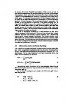
Introduction Genome science together with many other research fields of life sciences had entered the Era of Large-scale Data Acquisition in the early 1990s. The Era was led by the fast accumulation of human genomic sequences and followed by similar data from other large model organisms. Microbial genomics has also been pursued into both metagenomics [1, 2] and pan-genomics [3]. Recent advances in biotechnology and bioinformatics led to a flood of genomic (and metagenomic) data and a tremendous growth in the number of associated databases. As of June 2015, NCBI Genome collection contains more than 35,000 genome sequence assemblies from almost 13,000 different organisms (species) representing all major taxonomic groups in Eukaryotes (Fig. 1), Prokaryotes (Fig. 2), and Viruses. Prokaryotic genomes are the most abundant and rapidly growth portion of assembled genomes data collection in public archives.

Oliviero Carugo and Frank Eisenhaber (eds.), Data Mining Techniques for the Life Sciences, Methods in Molecular Biology, vol. 1415, DOI 10.1007/978-1-4939-3572-7_1, © Springer Science+Business Media New York 2016

3

Tatiana Tatusova

4

Fig. 1 Assembled eukaryotic genomes in public archives released by year by major taxonomic groups

Prokaryotic genomes (species) by year 2500

2000

1500

1000

500

0 2005

2006

2007 Proteobacteria

2008

2009

Firmicutes

2010 Actinobacteria

2011

2012

2013

Bacteroidetes/Chlorobi group

Fig. 2 Assembled prokaryotic genomes in public archives released by year by major phyla

2014

2015

Update on Genomic Databases and Resources at the National Center…

5

NCBI, major public sequence archive, accepts primary submission from the large sequencing centers, small laboratories, and individual researches. Raw sequence data and alignments of the read data produced by Next Generation Sequencing (NGS) are stored in SRA (Sequence Read Archive) database. Massively parallel sequencing technologies (Illumina, 454, PacBio) [4] have opened an extensive new vista of research possibilities—personal genomics, human microbiome studies, analysis of bacterial and viral disease outbreaks, generating thousands of terabytes of short read data. More recently, new technologies of third and fourth generation sequencing [5] such as single cell molecule [6], nanopore-based [7] have been applied to whole-transcriptome analysis that opened a possibility for profiling rare or heterogeneous populations of cells. New generation sequencing platforms offer both high-throughput and long sequence reads. The new Pacific Bioscience RS (PacBio) third-generation sequencing platform offers high throughput of 50,000– 70,000 reads per reaction and a read length over 3 kb. Oxford Nanopore released the MinION® device, a small and low-cost single-molecule nanopore sequencer, which offers the possibility of sequencing DNA fragments up to 60 kB. These advanced technologies may solve assembly problems for large and complex genomes [8] and allow to obtain a highly contiguous (one single contig) and accurate assemblies for prokaryotic genomes [9, 10]. NCBI Sequence Read Archive accepts data submission in many different formats originated from various platforms adding additional formats as they become available (see Submission section 2.1 below). Assembled nucleotide sequence data and annotation with descriptive metadata including genome and transcriptome assemblies are submitted to the three public archive databases of the International Nucleotide Sequence Database Collaboration (INSDC, www.insdc.org)—European Nucleotide Archive (ENA) [11], GenBank [12], and the DNA Data Bank of Japan (DDBJ) [13]. Two new datatypes (GenBank divisions) have been recently introduced to accommodate the data from new sequencing technologies: (1) Whole Genome Shotgun (WGS) archives genome assemblies of incomplete genomes or chromosomes that are generally being sequenced by a whole genome shotgun strategy; (2) Transcriptome Shotgun Assembly (TSA) archives computationally assembled transcript sequences from primary read data. See Fig. 3 for the growth of sequence data in public archives. As the volume and complexity of data sets archived at NCBI grow rapidly, so does the need to gather and organize the associated metadata. Although metadata has been collected for some archival databases, previously, there was no centralized approach at NCBI for collecting this information and using it across databases. The BioProject database [14] was recently established to facilitate organization and classification of project data submitted to NCBI, EBI and DDBJ databases. It captures descriptive information

6

Tatiana Tatusova

Fig. 3 Growth of NCBI sequence archives: GenBank, WGS, TSA, and SRA

about research projects that result in high volume submissions to archival databases, ties together related data across multiple archives and serves as a central portal by which to inform users of data availability. Concomitantly, the BioSample database [14] is being developed to capture descriptive information about the biological samples investigated in projects. BioProject and BioSample records link to corresponding data stored in archival repositories. Additional information on biomedical data is stored in an increasing number of various databases. Navigating through the large number of genomic and other related “omic” resources and linking it to the metagenome (epidemiological, geographical) data becomes a great challenge to the average researcher. Understanding the basics of data management systems developed for the maintenance, search, and retrieval of the large volume of biological data will provide necessary assistance in navigating through the information space. This chapter is an update of the previous report on NCBI genome sequence data management system [15]. The updated version provides a description of new and/or completely redesigned genomic resources that became available since the first 2008 edition. NCBI, as a primary public repository of biomolecular information, collects and maintains enormous amounts of heterogeneous data. The databases vary in size, data types, design, and implementation. They cover most of the genomic biology data types including sequence data (genomic, transcript, protein sequences); metadata describing the objectives and goals of the project and environmental, clinical, and epidemiological data that

Update on Genomic Databases and Resources at the National Center…

7

is associated with the sample collections (BioSample); and related bibliographical data. All these databases are integrated in a single data management system and use a common engine for search and retrieval. This provides researchers with a common interface and simplifies navigation through the large information space. This chapter focuses on the primary genome sequence data and some related resources, but many other NCBI databases such as GEO, Epigenomics, dbSNP dbVar, and dbGaP, although related, are not in scope for the current review. There are many different ways of accessing genomic data at NCBI. Depending on the focus and the goal of the research project or the level of interest, the user would select a particular route for accessing the genomic databases and resources. These are: (1) text searches, (2) direct genome browsing, (3) searches by sequence similarity, and (4) pre-computed results of analysis. All of these search types enable navigation through pre-computed links to other NCBI resources. Recently redesigned genome FTP directories provide easy access to the individual genome assemblies as well as to large datasets arranged in organism groups.

2

Primary Data Submission and Storage The National Center for Biotechnology Information was established on November 4, 1988 as a division of the National Library of Medicine (NLM) at the National Institutes of Health (NIH) in order to develop computerized processing methods for biomedical research. As a national resource for molecular biology information, NCBI’s mission is to develop automated systems for storing and analyzing knowledge about molecular biology, biochemistry, and genetics; facilitating the use of such databases and software by the research and medical community; coordinating efforts to gather biotechnology information both nationally and internationally; and performing research into advanced methods of computerbased information processing for analyzing the structure and function of biologically important molecules. The fundamental sequence data resources at NCBI consist of both primary databases and derived or curated databases. Primary sequence databases such as SRA [16], GenBank [12] and metadata repositories such as BioProject and BioSample [17, 18] archive the original submissions that come from large sequencing centers or individual experimentalists. The database staff organizes the data but do not add additional information. Curated databases such as Reference Sequence Collection [14, 15] provide a curated/expert view by compilation and correction of the data. For more detailed information on all NCBI and database resources see also most recent NCBI databases review [19].

8

Tatiana Tatusova

This section provides an overview of genome submission processing, from the management of data submission to the generation of publicly available data products. 2.1 Primary Raw Sequence Data: Sequence Read Archive (SRA)

Most of the data generated in genome sequencing projects is produced by whole genome shotgun sequencing, resulting in random short fragments - raw sequence reads. For many years the raw sequence reads remained out of the public domain because the scientific community has focused its attention primarily on the end product: the fully assembled final genome sequence. As the analysis of genomic data progressed, the scientific community became more concerned with the quality of the genome assemblies and thought they’d need a place to store the primary sequence read data. Also, having all the read data in a single repository could also provide an option to combine reads from multiple sequencing centers and/or try different assembly algorithms on same public set of reads. Trace Archive has successfully served as a repository for the data produced by capillary-based sequencing technologies for many years. New parallel sequencing technologies (e.g., 454, Solexa, Illumina, ABI Solid,) have started to produce massive amounts of short sequence reads (20–100 kb). More recently, Pacific Biosystems (PacBio) and Oxford sequencing technologies have started producing much longer reads (10–15 kB on average) with really massive throughput. In addition to raw sequence data SRA can store alignment information from high-throughput sequencing assembly projects. The alignments provide the important information on mapping the reads to the consensus or reference assembly as well as the duplicated and not-mapped reads. The importance of storing the alignment of raw reads to the consensus sequence in public archives was emphasized from the very beginning af large-scale genome sequencing projects [21]. Trace archive has an option to capture and display assembly alignments. More recently, the research community in collaboration with major sequence archives have developed the standard formats for the assembly data. SAM, which stands for Sequence Alignment/Map format, is a TAB-delimited text format consisting of a header (optional) and an alignment. Typically, each alignment represents the linear alignment of a segment. BAM is a binary version of SAM format. NCBI SRA submission portal is accepting assembly data files in SAM/BAM formats. For more details see online specification of SAM/BAM format at https://samtools.github.io/hts-specs/ SAMv1.pdf For more information on SRA submission protocol and data structure see SRA documentation at http://www.ncbi.nlm.nih. gov/Traces/sra/sra.cgi?view = doc and NCBI SRA Handbook at http://www.ncbi.nlm.nih.gov/books/NBK242623/

Update on Genomic Databases and Resources at the National Center…

9

NGS parallel sequencing approach results in high level of redundancy in the sequence runs. By aligning the reads to the reference identical bases can be identified and collapsed, only the mismatching bases are stored. The original sequence may be restored by applying a function to the reference and the stored only differences. Continues growth of primary raw data requires further development of data compression and reducing the redundancy. At some point the need to store every read generated by sequencing machine may become unnecessary. The major objective of storing all primary data was the concern about data reproducibility. With the cost of sequencing dropping down so fast the cost of re-sequencing may become lower than the cost of storage of terabytes of data. 2.2 Primary Sequence Data—Genome and Transcriptome Assemblies Rapidly

Sequences assembled from raw machine reads are traditionally submitted to GenBank/EMBL/DDBJ consortium. Two new data types were recently created to accommodate assembled data from NGS projects. TSA is an archive of computationally assembled sequences from primary data such as ESTs, traces and Next Generation Sequencing Technologies. The overlapping sequence reads from a complete transcriptome are assembled into transcripts by computational methods instead of by traditional cloning and sequencing of cloned cDNAs. The primary sequence data used in the assemblies must have been experimentally determined by the same submitter. TSA sequence records differ from EST and GenBank records because there are no physical counterparts to the assemblies. For more details see http://www.ncbi.nlm.nih.gov/genbank/tsa Whole Genome Shotgun (WGS) projects are genome assemblies of incomplete genomes or incomplete chromosomes of prokaryotes or eukaryotes that are generally being sequenced by a whole genome shotgun strategy. A whole genome assembly may be a large hierarchical sequence structure: http://www.ncbi.nlm. nih.gov/genbank/wgs Shotgun technology generates high volume of reads that represent random fragments of the original genome or transcriptome sequence. A computational process of the reconstructing of the original sequence by merging the fragments back together is called assembly. The resulting sequence (gapless contig) or a collection of sequences represents assembly as on object. In large genome sequencing project a set of contigs can be linked (by employing linking information) together forming scaffolds. Scaffolds can be mapped to the chromosome coordinates if physical or genetic mapping information is available. Assembly instructions can be formally described in AGP format. A tab delimited file describes the assembly of a larger sequence object from smaller objects. The large object can be a contig, a scaffold (supercontig), or a chromosome. Each line (row) of the

10

Tatiana Tatusova

AGP file describes a different piece of the object. These files are provided by primary submitters of Whole Genome Sequence (WGS) data. For details see: http://www.ncbi.nlm.nih.gov/projects/genome/assembly/agp/AGP_Specification.shtml. 2.3 Primary Metadata: BioProject, BioSample

As the diversity, complexity, inter-relatedness and rate of generation of the genome sequence data continue to grow, it is becoming increasingly important to capture scholarly metadata and allow the identification of various elements of a research project, such as grant proposals, journal articles, and data repository information. With the recent advances in biotechnology researches gain access to new types of molecular data. The genome studies have expanded from just genome sequencing to capturing structural genome variations, genetic and phenotypic data, epigenome, trasncriptome, exome sequencing and more. The BioProject database [14] replaces NCBI's Genome Project database and reflects an expansion of project scope, a redesigned database structure and a redesigned website. The BioProject database organizes metadata for research projects for which a large volume of data is anticipated and provides a central portal to access the data once it is deposited into an archival database. A BioProject encompasses biological data related to a single initiative, originating from a single organization or from a consortium of coordinating organizations. Project materials (sample) information is captured and given a persistent identifiers in BioSample database [14]. Given the huge diversity of sample types handled by NCBI's archival databases, and the fact that appropriate sample descriptions are often dependent on the context of the study, the definition of what a BioSample represents is deliberately flexible. Typical examples of a BioSample include a cell line, a primary tissue biopsy, an individual organism or an environmental isolate. Together, these databases offer improved ways for users to query, locate, integrate, and interpret the masses of data held in NCBI's archival repositories.

2.4 Submission Portal

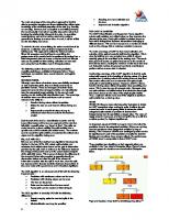
Submission portal is a single entry point that allows submitters to register a project (or a multiple projects) and deposit data to different NCBI databases. All primary data including metadata on the biological material, raw sequence reads, assembled genome, transcriptome, and functional genomic assays can be submitted using the same interface (https://submit.ncbi.nlm.nih.gov/). The data submission process at NCBI include multiple steps aiming to ensure the data quality and integrity. Quality Control is implemented as a set of automatic validation checks followed by manual review by NCBI staff. Figure 4 shows the major steps of primary submission process.

Update on Genomic Databases and Resources at the National Center…

11

Fig. 4 Primary submission data processing

3

Text Search and Retrieval system

3.1 Basic Organizing principles

Entrez is the text-based search and retrieval system used at NCBI for all of the major databases and it provides an organizing principle for biomedical information. Entrez integrates data from a large number of sources, formats, and databases into a uniform information model and retrieval system. The actual databases from which records are retrieved and on which the Entrez indexes are based have different designs, based on the type of data, and reside on different machines. These will be referred to as the “source databases”. A common theme in the implementation of Entrez is that some functions are unique to each source database, whereas others are common to all Entrez databases. An Entrez “node” is a collection of data that is grouped and indexed together. Some of the common routines and formats for every Entrez node include the term lists and posting files (i.e., the retrieval engine) used for Boolean Query, the links within and between nodes, and the summary format used for listing search results in which each record is called a DocSum. Generally, an Entrez query is a Boolean expression that is evaluated by the common Entrez engine and yields a list of unique ID numbers (UIDs), which identify records in an Entrez node. Given one or more UIDs, Entrez can retrieve the DocSum(s) very quickly.

12 3.1.1

Tatiana Tatusova Query Examples

Each Entrez database (“node”) can be searched independently by selecting the database from the main Entrez Web page (http:// www.ncbi.nlm.nih.gov/sites/gquery). Typing a query into a text box provided at the top of the Web page and clicking the “Go” button will return a list of DocSum records that match the query in each Entrez category. These include, for example, nucleotides, proteins, genomes, publications (PubMed), taxonomy, and many other databases. The numbers of results returned in each category are provided on a single summary page and provide the user with an easily visible view of the results in each of ~35 databases. The results are presented differently in each database but within the same framework which includes the common elements such as search bar, display options, page formatting, and links. In processing a query, Entrez parses the query string into a series of tokens separated by spaces and Boolean operators (AND, NOT, OR). An independent search is performed for each term, and the results are then combined according to the Boolean operators. Query uses the following syntax: term [field] OPERATOR term [field] where “term” refers to the search terms, “field” to the Search Field defined by specific Entrez database, and “OPERATOR” to the Boolean Operators. More sophisticated searches can be performed by constructing complex search strategies using Boolean operators, for example, in Genome database a query (Bacteria[organism] complete[Status]

OR

Archaea[organism])

AND

will return all genome records (species) from bacteria and Archaea domain for which complete genome sequence assemblies are available. The main goals of the information system are reliable data storage and maintenance, and efficient access to the information. The retrieval is considered reliable if the same information that was deposited can be successfully retrieved. The Entrez system goes beyond that by providing the links between the nodes and pre-computing links within the nodes. The links made within or between Entrez nodes from one or more UIDs (Unique IDentifier) is also a function across all Entrez source databases. Linking mechanisms are described in detail in the previous version [15]. On public facing Web pages links to other databases are presented to the user in Find related data section where the name of the related database can be selected from pulldown menu (Fig. 5a).

Update on Genomic Databases and Resources at the National Center…

13

Fig. 5 New features improving the presentation of search results: (a) pre-computed links to related data in other resources; (b) sensor, a provisional navigation path based on the analysis of the search query; (c) Faucets (filters)

3.1.2 Towards Discovery: Sensors and Adds, Faucets (Filters) and Alerts

More recently, several new features have been developed aiming to help the researches with understanding the results of the search and provide a provisional navigation path that is based on the analysis of the search query (Fig. 5b). Various filters can be applied to the search results to limit the result set to subset of a particular interest. In the previous version these filters can be applied using complex Boolean Query or using a custom-designed Limits page. In the recently redesigned version all filters applicable to the results set are shown on the result page and are implemented as faucets providing upfront options to focus on the subset of interest (Fig. 5c). Alert option provides a subscription to My NCBI which allows to retain user information and database preferences to provide customized services for many NCBI databases. My NCBI subscription provides various useful features that allow to save searches and create automatic e-mail alerts when new results become available: save display format preferences and filter options, store recent activity searches and results for 6 months, and many more. More information about Entrez system can be found from NCBI online Help Manual at http://www.ncbi.nlm.nih. gov/books/bv.fcgi?rid=helpentrez.chapter.EntrezHelp.

14

Tatiana Tatusova

3.2 Tools for Advanced Users

4

The Entrez Programming Utilities (E-Utils) are a set of eight server-side programs that provide a stable interface to the Entrez query and database system. The E-Utils use a fixed URL syntax that translates a standard set of input parameters into the values necessary for various NCBI software components to search for and retrieve data, and represent a structured interface to the Entrez system databases. To access these data, a piece of software first posts an eUtils URL to NCBI, then retrieves the results of this posting, after which it processes the data as required. The software can thus use any computer language that can send a URL to the eUtils server and interpret the XML response, such as Perl, Python, Java, and C++. Combining e-Utils components to form customized data pipelines within these applications is a powerful approach to data manipulation. More information and training on this process is available through a course on NCBI Powerscripting: http://www. ncbi.nlm.nih.gov/Class/PowerTools/eutils/course.html.

Genomic Databases; Public Reports The genome sequencing era that started about 20 years ago has brought into being a range of genome resources. Genomic studies of model organisms give insights into understanding of the biology of humans enabling better prevention and treatment of human diseases. Comparative genome analysis leads to further understanding of fundamental concepts of evolutionary biology and genetics. Species-specific genomic databases comprise a lot of invaluable information on genome biology, phenotype, and genetics. However, primary genomic sequences for all the species are archived in public repositories that provide reliable, free, and stable access to sequence information. In addition NCBI provides several genomic biology tools and online resources, including group-specific and organism-specific pages that contain links to many relevant websites and databases.

4.1 Sequence Read Archive (SRA)

The access to the SRA data is provided through SRA Web browser and specialized SRA BLAST search application. NCBI has developed a set of tools that allow the users to download sequencing files directly from SRA database. For the detailed description of SRA Toolkit visit documentation page http://www.ncbi.nlm.nih. gov/Traces/sra/?view=toolkit_doc. SRA data are organized in SRA studies, experiments and runs. SRA studies are registered in BioPorject database (see Subheading 2.3); the metadata include the aims and objectives of the project, title and brief description, and optional funding sources and publications. The description of biological material (sample) used in the experiment(s) within the study is captured and

Update on Genomic Databases and Resources at the National Center…

15

maintained in BioSample database (see Subheading 2.4). It includes description of the sample (collection date and location, age, gender, cell line, etc.) as well as information on sequencing methods and instrumental models used in the experiments. Multiple experiments can be performed with a same sample but using multiple samples in a same experiment is not allowed in the SRA data model. Data sets within an experiment are organized in runs usually associated with the sequencing libraries. Run browser (http://www.ncbi.nlm.nih.gov/Traces/sra/ ?view=run_browser) allows the user to search data for a single run with the run accession number. SRA Run selector Allow the user to search with accession(s) of the studies, samples, or experiments. The search, indexing, and Web presentation (Fig. 6) are implemented with the Solr database technology (http://lucene.apache.org/solr/). Special version of BLAST is using megablast [21]—nucleotide blast version optimized for highly similar sequences (see Subheading 5 below) 4.2

NCBI Taxonomy

Fig. 6 SRA Run browser

The NCBI Taxonomy Database [22] serves as the standard nomenclature and classification for the International Sequence Database (INSDC). Taxonomy was first indexed in Entrez in 1993—at the time there were just over 5000 species with formal scientific names represented in GenBank. As of June 2015 sequences from over 300 000 species are represented in INSDC. However, with common estimates of the species on the planet around two million the subset with sequence in GenBank represents only 15 % of the total.

16

Tatiana Tatusova

Several initiatives (e.g., Barcode of Life) are explicitly focused on extending sequence coverage to all species of life. Sequence entries in GenBank are identified with varying degrees of certainty. Some are taken from specimens (or cultures) that can be independently identified by a specialist—some of these come with species-level identifications (formal binomial names), the others get informal names of several sorts. Species with a formal name in the appropriate code of nomenclature are indexed in Taxonomy Entrez with the specified [property]. Taxonomy identifier often serves as the primary key that links together different data types related by organism. More recently, NCBI has started a project to curate sequence from type material [22]. Type material is the taxonomic device that ties formal names to the physical specimens that serve as exemplars for the species. For the prokaryotes these are strains submitted to the culture collections; for the eukaryotes they are specimens submitted to museums or herbaria. The NCBI Taxonomy Database (http://www.ncbi.nlm.nih.gov/taxonomy) now includes annotation of type material that is used to flag sequences from type in GenBank, Genomes, and BLAST (see below). 4.3

GenBank

GenBank is the NIH genetic sequence database, an archival collection of all publicly available DNA sequences [12]. Many journals require submission of sequence information to a database prior to publication to ensure an accession number will be available to appear in the paper. GenBank archives assembled nucleotide sequence data and annotations with descriptive metadata including genome and transcriptome assemblies. Due to the increasing volume of short genome survey sequences (GSS) and expressed sequence tags (EST) generated by high throughput sequencing studies the data in Nucleotide have been split into three search sets: GSS, EST and the rest of nucleotide sequences (nuccore). These sequences are accessible via Web interface by text Query using Entrez. Searching any of the three databases will provide links to results in the other using sensor mechanism described above (see Subheading 2). Unless you know that you are trying to find a specific set of EST or GSS sequences, searching the Nucleotide database (http://www.ncbi.nlm.nih.gov/nuccore/) with general text Query will produce the most relevant results. You can always follow links to results in EST and GSS from the Nucleotide database results. Quarterly GenBank releases are also downloadable via FTP (see Subheading 6). As of June, 15 2015 GenBank release 208.0 (ftp://ftp.ncbi. nih.gov/genbank/gbrel.txt) contains almost 194 billion bases in over 185 million sequence entries (compare to 80 million in 2008 at the time of previous addition). The data come from the large sequencing centers as well as from small experimental labs.

Update on Genomic Databases and Resources at the National Center…

4.4 Whole Genome Shotgun (WGS)

17

Genome assembly especially for large eukaryotic genomes with highly repetitive sequence remains one of the major challenges in genome bioinformatics [8–10]. While the cost of sequencing drops down dramatically, the genome assembly still takes considerable amount of time and effort. In some research projects (comparative analysis, population and variation studies) the researches might work with a high quality reference assembly and bunch of lower quality variant genomes for the same species. Thousands of draft genomes are assembled up to the contig level only, sometimes with very low assembly quality (low N50/L50, large number of contigs). These genomes typically remain unannotated. These fragmented genomes with no annotation might not be very useful compared to complete genome with full gene/protein complement. However, the contig sequences can be used for comparative analysis. These draft contig-level assemblies are treated differently than traditional sequence records. The contigs are not loaded to the main sequence repository, general identifiers (GI number) are not assigned, contigs sequences are not indexed and therefore are not searchable in Entrez Nucleotide except for the master record (Fig. 7). These projects can be browsed by organism in a custom made viewer (http://www.ncbi.nlm.nih.gov/Traces/wgs/).

Fig. 7 WGS and TSA customer reports. (a) organism browser; (b) contig report; (c) customized WGS project overview; (d) traditional GenBank flat file view of WGS project master record

18

Tatiana Tatusova

4.5 Genome Collection Database (Assembly)

The Assembly database (http://www.ncbi.nlm.nih.gov/assembly/) has information about the structure of assembled genomes as represented in an AGP file or as a collection of completely sequenced chromosomes. The database tracks changes to assemblies that are updated by submitting groups over time with a versioned Assembly accession number. The Web resource provides meta-data about assemblies such as assembly names (and alternate names), simple statistical reports of the assembly (type and number of contigs, scaffolds; N50s), and a history view of updates. It also tracks the relationship between an assembly submitted to the International Nucleotide Sequence Database Consortium (INSDC) and the assembly represented in the NCBI Reference Sequence (RefSeq) project. More information can be found at (http://www.ncbi.nlm. nih.gov/assembly/help/#find) Many genomes assemblies coming from single cell sequencing technology give only partial representation of DNA in a cell, ranging from 10 % to 90 %. Genome representation can be validated by comparative analysis if other genomes are available in closely related groups (species or genus). Assemblies with partial genome representation can be found in Entrez Assembly database by using the following query: Archaea[orgn] OR Bacteria[orgn] AND "partial genome representation"[Properties] Some genome assemblies come from mixed cultures, hybrid organisms and chimeras; these “anomalous” assemblies do not represent an organism. These assemblies are valid results of the experimental studies and are legitimate genome records in GenBank; however, they should be filtered out in genome analysis and comparative genome studies These assemblies can be found in Entrez Assembly database by using the following query: Archaea[orgn] OR Bacteria[orgn] AND "anomalous" [Properties] Modern high-throughput sequencing technologies vary in the size of raw sequence reads and the patterns of sequencing errors. Despite many computational advances to genome assembly, complete and accurate assembly from raw sequence read data remains a major challenge. There are two major approaches that have been used: de novo assembly from raw sequence reads and reference guided assembly if the closest reference genome is available. The quality of genome assembly can be assessed using a number of different quality metrics. For many years N50 and L50 contig and scaffold lengths have been major measure of assembly quality. N50 defines the length of contig (or scaffold) for which the set of all contigs of that length or longer contains at least 50 % of the total size of the assembly (sum of the lengths of all contigs). L50 is the number of sequences evaluated at the point when the sum length exceeds 50 % of the assembly size. More recently, a number of different metrics have been suggested [22, 23]. Some of the standard

Update on Genomic Databases and Resources at the National Center…

19

Fig. 8 Genome by assembly quality

global statistics measures and reference based statistics are used for quality assessment. Figure 8 illustrates the differences in N50 for eukaryotic genome assemblies. The user can access to assembly data by using Entrez text searches from the home Web page: (http://www.ncbi.nlm.nih.gov/assembly/), or by browsing and filtering assemblies by organism, and download the data from the FTP site (see Subheading 6). 4.6

BioProject

The BioProject resource [14] became public in May 2011, replacing the older NCBI Genome Project database, which had been created to organize the genome sequences in GenBank [12] and RefSeq [16]. The BioProject database was created to meet the need for an organizational database for research efforts beyond just genome sequencing, such as transcriptome and gene expression, proteomics, and variation studies. However, because a BioProject is defined by its multiple attributes, there is flexibility for additional

Tatiana Tatusova

20

types of projects in the future, beyond those that were included in 2011. The new BioProject database allows more flexible grouping of projects and can collect more data elements for each project, e.g., grant information and project relevance. BioProjects describe large-scale research efforts, ranging from genome and transcriptome sequencing efforts to epigenomic analyses, genome-wide association studies (GWAS), and variation analyses. Data are submitted to NCBI or other INSDC-associated databases citing the BioProject accession, thus providing navigation between the BioProject and its datasets. Consequently, the BioProject is a robust way to access data across multiple resources and multiple submission time points, e.g., when there are different types of data that had been submitted to multiple databases, or sequential submissions deposited over the course of a research project. Web access to all publicly registered bioporjects (http:// www.ncbi.nlm.nih.gov/bioproject/) has typical text search and browse by project data types options. 4.7

Genome

Entrez Genome, the integrated database of genomic information at the NCBI, organizes information on genomes including sequences, maps, chromosomes, assemblies, and annotations. The genome paradigm has transitioned from a single reference genome of an organisms to multiple genome representing the whole population. To reflect the change in the genome paradigm the Genome database has been completely redesign in 2013. In the past an entry in Genomes database used to represent a complete sequence of a single replicon such as a chromosome, organelle, or plasmid. New Genome records pull together genome data at various levels of completion, ranging from recently registered projects with SRA/ trace data to genomes represented by scaffolds/contigs or fully assembled chromosomes with annotation. Genome information is grouped by organism so that each record in the Entrez Genome database represents a taxonomic node at species level for the most part. In addition, group-specific pages provide links to relevant external websites and databases and to aggregated data and tools. As of June 2015 Entrez Genomes houses a collection of almost 13,000 entries (organism level) for almost 55,000 assemblies. Table 1 shows the number of genome records (species) and assemblies in major taxonomic groups.

Table 1 Data statistics in major organism groups and data categories Eukaryota Prokaryota Viruses

Organelles Plasmids Total

1424

6726

4658

6268

1024

12,808 (unique)

Genome (species)

2291

35,211

4714

6821

5954

53,991

Assembly

Update on Genomic Databases and Resources at the National Center…

21

Table 2 Differences between Entrez databases presenting genome and metagenome data Database

Definition

Central portal

Grouping

Genome

Total genetic content contained within an organism

A single portal to genome sequence and annotation

Defined by organism

BioProject

A set of related data tied together with unique identifier

A higher order organization of Defined by submitter, by funding source, by the data deposited into named collaboration several archival databases, it provides a central point to inform customers of data availability in these databases

BioSample

A single portal to sample Biological material under description and attributes investigation in a project. The attributes describe the role the sample holds in the project

Taxonomy

The conception, naming, and classification of organism groups

Organism groups organized in Rank-based biological a hierarchical classification classification: Kingdom, Phylum, Class, Order, Family, Genus, Species

Assembly

A data structure that maps the sequence data to a putative reconstruction of the target

Assembly structure, assembly version history

Nucleotide A collection of genomic and transcript sequences

Defined by the context of experimental study

Primary data defined by submitter or Refseq data defined by NCBI staff

A single portal to all DNA and Primary data defined by RNA sequences submitter or Refseq data defined by NCBI staff

The BioProject, Genome, and Assembly databases are interconnected and can be used to access and view genomes in different ways. Every prokaryotic and eukaryotic genome submission has BioProject, BioSample, Assembly, and GenBank accession numbers, so users can start in any of those resources and get to the others. The BioProject and BioSample databases allow users to find related datasets, e.g., multiple bacterial strains from a single isolation location, or the transcriptome and genome from a particular sample. The Assembly accession is assigned to the entire genome and is used to unambiguously identify the set of sequences in a particular version of a genome assembly from a particular submitter. Finally, the Genome database displays all of the genome assemblies in INSDC and RefSeq, organized by organism. A brief description of genome-related resources is summarized in Table 2.

22

Tatiana Tatusova

Genome information is accessible via Entrez text-based search Query or by browsing sortable tables organized by organism and BioProject accession. Links to Genome records may be found in several other Entrez databases including Taxonomy, BioProject, Assembly, PubMed, Nucleotide, Gene and Protein. Accessing actual sequence data, for example, all the nucleotide sequence data from a particular WGS genome is easily found via the Genome database from the organism overview page or browser table in two ways. First, by using the link to the assembly database and following the link to the Nucleotide database located under the related information heading. Second, from the assembly database the link to the WGS browser provide access to a table with a list of contigs and statistics as well as GNU zipped archive files for download. Genome Browser

The browser (http://www.ncbi.nlm.nih.gov/genome/browse/) divided in four tables each with genome attributes statistics. Table summaries include (1) an overview by organism and then lists of genome sequencing assemblies for (2) Eukaryotes, (3) Prokaryotes, (4) Viruses, (5) Organelles, and (6) Plasmids. Table displays can be filtered by lineage information and/or genome status and the results downloaded. Various filters can be applied to create a data set of interest. The Genome top level records can be filtered by the organisms groups at phylum and/or family level. Assemblies can be filtered by completeness and the highest level off assembly (complete, chromosome, scaffold, contig). Selected records can be downloaded in tab-delimited text files. The whole report can be downloaded from this FTP site (ftp://ftp.ncbi.nlm.nih.gov/ genomes/GENOME_REPORTS/).

4.7.2 Entrez Text-Based Searches

The organism search is expected to be the most frequent method to look for the data in Entrez Genome. One of the features of the Entrez system is “organism sensor” allowing to recognize a organism name in a query. Advanced searching in Entrez Genome allows for refined Query by specifying “organism” (or short version “orgn”) field in square brackets (e.g., yeast[orgn]). When a search term, for example “human” is recognized as an organism name, the original query is transformed to the organism-specific one “Homo sapiens [Organism] OR human[All Fields]”. Take note, a nonspecific search term such as “human” can result in the listing of several genome records which contain the word “human” as part of the text. However, the Entrez Genome record for human will be at the top of the list since the query has been transformed (http://www. ncbi.nlm.nih.gov/genome/?term=human). Only the search term “human [orgn]” or latin binomial “Homo sapiens[orgn]” will provide the specific Genome page for Homo sapiens (http://www.ncbi.nlm. nih.gov/genome/?term=human+[orgn]). A list of all fields indexed for a more refined search is available in the Genome Advanced

4.7.1

Update on Genomic Databases and Resources at the National Center…

23

Search Builder (http://www.ncbi.nlm.nih.gov/genome/advanced). The Limits page provides an easy way to limit a search by certain fields without having to use complex Boolean operations. Genome searches can be limited by organism groups or cell location of genetic content (chromosome, organelle, or plasmid). 4.7.3 Organelle and Plasmid

An organelle is a specialized structure that is enclosed within its own membrane inside a eukaryotic cell. The mitochondria and chloroplasts are maintained throughout the cell cycle, and replicate independently of the mitosis or meiosis of the cell. Mitochondrial and chloroplast DNA sequences are often used for phylogenetic analysis and population genetics, as well as cultivar identification and forensic studies. Due to the relatively small size, conserved gene order, and content of animal mitochondria, whole genome sequencing and comparisons across many species have been possible for many decades. NCBI maintains a special collection of reference organelle genomes. However, the organelle genome alone does not represent the full genetic content of an organism. The Entrez Genome organism search does not include organelle and plasmid data in the result listing but provides a short summary at the top of the search page linked to Genome records with organelle or plasmid data only. The search results are automatically weighted by scientific relevance, high quality genomes, model organisms will be shown at the top of the list. For example, the search for “Fungi” will result in 650 species-level records; Saccharomyces cerevisiae, the most studied model organism will be shown at the top of the list. The individual Genome report include Organism Overview, Genome Assembly and Annotation Report, and Protein Table. Organism Overview typically contains a short description of the organism, a picture if available, lineage as defined by NCBI Taxonomy, related publications, and summary statistics for the genome sequence data. For many species hundreds and thousands of genome assemblies are being sequenced and the number continues to grow. In Genome database a reference genome assembly is selected to serve as a single representative of a particular organism. A representative genome or genomes are chosen either by the community or calculated by comparative sequence analysis (see more details in [17]). Genomes of the highest quality sequence and annotation, often the most important isolates, historically used by the research community for clinical studies, experimental validation are marked as “Reference” genomes. One of the best known examples of the “Reference” genome is the genome of the non-pathogenic strain K-12 of Escherichia coli first obtained from a patient in 1922. The genome has been sequenced in 1997 [24] and was extensively curated by the research community ever since [25]. The genome information panel that provide a quick and easy access to the sequence data for the representative (or

24

Tatiana Tatusova

Fig. 9 Genome reports: organism overview

reference) genome is provided at the very top of the Organism Overview page (Fig. 9). The list of all representative and reference prokaryotic genomes is available at http://www.ncbi.nlm.nih.gov/ genome/browse/reference/. 4.7.4 Graphical View

Since the genome structure and biology of eukaryotes, prokaryotes and viruses are very different, the genomic data display between taxonomic groups varies to some extent. Virus genomes are small enough to display the whole annotated genome in graphic form and also have links to a virus specific genome resource. Hundreds of prokaryotic genomes are available for particular species thus making the display of the relationship of prokaryote genomes from a specific bacterial species relevant. Genome relationships are displayed in the form of a dendrogram based on genomic BLAST scores (Fig. 10). In addition, the prokaryotic genome can be displayed in a graphic form (like a virus genome) when an individual strain is selected from the dendrogram or table. The human Genome record on the other hand has a detailed ideogram of the 24 chromosomes with links to MapViewer. The ideogram display

Update on Genomic Databases and Resources at the National Center…

25

Fig. 10 Genome reports: BLAST based dendrogram

for a eukaryote organism originates from a single representative genome and may not represent the full variation in karyotypes observed in particular organisms (e.g., Fungi). 4.7.5 Assembly and Annotation Report

This section provides full details of the assembly and annotation (different feature types) for each assembly represented in a single Genome record (usually species). Microbial genomes represented by thousands of isolates are organized in clades and tight genomes groups calculated by sequence similarity as described in [17].

4.7.6 Protein Details Report

The Protein Details page provides a length histogram with descriptive statics (minimum, maximum, average and median) of all the relevant proteins listed in the table which expand over several pages (Fig. 11). Details about each protein are given in each row which includes protein name, accession, locus tag, location coordinates, strand info, length, a related structure link and links to other NCBI resources such as Entrez Gene, Protein, and Protein Clusters.

26

Tatiana Tatusova

Fig. 11 Genome reports: The Protein Details page provides a length histogram with descriptive statics and a table of protein information and links to related NCBI resources

5

Searching Data by Sequence Similarity (BLAST) The Basic Local Alignment Search Tool (BLAST) [20] finds regions of local similarity between sequences. By finding similarities between sequences, scientists can infer the function of newly sequenced genes, predict new members of gene families, and explore evolutionary relationships. New features include searching against SRA experiments, easy access to genomic BLAST databases by using auto-complete organism query option, Redesigned BLAST pages include new limit options; and a Tree View option that presents a graphical dendrogram display of the BLAST results.

5.1 Exploring NGS Experiments with SRA-BLAST

SRA-BLAST offers two different ways of finding data sets to search. The BLAST service itself provides an autocomplete feature under “Choose Search Set” that finds matches to experiment, study, and run accessions as well as text from experiment descriptions.

Update on Genomic Databases and Resources at the National Center…

27

Fig. 12 New feature on BLAST home page provide an easy way to organism-specific blast with assembled genomes

You can now also use the Entrez SRA system to identify experiments of interest and load these as BLAST databases in SRA BLAST through the “Send to” menu from the SRA search results 5.2 BLAST with Assembled Eukaryotic Genomes

In addition to the BLAST home page, the BLAST search tool can also be found on the Organism Overview page of the Genome database. Accessed from the Organism Overview page this search tool has BLAST databases limited to genome data of that specific organism. For each organism, if the data exist, the following default list of organism specific BLAST databases are available to search against: HTG sequences, ESTs, clone end sequences, RefSeq genomic, RefSeq RNA, RefSeq protein, non-RefSeq RNA, and non-RefSeq protein. These BLAST databases are defined by Entrez Query. In addition, some organisms have custom databases available. Specifying the BLAST database to genomes of a specific taxon is not only limited to the search tool found on the Organism Overview page in the Genome database. BLAST databases can be limited to any taxonomic level at the BLAST home page. For example Fig. 12 shows how to start searching against mouse genome from BLAST home page and select the search set from all datasets available for mouse on the specialized Mouse BLAST page.

5.3 Microbial Genomic BLAST: Reference and Representatives

Microbial Genomic BLAST provides access to complete and Whole Genome Sequence (WGS) draft assemblies, and plasmids. Sequenced microbial genomes represent a large collection of strains with different levels of quality and sampling density. Largely because of interest in human pathogens and advances in sequencing technologies, there are rapidly growing sets of very closely related genomes representing variations within the species. Many bacterial species are represented

28

Tatiana Tatusova

in the database in thousands of variant genomes. If the users are interested in multi-species comparative analysis they would need a single genomes which is designated to represent a species. Refseq group at NCBI has introduced new categories of “reference” and “representative” genomes defined as following. Reference Genome—manually selected “gold standard” complete genomes with high quality annotation and the highest level of experimental support for structural and functional annotation. They include community curated genomes if the annotation quality meets “reference genome” requirements that are manually reviewed by NCBI staff (http://www.ncbi.nlm.nih.gov/genome/browse/reference/). Representative Genome—representative genome for an organism (species); for some diverse species can be more than one. Corresponds to Sequence Ontology—[SO:0001505] [10] (www. ncbi.nlm.nih.gov/genome/browse/representative/). The users interested in the organism diversity in BLAST results have an option to select a search database of reference and representative genomes only.

6

FTP Resources for Genome Data NCBI has redesigned the genomes FTP site to expand the content and facilitate data access through an organized predictable directory hierarchy with consistent file names and formats. The updated site provides greater support for downloading assembled genome sequences and/or corresponding annotation data. The new FTP site structure provides a single entry point to access content representing either GenBank or Refseq data. More detailed information can be found at (http://www.ncbi.nlm.nih.gov/genome/doc/ftpfaq/). Refseq dataset is organized by major taxonomic groups. It provides curated sequence records for genomes, transcripts, and proteins. Download the curated RefSeq full release or daily updates (ftp://ftp.ncbi.nih.gov/refseq/).

7

Conclusion The tremendous increase in genomic data in the last 20 years has greatly expanded our understanding of biology. Genome sequencing projects now span from draft assemblies, complete genomes, large-scale comparative genomic projects, and the new field of metagenomics where genetic material is recovered directly from environmental samples and the entire complement of DNA from a given ecological niche is sequenced. Although these provide an ever greater resource for studying biology, there is still a long way to go from the initial submission of sequence data to the

Update on Genomic Databases and Resources at the National Center…

29

understanding of biological processes. By integrating different types of biological and bibliographical data, NCBI is building a discovery system that enables the researcher to discover more than would be possible from just the original data. By making links between different databases and computing associations within the same database, Entrez is designed to infer relationships between different data that may suggest future experiments or assist in interpretation of the available information. In addition, NCBI is developing the tools that provide users with extra layers of information leading to further discoveries. Genomics is a very rapidly evolving field. The advance in sequencing technologies has lead to new data types which require different approaches to data management and presentation. NCBI continues to add new databases and develop new tools to address the issue of ever increasing amounts of information.

Acknowledgements The authors would like to thank, in alphabetic order, Boris Fedorov and Sergei Resenchuk for their expertise and diligence in the design and maintenance of the databases highlighted in this publication and Stacy Ciufo for the helpful discussion and comments. These projects represent the efforts of many NCBI staff members along with the collective contributions of many dedicated scientists worldwide. References 1. Matsen FA (2015) Phylogenetics and the human microbiome. Syst Biol 64(1):e26–e41, Review 2. Hedlund BP, Dodsworth JA, Murugapiran SK, Rinke C, Woyke T (2014) Impact of single-cell genomics and metagenomics on the emerging view of extremophile "microbial dark matter". Extremophiles 18(5):865–875, Review 3. Vernikos G, Medini D, Riley DR, Tettelin H (2015) Ten years of pan-genome analyses. Curr Opin Microbiol 23:148–154, Review 4. Henson J, Tischler G, Ning Z (2012) Nextgeneration sequencing and large genome assemblies. Pharmacogenomics 13(8):901–915 5. Wang Y, Navin NE (2015) Advances and applications of single-cell sequencing technologies. Mol Cell 58(4):598–609 6. Feng Y, Zhang Y, Ying C, Wang D, Du C (2015) Nanopore-based fourth-generation DNA sequencing technology. Genomics Proteomics Bioinformatics 13(1):4–16

7. Wu AR, Neff NF, Kalisky T, Dalerba P, Treutlein B, Rothenberg ME, Mburu FM, Mantalas GL, Sim S, Clarke MF, Quake SR (2014) Quantitative assessment of single-cell RNA-sequencing methods. Nat Methods 11(1):41–46 8. Berlin K, Koren S, Chin CS, Drake JP, Landolin JM, Phillippy AM (2015) Assembling large genomes with single-molecule sequencing and locality sensitive hashing. Nat Biotechnol 33(6):623–630 9. Madoui MA, Engelen S, Cruaud C, Belser C, Bertrand L, Alberti A, Lemainque A, Wincker P, Aury JM (2015) Genome assembly using Nanopore-guided long and error-free DNA reads. BMC Genomics 16(1):327 10. Koren S, Phillippy AM (2015) One chromosome, one contig: complete microbial genomes from long-read sequencing and assembly. Curr Opin Microbiol 23:110–120 11. Silvester N, Alako B, Amid C, CerdeñoTárraga A et al (2015) Content discovery and retrieval services at the European Nucleotide

30

12.

13.

14.

15.

16.

17.

Tatiana Tatusova Archive. Nucleic Acids Res 43(Database issue): D23–D29 Benson DA, Clark K, Karsch-Mizrachi I, Lipman DJ, Ostell J, Sayers EW (2015) GenBank. Nucleic Acids Res 43(Database issue):D30–D35 Kodama Y, Mashima J, Kosuge T, Katayama T, Fujisawa T, Kaminuma E, Ogasawara O, Okubo K, Takagi T, Nakamura Y (2015) The DDBJ Japanese Genotype-phenotype Archive for genetic and phenotypic human data. Nucleic Acids Res 43(Database issue):D18–D22 Barrett T, Clark K, Gevorgyan R, Gorelenkov V, Gribov E, Karsch-Mizrachi I, Kimelman M, Pruitt KD, Resenchuk S, Tatusova T, Yaschenko E, Ostell J (2012) BioProject and BioSample databases at NCBI: facilitating capture and organization of metadata. Nucleic Acids Res 40(Database issue):D57–D63 Kodama Y, Shumway M, Leinonen R, International Nucleotide Sequence Database Collaboration (2012) The Sequence Read Archive: explosive growth of sequencing data. Nucleic Acids Res 40(Database issue): D54–D56 Pruitt KD, Brown GR, Hiatt SM et al (2014) RefSeq: an update on mammalian reference sequences. Nucleic Acids Res 42(Database issue):D756–D763 Tatusova T, Ciufo S, Federhen S, Fedorov B, McVeigh R, O'Neill K, Tolstoy I, Zaslavsky L (2015) Update on RefSeq microbial genome

18.

19.

20.

21. 22.

23.

24.

25.

resources. Nucleic Acids Res 43(Database issue):D599–D605 NCBI Resource Coordinators (2015) Database resources of the National Center for Biotechnology Information. Nucleic Acids Res 43 (Database issue):D6–D17 Salzberg SL, Church D, DiCuccio M, Yaschenko E, Ostell J (2004) The genome Assembly Archive: a new public resource. PLoS Biol 2(9), E285 Altschul SF, Madden TL, Schäffer AA, Zhang J, Zhang Z, Miller W, Lipman DJ (1997) Gapped BLAST and PSI-BLAST: a new generation of protein database search programs. Nucleic Acids Res 25(17):3389–3402, Review Federhen S (2012) The NCBI Taxonomy database. Nucleic Acids Res 40:D13–D25 Gurevich A, Saveliev V, Vyahhi N, Tesler G (2013) QUAST: quality assessment tool for genome assemblies. Bioinformatics 29(8): 1072–1075 Rahman A, Pachter L (2013) CGAL: computing genome assembly likelihoods. Genome Biol 14(1):R8 Blattner FR, Plunkett G 3rd, Bloch CA et al (1997) The complete genome sequence of Escherichia coli K-12. Science 277(5331): 1453–1462 Riley M, Abe T, Arnaud MB, Berlyn MK et al (2006) Escherichia coli K-12: a cooperatively developed annotation snapshot--2005. Nucleic Acids Res 34(1):1–9

Chapter 2 Protein Structure Databases Roman A. Laskowski Abstract Web-based protein structure databases come in a wide variety of types and levels of information content. Those having the most general interest are the various atlases that describe each experimentally determined protein structure and provide useful links, analyses, and schematic diagrams relating to its 3D structure and biological function. Also of great interest are the databases that classify 3D structures by their folds as these can reveal evolutionary relationships which may be hard to detect from sequence comparison alone. Related to these are the numerous servers that compare folds—particularly useful for newly solved structures, and especially those of unknown function. Beyond these are a vast number of databases for the more specialized user, dealing with specific families, diseases, structural features, and so on. Key words Protein structure, Protein Data Bank, PDB, wwPDB, JenaLib, OCA, PDBe, PDBsum, ESD, Pfam, CATH, SCOP, Secondary structure, Fold classification, Protein–ligand interactions

1

Introduction Looking back to 1971, when the Protein Data Bank was founded [1], one cannot help feeling that the study of protein structure must have been a lot simpler then. There were only seven experimentally determined protein structures at the time, and the data for each, including the proteins’ atomic coordinates, were stored in simple, fixed-format text files. Admittedly, accessing and displaying this information was trickier, and computers with graphics capabilities tended to be bulky and expensive things. These days, access and display of the data over the Web are vastly easier, but with this comes the problem, not only in the huge increase in the amount of information, but in the multiplicity of sources from which it can be obtained. New servers and services continually appear, while existing ones are modified and improved. Conversely, other servers are abandoned, switched off or neglected, becoming more and more out of date with time. Thus it has become really difficult to know where to go to get relevant answers most easily. Various lists are available on the Web—for example the Nucleic Acids Research

Oliviero Carugo and Frank Eisenhaber (eds.), Data Mining Techniques for the Life Sciences, Methods in Molecular Biology, vol. 1415, DOI 10.1007/978-1-4939-3572-7_2, © Springer Science+Business Media New York 2016

31

32

Roman A. Laskowski

(NAR) list at http://www.oxfordjournals.org/our_journals/nar/ database/a. This chapter aims to highlight some of the more useful, and up-to-date (at time of writing), sources of information on protein structure that are currently available.

2

Structures and Structural Data Terminology

Firstly, it is important to define what is meant by the term “protein structure.” It is a term that tends to be somewhat loosely used. A preferable term is “model,” as the 3D structures of large molecules such as proteins are models of the atom types, atomic x-, y-, z-coordinates and other parameters that best fit the experimental data. The reason the term “structure” is so commonly used for these models is to distinguish them from “theoretical,” or “homologybuilt,” models. Nevertheless, it is important to remember that all are models of reality and that only the former type is based on experimental evidence. Another loosely used term is “database.” Technically, the databases mentioned here are not databases at all, but rather “data resources”—many of which rely on a database for storing and serving up the data. However, the term “database” is becoming common usage for the types of resources described here (e.g., the NAR Database issues), so it is the meaning we adopt here.

2.2 The Protein Data Bank (PDB) and the wwPDB

The primary repository of 3D structural data on proteins (and other biological macromolecules, including RNA, fragments of DNA, carbohydrates, and different complexes of these molecules) is the Protein Data Bank. As mentioned above, this was founded in 1971 and was located at Brookhaven National Laboratories. In October 1998, the management of the archive was taken over by the Research Collaboratory for Structural Bioinformatics (RCSB), a consortium consisting of Rutgers University, the National Institute of Standards and Technology (NIST) and the San Diego Supercomputer Center [2]. Since 2003 the archive has been managed by an international consortium called the world-wide Protein Data Bank (wwPDB) whose partners comprise: the RSCB, the Protein Data Bank Europe (PDBe) at the European Bioinformatics Institute (EBI), the Protein Data Bank Japan (PDBj) at Osaka University, and, more recently, the BioMagResBank (BMRB) at the University of Wisconsin-Madison [3, 4]. Access to the primary data is via the wwPDB’s website: http://www.wwpdb.org. The data come in three different formats: old-style PDB-format files, macromolecular Crystallographic Information File (mmCIF) format [5], and a XML-style format called PDBML/XML [6]. Due to format limitations, the old-style PDB-format files are no longer available for extremely large structural models (i.e., those having too many

2.1

Protein Structure Databases

33

atoms, residues or chains than the fixed-format fields allow for). For many of the structures, the wwPDB also make the original experimental data available. Thus, for structural models solved by X-ray crystallography, one can often download the structure factors from which the model was derived, while for structures solved by nuclear magnetic resonance (NMR) spectroscopy, the original distance and angle restraints can be obtained. As of July 2015, the wwPDB contained over 110,000 structural models, each identified by a unique 4-character reference code, or PDB identifier. A key task the wwPDB have performed is the remediation of the legacy PDB archive to fix and make consistent the entire PDB data, in particular relating to ligands and literature references [7]. The PDBe and UniProt groups at the EBI have mapped the sequences in the PDB entries onto the appropriate sequences in UniProt [8]. More recently, the focus has been on validation of the structural data, with the establishment of several Validation Task Forces [9–11], and the reporting of quality indices or validation information for each structure. 2.3 Structural Data and Analyses

3

Rather than download the raw data from the wwPDB for each protein of interest, it is usually more convenient to obtain the required information directly from one of the myriad protein structure databases on the Web. These come in many shapes and sizes, catering for a variety of needs and interests. At the simplest level are the sites that provide “atlas” pages— one for every PDB entry—each containing general information obtained from the relevant PDB file. There are usually graphical representations of the structural model together with links that provide interactive 3D visualizations using Java-based, or other, viewers. Each of the founding members of the wwPDB have their own atlas pages: the RCSB, the PDBe, and PDBj. In addition, there are several other sites that have much to commend them, and some of these are mentioned below. Beyond the atlases, there are a host of other types of sites and servers. These include those providing information on specific structural motifs, focus on selected protein families, classify protein folds, compare protein structures, provide homology-built models for proteins for which no structure has been determined, and so on. This chapter cherry-picks a few of the more interesting and useful sites to visit.

Atlases Table 1 lists the seven best-known and useful of the atlas sites. All have been developed independently and, not unexpectedly, all have much in common as the information comes from the same source: the PDB entry. The protein name, authors, key reference,

34

Roman A. Laskowski

Table 1 Protein structure atlases Server

Location

URL

References

JenaLib

Fritz Lipmann Institute, Jena, Germany

jenalib.fli-leibniz.de/

[30]

MMDB

NCBI, USA

www.ncbi.nlm.nih.gov/Structure/ MMDB/mmdb.shtml

[55]

OCA

Weizmann Institute, Israel

oca.weizmann.ac.il

[56]

PDBe

EBI, Cambridge, UK

www.ebi.ac.uk/pdbe

[26]

PDBj

Osaka University, Japan

www.pdbj.org

[57]

PDBsum

EBI, Cambridge, UK

www.ebi.ac.uk/pdbsum

[32, 33]

RCSB

Rutgers and San Diego, USA

www.rcsb.org/pdb

[18]

experimental methods, atomic coordinates, and so on are obviously identical on all sites. Also common are certain derived data, including quality assessment of each structural model, and information about the protein’s likely “biological unit.” Quality assessment is a crucial issue as not all models are equally reliable, and much has been written on this topic over the years [9, 12–16]. The main problem is that the results of any experiment contain errors, but for structural models it is difficult to estimate the extent of those errors. For X-ray models, a rough guide of quality is provided by the resolution at which the structure was solved and its R-factor, but for NMR models there is no such ready measure. Some atlases do provide indications of which models are more reliable, as described shortly. The second important issue is knowing what a given protein’s biological unit is. This is not always obvious from the PDB entry. The problem is that the deposited coordinates from an X-ray crystal structure determination correspond to the molecule(s) in the asymmetric unit. This may give a false impression of how the protein operates in vivo. For example, what may look like a monomer from the PDB entry, is, in real life, a dimer, or a trimer, etc. Conversely, the PDB entry might give the coordinates of a dimer, yet the biological unit happens to be a monomer—the dimeric structure being the result of packing in the crystal. For any structural analysis it is crucial to know what the true biological unit is. For some proteins the biological unit has been determined experimentally, and so is known with great confidence. In others it has to be deduced computationally by analysis of the packing of the individual chains in the crystal. Some interfaces are more substantial than others and hence likely to represent genuine biological interactions rather than happenstance crystal contacts. Most of the atlases provide information

Protein Structure Databases

35

on the known, or predicted, biological unit. The most commonly used prediction method is Protein Interfaces, Surfaces and Assemblies (PISA) [17]. Beyond these general similarities, the atlases differ in sufficient respects to make them complement one another; they differ in what additional information they pull in, the links they make to external resources, and the analyses of the 3D structures they provide. Consequently, the atlas of choice can be either a matter of personal preference or depend on the type of information required at the time. Here we focus only those aspects that make each one unique, useful or interesting. We start with the atlases provided by the founding members of the wwPDB, and then discuss some of the others. 3.1

The RCSB PDB

The RCSB’s website [18] has been revamped several times and is an extremely rich source of information about each PDB entry. It used to be a little overwhelming for novices, but recently a great deal of effort has gone into simplifying the design as well as adding new information—such as the relationship of structures to their corresponding genes and to associated diseases and therapeutic drugs. A specific aim of the website has been to “bring a structural view of biology and medicine to a general audience.”

3.1.1

Summary Page

Figure 1 shows the summary page for PDB entry 1ayy, a glycosylasparaginase. The top box shows the primary citation for this entry, being the published description of the experiment that resulted in the structural model and any analysis the authors might have performed on it, including relating the structure to the protein’s biological function. To the right is a thumbnail image of the protein and links for viewing it in one of three molecular graphics viewers. The “More Images” link shows the asymmetric unit and the biological unit, as described above (although in many cases they are identical). The latter is either as defined by the depositors or as predicted by the PISA algorithm. The Molecular Description box provides a schematic diagram of the protein’s sequence and structural domains, together with its secondary structure, and which parts of the protein the structure corresponds to. An expanded view can be obtained by clicking on “Protein Feature View,” as shown in Fig. 2. Often structural models are not of the whole protein but merely cover one or two domains or, in some cases, are mere fragments of the protein. The diagram makes it clear what the coverage is. The little plus symbol at the bottom opens up a window showing other known structures of the same protein—which is particularly useful in identifying structures that may be more complete, or solved at a higher resolution. The sequence domains are as defined by Pfam [19], while the structural domain definitions come from SCOP [20].

36

Roman A. Laskowski

Fig. 1 Part of the RCSB atlas page for PDB entry 1ayy, a glycosylasparaginase determined by X-ray crystallography at 2.32 Å

Protein Structure Databases

37

Fig. 2 The Protein Feature View of PDB entry 1ayy on the RCSB PDB server. The diagram shows the protein’s sequence (Pfam) and structural (SCOP) domains, its hydrophathy, secondary structure, and structural coverage

The large box at the bottom of Fig. 1 is a “validation report slider” providing an at-a-glance assessment of the structure’s likely quality (only available for X-ray models). The graphic indicates how the structure compares on a number of quality-related parameters against all other structures in the database as well as structures solved at the same resolution. The parameters include the Rfree, an atom-atom “clash score,” number of Ramachandran plot outliers as computed by the MolProbity structure validation program [21], and the real-space R-value Z-score as computed by the Uppsala Electron-Density Server [22]. An almost identical schematic is provided by the PDBe website (see Fig. 3). A link above the schematic provides the full validation report for the structure in question. 3.1.2

Other Information

Besides the summary information, further structural details are presented on additional pages titled: 3D View, Sequence, Annotations, Seq. Similarity, 3D Similarity, Literature, Biology & Chemistry, Methods, and Links. For ligands there is the 3D Java-based Ligand Explorer [23] which allows you to select and view different types of protein–ligand interactions. There is also a schematic 2D PoseView [24] diagram of the protein–ligand interactions.

38

Roman A. Laskowski

Fig. 3 Validation schematics for PDB entry 1sqt, as shown on the PDBe website. Above the thumbnail images of the protein on the left are two “quality sliders.” The top one shows how well the overall model quality compares against all other structures in the PDB, and the second how well the model fits the experimental data from which it was derived. The red end of the slider indicates a poor model/fit, while the blue indicates the model is a good one. The right-hand set of sliders show the quality of the model as judged by four different global quality criteria: the Rfree, an atom-atom clash score computed by MolProbity, number of Ramachandran plot outliers, and the real-space R-value Z-score as computed by the Uppsala Electron-Density Server. The black vertical box on each slider corresponds to the percentile rank of the given score with respect to the scores of previously deposited PDB entries, while the white vertical box shows the rank with respect to entries solved at a similar resolution

The advanced search option allows for quite complex queries and subqueries on the data, telling you how many hits each set of conditions returns as you refine your search. 3.1.3 Molecule of the Month

One particularly eye-catching feature of the RCSB site is the “Molecule of the Month” pages written by David S. Goodsell of The Scripps Research Institute and illustrated with his beautiful plots [25]. Each month the structure and function of a different protein or protein family is described, with specific references to the PDB entries that have contributed to the understanding of how the proteins achieve their biological roles. The collection of short articles, which are suitable for specialists and non-specialists alike, dates back to the year 2000 and now numbers over 180 entries, providing a nice reference and educational resource. Additionally, and particularly useful as teaching materials, are the accompanying videos, posters, lesson plans and curricula provided by the PDB-101 educational portal.

3.2

The website of the Protein Data Bank Europe (PDBe) [26] has many similarities to the RCSB’s. The atlas pages for each entry show the usual summary information describing the structure and the experimental details used to obtain it. Additional pages relate to Structure analysis, Function and Biology, Ligands and Environments, and Experiments and Validation. The Molecular

The PDBe

Protein Structure Databases

39

Fig. 4 The “Molecule details” of PDB entry 2oig, a mouse dCTP pyrophosphatase 1, from the PDBe website. The tracks at the top represent the protein’s sequence and structure domains, its secondary structure and residue-by-residue quality indicators. It is similar to the RCSB’s Protein Feature View in Fig. 2. At bottom left is a topology diagram of the secondary structure elements—here four helices. Clicking on the diagram identifies the residues, and the corresponding residues are highlighted in the diagram above (by a shaded grey box) and in the JSmol 3D image on the right

Details link shows the protein’s sequence features, a diagram of its secondary structure topology and a 3D JSmol view (Fig. 4). These are connected such that clicking on one diagram highlights the corresponding residues in the others. 3.2.1

PDBeFold

In addition to the atlas pages, the PDBe website has a number of useful applications. These include PDBeFold which performs fold matching of any one or more protein structures against one or more others. The server makes use of the secondary structure similarity matching program SSM [27]. You can match a single PDB entry against another, or against all structures in the PDB. You can upload your own PDB-format file, or a list of PDB pairs to compare. The outputs include structure-based alignments with computed rmds values and various scores of significance. The superposed structures can be viewed or their coordinates downloaded.

Roman A. Laskowski

40 3.2.2

PDBeMotif

PDBeMotif [28, 29] allows searches for sequence and structural motifs as well as for ligands and specific protein–ligand interactions. Structural motifs can be defined in terms of patterns of secondary structure, φ/ψ and χ angles, and Cα and side-chain positions. Searches are entered either via a simple Web form or using a graphical query generator. The hits from a search can be viewed in three dimensions, aligned by ligand, PROSITE pattern, active site residues or by environment. One can generate various statistics on protein–ligand interactions (e.g., to compare the different distributions of residues binding to ATP and GTP). Of particular use is an option to upload a PDB file and scan its ligands and active sites against the PDBe data.

3.2.3

PDBePISA

PDBePISA is a service for computing the stability of protein–protein or other macromolecular complexes (protein, ligands, and DNA/RNA). It uses the PISA [17] program and provides an analysis of the surfaces, interfaces, and assemblies to suggest which groupings are likely to be biological assemblies rather than crystal packing ones. The assessment is based on the number, type, and strength of interactions across each interface. The service is especially useful for obtaining the full biological units for large multimeric complexes where the PDB entry consists only of a single protein chain.

3.3

JenaLib

The Jena Library of Biological Macromolecules, JenaLib [30], was one of the earliest sites offering atlas pages for each PDB entry, specializing in hand-curated images of the structures showing functionally informative views. Rather than split information across several pages, JenaLib shows all the information on a single page but has a collapse/expand mechanism for controlling what is shown and what is hidden. In addition to several of the standard 3D viewers the site features its own: the JenLib Jmol viewer. This viewer is an extension of Jmol which has a number of options not found in other viewers, such as highlighting of PROSITE motifs, single amino acid polymorphisms and CATH [31] or SCOP domain structures. JenaLib has more links to external databases than the other atlas sites and is particularly strong on its many visualizations of each entry—both in terms of its interactive viewing options and its preprepared still images. A particularly useful feature is a form for generating lists of PDB entries according to a number of criteria. Additionally, there are a number of precomputed lists of structures; for example, all nucleic acid structures without protein, all carbohydrate structures, and so on.

3.4

OCA

OCA’s main difference from the other atlases is its linkage between proteins and the diseases associated with them. It differs also in

Protein Structure Databases

41

that its home page is a search form, with searches possible on gene name, function, disease and membrane orientation (for membranespanning proteins). 3.5

3.5.1

PDBsum

Summary Page

The last of the atlases described here is PDBsum [32, 33]. Its original aim was to provide pictorial structural analyses where other sites were presenting tables of numbers, but the other atlases have come to include more schematic diagrams over the years. It still provides some unique features, including an option that allows users to upload their own PDB files and get a set of passwordprotected PDBsum pages generated for them. Each entry’s summary page has a thumbnail image of the structure, the usual header information and a clickable schematic diagram showing how much of the full-length protein sequence is actually represented by the 3D structural model. The diagram shows the protein’s secondary structure and annotates it with any Pfam sequence domains and CATH structural domains. Also included is a thumbnail Ramachandran plot of the protein and the primary citation.

3.5.2 Quality Assessment

Hovering the mouse over the thumbnail Ramachandran pops up a full-size version. A reliable model will have more points in the core regions (colored red) and, ideally, none in the cream-colored, disallowed regions. Residues in the latter are labeled, so if a model has many labeled residues, it might be an idea to look for an alternative. Clicking on the plot goes to a page showing the summary results from the PROCHECK quality assessment program [34] and from this page you can generate a full PROCHECK report.

3.5.3

For enzymes, the relevant reaction catalyzed by the enzyme is shown by a reaction diagram where possible. If any of the ligands bound to the protein correspond to any of the reactants, cofactors or products, the corresponding molecule in the diagram is boxed in red. If a ligand is merely similar to one of these, a blue box surrounds the molecule instead and a percentage similarity is quoted.

Enzyme Reactions

3.5.4 Figures from Key references

The majority of experimentally determined protein structures are reported in the scientific literature, often in high profile journals, and each PDB file cites the “key” reference—i.e., the one describing the structure determination, analysis and biological significance of the protein. Like the other atlas sites, PDBsum cites this reference, shows its abstract and provides links to both the PubMed entry and to the online version of the article. Where PDBsum differs is that for many of these references it also gives one or two figures (plus figure legends) taken directly from the key reference itself [35]. This is done with permission from the relevant publishers and is useful for two reasons. Firstly, a carefully selected figure

42

Roman A. Laskowski

can speak volumes about an important aspect of the protein’s structure or function. And secondly, each paper’s lead author is requested to review which figures have been selected by the automated process and, if need be, suggest better choices. About one in six authors take the trouble to do this. And some even add an additional comment to appear on the entry’s summary page (e.g., PDB entry 1hz0). 3.5.5 Secondary Structure and Topology Diagrams

From the summary page are various additional pages giving schematic diagrams of different aspects of the 3D structure. The “Protein” page shows a diagram of the chain’s secondary structure elements, much like the RCSB’s diagram shown in Fig. 2. Additional features include the annotation of residues that are catalytic—as defined in the Catalytic Site Atlas (CSA) [36]—or are included in the SITE records of the PDB file, or interact with a ligand, DNA/RNA or metal, or belong to a PROSITE pattern [37]. CATH structural domains are marked on the sequence, in contrast to the RCSB’s diagram which uses SCOP. Where there is information on the conservation of each residue in the sequence—obtained from the ConSurf-HSSP site [38]—the secondary structure plot can be redisplayed with the residues colored by their conservation. Next to the secondary structure plot is a topology diagram either of the whole chain or, where it has been divided into its constituent CATH domains, of each domain (Fig. 5). The diagram shows the connectivity of the secondary structure elements, with the constituent β-strands of each β-sheet laid side-by-side, parallel or antiparallel, to show how each sheet in the chain/domain is formed, and where any helices are found relative to the sheets.

3.5.6 Intermolecular Interactions

Some of the other pages are devoted to schematic representations of intermolecular interactions. Thus for each ligand molecule or metal ion in the structure there is a schematic LIGPLOT diagram [39] of the hydrogen bonds and non-bonded interactions between it and the residues of the protein to which it is bound (see Fig. 6). Similarly, any DNA–protein interactions are schematically depicted by a NUCPLOT diagram [40]. Protein–protein interactions at the interface between two or more chains are shown by two plots: the first shows an overview of which chains interact with which (Fig. 7b), while the second shows which residues actually interact across the interface (Fig. 7c).

4

Homology Models and Obsolete Entries

4.1 Homology Modeling Servers

As mentioned above, there were over 110,000 structural models in the wwPDB as of July 2015. However, some were not of proteins and many were duplicates: that is the same protein solved under different conditions, or with different ligands bound, or with one

Protein Structure Databases

43

Fig. 5 A topology diagram taken from PDBsum for the second domain of chain A in PDB entry 2b6d: a bovine lactoferrin. The diagram illustrates how the β-strands, represented by the block arrows, join up, side-by-side, to form the domain’s central β-sheet. The diagram also shows the relative locations of the α-helices, here represented by cylinders. The small arrows indicate the directionality of the protein chain, from the N- to the C-terminus. The numbers within the secondary structural elements correspond to the residue numbering given in the PDB file

or more point mutations. In terms of unique protein sequences, as defined by the UniProt identifier, this 110,000 corresponded to only about 33,000 unique proteins. (Compare this number with the 620 million protein sequences in the European Nucleotide

44

Roman A. Laskowski CE SD

˙Tyr 340(A)

Met 341(A) CG

CB

˙Leu 336(A) C CA

˙Ile 336(A) ˙Val 281(A)

N

O O

˙Ala 403(A)

2.96 C

C2

N3

N

C1

˙Ala 293(A)

C4

CA

Thr 338(A)

CB

˙Ile 294(A)

C5

CG2

˙Phe 405(A) N8

C7

2.97

C12

C

N10 C11

C19 C14

C

N CA

C15

O C18

O29

CA N

Asp 404(A)

N21 C22 CG

Glu 310(A) OE1

OD2

Sti 1001

2.89 CD

OD1 CB CG

2.82

C17 C16

CB

O

N13 C9

C20

˙Met 314(A)

˙Lys 295(A)

˙Leu 393(A)

C6

OG1

C23

OE2 C29

C25

C26

˙Val 383(A)

˙His 384

C28 C27

C46 C53 N48

˙Arg 385(A) C52

C49 N51 C50

C54

Fig. 6 LIGPLOT for PDB entry 2oig, tyrosine kinase c-Src, as given in PDBsum showing the interactions between the bound molecule imatinib (a drug, brand name Gleevec) with the residues of the protein. Hydrogen bonds are represented by dashed lines. Residues that interact with the ligand via non-bonded contacts only are represented by the eyelashes

Archive (ENA) [41]). Moreover, for many of these, the 3D structure represents only a part of the full sequence—a single domain or just a fragment. So for many proteins there is no corresponding structural model in the PDB. In these cases it is common to build a homology model based on the 3D structural model of a closely related protein (if there is one). The PDB used to accept homology-built models together with the experimentally determined ones but, as

Protein Structure Databases

45

c

a

Chain D

Chain G Thr20

Ile387

Asn15

Leu391

Ile19

Ile390

Ile16

Arg274

b

B

E

A

G

F

Gly273

Leu272

Ile275

Ala269

Gln385

Ser12

Asp386

Arg8

Pro276

Ile265

Glu395

Arg228

Val279

Glu261

Ala278

D Key:

Salt bridges

Disulphide bonds

C Hydrogen bonds

Non-bonded contacts

Fig. 7 Extracts from the protein–protein interaction diagrams in PDBsum for PDB entry 1cow, bovine mitochondrial F1-ATPase. (a) Thumbnail image of the 3D structural model which contains seven protein chains: three of ATPA1_BOVIN (chains A, B, and C), three of ATPB_BOVIN (chains D, E, and F), and a fragment of ATPG_BOVIN (chain G). (b) Schematic diagram showing the interactions between the chains. The area of each circle is proportional to the surface area of the corresponding protein chain. The extent of the interface region on each chain is represented by a colored wedge whose color corresponds to the color of the other chain and whose size signifies the interface surface area. (c) A schematic diagram showing the residue–residue interactions across one of the interfaces, namely that between chains D and G. Hydrogen bonds and salt bridges are shown as solid lines while non-bonded contacts are represented by dashed lines

of 1 July 2002, moved its holding of theoretical models out of the standard PDB archive to a separate ftp site and then, as of October 15, 2006, stopped accepting any new ones. As of July 2015 there were only 1358 models on the ftp site so, with such a small number, it is unlikely that one’s protein of interest will be among them. The alternative is to build a homology model oneself, and there are various servers that will perform the process largely, or completely, automatically. The best-known is SWISS-MODEL [42]. This accepts a protein sequence and will return a 3D model if it is able to build

46

Roman A. Laskowski

one. More advanced users can submit multiple sequence alignments and manually refine the final model. It is important to remember that any homology-built model will, at best, be imperfect and at worst totally misleading—particularly if one or more of the structural models that act as a template for the model contain errors. So a key part of SWISS-MODEL are the various validation checks applied to each model to provide the user with an idea of its likely quality. Table 2i shows a list of automated homology modeling Web servers. Aside from building a model yourself, it may be possible to download a ready-built, off-the-shelf one. The SWISS-MODEL Repository [43] contained over three million models in July 2015, each accessible by its UniProt accession number or identifier. Similarly ModBase [44] contains a large number of precomputed models for sequences in the SwissProt and TrEMBL databases—34 million models for 5.7 million proteins in July 2015. Table 2iii gives the URLs and references for these servers. Table 2 Homology model servers Server

Location

URL

References

i. Automatic homology modeling 3D-JIGSAW

Imperial Cancer Research bmm.cancerresearchuk.org/~3djigsaw Fund, UK

[58]

CPHmodels

Technical University of Denmark

www.cbs.dtu.dk/services/CPHmodels

[59]

ESyPred3D

University of Namur, Belgium

www.fundp.ac.be/urbm/bioinfo/esypred

[60]

SWISSMODEL

Biozentrum Basel, Switzerland

Swissmodel.expasy.org

[42]

www.cameo3d.org/

[61]

ii. Evaluation of modeling servers CAMEO

Swiss Institute of Bioinformatics and Biozentrum Basel, Switzerland

iii. Precomputed homology models SWISSMODEL Repository

Biozentrum Basel, Switzerland

Swissmodel.expasy.org/repository

[43]

ModBase

University of California San Francisco, USA

modbase.compbio.ucsf.edu

[44]

PDB archive

RCSB, USA

ftp://ftp.rcsb.org/pub/pdb/data/ structures/models

Protein Structure Databases

47

4.2 Threading Servers

What if there is no sufficiently similar protein of known structure and thus no possibility of building a homology model? In these cases, it is sometimes necessary to resort to desperate measures such as secondary structure prediction and fold recognition, or “threading.” The results from these methods need to be treated with extreme care. Occasionally, these methods approximate the right answer—usually for small, single-domain proteins where they may produce topologically near correct models [45]—and they are improving all the time [45], but perhaps should only be used only as a last resort.

4.3

As experimental methods improve, better data sets are collected or earlier errors are detected, so some structural models in the PDB become obsolete. Many are replaced by improved structural models, whereas others are simply quietly withdrawn. None of these obsolete entries disappear entirely, though. Some of the atlases mentioned above include the obsolete entries together with the current ones. The RCSB website provides a full list at: http:// www.rcsb.org/pdb/home/obs.do.

5

Obsolete Entries

Fold Databases

5.1 Classification Schemes

In 2006, it was estimated that there are around 900 known fold groups [46]. Many proteins comprise more than one structural domain, with each domain being described by its own fold and often able to fold independently of the rest of the protein. There have been a number of efforts to classify protein domains in a hierarchical manner. The two current market leaders in this field are the SCOP and CATH hierarchical classification systems (see Table 3i). In CATH, protein structures are classified using a combination of automated and manual procedures, with four major levels in the hierarchy: Class, Architecture, Topology (fold family) and Homologous superfamily [31, 47]. In SCOP the classification is more manual, although some automated methods are employed. Comparisons between the two classification schemes have shown there to be much in common, although there are differences, primarily in how the structures are chopped into domains [48]. However, it appears that protein folds are not the discrete units that these classification schemes might imply, but rather that protein structure space is a continuum [49] and folds can lose core element by a process of “domain atrophy” [50]. Nevertheless, the two databases are very valuable resources because they group domains by their evolutionary relationships even where this is not apparent from any similarities in the sequences.

Roman A. Laskowski

48

Table 3 Fold classification and comparison servers Server

Location

URL

References

i. Automatic homology modeling CATH

University College London, UK

www.cathdb.info

[62]

SCOP2

University of Cambridge, UK

scop2.mrc-lmb.cam.ac.uk/

[63]

RCSB PDB Protein Comparison Tool

RCSB, USA

www.rcsb.org/pdb/ workbench/workbench.do

[64]

Dali

University of Helsinki, Finland

ekhidna.biocenter.helsinki.fi/ dali_server

[65]

DBAli

University of California San Francisco, USA

www.salilab.org/DBAli/

[66]

MATRAS

Nara Institute of Science and Technology, Japan

strcomp.protein.osaka-u. ac.jp/matras

[67]

PDBeFold

European Bioinformatics Institute, UK

www.ebi.ac.uk/msd-srv/ssm

[27]

TOPSCAN

University College London, UK

www.bioinf.org.uk/topscan

[68]

VAST+

NCBI, USA

www.ncbi.nlm.nih.gov/ Structure/vastplus/ vastplus.cgi

[55]

ii. Fold comparison

5.2

6

Fold Comparison

Often a given structural domain is associated with a specific biological function. However, the so-called superfolds, which are more common than other folds, tend to be responsible for a wide range of functions [51]. There are a large number of Web servers, such as PDBeFold mentioned above, that can identify all proteins sharing a given protein’s fold. Each server has a different algorithm or a different way of assessing the significance of a match. Table 3ii lists a selection of the more popular servers. A fuller list, together with brief descriptions of the algorithms and a comparison between them, can be found in various comparisons that have been made between them [52, 53].

Miscellaneous Databases

6.1 Selection of Data Sets

For any bioinformatics analysis involving 3D structural models it is important to get a valid and representative data set of models of as high a quality as possible. To help in this process there are various servers that allow you to obtain such lists based on various selection criteria. Table 4 lists several such servers.

Protein Structure Databases

49

Table 4 Selection of data sets Server

Location

URL

References

ASTRAL

University of Berkeley, USA

scop.berkeley.edu/astral

[69]

JenaLib (Entry Lists)

Fritz Lipmann Institute, Jena, Germany

jenalib.fli-leibniz.de/

PISCES

Fox Chase Cancer Center, Philadelphia, USA

dunbrack.fccc.edu/PISCES.php

[70]

6.2 Uppsala Electron Density Server (EDS) and PDB_REDO

As has been mentioned a couple of times already, a key aspect of any structural model is how reliably it represents the protein in question. A poor quality model limits what structural or functional conclusions can be drawn from it. For X-ray models, in addition to the geometrical checks mentioned in passing above, the most useful guide to reliability is how well the model agrees with the experimental data on which it was based. The Uppsala Electron Density Server, EDS [22], displays the electron density maps for PDB entries for which the experimental structure factors are available. The server also provides various useful statistics about the models. For example, the plots of the real-space R-factor (RSR) indicate how well each residue fits its electron density; any tall red spikes are regions to be wary of. Other useful plots include: the occupancyweighted average temperature factor and a Z-score associated with the residue’s RSR for the given resolution. The latter is used in the wwPDB’s quality slider (see Fig. 3). The above calculations require the original experimental data. Another use for the data is to rerefine the structural models. As refinement methods and software improve, so it is possible to revisit structural models solved in the past and rerefine them to, possibly, get better models. A server devoted to such improvement is PDB_REDO [54] (http://www.cmbi.ru.nl/pdb_redo). This provides validation measures before and after the new refinement showing the degree of improvement of the model.

6.3

Finally, there are various sites which deal with slightly more offbeat aspects of protein structure. Some are included in Table 5. A couple detect knots in protein folds: Protein Knots and the pKnot Web server. The former lists 44 PDB entries containing knotted proteins, classified according to the type of knot. Another interesting site, which can while away part of an afternoon, is the Database of Macromolecular Movement which holds many movies showing proteins in motion. Also included is a “Morph Server” which will produce 2D and 3D animations by interpolating between two submitted protein conformations—very useful for producing animations for presentations or websites.

Curiosities

Roman A. Laskowski

50

Table 5 Miscellaneous servers Server

Location

URL

References

3D Complex

MRC, Cambridge, UK

www.3dcomplex.org/

[71]

Database of Macromolecular Movements

Yale, USA

molmovdb.org

[72]

Electron Density Server (EDS)

Uppsala, Sweden

eds.bmc.uu.se/eds

[22]

Orientations of Proteins in Membranes (OPM)

University of Michigan, USA

opm.phar.umich.edu

[73]

pKnot server

National Chiao Tung University, Taiwan

pknot.life.nctu.edu.tw

[74]

Protein Knots

Massachusetts Institute of Technology, USA

knots.mit.edu

[75]

7

Summary This chapter describes some of the more generally useful protein structure databases. There are many, many more that are not mentioned. Some are very small and specialized, such as the so-called “hobby” databases, created by a single researcher and lovingly crafted and conscientiously updated—until, that is, the funding runs out, or the researcher moves on to another post and the database is abandoned and neglected. The larger and more widely used databases have better resources to keep them ticking over, but tend to suffer from a great deal of duplication and overlap. This can be seen in the large numbers of PDB atlases and fold comparison servers. Perhaps one day, a single server of each type will emerge combining the finer aspects of all others to make life a lot easier for the end users of the data.

Acknowledgments The author would like to thank Tom Oldfield for useful comments on this chapter. References 1. Bernstein FC, Koetzle TF, Williams GJ et al (1977) The Protein Data Bank: a computerbased archival file for macromolecular structures. J Mol Biol 112:535–542 2. Berman HM, Westbrook J, Feng Z et al (2000) The Protein Data Bank. Nucleic Acids Res 28:235–242

3. Berman H, Henrick K, Nakamura H (2003) Announcing the worldwide Protein Data Bank. Nat Struct Biol 10:980 4. Berman HM, Kleywegt GJ, Nakamura H, Markley JL (2012) The future of the protein data bank. Biopolymers 99:218–222

Protein Structure Databases 5. Westbrook JD, Fitzgerald PM (2003) The PDB format, mmCIF, and other data formats. Methods Biochem Anal 44:161–179 6. Westbrook J, Ito N, Nakamura H, Henrick K, Berman HM (2005) PDBML: the representation of archival macromolecular structure data in XML. Bioinformatics 21:988–992 7. Henrick K, Feng Z, Bluhm WF et al (2008) Remediation of the protein data bank archive. Nucleic Acids Res 36:D426–D433 8. Velankar S, Dana JM, Jacobsen J et al (2013) SIFTS: structure integration with function, taxonomy and sequences resource. Nucleic Acids Res 41:D483–D489 9. Read RJ, Adams PD, Arendall WB 3rd et al (2011) A new generation of crystallographic validation tools for the protein data bank. Structure 19:1395–1412 10. Montelione GT, Nilges M, Bax A et al (2013) Recommendations of the wwPDB NMR Validation Task Force. Structure 21:1563–1570 11. Henderson R, Sali A, Baker ML et al (2012) Outcome of the first electron microscopy validation task force meeting. Structure 20:205–214 12. Brändén C-I, Jones TA (1990) Between objectivity and subjectivity. Nature 343:687–689 13. Hooft RW, Vriend G, Sander C, Abola EE (1996) Errors in protein structures. Nature 381:272 14. Kleywegt GJ (2000) Validation of protein crystal structures. Acta Crystallogr D Biol Crystallogr 56:249–265 15. Laskowski RA (2009) Structural quality assurance. In: Gu J, Bourne PE (eds) Structural bioinformatics, 2nd edn. Wiley, New Jersey, pp 341–375 16. Brown EN, Ramaswamy S (2007) Quality of protein crystal structures. Acta Crystallogr D Biol Crystallogr 63:941–950 17. Krissinel E, Henrick K (2007) Inference of macromolecular assemblies from crystalline state. J Mol Biol 372:774–797 18. Rose PW, Prlic A, Bi C et al (2015) The RCSB Protein Data Bank: views of structural biology for basic and applied research and education. Nucleic Acids Res 43:D345–D356 19. Finn RD, Tate J, Mistry J et al (2008) The Pfam protein families database. Nucleic Acids Res 36:D281–D288 20. Murzin AG, Brenner SE, Hubbard T, Chothia C (1995) SCOP: a structural classification of proteins database for the investigation of sequences and structures. J Mol Biol 247:536–540 21. Lovell SC, Davis IW, Arendall WB 3rd et al (2003) Structure validation by Calpha geometry:

22.

23.

24.

25.

26.

27.

28.

29.

30.

31.

32.

33.

34.

35.

51

phi, psi and Cbeta deviation. Proteins 50:437–450 Kleywegt GJ, Harris MR, Zou JY, Taylor TC, Wahlby A, Jones TA (2004) The Uppsala Electron-Density Server. Acta Crystallogr D Biol Crystallogr 60:2240–2249 Moreland JL, Gramada A, Buzko OV, Zhang Q, Bourne PE (2005) The Molecular Biology Toolkit (MBT): a modular platform for developing molecular visualization applications. BMC Bioinformatics 6:21 Stierand K, Maass PC, Rarey M (2006) Molecular complexes at a glance: automated generation of two-dimensional complex diagrams. Bioinformatics 22:1710–1716 Goodsell DS, Dutta S, Zardecki C, Voigt M, Berman HM, Burley SK (2015) The RCSB PDB "Molecule of the Month": inspiring a molecular view of biology. PLoS Biol 13, e1002140 Gutmanas A, Alhroub Y, Battle GM et al (2014) PDBe: Protein Data Bank in Europe. Nucleic Acids Res 42:D285–D291 Krissinel E, Henrick K (2004) Secondarystructure matching (SSM), a new tool for fast protein structure alignment in three dimensions. Acta Crystallogr D Biol Crystallogr 60:2256–2268 Golovin A, Henrick K (2008) MSDmotif: exploring protein sites and motifs. BMC Bioinformatics 9:312 Golovin A, Henrick K (2009) Chemical substructure search in SQL. J Chem Inf Model 49:22–27 Reichert J, The SJ, IMB (2002) Jena Image Library of Biological Macromolecules: 2002 update. Nucleic Acids Res 30:253–254 Orengo CA, Michie AD, Jones S, Jones DT, Swindells MB, Thornton JM (1997) CATH: a hierarchic classification of protein domain structures. Structure 5:1093–1108 Laskowski RA, Hutchinson EG, Michie AD, Wallace AC, Jones ML, Thornton JM (1997) PDBsum: a web-based database of summaries and analyses of all PDB structures. Trends Biochem Sci 22:488–490 de Beer TA, Berka K, Thornton JM, Laskowski RA (2014) PDBsum additions. Nucleic Acids Res 42:D292–D296 Laskowski RA, MacArthur MW, Moss DS, Thornton JM (1993) PROCHECK - a program to check the stereochemical quality of protein structures. J Appl Crystallogr 26:283–291 Laskowski RA (2007) Enhancing the functional annotation of PDB structures in PDBsum using key figures extracted from the literature. Bioinformatics 23:1824–1827

52

Roman A. Laskowski

36. Porter CT, Bartlett GJ, Thornton JM (2004) The Catalytic Site Atlas: a resource of catalytic sites and residues identified in enzymes using structural data. Nucleic Acids Res 32: D129–D133 37. Sigrist CJ, de Castro E, Cerutti L et al (2012) New and continuing developments at PROSITE. Nucleic Acids Res 41:D344–D347 38. Glaser F, Pupko T, Paz I et al (2003) ConSurf: identification of functional regions in proteins by surface-mapping of phylogenetic information. Bioinformatics 19:163–164 39. Wallace AC, Laskowski RA, Thornton JM (1995) LIGPLOT: a program to generate schematic diagrams of protein-ligand interactions. Protein Eng 8:127–134 40. Luscombe NM, Laskowski RA, Thornton JM (1997) NUCPLOT: a program to generate schematic diagrams of protein-nucleic acid interactions. Nucleic Acids Res 25:4940–4945 41. Pakseresht N, Alako B, Amid C et al (2014) Assembly information services in the European Nucleotide Archive. Nucleic Acids Res 42: D38–D43 42. Biasini M, Bienert S, Waterhouse A et al (2014) SWISS-MODEL: modelling protein tertiary and quaternary structure using evolutionary information. Nucleic Acids Res 42:W252–W258 43. Kiefer F, Arnold K, Kunzli M, Bordoli L, Schwede T (2009) The SWISS-MODEL Repository and associated resources. Nucleic Acids Res 37:D387–D392 44. Pieper U, Webb BM, Dong GQ et al (2014) ModBase, a database of annotated comparative protein structure models and associated resources. Nucleic Acids Res 42:D336–D346 45. Moult J, Fidelis K, Kryshtafovych A, Schwede T, Tramontano A (2014) Critical assessment of methods of protein structure prediction (CASP)--round x. Proteins 82(Suppl 2):1–6 46. Marsden RL, Ranea JA, Sillero A et al (2006) Exploiting protein structure data to explore the evolution of protein function and biological complexity. Philos Trans R Soc Lond B Biol Sci 361:425–440 47. Das S, Lee D, Sillitoe I, Dawson NL, Lees JG, Orengo CA (2015) Functional classification of CATH superfamilies: a domain-based approach for protein function annotation. Bioinformatics 31(21):3460–3467 48. Jefferson ER, Walsh TP, Barton GJ (2008) A comparison of SCOP and CATH with respect to domain-domain interactions. Proteins 70:54–62 49. Kolodny R, Petrey D, Honig B (2006) Protein structure comparison: implications for the nature

50.

51.

52.

53.

54.

55.

56.

57.

58.

59.

60.

61.

62.

63.

of 'fold space', and structure and function prediction. Curr Opin Struct Biol 16:393–398 Prakash A, Bateman A (2015) Domain atrophy creates rare cases of functional partial protein domains. Genome Biol 16:88 Orengo CA, Jones DT, Thornton JM (1994) Protein superfamilies and domain superfolds. Nature 372:631–634 Novotny M, Madsen D, Kleywegt GJ (2004) Evaluation of protein fold comparison servers. Proteins 54:260–270 Carugo O (2006) Rapid methods for comparing protein structures and scanning structure databases. Curr Bioinformatics 1:75–83 Joosten RP, Long F, Murshudov GN, Perrakis A (2014) The PDB_REDO server for macromolecular structure model optimization. IUCrJ 1: 213–220 Madej T, Lanczycki CJ, Zhang D et al (2014) MMDB and VAST+: tracking structural similarities between macromolecular complexes. Nucleic Acids Res 42:D297–D303 OCA, a browser-database for protein structure/function. 1996. (Accessed at http://oca. weizmann.ac.il) Kinjo AR, Suzuki H, Yamashita R et al (2012) Protein Data Bank Japan (PDBj): maintaining a structural data archive and resource description framework format. Nucleic Acids Res 40:D453–D460 Bates PA, Kelley LA, MacCallum RM, Sternberg MJ (2001) Enhancement of protein modeling by human intervention in applying the automatic programs 3D-JIGSAW and 3D-PSSM. Proteins Suppl 5:39–46 Nielsen M, Lundegaard C, Lund O, Petersen TN (2010) CPHmodels-3.0--remote homology modeling using structure-guided sequence profiles. Nucleic Acids Res 38:W576–W581 Lambert C, Leonard N, De Bolle X, Depiereux E (2002) ESyPred3D: Prediction of proteins 3D structures. Bioinformatics 18:1250–1256 Haas J, Roth S, Arnold K, et al (2013) The Protein Model Portal--a comprehensive resource for protein structure and model information. Database (Oxford) 2013;2013:bat031 Sillitoe I, Lewis TE, Cuff A et al (2015) CATH: comprehensive structural and functional annotations for genome sequences. Nucleic Acids Res 43:D376–D381 Andreeva A, Howorth D, Chothia C, Kulesha E, Murzin AG (2014) SCOP2 prototype: a new approach to protein structure mining. Nucleic Acids Res 42:D310–D314

Protein Structure Databases 64. Prlic A, Bliven S, Rose PW et al (2010) Pre-calculated protein structure alignments at the RCSB PDB website. Bioinformatics 26:2983–2985 65. Holm L, Rosenstrom P (2010) Dali server: conservation mapping in 3D. Nucleic Acids Res 38:W545–W549 66. Marti-Renom MA, Pieper U, Madhusudhan MS et al (2007) DBAli tools: mining the protein structure space. Nucleic Acids Res 35: W393–W397 67. Kawabata T (2003) MATRAS: a program for protein 3D structure comparison. Nucleic Acids Res 31:3367–3369 68. Martin AC (2000) The ups and downs of protein topology; rapid comparison of protein structure. Protein Eng 13:829–837 69. Fox NK, Brenner SE, Chandonia JM (2014) SCOPe: Structural Classification of Proteins-extended, integrating SCOP and ASTRAL data and classification of new structures. Nucleic Acids Res 42:D304–D309

53

70. Wang G, Dunbrack RL Jr (2003) PISCES: a protein sequence culling server. Bioinformatics 19:1589–1591 71. Levy ED, Pereira-Leal JB, Chothia C, Teichmann SA (2006) 3D complex: a structural classification of protein complexes. PLoS Comput Biol 2, e155 72. Flores S, Echols N, Milburn D et al (2006) The Database of Macromolecular Motions: new features added at the decade mark. Nucleic Acids Res 34:D296–D301 73. Lomize MA, Lomize AL, Pogozheva ID, Mosberg HI (2006) OPM: orientations of proteins in membranes database. Bioinformatics 22:623–625 74. Lai YL, Chen CC, Hwang JK (2012) pKNOT v. 2: the protein KNOT web server. Nucleic Acids Res 40:W228–W231 75. Kolesov G, Virnau P, Kardar M, Mirny LA (2007) Protein knot server: detection of knots in protein structures. Nucleic Acids Res 35: W425–W428

Chapter 3 The MIntAct Project and Molecular Interaction Databases Luana Licata and Sandra Orchard Abstract Molecular interaction databases collect, organize, and enable the analysis of the increasing amounts of molecular interaction data being produced and published as we move towards a more complete understanding of the interactomes of key model organisms. The organization of these data in a structured format supports analyses such as the modeling of pairwise relationships between interactors into interaction networks and is a powerful tool for understanding the complex molecular machinery of the cell. This chapter gives an overview of the principal molecular interaction databases, in particular the IMEx databases, and their curation policies, use of standardized data formats and quality control rules. Special attention is given to the MIntAct project, in which IntAct and MINT joined forces to create a single resource to improve curation and software development efforts. This is exemplified as a model for the future of molecular interaction data collation and dissemination. Key words Molecular interactions, Databases, Manual curation, Molecular interaction standards, Controlled vocabulary, Bioinformatics

1

Introduction Each organism, from the simplest to the more complex, is an ensemble of interconnected biological elements, for example, protein–protein, lipid–protein, nucleic acids–protein, and small molecules–protein interactions, which orchestrates the cellular response to its immediate environment. Thus, a system wise understanding of the complexity of biological systems requires a comprehensive description of these interactions and of the molecular machinery that they regulate. For this reason, techniques and methods have been developed and used to generate data on the dynamics and complexity of an interaction network under various physiological and pathological conditions. As a result of these activities, both large-scale datasets of molecular interactions and more detailed analyses of individual interactions or complexes are constantly being published. In order to archive and subsequently disseminate molecular interaction data, numerous databases have been established to system-

Oliviero Carugo and Frank Eisenhaber (eds.), Data Mining Techniques for the Life Sciences, Methods in Molecular Biology, vol. 1415, DOI 10.1007/978-1-4939-3572-7_3, © Springer Science+Business Media New York 2016

55

56

Luana Licata and Sandra Orchard

atically capture molecular interaction information and to organize it in a structured format enabling users to perform searches and bioinformatics analyses. In the early 2000s, DIP [1] and BIND [2] were the first protein–protein interaction (PPI) repositories to contain freely available, manually curated interaction data. Since then, many others have been established (Table 1). A fuller list of molecular interaction databases is available at: http://www.pathguide.org. However, due to the increasing amount of interaction data available in the scientific literature, no individual database has sufficient resources to collate all the published data. Moreover, very often these data are not organized in either a user-friendly or structured format and many databases contain redundant information, with the same papers being curated by multiple different resources. In order to allow easier integration of the diverse protein interaction data originating from different databases, the Human Proteome Organisation Proteomics Standards Initiative (HUPO-PSI) [3] developed the PSI-MI XML format [4], a standardized data format for molecular interaction data representation. Following on from this, a number of databases have further cooperated to establish the International Molecular Exchange (IMEx) consortium (http:// www.imexconsortium.org/) [5], with the aim of coordinating and synchronizing the curation effort of all the participants and to offer a unified, freely available, consistently annotated and nonredundant molecular interaction dataset. Active members of IMEx consortium are IntAct [6], MINT [7], DIP, MatrixDB [8], MPIDB [9] and InnateDB [10], I2D, Molecular Connections, MBInfo, and the UniProt Consortium [11]. MPIDB was a former member of the IMEx Consortium but no longer exists as an actively curated database. Under the IMEx agreement, however, when MPIDB was retired, the IMEx data it contained was imported into the IntAct data repository and has since been updated and maintained by the IntAct group. In September 2013, MINT and IntAct databases established the MIntAct project [12], merging their separate efforts into a single database to maximize their developer resources and curation work.

2

Molecular Interaction Databases To date, more than 100 molecular interaction database exist (as listed in the PathGuide resource). Many of these resources do not contain experimentally determined interactions but predictions of hypothetical interactions or protein pairs obtained as a result of text-mining or other informatics strategies. Primary repositories of experimentally determined interactions use expert curators to annotate the entries while others import their data from these primary resources. The primary molecular interaction databases can be further divided into archival database, such as IntAct, MINT, and DIP

All

PPIs

PPIs

PPIs

PPIs

PPIs

PPIs; PSMIs

PPIs

PPIs

Drug-target PSMIs

Drug-target PSMIs

Drug-target PSMIs

PPIs

PPIs

IntAct

MINT

InnateDB

MPIDB

I2D

DIP

MatrixDB

BioGRID

HPRD

ChEMBL

BindingDB

PubChem BioAssay

PrimesDB

HPIDB

Model organisms and pathogens

Human and mouse

Targets mainly human or pathogens

All

Targets mainly human or pathogens

Human

Model organisms

Human and mouse

Full

Model organisms

Bacteria and archaea

Human and mouse

Full

Full

Main Taxonomies

Host–pathogen systems

EGFR network

Drug-target

Drug-target

Drug-target

Human

Archival

Extracellular matrix

Archival

Cancer related proteins

Microbial proteins

Proteins involved in innate immunity

Archival

Archival

Archival/thematic

IMEX/MIMIx—the database contains both IMEx and MIMIx standards data PPIs Protein–protein interactions PSMIs Protein–small molecule interactions

Data types

Database name

Table 1 Active molecular interaction databases

IMEx

Limited

MIABE/MIMIx

MIABE/MIMIx

MIABE [39]/ MIMIx

Limited

Limited

IMEx

IMEx

IMEx/MIMIx

IMEx/MIMIx

IMEx/MIMIx

IMEx/MIMIx

IMEx/MIMIx

Curation depth

Full

Observer

No

No

No

No

Observer

Full

Full

Full

Full

Full

Full

Full

IMEx Member

Application pending

No

No

Yes

Yes

No

Yes

Yes

Yes

Yes

Yes

Yes

Yes

Yes

PSICQUIC service

[34]

[19]

[40]

[16]

[38]

[13]

[8]

[1]

[9]

[10]

[7]

[6]

References

The MIntAct Project and Molecular Interaction Databases 57

58

Luana Licata and Sandra Orchard

that extract all PPIs described in the scientific literature, and thematic databases that select only the interactions related to a specific topic, often correlated to their research interest. MatrixDB (extracellular matrix protein interactions), InnateDB (innate immunity interactions network), and MPIDB (microbial protein interactions) are typically examples of thematic databases. Molecular interaction databases can also be classified by the type of data that are captured or by their curation policy. Many resources curate only protein–protein interactions (PPIs), for example MINT and DIP. However, there are others (MatrixDB, IntAct) that also collect interactions between proteins and other molecule types (DNA, RNA, small molecules). Additional resources, such as BioGRID [13], collect genetic interactions in addition to physical protein interactions. Finally, databases can be differentiated accordingly to their curation policies and by the accuracy of their quality control procedures. For example, the IMEx consortium databases have committed to curating all the articles they incorporate to a consistent, detailed curation model. According to this standard, all the protein–protein interaction evidences described in the paper, in enough detail to be captured by the database, must be annotated and the entries thus created are curated to contain a high level of experimental details. All entries are subject to strict quality control measures. Other databases may choose to describe interaction evidences in less detail, which may allow curators to curate a larger number of papers. However, significant increases in curation throughput may come at the expenses of data quality.

3

The Manual Curation Process Irrespective of the curation level adopted by a database, the curators have the task of manually extracting the appropriate data from the published literature. Any interaction is described by a specific experiment, and all the details of that experiment, such as how the interaction was detected, the role each participant played (for example bait, prey), experimental preparation, and features such as binding sites have to be carefully annotated. In this meticulous annotation, the identification and mapping of the molecular identifier is the most critically important piece of information. In the literature, there are several ways the authors may choose to describe molecules, especially proteins. Commonly, the authors utilize the gene name together with a general or detailed description of the characteristics of the protein. Occasionally, a protein or genomic database identifier is specified. It is also very common that authors of a paper give an inadequate description of protein constructs; in particular, there is frequently a lack of information on the taxonomy of a protein construct. Consequently, curators have to try to trace the species of the construct by going back to the

The MIntAct Project and Molecular Interaction Databases

59

original publication in which the construct had been described or by writing to the author and asking for information about the species of the construct. Both procedures are time consuming and often do not lead to any positive results. In 2007, in order to highlight this problem, several databases worked together in writing the “The Minimum Information about a Molecular Interaction experiment (MIMIx)” paper [14]. The main purpose of MIMIx was to assist authors by suggesting the information that should be included in a paper to fully describe the methodology by which an interaction has been described, and also to encourage journals to adopt these guidelines in their editorial policy. Once a protein has been identified, the curator has to map it onto the reference sequence repository chosen by its database. UniProtKB [15] is the protein sequence reference database chosen by the majority of the interaction databases. Choosing UniProtKB has the advantage of enabling the curator to annotate the specific isoform utilized in an experiment or to describe all isoforms simultaneously, by using the canonical sequence, or to specify a peptide, resulting from a post-translational cleavage. As interaction databases started to collate protein–small molecule data, and drug target databases such as ChEMBL [16] and DrugBank [17] came into existence, a need for reference resources for small molecules was recognized. ChEBI [18] is a dictionary of chemicals of biological interest and serves the community well as regards naturally occurring compounds and metabolites and small molecules approved form commercial sale but larger, less detailed resources such as PubChem [19] and UniChem [20] are required to match the production of potential drugs, herbicides and food additives produced by combinatorial chemistry. The annotation of nucleic acid interactions provides fresh challenges. Genome browsers, such as Ensembl [21], and model organism databases provide gene identifiers for gene–transcription factor binding. RNA is described by in an increasing number of databases, unified by the creation of RNAcentral [22], which enables databases to provide a single identifier for noncoding RNA molecules.

4

Molecular Interaction Standards The first molecular interaction databases independently established their own dataset formats and curation strategies, resulting in a mass of heterogeneous data, very complicated to use and interpretable only after downstream meticulous work by bioinformaticians. This made the data produced unattractive to the scientific community and it was therefore rarely used. The molecular interaction repositories community recognized that it was therefore necessary to move toward unification and standardization of their data. From 2002 onwards, under the umbrellas of the HUPO-PSI, the

60

Luana Licata and Sandra Orchard

molecular interaction group has worked to develop the PSI-MI XML [23] schema to facilitate the description of interactions between diverse molecular types and to allow the capture of information such as the biological role of each molecule participating in an interaction, the mapping of interacting domains, and the capture of any kinetic parameters generated. The PSI-MI XML format is a powerful mechanism for data exchange between multiple sources molecular interaction resources, moreover data can be integrated, analyzed, and visualized by a range of software tools. The Cytoscape open source software platform for visualizing complex networks can input PSI-MI XML files, and then integrate these with any type of ‘omics’ data, such as the results of transcriptomic or proteomics experiments. A range of applications then enables network analysis of the ‘omics’ data. A simpler, Excel-compatible, tab-delimited format, MITAB, has been developed for users who require only minimal information but in a more accessible configuration. PSI-MI XML has been incrementally developed and improved upon. Version 1.0 was limited in capacity; PSI-MI XML2.5 was developed as a broader and more flexible format [23], allowing a more detailed representation of the interaction data. More recently, the format has been further expanded and PSI-MI XML3.0 will be formally released in 2015, making it possible to describe interactions mediated by allosteric effects or existing only in a specific cellular context, and capture interaction dependencies, interaction effects and dynamic interaction networks. Abstracted information, which is taken from multiple publications, can also be described and can be used, for example to interchange reference protein complexes such as are described in the Complex Portal (www.ebi.ac.uk/intact/complex) [24]. The HUPO-PSI MITAB format has also been extended over time to contain more data, with MITAB2.6 version and 2.7 being released [23]. The PSI-MI formats have been broadly adopted and implemented by a large number of databases and are supported by a range of software tools. Having the ability to display molecular interactions as a single, unified PSI-MI format has represented a milestone in the field of molecular interactions. A common controlled vocabulary (CV) was developed in parallel and has been used throughout the PSI-MI schema to standardize interaction data and to enable the systematic capture of the majority of experimental detail. The controlled vocabularies have a hierarchical structure and each object can be mapped to both parent and child terms (Fig. 1). The adoption of the CV enables users to search the data without having to select the correct synonym for a term (two hybrid or 2-hybrid) or worry about alternative spelling, and allows the curators to uniformly annotate each experimental detail. For example, using the Interaction Type CV, it is possible to specify whether the experimental evidences have shown if the interaction between two molecules is direct (direct interaction, MI:0407)

The MIntAct Project and Molecular Interaction Databases

61

Fig. 1 The hierarchical structure of the PSI-MI controlled vocabularies as shown in the Ontology Lookup Service [41], a portal that allows accessing multiple ontologies from a centralized interface

or only that the molecules are part of a large affinity complex (association, MI:0914). Over the years, the number of controlled vocabulary terms has increased dramatically since the original release and have been expanded and improved in order to be in line with the data interchange standard updates. The use of CV terms has also enabled a rapid response to the development of novel technique such as proximity ligation assays (MI:0813), which have been developed over the past few years. New experimental methodologies can be captured by the simple addition of an appropriate CV term, without a change to the data interchange format. The use of common standards has also allowed the development of new applications to improve the retrieval of PSI-MI standard data. One example has been the development of the PSI Common QUery InterfaCe (PSICQUIC) [25] service that allows users to retrieve data from multiple resources in response to a single query. PSICQUIC data are directly accessible from the implementation view and can be downloaded in the current MITAB format. MIQL, the language for querying PSICQUIC has been extended according to the new MITAB2.7 format. From the PSICQUIC View Web application (http://www.ebi.ac.uk/Tools/ webservices/psicquic/view/home.xhtml), it is possible to query all the PSICQUIC Services and to search over 150 million binary interactions. Currently there are 31 PSICQUIC Services and they are all listed in the PSICQUIC Registry (http://www.ebi.ac.uk/ Tools/webservices/psicquic/registry/registry?action=STATUS).

62

Luana Licata and Sandra Orchard

Users are assured that the data is continuously updated as each PSICQUIC service is locally maintained.

5

IMEx Databases As stated above, the IMEx consortium is an international collaboration between the principal public interaction repositories that have agreed to share curation powers and to integrate and exchange protein interaction data. The members of the consortium have chosen to use a very detailed curation model, and to capture the full experimental details described in a paper. In particular, every aspect of each experiment is annotated, including full details of protein constructs such as the minimal region required for an interaction, any modifications and mutations and their effects on the interaction, and any tags or labels. A common curation manual (IMEx Curation Rules_01_12.pdf) has been developed and approved by IMEx databases and it contains all the curation rules and the information that has to be captured in an entry. The IMEx Consortium has adopted the PSI-MI standardized CV for annotation purposes and utilized the PSI-MI standard formats to export Molecular Interaction data. Controlled Vocabulary maintenance is achieved through the introduction of new child or root terms, the improvement description of existing terms, and the upgrading of the hierarchy of terms. Every IMEx member and every database curator contribute to CV maintenance during annual meetings, events or Jamborees or in an independent manner by using the tracker that allows the request of changes to the MI controlled vocabulary. Curation rule updates are also agreed with the consortium and workshops at which quality control procedures are unified are organized periodically. In order to release high fidelity data, quality control uses a “double-checking” strategy undertaken by expert curators and also the use of the PSI-MI validator. A double-check is made on each new entry annotated in the IMEx databases; any annotation is manually validated by a senior curator before public release. The semantic validator [26] is used to check the XML 2.5 syntax, the correctness in using the controlled vocabularies, the consistency of the database cross references using the PSI-MI ontology. Rules linking dependencies between different branches of the CV, for example the interaction detection method “two hybrid (MI:0018)” will be expected to have participant identification method of either “nucleotide sequence identification (MI:0078)” or “predetermined participant (MI:0396)”, have been created by the IMEx curators to enable automated checking of entries. Finally, on release, the authors of a paper are notified that the data is available in the public domain, and they are asked to check for correctness. Although it is

The MIntAct Project and Molecular Interaction Databases

63

not possible to dispense with all possible human error, all these quality control steps and rules ensure that IMEx data is of the highest quality.

6

The MIntAct Project IntAct is a freely available open-source (http://www.ebi.ac.uk/ intact) database containing molecular interaction data coming either from manually curated literature or from direct data depositions. The elaborate Web-based curation tool developed by IntAct is able to support both IMEx- and MIMIx-level curation. The IntAct curation interface has been developed as a Web-based platform in order to allow external curation teams to annotate data directly into the IntAct database. IntAct data are released monthly, and all available curated publications are accessible from the IntAct ftp site in PSI-MI XML and MITAB2.5, 2.6, and 2.7 formats. Alternatively, the complete dataset can be downloaded directly from the website in RDF and XGMML formats [6, 27]. Data can also be accessible through PSICQUIC Web service IMEx website. The Molecular Interaction team at the EBI also produces the Complex Portal [24], a manually curated resource that describes reference protein complexes from major model organisms. Each entry contains information about the participating molecules (including small molecules and nucleic acids), their stoichiometry, topology and structural assembly. All data are available for search, viewing, and download. MINT (the Molecular INTeraction Database, http://mint. bio.uniroma2.it/mint/) is a public database developed at the University of Tor Vergata, in Rome, that stores PPI described in peer-reviewed papers. Users can easily search, visualize, and download interactions data through the MINT Web interface. MINT curators collect data not only from the scientific journals selected by the IMEx consortium but also from papers with specific topics, often correlated to the experimental activity of the group, such as for example, SH3 domain-based interactions [28] or virus–human host interactions. From this interest, in 2006 a MINT sister database was developed, VirusMINT, focusing on virus–virus or virus– host interactions [29]. One of the major MINT activities was the collaboration with the FEBS Letters and FEBS Journal editorial boards, which led to the development of an editorial procedure capable to integrate each manuscript containing PPIs experimental evidences with a Structured Digital Abstract (SDA) [30, 31]. MINT data are freely accessible and downloadable via the PSICQUIC Web service, the IMEx website and from the IntAct ftp site. Currently, the MINT website is under maintenance, and from the MINT download page, it is only possible to download data until August 2013. By the end of 2015, an updated version of MINT

64

Luana Licata and Sandra Orchard

website will be available and it will be therefore possible to download all the updated information. Within the panorama of molecular interaction databases, IntAct and MINT were individually two of the largest databases, as determined both by the number of manuscripts curated and the number of nonredundant interactions. Both have made it their mission to adopt the highest possible data quality standards. Originally both databases were separately created and were independent in funding and organization. The two databases worked closely together on the data formats and standards, together with other partners of the Molecular Interaction work group of the HUPO-PSI, and were founder members of the IMEx Consortium. MINT used a local copy of the IntAct database to store their curated data but, despite their common infrastructure, the two databases remained two physically separate entities. In September 2013, in order to optimize limiting developer resources and improve the curation output, MINT and IntAct agreed to merge their efforts. All previously existing MINT manually curated data has been uploaded into the IntAct database at EMBL-EBI and combined with the IntAct original dataset and all the new entries captured by MINT are curated directly into the IntAct database using the IntAct editorial tool. Data maintenance, and the PSICQUIC and IMEx Web services are the responsibility of the IntAct team, while the curation effort is undertaken by both IntAct and MINT curators. This represents a significant cost saving in the development and maintenance of the informatics infrastructure. In addition, it ensures a complete consistency of the interaction data curated by the MINT and IntAct curation teams. The MINT Web interface continues to be separately maintained and is built on

Fig. 2 IntAct data growing and the effect of the MINT merge on data growth

The MIntAct Project and Molecular Interaction Databases

65

an IntAct-independent database structure. All the manually curated papers from VirusMINT were tagged under a new tagged data subset called Virus, and increased by additional IntAct papers containing virus–virus or virus–host interactions. The first merged dataset was released in August 2013 and increased the number of publications in IntAct from 6600 to almost 12,000. To date, IntAct stores 529,495 binary interactions and 13,684 publications (see Fig. 2). The mentha [32] and virusmentha [33] interactome browser, two resources developed in the MINT group, continue to utilize the PSICQUIC Web services of the IMEx databases and BioGRID to merge all the interaction data in a single resource, as it was before the merge. The merger of the two databases required intense work by both curators and developers. However, despite the size of the original MINT dataset, the procedure took approximately only 1 month, because of the use of community standard data representation and common curation strategies. The unification of MINT and IntAct dataset, curation activities and optimization of the developer resources provide users with a complete, up-to-date dataset of high quality interactions. 6.1 The IntAct Web-Based Curation Tool

The IntAct editorial tool has been designed in such a way as to allow external curators from different institutes to contribute to the dataset but at the same time giving full credit to their work. Institute Manager enables the linking of each individual curator to their parent institute or to a particular grant funding body. Any external database that uses the IntAct website as curation platform, can therefore specifically import its own data back into its own database. Moreover, each group can choose to embed its own dedicated PSICQUIC Web service within a Web page or tool. The IntAct Web-based editorial tool allows the systematic capture of any molecular interaction experiment details to either IMEx or MIMIx-level. A number of data resources now curate directly into IntAct and utilize the existing IntAct data maintenance pipeline. For example, some UniProtKB/Swiss-Prot and Gene Ontology curators annotate molecular interactions directly into IntAct. Among the various databases, there are I2D (Interologous Interaction Database), which curates PPIs data relevant to cancer development, InnateDB, capturing both protein and gene interactions connected to innate immunity process and MatrixDB a database focusing on extracellular proteins and polysaccharides interactions. The contract curation company, Molecular Connections (www.molecularconnections.com/), carries out pro bono public domain data curation through IntAct. AgBase, a curated resource of animal and plant gene products, captures data subsequently imported into their host–pathogen database, HPIDB [34]. The Cardiovascular Gene Ontology Annotation Initiative at University College London is collecting cardiovascular associated protein interactions (http://www.ucl.ac.uk/cardiovasculargeneontology/) [35].

66

Luana Licata and Sandra Orchard

In order to annotate molecular interactions other than PPIs, the IntAct editorial tool has been extended to enable access to both small molecule data from ChEBI and gene derived information from Ensembl. The ability to access noncoding RNA sequence data from the RNAcentral database will be added soon.

7

Future Plans One of the principal aims of the IntAct molecular interaction database has always been to be able to increase the literature coverage of database with a view to eventually being able to complete the interactomes of key model organisms. Whilst this remains an ambitious long-term goal, the merge with MINT has significantly increased the amount of molecular interaction data currently stored in IntAct. To date, more than half a million experimentally determined protein interactions are freely available via the IntAct website, PSICQUIC services and ftp site. This number could foreseeably grow to 750,000 binary interaction evidences in the next 5 years. As data become more sophisticated, new ways of visualizing data need to be developed or implemented, with a particular attention to the new generation of dynamic interaction data. IntAct has already developed an extension of the CytoscapeWeb viewer [36] that allows the user to visualize simple dynamic changes but this will to be extended as more parameters, such as molecule concentrations needs to be added to the equation. In the near future, the next challenge for the molecular interaction curation community will be to collect and collate the increasing amount of RNA-based interaction data, and the further development of reference resources such as RNAcentral will became essential. Finally, as the experience of MIntAct has taught us, the future of the molecular interaction databases requires a move towards the consolidation of yet more disparate resources into a single, central database, where data, curation effort, software and infrastructure development will be harmonized and optimized for the benefit of the end users, thus maximizing return for investment to grant funders and making the most of limited resources. Adopting the wwPDB model [37] of a single dataset, which member databases may then present to the user via their own customized website, will give the benefit of multiple ways of searching and displaying the data whilst removing the confusion engendered by have many separate resources producing overlapping datasets.

The MIntAct Project and Molecular Interaction Databases

67

References 1. Xenarios I, Salwínski L, Duan XJ, Higney P, Kim S-M, Eisenberg D (2002) DIP, the Database of Interacting Proteins: a research tool for studying cellular networks of protein interactions. Nucleic Acids Res 30:303–305 2. Alfarano C, Andrade CE, Anthony K, Bahroos N, Bajec M, Bantoft K, Betel D, Bobechko B, Boutilier K, Burgess E, Buzadzija K, Cavero R, D’Abreo C, Donaldson I, Dorairajoo D, Dumontier MJ, Dumontier MR, Earles V, Farrall R, Feldman H, Garderman E, Gong Y, Gonzaga R, Grytsan V, Gryz E, Gu V, Haldorsen E, Halupa A, Haw R, Hrvojic A, Hurrell L, Isserlin R, Jack F, Juma F, Khan A, Kon T, Konopinsky S, Le V, Lee E, Ling S, Magidin M, Moniakis J, Montojo J, Moore S, Muskat B, Ng I, Paraiso JP, Parker B, Pintilie G, Pirone R, Salama JJ, Sgro S, Shan T, Shu Y, Siew J, Skinner D, Snyder K, Stasiuk R, Strumpf D, Tuekam B, Tao S, Wang Z, White M, Willis R, Wolting C, Wong S, Wrong A, Xin C, Yao R, Yates B, Zhang S, Zheng K, Pawson T, Ouellette BFF, Hogue CWV (2005) The Biomolecular Interaction Network Database and related tools 2005 update. Nucleic Acids Res 33:D418–D424. doi:10.1093/nar/gki051 3. Taylor CF, Hermjakob H, Julian RK, Garavelli JS, Aebersold R, Apweiler R (2006) The work of the Human Proteome Organisation’s Proteomics Standards Initiative (HUPO PSI). OMICS 10:145–151. doi:10.1089/omi.2006.10.145 4. Hermjakob H, Montecchi-Palazzi L, Bader G, Wojcik J, Salwinski L, Ceol A, Moore S, Orchard S, Sarkans U, von Mering C, Roechert B, Poux S, Jung E, Mersch H, Kersey P, Lappe M, Li Y, Zeng R, Rana D, Nikolski M, Husi H, Brun C, Shanker K, Grant SGN, Sander C, Bork P, Zhu W, Pandey A, Brazma A, Jacq B, Vidal M, Sherman D, Legrain P, Cesareni G, Xenarios I, Eisenberg D, Steipe B, Hogue C, Apweiler R (2004) The HUPO PSI’s molecular interaction format--a community standard for the representation of protein interaction data. Nat Biotechnol 22:177–183. doi:10.1038/nbt926 5. Orchard S, Kerrien S, Abbani S, Aranda B, Bhate J, Bidwell S, Bridge A, Briganti L, Brinkman FSL, Brinkman F, Cesareni G, Chatr-aryamontri A, Chautard E, Chen C, Dumousseau M, Goll J, Hancock REW, Hancock R, Hannick LI, Jurisica I, Khadake J, Lynn DJ, Mahadevan U, Perfetto L, Raghunath A, Ricard-Blum S, Roechert B, Salwinski L, Stümpflen V, Tyers M, Uetz P, Xenarios I, Hermjakob H (2012) Protein interaction data curation: the International Molecular Exchange (IMEx) consortium. Nat Methods 9:345–350. doi:10.1038/nmeth.1931

6. Kerrien S, Aranda B, Breuza L, Bridge A, Broackes-Carter F, Chen C, Duesbury M, Dumousseau M, Feuermann M, Hinz U, Jandrasits C, Jimenez RC, Khadake J, Mahadevan U, Masson P, Pedruzzi I, Pfeiffenberger E, Porras P, Raghunath A, Roechert B, Orchard S, Hermjakob H (2012) The IntAct molecular interaction database in 2012. Nucleic Acids Res 40:D841–D846. doi:10.1093/nar/gkr1088 7. Licata L, Briganti L, Peluso D, Perfetto L, Iannuccelli M, Galeota E, Sacco F, Palma A, Nardozza AP, Santonico E, Castagnoli L, Cesareni G (2012) MINT, the molecular interaction database: 2012 update. Nucleic Acids Res 40:D857–D861. doi:10.1093/nar/gkr930 8. Launay G, Salza R, Multedo D, Thierry-Mieg N, Ricard-Blum S (2015) MatrixDB, the extracellular matrix interaction database: updated content, a new navigator and expanded functionalities. Nucleic Acids Res 43:D321–D327. doi:10.1093/nar/gku1091 9. Goll J, Rajagopala SV, Shiau SC, Wu H, Lamb BT, Uetz P (2008) MPIDB: the microbial protein interaction database. Bioinformatics 24:1743–1744. doi:10.1093/bioinformatics/ btn285 10. Lynn DJ, Winsor GL, Chan C, Richard N, Laird MR, Barsky A, Gardy JL, Roche FM, Chan THW, Shah N, Lo R, Naseer M, Que J, Yau M, Acab M, Tulpan D, Whiteside MD, Chikatamarla A, Mah B, Munzner T, Hokamp K, Hancock REW, Brinkman FSL (2008) InnateDB: facilitating systems-level analyses of the mammalian innate immune response. Mol Syst Biol 4:218. doi:10.1038/msb.2008.55 11. UniProt Consortium (2009) The Universal Protein Resource (UniProt) 2009. Nucleic Acids Res 37:D169–D174. doi:10.1093/nar/gkn664 12. Orchard S, Ammari M, Aranda B, Breuza L, Briganti L, Broackes-Carter F, Campbell NH, Chavali G, Chen C, del-Toro N, Duesbury M, Dumousseau M, Galeota E, Hinz U, Iannuccelli M, Jagannathan S, Jimenez R, Khadake J, Lagreid A, Licata L, Lovering RC, Meldal B, Melidoni AN, Milagros M, Peluso D, Perfetto L, Porras P, Raghunath A, Ricard-Blum S, Roechert B, Stutz A, Tognolli M, van Roey K, Cesareni G, Hermjakob H (2014) The MIntAct project--IntAct as a common curation platform for 11 molecular interaction databases. Nucleic Acids Res 42:D358–D363. doi:10.1093/nar/gkt1115 13. Chatr-Aryamontri A, Breitkreutz B-J, Oughtred R, Boucher L, Heinicke S, Chen D, Stark C, Breitkreutz A, Kolas N, O’Donnell L, Reguly T, Nixon J, Ramage L, Winter A, Sellam A, Chang C, Hirschman J, Theesfeld C, Rust J, Livstone

68

14.

15.

16.

17.

18.

19.

20.

21.

22.

Luana Licata and Sandra Orchard MS, Dolinski K, Tyers M (2015) The BioGRID interaction database: 2015 update. Nucleic Acids Res 43:D470–D478. doi:10.1093/ nar/gku1204 Orchard S, Salwinski L, Kerrien S, MontecchiPalazzi L, Oesterheld M, Stümpflen V, Ceol A, Chatr-aryamontri A, Armstrong J, Woollard P, Salama JJ, Moore S, Wojcik J, Bader GD, Vidal M, Cusick ME, Gerstein M, Gavin A-C, SupertiFurga G, Greenblatt J, Bader J, Uetz P, Tyers M, Legrain P, Fields S, Mulder N, Gilson M, Niepmann M, Burgoon L, De Las RJ, Prieto C, Perreau VM, Hogue C, Mewes H-W, Apweiler R, Xenarios I, Eisenberg D, Cesareni G, Hermjakob H (2007) The minimum information required for reporting a molecular interaction experiment (MIMIx). Nat Biotechnol 25:894–898. doi:10.1038/nbt1324 Magrane M, Consortium U (2011) UniProt Knowledgebase: a hub of integrated protein data. Database (Oxford) 2011:bar009. doi: 10.1093/database/bar009 Davies M, Nowotka M, Papadatos G, Dedman N, Gaulton A, Atkinson F, Bellis L, Overington JP (2015) ChEMBL web services: streamlining access to drug discovery data and utilities. Nucleic Acids Res. doi:10.1093/nar/gkv352 Knox C, Law V, Jewison T, Liu P, Ly S, Frolkis A, Pon A, Banco K, Mak C, Neveu V, Djoumbou Y, Eisner R, Guo AC, Wishart DS (2011) DrugBank 3.0: a comprehensive resource for “omics” research on drugs. Nucleic Acids Res 39:D1035–D1041. doi:10.1093/nar/gkq1126 Hastings J, de Matos P, Dekker A, Ennis M, Harsha B, Kale N, Muthukrishnan V, Owen G, Turner S, Williams M, Steinbeck C (2013) The ChEBI reference database and ontology for biologically relevant chemistry: enhancements for 2013. Nucleic Acids Res 41:D456–D463. doi:10.1093/nar/gks1146 Wang Y, Suzek T, Zhang J, Wang J, He S, Cheng T, Shoemaker BA, Gindulyte A, Bryant SH (2014) PubChem BioAssay: 2014 update. Nucleic Acids Res 42:D1075–D1082. doi: 10.1093/nar/gkt978 Chambers J, Davies M, Gaulton A, Hersey A, Velankar S, Petryszak R, Hastings J, Bellis L, McGlinchey S, Overington JP (2013) UniChem: a unified chemical structure cross-referencing and identifier tracking system. J Cheminform 5:3. doi:10.1186/1758-2946-5-3 Fernández-Suárez XM, Schuster MK (2010) Using the ensembl genome server to browse genomic sequence data. Curr Protoc Bioinformatics Chapter 1: Unit1.15. doi: 10.1002/ 0471250953.bi0115s30 Bateman A, Agrawal S, Birney E, Bruford EA, Bujnicki JM, Cochrane G, Cole JR, Dinger

23.

24.

25.

26.

27.

28.

ME, Enright AJ, Gardner PP, Gautheret D, Griffiths-Jones S, Harrow J, Herrero J, Holmes IH, Huang H-D, Kelly KA, Kersey P, Kozomara A, Lowe TM, Marz M, Moxon S, Pruitt KD, Samuelsson T, Stadler PF, Vilella AJ, Vogel J-H, Williams KP, Wright MW, Zwieb C (2011) RNAcentral: a vision for an international database of RNA sequences. RNA 17:1941–1946. doi:10.1261/rna.2750811 Kerrien S, Orchard S, Montecchi-Palazzi L, Aranda B, Quinn AF, Vinod N, Bader GD, Xenarios I, Wojcik J, Sherman D, Tyers M, Salama JJ, Moore S, Ceol A, Chatr-Aryamontri A, Oesterheld M, Stümpflen V, Salwinski L, Nerothin J, Cerami E, Cusick ME, Vidal M, Gilson M, Armstrong J, Woollard P, Hogue C, Eisenberg D, Cesareni G, Apweiler R, Hermjakob H (2007) Broadening the horizon--level 2.5 of the HUPOPSI format for molecular interactions. BMC Biol 5:44. doi:10.1186/1741-7007-5-44 Meldal BHM, Forner-Martinez O, Costanzo MC, Dana J, Demeter J, Dumousseau M, Dwight SS, Gaulton A, Licata L, Melidoni AN, Ricard-Blum S, Roechert B, Skyzypek MS, Tiwari M, Velankar S, Wong ED, Hermjakob H, Orchard S (2015) The complex portal--an encyclopaedia of macromolecular complexes. Nucleic Acids Res 43:D479–D484. doi:10.1093/nar/ gku975 Aranda B, Blankenburg H, Kerrien S, Brinkman FSL, Ceol A, Chautard E, Dana JM, De Las RJ, Dumousseau M, Galeota E, Gaulton A, Goll J, Hancock REW, Isserlin R, Jimenez RC, Kerssemakers J, Khadake J, Lynn DJ, Michaut M, O’Kelly G, Ono K, Orchard S, Prieto C, Razick S, Rigina O, Salwinski L, Simonovic M, Velankar S, Winter A, Wu G, Bader GD, Cesareni G, Donaldson IM, Eisenberg D, Kleywegt GJ, Overington J, Ricard-Blum S, Tyers M, Albrecht M, Hermjakob H (2011) PSICQUIC and PSISCORE: accessing and scoring molecular interactions. Nat Methods 8:528–529. doi:10.1038/nmeth.1637 Montecchi-Palazzi L, Kerrien S, Reisinger F, Aranda B, Jones AR, Martens L, Hermjakob H (2009) The PSI semantic validator: a framework to check MIAPE compliance of proteomics data. Proteomics 9:5112–5119. doi:10.1002/ pmic.200900189 del-Toro N, Dumousseau M, Orchard S, Jimenez RC, Galeota E, Launay G, Goll J, Breuer K, Ono K, Salwinski L, Hermjakob H (2013) A new reference implementation of the PSICQUIC web service. Nucleic Acids Res 41:W601–W606. doi:10.1093/nar/gkt392 Carducci M, Perfetto L, Briganti L, Paoluzi S, Costa S, Zerweck J, Schutkowski M, Castagnoli L, Cesareni G (2012) The protein interaction

The MIntAct Project and Molecular Interaction Databases

29.

30.

31.

32.

33.

34.

35.

36.

network mediated by human SH3 domains. Biotechnol Adv 30:4–15. doi:10.1016/j. biotechadv.2011.06.012 Chatr-aryamontri A, Ceol A, Peluso D, Nardozza A, Panni S, Sacco F, Tinti M, Smolyar A, Castagnoli L, Vidal M, Cusick ME, Cesareni G (2009) VirusMINT: a viral protein interaction database. Nucleic Acids Res 37:D669– D673. doi:10.1093/nar/gkn739 Ceol A, Chatr-Aryamontri A, Licata L, Cesareni G (2008) Linking entries in protein interaction database to structured text: the FEBS Letters experiment. FEBS Lett 582:1171–1177. doi:10.1016/j.febslet.2008.02.071 Leitner F, Chatr-aryamontri A, Mardis SA, Ceol A, Krallinger M, Licata L, Hirschman L, Cesareni G, Valencia A (2010) The FEBS Letters/ BioCreative II.5 experiment: making biological information accessible. Nat Biotechnol 28:897– 899. doi:10.1038/nbt0910-897 Calderone A, Castagnoli L, Cesareni G (2013) mentha: a resource for browsing integrated protein-interaction networks. Nat Methods 10:690–691. doi:10.1038/nmeth.2561 Calderone A, Licata L, Cesareni G (2015) VirusMentha: a new resource for virus-host protein interactions. Nucleic Acids Res 43:D588– D592. doi:10.1093/nar/gku830 Kumar R, Nanduri B (2010) HPIDB a unified resource for host-pathogen interactions. BMC Bioinformatics 11(Suppl 6):S16. doi:10.1186/ 1471-2105-11-S6-S16 Lovering RC, Dimmer EC, Talmud PJ (2009) Improvements to cardiovascular gene ontology. Atherosclerosis 205:9–14. doi:10.1016/j. atherosclerosis.2008.10.014 Smoot ME, Ono K, Ruscheinski J, Wang P-L, Ideker T (2011) Cytoscape 2.8: new features for data integration and network visualization.

37.

38.

39.

40.

41.

69

Bioinformatics 27:431–432. doi:10.1093/ bioinformatics/btq675 Berman HM, Kleywegt GJ, Nakamura H, Markley JL (2013) The future of the protein data bank. Biopolymers 99:218–222. doi:10.1002/ bip.22132 Keshava Prasad TS, Goel R, Kandasamy K, Keerthikumar S, Kumar S, Mathivanan S, Telikicherla D, Raju R, Shafreen B, Venugopal A, Balakrishnan L, Marimuthu A, Banerjee S, Somanathan DS, Sebastian A, Rani S, Ray S, Harrys Kishore CJ, Kanth S, Ahmed M, Kashyap MK, Mohmood R, Ramachandra YL, Krishna V, Rahiman BA, Mohan S, Ranganathan P, Ramabadran S, Chaerkady R, Pandey A (2009) Human Protein Reference Database--2009 update. Nucleic Acids Res 37:D767–D772. doi:10.1093/nar/gkn892 Orchard S, Al-Lazikani B, Bryant S, Clark D, Calder E, Dix I, Engkvist O, Forster M, Gaulton A, Gilson M, Glen R, Grigorov M, Hammond-Kosack K, Harland L, Hopkins A, Larminie C, Lynch N, Mann RK, Murray-Rust P, Lo Piparo E, Southan C, Steinbeck C, Wishart D, Hermjakob H, Overington J, Thornton J (2011) Minimum information about a bioactive entity (MIABE). Nat Rev Drug Discov 10:661–669. doi:10.1038/ nrd3503 Liu T, Lin Y, Wen X, Jorissen RN, Gilson MK (2007) BindingDB: a web-accessible database of experimentally determined protein-ligand binding affinities. Nucleic Acids Res 35:D198–D201. doi:10.1093/ nar/gkl999 Côté RG, Jones P, Apweiler R, Hermjakob H (2006) The Ontology Lookup Service, a lightweight cross-platform tool for controlled vocabulary queries. BMC Bioinformatics 7:97. doi:10.1186/1471-2105-7-97

Chapter 4 Applications of Protein Thermodynamic Database for Understanding Protein Mutant Stability and Designing Stable Mutants M. Michael Gromiha, P. Anoosha, and Liang-Tsung Huang Abstract Protein stability is the free energy difference between unfolded and folded states of a protein, which lies in the range of 5–25 kcal/mol. Experimentally, protein stability is measured with circular dichroism, differential scanning calorimetry, and fluorescence spectroscopy using thermal and denaturant denaturation methods. These experimental data have been accumulated in the form of a database, ProTherm, thermodynamic database for proteins and mutants. It also contains sequence and structure information of a protein, experimental methods and conditions, and literature information. Different features such as search, display, and sorting options and visualization tools have been incorporated in the database. ProTherm is a valuable resource for understanding/predicting the stability of proteins and it can be accessed at http:// www.abren.net/protherm/. ProTherm has been effectively used to examine the relationship among thermodynamics, structure, and function of proteins. We describe the recent progress on the development of methods for understanding/predicting protein stability, such as (1) general trends on mutational effects on stability, (2) relationship between the stability of protein mutants and amino acid properties, (3) applications of protein three-dimensional structures for predicting their stability upon point mutations, (4) prediction of protein stability upon single mutations from amino acid sequence, and (5) prediction methods for addressing double mutants. A list of online resources for predicting has also been provided. Key words Thermodynamics, Database, Protein stability, Prediction

1

Introduction Protein stability is achieved by a balance between enthalpy and entropy in the folded and unfolded states, respectively. Enthalpy is mainly attributed with various interactions such as hydrophobic, electrostatic, hydrogen bonding and van der Waals and disulfide bonds whereas entropy is dominant in the unfolded state [1]. Site-directed mutagenesis experiments provide a wealth of data on the stability of proteins upon amino acid substitutions and emphasize the importance of these interactions [2]. The experimental data on protein stability have been accumulated in

Oliviero Carugo and Frank Eisenhaber (eds.), Data Mining Techniques for the Life Sciences, Methods in Molecular Biology, vol. 1415, DOI 10.1007/978-1-4939-3572-7_4, © Springer Science+Business Media New York 2016

71

72

M. Michael Gromiha et al.

the form of a database, known as ProTherm, and made them available for scientific community to understand the stability of proteins and mutants [3–5]. ProTherm covers the information on protein sequence, structure, stability, and activity and serves as a unique resource with more than 25,000 data for understanding and predicting protein stability as well as designing stable mutants. It has been effectively used for understanding the relationship between amino acid properties and stability of protein mutants based on their secondary structure and locations in protein structure [6], inverse hydrophobic effect on the stability of exposed/partially exposed coil mutants [7], the stability of mutant proteins based on empirical energy functions [8, 9], stability scale [10], contact potentials [11], neural networks [12], support vector machines [13, 14], relative importance of secondary structure and solvent accessibility [15], average assignment [16], Bayesian networks [17], distance and torsion potentials [18], decision trees [19], and physical force field with atomic modeling [20]. This review is broadly divided into two parts: first part deals with the characteristics of ProTherm with specific examples, and the second part focuses on the applications of ProTherm and recent developments on the analysis and prediction of protein stability upon point and double mutations.

2

Thermodynamic Database for Proteins and Mutants, ProTherm

2.1 Contents of ProTherm

ProTherm is a large collection of thermodynamic data on protein stability, which has the following information [3, 21]:

2.1.1 Sequence and Structure Information

Name, source, length, and molecular weight of the protein, codes for protein sequence and structure databases [22–24], enzyme commission number [25], mutation details (wild and mutant residue names, residue number, and location of the mutant based on secondary structure and solvent accessibility), and number of transition states. The secondary structure and solvent-accessible surface area of each mutant was assigned using the programs, DSSP and ASC, respectively [26, 27].

2.1.2 Experimental Conditions

pH, temperature (T), buffer and ions, and their concentrations, protein concentration, measurement, and method.

2.1.3 Thermodynamic Data

Unfolding Gibbs free energy change (ΔGH2O) obtained with denaturant denaturation (urea, GdnHCl), difference in unfolding Gibbs free energy change for the mutants [ΔΔGH2O = ΔGH2O(mutant) − ΔG H2O (wild type)], midpoint of denaturant concentration (Cm), slope of denaturation curve (m) and reversibility of denaturation,

Applications of Protein Thermodynamic Database for Understanding Protein Mutant…

73

unfolding Gibbs free energy change (ΔG) obtained with thermal denaturation, difference in unfolding Gibbs free energy change for the mutants (ΔΔG), melting temperature (Tm), melting temperature change for the mutant (ΔTm), enthalpy change, (ΔH), heat capacity change (ΔCp) and reversibility of denaturation, enzyme activity, binding constants, etc. 2.1.4

Literature

2.2 Search and Display Options in ProTherm

Keywords, reference, authors, and remarks. A sample input file showing all these information is shown in Fig. 1. We have implemented several search and display options for the convenience to the users. 1. Retrieving data for a specific protein and source. It can also be searchable with Protein Data Bank (PDB) code. 2. Specifying the type of mutation as single, double, multiple, or wild type and mutant/mutated residue. In addition, it is possible to search by specifying the mutations in different secondary structures such as helix (H), strand (S), turn (T), and coil (C) regions as well as based on solvent accessibility/solventaccessible surface area (ASA; in % or Å2) of mutant residue. The mutations are classified into buried (ASA < 20 %), partially buried (20 % ≤ ASA ≤ 50 %), and exposed (ASA > 50 %). 3. Extracting data for a particular measurement (CD, DSC, Fl, etc.) and a specific method (thermal, GdnHCl, urea, etc.). It is allowed to limit data for a particular range of T, Tm, ΔTm, ΔG, ΔΔG, ΔGH2O, ΔΔGH2O, ΔH, ΔCp, and pH. 4. Obtaining the data reported with two- or three-state transitions and reversible/irreversible denaturation as well as literature information (authors, publication year, and keywords). 5. Specifying output format by selecting various output items and by sorting with year of publication, wild-type residue, mutant residue, residue number, secondary structure, solvent accessibility, pH, T, Tm, ΔTm, ΔG, ΔΔG, ΔGH2O, ΔΔGH2O, ΔH, ΔCp, and pH. Detailed tutorials describing the usage of ProTherm are available at the home page. As an example, inverse hydrophobic effect on protein stability can be studied by analyzing the relationship between hydrophobicity and free energy change upon mutation for coil mutations located at the surface [7, 28]. For this analysis, the necessary items to be filled or selected to obtain the free energy change upon single mutations located in exposed coil regions by thermal denaturation at pH between 5 and 7 are shown in Fig. 2a. In Fig. 2b, the items to be selected for the output are shown with sorting options. In the sorting procedure, the first item has the

74

M. Michael Gromiha et al.

Fig. 1 Input file showing the contents of ProTherm

Applications of Protein Thermodynamic Database for Understanding Protein Mutant…

75

Fig. 2 An example of searching conditions, display and sorting options, and results of ProTherm. (a) Main menu for the search options of ProTherm. In this example, items, single (mutation), coil (secondary structure), exposed (accessibility), and thermal (method) are selected from the menu and pH is specified by filling the boxes for the values from 5 to 9. For avoiding NULL data, ΔΔG has been set from −100 to 100 kcal/mol. (b) Display and sorting options of ProTherm. In this example, entry, protein, PDB wild, mutation, ASA, ΔΔG, pH, and reference are selected for the output. Residue number and ΔΔG are chosen for sorting the results in the order of priority. (c) Part of the results obtained from ProTherm

76

M. Michael Gromiha et al.

topmost priority. In this figure, entry, protein, PDB wild, mutation, ASA, ΔΔG, pH, and reference are selected for the output. The selected outputs are sorted with residue number as the first priority and ΔΔG as the second priority. The final results obtained from the search conditions (Fig. 2a) and sorting options of necessary items (Fig. 2b) are shown in Fig. 2c. 2.3 ProTherm Statistics

Currently, ProTherm has more than 25,000 data, which is more than eightfold compared with the first release. The data are obtained from 740 different proteins with 12561 single and 1744 double mutations. In terms of secondary structure, 5671 mutations are in helical segments, 4109 in strand, 2176 in turn, and 3157 in coil region. According to solvent accessibility, 6455 mutations are at buried, 4237 mutations are at partially buried, and 4052 are at exposed regions. The frequency of stabilizing and destabilizing mutations in all single mutants [5] showed that most of the mutational experiments have been carried out with hydrophobic substitutions (replacement of one hydrophobic residue with another, e.g., Val to Ala) and the mutations from any residue into Ala. Further, the aromatic mutations (Tyr to Phe) and few polar mutations (Thr to Ser, Asp to Asn, Glu to Gln, etc.) are dominant in ProTherm. The stability data were obtained by scanning about 2000 research papers.

2.4 General Trends on Mutational Effects on Protein Stability

We have analyzed the effect of mutation for all possible combinations and the frequency of stabilizing and destabilizing mutants obtained with denaturant denaturation methods is shown in Table 1. The results reveal that few mutants are specific to stabilizing or destabilizing a protein. For example, the substitutions V → A, W → A, Y → A, I → A, L → G, T → G, I → T, etc., mainly destabilize a protein. On the other hand, N → I, E → W, N → V, and K → S mainly stabilize a protein. Several substitutions such as K → M, K → A, V → I, E → K, T → I, etc., have the effect of both stabilizing and destabilizing depending on the location of the mutant. Further, the effect of most of these mutants is common to both thermal (ΔΔG) and denaturant denaturation (ΔΔGH2O) methods. However, the effect of several mutants is specific to either thermal or denaturant denaturation methods. The average free energy change for all the 380 mutants obtained with denaturant denaturation is presented in Table 2. These data show the dominance of specific mutants in stabilizing or destabilizing a protein or have both effects. The information on stabilizing and destabilizing mutants as well as their free energy change (or change in melting temperature) has been utilized for developing an “average assignment method” to discriminate the stabilizing and destabilizing mutants and predicting their stabilities. This method could distinguish the stabilizing and destabilizing mutants to an accuracy of 70–80 % at different

4 (2)

15 (9)

28 (9)

25 (2)

21 (13)

9 (12)

37 (0)

25 (17)

45 (4)

12 (1)

15 (2)

20 (6)

10 (5)

21 (3)

13 (8)

27 (3)

44 (4)

10 (0)

22 (1)

C

D

E

F

G

H

I

K

L

M

N

P

Q

R

S

T

V

W

Y

1 (0)

0 (0)

4 (2)

7 (1)

0 (1)

1 (0)

0 (0)

0 (0)

0 (0)

0 (0)

2 (0)

3 (0)

2 (1)

0 (0)

2 (1)

0 (0)

1 (1)

0 (1)

0 (0)

3 (1)

C

3 (1)

0 (1)

0 (0)

2 (0)

2 (3)

0 (0)

0 (1)

0 (0)

4 (2)

0 (0)

0 (0)

0 (1)

2 (0)

1 (1)

5 (1)

0 (1)

3 (3)

0 (0)

1 (0)

1 (0)

D

1 (0)

0 (0)

0 (0)

2 (0)

0 (1)

1 (0)

0 (1)

0 (0)

0 (0)

0 (1)

1 (0)

1 (3)

0 (0)

0 (1)

0 (1)

0 (0)

0 (0)

1 (0)

0 (0)

0 (1)

E

19 (5)

3 (2)

2 (0)

0 (0)

2 (0)

1 (0)

3 (0)

2 (1)

2 (0)

1 (0)

0 (1)

16 (1)

1 (0)

0 (2)

4 (0)

0 (0)

9 (1)

4 (0)

0 (0)

4 (0)

F

9 (0)

0 (0)

11 (0)

12 (0)

8 (0)

8 (3)

10 (3)

9 (1)

5 (3)

4 (0)

13 (0)

26 (6)

5 (1)

8 (1)

0 (0)

3 (0)

20 (3)

10 (1)

0 (0)

25 (4)

G

I

L

0 (0) 1 (0)

0 (0) 8 (0)

2 (0) 0 (0)

2 (0) 2 (0)

0 (0) 5 (0)

3 (5) 2 (2)

2 (2) 0 (0)

0 (0) 1 (0)

2 (0) 0 (6)

K

0 (0) 0 (0)

0 (1) 2 (1)

2 (0) 0 (2)

0 (0) 0 (1)

0 (0) 1 (1)

0 (0) 0 (1)

0 (0) 2 (0)

0 (0)

0 (0)

1 (0)

0 (0)

0 (0)

0 (1)

0 (0)

0 (0)

4 (5)

6 (0)

0 (0)

0 (0)

0 (0)

0 (1)

0 (0)

0 (0)

1 (0)

M

1 (0) 1 (0)

0 (0) 0 (0)

1 (0) 7 (1)

0 (0) 1 (0)

1 (0)

0 (0)

1 (0) 8 (10) 0 (0) 10 (3) 1 (0)

0 (2) 6 (5)

1 (0) 1 (0)

2 (0) 0 (0)

1 (0) 0 (1)

0 (0) 1 (0)

1 (0) 0 (2)

0 (0) 1 (0)

0 (0) 12 (0) 1 (0) 0 (0)

0 (0) 1 (0)

0 (0) 0 (0)

0 (0) 0 (0)

2 (0) 0 (0)

0 (1) 2 (2)

1 (1) 1 (1)

1 (0) 0 (0)

0 (0) 0 (1)

1 (0) 1 (1)

H

P

2 (0) 2 (0)

0 (0) 0 (0)

1 (0) 0 (1)

0 (0) 2 (0)

2 (0) 1 (0)

0 (0) 0 (0)

0 (0) 0 (0)

0 (0) 0 (0)

0 (0) 0 (0)

0 (0) 0 (1)

0 (0) 1 (0)

1 (1) 0 (0)

0 (0) 0 (0)

2 (2) 0 (1)

2 (0) 1 (0)

0 (1) 0 (0)

2 (1) 1 (1)

7 (2) 2 (1)

0 (0) 0 (0)

1 (0) 1 (3)

N

0 (0)

0 (0)

1 (0)

R

2 (0)

1 (0)

0 (0)

1 (0)

1 (0)

2 (0)

0 (0)

0 (0)

1 (0)

0 (0)

1 (0)

0 (1)

0 (0)

6 (0)

1 (0)

0 (0)

1 (0)

0 (0)

1 (0)

1 (2)

1 (0)

0 (0)

0 (0)

0 (0)

2 (0)

0 (0)

1 (2)

4 (2)

0 (0)

1 (0)

1 (0)

0 (0)

12 (4) 1 (1)

0 (0)

0 (0)

1 (0)

Q

3 (1)

1 (0)

0 (0)

1 (1)

0 (1)

0 (0)

2 (0)

1 (0)

8 (0)

1 (0)

1 (0)

1 (0)

2 (1)

0 (0)

0 (1)

3 (1)

T

3 (3)

0 (0)

9 (1)

4 (0)

0 (0)

16 (2)

14 (1) 0 (0)

0 (0)

1 (0)

0 (1)

4 (0)

2 (0)

0 (0)

1 (1)

0 (1)

1 (0)

1 (0)

2 (2)

2 (0)

3 (1)

2 (0)

8 (2)

2 (0)

S

Mutations are from left to right (first column, wild-type residues; first row, mutated residues). The frequency of stabilizing mutants is shown in parentheses.

0 (0)

A

A

Table 1 Frequency of destabilizing (and stabilizing) mutants upon denaturant denaturation (ΔΔGH2O) W

3 (2)

0 (2)

0 (0)

0 (0)

0 (0)

3 (0)

1 (0)

0 (1)

0 (0)

0 (0)

0 (0)

0 (0)

1 (0)

0 (0)

0 (0)

1 (1)

0 (0)

1 (1)

11 (1) 0 (1)

2 (1)

0 (0)

0 (0)

2 (1)

0 (1)

0 (0)

14 (0) 0 (1)

1 (0)

28 (2) 1 (0)

1 (0)

12 (0) 1 (0)

3 (0)

3 (1)

0 (0)

0 (0)

16 (2) 1 (0)

V

0 (0)

1 (0)

1 (0)

0 (0)

1 (0)

0 (0)

0 (0)

0 (0)

0 (0)

0 (0)

0 (0)

1 (0)

0 (0)

2 (2)

1 (0)

2 (4)

1 (1)

0 (0)

0 (0)

1 (0)

Y

−1.8(1.4) 0(0)

−1.1(0.6) −0.7 (2.8)

−2.9(0.3) 0(0)

−1.9(1.4) −1.0 (0.1)

−1.1(0.7) 0(0)

−2.8(0)

−1.0(0.5) −0.5 (0)

−2.3(1.0) −0.6 (0)

−1.9(0.2) 0(0)

−1.7(1.7) 0(0)

−1.8(1.7) 0(0)

D

E

F

G

H

I

K

L

M

N

P

−2.0 (1.4)

0 (0)

−1.9 (2.6)

C

−1.3 (2.0)

0 (0)

C

A

A

0(0)

−1.9 (0.4)

0(0)

0(0)

0(1.5)

−3.2(0)

−2.2 (1.3)

−2.9 (0.2)

0(0.6)

−2.1 (0.6)

0(0)

−1.6(0)

−0.4(0)

D

F

G

0(0)

0(0)

0(0)

−1.6 (2.9) −5.2(0)

−1.9 (0.7)

−3.5 (1.6)

−0.8 (0.1)

0(0)

0(0)

−0.5 (0.3)

−1.0 (1.3)

−1.6(0) −1.9 (0.4)

0(0.7) −1.6(0) −3.4(0)

−4.1(0)

−1.2 (0.5)

−1.2(0) −4.7(0)

−0.8(0) 0(0.9)

−4.9 (1.0)

0(0)

0(1.2) 0(0.5)

0(1.2) −1.7(0) 0(0)

0(0)

0(0)

−0.3(0) −3.0(0) −1.3 (0.3)

0(0)

0(0.1) −1.1(0) −1.4 (0.4)

E

−2.7 (6.6)

0(0)

−1.7 (0)

0(0)

0(0)

0(0)

0(0)

0(0)

−1.2 (0)

0(0)

−1.4(0)

0(0)

0(0)

−2.1(0)

−1.8(0)

−1.7 (0)

0(0)

0(0)

0(0)

−1.8 (0.5)

−1.7 (0.2)

0(4.7)

−1.0 (1.5)

0(0)

0(0)

−1.7 (0.7)

−1.6 (2.9)

0(0)

0(0)

0(0)

−1.2 (0.3)

0(0)

−2.0 (0.6)

0(0)

0(0)

0(0)

0(0)

−3.4 (0.9)

0(0)

0(0)

−4.3(0)

−1.3 (0.8)

−0.8(0)

−1.9 (1.0)

0(0)

−1.4 (0)

0(0)

0(0)

−0.8(0)−3.9 (0)

0(0)

−0.7 (1.2)

−1.7 (0.4)

V

−1.8 (2.9)

0(0)

−0.4(0)

−1.7 (1.1)

−3.0 (2.0)

0(1.9) 0(2.0)

−1.1(0)

0(0)

0(0)

0(0)

0(0)

−2.6(0) −1.7(0) 0(0.1)

−1.3(0) −1.4(0) −1.1(0)

−2.8(0) −1.1 (0.3)

−0.2(0) −3.8(0) 0(0)

−3.2(0) −2.6(0) −1.0(0)

0(0)

−0.8(0)

0(0.6)

0(0)

0(0)

−1.1 (0)

W

−5.3(0) −2.1(0) −0.4 (0.4)

−1.2 (1.0)

0(0)

0(2.3) 0(0)

−1.6 (1.7)

T

0(0)

−0.4 (0.7)

0(1.0)

−4.3(0)

−1.0(0) −2.1(0)

0(1.6) −0.3 (0.8)

0(0)

0(1.0) 0(0)

−1.5 (0)

0(0)

0(0)

S

−0.2(0) −1.0(0)

R

−0.9(0)−2.8(0) −2.8 (0.5)

0(0)

−1.0 (0.4)

0(0)

0(0)

−0.4 (0)

Q

0(0.7) −1.1 (0)

−1.7(0)−0.1 (0)

0(2.9) 0(0)

0(4.0) 0(0)

−1.8(0) 0(0)

0(0)

0(0)

−0.4(0) −1.1 (0)

0(0)

−0.6(0) 0(0)

P

−0.3(0)−4.1 (1.6)

N

0(3.3) −0.2 (0.4)

0(0)

−2.0(0) 0(0)

−3.1(1.0) −2.1 (4.0) 0(0)

−0.1 (0)

M

−1.8(0) 0(0)

0(0.3)

L

−0.3(0.8) 0(0)

0(1.2) 0(0)

−0.6 (0)

−1.6 (0)

−1.2 (0)

0(0)

0(0)

0(0)

0(1.0) −3.5 (2.3)

−1.0 (2.8)

−0.9(0)

K

0(0.4) 0(0)

−0.7 (2.4)

I

−4.6(0) 0(0)

0(0)

−0.7 (0)

H

Table 2 Average ΔΔGH2O values for the destabilizing (and stabilizing) mutants

0(0)

0(0)

0(0)

0(0)

−1.1(0)

0(0)

−1.1 (0.7)

−0.2(0)

−4.1 (1.0)

−2.4 (0.5)

0(0)

0(0)

−0.7(0)

Y

−1.5(0.3) −2.7(0)

−1.4(0.3) 0(1.0)

−1.4(0.3) −0.9 (0.6)

−2.1(0.7) −1.8 (0.4)

−2.5(0)

−2.9(1.9) −2.9(0)

R

S

T

V

W

Y

G

−0.7(0) −1.3 (0.9)

F

0(0)

0(0)

−1.7(0)

−1.9 (0.9)

0(0)

−2.5(0) −4.3(0)

−1.7(0) 0(0)

0(0.6) −1.5(0) −1.1(0)

−0.8(0) −3.1(0) −2.3 (0.5)

0(0)

E

−4.8(1.7) −5.0(0) −1.1(1.8)−3.6(0)

0(0.2)

0(0)

−0.5(0)

−1.7 (0.3)

0(0)

0(1.5)

D

−1.4 (0)

0(0)

0(0)

−0.7 (0.4) 0(0)

0(0)

0(0)

0(0.1)

−5.5(0)

−1.6(0) −2.5(0) −3.9(0)

0(0)

−1.7 (0)

K

0(1.4) 0(0)

I

0(1.2) −1.0 (1.3)

−1.3 (0)

−1.7 (0)

−0.8 (0)

H

The average ΔΔGH2O values for the stabilizing mutants are given in parentheses.

0(0)

−0.4(0.3) 0(0)

C

Q

A

−1.1 (0)

0(0)

0(0)

−3.6 (0)

0(0)

M

0(0)

−0.8 (0)

0(0)

−0.5 (0)

0(0)

0(0)

N

−4.4 (0)

−1.5 (0)

−1.3 (0)

0(0)

Q

0(0)

−3.6 (0)

0(2.4) 0(0)

−2.7 (0)

−0.3 (0)

0(0)

0(0)

P

0(0)

−1.2 (0)

−0.1 (0.8)

−0.2 (0)

0(0)

0(0)

R

0(0)

−3.9 (0.3)

−1.1 (0.1)

0(0)

−2.0(0)

0(0.2)

S 0(0)

V

0(0)

−2.3 (0.3)

0(0)

−0.9 (0.1)

0(0)

0(0)

−1.3 (0.4)

−1.2 (1.3)

−3.5(0) 0(0)

0(0)

T

0(0)

−3.5 (1.0)

0(0.7)

−0.2(0)

0(0.6)

0(0)

W

−1.4(0)

−1.3 (0)

0(0)

−2.3 (0)

0(0)

0(0)

Y

−2.5(0.2)−2.0(0)−3.9(0)−3.9(0) −2.1(0)−2.9(0) −2.4(11.7) −2.0(0) −3.0(0) −0.6(0.2) 0(0)

−2.4(0) 0(0)

−0.7 (0.9)

0(0)

−0.7 (0.8)

0(0.9)

0(0.4)

L

80

M. Michael Gromiha et al.

measures of stability (ΔTm, ΔΔG, or ΔΔGH2O). Some of the mutants have both stabilizing and destabilizing effects as mentioned above and these mutants could not be assigned correctly. Hence, the mutants have been classified into nine subclasses based on secondary structure (helix, strand, and coil) and solvent accessibility (buried, partially buried, or surface) and the classification improved the accuracy of assigning stabilizing/destabilizing mutants to 84–89 % for the three datasets.

3

Factors Influencing the Stability of Proteins and Mutants The influence of specific properties, which dictate protein stability, could be analyzed with the relationship between amino acid properties and protein stability upon mutation [29]. ProTherm is a reliable resource to obtain the experimental data (ΔTm, ΔΔG, ΔΔGH2O) and physicochemical, energetic, and conformational properties of the 20 amino acid residues could explicitly relate the experimental data to reveal the important features. The values for a set of 49 selected properties of the 20 amino acid residues and their brief explanations are available at http://www.iitm.ac.in/bioinfo/fold_ rate/property.html. The mutation-induced changes in property values, ΔP(i), are computed using the equation [11]: ΔP(i) = Pmut(i) − Pwild(i), where Pmut (i) and Pwild (i) are, respectively, the normalized property value of the ith mutant and wild-type residue; i varies from 1 to N, where N is the total number of mutants. The computed differences in property values (ΔP) were related to the changes in experimental stability values (ΔTm, ΔΔG, or ΔΔGH2O) using Pearson correlation coefficient, r = [N ΣXY − (ΣX ΣY)]/{[N ΣX2 − (ΣX)2] [N ΣY 2 − (ΣY)2]}1/2, where N, X, and Y are, respectively, the number of data, property, and experimental stability values, respectively. In buried mutations, the properties reflecting hydrophobicity showed a strong correlation with stability indicating the direct relationship between hydrophobicity and stability [29, 30]. In partially buried and exposed mutations, hydrogen bonds and the location of amino acid residues in protein structures are found to be important for understanding the stability. Further, the inclusion of neighboring residues along the sequence and surrounding residues around the mutant did not show any significant improvement in the correlation between amino acid properties and protein stability in buried mutation [29, 30]. This might be due to the hydrophobic environment of the mutant site, which is surrounded mainly by hydrophobic residues, and nonspecific interactions dominate in the interior of proteins. On the other hand, the inclusion of neighboring and surrounding residues remarkably improved the correlation in partially buried and exposed mutations, which indicates that the information from nearby polar/charged residues and/or

Applications of Protein Thermodynamic Database for Understanding Protein Mutant…

81

the residues that are close in space are important for the stability of partially buried and exposed mutations. The local sequence effect (neighboring residues information) has é j =i + k ù been included using the equation [11]: Pseq ( i ) = ê å Pj ( i ) ú - Pmut ( i ) , ë j =i - k û where Pmut (i) is the property value of the ith mutant residue and ΣPj(i) is the total property value of a segment of (2 k + 1) residues, ranging from i − k to i + k about the ith wild-type residue [36]. The structural information (surrounding residues information), Pstr(i), é ù was included using the equation [29]: Pstr ( i ) = ê ånij.Pj ú - Pmut ( i ) , ë j û where nij is the total number of type j residues surrounding the ith residue of the protein within the sphere of radius 8 Å [31] and Pj is the property value of the type j residue.

4

Prediction of Protein Mutant Stability Several methods have been proposed for predicting the stability of proteins upon single-amino acid substitutions and multiple mutations. The predictions are of two types: (1) discriminating the stabilizing and destabilizing residues and the performance evaluated with sensitivity, specificity, and accuracy. Sensitivity = TP / ( TP + FN ) ,

(1)

Specificity = TN / ( TN + FP ) ,

(2)

Accuracy = ( TP + TN ) / ( TP + TN + FP + FN ) ,

(3)

where TP, TN, FP, and FN are true positives (stabilizing residues predicted as stabilizing), true negatives (destabilizing residues predicted as destabilizing), false positives (destabilizing residues predicted as stabilizing), and false negatives (stabilizing residues predicted as destabilizing), respectively, and (2) predicting the change in free energy upon mutation (real value), which is evaluated with correlation and mean-absolute error (MAE). The MAE is defined as the absolute difference between predicted and experi1 mental stability values: MAE = å X i - Yi , where Xi and Yi are N i the experimental and predicted stability values, respectively, and i varies from 1 to N, where N is the total number of mutants. The online servers available for predicting protein mutant stability are listed in Table 3. 4.1 Prediction of Protein Stability Using Structural Information

The availability of protein three-dimensional structures has been effectively used to predict the stability of proteins upon point mutations. Different energy functions and potentials have been derived using structural information, which have been utilized for developing methods to predict protein mutant stability. The major

82

M. Michael Gromiha et al.

Table 3 Online resources for protein stability Name

Web site URL

Ref.

Thermodynamic database for proteins and mutants ProTherm

http://www.abren.net/protherm/

[3, 21]

Prediction of protein mutant stability FOLD-X

http://fold-x.embl-heidelberg.de

[8]

CUPSAT

http://cupsat.tu-bs.de/

[35]

I-Mutant2.0

http://folding.biofold.org/i-mutant/i-mutant2.0.html

[13]

MUpro

http://www.ics.uci.edu/~baldig/mutation.html

[14]

iPTREE-STAB

http://bioinformatics.myweb.hinet.net/iptree.htm

[19]

Eris

http://eris.dokhlab.org

[20]

AUTO-MUTE

http://proteins.gmu.edu/automute

[36]

MuStab

http://bioinfo.ggc.org/mustab/

[54]

PoPMuSiC 2.1

http://dezyme.com

[37]

ProMaya

http://bental.tau.ac.il/ProMaya/

[56]

SDM

http://www-cryst.bioc.cam.ac.uk/~sdm/sdm.php

[41]

iStable

http://predictor.nchu.edu.tw/iStable/

[59]

NeEMO

http://protein.bio.unipd.it/neemo/

[47]

mCSM

http://structure.bioc.cam.ac.uk/mcsm

[48]

DUET

http://structure.bioc.cam.ac.uk/duet

[49]

INPS

http://inps.biocomp.unibo.it/

[55]

ENCoM

http://bcb.med.usherbrooke.ca/encom

[50]

features include environment-dependent amino acid substitution matrices [32], contact potentials [11], distance and torsion potentials [33–35], empirical energy functions [9], physical force fields with atomic modeling and packing [20], and free energy of unfolding using the contributions from van der Waals interactions, solvation energy, hydrogen bonds, and electrostatic interactions [8]. Recently, the potentials and energy functions have been refined on various aspects, which improved the performance of prediction methods significantly. The refinement includes four-body statistical potential [36], linear combination of statistical potentials [37], fourresidue fragment-based potential [38], and temperature-dependent statistical potential [39]. Further, energy-based methods have also been updated with various sources of information, such as alchemical free energy simulations [40], environment-specific amino acid

Applications of Protein Thermodynamic Database for Understanding Protein Mutant…

83

substitution frequencies within homologous protein families [41], linear interaction energy (LIE) approximation [42], combination of semiempirical energy terms with sequence conservation [43], and pairwise atom-type non-bonded interaction term [44]. Lonquety et al. developed the “most interacting residues algorithm” to position tightened end fragments, which is essential for defining core stability [45]. Zhang et al. reported an approach, which is based on variation of the molecular mechanics, generalized Born method to predict the free energy change [46]. Giollo et al. developed a NeEMO tool for evaluating the stability changes using residue interaction networks [47]. Pires et al. represented proteinresidue environment using graph-based signatures and utilized the information for predicting protein stability upon missense mutations [48]. Later, they integrated two complementary approaches based on (1) structural environment-dependent amino acid substitution and propensity tables and (2) potential energy functions and optimized with support vector machines to improve the prediction accuracy [49]. Frappier et al. introduced a coarse-grained normal mode analysis to predict the effect of single-point mutations [50]. 4.2 Prediction of Protein Mutant Stability from Amino Acid Sequence

Owing to the large-scale analysis of protein mutants, methods have been developed to predict the stability of protein mutants from amino acid sequence. These methods utilize the mutation information (wild-type and mutant residues), location of residues based on predicted secondary structure and solvent accessibility [51], experimental conditions, neighboring residue information, amino acid properties [52], and evolutionary information [53] for prediction. These features were fed into machine learning techniques such as support vector machines [14, 54, 55], decision trees [19], neural networks [12], random forests [56], etc., for discriminating the stabilizing and destabilizing mutants and predicting the change in free energy upon mutation. Further, structural information has been combined with sequence for improving the performance of the method using statistical methods and machine learning techniques [57, 58]. Chen et al. developed an integrated predictor, iStable, by combining sequence information and individual prediction results from different methods to predict protein stability changes [59]. For exploring more information from ProTherm database, Huang et al. developed a knowledge-based system for predicting the stability [60] and a human-readable rule generator for integrating amino acid sequence information and stability of mutant proteins [61].

4.3 Prediction of Protein Stability upon Multiple Mutations

The mutation of multiple residues in a protein aid for designing thermostable proteins. It will also help to form or remove specific interactions, for example, ion pairs, hydrogen bonds, hydrophobic bonds, and so on. Huang and Gromiha [62] made an attempt to predict the stability change of double mutations from amino acid

84

M. Michael Gromiha et al.

sequence. The stability data for a set of 180 double mutants have been collected from ProTherm database [3, 5] and related them with sequence based features such as wild-type residue, mutant residue, and three neighboring residues on both directions of the mutant site. They have developed a method based on weighted decision table (WET), which showed an accuracy of 82 % for discriminating the stabilizing and destabilizing mutants and a correlation coefficient of 0.75 between experimental and predicted stability changes. The prediction method is available at http:// bioinformatics.myweb.hinet.net/wetstab.htm. Tian et al. subsequently developed Prethermut, based on known structural changes to predict the effect of single or multiple mutations [63]. Li and Fang presented an algorithm based on random forest, PROTS-RF, for predicting thermostability changes induced by single, double, or multiple mutations using evolutionary information, secondary structure, and solvent accessibility [64]. Laimer et al. implemented a multi-agent machine learning system, MAESTRO, to provide the predicted free energy change for single mutations and multi-point mutations, where sites and types of mutation can be comprehensively controlled using structure information [65]. 4.4 Applications and Evaluation of Protein Stability Prediction Tools

The accurate prediction of protein stability change upon mutation helps to design thermostable mutants, and several thermostable proteins such as glucoamylase, trehalose, and xylanase are reported to have potential industrial applications [66]. Further, those methods are useful for understanding the effects of nonsynonymous single nucleotide polymorphisms, nsSNPs [67]. It has been shown that structurally destabilizing mutants are common among disease mutations and nearly half of the variants present in the human population may be structurally destabilizing [68–70]. Hence, the predictors of protein mutant stability aid the experimentalists to avoid unnecessary amino acid substitutions and suggest probable mutants to stabilize/destabilize a protein. The disease-causing variants frequently involve significant changes in amino acid properties and there is a preference for amino acid substitutions to be associated with diseases [71]. George et al. investigated missense mutations in the glycolytic enzyme glucokinase gene using structured-based computational methods and showed that the disease-causing mutations alter protein stability mutations along with flexibility and solvent-accessible surface area of the protein [72]. The risk in von Hippel-Lindau (VHL) disease is linked to the degree of destabilization resulting from missense mutations [73]. Further, single nucleotide polymorphisms (SNPs) in a protein play an important role in defining individual’s susceptibility to disease and drug response. Doss and Chakraborty analyzed the impact of anaplastic lymphoma kinase

Applications of Protein Thermodynamic Database for Understanding Protein Mutant…

85

(ALK) missense mutations by integrating in silico prediction methods on protein mutant stability and functional context, along with molecular dynamics simulations and docking studies [74]. Serohijos and Shakhnovich revealed that the selection of mutations based on protein folding/stability predominantly shapes the patterns of polymorphisms in coding regions [75]. It is noteworthy that most of the methods are developed for predicting the stability of single mutants and the performance is good for the mutants that cause moderate stability and not for those that cause extreme stability. In fact, most of the users are interested to identify the mutants that affect the stability of a protein drastically and the available stability predictors are commonly used for the analysis. However, recent analysis revealed the limitations of these methods and insisted the necessity of additional tools with high accuracy. Potapov et al. [76] evaluated several computational methods for predicting protein stability and reported that those methods are good on an average, yet the accuracy is poor at predicting the stability of individual mutations. Recently, Khan and Vihinen [77] analyzed the performance of several protein stability predictors and showed that the predictions are only moderately accurate. Hence, significantly better tools are still necessary for the analysis of mutation effects.

5

Conclusions We have developed a thermodynamic database for proteins and mutants, which has a collection of experimental stability data along with sequence and structure information, methods and conditions, and literature information. The analysis on protein mutant stability revealed that the stability of buried mutations is dominated by hydrophobic interactions whereas the partially buried and exposed mutations are influenced with hydrophobic, hydrogen bonds and other polar interactions. The inverse hydrophobic effect is applicable only to partially exposed and exposed coil mutations. The classification of mutants based on secondary structures and solvent accessibility could predict the stability of protein mutants with high accuracy. Different methods have been proposed for predicting protein stability upon amino acid substitution using mutated and mutant residues, neighboring residues in amino acid sequence, and structural information in the form of contact and energy potentials. These predicted stability data have been effectively utilized to relate the disease-causing missense mutations. Further, web servers have been set up for discriminating the stabilizing and destabilizing mutants as well as predicting protein mutant stability, which can be used for discriminating/predicting the stability of new mutants.

86

M. Michael Gromiha et al.

Acknowledgments The work was dedicated to the memory of Prof. Akinori Sarai, the principal investigator for the development and maintenance of ProTherm database. We thank Dr. Oliviero Carugo for the invitation to contribute the article. We also acknowledge Prof. M.N. Ponnuswamy, Dr. A. Bava, Dr. H. Uedaira, Dr. H. Kono, Mr. K. Kitajima, Dr. V. Parthiban, and Dr. K. Saraboji for their stimulating discussions and help at various stages of the work. References 1. Casadio R, Compiani M, Fariselli P, Vivarelli F (1995) Predicting free energy contributions to the conformational stability of folded proteins from the residue sequence with radial basis function networks. Proc Int Conf Intell Syst Mol Biol 3:81–88 2. Pfeil W (1998) Protein stability and folding: a collection of thermodynamic data. Springer, New York, NY 3. Gromiha MM, An J, Kono H, Oobatake M, Uedaira H, Sarai A (1999) ProTherm: thermodynamic database for proteins and mutants. Nucleic Acids Res 27(1):286–288 4. Kumar MD, Bava KA, Gromiha MM, Prabakaran P, Kitajima K, Uedaira H, Sarai A (2006) ProTherm and ProNIT: thermodynamic databases for proteins and protein-nucleic acid interactions. Nucleic Acids Res 34(Database issue):D204–D206 5. Gromiha MM, Sarai A (2010) Thermodynamic database for proteins: features and applications. Methods Mol Biol 609:97–112 6. Gromiha MM (2007) Prediction of protein stability upon point mutations. Biochem Soc Trans 35(Pt 6):1569–1573 7. Gromiha MM (2009) Revisiting “reverse hydrophobic effect”: applicable only to coil mutations at the surface. Biopolymers 91(7):591–599 8. Guerois R, Nielsen JE, Serrano L (2002) Predicting changes in the stability of proteins and protein complexes: a study of more than 1000 mutations. J Mol Biol 320(2):369–387 9. Bordner AJ, Abagyan RA (2004) Large-scale prediction of protein geometry and stability changes for arbitrary single point mutations. Proteins 57(2):400–413 10. Zhou H, Zhou Y (2002) Stability scale and atomic solvation parameters extracted from 1023 mutation experiments. Proteins 49(4):483–492 11. Khatun J, Khare SD, Dokholyan NV (2004) Can contact potentials reliably predict stability of proteins? J Mol Biol 336(5):1223–1238

12. Capriotti E, Fariselli P, Casadio R (2004) A neural-network-based method for predicting protein stability changes upon single point mutations. Bioinformatics 20(Suppl 1):i63–i68 13. Capriotti E, Fariselli P, Calabrese R, Casadio R (2005) Predicting protein stability changes from sequences using support vector machines. Bioinformatics 21(Suppl 2):ii54–ii58 14. Cheng J, Randall A, Baldi P (2006) Prediction of protein stability changes for single-site mutations using support vector machines. Proteins 62(4):1125–1132 15. Saraboji K, Gromiha MM, Ponnuswamy MN (2005) Relative importance of secondary structure and solvent accessibility to the stability of protein mutants. A case study with amino acid properties and energetics on T4 and human lysozymes. Comput Biol Chem 29(1):25–35 16. Saraboji K, Gromiha MM, Ponnuswamy MN (2006) Average assignment method for predicting the stability of protein mutants. Biopolymers 82(1):80–92 17. Caballero J, Fernandez L, Abreu JI, Fernandez M (2006) Amino acid sequence autocorrelation vectors and ensembles of Bayesian-regularized genetic neural networks for prediction of conformational stability of human lysozyme mutants. J Chem Inf Model 46(3):1255–1268 18. Parthiban V, Gromiha MM, Hoppe C, Schomburg D (2007) Structural analysis and prediction of protein mutant stability using distance and torsion potentials: role of secondary structure and solvent accessibility. Proteins 66(1):41–52 19. Huang LT, Gromiha MM, Ho SY (2007) iPTREE-STAB: interpretable decision tree based method for predicting protein stability changes upon mutations. Bioinformatics 23(10): 1292–1293 20. Yin S, Ding F, Dokholyan NV (2007) Eris: an automated estimator of protein stability. Nat Methods 4(6):466–467

Applications of Protein Thermodynamic Database for Understanding Protein Mutant… 21. Bava KA, Gromiha MM, Uedaira H, Kitajima K, Sarai A (2004) ProTherm, version 4.0: thermodynamic database for proteins and mutants. Nucleic Acids Res 32(Database issue): D120–D121 22. Barker WC, Garavelli JS, Huang H, McGarvey PB, Orcutt BC, Srinivasarao GY, Xiao C, Yeh LS, Ledley RS, Janda JF, Pfeiffer F, Mewes HW, Tsugita A, Wu C (2000) The protein information resource (PIR). Nucleic Acids Res 28(1):41–44 23. Bairoch A, Apweiler R (2000) The SWISSPROT protein sequence database and its supplement TrEMBL in 2000. Nucleic Acids Res 28(1):45–48 24. Berman HM, Westbrook J, Feng Z, Gilliland G, Bhat TN, Weissig H, Shindyalov IN, Bourne PE (2000) The Protein Data Bank. Nucleic Acids Res 28(1):235–242 25. Schomburg I, Chang A, Hofmann O, Ebeling C, Ehrentreich F, Schomburg D (2002) BRENDA: a resource for enzyme data and metabolic information. Trends Biochem Sci 27(1):54–56 26. Kabsch W, Sander C (1983) Dictionary of protein secondary structure: pattern recognition of hydrogen-bonded and geometrical features. Biopolymers 22(12):2577–2637 27. Eisenhaber F, Argos P (1993) Improved strategy in analytic surface calculation for molecular systems: handling of singularities and computational efficiency. J Comput Chem 14(11):1272–1280 28. Pakula AA, Sauer RT (1990) Reverse hydrophobic effects relieved by amino-acid substitutions at a protein surface. Nature 344(6264):363–364 29. Gromiha MM, Oobatake M, Kono H, Uedaira H, Sarai A (1999) Role of structural and sequence information in the prediction of protein stability changes: comparison between buried and partially buried mutations. Protein Eng 12(7):549–555 30. Gromiha MM, Oobatake M, Kono H, Uedaira H, Sarai A (1999) Relationship between amino acid properties and protein stability: buried mutations. J Protein Chem 18(5):565–578 31. Kursula I, Partanen S, Lambeir AM, Wierenga RK (2002) The importance of the conserved Arg191-Asp227 salt bridge of triosephosphate isomerase for folding, stability, and catalysis. FEBS Lett 518(1-3):39–42 32. Topham CM, Srinivasan N, Blundell TL (1997) Prediction of the stability of protein mutants based on structural environmentdependent amino acid substitution and propensity tables. Protein Eng 10(1):7–21

87

33. Gilis D, Rooman M (1997) Predicting protein stability changes upon mutation using databasederived potentials: solvent accessibility determines the importance of local versus non-local interactions along the sequence. J Mol Biol 272(2):276–290 34. Hoppe C, Schomburg D (2005) Prediction of protein thermostability with a direction- and distance-dependent knowledge-based potential. Protein Sci 14(10):2682–2692 35. Parthiban V, Gromiha MM, Schomburg D (2006) CUPSAT: prediction of protein stability upon point mutations. Nucleic Acids Res 34(Web Server issue):W239–W242 36. Masso M, Vaisman II (2010) AUTO-MUTE: web-based tools for predicting stability changes in proteins due to single amino acid replacements. Protein Eng 23(8):683–687 37. Dehouck Y, Kwasigroch JM, Gilis D, Rooman M (2011) PoPMuSiC 2.1: a web server for the estimation of protein stability changes upon mutation and sequence optimality. BMC Bioinformatics 12:151 38. Li Y, Zhang J, Tai D, Middaugh CR, Zhang Y, Fang J (2012) PROTS: a fragment based protein thermo-stability potential. Proteins 80(1):81–92 39. Pucci F, Dhanani M, Dehouck Y, Rooman M (2014) Protein thermostability prediction within homologous families using temperaturedependent statistical potentials. PLoS One 9(3):e91659 40. Seeliger D, de Groot BL (2010) Protein thermostability calculations using alchemical free energy simulations. Biophys J 98(10): 2309–2316 41. Worth CL, Preissner R, Blundell TL (2011) SDM--a server for predicting effects of mutations on protein stability and malfunction. Nucleic Acids Res 39(Web Server issue): W215–W222 42. Wickstrom L, Gallicchio E, Levy RM (2012) The linear interaction energy method for the prediction of protein stability changes upon mutation. Proteins 80(1):111–125 43. Berliner N, Teyra J, Colak R, Garcia Lopez S, Kim PM (2014) Combining structural modeling with ensemble machine learning to accurately predict protein fold stability and binding affinity effects upon mutation. PLoS One 9(9):e107353 44. Frappier V, Najmanovich RJ (2014) A coarsegrained elastic network atom contact model and its use in the simulation of protein dynamics and the prediction of the effect of mutations. PLoS Comput Biol 10(4):e1003569

88

M. Michael Gromiha et al.

45. Lonquety M, Chomilier J, Papandreou N, Lacroix Z (2010) Prediction of stability upon point mutation in the context of the folding nucleus. Omics 14(2):151–156 46. Zhang Z, Wang L, Gao Y, Zhang J, Zhenirovskyy M, Alexov E (2012) Predicting folding free energy changes upon single point mutations. Bioinformatics 28(5):664–671 47. Giollo M, Martin AJ, Walsh I, Ferrari C, Tosatto SC (2014) NeEMO: a method using residue interaction networks to improve prediction of protein stability upon mutation. BMC Genomics 15(Suppl 4):S7 48. Pires DE, Ascher DB, Blundell TL (2014) mCSM: predicting the effects of mutations in proteins using graph-based signatures. Bioinformatics 30(3):335–342 49. Pires DE, Ascher DB, Blundell TL (2014) DUET: a server for predicting effects of mutations on protein stability using an integrated computational approach. Nucleic Acids Res 42(Web Server issue):W314–W319 50. Frappier V, Chartier M, Najmanovich RJ (2015) ENCoM server: exploring protein conformational space and the effect of mutations on protein function and stability. Nucleic Acids Res. doi:10.1093/nar/gkv343 51. Folkman L, Stantic B, Sattar A (2014) Feature-based multiple models improve classification of mutation-induced stability changes. BMC Genomics 15(Suppl 4):S6 52. Liu J, Kang X (2012) Grading amino acid properties increased accuracies of single point mutation on protein stability prediction. BMCBioinformatics 13:44 53. Folkman L, Stantic B, Sattar A (2013) Sequenceonly evolutionary and predicted structural features for the prediction of stability changes in protein mutants. BMC Bioinformatics 14(Suppl 2):S6 54. Teng S, Srivastava AK, Wang L (2010) Sequence feature-based prediction of protein stability changes upon amino acid substitutions. BMC Genomics 11(Suppl 2):S5 55. Fariselli P, Martelli PL, Savojardo C, Casadio R (2015) INPS: predicting the impact of nonsynonymous variations on protein stability from sequence. Bioinformatics. doi:10.1093/ bioinformatics/btv291 56. Wainreb G, Wolf L, Ashkenazy H, Dehouck Y, Ben-Tal N (2011) Protein stability: a single recorded mutation aids in predicting the effects of other mutations in the same amino acid site. Bioinformatics 27(23):3286–3292 57. Masso M, Vaisman II (2008) Accurate prediction of stability changes in protein mutants by combining machine learning with structure

58.

59.

60.

61.

62.

63.

64.

65.

66.

67.

68. 69.

70.

based computational mutagenesis. Bioinformatics 24(18):2002–2009 Dehouck Y, Grosfils A, Folch B, Gilis D, Bogaerts P, Rooman M (2009) Fast and accurate predictions of protein stability changes upon mutations using statistical potentials and neural networks: PoPMuSiC-2.0. Bioinformatics 25(19):2537–2543 Chen CW, Lin J, Chu YW (2013) iStable: offthe-shelf predictor integration for predicting protein stability changes. BMC Bioinformatics 14(Suppl 2):S5 Huang L-T, Lai L-F, Wu C-C, Michael Gromiha M (2010) Development of knowledge-based system for predicting the stability of proteins upon point mutations. Neurocomputing 73(13–15): 2293–2299 Huang LT, Lai LF, Gromiha MM (2010) Human-readable rule generator for integrating amino acid sequence information and stability of mutant proteins. IEEE/ACM Trans Comput Biol Bioinform 7(4):681–687 Huang LT, Gromiha MM (2009) Reliable prediction of protein thermostability change upon double mutation from amino acid sequence. Bioinformatics 25(17):2181–2187 Tian J, Wu N, Chu X, Fan Y (2010) Predicting changes in protein thermostability brought about by single- or multi-site mutations. BMC Bioinformatics 11:370 Li Y, Fang J (2012) PROTS-RF: a robust model for predicting mutation-induced protein stability changes. PLoS One 7(10):e47247 Laimer J, Hofer H, Fritz M, Wegenkittl S, Lackner P (2015) MAESTRO—multi agent stability prediction upon point mutations. BMC Bioinformatics 16(1):116 Egorova K, Antranikian G (2005) Industrial relevance of thermophilic Archaea. Curr Opin Microbiol 8(6):649–655 Jordan DM, Ramensky VE, Sunyaev SR (2010) Human allelic variation: perspective from protein function, structure, and evolution. Curr Opin Struct Biol 20(3):342–350 Wang Z, Moult J (2001) SNPs, protein structure, and disease. Hum Mutat 17(4):263–270 Yue P, Li Z, Moult J (2005) Loss of protein structure stability as a major causative factor in monogenic disease. J Mol Biol 353(2):459–473 Allali-Hassani A, Wasney GA, Chau I, Hong BS, Senisterra G, Loppnau P, Shi Z, Moult J, Edwards AM, Arrowsmith CH, Park HW, Schapira M, Vedadi M (2009) A survey of proteins encoded by non-synonymous single nucleotide polymorphisms reveals a significant fraction with altered stability and activity. Biochem J 424(1):15–26

Applications of Protein Thermodynamic Database for Understanding Protein Mutant… 71. Petukh M, Kucukkal TG, Alexov E (2015) On human disease-causing amino acid variants: statistical study of sequence and structural patterns. Hum Mutat 36(5):524–534 72. George DC, Chakraborty C, Haneef SA, Nagasundaram N, Chen L, Zhu H (2014) Evolution- and structure-based computational strategy reveals the impact of deleterious missense mutations on MODY 2 (maturity-onset diabetes of the young, type 2). Theranostics 4(4):366–385 73. Gossage L, Pires DE, Olivera-Nappa A, Asenjo J, Bycroft M, Blundell TL, Eisen T (2014) An integrated computational approach can classify VHL missense mutations according to risk of clear cell renal carcinoma. Hum Mol Genet 23(22):5976–5988

89

74. Doss CG, Chakraborty C (2014) Integrating in silico prediction methods, molecular docking, and molecular dynamics simulation to predict the impact of ALK missense mutations in structural perspective. BioMed Res Int 2014:895831 75. Serohijos AW, Shakhnovich EI (2014) Contribution of selection for protein folding stability in shaping the patterns of polymorphisms in coding regions. Mol Biol Evol 31(1):165–176 76. Potapov V, Cohen M, Schreiber G (2009) Assessing computational methods for predicting protein stability upon mutation: good on average but not in the details. Protein Eng Des Sel 22(9):553–560 77. Khan S, Vihinen M (2010) Performance of protein stability predictors. Hum Mutat 31(6): 675–684

Chapter 5 Classification and Exploration of 3D Protein Domain Interactions Using Kbdock Anisah W. Ghoorah, Marie-Dominique Devignes, Malika Smaïl-Tabbone, and David W. Ritchie Abstract Comparing and classifying protein domain interactions according to their three-dimensional (3D) structures can help to understand protein structure-function and evolutionary relationships. Additionally, structural knowledge of existing domain–domain interactions can provide a useful way to find structural templates with which to model the 3D structures of unsolved protein complexes. Here we present a straightforward guide to using the “Kbdock” protein domain structure database and its associated web site for exploring and comparing protein domain–domain interactions (DDIs) and domain–peptide interactions (DPIs) at the Pfam domain family level. We also briefly explain how the Kbdock web site works, and we provide some notes and suggestions which should help to avoid some common pitfalls when working with 3D protein domain structures. Key words Structural biology, Structural homology, Protein domains, Protein domain family, Domain–domain interactions, Domain–peptide interactions, Domain family interactions, Domain family binding sites

1

Introduction Protein–protein interactions (PPIs) are fundamental biophysical interactions. Consequently, comparing and classifying PPIs at the molecular level can enrich our understanding of many biological processes. In order to relate the structure and function of different proteins in a systematic way, PPIs are often described in terms of domain–domain interactions (DDIs) because protein domains may often be identified as structural and functional units. While many PPIs may involve rapid or transitory interactions in vivo, many others involve the formation of long-lasting three-dimensional (3D) protein–protein complexes. Under favorable conditions, these 3D structures may be observed at low resolution using cryo-electron microscopy, or they may be captured at atomic resolution using X-ray crystallography or nuclear magnetic resonance spectroscopy. These complexes may consist of homodimers or

Oliviero Carugo and Frank Eisenhaber (eds.), Data Mining Techniques for the Life Sciences, Methods in Molecular Biology, vol. 1415, DOI 10.1007/978-1-4939-3572-7_5, © Springer Science+Business Media New York 2016

91

92

Anisah W. Ghoorah et al.

higher order homo-multimers, or they may involve heteromeric interactions between different protein chains. While homointeractions are observed relatively often in crystal structures, most processes of biological interest involve hetero-interactions, and the corresponding structures are normally much more difficult to determine experimentally and to predict computationally [1]. Consequently, although the number of solved 3D protein structures appears to be growing exponentially [2], there is an equally growing need to be able to classify and analyze the structural repertoire of known hetero-PPIs using computational modeling and analysis techniques. Three widely used domain definitions are Pfam [3], SCOP [4], and CATH [5]. Pfam defines domains using multiple sequence alignments in order to identify families of sequences which will often correspond to distinct functional and structural regions. The SCOP and CATH classifications use both sequence and structural similarities to collect protein domains in a hierarchical system of related domain families. However, these two classifications are constructed using different sequence-based and structure-based alignment tools, and they both require the use of considerable human expertise to deal with novel structures which cannot be classified automatically. We therefore choose to work directly with the sequence-based Pfam classification which does not attempt to define a complex structural hierarchy like SCOP and CATH, but which nonetheless provides a domain-based classification of protein folds that is straightforward to map onto known 3D structures in the Protein Data Bank (PDB) [6]. Since it is well known that protein folds are often more evolutionarily conserved than their sequences [7], and since it has been shown that proteins with similar sequences often interact in similar ways [8], it is natural to suppose that close structural homologues should also interact in similar ways. Indeed, several studies have found that the locations of protein interaction sites are often conserved, especially within domain families, regardless of the structures of their binding partners [9–12]. Additionally, it has also been observed that many protein families employ only one or a small number of binding sites [13, 14], suggesting that the same surface patch is often reused. Furthermore, it has been demonstrated previously that the structure of an unknown protein complex may often be successfully modeled using the known binding sites of homologous domains [15, 16]. This may be described as template-based docking or docking by homology [11, 17]. In order to exploit the above observations, we developed Kbdock to compare and cluster the 3D structures of known DDIs and to provide a systematic way to find structural templates for docking by homology [18, 19]. Essentially, Kbdock is a dedicated relational database which combines the Pfam domain classification

Classification and Exploration of 3D Protein Domain Interactions Using Kbdock

93

with coordinate data from the PDB to analyze and model domain– domain interactions (DDIs) in 3D space. The Kbdock database can be queried using Pfam domain identifiers, protein sequences, or 3D protein structures. For a given query domain or pair of domains, Kbdock retrieves and displays a non-redundant list of homologous DDIs or domain–peptide interactions (DPIs) in a common coordinate frame. Kbdock may also be used to search for and visualize interactions involving different but structurally similar Pfam families. Thus, structural DDI templates may be proposed even when there is little or no sequence similarity to the query domains. A fundamental concept in Kbdock is the notion of a protein domain family binding site (DFBSs). If one extracts all of the structures from the PDB that involve a given Pfam domain, and if one superposes all such structures onto a representative example of the chosen domain, it is often found that the interaction partner domains of the domain of interest are distributed around just one or a small number of binding sites on the given domain. If the various interaction partners are clustered in 3D space, each cluster may then be used to describe a common family-level binding site on the domain of interest (see Note 1). In other words, a DFBS is an abstract representation of all 3D binding-site instances located at the same position within a given domain family. As a natural extension of this idea, we then define a domain family interaction (DFI) as an interaction between two DFBSs. Thus a DFI is the abstract representation of all DDI instances that involve the same pair of DFBSs on the two interacting domain families [18]. This gives a way to define and compare DDIs at a structural level, without needing to be concerned with the precise nature of the residue–residue contacts that might occur within a particular interface between two domains [20]. Indeed, the notion and use of DFBSs and DFIs provide a clear separation between Kbdock and other structural DDI databases such as 3DID [21] and Interactome3D [22].

2

Materials

2.1 The Kbdock Database

The Kbdock database has been described previously [18, 23]. Briefly, Kbdock combines information extracted from the Pfam protein domain classification [24] with coordinate data for structural DDIs from the PDB. Each DDI is classified as “intra” or “inter” and “homo” or “hetero” according to whether the interaction is within one chain or across two chains and whether it involves the same or different chains, respectively. The current version of Kbdock uses Pfam version 27.0 and a snapshot of the PDB that was taken in June 2013. After duplicate or near-duplicate interactions are removed (see Note 2), the Kbdock database contains a

94

Anisah W. Ghoorah et al.

total of 4,001 Pfam DFBSs located on 2,153 different Pfam domains or families and involved in a total of 5139 non-redundant DDIs. As two or more non-redundant DDIs can still correspond to the binding between the same two Pfam domains at the same binding sites, the 5139 non-redundant hetero-DDIs have been mapped to a total of 3084 distinct DFIs. A full dump of the database is available from the Kbdock web site (http://kbdock.loria. fr/download.php). 2.2 The Kbdock Web Interface

Kbdock is normally used via its online interface (http://kbdock. loria.fr/) [18, 23], although it may also be queried programmatically by expert users in order to execute complex or specialized queries. Here, we describe only the features of Kbdock that are publicly and freely available to the community via the Kbdock web site. This web site has been tested using a range of popular web browsers such as Firefox, Safari, Chrome, and Explorer. Most queries are executed in just a few seconds or less. Thus, there are no log-in requirements, and all results are presented to the user as new web pages which are generated on the fly. Most results pages link out to the Pfam web site (http://pfam.xfam.org/) to allow the user to see detailed descriptions and references for the domains of interest. DDIs stored in Kbdock may be visualized as a network and navigated interactively using the Cytoscape plug-in [25].

2.3

To support online 3D visualization of results, Kbdock currently uses the Java-based “Jmol” web plug-in (http://jmol.sourceforge.net/) and, optionally, the more recent JavaScript-based “JSmol” plug-in (http://jsmol.sourceforge.net/). These may easily be installed from the user’s web browser. Additionally, Kbdock allows the results of all queries involving 3D structures to be downloaded to the user’s workstation and visualized using a high-quality 3D molecular visualization program such as “VMD” [26] or “PyMOL” [27]. Command scripts for these programs may be downloaded (http://kbdock.loria. fr/download.php) which let the user view the retrieved structures in high resolution with a minimum of effort.

3

3D Visualization

Methods This section describes various ways in which the Kbdock web site may be browsed and queried. Additional help and examples are available online at http://kbdock.loria.fr/help.php.

3.1 Browsing the Kbdock Database

Probably the easiest way to learn and understand the Kbdock web interface is to browse the database. If the user selects the Browse button at the top of the main Kbdock web page, he or she is then presented with a short form to choose which category of interaction to browse: interchain hetero-DDIs, interchain homo-DDIs,

Classification and Exploration of 3D Protein Domain Interactions Using Kbdock

95

intra-chain hetero-DDIs, and intra-chain homo-DDIs. The user may also choose to browse interchain or intra-chain DPIs. The default choice is to browse interchain hetero-DDIs. Pressing the Show Pfam families button then leads to a new page which tabulates the contents of the database for the chosen category. This table shows the total number of DDIs for each Pfam family, the number of representative DDIs (see Note 3), and the number of DFBSs within each family. For example, the row beginning with Asp indicates that this domain family (Pfam accession code PF00026) has a total of 19 DDIs which together may be described by six representative DDIs and five DFBSs. Clicking on the Pfam AC link for this domain (PF00026) links out to the Pfam entry for Asp (http://pfam.xfam. org/family/PF00026). This Pfam entry reports that domains in the Asp (aspartate protease) family generally have two highly conserved catalytic aspartate residues in an active site cleft that lies between two lobes which appear to be related to each other by a gene duplication event and that these enzymes typically cleave a peptide substrate which sites in the active site cleft. On the other hand, clicking on the show link in the DDI (REP) column for Asp leads to a new Kbdock page which allows the user to view the six representative DDIs graphically. This page shows the PDB structure codes, chain identifiers, start and end residue numbers, and the Pfam IDs of the six representative DDIs (Fig. 1). This page also shows a Jmol window containing those DDIs superposed using the coordinates of the individual Asp domains. It can be seen that Kbdock contains DDIs involving Asp and three different protease inhibitor families, namely, Inhibitor_I34, Pepsin-I3, and Serpin. It can also be seen that Asp also has interactions for which structures exist with the SH3_1 and the antibody V-set domains (with the V-set interactions being mediated by two distinct DFBSs). It is also possible to browse DDIs using the Cytoscape plug-in. For example, if the user selects the Network button at the top of the main Kbdock web page, he is then presented with a short form to specify the principal Pfam domain of interest and to choose which category of DDI to browse. By default, the Cytoscape plug-in shows interaction networks to a depth of two interactors with respect to a given domain. Figure 2 shows a screenshot of the DDI network that is presented when the user chooses to view the interchain heterointeractions that involve the Asp domain (PF00026). This network shows the five different domains which interact directly with Asp, namely, Inhibitor_I34, Pepsin-I3, Serpin, SH3_1, and V-set, along with all of the DDI partners of those five (the majority of which involve interactions with the large antibody V-set family). 3.2 Domain–Peptide Interactions

Kbdock’s network view provides a convenient and rapid way to see which domains in a protein interaction network have 3D structures. However, because DDIs and DPIs are treated separately in both Kbdock and Pfam, it is often advisable to perform a separate

96

Anisah W. Ghoorah et al.

Fig. 1 Screenshot of part of the Kbdock results page that is displayed for the six representative interactions involving the Asp (PF00026) domain. The six Asp domains are superposed in gray. Inhibitor_I34 is shown in cyan, Pepsin-I3 in yellow, Serpin in purple, and SH3_1 in red, and two different antibody V-set domain interactions are shown in pink and blue. The Kbdock results page also contains an annotated multiple sequence alignment of the Asp domains, which is not shown here

search for DPIs for the domain of interest. For example, searching for DPIs with the Asp domain as query retrieves two representative interactions involving the proenzyme forms of two aspartate proteases, in which the active site is blocked by the short A1_propeptide motif, as shown in Fig. 3. It should be noted that this figure shows two different DFBSs on the protease. The first DFBS, extracted from PDB structure 1HTR, shows the propeptide blocking the binding-site cleft of the protease. This binding mode may be considered as the “true” biological interaction. The second DFBS, extracted from PDB structure 3VCM, shows a smaller contact somewhat away from the protease active site cleft. This secondary contact is most probably a non-biological crystal contact which arises from the fact that the Asp domains often crystallize as homodimer structures. Note 4 provides some additional remarks on distinguishing biological from non-biological contacts.

Classification and Exploration of 3D Protein Domain Interactions Using Kbdock

97

Fig. 2 Screenshot of the DDI network involving the Asp (PF00026) domain, drawn using the Cytoscape plug-in. Here, the Asp domain is shown as a red circle. The five domains that interact with Asp are shown in orange (Inhibitor_I34, Pepsin-I3, Serpin, SH3_1, and V-set), and all domains having additional interactions with those five interactors are shown as yellow circles. Moving the mouse cursor over a domain will cause some details about that domain to replace the dashes at the bottom of the image. Clicking on a domain will cause a new Kbdock window to appear in which the selected domain is treated as a new query for which its interaction partners are shown. Similarly, clicking on an edge between two domains will generate a new Jmol window which shows the interaction in 3D 3.3 Structural Neighbor Interactions

It can sometimes be interesting to view structural neighbor interactions of a given domain, either because relatively few DDIs exist for the domain of interest or because one wishes to explore possible structural homologies which might not be detected by conventional sequence alignment searches. For each Pfam domain for which

98

Anisah W. Ghoorah et al.

Fig. 3 Screenshot of part of the Kbdock results page that is displayed to show the two DPIs involving the Asp (PF00026) domain (shown in gray). The first DPI (PDB code 1HTR) is shown in cyan, and the second DPI (PDB code 3VCM) is shown in yellow. Because the coordinates provided in the two PDB files show that both PDB structures were solved as homodimers, and because the interface in 1HTR is much more extensive than in 3VCM, it may be supposed that the former interface corresponds to the “true” biological interface, whereas the latter represents a non-biological crystallographic contact. Note that the peptide colors in this image are not related to those of Fig. 2

structural interactions exist, Kbdock maintains a list of similar structures from different Pfam domains which have been found by our “Kpax” structural alignment program [28] (see Note 5). Then, using these lists, Kbdock searches for and retrieves structural neighbor interactions in the same way as for DDIs that directly involve the given query structure(s). For example, the results page mentioned above for Asp DDIs shows that two interchain hetero- and two intra-chain homo-DDIs exist for structural neighbors of the Asp query domain, both involving the TAXi_N and TAXi_C xylanase inhibitor domains. There also exist three interchain homo- and one intra-chain homo-DDIs, all of which involve the RVP (retroviral aspartyl protease) domain (PF00077).

Classification and Exploration of 3D Protein Domain Interactions Using Kbdock

99

Following the link for the representative intra-chain homointeraction with RVP shows that the representative structure (PDB code 4EP3) for this domain superposes very well onto the N-terminal lobe of the representative structure for Asp (PDB code 4D8C) with 13 sequence identities out of 83 aligned residues (15.7 % identity) and with an aligned root mean squared deviation (RMSD) of 2.29 Å. This superposition supports the proposition that the Asp and RVP families are evolutionarily related, as described in more detail on the Pfam web site (http://pfam.xfam.org/family/PF00077). On the other hand, following the link for the representative interchain hetero-interactions, it can be seen (Fig. 4) that the TAXi_N and TAXi_C domains superpose very well onto the N-terminal and C-terminal lobes of Asp, respectively. Indeed, the superposition of TAXi_N from PDB structure 3AUP onto the representative Asp structure (4D8C) gives 112 aligned residues with 21 sequence identities (18.7 % identity), with an aligned RMSD of 2.76 Å. The corresponding superposition of TAXi_C onto Asp using the same PDB structure gives 19 identities out of 129 aligned residues (14.7 %) with a of 2.23 Å. These very tight superpositions strongly suggest that these xylanase inhibitor domains are also evolutionarily related to the Asp family. 3.4 Searching for DDI Docking Templates

Because one of the principal aims of Kbdock is to be able to exploit existing 3D structures to find candidate templates with which to model an unsolved complex, Kbdock naturally supports queries involving a pair of sequences or structures which are presumed to interact, or “dock.” To support searching for docking templates, the user may query Kbdock by pasting two amino acid sequences

Fig. 4 Kbdock superpositions of the Asp domain (PF00026) with its nearest structural neighbor domains, TAXi_N (PF14543) and TAXi_C (PF14541), found by Kpax. The image on the left shows the superposition of the TAXi_N domain onto the N-terminal domain of Asp drawn in gray using PDB structure 4D8C as the representative structure for Asp, along with its DDI partner domain Glyco_hydro_11 (PF00457) drawn in cyan using PDB structure 1T6G. The image on the right shows the superposition of four TAXi_C domains onto the C-terminal domain of Asp drawn in gray using PDB structure 4D8C, along with its DDI partner domains Glyco_hydro_11 (cyan, PDB code 2B42; gold, PDB code 3HD8) and Glyco_hydro_12 (PF01670; pink PDSB code 3VLB, chain A; violet PDB code 3VLB, chain C). These tight superpositions strongly suggest that the TAXi_N and TAXi_C domains are evolutionarily related to Asp

100

Anisah W. Ghoorah et al.

into a query form or by uploading two 3D protein structures. In either case, Kbdock uses the “PfamScan” utility [24] to identify the Pfam domains within the given sequences or structures, and it then asks the user to select which structures should be considered as queries for the docking template search. As a worked example, we will consider the arrowhead protease inhibitor A (API-A) enzyme-inhibitor complex, which was presented to the docking community as target 40 in Round 18 of the CAPRI blind docking experiment [29]. This target is a complex between API-A and two trypsin molecules [30]. At the time that this target was first presented to the CAPRI predictors, the Kbdock database had not yet been implemented. Nonetheless, it is an interesting complex to consider because it allows the capabilities of Kbdock to be demonstrated easily. If the user navigates to the Search page on the Kbdock web site and then selects the option Identify Pfam domains for a given structure, he can upload the 3D structure files for target 40 that were provided by the CAPRI organizers (comprising the API-A protease inhibitor and two trypsins). Selecting Continue then takes the user to a results page which shows that his PDB files contain three domains, namely, Kunitz_legume (PF00197) and two copies of Trypsin (PF00089), which were found automatically using the PfamScan utility. In this page, the Pfam AC numbers are presented as active links to the corresponding pages on the Pfam web site. These links allow the user to view more detailed information and references about the query domains in a fresh browser window or tab. Returning to the results page, if the user checks the selection button next to Kunitz_legume and one of the two Trypsins, he may then press the Find Templates button to search for existing DDIs which could serve as a 3D docking template for the selected pair of domains. Kbdock then presents a summary page which shows that a total of eight DDIs involving Kunitz_legume and Trypsin are available and that these interactions may be described by two representative DDIs. Clicking on the show all link then leads to a results page (Fig. 5) which shows the selected interactions superposed in a Jmol window. In this figure, it can be seen that a trypsin from PDB structure 3E8L occupies one binding site on the Kunitz_legume domain (arbitrarily numbered DFBS 1 by Kbdock), while the remaining seven trypsins (extracted from other non-redundant instances of PDB structures) occupy another Kunitz_legume binding site (DFBS 2). In other words, it may be observed that the majority of the Kunitz_legume inhibitors use the same surface loop region to bind to trypsin but at least one member of this family binds trypsin via a different surface loop. In fact, the PDB structure 3E8L is the published solution structure for CAPRI target T40 [30]. Thus, at the time that this target was presented to the CAPRI predictors, no structural template was available for the DFBS 1 interaction. Nonetheless,

Classification and Exploration of 3D Protein Domain Interactions Using Kbdock

101

Fig. 5 Screenshot of the Kbdock results page shown after searching for interactions involving the Kunitz_ legume (PF00197) and Trypsin (PF00089) domains. In this figure, eight Kunitz_legume domains are superposed to reveal that seven of the Trypsin domains occupy the same binding site (DFBS 2 in Kbdock), while in the 3E8L structure another trypsin occupies a different binding site (DFBS 1). In fact, the PDB structure 3E8L contains the solution structure for CAPRI target 40, namely, the API-A/trypsin complex in which one API-A protein binds two trypsins simultaneously using the two DFBSs shown here. Therefore, at the time that this target was presented to the CAPRI predictors, a structural template was available for the DFBS 2 interaction, but not for DFBS 1

we correctly predicted the second API-A inhibitory loop based on its structural similarity to the known binding-site loop (DBFS 2) [31]. This demonstrates that retrieving and analyzing the structures of existing DDIs can provide useful clues or hypotheses for the prediction of new interactions. Of course, because today both of the above DBFSs exist in Kbdock, we now have a richer set of templates with which to model other new interactions involving the same domain families.

102

Anisah W. Ghoorah et al.

Furthermore, even in cases where DDI templates do not exist for precisely the same Pfam families of a docking target, we showed recently that structural neighbor DDIs can provide a useful additional source of docking templates [23]. We therefore encourage the user to consider this possibility when using Kbdock to model protein complexes by homology.

4

Notes 1. The Kbdock database is populated using a number of in-house scripts [18, 23]. For every protein chain in the PDB, its sequence is processed by PfamScan in order to cut the chain into separate domains. Then, using the same criteria as Stein et al. [21], each domain having five or more atomic contacts (i.e., van der Waals contacts, hydrogen bonds, or salt bridges) with another domain is considered to participate in a DDI, and each DDI is classified as “intra” or “inter” and “homo” or “hetero” according to whether the interaction is within one chain or across two chains and whether it involves the same or different chains, respectively. Each domain is annotated with secondary structural information from the “DSSP” program [32] For each Pfam family, all of the domains of a given interaction type are then aligned and superposed along with their interaction partners using our Kpax structural alignment program in order to place all related DDIs into a common coordinate frame. For each such DDI, a vector is calculated between the center of the domain of interest and a weighted average of its interface residues. These vectors are then clustered in order to define shared binding sites on the domain, irrespective of the type of binding partner. We call each such distinct cluster a DFBS, as it represents a binding site that is common to all domains within the given Pfam family regardless of the nature of the residues in any particular instance of a DDI. Within the Kbdock database, each DFBS is identified by its Pfam family identifier and a numerical identifier arising from the clustering step. Thus, each DFBS is essentially a composite database key, and each DDI involves a pair of such keys. Consequently, DDIs may be retrieved and manipulated very efficiently, which led us to propose a systematic case-based reasoning approach for docking by homology [19]. 2. Many of the DDIs extracted directly from PDB structures are redundant, either because a single crystal structure may contain several symmetry mates or because a given complex may have been solved several times under different crystallographic conditions, for example. Therefore, to achieve a robust classification and reliable statistics, Kbdock eliminates redundant

Classification and Exploration of 3D Protein Domain Interactions Using Kbdock

103

DDIs by applying the NRDB90 program [33] with a threshold of 99 % sequence identity to the entire set of sequences built from the concatenation of the two interacting domain sequences in each DDI. This filtered set of DDIs is then clustered using our binding-site direction vector algorithm in order to define the DFBSs. Finally, the DDI instances involving each DFBS are filtered again using a 60 % sequence similarity threshold in order to retain mostly distinct pairs of domains associated with any given DFBS. 3. Because some Pfam domains can have many 3D structures in the PDB that have interactions with other domains, it can be difficult and slow to visualize all of the relevant structures together, even after obvious duplicate structures have been removed (see Note 2). Therefore, when Kbdock initially clusters DDIs to define the binding sites within each Pfam family, it selects a single representative example for each of the four interaction types (hetero/homo–inter/intra). More specifically, since each DFBS is defined as a cluster of binding-site vectors, Kbdock selects the domain instance whose bindingsite vector lies closest to the average of all vectors as the representative 3D structure for that domain family. 4. When browsing structural databases such as Kbdock, or indeed the PDB itself, it is easy to forget that many 3D protein structures derive from regular crystal structures which can have multiple domain–domain contacts and that it is often difficult to discern which, if any, contacts correspond to in vivo biological interactions and which contacts are merely artifacts of the crystal packing. Furthermore, even if it might be known that a given protein exists in vivo as a homodimer, for example, this knowledge is often not apparent from the annotations or coordinates in a PDB file [34]. Consequently, Kbdock does not attempt to distinguish “true” biological interfaces from crystal contacts, and it therefore collects and reports all observed contacts according to the criteria described above. It has been noted previously that interfaces with large surface areas often correspond to the true biological interfaces, but this rule of thumb does not hold in every case [34]. Thus, if Kbdock reports two or more interactions involving the same pair of domains, the user is advised to download and examine the original PDB files and references in order to try to distinguish “true” biological interactions from crystallographic artifacts. 5. Kbdock uses our Kpax structural alignment program to calculate a list of structural neighbors for the members of each Pfam family. This list is then cross-checked with Kbdock’s table of DDIs in order to provide a pre-calculated list of “structural neighbor” interactions—i.e., DDIs which are structurally similar to the query domains, but which do not belong to exactly

104

Anisah W. Ghoorah et al.

the same Pfam domain as the query. Kpax measures structural similarity using a normalized Gaussian overlap score calculated between aligned pairs of atom coordinates. In Kbdock, any pair of domains that give a Kpax similarity score of 0.25 or greater are assumed to be structurally similar (i.e., they have largely the same overall fold). The Kpax program may be downloaded for academic use at http://kpax.loria.fr/.

Acknowledgments This work was funded in part by the Agence Nationale de la Recherche, grant reference numbers ANR-08-CEXC-017-01 and ANR-MNU-006-02. References 1. Ezkurdia I, Bartoli L, Fariselli P, Casadio R, Valencia A, Tress ML (2009) Progress and challenges in predicting protein-protein interaction sites. Brief Bioinform 10(3):233–246 2. Berman HM (2008) The protein data bank: a historical perspective. Acta Crystallogr A38: 88–95 3. Finn RD, Mistry J, Tate J, Coggill P, Heger A, Pollington JE, Gavin OL, Gunasekaran P, Ceric G, Forslund K, Holm L, Sonnhammer ELL, Eddy SR, Bateman A (2010) The Pfam protein families database. Nucleic Acids Res 38:D211–D222 4. Murzin AG, Brenner SE, Hubbard T, Chothia C (1995) SCOP – a structural classification of proteins database for the investigation of sequences and structures. J Mol Biol 247(4):536–540 5. Cuff AL, Sillitoe I, Lewis T, Redfern OC, Garratt R, Thornton J, Orengo CA (2009) The CATH classification revisited – architectures reviewed and new ways to characterize structural divergence in superfamilies. Nucleic Acids Res 37:D310–D314 6. Berman HM, Battistuz T, Bhat TN, Bluhm WF, Bourne PE, Burkhardt K, Iype L, Jain S, Fagan P, Marvin J, Padilla D, Ravichandran V, Schneider B, Thanki N, Weissig H, Westbrook JD, Zardecki C (2002) The protein data bank. Acta Crystallogr D Biol Crystallogr 58:899–907 7. Chothia C, Lesk AM (1986) The relation between the divergence of sequence and structure in proteins. EMBO J 5:823–826 8. Aloy P, Ceulemans H, Stark A, Russell RB (2003) The relationship between sequence and interaction divergence in proteins. J Mol Biol 332(5):989–998

9. Keskin O, Ma BY, Nussinov R (2005) Hot regions in protein-protein interactions: the organization and contribution of structurally conserved hot spot residues. J Mol Biol 345(5):1281–1294 10. Korkin D, Davis FP, Sali A (2005) Localization of protein-binding sites within families of proteins. Protein Sci 14:2350–2360 11. Korkin D, Davis FP, Alber F, Luong T, Shen MY, Lucic V, Kennedy MB, Sali A (2006) Structural modeling of protein interactions by analogy: application to PSD-95. PLoS Comput Biol 2(11):e153 12. Gunther S, May P, Hoppe A, Frommel C, Preissner R (2007) Docking without docking: ISEARCH – prediction of interactions using known interfaces. Proteins 69(4):839–844 13. Shoemaker BA, Panchenko AR, Bryant SH (2006) Finding biologically relevant protein domain interactions: conserved binding mode analysis. Protein Sci 15(2):352–361 14. Keskin O, Nussinov R (2007) Similar binding sites and different partners: implications to shared proteins in cellular pathways. Structure 15:341–354 15. Launay G, Simonson T (2008) Homology modelling of protein-protein complexes: a simple method and its possibilities and limitations. BMC Bioinformatics 9:427 16. Kundrotas PJ, Lensink MF, Alexov E (2008) Homology-based modeling of 3D structures of protein-protein complexes using alignments of modified sequence profiles. Int J Biol Macromol 43(2):198–208 17. Kundrotas PJ, Alexov E (2006) Predicting 3D structures of transient protein-protein

Classification and Exploration of 3D Protein Domain Interactions Using Kbdock

18.

19.

20.

21.

22.

23.

24.

25.

complexes by homology. Biochim Biophys Acta 1764(9):1498–1511 Ghoorah AW, Devignes M-D, Smail-Tabbone M, Ritchie DW (2011) Spatial clustering of protein binding sites for template based protein docking. Bioinformatics 27(20):2820–2827 Ghoorah AW, Smail-Tabbone M, Devignes M-D, Ritchie DW (2013) Protein docking using case-based reasoning. Proteins 81:2150–2158 Ghoorah AW, Devignes M-D, Alborzi S-Z, Smail-Tabbone M, Ritchie DW (2015) A structure-based classification and analysis of protein domain family binding sites and their interactions. Biology 4:327–343 Stein A, Ceol A, Aloy P (2011) 3did: identification and classification of domain-based interactions of known three-dimensional structure. Nucleic Acids Res 39:D718–D723 Mosca R, Ceol A, Aloy P (2013) Interactome3D: adding structural details to protein networks. Nat Methods 10(1):47–53 Ghoorah AW, Devignes M-D, Smail-Tabbone M, Ritchie DW (2014) KBDOCK 2013: a spatial classification of 3D protein domain family interactions. Nucleic Acids Res D42:389–395 Finn RD, Bateman A, Clements J, Coggill P, Eberhardt RY, Eddy DR, Heger A, Hetherington K, Holm L, Mistry J, Sonnhammer ELL, Tate J, Punta M (2014) Pfam: the protein families database. Nucleic Acids Res D42:220–230 Saito R, Smoot ME, Ono K, Ruscheinski J, Wang PL, Lotia S, Pico AR, Bader GD, Ideker T (2012) A travel guide to Cytoscape plugins. Nat Methods 9(11):1069–1076

105

26. Humphrey W, Dalke A, Schulten K (1996) VMD: visual molecular dynamics. J Mol Graph 14(1):33–38 27. Schrödinger LLC (2010) The PyMOL molecular graphics system, version 1.3r1. http:// www.schroedinger.com. Accessed 10 July 2015 28. Ritchie DW, Ghoorah AW, Mavridis L, Venkatraman V (2012) Fast protein structure alignment using Gaussian overlap scoring of backbone peptide fragment similarity. Bioinformatics 28:3274–3281 29. Janin J (2010) The targets of CAPRI rounds 13–19. Proteins 78:3067–3072 30. Bao R, Zhou C-J, Jiang C, Lin S-X, Chi C-W, Chen Y (2009) The ternary structure of the double-headed arrowhead protease inhibitor API-A complexed with two trypsins reveals a novel reactive site conformation. J Biol Chem 284:26676–26684 31. Lensink MF, Wodak SJ (2010) Docking and scoring protein interactions: Capri 2009. Proteins 78(15):3073–3084 32. Kabsch W, Sander C (1983) Dictionary of protein secondary structure-pattern-recognition of hydrogen-bonded and geometrical features. Biopolymers 22(12):2577–2637 33. Holm L, Sander C (1998) Removing nearneighbour redundancy from large protein sequence collections. Bioinformatics 14(5): 423–429 34. Krissinel E, Henrick K (2007) Inference of macromolecular assemblies from crystalline state. J Mol Biol 372(3):774–797

Chapter 6 Data Mining of Macromolecular Structures Bart van Beusekom, Anastassis Perrakis, and Robbie P. Joosten Abstract The use of macromolecular structures is widespread for a variety of applications, from teaching protein structure principles all the way to ligand optimization in drug development. Applying data mining techniques on these experimentally determined structures requires a highly uniform, standardized structural data source. The Protein Data Bank (PDB) has evolved over the years toward becoming the standard resource for macromolecular structures. However, the process selecting the data most suitable for specific applications is still very much based on personal preferences and understanding of the experimental techniques used to obtain these models. In this chapter, we will first explain the challenges with data standardization, annotation, and uniformity in the PDB entries determined by X-ray crystallography. We then discuss the specific effect that crystallographic data quality and model optimization methods have on structural models and how validation tools can be used to make informed choices. We also discuss specific advantages of using the PDB_REDO databank as a resource for structural data. Finally, we will provide guidelines on how to select the most suitable protein structure models for detailed analysis and how to select a set of structure models suitable for data mining. Key words Data mining, PDB, PDB_REDO, Standardization, Uniformity, Validation, Annotation

1

Introduction Macromolecular structures are an important resource for research in biology, (bio)chemistry, medicine, and many other fields. The threedimensional molecular description in the form of atomic coordinates gives a unique perspective on the protein, nucleic acid, or complex of interest. Structural data can be used directly, e.g., by visual inspection of the binding site of a protein-antibody structure model, or indirectly, e.g., by using an experimental structure model as a template to make a model of a homologous protein (homology modeling) [1] for further structural analysis. Structure models can be studied individually, but in many cases multiple models are needed. For instance, a pharmacophore description of an inhibitor binding site [2] requires the combined knowledge of many structures of the same macromolecule in complex with different inhibitory ligands. Even larger sets of structure models are needed to extract more general features of

Oliviero Carugo and Frank Eisenhaber (eds.), Data Mining Techniques for the Life Sciences, Methods in Molecular Biology, vol. 1415, DOI 10.1007/978-1-4939-3572-7_6, © Springer Science+Business Media New York 2016

107

108

Bart van Beusekom et al.

macromolecular structure, such as the analysis of which protein backbone conformations should be considered “normal” in the so-called Ramachandran plot [3, 4] that is commonly used in protein structure model quality assessment. 1.1 The Protein Data Bank

The analysis of structural data thus requires selection of one or more structure models. The Protein Data Bank (PDB) [5], the freely accessible repository of experimentally obtained macromolecular structure models, is the primary source of these structural data. The PDB has served as a historical archive of published (and unpublished) structure models since the 1970s [6] and nowadays nearly all scientific journals require deposition of structure models and their experimental data in the PDB. As a result of the major advances in automating X-ray crystallography but also NMR data analysis [7] and the structural genomics efforts [8], the PDB has grown beyond 100,000 entries and has now achieved an appreciable, more or less constant growth rate for the last few years (Fig. 1a). Another important development is that due to various methodological advances in the last two decades, the average size of structure models in the PDB has increased by a factor of 3 (Fig. 1b). A major consideration in using the PDB is the experimental method with which a structure was obtained. By far the largest fraction of PDB structure models has been obtained by X-ray diffraction (89 %), but there are also over 10,000 NMR models (±10 % of the PDB) and the number of cryo-electron microscopy (EM) structure models is rapidly increasing. As all these methodologies have their own characteristics, it is advisable to select certain methods depending on the research question. For example, crystal structure models are generally more accurate, but surface loop conformations can be influenced by crystal contacts: if one would want to analyze surface properties or loop dynamics, it is good to be aware of such experimental idiosyncrasies. In addition, the methods of data deposition and validation [4, 9, 10] differ significantly between experimental methods. For these and other reasons, in this paper we are focusing on issues mostly related to structures determined by X-ray crystallography. Selecting macromolecular structure models from the PDB to use in a research project can be performed on the basis of many different criteria and is thus complicated. When searching the data bank by sequence, one often finds multiple hits that are (almost) identical in sequence. Many researchers tend to base their selection on experimental considerations, mostly crystallographic quality indicators such as “resolution” (actually the limit, not the quality, of the diffraction data) or the free crystallographic R-factor (Rfree) [11]. Experimental conditions like the presence of a certain ligand may also guide the selection of certain PDB entries. Choosing the “best” entry from a list of structure models is not trivial and is

Data Mining of Macromolecular Structures

109

Growth of the PDB

a

60000 40000

1990 1991 1992 1993 1994 1995 1996 1997 1998 1999 2000 2001 2002 2003 2004 2005 2006 2007 2008 2009 2010 2011 2012 2013 2014

0

20000

Number of entries

80000

New entries Total number of entries

Year b

6000 4000 2000

Average number of atoms

8000

Size of PDB entries

1985

1990

1995

2000

2005

2010

2015

Year Fig. 1 (a) Annual growth of the number of crystallographic entries in the PDB since 1990. (b) The average number of atoms in a crystallographic PDB entry by year. Evidently, the size of crystallized proteins and complexes has been growing for 30 years. Deposited hydrogen atoms were excluded from this calculation

110

Bart van Beusekom et al.

invariably subjective. Moreover, the selection process becomes more difficult if the data is nonuniform and non-standardized. A parameter used as selection criterion may be present in one entry, but not available in another. Apart from missing values, there are other, potentially worse cases where the parameters are present in both entries but incomparable because they were determined differently, e.g., by different programs that have different implementations of the same formula. The growth of the PDB archive and the evolution of the methods used to create the structure models that are deposited have led to changes in requirements from both depositors, e.g., X-ray crystallographers, and users of the PDB. The increasing number of structure models has made data mining applications feasible. However, the increased difficulties and demand in structural data selection require that the data is collected and stored in files more uniformly formatted than those in the early years of the PDB. Although the uniformity and standardization were improved by PDB remediation efforts [12– 14], the data in the PDB has been obtained from many depositors in a timespan of several decades and improving completeness of information is therefore very difficult and time-consuming. In addition, some information should be regarded as unrecoverable. 1.2 The PDB_REDO Data Bank

The PDB_REDO databank was created to address some of the issues outlined above. It provides re-refined and partially rebuilt crystallographic structure models for PDB entries with available diffraction data in the form of reflection files [15, 16]. The entries in the PDB_REDO databank are created using a fully automated protocol [16] that uses state-of-the-art crystallographic software and consistent, reproducible decision-making algorithms. This approach partially eliminates the “problem” that structure models are created by different people, using different methods in different eras. As a result, the PDB_REDO entries form a more consistent and more up-to-date set of structure models than their PDB counterparts. Over 99 % of X-ray structure models with data deposited to the PDB is represented in PDB_REDO. The remaining 1 % could not be added, due to problems in annotation such as missing or unreproducible R-factors or due to technical issues in the PDB_REDO procedure (see Note 1). Recently, the PDB_ REDO webserver [17] was introduced to allow application of the same protocol to crystallographic models before they are finalized and submitted to the PDB. The objective of this chapter is to provide an overview of the chief difficulties encountered upon selection of macromolecular structure models for analysis. Additionally, we aim to provide guidelines to aid researchers in the selection of a suitable dataset for structural research. The benefit of using a combination of the PDB and PDB_REDO databanks will be covered extensively.

Data Mining of Macromolecular Structures

2

111

Understanding Model Quality in the PDB

2.1 On the Availability of Diffraction Data for Crystallographic Models

The availability of crystallographic diffraction data is very important in the selection of structures, because the inspection of electron density (the actual result of a crystallographic experiment) allows for thorough validation of model quality. In the past, when these data were not commonly deposited, gross errors (e.g., [18, 19]) and even some cases of fraud remained undetected for a long time (e.g., [20]). The deposition of reflection data was made mandatory by the wwPDB in 2008 [21], although many researchers already deposited their data in preceding years (almost 80 % by 2003 [22]). Deposition of crystallographic data now makes it easier to identify and possibly correct errors, either small or large. For example, the observation of irregularities in PDB_REDO results by an independent experienced user, led to the uncovering of fraud in 2012 [23]; the abnormalities in this structure could be detected largely thanks to the availability of structure factors. The electron density is the ultimate proof of the validity of a protein model. This holds true not only for the very rare cases of fraud but also for the many inevitable small errors present in macromolecular structure models. Especially when a small part of the model is analyzed, availability of electron density maps is vital because it allows a researcher to directly observe model quality and reliability in the relevant area. Therefore, we strongly advise to always prefer structures with available electron density over structures for which no structure factors have been deposited. Electron density maps can be created with crystallographic software and visualized with many different molecular graphics programs such as JMol [24], PyMol [25], CCP4mg [26], and the crystallographic model building program COOT [27]. Ready-made electron density maps for PDB entries are available from the Electron Density Server (EDS) [28] and from PDB_REDO and direct interfaces or plug-ins to obtain these maps are available in all of the aforementioned molecular graphics programs.

2.2 Considering Family Ties Between Structural Models

An important feature of the PDB is the redundancy or multiplicity of represented protein structures. Though there are now over 100,000 entries in the PDB, the number of nonhomologous structures is far lower. Often, several states of the same protein are crystallized or the protein is crystallized with a different ligand. The structures of mutants or homologs of the same protein are also frequently determined. When performing any statistical analysis of the PDB, the redundancy of structures can have a profound influence on the outcome. As a rule of thumb, if the sequence identity is 25 % or higher for a stretch of at least 80 residues, the structure is likely conserved [29]. Shorter aligned sequences require higher

112

Bart van Beusekom et al.

identity to be considered homologous. The PISCES webserver [30] allows culling of PDB entries based on sequence identity and some other criteria. Using a maximum sequence identity of 25 % and a minimum sequence length 80 residues, the webserver currently finds 9599 nonhomologous protein chains spread over 9169 entries in a PDB that comprises a total of 84,849 protein entries. It is common practice to simply pick one structure from each family of homologs at random. However, this strategy decreases the diversity in structures, especially for very large data sets [31]. A possible improvement is down-weighting of highly redundant homologs. Several weighting schemes have been developed [31–33] and they appear to outperform the general practice of employing a nonredundant data set [31]. The real added value of redundancy weighting, however, is not clear since it has hardly been applied. When selecting only one structure model, the problem arises that a BLAST [34] search of the PDB only seldom yields exactly one hit. Obvious criteria for choosing the “best” structure then include the sequence identity, species, crystallographic resolution, and Rfree [11] (a measure of fit to the crystallographic diffraction data), but other features such as the presence or absence of a certain ligand may be more important in specific cases. Advanced search possibilities, also sequence- and ligand-based, are offered in different implementations by worldwide PDB (wwPDB) [35] partners (i.e., the PDBe in Europe, the Research Collaboratory for Structural Bioinformatics (RCSB) in the USA, the PDBj in Japan, and the BioMagRes Bank (BMRB), specialized in NMR structure models, in the USA). Other databases such as PDBsum [36] summarize information per PDB entry that can be used for model selection. 2.3

Help the Aged

Structure models in the PDB are not updated after deposition, making it essentially a historical archive of structural data [37]. Old crystal structure models often cannot compete with current quality standards, because there has been great progress in refinement and validation methods over the last several decades and because simultaneously computational power has increased immensely. Therefore, older structure models can usually be substantially improved when optimized with modern crystallographic techniques (such as the ones used by PDB_REDO) if crystallographic data are available [38]. Similarly, NMR structure models can be improved by recalculation, as shown in the DRESS [39], RECOORD [40], and most recently in the logRECOORD [41] projects. Unfortunately, the associated databanks currently deal with only about 5 % of NMRbased PDB entries and are therefore not a viable source of up-todate NMR structure models. When mining data on large numbers of models from the PDB, it is important to be aware that older structure models may skew PDB-wide statistics, as the average of some structure quality indicators has improved and the frequency of certain model errors has

Data Mining of Macromolecular Structures

113

−0.5 −1.0 −1.5 −2.0

Ramachandran Z−score

0.0

Ramachandran Z−score versus year of deposition

PDB

PDB_REDO

1994 1996 1998 2000 2002 2004 2006 2008 2010 2012 2014

Year Fig. 2 The median quality of the protein backbone expressed as the Ramachandran plot Z-score from WHAT_ CHECK [42] for PDB and PDB_REDO entries per year. A value of zero is the average of very high-resolution structure models in the WHAT_CHECK test set; the higher the score, the better. The median Z-score for PDB entries gradually improves over the years. Model optimization in PDB_REDO brings older models to the same quality standard as the most recent ones and overall model quality is still better than recent PDB structures

decreased over the years (Fig. 2). Since crystallographic methods are continually improving, the gap in structural quality of new versus the oldest structure models is expected to increase. Structure models deposited before standardization and remediation efforts by the wwPDB can in some cases not be upgraded to the current degree of data uniformity, simply because the required data cannot (easily) be retrieved. Although these structure models represent an ever diminishing fraction of the PDB, the presence of entries that are missing certain data should be kept in mind when obtaining data on multiple PDB entries. 2.4 Annotation of PDB Entries and the PDB File Format

In 2008, a validation task force (VTF) for crystallographic structures [4] was established by the PDB to formulate recommendations on validation and annotation procedures that are to be implemented in the PDB, both in the deposition process and at the end-user interface [43]. The recommendations of the VTF [4] were published in

114

Bart van Beusekom et al.

2011 and are in majority implemented in the PDB [44]. Similar VTFs were established for NMR [9] and EM [10]. The regulation and semi-automation of the deposition and annotation process improves the data standardization in newly submitted structure models [45]. One program that is now part of the deposition pipeline is pdb_extract [22], a semiautomated annotation pipeline. The software extracts data from the output of commonly used crystallographic programs and adds the information to the file describing the structure model before it is deposited [22]. Due to the automation of pdb_extract, less manual input is required and deposited data are more consistent and more complete and contain fewer errors [22]. The process is also faster and more userfriendly which may have a positive effect on the willingness of depositors to provide more information on the experimental procedures even when this is not mandatory. Generally, the annotation is much improved. Nevertheless, the ultimate responsibility for correct administration lies with the depositors and PDB annotators, which leaves substantial room for deviations from uniformity and incomplete model annotation. 2.4.1 Considerations About the PDB File Format

Many problems in annotation are inherently attached to the way in which the files are formatted. The PDB format is an easily humanly readable file format that was based on 80-column punch cards in the pre-digital age and has only slightly evolved over time [44]. With the progress in crystallography over the last decades, limitations of this format were surpassed. For example, the number of atoms in a PDB file is limited to 99,999, which has been exceeded by several recent structure models that had to be split over multiple entries [46]. The PDB format was originally intended for accessing single entries, but user requirements now include analysis and comparison of data in the entire archive [47]. Such demands require a higher degree of data consistency and uniformity in PDB files [47]. A PDB file contains two main sections: the header and the coordinates [44]. The “atoms section” containing the coordinates is relatively straightforward and lists for each atom the residue and atom names and numbers, atom coordinates, polymeric chain identifiers, alternate position identifiers, occupancy, and temperature factor. The main technical limitations of the atoms section are those on the maximum number of atoms and chains and representation of complicated non-protein components such as (branched) carbohydrates [44]. At the interpretation level, crystallographic symmetry must be kept in mind when studying a PDB entry. Crystal contacts are not explicitly visible from the atoms in the coordinate section, but can influence regions of interest, including active sites in a structure (Fig. 3). Additionally, the atom records “as-is” and do not necessarily represent the true biological multimer of the molecule or complex. That is, a homo-tetramer may be represented as a monomer in the coordinate section with the biological tetramer

Data Mining of Macromolecular Structures

115

Fig. 3 The binding site of methotrexate to dihydrofolate reductase in PDB entry 4dfr [48]. The positively charged lysine 32 and arginine 52 coordinate the charged group of the ligand. However, the geometry of both amino acids is likely disturbed from the native conformation by glutamates 17 and 120 in a different symmetry copy of the protein that is not directly seen in the PDB entry [49]. This crystal contact can be easily missed when the symmetry is not properly assessed, leading to a misinterpretation of the binding mode of this chemotherapeutic agent

hidden in fourfold crystallographic symmetry. Additionally, a hetero-dimer may be represented as a dimer that is directly visible from the coordinates, but an unlucky choice of the crystallographic asymmetric unit may show the dimer as two separate proteins that only form dimers after the crystallographic symmetry is applied [50]. The latter, although crystallographically correct, does not clearly represent the functional unit. Apart from these limitations, the format is fairly straightforward so that data mining of the atom section is usually feasible. Obtaining reliable and complete data from the header section is much more difficult because it contains many different types of data that are usually more loosely formatted. The PDB header contains numbered REMARK records that describe specific aspects of the structure model. For instance, REMARK 3 describes the final model refinement and REMARK 200 describes the diffraction experiment. It should be noted that the header is frequently incomplete, i.e., “NULL” values are given. Even erroneous data is not uncommon, while other data elements, such as the crystallization conditions in REMARK 280, are highly inconsistent between PDB files because they allow free text input by the depositor. Obtaining reliable information from such remarks is nearly impossible, because they are not thoroughly checked during annotation and even contain a plethora of spelling errors. For instance, cacodylate, a common crystallization

116

Bart van Beusekom et al.

additive, has been spelled in PDB headers as “carcodylate,” “cacodilate,” “cacolylate,” “cacodyrate,” and “cacoldylate,” not to mention abbreviations such as “cacod” (notably, none of these—including the correct spelling—are known to the Microsoft Word spellchecker). 2.4.2 PDB Remediation and New Formats

The ongoing PDB remediation efforts have greatly improved the internal consistency and completeness of the PDB entries [14, 42, 51]. However, it is often not possible to bring entries deposited before the remediation to the new standard, because in older depositions part of the required data did not have to be deposited. Additionally, major changes in PDB format are hardly possible because much software depends on it and cannot cope with sudden large changes. Therefore, remediation efforts have to balance achieving maximal uniformity and maximal information content with minimizing impact on the format [14]. Transition to a new file format is therefore necessary and the wwPDB agreed to adopt the PDBx/mmCIF file format in 2011 [46]. A third possible representation of structural data, similar to mmCIF in setup, is the PDBML format [52]. Currently, the PDB format is still widely used. Many computer programs, including PDB_REDO, have yet to make the transition to mmCIF format which in many cases is a significant amount of work. Therefore, a complete transition to mmCIF files will take much time. The most important change from the PDB to the mmCIF and PDBML file formats with respect to data mining is the dictionaries used by depositors to enter data into the file. The dictionaries prevent the inconsistencies caused by free text formatting in PDB files. Unfortunately, data completeness might still be an issue, as values are allowed to be missing from mmCIF and PDBML files. The new file formats are better suited to future changes, because new data types can easily be added to the dictionary. Also, PDBML and mmCIF files can easily be converted into each other. Altogether, the only, unavoidable disadvantage of transition to new file formats is that all software has to be adapted to handle a very different format. Legacy software will therefore not function on the new file formats. For the foreseeable future, the PDB will provide structural data in all three formats whenever possible. Structure models that were so large that they had to span several PDB entries have been replaced by single entries that are now only available in mmCIF and PDBML format.

2.4.3 FormatIndependent Annotation Issues in the PDB

Apart from the file format, there are many other causes of discrepancies in annotation of PDB files. The most important remaining origins of dissimilarities are as follows: 1. Choice of software. Refinement programs optimize the fit of atomic parameters (coordinates, atomic displacement factors) and other model parameters (e.g., solvent models, domain dis-

Data Mining of Macromolecular Structures

117

placement models). Different programs deal differently with the data and will therefore result in nonuniform output. For example, refinement of isoleucines yielded small but systematic differences in rotamer angles between several widely used refinement programs [53]. Also, the calculation of seemingly standard model quality indicators can vary between programs due to implementation differences. For example, this is the case for the calculation of a model’s fit to the electron density map expressed as real-space R-values [4, 54]. Such deviations in programs have an unpredictable effect on data mining results if the relevant parameter is affected. 2. New or improved methods. The introduction of new or improved methods over the years also accounts for part of the lack in standardization and will probably continue to do so in the future. For example, Rfree was introduced in 1992 [11], well after the creation of the PDB, and took some time to be generally adopted. Naturally, all PDB entries from before 1992 (and a substantial number of entries deposited afterward) do not contain an Rfree value. Moreover, the nature of Rfree prohibits the post hoc calculation of this value without substantial changes to the structure model. Again, the fraction of structures without Rfree is ever decreasing. However, it should be noted this is potentially a recurrent problem, as new criteria may be introduced in the future which will then be missing in all current PDB entries. 3. Deposition process. The differences in the deposition processes between the RCSB, PDBj, and PDBe have caused dissimilarities in the data files, since different tools were used in all stages of deposition [44]. The use of different tools can have a systematic effect on the final data format. Currently, the wwPDB deposition system is in development to resolve these differences by using the same pipeline at all wwPDB sites. 4. Depositor. Depositors of structures have an important role in securing uniformity in the PDB. Occasionally, validation and annotation procedures are treated as an annoying obligation without fully realizing the possible impact of errors in the resulting structure model on follow-up studies [55]. Also, ignorance, caused by lack of experience or suitable education, causes discrepancies [55, 56]. Sometimes, missing data can be recovered from the corresponding publication. This is a manual, time-consuming process that is appropriate for research based on one or a few structures but not suitable for large data mining applications. In such cases, entries with missing relevant data must be discarded from the data set. 2.4.4 Remediation and Re-annotation

Recent efforts in PDB remediation have improved the annotation of new PDB entries substantially and have made the incorporation of new, future features easier. A challenge in the near future is the

118

Bart van Beusekom et al.

annotation of entries that use combinations of techniques to obtain full structural data [37]. Also, the newly emerging experimental methods require guidelines about the deposition of data. The wwPDB is making efforts to timely incorporate the novel requirements, for example, by setting up a task force for small-angle scattering (SAS) that will advise on the inclusion of SAS in the PDB pipelines [37]. In some cases, entries can be re-annotated automatically. For example, the substrate arginine in a structure of an arginine kinase (1p52, [57]) was included in the PDB as a d-arginine. However, the structural evidence suggests it is a regular l-arginine. If a structure is recalculated in PDB_REDO, mistakes in annotation of chiral centers generate incorrect restraints. As a result of these restraints, refinement programs attempt to push the structure into a different chirality, which often results in near-flat geometries that should have been tetrahedral. New versions of PDB_REDO are now capable of detecting and correcting certain chirality errors, thereby improving both annotation and structure model. Correct and uniform annotation of protein structure models aids in the fair comparison of multiple models and is therefore important in structure model selection. However, it is not only annotation within the PDB file that is important for structure selection. Protein sequence files often contain important information and can be a decisive criterion in selection of PDB data. Biological information on a protein structure model can be obtained through the Structure Integration with Function, Taxonomy and Sequences (SIFTS) resource [58]. SIFTS was developed at PDBe and semiautomatically cross-references PDB records to a UniProt [59] entry and to other biological resources. Cross-references are updated when new data becomes available, which greatly improves the quality of the annotation. This is in contrast to the cross-references in the header of PDB files that are created when the model is annotated and are not updated regularly. The partners in the wwPDB agreed to utilize SIFTS for keeping cross-references up-to-date [58] (see Note 2 on how to access SIFTS). When using such external annotation, it is important to keep in mind that the amino acid sequence of crystallization constructs often differs from the full-length protein. The residue numbering may therefore disagree between the PDB and other sources. Also, many mutated proteins are crystallized. External annotation based on sequence should therefore be critically assessed when the sequences are not entirely identical. 2.5 The Effect of the Crystallographic Experiment

Every macromolecular crystallographic structure is in essence a model explaining an experimental dataset. Therefore, each structure model gives a simplified image of reality and also contains many (mostly small) inaccuracies and errors. Each stage of the process of obtaining a crystal structure model produces its own types of artifacts and errors. The greatest influence in crystallographic

Data Mining of Macromolecular Structures

119

structure model quality is simply the crystal quality. Some crystals yield a better dataset than others in terms of diffraction resolution, data completeness, and many other aspects. The quality of a macromolecular crystal depends on the intrinsic properties of the macromolecules that are crystallized and on the crystallization conditions. Obtaining any crystals of previously unsolved proteins that allow for structure solution is often very challenging. Optimization of crystallization conditions to obtain better diffracting crystals is limited by time, money, and scientific needs. Some research questions can only be answered with a high-resolution structure model, whereas other questions may be answered with a 4.0 Å resolution structure model. In the latter case, it is not necessary to invest additional time and money in getting better crystals. 2.5.1 Diffraction Data Quality

After a crystal is obtained, the next step is the measurement of X-ray diffraction data. As for any experimental method, there are errors in data measurement, although these are usually relatively small. Changes in beam intensity and bad detector regions introduce small systematic errors into the data [60], but most errors come from the crystal itself. Compromises (or mistakes) are often made in accounting for radiation damage [60], because protein crystals are often swiftly disintegrated in a strong X-ray beam, resulting in incomplete datasets. In addition, errors in data collection strategy, time limitations, and saturation of detector electronics or recording media were often a serious source for incomplete data, but are largely alleviated by the use of new generation detectors [61]. The use of different software at this stage results in slight differences in the data as well. Currently, the diffraction images are rarely made publicly available due to the large storage memory demands. A notable exception comes from several structural genomics projects that do make diffraction images available, e.g., for crystallographic method development [62]. It will likely become feasible in the near future to make diffraction images available for all new structure models, which will eventually allow for re-evaluation of the data reduction process. The final product of the data reduction process is a list of crystallographic reflections with their intensities. Then, the next step is to select a resolution cutoff. However, the determination of a resolution cutoff is still a controversial subject [63, 64]. “Highresolution” reflections are generally weak in intensity and large in standard deviation. In principle, one would expect that the inclusion of weak reflections should not deteriorate a structure when the standard deviations of each measured intensity are taken into account, but there are several issues that cannot allow us to safely presume that the standard errors are in the correct absolute scale. Another consideration is data completeness (the part of reflections that are considered as “observed”), which also deteriorates at high resolution. The standards in previous years have been more “strict,”

120

Bart van Beusekom et al.

and recent developments [63] suggest that more “generous” statistical criteria can be used to decide the resolution cutoffs, in general. In practice, resolution cutoffs are typically manually determined and therefore this process is non-standardized. Moreover, cutoffs sometimes seem to be chosen simply to “suit the referees” [60], who tend to be more conservative than the software developers that establish guidelines based on current mathematical and empirical (crystallographic) understanding of the related problems. In PDB_REDO, if sufficient data higher than the original resolution cutoff is present, high-resolution reflections are included provided they do not deteriorate the structure model. 2.5.2 Model Building and Refinement

Once the diffraction dataset has been established, the actual structure solution process commences. This process consists of recovering the structure factor phases and constructing the three-dimensional electron density map. The dichotomy between homology-based methods (molecular replacement) and experimental methods (heavy atoms based) is nowadays less clear, as, e.g., hybrid methods exist [65] and sulfur containing residues (Cys or Met) can be used as “heavy” atoms [66]. The actual methods for structure solution, and the subsequent model building, performed either by automated methods, e.g., ARP/wARP [67], Buccaneer [68], or RESOLVE [69], or by interactive model building software like COOT [27], result in an initial atomic model that needs to be optimized to fit the diffraction data. This final process of model optimization, most commonly known as refinement, is what directly affects the quality of the model in the databank and subsequent decisions about data mining. There is a lot that can go wrong in that process, e.g., extensively using unsuitable program defaults because one does not have the know-how to optimize the parameters [55]. This is an inherent consequence of the increased user-friendliness of crystallographic software: push-button operation of a black box model building and refinement system gives reasonable results that users may accept as “good enough.” Despite the possibly decreased methodological knowledge of the average structural biologist, the quality of structure models continues to improve due to the ongoing progress in the development of refinement methods. A good example of such an improvement in DNA structures was the introduction of the Parkinson libraries [70] in 1996 for generation of bond length and bond angle restraints for DNA; the absence of this library before that causes structures before 1996 to be of lower average quality. It should be noted that the uniformity of the data is decreased by the introduction of novel methods, even though, more importantly, quality of new structure models is increased. The decisions made in model building and refinement are too numerous to deal with all of them here. Some choices that are made by crystallographer in that process, and affect the decision making

Data Mining of Macromolecular Structures

121

in data mining of structural data, are listed here. We also describe how these choices are made within the PDB_REDO procedure. 1. Hydrogen modeling. X-ray diffraction of macromolecules typically gives too little signal to reliably model hydrogen atoms explicitly. Instead, riding hydrogens, i.e., hydrogens constrained at ideal position from the bonded non-hydrogen atom, can be modeled during refinement. Generally, the addition of riding hydrogens gives more accurate van der Waals contacts, and as a result, the torsion angles are improved. Using riding hydrogens has only become standard practice in the last decade, but the methods have been available much longer. Whether riding hydrogens were used cannot be reliably mined from the protein databank except in more recent structure models where the riding hydrogens were deposited. It should be noted that riding hydrogens are implemented in different ways between refinement programs. To deal with hydrogens in a consistent manner, PDB_REDO deletes all hydrogens found in a structure model. Subsequently, riding hydrogens are added for all models for the re-refinement procedure. 2. Geometric restraint weighting. The data-to-parameter ratio in macromolecular crystallography is invariably too low to allow for unrestrained refinement. Restraints add prior knowledge of protein structure, e.g., of bond lengths and bond angles, to the refinement procedure. Generally, restraints become more important at lower resolution when the data-to-parameter ratio is lower, and as a consequence, the weight assigned to the restraints is usually higher. The optimal weight, however, varies between structures and should be determined case by case (see Note 3). 3. NCS restraints. The use of non-crystallographic symmetry (NCS) restraints can have large effects on the refinement procedure. When multiple copies of a macromolecule are found in the crystallographic asymmetric unit, they are typically similar in structure [71]. In such cases, imposing restraints on similarity between such molecules can greatly improve the effective data-to-parameter ratio [72], especially at low resolution [71]. NCS can be employed in various manners. Global structural alignment-based NCS restraints used to be the standard method, but regions that are not very similar such as flexible loops are likely to deteriorate in quality using global restraints. This can be avoided by defining separate NCS domains in a chain, each with its own restraint weight. The problem of this approach is that it is highly prone to subjectivity. Ideally, the choice of NCS domains would be documented in PDB entries, but unfortunately, in practice this data is either missing or not amenable to data mining. More recently, incorporation of local

122

Bart van Beusekom et al.

NCS restraints (based on either interatomic distance similarity or torsion angle similarity) has been automated [72]. Local NCS restraints are generally preferred over global restraints because they allow for more flexibility in refinement, particularly in combination with new refinement target functions that remove restraints for genuinely different parts of NCS-related structures. In PDB_REDO, local NCS restraints are used whenever a structure has NCS. 4. B-factor model. The “B-factor,” “temperature factor,” or “Debye-Waller factor” is applied to the X-ray scattering term for each atom (or for groups of atoms) and describes the degree to which the electron density is spread out. The B-factor indicates the true static or dynamic mobility of an atom but can also serve as a model for the estimated standard deviation of the atomic coordinates. One must choose between an isotropic or anisotropic B-factor model in refinement. The former describes the B-factor with a single parameter and thus requires four parameters per atom (x,y,z-coordinates and B-factor) to be refined while the latter uses six parameters to describe the B-factor as ellipsoid and therefore requires nine parameters per atom. Generally, refinements at high resolution allow for anisotropic B-factor refinement, but at low resolution isotropic B-factors are usually preferred. Clearly, there is a gray area in between where the choice can be based on personal preference. PDB_REDO uses anisotropic B-factors if there are more than 30 reflections per atom and isotropic B-factors are used when there are fewer than 13 reflections per atom. These cutoffs were empirically determined based on the refinement of 4000 structure models. For those cases with intermediate number of reflections per atom, both options are tried. The best B-factor model is then chosen based on the outcome of a statistical test [16, 73–75]. 5. Occupancy refinement. The occupancy shows the fractional presence of an atom (e.g., for the atoms of a ligand that partially occupies a binding site). Unlike the B-factor, the occupancy is usually fixed for the vast majority of the atoms in a structure model and is not optimized in refinement. The common assumption, i.e., the occupancy of protein components is 1.00, is fair in most cases. Exceptions include modeling of multiple conformations and protein degradation. For non-protein components, it is advisable to analyze whether the occupancy is also 1.00 or if the compound is not always present. Occupancy refinement is recommended for these compounds since the number of extra parameters to be determined is usually negligible compared to the total number of parameters. Unfortunately, occupancy refinement is not straightforward, since a low occupancy has similar effect on the electron density as a high B-factor if the resolution is limited. In addition, occupancy refinement

Data Mining of Macromolecular Structures

123

can be abused, for example, by introducing multiple occupancies in a single side chain or ligand while equal occupancy of all atoms in a molecule is expected. This constitutes a severe type of model over-fitting. For ligands, when there are at least three different occupancies, PDB_REDO resets the different occupancies to a single number and applies occupancy refinement [17]. 6. Modeling side chains. Poor or absent electron density for side chains is observed quite regularly as a result of side-chain disorder. This problem is dealt with in several ways. The side chains are either not modeled at all (typically keeping the correct residue name, but sometimes wrongly renaming it to, e.g., alanine), or modeled with an occupancy of 0.00 or 0.01, or modeled like any other side chain. Although there is no clear community consensus of the best, we prefer the final option because it is the best reflection of physical reality. PDB_REDO therefore models missing side chains if the resolution is better than 3.3 Å. For models with resolutions poorer than 3.3 Å (8 % of the PDB_REDO entries), automated side-chain building carries a substantial risk of making a structure model worse and is therefore not applied.

3

Model Validation The validation of structure models is vital as it gives important measures of model quality and reliability, providing perhaps the most important resource for those wishing to select good structure models. There exist many programs that perform a series of checks on protein structures, such as PROCHECK [76], WHAT_CHECK [77], and MolProbity [78]. Crystallographic model building tools such as O [79] and COOT [27], as well as structure analysis programs like YASARA [80], also have numerous validation routines. Validation measures can be divided into validation that is based on geometric features (and does not take electron density into account) and validation based on electron density analysis. The first category is not necessarily crystallography-specific, since it mostly concerns the chemistry of the compounds in the structure, such as geometry and bond lengths. The validation based on electron density does not merely entail a visual inspection but also includes quantifiable validation measures such as the real-space R-factor (RSR) [79], which is a measure for the match of the model to the density. However, the density-based metrics suffer from many shortcomings; for example, some portions of the structure are well-ordered (having very clear density) and others are not (having more blurred density), and additionally, properties of the maps are defined by diffraction quality and other crystal properties. Although electron density metrics can be used for relative comparisons of different regions in a structure (albeit with some caution),

124

Bart van Beusekom et al.

they are considerably less useful comparing the fit of a model between different crystal structure models. Validation measures can also be divided in local and global structure checks. For example, the number and severity of significant bond length deviations in a structure model, or the crystallographic Rfree factor, are global quality metrics that do not provide detailed information on particular sites. For example, even if the structure globally has a relatively low number of bond length deviations, or an excellent Rfree, important sites (such as the catalytic site or the ligand binding site) may still contain several large anomalies. Local problems should therefore be assessed using local criteria. Overall, bad global quality means that a model should not be used for further analysis, but good global quality does not necessarily mean that the site of interest in a structure model is correct. 3.1 PDB Validation Reports

Since the remediation efforts [14], the wwPDB provides validation reports for all entries. These reports are prepared automatically and their content is largely based on the recommendations of the VTF [4]. For each entry, a short overview of several important validation scores is shown on the website (Fig. 4, see Note 4) in the form of percentile ranks of the given structure compared to the entire PDB. Since many validation scores depend strongly on resolution [21], percentile scores are also given in comparison with structures of similar resolution. The overall validation scores are global measures of protein quality and as such do not provide information on local problems. Therefore, a full validation report is available that lists the results of more detailed checks. In the report, every molecule and amino acid residue in the file is analyzed separately for geometric criteria such as bond length and rotameric state.

Metric

Percentile Ranks

Value

Rfree

0.264

Clashscore

33

Ramachandran outliers

1.6%

Sidechain outliers

7.3%

RSRZ outliers

0 Worse

Better

Percentile relative to all X-ray structures Percentile relative to X-ray structures of similar resolution

Fig. 4 Model quality sliders from the PDB for entry 1vcg. The resolution of 1vcg (3.02 Å) is relatively low and it is therefore not surprising that it scores relatively badly compared to all X-ray structures. However, one can see that for structures of similar resolution, this model only has a bad clashscore

Data Mining of Macromolecular Structures

125

The PDB_REDO website lists several global measures for structural quality of the PDB model and the PDB_REDO models. Links to WHAT_CHECK reports allow for more detailed validation assessment. WHAT_CHECK is a program that, like most validation software, systematically executes a number of checks on protein structures [77]. The WHAT_CHECK reports for every PDB entry are also available in the PDBREPORT database [81]. 3.2 About Validation Metrics

Validation criteria should be represented on a relative scale to compare the quality of multiple structure models. Some statistics, such as Rfree, are relative by definition, whereas others, e.g., the number of unsatisfied hydrogen bond donors and acceptors or the number of atomic bumps, are on an absolute scale and need normalization to be comparable across structure models. Depending on the type of metric, normalization can be divided by the number of amino acids, parameters, or atoms [21]. The percentile ranks provided by the PDB validation report are an example of measures that are translated in a different framework so they may be compared between different structures. It should be noted again that common local quality metrics such the per-residue RSR or the related real-space correlation coefficient (RSCC; [82]), but also the average B-factor, depend both on the local quality of the model and on the quality of the experimental data [54]. Particularly at low resolution, the absolute values of these metrics become poor indicators of local model quality, meaning that these metrics are best evaluated in the local molecular context in a model rather than between models. The wwPDB does this for ligands and other nonstandard compounds by comparing the RSR to that of its surrounding residues. This so-called local ligand density fit (LLDF) provides a quick way of finding unreliable ligands, but a similar score for parts of the macromolecule is not yet provided.

3.2.1 Bias in Validation

A possible pitfall in validation is the bias that is introduced when a criterion is used in refinement. For example, bond lengths are generally used as restraints in refinement and therefore subsequent analysis of the bond length deviations is unreliable. This practice is difficult to prevent as the low data-to-parameter ratio in macromolecular crystallography necessitates the use of prior knowledge to aid refinement. Fortunately, not all validation criteria are restrained in refinement. For example, the ϕ- and ψ-angles used for constructing a Ramachandran plot are rarely restrained to optimize the refinement. Therefore, the Ramachandran plot quality is relatively unbiased and a major overall global validation criterion. In general, one may say that the dilemma of bias mostly applies to global measures. It is possible to bias one or a few validation measures during refinement, but structural quality can be assessed using multiple uncorrelated criteria, which cannot all be satisfied without a good quality model [21].

126

Bart van Beusekom et al.

3.2.2 An Overview of Popular Model Quality Indicators

There are a number of different local and global quality indicators that are widely used in model validation. Table 1 provides a summary of model quality indicators that can be used for selecting structure models for data mining. Table 2 lists macromolecular structure databanks from where pre-calculated model quality data can be retrieved. Many model quality indicators can be retrieved from different sources. For instance, the Rfree value can be obtained from the PDB as reported by the depositor and as recalculated at the PDB but also from EDS and PDB_REDO. The values should not be compared between different data sources as they are calculated in (slightly) different ways. However, within one data source the values are calculated in a consistent way. The exception here is the value provided by the depositor, because it can come from many different (model refinement) programs.

3.3 Validation of Non-protein Components

Non-protein components are often important for understanding the chemistry and biological process in which a macromolecule participates. The binding mode of ligands is often of interest in drug development and ions often play a decisive role in the catalysis of enzymatic reactions. Unfortunately, the ligand structural quality is generally inferior to the quality of the protein part of the structure model [84]. In this section, we will explain the most important causes of the lower ligand quality and list tools to analyze ligand quality. A full discussion of the shortcomings of ligand sites is beyond the scope of this chapter due to the huge diversity in ligands, but there is a large body of literature on this topic for further reading [4, 56, 84–90]. The chemical diversity among non-protein components is enormous. Therefore, it is difficult to deal with all non-protein components in a systematic way. The wwPDB Chemical Component Dictionary (CCD) describes non-protein components present in the PDB in terms of chemical properties such as geometry and stereochemical assignments [14]. The CCD has greatly improved in richness and accuracy of information with the PDB remediation efforts [14]. However, new compounds are continuously crystallized. These compounds are not described in the CCD and that requires crystallographers to define the stereochemistry of the compounds in a “dictionary” or “restraint file” while building the model. Upon deposition of the model, this chemical description of the new ligand is passed on to the PDB. The PDB then extracts similar chemical groups from the Cambridge Structural Database (CSD, [91]), which contains more than 700,000 small molecule crystal structure models, but this process is error-prone. Risk of error is particularly high when a compound covalently binds to the protein. In such cases the compound added in the experiment is different from what is present in the structure model. Another possible complication is that the identity of a ligand is sometimes

Data Mining of Macromolecular Structures

127

Table 1 List of structure quality indicators. The global scores are often featured prominently. Local problems are usually shown as lists of outliers Local or global?

Quality indicator

Description

R

Agreement between the structural model and the crystallographic data used for model optimization (refinement)

Global

Rfree

Agreement between the structural model and the crystallographic data that was set aside as a test set during refinement

Global

Real space R (RSR)

Per-residue agreement between model and electron density

Local

Real space correlation coefficient (RSCC)

Per-residue correlation coefficient of model and electron density

Local

Local ligand density fit (LLDF)

RSR of residue compared to surrounding residues

Local

Interatomic bumps

Clashes (bumps) based on accurately known atomic radii • Absolute number of bumps, WHAT_CHECK [77] • Relative number of bumps (taking protein size into account), MolProbity clashscore [78] • Weighted bump severity, PDB_REDO [17]

Both

Ramachandran quality

How well the ϕ,ψ angles of the protein backbone follow the expected distribution

Both

Rotamer normality

How well side-chain conformations follow expected distributions

Both

Table 2 List of protein structure-related databanks that can be used to extract protein quality data Databank

Description

Citation

PDB

Complete validation reports are available in the entry pages

[43]

EDS

Standardized metrics such as R-factors, RSR, and RSCC are available for each PDB entry with reflection data available

[28]

PDBREPORT

Contains complete WHAT_CHECK [77] validation reports for each PDB entry

[83]

PDB_REDO

Standardized metrics such as R-factors, RSR, RSCC, and geometric values for each PDB_REDO entry, as well as WHAT_CHECK validation reports for every PDB_REDO structure model

[16]

128

Bart van Beusekom et al.

undetermined in terms of chirality, particularly when the protein is crystallized in the presence of a racemic mixture of ligands: at lower resolution, the chirality of the ligand may be difficult to determine and errors in the description of the bound ligand can easily occur. 3.3.1 Pitfalls in Ligand Placement

Modeling mistakes set aside, ligand placement suffers on a more fundamental level. Often, crystallographers go a long way to convince themselves that the expected ligand is bound to the protein, as suggested by other experiments. However, the expected ligand might not actually be (fully) bound to the protein, or inaccurate information is communicated from the chemists to the crystallographers, resulting to erroneous expected chemistry in comparison to the ligand that is actually present. Unfortunately, there are many cases where researchers may have pushed the limits of what can be concluded based on little crystallographic evidence [84] and modeled ligands where they should not have been modeled. As a result, too many ligands in the PDB have no, or only partial, electron density to support their presence or are misidentified [92], or the assigned chemistry is wrong. Common mistakes include long, flexible molecules (notably oligosaccharides) that are added as a whole despite a lack of density for part of the molecule, ligands placed the wrong way around, ligands placed in uninterpretable density [84], and ligands modeled with the wrong chemistry (e.g., with an ortho- instead of a para- substitution in density). It is therefore recommended to always evaluate ligand structures with electron density maps (see Note 5). To enable easy examination of ligand quality, several programs, such as Twilight [92] and VHELIBS [85], have been developed to provide visualization, analysis, and annotation of ligand sites with electron density. VHELIBS [85] classifies each ligand as “good,” “dubious,” or “bad” dependent on the limits set by the user, with safe defaults set for inexperienced users. VHELIBS also takes the ligand surroundings in the protein pocket into account and allows users to choose between the PDB and the PDB_REDO model [85]. Table 3 gives a summary of validation tools specifically designed to deal with ligand geometry.

3.3.2 About Metal Ions

Metal ions can be very important functional groups, but also rather irrelevant artifacts caused by crystallization conditions (e.g., Na+ and K+ are often present as counterion of buffer moieties). Metal ions are relatively difficult to identify in the electron density, because they are often isoelectronic with multiple other compounds (e.g., Na+ and H2O both have ten electrons) and because they are merely a single atom and not part of a chain. Nonspecifically bound ions are especially difficult to identify since the coordination shell is often incomplete. When analyzing ions, it should be determined first if there really is an ion (and not a water molecule or simply noise) and only then the identity of the ion should be

Data Mining of Macromolecular Structures

129

Table 3 List of ligand validation tools Tool

Description

Citation

Twilight

Visualizes, analyzes, and annotates ligands, mainly based on electron density

[92]

VHELIBS

Visualizes ligands with electron density and analyzes their quality in context of binding site. Allows user to choose between PDB and PDB_REDO model

[85]

ValLigUrl

Validates ligand geometry and compares geometry with the same ligands across PDB

[86]

Mogul

Validates ligand geometry using automatically retrieved data from the CSD

[93]

CCD

wwPDB tool to describe non-protein components in terms of chemical properties

[14]

ValidatorDB

Validation report for every ligand in the PDB

[94]

pdb-care

Assigns and validates carbohydrate structures

[95]

Privateer

Validates carbohydrate geometry

[96]

carp

Validates carbohydrates based on Ramachandran-like plots

[97]

CheckMyMetal

Bins metal ions as “acceptable,” “borderline,” or “outlier,” gives possible [98] alternatives for identity of ion

MetalPDB

Information on the geometry of every metal site

[99]

MESPEUS

Search system for metal binding sites in the PDB

[100]

AffinDB

Affinities for ligands in PDB files

[101]

analyzed. The first steps in metal validation have been made by the CheckMyMetal database [98], which bins a number of parameters as “acceptable,” “borderline,” and “outlier.” When metal sites are studied more in depth, good starting points may be the MESPEUS [100] and MetalPDB [99] databases that provide much information on the geometry of metal sites. 3.4 Can a Deposited Model Be Improved? 3.4.1 The PDB_REDO Method

The main goal of PDB_REDO is to provide a better structure model, allowing more accurate insights into specific structures and in addition provide better comparative data for groups of structures. All models submitted to PDB_REDO undergo a computational pipeline (Fig. 5) to optimize the model. The first step is standardization of the input coordinates and reflection files. For example, explicit hydrogen atoms are deleted and side-chain atoms with occupancy set to zero are removed to be added back at full occupancy later in the process. The resulting standardized files can then be dealt with by the rest of the pipeline. Some parameters

130

Bart van Beusekom et al. Standardize reflection (CIF) and coordinate (PDB) file Recalculation of validation parameters Refinement parameterization Re-refinement Rebuilding and cleaning of structure model Additional refinement Validation Conservatively optimized model

Fully optimized model

Fig. 5 An overview of the different steps in the PDB_REDO pipeline. Some steps are not applied in “conservative optimization” and only executed to yield the “full optimization” models; however, most processes are executed for both models

such as the Rfree depend on the method of calculation. To standardize the data, PDB_REDO recalculates the R-factors of the initial model and also calculates several other validation metrics. After standardization and recalculation, the refinement is prepared. As the goal of PDB_REDO is providing the best quality model possible with automated procedures, decision-making algorithms are an important part of the pipeline. The algorithms try to answer questions like: “What are the optimal settings to run the refinement?” For example, optimal geometric restraint weights, B-factor model, and use of NCS restraints are decided on before the actual refinement (as described in Subheading 2.5.2). The first refinement then yields a model that is quite thoroughly optimized and which is made available as the “conservatively optimized” model. To get to the “fully optimized” model, various rebuilding tools tailored for the PDB_REDO procedure [73] are applied, and the model is refined again. The automated rebuilding methods make the structure model better in most cases, but unavoidably automation can lead to introduction of errors. To allow users to quickly evaluate the structural changes made by PDB_REDO to a model, a visualization script for COOT is provided for each entry. This script generates a button list that takes users directly to changed rotamers, peptide bonds with flipped orientations, peptide bonds

Data Mining of Macromolecular Structures

131

that have undergone cis-trans (or vice versa) conformational changes, and other significant structural changes. The scripts themselves are formatted to allow easy data mining. In the final stage of PDB_REDO, all the models are validated. The automated pipeline guarantees that the initial and final models can be compared easily and fairly. Additionally, statistics between multiple structure models can be compared relatively unbiased. Since PDB_REDO is under active development, new versions of the pipeline are continually applied to the data. However, due to the large computational demands, not all entries can be subjected to every version of PDB_REDO and therefore small differences in the way the data is handled exist (although these deviations are dwarfed by those in the PDB). PDB_REDO models are automatically created for existing PDB entries and are available from the PDB_REDO databank [16]. A webserver is provided to run PDB_REDO on an in-house structure model [17]. This requires only a computer with an Internet connection.

4

How to Select the Best Model for Analysis The manner of selecting macromolecular structures depends very much on the research question. However, there are some general principles that should be applied in almost all cases. Here, we provide an overview of the steps that we consider important to obtain a high-quality dataset. Naturally, the steps differ slightly from case to case. When one is looking to analyze a single structure, it is often the goal to select the best-suited structure from a family of protein structure models. In selecting a larger set of structures, the paradigm is shifted from selecting “the best” structure to a larger set of “good” structures. Therefore, we will indicate which steps should be and should not be executed under different circumstances. The Rfree values of PDB and PDB_REDO can be compared to obtain an indication of the quality of refinement. All Rfree values from the PDB are also recalculated by PDB_REDO for the original PDB structure model (see Note 6). If the Rfree in PDB_REDO is much lower, it is advisable to re-refine the structure model or to use the PDB_REDO alternative. PDB_REDO compares not only Rfree but also many more validation measures. Sometimes, performing the same analysis for both PDB and PDB_REDO structure models may increase the confidence in obtained results, but this is only feasible if the analysis is set up to require limited manual intervention. For the analysis of local problems, the real-space R-factor (RSR) and real-space correlation coefficient (RSCC) are more suitable than the Rfree, since they can be calculated for a subset of the real space, most commonly per residue [54]. The most evident way to detect errors is by inspection of the electron density map (see Note 7),

132

Bart van Beusekom et al.

especially those areas with high RSR and/or low RSCC. The difference density maps, available from the EDS or PDB_REDO, indicate regions of disagreement between the experimental data and the model and are very useful in manual inspection. 4.1 Selecting Structure Models

Data can be selected via (advanced) searches on PDB websites or via mining large text files containing the same data. Very complex queries or a set of similar queries are probably more easily handled by data mining, but for more simple queries, the graphical user interfaces suffice. For PDB_REDO, over a 100 parameters are listed for each entry in www.cmbi.ru.nl/pdb_redo/others/alldata.txt (currently a 47 MB text file formatted for easy handling in spreadsheets). The procedure below aims to provide suggestions that are often relevant in the selection of groups of structures. Obviously, some steps are not always necessary and other steps specific to the problem at hand may be added. The order of steps is not strict and adaptation may lead to more convenient model selection in some cases. 1. Obtain an initial selection of PDB entries. This initial selection may be composed of the entire PDB, or it may be a small set obtained by running BLAST on a template sequence. Try to obtain an initial selection that comprises all potentially relevant structure models. 2. Think about the experimental method used to determine the structure model. Does your research question allow you to analyze structure models determined by different methods? Note that crystallographic structure models are generally the most accurate models, but can perhaps deviate from the physiological structure due to the crystal environment. Pay special attention to models that are likely to be biased by the way in which the structure model was determined, such as models solved by molecular replacement with a different ligand. 3. For crystallographic structure models, filter on availability of electron density; this is always present if you use PDB_REDO. It is much more difficult to spot errors in models without available electron density. 4. Check if structure models contain all relevant data, as not all metrics have a value in each PDB entry. For instance, the wavelength of the X-rays used for the diffraction experiment can have a NULL value in the PDB file. 5. Filter out structures of poor quality, for example, using quality metrics such as listed in Table 1. These can often be obtained from one of the databanks listed in Table 2 or by running validation programs such as MolProbity. Remember that comparison of the PDB and PDB_REDO entries can give an indication if there is room for improvement of the PDB structure model.

Data Mining of Macromolecular Structures

133

6. If ligands are important for your analysis, look at Table 3 for an overview of ligand-specific tools. Are all ligands of the same type? If so, use specific tools such as pdb-care for carbohydrates. If not, use general tools. Use multiple tools if needed. 7. Consider filtering on resolution. Can the research question be more accurately addressed using higher resolution structure models? Is the selection of PDB entries large enough to filter on resolution, and if so, at what resolution are sufficient structure models retained? 8. Consider filtering on the date of deposition. Older structure models were refined with older refinement routines and are often less uniformly annotated than newer structure models. If you use PDB_REDO, older structure models are not refined using older methods: the Ramachandran scores shown in Fig. 3 show that old models are of similar quality as recent ones. Of course, the annotation uniformity issues remain. 9. If your goal to select a single, best-suited model for detailed analysis, it is advisable to retain all redundant structure models at this stage. However, if the desired outcome of model selection is a set of good protein structure models that are different from one another, filter the redundant models. Advanced GUI searches often have an option filtering on sequence identity, and the PISCES server (http://dunbrack.fccc.edu/pisces/) is built to do just this. Selecting the best structure model from a group of homologs is dealt with in the last step of this protocol. However, as selecting the best representative of each redundant group may present an enormous amount of work, selecting a random structure from each group should be possible at this stage, since all bad structures should by now have been filtered out. 10. Determine whether your research question can be answered more reliably using PDB data, PDB_REDO data, or data from yet another source. Use that data in the analysis. 11. Finally, if the structure set is small or quality is very important, analyze the models by hand. This is especially recommended when the end goal is selection of the single “best” model. ●

●

●

Inspect electron density map. Pay special attention to sites of importance and to areas with large amounts of difference density. COOT [27] is a suitable, easy-to-learn program to do this. Analyze B-factors and occupancies. Check that they do not highly deviate in regions of interest or throughout the structure. Ligands are known to deviate relatively often. In case of gross errors in the structure model, check if the problem is corrected in PDB_REDO. If not, consider manually correcting the problem followed by refinement.

134

Bart van Beusekom et al. ●

●

5

The areas in which the largest changes are made by PDB_REDO are often less reliable sites. It is therefore not a good idea to depend on these areas in your analysis. The areas in which changes are made can be inspected in COOT with a script generated by PDB_REDO. Check if important criteria match in the PDB entry and the corresponding publication(s).

Notes 1. The WHY_NOT databank (http://www.cmbi.ru.nl/WHY_ NOT, [81]) lists every PDB entry and gives an explanation why an entry is missing from multiple data banks including PDB_REDO. 2. SIFTS data are available in several formats at the website http://pdbe.org/sifts and at the ftp site ftp://ftp.ebi.ac.uk/ pub/databases/msd/sifts. Residue-level annotation is available for each PDB entry in XML format. 3. Weight optimization is usually performed simply by trying different weights in refinement and analyzing which refinement gives the best results. In PDB_REDO, the weights that are tried were empirically determined in a resolution-dependent analysis of earlier PDB_REDO results [73]. 4. On the RCSB PDB website (www.pdb.org), the validation percentile ranks are displayed on the summary page for each PDB structure model. The ranks are displayed below the “Molecular Description” box and a hyperlink to the full validation report is also available from there. 5. When observing a protein density map, the standard practice is to observe the maps at contour levels of 1.0σ for the 2mFo − DFc map and 3.0σ for the Fo − Fc difference map. Thorough evaluation of the maps requires dynamically changing the contour levels to deal with fluctuations in map quality throughout the structure. 6. Rfree values are recalculated for each PDB_REDO structure model [102]. Most recalculated free R-factors are slightly higher than their originals. Discrepancies can be caused by many reasons such as different models for the bulk solvent in the crystal [102, 103]. 7. COOT [27] is a widely used and easy-to-learn program to inspect protein models in the context of their electron density. It can fetch coordinate and map files from EDS and PDB_REDO at the click of a button and does therefore not require the user to find a suitable map file. Functions are available to move to your region of interest in the map quickly and the map contour level can be changed swiftly by scrolling the mouse wheel.

Data Mining of Macromolecular Structures

135

Acknowledgments This work was supported by VIDI grant 723.013.003 from the Netherlands Organisation for Scientific Research (NWO). References 1. Blundell T, Carney D, Gardner S et al (1988) Knowledge-based protein modelling and design. Eur J Biochem 172(3):513–520 2. Kier LB (1967) Molecular orbital calculation of preferred conformations of acetylcholine, muscarine, and muscarone. Mol Pharmacol 3(5):487–494 3. Ramachandran GN, Ramakrishnan C, Sasisekharan V (1963) Stereochemistry of polypeptide chain configurations. J Mol Biol 7(1):95–99 4. Read R, Adams P, Arendall W et al (2011) A new generation of crystallographic validation tools for the Protein Data Bank. Structure 19(10):1395–1412 5. Bernstein FC, Koetzle TF, Williams GJ et al (1977) The protein data bank. Eur J Biochem 80(2):319–324 6. Bank PD (1971) Protein Data Bank. Nat New Biol 233:223 7. Güntert P (2009) Automated structure determination from NMR spectra. Eur Biophys J 38(2):129–143 8. Joachimiak A (2009) High-throughput crystallography for structural genomics. Curr Opin Struct Biol 19(5):573–584 9. Montelione G, Nilges M, Bax A et al (2013) Recommendations of the wwPDB NMR Validation Task Force. Structure 21(9): 1563–1570 10. Henderson R, Sali A, Baker M et al (2012) Outcome of the first electron microscopy Validation Task Force meeting. Structure 20(2):205–214 11. Brünger A (1992) Free R value: a novel statistical quantity for assessing the accuracy of crystal structures. Nature 355:472–475 12. Bhat T, Bourne P, Feng Z et al (2001) The PDB data uniformity project. Nucleic Acids Res 29(1):214–218 13. Westbrook J, Fen Z, Jain S et al (2002) The Protein Data Bank: unifying the archive. Nucleic Acids Res 30(1):245–248 14. Henrick K, Feng Z, Bluhm WF et al (2007) Remediation of the protein data bank archive. Nucleic Acids Res 36(Database):D426–D433

15. Joosten RP, Vriend G (2007) PDB improvement starts with data deposition. Science 317(5835): 195–196 16. Joosten RP, Joosten K, Murshudov GN, Perrakis A (2012) PDB_REDO: constructive validation, more than just looking for errors. Acta Crystallogr D Biol Crystallogr 68(4):484–496 17. Joosten RP, Long F, Murshudov GN, Perrakis A (2014) The PDB_REDO server for macromolecular structure model optimization. IUCrJ 1(4):213–220 18. Ma C, Chang G (2007) Retraction for Ma and Chang, Structure of the multidrug resistance efflux transporter EmrE from Escherichia coli. Proc Natl Acad Sci U S A 104(9):3668 19. Chang G (2007) Retraction of structure of MsbA from Vibrio cholera: a multidrug resistance ABC transporter homolog in a closed conformation [J. Mol. Biol. (2003) 330 419– 430]. J Mol Biol 369(2):596 20. Baker EN, Dauter Z, Einspahr H, Weiss MS (2010) In defence of our science—validation now! Acta Crystallogr D Biol Crystallogr 66(D):115 21. Richardson JS, Prisant MG, Richardson DC (2013) Crystallographic model validation: from diagnosis to healing. Curr Opin Struct Biol 23(5):707–714 22. Yang H, Guranovic V, Dutta S et al (2004) Automated and accurate deposition of structures solved by X-ray diffraction to the Protein Data Bank. Acta Crystallogr D Biol Crystallogr 60(10):1833–1839 23. Rupp B (2012) Detection and analysis of unusual features in the structural model and structure-factor data of a birch pollen allergen. Acta Crystallogr Sect F Struct Biol Cryst Commun 68(4):366–376 24. Jmol: an open-source Java viewer for chemical structures in 3d. http://www.jmol.org/ 25. Schrödinger L (2015) The PyMOL molecular graphics system, version 1.3 26. McNicholas S, Potterton E, Wilson KS, Noble MEM (2011) Presenting your structures: the CCP4mg molecular-graphics software. Acta Crystallogr D Biol Crystallogr 67(4):386–394

136

Bart van Beusekom et al.

27. Emsley P, Cowtan K (2004) Coot: modelbuilding tools for molecular graphics. Acta Crystallogr D Biol Crystallogr 60(12): 2126–2132 28. Kleywegt GJ, Harris MR, Zou J-Y et al (2004) The Uppsala electron-density server. Acta Crystallogr D Biol Crystallogr 60(12): 2240–2249 29. Sander C, Schneider R (1993) The HSSP data base of protein structure-sequence alignments. Nucleic Acids Res 21(13):3105 30. Wang G, Dunbrack RL (2003) PISCES: a protein sequence culling server. Bioinformatics 19(12):1589–1591 31. Yanover C, Vanetik N, Levitt M et al (2014) Redundancy-weighting for better inference of protein structural features. Bioinformatics 30(16):2295–2301 32. Miyazawa S, Jernigan RL (1996) Residueresidue potentials with a favorable contact pair term and an unfavorable high packing density term, for simulation and threading. J Mol Biol 256(3):623–644 33. Miyazawa S, Jernigan RL (1999) Selfconsistent estimation of inter-residue protein contact energies based on an equilibrium mixture approximation of residues. Proteins 34(1):49–68 34. Altschul SF, Madden TL, Schäffer AA et al (1997) Gapped BLAST and PSI-BLAST: a new generation of protein database search programs. Nucleic Acids Res 25(17):3389–3402 35. Berman HM, Henrick K, Nakamura H, Markley JL (2007) The woldwide Protein Data Bank (wwPDB): ensuring a single, uniform archive of PDB data. Nucleic Acids Res 35(D):301–303 36. de Beer TAP, Berka K, Thornton JM, Laskowski RA (2014) PDBsum additions. Nucleic Acids Res 42(D1):D292–D296 37. Gutmanas A, Oldfield TJ, Patwardhan A et al (2013) The role of structural bioinformatics resources in the era of integrative structural biology. Acta Crystallogr D Biol Crystallogr 69(5):710–721 38. Joosten RP, Womack T, Vriend G, Bricogne G (2009) Re-refinement from deposited X-ray data can deliver improved models for most PDB entries. Acta Crystallogr D Biol Crystallogr 65(2):176–185 39. Nabuurs SB, Nederveen AJ, Vranken W et al (2004) DRESS: a database of REfined solution NMR structures. Proteins 55(3):483–486 40. Nederveen AJ, Doreleijers JF, Vranken W et al (2005) RECOORD: a recalculated coordinate database of 500+ proteins from the PDB using restraints from the BioMagResBank. Proteins 59(4):662–672 41. Bernard A, Vranken WF, Bardiaux B et al (2011) Bayesian estimation of NMR restraint potential and weight: a validation on a repre-

42.

43. 44.

45.

46.

47.

48.

49.

50. 51.

52.

53. 54. 55.

56.

sentative set of protein structures. Proteins 79(5):1525–1537 Hooft RW, Sander C, Vriend G (1997) Objectively judging the quality of a protein structure from a Ramachandran plot. CABIOS 13(4):425–430 Berman HM, Kleywegt GJ, Nakamura H, Markley JL (2013) The future of the protein data bank. Biopolymers 99(3):218–222 Gore S, Velankar S, Kleywegt GJ (2012) Implementing an X-ray validation pipeline for the Protein Data Bank. Acta Crystallogr D Biol Crystallogr 68(4):478–483 Dutta S, Burkhardt K, Young J et al (2009) Data deposition and annotation at the worldwide Protein Data Bank. Mol Biotechnol 42(1):1–13 Berman HM, Kleywegt GJ, Nakamura H, Markley JL (2014) The Protein Data Bank archive as an open data resource. J Comput Aided Mol Des 28(10):1009–1014 Westbrook JD, Fitzgerald PMD (2003) The PDB format, mmCIF formats, and other data formats. In: Bourne PE, Weissig H (eds) Structural bioinformatics. Wiley, Chichester, UK Bolin JT, Filman DJ, Matthews DA et al (1982) Crystal structures of Escherichia coli and Lactobacillus casei dihydrofolate reductase refined at 1.7 Ǻ resolution. J Biol Chem 257(22):13650–13662 Joosten RP, Chinea G, Kleywegt GJ, Vriend G (2013) Protein three-dimensional structure validation. In: Reedijk J (ed) Comprehensive medicinal chemistry II. Elsevier, Oxford, UK Dauter Z (2013) Placement of molecules in (not out of) the cell. Acta Crystallogr D Biol Crystallogr 69(1):2–4 Lawson CL, Dutta S, Westbrook JD et al (2008) Representation of viruses in the remediated PDB archive. Acta Crystallogr D Biol Crystallogr 64(8):874–882 Westbrook J, Ito N, Nakamura H et al (2005) PDBML: the representation of archival macromolecular structure data in XML. Bioinformatics 21(7):988–992 Berntsen KRM, Vriend G (2014) Anomalies in the refinement of isoleucine. Acta Crystallogr D Biol Crystallogr 70(4):1037–1049 Tickle IJ (2012) Statistical quality indicators for electron-density maps. Acta Crystallogr D Biol Crystallogr 68(4):454–467 Dauter Z, Wlodawer A, Minor W et al (2014) Avoidable errors in deposited macromolecular structures: an impediment to efficient data mining. IUCrJ 1(3):179–193 Rupp B (2010) Scientific inquiry, inference and critical reasoning in the macromolecular crystallography curriculum. J Appl Crystallogr 43(5):1242–1249

Data Mining of Macromolecular Structures 57. Pruett PS, Azzi A, Clark SA et al (2003) The putative catalytic bases have, at most, an accessory role in the mechanism of arginine kinase. J Biol Chem 278(29):26952–26957 58. Velankar S, Dana JM, Jacobsen J et al (2013) SIFTS: structure integration with function, taxonomy and sequences resource. Nucleic Acids Res 41(D1):D483–D489 59. The UniProt Consortium (2014) Activities at the Universal Protein Resource (UniProt). Nucleic Acids Res 42(D1):D191–D198 60. Evans PR (2011) An introduction to data reduction: space-group determination, scaling and intensity statistics. Acta Crystallogr D Biol Crystallogr 67(4):282–292 61. Kraft P, Bergamaschi A, Broennimann C et al (2009) Performance of single-photon-counting PILATUS detector modules. J Synchrotron Radiat 16(3):368–375 62. Domagalski MJ, Zheng H, Zimmerman MD et al (2014) The quality and validation of structures from structural genomics. In: Chen YW (ed) Structural genomics. Humana Press, New York 63. Karplus PA, Diederichs K (2012) Linking crystallographic model and data quality. Science 336(6084):1030–1033 64. Evans PR, Murshudov GN (2013) How good are my data and what is the resolution? Acta Crystallogr D Biol Crystallogr 69(7): 1204–1214 65. Read RJ, McCoy AJ (2011) Using SAD data in Phaser. Acta Crystallogr D Biol Crystallogr 67(4):338–344 66. Liu Q, Dahmane T, Zhang Z et al (2012) Structures from anomalous diffraction of native biological macromolecules. Science 336(6084):1033–1037 67. Perrakis A, Morris R, Lamzin VS (1999) Automated protein model building combined with iterative structure refinement. Nat Struct Mol Biol 6(5):458–463 68. Cowtan K (2006) The Buccaneer software for automated model building. 1. Tracing protein chains. Acta Crystallogr D Biol Crystallogr 62(9):1002–1011 69. Terwilliger T (2004) SOLVE and RESOLVE: automated structure solution, density modification and model building. J Synchrotron Radiat 11(1):49–52 70. Parkinson G, Vojtechovsky J, Clowney L et al (1996) New parameters for the refinement of nucleic acid-containing structures. Acta Crystallogr D Biol Crystallogr 52(1):57–64 71. Kleywegt GJ (1996) Use of non-crystallographic symmetry in protein structure refinement. Acta Crystallogr D Biol Crystallogr 52(4):842–857 72. Smart OS, Womack TO, Flensburg C et al (2012) Exploiting structure similarity in refinement: automated NCS and target-struc-

73.

74. 75. 76.

77. 78.

79.

80.

81. 82. 83.

84.

85.

86.

87.

88.

137

ture restraints in BUSTER. Acta Crystallogr D Biol Crystallogr 68(4):368–380 Joosten RP, Joosten K, Cohen SX et al (2011) Automatic rebuilding and optimization of crystallographic structures in the Protein Data Bank. Bioinformatics 27(24):3392–3398 Hamilton WC (1965) Significance tests on the crystallographic R factor. Acta Crystallogr 18(3):502–510 Merritt EA (2012) To B or not to B: a question of resolution? Acta Crystallogr D Biol Crystallogr 68(4):468–477 Laskowski RA, MacArthur MW, Moss DS, Thornton JM (1993) PROCHECK: a program to check the stereochemical quality of protein structures. J Appl Crystallogr 26(2):283–291 Hooft RWW, Vriend G, Sander C, Abola EE (1996) Errors in protein structures. Nature 381:272 Chen VB, Arendall WB, Headd JJ et al (2010) MolProbity: all-atom structure validation for macromolecular crystallography. Acta Crystallogr D Biol Crystallogr 66(1):12–21 Jones TA, Zou J-Y, Cowan SW, Kjeldgaard M (1991) Improved methods for building protein models in electron density maps and the location of errors in these models. Acta Crystallogr A 47(2):110–119 Krieger E, Koraimann G, Vriend G (2002) Increasing the precision of comparative models with YASARA NOVA—a self-parameterizing force field. Proteins 47(3):393–402 Joosten RP, te Beek TAH, Krieger E et al (2011) A series of PDB related databases for everyday needs. Nucleic Acids Res 39:D411–D419 Brändén C, Jones TA (1990) Between objectivity and subjectivity. Nature 343:687–689 Touw WG, Baakman C, Black J et al (2014) A series of PDB-related databanks for everyday needs. Nucleic Acids Res 43(Database issue): D364–D368 Pozharski E, Weichenberger CX, Rupp B (2013) Techniques, tools and best practices for ligand electron-density analysis and results from their application to deposited crystal structures. Acta Crystallogr D Biol Crystallogr 69(2):150–167 Cereto-Massagué A, Ojeda MJ, Joosten RP et al (2013) The good, the bad and the dubious: VHELIBS, a validation helper for ligands and binding sites. J Cheminform 5:36 Kleywegt GJ, Harris MR (2007) ValLigURL: a server for ligand-structure comparison and validation. Acta Crystallogr D Biol Crystallogr 63(8):935–938 Danley DE (2006) Crystallization to obtain protein-ligand complexes for structure-aided drug design. Acta Crystallogr D Biol Crystallogr 62(6):569–575 Warren GL, Do TD, Kelley BP et al (2012) Essential considerations for using protein-

138

89.

90.

91.

92.

93.

94.

95.

Bart van Beusekom et al. ligand structures in drug discovery. Drug Discov Today 17(23-24):1270–1281 Hartshorn MJ, Verdonk ML, Chessari G et al (2007) Diverse, high-quality test set for the validation of protein-ligand docking performance. J Med Chem 50(4):726–741 Smart OS, Bricogne G (2015) Achieving high quality ligand chemistry in protein-ligand crystal structures for drug design. In: Scapin G, Patel D, Arnold E (eds) Multifaceted roles of crystallography in modern drug discovery. Springer, New York Allen FH (2002) The Cambridge Structural Database: a quarter of a million crystal structures and rising. Acta Crystallogr B Struct Sci 58(3):380–388 Weichenberger CX, Pozharski E, Rupp B (2013) Visualizing ligand molecules in twilight electron density. Acta Crystallogr Sect F Struct Biol Cryst Commun 69(2):195–200 Bruno I, Cole J, Kessler M et al (2004) Retrieval of crystallographically-derived molecular geometry information. J Chem Inf Model 44(6):2133–2144 Sehnal D, Svobodová Vařeková R, Pravda L et al (2014) ValidatorDB: database of up-to-date validation results for ligands and non-standard residues from the Protein Data Bank. Nucleic Acids Res 43(Database issue):D369–D375 Lütteke T, Von Der Lieth C-W (2004) pdbcare (PDB CArbohydrate REsidue check): a program to support annotation of complex carbohydrate structures in PDB files. BMC Bioinformatics 5(1):69

96. Agirre J, Cowtan K (2015) Validation of carbohydrate structures in CCP4 6.5. Comput Crystallogr Newsl 6:10–12 97. Lutteke T (2004) Carbohydrate Structure Suite (CSS): analysis of carbohydrate 3d structures derived from the PDB. Nucleic Acids Res 33(Database issue):D242–D246 98. Zheng H, Chordia MD, Cooper DR et al (2013) Validation of metal-binding sites in macromolecular structures with the CheckMyMetal web server. Nat Protoc 9(1):156–170 99. Andreini C, Cavallaro G, Lorenzini S, Rosato A (2013) MetalPDB: a database of metal sites in biological macromolecular structures. Nucleic Acids Res 41(D1):D312–D319 100. Hsin K, Sheng Y, Harding MM et al (2008) MESPEUS: a database of the geometry of metal sites in proteins. J Appl Crystallogr 41(5):963–968 101. Block P, Sotriffer CA, Dramburg I, Klebe G (2006) AffinDB: a freely accessible database of affinities for protein-ligand complexes from the PDB. Nucleic Acids Res 34(90001): D522–D526 102. Joosten RP, Salzemann J, Bloch V et al (2009) PDB_REDO: automated re-refinement of X-ray structure models in the PDB. J Appl Crystallogr 42(3):376–384 103. Afonine PV, Grosse-Kunstleve RW, Chen VB et al (2010) Phenix.model_vs_data: a highlevel tool for the calculation of crystallographic model and data statistics. J Appl Crystallogr 43(4):669–676

Chapter 7 Criteria to Extract High-Quality Protein Data Bank Subsets for Structure Users Oliviero Carugo and Kristina Djinovic´-Carugo Abstract It is often necessary to build subsets of the Protein Data Bank to extract structural trends and average values. For this purpose it is mandatory that the subsets are non-redundant and of high quality. The first problem can be solved relatively easily at the sequence level or at the structural level. The second, on the contrary, needs special attention. It is not sufficient, in fact, to consider the crystallographic resolution and other feature must be taken into account: the absence of strings of residues from the electron density maps and from the files deposited in the Protein Data Bank; the B-factor values; the appropriate validation of the structural models; the quality of the electron density maps, which is not uniform; and the temperature of the diffraction experiments. More stringent criteria produce smaller subsets, which can be enlarged with more tolerant selection criteria. The incessant growth of the Protein Data Bank and especially of the number of high-resolution structures is allowing the use of more stringent selection criteria, with a consequent improvement of the quality of the subsets of the Protein Data Bank. Key words Atomic displacement parameters, B-factors, Conformational disorder, Intrinsically disordered regions, Missing residues, Protein Data Bank, Resolution, Sequence redundancy, Validation, Conformational disorder

1

Introduction The Protein Data Bank is the primary source of information on protein three-dimensional structures, since it contains most of (if not all) the experimental results that have been accumulated during the past decades [1–3]. Most of these data were obtained with single crystal X-ray crystallography, a minor fraction with nuclear magnetic resonance (NMR) spectroscopy in solution, and few with other techniques. Given the systematic differences between crystal and NMR structures [4], most of the statistical surveys of the Protein Data Bank have been performed only on the more numerous crystal structures rather than on the less numerous NMR structures.

Oliviero Carugo and Frank Eisenhaber (eds.), Data Mining Techniques for the Life Sciences, Methods in Molecular Biology, vol. 1415, DOI 10.1007/978-1-4939-3572-7_7, © Springer Science+Business Media New York 2016

139

140

Oliviero Carugo and Kristina Djinović-Carugo

In the 90s of last century, data mining of the Protein Data Bank was limited to structural bioinformaticians with a background in structural biology and chemistry. Nowadays, on the contrary, structure users have diversified backgrounds and can use the browsing systems available online to scan the database, build subsets of the data, and extract information. It is therefore extremely important to allow structure users (SUs) to make right decisions and avoid pitfalls, which may be insidious if the structural biology of the data of the Protein Data Bank is not well understood. The present chapter is intended to provide a quick survey of the available software packages that allows one to control the quality of the subsets of data that must be extracted from the Protein Data Bank. Moreover, we focus the attention on some important points that must be considered in order to improve the Protein Data Bank data mining quality.

2

Redundancy in the PDB Two main biases concern the Protein Data Bank: representativeness and redundancy. The content of the Protein Data Bank is not representative of the protein universe. Although we do not have a clear picture of what the protein universe is, it is clear, for example, that membrane proteins are severely under-represented in the Protein Data Bank. Only 2–3 % of the entries of the Protein Data Bank contain a membrane protein, even if at least 10–25 % of the human proteome is made by membrane proteins [5–7]. This makes impossible to build subsets of the Protein Data Bank that are representative of Nature. Furthermore, the Protein Data Bank is highly redundant. Several structural studies have been dedicated to the same protein or to some of its single point mutants. For example, the structure of hen egg white lysozyme has been determined several times. More than 550 entries of the Protein Data Bank contain a chain that is more than 98 % identical to hen egg white lysozyme. The reason of this numerous repetitions is due to several factors. Hen egg white lysozyme is cheap, it crystallizes well (in several space groups), and it is easy to mutate it. Therefore, it has been used as a “playground” to verify and prove biophysical theories and hypothesis [8, 9]. While little can be done to overcome the problem of representativeness, it is rather simple to reduce the redundancy of the subsets of the Protein Data Bank on the basis of sequence similarity [10–12]. The basic idea is to reject proteins if their sequence identity is larger than a threshold value. The latter is fixed at 25 % in the database PDBselect (http://bioinfo.mni.th-mh.de/pdbselect/; [13]), though other criteria can be selected. Extremely flexible is

Criteria to Extract High-Quality Protein Data Bank Subsets for Structure Users

141

the web-service Pisces (http://dunbrack.fccc.edu/PISCES.php; [14]), where it is possible to download precompiled lists of nonredundant PDB chains and to upload a series of sequences, the redundancy of which must be reduced. A redundancy minimizer, based on Blast clustering, is also implemented in the “Advanced Search” utility of the Protein Data Bank web page (http://www. rcsb.org/pdb/search/advSearch.do?search=new). Similar computations are possible also with the routine SkipRedundant of the EMBOSS software suite (http://emboss.bioinformatics.nl/cgibin/emboss/skipredundant; [15]) and with the computer program cd-hit (http://weizhongli-lab.org/cd-hit/; [16]). It has been verified that similar (though not identical) results are obtained with several computer programs [17]. While these methods are fast and conceptually simple, they might be criticized, since sequence redundancy is not necessarily a synonymous of structure redundancy. For example, calmodulin can adopt two completely different shapes as a function of calcium concentration though its sequence does not change [18]. It would therefore better to retain both structures, while all redundancy minimizers would retain only one of them. For this reason, Sirocco and Tosatto developed a procedure based on the CATH database of protein structural domains [19], where structural topology is used as criterion of redundancy [20].

3 Missing Residues Diffraction data reveal the electronic structure of the crystal that is exposed to an incident beam, and the interpretation of the electron density maps allows crystallographers to identify the positions of the atoms in the unit cell. However, this interpretation is sometimes ambiguous and the position of some atoms and molecular moieties remains elusive. Crystallographers face this problem with three different attitudes, none of which is preferable to the others. On the one side, “invisible” atoms can simply be ignored and the resulting file in the Protein Data Bank will not contain their positional parameters. This will be annotated in the PDB file with appropriate remarks, which are unfortunately disregarded by most molecular graphics software packages, with the consequence that the Structure Users (SU) will see an incomplete representation of the molecule. On the other side, “invisible” atoms will be added to the structural model and refined like all the other (“visible”) atoms. The result will be a complete model, with some atoms characterized by astronomically large atomic displacement parameters (B-factors). Although most molecular graphics software packages allows one to easily color atoms and residues according to their seeming thermal motion, in most cases the SUs will not recognize how astronomical the atomic displacement

142

Oliviero Carugo and Kristina Djinović-Carugo

parameters can be. An intermediate approach is encountered too. “Invisible” atoms are included in the structural model with zero occupancy. This implies that they do are not included in any computation and are a simple decoration anchored to the “visible” atoms. Although this is annotated with pertinent remarks in the PDB file, in general the SU will not be alerted by molecular graphics software packages that some molecular details can be fictitious. The analysis of a non-redundant set of protein crystal structures showed that, even at atomic resolution, about one fifth of the PDB files contain residues that are invisible. At resolution lower than 1.5 Å, about 80 % of the PDB files include invisible residues. At atomic resolution, 2–3 % of the residues are not seen in the electron density maps. This percentage increases to 7 % at 2 Å resolution and to nearly 10 % at resolution lower than 3.5 Å. In principle, the absence of a molecular moiety in the electron density map does not indicate the exact reason of the absence. One might, for example, speculate that residues are invisible because they are really absent, perhaps as a consequence of some proteolytic reaction in the crystallization medium. Otherwise, one might guess that this is simply a consequence of the insufficient quality and quantity of the diffraction data, especially at low resolution. However, there is large evidence that invisible residues are conformationally disordered to such an extent that their exact position cannot be determined, even in ultrahigh-resolution crystal structures. Invisible residues are nearly always at the protein surface, and it is therefore mandatory to exclude crystal structures that contain them when surface properties are under investigation, for example, in the analysis of crystal packing [21] and the role of N- and C-termini in crystallogenesis [22]. In addition, the widespread analyses of electrostatic potentials at the protein surface are of questionable efficacy if the protein surface is ill-defined.

4

Conformational Disorder and Occupancy Some atoms may be disordered in the solid state. This means that they do not have a unique and well-defined position but are, one the contrary, spread over the space. When they have few stable positions, these can often be characterized crystallographically. On the contrary, when the atoms assume a large number of conformations, they become invisible, since the electron density is spread over a large volume. At medium to high resolution, it is quite common to observe multiple conformations for some side chains, especially when they are solvent exposed. As a function of the temperature, this conformational disorder can be static or dynamic. In the first case, at low temperature, the side chain is frozen in a certain conformation in a part of the unit cells, and it is frozen in a different conformation in

Criteria to Extract High-Quality Protein Data Bank Subsets for Structure Users

143

other unit cells. In the second case, if the temperature is sufficiently large, the side chain can spend some time in one of the conformations and the rest of the time in the other conformations, shuttling from one to the other by surmounting the activation energy barrier that divides the two conformations. Independently on the kinetics, in both cases the total occupancy, which is the sum of the occupancies of all the conformations, must be equal to one and the smallest occupancy observable in a stable conformation is about 0.2. A second type of disorder, associated with a total occupancy smaller than one, can occur, for example, when a ligand soaking in the protein crystal is insufficient and only a fraction of the proteins can form a complex with the ligand. In this case, the total ligand occupancy is minor than one. Analogously, the occupancy of a disulfide bond may be minor than one if it is damaged by the incident radiation. Disordered regions are properly annotated in the Protein Data Bank. However, most of the molecular graphics software packages handle them in an inappropriate way. Sometimes, all conformations are shown on the display, confusing the images for the SU. Sometimes, only the first conformation is taken into account and the others are ignored, though they exist. In particular, any property, especially at the protein surface, may depend on the presence of more than a single conformation. For example, it is certainly incorrect to compute the electrostatic potential at the protein surface if we consider only the first conformation.

5

Atomic Displacement Parameters Atomic vibrations vanish only at 0 K in a perfect crystal sand, and at higher temperature all the atoms oscillate around their average position. In crystallography, the amplitudes of these oscillations are modeled through the atomic displacement parameters, usually referred to as the B-factors. Several approximations are necessary. First, the oscillations are assumed to be harmonic. Second, they are assumed to be the same in each direction (isotropic B-factors). In this case, there are five positional parameters per atom, three coordinates, the occupancy, and the B-factor. Only at very high resolution, when the number of diffraction intensities is sufficiently high, it is possible to assume that vibrations are different in different directions (anisotropic B-factors). The B-factor needs then to be described by six variables, the axis and the orientation of an ellipsoid, and each atom is then characterized by ten positional variables. In the reality, the B-factors mirror a more complex reality. They are influenced also by crystal lattice defects and inhomogeneity, large-scale motions in the solid state, and local conformational disorder. For this reason, often they are normalized to zero mean and unit variance (Z-transformation) in order to compare B-factors of different crystal structures [23].

144

Oliviero Carugo and Kristina Djinović-Carugo

The relationship between several protein features and B-factors is documented by several studies. For example, the access path to internal cavities is associated with higher B-factors [24, 25]. Analogously, non-rotameric side chains have B-factors larger than rotameric side chains [26]. B-factors are related to atom packing in the protein, and they can be computed reasonably well on the basis of the atomic positions [27, 28]. Protein flexibility has been extensively analyzed through B-factors [29–31], and the relationships between thermal motion and protein thermostability have been investigated [32]. B-factors should not be ignored by SUs. It must be considered that they are more reliable at high resolution and for main-chain atoms [33]. Moreover, large B-factors may indicate a considerable uncertainty of the atomic position, and it may be necessary to exclude structures with large B-factors. For example, the structures with more than 20 % of the residues having a B-factor above two standard deviations were disregarded in an analysis of statistical potentials in globular proteins [34]. This is particularly important, since molecular dynamics studies suggest that B-factors underestimate structural heterogeneity even sixfold, since time and ensemble averaging of the atomic positions and treatment of the correlated motions might be inadequate [35].

6 Temperature It is possible to perform crystallographic experiments at various temperatures. Until the emergence of cryo-crystallography [36, 37], diffraction data were usually collected at room temperature, whatever it might be, and radiation damage was a major problem [38, 39]. It was necessary to use several crystals to collect incomplete datasets, which were then merged into a unique set of diffraction intensities. Later, data collections at the liquid nitrogen temperature became a routine exercise. This allows one to improve the crystallographic resolution, though it may compromise diffraction quality by increasing the mosaicity [40]. Figure 1 shows the distributions of the temperatures for X-ray crystal structures and for the structures determined with NMR that were deposited in the Protein Data Bank. While most of the crystal structures were determined at 100 k, most of the solution NMR structures were determined at room temperature. However, a reasonably large fraction of crystal structures have been determined at temperature higher than 100 k. About 20 % of the crystal structures deposited in the Protein Data Bank have been determined at room temperature. However, it is essential to consider that structures determined at different temperatures may present systematic differences.

% observations

Criteria to Extract High-Quality Protein Data Bank Subsets for Structure Users

80

X-ray

60 40 20 0 50

% observations

145

100

150

200

250

300

350

200

250

300

350

80 60

NMR

40 20 0 50

100

150

Temperature (k) Fig. 1 Distributions of the temperatures for X-ray crystal structures and for the structures determined with NMR that were deposited in the Protein Data Bank

At 100 k, many molecular motions, even methyl rotations, are nearly frozen out and molecular plasticity may be underestimated [41]. In thermodynamics terms, proteins undergo a glass transition when the temperature descends below 160–200 K [42]. The conformational disorder of some molecular moieties may be dynamic at high temperature and static at low temperature. Usually, it is easier to detect the latter, with the consequence that local disorder appears more clearly at low temperature. By analyzing 30 different proteins, Fraser and co-workers found that crystal cryocooling modifies the conformational distributions of more than 35 % of side chains and removes packing defects necessary for functional motions [43]. They consequently observed that “these results expose a bias in structural databases toward smaller, overpacked, and unrealistically unique models.”

7

Resolution and Maps The crystallographic resolution RES is defined as 1æ l ö RES = ç ÷ 2 è sin q ø where λ is the wavelength of the X-ray beam and θ is the maximal diffraction angle. Obviously, if θ rises, the RES values decreases. In the crystallographers’ jargon, this means the resolution increases. Therefore, at higher resolution, higher diffraction angles are

146

Oliviero Carugo and Kristina Djinović-Carugo

attainable and more diffracted intensities are measurable. More experimental data implies more reliable crystal structures. It is therefore obvious that low-resolution structures are usually snubbed by SUs. The impact of resolution on the final results can be described empirically in the following way. At very low resolution, worse than 4 Å, crystallographer can locate quite well most of the main chain, while most of the side chains are nearly “invisible.” At 3 Å resolution, secondary structural elements can be recognized like some side chains. Most side chains become recognizable at 2 Å resolution, and at resolution close to 1 Å (sometime referred to as “atomic resolution” or “ultrahigh resolution” [44, 45]), it is possible to recognize individual heavy atoms (carbon, nitrogen, oxygen, and sulfur atoms) and even some hydrogen atoms. Moreover, while B-factors can be refined isotropically at low resolution, at atomic resolution it is possible to refine them anisotropically (six variables instead of only one). However, resolution is just a global figure of merit, and the structure reliability usually varies significantly in different molecular moieties. Solvent exposed fragments are often less recognizable than regions well packed in the protein core. It is therefore prudent to examine, if possible, the electron density maps, which are generated on the basis of the experimental information, and the interpretation of which allows one to build a structural model made of atoms and covalent bonds. This is definitely the ultimate resource to evaluate the quality of a crystal structure [46]. If the resolution is probably the most popular indicator of structure quality, SUs should consider also the agreement R-factor, defined as R=

å

Fobs - Fcalc

åF

obs

where Fobs are the observed structure factor, which are proportional to the diffraction intensities, and Fcalc are the structure factors calculated on the basis of the positions of the atoms in the crystal. It is a global measure of the fit between the structural model and the experimental data and its values must be minimized. A similar figure of merit is the free R-factor (Rfree), computed on a small subset of the experimental data (usually 5 %) that are not used in the structure refinement, in such a way that it provides a partial, non-exhaustive cross-validation of the structural model [47]. Although other figures of merit have been proposed [48–51], resolution, R-factor, and free R-factor are the most commonly used figures of merit to evaluate crystal structure quality. Figure 2 shows their distributions and the relationship between R-factor and free R-factor. Most structures have been refined at a resolution better that 2.5 Å, to a final R-factor lower that 0.2, and to a final

Criteria to Extract High-Quality Protein Data Bank Subsets for Structure Users 0.5 0.4

free R-factor

% observations

15

10

5

0.3 0.2 0.1

0 1

2

3

0 0

4

0.1

0.2

resolution (Angstroms)

0.3

0.4

0.5

R-factor

15

15

% observations

% observations

147

10

5

0

10

5

0 0.06

0.12

0.18

0.24

0.3

0.06

R-factor

0.12

0.18

0.24

0.3

free R-factor

Fig. 2 Distributions of crystallographic resolution, R-factor, and free R-factor

free R-factor lower than 0.25. Unfortunately, per se, none of these three figures of merit can be used as a solid measure of structural quality. They simply allow one to rank structures, according to their quality. Therefore, a compromise is needed between information amount and quality. For example, structures refined at a resolution worse than 2 Å may be rejected if there are enough structures refined at a resolution better than 2 Å. Interestingly, resolution and R-factor can be used to rank the quality of protein crystal structures as a function of the empirical figure of merit Q: Q=

1 -R RES

High crystallographic resolution and low R-factor are associated with a superior quality structure, which is associated with a higher Q value.

8

Structure Validation The quality of the structural models deposited in the Protein Data Bank has been evaluated repeatedly with a wide variety of approaches, and it is impossible to analyze all of them here [52].

148

Oliviero Carugo and Kristina Djinović-Carugo

Seminal papers were published long ago [53, 54] and numerous other studies were published later. Several validation tools, like PROCHECK [54], WHAT_CHECK [55], or MolProbity [56, 57], examine the backbone conformation by using the Ramachandran plot [58, 59]. Side-chain rotameric preferences [60–62] are taken into account by these validation tools. Hydrogen atom positions and hydrogen bond quality are sometimes considered as measures of structure excellence [63–66]. Besides the stereochemistry, other validation tools, like ProSA [67], consider statistical distribution of interatomic contacts (not chemical bonds) and statistical potentials. Recently, the Protein Data Bank launched its own validation protocol (http://deposit.pdb.org/validate/), which is largely based in PROCHECK [54], SFCheck [68], and MolProbity [56, 57] and has a user-friendly interface. Interestingly, it does not limit the attention to the stereochemistry but it examines the fit between experimental data and structure. It must be always remembered, however, that all validation of the models against geometrical criteria can be misleading, since a stereochemical anomaly cannot be associated automatically and systematically with a structural mistake. In few cases, this anomaly might be, on the contrary, a genuine and interesting structural feature. As a consequence, geometrical criteria can be flanked by crystallographic re-refinements in order to better assess new structures. For example, testing of resolution limits, k-fold cross-validation for small test sets, density-fit metrics, and ligand validation protocols are performed with the PDB_REDO server (http:// xtal.nki.nl/PDB_REDO; [69]). Databases of validated structures are available. For example, PDB_REDO (http://www.cmbi.ru.nl/pdb_redo; [70]) contains structures re-refined according to an automated pipeline, which might occasionally be fragile at very low resolution. BDB (http:// www.cmbi.ru.nl/bdb; [71]) reformat in a consistent way the atomic displacement parameters of the Protein Data Bank, which can, occasionally, be reported according to different definitions.

9

Estimated Standard Errors In principle, it is possible to estimate the standard errors of the positions of the atoms determined with crystallographic methods. However, in protein crystallography, full-matrix least-squares refinements are only seldom possible, and it is often necessary to impose stereochemical restraints to overcome the paucity of the diffraction data. Consequently, it is impossible to get reliable estimates of the accuracy of the positional parameters of the atoms.

Criteria to Extract High-Quality Protein Data Bank Subsets for Structure Users

149

For long time, this question remained elusive and an approximate, and the upper limit of error in atomic coordinates was routinely determined with the Luzzati plot [72]. On the basis on the comparison of homologous protein structures, Janin observed more than 25 years ago that a precision better than 0.5 Å was commonly achieved, at least for main-chain atoms [73]. More recently, Cruickshank proposed a new empirical method to estimate the standard error in atomic coordinates [74]. The dispersion precision indicator of atomic coordinates is given by dpi 2 ( x ) = P

Na R 2 res 2 C -2 / 3 No - Np

where Na is the number of atoms that are refined, No is the number of observations, Np is the number of parameters that are refined, R is the R-factor, res is the crystallographic resolution, and C is the completeness. The parameter P may range from 0.65 to 1.00, being larger values more cautious. However, this expression can only give an average standard error and cannot indicate the relative precision of different parts of a structure. Moreover, it cannot be used at low resolution when (No − Np) is negative. Only more recently, faster computers with larger memories made error estimation from full-matrix least-square refinement a more operable procedure in protein crystallography. For example, Thaimattam and Jaskolski estimated that the standard errors in bond lengths are about 0.005–0.03 Å in the structures of trypsin complexed by two different inhibitors refined at 0.84 Å resolution [75]. Tickle and co-workers (1998) estimated standard errors ranging from 0.05 Å for main-chain atoms to 0.27 Å for water molecules in the crystal structure γB-crystallin refined at 1.49 Å and ranging from 0.08 to 0.35 Å for the corresponding atoms in the crystal structure of βB2-crystallin refined at 2.1 Å [76]. However, in general, the estimated standard errors of the position of the atoms are unavailable, and it is impossible to exploit this information, contrary to small molecule crystallography [77].

10 Concluding Remarks It has been described that the construction of high-quality data subsets of the Protein Data Bank is a rather complex exercise. Obviously, it is mandatory to control the crystallographic resolution and to handle the problem of redundancy of the data at the sequence or at the structure level. However, it is also necessary to consider the absence of some residues and the B-factor values— two aspects of the same problem, the conformational disorder. It is also essential to monitor the structure quality through appropriate

150

Oliviero Carugo and Kristina Djinović-Carugo

validation tools and to check the electron density map quality. The temperature at which the diffraction data have been collected is also a crucial parameter. One can expect that better (and larger) high-quality subsets of the Protein Data Bank will be available in the future, when more and more high-resolution structures will be deposited in the Protein Data Bank. It must however be observed that the growth of the databases will also allow one to use more rigorous selection criteria. References 1. Bernstein FC, Koetzle TF, Williams GJB, Meyer EFJ, Brice MD, Rodgers JR, Kennard O, Shimanouchi T, Tasumi M (1977) The Protein Data Bank: a computer-based archival file for macromolecular structures. J Mol Biol 112:535–542 2. Berman HM, Westbrook J, Feng Z, Gilliland G, Bhat TN, Weissig H, Shindyalov IN, Bourne PE (2000) The Protein Data Bank. Nucleic Acids Res 23:235–242 3. Berman HM, Henrick K, Nakamura HA (2003) Announcing the worldwide Protein Data Bank. Nat Struct Biol 10:980 4. Sikic K, Tomic S, Carugo O (2010) Systematic comparison of crystal and NMR protein structures deposited in the Protein Data Bank. Open Biochem J 4:83–95 5. Ahram M, Litou ZI, Fang R, Al-Tawallbeh G (2006) Estimation of membrane proteins in the human proteome. In Silico Biol 6:379–386 6. Almén MS, Nordström KJ, Fredriksson R, Schiöth HB (2009) Mapping the human membrane proteome a majority of the human membrane proteins can be classified according to function and evolutionary origin. BMC Biol 7:50 7. Fagerberg L, Jonasson K, von Heijne G, Uhlén M, Berglund L (2010) Prediction of the human membrane proteome. Proteomics 10: 1141–1149 8. Baase WA, Liu L, Tronrud DE, Matthews BW (2010) Lessons from the lysozyme of phage T4. Protein Sci 19:631–641 9. Mooers BH, Baase WA, Wray JW, Matthews BW (2009) Contributions of all 20 amino acids at site 96 to the stability and structure of T4 lysozyme. Protein Sci 18:871–880 10. Hobohm U, Sander C (1994) Enlarged representative set of protein structures. Protein Sci 3:522–524 11. Hobohm U, Scharf M, Schneider R, Sander C (1992) Selection of representative protein data sets. Protein Sci 1:409–417

12. Heringa J, Sommerfeldt H, Higgins D, Argos P (1992) OBSTRUCT: a program to obtain largest cliques from a protein sequence set according to structural resolution and sequence similarity. Comput Appl Biosci 8:599–600 13. Griep S, Hobohm U (2010) PDBselect 19922009 and PDBfilter-select. Nucleic Acids Res 38:D318–D319 14. Wang G, Dunbrack RLJ (2003) PISCES: a protein sequence culling server. Bioinformatics 19:1589–1591 15. Rice P, Longden I, Bleasby A (2000) EMBOSS: the European Molecular Biology Open Software Suite. Trends Genet 16:276–277 16. Li W, Godzik A (2006) Cd-hit: a fast program for clustering and comparing large sets of protein or nucleotide sequences. Bioinformatics 22:1658–1659 17. Sikic K, Carugo O (2010) Protein sequence redundancy reduction: comparison of various methods. Bioinformation 5:234–239 18. Chin D, Means AR (2010) Calmodulin: a prototypical calcium sensor. Trends Cell Biol 10: 322–328 19. Sillitoe I, Lewis TE, Cuff AL, Das S, Ashford P, Dawson NL, Furnham N, Laskowski RA, Lee D, Lees J, Lehtinen S, Studer R, Thornton JM, Orengo CA (2015) CATH: comprehensive structural and functional annotations for genome sequences. Nucleic Acids Res 43:D376–D381 20. Sirocco F, Tosatto SC (2008) TESE: generating specific protein structure test set ensembles. Bioinformatics 24:2632–2633 21. Carugo O, Djinovic-Carugo K (2012) How many packing contacts are observed in protein crystals? J Struct Biol 180:96–100 22. Carugo O (2011) Participation of protein sequence termini in crystal contacts. Protein Sci 20:2121–2124 23. Ringe D, Petsko GA (1986) Study of protein dynamics by X-ray diffraction. Methods Enzymol 131:389–433

Criteria to Extract High-Quality Protein Data Bank Subsets for Structure Users 24. Carugo O, Argos P (1998) Accessibility to internal cavities and ligand binding sites monitored by protein crystallographic thermal factors. Proteins 31:201–213 25. Lüdemann SK, Carugo O, Wade RC (1997) Substrate access to cytochrome P450cam: a comparison of a thermal motion pathway analysis with molecular dynamics simulation data. J Mol Model 3:369–374 26. Carugo O, Argos P (1997) Correlation between side chain mobility and conformation in protein structures. Protein Eng 10:777–787 27. Yin H, Li YZ, Li ML (2011) On the relation between residue flexibility and residue interactions in proteins. Protein Pept Lett 18:450–456 28. Weiss MS (2007) On the interrelationship between atomic displacement parameters (ADPs) and coordinates in protein structures. Acta Crystallogr D63:1235–1242 29. Vihinen M, Torkkila E, Riikonen P (1994) Accuracy of protein flexibility predictions. Proteins 19:141–149 30. Parthasarathy S, Murthy MRN (1997) Analysis of temperature factor distribution in highresolution protein structures. Protein Sci 6: 2561–2567 31. Parthasarathy S, Murthy MRN (1999) On the correlation between the main-chain and sidechain atomic displacement parameters (B values) in high-resolution protein structures. Acta Crystallogr D55:173–180 32. Parthasarathy S, Murthy MR (2000) Protein thermal stability: insights from atomic displacement parameters (B values). Protein Eng 13:9–13 33. Carugo O, Argos P (1999) Reliability of atomic displacement parameters in protein crystal structures. Acta Crystallogr D55:473–478 34. Benkert P, Tosatto SC, Schomburg D (2008) QMEAN: a comprehensive scoring function for model quality assessment. Proteins 71:261–277 35. Kuzmanic A, Pannu NS, Zagrovic B (2014) X-ray refinement significantly underestimates the level of microscopic heterogeneity in biomolecular crystals. Nat Commun 5:3220 36. Hope H (1988) Cryocrystallography of biological macromolecules: a generally applicable method. Acta Crystallogr B44:22–26 37. Garman E, Owen RL (2007) Cryocrystallography of macromolecules: practice and optimization. Methods Mol Biol 364:1–18 38. Garman EF, Owen RL (2006) Cryocooling and radiation damage in macromolecular crystallography. Acta Crystallogr D62:32–47 39. Carugo O, Carugo D (2005) When X-rays modify the protein structure: radiation damage at work. Trends Biochem Sci 30:213–219

151

40. Juers DH, Lovelace J, Bellamy HD, Snell EH, Matthews BW, Borgstahl GE (2007) Changes to crystals of Escherichia coli beta-galactosidase during room-temperature/low-temperature cycling and their relation to cryo-annealing. Acta Crystallogr D63:1139–1153 41. Miao Y, Yi Z, Glass DC, Hong L, Tyagi M, Baudry J, Jain N, Smith JC (2012) Temperaturedependent dynamical transitions of different classes of amino acid residue in a globular protein. J Am Chem Soc 134:19576–19579 42. Iben IE, Braunstein D, Doster W, Frauenfelder H, Hong MK, Johnson JB, Luck S, Ormos P, Schulte A, Steinbacj PJ, Xie AH, Young RD (1989) Glassy behavior of a protein. Phys Rev Lett 62:1916–1919 43. Fraser JS, van den Bedemb HE, Samelson AJ, Lang PT, Holton JM, Echols N, Alber T (2011) Accessing protein conformational ensembles using room-temperature X-ray crystallography. Proc Natl Acad Sci U S A 108:16247–16252 44. Dauter Z, Lamzin VS, Wilson KS (1997) The benefits of atomic resolution. Curr Opin Struct Biol 7:681–688 45. Longhi S, Czjzek M, Cambillau C (1998) Messages from ultrahigh resolution crystal structures. Curr Opin Struct Biol 8:730–737 46. Lamb AL, Kappock TJ, Silvaggi NR (2015) You are lost without a map: navigating the sea of protein structures. Biochim Biophys Acta 1854:258–268 47. Brunger AT (1992) Free R value: a novel statistical quantity for assessing the accuracy of crystal structures. Nature 355:472–475 48. Karplus PA, Diederichs K (2012) Linking crystallographic model and data quality. Science 336:1030–1033 49. Urzhumtsev A, Afonine PV, Adams PD (2009) On the use of logarithmic scales for analysis of diffraction data. Acta Crystallogr D65:1283–1291 50. Brown EN, Ramaswamy S (2007) Quality of protein crystal structures. Acta Crystallogr D63:941–950 51. Wang J (2015) Estimation of the quality of refined protein crystal structures. Protein Sci 24:661–669 52. Read RJ, Adams PD, Arendall WBR, Brunger AT, Emsley P, Joosten RP, Kleywegt GJ, Krissinel EB, Lütteke T, Otwinowski Z, Perrakis A, Richardson JS, Sheffler WH, Smith JL, Tickle IJ, Vriend G, Zwart PH (2011) A new generation of crystallographic validation tools for the protein data bank. Structure 19:1395–1412 53. Branden C-I, Jones TA (1990) Between objectivity and subjectivity. Nature 343:687–689 54. Laskowski RA, MacArthur MW, Moss DS, Thornton JM (1993) PROCHECK: a program

152

55.

56.

57.

58.

59.

60.

61.

62.

63.

64.

65.

66.

Oliviero Carugo and Kristina Djinović-Carugo to check the stereochemical quality of protein structures. J Appl Crystallogr 26:283–291 Hooft RWW, Vriend G, Sander C, Abola EE (1996) Errors in protein structures. Nature 381:272 Davis JW, Murray LW, Richardson JS, Richardson DC (2004) MolProbity: structure validation and all-atom contact analysis for nucleic acids and their complexes. Nucleic Acids Res 32:W615–W619 Lovell SC, Davis IW, Arendall WBR, de Bakker PIW, Word JM, Prisant MG, Richardson JS, Richardson DC (2003) Structure validation by Calpha geometry: ϕ, ψ and Cbeta deviation. Proteins 50:437–450 Ramachandran GN, Ramakrishnan C, Sasisekharan V (1963) Stereochemistry of polypeptide chain configurations. J Mol Biol 7:95–99 Carugo O, Djinovic-Carugo K (2013) Half a century of Ramachandran plots. Acta Crystallogr D69:1333–1341 Ponder JW, Richards FM (1987) Tertiary templates for proteins. Use of packing criteria in the enumeration of allowed sequences for different structural classes. J Mol Biol 193:775–791 Dunbrack RLJ, Cohen FE (1997) Bayesian statistical analysis of protein side-chain rotamer preferences. Protein Sci 6:1661–1681 Schrauber H, Eisenhaber F, Argos P (1993) Rotamers: to be or not to be? An analysis of amino acid side-chain conformations in globular proteins. J Mol Biol 230:592–612 Hooft RWW, Sander C, Vriend G (1996) Positioning hydrogen atoms by optimizing hydrogen-bond networks in protein structures. Proteins 26:363–376 Chen VB, Arendall WBR, Headd JJ, Keedy DA, Immormino RM, Kapral GJ, Murray LW, Richardson JS, Richardson DC (2010) MolProbity: all-atom structure validation for macromolecular crystallography. Acta Crystallogr D66:12–21 Word JM, Lovell SC, Richardson JS, Richardson DC (1999) Asparagine and glutamine: using hydrogen atom contacts in the choice of side-chain amide orientation. J Mol Biol 285:1735–1747 Word JM, Lovell SC, LaBean TH, Taylor HC, Zalis ME, Presley BK, Richardson JS, Richardson

67.

68.

69.

70.

71.

72.

73. 74.

75.

76.

77.

DC (1999) Visualizing and quantifying molecular goodness-of-fit: small-probe contact dots with explicit hydrogen atoms. J Mol Biol 285:1711–1733 Wiederstein M, Sippl MJ (2007) ProSA-web: interactive web service for the recognition of errors in three-dimensional structures of proteins. Nucleic Acids Res 35:W407–W410 Vaguine AA, Richelle J, Wodak SJ (1999) SFCHECK: a unified set of procedures for evaluating the quality of macromolecular structurefactor data and their agreement with the atomic model. Acta Crystallogr D55:191–205 Joosten RP, Long F, Murshudov GN, Perrakis A (2014) The PDB_REDO server for macromolecular structure model optimization. IUCrJ 1: 213–220 Joosten RP, Salzemann J, Bloch V, Stockinger H, Berglund A-C, Blanchet C, Bongcam-Rudloff E, Combet C, Da Costa AL, Deleage G, Diarena M, Fabbretti R, Fettahi G, Flegel V, Gisel A, Kasam V, Kervinen T, Korpelainen E, Mattila K, Pagni M, Reichstadt M, Breton V, Tickle IJ, Vriend G (2009) PDB_REDO: automated re-refinement of X-ray structure models in the PDB. J Appl Crystallogr 42:376–384 Touw WG, Vriend G (2014) BDB: databank of PDB files with consistent B-factors. Protein Eng 27:457–462 Luzzati V (1952) Traitement statistique des erreurs dans la determination des structures cristallines. Acta Crystallogr 5:802–810 Janin J (1990) Errors in three dimensions. Biochimie 72:705–709 Cruickshank DWJ (1996) Refinement of macromolecular structures. Proceedings of CCP4 Study weekend 1996. pp 11–22 Thaimattam R, Jaskolski M (2004) Synchrotron radiation in atomic-resolution studies of protein structure. J Alloys Compounds 362:12–20 Tickle IJ, Laskowski RA, Moss DS (1998) Error estimates of protein structure coordinates and deviations from standard geometry by full-matrix refinement of γB- and βB2-crystallin. Acta Crystallogr D54: 243–252 Carugo O (1995) Use of the estimated errors of the data in structure-correlation studies. Acta Crystallogr B51:314–328

Chapter 8 Homology-Based Annotation of Large Protein Datasets Marco Punta and Jaina Mistry Abstract Advances in DNA sequencing technologies have led to an increasing amount of protein sequence data being generated. Only a small fraction of this protein sequence data will have experimental annotation associated with them. Here, we describe a protocol for in silico homology-based annotation of large protein datasets that makes extensive use of manually curated collections of protein families. We focus on annotations provided by the Pfam database and suggest ways to identify family outliers and family variations. This protocol may be useful to people who are new to protein data analysis, or who are unfamiliar with the current computational tools that are available. Key words Protein annotation, Homology, Protein family databases, Profile-hidden Markov models, Sequence clustering

1

Introduction Large numbers of protein sequences are being generated by genomics, transcriptomics, metagenomics, and metatranscriptomics projects [1]. Typically, at the time of sequencing, only a small fraction of proteins in an organism or group of organisms will be experimentally structurally or functionally characterized. As a consequence, in silico methods that enable protein annotation are invaluable tools for adding to the knowledge of organisms’ evolution and biology. Homology detection, in particular, has emerged as the main approach for large-scale annotation of protein sequences. Proteins are said to be homologous if they have a common ancestor, and groups of homologs are termed “protein families”. The power of homology in protein annotation descends from the fact that family members share common structural features and in many cases have retained at least some degree of functional similarity [2, 3]. Most commonly homology is established by analysis of sequence and/or structural similarity. Excess structural or sequence similarity

Oliviero Carugo and Frank Eisenhaber (eds.), Data Mining Techniques for the Life Sciences, Methods in Molecular Biology, vol. 1415, DOI 10.1007/978-1-4939-3572-7_8, © Springer Science+Business Media New York 2016

153

154

Marco Punta and Jaina Mistry

between two proteins with respect to what is expected to be observed in unrelated proteins is taken as an indication of their common ancestry [4]. Since the structure of the majority of proteins found in newly sequenced organisms is unknown, sequence similarity is almost invariably the method of choice to study their network of homologous relationships [5]. Many public resources exist that provide ready-to-use collections of protein families for protein annotation [6]. They include databases that classify proteins into structural domains (SUPERFAMILY [7], GENE3D [8]), conserved evolutionary modules including structural domains (Pfam [9], SMART [10], TIGRFAMs [11]), conserved protein architectures (PANTHER [12], SFLD [13] and, again, TIGRFAMs), or orthologous groups [14, 15]. The resources each have a different focus and cover different but sometimes overlapping areas of sequence space. Conserved architecture families are particularly suitable for transferring annotation of rather specific functional terms. Domain and evolutionary module families can be used for dissecting the most remote homology relationships. Orthology groups are useful for phylogenetic analysis, and comparative genomics. Some databases target specific branches of the evolutionary tree; for example, TIGRFAM contains mostly sequences from prokaryotes. Others target a selection of functional classes; for instance, SMART contains mainly regulatory domains of signaling, extracellular, and chromatin-associated proteins, and SFLD contains functionally diverse enzyme superfamilies. There are databases that are limited to families for which the structure of at least one member is known; SUPERFAMILY is based on the SCOP structural classification of proteins [16, 17] and GENE3D is based on the CATH structural classification [18]. Pfam is a more general resource that aims at a comprehensive classification of evolutionary conserved regions in the protein sequence space. There are at least two databases (InterPro [19] and CDD [20]) that attempt to integrate a number of other resources in order to collate an even more comprehensive set of families. Besides providing annotation for proteins in protein sequence public repositories such as UniProtKB [21], protein family databases usually make available a collection of models (in particular, profile-hidden Markov models and other types of profiles, Subheading 2) that can be aligned against any sequence dataset to search for new family members. So, what exactly is the use of homology and, more specifically, of protein families for the study of the protein sequences? Protein families can be used for assisting manual or automatic annotation of newly sequenced proteins, enabling the study of protein domain expansion/depletion as well as protein function prediction by annotation transfer or comparative genomics [5]. They allow global surveys of evolutionary relationships in the protein sequence space [22] and have been used extensively in the past to inform the

Homology-Based Annotation of Proteins

155

target selection procedure of structural genomics enterprises [23]. Finally, they may help in defining the boundaries of the dark matter of the protein sequence space [24]. It should be noted however that while existing protein family resources are extensive and are constantly being updated, they are far from being complete [24]. The Pfam database, for example, adds about 1000 new families each year to its collection. For this reason, when analyzing a set of proteins, a sizable fraction of their sequences will feature no or partial matches to known protein families. As an example, in a recent survey, about 90 % sequences and less than 45 % amino acids in the human proteome matched a Pfam family [25] (see Note 1). Many of the regions with no match to a Pfam (or other database) model will turn out to be in one way or another related to existing families [24, 26]. For a start, we need to consider family outliers. The constant injection of new sequences in public databases leads to the continuous reshaping of a family landscape. As a consequence of this, manually curated family models or profiles that are used to define the boundaries of families (Subheading 2) tend to “age” and in time, if not updated, may end up missing a sizable fraction of all homologous family members. Indeed, in some cases families may become so diverse in terms of their members’ sequences that multiple models have to be built to increase family coverage (we will see how Pfam copes with these cases in the Subheading 2). A different issue is represented by the existence of structural extensions to already classified families. Structured domains, can support significant structural variations such as the addition of secondary structure elements; such variants will be common to only a portion of all family members. The presence of this type of variation may become evident only when a large enough number of sequences in the family is available or indeed, in most cases, when presented with new structural evidence. Once identified, these regions can be also incorporated into the database by building a family specifically covering the extension or a separate family for this particular variant of the whole domain. Finally, in a number of cases, family models will return only partial matches (i.e., only a fraction of the model will be aligned to a protein sequence). This might represent minimal versions of a classified domain (i.e., the original domain definition includes what is a structural extension to a more widely conserved core region) or, most often, will be cases in which the family model isn’t sensitive enough to capture the real extent of the homologous relationship [27]. Extensions, outliers, and partial matches cannot account, however, for all unannotated protein regions in current databases. Although it is reasonable to think that today protein family databases contain the vast majority of functional modules that are conserved over a large taxonomic range, their representation of taxonomically restricted families is likely to be largely incomplete.

156

Marco Punta and Jaina Mistry

Indeed, while existing families cover a remarkably high portion of the sequence space currently known to us, family size appears to follow a power law distribution [22]. This means that an increasingly high number of smaller and smaller families will be needed to cover the remaining parts of the sequence space. These yet uncovered regions constitute the true dark matter of the protein sequence space and, if characterized, may help revealing many interesting aspects of, for example, protein and organism adaptation [26]. Interestingly, a large portion of the yet uncovered protein regions in eukaryotes is predicted to be intrinsically disordered [28]. Intrinsically disordered regions are often taxonomically restricted, compositionally biased, and fast-evolving protein regions [29]. While this makes them more difficult targets for protein family building, the Pfam database has recently introduced a novel protein family type (“disordered”) [30], thus acknowledging that at least a subset of all IDRs is composed of conserved evolutionary modules [31], with state-of-the-art alignment methods such as HMMER (http://hmmer.org/) able to capture such conservation. This suggests one direction in which coverage of the protein sequence space by protein family databases could be improved in the future. In this chapter, we present protocols for the family annotation of protein sequence datasets. In doing so, we draw extensively from our own study of the protein family coverage of the human proteome [25] and from previous works by other groups such as the paper by Yooseph et al. that explored the presence of novel protein families in the Global Ocean Sampling (GOS) sequences [24]. The protocols utilize state-of-the-art sequence analysis methods. In selecting these methods, which by no means represent the only possible choice we could have made, we have been guided by three main criteria: (1) the methods are publicly available, (2) the methods are among the best methods in their field of applicability according to independent assessment experiments and/or our personal experience, and (3) we have good firsthand knowledge of the methods. When possible, we also try to provide alternative methods and comment on their added value. The rest of the chapter is structured in the following way. In the Subheading 2, we provide important background information about the methods used in our protocols. This includes information on how to download and run a method, as well as the discussion of the parameters or options that are relevant for their application in our protocols. The Subheading 3 describes the actual protocols (Fig. 1). Finally, the Subheading 4 contains useful tips or other comments that did not seem to fit into the previous two sections.

Homology-Based Annotation of Proteins

157

Fig. 1 Schematic view of the protocol for homology-based annotation of large protein datasets. White bars represent sequences in the original dataset. Green bars represent protein regions that have matches to protein families classified in databases such as Pfam. Black rectangles surrounding sequence bars indicate clusters of homologous unannotated sequences, and blue bars are used to label sequences within newly annotated (by linking them to known families or otherwise) protein clusters

2

Materials

2.1 The Pfam Database

The Pfam database [9] (pfam.xfam.org), currently based at the European Bioinformatics Institute and more than 15 years in the making, will serve as our protein family resource of choice. As of June 2015 and release 28.0, Pfam includes 16,230 entries. Pfam families are based on multiple sequence alignments (MSA) of representative members, that is, alignments of “trusted” homologs, which are also called the “seed alignments.” The seed alignments are used to train the profile-hidden Markov models (profile-HMMs) that are associated to each family. Profile-HMMs are statistical models that are particularly good at extracting a number of family-characterizing features from an MSA, including position-specific substitution probabilities and position-specific insertion/deletion probabilities. Pfam generates its family profileHMMs using the HMMER3 suite of programs (http://hmmer. org/). The model of a family can be run against any protein sequence dataset to identify new family members (see Note 2). Pfam families are labeled by type. The Pfam types include “domain,” “repeat,” “family,” “motif,” “disordered,” and “coiled coil.” About 46 % of Pfam families have a member of known

158

Marco Punta and Jaina Mistry

structure and may be assigned the type “domain” or “repeat.” Most of the Pfam families of the type “family” are also believed to represent structured regions, although in the absence of a family member of known structure, it is impossible to know whether they span individual structural domains, multiple domains, or a fraction of one or more domains. About 25 % of the 16,230 Pfam families are domains of unknown function (DUFs) or uncharacterized protein families (UPFs); these are conserved regions for which Pfam curators have so far been unable to find any experimentally functionally characterized member [32, 33]. In fact, there are several other families that, although not named DUFs or UPFs, are not linked to any direct functional information in Pfam. These include many families built around proteins from model organisms such as E. coli, yeast, and human. For example, the AroM Pfam family (PF07302) is named after the E. coli protein AroM; however, the function of AroM is unknown. Another example is the yeast Pfam family DUP (PF00674), which contains integral membrane proteins of unknown function. It should additionally be taken into consideration that in annotated Pfam families not all proteins may perform the same function(s). In other words, successfully linking a protein region to a Pfam family does not necessarily imply that we are being provided with some hypothesis as of its structure and/or function. Pfam is a two-tiered family classification with protein regions grouped into families and families further grouped into clans. Families in the same clan are believed, primarily on the basis of sequence and/or structure similarity, to be evolutionarily related [34]. The necessity to create clans stems from the existence of very diverse families that cannot currently be described by single profile-HMM models. This diversity may to some extent be driven by functional divergence, and as a consequence, families within the same clan may map to different functions. This, however, is by no means always the case. Indeed, Pfam curators main preoccupation, rather than being the creation of a precise functional classification, is increasing the coverage of the sequence space by identifying the largest possible number of evolutionary links between protein regions. It should also be noted that often substantial overlaps will exist between the significant hits provided by different family models within the same clan. This is neither wrong (all members of families in a clan are related) nor unusual (profile-HMMs are powerful tools). In general though, it is convenient to assign a given region to a specific family. Think, for example, of Pfam-based analysis of domain expansion in which taking all overlapping matches would lead to an overestimate of the total number of domains. Removal of clan overlaps in Pfam is achieved by exploiting the fact that matches from different families will generally differ in terms of their significance (E-value). Pfam assigns a region to the family within the clan that matches with the highest significance (lowest E-value). A script is provided to obtain the same result when

Homology-Based Annotation of Proteins

159

running the family profile-HMMs against a new dataset (see next paragraph). We will also see that there are situations in which it may be more sensible to consider all overlapping matches (see Note 3). Many protein family databases exist besides Pfam that can additionally be used to boost annotation of a protein sequence dataset. In fact, if your goal is to assign precise functional labels to the proteins, Pfam may not even be your first choice. Databases like InterPro, which comprises both domain (including Pfam) and full-length protein signatures, are better positioned, for example, to exploit resources like the Gene Ontology (GO) [35] (see Note 4). 2.2 Running Pfam Profile-HMM Models Against a Protein Dataset

There are two programs that we can use to find Pfam family matches in a set of protein sequences. The first is hmmsearch, which searches a profile HMM against a set of sequences. The second is hmmscan, which searches a sequence against a set of profileHMMs. Both programs are part of the HMMER3 suite. The latter program, hmmscan, can also be run by using a wrapper program called pfam_scan.pl, which can be downloaded from the Pfam website (see below). The benefit of using pfam_scan.pl to run hmmscan is that overlapping matches between families in the same Pfam clan are filtered out by default, while the option to not filter out these matches is also provided. When a protein region matches a profile-HMM (or vice versa), two bit scores, for sequence and domain, are calculated by the above programs. A single protein sequence may carry multiple copies of the same family, and domain scores are specific to each region of the protein that aligns to the family profile-HMM. The sequence score is instead a single number roughly corresponding to the sum of the domain scores for that sequence. When multiple regions of a protein align to the same profile-HMM, sequence score and individual domain scores can be very different. The reason why both scores are reported is that it may make sense to put more trust in a “lowish” domain score when one or more additional matches for the same family are found along the sequence. Think, for example, of some structural repeat families that tend to produce low (but numerous) individual domain scores due to a combination of their short length and their high level of divergence. To capture multiply occurring, low-scoring domains, Pfam defines (for some families) different significance thresholds for domain and sequence bit score. If, say, the domain significance threshold is set to 15 and the sequence significance threshold is set to 30, a domain scoring 16 will be considered as significant if the sequence score is at least 30, that is, if other matches have been found along the sequence that (cumulatively) score at least 14. Every Pfam family has associated gathering (GA) sequence and domain bit score significance thresholds, which are manually set by curators at the time of building the family. GAs are chosen so to minimize false positives (for a more

160

Marco Punta and Jaina Mistry

detailed discussion of GA thresholds see Ref. [33]). In all three programs that we discussed above, significance thresholds can be specified as E-values, bit scores, or Pfam GAs. Note that pfam_scan. pl reports all significant domain hits with their domain bit score but it does not report the sequence bit score. In order to run Pfam profile-HMMs against a database, we need to: 1. Obtain a copy of pfam_scan.pl from ftp://ftp.ebi.ac.uk/pub/ databases/Pfam/Tools/PfamScan.tar.gz. Follow the instructions for installing the software in the README file. You will additionally need to have a copy of HMMER3 installed (see http:// hmmer.org/). Alternatively, hmmscan or hmmsearch (both part of the HMMER3 package) can be used. 2. Obtain a copy of the file containing all of Pfam family profileHMMs (Pfam-A.hmm) and an associated data file (Pfam-A. hmm.dat) from ftp://ftp.ebi.ac.uk/pub/databases/Pfam/current_release/, and run HMMER3 hmmpress on the Pfam-A. hmm file to generate the additional binary files required by pfam_scan.pl (this step is not needed when using hmmsearch): hmmpress Pfam-A.hmm We can then run pfam_scan.pl: pfam_scan.pl -fastadir> There are several parameters that can be set on the command line. To see a full list of command line parameters, run “pfam_scan.pl -h.” Parameters we will use: –

The significance threshold can be set in terms of E-value (-e_seq and -e_dom) or bit score (-b_seq and -b_dom); alternatively, if no threshold is specified, the script will use the GA thresholds (default).

–

Running pfam_scan.pl in default mode will resolve clan overlaps (only the domain with the lowest E-value will be reported if there are multiple overlapping matches to families in the same clan). To switch off clan filtering, you can use the -clan_ overlap option.

The output from a pfam_scan.pl run should look similar to what is shown in Fig. 2a. In columns 2–5, you find the boundaries of the family match on the query sequence. Columns 2 and 3 represent alignment coordinates, or the boundaries of the region where HMMER can confidently generate an alignment, while columns 4 and 5 represent the envelope coordinates, or the extent of the homologous match identified by HMMER even if it cannot produce an alignment for all residues in the envelope. In the case shown in Fig. 2a, the two sets of boundaries differ by only one residue. Columns 6–8 report the accession, id, and type of the matching Pfam family, respectively. Columns 9–11 show the region of

Homology-Based Annotation of Proteins

161

Fig. 2 Sample outputs for pfam_scan.pl (Fig. 2A), jackhmmer (Fig. 2B), and hhblits (Fig. 2C), three of the programs utilized by protocols in this chapter. Note that from the pfam_scan.pl and hhblits output samples, we removed a number of lines (comment lines or otherwise) that were not relevant in this context. Additionally, we reported only the top hits in all three cases. Our query in all three cases was protein P53_HUMAN (UniProtKB accession number: P04637)

the profile-HMM model that matches your sequence region and the length of the model. Columns 9–11 are the ones that allow you to identify partial domain matches. In Fig. 2a, for example, the sequence matches the PF16477.1 model almost in its entirety, missing only one residue at the C-terminus. Columns 12 and 13 report the alignment bit score and corresponding E-value. The next column, 13, contains the significance of the hit, which will be 0 or 1 depending on whether the match scores above the GA threshold. If the Pfam GA thresholds are used as significance thresholds in the search, all matches will show a 1 in this column. The last column contains information about clan membership. In our example, PF16477.1 is not in a clan and so No_clan is seen. 2.3 Clustering Protein Sequences

There are at least two reasons why automatic protein sequence clustering is relevant to the topics treated in this chapter. First and foremost, it is an essential tool to try to make sense of those regions that fall outside the reach of current protein family classifications. Since homologous regions are expected to have roughly similar structural and functional characteristics, investigating yet unclassified regions is better done after grouping them based on their evolutionary relationships. In the absence of a manually curated classification for these regions, automatic clustering methods provide a valid alternative. Second, there are instances in which it may

162

Marco Punta and Jaina Mistry

be necessary or advisable to reduce redundancy in our sequence dataset. Once again, automatic clustering methods provide us with a solution. In order to cluster a protein sequence dataset, we need two basic ingredients: (1) a measure of similarity between the sequences and (2) an algorithm to cluster the sequences based on this measure. Often used measures of similarity include sequence identity and bit score or E-value derived from pairwise alignments. Once measures of similarities are assigned to all sequence pairs, clustering methods can be used to detect the most closely related groups of sequences. When dealing with large datasets (>105 sequences), running all vs. all sequence alignments from which to derive similarity scores becomes increasingly computationally intensive. To address these situations, algorithms have been developed that use heuristics to considerably reduce the number of pairwise alignments that have to be computed while missing only a small percentage of all true relationships. The catch is that, to this date, such methods only work at sequence identities higher than 30–40 %, so they are not applicable in the twilight zone of sequence similarity [36]. We will use two strategies for clustering protein regions into homologous groups: the heuristic algorithm CD-HIT [37] will be used for clustering sequence at high levels of identity, while the MCL [38] algorithm in combination with the sequence search method jackhmmer [39] will be used for clustering down to the twilight zone of sequence similarity. 2.3.1 CD-HIT

CD-HIT [37] exploits the statistics of short word identical pairs in highly similar sequences as a filter to significantly reduce the number of pairwise alignments that need to be computed to cluster protein sequences. After the filtering step, the pairs of sequences identified to be above the selected identity threshold are subjected to pairwise alignment. CD-HIT is effective for clustering sequences with identity not lower than 40 %. CD-HIT can be downloaded from http://weizhongli-lab.org/ cd-hit/download.php. Follow the instructions in the README file for installation. To run CD-HIT: cd-hit

CD-HIT comes with a large choice of parameters that can be modified to fit one’s needs. The parameters we will use in our protocols are briefly described below (for a full list, refer to the CDHIT manual cdhit-user-guide.pdf part of the documentation or simply type ./cd-hit from command line for a succinct description): -c -n . The -c parameter sets the sequence identity threshold we intend to use for the clustering; the

Homology-Based Annotation of Proteins

163

default value is 0.9 meaning that CD-HIT will cluster together sequences that have >90 % global sequence identity, defined as the number of identical amino acids in the alignment divided by the full length of the shorter sequence. The parameter -n represents the word length used for the alignment-free filtering step and has to be adjusted to the sequence identity threshold (see examples in Subheading 3 or the CD-HIT manual for a complete list of suggested -c -n pair values; in general, the lower the percentage identity value, the shorter the word length). -S. This sets the maximum length difference between sequences in the cluster. If, for example, we use -S 30 then sequences in a cluster cannot differ in length by more than 30 residues. Other options allow to keep in check length difference as a percentage of the longest sequence. -M -B . These parameters are useful when running CD-HIT on a large dataset (>105 sequences). -M 0 provides unlimited memory for the program, while with -B 1, sequences are stored in RAM. -T. This is the option for running CD-HIT in parallel on a multi-core machine. Performance gains tend to flatten out after 16 cores [40]. 2.3.2 MCL

MCL [38], for Markov cluster algorithm, is an unsupervised clustering method. Given a graph with nodes and edges between them, it first creates a stochastic matrix with transition probabilities in the matrix corresponding to edge values in the graph. The algorithm consists of successive cycles of expansion (matrix squaring) and inflation (Hadamard (entrywise) power of the matrix) of the transition matrix. The expansion operation reassigns transition probabilities between any two nodes by summing up the probabilities of all possible two-step transition paths between those nodes. This means that edges within dense areas of the graph (i.e., clusters) will be strengthened compared to edges between dense areas. The inflation operation has instead the straightforward effect of reinforcing strong edges and demoting weak edges. Successive cycles of expansion and inflation lead the graph to breaking up into disjoint regions (clusters). The inflation parameter is the main adjustable parameter of the algorithm (and for most practical applications the only one that one needs to adjust). The higher the inflation parameter, that is the exponent used when taking the Hadamard entrywise power of the transition matrix, the higher the number of resulting clusters. MCL has been shown [38] to be very successful in grouping together proteins that have the same domain architecture, thus rarely linking unrelated protein sequences by “domain hopping” (see Note 5). MCL can be downloaded from http://micans.org/mcl/ (click on the License and software link). On the same website, you can find extensive documentation on how to install it.

164

Marco Punta and Jaina Mistry

To run MCL: mcl.abc --abc -I .abc is a file that features one line for each pair of nodes in the graph. Each line has three columns containing the identifier of the first node, the identifier of the second node, and the value associated to the edge connecting them, respectively. The default value for the inflation parameter is 2.0, with higher/lower values corresponding to higher/lower granularity (more/less clusters). Its suggested range of variability is between 1.1 and ~10. Note that when using E-values from pairwise protein sequence alignments as input to MCL, it is highly recommended to apply a number of preprocessing steps before running MCL. We will discuss this further in Subheading 3. 2.3.3 Jackhmmer

Here, we additionally introduce jackhmmer or our method of choice for all vs. all sequence searches, a necessary preliminary step to be able to run MCL. jackhmmer is a profile-HMM-based iterative sequence search method [39]. It takes as input a single sequence and transforms it into a profile-HMM, “learning” the model emission parameters from the BLOSUM62 amino acid substitution matrix. The soobtained profile-HMM is run against a sequence database of choice. The first iteration should not return significantly different results with respect to running, for example, BLAST with the same BLOSUM62 matrix. In the second iteration, jackhmmer takes all significant hits from iteration 1 and uses them to build a profileHMM. This is then searched against the database. The following iterations are similar to the second one, each time with the profileHMM being built from the latest iteration (see Note 6). jackhmmer can be downloaded as part of the HMMER3 suite of programs (see above). To run it: jackhmmer < FASTA format query sequence filename > > Options we will use: --domtblout < tabular output filename>. This will produce a tabular output of the type shown in Fig. 2b. The column that will be of interest to us is the one containing the full sequence E-value (column 5). Indeed, we will use full sequence E-values to define the strength of edges between sequence nodes to use in the MCL input. Note that multiple matches to the same sequence are reported on separate lines. In our case, any of these matches is good to obtain the full sequence E-value. -N. This sets the number of jackhmmer iterations. --noali. Reduces the size of the output file (does not print the alignments). --incE. This is used to set the inclusion (significance) threshold for the sequence E-value.

Homology-Based Annotation of Proteins

165

2.4 Remote Homology Detection Via Profile-HMM– Profile-HMM Alignments

Profile–profile alignment methods attempt to capture similarity between protein family profiles and have been reported to be more sensitive than methods that simply compare a sequence to a profile [41]. We will use profile–profile alignments to detect outliers of known protein families in our dataset. In particular, we will use HHblits [41], a program that has proven to be a highly effective method for remote homology recognition at the CASP structure prediction experiment [42].

2.4.1 HHblits

HHblits [41] is an iterative program that can take as input a single sequence, a multiple sequence alignment, or a profile-HMM and aligns it against a profile-HMM dataset (performing pairwise profile–profile alignments). After the first iteration, HHblits uses all significant sequence matches to build a new profile-HMM to be used in the next search. HHblits can also use information from predicted (or observed) secondary structure. Here, we will use it without this additional option. In order to run HHblits, we need to: 1. Download HHblits as part of HH-suite (http://wwwuser.gwdg. de/~compbiol/data/hhsuite/releases/). Check the README file for instructions on how to install and compile HHblits. 2. Download a reformatted version of the Pfam profile-HMMs along with profile-HMM collections for the PDB [43] (www. rcsb.org) and UniProtKB [21] (www.uniprot.org) databases ( ftp://toolkit.genzentrum.lmu.de/pub/HH-suite/databases/hhsuite_dbs/). To run HHblits: hhblits -i -d-o Parameters that we will use: -e. Defines the E-value significance threshold. -n . This is used to set the maximum number of iterations that we want to run. -cpu. This allows to set the number of CPUs to use for decreasing HHblits running time. The output will look similar to the one shown in Fig. 2c. The column we will be interested in is the fourth one, which contains the E-value for the alignment between the two profile-HMMs.

3

Methods In all that follows, we will assume that the user has in hand a set of protein sequences in FASTA format (http://www.bioperl.org/ wiki/FASTA_sequence_format).

166

Marco Punta and Jaina Mistry

3.1 Redundancy Reduction

Genomics or metagenomics sequence datasets may feature a fairly high degree of redundancy. A significant fraction of the proteins are either identical or nearly identical to other entries in the dataset. In most practical cases, maintaining this type of redundancy will carry little advantage at the cost of potentially slowing down the downstream analysis considerably. In fact, if the observed redundancy reflects a particular bias in the data, filtering very similar sequences may produce more meaningful results. For these reasons, it may be a good idea to remove highly redundant sequences before taking any further step. For this purpose, we can run CD-HIT using a 98 % sequence identity cutoff, with a word length of 5: cd-hit -io-c 0.98 -n 5 -S 30 -M 0 -B 1 -T 16 While clustering at lower sequence identity is also possible, it should be kept in mind that the sequences removed at this stage will not be considered further (although in principle they could be reintroduced at later stages). It follows that we will need to find a trade-off between having a dataset of manageable size and losing interesting data. With -S 30, we ask that no pairs of sequences in a cluster have more than 30 residue difference in length; this is done in order to reduce the chance that proteins with a different domain composition be clustered together (the shortest known structural domains are found in the 30–35 length range). This threshold can be relaxed if we are willing to allow for less homogeneity in our clusters. The other options are as explained in Subheading 2.

3.2 Family Annotation

For the purpose of obtaining a set of matches to perform family annotation and comparative genomics, we strongly suggest using pfam_scan.pl so that overlapping families belonging to the same clan can be filtered out. Also, we recommend using the Pfam GA thresholds as they have been manually set by the database curators for each Pfam family; they are likely to give a lower rate of false positives while still annotating a large fraction of sequences when compared with a fixed (i.e. same for all families) E-value or bit score threshold. Run (clan filtering is switched on by default): pfam_scan.pl -fastadir> Once we have collected all Pfam family matches in our dataset, we can use the Pfam annotations to learn more about our protein dataset and the organisms represented in it. First we may want to look at expansion or depletion of families/clans or domain architectures. This can be done by first counting the number of protein sequences carrying a certain clan/family/architecture signature and then choosing a background dataset of sequences to compare to. If what we have in hand is a set of sequences from a fully

Homology-Based Annotation of Proteins

167

sequenced genome, for example, it could make sense to compare our collection of matches with the annotations found in a closely related organism or set of organisms, if available. This could help us to spot some unusual characteristic of our proteome with respect to its evolutionary neighbors, one that could, for example, be responsible for some type of functional adaptation. Further we may want to look at the presence/absence of specific families/clans or architectures in our dataset and map them to, for example, cellular pathways or large protein complexes. Pfam is an especially good choice when analyzing sequences of organisms that are remote homologs of model organisms. This is due to the wide-ranging nature of Pfam families and the fact that they tend to represent individual evolutionary modules rather than full-length proteins, which may not be fully conserved at long evolutionary distances. The reverse of the coin is that at long evolutionary distances, automatic function annotation transfer becomes less reliable, implying that in this case family classification should be mostly used to guide manual annotation. Also, it should be kept in mind that the results of any comparison will heavily depend on the quality and completeness of the sequence datasets that are being considered. 3.3 Classification of Unannotated Regions

This section presents protocols for the annotation of protein regions in our dataset that are not detected by pfam_scan.pl as matching Pfam family models. Most of what is said below is applicable with minimal changes even when using family databases other than Pfam for protein annotation. Our strategy will consist of extracting all unannotated regions, clustering them into homologous groups using sequence similarity, and looking for remote links to existing families using profile-HMM–profile-HMM technologies.

3.3.1 Identification of Regions with No Significant Match to Pfam Families

Contrary to what we did in the previous section, in this case we suggest running pfam_scan.pl with the clan filtering switched off. Different matches belonging to families within a same clan will in general have different boundaries, so that the full range of residues having a significant match to a Pfam family will often extend beyond the boundaries of the single most significant family match. Thus, if one wants to truly stay away from regions that show significant similarity to known families, it seems sensible to exclude all matching residues. For the same reason, we will consider envelope coordinates to define match boundaries rather than alignment coordinates. We run: pfam_scan.pl -fastadir-clan_overlap>

3.3.2 Creation of Dataset of All Regions not Matching Any Pfam family

In order to generate a FASTA format file containing all unannotated regions of our dataset, we will have to write a script (e.g., in Perl [40]) to parse the tabular output of pfam_scan.pl (see

168

Marco Punta and Jaina Mistry

Subheading 2 and Fig. 2a) and extract all Pfam family match boundaries. With the boundaries in hand, we can extract the unannotated subsequences for our protein list. Naturally, there are many ways to write such a script. One possible way to proceed is the following. For each protein in our dataset, the script will: –

Read the envelope start and end coordinates for every match (columns 4 and 5 of the pfam_scan.pl output) and mark all residues in the region of the protein between the start and end positions (included) as “annotated.”

–

Read the protein sequence from the original FASTA format file and save into separate FASTA format files all consecutive regions that have not been marked up as annotated in the previous step.

So, for example, if a protein is 302 residues long and regions 1–48, 1–53, and 121–210 have matches to Pfam families (the overlapping first two matches most likely corresponding to families in the same clan), our script will produce a total of two unannotated fragments spanning regions 54–120 and 211–302, respectively. Note that for proteins with no marked up residues (i.e., with no Pfam match in the pfam_scan.pl output), the whole sequence will have to be retained. 3.3.3 Clustering of Unannotated Fragments Based on Sequence Similarity

Our next goal is to cluster all unannotated sequences into homologous clusters using sequence similarity. We first run all vs. all pairwise jackhmmer searches for sequences in our dataset of unannotated regions (see Note 7): jackhmmer -N 1 --noali --incE 0.001 --tblout

We use an E-value sequence threshold of 0.001. If, for example, our dataset is contained in the range of about 105 sequences, this choice of threshold would correspond to a total (i.e., for all searches) estimated number of false positives equal to 100. Clearly, the significance threshold will need to be adjusted depending on the balance between precision and recall that we want to achieve. Note that in this case, we have not picked different thresholds for sequence and domain significance since what we are really interested in is the sequence E-value. We run a single iteration (-N 1) to keep the number of false positives low in this automatic step; however, more iterations can be run if precision is less of a concern to the user (see Note 6). BLAST [44] is an obviously valid alternative to using jackhmmer for a noniterative pairwise sequence search. Our next step consists in running the MCL clustering algorithm, using the jackhmmer sequence E-values as a starting point for defining edges between unannotated protein regions (which, themselves, represent the nodes of the graph).

Homology-Based Annotation of Proteins

169

We first need to write a script to create an abc file from the jackhmmer tabular output. As mentioned in Subheading 2, the abc file features one line for each pair of nodes (in our case, pair of protein sequences in the dataset) (see Note 8). For our set of protein sequences, a line in the abc file should then look like: After building the abc file, in order to obtain the best performance from MCL, we proceed to preprocess the E-values before running the clustering algorithm. In this we follow suggestions from the MCL online manual. –

We run (note: mcxload is a program that comes with the MCL package):

mcxload -abc.abc --stream-mirror --streamneg-log10 -stream-tf 'ceil(200)' -o.mci -write-tab .tab --stream-mirror is used to symmetrize the edges, thus creating an undirected graph, which is the preferred input for MCL. This is needed since E-value associated to the alignment of sequence a with sequence b will in general differ from the E-value associated to the alignment of sequence b with sequence a. Note that --streammirror assigns the lower of the two E-values to both pairs. --streamneg-log10 takes the negative logarithm in base 10 of the E-value, while -stream-tf 'ceil(200)' caps at 200 the maximum edge value allowed (for -log10 values). –

Next, we run:

mcl.mci -I 2.0 -use-tab.tab This will produce an output file named out..mci.I20 with one line per cluster, ordered from the largest to the smallest and featuring in each line a list of ids of all members of that particular cluster. Here we have used the default value for the inflation parameter. As explained in Subheading 2, the larger the inflation value, the higher the number of clusters that will be generated (see Note 9). 3.3.4 Cluster Analysis

As said in the Subheading 1, regions that apparently fall outside of existing protein families may for a good part be comprised of family outliers, extensions, or incomplete annotations. For finding family outliers, we will take advantage of profile– profile search technologies using, in particular, the program HHblits (see Subheading 2). We first “expand” our clusters into the UniProtKB sequence database. This means that for each one of our clusters, we will perform a search against UniProtKB looking for additional homologs. To this end, we will run our clusters against a pre-compiled list of profile-HMMs representing UniProtKB. We can do this in two

170

Marco Punta and Jaina Mistry

ways. We can either (1) select a representative cluster sequence (e.g., the longest) or (2) create an MSA by aligning all cluster members. For (2) we can use one of the several available multiple sequence alignment methods such as, for example, MAFFT [42]. We would run: mafft> This will produce a FASTA format MSA file for all sequences in the cluster. For clusters with fewer than 200 sequences, MAFFT can be run in a more accurate mode “linsi < input> > .” See http://mafft.cbrc.jp/alignment/software/ for MAFFT download and installation instructions and http://mafft.cbrc.jp/alignment/ software/manual/manual.html for how to run it under different circumstances. Irrespective of whether we have selected a sequence representative or we have produced an MSA for the cluster, we now run hhblits -cpu 4 -i-d-oa3m-n 1 where uniprot20 is the set of profile-HMM representing the UniProtKB database provided by HH-suite. The output is an MSA containing homologs of our cluster sequences in UniProtKB plus all our original sequences. We can now use this MSA to try and identify remote homology relationships between our clusters and Pfam families. We run: hhblits -cpu 4 -i-d-o-n 1 The file (see Subheading 2 and Fig. 2c) will need to be parsed to extract significant matches and relative annotations. Assuming that we have performed of the order of 105 searches, an E-value = 0.001 may be an appropriate choice as a significance threshold. As usual, more than one iteration can be performed depending on goals and the type of follow-up analysis that will be performed (i.e., manual vs. automatic). Clade-specific family extensions are relatively common occurrences since with increasing evolutionary distance, structural domains, for example, tend to develop variations to their (mostly conserved) core structures. Our biggest chance at recognizing these extensions is the existence of some structural evidence. To look for such evidence, we can run hhblits -cpu 4 -i-d-oa3m-n 1 where pdb70 is the set of profile-HMMs representing the PDB database provided by HH-suite. Significant matches can highlight different situations: (1) structural domains not yet classified by Pfam (Pfam will typically lag

Homology-Based Annotation of Proteins

171

behind the latest version of the PDB), (2) extensions of/partially matched existing Pfam families, or (3) mis-annotated families in Pfam. Deciding to which of the above cases our match belongs will require some manual work (see Note 10). Manual work can indeed bring rewards even in the absence of direct structural evidence as testified, for example, by a case we stumbled upon when looking at unannotated regions of the human proteome [25]. The biggest unannotated clusters that we obtained in that study were regions found at the N-terminus of olfactory receptor proteins, N-terminal to the PF13853 Pfam family. Olfactory receptors are proteins that feature a seven-helix transmembrane domain. By looking at the predicted transmembrane helices in these proteins, we quickly realized that the original Pfam family PF13853 covered only a fraction of the proteins’ transmembrane region and that the unannotated regions in our cluster represented its uncovered N-terminal part. As a consequence, family PF13853 was N-terminally extended as can now be seen in the current Pfam release 28. In a different example, several structures were available for members of the PF00378 Pfam family (Enoyl-CoA hydratase/isomerase). While the Pfam family covered a common structural core conserved across all available structures, two different structural extensions to this core could be observed. Following this analysis, two different Pfam families were created, ECH_1 (PF00378) and ECH_2 (PF16113), covering domains with the two different extensions and both part of the ClpP_crotonase clan (CL0127). Once our best efforts to link the clusters to either known families or known structures have been made, we can start to look into the possibility that the remaining clusters may represent as yet unclassified evolutionary modules. In general, we can expect that these regions will represent a sizable fraction of all our clusters. For this reason, it may be a good idea to focus on a subset of them. In the absence of more specific criteria of selection, the first sensible step may be to filter out poorly populated clusters. Another strategy (possibly in combination with the first) is to look only at those clusters that are most enriched in our dataset with respect to some reference, thus focusing on those families that are specific (or particularly enriched) in our sequences and have the potential to carry some interesting information about the specific biology of the organisms represented in our dataset. Needless to say, adding annotation to these clusters will in general be a difficult task [45]. Success will likely depend on the availability of additional data, such as expression data, protein interaction data, metadata (the latter, in the case of metagenomics/metatranscriptomics datasets), etc. Even in the absence of any valuable annotation, however, collections of unannotated clusters can still be used for prioritizing dark matter sequences for follow-up experimental studies, such as structural determination [46].

172

4

Marco Punta and Jaina Mistry

Notes 1. As of release 28, Pfam coverage of the UniProtKB database is 81.5 % of sequences and 61.4 % of residues (using Pfam familyspecific GA thresholds for defining significance). Sequence coverage refers to the percentage of protein sequences in UniProtKB that have at least one Pfam match, and residue coverage is the percentage of residues in UniProtKB that fall within Pfam families. Particularly in eukaryotes, which have several long protein sequences, these two numbers may be quite different. Also, coverage levels will vary greatly across different organisms [25]. 2. Prior to release 28.0, the Pfam database contained two sets of families, Pfam-A and Pfam-B. Pfam-A families are the families that we describe in the main text and that are built around a manually curated seed alignment. The second set, Pfam-B families, was derived from alignments automatically generated by the ADDA database [47]. As of Pfam 28.0, however, Pfam no longer produces the Pfam-B set of families. 3. Overlaps are not allowed between families that are not in the same clan and Pfam curators “resolve” them by trimming family boundaries and/or raising family GA thresholds. Prior to Pfam 28.0, this rule was applied to all protein sequences in the UniProtKB database [21], but since Pfam 28 (released March 2015), this condition is only applied to proteins that are in UniProtKB reference proteomes, a subset of the whole UniProtKB database. 4. The Gene Ontology (GO) is constituted of three different ontologies that collectively aim to provide a comprehensive description of gene products. In particular, the three ontologies deal with molecular function, cellular process, and cellular component. A particular protein (gene product) can be assigned numerous GO terms from each of the three ontologies. For example, protein P07550 is associated, among many others, with molecular function terms beta2-adrenergic receptor activity, dopamine binding, and potassium channel regulator activity; with cellular process terms activation of adenylate cyclase activity, aging, and fat cell differentiation; and with cellular component nucleus, cytoplasm, plasma membrane, etc. 5. While homology is a transitive property, transitivity at the protein level may break in multifamily/domain proteins. Imagine to have four protein families A, B, C, and D and three proteins with family composition AB, BC, and CD. Protein AB and BC share the homologous region B and protein BC and CD share the homologous region C. It would be clearly wrong, however, to conclude that AB and CD have any kind of homolo-

Homology-Based Annotation of Proteins

173

gous relationship. Domain hopping may not be so trivial to resolve when considering large sets of proteins and their complex network of homologous relationships. MCL has been shown to handle these situations well [38]. 6. Running a single iteration of jackhmmer is equivalent to using the noniterative method phmmer, which is also part of the HMMER3 suite. The reason why here we use jackhmmer is that users may want to iterate their sequence searches to find even more remote relationships to report in the MCL input matrix. Note, however, that iterative searches are more prone than simple searches to generate false positives. When running automatic iterative sequence searches, it is always advisable to use a more stringent significance threshold in early iterations with respect to the last one. Manual inspection of the results is always advisable. 7. Here we are assuming we have enough resources to be able to run all vs. all pairwise alignments on the whole dataset. Should this not be the case, we could try to first reduce redundancy in the set of unannotated sequences using, for example, CD-HIT (we could use the following parameters: -c 0.40 -n 2 -S 30, for clustering sequences at >40 % sequence identity). We could then apply the same protocol outlined in the text to the smaller number of sequences that are left in the redundancy reduced dataset. 8. If a pair of regions a–b is missing from the list (this, in the example reported in the text, would correspond to a and b not producing any alignment with E-values < 0.001), MCL will automatically set this edge value to zero. In other words, there is no need to create lines for nonmatching pairs. 9. It is a good idea to experiment with the inflation parameter. The MCL manual suggests to try the following set of values to have a feel of the internal structure of your dataset: 1.4, 2, 4, and 6. By looking at a number of clusters and monitoring how they change as a function of the inflation parameter, one can hope to get a better idea of what value may be more appropriate for the specific dataset in hand. 10. Some clusters may represent multi-domain protein sequences. In these cases, we may find significant matches to PDB structures only on subregions of the cluster sequences.

Acknowledgements The authors would like to thank Stijn van Dongen (European Bioinformatics Institute) for some important clarifications concerning the clustering method MCL.

174

Marco Punta and Jaina Mistry

References 1. Stephens ZD, Lee SY, Faghri F, Campbell RH, Zhai C, Efron MJ, Iyer R, Schatz MC, Sinha S, Robinson GE (2015) Big data: astronomical or genomical? PLoS Biol 13(7):e1002195. doi:10.1371/journal.pbio.1002195 2. Chothia C, Lesk AM (1986) The relation between the divergence of sequence and structure in proteins. EMBO J 5(4):823–826 3. Tian W, Skolnick J (2003) How well is enzyme function conserved as a function of pairwise sequence identity? J Mol Biol 333(4):863–882 4. Pearson WR (2013) An introduction to sequence similarity (“homology”) searching. Curr Protoc Bioinform. Chapter 3: Unit3 1. doi:10.1002/0471250953.bi0301s42 5. Friedberg I (2006) Automated protein function prediction—the genomic challenge. Brief Bioinform 7(3):225–242. doi:10.1093/bib/ bbl004 6. Redfern O, Grant A, Maibaum M, Orengo C (2005) Survey of current protein family databases and their application in comparative, structural and functional genomics. J Chromatogr B Analyt Technol Biomed Life Sci 815(1-2):97– 107. doi:10.1016/j.jchromb.2004.11.010 7. Wilson D, Pethica R, Zhou Y, Talbot C, Vogel C, Madera M, Chothia C, Gough J (2009) SUPERFAMILY--sophisticated comparative genomics, data mining, visualization and phylogeny. Nucleic Acids Res 37(Database issue):D380–D386. doi:10.1093/nar/gkn762 8. Lees J, Yeats C, Perkins J, Sillitoe I, Rentzsch R, Dessailly BH, Orengo C (2012) Gene3D: a domain-based resource for comparative genomics, functional annotation and protein network analysis. Nucleic Acids Res 40(Database issue):D465–D471. doi:10.1093/nar/gkr1181 9. Finn RD, Bateman A, Clements J, Coggill P, Eberhardt RY, Eddy SR, Heger A, Hetherington K, Holm L, Mistry J, Sonnhammer EL, Tate J, Punta M (2014) Pfam: the protein families database. Nucleic Acids Res 42(Database issue): D222–D230. doi:10.1093/nar/gkt1223 10. Letunic I, Doerks T, Bork P (2015) SMART: recent updates, new developments and status in 2015. Nucleic Acids Res 43(Database issue): D257–D260. doi:10.1093/nar/gku949 11. Selengut JD, Haft DH, Davidsen T, Ganapathy A, Gwinn-Giglio M, Nelson WC, Richter AR, White O (2007) TIGRFAMs and genome properties: tools for the assignment of molecular function and biological process in prokaryotic genomes. Nucleic Acids Res 35(Database issue):D260–D264. doi:10.1093/nar/gkl1043

12. Mi H, Muruganujan A, Thomas PD (2013) PANTHER in 2013: modeling the evolution of gene function, and other gene attributes, in the context of phylogenetic trees. Nucleic Acids Res 41(Database issue):D377–D386. doi:10.1093/nar/gks1118 13. Akiva E, Brown S, Almonacid DE, Barber AE 2nd, Custer AF, Hicks MA, Huang CC, Lauck F, Mashiyama ST, Meng EC, Mischel D, Morris JH, Ojha S, Schnoes AM, Stryke D, Yunes JM, Ferrin TE, Holliday GL, Babbitt PC (2014) The Structure-Function Linkage Database. Nucleic Acids Res 42(Database issue):D521–D530. doi:10.1093/nar/gkt1130 14. Alexeyenko A, Lindberg J, Perez-Bercoff A, Sonnhammer EL (2006) Overview and comparison of ortholog databases. Drug Discov Today Technol 3(2):137–143. doi:10.1016/j. ddtec.2006.06.002 15. Gabaldon T, Koonin EV (2013) Functional and evolutionary implications of gene orthology. Nat Rev Genet 14(5):360–366. doi:10.1038/ nrg3456 16. Andreeva A, Howorth D, Chandonia JM, Brenner SE, Hubbard TJ, Chothia C, Murzin AG (2008) Data growth and its impact on the SCOP database: new developments. Nucleic Acids Res 36(Database issue):D419–D425. doi:10.1093/nar/gkm993 17. Andreeva A, Howorth D, Chothia C, Kulesha E, Murzin AG (2014) SCOP2 prototype: a new approach to protein structure mining. Nucleic Acids Res 42(Database issue):D310– D314. doi:10.1093/nar/gkt1242 18. Sillitoe I, Lewis TE, Cuff A, Das S, Ashford P, Dawson NL, Furnham N, Laskowski RA, Lee D, Lees JG, Lehtinen S, Studer RA, Thornton J, Orengo CA (2015) CATH: comprehensive structural and functional annotations for genome sequences. Nucleic Acids Res 43(Database issue):D376–D381. doi:10.1093/nar/gku947 19. Mitchell A, Chang HY, Daugherty L, Fraser M, Hunter S, Lopez R, McAnulla C, McMenamin C, Nuka G, Pesseat S, SangradorVegas A, Scheremetjew M, Rato C, Yong SY, Bateman A, Punta M, Attwood TK, Sigrist CJ, Redaschi N, Rivoire C, Xenarios I, Kahn D, Guyot D, Bork P, Letunic I, Gough J, Oates M, Haft D, Huang H, Natale DA, Wu CH, Orengo C, Sillitoe I, Mi H, Thomas PD, Finn RD (2015) The InterPro protein families database: the classification resource after 15 years. Nucleic Acids Res 43(Database issue):D213– D221. doi:10.1093/nar/gku1243 20. Marchler-Bauer A, Derbyshire MK, Gonzales NR, Lu S, Chitsaz F, Geer LY, Geer RC, He J,

Homology-Based Annotation of Proteins

21.

22.

23.

24.

25.

26.

27.

28.

29.

30.

31.

Gwadz M, Hurwitz DI, Lanczycki CJ, Lu F, Marchler GH, Song JS, Thanki N, Wang Z, Yamashita RA, Zhang D, Zheng C, Bryant SH (2015) CDD: NCBI's conserved domain database. Nucleic Acids Res 43(Database issue): D222–D226. doi:10.1093/nar/gku1221 UniProt C (2015) UniProt: a hub for protein information. Nucleic Acids Res 43(Database issue):D204–D212. doi:10.1093/nar/gku989 Kunin V, Teichmann SA, Huynen MA, Ouzounis CA (2005) The properties of protein family space depend on experimental design. Bioinformatics 21(11):2618–2622. doi:10.1093/bioinformatics/bti386 Dessailly BH, Nair R, Jaroszewski L, Fajardo JE, Kouranov A, Lee D, Fiser A, Godzik A, Rost B, Orengo C (2009) PSI-2: structural genomics to cover protein domain family space. Structure 17(6):869–881. doi:10.1016/ j.str.2009.03.015 Levitt M (2009) Nature of the protein universe. Proc Natl Acad Sci U S A 106(27): 11079–11084. doi:10.1073/pnas.0905029106, 0905029106 [pii] Mistry J, Coggill P, Eberhardt RY, Deiana A, Giansanti A, Finn RD, Bateman A, Punta M (2013) The challenge of increasing Pfam coverage of the human proteome. Database (Oxford) 2013: bat023. Godzik A (2011) Metagenomics and the protein universe. Curr Opin Struct Biol 21(3):398– 403. doi:10.1016/j.sbi.2011.03.010 Triant DA, Pearson WR (2015) Most partial domains in proteins are alignment and annotation artifacts. Genome Biol 16:99. doi:10.1186/ s13059-015-0656-7 Schlessinger A, Schaefer C, Vicedo E, Schmidberger M, Punta M, Rost B (2011) Protein disorder—a breakthrough invention of evolution? Curr Opin Struct Biol 21(3):412– 418. doi:10.1016/j.sbi.2011.03.014 Brown CJ, Johnson AK, Dunker AK, Daughdrill GW (2011) Evolution and disorder. Curr Opin Struct Biol 21(3):441–446. doi:10.1016/j.sbi.2011.02.005 Finn RD, Coggill P, Eberhardt RY, Eddy SR, Mistry J, Mitchell AL, Potter SC, Punta M, Qureshi M, Sangrador-Vegas A, Salazar GA, Tate J, Bateman A (2016) The Pfam protein families database: towards a more sustainable future. Nucleic Acids Res 44(D1):D279–85. doi:10.1093/nar/gkv1344, Epub 2015 Dec 15 Yooseph S, Sutton G, Rusch DB, Halpern AL, Williamson SJ, Remington K, Eisen JA, Heidelberg KB, Manning G, Li W, Jaroszewski L, Cieplak P, Miller CS, Li H, Mashiyama ST, Joachimiak MP, van Belle C, Chandonia JM, Soergel DA, Zhai Y, Natarajan K, Lee S,

32.

33.

34.

35.

36. 37.

38.

39.

40.

41.

42.

175

Raphael BJ, Bafna V, Friedman R, Brenner SE, Godzik A, Eisenberg D, Dixon JE, Taylor SS, Strausberg RL, Frazier M, Venter JC, 2007. The Sorcerer II Global Ocean Sampling expedition: expanding the universe of protein families. PLoS Biol 5(3), e16 Bateman A, Coggill P, Finn RD (2010) DUFs: families in search of function. Acta Crystallogr Sect F: Struct Biol Cryst Commun 66(Pt 10): 1148–1152. doi:10.1107/S1744309110001685 Punta M, Coggill PC, Eberhardt RY, Mistry J, Tate J, Boursnell C, Pang N, Forslund K, Ceric G, Clements J, Heger A, Holm L, Sonnhammer EL, Eddy SR, Bateman A, Finn RD (2012) The Pfam protein families database. Nucleic Acids Res 40(Database issue):D290–D301. doi:10.1093/nar/gkr1065 Finn RD, Mistry J, Schuster-Bockler B, Griffiths-Jones S, Hollich V, Lassmann T, Moxon S, Marshall M, Khanna A, Durbin R, Eddy SR, Sonnhammer EL, Bateman A (2006) Pfam: clans, web tools and services. Nucleic Acids Res 34(Database issue):D247–D251. doi:10.1093/nar/gkj149 Gene Ontology C (2015) Gene Ontology Consortium: going forward. Nucleic Acids Res 43(Database issue):D1049–D1056. doi:10. 1093/nar/gku1179 Rost B (1999) Twilight zone of protein sequence alignments. Protein Eng 12(2):85–94 Li W, Godzik A (2006) Cd-hit: a fast program for clustering and comparing large sets of protein or nucleotide sequences. Bioinformatics 22(13):1658–1659. doi:10.1093/bioinformatics/btl158 Enright AJ, Van Dongen S, Ouzounis CA (2002) An efficient algorithm for large-scale detection of protein families. Nucleic Acids Res 30(7):1575–1584 Eddy SR (2011) Accelerated profile HMM searches. PLoS Comput Biol 7(10):e1002195. doi:10.1371/journal.pcbi.1002195, Pii: PCOMPBIOL-D-11-00572 Fu L, Niu B, Zhu Z, Wu S, Li W (2012) CD-HIT: accelerated for clustering the nextgeneration sequencing data. Bioinformatics 28(23):3150–3152. doi:10.1093/bioinformatics/bts565, Pii: bts565 Remmert M, Biegert A, Hauser A, Soding J (2012) HHblits: lightning-fast iterative protein sequence searching by HMM-HMM alignment. Nat Methods 9(2):173–175. doi:10.1038/ nmeth.1818 Huang YJ, Mao B, Aramini JM, Montelione GT (2014) Assessment of template-based protein structure predictions in CASP10. Proteins 82(Suppl 2):43–56. doi:10.1002/prot.24488

176

Marco Punta and Jaina Mistry

43. Berman HM, Westbrook J, Feng Z, Gilliland G, Bhat TN, Weissig H, Shindyalov IN, Bourne PE (2000) The Protein Data Bank. Nucleic Acids Res 28(1):235–242, doi:gkd090 [pii] 44. Altschul SF, Madden TL, Schaffer AA, Zhang J, Zhang Z, Miller W, Lipman DJ (1997) Gapped BLAST and PSI-BLAST: a new generation of protein database search programs. Nucleic Acids Res 25(17):3389–3402 45. Gillis J, Pavlidis P (2013) Characterizing the state of the art in the computational assignment of gene function: lessons from the first critical

assessment of functional annotation (CAFA). BMC Bioinformatics 14(Suppl 3):S15 46. Sheydina A, Eberhardt RY, Rigden DJ, Chang Y, Li Z, Zmasek CC, Axelrod HL, Godzik A (2014) Structural genomics analysis of uncharacterized protein families overrepresented in human gut bacteria identifies a novel glycoside hydrolase. BMC Bioinformatics 15:112. doi:10. 1186/1471-2105-15-112 47. Heger A, Holm L (2003) Exhaustive enumeration of protein domain families. J Mol Biol 328(3):749–767

Part II Computational Techniques

Chapter 9 Identification and Correction of Erroneous Protein Sequences in Public Databases László Patthy Abstract Correct prediction of the structure of protein-coding genes of higher eukaryotes is a difficult task therefore public sequence databases incorporating predicted sequences are increasingly contaminated with erroneous sequences. The high rate of misprediction has serious consequences since it significantly affects the conclusions that may be drawn from genome-scale sequence analyses. Here we describe the MisPred and FixPred approaches that may help the identification and correction of erroneous sequences. The rationale of these approaches is that a protein sequence is likely to be erroneous if some of its features conflict with our current knowledge about proteins. Key words Gene prediction, Genome annotation, Genome assembly, Misannotation, Misassembly, Misprediction, Protein-coding genes, Proteins, Sequencing errors

1

Introduction With the advent of the age of genomics the use of high throughput genomics technologies started to generate biological data at an unprecedented rate. The massive amount of data offers unique opportunities for genome-level or system-level studies and opens the way for novel biological discoveries. This new paradigm, however, poses serious challenges: the quality of data must be carefully controlled at the genome-scale since analysis of datasets contaminated with erroneous data is likely to lead to erroneous conclusions. This chapter will illustrate the significance of this danger in the case of protein sequence databases and offers some solutions to alleviate this problem. There are several reasons why protein sequence databases tend to be contaminated with erroneous sequences. First, an increasing proportion of protein sequences originate from genome sequencing projects, but since finished genome sequences and assemblies of higher eukaryotes are available for only a few species, investigators studying eukaryotic species have to rely on draft genomes. In the case

Oliviero Carugo and Frank Eisenhaber (eds.), Data Mining Techniques for the Life Sciences, Methods in Molecular Biology, vol. 1415, DOI 10.1007/978-1-4939-3572-7_9, © Springer Science+Business Media New York 2016

179

180

László Patthy

of draft genomes, however, sequencing errors, gaps in sequence and misassemblies result in a very high rate of misannotation of proteincoding genes [1]. A major source of error is that in draft genomes genes may be fragmented onto multiple individual contigs, with concomitant increase in the apparent number of genes [2]. Denton et al. [2] have demonstrated the usefulness of RNA-Seq in improving gene annotation of draft assemblies, largely by connecting genes that have been fragmented in the assembly process. Second, even if we have finished, correct genome sequences and genome assemblies we have to face the problem of errors in prediction of protein-coding genes. The ENCODE Genome Annotation Assessment Project [3] has clearly shown that—in the case of intronrich genomes of higher eukaryotes—prediction of the correct structure of protein-coding genes remains a difficult task. In this study a set of well annotated ENCODE sequences were blind-analyzed with different gene finding programs and the predictions obtained were analyzed to evaluate how well they reproduce the annotations. None of strategies produced perfect predictions but prediction methods that rely on experimentally determined mRNA and protein sequences were generally the most accurate. Nevertheless, such analyses have shown that the exact genomic structure of protein-coding genes is correctly predicted for only ~60 % of the genes [3, 4]. The most commonly used gene prediction pipelines, such as EnsEMBL [5] and NCBI’s eukaryotic gene prediction tool, Gnomon [6] are automated techniques for large datasets thus it is inevitable that mispredicted gene and protein sequences accumulate in these and related resources, such as RefSeq [7]. In view of the conclusions of the EGASP study [3] the problem of misprediction is likely to be most severe in the case of genomes where gene prediction is only weakly supported by expressed sequence information. Third, availability of expressed sequence information, such as mRNA sequences, does not provide a full guarantee that the corresponding protein sequence is not erroneous, since a large proportion of mRNA sequences (many of which are claimed to be full-length) are incomplete. Furthermore, a detailed analysis of the gene products annotated in the ENCODE pilot project revealed that many of the transcripts encode non-viable proteins that arose by aberrant splicing of the primary transcript [8]. Several recent studies indicate that contamination of public databases with erroneous (incomplete, abnormal or mispredicted) sequences is a far more serious problem than previously thought and that this may significantly distort the results of genome-scale evolutionary analyses. For example, our genome-scale studies on domain architecture evolution of metazoan proteins revealed that in the case of EnsEMBL and NCBI’s GNOMON predicted protein sequences of Metazoan species, the contribution of gene prediction errors to domain architecture differences of orthologs is comparable to or greater than those due to true gene rearrangements, emphasizing the danger that this may have led to serious

Erroneous Protein Sequences

181

misinterpretations in several genome-scale analyses of domain architecture evolution [9, 10]. The urgent need for quality control of sequence-databases was also underlined by a study that focused on the detection of asymmetric evolution after gene duplication [11]. Using the human genome as a reference, Prosdocimi et al. [11] established a reliable set of 688 duplicated genes in 13 complete vertebrate genomes, where significantly different evolutionary rates were observed. However, they have shown that the majority of the detected events (57 %) are in fact artifacts due to erroneous sequences and that these artifacts mask the true significance of the events. In summary, there is an increasing awareness in the scientific community that the foremost challenge to protein sequence databases is the issue of the accuracy of the data and that genome-scale solutions must be found for the identification and correction of erroneous sequences. The main objective of our MisPred and FixPred projects was to identify and correct erroneous (abnormal, incomplete or mispredicted) protein sequences in public databases to improve the quality of these datasets. For these projects the key question was: are there signs that might indicate that a protein-sequence is erroneous? Our answer to this question, the rationale of our MisPred approach [12, 13] is that a protein sequence is likely to be erroneous if some of its features (or features of the gene that encodes it) conflict with our current knowledge about protein-coding genes and proteins. In principle, any generally valid rule about proteins (and proteincoding genes) may be the starting point for the development of a MisPred tool, provided that sensitive and specific bionformatic programs are available that can detect the violation of that rule. As will be illustrated below, the current version of the MisPred pipeline (http://www.mispred.com/) uses eleven rules; most of the MisPred tools designed to detect the violation of these rules combine bioinformatic methodologies of high sensitivity and specificity [12, 13].

2

Identification of Erroneous Sequences with the MisPred Pipeline

2.1 Rationale and Logic of MisPred Tools

Several MisPred tools exploit the observation that some protein domain-types occur exclusively in the extracytoplasmic space, some may occur only in the cytoplasm and others are restricted to the nucleus, therefore their presence in a protein may be used to predict the subcellular localization of that protein [14, 15]. The subcellular localization of proteins, however, is determined primarily by appropriate sequence signals therefore the presence or absence of such signals must be in harmony with the subcellular localization predicted on the basis of the presence of extracellular, cytoplasmic or nuclear domains. According to the MisPred approach: proteins that violate this rule are considered to be erroneous.

182

László Patthy

MisPred tool 1 is based on the rule that proteins containing obligatory extracellular Pfam-A domains are, at least in part, extracellular therefore they must have secretory signal peptide, signal anchor or transmembrane segment(s). This MisPred tool identifies proteins containing extracellular Pfam-A domains which occur exclusively in extracellular proteins or extracytoplasmic parts of type I, type II, and type III single pass or multispanning transmembrane proteins and examines whether the proteins also have secretory signal peptide, signal anchor or transmembrane segments that could target these domains to the extracellular space. Proteins found to contain extracellular Pfam-A domains (by Pfam) are analyzed with the PrediSi and SignalP programs to identify the presence of eukaryotic signal peptide sequences, with the TMHMM and Phobius programs to detect the presence of transmembrane helices and signal anchor sequences. Proteins that contain obligatory extracellular Pfam-A domains but lack secretory signal peptide, signal anchor and transmembrane segment(s) are considered erroneous (incomplete, abnormal or mispredicted) since in the absence of these signals their extracellular domain will not be delivered to the extracytoplasmic space where it is properly folded, stable and functional. MisPred tool 2 is based on the rule that multidomain proteins that contain both obligatory extracellular and obligatory cytoplasmic Pfam-A domains must have at least one transmembrane segment to pass through the cell membrane. This MisPred tool identifies proteins containing both extracellular and cytoplasmic Pfam-A domains and examines whether they also contain transmembrane helices. Proteins found to contain both extracellular and cytoplasmic Pfam-A domains (by Pfam) are analyzed with the TMHMM and Phobius programs to detect transmembrane helices. If a protein contains both obligatory extra- and cytoplasmic Pfam-A domains but lacks transmembrane segment(s) it is considered to be erroneous (abnormal or mispredicted). MisPred tool 3 is based on the observation that Pfam-A domains that occur exclusively in the extracellular space and those that occur exclusively in the nuclear compartment do not co-occur in proteins [15]. Proteins that violate this rule, i.e., they contain both extracellular and nuclear Pfam-A domains are identified by MisPred tool 3 as erroneous (abnormal or mispredicted). MisPred tool 4 is based on the observation that the number of residues in closely related members of a globular domain family usually fall into a relatively narrow range [16]. The structural-functional basis of this rule is that insertion/deletion of large segments into/from globular domains is likely to yield proteins that are

Erroneous Protein Sequences

183

unable to fold efficiently into a correctly folded, viable and stable protein [17]. This MisPred tool (the Domain Size Deviation tool) uses only Pfam-A domain families that obey this rule, i.e., they have a welldefined and conserved sequence length range and well-characterized members of the family do not deviate from the average domain size by more than 2 SD values. Proteins containing Pfam-A domains whose length deviates by more than 2 SD from the average length of that domain family are identified by MisPred tool 4 as erroneous (incomplete, abnormal or mispredicted). Mispred tool 5 is based on the rule that proteins are encoded by exons located on a single chromosome. This tool examines whether the entire protein sequence is encoded on a single chromosome. MisPred tool 5 uses the BLAT program to match protein sequences to the genome of the given species. If different parts of a protein match exons assigned to different chromosomes the protein is identified by MisPred as erroneous (an interchromosomal chimera). MisPred tool 6 is based on the rule that proteins that contain both secretory signal peptide and obligatory cytoplasmic domains must have at least one transmembrane segment to pass through the cell membrane. This MisPred tool identifies proteins containing both secretory signal peptide and cytoplasmic Pfam-A domains and examines whether they also contain transmembrane helices. Proteins found to contain cytoplasmic Pfam-A domains (by Pfam) are analyzed with the PrediSi and SignalP programs to identify the presence of eukaryotic signal peptide sequences and with the TMHMM and Phobius programs to detect the presence of transmembrane helices. If a protein contains both a secretory signal peptide and obligatory cytoplasmic domain(s) but lacks transmembrane segment(s) it is considered to be erroneous (abnormal or mispredicted). MisPred tool 7 is based on the rule that proteins to be attached to the outer cell membrane via a C-terminal glycosylphosphatidylinositol (GPI) anchor must contain a secretory signal peptide that directs them to the extracellular space. This MisPred tool identifies proteins containing GPI anchor sequences and examines whether they also have secretory signal peptide sequences. Protein sequences are analyzed with the DGPI program to identify GPI-anchors and those predicted to contain a GPI-anchor are analyzed with the PrediSi and SignalP programs to identify the presence of eukaryotic signal peptide sequences.

184

László Patthy

Proteins that contain a GPI-anchor sequence but lack a secretory signal peptide are identified by MisPred as erroneous (incomplete, abnormal or mispredicted). MisPred tool 8 is based on the rule that proteins attached to the outer cell membrane via a C-terminal GPI-anchor reside in the extracellular space therefore they can’t contain cytoplasmic domains. This MisPred tool identifies proteins containing GPI anchor sequences and examines whether they also contain cytoplasmic domains. Protein sequences are analyzed with the DGPI program to identify GPI-anchors and those predicted to contain a GPI-anchor are analyzed for the presence of cytoplasmic Pfam-A domains with Pfam. If a GPI-anchored protein contains cytoplasmic domain(s) it is identified by MisPred as erroneous (abnormal or mispredicted). MisPred tool 9 is based on the rule that proteins attached to the outer cell membrane via a C-terminal GPI-anchor reside in the extracellular space therefore they can’t contain nuclear domains. This MisPred tool identifies proteins containing GPI anchor sequences and examines whether they also contain nuclear domains. Protein sequences are analyzed with the DGPI program to identify GPI-anchors and those predicted to contain a GPI-anchor are analyzed for the presence of nuclear Pfam-A domains. If a GPI-anchored protein contains nuclear domain(s) it is identified by MisPred as erroneous (abnormal or mispredicted). MisPred tool 10 is based on the rule that proteins attached to the outer cell membrane via a C-terminal GPI-anchor reside in the extracellular space therefore they can’t contain transmembrane helices. This MisPred tool identifies proteins containing GPI anchor sequences and examines whether they also have transmembrane domains. Protein sequences are analyzed with the DGPI program to identify GPI-anchors and those predicted to contain a GPI-anchor are analyzed with the TMHMM 2.0 and Phobius programs for the presence of transmembrane segments. If a GPI-anchored protein contains contain transmembrane segments it is identified by MisPred as erroneous. MisPred tool 11 is based on the observation that changes in domain architecture of proteins are rare evolutionary events, whereas the error rate in gene prediction is relatively high, therefore if we find a protein whose domain architecture differs from those of its orthologs then this is more likely to reflect an error in gene prediction than true change in domain architecture [9]. This MisPred tool (the Domain Architecture Deviation tool) defines the domain architecture of a protein and examines whether it deviates from those of its orthologs.

Erroneous Protein Sequences

185

MisPred tool 11 searches protein sequences for the presence of domains using RPS-BLAST against the Conserved Domain Database using Pfam-derived position-specific scoring matrices, determines the domain architecture (the linear sequence of domains) of the protein and compares it with those of its orthologs. Mispred identifies proteins whose domain architecture differs from those of their orthologs as erroneous (incomplete or mispredicted). 2.2 Constituents of the MisPred Pipeline

Pfam-A domains are identified using the Pfam database and the HMMER program [18, 19]; CDD domains are identified by reversed position specific blast against the Conserved Domain Database using Pfam-derived position-specific scoring matrices [20]. Obligatory extracellular, cytoplasmic and nuclear Pfam-A domains, Pfam-A domain families suitable for the study of domain size deviation were defined as described previously [12, 13]. The various MisPred tools identify secretory signal peptides with PrediSi [21] and SignalP [22], transmembrane helices and signal anchor sequences with TMHMM and Phobius [23, 24] and GPI anchors with DGPI [25]. MisPred tool 5 uses the BLAST-like alignment tool BLAT [26] to identify interchromosomal protein chimeras.

2.3 Reliability of MisPred Tools

Whether or not a sequence identified by a MisPred tool as erroneous is truly erroneous depends on the reliability of the bioinformatic programs incorporated into the MisPred pipeline as well as the validity of the rules underlying the MisPred tools. The various programs employed by the MisPred pipeline are predictive methodologies with false positive and false negative rates significantly greater than 0.00, therefore sequences may be incorrectly identified as erroneous if, for example, the bioinformatic tools misidentify signal peptide sequences, transmembrane helices, full-length PfamA domains, GPI-anchors etc. This problem is most serious for MisPred tools 7–10 since the GPI identification program employed by these MisPred tools tends to overpredict GPI-anchors [13]. As to the validity of the MisPred rules: in-depth analyses of Swiss-Prot entries identified several genuine exceptions to some of these rules. For example, some of the proteins identified by MisPred tool 1 as erroneous (absence of secretory signal peptides in some secreted proteins) turned out to be false positives: they are secreted to the extracellular space via non-classical means through leaderless secretion [27]. Similarly, MisPred tools 1, 2, and 3 identified several correct Swiss-Prot entries as erroneous since some Pfam-A domain families previously thought to be useful for the prediction of subcellular localization turned out to be multilocale, i.e., they are not restricted to a single subcellular compartment.

186

László Patthy

2.4 Types of Erroneous Entries Identified by MisPred in Public Databases 2.4.1 The UniProtKB/ Swiss-Prot Database

As expected for this high quality, manually curated database, MisPred identified very few Swiss-Prot sequences that turned out to be truly erroneous. In the case of human, mouse, rat, chick, zebrafish, worm and fly SwissProt entries the majority of truly erroneous (incomplete) sequences were identified by MisPred tools 1 and 4, however, these affected less than 1 % of the entries.

2.4.2 The UniProtKB/ TrEMBL Database

Analysis of human protein sequences deposited in the UniProtKB/ TrEMBL database revealed that the proportions of erroneous sequences identified by MisPred tool 1, MisPred tool 4, MisPred tool 5 and MisPred tool 11 are orders of magnitude higher than in the case of the UniProtKB/Swiss-Prot dataset [10, 12]. The large number of erroneous sequences detectable with MisPred tool 1 (absence of N-terminal secretory signal peptides in extracellular proteins), MisPred tool 4 (domain size deviation) and MisPred tool 11 (domain architecture deviation) is readily explained by the fact that these TrEMBL entries correspond to protein fragments translated from non-full length cDNAs: the incomplete, N-terminally truncated proteins tend to lack signal peptides, parts of domains, entire domains [10, 12]. The relatively high rate of erroneous human proteins detected by MisPred tool 5 in TrEMBL (parts of proteins are encoded by different chromosomes) reflects the abundance of chimeric proteins generated by chromosomal translocation in cancer cell lines. Surprisingly, a large proportion of these chimeric human TrEMBL entries were derived from cDNAs cloned from apparently normal tissues [12].

2.4.3 The EnsEMBL and NCBI/GNOMON Datasets

MisPred analyses of sequences predicted by the EnsEMBL and NCBI/GNOMON t pipelines have revealed that in the case of both datasets the majority of erroneous entries violate the rules behind MisPred tools 1, 4 and 11, i.e., in this respect the two datasets are similar to the TrEMBL database. The explanation for this similarity is that both gene prediction pipelines rely on expressed sequence information (present in the TrEMBL section of UniProtKB), thereby inheriting the problems caused by incomplete sequences. Unlike the TrEMBL database, MisPred tool 5 identified no human EnsEMBL or GNOMON-predicted entries as being interchromosomal chimeras. This is not unexpected in view of the high quality of contig assembly and chromosomal assignment in the case of the human genome: the interchromosomal chimeras present in TrEMBL have no effect on gene annotation. Analysis of Danio rerio sequences with MisPred tool 5, however, identified several EnsEMBL- or GNOMON-predicted entries as interchromosomal chimeras, probably reflecting inaccurate contig assembly and/or chromosomal assignment in the case of the zebrafish genome [12].

Erroneous Protein Sequences

3

187

Correction of Erroneous Sequences with the FixPred Pipeline Identification of erroneous sequences in public databases is of crucial importance but is only the first step in the quality control of these datasets: erroneous entries must be replaced by correct entries. Our FixPred computational pipeline (http://www.fixpred.com) is designed to automatically correct sequences identified by MisPred as erroneous [28].

3.1 Rationale and Logic of the FixPred Pipeline

The rationale of the FixPred approach is that an erroneous sequence (identified as such by MisPred) is judged to be corrected if the correction eliminates the error(s) identified by MisPred. An important aspect of the FixPred logic is that MisPred does not only state that a sequence is erroneous but also identifies the type of error thereby pinpointing the location of the error. For example, if a protein is identified as erroneous by MisPred tool 1 (i.e., the protein contains domains that occur exclusively in the extracellular space but lacks a secretory signal peptide) then we know that the error affects the N-terminal part of the sequence and this error may be corrected by identifying the missing secretory signal peptide or signal anchor sequence (Fig. 1). Similarly, if a protein is identified as erroneous by MisPred tool 2 (i.e., it contains both extracellular and cytoplasmic protein domains but lacks a transmembrane helix that passes through the membrane), then we know that the error is located internally, between the extracellular and cytoplasmic domains of the protein, and this error may be corrected by identifying the missing transmembrane helix (Fig. 2). There are multiple ways to correct an erroneous protein sequence: –

The correct sequence may already exist in other protein databases.

–

Protein-, cDNA- and EST-databases may contain sufficient amount of information to assemble a corrected version of the erroneous sequence. Extracellular domains

Erroneous sequence

*

Corrected sequence

Signal peptide

Extracellular domains

Fig. 1 The erroneous protein sequence contains domains that occur exclusively in the extracellular space but lacks a secretory signal peptide or signal anchor sequence. The asterisk marks the suspected location of the error. The corrected sequence differs from the erroneous sequence in as much as it contains a signal peptide sequence. The vertical lines indicate the regions where the erroneous and corrected sequences are identical

188

László Patthy Cytoplasmic domain

Extracellular domains

Signal peptide

*

Erroneous sequence Corrected sequence Signal peptide Extracellular domain

Cytoplasmic domain

Transmembrane helix

Fig. 2 The erroneous protein sequence contains both extracellular and cytoplasmic domains but lacks transmembrane helices [28]. The asterisk marks the location of the error. The corrected sequence differs from the erroneous sequence in as much as it contains a transmembrane helix. The vertical lines indicate the regions where the erroneous and corrected sequences are identical

–

A corrected version of the protein may be predicted by subjecting the genome sequence to computational gene predictions.

The FixPred pipeline attempts to correct erroneous sequences in several steps, starting with the simplest solution (finding evidence for the correct sequence version in existing protein or cDNA and EST databases), progressing to more time-consuming gene predictions. The FixPred software package corrects erroneous sequences in the following steps: Step 1. MisPred identifies a sequence as erroneous. Since the false-positive rates of some MisPred tools are relatively high (see Subheading 2.3), sequences identified by MisPred as erroneous are subjected to additional analyses to decide whether the protein is truly erroneous (or a false positive) before it is submitted to correction by the FixPred pipeline. Step 2. Search for a correct version of the erroneous sequence in other protein databases. If these searches find a correct version (i.e., a version that is not affected by the error detected by MisPred) the correction procedure is terminated. In case of failure the erroneous sequence is used as input in Step 3. Step 3. Reconstruction of a correct protein sequence using overlapping protein fragments. If sequence searches in Step 2 identified fragments that overlap with the erroneous sequence but differ from it in the region affected by the error FixPred uses the overlapping fragments to reconstruct sequences (see Fig. 3). If these reconstructions correct the error identified by MisPred the correction procedure is terminated. In case of failure the erroneous sequence is used as input in Step 4. Step 4. Reconstruction of a correct protein sequence using overlapping ESTs or cDNAs. ESTs/cDNAs that overlap with the erroneous sequence but differ from it in the region affected by the

Erroneous Protein Sequences Extracellular domain

189

Cytoplasmic domain *

Erroneous sequence protein fragment 1 protein fragment 2 Corrected sequence Extracellular domain

Cytoplasmic domain

Transmembrane helix

Fig. 3 Reconstruction of correct sequences from protein fragments. In this example, the erroneous protein sequence contains both extracellular and cytoplasmic domains but lacks transmembrane helices. The asterisk marks the location of the error. A corrected version of the sequence (containing a transmembrane helix) may be reconstructed using protein fragments that overlap with the erroneous sequence but differ from it in the region affected by the error in as much as they contain the missing transmembrane helix. The vertical lines indicate the regions where the protein sequences are identical

error are used to reconstruct sequences. If these reconstructions correct the error identified by MisPred the correction procedure is terminated. In case of failure the erroneous sequence is used as input in Step 5. Step 5. Homology-based prediction of a correct version of the erroneous sequence using genomic sequence. The erroneous sequence is used to search for non-erroneous homologs from the same species (paralogs) and from other species (orthologs and paralogs). The genomic region that encodes the erroneous sequence is subjected to homology-based gene prediction, using the closest non-erroneous homologs. If the predictions include sequences (or sequence fragments) that are not affected by the original error then these are used to correct the erroneous sequence. If these reconstructions correct the error identified by MisPred the correction procedure is terminated. In case of failure the erroneous sequence is used as input in Step 6. Step 6. De novo prediction of a correct version of the erroneous sequence using genomic sequence. The genomic region that encodes the erroneous sequence is analyzed with tools of de novo gene prediction. If the predictions include sequences (or sequence fragments) that are not affected by the original error these are used to correct the erroneous sequence. 3.2 Constituents of the FixPred Pipeline

The FixPred pipeline exploits public sequence databases and a variety of standard software. In Steps 2 and 3 the pipeline uses the erroneous sequence as a query to search the UniProtKB/Swiss-Prot, UniProtKB/TrEMBL [29], EnsEMBL [5] and NCBI/RefSeq [7] protein databases with blastp [30] limiting the search to the same species as the source of the query sequence.

190

László Patthy

In Step 4 the erroneous sequence is used as query to search NCBI’s EST and cDNA databases [31] with tblastn [30], limiting the search to the species from which the erroneous sequence originates. EST or cDNA sequences thus selected are translated in the reading frame corresponding to the query sequence using Transeq [32]. If these analyses find fragments that overlap with the erroneous protein sequence but differ from it in the region affected by the error, the erroneous sequence is corrected with these overlapping sequences. In Step 5 the correct version of the erroneous sequence is predicted with GeneWise [33], using sequences of the closest nonerroneous homologs (with highest per cent identity) as input. In Step 6 the genomic region encoding the erroneous sequence is analyzed with de novo gene-finding programs GeneScan [34] and Augustus [35] and predicted protein sequences that resolve the original error are used to correct the erroneous sequence. 3.3 Performance of the FixPred Pipeline

The rate of correction showed significant variation with respect to the Metazoan species from which the erroneous sequence originated [28]. The highest rate of correction was observed in the case of Homo sapiens sequences (35 %), whereas the lowest rates weree observed in the case of Branchiostoma floridae (3 %) and Ciona intestinalis (7 %). The most plausible explanation for these differences in rate of correction is that they reflect differences in the availability of experimental information on protein sequences (full length proteins in other databases, protein fragments, cDNA etc.) that facilitate the correction process through Steps 2 and 3 of the FixPred pipeline. This interpretation is also supported by the observation that the highest proportion of the corrections was completed in Steps 2 (56.2 %) and 3 (37.0 %), i.e., a correct version of the erroneous sequence is present in other databases or can be reconstructed from fragments. With respect to the type of sequence error, the rates of correction were highest for protein sequences affected by domain size deviation (MisPred tool 4, 29.1 %), for extracellular proteins lacking secretory signal peptides (MisPred tool 1, 23.5 %) and proteins containing both obligatory extracellular and oblogatory cytoplasmic Pfam-A domains but lacking transmembrane segment (MisPred tool 2, 20.0 %).

Acknowledgement This work was supported by grants from the National Office for Research and Technology of Hungary (TECH_09_A1-FixPred9) and the Hungarian Scientific Research Fund (OTKA 101201).

Erroneous Protein Sequences

191

References 1. Zhang X, Goodsell J, Norgren RB Jr (2012) Limitations of the rhesus macaque draft genome assembly and annotation. BMC Genomics 13:206 2. Denton JF, Lugo-Martinez J, Tucker AE et al (2014) Extensive error in the number of genes inferred from draft genome assemblies. PLoS Comput Biol 10(12), e1003998 3. Guigó R, Flicek P, Abril JF et al (2006) EGASP: the human ENCODE Genome Annotation Assessment Project. Genome Biol 7(Suppl 1): S2.1–S2.31 4. Harrow J, Nagy A, Reymond A et al (2009) Identifying protein-coding genes in genomic sequences. Genome Biol 10(1):201 5. Cunningham F, Amode MR, Barrell D et al (2015) Ensembl 2015. Nucleic Acids Res 43(Database issue):D662–D669 6. Souvorov A, Kapustin Y, Kiryutin B et al. (2010) Gnomon – NCBI eukaryotic gene prediction tool. Accessed from http://www.ncbi. nlm.nih.gov/core/assets/genome/files/ Gnomon-description.pdf, http://www.ncbi. nlm.nih.gov/genome/guide/gnomon.shtml 7. Pruitt KD, Tatusova T, Brown GR et al (2012) NCBI Reference Sequences (RefSeq): current status, new features and genome annotation policy. Nucleic Acids Res 40(Database issue): D130–D135 8. Tress ML, Martelli PL, Frankish A et al (2007) The implications of alternative splicing in the ENCODE protein complement. Proc Natl Acad Sci U S A 104:5495–5500 9. Nagy A, Szláma G, Szarka E et al (2011) Reassessing domain architecture evolution of metazoan proteins: major impact of gene prediction errors. Genes (Basel) 2:449–501 10. Nagy A, Patthy L (2011) Reassessing domain architecture evolution of metazoan proteins: the contribution of different evolutionary mechanisms. Genes (Basel) 2:578–598 11. Prosdocimi F, Linard B, Pontarotti P, Poch O, Thompson JD (2012) Controversies in modern evolutionary biology: the imperative for error detection and quality control. BMC Genomics 13:5 12. Nagy A, Hegyi H, Farkas K et al (2008) Identification and correction of abnormal, incomplete and mispredicted proteins in public databases. BMC Bioinformatics 9:353 13. Nagy A, Patthy L (2013) MisPred: a resource for identification of erroneous protein sequences in public databases. Database (Oxford). 2013: bat053

14. Mott R, Schultz J, Bork P et al (2002) Predicting protein cellular localization using a domain projection method. Genome Res 12:1168–1174 15. Tordai H, Nagy A, Farkas K et al (2005) Modules, multidomain proteins and organismic complexity. FEBS J 272:5064–5078 16. Wheelan S, Marchler-Bauer A, Bryant S (2000) Domain size distributions can predict domain boundaries. Bioinformatics 16:613–618 17. Wolf Y, Madej T, Babenko V et al (2007) Long-term trends in evolution of indels in protein sequences. BMC Evol Biol 7:19 18. Finn RD, Bateman A, Clements J et al (2014) Pfam: the protein families database. Nucleic Acids Res 42(Database issue):D222–D230 19. Finn RD, Clements J, Eddy SR (2011) HMMER web server: interactive sequence similarity searching. Nucleic Acids Res 39:W29–W37 20. Marchler-Bauer A, Derbyshire MK, Gonzales NR et al (2015) CDD: NCBI’s conserved domain database. Nucleic Acids Res 43(Database issue):D222–D226 21. Hiller K, Grote A, Scheer M et al (2004) PrediSi: prediction of signal peptides and their cleavage positions. Nucleic Acids Res 32:W375–W379 22. Bendtsen JD, Nielsen H, von Heijne G et al (2004) Improved prediction of signal peptides: SignalP 3.0. J Mol Biol 340:783–795 23. Krogh AL, Larsson B, von Heijne G et al (2001) Predicting transmembrane protein topology with a hidden Markov model: application to complete genomes. J Mol Biol 305: 567–580 24. Käll L, Krogh A, Sonnhammer EL (2007) Advantages of combined transmembrane topology and signal peptide prediction—the Phobius web server. Nucleic Acids Res 35:W429–W432 25. Kronegg J, Buloz D (1999) Detection/prediction of GPI cleavage site (GPI-anchor) in a protein (DGPI). Accessed from http://dgpi. pathbot.com/ 26. Kent WJ (2002) BLAT– the BLAST-like alignment tool. Genome Res 12:656–664 27. Bendtsen J, Jensen L, Blom N et al (2004) Feature-based prediction of non-classical and leaderless protein secretion. Protein Eng Des Sel 17:349–356 28. Nagy A, Patthy L (2014) FixPred: a resource for correction of erroneous protein sequences. Database (Oxford). 2014: bau032 29. UniProt Consortium (2014) Activities at the Universal Protein Resource (UniProt). Nucleic Acids Res 42(Database issue):D191–D198

192

László Patthy

30. Altschul SF, Madden TL, Schäffer AA et al (1997) Gapped BLAST and PSI-BLAST: a new generation of protein database search programs. Nucleic Acids Res 25:3389–3402 31. Benson DA, Clark K, Karsch-Mizrachi I et al (2015) GenBank. Nucleic Acids Res 43(Database issue):D30–D35 32. Rice P, Longden I, Bleasby A (2000) EMBOSS: The European Molecular Biology Open Software Suite. Trends Genet 16:276–277

33. Birney E, Clamp M, Durbin R (2004) GeneWise and Genomewise. Genome Res 4:988–995 34. Burge C, Karlin S (1997) Prediction of complete gene structures in human genomic DNA. J Mol Biol 268:78–94 35. Stanke M, Steinkamp R, Waack S et al (2004) AUGUSTUS: a web server for gene finding in eukaryotes. Nucleic Acids Res 32: W309–W312

Chapter 10 Improving the Accuracy of Fitted Atomic Models in Cryo-EM Density Maps of Protein Assemblies Using Evolutionary Information from Aligned Homologous Proteins Ramachandran Rakesh and Narayanaswamy Srinivasan Abstract Cryo-Electron Microscopy (cryo-EM) has become an important technique to obtain structural insights into large macromolecular assemblies. However the resolution of the density maps do not allow for its interpretation at atomic level. Hence they are combined with high resolution structures along with information from other experimental or bioinformatics techniques to obtain pseudo-atomic models. Here, we describe the use of evolutionary conservation of residues as obtained from protein structures and alignments of homologous proteins to detect errors in the fitting of atomic structures as well as improve accuracy of the protein–protein interfacial regions in the cryo-EM density maps. Key words cryo-EM, Protein-protein complexes, Evolutionary conservation, cryo-EM density fitting, Protein structure and sequence alignments

1

Introduction Proteins form complexes with other proteins in order to carry out biologically important functions and are also involved in many disease processes [1, 2]. It is important to obtain the structural information of these complexes in order to have a deeper understanding about the biological processes as well as its various disease manifestations [3]. The most widely used technique for structure determination is X-ray crystallography which provides much of the structural information at atomic resolution for majority of protein–protein complexes. But as the targets have become challenging mainly due to the large size and internal flexibility in these complexes, crystallization has become a limitation and NMR cannot be used for complexes of larger size [4]. However cryo-EM has emerged as a powerful alternative technique to characterize the structures of

Oliviero Carugo and Frank Eisenhaber (eds.), Data Mining Techniques for the Life Sciences, Methods in Molecular Biology, vol. 1415, DOI 10.1007/978-1-4939-3572-7_10, © Springer Science+Business Media New York 2016

193

194

Ramachandran Rakesh and Narayanaswamy Srinivasan

macromolecular assemblies [5]. It has the advantage of using small amounts of sample and as it is embedded in vitreous ice, it takes into account conformational heterogeneity within the complexes [6]. Hence in some cases the dynamics of complexes can also be characterized as seen in the case of ratcheting motions observed in ribosome cryo-EM density maps [7]. But the technique is still limited by its resolution and hence the integration of other experimental and bioinformatics methods is important for the interpretation of the cryo-EM density [8]. 1.1 Integration of X-ray, NMR or Homology Models into Cryo-EM Density Maps

The low resolution nature of cryo-EM maps causes major difficulties in the interpretation of density maps at atomic resolution. Often structures of components of the assembly, obtained from either X-ray crystallography, NMR or homology models are fitted in the density using fitting methods [9]. The density fitting methods generally use six-dimensional searches of the above mentioned structures as simulated probe structure (atomic structure blurred to a lower resolution) in the experimental cryo-EM density and maximize the cross-correlation score [10]. Other methods include the use of shape descriptors [11] or pattern recognition techniques [12]. For the above mentioned methods the location of proteins in the cryo-EM density needs to be known a priori both due to the huge computational costs involved as well as limitations in the methods. In addition there are methods such as multiple protein density fitting which use techniques such as Gaussian mixture models to determine the protein locations within the density and fit the probe structure at its respective locations [13, 14]. But since they employ crude approximations other sources of information needs to be incorporated to achieve accuracy both in the localization and positioning of the proteins inside the density. Hence, one can incorporate principles learned from the analysis of protein– protein complexes to improve the accuracy of these methods.

1.2 Evolutionary Conservation of Residues in Protein–Protein Complexes

Though in general residues at the surfaces of protein structures are variable during the course of evolution some of the surface residues are conserved. These residues are often functionally important such as in enzyme catalysis and ligand binding or involved in the formation of protein–protein complexes [15, 16]. In protein– protein complexes they form the interface residues and generally are conserved better than the rest of the protein surface [17]. The patch of residues at the protein–protein interface can be classified into core and rim residues which correspond to residues in the middle and periphery of the patch respectively. Conservation of core interface residues are higher when compared to the rim [18]. Further due to the differences in evolutionary pressure, the interface residues in obligate complexes (often permanent) are better conserved than in non-obligate complexes (often transient) [19]. Therefore one can use this feature of occurrence of conserved residues at the interface during protein complex modelling or fitting

Cryo-EM Density Fitting using Evolutionary Information

195

in the cryoEM density maps. The extent of conservation of these residues can be obtained from protein multiple sequence or structural alignments. 1.3 Importance of Protein Structural and Sequence Alignment Databases in Evolutionary Studies

2

Protein structural and sequence alignments are important for understanding the sequence–structure–function relationships. This becomes especially important for the annotation of proteins with unknown function [20]. Repositories such as SCOP [21] and Pfam [22] have provided important insights in terms of evolutionary relationships by classifying the protein structural and sequence space respectively. There are also databases derived from the above repositories such as HOMSTRAD [23], PALI [24] and DoSA [25] which are valuable resources for sequence and structural alignments. These databases help in functional annotation as well as provide benchmarks for the validation and development of various methods both in the fields of remote homology detection and fold recognition [26]. Apart from this, as they contain multiple structure/sequence alignments (MSA) they can provide information about the extent of conservation of residues in the alignment positions. This is especially important in predicting functionally important residues and the residues lining the interfaces of protein–protein complexes [16]. Moreover, recent residue based coevolution prediction methods are providing important spatial restraints to model individual protein structures [27, 28] as well as protein–protein complexes [29, 30]; hence the availability of these MSAs have become even more important. In this article we show how evolutionary conservation of residues at the interfaces of protein–protein complexes can be used to determine errors in the case of multiple protein cryo-EM density fitting. The conservation information obtained from the multiple sequence or structure alignments acts as an effective filter to distinguish the incorrectly fitted structures and improves the accuracy of the fitting of the protein structures in the density maps.

Materials and Methods

2.1 Simulated Cryo-EM Density Maps for Crystal Structures of Protein–Protein Complexes

In order to benchmark and test the application of evolutionary conservation filter to improve the fitting process we created a dataset of 85 protein–protein complexes from the protein–protein docking benchmark 4.0 [31]. The protein–protein docking benchmark consists of non-redundant structures of protein–protein complexes with the protein components having structures in both bound and unbound forms. The resolution of the crystal structures of protein–protein complexes in the dataset ranges from 1.45 to 3.5 Å. The bound form structures were concatenated to obtain complex structures and blurred to the resolutions of 10, 15, 20 and 25 Å using the e2pdb2mrc.py script in EMAN 2.0 package [32] with a grid spacing of 2 Å/ voxel.

196

Ramachandran Rakesh and Narayanaswamy Srinivasan

2.2 Multiple Protein Cryo-EM Density Fitting Using GMFit

For fitting of the individual protein chains into the simulated density maps of the complexes, we used the GMFit program [14] which uses a Gaussian mixture model (GMM) to determine the locations as well as fit the tertiary structures in the density. GMM allows calculation of the fitness between the density of the complex and the atomic structures of the protein components by approximating their geometry using a Gaussian distribution function (GDF) and analytically obtaining the overlap of the GDFs. This entire process of fitting was performed for the 85 complexes at four different resolutions (10, 15, 20 and 25 Å). Before fitting, the protein structures and complex density were represented using 8 and 16 Gaussian functions respectively. The fitting process involved using 1000 random initial configurations followed by 100 local search configurations and finally generating ten output configurations with best total energies ( Etotal = Efitting + Erepulsive ). In total 3400 fitted complexes were generated across the five different resolutions for the 85 complexes. Finally, for each of these 85 complexes the best fitted structure based on the total energy (Etotal) at its respective resolution provided a total of 340 complexes which was used for further analysis.

2.3 Detection of Core Interfacial Residues in Crystal and Fitted Complex Structures

The core interface residues both in the crystal structures and in the fitted complex structures were identified using the NACCESS [33] program. These residues were identified based on the accessibility criteria ≥10 % in the uncomplexed form and accessibility ≤7 % in the complexed form [34].

2.4 Average Conservation Score Calculation for Core of the Interface

First the multiple sequence alignments (MSA) for the proteins in the complexes were obtained from the InterEvScore [35] evaluation docking benchmark. The alignments in this benchmark were generated using the InterEvolAlign [36] server which ensures that the MSA contain only the most likely orthologous sequences (one per species) of each protein by applying various filters and exclude spurious sequences. It uses PSI-BLAST [37] to retrieve the sequences of homologues with an E-value threshold of 0.0001. The homologous sequences retrieved have sequence identities ranging between 35 and 95 %. The MSAs were generated using MUSCLE [38] program and every alignment has at least 10 homologous sequences. The MSAs were further used to compute the Jensen Shannon divergence (JSD) scores. The JSD scores are calculated for each column in the MSA by comparing its amino acid distribution with a background distribution (BLOSUM62 in this case) obtained from a large sequence database. The columns in the MSA which have a very different distribution from that of the background are implicated to be under selection pressure due to evolution as JSD provides information about the similarity between the distributions. Further, these raw JSD scores for each residue are normalized by converting them to a Z-score [16]. These normalized JSD

Cryo-EM Density Fitting using Evolutionary Information

197

scores were used to calculate the average conservation scores for the core of the interfaces as follows: < CIS

å >=

N Res i =1

Ci , N

N Res

.

where < CIS > is the average conservation score for the core of the interface, Ci,N is the normalized conservation score for the core interface residue (i), and NRes number of residues in the core of the interface. 2.5 Calculation of F-Measure to Evaluate the Performance of Cryo-EM Density Fitting

To evaluate the performance of the density fitting we calculated the balanced F-measure for each fitted protein–protein complex across four different resolutions. F-measure is the harmonic mean of precision and recall, it is generally used in evaluating the performance of classifiers in machine learning or natural language processing. The F-measure ranges from 0 to 1, with 1 indicating the best performance. Since we are evaluating the performance of the density fitting process to correctly align or identify the actual interface residues for each complex, F-measure is calculated for each complex as TP . TP + FP TP . Recall = TP + FN Precison ´ Recall F - Measure = 2 ´ Precision + Recall Precision =

Where TP - True Positives, FP - False Positives, FN - False Negatives 2.6 Refinement of Fits with Lower Interface Conservation Scores Compared to the Crystal Structures

For the refinement of the fitted complexes with errors detected based on lower interface conservation scores compared to the crystal structures, first the imperfectly fitted protein based on comparison with crystal structure was identified. Then using the “color zone” tool in UCSF Chimera [39, 40], the region of density map around the imperfectly fitted protein was coloured and segmented. Then a six-dimensional lattice search was performed in this segmented region with an angular step of 3° using the “colores” program to generate top 50 fitted orientations based on cross-correlation values. These orientations were then combined with the protein which was fitted perfectly in the complex density to obtain 50 complexes. Further these complexes were refined using the multifragment fitting “collage” program to perform local density fitting optimization and remove any steric clashes if present. The two programs mentioned above belong to the Situs package [41, 42].

198

Ramachandran Rakesh and Narayanaswamy Srinivasan

For comparison of the refined fitted complexes with that of crystal complexes a CAPRI based metric [43] i-RMSD was calculated using the ProFit program [44]. Further the average conservation score for core of the interface ( < CIS > ) and the density based crosscorrelation scores of the refined fitted complexes were converted into Z-scores. These scores were then combined to improve the ranking as follows: Z Combined = w1 ´ Z Cross　 correlation + w2 ´ Z Conservation where w1 = 0.7 and w2 = 0.3 were fixed in such a way to give more weightage to the cross-correlation score. All the Z-scores were normalized between 0 to 1 for ranking the refined fitted complexes. 2.7 Statistical Analysis

To check for the normality of the distributions (P > 0.05) ShapiroWilk test was performed and homogeneity of variance between the variables were checked (P > 0.05) using Levene’s median test. In order to compare the variables with normal distributions, Student's paired t-test with unequal variances was performed. For the repeated measures ANOVA, non-parametric Friedman’s test was performed to compare the differences between the means and post-hoc tests were performed using the non-parametric paired Wilcoxon signedrank test. In all the tests the P-values are statistically significant at α < 0.05. The details of the tests performed for the different cases are provided in Table 1. All the statistical tests were performed using R statistical package [45] and graphs were plotted using Plotly [46].

Table 1 The different statistical tests performed on variables in the dataset Dataset for distribution

Variable

Statistical test

P-value

Figure

Crystal vs. GMFit 10 Å

Paired t-test

9.8E-2

2

Crystal vs. GMFit 15 Å

Paired t-test

2.7E-2

2

Crystal vs. GMFit 20 Å

Paired t-test

3.2E-2

2

Crystal vs. GMFit 25 Å

Paired t-test

9.9E-3

2

GMFit (10 Å–25 Å)

F-measure

Friedman’s ANOVA

2.2E-16

3

GMFit (10 Å vs. 15 Å)

F-measure

Wilcoxon Paired Post-Hoc

8.4E-3

3

GMFit (10 Å vs. 20 Å)

F-measure

Wilcoxon Paired Post-Hoc

7.7E-3

3

GMFit (10 Å vs. 25 Å)

F-measure

Wilcoxon Paired Post-Hoc

2.5E-5

3

GMFit (15 Å vs. 20 Å)

F-measure

Wilcoxon Paired Post-Hoc

1.0E0

3

GMFit (15 Å vs. 25 Å)

F-measure

Wilcoxon Paired Post-Hoc

4.0E-2

3

GMFit (20 Å vs. 25 Å)

F-measure

Wilcoxon Paired Post-Hoc

1.5E-3

3

The significant P-values at α < 0.05 are shown in bold

Cryo-EM Density Fitting using Evolutionary Information

2.8 Molecular Visualization and Scripting for Data Analysis

3

199

USCF Chimera [39, 40] was used to visualize maps as well as fitted structures and also to generate figures. For data analysis scripts were written in Python also utilizing Biopython library [47].

Results and Discussion

3.1 Large Scale Density Fitting for Estimation of Errors Based on Conservation Criteria

The workflow to estimate the fitting errors on a large scale as shown in Fig. 1 is described here. Initially we generated simulated density maps at four different resolutions (10, 15, 20 and 25 Å) for the 85 protein–protein complexes from the protein–protein docking benchmark 4.0 [31] (Fig. 1a, b). We then fitted these density maps

Fig. 1 Workflow for the analysis of fitted complexes generated using GMFit. (a) The structures for 85 protein– protein complexes were taken from the Protein–Protein docking benchmark 4.0. (b) Simulated density maps (340 in number) generated at four different resolutions (10, 15, 20 and 25 Å) from the crystal structures. (c) Fitted protein–protein complexes obtained from multiple protein density fitting using GMFit of individual chains. (d) Average core interface conservation scores () obtained after using NACCESS to get interface residues information and calculation of Jensen–Shannon Divergence scores from multiple sequence alignments

200

Ramachandran Rakesh and Narayanaswamy Srinivasan

with their respective individual protein chains (bound form) using the program GMFit [14] to obtain a total of 340 fitted complexes (refer Subheading 2.2) (Fig. 1c). Further we identified the core interface residues using the accessibility criteria for these fitted protein–protein complexes as well as their corresponding crystal structures [34]. We calculated the conservation scores for these core interface residues from the multiple sequence alignments using the Jenson Shannon divergence method [16]. Finally, we computed the average interface conservation scores for the interface core in both the crystal and fitted complexes for further analysis (Fig. 1d). 3.2 Comparison of Average Interface Conservation Scores Between Crystal Structures and Fitted Complexes

We analyzed the distribution of average interface conservation scores for core of the interface in both the crystal structures ( < CIS >Crystal ) and the fitted complexes ( < CIS >GMFit ) at the four different resolutions (10 − 25 Å). We did not observe any general trend among the distribution of conservation scores ( < CIS > ) for the fitted complexes (Fig. 2). Further in the case of intermediate resolution (10 Å) though the conservation scores ( < CIS >Crystal = 0.65 ± 0.06 ) are higher for the crystal structures when compared to that of the fitted complexes < CIS >GMFit10 Å = 0.62 ± 0.06 the differences are not statistically significant ( P = 9.8e - 2 ) . However in the case of fitted complexes at

(

)

Fig. 2 Average conservation scores for core of the interface in the crystal and fitted structures. The box plot shows distribution of average conservation scores for core of the interface in both the crystal and fitted structures at the four different resolutions, computed using the normalized Jensen–Shannon divergence method. The thick line shows the median and the dotted line shows the mean of the scores in the box plot

Cryo-EM Density Fitting using Evolutionary Information

201

lower resolutions (15–25 Å), the conservation scores at each of the resolutions are lower compared to that of the crystal structures ( < CIS >Crystal = 0.65 ± 0.06 ) with statistically significant differences æ < CIS >GMFit15 Å = 0.60 ± 0.06 , P = 2.7 e - 2; < CIS >GMFit 20Å 0.62 ± 0.05, P = 3.2e - 2 ç ç and < CIS >GMFit = 0.61 ± 0.05, P = 9.9e - 3 25 Å è

ö ÷ ÷ ø

(Table 1). The lack of trend and the significant differences only at lower resolutions might be attributed to the element of stochasticity involved in the fitting process. Hence we further analyzed the conservation scores ( < CIS > ) for each fitted complex at the four different resolutions on a case by case basis and compared it with its corresponding crystal structure. We found a total of 212 cases out of the total 340 fitted complexes, where the conservation scores are lower when compared to the crystal structures ( < CIS >GMFit / < CIS >Crystal ) < 1.0 .

(

3.3 Evaluation of Density Fitting Based on F-Measure

(GMFit

(GMFit

15 Å

15 Å

)

As the conservation scores are lower for only a subset of fitted complexes ( < CIS >GMFit ) in comparison to the crystal structures ( < CIS >Crystal ) and the differences also varied on a case by case basis, we wanted to quantify the performance of the density fitting for each fitted complex. We calculated the balanced F-measure (refer Subheading 2.5) for each fitted complex at their respective resolution and it allows for assessment of the performance based on the overlap of the number of interface residues between the crystal and the fitted structures. Based on F-measure there was an overall decreasing trend of performance as the resolution became poorer (Fig. 3) with better performance at the intermediate resolution ( GMFit10 Å = 0.79 ± 0.02 ) compared to lower resolutions = 0.76 ± 0.02, GMFit 20 Å = 0.76 ± 0.02, GMFit 25 Å = 0.73 ± 0.02 ) . The differences in performance based on F-measure are statistically significant ( P < 2.2e - 16 ) across different resolutions (Table 1). As F-measure is dependent on both precision and recall we also looked at their mean values. We found that the precision values varied with respect to the resolution again with better values for intermediate resolution ( GMFit10 Å = 0.80 ± 0.02 ) when compared to lower resolutions = 0.75 ± 0.02, GMFit 20 Å = 0.76 ± 0.02, GMFit 25 Å = 0.73 ± 0.02 ) . On the other hand the recall values did not vary much across the different resolutions ( GMFit 5 Å - 25 Å = 0.80 ± 0.02 ) . Hence based on precision and recall values the multiple protein density fitting program appears to position accurately only a certain fraction of interface residues during the process of fitting.

202

Ramachandran Rakesh and Narayanaswamy Srinivasan

Fig. 3 F-Measure for the fitted complexes using multiple protein density fitting. The box plot shows distribution of F-measure for the 85 fitted protein–protein complexes at each of the four different resolutions which measures the performance of the density fitting. The F-measure ranges from 0 to 1, with 1 indicating the best performance. The thick line shows the median and the dotted line shows the mean of the scores in the box plot

3.4 Use of Interface Conservation Scores to Detect Fitting Errors and for Refining the Fits

From the evaluation of performance of density fitting it is apparent that there are errors associated with the positioning of interface residues of the interacting proteins. Hence we identified a subset of four fitted complexes with lower core interface conservation scores ( < CIS >GMFit ) compared to crystal structures ( < CIS >Crystal ), one for each of the four different resolutions (Table 2). On comparing these fitted complexes with their corresponding crystal structures we found that one of the proteins was fitted in an incorrect orientation within the density with the larger protein positioned correctly in all the cases (Fig. 4a). Hence, we performed a six-dimensional search for the incorrectly fitted protein within its segmented density in order to generate various orientations and perform refinement of the fittings along with the correctly fitted protein to obtain refined complexes (Fig. 4b). Further, we used the ZConservation scores to rank the refined complexes and compare it with its corresponding crystal structure using the iRMSD metric (refer Subheading 2.6). Based on this ranking we assessed the number of fitted complexes with 1 for multimappers) index for the multimapping alignments (starts with 1, =1 for unique mappers) alignment score (see Subsection 3.2.5) number of mismatches (sum from both mates for paired-end reads) edit distance (number of mismatches + number of insertion/ deletion bases) for each mate string for mismatching positions, see [2] and SAM specifications

jM jM:B:c,M1,M2,… List of intron motifs for all junctions (i.e., N operations in CIGAR) 0-noncanonical; 1-GT/AG; 2-CT/AC; 3-GC/AG; 4-CT/GC; 5-AT/AC; 6-GT/AT. Note that intron motif here is determine always with respect to the (+) strand. To indicate annotated splice junctions, 20 is added to the intron motif numbers: jI

jI:B:I,Start1,End1,Start2,End2,…

Starts/ends of introns for all junctions. strand attribute for spliced alignments. The nM tag is different from the standard NM: nM is the number of mismatches per pair (not per mate), and it does not include the indels (i.e., it is not edit distance per mate like NM). jM jI attributes require samtools 0.1.18 or later and may be incompatible with some downstream tools. --outSAMattributes can also accept the following options: Standard for (NH HI AS nM), All (for NH HI AS nM NM MD jM jI), and None. XS

SAM Read Groups

Read groups can be added to SAM/BAM records while mapping using --outSAMattrRGline . The read group fields should be separated by space, and the first field should be “ID:.” If field values contain spaces, they should be double quoted, e.g., --outSAMattrRGline ID:zzz “DS:z z.” The entire string will be added as @RG line in the SAM header, and the ID field will be added as attribute to each alignment.

252

Alexander Dobin and Thomas R. Gingeras

If multiple files were supplied as comma-separated list in --readFilesIn (see Subsection 3.2.3), corresponding read group entries may be supplied as a comma-separated list as well, e.g., --outSAMattrRGline ID:sampleA CN:AA DS:AAA, ID:sampleBB CN:bb DS:bbbb, ID:sampleC CN:ccc DS:cccc. Note that in this list commas have to be surrounded by spaces. This list will be split into multiple @RG lines in the SAM header, and the reads from different input files will be given matching read group IDs. Output File Name Prefix

By default, STAR will write all output files in the current working directory. This can be changed with the --outFileNamePrefix /path/to/output/prefix/ option which will add the specified prefix to all output file names.

Standard Output

Some of the output files can be redirected into the standard output, which may facilitate in creating the pipelines: --outStd Log This option controls which output will be directed to stdout (standard-out) stream. Log logging messages SAM alignments in SAM format (which normally are output to Aligned.out.sam file) BAM_Unsorted unsorted BAM with --outSAMtype BAM Unsorted BAM_SortedByCoordinate coordinate-sorted BAM with --outSAMtype BAM SortedByCoordinate BAM_Quant unsorted transcriptome alignments with --quantMode TranscriptomeSAM

Temporary Output Directory

STAR writes temporary files into a temporary output directory, which, by default, is _STARtmp within the STAR mapping directory. If the --outFileNamePrefix option is used, the temporary directory is outFileNamePrefix_STARtmp. The --outTmpDir option can be used to change the location of the temporary directory, which might increase the speed in cases where large temporary files are written into this directory, e.g., sorted BAM output. For instance, if the mapping directory (where the final output files will be stored) is on a slow network drive, the --outTmpDir may be pointed to a much faster local drive.

3.2.5 Filtering of the Alignments

STAR performs extensive filtering of the alignments by alignment score, mapped length, number of mismatches, and multimapping status. Only alignments that pass these filters are output into the SAM/BAM files. All the filtering conditions are combined with AND operations, i.e., all the conditions have to be satisfied for an acceptable alignment.

Optimizing RNA-Seq Mapping with STAR

253

Alignment Scoring

For each of the putative alignments, STAR calculates the local alignment score, equal to the sum of +1/−1 for matched/mismatched nucleotides, as well as user-definable scores (see below) for insertions/deletions, genomic alignment length, and annotated splice junctions. For paired-end reads, alignment score is a sum of the scores for both mates. Alignment score can be saved as SAM attribute AS (see Subsection 3.2.4). --scoreGap (=0 by default) splice junction penalty (independent on intron motif) --scoreGapNoncan (=-8 by default) noncanonical junction penalty --scoreGapGCAG (=-4 by default) GC/AG (CT/GC) junction penalty --scoreGapATAC (=-8 by default) AT/AC (GT/AT) junction penalty --scoreGenomicLengthLog2scale (=-0.25 by default) penalty logarithmically scaled with genomic length of the alignment: scoreGenomicLengthLog2scale*log2(genomic Length) --scoreDelOpen (=-2 by default) deletion “open” penalty --scoreDelBase (=-2 by default) deletion “extension” penalty per base (in addition to --scoreDelOpen) --scoreInsOpen (=-2 by default) insertion “open” penalty --scoreInsBase (=-2 by default) insertion “extension” penalty per base (in addition to --scoreInsOpen) --sjdbScore 2 bonus score for alignments that crossannotated junctions (See Subsection 3.1.2).

Minimum Alignment Score and Length

To filter out poor alignments, users can define the minimum alignment score and the minimum number of matched bases: --outFilterScoreMin (=0 by default) minimum alignment score --outFilterMatchNmin (=0 by default) minimum number of matched bases The same filtering condition can also be specified with normalization over the read length (sum of the mates’ lengths for pairedend reads): --outFilterScoreMinOverLread (=0.66 by default) minimum alignment score normalized to read length --outFilterMatchNminOverLread (=0.66 by default) minimum number of matched bases normalized to read length Note that the four conditions are combined with the AND operation, i.e., the most stringent condition determines whether an alignment is valid. By default, valid alignments have to have score >0.66*readLength and number of matched bases >0.66*readLength. As always, the readLength is the sum of the mate’s length for paired-end reads.

254

Alexander Dobin and Thomas R. Gingeras

Paired-End Alignments

The mates of a paired-end read are the end sequences of one cDNA molecule (“insert”), and therefore STAR normally does not consider the mates separately, but rather treats the mates as end portions of one read. Following this logic, by default STAR only allows correctly (“concordantly”) paired alignments. Both single-end and non-concordantly paired alignments are considered invalid and are not output into the main alignment files. In principle, unpaired alignments can be output into the main SAM/BAM files by reducing --outFilterMatchNminOverLread and --outFilterScoreMinOverLread to below 0.5. However, the unpaired alignments typically contain a large number of false positives, and their usage is strongly discouraged except for detecting chimeric (fusion) transcripts. The non-concordant pairs can be output in the separate Chimeric.out.sam file if chimeric detection is switched on.

Mismatches

The maximum number of mismatches is controlled by tow parameters (combined with the AND operation, as always): --outFilterMismatchNmax

(=10 by default)

Maximum allowed number of mismatches per alignment. --outFilterMismatchNoverLmax

(=0.3 by default)

Maximum allowed number of mismatches per alignment normalized to the mapped length is less than this value. --outFilterMismatchNoverReadLmax (=1 by default) Maximum allowed number of mismatches per alignment normalized to the full read length. The default value of --outFilterMismatchNmax 10 mismatches in STAR is quite arbitrary and needs to be adjusted in each particular situation. All of these parameters relate to the total number of mismatches in the paired alignment (i.e., sum of two mates). For example, setting --outFilterMismatchNoverReadLmax 0.04 will allow no more than 8 mismatches for 2 × 100 paired-end reads. The mismatches can be caused by sequencing errors, SNPs, and RNA editing, which may require setting high thresholds in some cases. However, unless the “end-to-end” alignment (see Subsection 3.2.5) is requested, STAR will trim (“soft-clip”) reads whenever the number of mismatches exceeds the above thresholds and may still be able to map the reads if the alignments satisfy minimum score and mapped length criteria. Note that mismatches are not counted in the trimmed (“softclipped”) portion of the reads. Soft-Clipping

STAR utilizes a “local alignment”-like strategy and tries to find the alignment with the best alignment score, rather than trying to map reads end-to-end (which is a common strategy in many popular RNA and DNA aligners). STAR will trim reads at the 5′ and 3′ ends in case such trimming gives a better alignment score than the end-to-end alignment with extra mismatches.

Optimizing RNA-Seq Mapping with STAR

255

There are several reasons for the trimming the ends, such as (1) poor sequencing quality of the tails, (2) adapter/polyA tails sequences, (3) and short splice overhangs. The trimming (“soft-clipping”) of the read ends improves mapping accuracy (both sensitivity and precision) because: 1. Sequencing error rate increase toward the ends, and soft-clipping helps to map reads with poor quality tails—this is especially true for longer reads. 2. Soft-clipping allows to trim unwanted sequences at the end of the reads (adapters, A-tails, etc). 3. Note that short splice overhangs (~= maxScore-scoreRange are considered multimapping alignments for this read. The value of scoreRange is defined by input parameter --outFilterMultimapScoreRange. By default, this parameter is set to 1, which means that any alignment which has an extra mismatch compared to the best alignment will not be in the multimapping score range, since a mismatch reduces alignment score by 2. If the number of multimapping alignments for a read is less than --outFilterMultimapNmax (=10 by default), all of these alignments will be output into the main SAM/ BAM files; otherwise, the read will be considered unmapped and none of the alignments will be output. The number of alignments is reported in the “NH:i” SAM attribute (see Subsection 3.2.4). By default, only one of the multimapping alignments is considered primary; all others are marked as “secondary” (0 × 100 in the FLAG), even if they have the same score as the best alignment. This behavior can be changed by specifying --outSAMprimaryFlag AllBestScore, in which case all alignments with the score equal to the best are reported as primary, while all lower score multimapping alignments are marked with 0 × 100.

256

Alexander Dobin and Thomas R. Gingeras

3.2.6 Tuning Mapping Sensitivity

The main parameters that can be tweaked to improve accuracy of the alignments are: --seedSearchStartLmax (=50 by default) This parameter defines the maximum length of the blocks the read is split into by seed search start points. Reducing this parameter will increase the overall sensitivity of mapping, including annotated and unannotated junctions, indels, multiple mismatches, and other complicated cases. The effect will be especially pronounced in cases of poor sequencing quality or mapping to a divergent genome. It is recommended that this parameter is reduced for reads shorter than 50 nt and is set at ½ to ¾ of the read length: --seedSearchStartLmaxOverLread (=1.0 by default) This parameter has the same meaning but is normalized to the read length. The shorter of the two parameters will be utilized. --winAnchorMultimapNmax

(=50 by default)

This parameter defines the maximum number of loci anchor seeds can be mapped to. Decreasing this parameter allows for shorter anchor seeds, which increases the search space and improves the mapping accuracy. However, this improvement in accuracy comes at the cost of reduced mapping speed. In general, the following strategy for tuning mapping parameter to achieve higher accuracy is recommended: 1. Choose a good metric for false positives and false negatives; for instance, annotated splice sites can be considered pseudo-true positive, while unannotated ones pseudo-false positive. 2. Map one or a few representative samples under study tuning several selected parameters, and calculate the sensitivity and precision using the selected metrics. This will yield a pseudoROC curve that can be used to select the best parameters based on your preference for sensitivity and precision. 3.2.7 Filtering Splice Junctions

Detection of spliced alignments is the crucial task in mapping RNA-seq data. STAR has a number of parameters that control the filtering of the spliced reads and junctions which can be used to optimize the accuracy of the splice junction detection and allows for tradeoff between sensitivity and precision.

Filtering Introns

The following filters control the introns of the alignments for each read: --alignIntronMin (=21 by default) defines the minimum intron size, i.e., the genomic gap in the alignments is considered splice junction intro if the gap length is bigger than --alignIntronMin; otherwise, the gap is considered “deletion”: --alignIntronMax (=0 by default)

Optimizing RNA-Seq Mapping with STAR

257

defines maximum intron size: alignments with larger gaps are considered chimeric and are not allowed in the normal output. The default 0 sets this parameter to (2^winBinNbits)*winAn chorDistNbins=589,824 --alignMatesGapMax (=0 by default) Similarly to the --alignIntronMax, this parameter defines the maximum gap between two mates. The gap between the mates may contain one or more splice junctions, and thus it is expected to be larger or equal than the --alignIntronMax. --alignSJoverhangMin (=5 by default) Sequence of a spliced read is split on two sides of the splice junction. This parameter defines the minimum allowed length of this sequence (overhang). The alignments with short splice overhangs are less reliable since short sequences may map to many loci. --alignSJDBoverhangMin (=3 by default) This parameter is similar to the --alignSJoverhangMin; this parameter defines the minimum overhang but only for the annotated junctions (see Subsection 3.1.2). While annotated junctions are considered more reliable than unannotated ones, the very short splice overhangs may nevertheless yield false splices. --outFilterIntronMotifs

(=None by default)

This parameter controls the intron motifs of the spliced alignments. The GT/AG, GC/AG, and CT/AC are considered canonical motifs, while all others are noncanonical. RemoveNoncanonical prohibits alignments that contain any splice junctions with noncanonical intron motifs. RemoveNoncanonicalUnannotated prohibits alignments that contain unannotated splice junctions with noncanonical intron motifs. Filtering Output to SJ.out. tab

STAR collects information from spliced reads that supports a particular junction and outputs it into the SJ.out.tab file. Each line in this file contains information about one splice junction, which is crossed by one or many spliced reads. While there are many millions of spliced reads, there are only a few hundred thousands of “collapsed” junctions. The parameters described below control filtering of splice junctions into the SJ.out.tab file, creating a highly trustworthy set of junctions. Unlike the filters in Subsection 3.2.7, these filters work not on individual splices reads but rather on collapsed (aggregated) splice junctions. Only unannotated junctions are affected by these filters; all annotated junctions are output into SJ.out.tab without filtering. The filtering depends on the junction intron motifs; by default, the noncanonical junctions are considered less trustworthy and thus require much more stringent filters. --outSJfilterCountUniqueMin (=3 1 1 1 by default)

258

Alexander Dobin and Thomas R. Gingeras

The four numbers define the minimum numbers of uniquely mapped reads that support each junction for different junction intron motifs: (1) noncanonical, (2) GT/AG, (3) GC/AG, (4) AT/AC. By default, noncanonical junctions require at least three unique reads per junction, while all noncanonical motifs require only 1 unique read per junction. Increasing these numbers increases the precision (i.e., decreases false discovery rate) for the junction detection while at the same time decreasing the sensitivity (i.e., increasing the false-negative rate). --outSJfilterCountTotalMin (=3 1 1 1 by default) Same as before, but both unique and multimapping reads are counted. Note that junctions pass these two filters if either of the --outSJfilterCountUniqueMin OR --outSJfilterCountTotalMin conditions is satisfied. --outSJfilterOverhangMin (=30 12 12 12 by default) The four numbers define the minimum splice overhangs for reads supporting each junction for different junction intron motifs. This means that at least one read should have an overhang of at least 30 nt for noncanonical junctions and 12 nt for all canonical junctions. --outSJfilterDistToOtherSJmin (=10 0 5 10 by default) The four numbers define the minimum distance from the junction donor/acceptor sites to other junction sites for different junction intron motifs. This means junction acceptor/donor sites should be at least 10 nt away from other junctions for the noncanonical junctions, 0 nt, for GT/AG motifs; 5 nt, for GC/AG; and 10 nt, for AT/AC. This parameter prevents output of non-reliable junctions with donor/acceptor sites only shifted from the other junctions, --outSJfilterIntronMaxVsReadN (=50000 100000 200000 by default) The numbers define maximum gap (intron) allowed for junctions supported by 1,2,3,… reads. By default, junctions supported by 1 read can have gaps 50 residues in length, length distribution of segments).

ESpritz

ESpritz (http://protein.bio.unipd.it/espritz/) is based on a machine learning method which does not require sliding windows or any complex sources of information (bidirectional recursive neural networks (BRNN)) [52]. 1. Enter the e-mail address (optional) and the name of the query sequence (optional), and then paste the sequence in raw format. 2. Choose the type of disorder (i.e., X-ray, Disprot, or NMR) and click on “Predict.” 3. Prediction results are sent by e-mail. Residues predicted to be disordered are tagged with a D character. It is also possible to get disorder predictions (with disorder probability) in text format by using the corresponding link on the top of the result page.

SPINE-D

SPINE-D (http://sparks-lab.org/SPINE-D/) makes use of a single neural-network-based technique that makes a three-state prediction reduced into a two-state prediction afterwards (ordered–disordered) [53]. The predictions made by SPINE-D is strongly dependent on the balance in the relative populations of ordered and disordered

284

Philippe Lieutaud et al.

residues in short and long disordered regions in the test set. The program is also available as a stand-alone version that is recommended for analysis of large data sets (e.g., genomics projects). 1. Paste the sequence in fasta format and optionally provide the system with the e-mail address and a target ID in the corresponding field. Then, click on the Submit button. 2. Results are provided in CASP format for disorder predictions (four columns: position, sequence, disordered or ordered status, probability of the prediction). DICHOT

DICHOT (http://idp1.force.cs.is.nagoya-u.ac.jp/dichot/index. html) was developed by the same research group that built the IDEAL database [54]. In the process of disorder prediction, DICHOT includes the assignment of structural domains (SDs). It divides the entire amino acid sequence of a query protein into SDs and IDRs. In addition, DICHOT also introduces sequence conservation as a third factor, based on the common observation that IDRs are less conserved than structured regions. 1. Enter the e-mail address, paste the protein sequence (plain text), and click on the “Submit” button. 2. The results are sent by e-mail. Regions predicted to be disordered are highlighted by red bars. Prediction results from: SEG (low-complexity region), PDB (3D structures), sequence motifs (PFAM domain), and SCOP domains (classified structures) are shown with colored boxes. A graph showing the probability of the prediction of disorder at each position is also shown. At the bottom of the page, the boundaries of the various regions are shown.

OnD-CRF

OnD-CRF (http://babel.ucmp.umu.se/ond-crf/) predicts disorder using conditional random fields (CRF) [55]. 1. Paste the sequence in raw or fasta format or upload the query sequence from a file, and click on “Submit query” (It is possible to receive the results by e-mail). 2. Prediction results are returned online. The plot can be saved as an image (png format) by clicking on it with the mouse right button. The threshold above which residues are considered as disordered is dynamic and indicated above the plot. Below the graph, boundaries of disordered regions are provided, and the amino acid sequence is also given, with disordered residues shown in red. Disorder probabilities per residue are given upon positioning the pointer on the amino acid sequence shown below the graph.

Conformational Disorder PrDOS

285

PrDOS (http://prdos.hgc.jp/cgi-bin/top.cgi) is composed of two predictors: a predictor based on the local amino acid sequence and one based on template proteins (or homologous proteins for which structural information is available) [56]. The first part is the implemented using support vector machine algorithm for the position specific score matrix (or profile) of the input sequence. More precisely, a sliding window is used to map individual residues into a feature space. A similar idea has already been used in secondary structure prediction, as in PSIPRED. The second part assumes the conservation of intrinsic disorder in protein families and is simply implemented using PSI-BLAST and a specific measure of disorder. The final prediction is a combination of the results of the two predictors. 1. Paste the sequence in raw format, enter the sequence name and the e-mail address (optional), and click on “predict.” 2. A new page appears where the estimated calculation time is indicated. The user is asked to confirm the submission by clicking on the OK button. 3. On the results page, the plot can be saved as an image (png format) by clicking on it with the mouse right button. Residues with disorder probabilities higher than 0.5 are considered to be disordered. Above the graph, the amino acid sequence is shown and disordered residues are shown in red. Disorder probabilities per residue can be obtained by clicking on the download button (below the graph), which yields an output in the casp or csv format.

POODLE-I

POODLE-I (Prediction Of Order and Disorder by machine LEarning) is a predictor that uses machine learning approaches on amino acid sequences only, in order to predict disordered regions. There are three different versions of this program (S-L-W) that are all specialized in the detection of different categories of disordered regions: POODLE-S is specialized for short disordered regions, POODLE-L for long disordered regions (more than 40 consecutive amino acids), and POODLE-W for proteins that are mostly disordered. POODLE-I constitutes a metapredictor approach of the poodle series that was made available in 2008. It integrates the three POODLE versions (S-L-W) and optionally proposes to also include structural information predictors based on a work-flow approach [57]. All POODLE series can be used from http://mbs. cbrc.jp/poodle/poodle.html. The results are sent by e-mail in CASP format, and a link toward an HTML page is also provided, leading to a web page displaying a graphical plot of the POODLE prediction and a table that indicates for each residue in the input sequence the probability to be disordered.

286

Philippe Lieutaud et al.

1. Paste the sequence in raw format, enter the e-mail address, choose the type of prediction (“missing residues” or “high B-factor residues”), and click on “Submit.” 2. Prediction results are sent by e-mail, where a link to a graphical output is given. Residues with disorder probabilities higher than 0.5 are considered to be disordered. Probabilities per residue are given upon positioning the pointer on the disorder curve. The plot can be saved by using the “screen capture” option of the user’s computer. Predictors that Have Not Been Trained on Disordered Proteins IUPred

IUPred (http://iupred.enzim.hu) uses a novel algorithm that evaluates the energy, resulting from inter-residue interactions [58]. Although it was derived from the analysis of the sequences of globular proteins only, it allows the recognition of disordered proteins based on their lower interaction energy. This provides a new way to look at the lack of a well-defined structure, which can be viewed as a consequence of a significantly lower capacity to form favorable contacts, correlating with studies by the group of Galzitskaya [59]. 1. Enter the sequence name (optional), paste the sequence in raw format, choose the prediction type (long disorder, short disorder, structured regions), choose “plot” in output type and adjust the plot window size, and click on “Submit.” 2. Prediction results are promptly returned online, and the plot can be saved (png format) by clicking on it with the mouse right button. The output also provides a table with disorder probabilities per residue. The significance threshold above which residues are considered to be disordered is 0.5.

FoldUnfold

FoldUnfold (http://bioinfo.protres.ru/ogu/) calculates the expected average number of contacts per residue from the amino acid sequence alone [59]. The average number of contacts per residue was computed from a dataset of globular proteins. A region is considered as natively unfolded when the expected number of close residues is less than 20.4 for its amino acids and the region is greater or equal in size to the averaging window. 1. Paste the sequence in fasta format, and click on the “Predict” button. 2. Prediction results are returned online. Boundaries of disordered regions (unfolded) are given at the bottom of the page. In the profile, disordered residues are shown in red.

DRIP-PRED

DRIP-PRED (Disordered Regions In Proteins PREDiction) (http://www.sbc.su.se/~maccallr/disorder/cgi-bin/submit.cgi) is based on search of sequence patterns obtained by PSI-BLAST that are not typically found in the PDB (http://www.forcasp.org/ paper2127.html). If a sequence profile is not well represented in

Conformational Disorder

287

the PDB, then it is expected to have no ordered 3D structure. For a query sequence, sequence profile windows are extracted and compared to the reference sequence profile windows, and then an estimation of disorder is performed for each position. As a last step, the results of this comparison are weighted by PSIPRED. Considering that running time for prediction can take up to 8 hours, it is preferred to choose to receive results by e-mail as well. In this latter case, the user is sent an e-mail with a link to the result page. 1. Enter the e-mail address (optional), paste the sequence in raw format, click on “Submit,” and give the job a name (optional). 2. Prediction results are shown in the amino acid sequence format with disordered residues underlined and a color code as a function of disorder probabilities. Per-residue disorder probabilities are given below the amino acid sequence in the casp format. Binary Disorder Predictors The Charge/Hydropathy Method and Its Derivative FoldIndex

The charge/hydropathy analysis, a predictor that has not been trained on disordered proteins, is based on the elegant reasoning that folding of a protein is governed by a balance between attractive forces (of hydrophobic nature) and repulsive forces (electrostatic, between similarly charged residues) [60]. Thus, globular proteins can be distinguished from unstructured ones based on the ratio of their net charge versus their hydropathy. The mean net charge (R) of a protein is determined as the absolute value of the difference between the number of positively and negatively charged residues divided by the total number of amino acid residues. It can be calculated using the program ProtParam at the ExPASy server (http://www.expasy.ch/tools). The mean hydrophobicity (H) is the sum of normalized hydrophobicities of individual residues divided by the total number of amino acid residues minus 4 residues (to take into account fringe effects in the calculation of hydrophobicity). Individual hydrophobicities can be determined using the ProtScale program at the ExPASy server, using the options “Hphob/Kyte & Doolittle,” a window size of 5, and normalizing the scale from 0 to 1. The values computed for individual residues are then exported to a spreadsheet, summed, and divided by the total number of residues minus 4 to yield (H). A protein is predicted as disordered if H < [(R + 1.151)/2.785]. Alternatively, charge/hydropathy analysis of a query sequence can be obtained by choosing this option on the main page of the PONDR server (Subheading “PONDR”). A drawback of this approach is that it is a binary predictor, i.e., it gives only a global (i.e., not positional) indication, which is not valid if the protein is composed of both ordered and disordered regions. It can be only applied to protein domains, implying that a prior knowledge of the modular organization of the protein is required.

288

Philippe Lieutaud et al.

A derivative of this method, FoldIndex (http://bip.weizmann. ac.il/fldbin/findex), solves this problem by computing the charge/ hydropathy ratio using a sliding window along the protein [61]. However, since the default sliding window is set to 51 residues, FoldIndex does not provide reliable predictions for the N- and C-termini and is therefore not recommended for proteins with less than 100 residues. 1. Paste the sequence in raw format and click on “process.” 2. The result page shows a plot that can be saved as an image (png format) by clicking on it with the mouse right button. Disordered regions are shown in red and have a negative “foldability” value, while ordered regions are shown in green and have a positive value. Disorder statistics (number of disordered regions, longest disordered region, number of disordered residues, and scores) are given below the plot. The Cumulative Distribution Function (CDF)

The cumulative distribution function (CDF) is another binary classification method [62, 63]. The CDF analysis summarizes the perresidue predictions by plotting predicted disorder scores against their cumulative frequency, which allows ordered and disordered proteins to be distinguished based on the distribution of prediction scores [62, 63]. A CDF curve gives the fraction of the outputs that are less than or equal to a given value. At any given point on the CDF curve, the ordinate gives the proportion of residues with a disorder score less than or equal to the abscissa. The outputs of predictors are unified to produce per-residue disorder scores ranging from 0 (ordered) to 1 (disordered). In this way, CDF curves for various disorder predictors always begin at the point (0, 0) and end at the point (1, 1) because disorder predictions are defined only in the range [0, 1] with values less than 0.5 indicating a propensity for order and values greater than or equal to 0.5 indicating a propensity for disorder. Fully disordered proteins have very low percentage of residues with low predicted disorder scores, as the majority of their residues possess high predicted disorder scores. On the contrary, the majority of residues in ordered proteins are predicted to have low disorder scores. Therefore, the CDF curve of a structured protein would increase very quickly in the domain of low disorder scores and then goes flat in the domain of high disorder scores. For disordered proteins, the CDF curve would go upward slightly in the domain of low disorder scores and then increase quickly in the domain of high disorder scores. Fully ordered proteins thus yield convex CDF curves because a high proportion of the prediction outputs are below 0.5, while fully disordered proteins typically yield concave curves because a high proportion of the prediction outputs are above 0.5. Hence, theoretically, all fully disordered proteins should be located at the lower right half of the CDF plot, whereas all the fully ordered proteins should fall in the upper left half of this

Conformational Disorder

289

plot [62, 63]. By comparing the locations of CDF curves for a group of fully disordered and fully ordered proteins, a boundary line between these two groups of proteins could be identified. This boundary line can therefore be used to separate ordered and disordered proteins with an acceptable accuracy, with proteins whose CDF curves are located above the boundary line being likely to be structured and proteins with CDF curves below the boundary being likely to be disordered [62, 63]. CDF plots based on various disorder predictors have different accuracies [63]. PONDR® VSL2based CDF was found to achieve the highest accuracy, which was up to 5–10 % higher than the second best of the other five CDF functions for the separation of fully disordered proteins from structured proteins also containing disordered loops or tails. As for the separation of fully structured from fully disordered proteins, the CDF curves derived from the various disorder predictors all were found to exhibit similar accuracies [63]. CDF analysis can be run from the PONDR server (see Subheading “PONDR”). 1. Enter the protein name and paste the sequence in raw (or fasta) format, choose the disorder predictor to be run, tick CDF, and click on “Submit.” 2. The result is provided as a plot that can be saved (gif format) by clicking on it with the right mouse button. The CH–CDF Plot

The CH–CDF plot is an analytical tool combining the outputs of two binary predictors, the charge–hydropathy (CH) plot and the CDF plot, both predicting an entire protein as being ordered or disordered [64]. The CH plot places each protein onto a 2D graph as a single point by taking the mean Kyte–Doolittle hydropathy of a protein as its X coordinate and the mean net charge of the same protein as its Y coordinate. In a CH plot, structured and fully disordered globular proteins can be separated by a boundary line [60]. Proteins located above this boundary are likely to be disordered, while proteins located below this line are likely to be structured. The vertical distance on CH plot from the location of the protein to the boundary line is then a scale of disorder (or structure) tendency of the protein. This distance is referred to as the CH distance. As explained above, in CDF plots, ordered protein curves tend to stay on the upper left half, whereas disordered protein curves tend to locate at the lower right half of the plot. An approximately diagonal boundary line separating the two groups can be identified, and the average distance of the CDF curves from this boundary is a measure of the disorder (order) status of a given protein and is referred to as CDF distance. By putting together both the CH distance and the CDF distance, a new method called the CH–CDF plot was developed [64]. The CH–CDF plot provides very useful information on the general disorder status of a given protein. After setting up boundaries at CH = 0 and CDF = 0,

290

Philippe Lieutaud et al.

the entire CH–CDF plot can be split into four quadrants. Starting from the upper right quadrant, by taking the clockwise sequence, the four quadrants are named Q1 (upper right), Q2 (lower right), Q3 (lower left), and Q4 (upper left). Proteins in Q1 are structured by CDF, but disordered by CH; proteins in Q2 are predicted to be structured by both CDF and CH; proteins in Q3 are disordered by CDF but structured by CH; and proteins in Q4 are predicted to be disordered by both methods. The location of a given protein in this CH–CDF plot gives information about its overall physical and structural characteristics. Presently, there is no publicly available automated server for the generation of CH–CDF plots. Nonconventional Disorder Predictors The Hydrophobic Cluster Analysis (HCA)

The hydrophobic cluster analysis (HCA) is a nonconventional disorder predictor in that it provides a graphical representation of the sequence that helps in identifying disordered regions. Although HCA was not originally intended to predict disorder, it is very useful for unveiling disordered regions [65]. HCA outputs can be obtained from http://mobyle.rpbs.univ-paris-diderot.fr/cgi-bin/ portal.py?form=HCA#forms::HCA and from the MeDor metaservver (http://www.vazymolo.org/MeDor/). HCA provides a twodimensional helical representation of protein sequences in which hydrophobic clusters are plotted along the sequence (Fig. 2) [65]. As such, HCA is not stricto sensu a predictor. Disordered regions are recognizable as they are depleted (or devoid) in hydrophobic clusters. HCA stands aside from other predictors, since it provides a representation of the short range environment of each amino acid, thus giving information not only on order/disorder but also on the folding potential (see Subheading 3.3). Although HCA does not provide a quantitative prediction of disorder and rather requires human interpretation, it provides additional, qualitative information as compared to automated predictors. In particular, HCA highlights coiled coils, regions with a biased composition, regions with potential for induced folding, and very short potential globular domains (for examples, see refs. 8, 9, 11). Finally, it allows meaningful comparison with related protein sequences and enables a better definition of the boundaries of disordered regions. On the other hand, if HCA is a powerful tool to delineate regions devoid of regular secondary structure elements, it is poorly suited to recognize molten and premolten globules, i.e., proteins with a substantial amount of secondary structure but devoid of stable tertiary structure. 1. Paste the sequence (raw format) in the appropriate field using either the Mobyle portal or the MeDor metaserver (see Subheading “MeDor”). 2. When running HCA from the Mobyle portal, click on the “Run” button, and then to validate the submission, type the text displayed in the window in the appropriate field. 3. The HCA plot is returned online and can be saved (pdf format).

Conformational Disorder

291

Disordered

MoRE

Disordered

Globular

Coiled-coil

LNK

Globular

Fig. 2 HCA plot of Hendra virus phosphoprotein (UniProt ID O55778). Hydrophobic amino acids (V, I, L, F, M, Y, W) are shown in green and are encircled, and their contours are joined forming clusters. Clusters mainly correspond to regular secondary structures (α-helices and β-strands). The shape of the clusters is often typical of the associated secondary structures. Hence, horizontal and vertical clusters are mainly associated with α-helices and β-strands, respectively. A dictionary of hydrophobic clusters, gathering the main structural features of the most frequent hydrophobic clusters, has been published helping the interpretation of HCA plots [84]. Sequence segments separating hydrophobic clusters (at least four nonhydrophobic amino acids) mainly correspond to loops or linker (LNK) regions between globular domains. Long regions devoid of clusters correspond to disordered regions and small clusters within disordered regions correspond to putative MoREs. Coiled-coil regions have a peculiar and easily recognizable appearance in the form of long horizontal clusters. Symbols are used to represent amino acids with peculiar structural properties (stars for prolines, black diamonds for glycines, squares and dotted squares for threonines and serines, respectively). Basic and acidic residues are shown in blue and red, respectively

3.2.3 Combining Predictors and Experimental Data

An extreme extension of the combined use of different predictors is the combined use of in silico and experimental approaches with the ultimate goal of inferring as many structural information as possible while limiting the experimental characterization to relatively low-demanding experiments. An illustration of such an approach can be found in [66], where a spectroscopic and computational analysis were combined. In that study, the authors plotted the ratio between the Θ222 and Θ200 (Θ222/Θ200) of a set of IDPs under study, along with the Θ222/Θ200 ratio of a set of well-characterized random coil-like and premolten globule-like proteins [67]. The authors then set an arbitrary threshold of the Θ222/Θ200 ratio that allows discrimination between random coil-like IDPs and IDPs adopting a premolten-like conformation. Then, they generated a plot in which the distance of each IDP under study from this threshold was plotted as a function of its C distance in the CH plot. This analysis was intended to combine, and hence extend, the two methods previously introduced by Uversky [60, 67] so as to allow random coil-like forms to be readily and easily distinguished from premolten globule-like forms among proteins predicted to be intrinsically disordered by the hydropathy/charge method. In the resulting plot, increasingly negative CH distances designate proteins with increasing disorder, while increasingly positive Θ222/Θ200 distances designate IDPs becoming progressively more collapsed, as a consequence of an increased content in regular secondary

292

Philippe Lieutaud et al.

structure. Thus, the left bottom quadrant is expected to correspond to IDPs adopting a random coil-like conformation, while the right bottom quadrant is supposed to designate IDPs adopting a premolten globule-like conformation. 3.3 Identifying Regions of Induced Folding

IDPs bind to their target(s) through interaction-prone short segments that become ordered upon binding to partner(s). These regions are referred to as “molecular recognition elements” (MoREs) or “molecular recognition features” (MoRFs) [68–70] or “intrinsically disordered binding” (IDB) sites [71]. Before specific predictors became publicly available, these regions could be successfully identified using tools that had not been specifically designed to this aim: indeed, PONDR-VLXT and HCA were found to be very helpful to identify disordered binding regions. Owing to its high sensitivity to local sequence peculiarities, PONDR-VLXT was noticed to be able to identify disorderbased interaction sites [68] (for examples see refs. 72, 73). HCA is similarly instrumental for the identification of regions undergoing induced folding, because burying of hydrophobic residues at the protein–partner interface is often the major driving force in protein folding [71, 74]. In some cases, hydrophobic clusters are found within secondary structure elements that are unstable in the native protein, but can stably fold upon binding to a partner. Therefore, HCA can be very informative in highlighting potential induced folding regions (for examples see refs. 28, 66, 75). 1. Perform HCA on the query sequence using either the Mobyle portal or the MeDor metaserver (see Subheading “MeDor”), and look for short hydrophobic clusters occurring within disordered regions. 2. Perform prediction using PONDR-VLXT (see Subheading “PONDR”), and look for sharp (and short) drops in the middle of disorder predictions. More recently, a few specific predictors aimed at identifying disorder-based regions have become publicly available. Below, we provide a short description of their philosophy and detail how to run them.

3.3.1 ANCHOR

ANCHOR (http://anchor.enzim.hu/) seeks to identify segments that reside in disordered regions that cannot form enough favorable intrachain interactions to fold on their own and are likely to gain stabilizing energy by interacting with a globular protein partner. The underlying philosophy of ANCHOR relies on the pairwise energy estimation approach developed for IUPred [76]. 1. Enter the SwissProt/TrEMBL ID or accession number of the query sequence or paste the sequence in fasta or raw format. Optionally, ELM and other motifs can also be searched for by entering the motif names in proper format in the appropriate field.

Conformational Disorder

293

2. Click on “Submit.” 3. Results are returned online in the form of a plot that contains the per-residue IUPred and ANCHOR probabilities as a function of residue positions. Below the plots, predicted binding regions are shown as blue boxes along the sequence. The plot can be saved (png format) by clicking on it with the mouse right button. The output also provides a summary of the predicted binding sites (in the form of a Table) along with a Table with position specific scores. 3.3.2 MoRFpred

MoRFpred (http://biomine-ws.ece.ualberta.ca/MoRFpred/index. html) identifies all types of MoRF (α, β, coil, and complex) [77]. MoRFpred uses a novel design in which annotations generated by sequence alignment are fused with predictions generated by a support vector machine, which uses a custom designed set of sequencederived features. The features provide information about evolutionary profiles, selected physiochemical properties of amino acids, predicted disorder, solvent accessibility, and B-factors. Empirical evaluation on several datasets shows that MoRFpred outperforms α-MoRFpred (which predicts α-MoRFs) [69] and ANCHOR. 1. Paste the sequence in fasta format, provide the e-mail address (required), and then click on “Run MoRFpred.” 2. Results are returned online by clicking on a link to the results page (an e-mail is also sent as soon as results are available). The first line displays the query sequence, while the second and third lines show the predictions. The second row annotates molecular recognition feature (MoRF) (marked as “M,” in red) and non-MoRF (marked as “n,” in green) residues, and the third row gives prediction scores (the higher the score, the more likely it is that a given residue is MoRF). A horizontal scroll bar allows moving along the sequence. Results can also be downloaded in csv format.

3.4 General Procedure for Disorder Prediction

As already discussed, the performance of predictors is dependent on both the type of disorder they predict and on the type of disorder against which they were trained; multiple prediction methods need to be combined to improve the accuracy and specificity of disorder predictions. Figure 3 illustrates a general sequence analysis procedure that integrates the peculiarities of each method to predict disordered regions. 1. Retrieve the amino acid sequence and the description file of the protein of interest by entering the protein name at the UniProt (http://www.uniprot.org) in the “Search” field. 2. Generate a multiple sequence alignment. A set of related sequences can be obtained by running HHblits (http://toolkit.tuebingen. mpg.de/hhblits). Click on the “get selected sequences” option

294

Philippe Lieutaud et al.

REFINEMENT

ANALYSIS PRELIMINARY ANALYSIS

Sequence of interest Analysis of multiple sequence alignments Individual sequence identification Search UniProt to identify pre-compiled information Search D2P2, MobiDB, IDEAL and pE-DB

Generate multiple sequence alignment Variable

If no or incomplete information

Analysis of the individual sequence Perform analysis of sequence composition Identify regions of low sequence complexity (SEG) Identify predicted coiled-coils (Coils, ParCoil2), transmembrane segments and signal peptides (Phobius),

Premark variable regions that might correspond to linkers between domains Identify long (>50aa) regions devoid of predicted

zinc-fingers, leucine zippers (2ZIP), disulfide bridges (DIpro) Run disorder predictions using metapredictors (such as MeDor and MD2) and identify consensus predictions of (dis)order Run charge-hydropathy method on putative domains and provisionally classify them as structured or unstructured

Compare disorder predictions with premarked regions and with domain architecture Run charge-hydropathy method on regions with dubious structural status Delineate boundaries of ordered/disordered regions more precisely using HCA plot and the multiple alignment Identify potential binding sites within disordered regions using ANCHOR and MoRFpred

Fig. 3 Proposed general scheme for prediction of disordered regions in a protein

and save them to a file in fasta format. Use this file as input for building up a multiple sequence alignment using T-Coffee (http://tcoffee.crg.cat/apps/tcoffee/do:regular). Mark variable regions as likely corresponding to flexible linkers or long disordered regions. 3. Search for long (>50 residues) regions devoid of predicted secondary structure using the PSIPRED (http://bioinf.cs.ucl.ac. uk/psipred/psiform.html) [78] and PredictProtein (http:// www.predictprotein.org/) servers. 4. Using either the amino acid sequence or the UniProt ID, search the D2P2 and MobiDB databases. As D2P2 does not cover all organisms, and MobiDB does not include IDEAL entries, it is also recommended to search the IDEAL database. In case no or incomplete information about disordered regions is obtained in this way, the analysis will have to be refined by performing the following steps. 5. Perform an analysis of sequence composition using the ProtParam ExPASy server (http://www.expasy.ch/tools/protparam.html), and compare the results with the average sequence

Conformational Disorder

295

composition of proteins within the UniProtKB/SwissProt database (http://www.expasy.ch/sprot/relnotes/relstat.html). 6. Perform an analysis of sequence complexity using the SEG program [79]. Although the SEG program is implemented in many protein prediction servers (such as PredictProtein, for instance), the program can also be downloaded from ftp://ftp. ncbi.nih.gov/pub/seg/seg, while simplified versions with default settings can be run at either http://mendel.imp.univie. ac.at/METHODS/seg.server.html or http://www.ncbi.nlm. nih.gov/BLAST or http://mendel.imp.ac.at/METHODS/ seg.server.html. The stringency of the search for low-complexity segments is determined by three user-defined parameters: trigger window length [W], trigger complexity [K(1)], and extension complexity [K(2)]. Typical parameters for disorder prediction of long non-globular domains are [W] = 45, [K(1)] = 3.4, and [K(2)] = 3.75, while for short non-globular domains are [W] = 25, [K(1)] = 3.0, and [K(2)] = 3.3. Note, however, that low-complexity regions can also be found in ordered proteins, such as coiled coils and other non-globular proteins like collagen. 7. Search for (1) signal peptides and transmembrane regions using the Phobius server (http://phobius.sbc.su.se/index.html) [80], (2) leucine zippers using the 2ZIP server (http://2zip.molgen. mpg.de/) [81], and (3) coiled coils using programs such as Coils (http://www.ch.embnet.org/software/COILS_form.html) [82]. Note that the identification of coiled coils is crucial since they can lead to mispredictions of disorder (for examples, see refs. 8, 11). It is also recommended to use DIpro (http://contact.ics. uci.edu/bridge.html) [83] to identify possible disulfide bridges and to search for possible metal-binding regions by looking for conserved Cys3–His or Cys2–His2 motifs in multiple sequence alignments. Indeed, the presence of conserved cysteines and/or of metal-binding motifs prevents meaningful local predictions of disorder within these regions, as they may display features typifying disorder while gaining structure upon disulfide formation or upon binding to metal ions [60]. 8. Run HCA to highlight regions devoid of hydrophobic clusters and with obvious sequence bias composition. 9. Run disorder predictions and identify a consensus of disorder. Since running multiple prediction methods is a time-consuming procedure and since combining several predictors often allows achieving accuracies higher than those of each of the component predictors, it is recommended to perform predictions using metapredictors. As a first approach, we suggest to use the default parameters of each metapredictor, as they generally perform at best in terms of accuracy, specificity, and sen-

296

Philippe Lieutaud et al.

sitivity. Once a gross domain architecture for the protein of interest is established, the case of domains whose structural state is uncertain can be settled using the charge–hydropathy method, which has a quite low error rate. As a last step, boundaries between ordered and disordered regions can be refined using HCA, and regions with propensity to undergo induced folding can be identified using ANCHOR and MoRFpred. References 1. Ward JJ, Sodhi JS, McGuffin LJ, Buxton BF, Jones DT (2004) Prediction and functional analysis of native disorder in proteins from the three kingdoms of life. J Mol Biol 337(3):635–645 2. Bogatyreva NS, Finkelstein AV, Galzitskaya OV (2006) Trend of amino acid composition of proteins of different taxa. J Bioinform Comput Biol 4(2):597–608 3. Dunker AK, Babu MM, Barbar E, Blackledge M, Bondos SE, Dosztányi Z, Dyson HJ, Forman-Kay J, Fuxreiter M, Gsponer J, Han K-H, Jones DT, Longhi S, Metallo SJ, Nishikawa K, Nussinov R, Obradovic Z, Pappu RV, Rost B, Selenko P, Subramaniam V, Sussman JL, Tompa P, Uversky VN (2013) What’s in a name? Why these proteins are intrinsically disordered. Intrinsically Disord Proteins 1:e24157 4. Uversky VN (2015) The multifaceted roles of intrinsic disorder in protein complexes. FEBS Lett. doi:10.1016/j.febslet.2015.06.004 5. Haynes C, Oldfield CJ, Ji F, Klitgord N, Cusick ME, Radivojac P, Uversky VN, Vidal M, Iakoucheva LM (2006) Intrinsic disorder is a common feature of hub proteins from four eukaryotic interactomes. PLoS Comput Biol 2(8):e100 6. Habchi J, Tompa P, Longhi S, Uversky VN (2014) Introducing protein intrinsic disorder. Chem Rev 114(13):6561–6588. doi:10.1021/ cr400514h 7. Lobley A, Swindells MB, Orengo CA, Jones DT (2007) Inferring function using patterns of native disorder in proteins. PLoS Comput Biol 3(8):e162 8. Ferron F, Longhi S, Canard B, Karlin D (2006) A practical overview of protein disorder prediction methods. Proteins 65(1):1–14 9. Ferron F, Rancurel C, Longhi S, Cambillau C, Henrissat B, Canard B (2005) VaZyMolO: a tool to define and classify modularity in viral proteins. J Gen Virol 86(Pt 3):743–749 10. Lieutaud P, Ferron F, Habchi J, Canard B, Longhi S (2013) Predicting protein disorder and induced folding: a practical approach. In:

11.

12.

13.

14.

15.

16.

17.

18.

19.

20.

Dunn B (ed) Advances in protein and peptide sciences, vol 1. Bentham Science Publishers, Beijing, pp 441–492 (452) Bourhis JM, Canard B, Longhi S (2007) Predicting protein disorder and induced folding: from theoretical principles to practical applications. Curr Protein Pept Sci 8(2):135–149 Uversky VN, Radivojac P, Iakoucheva LM, Obradovic Z, Dunker AK (2007) Prediction of intrinsic disorder and its use in functional proteomics. Methods Mol Biol 408:69–92 He B, Wang K, Liu Y, Xue B, Uversky VN, Dunker AK (2009) Predicting intrinsic disorder in proteins: an overview. Cell Res. doi:10.1038/cr.2009.87, cr200987 [pii] Longhi S, Lieutaud P, Canard B (2010) Conformational disorder. Methods Mol Biol 609:307–325 Monastyrskyy B, Kryshtafovych A, Moult J, Tramontano A, Fidelis K (2014) Assessment of protein disorder region predictions in CASP10. Proteins 82(Suppl 2):127–137. doi:10.1002/ prot.24391 Ishida T, Kinoshita K (2008) Prediction of disordered regions in proteins based on the meta approach. Bioinformatics 24(11):1344–1348. doi:10.1093/bioinformatics/btn195 Lieutaud P, Canard B, Longhi S (2008) MeDor: a metaserver for predicting protein disorder. BMC Genomics 9(Suppl 2):S25 Brown CJ, Johnson AK, Dunker AK, Daughdrill GW (2011) Evolution and disorder. Curr Opin Struct Biol 21(3):441–446. doi:10.1016/j.sbi.2011.02.005, S0959440X(11)00036-4 [pii] Oates ME, Romero P, Ishida T, Ghalwash M, Mizianty MJ, Xue B, Dosztanyi Z, Uversky VN, Obradovic Z, Kurgan L, Dunker AK, Gough J (2013) D(2)P(2): database of disordered protein predictions. Nucleic Acids Res 41(Database issue):D508–D516. doi:10.1093/nar/gks1226, gks1226 [pii] Potenza E, Di Domenico T, Walsh I, Tosatto SC (2015) MobiDB 2.0: an improved database

Conformational Disorder

21.

22.

23.

24.

25.

26.

27.

28.

29.

30.

of intrinsically disordered and mobile proteins. Nucleic Acids Res 43(Database issue):D315– D320. doi:10.1093/nar/gku982 Sickmeier M, Hamilton JA, LeGall T, Vacic V, Cortese MS, Tantos A, Szabo B, Tompa P, Chen J, Uversky VN, Obradovic Z, Dunker AK (2007) DisProt: the database of disordered proteins. Nucleic Acids Res 35(Database issue):D786–D793 Fukuchi S, Amemiya T, Sakamoto S, Nobe Y, Hosoda K, Kado Y, Murakami SD, Koike R, Hiroaki H, Ota M (2014) IDEAL in 2014 illustrates interaction networks composed of intrinsically disordered proteins and their binding partners. Nucleic Acids Res 42(Database issue): D320–D325. doi:10.1093/nar/gkt1010 Varadi M, Kosol S, Lebrun P, Valentini E, Blackledge M, Dunker AK, Felli IC, FormanKay JD, Kriwacki RW, Pierattelli R, Sussman J, Svergun DI, Uversky VN, Vendruscolo M, Wishart D, Wright PE, Tompa P (2014) pE-DB: a database of structural ensembles of intrinsically disordered and of unfolded proteins. Nucleic Acids Res 42(Database issue):D326–D335. doi:10.1093/nar/gkt960 Vucetic S, Brown C, Dunker K, Obradovic Z (2003) Flavors of protein disorder. Proteins 52:573–584 Karlin D, Ferron F, Canard B, Longhi S (2003) Structural disorder and modular organization in Paramyxovirinae N and P. J Gen Virol 84(Pt 12):3239–3252 Severson W, Xu X, Kuhn M, Senutovitch N, Thokala M, Ferron F, Longhi S, Canard B, Jonsson CB (2005) Essential amino acids of the hantaan virus N protein in its interaction with RNA. J Virol 79(15):10032–10039 Llorente MT, Barreno-Garcia B, Calero M, Camafeita E, Lopez JA, Longhi S, Ferron F, Varela PF, Melero JA (2006) Structural analysis of the human respiratory syncitial virus phosphoprotein: characterization of an a-helical domain involved in oligomerization. J Gen Virol 87:159–169 Habchi J, Mamelli L, Darbon H, Longhi S (2010) Structural disorder within henipavirus nucleoprotein and phosphoprotein: from predictions to experimental assessment. PLoS One 5(7):e11684. doi:10.1371/journal.pone.0011684 Kozlowski LP, Bujnicki JM (2012) MetaDisorder: a meta-server for the prediction of intrinsic disorder in proteins. BMC Bioinformatics 13(1): 111. doi:10.1186/1471-2105-13-111, 14712105-13-111 [pii] Bordoli L, Kiefer F, Schwede T (2007) Assessment of disorder predictions in CASP7. Proteins 69(Suppl 8):129–136. doi:10.1002/ prot.21671

297

31. Deng X, Eickholt J, Cheng J (2009) PreDisorder: ab initio sequence-based prediction of protein disordered regions. BMC Bioinformatics 10:436. doi:10.1186/14712105-10-436, 1471-2105-10-436 [pii] 32. Noivirt-Brik O, Prilusky J, Sussman JL (2009) Assessment of disorder predictions in CASP8. Proteins 77(Suppl 9):210–216. doi:10.1002/ prot.22586 33. Mizianty MJ, Stach W, Chen K, Kedarisetti KD, Disfani FM, Kurgan L (2010) Improved sequence-based prediction of disordered regions with multilayer fusion of multiple information sources. Bioinformatics 26(18):i489–i496. doi:10.1093/ bioinformatics/btq373, btq373 [pii] 34. Mizianty MJ, Uversky V, Kurgan L (2014) Prediction of intrinsic disorder in proteins using MFDp2. Methods Mol Biol 1137:147– 162. doi:10.1007/978-1-4939-0366-5_11 35. Xue B, Dunbrack RL, Williams RW, Dunker AK, Uversky VN (2010) PONDR-FIT: a metapredictor of intrinsically disordered amino acids. Biochim Biophys Acta 1804(4):996–1010. doi:10.1016/j.bbapap.2010.01.011, S1570-9639(10)00013-0 [pii] 36. Schlessinger A, Liu J, Rost B (2007) Natively unstructured loops differ from other loops. PLoS Comput Biol 3(7):e140. doi:10.1371/ journal.pcbi.0030140 37. Schlessinger A, Punta M, Rost B (2007) Natively unstructured regions in proteins identified from contact predictions. Bioinformatics 23(18):2376–2384 38. Schlessinger A, Punta M, Yachdav G, Kajan L, Rost B (2009) Improved disorder prediction by combination of orthogonal approaches. PLoS One 4(2):e4433. doi:10.1371/journal. pone.0004433 39. Schlessinger A, Yachdav G, Rost B (2006) PROFbval: predict flexible and rigid residues in proteins. Bioinformatics 22(7):891–893. doi:10.1093/bioinformatics/btl032 40. Chandonia JM (2007) StrBioLib: a Java library for development of custom computational structural biology applications. Bioinformatics 23(15):2018–2020 41. Eickholt J, Cheng J (2013) DNdisorder: predicting protein disorder using boosting and deep networks. BMC Bioinformatics 14:88. doi:10.1186/1471-2105-14-88 42. Romero P, Obradovic Z, Li X, Garner EC, Brown CJ, Dunker AK (2001) Sequence complexity of disordered proteins. Proteins 42(1): 38–48 43. Obradovic Z, Peng K, Vucetic S, Radivojac P, Dunker AK (2005) Exploiting heterogeneous sequence properties improves prediction of protein disorder. Proteins 61(Suppl 7):176–182

298

Philippe Lieutaud et al.

44. Obradovic Z, Peng K, Vucetic S, Radivojac P, Brown CJ, Dunker AK (2003) Predicting intrinsic disorder from amino acid sequence. Proteins 53(Suppl 6):566–572 45. Peng K, Vucetic S, Radivojac P, Brown CJ, Dunker AK, Obradovic Z (2005) Optimizing long intrinsic disorder predictors with protein evolutionary information. J Bioinformatics Comput Biol 3(1):35–60 46. Linding R, Russell RB, Neduva V, Gibson TJ (2003) GlobPlot: exploring protein sequences for globularity and disorder. Nucleic Acids Res 31(13):3701–3708 47. Linding R, Jensen LJ, Diella F, Bork P, Gibson TJ, Russell RB (2003) Protein disorder prediction: implications for structural proteomics. Structure (Camb) 11(11):1453–1459 48. Ward JJ, McGuffin LJ, Bryson K, Buxton BF, Jones DT (2004) The DISOPRED server for the prediction of protein disorder. Bioinformatics 20(13):2138–2139 49. Yang ZR, Thomson R, McNeil P, Esnouf RM (2005) RONN: the bio-basis function neural network technique applied to the detection of natively disordered regions in proteins. Bioinformatics 21(16):3369–3376 50. Cheng J, Sweredoski M, Baldi P (2005) Accurate prediction of protein disordered regions by mining protein structure data. Data Min Knowl Disc 11:213–222 51. Pollastri G, McLysaght A (2005) Porter: a new, accurate server for protein secondary structure prediction. Bioinformatics 21(8):1719–1720 52. Walsh I, Martin AJ, Di Domenico T, Tosatto SC (2012) ESpritz: accurate and fast prediction of protein disorder. Bioinformatics 28(4):503– 509. doi:10.1093/bioinformatics/btr682 53. Zhang T, Faraggi E, Xue B, Dunker AK, Uversky VN, Zhou Y (2012) SPINE-D: accurate prediction of short and long disordered regions by a single neural-network based method. J Biomol Struct Dyn 29(4):799–813, c4317/ SPINE-D-Accurate-Prediction-of-Short-andLong-Disordered-Regions-by-a-Singl e-NeuralNetwork-Based-Method-p18379.html [pii] 54. Fukuchi S, Hosoda K, Homma K, Gojobori T, Nishikawa K (2011) Binary classification of protein molecules into intrinsically disordered and ordered segments. BMC Struct Biol 11:29. doi:10.1186/1472-6807-11-29 55. Wang L, Sauer UH (2008) OnD-CRF: predicting order and disorder in proteins using [corrected] conditional random fields. Bioinformatics 24(11):1401–1402. doi:10.1093/bioinformatics/btn132, btn132 [pii] 56. Ishida T, Kinoshita K (2007) PrDOS: prediction of disordered protein regions from amino acid sequence. Nucleic Acids Res 35(Web

57.

58.

59.

60.

61.

62.

63.

64.

65.

66.

67.

Server issue):W460–W464. doi:10.1093/nar/ gkm363, gkm363 [pii] Hirose S, Shimizu K, Noguchi T (2010) POODLE-I: disordered region prediction by integrating POODLE series and structural information predictors based on a workflow approach. Silico Biol 10(3):185–191. doi:10.3233/ISB2010-0426, X5W186151360G147 [pii] Dosztanyi Z, Csizmok V, Tompa P, Simon I (2005) IUPred: web server for the prediction of intrinsically unstructured regions of proteins based on estimated energy content. Bioinformatics 21(16):3433–3434 Galzitskaya OV, Garbuzynskiy SO, Lobanov MY (2006) FoldUnfold: web server for the prediction of disordered regions in protein chain. Bioinformatics 22(23):2948–2949 Uversky VN, Gillespie JR, Fink AL (2000) Why are “natively unfolded” proteins unstructured under physiologic conditions? Proteins 41(3):415–427 Zeev-Ben-Mordehai T, Rydberg EH, Solomon A, Toker L, Auld VJ, Silman I, Botti S, Sussman JL (2003) The intracellular domain of the Drosophila cholinesterase-like neural adhesion protein, gliotactin, is natively unfolded. Proteins 53(3):758–767 Oldfield CJ, Cheng Y, Cortese MS, Brown CJ, Uversky VN, Dunker AK (2005) Comparing and combining predictors of mostly disordered proteins. Biochemistry 44(6):1989–2000 Xue B, Oldfield CJ, Dunker AK, Uversky VN (2009) CDF it all: consensus prediction of intrinsically disordered proteins based on various cumulative distribution functions. FEBS Lett 583(9):1469–1474. doi:10.1016/j.febslet.2009. 03.070, S0014-5793(09)00260-9 [pii] Mohan A, Sullivan WJ Jr, Radivojac P, Dunker AK, Uversky VN (2008) Intrinsic disorder in pathogenic and non-pathogenic microbes: discovering and analyzing the unfoldomes of early-branching eukaryotes. Mol Biosyst 4(4): 328–340 Callebaut I, Labesse G, Durand P, Poupon A, Canard L, Chomilier J, Henrissat B, Mornon JP (1997) Deciphering protein sequence information through hydrophobic cluster analysis (HCA): current status and perspectives. Cell Mol Life Sci 53(8):621–645 Blocquel D, Habchi J, Gruet A, Blangy S, Longhi S (2012) Compaction and binding properties of the intrinsically disordered C-terminal domain of Henipavirus nucleoprotein as unveiled by deletion studies. Mol Biosyst 8(1):392–410. doi:10.1039/c1mb05401e Uversky VN (2002) Natively unfolded proteins: a point where biology waits for physics. Protein Sci 11(4):739–756

Conformational Disorder 68. Oldfield CJ, Cheng Y, Cortese MS, Romero P, Uversky VN, Dunker AK (2005) Coupled folding and binding with alpha-helix-forming molecular recognition elements. Biochemistry 44(37):12454–12470 69. Cheng Y, Oldfield CJ, Meng J, Romero P, Uversky VN, Dunker AK (2007) Mining alphahelix-forming molecular recognition features with cross species sequence alignments. Biochemistry 46(47):13468–13477. doi:10.1021/ bi7012273 70. Vacic V, Oldfield CJ, Mohan A, Radivojac P, Cortese MS, Uversky VN, Dunker AK (2007) Characterization of molecular recognition features, MoRFs, and their binding partners. J Proteome Res 6(6):2351–2366 71. Meszaros B, Simon I, Dosztanyi Z (2009) Prediction of protein binding regions in disordered proteins. PLoS Comput Biol 5(5): e1000376. doi:10.1371/journal.pcbi.1000376 72. Bourhis J, Johansson K, Receveur-Bréchot V, Oldfield CJ, Dunker AK, Canard B, Longhi S (2004) The C-terminal domain of measles virus nucleoprotein belongs to the class of intrinsically disordered proteins that fold upon binding to their physiological partner. Virus Res 99:157–167 73. John SP, Wang T, Steffen S, Longhi S, Schmaljohn CS, Jonsson CB (2007) Ebola virus VP30 is an RNA binding protein. J Virol 81(17):8967–8976 74. Meszaros B, Tompa P, Simon I, Dosztanyi Z (2007) Molecular principles of the interactions of disordered proteins. J Mol Biol 372(2): 549–561 75. Habchi J, Blangy S, Mamelli L, Ringkjobing Jensen M, Blackledge M, Darbon H, Oglesbee M, Shu Y, Longhi S (2011) Characterization of the interactions between the nucleoprotein and the phosphoprotein of Henipaviruses. J Biol Chem 286(15):13583–13602

299

76. Dosztanyi Z, Meszaros B, Simon I (2009) ANCHOR: web server for predicting protein binding regions in disordered proteins. Bioinformatics 25(20):2745–2746. doi:10.1093/ bioinformatics/btp518, btp518 [pii] 77. Disfani FM, Hsu WL, Mizianty MJ, Oldfield CJ, Xue B, Dunker AK, Uversky VN, Kurgan L (2012) MoRFpred, a computational tool for sequence-based prediction and characterization of short disorder-to-order transitioning binding regions in proteins. Bioinformatics 28(12):i75–i83. doi:10.1093/bioinformatics/bts209, bts209 [pii] 78. McGuffin LJ, Bryson K, Jones DT (2000) The PSIPRED protein structure prediction server. Bioinformatics 16(4):404–405 79. Wootton JC (1994) Non-globular domains in protein sequences: automated segmentation using complexity measures. Comput Chem 18(3):269–285 80. Kall L, Krogh A, Sonnhammer EL (2007) Advantages of combined transmembrane topology and signal peptide prediction—the Phobius web server. Nucleic Acids Res 35(Web Server issue):W429–W432 81. Bornberg-Bauer E, Rivals E, Vingron M (1998) Computational approaches to identify leucine zippers. Nucleic Acids Res 26(11):2740–2746 82. Lupas A, Van Dyke M, Stock J (1991) Predicting coiled coils from protein sequences. Science 252(5009):1162–1164 83. Baldi P, Cheng J, Vullo A (2004) Large-scale prediction of disulphide bond connectivity. Adv Neural Inf Process Syst 17:97–104 84. Eudes R, Le Tuan K, Delettre J, Mornon JP, Callebaut I (2007) A generalized analysis of hydrophobic and loop clusters within globular protein sequences. BMC Struct Biol 7:2. doi:10.1186/1472-6807-7-2

Chapter 15 Classification of Protein Kinases Influenced by Conservation of Substrate Binding Residues Chintalapati Janaki, Narayanaswamy Srinivasan, and Malini Manoharan Abstract With the advent of genome sequencing projects in the recent past, several kinases have come to light as regulating different signaling pathways. These kinases are generally classified into different subfamilies based on their sequence similarity with members of known subfamilies of kinases. A functional association is then defined to the kinase based on the subfamily to which it has been characterized. However, one of the key factors that give identity to a kinase in a subfamily is its ability to phosphorylate a given set of substrates. Substrate specificity of a kinase is largely determined by the residues at the substrate binding site. Though in general the sequence similarity based measure for classification more or less gives the preliminary idea on subfamily, understanding the molecular basis of kinase substrate recognition could further refine the classification scheme for kinases and render a better understanding of their functional role. In this analysis we emphasize on the possibility of using putative substrate binding information in the classification of a given kinase into a particular subfamily. Key words Protein kinases, Kinase subfamily classification, Kinase substrate sequence pattern, Catalytic domain-based classification

1

Introduction Protein kinases are a major class of enzymes that regulate a wide range of cellular processes including carbohydrate and lipid metabolism, stress responses, transcription, translation, DNA replication, neurotransmitter biosynthesis, and cell-cycle control [1, 2]. A single phosphoryl group at the γ position of ATP is transferred to the hydroxyl group of serine, threonine, and tyrosine side chain in protein substrates. Reversible protein phosphorylation is one of the key mechanisms commonly used in signal transduction to alter the functional states of the signaling proteins [3]. Many protein kinases themselves are regulated by autophosphorylation, i.e., the functional levels of kinases are influenced by phosphorylation by other kinases. Eukaryotic protein kinase superfamily containing serine/threonine and tyrosine kinase families is among the largest protein families.

Oliviero Carugo and Frank Eisenhaber (eds.), Data Mining Techniques for the Life Sciences, Methods in Molecular Biology, vol. 1415, DOI 10.1007/978-1-4939-3572-7_15, © Springer Science+Business Media New York 2016

301

302

Chintalapati Janaki et al.

Though eukaryotic protein kinase superfamily represents a large structurally diverse family of enzymes, the kinase catalytic core consisting of N-terminal lobe formed mostly by antiparallel β-sheet, and a larger C-terminal subdomain formed mostly by α-helical regions, is commonly shared across all typical protein kinases (TPKs) [4]. ATP binds at the interface of two lobes, but localized mostly at the N-terminal lobe close to a glycine-rich region. In many kinases an activation loop localized between the two lobes varies its conformation and spatial orientation, contributing to the regulation of functional levels of the kinase. Classification of kinases into groups and subfamilies provides first indications on the signal transduction pathways in which a kinase is likely to be involved, mode of regulation and kinds of substrates it is likely to phosphorylate. The classification of kinases inferred from genome sequencing projects is often carried out using computational methods traditionally on the basis of the catalytic domain sequences. This was pioneered by Hanks and Hunter several years ago [5]. In their work, phylogenetic analysis of the catalytic domains of eukaryotic protein kinases revealed conserved features of the catalytic domain typically organized into 12 subdomains. The entire protein kinase family has been classified into five different groups and these groups are further classified into 55 subfamilies. Kinases with a common three-dimensional fold having similar modes of regulation or substrate specificities, and participating in the same signal transduction pathway are found to cluster together in the dendrogram. By and large it is observed that a given kinase subfamily is consistent with a specific domain architecture. Manning and coworkers extended this classification scheme by considering biological functions of kinases along with sequence similarity in the catalytic domain region (www.kinase.com). Many kinase data repositories are built based on such existing classification schemes. KinG [6] is one such repository of prokaryotic and eukaryotic kinases that provides amino acid sequences, subfamily classification and functional domain assignments of gene products containing protein kinase domain. In KinG repository, profilebased methods such as hidden Markov model (HMM) [7] and PSI-BLAST [8] are used in conjunction to detect protein kinases from sequence information. Based on the presence of crucial functional residues in the catalytic domain, putative kinases are assigned into one of the 55 Hanks and Hunter subfamilies. An invariant aspartic acid residue in the catalytic loop serves as a base to activate hydroxyl group in the Ser/Thr/Tyr side chains in the substrate which is the phosphate acceptor. Conventional classification approaches use only the amino acid sequences of catalytic kinase domain and ignore the sequence of the regions outside the catalytic domain. Most of the eukaryotic kinases are multi-domain proteins, where the catalytic domain is tethered to one or more non-kinase domains that are responsible for

Classification of Protein Kinases Influenced by Conservation of Substrate...

303

regulation, substrate recruitment, scaffolding, etc. [9]. Considering the limitations of catalytic domain-based approach of classification, Martin et al. proposed an approach for classification of full-length proteins considered at the multi-domain level using an alignmentfree sequence comparison method [2]. Use of alignment-free method for the analysis of multi-domain protein kinases and immunoglobulins was found to have merit in clustering proteins with similar domain architectures together and also grouping them into functionally meaningful clusters [10]. It is also observed that a given kinase subfamily type is consistent with a specific domain architecture. In recent times, two types of outliers, i.e., hybrid kinases and rogues kinases that do not have domain architectures consistent with the kinase subfamily type inferred solely on the basis of sequence of kinase catalytic domain are proposed [9, 11]. “Hybrid” kinase has a catalytic domain having characteristic features of a kinase subfamily whereas the non-kinase domains in the same protein have characteristic features of another kinase subfamily. A rogue kinase is one where the non-kinase domain and its architecture is unique and usually not observed among currently known Ser/Thr/Tyr kinases. Though the existing classification methods are widely used in classifying kinases, there is an inherent limitation with these methods as they are solely based on overall sequence conservation. None of these methods consider the substrate specificity or conservation at substrate binding region. Kinase classification into subfamilies must bring out their differences in terms of the signal transduction pathways and the biological processes in which these kinases may be participating. For example, cyclin-dependent kinases (CDK) are a family of closely related Ser/Thr protein kinases that play a central role in the control of the eukaryotic cell division cycle and their activity requires association with specific cyclin subunits [12]. If a kinase is classified as a CDK, it is implicit that its functional role is in the cell cycle and it regulated by the binding of cyclin to the kinase domain. Therefore, a wrong classification will convey wrong message on the biological role and mode of regulation of a kinase. Each protein kinase exhibits substrate specificity, broad or narrow, and classification of the kinase into a particular subfamily is expected to yield unambiguous information about the substrates of that kinase. For example, substrates of CDK are all expected to have a specific sequence motif. Once a kinase is classified into a CDK, the known substrates of other CDKs are usually assumed to be substrates for the newly classified CDK as well, but this may not be true. This particular point has been neglected in all the current kinase classification approaches. In order to address this problem which could have an impact on the classification of the kinases, in the current approach the likely substrate binding residues in the kinase subfamilies are investigated. The basic underlying assumption is

304

Chintalapati Janaki et al.

that the substrate binding residues in a given kinase subfamily are generally conserved. This assumption stems from the fact that for many kinase subfamilies the subfamily-specific sequence motifs of the substrates have been derived. A set of residues conserved within a subfamily is expected to selectively bind to the substrate sequence pattern characteristic to that subfamily. Therefore, conservation of substrate binding residues within the subfamily of a kinase can be used as a diagnostic feature to identify new members of the subfamily, While sequence conservation has been well known and well used from the view point of subfamily-specific substrates, this is completely neglected till date from the view point of the kinase subfamily. So, the objective of this work is to investigate and use the conservation of substrate binding residues within the kinase catalytic domain to reinforce the classification of protein kinases into subfamilies.

2

Materials and Methods We selected kinases of known structures determined in the active form and in complex with a substrate or substrate analog. The 3D structures of these kinases are aligned. The residues in the kinase catalytic domain that interact with substrates or substrate analogs have been identified from the 3D structure of the complexes and are mapped in to the structure based alignment of kinases. The residue positions in the alignment that corresponds to substrate recognition have been identified. Further conservation of residues in kinase that interact with substrate has been investigated within its subfamily and their use as a diagnostic feature to classify a kinase into that subfamily has been explored.

2.1

Dataset

2.1.1 Selection of Representative Kinase Complexes Bound to Their Substrates

According to Hanks and Hunter classification scheme, protein kinases are grouped into five major groups [5] and their related clusters: (a) AGC—PKA, PKG, PKC, the ribosomal s6 kinase, etc., (b) CaMK (calcium/calmodulin regulated)—CAMK1, CAMK2, PHK, etc. (c) CMGC—cyclin dependent kinases (CDK), the Erk (MAP) kinase family, the glycogen synthase 3 (GSK3) family, the casein kinase 2 family, the Clk family, etc. (d) PTK (Protein-tyrosine kinases)—epidermal growth factor receptor, insulin receptor, Src, Abl protein kinases, (e) Others—kinases that do not fall into any major group, for example, activin/TGFβ receptor, casein kinase, MEKK, MEK, etc. In this study, nine representative kinase–peptide complexes whose three-dimensional structure is available in their active form have been chosen and downloaded from protein data bank (www.rcsb.org) (Table 1).

Classification of Protein Kinases Influenced by Conservation of Substrate...

305

Table 1 Representative kinase–peptide complexes used in the analysis of substrate binding residues PDB ID Kinase

Kinase group Structure details

1ATP

cAMP-dependent protein kinase A (PKA)

AGC

1IR3

1O6K

Resolution in Å

2.2 A refined crystal structure of the catalytic subunit of cAMP-dependent protein kinase complexed with MnATP and a peptide inhibitor

2.20

Insulin receptor kinase PTK

Phosphorylated insulin receptor tyrosine kinase in complex with peptide substrate and ATP analog

1.90

Protein kinase Akt/ PKB

AGC

Structure of activated form of PKB kinase domain s474d with gsk3 peptide and amp-pnp

1.70

1QMZ Cyclin-dependent kinase (CDK2)

CMGC

Phosphorylated CDK2-Cyclin A-substrate peptide complex

2.20

2PHK Phosphorylase kinase (PHK)

CAMK

The crystal structure of a phosphorylase kinase–peptide substrate complex: kinase substrate recognition

2.60

4 DC2 Protein kinase C (PKC) AGC

Structure of PKC in complex with a cubstrate peptide from Par-3

2.40

4JDH

Crystal structure of serine/threonineprotein kinase PAK 4 in complex with Paktide T peptide substrate

2.00

Structure of human haspin in complex with histone H3 substrate

1.90

Crystal structure of the human Pim1 in complex with Amppnp and Pimtide

2.45

p21 protein (Cdc42/ PAK Rac)-activated kinase 4 (PAK4)

4OUC Haspin

Others

2BZKa Proto-oncogene serine/CAMK threonine-protein kinase (PIM) a

PIM kinase complex (PDBID: 2BZK) with its substrate peptide is used as a test case

2.2 Structure-Based Alignment of Representative Kinase–Peptide Complexes

PROMALS3D [13], a tool for multiple protein sequence and structure alignments is used for constructing structure-based alignments of the nine representative complexes. The program first uses homolog3D to identify homologues with 3D structures for target sequences resulting from the first fast alignment stage. PSI-BLAST [8] is used in the first step to search each target sequence against the UNIREF90 database and SCOP40 domain database containing structure information [14]. An E-value cutoff of 0.001 was set for PSI-BLAST runs against structural database. The structural domains meeting this similarity criterion are considered for the next step and those with identity cutoff below 0.2 are ignored. In the next step, the homologues of known 3D structure are aligned using FAST [15] and TM-ALIGN [16] for structural alignment.

306

Chintalapati Janaki et al.

2.3 Identification of Substrate Binding Residues

3

The PEPBIND [17] server was used to identify the substrate binding residues of kinases for the known kinase–substrate complexes. The Peptide Binding Protein Database (PepBind) is a curated and searchable repository of the structures, sequences, and experimental observations of 3100 protein–peptide complexes. It provides details of various interface interactions and helps in the analysis of protein–peptide interactions. In this particular study, we have considered only side chain–side chain interactions between kinase and its respective substrate.

Results and Discussion

3.1 Kinase Substrate Binding Residues

Protein kinases have evolved diverse specificities, which are characterized by different subfamilies, to enable more complex cellular information processing during the evolution of metazoans [1]. To achieve precise regulation, kinases have evolved mechanisms to selectively phosphorylate specific substrates. While this specificity can be encoded at multiple levels, the current analysis is focused on using the information on the substrate-binding site of kinases which is optimized to bind to specific substrates also referred to as primary specificity [18]. Though classical protein kinases share a common fold (Fig. 1), they differ in terms of the charge and hydrophobicity of surface residues which are important for rendering specificity. All protein kinases adopt a common fold which comprises two lobes; one lobe consists of mainly β-sheet structure and the other lobe consists of α-helical regions. These lobes form an ATP-binding pocket which is largely located in the N-terminal lobe. The protein substrate binds along the cleft and a set of conserved residues within the kinase catalytic domain catalyze the transfer of the γ-phosphate of ATP to the hydroxyl oxygen of the Ser, Thr, or Tyr residue in the substrate. Our protocol for systematic use of conservation of substrate binding residues in the classification of kinases into subfamilies is presented in (Fig. 2). Structure-based alignment of nine representative kinase was made using PROMALS3D and the substrate binding residue information was mapped to the alignment. By performing structure-based sequence alignment, it was observed that residues that interact with substrate residues are mapped at topologically equivalent position in many columns in the alignment. It was also observed that most of these residues in kinases are distributed in five blocks in the alignment which has been defined based on the distribution of interacting residues in the alignment (Fig. 3). These regions in this analysis are considered as important sites of the kinases which are involved in the binding of their substrate and can be further used to study the specificity of the different subfamily of kinases and also in the prediction of substrate binding residues in kinases where the structures of the complexes with their substrate are not yet available.

Classification of Protein Kinases Influenced by Conservation of Substrate...

307

Fig. 1 Kinase fold: Superimposition of the α-carbon backbone of cAMP-dependent protein kinase (PKA) and cyclindependent kinase (CDK). PKA (PDBID: 1ATP) is represented in blue and CDK (PDBID: 1QMZ) is represented in red

Fig. 2 Proposed method for building the 3D template by identifying substrate binding residues and kinase classification

308

Chintalapati Janaki et al.

Fig. 3 Structure based alignment of kinase–substrate complex representatives. The kinases residues that interact with substrates are colored yellow. The blue blocks indicate the substrate binding blocks defined based on the sequential proximity of substrate binding residues. The conservation of residues in an alignment position within the blocks are highlighted in red

Classification of Protein Kinases Influenced by Conservation of Substrate...

309

3.2 Conserved Segments of Kinase Regions Identified as Substrate Binding Blocks

The substrate binding blocks are those segments of alignment in which substrate binding information for different kinase–substrate complexes are mapped (Fig. 3). These segments when mapped back to the structure are seen to be located in subdomains of the protein kinase domain which are known to play important roles in function and specificity of any given kinase. The substrate binding block 1 (B1) is a part of Subdomain I which is also known as the glycine rich loop that is contained in all the kinases. The second block B2 is a part of the subdomain that links the large and small lobes of protein kinase. B3 and B4 are mapped to the N and C terminal segments of the activation loop. The B5 region is mapped as a part of the large alpha helix and the G-helix which has been shown to play an important role in substrate recognition in kinases.

3.3 Prediction of Substrate Binding Residues in a Subfamily of Kinases Using Substrate Binding Blocks

The proposed method for the identification of substrate binding residues using substrate binding blocks is described in (Fig. 2). The well-annotated sequences of the close homologues of the query were collected using BLAST [19] against Swiss-Prot [20]. A multiple sequence alignment of such homologues was then performed using ClustalW [21]. This alignment was then aligned to the structure-based alignment using the Profile–Profile alignment option in ClustalW. The boundaries of the substrate binding blocks are then extrapolated on the alignment of homologues. It is known that residues that are involved in function are in general highly conserved. Hence the conservation of residues in the blocks was analyzed and those positions that show complete conservation of residues are considered as the putative substrate binding residue for that kinase subfamily. These residues are also topologically equivalent to the substrate binding residue position in known kinase–substrate complex structures.

3.4 Conserved Substrate Binding Residues in Various Protein Kinase Subfamilies

To ensure that the substrate binding residues are conserved across the kinases belonging to a particular subfamily, the reviewed kinase sequences are picked up from the UniProt database (www.uniprot. org). Members belonging to each kinase subfamily used in the construction of the structure alignment have been aligned using ClustalW. The multiple alignments are analyzed to find the conserved residues in all the five substrate binding blocks as defined in Fig. 3 and evolutionary divergence across subfamilies in these five blocks is studied. By analyzing alignments of sequences which are known to belong to a subfamily of kinases with the sequences of another kinase subfamily, it is revealed that the conserved residues in each block are different across subfamilies (data not shown). For example, in Block B1, CDK kinases have VY as conserved residues, whereas in PKA, FG are found to be conserved. Similarly, Block B3 having DLKPE residues is found to be 100 % conserved among all

310

Chintalapati Janaki et al.

reviewed PKA sequences, whereas in CDK, the conservation of DLKPE within corresponding block is not very significant. Comparative analysis of substrate binding blocks within different subfamilies will be helpful contributor in robust kinase classification. 3.5 Implication of Conservation of Substrate Binding Residues in the Classification of Kinases

4

In order to test the efficiency of using substrate binding blocks in the prediction of substrate binding residues of a given kinase, which in turn will aid in the classification of that kinase into a particular subfamily, one of the representative known kinase–substrate complexes was retained as a test case. The test case used in this analysis is a PIM kinase complex with its substrate peptide (PDB ID—2bzk). The homologues of the PIM kinase were obtained using BLAST against the UniProt database. Only the reviewed entries from Swiss-Prot were retained to identify the substrate binding residues in the PIM kinase subfamily. The alignment of the PIM kinase representative homologues with the structure alignment along with the query sequence has been shown in (Fig. 4). The conservation of the residues in the alignment positions in the substrate binding blocks have been extrapolated on the alignment of PIM kinase homologues and it is observed that there is preference of certain residue conservation in these positions. An observation of same or similar residues as the other homologous PIM kinase was also observed in the query kinase that has been used as a test case. Thus, the above analysis not only helps in classifying the query sequence as a PIM kinase but also helps in the identification of substrate binding residues in the kinase. It can be observed that the residues actually involved in substrate binding known experimentally are a subset of the residues predicted using the proposed method (Fig. 5). This indicates that the method accurately identifies the substrate binding residues in the query sequence and also highlights other important functional residues that might bind to other possible substrates.

Conclusion Protein phosphorylation is the most widespread type of posttranslational modification used in signal transduction. Metabolism, growth, division, differentiation, motility, organelle trafficking, membrane transport, muscle contraction, immunity, learning, and memory are all directly impacted by protein phosphorylation [22]. A protein kinase must recognize between one and a few hundred bona fide phosphorylation sites in a background of ~700,000 potentially phosphorylatable residues [18]. Thus, understanding the role of kinase–substrate relationship is crucial to gain insight into the exact molecular mechanism of signal transduction pathway. In the current analysis it has been observed that kinase

Fig. 4 Sequence alignment of PIM kinase homologues aligned to the structure-based alignment. The kinases residues in the structure alignment that interact with substrates are colored yellow. The blue blocks indicate the substrate binding blocks defined based on the substrate binding information. The conservation of residues in an alignment position within the blocks are highlighted in red. The PIM kinase homologues are colored red. The substrate binding blocks in the sequence alignment are colored in yellow and the conservation within the blocks are colored red

312

Chintalapati Janaki et al.

Fig. 5 Known and predicted substrate binding residues mapped on PIM kinase structure. The kinase protein is colored gray and the peptide is represented in magenta. (a) The known residues interacting with the substrate peptide are colored red. (b) The known substrate binding residues that are also predicted by the current method are colored blue and the additional residues are represented in green

residues that interact with the substrate residue are at topologically equivalent positions despite belonging to different protein kinase subfamilies. The key residues are also distributed in topologically equivalent positions in important sub domains of the kinase domain architecture and have been proposed as substrate binding blocks. Conservation of residues at these blocks across homologues of a given protein structure suggest that they can play important role in identification of substrates and such an identification also helps in the classification of a given kinase into its subfamily. Thus, the method could be effectively used in the prediction of substrate binding residues in kinases and also in the classification of kinases.

Acknowledgments This research is supported by Department of Biotechnology, Government of India as well as by the Mathematical Biology initiative sponsored by Department of Science and Technology, Government of India. MM is supported by Kothari fellowship, University Grants Commission. NS is a J C Bose National Fellow. CJ gratefully acknowledges the support provided by her research supervisor at C-DAC, Dr Sarat Chandra Babu, in carrying out her research work.

Classification of Protein Kinases Influenced by Conservation of Substrate...

313

References 1. Manning G, Whyte DB, Martinez R et al (2002) The protein kinase complement of the human genome. Science 298:1912–1934. doi:10.1126/ science.1075762 2. Martin J, Anamika K, Srinivasan N (2010) Classification of protein kinases on the basis of both kinase and non-kinase regions. PLoS ONE 5, e12460. doi:10.1371/journal.pone.0012460 3. Krupa A, Srinivasan N (2002) The repertoire of protein kinases encoded in the draft version of the human genome: atypical variations and uncommon domain combinations. Genome Biol 3:research0066.1–research0066.14 4. Taylor SS, Radzio-Andzelm E (1994) Three protein kinase structures define a common motif. Structure 2:345–355 5. Hanks SK, Hunter T (1995) Protein kinases 6. The eukaryotic protein kinase superfamily: kinase (catalytic) domain structure and classification. FASEB J 9:576–596 6. Krupa A, Abhinandan KR, Srinivasan N (2004) KinG: a database of protein kinases in genomes. Nucleic Acids Res 32:D153–D155. doi:10.1093/ nar/gkh019 7. Eddy SR (2011) Accelerated profile HMM searches. PLoS Comput Biol 7, e1002195. doi:10.1371/journal.pcbi.1002195 8. Altschul SF, Madden TL, Schäffer AA et al (1997) Gapped BLAST and PSI-BLAST: a new generation of protein database search programs. Nucleic Acids Res 25:3389–3402 9. Deshmukh K, Anamika K, Srinivasan N (2010) Evolution of domain combinations in protein kinases and its implications for functional diversity. Prog Biophys Mol Biol 102:1–15. doi:10.1016/j.pbiomolbio.2009.12.009 10. Bhaskara RM, Mehrotra P, Rakshambikai R et al (2014) The relationship between classification of multi-domain proteins using an alignment-free approach and their functions: a case study with immunoglobulins. Mol Biosyst 10:1082–1093. doi:10.1039/c3mb70443b 11. Rakshambikai R, Manoharan M, Gnanavel M, Srinivasan N (2015) Typical and atypical domain combinations in human protein kinases: functions, disease causing mutations and conserva-

12.

13.

14.

15.

16.

17.

18.

19.

20.

21.

22.

tion in other primates. RSC Adv 5:25132–25148. doi:10.1039/C4RA11685B Malumbres M, Harlow E, Hunt T et al (2009) Cyclin-dependent kinases: a family portrait. Nat Cell Biol 11:1275–1276. doi:10.1038/ ncb1109-1275 Pei J, Grishin NV (2014) PROMALS3D: multiple protein sequence alignment enhanced with evolutionary and three-dimensional structural information. Methods Mol Biol 1079:263–271. doi:10.1007/978-1-62703-646-7_17 Fox NK, Brenner SE, Chandonia JM (2014) SCOPe: structural classification of proteins— extended, integrating SCOP and ASTRAL data and classification of new structures. Nucleic Acids Res 42:D304–D309. doi:10.1093/nar/gkt1240 Zhu J, Weng Z (2005) FAST: a novel protein structure alignment algorithm. Proteins 58:618– 627. doi:10.1002/prot.20331 Zhang Y, Skolnick J (2005) TM-align: a protein structure alignment algorithm based on the TM-score. Nucleic Acids Res 33:2302– 2309. doi:10.1093/nar/gki524 Das AA, Sharma OP, Kumar MS et al (2013) PepBind: a comprehensive database and computational tool for analysis of protein-peptide interactions. Genomics Proteomics Bioinformatics 11:241–246. doi:10.1016/j.gpb.2013.03.002 Ubersax JA, Ferrell JE (2007) Mechanisms of specificity in protein phosphorylation. Nat Rev Mol Cell Biol 8:530–541. doi:10.1038/nrm2203 Altschul SF, Gish W, Miller W et al (1990) Basic local alignment search tool. J Mol Biol 215:403– 410. doi:10.1016/S0022-2836(05)80360-2 Bairoch A, Apweiler R (1998) The SWISS-PROT protein sequence data bank and its supplement TrEMBL in 1998. Nucleic Acids Res 26:38–42 Thompson JD, Higgins DG, Gibson TJ (1994) CLUSTAL W: improving the sensitivity of progressive multiple sequence alignment through sequence weighting, position-specific gap penalties and weight matrix choice. Nucleic Acids Res 22:4673–4680 Manning G (2005) Genomic overview of protein kinases. WormBook 13:1–19. doi:10.1895/ wormbook.1.60.1

Chapter 16 Spectral–Statistical Approach for Revealing Latent Regular Structures in DNA Sequence Maria Chaley and Vladimir Kutyrkin Abstract Methods of the spectral–statistical approach (2S-approach) for revealing latent periodicity in DNA sequences are described. The results of data analysis in the HeteroGenome database which collects the sequences similar to approximate tandem repeats in the genomes of model organisms are adduced. In consequence of further developing of the spectral–statistical approach, the techniques for recognizing latent profile periodicity are considered. These techniques are basing on extension of the notion of approximate tandem repeat. Examples of correlation of latent profile periodicity revealed in the CDSs with structural–functional properties in the proteins are given. Key words Latent periodicity, Approximate tandem repeats, Profile periodicity, HeteroGenome database, CDS, Spectral–statistical approach

1

Introduction Until recently the reliable methods for recognizing latent periodicity in genome were based on the notion of approximate tandem repeat [1, 2]. However, employment of these methods has shown that approximate tandem repeats constitute a small part in the genome sequences of various organisms. So, the indirect methods for estimating latent periodicity period have spread, exploited without determination of periodicity type and its corresponding pattern. Fourier analysis [3–7] and the other techniques [8–15] displaying dominant peaks in the graphs of a single statistical parameter which values depend on the tested periods of DNA sequence can be referred to such methods. Without a model of periodicity, the latent period estimate obtained by such methods cannot be unambiguously interpreted. Spectral–statistical approach to revealing latent periodicity has been originally developed in the work [12]. Initially the problem was set to select quantitative statistical parameters for revealing approximate tandem repeats and DNA sequences that are similar

Oliviero Carugo and Frank Eisenhaber (eds.), Data Mining Techniques for the Life Sciences, Methods in Molecular Biology, vol. 1415, DOI 10.1007/978-1-4939-3572-7_16, © Springer Science+Business Media New York 2016

315

316

Maria Chaley and Vladimir Kutyrkin

with the repeats. In investigating approximate tandem repeats in the TRDB database [16], two characteristic statistical parameters have been revealed. One of them characterized heterogeneity level that in approximate tandem repeats has sufficiently high values. Another one described a mean level of character (base) preservation at tested period. This mean level is close to unity (~0.8), if a tested period coincides with latent period in the approximate tandem repeats. In the framework of spectral–statistical approach (the 2S-approach), these statistical parameters are considered in accordance with a length of tested period in analyzed DNA sequence. The graphics of these parameters are called spectra. They characterize initial stage in the developing of the 2S-approach with methodology represented in the works [12, 17, 18]. The analysis of genome sequences from the model organisms Saccharomyces cerevisiae, Arabidopsis thaliana, Caenorhabditis elegans, and Drosophila melanogaster has been done with the help of the 2S-approach spectra. In the result of the analysis, the HeteroGenome database (http://www.jcbi.ru/lp_baze/) has been created [18] for which the sequences similar to the approximate tandem repeats were selected from DNA sequences of the organisms. The description of the HeteroGenome database methodology will be done in the next sections. However, according to the data from the HeteroGenome, DNA sequences similar to approximate tandem repeats cover a small part of genome (~10 %). So, the methods, searching for latent periodicity of unknown type, are widely spread that could be called indirect, as they are not based on any model of periodicity. For example, Fourier analysis and the like techniques can be placed to such methods [3–9]. Dominant peaks revealed by these methods in the spectra are used to estimate period length of latent periodicity. In the strict sense, such estimates of period length demand an additional instantiation [19]. A new notion of latent periodicity called latent profile periodicity has been proposed in the works [12, 20]. This new notion is based on a model of profile periodicity (profility) [20, 21] allowing generalize notion of approximate tandem repeat. Basing on this model, the 2S-approach has got a shot in the arm of recognizing the latent profile periodicity in DNA sequences [21, 22]. Since new type of periodicity generalizes the notion of approximate tandem repeat, one can suppose a share of recognizable latent periodicity will sufficiently grow. This assumption is proved by the examples of analysis of DNA sequences from human genome [21]. The results of the analysis allowed putting forward a hypothesis about the existence of two-level organization of encoding in the CDSs. Besides, it appears that latent profility, revealed in coding DNA regions, can be translated into structural particularities of protein sequence. Direct revelation of such particularities is a sufficiently complicated problem because the goal of the search is a priori unknown.

Spectral-Statistical Approach for Revealing Latent Regularities in DNA

317

New methods of the 2S-approach have been proposed [20– 22] for recognizing latent profile periodicity. They are based on a model of profile string that is special periodic random string with a pattern of independent random characters. Every one of such the random characters is a random variable taking on the values from textual alphabet of DNA sequences. In the frames of the 2S-approach, DNA sequence with displayed latent profile periodicity is considered as realization of a profile string. Therefore, statistical methods and criteria have to be used for recognizing latent profile periodicity. Existence of latent profile periodicity in DNA sequence is recognized in that case, when this sequence is statistically close to a profile string. In fact, the problem of latent profile periodicity recognition in DNA sequence leads to the problem of specifying a profile string considered as periodicity etalon for the sequence. Random pattern of such a profile string is an analogue of consensus-pattern deduced from the sequence of approximate tandem repeat. One of the next sections is deduced to the description of the 2S-approach for recognizing latent profile periodicity.

2

HeteroGenome Database. Materials, Methodology, and Analysis of the Results The methods of the 2S-approach to search for the regions in DNA sequence that are close to approximate tandem repeats have been applied to the genome sequences of well-studied model organisms [23] S. cerevisiae, A. thaliana, C. elegans, and D. melanogaster. These organisms represent a genome of the eukaryotes ranging from unicellular organism (baker’s yeast) to multicellular plants (Arabidopsis) and animals (nematode), which facilitates the general study of the phenomenon of latent periodicity in genome. Original DNA sequences of the whole genomes of model organisms have been obtained from the GenBank [24] at ftp://ftp.ncbi.nih.gov/ genomes/. The results of genome analysis have been systemized in the HeteroGenome database (http://www.jcbi.ru/lp_baze/) described in the work [18]. Approximate tandem repeats are the most studied type of latent periodicity in DNA sequences, because this type is described by relevant models [1, 2]. A significant number of publications are devoted to search for approximate tandem repeats and their recognition (e.g., see Refs. [25–28]). However, such repeats constitute sufficiently small part in genome sequences of various organisms [18]. Besides, the methods, estimating length of latent period in the sequences which are not approximate tandem repeats, gained widespread acceptance in scientific literature (e.g., see Ref. [9]). At that, type of periodicity remains unknown, and it is not based on any model. So, in creating the HeteroGenome database, the following compromise approach to search for the sequences with latent periodicity was chosen. The sequences similar to

318

Maria Chaley and Vladimir Kutyrkin

approximate tandem repeats were selected. As similarity estimate two parameters have been chosen whose high values are characteristic for the periods of approximate tandem repeats. These parameters will be further described in detail. 2.1 Spectral– Statistical Approach for Revealing DNA Sequences Similar to Approximate Tandem Repeats

The revelation of latent periodicity close to approximate tandem repeats was done by determining heterogeneity of high significance level ( ~ 10-6 ) at the test periods of an analyzed nucleotide sequence. A test period of DNA sequence is called an integer number which does not exceed one-half the sequence length. For each test-period λ analyzed sequence is divided into the substrings of length λ (last substring can be of smaller length). Division into the substrings of length λ allows calculating a frequency p ij £ 1 i = 1, 4, j = 1, l to find a character ai from nucleotide sequence alphabet A < a = a1 , t = a2 , g = aK3 , c = a4 > in the jth position of the test period λ. Matrix p = (p ij ) is called a sample l λ-profile matrix for analyzed sequence, where K = 4 is the size of alphabet A. Then in analyzed sequence a character preservation level pl (λ) at the test-period λ is determined by a formula:

(

pl ( l ) =

)

1 l å max {p ij : i Î1,¼, K }. l j =1

(1)

By such a way, for an analyzed sequence at its test periods, a spectrum of character preservation level pl is introduced. According to the results of numerical experiments [12], character preservation level pl ( L ) ³ 0.5 corresponds to the sequences of approximate tandem repeats with period length equal to L. Along with the high value of the pl spectrum, high level of the repeat’s heterogeneity is observed at period length in approximate tandem repeat. In the HeteroGenome, a check on heterogeneity in the sequence of length n at the test-period λ is done with the help of Pearson χ2-statistics [29]:

n ( l ,n ) =

2 n l K p ij - p i ) / p i (1 - p i ) . ( åå l j =1 i =1

(2)

In accordance with the results of numerical experiments done in the work [12], high character preservation level allows omitting claim of a large number of the repeats for the test-period λ. When character preservation level is high ( pl ( l ) ~ 0.8 and more), a value of the statistics (Eq. 2) is not taken into consideration, even though n the number of repeats < 5 is small. l In searching for the sequences similar to approximate tandem repeats, check on heterogeneity in DNA sequence is carried out at a level of significance a = 10-6 [12]. For the test-period L, a critical 2 value χcrit (α, N) with N = ( K - 1) ( L - 1) freedom degrees corresponds to this level. If character preservation level pl(L) is sufficiently high and value of statistics ν(L, n) meets a condition

Spectral-Statistical Approach for Revealing Latent Regularities in DNA 2 n ( L,n ) / c crit (a , ( K - 1) ( L - 1) ) ³ 1,

319

(3)

then the sequence is recognized similar to approximate tandem repeat with period L. In this case it is supposed that the value of pl(L) is close to a maximal value of the pl-spectrum in a range of the test periods of the sequence. So, as spectral characteristics of analyzed nucleotide sequence in the HeteroGenome database, a spectrum H is used that at the test-period λ takes on a value 2 H ( l ) = n ( l ,n ) / c crit (a , ( K - 1) ( l - 1) ) , a = 10-6.

(4)

The graphic of the H-spectrum obviously demonstrates a display of significant heterogeneities in a sequence at those test periods, where H ( l ) > 1, and these test periods are further analyzed with the help of the pl-spectrum. As it was mentioned above, one of these test periods is selected as an estimate for the period length of latent periodicity that is pointed at by the first clear-cut maximal value in the pl-spectrum (see Fig. 1). Such a maximal value of the pl-spectrum can be interpreted as an index of preservation for the copies of periodicity pattern. Figure 1 gives an example of how, by jointly using both of the parameters (H-spectrum and

H(λ)

29675 - 29973, λ=21, PL=0.65, HL=2.34, RL=14.24

Define new range

Help

3.99 3.59 3.19 2.8 2.4 2 1.6 1.2 0.8 0.4 0 2

pl (λ)

2 1, then the test-period L is considered as an estimate of latent period of profile periodicity. Spectrum D1 of deviation from homogeneity is shown in Fig. 6a which has been obtained from the general spectrum Ψ1 (see Figs. 5d or 6c). Characteristic spectrum С (Fig. 6b) is corresponded to these spectra. According to the rule accepted above, an estimate of 9 bp is proposed as length of latent period of profile periodicity in analyzed coding DNA sequence (KEGG, hsa:338872) from human genome. Efficiency of the rule formulated above for estimating period of latent profile periodicity in heterogeneous DNA sequences which cannot be considered as approximate tandem repeats has been proved in the works [20–22]. For such sequences, Fig. 7 shows the examples of characteristic spectra and spectra of deviations from homogeneity. It will be shown further that in these sequences the latent periodicities with the periods of L = 10 (Fig. 7a), L = 84 (Fig. 7c), and L = 9 (Fig. 7e) are revealed. 3.1.3 Pattern Estimate for Etalon of Latent Profile Periodicity on Basis of Goodness-of-Fit Test

For textual string str, an estimate of the period of latent profile periodicity L > 1 has been obtained basing on the C (see Eq. 9) and D1 (see Eq. 8) spectra of the string. Then by analogy with a general spectrum (see Eq. 6), to test whether the test-period L is a period of latent profile periodicity, the spectrum ΨL is used which at testperiod λ takes on value:

332

Maria Chaley and Vladimir Kutyrkin

(

)

Y L ( l ) = Y L P str ( l ) , PTdmL ( l ) , n =

2 n l K *i p j - p ij ) / p ij ~ c (2K -1)( l -1) , ( åå l j =1 i =1 K

K

l

l

(10)

where P str ( l ) = (p *ji ) and PTdmL ( l ) = (p ij ) are λ-profile matrices of the textual string str and L-profile string TdmL = TdmL ( P str ( L ) , n ) , correspondingly. For the realizations of L-profile string according to Pearson goodness-of-fit test [29], the following ratio is true: Y L ( l ) ~ c (2K -1)( l -1) .

(11)

Using the statistics (Eq. 10) and the ratio (Eq. 11), the DL spectrum of string str deviation from L-profility is introduced, taking (at the test-period λ) on the value: 2 DL ( l ) = Y L ( l ) / c crit ( ( K - 1) ( l - 1) ,a ) ,

(12)

2 (N, α) is a critical value of the χN2-distribution with N where χcrit freedom degrees at significance level a = 0.05 . The DL spectrum is used for checking a hypothesis about L-profility existence in analyzed textual string according to the following rule. Let Q be a relative fraction of the test periods for an analyzed string at which the values of the DL spectrum are greater than unity. The hypothesis about L-profility existence in the string is accepted, if Q < 0.05 . Let us give an example of how this rule is used. According to the spectra in Fig. 7, for three DNA sequences which are not approximate tandem repeats, the length estimates of 10, 84, and 9 bp have been proposed for the latent periods of profile periodicity. These estimates are visually confirmed in Fig. 8 with the help of the spectra of deviation from the corresponding profility. The results of analysis for textual string str, where latent L-profile periodicity was revealed, allow supposing a random string PtnL ( P str ( L ) ) = StrL ( P str ( L ) ) of independent random characters as an estimate of this periodicity pattern. This random string is unambiguously characterized by profile matrix Πstr(L) of string str. In this case a hypothesis about string str statistical similarity (at the significance level a = 0.05 ) with profile string Tdm L(Πstr(L), n) is accepted. Thereby, profile string Tdm L(Πstr(L), n) is an etalon of profile periodicity for the string str. Besides, random string Ptn L(Πstr(L)) is an estimate for pattern of this latent profile periodicity. Pattern Ptn L(Πstr(L)) is an analogue of consensus-pattern deducing when approximate tandem repeats are recognized.

3.1.4 Methods, Reconstructing Spectrum of Deviation from Homogeneity and Confirming a Pattern Estimate for Etalon of Latent Profile Periodicity

Let a hypothesis about latent L-profility existence be accepted for heterogeneous textual string str (see Eq. 12 and text below). Consequently, the string str can be considered as a realization of L-profile etalon string TdmL = TdmL ( P str ( L ) , n ) . In forming etalon of profile periodicity TdmL = TdmL ( P str ( L ) , n ) , goodness-of-fit test was used for an analyzed string str. But for obtained estimate of latent profile periodicity pattern, an additional

Spectral-Statistical Approach for Revealing Latent Regularities in DNA

333

Fig. 7 The characteristic spectra C (a, c, e) and the D1 spectra of deviation from homogeneity (b, d, f) for the sequences that are not approximate tandem repeats. (a, b) Sequence on chromosome III of C. elegans (HeteroGenome, indices: 307381–308580, 1200 bp.). (c, d) CDS of human zinc finger protein (KEGG, hsa:26974, 1794 bp). (e, f) CDS of human tumor necrosis factor-related protein (KEGG, hsa:338872, 1002 bp)

conformation can be obtained. By analogy to the D1 spectrum (see Eq. 8), for random profile string TdmL, a spectrum ThL is introduced, representing the string deviation from homogeneity, which at the test-period λ takes on value:

(

)

2 ThL ( l ) = Y1 PTdm L ( l ) , PTdm1 ( l ) , n / c crit ( ( K - 1) ( l - 1) ,a ) .

(13)

In fact, the ThL spectrum is a theoretical reconstruction of the D1 spectrum for string str. To confirm an estimate of latent profile periodicity pattern, a method of comparing the spectra D1 and ThL of deviation from homogeneity for the strings str and TdmL, correspondingly, was proposed in the works [20–22]. If for the string str a pattern estimate of latent profile periodicity etalon

334

Maria Chaley and Vladimir Kutyrkin

Fig. 8 Spectra of deviation from λ-profility ( l = 10, 5, 84, 42, 9, 3) for the following DNA sequences. (a, b) DNA fragment on chromosome III of C. elegans (HeteroGenome, indices: 307381–308580, 1200 bp); (c, d) CDS of human zinc finger protein (KEGG, hsa:26974, 1794 bp); (e, f) CDS of human tumor necrosis factor-related protein (KEGG, hsa:338872, 1002 bp)

TdmL = TdmL ( P str ( L ) , n ) is correct, then the spectrum ThL is obviously similar to the D1 spectrum. Figure 9d shows theoretical reconstruction of the D1 spectrum for human CDS (KEGG, hsa:26974). Visual similarity of this reconstruction with the original D1 spectrum of deviation from homogeneity (Fig. 9b) provides support for the revealed latent 84-profile periodicity. 3.2 Notion of 3-Regularity in Coding Regions of DNA Sequences

Earlier [21] in characteristic spectra of heterogeneous coding DNA sequences, regular repetition of the peaks at the test-periods multiple of three (see, e.g., Fig. 10a) was observed. Such a phenomenon contrary to the latent profility was called as 3-regularity of DNA sequences. Let us describe a criterion of 3-regularity existence in DNA sequence [35]. Let us divide a range of definition for characteristic

Spectral-Statistical Approach for Revealing Latent Regularities in DNA

335

Fig. 9 Instantiation of pattern estimate for an etalon of latent profile periodicity with the help of the 2S-approach spectra for various DNA sequences. (a–d) CDS of human zinc finger protein (KEGG, hsa:26974, 1794 bp); (e–h) CDS of human tumor necrosis factor-related protein (KEGG, hsa:338872, 1002 bp)

spectrum of an analyzed DNA region into sequential triplets of the test periods. Within each triplet a test-period, corresponding to local maximal value in characteristic spectrum, is associated to unity, and the rest two test-periods are associated to zeros. As the result a binary string of the zeros and units is formed, i.e., textual string str in alphabet A = 0,1 of size K = 2. This string is compared with perfect periodic string of the same length and with periodicity

336

Maria Chaley and Vladimir Kutyrkin

pattern: 001. Index I3, equal to a ratio of coinciding components between binary strings str and the perfect periodic one to the strings’ length, is called an index of 3-regularity for analyzed sequence. If index I3 > 0.7 , then 3-regularity is observed in characteristic spectrum. For example, according to such a criterion in the characteristic spectra in Figs. 10a and 11b, d, f, corresponding to coding DNA sequences, 3-regularity is observed. In characteristic spectrum in Fig. 10b, corresponding to intron sequence,

Fig. 10 Characteristic spectra of coding and noncoding DNA sequences: (a) Human transmembrane protein CDS (KEGG, hsa:80757, 960 bp); (b) Intron of human gene UCHL1 (ubiquitin carboxyl-terminal hydrolase isozyme L1) on chromosome IV (EID, INTRON_4 4383_NT_006238 protein_id:NP_004172.2, 917 bp.)

Fig. 11 Characteristic spectra of human CDSs from the KEGG database. (a) (hsa: 338872, 1002 bp) tumor necrosis factor-related protein; (b) (hsa:57055,1605 bp) deleted in azoospermia protein; (c) (hsa:149998, 1446 bp) lipase

Spectral-Statistical Approach for Revealing Latent Regularities in DNA

337

3-regularity is not revealed, which is confirmed by the value of index I3 = 0.42 < 0.7 . In Figs. 10a and 11b, 3-regularity of the characteristic spectra is obvious. With the existence of 3-regularity in characteristic spectra in Fig. 11d, f is confirmed by the values of 3-regularity index I3 = 0.87 and I3 = 0.78 , correspondingly. 3.3 Results of the 2S-Approach Application to Recognizing Latent Profile Periodicity and Regularity in DNA Sequences

Here, let us give a number of the examples of the 2S-approach application results for recognizing latent profile periodicity and 3-regularity in DNA sequences. The methods of the 2S-approach revealed existence of latent profility of 33 bp (33-profility) in the genes of apolipoprotein family PF01442 from the Pfam (database of Protein families, http:// pfam.sanger.ac.uk/) [36]. This family includes the apolipoproteins Apo A, Apo C, and Apo E which are the members of multigene family that, probably, has evolved from a common ancestor gene. Apolipoproteins perform lipid transport and serve as enzyme cofactors and the ligands of cellular receptors. The family amounts greater than 800 proteins from 100 different species. In Fig. 12a, b, c, the characteristic spectra of the coding regions of apolipoproteins for sea bream Sparus aurata (Apo A-I), chicken Gallus gallus (Apo A-IV), and mouse Mus musculus (Apo E) are shown. The maximal values in these spectra are achieved at test-periods

Fig. 12 Characteristic (C) and Fourier spectra for the coding regions in mRNAs of apolipoprotein family PF01442 (Pfam). (a) Apo A-I of S. aurata (GenBank AF013120, 34–816 bp); (b) Apo A-IV of G. gallus (GenBank Y16534, 37–1137 bp); (c) Apo E of M. musculus (GenBank M12414, 1–936 bp); (d) Fourier spectrum for the same sequence as in (c). Maximal peak in the spectrum is achieved at frequency 0.33, corresponding to regular heterogeneity of three bases

338

Maria Chaley and Vladimir Kutyrkin

multiple of 33 bp. According to the 2S-approach, the latent 33-profility is recognized in these regions. The well-known secondary structure of apolipoprotein family PF01442 consists of a few pairs of alpha-helix with 11 and 22 amino acid residues. Such a structure correlates with the profile periodicity of apolipoprotein genes of 33 bp. The peculiar pattern size of the latent profile periodicity in the genes of PF01442 family, possibly, influences on the formation of typical secondary structure in the protein family, and it is in agreement with the hypothesis about that family had originated from a common ancient gene. In the characteristic spectra of coding regions, a regularity of the peaks at the test-periods multiple of three is observed (see, e.g., Fig. 12a, b, c). Thus, the first level of coding organization is manifested, that is, conditional by the genetic triplet code. Frequently, dominant peak in Fourier spectra at frequency 0.33 corresponds to this level (see, e.g., Fig. 12d). In existing 3-regularity, latent profility, which is distinct from 3-profility, reveals the second level in coding organization. Clear-cut maximal value in characteristic spectrum points at such level of the organization (Fig. 12a, b, c). Existence of the latent 84-profility in coding DNA sequence (see Figs. 8c, and 9c, d) corresponds in protein to repeating zinc finger domain which includes one alpha-helix and two antiparallel beta-structures. As a rule, zinc finger domain counts about 20 amino acid residues, and it is stabilized by one or two zinc ions. DNA-binding transcription factors are the main group of the proteins with “zinc fingers.” With the help of the 2S-approach, proposed methods search for 3-regularity and latent profility was done in 18140 human CDS from the KEGG database (Kyoto Encyclopedia of Genes and Genomes, http://www.genome.jp/kegg/) whose functional activity received experimental evidence. Within statistical errors of the methods, the CDSs are heterogeneous and 3-regular. Moreover, latent profile periodicity is observed for 74 % of the CDSs. The second level of encoding (different from 3-regularity and 3-profility) was revealed for 11 % of the analyzed CDSs, in that latent profility is displayed with period length multiple of three [21]. Analogous analysis was done for the introns also. The sequences of 277477 human introns (noncoding gene parts) from the EID (The Exon-Intron Database, http://utoledo.edu/med/depts/ bioinfo/database) [37] were considered. Only 3 % of 3-regular sequences were revealed among them [21]. That is, in the frame of statistical method error, one can believe that the absence of 3-regularity is characteristic property for the introns.

Spectral-Statistical Approach for Revealing Latent Regularities in DNA

4

339

Conclusion Within the framework of the 2S-approach, the methods for recognizing two types of latent periodicity in DNA sequences were under consideration in the work. The first type was represented by the sequences which are similar to approximate tandem repeats. The second type is based on earlier introduced notion of latent profile periodicity (profility). The notion of latent profile periodicity generalizes notion of approximate tandem repeat. Presented methods of the 2S-approach allow recognizing these types in DNA sequences. The application of the methods recognizing DNA sequences similar to approximate tandem repeats was demonstrated on the examples of genome analysis for model organisms from the HeteroGenome database. Special structure of the records in the HeteroGenome presents data on nonoverlapping latent periodicity regions on the chromosomes, providing with nonredundant data overview. The HeteroGenome database was design for moleculargenetic research and further study of latent periodicity phenomenon in DNA sequences. The analysis of data from the HeteroGenome has served to developing the spectral–statistical approach and passing on recognition of new type latent periodicity, called latent profile periodicity. Actuality of recognizing the latent profile periodicity due to such periodicity can correlate with the structural–functional organization of DNA sequences and their encoded proteins.

References 1. Benson G (1999) Tandem repeats finder: a program to analyze DNA sequences. Nucleic Acids Res 27:573–580 2. Sokol D, Benson G, Tojeira J (2007) Tandem repeats over the edit distance. Bioinformatics 23:e30–e35 3. Issac B, Singh H, Kaur H, Raghava GPS (2002) Locating probable genes using Fourier transform approach. Bioinformatics 18:196–197 4. Sharma D, Issac B, Raghava GPS, Ramaswamy R (2004) Spectral Repeat Finder (SRF): identification of repetitive sequences using Fourier transformation. Bioinformatics 20:1405–1412 5. Paar V, Pavin N, Basar I, Rosandić M, Gluncić M, Paar N (2008) Hierarchical structure of cascade of primary and secondary periodicities in Fourier power spectrum of alphoid higher order repeats. BMC Bioinformatics 9:466 6. Wang L, Stein LD (2010) Localizing triplet periodicity in DNA and cDNA sequences. BMC Bioinformatics 11:550

7. Nunes MC, Wanner EF, Weber G (2011) Origin of multiple periodicities in the Fourier power spectra of the Plasmodium falciparum genome. BMC Genomics 12(Suppl 4):S4 8. Stoffer DS, Tyler DE, Wendt DA (2000) The spectral envelope and its applications. Stat Sci 15:224–253 9. Korotkov EV, Korotkova MA, Kudryashov NA (2003) Information decomposition method for analysis of symbolical sequences. Phys Lett A 312:198–210 10. Kumar L, Futschik M, Herzel H (2006) DNA motifs and sequence periodicities. In Silico Biol 6:71–78 11. Nair AS, Mahalakshmi T (2006) Are categorical periodograms and indicator sequences of genomes spectrally equivalent? In Silico Biol 6:215–222 12. Chaley M, Kutyrkin V (2008) Model of perfect tandem repeat with random pattern and empirical homogeneity testing poly-criteria for

340

13.

14.

15.

16.

17.

18.

19.

20.

21.

22.

23.

24.

25.

Maria Chaley and Vladimir Kutyrkin latent periodicity revelation in biological sequences. Math Biosci 211:186–204 Salih F, Salih B, Trifonov EN (2008) Sequence structure of hidden 10.4-base repeat in the nucleosomes of C. elegans. J Biomol Struct Dyn 26:273–281 Epps J (2009) A hybrid technique for the periodicity characterization of genomic sequence data. EURASIP J Bioinform Syst Biol 2009:924601 Glunčić M, Paar V (2013) Direct mapping of symbolic DNA sequence into frequency domain in global repeat map algorithm. Nucleic Acids Res 41(1):e17 Gelfand Y, Rodriguez A, Benson G (2006) TRDB – The Tandem Repeats Database. Nucleic Acids Res 00(Database issue):D1–D8 Chaley MB, Kutyrkin VA, Tuylbasheva GE, Teplukhina EI, Nazipova NN (2013) Investigation of latent periodicity phenomenon in the genomes of eukaryotic organisms. Math Biol Bioinform 8:480–501 Chaley M, Kutyrkin V, Tulbasheva G, Teplukhina E, Nazipova N (2014) HeteroGenome: database of genome periodicity. Database article ID bau40 Epps J, Ying H, Huttley GA (2011) Statistical methods for detecting periodic fragments in DNA sequence data. Biol Direct 6:21 Chaley MB, Kutyrkin VA (2010) Structure of proteins and latent periodicity in their genes. Moscow Univ Biol Sci Bull 65:133–135 Chaley M, Kutyrkin V (2011) Profile-statistical periodicity of DNA coding regions. DNA Res 18:353–362 Kutyrkin VA, Chaley MB (2014) Spectralstatistical approach to latent profile periodicity recognition in DNA sequences. Math Biol Bioinform 9:33–62 Fields S, Johnston M (2005) Cell biology. Whither model organism research? Science 307:1885–1886 Benson DA, Clark K, Karsch-Mizrachi I, Lipman DJ, Ostell J, Sayers EW (2015) GenBank. Nucleic Acids Res 43(Database issue):D30–D35 Boeva V, Regnier M, Papatsenko D, Makeev V (2006) Short fuzzy tandem repeats in genomic sequences, identification, and possible role in

26.

27.

28.

29. 30.

31.

32.

33.

34.

35.

36.

37.

regulation of gene expression. Bioinformatics 22:676–684 Grover A, Aishwarya V, Sharma PC (2012) Searching microsatellites in DNA sequences: approaches used and tools developed. Physiol Mol Biol Plants 18:11–19 Gelfand Y, Hernandez Y, Loving J, Benson G (2014) VNTRseek – a computational tool to detect tandem repeat variants in high-throughput sequencing data. Nucleic Acids Res 42:8884–8894 Anisimova M, Pečerska J, Schaper E (2015) Statistical approaches to detecting and analyzing tandem repeats in genomic sequences. Front Bioeng Biotechnol 3:31 Cramer H (1999) Mathematical methods of statistics. Princeton University Press, Princeton, NJ International Human Genome Sequencing Consortium (2001) Initial sequencing and analysis of the human genome. Nature 409:860–921 Dieringer D, Schlötterer C (2003) Two distinct modes of microsatellite mutation processes: evidence from the complete genomic sequences of nine species. Genome Res 13: 2242–2251 Ellegren H (2004) Microsatellites: simple sequences with complex evolution. Nat Rev Genet 5:435–445 Richard GF, Kerrest A, Dujon B (2008) Comparative genomics and molecular dynamics of DNA repeats in eukaryotes. Microbiol Mol Biol Rev 72:686–727 Kanehisa M, Goto S, Sato Y, Furumichi M, Tanabe M (2012) KEGG for integration and interpretation of large-scale molecular datasets. Nucleic Acids Res 40(Database issue): D109–D114 Chaley M, Kutyrkin V (2016) Stochastic model of homogeneous coding and latent periodicity in DNA sequences. J Theor Biol 390:106–116 Finn RD, Bateman A, Clements J, Coggill P, Eberhardt RY, Eddy SR et al (2014) Pfam: the protein families database. Nucleic Acids Res 42(Database issue):D222–D230 Shepelev V, Fedorov A (2006) Advances in the Exon-Intron Database. Brief Bioinform 7: 178–185

Chapter 17 Protein Crystallizability Pawel Smialowski and Philip Wong Abstract Obtaining diffracting quality crystals remains a major challenge in protein structure research. We summarize and compare methods for selecting the best protein targets for crystallization, construct optimization and crystallization condition design. Target selection methods are divided into algorithms predicting the chance of successful progression through all stages of structural determination (from cloning to solving the structure) and those focusing only on the crystallization step. We tried to highlight pros and cons of different approaches examining the following aspects: data size, redundancy and representativeness, overfitting during model construction, and results evaluation. In summary, although in recent years progress was made and several sequence properties were reported to be relevant for crystallization, the successful prediction of protein crystallization behavior and selection of corresponding crystallization conditions continue to challenge structural researchers. Key words Protein crystallization, Construct optimization, Improving crystallization, Crystallization conditions

1

Introduction

1.1 Protein Crystallization

The study of structural properties is crucial for understanding the function of biological macromolecules [1]. Three major methods for protein structure determination are X-ray, nuclear magnetic resonance (NMR), and electron microscopy (EM). Although NMR and EM both play important roles in solving structures of small proteins and large macromolecular complexes, respectively, the primary method of choice for solving structures across a spectrum of molecule sizes is X-ray crystallography. The main disadvantage of X-ray crystallography is the high failure rate of crystallization. Obtaining well diffracting crystals remains a highly laborious process of trial and error. Crystals are grown from supersaturated solutions [2]. The first phase, called nucleation, is followed by growth. Crystal growth depends on the concentration and uniformity of molecules in solution. On average, proteins with high chances of yielding quality crystals are relatively easy to express and purify, stable, present in single structural form, and

Oliviero Carugo and Frank Eisenhaber (eds.), Data Mining Techniques for the Life Sciences, Methods in Molecular Biology, vol. 1415, DOI 10.1007/978-1-4939-3572-7_17, © Springer Science+Business Media New York 2016

341

342

Pawel Smialowski and Philip Wong

monodisperse (as a monomer or single oligomerization state) in high concentrations. Biophysical properties of the protein molecular surface (e.g., side chain entropy) have to be compatible with the formation of a repetitive crystal lattice. It is not uncommon for some proteins to form crystals of different geometries under the same crystallization conditions [3]. There are only few examples (e.g., crystallins in the eye) where crystallization plays a vital role in a biological process. In contrast, considering the high protein concentration in the intracellular environment it is feasible that evolution positively selects against unspecific interactions protecting the cell from protein aggregation or crystallization [4]. As a result many naturally occurring proteins are equipped with features preventing crystallization explaining their relatively low crystallization success rate under laboratory conditions. Currently, the standard approach to crystallization requires sampling of physical and chemical conditions including temperature, pH, and ionic strength. Typically, a vast number of different buffers, salts, and precipitating agents have to be tested [5]. Small molecular cofactors or inhibitors often play a crucial role in the crystallization process [6]. While the standard approach to crystallization is to search for successful crystallization conditions [3], it is also common to optimize the protein construct used for crystallization or replace the protein of interest by an ortholog with a higher crystallization probability. Many proteins which were recalcitrant to crystallization in wildtype form become tractable after editing their sequence [7–14]. There is also a range of protein tags, which were shown to increase crystallization properties of proteins. The most accepted ones include: thioredoxin, glutathione-S-transferase, and maltose-binding protein [15, 16]. As a consequence of construct optimization (e.g., removal of flexible loops, etc.), many of the structures deposited in the PDB (the databank of protein structures [17]) cover only protein fragments or domains. 1.2 Structural Genomics

Structural genomics/proteomics is a coordinated effort to determine at atomic resolutions three-dimensional structures of proteins on a large scale in a high-throughput fashion. The structural genomics pipeline consists of successive experimental steps from cloning up to structure determination and data deposition. The proportion of recalcitrant instances at each step is substantial: on average, from 100 selected proteins only ~3 yield three-dimensional structures deposited with the PDB databank (Fig. 1). The statistics obtained by structural genomics projects is also a reasonably good estimate of the success rate in structural biology in general.

Protein Crystallizability

343

Fig. 1 The number of proteins surviving successive stages of structure determination (data from PepcDB (http://pepcdb.pdb.org) (Status: 15/March/2015)). Out of the 330,875 initially selected targets, only 9952 (3 %) have reached the PDB

This notoriously low success rate of structure determination stimulated the development of bioinformatics methods to select potentially tractable proteins. The ability to estimate a priori the prospect of a given protein to be experimentally tractable is highly valuable. Even a minimal advance in this direction would cause significant reduction of cost and possibly yield dozens of additional structures. The systematic approach to data collection taken by structural genomics consortia gave rise to an abundance of both positive and negative experimental data from all stages of the protein structure determination pipeline. This quickly growing corpus of experimental success and failure data creates a unique opportunity for retrospective data mining. Systematic characterization of the protein features influencing solubility, crystallization, or more generally structural determination success rate began around the year 2000 [18, 19] when highthroughput structural proteomics consortia accumulated enough experimental data to start the first round of retrospective evaluation. Until that time a number of rules of thumb, describing the experimental behavior of proteins, had been known: transmembrane proteins are hard to express, solubilize, and crystallize; structures of long proteins are hard to solve by nuclear magnetic

344

Pawel Smialowski and Philip Wong

resonance (NMR); prokaryotic proteins are generally easier to work with than eukaryotic ones; proteins from thermophilic organisms are more stable. In this chapter, we review different approaches to predict the crystallization behavior of proteins from their amino acid sequences and present publicly available methods and tools.

2

Methods Currently, there are several methods constructed specifically to estimate the probability of protein crystallization or the overall success in structure determination. Many of the recently published methods provide a web-server or stand-alone software capable of classifying or scoring provided protein sequences. In contrast, the earlier data mining efforts were much more focused on elucidating and describing the dependencies between sequence features and experimental behaviors of proteins. Therefore, learning about the results of these early efforts should be useful for the reader. The most relevant databases and methods described below are summarized in Table 1. Although machine learning models are very potent in finding patterns in data, they are at the same time heavily reliant on the quality and the nature of the input data [20]. One crucial aspect of the methods presented below is the extent of the sequence redundancy reduction by clustering used during the data construction. On the one hand, absence of redundancy reduction may cause classification bias toward over-represented protein families. On the other hand, too extensive clustering, especially across the classes (crystallizable/non-crystallizable) can be detrimental as explained below. Some methods go as far as representing each fold by a single crystallizable or non-crystallizable protein sequence. By representing all proteins sharing the same fold by a single randomly drawn member, they lose information of sequence variability inside the group. The claim that a given fold can be assigned to only one experimental outcome is in direct conflict with the vast body of experimental results (ortholog selection, construct optimization). The extent of the sequence redundancy reduction determines whether an input instance represents a group of highly similar proteins or a fold or somewhere in between. Simplifying the problem, a method trained with folds is built to classify folds. Because of their high propensity to find patterns, machine learning methods present significant risk of overfitting, if not evaluated properly. Feature selection is often used as a step preceding the building of the classification model. Such pre-processing can simplify analysis and reduce calculation time connected with training and evaluation. The integrity of the whole procedure can get compromised when preceding class-guided attribute selection uses

http://bioinformatics.anl.gov/ cgi-bin/tools/pdpredictor

http://www.nesg.org/PXS

MCSG-Z [67]

PXS [65]

PDB, TargetDB

http://www.compbio.dundee.ac.uk/ parcrys

http://www.compbio.dundee.ac.uk/ xannpred

http://biomine-ws.ece.ualberta.ca/ CRYSTALP2.html

ParCrys [29]

XANNPred [43]

CRYSTALP2 [39]

Secret, ParCrys, TargetDB, PepcDB

SCOP, PepcDB

PDB, UniProt, TargetDB

http://www.compbio.dundee.ac.uk/ obscore/

PSI TargetTrack

NESG

OB-Score [27]

XtalPred-RF [61] http://ffas.burnham.org/XtalPred

PDB

http://webclu.bio.wzw.tum.de: 8080/secret

SECRET [40] MSCG

Dataset origin

URL

Name

Table 1 Predictive methods and databases for protein crystallization

SG Overall

SG Overall Cryst.

high

SG Overall

SG Overall

Cryst.

Cryst.

Cryst.

Cryst.

Low

Low

N.A.

Medium

N.A.

Medium

Low

Overfitting probability Predicts

(continued)

Very stringent clustering of input data. Extremely high number of features. Overfitting by feature selection

The method optionally plots propensity values along the protein sequence. Very stringent clustering of input data

Very stringent clustering of input data

Trained on a big dataset and uses a simple method based on pI and hydrophobicity to estimate the probability of success in structure determination by crystallizability

Additionally lists proposed bacterial homologs. Some overfitting due to the class-guided feature selection

Trained with a small, well-controlled experimental dataset. Makes use of a simple equation to score proteins. Very stringent positive dataset

Trained with a small dataset. Probability of some overfitting due to class-guided feature selection

Trained with a small dataset of highly soluble proteins

Notes

Protein Crystallizability 345

PepcDB

N.A. N.A.

N.A. N.A.

http://biomine-ws.ece.ualberta.ca/ PPCpred.html

http://www.structbioinfor.org/ PredPPCrys

http://nihserver.mbi.ucla.edu/SER/

http://www.ruppweb.org/ cryspred/default.html

http://conseq.bioinfo.tau.ac.il/

http://jmr.xtal.pitt.edu/xtalgrow/

http://wwwbmcd.nist.gov:8080/ bmcd/bmcd.html

http://www.crmcn.univ-mrs.fr/ mpcd/

PPCpred [48]

PredPPCrys [52]

SERp [14]

CrysPres [97]

ConSeq [73]

XtalGrow [92]

BMCD [93]

MPCD [111]

N.A.

N.A.

N.A.

N.A.

N.A.

N.A.

high

High

N.A.

N.A.

N.A.

N.A.

N.A.

N.A.

SG Stages

SG Stages

Overfitting probability Predicts

Marseille Protein Crystallization Database—a compilation of two crystallization databases, CYCLOP and BMCD (v2.0)

Biological macromolecule crystallization database. It includes information about the crystallization conditions and crystal data

Helps to construct and manage custom factorial crystallization tests

Highlights protein residues important for function and structure

For designing crystal screen conditions

Suggests protein construct optimization by point mutations

Predicts success probability of 5 consecutive steps in the structural genomics pipeline. Overfitting by feature selection. Very high number of features used

Predicts probability of success of 4 consecutive steps in the structural genomics pipeline. Overfitting by feature selection. Very high number of features used

Notes

Cryst. crystallization; SG Overall structural genomics pipeline overall success; SG Stages success of separate steps in the structural genomics pipeline; N.A. non-applicable; NESG Northeast Structural Genomic Consortium; MSCG Midwest center for structural genomics; PDB Protein Data Bank (http://www.rcsb.org); SCOP Structural classification of proteins (http://scop.mrc-lmb.cam.ac.uk/scop/); PepcDB The Protein Expression and Purification DataBase (http://pepcdb.pdb.org); TargetDB centralized target registration database (http://targetdb.pdb.org/); UniProt Universal protein resource (http://www.uniprot.org/); PSI TargetTrack Structural biology target registration database (http://sbkb.org/tt/)

N.A.

N.A.

PepcDB

Dataset origin

URL

Name

Table 1 (continued)

346 Pawel Smialowski and Philip Wong

Protein Crystallizability

347

the same instances as following classification (training and evaluation) in a reduced attribute space. It can be described as leakage of class identity information. From logical point of view, such approach is always wrong but depending on the size and dimensionality of the studied dataset degree of over-fitting and over-optimism in performance estimation can vary from slight to extensive [21, 22]. Therefore, a high degree of caution is well advised when evaluating or using methods having classification models built on data filtered by class-guided feature selection. The methods described below can be divided into three groups: those that score protein amenability for structure determination or crystallization, those that help to optimize the protein construct, and those that guide crystallization condition screens. 2.1 Crystallization Target Selection

Working with proteins that do not yield crystals under standard test conditions can be futile [23]. Structural genomics projects often resort to alternative targets that share function and high sequence similarity with the original protein of interest, but having higher chances of crystallization. Orthologs from thermostable organisms were frequently used in the early days of structural genomics [18] as it was believed that thermostable proteins are generally more promising crystallization targets. In contrast to the simplistic target selection strategy guided solely by the organism of origin, currently available methods can score the probability of protein crystallization based on a large body of success/failure data from high-throughput structure determination efforts. Each method described below (with one exception) claims to provide a publicly available web-server or allows for download of source code or executable files. This requirement disqualified from consideration in this review several methods, which were published without being accessible to the general public.

2.1.1 Overall Structural Determination Success

The overall success in structure determination is defined by the percentage of initially selected targets that progressed through all successive experimental stages from cloning to structure deposition in the PDB. It is not always equivalent to protein crystallization since many structures are solved at atomic resolution using nuclear magnetic resonance (NMR). Sample quality requirements for both methods partially overlap. In particular, the protein has to be structurally stable and highly soluble in aqueous solution. For the scope of this paragraph, we define overall structural determination success without differentiating between the NMR and X-ray methods. Goh and coworkers [24] identified the following factors that correlate with the overall success rate of structure determination: membership in an orthologous family defined in the COG database [25], higher percentage of acidic (DE > 9.7 %) and non-polar (GAVLI > 31.7 %) amino acids as well as lower content of cysteine (C < 1.8 %) and higher content of sulfur or oxygen containing

348

Pawel Smialowski and Philip Wong

residues (SCTM > 10 %). Annotation with a COG family in this case reflects the fact that the given protein is already functionally characterized and thus presumably constitutes a more tractable experimental target. Canaves et al. [26] attempted resolving three-dimensional structures of the entire protein complement of the hypothermophilic bacteria Thermatoga maritima. Out of 1877 gene products encoded in this organism, 539 were purified and 465 of them crystallized. They described differences between the whole proteome and those proteins that yielded structures by crystallization. The set successful for crystallization was depleted in proteins containing hydrophobic regions predicted to be transmembrane helices and low-complexity regions, with very few crystallized targets having more than 41 residues of such regions [26]. The average length of a successful protein was 274 residues, notably lower than the 311 residues for the entire proteome. Very long (over 560 residues) and very short (fewer than 80 amino acids) proteins were shown to crystallize less frequently. Isoelectric point distributions for both sets were similar and bimodal, with the minimums at 7.5 (physiological pH of Thermatoga maritima) and two maxima for each set at 5.8 and 9.6. For crystallizable proteins, the second maximum was slightly shifted from 9.6 to 9.3. Moreover, success rate analysis showed that the probability of crystallization is elevated (to 32–36 %) for the proteins having a pI between 5.1 and 7.5. Hydrophobicity measured by the GRAVY index (grand average of hydropathy) was also found to be a very potent feature for predicting crystallization [26]. The distribution of the GRAVY index values for the subset of successful proteins was mono-modal, centered at −0.3, while the distribution for the entire proteome was bimodal with a second peak centered about 0.7. As a result of this divergence, proteins with GRAVY between −1 and 0.2 crystallized with the probability of ~17 % and those with values higher than 0.4 or lower than −1 almost never. Furthermore, amino acid composition was shown to be a very important determinant of structural genomics success rate. Similar to the GRAVY index, the distribution of charged residue occurrence (Glu, Asp, Lys, Arg, and/or His) for the proteome was bi-modal while for the crystallizable subset, it was uni-modal with a peak at 30 %. There were practically no crystallizing proteins with the content of charged residues below 24 % [26]. Interestingly, a 2D drawing of GRAVY against isoelectric point revealed the presence of areas with a higher density of success instances as well as other areas with a lower probability of success. The region defined by the pI values of 4.3–7.5 and GRAVY from −0.67 to 0.33 was highly enriched in tractable proteins, containing 75 % of all crystallized proteins and only 60 % of the entire proteome. On the other hand, the proteins with pI higher than 9.1 and GRAVY higher than 0.53 were almost exclusively not crystallizable.

Protein Crystallizability

349

The idea of building a simple predictor of structure determination success based on pI and GRAVY values sparked by Canaves et al. [26] was further developed by Overton et al. [27]. A classifier (http://www.compbio.dundee.ac.uk/obscore) was constructed comparing 5454 PDB sequences against the UniRef50 data using a Z-score-based statistical test in the pI, GRAVY space, resulting in a matrix of differential Z-score values. The UniRef50 dataset was derived from UniProt [28] by sequence clustering such that no two sequences share more than 50 % identity. The method calculates the pI, GRAVY, and Z-score (called here OB-score) values for the query sequence using the pre-calculated differential Z-score matrix. Proteins with an OB-score ≥5 were shown to have a higher relative probability of success. Since the method does not take into account NMR-derived structures and is trained on the contrast between X-ray structures from the PDB and the UniProt sequences, it essentially evaluates only the probability of overall success by crystallization. ParCrys was introduced by Overton et al. in 2008 [29]. The authors culled 3958 proteins from the PDB database [17] on the level of 25 % sequence identity with R factors better than 0.3 and resolutions better than 3.0 Å as provided by PISCES [30] on August 4, 2006. A Parzen windows model [31] was trained on this base dataset of proteins. Additional datasets were constructed, as described below, to select a classification threshold and evaluate results. TargetDB [32] serves as a source of DIF728 (positive) and WS6025 (negative) datasets used to adjust the threshold of the model. While the first dataset contains 728 proteins that were successfully crystallized and diffracting, the latter dataset has 6025 sequences where work has been stopped before crystals were obtained (for different reasons). The positive independent test dataset was constructed based on TargetDB sequences with the annotation “diffraction quality crystals” from April 2006 to April 2007. Sequences annotated “In PDB” or having any similarity to positive or negative training or threshold selection sets (five iterations/steps of PSIBLAST [33]) were removed. The resulting test data were clustered against PFAM [34] using HMMER [35] and subsequently with AMPS [36] with a Z-score threshold of 5. The resulting positive test dataset has only 72 instances. The negative independent set was based on PepcDB (http://pepcdb.pdb.org) database sequences with the annotation “work stopped” and at least “cloned” but without indication of crystallization. The same steps of filtering and clustering lead to a negative dataset of 614 instances. In the next step, the authors filtered the negative dataset against positive. This step by definition increases the class separation and artificially boosts the classification performance. In this approach training and testing datasets were very extensively clustered to the point that each data point represents single fold, which makes this method a fold

350

Pawel Smialowski and Philip Wong

classification algorithm. The tiny size of the test set taken together with imposed dissimilarity between positive and negative test sets makes reported performances less reliable. The features used for sequence classification were: pI, hydrophobicity (GES scale [37]), amino acid composition, and the number of low complexity regions as defined by SEG [38]. Classguided feature selection shows that the most important features for classification are: pI, hydrophobicity (GES), and the content of Ser, Cys, Gly, Phe, Tyr, and Met. Reading the manuscript it is not clear whether the classification was done on all or just the selected features. The propensities of the test sequences to achieve the stage of diffraction-quality crystals were calculated by a Parzen window model, built on the PDB positive dataset. Two versions of the classification method are reported. The classification threshold of ParCrys was established using datasets DIF728 and WS728 (ParCrys-W used DIF728 and WS6025). The maximum reported accuracy of 79 % was calculated for a small dataset of only 86 (43 positive, 43 negative) protein fold representatives where the positive dataset was filtered against the negative. The authors claim that the algorithm has no length limit which is misleading. The model was trained on a finite dataset with corresponding minimum and maximum sequence length. The method is made available under the URL: http:// ww.compbio.dundee.ac.uk/parcrys. Although it is not stated explicitly in manuscript we guess that the website hosts ParCrys and not the ParCrys-W version of the classifier. CRYSTALP2 [39] is based on the datasets originally introduced in SECRET [40] and ParCrys [29]. An additional test dataset TEST-NEW of 2000 sequences was constructed consisting of 1000 positive and 1000 negative instances. Positive proteins were selected from proteins deposited in TargetDB after July 2006 and before December 31, 2008 and annotated as “diffraction-quality Crystals” but not “in PDB”. Because the CRYSTALP2 method is supposed to be generally applicable, excluding the proteins annotated “in PDB” is disputable. The negative dataset contained 1000 proteins from PepcDB annotated “work stopped” and “cloned” but without hints of successful crystallization. Targets annotated with “duplicate target found” were removed. N-terminal His-tags were removed from all sequences and duplicate sequences were deleted (sequence clustering on the level of 100 % identity). For each protein sequence, the following attributes were calculated: pI, hydrophobicity, amino acid composition, and collocation of amino acid pairs. Collocation features included frequencies of pairs of amino acids separated by up to 4 residues (5 times 400 features) and triplets of amino acids separated by 0 or 1 residue gap (4 times 8000 features).

Protein Crystallizability

351

To limit the number of features, the authors utilized two-step class-guided feature selection. The first step was a correlation and redundancy-based CFSS method [41] as described in CRYSTALP [42] and was run on the dataset from SECRET, which has only 418 protein sequences. This step was able to reduce the dimensionality from at least 34,000 to 1103. Those features were merged together (no further details were provided by the authors) and a second round of feature selection resulted in 88 attributes being selected. Class-guided feature selection from such an extraordinary high number of dimensions being supported by so few instances has a particularly high risk of leaking class assignment information to the subsequent classification method [21]. Following attribute selection, classification was done on a selected 88 dimensions using a kernel-based normalized Gaussian radial basis function network kernel method. The classifier was trained and evaluated on the 418 sequences (the accuracy was 77.5 %). In a separate run, the same procedure was employed for a 1456 instance class-balanced FEATURE dataset from ParCrys [29]. The classifier based on the FEATURE dataset was then evaluated using small TEST (144 sequences, balanced) (accuracy 69.8 %) and TEST-RL (86 sequences, balanced) (accuracy 75.7 %) sets defined in the same manuscript [29]. Additionally, the classifier was also tested with a TEST-NEW dataset described above (accuracy 69.3 %). CRYSTALP2 can be accessed under the URL: http://biomine-ws.ece.ualberta.ca/CRYSTALP2.html The second method from Overton et al. XANNPred [43] was constructed to predict the propensity of proteins to produce diffracting-quality crystals by current structural biology methods. The publication describes two algorithms XANNpred-SG and XANNpred-PDB: the first one is more applicable to “highthroughput” efforts (e.g., structural genomics consortia), while the second one is supposed to be more suitable for a general (non high-throughput) structural approach. Both methods share classification algorithms but were trained using different data. A total of 1538 SCOP 1.69 superfamilies were searched against the PDB to select representative proteins with crystal structures with resolutions equal or better than 3 Å. The 1180 resulting sequences were additionally single-linkage clustered using PSIBLAST [33] similarities and AMPS [36] resulting in a dataset of 888 positive sequences. A dataset of proteins from PepcDB (http://pepcdb.pdb.org) with the annotation “work stopped” and “cloned” but without any indication of successful crystallization was selected. The targets annotated with “duplicate target found” were excluded. In the following step, the authors filtered the dataset against the whole PDB embedded in UniRef50 using published thresholds [44]. This step makes the classification task

352

Pawel Smialowski and Philip Wong

artificially much simpler and falsely boosts its overall performance. The PepcDB-negative dataset was subsequently clustered with PSI-BLAST, HMMER to PFAM and AMPS. The resulting dataset has 747 negative instances. An additional positive dataset was constructed using sequences annotated to produce “diffraction-quality crystals” from the PepcDB database. It was processed in the same way as the negative dataset, omitting filtering against the PDB, resulting in a dataset of 521 positive instances. Randomly drawn 747 positive sequences from 888 PDB dataset sequences were matched with 747 negative ones to build XANNpredPDB. Out of each class 672 were used for training and 75 for evaluation (onefold cross-validation). A similar procedure was applied to construct XANNpred-SG where 521 positive instances were matched with 521 randomly drawn sequences. The method was evaluated using 52 proteins and trained using 469 proteins. By clustering datasets against SCOP and PFAM the authors, for most of the cases, imply that a given fold is exclusively crystallizable or non-crystallizable. This bipolar view is counter-intuitive and can be deceiving as anyone working in structural biology can testify. It is well documented that features like crystallizability, protein–protein interaction or enzymatic activity are notoriously sensitive to even small changes in protein sequence and that proteins sharing the same fold (with some exceptions) can have vastly different crystallization behavior. For each protein sequence, the authors calculated 428 features, including amino acid content, dipeptide frequencies, sequence length, molecular weight, pI, average GES [37], hydrophobicity, fraction of: strand and helix residues as predicted by Jpred 3 [45], disordered residues as predicted by RONN [46], and transmembrane regions predicted by TMHMM2 [47]. Two feed forward artificial neural networks (ANN) were created with SNNS (http://www.ra.cs.uni-tuebingen.de/SNNS/) with a single hidden layer with 100 nodes and 1 output node. ANNs were trained with both full-length proteins and with 61 residue windows of such proteins. The Matthew correlation coefficient (MCC) was calculated to be 0.63 for XANNpred-PDB and 0.58 for XANNpred-SG. The performance values are influenced by the small test set size and by stringent filtering of the negative class against the positive. The XANNpred is available under the URL: http://www. compbio.dundee.ac.uk/xannpred. The method classifies input sequences and optionally plots propensity values along the protein sequence. PPCpred by Mizianty et al. [48] claims to be an improvement over CRYSTALP2 due to: the use of more recent training data and an algorithm, which predicts not only crystallizability but also the probability of two steps proceeding crystallization (protein production, protein purification).

Protein Crystallizability

353

The authors noticed that some samples were stopped from being pursued based on changing priorities and not on experimental outcomes. To mitigate this problem they selected from PepcDB (http://pepcdb.pdb.org) only the targets with the stop status provided. Crystallized targets were selected using the annotation “In PDB”, “crystal structure”, “structure successful”, “PDB duplicate found” or “TargetDB duplicate target found” (the last one seems not to be indicative for crystallization). Non-crystallizable targets were divided based on their stage of failure into three following classes: MF (protein production failure), PF (purification failure), and CF (crystallization failure). Proteins solved by NMR were removed. Only the trials dated between January 1, 2006 and December 31, 2009 were allowed. Additionally, the authors reduced the sequence redundancy up to 25 % sequence identity for each dataset separately. The final datasets have 2486 (MF), 1431 (PF), 849 (CF), and 2408 (crystallizable) sequences. In addition to splitting the data into stages it was also split into a training set of size 3587 and a test set of 3585 instances. Removing older samples seems to be arbitrary. The authors claim that the structural genomics methods and success rates were substantially different before January 1, 2006. PPCpred relies on the set of attributes based on: pI, amino acid composition, energy (see the publication [48]), hydrophobicity, predicted secondary structure (PSIPRED 3.2 [49]), disordered (DISOPRED2 [50]), and solvent accessible regions (Real-SPINE3 [51]). In total 828 features were generated. In the multistage class-guided feature selection, all attributes were first evaluated based on redundancy and bi-serial correlation to the class assignments. 86, 100, 115, and 95 features were selected for the MF, PF, CF, and CRYS datasets, respectively. Further feature selection was done as follows: (1) The 10 best features from the previous step was used to select a type of kernelbased SVM model (linear, polynomial, RBF, or Sigmoid) and a parameter optimization (optimization of kernel parameters) toward highest MCC. (2) The combination of kernel and parameters which resulted in the highest MCC on the 10 features was used to search the whole filtered feature space using the wrapper approach with best first selection. (3) An additional step of parameter optimization for highest MCC (at least 2-dimensional grid search) was performed using the space of features selected in stage 2. Fivefold cross-validation was used on each step on this approach and the average performance (MCC) of the features or parameters across all fivefolds were decisive for selection. The same dataset previously utilized for class-guided feature selection was reused for SVM model building and evaluation. Additionally, built models were tested on a hold-out test-set. The authors reported an accuracy of 76.8 % in predicting overall success in obtaining diffraction quality crystals which is 10.4 percentage points better than the 66.4 % from the dummy (all to one class)

354

Pawel Smialowski and Philip Wong

classification guided by class distribution (4766 negative versus 2408 positive). PPCpred is available under the URL: http://biomine-ws.ece. ualberta.ca/PPCpred.html. In addition to overall structural genomic success chance, it also predicts chances of failure in protein production, purification, and crystallization. The authors of PredPPCrys [52] combined a novel dataset, multi-step feature selection, and SVM classification in an attempt to improve the quality of crystallization success predictions. Similar to PPCpred, their model is able to predict the success rate of individual experimental steps in the structural genomic pipeline. The authors claimed that one of their motivations behind PredPPCrys was that the performance of PPCpred declined substantially on the newer, larger datasets. The five-class experimental progress dataset was derived from PepcDB. All the positive trials prior to January 1, 2006 were removed to account for supposedly novel crystallization methods. The trials after December 31, 2010 were also removed as they might be incomplete or still in progress. Such arbitrary selection of data is suspicious and can be indicative of over-optimization. The following five classes were defined: CLF (cloning failure), MF (protein production failure), PF (purification failure), CF (crystallization failure), and CRYS (crystallizable). Only targets with the current status annotation “work stopped”, “in PDB” or “crystal structure” were allowed. Sequence redundancy in each class was reduced up to 40 % sequence identity. The final dataset contained 23348 non-crystallizable and 5383 crystallizable proteins. Onesixth of the dataset was separated to be a holdout test set (Crys_ test). Sequence redundancy between test set and the rest of the data was reduced up to 25 % identity using BLAST resulting in 2342 proteins in the Crys_test. All sequences were represented by features including: pI, DISOPRED [53], PSIPRED [49], SSpro [54], PROFEAT [55] (1060 features), frequencies of 1, 2, 3 k-mers of amino acid, and reduced alphabets having from 3 to 10 distinct letters (based on hydrophobicity, charge, functional groups on side chains, multiple properties from the AAindex database (http://www.genome.jp/ aaindex/)). To increase the number of features certain attributes were combined. For example, the AAindex amino acid properties were combined with exposed/buried status and secondary structure (for example, an Asp residue might be described as a, hydrophilic residue, located in a helix, predicted to be disordered and buried). The total number of features was 2924, which is in the same order of magnitude as the number of holdout test instances. The first stage of class-guided feature selection consisted of two parallel procedures (1—one step; 2—two steps) run in parallel. In both of them 300 features were selected based on their redundancy and correlation with class. Subsequently, the features

Protein Crystallizability

355

were incrementally evaluated with an SVM to seek the subset with the highest AUC (area under the ROC curve). The set of optimal features were used with the same dataset to build and evaluate SVM models in fivefold cross-validation. Such approach has a high risk of overfitting and producing skewed performance estimations [22]. The authors further optimized the kernel type and parameters. The first-level SVMs were constructed and optimized for each experimental stage. Their results were fed into a second-level SVM classifier. Classifiers for all five stages were primarily evaluated by fivefold cross-validation on the same dataset that was used for classguided feature selection. Additional evaluations with holdout datasets were provided. Uncommonly and surprisingly, on the MF, PF, and CRYS data the accuracy over the holdout set was higher than the one from cross-validation. Evaluation of the primary and secondary classifiers on the training set for the crystallization step shows accuracies of 69.2 % and 76.04 %, respectively, which is less than the 81.2 % for the dummy classifier based on the class distribution. The holdout set accuracy was slightly higher reaching 72.63 % (MCC = 0.379) and 78.35 % (MCC = 0.502) for the primary and second-level classifiers, respectively. According to the manuscript, the first-level classifiers took all selected attributes as an input and outputted propensity. The propensity served as a single input to the second-level classifier. It is unusual to see such a high increase in performance (around 6 %) not by data aggregation but by simply adding a second layer of classification on single dimension data. Especially considering that the first level of classification used non-linear kernel methods. Such a second-level classifier operating on a single dimension and two classes is equivalent to adjusting the threshold for the first-level classifier. By using extensive class-guided feature selection the authors also gained insight into the features correlating with crystallization. One interesting finding was that the predictions of crystallization success were highly correlated with predicted success rate of protein production (correlation coefficient R = 0.77). PredPPCrys can be found under the URL: http://www. structbioinfor.org/PredPPCrys/server.html. 2.1.2 Probability of Protein Crystallization

All currently available methods to predict crystallization propensity attempted to relate the query sequence to the body of known experimental results. The most straightforward method to evaluate the chances of a protein being crystallizable is to check whether its homologs had been already crystallized. In some cases this simple approach can also provide hints for construct optimization. More sophisticated methods go one step further and relate the query sequences not directly to the experimental instances but to the statistical probabilistic models generalizing over the observed data. Based on the analysis of structural genomics data, it was demonstrated that proteins determined structurally by X-ray or NMR tend

356

Pawel Smialowski and Philip Wong

to have different amino acid composition in comparison to those that reached only the “purified” stage. The proteins unsuccessful at the structure determination stage (X-ray or NMR) have low alanine content (A < 8.5 %) and a high percentage of hydrophobic residues (GAVLI > 26.7 %) while successful targets are characterized by higher alanine frequency [24]. Christendat et al. [18] found that 18 out of 25 crystallizable proteins, but only one out of 39 non-crystallizable proteins have an Asn composition below 3.5 %. These values can be used for threshold-based estimation of success chances. The method developed by our group is based on the frequencies of single amino acids, their doublets and triplets as input to the two layers: SVM and Naive Bayes classifier [40]. To learn specific features of crystallizable proteins we explored the difference between two sets of proteins whose structures were solved by NMR: those determined only by NMR and without any sequence similarity to proteins with known X-ray structures (negative class) and those with high sequence similar (>75 % identity, +/− 10 % length difference) to known X-ray structures (positive class). This approach was inspired by the previous work of Valafar et al. [56] and also by the fact that NMR is frequently being used by structural genomics consortia as a complementary technique to determine structures of proteins that did not yield to crystallographic attempts. Using as input the frequencies of one, two, and three amino acid stretches (optionally grouped by amino acid properties such as hydrophobicity) we built a two-layer classifier with a number of SVMs as primary classifiers and a Naive Bayes classifier as a result integrator. Employing ten-fold cross-validation, we achieved an accuracy of 67 % (65 % on the positive crystallizable and 69 % on the negative non–crystallizable class) not using class-guided feature selection [40]. The dataset size was 226 positive and 192 negative sequences (of size 46–200 amino acids) clustered at 50 % sequence identity with CD-HIT [57]. The crystallization predictor is accessible as a web-server (http://webclu.bio.wzw.tum.de:8080/secret). Based on the dataset from SECRET, Chen et al. constructed a method called CRYSTALP [42]. The authors used amino acid composition and pairs of collocated amino acids as their feature space. The collocated amino acids were defined as amino acid pairs separated by 0–4 residues. The total number of features before class-guided feature selection was 2020—thus there are around five times more features than instances (418). Using a correlationbased feature subset selection method (CFSS) [41], 46 attributes were selected. The reported accuracy improvement of about 10 % points is very similar to this observed by the SECRET authors when class-guided feature selection was tested (Table IV of the SECRET manuscript [40]). Examining the data and CRYSTALP algorithm, we concluded that the reported improvement was unfortunately just an effect of overfitting. As described above, classification using data pre-filtered by class-guided feature selection

Protein Crystallizability

357

(especially on a dataset of moderate size and a huge number of attributes) leads to significant overfitting. Inferior generalization power and lower accuracy of CRYSTALP was later confirmed by other authors (“Interestingly, SECRET out-performed CRYSTALP, despite a reported 77 % accuracy”) [29]. CRYSTALP does not provide a web-server or executable software. The second version of this method called CRYSTALP2 came out in 2009 and is discussed in Subheading 2.1.1. Analysis of high-throughput experiments from TargetDB extended with data from PSI (Protein Structure Initiative) participants and protein structures deposited in the PDB allowed Slabinski et al. [58] to extract features decisive for crystallization. They found that the probability of protein crystallization correlates with sequence length, pI, the GRAVY hydrophobicity index, an instability index, the number of residues predicted to be in a coiled-coil (as calculated by COILS [59]), the length of the longest disordered region (as calculated by DISOPRED2 [50]), and a sequence conservation metric called the insertion score (measured as a percentage of insertions in a sequence when aligned with homologs from a non-redundant database). Based on the value of those features calculated for crystallizable and non-crystallizable structural genomics targets they derived a probabilistic feasibility score using a logarithmic opinion pool method [60]. Targets at the top and bottom 20 % scores were successfully crystallized in 57 % and 10 % of the cases, respectively. The main limitation of this method is the absence of an appropriate statistical evaluation on a protein set not used to formulate the rules (holdout dataset). The algorithm was previously available on a web-server (http://ffas.burnham.org/XtalPred) which currently holds an updated version called XtalPred-RF. XtalPred-RF [61] was constructed as an improvement of an older method. The authors extended the feature set by adding: amino acid composition, surface entropy, and hydrophobicity (GRAVY scale). All those attributes were used as: simple average values over exposed residues and as weighted averages modulated by the extent of solvent accessibility. In both approaches solvent accessibility was predicted using NetSurfP [62]. Additionally, the feature “surface ruggedness” was defined as the ratio between total predicted surface area (NetSurfP) and total estimated accessible area for globular proteins as calculated from molecular weight by Eq. 3 from Miller et al. [63]. The size of the dataset was increased by adding all the experimental data collected by the PSI TargetTrack database (http:// sbkb.org/tt/) up until 2012. The positive set was defined by the annotation, “Crystal Structure”. The negative set consisted of proteins annotated “Purified” as of January 2011 excluding targets, which were either crystallized, solved by NMR, stopped because of duplicates or have transmembrane segments or signal peptides. The size of the negative class was further reduced by clustering

358

Pawel Smialowski and Philip Wong

(to 66 % sequence identity) and randomly under-sampled (1/3) to match the size of positive class. The sequence similarity between the training and test sets was reduced using PSI-BLAST. All proteins have a sequence length between 50 and 800 amino acids. The final size of the datasets used for constructing the classifier was 2265 and 2355 for the positive and negative training sets, respectively, and 2445 and 2440 for the positive and negative test sets, respectively. The classification model was trained and evaluated using single-fold cross-validation with designated training and testing sets. As a classification algorithm, the authors used the Random Forest method [64] which outperformed the tested SVM and ANN. The authors decided for or against adding features based on their performance on the same data as used for the final evaluation. They claimed it served to avoid: “irrelevant features by testing the effect of adding novel features on the performance”. Therefore, we should with high probability expect some degree of overfitting in their model and overoptimism in their accuracy estimation. Based on random forest classification, an optimal set of features were calculated to be: length, pI, instability index, longest predicted disordered region, insertion score, surface hydrophobicity, surface entropy, surface ruggedness, surface amino-acid composition, and overall amino-acid composition. The classification performance using whole set of features (no feature selection) was reported to be 68 % and 0.36 for accuracy and MCC, respectively. Following overfitting with class-guided feature selection, those measurements increased to 74 % and 0.47. Testing with the Gini importance index, the most important single feature was found to be surface ruggedness, which captures protein-predicted globularity [61]. The selected features in order of importance (Gini importance index [61]) were: longest region of predicted disorder, overall Serine %, overall Glycine %, and surface Serine % are in good agreement with known determinants of crystallizability. Lower values of both surface hydrophobicity (GRAVY) and ruggedness correlate with higher probability of crystallization. Surprisingly, higher surface entropy seems to also increase the chances for crystallization. The authors provide a web-server (http://ffas.burnham.org/ XtalPred) categorizing proteins according to a feasibility score into optimal, suboptimal, average, difficult, and very difficult categories. Additionally, XtalPred-RF provides bacterial orthologs, which are most similar to the original protein but are supposed to be more likely to crystallize. Pxs (Protein Crystal Structure Propensity) is a web-server published by Price et al. [65], which estimates the probability of an amino acid sequence to yield high quality crystals resulting in highresolution structures. Using data generated by the NESG (Northeast Structural Genomic Consortium), the authors determined that several individual sequence features were statistically predictive of high-quality protein crystals. It is exceptional that all

Protein Crystallizability

359

the proteins used in this work were produced, purified, crystallized, solved, and evaluated by the same set of standard procedures. All tested proteins passed aggregation screening (via static light scattering) and were concentrated to 5–12 mg/ml. Proteins with transmembrane helices (as predicted by TMHMM) or >20 % low complexity content were excluded. Proteins were marked as “successful” if their structures were deposited in the PDB and marked “failure” otherwise, even if diffracting crystals were observed. Two crystallization screenings were deployed. In the first attempt, the screening was performed using a 1536-well micro-batch robotic screen. Proteins failing the first stage were subjected to a vapor diffusion screening with 300–500 conditions. All screenings were performed at both 4 and 20 °C and the substrate/product was used to improve crystallization of certain proteins. In total, the following analysis used 679 training and 200 validation sequences. Each sequence was represented by a set of features including: hydrophobicity (GRAVY scale), mean side chain entropy (SCE), amino acid content, mean and net charge, pI, length, percentage of non-structured regions (DISOPRED [53]), content of solvent exposed residues, and distribution of secondary structures (PHD/ PROF [66]). Correlation of the features with crystallization success was evaluated using logistic regression with Z-scores for individual variables and chi-squared distributions for models. Excluding predominantly unfolded and hyperstable proteins, no significant relationship between overall protein stability and structure determination rate was found. The authors found that the content of structured disordered sequence significantly anticorrelates with crystallization success regardless of whether disordered regions were located near the center or the N- or C-terminus of the sequence. Measuring oligomerization states of the proteins, the authors showed that those forming monomers yield solvable crystals at a significant lower rate than those forming dimers and trimers. Monodisperse proteins were statistically more successful than polydisperse proteins, even when compared with mostly monodisperse proteins. The authors concluded that although the oligomerization promotes crystallization, heterogeneous self-association inhibits it. Both pI and length show bimodal effects with the success rate first increasing and later decreasing with these attributes. The content of disordered regions has an effect of opposing protein crystallization regardless of location in the protein chain. GRAVY and SCE are anti-correlated and both strongly influence crystallization. GRAVY correlates positively and SCE negatively with well diffracting crystals. Interestingly, those two features correlate to such an extent that authors claimed that GRAVY adds insignificantly to logistic performance when used alongside SCE. They also noticed that the higher hydrophobicity correlates with lower side-chain entropy. Success in crystallization correlates especially well with the content of SCE in predicted solventexposed residues. The authors, guided by the results from logistic

360

Pawel Smialowski and Philip Wong

regression, concluded that charge and most of the amino acid content effects are redundant to SCE except the frequencies of predicted buried glycine and exposed phenylalanine. Analyzing amino acid content, the authors showed that higher content of glycine, alanine, and phenylalanine significantly increases structure determination rate whereas higher fraction of lysine, glutamate, or charged residues correlates negatively with success. Those fractional charge and single amino acid effects were shown to be mostly redundant to SCE with the exception of the frequencies of buried glycine and exposed phenylalanine. When analyzing sequences normalized to have equivalent SCE distributions, only higher content of glycine, alanine, and phenylalanine correlates statistically with successful structure determination. This suggests that the effects of glycine, alanine, and phenylalanine frequencies are independent from SCE. As a summary of the analysis, the authors combined four nonredundant sequence features with statistical significant correlation with crystallization success into a single predictive metric using logistic regression:

(

PXS = 1 / 1 + exp ( - (1.85 - 3.2 * Diso - 3.77* < SCE > PE +8.14 * G PB + 14.26 * F ) )

)

where PXS is the probability of solving the protein crystal structure, Diso is the fraction of residues predicted to be disordered by DISPRED2, PE is the mean side chain entropy of predicted exposed residues, GPB is the fraction of predicted buried Glycine, and F is the fraction of phenylalanine. The web-server calculating PXS can be found under http://www.nesg.org/PXS and the results are sent to an e-mail address. A different approach to model crystallization success was taken by the authors of the method called MCSG Z-score [67]. MCSG Z-score was built based on contrasting properties of insoluble and X-ray solvable proteins. The authors aim on developing the method so that it is capable of not only predicting crystallizability but also providing optimal construct boundaries and data visualization. Because variability in experimental settings may affect crystallization outcome, the authors decided to restrict analysis to a small set of sequences originating from the Midwest Center for Structural Genomics (MCSG). All examined proteins were subjected to the same set of experimental steps. The proteins come from 130 species and were all expressed with N-terminal His-tag in E. coli. Sequences were clustered up to 30 % sequence identity with CD-HIT. The final dataset contains 1346 sequences of insoluble proteins and 723 sequences of proteins with structures solved by X-ray. Analyzed attributes included: molecular weight, the GRAVY index, pI (calculated using a non-standard method described in Babnigg et al. [68]), amino acid composition, dipeptides frequencies and 60 synthetic features extracted from 500 entries from the AAindex database

Protein Crystallizability

361

[69] using Kohonen self-organizing maps (SOM) [70]. Those features were calculated not only for whole sequences but also over seven residue-sliding windows to find overall minimum and maximum values for each protein. Overall more than 400 attributes were calculated for every sequence. The top 20 attributes were selected based on their importance using the following procedure. Student’s t-test probabilities and binning were calculated separately for each feature. Attribute values were divided amongst 11 bins guided by the standard deviation within the dataset. Both positive and negative datasets were separately randomly sampled 1000 times with sample size of 500 (Monte Carlo sampling) to establish degrees of correlation with crystallization success. Features set selected by the Student’s t-test was in good agreement with the set of features calculated by the above described procedure. Most selected attributes originated from the AAindex database and corresponded to protein structural information or the propensity to form transmembrane helices. Interestingly, pI but not GRAVY was also selected. Some amino acid content values were also reported to correlate well with crystallizability (C, E, H, M, N, S, and Y). The features were selected based on their correlation with class and constituted input to SVM model building. This approach clearly leads to the over-fitting. The classifier was trained and evaluated by five times random sub-sampling with 60 % of the sequences used for training and the 40 % of the sequences for the testing dataset. The authors compared the performance of their method with the Z-score calculated as described in the OB-score manuscript [27] except for the pI where they adopted slightly different pKa values [67]. Using Monte Carlo sampling in the similar fashion as for feature selection they established that AUC-ROC for OB-score was 0.52 compared to 0.61 for MCSG Z-score. It is important to notice that MCSG datasets do not contain membrane proteins whereas other authors like, e.g., OB-score [27] contrast the PDB with a whole proteome (UniRef50), which contain on average 30 % membrane proteins. The authors emphasized that the standardization of experimental procedure (expression vector, cell line, growth, purification, and crystallization) which is given by using data from just one structural genomics center is a paramount feature of their model. Comparing MCSG Z-score with the OB-score the authors claim better applicability of their method to structural genomics targets. One reason is that most SG-centers filter their targets removing sequences containing transmembrane and signal segments. The shortcomings of this method are: overfitting and creation of a smaller dataset than OB-score. The algorithm is available under the URL: http://bioinformatics.anl.gov/cgi-bin/tools/pdpredictor. The server calculates also scores for sub-constructs (of at least 100 residues) of query proteins.

362

Pawel Smialowski and Philip Wong

2.2 Construct Optimization

Complementary to selecting the most crystallizable proteins there exists a number of procedures, both experimental and computational, to improve protein constructs. This includes theoretical methods to detect domain boundaries [34, 71] and fold types [72]; the presence of conserved or functionally crucial regions or residues [73, 74]; loops, unstructured [53, 75] or low complexity regions [76]; secondary structure elements [77]; and high entropy or hydrophobic patches on the predicted protein surface [7, 78]. There is also an array of experimental techniques helping to measure protein stability (DSC—differential scanning calorimetry), aggregation state (DLS—dynamic light scattering, size exclusion chromatography), the presence of flexible elements (NMR [79], DXMS—deuterium exchange mass spectrometry [80]), and domain boundaries (proteolytic mass spectrometry [81]). All these standard tools serve as guidance to adjust and modify the protein sequence in order to make it more structurally stable without affecting domains, active/binding sites, or conserved regions of interest. Because many of the computational methods listed above are covered in other chapters of this book, in this paragraph we will focus primarily on methods for improving putative crystal contact interfaces. A crystal’s nucleation and growth can be hindered by high entropy of the protein surface. Quite often removing surface loops or unstructured regions leads to improved crystallization behavior. But not only can loops be the source of unfavorable surface flexibility, Derewenda and coworkers [7–9] showed that a substantial improvement in crystallization behavior can be achieved by engineering crystal contacts. Working with proteins of unknown structure, it is not possible to know for certain which residues will build the crystal contacts. The Derewenda method [14] detects clusters of non-conserved, solvent-exposed residues with high-conformational entropy (lysine, glutamine, glutamine acid) which can impede the formation of crystal contacts. These residues are then substituted by smaller, low-entropy amino acids such as alanine, serine, histidine, tyrosine, or threonine [9]. In many cases the latter substitutions are superior over alanine as they do not interfere with protein solubility and for some proteins (e.g., RhoGDI) they result in better crystal quality. Selection of amino acid types to be replaced is based on the observed lower frequency of lysine, glutamine, and glutamic acid at the stable protein–protein interaction interfaces [82, 83]. Hence, their presence at the crystallization interface should be also avoided. The choice of substituting amino acids is motivated by the amino acid occurrence in interaction interfaces, where tyrosine, histidine, and serine are more frequent [83–85]. Other amino acids (alanine and threonine) are used primary because of their small size, low entropy, and limited hydrophobicity. Upon building for each protein a spectrum of constructs harboring mutations on different high-entropy patches, the Derewenda group reported improved crystallization and better

Protein Crystallizability

363

crystal diffraction for almost all tested proteins [7–9]. Interestingly they also observed that mutated proteins crystallized in a greater variety of conditions, which brings us to the next topic. 2.3 Optimizing Initial Crystallization Conditions

It is generally accepted that certain proteins will readily crystallize in a wide range of different conditions, while others are less amenable to crystallization and will require extensive optimization of conditions [23, 86]. Nevertheless, screening a wide variety of chemical and physical conditions remains currently the most common approach to crystallization optimization. Various strategies are used to screen conditions for crystallization. Those include simplified rational approaches (screening guided by pI), highly regimented approaches (successive grid screening) [87], and analytical approaches (incomplete factorials, solubility assays, perturbation, sparse-matrix) [88–90]. The incomplete factorial method was pioneered by Carter and Carter [88]. It is based on random permutation of specific aspects of the crystallization conditions (e.g., pH, precipitant, additives). Random sampling is supposed to provide a broad coverage of the parameter space. The follow-up of this approach is the so-called sparse-matrix method proposed by Jancarik and Kim [89, 91]. It has arguably become the most popular approach for initial crystallization screening. In the sparse-matrix method, the parameters of crystallization conditions are constrained to the value ranges known to crystallize proteins. To further limit the number of tests those combinations of parameters that can be at least partially represented by the results of other conditions were removed, resulting in the final number of 50 unique conditions. Thanks to a limited number of conditions the sparse-matrix method requires the least amount of samples. Most of the commercially available screens are based on either the sparse-matrix or the grid method. The choice of the strategy should be based on the a priori knowledge about the protein. A non-standard screen can be designed using one of the publicly available programs. For example, Bayesian-based XtalGrow (http://jmr.xtal.pitt.edu/xtalgrow/) [92] that extends the Jancarik and Kim work [89] can facilitate calculation of a factorial matrix setup guided by the protein properties and functions or based on the range of chemical parameters provided by the user. One of the assumptions made by the XtalGrow authors is that similar macromolecules crystallize in clusters of similar experimental conditions. The guidelines for specific types of molecules (proteins were organized hierarchically according to function) embedded into XtalGrow are based on the crystallization data gathered from the Biological Macromolecular Crystallization Database (BMCD [93]). The complexity of the screening procedure can be further extended by using two different buffers: one to mix with the protein and a second one to fill the reservoir [94, 95]. The same crystallization conditions but over different reservoir solutions were shown to lead to different crystallization/precipitation

364

Pawel Smialowski and Philip Wong

behavior of the protein. Optimizing the reservoir solution can lead to a substantial improvement in success rate. Although the importance of crystallization condition’s pH is well known, it remains a subject of intense debate whether the pH optimal for crystallization can be deduced from the protein pI [96–98]. Optimizing buffering conditions for increased protein solubility can lead to higher success rates in subsequent crystallization tests as demonstrated by Izaac et al. [99]. By adjusting the formulation of the protein solution they improved the appearance of crystals for eight out of ten tested proteins. A very promising approach was presented by Anderson and coworkers [100]. They performed multiple solubility experiments to derive phase diagrams for each protein separately. Equipped with this knowledge they were able to design protein-specific crystallization screens leading to successful crystallization for nine out of twelve proteins, most of which failed on traditional screens. Many groups try to define the smallest subset of conditions capable of crystallizing the maximum number of proteins. Kimber et al. [23] studied crystallization behavior of 755 proteins from six organisms using the sparse-matrix screen described in Jancarik and Kim [89]. They suggested that it will be reasonable to reduce the number of different conditions even further than originally proposed by Jancarik and Kim. Kimber and coworkers derived 3 minimal sparse screens with 6, 12, and 24 conditions covering 61, 79, and 94 %, respectively, of successful crystallizations relative to the full sparse screen with 48 conditions. Table 2 contains the formulation of the minimal sparse screen with 12 conditions from Kimber et al. [23]. Following Jancarik and Kim [89] reasoning they conclude that minimal screens are more practical and economical than their original screen which was found to be over-sampled toward high-molecular-weight PEGs (polyethylglycol). Page and coworkers [101, 102] proposed a 67-condition screen based on the expertise gathered by the Joint Center for Structural Genomics (JCSG) and the University of Toronto during structural studies on bacterial targets. They indicated that such limited subset can outperform typical sparse-matrix screens in identifying initial conditions. The same group also showed that 75 % of diffracting crystals can be obtained directly from initial coarse screens indicating that less than 25 % of them required fine screening [102]. In a similar effort, Gao and coworkers [103] derived a simplified screen based on the BMCD database which allowed them to reduce the total number of conditions and to crystallize proteins which failed with commercial screens. Another optimization venue is the search for the optimal inhibitor or substrate that stabilizes a given protein’s structure. This approach requires a priori knowledge or extensive experimental testing using libraries of putative compounds to find the one with sufficient affinity to the protein. Usually researchers tend to

Protein Crystallizability

365

Table 2 Minimal sparse screen with 12 conditions from Kimber et al. [23]. It covers 79 % of the crystals produced by the standard 48 conditions from the Jancarik and Kim screen [89] Condition numbers according to Jancarik and Kim [90] Salt

Buffer

Precipitant

4

0.1 M Tris–HCl, pH 8.5

2 M NH4 Sulfate

0.1 M Tris–HCl, pH 8.5

30 % PEG 4000

6

0.2 M MgCl2

10

0.2 M NH4 Acetate 0.1 M Na Acetate, pH 4.6

30 % PEG 4000

17

0.2 M Li Sulfate

0.1 M Tris–HCl, pH 8.5

30 % PEG 4000

18

0.2 M Mg Acetate

0.1 M Na Cacodylate, pH 6.5 20 % PEG 8000

30

0.2 M (NH4)2SO4

30 % PEG 8000

36

0.1 M Tris–HCl, pH 8.5

8 % PEG 8000

38

0.1 M Na Hepes, pH 7.5

1.4 M Na Citrate

39

0.1 M Na Hepes, pH 7.5

2 % PEG 400 2 M NH4 Sulfate

41

0.1 M Na Hepes, pH 7.5

10 % 2-Propanol 20 % PEG 4000

43

30 % PEG 1500

45

0.2 M Zn Acetate

0.1 M Na Cacodylate pH 6.5 18 % PEG 8000

employ virtual ligand screening coupled with subsequent experimental measurements of the binding strength (e.g., fluorometry, calorimetry, or NMR). This protocol proved to be very successful in stabilizing proteins for crystallization and resulted in crystallization of previously unsuccessful targets [6, 104]. Because of the size limits this paragraph covers only a small fraction of the work done toward crystallization condition optimization. For further reading please refer to specialized reviews [105] or textbooks [5].

3

Notes Considering protein properties leading to overall tractability in the structure determination pipeline one should not forget that often, different protein properties are pivotal for success at different stages along the experimental pipeline. Examples of such cases can be found above or in Smialowski et al. [106]. Considering construct optimization one potential problem is that removing loops and unstructured regions can interfere with or even prevent protein folding and lead to aggregation and

366

Pawel Smialowski and Philip Wong

formation of inclusion bodies. A possible way around this obstacle is to conduct expression and purification on the longer construct and then to remove the unstructured region using engineered cleavage sites [107], nonspecific enzymatic cleavage [108], or even spontaneous protein degradation [109]. The quality of commercially available crystallization screens still requires attention as even identical formulations from different manufacturers can yield dramatically different results [110]. 3.1

Data

One of the major constraints of the methods for predicting experimental tractability of proteins is the limited amount of available data. A particularly difficult challenge is the scarceness of negative experimental data. Data deficiency is the main reason why there are so few studies considering transmembrane proteins. Every set of rules or classification model is a form of statistical generalization over the input data. Hence, it is possible that a new protein will be sufficiently different from the dataset used for training as to render attempts of predicting its experimental tractability to be inadequate (e.g., crystallizability). Obviously, this problem diminishes with the accumulation of experimental data but nevertheless it will never disappear completely. Applying rules and using predictors described in this chapter, one has to consider the similarity of the query proteins to the sequences used to construct algorithms. Another consequence of the low amount of data is that the available methods are too general. They are built based on the assumption that protein crystallization is governed by general rules and is not, for example, fold-specific. In fact, it seems sensible to expect that different rules will apply to proteins having very different folds even if they are all non-transmembrane proteins. Crystallization of some of the types of proteins under-represented in the current data can be driven by different rules and therefore not well predicted by general protein crystallization algorithms. It remains to be investigated whether protein crystallization is prevalently governed by universal rules or whether it is rather fold-specific. Symptomatic is the experimental behavior of transmembrane proteins.

3.2

Methods

An important limitation of the methods and studies described in this chapter is that except for the work of Hennessy et al. [92] all of them consider proteins in isolation and do not take into account chemical crystallization conditions. Such focus on the amino acid sequence is based on the experimental reports suggesting that individual proteins tend to either crystallize under many different conditions, or not at all [23]. Nevertheless, it is also well documented that the presence of post-translational modifications [110] or addition of cofactors and inhibitors [6] can dramatically affect protein crystallization. Additionally, none of the methods consider physical crystallization setup.

Protein Crystallizability

367

Prediction algorithms are unperceptive to progress in crystallization methods. It is conceivable that a protein that failed to crystallize some years ago can be crystallized nowadays. Steady improvement of crystallization methods makes earlier predictions based on previously available data obsolete. References 1. Laskowski RA, Thornton JM (2008) Understanding the molecular machinery of genetics through 3D structures. Nature 9:141–151 2. Sanderson MR, Skelly JV (2007) Macromolecular crystallography conventional and high-throughput methods. Oxford University Press, Oxford 3. McPherson A (1999) Crystallization of biological macromolecules. Cold Spring Harbor Laboratory Press, Cold Spring Harbor, NY 4. Doye JPK, Louis AA, Vendruscolo M (2004) Inhibition of protein crystallization by evolutionary negative design. Phys Biol 1:P9–P13 5. Bergfors T (1999) Protein crystallization: techniques, strategies, and tips. International University Line, Uppsala 6. Niesen FH, Berglund H, Vedadi M (2007) The use of differential scanning fluorimetry to detect ligand interactions that promote protein stability. Nat Protoc 2:2212–2221 7. Derewenda ZS (2004) Rational protein crystallization by mutational surface engineering. Structure 12:529–535 8. Derewenda ZS (2004) The use of recombinant methods and molecular engineering in protein crystallization. Methods 34:354–363 9. Cooper DR, Boczek T, Grelewska K et al (2007) Protein crystallization by surface entropy reduction: optimization of the SER strategy. Acta Crystallogr D Biol Crystallogr 63:636–645 10. Braig K, Otwinowski Z, Hegde R et al (1994) The crystal structure of the bacterial chaperonin GroEL at 2.8 A. Nature 371:578–586 11. Lawson DM, Artymiuk PJ, Yewdall SJ et al (1991) Solving the structure of human H ferritin by genetically engineering intermolecular crystal contacts. Nature 349:541–544 12. McElroy HE, Sisson GW, Schoettlin WE et al (1992) Studies on engineering crystallizability by mutation of surface residues of human thymidylate synthase. J Cryst Growth 122: 265–272 13. Yamada H, Tamada T, Kosaka M et al (2007) “Crystal lattice engineering”, an approach to engineer protein crystal contacts by creating intermolecular symmetry: crystallization and

14.

15.

16.

17.

18.

19. 20.

21.

22.

23.

24.

25.

structure determination of a mutant human RNase 1 with a hydrophobic interface of leucines. Protein Sci 16:1389–1397 Goldschmidt L, Cooper DR, Derewenda ZS, Eisenberg D (2007) Toward rational protein crystallization: a Web server for the design of crystallizable protein variants. Protein Sci 16:1569–1576 Smyth DR, Mrozkiewicz MK, McGrath WJ et al (2003) Crystal structures of fusion proteins with large-affinity tags. Protein Sci 12:1313–1322 Kobe B, Ve T, Williams SJ (2015) Fusionprotein-assisted protein crystallization. Acta Crystallogr F Struct Biol Commun 71:861–869 Berman HM, Westbrook J, Feng Z et al (2000) The Protein Data Bank. Nucleic Acids Res 28:235–242 Christendat D, Yee A, Dharamsi A et al (2000) Structural proteomics of an archaeon. Nat Struct Biol 7:903–909 Burley SK (2000) An overview of structural genomics. Nat Struct Biol 7(Suppl):932–934 Witten IH, Frank E (2005) Data Mining: practical machine learning tools and techniques, 2nd Edition. Morgan Kaufmann, San Francisco Smialowski P, Frishman D, Kramer S (2010) Pitfalls of supervised feature selection. Bioinformatics 26:440–443 Krstajic D, Buturovic LJ, Leahy DE, Thomas S (2014) Cross-validation pitfalls when selecting and assessing regression and classification models. J Cheminform 6:10 Kimber MS, Houston S, Nec A et al (2003) Data mining crystallization databases: knowledge-based approaches to optimize protein crystal screens. Proteins 568:562–568 Goh CS, Lan N, Douglas SM et al (2004) Mining the structural genomics pipeline: identification of protein properties that affect high-throughput experimental analysis. J Mol Biol 336:115–130 Tatusov RL, Galperin MY, Natale DA, Koonin EV (2000) The COG database: a tool for genome-scale analysis of protein functions and evolution. Nucleic Acids Res 28:33–36

368

Pawel Smialowski and Philip Wong

26. Canaves JM, Page R, Wilson IA, Stevens RC (2004) Protein biophysical properties that correlate with crystallization success in Thermotoga maritima: maximum clustering strategy for structural genomics. J Mol Biol 344:977–991 27. Overton IM, Barton GJ (2006) A normalised scale for structural genomics target ranking: the OB-Score. FEBS Lett 580:4005–4009 28. Apweiler R, Bairoch A, Wu CH et al (2004) UniProt: the Universal Protein knowledgebase. Nucleic Acids Res 32(Database): D115–D119 29. Overton IM, Padovani G, Girolami MA, Barton GJ (2008) ParCrys: a Parzen window density estimation approach to protein crystallization propensity prediction. Bioinformatics 24:901–907 30. Wang G, Dunbrack RL (2003) PISCES: a protein sequence culling server. Bioinformatics 19:1589–1591 31. Richard O, Duda PEH (1973) Pattern classification and scene analysis. Wiley-Interscience, New York 32. Chen L, Oughtred R, Berman HM, Westbrook J (2004) TargetDB: a target registration database for structural genomics projects. Bioinformatics 20:2860–2862 33. Altschul SF, Madden TL, Schaffer AA et al (1997) Gapped BLAST and PSI-BLAST: a new generation of protein database search programs. Nucleic Acids Res 25:3389–3402 34. Bateman A, Birney E, Durbin R et al (2000) The Pfam protein families database. Nucleic Acids Res 28:263–266 35. Eddy S (2003) HMMER user’s guide (http://saf.bio.caltech.edu/saf_manuals/ hmmer/v2_3_2.pdf) 36. Barton GJ, Sternberg MJ (1987) A strategy for the rapid multiple alignment of protein sequences. Confidence levels from tertiary structure comparisons. J Mol Biol 198:327–337 37. Engelman DM, Steitz TA, Goldman A (1986) Identifying nonpolar transbilayer helices in amino acid sequences of membrane proteins. Annu Rev Biophys Biophys Chem 15:321–353 38. Wootton JC (1994) Non-globular domains in protein sequences: automated segmentation using complexity measures. Comput Chem 18:269–285 39. Kurgan L, Razib AA, Aghakhani S et al (2009) CRYSTALP2: sequence-based protein crystallization propensity prediction. BMC Struct Biol 9:50 40. Smialowski P, Schmidt T, Cox J et al (2006) Will my protein crystallize? A sequence-based predictor. Proteins 62:343–355

41. Hall MA (1999) Correlation-based Feature Selection for Machine Learning. Methodology i20:1–5 42. Chen K, Kurgan L, Rahbari M (2007) Prediction of protein crystallization using collocation of amino acid pairs. Biochem Biophys Res Commun 355:764–769 43. Overton IM, van Niekerk CAJ, Barton GJ (2011) XANNpred: Neural nets that predict the propensity of a protein to yield diffraction-quality crystals. Proteins 79:1027–1033 44. Rost B (1999) Twilight zone of protein sequence alignments. Protein Eng 12:85–94 45. Cole C, Barber JD, Barton GJ (2008) The Jpred 3 secondary structure prediction server. Nucleic Acids Res 36:W197–W201 46. Yang ZR, Thomson R, Mcneil P, Esnouf RM (2005) Structural bioinformatics RONN: the bio-basis function neural network technique applied to the detection of natively disordered regions in proteins. Bioinformatics 21: 3369–3376 47. Krogh A, Larsson B, von Heijne G, Sonnhammer EL (2001) Predicting transmembrane protein topology with a hidden Markov model: application to complete genomes. J Mol Biol 305:567–580 48. Mizianty MJ, Kurgan L (2011) Sequencebased prediction of protein crystallization, purification and production propensity. Bioinformatics 27:i24–i33 49. McGuffin LJ, Bryson K, Jones DT (2000) The PSIPRED protein structure prediction server. Bioinformatics 16:404–405 50. Ward JJ, Sodhi JS, McGuffin LJ et al (2004) Prediction and functional analysis of native disorder in proteins from the three kingdoms of life. J Mol Biol 337:635–645 51. Faraggi E, Xue B, Zhou Y (2009) Improving the prediction accuracy of residue solvent accessibility and real-value backbone torsion angles of proteins by guided-learning through a twolayer neural network. Proteins 74:847–856 52. Wang H, Wang M, Tan H et al (2014) PredPPCrys: accurate prediction of sequence cloning, protein production, purification and crystallization propensity from protein sequences using multi-step heterogeneous feature fusion and selection. PLoS One 9:e105902 53. Ward JJ, McGuffin LJ, Bryson K et al (2004) The DISOPRED server for the prediction of protein disorder. Bioinformatics 20: 2138–2139 54. Magnan CN, Baldi P (2014) SSpro/ACCpro 5: almost perfect prediction of protein secondary structure and relative solvent accessibility using profiles, machine learning and structural similarity. Bioinformatics 30:2592–2597

Protein Crystallizability 55. Rao HB, Zhu F, Yang GB et al (2011) Update of PROFEAT: a web server for computing structural and physicochemical features of proteins and peptides from amino acid sequence. Nucleic Acids Res 39:W385–W390 56. Valafar H, Prestegard JH, Valafar F (2002) Datamining protein structure databanks for crystallization patterns of proteins. Ann N Y Acad Sci 980:13–22 57. Huang Y, Niu B, Gao Y et al (2010) CD-HIT Suite: a web server for clustering and comparing biological sequences. Bioinformatics 26:680–682 58. Slabinski L, Jaroszewski L, Rychlewski L et al (2007) XtalPred: a web server for prediction of protein crystallizability. Bioinformatics 23:3403–3405 59. Lupas A, Van Dyke M, Stock J (1991) Predicting coiled coils from protein sequences. Science 252:1162–1164 60. Genest C (1984) Aggregation opinions through logarithmic pooling. Theor Decis 17:61–70 61. Jahandideh S, Jaroszewski L, Godzik A (2014) Improving the chances of successful protein structure determination with a random forest classifier. Acta Crystallogr D Biol Crystallogr 70:627–635 62. Petersen B, Petersen TN, Andersen P et al (2009) A generic method for assignment of reliability scores applied to solvent accessibility predictions. BMC Struct Biol 9:51 63. Miller S, Janin J, Lesk AM, Chothia C (1987) Interior and surface of monomeric proteins. J Mol Biol 196:641–656 64. Breiman L (2001) Random forests. Mach Learn 45:5–32 65. Price WN, Chen Y, Handelman SK et al (2009) Understanding the physical properties that control protein crystallization by analysis of large-scale experimental data. Nat Biotechnol 27:51–57 66. Rost B, Yachdav G, Liu J (2004) The PredictProtein server. Nucleic Acids Res 32:W321–W326 67. Babnigg G, Joachimiak A (2010) Predicting protein crystallization propensity from protein sequence. J Struct Funct Genomics 11:71–80 68. Babnigg G, Giometti CS (2004) GELBANK: a database of annotated two-dimensional gel electrophoresis patterns of biological systems with completed genomes. Nucleic Acids Res 32:D582–D585 69. Kawashima S, Ogata H, Kanehisa M (1999) AAindex: Amino Acid Index Database. Nucleic Acids Res 27:368–369 70. Kohonen T (1982) Self-organized formation of topologically correct feature maps. Biol Cybern 43:56–69

369

71. Liu J, Rost B (2004) Sequence-based prediction of protein domains. Nucleic Acids Res 32:3522–3530 72. Orengo CA, Michie AD, Jones S et al (1997) CATH--a hierarchic classification of protein domain structures. Structure 5:1093–1108 73. Berezin C, Glaser F, Rosenberg J et al (2004) ConSeq: the identification of functionally and structurally important residues in protein sequences. Bioinformatics 20:1322–1324 74. Thibert B, Bredesen DE, del Rio G (2005) Improved prediction of critical residues for protein function based on network and phylogenetic analyses. BMC Bioinformatics 6:213 75. Dosztanyi Z, Csizmok V, Tompa P et al (2005) IUPred: web server for the prediction of intrinsically unstructured regions of proteins based on estimated energy content. Bioinformatics 21:3433–3434 76. Wootton JC, Federhen S (1996) Analysis of compositionally biased regions in sequence databases. Methods Enzymol 266:554–571 77. Pollastri G, McLysaght A (2005) Porter: a new, accurate server for protein secondary structure prediction. Bioinformatics 21:1719–1720 78. Adamczak R, Porollo A, Meller J (2004) Accurate prediction of solvent accessibility using neural networks – based regression. Bioinformatics 767:753–767 79. Rehm T, Huber R, Holak TA (2002) Application of NMR in structural proteomics: screening for proteins amenable to structural analysis. Structure 10:1613–1618 80. Hamuro Y, Burns L, Canaves J et al (2002) Domain organization of D-AKAP2 revealed by enhanced deuterium exchange-mass spectrometry (DXMS). J Mol Biol 321:703–714 81. Cohen SL, Ferre-D’Amare AR, Burley SK, Chait BT (1995) Probing the solution structure of the DNA-binding protein Max by a combination of proteolysis and mass spectrometry. Protein Sci 4:1088–1099 82. Bordner AJ, Abagyan R (2005) Statistical analysis and prediction of protein-protein interfaces. Proteins 60:353–366 83. Ofran Y, Rost B (2003) Analysing six types of protein-protein interfaces. J Mol Biol 325: 377–387 84. Fellouse FA, Wiesmann C, Sidhu SS (2004) Synthetic antibodies from a four-amino-acid code: a dominant role for tyrosine in antigen recognition. PNAS 101:12467–12472 85. Lo Conte L, Chothia C, Janin J (1999) The atomic structure of protein-protein recognition sites. J Mol Biol 285:2177–2198 86. Dale GE, Oefner C, D’Arcy A (2003) The protein as a variable in protein crystallization. J Struct Biol 142:88–97

370

Pawel Smialowski and Philip Wong

87. Cox M, Weber PC (1988) An investigation of protein crystallization parameters using successive automated grid search (SAGS). J Cryst Growth 90:318–324 88. Carter CW Jr, Carter CW (1979) Protein crystallization using incomplete factorial experiments. J Biol Chem 254:12219–12223 89. Jancarik J, Kim SH (1991) Sparse matrix sampling: a screening method for crystallization of proteins. J Appl Crystallogr 24:409–411 90. Stura EA, Nemerow GR, Wilson IA (1991) Strategies in protein crystallization. J Cryst Growth 110:1–12 91. McPherson A (1992) Two approaches to the rapid screening of crystallization conditions. J Cryst Growth 122:161–167 92. Hennessy D, Buchanan B, Subramanian D et al (2000) Statistical methods for the objective design of screening procedures for macromolecular crystallization. Acta Crystallogr D Biol Crystallogr 56:817–827 93. Gilliland GL, Tung M, Blakeslee DM, Ladner JE (1994) Biological Macromolecule Crystallization Database, Version 3.0: new features, data and the NASA archive for protein crystal growth data. Acta Crystallogr D Biol Crystallogr 50:408–413 94. Newman J (2005) Expanding screening space through the use of alternative reservoirs in vapor-diffusion experiments. Acta Crystallogr D Biol Crystallogr 61:490–493 95. Dunlop KV, Hazes B (2005) A modified vapor-diffusion crystallization protocol that uses a common dehydrating agent. Acta Crystallogr D Biol Crystallogr 61:1041–1048 96. Kantardjieff KA, Jamshidian M, Rupp B (2004) Distributions of pI versus pH provide prior information for the design of crystallization screening experiments: response to comment on “Protein isoelectric point as a predictor for increased crystallization screening efficiency”. Bioinformatics 20:2171–2174 97. Kantardjieff KA, Rupp B (2004) Protein isoelectric point as a predictor for increased crystallization screening efficiency. Bioinformatics 20:2162–2168 98. Page R, Grzechnik SK, Canaves JM et al (2003) Shotgun crystallization strategy for structural genomics: an optimized two-tiered crystallization screen against the Thermatoga maritima proteome. Acta Crystallogr D Biol Crystallogr 59:1028–1037 99. Izaac A, Schall CA, Mueser TC (2006) Assessment of a preliminary solubility screen to improve crystallization trials: uncoupling crystal condition searches. Acta Crystallogr D Biol Crystallogr 62:833–42

100. Anderson MJ, Hansen CL, Quake SR (2006) Phase knowledge enables rational screens for protein crystallization. PNAS 103: 16746–16751 101. Page R, Stevens RC (2004) Crystallization data mining in structural genomics: using positive and negative results to optimize protein crystallization screens. Methods 34: 373–389 102. Page R, Deacon AM, Lesley SA, Stevens RC (2005) Shotgun crystallization strategy for structural genomics II: crystallization conditions that produce high resolution structures for T. maritima proteins. J Struct Funct Genomics 6:209–217 103. Gao W, Li SX, Bi RC (2005) An attempt to increase the efficiency of protein crystal screening: a simplified screen and experiments. Acta Crystallogr D Biol Crystallogr 61:776–779 104. Gileadi O, Knapp S, Lee WH et al (2007) The scientific impact of the Structural Genomics Consortium: a protein family and ligand-centered approach to medically-relevant human proteins. J Struct Funct Genomics 8:107–119 105. Durbin SD, Feher G (1996) Protein crystallization. Annu Rev Phys Chem 47:171–204 106. Smialowski P, Martin-Galiano AJ, Cox J, Frishman D (2007) Predicting experimental properties of proteins from sequence by machine learning techniques. Curr Protein Pept Sci 8:121–133 107. Mikolajka A, Yan X, Popowicz GM et al (2006) Structure of the N-terminal domain of the FOP (FGFR1OP) protein and implications for its dimerization and centrosomal localization. J Mol Biol 359:863–875 108. Dong A, Xu X, Edwards AM et al (2007) In situ proteolysis for protein crystallization and structure determination. Nat Methods 4: 1019–1021 109. Ksiazek D, Brandstetter H, Israel L et al (2003) Structure of the N-terminal domain of the adenylyl cyclase-associated protein (CAP) from Dictyostelium discoideum. Structure 11:1171–1178 110. Kim KM, Yi EC, Baker D, Zhang KY (2001) Post-translational modification of the N-terminal His tag interferes with the crystallization of the wild-type and mutant SH3 domains from chicken src tyrosine kinase. Acta Crystallogr D Biol Crystallogr 57:759–762 111. Charles M, Veesler S, Bonnete F (2006) MPCD: a new interactive on-line crystallization data bank for screening strategies. Acta Crystallogr D Biol Crystallogr 62:1311–1318

Chapter 18 Analysis and Visualization of ChIP-Seq and RNA-Seq Sequence Alignments Using ngs.plot Yong-Hwee Eddie Loh and Li Shen Abstract The continual maturation and increasing applications of next-generation sequencing technology in scientific research have yielded ever-increasing amounts of data that need to be effectively and efficiently analyzed and innovatively mined for new biological insights. We have developed ngs.plot—a quick and easy-to-use bioinformatics tool that performs visualizations of the spatial relationships between sequencing alignment enrichment and specific genomic features or regions. More importantly, ngs.plot is customizable beyond the use of standard genomic feature databases to allow the analysis and visualization of user-specified regions of interest generated by the user’s own hypotheses. In this protocol, we demonstrate and explain the use of ngs.plot using command line executions, as well as a web-based workflow on the Galaxy framework. We replicate the underlying commands used in the analysis of a true biological dataset that we had reported and published earlier and demonstrate how ngs.plot can easily generate publication-ready figures. With ngs.plot, users would be able to efficiently and innovatively mine their own datasets without having to be involved in the technical aspects of sequence coverage calculations and genomic databases. Key words ngs.plot, ChIP-seq, RNA-seq, Visualization, Heatmap

1

Introduction The continual maturation of next-generation sequencing (NGS) technology over recent years has led to rapid advances in the study of genomics and epigenomics. Applications of this technology include ChIP-seq to identify transcription factor binding and histone modification sites and RNA-seq to profile gene expression levels, among others [1]. While NGS now allows tens of thousands of biological events to be investigated simultaneously, the massive amount of data generated by NGS brings about our next challenges: How to efficiently and innovatively visualize and mine the data for meaningful insights? The accompanying rapid growth of the bioinformatics field reflects the responses to these challenges, with innumerous

Electronic supplementary material: The online version of this chapter (doi:10.1007/978-1-4939-35727_18) contains supplementary material, which is available to authorized users Oliviero Carugo and Frank Eisenhaber (eds.), Data Mining Techniques for the Life Sciences, Methods in Molecular Biology, vol. 1415, DOI 10.1007/978-1-4939-3572-7_18, © Springer Science+Business Media New York 2016

371

372

Yong-Hwee Eddie Loh and Li Shen

bioinformatics tools being constantly developed and improved [2]. However, there are several basic principles that would vastly improve the usability and effectiveness of such tools: they need to be fast; they need to be easy to use; they need to be able to incorporate and use state-of-the-art expert knowledge bases (i.e., databases). And just as importantly, they need to be flexible and customizable to accommodate evolving ideas and hypotheses. In accord with these important development principles, we have developed ngs.plot: a quick mining and visualization tool for NGS data [3]. The basic functionality of ngs.plot is to perform a visual inspection of the spatial relationship between the enrichment of sequence alignments with respect to specific genomic features or regions. The workflow of ngs.plot involves three main steps. First, it retrieves genomic coordinates for the regions to be investigated by either searching through its databases (e.g., classical function elements such as transcription start sites (TSS), transcription end sites (TES), genebodies, exons, or CpG islands) or a file of genomic regions based on the user’s own hypotheses. Second, it queries the alignment files of an NGS dataset and calculates the coverage vectors for each query region. Third, it performs normalization and transformation of the coverage vectors to generate: (1) a profile plot of average sequence coverage over all queried regions of interest to allow the visualization and detection of any distinctive overall patterns and (2) a heatmap that shows the enrichment of each individual region to provide three-dimensional details (enrichment, region, and spatial position) of the samples under study. In this protocol, we will demonstrate two different methods to perform ngs.plot analyses. Firstly, we will cover the command line method for program executions. This would allow experienced bioinformatics users to exploit the full features and functionalities of ngs.plot or to incorporate ngs.plot into their analytic pipelines. Secondly, we will explain and demonstrate a web-based workflow on Galaxy [4–6]. Galaxy is a web-based genomic analysis framework designed to support accessible, reproducible, and transparent computational research in the life sciences, via the implementation of bioinformatics tools and packages in a user-friendly graphical interface. Our ngs.plot plug-in for Galaxy will allow less bioinformatics-savvy users to utilize our tool easily and confidently. Although ngs.plot is currently not available on the main public Galaxy servers, many individual users and institutions today can set up their own local Galaxy servers, on which ngs.plot can be easily installed from the Galaxy Toolshed [7] (see Subheading 2). In order to provide an easy-to-follow and comprehensive example of how ngs.plot can be used in a real-life research setting, we have chosen to use ngs.plot to investigate the relationship between Tet1 (ten-eleven translocation protein-1) and 5hmC (5-hydroxymethycytosine) in the differentiation of mouse embryonal carcinoma P19.6 cells. These analyses were originally reported in our ngs.plot publication [3] and will be replicated as examples here. Briefly, we will first

Analysis and Visualization of ChIP-Seq and RNA-Seq Sequence Alignments...

373

demonstrate a simple ngs.plot analysis to study how Tet1 and 5hmC show different enrichment profiles at a few genomic features, including genebodies, exons, enhancers, and CpG islands (Subheading 3.1.2). Next, we will use ngs.plot to perform a direct comparison of different protein bindings in retinoic acid (RA)-treated versus non-treated control samples at genomic regions that had arisen from our own biological hypothesis (Subheading 3.1.3). Finally, with ngs.plot’s ability to systematically graph both ChIP-seq and RNA-seq samples, we will be able to quickly integrate both types of data to establish correlations between multiple epigenetic marks and gene expression levels (Subheading 3.1.4). These same ngs.plot analysis runs were used to generate the figures originally reported in our previous publication [3]. In addition to the reference publication [3], this protocol will give users a more complete and fuller understanding of ngs. plot’s usage to accommodate different research hypotheses, thus allowing users to innovatively analyze and mine their own datasets.

2

Materials

2.1

Datasets

The fundamental data being processed and analyzed by ngs.plot are sequence alignment files stored in the Binary Alignment/Map (BAM) format [8]. The BAM format is a specialized format that not only enables efficient compression and storing of the typically massive volumes of NGS alignments but also allows efficient random access for retrieval of the aligned reads. The BAM format has become the de facto format of choice for bioinformatics and can be generated by most short-read alignment programs, such as Bowtie [9, 10], BWA [11], and CUSHAW2 [12]. Optional files that may be provided to ngs.plot to fine-tune the results include plain text (.txt) files containing lists of gene names to restrict the analyses and Browser Extensible Data (BED; https://genome.ucsc.edu/FAQ/ FAQformat.html) files containing the genomic coordinates of regions of interest. For this protocol, the data files listed in Table 1 are used and are available for download at https://usegalaxy.org/u/ shenlab-ngsplot/h/shenlab-ngsplot. The ngsplot_mmb2015_pack1. tar file contains all the text-based files specific to this protocol, while the remaining 13 files contain the BAM alignment files used. As these BAM files are large (averaging 2.5GB each), users may alternatively choose to download the raw sequencing reads from Gene Expression Omnibus database (GEO; http://www.ncbi.nlm.nih. gov/geo/) using the accession numbers provided in Supplementary Table 1 to perform their own sequence alignments (not covered in this protocol).

2.2

Software

To perform this protocol using the command line method, users need to download and install ngs.plot on their computers by following the instructions at https://github.com/shenlab-sinai/

374

Yong-Hwee Eddie Loh and Li Shen

Table 1 List of data files used in this protocol File description

File names

BAM alignment files of input DNA and ChIP-seq of various p196ra_5hmc.bam proteins in retinoic acid treated and untreated mouse p196ra_tet1.bam P19.6 embryonic stem cells p196ra_input.bam p196_5hmc.bam p196_tet1.bam p196_input.bam BAM alignment files of ChIP-seq of various proteins and mesc_h3k27ac.bam histone marks and mRNA in mouse embryonic stem cells mesc_h3k27me3.bam mesc_h3k4me3.bam mesc_oct4.bam mesc_suz12.bam mesc_tet1.bam mesc_mrna.bam Gene lists of polycomb and non-polycomb-targeted genes, listed in the order of decreasing GC percent

polycombtargeted.cgsorted.genelist nonpolycombtargeted.cgsorted.genelist

BED files of regions showing increased or decreased enhancer-specific Tet1 binding

tet1_regions_down.bed tet1_regions_up.bed

Configuration text files

config.fig2_tet1_up.txt config.fig2_tet1_down.txt config.fig2_5hmc_up.txt config.fig2_5hmc_down.txt config.fig3_PT.txt config.fig3_nPT.txt config.fig3_mrna.txt

ngsplot. We assume that users are under an Unix-like environment such as Linux and Mac. To perform analyses using a local Galaxy server, users need to request their Galaxy administrators to install the ngs.plot tool from the Galaxy Toolshed (https://toolshed. g2.bx.psu.edu/).

3

Methods

3.1 Command Line Protocol 3.1.1 Download Data and Folder Organization

1. Download the data files to an empty folder, such as ~/Downloads/ ngsplot_eg. As the downloaded files have extraneous characters automatically appended to their filenames, we will rename them to the original filenames. $ cd ~/Downloads/ngsplot_eg $ mv Galaxy1-[ngsplot_mmb2015_pack1.tar]. data ngsplot_mmb2015_pack1.tar

Analysis and Visualization of ChIP-Seq and RNA-Seq Sequence Alignments...

375

2. Unpack the downloaded .tar file, which will extract the individual text-based data files into the ~/Downloads/ngsplot_ eg/data subdirectory. For better file organization, move all BAM files to the data subdirectory, and also create a “results” directory to store the results files separately: $ tar –xvf ngsplot_mmb2015_pack1.tar $ mv *.bam data $ mkdir results 3.1.2 A Basic ngs.plot Analysis Run

$ ngs.plot.r -G mm9 -R genebody -C data/p196_ tet1.bam –O results/p196_tet1_genebody -T Tet1_Genebody -L 3000 -P 0 1. The command above executes an ngs.plot analysis. Four mandatory arguments are required for every run: the –G argument specifies the genome to use (mouse mm9); the –R argument specifies the region we want to investigate (genebody); the –C argument specifies the bam file to analyze; the –O argument specifies the output filename prefix. Additional arguments can be supplied to further specify various settings for the output graphs. Here, we use the following: the –T argument to set the text to be used in the legend and title of the output figures, the –L argument to set the flanking length (in bps), and the –P argument to set the number of CPU cores to use (0 indicates the usage of all available cores). To view the full list of arguments that can be set, simply execute “ngs.plot.r” with no arguments. The full list of arguments is also provided in Supplementary Table 2. 2. Three output files will be generated by default from an ngs. plot run. For the command executed above, “p196_tet1_genebody.avgprof.pdf” graphs the average enrichment profile across the genebodies of all protein coding genes of the mm9 genome, “p196_tet1_genebody.heatmap.pdf” graphs the heatmap for all the genes ranked by their total enrichment levels in descending order (this is the default), and “p196_tet1_genebody.zip” stores all the calculated statistical data that can be used to regenerate the graphs (see Subheading 3.1.5). Figure 1 shows the enrichment profile and the heatmap generated. 3. By repeatedly executing the above command but varying the input BAM files (Tet1 or 5hmC) and the regions to investigate (e.g., “genebody,” “exon,” “enhancer,” and “cgi”), we can compare the different enrichment profiles, similar to Fig. 4a of [3].

3.1.3 Incorporating More Complex Functionalities into an ngs.plot Analysis

1. Here, we want to compare the Tet1 enrichment profiles of RAtreated versus control samples. This is achieved by supplying two BAM files (i.e., RA treated and control) to a single analysis run. Additionally, we want to test our hypothesis that it is the enhancer-specific Tet1 sites induced by RA, which would show

376

Yong-Hwee Eddie Loh and Li Shen

Fig. 1 Graphs generated by a basic ngs.plot analysis executed in Subheading 3.1.2. (a) Enrichment profile plot; (b) heatmap graph (bottom portion cropped away for better display sizing here)

differential enrichment profiles. Although such enhancer-specific Tet1 sites are not available through the built-in databases of ngs.plot, we can generate the genomic locations of these sites (via other bioinformatics tools, see [3]) in BED format and then supply them to ngs.plot. 2. The key to running ngs.plot with more complex functionalities mentioned above is the specification of a configuration file that is used in place of the BAM file. The configuration file (here, “config.fig2_tet1_up.txt” as shown in Fig. 2c) is in the form of a text file that can be generated via any text editor program. Information to be included in the configuration file consists of one line per sample to be analyzed (two here) with three to five tab-separated columns. The columns include these entries: (1) the BAM alignment file name; (2) a text file containing the list of gene names to restrict the analysis. “-1” can be used to include all genes on the genome. A BED file can also be used for custom regions; (3) the title for the sample; (4) the expected fragment (to be more specific, insert) length (optional); (5) the color for the sample to use in the average profile plot (optional). After the configuration file is created, we execute the command: $ ngs.plot.r -Gmm9 -R bed -C data/config.fig2_tet1_ up.txt -O results/fig2_tet1_up -L 3000 -P 0 3. Similar to the basic ngs.plot run, three output files will be generated. Here, the average enrichment profiles of each sample are overlaid on a single graph (“fig2_tet1_up.avgprof.pdf”; Fig. 2a), allowing direct comparison between the two samples at the same scale. The heatmaps are plotted side by side in a single

Analysis and Visualization of ChIP-Seq and RNA-Seq Sequence Alignments...

377

Fig. 2 Graphs generated by the ngs.plot analysis executed in Subheading 3.1.3. (a) Enrichment profile plot; (b) heatmap graph; (c) contents of config.fig2_tet1_up.txt configuration file

image (“fig2_tet1_up.heatmap.pdf”; Fig. 2b). Finally, “fig3_ tet1_up.zip” stores all the calculated statistical data. 4. With these results, coupled with subsequent runs using their respective configuration files specifying different ChIP-seq samples (Tet1 or 5hmC) and genomic regions (up- or downregulated enhancer-specific Tet1 sites), we can reproduce the findings of differential enrichment at our novel analysis regions, similar to Fig. 4b of [3].

378

Yong-Hwee Eddie Loh and Li Shen

3.1.4 Multiple Plots, Paired Samples for Normalization, and Gene/Region Ranking

1. The general concepts of ngs.plot execution covered in the earlier two sections provide the basis on which to use all the functionalities in an ngs.plot analysis. As a further example, the following command, along with its specific configuration file, generates the graphs shown in Fig. 3 (also Fig. 5 of [3]): $ ngs.plot.r -G mm9 -R tss -C data/config.fig3_ PT.txt -O results/fig3_PT -L 3000 -P 0 -CO green:black:red -SC global -GO none 2. Here, we highlight the usage of several arguments not used previously, as well as some differences in the configuration file compared to earlier examples. The –CO argument specifies three colors, separated by the colon mark “:”, to be used in the heatmap for negative, neutral, and positive values, respectively. The –SC argument, set to “global,” is used in conjunction with the –CO argument and specifies that the heatmap color scheme is to be used globally for all the heatmaps generated by the command. In the first column of the configuration file, rather than specifying a single bam file, we now give a pair of BAM files separated by a colon mark. The specification of such “paired” BAM files indicates that the read counts in the first BAM file is to be normalized by the read counts in the second BAM file. Therefore, the read enrichment is reported in log2 rather than absolute scale. The genomic regions that are being investigated here are Polycomb-targeted promoter regions, sorted in decreasing order of CG-dinucleotide percentages (see [3]). Finally, the –GO argument, set to “none,” specifies the ChIP-seq data to be plotted in the same order as CG-dinucleotide percentages (supplied in the “polycombtargeted.cgsorted.genelist” file). Notably, there are several options for setting the –GO argument, including “total” for ordering based on overall enrichment, “hc” for hierarchical clustering, and “km” for K-means clustering. 3. Finally, we use ngs.plot to analyze an mRNA dataset for comparison with the ChIP-seq data used above. The –F argument is used to specify that this is RNA-seq data, as shown in the command below: $ ngs.plot.r -Gmm9 -R genebody -C data/config. fig3_mrna.txt -O results/fig3_mrna -L 3000 -P 0 -SC global -F rnaseq -GO none

3.1.5 Replotting and Plotting Correlations

1. As ngs.plot is essentially a visualization tool to assist in the processing and visualization of NGS data, it is expected that the graphical outputs would be subsequently included as figures in publications. Thus, rather than to redo the analysis every time a figure needs to be adjusted, ngs.plot has been designed to regenerate graphs solely based on the output zipped file with parameters that control various graphical aspects. With this, users can bypass the analysis process and save computational

Analysis and Visualization of ChIP-Seq and RNA-Seq Sequence Alignments...

379

Fig. 3 Graphs generated by the ngs.plot analysis executed in Subheading 3.1.4. (a) Heatmap graph; (b) contents of config.fig3_tet1_up.txt configuration file

380

Yong-Hwee Eddie Loh and Li Shen

resources. Two example commands, one generating an average profile and the other generating a heatmap, are as follows: $ replot.r prof –I results/p196_tet1_genebody.zip –O results/p196_tet1_genebody_ adjusted_profile –WD 5 –HG 4 –BOX 1 $ replot.r heatmap –I results/p196_tet1_genebody.zip –O results/p196_tet1_genebody_ adjusted_heatmap –GO km –KNC 3 –MIT 25 –NRS 35 2. The replot.r script requires three mandatory arguments: first, we need to specify whether we want to replot the average profile (“prof”) or the heatmap (“heatmap”); next, we need to specify the input zip file name (“results/p196_tet1_genebody. zip”) and an output name prefix, using the –I and –O arguments, respectively. In addition, optional arguments controlling graphics are set. In the first command above, we specify the average profile graph to be 5 in. wide and 4 in. tall, with a box around the plot. In the second command above, we group the genes using K-means clustering with three clusters (-KNC), each using 25 iterations maximum (-MIT) and 35 random restarts (-NRS). The full list of arguments for replotting is provided in Supplementary Table 2. 3. Additionally, the plotCorrGram.r script allows corrgrams to be generated from ngs.plot’s output zip files. A corrgram shows the pairwise correlations between all the NGS samples in the user’s dataset. Two mandatory arguments are required: the input zip file name (-I) and the output filename prefix (-O). An example corrgram can be found in additional file 3 of [3]. The command is listed here: $

3.2 A Web-Based Workflow Based on Galaxy

3.2.1 Introduction to the Galaxy Web Interface

plotCorrGram.r -I results/fig3_PT.zip results/fig3_PT_corrgram

–O

The principles and explanations of the ngs.plot settings and arguments used in the examples are covered in the command line protocol above and are not repeated here for the Galaxy protocol. Readers who have skipped directly to this section are advised to refer to explanations in the command line protocol. 1. We assume that the ngs.plot plug-in has already been installed on your local Galaxy server (see Subheading 2.2). Now, go to your local Galaxy homepage using a web browser and click the “Analyze Data” tab at the top of the page (Fig. 4-1). This would load a page that is separated into three columns: the left column displays all the tools and plug-ins available on your Galaxy server; the middle column is the main display area and will show a form interface for you to interact with the selected tool and the result of your analysis; and the right column lists all the steps and the output files of your analysis runs.

Analysis and Visualization of ChIP-Seq and RNA-Seq Sequence Alignments...

381

Fig. 4 Screenshot of ngs.plot interface on Galaxy, showing numbered labels as mentioned in the text 3.2.2 Uploading Input Files

1. On the left column, click “Get Data,” followed by “Upload File” (Fig. 4-2). A pop-up window will appear and follow the instructions to select one or more files to upload. The list of uploaded files will then appear on the right column. Figure 4-3 shows that we uploaded the two BAM and one BED files as used in Subheadings 3.1.2 and 3.1.3.

3.2.3 Running ngs.plot

1. Back to the left column, click “NGS.PLOT V2.47.1,” followed by “ngs.plot” (Fig. 4-4). This will load the ngs.plot interface onto the center column (Fig. 4-5). This interface consists of a form showing the arguments for ngs.plot, which has already been filled with the default settings. 2. For example, to run the basic analysis covered in Subheading 3.1.2, users have to change the “Genomic region” field to “Genebody” (Fig. 4-6), the “Flanking region size” field to “3000” (Fig. 47), and the “Sample 1: Image title” field to “Tet1_Genebody,” and for the “Sample 1: Input BAM file” field, users are to choose from among the dropdown list showing the same files as they are listed on the right column (here, choose “1:p196_tet1. bam”). Finally, click “Execute” at the bottom of the page. 3. A message will then appear to inform that the job has been submitted and will list the three output files from the run (Fig. 4-8). These output files will be kept on the Galaxy server and be added to the right column. During the progress of an analysis run, the output files will be displayed on a yellow background that will

382

Yong-Hwee Eddie Loh and Li Shen

change to green once the analysis run is complete (Fig. 4-8). Users can then click on each file to view or download them. 4. Note that this ngs.plot form interface has been designed to be fully interactive and will adapt to user inputs. For example, the same interface can be used to perform the more advanced functionalities of ngs.plot covered in Subheadings 3.1.3 and 3.1.4. Additional arguments will be added, and nonrelevant ones will be removed automatically as the user adds more program execution information. Therefore, to execute the examples in Subheadings 3.1.3 and 3.1.4, the user just needs to fill in the entire form provided by the Galaxy interface and is not required to create the configuration file. Users are advised to fill the form from the top to the bottom of the page, in order not to miss out on fields that may change along the process. 3.2.4 Replotting

4

1. In Subheading 3.1.5, we replot the average profile and the heatmap based on the output zip file from an earlier ngs.plot run. The process on Galaxy is similar: first, click “NGS.PLOT V2.47.1” and then “replot” to load the replot interface on the center column (Fig. 4-9); since the zip file of the earlier run is already stored on the Galaxy server (Fig. 4-10), simply select it for the “Input zip file created by ngsplot” field in the replot form interface; proceed to fill the rest of the form and click “Execute” to run. As before, the replotting output files will also remain on the Galaxy system and will appear on the right column (Fig. 4-11), where they can be viewed or downloaded.

Notes To keep the download size of the program small, as well as to accommodate future database updates, ngs.plot uses an approach that allows users to install genomes on demand. We currently maintain 45 genome annotation files that are available for download (https://drive.google.com/folderview?id=0B1PVLadG_dCKNEsybkh5TE9XZ1E) and installation. This list includes many model species (human, mouse, chicken, zebra fish, drosophila, C. elegans, S. cerevisiae, etc.) and some recent annotation versions. We use the ngsplotdb.py script available in the standard ngs.plot package to manage the installation of these annotation databases (https:// github.com/shenlab-sinai/ngsplot). 1. To view a list of genomes currently installed, execute the following command: $ ngsplotdb.py list. 2. To install a new genome (e.g., ngsplotdb_rn4_69_3.00.tar.gz): $ ngsplotdb.py install ngsplotdb_rn4_69_3.00. tar.gz.

Analysis and Visualization of ChIP-Seq and RNA-Seq Sequence Alignments...

383

3. To display the chromosome name list for a genome (e.g., rn4) and a database (“ensembl” or “refseq”): We use the ngsplotdb. py script available in the standard ngs.plot package to manage the installation of these annotation databases (https://github. com/shenlab sinai/ngsplot). $ ngsplotdb.py chrnames rn4 ensembl 4. To remove an installed genome (e.g., rn4): $ ngsplotdb.py remove rn4 5. For Galaxy, such management of genome databases is done by the Galaxy administrator and not the end users. Please convey the above instructions to your Galaxy administrator for database management. References 1. van Dijk EL, Auger H, Jaszczyszyn Y, Thermes C (2014) Ten years of next-generation sequencing technology. Trends Genet 30(9):418–426 2. Schneider MV, Orchard S (2011) Omics technologies, data and bioinformatics principles. Methods Mol Biol 719:3–30 3. Shen L, Shao N, Liu X, Nestler E (2014) ngs. plot: quick mining and visualization of nextgeneration sequencing data by integrating genomic databases. BMC Genomics 15:284 4. Goecks J, Nekrutenko A, Taylor J, The Galaxy Team (2010) Galaxy: a comprehensive approach for supporting accessible, reproducible, and transparent computational research in the life sciences. Genome Biol 11(8):R86 5. Blankenberg D, Von Kuster G, Coraor N, Ananda G, Lazarus R, Mangan M, Nekrutenko A, Taylor J (2010) Galaxy: a web-based genome analysis tool for experimentalists. Curr Protoc Mol Biol Chapter 19:Unit 19.10.1–21 6. Giardine B, Riemer C, Hardison RC, Burhans R, Elnitski L, Shah P, Zhang Y, Blankenberg D, Albert I, Taylor J, Miller W, Kent WJ, Nekrutenko A (2005) Galaxy: a platform for

7.

8.

9.

10.

11.

12.

interactive large-scale genome analysis. Genome Res 15(10):1451–1455 Blankenberg D, Von Kuster G, Bouvier E, Baker D, Afgan E, Stoler N, The Galaxy Team, Taylor J, Nekrutenko A (2014) Dissemination of scientific software with Galaxy ToolShed. Genome Biol 15:403 Li H, Handsaker B, Wysoker A, Fennell T, Ruan J, Homer N, Marth G, Abecasis G, Durbin R, 1000 Genome Project Data Processing Subgroup (2009) The sequence alignment/map (SAM) format and SAMtools. Bioinformatics 25:2078–2079 Langmead B, Trapnell C, Pop M, Salzberg SL (2009) Ultrafast and memory-efficient alignment of short DNA sequences to the human genome. Genome Biol 10(3):R25 Langmead B, Salzberg SL (2012) Fast gappedread alignment with Bowtie2. Nat Methds 9(4):357–359 Li H, Durbin R (2009) Fast and accurate short read alignment with Burrows-Wheeler transform. Bioinformatics 25:1754–1760 Liu Y, Schmidt B (2012) Long read alignment based on maximal exact match seeds. Bioinformatics 28(18):i1318–i1324

Chapter 19 Datamining with Ontologies Robert Hoehndorf, Georgios V. Gkoutos, and Paul N. Schofield Abstract The use of ontologies has increased rapidly over the past decade and they now provide a key component of most major databases in biology and biomedicine. Consequently, datamining over these databases benefits from considering the specific structure and content of ontologies, and several methods have been developed to use ontologies in datamining applications. Here, we discuss the principles of ontology structure, and datamining methods that rely on ontologies. The impact of these methods in the biological and biomedical sciences has been profound and is likely to increase as more datasets are becoming available using common, shared ontologies. Key words Ontology, Semantic Web, Semantic similarity, Enrichment, Data integration, Graph algorithms, Automated reasoning, Web Ontology Language (OWL)

1

A Brief Overview of Ontologies Ontologies are explicit representations of the concepts and relations within a domain of knowledge [1, 2], i.e., they represent the types of entities within a domain and their characteristics. Currently, there are over 400 ontologies publicly available in biology and biomedicine that can be accessed through ontology repositories such as the BioPortal [3], the Ontology Lookup Service [4], OntoBee [5], or Aber-OWL [6]. Most of these ontologies are formalized in a Semantic Web [7] language such as the Web Ontology Language (OWL) [8] or the OBO Flatfile Format [9], both of which are formal languages based on description logics [10]. Ontologies contain both formal and informal components. Formal components are those that explicitly represent meaning (semantics) using a formal language and are amenable to automated processing, while informal components represent meaning without using a formal language and are mainly intended for human users. The formal components of ontologies include: Classes A class (also called concept, type, category, or universal) is an entity that refers to a set of entities in the world (the instances

Oliviero Carugo and Frank Eisenhaber (eds.), Data Mining Techniques for the Life Sciences, Methods in Molecular Biology, vol. 1415, DOI 10.1007/978-1-4939-3572-7_19, © Springer Science+Business Media New York 2016

385

386

Robert Hoehndorf et al.

of the class). Classes are usually defined by the characteristics that its instances must have. Examples of classes include Shrub, Growth, or Green. Relations A relation (also referred to as a property or object property) is what connects two or more entities together (i.e., “the glue that holds things together” [11]). Examples of relations include part-of or regulates. Axioms An axiom is what formally defines the characteristics of a class or relation. Examples include subclass (or is-a) axioms (i.e., a class A is a subclass of B, if and only if, every instance of A is also an instance of B), or reflexivity for relations such as part-of (i.e., every entity is a part-of itself).

The informal components of ontologies include the natural language labels and definitions of the classes and relations, as well as descriptions and examples of intended use of the formal components. Datamining with ontologies relies on the formal components of ontologies, often combined with the informal features (for example, when applying text mining based on the labels as representations of the ontology classes).

2

Datamining with Ontologies

2.1 Ontologies and Graph Structures

The majority of datamining applications of ontologies exploit the ontologies’ graph structure in one form or another. When treating ontologies as graphs, nodes represent classes and directed edges between two nodes represent axioms involving the classes represented by the nodes. The first step in generating an ontology graph structure to use in datamining is to identify the types of axioms in the ontology from which the graph is generated. In most cases, the graph structure includes the taxonomy underlying an ontology—a representation of the subclass relations between the ontology’s classes in which edges represent subclass axioms. However, ontologies can also give rise to graphs through other kinds of axioms. In particular, parthood axioms between classes (i.e., axioms of the form: all instances of A stand in the relation part-of to some instance of B), developmental (e.g., all instances of class A develop-from some instance of class B) and regulatory relations can be used to generate a graph structure that can be applied in datamining. The result is, in most cases, a directed, hierarchical graph, with nodes representing classes and labeled, directed edges representing types of axioms between the classes. There are two general approaches to extracting these graph structures. The first approach is syntactic and generates one node for each class in the ontology and then evaluates the asserted axioms in the ontology for the desired patterns (e.g., X SubClassOf: Y) to generate edges between the nodes. The second approach to generating a graph from an ontology is semantic and relies on

Datamining with Ontologies

387

evaluating the axioms in an ontology semantically to generate nodes, edges, or both. Automatically generating the graph structures semantically relies on using an automated reasoner. Automated reasoners evaluate the axioms in ontologies and can, for example, determine whether two classes in the ontology are equivalent—in which case they may both be represented by a single node instead of two as in the syntactic approach. Automated reasoners can further classify an ontology; classification identifies, for each class in the ontology, the most specific sub- and superclasses, thereby generating the taxonomy underlying an ontology. They can also determine whether an axiom is entailed by the axioms asserted in an ontology (i.e., given the axioms in the ontology, they determine if another statement must also be true), and therefore generate graph structures in which edges represent different types of axioms. When generating a graph from an ontology semantically, each node represents a class or a set of classes (all of which are inferred to be equivalent), and an edge represents an axiom that is inferred from the asserted axioms in the ontology. Working with ontologies both syntactically and semantically relies on tools or libraries designed for accessing ontologies. The Protege ontology editor [12] (see the Notes at the end of the chapter) is the tool most widely used to access, browse, and manipulate ontologies, and can be used in conjunction with an automated reasoner to evaluate inferences from ontologies’ axioms and generate graph structures from ontologies. If more customization is needed, or several ontologies need to be processed so that manually working with ontologies is unfeasible, software libraries such as the OWL API [13] or Apache Jena [14] can be applied. 2.2 Distributing Data Over Ontology Graphs

Once the graph structure is generated, datasets need to be associated with nodes in this graph. The success of ontologies in data integration lies in the reuse of identifiers for ontology classes and relations across multiple databases [15]. Identifiers for classes and relations in OWL ontologies are the URIs used to refer to the classes and relations, while ontologies in the OBO Flatfile Format generally take the form of a prefix representing the ontology, a colon, and a numerical identifier (e.g., GO:0008150). Data is associated with nodes in the ontology graph based on these identifiers (which refer to nodes in the graph). In some cases, however, data is characterized not with a single class, but rather with a complex description of a class that does not have a directly corresponding node in the ontology graph. An example of such a case is a complex phenotype description based on combining classes from multiple ontologies [16, 17] as applied, for example, in the description of mutant zebrafish phenotypes [18]. If entities are characterized with complex class descriptions, there are two options to associate them with nodes in an ontology graph. Either, new classes are created in the ontology that correspond to such complex

388

Robert Hoehndorf et al.

descriptions—following axiom patterns that are used in the ontology so that inferences can be drawn correctly—and the ontology graph is generated following the addition of these classes. Or, for each complex description, the closest position in the ontology graph is inferred (for example, by identifying sub- and super-classes of the complex class description using an automated reasoner). The data items are then propagated along the graph, based on the semantics of the edges. In most cases (depending on the axioms that were used to generate the ontology graph), data that is associated with a node in the graph is also associated with all the ancestors of this node. It is this property of ontologies that makes them powerful tools in data analysis and datamining, and this feature is used in the majority of datamining applications with ontologies. 2.3

Enrichment

Ontology enrichment analysis is a method in which an ontology is used for interpreting complex datasets by identifying significantly over- or under-represented classes. Enrichment analysis has first been applied to the interpretation of gene expression datasets using the Gene Ontology (GO) [19], and subsequently a large number of tools have been developed to support similar types of analyses, either using different ontologies, different types of datasets, or different analysis methods [20]. Generally, an enrichment analysis follows the steps below (see [20] for a detailed review and evaluation of gene set enrichment analysis over the GO, and Fig. 1 for an overview): 1. select an ontology over which enrichment is performed; 2. generate an appropriate graph structure from the ontology, based on the axioms over which enrichment is performed (e.g., use the axioms for taxonomy, parthood, regulation, or development); 3. associate entities (data items) with nodes in the graph; 4. select an appropriate statistical test for the dataset; 5. generate, or select, a background distribution, taking into account the structure of the ontology; 6. test the null hypothesis for each node in the graph using the selected statistical test; and 7. perform correction for multiple testing, considering that a separate test is performed for each class in the ontology. A large number of tools have been developed to support enrichment analysis over ontologies. These use different methods to detect over- and under-representation, utilize different ontologies, and are applicable to different kinds of datasets (categorical, numeric, etc.). The following data types are common and tools to use them for enrichment analysis are available: binary When the dataset can be clearly divided into two distinct classes, such as differentially expressed and not differentially expressed, or present and absent, a test such as the hypergeometric test can be applied [21].

Datamining with Ontologies

389

Generate graph structure

Select an appropriate statistical test for the dataset

Determine a node specificity measure using the dataset associated with the nodes or the structure of the graph alone

Select, background distribution select a similarity measure Test the null hypothesis for each node in the graph using the selected statistical test

Correct for multiple testing

Compute the similarity between entities using the selected similarity and node specificity measure

Similarity

Enrichment

Associate entities with nodes

Fig. 1 Overview over generation of ontology graph structures, enrichment analysis and semantic similarity computation

numerical When data items are numerical and the magnitude represents the extent of the phenomenon under investigation, a test such as the Mann–Whitney U test can be used. For example, when raw expression values are associated with data items, a Mann–Whitney U test can be used to determine if the data items associated with an ontology class are ranked higher or lower than the background distribution [22]. distribution of two categories To compare the distribution of two categories, a test such as the binomial test can be applied. For example, given the incidence rates of diseases within a male and a female population, the binomial test can be used to determine if a class of diseases occurs significantly more often in a male or female population [23].

390

2.4

Robert Hoehndorf et al.

Similarity

A second major application of ontologies is their use in determining similarity between data items, and this approach has been applied to identify protein–protein interactions [24], participation in pathways [25], candidate genes for disease [26], drug targets [27], causal genes in GWAS studies [28], and classification of chemicals [29]. Couto et al. [30] provide an excellent overview of semantic similarity measures and related concepts. When using ontologies to determine similarity, a similarity measure is defined over the graph extracted from an ontology (see Fig. 1). The choice of the ontology and the graph extracted from the ontology determine the type of similarity that is measured. For example, when using an ontology of functions (such as the Gene Ontology), functional similarity is determined; when using an ontology of phenotypes (such as the Mammalian Phenotype ontology), phenotypic similarity is measured; when using an ontology of chemicals, chemical structural similarity is measured. Therefore, the choice of the ontology and the types of axioms that are used to generate the ontology graph are a crucial first step. In most cases, a weight is assigned to the nodes or edges of the graph based on their relative specificity. In principle, classes (and their corresponding nodes) that are more specific, i.e., apply to fewer entities, hold more information, and sharing a more informative class is usually indicative of higher similarity. For example, if the ontology graph represents a taxonomy, the root node is shared by all classes and all the data items that are associated with any class; however, it plays no role in determining similarity as it does not enable the discrimination between different classes or data items. A highly specific class, on the other hand, positioned deep in the ontology hierarchy, will likely apply to only few entities in the world, and has therefore more potential to facilitate the discrimination between entities and hence will make a greater contribution to the determination of similarity. The specificity of nodes and their associated classes can be determined either based on the structure of the ontology graph alone or on their information content relative to a set of annotated data items. In the first case, the depth of a node in the graph can used to determine its specificity, or the number of descendants associated with a node. In the second case, the most widely used measure is the information content (IC) of a node within a defined set of entities associated with ontology classes. Information content of the class c, IC(c), is defined as IC (c ) = - log ( p (c ) ) lim , x ®¥ where p(c) is the probability that an entity is annotated with c within a corpus (i.e., a set of entities annotated with ontologies). Probability p(c) of an entity having an annotation with c is usually determined empirically as the proportion of entities within a corpus having an annotation c [31]. Similarity can then either be defined between two nodes in the ontology graph, or between two sets of nodes (representing sets of

Datamining with Ontologies

391

classes that are annotations of some entity). Different similarity measures have been developed for each of these cases, and Couto et al. [30] provide an excellent overview and guidance (for further information, see Notes at the end of the chapter). The general approach to determining similarity can be summarized in the following steps, where the input consists of a set of entities S, each e ∈ S is annotated or characterized with one or more classes from an ontology O, and the output consists of a similarity score for each pair of entities: 1. generate an ontology graph that represents the kinds of relations used to determine similarity; 2. associate entities with nodes in the ontology graph; 3. determine a node specificity measure (either using the set of entities associated with the nodes, or using the structure of the graph alone); 4. select a similarity measure (see Notes at the end of the chapter for guidance); and 5. compute the similarity between entities using the selected similarity and node specificity measure. With the increasing success of semantic similarity measures in computational analysis of datasets, several tools and libraries have been developed recently to facilitate similarity computation. Among these, the most comprehensive is the Semantic Measures Library (SML) and its associated toolkit [32], in which the majority of published semantic similarity measures are implemented. The library can either be used directly using Java, or based on the associated toolkit in which a similarity task is defined using a configuration file and executed using the provided tools. Care must be taken when using the SML in that SML—like most semantic similarity tools and libraries—does not apply any automated reasoning over the ontologies, but rather uses only the asserted taxonomic structure of the ontologies. Should inference of the ontology graph be required, it must be generated prior to using the SML. Further software tools that are applied generically or in particular domains include OwlSim, which is specifically applied to compute semantic similarity over phenotype ontologies [33], Phenomizer to compute semantic similarity over the Human Phenotype Ontology for clinical diagnosis [34], the R software package DOSE for semantic similarity and enrichment over the Human Disease Ontology [35], the R package GoSemSim for semantic similarity computation over the Gene Ontology [36], HPOSim for semantic similarity computation over the Human Phenotype Ontology [37], and the MeSHSim R package to compute semantic similarity over the Medical Subjects Heading Thesaurus [38].

392

Robert Hoehndorf et al.

2.5 Further Uses of Ontologies in Datamining

Further datamining applications utilize ontologies primarily as graphs, and the role of the ontology is to provide abstractions— based on the semantics of the edges in the graph—from specific biological phenomena to more general. One example of such an application is association rule mining. When using ontologies in association rule mining, transactions are closed with respect to the ontology graph, i.e., if e is in a transaction S, e ∈ S, and e is a descendant node of e′, then e′ will also be in the transaction. Consequently, when constructing frequent itemsets from the transactions, if e is contained in an itemset {x1 , ¼, e, ¼, xn } that is frequent, and e is a descendant of e′, then the itemset {x1 , ¼, e ¢, ¼, xn } will also be frequent with at least the support of {x1 , ¼, e , ¼, xn } . The confidence in a rule involving either e or e′, on the other hand, does not satisfy a similar property and may be either lower or higher, depending on the structure of the database. Association rule mining has been used, for example, in conjunction with phenotype ontologies to identify phenotypes that frequently co-occur in mutant mouse models [39]. Ontologies are also used to improve the performance of clustering algorithms in which ontology-based semantic similarity measures are used to define the distance matrix between objects that are dominantly characterized with ontologies. Ontologydefined similarity measures can also give rise to similarity networks, which can be used to reveal similarity-induced modules or other biological connections between the entities in the network. For example, the similarity between signs and symptoms of diseases has been used to reveal molecular networks shared by different diseases [40, 41]. Finally, ontologies are widely used for text mining. The labels of the classes and relations in ontologies constitute a large, in some cases almost complete, vocabulary of the kind of phenomena of interest within a domain [15], and can be used to identify concepts used in natural language texts and assertions in which they are involved [42, 43]. The axioms in the ontology can further be applied to improve the coverage of terms used to refer to a concept (i.e., by including the labels of subclasses in the set of terms used to refer to a class) as well as to place constraints on relations that are extracted [44].

2.6 Ontologies as Formalized Theories

The second major kind of application of ontologies in datamining relies on the use of ontologies as formalized theories. In these applications, deductive inference is applied on a set of properties of an entity to determine whether or not it belongs to a certain class, or whether a certain property applies to the entity. In the past, one of the most prominent applications of using deductive inference over ontologies for datamining and knowledge discovery in biology has been the classification of proteins based on their domain architecture. In this use case, human knowledge about how to

Datamining with Ontologies

393

classify proteins based on their domain architecture has been encoded as an ontology, and new instances (i.e., proteins) are automatically classified based on this information [45]. Another example of using deductive inference for datamining is the integration of phenotype information across multiple species based on ontology patterns that represent homology relations between anatomical structures and functions [26, 33]. In this case, entities are not classified but properties of classes of phenotypes are inferred based on the information represented in multiple ontologies and a combination of ontology design patterns. In biology and biomedicine, deductive inference over ontologies alone is rarely used for datamining. Instead, the major application of deductive inference is to generate a graph structure that is subsequently used as part of statistical approaches to datamining. With the emergence of more expressive and faster reasoners that can be applied to large biomedical ontologies, the role of deductive inference in datamining with ontologies will likely increase.

3

Notes

3.1 Browsing and Manipulating Ontologies

To obtain an overview over the classes, relations, and axioms in an ontology, the Protege ontology editor is one of the most useful available tools. It can be used to identify the URIs and axioms associated with classes and relations in an ontology, classify the ontology using a variety of different automated reasoners, and detect and explain inferences that can be drawn from the axioms. To obtain an overview over an ontology, or when first starting to work with an ontology, it is usually a good idea to open it in Protege first. Protege is built on the OWL API [13], a reference library for OWL, which can be used to built applications and analysis pipelines involving OWL ontologies. The OWL API is also supported by the majority of automated reasoners for OWL. Several convenience libraries have been developed implementing commonly used tasks that combine operations on OWL ontologies and automated reasoners, including the Brain library [46] and the OWLTools library [47].

3.2 Working with Large Ontologies

One common problem is the computational complexity in working with ontologies and the amount of memory required. Automated reasoning (i.e., automatically determining satisfiability of a class, to which several reasoning tasks can be reduced) over OWL 2 DL ontologies is 2-NExpTime-complete [48] and therefore, in theory, not feasible even for medium-sized ontologies. However, most “real-world” ontologies can be classified significantly faster, and advances in reasoner technologies have made it

394

Robert Hoehndorf et al.

possible to process even large ontologies in biology and biomedicine efficiently. Nevertheless, complexity remains one of the largest challenges when working with ontologies semantically. If an ontology is too large or too complex to process using an automated reasoner, several solutions may be tried (possibly in combination): Modularization Ontologies often contain a large amount of classes, relations, and axioms, and for some application or a given dataset, only a small number of these classes are actually required. Modularization approaches attempt to extract only the components of an ontology that are actually required to perform a certain task, resulting in smaller ontologies that can be processed more quickly. The most successful approach is the use of locality-based modules, in which a subset of the axioms of an ontology is extracted given an ontology and a set of classes and relations [49]. Localitybased modules can be extracted using either the Protege ontology editor or programmatically using the OWLAPI. Use of OWL 2 profiles To address the complexity challenges in reasoning over OWL 2, several OWL profiles have been defined that guarantee polynomial-time complexity [50]. For ontologies in biology, the OWL 2 EL profile is widely applicable [51], and highly efficient automated reasoners have been developed for the OWL 2 EL profile [52]. Different reasoners It often also pays off to experiment with different reasoners, as some reasoners may work better with some ontologies than others. One source of up-to-date information on the performance of different reasoners for various ontologies and OWL 2 profiles are the OWL reasoner evaluation challenges [53]. 3.3 Choosing the “Right” Similarity Measure

A large number of semantic similarity measures have been developed for different purposes. They vary widely in performance depending on the chosen dataset and the problems to which they are applied [30, 54, 55]. Additional considerations are also the computational performance of similarity computation, in particular when many such computations need to be performed (e.g., when selecting a document or data item that is most similar to a query from a large corpus). Using a fixed ontology graph, two factors determine the similarity computation: the choice of the term specificity measure, and the choice of the similarity measure. For the term specificity measure, it is often better to use one that is based on the dataset analyzed, specifically Resnik’s measure [31] in which the information content of a class is determined by the number of data items associated with the class. Use of a measure that considers the actual distribution of the dataset can account for the dataset’s properties better than a measure based only on the structure of the ontology graph.

Datamining with Ontologies

395

The similarity measures can be broadly grouped in the two classes of node-based and set-based measures, where the first compares single nodes in the ontology graph to other nodes, while the latters compare sets of nodes. If sets of nodes are compared using node-based measures, an appropriate mixing strategy must be used that combines the node-based similarities into a set-based one (the best matching average mixing strategy shows good performance in many applications). The only reliable way to determine the “best” similarity measure for a dataset is to apply a variety of similarity measures and term specificity measures, and evaluate the results. When testing these measures, it is a good idea to select at least one measure from each different type: a corpus-based term specificity measure and a structure-based term specificity measure; a set-based similarity measure and a node-based similarity measure (with different mixing strategies, starting with the best matching average). References 1. Herre H, Heller B, Burek P, Hoehndorf R, Loebe F, Michalek H (2006) General Formal Ontology (GFO) – a foundational ontology integrating objects and processes [Version 1.0]. Onto-Med Report, IMISE, University of Leipzig, Leipzig, Germany 2. Gruber TR (1995) Toward principles for the design of ontologies used for knowledge sharing. Int J Hum Comput Stud 43:907–928 3. Salvadores M, Alexander PR, Musen MA, Noy NF (2013) Bioportal as a dataset of linked biomedical ontologies and terminologies in RDF. Semant Web 4:277–284 4. Cote R, Jones P, Apweiler R, Hermjakob H (2006) The Ontology Lookup Service, a lightweight cross-platform tool for controlled vocabulary queries. BMC Bioinformatics 7:97+ 5. Xiang Z, Mungall CJ, Ruttenberg A, He Y (2011) Ontobee: a linked data server and browser for ontology terms. In: Proceedings of international conference on biomedical ontology, pp 279–281 6. Hoehndorf R, Slater L, Schofield PN, Gkoutos GV (2015) Aber-OWL: a framework for ontology-based data access in biology. BMC Bioinformatics 16:26 7. Berners-Lee T, Hendler J, Lassila O, et al. (2001) The semantic web. Sci Am 284:28–37 8. Grau B, Horrocks I, Motik B, Parsia B, Patelschneider P, Sattler U (2008) OWL 2: the next step for OWL. Web Semant 6:309–322 9. Horrocks I (2007) OBO flat file format syntax and semantics and mapping to OWL Web Ontology Language. Tech. rep. http://www.

10.

11. 12.

13.

14.

15.

16.

17.

18.

cs.man.ac.uk/~horrocks/obo/, University of Manchester Baader F (2003) The description logic handbook: theory implementation and applications. Cambridge University Press, Cambridge Barwise J (1989) The situation in logic. CSLI, Stanford, CA Noy NF, Sintek M, Decker S, Crubezy M, Fergerson RW, Musen MA (2001) Creating semantic web contents with protege-2000. IEEE Intell Syst 16:60–71 Horridge M, Bechhofer S, Noppens O (2007) Igniting the OWL 1.1 touch paper: the OWL API. In: Proceedings of OWLED 2007: third international workshop on OWL experiences and directions Carroll JJ, Dickinson I, Dollin C, Reynolds D, Seaborne A, Wilkinson K (2003) Jena: implementing the semantic web recommendations. Technical Report, Hewlett Packard, Bristol, UK Hoehndorf R, Schofield PN, Gkoutos GV (2015) The role of ontologies in biological and biomedical research: a functional perspective. Brief Bioinform 16:1069–1080 Gkoutos GV, Green EC, Mallon AMM, Hancock JM, Davidson D (2005) Using ontologies to describe mouse phenotypes. Genome Biol 6:R5 Mungall C, Gkoutos G, Smith C, Haendel M, Lewis S, Ashburner M (2010) Integrating phenotype ontologies across multiple species. Genome Biol 11:R2+ Bradford Y, Conlin T, Dunn N, Fashena D, Frazer K, Howe DG, Knight J, Mani P, Martin

396

19.

20.

21.

22.

23.

24.

25.

26.

27.

28.

Robert Hoehndorf et al. R, Moxon SA, Paddock H, Pich C, Ramachandran S, Ruef BJ, Ruzicka L, Bauer Schaper H, Schaper K, Shao X, Singer A, Sprague J, Sprunger B, Van Slyke C, Westerfield M (2011) ZFIN: enhancements and updates to the Zebrafish Model Organism Database. Nucleic Acids Res 39(Suppl 1):D822–D829 Subramanian A, Tamayo P, Mootha VK, Mukherjee S, Ebert BL, Gillette MA, Paulovich A, Pomeroy SL, Golub TR, Lander ES, Mesirov JP (2005) Gene set enrichment analysis: a knowledge-based approach for interpreting genome-wide expression profiles. Proc Natl Acad Sci USA 102:15545–15550 Hung JH, Yang TH, Hu Z, Weng Z, DeLisi C (2012) Gene set enrichment analysis: performance evaluation and usage guidelines. Brief Bioinform 13:281–291 Wittkop T, TerAvest E, Evani U, Fleisch K, Berman A, Powell C, Shah N, Mooney S (2013) STOP using just GO: a multi-ontology hypothesis generation tool for high throughput experimentation. BMC Bioinformatics 14:53 Hoehndorf R, Hancock JM, Hardy NW, Mallon AM, Schofield PN, Gkoutos GV (2014) Analyzing gene expression data in mice with the Neuro Behavior Ontology. Mamm Genome 25:32–40 Prfer K, Muetzel B, Do HH, Weiss G, Khaitovich P, Rahm E, Paabo S, Lachmann M, Enard W (2007) FUNC: a package for detecting significant associations between gene sets and ontological annotations. BMC Bioinformatics 8:41+ Guzzi PH, Mina M, Guerra C, Cannataro M (2011) Semantic similarity analysis of protein data: assessment with biological features and issues. Brief Bioinform 13:569–585 Benabderrahmane S, Smail-Tabbone M, Poch O, Napoli A, Devignes MD (2010) IntelliGO: a new vector-based semantic similarity measure including annotation origin. BMC Bioinformatics 11:588 Hoehndorf R, Schofield PN, Gkoutos GV (2011) PhenomeNET: a whole-phenome approach to disease gene discovery. Nucleic Acids Res 39:e119 Hoehndorf R, Hiebert T, Hardy NW, Schofield PN, Gkoutos GV, Dumontier M (2014) Mouse model phenotypes provide information about human drug targets. Bioinformatics 30:719–725 Zemojtel T, Khler S, Mackenroth L, Jger M, Hecht J, Krawitz P, Graul-Neumann L, Doelken S, Ehmke N, Spielmann M, ien NC, Schweiger MR, Krger U, Frommer G, Fischer B, Kornak U, Flttmann R, Ardeshirdavani A,

29.

30.

31.

32.

33.

34.

35.

36.

37.

38.

39.

40.

41.

Moreau Y, Lewis SE, Haendel M, Smedley D, Horn D, Mundlos S, Robinson PN (2014) Effective diagnosis of genetic disease by computational phenotype analysis of the diseaseassociated genome. Sci Transl Med 6:252ra123 Ferreira JD, Couto FM (2010) Semantic similarity for automatic classification of chemical compounds. PLoS Comput Biol 6:e1000937 Pesquita C, Faria D, Falcao AO, Lord P, Couto FM (2009) Semantic similarity in biomedical ontologies. PLoS Comput Biol 5:e1000443 Resnik P (1999) Semantic similarity in a taxonomy: an information-based measure and its application to problems of ambiguity in natural language. J Artif Intell Res 11:95–130 Harispe S, Ranwez S, Janaqi S, Montmain J (2014) The semantic measures library and toolkit: fast computation of semantic similarity and relatedness using biomedical ontologies. Bioinformatics 30:740–742 Washington NL, Haendel MA, Mungall CJ, Ashburner M, Westerfield M, Lewis SE (2009) Linking human diseases to animal models using ontology-based phenotype annotation. PLoS Biol 7:e1000247 Khler S, Schulz MH, Krawitz P, Bauer S, Doelken S, Ott CE, Mundlos C, Horn D, Mundlos S, Robinson PN (2009) Clinical diagnostics in human genetics with semantic similarity searches in ontologies. Am J Hum Genet 85:457–464 Yu G, Wang LG, Yan GR, He QY (2015) DOSE: an R/Bioconductor package for disease ontology semantic and enrichment analysis. Bioinformatics 31:608–609 Yu G, Li F, Qin Y, Bo X, Wu Y, Wang S (2010) GOSemSim: an R package for measuring semantic similarity among GO terms and gene products. Bioinformatics 26:976–978 Deng Y, Gao L, Wang B, Guo X (2015) HPOSim: an R package for phenotypic similarity measure and enrichment analysis based on the human phenotype ontology. PLoS ONE 10:e0115692 Zhu S, Zeng J, Mamitsuka H (2009) Enhancing MEDLINE document clustering by incorporating MeSH semantic similarity. Bioinformatics 25:1944–1951 Oellrich A, Jacobsen J, Papatheodorou I, Project TSMG, Smedley D (2014) Using association rule mining to determine promising secondary phenotyping hypotheses. Bioinformatics 30:i52–i59 Zhou X, Menche J, Barabsi AL, Sharma A (2014) Human symptoms–disease network. Nat Commun 5:4212 Hoehndorf R, Schofield PN, Gkoutos GV (2015b) Analysis of the human diseasome

Datamining with Ontologies

42.

43.

44.

45.

46.

47.

using phenotype similarity between common, genetic, and infectious diseases. Sci Rep 5:10888 Mao Y, Van Auken K, Li D, Arighi CN, McQuilton P, Hayman GT, Tweedie S, Schaeffer ML, Laulederkind SJF, Wang SJ, Gobeill J, Ruch P, Luu AT, Kim JJ, Chiang JH, Chen YD, Yang CJ, Liu H, Zhu D, Li Y, Yu H, Emadzadeh E, Gonzalez G, Chen JM, Dai HJ, Lu Z (2014) Overview of the gene ontology task at BioCreative IV. Database 2014:bau086 Funk C, Baumgartner W, Garcia B, Roeder C, Bada M, Cohen K, Hunter L, Verspoor K (2014) Large-scale biomedical concept recognition: an evaluation of current automatic annotators and their parameters. BMC Bioinformatics 15:59 Rebholz-Schuhmann D, Oellrich A, Hoehndorf R (2012) Text-mining solutions for biomedical research: enabling integrative biology. Nat Rev Genet 13:829–839 Wolstencroft K, Lord P, Tabernero L, Brass A, Stevens R (2006) Protein classification using ontology classification. Bioinformatics 22: e530–e538 Croset S, Overington JP, Rebholz-Schuhmann D (2013) Brain: biomedical knowledge manipulation. Bioinformatics 29:1238–1239 Huntley R, Harris M, Alam-Faruque Y, Blake J, Carbon S, Dietze H, Dimmer E, Foulger R, Hill D, Khodiyar V, Lock A, Lomax J, Lovering R, Mutowo-Meullenet P, Sawford T, Van Auken K, Wood V, Mungall C (2014) A method for increasing expressivity of Gene Ontology annotations using a compositional approach. BMC Bioinformatics 15:155

397

48. Kazakov Y (2008) RIQ and SROIQ are harder than SHOIQ . In: Proceeding of KR. AAAI Press, Menlo Park, pp 274–284 49. Stuckenschmidt H, Parent C, Spaccapietra S (2009) Modular ontologies: concepts, theories and techniques for knowledge modularization, 1st edn. Springer, Berlin 50. Motik B, Grau BC, Horrocks I, Wu Z, Fokoue A, Lutz C (2009) OWL 2 Web Ontology Language: profiles. Recommendation, World Wide Web Consortium (W3C) 51. Hoehndorf R, Dumontier M, Oellrich A, Wimalaratne S, Rebholz-Schuhmann D, Schofield P, Gkoutos GV (2011) A common layer of interoperability for biomedical ontologies based on OWL EL. Bioinformatics 27:1001–1008 52. Kazakov Y, Krtzsch M, Simank F (2011) Unchain my EL reasoner. In: Proceedings of the 23rd international workshop on description logics (DL’10). CEUR workshop proceedings. CEUR-WS.org 53. Bail S, Glimm B, Jimnez-Ruiz E, Matentzoglu N, Parsia B, Steigmiller A (eds) (2014) ORE 2014: OWL reasoner evaluation workshop. CEUR workshop proceedings. CEUR-WS. org, Aachen, Germany 54. McInnes BT, Pedersen T (2013) Evaluating measures of semantic similarity and relatedness to disambiguate terms in biomedical text. J Biomed Inform 46:1116–1124 (Spec Sect Soc Media Environ) 55. Lord PW, Stevens RD, Brass A, Goble CA (2003) Investigating semantic similarity measures across the Gene Ontology: the relationship between sequence and annotation. Bioinformatics 19:1275–1283

Chapter 20 Functional Analysis of Metabolomics Data Mónica Chagoyen, Javier López-Ibáñez, and Florencio Pazos Abstract Metabolomics aims at characterizing the repertory of small chemical compounds in a biological sample. As it becomes more massive and larger sets of compounds are detected, a functional analysis is required to convert these raw lists of compounds into biological knowledge. The most common way of performing such analysis is “annotation enrichment analysis,” also used in transcriptomics and proteomics. This approach extracts the annotations overrepresented in the set of chemical compounds arisen in a given experiment. Here, we describe the protocols for performing such analysis as well as for visualizing a set of compounds in different representations of the metabolic networks, in both cases using free accessible web tools. Key words Metabolomics, Metabolic pathway, Metabolite, Functional enrichment, Metabolism, Bioinformatics

1

Introduction The so-called omics technologies aim at characterizing, in a highthroughput way, the whole repertories of different types of molecules in biological samples. Within the main omics technologies, we can cite genomics (the characterization of the gene content of an organism/ sample), transcriptomics (the characterization of expression levels, generally of mRNAs), proteomics (characterization of the repertory of translated proteins), and metabolomics (characterization of the repertory of small molecules) [1]. These approaches complement each other since genes, mRNAs, proteins, and metabolites represent different, albeit somehow related, levels of the cellular complexity. A common characteristic of these approaches is that, in general, the results they produce (i.e., long lists of expressed genes or identified proteins in a given sample) need some sort of “post-processing” in order to extract useful information from them. This is called “biological/functional analysis,” or “secondary analysis” to distinguish it from the “primary analysis” aimed at processing the original “raw” data of the experiment (e.g., intensity values, sequence reads, spectral peaks) so as to obtain the list of genes/proteins. This secondary

Oliviero Carugo and Frank Eisenhaber (eds.), Data Mining Techniques for the Life Sciences, Methods in Molecular Biology, vol. 1415, DOI 10.1007/978-1-4939-3572-7_20, © Springer Science+Business Media New York 2016

399

400

Mónica Chagoyen et al.

analysis can translate, for example, a long list of hundreds of genes, without an evident meaning by itself, into a reduced list of 2–5 biological pathways (those enriched in the genes/proteins of the original list) that do have a biological meaning for the researcher. Indeed, the most common form of secondary analysis of transcriptomics and proteomics data is called “annotation enrichment analysis” [2]. While there are tens of tools and web servers for performing enrichment analysis of transcriptomics and metabolomics data, the number of tools for performing such analysis over metabolomics data is much lower [3]. In part, this is due to the fact that metabolomics was one of the latest comers to the omics club. But another reason is that it is not as massive as its other omics counterparts, and in many cases, metabolomics experiments are targeted to the identification of a relatively low number of metabolites, and hence secondary analysis is not mandatory. But as metabolomics workflows are able to identify more and more metabolites, these analyses become more important. The goal of metabolomics functional analysis is the same as in transcriptomics: convert a long list of metabolites showing up in a given experiment into a reduced set of meaningful biological terms, such as the pathways/biological processes enriched in them. Consequently, the methodologies for performing this analysis are also the same: these generally look for keywords (i.e., pathway names, functional groups, associated genes, diseases) significantly overrepresented (according to some statistical test) in the set of metabolites with respect to a background set. In the case of metabolomics, this background set is also problematic since while in other omics it is naturally given by the gene content of the organism of interest or the set of genes assayed (e.g., those on the chip), the whole set of metabolites “used” by a given organism is not known. Another way of interactively and qualitatively inferring the pathways or metabolic context of a set of metabolites is simply to visualize them in a representation of the metabolic network. In this way, one can easily grasp whether these compounds are clustered together and if so, in which pathways; infer other related metabolites not detected in the experiment, etc. In the following, we describe in detail the protocols for using a freely available web server for performing functional (enrichment) analysis of metabolomics data. We also describe two other servers which allow visualizing a set of metabolites entered by the user in different representations of metabolic networks. Together, these tools allow obtaining functional knowledge from a raw list of metabolites coming from a metabolomics experiment.

2

Methods This chapter explains how to analyze the biological context of a set of compounds, typically obtained in a metabolomics experiment, through the use of three web-accessible computational tools:

Functional Analysis of Metabolomics

401

Interactive Pathways Explorer (iPath) [4]: http://pathways.embl.de. KEGG PATHWAY Database [5]: http://www.genome.jp/ kegg/pathway.html. Metabolites Biological Role (MBRole) [6]: http://csbg.cnb. csic.es/mbrole. Data Preparation

The main input for our analysis is a set of compounds, given by their identifiers (IDs) in some database. In this chapter, we will use KEGG compound IDs (www.genome.jp/kegg/compound/) to perform the analysis. If you do not know the KEGG IDs of your compounds, you can use a compound ID conversion tool, like the Batch Conversion of the Chemical Translation Service (cts.fiehnlab.ucdavis.edu), or the ID conversion utility of the MBRole server (csbg.cnb.csic.es/mbrole). See Note 1 on how to share metabolomics results.

2.2 Pathway Mapping and Visualization

iPath allows visualizing a set of chemical compounds in the context of three global pathway maps: “metabolic pathways,” “regulatory pathways,” and “biosynthesis of secondary metabolites.” These global pathway maps are based on the information provided by KEGG.

2.1

2.2.1 Global View (with iPath) 2.2.2 Simple Visualization

To open the iPath interface, point your web browser to the iPath website (pathways.embl.de) and click on the image next to the “iPath v2: the main interface” label (Fig. 1). A global pathway map appears that corresponds to the “Metabolic pathways” section. You can navigate to the other two sections (“Regulatory pathways” and “Biosynthesis of secondary metabolites”) by selecting the corresponding tabs at the top of the pathway map (Fig. 1). To highlight your compounds of interest in the pathway maps, click on the “Customize” button at the top right corner. In the form which shows up (Fig. 1), enter the following data: ●

●

●

●

Write a name in the “Selection title” to identify your set of compounds (e.g., name of the experiment). First paste the list of compound IDs in the “Element selection” or, alternatively, load a file containing this list (by clicking the “Select file” button). Activate the “Query reaction compounds” checkbox. Optionally, you can restrict your analysis to the pathways of a particular organism. Do it by entering the NCBI taxonomy ID or the KEGG three-letter code of your organism in the “Species filter” field. If you don’t know this information, you can search by organism name by clicking the “Select” button. A “Species search” window will appear. Write the name of the organism, and select from the list of matches. The NCBI taxonomy ID of the selected organism will appear on the Species filter. Close the “Species search” window. Click on “Submit data and customize maps.” Now, the compounds entered are highlighted in the pathway map, by default as thick red lines marking the reactions they are involved in (Fig. 1). You can zoom in, zoom out, and drag the pathway

402

Mónica Chagoyen et al.

Fig. 1 Screenshots of the iPath system. (1) Main entry page taking to zoomable/navigable global maps. (2) The “Customize” tab contains the main form for entering the list of compounds that are going to be highlighted in the maps (3). This list can include codes associated to the individual compounds to differentially change their color, line width, etc. (e.g., green circle). The “Search” tab allows to look for items in the maps (4)

map using the gray navigation controls (shown on the upper left corner of the map) or the mouse wheel. Now, you are ready to navigate through the global maps to visualize the highlighted pathways/compounds in detail. Move the mouse over each red line to show a summary of its content in terms of Nodes (compounds) and Edges (pathways, reactions, modules, and enzymes) related to your compounds (Fig. 1). Move the mouse to locate each compound. When clicking a compound, a “Node information” window will show its Names, Mass, DB Links, and Structure. Move the mouse to locate Edge information. A list of matching pathways, reactions, enzymes, orthologous groups, and genes is shown. Click and an “Edge information” window will appear. To save the current visualization, use the “Export” button on the top right corner. Enter a title in the “Export title” and check the global maps you want to include. Finally, select the “Output format” and click the “Export maps” button. You can save the map in scalable vector format (SVG), encapsulated postscript (EPS), postscript (PS),

Functional Analysis of Metabolomics

403

portable document format (PDF), or portable network graphics (PNG). You can look for different items in the pathway maps by clicking the “Search” button on the top right corner. A text search, to search for entities in the maps (pathways, enzymes, reactions, compounds, etc.) shows up. Introduce the text you want to search and select an entity from the matches provided. This entity will be highlighted in the map as a blue telescopic sight sign (Fig. 1). 2.2.3 Advanced Customization

You can customize the representation of your set of compounds in the pathway visualization. It is possible to change the color, width, and opacity for each compound independently. This is possible by providing some extra labels next to the compound IDs in the input file (Fig. 1). To indicate colors, you should provide a color code in either hexadecimal, RGB, or CMYK notations. See Note 2 for help on how to obtain color codes. For example, green should be indicated as #00ff00 (hexadecimal), RGB(0,255,0), or CMYK(100,0,100,0). To change line width, write W and a number (e.g., W20). To indicate opacity, just write a number in the range 0–1 (from fully transparent to fully opaque), for example, 0.5 (for a 50 % opacity). This panel also allows changing the representation for the items not included in your selection (default values).

2.2.4 Detailed View in KEGG

To analyze in detail the roles of a set of compounds in an organism, this section will guide you through the KEGG PATHWAY Database. KEGG PATHWAY contains graphical representations for metabolic, genetic information processing, environmental information processing, and some cellular as well as organismal systems pathways. It also contains information on various human diseases and drugs. Go to the KEGG PATHWAY website (www.genome.jp/kegg/ pathway.html), and follow the “Search&Color Pathway” link (in the Pathway Mapping section). If you want to restrict your analysis to a particular organism, click the “org” button in the “Search against” section. This will open a window to enter a 3-letter KEGG organism code (if you already know it) or to search by organism name (in case you do not know the KEGG code). Paste the list of compound IDs in the “Enter objects…” text area, or alternatively upload a file containing the data (by clicking the “Browse” button). Enter the color you want to use for highlighting compounds in the “default bgcolor” section (by default, they will be painted in pink). Click the “Exec” button. A summary page with a list of all the pathways that contain at least one of the compounds entered appears. Now you can follow each link to show a map of the corresponding pathway, in which your input compounds will be highlighted (in pink by default or in the color specified in the previous form).

404

Mónica Chagoyen et al.

Detailed information on the compounds, enzymes, and related pathways can be accessed by clicking on the corresponding elements in the pathway image. You can change the size of the image (with the % menu at top of the map). To save the pathway image, right-click and select “Save Image As…” from the menu. As with iPath (previous section), it is possible to customize the colors used to highlight your compounds. To do so, add the color you want to use right after the compound ID. You can use color names (in English), as well as hexadecimal codes (e.g., #00ff00 for green). See Note 2 for help on obtaining color codes.

3

Enrichment Analysis Functional enrichment analysis (or overrepresentation analysis) detects the functional annotations that are significantly associated with our set of compounds. This type of statistical analysis was originally developed for the interpretation of transcriptomics experiments, and it is now widely used in both genomics and proteomics experiments [2]. In the last years, it was first adapted for the analysis of human metabolites [7] and it is increasingly used in the field of metabolomics [3]. Annotations of chemical compounds are keywords of different vocabularies representing different aspects of them: they can refer to biological functions (metabolic pathways, enzyme interactions, etc.), intended uses (drug pharmacological actions, chemical applications, etc.), biomedical associations (disease biomarkers, sample localization, etc.), or physicochemical characteristics (chemical taxonomies, functional groups, etc.). This section will show you how to do enrichment analysis with MBRole. Go to the MBRole website (http://csbg.cnb.csic.es/mbrole) and follow the “Analysis” link (Fig. 2). First, paste the list of compound IDs in the “Compound set” section, or alternatively upload a file with them (by clicking on the “Browse…” button in the same section). Select the annotations you want to analyze (in the “Annotations” section). See Note 3 on the input IDs accepted by MBRole and corresponding annotations. Select a “Background set” from those provided or upload your own (Fig. 2): ●

In case you want to analyze KEGG annotations, you need to select an organism from the menu (check “Pre-compiled” option), or provide a list of compounds for background (check “Provided by user,” and enter or upload the background set).

Functional Analysis of Metabolomics

405

Fig. 2 Screenshots of the MBRole web interface. In the “Analysis” form (left), the user has to provide the list of compounds, the annotations (vocabulary) he/she wants to analyze and select a background set. The results page (right) contains tables with the list of enriched keywords and outgoing links to other databases

●

In case you want to analyze any other annotation, you can choose to use the “Pre-compiled” background set (i.e., the full database) or provide your own set.

Click “Send request.” MBRole will then search for the annotations in your compound list and compute statistics. The information generated by MBRole is a list of annotations (from the types of annotations selected – vocabularies) and their corresponding statistical estimates (namely, p-value and adjusted p-value). MBRole generates a table for each type of annotation (vocabulary) requested. These are available in the left column of the results page (Fig. 2). The number of top-scoring annotations shown can be changed by modifying the p-value threshold of the statistical test (“Set filter”). You can add to the table the list of compounds associated to each annotation with the corresponding checkbox at the top of the table (Fig. 2). You can download the table by clicking on “Export to .csv.” This will generate a comma-separated file that can be saved to your computer and opened with a text editor or a spreadsheet (like MS Excel). When the annotations of this table are KEGG pathways, these are active links to the corresponding pathway diagrams, where the compounds entered by the user are highlighted as red circles.

406

4

Mónica Chagoyen et al.

Notes 1. Although in reports/publications we often refer to chemical compounds by their names (once we know their chemical identity), it is always convenient to provide a list of public database IDs, to avoid ambiguities and to facilitate re-usage of your data by future studies. Providing a table with that information as supplementary material or submitting results to public databases like MetaboLights [8] is always a good practice. 2. If you are not familiar with color codes (like hexadecimal, RGB, or CMYK), you can use a visual color picker (e.g., https://www. colorcodehex.com/html-color-picker.html). Select the color from the visual palette, and obtain the corresponding color code. 3. The current version of MBRole needs as input a list of compound IDs from a given database (KEGG, HMDB, PubChem, and ChEBI). If you want to analyze a mixture of IDs from several databases, you need to convert the IDs and run the analysis for each of them. (This will be much simpler in the next version of MBRole, which is underway.)

References 1. Hollywood K, Brison DR, Goodacre R (2006) Metabolomics: current technologies and future trends. Proteomics 6(17):4716–4723. doi:10. 1002/pmic.200600106 2. da Huang W, Sherman BT, Lempicki RA (2009) Bioinformatics enrichment tools: paths toward the comprehensive functional analysis of large gene lists. Nucleic Acids Res 37(1):1–13. doi:10.1093/nar/gkn923 3. Chagoyen M, Pazos F (2013) Tools for the functional interpretation of metabolomic experiments. Brief Bioinform 14(6):737–744. doi:10.1093/ bib/bbs055 4. Yamada T, Letunic I, Okuda S, Kanehisa M, Bork P (2011) iPath2.0: interactive pathway explorer. Nucleic Acids Res 39(Web Server Issue):W412– W415. doi:10.1093/nar/gkr313 5. Kanehisa M, Goto S, Sato Y, Kawashima M, Furumichi M, Tanabe M (2014) Data, information, knowledge and principle: back to metabo-

lism in KEGG. Nucleic Acids Res 42(Database issue):D199–D205. doi:10.1093/nar/gkt1076 6. Chagoyen M, Pazos F (2011) MBRole: enrichment analysis of metabolomic data. Bioinformatics 27(5):730–731. doi:10.1093/bioinformatics/ btr001 7. Xia J, Wishart DS (2010) MSEA: a web-based tool to identify biologically meaningful patterns in quantitative metabolomic data. Nucleic Acids Res 38(Web Server Issue):W71–W77. doi:10.1093/ nar/gkq329 8. Haug K, Salek RM, Conesa P, Hastings J, de Matos P, Rijnbeek M, Mahendraker T, Williams M, Neumann S, Rocca-Serra P, Maguire E, Gonzalez-Beltran A, Sansone SA, Griffin JL, Steinbeck C (2013) MetaboLights—an openaccess general-purpose repository for metabolomics studies and associated meta-data. Nucleic Acids Res 41(Database Issue):D781–D786. doi:10.1093/nar/gks1004

Chapter 21 Bacterial Genomic Data Analysis in the Next-Generation Sequencing Era Massimiliano Orsini, Gianmauro Cuccuru, Paolo Uva, and Giorgio Fotia Abstract Bacterial genome sequencing is now an affordable choice for many laboratories for applications in research, diagnostic, and clinical microbiology. Nowadays, an overabundance of tools is available for genomic data analysis. However, tools differ for algorithms, languages, hardware requirements, and user interface, and combining them as it is necessary for sequence data interpretation often requires (bio)informatics skills which can be difficult to find in many laboratories. In addition, multiple data sources, as well as exceedingly large dataset sizes, and increasingly computational complexity further challenge the accessibility, reproducibility, and transparency of the entire process. In this chapter we will cover the main bioinformatics steps required for a complete bacterial genome analysis using next-generation sequencing data, from the raw sequence data to assembled and annotated genomes. All the tools described are available in the Orione framework (http:// orione.crs4.it), which uniquely combines in a transparent way the most used open source bioinformatics tools for microbiology, allowing microbiologist without any specific hardware or informatics skill to conduct data-intensive computational analyses from quality control to microbial gene annotation. Key words Microbiology, Sequence analysis, Genome assembly, Next-generation sequencing, Galaxy, Computational biology, Genomics, Bioinformatics

1

Introduction High-throughput sequencing is now fast and cheap enough to be considered part of standard analysis in microbiology. This allows clinicians, environmental microbiologists, epidemiologists, and public health operators to have available new tools for their researches. But even if the technology behind the production of sequence data is growing fast, providing higher throughputs, longer sequences, and lower costs, the dry side of next-generation sequencing (NGS) analysis is still in the cradle with new and better computational methods and analysis tools appearing all the time. In essence, end-to-end NGS microbiology data analysis requires chaining a number of analysis tools together to form computational analysis pipelines. Due to high data volumes and sophisticated

Oliviero Carugo and Frank Eisenhaber (eds.), Data Mining Techniques for the Life Sciences, Methods in Molecular Biology, vol. 1415, DOI 10.1007/978-1-4939-3572-7_21, © Springer Science+Business Media New York 2016

407

408

Massimiliano Orsini et al.

computational methods, NGS analysis pipelines can be extremely compute-intensive. Integrating new algorithms into those pipelines using traditional scripting languages can be laborious and time consuming due to the variety of interfaces, input and output formats, and deployment requirements. Furthermore, there are emerging requirements that have to be properly addressed in this context, namely, interoperability, reproducibility, and transparency [1]. On this way, Galaxy [2–4] is a well-known open platform for reproducible data-intensive computational analysis in many diverse biomedical research environments. It provides a web-based interface that permits users to bind together computational tools that have been prewrapped and provides developers a simple way to encapsulate computational tools and datasets in a graphical user interface. One of the most appreciated aspects of Galaxy, by nonprogrammers users, is the possibility to access complex workflows without the need to learn the implementation details of every single tool involved. While this feature is extremely useful for biologists, other advanced users may have a need for a programmatic access to single tools or a way to automate bulk processing. To deal with those tasks, Galaxy includes a RESTful API that allows programmatic access to a consistent subset of its workflow management infrastructure. A Python library, called BioBlend [5], provides a high-level interface for controlling operations performed with Galaxy. For example, loading a dataset and run a Galaxy workflow on it can be accomplished with just a few lines of code [6]. Leveraging on Galaxy, we developed Orione (http://orione. crs4.it) [7], a specialized domain server for integrative analysis of NGS microbial data, which covers the whole life cycle of microbiology research data, bringing together all the tools to perform steps such as quality check, alignment, assembly, scaffolding, and annotation. Integration into Galaxy permits the analysis results to be documented, shared, and published guaranteeing transparency and reproducibility. Orione complements the modular Galaxy environment, consolidating publicly available research software and newly developed tools and workflows to build complex, reproducible pipelines for “straight on target” microbiological analysis. Furthermore, Orione is part of an integrated infrastructure at CRS4 for automated NGS data management and processing (Fig. 1), and as such it provides seamless integration to computing and advanced data facilities and resources [8]. Orione adds to a number of Galaxy servers developed in the last few years by the Galaxy Community, see http://wiki.galaxyproject. org/PublicGalaxyServers for a complete, updated list. Many of these servers are specialized in a particular type of analysis, like ChIP-Seq analysis (Cistrome [9], Nebula [10]), adaptive divergence in prokaryotes (OdoSE [11]), metagenomic taxonomy (MGTAXA [12]),

Bacterial Genomics Data Analysis

Experimental Core Facility

OMERO.biobank

409

Dense data center Orione

iRODS

NGS GT Gene sequences

Data repository

Genomics

Any assay data

Data integration

Transcriptomics

Security

Microbiology Any data analysis

3200+ cores HPC Cluster 5 PB Storage

Fig. 1 Orione is a key component of the fully automated infrastructure to support the analysis of the DNA sequencing data generated by the CRS4 NGS facility, currently the largest in Italy by throughput, number of samples processed, and amount of data generated. Such infrastructure includes iRODS [63] for efficient interinstitutional data sharing, OMERO.biobank [64] to model biomedical data and the chain of actions that connect them, and Hadoop-based tools to provide scalable computing [65]. GT genotyping arrays

microbiome, metabolome, and immunome data analysis (MBAC Metabiome Portal [13]) or microbial communities comparison (Fast UniFrac [14]). The remainder of this chapter is structured as follows. Throughout this chapter, we use Orione as our reference. We begin by describing the main steps of the bacterial NGS data analysis, namely, preprocessing, alignment, de novo assembly, scaffolding, post-assembly, variant calling, and annotation. We then continue illustrating a selection of pipelines we implemented that summarize the current best practices in data pre-processing, genome re-sequencing, and de novo assembly. A description of the sequencing technologies is out of the scope of this chapter. We refer the reader to Ref. [15] for a recent review on this topic.

2

Delving into Microbiology NGS Data Analysis Sequencing of microbial genomes is now a widely used strategy in microbiology research, with applications in a wide range of topics such as pathogenicity, drug resistance, and evolutionary and epidemiological studies. Despite impressive technological advances that currently enable microbiological laboratories to routinely perform bacterial whole genome sequencing [15], the bioinformatics analysis of bacterial genome data is still a challenging task. The data analysis workflow has been divided into seven logical sections:

410

Massimiliano Orsini et al.

pre-processing, alignment, de novo assembly, scaffolding, postassembly, variant calling, and annotation. Each section includes a list of freely available programs, recommendation on how to use them, and references to more detailed technical information. 2.1

Pre-Processing

During the past decade, the overall quality of NGS data has significantly improved and it is still growing, thanks to the progress being made in NGS technology. However, mapping/assembly artifacts can still arise from errors in base calling, sequence contamination (e.g., primer or adapter retention, DNA contamination), and lowquality reads. Some recent software for NGS data analysis can partially compensate for noisy data and improve the quality of the final results of the sequencing experiment, e.g., low-quality read tails will be automatically clipped by the BWA-MEM aligner [16], but will strongly reduce the sensitivity of other programs such as BWAbacktrack [17] and Bowtie [18] which perform an end-to-end alignment. For these reasons we always recommend readers to perform an accurate quality control of reads before any alignment or assembly steps. We note that different NGS platforms share several sources of error such as the presence of homopolymers/low-complexity regions, with an impact on the identification of sequence variants and the genome assembly, while other quality issues are platform specific [19]. The following metrics should be considered to assess the read quality: percentage of reads filtered by the software supplied with the sequencing machines, per read and per base sequence quality, per base sequence content, percentage of duplicated reads (PCR artifacts), and presence of overrepresented sequences. Once a quality issue is detected, possible actions include the trimming of the low-quality reads (i.e., progressive removal of bases at 5′ and 3′ of the read), the removal of poor quality reads, or a combination of both strategies. Orione integrates tools for read quality control, such as the widely adopted FastQC software [20] which computes several quality statistics and programs for trimming/filtering specifically developed for Orione such as FASTQ positional and quality trimming and Paired-end compositional filtering. FASTQ positional and quality trimming trims FASTQ files by position, minimum Phred quality score, average Phred score using sliding windows (bases will be trimmed one-by-one until the average read quality reaches this value), and filters reads by residual minimum length after trimming. Paired-end compositional filtering filters low-complexity sequences by frequency of monomers, dimers, and trimers. They both accept paired-end FASTQ files as input and preserve mate integrity. Unpaired reads after filtering are kept in separated files. Subheading 3 describes a general NGS quality control workflow, which should enable researchers to detect and remove lowquality sequences and ensure that biological conclusions are not plagued by sequencing quality issues.

Bacterial Genomics Data Analysis

2.2

Alignment

411

Once the raw data have been filtered for low-quality reads and artifacts have been removed, the next step is to align the sequences against a suitable reference genome. Programs for read alignment have been developed to optimize the trade-off between accuracy of the alignment and speed and to exploit the specific features of the different sequencing technologies, namely, long reads (Roche 454, Ion Torrent, PacBio), short reads (Illumina), and color space encoding (SOLiD). The selection of software for short read alignment available in Orione is far from being exhaustive. To date, more than 100 NGS aligners have been developed [21], and benchmarks have been published comparing the aligners alone [22] or combinations of aligners with software for downstream analyses (e.g., variant calling [23]). Notwithstanding the plethora of aligners, they can be grouped based on the underlying algorithms in hashed-seed and suffix tree methods. Members of the hashing-based category share the seed-and-extend algorithm, which starts with an exact match of a seed sequence against the reference, and then tries to extend the alignment. These include the classical BLAST program (slow, not well suited for large NGS datasets) [24] and BLAT (fast, for closely related species as it requires multiple perfect matches in close proximity, enabling the detection of small indels within homologous regions) [25]. Other options include LASTZ [26] which has been developed for large-scale genome alignment and that natively handles long sequences as those produced by Roche 454, but can be adapted to align short reads, and MOSAIK [27] which support reads of different lengths, being part of a suite to produce reference-guided assemblies with gapped alignments. Suffix tree-based methods are faster and require a lower memory usage than hashing-based methods but are less accurate. Members of this class are Bowtie (supports ungapped alignments only), Bowtie 2 [28] (performs gapped alignments, designed for sequences longer than 50 bp), BWA-backtrack (for sequences up to 100 bp), BWA-MEM (for sequences longer than 70 bp), and SOAP2 [29] (robust for closely related species with small numbers of SNPs and indels). We refer to [30, 31] for a comprehensive description of the algorithms used by the different programs. We suggest to first align short reads by using the suffix tree-based methods, while longer reads are better mapped with software supporting higher number of mismatches/indels. Then, if the mapping percentage is low, multiple programs should be tested. Fortunately, running multiple aligners in Orione is straightforward. The output of short read aligners is often in SAM/BAM format, ready to be processed by downstream applications. Where the format is different, e.g., alignments produced by SOAP2, tools for format conversion are available in Orione. It is important to remark the limits of the mapping-to-reference approach for the re-sequencing of bacterial genomes. If the divergence between the target species and the reference genome is high,

412

Massimiliano Orsini et al.

this approach will not align a large portion of the reads; hence the user should opt for a de novo assembly strategy or a combination of both approaches. In some cases even for different strains of the same bacteria, a de novo approach may be preferred. 2.3 De Novo Assembly

A crucial step in bacterial genomics is to obtain a whole chromosome sequence directly from sequencing reads, without the bias of choosing a reference genome as a guide. This is particularly true when the genome of the organism being studied is not particularly stable, and it is known to exhibit high intraspecies variability. De novo assembly is the process of obtaining a whole genome sequence from short reads by finding common subsequences and assembling overlapping reads in longer sequences (contigs) supposing that they have been generated by the same genomic location. Due to the complexity of this task, a plethora of genome assemblers have been implemented based on different algorithms. In general, most current assembly algorithms can be assigned to one of three classes based on their underlying data structure: De Bruijn graph, overlap layout consensus, and read layout (or greedy approach) assemblers. While the latter is based on a self-aligning algorithm, the two former approaches utilize a graph structure built upon the sequencing reads and algorithms for graph walking to derive overlapping sequences. We refer to [32, 33] for a detailed description of the algorithms and to [34] for a comparison between de novo assemblers. Different software for de novo genome assembly are available in Orione. These include Velvet and ABySS [35] which assemble k-mers using a de Bruijn graph, EDENA [36] which is based on the overlap-layout-consensus algorithm, and the greedy assembler SSAKE [37]. Long reads as those produced by Ion Torrent, Roche 454, and PacBio technologies are well suited for the MIRA assembler [38], which relies on a modified Smith-Waterman algorithm and generates hybrid assemblies using a mixture of reads from different technologies, when available. The depth of coverage and read length drive the appropriate k-mer selection of de Bruijn graph assemblers. The VelvetOptimiser [39] program can assist in selecting the optimal k-mer size to achieve a trade-off between the specificity of long k-mers and the sensitivity of shorter ones by running a number of Velvet [40] steps at different k-mer sizes.

2.4

Both de novo and re-sequencing approaches return contigs, but small-sized contigs limit the applicability of whole genome sequences for genetic analysis. To enhance the quality of de novo sequence assemblies, contigs have to be elongated or joined and correctly orientated to build scaffolds, i.e., an ordered sequence consisting of contigs and gaps of known sizes. If read pairs with a known insert size are

Scaffolding

Bacterial Genomics Data Analysis

413

available, i.e., mate-pair or paired-end reads, this information can be used to scaffold contigs. This strategy is useful to span gaps due to misassembled regions containing long repetitive elements which are hard to resolve solely by overlapping reads of limited length. Using paired-read sequencing data, it is also possible to assess the order, distance, and orientation of contigs and combine them. Although the latter process is a crucial step in finishing genomes, scaffolding algorithms are often built-in functions in de novo assembly tools and cannot be independently controlled. This led us to include in Orione several scaffolders, such as SSPACE [41], SSAKE, SEQuel [42], and SOPRA [43]. Similarly to de novo assemblers, scaffolders’ performance is affected by sequencing platform and read quality. 2.5

Post-assembly

Obtaining a genome as complete as possible is crucial for successive genomic analysis and strain comparison. We present here a selection of tools to perform assembly evaluation, integration of multiple assemblies produced with different approaches, and contigs ordering against a reference genome, once de novo or reference-based assemblies have been obtained. For a preliminary evaluation of the assembly, we implemented the Check bacterial contigs and Check bacterial draft tools which compute metrics such as the number of assembled nucleotides, the average coverage, N50, NG50 and contigs length statistics. Genomic regions corresponding to high-quality segments and contigs longer than a given threshold can be extracted from genome drafts by running Extract contigs tool. Contigs coming from different assemblies can be merged by CISA contigs integrator [44] which improves the accuracy of the final assembly by extending contigs and by removing the misassembled ones. Contigs may be ordered against a reference genome, usually the most closely related bacterium with a “finished” genome, under the hypothesis that the two organisms share synteny. Ordering of contigs can be achieved using tools such as MUMmer [45], Mugsy [46], or BLAST and then processing the results. However the easiest way is to run the contig ordering tool in the program Mauve [47]. At the end of the post-processing procedure, draft genomes and scaffolds can still include errors, gaps, and misassembled regions due to technical artifacts, evolutionary differences, the presence of clustered regularly interspaced short palindromic repeats (CRISPRs), and prophages. In fact, as demonstrated during the Genome Assembly Gold-standard Evaluations (GAGE) [34], all the assemblies contained errors. An accurate estimate of the error rate can be only calculated if a closely related reference genome is available, e.g., by aligning the contigs against the reference with Mauve or MUMmer and then counting the number of miscalled based, missing calls, and missing and extra segments.

414

Massimiliano Orsini et al.

2.6

Variant Calling

Nucleotide polymorphisms can be directly identified from the alignment of assembly-based contigs and scaffolds against the reference genome using MUMmer and Mauve. However, for closely related species, we suggest to align the preprocessed reads with a short read aligner, and once the alignment has been obtained, genetic variants can be identified with the SAMtools-BCFtools pipeline [48] (wrapped as BAM to consensus in Orione), FreeBayes [49], GATK Unified Genotyper (UG), and GATK Haplotype Caller (HC) [50]. When comparing output from multiple variant callers, differences emerge [23] which reflect the differences between algorithms: SAMtools-BCFtools and GATK variant callers report variants based on the alignments of the sequence reads against the reference genome, while GATK HC and FreeBayes perform an additional local realignment of reads (haplotype-based callers). All these tools have been developed for diploid organisms, but their use with haploid genomes has been described in literature [51–53]. GATK HC/UG and FreeBayes have an option for explicitly setting the ploidy when executed on bacterial genomes (default value is 2). The full list of variants can be further filtered based on variant and genotype quality values using the Filter a VCF file tool or alternatively can be converted with VCF to tabular converter and opened with any spreadsheet program.

2.7

Annotation

Once obtained a FASTA sequence for the assembled genome, most researchers will be interested in identifying all the genes and other relevant features of the sequence such as ribosomal and transfer RNAs, other noncoding RNAs, and the presence of signal peptides. Orione includes Glimmer (Gene Locator and Interpolated Markov ModelER) [54], which uses interpolated Markov models for finding genes, and it is best suited for the genomes of bacteria, archaea, and viruses; tRNAscan-SE [55], which combines multiple tRNA search methods for the identification of transfer RNA; and Prokka [56], a software that combines multiple BLAST searches and a suite of feature prediction tools (Prodigal [57] for coding sequence (CDS), RNAmmer [58] for ribosomal RNA genes (rRNA), Aragorn [59] for transfer RNA and tmRNA genes, SignalP [60] for signal peptides (at N-term of CDS), and Infernal [61] for noncoding RNA) to provide the most complete set of annotations, from the translated coding genes to the annotated files with the predicted features in multiple formats, ready for submission to public repositories such as NCBI. The prediction of the effect of genetic variants (e.g., amino acid change) can be assessed by SnpEff [62].

2.8 Complementary Tasks

A collection of additional tools and utilities complete the Orione framework with the aim of providing an accessible toolkit to facilitate the dataflow and ultimately support the creation of analysis workflows. Orione makes available to the users various tools and

Bacterial Genomics Data Analysis

415

scripts that can be used to get data from external repositories, manipulate FASTQ, SAM, or FASTA files, as well as to convert files from one format to another, filter, join, or parse complex data.

3

Advanced Workflow Examples Galaxy workflows allow the user to combine different tools into reproducible processing pipelines that can run automatically over different set of data, without the need of recall single tools or resetting parameters. In the following, we illustrate a set of workflows that summarize the current best practice in NGS-based bacterial genome analysis: pre-processing, bacterial re-sequencing, and de novo assembly. All these pipelines are available as public workflows in the shared data section of Orione and can be used as starting points, which can then be further tailored. For the sake of simplicity, all the workflows described in this section refer to paired-end datasets.

3.1 Workflow #1: Pre-processing

The workflow “W1—Pre-processing|Paired-end” (Fig. 2 and Table 1) proposes nine steps to improve the overall paired-end dataset quality. To emphasize the outcome of the process, a quality report from FastQC has been placed before and after the editing steps.

Input

•

Raw FASTQ paired-end reads

Output

•

Processed FASTQ paired-end reads

3.2 Workflow #2: Bacterial Re-sequencing

We designed the workflow “W2—Bacterial re-sequencing|Pairedend” (Fig. 3 and Table 2) with the aim of assembling genomes of well-known or already characterized isolates. The primary task is to identify variants rather than the genome assembly itself. The

Fig. 2 Workflow “W1—Pre-processing|Paired-end” canvas

416

Massimiliano Orsini et al.

Table 1 Tools used in workflow “W1—Pre-processing|Paired-end” Steps

Tools

References

Convert forward reads to fastqsanger encoding

FASTQ groomer

[66]

Convert reverse reads to fastqsanger encoding

FASTQ groomer

[66]

Quality control of unaltered forward reads

FastQC

[20]

Quality control of unaltered reverse reads

FastQC

[20]

Trimming/filtering based on sequence quality and length

FASTQ positional and quality trimming

[7]

Filter reads based on frequency of monomers, dimers, and trimers

Paired-end compositional filtering

[7]

Quality control of filtered forward reads

FastQC

[20]

Quality control of filtered reverse reads

FastQC

[20]

Concatenate filtered reads

Concatenate datasets

[4]

Fig. 3 Workflow “W2—Bacterial re-sequencing|Paired-end” canvas

workflow uses the BWA-MEM aligner since it permits gapped alignment. We highlight that recent versions of BWA include three different algorithms optimized for different read lengths (backtrack, MEM, SW) allowing users to customize the workflow according to the sequencing platform used for generating data. Users can easily customize the workflow. As an example, to align long reads with LASTZ instead of BWA-MEM, the first step can be replaced by

Bacterial Genomics Data Analysis

417

Table 2 Tools used in workflow “W2—Bacterial re-sequencing|Paired-end” Steps

Tools

References

Align against a reference genome with

BWA-MEM

[16]

Convert alignment from SAM to BAM format

SAM-to-BAM

[48]

Extract a draft consensus sequence

BAM to consensus

[48]

Convert the draft from FASTQ to FASTA

FASTQ to FASTA

[66]

Evaluate draft quality

Check bacterial draft

[7]

Extract contigs (longer than a given threshold) from draft

Extract contigs

[7]

Evaluate contigs quality

Check bacterial contigs

[7]

Contigs scaffolding

SSPACE

[41]

Scaffolds evaluation

Check bacterial contigs

[7]

Align scaffolds against reference

Mugsy

[46]

Convert MUMmer output to FASTA

MAF to FASTA

[67]

Annotate draft/contigs

Prokka

[56]

FASTQ to FASTA conversion and LASTZ mapping. The alignment file is used to derive a consensus draft sequence and a list of variants. Contigs are extracted from the draft genome and submitted to SSPACE scaffolder. Scaffolds are subsequently width formatted, realigned to the reference genome using MUMmer for SNP detection, and finally annotated by Prokka. Basic statistics are calculated in each key step (draft, contigs, scaffolds) by the appropriate Check bacterial draft/contigs tool. A simpler workflow, where Prokka directly annotates the draft sequence, can be extracted by skipping the last steps. In addition, Mauve can replace Mugsy for the alignment of the scaffolds against the reference genome, and the scaffolds can be eventually integrated with the scaffolds generated by de novo assembly using CISA. Input

Output

•

Processed FASTQ reads

●

Reference genome

•

Contigs sequences (FASTA)

●

Scaffolds sequences (FASTA)

●

Scaffolds annotations (multiple formats available)

●

Report with draft/contigs/scaffolds quality

●

Variants with respect to the reference genome

418

Massimiliano Orsini et al.

3.3 Workflow #3: Bacterial De Novo Assembly

The workflow “W3—Bacterial de novo assembly|Paired-end 15.06” (Fig. 4 and Table 3) executes multiple de novo assemblers: VelvetOptimiser at different k-mer values, SPADES, which also runs a scaffolding step, and ABySS. Contigs obtained with the different tools are then integrated using CISA. Basic statistics are calculated on the combined contigs using the Check bacterial contigs tool. Finally, sequences are annotated using Prokka.

Input

•

Processed FASTQ reads

Output

•

Contigs/scaffolds from each assembler (FASTA)

●

Integrated contig sequences (FASTA)

Fig. 4 Workflow “W3—Bacterial de novo assembly|Paired-end 15.06” canvas

Table 3 Tools used in workflow “W3—Bacterial de novo assembly|Paired-end 15.06” Steps

Tools

References

Prepare reads for assemblers

FASTQ interlacer

[68]

De novo assembly

VelvetOptimiser

[69]

De novo assembly

ABySS

[35]

De novo assembly

SPAdes

[70]

Integrates contigs by

CISA

[44]

Evaluate contigs/scaffolds quality

Check bacterial contigs

[7]

Annotate sequences

Prokka

[56]

Bacterial Genomics Data Analysis

4

●

Sequence annotations (multiple formats available)

●

Report with de novo assembly statistics

419

Conclusions Next-generation sequencing microbiology data analysis requires a diversity of tools from bacterial re-sequencing, de novo assembly to scaffolding, bacterial RNA-Seq, gene annotation, and metagenomics. Sophisticated frameworks are needed to integrate state-ofthe-art software to build computational pipelines and complex workflows and, more importantly, to cope with the lack of interoperability, reproducibility, and transparency. Leveraging on the Galaxy framework, Orione provides an integrated web-based environment that enables microbiology researchers to conduct their own custom NGS analysis and data manipulation without software installation or programming. Providing microbiologist with many different tools, workflows, and options for bacterial genomics analysis—for applications ranging from bacterial genome assembling to emerging fields (e.g., differential transcriptional or microbiome analysis)—Orione supports the whole life cycle of microbiology research data, from creation, annotation to publication and reuse. Orione is available at http://orione.crs4.it.

Acknowledgments This work was partially supported by the Sardinian Regional Authorities. References 1. Sandve GK, Nekrutenko A, Taylor J, Hovig E (2013) Ten simple rules for reproducible computational research. PLoS Comput Biol 9:e1003285 2. Giardine B, Riemer C, Hardison RC, Burhans R, Elnitski L, Shah P, Zhang Y, Blankenberg D, Albert I, Taylor J, Miller W, Kent WJ, Nekrutenko A (2005) Galaxy: a platform for interactive large-scale genome analysis. Genome Res 15: 1451–1455 3. Goecks J, Nekrutenko A, Taylor J (2010) Galaxy: a comprehensive approach for supporting accessible, reproducible, and transparent computational research in the life sciences. Genome Biol 11:R86 4. Blankenberg D, Von Kuster G, Coraor N, Ananda G, Lazarus R, Mangan M, Nekrutenko A, Taylor J (2010) Galaxy: a web-based genome

analysis tool for experimentalists. Curr Protoc Mol Biol Chapter 19: Unit 19.10.1–21 5. Sloggett C, Goonasekera N, Afgan E (2013) BioBlend: automating pipeline analyses within Galaxy and CloudMan. Bioinformatics 29:1685–1686 6. Leo S, Pireddu L, Cuccuru G, Lianas L, Soranzo N, Afgan E, Zanetti G (2014) BioBlend.objects: metacomputing with Galaxy. Bioinformatics 30:2816–2817. doi:10.1093/ bioinformatics/btu386 7. Cuccuru G, Orsini M, Pinna A, Sbardellati A, Soranzo N, Travaglione A, Uva P, Zanetti G, Fotia G (2014) Orione, a web-based framework for NGS analysis in microbiology. Bioinformatics 30:1928–1929. doi:10.1093/ bioinformatics/btu135

420

Massimiliano Orsini et al.

8. Cuccuru G, Leo S, Lianas L, Muggiri M, Pinna A, Pireddu L, Uva P, Angius A, Fotia G, Zanetti G, Bioinformatics H (2014) An automated infrastructure to support high-troughput bioinformatics. In: Smari, Waleed W, Zeljkovic V (eds) Proc. IEEE Int. Conf. High Perform. Comput. Simul. (HPCS 2014). IEEE. pp 600–607 9. Liu T, Ortiz JA, Taing L, Meyer CA, Lee B, Zhang Y, Shin H, Wong SS, Ma J, Lei Y, Pape UJ, Poidinger M, Chen Y, Yeung K, Brown M, Turpaz Y, Liu XS (2011) Cistrome: an integrative platform for transcriptional regulation studies. Genome Biol 12:R83. doi:10.1186/ gb-2011-12-8-r83 10. Boeva V, Lermine A, Barette C, Guillouf C, Barillot E (2012) Nebula--a web-server for advanced ChIP-seq data analysis. Bioinformatics 28:2517–2519. doi:10.1093/bioinformatics/ bts463 11. Vos M, te Beek TAH, van Driel MA, Huynen MA, Eyre-Walker A, van Passel MWJ (2013) ODoSE: a webserver for genome-wide calculation of adaptive divergence in prokaryotes. PLoS One 8:e62447. doi:10.1371/journal. pone.0062447 12. Williamson SJ, Allen LZ, Lorenzi HA, Fadrosh DW, Brami D, Thiagarajan M, McCrow JP, Tovchigrechko A, Yooseph S, Venter JC (2012) Metagenomic exploration of viruses throughout the Indian Ocean. PLoS One 7:e42047. doi:10.1371/journal.pone.0042047 13. MBAC metabiome portal. Accessed 15 Jun 2015 from http://mbac.gmu.edu:8080 14. Hamady M, Lozupone C, Knight R (2010) Fast UniFrac: facilitating high-throughput phylogenetic analyses of microbial communities including analysis of pyrosequencing and PhyloChip data. ISME J 4:17–27 15. Loman NJ, Constantinidou C, Chan JZM, Halachev M, Sergeant M, Penn CW, Robinson ER, Pallen MJ (2012) High-throughput bacterial genome sequencing: an embarrassment of choice, a world of opportunity. Nat Rev Microbiol 10:599–606 16. BWA-MEM. Accessed 15 Jun 2015 from http://bio-bwa.sourceforge.net/bwa.shtml 17. Li H, Durbin R (2009) Fast and accurate short read alignment with Burrows-Wheeler transform. Bioinformatics 25:1754–1760. doi:10.1093/bioinformatics/btp324 18. Langmead B (2010) Aligning short sequencing reads with Bowtie. Curr Protoc Bioinformatics Chapter 11: 11–7 19. Quail MA, Smith M, Coupland P, Otto TD, Harris SR, Connor TR, Bertoni A, Swerdlow HP, Gu Y (2012) A tale of three next generation sequencing platforms: comparison of Ion

20.

21. 22.

23.

24.

25.

26.

27.

28.

29.

30.

31.

32.

33.

34.

Torrent, Pacific Biosciences and Illumina MiSeq sequencers. BMC Genomics 13:341 Andrews S FastQC a quality control tool for high throughput sequence data. Accessed 15 Jun 2015 from http://www.bioinformatics. babraham.ac.uk/projects/fastqc/ SeqAnswers. Accessed 15 Jun 2015 from http://seqanswers.com/wiki/Software/list Hatem A, Bozdağ D, Toland AE, Çatalyürek ÜV (2013) Benchmarking short sequence mapping tools. BMC Bioinformatics 14:184. doi:10.1186/1471-2105-14-184 Cornish A, Guda C (2015) A comparison of variant calling pipelines using genome in a bottle as a reference. Biomed Res Int 2015:456479 Camacho C, Coulouris G, Avagyan V, Ma N, Papadopoulos J, Bealer K, Madden TL (2009) BLAST+: architecture and applications. BMC Bioinformatics 10:421 Kent WJ (2002) BLAT—the BLAST-like alignment tool. Genome Res 12:656–664. doi:10.1101/gr.229202 Harris RS (2007) Improved pairwise alignment of genomic DNA. Pennsylvania State University, State College, PA Lee W-P, Stromberg MP, Ward A, Stewart C, Garrison EP, Marth GT (2014) MOSAIK: a hash-based algorithm for accurate next-generation sequencing short-read mapping. PLoS One 9:e90581 Langmead B, Salzberg SL (2012) Fast gappedread alignment with Bowtie 2. Nat Methods 9:357–359. doi:10.1038/nmeth.1923 Li R, Yu C, Li Y, Lam T-W, Yiu S-M, Kristiansen K, Wang J (2009) SOAP2: an improved ultrafast tool for short read alignment. Bioinformatics 25:1966–1967. doi:10.1093/bioinformatics/ btp336 Li H, Homer N (2010) A survey of sequence alignment algorithms for next-generation sequencing. Brief Bioinform 11:473–483. doi:10.1093/bib/bbq015 Mielczarek M, Szyda J (2015) Review of alignment and SNP calling algorithms for next-generation sequencing data. J Appl Genet (in press) Wajid B, Serpedin E (2012) Review of general algorithmic features for genome assemblers for next generation sequencers. Genomics Proteomics Bioinformatics 10:58–73 El-Metwally S, Hamza T, Zakaria M, Helmy M (2013) Next-generation sequence assembly: four stages of data processing and computational challenges. PLoS Comput Biol 9:e1003345 Salzberg SL, Phillippy AM, Zimin A, Puiu D, Magoc T, Koren S, Treangen TJ, Schatz MC, Delcher AL, Roberts M, Marçais G, Pop M,

Bacterial Genomics Data Analysis

35.

36.

37.

38.

39.

40.

41.

42.

43.

44.

45.

46.

47.

48.

Yorke JA (2012) GAGE: a critical evaluation of genome assemblies and assembly algorithms. Genome Res 22:557–567 Simpson JT, Wong K, Jackman SD, Schein JE, Jones SJM, Birol I (2009) ABySS: a parallel assembler for short read sequence data. Genome Res 19:1117–1123 Hernandez D, François P, Farinelli L, Osterås M, Schrenzel J (2008) De novo bacterial genome sequencing: millions of very short reads assembled on a desktop computer. Genome Res 18:802–809 Warren RL, Sutton GG, Jones SJM, Holt RA (2007) Assembling millions of short DNA sequences using SSAKE. Bioinformatics 23:500– 501. doi:10.1093/bioinformatics/btl629 The MIRA assembler. Accessed 15 Jun 2015 from http://sourceforge.net/projects/miraassembler/ Gladman S, Seemann T VelvetOptimiser. Accessed 15 Jun 2015 from http://bioinformatics.net.au/software.velvetoptimiser.shtml Zerbino DR, Birney E (2008) Velvet: algorithms for de novo short read assembly using de Bruijn graphs. Genome Res 18:821–829 Boetzer M, Henkel CV, Jansen HJ, Butler D, Pirovano W (2011) Scaffolding pre-assembled contigs using SSPACE. Bioinformatics 27:578– 579. doi:10.1093/bioinformatics/btq683 Ronen R, Boucher C, Chitsaz H, Pevzner P (2012) SEQuel: improving the accuracy of genome assemblies. Bioinformatics 28:i188– i196. doi:10.1093/bioinformatics/bts219 Dayarian A, Michael TP, Sengupta AM (2010) SOPRA: scaffolding algorithm for paired reads via statistical optimization. BMC Bioinformatics 11:345. doi:10.1186/1471-2105-11-345 Lin S-H, Liao Y-C (2013) CISA: contig integrator for sequence assembly of bacterial genomes. PLoS One 8:e60843. doi:10.1371/ journal.pone.0060843 Kurtz S, Phillippy A, Delcher AL, Smoot M, Shumway M, Antonescu C, Salzberg SL (2004) Versatile and open software for comparing large genomes. Genome Biol 5:R12 Angiuoli SV, Salzberg SL (2011) Mugsy: fast multiple alignment of closely related whole genomes. Bioinformatics 27:334–342 Darling AE, Mau B, Perna NT (2010) progressiveMauve: multiple genome alignment with gene gain, loss and rearrangement. PLoS One 5:e11147 Li H, Handsaker B, Wysoker A, Fennell T, Ruan J, Homer N, Marth G, Abecasis G, Durbin R (2009) The Sequence Alignment/Map format and SAMtools. Bioinformatics 25:2078–2079. doi:10.1093/bioinformatics/btp352

421

49. Garrison E, Marth G (2012) Haplotype-based variant detection from short-read sequencing. arXiv Prepr arXiv12073907 342:9. doi: arXiv: 1207.3907 [q-bio.GN] 50. McKenna A, Hanna M, Banks E, Sivachenko A, Cibulskis K, Kernytsky A, Garimella K, Altshuler D, Gabriel S, Daly M, DePristo MA (2010) The Genome Analysis Toolkit: a MapReduce framework for analyzing next-generation DNA sequencing data. Genome Res 20:1297–1303. doi:10.1101/gr.107524.110 51. Lukens AK, Ross LS, Heidebrecht R, Javier Gamo F, Lafuente-Monasterio MJ, Booker ML, Hartl DL, Wiegand RC, Wirth DF (2014) Harnessing evolutionary fitness in Plasmodium falciparum for drug discovery and suppressing resistance. Proc Natl Acad Sci U S A 111:799–804 52. Veenemans J, Overdevest IT, Snelders E, Willemsen I, Hendriks Y, Adesokan A, Doran G, Bruso S, Rolfe A, Pettersson A, Kluytmans JAJW (2014) Next-generation sequencing for typing and detection of resistance genes: performance of a new commercial method during an outbreak of extended-spectrum-beta-lactamase-producing Escherichia coli. J Clin Microbiol 52:2454–2460 53. Al-Shahib A, Underwood A (2013) snp-search: simple processing, manipulation and searching of SNPs from high-throughput sequencing. BMC Bioinformatics 14:326 54. Delcher AL, Bratke KA, Powers EC, Salzberg SL (2007) Identifying bacterial genes and endosymbiont DNA with Glimmer. Bioinformatics 23:673–679 55. Lowe TM, Eddy SR (1997) tRNAscan-SE: a program for improved detection of transfer RNA genes in genomic sequence. Nucleic Acids Res 25:955–964 56. Seemann T (2014) Prokka: rapid prokaryotic genome annotation. Bioinformatics 30:2068– 2069. doi:10.1093/bioinformatics/btu153 57. Hyatt D, Chen G-L, Locascio PF, Land ML, Larimer FW, Hauser LJ (2010) Prodigal: prokaryotic gene recognition and translation initiation site identification. BMC Bioinformatics 11:119 58. Lagesen K, Hallin P, Rødland EA, Staerfeldt H-H, Rognes T, Ussery DW (2007) RNAmmer: consistent and rapid annotation of ribosomal RNA genes. Nucleic Acids Res 35:3100–3108 59. Laslett D (2004) ARAGORN, a program to detect tRNA genes and tmRNA genes in nucleotide sequences. Nucleic Acids Res 32:11–16 60. Petersen TN, Brunak S, von Heijne G, Nielsen H (2011) SignalP 4.0: discriminating signal peptides from transmembrane regions. Nat Methods 8:785–786

422

Massimiliano Orsini et al.

61. Nawrocki EP, Eddy SR (2013) Infernal 1.1: 100-fold faster RNA homology searches. Bioinformatics 29:2933–2935 62. Cingolani P, Platts A, Wang L, Coon M, Nguyen T, Land S, Lu X, Ruden D (2012) A program for annotating and predicting the effects of single nucleotide polymorphisms, SnpEff: SNPs in the genome of Drosophila melanogaster strain w1118; iso-2; iso-3. Fly 6:80–92. doi:10.4161/fly.19695 63. Rajasekar A, Moore R, Hou C-Y, Lee CA, Marciano R, de Torcy A, Wan M, Schroeder W, Chen S-Y, Gilbert L, Tooby P, Zhu B (2010) iRODS primer: integrated rule-oriented data system. Synth Lect Inf Concepts, Retrieval, Serv 2:1–143. doi: 10.2200/ S00233ED1V01Y200912ICR012 64. Allan C, Burel J-M, Moore J, Blackburn C, Linkert M, Loynton S, MacDonald D, Moore WJ, Neves C, Patterson A, Porter M, Tarkowska A, Loranger B, Avondo J, Lagerstedt I, Lianas L, Leo S, Hands K, Hay RT, Patwardhan A, Best C, Kleywegt GJ, Zanetti G, Swedlow JR (2012) OMERO: flexible, model-driven data management for experimental biology. Nat Methods 9:245– 253. doi:10.1038/nmeth.1896

65. Leo S, Pireddu L, Zanetti G (2012) SNP genotype calling with MapReduce, Proc. third Int. Work. MapReduce its Appl. Date MapReduce’12. ACM, New York, NY, p 49 66. Blankenberg D, Gordon A, Von Kuster G, Coraor N, Taylor J, Nekrutenko A (2010) Manipulation of FASTQ data with Galaxy. Bioinformatics 26:1783–1785 67. Blankenberg D, Taylor J, Nekrutenko A (2011) Making whole genome multiple alignments usable for biologists. Bioinformatics 27:2426–2428 68. FASTQ paired-end interlacer. Accessed 15 Jun 2015 from https://toolshed.g2.bx.psu.edu/ view/devteam/fastq_paired_end_interlacer/ b89bdf6acb6c 69. VelvetOptimizer. Accessed 15 Jun 2015 from https://github.com/tseemann/ VelvetOptimiser 70. Bankevich A, Nurk S, Antipov D, Gurevich AA, Dvorkin M, Kulikov AS, Lesin VM, Nikolenko SI, Pham S, Prjibelski AD, Pyshkin AV, Sirotkin AV, Vyahhi N, Tesler G, Alekseyev MA, Pevzner PA (2012) SPAdes: a new genome assembly algorithm and its applications to single-cell sequencing. J Comput Biol 19:455–477. doi:10.1089/ cmb.2012.0021

Chapter 22 A Broad Overview of Computational Methods for Predicting the Pathophysiological Effects of Non-synonymous Variants Stefano Castellana, Caterina Fusilli, and Tommaso Mazza Abstract Next-generation sequencing has provided extraordinary opportunities to investigate the massive human genetic variability. It helped identifying several kinds of genomic mismatches from the wild-type reference genome sequences and to explain the onset of several pathogenic phenotypes and diseases susceptibility. In this context, distinguishing pathogenic from functionally neutral amino acid changes turns out to be a task as useful as complex, expensive, and time-consuming. Here, we present an exhaustive and up-to-dated survey of the algorithms and software packages conceived for the estimation of the putative pathogenicity of mutations, along with a description of the most popular mutation datasets that these tools used as training sets. Finally, we present and describe software for the prediction of cancer-related mutations. Key words Next-generation sequencing, Whole exome sequencing, Pathogenicity prediction, Genomic mutations

1

Introduction Recent developments in DNA sequencing technology have allowed researchers to go deeply into the genetics of several species. Nextgeneration sequencing (NGS) and microarray-based platforms helped searching through thousands of point mutations or short insertions–deletions (indels), and in many cases finding the putative causes of several diseases. Due to the clear pathogenic character of some of such mutations, numerous scientists devoted a significant portion of their research to design new algorithms and to develop new tools capable of assessing the harmfulness of mutations. This trend was encouraged by the excessive costs of in-vitro or in-vivo experiments or by the absolute impossibility of properly validating the impact of certain mutations by any means. Whole exome sequencing represents one of the most popular high-throughput analysis strategies, which is today extensively

Oliviero Carugo and Frank Eisenhaber (eds.), Data Mining Techniques for the Life Sciences, Methods in Molecular Biology, vol. 1415, DOI 10.1007/978-1-4939-3572-7_22, © Springer Science+Business Media New York 2016

423

424

Stefano Castellana et al.

used to analyze the coding part of the genome, i.e., the exome, quickly and at low costs. The exome comprises a rough total of 50 Mb, i.e., 50 million bases. Large population studies conducted on hundreds of thousands of human exomes taught that about 20–30,000 single-nucleotide variants (SNVs) can actually be found in every exome, and that their frequencies may change according to the ethnical groups [1]. Most variants are said synonymous, because they do not cause any amino acid change in the encoded proteins. Forty percent of the exonic SNVs are non-synonymous. At lower rates, we count fewer high-impact variations, which are called frameshift and that cause dramatic changes in the reading frame of the genes or stop gain/loss, which cause the premature truncation or the skipping of the transcription ending site of a gene. Irrespective of the rarity (1 %) of a variant, the assessment of the physiological effects of coding variants is currently a matter of debate, especially when these regard human diseases. The first step of this process is a novelty check, which usually consists in the search of a variant in a number, typically three, of SNV databases. Historically, dbSNP is the reference repository [2]. Hundreds of independent institutions or consortia stably feed dbSNP with variants of different types (e.g., SNVs, short indels, microsatellites). The consequence of that is that more than 140 million variants are currently recorded in dbSNP v144, 3.7 million of which have been annotated as non-synonymous. These numbers are destined to rapidly grow. Other two similar databases exist: ESP from the NHLBI GO Exome Sequencing Project (around 6500 exomes) and ExAC from the Exome Aggregation Consortium (around 65,000 exomes). These two databases are finer than dbSNP in the description of ethnic-based allelic frequencies. The rationale behind the search of variants in public databases is that of confirming their novelty and, eventually, to measure their frequencies in the total population, or in specific ethnic groups. Generally, but not absolutely, only novel or low frequent variants are considered as candidate disease-causing mutations. Novel or low frequent variants are sometimes too many to be all validated in-vitro or in-vivo. Thus, their number is usually purged of low priority variants. Assignment of priorities is a task as interesting as tricky, which has been long since pursued by many computational tools. These borrow algorithms from several research fields, like comparative genomics, structural biology, molecular evolution, biochemistry, cell physiology, pharmacology, and work on features like the sequence alignments, the peptide ternary or quaternary structures, the biochemical properties of molecules and their evolutionary dynamics, with the only aim to sort SNVs by pathogenicity. The study of the evolutionary path of SNVs deserves particular attention, since the impact of an amino acid substitution on a host-

Pathogenicity Prediction of Missense Variants

425

ing organism is tightly connected to its conservation through species. Different site-specific measures of conservation are available: PhyloP, PhastCons, Gerp++ [3, 4]. Although the concepts of pathogenicity and conservation are tightly bound, these indices do not give any direct estimation of the harmfulness of a substitution. Evolutionary indexes are constantly updated as long as gene phylogenies are extended, namely when new genomes are sequenced (especially those of vertebrates). Being the function of a protein strictly bound to its structure, most pathogenicity predictors map the mutant amino acids to the three-dimensional structure of proteins. If a mutation causes a drastic conformational change of a protein, then it is considered harmful. All such software packages rely on the structural data deposited in the Protein Data Bank [5] and on the domain information available from Pfam or Uniprot [6, 7]. The main weakness is their reduced applicability, since the number of wild type or mutant structures from crystallized proteins is limited as the number of proteins with structure similar to those of the proteins of interest. On these arguments, the following sections will present public collections of disease-associated and neutral missense variants, as well as a comprehensive review of the most popular prediction tools. In addition, consensus and cancer-centered algorithms will be also presented in the final section.

2

Materials Several bioinformatics resources (see Table 1), together with a series of feature-specific databanks, e.g., of sequence homologs, domains, interactions, and functional annotations, are nowadays widely used to annotate proteomic data. In particular, we report two popular mutation datasets [8]. The first release of HumDiv was built upon 3,155 amino acid mutations associated with several mendelian disorders and upon 6,300 variants with supposedly non-functional consequences. The HumVar set of variants contained a total of 21,978 mutations, 13,032 of which exhibiting any clinical association by the Uniprot Knowledge Base (UniprotKB). At the time of this writing, Uniprot has released a large collection of human protein changes with annotated clinical consequences, consisting of 26,551 deleterious, 38,104 polymorphic (neutral), and 6,809 uncertain/unclassified variants: the Humsavar dataset (accessed in May 2015). This dataset provides the official gene symbols, Uniprot accession numbers, eventual dbSNP IDs, and disease names for each reported amino acid change. ExoVar dataset has been built by Li et al. 2013 [8] as a benchmark dataset for testing the performance of some predictors. It comprises 5,340 amino acid mutations with effects on mendelian

426

Stefano Castellana et al.

Table 1 Name, web-links, and features of the most popular bioinformatics resources that collect genetic and phenotypic information data Source

Link

Features

dbSNP

http://www.ncbi.nlm.nih.gov/SNP/

World’s largest public collection of SNVs and short indels

ClinVar

https://www.ncbi.nlm.nih.gov/clinvar/

Public archive of clinically relevant mutations (SNVs, short indels, structural variants)

COSMIC

http://cancer.sanger.ac.uk/cosmic

Public catalog of human cancerrelated mutations (SNVs, short indels, structural variants)

HGMD

http://www.hgmd.cf.ac.uk/ac/index.php

Collection of disease-related variants (SNVs, short indels, structural variants) with restricted access

PhenCode

http://phencode.bx.psu.edu/

Collection of variants retrieved from Swiss-Prot, HGMD, and multiple Locus Specific Databases

Uniprot

http://www.uniprot.org/

Public resource for proteomic data

MITOMAP

http://www.mitomap.org/MITOMAP

Public resource for human mitochondrial DNA data

diseases (taken from the Uniprot database) and merged with 4,572 rare, non-synonymous variants with a MAF < 1 % (Minor Allele Frequency as calculated by the 1000 Genomes Project [9]). SwissVar [10] from ExPASy contains information for around 70,000 variants (31,061 associated with complex or mendelian diseases, 38,024 neutral). These were later partially incorporated into UniprotKB [7]. Together with the tool PredictSNP [11], which will be described later in this chapter, Bendl and colleagues released a dataset made of 24,082 neutral and 19,800 deleterious variants, which they used as training set in the definition of the classification strategy of their algorithm. Similarly, Thusberg et al. [12] collected 19,335 pathogenic mutations from the PhenCode database (2009 version) [13], and putatively neutral mutations from dbSNP v131 (allele frequency > 1 % for SNVs with at least 49 allele counts) in VariBench [14]. PhenCode variants were ultimately derived from Swiss-Prot [15] and a series of locus specific databases (data not available). These datasets were largely overlapping. This problem was systematically faced by Grimm et al. They prepared a public collection of revised benchmark datasets for testing new algorithms that are now available at http://structure. bmc.lu.se/VariBench/GrimmDatasets.php. HumVar, ExoVar, PredictSNP, VariBench, and SwissVar variant pools were compared

Pathogenicity Prediction of Missense Variants

427

in [16] and discussed in terms of “data circularity.” VariSNP is yet another attempt to cluster together all the (supposedly) neutral variant classes within the human genome. A total of 222,349 nonsynonymous SNVs, thousands of known splice-site, frameshifts, stop gain/loss, and UTR variants with no functional consequences were collected and made available [17]. Data were initially retrieved from dbSNP v142. Then, SNVs with functional consequences according to ClinVar [18], Uniprot KB, and PhenCode were filtered out by considering Sequence Ontology [19] or HGVS identifiers, as comparative terms. As for the exome, an array of mitochondrial genetics and pathophysiology studies has helped inspecting the functional consequences of amino acid changing mutations in the human mtDNA. MITOMAP [20] represents the most important bioinformatics resource. It provides a detailed view of damaging nonsynonymous variants only. Variants are annotated as “reported,” if one or more publications describe a possible pathological implication for a certain amino acid change; “confirmed” for potentially harmful mutations, “P.M.” and “haplogroup marker” for polymorphic neutral variants and haplogroup determining mutations. In addition, “possibly synergistic” and “unclear” labels are stuck to mutations with undetermined roles. A subset of 173 missense damaging mutations from MITOMAP were used in [21] for evaluating the performance of a series of prediction tools. This subset comprised only “reported” and “confirmed” non-synonymous variants from the Spring 2013 release of MITOMAP.

3

Methods

3.1 Pathogenicity Predictors for Nonsynonymous Variants 3.1.1 PolyPhen-2

3.1.2 SIFT

PolyPhen-2 was implemented by Adzhubei I. et al. [22] in Perl and is made of three components: a genomic SNV annotation tool (MapSNPs), a protein variant annotation tool, and a probabilistic variant classifier (PolyPhen-2). It is freely available as standalone program and web service. It uses a Naïve Bayes classifier, trained on the HumDiv and HumVar, to evaluate the final probability that a mutation is damaging. Paired false-positive rates were separately optimized for each dataset and used as thresholds to carry out a qualitative classification: benign, possibly damaging, or probably damaging. The web interface reacts to queries submitted as amino acid substitutions or dbSNP IDs. Additionally, PolyPhen-2 gives the user with the possibility to submit batch queries to WHESS. db, a precomputed set of PolyPhen-2 predictions for the whole human exome. SIFT [23] is a sequence homology-based tool that Sorts Intolerant From Tolerant amino acid substitutions and classifies substitutions at particular positions in a protein as tolerated or deleterious. SIFT

428

Stefano Castellana et al.

bases on the assumption that the evolution of a protein correlates with its function. Positions that are important for the fulfillment of a particular function should conserve, whereas unimportant positions might change during evolution. Starting from a protein sequence, SIFT performs several steps: first, it searches for similar sequences; secondly, it chooses among closely related sequences that may share similar functions; then it obtains the multiple alignment of the chosen sequences; finally, it calculates the normalized probabilities for all the possible substitutions at each position of the alignment. SIFT’s performance was assessed on HumDiv and HumVar datasets. Deleteriousness of a variant is predicted if its normalized probability is less than 0.05, which means that only one amino acid on 20 is likely to appear in a determinate position. SIFT is available as web service and takes several input query types: NCBI Gene ID, protein sequence, or multi-sequences in FASTA formats. Its output consists in a categorical (tolerated or deleterious) result and a numerical score. 3.1.3 MutationAssessor

MutationAssessor [24] bases on the assumption that the sequences of the proteins belonging to same families reflect continuity of functional constraints. This assumption impinges upon the frequency that a mutation is found in a sequence position during evolution. On this basis, Reva et al. used a differential entropy function to convert an observed frequency in a numerical score of the functional impact of a given mutation. The combination of this score with a specificity score, which is a quantification of the entropy difference from a mutation that affects conserved residue patterns in protein subfamilies, yields the FIS, i.e., the functional impact score based on evolutionary information. The prediction ability of FIS was validated on the known disease-associated and common polymorphism variants and mutations deposited in UniProt (Humsavar, release 2010_08). The website of Mutation Assessor takes a list of variants as input and returns neutral, low, medium, or high impact classification labels, together with the FIS numerical estimate.

3.1.4 CADD

Combined Annotation-Dependent Depletion (CADD) [16] relies on a combination of 63 annotation datasets, which contain information on evolutionary conservation, transcripts, regulation, and protein-level scores. Fixed or nearly fixed evolutionary amino acid changes were identified by Kircher et al. in the differences between 1000 Genomes and the EnsemblCompara [25] human–chimpanzee ancestral genomes. Each variant was annotated with the Ensembl Variant Effect Predictor (VEP) [26], with data from the ENCODE project [27] and information from the UCSC genome browser tracks. The pathogenicity of each variant was assessed by a Support Vector Machines method trained on a number of simulated SNVs and of the Ensembl EPO 6 primate alignments.

Pathogenicity Prediction of Missense Variants

429

A pathogenicity score was produced for each variant, whose cutoff was suggested by the authors to be set somewhere between 10 and 20. Input data (list of variants) can be provided as *.vcf format. 3.1.5 MutationTaster2

MutationTaster2 [28] is designed to predict the functional consequences not only of amino acid substitutions but also of intronic and synonymous alterations, short insertions/deletions and variants spanning intron–exon borders. Schwarz et al. trained three different classification models based on a Bayes classifier to generate predictions. The Bayes classifier was trained and tested with single base exchanges and short indels, comprising more than six millions validated polymorphisms from the 1000 Genomes Project and over than 100,000 known disease mutations from the Human Gene Mutation Database (HGMD). MutationTaster2 selects automatically the model to be applied according to the kind of alteration. The web-tool can be queried with the gene symbol, transcript ID, variant position and change. Batch submissions are additionally allowed. Variants are classified into disease-associated or neutral.

3.1.6 Fathmm

Functional Analysis Through Hidden Markov Model (Fathmm) [29] uses Hidden Markov Models (HMMs) on a set of five datasets of mutations: HGMD for disease-causing amino acid substitutions, putative functionally neutral substitutions from Uniprot, VariBench, SwissVar and the dataset of Hicks et al. [30]. Predictions were performed through the JackHMMER software component of HMMER3 [31] and combined with protein domain annotations retrieved from Pfam database, with the aim to keep only those domains that resulted significantly in the HMM model. Since FatHMM is sensitive to small fluctuations in the amino acid probabilities modeled by the HMM, a hard threshold for determining the pathogenicity of a mutation does not exist. It can be tuned, according to the experimental needs, by maximization of both sensitivity and specificity. The web server accepts Swiss-Prot, Ncbi RefSeq, and Ensembl protein identifiers. FatHmm score is provided together with “neutral/deleterious” labels.

3.1.7 PANTHER

The main goal of Protein ANalysis THrough Evolutionary Relationships (PANTHER) [32] is the classification of genes and proteins according to protein families and subfamilies, molecular functions, biological processes and pathways. Along with the classification system, PANTHER provides also a pathogenicity scoring tool. It uses HMMs to construct clusters of families of related proteins for which a good multiple sequence alignment can be made. HMM probabilities were used for calculating position-specific evolutionary conservation (PSEC) scores, which were tested on two different databases: HGMD (for disease-associated mutations) and dbSNP (from which supposedly neutral variants were

430

Stefano Castellana et al.

collected randomly). PANTHER works with FASTA protein sequences and amino acid changes, returning neutral or disease categorical predictions. 3.1.8 SNPs&GO

SNPs&GO [33] is a web server for the prediction of human disease-related single-point protein mutations. It builds SVMs on information related to the local sequence environment of the mutation at hand, the features derived from the sequence alignment, the prediction data provided by the PANTHER classification system, and a functional-based log-odds score calculated considering the Gene Ontology (GO) classification. The method was implemented on data derived from the release 55.2 of SwissProt database. SNPs&GO web-application works with Uniprot accession numbers as single query. Disease and neutral responses are associated to the input variants: a “Reliability Index” for the prediction is also available.

3.1.9 EFIN

Evaluation of Functional Impact of Non-synonymous SNPs (EFIN) [34] predicts the functional impact of amino acid substitutions by using conservation information. The web tool accepts three types of information: Uniprot ID with amino acid substitution, the variant genomic location, and the dbSNP ID. The algorithm performs four steps: it builds a multiple sequences alignment by BLAST for protein ortholog sequences and sorts sequences on the basis of the alignment scores. Then, it annotates these sequences with species information and separates homologous sequences into five ortholog blocks and one paralog block. For each block, the third step consists in the evaluation of the amino acid conservation through the Shannon entropy. The last step is based on a Random Forest classifier for distinguishing neutral from damaging amino acid substitutions. HumDiv and UniProt-Swiss-Prot datasets were used as training datasets for the method.

3.1.10 Align-GVGD

Align-GVGD [35] is a freely available, web-based, program that combines the biophysical characteristics of amino acids and the protein multiple sequence alignments to predict where missense substitutions in genes of interest fall in a pathogenic spectrum that ranges from enriched deleterious to enriched neutral. Align-GVGD calculates the Grantham Variation (GV) for positions in a protein sequence alignment and the Grantham Deviation (GD) for missense substitutions at those positions. The output is in the form of two variables, GV and GD; the scores from the two variables are combined to provide a classifier. The classifier does not attempt a binary division into deleterious and neutral categories, rather it provides a series of ordered grades ranging from the most likely deleterious “C65” to the least likely deleterious “C0”. Users can score their missense substitutions against the alignments provided at the website. Users can either supply their own protein multiple sequence

Pathogenicity Prediction of Missense Variants

431

alignments (in FASTA format) or else select from a small but growing library of alignments. Currently, the software provides alignments for ATM, BRCA1, BRCA2, CHEK2, and TP53. 3.1.11 KD4V

KD4V (Comprehensible Knowledge Discovery System for Missense Variant) [36] characterizes and predicts the phenotypic effects (deleterious or neutral) of missense variants. The server provides a set of rules learned by Induction Logic Programming (ILP) on a set of missense variants described by conservation, physico-chemical, functional and 3D structure predicates. This is the same training set used by PolyPhen-2. Descriptions can be divided into two major types of predicates: those describing the mutated residue or protein (functional and structural features) and those describing the physical, chemical, or structural changes introduced by the substitution. The tool has been published as web server and accepts input data in the form of FASTA amino acid sequence (together with a specific residue substitution). This resource is currently under maintenance.

3.1.12 MutPred

MutPred [37] is a web tool developed to classify an amino acid substitution as disease-associated or neutral in human. In addition, it predicts the molecular cause of disease. The model was trained on the HGMD and on a set of neutral polymorphisms taken from Swiss-Prot. A set of evolutionary attributes was calculated with PSI-BLAST, together with SIFT scores and Pfam amino acid transition frequencies. These frequencies measured the likelihood of observing a given mutation in the UniRef80 database and in the Protein Data Bank. From these quantities, probabilities to gain or lose a property were calculated. Classification models for discriminating between disease-associated mutations and neutral polymorphisms were constructed with a random forest classifier. Single protein FASTA sequence and a list of amino acid substitutions (in the canonical format: wild type amino acid, site position, mutant amino acid) are accepted as input.

3.1.13 PROVEAN

PROtein Variation Effect Analyzer [38] is a web-based tool that classifies missense SNVs (and other types of variants) by a two-step approach. First, it performs a sequence similarity search for the input sequences, i.e., by using BLASTP on NCBI non-redundant protein database. The second step consists on a measure of the effect of a variation (called delta alignment score) that calculates the distance between two homologous protein sequences. Variants are classified as damaging or neutral, if the overall prediction score is greater or less than −2.5, respectively. PROVEAN recognizes protein FASTA sequences, list of amino acid substitutions or genomic variants as input data.

3.1.14 EvoD

Evolutionary Diagnosis (EvoD) [39] models the relationships between evolutionary and mutational features of non-synonymous SNVs and their phenotypes (neutral or non-neutral) using a sparse-learning

432

Stefano Castellana et al.

framework. It applies a linear regression model that has coefficients, representing weights of a feature (which usually expresses a phenotype), and exploratory variables, which are z-transformed values of features for each SNV. The final result consists of impact scores that determine the degree of neutrality of the examined variants. A zero value means neutrality; 100 stands for non-neutral SNV. EvoD model is trained on HumVar, for neutral variants, and on a standard set of non-neutral variants. EvoD requires lists of Ncbi RefSeq Protein accession numbers, protein positions, and corresponding mutant amino acid, as input files. It is further available as standalone desktop client, named MEGA-MD. 3.1.15 HOPE

Have (y)Our Protein Explained (HOPE) [40] is a fully automatic web-tool program that analyzes the structural and functional effects of point mutations. HOPE works with single protein FASTA sequences or PDB accession numbers, along with amino acid substitutions. Homology models and protein structures are analyzed through YASARA [41] and WHAT IF [42] web services, respectively. In particular, YASARA is used to build a homology model, when possible. It then creates a protein structure of interest to be analyzed by WHAT IF. Then, the UniProt database is interrogated for extracting sequence features and for predicting the features of interest. The final output consists of five sections, where the user can find information on the input sequence. The provided output tries to explain the structural consequences of the input amino acid variant, by presenting text, schemes and images (i.e., structural models), rather than the canonical categorical description and scores.

3.1.16 SNPEffect

SNPEffect [43] predicts the impact of non-synonymous SNVs through different algorithms that calculate the chance of (1) protein aggregation and amyloid formation (by TANGO and WALTZ, respectively), (2) chaperone binding (by LIMBO), and (3) alterations of structural stability (FoldX). This tool accepts protein FASTA sequences and amino acid substitutions, even if it makes available a set of pre-computed functional scores for 63,410 known human SNVs, taken from the UniProt human variation database. User can choose if a set of variants has to be analyzed in a proteincentered or variant-centered view. SNPeffect provides a detailed textual report containing the description of the possible variant effect as calculated by the integrated algorithms.

3.1.17 VEST

Variant Effect Scoring Tool (VEST) [44] identifies missense mutations which are likely to be involved in human disease by a Random Forest-based classifier. VEST was trained on 47,724 missense mutations retrieved from HGMD and on 45,818 harmless missense variants reported by the Exome Sequencing Project (ESP). Its output consists of a score that ranges from 0 (neutral) to 1

Pathogenicity Prediction of Missense Variants

433

(harmful), according to the fraction of decision trees in the Random Forest that voted for the disease mutation class. When multiple missense mutations are scored, False Discovery Rates are estimated using the Benjamini–Hochberg procedure. VEST is available as a standalone tool, even if it is also integrated in CRAVAT web-tool [45]. It requires protein FASTA sequences and corresponding mutant amino acid residues or the variant genomic coordinates in Variant Call Format as input data. Thresholds for VEST score and False Discovery Rate are subjective, in order to let the user define a reliable tradeoff for his specific classified mutations and their associated FDR values. 3.1.18 SNPs3D

SNPs3D [46] provides, together with other gene prioritization strategies, an SVM-based classifier for non-synonymous SNPs based on structure and sequence analysis. Starting from NCBI Locuslink, authors identified genes associated with monogenic diseases against the HGMD. Genes not related to any disease were retrieved and protein sequences of such genes were compared to all mammalian protein sequences in Swiss-Prot using BLAST. These data, together with a 15-dimensional space of parameters (stability factors), were used to train an SVM model through a linear kernel and to sort deleterious from neutral SNPs. SNPs3D web-service accepts gene symbols or dbSNP IDs as input data. Unfortunately, it is no longer updated.

3.2 Public Collections of Precomputed Predictions

A few pre-calculated pathogenicity predictions are currently available throughout the WWW and are collected in Table 2. A very exhaustive collection is dbNSFP [47]. It gathers predictions and annotations for all possible non-synonymous variants of the human genome. Genomic variants that cause amino acid sub-

Table 2 Popular web-services for variant annotation and their integrated pathogenicity predictions Pathogenicity predictors

Link

Variant Effect Predictor

PolyPhen-2, SIFT

http://www.ensembl.org/info/docs/tools/vep/index.html

SNPnexus

PolyPhen-2, SIFT

http://snp-nexus.org/

wANNOVAR

PolyPhen-2, SIFT

http://wannovar.usc.edu/

Pupasuite3

SNPeffect

http://pupasuite.bioinfo.cipf.es/

SeattleSeq

PolyPhen-2, CADD

http://snp.gs.washington.edu/SeattleSeqAnnotation141/

F-SNP

PolyPhen, SIFT, http://compbio.cs.queensu.ca/F-SNP/ SNPeffect, LS-SNP, SNPs3D

Tool

434

Stefano Castellana et al.

stitutions were obtained from the Consensus Coding Sequence Project (update 2009), for a total of 75,931,005 sites. In one of the latest release (April 2015), it collects predictions of SIFT 4.0, PROVEAN 1.1, PolyPhen v2.2.2, LRT [48], MutationTaster2, MutationAssessor 2, FatHmm 2.3, CADD 1.2, VEST v3.0, and two consensus predictors: MetaSVM and MetaLR [49]. The whole database can be downloaded locally as flat file along with a Java search program, which allows batch queries of multiple variants. This resource is updated monthly, with the addition of new classifications and annotation features. MitImpact has been conceived as a comprehensive collection of functional effect predictions for all the mitochondrial non-synonymous variants. An array of pathogenicity predictors were screened for their capacity of recognizing mtDNA mutations and allowing massive submissions. For each nucleotide site within the human reference mitochondrial genome (Ncbi accession number: NC_012920), all the amino acid changing substitutions were calculated and annotated by using the Variant Effect Predictor tool. These were further annotated with SIFT v5.0.3, PolyPhen v2.2.2, FatHmm v2.2, and PROVEAN 1.1.3. Moreover, two consensus algorithms, Condel and CAROL, were also considered. Additionally, variants were annotated with conservation scores taken from PhyloP, PhastCons, and SiteVar [50], disease-association data from MITOMAP 2013, allele frequency data from dbSNP v137 and domain annotations from Uniprot (release 04_2013). Its second and most recent release provides the user with a new RESTful interface, for programmatic access. MitImpact is also available as a bulk textual file. 3.3 Consensus Methods 3.3.1 Condel

3.3.2 CAROL

Consensus deleteriousness (Condel) [51] uses a weighting strategy for merging scores of five tools: SIFT, PolyPhen-2, Logre [52], MAPP [53], and MutationAssessor. Also this tool was trained on HumDiv and HumVar datasets. The weighting strategy was applied on true positive/negative predictions, deleterious or neutral indicators, normalized scores, and probabilities of finding a damaging or neutral mutations based on the tools scores. Condel is freely available as a web application (and standalone executable) and processes lists of pre-computed pathogenicity scores for the abovementioned tools in order to yield a prediction. Scores range from 0 (neutral) to 1 (deleterious). Combined Annotation scoRing tool (CAROL) [54] uses SIFT and PolyPhen-2 scores to predict the functional effect of nonsynonymous variants. Starting from HGMD and other genomic projects databases, this tool implements a weighted Z-score method, which is used to standardize the probabilistic PolyPhen-2 and SIFT scores and, then, to make weights to be applied to the numerical scores of both tools. This tool is freely available and works with lists of pre-computed scores, which vary from 0 (neutral) to 1 (deleterious).

Pathogenicity Prediction of Missense Variants

435

3.3.3 COVEC

Consensus Variant Effect Classification (COVEC) [55] applies a double approach for obtaining a consensus classification from the raw output scores of SIFT, PolyPhen-2, SNPs&GO, and MutationAssessor. The first approach, named Weighted Majority Vote, calculates the mere sum of the numerical scores and assigns a score to the functional classes damaging, intermediate and neutral, as given by each of the above-mentioned tool. The second approach uses a SVM-based method with RBF kernel to predict the pathogenicity of the input variants based on the pre-computed scores. It thus performs a 10-fold cross-validation for testing the classifier. COVEC is freely available as web service and can accept two kinds of input: numerical scores or categorical predictions, for the four cited tools. Negative scores for COVEC WMV indicate agreement toward a neutral prediction among the above-mentioned tool; positive scores indicate, conversely, uniformity toward a deleterious assignment. The SVM-based method returns also a numerical score.

3.3.4 PON-P

Pathogenic-or-Not-Pipeline (PON-P) [56] integrates SIFT, PhDSNP [57], PolyPhen-2, and SNAP [58] results using Random Forests. The training set was constructed with dbSNP, PhenCode, and with various individual locus-specific databases. The output consists of the probability that a variation is pathogenic or not and can be interpreted as a measure of how likely the variation affects a function of a protein. Multi-FASTA sequences and amino acid variations should be given as input data.

3.3.5 PredictSNP

PredictSNP [11] is a consensus classifier based on six prediction tools: MAPP, PhD-SNP, PolyPhen-1, PolyPhen-2, SIFT, and SNAP. The final score is calculated by a weighted index of transformed confidence scores and a dichotomized variable of overall prediction (-1 for neutral and 1 for deleterious). A majority vote model was applied on scores through six different machine learning techniques: Naïve Bayes, multinomial logistic regression model, Neural Network, SVM with polynomial kernel, k-nearest neighborhood, and Random Forest. PredictSNP is freely available as web service and requires FASTA protein sequence and a mutations list for mutation classification.

3.3.6 PaPI

PaPI [59] is a free-phenotype, i.e., without prior information on phenotypes, machine learning algorithm. It uses a pseudo amino acid composition (PseAAC) strategy in combination with SIFT and PolyPhen-2 scores. In particular, PseAAC computes the differences between wild-type and mutated protein sequences in terms of hydrophobicity and hydrophilicity arrangements. These are used as features, together with evolutionary conservation scores (GERP++, PhyloP, and Siphy) of the altered bases and several fulllength protein attributes, to train a Random Forest (RF) model

436

Stefano Castellana et al.

and a Logistic Regression model. The voting strategy is then applied by combining the RF model with SIFT and PolyPhen-2, finally leading to a PaPI class score. Training sets were retrieved from HGMD for positive variants and ESP for negative variants. The web tool is freely available and usable by submitting variant genomic coordinates, VCF files and mutation lists. 3.3.7 Meta-SNP

Meta-SNP [60] is a meta-predictor of disease-causing variants. It integrates PANTHER, PhD-SNP, SIFT, and SNAP predictions and implements a 100-tree Random Forest model for discriminating disease-related and polymorphic non-synonymous SNVs. The classifier was trained and tested on variants extracted from SwissVar. The output is the probability that a given non-synonymous SNV is disease-related, this is confirmed if such probability is greater than 0.5. Meta-SNP server is freely accessible: FASTA sequence of the interesting protein and corresponding amino acid mutations must be provided as input.

3.4 Pathogenicity Prediction in Cancer

Most of the above-mentioned tools have been conceived for supporting researchers in the candidate variant discovery process, especially in case of mendelian diseases. However, this need is urgent also in the cancer genetics research field. Some computational methods have been specifically devised for the detection of functionally relevant missense variants that could arise during cancer cell transformation. CHASM [61] is a Random-Forest-based classifier that has been trained on 2488 driver missense mutations, which are available in COSMIC ([62], release 2009), and on variants extracted from some cancer-specific resequencing studies conducted on breast, colorectal, and pancreatic cancer samples. Passenger mutations, i.e., the mutations that are co-inherited with the most advantageous driver ones, were simulated by sampling from multinomial distributions (calculated by dinucleotide occurrence frequencies within the cancer samples). For each driver and simulated variant, 49 predictive features were collected, from physico-chemical amino acid properties to Uniprot functional annotations. The tool is frequently updated and it is provided as a standalone package or accessible by CRAVAT web service [45]. Required input formats are: variant genomic coordinates, protein substitution with Ncbi Protein RefSeq accession number, and variant calls grouped in VCF files. TransFIC (TRANSformed Functional Impact for Cancer) [63] is a web service that calculates a Functional Impact Scores (FISs) taking into account the differences in basal tolerance to germline SNVs of genes that belong to different functional classes (GO Biological Process, GO Molecular Function, Canonical Pathways, Pfam Domains). It uses the scores provided by SIFT, PolyPhen-2, and MutationAssessor to rank the functional impact of cancer

Pathogenicity Prediction of Missense Variants

437

somatic mutations. In particular, for each somatic missense SNV given in input, the tool calculates the corresponding pathogenicity score and compares it to the score distribution related to known SNVs within genes with similar functions and taken from the 1000 Genomes Project (2011 release). A transformed FIS is then estimated, with the result that original FISs are amplified toward pathogenicity for genes that are less tolerant to germinal missense mutations. TransFIC has been released as web-server or standalone executable software package and takes the genomic coordinates of variants or amino acid substitutions (with RefSeq or Uniprot ID provided) as input formats. CanDrA [64] extends CHASM by collecting driver missense mutations from COSMIC, The Cancer Genome Atlas [65], and the Cancer Cell Line Encyclopedia projects [66]. CanDrA predictions are based on a very large number of amino acid and cancerrelated features (95 parameters, including SIFT, PolyPhen-2, Condel, Mutation Assessor, PhyloP, GERP++, and LRT scores). CanDrA is a SVM-based classifier, which was trained with several cancer-specific annotation datasets, including breast-, colorectal-, glioblastoma multiforme, malignant melanoma, ovarian- and squamous cell skin cancer. It is released as standalone package (with gene and cancer-specific annotation files) and requires variant genomic coordinates as input. A CanDrA functional score along with categorical prediction (driver, passenger, no-call) is returned for any given input mutation. References 1. Marth GT, Yu F, Indap AR, Garimella K, Gravel S, Leong WF, Tyler-Smith C, Bainbridge M, Blackwell T, Zheng-Bradley X, Chen Y, Challis D, Clarke L, Ball EV, Cibulskis K, Cooper DN, Fulton B, Hartl C, Koboldt D, Muzny D, Smith R, Sougnez C, Stewart C, Ward A, Yu J, Xue Y, Altshuler D, Bustamante CD, Clark AG, Daly M, DePristo M, Flicek P, Gabriel S, Mardis E, Palotie A, Gibbs R, Genomes P (2011) The functional spectrum of low-frequency coding variation. Genome Biol 12(9):R84. doi:10.1186/gb-2011-12-9-r84 2. Sherry ST, Ward MH, Kholodov M, Baker J, Phan L, Smigielski EM, Sirotkin K (2001) dbSNP: the NCBI database of genetic variation. Nucleic Acids Res 29(1):308–311 3. Pollard KS, Hubisz MJ, Rosenbloom KR, Siepel A (2010) Detection of nonneutral substitution rates on mammalian phylogenies. Genome Res 20(1):110–121. doi:10.1101/ gr.097857.109 4. Davydov EV, Goode DL, Sirota M, Cooper GM, Sidow A, Batzoglou S (2010) Identifying a high fraction of the human genome to be

5.

6.

7.

8.

under selective constraint using GERP++. PLoS Comput Biol 6(12):e1001025. doi:10.1371/journal.pcbi.1001025 Berman HM, Battistuz T, Bhat TN, Bluhm WF, Bourne PE, Burkhardt K, Feng Z, Gilliland GL, Iype L, Jain S, Fagan P, Marvin J, Padilla D, Ravichandran V, Schneider B, Thanki N, Weissig H, Westbrook JD, Zardecki C (2002) The Protein Data Bank. Acta Crystallogr D Biol Crystallogr 58(Pt 6 No 1):899–907 Finn RD, Bateman A, Clements J, Coggill P, Eberhardt RY, Eddy SR, Heger A, Hetherington K, Holm L, Mistry J, Sonnhammer EL, Tate J, Punta M (2014) Pfam: the protein families database. Nucleic Acids Res 42(Database issue):D222–D230. doi:10.1093/nar/gkt1223 UniProt C (2015) UniProt: a hub for protein information. Nucleic Acids Res 43(Database issue):D204–D212. doi:10.1093/nar/gku989 Li MX, Kwan JS, Bao SY, Yang W, Ho SL, Song YQ, Sham PC (2013) Predicting mendelian disease-causing non-synonymous single nucleotide variants in exome sequencing studies. PLoS

438

9.

10.

11.

12.

13.

14.

15.

16.

17.

18.

Stefano Castellana et al. Genet 9(1):e1003143. doi:10.1371/journal. pgen.1003143 Abecasis GR, Altshuler D, Auton A, Brooks LD, Durbin RM, Gibbs RA, Hurles ME, McVean GA, 1000 Genomes Project Consortium (2010) A map of human genome variation from population-scale sequencing. Nature 467(7319):1061–1073. doi:10.1038/ nature09534 Mottaz A, David FP, Veuthey AL, Yip YL (2010) Easy retrieval of single amino-acid polymorphisms and phenotype information using SwissVar. Bioinformatics 26(6):851–852. doi:10.1093/bioinformatics/btq028 Bendl J, Stourac J, Salanda O, Pavelka A, Wieben ED, Zendulka J, Brezovsky J, Damborsky J (2014) PredictSNP: robust and accurate consensus classifier for prediction of disease-related mutations. PLoS Comput Biol 10(1):e1003440. doi:10.1371/journal.pcbi.1003440 Thusberg J, Olatubosun A, Vihinen M (2011) Performance of mutation pathogenicity prediction methods on missense variants. Hum Mutat 32(4):358–368. doi:10.1002/humu.21445 Giardine B, Riemer C, Hefferon T, Thomas D, Hsu F, Zielenski J, Sang Y, Elnitski L, Cutting G, Trumbower H, Kern A, Kuhn R, Patrinos GP, Hughes J, Higgs D, Chui D, Scriver C, Phommarinh M, Patnaik SK, Blumenfeld O, Gottlieb B, Vihinen M, Valiaho J, Kent J, Miller W, Hardison RC (2007) PhenCode: connecting ENCODE data with mutations and phenotype. Hum Mutat 28(6):554–562. doi:10.1002/humu.20484 Grimm DG, Azencott CA, Aicheler F, Gieraths U, MacArthur DG, Samocha KE, Cooper DN, Stenson PD, Daly MJ, Smoller JW, Duncan LE, Borgwardt KM (2015) The evaluation of tools used to predict the impact of missense variants is hindered by two types of circularity. Hum Mutat 36(5):513–523. doi:10.1002/ humu.22768 Yip YL, Famiglietti M, Gos A, Duek PD, David FP, Gateau A, Bairoch A (2008) Annotating single amino acid polymorphisms in the UniProt/ Swiss-Prot knowledgebase. Hum Mutat 29(3):361–366. doi:10.1002/humu.20671 Kircher M, Witten DM, Jain P, O'Roak BJ, Cooper GM, Shendure J (2014) A general framework for estimating the relative pathogenicity of human genetic variants. Nat Genet 46(3):310–315. doi:10.1038/ng.2892 Schaafsma GC, Vihinen M (2015) VariSNP, a benchmark database for variations from dbSNP. Hum Mutat 36(2):161–166. doi:10.1002/humu.22727 Landrum MJ, Lee JM, Riley GR, Jang W, Rubinstein WS, Church DM, Maglott DR (2014) ClinVar: public archive of relationships

19.

20.

21.

22.

23.

24.

25.

26.

27.

28.

29.

among sequence variation and human phenotype. Nucleic Acids Res 42(Database issue):D980–D985. doi:10.1093/nar/gkt1113 Eilbeck K, Lewis SE, Mungall CJ, Yandell M, Stein L, Durbin R, Ashburner M (2005) The Sequence Ontology: a tool for the unification of genome annotations. Genome Biol 6(5):R44. doi:10.1186/gb-2005-6-5-r44 Ruiz-Pesini E, Lott MT, Procaccio V, Poole JC, Brandon MC, Mishmar D, Yi C, Kreuziger J, Baldi P, Wallace DC (2007) An enhanced MITOMAP with a global mtDNA mutational phylogeny. Nucleic Acids Res 35(Database issue):D823–D828. doi:10.1093/nar/gkl927 Castellana S, Ronai J, Mazza T (2015) MitImpact: an exhaustive collection of precomputed pathogenicity predictions of human mitochondrial non-synonymous variants. Hum Mutat 36(2):E2413–E2422. doi:10.1002/ humu.22720 Adzhubei IA, Schmidt S, Peshkin L, Ramensky VE, Gerasimova A, Bork P, Kondrashov AS, Sunyaev SR (2010) A method and server for predicting damaging missense mutations. Nat Methods 7(4):248–249. doi:10.1038/ nmeth0410-248 Ng PC, Henikoff S (2003) SIFT: predicting amino acid changes that affect protein function. Nucleic Acids Res 31(13):3812–3814 Reva B, Antipin Y, Sander C (2011) Predicting the functional impact of protein mutations: application to cancer genomics. Nucleic Acids Res 39(17):e118. doi:10.1093/nar/gkr407 Vilella AJ, Severin J, Ureta-Vidal A, Heng L, Durbin R, Birney E (2009) EnsemblCompara GeneTrees: complete, duplication-aware phylogenetic trees in vertebrates. Genome Res 19(2):327–335. doi:10.1101/gr.073585.107 McLaren W, Pritchard B, Rios D, Chen Y, Flicek P, Cunningham F (2010) Deriving the consequences of genomic variants with the Ensembl API and SNP Effect Predictor. Bioinformatics 26(16):2069–2070. doi:10.1093/bioinformatics/btq330 Consortium EP (2004) The ENCODE (ENCyclopedia Of DNA Elements) Project. Science 306(5696):636–640. doi:10.1126/ science.1105136 Schwarz JM, Cooper DN, Schuelke M, Seelow D (2014) MutationTaster2: mutation prediction for the deep-sequencing age. Nat Methods 11(4):361–362. doi:10.1038/nmeth.2890 Shihab HA, Gough J, Cooper DN, Stenson PD, Barker GL, Edwards KJ, Day IN, Gaunt TR (2013) Predicting the functional, molecular, and phenotypic consequences of amino acid substitutions using hidden Markov models. Hum Mutat 34(1):57–65. doi:10.1002/ humu.22225

Pathogenicity Prediction of Missense Variants 30. Hicks S, Wheeler DA, Plon SE, Kimmel M (2011) Prediction of missense mutation functionality depends on both the algorithm and sequence alignment employed. Hum Mutat 32(6):661–668. doi:10.1002/humu.21490 31. Mistry J, Finn RD, Eddy SR, Bateman A, Punta M (2013) Challenges in homology search: HMMER3 and convergent evolution of coiled-coil regions. Nucleic Acids Res 41(12):e121. doi:10.1093/nar/gkt263 32. Mi H, Muruganujan A, Casagrande JT, Thomas PD (2013) Large-scale gene function analysis with the PANTHER classification system. Nat Protoc 8(8):1551–1566. doi:10.1038/nprot.2013.092 33. Calabrese R, Capriotti E, Fariselli P, Martelli PL, Casadio R (2009) Functional annotations improve the predictive score of human diseaserelated mutations in proteins. Hum Mutat 30(8):1237–1244. doi:10.1002/humu.21047 34. Zeng S, Yang J, Chung BH, Lau YL, Yang W (2014) EFIN: predicting the functional impact of nonsynonymous single nucleotide polymorphisms in human genome. BMC Genomics 15:455. doi:10.1186/1471-2164-15-455 35. Tavtigian SV, Deffenbaugh AM, Yin L, Judkins T, Scholl T, Samollow PB, de Silva D, Zharkikh A, Thomas A (2006) Comprehensive statistical study of 452 BRCA1 missense substitutions with classification of eight recurrent substitutions as neutral. J Med Genet 43(4):295–305. doi:10.1136/jmg.2005.033878 36. Luu TD, Rusu A, Walter V, Linard B, Poidevin L, Ripp R, Moulinier L, Muller J, Raffelsberger W, Wicker N, Lecompte O, Thompson JD, Poch O, Nguyen H (2012) KD4v: comprehensible knowledge discovery system for missense variant. Nucleic Acids Res 40(Web Server issue):W71–W75. doi:10.1093/nar/gks474 37. Li B, Krishnan VG, Mort ME, Xin F, Kamati KK, Cooper DN, Mooney SD, Radivojac P (2009) Automated inference of molecular mechanisms of disease from amino acid substitutions. Bioinformatics 25(21):2744–2750. doi:10.1093/bioinformatics/btp528 38. Choi Y, Sims GE, Murphy S, Miller JR, Chan AP (2012) Predicting the functional effect of amino acid substitutions and indels. PLoS One 7(10):e46688. doi:10.1371/journal. pone.0046688 39. Kumar S, Sanderford M, Gray VE, Ye J, Liu L (2012) Evolutionary diagnosis method for variants in personal exomes. Nat Methods 9(9):855–856. doi:10.1038/nmeth.2147 40. Venselaar H, Te Beek TA, Kuipers RK, Hekkelman ML, Vriend G (2010) Protein structure analysis of mutations causing inheritable diseases. An e-Science approach with life

41.

42.

43.

44.

45.

46.

47.

48.

49.

50.

51.

439

scientist friendly interfaces. BMC Bioinformatics 11:548. doi:10.1186/14712105-11-548 Krieger E, Koraimann G, Vriend G (2002) Increasing the precision of comparative models with YASARA NOVA—a self-parameterizing force field. Proteins 47(3):393–402 Hekkelman ML, Te Beek TA, Pettifer SR, Thorne D, Attwood TK, Vriend G (2010) WIWS: a protein structure bioinformatics Web service collection. Nucleic Acids Res 38(Web Server issue):W719–W723. doi:10.1093/nar/ gkq453 De Baets G, Van Durme J, Reumers J, MaurerStroh S, Vanhee P, Dopazo J, Schymkowitz J, Rousseau F (2012) SNPeffect 4.0: on-line prediction of molecular and structural effects of protein-coding variants. Nucleic Acids Res 40(Database issue):D935–D939. doi:10.1093/nar/gkr996 Carter H, Douville C, Stenson PD, Cooper DN, Karchin R (2013) Identifying Mendelian disease genes with the variant effect scoring tool. BMC Genomics 14(Suppl 3):S3. doi:10.1186/1471-2164-14-S3-S3 Douville C, Carter H, Kim R, Niknafs N, Diekhans M, Stenson PD, Cooper DN, Ryan M, Karchin R (2013) CRAVAT: cancer-related analysis of variants toolkit. Bioinformatics 29(5):647–648. doi:10.1093/bioinformatics/ btt017 Yue P, Moult J (2006) Identification and analysis of deleterious human SNPs. J Mol Biol 356(5):1263–1274. doi:10.1016/j.jmb.2005. 12.025 Liu X, Jian X, Boerwinkle E (2011) dbNSFP: a lightweight database of human nonsynonymous SNPs and their functional predictions. Hum Mutat 32(8):894–899. doi:10.1002/ humu.21517 Chun S, Fay JC (2009) Identification of deleterious mutations within three human genomes. Genome Res 19(9):1553–1561. doi:10.1101/gr.092619.109 Dong C, Wei P, Jian X, Gibbs R, Boerwinkle E, Wang K, Liu X (2015) Comparison and integration of deleteriousness prediction methods for nonsynonymous SNVs in whole exome sequencing studies. Hum Mol Genet 24(8):2125–2137. doi:10.1093/hmg/ddu733 Pesole G, Saccone C (2001) A novel method for estimating substitution rate variation among sites in a large dataset of homologous DNA sequences. Genetics 157(2):859–865 Gonzalez-Perez A, Lopez-Bigas N (2011) Improving the assessment of the outcome of nonsynonymous SNVs with a consensus deleteriousness score, Condel. Am J Hum Genet

440

52.

53.

54.

55.

56.

57.

58.

59.

60.

Stefano Castellana et al. 88(4):440–449. doi:10.1016/j.ajhg.2011. 03.004 Clifford RJ, Edmonson MN, Nguyen C, Buetow KH (2004) Large-scale analysis of non-synonymous coding region single nucleotide polymorphisms. Bioinformatics 20(7):1006–1014. doi:10.1093/bioinformatics/bth029 Stone EA, Sidow A (2005) Physicochemical constraint violation by missense substitutions mediates impairment of protein function and disease severity. Genome Res 15(7):978–986. doi:10.1101/gr.3804205 Lopes MC, Joyce C, Ritchie GR, John SL, Cunningham F, Asimit J, Zeggini E (2012) A combined functional annotation score for nonsynonymous variants. Hum Hered 73(1):47– 51. doi:10.1159/000334984 Frousios K, Iliopoulos CS, Schlitt T, Simpson MA (2013) Predicting the functional consequences of non-synonymous DNA sequence variants--evaluation of bioinformatics tools and development of a consensus strategy. Genomics 102(4):223–228. doi:10.1016/j.ygeno.2013.06.005 Olatubosun A, Valiaho J, Harkonen J, Thusberg J, Vihinen M (2012) PON-P: integrated predictor for pathogenicity of missense variants. Hum Mutat 33(8):1166–1174. doi:10.1002/humu.22102 Capriotti E, Calabrese R, Casadio R (2006) Predicting the insurgence of human genetic diseases associated to single point protein mutations with support vector machines and evolutionary information. Bioinformatics 22(22):2729–2734. doi:10.1093/bioinformatics/btl423 Bromberg Y, Rost B (2007) SNAP: predict effect of non-synonymous polymorphisms on function. Nucleic Acids Res 35(11):3823– 3835. doi:10.1093/nar/gkm238 Limongelli I, Marini S, Bellazzi R (2015) PaPI: pseudo amino acid composition to score human protein-coding variants. BMC Bioinformatics 16:123. doi:10.1186/s12859015-0554-8 Capriotti E, Altman RB, Bromberg Y (2013) Collective judgment predicts disease-associated single nucleotide variants. BMC Genomics 14(Suppl 3):S2. doi:10.1186/1471-216414-S3-S2

61. Carter H, Chen S, Isik L, Tyekucheva S, Velculescu VE, Kinzler KW, Vogelstein B, Karchin R (2009) Cancer-specific high-throughput annotation of somatic mutations: computational prediction of driver missense mutations. Cancer Res 69(16):6660–6667. doi:10.1158/00085472.CAN-09-1133 62. Forbes SA, Bindal N, Bamford S, Cole C, Kok CY, Beare D, Jia M, Shepherd R, Leung K, Menzies A, Teague JW, Campbell PJ, Stratton MR, Futreal PA (2011) COSMIC: mining complete cancer genomes in the Catalogue of Somatic Mutations in Cancer. Nucleic Acids Res 39(Database issue):D945–D950. doi:10.1093/nar/gkq929 63. Gonzalez-Perez A, Deu-Pons J, Lopez-Bigas N (2012) Improving the prediction of the functional impact of cancer mutations by baseline tolerance transformation. Genome Med 4(11):89. doi:10.1186/gm390 64. Mao Y, Chen H, Liang H, Meric-Bernstam F, Mills GB, Chen K (2013) CanDrA: cancer-specific driver missense mutation annotation with optimized features. PLoS One 8(10):e77945. doi:10.1371/journal.pone.0077945 65. Cancer Genome Atlas Research Network (2008) Comprehensive genomic characterization defines human glioblastoma genes and core pathways. Nature 455(7216):1061–1068. doi:10.1038/nature07385 66. Barretina J, Caponigro G, Stransky N, Venkatesan K, Margolin AA, Kim S, Wilson CJ, Lehar J, Kryukov GV, Sonkin D, Reddy A, Liu M, Murray L, Berger MF, Monahan JE, Morais P, Meltzer J, Korejwa A, Jane-Valbuena J, Mapa FA, Thibault J, Bric-Furlong E, Raman P, Shipway A, Engels IH, Cheng J, Yu GK, Yu J, Aspesi P Jr, de Silva M, Jagtap K, Jones MD, Wang L, Hatton C, Palescandolo E, Gupta S, Mahan S, Sougnez C, Onofrio RC, Liefeld T, MacConaill L, Winckler W, Reich M, Li N, Mesirov JP, Gabriel SB, Getz G, Ardlie K, Chan V, Myer VE, Weber BL, Porter J, Warmuth M, Finan P, Harris JL, Meyerson M, Golub TR, Morrissey MP, Sellers WR, Schlegel R, Garraway LA (2012) The Cancer Cell Line Encyclopedia enables predictive modelling of anticancer drug sensitivity. Nature 483(7391):603–607. doi:10.1038/nature11003

Chapter 23 Recommendation Techniques for Drug–Target Interaction Prediction and Drug Repositioning Salvatore Alaimo, Rosalba Giugno, and Alfredo Pulvirenti Abstract The usage of computational methods in drug discovery is a common practice. More recently, by exploiting the wealth of biological knowledge bases, a novel approach called drug repositioning has raised. Several computational methods are available, and these try to make a high-level integration of all the knowledge in order to discover unknown mechanisms. In this chapter, we review drug–target interaction prediction methods based on a recommendation system. We also give some extensions which go beyond the bipartite network case. Key words Drug–target interaction prediction, Drug combination prediction, Drug repositioning, Hybrid methods network-based prediction, Recommendation systems

1

Introduction Historically, some proteins have been chosen as druggable [1] and it has been shown that drugs with very different chemical structures target the same proteins and the same protein is druggable from different drugs. This gives the intuition that drugs are not specifically designed to diseases [2]. Recently, the trend in the pharmaceutical industry, thanks to the bioinformatics predictions methods, has changed. The new experimental drugs have a wider variety of target proteins and analysis on drug–target and gene–disease networks highlighted that few of them are essential proteins and they are correlated with tissue specificity and are more disease-specific [3]. Following this trend, one of the very attractive drug discovery techniques is drug repositioning [4]. The usage of known drugs for new therapeutically scope represents a fast and costly effective strategy for drug discovery. The prevalence of studies has raised a wide variety of models and computational methods to identify new therapeutic purposes for drugs already on the market and sometimes even in disuse. Computational methods try to make a high level of integration of all the knowledge in order to discover any

Oliviero Carugo and Frank Eisenhaber (eds.), Data Mining Techniques for the Life Sciences, Methods in Molecular Biology, vol. 1415, DOI 10.1007/978-1-4939-3572-7_23, © Springer Science+Business Media New York 2016

441

442

Salvatore Alaimo et al.

unknown mechanisms. In [5], a compressive survey on the techniques and models is given. These models using tools available in chemoinformatics [1, 6, 7], bioinformatics [8–11], network and system biology [1] allow the development of methods that can speed up the design of the drug. Following [5], repositioning methods can be grouped into the following categories: blinded, target-based, knowledge-based, signature-based, pathway- or network-based, and targeted-mechanism-based. The basic approach to repositioning is known as blinded. Blind methods do not include biological information or pharmaceutical discoveries and commonly relies on serendipity and depend on random tests on specific diseases [12, 13]. Target-based repositioning includes high-throughput experiments on drug and biomarkers of interest in connection with insilico screening for the extraction of compounds from libraries based, for example, on docking [2–4] or on comparisons of the molecular structures [5, 6]. This approach compared to the blind one is more effective as different targets link directly to the mechanisms of the disease. Therefore, these methods in a short time (i.e., a few days) are used to do the screening of all molecules for which the chemical structure is known. In [1], authors designed a framework for drug repositioning based on the functional role of novel drug targets. They proceeded by detecting and annotating druginduced transcriptional modules in cell-specific contexts which allowed also to detect novel drug mechanism of action. In silico results were confirmed by in vitro validation of several predicted genes as modulators of cholesterol homeostasis. Knowledge-based drug repositioning takes into account information concerning drugs, drug–target interaction networks [7–9], drug chemical structure, the structure of its targets (including also their similarity), side effects, and affected metabolic pathways [10]. This knowledge enables the development of integrated high-performance predictive models [11]. In [8], a bipartite graph linking US Food and Drug Administration-approved drugs to proteins by drug target binary associations is exploited. In [10], the authors identified new drug–target interactions (DTI) using side effect similarity. In [14], the authors make use of transcriptional responses, predicted and validated new drug modes of action, and drug repositioning. Furthermore, in [15], the authors presented a bipartite graph learning method to predict DTI by integrating chemical and genomic data. In [16], Cheng et al. (2012) presented a technique based on network-based inference (NBI) implementing a naive version of the algorithm proposed in [17]. In [18], Alaimo et al. extended the approach of [17] presenting a hybrid approach for the network-based inference drug–target interaction prediction and drug repositioning. In [19], the authors used a machine learning method to predict new ones with high accuracy. In [12], the

Recommendation Techniques for Drug–Target Interaction Prediction…

443

authors introduced a Network-based Random Walk with Restart on the Heterogeneous network (NRWRH) algorithm predicting new interactions between drugs and targets by means of a model dealing with an “heterogeneous” network. In [13], the authors proposed the Bipartite Local Model-Interaction-profile Inferring (BLM-NII) algorithm. Interactions between drugs and targets are deduced by training a classifier. Signature-based methods use expression data to discover offtarget related to known molecules for the treatment of other pathologies [20]. Some of these methods also incorporate timecourse quantitative data showing that a drug can give the survival outcome in connection to the clinical conditions [21]. This allows to stratify patients. Furthermore, these methods by integrating the quantitative information are able to discover additional mechanisms of action not yet known to molecules and known compounds. In [22], the authors predicted therapeutic relationship drug–disease so far not described by combining publicly available disease microarray data of human cell lines treated with drugs or small molecules obtained from Gene Expression Omnibus (GEO) of the National Center for Biotechnology Information (NCBI). With this approach they identified about 16,000 pairs of possible drug–disease, in which 2664 are statistically significant and more than half suggest a therapeutic relationship. To validate the hypothesis, the authors tested the cimetidine as a therapeutic approach for lung adenocarcinoma (LA). Cancer cells exposed to cimetidine showed a dose-dependent reduction in growth and proliferation (experiments performed on mice implanted with human cell lines of LA). Furthermore, to test the specificity of this proposal, a similar experiment was carried out in mice with cell lines of ACHN renal cell carcinoma (the score of the signature was not significant for cimetidine), and in agreement with the computational analysis there has been no effect. In [23] by integrating publicly available gene expression data, the authors discovered that anticonvulsant topiramate is a hypothetical new therapeutic agent for inflammatory bowel diseases (IBD). They experimentally validated the topiramate’s efficacy in ameliorating atrinitrobenzenesulfonic (TNBS)-induced rodent model of IBD even though the exact pharmacodynamics mechanism of action is not known. The pathway/network-based approaches use omic data, signaling pathways, and networks of protein–protein interaction to build disease-specific pathways containing end-point targets of repositioned drugs [24–26]. These methods have the advantage to identify signaling mechanisms hidden within the pathway and the signatures of the genes. The above approaches together with largescale drug sensitivity screening led to predict combinations of drugs for therapeutically aims. In [27], the straight of the inference model is to use druggable targets resulting from taking into account

444

Salvatore Alaimo et al.

drug treatment efficacies and drug–target binding affinities information. They validated the model in breast and pancreatic cancers data by using siRNA-mediated target silencing highlighting also the drug mechanism of action in cancer cell survival pathways. More recently, the development of multi-target drugs or drug combinations has been considered crucial to deal with complex diseases [28, 29]. Effective methods to improve the combinations prediction include: the choke point analysis [30, 31], a reaction that either uniquely consumes a specific substrate or produces a specific product in a metabolic network, and the comparison of metabolic networks of pathogenic and non-pathogenic strains [32]. These approaches commonly share the identification of nodes having a high ratio of incident k-shortest paths [32, 33]. On the other hand, it has been shown that the co-targeting of crucial pathway points [34, 35] is efficient against drug resistances both in anti-infective [36] and anti-cancer [37, 38] strategies. Two relevant examples are RAS [39, 40] and Survivin [41]-associated diseases. In practice, a fundamental question is if the chosen drug is effective to the treated patient. A large amount of money is spent on drugs that have no beneficial effects on patients causing dangerous side effects. It is known that this is due to the genetic variants of individuals that influence metabolism, drug absorption, and pharmacodynamics. Although this, frequently GWAS for drugs are not replicated in either the same or different populations. Genomic and epigenomic profiling of individuals should be investigated before prescription, and a database of such profiling should be maintained to design new drugs and understand the correct use of the existing ones for the specific individual. Such profiling should exist for each individual and not as in the current era related only to publications which are sample case-specific and results are in some case difficult to replicate [42]. In this chapter, we review drug–target prediction and drug repositioning techniques based on hybrid recommendation methods. We give an in-depth review of our systems DT-Hybrid [18] and DT-web [43]. Then we present some generalization of our models that goes beyond the bipartite case.

2

Materials and Methods In what follows, we introduce recommendation techniques especially focusing on those named Network-Based Inference Methods. These have been successfully applied in the prediction of drug–target interaction prediction and drug repositioning. We then describe our methodology DT-Hybrid and its application also on drug combination.

Recommendation Techniques for Drug–Target Interaction Prediction…

2.1 Recommendation Techniques for DTI Prediction 2.1.1 Background on Recommendation Algorithms

445

Recommendation algorithms are a class of systems for information filtering whose main objective is the prediction of users’ preferences for some objects. In recent years, they have become commonly used and applied in various fields. Their main application lies in e-commerce in the form of web-based software. However, they have been successfully employed in other areas related, for example, to bioinformatics [16, 45]. A recommendation system consists of users and objects. Each user collects some objects, for which he can also express a degree of preference. The purpose of the algorithm is to infer the user’s preferences and provide scores to objects not yet owned, so that the ones, which most likely will appeal the user, will be rated higher than the others. In a recommendation system, we denote the set of objects as O = {o1 , o2 ,¼, on } and the set of users as U = {u1 , u2 ,¼, um } . The whole system can be fully described by a sparse matrix T = {tij } n´ m

called utility matrix. In such a matrix, tij has a value if and only if the user uj has collected and provided feedback on the object oi. In the event that users can only collect objects without providing any rating, the system can be described by a bipartite graph G(O, U, E) where E = {eij : oi Î O, u j Î U } is the set of edges. Each edge indicates that a user has collected an object. This graph can be described in a more compact form by means of an adjacency matrix A = {aij } , n´ m

where aij = 1 if uj collected oi, and aij = 0 otherwise. A reasonable assumption in this case is that the objects collected by a user corresponds to his preferences, and the recommendation algorithm aims to predict users’ views on other items. Up to now, the algorithm mostly applied in this context is collaborative filtering (CF) [44, 46]. It is based on a similarity measure between users. Consequently, the prediction for a particular user is computed employing information provided by similar ones. A Pearson-like evaluation is typically used to evaluate similarity between two users: n

åa a

li lj

sij =

l =1

{

}

min k ( ui ) , k ( u j )

,

(1)

where k(ui) is the number of items collected by the user ui. For any user–object pair (ui - o j ), if not already collected (aij = 0 ), a predicted score vij can be computed as: m

ås a li

vij =

l =1,l ¹ i m

.

ås

li

l =1,l ¹ i

jl

(2)

446

Salvatore Alaimo et al.

Two factors influence positively vij: objects collected from a large number of users, and objects collected frequently from users very similar to ui. The latter correspond to the most significant predictions. All items are then sorted in descending order using their prediction score, and only those at the top will be recommended. Verifying the reliability of a recommender system result is typically a complex phase. A basic evaluation strategy considers the system as a classification algorithm that distinguishes, for each user, liked objects from un-liked ones. We can then apply traditional metrics such as mean squared error or receiver operating characteristic curves to evaluate results. Another strategy is to define new metrics specifically designed to assess performances of a recommendation system [17]. In common between the two approaches is the application of a k-fold cross-validation to obtain a more accurate estimate of methods reliability. The set of all user–object preferences is randomly partitioned into k disjoint subsets. One is selected as a test set, and the recommendation algorithm is applied to the others. Evaluation metrics are then computed using the test set as a reference. The process is repeated until all the partitions have been selected as test set, and the results of each metric are averaged in order to obtain an unbiased estimate of the quality of the methodology. Four metrics have been specifically developed to assess the quality of a recommender algorithm: two measure performances in terms of predictions accuracy, by measuring the capability of recovering interactions in the test set, whereas the other two measure recommendation diversity: (a) Recovery of deleted links, r. An accurate method typically will place potentially preferable objects higher than non-preferable ones. Assuming that a user has collected only liked items, the pairs present in the test set, in principle, should have a higher score than the others. Therefore, by applying the recommendation algorithm and computing the sorted set of predictions for a user uj, we can compute a relative rank for an uncollected object oi, whose position in the list is p, as: rij =

p , o - kj

(3)

Such a rank should be smaller if the pair u j - oi is part of the test set. The recovery (r) corresponds to the average of such relative ranking for all user–object pairs in the test set. The lower its value, the greater is the ability of the algorithm to recover deleted interactions, and therefore to achieve accurate results.

Recommendation Techniques for Drug–Target Interaction Prediction…

447

(b) Precision and recall enhancement, eP(L) and eR(L). Typically, only the highest portion of the recommendation list of a user is employed for further purposes, which is why a more practical measure of the reliability of a recommendation system may consider only the Top-L predictions. For a user ui, let Di be the number of deleted object for user ui, and di(L) the ones predicted in the Top-L places. An average of the ratios di(L)/L and di(L)/Di for all users with at least one object in the test set, correspond, respectively, to the precision P(L) and recall R(L) for the recommendation process [46, 47]. We can get a better perspective by considering these values with respect to random model. Let Prand(L) and Rrand(L) be, respectively, the precision and the recall of a recommendation algorithm that randomly assign scores to user–object pairs. If the user ui has a total of Di objects in the test set, then i Prand ( L ) = Di / ( o - ki ) » Di / o , since the total number of objects is much greater than the number of collected ones. Averaging for all users, we obtain Prand ( L ) = D , where D is the size of ou the test set. By contrast, the average number of deleted objects in the Top-L positions is given by L × Di / ( o - ki ) » L × Di / o and, therefore, Rrand ( L ) = L . We can now define precision o and recall enhancement as: eP ( L ) = eR ( L ) =

P ( L)

= P ( L) ×

Prand ( L ) R ( L) Rrand ( L )

ou , D

(4)

o , L

(5)

= R ( L) ×

A high value of precision enhancement indicates that the fraction of relevant predictions made by the algorithm is substantially higher than a completely random one. A high recall enhancement indicates that the percentage of correct predictions is significantly higher than the null model. (c) Personalization, h(L). A first measure of diversity to consider when evaluating a recommendation algorithm is the uniqueness of the predictions made for different users, namely the inter-user diversity. Given two users ui and uj, a measure of inter-list distance can be computed as: hij ( L ) = 1 -

qij ( L ) L

,

(6)

where qij(L) is the number of common Top-L predictions between the two users. It follows immediately that this distance has a value 0 if the two users have the same prediction, 1 in the case of completely different lists. The average distance calculated for all possible pairs of users corresponds to the personalization

448

Salvatore Alaimo et al.

metric. Higher, or lower, values correspond, respectively, to a greater, or lesser, diversity of recommendations. (d) Surprisal/novelty, I(L). Evaluating the ability of a recommendation system to generate novel and unexpected predictions is a key measure. In this context, we define as unpredictability of results, the ability to suggest items for which it is very unlikely that a user may already know them. To measure this, we use the concept of self-information or “surprisal” [52], which determines how unexpected is an object with respect to its global popularity. Given an object oj, the probability that a user has collected it is given by k(j)/m. Its self-information is therefore I j = log 2 ( m / k ( j ) ) . The average of such values for the Top-L predictions of a user ui correspond to its self-information, Ii(L). By averaging for all users, we get a measure of the global surprisal I(L). In classical applications, a value L equal to 30 is chosen a priori. In any case, no variations in the relative performances of the algorithms can be observed by varying L, as long as its value is significantly smaller than the number of objects in the system. Typically, drug–target interaction (DTI) prediction methods are divided into two main classes: • Traditional methods, in which new drugs are predicted for a specific target; • Chemical biology methods, where new potential targets are predicted for a given drug [15]. Recommendation algorithms have the advantage of using both strategies at the same time: they can simultaneously assess new drug candidate for a specific target, and new potential targets for a given drug [17]. In order to use recommendation systems for the prediction of DTI, targets may be considered as objects, drugs as users, and experimentally validated DTI as the set of known user–object preferences. In such a system, only information about the presence or absence of an interaction will be available. Hence, it is easily possible to represent the entire knowledge in the form of a bipartite network. The prediction of user preferences, and their subsequent ranking, can be seen as the usage of the bipartite network to infer common features between drugs, and the employment of such characteristics in order to predict novel biologically significant DTIs. In this sense, it prevails the idea that structurally similar drugs will have similar target and vice versa. The four metrics previously presented radically change meaning in the application to the DTI prediction. Recovery, precision,

Recommendation Techniques for Drug–Target Interaction Prediction…

449

and recall enhancement are directly related to the ability of the algorithm to predict biologically significant interactions. This is derived from the fact that, in the k-fold cross-validation procedure, test set elements should be ranked higher with respect to others. The recall provides information on the ability of the algorithm to find the real unknown interactions, while the precision indicates the ability to discern biologically meaningful interactions from untrue ones. The other two metrics (personalization and surprisal) are less important even if the capability of predicting unexpected interactions, combined with the ability to identify only significant results, can be critical for the purposes of producing novel biological knowledge previously totally ignored. 2.1.2 The DT-Hybrid Algorithm

In this section we will introduce the DT-Hybrid algorithm, a recommender system whose purpose is predicting DT interactions. To this end, we will initially describe graph-based recommendation methods, their versatility and main limitations. This will help understanding the idea behind DT-Hybrid and how it has been developed. Graph-based recommendation algorithm is a class of collaborative filtering (CF)-like techniques, which use a network representation of user–object preferences to infer predictions. They apply a network projection technique to compress the information contained in the preferences network. Given a bipartite graph that represents a recommendation system G(U, O, E), an object-projection corresponds to a new graph where: ●●

●●

●●

Nodes are only objects, Edges between two nodes are present if there is at least one path that connects two objects through a user in G, Weights in each edge are proportional to the probability that a user who has collected an object will want to collect another one.

More generally, a quantity of resource is associated with each object node, and the weight wij of the projection is the portion of the resource that j would distribute to i. In these terms, the calculation of weights may be associated with a two-step resource allocation process. In a first phase, the resource is transferred from object nodes to user ones. In the second step the resource now present in the user nodes is transferred back to object ones. Since the bipartite network is unweighted, the resource of a node should be equally distributed to its neighborhood. Therefore, given a bipartite graph G(U, O, E), which represents the set of user–object preferences, A = {aij } is its adjacency n´ m matrix. Now, let f ( s ) ³ 0 be the initial resource allocated in the node oj. After the first pass, all the resource flows from O nodes to

450

Salvatore Alaimo et al.

U nodes. The amount of resource allocated in node ul can be calculated as: ail f ( oi )

n

f ( ul ) = å

k ( oi )

i =1

,

(7)

where k(x) is the degree of node x in the bipartite network. In the subsequent phase, the resource is transferred back to object nodes and its final amount in node oi can be assessed as: m

f ¢ ( oi ) = å l =1

ail f ( ul ) k ( ul )

m

=å l =1

ail n a jl f ( o j ) , å k ( ul ) j =1 k ( o j )

(8)

which can be further rewritten as: n

f ¢ ( oi ) = åwij f ( o j ) ,

(8a)

1 m ail a jl , ( i ,j ) å l =1 k ( ul )

(9)

j =1

where wij = and

( i,j ) = k ( o j ) .

(10)

The matrix W = {wij } is the object-projection of the bipartite n´ n network, and the whole set of predictions will be computed as: R = W ´ A.

(11)

This methodology, called network-based inference (NBI), can be easily adapted to any bipartite network. In [16], it has been successfully used to predict possible novel DTI interactions. Let D = {d1 , d 2 ,¼, d m } denote the set of drugs and T = {t1 , t2 ,¼, tn } the set of targets. The DTI network can be fully represented by a bipartite graph G(D, T, E) as previously described. An adjacency matrix A = {aij } can also be associated with the bipartite netm´ n work, where aij = 1 if drug di and target tj interacts, aij = 0 otherwise. Therefore, by applying the NBI methodology, putative DTI may be computed. The recommendation algorithm previously described is extremely versatile and practical for the production of possible novel DTIs. However, it does not include any knowledge on the application domain. DT-Hybrid [18] is a recommendation algorithm that extends [16] by adding information on the similarity between drugs and targets. Despite its simplicity, the technique provides a comprehensive and practical framework for the in silico prediction of DTIs.

Recommendation Techniques for Drug–Target Interaction Prediction…

Let S = {sij }

n´ n

451

be a targets similarity matrix (i.e., BLAST bit

scores [48] or Smith–Waterman local alignment scores [49]), and S 1 = {sij¢ }

m´ m

a drug structural similarity matrix (i.e., SIMCOMP

similarity score [50]). In order to be able to introduce such a similarity in the recommender model, it is necessary to build a pro² 2 cessed similarity matrix S = {sij }n´n , where each element s"ij describes the similarity between two targets ti and tj based on the common interactions in the network, weighting each one by drugs similarity. In other words, if two targets ti and tj are linked by many highly similar drugs then s"ij will be high. S2 can be computed as: m

m

åå ( a a il

sij¢¢ =

s¢

jk lk

k =1 l =1 m m

) .

(12)

åå ( a a ) il

jk

k =1 l =1

By linearly combining the matrices S and S2, it is possible to 1 1 obtain the final similarity matrix S ( ) = sij( ) :

{ }

n´ n

S ( ) = a × S + (1 - a ) × S 2 , 1

(13)

where α is a tuning parameter. It is now possible to modulate the weights wij of the resourceallocation procedure by using the matrix S(1) and suitably modifying the Eq. 10: 1- l

( i,j ) =

k ( ti )

× k (t j )

sij( ) 1

l

,

(14)

where λ is a fundamental parameter that mediates between two different resource distribution processes: an equal distribution among neighbors (as the NBI algorithm) and a nearest-neighbor averaging process. This aspect has been added to DT-Hybrid to ensure greater reliability in the presence of very sparse networks, for which it is necessary to be less conservative when producing predictions. Finally, by means of Eqs. 9, 11 and 14, it is possible to compute candidate DTI interactions. For each drug, DT-Hybrid will return the Top-L predicted targets sorted by score in descending order. In order to fairly evaluate and compare the methodologies described before, common data sets and protocols are needed. For this purpose, each algorithm has been evaluated using five datasets that contain experimentally verified interactions between drugs and targets. Four data sets were built by grouping all possible experimentally validated DTIs based on their main target type: enzymes, ion channels, G-protein-coupled receptors (GPCRs), and nuclear receptors (Table 1). Another data set was built by taking all information on drug and targets available in DrugBank.

452

Salvatore Alaimo et al.

Table 1 Description of the dataset: number of biological structures, targets, and interactions together with a measure of sparsity Dataset

Structures

Targets

Interactions

Sparsity

Enzymes

445

664

2926

0.0099

Ion channels

210

204

1476

0.0344

GPCRs

223

95

635

0.0299

Nuclear receptors

54

26

90

0.0641

Complete DrugBank

4,398

3,784

12,446

0.0007

Note: The sparsity is obtained as the ratio between the number of known interactions and the number of all possible interactions

To assess the similarity between drugs, a SIMCOMP 2D chemical similarity has been chosen [50]. SIMCOMP represents the two-dimensional structure of a compound through a graph of connections between molecules. The similarity is obtained by seeking the maximum common sub-graph between two drugs. This is obtained by seeking the maximal cliques in associated graphs. The similarity between targets has been assessed through the Smith–Waterman local sequence alignment algorithm [49]. The idea behind this choice is to find common docking sites between two targets, namely similar portions of the target sequence. Although this assumption is not always valid, such a choice was made also for performance reasons. The similarities calculated by the two algorithms were normalized using the equation introduced in [15]: Snorm ( i, j ) =

S ( i, j ) S ( i, i ) × S ( j , j )

.

(15)

In this way, resulting similarity matrices will hold the main properties of distances (positivity, symmetry, triangle inequality). For the evaluation of the results a tenfold cross-validation procedure was applied and the four metrics defined previously were computed, focusing mainly on the two that are synonymous with the biological reliability of results. Everything was repeated 30 times in order to obtain more unbiased results. It is important to note that the random partitioning method associated with the cross-validation can cause the isolation of some nodes in the network on which the tests are being performed. A main limitation of recommendation algorithms just described is the inability to predict new interactions for drugs or targets for which no information is available. This implies that in the presence of isolated nodes a bias is introduced in the evaluation of results. For this reason,

Recommendation Techniques for Drug–Target Interaction Prediction…

453

Table 2 Optimal values of λ and α parameters for the data sets used in the experiments (Enzymes, ion channels, GPCRs, nuclear receptors, complete DrugBank) Data set

λ

α

Enzymes

0.5

0.4

Ion channels

0.5

0.3

GPCRs

0.5

0.2

Nuclear receptors

0.5

0.4

Complete DrugBank

0.8

0.7

during the computation of each partition it must be ensured that each node in the bipartite network has at least a link to another node. Finally, the algorithms were compared by choosing only the Top-30 predictions in descending order of score for each drug. To better assess the impact of adding information about the application domain, an additional algorithm called Hybrid was evaluated. Hybrid can be considered as a variation of DT-Hybrid that does not include any similarity. DT-Hybrid and Hybrid depend on the λ parameter, while DT-Hybrid also on the α parameter. For this reason, an a priori analysis of the two is needed to understand their behavior. Table 2 shows their values, which allow best performance in terms of biological reliability of predictions. No law regulating their behavior has been discovered, as they depend heavily on the specific characteristics of each data set. For this reason, a prior analysis is necessary in order to select the best ones according to each specific situation. An evaluation of the algorithms in terms of precision and recall enhancement (Tables 3 and 4) shows that DT-Hybrid is able to surpass both NBI and Hybrid in terms of interactions recovery.

Table 3 Comparison between DT-Hybrid, Hybrid, and NBI Algorithm

eP(30)

eR(30)

AUC(30)

NBI

538.7

55.0

0.9619 ± 0.0005

Hybrid

861.3

85.7

0.9976 ± 0.0003

DT-Hybrid

1141.8

113.6

0.9989 ± 0.0002

Note: For each algorithm the complete DrugBank dataset was used to compute the precision and recall metrics, and the average area under ROC curve (AUC). Bold values represent best results

27.9

28.9

GPCRs

Nuclear receptors

31.5

33.7

25.4

104.6

Hybrid

NBI 19.9 9.1 7.5 0.3

DT-Hybrid 228.3 37.0 50.4 70.2

eR(30)

1.3

8.8

9.7

20.9

Hybrid

1.3

5.0

10.1

32.9

DT-Hybrid

0.9944 ± 0.0007

0.9690 ± 0.0015

0.9320 ± 0.0046

0.9789 ± 0.0007

NBI

AUC(30)

0.9995 ± 0.0006 1.0000 ± 0.0000 0.9986 ± 0.0004

0.9973 ± 0.0006

0.9995 ± 0.0001

DT-Hybrid

0.9961 ± 0.0007

0.9929 ± 0.008

0.9982 ± 0.0002

Hybrid

Note: The results were obtained using the optimal values for λ and α parameters as shown in Table 2. Bold values represent best results

22.8

103.3

Enzymes

Ion channels

NBI

Data set

eP(30)

Table 4 Comparison of DT-Hybrid, Hybrid, and NBI through the precision and recall enhancement metric, and the average area under ROC curve (AUC) calculated for each of the four datasets listed in Table 1

454 Salvatore Alaimo et al.

Recommendation Techniques for Drug–Target Interaction Prediction…

455

A significant improvement has been achieved mainly in the recall (eR), which measures the ability of a recommendation algorithm to recover the true significant interactions, so it is synonymous with the biological quality of the results. The use of receiver operating characteristic curves (ROC) to evaluate the performance of the algorithm further demonstrates that the integration of specific information of the application domain is crucial to achieve results that are more significant. This is reflected further by analysis of the average areas under the ROC curves (AUC) which show an increase in performance (Tables 3 and 4). A more comprehensive analysis and comparison of DT-Hybrid is available in [18]. 2.1.3 An Extension to DT-Hybrid: p-ValueBased Selection of DTI Interactions

One of the main limitations of the approaches described above lies in the selection of significant predictions. A classic methodology used for recommendation algorithm consists of ordering the predictions for each drug in descending order, and collecting only the Top-L ones. This however is not always a good choice when predicting interactions between drugs and targets. A more objective methodology based on statistical criteria is required [43]. A good idea might be calculating an additional similarity between targets that take into account their function. Therefore, such a similarity can be used to build a correlation measure between subsets of targets, and evaluate, for each drug, which subset of predicted targets has a similarity unexpectedly high with respect to the validated ones. All this can be achieved using a similarity based on ontological terms (i.e., GO terms), and the computation of a p-value score. First, after applying DT-Hybrid and computing an initial list of predictions for the drugs, each target is annotated with the corresponding ontological terms. Using, then, the ontology DAG (Directed Acyclic Graph), a similarity between terms can be defined on the basis of their distance. A DAG can be constituted by a set of disconnected trees, which could make impossible to obtain a finite similarity value for each pair of nodes. For this reason, all the root nodes of the trees that make up the DAG have been connected to a new single dummy root node. This does not alter the properties of the network but allows the computation of a similarity for each possible pair of ontological terms. Now, for each predicted target of a drug, a correlation measure can be defined as the maximum similarity between the ontological terms associated with its predicted target and the validated ones. The correlation of a subset of predicted targets can be defined as the minimum correlation calculated for each target within the subset. Therefore, let Mi be a subset of predicted targets for the drug di, m be the total number of targets, and qi be the number of targets having a correlation greater than that of Mi. The p-value, p(Mi), is the probability of drawing by chance M i = ki terms whose correlation is greater than the observed minima.

456

Salvatore Alaimo et al.

This can be computed through a hypergeometric distribution in the following way: æ qi ö æ m - qi ö æ qi ö ÷ ç ÷ ç ÷ç k i ø è ki - ki ø è ki ø è = (16) . p (Mi ) = æmö æmö ç ÷ ç ÷ è ki ø è ki ø The p-value is used to provide a quality score for the association between predicted targets and validated ones of a single drug. No correction for multiple testing was applied, as each p-value is considered independent of the others. The subset of predictions chosen as a result of the algorithm is the one that simultaneously maximizes the correlation and minimizes the p-value. At this point, it is essential to establish a criterion for selecting subsets of targets. An objective assessment would occur by calculating all possible subsets of predicted targets. However, this is not feasible given their large number. A strategy that is based on the classic Top-L selection can be employed. Divide the range of correlation values for a drug in L parts, and use the minimum in each partitions as the lower bound used for the selection of targets to put in a subset. 2.1.4 Applying DT-Hybrid for Drug Combinations Prediction

Because of the complexity of diseases, the development of multitarget drugs or combinations of existing drugs is a crucial problem in today's medicine. In particular, existing drugs have a huge number of targets still unknown, and the use of DTI prediction techniques is essential in order to elucidate their functioning. This can pave the way to the production of more effective drug combinations with fewer side effects than in the past. The idea, which is at the basis of the prediction of drug combinations, is the discovery of the minimum set of targets that can influence a set of genes of interest [43]. In order to do so, it is necessary to work in a multi-pathway environment in which all the chains of interactions between genes are taken into account simultaneously. The genes of interest for a disease must not be directly targeted in order to minimize side effects. First, from the most common databases, a single multi-pathway environment should be built. This can be achieved by merging metabolic and signaling pathways (Reactome, PID, and KEGG). In this phase, it is essential to normalize entity names in each pathway, as different databases may use different types of nomenclature. To do so, a reference identifier is needed. Entrez identifiers are associated in this phase with each entity, where available. The environment so built can be queried for information about the best targets for a combined therapy. Starting from a set of genes associated with a particular condition, all pairs that are within a specified range (Direct–Indirect Range) are selected. Such a range may be chosen in order to

Recommendation Techniques for Drug–Target Interaction Prediction…

457

minimize side effect. The potential targets are filtered, to avoid further side effects, by removing targets that lie outside a pair range. At this point, it is necessary to apply a heuristic to select the minimum list of targets needed to affect all genes of interest [51]. We select the targets that reach the largest number of genes of interest, and remove them from our list. The process is repeated until all genes of interest are reached. Each gene thus selected is, then, connected to predicted or validated drugs by means of DT-Hybrid and the results thus obtained can be used for subsequent experiments. In this way, we seek to obtain the minimum set of drugs that allows acting on the genes of interest, minimizing possible side effects, thus reducing toxicity associated with combined therapy. 2.2 Beyond Hybrid Methods and Drug Repositioning 2.2.1 Limitations of Recommendation Algorithms

The DTI prediction algorithms should also work in case new compounds or new targets, for which no information is yet known, are introduced into the system. The main problem of recommendation algorithms is that, despite their accuracy, they fail to produce predictions in presence of these conditions. Consider, for example, the addition of a new compound for which only structure is known, but no specific targets are available. The initial resource f(oi) to be assigned to known target nodes would be zero. Therefore, Eqs. 8 and 8a would always return null values, and no prediction can be made. This situation is not unrealistic, there are many drugs designed for a specific purpose, which, however, fail the early trial stages because they do not work on the targets for which they were developed. In this case, finding possible targets is fundamental in order to predict new uses for them. The process described here is an example of drug repurposing. A simple and natural strategy to formulate predictions of drugs for which no known information is available can exploit a CF-like approach. Let dt be a drug for which there is no known target, but only structural information is available. We can compute the similarity of such a drug with the others, and select those that have a high similarity (i.e., greater than 0.8). Such targets can be exploited as possible initial knowledge for dt, filtering out those that do not appear in the majority of cases. This also applies in the presence of new targets for which no known drug is known to work. In this case, suggesting possible novel therapies is important if they represent key molecular elements in disease processes. The CF-like strategy described above presents some problems: the main choices, such as the similarity threshold and the selection of the initial targets, are arbitrary and depend strongly on the user. Recommendation applied on tripartite networks is a way to reduce the number of arbitrary choices, leaving to the user only the selection of the initial number of predicted targets to use in the DTI prediction phase.

458

Salvatore Alaimo et al.

Consider, for example, the problem of predicting an initial set of target for a new drug. A drug–drug–target tripartite network can be built, and, by means of a tripartite network recommendation algorithm, an initial set of targets can be predicted and exploited for the real DTI inference phase. Let G(D, D, T, E, w) be such a tripartite graph, where D is the set of drug, T is the set of targets, E is a set of edges, and w : E ® ℝ a weight function. The last two entities in the graph can be built as follows: ●●

●●

Take all the experimentally verified DTI and assign them a weight equal to 1; Take all possible drug–drug pairs (avoiding self-connection) and assign them a weight equal to their similarity, computed as described previously.

In particular, this tripartite network can be compactly described by means of two adjacency matrices: the similarity matrix between drugs (S1) and the original DTI adjacency matrix (A). The application of a tripartite network recommendation algorithm will return a list of drug–target predictions. Inferences will be available also for each drug for which there was no initial information. By taking the Top-L predictions of such drugs, we can build an initial set of targets to employ in a subsequent DTI prediction phase. In [45], a methodology that extends DT-Hybrid to tripartite networks was defined. It uses a multi-level resource allocation process, which in each step takes into account the resource of the previous one. For simplicity, we call D′ the first partition in our network, D the second one, and T the third. In the first level of the allocation process, an initial amount of resource is moved from D nodes to D′ node and vice versa. In the second level, the resource is initially transferred from T nodes to D nodes, where it is combined with the previous level amount and, then, moved back to T nodes. In this way, we can define a procedure for the computation of predictions. The process just described can be summarized in a cascaded application of DT-Hybrid. DT-Hybrid is applied1 separately to the S1 and A matrices, obtaining, respectively, the R S and RA matrices. The final result of the algorithm is the matrix R¢ = {rij’ } comm´ n puted as: 1

R¢ = R S × R A .

(17)

The methodology described above can also be applied when no acting drug is known for some targets. In order to achieve this, we need to build a tripartite network G(T, T, D, E, w) where D and T are, respectively, the set of drugs and targets, E is the set of edges, and w : E ® ℝ is an edges weight function. As before, such a network can be described in a compact manner by two matrices: the targets

Recommendation Techniques for Drug–Target Interaction Prediction…

459

similarity matrix (S) and the DTI network adjacency matrix (A). Therefore, by applying our tripartite recommendation, the Top-L predictions, provided for a target of which no initial information is known, will constitute the list of drugs to be used for the subsequent DTI prediction phase. The methodology described above is not a definitive solution to the problem of new drugs and targets, but it is a starting point to increase the usage of recommendation systems in this application field. 2.2.2 Tripartite Network Recommendation: An Approach to Drug Repositioning

An additional problem in the field of computational drug design is drug repositioning. It is the process of automating the discovery of new uses for existing drugs, resulting in a positive impact on time and cost for the discovery of such therapies. In principle, knowing all possible targets of a drug allows researcher to check under which diseases it will work, and what will be its possible effect. Such knowledge is rarely available, but the use of DTI prediction techniques can have a positive influence in this type of study. Predicting unknown targets and associating them with the related diseases is a technique to guide the experimental work and define possible new uses for drugs already employed in clinical practice. In this sense, the recommendation techniques applied on tripartite networks can automate the process previously described. Let D = {d1 , d 2 ,¼, d n } be a set of drugs, T = {t1 , t2 ,¼, tm } be a set of targets, and P = { p1 , p2 ,¼, pk } be a set of diseases. From experimentally validated information we can build a tripartite graph G(D, T, P, E), where E is the set of all possible edges, namely all drug–target and target–disease interactions. The information contained in such a graph can be summarized in two matrices: ●●

●●

ADT = {aijDT } , where aijDT = 1 if drug di acts on target tj, n´ m aijDT = 0 otherwise; ATP = {aloTP }

m´ k

, where aloTP = 1 if target tl is associated with dis-

ease po, aloTP = 0 otherwise. The tripartite recommendation algorithm described above ¢ ¢ applied to graph G will result in the matrix R = {rio }n´k , where rio' indicates the degree of certainty with which we can associate the drug di with pathology po. Such a drug-disease score is computed simultaneously based on the number of predicted and validated targets that act on a drug, and the number of diseases associated with such targets. This implies that a drug that acts on many targets associated with the same disease will obtain high score. The methodology described above allows us to infer possible novel connections between drugs and diseases that can make experimental research more focused, getting the most significant results in less time and with lower costs.

460

3

Salvatore Alaimo et al.

Conclusions An important role in the reduction of the costly and time-consuming phases of drug discovery and design is played by bioinformatics. The usage of algorithms and systems for the prediction of novel drug–target interactions is a common practice. Be aware of the possible unknown effects on the proteome of a drug which can be crucial in exploiting its true potential or predicting side effects. Drug repositioning, drug combinations or substitutions reduce the need to develop new drugs. Drug repositioning identify new therapeutically purposes for drugs, while drug combination tries to modify or intensify the overall effect of two or more drugs. This is the context in which our approach DT-Web (available at http:// alpha.dmi.unict.it/dtweb/) fits. Its main goal is to provide a simple system allowing users to quickly browse predictions of probable novel DTI, to produce new ones from their own data, or to simplify the experimental studies described above. This objective is achieved by using a database which combines our resource DT-Hybrid with data extracted from Drug-Bank and Pathway Commons. We also extended in a simple and natural way our DT-Hybrid algorithm to deal with compounds or molecules that are isolated within the bipartite networks (have not known target). Finally, we described a generalization of our methodology that goes beyond bipartite network and is able to deal with multipartite one.

References 1. Iskar M, Zeller G, Blattmann P et al (2013) Characterization of drug-induced transcriptional modules: towards drug repositioning and functional understanding. Mol Syst Biol 9:662 2. Li H, Gao Z, Kang L et al (2006) TarFisDock: a web server for identifying drug targets with docking approach. Nucleic Acids Res 34: W219–W224 3. Keiser MJ, Roth BL, Armbruster BN et al (2007) Relating protein pharmacology by ligand chemistry. Nat Biotechnol 25:197–206 4. Hopkins AL (2008) Network pharmacology: the next paradigm in drug discovery. Nat Chem Biol 4:682–690 5. González-Díaz H, Prado-Prado F, García-Mera X et al (2011) MIND-BEST: web server for drugs and target discovery; design, synthesis, and assay of MAO-B inhibitors and theoreticalexperimental study of G3PDH protein from Trichomonas gallinae. J Proteome Res 10: 1698–1718 6. Keiser MJ, Setola V, Irwin JJ et al (2009) Predicting new molecular targets for known drugs. Nature 462:175–181

7. Kuhn M, Szklarczyk D, Pletscher-Frankild S et al (2014) STITCH 4: integration of protein–chemical interactions with user data. Nucleic Acids Res 42:D401–D407 8. Yildirim MA, Goh KI, Cusick ME et al (2007) Drug-target network. Nat Biotechnol 25: 1119–1126 9. Phatak SS, Zhang S (2013) A novel multimodal drug repurposing approach for identification of potent ACK1 inhibitors. Pacific Symposium on Biocomputing. Pacific Symposium on Biocomputing. NIH Public Access, 2013. 10. Campillos M, Kuhn M, Gavin AC et al (2008) Drug target identification using side-effect similarity. Science 321:263–266 11. Jin G, Wong STC (2014) Toward better drug repositioning: prioritizing and integrating existing methods into efficient pipelines. Drug Discov Today 19:637–644 12. Chen X, Liu MX, Yan G (2012) Drug-target interaction prediction by random walk on the heterogeneous network. Mol BioSyst 6: 1970–1978

Recommendation Techniques for Drug–Target Interaction Prediction… 13. Mei JP, Kwoh CK, Yang P et al (2013) Drugtarget interaction prediction by learning from local information and neighbors. Bioinformatics 29:238–245 14. Iorio F, Bosotti R, Scacheri E et al (2010) Discovery of drug mode of action and drug repositioning from transcriptional responses. Proc Natl Acad Sci 107:14621–14626 15. Yamanishi Y, Araki M, Gutteridge A et al (2008) Prediction of drug--target interaction networks from the integration of chemical and genomic spaces. Bioinformatics 24:i232–i240 16. Cheng F, Liu C, Jiang J et al (2012) Prediction of drug-target interactions and drug repositioning via network-based inference. PLoS Comput Biol 8(e1002503) 17. Zhou T, Ren J, Medo M et al (2007) Bipartite network projection and personal recommendation. Phys Rev E 76:046115–046122 18. Alaimo S, Pulvirenti A, Giugno R et al (2013) Drug–target interaction prediction through domain-tuned network-based inference. Bioinformatics 29:2004–2008 19. van Laarhoven T, Nabuurs SB, Marchiori E (2011) Gaussian interaction profile kernels for predicting drug–target interaction. Bioinformatics 27:3036–3043 20. Lamb J, Crawford ED, Peck D et al (2006) The Connectivity Map: using gene-expression signatures to connect small molecules, genes, and disease. Science 313:1929–1935 21. Amelio I, Gostev M, Knight RA et al (2014) DRUGSURV: a resource for repositioning of approved and experimental drugs in oncology based on patient survival information. Cell Death Dis 5:e1051–e1055 22. Dudley JT, Sirota M, Shenoy M et al (2011) Computational repositioning of the anticonvulsant topiramate for inflammatory bowel disease. Sci Transl Med 3:96ra76 23. Sirota M, Dudley JT, Kim J et al (2011) Discovery and preclinical validation of drug indications using compendia of public gene expression data. Sci Transl Med 3:77 24. Li J, Lu Z (2012) A new method for computational drug repositioning using drug pairwise similarity. Presented at the IEEE International Conference on Bioinformatics and Biomedicine (BIBM), 2012, Ottawa, ON, Canada 25. Li J, Lu Z (2013) Pathway-based drug repositioning using causal inference. BMC Bioinformatics 14:S3 26. Li Y, Agarwal P (2009) A pathway-based view of human diseases and disease relationships. PLoS ONE 4:e4346 27. Tang J, Karhinen L, Xu T et al (2013) Target inhibition networks: predicting selective

28.

29.

30.

31.

32.

33.

34.

35.

36.

37. 38.

39.

40.

41.

461

combinations of druggable targets to block cancer survival pathways. PLoS Comput Biol 9:e1003226–16 Ma J, Zhang X, Ung CY et al (2012) Metabolic network analysis revealed distinct routes of deletion effects between essential and nonessential genes. Mol BioSyst 8:1179–1186 Barve A, Rodrigues JFM, Wagner A (2012) Superessential reactions in metabolic networks. Proc Natl Acad Sci 109:E1121–E1130 Yeh I, Hanekamp T, Tsoka S et al (2004) Computational analysis of Plasmodium falciparum metabolism: organizing genomic information to facilitate drug discovery. Genome Res 14:917–924 Singh S, Malik BK, Sharma DK (2007) Choke point analysis of metabolic pathways in E. histolytica: a computational approach for drug target identification. Bioinformation 2:68 Perumal D, Lim CS, Sakharkar MK (2009) A comparative study of metabolic network topology between a pathogenic and a non-pathogenic bacterium for potential drug target identification. Summit on Translat Bioinforma 2009:100 Fatumo S, Plaimas K, Mallm J-P et al (2009) Estimating novel potential drug targets of Plasmodium falciparum by analysing the metabolic network of knock-out strains in silico. Infect Genet Evol 9:351–358 Zimmermann GR, Lehar J, Keith CT (2007) Multi-target therapeutics: when the whole is greater than the sum of the parts. Drug Discov Today 12:34–42 Savino R, Paduano S, Preianò M et al (2012) The proteomics big challenge for biomarkers and new drug-targets discovery. Int J Mol Sci 13:13926–13948 Bush K, Courvalin P, Dantas G et al (2011) Tackling antibiotic resistance. Nat Rev Microbiol 9:894–896 Kitano H (2004) Biological robustness. Nat Rev Genet 5:826–837 Logue JS, Morrison DK (2012) Complexity in the signaling network: insights from the use of targeted inhibitors in cancer therapy. Genes Dev 26:641–650 Nussinov R, Tsai C-J, Mattos C (2013) “Pathway drug cocktail”: targeting Ras signaling based on structural pathways. Trends Mol Med 19:695–704 Holzapfel G, Buhrman G, Mattos C (2012) Shift in the equilibrium between on and off states of the allosteric switch in Ras-GppNHp affected by small molecules and bulk solvent composition. Biochemistry 51:6114–6126 van der Greef J, McBurney RN (2005) Rescuing drug discovery: in vivo systems

462

42.

43.

44.

45.

46.

Salvatore Alaimo et al. pathology and systems pharmacology. Nat Rev Drug Discov 4:961–967 Haibe-Kains B, El-Hachem N, Birkbak NJ et al (2013) Inconsistency in large pharmacogenomic studies. Nature 504:389–393 Alaimo S, Bonnici V, Cancemi D et al (2015) DT-Web: a web-based application for drugtarget interaction and drug combination prediction through domain-tuned network-based inference. BMC Syst Biol 9:S4 Konstan JA, Miller BN, Maltz D et al (1997) GroupLens: applying collaborative filtering to Usenet news. Commun ACM 40:77–87 Alaimo S, Giugno R, Pulvirenti A (2014) ncPred: ncRNA-disease association prediction through tripartite network-based inference. Front Bioeng Biotechnol 2:71. Herlocker JL, Konstan JA, Terveen LG et al (2004) Evaluating collaborative filtering recommender systems. ACM Transact Inform Syst 22:5–53

47. Swets JA (1963) Information retrieval systems. Science 141:245–250 48. Altschul SF, Gish W, Miller W et al (1990) Basic local alignment search tool. J Mol Biol 215:403–410 49. Smith TF, Waterman MS (1981) Identification of common molecular subsequences. J Mol Biol 147:195–197 50. Hattori M, Okuno Y, Goto S et al (2003) Development of a chemical structure comparison method for integrated analysis of chemical and genomic information in the metabolic pathways. J Am Chem Soc 125: 11853–11865 51. Chvatal V (1979) A greedy heuristic for the set-covering problem. Math Oper Res 4: 233–235 52. Tribus Myron Thermostatics and thermodynamics: an introduction to energy, information and states of matter, with engineering applications. van Nostrand, 1961.

Chapter 24 Protein Residue Contacts and Prediction Methods Badri Adhikari and Jianlin Cheng Abstract In the field of computational structural proteomics, contact predictions have shown new prospects of solving the longstanding problem of ab initio protein structure prediction. In the last few years, application of deep learning algorithms and availability of large protein sequence databases, combined with improvement in methods that derive contacts from multiple sequence alignments, have shown a huge increase in the precision of contact prediction. In addition, these predicted contacts have also been used to build three-dimensional models from scratch. In this chapter, we briefly discuss many elements of protein residue–residue contacts and the methods available for prediction, focusing on a state-of-the-art contact prediction tool, DNcon. Illustrating with a case study, we describe how DNcon can be used to make ab initio contact predictions for a given protein sequence and discuss how the predicted contacts may be analyzed and evaluated. Key words Protein contact prediction methods, Deep learning

1

Introduction For protein structure prediction, ab initio methods are gaining importance because the well-established traditional method of template-based modeling is limited by the number of structural templates available in the Protein Data Bank [1]. Initially, fragment-based ab initio structure prediction tools like Rosetta [2] and FRAGFOLD [3] demonstrated great success. However, recent residue contact-based methods like EVFOLD [4] and CONFOLD [5] have shown a promising new direction for contact-guided ab initio protein structure prediction. Although the idea of predicting residue–residue contact maps and using them to predict threedimensional (3-D) models was introduced around two decades ago [6, 7], the realization of that idea has only recently come into practice as many authors have shown how residue contacts can be predicted with reasonable accuracy [8, 9]. The primary interest in predicting residue–residue contacts has always been to use them to reconstruct 3-D models, although residue contacts are useful in

Oliviero Carugo and Frank Eisenhaber (eds.), Data Mining Techniques for the Life Sciences, Methods in Molecular Biology, vol. 1415, DOI 10.1007/978-1-4939-3572-7_24, © Springer Science+Business Media New York 2016

463

464

Badri Adhikari and Jianlin Cheng

drug design [10] and model ranking, selection and evaluation [11, 12] as well. In 2011, Debora et al. predicted the correct folds for 15 proteins using predicted contacts and secondary structures, and in 2014, Jones et al. reconstructed 150 globular proteins with a mean TM-score of 0.54 [4, 9]. Currently, the problem of correctly predicting contacts and using them to build 3-D models is largely unsolved, but the field of contact-based structure prediction is rapidly moving forward. 1.1 Definition of Contacts

Residue–residue contacts (or simply “contacts”) in protein 3-D structures are pairs of spatially close residues. A 3-D structure of a protein is expressed as x, y, and z coordinates of the amino acids’ atoms in the form of a pdb file,1 and hence, contacts can be defined using a distance threshold. A pair of amino acids are in contact if the distance between their specific atoms (mostly carbon-alpha or carbon-beta) is less than a distance threshold (usually 8 Å), see Fig. 1. In addition, a minimum sequence separation in the corresponding protein sequence is also usually defined so that sequentially close residues, which are spatially close as well, are excluded. Although proteins can be better reconstructed with carbon-beta (Cβ) atoms [13], carbon-alpha (Cɑ), being a backbone atom, is still widely used. The choice of distance threshold and sequence separation threshold also defines the number of contacts in a protein. At lower distance thresholds, a protein has fewer number of contacts and at a smaller sequence separation threshold, the

Fig. 1 Two globular proteins with some contacts in them shown in black dotted lines along with the contact distance in Armstrong. The alpha helical protein 1bkr (left) has many long-range contacts and the beta sheet protein 1c9o (right) has more short- and medium-range contacts 1

http://www.wwpdb.org/documentation/file-format

Protein Residue Contacts and Prediction Methods

465

protein has many local contacts. In the Critical Assessment of Techniques for Protein Structure Prediction (CASP) competition, a pair of residues are defined as a contact if the distance between their Cβ atoms is less than or equal to 8 Å, provided they are separated by at least five residues in the sequence. In recent works by Jones et al., a pair of residues are said to be in contact if their Cɑ atoms are separated by at least 7 Å with no minimum sequence separation distance defined [14]. 1.2 Contact Evaluation

Realizing that the contacting residues which are far apart in the protein sequence but close together in the 3-D space are important for protein folding [15], contacts are widely categorized as shortrange, medium-range, and long-range. Short-range contacts are those separated by 6–11 residues in the sequence; medium-range contacts are those separated by 12–23 residues, and long-range contacts are those separated by at least 24 residues. Most contact prediction assessment methods evaluate long-range contacts separately as they are the most important of the three and also the hardest to predict [16–18]. Depending upon the 3-D shape (fold), some proteins have a lot of short-range contacts while others have more long-range contacts, as shown in Fig. 1. Besides the three categories of contacts, the total number of contacts in a protein is also important if we are to utilize the contacts to reconstruct 3-D models for the protein. Certain proteins, such as those having long tail-like structures, have fewer contacts and are difficult to reconstruct even using true contacts while others, for example compact globular proteins, have a lot of contacts and can be reconstructed with high accuracy. Another important element of predicted contacts is the coverage of contacts, i.e., how well the contacts are distributed over the structure of a protein. A set of contacts having low coverage will have most of the contacts clustered in a specific region of the structure, which means that even if all predicted contacts are correct, we may still need additional information to reconstruct the protein with high accuracy. Predicted contacts are evaluated using precision, i.e., the number of contacts that are correct out of all predicted contacts. For a lot of proteins, as few as 8 % of native contacts are sufficient to reconstruct the fold of proteins [19]. Moreover, all proteins do not have their number of contacts proportional to the sequence length. Hence, it is common to evaluate the top L/2 or just the top L/5 predicted contacts using precision, with L being the sequence length of the protein. Since short/medium-range contacts are relatively easier to predict (especially for proteins having beta-sheets), the CASP competition focuses on evaluating predicted long-range contacts. The evaluation of contact prediction using precision is simple and is currently being used widely, but it does not cover two important aspects: number of contacts and coverage. Regarding the number of contacts needed for accurate folding, the top 1 L

466

Badri Adhikari and Jianlin Cheng

contacts have shown to produce good results [5, 20], but the authors have suggested that the number of contacts needed can be specific to prediction methods. Moreover, predicted top L/5 contacts may be highly precise and sufficient in number, but can have a low coverage, such that they only cover a part of the protein and, thus, cannot capture the overall fold of the protein. Debora et al. attempted to qualitatively assess the coverage of contacts and Eickholt et al. discussed evaluating coverage using the idea of omitting neighboring contacts [4, 18], and yet, the question of how to decide coverage and number of predicted contacts to fold a protein remains unanswered. 1.3 Contact Evaluation in CASP Competition

2

In the contact prediction category of recent CASP competitions, where predictors are evaluated based on blind predictions, machine learning approaches and coevolution-derived approaches have shown the best performance. Among the target proteins, free-modeling (FM) category proteins are the hardest of all to predict because no tertiary structure templates are available for them, and CASP focuses on evaluating participating methods based on FM protein performance. The best contact prediction methods in CASP10 and CASP12, DNcon [21] and CONSIP2/metaPSICOV [22], have shown a precision of 20 and 27 %, respectively, for top L/5 longrange contact predictions on FM targets. Both of these sequencebased methods, DNcon and CONSIP2, rely on neural networks to make contact predictions. The improvement in CONSIP2 is observed because of the integration of correlated mutation-based features with other ab initio features.

Materials Existing methods for residue contact prediction can be broadly classified into five categories based on the type of information they use to make predictions: (1) coevolution-derived informationbased, (2) machine learning methods-based, (3) template-based, (4) physiochemical information-based, and (5) hybrid methods [23]. Other authors, however, have suggested different classifications. Di Lena et al. classify contact prediction approaches into four groups: (a) machine learning, (b) template-based, (c) correlated mutations, and (d) 3-D model-based [24]. Björkholm et al., on the other hand, suggest dividing classification into three categories: (a) machine learning, (b) template-based, and (c) statistical methods [25]. All suggested classifications take into account the two largest groups of contact prediction methods—machine learning-based and correlated mutation-based. Currently, methods that integrate these two approaches, like PconsC2 [26], CONSIP2 [27], and EPC-map [23], are being developed, and because of their integrated approach, it is difficult to distinguish them as machine learning-based or coevolution-based.

Protein Residue Contacts and Prediction Methods

467

2.1 Machine Learning-Based Methods

Many machine learning algorithms have been applied to predict protein residue contacts, and the most recent ones based on deep learning methods have shown the best results. Early approaches to ab initio contact prediction used artificial neural networks [28– 32], genetic algorithm [33, 34], random forest [35], hidden Markov model [25, 36], and support vector machines [37, 38]. Most recent approaches, however, focus on using deep learning architectures with and without including correlated mutation information [18, 24, 26]. Many of these methods, available online as web servers or downloadable, are listed in Table 1. These machine learning-based methods use a wide range of features as input including features related to local window of the residues, information about the residue type, and the protein itself. This includes features like secondary structure, sequence profiles, solvent accessibility, mutual information of sequence profiles, residue type information (polarity and acidic properties), sequence separation length between the residues under consideration, and pairwise information between all the residues involved.

2.2 CoevolutionDerived Methods

Coevolution-derived methods are based on the principle of “correlated mutation,” which suggests that mutations are usually accompanied by joint mutation of other residues around the local structure in order to maintain the overall structure of the protein [39–41]. Early attempts to identify structural contacts from sequences performed poorly mainly because of (1) insufficient sequences in input multiple sequence alignments, (2) the issue of phylogenetic bias, and (3) indirect couplings mixed with direct couplings [42–44]. However, recently, methods based on direct coupling analysis (DCA) have been able to disentangle direct couplings and have shown considerable success by addressing the problem of correlation chaining, i.e., causation versus correlation issue. Some recent methods use message passing-based DCA (mpDCA [43]) and mean-field DCA (mfDCA [45]), while others use sparse inverse covariance methods (PSICOV [14]) and some more recent approaches use pseudo-likelihood-based optimization (plmDCA [46, 47]/gplmDCA [48] and GREMLIN [49]). In addition to the DCA methods, another set of methods based on mutual information (MI) have revived recently with new developments of their global statistical versions [50]. Some of these recent methods are summarized in Table 2. Most of these coevolutionderived methods accept multiple sequence alignment as input, which can be generated using methods like PSI-Blast at http:// blast.ncbi.nlm.nih.gov/Blast.cgi, HHblits at http://toolkit.tuebingen.mpg.de/hhblits, or Jackhmmer at http://www.ebi.ac.uk/ Tools/hmmer/search/jackhmmer.

2.3 Brief Overview of DNcon

Taking help of graphics processing units (GPUs) and CUDA parallel computing technology, DNcon [21], predicts residue– residue contacts using deep networks and boosting techniques.

468

Badri Adhikari and Jianlin Cheng

Table 1 Machine learning-based contact prediction methods Method summary

Availability

Published

http://c2.pcons.net/ and PconsC2 [26]—Integration of contact predictions from PSICOV, plmDCA, and downloadable at http://c.pcons.net deep learning techniques with other features

2014

DNcon [21]—Uses deep networks and boosting techniques making use of GPUs and CUDA parallel computing technology

2012

http://iris.rnet.missouri.edu/dncon/

CMAPpro [24]—Progressive refinement of http://scratch.proteomics.ics.uci.edu/ contacts using 2D recursive neural networks, secondary structure alignment, and deep neural network architecture

2012

ICOS [53]—Applies predicted structural aspects of proteins to a genetic algorithmsbased rule learning system (BioHEL)

http://cruncher.ncl.ac.uk/ psp/prediction/action/home

2012

Proc_s3 [35]—Uses a set of Random Forest algorithm-based models

http://www.abl.ku.edu/proc/ proc_s3.html (under maintenance)

2011

NNcon [28]—Uses 2D-Recursive Neural http://sysbio.rnet.missouri.edu/ Network (2D-RNN) models to predict multicom_toolbox/tools.html general residue–residue contacts and specific (downloadable) beta contacts, and combines them

2009

FragHMMent [25]—A hidden Markov model (HMM)-based method

http://fraghmment.limbo.ifm.liu.se/

2009

SVMSEQ [38]—A support vector machinebased contact prediction server

http://zhanglab.ccmb.med.umich.edu/ SVMSEQ/

2008

SVMcon [37]—Uses support vector machines http://sysbio.rnet.missouri.edu/ to predict medium- and long-range contacts multicom_toolbox/tools.html with profiles, secondary structure, relative (downloadable) solvent accessibility, contact potentials, etc., as features

2007

SAM-T06 [30]—Neural network is applied to calculate the probability of contact between residue positions along with a novel statistic for correlated mutation

http://www.soe.ucsc.edu/research/ compbio/SAM_T06/T06-query.html (under maintenance)

2007

DISTILL [54]—The prediction of a contact map’s principal eigenvector (PE) from the primary sequence, followed by the reconstruction of the contact map from the PE and primary sequence

http://distillf.ucd.ie/distill/

2006

CORNET [32]—Based on neural networks with evolutionary information included in the form of sequence profile, sequence conservation, correlated mutations, and predicted secondary structures

http://gpcr.biocomp.unibo.it/cgi/ predictors/cornet/pred_cmapcgi.cgi

1999

Protein Residue Contacts and Prediction Methods

469

Table 2 Coevolution-derived contact prediction methods Method summary

Availability

Published

EPC-map [23]—Evolutionary and physicochemical http://compbio.robotics.tu-berlin. sources of information are combined to make de/epc-map/ predictions and, hence, work well even when only a few sequence homologs are present

2014

MetaPSICOV [27]—Combines three approaches: PSICOV, FreeContact, and CCMpred

http://bioinf.cs.ucl.ac.uk/ MetaPSICOV/

2014

CCMpred [55]—Performance optimized implementation of the pseudolikelihood maximization (PLM) algorithm using C and CUDA

https://bitbucket.org/soedinglab/ ccmpred (downloadable)

2014

FreeContact [56]—Open source implementation of https://rostlab.org/owiki/index. mfDCA and PSICOV php/FreeContact (downloadable)

2014

GREMLIN [49]—DCA with pseudolikelihood http://gremlin.bakerlab.org/ optimization but performs better even with fewer submit.php sequences

2013

plmDCA [46]—Pseudolikelihood optimizationbased method using statistical properties of families of evolutionarily related proteins

2013

http://plmdca.csc.kth.se/ (downloadable)

CMAT [57]—Fully automated web server for http://binfolab12.kaist.ac.kr/ correlated mutation analysis; performs homology cmat/analyze/ search, multiple sequence alignment construction, sequence redundancy treatment, and calculates various correlated mutation score measures

2012

mfDCA [45]—Computationally efficient implementation of direct coupling analysis

http://dca.rice.edu/portal/dca/

2011

EVCouplings [4]—Direct coupling analysis using maximum entropy model

http://evfold.org/

2011

MISTIC [58]—Mutual information (MI) theory with sequence-weighting techniques to improve predictability

http://mistic.leloir.org.ar/ index.php

2009

DNcon was trained and tested using 1426 proteins of which 1230 were used for training and 196 for testing. Multiple ensembles of deep networks were trained using several pairwise potentials, global features, and values characterizing the sequence between contact pairs for predicting medium/long-range contacts. Recently, DNcon’s performance was evaluated in various neighborhood sizes to find that it performs particularly well achieving an accuracy of 66 % for the top L/10 long-range contacts [18]. DNcon showed the best performance among the sequence-based contact predictors in the CASP9 experiment for top L/5 long-range contacts in the free-modeling category, which is the most difficult [17].

470

3

Badri Adhikari and Jianlin Cheng

Methods The overall steps for using a contact prediction web server (or a downloadable tool) are shown in Fig. 2. The first step in predicting contacts of a protein sequence is to search the input sequence against existing sequence databases and template databases. This is done to check if there are homologous templates and/or other sequences available. If we are really lucky, which is not usually the case, we will find that at least one good homologous template and many predictions about our input sequence can be derived from the template. If we are less lucky, we will find many homologous sequences, if not structural templates, suggesting that we can rely on coevolution-based tools based on the size of the multiple sequence alignment. However, many times the sequence becomes an ab initio target suggesting that we should focus on using sequence-based contact prediction tools. An appropriate contact prediction tool may be selected based on this analysis on availability of homologous sequences and structures. A contact prediction tool predicts contacts with a confidence score associated with each pair, and the predicted contacts are usually ranked according to this confidence score. Depending upon requirement, an appropriate number of contacts need to be selected, for example the top L/5 or top L/2 or top L. Below, we outline the steps that need to be executed to predict residue contacts using DNcon. 1. Analyze the input sequence against template databases and sequence databases (for example at http://toolkit.tuebingen. mpg.de/hhpred and http://blast.ncbi.nlm.nih.gov/Blast.cgi) to check if any closely homologous template structures exist. If any such homologous templates are found, template-based contact prediction can generate better results [38, 51]. Instead, if a lot of homologous sequences are found (at least a few hundred), coevolution-derived methods can utilize the homologous sequences’ alignments to make accurate predictions. 2. Supply the input sequence to DNcon at http://iris.rnet. missouri.edu/dncon/ filling the email address field as well (see Fig. 3). The generated results are sent through an email, and the contents of the email may be saved to a text file.

protein sequence

Check against sequence DBs and template DB

Predict contacts

Fig. 2 The process in predicting protein residue contacts

Filter and select contacts

contacts

Protein Residue Contacts and Prediction Methods

471

Fig. 3 A screenshot of DNcon web server at http://iris.rnet.missouri.edu/dncon/. By default, top L contacts are predicted

Many other contact prediction servers, however, produce the results in RR format; the description of RR format is at http:// predictioncenter.org/casprol/index.cgi?page=format#RR. The contacts predicted by DNcon web server (sent in email) are in a three-column format and the results are sorted according to the prediction confidence score. In each contact row, the first two numbers are residue numbers of the pair of residues predicted as a contact, and the last number is the confidence score of prediction with a score of 1.0 being the most confident prediction. 3. Decide the minimum sequence separation and calculate the number of contacts required (top L/5, top L, etc.) and filter out all other contacts in the rank below. 4. In the case that contacts are being predicted to evaluate the contact prediction server, precision may be calculated for the selected top contacts. For each predicted contact in the list, the user needs to check if the true distance between the two residues is less than the contact threshold. Specifically, for the contacts predicted by DNcon, the Euclidean distance between the two Cβ atoms of the two residues needs to be computed (also see Notes 1 and 2). precision =

number of correctly predicted contacts total number of predicted contacts

472

Badri Adhikari and Jianlin Cheng

5. The selected contacts may be further visualized within the native structure to observe the coverage of the predicted contacts. In USEF Chimera [52], this can be accomplished using the following steps: (a) Convert the predicted text file’s contact rows into Chimera’s distance calculation commands, ignoring everything but the first two numbers. For example, “2 50 0.85” will become “distance :10@ca :11@ca”. For precise distance computations “ca” must be replaced by “cb” but since it is convenient to visualize using “ca” (carbon alpha) atoms, using ca atoms is perfectly fine if we only care about visualizing the coverage. Save these distance command rows in a text file, for example, “commands.txt”. (b) Open the true structure (pdb file) in Chimera. (c) Open the command line in Chimera from the Tools menu. (d) Load the distance commands file, commands.txt, using the command “read full_path_to_comands.txt”.

4

Case Study As a case study for using DNcon, consider a small globular protein “1wvn” of 74 residues (accessible at http://www.rcsb.org/pdb/ explore/explore.do?structureId=1wvn), which is considered as one of the data sets in EVFOLD [4]. We supplied the sequence to DNcon and saved the contents received in email to the file: 1wvn. txt. It took about 45 min for the web server to send the results. For analysis, we evaluated top L/10 long-range contacts and top L/10 medium-range contacts, i.e., 74 /10 = 7 contacts for each group. First we filtered out all contacts that have sequence separation less than 24 residues, and then we kept only the top seven contacts, to get the long-range contacts. Similarly, for mediumrange contacts, we filtered out all contacts with sequence separation of less than 12 residues. In order to evaluate these top seven long- and top seven medium-range contacts, we computed the true distances between the Cβ atoms for each contact in the native structure. From Table 3, we find that the precision of top L/10 long-range contacts is 0.14 and the precision of top L/10 mediumrange contacts is 0.86. Furthermore, to visualize how these contacts are distributed over the structure we converted this contact information into the Chimera’s distance command format (for example, “distance :10@ca :39@ca”) and wrote to a text file chimera.txt. After opening the native “pdb” in Chimera, we read the file from command line using the “read” command. Visualization (see Fig. 4) shows that most contacts are clustered around the beta sheet region of the protein.

Protein Residue Contacts and Prediction Methods

473

Table 3 Top L/10 long-range (left) and medium-range (right) contacts predicted by DNcon for the protein 1wvn and their true distance in the native structure R1–R2

Sep

Conf

dpdb

R1-R2

Sep

Conf

dpdb

10-39

29

0.902

10.3

39–55

16

0.946

5.3

8–41

33

0.892

13.9

38–56

18

0.946

4.7

20–53

33

0.886

7.6

39–53

14

0.936

6.5

7–42

35

0.873

13.0

38–54

16

0.931

8.2

8–40

32

0.871

11.1

38–55

17

0.923

7.2

10–41

31

0.871

11.2

37–57

20

0.921

5.1

9–40

31

0.869

9.9

41–53

12

0.914

5.8

0.14

Precision

Precision

0.86

First, second, and third columns are the contacting residue pairs with sequence separation between them, and predicted confidence score, respectively. The last column, dpdb, is the true distance in native structure. Precision is calculated for each category

Fig. 4 Predicted top 14 long- and medium-range contacts highlighted in the native structure. The lines were shown using distance commands in USEF Chimera

5

Notes 1. When evaluating predicted contacts against native structure, we must make sure that the residue sequence contained in the structure file exactly matches the sequence used to make contact predictions. Usually “pdb” files have gaps, alternate residues and inserted residues, and reindexing the residue numbers is the best way to create a clean pdb file to evaluate the predicted contacts.

474

Badri Adhikari and Jianlin Cheng

2. When analyzing or evaluating predicted contacts, it is important to consider contact coverage or contact distribution over the sequence/structure. When we select very few contacts, like top L/10, it is very likely that the contacts will only cover a part of the 3-D structure suggesting that we need to pick more contacts from the predicted rank in order to have a better coverage. References 1. Berman HM, Westbrook J, Feng Z, Gilliland G, Bhat TN, Weissig H, Shindyalov IN, Bourne PE (2000) The Protein Data Bank. Nucleic Acids Res 28(1):235–242. doi:10.1093/nar/28.1.235 2. Rohl CA, Strauss CEM, Misura KMS, Baker D (2004) Protein structure prediction using Rosetta. In: Ludwig B, Michael LJ (eds) Methods in enzymology, vol 383. Academic, Cambridge, MA, pp 66–93, http://dx.doi. org/10.1016/S0076-6879(04)83004-0 3. Kosciolek T, Jones DT (2014) De Novo Structure Prediction of Globular Proteins Aided by Sequence Variation-Derived Contacts. PLoS One 9(3):e92197 4. Marks DS, Colwell LJ, Sheridan R, Hopf TA, Pagnani A, Zecchina R, Sander C (2011) Protein 3D structure computed from evolutionary sequence variation. PLoS One 6(12):e28766 5. Adhikari B, Bhattacharya D, Cao R, Cheng J (2015) CONFOLD: residue‐residue contact‐ guided ab initio protein folding. Protein Struct Funct Bioinform. doi:10.1002/prot.24829 6. Vendruscolo M, Domany E (2000) Protein folding using contact maps. Vitam Horm 58: 171–212 7. Mirny L, Domany E (1996) Protein fold recognition and dynamics in the space of contact maps. Protein Struct Funct Bioinform 26(4):391–410. doi:10.1002/(SICI)1097-0134 (199612)26:43.0.CO;2-F 8. Rohl CA, Strauss CE, Misura KM, Baker D (2004) Protein structure prediction using Rosetta. Methods Enzymol 383:66–93. doi:10.1016/s0076-6879(04)83004-0 9. Jones DT (2001) Predicting novel protein folds by using FRAGFOLD. Proteins 5:127–132 10. Kliger Y, Levy O, Oren A, Ashkenazy H, Tiran Z, Novik A, Rosenberg A, Amir A, Wool A, Toporik A, Schreiber E, Eshel D, Levine Z, Cohen Y, Nold-Petry C, Dinarello CA, Borukhov I (2009) Peptides modulating conformational changes in secreted chaperones:

11.

12.

13.

14.

15.

16.

17.

18.

19.

from in silico design to preclinical proof of concept. Proc Natl Acad Sci U S A 106(33): 13797–13801. doi:10.1073/pnas.0906514106 Miller CS, Eisenberg D (2008) Using inferred residue contacts to distinguish between correct and incorrect protein models. Bioinformatics 24(14):1575–1582. doi:10.1093/bioinformatics/btn248 Wang Z, Eickholt J, Cheng J (2011) APOLLO: a quality assessment service for single and multiple protein models. Bioinformatics 27(12):1715–1716. doi:10.1093/bioinformatics/btr268 Duarte JM, Sathyapriya R, Stehr H, Filippis I, Lappe M (2010) Optimal contact definition for reconstruction of contact maps. BMC Bioinformatics 11(1):283 Jones DT, Buchan DW, Cozzetto D, Pontil M (2012) PSICOV: precise structural contact prediction using sparse inverse covariance estimation on large multiple sequence alignments. Bioinformatics 28(2):184–190 Niggemann M, Steipe B (2000) Exploring local and non-local interactions for protein stability by structural motif engineering. J Mol Biol 296(1):181–195. doi:10.1006/jmbi.1999.3385 Monastyrskyy B, Fidelis K, Tramontano A, Kryshtafovych A (2011) Evaluation of residue– residue contact predictions in CASP9. Protein Struct Funct Bioinform 79(S10):119–125 Monastyrskyy B, D’Andrea D, Fidelis K, Tramontano A, Kryshtafovych A (2014) Evaluation of residue–residue contact prediction in CASP10. Protein Struct Funct Bioinform 82(S2):138–153 Eickholt J, Cheng J (2013) A study and benchmark of DNcon: a method for protein residueresidue contact prediction using deep networks. BMC Bioinformatics 14(Suppl 14):S12 Sathyapriya R, Duarte JM, Stehr H, Filippis I, Lappe M (2009) Defining an essence of structure determining residue contacts in proteins. PLoS Comput Biol 5(12):e1000584

Protein Residue Contacts and Prediction Methods 20. Michel M, Hayat S, Skwark MJ, Sander C, Marks DS, Elofsson A (2014) PconsFold: improved contact predictions improve protein models. Bioinformatics 30(17):i482–i488 21. Eickholt J, Cheng J (2012) Predicting protein residue–residue contacts using deep networks and boosting. Bioinformatics 28(23): 3066–3072 22. Jones DT, Singh T, Kosciolek T, Tetchner S (2015) MetaPSICOV: combining coevolution methods for accurate prediction of contacts and long range hydrogen bonding in proteins. Bioinformatics 31(7):999–1006. doi: 10.1093/bioinformatics/btu791 23. Schneider M, Brock O (2014) Combining physicochemical and evolutionary information for protein contact prediction. PLoS One 9(10):e108438. doi:10.1371/journal. pone.0108438 24. Di Lena P, Nagata K, Baldi P (2012) Deep architectures for protein contact map prediction. Bioinformatics 28(19):2449– 2457. doi:10.1093/bioinformatics/bts475 25. Björkholm P, Daniluk P, Kryshtafovych A, Fidelis K, Andersson R, Hvidsten TR (2009) Using multi-data hidden Markov models trained on local neighborhoods of protein structure to predict residue–residue contacts. Bioinformatics 25(10):1264–1270. doi:10.1093/bioinformatics/btp149 26. Skwark MJ, Raimondi D, Michel M, Elofsson A (2014) Improved contact predictions using the recognition of protein like contact patterns. PLoS Comput Biol 10(11):e1003889 27. Jones DT, Singh T, Kosciolek T, Tetchner S (2014) MetaPSICOV: combining coevolution methods for accurate prediction of contacts and long range hydrogen bonding in proteins. Bioinformatics 31(7):999–1006, btu791 28. Tegge AN, Wang Z, Eickholt J, Cheng J (2009) NNcon: improved protein contact map prediction using 2D-recursive neural networks. Nucleic Acids Res 37(suppl 2): W515–W518 29. Xue B, Faraggi E, Zhou Y (2009) Predicting residue–residue contact maps by a two-layer, integrated neural-network method. Protein Struct Funct Bioinform 76(1):176–183. doi:10.1002/prot.22329 30. Shackelford G, Karplus K (2007) Contact prediction using mutual information and neural nets. Protein Struct Funct Bioinform 69(S8):159–164. doi:10.1002/prot.21791 31. Fariselli P, Casadio R (1999) A neural network based predictor of residue contacts in proteins. Protein Eng 12(1):15–21. doi:10.1093/ protein/12.1.15

475

32. Fariselli P, Olmea O, Valencia A, Casadio R (2001) Progress in predicting inter-residue contacts of proteins with neural networks and correlated mutations. Proteins 5:157–162 33. MacCallum RM (2004) Striped sheets and protein contact prediction. Bioinformatics 20(Suppl 1):i224–i231. doi:10.1093/bioinformatics/bth913 34. Chen P, Li J (2010) Prediction of protein long-range contacts using an ensemble of genetic algorithm classifiers with sequence profile centers. BMC Struct Biol 10(Suppl 1):S2 35. Li Y, Fang Y, Fang J (2011) Predicting residue–residue contacts using random forest models. Bioinformatics 27(24):3379–3384. doi:10.1093/bioinformatics/btr579 36. Lippi M, Frasconi P (2009) Prediction of protein β-residue contacts by Markov logic networks with grounding-specific weights. Bioinformatics 25(18):2326–2333. doi:10.1093/bioinformatics/btp421 37. Cheng J, Baldi P (2007) Improved residue contact prediction using support vector machines and a large feature set. BMC Bioinformatics 8(1):113 38. Wu S, Zhang Y (2008) A comprehensive assessment of sequence-based and templatebased methods for protein contact prediction. Bioinformatics 24(7):924–931. doi:10.1093/ bioinformatics/btn069 39. Shindyalov IN, Kolchanov NA, Sander C (1994) Can three-dimensional contacts in protein structures be predicted by analysis of correlated mutations? Protein Eng 7(3):349–358 40. Gobel U, Sander C, Schneider R, Valencia A (1994) Correlated mutations and residue contacts in proteins. Proteins 18(4):309–317. doi:10.1002/prot.340180402 41. Olmea O, Valencia A (1997) Improving contact predictions by the combination of correlated mutations and other sources of sequence information. Folding Des 2(Suppl 1):S25– S32. doi:10.1016/S1359-0278(97)00060-6, http://dx.doi.org/ 42. Lapedes AS, Giraud B, Liu L, Stormo GD (1999) Correlated mutations in models of protein sequences: phylogenetic and structural effects. In: Seillier-Moiseiwitsch F (ed) Statistics in molecular biology and genetics, vol 33, Lecture Notes--Monograph Series. Institute of Mathematical Statistics, Hayward, CA, pp 236–256. doi:10.1214/lnms/1215455556 43. Weigt M, White RA, Szurmant H, Hoch JA, Hwa T (2009) Identification of direct residue contacts in protein–protein interaction by message passing. Proc Natl Acad Sci 106(1): 67–72. doi:10.1073/pnas.0805923106

476

Badri Adhikari and Jianlin Cheng

44. Tetchner S, Kosciolek T, Jones DT (2014) Opportunities and limitations in applying coevolution-derived contacts to protein structure prediction. Bio Algorithm Med Syst 10(4):243–254 45. Morcos F, Pagnani A, Lunt B, Bertolino A, Marks DS, Sander C, Zecchina R, Onuchic JN, Hwa T, Weigt M (2011) Direct-coupling analysis of residue coevolution captures native contacts across many protein families. Proc Natl Acad Sci 108(49):E1293–E1301. doi:10.1073/pnas.1111471108 46. Ekeberg M, Lövkvist C, Lan Y, Weigt M, Aurell E (2013) Improved contact prediction in proteins: using pseudolikelihoods to infer Potts models. Phys Rev E 87(1):012707 47. Ekeberg M, Hartonen T, Aurell E (2014) Fast pseudolikelihood maximization for directcoupling analysis of protein structure from many homologous amino-acid sequences. J Comput Phys 276:341–356. doi:10.1016/j. jcp.2014.07.024, http://dx.doi.org/ 48. Feinauer C, Skwark MJ, Pagnani A, Aurell E (2014) Improving contact prediction along three dimensions. PLoS Comput Biol 10(10):e1003847. doi:10.1371/journal. pcbi.1003847 49. Kamisetty H, Ovchinnikov S, Baker D (2013) Assessing the utility of coevolution-based residue–residue contact predictions in a sequenceand structure-rich era. Proc Natl Acad Sci 110(39):15674–15679. doi:10.1073/ pnas.1314045110 50. Clark GW, Ackerman SH, Tillier ER, Gatti DL (2014) Multidimensional mutual information methods for the analysis of covariation in multiple sequence alignments. BMC Bioinformatics 15(1):157 51. Misura KM, Chivian D, Rohl CA, Kim DE, Baker D (2006) Physically realistic homology

52.

53.

54.

55.

56.

57.

58.

models built with ROSETTA can be more accurate than their templates. Proc Natl Acad Sci U S A 103(14):5361–5366. doi:10.1073/ pnas.0509355103 Pettersen EF, Goddard TD, Huang CC, Couch GS, Greenblatt DM, Meng EC, Ferrin TE (2004) UCSF Chimera--a visualization system for exploratory research and analysis. J Comput Chem 25(13):1605–1612. doi:10.1002/jcc.20084 Bacardit J, Widera P, Márquez-Chamorro A, Divina F, Aguilar-Ruiz JS, Krasnogor N (2012) Contact map prediction using a largescale ensemble of rule sets and the fusion of multiple predicted structural features. Bioinformatics. doi:10.1093/bioinformatics/ bts472 Vullo A, Walsh I, Pollastri G (2006) A twostage approach for improved prediction of residue contact maps. BMC Bioinformatics 7:180. doi:10.1186/1471-2105-7-180 Seemayer S, Gruber M, Söding J (2014) CCMpred—fast and precise prediction of protein residue–residue contacts from correlated mutations. Bioinformatics 30(21):3128–3130 Kaján L, Hopf TA, Marks DS, Rost B (2014) FreeContact: fast and free software for protein contact prediction from residue co-evolution. BMC Bioinformatics 15(1):85 Jeong CS, Kim D (2012) Reliable and robust detection of coevolving protein residues. Protein Eng Des Sel 25(11):705–713. doi:10.1093/protein/gzs081 Buslje CM, Santos J, Delfino JM, Nielsen M (2009) Correction for phylogeny, small number of observations and data redundancy improves the identification of coevolving amino acid pairs using mutual information. Bioinformatics 25(9):1125–1131. doi:10.1093/bioinformatics/btp135

Chapter 25 The Recipe for Protein Sequence-Based Function Prediction and Its Implementation in the ANNOTATOR Software Environment Birgit Eisenhaber, Durga Kuchibhatla, Westley Sherman, Fernanda L. Sirota, Igor N. Berezovsky, Wing-Cheong Wong, and Frank Eisenhaber Abstract As biomolecular sequencing is becoming the main technique in life sciences, functional interpretation of sequences in terms of biomolecular mechanisms with in silico approaches is getting increasingly significant. Function prediction tools are most powerful for protein-coding sequences; yet, the concepts and technologies used for this purpose are not well reflected in bioinformatics textbooks. Notably, protein sequences typically consist of globular domains and non-globular segments. The two types of regions require cardinally different approaches for function prediction. Whereas the former are classic targets for homologyinspired function transfer based on remnant, yet statistically significant sequence similarity to other, characterized sequences, the latter type of regions are characterized by compositional bias or simple, repetitive patterns and require lexical analysis and/or empirical sequence pattern–function correlations. The recipe for function prediction recommends first to find all types of non-globular segments and, then, to subject the remaining query sequence to sequence similarity searches. We provide an updated description of the ANNOTATOR software environment as an advanced example of a software platform that facilitates protein sequence-based function prediction. Key words Protein sequence analysis, Protein function prediction, Globular domain, Non-globular segment, Genome annotation, ANNOTATOR

1

Introduction Advances in sequencing technology have driven costs to such low levels that DNA, genome, and RNA sequencing have become the main research technologies in life sciences and they get applied in various context not necessarily because these methods are the most appropriate ones for the task but they have become the most accurate, affordable methods and they are also increasingly generally available; so, people just do it [1–3]. The results are heaps of sequence data where only a minor fraction is functionally understood and interpreted.

Oliviero Carugo and Frank Eisenhaber (eds.), Data Mining Techniques for the Life Sciences, Methods in Molecular Biology, vol. 1415, DOI 10.1007/978-1-4939-3572-7_25, © Springer Science+Business Media New York 2016

477

478

Birgit Eisenhaber et al.

The issue is best illustrated by the number of genes that remain without function despite having been sequenced longer than a decade ago. For example, among the almost 7000 genes of the yeast Saccharomyces cerevisae, more than 1000 still awaited their functional characterization in 2007 [4] and little has changed since then. To note, the yeast genome has been available since 1997 and yeast is one of the best studied organisms. In human, just 1.5 % of the genome is protein coding with 20000–25000 genes and about half of them lack function description at the molecular and/or cellular level. The remaining genome is known also to be functionally significant; yet, the molecular mechanisms involving the various non-coding transcripts are largely unknown. The classical route to functional characterization involving experimental methods from the genetic and biochemical toolbox like specific knock-outs, targeted mutations, and a battery of biochemical assays is laborious, time-consuming, and expensive. Thus, concepts, approaches, and tools for sequence-based function prediction are very much needed to guide experimental biological and biomedical discovery-oriented research along promising hypotheses. As proteins are known to be for a large variety of biological functions and mechanisms, hints about their function are especially valuable. Notably, protein function is described within hierarchical concept [5]. The protein’s molecular function set are the functional opportunities that a protein provides for interactions with other molecular players, its binding capacities and enzymatic activities, the range of conformational changes and posttranslational modifications. A subset of these molecular functions becomes actually relevant in the biological context at the cellular level, in biomolecular mechanisms such as metabolic pathways, signaling cascades or supramolecular complexes together with other biomacromolecules (cellular function). Finally, a protein’s phenotypic function is its result of cooperation with various biomolecular mechanisms under certain environmental conditions. As experimental characterization of an uncharacterized protein’s function is time-consuming, costly and risky and as researchers follow the pressure toward short-term publishable results, experimentalists tend to concentrate on very few widely studied gene examples which apparently show the greatest promise for the development of drugs, while ignoring a treasure trove of uncharacterized ones that might hold the key to completely new pathways. In-silico sequence analysis aimed at structure/function prediction can become extremely helpful in generating trusted functional hypotheses. In principle, it is fast (up to a few months of effort) and, with the exception of some compute-intensive homology search heuristics [6], it has become affordable for even small-scale research operations independently or, the easiest way, in collaboration with an internationally well-known sequence-analytic research group.

The Recipe for Protein Sequence-Based Function Prediction and Its Implementation…

479

This is not to say that in-silico analysis generates a function discovery for any query sequence or assesses the effect of any mutation in a functionally characterized gene. Nothing is farther from the truth. Yet, if properly applied, the set of sequence-analytic methods provides options and insights that are orthogonal to those provided by other, especially experimental methods and, with some luck, they can deliver the critical information for the path to the success [7]. The field of function prediction from protein sequence is still evolving. Only for some fraction of the uncharacterized sequence targets, predictions that provide useful hints can be made; yet, with a growing body of biological sequences and other life science knowledge, the number of such targets increases. For example, more sequences imply a denser sequence space and greater chances of success for homology-based function prediction as the recent breakthrough for Gaa1/Gpaa1, a subunit of the transamidase complex with predicted metallo-peptide-synthetase activity, has demonstrated [8, 9]. As a matter of fact, function prediction from sequence has made bioinformatics center stage in life science and exercises its influence in all research fields. Further examples are provided in these references [10–13]. It should be noted that certain prediction algorithms, especially many among those for predicting functional features in non-globular segments, are plagued by high false-positive rates. Nevertheless, they might be not completely useless. This is especially true if they are applied in conjunction with experimental screening methods with large lists of genes relevant for certain physiological situations as output. Gene expression studies at the RNA or protein level are typical examples. Function prediction tools can serve as filters for dramatically reducing the list, thus, helping to select gene targets for further experimental follow-up studies. Taken together, the number and the order of structural and functional segments in a protein sequence are called the sequence architecture (historically, it was just the order of globular domains in the sequence). The sequence architecture is computed by using a variety of sequence-analytic tools over the query sequence. One of the practical problems is that, for each query sequence, it is desirable to apply all known good prediction tools (those with good prediction accuracy) with the hope that at least some of them generate useful information for the query. There are about 40 of such tools available at this time point and many of them need to be run with several parameter sets. Historically, bioinformatics researchers provide their individual prediction algorithms as downloadable programs or web-based services. While generally useful for very specific questions, the input and output formats of these programs tend to be incompatible. It is a considerable workload to feed all the programs and web services with suitable input and to collect the output. Further, the total output for a single protein

480

Birgit Eisenhaber et al.

with ~1000 amino acids can run into GBs and just reading and extracting the useful annotation correctly can become difficult. These problems multiply with the number of queries to study. Large sequencing projects require the annotation of thousands of proteins. The answer to this challenge is the implementation of script-based annotation pipelines that chain together several prediction tools and perform the necessary reformatting of inputs and outputs with web-accessible visualization of final results. While being adequate for a particular project, these pipelines lack the flexibility of applying modified sets of algorithms with change of task. An alternative are workflow tools that allow for the integration of a large number of individual prediction algorithms while presenting the results through a unified visual interface and keeping them persisted as well as traceable to the original raw output of sequence-analytic programs. The ANNOTATOR [13, 14] and its derivatives ANNIE [15], a fast tool for generating sequence architectures, and HPMV [16], a tool for mapping and evaluating sequence mutations with regard to their effect on sequence architecture, are representatives of this advanced class of sequence analysis frameworks.

2

Concepts in Protein Sequence Analysis and Function Prediction The most basic concept in protein sequence studies is centered on the idea of segment-based analysis. Proteins are known to consist of structural and functional modules [17], of segments that have structural properties relatively independent from the rest of the protein and that carry an own molecular function. The final interpretation of protein function arises as a synthesis of the individual segment’s functions. Notably, there are two types of segments. Protein sequences typically consist of globular domains and non-globular segments [18–21]. The two types of regions require cardinally different approaches for function prediction. Sequence segments for globular domains have typically a mixed, lexically complex protein sequence with a balanced composition of hydrophobic and hydrophilic residues where the former tend to compose the tightly packed core and the latter form the surface of the globule [17, 21]. Functionally, globular domains with their unique 3D structure offer enzymatic and docking sites. Since the hydrophobic sequence pattern is characteristic for the fold, even a remnant sequence similarity without any sequence identity just with coincidence of the polar/non-polar succession is strongly indicative for fold similarity, common evolutionary origin, and similarity of function. Therefore, function annotation transfer justified by the sequence homology concept is possible within families of such protein segments that have statistically significant sequence similarity [22].

The Recipe for Protein Sequence-Based Function Prediction and Its Implementation…

481

In contrast, non-globular regions have typically a biased amino composition or a simple, repetitive pattern (e.g., [GXP]n in the case of collagen) due to physical constraints as a result of conformational flexibility in an aqueous environment, membrane embedding, or fibrillar structure [22–24]. As a consequence, sequence similarity is not necessarily a sign of common evolutionary origin and common function. Non-globular regions carry important functions hosting sequence signals for intracellular translocation (targeting peptides) and posttranslational modifications [24], serving as linkers or fitting sites for interactions. For their functional study, lexical analysis is required and the application of certain types of pattern–function correlation schemes is recommended. Thus, non-globular features require many dozens of tools to locate them in the sequence whereas globular domains are functionally annotated uniformly with a battery of sequence similarity search programs. Correspondingly, the recipe for function prediction recommends first to find all types of non-globular segments with all available tools for that purpose (step one) and, then to subtract these non-globular regions from the query sequence [21]. The remaining sequence is then considered to consist of globular domains. Since most sequence similarity programs have an upper limit in the number of similar protein sequences in the output, it might happen that sequences corresponding to domains very frequent in the sequence databases overwhelm the output and certain section of the sequence are not covered by hits of sequence-similarity searching programs at all, even if they exist in the database. Therefore, it is recommended to check for the occurrence of well-studied domains in the remainder of the query sequence (step two). A variety of protein domain libraries is available for this purpose. After subtracting the sequence segments that represent known domains from the query, the final remainder is believed to consist of new domains not represented in the domain libraries. At this time point, the actual sequence similarity search tools have to kick in to collect the family of statistically similar sequence segments (step three). The hope is that at least one of the sequences found was previously functionally characterized so that it becomes possible to speculate about the function of this domain as, for example, in [25–29]. The existence of homologous sequences with experimentally determined three-dimensional structures opens the possibility to use them as templates for computationally modeling the 3D structure of the query sequence. Determining the evolutionary conservation of individual residues and, then, projecting these values onto the modeled 3D structure can give valuable hints as to interaction interfaces or catalytic sites. This approach was useful to provide crucial insights into mechanisms for the development of drug resistance as the example of the H1N1-Neuraminidase shows [30] but also in other contexts [31]. 3D structure modeling within

482

Birgit Eisenhaber et al.

the homology concept is a complex task with many own parameters that is best executed outside of the ANNOTATOR, for example with the MODELLER tool [32–35].

3

ANNOTATOR: The Integration of Protein Sequence-Analytic Tools The ANNOTATOR software environment is actively being developed at the Bioinformatics Institute, A*STAR (http://www.annotator.org). This software environment implements many of the features discussed above. Biological objects are represented in a unified data model and long-term persistence in a relational database is supplied by an object-relational mapping layer. Data to be analyzed can be provided in different formats ranging from web-based forms, FASTA formatted flat files to remote import over a SOAP interface. This interface provides also an opportunity for other programs to use the ANNOTATOR as a compute engine and process the prediction results in their own unique way (e.g., ANNIE [15] and HPMV [16]). At the moment, about 40 external sequence-analytic algorithms from own developments or from the academic community are integrated using a plugin-style mechanism and can be applied to uploaded sets of sequences (see the large Table 1 for details). The display of applicable algorithms follows the three-step recipe described above. Integrated algorithms that execute complex tasks such as ortholog or sequence family searches constitute a further group of algorithms. Finally, the ANNOTATOR provides tools to manage sequence sets (alignments and sequence clustering). 1. Searching for non-globular domains. (a) Tests for segments with amino acid compositional bias and disordered regions. (b) Tests for sequence complexity. (c) Prediction of posttranslational modifications. (d) Prediction of targeting signals. (e) Prediction of membrane-embedded regions. (f) Prediction of fibrillar structures and secondary structure. 2. Searching for well-studied globular domains. (a) Searches in protein domain libraries. (b) Tests for small motifs. (c) Searches for repeated sequence segments. 3. Searching for families of sequence segments corresponding to new domains. 4. Integrated algorithms.

The CAST algorithm is based on multiple-pass Smith–Waterman comparison of the query sequence against 20 homopolymers with infinite gap penalties. The detection of low-complexity regions is highly specific for single residue types. CAST might be used as alternative to SEG for masking compositionally biased regions in queries prior to database-wide sequence comparisons such as BLAST

DisEMBL is a computational tool for prediction of disordered/unstructured regions within a protein sequence. The method is based on artificial neural networks trained for predicting three different definitions of disorder: loops/coils, hot-loops, and Remark-465 (missing coordinates)

The GlobPlot algorithm measures and displays the propensity of protein sequences to be ordered or disordered. It is a simple approach based on a running sum of the propensity for amino acids to be in an ordered or disordered state

IUPred is a prediction method for recognizing ordered and intrinsically unstructured/ disordered regions in proteins. It is based on estimating the capacity of polypeptides to form stabilizing contacts. The underlying assumption is that globular proteins make a large number of inter-residue interactions, whereas intrinsically unstructured/disordered regions have special amino acid compositions not allowing sufficient favorable interactions to form a stable tertiary structure

DisEMBL [50, 51]

GlobPlot 1.2 [52]

IUPred [53, 54]

Description

CAST [48, 49]

Compositional bias

Non-globular regions

Algorithm

Table 1 Algorithms and sequence-analytic tools integrated in the ANNOTATOR

(continued)

Long disorder sequential neighborhood = 100aa Short disorder sequential neighborhood = 25aa Structured regions minimum size = 30aa

Minimum peak width (disorder prediction) = 8 Minimum peak width (globular domain hunting) = 8 Maximum join distance (disorder prediction) = 4 Maximum join distance (globular domain hunting) = 4, Smoothing frame = 8 (Savitzky–Golay) Propensity set = Russell/Linding

Minimum peak width = 8 Maximum join distance = 4, coils threshold = 1.2 Remark465 threshold = 1.2 Hot loops threshold = 1.4

Threshold = 40

Standard-parameters

The Recipe for Protein Sequence-Based Function Prediction and Its Implementation… 483

XNU identifies self-redundancy within a protein sequence classified into two categories: internal repeats and intrinsic repeats. Internal repeats are the tandem arrangements of discrete units (which can also be globular domains like IG, EGF, and other typical repeat domains). Intrinsic repeats are the compositionally biased segments of a small number of distinct amino acids with no clear repeating pattern. These repeats are identified on a dot-plot matrix of self-comparison of the query sequence by scoring the local similarity with a PAM matrix and estimating the statistical significance of the score

DISOPRED predicts protein disorder DISOPRED2 was trained on a set of sequences with high-resolution X-ray structures where residues appear in the sequence records but not in the coordinates (missing electron density). Sequence profile was generated using PSI-BLAST and the data were used to train linear supportvector machines

XNU [56, 57]

DisoPred [58]

SEG [59–62]

Low complexity regions (LCRs) represent sequences of very non-random composition (“simple sequences”, “compositionally biased regions”). They are abundant in natural sequences. SEG is a program providing a measure of compositional complexity of a segment of sequence and divides sequences into contrasting segments of low-complexity and high-complexity. Typically, globular domains have higher sequence complexity than fibrillar or conformationally disordered protein segments

SAPS evaluates a wide variety of protein sequence properties by statistical criteria. Properties include global compositional biases, local clustering of different residue types (e.g., charged residues, hydrophobic residues, Ser/Thr), long runs of charged or uncharged residues, periodic patterns, counts and distribution of homooligopeptides, and unusual spacings between particular residue types

SAPS [55]

Sequence complexity

Description

Algorithm

Table 1 (continued)

Annotator provides three parameter sets: (1) SEG12: Window Size = 12; Locut = 2.2; Hicut = 2.5 (2) SEG25: Window Size = 25; Locut = 3.0; Hicut = 3.3 (3) SEG45: Window Size = 45; Locut = 3.4; Hicut = 3.75

False-positive threshold = 5 % Min length of detected region = 2 Max gap within region = 2 Subject sets: NCBI non-redundant protein set PDB PDB and UniRef90 UniRef90 sequence clusters

Probability cutoff = 0.01 Search-width = 10 Scoring matrix = PAM120

The residue composition of the input protein sequence is evaluated relative to SWISSPROT (from the year of SAPS publication 1992) by default

Standard-parameters

484 Birgit Eisenhaber et al.

Description

None

None

Myristoylation is a lipid modification at the N-terminus of eukaryotic and viral proteins. The enzyme myristoylCoA:protein N-myristoyltransferase (NMT) recognizes certain characteristics within the N-termini of substrate proteins and finally attaches the lipid moiety to a required N-terminal glycine By analysis of known substrate protein sequences and kinetic data, the motif for N-terminal (glycine) myristoylation was refined and three motif regions were identified: region 1 (positions 1–6) fitting the binding pocket, region 2 (positions 7–10) interacting with the NMT’s surface at the mouth of the catalytic cavity, and region 3 (positions 11–17) comprising a hydrophilic linker. Each region was characterized by specific requirements concerning volume compensations, polarity, flexibility parameters, and other typical properties of amino acid side chains. Additionally, evolutionary shifts between lower and higher eukaryotic NMT sequences resulting in taxon-specific substrate preferences were observed. This motif description was implemented in a function that scores query sequences for suitability as NMT substrates and the scores are also translated into probabilities of false-positive predictions. .

Prenylation refers to the posttranslational modification of proteins with isoprenyl anchors. This predictor aims to model the substrate–enzyme interaction based on refinement of the recognition motif of the eukaryotic enzyme farnesyltransferase (FT) Motif information has been extracted from sets of known substrates (learning sets). Specific scoring functions have been created utilizing both sequence as well as physical property profiles including interpositional correlations and accounting for partially overlapping substrate specificities with other prenyltransferases

This is a prenylation predictor similar to Prenylation-FT and Prenylation-GGT2. It aims to model the substrate–enzyme interaction based on refinement of the recognition motif of the eukaryotic enzyme geranylgeranyltransferase 1 (GGT1)

MyrPS/NMT [18, 67–70]

PrePS/PrenylationFT [71–73]

PrePS/PrenylationGGT1 [71–73]

(continued)

Parameter set: Non-fungal eukaryotes and their viruses

Posttranslational modification with a glycosylphosphatidylinositol (GPI) lipid anchor is an important mechanism for tethering proteins of eukaryotic organisms and their viruses to cellular membranes Big-Pi is a program for the prediction of suitable candidates for GPI lipid anchoring. It identifies the cleavage site in the C-terminally located GPI signal. The predictive accuracy is estimated to be clearly over 80 % for metazoan, plant, and fungal proteins and almost 80 % for protozoan proteins. The false-positive prediction rate is estimated to be in the range of 0.1 %

Learning sets: Big PI: Metazoa Protozoa Big Pi3.2: Metazoa Protozoa Fungi Viridiplantae

Standard-parameters

Big PI [63–66]

Posttranslational modifications

Algorithm

The Recipe for Protein Sequence-Based Function Prediction and Its Implementation… 485

Description

This is a prenylation predictor similar to Prenylation-FT and Prenylation-GGT1. It aims to model the substrate–enzyme interaction based on refinement of the recognition motif of the eukaryotic enzyme geranylgeranyltransferase 2 (GGT2 or RabGGT)

Table 1 (continued)

Algorithm

PrePS/PrenylationGGT2 [71–73]

SIGNALP predicts the presence and location of signal peptide cleavage sites in amino acid sequences from different organisms: Gram-positive bacteria, gramnegative bacteria, and eukaryotes. The method incorporates a prediction of cleavage sites and a signal peptide/non-signal peptide prediction based on a combination of several artificial neural networks. It also incorporates predictions done by a hidden Markov model specifically designed to distinguish between signal peptides, non-secretory proteins, and signal anchors (signal peptides that are not cleaved, for eukaryotes only)

SignalP-3.0 [78–80]

DAS-TMfilter [81, 82]

The method discriminates between genuine TM and non-TM queries than the location of the TM regions is predicted when it is appropriate. The tool is based on the “Dense Alignment Surface” algorithm. The estimated efficiency of the method is around 95 % in terms of the location of the TM segments and 99 % in terms of the type of the query

Quality Cutoff: 0.72

Taxon: all available taxa

Signal peptide-mediated translocation of nascent proteins from the cytoplasm across the endoplasmic reticulum membrane is a major export mechanism in eukaryotes. In prokaryotes, signal peptides mediate translocation across the cellular membrane. SigCleave is a program (originally part of the EGCG molecular biology package) to predict signal sequences. It identifies the cleavage site between a signal sequence and the mature exported protein based on the von Heijne (1986) algorithm. The predictive accuracy is estimated to be 75–80 % for both prokaryotic and eukaryotic proteins (Menne KM, Hermjakob H, Apweiler R (2000) Bioinformaticss 16,741–2)

SIGCLEAVE [76, 77]

Membrane-embedded regions

Taxon: prokaryotes and eukaryotes Threshold: 3.5

Peroxisomal matrix proteins have to be imported into their target organelle posttranslationally. The major translocation pathway depends on a C-terminal targeting signal, termed PTS1. The PTS1 signal predictor finds proteins with a C-terminus appropriate for peroxisomal import. It is capable of recognizing potential PTS1s in query sequences

Prediction function = General

None

PeroxyPS/PTS1 [74, 75]

Targeting signals

Birgit Eisenhaber et al.

Standard-parameters

486

The tool implements a Hidden-Markov Model to predict TM protein topology. The engine uses a five-state model: TM helix (H), inner and outer helix tails (i,o), inner and outer loops (I,O). The predictive power of the method is around 95 %

The predictor is based on a hidden Markov model (HMM) that models the different sequence regions of a signal peptide and the different regions of a transmembrane protein in a series of interconnected states

TMHMM is a membrane protein topology prediction method based on a hidden Markov model. It can discriminate between soluble and membrane proteins with both specificity and sensitivity better than 99 %, although the accuracy drops when signal peptides are present

TOPPRED predicts the location of the TM segments in the query using one of the three popular hydrophobicity scale. The topology of the sequence also predicted based on the “positive inside” rule. The predictive power of the method is moderate

Each predicted transmembrane segment is classified with regard to sequence complexity as simple (simple hydrophobic anchor), twilight, or complex (transmembrane region with additional functional or structural role) as defined in [22, 23, 47]

HMMTOP 2.0 [83]

PHOBIUS [84, 85]

TMHMM [86, 87]

TOPPRED [88, 89]

TM-complexity [22, 23, 47]

Coiled coil regions in proteins are bent alpha-helices that are packed together in dimer, trimer, or tetramer arrangements. The small docking angle of the helix packing (almost parallel or antiparallel packing) is achieved with high helix radii; i.e., leucine residues or other amino acid types with long hydrophobic side chains are placed at the first and fourth ("a" and "d") positions of an heptade repeat. Sequence profiles of typical heptade repeats have been derived by Lupas et al. which are used in this implementation. High scoring segments are predicted to have helical structure involved in coiled coil packings

PREDATOR program combines propensities of long-range interactions (hydrogen bondings) with a nearest neighbor and a statistical approach. (Frishman D, Argos P, (1997) Proteins 27(3), 329–335). The accuracy of a secondary structure prediction is measured by the Q3 value, which is defined as the overall percentage of the predicted to the observed secondary structures of specific protein sets. The Q3 value lies between 68 and 71 %. (Cuff JA, Barton GJ (1999) Proteins 34 (4), 508–519)

ImpCOIL [89–91], implementation of a slightly modified algorithm by Frank Eisenhaber (2000)

Predator [89, 92, 93]

Secondary structure

Description

Algorithm

None

None

No adjustable parameters

Peak Cutoff = 1.0 Organism: Metazoa Protozoa

No major adjustable parameters

No major adjustable parameters

No major adjustable parameters

Standard-parameters

(continued)

The Recipe for Protein Sequence-Based Function Prediction and Its Implementation… 487

Description

Secondary structural content is the relative distribution of residues among alpha-helix, beta-strand, and coil state The SSCP tool predicts the secondary structural content of a query protein from its amino acid composition with two independent regression methods, (a) by ignoring correlations between pairs of amino acid types and (b) by taking them into account. The predicted secondary structural content can be considered only indicative for the query protein since the exact sequence cannot be ignored in secondary structural content prediction

Table 1 (continued)

Algorithm

SSCP [94, 95]

HMMER2 is based on hmmpfam. It searches libraries of HMMs for known domains and motifs in a query sequence. Available HMM libraries in ANNOTATOR are Pfam, Smart Fragments, Repeats (Miguel Andrade), Smart, Huf-zinc, Pfam-zinc as well as an internal library

HMMER3 is based on hmmscan. It searches a library of HMM profiles for known domains in query sequence(s). Available HMMER3 libraries in ANNOTATOR are Pfam, dbCAN, and antiSMASH

The ModEnzA algorithm is an implementation of the method HMM-ModE for the identification of metabolic enzymes. HMM-ModE is a protocol to generate familyspecific HMMs. It first constructs a profile HMM from an alignment of the family’s sequences and then uses this model to identify sequences belonging to other classes that score above the default threshold (false positives). Tenfold cross-validation is used to optimize the discrimination threshold score for the model resulting in HMM-T profiles. The advent of fast multiple alignment methods enables the use of the profile alignments to align the true and false-positive sequences, and the resulting alignments are used to modify the emission probabilities in the original model generating HMM-ModE profiles. The same algorithm is implemented for the pre-classified sequence set of ENZYME nomenclature database and named as ModEnzA. The resulting HMM-T and HMM-ModE profiles are used to annotate a novel sequence for possible similarity with the available profiles

HMMER2 [36, 43–45, 96–98]

HMMER3 [36, 37, 99–102] Documentation is available at http:// hmmer.org/

ModEnzA [103]

Known sequence domains

Birgit Eisenhaber et al.

Database: ModEnzA_hmmT_Enzyme

E-Value-cutoff = 0.01 HMMER3 database = Pfam

E-value-cutoff = 0.01 HMMER Database = Pfam

None

Standard-parameters

488

Subject set: pdb70 Match states: 50 E-value: 0.001 Alignment: local None

HHpred is based on HHsearch—which searches a query HMM (Hidden Markov Model) against databases of HMMs. The original HHpred takes a query sequence (or MSA) and builds up a query HMM using PSI-BLAST which it then passes to HHsearch. Later versions of HHpred use HHblits to build up the query HMM

HHblits (HMM-HMM-based lightning-fast iterative sequence search), a HMMHMM-based alignment method, builds high quality alignments by converting query sequence(s) or MSAs into query HMM and searching iteratively through uniprot20 or nr20 databases

HHsearch, a HMM-HMM comparison method, is used for detecting distant homologous relationships between proteins. HHsearch converts query sequence or MSA into profile HMM and searches through a database of HMMs for homologous proteins. It is often used in homology modeling In ANNOTATOR, HHsearch can search against PDB70 or Pfam databases

The identification of functional or structural domains and protein families with extreme sequence divergence cannot be easily achieved by using patterns detection(See PROSITE). To overcome this limitation, techniques based on weight matrices (also known as profiles) were developed and implemented to detect such proteins or domains

HHPRED [41, 42]

HHblits [40]

HHsearch [41, 42]

PROSITEProfile [105, 106]

Subject set: nr20 Match states: 50 Number of iterations : 2 E-value: 0.001 Alignment: local

E-value = 0.001 HMM databases: Pfam PDB70 SCOP

(continued)

E-value-cutoff = 10 Filter = false Subject set = PSSM aravind105, PSSM wolf1187

IMPALA (Integrating Matrix Profiles And Local Alignments) package (Schaffer et al., 1999) provides tools to compare a query sequence against a library of positionspecific scoring matrices (PSSMs) produced by PSI-BLAST (Altschul et al. 1997). It performs a Smith–Waterman calculation between the query and each profile. Using a Smith–Waterman calculation guarantees to find optimal local alignments, but is time-consuming. Being complementary to and sharing algorithmic solutions to statistical problems with PSI-BLAST, IMPALA turns out to be comparable to PSI-BLAST concerning sensitivity and error rate. The databases of PSSMs are courtesy of Yuri I. Wolf and L. Aravind

IMPALA [39, 46, 104]

Standard-parameters

Description

Algorithm

The Recipe for Protein Sequence-Based Function Prediction and Its Implementation… 489

RPS-BLAST (Reverse PSI-BLAST) allows the comparison of a query sequence against a library of position-specific scoring matrices (PSSMs), and can thereby facilitate the classification and functional annotation of a sequence. RPS-BLAST uses an implementation of a BLAST-like algorithm In ANNOTATOR, RPS_Blast can be run against versions of the common domain databases SMART and PFAM (CDD SMART, and CDD Pfam), the orthologous database COG (CDD COG),eukaryotic orthologous database KOG (CDD Kog), CDD Tigr(TIGRFAMs), NCBI Protein Clusters PRK(CDD Prk), PRK subsets CDD Chl(Chloroplast and organelle proteins), CDD Mth(Mitochondrial proteins), CDD Pha(Phage proteins), CDD Pln(Plant-specific, non-chloroplast proteins), CDD Ptz(Protozoan proteins),as well as a compilation of all these (CDD All)

RPS-Blast [38]

BioMotif is an external program, written by Gerard Mennessier, which can be called from the Annotator. Its aim is to help the user to find motifs within sets of sequences It can be defined as a language, which allows to store as variables, positions, subsequences, along the search path, for further reference. It also includes a large class of functions and several boolean operators

Short linear peptide motifs are used for cell compartment targeting, protein–protein interaction, regulation by phosphorylation, acetylation, glycosylation, and a host of other posttranslational modifications. ELM is a resource for predicting functional sites in eukaryotic proteins. Putative functional sites are identified by patterns (regular expressions). Sequence comparisons with short motifs are difficult to evaluate because the usual significance assessments are inappropriate. To improve the predictive power, context-based rules and logical filters are applied to reduce the amount of false positives

BioMotif-IMPlibrary Documentation on bioMotif can be obtained at: http:// www.lpta.univmontp2.fr/users/ menes/bioMotif_ pub/bioMotif. article.1c.b.ps

ELM-patterns [107]

Small sequence motif libraries

Description

Algorithm

Table 1 (continued)

ELM pattern: All ELM patterns

None

E-Value-cutoff = 10 Filter = false Subject set = CDD All

Standard-parameters

490 Birgit Eisenhaber et al.

Specific amino acid residues which are important for the biological function (catalytic site, binding sites of prosthetic groups, metal ions or molecules, etc.) of a protein group are more conserved than the overall sequence. Patterns (or regular expressions) are a qualitative description of the consensus sequences for these biological relevant residues. In contrast to profiles (PROSITE-Profiles), there is no statistical evaluation. The pattern either matches or does not. PROSITE is an annotated collection of protein motifs which can be searched for matching patterns with the application PPSearch

PROSITE-patterns [105, 106]

BLAST (Basic Local Alignment Search Tool) sequence comparison is used for the task of comparing novel proteins with previously characterized ones, or for delineating regions of sequence conservation. Search speed has been increased compared to initial sequence comparison methods by breaking the query and database sequences into fragments called words. Words found to be similar are extended in both directions attempting to construct an alignment with a score higher than a given threshold. Consequently, BLAST reports local alignment as opposed to global alignment

OMA-Blast is used to find the orthologs of the query protein. BLAST is run against OMA-Set to find orthologous groups of proteins

OMA-Blast [114, 115]

PROSPERO can compare a sequence to itself, another sequence or a profile, and print all local alignments with p-values less than some user-defined threshold. Thus prospero is ideal for the analysis of repeats within a sequence. Implementation follows advice of Chris Ponting

NCBI-Blast [62, 112, 113]

DB search

PROSPERO [111]

Repeated sequence domains

EF-Patterns [108–110] EF patterns can be used in the function annotation/prediction, where protein function is being inferred as a combination of Elementary Functions described by the patterns. Structural representatives of EF patterns are Elementary Functional Loops—closed loops (or returns of the protein backbone) determined by the polymer nature of the polypeptide chains with a functional signature. The latter is encoded in the position-specific matrix (PSSM) of the EF pattern, describing the relative importance of every position and frequencies of amino acids performing the function, maintaining the EFL, and its interactions with the rest of the protein

Description

Algorithm

E-value-cutoff = 1E-03 Filter = no filtering Subject set = OMA-Set Matrix = BLOSUM62

(continued)

E-value-cutoff = 1E-03 Filter = no filtering Subject set = NCBI non-redundant protein set Matrix = BLOSUM62

E thresh = 0.1, Matrix = BLOSUM62

E-value: 1.0

None

Standard-parameters

The Recipe for Protein Sequence-Based Function Prediction and Its Implementation… 491

GLSearch is part of the Fasta36 program suite. It searches a query sequence against a sequence database using an optimal algorithm that requires the entire query to match (global) at least part (local) of the database sequences. For small sequence databases statistics can be calculated using sequence shuffling

GLSearch [117, 118]

E-value = 0.001, E-value cutoff = 0.001, Min E-value = 0.0, Filter = pseg, Matrix = BLOSUM50, Gap-Open = -12, Gap-Extend = -2 Subject Sets: brix-and-nr999 NCBI NR PDB SeqRes UniRef90 UniRef90 Clusters

E-value-cutoff = 10 Inclusion-cutoff = 0.001 Filter = false Subject set = NCBI non-redundant protein set Number of rounds = 10

CS BLAST method derives sequence context-specific amino acid similarities from windows of length 13 centered on each residue. A sequence profile for the query sequence is generated using context-specific pseudocounts and then PSI-BLAST is started with this profile CS BLAST is a simple extension of BLAST. PSI-BLAST is extended to the contextspecific protein sequence searching, CSI-BLAST, in a similar fashion

CSI-Blast [116]

Standard-parameters E-value-cutoff = 10 Inclusion-cutoff = 0.001 Filter = false Subject set = NCBI non-redundant protein set Matrix = BLOSUM62 Number of rounds = 10

Description

PSI-Blast [46, 59, 115] Position-specific iterative BLAST (PSI-BLAST) is a program of the BLAST package that can be used to search sequence databases for distant, but biologically significant relatives of a query sequence. PSI-BLAST starts with a single input protein sequence and initially conducts a simple BLAST search. In a second step, a reduced multiple sequence alignment is constructed from the initial BLAST, with the length corresponding to the query sequence length (gaps inserted into the query sequence are ignored). For each column of the reduced multiple sequence alignment, the observed residue frequencies are determined, and used to generate a profile of weights (Position-Specific Scoring Matrix). This score matrix is used in the next BLAST run (first iteration) The results of the first iteration BLAST are used to modify the profile which can than be applied to further iterations. Optimally, the iterations are expected to converge on a set of sequences

Algorithm

Table 1 (continued)

492 Birgit Eisenhaber et al.

Prim-Seq-An [14]

Integrated

Algorithm

Prim-Seq-An (“Primary Sequence Analysis”) runs a standard set of algorithms on a sequence of interest

Description

(continued)

Algorithms: SAPS GlobPlot ( Disorder peak = 8 Globular peak = 8 Disorder join = 4 Globular join = 4 Hunting = DIS) CAST (Threshold = 40) SEG ( Window Size = 12 Hicut = 2.5 Locut = 2.2) SEG ( Window Size = 25 Hicut = 3.3 Locut = 3.0) SEG ( Window Size = 45 Hicut = 3.75 Locut = 3.4) big-PI (Learning Set: protozoa) big-PI (Learning Set: metazoa) big-PI3.2 (Learning Set: protozoa) big-PI3.2 (Learning Set: metazoa) big-PI3.2 (Learning Set: fungi) big-PI3.2 (Learning Set: viridiplantae) MyrPS/NMT (Parameter Set: default) MyrPS/NMT (Parameter Set: fungi) PeroxyPS/PTS1 (Function: general) PeroxyPS/PTS1 (Function: metazoan) PeroxyPS/PTS1 (Function: fungi) PrePS/Prenylation-FT PrePS/Prenylation-GGT1 PrePS/Prenylation-GGT2 SIGCLEAVE (

Standard-parameters

The Recipe for Protein Sequence-Based Function Prediction and Its Implementation… 493

Algorithm

Table 1 (continued)

Description

Threshold =3.5 Cell Type = Both) SignalP DAS-TMfilter (Quality Cutoff: 0.72) TMHMM HMMTOP PHOBIUS impCOIL HMMER ( E-Value-Cutoff = 0.01 Display-Cutoff = 20.0 against smart_patterns) RPS-BLAST ( E-Value-Cutoff = 0.001 Display-Cutoff = 1.0 Filter: false against CDD All) IMPALA ( E-Value-Cutoff = 1.0E-5 Display-Cutoff = 5.0 Filter: false against PSSM wolf1187) IMPALA ( E-Value-Cutoff: 1.0E-5 Display-Cutoff: 5.0 Filter: false against PSSM aravind105) PROSITE-Profile

Standard-parameters

494 Birgit Eisenhaber et al.

Blast Type = PSI-BLAST Blast Flags: Blast DB = NCBI NR Inclusion Cutoff = 0.001 E-Value Cutoff = 0.1 Rounds = 5 Filter = No Filtering Matrix = Blosum62 Family-Searcher Flags: Substitution E-Value = 1E-8 Grand-Parent Check = true Grand-Parent Check E-Value = 1E-2 Ancestors-Check = false Next Query E-Value Cutoff = 1E-3

Family Searcher is an efficient tool for tracing distant evolutionary relationships involving large protein families. It is an unsupervised, sensitive sequence segment collection heuristic suitable for assembling very large protein families. It is based on fan-like expanding, iterative database searches. Additional criteria like minimal alignment length, overlap with starting sequence segments, finding starting sequences in reciprocal searches, automated filtering for compositional bias, and repetitive patterns are introduced to prevent inclusion of unrelated hits

Family-Searcher [6, 14]

(continued)

Parameters: SEG-1 ( Window Size = 12 Hicut = 2.5 Locut = 2.2) SEG-2 ( Window Size = 25 Hicut = 3.3 Locut = 3.0) Coil ( Minimum-Length = 25 Marking Type = Mark with Xs Orphan ( E-Value-Cutoff = 1e-5 Display-Cutoff = 1e-5 Filter = no Subject Set: brix-and-nr999 NCBI Non-Redundant Protein Set PDB UniRef90 Sequence Clusters Set PDB and UniRef90 Matrix = BLOSUM62

Orphan-Search determines whether a sequence is an orphan within a specific sequence database

Orphan-Search [14]

Standard-parameters

Description

Algorithm

The Recipe for Protein Sequence-Based Function Prediction and Its Implementation… 495

Orthologue Search is an efficient algorithm to identify the orthologs of a protein. This algorithm applies the Reciprocal-Best-Blast-hit approach. It operates on a single seed sequence for each ortholog group and identifies orthologs and inparalogs. It requires a non-redundant multi-species database of proteomes

Disan (“Disorder Analysis”) runs a set of disorder predictors with settings that allow Algorithms: consensus and complimentary predictions (e.g., the different predictors have the same DISOPRED2 false-positive rate) IUPred: long, short CAST DisEmBL: CoilsThreshold, Rem465Threshold, HotloopsThreshold SEG45, SEG25, SEG12 Disorder Analysis Type: Default 5 % FPR—Short and Long Disordered Regions 5 % FPR—Short Disordered Regions 5 % FPR—Long Disordered Regions

Disan [119]

E-Value Cutoff = 1E-03 Filter = No Filtering Subject Set = NCBI NR Matrix = BLOSUM62 Maximum Number of Alignments = 250

Concatenate Hits = true Merge Hits with X = true Clean with SEG = true Clean with Coil = true Window Size = 12 Locut = 2.2 Hicut = 2.5 Max Rounds = 5 Max Blasts per Round = 100 Clustering = No

Orthologue Search [6, 14]

Standard-parameters

Description

Algorithm

(continued)

Table 1

496 Birgit Eisenhaber et al.

Muscle applies iterative improvements to the progressive alignments with fast distance estimation using kmer counting, a log‐expectation score, and refinement using tree‐dependent restricted partitioning

Muscle [126, 127]

(continued)

No major adjustable parameters for algorithm itself but a better alignment may result from discarding input sequences that differ significantly from the median input sequence length

T-coffee is broadly based on the progressive approach to multiple alignment. It creates a No major adjustable parameters for algorithm library of all pairwise sequence alignments. Intermediate alignments are based on the itself but a better alignment may result from sequences to be aligned next and also on how all of the sequences align with each discarding input sequences that differ other significantly from the median input sequence length

T-coffee [125]

Multiple sequence alignment

Cluster identity threshold = 0.9 Word size = 5 Length of throw-away-sequences = 10 Tolerance for redundance = 2

CD-HIT is a widely used sequence clustering program that is very fast and can handle large sequence databases. It estimates percent identity by counting the number of identical “words” in a pair of sequences. The shared word count for a sequence being clustered is calculated from a look-up table that maps each possible word to the cluster representatives that contain that word

CD-HIT Clustering [121–124]

Highest MCC—Short and Long Disordered Regions Highest MCC—Short Disordered Regions Subject Set: UniRef90 Sequence Clusters Set PDB and UniRef90 PDB NCBI Non-Redundant Protein Set brix-and-nr999

Standard-parameters

MCL clustering uses the “Markov Cluster Algorithm”. The MCL algorithm is based on Inflation parameter = 5 the idea that random walks on a graph will infrequently go from one natural cluster to Clustering scheme = 7 another. By iterating alternating “expansion” and “inflation” operations, the graph is separated into segments (clusters) where there are no longer any paths between segments. MCL clustering takes a set of sequences runs all-against-all BLAST (blastall) and applies the MCL algorithm to the results

Description

MCL Clustering [120, 121]

Clustering

Algorithm

The Recipe for Protein Sequence-Based Function Prediction and Its Implementation… 497

Probcons uses an approach somewhat similar to T-coffee but with the quality of the pairwise alignments calculated using an HMM formalism (“probabilistic consistency”). It also provides iterative post-processing by partitioning the alignment and re-aligning

Mafft is based on using Fast Fourier Transforms (FFT) with residue volume and polarity to quickly find homologous regions. It offers a variety of different methods: the original very fast “FFT” methods, “NW” methods that use the Needleman–Wunch algorithm instead of FFT, and newer “INS” methods with iterative refinement based on pairwise alignments

Probcons [128]

Mafft [129–132]

HMMERsearch is based on hmmer2 hmmsearch. It takes a query HMM and searches against a sequence database to find similar sequences In ANNOTATOR, hmmsearch can search against NCBI Non-Redundant Protein database, PDB or UniRef90 databases

HMMERsearch [36]

E-value-cutoff: 0.01 Subject Set: NCBI Non-Redundant Protein database

None

ACCURACY ORIENTED METHODS: L-INS-i (local pairwise alignments) G-INS-i (global pairwise alignments) E-INS-i (for large unalignable regions) SPEED ORIENTED METHODS: FFT-NS-2 (fast; progressive method) FFT-NS-1 (very fast; progressive with a rough guide tree) FFT-NS-2 (2 iterative refinements) FFT-NS-i (i iterative refinements) NW-NS-2 (2 refinements without FFT) NW-NS-i (I refinements without FFT) NW-NS-PartTree-1 (PartTree algorithm)

Consistency reps = 2 Iterative refinement reps = 100 Pre-training reps = 0 And a better alignment may result from discard input sequences that differ significantly from the median input sequence length

Standard-parameters

This table provides an overview about all the elementary and integrated prediction and annotation tools available in the ANNOTATOR system. The table is an update from the respective compilation in [13]

Hmmer2 Profile constructs a hmm profile for query MSA. It is based on hmmbuild and hmmcalibrate of hmmer2

Hmmer2 Profile [36]

Others

Description

Algorithm

Table 1 (continued)

498 Birgit Eisenhaber et al.

The Recipe for Protein Sequence-Based Function Prediction and Its Implementation…

499

5. Sequence sets: Clustering algorithms. 6. Sequence sets: Multiple alignment algorithms. 7. Sequence sets: Miscellaneous algorithms. Integrated algorithms offer either complex operations over individual sequences or also over sequence sets. The ANNOTATOR provides an integrated algorithm (“Prim-Seq-An”) that executes automatically the first two steps of the protein sequence analysis recipe. It tests the query sequence for the occurrence of any nonglobular feature as well as for hits by any globular domain or motive database. For this purpose, the complete query sequence is subjected to the full set of respective prediction tools. The results can be viewed in an aggregated interactive cartoon. The matching of domain models with query sequence segments is, similar to many other sequence-analytic problems, a continuing area of research and, consequently, the ANNOTATOR is subject to continuous change in adopted external algorithms. Domain model matching is mostly performed with HMMER-style [36, 37], other profile-based [38, 39], or profile–profile searches [40–42]. There are issues with the P-value statistics applied that have significance for hit selection and that can be improved compared with the original implementation [43]. The sensitivity for remote similarities increases in searches where domain models are reduced to the fold-critical contributions; profile sections corresponding to non-globular parts are advised to be suppressed as in the dissectHMMER concept [44, 45]. Within the third step of the segment-based analysis approach, the identification of distantly related homologs to query sequence segments that remain without match in the preceding two analysis steps is the key task. While tools like PSI-BLAST [46] exist that provide a standard form of iterative family collection, it is often necessary to implement a more sophisticated heuristic to detect weaker links throughout the sequence space. The implementation of such a heuristic might require, among other tasks, the combination of numerous external algorithms such as PSI-BLAST or other similarity search tools with masking of low complexity segments, coiled coils, simple transmembrane regions [23] and other types of non-globular regions, the manipulation of alignments as well as the persistence of intermediate results (e.g., spawning of new similarity searches with sequence hits from previous steps). Obviously, the mechanism of wrapping an external algorithm would not be sufficient in this case. While the logics of the heuristic could be implemented externally, it would still need access to internal data objects, as well as the ability to submit jobs to a compute-cluster. For this reason, an extension mechanism for the ANNOTATOR was devised which allows for the integration of algorithms that need access to internal mechanisms and data. A typical example for using this extension mechanism to implement a sophisticated search heuristic is the “Family-Searcher”, an integrated algorithm that is used to

500

Birgit Eisenhaber et al.

uncover homology relationships within large superfamilies of protein sequences. Applying this algorithm, the evolutionary relationship between classical mammalian lipases and the human adipose triglyceride lipase (ATGL) was established [6]. For such large sequence families, the amount of data produced when starting with one particular sequence as a seed can easily cross the Terabyte barrier. At the same time, the iterative procedure will spawn the execution of tens of thousands of individual homology searches. It is clearly necessary to have access to a cluster of compute nodes for the heuristic and to have sophisticated software tools for the analysis of the vast output to terminate the task in a reasonable timeframe. 3.1

4

Visualization

The visualization of results is an important aspect of a sequence analysis system because it allows an expert to gain an immediate condensed overview of possible functional assignments. The ANNOTATOR offers specific visualizers both at the individual sequence as well as at the set level. The visualizer for an individual sequence projects all regions that have been found to be functionally relevant onto the original sequence. The regions are grouped into panes and are color-coded, which makes it easy to spot consensus among a number of predictors for the same kind of feature (e.g., transmembrane regions that are simple (blue), twilight (yellow-orange), and complex (red) are differently color-coded [23, 47]). Zooming capabilities as well as rulers facilitate the exact localization of relevant amino acids. The ability to analyze potentially large sets of sequences marks a qualitative step up from the focus on individual proteins. Alternative views of sets of proteins make it possible to find features that are conspicuously more frequent pointing to some interesting property of the sequence set in question. The histogram view in the ANNOTATOR is an example of such a view. It displays a diagram where individual features (e.g., domains) are ordered by their abundance within a set of sequences. Another example is the taxonomy view. It shows the taxonomic distribution of sequences within a particular sequence set. It is then possible to apply certain operators that will extract a portion of the set that corresponds to a branch of the taxonomic tree which can then be further analyzed. One has to keep in mind that a set of sequences is not only created when a user uploads one but also when a particular result returns more than one sequence. Alignments from homology searches are treated in a similar manner and the same operators can be applied to them.

Conclusions The large amount of sequence data generated with modern sequencing methods makes the applications that can relate sequences and complex function patterns an absolute necessity. At

The Recipe for Protein Sequence-Based Function Prediction and Its Implementation…

501

the same time, many algorithms for predicting a particular function or uncovering distant evolutionary relationships (which, at the end, allows functional annotations transfer) have become more demanding on compute resources. The output as well as intermediate results can no longer be manually assessed and require sophisticated integrated frameworks. The ANNOTATOR software provides critical support for many protein sequence-analytic tasks by supplying an appropriate infrastructure capable of supporting a large array of sequence-analytic methods, presenting the user with a condensed view of possible functional assignments and, at the same time, allowing to drill down to raw data from the original prediction tool for validation purposes. References 1. Eisenhaber F (2012) A decade after the first full human genome sequencing: when will we understand our own genome? J Bioinform Comput Biol 10:1271001 2. Kuznetsov V, Lee HK, Maurer-Stroh S, Molnar MJ, Pongor S, Eisenhaber B, Eisenhaber F (2013) How bioinformatics influences health informatics: usage of biomolecular sequences, expression profiles and automated microscopic image analyses for clinical needs and public health. Health Inf Sci Syst 1:2 3. Eisenhaber F, Sung WK, Wong L (2013) The 24th International Conference on Genome Informatics, GIW2013, in Singapore. J Bioinform Comput Biol 11:1302003 4. Pena-Castillo L, Hughes TR (2007) Why are there still over 1000 uncharacterized yeast genes? Genetics 176:7–14 5. Bork P, Dandekar T, az-Lazcoz Y, Eisenhaber F, Huynen M, Yuan Y (1998) Predicting function: from genes to genomes and back. J Mol Biol 283:707–725 6. Schneider G, Neuberger G, Wildpaner M, Tian S, Berezovsky I, Eisenhaber F (2006) Application of a sensitive collection heuristic for very large protein families: evolutionary relationship between adipose triglyceride lipase (ATGL) and classic mammalian lipases. BMC Bioinformatics 7:164 7. Eisenhaber F (2006) Bioinformatics: mystery, astrology or service technology. In: Eisenhaber F (ed) Preface for “Discovering Biomolecular Mechanisms with Computational Biology”, 1st edn. Landes Biosciences and Eurekah. com, Georgetown, pp 1–10 8. Eisenhaber B, Eisenhaber S, Kwang TY, Gruber G, Eisenhaber F (2014) Transamidase subunit GAA1/GPAA1 is a M28 family

9.

10.

11.

12.

13.

14.

15.

metallo-peptide-synthetase that catalyzes the peptide bond formation between the substrate protein’s omega-site and the GPI lipid anchor’s phosphoethanolamine. Cell Cycle 13:1912–1917 Kinoshita T (2014) Enzymatic mechanism of GPI anchor attachment clarified. Cell Cycle 13:1838–1839 Novatchkova M, Bachmair A, Eisenhaber B, Eisenhaber F (2005) Proteins with two SUMO-like domains in chromatin-associated complexes: the RENi (Rad60-Esc2-NIP45) family. BMC Bioinformatics 6:22 Panizza S, Tanaka T, Hochwagen A, Eisenhaber F, Nasmyth K (2000) Pds5 cooperates with cohesin in maintaining sister chromatid cohesion. Curr Biol 10:1557–1564 Prokesch A, Bogner-Strauss JG, Hackl H, Rieder D, Neuhold C, Walenta E, Krogsdam A, Scheideler M, Papak C, Wong WC et al (2011) Arxes: retrotransposed genes required for adipogenesis. Nucleic Acids Res 39:3224–3239 Schneider G, Sherman W, Kuchibhatla D, Ooi HS, Sirota FL, Maurer-Stroh S, Eisenhaber B, Eisenhaber F (2012) Protein sequence-structure-function-network links discovered with the ANNOTATOR software suite: application to Elys/Mel-28. In: Trajanoski Z (ed) Computational medicine. Springer, Vienna, pp 111–143 Schneider G, Wildpaner M, Sirota FL, Maurer-Stroh S, Eisenhaber B, Eisenhaber F (2010) Integrated tools for biomolecular sequence-based function prediction as exemplified by the ANNOTATOR software environment. Methods Mol Biol 609:257–267 Ooi HS, Kwo CY, Wildpaner M, Sirota FL, Eisenhaber B, Maurer-Stroh S, Wong WC,

502

16.

17.

18.

19.

20.

21.

22.

23.

24.

25.

Birgit Eisenhaber et al. Schleiffer A, Eisenhaber F, Schneider G (2009) ANNIE: integrated de novo protein sequence annotation. Nucleic Acids Res 37:W435–W440 Sherman W, Kuchibhatla D, Limviphuvadh V, Maurer-Stroh S, Eisenhaber B, Eisenhaber F (2015) HPMV: Human protein mutation viewer—relating sequence mutations to protein sequence architecture and function changes. J Bioinform Comput Biol 13 (in press) Eisenhaber F, Bork P (1998) Sequence and structure of proteins. In: Schomburg D (ed) Recombinant proteins, monoclonal antibodies and therapeutic genes. Wiley-VCH, Weinheim, pp 43–86 Eisenhaber B, Eisenhaber F, Maurer-Stroh S, Neuberger G (2004) Prediction of sequence signals for lipid post-translational modifications: insights from case studies. Proteomics 4:1614–1625 Eisenhaber B, Eisenhaber F (2005) Sequence complexity of proteins and its significance in annotation. In: Subramaniam S (ed) “Bioinformatics” in the encyclopedia of genetics, genomics, proteomics and bioinformatics. Wiley Interscience, New York. doi:10.1002/047001153X.g403313 Eisenhaber B, Eisenhaber F (2007) Posttranslational modifications and subcellular localization signals: indicators of sequence regions without inherent 3D structure? Curr Protein Pept Sci 8:197–203 Eisenhaber F (2006) Prediction of protein function: two basic concepts and one practical recipe (Chapter 3). In: Eisenhaber F (ed) Discovering biomolecular mechanisms with computational biology, 1st edn. Landes Biosciences and Eurekah.com, Georgetown, pp 39–54 Wong WC, Maurer-Stroh S, Eisenhaber F (2010) More than 1,001 problems with protein domain databases: transmembrane regions, signal peptides and the issue of sequence homology. PLoS Comput Biol 6:e1000867 Wong WC, Maurer-Stroh S, Eisenhaber F (2011) Not all transmembrane helices are born equal: towards the extension of the sequence homology concept to membrane proteins. Biol Direct 6:57 Sirota FL, Maurer-Stroh S, Eisenhaber B, Eisenhaber F (2015) Single-residue posttranslational modification sites at the N-terminus, C-terminus or in-between: to be or not to be exposed for enzyme access. Proteomics 15:2525–2546 Eisenhaber F, Wechselberger C, Kreil G (2001) The Brix domain protein family -- a key to the ribosomal biogenesis pathway? Trends Biochem Sci 26:345–347

26. Maurer-Stroh S, Dickens NJ, Hughes-Davies L, Kouzarides T, Eisenhaber F, Ponting CP (2003) The Tudor domain ‘Royal Family’: Tudor, plant Agenet, Chromo PWWP and MBT domains. Trends Biochem Sci 28:69–74 27. Novatchkova M, Leibbrandt A, Werzowa J, Neubuser A, Eisenhaber F (2003) The STIRdomain superfamily in signal transduction, development and immunity. Trends Biochem Sci 28:226–229 28. Novatchkova M, Eisenhaber F (2004) Linking transcriptional mediators via the GACKIX domain super family. Curr Biol 14:R54–R55 29. Bogner-Strauss JG, Prokesch A, Sanchez-Cabo F, Rieder D, Hackl H, Duszka K, Krogsdam A, Di CB, Walenta E, Klatzer A et al (2010) Reconstruction of gene association network reveals a transmembrane protein required for adipogenesis and targeted by PPARgamma. Cell Mol Life Sci 67:4049–4064 30. Maurer-Stroh S, Ma J, Lee RT, Sirota FL, Eisenhaber F (2009) Mapping the sequence mutations of the 2009 H1N1 influenza A virus neuraminidase relative to drug and antibody binding sites. Biol Direct 4:18 31. Vodermaier HC, Gieffers C, Maurer-Stroh S, Eisenhaber F, Peters JM (2003) TPR subunits of the anaphase-promoting complex mediate binding to the activator protein CDH1. Curr Biol 13:1459–1468 32. Eswar N, Webb B, Marti-Renom MA, Madhusudhan MS, Eramian D, Shen MY, Pieper U, Sali A (2006) Comparative protein structure modeling using Modeller. Curr Protoc Bioinformatics Chapter 5, Unit 5.6 33. Eswar N, Webb B, Marti-Renom MA, Madhusudhan MS, Eramian D, Shen MY, Pieper U, Sali A (2007) Comparative protein structure modeling using MODELLER. Curr Protoc Protein Sci Chapter 2, Unit 2.9 34. Fiser A, Do RK, Sali A (2000) Modeling of loops in protein structures. Protein Sci 9:1753–1773 35. Sali A, Blundell TL (1993) Comparative protein modelling by satisfaction of spatial restraints. J Mol Biol 234:779–815 36. Eddy SR (1998) Profile hidden Markov models. Bioinformatics 14:755–763 37. Eddy SR (2011) Accelerated profile HMM searches. PLoS Comput Biol 7:e1002195 38. Marchler-Bauer A, Lu S, Anderson JB, Chitsaz F, Derbyshire MK, Weese-Scott C, Fong JH, Geer LY, Geer RC, Gonzales NR et al (2011) CDD: a Conserved Domain Database for the functional annotation of proteins. Nucleic Acids Res 39:D225– D229

The Recipe for Protein Sequence-Based Function Prediction and Its Implementation… 39. Schaffer AA, Wolf YI, Ponting CP, Koonin EV, Aravind L, Altschul SF (1999) IMPALA: matching a protein sequence against a collection of PSI-BLAST-constructed position-specific score matrices. Bioinformatics 15:1000–1011 40. Remmert M, Biegert A, Hauser A, Soding J (2012) HHblits: lightning-fast iterative protein sequence searching by HMM-HMM alignment. Nat Methods 9:173–175 41. Soding J, Biegert A, Lupas AN (2005) The HHpred interactive server for protein homology detection and structure prediction. Nucleic Acids Res 33:W244–W248 42. Soding J (2005) Protein homology detection by HMM-HMM comparison. Bioinformatics 21:951–960 43. Wong WC, Maurer-Stroh S, Eisenhaber F (2011) The Janus-faced E-values of HMMER2: extreme value distribution or logistic function? J Bioinform Comput Biol 9:179–206 44. Wong WC, Maurer-Stroh S, Eisenhaber B, Eisenhaber F (2014) On the necessity of dissecting sequence similarity scores into segment-specific contributions for inferring protein homology, function prediction and annotation. BMC Bioinformatics 15:166 45. Wong WC, Yap CK, Eisenhaber B, Eisenhaber F (2015) dissectHMMER: a HMMER-based score dissection framework that statistically evaluates fold-critical sequence segments for domain fold similarity. Biol Direct 10:39 46. Altschul SF, Madden TL, Schaffer AA, Zhang J, Zhang Z, Miller W, Lipman DJ (1997) Gapped BLAST and PSI-BLAST: a new generation of protein database search programs. Nucleic Acids Res 25:3389–3402 47. Wong WC, Maurer-Stroh S, Schneider G, Eisenhaber F (2012) Transmembrane helix: simple or complex. Nucleic Acids Res 40:W370–W375 48. Kreil DP, Ouzounis CA (2003) Comparison of sequence masking algorithms and the detection of biased protein sequence regions. Bioinformatics 19:1672–1681 49. Promponas VJ, Enright AJ, Tsoka S, Kreil DP, Leroy C, Hamodrakas S, Sander C, Ouzounis CA (2000) CAST: an iterative algorithm for the complexity analysis of sequence tracts. Complexity analysis of sequence tracts. Bioinformatics 16:915–922 50. Iakoucheva LM, Dunker AK (2003) Order, disorder, and flexibility: prediction from protein sequence. Structure 11:1316–1317 51. Linding R, Jensen LJ, Diella F, Bork P, Gibson TJ, Russell RB (2003) Protein disorder prediction: implications for structural proteomics. Structure 11:1453–1459

503

52. Linding R, Russell RB, Neduva V, Gibson TJ (2003) GlobPlot: exploring protein sequences for globularity and disorder. Nucleic Acids Res 31:3701–3708 53. Dosztanyi Z, Csizmok V, Tompa P, Simon I (2005) IUPred: web server for the prediction of intrinsically unstructured regions of proteins based on estimated energy content. Bioinformatics 21:3433–3434 54. Dosztanyi Z, Csizmok V, Tompa P, Simon I (2005) The pairwise energy content estimated from amino acid composition discriminates between folded and intrinsically unstructured proteins. J Mol Biol 347:827–839 55. Brendel V, Bucher P, Nourbakhsh IR, Blaisdell BE, Karlin S (1992) Methods and algorithms for statistical analysis of protein sequences. Proc Natl Acad Sci U S A 89:2002–2006 56. Claverie JM (1994) Large scale sequence analysis. In: Adams MD, Fields C, Venter JC (eds.), Automated DNA sequencing and analysis. Academic Press, San Diego, pp. 267–279. 57. Claverie JM, States DJ (1993) Information enhancement methods for large scale sequence analysis. Comput Chem 17:191–201 58. Ward JJ, Sodhi JS, McGuffin LJ, Buxton BF, Jones DT (2004) Prediction and functional analysis of native disorder in proteins from the three kingdoms of life. J Mol Biol 337:635–645 59. Wootton JC, Federhen S (1993) Statistics of local complexity in amino acid sequences and sequence databases. Comput Chem 17:149–163 60. Wootton JC (1994) Non-globular domains in protein sequences: automated segmentation using complexity measures. Comput Chem 18:269–285 61. Wootton JC (1994) Sequences with “unusual” amino acid compositions. Curr Opin Struct Biol 4:413–421 62. Wootton JC, Federhen S (1996) Analysis of compositionally biased regions in sequence databases. Methods Enzymol 266:554–571 63. Eisenhaber B, Bork P, Eisenhaber F (1999) Prediction of potential GPI-modification sites in proprotein sequences. J Mol Biol 292:741–758 64. Eisenhaber B, Wildpaner M, Schultz CJ, Borner GH, Dupree P, Eisenhaber F (2003) Glycosylphosphatidylinositol lipid anchoring of plant proteins. Sensitive prediction from sequence- and genome-wide studies for Arabidopsis and rice. Plant Physiol 133:1691– 1701 65. Eisenhaber B, Maurer-Stroh S, Novatchkova M, Schneider G, Eisenhaber F (2003) Enzymes and auxiliary factors for GPI lipid anchor biosynthesis and post-translational transfer to proteins. Bioessays 25:367–385

504

Birgit Eisenhaber et al.

66. Eisenhaber B, Schneider G, Wildpaner M, Eisenhaber F (2004) A sensitive predictor for potential GPI lipid modification sites in fungal protein sequences and its application to genomewide studies for Aspergillus nidulans, Candida albicans, Neurospora crassa, Saccharomyces cerevisiae and Schizosaccharomyces pombe. J Mol Biol 337:243–253 67. Maurer-Stroh S, Eisenhaber B, Eisenhaber F (2002) N-terminal N-myristoylation of proteins: prediction of substrate proteins from amino acid sequence. J Mol Biol 317:541–557 68. Maurer-Stroh S, Eisenhaber B, Eisenhaber F (2002) N-terminal N-myristoylation of proteins: refinement of the sequence motif and its taxon-specific differences. J Mol Biol 317:523–540 69. Maurer-Stroh S, Gouda M, Novatchkova M, Schleiffer A, Schneider G, Sirota FL, Wildpaner M, Hayashi N, Eisenhaber F (2004) MYRbase: analysis of genome-wide glycine myristoylation enlarges the functional spectrum of eukaryotic myristoylated proteins. Genome Biol 5:R21 70. Maurer-Stroh S, Eisenhaber F (2004) Myristoylation of viral and bacterial proteins. Trends Microbiol 12:178–185 71. Maurer-Stroh S, Washietl S, Eisenhaber F (2003) Protein prenyltransferases. Genome Biol 4:212 72. Maurer-Stroh S, Eisenhaber F (2005) Refinement and prediction of protein prenylation motifs. Genome Biol 6:R55 73. Maurer-Stroh S, Koranda M, Benetka W, Schneider G, Sirota FL, Eisenhaber F (2007) Towards complete sets of farnesylated and geranylgeranylated proteins. PLoS Comput Biol 3, e66 74. Neuberger G, Maurer-Stroh S, Eisenhaber B, Hartig A, Eisenhaber F (2003) Prediction of peroxisomal targeting signal 1 containing proteins from amino acid sequence. J Mol Biol 328:581–592 75. Neuberger G, Maurer-Stroh S, Eisenhaber B, Hartig A, Eisenhaber F (2003) Motif refinement of the peroxisomal targeting signal 1 and evaluation of taxon-specific differences. J Mol Biol 328:567–579 76. von Heijne G (1986) A new method for predicting signal sequence cleavage sites. Nucleic Acids Res 14:4683–4690 77. von Heijne G (1987) Sequence analysis in molecular biology? Treasure trove or trivial pursuit. Academic, San Diego 78. Bendtsen JD, Nielsen H, von Heijne G, Brunak S (2004) Improved prediction of sig-

79.

80.

81.

82.

83.

84.

85.

86.

87.

88.

89.

90.

91.

92.

nal peptides: SignalP 3.0. J Mol Biol 340:783–795 Nielsen H, Engelbrecht J, Brunak S, von HG (1997) Identification of prokaryotic and eukaryotic signal peptides and prediction of their cleavage sites. Protein Eng 10:1–6 Nielsen H, Krogh A (1998) Prediction of signal peptides and signal anchors by a hidden Markov model. Proc Int Conf Intell Syst Mol Biol 6:122–130 Cserzo M, Eisenhaber F, Eisenhaber B, Simon I (2002) On filtering false positive transmembrane protein predictions. Protein Eng 15:745–752 Cserzo M, Eisenhaber F, Eisenhaber B, Simon I (2004) TM or not TM: transmembrane protein prediction with low false positive rate using DAS-TMfilter. Bioinformatics 20:136–137 Tusnady GE, Simon I (1998) Principles governing amino acid composition of integral membrane proteins: application to topology prediction. J Mol Biol 283:489–506 Kall L, Krogh A, Sonnhammer EL (2004) A combined transmembrane topology and signal peptide prediction method. J Mol Biol 338:1027–1036 Kall L, Krogh A, Sonnhammer EL (2007) Advantages of combined transmembrane topology and signal peptide prediction--the Phobius web server. Nucleic Acids Res 35:W429–W432 Krogh A, Larsson B, von HG, Sonnhammer EL (2001) Predicting transmembrane protein topology with a hidden Markov model: application to complete genomes. J Mol Biol 305:567–580 Sonnhammer EL, Von HG, Krogh A (1998) A hidden Markov model for predicting transmembrane helices in protein sequences. Proc Int Conf Intell Syst Mol Biol 6:175–182 Claros MG, von Heijne G (1994) TopPred II: an improved software for membrane protein structure predictions. Comput Appl Biosci 10:685–686 von Heijne G (1992) Membrane protein structure prediction. Hydrophobicity analysis and the positive-inside rule. J Mol Biol 225:487–494 Lupas A, Van DM, Stock J (1991) Predicting coiled coils from protein sequences. Science 252:1162–1164 Lupas A (1996) Prediction and analysis of coiled-coil structures. Methods Enzymol 266:513–525 Frishman D, Argos P (1996) Incorporation of non-local interactions in protein secondary

The Recipe for Protein Sequence-Based Function Prediction and Its Implementation…

93.

94.

95.

96.

97.

98.

99.

100.

101.

102.

103.

structure prediction from the amino acid sequence. Protein Eng 9:133–142 Frishman D, Argos P (1997) Seventy-five percent accuracy in protein secondary structure prediction. Proteins 27:329–335 Eisenhaber F, Imperiale F, Argos P, Frommel C (1996) Prediction of secondary structural content of proteins from their amino acid composition alone. I New analytic vector decomposition methods. Proteins 25:157–168 Eisenhaber F, Frommel C, Argos P (1996) Prediction of secondary structural content of proteins from their amino acid composition alone. II The paradox with secondary structural class. Proteins 25:169–179 Maurer-Stroh S, Gao H, Han H, Baeten L, Schymkowitz J, Rousseau F, Zhang L, Eisenhaber F (2013) Motif discovery with data mining in 3D protein structure databases: discovery, validation and prediction of the U-shape zinc binding (“Huf-Zinc”) motif. J Bioinform Comput Biol 11:1340008 Andrade MA, Ponting CP, Gibson TJ, Bork P (2000) Homology-based method for identification of protein repeats using statistical significance estimates. J Mol Biol 298:521–537 Andrade MA, Petosa C, O’Donoghue SI, Muller CW, Bork P (2001) Comparison of ARM and HEAT protein repeats. J Mol Biol 309:1–18 Medema MH, Blin K, Cimermancic P, de Jager V, Zakrzewski P, Fischbach MA, Weber T, Takano E, Breitling R (2011) antiSMASH: rapid identification, annotation and analysis of secondary metabolite biosynthesis gene clusters in bacterial and fungal genome sequences. Nucleic Acids Res 39:W339–W346 Blin K, Medema MH, Kazempour D, Fischbach MA, Breitling R, Takano E, Weber T (2013) antiSMASH 2.0--a versatile platform for genome mining of secondary metabolite producers. Nucleic Acids Res 41:W204–W212 Weber T, Blin K, Duddela S, Krug D, Kim HU, Bruccoleri R, Lee SY, Fischbach MA, Muller R, Wohlleben W et al (2015) antiSMASH 3.0-a comprehensive resource for the genome mining of biosynthetic gene clusters. Nucleic Acids Res 43:W237–W243 Yin Y, Mao X, Yang J, Chen X, Mao F, Xu Y (2012) dbCAN: a web resource for automated carbohydrate-active enzyme annotation. Nucleic Acids Res 40:W445–W451 Desai DK, Nandi S, Srivastava PK, Lynn AM (2011) ModEnzA: accurate identification of metabolic enzymes using function specific profile HMMs with optimised discrimination

104.

105.

106.

107.

108.

109.

110.

111.

112.

113.

114.

115.

116.

117.

505

threshold and modified emission probabilities. Adv Bioinformatics 2011:743782 Wolf YI, Brenner SE, Bash PA, Koonin EV (1999) Distribution of protein folds in the three superkingdoms of life. Genome Res 9:17–26 Sigrist CJ, Cerutti L, Hulo N, Gattiker A, Falquet L, Pagni M, Bairoch A, Bucher P (2002) PROSITE: a documented database using patterns and profiles as motif descriptors. Brief Bioinform 3:265–274 Sigrist CJ, de CE, Cerutti L, Cuche BA, Hulo N, Bridge A, Bougueleret L, Xenarios I (2013) New and continuing developments at PROSITE. Nucleic Acids Res 41:D344–D347 Puntervoll P, Linding R, Gemund C, Chabanis-Davidson S, Mattingsdal M, Cameron S, Martin DM, Ausiello G, Brannetti B, Costantini A et al (2003) ELM server: a new resource for investigating short functional sites in modular eukaryotic proteins. Nucleic Acids Res 31:3625–3630 Berezovsky IN, Grosberg AY, Trifonov EN (2000) Closed loops of nearly standard size: common basic element of protein structure. FEBS Lett 466:283–286 Goncearenco A, Berezovsky IN (2010) Prototypes of elementary functional loops unravel evolutionary connections between protein functions. Bioinformatics 26:i497–i503 Goncearenco A, Berezovsky IN (2015) Protein function from its emergence to diversity in contemporary proteins. Phys Biol 12:045002 Mott R (2000) Accurate formula for P-values of gapped local sequence and profile alignments. J Mol Biol 300:649–659 Altschul SF, Gish W, Miller W, Myers EW, Lipman DJ (1990) Basic local alignment search tool. J Mol Biol 215:403–410 Dayhoff M (1979) Atlas of protein sequence and structure. National Biomedical Research Foundation, Washington, DC Altenhoff AM, Schneider A, Gonnet GH, Dessimoz C (2011) OMA 2011: orthology inference among 1000 complete genomes. Nucleic Acids Res 39:D289–D294 Roth AC, Gonnet GH, Dessimoz C (2008) Algorithm of OMA for large-scale orthology inference. BMC Bioinformatics 9:518 Biegert A, Soding J (2009) Sequence contextspecific profiles for homology searching. Proc Natl Acad Sci U S A 106:3770–3775 Pearson WR (1998) Empirical statistical estimates for sequence similarity searches. J Mol Biol 276:71–84

506

Birgit Eisenhaber et al.

118. Pearson WR (2000) Flexible sequence similarity searching with the FASTA3 program package. Methods Mol Biol 132:185–219 119. Sirota FL, Ooi HS, Gattermayer T, Schneider G, Eisenhaber F, Maurer-Stroh S (2010) Parameterization of disorder predictors for large-scale applications requiring high specificity by using an extended benchmark dataset. BMC Genomics 11(Suppl 1):S15 120. Enright AJ, Van DS, Ouzounis CA (2002) An efficient algorithm for large-scale detection of protein families. Nucleic Acids Res 30:1575– 1584 121. van Dongen S (2008) Graph clustering via a discrete uncoupling process. SIAM J Matrix Anal Appl 30:121–141 122. Li W, Jaroszewski L, Godzik A (2001) Clustering of highly homologous sequences to reduce the size of large protein databases. Bioinformatics 17:282–283 123. Li W, Jaroszewski L, Godzik A (2002) Tolerating some redundancy significantly speeds up clustering of large protein databases. Bioinformatics 18:77–82 124. Li W, Godzik A (2006) Cd-hit: a fast program for clustering and comparing large sets of protein or nucleotide sequences. Bioinformatics 22:1658–1659 125. Notredame C, Higgins DG, Heringa J (2000) T-Coffee: a novel method for fast and accu-

126.

127.

128.

129.

130.

131.

132.

rate multiple sequence alignment. J Mol Biol 302:205–217 Edgar RC (2004) MUSCLE: multiple sequence alignment with high accuracy and high throughput. Nucleic Acids Res 32:1792–1797 Edgar RC (2004) MUSCLE: a multiple sequence alignment method with reduced time and space complexity. BMC Bioinformatics 5:113 Do CB, Mahabhashyam MS, Brudno M, Batzoglou S (2005) ProbCons: probabilistic consistency-based multiple sequence alignment. Genome Res 15:330–340 Katoh K, Misawa K, Kuma K, Miyata T (2002) MAFFT: a novel method for rapid multiple sequence alignment based on fast Fourier transform. Nucleic Acids Res 30:3059–3066 Katoh K, Kuma K, Toh H, Miyata T (2005) MAFFT version 5: improvement in accuracy of multiple sequence alignment. Nucleic Acids Res 33:511–518 Katoh K, Toh H (2007) PartTree: an algorithm to build an approximate tree from a large number of unaligned sequences. Bioinformatics 23:372–374 Katoh K, Toh H (2008) Recent developments in the MAFFT multiple sequence alignment program. Brief Bioinform 9:286–298

Part IV Big Data

Chapter 26 Big Data, Evolution, and Metagenomes: Predicting Disease from Gut Microbiota Codon Usage Profiles Maja Fabijanić and Kristian Vlahoviček Abstract Metagenomics projects use next-generation sequencing to unravel genetic potential in microbial communities from a wealth of environmental niches, including those associated with human body and relevant to human health. In order to understand large datasets collected in metagenomics surveys and interpret them in context of how a community metabolism as a whole adapts and interacts with the environment, it is necessary to extend beyond the conventional approaches of decomposing metagenomes into microbial species’ constituents and performing analysis on separate components. By applying concepts of translational optimization through codon usage adaptation on entire metagenomic datasets, we demonstrate that a bias in codon usage present throughout the entire microbial community can be used as a powerful analytical tool to predict for community lifestyle-specific metabolism. Here we demonstrate this approach combined with machine learning, to classify human gut microbiome samples according to the pathological condition diagnosed in the human host. Key words Human metagenome, Cirrhosis, Translational optimization, Enrichment analysis, Variable selection, Random forests

1

Introduction Prokaryotes occupy two of three domains of life, yet only 1 % of them are amenable to cultivation in laboratory conditions [1]. Metagenomics is an approach that utilizes extraction of genomic information directly from the environmental sample, thus bypassing the need for prior culturing. This way, sampled genetic information is more representative for a given environment and provides a better insight into microbial environmental and metabolic diversity. Most of the analyses of sampled environments are focused in two directions. The first one estimates the phyletic distribution of microbial species represented in the environment. This is based on similarity searches of sampled DNA from the environment against known microbial species’ sequences [2]. The second direction

Oliviero Carugo and Frank Eisenhaber (eds.), Data Mining Techniques for the Life Sciences, Methods in Molecular Biology, vol. 1415, DOI 10.1007/978-1-4939-3572-7_26, © Springer Science+Business Media New York 2016

509

510

Maja Fabijanić and Kristian Vlahoviček

classifies functions of identified genes (open reading frames, ORFs) according to annotation available through orthology databases such as eggNOG (evolutionary genealogy of genes: Nonsupervised Orthologous Groups database) [3] or KEGG (Kyoto Encyclopedia of Genes and Genomes) [4] and subsequently ranks the relative “importance” of a particular function according to its abundance in the environmental sample. This approach is not applicable to sequences with no detectable regions of homology to any other known sequence. The overall functional annotation achieved in the case of some example bacterial metagenomes is 50–75 %, with the remaining sequences being unannotated [5]. Also, ranking importance of functions according to their respective abundance measured from metagenomic data alone might fail to identify functions, or even entire pathways, that are differentially regulated rather than dependent on presence or absence of a particular gene, as demonstrated by recent comparison of metagenomic and metatranscriptomic data of human gut microbiota [6]. While metatranscriptomic, and subsequently metaproteomic approaches provide more biologically relevant information, experimental methods to obtain the data are less robust, more complex, and expensive [7]. We propose to address these points by exploring the known property of prokaryote gene regulation known as translational optimization. Briefly, translational optimization in prokaryote genomes is a gene expression regulation mechanism driven by the intra-genomic bias in synonymous codon usage (CU). ORFs that are relevant for the specific microbial lifestyle and metabolism tend to get selected for “optimal” synonymous codons that facilitate their translation, i.e., those that correspond to the relative cognate tRNA abundance [8]. By ranking genes based on the distance of their codon usage frequency spectrum to the expected distribution derived from genes known to be optimized for translation and therefore efficiently expressed, we introduce an additional level of information that represents gene regulation and therefore confers knowledge on prokaryote metabolism. We have recently demonstrated that the CU bias is evident at the level of entire microbial environments and, consequently, that translational optimization effects can be used to construct environment-specific panels of functionally relevant genes, without relying solely on gene abundance or sequence similarity for homology inference [9]. Several metrics exist that do not rely on initial homology inference and can be calculated from sequence data alone [10]. We used one such metric, MILC (Measure Independent of Length and Composition), to detect community-specific signatures of synonymous codon usage bias in metagenomics samples from different ecological niches [9]. MILC is a measure based on goodness of fit between codon usage in a certain ORF and expected

Big Data, Evolution, and Metagenomes: Predicting Disease from Gut Microbiota…

511

distribution of codons that characterizes a “reference” set, i.e., a collection of genes expected to be optimally encoded, such as ribosomal protein genes [11]. MILC is defined as MILC =

å

a

Ma

L

-C

where Ma represents contribution of each amino acid, defined as O M a = 2å cO c ln c , where Oc is the observed number of codons Ec and Ec the expected. C is the correction factor defined as

å (r a

a

- 1)

- 0.5 , where ra is the number of different codons L coding for amino acid a. MILC-based Expression Level Predictor, MELP, a measure ranking genes based on their predicted expresMILC genome sivity, is then defined as: MELP = [12]. MILC reference set We demonstrated that microbes living in the same ecological niche share a common preference for synonymous codon usage. CU bias is present at the community level and is different between distinct communities. CU also varies within the community, and its distribution resembles that of single microbial species, where a distinct set of environmentally relevant genes share their synonymous CU patterns with meta-ribosomal protein genes, and they cluster further from the bulk of ORFs in the community sample . These genes have high predicted expression relative to the entire microbial community, and define its “functional fingerprint”. In this way, CU bias in metagenomes can be used to predict the expressivity of genes in the same manner as is routinely used to predict genes optimized for high levels of expression in single microbial genomes [12–14]. The role of human microbiome in health and disease has recently received considerable attention [15], and various diseases have been associated with gut microbiota [16–20]. By exploring synonymous codon usage selection and their adaptation across the community, we determined levels of translational optimization and predicted genes optimized for high levels of expression in intestinal metagenomes of cirrhotic patients and healthy individuals. Based on their translational optimization and predicted expressivity, we used Random Forests machine learning method to classify genes and metagenome samples into groups associated with healthy and diseased phenotype [21]. We also classified gene functions according to their annotations available through the orthology database KEGG, sorted them in corresponding metabolic pathways, and analyzed in terms of abundance of translationally optimized genes. Unequal abundance of translationally optimized genes in different metabolic pathways of intestinal microbial communities of healthy and sick individuals provides a C=

512

Maja Fabijanić and Kristian Vlahoviček

diagnostically relevant signal and opens up a possibility for mechanistic insight into the interaction between microbial and human metabolism in development of this disease.

2

Materials and Data Preparation Thirty samples were randomly chosen from healthy individuals and 30 from patients with cirrhosis from the publicly available dataset of Qin et al. [18]. Raw read data for all 60 DNA samples were downloaded from ENA (ERP005860) (see Table 1 for sample IDs). We followed the described protocol for filtering and

Table 1 List of analyzed subset of sample identifiers from the original submission by Qin et al. Sample ID #

Individuals with cirrhosis

Healthy individuals

1

LD1

HD1

2

LD2

HD2

3

LD3

HD4

4

LD4

HD5

5

LD5

HD6

6

LD6

HD7

7

LD7

HD8

8

LD12

HD15

9

LD13

HD17

10

LD14

HD18

11

LD17

HD19

12

LD30

HD20

13

LD31

HD21

14

LD32

HD23

15

LD50

HD24

16

LD52

HD25

17

LD61

HD26

18

LD63

HD27 (continued)

Big Data, Evolution, and Metagenomes: Predicting Disease from Gut Microbiota…

513

Table 1 (continued) Sample ID #

Individuals with cirrhosis

Healthy individuals

19

LD66

HD59

20

LD69

HD62

21

LD74

HD63

22

LD75

HD64

23

LD76

HD65

24

LD79

HD66

25

LD84

HD67

26

LD94

HD68

27

LD95

HD78

28

LD96

HD81

29

LD97

HD82

30

LD98

HD83

assembly and ORF calling of raw reads. In short; reads that did not originate from human genome were filtered out. After removing reads that contained more than THREE “N” bases, reads with more than 50 bases with lowest quality (“#”) were removed, and reads were trimmed from 3′ end if quality of base was “#” (lowest), to a minimum length of 90 nucleotides. Original set of 3.5 × 109 metagenomic reads from all 60 samples was downsized to 2.8 × 109 filtered reads (Table 2). SOAPdenovo (version 1.05) was used in Illumina short read assembly with parameters “-d -M 3”. In all, 2843733161 reads from 60 samples were assembled into 1482727 contigs with total length of 2937086113 base pairs, and average N50 of 4620 (see Table 3 for details). MetaGeneMark (prokaryotic GeneMark.hmm version 2.8) was used to predict open reading frames (ORFs) from assembled and filtered contigs. We predicted 3601234 ORFs in total and used the predicted ORFs as queries to the KEGG database (07.07.2010) in a BLASTX search with parameter “–evalue 1e-5”. KEGG category was assigned to an ORF only if the three best hits (smallest E-values and bitscore ≥60) were all from the same orthologous group. Following this rule, 1208794 ORFs were annotated with a KO (KEGG orthology) function (Table 4). Annotated ORFs were saved in 60 fasta files, designating initial samples.

514

Maja Fabijanić and Kristian Vlahoviček

Table 2 Read statistics on analyzed samples. Read counts are given before and after quality filtering (see Subheading 3 for details on filtering) # Reads in metagenome

# Filtered reads

Sample ID

# Reads in metagenome

# Filtered reads

LD1

33,454,542

26,197,227

HD1

30,363,084

27,045,480

LD2

35,053,782

28,064,408

HD2

29,340,068

26,003,415

LD3

63,060,022

55,839,171

HD4

51,629,990

40,649,724

LD4

42,936,780

32,972,723

HD5

31,658,258

26,411,159

LD5

40,642,762

32,655,622

HD6

71,449,782

59,825,207

LD6

106,332,924

85,299,246

HD7

54,778,534

46,398,814

LD7

66,765,480

50,732,270

HD8

98,148,348

80,372,583

LD12

44,243,110

31,244,665

HD15

83,452,056

66,510,552

LD13

63,748,028

52,130,334

HD17

42,639,042

35,508,986

LD14

46,862,302

39,203,907

HD18

38,306,954

31,655,924

LD17

99,623,118

68,663,694

HD19

53,123,420

46,091,858

LD30

91,888,542

80,207,816

HD20

56,486,348

43,216,043

LD31

29,028,876

24,574,165

HD21

51,623,474

42,784,109

LD32

39,166,804

31,336,370

HD23

52,184,770

45,350,518

LD50

49,082,910

43,024,705

HD24

34,499,188

26,641,150

LD52

55,423,012

45,103,843

HD25

36,928,836

30,523,458

LD61

49,256,794

41,706,663

HD26

39,296,662

31,151,768

LD63

35,835,300

28,963,315

HD27

50,308,570

39,051,528

LD66

44,884,242

38,356,566

HD59

49,695,512

36,131,313

LD69

88,651,320

75,668,698

HD62

55,613,486

48,949,320

LD74

71,905,768

60,249,518

HD63

45,238,358

39,432,943

LD75

162,386,110

139,114,242

HD64

31,361,754

27,510,551

LD76

132,805,776

111,996,216

HD65

61,195,352

48,937,661

LD79

60,845,942

50,788,798

HD66

44,515,410

35,284,845

LD84

89,490,776

76,375,718

HD67

52,399,336

39,976,099

LD94

61,492,856

50,169,777

HD68

52,091,294

42,192,567

LD95

107,866,604

79,049,687

HD78

34,865,102

26,457,857

LD96

44,261,288

34,707,843

HD81

48,191,744

36,592,607

LD97

187,822,526

97,284,211

HD82

35,655,800

28,042,040

LD98

45,479,164

39,819,698

HD83

47,589,374

37,531,966

Sample ID

Big Data, Evolution, and Metagenomes: Predicting Disease from Gut Microbiota…

515

Table 3 Per-sample assembly statistics. Each sample has an associated chosen k-mer value that was used as input parameter for SOAPDenovo after performing search across the k-mer space Sample ID Length (bp)

N50

k-mer Sample # Contigs used ID Length (bp) N50

k-mer # contigs used

LD1

31,445,044

3,946 17,007

55

HD1

32,498,032 2,779

20,148

59

LD2

24,115,702

2,807 14,235

59

HD2

33,194,373 2,592

20,251

59

LD3

53,155,593

4,349 26,573

59

HD4

29,506,133 2,072

19,877

59

LD4

36,083,224

3,354 19,313

55

HD5

32,662,070 2,568

20,410

57

LD5

22,445,254

5,686 10,774

59

HD6

43,482,462 2,954

25,287

59

LD6

90,801,042

6,495 33,303

49

HD7

58,958,439 2,018

39,289

31

LD7

22,858,432

2,400 13,799

49

HD8

91,059,228 2,583

54,783

55

LD12

36,941,930

3,576 17,537

55

HD15

61,582,439 3,184

35,881

59

LD13

23,250,547

1,914 16,552

59

HD17

47,534,217 4,293

23,513

59

LD14

68,376,278

3,040 36,794

47

HD18

48,577,477 2,460

30,154

47

LD17

35,255,320

3,094 20,753

59

HD19

44,795,071 8,934

15,600

57

LD30

83,513,807

4,069 40,312

49

HD20

42,625,187 8,055

14,543

57

LD31

26,124,924

2,275 16,604

55

HD21

33,620,577 6,905

14,107

59

LD32

60,545,532

2,359 36,740

43

HD23

61,110,286 3,258

33,490

41

LD50

48,867,893

7,648 20,111

59

HD24

26,597,043 6,884

10,917

55

LD52

40,956,888

4,734 20,107

59

HD25

27,263,381 4,128

12,275

53

LD61

44,183,582

8,116 16,461

57

HD26

44,640,740 4,674

20,292

45

LD63

28,603,212

4,827 14,287

59

HD27

49,127,177 3,274

25,905

49

LD66

36,201,460

4,115 17,895

49

HD59

40,897,295 1,676

30,475

49

LD69

52,340,159

7,039 18,088

45

HD62

59,076,512 3,261

31,954

43

LD74

59,254,928

2,212 38,485

59

HD63

62,289,518 3,181

34,888

49

LD75

112,147,364

5,065 48,485

59

HD64

36,496,394 10,500 12,891

59

LD76

59,107,012

2,985 32,722

57

HD65

79,027,701 4,323

37,192

47

LD79

89,420,723

2,406 54,622

35

HD66

54,822,495 3,206

30,788

45

LD84

89,120,701

8,633 34,206

57

HD67

61,695,452 3,965

30,322

45

LD94

54,758,062

5,440 24,345

59

HD68

63,723,791 3,610

32,704

41

LD95

58,452,539

10,103 17,284

53

HD78

32,253,618 4,438

15,912

49

LD96

28,493,928

8,770 10,869

59

HD81

39,301,539 2,783

23,307

59

LD97

84,704,384

5,094 36,306

59

HD82

24,480,173 12,424 8,662

59

LD98

39,922,846

9,978 14,050

59

HD83

32,738,983 3,716

59

18,291

516

Maja Fabijanić and Kristian Vlahoviček

Table 4 Open reading frame (ORF) search in assembled samples. Count of annotated ORFs corresponds to those we were able to assign a KO category unambiguously

Sample ID

# ORFs

# Annotated ORFs

#ORFs ≥100 bp

Sample ID

# ORFs

# Annotated ORFs

#ORFs ≥100 bp

LD1

40,313

13,100

39,368

HD1

44,249

13,428

41,145

LD2

30,565

10,997

29,901

HD2

43,579

14,218

42,591

LD3

61,505

19,796

60,225

HD4

38,637

12,939

37,525

LD4

44,325

14,641

43,391

HD5

57,021

17,909

55,403

LD5

27,383

9,070

26,763

HD6

58,439

18,510

56,939

LD6

103,532

37,391

101,486

HD7

77,564

25,777

75,403

LD7

29,378

9,218

28,546

HD8

120,174

40,714

117,227

LD12

47,871

13,981

40,998

HD15

82,601

27,061

80,399

LD13

30,763

9,216

29,927

HD17

57,359

20,244

56,016

LD14

82,928

29,145

80,805

HD18

64,200

22,117

62,461

LD17

44,444

16,800

43,354

HD19

49,699

18,032

48,798

LD30

96,839

32,315

94,742

HD20

47,096

17,761

46,200

LD31

32,933

10,183

32,164

HD21

38,885

13,327

38,056

LD32

76,699

25,472

74,794

HD23

77,571

25,803

75,628

LD50

56,838

21,146

55,560

HD24

29,507

9,892

28,909

LD52

52,217

17,564

51,028

HD25

30,448

11,110

29,839

LD61

48,812

16,395

47,932

HD26

54,378

17,912

53,070

LD63

34,587

10,960

33,871

HD27

61,199

19,201

59,708

LD66

42,168

14,397

41,187

HD59

57,971

19,161

56,372

LD69

56,947

20,443

55,899

HD62

75,552

24,211

73,587

LD74

80,739

27,700

78,480

HD63

79,211

25,243

77,210

LD75

128,660

42,726

125,821

HD64

36,709

10,593

36,077

LD76

77,278

29,418

75,251

HD65

93,504

31,558

91,491

LD79

116,392

40,240

113,631

HD66

68,332

20,878

66,812

LD84

98,542

34,045

96,648

HD67

75,716

24,728

73,881

LD94

64,903

20,995

63,488

HD68

76,036

24,481

74,252

LD95

61,570

20,585

60,592

HD78

37,127

10,944

36,322

LD96

31,183

11,421

30,657

HD81

51,947

16,032

50,613

LD97

99,639

34,333

97,503

HD82

27,477

10,252

26,931

LD98

45,943

17,037

45,026

HD83

43,150

14,028

41,965

Big Data, Evolution, and Metagenomes: Predicting Disease from Gut Microbiota…

3

517

Methods To execute code described below, user should have basic knowledge of R language for statistical computing. We recommend using R version 3.2.0.

3.1 Required Software

Additional packages for the R environment are required: Bioconductor (http://www.bioconductor.org/) is an open source software that provides tools for analysis and comprehension of high-throughput genomic data. We will be using libraries Biobase and Biostrings so prior installation of Bioconductor is needed: source("http://bioconductor.org/biocLite.R") biocLite() biocLite("Biostrings") biocLite("Biobase")

Plyr and dplyr are tools for splitting, applying, and combining data (http://cran.r-project.org/web/packages/plyr/index.html, https://cran.r-project.org/web/packages/dplyr/index.html). They are available on CRAN: install.packages("dplyr") install.packages("plyr")

Stringr package used for string handling (http://cran.r-project.org/web/packages/stringr/stringr.pdf) is also available on CRAN: install.packages("stringr")

coRdon package (Fabijanic et al., manuscript in preparation) is used for quantification of translational optimization and expression level predictions for annotated or unannotated open reading frames (fasta sequences). It can be downloaded from the GitHub repository: install.packages("devtools") library(devtools) install_github("BioinfoHR/coRdon")

randomForest package enables classification and regression by random forests [22]. For feature selection, Boruta (https://cran.rproject.org/web/packages/Boruta/index.html) and RRF (https:// cran.r-project.org/web/packages/RRF/RRF.pdf) were used. install.packages("randomForest") install.packages("Boruta") install.packages("RRF")

ipred (https://cran.r-project.org/web/packages/ipred/index. html) package enables improved predictive models. install.packages("ipred")

518

Maja Fabijanić and Kristian Vlahoviček

3.2 Prediction of Expression Levels

1. To quantify codon usage in ORFs and predict their expression levels, first load the coRdon package into R, and use readSet function to read in fasta sequences from all samples. library(coRdon) # change to relect the folder where fasta iles are stored my_fasta_ile_folder