Chemical Enhanced Oil Recovery: Advances in Polymer Flooding and Nanotechnology 9783110640250, 9783110640243

Citation preview

Patrizio Raffa, Pablo Druetta Chemical Enhanced Oil Recovery

Also of Interest Process Intensification. Design Methodologies. Gómez-Castro, Segovia-Hernández, 2019 ISBN 978-3-11-059607-6, e-ISBN 978-3-11-059612-0

Combustible Organic Materials. Determination and Prediction of Combustion Properties. Keshavarz, 2018 ISBN 978-3-11-057220-9, e-ISBN 978-3-11-057222-3

Chemical Product Technology. Murzin, 2018 ISBN 978-3-11-047531-9, e-ISBN 978-3-11-047552-4

Nanodispersions. Tadros, 2015 ISBN 978-3-11-029033-2, e-ISBN 978-3-11-029034-9

Patrizio Raffa, Pablo Druetta

Chemical Enhanced Oil Recovery | Advances in Polymer Flooding and Nanotechnology

Authors Dr. Patrizio Raffa University of Groningen Faculty of Science and Engineering Product Technology Nijenborgh 4 9747 AG Groningen The Netherlands [email protected] Dr. Pablo Druetta University of Groningen Faculty of Science and Engineering Product Technology Nijenborgh 4 9747 AG Groningen The Netherlands [email protected]

ISBN 978-3-11-064024-3 e-ISBN (PDF) 978-3-11-064025-0 e-ISBN (EPUB) 978-3-11-064043-4 Library of Congress Control Number: 2019941241 Bibliographic information published by the Deutsche Nationalbibliothek The Deutsche Nationalbibliothek lists this publication in the Deutsche Nationalbibliografie; detailed bibliographic data are available on the Internet at http://dnb.dnb.de. © 2019 Walter de Gruyter GmbH, Berlin/Boston Cover image: grandriver / E+ / Getty Images Typesetting: le-tex publishing services GmbH, Leipzig Printing and binding: CPI books GmbH, Leck www.degruyter.com

Contents List of Abbreviations | IX List of Symbols | XI 1 An introduction to chemical enhanced oil recovery | 1 1.1 Current trends in oil recovery | 1 1.2 Enhanced oil recovery | 4 1.3 Reservoir lithology | 8 1.4 Types of crude oil | 9 1.5 Chemical EOR | 10 References | 12 2 2.1 2.2 2.2.1 2.2.2 2.2.3 2.2.4 2.3 2.3.1 2.3.2 2.3.3 2.3.4 2.3.5 2.3.6 2.3.7 2.3.8 2.3.9 2.4 2.5 2.5.1 2.5.2 2.5.3 2.5.4 2.6 2.6.1 2.6.2 2.6.3

Polymer flooding | 15 Introduction | 15 Theory | 16 Mobility control | 17 Permeability reduction | 20 Flow resistance | 20 Polymer solution rheology | 21 Criteria for polymer selection | 23 Costs | 23 Filtration properties | 24 Viscosity | 24 Interactions with surfactants | 26 Salinity resistance | 26 Thermal and mechanical stability | 27 Injectivity, retention and polymer adsorption | 27 Microbial and chemical degradation | 28 Conclusions on selection criteria | 28 Currently used polymers for chemical enhanced oil recovery | 29 PAM and HPAM | 29 Synthesis | 29 Molecular structure | 30 Degree of hydrolysis | 32 Degradation | 33 Modified PAM and HPAM | 34 HPAM modified with charged monomers | 35 Hydrophobically associating HPAM | 36 Thermo-thickening HPAM | 40

VI | Contents

2.6.4 Other PAM-derived polymers proposed for EOR | 41 2.7 Biopolymers | 44 2.7.1 Xanthan gum | 44 2.7.2 Other biopolymers | 46 2.8 Other miscellaneous polymers | 47 2.9 Conclusions on polymer flooding | 47 References | 47 3 Numerical simulation of chemical EOR | 53 3.1 Oil extraction and fluid flow equations | 53 3.1.1 Introduction | 53 3.1.2 Reservoir characterization and formation | 56 3.1.3 Fluid flow models | 61 3.2 Numerical techniques for fluid flow in porous media | 70 3.2.1 Numerical schemes | 72 3.2.2 Numerical dissipation and dispersion | 75 3.2.3 Flux limiters | 78 3.2.4 Consistency and stability | 81 3.3 Conclusions | 83 References | 84 4 Compositional simulation applied to EOR polymer flooding | 91 4.1 Introduction | 91 4.1.1 Polymer flooding | 91 4.1.2 Previous numerical work | 93 4.2 Aim of this chapter | 94 4.3 Physical model | 95 4.4 Mathematical model | 97 4.4.1 Flow equations | 97 4.4.2 Physical properties | 99 4.4.3 Boundary conditions | 109 4.4.4 Nondimensionalization of the transport equations | 110 4.4.5 Discretization of the partial differential equations | 110 4.4.6 Solution algorithm | 114 4.5 Solution and validation | 116 4.5.1 Validation of the model | 116 4.6 Conclusions | 117 References | 118 5 5.1 5.1.1

Nanotechnology in enhanced oil recovery | 123 Introduction | 123 Nanotechnology | 123

Contents |

5.1.2 Nanotechnology in EOR | 124 5.2 Nanofluids | 126 5.2.1 Introduction | 126 5.2.2 Properties of nanoparticles | 128 5.2.3 Polysilicon nanoparticles in porous media | 129 5.2.4 Effect of nanoparticles on reservoir and fluid properties | 131 5.3 Nanoemulsions | 143 5.3.1 Introduction | 143 5.3.2 Nanoemulsion stability | 147 5.3.3 Preparation of nanoemulsions | 150 5.4 Conclusions | 153 References | 154 Index | 171

VII

List of Abbreviations Abbreviation AA AIM AM AMPDAC AMPDAPS AMPS AMR API ASP ATRP BP CDC CDG cEOR CMC cP DLVO DPR EIA EIP EOR EOS E&P FENE FTUS GPC HEC HPAM HLP IAPV IEA IFT IMPEC IMPES IMPSAT IOR

Description Acrylic Acid Adaptive Implicit Acrylamide (2-acrylamido-2-methylpropyl)dimethylammonium Chloride 3-(2-acrylamido-2-methylpropanedimethylammonio)-1-propanesulfonate 2-acrylamide-2-methylpropane sulfonic acid Adaptive Mesh Refinement American Petroleum Institute Alkaline-Surfactant-Polymer Flooding Atom Transfer Radical Polymerization British Petroleum Capillary Desaturation Curve Colloidal Dispersion Gel Chemical Enhanced Oil Recovery Carboxy methyl cellulose centiPoise Derjaguin, Landau, Verwey and Overbeek Theory Disproportionate Permeability Reduction Energy Information Administration Emulsion Inversion Point Enhanced Oil Recovery Equation of State Exploration and Production Finitely Extensible Non-linear Elastic Forward in Time, Upwind Scheme Gel Permeation Chromatography Hydroxy ethyl cellulose Hydrolyzed Polyacrylamide Hydrophobic and Lipophilic Polysilicon Inaccessible Pore Volume International Energy Agency Interfacial Tension Implicit in Pressure, Explicit in Concentration Implicit in Pressure, Explicit in Saturation Implicit in Pressure and Saturation Improved Oil Recovery

https://doi.org/10.1515/9783110640250-201

X | List of Abbreviations

Abbreviation LCST LHP LTE MTOE NaAMB NWT OOIP O/W PAM PDE PIT PNP PSNP PVT RAFT REV RF RPM SG SSCP SP SSNa SWCNT TDS TVD UCM UNFCCC UVM WEO β-CD

Description Lower Critical Solubility Temperature Lipophobic and Hydrophilic Polysilicon Local Truncation Error Million Tons of Oil Equivalent Sodium 3-acrylamido-3-methylbutanoate Neutral Wet Polysilicon Original Oil in Place Oil/Water Polyacrylamide Partial Differential Equation Phase Inversion Temperature Polymer Coated Nanoparticle Polysilicon Nanoparticle Pressure-Volume-Temperature Reversible Addition-Fragmentation Chain-Transfer Polymerization Representative Elementary Volume Oil Recovery Factor Relative Permeability Modification Specific Gravity Smart-Covered Polymeric Particles Surfactant-Polymer Flooding Sodium Styrene Sulfonate Single-Walled Carbon Nanotube Total Dissolved Solids Total Variation Dimishing Upper Convected Maxwell United Nations Framework Convention on Climate Change Unified Viscosity Model World Energy Outlook β-cyclodextrin

List of Symbols Symbol Ad i Bbl c c(r) cr Cr D d dl dm dt f K KMH kr kf M Mw n n2 Nc p pwf q Rf rw S s T u V z

Description Adsorption of Component i Oil Barrel (approximately 0.159 m3 ) Volumetric Concentration Solubility around a particle of radius r Rock Compressibility Courant Number Dispersion Tensor Nanoparticle Diameter [nm] Longitudinal Dispersion Coefficient [m2 /s] Molecular Diffusion Coefficient [m2 /s] Transversal Dispersion Coefficient [m2 /s] Flow Efficiency Factor (nanoparticles) Absolute Permeability [m2 ] or [Darcy] Mark–Houwink Parameter Relative Permeability Constant for Fluid Seepage (nanoparticles) Mobility Ratio Molecular Weight Power Law Exponent UVM Parameter Capillary Number Pressure [Pa] Bottomhole Pressure [Pa] Flowrate Resistance Factor Well Radius [m] Phase Saturation Skin Factor Temperature Darcy Velocity Volumetric Concentration Overall Concentration

Greek Letters α MH Mark–Houwink Parameter Γ Boundary of the Domain ̇γ Shear Rate https://doi.org/10.1515/9783110640250-202

XII | List of Symbols

Symbol γ γow δ ij η λ λ2 λj μ μ MAX Π τ2 τr ϕ Ω

Description Interfacial Tension [mN/m] Interfacial Tension of the Water-Oil System Kronecker Delta Intrinsic Viscosity Polymer Degradation Parameter UVM Parameter Phase Mobility [m2 /(Pa ⋅ s)] Dynamic Viscosity [Pa ⋅ s] UVM Parameter Disjoining Pressure UVM Parameter Critical Shear Rate (Carreau Model) Rock Formation Porosity Reservoir Physical Model

Superscripts a Aqueous Phase H Water-Oil System (no Chemical) j Phase [k] Number of Iterations ⟨n⟩ Time Step Number o Liquid Hydrocarbon Phase r Residual Subscripts 0 0sr c cf i in m, n nf p r s sp t w

Initial Condition Zero Shear-Rate Capillary, Chemical Component Carrier Fluid Component Injection Grid Blocks Nanofluid Petroleum Component Residual Salt Component Specific Total Wetting Phase, Water Component

1 An introduction to chemical enhanced oil recovery 1.1 Current trends in oil recovery One of the main challenges of the current society is to replace fossil fuels with more sustainable and green resources [1–5]. The reasons for this need are simple: fossil fuels are 1) polluting and 2) finite. These issues are becoming more and more critical, and many experts agree that we have to focus all our efforts on finding ways to become independent from fossil fuels as soon as possible. The agreement recently negotiated in Paris by the United Nations Framework Convention on Climate Change (UNFCCC) [6], aims at contrasting climate change by significantly reducing emissions of greenhouse gases (mainly CO2 ) generated by human activity worldwide in a relatively short time. In Europe, the energy-focused scenarios recently developed by Shell [7], denominated respectively the Sky, Oceans, and Mountains scenario, aimed at responding to the challenges posed by the Paris agreement, and describe a technologically, industrially, and economically possible way forward, consistent with limiting the global average temperature rise to well below 2 °C from pre-industrial levels. Fossil fuels are nowadays our main source of both energy and platform chemicals, thus the challenge is actually twofold: the use of fossil fuels for the production of energy should be increasingly replaced by renewable resources (solar, wind, hydroelectric, geothermal, biofuels, etc.); and, platform chemicals should be obtained by bio-based resources, according to the concept of bio-refineries, which has become a familiar term in recent times [5]. Some worrying questions comes naturally to mind when thinking about this resource problem: how far are we from becoming independent from fossil fuels? Do we have enough of them to keep going until we manage to do so? Are we already late? Of course, the answers to these questions are not straightforward, but we can have a look at some recent data. Figure 1.1 shows the global primary energy consumption (in million tonnes oil equivalent) from 1991 to 2016, according to the BP (British Petroleum) statistical review of world energy 2017 [8]. The BP report shows that the total world primary energy consumption grew by 1.0% in 2016, well below the last 10-year average of 1.8% and the third consecutive year at or below 1%. All fuels except oil and nuclear power grew at below-average rates. Oil provided the largest increment to energy consumption at 77 million tonnes of oil equivalent (mtoe), followed by natural gas (57 mtoe) and renewable power (53 mtoe). On a very simple level, it appears very clearly that even though the trend is positive (Fig. 1.2), renewable sources are not gaining much ground on fossil fuels yet and a “fossil fuel free” world is still far off.

https://doi.org/10.1515/9783110640250-001

2 | 1 An introduction to chemical enhanced oil recovery

14000

Coal Renewables Hydroelectricity Nuclear energy Natural gas Oil

13000 12000 11000 10000 9000 8000 7000 6000 5000 4000 3000 2000 1000

91

92

93

94

95

96

97

98

99

00

01

02

03

04

05

06

07

08

09

10

11

12

13

14

15

16

0

Fig. 1.1: Global primary energy consumption between 1991 and 2016 (in million ton oil equivalent) [8]. Hydroelectricity 50 Nuclear energy Renewables

Oil Coal Natural gas

40

30

20

10

66

68

70

72

74

76

78

80

82

84

86

88

90

92

94

96

98

00

02

04

06

08

10

12

14

16 0

Fig. 1.2: Shares of global primary energy consumption (in %) between 1966 and 2016 [8].

Looking more specifically at the oil situation, Fig. 1.3 illustrates the world oil demand and supply over the last few years, as reported by the International Energy Agency (IEA) in 2017, including predictions for 2018 [9]. Of course, the overall scenario of demand and supply is extremely complicated, due to all the political and economic fac-

1.1 Current trends in oil recovery

Demand/Supply Balance until 4Q18

mb/b

| 3

mb/b

102

3.0

100

2.0

98

1.0

96 0.0

94

–1.0

92

–2.0

90 4Q14

4Q15

Total Stock Ch. & Misc

4Q16

4Q17 Demand

4Q18 Supply*

*Note: For scenario purposes, OPEC/non-OPEC cuts remain constant Fig. 1.3: Balance between world supply and demand of oil (in million barrel per day) until 2017, with predictions for 2018, according to [9].

tors in play, but it is again clear to the non-expert eye, that both are increasing and are predicted to keep on doing so. Oil is obviously a limited resource and it will eventually become unavailable, when there will be no new reservoirs to be discovered and the existing one will be no longer exploitable. It is practically impossible to foresee such a moment, but several theories, the first rigorous one being proposed by geophysicist Hubbert (as early as in 1956), have predicted the existence of a “peak oil” [10–13]. According to the theory, the current increase in oil production will reach a peak, followed by a steady decline until full depletion of economically exploitable oil resources. This follows the evolution of every oil reservoir, which generally experiences a rise, peak, decline and depletion. Several studies have tried to place the position of the peak in a specific year. This will depend on many factors, such as the global economy, the discovery of new reservoirs, the development of new technologies or improvement of existing ones, which are so complex they make such an estimate very impractical. The most recent estimates places the “oil peak” around 2020, and in any case it seems very unlikely that it will be reached after 2030 [13]. The current and prospective worldwide energy demand has led either to exploiting more difficult and costly unconventional oil reserves (oil shale, tar sands, etc.), or to maximizing the exploitation of conventional oil sources. The latter triggered and still drives the development of new techniques aimed at improving the efficiency and

4 | 1 An introduction to chemical enhanced oil recovery

Non-recoverable Oil 4120 Gbbl

Recoverable Oil 3000 Gbbl

Produced so far 1311,13 Gbbl

Remaining as Proved Reserved 1687,9 Gbbl

World Total Conventional Oil Resources = 7120 Gbbl

Non-recoverable Oil 6390 Gbbl

Recoverable Oil 2210 Gbbl

Remaining as Proved Reserved 2120 Gbbl

World Total Unconventional Oil Resources = 8600 Gbbl

Produced so far 90 Gbbl

Fig. 1.4: Conventional (top) and unconventional (bottom) oil resources expressed in Giga barrels [14].

lifetime of mature oil fields. These techniques usually go under the collective term of enhanced oil recovery (EOR). Figure 1.4 gives an estimate of total conventional and unconventional oil made by BP and IEA [14].

1.2 Enhanced oil recovery Oil recovery processes can be divided into three main stages: primary, secondary and tertiary recovery. The latter is also known as enhanced oil recovery, (EOR) [15]. Primary recovery uses natural forces to produce the oil, through three different mechanisms: the aquifer drive, the gas cap drive and the gravity flow. The aquifer drive, according to which the pressure that is exerted on the oil by the aquifer represents the driving force for extraction, is the most efficient mechanism. The production of oil leads to a decrease in pressure of the reservoir, and the aquifer moves towards the production well. The oil cut decreases as more and more water is produced along

1.2 Enhanced oil recovery

|

5

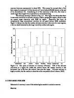
with the oil. The gas cap drives the oil in a similar fashion as the aquifer drive. Gas production (along with the oil) is not seen as a disadvantage, since it also can be used as an energy source. Finally, gravity is the important factor in the gravity flow, for which the well placement is obviously relevant. The use of this method is limited and is heavily dependent on the geology of the reservoir. The primary techniques recover, depending on the oil reservoir, on average between 5 and 25% of the original oil in place (OOIP) [15]. The secondary method involves the injection of either water or gas to increase the pressure in the reservoir, which in turn drives the oil out. After a given time, the injected water breaks through in the production wells. As the production well ages, after the water breakthrough, the water cut increases. The use of the secondary methods enables the extraction of additional 5–30% of the OOIP depending on the reservoir after primary extraction. At most 55% of the OOIP can be recovered (in most cases this value is much lower) using the primary and secondary techniques. Therefore, a large portion of the OOIP remains embedded in the reservoir. Since the 1970s, many different methods have been developed to increase the oil recovery as a response to the oil crisis. These all belong to the category improved oil recovery (IOR). Improved oil recovery implies improving the oil recovery by any means, such as operational strategies. Enhanced oil recovery, a subgroup of IOR, is different in that the objective is to reduce the oil saturation below the residual oil saturation (the latter being defined as the oil saturation after a prolonged waterflood). Figure 1.5 shows schematically an oil well with implemented chemical EOR techniques [14]. Injection wells have to be built around the main production well, which of course means a significant economic investment. Looking at the evolution of EOR in the USA, the number of projects kept growing until reaching a peak in the mid-80s (Fig. 1.6) [16], when the drop in oil prices discouraged further investments. Recent times, however, experienced again a growth of EOR techniques, as the resources become scarcer and fewer new reservoirs are discovered. The term EOR includes a series of techniques, summarized in Fig. 1.7 [17]. They can roughly be divided into two groups, thermal and non-thermal. Thermal methods have been tested since the 1950s, and they are the most advanced EOR methods, as far as field experience and technology are concerned. They are best suited for heavy oils (10–20°API) and tar sands (≤ 10°API). Thermal methods supply heat to the reservoir and vaporize some of the oil. The major mechanisms include a large reduction in viscosity, and hence mobility ratio. Thermal methods have been highly successful in Canada, USA, Venezuela, Indonesia and other countries [15]. While thermal methods rely on the introduction of energy into the well in the form of heat, the non-thermal methods involve the injection of substances to ensure better oil extraction. These can be miscible with the oil (organic solvents, gases) or non-

6 | 1 An introduction to chemical enhanced oil recovery

Oil remaining after waterflooding

ASP injection, creating an oil bank

Alkali untraps oil

Surfactant breaks the oil drops

Production well Injection well

Polymer displaces trapped oil

Remaining oil after ASP

Fig. 1.5: Schematic representation of a chemical EOR process [14].

600

Thermal Chemical

500 No. of projects

Gases 400

Total

300 200 100 0 1971

1976

1980

1984

1988 1992 Year

1996

2000

2004

2008

Fig. 1.6: Evolution of EOR projects in the USA [16].

miscible. The latter include all the chemical EOR methods, for brevity cEOR, which are the focus of this book. One non-thermal and non-chemical EOR method worthy of

1.2 Enhanced oil recovery |

7

Oil Recovery Mechanisms Conventional Oil Recovery

Primary

Natural Flow

Secondary

Waterflood

Artifical Lift

Tertiary

Pressure Maintenance

Thermal

Miscible

EOR Chemical Nanotechnology

Surfactant

Nanotechnology

Polymer

Steam stimulation or cyclic steam injection

Miscible solvent

Alkaline

ASP

In-situ combustion

Other: microbial, electrical chemical leaching, mechanical ( vibrating, horizontal drilling)

CO2

Inert gas

Alternating techniques: WAG,PAG,SAG,PSAG

Steam or hot water

Foam Displacement

Fig. 1.7: Summary of chemical EOR techniques [17].

mention is CO2 flooding, which is gaining a lot of popularity [15, 16]. The use of CO2 is attractive for both economic and environmental reasons: it is cheap and readily available and when used for oil extraction it can be trapped under the soil, reducing its emission into the atmosphere. The vast majority of cEOR methods are constituted by mainly three of them, and their combinations: polymer flooding, surfactant flooding and alkaline flooding [18]. Combined surfactant-polymer flooding (usually abbreviated to SP flooding) and alkali-surfactant-polymer flooding (ASP flooding) have been also intensively investigated [19–21]. Which EOR method is more suitable for a particular case depends on many factors, including reservoir lithology and the type of oil, which will be discussed in the following sections.

8 | 1 An introduction to chemical enhanced oil recovery

1.3 Reservoir lithology Reservoir lithology is one of the screening considerations for EOR methods, often limiting the applicability of specific EOR methods. The vast majority of reservoirs can either be classified as sandstone or carbonate (or limestone). Sandstone is composed mainly of silicates (quartz and feldspar), while the main components of carbonates are CaCO3 and MgCO3 in various crystalline structures. About 60% of all petroleum reservoirs are sandstones; outside the Middle East, carbonate reservoirs are less common, and the percentage is even higher. The most important reservoir properties are porosity and permeability, but pore geometry and wetting properties of the mineral surfaces may also influence petroleum production [22]. It is generally accepted that oil recovery is more efficient in water-wet rocks rather than in oil-wet ones [23]. Most EOR applications have been in sandstone reservoirs, as derived from a collection of over 1500 international EOR projects [16]. EOR thermal and chemical projects are the most frequently used in sandstone reservoirs compared to other lithologies (e.g., carbonates and turbiditic formations) [16]. Sandstones usually possess higher porosity and permeability and favorable wetting properties (water-wet). However, a considerable portion of the world’s hydrocarbon endowment is in carbonate reservoirs, which poses more challenges. Carbonate reservoirs usually exhibit lower porosity and may be fractured. These two characteristics along with rock wetting properties, usually result in lowered hydrocarbon recovery rates [24, 25]. Another problem associated with carbonate reservoirs is related to their chemical composition: they are composed mainly by CaCO3 and MgCO3 , thus they contain significant amounts of Ca2+ and Mg2+ ions in their structure. As we will see later, this limits the implementation of chemical EOR methods, due to precipitation of most chemicals employed in the processes (polymers and surfactants) in the form of calcium and magnesium salts. The recoverable reserves of carbonate reservoirs are huge and thus it is considered that the exploitation of them has tremendous economic value, so people are shifting attention from traditional sandstone reservoirs to carbonate reservoirs which are widely distributed around the world, in North America, North Europe, China and Australia (Fig. 1.8) [26, 27]. Applying EOR technology to improve oil recovery is critical. Worldwide EOR projects for carbonate reservoir development have been undertaken since the 1970s. The main techniques to enhance oil recovery for carbonate reservoirs include air injection, thermal recovery and chemical flooding. The injected gas can be carbon dioxide, nitrogen or air, and hydrocarbon gas where carbon dioxide flooding is the dominant EOR process used in the US because of the high availability of low-cost CO2 . Steam injection in viscous oil carbonates has been piloted in the Middle East and Canada because it can change reservoir behaviors, leading to production enhancement. Be-

1.4 Types of crude oil

Asia Pacific North America

40.5 59.9

South and Central America

103.5

Africa

117.2

Europe and Eurasia

Proved oil reserves+

| 9

Reef

Oil in carbonates+ Shelf carbonates Deep carbonates

144.4 742.7

Middle East

Carbonates oil province

Thousand million barrels

Fig. 1.8: Geographical distribution of large carbonate reservoirs worldwide [27].

sides, SiO2 nanoparticles and microbial biomass have also been investigated for EOR of carbonate reservoirs [26].

1.4 Types of crude oil The most common distinction made when referring to crude oil is between light, heavy and extra-heavy oil. The latter are also called bitumen, tar or oil sands. Although the distinction can be made somewhat arbitrarily, it is generally accepted to define as heavy any oil with a gravity of 20°API or lower [28]. It is worth mentioning here that the API gravity is an inverse measure of a petroleum liquid’s density relative to that of water. Another distinction can be made based on viscosity. Table 1.1 gives an overview of a general classification of oils based on these physical properties. The viscosity of heavy oil is typically higher than 100 cP, while extra-heavy oils are those which do not flow significantly in ordinary conditions. Since these cannot be extracted using conventional methods (the ones discussed in this book), they are also referred to as “unconventional oils”.

10 | 1 An introduction to chemical enhanced oil recovery

Tab. 1.1: General oil classification according to their physical properties. oil classification

API Gravity °API

Dynamic Viscosity cP

Light oils Medium oils Heavy oils Extra-heavy oils Natural bitumen (or tar sands)

> 31.1 22.3 < °API < 31.1 10 < °API < 22.3 < 10 < 10

< 100 cP < 100 cP < 100 cP < 10.000 cP > 10.000 cP

Light oils

Heavy oils Water

EOR Target 45% OIP

Tar sands Water

Primary 25% OIP

Secondary 30% OIP

Primary 5% OIP Secondary 5% OIP

EOR Target 90% OIP

Water

EOR Target 100% OIP

(Assuming Soi = 85% PV and Sw = 15% PV)

Fig. 1.9: EOR target for different kind of hydrocarbons. From ref [15].

From a chemical point of view, compared to light oils, heavy oils contain higher amounts of aromatic hydrocarbons, simple (benzene derivatives) or polycondensate (asphaltenes), as well as higher amounts of heteroatoms (sulfur, nitrogen, and heavy metals). Due to their higher density and viscosity, heavy oils and tar sands respond poorly to primary and secondary recovery methods, and the bulk of the production from such reservoirs come from EOR methods (Fig. 1.9) [15].

1.5 Chemical EOR Chemical EOR methods had their best times in the 1980s, most of them in sandstone reservoirs. The total number of active projects peaked in 1986 with polymer flooding as the most important chemical EOR method. However, since 1990s, oil production from chemical EOR methods has dropped down significantly. Nowadays the biggest cEOR projects are running in China. Nevertheless, chemical flooding has been shown to be sensitive to the volatility of oil markets despite recent advances (e.g., low surfactant concentrations) and lower costs of chemical additives.

1.5 Chemical EOR |

11

Chemical EOR includes various interesting techniques. The most important among them are polymer flooding, which is the most mature and used, surfactant flooding, alkaline flooding and combinations of the above, such as surfactant-polymer (SP) flooding and alkali-surfactant-polymer (ASP) flooding [18, 20, 21, 29]. Besides these, microbial flooding [30], and more recently, nanofluids [31] flooding are also relevant cEOR methods. Polymeric surfactants, as an alternative to polymer and SP flooding have also been investigated [32]. Polymer flooding can date its origins back to the 1950s, when the importance of fluid mobility for oil recovery was proposed and proved experimentally shortly after [33]. It was observed that increasing the viscosity of water used in waterflooding by dissolving a small amount of high molecular weight soluble polymer, would greatly improve the macroscopic sweep efficiency. Polymer flooding will be discussed in detail in the next chapter. Surfactants are known to decrease the interfacial tension between water and oil. This allows the formation of emulsions when a surfactant solution is flooded into an oil reservoir, also known as micellar flooding. This causes a significant decrease in residual oil saturation, with subsequently better microscopic oil displacement. The role of an alkali in alkaline flooding, is basically the same as the surfactant, but it is achieved by a different mechanism. The alkali (or base), is able to generate surfactant species in situ, simply by neutralizing fatty acids present in the crude oil, turning them in amphiphilic molecules. Alkaline flooding is generally used in combination with the previous ones, in what is called ASP flooding (from alkali-surfactant-polymer). Besides the role already mentioned, the chemicals used for cEOR can also alter the rocks wettability, which can also result in better recovery. Important phenomena to take into account in cEOR are adsorption and retention of the chemicals onto the porous rock systems. Adsorption is generated by all kind of interactions (Van der Waals, electrostatic, and hydrogen bonding) between the chemicals and the rock surface. Polymers generally display high adsorption and retention, due to their high molecular weight, and this can cause a significant change in rocks permeability and porosity. Both polymers and surfactants are very often constituted by charged molecules that able to adsorb onto the rock surfaces via electrostatic interactions with the ions present in the rock crystalline structure. Another relevant aspect is the environmental impact of the chemicals used for cEOR. Underground injection of huge amounts of chemicals can have a significant and often unpredictable effect on ecosystems. Water flooding should be performed after cEOR methods are implemented, in order to remove residual chemicals from the reservoir. The use of chemical products such as polymers, surfactants, alkali, microorganisms, nanomaterials and nanofluids, has attracted a lot of interest and poses several scientific challenges, which have been tackled by many researchers. The chemicals

12 | 1 An introduction to chemical enhanced oil recovery

used should be designed to withstand the harsh conditions present in the reservoir (e.g., dissolved salts, pH, temperature, presence of bacteria) and increase the efficiency of the process. One of the key factors in this development is the (macro)molecules architecture and its influence on the physical properties of the fluids being injected: from linear to branched polymers, and from monomeric to gemini surfactants. The most recent advancements in cEOR will be treated in the rest of the book, with particular focus on academic studies aimed at designing new polymers for EOR, with the aid of both experimental work and mathematical simulations.

References [1] [2]

[3] [4] [5] [6] [7] [8]

[9] [10] [11] [12] [13] [14] [15] [16]

Dresselhaus, M. S. and Thomas, I. L. Alternative energy technologies. Nature, 414:332–337, 2001. Hoffert, M. I., Caldeira, K., Benford, G., Criswell, D. R., Green, C., Herzog, H., Jain, A. K., Kheshgi, H. S., Lackner, K. S., Lewis, J. S., Lightfoot, H. D., Manheimer, W., Mankins, J. C., Mauel, M. E., Perkins, L. J., Schlesinger, M. E., Volk, T., and Wigley, T. M. L. Advanced technology paths to global climate stability: energy for a greenhouse planet. Science, 298:981–987, 2002. York, R. Do alternative energy sources displace fossil fuels? Nat. Clim. Chang., 2:441–443, 2012. McGlade, C. and Ekins, P. The geographical distribution of fossil fuels unused when limiting global warming to 2 °C. Nature, 517:187–190, 2015. Cherubini, F. The biorefinery concept: Using biomass instead of oil for producing energy and chemicals. Energy Convers. Manag., 51:1412–1421, 2010. UNFCCC. The Paris Agreement. Available online: https://unfccc.int/process-and-meetings/theparis-agreement/the-paris-agreement (accessed on Jun 6, 2018). Shell Global. Sky Scenario. Available online: https://www.shell.com/energy-and-innovation/ the-energy-future/scenarios/shell-scenario-sky.html (accessed on Feb 15, 2019). BP. Statistical Review of World Energy | Energy economics. Available online: https://www.bp. com/en/global/corporate/energy-economics/statistical-review-of-world-energy.html (accessed on May 23, 2018). OMR. OMR Public. Available online: https://www.iea.org/oilmarketreport/omrpublic/ (accessed on May 23, 2018). Bardi, U. Peak oil: The four stages of a new idea. Energy, 34:323–326, 2009. De Almeida, P. and Silva, P. D. The peak of oil production—Timings and market recognition. Energy Policy, 37:1267–1276, 2009. Kerr, R. A. Peak Oil Production May Already Be Here. Science (80-. )., 331:1510–1511, 2011. Madureira, N. L. Oil Reserves and Peak Oil. In Key Concepts in Energy, pp. 101–130. Springer International Publishing, Cham, 2014. Druetta, P. D., Picchioni, F., and Rijksuniversiteit Groningen. Numerical simulation of chemical EOR processes. University of Groningen, 2018. Thomas, S. Enhanced oil recovery – An overview. Oil Gas Sci. Technol. L Inst. Fr. Du Pet., 63:9– 19, 2008. Alvarado, V. and Manrique, E. Enhanced Oil Recovery: An Update Review. Energies, 3:1529– 1575, 2010.

References | 13

[17] Druetta, P., Raffa, P., and Picchioni, F. Plenty of Room at the Bottom: Nanotechnology as Solution to an Old Issue in Enhanced Oil Recovery. Appl. Sci., 8:2596, 2018. [18] Lake, L. W. Enhanced Oil Recovery. New Jersey, Prentice Hall, 1989. [19] Li, G. Z., Mu, J. H., Li, Y., and Yuan, S. L. An experimental study on alkaline/surfactant/polymer flooding systems using nature mixed carboxylate. Colloids Surfaces A Physicochem. Eng. Asp., 173:219–229, 2000. [20] Sheng, J. J. A comprehensive review of alkaline-surfactant-polymer (ASP) flooding. Asia-Pacific J. Chem. Eng., 2014. [21] Olajire, A. A. Review of ASP EOR (alkaline surfactant polymer enhanced oil recovery) technology in the petroleum industry: Prospects and challenges. Energy, 77:963–982, 2014. [22] Bjørlykke, K. and Jahren, J. Petroleum Geoscience, chapter Sandstones and Sandstone Reservoirs, pp. 113–140. Springer Berlin Heidelberg, Berlin, Heidelberg, 2010. [23] El-hoshoudy, A. N. N., Desouky, S. E. M. E. M., Elkady, M. Y. Y., Al-Sabagh, A. M. M., Betiha, M. A. A., and Mahmoud, S. Hydrophobically associated polymers for wettability alteration and enhanced oil recovery – Article review. Elsevier, 26:757–762, 2017. [24] Manrique, E. J., Muci, V. E., and Gurfinkel, M. E. EOR Field Experiences in Carbonate Reservoirs in the United States. SPE Reserv. Eval. Eng., 10:667–686, 2007. [25] Chilingar, G. V. and Yen, T. F. Some Notes on Wettability and Relative Permeabilities of Carbonate Reservoir Rocks, II. Energy Sources, 7:67–75, 1983. [26] Bai, M., Zhang, Z., Cui, X., and Song, K. Studies of injection parameters for chemical flooding in carbonate reservoirs. Renew. Sustain. Energy Rev., 75:1464–1471, 2017. [27] Schlumberger. Carbonate Reservoirs. Available online: https://www.slb.com/services/ technical_challenges/carbonates.aspx (accessed on Feb 19, 2019). [28] Saboorian-Jooybari, H., Dejam, M., and Chen, Z. Heavy oil polymer flooding from laboratory core floods to pilot tests and field applications: Half-century studies. J. Pet. Sci. Eng., 142:85– 100, 2016. [29] Chang, H. L. ASP Process and Field Results. In Enhanced Oil Recovery Field Case Studies. Gulf Professional Publishing (Elsevier), Waltham, MA, 2013. [30] Sen, R. Biotechnology in petroleum recovery: The microbial EOR. Prog. Energy Combust. Sci., 34:714–724, 2008. [31] Peng, B., Zhang, L., Luo, J., Wang, P., Ding, B., Zeng, M., and Cheng, Z. A review of nanomaterials for nanofluid enhanced oil recovery. RSC Adv., 7, 2017. [32] Raffa, P., Broekhuis, A. A., and Picchioni, F. Polymeric surfactants for enhanced oil recovery: A review. J. Pet. Sci. Eng., 145, 2016. [33] Thomas, A. Polymer Flooding. In Romero-Zeron, L., ed., Chemical Enhanced Oil Recovery (cEOR) – a Practical Overview, p. Ch. 02. InTech, Rijeka, 2016.

2 Polymer flooding 2.1 Introduction Polymer flooding is the most established chemical EOR method. It has a long history and demonstrated effectiveness. This technology outnumbers other chemical technologies, because it is easier to implement, it’s applicable in a large range of reservoir conditions and it has low risks when compared to others. The environmental aspects are seldom considered and the long-term effects on the ecosystems of injection of tons of polymers underground is still unclear. However, polymer flooding can be expected to have a lower environmental impact when compared, for example, to surfactants or microbial flooding. From this point of view, it could be considered a positive sign that after polyacrylamides, the most used polymers for EOR are biopolymers such as Xanthan gum and cellulose. However, this is not necessarily better for the environment, because the introduction of huge amount of these materials, which are nutrients for microorganisms, could affect the underground flora and fauna, with unpredictable consequences. Nonetheless, the application of polymer flooding has increased over the past years, especially in high temperature and high salinity reservoirs [1–8]. Polymer flooding consists of injecting a polymer water solution into a subterranean oil formation in order to improve the sweep efficiency in the reservoir. The increased viscosity of the water due to the dissolved polymer causes a better mobility control between the injected fluid and the hydrocarbons within the reservoir, allowing to recover an additional 12 to 15% of the original oil in place (OOIP) [3, 9]. Usually polymer flooding follows water flooding, but it can be implemented also directly after primary recovery. The early pioneering work on polymer flooding dates back to the 60s, and the first large commercial uses of polymers to increase oil recovery were performed in the United States, during a crude oil price control period between the 60s and the 70s [1]. After peaking during the 80s, the number of projects abruptly decreased for several economic and technological reasons. However, research has continued over the years and polymer flooding regained interest, especially in China, in the 90s. The largest polymer flooding project is currently running in the Daqing oilfield, after being started in 1996. Another example of successful polymer injection in the 1990s was in Courtenay, France, where extra oil recoveries from 5 to 30% have been reported after the technology was conducted in a secondary recovery mode as augmented water flooding. Germany, Austria, Oman and North Kuwait have also running EOR projects [4]. As of 2004, more than 30 commercial projects were implemented, involving approximately 2427 injection wells and 2916 production wells according to [1]. Polymer injection in the Shengli and Daqing oilfields yielded incremental oil recoveries ranging from 6 to 12%, contributing to 250.000 barrels per day in 2004 [1].

https://doi.org/10.1515/9783110640250-002

16 | 2 Polymer flooding

An extensive recent update from researchers in Norway [7] reports results from 72 documented polymer projects (including pilots). Among these, 66 projects were implemented onshore and only 6 offshore. Of the reported projects, 40 were classified as successes and 6 were assessed discouraging. 46 projects have been performed in the U.S.A., followed by 6 in Canada, 6 in China and 4 in Germany. Partially hydrolysed polyacrylamide (HPAM) was used as polymer in 92% of the cases and the rest were using biopolymers. Only one project used a hydrophobic associative polymer [7]. Several polymers are commercially available for chemical EOR applications, HPAM being the most widely used. Water soluble polymers for chemical EOR applications have been reviewed several times. The main contributions from the last years include general reviews on polymer flooding [1, 3–7, 10–12] as well as reviews focusing on particular classes of polymers for EOR such as hydrophobically associating polymers [13, 14], or particular aspects such as oil displacement mechanisms [9] and injection parameters [15, 16]. Our own group also recently contributed with reviews focusing on solution properties [2] and on polymeric surfactants [17]. Currently used polymers suffer various limitations and cannot generally be used in severe conditions of salinity and temperature or in low porosity rock formations. Therefore, considering the still high and actually increasing demand of oil and its decreasing availability, which is expected to cause the oil price to rise again in the near future, research of new systems for polymer flooding is still active. The number of patents filed by many companies, even in recent times, about new polymers for EOR certainly supports this statement [17]. In our opinion, along with elucidating the oil recovery mechanisms, establishing proper structure-properties relationships for water-soluble polymer is the key to design new successful systems. This chapter will shortly illustrate the underlying theory of polymer flooding and will then describe from a chemical point of view the polymers currently used and proposed as flooding agents, with particular emphasis on structure-properties relationship and how those could determine possible advantages and disadvantages in chemical EOR processes.

2.2 Theory The overall oil recovery efficiency in oil production processes is generally divided in two distinct contributions: macroscopic and microscopic recovery efficiency. The macroscopic recovery efficiency refers to the volume that the flooding agents are able to sweep and it is also referred to as volumetric sweep efficiency; the microscopic recovery efficiency is a measure of the effectiveness of the displacing fluid(s) in mobilizing the oil trapped at pore scale by capillary forces. In other words, any mechanism that can improve either macroscale or microscale oil recovery efficiency is beneficial for increasing oil production [3].

2.2 Theory | 17

The mechanisms of polymer flooding have been elucidated and discussed thoroughly. It is normally suggested that polymer flooding can only improve the volumetric sweep efficiency without any effect on the microscopic displacement efficiency. The well-established relationship between capillary number and oil recovery indicates that a substantial increase in oil recovery at the pore level (microscale) can be obtained only when the capillary number is increased by at least three orders of magnitude. For polymer flooding, the capillary number is normally increased less than 100 times. This can be visualized considering that the capillary number can be expressed as the viscous-to-capillary forces, according to Eq. (2.1): uμ c Nc = (2.1) γ Where u is the velocity gradient, μc is the viscosity of the displacing fluid (or continuous phase) and γ the interfacial tension between displacing fluid and oil. Therefore, as the polymer can increase water viscosity by two to three orders of magnitude, the effect on capillary number will be of the same order of magnitude. Microscopic efficiency is much more affected by reduction of interfacial tension operated by the presence of surfactants. However, many reported values of increased oil recovery seem to be higher than those achievable only by sweep efficiency improvement [3]. This fact made researchers to revisit the oil recovery mechanisms occurring in polymer flooding. It is now proposed that incremental oil recovery by polymer flooding can also be explained by the simultaneously increased microscopic displacement efficiency due to the distinctive flow characteristic of polymer solutions [3]. In any case, the main mechanism of oil recovery achieved by polymer flooding is the increase of macroscopic efficiency by increasing water viscosity, in order to achieve better mobility control. The mobility can be also altered by changing the permeability of the rock formation. The second most important mechanism of oil recovery is permeability reduction. Viscoelastic behaviour of polymer solutions might also play a role, as discussed later. Mobility control is discussed in the next section.

2.2.1 Mobility control Mobility control remains one of the most important concepts in any enhanced oil recovery process. According to the most general consensus, mobility control can be achieved through injection of chemicals to change displacing fluid viscosity or to preferentially reduce specific fluid relative permeability through injection of foams, or even through injection of chemicals, to modify wettability [18]. The existing concept of mobility control is that the displacing fluid mobility should be equal to or less than the (minimum) total mobility of displaced multiphase fluids. This statement has been recently challenged [18].

18 | 2 Polymer flooding

The mobility of a fluid in a porous formation (λ) is usually defined as the ratio between the effective permeability of the fluid (which is the product of the absolute permeability K and the relative permeability of the phase k r ) and its viscosity (μ), as shown in Eq. (2.2): Kk r λ= (2.2) μ What matters in an EOR process, is the ratio between the mobility of the displacing fluid (water, or as in the case of polymer flooding, polymer solution) and the displaced fluid (oil), called the mobility ratio (M), as expressed as in Eq. (2.3) (the superscripts w and o, stand for water phase and oil phase respectively): λw M= o = λ

kw μw ko μo

=

kw μo ko μw

(2.3)

Mobility ratio influences the microscopic (pore level) and macroscopic (areal and vertical sweep) displacement efficiencies. A value of M much higher than one, which results from a high difference in viscosity between the water and the oil phases (this is can be easily seen by Eq. (2.2)) is considered unfavourable, because it indicates that the displacing fluid flows more readily than the displaced fluid (oil), and it can cause channeling of the displacing fluid, and as a result, bypassing some of the residual oil. Under such conditions, and in the absence of viscous instabilities, more displacing fluid is needed to obtain a given residual oil saturation. The effect of mobility ratio on displaceable oil is shown in Fig. 2.1 [8]. The three curves represent one, two and three pore volumes of total fluid injected, respectively. Displacement efficiency is increased when M = 1 and is denoted a “favourable” mobility ratio. It has been established that during a typical flooding, for a mobility ratio close to one, the displacing fluid will push the oil in a “piston-like” fashion while, as the value becomes higher, the phenomena of viscous fingering and channeling will become relevant (Fig. 2.2) [19, 20], with subsequent lowered sweep efficiency. Simply put, as the viscosity of the oil phase is always bigger than that of water, increasing the water viscosity should have beneficial effects in sweep efficiency and thus in oil recovery. This consideration is at the basis of the use of water thickeners, particularly water-soluble polymers, in chemical enhanced oil recovery. In the next section, the viscosity of polymer water solutions and rheological behaviour, will be discussed in the context of enhanced oil recovery. It has been recently proposed by Sheng [9, 18] that the mobility ratio M value used to determine the most favourable viscosity conditions for the displacing fluid, should be corrected by a multiplicative factor, which he called “normalized movable oil saturation”.

2.2 Theory

1.0 1 PV lnj 2 PV lnj 3 PV lnj

0.9

Displaceable oil (PV)

0.8 0.7 0.6 0.5 0.4 0.3 0.2

1

10

100 Mobility ratio (M)

1000

Fig. 2.1: Effect of mobility ratio on displaceable oil (simulated) [8].

B.T.

M = 0.151 B.T.

M = 4.58

B.T.

M = 1.0

B.T.

M = 2.40

B.T.

M = 17.3

B.T.

M = 71.5

Fig. 2.2: Water flooding at different mobility ratios, showing viscous fingering [20].

| 19

20 | 2 Polymer flooding

2.2.2 Permeability reduction Viscosity is not the only relevant phenomena affecting mobility in polymer flooding. Another mechanism, known as disproportionate permeability reduction (DPR), or simply permeability reduction, can facilitate polymer flooding to improve the macroscopic sweep efficiency. This refers to a reduction of water permeability (k w , Eq. (2.3)) by the polymer, while the oil permeability remains basically unaffected [3]. The reasons for DPR are varied and include mainly segregation of flow pathways of oil and water and adsorption of the polymer, but also wettability alteration and polymer swelling phenomena, to a minor extent [3]. By looking at Eq. (2.3), it is apparent that the effect achieved by DPR is the same as the increase of viscosity of the water phase with respect to the oil phase: a decrease of the mobility ratio. The permeability reduction is also known as the residual resistance factor [1] and mathematically it can be expressed as the mobility ratio of water (brine) before and after polymer flooding: RRf =

λbp = λap

kap ηap kbp ηbp

≅

kw kp

(2.4)

where the symbols have the meanings as defined above, and the indexes bp and ap refer respectively to before and after polymer flooding, while k p and k w are the permeabilities of the polymer solution and water respectively. The k w /k p ratio is called the permeability reduction factor and is often used for the quality estimation of polymer solutions [19]. The residual resistance factor RRf should not be confused with the resistance factor Rf , another important parameter in EOR, which is defined as the ratio of the mobility of water (brine) to that of the polymer solution under the same conditions [19]: λw (2.5) λp The residual resistance factor can be used to estimate the thickness layer of adsorbed polymer χ p , according to the formula [21]: Rf =

−1

χ p = dp (1 − RRf4 )

(2.6)

where dp is the average pore diameter that, in turn, can be estimated from the water permeability and rock porosity Φ [21]: dp = 1.15 (

8k w 1/2 ) Φ

(2.7)

2.2.3 Flow resistance Flow resistance is another mechanism believed to improve the macroscopic sweep efficiency during polymer flooding. Some authors reported a positive contribution of

2.2 Theory

| 21

polymer elasticity in EOR and they connected it to higher resistance to flow through porous media, compared to less elastic polymers, at identical shear viscosities [3]. Since elastic behaviour is related to the polymer structure, this will play a relevant role in the design of polymers for polymer flooding. Indeed, it has been proposed that branched PAM would perform better in polymer flooding compared to linear structures, at comparable shear viscosity. Control over the polymer structure, however, might prove to be challenging and expensive from a synthetic point of view. Synthetic polymers traditionally used for EOR are prepared by methods based on free-radical polymerization, which allows hardly any control. The structures obtained are usually high-molecular weight polymers, with large distributions of molecular weights and mostly linear structures, containing random branching. Later, synthetic strategies aimed at controlling polymer structures and branching will be discussed. In the next sections, the effect of polymer structure’s viscoelastic properties in solution, will be discussed.

2.2.4 Polymer solution rheology Based on the previous considerations, solution rheology, particularly viscosity, has a relevant role in polymer flooding. Many well-known water-soluble polymers are effective thickening agents. These includes natural ones such as polysaccharides or proteins and synthetic ones such as polyethylene glycol and polyacrylamide. Generally speaking, the viscosity of a polymer solution increases with the hydrodynamic volume of the polymer chains, and therefore with the molecular weight, according to the well-known Mark–Houwink–Sakurada Eq. (2.8): α

[η] = KMH MwMH

(2.8)

Where [η] is the intrinsic viscosity, Mw is an average molecular weight and KMH and α MH are semi-empirical parameter characteristics for a polymer-solvent pair, related to the Flory–Huggins interaction parameter and the conformation of polymer in solution. In particular, the value of α can vary from 0.5 for a polymer in a theta solvent, to 0.7–0.8 for a polymer in a good solvent, to values higher than one for polymers in extended conformation [22]. This latter case can present itself in water for polymers bearing charges along the backbones, also known as polyelectrolytes, due to Coulombic and osmotic effects [23]. These considerations suggest that high molecular weight polyelectrolytes would be the most effective water viscosifiers and this is indeed often the case. In fact, the most used polymers in EOR are HPAM, which are high-molecular weight polyelectrolytes. Their chemical and physical characteristics will be described later. However, when talking about polymer flooding, we must consider that the solution is forced to flow through a porous media, which causes shear forces to act on the system. Therefore, the most representative rheological parameter is the shear viscos-

22 | 2 Polymer flooding

ity; polymer solutions generally present a non-Newtonian behaviour, therefore effects such as shear thinning and shear thickening, should be taken into account [18]. The typical viscosity profile of a polymer solution in a porous media is shown in Fig. 2.3 [20]. At low shear rates, the solution behaves as a typical polymer solution, with a Newtonian plateau followed by a shear thinning region as the shear increases. As the shear increases even further, a shear thickening effect is observed, attributed to a transition from shear flow to elongational flow occurring in the porous media. In the high shear region, further shear thinning can occur, due to polymer degradation causing a decrease in molecular weight.

Shear Thinning Due First Critical Shear Rate to Mechanical Degradation

Viscosity

Shear Thinning Region

Shear Thickening Region Second Critical Shear Rate

Shear Rate Fig. 2.3: Schematic illustration of viscosity profile in porous media [20].

The role of viscoelasticity, rather than just viscosity, has been often emphasized [2, 9]. This has been used to justify oil recovery values higher than the ones expected purely by an increase in macroscopic sweeping efficiency [3]. It has been suggested by Wang et al. [24–26] that if a fluid with elastic properties flows over dead ends, normal stresses between the oil and polymer solution are generated in addition to the shear stresses resulting from the long molecular chains. Thus, polymer imposes a larger force on oil droplets and pulls them out of dead ends. The amount of residual oil pulled out from dead ends is proportional to the elasticity of the driving fluid; these observations are presented in Fig. 2.4, where the effect is shown comparing a HPAM solution to a viscous liquid without an elastic component, such as glycerine [18, 26]. It was also shown in core flood experiments that after glycerine flooding, polymer flooding further increases the recovery by an extra 6% OOIP [18]. Since viscosity and interfacial tension were comparable, the increased recovery was explained in terms of elasticity of the polymer solution.

2.3 Criteria for polymer selection |

(a)

(b)

23

(c)

Fig. 2.4: Schematic representation of residual oil in “dead ends” after (a) water, (b) glycerine, and (c) HPAM floods.

Various displacing mechanisms have been proposed and studied via numerical simulations, based on “pulling” or “stripping” from dead ends, formation of oil threads, and shear thickening [18].

2.3 Criteria for polymer selection Knowing the theoretical background can help in screening polymers and conditions for optimal recovery. However, there are several empirical factors to take into account. In chemical EOR, given the harsh conditions present in most oil reservoirs, some problems and limitations arise with the use of water-soluble polymers. For example, high ionic strength drastically reduces polyelectrolytes viscosity due to the charge screening effect. Moreover, high salt concentration can cause “salting out” effects or flocculation, especially in the presence of polyvalent cations such as calcium and magnesium. High temperatures greatly accelerate polymer chemical degradation and/or transformations, the porosity of the rocks favour obstruction and polymer adsorption, shear forces cause mechanical degradation. all these aspects will be discussed later. The aforementioned factors can seriously limit the choice of polymers for oil recovery. Moreover, and this is often the most stringent requirement, the polymer should be cheap and easily available in large quantities, in order to make the recovery process cost-effective. The selection criteria, based on those recently summarized by Rellegadla et al. [6], are presented and further elaborated as follows.

2.3.1 Costs Costs are obviously one of the main criteria for the selection of polymers for chemical EOR. These include not only the cost of the chemicals employed, but also process costs, operation costs, transportation, etc. For synthetic polymers, the price is strictly related to oil price, which in turn can be affected by EOR processes in use, creating a paradoxical situation, like a dog chasing its tail. Polyacrylamides, belonging to this category, are the cheapest polymers used for EOR, but their price can indeed fluctuate depending on oil prices, while biopolymers such xanthan gum, have higher but more stable prices. Hydroxy ethyl cellulose (HEC)

24 | 2 Polymer flooding

and carboxy methyl cellulose (CMC) are relatively cheap biopolymers, compared to xanthan gum [6]. When new polymers are proposed for chemical EOR, one should always consider if the improved recovery surpasses or at least balances out the increased costs for production, which is normally very difficult to evaluate.

2.3.2 Filtration properties Suitable polymers for chemical EOR should not cause wellbore plugging. This is why polymers proposed for EOR are usually subject to filtration tests of various types [6]. Issues can be generated by a not proper dissolution of the polymer: if the hydration is not efficient, structures such as “fish eyes” or “gel balls” can form, potentially causing near wellbore plugging. This can be avoided by slow addition and vigorous agitation. Polymer cross-linking can be a further cause of plugging. Problems can be minimized by using good quality water and filtering the solution prior to injection, even though this increases operation costs. Enzyme clarification and diatomaceous earth filtration are now being implemented for treatment process of polymer solutions prior to flooding.

2.3.3 Viscosity The general theoretical background about viscosity is given in Section 2.2.3. Polymer flooding has proven particularly effective for oils with medium viscosity, typically lower than 150 cP [4, 7]. It is generally believed that polymer flooding is only suitable for oils with a viscosity not higher than 100 cP, while for heavy or extra-heavy oils, thermal methods or miscible solvents methods seem to be better [11]. However, applications of the latter to many reservoirs is restricted by technical, economical, and environmental issues. For this reason, and because polymer flooding still remains the most practical EOR method, it is of particular research interest in the investigation of possible implementation of polymer flooding processes for heavy oils. Core flood experiments have been performed to evaluate the effectiveness of polymer flood for oils with high viscosities, in the range 200–8400 cP, which has been recently reviewed [11]. A very important finding from a set of experiments performed by Wang and Dong on oils with viscosities from 430 to 5500 cP [27], is the existence of a S-shape region in the viscosity/recovery profile (Fig. 2.5). This defines a range within which tertiary oil recovery by polymer flooding increases significantly with an increase in the viscosity of the polymer solution. On the other hand, for the polymer viscosity outside of this region, incremental oil recovery changes slightly with polymer viscosity. A master curve has been built with this data by Guo et al. [28], where the dependence on the oil viscosity is normalized via the mobility ratio M (Fig. 2.6).

2.3 Criteria for polymer selection |

25

Tertiary Oil Recovery, %OOIP

25 20 15

Oil Viscosity 430 mPa.s 1108 mPa.s 1450 mPa.s 2900 mPa.s 5500 mPa.s

10 5 0

10

1

100

1000

Effective Viscosity of Polymer Solution, mPa.s Fig. 2.5: Tertiary oil recovery as a function of polymer solution viscosity at different oil viscosities. Adapted from [27].

Tertirary Oil Recovery, %OOIP

25

20

15

10

Oil Viscosity 430 mPa.s

5

1450 mPa.s 2900 mPa.s

0 0.00

0.10

0.20

0.30

0.40

0.50

0.60

Mobility Ratio at the End of Waterflooding, dimensionless Fig. 2.6: Normalized relationship between tertiary oil recovery and oil/water mobility ratio. Reproduced from [28].

Analogous observations were made by other researchers for oils with viscosity as high as 8400 cP. The main overall conclusion is that in order to have an effective polymer flooding, a threshold value of viscosity (and thus of polymer concentration) must be reached [11]. As it is known, the polymer solution viscosity can be increased by increasing polymer concentration, polymer molecular weight, or reducing salinity. However, increas-

26 | 2 Polymer flooding

ing the polymer solution viscosity can have severe negative effects in injectivity. As a matter of fact, real field polymer flooding operations in heavy oil reservoirs have been conducted with solution viscosities in the range of 12–100 cP [11]. Keeping all other parameters constant, a higher molecular weight polymer achieves a higher viscosity polymer solution, more permeability reduction, and consequently better mobility control. But if the molecules are too large, they may block the pores. In other words, there exists an optimum molecular weight of polymer for a particular formation that must be determined from laboratory test results. As a rule of thumb, the experiments suggests that if the radius of a polymer molecule is smaller than one-fifth of the mean pore throat size of a reservoir, pore plugging will not occur [11, 29]. This emphasizes the importance of the polymers structures in determining their efficiency in enhanced oil recovery.

2.3.4 Interactions with surfactants This is relevant for SP and ASP flooding, and will not be considered in this book. Some comprehensive reviews of these EOR methods can be found in recent literature [19, 30]. Interactions between polymers and surfactants during a chemical flooding process can be really complicated. In general, the surfactant can influence polymer adsorption on the rocks, polymer solubility, and the solution viscosity.

2.3.5 Salinity resistance Salinity is known to have a big influence in polymer flooding. This is particularly true for polymers containing charged moieties, as in the case of HPAM, which is defacto a copolymer of acrylamide and acrylic acid [2]. Since acrylic acid is a weak acid, it exists in water solution in both associated and dissociated forms, which is negatively charged. HPAM is therefore a polyelectrolyte. Due to Columbic repulsion and osmotic effects, the charged acrylate groups cause the polymer chains to extend in solution, which has a positive effect on its hydrodynamic volume and therefore it increases the viscosity [31]. The presence of salts dissolved in water has a shielding effect, which reduces the viscosity. The higher the degree of hydrolysis of the HPAM, the more pronounced this effect [6]. The chemical nature of the ions also has an influence on polymer flooding. At the same concentration, ions with a higher multiplicity of charges have a more pronounced effect, due to higher ionic strength. Hard cations such as Ca2+ and Mg2+ can also cause the precipitation of the polymer, for example in case of HPAM, with subsequent loss of viscosity and negative effects on EOR. On the other hand, some polyvalent cations can act as binders for polysaccharides, causing partial plugging, that can have positive effects

2.3 Criteria for polymer selection |

27

for EOR [6]. Generally speaking, in an EOR process, for low salinity/hardness brine it is recommended the use of HPAM, while for high salinity/hardness the use of biopolymers is preferred [1]. Salinity can also affect adsorption of anionic polymers on reservoir rock surface, that occur by several types of interactions, such as hydrogen bonding, hydrophobic interaction, ion binding, electrostatic interaction, and Van der Waals forces. Rocks are themselves constituted by ionic species, with the possibility of increased interaction and adsorption.

2.3.6 Thermal and mechanical stability High temperatures can be reached in a reservoir. As a result, all chemical reactions are accelerated, including hydrolysis. Hydrolysis of HPAM causes amide group conversion to carboxylic acid groups, with increased salt sensitivity, which causes a loss of viscosity (see the previous section). The glyosidic bond of polysaccharides is also susceptible to hydrolysis, which in this case causes a drastic reduction in molecular weight and then viscosity. The rate of hydrolysis for HPAM seems to be reasonably low at 50 °C, with polymer solutions being stable for months, even in the presence of a high concentration of divalent cations, but it increases rapidly above the 60–70 °C. At 90 °C the hydrolysis is very fast and polymer solutions lose viscosity and precipitate very quickly in presence of divalent cations [6]. Another important factor is the mechanical stability of polymeric chains. When polymer solutions are forced through the rock pores they experience strong shear forces, which can cause mechanical degradation of the polymer. Intuitively higher molecular weight polymers are more sensitive to this kind of degradation and this is confirmed by experiments [6].

2.3.7 Injectivity, retention and polymer adsorption Injectivity can be an issue in EOR process, especially for low-permeability reservoirs, where high molecular weight polymers are likely to cause plugging of the pore throats and further reduce permeability, causing lower injectivity. This, in the end, makes it harder to maintain pressure in low-permeability reservoirs. The effective permeability can be reduced also by chemical adsorption of the polymers in the pore throats. It can be noted here, however, that polymer adsorption can also vary the wettability of the rocks. This can increase oil mobility, having a positive effect on oil recovery [6].

28 | 2 Polymer flooding

2.3.8 Microbial and chemical degradation Besides the already mentioned hydrolysis reactions – favoured by high temperatures – and mechanical degradation, a series of biological and chemical transformations can occur in the polymers employed for EOR processes. Microbial degradation is an issue particularly for biopolymers such as xanthan gum. These are obviously susceptible to degradation by bacteria, fungi, yeasts and other microorganisms possibly living in the reservoir. When the polymer is stocked as a solution, biological degradation can start occurring even at this stage. To prevent this, biocides such as formaldehyde or sodium azide are added to the solutions. However, this causes environmental concerns and the use of biocides should be avoided in field applications. Synthetic polymers such as HPAM are much less affected by microbial degradation, but some microorganisms can still use them as a source of nutrients. Chemical degradation can occur mostly by the action of oxygen or by non-neutral pH levels. Oxygen, especially in presence of catalysts such as Fe2+ ions, can trigger formation of radicals which eventually may lead to de-polymerization or other side reactions. Acidic or basic pH can accelerate hydrolysis and alter the ionization degree of polyelectrolytes causing more rock adsorption, with related problems as discussed before.

2.3.9 Conclusions on selection criteria Many of the factor discussed in this paragraph are inter-connected. Often one structural parameter influences others, adding extra challenges in the design of polymers for EOR applications. For example, salinity can simultaneously affect time viscosity, polymer adsorption and chemical degradation. all this can have an effect on polymer injectivity, and so on. Also the reservoir characteristics (homogeneity, sandstone versus carbonate, reservoir temperature, etc.) are important in the selection of the right polymer to use. For example, for sandstone and clay reservoirs, which are negatively charged, the injection of anionic macromolecules is obviously preferred to limit ionic interactions [1]. Here we have decided to focus on the polymers, thus we will not examine the reservoir characteristics, but they will be mentioned in relation to polymer structure where necessary. When polymers are evaluated by researchers for EOR applications, these aspects should be taken into account. In the following sections we present the most used polymers for EOR and the most recently proposed ones, emphasizing their chemical characteristics, in relation to their applicability to EOR, based on the discussed selection criteria.

2.5 PAM and HPAM

| 29

2.4 Currently used polymers for chemical enhanced oil recovery Despite the many possible water-soluble polymers that are potentially viable for EOR applications, once the previously mentioned selection criteria are applied, only few candidates remain. As mentioned several times, the most used polymer for EOR is by far HPAM. A recent survey shows that HPAM is the polymer used in the vast majority of running chemical EOR projects [7]. As it will be shown later, many of the new polymers proposed for EOR are derivatives of HPAM. The next Section (2.5) describes in detail PAM and HPAM, while Section 2.6 includes their main derivatives proposed as improved systems for EOR. After HPAM, the most used polymer for EOR application is a biopolymer, in particular Xanthan gum, a polysaccharide. Section 2.7 will illustrate Xanthan gum and other biopolymers used or proposed for EOR. The final section of this chapter will present miscellaneous alternative polymers proposed for EOR, not belonging to the previously mentioned classes.

2.5 PAM and HPAM Partially hydrolysed polyacrylamide (HPAM) is a synthetic copolymer constituted by acrylamide (AM) and acrylic acid (AA), which is its hydrolysis product. The AA units are neutralized (often as sodium salt), thus the resulting polymer is anionic in nature and its pH in solution is slightly basic, due to the weak acid nature of the carboxylic groups. The chemical structure of HPAM is reported in Fig. 2.7. In the polymers used for EOR applications, the typical amount of AA units, which is referred to as the degree of hydrolysis, is between 25 and 35% and the molecular weight ranges between 4 and 30 million g/mol, as determined by intrinsic viscosity measurements [1]. The largest producer worldwide of HPAM is SNF in France.

CH2

CH

CH2

C O

C O NH2

CH

n-m

O–

m

Fig. 2.7: Chemical structure of HPAM.

2.5.1 Synthesis At the industrial level, HPAM can be produced either by free radical polymerization of polyacrylamide, followed by partial hydrolysis, or directly by co-polymerization of acrylamide and sodium acrylate [2].

30 | 2 Polymer flooding

Acrylamide Sodium Acrylate Water

Nitrogen Oxygen

Initiator

Liquid

Gel 50ᵒ C

9ᵒ C

(a) Acrylamide Water

Nitrogen Oxygen

Liquid 9ᵒ C

Initiator

Gel 50ᵒ C

Liquid Sodium Hydroxide Ammoniac

(b) Fig. 2.8: Synthesis of HPAM by a) post-hydrolysis and b) co-polymerization. Adapted from [1].

In the first case (Fig. 2.8a), acrylamide is polymerized in water, upon removal of oxygen and the introduction of a radical initiator. The obtained gel is ground up, and the hydrolysis step is performed with sodium hydroxide or ammonia. The product is then dried and stored. When the polymer is produced by co-polymerization, the hydrolysis step is not necessary, thus the polymerization is followed by grinding of the obtained gel and drying (Fig. 2.8b).

2.5.2 Molecular structure Depending upon the manufacturing process, the structure of the polymer will differ, resulting in polymers with different properties. For example, a different charge distribution can be expected. Post-hydrolyzed polyacrylamides are composed of a wide range of chains, some being highly charged and others less charged. The copolymerization method produces a polymer with a more even charge distribution along the backbone [1]. These properties are of paramount importance for the behaviour of the

2.5 PAM and HPAM

| 31

polymers in an aqueous solution, especially in the presence of divalent cations such as calcium and magnesium. Not much can be said about the molecular weight distribution of commercial PAM and HPAM. Values of molecular weight can be obtained by intrinsic viscosity measurements, but more direct analysis such as gel permeation chromatography (GPC) are not possible or reliable in these cases [1]. Note that free-radical polymerization processes do not allow any control over the polymer structure and architecture. Most likely, the obtained polymers possess very large molecular weight distributions, and extensive branching and cross-linking can be expected. Laboratory scale studies are customarily performed with the aim of evaluating the effects of the HPAM structure and composition on the recovery efficiency [11]. The general approach used for these studies is the preparation of copolymers with different structures, the measurement of the relevant properties of the obtained polymers, and the evaluation of the performances in core flood experiments, possibly simulating typical reservoir conditions. A recent good example of this kind of investigation is represented by the quite extensive work of Riahinezhadet al. [32–37]. They systematically studied the influence of several parameters in the kinetics of aqueous free radical copolymerization of AA and AM, such as monomer concentration, pH and ionic strength, with the aim of providing the tools for the synthesis of polymers with tailored characteristics for EOR applications. By carefully evaluating the reactivity ratio for the monomers, the authors were able to produce HPAM with tailored molecular weight, degree of hydrolysis and monomers distribution [37]. In follow-up works, they evaluate the relevant rheological properties [35] and performances in core flood experiments with heavy oil [36]. The studied polymers had molecular weights between 4 and 9 million g/mol and degree of hydrolysis between 8 and 33%. The main finding seems to be that the polymers with higher molecular weights experience higher retention in the sand-pack cores, with subsequent worse performance in oil recovery. This study is quite empirical in nature and, even though the differences in molecular characteristics and resulting properties are evaluated, it does not attempt to correlate them with oil recovery efficiency. Molecular weight and the degree of hydrolysis affect the most relevant property of HPAM for its use in EOR, which is its thickening ability (see Section 2.2). The correlation between molecular weight and viscosity in solution is quite straightforward: with other parameters being constant, viscosity increases with molecular weight [12]. As typical for high molecular weight polymers, HPAM solutions show non-Newtonian viscosity profiles. although the HPAM solutions display pseudoplastic behavior (shear thinning) in simple viscometers, it has been demonstrated that these solutions show pseudodilatant characteristics (shear thickening) in porous media as well as in viscometers at relatively high shear rates [2]. The pseudoplastic behaviour is related to uncoiling of polymer chains and the disentanglement between separate polymer coils due to shear, thus it is expected to be more pronounced for higher molecular weight HPAM [2] and possibly the ones with more branched structures. However, accurate

32 | 2 Polymer flooding

structural information about the polymer is usually not available, thus no direct observations can be made. As we have also observed in Section 2.2.4, it is often speculated that the viscoelasticity of polymer solutions might play a relevant role in the recovery mechanisms, by affecting in-situ viscosity or even by reducing residual oil saturation [38]. It is well known that viscoelastic behaviour is influenced by the molecular characteristics of the polymer, including molecular architecture. Since viscoelastic behaviour arises from molecular entanglement in solution, linear polymeric chains will exhibit different viscoelasticity than more branched ones. This makes it interesting to study the effect of the molecular architecture of polymers in EOR processes. Unfortunately, these kind of studies are hampered by the fact that the vast majority of PAM and HPAM evaluated for EOR applications are prepared via free-radical polymerization, which produces polymers with undefined and non-homogeneous architectures. Wever et al. performed the synthesis of PAM with well-defined non-linear architectures, achieved via controlled radical polymerization methods, and tried to correlate their molecular architecture with viscoelasticity of water solutions [39–41]. They compared a series of star-like PAM with comparable arm lengths and observed that polymers with a low number of branches have lower viscosities than the analogous linear ones, but the more highly branched polymers possess a more pronounced viscosifying effect and more pronounced shear thinning. More recently, various long chain branched PAM were synthesized by RAFT (reversible addition-fragmentation chain-transfer polymerization) and the influence of viscoelastic effects on oil recovery was systematically investigated [42, 43]. It was found that branched polymers possess higher robustness under shear and higher salt tolerance than their linear analogues. They perform approximately 3–5 times better than their linear analogues of similar molecular weight. The use of controlled radical polymerization methods for large-scale production of polymers is still quite limited [44], however they represent a great tool for the study of the structure-properties relationship of polymeric products, enabling the design of new products for desired applications, such as EOR [45–47].

2.5.3 Degree of hydrolysis Besides the molecular architecture, one of the most important features in determining the polymer’s properties is the degree of hydrolysis. The presence of hydrolysed units in HPAM introduces charges into the structure, which influences several characteristics. In line with the general theory of polyelectrolytes solutions, the presence of electrostatic charges along a polymer backbone is responsible for stretching (due to electric repulsion) of the polymeric chains in water which results in a higher viscosity than the corresponding uncharged analogue, as a consequence of the increased hydrodynamic radius [2]. It has indeed been observed that increasing the relative amount of AA units in the polymer with respect to the neutral AM units, causes an increase in

2.5 PAM and HPAM

| 33

shear viscosity. However, higher amounts of AA in the monomer feed ratio also causes a decrease in the molecular weight of the polymer. As a result, there seems to be an optimum viscosity at around a 30% content of AA [35]. It is known that the viscosifying effect of polyelectrolytes is greatly influenced by the type and amount of salts dissolved in the water used to prepare the solution. In particular, the presence of salt causes a decrease in viscosity of polyelectrolytes solutions. This is attributed to the shielding effect of the charges leading to a decreased electrostatic repulsion and therefore to a reduced expansion of the polymer coils in the aqueous solution. This results in a lower hydrodynamic volume and consequently a lower viscosity. Therefore, to reduce the extent of the salt sensitivity, the charge density on the polymer backbone cannot be too high. A further complication comes from the presence of divalent cations such as Ca2+ and Mg2+ or other polyvalent cations. These are known to cause aggregation and eventually precipitation of HPAM, because of their ability to bridge carboxylic groups. This is of course a problem because it causes a loss of viscosity and pore plugging. As briefly discussed before, the presence of charged moieties in the polymer also influences its adsorption on the rock surface during flooding. HPAM being anionic, it will be preferentially adsorbed on those surfaces bearing an excess of positive charges, present in both limestone and sandstone reservoirs [4, 17, 19]. However, adsorption of HPAM is very high in carbonate reservoirs when compared to sandstone reservoirs, because of the strong interaction between carboxylate anion and Ca2+ cations [4]. The degree of hydrolysis also has an influence on the shear-thinning region, with this interval being reduced by the increase in the degree of hydrolysis. This can be attributed to the increased rigidity of the polymer structure with increased charge density [2]. Another effect of the high shear experienced by HPAM during EOR processes is possible mechanical degradation. HPAM is sensitive to shear degradation because of its long and flexible chains [4]. The incorporation of more AA groups increases chain stiffness due to charge repulsion. Thus, HPAM become less sensitive to shear degradation as the degree of hydrolysis increases. also, longer chains are more flexible and more susceptible of degradation, thus high molecular weight HPAM are more sensitive to shear degradation when compared to low molecular weight ones.

2.5.4 Degradation The viscosity of HPAM decreases with temperature, as it is the case for most polymer solutions. However, the main effect of temperature on HPAM solution viscosity during polymer flooding, derives from the significant influence of temperature on polymer stability, in particular towards further hydrolysis, as discussed before (see Section 2.2). The hydrolysis rate of HPAM is dependent on pH, salinity and temperature. Up until 50 °C HPAM is rather stable towards hydrolysis, but the rate increases significantly

34 | 2 Polymer flooding

at 70 °C and becomes very rapid at 90 °C [4]. Especially when high salinity brines are used, this almost always results in a decrease in performance, due to a lowering of viscosity and partial precipitation of the polymer. As observed, a certain degree of hydrolysis is desirable, but if the hydrolysed fraction increases too much during polymer flooding, salting out effects and adsorption on the rock surface become the predominant phenomena, with negative effects on the recovery. Hydrolysis is the most relevant chemical degradation for HPAM, but it is not the only one. Another cause of chemical degradation is the presence of free radicals, which can cause chain scission, depolymerisation, and chain transfer reactions, ultimately leading to a decrease in molecular weight [1, 48]. Free radicals can be generated from various sources, including molecular oxygen. Again, high temperatures favour the formation of free-radical, accelerating degradation. Overall, considering all the mentioned effects, application of HPAM is limited to 75 °C in the presence of divalent cations and can be extended to 100 °C in the presence of negligible amounts of divalent cations (< 200 ppm). Unfortunately, most of the reservoirs with residual oil have more hostile levels of temperature and salinity [4]. Mechanical degradation is another relevant phenomena for PAM and HPAM [1]. Shear forces and flow through narrow pores can cause chain scission due to mechanical stress, proportional to the molecular weight of the polymer. Shear forces are strong near injection, thus mechanical degradation occurs already in the first stages of polymer flooding. Biological degradation is generally not considered relevant for PAM and HPAM, but it is for biopolymers, and will be treated later in this chapter.

2.6 Modified PAM and HPAM From the overview given in the previous section, it is apparent that, even though HPAM is the most used polymer in EOR processes, it suffers from several limitations, especially for high-temperature, high-salinity reservoirs. This is why the research into new polymers for EOR is still very active. Due to the prominent role of HPAM in this respect, the proposed alternatives are mostly based on modifications of PAM or HPAM structures, designed to cope with some of the presented limitations. Many approaches have been used. The most common method to extend the application of PAM and HPAM is copolymerization of AM and AA with suitable monomers that can introduce some advantages. For example, incorporation of N-vinylpyrrolidone up to 50% in HPAM provides better shear and thermal stability [1, 49, 50]. The studied systems can be roughly divided into three categories, which will be treated separately in the following sections. The first category consists of those copolymers or ter-polymers synthesized by incorporating another charged unit. These

2.6 Modified PAM and HPAM

| 35

monomers, compared to AA, are more resistant to chemical degradation, more resistant to charge shielding, and sometimes can sterically hinder the polymer chain to keep the hydrodynamic radius at a reasonable value at high salinity [4]. The second category includes those polymers synthesized by incorporating a hydrophobic monomer, which provides intermolecular association with subsequent enhancement of the viscosity. The third category consists of PAM-based thermo-viscosifying polymers having a thermo-responsive monomer on the main chain. Many modified polymers based on HPAM (acrylamide, acrylic acid plus one or more acrylate or vinyl monomers) have been tested or proposed for EOR. Extensive lists can be found in previously published reviews [2, 4]. Since the method used to prepare these polymers is based on free-radical polymerization, the monomer distribution is most likely random and there is little or no control over the structure and molecular weight of the produced polymers. The synthesis is easy to implement but it usually increases costs because the additional monomer is more expensive than AA or AM so the benefits should obviously compensate for the increased production expenses.

2.6.1 HPAM modified with charged monomers Even though the presence of AA in HPAM provides a higher viscosity because of electrostatic repulsions, it also introduces problems, because the carboxylic group has the ability to strongly bind cationic species such as Ca2+ and Mg2+ , causing precipitation and increased adsorption on the rock surfaces, especially in carbonate reservoirs. In order to minimize this effect without losing the advantages of using polyelectrolytes, AA can be replaced (partially or completely) with another charged monomer. This strategy has been used in the design of polymers for EOR. A list of charged monomers typically incorporated in PAM for EOR applications is shown in Fig. 2.9. For a more complete list and related references the reader can refer to the review by Weveret al. [2]. The incorporation of sulfonate monomers such AMPS, (also abbreviated as ATBS) or styrene sulfonate to the polymer backbone improves its tolerance to salinity, especially calcium cations, because of the lower tendency of sulfonate groups to bind such cations. In most cases, the temperature stability is also improved [1, 3, 4, 6]. The problem of adsorption in carbonate reservoirs can be solved by using cationic PAMs. Synthesis of HPAM with incorporated cationic monomers or cross-linker, and their performances in core flood in chalk pack have been reported [51]. Often, the monomers used are amphiphilic in nature (so called “surfmers”) and the resulting polymers are also surface active, which has beneficial effects in terms of wettability alteration and oil emulsification [51, 52]. Various zwitterionic monomers have been incorporated in PAM or HPAM. The presence of charged moieties is beneficial because it increases water solubility and viscosity, the latter due to the electrostatic effects discussed previously. The presence

36 | 2 Polymer flooding

Anionic

O

O

HN

HN

SO3– Na+ SSNa

SO3– Na+

COO– Na+

sodium styrene sulfonate

AMPS

NaAMB

sodium 3-acrylamido-3-methylbutanoate

2-acrylamido-2-methylpropanesulfonate

Cationic

O HN

N Cl– NH+ Cl– diallyl dimethylammonium chloride

AMPDAC

(2-acrylamido-2-methylpropyl)dimethylammonium chloride

Zwitterionic

O HN

AMPDAPS 3-(2-acrylamido-2-methylpropane-dimethylammonio)-1-propanesulfonate N+ SO3–

Fig. 2.9: Charged co-monomers typically incorporated in HPAM for EOR applications.

of zwitterionic monomers in the polyelectrolyte chain should provide a better resistance to salinity and pH, with potential beneficial effects for EOR applications. The addition of a zwitterionic monomer into PAM can also provide thermo-thickening behaviour [2].

2.6.2 Hydrophobically associating HPAM Various hydrophobically associating (or hydrophobically modified) HPAM also received attention as polymers with improved characteristics for EOR [2, 13, 14, 17, 53]. This class of polymers is probably the most investigated for EOR purposes.

2.6 Modified PAM and HPAM

| 37

HPAM chain hydrophobic group

Fig. 2.10: Intermolecular hydrophobic association in HPAM.

Hydrophobic monomer Hydrophilic monomer Surfactant Initiator Fig. 2.11: Schematic representation of synthesis of hydrophobically modified HPAM in emulsion. Adapted from [2].

The main idea behind the use of such polymers is that the presence of hydrophobic groups allows intermolecular aggregation [2], as schematically shown in Fig. 2.10, with a subsequent thickening effect. Moreover, due to the amphiphilic character of these polymers, theyhave the ability to lower the surface tension of water and stabilize emulsions of the oil. This can contribute to better performances in oil recovery [17]. The synthesis of hydrophobically modified PAM or HPAM can be performed via free radical polymerization, analogously to the non-modified versions of the polymer [2]. However, while PAM and HPAM can be prepared in homogeneous aqueous conditions, this is obviously not possible when hydrophobic monomers (which are, by definition, water-insoluble) are incorporated in the HPAM structure. In these cases the polymers can still be prepared in homogeneous conditions in the presence of a cosolvent, such an alcohol, or more frequently, via emulsion polymerization. The latter makes use of a surfactant to generate micelles containing the hydrophobic monomer, while the hydrophilic monomers and the initiator are in water. The final structure of the polymer is obviously affected by the polymerization method used. Polymerization in homogeneous solution affords random copolymers, while emulsion polymerization gives a “multi-block” structure. This is inherent to the method itself, as shown schematically in Fig. 2.11: chains of the hydrophilic monomers grow in water, generating hydrophilic blocks; when the growing radical meets a droplet of hydrophobic monomer, the polymerization proceeds in the new environment, where mostly hy-

38 | 2 Polymer flooding

drophobic monomers are incorporated, until the monomer is consumed and the radical keeps growing in water with the hydrophilic monomers. It has been reported that hydrophobically modified HPAM prepared with different methods (solutions versus emulsion), present sensibly different rheological properties [2, 54]. Various hydrophobic groups have been used to modify PAM and HPAM. Many of them are based on AM and/or AA monomers, substituted with alkyl chains or aromatic groups. Reference [2] provides a quite complete list of hydrophobically modified HPAM prepared and proposed for EOR. Associating polymers have been prepared by incorporating hydrophobic groups into the polymer after the polymerization process. The advantage of this approach is that commercially available polymers can be used as a starting material. A disadvantage is that reactions involving viscous polymer solutions are not easily carried out because of problems associated with the mixing and reaction homogeneity [13]. This approach is used mostly for the preparation of hydrophobically modified polysaccharides, that will be treated later. A quite general approach found in the literature is to use a combination of AM with charged monomers (AA, AMPS) and hydrophobic ones (alkyl, aryl, perfluoroalkyl). The polymers are usually synthesized via free-radical emulsion polymerization, with the composition optimized for EOR purposes (mostly aimed at maximize the viscosity), then the rheological properties and performances in core flood experiments are evaluated [2, 17]. The great popularity of hydrophobically modified HPAM for EOR applications, especially for high-salinity, high-temperature reservoirs, is due to their unique properties, which can be summarized as follows [14]: – in aqueous solutions, above a critical association concentration (C*), their hydrophobic groups develop inter-molecular hydrophobic associations in nanodomains, leading to a build up of a 3D-transient network structure in high ionic strength medium, providing excellent viscosity building capacity, remarkable rheological properties and better stability with respect to salts than the unmodified HPAM precursors; – reduced interfacial tension at the solid/liquid interface, since hydrophobic moieties associate forming aggregates or micelles; – wettability alteration due to an unusual adsorption isotherm; – improved resistance to mechanical degradation under high shear stress such as those encountered in pumps and near the well bore area, since the physical links between chains are disrupted before any irreversible degradation occurs, also they reform and retain their viscosity upon shear decreasing; – high resistance to physicochemical conditions (temperature, pH, and ion content) prevailing around the wells. Hydrophobically modified HPAM can show anti-polyelectrolyte behaviour (increase of viscosity with salinity, instead of decrease).

2.6 Modified PAM and HPAM |

39

Several studies confirmed experimentally that hydrophobically modified HPAM possess higher viscosity, shear and temperature stability than HPAM [53, 55–57]. It has been proposed that the resistance to mechanical degradation comes from the fact that the hydrophobic Van der Waals interactions between chains are reversibly disrupted before any irreversible degradation can occur, and they reform when shear forces cease, thus high viscosity can be regained upon decreasing the shear [14, 58]. It has been observed in flooding experiments that hydrophobically modified HPAM present a high resistance factor (Rf ) and residual resistance factor (RRf ). This can be explained by the increased polymer adsorption, due to the presence of hydrophobic groups, which can cause permeability reduction with beneficial effects on mobility [58]. Particularly relevant is the amphiphilic character of hydrophobically modified PAM and HPAM, which makes them suitable as polymeric surfactants. The idea of using polymeric surfactants for EOR is interesting because it can combine the advantages of solution thickening and interfacial tension (IFT) reduction, without suffering the problems of SP and ASP flooding, such as differential adsorption, polymer-surfactant interactions and chromatographic separations in the porous rocks [17, 18]. It is worth noticing that it is normally reported that in order to have an effect on oil recovery, a surfactant should give ultralow interfacial tension (IFT) values (on the order of magnitude of 10−3 mN/m), while polymeric surfactants are usually only able to achieve moderate IFT reduction (in the best cases around 0.1 mN/m) [17]. Nonetheless, it has been recently shown that an surface active modified HPAM solution with a measured IFT of 0.1 mN/m can give ~5% more oil recovery than a conventional HPAM in a core-flood experiment, at even lower viscosity [59]. The authors of this work attribute the better performance to the emulsification properties of the polymer and claim that, even though the recovery is not as good as for an SP flooding, the addition of a small percentage of the hydrophobic monomer (which is not specified) could still be competitive because of the low costs of implementation. In some cases they proved to be even more effective than a SP formulation in sandpack core flood experiments, showing excellent temperature and shear resistance [60]. Interfacial properties of hydrophobically modified PAM and HPAM proposed for chemical EOR have been studied. As already mentioned, the IFT values obtained are not as low as for traditional low-molecular weight surfactants, but the polymer solutions are able to form stable emulsions with crude oil, which should result in better microscopic displacement efficiency [17]. In conclusion the improved performance in oil recovery by hydrophobically modified HPAM, compared to the non-modified version, can most likely be attributed to both rheological and interfacial effects [17].

40 | 2 Polymer flooding

2.6.3 Thermo-thickening HPAM One of the main drawbacks of PAM and HPAM for polymer flooding is their sensitivity to temperature, which limits their use in high temperature reservoirs. As we have already discussed, hydrolysis, oxidations and various degradation reactions occur much faster at high temperature, causing a sharp decrease in viscosity. Moreover, the viscosity of water-soluble polymers it is known to generally decrease with temperature and HPAM it is not an exception to that (thermo-thinning behaviour) [61]. However, the high temperature can be turned into an advantage by making use of thermo-thickening (or thermo-viscosifying polymers), that are polymers which, contrarily to the usual behaviour, experience an increase in viscosity with temperature. Thermo-viscosifying polymers for chemical EOR based on PAM and HPAM have indeed been developed and tested [61–64]. In order to give thermo-thickening behaviour to PAM, chains of a polymer exhibiting a lower critical solubility temperature (LCST) have been grafted to it. Below LCST the polymer is completely hydrophilic and exhibits the usual thickening ability of PAM solutions, but as the temperature increases above the LCST value, the grafted chains become insoluble and aggregate, causing an increase in viscosity in the same fashion as hydrophobically modified PAM (Fig. 2.12) [2]. Conveniently, various polymers from N-alkyl substituted acrylamide possess a LCST above room temperature [65]. In comparative core flood experiments, thermo-thickening PAM showed better recovery than PAM both at 45 and 85 °C [61]. However, the thermal stability can be an issue for these kind of polymers. Aging experiments showed that the viscosity of the

Water soluble polymer

T > LCST T < LCST

LCST groups

Thermally induced micro-domains

Fig. 2.12: Thermally induced aggregation at LCST. Adapted from [2].

2.6 Modified PAM and HPAM

| 41

thermo-thickening polymer decreases very quickly, even though the retained viscosity of the modified polymer is still high than the unmodified PAM after one month at both 45 and 85 °C.

2.6.4 Other PAM-derived polymers proposed for EOR Even though the vast majority of the PAM-derived polymers used or proposed for EOR are included in one of the previously discussed categories, the search for new and more efficient polymers is still quite active. The recent scientific literature presents few other systems based on PAM as potential candidates for chemical EOR, some of which are worth mentioning because they introduce new concepts to improve oil recovery. The fact that the polymers are still based on PAM presents the clear advantage that they could be easily implemented in the already existing production processes. One interesting concept, used recently by Zou et al., is the introduction of β-cyclodextrin (β-CD) as side group in the PAM-based polymer [66–69]. β-CD are cyclic oligosaccharides, characterized by a toroidal ring structure. The interior cavity of β-CD is hydrophobic, while the exterior shell is hydrophilic. Due to its specific architectural conformation, β-CD can selectively incorporate hydrophobic molecules of appropriate size as guests into its cavity to generate host/guest inclusion complexes [70]. The polymers proposed for EOR by Zou et al. are characterized by the incorporation of a vinyl monomer containing β-CD (which needs to be synthesized) on HPAM [66] or hydrophobically modified PAM [68]. These systems are able to form a network-like system in solution, alone or in combination with surfactants (Fig. 2.13). The authors suggest that when this polymer is used in combination with surfactants, the surfactant is trapped into the β-CD cavities during flooding, which prevents loss of surfactant by adsorption on the rocks; when oil is struck, because of the competition between oil molecule and surfactant in the cyclodextrin cavity, surfactant would be released, resulting in the increase of local surfactant concentration. This would cause a reduction of viscosity, due to disruption of intermolecular association and a decrease in interfacial tension and emulsification of the oil, with a subsequent improved recovery (Fig. 2.13) [68]. This mechanism is of course difficult to prove, nonetheless the author found an improved oil recovery in sand pack flood tests. Slightly different approaches have been used by other researchers [69, 70]. It these cases β-CD are used to induce viscosity enhancement by association in two ways: 1) incorporating β-CD and adamantane (hydrophobic) moieties [69], obtaining a system similar to the one illustrated in Fig. 2.13; 2) mixing β-CD with HPAM and surfactants or hydrophobically modified HPAM, obtaining intermolecular association as described in Fig. 2.14 [70]. also these systems are able to give better performances in core flood experiments, when compared to HPAM.

42 | 2 Polymer flooding

Polymer backbone

Hydrophobic group

Cyclodextrin

Surfactant

Oil

Fig. 2.13: Interaction of cyclodextrin-containing polymers with surfactant and oil. Reproduced with permission from [68].

HPAM or xanthan gum

Surfactant ß-CD

HMSPAM Pendant

Fig. 2.14: Intermolecular association via cyclodextrin. Reproduced with permission from [70].

A very interesting concept introduced recently is the use of smart-covered polymeric particles (SCPP) [71]. The systems proposed here is consists of core-shell nanoparticles, with a core of high-molecular weight PAM covered by a thin layer of low-molecular weight polystyrene (Fig. 2.15). The particles are prepared by inverse emulsion polymerization of AM, followed by styrene, affording basically a nanoparticles colloid. The idea proposed by the author is that the smart polymer (SCPP) dissolves at the water-oil interface in three successive steps: 1) due to the hydrophobic behaviour of the shell layer during polymer flooding, the SCPP remains insoluble in the injected water until transported to the water-oil interface, thus the viscosity

2.6 Modified PAM and HPAM

| 43

S R n HN2

O

n

Polyacrylamide

Polystyrene

Fig. 2.15: Nanocapsules of PAM coated with PS obtained by emulsion polymerization. Adapted from [71].

30 nm O

H N

O– O

O H N

SiO2

O–

HO N

SiO SiO22

O–

O

spacer

AM AA

O N

O

dendrimer free radical polymerization

Fig. 2.16: Silica nanoparticles-grafted hydrophobically modified PAM [76].

remains low; 2) at the interface, the oil-soluble shell layer starts dissolving into the oil phase; 3) after full dissolution of the coating, the main hydrophilic core polymer (i.e., polyacrylamide) diffuses and dissolves in the aqueous phase, increasing its viscosity, particularly in the region of the interface. The concept has been tested in a glass-etched micromodel, with good results. Another popular recent approach to new systems for chemical EOR, is the use of nano-hybrids constituted by opportunely modified HPAM grafted to various nanoparticles [72–76]. One recent interesting example is illustrated in Fig. 2.16 [76]. In this case, the silica nanoparticle core is surrounded by hydrophobically associative PAM grafts. This system shows a much higher viscosity than a corresponding HPAM at the same concentration, better stability, shear thickening behaviour and better recovery in core flood experiments. However, in general these cannot be considered strictly as systems for polymer flooding, as the polymers here are used mainly as a means to stabilize the nanoparticles, which are the ones responsible for the oil recovery. Somewhat border-line sys-

44 | 2 Polymer flooding

tems are constituted by nano- or micro-spheres of cross-linked polymers made by inverse emulsion polymerization [77]. A later chapter will illustrate in detail the use of nanoparticles and nanotechnology, in EOR.

2.7 Biopolymers The use of biopolymers for chemical EOR is certainly attractive for economic and environmental reasons. In fact, after polyacrylamides, the most used polymer for EOR is xanthan gum, a polysaccharide. High molecular weight polysaccharides have good viscosifying properties in water solutions, with the advantage over PAM of being bioderived and biocompatible. However, the biocompatibility of these polymers is not only their strength but also their weakness: microorganisms are always present in water, and are able to digest them, quickly reducing their effectiveness as water thickeners. To overcome this problem, biocides (e.g., formaldehyde, azides) are often added to the polymer solutions [1, 6]. Interestingly, utilization of biopolymer by resident bacteria inside the reservoir can lead to bio-plugging and increased oil recovery. The idea of using bacteria to improve oil recovery it is a separate EOR technique, which goes under the name of microbial EOR [78]. Besides xanthan gum, other polysaccharides have been proposed as biopolymer for EOR. They will be discussed in a separate section.

2.7.1 Xanthan gum Xanthan gum is a polysaccharide produced through fermentation of glucose or fructose by different bacteria, such as Xanthomonas campestris [1–4, 13]. The addition of “gum” to the name refers to the fact that these polysaccharides are able to form highly viscous solutions at relatively low concentration, hence their use in EOR [4]. To date it’s the only biopolymer significantly used in field applications [7]. The structure of xanthan is shown in Fig. 2.17 [2]. The backbone consists of a glucose unit, not much different from cellulose; however, the side chain consists of β-D-mannose-1,4-β-D-glucuronic acid-1,2-α-D-mannose and the terminal mannose is normally in the form of a 4,6- linked pyruvic acid ketal [4]. X-ray diffraction studies showed that the xanthan backbone has a helical structure where the side chains fold down along the helix. The average molecular weight of xanthan gum used in EOR processes is from 1 to 15 million [3]. Xanthan gum has a more rigid structure than PAM and it is more resistant to shear degradation.

2.7 Biopolymers

OH O

O

O

HO

O

OH

O OH

O

Me

45

OH O

COO–

|

n

OH O

COO–

O

HO OH

O O HO OH

OH

O O O

O Me

Fig. 2.17: Chemical structure of Xanthan gum.

In water solutions, xanthan gum has non-Newtonian pseudo-plastic behaviour, showing shear thinning. The higher shear resistance, when compared to HPAM, can be attributed to the rigid or rod-like structure of xanthan. The viscoelastic behaviour of HPAM is due to chain entanglement, and on applying high shear HPAM chains are unable to relax fast and breakage may occur. On the contrary, at high shear rigid rodlike chains of xanthan tend to align with the flow field with minimum breakage. A highly viscous solution is obtained due to the helical conformation and it is stabilized by the formation of hydrogen bonds between the backbone and the side chains. At high concentrations xanthan solutions can even form a liquid crystalline phase [4]. Moreover, Xanthan is much less sensitive to salinity and particularly to the presence of divalent cations with respect to HPAM. Screening effects typical for polyelectrolytes are present also in this case, due the presence of charged groups on the side chains, but to a much limited extent. These constitute clear advantages over HPAM, especially in high salinity and low permeability reservoirs. Disadvantages of xanthan are higher cost, high susceptibility to biodegradation and potential for injectivity problems due to cellular debris remaining from the manufacturing process. Xanthan is used extensively in drilling fluids because it is not subject to shear degradation. In general, polyacrylamide is efficient at increasing viscosity up to about one mass percent sodium chloride, while xanthan gum is more efficient at higher salt concentrations [13]. It is relatively compatible with most surfactants and other injection fluid additives used in tertiary oil recovery formulations [5]. In general, xanthan gum seems to be more temperature stable than PAM and HPAM: its stability seem to be excellent up to 70 °C and still acceptable at 80 °C, while

46 | 2 Polymer flooding

degradation starts to be significant above 90 °C [2–4]. Xanthan gum adsorption on rocks is salinity and pH dependent, similarly to HPAM. Overall, xanthan gum injection is more effective than HPAM under higher salinity reservoir conditions, as it has proven in comparative flooding experiments [79].

2.7.2 Other biopolymers Xanthan gum is not the only polysaccharide proposed for EOR. Scleroglucan and schyzophyllan, non-ionic analogous polysaccharides obtained by the fermentation of fungi, have been tested for EOR [1, 4]. The non-ionic nature of the polymers makes them salt resistant, and their helix structures are semi-rigid in aqueous solution. As a consequence, the viscosity, shear resistance and thermal resistance of these polymers are high in aqueous solution, which makes them suitable candidates for polymer flooding. Welan gum and guar gum are similar systems also proposed for EOR [1]. Hydroxyethlcellulose (HEC) has actually been used in at least one EOR project [3]. It is produced by the reaction of cellulose with ethylene glycol, to obtain a more watersoluble form [3, 4]. It actually gives less injectivity problems than xanthan gum. HEC has good salinity resistance, due to its non-ionic nature, but it does not have a helix structure in solution, therefore its viscosity decreases significantly with temperature and its thermal stability is in general lower than xanthan gum. For these reasons, HEC is suitable for polymer flooding in high salinity but low temperature formations. Chemically cross-linked nanoparticles of HEC, obtained by reaction of the biopolymer with divinyl sulfone, have also been proposed for EOR [80]. Hydrophobic modification of HEC and other polysaccharides has also been proposed for EOR [2, 13]. The hydroxyl side groups present on the polysaccharides chains can be modified rather easily by reaction with organic halides. The purpose is logically the same as for hydrophobically modified HPAM, to increase viscosity via association in solution. However, these systems present many drawbacks, such as low viscosity at low concentrations and poor thermal stability, and have not been exploited significantly [13]. Polysaccharides bearing charged groups, such as carrageenan (an anionic polysaccharide containing sulfonate groups) [81] and cationic starch [82, 83] have also been proposed as thickeners for EOR. Another approach, based on grafting of PAM chains on polysaccharide backbones has also been attempted for EOR purposes [84–86]. For example starch-graft-poly(AMco-AMPS) was synthesized and tested for EOR, showing better results than HPAM in oil recovery, attributed to much better resistance to temperature and shear [84].

References | 47

2.8 Other miscellaneous polymers Besides PAM-derived polymers and biopolymers, other synthetic polymers have been proposed for chemical EOR. Not much remains after excluding the previous mentioned categories, however the scientific literature still contains few systems that we will mention in this paragraph. Most of these systems can be classified as polymeric surfactants and have been reviewed recently [17]. The general idea is to obtain good viscosifying properties and interfacial activity reduction, in the same direction of what it is accomplished with hydrophobically modified PAM. Many of these systems are found in patent literature [17] and include statistic copolymers of styrene and maleimide derivatives, as well as block copolymers of styrene and acrylic acid. Some examples from open literature are copolymers of carboxymethylcellulose and an alkyl acrylate with a blocky structure [87], low molecular weight nonionic co-polyester surfactants [88]. The research group of the authors of this book recently proposed block copolymers prepared by ATRP (atom transfer radical polymerization) as a potential surface active viscosifiers for EOR [47].

2.9 Conclusions on polymer flooding Polymer flooding is a very well established technique for chemical EOR. Even though it experienced a decrease of interest after booming in the 80s, connected with a drop in crude oil prices, it might become more popular again in the future, as the global energy demand become more and more difficult to handle. For this reason, parallel to the search for more sustainable sources of energy and chemicals, the scientific investigation of polymer flooding is still active, as described in this chapter. Here, a survey of old and new polymers proposed for chemical EOR, with their problems and advantages have been illustrated. The main target of the current research is to find suitable polymers for high-temperature high-salinity reservoirs, carbonate and low permeability rock formations. Studies aimed at elucidating more details of the mechanisms of polymer flooding are frequently performed, also with the aid of mathematical simulation, which will be illustrated in a following chapter of this book.

References [1] [2] [3]

Thomas, A. Polymer Flooding. In Romero-Zeron, L., ed., Chemical Enhanced Oil Recovery (cEOR) – a Practical Overview. InTech, Rijeka, 2016. Ch. 02. Wever, D. A. Z., Picchioni, F., and Broekhuis, A. A. Polymers for enhanced oil recovery: A paradigm for structure-property relationship in aqueous solution. Prog. Polym. Sci., 36:1558, 2011. Wei, B. Advances in Polymer Flooding. In El-Amin, M. F., ed., V. and V. M. InTech, Rijeka, 2016. Ch. 01.

48 | 2 Polymer flooding

[4]

[5] [6] [7] [8] [9] [10] [11]

[12] [13] [14]

[15] [16] [17] [18] [19] [20] [21] [22] [23] [24]

[25]

Kamal, M. S., Sultan, A. S., al Mubaiyedh, U. A., and Hussein, I. A. Review on Polymer Flooding: Rheology, Adsorption, Stability, and Field Applications of Various Polymer Systems. Polym. Rev., 55:491–530, 2015. Abidin, A. Z., Puspasari, T., and Nugroho, W. A. Polymers for Enhanced Oil Recovery Technology. Procedia Chem., 4:11–16, 2012. Rellegadla, S., Prajapat, G., and Agrawal, A. Polymers for enhanced oil recovery: fundamentals and selection criteria. Appl. Microbiol. Biotechnol., 101:4387–4402, 2017. Standnes, D. C. and Skjevrak, I. Literature review of implemented polymer field projects. J. Pet. Sci. Eng., 122:761–775, 2014. Thomas, S. Enhanced oil recovery – An overview. Oil Gas Sci. Technol. L Inst. Fr. Du Pet., 63:9– 19, 2008. Wei, B., Romero-Zerón, L., and Rodrigue, D. Oil displacement mechanisms of viscoelastic polymers in enhanced oil recovery (EOR): a review. J. Pet. Explor. Prod. Technol., 4, 2014. Sheng, J. J., Leonhardt, B., and Azri, N. Status of polymer-flooding technology. J. Can. Pet. Technol., 54:116–126, 2015. Saboorian-Jooybari, H., Dejam, M., and Chen, Z. Heavy oil polymer flooding from laboratory core floods to pilot tests and field applications: Half-century studies. J. Pet. Sci. Eng., 142:85– 100, 2016. Morgan, S. E. and McCormick, C. L. Water-soluble polymers in enhanced oil recovery. Prog. Polym. Sci., 15:103–145, 1990. Taylor, K. C. and Nasr-El-Din, H. A. Water-soluble hydrophobically associating polymers for improved oil recovery: A literature review. J. Pet. Sci. Eng., 19:265–280, 1998. El-hoshoudy, A. N. N., Desouky, S. E. M. E. M., Elkady, M. Y. Y., al Sabagh, A. M. M., Betiha, M. A. A., and Mahmoud, S. Hydrophobically associated polymers for wettability alteration and enhanced oil recovery – Article review. Elsevier, 26:757–762, 2017. Bai, M., Zhang, Z., Cui, X., and Song, K. Studies of injection parameters for chemical flooding in carbonate reservoirs. Renew. Sustain. Energy Rev., 75:1464–1471, 2017. Seright, R. S. How Much Polymer Should Be Injected During a Polymer Flood? Review of Previous and Current Practices. SPE J., 22:001–018, 2017. Raffa, P., Broekhuis, A. A. A. A. A., and Picchioni, F. Polymeric surfactants for enhanced oil recovery: A review. J. Pet. Sci. Eng., 145:723–733, 2016. Sheng, J. J. Modern Chemical Enhanced Oil recovery: Theory and Practice. Elsevier, 2010. Olajire, A. A. Review of ASP EOR (alkaline surfactant polymer enhanced oil recovery) technology in the petroleum industry: Prospects and challenges. Energy, 77:963–982, 2014. Druetta, P. D., Picchioni, F., and Rijksuniversiteit Groningen. Numerical simulation of chemical EOR processes. University of Groningen, 2018. Mishra, S., Bera, A., and Mandal, A. Effect of Polymer Adsorption on Permeability Reduction in Enhanced Oil Recovery. J. Pet. Eng., 2014:1–9, 2014. Teraoka, I. Dynamics of Dilute Polymer Solutions. In Polymer Solutions, pp. 167–275. Wiley, New York, USA. Dobrynin, A. V., Colby, R. H., and Rubinstein, M. Scaling Theory of Polyelectrolyte Solutions. Macromolecules, 28:1859–1871, 1995. Wang, D., Wang, G., Wu, W., Xia, H., and Yin, H. The Influence of Viscoelasticity on Displacement Efficiency–From Micro to Macro Scale. In SPE Annual Technical Conference and Exhibition. Society of Petroleum Engineers, 2007. Wang, D., Wang, G., and Xia, H. Large Scale High Visco-Elastic Fluid Flooding in the Field Achieves High Recoveries. In SPE Enhanced Oil Recovery Conference. Society of Petroleum Engineers, 2011.

References |

49

[26] Wang, D. M. Development of new tertiary recovery theories and technologies to sustain Daqing oil production. P.G.O.D.D., 20:1–7, 2001. [27] Wang, J. and Dong, M. Optimum effective viscosity of polymer solution for improving heavy oil recovery. J. Pet. Sci. Eng., 67:155–158, 2009. [28] Guo, Z., Dong, M., Chen, Z., and Yao, J. A fast and effective method to evaluate the polymer flooding potential for heavy oil reservoirs in Western Canada. J. Pet. Sci. Eng., 112:335–340, 2013. [29] Wang, D., Liu, H., Niu, J., and Chen, F. Application Results and Understanding of Several Problems of Industrial Scale Polymer Flooding in Daqing Oil Field. In SPE International Oil and Gas Conference and Exhibition in China. Society of Petroleum Engineers, 1998. [30] Sheng, J. J. A comprehensive review of alkaline-surfactant-polymer (ASP) flooding. Asia-Pacific J. Chem. Eng., 2014. [31] Raffa, P., Brandeburg, P., Wever, D. A. Z., Picchioni, F., and Broekhuis, A. A. PolystyrenePoly(sodium methacrylate) amphiphilic block copolymers with different molecular architectures synthesized by ATRP: the effect of structure, pH and ionic strength on their rheological properties in water. Macromolecules, 46:7106–7111, 2013. [32] Riahinezhad, M., Kazemi, N., McManus, N., and Penlidis, A. Optimal estimation of reactivity ratios for acrylamide/acrylic acid copolymerization. J. Polym. Sci. Part A Polym. Chem., 51:4819– 4827, 2013. [33] Riahinezhad, M., Kazemi, N., McManus, N., and Penlidis, A. Effect of ionic strength on the reactivity ratios of acrylamide/acrylic acid (sodium acrylate) copolymerization. J. Appl. Polym. Sci., 131:40949, 2014. [34] Riahinezhad, M., McManus, N., and Penlidis, A. Effect of Monomer Concentration and pH on Reaction Kinetics and Copolymer Microstructure of Acrylamide/Acrylic Acid Copolymer. Macromol. React. Eng., 9:100–113, 2015. [35] Riahinezhad, M., McManus, N., and Penlidis, A. Shear Viscosity of Poly (Acrylamide/Acrylic Acid) Solutions. Macromol. Symp., 360:179–184, 2016. [36] Riahinezhad, M., Romero-Zerón, L., McManus, N., and Penlidis, A. Evaluating the performance of tailor-made water-soluble copolymers for enhanced oil recovery polymer flooding applications. Fuel, 11:269–278, 2017. [37] Riahinezhad, M., Romero-Zerón, L., McManus, N., and Penlidis, A. Design of Tailor-Made Water-Soluble Copolymers for Enhanced Oil Recovery Polymer Flooding Applications. Macromol. React. Eng., 11, 2017. [38] Sandengen, K., Melhuus, K., and Kristoffersen, A. Polymer “viscoelastic effect”; does it reduce residual oil saturation*. J. Pet. Sci. Eng., 153:355–363, 2017. [39] Wever, D. A. Z., Picchioni, F., and Broekhuis, A. A. Branched polyacrylamides: Synthesis and effect of molecular architecture on solution rheology. Eur. Polym. J., 49:3289–3301, 2013. [40] Wever, D. A. Z., Polgar, L. M., Stuart, M. C. A., Picchioni, F., and Broekhuis, A. A. Polymer Molecular Architecture As a Tool for Controlling the Rheological Properties of Aqueous Polyacrylamide Solutions for Enhanced Oil Recovery. Ind. Eng. Chem. Res., 52:16993–17005, 2013. [41] Wever, D. A. Z., Riemsma, E., Picchioni, F., and Broekhuis, A. A. Comb-like thermoresponsive polymeric materials: Synthesis and effect of macromolecular structure on solution properties. Polymer (Guildf)., 54:5456–5466, 2013. [42] Klemm, B., Picchioni, F., van Mastrigt, F., and Raffa, P. Starlike Branched Polyacrylamides by RAFT Polymerization—Part I: Synthesis and Characterization. ACS Omega, 3:18762–18770, 2018. [43] Klemm, B., Picchioni, F., Raffa, P., and van Mastrigt, F. Star-Like Branched Polyacrylamides by RAFT polymerization – Part II: Performance Evaluation in Enhanced Oil Recovery (EOR). Ind. Eng. Chem. Res., p. acs.iecr.7b03368, 2018.

50 | 2 Polymer flooding

[44] Destarac, M. Controlled Radical Polymerization: Industrial Stakes, Obstacles and Achievements. Macromol. React. Eng., 4:165–179, 2010. [45] Raffa, P., Wever, D. A. Z., Picchioni, F., and Broekhuis, A. A. Polymeric surfactants: Synthesis, properties, and links to applications. Chem. Rev., 115, 2015. [46] Raffa, P., Stuart, M. C. A., Broekhuis, A. A., and Picchioni, F. The effect of hydrophilic and hydrophobic block length on the rheology of amphiphilic diblock Polystyrene-b-Poly(sodium methacrylate) copolymers prepared by ATRP. J. Colloid Interface Sci., p. 428, 2014. [47] Raffa, P., Broekhuis, A. A. A. A., and Picchioni, F. Amphiphilic copolymers based on PEGacrylate as surface active water viscosifiers: Towards new potential systems for enhanced oil recovery. J. Appl. Polym. Sci., 133, 2016. [48] Lake, L. W. Enhanced Oil Recovery. Prentice Hall, New Jersey, 1989. [49] Zaitoun, A., Makakou, P., Blin, N., al Maamari, R. S., al Hashmi, A. A. R., and Abdel-Goad, M. Shear Stability of EOR Polymers. SPE J., 17:335–339, 2012. [50] Gaillard, N., Giovannetti, B., Favero, C., Caritey, J. P., Dupuis, G., and Zaitoun, A. New Water Soluble Anionic NVP Acrylamide Terpolymers for Use in Harsh EOR Conditions. In SPE Improv. Oil Recover. Symp., 12–16 April 2014, Tulsa, Oklahoma, USA. [51] El-hoshoudy, A. N. Quaternary ammonium based surfmer-co-acrylamide polymers for altering carbonate rock wettability during water flooding. J. Mol. Liq., 250:35–43, 2018. [52] Hussein, I. A., Ali, S. K. A., Suleiman, M. A., and Umar, Y. Rheological behavior of associating ionic polymers based on diallylammonium salts containing single-, twin-, and triple-tailed hydrophobes. Eur. Polym. J., 46:1063–1073, 2010. [53] Dastan, S., Hassnajili, S., and Abdollahi, E. Hydrophobically associating terpolymers of acrylamide, alkyl acrylamide, and methacrylic acid as EOR thickeners. J. Polym. Res., 23:175, 2016. [54] Hill, A., Candau, F., and Selb, J. Properties of Hydrophobically Associating Polyacrylamides – Influence of the Method of Synthesis. Macromolecules, 26:4521–4532, 1993. [55] El-hoshoudy, A. N. N., Desouky, S. E. M. E. M., al Sabagh, A. M. M., Betiha, M. A. A., M.Y., E. K., and Mahmoud, S. Evaluation of solution and rheological properties for hydrophobically associated polyacrylamide copolymer as a promised enhanced oil recovery candidate. Egypt. J. Pet., 26:779–785, 2017. [56] Sarsenbekuly, B., Kang, W., Fan, H., Yang, H., Dai, C., Zhao, B., and Aidarova, S. B. Study of salt tolerance and temperature resistance of a hydrophobically modified polyacrylamide based novel functional polymer for EOR. Colloids Surfaces A Physicochem. Eng. Asp., 514:91–97, 2017. [57] Viken, A. L., Spildo, K., Reichenbach-Klinke, R., Djurhuus, K., Skauge, T., Løbø Viken, A., Spildo, K., Reichenbach-Klinke, R., Djurhuus, K., and Skauge, T. Influence of Weak Hydrophobic Interactions on in Situ Viscosity of a Hydrophobically Modified Water-Soluble Polymer. Energy & Fuels, 32:89–98, 2018. [58] Zhang, P., Wang, Y., Chen, W., Yu, H., Qi, Z., and Li, K. Preparation and Solution Characteristics of a Novel Hydrophobically Associating Terpolymer for Enhanced Oil Recovery. J. Solution Chem., 40:447–457, 2011. [59] Co, L., Zhang, Z., Ma, Q., Watts, G., Zhao, L., Shuler, P. J., and Tang, Y. Evaluation of functionalized polymeric surfactants for EOR applications in the Illinois Basin. J. Pet. Sci. Eng., 134:167– 175, 2015. [60] Li, F., Luo, Y., Hu, P., and Yan, X. Intrinsic viscosity, rheological property, and oil displacement of hydrophobically associating fluorinated polyacrylamide. J. Appl. Polym. Sci., 134, 2017. [61] Li, X., Xu, Z., Yin, H., Feng, Y., and Quan, H. Comparative Studies on Enhanced Oil Recovery: Thermoviscosifying Polymer Versus Polyacrylamide. Energy & Fuels, 31:2479–2487, 2017. [62] Chen, Q., Wang, Y., Lu, Z., and Feng, Y. Thermoviscosifying polymer used for enhanced oil recovery: Rheological behaviors and core flooding test. Polym. Bull., 2013.

References |

51

[63] Kamal, M. S., Sultan, A. S., al Mubaiyedh, U. A., Hussein, I. A., and Feng, Y. Rheological Properties of Thermoviscosifying Polymers in High-temperature and High-salinity Environments. Can. J. Chem. Eng., 93:1194–1200, 2015. [64] Akbari, S., Mahmood, S., Tan, I., Ghaedi, H., and Ling, O. Assessment of Polyacrylamide Based Co-Polymers Enhanced by Functional Group Modifications with Regards to Salinity and Hardness. Polymers (Basel)., 9:647, 2017. [65] Hocine, S. and Li, M. H. Thermoresponsive self-assembled polymer colloids in water. Soft Matter, 9:5839–5861, 2013. [66] Zou, C., Wu, H., Ma, L., and Lei, Y. Preparation and Application of a Series of Novel Anionic Acrylamide Polymers with Cyclodextrin Sides. J. Appl. Polym. Sci., 119:953–961, 2011. [67] Zou, C., Zhao, P., Ge, J., Lei, Y., and Luo, P. β-Cyclodextrin modified anionic and cationic acrylamide polymers for enhancing oil recovery. Carbohydr. Polym., 87:607–613, 2012. [68] Zou, C., Zhao, P., Hu, X., Yan, X., Zhang, Y., Wang, X., Song, R., and Luo, P. β-Cyclodextrin-functionalized hydrophobically associating acrylamide copolymer for enhanced oil recovery. Energy and Fuels, 27:2827–2834, 2013. [69] Pu, W. F., Yang, Y., Wei, B., and Yuan, C. D. Potential of a β-Cyclodextrin/Adamantane Modified Copolymer in Enhancing Oil Recovery through Host–Guest Interactions. Ind. Eng. Chem. Res., 55:8679–8689, 2016. [70] Wei, B. beta-Cyclodextrin associated polymeric systems: Rheology, flow behavior in porous media and enhanced heavy oil recovery performance. Carbohydr. Polym., 134:398–405, 2015. [71] Ashrafizadeh, M., S. A., A. R., and Sadeghnejad, S. Enhanced polymer flooding using a novel nano-scale smart polymer: Experimental investigation. Can. J. Chem. Eng., 95:2168–2175, 2017. [72] Zhu, D., Wei, L., Wang, B., and Feng, Y. Aqueous hybrids of silica nanoparticles and hydrophobically associating hydrolyzed polyacrylamide used for EOR in high-temperature and highsalinity reservoirs. Energies, 7, 2014. [73] Rezaei, A., Abdi-Khangah, M., Mohebbi, A., Tatar, A., and Mohammadi, A. H. Using surface modified clay nanoparticles to improve rheological behavior of Hydrolized Polyacrylamid (HPAM) solution for enhanced oil recovery with polymer flooding. J. Mol. Liq., 222:1148–1156, 2016. [74] Cheraghian, G. and Hendraningrat, L. A review on applications of nanotechnology in the enhanced oil recovery part A: effects of nanoparticles on interfacial tension. Int. Nano Lett., 6:129–138, 2016. [75] Bera, A. and Belhaj, H. Application of nanotechnology by means of nanoparticles and nanodispersions in oil recovery – A comprehensive review. J. Nat. Gas Sci. Eng., 34:1284–1309, 2016. [76] Liu, R., Pu, W., Sheng, J. J., and Du, D. Star-like hydrophobically associative polyacrylamide for enhanced oil recovery: Comprehensive properties in harsh reservoir conditions. J. Taiwan Inst. Chem. Eng., 80:639–649, 2017. [77] Pu, W., Zhao, S., Wang, S., Wei, B., Yuan, C., and Li, Y. Investigation into the migration of polymer microspheres (PMs) in porous media: Implications for profile control and oil displacement. Colloids Surfaces A, 540:265–275, 2018. [78] Sen, R. Biotechnology in petroleum recovery: The microbial EOR. Prog. Energy Combust. Sci., 34:714–724, 2008. [79] Jang, H. Y., Zhang, K., Chon, B. H., and Choi, H. J. Enhanced oil recovery performance and viscosity characteristics of polysaccharide xanthan gum solution. J. Ind. Eng. Chem., 21:741–745, 2015. [80] al Manasir, N., Kjoniksen, A. L., and Nystrom, B. Preparation and Characterization of CrossLinked Polymeric Nanoparticles for Enhanced Oil Recovery Applications. J. Appl. Polym. Sci., 113:1916–1924, 2009.

52 | 2 Polymer flooding

[81] Iglauer, S., Wu, Y., Shuler, P., Tang, Y., and Goddard, W. A. Dilute iota- and kappa-Carrageenan solutions with high viscosities in high salinity brines. J. Pet. Sci. Eng., 75:304–311, 2011. [82] Haicun, Y., Weiqun, Z., Ning, S., Yunfei, Z., and Xin, L. Preliminary study on mechanisms and oil displacement performance of cationic starch. J. Pet. Sci. Eng., 65:188–192, 2009. [83] Yang, S., Dai, C., Wu, X., Liu, Y., Li, Y., Wu, Y., and Sun, Y. Novel investigation based on cationic modified starch with residual anionic polymer for enhanced oil recovery. J. Dispers. Sci. Technol., 38:199–205, 2017. [84] Song, H., Zhang, S. F., Ma, X. C., Wang, D. Z., and Yang, J. Z. Synthesis and application of starch-graft-poly(AM-co-AMPS) by using a complex initiation system of CS-APS. Carbohydr. Polym., 69:189–195, 2007. [85] Singh, R. and Mahto, V. Synthesis, characterization and evaluation of polyacrylamide graft starch/clay nanocomposite hydrogel system for enhanced oil recovery. Pet. Sci., 14:765–779, 2017. [86] Gou, S., Li, S., Feng, M., Zhang, Q., Pan, Q., Wen, J., Wu, Y., and Guo, Q. Novel Biodegradable Graft-Modified Water-Soluble Copolymer Using Acrylamide and Konjac Glucomannan for Enhanced Oil Recovery. Ind. Eng. Chem. Res., 56:942–951, 2017. [87] Cao, Y. and Li, H. L. Interfacial activity of a novel family of polymeric surfactants. Eur. Polym. J., 38:1457–1463, 2002. [88] al Sabagh, A. M. Surface activity and thermodynamic properties of water-soluble polyester surfactants based on 1,3-dicarboxymethoxybenzene used for enhanced oil recovery. Polym. Adv. Technol., 11:48–56, 2000.

3 Numerical simulation of chemical EOR 3.1 Oil extraction and fluid flow equations 3.1.1 Introduction The era of discovery and subsequent exploitation of the denominated “easy oil” (part of the so-called conventional reserves) is over [1–5]. After primary and secondary recovery stages, the oil companies have shifted to more complex enhanced oil recovery (EOR) processes, involving the injection of different fluids or chemical agents causing a modification of the physical properties of fluids and/or rock formation. Thus, these techniques require a greater understanding of the phenomena taking place in the porous medium. In addition to these complications, there are non-technical related factors that might increase the risk of an investment [6]. An example of this may be the developing of off-shore platforms, plants located in remote areas of the world, or the exploitation of unconventional deposits (heavy oil, shale oil, tar sands). All these projects require a prior investment (on the order of several tens of millions of dollars in high risk projects), so companies make use of several techniques in the stage of feasibility analysis to limit this risk and increase the chances of success of the operation (Figs. 3.1 and 3.2) [7, 8]. Along with the steps necessary during the exploration, exploitation and subsequent abandonment of an oil field, any EOR process demands a number of previous steps in order to guarantee the success of the operations (Fig. 3.2). Primary and secondary stages may be used to achieve a better determination of the physical dimensions and properties of the rock formation before the application of the more expensive EOR processes. These determine a number of requisites for the chemicals to be injected, which are then tested at a minor scale in the reservoir, providing the necessary feedback to optimize them. Finally, after all these steps are met, the large-field application is implemented, which increases the operational life of the reservoir (Fig. 3.3). These characterization techniques, used to predict and optimize the exploitation, include laboratory and field tests (e.g., seismic 2D/3D/4C before starting operations and 4D to follow up the changes during exploitation, geostatistics) to give an idea of the conditions of the porous medium and its production performance [12–17]. However, these tools have proven to be insufficient [14, 18, 19] since there is a gap in the reservoir resolution than current techniques cannot resolve, and thus are complemented with geostatistics tools in order determine the reservoir characteristics (Fig. 3.4). Therefore, oil companies have begun using computational tools to predict and optimize their projects and production facilities, which is known as reservoir

https://doi.org/10.1515/9783110640250-003

54 | 3 Numerical simulation of chemical EOR

Pre-Development Feasibility Studies (5 to 10 years)

CASH FLOW ($)

+

Development Phase (15 to 30 years)

Farm-in or New Area Acquisition Acquisition Commercial Development Discovery Plan Approval Seismic (3D/4D)

Economic Bound PRODUCTION REVENUE PROFIT Fees, Taxes and Royalties

0

Geological Studies

CAPEX

OPEX Abandonment Costs

–

Evaluation Wells, Additional Studies, Development Plan Evaluation Work (Drilling, Logging, Coring, Formation Tests) Fig. 3.1: A typical cash-flow of an exploration and production project, where the blue dashed line represents the instantaneous total cash-flow [9].

simulation. The latter consists of numerically solving the differential equations describing the fluid flow in porous media, which have no analytical solution, by taking into account all geological, physical, chemical and/or mechanical phenomena occurring during operation so as to analyze and predict behavior as a function of time. The reservoir simulation can be used as well in inverse engineering problems for optimizing existing numerical models and to couple the dynamic/historic data (production) in the simulation [19–22]. Generally speaking, reservoir simulation consists of three main parts: the physical characterization of a geological model describing the rock formation; a model characterizing the fluid flow; and finally “well models” which describe the conditions under which fluids are injected or extracted from the reservoir [23]. The latter, along with the wellbore and the primary surface facilities, constitutes what is known as upstream. During the last 30 years numerous theoretical and practical advances have been developed due to the appearance of new numerical techniques and increased computational power, respectively [19, 20, 24–26]. This led to a new generation of more complex and detailed models. The accurate representation of the reservoir and the fluid contained in it is an issue that still needs to be more carefully addressed in order to

3.1 Oil extraction and fluid flow equations |

Chemical Supplier

55

Field Implementation of EOR method

Oil Company

Commercial Production of Chemicals

Costs/Risks

Pilot Field Test and Evaluation Chemical Scale-Up Geologic Studies - Reservoir Simulations to optimize injection schemes Laboratory Test (Phase Behavior, Rheology, Coreflooding) and Method Selection (Polymer, Surfactant, SP, ASP) Reservoir Screening and Field Selection

Chemical Development

Previous Primary/Secondary Recoveries and IOR operations Time

Fig. 3.2: Typical phases of a chemical EOR project, including previous primary and secondary recoveries (adapted from Jürgensson [10]).

reduce risks in exploration and production (E&P) projects. One of the most important points is related to the scales of the models: current grids are still large when compared to the geological characterization, description of chemical processes or fluid flow. Most of the current numerical models used in reservoir simulation may contain from 105 to 108 grid blocks, depending on the model type, complexity, computational power available and fluid behavior. The development of increasingly complex and detailed models requires the use of numerical techniques to solve these within reasonable times. Moreover, the representation of the properties of the porous medium and the characteristics of crude oil and natural gas at high pressures and temperatures may differ from laboratory tests, causing differences between the results and simulation. Another important topic is how to assess and properly estimate the properties of the rock formation. Geologists use statistical techniques in order to recreate the model properties of a porous medium, which are determined by several tests (e.g., seismic studies, drill core sam-

56 | 3 Numerical simulation of chemical EOR

160000

EOR oil rate oil rate without EOR

120000 100000 80000 60000

1988: WAG injection begins 2000: decline in oil rate arrested

40000 20000

2006-9 : failure of production wells

average oil production stb per day

140000

1988: water injection begins

2009: full production resumes

1986 1987 1988 1989 1990 1991 1992 1993 1994 1995 1996 1997 1998 1999 2000 2001 2002 2003 2004 2005 2006 2007 2008 2009 2010 2011 2012

0

year Fig. 3.3: Daily oil production rate (in STB – stock tank barrels per day) from the Magnus oilfield (North Sea – UK) since the start of the recovery in 1983. Water-alternating-gas (WAG) injection started in 2002 and by 2005 it was clear that the decline in oil production had been reduced. The oil rate expected without EOR was estimated using numerical simulation [11].

ples and even production data). However, other numerical tools are required (e.g., Monte-Carlo or stochastic processes) to take into account the effects of uncertainties in the model [26–28].

3.1.2 Reservoir characterization and formation Origin of the oil A reservoir is an underground trap where different fluids (water, oil and gas) have accumulated due to a migration from the source rock where they were originated. The porous medium is generally considered of sedimentary origin and consists of a series of microchannels (about 1–100 µm diameter) interconnected where these fluids can flow (Fig. 3.5). These formations may have some tens of meters of thickness, but may extend several kilometers in the lateral directions [29]. The origin of crude oil prior to the migration and deposit of hydrocarbons in the porous media is also a long and complex process [30–32]. The source of hydrocarbons consists of a series of phenomena, both organic and inorganic, taking place over long periods of time (in the order of million years) [33]. Most of these hydrocarbons originate in organic decomposition processes. The first stage (called diagenesis) involves the sedimentation of remains of dead plants and animals. Under these condi-

104

Crosswell Seismic Imaging

103

Vertical Seismic Profiling

3.1 Oil extraction and fluid flow equations | 57

3D Surface Seismic

100

Wireline Logs

Sonic Logs

10

1 Cores

Vertical Resolution (m)

Well Test

0.1 Physical Data Gap Geostatistics and data are used to fill the properties at these scales

0.01

0.001 0.001

0.01

0.1

1

10

100

Horizontal Resolution (m) 0.001

0.00001

103

1

104 100

Typical Reservoir Coverage (%) Fig. 3.4: Horizontal and vertical resolution for different reservoir characterization techniques, in which a physical data gap is clearly noticeable. Horizontal well

Dry hole/ Injection well

Pumpjack

cap rock

gas-oil contact oil

free gas cap

oil-water contact

Brine reservoir rock Fig. 3.5: Anticlinal type petroleum trap [9].

Brine reservoir rock

58 | 3 Numerical simulation of chemical EOR

Lignin

Carbohydrates

415

Fulvic Acids Humic Acids Humin

Release of Trapped Molecules

Kerogen Thermal Degradation

100

448

Small to Medium Hydrocarbons

oil 4

455

150

Cracking

Cracking Methane and Light Hydrocarbons

475

Crude Oil Heavy Hydrocarbons (and Bitumen) Natural Gas

6

4

CH

aq

250

CO

va p

4

p va

CH

aq

200

CO

dry gas wet gas oil window

CATAGENESIS

Depth [km]

50

500 destruction

Microbial Degradation Polymerization Condensation Geochemical Fossils

2 430

METAGEN.

Temp [ᵒC]

0

immature

DIAGENESIS

Tmax [ᵒC]

Lipids Minor or no Alteration Retaining Carbon Skeleton

Living Organisms Zone

Proteins

8 0

Carbon Residue

100 rel. abundance (%)

Fig. 3.6: Origin of oil [9].

tions, at low depths, the action of bacteria produce methane, water and CO2 , leaving as reaction products, kerogen substances (cyclic and large hydrocarbon molecules containing oxygen, nitrogen and sulfur). The second process, called catagenesis, occurs at greater depths and temperatures. In this region, known as the oil window zone, the kerogen molecules break into smaller, heavy hydrocarbons forming the oil phase. At higher temperatures the cracking of hydrocarbons continues creating lighter compounds, first wet gas and subsequently dry gas. Finally, at even greater depths, the last process takes place (called metagenesis), where the remaining kerogen is out of hydrocarbons and subsequent cracking processes terminate when there is no hydrogen in the compound. The result of these reactions is the formation of graphite (Fig. 3.6). Porosity and permeability A porous rock formation is composed of a solid part, called the solid matrix, and the remaining void space or microchannels whereto oil migrates [34]. The volumetric frac-

3.1 Oil extraction and fluid flow equations |

59

tion of these channels is denominated the porosity of the porous media. The latter depends on the fluid pressure, if the rock is compressible, or in some other phenomena which may take place (e.g., adsorption of chemical components during EOR processes). The following list provides typical values of porosity according to the origin of the rock formation [35, 36]: Consolidated sandstones 0.05 to 0.3; limestones 0.1 to 0.4; uniform spheres with minimal porosity packing 0.25; uniform spheres with normal packing 0.35; unconsolidated sands with normal packing 0.40 and unconsolidated clays 0.60. The permeability of the formation is a property that characterizes the ease with which fluids can flow when a pressure gradient is applied between two points. Nonetheless, reservoir rocks usually have no uniformity in their properties because of the mechanisms involved in its formation, thus the permeability will have a large dispersity in its values [37, 38]. The fluids commonly used in EOR operations, are more mobile than oil, occupy high-permeability zones (e.g., faults or fractures), with the result that large areas of oil will be bypassed, reducing the efficiency of the process. Mathematically, the permeability can be expressed as a diagonal tensor (K). When the medium is isotropic then the permeability can be represented as a scalar function. Due to transitions between different rock types, the permeability may vary swiftly throughout the reservoir, going from extremely low permeability areas of 1 mD to areas with permeabilities exceeding 10 D. In order to develop a mathematical model of the porous medium, Corey [35] established several restrictions: the whole void space of the porous medium is interconnected; the mean free path length of the fluid molecules or molecules contained in the fluid must be negligible when compared to the dimensions of the pore channels, and the dimensions of the void space must be small enough so that the fluid flow is controlled by adhesive forces at fluid-solid interfaces and cohesive forces at fluidfluid interfaces (in multiphase systems) [34]. These assumptions allow excluding of any disconnected channels in which there can be no fluid flow, eliminating the difference between the concepts of total and effective porosities. Furthermore, since the dimensions of the molecules or particles in the fluid are negligible with respect to the microchannels, a suitable replacement can be performed for a hypothetical continuous medium. Finally, considering the microscopic size of the channels allows taking into account physical phenomena that in other cases would be negligible. In order to derive a mathematical model at the macroscopic level, each point in the continuum is the assigned average values over the representative elementary volumes (REV’s) of the quantities at the microscopic level. The advantage of this technique is that it leads to a set of macroscopic equations that do not need an exact description of the microscopic configuration, as would be the case with the Navier–Stokes equations [34].

60 | 3 Numerical simulation of chemical EOR

Representative elementary volume The flow of reservoir fluids in porous media can be described on several different scales, from a microscopic scale to a macroscopic/formation scale. In order to perform large-scale reservoir simulations, a microscopic description of the flow channels would be too demanding for the computational power available and besides, to characterize a reservoir rock so accurately to determine the geometry of the pore network is beyond the scope of modern techniques and equipment. A continuum scale description is then utilized, and its behavior is governed by forces acting between the different fluids and the rock formation. The goal of a reservoir continuum model is then to average both the fluids and reservoir rock [33, 39–42]. In order to develop the mathematical model based on a continuum, the concept of representative elementary volume (REV) (Fig. 3.4) is introduced. This is based on the hypothesis that certain properties of both the fluid and the rock may be considered constant along a certain range of scale and thus it establishes limits for the physical scales in the numerical models. If a REV cannot be identified for a specific porous medium then this concept cannot be applied and the macroscopic approach should be discarded [43]. The procedure for estimating REV dimensions and for establishing boundaries between microscopic and macroscopic scales is explained below using the porosity in Fig. 3.4 as an example [34]. A porous medium is then considered as occupying the domain Ω, with a volume V(Ω). A subdomain Ω0 (d) ⊂ Ω with a characteristic dimension d is also determined. Furthermore, the porosity piece-wise function is defined in Eq. (3.1) as follows, {1 f(x) = { 0 {

if x ∈ void space if x ∈ solid matrix

∀x ∈Ω

(3.1)

Then, the porosity of an element with characteristic dimension d is defined by Eq. (3.2) as, 1 ϕ [Ω0 (d)] = (3.2) ⋅ ∫ f(x)dΩ0 V(Ω0 ) Ω0

This relationship allows explaining the evaluation of the porosity as a function of the dimension d. For sizes smaller then a value d m the porosity varies significantly, with no particular pattern or trend; then, if the value of said dimension is between d m and d M , the value of the porosity plateaus and remains constant for the entire considered range. Finally, for values greater than d M , the porosity may remain constant in the case of a homogeneous medium, while in the case of an heterogeneous one, the function again becomes chaotic [44, 45]. The volume with dimensions between d m and d M is called a representative elementary volume (REV) (Fig. 3.7).

3.1 Oil extraction and fluid flow equations |

ώ ώ0 (d)

61

Isolated Porosity Total Porosity Effective Porosity

Domain of Microscopic Effects

Domain of Porous Medium

Void REV Zone Rock Formation Detail

Homogeneous Media Heterogeneous Media

dm

dM

d

Fig. 3.7: Scheme showing the boundaries to determine the REV [46].

3.1.3 Fluid flow models In underground processes in porous media, fluid flow involves mainly convection (advection and diffusion) of the different phases and components through a heterogeneous medium. Generally speaking there are two approaches to calculate the flow in porous media: direct and continuum modeling. The former is also known as porescale approach, because the equations are solved without making any assumptions regarding the pore geometry. The equations used to describe the flow at a microscopic level or pore scale are variations of Navier–Stokes (creeping flow) and the mass conservation, and are used in limited cases in porous media flow. The second approach considers the quantities or properties involved averaged over control volumes. At this macroscopic level, Darcy’s law [47] was derived and it is used to describe flow behavior (Fig. 3.8). Also, the effects of the displacing process on the rock formation will be considered negligible even though these mechanisms are sometimes necessary to represent first-order effects (e.g., adsorption) [48, 49]. When dealing with multiphase/multicomponent flows, some of the processes therein involved are characterized by the chemical and physical interaction among the components present in the

62 | 3 Numerical simulation of chemical EOR

2.05 x 104 x 104 2 1.8 1.6 1.4 1.2 1.0 0.8 0.6 0.4 0.2 0.0 0

500

55

450 400

50

350 300 Y axis (m)

Dimensionless Velocity Field

45

250 40

200 150

35

100 50 0

0

100

200

300

400

500

30

X axis (m)

Fig. 3.8: Examples of the direct approach (left) solving the Navier–Stokes equations for a 640 μm × 320 μm porous domain, and of the continuum approach (right) depicting the pressure [in MPa] over a square reservoir, using the Darcy equation, with the properties averaged over every elementary volume [46].

fluids. Therefore, diffusive and/or dispersive mixing of these components is often critical and must be correctly understood and modeled in order to get accurate results. Molecular diffusion is typically quite small in porous media processes. Nevertheless, hydrodynamic dispersion may be important and therefore it should be incorporated in the flow equations. This can be done by means of the standard diffusion/dispersion tensor [50, 51], provided that the degree of the heterogeneity is not too large (Dykstra– Parsons coefficient < 0.50) resulting in a Fickian behavior. However, when the permeability variations are large a non-Fickian behavior was reported (anomalous dispersion) [52–56]. Generally, three fluid phases may exist inside a reservoir (Fig. 3.5): aqueous/brine (the phase containing predominantly water), hydrocarbon/organic (the phase containing liquid hydrocarbons) and gas phase, which contains lighter gaseous hydrocarbons. In the case of single phase systems, the void space of the porous medium is filled by a single fluid or by several fluids completely miscible with each other. In multiphase systems the void space is filled by two or more fluids that are immiscible with each other, thus maintaining a distinct boundary between them. Formally speaking, the solid matrix of the porous medium can also be considered as a phase called the solid phase. Each phase may also be composed by many chemical components. For example, oil is a very complex mixture of hundreds of hydrocarbons with different chemical properties. In order to derive a set of equations for the fluid flow some terms should be defined beforehand. Firstly, the term phase stands for matter that has a homogeneous chemical composition and physical state of a system under consideration that is separated from other such portions by a definite physical boundary. Secondly, it is defined as component present in a phase to the matter that is composed of an identifiable homogeneous unique chemical species or an assembly thereof [44].

3.1 Oil extraction and fluid flow equations | 63

The number of components needed to describe a phase is given by the conceptual model, i.e., it depends on the physical processes to be modeled and the desired accuracy. In many oil reservoirs (above the bubble point pressure) crude oil contains some amount of dissolved gas. It is acceptable to assume that the oil and gas compositions are fixed [20, 24, 31], and that the solubility of the gas in the oil depends on pressure only. Provided these conditions are met, then it is possible to consider the pseudocomponents oil and gas. Both microscopic and macroscopic effects control the movement of fluids in the reservoir. At the pore scale, interfacial tension (IFT) and capillary effects control the fluid behavior. Macroscopically, fluid flow is controlled by reservoir heterogeneity and mobility differences between the fluids. Viscosities, capillary pressure, IFT and mobility differences vary throughout the reservoir and depend mainly on phase saturations, their interactions and molecular compositions. Chemical components may transfer between contacting phases, altering the fluid properties of both. Interactions between the fluids or their components and the reservoir rock may also impact performance (e.g., adsorption of chemical components onto the surface of the rock altering the wettability). Thermal effects are generally very small due to the large heat capacity of the rock. However, in EOR thermal processes (steam flooding or in-situ combustion), the conservation of energy in the REV should be considered. Single phase flow The governing equations for single phase flow in porous media are the conservation of mass, Darcy’s Law and an equation of state (EOS). Considering the flow of a single fluid with density ρ through a REV of a porous medium the differential form of the continuity Eq. (3.3) can be expressed as [20, 23, 24, 37, 39, 57–59], ∂(ρϕ) + ∇ ⋅ (ρu) = q ∂t

(3.3)

Where ϕ is the porosity of the rock formation, q represents the fluid source/sink term and u is the velocity vector. The fundamental law of fluid flow in a porous medium is Darcy’s law [47]. It gives the effective flow velocity across a REV of porous media and thus does not analyze the flow at a microscopic scale. In differential form, the relationship between velocity and pressure drop is given by Eq. (3.4), 1 u = − K (∇p − ρg∇z) μ

(3.4)

Where K is the absolute permeability tensor of the porous medium, μ the fluid viscosity, g the acceleration field, and z represents physical dimensions. In most of the cases, it is possible to assume that K is a diagonal tensor as presented in Eq. (3.5), k 11 K=( 0 0

0 k 22 0

0 0 ) k 33

(3.5)

64 | 3 Numerical simulation of chemical EOR When k 11 = k 22 = k 33 , the porous medium is called isotropic; otherwise, it is anisotropic. Generally in porous media it can be considered that both lateral permeabilities are of the same order of magnitude while the vertical permeability is considerably lower (at least one order of magnitude) than the other two components. Originally, Darcy’s law was derived experimentally and was thus considered an empirical law [33]. Several authors have reported the derivation of Darcy’s law based on volume averaging of the Navier–Stokes momentum equations [41, 44, 50, 60–65]. The assumptions needed for the derivation of Darcy’s law include low flow speeds, Newtonian behavior and that the pore/fluid friction is the dominating force acting on the fluid. Also, the porous medium is assumed to be rigid and not compacted due to fluid flow. By introducing rock and fluid compressibilities in Eq. (3.6), cr and cf respectively, both equations can be coupled in the parabolic Eq. (3.7) for the fluid pressure, 1 dϕ 1 dρ and cf = ϕ dp ρ dp ∂p ρ − ∇ ⋅ [ K (∇p − ρg∇z)] = q ϕρ(cr + cf ) ∂t μ cr =

(3.6) (3.7)

In the special case of incompressible rock and fluid (generally acceptable for liquid systems) the PDE simplifies to a Poisson elliptic equation. Two phase flow The space in a reservoir is generally filled by both the hydrocarbon phase and brine. In addition, during secondary recovery processes, water is frequently injected in order to improve oil recovery. If the fluids are immiscible, they are referred to as phases. A two-phase system is commonly divided into a wetting and a non-wetting phase, given by the contact angle between the solid surface and the fluid-fluid interface on the microscale. For each pair of phases, one phase will wet the rock more than the other phase, and that phase will be referred to as the wetting phase (j = w). The other phase is then the non-wetting phase (j = nw). Normally, water is the wetting phase in a water-oil system, and oil is the wetting phase in an oil-gas system. In the absence of phase transitions, the saturations change when one phase displaces the other. During the displacement, the ability of one phase to move is affected by the interaction with the other phase at the pore scale. In the mathematical model at a macroscopic j scale this effect is represented by the relative permeabilities k r (j = w, nw), that are dimensionless scaling factors that depend on the saturation and modify the absolute permeability to account for the rock’s reduced capability to make one phase flow in the presence of the other. Then, the mass conservation Eq. (3.8) for each phase yields [20], ∂(ρ j ϕS j ) + ∇ ⋅ (ρ j u j ) = q j ∂t and the multiphase extension of Darcy’s law reads,

(3.8)

j

uj = −

kr K (∇p j − ρ j g∇z) μj

(3.9)

3.1 Oil extraction and fluid flow equations | 65

Together, they form the basic system of equations. Because of the interfacial tension (IFT), the pressure in the two phases will differ. This difference is called capillary pressure (pc = pnw − pw ), which is usually assumed on the macroscale to be a function of saturation. From the formulation exposed previously, the following relationships can be derived, Np

uT = ∑ ui

(3.10)

i=1

fw (Sw ) =

krw μw krw μw

+

(3.11)

krnw μ nw

Where u T is the total Darcy velocity, which is useful in schemes employed to solve the system of equations, and fw (Sw ) is the fractional flow of the wetting phase. The system of equations derived from the formulation of two phases can be solved using various numerical techniques. The most used are: formulations using the pressure of both phases, known as simultaneous solutions (SS); formulations using a pressure and saturation phase, known as IMPES or IMPSAT, depending on the numerical treatment of the saturation equation (explicit or implicit, respectively); and the global pressure formulation [66]. Saturation The volume fraction occupied by each phase is defined as the saturation of that phase. Thus, for a two-phase system, and considering no phase transitions, the sum of the saturation of both the wetting and non-wetting phases is equal to unity (Eq. (3.12)). Similar to what was done for the void space, the phase indicator piece-wise function is defined by Eq. (3.13), Np

∑ S i (x, t) = 1

(3.12)

i=1

{1 f j (x, t) = { 0 {

if x ∈ phase j at time t if x ∉ phase j at time t

∀x∈Ω

(3.13)

Then, the saturation of the phase j in an REV Ω0 element with characteristic dimension x0 will be defined by Eq. (3.14), S j (x, t) =

j Volume of phase j in REV at time t ∫Ω0 f (x, t) dΩ0 = Volume of void space in REV ∫Ω f (x) dΩ0

(3.14)

0

Relative permeabilities The relative permeability of each phase depends on the phase saturations but does not depend directly on fluid flow properties [67]. If only a single phase is present the

66 | 3 Numerical simulation of chemical EOR 1.0

1.0 Water Relative Permeability Oil Relative Permeability

0.9

0.8 Relative Permeability

0.8 Relative Permeability

Water Relative Permeability Oil Relative Permeability

0.9

0.7 0.6 0.5 0.4 0.3

0.7 0.6 0.5 0.4 0.3 0.2

0.2 0.1

0.1

0.0

0.0

0

20

40 60 Water Saturation (%PV)

80

100

0 0

20

40 60 Water Saturation (%PV)

80

100

Fig. 3.9: Relative permeability for oil-wet (left) and water-wet (right) formation rocks [46].

relative permeability has no physical meaning, but in a multiphase system, the flow of one phase interferes with the others, hence this influence is taken into account in the j Darcy equation (k r ≤ 1). It is usual in multiphase systems to use correlations of the relative permeabilities expressed as functions of the wetting phase saturation (Eq. (3.15) and Fig. 3.9), k rw = k rw (Sw ) , k rnw = k rnw (Sw ) (3.15) In addition to relative permeability correlations, also analytical capillary pressure functions are needed. In two phase simulations it is standard to use the relations provided by either Brooks–Corey or Van Genuchten [39]. As for the relative permeability, these depend on empirical constants (e.g., if the system is oil-wet or water-wet), so several models have been developed through the years [68–74]. Compositional models In the two phase models a no mass transfer condition between the phases is assumed. This assumption is valid for two phase flows of water/brine and oil, which is often the case in primary and secondary recovery mechanisms. In EOR processes, mass transfer and compositional effects are deemed essential to accurately model as they may become the driving mechanisms for the displacing process. A typical reservoir fluid may consist of several different chemical pseudo-components and fully compositional models must be used when the fluid flow depends strongly on component transfer between phases. In fact, many EOR techniques, mainly chemical and miscible gas processes, are specifically designed to take advantage of the phase behavior of multicomponent fluid systems. Because these components may be transferred between phases (and change their composition), the basic conservation laws must be expressed for each component instead for each phase. For a chemical flooding compositional model, the governing differential equations consist of a mass conservation

3.1 Oil extraction and fluid flow equations | 67

equation for each component and Darcy’s law for each phase [24, 75, 76]. N

p ∂ ∂ j j (ρ j ϕz i ) = −∇ ⋅ [ ∑ ρ j (c i u j − D j ∇c i )] + q i − (ρ j ϕAd i ) , i ∂t ∂t [j=1 ]

Np

j

zi = ∑ Sj ci , j=1

N comp

j

∑ ci = 1

i = 1, 2, . . . , Ncomp (3.16) (3.17)

i=1

Here z i is the overall concentration of component i calculated by Eq. (3.17), Ncomp is j the number of components in the system, c i is the volumetric concentration of the component i in the phase j, D j is the diffusion-dispersion tensor of the component i i in the phase j, and Ad i is the amount of component i adsorbed by the rock formation. In this formulation the reduction of pore volume due to adsorption of chemical components onto the rock surface is neglected. As in the previous models, the velocities are modeled using the multiphase extension of Darcy’s law. This system is just the starting point of modeling and must be further manipulated and supplied with extra equations (PVT models, phase equilibrium conditions, see Phase Partitioning) for specific fluid systems. This model is developed under the following assumptions: local thermodynamic equilibrium, immobile solid phase, Fickian dispersion, ideal mixing and Darcy’s law, though some of these fluids may not have a Newtonian behavior. Sources and sinks of a component can result from injection and production of the latter by external means. The advantage of the compositional approach is the ability to handle various processes within the fluid phase, such as chemical reactions among components, radioactive decay, any kind of degradation and growth due to bacterial activities that cause the quantity of this component and/or its properties to increase or decrease. When miscibility develops, relative permeabilities vary with IFT due to the influence of the latter in the capillary desaturation curves. Phase viscosities are generally given by empirical correlations that consider the viscosity a function of the mole fractions and molar density for the phase. However, the non-Newtonian behavior of some oils and solutions used in chemical EOR should be taken into account by means of proper rheological correlations (Power-Law, Carreau–Yasuda, unified viscosity model [77]). Dispersion In addition to the advective, directional movement of a component described by the Darcy phase velocity, components may also move due to dispersive forces. The simplest movement is molecular diffusion described by the random Brownian motion of molecules. Such motion in reservoir simulation, is usually considered to be of negligible importance compared to other forces acting on the fluid. A more substantial phenomenon is mechanical dispersion. Narrow channel flows experience parabolic diffusion along the fronts (Taylor dispersion) and the irregular pore networks disperse

68 | 3 Numerical simulation of chemical EOR

(a)

(b)

(c)

Fig. 3.10: Different types of mechanical dispersion phenomena: the velocity profile developed due to the no-slip boundary condition (a) leads to a longitudinal spreading of the component (Taylor diffusion); the stream splitting in (b) leads to a transversal spreading, and the tortuosity effect in (c) leads also to a longitudinal spreading [46].

the mass at a microscale (Fig. 3.10). The tensor of hydrodynamic dispersion taking into account the mentioned effects is expressed in Eq. (3.18) [24, 42, 50, 51, 78], D j = ϕS j dmi I + ‖u j ‖2 [dlj E (u j ) + dtj E⊥ (u j )] j

i

j 2

E (u j ) =

1 j

2

(‖u ‖2 )

j

ux uy

( u jy u jx

(u y )

j j uz ux

j j uz uy

E⊥ (u j ) = I − E (u j ) j

j

(u x )

j 2

j

j

j

j

(3.18)

ux uz uy uz )

(3.19)

j 2 (u z )

(3.20)

where dmi denotes the molecular diffusion constant of the component i in the phase j, the factors dl j and dt j are the parameters of longitudinal and transversal dispersivity of the phase j, ‖u j ‖2 is the Euclidean norm of the phase velocity, and E(u j ) is the orthogonal projection along the velocity field as expressed in Eqs. (3.19) and (3.20). Mechanical dispersion models the spreading of the component on the macroscopic level due to the random structure of the porous medium and depends on the size and direction of the flow velocity. The dispersion part of the tensor is significantly larger than the molecular diffusion; also, dl j is usually considerably larger than dtj and their relationship can be expressed as a function of the Peclet number [24, 50]. Nevertheless, at low Peclet numbers (Pe < 10) both dispersitivies are of the same order of magnitude [79–81]. Dispersion can represent small scale movements not captured by the REV used in the mathematical model, but according to Heimsund [33], taking this into account in the numerical model may be troublesome [82, 83]. It is worth mentioning that some numerical schemes, especially first order methods (see Point 3.2.2), add artificial diffusion which is most of the times far greater than the physical dispersion discussed here. It is then advisable that when using numerical dissipative schemes the physical dispersion should be neglected [33, 58, 84].

3.1 Oil extraction and fluid flow equations | 69

Phase partitioning If a compositional model is formed by a system of Ncomp components and Np phases, there are a total of Np ⋅ (Ncomp + 3) unknowns. These in each grid block are: Np ⋅ Ncomp concentrations, for each component on each phase, and 3Np values for saturation, pressure and Darcy velocities. The governing system described previously include Ncomp conservation of mass equations, Np − 1 capillary pressure relationships, Np Darcy equations, Np phase constraints, and one saturation constraint. To define the system of equations a number of Ncomp ⋅ (Np − 1) extra relationships shall be defined so as to define the system considering an isothermal medium and local thermodynamic equilibrium [24, 45, 85–87]. These relationships take the form of Eq. (3.21) relating components i1 and i2 of phase j, j

c i1 j

c i2

j

j

j

= K i1 ,i2 (T, p i1 , p i2 , c i1 , c i2 )

(3.21)

Energy equation In case the flow cannot be considered isothermal, or the recovery process involves the addition of considerable amounts of energy to the reservoir, an extra condition and variable must be introduced to the system. The energy conservation (Eq. (3.22)) and its dependent variable, the temperature, are then added to the system. The major difference with respect to the other equations is that the energy is also conducted by the rock formation, and not only between the phases. If the local thermal equilibrium concept is applied, the temperature in the REV for all the phases and the porous medium is considered to be the same and the energy equation is as follows [24], N

N

p p ∂ [ ϕ ∑ (ρ j S j U j ) + (1 − ϕ) ρ s Cs T ] + ∇ ⋅ [ ∑ (ρ j u j H j ) − k ∇T ] = q H − qL t ∂t ] ] [j=1 [ j=1

(3.22)

where U j is the specific internal energy, Cs the specific heat capacity of the rock, H j the enthalpy of the phase, k the thermal conductivity tensor, q H the enthalpy source t term, and qL the heat loss. In most of the chemical EOR operations, the heat transfer is considered negligible and therefore an isothermal assumption is valid. Well models A production/injection well is a vertical (or vertical/horizontal in case of horizontal wells), open hole through which fluid can flow in and out of the reservoir, according to the strategies or its degree of maturity. These are cemented and then perforated along specific intervals (multi-zone wells). The primary function of production wells is to extract hydrocarbons and later on, the water/chemical products injected as part of EOR processes. Injection wells can also be used for disposal of certain fluids (e.g., CO2 storage) as well as to inject chemical solutions so as to increase the recovery efficiency,

70 | 3 Numerical simulation of chemical EOR

sweeping the oil towards production wells. These wells are controlled through surface facilities (e.g., choke valves, Christmas trees) (Fig. 3.11). The main purpose of a well model is to represent the flow in the wellbore and provide equations that serve as input for the mass conservation and Darcy equations, to calculate the flow rate of each component being injected or produced. Generally, the bottomhole pressure is significantly different from the average one in the perforated grid blocks. Modeling injection and production of fluids using point sources causes numerical problems in the flow field, so the concept of a productivity/well index (PI) was introduced in the form −q = PI(p − pwf ), to relate the bottomhole pressure pwf to the numerically computed pressure p inside the model [23]. Here, the well index PI takes into account the geometric characteristics of the well and the properties of the surrounding rock, as is indicated in Eq. (3.23). The most used model was developed by Peaceman [88]. Assuming steady-state radial flow, the well index for an anisotropic medium represented on a Cartesian grid in three dimensions yields, /

1 2

PIj =

2π√K x Ky∆z [ln ( rrw0 ) + s]

⋅

j kr μj

,

r0 = 0.28

K

/

1 2

/

1 4

K

/

1 2

[( KK xy ) ∆y2 + ( K yx ) ∆x2 ] /

1 4

( KK xy ) + ( K yx )

(3.23)

where s is the skin factor, rw is the well radius and r0 is the effective block radius at which the steady-state pressure equals the computed block one. The Peaceman model has been also extended to horizontal wells and modified to take into account nonsquare grids, boundary blocks, and non-Darcy effects [49, 89–92].

3.2 Numerical techniques for fluid flow in porous media Reservoir flow problems can be highly complex, consisting of many different physical effects when it comes to EOR processes. The analysis of all these phenomena can be achieved, up to some extent, by laboratory experiments or field tests at small scale, but these tend to be expensive to conduct and may not be extrapolated to the whole reservoir. In order to solve this problem, mathematical models became progressively more important. Using these along with analytical solutions, engineers provided basic performance predictions so as to modify production strategies. Several numerical formulations are employed to solve the non-linear systems of equations. The most stable approach is a fully implicit solution technique in pressure and saturation/concentration, but this generally leads to large, ill-conditioned matrices. Another scheme broadly utilized in compositional formulation consists, in order to reduce the level of implicitness, to solve the pressure equation system implicitly (which can be viewed as an overall volume balance) plus a sequence of (Ncomp − 1) components conservation equations [24, 26, 93–97]. This equation has a strongly hyperbolic character due to the advective term. The overall technique chosen to solve

3.2 Numerical techniques for fluid flow in porous media | 71

Christmas Tree

Cement

Surface Casing

Production Casing

Casing-Tubing Annulus

Tubing String

Packer

Perforations

Fig. 3.11: Schematic representation (out of scale) of a single-zone, conventional oil well [9].

72 | 3 Numerical simulation of chemical EOR

the system during this chapter is called IMPEC (implicit in pressure, explicit in concentration). IMPEC methods are often limited by stability restrictions on the time step size due to their explicit scheme, but solutions do not suffer less smoothing than fully implicit methods, which strongly affect the performance prediction of compositional models [76]. Different implicit techniques are also used and often provide enhanced efficiency, allowing bigger time steps than those employed with IMPEC. One of these methods is the implicit pressure and saturation (IMPSAT) procedure, in which pressures and (Np − 1) saturations (but not compositions) are determined implicitly [86]. Different techniques worth of mentioning are: Adaptive implicit (AIM) [86, 98], bilinear approximation techniques [99], preconditioning schemes [100, 101], parallel computing and adaptive mesh refinement (AMR) in compositional simulation [76, 102, 103].

3.2.1 Numerical schemes The aim of this section is the derivation and explanation of the numerical schemes to be used for solving differential equations presented above, as well as to also explain the reasons for the occurrence and possible numerical solutions of certain phenomena that affect simulation results [104]. The equation to be used as a model is the advection-diffusion equation in 1D, which is a simplification of the continuity equation presented for the compositional model. ∂u ∂u ∂2 u +v =D 2 ∂t ∂x ∂x

(3.24)

By means of finite-difference techniques a continuous medium is transformed into a discrete representation with a finite number of points in a spatial (i) and temporal (⟨n⟩) grids. Then, the time derivative in previous equation is expressed using a Taylor ⟨n⟩ series expansion around the point u i yielding Eqs. (3.25) and (3.26), ⟨n+1⟩

ui

⟨n⟩

= ui

+ ∆t

∂u 󵄨󵄨󵄨⟨n⟩ ∆t2 ∂2 u 󵄨󵄨󵄨⟨n⟩ 󵄨 + O (∆t3 ) 󵄨 + ∂t 󵄨󵄨󵄨i 2 ∂t2 󵄨󵄨󵄨i ⟨n+1⟩

∂u 󵄨󵄨󵄨⟨n⟩ u i 󵄨󵄨 = ∂t 󵄨󵄨i

(3.25)

⟨n⟩

− ui ∆t

+ O (∆t)

(3.26)

where O(∆t) is part of the Bachmann–Landau notation, used to describe the error term in an approximation to a mathematical function (of one or several variables). Therefore, the significant terms in the approximation are written explicitly, whilst the least-important terms are summarized using this notation. In numerical analysis, the

3.2 Numerical techniques for fluid flow in porous media | 73

big-O is used to describe how closely a finite series using Taylor expansion approximates the derivative being discretized. Time and spatial operators may have finitedifference schemes with different orders of accuracy and in this case the overall order of the equation is determined by the differential operator with the largest truncation error. Noteworthy is that while the latter is expressed for the differential operator, the numerical algorithms will not be expressed in terms of the differential operators and will therefore have different truncation errors. Following a similar procedure, finitedifference approximations can be obtained (Eqs. (3.27) and (3.28)) for the space derivative in backwards and centered forms as, ⟨n⟩

⟨n⟩

∂u 󵄨󵄨󵄨⟨n⟩ u i − u i−1 󵄨 = + O (∆x) ∂x 󵄨󵄨󵄨i ∆x ⟨n⟩ ⟨n⟩ ∂u 󵄨󵄨󵄨⟨n⟩ u i+1 − u i−1 󵄨󵄨 = + O (∆x2 ) ∂x 󵄨󵄨i 2∆x

(3.27) (3.28)

Even though the centered scheme has a higher order of precision, it generates unstable results when applied to the advection equation (wave transport equation). Hence, numerical methods are employed which only use points located “upwind” of the wavefront [105]. The inclusion of diffusion phenomena in the description of a fluid flow leads to non-trivial complications in the numerical solution of the mass conservation equations. From an analytical point of view, the resulting equations are no longer purely hyperbolic partial differential equations (PDE’s) but rather mixed hyperbolic-parabolic PDE’s. This means that the numerical method used to solve them must necessarily be able to cope with the parabolic part of the equations. For the diffusive term, the second order derivative is usually discretized using a centered scheme yielding, ⟨n⟩ ⟨n⟩ ⟨n⟩ ∂2 u 󵄨󵄨󵄨⟨n⟩ u i+1 − 2u i + u i−1 󵄨󵄨 = + O (∆x2 ) ∂x2 󵄨󵄨i ∆x2

(3.29)

The final upwind discretized equation (FTUS – forward in time, upwind in space) and its matrix form for the advective-diffusive system are then presented in Eqs. (3.30) and (3.31), respectively. ⟨n+1⟩

ui

⟨n⟩

⟨n⟩

− ui ∆t

+v

ui

⟨n⟩

⟨n⟩

⟨n⟩

⟨n⟩

− u i−1 u − 2u i + u i−1 + O (∆x, ∆t) = D i+1 ∆x ∆x2 Au ⟨n+1⟩ = Bu ⟨n⟩ + C

(3.30) (3.31)

In Eq. (3.30) the order of accuracy is expressed as a function of both independent variables O(∆x, ∆t), inferring that both discretization schemes for spatial and temporal

74 | 3 Numerical simulation of chemical EOR

grids have influence in the total error of the numerical model. The solution at the new time-step ⟨n + 1⟩ can be calculated explicitly from the quantities that are already known at the previous step ⟨n⟩. This differs with an implicit scheme in which the finite-difference representations of the differential equation are expressed in terms of the new time-level ⟨n + 1⟩. These methods require solving a number of coupled algebraic equations. In Tab. 3.1 several schemes of different finite-difference operators are summarized indicating the truncation errors and the their representation in a purely advective or diffusive 1D equation. Tab. 3.1: Most common numerical schemes used in reservoir simulation. Method

Order

Finite-Difference Form

O(∆x, ∆t)

ui

Purely Advective Upwind (FTUS) Centered (FTCS)

O(∆x 2 , ∆t)

Lax–Friedrichs

O(∆x 2 , ∆t)

Lax–Wendroff

O(∆x 2 , ∆t 2 )

Beam–Warming

O(∆x 2 , ∆t 2 )

⟨n+1⟩

⟨n⟩

−u i ∆t

⟨n+1⟩ ⟨n⟩ ui −u i

∆t

+v +v

⟨n⟩

⟨n⟩

−u i−1 ∆x

ui

∆t ⟨n+1⟩

⟨n⟩

−u i ∆t

⟨n+1⟩ ⟨n⟩ ui −u i

∆t

+v +v

=0

2∆x

⟨n+1⟩ 1 ⟨n⟩ ⟨n⟩ ui − /2(u i−1 +u i+1 )

ui

=0

⟨n⟩ ⟨n⟩ u i+1 −u i−1

+v

⟨n⟩

⟨n⟩

⟨n⟩

u i+1 −u i−1 2∆x

⟨n⟩

u i+1 −u i−1 2∆x

=

v 2 ∆t 2

⟨n⟩ ⟨n⟩ ⟨n⟩ 3u i −4u i−1 +u i−2

2∆x

=0

( =

⟨n⟩

⟨n⟩

u i+1 −2u i

⟨n⟩

+u i−1

∆x 2 v 2 ∆t 2

(

)

⟨n⟩ ⟨n⟩ ⟨n⟩ u i+1 −2u i +u i−1 ∆x 2

)

Purely Diffusive ⟨n+1⟩

Leapfrog

O(∆x 2 , ∆t 2 )

ui

Crank–Nicholson

O(∆x 2 , ∆t 2 )

ui

DuFort–Frankel

O(∆x 2 , ∆t 2 , ∆t 2/∆x2 )

⟨n−1⟩

−u i 2∆t

⟨n+1⟩

⟨n⟩

−u i ∆t

=

⟨n+1⟩ ⟨n−1⟩ ui −u i

2∆t

=D D 2

⟨n⟩

⟨n⟩

+u i−1

∆x 2

(

=D

⟨n⟩

u i+1 −2u i ⟨n⟩

⟨n⟩

u i+1 −2u i

∆x 2

⟨n⟩

+u i−1

+

⟨n+1⟩

u i+1

⟨n+1⟩

−2u i

∆x 2

⟨n+1⟩

+u i−1

)

⟨n⟩ ⟨n+1⟩ ⟨n−1⟩ ⟨n⟩ u i+1 −u i −u i +u i−1 ∆x 2

Moreover, Tab. 3.2 summarizes the most common discretization stencils and their orders of accuracy [104]. Higher-order schemes allow increasing the latter at the cost of requiring a higher number of points to make the evaluation of the derivatives. This increases both the computational cost and the difficulty of evaluating derivatives near the boundaries. A key factor in all numerical schemes is the issue of how treating the solution on the boundaries of the spatial grid as the time evolution proceeds. Two types of conditions are generally used in reservoir simulation to describe whether the Darcy velocity or the pressure of a phase at the boundaries. These are: Dirichlet type conditions,

3.2 Numerical techniques for fluid flow in porous media | 75

Tab. 3.2: Higher order schemes for first and second order derivatives. Type

Difference Stencil

Order

/

∂u ∂x

⟨n⟩

ui

Backward

⟨n⟩

−u i−1 ∆x

O(∆x)

⟨n⟩ ⟨n⟩ ⟨n⟩ 3u i −4u i−1 +u i−2

Backward

O(∆x 2 )

2∆x ⟨n⟩

⟨n⟩

u i+1 −u i−1 2∆x

Centered

⟨n⟩

⟨n⟩

2u i+1 +3u i

Backward

⟨n⟩

25u i

Backward

O(∆x 2 ) ⟨n⟩

⟨n⟩

−6u i−1 +u i−2 6∆x ⟨n⟩

⟨n⟩

O(∆x 3 ) ⟨n⟩

⟨n⟩

−48u i−1 +36u i−2 −16u i−3 +3u i−4 12∆x

O(∆x 4 )

/

∂2 u ∂x 2

⟨n⟩

⟨n⟩

u i+1 −2u i

Centered

⟨n⟩

+u i−1

O(∆x 2 )

∆x 2 ⟨n⟩

⟨n⟩

⟨n⟩

−u i+2 +16u i+1 −30u i

Centered

⟨n⟩

⟨n⟩

+16u i−1 −u i−2

12∆x 2

O(∆x 4 )

when the values of the relevant quantity are imposed at the boundaries of the grid (these values can be either functions of time or be held constant), and Neumann type conditions, when the values of the derivatives of the relevant quantity are imposed.

3.2.2 Numerical dissipation and dispersion The exact solution of the discretized equation satisfies a PDE different from the one being solved. This difference is represented by the local truncation error (LTE) of the numerical scheme. The LTE can be expressed as a function of higher order derivatives [106, 107], Original PDE ∂u ∂t

+v

∂u ∂x

−

2 D ∂∂x2u

Modified Equation =0

∂u ∂t

∞ u ∂ u ∂ + v ∂u − D ∂∂x2u = ∑∞ n=1 a 2n ∂x 2n + ∑n=1 a 2n+1 ∂x 2n+1 ∂x 2

2n

2n+1

The procedure to calculate this error and assess its contribution to the numeric solution is straightforward. It consists of performing an expansion in a double Taylor ⟨n⟩ series around a single point u i , both in spatial and temporal grids to obtain a modified PDE. Besides, the high-order time derivatives as well as mixed derivatives must be transformed in terms of space derivatives using this modified PDE. The analysis for

76 | 3 Numerical simulation of chemical EOR

the truncation error in the 1D advective-diffusive equation is presented using two numerical schemes: firstly the upwind scheme and subsequently the Lax–Wendroff. For the upwind scheme it yields Eq. (3.32), ⟨n+1⟩

⟨n+1⟩

ui

⟨n⟩

u i+1 ⟨n⟩

u i−1

⟨n⟩

⟨n⟩

⟨n⟩

⟨n⟩

⟨n⟩

⟨n⟩

− u i−1 u − 2u i + u i−1 + O (∆x, ∆t) = D i+1 ∆x ∆x2 ∂u 󵄨󵄨⟨n⟩ ∆t2 ∂2 u 󵄨󵄨󵄨⟨n⟩ ∆t3 ∂3 u 󵄨󵄨󵄨⟨n⟩ ⟨n⟩ 󵄨 + 󵄨 + O (∆t4 ) = u i + ∆t 󵄨󵄨󵄨󵄨 + ∂t 󵄨i 2 ∂t2 󵄨󵄨󵄨i 6 ∂t3 󵄨󵄨󵄨i ∂u 󵄨󵄨⟨n⟩ ∆x2 ∂2 u 󵄨󵄨󵄨⟨n⟩ ∆x3 ∂3 u 󵄨󵄨󵄨⟨n⟩ ∆x4 ∂4 u 󵄨󵄨󵄨⟨n⟩ ⟨n⟩ 󵄨󵄨 + 󵄨󵄨 + 󵄨󵄨 + O (∆x5 ) = u i + ∆x 󵄨󵄨󵄨󵄨 + ∂x 󵄨i 2 ∂x2 󵄨󵄨i 6 ∂x3 󵄨󵄨i 24 ∂x4 󵄨󵄨i ∂u 󵄨󵄨⟨n⟩ ∆x2 ∂2 u 󵄨󵄨󵄨⟨n⟩ ∆x3 ∂3 u 󵄨󵄨󵄨⟨n⟩ ∆x4 ∂4 u 󵄨󵄨󵄨⟨n⟩ ⟨n⟩ 󵄨󵄨 − 󵄨󵄨 + 󵄨󵄨 + O (∆x5 ) = u i − ∆x 󵄨󵄨󵄨󵄨 + ∂x 󵄨i 2 ∂x2 󵄨󵄨i 6 ∂x3 󵄨󵄨i 24 ∂x4 󵄨󵄨i

ui

− ui ∆t

+v

ui

(3.32) (3.33) (3.34) (3.35)

Introducing these terms from Eqs. (3.33), (3.34) and (3.35) in the numerical scheme presented in Eq. (3.32) yields (

∂u ∆t ∂2 u ∆t2 ∂3 u 󵄨󵄨󵄨⟨n⟩ v ∂u ∆x2 ∂2 u ∆x3 ∂3 u ∆x4 ∂4 u 󵄨󵄨󵄨⟨n⟩ + )󵄨󵄨󵄨 + + − )󵄨 + (∆x − 2 3 ∂t 2 ∂t 6 ∂t 󵄨i ∆x ∂x 2 ∂x2 6 ∂x3 24 ∂x4 󵄨󵄨󵄨i 2 D ∆x2 ∂4 u 󵄨󵄨󵄨⟨n⟩ 2∂ u = (∆x + )󵄨󵄨 + O (∆x4 , ∆t3 ) (3.36) 12 ∂x4 󵄨󵄨i ∆x2 ∂x2

Rearranging Eq. (3.36) to split the original PDE and the truncation error gives ∂u 󵄨󵄨󵄨⟨n⟩ ∂u 󵄨󵄨⟨n⟩ ∂2 u 󵄨󵄨󵄨⟨n⟩ ∆t ∂2 u 󵄨󵄨󵄨⟨n⟩ ∆t2 ∂3 u 󵄨󵄨󵄨⟨n⟩ 󵄨󵄨 = − 󵄨 − 󵄨 󵄨󵄨 + v 󵄨󵄨󵄨 − D 2 󵄨 󵄨 󵄨 ∂t 󵄨i ∂x 󵄨i 2 ∂t2 󵄨󵄨󵄨i 6 ∂t3 󵄨󵄨󵄨i ∂x 󵄨i v∆x ∂2 u 󵄨󵄨󵄨⟨n⟩ v∆x2 ∂3 u 󵄨󵄨󵄨⟨n⟩ v∆x3 ∂4 u 󵄨󵄨󵄨⟨n⟩ 󵄨󵄨 − 󵄨󵄨 + 󵄨󵄨 + 2 ∂x2 󵄨󵄨i 6 ∂x3 󵄨󵄨i 24 ∂x4 󵄨󵄨i D∆x2 ∂4 u 󵄨󵄨󵄨⟨n⟩ 󵄨 + O (∆x3 , ∆t3 ) + (3.37) 12 ∂x4 󵄨󵄨󵄨i The temporal derivatives in Eq. (3.37) are transformed into space derivatives. Furthermore, using Courant and Peclet dimensionless groups, the LTE for the method is derived in Eq. (3.39). v∆t ∆xv , Pe = ∆x D ∂2 u 󵄨󵄨󵄨⟨n⟩ v∆x =− (1 − Cr) 2 󵄨󵄨󵄨 2 ∂x 󵄨i v∆x2 6Cr ∂3 u 󵄨󵄨󵄨⟨n⟩ 󵄨󵄨 + (3Cr − 2Cr2 − 1 + ) 6 Pe ∂x3 󵄨󵄨i

Cr = ∂2 u 󵄨⟨n⟩

∂u 󵄨󵄨⟨n⟩ ∂u 󵄨󵄨󵄨⟨n⟩ 󵄨󵄨 󵄨󵄨 󵄨󵄨 + v 󵄨󵄨󵄨 − D 2 󵄨 󵄨 ∂t 󵄨i ∂x 󵄨i ∂x 󵄨󵄨i

+ O (∆x3 , ∆t3 )

(3.38)

(3.39)

3.2 Numerical techniques for fluid flow in porous media | 77

1.2

1.2

1.0

1.0

v

v 0.8

0.8

0.6

0.6

0.4

0.4

0.2

0.2

0.0

0.0 –0.2

–0.2 0.0

0.1

0.2

0.3

0.4

0.5

0.6

0.7

0.8

0.9

1.0

0.0

0.1

0.2

0.3

0.4

0.5

0.6

0.7

0.8

0.9

1.0

Fig. 3.12: Influence of even (left) and odd (right) higher order derivatives in the numerical solution [9].

The numerical scheme does not solve the original PDE, but a modified PDE with extra terms of higher order derivatives. The extra term containing the second order derivative is interpreted as a numerical diffusion, additional to the physical coefficient D. As long as the Cr < 1 condition is met, the numerical solution will produce an artificial smearing given by the term (v∆x/2)(1 − Cr). The term containing the third order derivative is interpreted as a numerical dispersion, which causes phase errors in the wave speed v. As this term is positive spurious oscillations occur ahead of steep wave fronts, and vice versa. To summarize this analysis, the terms of derivatives of evenorder provoke a numerical diffusion which modifies the amplitude of the wave, while odd-terms cause numerical dispersion, which translates as oscillations in the wave front (Fig. 3.12). One way to reduce these numerical errors is by means of additional, artificial factors which stabilize or decrease the previously seen effects. As an example, the streamline diffusion method consists of adding a term of artificial diffusion to counteract the added terms by the numerical scheme; the non-oscillatory shock-capturing methods, TVD (total variation diminishing) or flux-limiters [23] can also be listed as improved schemes to overcome these effects. To reduce the influence of these differences a possible solution is also to use schemes of superior orders (Tab. 3.2). As an example of these techniques, the same analysis done for the upwind scheme is performed using the Lax–Wendroff method. In the latter the time derivative is expressed as a second order Taylor series expansion [106, 107]. The numerical model to solve is presented in Eq. (3.40), ⟨n+1⟩

ui

⟨n⟩

⟨n⟩

− ui ∆t

+v

⟨n⟩

⟨n⟩

⟨n⟩

⟨n⟩

u i+1 − u i−1 v2 ∆t u i+1 − 2u i + u i−1 = (D + ) + O (∆x2 , ∆t2 ) (3.40) 2∆x 2 ∆x2

78 | 3 Numerical simulation of chemical EOR

Following a procedure similar to the previous scheme it renders Eq. (3.41), ∂u 󵄨󵄨󵄨⟨n⟩ ∂u 󵄨󵄨⟨n⟩ ∂2 u 󵄨󵄨󵄨⟨n⟩ v∆x2 6Cr ∂3 u 󵄨󵄨󵄨⟨n⟩ 󵄨󵄨 = − 󵄨󵄨 + O (∆x3 , ∆t3 ) 󵄨󵄨 + v 󵄨󵄨󵄨 − D (1 − Cr2 + ) 2 󵄨 󵄨 󵄨 ∂t 󵄨i ∂x 󵄨i 6 Pe ∂x3 󵄨󵄨i ∂x 󵄨i (3.41) As shown, the first diffusive term in the LTE has disappeared, leaving the dispersive term as the main source of error. Since this term is negative, the spurious oscillations occur behind steep fronts. It is worth mentioning that a more accurate numerical scheme is not necessarily a preferable one. As an example, the upwind and the Lax– Friedrichs methods are both dissipative, although the latter is generically more despite being of higher order accuracy in space.

3.2.3 Flux limiters In the previous section two of the most common numerical schemes utilized were introduced, and the advantages/disadvantages of each were studied and inferred. While the upwind scheme can handle steep gradients, it is very diffusive and moreover a first order scheme; on the other hand, Lax–Wendroff is a second order scheme, less diffusive but presents serious problems when sharp gradients are present in the system. Therefore, new numerical schemes were published coupling low- and high-resolution methods, taking advantage of the mentioned characteristics [106, 108–117]. For this ⟨n⟩ analysis, the 1D advection-diffusion equation is considered in terms of fluxes (F i ) (Eq. (3.42)), with no diffusive terms. ⟨n+1⟩

ui

⟨n⟩

− ui ∆t

1 ⟨n⟩ ⟨n⟩ (F 1 − F i−1/2 ) = 0 ∆x i+ /2

+

(3.42)

The idea behind this concept is then to write the fluxes as a function of low- and highresolution numerical schemes, using a proportionality factor. ⟨n⟩

high

F i±1/2 = ψ i±1/2 (r i ) ⋅ F i±1/2 + [1 − ψ i±1/2 (r i )] ⋅ F low i±1/2

(3.43)

The proportionality factor ψ i±1/2 (r i ), also called the flux limiter function, depends on the ratio of consecutive gradients in the numerical mesh (Eq. (3.44)), this is, ri =

u i − u i−1 u i+1 − u i

(3.44)

Using the FTUS and Lax–Wendroff as low- and high-resolution schemes respectively, the flux is calculated according to Eq. (3.46). v (1 − Cr) (u i+1 − u i ) 2 v (1 − Cr) = v ⋅ u i + ψ i+1/2 (r i ) ⋅ (u i+1 − u i ) 2

F low i+1/2 = v ⋅ u i , ⟨n⟩

F i+1/2

high

F i+1/2 = v ⋅ u i +

(3.45) (3.46)

3.2 Numerical techniques for fluid flow in porous media | 79

3

ψ(r)

2

1

0 0

1

2 r

3

4

Fig. 3.13: Total variation diminishing (TVD) region for the flux limiter function [9].

Finally, the discretized advection Eq. (3.47) is written in terms of the flux limiter parameter. ⟨n+1⟩

ui

⟨n⟩

= ui

− [Cr −

Cr (1 − Cr) ⟨n⟩ ⟨n⟩ ψ i−1/2 (r i )] (u i − u i−1 ) 2

Cr (1 − Cr) ⟨n⟩ ⟨n⟩ ψ i+1/2 (r i ) (u i+1 − u i ) 2 (1 − Cr) ⟨n⟩ = u i − Cr [1 − ψ i−1/2 (r i ) 2 (1 − Cr) ψ i+1/2 (r i ) ⟨n⟩ ⟨n⟩ ] (u i − u i−1 ) + 2 r i+1/2 −

⟨n+1⟩

ui

(3.47)

(3.48)

Equation (3.48) resembles the FTUS scheme with a modified Courant number [109, 112, 113]. The properties of stability and monotony of the FTUS are well-known. So for the new numerical scheme to meet these requirements the inequation (3.49) must be valid, (1 − Cr) ψ i+1/2 (r i ) (1 − Cr) ]≤1 (3.49) ψ i−1/2 (r i ) + 0 ≤ Cr [1 − 2 2 r i+1/2 This is valid for positives values of r, when the following two conditions in equation (3.50) are met (Fig. 3.13). 0≤(

ψ(r) , ψ(r)) ≤ 2 r

(3.50)

80 | 3 Numerical simulation of chemical EOR

3

ψ(r)

2

1

0 0

1

2 r

3

4

Fig. 3.14: Total variation diminishing, second-order accuracy region for the flux limiter function [9].

Further, more restrictive constraints are applied in order to make the scheme second order in accuracy (Fig. 3.14). Several high-order flux limiter functions were developed within this region. These are characterized by a low numerical dispersion in high gradient fields as well as being less diffusive than traditional schemes (e.g., FTUS) in low gradient advection phenomena (Tab. 3.3 and Fig. 3.15). Tab. 3.3: Most commonly used flux limiter functions. Type

Flux Limiter Function

Reference

Superbee

max[0, min(2r, 1), min(r, 2)]

Roe [118]

Minmod

max[0, min(r, 1)]

Roe [119]

Van Leer

r+|r| 1+|r|

Van Leer [120]

Van Albada

r+r 2 1+r 2

Van Albada [121]

Koren

max[0, min(2r,

CHARM

r⋅(3r+1) (r+1)2

MUSCL

max[0, min(2r,

2+r 3 , 2)]

Koren [122] Zhou [123]

1+r 2 , 2)]

Van Leer [124]

3.2 Numerical techniques for fluid flow in porous media |

81

3

Van Leer Van Albada CHARM Superbee Minmod Koren MUSCL

ψ(r)

2

1

0

0

1

2 r

4

3

Fig. 3.15: Second-order TVD functions presented in Table 3.3 [9].

3.2.4 Consistency and stability This chapter concludes with the study of concepts related to numerical simulation. The first to be defined is the consistency of a numerical scheme. Given a PDE in its oper⟨n⟩ ⟨n⟩ ator form, L(u)− f = 0, a finite difference scheme applied to this PDE, L ∆ (u i )− f i = p p 0 + O(∆x , ∆t ), and the LTE being expressed by means of a representative variable, δ(h) = Ch p = O(h p ), ∀C ∈ ℝ, then the finite difference scheme is consistent with the PDE if and only if limh→0 δ(h) = 0. This means that the operator of the finite difference scheme converges towards the continuous operator of the PDE as the increments in the independent variables ∆x, ∆t vanish (LTE → 0). While the concept of consistency associates the original PDE with the discretized equation, it is necessary but not sufficient to ensure that the numerical results converge to the exact solution. It should also be ensured that the numerical results of the discretized equation converge to the exact results of the latter. This concept may seem trivial, but numerical errors introduced during simulation can grow boundlessly, thus amplifying the errors until the system eventually collapses. This is ensured by introducing the concept of numerical stability. To understand this, a system of equations is analyzed, and written in the form of the modified PDE (Eq. (3.31)). Perturbations at the baseline as well as at a generic time ⟨n⟩ = m∆t are introduced due to numerical errors ⟨n⟩ ⟨n⟩ ⟨n⟩ ⟨0⟩ ⟨0⟩ ⟨0⟩ during the simulation. This is expressed as ũ i = u i + ϵ i and ũ i = u i + ϵ i . Replacing these values it renders Eq. (3.51), A ũ

⟨n+1⟩

= B ũ

⟨n⟩

→

Aϵ⟨n+1⟩ = Bϵ ⟨n⟩

→

ϵ⟨n+1⟩ = Gϵ⟨n⟩

(3.51)

82 | 3 Numerical simulation of chemical EOR

where G is the amplification matrix of the numerical perturbations in the system. Using Eq. (3.51), a relationship is established between the perturbation at time n with the initial perturbation. ϵ⟨n+1⟩ = Gϵ⟨n⟩ = G2 ϵ⟨n−1⟩ = ⋅ ⋅ ⋅ = G n ϵ ⟨0⟩

(3.52)

Equation (3.52) exposes a central issue in the stability analysis: the question of whether amplification matrices have their powers uniformly bounded. In order for the numerical errors to not be amplified during the simulation, a stability restriction is then defined, ‖G n ‖2 ≤ K, K ∈ ℝ. According to this condition, the only way to keep the errors limited and prevent their propagation and amplification is fulfilling the condition established in Eq. (3.53), ensuring the existence of K. Therefore, a numerical scheme applied to a differential equation is stable if the error caused by a small perturbation in the numerical solution remains bound. Thus, stability means that the numerical solution of the discretized equation converges to the exact solution of the latter. 󵄩󵄩 n 󵄩󵄩 󵄩󵄩G 󵄩󵄩 ≤ K , n → ∞ ⇔ ρ (G) ≤ 1 (3.53) 󵄩󵄩 󵄩󵄩2 Where ρ(G) is the spectral radius of the amplification matrix. Hence, a one-step finite difference scheme approximating a PDE is convergent if and only if it renders the exact

Partial Differential Equation

Discretized Equation

h

Exact Solution of the Discretized Equation

0

Consistency

Stability

Lax Equivalence Theorem

Convergence

Numerical Solution of the Discretized Equation

Solution of the Partial Differential Equation

Fig. 3.16: Scheme of the Lax–Richtmyer equivalence theorem [46].

Numerical Solution of the Discretized Equation

3.3 Conclusions | 83

solution of the original PDE, expressed mathematically in Eq. (3.54), ⟨m∆t⟩

lim [u(x, t) − u n∆x ] = 0 ,

∆x→0 ∆t→0

∀m, n ∈ ℕ+0 ∧ x = n∆x, t = m∆t

(3.54)

These three concepts can be summarized by the following theorem: Given a properly posed initial-value problem and a finite difference approximation to it, that satisfies the consistency criterion, stability is the necessary and sufficient condition for convergence. This theorem, known as the “Lax–Richtmyer equivalence theorem” or the fundamental theorem of numerical analysis (Fig. 3.16), is important since it shows that consistency, stability and convergence are strictly related. In general, proving that the numerical scheme adopted is stable will validate that the discretized equations represent the PDE as well as the numerical errors in the simulation are bounded at all times [104].

3.3 Conclusions Reservoir simulation is a branch of engineering that emerged in recent years, since oil companies needed to justify and evaluate E&P investments. The former is not related to only one discipline, but includes the assistance and collaboration of various specialists so as to characterize a reservoir, estimate its profitability and give the “green light” to the project development phase. Oil reservoirs are geological traps where oil migrated and remained for long periods of time. An accurate determination of their physical characteristics has not yet been developed and statistical tools are used along with complex field tests to extrapolate these properties. In addition, oil is not a homogeneous, pure fluid but is composed by a large group of different components which may alter its properties. Hence, a set of variables must be previously evaluated and studied in order to get feasible results. The research and development of new exploration technologies to reduce the model uncertainties is deemed essential. These, along with production studies at reservoir scale on pilot wells will allow the performing of accurate history matching analysis. Due to the current oil reserve conditions and future production estimates, these new technologies should also consider their applicability also in non-conventional oil reservoirs (e.g., oil sands, tight oil, shale oil), or in geographical areas with harsh conditions (e.g., off-shore platforms). Fluid flow simulations are performed using two different approaches: the Navier– Stokes equations throughout a complex network of microchannels in the porous medium; or the assumption of a continuum with averaged properties using Darcy’s equation, rendering a system independent of the geometry at a microscopic scale. The first is only circumscribed to specific laboratory tests and has limited application in field studies. This is due to several factors, among them the uncertainties associated with the poral geometry in the field as well as high computational costs required to solve the system of equations. However, this approach might be useful in the design

84 | 3 Numerical simulation of chemical EOR

of new chemicals while being evaluated at a microscopic level. These studies should then be supplemented with scale reservoir simulations and field tests using Darcy’s equation. Subsequently, the mathematical tools for reservoir simulation were presented using finite difference methods (FDM). The errors introduced by these schemes have been addressed, as well as possible solutions to tackle these problems. The numerical convergence of a system of PDE’s is a critical aspect that must be taken into account in order to limit numerical errors. In addition, the continuous increase in the complexity of numerical models has demanded a proportional increase of computational power to obtain results in a reasonable time frame. The development of new schemes of higher orders of accuracy as well as models dealing with the non-linearities present in the simulation could reduce either the computational requirements or the numerical errors produced. Besides the FDM’s discussed in this chapter, other numerical schemes of higher complexity are used and offer certain advantages, such as the capability of dealing with complex geometries or geological faults. These techniques are, among others: finite element methods (FEM), finite volume methods (FVM), immersed boundary (IB), hybrid methods, etc. However, these advantages are related to the degree of certainty in the definition of the physical boundaries and properties of the reservoir. Then, the development of the aforementioned technologies and the application of these methods are strongly connected and will allow for increasing computational efficiency and reliability of reservoir simulations.

References [1] [2] [3] [4] [5] [6]

[7]

[8] [9]

Owen, N. A., Inderwildi, O. R., and King, D. A. The status of conventional world oil reserveshype or cause for concern? Energy Policy, 38:4743–4749, 2010. Maugeri, L. Oil: The next revolution discussion paper. Tech. Rep. 2012-10, Belfer Center for Science and International Affairs, 2012. Maggio, G. and Cacciola, G. When will oil, natural gas, and coal peak? Fuel, 98:111–123, 2012. Chapman, I. The end of peak oil? Why this topic is still relevant despite recent denials. Energy Policy, 64:93–101, 2014. Hughes, L. and Rudolph, J. Future world oil production: growth, plateau, or peak? Current Opinion in Environmental Sustainability, 3:225–234, 2011. Pinto, A. C. C. et al. Marlim complex development: A reservoir engineering overview. In SPE Latin American and Caribbean Petroleum Engineering Conference. Society of Petroleum Engineers, Buenos Aires, Argentina, 2001. Asrilhant, B. A program for excellence in the management of exploration and production projects. In Offshore Technology Conference. Society of Petroleum Engineers, Houston, USA, 2005. Suslick, S. B., Schiozer, D., and Rodriguez, M. R. Uncertainty and risk analysis in petroleum exploration and production. Terrae, 6:30–41, 2009. Druetta, P., Tesi, P., de Persis, C., and Picchioni, F. Methods in Oil Recovery Processes and Reservoir Simulation. Advances in Chemical Engineering and Science, 6:399–435, 2016.

References | 85

[10]

[11]

[12]

[13] [14] [15] [16] [17] [18]

[19] [20] [21]

[22]

[23] [24] [25] [26] [27]

[28]

[29]

[30]

Jürgenson, G. A., Bittner, C., Stein, S., and Büschel, M. Chemical EOR – a multidisciplinary effort to maximize value. Journal of Petroleum Technology, 69:52–53, 2017. J2: SPE-06170052-JPT. Muggeridge, A. et al. Recovery rates, enhanced oil recovery and technological limits. Philosophical Transactions of the Royal Society A-Mathematical Physical and Engineering Sciences, 372:20120320, 2014. Yilmaz, O. Earthquake seismology, exploration seismology, and engineering seismology: How sweet it is — listening to the earth. In 2007 SEG Annual Meeting. Society of Petroleum Engineers, San Antonio, USA, 2007. Yilmaz, O. and Doherty, S. M. Seismic Data Analysis: Processing, Inversion and Interpretation of Seismic Data. Society of Exploration Geophysicists, Tulsa, USA, 2000. Lumley, D. E. Time-lapse seismic reservoir monitoring. Geophysics, 66:50–53, 2001. Lumley, D. Business and technology challenges for 4D seismic reservoir monitoring. The Leading Edge, 23:1166–1168, 2004. Goloshubin, G., Schuyver, C. V., Korneev, V., Silin, D., and Vingalov, V. Reservoir imaging using low frequencies of seismic reflections. The Leading Edge, 25:527–531, 2006. Alford, J. et al. Sonic logging while drilling-shear answers. Oilfield Review, 24:4–15, 2012. Farfour, M. Seismic Attributes in Hydrocarbon Reservoirs Detection and Characterization. In Advances in Data, Methods, Models and Their Applications in Oil/Gas Exploration, pp. 151– 196. Science Publishing Group, New York, USA, 2014. Fanchi, J. R. Principles of Applied Reservoir Simulation. Gulf Professional Publishing, Burlington, USA, 2005. Aziz, K., Aziz, K., and Settari, A. Petroleum reservoir simulation. Springer, Amsterdam, the Netherlands, 1979. Cancelliere, M., Viberti, D., and Verga, F. A step forward to closing the loop between static and dynamic reservoir modeling. Oil & Gas Science and Technology-Revue D Ifp Energies Nouvelles, 69:1201–1225, 2014. Seiler, A., Rivenaes, J. C., Aanonsen, S. I., and Evensen, G. Structural uncertainty modelling and updating by production data integration. In SPE/EAGE Reservoir Characterization and Simulation Conference. Society of Petroleum Engineers, Abu Dhabi, UAE, 2009. Lie, K. A. and Mallison, B. T. Mathematical models for oil reservoir simulation. Encyclopedia of Applied and Computational Mathematics, pp. 1–8, 2013. Chen, Z., Huan, G., and Ma, Y. Computational Methods for Multiphase Flows in Porous Media. Society for Industrial and Applied Mathematics, Philadelphia, USA, 2006. Horgue, P., Soulaine, C., Franc, J., Guibert, R., and Debenest, G. An open-source toolbox for multiphase flow in porous media. Computer Physics Communications, 187:217–226, 2015. Edwards, D. et al. Reservoir simulation: Keeping pace with oilfield complexity. Oilfield Review, 23:4–15, 2011. Zafari, M. and Reynolds, A. C. Assessing the uncertainty in reservoir description and performance predictions with the ensemble kalman filter. In SPE Annual Technical Conference and Exhibition. Society of Petroleum Engineers, Dallas, USA, 2005. Zhang, Y. and Oliver, D. S. History matching using a hierarchical stochastic model with the ensemble kalman filter: A field case study. In SPE Reservoir Simulation Symposium. Society of Petroleum Engineers, The Woodlands, USA, 2009. Aarnes, J. E., Gimse, T., and Lie, K. A. An introduction to the numerics of flow in porous media using Matlab. In Geometric modelling, numerical simulation, and optimization, pp. 265–306. Springer-Verlag Berlin Heidelberg, Berlin, Germany, 2007. Huc, A. Y. Heavy crude oils: from geology to upgrading: an overview. Editions Technip, Paris, France, 2010.

86 | 3 Numerical simulation of chemical EOR

[31] [32] [33] [34] [35] [36] [37] [38] [39]

[40]

[41]

[42] [43] [44]

[45] [46] [47]

[48]

[49] [50] [51] [52]

Bidner, M. S. Propiedades de la Roca y los Fluidos en Reservorios de Petroleo. EUDEBA, Buenos Aires, Argentina, 2001. McCarthy, K. et al. Basic petroleum geochemistry for source rock evaluation. Oilfield Review, 23:32–43, 2011. Heimsund, B. O. Mathematical and Numerical Methods for Reservoir Fluid Flow Simulation. PhD thesis, University of Bergen, Bergen, Norway, 2005. Bastian, P. Numerical Computation of Multiphase Flows in Porous Media. PhD thesis, Christian-Albrechts-Universität zu Kiel, Kiel, Germany, 1999. Corey, A. T. Mechanics of Immiscible Fluids in Porous Media. Water Resources Publications, Highlands Ranch, USA, 1994. Dietrich, P. et al. Flow and Transport in Fractured Porous Media. Springer Berlin Heidelberg, Berlin, Germany, 2005. Dake, L. P. Fundamentals of reservoir engineering. Elsevier, Amsterdam, the Netherlands, 1978. Sahimi, M. Flow and transport in porous media and fractured rock: from classical methods to modern approaches. Wiley, Morlenbach, Germany, 2011. Szymkiewicz, A. Upscaling from Darcy Scale to Field Scale. In Modelling Water Flow in Unsaturated Porous Media: Accounting for Nonlinear Permeability and Material Heterogeneity, pp. 139–175. Springer Berlin Heidelberg, Berlin, Germany, 2013. Costanza-Robinson, M. S., Estabrook, B. D., and Fouhey, D. F. Representative elementary volume estimation for porosity, moisture saturation, and air-water interfacial areas in unsaturated porous media: Data quality implications. Water Resources Research, 47:W07513, 2011. Bear, J. and Bachmat, Y. Heat and Mass Transport. In Introduction to Modeling of Transport Phenomena in Porous Media, pp. 449–480. Springer Netherlands, Dordrecht, the Netherlands, 1990. Bear, J. Modelling Transport Phenomena in Porous Media. In Convective Heat and Mass Transfer in Porous Media, pp. 7–69. Springer Netherlands, Dordrecht, the Netherlands, 1991. Hassanizadeh, M. and Gray, W. G. General conservation equations for multi-phase systems: 1. averaging procedure. Advances in Water Resources, 2:131–144, 1979. Bear, J. and Bachmat, Y. Macroscopic modeling of transport phenomena in porous-media .2. applications to mass, momentum and energy-transport. Transport in Porous Media, 1:241– 269, 1986. Helmig, R. Multiphase flow and transport processes in the subsurface: a contribution to the modeling of hydrosystems. Springer-Verlag Berlin Heidelberg, Berlin, Germany, 1997. Druetta, P. Numerical Simulation of Chemical EOR Processes. PhD thesis, University of Groningen, Groningen, the Netherlands, 2018. Darcy, H. Les fontaines publiques de la ville de Dijon: exposition et application des principes a suivre et des formules a employer dans les questions de distribution d’eau. Victor Dalmont, editeur, Paris, 1856. Ewing, R. E. Mathematical Modeling and Simulation for Applications of Fluid Flow in Porous Media. In Current and Future Directions in Applied Mathematics, pp. 161–182. Birkhäuser Boston, Boston, USA, 1997. Ewing, R. and Lin, Y. A mathematical analysis for numerical well models for non-Darcy flows. Applied Numerical Mathematics, 39:17–30, 2001. Bear, J. Dynamics of Fluids In Porous Media. American Elsevier Publishing Company, New York, USA, 1972. Jacob, B. Hydraulics of groundwater. MacGraw-Hill, New York, USA, 1979. Glimm, J. and Sharp, D. H. A random field model for anomalous diffusion in heterogeneous porous media. Journal of Statistical Physics, 62:415–424, 1991.

References |

[53] [54] [55] [56] [57] [58] [59] [60] [61] [62]

[63] [64] [65] [66] [67] [68] [69] [70] [71] [72] [73] [74] [75] [76]

87

Glimm, J. and Lindquist, W. Scaling laws for macrodispersion. In Proceedings of the Ninth Int. Conf. on Comp. Meth. in Water Resources, vol. 2, pp. 35–49, 1992. de Anna, P. et al. Flow intermittent, dispersion, and correlated continuous time random walks in porous media. Physical Review Letters, 110:184502, 2013. Berkowitz, B. and Scher, H. On characterization of anomalous-dispersion in porous and fractured media. Water Resources Research, 31:1461–1466, 1995. Zhang, X. and Lv, M. Persistence of anomalous dispersion in uniform porous media demonstrated by pore-scale simulations. Water Resources Research, 43:W07437, 2007. Chavent, G. and Salzano, G. A finite-element method for the 1-D water flooding problem with gravity. Journal of Computational Physics, 45:307–344, 1982. Ewing, R. E. The mathematics of reservoir simulation. SIAM, Philadelphia, USA, 1983. Peaceman, D. W. Fundamentals of Numerical Reservoir Simulation. Elsevier Science, Amsterdam, the Netherlands, 2000. Bachmat, Y. and Bear, J. Macroscopic modeling of transport phenomena in porous-media: 1. the continuum approach. Transport in Porous Media, 1:213–240, 1986. Hassanizadeh, M. and Gray, W. G. General conservation equations for multi-phase systems: 3. constitutive theory for porous media flow. Advances in Water Resources, 3:25–40, 1980. Hassanizadeh, M. and Gray, W. G. General conservation equations for multi-phase systems: 2. mass, momenta, energy, and entropy equations. Advances in Water Resources, 2:191–203, 1979. Whitaker, S. Flow in porous-media: 1. a theoretical derivation of Darcy’s-Law. Transport in Porous Media, 1:3–25, 1986. Whitaker, S. Flow in porous-media: 2. the governing equations for immiscible, 2-phase flow. Transport in Porous Media, 1:105–125, 1986. Whitaker, S. Flow in porous-media: 3. deformable media. Transport in Porous Media, 1:127– 154, 1986. Stevenson, M., Kagan, M., and Pinczewski, W. Computational methods in petroleum reservoir simulation. Computers & Fluids, 19:1–19, 1991. Lake, L. W. Enhanced Oil Recovery. Prentice-Hall Inc., Englewood Cliffs, USA, 1989. Brooks, R. H. and Corey, A. T. Properties of porous media affecting fluid flow. Journal of the Irrigation and Drainage Division, 92:61–90, 1966. Camilleri, D. et al. Description of an improved compositional micellar/polymer simulator. SPE Reservoir Engineering, 2:427–432, 1987. Lassabatere, L. et al. Beerkan estimation of soil transfer parameters through infiltration experiments – best. Soil Science Society of America Journal, 70:521–532, 2006. Pinder, G. F. and Gray, W. G. Essentials of multiphase flow in porous media. Wiley, Hoboken, USA, 2008. Burdine, N. Relative permeability calculations from pore size distribution data. Transactions of the American Institute of Mining and Metallurgical Engineers, 198:71–78, 1953. Mualem, Y. New model for predicting hydraulic conductivity of unsaturated porous-media. Water Resources Research, 12:513–522, 1976. Delshad, M. and Pope, G. A. Comparison of the three-phase oil relative permeability models. Transport in Porous Media, 4:59–83, 1989. Acs, G., Doleschall, S., and Farkas, E. General-purpose compositional model. Society of Petroleum Engineers Journal, 25:543–553, 1985. Gerritsen, M. and Durlofsky, L. Modeling fluid flow in oil reservoirs. Annual Review of Fluid Mechanics, 37:211–238, 2005.

88 | 3 Numerical simulation of chemical EOR

[77]

[78] [79] [80] [81]

[82]

[83] [84] [85] [86]

[87] [88]

[89]

[90] [91] [92] [93] [94] [95]

[96]

Delshad, M. et al. Mechanistic interpretation and utilization of viscoselastic behavior of polymer solutions for improved polymer-flood efficiency. In SPE Symposium on Improved Oil Recovery. Society of Petroleum Engineers, Tulsa, USA, 2008. Scheidegger, A. General theory of dispersion in porous media. Journal of Geophysical Research, 66:3273–&, 1961. Delgado, J. M. P. Q. Longitudinal and transverse dispersion in porous media. Chemical Engineering Research & Design, 85:1245–1252, 2007. Bijeljic, B. and Blunt, M. J. Pore-scale modeling of transverse dispersion in porous media. Water Resources Research, 43:W12S11, 2007. Bruining, H., Darwish, M., and Rijnks, A. Computation of the longitudinal and transverse dispersion coefficient in an adsorbing porous medium using homogenization. Transport in Porous Media, 91:833–859, 2012. Espedal, M. S., Langlo, P., Saevareid, O., Gislefoss, E., and Hansen, R. Heterogeneous reservoir models: Local refinement and effective parameters. In SPE Symposium on Reservoir Simulation. Society of Petroleum Engineers, Anaheim, USA, 1991. Langlo, P. Macrodispersion for 2-phase, immiscible flow in heterogeneous media. PhD thesis, University of Bergen, Bergen, Norway, 1992. Bidner, M. S. and Savioli, G. B. On the numerical modeling for surfactant flooding of oil reservoirs. Mecanica Computacional, XXI:566–585, 2002. Allen, M. B. I. I. I., Behie, G. A., and Trangenstein, J. A. Multiphase Flow in Porous Media: Mechanics, Mathematics, and Numerics. Springer New York, New York, USA, 2013. Cao, H. and Aziz, K. Performance of impsat and IMPSAT-AIM models in compositional simulation. In SPE Annual Technical Conference and Exhibition. Society of Petroleum Engineers, San Antonio, USA, 2008. Chen, Z. Homogenization and simulation for compositional flow in naturally fractured reservoirs. Journal of Mathematical Analysis and Applications, 326:12–32, 2007. Peaceman, D. Interpretation of well-block pressures in numerical reservoir simulation with non-square grid blocks and anisotropic permeability. Society of Petroleum Engineers Journal, 23:531–543, 1983. Babu, D. K., Odeh, A. S., Al-Khalifa, A., and McCann, R. C. The relation between wellblock and wellbore pressures in numerical simulation of horizontal wells. SPE Reservoir Engineering, 6:324–328, 1991. Chen, Z. and Zhang, Y. Well flow models for various numerical methods. International Journal of Numerical Analysis and Modeling, 6:375–388, 2009. Ewing, R. et al. Numerical well model for non-Darcy flow through isotropic porous media. Computational Geosciences, 3:185–204, 1999. Wolfsteiner, C., Durlofsky, L., and Aziz, K. Calculation of well index for nonconventional wells on arbitrary grids. Computational Geosciences, 7:61–82, 2003. Coats, K. H. A note on IMPES and some IMPES-based simulation models. SPE Journal, 5:245– 251, 2000. Trangenstein, J. and Bell, J. Mathematical structure of compositional reservoir simulation. SIAM Journal on Scientific and Statistical Computing, 10:817–845, 1989. Wong, T. W., Firoozabadi, A., and Aziz, K. Relationship of the volume-balance method of compositional simulation to the Newton-Raphson method. SPE Reservoir Engineering, 5:415–422, 1990. Zaydullin, R., Voskov, D. V., James, S. C., Henley, H., and Lucia, A. Fully compositional and thermal reservoir simulation. Computers & Chemical Engineering, 63:51–65, 2014.

References | 89

[97]

[98] [99]

[100] [101]

[102] [103]

[104] [105] [106] [107] [108] [109] [110] [111] [112] [113]

[114]

[115] [116] [117] [118]

Moortgat, J., Sun, S., and Firoozabadi, A. Compositional modeling of three-phase flow with gravity using higher-order finite element methods. Water Resources Research, 47:W05511, 2011. Thomas, G. and Thurnau, D. Reservoir simulation using an adaptive implicit method. Society of Petroleum Engineers Journal, 23:759–768, 1983. Ghasemi, M., Ibrahim, A., and Gildin, E. Reduced order modeling in reservoir simulation using the bilinear approximation techniques. In SPE Latin America and Caribbean Petroleum Engineering. Society of Petroleum Engineers, Maracaibo, Venezuela, 2014. Hu, X. et al. Combined preconditioning with applications in reservoir simulation. Multiscale Modeling & Simulation, 11:507–521, 2013. Liu, H., Wang, K., Chen, Z., and Jordan, K. E. Efficient multi-stage preconditioners for highly heterogeneous reservoir simulations on parallel distributed systems. In SPE Reservoir Simulation Symposium. Society of Petroleum Engineers, Houston, USA, 2015. Sammon, P. H. Dynamic grid refinement and amalgamation for compositional simulation. In SPE Reservoir Simulation Symposium. Society of Petroleum Engineers, Houston, USA, 2003. Jackson, M. D. et al. Reservoir modeling for flow simulation using surfaces, adaptive unstructured meshes, and control-volume-finite-element methods. In SPE Reservoir Simulation Symposium. Society of Petroleum Engineers, The Woodlands, USA, 2013. Rezzolla, L. Numerical methods for the solution of partial differential equations. Lecture Notes for the COMPSTAR School on Computational Astrophysics, pp. 8–13, 2011. Faires, J. D. and Burden, R. L. Numerical Methods. Cengage Learning, Boston, USA, 2012. Kuzmin, D. and Turek, S. Flux correction tools for finite elements. Journal of Computational Physics, 175:525–558, 2002. Kuzmin, D. and Turek, S. High-resolution FEM-TVD schemes based on a fully multidimensional flux limiter. Journal of Computational Physics, 198:131–158, 2004. Sweby, P. High-resolution schemes using flux limiters for hyperbolic conservation-laws. SIAM Journal on Numerical Analysis, 21:995–1011, 1984. Berger, M., Aftosmis, M. J., and Murman, S. M. Analysis of slope limiters on irregular grids. AIAA paper, 490:1–22, 2005. Blunt, M. and Rubin, B. Implicit flux limiting schemes for petroleum reservoir simulation. Journal of Computational Physics, 102:194–210, 1992. Alhumaizi, K. Flux-limiting solution techniques for simulation of reaction-diffusion-convection system. Communications in Nonlinear Science and Numerical Simulation, 12:953–965, 2007. Liu, J., Delshad, M., Pope, G. A., and Sepehrnoori, K. Application of higher-order flux-limited methods in compositional simulation. Transport in Porous Media, 16:1–29, 1994. Smaoui, H., Zouhri, L., and Ouahsine, A. Flux-limiting techniques for simulation of pollutant transport in porous media: Application to groundwater management. Mathematical and Computer Modelling, 47:47–59, 2008. Hou, J., Simons, F., and Hinkelmann, R. Improved total variation diminishing schemes for advection simulation on arbitrary grids. International Journal for Numerical Methods in Fluids, 70:359–382, 2012. Harimi, I. and Pishevar, A. R. Evaluating the capability of the flux-limiter schemes in capturing strong shocks and discontinuities. Shock and Vibration, 20:287–296, 2013. Galiano, S. J. and Zapata, M. U. A new TVD flux-limiter method for solving nonlinear hyperbolic equations. Journal of Computational and Applied Mathematics, 234:1395–1403, 2010. Fazio, R. and Jannelli, A. Second order positive schemes by means of flux limiters for the advection equation. IAENG International Journal of Applied Mathematics, 39:1–11, 2009. Roe, P. Upwind differencing schemes for hyperbolic conservation-laws with source terms. Lecture Notes in Mathematics, 1270:41–51, 1987.

90 | 3 Numerical simulation of chemical EOR

[119] Roe, P. Characteristic-based schemes for the Euler equations. Annual Review of Fluid Mechanics, 18:337–365, 1986. [120] Leer, B. V. Towards ultimate conservative difference scheme .2. monotonicity and conservation combined in a second-order scheme. Journal of Computational Physics, 14:361–370, 1974. [121] Albada, G. V., Leer, B. V., and Roberts, W. A comparative-study of computational methods in cosmic gasdynamics. Astronomy & Astrophysics, 108:76–84, 1982. [122] Koren, B. A robust upwind discretization method for advection, diffusion and source terms. In Advances in Data, Methods, Models and Their Applications in Oil/Gas Exploration, pp. 117– 138. Centrum voor Wiskunde en Informatica, Amsterdam, the Netherlands, 1993. [123] Zhou, G. Numerical simulations of physical discontinuities in single and multi-fluid flows for arbitrary Mach numbers. PhD thesis, Chalmers University of Technology, Gothenburg, Sweden, 1995. [124] Leer, B. V. Towards the ultimate conservative difference scheme: 5. second order sequel to Godunov’s method. Journal of Computational Physics, 32:101–136, 1979.

4 Compositional simulation applied to EOR polymer flooding 4.1 Introduction The demand for energy has been steadily increasing over the last 150 years, and along with it, the need to discover and/or develop new sources in order to fulfill the demand. Oil has been the main source of energy and also the main feedstock for the plastic industry [1]. The exploitation of oil reservoirs can be divided according to the mechanisms employed to recover it [2–4]. Primary recovery uses natural driven mechanisms present in the porous medium; then, water is injected in order to repressurize the medium as well as to sweep the remaining oil to the producer wells. It is usually considered that after these two stages around 45% to 55% of the original oil in place is still trapped underground [5]. This fact, along with increasing energy demand and the decreasing number of new fields being discovered, has led researchers and the oil industry to look for ways to increment the efficiency of existing fields. This marked the beginning of the tertiary oil recovery (EOR) techniques, which have become profitable over the last years due to the existing economic constraints [1]. There are many EOR methods, aimed at modifying the properties of the oil, water and/or rock formation. The employment of these techniques depends mainly on the physical characteristics of the crude oil trapped the porous medium. For medium and low viscosity oils, chemical EOR (CEOR) represents a good alternative to increase the lifespan of a reservoir [6]. The standard techniques in CEOR include polymers, surfactants or alkali injection in order to modify the rheological interfacial properties of the phases present in order to mobilize the remaining trapped oil. In this chapter a novel compositional numerical simulator is described and proposed for CEOR processes.

4.1.1 Polymer flooding Water soluble polymers were one of the first methods developed to increase the efficiency of waterflooding processes, thanks to the pioneering work developed by Sandiford [7] and Pye [8]. The main objective with polymer molecules is to alter the rheological properties of the carrying phase (i.e., water/brine), and to reduce the mobility ratio, which is the relationship between the flowabilities of water and oil phases [6, 7, 9–11]. This can be accomplished in two different ways: modify the rock wettability and/or the phase viscosities. Even though a Newtonian behavior for medium and low viscosity oils can be adopted, this is not the case for the polymer carrying phase. The solution viscosity depends on the polymer concentration, architecture and molecular weight, the temperature, water salinity, total dissolved solids (TDS) and the concentration of divalent cations [10]. The possibility that the polymer can alter the microscopic effihttps://doi.org/10.1515/9783110640250-004

92 | 4 Compositional simulation applied to EOR polymer flooding

ciency factor and with this, the residual oil saturation is also considered. The results, supported by the literature [12–14], indicate that the viscoelastic and interfacial effects of the polymer molecules affect the latter, and this is taken into account in the new simulator [10, 12–15]. A series of numerical simulations are then performed in order to understand how to increase the efficiency of both the process and the polymers used. The simulation of multiphase multicomponent flow in porous media involves solving a number of coupled, highly non-linear systems of equations dealing with temporal and spatial variations of pressure and mass concentrations. The compositional flow results in a suitable approach to study chemical EOR processes, which can be described as the mass transfer of a number of components (e.g., polymers, surfactants, salts, etc.) in a two- or three-phase system. This model can be also applied to underground flow in several disciplines, such as groundwater hydrology [16–18], storage [19], environmental [18, 20], and/or chemical engineering (involving chemical reactions between rock and the fluids) [21, 22]. However, the polymer flooding process is affected by a number of physical and chemical factors additional to those already known in mass transfer processes that must be taken into account during the simulation. The rheology of the injected solution is one of these key factors. The economic success of the whole process is susceptible to the injection rate, which is directly related to the viscosity of the polymeric solution [3]. The polymer solutions used in the industry have the characteristic of being non-Newtonian, different to the Newtonian rheology found during waterflooding. The viscosity depends on the polymer concentration and the shear-rate, which in the case of flow in porous media can reach high values. In laboratory tests a shear-thinning behavior has been reported. During flow in porous media, at high shear-rates, a shearthickening rheology has been found, thus increasing the viscosity of the solution as the shear-rate increases. This was studied by many authors [10, 23] who developed coupled rheological models in order to fit the experimental tests. The viscosity depends, through the Flory and Mark–Houwink correlations, on the molecular weight of the polymer, which is a function of the length of the backbone chain. It is known from literature that polymers, during flow in porous media, are subjected to processes of thermal [24, 25], mechanical [26–28], chemical [3, 29, 30], and/or biological [10, 31, 32] degradation, which produce a chain-scission of the backbone, negatively affecting the viscosifying properties. In addition to the rheology, the presence of the polymer causes two phenomena that must be taken into account during the simulation: the permeability reduction of the aqueous phase and the inaccessible pore volume (IAPV). The first is caused by the polymer molecules adsorbed by the rock surface, which resist the flow of the aqueous phase. This can be modeled as an irreversible process reducing the relative permeability of latter. The second is caused because the polymer molecules, being much larger than water ones, can enter a limited region of the rock’s poral volume. This is modeled as a “reduced pseudo-porosity” that only affects the mass conservation of the chemical component [10, 33].

4.1 Introduction

|

93

4.1.2 Previous numerical work The numerical modeling of the EOR processes in porous media can be categorized according to the approach used in direct (Navier–Stokes) or continuum (Darcy) modeling. The direct analysis involves solving the Navier–Stokes equations and thus its application in reservoir simulation is very limited. In this chapter the continuum approach is employed in order to simulate the recovery process in a reservoir. It is usually employed in CEOR techniques, the compositional method used to model the transport equations. This allows studying in a multiphase system, a number of chemical components present in the latter that affect the properties of fluids and rock. The mathematical simulation of such system has already been analyzed by several authors [34–38]. This has led to the development of commercial and academic simulators like UTCHEM and IPARS (University of Texas at Austin) [39], MRST (open code for MATLAB) [40–42], CMG (Stars) and Eclipse (Schlumberger), as well as several others that can be found in the literature [33, 43–51]. There are two main approaches concerning the treatment of the viscoelastic terms in polymer flooding. The first consists of solving the extra stress tensor in the Navier– Stokes equations using a known correlation (e.g., FENE, UCM, Oldroyd). The second, which is used in this simulator, consists of including the viscoelasticity in terms of shear thickening terms in the rheology behavior of the water phase. However, a correction to actual models is proposed in order to extend the viscoelasticity influence, considering it also in the calculation of the residual oil saturation. Lee [52] employed UTCHEM as a tool to test polymer flooding without degradation mechanisms involved in heterogeneous layered formations and how the injection rate affects the recovery process. He reported that the shear-thinning behavior is beneficial from the point of view of the injection rate, due to the fact that viscosity near injection wells is lower due to a higher shear rate, which provides more favorable injectivity. This might be troublesome if the shear rates are high enough so pseudo-dilatant behavior in the polymeric solution appears. His objective was also to analyze how the degree of crossflow among the layers affects the flooding performance. The results showed that shear-thinning behavior did not affect the oil recovery in a homogeneous reservoir, but the latter decreases among layers as reservoir heterogeneity becomes larger. With an increase in the degree of crossflow, oil migrates to other layers more easily due to a higher sweep by the displacing fluid. The injectivity was also affected directly because different pressure gradients altered the viscosity of the displacing fluid. Yuan [53] also utilized well-known software to study polymer flooding in porous media, coupling the multiphase reactive transport module (TRCHEM) with IPARS. Polymer flow characteristics are: adsorption, non-Newtonian shear-thinning polymer viscosity (without degradation), polymer and electrolytes concentrations, permeability reduction, and inaccessible pore volume. His results showed that finer grids in the areal direction yielded higher recovery factors than those with a more vertical resolution whilst simulations with fewer vertical layers yielded higher oil recovery due to less

94 | 4 Compositional simulation applied to EOR polymer flooding

permeability contrast. Wang [54] developed a mechanistic simulator, flooding with three phases and five components in order to take into account what the author called the viscoelastic behavior of the polymer solution. In order to numerically solve the system of non-linear equations, he used the IMPES method, considering the pseudo-dilatant characteristics of the solution at high shear rates, and moreover the degradation of the polymer molecules. However, as has already been presented in the literature, the phenomena associated with viscoelasticity are not only limited to this rheological feature, but other factors should be also taken into account [12–14, 23]. Nevertheless, to our best knowledge, it is the only one simulator present in the literature detailing the degradation phenomenon which adversely affects the efficiency of polymer flooding process. He also showed, as the literature has reported, that the earlier the polymer solution is injected, the shorter the whole process will take and therefore, the better the EOR flooding is in economical terms. The polymer solution should be injected as early as possible, according to the field conditions.

4.2 Aim of this chapter The current numerical models used in polymer flooding simulator were presented in the previous section, describing their problems regarding the formulation of the physical properties. Most commercial simulators do not consider one or more of these aspects, so the purpose of this research is the development of a new simulator that includes all these phenomena. The model proposed and developed comprises a complete study of degradation due to breakage of the backbone chain, which to the extent of our knowledge, has not been reported yet in an appropriate way. The degradation process is also a parameter not considered so far in most of simulators. This plays a major role in polymer flooding since the rheological properties are based on the molecular weight. Even though in the literature there are models considering the degradation as mentioned before [54], these are based on models affecting the viscosity itself and not the molecular weight. This approach is not correct since it is not the rheological properties but the molecular structure the first parameter affected by the scission of the backbone, and subsequently the radius of gyration, relaxation times, and intrinsic, reduced and zero-shear viscosities. Recently, Lohne [55] developed an in-house simulator IORCoreSim® also considering the approach that the degradation takes place in the molecular weight and therefore affecting not only the viscosity. However, this model does not consider the possible influence of the polymer on the interfacial forces. Moreover, even though the effect of degradation on the shear-thickening was considered, its influence on the residual oil saturation due to the viscoelastic nature of the polymer was not modeled. If the viscoelasticity is considered in the model, it must be taken into account that the viscoelastic properties depend on the relaxation time, which is a function of the molecular structure. Considering the degradation affects only the viscosity and not the viscoelastic properties leaves a number of parame-

4.3 Physical model |

95

ters related to the viscoelasticity and the residual oil saturation unaffected. That is the main reason a complete degradation mechanism is proposed in this new simulator, based on the variation of the molecular weight, hence affecting all the other related properties. In addition to the previously mentioned physical phenomena, some problems of a numerical source have been studied when the mass conservation equation is discretized. It is well known that first order, linear schemes produce artificial diffusion of the different components which, in the case of the polymer, provokes a smearing of the chemical slug, decreasing the viscosity and thus the efficiency. Non-linear TVD schemes with flux limiting functions are proposed as a means of decreasing this undesired phenomena and allows a better tracking of the chemical front, without the appearance of spurious oscillations, commonly found in traditional finite difference method schemes [5]. The combination of the mentioned factors has resulted in a novel and complete simulator, which can be used for the design and screening of new polymers to be used in EOR.

4.3 Physical model In order to model the process of polymer flooding a 2D geometrical model is used, with a geometric pattern usually found in the oil industry. The five-spot scheme is a good model which relatively satisfies the previous requirement. It consists of a square domain, with constant or variable properties, where an injection well is placed at the center, and four producing wells are located at the corners. During this analysis, a simplification of the model was performed in what is known as quarter five-spot (Fig. 4.1). Producer

y = ny Injector

y=1

z=1 z

x=1

y

x = nx

x Fig. 4.1: Schematic representation of the quarter 5-spot used for the simulations [56].

96 | 4 Compositional simulation applied to EOR polymer flooding

A problem associated with these geometries is the high speed and pressure gradients occurring at the vicinity of the wells, which may cause problems during the numerical simulation. The physical model is composed by a reservoir (Ω) of known geometric characteristics, with an absolute permeability (K) and porosity (ϕ), which can be considered constants or to have a statistical distribution. The flow is considered isothermal, incompressible and 2-dimensional (since it is assumed that the vertical permeability is negligible when compared to horizontal ones); it is also considered that the system is in local thermodynamic (phase) equilibrium. The domain is then discretized in a system of n x × n y blocks to perform the numerical simulation. Darcy’s law is valid and gravitational forces are negligible compared to the viscous ones [57]. The fluids can be considered Newtonian or non-Newtonian, depending on the presence of the chemical in the corresponding phase. Although Darcy’s Law is valid only for Newtonian fluids, literature shows that the approach of considering non-Newtonian in the whole domain but Newtonian in each cell yielded good results. Polymer EOR flooding, as with other chemical techniques, involves the flow of fluids in two phases (aqueous and hydrocarbon), and various components (water, chemical, salt and petroleum). It is noteworthy that these can be mixtures of a number of pure components, since petroleum is a mixture of many hydrocarbons, water contains dissolved salts and the polymer is composed of a number of molecules of different lengths and architectures [2–4]. The recovery process involves injecting in as a first stage, an aqueous solution with the polymer and thereafter a water bank is injected in order to drive the chemical plug, sweeping the mobilized oil into the producing wells. This model is represented by a system of strongly non-linear partial differential equations (PDE) which are completed by a set of algebraic relationships representing physical properties of the fluid and the rock, namely: interfacial tension, residual phase saturations, relative permeabilities, rock wettability, disproportionate permeability reduction, inaccessible pore volume, phase viscosities, capillary pressure, adsorption on the formation, and dispersion. It is clear that most of these properties are strongly dependent on the polymer concentration, which alters the flowability of the aqueous phase. The interfacial tension depends on the former and it affects the residual saturations, which are dependent on the capillary number, a dimensionless parameter based on the IFT and the viscosity. The latter depends on the volumetric concentrations of each of the three components and the shear rate. Another factor this new simulator will consider is the compressibility of the formation. Underground porous media are subject to internal and external stresses due to the forces acting on them. Internal stresses result mainly from the fluid pressure field whilst external stresses originate from the weight of the overburden and, if any, tectonic stresses. The combination of the aforementioned forces causes a corresponding stress-strain condition in the formation. External stresses tend to compact and therefore reduce the pore volume. Internal pressure forces exert an opposite stress condition, resisting pore volume reduction or increasing it. As time goes on, and the

4.4 Mathematical model

| 97

reservoir is exploited, the pressure decreases resulting in a porosity reduction. Similarly, in deeper formations the overburden pressure increases hence the porosity is reduced [5, 58, 59]. The numerical technique adopted for the resolution of these equations is the IMPEC method, which calculates pressures implicitly and the concentration for each of the component explicitly. In conclusion, it can be stated that the first step in the successful development of a numerical simulation of chemical flooding is to have a model that allows accurately predicting what the behavior of the phases present in the reservoir will be. All other properties are dependent on this, hence the recovered oil is a function of phase behavior [38, 60].

4.4 Mathematical model 4.4.1 Flow equations The aim of this chapter is to develop a simulator based on the compositional system for the analysis of polymer flooding in porous media. Therefore, the equations used to describe the process are the Darcy equation for each phase and the mass conservation equation applied to each component [54, 61]. The compositional method was chosen because of its versatility in modelling the different physical properties of the phases according to the concentration of these components. This makes it an ideal approach for chemical EOR processes. These equations are then applied on a representative volume element (REV) of the porous medium. Considering Darcy’s equation for each phase first, j k ⃗ j ; j = o, a u⃗ j = −K ⋅ rj ⋅ ∇p (4.1) μ Considering Eq. (4.1) for each phase and adding for the number of phases is obtained, ⃗ a − λo ⋅ ∇p ⃗ c u⃗ = u⃗ o + u⃗ a = −λ ⋅ ∇p

(4.2)

where pc is the capillary pressure for the water-oil system and the j-phase and total mobilities are also introduced and defined as j

λ = λo + λa

and

λj = K ⋅

kr ; μj

j = o, a

(4.3)

Along with Darcy’s equation, the mass balance is applied for each component within the REV, considering the prevailing mechanisms in the flow in porous media, that is, flow by advection and diffusion. The loss of the chemical component due to adsorption in the rock, and finally the source/sinks terms to represent the wells, are also considered in the formulation. Then, the equation is written as, ∂ (ϕz i ) ∂ (ϕAd i ) j j + ∇ ⋅ ∑ V i ⋅ u⃗ j − ∇ ⋅ ∑ D j ⋅ ∇ ⋅ V i = − + qi ; i ∂t ∂t j j

i = p, c, w, s

(4.4)

98 | 4 Compositional simulation applied to EOR polymer flooding

When the details of the phenomena causing the diffusive flux are studied, it can be inferred that it is caused by several sources. The simplest movement is molecular diffusion described by the random Brownian motion of molecules. Usually in reservoir simulations the latter is negligible when compared to other considered forces acting on the fluids. Mechanical dispersion is also present. Narrow channel flows experience parabolic diffusion along the fronts (Taylor dispersion) and the irregular pore networks disperse the mass at a microscale. Besides this, the phenomena of transverse and longitudinal (tortuosity effect) spreading are also present. The tensor of hydrodynamic dispersion taking into account the mentioned effects is expressed as follows [61–63]: Dj i

=

j j dmi ⋅ ϕ ⋅ S j ⋅ δ i + ‖u⃗ j ‖⋅ [

[

dlj ‖u⃗ j ‖2

󵄨󵄨 j (u x )2 j j󵄨 󵄨󵄨 u x ⋅ u y 󵄨󵄨󵄨󵄨 j 󵄨󵄨󵄨1 − ‖ u⃗ j ‖2 󵄨󵄨 + dt ⋅ 󵄨󵄨 u j ⋅u j j 󵄨󵄨 − y x (u y )2 󵄨󵄨󵄨 󵄨󵄨 ‖u⃗ j ‖2

󵄨󵄨 j 2 󵄨󵄨 (u ) ⋅ 󵄨󵄨󵄨 j x j 󵄨󵄨u y ⋅ u x 󵄨

j j 󵄨 u ⋅u 󵄨 − ‖ux⃗ j ‖2y 󵄨󵄨󵄨󵄨 󵄨] (4.5) j (u )2 󵄨󵄨 1 − ‖u⃗yj ‖2 󵄨󵄨󵄨󵄨]

The above equations are complemented by a number of algebraic relations derived from the mass balance [63]. j

zi = ∑ Vi ⋅ Sj

(4.6)

j

∑ Sj = 1

(4.7)

j j

(4.8)

∑ zi = 1

(4.9)

∑ Vi = 1 i

i j

∑ Dj ⋅ ∇ ⋅ Vi = 0 i

(4.10)

i

One possible way to solve this system of equations is to use the pressure formulation and concentrations. This consists of obtaining the pressure of one phase (aqueous or hydrocarbon), by introducing the concept of capillary pressure. In this chapter, this is achieved by adding the mass conservation equation applied to each component and take into account the constraints established by Eqs. (4.2), (4.3), (4.7) to (4.10). Thus, ϕcr

∂pa ∂ + ∇⃗ ⋅ (λ ⋅ ∇pa ) = (ϕ ⋅ ∑ Ad i ) − ∇⃗ ⋅ (λo ⋅ ∇pc ) + qt ∂t ∂t i ⟨n+1⟩

a,⟨n+1⟩

ϕ m,n = ϕref m,n [1 + c r (p m,n

− pref )]

(4.11) (4.12)

Equation (4.11) is the parabolic-type PDE usually found in reservoir simulation due to the formation and/or fluid compressibility. If the latter is assumed incompressible, the PDE becomes an elliptic-type (see Chapter 3). The resulting numerical model has for each REV 19 unknowns, they are: the Darcy velocities (u o,a ), pressures (pc , po,a ) o,a and saturation (So,a ) of each phase, volumetric (Vp,w,c ) and overall concentrations

4.4 Mathematical model | 99

(zp,w,c ) of each component. Nevertheless, the model contains thus far only 15 equations (Eq. (4.1) for each phase, capillary pressure relationship, Eq. (4.4) for three components, Eq. (4.6) for each component, Eqs. (4.7), (4.8) for each phase, Eq. (4.9), and Eq. (4.11)). The remaining necessary equations, which are equal to Ncomp ⋅ (Nphase − 1) for the system to be numerically determined, are obtained from algebraic relationships between the volumetric concentrations of the components on the phases [5]. These describe the phase behavior, of which its understanding and correct modeling is a vital concept in chemical EOR processes. These will be addressed in each chapter in particular since each CEOR process has its own characteristics in terms of how the chemical is distributed between the phases present in the reservoir.

4.4.2 Physical properties Since the aim of this chapter is to define the numerical model to be used in CEOR processes, the goal is to discuss and present the general physical properties of a multicomponent CEOR simulator. These phenomena are generally present in every chemical recovery process and affect to a greater or lesser extent the efficiency of the EOR agent. Chemical component partition The most important part of a numerical simulation using a compositional model is to understand how the components distribute into the phase, what it is called the phase behavior of the system. The component partition in polymer flooding is relatively simple, since it is assumed that the hydrocarbon phase is purely composed by the petroleum component present in the system. Therefore, water and chemical components are only present in the aqueous phase. This is represented in Eq. (4.13) by the volumetric concentrations of petroleum, polymer and water in the hydrocarbon phase. With these relationships the system becomes numerically determined with a unique solution, and the parameters previously introduced can be calculated for each representative elementary volume (REV). Vpo = 1 ∧ Vco = Vwo = Vso = 0

(4.13)

Interfacial tension The interfacial tension of the water-oil system depends on the presence and concentration of the polymer in the porous media. However, the effect of the polymer on the IFT is not the most important in the whole process and it is not as effective as in the case of surfactant flooding. Most importantly, the influence of the polymer also depends on its structure. When the latter is fully soluble in water, such as HPAM, the polymer does not influence the water-oil interfacial properties [64, 65]. However, when the polymer

100 | 4 Compositional simulation applied to EOR polymer flooding

molecule has hydrophobic groups distributed along the backbone, these will affect the IFT and lower the interfacial energy [66–68]. In order to model the influence of these hydrophobically modified polymers, a simple correlation is introduced based on the work presented by Wever [69] and Pancharoen [70], in which the IFT varies linearly with the concentration of the polymer from a maximum value γow to its minimum constant value for higher concentrations of polymer (Fig. 4.2). The reduction of IFT allows mobilizing the oil trapped in the reservoir and its influence is measured by the capillary number. 55

Interfacial Tension (mN/m)

50

45

40

35

30 1E-7

cmin 1E-6

cmax 1E-5 1E-4 Polymer Concentration (M)

1E-3

Fig. 4.2: Adopted model of the IFT as a function of polymer concentration [71].

Residual saturation Residual saturations play an important role in oil recovery processes. They establish a certain limit to how much oil can be mobilized during the process. If such saturations can be reduced, this will increase the efficiency of the whole process. As explained in the previous section, they depend on the IFT in the water-oil two-phase system. The presence of the polymer can modify the residuals saturations in the porous medium. This relationship is ruled by a dimensionless group, the capillary number, defined by the following equation: u⋅K Nc = (4.14) λ⋅γ

4.4 Mathematical model

| 101

Normalized Residual Saturation

1.00

0.75

0.50

0.25

0.00 1E-8

Oleous phase Aqueous phase 1E-7

1E-6

1E-5

1E-4

1E-3

0.01

0.1

1

10

Capillary number Fig. 4.3: Capillary desaturation curves (CDC) for non-wetting (hydrocarbon) and wetting (aqueous) phases used for this simulation [71].

The functionality between the capillary number and the residual saturation for both phases is described by the following model [57]:

S jrH

j

1 if Nc < 10( /T )−T2 { { { j j j 1 j = { T1 ⋅ [log(Nc ) + T2 ] if 10( /T )−T2 ≤ Nc ≤ 10−T2 { { j if Nc > 10−T2 {0 1

S jr

j 1

j 1

(4.15)

The piecewise function is defined by constant parameters which depend on the fluids and the porous medium being simulated. The relationship between the residual saturation after chemical and waterflooding processes is known as normalized residual saturation of phase j. The form of Eq. (4.15) for both phases determines what is known as capillary desaturation curves (Fig. 4.3). At low capillary numbers, the behavior is similar to a process of waterflooding and the normalized residual saturation is not decreased. As the IFT decreases and/or the viscosity increases, the capillary number rises to higher values than those of the secondary recovery. It is for this reason that in areas of high speeds (i.e., nearby the wells) oil saturation values lower than those of waterflooding can be achieved. As can be seen, the aqueous phase requires much higher values of Nc to achieve a full desaturation [3]. However, several authors have discussed how the viscoelastic properties of polymer solutions influence the residual oil viscosity, and this is not only evidenced in the shear-thickening region polymer solutions develop at high shear-rates, but also

102 | 4 Compositional simulation applied to EOR polymer flooding

in the microscopic recovery efficiency [11]. It is because of this reason that a modification to Eq. (4.15) is proposed in this chapter in order to take into account the effects of viscoelasticity in the polymer solution. With that purpose, when this equation is applied for the aqueous phase, the factor T2o is considered as a function of a parameter which takes into account the shear rate and the viscoelastic properties of the polymer (Eq. (4.16)). The Weissenberg number (Wi) relates both phenomena and it is therefore the factor modifying T2o (Eq. (4.17)). o T2,mod = T2o ⋅ (1 + T2o,v Vca Win )

Wi = λ

(4.16)

ua

(4.17)

L 6Mw (μ 0sr − μwater ) λ= π2 Rg Vca T

(4.18)

Where λ is the polymer relaxation time, Rg is the universal gas constant, T is the field temperature, and n and T2o,v are constants to fit the experimental data. This is calculated according to the radius of gyration, which is a function of the molecular weight. With this parameter the effects of the viscoelasticity can be quantified in a typical oil/water desaturation curves (Fig. 4.4). The hydrocarbon line is then displaced to the

1.3 Aqueous Phase 1.2

Oleous Phase (no viscoelasticity)

Normalized residual phase saturation

1.1

Oleous Phase (viscoelasticity)

1.0 0.9 0.8 0.7 0.6 0.5 0.4 0.3 0.2 0.1 0.0 1E-8

1E-7

1E-6

1E-5

1E-4

1E-3

0.01

0.1

1

10

Capillary number Fig. 4.4: Capillary desaturation curves for non-wetting (hydrocarbon) and wetting (aqueous) phases, showing the influence of the new model on the hydrocarbon residual saturation [71].

103

4.4 Mathematical model |

left, decreasing the normalized residual oil saturation for the same Nc . In waterflooding processes, the relaxation time of the water is negligible, rendering the waterflooding desaturation curve. When a polymer solution is injected, the viscoelasticity shifts the desaturation curve to the left, causing the hydrocarbon phase to be desaturated at lower capillary numbers [51]. Moreover, the relaxation time is a function of the molecular weight, so in order to fully couple the numerical model with the degradation process the relationship between both factors is taken into account (Eq. (4.18)) [12– 15, 51, 72]. This model takes into account the degradation process to a full extent, with molecular weight, relaxation time, desaturation curves, and relative permeabilities varying as a function of time. Relative permeabilities Relative permeabilities influence Darcy’s equation on the phase velocities, and therefore the efficiency of oil recovery. They depend on the residual saturations which were calculated in the previous section. The model used to calculate the relative permeabilities is taken from Camilleri [73, 74], which is used for most chemical flooding processes. By knowing beforehand the phase saturations, the relative permeabilities are calculated according to the following formula: j

j0

kr = kr ⋅ (

S j − S jr ) 󸀠 1 − S jr − S j r

ej

;

j = o, a ; j ≠ j󸀠

j0

(4.19) j

Where kr and e j represent the end point and the curvature of the function k r (S j ). These values are calculated by the following equations: 󸀠

j0

j0H

kr = kr

j0H

+ (1 − k r ) ⋅ (1 −

Sj r ); S j󸀠 rH

j = o, a ; j ≠ j󸀠

(4.20)

j = o, a ; j ≠ j󸀠

(4.21)

󸀠

e j = e jH + (1 − e jH ) ⋅ (1 −

Sj r ); 󸀠 S j rH

j0H

where k r and e jH are the endpoint values of curvature and relative permeability function system for water-oil without the presence of chemical agents, respectively. Inaccessible pore volume This phenomenon was first reported by Dawson and Lantz [75], who noticed that polymer molecules traveled faster than other chemical species in the water phase. This is due to the size of the polymer molecules which cannot penetrate into the entire poral volume, whereas other small molecules (e.g., water, tracers) can access the whole domain. This is then influenced by the size and architecture of the polymer and the physical properties of the porous medium. The purpose of this parameter (IAPV) is to compensate the retention process causing the polymer to flow faster than the other

104 | 4 Compositional simulation applied to EOR polymer flooding

components. Since then, several authors in laboratory-scale experiments have confirmed this phenomenon [76–78]. This is quantified in the polymer mass conservation (Eq. (4.2)) where an extra-term is added affecting the porosity [33]. ϕIAPV = 1 −

IAPV ∧ ϕ i=c = ϕ ⋅ ϕIAPV ϕ

(4.22)

Phase viscosities Much has been written about the rheological characteristics of polymer solutions. They present a non-Newtonian behavior with a shear-thinning profile in rheometry experiments [52, 79]. The most used correlations to describe this are the Power-law and the Carreau–Yasuda law. Three different zones can be distinguished (Fig. 4.5), namely: the upper Newtonian where the viscosity remains somewhat constant and similar to the zero-shear viscosity; then, a shear-thinning region similar to the one described by the Power-law; and finally the lower Newtonian region at high shear rates where the viscosity is similar to the pure solvent viscosity. However, it has been reported that the rheological behavior of a polymer solution is different in a porous media, where shear rates can reach high values. At low- and medium-shear rates the solution has the same behavior as in the experiments. But after a critical value, a shear-thickening behavior is observed [80]. This is also called extensional flow, and the viscosity is described as the sum of the shear-thinning and the extensional (or elastic) viscosity. This phenomenon is caused by the elasticity of polymer molecules. It is noteworthy to mention that at even higher shear rates a maximum viscosity is achieved followed by a gradual decrease. This is due to the mechanical degradation phenomenon when the polymer chains are ruptured by the fluid acceleration field, lowering the molecular weight and the viscosity. The first step to model the rheology of the solution is to adopt a model that allows quantifying and evaluating both phenomena. The unified viscosity model (UVM) developed by Delshad [23] is a correlation used and validated for the entire range of shear rates encountered in porous media. The overall viscosity consists of two terms, the shear-thinning viscosity, dominant at low and medium shear-rates, and the elastic viscosity which becomes important as the shear rate increases (Fig. 4.5). The shear thinning term is expressed according to the Carreau relationship, μUVM = μ ST + μELAS

(4.23)

μST = μ 0sr + (μw − μ0sr ) ⋅ [1 + ( μ ELAS = μ MAX ⋅ [1 − e−(λ 2 τ2 γ)̇

n2 −1

]

( γ̇ 2 ) ] τr

n−1 2

) (4.24) (4.25)

where μ0sr is the viscosity of the solution at zero shear-rate, μw is the viscosity of water, γ̇ is the shear rate, and β 1 , β 2 and n are input parameters according to the rheological behavior, which defines the first critical shear rate, where the fluid passes from the

4.4 Mathematical model | 105

Shear Thinning Due First Critical Shear Rate to Mechanical Degradation

Viscosity

Shear Thinning Region

Shear Thickening Region Second Critical Shear Rate

Shear Rate Fig. 4.5: Rheological model used in the simulation (UVM) compared to the Carreau–Yasuda regions [71].

upper Newtonian regime to the shear thinning region. The elastic viscosity is defined as, a

τr = β1 ⋅ e β2 Vc τ2 = τ0 + τ1 ⋅ μ MAX =

(4.26)

Vca

(4.27)

μw (AP11 + AP22 ⋅ ln Vca )

(4.28)

Where λ2 , n2 , τ 0 , τ 1 , AP11 , AP22 are the input parameters of the shear thickening region. The main concern of this formulation is then to find a way to calculate or measure the critical parameters, namely: μ MAX and μ 0sr . For instance, Wang [72] suggested using a function to relate the elastic and the shear thinning viscosities. This approach will be followed in the model to express the critical parameters, accepting that the maximum shear thickening viscosity will be a function of the zero shear viscosity. The problem then has been reduced to finding a proper relationship for the zero shear viscosity [52, 81]. The modified Flory equation [82] is adopted to calculate this viscosity, 2

3

Sp

μ0sr = μw [1 + (AP1 Vca + AP2 Vca + AP3 Vca ) CSEP ]

(4.29)

Where AP1 , AP2 , and AP3 are input parameters which can be obtained from laboratory Sp experiments. The term CSEP takes into account the dependence of the polymer viscosity on the salinity and the percentage of divalent cations in the latter present in the porous medium. This can be written as the specific viscosity, and the terms expressed as functions of the intrinsic viscosity as follows, CSEP =

Vsa + (β pol − 1) CaDIV Vwa

(4.30)

106 | 4 Compositional simulation applied to EOR polymer flooding where CaDIV is the concentration of divalent cations in the water phase. The constant β pol is obtained from laboratory measurements [33]. 2

3

Sp

μsp = (AP1 Vca + AP2 Vca + AP3 Vca ) CSEP

(4.31)

where APi are expressed as a function of the intrinsic viscosity, AP1 = k 1 ⋅ [η] ;

AP2 = k 2 ⋅ [η]2 ;

AP3 = k 3 ⋅ [η]3

(4.32)

where k i are constants affecting the specific viscosity. Finally, the intrinsic viscosity can be related to the average molecular weight using the Mark–Houwink formula, α

[η] = KMH ⋅ MwMH

(4.33)

A relationship between the rheological behavior of the polymer solution and the molecular weight has been reached which, to our best knowledge, has never been proposed in polymer simulators in the literature. It is well documented that polymer solutions undergo several degradation mechanisms in underground porous media, namely: mechanical (due to high shear rates), chemical (due to the presence of salts), thermal (related to high temperature reservoirs), and biological (bacteria affecting mostly biopolymers) [24–32]. These mechanisms cannot be excluded when longer flooding processes are being performed. The problem consists then in understanding how the polymer degrades as a function of the time it remains underground. This degradation will cause the scission of the backbone chain, modifying the molecular weight and therefore the rheological properties. In order to simulate the degradation, an exponential decay law will be assumed in the average molecular weight. This law was selected based on degradation experiments presented in the literature as well as numerical models developed to consider the degradation of polymer chains in porous media [83–88]. This yields, dMw (4.34) = −λdegmec Mw dt The degradation parameter (λdegmec ) will regulate how fast the (macro)molecules degrade and the molecular weight decreases with time (Fig. 4.6). For the purpose of this simulation, the decay parameter will be considered constant. However, this depends on many factors according to the mechanisms involved and the polymers used. For instance, the salinity or bacteria concentration are not constant throughout the whole domain, and these values affect seriously the degradation rate. For the oil phase, since it was assumed that no water or chemicals are present in the phase, the rheology behavior can be considered as that of pure oil. According to the literature [2, 3, 6, 33], light and medium oil cuts exhibit Newtonian behavior while heavy oil might present a slight shear-thinning rheology [89]. For the purpose of this simulator, it will be considered that the hydrocarbon phase is a Newtonian fluid.

107

4.4 Mathematical model |

Molecular Weight (Da)

5500000 5000000 4500000

Molecular Weight (Da)

4000000 3500000

1000000 900000 700000 600000 500000 400000 300000 200000 100000 0

0.0002 day–1 0.0004 day–1 0.0008 day–1 0.002 day–1 0

200

400

600 800 Time (days)

1000

1200

0.006 day–1 0.012 day–1

3000000 2500000 2000000 1500000 1000000 500000 0 0

1000

2000

3000

4000

5000

6000

Time (days) Fig. 4.6: Degradation rates (λdegmec ) and their influence on the polymer average molecular weight (degradation rates based on Wang [72]) [71].

Adsorption The adsorption process occurs when polymer aggregates onto the surface of the formation rock. This irreversible phenomenon will cause a loss of polymer in the porous media, making the whole process economically unfeasible in case of high rates of adsorption. This is due to the fact that extra chemicals would be necessary and the viscosifying properties will be decreased. The adsorption isotherm is rather dependent on the type of polymer, the characteristics of the rock and the type of electrolytes present in the solution. The process starts with aggregates which are formed at the surface. The adsorption of the chemical component onto the rock used in this simulator is described by the Langmuir monolayer model: [33, 57] Adc = min [(Zc + Adc ) ,

a1,c ⋅ Zc ] 1 + a2,c ⋅ Zc

a1,c = (a11,c + a12,c ⋅ CSEP )

(4.35) (4.36)

where a1 and a2 are the adsorption rate parameters, based on the salinity and the absolute permeability, and Adc is a dimensionless parameter representing the adsorbed volume of chemical component per unit of volume of the porous media. Since it was assumed the fluids are incompressible, adsorption is then formulated on a volume basis.

108 | 4 Compositional simulation applied to EOR polymer flooding

Disproportionate permeability reduction As a result of the adsorption process, polymer molecules in the rock will resist the flow of the aqueous phase, which can be interpreted as a decrease in the relative permeability function. This phenomenon is denominated as the disproportionate permeability reduction (DPR) or relative permeability modification (RPM). It is noteworthy to point out that both DPR and RPM are terms which may refer to the same concept, but in the oil industry DPR is used more commonly for gels whilst RPM is used for water-soluble polymer solutions. However, in this book we refer to this concept using the term DPR. There is a direct relationship between the adsorbed molecules and the permeability reduction. This is an irreversible process, since the DPR does not decrease if the polymer concentration does, and it can be used as an indicator for the degree of channel blocking in the porous media. Then, the DPR factor can be modeled as [10, 33, 90, 91], Rk = 1 +

(R k,max − 1) b rk Vca 1 + b rk Vca

(4.37)

where R k,max is the maximum permeability reduction factor and b rk is an input parameter related to the adsorption process. This value can be obtained from core experiments or according to the following expression: [10, 33, 72]

R k,max

1/3 { { Sp [ { { crk (AP1 CSEP ) ] {[ ] ] 1− = min {[ 1/2 [ ] {[ { ] √K x K y { { ( ϕ ) {[ ]

−4

} } } } } , R k,cut } } } } } }

(4.38)

where crk is an input parameters related to the physical properties of the porous medium and the salinity present in the domain. The empirically-determined term R k,cut is used as the upper limit of DPR and set in the simulator to a value of 10, although factors higher than this value were reported in low permeability fields (Fig. 4.7) [10, 92]. Capillary pressure The capillary pressure is defined as the difference between the non-wetting (hydrocarbon) and the wetting (aqueous) phases. This parameter is usually defined as a function of the water saturation. In this chapter this relationship is described by the following power function [3]: pc = C ⋅ √

ϕ γ 1 − Sa − Sor n ⋅ H ⋅( ) K γ 1 − Sar − Sor

(4.39)

where C is a constant parameter and n defines the curvature of the function. The capillary pressure parameter C relates the capillary forces in the three component system (petroleum, water and chemical) to the capillary forces in the oil-water system.

4.4 Mathematical model | 109

11 10

Maximum DPR factor (–)

9 8 7 6 5 4 3 2 1 0 0

100

200

300 400 Permeability (mD)

500

600

700

Fig. 4.7: Maximum DPR factor as a function of the absolute permeability [71].

4.4.3 Boundary conditions At the start of the polymer flooding process, the residual saturation in the reservoir is either the result of a primary recovery process, or the saturation after a waterflooding which reached an economic limit of the fractional flow at the producing well. There is no chemical present and the initial pressure is constant throughout the reservoir. Thus: t = 0 ; ∀(x, y) ∈ Ω : zc = 0 ; zp = SorH ; pa = p i (4.40) The flooding process begins injecting, for a certain period of time, a polymer or chemical solution with constant concentration. After this period, the chemical slug is followed by a bank of water in order to sweep the remaining oil. As the boundary conditions, ‘no flow’ is imposed on the contour (Γ), since it is assumed that the porous medium is surrounded by an impermeable rock layer. In the case of advective flux, this condition is satisfied if the transmissibilities (or mobilities) are zero on the boundary. In the case of diffusive flux, Fick’s first law in the contour of the domain is applied, thus yielding: {0 ≤ t ≤ tin : zc = zin Injecting Well ⇒ { t > tin : zin = zw , zc = 0 { ∂z i j Boundaries ⇒ λ m,n = 0 ∧ = 0 ; i = p, c ; ∂ ň Γ

(4.41) ∀t ∧ ∀(m, n) ∈ Γ

(4.42)

110 | 4 Compositional simulation applied to EOR polymer flooding

4.4.4 Nondimensionalization of the transport equations It is important in every physical model to establish the influence and degree of dominance of the different phenomena involved. Thus, the dimensionless forms of Darcy and mass conservation equations were derived (Eqs. (4.43) and (4.44)) and expressed using the Capillary (Eq. (4.14)) and Peclet numbers (Eq. (4.45)). The dimensionless variables and derivatives are represented using a breve symbol (˘). ko ka ∂ ko ∇̆ ⋅ [( ro + ra ) ⋅ ∇̆ p̆ a ] = ϕ ⋅ (∑ Adi ) − ∇̆ ⋅ ( ro ⋅ ∇̆ p̆ c ) + tref ⋅ qt Nc Nc Nc ∂t̆ i ϕ⋅

1 ∂Adi ∂z i j j + ∇̆ ⋅ ∑ V i ⋅ ŭ j − ∇̆ ⋅ ∑ j ⋅ ∇̆ ⋅ V i = −ϕ ⋅ + tref ⋅ q i ̆ ∂t ∂t̆ j j Pe i

(4.43) (4.44)

j

j

Pei =

lref ⋅ u ref j

(4.45)

Di

The capillary number describes the relationship between viscous and capillary forces and affects the pressure equation. The objective in a surfactant flooding is to make these forces of a similar order so the trapped oil can be displaced. The Peclet number defines the relative importance of the diffusion mechanism in the transport process. j With negligible diffusion coefficients the Peclet number is high (Pe i ≫ 1) and then advection dominates the process. Increasing this coefficient renders lower Peclet numj j bers (Pei ≈ 1 or Pei < 1) and diffusion mechanisms can no longer be neglected.

4.4.5 Discretization of the partial differential equations The above formulation based on the Darcy’s and mass conservation equations yielded a system of non-linear parabolic partial differential equations, which will be discretized and solved by the finite difference method. The first equation to analyze is the pressure of the aqueous phase (Eq. (4.11)), which is implicitly solved using a centered discretization scheme for the pressure terms and a second order Taylor approximation of the time derivatives. This scheme is often used in systems with a derived second order, with coefficients that are not constants in the domain in studio. Besides the Darcy equation, the discretization of the total and aqueous Darcy velocities is also presented, which are explicitly solved using a centered difference scheme.

4.4 Mathematical model | 111

Therefore, Eqs. (4.11), (4.1) and (4.2) are discretized as follows, respectively [93]: [k+1]

− p m,n ∆t ∂ϕ ⟨n+1⟩,[k] p m,n ( ) ) cr (ϕ + 2 ∂t m,n ∆t a,⟨n+1⟩

⟨n+1⟩,[k]

+

λ x,m+1/2,n ∆x2

⟨n+1⟩,[k+1]

⋅ (pam+1,n − pam,n )

⟨n+1⟩,[k]

+

λ y,m+1/2,n ∆y2

⋅ (pam,n+1 − pam,n )

⟨n+1⟩,[k+1]

⟨n+1⟩

= (ϕ +

a,⟨n⟩

⟨n+1⟩,[k]

λ x,m−1/2,n

−

∆x2

⟨n+1⟩,[k+1]

⋅ (pam,n − pam−1,n )

⟨n+1⟩,[k]

λ y,m−1/2,n

−

∆y2

⟨n+1⟩,[k+1]

⋅ (pam,n − pam,n−1 )

[k+1]

⟨n⟩

∆t ∂ϕ ⟨n+1⟩,[k] Adm,n − Adm,n ) ) ( 2 ∂t m,n ∆t ⟨n+1⟩

⟨n⟩

[k+1]

∆t ∂Ad ⟨n+1⟩,[k] ϕ m,n − ϕ m,n + (Ad + ( ) ) 2 ∂t m,n ∆t o,⟨n+1⟩,[k]

+

λ x,m+1/2,n ∆x2

⟨n+1⟩,[k+1]

⋅ (p cm+1,n − p cm,n )

o,⟨n+1⟩,[k]

+

λ y,m+1/2,n ∆y2

⋅

(p cm,n+1

−

⟨n+1⟩,[k+1] p cm,n )

o,⟨n+1⟩,[k]

−

λ x,m−1/2 ,n ∆x2

⟨n+1⟩,[k+1]

⋅ (p cm,n − p cm−1,n )

o,⟨n+1⟩,[k]

−

λ y,m−1/2,n ∆y2

⟨n+1⟩,[k+1]

⋅ (p cm,n − p cm,n−1 )

t,⟨n+1⟩,[k]

+ q m,n

(4.46)

⟨n+1⟩,[k+1] u⃗ m,n = [−

[k]

λ x,m,n [k+1] ⋅ (pam+1,n − pam−1,n ) 2 ⋅ ∆x o,[k]

λ x,m,n [k+1] − ] ⋅ (pac,m+1,n − pac,m−1,n ) 2 ⋅ ∆x

⟨n+1⟩

⋅ î

[k]

+ [−

λ y,m,n [k+1] ⋅ (pam,n+1 − pam,n−1 ) 2 ⋅ ∆y o,[k]

−

λ y,m,n [k+1] ] ⋅ (pac,m,n+1 − pac,m,n−1) 2 ⋅ ∆y a,[k]

a,⟨n+1⟩,[k+1] u⃗ m,n

λ x,m,n [k+1] = [− ] ⋅ (pam+1,n − pam−1,n ) 2 ⋅ ∆x a,[k]

⟨n+1⟩

⋅ ĵ

(4.47)

⋅ ĵ

(4.48)

⟨n+1⟩

λ y,m,n [k+1] ⋅ (pam,n+1 − pam,n−1 ) + [− ] 2 ⋅ ∆y

⋅ î ⟨n+1⟩

112 | 4 Compositional simulation applied to EOR polymer flooding

In the discretized equations the notation is as follows: m, n represent the cells in the axes of the physical numerical domain (x, y) = (m ⋅ ∆x, n ⋅ ∆y), respectively, ⟨n⟩ represents the temporal-step (time = ⟨n⟩ ⋅ ∆t) in the simulation and [k], ∀k ∈ ℕ+ , is the iteration number within each time-step. One of the most sensitive points of reservoir models is to calculate the in- and outflows in the well blocks. Wells models are commonly used for reservoir simulation [94], and for the purpose of this book, it was adopted as the operating regime that producing wells operate at a constant total flow rate, and the injector will operate at a constant bottomhole pressure. For wells, both injectors and producers, in Cartesian coordinates, the following formula applies: j,[k]

j,[k+1]

Q = [PIm,n ⋅ (pwf − p m,n

)]

⟨n+1⟩

(4.49)

Where the productivity ratio is calculated for two-dimensional systems with the following formula: j 2 ⋅ π ⋅ √k x ⋅ k y ⋅ ∆z kr j,[k] ⋅ (4.50) PIm,n = 0.15802 ⋅ [ln ( rrwo ) + s] μ jm,n The equivalent radius necessary in the previous equation is obtained using the Peaceman model for heterogeneous models: [94] /

1 2

r o = 0.28 ⋅

/

1 2

k

/

1 4

k

( kk xy ) + ( k yx )

/

1 4

/

1 2

kx [( ky ) ⋅ ∆y2 + ( kxy ) ⋅ ∆x2 ]

(4.51)

Due to the scheme chosen (quarter five-spot), the wells are located in boundary blocks. This affects the value of the equivalent radius. The Peaceman model was extended to take into account this and other factors (e.g., non-square grids and non-Darcy effects). This correction has been already addressed in the literature [63] and it has been considered in the proposed model. As the last step of the model, the analysis of the discretization of the mass conservation equation is analyzed. Equation (4.4) is the typical advection – diffusion PDE, which is employed in many phenomena in hydraulic and fluid studies in porous media. Advective terms are of a hyperbolic nature, and upwind discretization schemes cause a numerical diffusion/dispersion in the solution of the overall total compositions, as reported in the literature [95, 96]. In order to solve this, higher order schemes should be used [97]. In this chapter a fully second order explicit discretization scheme in time and space is derived, based on flux limiting techniques, as explained in Chapter 3. This allows increasing of the numerical accuracy of the simulator as well as decreasing the influence of numerical diffusion and dispersion on the recovery factor. The diffusive term is discretized using a centered second order scheme. In the present study, the longitudinal and transversal dispersive terms

| 113

4.4 Mathematical model

in the diffusion tensor will be neglected. The second order in time is achieved using a Taylor expansion of the second order [97]. Finally, a functional relationship is established between the gradient of the volumetric concentration and the limiting function ψ. Several second order methods have been proposed and studied. These depend on the ratio of the concentrations’ consecutive gradients in the numerical j,[k] j,[k] j,[k] j,[k] mesh (r x,i = (V i,m,n − V i,m−1,n )/(V i,m+1,n − V i,m,n )). All in all, the discretized mass conservation equation yields, ⟨n+1⟩ C1 ⟨n+1⟩ C3 j,⟨n+1⟩,[k+1] j,[k+1] j,[k] j,[k+1] j,[k] ⟨n⟩ = C2 z i + z ⋅∑F (u x,m,n ⋅ V i,m,n − u x,m−1,n ⋅ V i,m−1,n ) ∆t i ∆x j LIM,x

+

⟨n+1⟩ C3 j,⟨n+1⟩,[k+1] j,[k+1] j,[k] j,[k+1] j,[k] (u y,m,n ⋅ V i,m,n − u y,m,n−1 ⋅ V i,m,n−1 ) ⋅∑F ∆y j LIM,y

+

1 j j j ⋅ ∑ [(S j ϕdmi ) 1 ⋅ (V i,m+1,n − V i,m,n ) m+ /2,n ∆x 2 j j

− (S j ϕdmi ) +

j

m−1/2,n

⟨n+1⟩,[k]

j

⋅ (V i,m,n − V i,m−1,n )]

1 j j j ⋅ ∑ [(S j ϕdmi ) ⋅ (V i,m,n+1 − V i,m,n ) m,n+1/2 ∆y2 j j

− (S j ϕdmi )

j

m,n−1/2

⟨n+1⟩,[k]

j

⋅ (V i,m,n − V i,m,n−1 )]

⟨n+1⟩,[k]

−

Adi,m,n 1 ∂ϕ ⟨n+1⟩,[k+1] ⟨n+1⟩ ⟨n⟩ [k] ⋅ (Adi − Adi ) − (ϕ + ∆t ) m,n ∆t ∂t m,n ∆t ⟨n+1⟩,[k+1]

+ q i,m,n

j

u x,m,n ∆t

u y,m,n ∆t

⟨n+1⟩,[k+1] j 2ϕ m,n

⋅(

⟨n+1⟩,[k+1]

2ϕ m,n

∂Ad ∂ϕ ∂2 ϕ ∂ϕ ∂Ad + Ad + ) ∂x ∂t ∂t∂x ∂x ∂t i,m,n ⟨n+1⟩,[k]

j,[k+1]

+∑

⟨n+1⟩,[k]

j,[k+1]

+∑

⋅(

∂Ad ∂ϕ ∂2 ϕ ∂ϕ ∂Ad + Ad + ) ∂y ∂t ∂t∂y ∂y ∂t i,m,n j,[k+1]

j,[k+1]

⟨n+1⟩,[k]

u x,m,n ∆t ∂2 Ad u y,m,n ∆t ∂2 Ad −∑( + ) 2 ∂t∂x 2 ∂t∂y j 2 j,[k] ∆t j,[k+1] 2 ∂ V i,m,n [(u x,m,n +∑ ) ⟨n+1⟩,[k+1] ∂x 2 j 2ϕ m,n [ j,[k]

j,[k+1] j,[k+1] +2u x,m,n u y,m,n

C1 = (ϕ m,n + ∆t

[k]

⋅ (ϕ ⟨n+1⟩ − ϕ ⟨n⟩ )m,n

∂2 V i,m,n ∂x∂y

i,m,n j,[k+1] 2

+ (u y,m,n )

j,[k]

∂2 V i,m,n ∂y2

⟨n+1⟩

]

(4.52)

]

∂ϕ u tx,m,n ∆t ∂ϕ u ty,m,n ∆t ∂ϕ − − ) ∂t 2ϕ m,n ∂x 2ϕ m,n ∂y

⟨n+1⟩,[k+1]

⟨n+1⟩,[k+1]

C2 = (

ϕ m,n u tx,m,n ∂ϕ u ty,m,n ∂ϕ u tx,m,n ∆t ∂2 ϕ u ty,m,n ∆t ∂2 ϕ − − + + ) ∆t 2ϕ m,n ∂x 2ϕ m,n ∂y 2ϕ m,n ∂t∂x 2ϕ m,n ∂t∂y

C3 = (1 −

∆t ∂ϕ ⟨n+1⟩,[k+1] ) 2ϕ m,n ∂t

(4.53)

114 | 4 Compositional simulation applied to EOR polymer flooding

4.4.6 Solution algorithm The discretization carried out in the previous section leads to a coupled system of strongly non-linear equations, which are solved by an implicit-explicit combined method known as IMPEC, calculating implicitly the pressures of the aqueous phase throughout the domain. Then, the hydrocarbon pressure, Darcy velocities and total concentrations of two components are obtained by an explicit method. The complexity of this problem lies in the fact that many of the auxiliary properties used in the formulas are functions of both the pressure and concentrations being calculated for the corresponding time step. This is solved using an iterative method in each time step. The difference between two consecutive iterations within the same time step in a parameter is required to be less than a preset error tolerance, which is set using a criterion based in the literature as well as in the numerical conditions adopted for the simulation [56, 57]. This difference is calculated using a specific vector norm for the overall concentrations, which can be also modified in the simulator. Then, with the data values of the parameters in the previous time step (n and k = k max n+1 ), are used as starting values for the next step (n + ∆t and k = 1) (Fig. 4.8). Procedure 1. The aqueous pressure is calculated in the domain with the resulting system from Eq. (4.46). 2. The pressure of the oil phase is calculated with the capillary pressure relationship. 3. Darcy velocities are calculated with Eqs. (4.2), (4.47) and (4.48). 4. Flowrates in the wells are obtained for each component with Eqs. (4.49), (4.50) and (4.51). 5. The overall composition of the oil and chemical is calculated with Eqs. (4.52) and (4.53). 6. The water overall concentration, volume fractions of the components and phase saturations are calculated with Eqs. (4.6), (4.7), (4.8), (4.9) and the phase behavior equations. 7. Finally, having all parameters calculated at iteration k + 1, a set of norms are evaluated for the overall concentrations of n − 1 components with Eq. (4.54). 󵄨󵄨 ⟨n⟩,[k+1] ⟨n⟩,[k] 󵄨󵄨 e i = max 󵄨󵄨󵄨(z i,m,n − z i,m,n )󵄨󵄨󵄨 ; 󵄨 󵄨 ∀m,n∈Ω

i = p, c, s

(4.54)

Equation (4.54) represents the max norm of the error matrices. These norm can be adjusted in the model to change the convergence criteria. The ℓ1,2,∞ norms may also be

4.4 Mathematical model |

115

Iterative IMPEC Simulator START

Initial Data: Field Description, wells,physical properties and chemical description. Calculate initial parameters to start simulation

Upload reservoir properties and initial saturation conditions

Start Simulation

Solve pressure equations

Update properties

k=k+1

Calculate overall concentrations of petroleum and chemical components

Water Saturation

0.8

Calculate Darcy velocities and flowrates in wells

NO

0.7

1.0 0.8 0.6 0.4 0.2 0.0 0

0.6 0.5

20 40 Axis X60 80 100 0

Converged?

0.4

20

40

60

80

0.3 0.2

Axis Y

0.8

YES

Save data for next time step

Analyze results

Oil Saturation

0.7

Calculate overall concentrations of water, volume fractions and phase saturations

0.8 0.6 0.4 0.2 0.0 0

0.6 0.5 0.4 80 20

40

60

40 60 20 Axis Y 80 Axis X 100 0

Calculate physical properties (IFT, viscosities, relative permeabilities, etc.)

0.3 0.2

Time = Time + ∆t

NO

Time > Tmax

YES

Output results and graphs

FINISH

Fig. 4.8: Flowchart representing the steps of the iterative IMPEC model [93].

employed in the simulations to determine the convergence criterion. When both errors comply with a maximum allowable error given as the input, the calculation is concluded in a time step n and passed to n + 1, using as the next input, the data obtained in the last iteration of the previous time-step. If the errors do not meet the compliance, the values obtained are used as input data for a new iteration in the same time step.

116 | 4 Compositional simulation applied to EOR polymer flooding

4.5 Solution and validation The simulator can be easily programmed to solve the non-linear system of equations that results from evaluating Eq. (4.11) in the domain. The assembly of the matrices (aqueous and capillary pressure terms) is solved using a direct or the sparse matrix tools, chosen due for its fast convergence to the solution. This is based on the size of the reservoir mesh. The system is then expressed as, a,⟨n+1⟩,[k+1] c,⟨n+1⟩,[k] ⟨n+1⟩,[k] H ⟨n+1⟩,[k] ⋅ P⃗ Ω = G⟨n+1⟩,[k] ⋅ P⃗ Ω + J T⃗ Ω

Ω

(4.55)

Due to the fact that the compositional approach employed in this simulator, secondary recovery processes (waterflooding) can also be simulated. The governing equations are easily modified to take into account this technique, reducing the system to the wellknown implicit pressure and explicit saturation (IMPES) method. One point worth mentioning is that the traditional IMPES method is not iterative, unlike the model developed here, which is reflected in the processing time between the two methods (IMPES and iterative IMPEC), although the feature of being iterative confers better numerical stability than the IMPES method. The code has the option to perform the simulation of a secondary recovery based on an iterative or non-iterative method.

4.5.1 Validation of the model In order to validate the new simulator, a two-dimensional field was considered, which is operated under a waterflooding scheme. The data and geometric characteristics were adopted from Najafabadi [98] and compared to the results obtained in UTCHEM and GPAS (a fully implicit, parallel EOS compositional reservoir simulator). The model dimensions are 201 m × 201 m × 30.5 m and it is discretized in a 10 × 10 gridblock scheme. The permeability is 100 mD and constant throughout the reservoir. At the beginning of the process, the water saturation is 0.3. Fig. 4.9 shows the result of the oil recovery factor and producing flowrates for the validation process and the comparison with the results reported by Najafabadi [98]. Although the new simulator presents larger numerical dispersion than UTCHEM, the final oil recovery factor is comparable to the latter. The major differences are observed when the waterfront reached the production well (≈ 0.5 PV) yielding an oil recovery factor slightly lower than the value in UTCHEM, mainly due to numerical errors. This numerical diffusion is not negligible but does not modify the final values in the new simulator and these are still accurate in terms of front location and cumulative oil production. This waterflooding test validates the behavior of the new simulator in two-dimensional fields.

4.6 Conclusions

| 117

60 55 50 Oil recovery (%OOIP)

45 40 35 30 25 20 New simulator (Grid = 10) New simulator (Grid = 20) UTCHEM GPAS (Tol. = 1) GPAS (Tol. = 0.1)

15 10 5 0 0.0

0.5

1.0 Time (PV)

1.5

2.0

Fig. 4.9: Oil recovery factor during a waterflooding and comparison with the results obtained with UTCHEM and GPAS [93].

4.6 Conclusions A new numerical simulator for a two-phase, four-component compositional flow has been presented and discussed, aimed at studying chemical EOR processes. The new simulator has been designed using the compositional approach in order to create a versatile source for the different chemical products used in industry. In order to diminish the numerical influence the differential equations were discretized using a fully second-order approach. This, coupled with a TVD flux-limiter function, allowed improving the front tracking of the chemicals being injected as well as reducing the numerical smearing of the latter, which causes a decrease in the recovery factor. The validation process showed a good correspondence with commercial and academic simulators used for 2D waterflooding processes. The compositional method also allows simulations of secondary or tertiary recovery processes without further complications. This chapter was aimed at developing, validating and then testing the numerical code in waterflooding processes. The simulator can be numerically operated in two different ways (with constant or random permeability fields): iterative and noniterative schemes. Due to the number of properties involved in EOR, only the iterative process will be used to simulate chemical tertiary recovery methods. However, waterflooding scenarios were also tested using the non-iterative method, faster than the iterative, but prone to be affected by numerical instabilities. There is a critical time

118 | 4 Compositional simulation applied to EOR polymer flooding

step, a function of the simulation time and time-step, beyond which the system becomes unstable. This can be temporary and fade out as the simulation evolves, or it can cause the numerical crashing of the process. This simulator can be used as the base for developing further flooding process meant both to test and to set design standards for new different chemical products for EOR.

References [1] [2] [3] [4] [5] [6] [7] [8] [9] [10] [11] [12]

[13]

[14] [15] [16]

[17]

[18]

IEA. Resources to Reserves 2013. Organisation for Economic Co-operation and Development, 2013. Dake, L. P. Fundamentals of reservoir engineering. Elsevier, Amsterdam, the Netherlands, 1978. Lake, L. W. Enhanced Oil Recovery. Prentice-Hall Inc., Englewood Cliffs, USA, 1989. Green, D. W. and Willhite, G. P. Enhanced Oil Recovery. Society of Petroleum Engineers, Richardson, USA, 1998. Druetta, P., Tesi, P., Persis, C. D., and Picchioni, F. Methods in oil recovery processes and reservoir simulation. Advances in Chemical Engineering and Science, 6:39, 2016. Donaldson, E. C., Chilingarian, G. V., and Yen, T. F. Enhanced Oil Recovery, I: Fundamentals and Analyses. Elsevier Science, Amsterdam, 1985. Sandiford, B. B. Laboratory + field studies of water floods using polymer solutions to increase oil recoveries. Journal of Petroleum Technology, 16:917–&, 1964. Pye, D. J. Improved secondary recovery by control of water mobility. Journal of Petroleum Technology, 16:911–&, 1964. Seright, R. S., Seheult, M., and Talashek, T. Injectivity characteristics of eor polymers. Spe Reservoir Evaluation & Engineering, 12:783–792, 2009. Sheng, J. Modern chemical enhanced oil recovery. Elsevier, Amsterdam, the Netherlands, 2011. Wreath, D. G. A Study of Polymer Flooding and Residual Oil Saturation. Master’s thesis, University of Texas at Austin, Austin, USA, 1989. Wang, D., Wang, G., Wu, W., Xia, H., and Yin, H. The influence of viscoelasticity on displacement efficiency – from micro to macro scale. In SPE Annual Technical Conference and Exhibition. Society of Petroleum Engineers, Anaheim, USA, 2007. Wang, D., Xia, H., Yang, S., and Wang, G. The influence of visco-elasticity on microforces and displacement efficiency in pores, cores and in the field. In SPE EOR Conference at Oil & Gas West Asia. Society of Petroleum Engineers, Muscat, Oman, 2010. Wei, B., Romero-Zerón, L., and Rodrigue, D. Mechanical properties and flow behavior of polymers for enhanced oil recovery. Journal of Macromolecular Science, Part B, 53:625–644, 2014. Lijuan, Z., Xiang’an, Y., and Fenqiao, G. Micro-mechanisms of residual oil mobilization by viscoelastic fluids. Petroleum Science, 5:56–61, 2008. Baehr, A. and Corapcioglu, M. A compositional multiphase model for groundwater contamination by petroleum-products. 2. numerical-solution. Water Resources Research, 23:201–213, 1987. Corapcioglu, M. and Baehr, A. A compositional multiphase model for groundwater contamination by petroleum-products. 1. theoretical considerations. Water Resources Research, 23:191– 200, 1987. Smaoui, H., Zouhri, L., and Ouahsine, A. Flux-limiting techniques for simulation of pollutant transport in porous media: Application to groundwater management. Mathematical and Computer Modelling, 47:47–59, 2008.

References |

119

[19] Wang, B. and Bauer, S. Pressure response of large-scale compressed air energy storage in porous formations. Energy Procedia, 125:588–595, 2017. [20] Peter, B., Johannes, K., Robert, S., and Mary, W. Simulation of Flow in Porous Media, Applications in Energy and Environment. De Gruyter, Berlin, Germany, 2013. [21] Ahusborde, E. and Ossmani, M. E. A sequential approach for numerical simulation of twophase multicomponent flow with reactive transport in porous media. Mathematics and Computers in Simulation, 137:71–89, 2017. [22] Sleep, B. E. A method of characteristics model for equation of state compositional simulation of organic compounds in groundwater. Journal of contaminant hydrology, 17:189–212, 1995. [23] Delshad, M. et al. Mechanistic interpretation and utilization of viscoselastic behavior of polymer solutions for improved polymer-flood efficiency. In SPE Symposium on Improved Oil Recovery. Society of Petroleum Engineers, Tulsa, USA, 2008. [24] Maurer, J. J. and Harvey, G. D. Thermal degradation characteristics of poly(acrylamide-coacrylic acid) and poly(acrylamide-co-sodium acrylate) copolymers. Thermochimica Acta, 121:295–306, 1987. [25] Al-Sharji, H., Zaitoun, A., Dupuis, G., Al-Hashmi, A., and Al-maamari, R. Mechanical and thermal stability of polyacrylamide-based microgel products for EOR. In SPE International Symposium on Oilfield Chemistry. Society of Petroleum Engineers, The Woodlands, USA, 2013. [26] Booth, C. The mechanical degradation of polymers. Polymer, 4:471–478, 1963. [27] Argillier, J. F. et al. Impact of polymer mechanical degradation on shear and extensional viscosities: Toward better injectivity forecasts in polymer flooding operations. In SPE International Symposium on Oilfield Chemistry. Society of Petroleum Engineers, The Woodlands, USA, 2013. [28] Farinato, R. and Yen, W. Polymer degradation in porous-media flow. Journal of Applied Polymer Science, 33:2353–2368, 1987. [29] Shupe, R. D. Chemical-stability of polyacrylamide polymers. Journal of Petroleum Technology, 33:1513–1529, 1981. [30] Kheradmand, H., François, J., and Plazanet, V. Hydrolysis of polyacrylamide and acrylic acidacrylamide copolymers at neutral ph and high temperature. Polymer, 29:860–870, 1988. [31] Bao, M., Chen, Q., Li, Y., and Jiang, G. Biodegradation of partially hydrolyzed polyacrylamide by bacteria isolated from production water after polymer flooding in an oil field. Journal of hazardous materials, 184:105–110, 2010. [32] Fang, M. and Li, W. The molecular biology identification of a hydrolyzed polyacrylamide (hpam) degrading bacteria strain h5 and biodegradation product analysis. In International Conference on Environmental Science and Technology, pp. 135–141, 2007. [33] Delshad, M., Pope, G., and Sepehrnoori, K. UTCHEM version 9.0 Technical Documentation. Center for Petroleum and Geosystems Engineering, The University of Texas at Austin, Austin, USA 78751, 2000. [34] Lake, L., Pope, G., Carey, G., and Sepehrnoori, K. Isothermal, multiphase, multicomponent fluid-flow in permeable media .1. description and mathematical formulation. In Situ, 8:1–40, 1984. [35] Pope, G. A., Carey, G. F., and Sepehrnoori, K. Isothermal, multiphase, multicomponent fluid flow in permeable media. part ii: Numerical techniques and solution. In Situ, 8:41–97, 1984. [36] Helfferich, F. Theory of multicomponent, multiphase displacement in porous-media. Society of Petroleum Engineers Journal, 21:51–62, 1981. [37] Fleming, P., Thomas, C., and Winter, W. Formulation of a general multiphase, multicomponent chemical flood model. Society of Petroleum Engineers Journal, 21:63–76, 1981.

120 | 4 Compositional simulation applied to EOR polymer flooding

[38] Hirasaki, G. J. Application of the theory of multicomponent, multiphase displacement to 3-component, 2-phase surfactant flooding. Society of Petroleum Engineers Journal, 21:191–204, 1981. [39] Li, Z., Luo, H., Bhardwaj, P., Wang, B., and Delshad, M. Modeling dynamic fracture growth induced by non-newtonian polymer injection. Journal of Petroleum Science and Engineering, 147:395–407, 2016. [40] Bao, K., Lie, K. A., Moyner, O., and Liu, M. Fully implicit simulation of polymer flooding with mrst. Computational Geosciences, 21:1219–1244, 2017. [41] Krogstad, S., Lie, K. A., Nilsen, H. M., Berg, C. F., and Kippe, V. Efficient flow diagnostics proxies for polymer flooding. Computational Geosciences, 21:1203–1218, 2017. [42] Mykkeltvedt, T. S., Raynaud, X., and Lie, K. A. Fully implicit higher-order schemes applied to polymer flooding. Computational Geosciences, 21:1245–1266, 2017. [43] Bourgeat, A., Granet, S., and Smaï, F. Compositional two-phase flow in saturated-unsaturated porous media: benchmarks for phase appearance/disappearance. In Simulation of Flow in Porous Media. Applications in Energy and Environment, pp. 81–106. Walter de Gruyter, 2013. [44] Braconnier, B., Preux, C., Flauraud, E., Tran, Q. H., and Berthon, C. An analysis of physical models and numerical schemes for polymer flooding simulations. Computational Geosciences, 21:1267–1279, 2017. [45] Cao, R., Cheng, L., and Lian, P. Flow behavior of viscoelastic polymer solution in porous media. Journal of Dispersion Science and Technology, 36:41–50, 2015. [46] Dang, C., Nghiem, L., Nguyen, N., Chen, Z., and Nguyen, Q. Evaluation of CO2 low salinity water-alternating-gas for enhanced oil recovery. Journal of Natural Gas Science and Engineering, 35:237–258, 2016. [47] Ebaga-Ololo, J. and Chon, B. H. Prediction of polymer flooding performance with an artificial neural network: A two-polymer-slug case. Energies, 10:844, 2017. [48] Hilden, S. T., Moyner, O., Lie, K. A., and Bao, K. Multiscale simulation of polymer flooding with shear effects. Transport in Porous Media, 113:111–135, 2016. [49] Janiga, D., Czarnota, R., Stopa, J., Wojnarowski, P., and Kosowski, P. Performance of nature inspired optimization algorithms for polymer enhanced oil recovery process. Journal of Petroleum Science and Engineering, 154:354–366, 2017. [50] Lotfollahi, M. et al. Mechanistic simulation of polymer injectivity in field tests. Spe Journal, 21:1178–1191, 2016. [51] Lotfollahi, M., Koh, H., Li, Z., Delshad, M., and Pope, G. A. Mechanistic simulation of residual oil saturation in viscoelastic polymer floods. In SPE EOR Conference at Oil and Gas West Asia. Society of Petroleum Engineers, Muscat, Oman, 2016. [52] Lee, K. S. Performance of a polymer flood with shear-thinning fluid in heterogeneous layered systems with crossflow. Energies, 4:1112–1128, 2011. [53] Yuan, C., Delshad, M., and Wheeler, M. F. Modeling multiphase non-newtonian polymer flow in ipars parallel framework. Networks and Heterogeneous Media, 5:583–602, 2010. [54] Wang, J., Liu, H. Q., and Xu, J. Mechanistic simulation studies on viscous-elastic polymer flooding in petroleum reservoirs. Journal of Dispersion Science and Technology, 34:417–426, 2013. [55] Lohne, A., Nodland, O., Stavland, A., and Hiorth, A. A model for non-Newtonian flow in porous media at different flow regimes. Computational Geosciences, 21:1289–1312, 2017. [56] Druetta, P., Yue, J., Tesi, P., Persis, C. D., and Picchioni, F. Numerical modeling of a compositional flow for chemical eor and its stability analysis. Applied Mathematical Modelling, 47:141– 159, 2017. [57] Bidner, M. S. and Savioli, G. B. On the numerical modeling for surfactant flooding of oil reservoirs. Mecanica Computational, XXI:566–585, 2002.

References |

121

[58] Jonsson, K. and Jonsson, B. Fluid-flow in compressible porous-media .1. steady-state conditions. AIChE Journal, 38:1340–1348, 1992. [59] Jonsson, K. and Jonsson, B. Fluid-flow in compressible porous-media .2. dynamic behavior. AIChE Journal, 38:1349–1356, 1992. [60] Bidner, M. and Porcelli, P. Influence of phase behavior on chemical flood transport phenomena. Transport in Porous Media, 24:247–273, 1996. [61] Bear, J. Dynamics of Fluids In Porous Media. American Elsevier Publishing Company, New York, USA, 1972. [62] Bear, J. and Bachmat, Y. Macroscopic modeling of transport phenomena in porous-media .2. applications to mass, momentum and energy-transport. Transport in Porous Media, 1:241– 269, 1986. [63] Chen, Z., Huan, G., and Ma, Y. Computational Methods for Multiphase Flows in Porous Media. Society for Industrial and Applied Mathematics, Philadelphia, USA, 2006. [64] Li, M., Xu, M., Lin, M., and Wu, Z. The effect of hpam on crude oil/water interfacial properties and the stability of crude oil emulsions. Journal of Dispersion Science and Technology, 28:189–192, 2007. [65] Bataweel, M. A. Enhanced Oil Recovery in High Salinity High Temperature Reservoir by Chemical Flooding. PhD thesis, Texas A&M University, College Station, USA, 2011. [66] El-hoshoudy, A. N. et al. Evaluation of solution and rheological properties for hydrophobically associated polyacrylamide copolymer as a promised enhanced oil recovery candidate. Egyptian Journal of Petroleum, 26:779–785, 2017. [67] Shen, M. et al. Relationship between the polymer structures and destabilization of polymercontaining water-in-oil emulsions. Journal of Dispersion Science and Technology, 28:1178– 1182, 2007. [68] Ye, Z., Guo, G., Chen, H., and Shu, Z. Interaction between aqueous solutions of hydrophobically associating polyacrylamide and dodecyl dimethyl betaine. Journal of Chemistry, 2014:932082, 2014. [69] Wever, D. A. Z., Picchioni, F., and Broekhuis, A. A. Polymers for enhanced oil recovery: A paradigm for structure-property relationship in aqueous solution. Progress in Polymer Science, 36:1558–1628, 2011. [70] Pancharoen, M. Physical Properties of Associative Polymer Solutions. Master’s thesis, Stanford University, Stanford, USA, 2009. [71] Druetta, P. Numerical Simulation of Chemical EOR Processes. PhD thesis, University of Groningen, Groningen, the Netherlands, 2018. [72] Wang, J., Liu, H. Q., and Xu, J. Mechanistic simulation studies on viscous-elastic polymer flooding in petroleum reservoirs. Journal of Dispersion Science and Technology, 34:417–426, 2013. [73] Camilleri, D. et al. Description of an improved compositional micellar/polymer simulator. SPE Reservoir Engineering, 2:427–432, 1987. [74] Camilleri, D., Fil, A., Pope, G. A., Rouse, B. A., and Sepehrnoori, K. Comparison of an improved compositional micellar/polymer simulator with laboratory corefloods. SPE Reservoir Engineering, 2:441–451, 1987. [75] Dawson, R. and Lantz, R. B. Inaccessible pore volume in polymer flooding. Society of Petroleum Engineers Journal, 12:448–&, 1972. [76] Gilman, J. R. and MacMillan, D. J. Improved interpretation of the inaccessible pore-volume phenomenon. SPE Formation Evaluation, 2:442–448, 1987. [77] Liauh, W. C., Duda, J. L., and Klaus, E. E. An investigation of the inaccessible pore volume phenomena. Interfacial Phenomena in Enhanced Oil Recovery, AIChE Symposium Series, 78:70–76, 1979.

122 | 4 Compositional simulation applied to EOR polymer flooding

[78] Pancharoen, M., Thiele, M. R., and Kovscek, A. R. Inaccessible pore volume of associative polymer floods. In SPE Improved Oil Recovery Symposium. Society of Petroleum Engineers, Tulsa, USA, 2010. [79] Seright, R. Use of polymers to recover viscous oil from unconventional reservoirs. final report. Technical Report DE-NT0006555, US Department of Energy, 2011. [80] Cao, R., Cheng, L., and Lian, P. Flow behavior of viscoelastic polymer solution in porous media. Journal of Dispersion Science and Technology, 36:41–50, 2015. [81] Yacob, N. et al. Determination of viscosity-average molecular weight of chitosan using intrinsic viscosity measurement. Journal of Nuclear and Related Technologies, 10:39–44, 2013. [82] Flory, P. J. Principles of Polymer Chemistry. Cornell University Press, Ithaca, USA, 1953. [83] Gleadall, A. and Pan, J. Computer simulation of polymer chain scission in biodegradable polymers. J Biotechnol Biomater, 3:154–&, 2013. [84] Gleadall, A., Pan, J., Kruft, M. A., and Kellomaki, M. Degradation mechanisms of bioresorbable polyesters. part 1. effects of random scission, end scission and autocatalysis. Acta Biomaterialia, 10:2223–2232, 2014. [85] Gleadall, A., Pan, J., Kruft, M. A., and Kellomaki, M. Degradation mechanisms of bioresorbable polyesters. part 2. effects of initial molecular weight and residual monomer. Acta Biomaterialia, 10:2233–2240, 2014. [86] McCoy, B. and Madras, G. Degradation kinetics of polymers in solution: Dynamics of molecular weight distributions. AIChE Journal, 43:802–810, 1997. [87] Moreno, R., Muller, A., and Saez, A. Flow-induced degradation of hydrolyzed polyacrylamide in porous media. Polymer Bulletin, 37:663–670, 1996. [88] Tayal, A. and Khan, S. Degradation of a water-soluble polymer: Molecular weight changes and chain scission characteristics. Macromolecules, 33:9488–9493, 2000. [89] Ghannam, M. T., Hasan, S. W., Abu-Jdayil, B., and Esmail, N. Rheological properties of heavy & light crude oil mixtures for improving flowability. Journal of Petroleum Science and Engineering, 81:122–128, 2012. [90] Liang, B., Jiang, H., Li, J., Seright, R. S., and Lake, L. W. Further insights into the mechanism of disproportionate permeability reduction. In SPE Annual Technical Conference and Exhibition. Society of Petroleum Engineers, San Antonio, USA, 2017. [91] Seright, R. S. Optimizing disproportionate permeability reduction. In SPE/DOE Symposium on Improved Oil Recovery. Society of Petroleum Engineers, Tulsa, USA, 2006. [92] Nilsson, S., Stavland, A., and Jonsbraten, H. C. Mechanistic study of disproportionate permeability reduction. In SPE/DOE Improved Oil Recovery Symposium. Society of Petroleum Engineers, Tulsa, USA, 1998. [93] Druetta, P. and Picchioni, F. Numerical Modeling and Validation of a Novel 2D Compositional Flooding Simulator Using a Second-Order TVD Scheme. Energies, 11:2280, 2018. [94] Peaceman, D. W. Interpretation of well-block pressures in numerical reservoir simulation (includes associated paper 6988). Society of Petroleum Engineers Journal, 18:183–194, 1978. [95] Saad, N., Pope, G. A., and Sepehrnoorl, K. Application of higher-order methods in compositional simulation. SPE Reservoir Engineering (Society of Petroleum Engineers), 5:623–630, 1990. [96] Kamalyar, K., Kharrat, R., and Nikbakht, M. Numerical aspects of the convection-dispersion equation. Petroleum Science and Technology, 32:1729–1762, 2014. [97] Liu, J., Delshad, M., Pope, G. A., and Sepehrnoori, K. Application of higher-order flux-limited methods in compositional simulation. Transport in Porous Media, 16:1–29, 1994. [98] Najafabadi, N. F. Modeling chemical EOR processes using IMPEC and fully IMPLICIT reservoir simulators. PhD thesis, University of Texas at Austin, Austin, USA, 2009.

5 Nanotechnology in enhanced oil recovery 5.1 Introduction The main objective in enhanced oil recovery processes is to alter the fluid and/or rock properties in order to diminish the oil saturation below the residual (Sor ) after waterflooding [1]. Even though nanotechnology is not an EOR technique per se, the unique features found at the nanoscale allow boosting and improving of the performance of current methods, and modifying of parameters that result in an increase in the oil recovered. Therefore, the main objective of the nanotechnology assisted EOR processes is acting on one (or several) of the following factors: mobility control using viscosityincreasing water/polymer/nanoparticles solutions; altering the rock wettability; interfacial tension (IFT) reduction by adding surfactants; and lowering the oil viscosity by means of nanocatalysts which react at high temperatures, producing lighter fractions that are easier to recover. The use of nanotechnology in chemical EOR, such as polymer nano-composites (PNP’s or polymer coated nanoparticles) [2–8] and silica nanoparticles have been reported [8–22].

5.1.1 Nanotechnology Nanotechnology is defined as the science of manipulating matter on an atomic or molecular scale, comprising the design, characterization, production and application structures, devices and/or systems that have novel/superior properties and functions as a result of their physical size, with at least one dimension in the range from 1 to 100 nanometers (Fig. 5.1) [23, 24]. The first concept was laid down in 1959 by the physicist Richard Feynman when, in his renowned lecture [25], he discussed the capability of manipulating material at the scale of individual atoms and molecules, imagining the whole Encyclopedia Britannica written on the head of a pin and foreseeing the ability to examine and control matter at the nanoscale. Since the word “nanotechnology” was coined in 1974 when the term was utilized to refer to the capability of designing materials precisely at the nanometre scale [26], there has been a tremendous advance full of breakthroughs in several disciplines including medicine, materials, oil recovery and so forth [27, 28]. What makes nanotechnology attractive for research is not only the scale of things, but the properties objects show at these scales. Nanoparticles have, for instance, ultrahigh specific surface area ratio (per unit mass) [27, 29, 30], meaning more atoms are at or close to the surface, making them more weakly bonded and more reactive and giving them unique properties, such as high adsorption potential and heat conductivity. These particles are used in mixes with base fluids, leading to nanofluids, which show useful properties for their use in enhanced oil recovery, thus improving https://doi.org/10.1515/9783110640250-005

124 | 5 Nanotechnology in enhanced oil recovery

Nanomaterials (1-100 nm) Water molecule 10–1 nm

Gold atom 3 x 10–1 nm

Glucose molecule Hemoglobin 5 nm

DNA

1 nm Liposome

Fullerene

Dendrimer

Carbon Nanotube

10 nm Virus 100 nm

Bacteria 1000 nm Red cells 10000 nm Hair

100000 nm

Ant 106 nm

Base ball

Graphene

108 nm

Fig. 5.1: Comparison of sizes between nanomaterials and common objects [27].

an oil field’s performance. Also, since the size of structures is on same scale as single atoms or molecules, quantum mechanical effects take preponderance, namely: quantum confinement and fluorescence, wave-corpuscle duality, tunneling, surface plasmon resonance, size quantization, single-electron charging, metastable crystal phases, charge depletion, ballistic electron transport, enhanced catalytic activity and super paramagnetism [31–37], resulting in changes in electronic, mechanical, magnetic, chemical and optical properties [38].

5.1.2 Nanotechnology in EOR The relationship between nanotechnology and the petroleum industry is not new but it has been developing for some time since now, for instance in downstream processes such as petroleum refining, where zeolites are now used to extract up to 40% more

5.1 Introduction

| 125

gasoline than their predecessors in fuel catalytic cracking (FCC) or in hydrocracking units [39–46]. As far as upstream operations are concerned, the first application of nanotechnology was the development of nanoenhanced agents [47] to provide the oil industry with strong and stable materials [48]. By means of nanotechnology and the enhanced and unique properties developed, lighter equipment could be produced, capable of withstanding harsh conditions. Nanotechnology could also help develop new metering techniques with nanosensors for improved temperature and pressure ratings in deep wells and hostile environments, or for reservoir characterization, fluid flow monitoring, and fluid type recognition or new imaging and computational techniques to allow better discovery, sizing and characterization of reservoirs [48–56]. This chapter is focused on the use of nanotechnology for enhanced oil recovery applications. Then, the mechanisms previously mentioned such as changing the properties of the displacing agent; altering the wettability of the porous media; lowering the interfacial tension (IFT) or the oil viscosity in-situ by means of catalysts; emulsion improvement; and increasing the mobility of the capillary-trapped oil are all properties that can be enhanced using nanotechnology [19, 47, 57–59]. In tight oil fields, the surface interactions play a major role where these mechanisms are especially relevant. Moreover, the scale of the nanomaterials makes for suitable injection into porous media, even in low permeabilities fields, since it has been established statistically that the pore throat openings commonly range between 100 and 10,000 nanometers in width. That is large enough for nanofluids to flow through relatively freely. Customized nanoparticles have the ability to enhance oil recovery, improve exploration, and be useful in formation scale control. Nanoparticles can be tailored to alter reservoir properties such as wettability, improve mobility ratio, or control formation fines migration. Nanofluids have been successfully developed in laboratories, and the upcoming challenge is to develop techniques for cost-efficient industrial-scale production of nanofluids [60]. Nanotechnology has the possibility to improve these methods beyond current applications. With ultra-small size and high surface area to volume ratio, nanoparticles have the ability to penetrate pores where conventional recovery methods are unable to. Recently, studies have explored the potential of Al2 O3 , MgO, Fe2 O3 in addition to SiO2 nanoparticles, observing that some combinations have yielded better recoveries than SiO2 nanoparticles [16, 61, 62]. Another field of reservoir engineering where nanotechnology is being utilized is in the developing of new types of nanofluids or “smart fluids” for IOR/EOR, such as nanofluids of surfactants/polymers, nanoemulsions and colloidal dispersion gels (CDG). These fluids are composed of small volumetric fractions of nanoparticles in a liquid in order to enhance or improve some of the fluid’s properties. Nanofluids can be designed to be compatible with reservoir fluids/rocks and be environmentally friendly [50]. Some newly developed nanofluids have shown highly improved properties in such applications as drag reduction, binders for sand consolidation, gels, wettability alteration and anticorrosive coatings [47, 63–67]

126 | 5 Nanotechnology in enhanced oil recovery

(a)

(b)

(d)

(c)

(e)

Fig. 5.2: Different core/shell nanoparticles: (a) Spherical core/shell, (b) Hexagonal core/shell, (c) Multiple small core materials coated by single shell material, (d) Nanomatryushka material, and (e) Movable core within hollow shell material [72].

Bottom-up

Top-down

Chemical synthesis

Self-assembly

Positional assembly

Lithography

Cutting, Etching, Grinding

Particles Molecules

Crystals Films, Tubes

Experimental atomic or molecular devices

Electronic devices chip masks

Precision engineered surfaces

Cosmetics, Fuel additives

Displays

Quantum well lasers Computer chips MEMS

High quality optical mirrors

Fig. 5.3: Bottom-Up and Top-Down techniques used in nanotechnology [23].

5.2 Nanofluids 5.2.1 Introduction Nanofluids are dilute liquid colloidal suspensions of nanoparticles (around 0.0001– 10%) with at least one of their principal dimensions smaller than 100 nm [68]. They are characterized by the fact that Brownian agitation overcomes gravitational settlement. Nanofluids are mixtures of disperse nanoparticles in a base fluid with the purpose of enhancing one or several of its properties [69]. Since Choi [70] coined the term, there has been numerous publications and research about the many applications of nanofluids in different fields [30, 69]. Nanoparticles have, broadly speaking, a core/ shell structure [71], with different geometric configurations and material combinations which allow them to fulfill a broad spectrum of requirements. Chaudhuri [72] reviewed the different possible combinations as well as their synthesis procedure and characteristics (Fig. 5.2). There are several techniques or processes capable of creating these nanostructures with different degrees of quality, speed and cost. These approaches can be classified into two categories: Bottom-up and Top-down (Fig. 5.3) [23, 73–75]. Several preparation techniques for nanoparticles based on these two approaches can be found in the literature [76–81, 81, 82].

5.2 Nanofluids | 127

1 mm Top-down Approach 100 µm Physical methods, e.g.: 10 µm

Mechanical techniques (grinding and polishing) Laser-beam processing Photolitography

1 µm

100 nm Bottom-up Approach 10 nm Physical methods, e.g.: 1 nm

Self-assembly Colloidal aggregation Organic synthesis

0.1 nm Fig. 5.4: Methods to prepare nanoparticles [83].

Top-down methods are those in which nanoparticles are directly prepared from bulk materials through the generation of isolated atoms, using distribution techniques involving physical methods such as milling or grinding, laser beam processing, repeated quenching and photolithography [82]. Generally speaking, Top-down techniques start with a larger piece of material and create by means of etching, milling or machining a nanostructure by removing material. This can be done by using methods such as precision engineering and lithography, which has been developed and improved by the semiconductor industry over the past 40 years. As for advantages, TopDown methods offer reliability and device complexity, but they are generally higher in energy usage, and produce more waste than Bottom-Up procedures (Fig. 5.4) [23]. Bottom-Up methods involve molecular components as the starting materials linked to each other by means of chemical reactions, nucleation and growth processes so as to promote the formation of nanoparticles [76, 84–94]. Bottom-up processes involve the building of structures in a way that could be described as atom-by-atom or molecule-by-molecule. These techniques can be split into three categories: chemical synthesis, self-assembly, and positional assembly. So far according to the literature, positional assembly (with its many practical drawbacks as a manufacturing tool) is the only technique in which single atoms or molecules can be placed deliberately one-by-one. More typically, large numbers of atoms, molecules or particles are used or created by chemical synthesis, and then arranged through naturally occurring processes into a desired structure (Fig. 5.4) [23].

128 | 5 Nanotechnology in enhanced oil recovery

5.2.2 Properties of nanoparticles Structural properties One of the most important features of nanoparticles is their high surface area to volume ratio. Decreasing particle size, which increases the total surface area, leads to changes in interatomic spacing. This effect, according to Engeset [60], can be related to the compressive strains induced by internal pressure as a consequence o the small radius of curvature in the nanoparticles. There is also an apparent stability of metastable structures in small nanoparticles and clusters. What it is noticeable is that these and nano-dimensional layers, may adopt different crystal structures than normal bulk material [74]. Chemical properties As pointed out previously, the reduction of the particle size increases the total surface/ volume ratio. The chemical reactivity increases because of this increase in the surface area to volume ratio. Nanocatalysts, using finely divided nanoscale systems, can increase the rate, selectivity and efficiency of chemical reactions such as combustion or synthesis, whilst simultaneously significantly reducing waste and pollution. Furthermore, nanoscale catalytic supports with controlled pore sizes can select the products and reactants of chemical reactions based on their physical size and thus ease of transport to and from internal reaction sites within the nanoporous structure [74]. It was also reported [60] that nanoparticles present a different chemical behavior from their respective bulk material. A substance may for example not be soluble in water at a micro scale, but will dissolve easily when at the nanostructure scale [74]. Mechanical properties Mechanical properties are strongly dependent on both the ease of the formation, or the presence of defects within a material. When the particle size decreases, the ability to support such defects becomes more difficult, and mechanical properties are significantly altered [74]. Nanostructures, which are very different from bulk structures in terms of the atomic structural arrangement, will obviously show very different mechanical properties. For instance, single-walled carbon nanotubes (SWCNT’s) have proved to be stronger than steel due to its high mechanical strengths [95]. In addition, many nanostructured metals and ceramics are observed to be super elastic. They have the ability to undergo extensive deformation without necking or fracture [74]. These are properties that extend the current strength-ductility of conventional materials, and give nanomaterials a great advantage when it comes to mechanical properties.

5.2 Nanofluids | 129

5.2.3 Polysilicon nanoparticles in porous media When the solution of PSNP and solvent is injected in a porous media, four phenomena will occur with the nanoparticles: adsorption, desorption, blocking and transportation [96]. Since PSNPs can be considered as Brownian particles, then different forces are responsible for the interactions between PSNP and porous walls: the attractive potential energy of London-Van der Waals, gravity, inertia, electrostatic forces between the particles, repulsion energy of electric double layers, Born repulsion, buoyancy, acid-base interaction, and hydrodynamics [96–101]. The effects of these forces on the phenomena previously mentioned are presented below. Since the mass of nanosized particles is practically negligible, the gravity force is much smaller than the others existing in the system. Nevertheless, due to the attractive forces, the particles can undergo agglomeration and form bigger particles or clusters with significant mass, which may result in deposition and destabilization of the suspension. An opposing force to gravity is the buoyancy force, which depends on the volume of the particle and the solvent density. This force is also insignificant for nanoparticles due to their very small volume. If particles and porous media have opposite charges, then, depending on the position of particles, there might be a significant other gravity-opposing force. This is the attractive electrostatic force between the particle and the matrix grain, or the attractive Van der Waals force with the particles above it. Also, the same attractive forces between the particle and the matrix/particle below it may result in a faster deposition. Thus, there are both repulsive and attractive electrostatic forces influencing the particles. If only the bulk of the suspension is considered, far from the matrix rock, the two significant forces that affect the stability of particles are the attractive Van der Waals and repulsive electrostatic forces, which are described by the classical DLVO (Derjaguin, Landau, Verwey and Overbeek) theory. The magnitude of the attractive force depends on the size, shape, and type of the particles. However, the magnitude of the electrostatic repulsive force can be changed by modifying the surface charges of the medium [101]. When the resultant of these forces is negative, the attraction is larger than repulsion between PSNP and the porous wall, and this will cause the PSNPs to be adsorbed onto the porous wall. On the contrary, when the repulsion is larger than attraction, then desorption from the porous wall will occur. These phenomena are then the result of a dynamic balance controlled by the total energy between the particle and the porous media. Blocking is due to physical or geometric reasons. It will take place when the diameter of the PNSP is larger than the size of pore throat, or when several PNSP bridge at the pore throat. Finally, transportation of PNSP in the porous media is governed by diffusion and convection.

130 | 5 Nanotechnology in enhanced oil recovery

The phenomena examined above have two important impacts on the properties of flow through the reservoir rock. The wettability of the rock due to the adsorption will be altered, hence these changes will affect the relative permeabilities. Also, the adsorption of the PSNPs and blocking at the small pore throats will result in a decrease in the porosity and absolute permeability of the porous media. The first impact is favorable for improving water flooding, but the second, however, has an unfavorable effect on the enhancement of water flooding. Lipophobic and hydrophilic polysilicon (LHP) LHP nanoparticles can alter the wettability of a rock turning an oil-wet rock to a waterwet, or make a water-wet rock strongly water-wet. As mentioned previously, a fluid is needed for injecting the nanoparticles into the rock matrix. LHP particles are one kind of hydrophilic nanopowder. Because of this feature, water is a common choice for LHP injection. When the nanoparticles are injected into porous media, the hydrophobic behavior of pore walls will be changed to hydrophilic due to the adsorption of LHP’s. This alteration of wettability will cause a change in the flowing conditions in the porous media, since the relative permeability of the oil phase (k ro ) increases, decreasing the resistance to oil flow, while at the same time, the relative permeability of the water phase (k rw ) declines considerably. Furthermore, oil trapped in the small pores will be displaced due to LHP adsorption and wettability change, and the effective pore diameters for oil flow in the porous medium may, in turn, be enlarged [96, 102–104]. Hydrophobic and lipophilic polysilicon (HLP) HLP nanoparticles have the opposite behavior than LHPs. They alter the wettability of the rock making a water-wet rock into oil-wet, or enhancing the wettability features of an already oil-wet rock. Because HLP nanoparticles have hydrophobic characteristics, water cannot be used as a dispersing agent, so in this case organic solvents are preferred. By injection of HLP suspension into the reservoir rock, the wettability of the pore surface goes from hydrophilic to hydrophobic. Then, the relative permeability of the water phase (k rw ) increases, hence the resistance of water to flow decreases to a certain extent. Secondly, water film on the surface of pores will be displaced by HLP adsorption and wettability change. Moreover, the effective pore diameters for water flow in porous media may be increased [9, 96, 102–105]. Neutral wet polysilicon (NWP) NWP nanoparticles present intermediate characteristics. They can change either oilor water-wet formations to a mixed state because NWPs is composed of both hydrophilic and hydrophobic nanoparticles. Due to its features, NWPs are only partially dispersed in water, thus water will not be a suitable fluid for dissolving its particles. Actually, some of these are absorbed and suspended in water, while the rest will keep

5.2 Nanofluids | 131

floating. So, a bipolar carrier fluid like ethanol must be used for dispersing NWP nanoparticles. The mechanisms of EOR using NWPN are a reduction of interfacial tension by the improved quality of ethanol and wettability alteration. Onyekonwu [104] showed that the displacement efficiency of NWP is higher than other types of polysilicon nanoparticles when used with light oils. However, its displacement efficiency is not as efficient as HLP in intermediate to heavy oils [9, 96, 102, 103, 105].

5.2.4 Effect of nanoparticles on reservoir and fluid properties Formation damage is an undesirable operational and economical problem that can occur during the various phases of oil and gas recovery from subsurface reservoirs, including production, drilling, hydraulic fracturing, and workover operations. The immediate effect of this problem is a detriment to the productivity of the oil field/wells. Formation damage can be caused by different unfavorable processes including chemical, physical, biological, and thermal interactions of rock and fluids. The indicators of formation damage include permeability impairment, skin damage, and deformation of formation under stress and fluid shear [106, 107]. Nanoparticles can also be a source of formation damage, since once they are injected, retention in porous media can damage formation properties, and is one of the major issues regarding nanoparticle transport that should be analyzed before the beginning of EOR operations. Retention in porous media Porous media is composed of a complex and random structure of pore bodies and throats covering a wide variety of sizes. Particle retention in porous media has been a serious issue for many industries, since the transport of particles is limited to the degree to which these are retained, by means of different mechanisms. Nanoparticles are transported through a porous media through diffusion, convection and hydrodynamics. Reservoir rocks then can be severely affected by particle invasion [60, 108, 109]. Li [110, 111] performed core flooding experiments and reported that nanofluids have a tendency to reduce the porosity and permeability of a porous rock. During the early stage of flooding, adsorption and desorption of nanoparticles will occur at the pore wall [112]. This is a dynamic balancing process which will eventually reach an equilibrium state, where a nanofluid can travel through the pore system without significant adsorption and diffusion [113]. Particle movement in a porous media is a very complex process due to the complexity of forces controlling the solid movement in porous media. Flow and retention of solid particles in porous media is an intricate process ruled by several factors such as particle size and shape, flowrate, chemistry of the carrying fluid, properties of the rock and concentration suspended particles [56, 114–116]. Four different mechanisms can lead to formation damage: [106–108, 113, 117–119] (1) adsorption of nanoparticles

132 | 5 Nanotechnology in enhanced oil recovery

Flow Direction

Adsorption

Gravity Settling

Log-Jamming

Size Exclusion Fig. 5.5: Mechanisms of nanoparticles entrapment in porous media [83].

onto the rock surface due to particles Brownian motion and their electrostatic interactions with the surface of the porous rock, (2) mechanical entrapment, or deep-bed filtration, where the size of the nanoparticle is larger than the pore throat, (3) sedimentation or gravity settling when the densities of moving particles and the carrying fluid are very dissimilar, and finally (4) log-jamming where particles (smaller than the pore throat) move at lower velocities compared to the carrying fluid and accumulate at the pore throats, eventually leading to the blockage of the channel (Fig. 5.5). The adsorption of nanoparticles can take place both on the surface of the reservoir rock and also at the interfaces between oil and water phases. Mechanical entrapment, also known as straining, leads to blocking of narrow pore throats by larger particles. The evidence for mechanical entrapment is taken to be either that the particle concentration in the effluent does not reach the injected concentration, or that it would do so only after injecting a large volume of particles [120, 121]. Even though mechanical entrapment was listed as a mechanism of retention, it is noteworthy that pore throats are usually significantly larger than nanoparticle sizes, which means that few particles are retained from mechanical entrapment [8, 122]. Log-jamming is similar to straining, but in this case the size of particles might not be larger than the particle size. Due to density differences between moving particles and the carrying fluid, sedimentation or gravity settling will also take place. When pore throats narrow, flow velocity will increase. Water molecules will then accelerate faster than heavier particles, and accumulation will occur. Due to gravity settling the pore throat will gradually be reduced and eventually blocked. The main factors governing the log-jamming effect are particle concentration and effective hydrodynamic size, pore size distribution and flow rate [60]. Dahle [113] reported that temperature has a negligible effect on the particle retention, with two percent points greater at 80 °C when compared to 21 °C [123]. However, the existence of salt ions in the carrying fluid has been observed to significantly delay nanoparticle breakthrough time and to increase retention [56].

5.2 Nanofluids |

133

Effect on permeability and porosity due to adsorption of nanoparticles As a direct consequence of the previous point, the retention of nanoparticles in the porous media will alter some reservoir properties [123, 124]. Ju [66, 67] studied the wettability and permeability changes caused by adsorption of nanometer particles onto rock surfaces, and evaluated the changes of porosity and absolute permeability caused by particle injection and subsequent retention. The reduction in the porosity can be expressed as follows, ϕ = ϕ0 − ∑ ∆ϕ (5.1) where ϕ0 represents the initial porosity and ∑ ∆ϕ the variation caused by retention. In addition to this formula, a modification of Xianghui and Civan’s model for permeability is presented as an expression for instantaneous permeability [60]. K = K0 ⋅ [(1 − f ) ⋅ k f +

fϕ n ] ϕ0

(5.2)

Here K0 is the initial absolute permeability, k f is given as a constant for fluid seepage allowed by the plugged cores, the value of the exponent n ranges from 2.5 to 3.5 [125], and f is a flow efficiency factor of the cross-section area open to flow [67]. Ju [67] also analyzed how the relative permeabilities vary as a function of the wettability alteration, a product of the nanoparticles retention in the porous media. He considered that these would be gradually adsorbed by the rock, altering the wettability and the permeabilities. This retention would come to a limit when all of the surface of the rock gets covered by the nanoparticles, reaching the maximum wettability alteration in the porous media. From that point onwards, further retention of nanoparticles will affect the porosity and absolute permeability. Both ratios (K/K0 and ϕ/ϕ0 ) decline as the volume of nanofluid injected increases. Also, numerical solutions show that porosity and permeability ratios are smaller close to the inlet than to the outlet. Both ratios are functions of dimensionless distance (in 1D models), and increase gradually toward the initial value when the dimensionless distance approaches one. These results imply that nanoparticle adsorption at pore walls, and pore throat blocking, occur at a higher frequency closer to the inlet [60, 66]. Effect on rheology and viscoelasticity Experiments have shown that adding nanoparticles to water increases the shear viscosity. Water molecules layered at the nanoparticles’ surface decrease the fraction of adjacent mobile fluid molecules, increasing the shear viscosity and elastic properties [126, 127]. This effect becomes more noticeable in polymer/nanoparticle solutions in which the storage and loss moduli are strongly affected by the nanoparticle concentration. This enhances the viscoelastic properties of the sweeping agent and therefore increases the oil recovery factor [128, 129]. The former can be increased by either increasing the nanoparticle concentration, or by modifying the size of the particles [130]. Einstein was the first to study the influence of particles on the viscosity of

134 | 5 Nanotechnology in enhanced oil recovery a fluid at very low volume fractions (c < 0.02), predicting a linear increase with the particle volume concentration. Since Einstein’s formula, new correlations were published taking into account the particle size and shape, higher volume concentration, temperature, pH, and size distribution [131, 132]. μnf = μ cf ⋅ (1 + 2.5c)

(5.3)

Here μnf is the viscosity of the nanofluid, μcf is the viscosity of the carrier fluid and c is the volume fraction of the particle in suspension. This formula shows a linear increase in viscosity with particle volume concentration, which shows a good agreement with experimental results at low concentrations. Nevertheless, this formula has some limitations, as it does not consider structure and particle-particle interaction within the solution and higher particle concentrations. The new numerical correlations for the viscosity of nanofluids take into account the effect of particle size and shape, the volume concentration (for higher values than Einstein’s formula), the temperature, the particle aggregation, the effect of pH, and the size distribution [132]. It is important to note that there are contradictory results in the literature showing different trends with respect to the viscosity dependency on the particle size: both an increase and a decrease were observed with smaller particle sizes as well as an independence of the rheological properties on the particle size [131, 133]. However, it is considered, in accordance with Meyer [131], that the increase in viscosity in nanofluids comes from two major sources: fluid-particle and particle-particle interactions. These are dependent on the overall surface area of the nanoparticles. At a same concentration, smaller particles show a larger surface area, and thus the viscosity should be higher. Aggregation of nanoparticles is then one of the major detrimental effects in the rheological properties of nanofluids. Effect on IFT Oil and water are immiscible fluids, this means that the IFT between them is high. Several authors reported that introducing silica hydrophilic nanoparticles to the system has been observed to decrease the IFT, which may potentially lead to the production of more oil. The nanoparticles will structure themselves at the oil/brine interface, reducing the contact between the two phases. The layer of particles generates a lower IFT between the two phases, in a similar way to how surfactants work, but using a different principle. The IFT is reported to be sensitive to nanofluid concentration: as the latter increases, the IFT decreases [110, 111, 113, 134–136]. Moreover, Frijters [137] described the mechanisms behind the adsorption of neutral particles by using the Lattice–Boltzmann method, and compared it with surfactants. What the latter (amphiphiles) do is to adsorb at the interface due to their hydrophilic head and hydrophobic tail, whilst neutral wetting nanoparticles adsorb by maintaining a particlefluid interface that requires less energy. Neutral wetting nanoparticles were reported to change the interfacial free energy by taking away energetically expensive fluid-fluid

5.2 Nanofluids |

135

(a)

(b)

(c)

(d)

(e)

(d)

(g)

Fig. 5.6: Oil droplet breakup in presence of nanoparticles [83].

interfaces and replacing them with a cheaper particle-fluid interface [113]. This behavior can be explained using the free energy term, expressed as a function of the IFT and the interface area. F γ = ∮ γdA (5.4) ∂D

The reduction of the interfacial free energy requires either a decrease of the IFT, which is done by adding surfactants, or the reduction of the area of contact, which is the effect of adsorbed particles. This formulation shows that neutral wetting nanoparticles can reduce the overall interfacial free energy not by reducing the IFT itself, but by removing parts of the energetically unfavorable fluid-fluid interface area. For emulsions, the assembly of particles on the oil droplet’s surface is favorable because it blocks destabilization by Ostwald ripening (larger droplets grow at the expense of smaller ones). It can also break up oil droplets (Fig. 5.6), making it easier for the emulsion to migrate through the porous media [113, 137, 138]. Effect on the rock wettability and surface wetting As mentioned previously, different types of nanoparticles can alter the wettability depending on their surface coating. Most of the particles that have been utilized in EOR applications are polysilicon nanoparticles. The untreated LHPN turns an already

136 | 5 Nanotechnology in enhanced oil recovery

Structural disjoining pressure

Bulk viscous dissipation

Fig. 5.7: Illustration of nanoparticle ordering in the wedge of a spreading meniscus (left) and the lubrication effect caused by nanoparticle adsorption on the solid (right) [83].

water-wet rock strongly water-wet or makes an oil-wet rock water-wet. HLPN is treated with single layer organic compound, and can alter a water-wet rock to be oil-wet, or make an already oil-wet rock strongly oil-wet. While NWNP is treated with silane, and can achieve mixed wettability conditions by making a rock either strongly oilwet and strongly water-wet at the same time, or make the rock neither oil or waterwet [104, 138–140]. For these nanoparticles to change the wettability of a rock surface, they need to be adsorbed onto the rock formation. Furthermore, in order to achieve an optimal distribution, parameters such as concentration and particle size take relevance. The degree of dispersion also plays an important role in the change of contact angle and wettability, and has been widely addressed by various authors [60, 141]. Vafaei [142] studied the effect of nanoparticles on the sessile droplet contact angle. His results indicated that the concentration and size of nanoparticles in solution have an important role in the variation of the droplet contact angle. With increasing concentration, the latter increases linearly for the same droplet volume until it reaches a peak, before decreasing with increasing concentration. Observations from the study also show that smaller nanoparticles were more effective in raising the contact angle. Sefiane [143] suggested that the improvement in contact line motion affected by the presence of a nanoparticle solution may have two potential underlying mechanisms. These could be either the pressure gradient within the nanofluid which is created due to the nanoparticles forming a solid-like ordering in the fluid “wedge” in the vicinity of the three-phase contact line (Fig. 5.7 – left), or the nanoparticle adsorption on the solid surface and the resulting reduction in friction could be also contributing to the observed enhancement (Fig. 5.7 – right). Wasan [144, 146] stated that the wetting and spreading behavior of liquids over solid surfaces changes if the former contain nanoparticles or surfactant micelles, globular proteins and macromolecules. He discussed the progress made in the wetting and spreading of nanofluids over solid surfaces with an emphasis on the interactions between the particles and with the solid substrate, as well as the spreading of thin nanofluid films containing nanoparticles on hydrophilic surfaces driven by the struc-

5.2 Nanofluids | 137

Objective

Immersion Oil Glass Wedge Film Region

Aqueous Film Air Bubble

Latex Suspension

Aqueous film region wedge region

Bulk

Fig. 5.8: Nanoparticles in a wedge film, the scheme of the experimental set-up (top) [83], and the nanoparticle distribution in a wedge film (bottom). Latex particles had diameter of 1 μm [144].

tural disjoining pressure gradient. The latter can be defined as the pressure produced when two surface layers reciprocally overlap, and it is caused by the total effect of forces of a different nature: electrostatic, the forces of “elastic” resistance of solvated, or adsorbed solvated, films, and the forces of molecular interaction can act as components of the disjoining pressure [60]. He also reported in this study that the driving force for the spreading of a nanofluid is the structural disjoining pressure or film tension gradient (∆γ) direct towards the wedge from the bulk solution (Figs. 5.8 and 5.9). The film tension is high near the vertex, because the particles are structuring into a wedge confinement. As the tension on the film increases towards the top of the wedge, it will cause the nanofluid to spread at the wedge tip. This will enhance the dynamic spreading behavior of the nanofluid. The result of this process is that the nanoparticles will exert a large pressure through the wedge film relative to the bulk solution. This effect, also called disjoining pressure, will eventually separate the two phases from each other [60]. An analytical expression for this pressure, based on the Ornstein–Zernike

138 | 5 Nanotechnology in enhanced oil recovery

Photomicrograph of oil drop on a solid surface

glass/oil Objective

Inner line

Outer line

Immersion oil Glass

Nanofluid Film

Oil droplet

Meniscus

Film tension gradient Nanofluid

Fig. 5.9: Photomicrograph taken using reflected-light interferometry depicting the inner and outer contact lines and the nanofluid film region [145].

equation, was introduced by Wasan [146], from Trokhymchuk [147], which is applicable for hard sphere particles in vacuum, confined between two rigid hard walls which form symmetric films. { Π1 cos (ωh + ϕ2 ) e−κh + Π2 e−δ(h−d) Πst (h) = { −P {

for h ≥ d for 0 ≤ h < d

(5.5)

where d is the diameter of the nanoparticle and the other parameters (Π1 , ϕ2 , ω, κ) are fitted as cubic polynomials in terms of the nanoparticle’s volume fraction. The term P refers to the bulk osmotic pressure of the nanofluid. The film-meniscus microscopic contact angle, θ e , is related to the disjoining pressure, given by the Frumkin– Derjaguin equation [144, 146]. ∞

Π0 (h e ) h e + ∫ Π(h)dh = γo/nf (cos θ e − 1) = S

(5.6)

he

Here S is the spreading coefficient, γo/nf is the IFT between the oil and nanofluid, h e is the equilibrium thickness of a thin film, Π0 is represented by the sum of the capillary pressure and the hydrostatic pressure of the droplet, and Π is the disjoining pressure represented by the terms, Π = Πvw + Π d + Πst . The first represents the short-range Van der Waals force, the second the forces which are electrostatic or steric in nature, and the last one represents the long range structural forces arising from the ordering of the nanofluid’s particles in the wedge film. Wasan [144], Kondiparty [145, 148], and Nikolov [149] were able to use different reflected-light digital video microscopy techniques to study the mechanism of spreading dynamics in a liquid containing different latex and silicon nanoparticles (Figs. 5.8

5.2 Nanofluids | 139

and 5.9). They were able to demonstrate the two dimensional crystal-like formation of the nanoparticles in water and how this phenomenon increases the spreading dynamics of a micellar fluid at the three-phase region. When an oil drop is surrounded by the nanofluid, the nanoparticles will concentrate and reorder around the drop creating a wedge-like region between the surface and the oil drop (Fig. 5.9). The nanoparticles then diffuse into the wedge film and cause an increase in concentration and hence an increment in the disjoining pressure around the film region. Due to this, the oil-solution interface moves forward allowing the nanoparticles to spread along the surface. It is this mechanism that causes the oil drop to eventually detach completely from the surface. The wetting and spreading of nanofluids composed by liquid suspensions of nanoparticles might have significant applications in EOR. Recent studies have revealed that the spreading of liquids without nanoparticles is not as effective as the spreading of nanofluids on solid surfaces, and this is due to the action of the structural disjoining pressure. Kondiparty [148] presented experimental observations and results of the statics analysis based on the augmented Laplace equation, which includes a term for the contribution of the structural disjoining pressure, taking into account the effects of several parameters such as the nanoparticle concentration and size, contact angle, and drop size. Furthermore, he examined the effects on the displacement of the dropmeniscus profile and spontaneous spreading of a nanofluid as a film on a solid surface. Their analysis showed that a suitable combination of the previous parameters can result not only in the displacement of the three-phase contact line, but also in the spontaneous spreading of the nanofluid film on the surface. Moreover, he also showed that the complete wetting and spontaneous spreading of the nanofluid film, driven by the structural disjoining pressure gradient, is possible by decreasing the nanoparticle size and the interfacial tension. This ordering of the nanoparticles inside the wedge is a consequence of the fact that this increases the entropy of the overall dispersion by permitting greater freedom for the nanoparticles in the bulk liquid. The electrostatic repulsion between the particles will rise as the size of the nanoparticles decreases, therefore increasing the structural disjoining pressure. Also, the amount of particles is directly related to the force working on the wedge film. On the basis of their results, they concluded that a nanofluid with an effective particle size (including the electrical double layer) of about 40 nm, a low equilibrium contact angle (< 3°), and a high effective volume concentration (> 30 vol.%) is desirable for the dynamic spreading of a nanofluid system with an interfacial tension of 0.5 mN/m. Wasan [144] also showed that the spreading behavior increased with decreasing film thickness, this is the number of particle layers in the film (Fig. 5.10). The force will be at a maximum at the tip of the wedge (Figs. 5.11 and 5.12). The magnitude of this pressure depends, on parameters such as the particle size and volume fraction, polydispersity, temperature, salinity and rock properties. The presence of more electrolytes will lower the disjoining pressure. Increasing salt concentration will lower the

140 | 5 Nanotechnology in enhanced oil recovery

Meniscus

Three layers of Particles No Particles Two layers of Particles

Film Region

One layer of Particles

meniscus film solid Fig. 5.10: Photomicrograph depicting particle layering of a 10 vol.% aqueous silica nanofluid with a particle diameter d = 19 nm on a solid surface (film size = 868 μm) [149].

repulsive forces between nanoparticles and hence reduce the pressure that drives the wedge film. Because of this, an increase in salinity have a negative effect on oil removal in the case of nanofluids [113, 150]. Feng-Chao Wang [151] studied the oil droplet detachment from solid surfaces immersed in charged nanoparticle suspensions via molecular dynamics simulations. The results obtained indicated that the surface wettability of the nanoparticles plays an essential role in the oil removal processes. An increase in the interactions between nanoparticles and water molecules would obstruct the oil droplet detachment. According to the results, suspensions of charged hydrophobic nanoparticles can be considered to be high-performance agents in removing oil droplets from solid surfaces in EOR applications. The process of detachment can be divided into three stages [151– 153]: (1) the contact line shrinks due to the decrease of IFT induced by the adsorption of surfactant at the oil-water interface; (2) the diffusion of water disjoins the oil from the solid substrate in the vicinity of the contact line; and (3) the contact radius becomes sufficiently small and the droplet detaches.

5.2 Nanofluids |

141

Oil Nanoparticle suspension

10

Disjoining Pressure: ( ∏x 10–3 Pa)

8

Vertex θ = 0.5ᵒ

6

Solid

4 2 0 –2 Surface Tension = 70 mN/m Radius of bubble = 100 µm Capillary pressure = 1400 Pa Particle size = 10 nm

–4 –6 1

0

2

3

4

Particle Center-center Distance Scaled by Particle Diameter (r/d) Fig. 5.11: Pressure on the walls of wedge for 0.5° contact angle at the vertex as a function of radial distance. Particle volume fraction V m = 0.36 and particle diameter d = 10 nm [148].

Nanoparticle suspension Oil SOLID

Oil droplet

Oil droplet Nanoparticle

∆γ

Structural disjoining pressure gradient θ SOLID

Wedge-Film

Spreading force ∆γ

Wedge-Film SOLID

Fig. 5.12: Scheme of the disjoining pressure acting onto an oil droplet [148].

142 | 5 Nanotechnology in enhanced oil recovery

Summary of factors affecting nanofluid EOR applications As reviewed in the previous points, EOR flooding techniques involving nanoparticles depend on several factors which must be taken into account before carrying out any operation. Some of these topics have not been fully addressed and further research is necessary before a full implementation of nanoparticles flooding in porous media. – Size of nanoparticles: increasing the size decreases the surface/area ratio, and lowers the disjoining pressure. – Concentration of nanoparticles: the viscosity of the nanofluid is directly related to the concentration of nanoparticles, among other factors. – Type of nanoparticles: as discussed, the particles alter the wettability of the rock, which is relevant to the recovery efficiency. – Brine concentration: increasing the TDS decreases the disjoining pressure, negatively affecting the recovery process. – Brine pH: increasing the pH decreases the disjoining pressure. – Rock composition: since the rock has a charged surface and the gravitational forces acting on nanoparticles are neglected, the interactions between the latter and the rock formation become significant. – Oil composition: the concentration of nanoparticles necessary to achieve an efficient sweeping process depends on the crude oil composition in the reservoir. The particle size is, by far, the most important parameter in the previous list. If the particle size becomes too large, the special characteristics of the nanofluid decrease and become negligible. This has special relevance during the preparation techniques, presented in this section. The improvement of existing methods or the development of newer tools in order to produce smaller nanoparticles with minimum variability is still to be addressed and investigated. However, not only does their size matter, but also their concentration in the nanofluid. Larger concentrations increase viscosity and recovery efficiency. Nonetheless, at very large concentrations, the probability of blocking/logging the pore throats becomes important. This means that each nanofluid should be tested in order to determine the optimum valor of concentration in order to reach a balance between these processes. In chemical EOR, the concentration of salts (and divalent cations) and the acidity negatively affects the fluid properties. Further research is necessary on this topic, in order to develop resistant nanofluids, for long period of time, to the action of a saline environment, as well as be less susceptible to the pH of the fluids present in the porous media. The latter are also important to determine the strategy of the flooding process. Not only are the rock formation and its geological features relevant in the balance of forces present during the process, but also the chemical properties of the oil being swept towards the production wells. In summary, the use of nanofluids in EOR is in its infancy sand research must be done in order to improve the performance of the whole process.

5.3 Nanoemulsions | 143

5.3 Nanoemulsions 5.3.1 Introduction According to the literature [154, 155], an emulsion consists of at least two immiscible liquids, where one of these liquids is dispersed as small droplets in the other [156– 160]. Standard emulsions usually have droplets with mean radii of between 100 nm and 100 μm. The purpose of this section is to analyze the role of emulsions at a nanometric scale. A nanoemulsion it is defined generally as an emulsion that contains very small droplets, with a mean radii between 10 to 100 nm [161–165] or, according to different sources and authors, covering the size range of 50 to 500 nm [166–174]. Nanoemulsions exhibit the typical properties of all emulsions, but with some specific ones which distinguish them from standard macroemulsions [161, 169, 175, 176]. The particles can exist as an oil-in-water (o/w) or water-in-oil (w/o) form, where the core of the particle is either oil or water, respectively [177]. However, such as happens with nanoparticles, the scale size in nanoemulsions provokes different and new properties to appear. The droplet size in nanoemulsions is smaller than the wavelength of light (r ≪ λ) that make them transparent, or to present a slight turbidity. Furthermore, the droplet size leads to a better stability in gravitational separation and aggregation than conventional emulsions [161, 162, 175]. Since this interaction depends strongly on to the drop size, changes in visual aspects will occur as soon as there is some evolution in the drop size. Because of their drop size, nanoemulsions, as nanoparticles, present a higher surface area and consequently higher quantities of surfactant are required to stabilize them. Furthermore, gravitational forces have a negligible effect on nanoemulsions, whilst Brownian motion is likely to put the droplets into motion and provide them with a driving force for destabilization processes, such as flocculation and coalescence. If the Laplace pressure excess inside the drops is quite large due to their size, then the drops are difficult to deform (shear, elongation or break), provided the IFT is very low. This pressure also results in a strong osmotic driving force from smaller to larger droplets, that it is called Ostwald ripening [175]. Unlike microemulsions (size range < 50 nm), which are also transparent or translucent and present thermodynamic stability, nanoemulsions are only kinetically stable. Nonetheless, their long-term physical stability (with no apparent flocculation or coalescence) make some authors describe them as “approaching thermodynamic stability”. However, if they are not adequately prepared and stabilized against Ostwald ripening, nanoemulsions will lose their transparency and properties with time, as a result of an increasing droplet size. As mentioned, nanoemulsions are thermodynamically unstable since the separated oil and water phases have a lower free energy than the emulsified ones. Thus, they have a tendency to lose their properties over time due to several factors such as gravitational separation, flocculation, coalescence or Ostwald ripening [154, 155]. Therefore, researchers are focused on developing na-

144 | 5 Nanotechnology in enhanced oil recovery

(a)

(b)

(c)

0.5 µm

Fig. 5.13: Scanning electron microscope image of a dried, 10 μm-diameter colloidosome composed of 0.9 μm-diameter polystyrene spheres, sintered at 105 °C for 5 min. The colloidosome was formed with an oil droplet, containing 50 vol% vegetable oil and 50 vol% toluene. The water phase contained 50 vol% glycerol to increase its boiling temperature to allow sintering (a). Close-ups of the first image: the arrow points to one of the 0.15 μm holes that define the permeability. To view these colloidosomes with the electron microscope, they were washed with ethanol and dried in vacuum (b and c) [207].

noemulsions with a long kinetic stability for commercial applications, among them, EOR processes. This stability can be improved by controlling their composition, microstructure or by incorporating substances known as stabilizers. Nanoemulsions are generally stabilized by the use of surfactants, but solid particles dissolved in one phase can also stabilize emulsions. Emulsions stabilized by solid particles have been known for more than a century and were named after Pickering, who discovered that coalescence of droplets is suppressed when solid particles are adsorbed at the oil-water interface [178], which are known as Pickering emulsions (Figs. 5.13 and 5.14). The solid particles adsorbs at the interface of the two liquids, thereby creating a physical barrier that hinders coalescence [179, 180]. It is widely accepted that this suppression in the coalescence is a kinetic effect caused by a combination of the formation of a rigid interfacial film and the increase in viscosity of the continuous phase [181–197]. One of the attractive features of Pickering emulsions is the great ease in breaking the emulsion and recovering the two phases when needed [187, 198]. The stability of Pickering emulsions is greatly affected by several parameters, among them, the composition of the organic and aqueous phases, contact angle among the phases, particle size, concentration and particle/particle interaction at the interface [181–189, 199–205]. Clay minerals and other nanoparticles are reported in the literature to produce very stable Pickering emulsions [206].

5.3 Nanoemulsions |

145

Oil Surfactant Nanoparticle

Water Pool

Fig. 5.14: Scheme of a water-in-oil emulsion stabilized with surfactant and nanoparticles [81].

The use of nanoparticles in nanoemulsions is not only applied to the cases previously analyzed. It is well-known that, because of the low density and more importantly very low viscosity of the supercritical and liquid CO2 , the macroscopic recovery efficiency of CO2 -related EOR processes is poor. The surfactant stabilized CO2 foams is one way to approach and solve the mobility problem, but a different one arises: the long-term stability. The surfactant-stabilized foams require continuous regeneration; moreover, a fraction of the surfactant is adsorbed on the rock, increasing material related costs and besides, the surfactant is sensitive to harsh reservoir conditions. Thus, the use of nanotechnology proved to be a way to tackle this issue by using nanoparticles in stabilizing CO2 foams (Fig. 5.15). Several results [123, 208–218] have shown improved viscosity properties, lowering of the mobility ratio and thereby improving the volumetric sweep efficiency and, more importantly, achieving stability even at high temperatures or with salts present in the aqueous phase. These studies have shown that nanoparticle foams are significantly more stable than surfactant foam because of the high adsorption energy of the nanoparticles at the gas-liquid interface. Furthermore, the attraction between nanoparticles and the gas-liquid interface is believed to help in minimizing nanoparticle loss to the rock surface, and silica nanoparticles are expected to withstand reservoir conditions better than surfactants [210]. Furthermore, commercial silica nanoparticles can be obtained at lower costs than commercial surfactants. Another advantage in using nanoparticles is their strong and selective ad-

146 | 5 Nanotechnology in enhanced oil recovery (a) Surfactant foam

0h

0h

(b) Nanoparticle stabilizes foam 0h

20 h

20 h

20 h

0h

(c)

(d)

200

35

180 160 140

Surfactant foam

120

Nanoparticle co2 foam

100 80 60

Foam density (foam/mm^2)

Bubble diameter (µm)

10 days

30 25

Nanoparticle co2 foam Surfactant foam

20 15 10 5

0

5

10

15 20 Time (hour)

0

5

10

15 20 Time (hour)

Fig. 5.15: Foam stability results in (a) SDS surfactant foam, (b) nanoparticle-stabilized CO2 foam, (c) foam coalescence measurement as a function of changes in the bubble diameter and (d) foam quality measurement as a function of the bubble density (bubbles/mm2). Scale bars = 400 μm [210].

sorption at fluid-to-fluid interfaces. As mentioned previously (see nanofluids), their shell can be tailored to enhance the creation of CO2 /water foams without creating oil/water emulsions [209]. According to Engeset [60], the use of nanoparticles in EOR processes may be valuable, since they are solid and around two orders of magnitude smaller than colloidal particles. Nanoparticles can stabilize emulsions droplets (Pickering emulsions), as they are small enough to pass typical pores and flow throughout the reservoir rock without much retention [123, 208, 219]. Spherical silica nanoparticles with a diameter in the range of several to tens of nanometers are the most commonly used (see previous section). With hydrophilic nanoparticles, a stable oil-in-water emulsion will be formed. On the other hand, if the silica particles are hydrophobic, they will form a water-in-oil emulsion [123, 208, 220]. Nanoemulsions of nanoparticles are very stable over time, and resistant to coalescence and the exchange of the dispersed phase between droplets [221]. The nanoparticles are also able to stabilize supercritical CO2 -inwater [195] and water-in-supercritical CO2 emulsions [222]. As mentioned earlier, emulsions and microemulsions are well known in the oil and gas industry [172, 173]. Nanoemulsions containing oilfield chemicals may be applicable to a wide number of applications such as well treatments (scale inhibition, fracture acidizing, etc.), flow assurance (multiple additive packages), deposit removal/

5.3 Nanoemulsions | 147

clean-up and also for EOR operations. Their long-term stability and ease of preparation are compatible with the demands from the oil industry. The stability and characteristics of nanoemulsions depend upon the preparation methodology, the order of addition of the components and the nature of the phases generated during the emulsification process, since nanoemulsions do not form spontaneously [161, 172, 173, 223– 225]. Nanoemulsions can be tailored to withstand the harsh conditions present in reservoirs, for long periods of time. Something to be taken into account is the difference between surfactants and nanoemulsions is that the nanoparticles attach to the fluid/fluid interface, and the required energy to attach nanoparticles to the interface is higher than with surfactants, thus the process can be considered irreversible.

5.3.2 Nanoemulsion stability Nanoemulsions will eventually evolve according to several physicochemical mechanisms susceptible to affect any kind of emulsion (Fig. 5.16), but in their particular case, some particularities will arise [175]. Emulsions will tend to present an unstable behavior over time due to these mechanisms, such as creaming, sedimentation, flocculation, coalescence and Ostwald ripening [154–157, 159, 160, 226]. Kinetically Stable Nanoemulsion

Gravitational Separation

Sedimentation Creaming

Coalescence or Ostwald Ripening

Phase Separation

Flocculation Fig. 5.16: Schematic diagram of the most common instability mechanisms that occur in emulsions: creaming, sedimentation, flocculation, coalescence, Ostwald ripening and phase inversion [155].

148 | 5 Nanotechnology in enhanced oil recovery

Generally speaking, the small droplet size of nanoemulsions confers a better physicochemical stability than for conventional emulsions because of Brownian motion, and consequently the diffusion rate is higher than the phenomena caused by the gravity field. Ostwald ripening or molecular diffusion, which arises from emulsion polydispersity and the difference in solubility between small and large droplets, is the main mechanism for nanoemulsion destabilization [169]. Compared to conventional emulsions, nanoemulsions present better stability to gravitational separation (sedimentation or creaming) and droplet aggregation (flocculation and coalescence), but they are more susceptible to Ostwald ripening, because of the influence of their small particle size on the colloidal interactions [154, 161]. Creaming is the upward movement of the droplets due to a lower density than the surrounding liquid, whereas sedimentation represents the opposite phenomenon. Furthermore, nanoemulsions may be more susceptible to chemical degradation since they have very large specific surface areas, and any chemical degradation reaction taking place at the oil-water interface may be promoted [154, 155]. In addition, since nanoemulsions are transparent or slightly turbid, UV and visible light can easily penetrate into them, which may trigger light-sensitive chemical degradation reactions [227]. Thus, it will be necessary to take additional steps to improve the chemical stability of the components within nanoemulsions [154, 155, 228]. Ostwald ripening Ostwald ripening is an important physical process that occurs because larger particles are, energetically speaking, more stable than smaller ones. The mean size of the droplets in an emulsion increases over time due to diffusion of oil molecules from small to large droplets as the system tries to lower its overall energy [154, 155, 229– 231]. The mechanism involved in this process is the Kelvin effect, whereby small droplets have higher local oil solubility than larger ones due to the difference in Laplace pressures [162]. The molecules on the surface of small particles will tend to continuously detach, diffuse through the solution and then finally attach to the surface of the larger particles. As time goes on, the number of smaller ones diminishes, whilst larger ones will steadily grow. This is the major destabilization mechanism of nanoemulsions [229, 232]. This effect is one of the main problems for their stability, which results from the difference in solubility between small and large droplets. The difference in chemical potential of the dispersed phase between different sized droplets was given by Lord Kelvin [161, 233]. 2γV m c(r) = c(∞)e rRT (5.7) Here c(r) is the solubility surrounding a particle of radius r, c(∞) is the bulk phase solubility and V m is the molar volume of the dispersed phase. The quantity (2γV m /(rRT)) is referred to as the characteristic length. Theoretically speaking, the process should

5.3 Nanoemulsions |

149

250x103 Dodecane Tetradecane Hexadecane Octadecane

r3 (mm3)

200

150

100

50

0 0

5

10

15

20x103 Time (min)

Fig. 5.17: Ostwald ripening plots for alkane oil nanoemulsions stabilized by the SDS-PEG surfactant system [162].

lead to the formation of one single drop. This does not take place in practice since the rate of this phenomenon decreases as the droplet size increases [161]. Considering two droplets of radii r1 and r2 (where r1 < r2 ), (

c (r1 ) 1 1 RT ) ln [ ] = 2γ ( − ) Vm c (r2 ) r1 r2

(5.8)

Then, when the radii of the particles tend to be of the same magnitude, the process will slow down its conversion rate. Ostwald ripening can be quantitatively assessed from plots of the cube of the radius as a function of time t (Lifshitz–Slyozov–Wagner Theory) [234] [235] (Fig. 5.17), ω=

dr3 8 c(∞)γV m D = [ ] dt 9 ρRT

(5.9)

where D is the diffusion coefficient of the disperse phase in the continuous phase and ρ is the density of the disperse phase. In order to prevent Ostwald ripening, two methods were proposed [230, 231, 236]. – The addition of a second disperse phase component that is insoluble or nearly insoluble in the continuous phase. Then, a partitioning between different droplets

150 | 5 Nanotechnology in enhanced oil recovery

–

occurs; the component with low solubility in the continuous phase will concentrate in the smaller droplets. If the Ostwald ripening phenomenon takes place in a two-component disperse phase system, an equilibrium is created when the chemical potential from different droplets is balanced by the difference in the potential resulting from partitioning of the two components. If the secondary component has zero solubility in the continuous phase, the size distribution will not deviate from the initial one (ω = 0). For a nearly insoluble secondary component, there will be a growth rate, but lower than the one registered for the more soluble component [161]. The applicability of this method is limited since it requires a highly insoluble oil as the secondary phase, which is miscible with the primary phase (Fig. 5.17). Modifying the interfacial film at the O/W interface. According to the previous equations, a reduction in γ will lead to a decrease of this phenomenon. This alone is not enough since this reduction should be significant. Walstra [237] theorized that using polymeric surfactants adsorbed at the O/W interface, which do not desorb during ripening, could lower the rate, and hence reduce the latter (Gibbs– Marangoni Effect). Tadros [161] suggested that A-B-A block copolymers soluble in the oil phase and insoluble in the continuous phase are useful in achieving the above effect. The polymeric surfactant should enhance the lowering of γ by the emulsifier.

5.3.3 Preparation of nanoemulsions According to the literature, stable nanoemulsions can be prepared either by high or low energy techniques [154, 155, 161, 238–243]. Since nanoemulsions are nonequilibrated systems [165, 177, 239, 244], their elaboration demands energy, surfactants and in some cases both. The presence of the latter will help with lowering the IFT between the phases. Small molecules such as non-ionic surfactants lower surface tension more than polymeric surfactants [177]. Surfactant mixtures are used in the practice yielding good results in lowering IFT. One of the goals of the emulsifier is to prevent shear induced coalescence during emulsification. High energy processes use mechanical devices capable of generating disruptive forces that mix and disrupt oil and water phases leading to the formation of tiny oil droplets [154, 155, 162, 164, 240, 245–247]. On the other hand, low energy approaches depend on the spontaneous formation of tiny oil droplets when the solution or environmental conditions are altered [161, 163, 239, 248, 249]. The final size of the droplets will depend then on the technique, the operating conditions and the composition of the system.

5.3 Nanoemulsions | 151

γint

Coalescence Rate

Curvature W/O Emulsion

PIT

PIT + 15 ᵒC

Bicontinuous Microemulsion

O/W

PIT

W/O

Temperature

Heat

Cool

PIT – 30 ᵒC

O/W O/W Emulsion Nanoemulsion

After Inversion

Before Inversion

Fig. 5.18: Schematic diagram of the formation of nanoemulsions by the PIT method [155].

Low energy methods These approaches are mainly dependent on the variation of interfacial phenomenon/ phase transitions and physicochemical properties of the surfactants and oil to produce the nanoemulsion [177, 250–252]. Low energy processes were developed taking into account the phase behavior and properties of the involved components, leading to the formation of nanodroplets [169, 253–256]. For instance, the condensation method is based on the phase transitions occurring during the emulsification process [176, 257]. These can be achieved, according to Chime [177], by either by changing the spontaneous curvature of non-ionic surfactants with changes in the temperature (keeping a constant composition), that turns out to be phase inversion temperature (PIT) [258, 259] (Fig. 5.18), or by changing the composition of the system (at a constant temperature), which is the emulsion inversion point (EIP) method [224, 260, 261]. An advantage of this is that it uses the available energy of the whole system to form the nanoemulsion. On the other hand, the disadvantages are, complexity, a precise approach is required, and the use of synthetic surfactants [177]. The most commonly used low-

152 | 5 Nanotechnology in enhanced oil recovery

energy emulsification methods include: spontaneous emulsification, PIT, the solvent displacement method and the phase inversion composition method (self-nanoemulsification method), membrane emulsification and liquid-liquid nucleation [239, 252, 260, 262–272]. High energy methods These methods utilize high mechanical energy devices which create nanoemulsions by means of transferring it to the system as kinetic energy. These generate disruptive forces which eventually will break up the oil and water phases, thus creating nanosized droplets. The most common equipment used are ultrasonicators, high pressure homogenizers and microfluidizers (Fig. 5.19) [165, 274–277]. The final size in the nanoemulsion will depend on the instruments utilized, their operating conditions and sample properties and composition [278]. From all the high energy techniques, highpressure homogenization is the most commonly process used. Several effects, such as hydraulic shear, turbulence and cavitation, create emulsions with nanosized droplets. Microfluidization employs a high-pressure positive displacement pump operating at very high pressures [177], forcing the emulsion through a series of micro-channels.

high pressure homogenization

nanoemulsion

O/W macroemulsion ultrasonication

Oil/Water/Emulsifier

Intensifier pump

Nanoemulsion

Interaction Chamber

Fig. 5.19: High-pressure homogenizer (top) [243] and the basic concept of a microfluidizer (bottom) [273].

5.4 Conclusions

| 153

The collisions resulting from this flow create very fine nanoemulsions. Moreover, ultrasonic emulsification uses waves to disintegrate the emulsion droplets by means of cavitation [274, 276, 278]. According to the literature, high-pressure homogenization and microfluidization are used for fabrication of nanoemulsions on laboratory and industrial scales, whereas ultrasonic is used only on a laboratory scale. One disadvantage of these processes is that they usually require sophisticated instruments and a high energy input, thus increasing the cost of the final product. An advantage is that they allow a greater control of particle size and composition, which in the end controls the stability, rheology and turbidity of the emulsion. Examples of these techniques include high-pressure microfluidic homogenization, ultrasonic emulsification, flow focusing and satellite droplets [162, 240, 266, 279–290].

5.4 Conclusions This chapter was aimed at presenting how nanotechnology can be employed in EOR applications, focusing on the application of nanoparticles to create nanofluids and nanoemulsion in order to increase the productivity and efficiency of existing recovery techniques. Many authors agree that nanotechnology allowed the addressing of EOR issues from a novel point of view. This is due to the unique properties presented at the nanoscale, such as the particle size and surface area to volume ratio. Nanoparticles present a distinctive advantage over other techniques since the scale of pore throats in porous media causes some problems regarding the flowability of micro- and macroparticles. Nanoparticles can flow freely since its size is one order of magnitude smaller than normal pore throats and channels, allowing them to reach regions of the oil field previously unreachable without the risk of blockage. This chapter presented a brief historical introduction to the origins of nanotechnology, followed by its potential uses and how it can be applied to oil recovery methods (upstream and downstream). Clearly, nanotechnology is a new branch of science, and although much progress has been made lately, there are still many questions to be answered. This can be appreciated in that most of the literature found on direct applications at the nanoscale are recent, and numerous investigations are still being carried out. For instance, there are several environmental concerns on the application of nanoparticles not only in EOR but in all branches of science. How these particles affect our health and the environment is still being discussed. Production methods are also being researched nowadays in order to produce smaller sizes with less variability in their size, since the particle diameter is one of the most important factors in the success or failure of the technique being employed. Out of the possible uses in EOR, the employment of nanoparticles to create “smart fluids” or nanofluids is by far the most developed. This chapter discussed their particularities, for instance, how particles can alter the rheology of the injected fluid or the wettability of the rock formation. Furthermore, the disjoining mechanism of the oil drops from the porous medium, thanks to the pioneering work

154 | 5 Nanotechnology in enhanced oil recovery

carried out by Wasan and Nikolov, was also analyzed. Several research developments have also been presented, both in laboratory-scale projects as well as in field tests. The observations show that nanoparticles can actually increase the oil recovery factor by means of enhancing traditional techniques, such as waterflooding, polymer flooding, or thermal/chemical EOR processes. The procedure carried out in this chapter for nanofluids was adopted to analyze nanoemulsions, which in laboratory tests have demonstrated improved stability characteristics, either by using surfactants or nanoparticles (Pickering emulsions). The main problem reported about the nanoemulsions, that should be subjected to further investigation, is their stability under the harsh conditions usually found in reservoirs (high pressure, temperature and the presence of dissolved salts). Similarly to the analysis done with the nanoparticles, the production methods were also discussed, along with their advantages, disadvantages and problems which still required further research. As presented in the literature, it is considered that EOR is not an exclusive field belonging to a single discipline. The use of nanotechnology in EOR as a tool to enhance traditional techniques has demonstrated a promising future, although there are still many unanswered questions. Nanotechnology cannot be addressed as an independent recovery process in EOR, but it was developed as a way to enhance standard recovery techniques. This cannot be considered as a new branch in petroleum engineering but, such as every process in EOR, a combination of different disciplines working together for the greater good. It is the intersection of the already well-known disciplines in EOR together with nanotechnology, which collaborates with its unique features allowing the development of a whole new branch of research in the oil industry. This chapter showed clearly how using new technologies to deal with old problems can be an interesting approach to increase or enhance the productivity or performance of current processes. This does not apply exclusively to the oil industry, but it is an example of a novel course of action applicable to all branches of science. It is to our best understanding that future research, not only on the laboratory scale but also in real field tests, will allow nanotechnology to give a boost to facilities which were considered to be at the limit of their operational life.

References [1]

[2] [3]

Morrow, N. R. A review of the effects of initial saturation, pore structure and wettability on oil recovery by waterflooding. In Proceedings of the North Sea Oil and Gas Reservoirs Seminar, pp. 179–191, Graham and Trotman, London, UK, 1987. Pourjavadi, A. and Doulabi, M. Improvement in oil absorbency by using modified carbon nanotubes in preparation of oil sorbents. Advances in Polymer Technology, 32:n/a–n/a, 2013. Pourjavadi, A., Doulabi, M., and Soleyman, R. Novel carbon-nanotube-based organogels as candidates for oil recovery. Polymer International, 62:179–183, 2013.

References | 155

[4]

[5]

[6]

[7] [8]

[9]

[10] [11] [12]

[13]

[14]

[15]

[16]

[17]

[18]

[19] [20]

[21]

Wang, L. et al. Preparation of microgel nanospheres and their application in EOR. In International Oil and Gas Conference and Exhibition in China. Society of Petroleum Engineers, Beijing, China, 2010. Kanj, M. Y., Rashid, M. H., and Giannelis, E. Industry first field trial of reservoir nanoagents. In SPE Middle East Oil and Gas Show and Conference. Society of Petroleum Engineers, Manama, Bahrain, 2011. Qiu, F. and Mamora, D. D. Experimental study of solvent-based emulsion injection to enhance heavy oil recovery in Alaska North Slope area. In Canadian Unconventional Resources and International Petroleum Conference. Society of Petroleum Engineers, Calgary, Canada, 2010. ShamsiJazeyi, H., Miller, C. A., Wong, M. S., Tour, J. M., and Verduzco, R. Polymer-coated nanoparticles for enhanced oil recovery. Journal of Applied Polymer Science, 131:40576, 2014. Zhang, H., Nikolov, A., and Wasan, D. Enhanced oil recovery (EOR) using nanoparticle dispersions: Underlying mechanism and imbibition experiments. Energy Fuels, 28:3002–3009, 2014. Roustaei, A., Saffarzadeh, S., and Mohammadi, M. An evaluation of modified silica nanoparticles’ efficiency in enhancing oil recovery of light and intermediate oil reservoirs. Egyptian Journal of Petroleum, 22:427–433, 2013. Hendraningrat, L., Li, S., and Torster, O. A coreflood investigation of nanofluid enhanced oil recovery. Journal of Petroleum Science and Engineering, 111:128–138, 2013. Suleimanov, B. A., Ismailov, F. S., and Veliyev, E. F. Nanofluid for enhanced oil recovery. Journal of Petroleum Science and Engineering, 78:431–437, 2011. Maghzi, A., Kharrat, R., Mohebbi, A., and Ghazanfari, M. H. The impact of silica nanoparticles on the performance of polymer solution in presence of salts in polymer flooding for heavy oil recovery. Fuel, 123:123–132, 2014. Maghzi, A., Mohebbi, A., Kharrat, R., and Ghazanfari, M. H. Pore-scale monitoring of wettability alteration by silica nanoparticles during polymer flooding to heavy oil in a five-spot glass micromodel. Transport in Porous Media, 87:653–664, 2011. Zhu, D., Han, Y., Zhang, J., Li, X., and Feng, Y. Enhancing rheological properties of hydrophobically associative polyacrylamide aqueous solutions by hybriding with silica nanoparticles. Journal of Applied Polymer Science, 131:40876, 2014. Zhu, D., Wei, L., Wang, B., and Feng, Y. Aqueous hybrids of silica nanoparticles and hydrophobically associating hydrolyzed polyacrylamide used for eor in high-temperature and highsalinity reservoirs. Energies, 7:3858–3871, 2014. Ogolo, N. A., Olafuyi, O. A., and Onyekonwu, M. O. Enhanced oil recovery using nanoparticles. In SPE Saudi Arabia Section Technical Symposium and Exhibition. Society of Petroleum Engineers, Al-Khobar, Saudi Arabia, 2012. Zargartalebi, M., Barati, N., and Kharrat, R. Influences of hydrophilic and hydrophobic silica nanoparticles on anionic surfactant properties: Interfacial and adsorption behaviors. Journal of Petroleum Science and Engineering, 119:36–43, 2014. Zeyghami, M., Kharrat, R., and Ghazanfari, M. H. Investigation of the applicability of nano silica particles as a thickening additive for polymer solutions applied in eor processes. Energy Sources Part A-Recovery Utilization and Environmental Effects, 36:1315–1324, 2014. JPT. Technology tomorrow – jpt article series. 2006. J2: SPE-160929-MS. Ayatollahi, S. and Zerafat, M. M. Nanotechnology-assisted EOR techniques: New solutions to old challenges. In SPE International Oilfield Nanotechnology Conference and Exhibition, Society of Petroleum Engineers, Noordwijk, the Netherlands, 2012. Rahimi, K. and Adibifard, M. Experimental study of the nanoparticles effect on surfactant absorption and oil recovery in one of the iranian oil reservoirs. Petroleum Science and Technology, 33:79–85, 2015.

156 | 5 Nanotechnology in enhanced oil recovery

[22]

[23] [24] [25] [26] [27] [28] [29] [30] [31] [32] [33] [34] [35]

[36]

[37] [38] [39] [40] [41] [42] [43]

[44]

Khezrnejad, A., James, L. A., and Johansen, T. E. Water enhancement using nanoparticles in water alternating gas (WAG) micromodel experiments. In SPE Annual Technical Conference and Exhibition, Society of Petroleum Engineers, Amsterdam, the Netherlands, 2014. The Royal Society and The Royal Academy of Engineering. Nanoscience and Nanotechnologies: Opportunities and Uncertainties. The Royal Society, London, UK, 2004. Druetta, P., Raffa, P., and Picchioni, F. Plenty of Room at the Bottom: Nanotechnology as a Solution to an Old Issue in Enhanced Oil Recovery. Applied Sciences, 8:2596, 2018. Feynman, R. P. There’s plenty of room at the bottom. Engineering and Science, 23:22–36, 1960. Taniguchi, N. On the basic concept of ‘nano-technology’. In International Conference on Production Engineering, Japan Society for Precision Engineering, Tokyo, Japan, 1974. Panneerselvam, S. and Choi, S. Nanoinformatics: Emerging databases and available tools. International Journal of Molecular Sciences, 15:7158–7182, 2014. Foster, L. E. Nanotechnology: Science, Innovation, and Opportunity. Prentice Hall PTR, Upper Saddle River, USA, 2005. Bell, T. E. Understanding risk assessment of nanotechnology. National Nanotechnology Initiative, Alexandria, VA, USA, 2007. Taylor, R. et al. Small particles, big impacts: A review of the diverse applications of nanofluids. Journal of Applied Physics, 113:011301, 2013. Perez, J. M. Iron oxide nanoparticles – hidden talent. Nature Nanotechnology, 2:535–536, 2007. Loss, D. Quantum phenomena in nanotechnology. Nanotechnology, 20:430205, 2009. Hodes, G. When small is different: Some recent advances in concepts and applications of nanoscale phenomena. Advanced Materials, 19:639–655, 2007. Kim, B. Y. S., Rutka, J. T., and Chan, W. C. W. Current concepts: Nanomedicine. New England Journal of Medicine, 363:2434–2443, 2010. Koehler, E. O. Zeolite catalysts reduce the aromatics surplus in refinery and petrochemical streams. In 17th World Petroleum Congress, World Petroleum Congress, Rio de Janeiro, Brazil, 2002. Ju-Nam, Y. and Lead, J. R. Manufactured nanoparticles: An overview of their chemistry, interactions and potential environmental implications. Science of The Total Environment, 400:396–414, 2008. Bhushan, B. Springer Handbook of Nanotechnology. Springer, Würzburg, Germany, 2007. Murty, B. S., Shankar, P., Raj, B., Rath, B. B., and Murday, J. Textbook of Nanoscience and Nanotechnology. Springer Heidelberg, Berlin, Germany, 2013. Ratner, M. A. and Ratner, D. Nanotechnology: A Gentle Introduction to the Next Big Idea. Prentice Hall, Upper Saddle River, USA, 2003. Wilson, M., Kannangara, K., Smith, G., Simmons, M., and Raguse, B. Nanotechnology: Basic Science and Emerging Technologies. CRC Press, Singapore, 2002. Eastwood, S. C., Plank, C. J., and Weisz, P. B. New developments in catalytic cracking. In 8th World Petroleum Congress, World Petroleum Congress, Moscow, USSR, 1971. Letszch, W. S., Michaelis, D. G., and Pollock, J. D. New lz-210 zeolites produce superior FCC performance. Journal of Canadian Petroleum Technology, 28:102–105, 1989. Chekriy, P. S., Chernykh, S. P., Bitman, G. L., and Loktev, A. S. [11]P3 novel petrochemical alkylation processes based on zeolites. In 14th World Petroleum Congress, World Petroleum Congress, Stavanger, Norway, 1994. Loktev, A. and Chekriy, P. Alkylation of Binuclear Aromatics with Zeolite Catalysts. Elsevier Science, 84, 1994.

References |

[45] [46] [47]

[48] [49] [50] [51]

[52]

[53]

[54] [55]

[56] [57]

[58] [59]

[60] [61] [62] [63] [64]

157

Yamamoto, T., Sue, H., and Ohno, T. [18]5 Resid upgrading to produce transportation fuels. In 13th World Petroleum Congress, World Petroleum Congress, Buenos Aires, Argentina, 1991. Ciapetta, F. G. Trends in petroleum refining catalysis. In 7th World Petroleum Congress, World Petroleum Congress, Mexico City, Mexico, 1967. Evdokimov, I. N., Eliseev, N. Y., Losev, A. P., and Novikov, M. A. Emerging petroleum-oriented nanotechnologies for reservoir engineering. In SPE Russian Oil and Gas Technical Conference and Exhibition, Society of Petroleum Engineers, Moscow, Russia, 2006. Jackson, S. A. Innovation and human capital: Energy security and the quiet crisis. American Petroleum Institute, 2005. Cocuzza, M., Pirri, C., Rocca, V., and Verga, F. Current and future nanotech applications in the oil industry. American Journal of Applied Sciences, 9:784–793, 2012. Matteo, C., Candido, P., Vera, R. R., and Francesca, V. Current and future nanotech applications in the oil industry. American Journal of Applied Sciences, 9:784, 2012. Ryoo, S. et al. Theoretical and experimental investigation of the motion of multiphase fluids containing paramagnetic nanoparticles in porous media. In SPE Annual Technical Conference and Exhibition, Society of Petroleum Engineers, Florence, Italy, 2010. Terranova, M., Piccirillo, S., Sessa, V., Rossi, M., and Botti, S. Microstructure and properties of nanocomposite diamond films obtained by a new CVD-based technique. Journal De Physique IV, 9:365–371, 1999. Terranova, M., Piccirillo, S., Sessa, V., Rossi, M., and Cappuccio, G. A new CVD route for the synthesis of composite diamond-based materials. Chemical Vapor Deposition, 5:101–105, 1999. Jain, M., Sadangi, R., Cannon, W., and Kear, B. Processing of functionally graded WC/Co/diamond nanocomposites. Scripta Materialia, 44:2099–2103, 2001. Dubrovinskaia, N. et al. Superhard nanocomposite of dense polymorphs of boron nitride: Noncarbon material has reached diamond hardness. Applied Physics Letters, 90:101912, 2007. Yu, J. et al. Transport study of nanoparticles for oilfield application. In SPE International Conference on Oilfield Scale, Society of Petroleum Engineers, Aberdeen, UK, 2010. Odedele, T. O. Synthesis and applications of nanomaterials in enhanced oil recovery. In SPE Nigeria Annual International Conference and Exhibition, Society of Petroleum Engineers, Lagos, Nigeria, 2014. Fletcher, A. and Davis, J. How EOR can be transformed by nanotechnology. In SPE Improved Oil Recovery Symposium, Society of Petroleum Engineers, Tulsa, USA, 2010. Alomair, O. A., Matar, K. M., and Alsaeed, Y. H. Nanofluids application for heavy oil recovery. In SPE Asia Pacific Oil & Gas Conference and Exhibition, Society of Petroleum Engineers, Adelaide, Australia, 2014. Engeset, B. The Potential of Hydrophilic Silica Nanoparticles for EOR Purposes. Master’s thesis, Norwegian University of Science and Technology, Trondheim, Norway, 2012. Khalil, M., Jan, B. M., Tong, C. W., and Berawi, M. A. Advanced nanomaterials in oil and gas industry: Design, application and challenges. Applied Energy, 191:287–310, 2017. Sun, X., Zhang, Y., Chen, G., and Gai, Z. Application of nanoparticles in enhanced oil recovery: A critical review of recent progress. Energies, 10:345, 2017. Chaudhury, M. K. Complex fluids: Spread the word about nanofluids. Nature, 423:131–132, 2003. Esmaeili, A. Applications of nanotechnology in oil and gas industry. In Patel, R. B. and Singh, B. P., eds., American Institute of Physics Conference Series, vol. 1414, pp. 133–136. AIP Conference Proceedings, 2011.

158 | 5 Nanotechnology in enhanced oil recovery

[65] [66]

[67] [68] [69] [70] [71]

[72] [73]

[74] [75]

[76]

[77] [78]

[79] [80] [81]

[82] [83] [84]

Karimi, A. et al. Wettability alteration in carbonates using zirconium oxide nanofluids: Eor implications. Energy & Fuels, 26:1028–1036, 2012. Ju, B. et al. A study of wettability and permeability change caused by adsorption of nanometer structured polysilicon on the surface of porous media. In SPE Asia Pacific Oil and Gas Conference and Exhibition, Society of Petroleum Engineers, Melbourne, Australia, 2002. Ju, B. and Fan, T. Experimental study and mathematical model of nanoparticle transport in porous media. Powder Technology, 192:195–202, 2009. Sergis, A. and Hardalupas, Y. Anomalous heat transfer modes of nanofluids: a review based on statistical analysis. Nanoscale Research Letters, 6:391, 2011. Wong, K. V. and Leon, O. D. Applications of nanofluids: Current and future. Advances in Mechanical Engineering, 2:1–11, 2010. Choi, S. U. S. and Eastman, J. A. Enhancing thermal conductivity of fluids with nanoparticles. ASME-Publications-Fed, 231:99–106, 1995. Das, B. C. and Pal, A. J. Core-shell hybrid nanoparticles with functionalized quantum dots and ionic dyes: Growth, monolayer formation, and electrical bistability. Acs Nano, 2:1930–1938, 2008. Chaudhuri, R. G. and Paria, S. Core/shell nanoparticles: Classes, properties, synthesis mechanisms, characterization, and applications. Chemical reviews, 112:2373–2433, 2012. Nassar, N. Iron Oxide Nanoadsorbents for Removal of Various Pollutants from Wastewater: An Overview. In Application of Adsorbents for Water Pollution Control, pp. 81–118. Bentham Science Publishers, Bussum, the Netherlands, 2012. Kelsall, R., Hamley, I. W., and Geoghegan, M. Nanoscale Science and Technology. Wiley, Chichester, UK, 2005. Köhler, M. and Fritzsche, W. Introduction. In Nanotechnology: An Introduction to Nanostructuring Techniques, pp. 1–11. Wiley-VCH Verlag GmbH & Co. KGaA, Mörlenbach, Germany, 2007. Hashemi, R., Nassar, N. N., and Almao, P. P. Nanoparticle technology for heavy oil in-situ upgrading and recovery enhancement: Opportunities and challenges. Applied Energy, 133:374– 387, 2014. Wang, D., Xie, T., and Li, Y. Nanocrystals: Solution-based synthesis and applications as nanocatalysts. Nano Research, 2:30–46, 2009. Khoudiakov, M., Gupta, M., and Deevi, S. Au/fe2o3 nanocatalysts for co oxidation: A comparative study of deposition-precipitation and coprecipitation techniques. Applied Catalysis A-General, 291:151–161, 2005. Somorjai, G. A., Tao, F., and Park, J. Y. The nanoscience revolution: Merging of colloid science, catalysis and nanoelectronics. Topics in Catalysis, 47:1–14, 2008. Husein, M. M. and Nassar, N. N. Nanoparticle preparation using the single microemulsions scheme. Current Nanoscience, 4:370–380, 2008. Nassar, N. N., Husein, M. M., and Pereira-Almao, P. In-situ prepared nanoparticles in support of oilsands industry meeting future environmental challenges. Explor.Prod.: Oil Gas Rev, 9:46–48, 2011. Niemeyer, C. Nanoparticles, proteins, and nucleic acids: Biotechnology meets materials science. Angewandte Chemie-International Edition, 40:4128–4158, 2001. Druetta, P. Numerical Simulation of Chemical EOR Processes. PhD thesis, University of Groningen, Groningen, the Netherlands, 2018. Gobe, M., Konno, K., Kandori, K., and Kitahara, A. Preparation and characterization of monodisperse magnetite sols in w/o microemulsion. Journal of colloid and interface science, 93:293–295, 1983.

References | 159

[85]

[86]

[87] [88]

[89]

[90] [91] [92] [93] [94] [95] [96]

[97]

[98]

[99] [100]

[101]

[102]

[103]

Bock, C., Paquet, C., Couillard, M., Botton, G., and MacDougall, B. Size-selected synthesis of PtRu nano-catalysts: Reaction and size control mechanism. Journal of the American Chemical Society, 126:8028–8037, 2004. Murray, C., Norris, D., and Bawendi, M. Synthesis and characterization of nearly monodisperse CdE (E = S, Se, Te) semiconductor nanocrystallites. Journal of the American Chemical Society, 115:8706–8715, 1993. Alivisatos, A. Semiconductor clusters, nanocrystals, and quantum dots. Science, 271:933– 937, 1996. Shen, S. C., Hidajat, K., Yu, L. E., and Kawi, S. Simple hydrothermal synthesis of nanostructured and nanorod Zn-Al complex oxides as novel nanocatalysts. Advanced Materials, 16:541– 545, 2004. Li Yao, Y., Ding, Y., Ye, L. S., and Xia, X. H. Two-step pyrolysis process to synthesize highly dispersed Pt-Ru/carbon nanotube catalysts for methanol electrooxidation. Carbon, 44:61– 66, 2006. Pluym, T. et al. Palladium metal and palladium oxide particle-production by spray pyrolysis. Materials Research Bulletin, 28:369–376, 1993. Pluym, T. et al. Solid silver particle-production by spray pyrolysis. Journal of Aerosol Science, 24:383–392, 1993. Hellweg, T. Phase structures of microemulsions. Current Opinion in Colloid & Interface Science, 7:50–56, 2002. Gurav, A., Kodas, T., Pluym, T., and Xiong, Y. Aerosol processing of materials. Aerosol Science and Technology, 19:411–452, 1993. Altavilla, C. and Ciliberto, E. Inorganic Nanoparticles: Synthesis, Applications, and Perspectives. CRC Press, Boca Raton, USA, 2010. Dalton, A. B. et al. Super-tough carbon-nanotube fibres. Nature, 423:703–703, 2003. Bagherzadeh, H., Roostaie, A., and Shahrabadi, A. A comprehensive study of polysilicon nanoparticles applications in enhanced oil recovery. In 3rd National Iranian Chemical Engineering Congress, pp. 1–12, 1998. Ahmadi, M., Habibi, A., Pourafshari, P., and Ayatollahi, S. Zeta potential investigation and mathematical modeling of nanoparticles deposited on the rock surface to reduce fine migration. In SPE Middle East Oil and Gas Show and Conference. Society of Petroleum Engineers, Manama, Bahrain, 2011. Ahmadi, M. A. and Shadizadeh, S. R. Nanofluid in hydrophilic state for eor implication through carbonate reservoir. Journal of Dispersion Science and Technology, 35:1537–1542, 2014. Ruths, M. and Israelachvili, J. N. Surface forces and nanorheology of molecularly thin films. In Nanotribology and Nanomechanics II, pp. 107–202. Springer, 2011. Shokrlu, Y. H. and Babadagli, T. In-situ upgrading of heavy oil/bitumen during steam injection by use of metal nanoparticles: A study on in-situ catalysis and catalyst transportation. SPE Reservoir Evaluation & Engineering, 16:333–344, 2013. Mcelfresh, P. M., Holcomb, D. L., and Ector, D. Application of nanofluid technology to improve recovery in oil and gas wells. In SPE International Oilfield Nanotechnology Conference and Exhibition, Society of Petroleum Engineers, Noordwijk, the Netherlands, 2012. Torsater, O., Engeset, B., Hendraningrat, L., and Suwarno, S. Improved oil recovery by nanofluids flooding: An experimental study. In SPE Kuwait International Petroleum Conference and Exhibition, Society of Petroleum Engineers, Kuwait City, Kuwait, 2012. Torsater, O., Li, S., and Hendraningrat, L. Effect of some parameters influencing enhanced oil recovery process using silica nanoparticles: An experimental investigation. In SPE Reservoir

160 | 5 Nanotechnology in enhanced oil recovery

[104]

[105]

[106] [107]

[108] [109] [110]

[111]

[112]

[113]

[114]

[115]

[116]

[117] [118] [119]

[120]

Characterization and Simulation Conference and Exhibition, Society of Petroleum Engineers, Abu Dhabi, UAE, 2013. Onyekonwu, M. O. and Ogolo, N. A. Investigating the use of nanoparticles in enhancing oil recovery. In Nigeria Annual International Conference and Exhibition, Society of Petroleum Engineers, Calabar, Nigeria, 2010. Roustaei, A., Moghadasi, J., Bagherzadeh, H., and Shahrabadi, A. An experimental investigation of polysilicon nanoparticles’ recovery efficiencies through changes in interfacial tension and wettability alteration. In SPE International Oilfield Nanotechnology Conference and Exhibition, Society of Petroleum Engineers, Noordwijk, the Netherlands, 2012. Civan, F. Reservoir Formation Damage. Elsevier Science, Boston, USA, 2016. Civan, F. Formation damage mechanisms and their phenomenological modeling- an overview. In European Formation Damage Conference, Society of Petroleum Engineers, Scheveningen, the Netherlands, 2007. Gao, C. Factors affecting particle retention in porous media. Emirates Journal for Engineering Research, 12:1–7, 2007. Khilar, K. C. and Fogler, H. S. Migrations of Fines in Porous Media. Springer, Dordrecht, the Netherlands, 1998. Li, S., Hendraningrat, L., and Torsaeter, O. Improved oil recovery by hydrophilic silica nanoparticles suspension: 2-phase flow experimental studies. In International Petroleum Technology Conference, Society of Petroleum Engineers, Beijing, China, 2013. Li, S., Kaasa, A. T., Hendraningrat, L., and Torsæter, O. Effect of silica nanoparticles adsorption on the wettability index of Berea sandstone. In International Symposium of the Society of Core Analysts, Society of Petroleum Engineers, Napa Valley, USA, 2013. Li, K. and Xie, R. Effect of heterogeneity on production performance in low permeability reservoirs. In SPE EUROPEC/EAGE Annual Conference and Exhibition, Society of Petroleum Engineers, Vienna, Austria, 2011. Dahle, G. Investigation of how Hydrophilic Silica Nanoparticles Affect Oil Recovery in Berea Sandstone. Master’s thesis, Norwegian University of Science and Technology, Trondheim, Norway, 2014. Todd, A. C., Somerville, J. E., and Scott, G. The application of depth of formation damage measurements in predicting water injectivity decline. In SPE Formation Damage Control Symposium, Society of Petroleum Engineers, Bakersfield, USA, 1984. Vetter, O. J., Kandarpa, V., Stratton, M., and Veith, E. Particle invasion into porous medium and related injectivity problems. In SPE International Symposium on Oilfield Chemistry, Society of Petroleum Engineers, San Antonio, USA, 1987. Moghadasi, J., Müller-Steinhagen, H., Jamialahmadi, M., and Sharif, A. Theoretical and experimental study of particle movement and deposition in porous media during water injection. Journal of Petroleum Science and Engineering, 43:163–181, 2004. Huh, C., Lange, E. A., and Cannella, W. J. Polymer retention in porous media. In SPE/DOE Enhanced Oil Recovery Symposium, Society of Petroleum Engineers, Tulsa, USA, 1990. Bolandtaba, S. F. et al. Pore scale modelling of linked polymer solution (LPS). In 15th European Symposium on Improved Oil Recovery 2009, Paris, France, 2009. Markus, A. A., Parsons, J. R., Roex, E. W. M., de Voogt, P., and Laane, R. W. P. M. Modeling aggregation and sedimentation of nanoparticles in the aquatic environment. Science of the Total Environment, 506:323–329, 2015. Skauge, T., Spildo, K., and Skauge, A. Nano-sized particles for EOR. In SPE Improved Oil Recovery Symposium, Society of Petroleum Engineers, Tulsa, USA, 2010.

References | 161

[121] Caldelas, F. M., Murphy, M., Huh, C., and Bryant, S. L. Factors governing distance of nanoparticle propagation in porous media. In SPE Production and Operations Symposium, Society of Petroleum Engineers, Oklahoma City, USA, 2011. [122] Zhang, T. et al. Investigation of nanoparticle adsorption during transport in porous media. In SPE Annual Technical Conference and Exhibition, Society of Petroleum Engineers, New Orleans, USA, 2013. [123] Zhang, T. et al. Engineered nanoparticles as harsh-condition emulsion and foam stabilizers and as novel sensors. In Offshore Technology Conference, Offshore Technology Conference, Houston, USA, 2011. [124] Li, S. and Torsæter, O. The impact of nanoparticles adsorption and transport on wettability alteration of water-wet Berea sandstone. In SPE/IATMI Asia Pacific Oil & Gas Conference and Exhibition, Society of Petroleum Engineers, Nusa Dua, Bali, Indonesia, 2015. [125] El-Amin, M., Sun, S., and Salama, A. Enhanced oil recovery by nanoparticles injection: Modeling and simulation. In SPE Middle East Oil and Gas Show and Conference, Society of Petroleum Engineers, Manama, Bahrain, 2013. [126] Hu, Z., Haruna, M., Gao, H., Nourafkan, E., and Wen, D. Rheological properties of partially hydrolyzed polyacrylamide seeded by nanoparticles. Industrial & Engineering Chemistry Research, 56:3456–3463, 2017. [127] Maurya, N. K. and Mandal, A. Studies on behavior of suspension of silica nanoparticle in aqueous polyacrylamide solution for application in enhanced oil recovery. Petroleum Science and Technology, 34:429–436, 2016. [128] Ye, Z. et al. Synthesis and performance of an acrylamide copolymer containing nano-SiO2 as enhanced oil recovery chemical. Journal of Chemistry, 2013:1–10, 2013. [129] Khandavalli, S. and Rothstein, J. P. Extensional rheology of shear-thickening fumed silica nanoparticles dispersed in an aqueous polyethylene oxide solution. Journal of Rheology, 58:411–431, 2014. [130] Balasubramanian, G., Sen, S., and Puri, I. K. Shear viscosity enhancement in water-nanoparticle suspensions. Physics Letters A, 376:860–863, 2012. [131] Meyer, J. P., Adio, S. A., Sharifpur, M., and Nwosu, P. N. The viscosity of nanofluids: A review of the theoretical, empirical, and numerical models. Heat Transfer Engineering, 37:387–421, 2016. [132] Mishra, P., Mukherjee, S., Nayak, S., and Panda, A. A brief review on viscosity of nanofluids. International Nano Letters, 4:109–120, 2014. [133] Rudyak, V. Y. Viscosity of nanofluids. why it is not described by the classical theories. Advances in Nanoparticles, 2:266, 2013. [134] Ma, H., Luo, M., and Dai, L. L. Influences of surfactant and nanoparticle assembly on effective interfacial tensions. Physical Chemistry Chemical Physics, 10:2207–2213, 2008. [135] Fan, H. and Striolo, A. Nanoparticle effects on the water-oil interfacial tension. Physical Review E, 86:051610, 2012. [136] Metin, C. Characterization of Nanoparticle Transport in Flow Through Permeable Media. PhD thesis, University of Texas at Austin, Austin, USA, 2012. [137] Frijters, S., Gunther, F., and Harting, J. Effects of nanoparticles and surfactant on droplets in shear flow. Soft Matter, 8:6542–6556, 2012. [138] Birkeland, M. Investigation of Nanoparticle Effect on Wettability and Interfacial tension. Master’s thesis, Norwegian University of Science and Technology, Trondheim, Norway, 2013. [139] Al-Anssari, S., Barifcani, A., Wang, S., Maxim, L., and Iglauer, S. Wettability alteration of oilwet carbonate by silica nanofluid. Journal of colloid and interface science, 461:435–442, 2016.

162 | 5 Nanotechnology in enhanced oil recovery

[140] Moghaddam, R. N., Bahramian, A., Fakhroueian, Z., Karimi, A., and Arya, S. Comparative study of using nanoparticles for enhanced oil recovery: Wettability alteration of carbonate rocks. Energy & Fuels, 29:2111–2119, 2015. [141] Safari, M. Variations in wettability caused by nanoparticles. Petroleum Science and Technology, 32:1505–1511, 2014. [142] Vafaei, S. et al. Effect of nanoparticles on sessile droplet contact angle. Nanotechnology, 17:2523–2527, 2006. [143] Sefiane, K., Skilling, J., and MacGillivray, J. Contact line motion and dynamic wetting of nanofluid solutions. Advances in Colloid and Interface Science, 138:101–120, 2008. [144] Wasan, D. and Nikolov, A. Spreading of nanofluids on solids. Nature, 423:156–159, 2003. [145] Kondiparty, K., Nikolov, A. D., Wasan, D., and Liu, K. L. Dynamic spreading of nanofluids on solids. part i: Experimental. Langmuir, 28:14618–14623, 2012. [146] Wasan, D., Nikolov, A., and Kondiparty, K. The wetting and spreading of nanofluids on solids: Role of the structural disjoining pressure. Current Opinion in Colloid & Interface Science, 16:344–349, 2011. [147] Trokhymchuk, A., Henderson, D., Nikolov, A., and Wasan, D. T. A simple calculation of structural and depletion forces for fluids/suspensions confined in a film. Langmuir, 17:4940– 4947, 2001. [148] Kondiparty, K., Nikolov, A., Wu, S., and Wasan, D. Wetting and spreading of nanofluids on solid surfaces driven by the structural disjoining pressure: Statics analysis and experiments. Langmuir, 27:3324–3335, 2011. [149] Nikolov, A., Kondiparty, K., and Wasan, D. Nanoparticle self-structuring in a nanofluid film spreading on a solid surface. Langmuir, 26:7665–7670, 2010. [150] Miranda, C. R., de Lara, L. S., and Tonetto, B. C. Stability and mobility of functionalized silica nanoparticles for enhanced oil recovery applications. In SPE International Oilfield Nanotechnology Conference and Exhibition, Society of Petroleum Engineers, Noordwijk, the Netherlands, 2012. [151] Wang, F. C. and Wu, H. A. Enhanced oil droplet detachment from solid surfaces in charged nanoparticle suspensions. Soft Matter, 9:7974–7980, 2013. [152] Kolev, V. et al. Spontaneous detachment of oil drops from solid substrates: governing factors. Journal of colloid and interface science, 257:357–363, 2003. [153] Liu, K. L., Kondiparty, K., Nikolov, A. D., and Wasan, D. Dynamic spreading of nanofluids on solids part ii: Modeling. Langmuir, 28:16274–16284, 2012. [154] McClements, D. J. Edible nanoemulsions: fabrication, properties, and functional performance. Soft Matter, 7:2297–2316, 2011. [155] McClements, D. J. and Rao, J. Food-grade nanoemulsions: formulation, fabrication, properties, performance, biological fate, and potential toxicity. Critical reviews in food science and nutrition, 51:285–330, 2011. [156] Friberg, S., Larsson, K., and Sjoblom, J. Food Emulsions. CRC Press, New York, USA, 2003. [157] McClements, D. J. and Weiss, J. Lipid Emulsions. In Bailey’s Industrial Oil and Fat Products. Wiley, Inc., 2005. [158] McClements, D. J. Food Emulsions: Principles, Practices, and Techniques. Taylor & Francis, Boca Raton, USA, 2004. [159] Dickinson, E. and Stainsby, G. Colloids in food. Applied Science Publishers, London, UK, 1982. [160] Dickinson, E. An Introduction to Food Colloids. Oxford University Press, Oxford, UK, 1992. [161] Tadros, T., Izquierdo, R., Esquena, J., and Solans, C. Formation and stability of nano-emulsions. Advances in Colloid and Interface Science, 108:303–318, 2004.

References | 163

[162] Wooster, T. J., Golding, M., and Sanguansri, P. Impact of oil type on nanoemulsion formation and ostwald ripening stability. Langmuir, 24:12758–12765, 2008. [163] Bouchemal, K., Briancon, S., Perrier, E., and Fessi, H. Nano-emulsion formulation using spontaneous emulsification: solvent, oil and surfactant optimisation. International journal of pharmaceutics, 280:241–251, 2004. [164] Velikov, K. P. and Pelan, E. Colloidal delivery systems for micronutrients and nutraceuticals. Soft Matter, 4:1964–1980, 2008. [165] Mason, T. G., Wilking, J. N., Meleson, K., Chang, C. B., and Graves, S. M. Nanoemulsions: formation, structure, and physical properties. Journal of Physics-Condensed Matter, 18:R635– R666, 2006. [166] Tadros, T. F. Applied surfactants: principles and applications. Wiley-VCH Verlag GmbH & Co. KGaA, Weinheim, Germany, 2006. [167] Nakajima, H., Tomomasa, S., and Okabe, M. Preparation of nanoemulsions. In First Emulsion Conference, vol. 1, 1993. [168] Solans, C. and Kunieda, H. Industrial applications of microemulsions, vol. 66. CRC Press, New York, USA, 1996. [169] Solans, C., Izquierdo, P., Nolla, J., Azemar, N., and Garcia-Celma, M. Nano-emulsions. Current Opinion in Colloid & Interface Science, 10:102–110, 2005. [170] Ugelstad, J., Elaasser, M., and Vanderho, J. Emulsion polymerization – initiation of polymerization in monomer droplets. Journal of Polymer Science Part C-Polymer Letters, 11:503–513, 1973. [171] Lovell, P. A. Emulsion polymerization and emulsion polymers. Wiley, Chichester, UK, 2011. [172] Mandal, A. and Bera, A. Surfactant stabilized nanoemulsion: Characterization and application in enhanced oil recovery. In Proceedings of World Academy of Science, Engineering and Technology. International Journal of Chemical, Molecular, Nuclear, Materials and Metallurgical Engineering, vol. 6, pp. 537–542, 2012. [173] Mandal, A., Bera, A., Ojha, K., and Kumar, T. Characterization of surfactant stabilized nanoemulsion and its use in enhanced oil recovery. In SPE International Oilfield Nanotechnology Conference and Exhibition, Society of Petroleum Engineers, Noordwijk, the Netherlands, 2012. [174] Starov, V. M. Nanoscience: Colloidal and Interfacial Aspects. CRC Press, Boca Raton, USA, 2011. [175] Salager, J., Forgiarini, A., and Marquez, L. Nanoemulsions. FIRP Booklet nE237A Laboratorio FIRP, Escuela De Ingenieria Quimica, Universidad de Los Andes, Merida, Venezuela, 2006. [176] Mittal, K. L. and Shah, D. O. Adsorption and aggregation of surfactants in solution. CRC Press, Boca Raton, USA, 2002. [177] Chime, S., Kenechukwu, F., and Attama, A. Nanoemulsions – Advances in Formulation, Characterization and Applications in Drug Delivery. In Application of Nanotechnology in Drug Delivery, chapter 3, pp. 77–126. InTech, Rijeka, Croatia, 2014. [178] Shen, M. and Resasco, D. E. Emulsions stabilized by carbon nanotube-silica nanohybrids. Langmuir, 25:10843–10851, 2009. [179] Ramsden, W. Separation of solids in the surface-layers of solutions and ‘suspensions’ (observations on surface-membranes, bubbles, emulsions, and mechanical coagulation).– preliminary account. Proceedings of the Royal Society of London, pp. 156–164, 1903. [180] Pickering, S. U. CXCVI – emulsions. Journal of the Chemical Society, Transactions, 91:2001– 2021, 1907. [181] Binks, B. P. and Kirkland, M. Interfacial structure of solid-stabilised emulsions studied by scanning electron microscopy. Physical Chemistry Chemical Physics, 4:3727–3733.

164 | 5 Nanotechnology in enhanced oil recovery

[182] Binks, B. P. and Lumsdon, S. O. Pickering emulsions stabilized by monodisperse latex particles: effects of particle size. Langmuir, 17:4540–4547, 2001. [183] Binks, B. P. and Clint, J. H. Solid wettability from surface energy components: Relevance to pickering emulsions. Langmuir, 18:1270–1273, 2002. [184] Binks, B., Murakami, R., Armes, S., and Fujii, S. Effects of pH and salt concentration on oil-inwater emulsions stabilized solely by nanocomposite microgel particles. Langmuir, 22:2050– 2057, 2006. [185] Binks, B., Philip, J., and Rodrigues, J. Inversion of silica-stabilized emulsions induced by particle concentration. Langmuir, 21:3296–3302, 2005. [186] Binks, B. and Whitby, C. Nanoparticle silica-stabilised oil-in-water emulsions: improving emulsion stability. Colloids and Surfaces A-Physicochemical and Engineering Aspects, 253:105–115, 2005. [187] Binks, B. and Lumsdon, S. Stability of oil-in-water emulsions stabilised by silica particles. Physical Chemistry Chemical Physics, 1:3007–3016, 1999. [188] Binks, B. P., Liu, W., and Rodrigues, J. A. Novel stabilization of emulsions via the heteroaggregation of nanoparticles. Langmuir, 24:4443–4446, 2008. [189] Binks, B. P., Kirkland, M., and Rodrigues, J. A. Origin of stabilisation of aqueous foams in nanoparticle-surfactant mixtures. Soft Matter, 4:2373–2382, 2008. [190] Hunter, T. N., Pugh, R. J., Franks, G. V., and Jameson, G. J. The role of particles in stabilising foams and emulsions. Advances in Colloid and Interface Science, 137:57–81, 2008. [191] Arditty, S., Whitby, C., Binks, B., Schmitt, V., and Leal-Calderon, F. Some general features of limited coalescence in solid-stabilized emulsions. European Physical Journal E, 11:273–281, 2003. [192] Horozov, T., Aveyard, R., Binks, B., and Clint, J. Structure and stability of silica particle monolayers at horizontal and vertical octane-water interfaces. Langmuir, 21:7405–7412, 2005. [193] Kralchevsky, P., Ivanov, I., Ananthapadmanabhan, K., and Lips, A. On the thermodynamics of particle-stabilized emulsions: Curvature effects and catastrophic phase inversion. Langmuir, 21:50–63, 2005. [194] Stocco, A., Rio, E., Binks, B. P., and Langevin, D. Aqueous foams stabilized solely by particles. Soft Matter, 7:1260–1267, 2011. [195] Dickson, J., Binks, B., and Johnston, K. Stabilization of carbon dioxide-in-water emulsions with silica nanoparticles. Langmuir, 20:7976–7983, 2004. [196] Son, H., Kim, H., Lee, G., Kim, J., and Sung, W. Enhanced oil recovery using nanoparticlestabilized oil/water emulsions. Korean Journal of Chemical Engineering, 31:338–342, 2014. [197] Du, Z. et al. Outstanding stability of particle-stabilized bubbles. Langmuir, 19:3106–3108, 2003. [198] Tambe, D. and Sharma, M. The effect of colloidal particles on fluid-fluid interfacial properties and emulsion stability. Advances in Colloid and Interface Science, 52:1–63, 1994. [199] Drexler, S., Faria, J., Ruiz, M. P., Harwell, J. H., and Resasco, D. E. Amphiphilic nanohybrid catalysts for reactions at the water/oil interface in subsurface reservoirs. Energy & Fuels, 26:2231–2241, 2012. [200] Ashby, N. P. and Binks, B. P. Pickering emulsions stabilised by laponite clay particles. Physical Chemistry Chemical Physics, 2:5640–5646, 2000. [201] Giermanska-Kahn, J., Schmitt, V., Binks, B. P., and Leal-Calderon, F. A new method to prepare monodisperse pickering emulsions. Langmuir, 18:2515–2518, 2002. [202] Paunov, V. N., Binks, B. P., and Ashby, N. P. Adsorption of charged colloid particles to charged liquid surfaces. Langmuir, 18:6946–6955, 2002.

References | 165

[203] Binks, B. P. and Lumsdon, S. O. Effects of oil type and aqueous phase composition on oilwater mixtures containing particles of intermediate hydrophobicity. Physical Chemistry Chemical Physics, 2:2959–2967, 2000. [204] Binks, B. P. and Lumsdon, S. O. Catastrophic phase inversion of water-in-oil emulsions stabilized by hydrophobic silica. Langmuir, 16:2539–2547, 2000. [205] Binks, B. and Rodrigues, J. Inversion of emulsions stabilized solely by ionizable nanoparticles. Angewandte Chemie-International Edition, 44:441–444, 2005. [206] Khosravani, S., Alaei, M., Rashidi, A. M., Ramazani, A., and Ershadi, M. O/w emulsions stabilized with gamma-alumina nanostructures for chemical enhanced oil recovery. Materials Research Bulletin, 48:2186–2190, 2013. [207] Dinsmore, A. et al. Colloidosomes: Selectively permeable capsules composed of colloidal particles. Science, 298:1006–1009, 2002. [208] Zhang, T., Davidson, D., Bryant, S. L., and Huh, C. Nanoparticle-stabilized emulsions for applications in enhanced oil recovery. In SPE Improved Oil Recovery Symposium, Society of Petroleum Engineers, Tulsa, USA, 2010. [209] Jikich, S. J. CO2 EOR: Nanotechnology for mobility control studied. JPT Technology Update, 64:28–31, 2012. [210] Nguyen, P., Fadaei, H., and Sinton, D. Pore-scale assessment of nanoparticle-stabilized CO2 foam for enhanced oil recovery. Energy & Fuels, 28:6221–6227, 2014. [211] Espinoza, D. A., Caldelas, F. M., Johnston, K. P., Bryant, S. L., and Huh, C. Nanoparticle-stabilized supercritical CO2 foams for potential mobility control applications. In SPE Improved Oil Recovery Symposium, Society of Petroleum Engineers, Tulsa, USA, 2010. [212] Aroonsri, A. et al. Conditions for generating nanoparticle-stabilized CO2 foams in fracture and matrix flow. In SPE Annual Technical Conference and Exhibition, Society of Petroleum Engineers, New Orleans, USA, 2013. [213] Carpenter, C. Gelled emulsions of CO2 water, and nanoparticles. Journal of Petroleum Technology, 66:135–137, 2014. [214] Zargartalebi, M., Kharrat, R., and Barati, N. Enhancement of surfactant flooding performance by the use of silica nanoparticles. Fuel, 143:21–27, 2015. [215] Worthen, A. J., Bryant, S. L., Huh, C., and Johnston, K. P. Carbon dioxide-in-water foams stabilized with nanoparticles and surfactant acting in synergy. AIChE Journal, 59:3490–3501, 2013. [216] Worthen, A. J. et al. Nanoparticle-stabilized carbon dioxide-in-water foams with fine texture. Journal of colloid and interface science, 391:142–151, 2013. [217] Yu, J., An, C., Mo, D., Liu, N., and Lee, R. L. Foam mobility control for nanoparticle-stabilized supercritical CO2 foam. In SPE Improved Oil Recovery Symposium, Society of Petroleum Engineers, Tulsa, USA, 2012. [218] Yu, J., Liu, N., Li, L., and Lee, R. L. Generation of nanoparticle-stabilized supercritical CO2 foams. In Carbon Management Technology Conference, Carbon Management Technology Conference, Orlando, USA, 2012. [219] Avila, J. N. L. D., Grecco Cavalcanti De Araujo, L. L., Drexler, S., de Almeida Rodrigues, J., and Nascimento, R. S. V. Polystyrene nanoparticles as surfactant carriers for enhanced oil recovery. Journal of Applied Polymer Science, 133:43789, 2016. [220] Zhang, K., Wu, W., Meng, H., Guo, K., and Chen, J. F. Pickering emulsion polymerization: Preparation of polystyrene/nano-SiO2 composite microspheres with core-shell structure. Powder Technology, 190:393–400, 2009. [221] Kong, X. and Ohadi, M. Applications of micro and nano technologies in the oil and gas industry – overview of the recent progress. In Abu Dhabi International Petroleum Exhibition and Conference, Society of Petroleum Engineers, Abu Dhabi, UAE, 2010.

166 | 5 Nanotechnology in enhanced oil recovery

[222] Adkins, S. S., Gohil, D., Dickson, J. L., Webber, S. E., and Johnston, K. P. Water-in-carbon dioxide emulsions stabilized with hydrophobic silica particles. Physical Chemistry Chemical Physics, 9:6333–6343, 2007. [223] Morales, D., Gutierrez, J., Garcia-Celma, M., and Solans, Y. A study of the relation between bicontinuous microemulsions and oil/water nano-emulsion formation. Langmuir, 19:7196– 7200, 2003. [224] Forgiarini, A., Esquena, J., Gonzalez, C., and Solans, C. Formation of nano-emulsions by lowenergy emulsification methods at constant temperature. Langmuir, 17:2076–2083, 2001. [225] Uson, N., Garcia, M., and Solans, C. Formation of water-in-oil (w/o) nano-emulsions in a water/mixed non-ionic surfactant/oil systems prepared by a low-energy emulsification method. Colloids and Surfaces A-Physicochemical and Engineering Aspects, 250:415–421, 2004. [226] Setya, S., Talegaonkar, S., and Razdan, B. Nanoemulsions: Formulation methods and stability aspects. World J. Pharm. Pharm. Sci, 3:2214–2228, 2013. [227] Huang, Q. Nanotechnology in the Food, Beverage and Nutraceutical Industries. Woodhead Publishing, Cambridge, UK, 2012. [228] Mao, L. et al. Effects of small and large molecule emulsifiers on the characteristics of betacarotene nanoemulsions prepared by high pressure homogenization. Food Technology and Biotechnology, 47:336–342, 2009. [229] Kabalnov, A. Ostwald ripening and related phenomena. Journal of Dispersion Science and Technology, 22:1–12, 2001. [230] Kabalnov, A. Effects of micellar pseudophase on Ostwald ripening in emulsions. Abstracts of Papers of the American Chemical Society, 206:49–COLL, 1993. [231] Kabalnov, A. and Shchukin, E. Ostwald ripening theory – applications to fluorocarbon emulsion stability. Advances in Colloid and Interface Science, 38:69–97, 1992. [232] Taylor, P. Ostwald ripening in emulsions. Advances in Colloid and Interface Science, 75:107– 163, 1998. [233] Thomson, W. 4. on the equilibrium of vapour at a curved surface of liquid. Proceedings of the Royal Society of Edinburgh, 7:63–68, 1872. [234] Lifshitz, I. M. and Slyozov, V. V. The kinetics of precipitation from supersaturated solid solutions. Journal of Physics and Chemistry of Solids, 19:35–50, 1961. [235] Wagner, C. Theorie der Alterung von Niederschlägen durch Umlösen (Ostwaldreifung). Zeitschrift für Elektrochemie, Berichte der Bunsengesellschaft für physikalische Chemie, 65:581– 591, 1961. [236] Weers, J. G. Chapter 9 Molecular Diffusion in Emulsions and Emulsion Mixtures. The Royal Society of Chemistry, 1998. [237] WALSTRA, P. Principles of emulsion formation. Chemical Engineering Science, 48:333–349, 1993. [238] Acosta, E. Bioavailability of nanoparticles in nutrient and nutraceutical delivery. Current Opinion in Colloid & Interface Science, 14:3–15, 2009. [239] Anton, N. and Vandamme, T. F. The universality of low-energy nano-emulsification. International journal of pharmaceutics, 377:142–147, 2009. [240] Leong, T. S. H., Wooster, T. J., Kentish, S. E., and Ashokkumar, M. Minimising oil droplet size using ultrasonic emulsification. Ultrasonics sonochemistry, 16:721–727, 2009. [241] Pouton, C. W. and Porter, C. J. H. Formulation of lipid-based delivery systems for oral administration: Materials, methods and strategies. Advanced Drug Delivery Reviews; Lipid-Based Systems for the Enhanced Delivery of Poorly Water Soluble Drugs, 60:625–637, 2008. [242] Maali, A. and Mosavian, M. T. H. Preparation and application of nanoemulsions in the last decade (2000–2010). Journal of Dispersion Science and Technology, 34:92–105, 2013.

References | 167

[243] Gupta, A., Eral, H. B., Hatton, T. A., and Doyle, P. S. Nanoemulsions: formation, properties and applications. Soft Matter, 12:2826–2841, 2016. [244] Prakash, R. and Thiagarajan, P. Nanoemulsions for drug delivery through different routes. Res J Biotechnol, 2:1–13, 2011. [245] Gutierrez, J. M. et al. Nano-emulsions: New applications and optimization of their preparation. Current Opinion in Colloid & Interface Science, 13:245–251, 2008. [246] Freitas, S., Rudolf, B., Merkle, H., and Gander, B. Flow-through ultrasonic emulsification combined with static micromixing for aseptic production of microspheres by solvent extraction. European Journal of Pharmaceutics and Biopharmaceutics, 61:181–187, 2005. [247] Freitas, S., Hielscher, G., Merkle, H., and Gander, B. Continuous contact- and contaminationfree ultrasonic emulsification – a useful tool for pharmaceutical development and production. Ultrasonics sonochemistry, 13:76–85, 2006. [248] Yin, L. J., Chu, B. S., Kobayashi, I., and Nakajima, M. Performance of selected emulsifiers and their combinations in the preparation of beta-carotene nanodispersions. Food Hydrocolloids, 23:1617–1622, 2009. [249] Chu, B. S., Ichikawa, S., Kanafusa, S., and Nakajima, M. Preparation and characterization of beta-carotene nanodispersions prepared by solvent displacement technique. Journal of Agricultural and Food Chemistry, 55:6754–6760, 2007. [250] Sole, I. et al. Nano-emulsions preparation by low energy methods in an ionic surfactant system. Colloids and Surfaces A-Physicochemical and Engineering Aspects, 288:138–143, 2006. [251] Sole, I., Maestro, A., Gonzalez, C., Solans, C., and Gutierrez, J. M. Optimization of nanoemulsion preparation by low-energy methods in an ionic surfactant system. Langmuir, 22:8326–8332, 2006. [252] Sole, I. et al. Nano-emulsions prepared by the phase inversion composition method: Preparation variables and scale up. Journal of colloid and interface science, 344:417–423, 2010. [253] Sonneville-Aubrun, O., Simonnet, J., and L’Alloret, F. Nanoemulsions: a new vehicle for skincare products. Advances in Colloid and Interface Science, 108:145–149, 2004. [254] Wang, L., Li, X., Zhang, G., Dong, J., and Eastoe, J. Oil-in-water nanoemulsions for pesticide formulations. Journal of colloid and interface science, 314:230–235, 2007. [255] Wang, L., Mutch, K. J., Eastoe, J., Heenan, R. K., and Dong, J. Nanoemulsions prepared by a two-step low-energy process. Langmuir, 24:6092–6099, 2008. [256] Wang, L. et al. Formation and stability of nanoemulsions with mixed ionic-nonionic surfactants. Physical Chemistry Chemical Physics, 11:9772–9778, 2009. [257] Lamaallam, S., Bataller, H., Dicharry, C., and Lachaise, J. Formation and stability of miniemulsions produced by dispersion of water/oil/surfactants concentrates in a large amount of water. Colloids and Surfaces A-Physicochemical and Engineering Aspects, 270:44–51, 2005. [258] Izquierdo, P. et al. The influence of surfactant mixing ratio on nano-emulsion formation by the pit method. Journal of colloid and interface science, 285:388–394, 2005. [259] Shinoda, K. and Saito, H. Stability of o/w type emulsions as functions of temperature and hlb of emulsifiers – emulsification by pit-method. Journal of colloid and interface science, 30:258–&, 1969. [260] Pey, C. M. et al. Optimization of nano-emulsions prepared by low-energy emulsification methods at constant temperature using a factorial design study. Colloids and Surfaces APhysicochemical and Engineering Aspects, 288:144–150, 2006. [261] Porras, M., Solans, C., Gonzalez, C., and Gutierrez, J. M. Properties of water-in-oil (w/o) nano-emulsions prepared by a low-energy emulsification method. Colloids and Surfaces APhysicochemical and Engineering Aspects, 324:181–188, 2008. [262] Sajjadi, S. and Jahanzad, F. Nanoparticle formation by highly diffusion-controlled emulsion polymerisation. Chemical Engineering Science, 61:3001–3008, 2006.

168 | 5 Nanotechnology in enhanced oil recovery

[263] Sajjadi, S. Nanoemulsion formation by phase inversion emulsification: On the nature of inversion. Langmuir, 22:5597–5603, 2006. [264] Sajjadi, S. Formation of fine emulsions by emulsification at high viscosity or low interfacial tension; a comparative study. Colloids and Surfaces A-Physicochemical and Engineering Aspects, 299:73–78, 2007. [265] Fernandez, P., Andre, V., Rieger, J., and Kuhnle, A. Nano-emulsion formation by emulsion phase inversion. Colloids and Surfaces A-Physicochemical and Engineering Aspects, 251:53– 58, 2004. [266] Rallison, J. The deformation of small viscous drops and bubbles in shear flows. Annual Review of Fluid Mechanics, 16:45–66, 1984. [267] Oh, D. H. et al. Effect of process parameters on nanoemulsion droplet size and distribution in spg membrane emulsification. International journal of pharmaceutics, 404:191–197, 2011. [268] Vladisavljevic, G. and Williams, R. Recent developments in manufacturing emulsions and particulate products using membranes. Advances in Colloid and Interface Science, 113:1–20, 2005. [269] Vitale, S. and Katz, J. Liquid droplet dispersions formed by homogeneous liquid-liquid nucleation: “the ouzo effect”. Langmuir, 19:4105–4110, 2003. [270] MILLER, C. Spontaneous emulsification produced by diffusion – a review. Colloids and Surfaces, 29:89–102, 1988. [271] Aryanti, N., Williams, R. A., Hou, R., and Vladisavljevic, G. T. Performance of rotating membrane emulsification for o/w production. Desalination, 200:572–574, 2006. [272] El-Din, M. R. N. and Al-Sabagh, A. Preparation of water-in-hexane nanoemulsions using low energy emulsification method. Journal of Dispersion Science and Technology, 33:68–74, 2012. [273] Panagiotou, T. and Fisher, R. Improving Product Quality with Entrapped Stable Emulsions: From Theory to Industrial Application. Challenges, 3:84–113, 2012. [274] Graves, S., Meleson, K., Wilking, J., Lin, M. Y., and Mason, T. G. Structure of concentrated nanoemulsions. The Journal of chemical physics, 122:134703, 2005. [275] Jafari, S. M., Assadpoor, E., He, Y., and Bhandari, B. Re-coalescence of emulsion droplets during high-energy emulsification. Food Hydrocolloids, 22:1191–1202, 2008. [276] Jafari, S. M., He, Y., and Bhandari, B. Production of sub-micron emulsions by ultrasound and microfluidization techniques. Journal of Food Engineering, 82:478–488, 2007. [277] Jafari, S. M., He, Y., and Bhandari, B. Optimization of nano-emulsions production by microfluidization. European Food Research and Technology, 225:733–741, 2007. [278] Qian, C. and McClements, D. J. Formation of nanoemulsions stabilized by model food-grade emulsifiers using high-pressure homogenization: Factors affecting particle size. Food Hydrocolloids, 25:1000–1008, 2011. [279] Meleson, K., Graves, S., and Mason, T. Formation of concentrated nanoemulsions by extreme shear. Soft Materials, 2:109–123, 2004. [280] Fryd, M. M. and Mason, T. G. Time-dependent nanoemulsion droplet size reduction by evaporative ripening. Journal of Physical Chemistry Letters, 1:3349–3353, 2010. [281] Lee, S. J. and McClements, D. J. Fabrication of protein-stabilized nanoemulsions using a combined homogenization and amphiphilic solvent dissolution/evaporation approach. Food Hydrocolloids, 24:560–569, 2010. [282] Abismail, B., Canselier, J., Wilhelm, A., Delmas, H., and Gourdon, C. Emulsification by ultrasound: drop size distribution and stability. Ultrasonics sonochemistry, 6:75–83, 1999. [283] Bondy, C. and Söllner, K. Quantitative experiments on emulsification by ultrasonic waves. Transactions of the Faraday Society, 32:556–567, 1936.

References |

169

[284] Anna, S., Bontoux, N., and Stone, H. Formation of dispersions using “flow focusing” in microchannels. Applied Physics Letters, 82:364–366, 2003. [285] Squires, T. and Quake, S. Microfluidics: Fluid physics at the nanoliter scale. Reviews of Modern Physics, 77:977–1026, 2005. [286] Torza, S., Cox, R. G., and Mason, S. G. Particle motions in sheared suspensions xxvii. transient and steady deformation and burst of liquid drops. Journal of colloid and interface science, 38:395–411, 1972. [287] Kentish, S. et al. The use of ultrasonics for nanoemulsion preparation. Innovative Food Science & Emerging Technologies, 9:170–175, 2008. [288] Sutradhar, K. B. and Lutful, A. M. Nanoemulsions: increasing possibilities in drug delivery. European Journal of Nanomedicine, 5:97–110, 2013. [289] Shah, P., Bhalodia, D., and Shelat, P. Nanoemulsion: A pharmaceutical review. Systematic Reviews in Pharmacy, 1:24–32, 2010. [290] Strydom, S. J., Rose, W. E., Otto, D. P., Liebenberg, W., and de Villiers, M. M. Poly(amidoamine) dendrimer-mediated synthesis and stabilization of silver sulfonamide nanoparticles with increased antibacterial activity. Nanomedicine-Nanotechnology Biology and Medicine, 9:85– 93, 2013.

Index adsorption 67 alkali flooding 7, 11 alkali-surfactant-polymer flooding 7, 11, 26, 39 API gravity 9 biopolymers 15, 16, 23, 24, 27–29, 34, 44, 46, 106 – cellulose 15, 23, 24, 44, 46, 47 – Xanthan gum 15, 23, 24, 28, 29, 44–46 Brownian motion 67, 98, 126, 129, 132, 143, 148 capillary forces 16, 17, 108 capillary number 17, 96, 100, 101, 103, 110 capillary pressure 63, 65, 66, 69, 96–99, 108, 114, 116, 138 catagenesis 58 contact angle 64 continuous medium 59, 72 continuum modeling 59–61, 83, 93 core flood experiments 22, 24, 31, 35, 38–41, 43, 108, 131 Courant number 76, 79 Darcy equation 61, 63, 64, 66, 67, 70, 93, 96, 97, 110 degree of hydrolysis 26, 29, 31–34 diagenesis 56 differential equation 54, 66, 72–74, 82, 96, 110 direct modeling 61, 93 disjoining pressure 137, 139, 142 displacing fluid/displacing agent 16–18, 93, 125 emulsions 11, 37–39, 42, 44, 125, 135, 143, 144, 146–148, 151–154 – high energy 152 – low energy 151 – Ostwald ripening 135, 143, 148 – Pickering 154 – stability 148 filtration tests 24 finite difference method 74 flow – advective 67, 72, 73 – component 62, 69 – compositional 67 https://doi.org/10.1515/9783110640250-006

– compressibility 64 – diffusive 61, 62, 67, 68, 72–74, 97, 98, 109, 110, 113, 129, 131, 148, 149 – dispersive 62, 67, 68, 96, 98, 136 – multicomponent 61, 66, 92, 99 – multiphase 17, 59, 61, 62, 64, 66, 92 – phase 62, 69 flux limiter 77, 78, 112 fossil fuels 1 hydrodynamic volume 21 hydrophobically associating polymers 16 hydrophobically modified HPAM 38 interfacial tension (IFT) 11, 17, 38, 39, 41, 63, 65, 96, 99, 123, 125, 131, 134, 139 lower critical solubility temperature (LCST) 40 macroscopic (sweep) efficiency/volumetric sweep efficiency 11, 17, 20, 22, 145 macroscopic displacement efficiency 16, 18 macroscopic recovery efficiency 145 metagenesis 58 microscopic (sweep) efficiency 92 microscopic displacement efficiency 17, 18, 39 microscopic oil displacement 11 microscopic recovery efficiency 16, 102 mobility control 15, 17, 26, 123 mobility ratio 5, 18, 20, 24, 91, 125, 145 molecular weight 31 nanofluids 126 – bottom-up 127 – top-down 127 nanotechnology 123 Navier–Stokes equations 59, 61, 64, 93 non-wetting 64, 65, 101, 102, 108 numerical – consistency 81 – convergence 82 – diffusion 68, 77, 78, 80, 95, 112, 116 – dispersion 77, 78, 80, 112, 116 – explicit scheme 72 – implicit scheme 70 – LTE 81

172 | Index

– stability 81 – truncation error 73, 75 O(∆t) 72 oil – conventional 3, 4, 9, 53 – heavy 5, 9, 10, 24, 26, 31, 106, 131 – oil window zone 58 – original oil in place 5, 15, 22, 91 – peak 3, 5 – shale 3, 53, 83 – unconventional/non-conventional 3, 4, 9, 53, 83 oil saturation 123 Peclet number 68, 110 phases 64 polyacrylamide (PAM) 15, 21, 23, 30–32, 34–36, 40, 42–45 – branched PAM 21 – hydrophobically modified 36–39, 41, 47 – partially hydrolysed (HPAM) 16, 21, 22, 26–29, 31–35, 38, 40, 43, 45, 99 polyelectrolytes 21, 23, 28, 32, 33, 35, 45 polymer 11 – adsorption 11, 20, 23, 26–28, 33–35, 39 – degradation 22, 23, 27, 28, 33–35, 38–40, 44–46, 92–95, 103, 104, 106 – molecular weight 11, 21, 22, 25–27, 29, 31–35, 44, 47, 91, 94, 95, 102–104, 106 – radius of gyration 102 polymer flooding 7, 10, 11, 15–17, 20–22, 24, 25, 33, 34, 40, 42, 43, 46, 47, 92–95, 97, 99, 109, 154 polymeric surfactants 11, 16, 39, 47, 150 polymerization 21, 29–32, 34, 35, 37, 38, 42, 44, 47

representative elementary volume 59, 60, 63, 65, 69, 97, 99 reservoir 3, 5, 8, 9, 15, 26–28, 31, 33, 46, 53–56, 59, 60, 83, 84, 91, 93, 96, 125, 131, 145, 154 – carbonate 8, 9, 28, 33, 35, 47 – characterization 53, 55, 125 – fault 59, 84 – limestone 59 – rock 64 – sandstone 8, 10, 28, 33, 59 – scales 55, 60 – simulation 54, 60, 67, 74, 93, 98 residual 123 residual oil saturation 5, 11, 18, 32, 92–95, 103 residual resistance factor 20, 39 REV see representative elementary volume rheology/rheological properties 18, 21, 31, 38, 39, 67, 91–94, 104, 106, 134, 153 rock permeability 8, 11, 17, 18, 20, 27, 47, 59, 62–64, 96, 107, 116, 117, 130, 131, 133 – reduction 17, 20, 26, 39, 92, 93, 96, 108 – relative 18, 64–66, 92, 103, 108, 130 rock porosity 8, 11, 16, 20, 23, 59, 60, 63, 96, 104, 133 saturation 63–65, 69, 96, 98, 108, 114 – residual 96, 100, 101, 103, 109 shear forces 27, 34, 39 shear thickening 22, 23, 43, 92–94, 101, 104, 105 shear thinning 22, 31–33, 45, 92, 93, 104–106 surface tension 37, 150 surfactant 8, 11, 12, 15, 17, 26, 37, 39, 41, 45, 47, 91, 92, 123, 125, 134–136, 140, 143–145, 147, 150, 151, 154 surfactant flooding 7, 11, 99, 110 surfactant-polymer flooding 7, 11, 26, 39

quarter five-spot 95, 112 recovery 64, 117 – chemical EOR 5, 6, 8, 10, 11, 15, 16, 18, 23, 24, 29, 39–41, 43, 44, 47, 67, 69, 91, 92, 97, 99, 117, 123, 142, 154 – enhanced oil recovery 4, 5, 17, 53, 123, 125 – primary 4, 5, 10, 15, 53, 66, 91, 109 – secondary 4, 5, 10, 15, 53, 64, 66, 101, 116, 117 – tertiary 91 – thermal methods 5, 8, 24, 63, 154

tar sands 3, 5, 9, 10, 53, 83 tensor 59, 62, 63, 68, 69, 93, 98 thermo-thickening 36, 40, 41 thickening 31 viscoelastic/viscoelasticity 17, 21, 22, 32, 45, 92–95, 101–103, 133 viscosity 5, 9–11, 15, 17, 18, 20–29, 31–35, 38–43, 45, 46, 63, 67, 91–96, 101, 104–106, 123, 125, 133, 134, 142, 144, 145

Index | 173

waterflooding 5, 11, 15, 91, 92, 101, 103, 109, 116, 117, 123, 130, 154 Weissenberg number 102 well models 54, 70, 112 – productivity index (PI) 70 wetting/wettability 8, 11, 17, 20, 27, 35, 38, 63–66, 91, 96, 101, 102, 108, 123, 125, 130, 131, 133–136, 139, 140, 142, 153