Enhanced oil recovery 0132816016, 9780132816014
498 93 11MB
English Pages xxv, 550 p. : ill. ; 25 cm [414] Year 1989
Recommend Papers


![Principles of Enhanced Oil Recovery [1st ed. 2023]
9819901928, 9789819901920](https://ebin.pub/img/200x200/principles-of-enhanced-oil-recovery-1st-ed-2023-9819901928-9789819901920.jpg)


![Fundamentals of Enhanced Oil Recovery [1 ed.]
9781613994078, 9781613993286](https://ebin.pub/img/200x200/fundamentals-of-enhanced-oil-recovery-1nbsped-9781613994078-9781613993286.jpg)

![Hybrid Enhanced Oil Recovery Processes for Heavy Oil Reservoirs [1 ed.]
0128239549, 9780128239544](https://ebin.pub/img/200x200/hybrid-enhanced-oil-recovery-processes-for-heavy-oil-reservoirs-1nbsped-0128239549-9780128239544.jpg)
File loading please wait...
Citation preview
1
1 De fining Enhanc e d Oil Re c o ve ry
Enhanced oil recovery (EOR) is oil recovery by the injection of materials not normally present in the reservoir. This definition covers all modes of oil recovery processes (drive, push-pull, and well treatments) and most oil recovery agents. Enhanced oil recovery technologies are also being used for in-situ extraction of organic pollutants from permeable media. In these applications, the extraction is referred to as cleanup or remediation, and the hydrocarbon as product. Various sections of this text will discuss remediation technologies specifically, although we will mainly discuss petroleum reservoirs. The text will also describe the application of EOR technology to carbon dioxide storage where appropriate. The definition does not restrict EOR to a particular phase (primary, secondary, or tertiary) in the producing life of a reservoir. Primary recovery is oil recovery by natural drive mechanisms: solution gas, water influx, and gas cap drives, or gravity drainage. Figure 1-1 illustrates. Secondary recovery refers to techniques, such as gas or water injection, whose purpose is mainly to raise or maintain reservoir pressure. Tertiary recovery is any technique applied after secondary recovery. Nearly all EOR processes have been at least field tested as secondary displacements. Many thermal methods are commercial in both primary and secondary modes. Much interest has been focused on tertiary EOR, but the definition given here is not so restricted. The definition does exclude waterflooding but is intended to exclude all pressure maintenance processes. The distinction between pressure maintenance
2
and displacement is not clear, since some displacement occurs in all pressure maintenance processes. Moreover, agents such as methane in a high-pressure gas drive, or carbon dioxide in a reservoir with substantial native CO2, do not satisfy the definition, yet both are clearly EOR processes. The same can be said of CO2 storage. Usually the EOR cases that fall outside the definition are clearly classified by the intent of the process. In the last decade, improved oil recovery (IOR) has been used interchangeably with EOR or even in place of it. Although there is no formal definition, IOR typically refers to any process or practice that improves oil recovery (Stosur et al., 2003). IOR therefore includes EOR processes but can also include other practices such as waterflooding, pressure maintenance, infill drilling, and horizontal wells.
Primary Recovery Artificial Lift
Natural F low
Pump - Gas Lift
Conventional Recovery
Secondary Recovery Pressure Maintenance
Waterflood
Water/Gas Reinjection Tertiary Recovery Thermal
Enhanced Recovery
Chemical Solvent
Other
Figure 1-1. Oil recovery classifications (adapted from the Oil and Gas Journal biennial surveys).
1-1 EOR INTRODUCTION The EOR Target We are interested in EOR because of the amount of oil to which it is potentially applicable. This EOR target oil is the amount unrecoverable by conventional means (Fig. 1-1). A large body of statistics shows that conventional ultimate oil recovery (the percentage of the original oil in place at the time for which further conventional
3
recovery becomes uneconomic) is about 35%. This means for example that a field that originally contained 1 billion barrels will leave behind 650,000 barrels at the end of its conventional life. Considering all of the reservoirs in the U.S., this value is much larger than targets from exploration or increased drilling. The ultimate recovery is shown in Fig. 1-2. This figure also shows that there is enormous variability in ultimate recovery within a geographic region, which is why we cannot target reservoirs with EOR by region. Reservoirs that have an exceptionally large conventional recovery are not good tertiary EOR candidates. Figure 1-2 shows also that the median ultimate recovery is the same for most regions, a fact no doubt bolstered by the large variability within each region. 100
Ultimate Recovery Efficiency, %
80
60
40
20
0
Middle East
CIS
LatAm
Africa
Far East
Europe Austral Asia
US
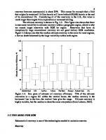
Figure 1-2. Box plots of ultimate oil recovery efficiency. 75% of the ultimate recoveries in a region fall within the vertical boxes; the median recovery is the horizontal line in the box; the vertical lines give the range. Ultimate recovery is highly variable, but the median is about the same everywhere (from Laherre, 2001).
1-2 THE NEED FOR EOR Enhanced oil recovery is one of the technologies needed to maintain reserves. Reserves
4
Reserves are petroleum (crude and condensate) recoverable from known reservoirs under prevailing economics and technology. They are given by the following material balance equation:
⎛ Production ⎞ ⎛ Present ⎞ ⎛ Past ⎞ ⎛ Additions ⎞ ⎜ ⎟ ⎜ ⎟=⎜ ⎟+⎜ ⎟ − ⎜ from ⎟ reserves reserves to reserves ⎝ ⎠ ⎝ ⎠ ⎝ ⎠ ⎜ reserves ⎟ ⎝ ⎠ There are actually several categories of reservoirs (proven, etc.) which distinctions are very important to economic evaluation (Rose, 2001; Cronquist, 2001). Clearly, reserves can change with time because the last two terms on the right do change with time. It is in the best interests of producers to maintain reserves constant with time, or even to have them increase. Adding to Reserves
The four categories of adding to reserves are 1. 2. 3. 4.
Discovering new fields Discovering new reservoirs Extending reservoirs in known fields Redefining reserves because of changes in economics of extraction technology
We discuss category 4 in the remainder of this text. Here we substantiate its importance by briefly discussing categories 1 to 3. Reserves in categories 1 to 3 are added through drilling, historically the most important way to add reserves. Given the 2% annual increase in world-wide consumption and the already large consumption rate, it has become evident that reserves can be maintained constant only by discovering large reservoirs. But the discovery rate of large fields is declining. More importantly, the discovery rate no longer depends strongly on the drilling rate. Equally important, drilling requires a substantial capital investment even after a field is discovered. By contrast, the majority of the capital investment for EOR has already been made (if previous wells can be used). The location of the target field is known (no need to explore), and targets tend to be close to existing markets. Enhanced oil recovery is actually a competitor with conventional oil recovery because most producers have assets or access to assets in all of the Fig. 1-1 categories. The competition then is joined largely on the basis of economics in addition to reserve replacement. At the present, many EOR technologies are competitive with drilling-based reserve additions. The key to economic competitiveness is how much oil can be recovered with EOR, a topic to which we next turn.
5
1-3 INCREMENTAL OIL Defintion
A universal technical measure of the success of an EOR project is the amount of incremental oil recovered. Figure 1-3 defines incremental oil. Imagine a field, reservoir, or well whose oil rate is declining as from A to B. At B, an EOR project is initiated and, if successful, the rate should show a deviation from the projected decline at some time after B. Incremental oil is the difference between what was actually recovered, B to D, and what would have been recovered had the process not been initiated, B to C. Since areas under rate-time curves are amounts, this is the shaded region in Fig. 1-3.
Figure 1-3. Incremental oil recovery from typical EOR response (from Prats, 1982)
6
As simple as the concept in Fig. 1-3 is, EOR is difficult to determine in practice. There are several reasons for this. 1. Combined (comingled) production from EOR and nonEOR wells. Such production makes it difficult to allocate the EOR-produced oil to the EOR project. Comingling occurs when, as is usually the case, the EOR project is phased into a field undergoing other types of recovery. 2. Oil from other sources. Usually the EOR project has experienced substantial well cleanup or other improvements before startup. The oil produced as a result of such treatment is not easily differentiated from the EOR oil. 3. Inaccurate estimate of hypothetical decline. The curve from B to C in Fig. 13 must be accurately estimated. But since it did not occur, there is no way of assessing this accuracy. Ways to infer incremental oil recovery from production data range from highly sophisticated numerical models to graphical procedures. One of the latter, based on decine curve analysis, is covered in the next section. Estimating Incremental Oil Recovery Through Decline Curves
Decline curve analysis can be applied to virtually any hydrocarbon production operation. The following is an abstraction of the practice as it applies to EOR. See Walsh and Lake (2003) for more discussion. The objective is to derive relations between oil rate and time, and then between cumulative production and rate. The oil rate q changes with time t in a manner that defines a decline rate D according to
1 dq = −D q dt
1.3-1
The rate has units of (or [=]) amount or volume per time and D [=]1/time. Time is in units of days, months, or even years consistent with the units of q. D itself can be a function of rate, but we take it to be constant. Integrating Eq. 1.3-1 gives
q = qi e− Dt
1.3-2
where qi is the initial rate or q evaluated at t = 0. Equation 1.3-2 suggests a semilogarithmic relationship between rate and time as illustrated in Fig. 1-3. Exponential decline is the most common type of analysis employed.
7
log (q)
qi -D Slope = 2.303 Decline period begins q EL
Life t
0 Figure 1-3. Schematic of exponential decline on a rate-time plot.
Figure 1-3 schematically illustrates a set of data (points) which begin an exponential decline at the ninth point where, by definition t = 0. The solid line represents the fit of the decline curve model to the data points. qi is the rate given by the model at t=0, not necessarily the measured rate at this point. The slope of the model is the negative of the decline rate divided by 2.303, since standard semilog graphs are plots of base 10 rather than natural logarithms. Because the model is a straight line, it can be extrapolated to some future rate. If we let qEL designate the economically limiting rate (simply the economic limit) of the project under consideration, then where the model extrapolation attains qEL is an estimate of the project’s (of well’s, etc.) economic life. The economic limit is a nominal measure of the rate at which the revenues become equal to operating expenses plus overhead. qEL can vary from a fraction to a few hundred barrels per day depending on the operating conditions. It is also a function of the prevailing economics: as oil price increases, qEL decreases, an important factor in reserve considerations. The rate-time analysis is useful, but the rate-cumulative curve is more helpful. The cumulative oil produced is given by
Np =
∫ qdξ
ξ =t
ξ =0
.
8
The definition in this equation is general and will be employed throughout the text, but especially in Chap. 2. To derive a rate -cumulative expression, insert Eq. 1.3-1, integrate, and identify the resulting terms with (again) Eq. 1.3-1. This gives
q = qi − DN p
1.3-3
Equation 1.3-3 says that a plot of oil rate versus cumulative production should be a straight line on linear coordinates. Figure 1-4 illustrates.
q
qi Slope = -D
Mobile oil
q EL
Recoverable oil 0
Np
Figure 1-4. Schematic of exponential decline on a rate-cumulative plot. You should note that the cumulative oil points being plotted on the horizontal axis of this figure are from the oil rate data, not the decline curve. It this were not so, there would be no additional information in the rate-cumulative plot. Calculating Np normally requires a numerical integration with something like the trapezoid rule. Using model Eqs 1.3-2 and 1.3-3 to interpret a set of data as illustrated in Figs. 1-3 and 1-4 is the essence of reservoir engineering practice, namely 1. Develop a model as we have done to arrive at Eqs. 1.3-2 and 1.3-3. Often the model equations are far more complicated than these, but the method is the same regardless of the model. 2. Fit the model to the data. Remember that the points in Figs. 1-3 and 1-4 are data. The lines are the model. 3. With the model fit to the data (the model is now calibrated), extrapolate the model to make predictions.
9
At the onset of the decline period, the data again start to follow a straight line through which can be fit a linear model. In effect, what has occurred with this plot is that we have replaced time on Fig. 1-3 with cumulative oil produced on Fig. 1-4, but there is one very important distinction: both axes in Fig. 1-4 are now linear. This has three important consequences. 1. 2. 3.
The slope of the model is now –D since no correction for log scales is required. The origin of the model can be shifted in either direction by simple additions. The rate can now be extrapolated to zero.
Point 2 simply means that we can plot the cumulative oil produced for all periods prior to the decline curve period (or for previous decline curve periods) on the same rate-cumulative plot. Point 3 means that we can extrapolate the model to find the total mobile oil (when the rate is zero) rather than just the recoverable oil (when the rate is at the economic limit). Rate-cumulative plots are simple yet informative tools for interpreting EOR processes because they allow estimates of incremental oil recovery (IOR) by distinguishing between recoverable and mobile oil. We illustrate how this comes about through some idealized cases. Figure 1-5 shows a rate-cumulative plot for a project having an exponential decline just prior to and immediately after the initiation of an EOR process.
q
q EL
Project begins
IOR Incremental mobile oil
Np
10
Figure 1-5. Schematic of exponential decline curve behavior on a rate-cumulative plot. The EOR project produces both incremental oil (IOR), and increases the mobile oil. The pre- and post-EOR decline rates are the same. We have replaced the data points with the models only for ease of presentation. Placing both periods on the same horizontal axis is permissible because of the scaling arguments mentioned above. In this case, the EOR process did not accelerate the production because the decline rates in both periods are the same; however, the process did increase the amount of mobile oil, which in turn caused some incremental oil production. In this case, the incremental recovery and mobile oil are the same. Such idealized behavior would be characteristic of thermal, micellar-polymer, and solvent processes.
q
IOR q EL Np Project begins Figure 1-6. Schematic of exponential decline curve behavior on a rate-cumulative plot. The EOR project produces incremental oil at the indicated economic limit but does not increase the mobile oil. Figure 1-6 shows another extreme where production is only accelerated, the pre- and post-EOR decline rates being different. Now the curves extrapolate to a common mobile oil but with still a nonzero IOR. We expect correctly that processes that behave as this will produce less oil than ones that increase mobile oil, but they can still be profitable, particularly, if the agent used to bring about this result is inexpensive. Processes that ideally behave in this manner are polymer floods and polymer gel processes, which do not affect residual oil saturation. Acceleration processes are especially sensitive to the economic limit; large economic limits imply large IOR.
11
Example 1-1. Estimating incremental oil recovery.
Monthly Rate, M std. m3/month
Sometimes estimating IOR can be fairly subtle as this example illustrates. Figure 1-7 shows a portion of rate-cumulative data from a field that started EOR about half-way through the total production shown. 0.20
0.15
Pre EOR 0.10
Post EOR
0.05
qEL 0.00 0.0
1.0
2.0 3.0 4.0 5.0 Cumulative Oil Produced, M std. m3 Figure 1-7. Rate (vertical axis) - cumulative (horizontal axis) plot for a field undergoing and EOR process.
a. Identify the pre- and post-EOR decline periods. The pre-EOR decline ends at about 2.5 M std. m3 of oil produced, at which time the post-EOR period begins. This point does not necessarily coincide with the start of the EOR process. The start cannot be inferred from the rate-cumulative plot. b. Calculate the decline rates ([=] mo-1) for both periods. Both decline periods are fitted by the straight lines indicated. The fitting is done through standard means; the difficulty is always identifying when the periods start and end. For the pre-EOR decline,
⎛ M std.m3 0.11 0.18 − ( ) ⎜ month D = −⎜ 3 ⎜ ( 2.55 − 0 ) M std.m ⎜ ⎝ and for the post-EOR decline,
⎞ ⎟ −1 ⎟ = 0.027 month ⎟ ⎟ ⎠
⎛ M std.m ⎜ ( 0.09 − 0.11) month D = −⎜ 3 ⎜ ( 4 − 2.55 ) M std.m ⎜ ⎝
3
⎞ ⎟ −1 ⎟ = 0.0137 month ⎟ ⎟ ⎠
12
The EOR project has about halved the decline rate even though there is no increase in rate. c. Estimate the IOR ([=] M std. m3) for this project at the indicated economic limit. The oil to be recovered by continued operations is 4.7 M std. m3. That from EOR is (by extrapolation) 7 M std. m3 for an incremental oil recovery of 2.3 M std. m3.
1-4 CATEGORY COMPARISONS Comparative Performances
Most of this text covers the details of EOR processes. At this point, we compare performances of the three basic EOR processes and introduce some issues to be discussed later in the form of screening guides. The performance is represented as typical oil recoveries (incremental oil expressed as a percent of original oil in place) and by various utilization factors. Both are based on actual experience. Utilization factors express the amount of an EOR agent required to produce a barrel of incremental oil. They are a rough measure of process profitability. Table 1-1 shows sensitivity to high salinities is common to all chemical flooding EOR. Total dissolved solids should be less than 100,000 g/m3, and hardness should be less than 2,000 g/m3. Chemical agents are also susceptible to loss through rock–fluid interactions. Maintaining adequate injectivity is a persistent issue with chemical methods. Historical oil recoveries have ranged from small to moderately large. Chemical utilization factors have meaning only when compared to the costs of the individual agents; polymer, for example, is usually three to four times as expensive (per unit mass) as surfactants. TABLE 1-1 CHEMICAL EOR PROCESSES Process Polymer
Micellar polymer
Recovery mechanism Improves volumetric sweep by mobility reduction Same as polymer plus reduces capillary forces
Issues Injectivity Stability High salinity Same as polymer plus chemical availability, retention, and high salinity
Typical recovery (%)
Typical agent utilization*
5
0.3–0.5 lb polymer per bbl oil produced
15
15–25 lb surfactant per bbl oil produced
13 Alkaline polymer
Same as micellar polymer plus oil solubilization and wettability alteration
Same as micellar polymer plus oil composition
5
35–45 lb chemical per bbl oil produced
*1 lb/bbl ≅ 2.86 kg/m3
Table 1-2 shows a similar comparison for thermal processes. Recoveries are generally higher for these processes than for the chemical methods. Again, the issues are similar within a given category, centering on heat losses, override, and air pollution. Air pollution occurs because steam is usually generated by burning a
TABLE 1-2 THERMAL EOR PROCESSES Process Steam (drive and stimulation) In situ combustion
Recovery mechanism
Issues
Reduces oil viscosity Vaporization of light ends Same as steam plus cracking
*1 Mscf/stb ≅ 178std. m gas/std. m oil 3
Depth Heat losses Override Pollution Same as steam plus control of combustion
Typical recovery (%)
Typical agent utilization*
50–65
0.5 bbl oil consumed per bbl oil produced
10–15
10 Mscf air per bbl oil produced*
3
portion of the resident oil. If this burning occurs on the surface, the emission products contribute to air pollution; if the burning is in situ, production wells can be a source of pollutants. Table 1-3 compares solvent flooding processes. Only two groups are in this category, corresponding to whether or not the solvent develops miscibility with the oil. Oil recoveries are generally lower than for micellar-polymer recoveries. The solvent utilization factors as well as the relatively low cost of the solvents have brought these processes, particularly carbon dioxide flooding, to commercial application. The distinction between a miscible and an immiscible process is slight. TABLE 1-3 SOLVENT EOR METHODS Process Immiscible
Miscible
Recovery mechanism Reduces oil viscosity Oil swelling Solution gas Same as immiscible plus development of miscible
Issues
Typical recovery (%)
Typical agent utilization*
Stability Override Supply
5–15
10 Mscf solvent per bbl oil produced
Same as immiscible
5–10
10 Mscf solvent per bbl oil produced
14 displacement *1 Mscf/stb ≅ 178 std. m solvent/ std. m oil 3
3
Screening Guides
Many of the issues in Tables 1-1 through 1-3 can be better illustrated by giving quantitative limits. These screening guides can also serve as a first approximate for when a process would apply to a given reservoir. Table 1-4 gives screening guides of EOR processes in terms of oil and reservoir properties. TABLE 1-4. SUMMARY OF SCREENING CRITERIA FOR EOR METHODS (adapted from Taber et al., 1997). TABLE 3: SUMMARY OF SCREENING CRITERIA FOR EOR METHODS Oil Properties Reservoir Characteristics Net Average Reservoir Initial Oil Saturation Formation Thickness Permeability Gravity Viscosity (%PV) Type (m) (md) EOR Method (ºAPI) mPa-s Compostion Solvent Methods Nitrogen and Large % of flue gas >35 40 NC NC NC C1 to C7 Hydrocarbon
>23
22
12
20
15
10-150
NC
8 to 13.5
Depth (m)
>1800
>30
NC
NC
NC
>1250
>20
NC
NC
NC
>750
>35 NC Chemical Methods
NC
NC
>640
NC
>10
10
50
>3
>50
40
>6
>200
50 preferred Thermal Methods >35
These should be regarded as rough guidelines, not as hard limits because special circumstances (economics, gas supply for example) can extend the applications. The limits have a physical base as we will see. For example, the restriction of thermal processes to relatively shallow reservoirs is because of potential heat losses through lengthy wellbores. The restriction on many of the processes to light crudes comes about because of sweep efficiency considerations; displacing viscous
15
oil is difficult because of the propensity for a displacing agent to channel through the fluid being recovered. Finally, you should realize that some of categorizations in Table 1-7 are fairly coarse. Steam methods, in particular, have additional divisions into steam soak, steam drive, and gravity drainage methods. There are likewise several variations of combustion and chemical methods.
1-5 UNITS AND NOTATION SI Units
The basic set of units in the text is the System International (SI) system. We cannot be entirely rigorous about SI units because many figures and tables has been developed in more traditional units. It is impractical to convert these; therefore, we give a list of the more important conversions in Table 1-7 and some helpful pointers in this section. TABLE 1-5 AN ABRIDGED SI UNITS GUIDE (adapted from Campbell et al.., 1977) SI base quantities and units Base quantity or dimension
SI unit symbol
SPE dimensions symbol
SI unit
Length Mass Time Thermodynamic temperature Amount of substance
Meter Kilogram Second Kelvin Mole*
m kg S K mol
L m t T
*When the mole is used, the elementary entities must be specified; they may be atoms, molecules, ions, electrons, other particles, or specified groups of such particles in petroleum work. The terms kilogram mole, pound mole, and so on are often erroneously shortened to mole. Some common SI derived units SI unit symbol Quantity
Unit
Acceleration Area Density Energy, work Force Pressure Velocity Viscosity, dynamic Viscosity, kinematic Volume
Meter per second squared Square meter Kilogram per cubic meter Joule Newton Pascal Meter per second Pascal-second Square meter per second Cubic meter
–– –– –– J N Pa –– –– –– ––
Selected conversion factors
Formula m/s2 m2 kg/m3 N·m kg · m/s2 N/m2 m/s Pa · s m2/s m3
16 To convert from 2
Acre (U.S. survey) Acres Atmosphere (standard) Bar Barrel (for petroleum 42 gal) Barrel British thermal unit (International Table) Darcy Day (mean solar) Dyne Gallon (U.S. liquid) Gram Hectare Mile (U.S. survey) Pound (lbm avoirdupois) Ton (short, 2000 lbm)
To
Multiply by
2
4.046 872 E+03 4.356 000 E+04 1.013 250 E+05 1.000 000 E+05 1.589 873 E–01 5.615 E+00 1.055 056 E+03 9.869 232 E–13 8.640 000 E+04 1.000 000 E–05 3.785 412 E–03 1.000 000 E–03 1.000 000 E+04 1.609 347 E+03 4.535 924 E–01 9.071 847 E+02
Meter (m ) Feet2 (ft2) Pascal (Pa) Pascal (Pa) Meter3 (m3) Feet3 (ft3) Joule (J) Meter2 (m2) Second (s) Newton (N) Meter3 (m3) Kilogram (kg) Meter2 (m2) Meter (m) Kilogram (kg) Kilogram (kg)
TABLE 1-5 CONTINUED Selected SI unit prefixes
Factor
SI prefix
1012 109 106 103 102 10 10–1 10–2 10–3 10–6 10–9
tera giga mega kilo hecto deka deci centi milli micro nano
SI prefix symbol (use roman type) T G M k H Da D c m
μ
N
Meaning (U.S.) One trillion times One billion times One million times One thousand times One hundred times Ten times One tenth of One hundredth of One thousandth of One millionth of One billionth of
Meaning outside US Billion Milliard
Milliardth
1. There are several cognates, quantities having the exact or approximate numerical value, between SI and practical units. The most useful for EOR are 1 cp 1 dyne/cm 1 Btu 1 Darcy 1 ppm
= 1 mPa-s = 1 mN/m ≅ 1 kJ ≅ 1 μm2 ≅ 1 g/m3
17
2. Use of the unit prefixes (lower part of Table 1-5) requires care. When a prefixed unit is exponentiated, the exponent applies to the prefix as well as the unit. Thus 1 km2 = 1(km)2 = 1(103 m)2 = 1 × 10⁶m2. We have already used this convention where 1 μm2 = 10–12 m2 ≅ 1 Darcy. 3. Two troublesome conversions are between pressure (147 psia ≅ 1 MPa) and temperature (1 K = 1.8 oR). Since neither the Fahrenheit nor the Celsius scale is absolute, an additional translation is required. °C = K – 273 and °F = °R – 460 The superscript ° is not used on the Kelvin scale.
4. The volume conversions are complicated by the interchangeable use of mass and standard volumes. Thus we have 0.159 m3 = 1 reservoir barrel, or bbl and 0.159 std. m3 = 1 standard barrel, or stb The standard cubic meter, std. m3, is not standard SI; it represents the amount of mass contained in one cubic meter evaluated at standard temperature and pressure. Consistency
Maintaining unit consistency is important in all exercises, and for this reason both units and numerical values should be carried in all calculations. This ensures that the unit conversions are done correctly and indicates if the calculation procedure itself is appropriate. In maintaining consistency, three steps are required. 1. Clear all unit prefixes. 2. Reduce all units to the most primitive level necessary. For many cases, this will mean reverting to the fundamental units given in Table 1-7. 3. After calculations are complete, reincorporate the unit prefixes so that the numerical value of the result is as close to 1 as possible. Many adopt the convention that only the prefixes representing multiples of 1,000 are used. Example 1-2. Converting from Darcy units.
18
Maintaining unit consistency in an equation is easy. For example, suppose we want to use the typical oilfield units in Darcy’s law: q in units of ([=]) bbl/day; k [=] md; A [=] ft2; p [=] psia; μ [=] cp; and x [=] ft. First we write Darcy’s law: q=
kA dp μ dx
This is elementary form of Darcy's law is valid for 1-D horizontal flow Darcy's law is self-consistent in so-called Darcy’s units; hence, a "units" balance for this equation is ⎛ q − cm3 ⎞ ( k − D ) ( A − cm ⎜ ⎟= s ⎠ ( μ − cp ) ⎝
2
) ⎛ dp − atm ⎞
⎜ ⎟ ⎝ dx − cm ⎠
where k-D means that the permeability k is in D or Darcys. The other units given in the equation are Darcy units. Note that the minus sign is unnecessary since we are dealing only with units. Next, we write this same equation into the units that we want , maintaining the unit consistency. That is, ⎫⎪ ⎧ 1 hr ⎫ ⎧ 1 hr ⎫ ⎧⎪ ( 30.48 )3 cm3 ⎫⎪ ⎬⎨ ⎬= ⎬⎨ ⎬⎨ ft 3 ⎪⎭ ⎩ 3600 s ⎭ ⎩ 3600 s ⎭ ⎪⎩ ⎪⎭ 2 2 ⎫ ⎧ ⎧ 1 D ⎫⎡ 2 ⎤ ⎪ ( 30.48 ) cm ⎪ ⎡ k − md ⎤ ⎨ A − ft ⎨ ⎬ ⎬ ⎣ ⎦ 1000 md ⎣ ⎦ ft 2 ⎩ ⎭ ⎩⎪ ⎭⎪ × cp − μ [ ]
⎡ q − bbl ⎢ ⎢⎣ day
⎤ ⎧⎪ 1 day ⎥⎨ ⎥⎦ ⎪⎩ 24 hrs
⎡ dp − psia ⎢ ⎣⎢ dx − ft
⎤ ⎧⎪ 1 atm ⎥⎨ ⎦⎥ ⎩⎪14.70 psia
⎫⎪ ⎧⎪ 1 ft ⎫⎪ ⎬ ⎬⎨ ⎭⎪ ⎩⎪ 30.48 cm ⎭⎪
Although each term is written in the units we wish, each term reduces to the units of the original equation. This is illustrated in the above equation by canceling all similar units. By writing the above equation and checking the unit consistency, you are assured of making no errors. The equation also introduces the practice of putting ratios that are conversion factors in {}. The last step is to rewrite the equation by grouping all numerical constants and calculating the appropriate constant that must appear before the right side of the equation. Darcy’s law becomes ⎫⎪ ( k − md ) ( A − ft 2 ) ⎛ dp − psia ⎞ ( 24 )( 3600 ) ( 30.482 ) ⎛ q − bbl ⎞ ⎧⎪ = ⎬ ⎜ ⎟ ⎨ ⎜ ⎟ 3 ( μ − cp ) ⎝ day ⎠ ⎪⎩ ( 5.615 ) ( 30.48 ) (1000 )(14.70 )( 30.48 ) ⎪⎭ ⎝ dx − ft ⎠
or
( k − md ) ( A − ft ⎛ q − bbl ⎞ ⎪⎧ −3 ⎜ ⎟ = ⎨1.127 × 10 ( μ − cp ) ⎝ day ⎠ ⎪⎩
2
) ⎪⎫ ⎛ dp − psia ⎞ .
19
⎬⎜ ⎟ ⎪⎭ ⎝ dx − ft ⎠
The constant, which is accurate to four digits, is the well-known constant for Darcy’s law written in oil field units. The above equation also illustrates a common practice in petroleum engineering--in our opinion bad and used sparingly in this text--of including a conversion factor directly in an equation. The important point the above procedure is that there is no guessing involved. Any equation can be converted to the desired units as long as the procedure is followed exactly. Naming Conventions
The diversity of EOR makes it possible to assign symbols to components without some duplication or undue complication. In the hope of minimizing the latter by adding a little of the former, Table 1-8 gives the naming conventions of phases and components used throughout this text. The nomenclature section defines other symbols. Phase always carry the subscript j, which occupies the second position in a doubly subscripted quantity. j = 1 is always a water-rich, or the aqueous phase, thus freeing up the symbol w for wetting (and nw for nonwetting). The subscript s designates the solid, nonflowing phase. A subscript i, occurring in the first position, indicates the component. Singly subscripted quantities indicate components. In general, i = 1 is always water; i = 2 is oil or hydrocarbon; and i = 3 refers to a displacing component, whether surfactant or light hydrocarbon. Component indices greater than 3 are used exclusively in Chaps. 8–10, the chemical flooding part of the text.
1-6 SUMMARY No summary can do justice to what is a large, diverse, continuously changing, and complicated technology. The Oil and Gas Journal has provided an excellent service in documenting the progress of EOR, and you should consult those surveys for up to date information. The fundamentals of the processes change more slowly than the applications, and it is to these fundamentals that the remainder of the text is devoted.
20 TABLE 1-4 NAMING CONVENTIONS FOR PHASES AND COMPONENTS Phases j
Text locations
Identity
1 2 3
Water-rich or aqueous Oil-rich or oleic Gas-rich, gaseous or light hydrocarbon Microemulsion Solid Wetting Nonwetting
s w nw
Throughout Throughout Secs. 5-6 and 7-7 Chap. 9 Chaps 2, 3, and 8 to10 Throughout Throughout
Components i
Identity
1 2
Water Oil or intermediate hydrocarbon Gas Light hydrocarbon Surfactant Polymer Anions Divalents Divalent-surfactant component Monovalents
3
4 5 6 7 8
Text locations Throughout Throughout Sec. 5-6 Sec. 7-6 Chap. 9 Chaps. 8 and 9 Secs. 3-4 and 9-5 Secs. 3-4 and 9-5 Sec. 9-6 Secs. 3-4 and 9-5
EXERCISES 1A. Determining Incremental Oil Production. The easiest way to estimate incremental oil recovery IOR is through decline curve analysis, which is the subject of this exercise. The oil rate and cumulative oil produced versus time data for the Sage Spring Creek Unit A field is shown below (Mack and Warren, 1984) Date 1/76 7/76 1/77 7/77 1/78 7/78 1/79 7/79 1/80 7/80 1/81 7/81
Oil Rate std. m3/day 274.0 258.1 231.0 213.5 191.2 175.2 (Start Polymer) 159.3 175.2 167.3 159.3 159.3 157.7
21 1/82 7/82 1/83 7/83 1/84 7/84 1/85 7/85 1/86 7/86 1/87 7/87
151.3 148.2 141.8 132.2 111.5 106.7 95.6 87.6 81.2 74.9 70.1 65.3
In 7/78 the ongoing waterflood was replaced with a polymer flood. (Actually, there was a polymer gel treatment conducted in 1984, but we neglect it here.) The economic limit is 50 std. m3/D in this field. (a) Plot the oil rate versus cumulative oil produced on linear axes. The oil rate axis should extend to q = 0. (b) Extrapolate the straight line portion of the data to determine the ultimate economic oil to be recovered from the field and the total mobile oil, both in Mstd. m3, for both the water and the polymer flood. Determine the incremental economic oil (IOR) and the incremental mobile oil caused by the polymer flood. (c) Determine the decline rates appropriate for the waterflood and polymer flood declines. (d) Use the decline rates in step c to determine the economic life of the polymer flood. Also determine what the economic life would have been if there were no polymer flood. 1B. Maintaining Unit Conversions (Darcy’s Law). There are several unit systems used throughout the world and you should be able to convert equations easily between systems. Convert Darcy’s Law for 1-D horizontal flow,
q=
kA dp μ dx
from Darcy units to the unit system where q [=] m3/day, k [=] md, A[=] m2, μ [=] cp, p [=] kgf/cm2, and x [=] meters. This is the reverse of that in Example 1-2. 1C. Maintaining Unit Conversions (Dimensionless Time). A dimensionless time often appears in petroleum engineering. One definition for dimensionless time used in radial flow is
tD =
φμ ct rw2 where the equation is written in Darcy units ( rw [=] cm, φ is dimensionless, ct [=] of atm-1). Convert kt
the equation for dimensionless time from Darcy units to (a) oil-field units. (b) SI units. This means write the equation with a conversion factor in it so that quantities with the indicated units may be substituted directly.
22 1D. Maintaining Unit Conversions (Dimensionless Pressure). A dimensionless pressure often appears in petroleum engineering. One definition for dimensionless pressure is
pD =
2π khΔp qμ
where the equation is written in Darcy units (h in cm, Δp in atm). dimensionless pressure from Darcy units to (a) oil-field units. (b) SI units.
Convert the equation for
1
2 Basic Eq uatio ns fo r Fluid Flo w in Pe rm e ab le Me dia Successful enhanced oil recovery requires knowledge of equal parts chemistry, physics, geology and engineering. Each of these enters our understanding through elements of the equations that describe flow through permeable media. Each EOR process involves at least one flowing phase that may contain several components. Moreover, because of varying temperature, pressure, and composition, these components may mix completely in some regions of the flow domain, causing the disappearance of a phase in those regions. Atmospheric pollution and chemical and nuclear waste storage lead to similar problems. This chapter gives the equations that describe multiphase, multicomponent fluid flow through permeable media based on conservation laws and linear constitutive theory. Initially, we strive for the most generality possible by considering the transport of each component in each phase. Then, special cases are obtained from the general equations by making additional assumptions. The approach in arriving at the special equations is as important as the equations themselves, since it will help to understand the specific assumptions--and the limitations--that are being made for a particular application. The formulation initially contains two fundamentally different forms for the general equations: overall compositional balances, and the phase conservation equations. The overall compositional balances are useful for modeling how components are transported through permeable media in local thermodynamic equilibrium. The phase conservation equations are useful for modeling finite mass transfer among phases. Figure 2-1 illustrates the relationships among several equations developed as special cases in this chapter. From the overall compositional balances, the list of special cases includes the multicomponent, single-phase flow equations (Bear, 1972) and the three-phase,
2
multicomponent equations (Crichlow, 1977; Peaceman, 1977; Coats, 1980). In addition, others (Todd and Chase, 1979; Fleming et al., 1981; Larson, 1979) have presented multicomponent, multiphase formulations for flow in permeable media but with assumptions such as ideal mixing or incompressible fluids. Many of these assumptions must be made before the equations are solved, but we try to keep the formulation as general as possible as long as possible.
Figure 2-1 Flow diagram showing the relationships among the fundamental equations and selected special cases. There are NC components and NP phases.
2-1 MASS CONSERVATION This section describes the conceptual nature of multiphase, multicomponent flows through permeable media and the mathematical formulation of the conservation equations.
3
The four most important mechanisms causing transport of chemical components in naturally occurring permeable media are viscous forces, gravity forces, dispersion (diffusion), and capillary forces. The driving forces for the first three are pressure, density, and concentration gradients, respectively. Capillary or surface forces are caused by high-curvature boundaries between the various homogeneous phases. This curvature is the result of such phases being constrained by the pore walls of the permeable medium. Capillary forces imply differing pressures in each homogeneous fluid phase so that the driving force for capillary pressure is, like viscous forces, pressure differences. The ratios of these forces are often given as dimensionless groups and given particular names. For example, the ratio of gravity to capillary forces is the Bond number. When capillary forces are small compared to gravity forces, the Bond number is large and the process (or displacement) is said to be gravity dominated. The ratio of viscous to capillary forces is the capillary number, a quantity that will figure prominently through this text. The ratio of gravity to viscous forces is the gravity or buoyancy number. The magnitude of these and other dimensionless groups help in comparing or scaling one process to another; they will appear at various points throughout this text. The Continuum Assumption Transport of chemical components in multiple homogeneous phases occurs because of the above forces, the flow being restricted to the highly irregular flow channels within the permeable medium. The conservation equations for each component apply at each point in the medium, including the solid phase. In principle, given constitutive relations, reaction rates, and boundary conditions, it is possible to formulate a mathematical system for all flow channels in the medium. But the phase boundaries in such are extremely tortuous and their locations are unknown; hence, we cannot solve component conservation equations in individual channels except for only the simplest microscopic permeable media geometry. The practical way of avoiding this difficulty is to apply a continuum definition to the flow so that a point within a permeable medium is associated with a representative elementary volume (REV), a volume that is large with respect to the pore dimensions of the solid phase but small compared to the dimensions of the permeable medium. The REV is defined as a volume below which local fluctuations in some primary property of the permeable medium, usually the porosity, become large (Bear, 1972). A volume-averaged form of the component conservation equations applies for each REV within the now-continuous domain of the macroscopic permeable medium. (Volume averaging is actually a formal process; see Bear, 1972; Gray, 1975; and Quintard and Whitaker, 1988.) The volume-averaged component conservation equations are identical to the conservation equations outside a permeable medium except for altered definitions for the accumulation, flux, and source terms. These definitions now include permeable media porosity, permeability, tortuosity, and dispersivity, all made locally smooth because of the definition of the
4
REV. Approximating the locally discontinuous permeable medium with a locally smooth one is called the continuum assumption. A good way to understand the REV scale is to consider a microscopic view of pores and grains within a medium. Figure 2-2 illustrates a cube of small volume placed within a permeable medium. The porosity in the cube is defined as the pore volume within the cube divided by the bulk volume of the cube. If the cube volume is infinitesimally small, the porosity will be either 1.0 or 0.0 depending on whether it is initially located inside a grain or a pore. We now let the cube increase from its original size. As the cube volume increases, the porosity changes in an erratic fashion as more and more grains and pores pass inside the cube (see Figure 2-3).
Figure 2-2 Illustration of microscopic cube placed within a permeable medium. The cube is initially within a pore so that its porosity is 1.0. As the cube volume increases, it takes in more grains so that its porosity decreases. As the cube volume increases sufficiently, the porosity approaches a constant value representative of the porous medium. This is the porosity at the REV scale, which defines the onset of the permeable medium domain. Above the REV size, the cube porosity remains constant within the domain of the permeable medium. As the cube volume increases further, however, the cube porosity is affected by layering and other heterogeneities. The formation is homogeneous if the porosity remains fixed as the REV-sized cube is moved to any location within the permeable medium. A heterogeneous formation is one in which the porosity (or any other petrophysical property) varies from one spatial location to another when measured at the REV scale.
5
Figure 2-3 Idealization of the microscopic and permeable medium domains. The REV size separates these two domains. Rather than beginning with the nonpermeable media flow equations, and then volume-averaging over the REV, we invoke the continuum assumption at the outset and derive the mass conservation on this basis. This approach skips over many of the physical insights obtained from volume averaging, but it is far more direct. Mass Balance for a Component in a Phase Consider an arbitrary, fixed volume V embedded within a permeable medium through which is flowing an arbitrary number of chemical components and phases. You must constantly be aware of the distinction between components and phases in this discussion. (This can be a source of confusion because under some circumstances phases and components are the same.) A component is any identifiable chemical entity. Components can be pure substances such as methane, a cation, or even combinations of elements. See Lake et al., 2002 for more discussion. A phase is a physically distinct part of a region in space that is bound by interfaces with macroscopic physical properties, such as density and viscosity. A phase can consist of many components. There are up to i = 1, . . . , NC components, and up to j = 1, . . . , NP phases. The "up to" is because both components and phases can vanish in regions of the flow domain. The conservation laws are written over a control volume V that is greater than or equal to the REV but smaller than or equal to the permeable medium dimensions. Except for some restrictions on the connectivity of the surface, V can be quite general. As Fig. 2-4 (a) shows, the surface area A
6
Figure 2-4 Geometries for conservation law derivations.
of V is made up of elemental surface areas ΔA from the center of which is pointing a unit outward normal vector n. The sum of all the surface elements ΔA is the total surface area A of V. This sum of all the ΔA becomes the total surface area A as the largest ΔA approaches zero. The conservation equation for each component in each phase in volume V is 7
Rate of Net rate of ⎧ ⎫ ⎧ Net rate of i ⎫ ⎧ ⎫ ⎪ ⎪ ⎪ ⎪ ⎪ ⎪ in phase j ⎨accumulation of i ⎬ = ⎨ ⎬ + ⎨ generation of i ⎬ ⎪ in phase j in V ⎪ ⎪ transported into V ⎪ ⎪in phase j inside V ⎪ ⎩ ⎭ ⎩ ⎭ ⎩ ⎭ i = 1, . . . , N C j = 1, . . . , N P .
(2.1-1)
There are a total of N C N P equations represented by Eq. (2.1-1). This equation is the rate form of the conservation equation; an equivalent form based on cumulative flow follows from integrating Eq. (2.1-1) with respect to time (see Sec. 2-5). From left to right in Eq. (2.1-1) are the accumulation, flux, and source terms, respectively. A component can be transported within a phase by convection or hydrodynamic dispersion. The generation of a component in a given phase can be the result of chemical or biological reactions, injection or production of a component into or from wells, or mass transfer from one phase to the next owing to phase changes. These physical processes are discussed in more detail in Sec. 2.2. The first term on the right side of Eq. (2.1-1) can be written as Rate of i Rate of i ⎧ Net rate of i ⎫ ⎧ ⎫ ⎧ ⎫ ⎪ ⎪ ⎪ ⎪ ⎪ ⎪ in phase in phase in phase j j j = − ⎨ ⎬ ⎨ ⎬ ⎨ ⎬ ⎪ transported into V ⎪ ⎪ transported into V ⎪ ⎪ transported from V ⎪ ⎩ ⎭ ⎩ ⎭ ⎩ ⎭ i = 1, . . . , N C
j = 1, . . . , N P .
(2.1-2)
We give mathematical form to each term in the following paragraphs. The accumulation term for component i in phase j is Rate of ⎧ ⎪ ⎨accumulation of i ⎪ in phase j in V ⎩
⎫ ⎧Total mass of ⎫ ⎪ d ⎪ ⎪ d ⎬ = ⎨ i in phase j ⎬ = ⎪ dt ⎪ ⎪ dt in V ⎭ ⎩ ⎭
{∫ W dV } V
ij
(2.1-3)
where Wij is the component concentration in units of mass of i in phase j per unit bulk volume. The units of Eq. (2.1-3) are mass per time. The volume integral represents the sum of infinitesimal volume elements in V weighted by the concentration. Since V is stationary, d dt
{∫ W dV } = ∫ dWdt dV . ij
V
ij
V
(2.1-4)
8
This entire development may be repeated with a time-varying V with the same result (Slattery, 1972). The net flux term follows from considering the rate of transport across a single surface element into V as shown in Fig. 2-4(b). Let N ij be the flux vector of component i in phase j evaluated at the center of ΔA in units of mass of i in phase j per surface area-time. N ij consists of components normal and tangential to n. However, only the normal component n i N ij is crossing ΔA, and the rate of transport across ΔA is ⎧ Rate of transport ⎫ ⎪ ⎪ ⎨ of i in phase j ⎬ = −n i N ij ΔA ⎪across ΔA into V ⎪ ⎩ ⎭
(2.1-5)
The minus sign arises because n and N ij are in opposing directions for transport across ΔA into V ( n i N ij < 0 ), and this term must be positive from Eq. (2.1-1). An inherent assumption in Eq. (2.1-5) is that the flux across ΔA is uniform, an assumption that is valid as ΔA approaches zero. (Always remember that the continuum assumption assures continuity in taking limits.) The summation of infinitesimal surface elements yields ⎧ Net rate of i ⎫ ⎪ ⎪ in phase j ⎨ ⎬ = − ∫A n i N ij dA . ⎪ transported into V ⎪ ⎩ ⎭
(2.1-6)
Since the surface integral is over the entire surface of V, both flow into and from V are included in Eq. (2.1-6). The net rate of generation of i in phase j inside V is Net rate of ⎧ ⎫ ⎪ ⎪ ⎨ generation of i ⎬ = ∫V Rij dV + ∫V rmij dV , ⎪in phase j inside V ⎪ ⎩ ⎭
(2.1-7)
where Rij is the rate of mass generation in units of mass of i in phase j per bulk volume-time. This term can account for both generation (Rij >0) and destruction (Rij Tc) though it would seem that defining it to be the region to the right and above the critical point (T > Tc and P > Pc) would be more consistent with the behavior of mixtures. The behavior shown in Fig. 4-1 for a pure component is qualitatively correct though less detailed than what can be observed. There can exist, in fact, more than one triple point where solid–solid–liquid equilibria are observed. Water is a familiar example of a pure component that has this behavior. Remarkably, observations of multiple gas phases for pure components have also been reported (Schneider, 1970). Such nuances are not the concern of this text, which emphasizes gas–liquid and liquid–liquid equilibria. In fact, in all further discussions of phase behavior, we ignore triple points and solid-phase equilibria. Even with these things omitted, the P-T diagrams in this chapter are only qualitatively correct since the critical point and the vapor pressure curve vary greatly among components. Figure 7-2 shows some quantitative comparisons. Critical phenomena do play an important role in the properties of EOR fluids. If a laboratory pressure cell contains a pure component on its vapor pressure curve
97
(Fig. 4-1), the pure component exists in two phases (gas and liquid) at this point, and the cell pressure is Pv. Thus the cell will contain two regions of distinctly different properties. One of these properties being the density, one phase will segregate to the top of the cell, and the other to the bottom. The phases will most likely have different light transmittance properties so that one phase, usually the upper or light phase, will be clear, whereas the other phase, the lower or heavy phase, will be translucent or dark. We can simultaneously adjust the heat transferred to the cell so that the relative volumes of each phase remain constant, and both the temperature and pressure of the cell increase if the fluid remains on the vapor pressure curve. For most of the travel from the original point to the critical point, no change occurs in the condition of the material in the cell. But the properties of the individual phases are approaching each other. In some region near the critical point, the light phase would become darker, and the heavy phase lighter. Very near the critical point, the interface between the phases, which was sharp at the original temperature and pressure, will become blurred and may even appear to take on a finite thickness. At the critical point, these trends will continue until there is no longer a distinction between phases–that is, two phases have ceased to exist. If we continue on an extension of the vapor pressure curve, there would be a single-fluid phase and gradual changes in properties. Pressure–Molar-Volume Diagram
A way of representing how the discontinuity in intensive properties between phases vanishes at the critical point is the pressure–molar-volume diagram. Figure 4-2 compares such a diagram with the corresponding P-T diagram. Both schematic plots show isotherms, changes in pressure from a high pressure P1 to a lower pressure P2, at four constant temperatures, T1 through T4. At conditions (P, T)1, the pure component is a single-phase liquid. As pressure decreases at constant temperature, the molar volume increases but only slightly since liquids are relatively incompressible. At P = Pv(T1), the molar volume increases discontinuously from some small value to a much larger value as the material changes from a single-liquid to a single-gas phase. Since the change takes place at constant temperature and pressure, this vaporization appears as a horizontal line in Fig. 4-2(b). Subsequent pressure lowering again causes the molar volume to increase, now at a much faster rate since the compressibility of the gas phase is much greater than that of the liquid phase. The endpoints of the horizontal segment of the pressure–molar-volume plot represent two coexisting phases in equilibrium with each other at the same temperature and pressure. The liquid and vapor phases are said to be saturated at P = Pv(T1). At a higher temperature T2, the behavior is qualitatively the same. The isotherm starts at a slightly higher molar volume, the vaporization at P = Pv(T2) is at a higher pressure, and the discontinuous change from saturated liquid to saturated vapor VM is not as large as at T1. Clearly, these trends continue as the isotherm
98
Figure 4-2 Schematic pressure–temperature and pressure–molar-volume diagrams
temperature approaches T3 = Tc. All isotherms on the pressure–molar-volume plot are continuously nonincreasing functions with discontinuous first derivatives at the vapor pressure line. At the critical temperature, the two phases become identical, and the saturated liquid and gas molar volumes coincide. Since this temperature is only infinitesimally higher than one at which there would still be distinguishable liquid and gas phases, the isotherm at T = Tc, the critical isotherm, continuously decreases with continuous first derivatives. At the critical point P = Pc, the critical isotherm must have zero slope and zero curvature, or
⎛ ∂P ⎞ ⎛ ∂2 P ⎞ = =0 ⎜ ⎟ ⎜ 2⎟ ⎝ ∂VM ⎠Tc , Pc ⎝ ∂VM ⎠Tc , Pc
(4.1-3)
These critical constraints follow from the physical argument given above and can also be derived by requiring a minimum in the Gibbs free energy at the critical point (Denbigh, 1968). At isotherm temperatures above the critical temperature, T = T4 in Fig. 4-2, the isotherm is monotonically decreasing with continuous first derivatives but without points of zero slope or curvature. The endpoints of all the horizontal line segments below the critical points in the pressure–molar-volume plot define a two-phase envelope as in Fig. 4-2(b). Though rarely done, it is also possible to show lines of constant relative amounts of liquid and gas within the two-phase envelope. These quality lines (dotted lines in Fig. 4-2b) must converge to the critical point. The two-phase envelope on a pressure–
99
molar-volume plot for a pure component, which projects onto a line in a P-T diagram, is not the same as the two-phase envelope on a P-T diagram for mixtures. Both Figs. 4-2(a) and 4-2(b) are merely individual planar representations of the three-dimensional relation among temperature, pressure, and molar volume. Figure 4-3 illustrates the three-dimensional character of this relation for water. Finally, though we illustrate the phase envelope of a pure component on a pressure–molar-volume diagram, discontinuities in properties below the critical point are present in all other intensive properties except temperature and pressure (see Fig. 11-3, the pressure–enthalpy diagram for water).
4-2 PHASE BEHAVIOR OF MIXTURES Because the purpose of EOR is to recover crude oil, an unrefined product, we need not deal with the phase behavior of pure components except as an aid to understanding mixtures. Since the phase behavior of hydrocarbon mixtures is so complex, in this and the next section, we simply compare the phase behavior of mixtures to pure components and introduce pressure–composition (P-z) and ternary diagrams. Pressure–Temperature Diagrams
For a multicomponent mixture, NF > 2 when two phases are present. Therefore, two (or more) phases can coexist in a planar region in P-T space, compared to the single component case, where two phases coexist only along a line in P-T space. Mixtures have two phases in a region, or envelope, in P-T space (Fig. 4-4). Consider, along with this figure, a change in pressure from P1 to P5 at constant temperature T2. The phase envelope is fixed for constant overall composition (ωi or zi). Since the indicated change is usually brought about by changing the volume of a pressure cell at constant composition and temperature, the process is frequently called a constant composition expansion. From P1 to P3, the material in the cell is a single-liquid phase. At P3, a small amount of vapor phase begins to form. The upper boundary of the phase envelope passing through this point is the bubble point curve, and the y coordinate at this point is the bubble point pressure at the fixed temperature. From P3 to P5, successively, more gas forms as the liquid phase vaporizes. This vaporization takes place over a finite pressure range in contrast to the behavior of a pure component. Continuing the constant composition expansion to pressures lower than P5 would result in eventually reaching a pressure where the liquid phase would disappear, appearing only as drops in the cell just before this point. The pressure the liquid vanishes at is the dew point pressure at the fixed temperature, and the lower boundary of the phase envelope is the dew point curve. For a pure component (Fig. 4-1), the dew and bubble point curves coincide. Within the two-phase envelope, there exist quality lines that as before, indicate constant relative amounts of liquid and vapor. The composition of the liquid
100
Figure 4-3 Schematic pressure-specific volume–temperature surface and projections (from Himmelblau, 1982)
101
Figure 4-4 Schematic pressure– temperature diagram for hydrocarbon mixtures (constant composition)
and gas phases is different at each point within the envelope, and both change continuously as the pressure decreases. Phase compositions are not shown on the P-T plot. But we do know that the liquid and gas phases are saturated with respect to each other in the two-phase envelope. Hence at any T and P within the envelope, the liquid phase is at its bubble point, and the gas phase at its dew point. The quality lines converge to a common point at the critical point of the mixture though this point does not, in general, occur at extreme values of the temperature and pressure on the phase envelope boundary. The maximum pressure on the phase envelope boundary is the cricondenbar, the pressure above which a liquid cannot be vaporized. The maximum temperature on the phase envelope is the cricondentherm, the temperature above which a gas cannot be condensed. These definitions are the same as for the critical point in pure component systems; hence the best definition of the critical point for mixtures is the temperature and pressure at which the two phases become identical. For mixtures, there exists, in general, a pressure range between the cricondenbar and Pc and between the cricondentherm and Tc where retrograde behavior can occur. A horizontal constant pressure line in Fig. 4-4 at P = P4 begins in the liquid region at T0 and ends in the fluid region at T4. As temperature is increased, gas begins to form at the bubble point temperature T1 and increases in amount from
102
then on. But at T2, the amount of gas begins to decrease, and the gas phase vanishes entirely at a second bubble point T3. From T2 to T3, the behavior is contrary to intuition––a gas phase disappearing as temperature increases––and the phenomenon is called retrograde vaporization. Retrograde behavior does not occur over the entire range between the two bubble point temperatures but only over the range from T2 to T3. By performing the above thought experiment at several pressures, one can show that retrograde behavior occurs only over a region bounded by the bubble point curve on the right and a curve connecting the points of zero slope on the quality lines on the left (McCain, 1973). Though not possible in the P-T diagram in Fig. 4-4, retrograde phenomena are also observed for changes in pressure at constant temperature. This case, which is of more interest to a reservoir engineer, happens when the cricondentherm is larger than Tc and the constant temperature is between these extremes. This type of retrograde behavior is a prominent feature of many hydrocarbon reservoirs, but it impacts little on EOR. We do not discuss the pressure–molar-volume behavior of hydrocarbon mixtures in detail. The main differences between the behavior of pure components and mixtures is that the discontinuous changes in VM do not occur at constant P, and the critical point no longer occurs at the top of the two-phase region (see Exercise 4B). These differences cause interesting variations in the shape of pressure–molarvolume diagrams for mixtures but, again, are not directly relevant to EOR. Since EOR processes are highly composition dependent, the behavior of the P-T envelope as the overall composition of the mixture changes is highly important. Consider the dilution of a crude oil M4 with a more volatile pure component A as shown in Fig. 4-5. As the overall mole fraction of A increases, the phase envelope migrates toward the vertical axis, increasing the size of the gas region. Simultaneously, the phase envelope shrinks as it approaches the vapor pressure curve of the pure component A. There are, of course, an infinite number of mixtures (Fig. 4-5 shows only three) of the crude oil with A. Each mixture has its respective critical point in P-T space, which also migrates to the critical point of the pure component on a critical locus. The overall composition of a mixture at a critical point is the critical mixture at that temperature and pressure.
Pressure–Composition Diagrams
The phase behavior of the dilution in Fig. 4-5 on a plot of mole fraction of component A versus pressure at fixed temperature shows composition information directly. Such a plot is a pressure composition, or P-z, plot. The P-z plot for the sequence of mixtures in Fig. 4-5 is shown in Fig. 4-6. Since the P-T diagram in Fig. 4-5 shows only three mixtures and does not show quality lines, phase envelope boundaries are represented at relatively few points in Fig. 4-6 (see Exercise 4C). Starting at some high pressure in Fig. 4-5 and following a line of constant temperature as pressure is reduced produces a dew point curve for mixture M1 at
103
Figure 4-5 Schematic dilution of a crude oil by a more volatile pure component
Figure 4-6 The pressure–composition plot for the dilution in Fig. 4-5
104
pressure P6. Since this mixture is rich in component A, this point plots nearest the right vertical axis in Fig. 4-6 at the pressure coordinate P6. Continuing down the constant temperature line, at P5 the critical point for mixture M2 is encountered (mixture M2 is the critical composition at this temperature and pressure). But this point is also a second dew point for mixture M1; hence P5 plots at the same vertical coordinate for both mixtures in Fig. 4-6 but with different horizontal coordinates. At P4 there is a bubble point for mixture M3 and a dew point for M2. These points again define the corresponding phase boundaries of the P-z plot in Fig. 4-6. The process continues to successively lower pressures in the same manner. Each pressure below the critical is simultaneously a bubble point and a dew point pressure for mixtures of different overall compositions. The pressures P2 and P1 are the bubble and dew point pressures of the undiluted crude oil. The two-phase envelope in Fig. 4-6 does not intersect the right vertical axis since the fixed temperature is above the critical temperature of the pure component A. The diagram shows the closure of the two-phase envelope as well as a few quality lines. Since the entire P-z diagram is at constant temperature, we cannot represent the phase behavior at another temperature without showing several diagrams. More important, the composition plotted on the horizontal axis of the P-z plot is the overall composition, not either of the phase compositions. Thus horizontal lines do not connect equilibrium mixtures. Such tie lines do exist but are, in general, oriented on a horizontal line in a hyperspace whose coordinates are the phase compositions. However, for binary mixtures, the tie lines are in the plane of the P-z plot, and the critical point is necessarily located at the top of the two-phase region. Finally, though Fig. 4-6 is schematic, it bears qualitative similarity to the actual P-z diagrams shown in Figs. 7-10 through 7-12.
4-3 TERNARY DIAGRAMS On a P-z plot, we sacrifice a degree of freedom (temperature) to obtain compositional information. But the diagrams can show only the composition of one component, and this representation is often insufficient for the multitude of compositions that can form in an EOR displacement. A plot that represents more composition information is the ternary diagram. Definitions
Imagine a mixture, at fixed temperature and pressure, consisting of three components 1, 2, and 3. The components may be pure components. But more commonly in EOR, they are pseudocomponents, consisting of several pure components. The composition of the mixture will be a point on a plot of the mole fraction of component 3 versus that of component 2. In fact, this entire two-dimensional space is made up of points that represent the component concentrations of all possible mixtures. We need to plot the concentrations of only two of the components since the
105
concentration of the third may always be obtained by subtracting the sum of the mole fractions of components 2 and 3 from 1. This means all possible compositions will plot into a right triangle whose hypotenuse is a line from the 1.0 on the y axis to the 1.0 on the x axis. Though ternary diagrams are on occasion shown this way (see Fig. 7-15), they are most commonly plotted so that the right triangle is shifted to an equilateral triangle, as in Fig. 4-7.
Figure 4-7 Ternary Diagram
All possible ternary compositions fall on the interior of the equilateral triangle; the boundaries of the triangle represent binary mixtures (the component at the apex opposite to the particular side is absent), and the apexes represent pure components. Thus in Fig. 4-7, point M1 is a mixture having 20%, 50%, and 30% components 1, 2, and 3, respectively; point M2 is a binary mixture of 70% component 1 and 30% component 3, and point M3 is 100% component 2. Representing the compositions in this manner is possible for any concentration variable (mole fraction, volume fraction, mass fraction) that sums to a constant. Ternary diagrams are extremely useful tools in EOR because they can simultaneously represent phase and overall compositions as well as relative amounts. The correspondence of the P-T diagram to the ternary diagram in Figs. 4-8 and 4-9 compares to the P-z diagram in Figs. 4-5 and 4-6. Here we consider a ternary system consisting of components 1, 2, and 3, and consider the dilution of mixtures having constant ratios of components 2 and 3 by component 1. Each dilution represents a line corresponding to a fixed 2 : 3 ratio on the ternary in Fig. 4-9.
106
Figure 4-8 Schematic evolution of P-T diagram in three component systems
We want to follow the formation and disappearance of phases on the ternary diagram at the fixed temperature and pressure indicated by the box in Fig. 4-8. For the dilution of component 3 by component 1, the reference temperature and pressure is above the critical locus in the upper left-hand panel (Fig. 4-8a). Thus the C1-C3 axis of the ternary indicates no phase changes. The C1-C2 binary dilution in the upper right-hand panel (Fig. 4-8a) does encounter phase changes, and in fact, the reference temperature and pressure is a bubble point for a mixture of 25% C1 and a dew point for a mixture of 85% C1. These phase transitions are shown on the C1-C2 axis on the
107
Figure 4-9 Schematic ternary diagram of dilutions in Fig. 4-8
ternary. The dilution indicated in the middle left-hand panel (Fig. 4-8b) shows phase transitions at 82% and 21%, respectively, which are also plotted on the ternary. For the dilution of the 1 : 3 mixture, the critical locus passes through the fixed temperature and pressure, and this composition, 25% C1, is the critical composition of the ternary mixture. This composition is indicated on the ternary diagram in Fig. 4-9 as a plait point after the more common designation of the critical mixture in liquid–liquid phase equilibria. At the fixed temperature and pressure, there can exist a second phase transition––a dew point at 67% C1––at the same temperature and pressure. After making several dilution passes through the ternary diagram, the points where there are phase transitions define a closed curve in Fig. 4-9. This curve, the binodal curve, separates regions of one- and two-phase behavior. Within the region enclosed by the binodal curve, two phases exist, and outside this region, all components are in a single phase. Phase Compositions
One useful but potentially confusing feature of ternary diagrams is that it is possible to represent the composition of the phases as well as the overall composition on the same diagram. Consider an overall composition Ci on the inside of the binodal curve in Fig. 4-10 Ci = Ci1 S1 + Ci 2 S2 ,
i = 1, 2, 3
(4.3-1)
108
Figure 4-10 Two-phase ternary equilibria
where Cij is the concentration of component i in phase j, and Sj is the relative amount of phase j. By convention, we take phase 1 to be the C1-rich phase and phase 2 to be the C1-lean phase. Since S1 + S2 = 1, we can eliminate S1 from two of the equations in Eq. (4.3-1) to give S2 =
C3 − C31 C − C11 = 1 C32 − C31 C12 − C11
(4.3-2)
This equation says a line through the composition of phase 1 and the overall composition has the same slope as a line passing through the composition of phase 2 and the overall composition. Both lines, therefore, are merely segments of the same straight line that passes through both phase compositions and the overall composition. The intersection of these tie lines with the binodal curve gives the phase compositions shown in Fig. 4-10. The entire region within the binodal curve can be filled with an infinite number of these tie lines, which must vanish as the plait point is approached since all phase compositions are equal at this point. Of course, there are no tie lines in the single-phase region. Further, Eq. (4.3-2) implies, by a similar triangle argument, that the length of the line segment between Ci and Ci1 divided by the length of the segment between Ci2 and Ci1 is the relative amount S2. This, of course, is the well-known lever rule, which can also be derived for S1. By holding S2 constant and allowing Ci to vary, we can construct quality lines, as indicated in Fig. 4-10, which must also converge to the plait point as do the tie lines.
109
Tie lines are graphical representations of the equilibrium relations (Eq. 2.211). Assuming, for the moment, the apexes of the ternary diagram represent true components, the phase rule predicts there will be NF = 1 degrees of freedom for mixtures within the binodal curve since temperature and pressure are already specified. Thus it is sufficient to specify one concentration in either phase to completely specify the state of the mixture. A single coordinate of any point on the binodal curve gives both phase compositions if the tie lines are known. This exercise does not determine the relative amounts of the phases present since these are not state variables. Nor does specifying a single coordinate of the overall concentration suffice since these, in general, do not lie on the binodal curve. Of course, it is possible to calculate the phase compositions and the relative amounts from equilibrium relations, but these must be supplemented in “flash calculations” by additional mass balance relations to give the amounts of each phase. Three-Phase Behavior
When three phases form, there are no degrees of freedom (NF = 0). The state of the system is entirely determined. It follows from this that three-phase regions are represented on ternary diagrams as smaller subtriangles embedded within the larger ternary triangle (Fig. 4-11). Since no tie lines are in three-phase regions, the apexes or invariant points of the subtriangle give the phase compositions of any overall composition within that subtriangle. The graphical construction indicated in Fig. 4-11 gives the relative amounts of the three phases present (see Hougen et al., 1966, and Exercise 4D).
Figure 4-11 Three-phase diagram example (from Lake, 1984)
110
A point on a nonapex side of the subtriangle may be regarded as being simultaneously in the three-phase region or in a two-phase region; thus the subtriangle must always be bounded on a nonapex side by a two-phase region for which the side of the subtriangle is a tie line of the adjoining two-phase region. By the same argument, the apexes of the subtriangle must adjoin, at least in some nonzero region, a single-phase region. To be sure, the adjoining two-phase regions can be quite small (see Fig. 9-6). Thus points A and C in Fig. 4-11 are two-phase mixtures, point B is three phase, and points D and E are single phase, though point D is saturated with respect to phase 1. (For more detail on the geometric and thermodynamic restrictions of ternary equilibria, see Francis, 1963.)
4-4 QUANTITATIVE REPRESENTATION OF TWO-PHASE EQUILIBRIA Several mathematical relations describe the qualitative representations in the previous section. The most common are those based on (1) equilibrium flash vaporization ratios, (2) equations of state, and (3) a variety of empirical relations. In this section, we concentrate only on those two-phase equilibria aspects directly related to EOR. Three-phase equilibria calculations are discussed elsewhere in the literature (Mehra et al., 1980; Risnes and Dalen, 1982; Peng and Robinson, 1976) and in Chap. 9, which covers three-phase equilibria for micellar systems. Equilibrium Flash Vaporization Ratios
If we let xi and yi be the mole fractions of component i in a liquid and in contact with a vapor phase, the equilibrium flash vaporization ratio for component i is defined by Ki =
yi , xi
i = 1, . . . , N C
(4.4-1)
This quantity is universally known as the K-value for component i. At low pressures, the K-values are readily related to the mixture temperature and pressure. The partial pressure of component i in a low-pressure gas phase is yiP from Dalton’s law of additive pressures. The partial pressure of component i in the vapor above an ideal liquid phase is xiPvi from Raoult’s law, where Pvi is the pure component vapor pressure of component i (see Figs. 4-1 and 7-2). At equilibrium for this special case, the partial pressures of component i calculated by either means must be equal; hence y P K i = i = vi , i = 1, . . . , N C (4.4-2) xi P Equation (4.4-2) says at low pressures, a plot of the equilibrium K-value for a particular component at a fixed temperature will be a straight line of slope –1 on a
111
log–log plot. Under these conditions, the K-value itself may be estimated from pure component vapor pressure data. At higher pressures, where the assumptions behind Dalton’s and Raoult’s laws are inaccurate, the K-values are functions of overall composition. The additional composition information, usually based on the liquid-phase composition, can be incorporated into a convergence pressure, which is then correlated to the K-values. Convergence pressure correlations are usually presented in graphical form (GPSA Data Book, 1983) or as equations. The introduction of a composition variable directly into the K-value functions adds considerable complexity to the flash procedure. The flash calculation proceeds as follows: Let zi be the overall mole fraction of component i in the mixture (analogous to ωi, the overall mass fraction in Chap. 2). Then (4.4-3) zi = nL xi + nV yi , i = 1, . . . , N C where nL and nV are the relative molar amounts of the liquid and gas phases, respectively. Since all quantities in Eq. (4.4-3) are relative, they are subject to the following constraints
∑ xi = ∑ yi = ∑ zi = nL + nV = 1 NC
NC
NC
i =1
i =1
i =1
(4.4-4)
Eliminating nL from Eq. (4.4-3) with this equation, and substituting the definition (Eq. 4.4-1) for yi, yields the following for the liquid-phase composition: zi xi = , i = 1, . . . , N C (4.4-5) 1 + ( K i − 1) nV But these concentrations must also sum to 1.
∑1+ ( K NC
i =1
zi =1 i − 1) nV
(4.4-6a)
Equation (4.4-6a) is a single polynomial expression for nV, with Ki and zi known, that must be solved by trial and error. The equation itself is not unique since we could have eliminated nV and xi from Eq. (4.4-3) to give the entirely equivalent result
∑ NC
i =1
zi
⎛ 1 ⎞ − 1 ⎟ nL 1+ ⎜ ⎝ Ki ⎠
=1
(4.4-6b)
The usual flash procedure is to calculate nV or nL by trial and error, and then use Eqs. (4.4-1) and (4.4-5) to calculate the phase concentrations. Alternatively, Eqs. (4.4-6a) and (4.4-6b) can be used to calculate quality lines in a P-T diagram by specifying nV or nL and then performing trial-and-error solutions
112
for pressure at various fixed temperatures. Two special cases of the above procedure follow directly. The bubble point curve for a mixture (nL = 1) is given implicitly from Eq. (4.4-6b) as 1 = ∑ zi K i NC
i =1
(4.4-7a)
and the dew point curve (nV = 1) from Eq. (4.4-6a) as 1= ∑ NC
zi (4.4-7b) i =1 K i These equations suggest the necessity of doing a flash calculation. Because the K-values increase as temperature increases, a mixture of overall composition zi at fixed temperature and pressure will be two phase only if NC NC zi 1 and > >1 (4.4-8) z K ∑ ∑ i i i =1 i =1 K i If the first inequality in Eq. (4.4-8) is violated, the mixture is a single-phase liquid; if the second is violated, the mixture is a single-phase gas. Equations of State
Though the K-value approach is easily the most common representation of two-phase equilibria, it suffers from a lack of generality and may result in inaccuracies particularly near the convergence pressure. In recent years, the trend has been toward equation of state (EOS) representations since these are potentially able to work near the critical point and yield internally consistent densities and molar volumes. (For more details on EOS and its underlying thermodynamic principles, see Smith and van Ness, 1975, and Denbigh, 1968.) Pure components. An EOS is any mathematical relationship among the three intensive properties molar volume, temperature, and pressure. Usually, the relation is written in a pressure-explicit form P = f (VM , T ), and the most elementary form is the ideal gas equation RT P= (4.4-9) VM
This equation applies only to gases at low pressure. Equation (4.4-9) can be corrected to apply to real gases by introducing a correction factor z, the compressibility factor P=
zRT VM
(4.4-10)
The compressibility factor is itself a function of temperature and pressure that is given in many sources (see McCain, 1973, for example). Since Eq. (4.4-10) is
113
actually a definition of the compressibility factor, the equation can also be applied to fluids and liquids though the latter is rarely done. Given the relation between z and T and P, Eq. (4.4-10) could predict volumetric behavior for all T and P. Consider the pressure–molar-volume behavior of a pure component as shown in Fig. 4-2. Figure 4-12 also shows this type of plot with two isotherms T1 and T2, both below the critical temperature. Equation (4.4-9) is the equation of a hyperbola on this plot that matches the experimental isotherm well at low pressure or high molar volume. The ideal gas law fails badly in the liquid region, particularly for pressure predictions, since it predicts a zero asymptote on the molar volume axis. This is equivalent to saying the component molecules themselves have no intrinsic volume even at the highest pressure, which is, of course, a basic hypothesis in the derivation of the ideal gas law from statistical mechanics.
Figure 4-12 General features of cubic equations of state
To introduce a nonzero asymptote, we try an equation of the form
P=
RT (VM − b )
(4.4-11)
where b is now the asymptotic value of VM as pressure increases. Figure 4-12 shows this equation can be made to match the liquid molar volumes reasonably well at high
114
pressures. The value of b, the intrinsic molecular volume, is usually so small that Eq. (4.4-11) still provides a good estimate at low pressures. But Eq. (4.4-11) still fails for temperature and pressure combinations that are fairly close to the pure component vapor pressure curve. To predict the molar volume up to and including the vapor pressure curve requires a function of the form
P=
RT − f (T ,VM ) (VM − b )
(4.4-12)
where the term f (T ,VM ) is specific to the particular EOS. Equation (4.4-12) is frequently interpreted as a sum of forces, the first term being the force that will not allow the molecules to be compressed to zero volume (repulsive force), and the second being the force due to the intermolecular attraction among molecules. A practical EOS must be accurate, internally consistent near the critical point, and relatively simple. Moreover, since we are to use it to predict vapor–liquid equilibria, it must predict both liquid and gas properties. For pure components, there can exist two values of molar volume at a particular temperature and pressure; hence Eq. (4.4-12) must have at least two real roots at this point. Moreover, since P is a monotonically decreasing function of VM regardless of the fluid-phase identity, f must be at least second order in VM so that the entire function (Eq. 4.4-12) must be at least cubic in molar volume. Cubic EOS, therefore, are the simplest form that satisfy the three criteria mentioned. Though there have been more than 100 EOS proposed in the technical literature, many of which are quite complicated and have more thermodynamic rigor, we discuss only cubic EOS since these seem to be the most commonly used class of equations in EOR. In the vicinity of the vapor pressure curve (pressures between P1 and P2 at temperature T1 in Fig. 4-12), there are three real roots to the cubic EOS. The vapor pressure Pv corresponding to T1 is the y-coordinate value that causes the shaded areas above and below Pv to have equal areas (Abbott and van Ness, 1972). For pressures above Pv, only the smallest root has physical significance and corresponds to VM of a compressed liquid; at pressures below Pv, the largest root corresponds to VM of a superheated vapor. At the vapor pressure, both the smallest and largest roots have physical significance corresponding to the saturated liquid and vapor molar volumes, respectively. The intermediate root has no physical significance. As the critical point is approached, all three roots converge to the value of VM at the critical point VMc . For temperatures above Tc, cubic equations have only one real root, that of the molar volume of a fluid. For the critical isotherm itself, there is also only one real root, and the critical constraints Eq. (4.1-3) are satisfied at the critical pressure. Within the two-phase region on the pressure–molar-volume plot, the quadratic curves defined by (∂P / ∂VM )T = 0 for P < Pc are the spinodal curves. They represent the maximum degree of supersaturation with respect to the particular phase transition. Thus theoretically at least, we could lower the pressure on a single compressed liquid phase at T1 to P2 without changing phase. The liquid between Pv and P2 is supersaturated with respect to the vapor phase. A phase transition must
occur beyond this pressure since the partial derivative (∂P / ∂VM )T is constrained to be negative on thermodynamic and physical grounds. Similarly, a vapor phase at pressure P1 could be supercooled down to only temperature T2 without causing a phase change, and the vapor at P1 and T2 is supersaturated with respect to the liquid phase. These are metastable states that will change to stable states on perturbation. The above discussion gives the properties of any general cubic EOS. The particular form of such equations, of course, can take a wide variety of forms. Abbott (1973) gives the general form 115
P=
θ (VM − η ) RT − (VM − b ) (VM − b ) (VM 2 + δ VM + ε )
(4.4-13)
where the parameters θ, η, , and ε are given in Table 4-1 for nine specific equations of state. Equation (4.4-13) is, perhaps, not the most general form of the cubic equations available (Martin, 1979), but it does include most of the commonly accepted equations used in predicting the phase behavior of EOR fluids. Abbott’s original work (1973) contains complete references on each of the equations in Table 4-1. Thus far, only two of these equations have seen extensive use in predicting EOR phase behavior: the Soave modification (1972) of the RedlichKwong equation (RKS) and the Peng-Robinson (1976) equation (PR). We discuss these two equations here. Except for the Clausius equation, all the equations in Table 4-1 are twoparameter equations. The value of these parameters may be chosen to force the equation to make internally consistent predictions in the vicinity of the critical point for pure components. Thus the values of the parameters come from enforcing the critical constraints (Eq. 4.1-3) and from evaluating the original equation at the critical point. Since there are three equations, the procedure also specifies a specific value of the critical molar volume VM or critical z-factor zc in addition to a and b. It is somewhat easier, though entirely equivalent, to use the procedure of Martin and Hou (1955) to determine the parameters a and b. Expressing the RKS equation in the z-factor form will eliminate VM between Eq. (4.4-10) and the RKS equation. By applying Descartes’ rule of roots to this equation, there is either one or TABLE 4-1 CLASSIFICATION OF SOME CUBIC EQUATIONS OF STATE (FROM ABBOTT, 1978) Equation van der Waals (1873) Berthelot (1900) Clausius (1880) Redlich-Kwong (1949) Wilson (1964)* Peng-Robinson (1976) Lee-Erbar-Edmister (1973) *Similarly, Barner et al. (1966) and Soave (1972)
θ a a/T a/T a/T1/2 θw(T) θPR(T) θLEE(T)
η b b b b b b (T)
ε 0 0 2c b b 2b b
0 0 c2 0 0 –b2 0
116
three positive and no negative real roots. The z-factor equation evaluated at the critical point must have only one real root; hence 3 (4.4-14) ( z − zc ) = z 3 − 3zc z 2 + 3zc2 z − zc3 = 0 This equation is identically equal to the form in Table 4-2; hence equating coefficients, we immediately have zc = 1/3 and 3 zc2 = A − B − B 2
z = AB Eliminating A from these equations gives the cubic form 27 B 3 + 27 B 2 + 9 B = 1 3 c
(4.4-15a) (4.4-15b) (4.4-16)
Moreover, using Descartes’ rule, it follows that this equation has only one real positive root, which may be solved for directly to give B = (21/3–1)/3 = 0.08664. Solving for A from Eq. (4.4-15b) gives A = (9(21/3–1))–l = 0.4247. Using the definitions for A and B gives the forms in Table 4-2 for a and b. Clearly, the above procedure is valid for any a and b that are a function of temperature only. To match experimental vapor pressure data to subcritical temperatures, the a given by this procedure is multiplied by a factor αi, a function of temperature that reduces to unity at the critical temperature. The factor αi is also component specific through its dependence on the acentric factor ωi. Acentric factors roughly express the deviation of the shape of a molecule from a sphere and are available in extensive tabulations (Reid et al., 1977). Mixtures. The true test and practical utility of any EOS is in its prediction of mixture properties. For mixtures, many of the arguments advanced above in conjunction with Fig. 4-12 do not apply. In particular, the critical constraints are no longer satisfied at the critical point since this point is no longer at the top of the twophase envelope. To account for mixture behavior, the pure component parameters ai and bi come from various mixing rules, as shown in Table 4-2. The inclusion of the component index in Table 4-2 means the parameters used in the definitions of these quantities––Tci, Pci, and ωi––are those for the pure component i. The most general form of the mixing rules incorporates another parameter, the binary interaction coefficient ij into the RKS and PR equations, which accounts for molecular interactions between two unlike molecules. By definition ij is zero when i and j represent the same component, small when i and j represent components that do not differ greatly (for example, if i and j were both alkanes), and large when i and j represent components that have substantially different properties. Ideally, the ij are both temperature and pressure independent (Zudkevitch and Joffe, 1970), depending only on the identities of components i and j. Though the interaction coefficients are considerably less available than acentric factors, literature tabulations are becoming more common (Yarborough, 1978; Whitson, 1982; Prausnitz et al., 1980).
117
TABLE 4-2 COMPARISON OF THE RKS AND PR EQUATIONS OF STATE (FROM NGHIEM AND AZIZ, 1979) RKS PR RT a RT a P= − P= − Equation V − b VM (VM + b ) VM − b VM2 + 2bVM − b 2 z 3 − z 2 + z ( A − B − B 2 ) − AB = 0
z-factor
A=
bi =
let a = ai b = bi
2
mi = 0.480 + 1.57ω i − 0.176ωi2
bi =
bP RT
0.45724 R 2Tci2.5α i , zc = 0.307 Pci 0.07780 RTci Pci
mi = 0.37464 + 1.54226ωi − 0.26992ωi2
⎡ ⎡ ⎛ T ⎞1/ 2 ⎤ ⎤ α i = ⎢1 + mi ⎢1 − ⎜ ⎟ ⎥ ⎥ ⎣⎢ ⎝ Tci ⎠ ⎦⎥ ⎦⎥ ⎣⎢
2
am = ∑∑ xi x j aij , bm = ∑ xi bi aij = (1 − δ ij )( ai a j ) ij
let a = am b = bm
i
1/ 2
Pure component fugacity
ln
f A = z − 1 − ln ( z − B ) − . P B
⎡z + B⎤ ln ⎢ ⎥ ⎣ z ⎦
use zL for fL zV for fV
⎛ f ⎞ b ln ⎜ i ⎟ = i ( z − 1) − ln ( z − B ) − ⎝ Pxi ⎠ b
Fugacity of component i use zL and xi for f i L z and yi for fi
ai =
0.08664 RTci Pci
Mixture
V
B=
aP
0.42747 R 2Tci2.5α i , zc = 0.333 Pci
ai =
Pure component i
( RT )
z 3 − (1 − B ) z 2 + ( A − 3B 2 − 2 B ) z − ( AB − B 3 − B 2 ) = 0
V
⎛ 2∑ x a ⎞ A ⎜ j j ij bi ⎟ ⎛ z + B ⎞ − ⎟ ln ⎜ ⎜ ⎟ B⎝ a b⎠ ⎝ z ⎠
ln
f A = z − 1 − ln ( z − B ) − . P 2 2B
⎡ z + 2.414 B ⎤ ln ⎢ ⎥ ⎣ z − 0.414 B ⎦
⎛ f ⎞ b ln ⎜ i ⎟ = i ( z − 1) − ln ( z − B ) − ⎝ xi P ⎠ b
⎛ 2∑ x a ⎞ A ⎜ j j ij bi ⎟ ⎛ z + 2.414 B ⎞ − ⎟ ln ⎜ ⎜ ⎟ a b ⎠ ⎝ z − 0.414 B ⎠ 2 2B ⎝
118
Flash calculations. To calculate vapor–liquid equilibria for mixtures from the RKS equation, an expression for the fugacity of a component i in a mixture is needed. This is most conveniently done by introducing a fugacity coefficient of component i defined as f φi = i (4.4-17) xi P In Eq. (4.4-17), and all subsequent equations in this section, the composition variable may be either the liquid-phase mole fraction xi, if calculating the fugacity coefficient of component i in the liquid phase, or the vapor-phase mole fraction yi, if calculating the fugacity coefficient in the vapor phase. Following the arguments presented in standard texts (Smith and van Ness, 1975), the fugacity coefficient is, for a mixture,
⎤ dV ∞ ⎡⎛ ∂ ( nz ) ⎞ M ln φi = ∫ ⎢⎜ 1 − − ln z ⎥ ⎟ VM n V ∂ ⎢⎣⎝ ⎥⎦ M i ⎠T ,V , n and, for a pure component, ∞ dV ln φ = ∫ ( z − 1) M + z − 1 − ln z VM VM
(4.4-18a)
(4.4-18b)
Equation (4.4-18b) is a special case of Eq. (4.4-18a) as one of the xi becomes unity. The partial derivative in the integral of Eq. (4.4-18a) is taken at constant temperature and total volume V, where n is the total number of moles in the mixture, and ni is the total number of moles of species i in the phase. Clearly, V = nVM , n = ∑ ni , and xi = ni / n. NC
i =1
The fugacity coefficient definition (Eq. 4.4-18a) also can be written in a variety of equivalent forms (Smith and van Ness, 1975; Coats, 1980). To evaluate the integral in Eq. (4.4-18a), it is convenient to express z in an explicit form V a (4.4-19) z= M − VM − b RT (VM + b ) After multiplying Eq. (4.4-19) by n and introducing the mixing rules for a and b from Table 4-2, the resulting expression may be differentiated with respect to ni. After some algebra, this gives ⎞ ⎛ ∂ ( nz ) ⎞ VM bi abi VM 1 ⎛⎜ ∑ j x j aij ⎟ (4.4-20) = − − − ⎜ ⎟ 2 RT ⎜ VM + bm (VM + bm )2 ⎟ ⎝ ∂ni ⎠T ,V ,n VM − b (VM − bm ) ⎝ ⎠
Equation (4.4-20) is explicit in VM which, when substituted into Eq. (4.4-18a) and integrated, leads to the closed-form expression given in Table 4-2. Similar procedures may be used on the PR equation (see Exercise 4F).
119
The actual calculation of vapor–liquid equilibria follows from two general procedures based on the EOS approach. From Eqs. (4.4-1) and (4.4-17), the equilibrium K-values become Ki =
φiL , φiV
i = 1, . . . , N C
(4.4-21)
since the component fugacities are equal at equilibrium. Thus based on an initial estimate of the Ki, a flash calculation, as described above, will obtain the vapor and liquid compositions from Eq. (4.4-5), the K-value definition, and the Ki calculated from Eq. (4.4-21). If the beginning and initial K-value estimates agree, the calculated compositions are the correct values; if they do not agree, new values of the Ki must be estimated and the entire procedure repeated until the K-values do not change. Since the flash calculation is itself a trial-and-error procedure, this procedure is somewhat analogous to the convergence pressure approach we already described. The second approach to calculating vapor–liquid equilibria from EOS is to directly use the equilibrium constraints. Thus the equations f i L = f iV ,
i = 1, . . . , N C
(4.4-22a)
may be regarded as a set of NC independent simultaneous nonlinear equations in either xi or yi (but not both since xi and yi are related through the K-values) that may be linearized, solved as a system of simultaneous linear equations, and iterated until the phase compositions do not change. Either way the calculation is fairly convoluted, so it is not surprising that many variations of the procedure exist (Fussell and Fussell, 1979; Mehra et al., 1980). Equation (4.4-22a) is easily generalized to the condition for equilibrium among any number of phases NP fij = f ik ,
i = 1, . . . , N C ;
j , k = 1, . . . , N P
(4.4-22b)
Empirical Representations
There are three common empirical representations of phase behavior. All are used primarily for liquid–liquid equilibria. Hand’s rule. Hand (1939) gave a fairly simple representation of two-phase equilibria that has proved useful for some EOR systems (Pope and Nelson, 1978; Young and Stephenson, 1982). The procedure is based on the empirical observation that certain ratios of equilibrium phase concentrations are straight lines on log–log or Hand plots. In this section, the concentration variable Cij is the volume fraction of component i(i = 1, 2, or 3) in phase j(j = 1 or 2). Using volume fractions has become conventional in the Hand representation since these are convenient in liquid–liquid equilibria.
120
Figure 4-13 shows the one- and two-phase regions on the ternary diagram and its correspondence to the Hand plot. The line segments AP and PB represent the binodal curve portions for phase 1 and 2, respectively, and curve CP represents the distribution curve of the indicated components between the two phases. The ratios on the distribution curve are analogous to, but entirely different from, the definitions of the K-values given above. The equilibria relations based on the Hand plot are
C3 j C2 j
⎛ C3 j = AH ⎜ ⎜C j ⎝ 1
⎞ ⎟⎟ ⎠
⎛C ⎞ C32 = EH ⎜ 31 ⎟ C22 ⎝ C11 ⎠
BH
,
j = 1, 2
(4.4-23)
FH
(4.4-24)
where AH, BH, EH, FH are empirical parameters. Equation (4.4-23) represents the binodal curve, and Eq. (4.4-24) represents the distribution curve. In this form, these equations require the binodal curve to enter the corresponding apex of the ternary diagram. A simple modification overcomes this restriction (see Exercise 4G).
Figure 4-13 Correspondence between ternary diagram and Hand plot
Within the two-phase region of the binodal curve, there are six unknowns, the Cij phase concentrations and five equations, three from Eqs. (4.4-23) and (4.4-24) and two consistency constraints
∑C 3
i =1
ij
= 1,
j = 1, 2
(4.4-25)
Thus there is NF = 1 degree of freedom as required by the phase rule since temperature and pressure are fixed for ternary equilibria.
121
A flash calculation using the Hand procedure solves for the relative amounts of the two phases. This introduces two additional variables, S1 and S2, into the calculation, but there are now three additional equations, the mass balance Eq. (4.3-1) with the overall concentrations Ci known and S1 + S2 = 1. As in all the phase equilibria flash calculations, the procedure is trial and error though for certain special cases, phase concentrations follow from direct calculation. The iterative procedure is to first pick a phase concentration (say, C32), calculate all the other phase concentrations from Eqs. (4.4-23) through (4.4-25), and then substitute these into the tie line Eq. (4.3-2). If this equation is satisfied, convergence has been attained; if it is not satisfied, a new C32 must be picked and the procedure repeated until either C32 does not change or Eq. (4.3-2) is satisfied. Two other empirical representations of the distribution of components between phases are of interest: the conjugate curve and the tie line extension curve. Both require separate representations of the binodal curve, as in Eq. (4.4-23). Conjugate curve. The conjugate curve is a curve in ternary space whose coordinates define the ends of the tie lines. Thus for phases 1 and 2, the conjugate curve would be of the form C11 = f ( C22 ) (4.4-26)
Figure 4-14 shows the projections of the coordinates of this curve onto the binodal curve. The Hand distribution curve is of the form shown in Eq. (4.4-26). The conjugate curve must pass through the plait point. Tie line extension curve. The tie line extension curve is anq~her curve C = f (C20 ) in ternary space that passes through the plait point, at which point it is tangent to the binodal curve (Fig. 4-15a). The two-phase tie lines are extensions of tangents from this curve through the binodal curve. Thus equations of the tie lines are given by straight lines having the equation 0 3
C3 j − f ( C20 ) = f ′ C 0 ( C2 j − C20 ) , 2
j = 1 or 2
(4.4-27a)
where f ′ C 0 is the slope of the tie line extension curve evaluated at the coordinate 2 C20 . The tie lines follow from Eq. (4.4-27a), the equation of the extension curve, and the equation for the binodal curve. A useful special case of the tie line extension curve occurs when all tie lines extend to a common point, as in Fig. 4-15(b). We need specify only the coordinates of this common point to define the equation for the tie lines C3 j − C30 = η ( C2 j − C20 ) ,
j = 1 or 2
(4.4-27b)
where η is the slope of the tie line. Note that if C30 > 0, the selectivity of the components for the two phases can reverse near the base of the ternary. The representation is extremely simple because it requires only two values: any two of the
122
Figure 4-14 Schematic representation of a conjugate curve
coordinates Ci0 or, alternatively, any of the plait point coordinates and one of the Ci0 since the tie lines must be tangent to the binodal curve there. This representation is far less general than either Eq. (4.4-24), (4.4-26), or (4.4-27). But experimental accuracy is often not enough to warrant more complicated equations. Moreover, the form (Eq. 4.4-27b) is extremely convenient for calculating the flow behavior of two-phase mixtures; we use it extensively in Chaps. 7 and 9.
4-5 CONCLUDING REMARKS
Multiple representations of phase behavior are clear evidence that no single method is sufficient. In most cases we find ourselves compromising between accuracy and mathematical ease in the resulting calculation. Our goal here is the exposition of the
123
Figure 4-15 Tie line extension representation of phase behavior
underlying principles of EOR phenomena; hence we emphasize phase behavior representations which lend themselves to visual or graphical analysis in later calculations––as long as the representations themselves are qualitatively correct. The important points to grasp in this chapter, then, are graphical representations in Sec. 4-3, particularly as related to the ternary diagram; the physical meaning of tie lines and binodal curves; and the component distribution expressed by Eqs. (4.4-23), (4.4-24), and (4.4-27b).
EXERCISES 4A.
Pure Component Phase Behavior. Sketch the following for a pure component: (a) Lines of constant pressure on a temperature–molar-volume plot (b) Lines of constant temperature on a density–pressure plot (c) Lines of constant molar volume on a temperature–pressure plot
4B.
124 Paths on a Pressure–Volume Plot. Indicate the paths AA′, BB′, and DD′, shown on the pressure–specific-volume plot in Fig. 4B, on the corresponding pressure– temperature plot.
Figure 4B Pressure–specific-volume plot for Exercise 4B
4C.
4D.
4E.
Migration of P-T Envelope. Figure 4C shows the hypothetical change in the pressure– temperature envelope of a crude oil as it is diluted with a more volatile component (CO2). The quality lines within each envelope are in volume percent. For this data, sketch the pressure–composition diagram at 340 K and 359 K (152°F and 180°F). These temperatures are the critical temperatures for the 40% and 20% CO2 mixtures. Include as many quality lines as possible. Lever Rule Application. Consider the three-component system represented in Fig. 4-11. (a) Estimate the relative amounts of each phase present at overall compositions A, C, D, and E. (b) Derive the expressions (indicated on the figure) for the relative amounts of each phase present at the three-phase overall composition. (c) Estimate the relative amounts of each phase present at B. Parameters for RKS and RP Equations of State (a) Derive the parameters a and b for the RKS equation using the critical constraints and the original equation given in Table 4-1. (b) Derive the parameters a and b for the PR equation using the procedure of Martin and Hou (1955). Compare your results to Table 4-2.
125
Figure 4C Change in crude oil pressure–temperature diagram with dilution by CO2
4F.
4G.
Fugacity Coefficient from an Equation of State (a) Derive the expressions for the fugacity coefficient starting with Eq. (4.4-18a) for the PR equation. (b) Show for both the PR and RKS equations that the fugacity coefficient for a mixture approaches that of a pure component as one of the xi approaches 1. Partially Soluble Binaries (Welch, 1982). For cases when the partially soluble binaries on a ternary plot have some mutually soluble region, the Hand representation may be altered as C3′ j
⎛ C3′ j = AH ⎜ ⎜ C1′j C2′ j ⎝
⎞ ⎟⎟ ⎠
j = 1, 2
BH
,
(4G-1)
and ⎛ C′ ⎞ C32′ = EH ⎜ 31 ⎟ ′ C22 ⎝ C11′ ⎠
FH
(4G-2)
where the C1j are normalized concentrations C1′j =
C1 j − C1L
C1U − C1L
(4G-3)
C2′ j =
C2 j − (1 − C1U )
C3′ j =
126
C1U − C1L
(4G-4)
C3 j
C1U − C1L
(4G-5)
C1U and C1L are the upper and lower solubility limits of the 1-2 binary. Take BH = –1 and FH = 1 in the following. (a) Derive an expression for AH in terms of the true maximum height of the binodal curve C1 – C2. Show that the binodal curve takes value C3max when C1′ = C2′ (symmetrical in normalized concentrations). (b) Express EH as a function of AH and the component 1 coordinate of the plait point (C1p). The AH and EH in parts (a) and (b) will also be a function of C1U and C1L. (c) Plot the binodal curve and the two representative tie lines for C1U = 0.9, C1L = 0.2, C3max = 0.5, and C1p = 0.3. 4H.
Using the Hand Representations. The following data were collected from a threecomponent system at fixed temperature and pressure.
Phase 1
Phase 2
Component 1
Component 2
Component 1
Component 2
0.45 0.34 0.25 0.15
0.31 0.40 0.48 0.60
0.015 0.020 0.030 0.040
0.91 0.89 0.85 0.82
The concentrations are in volume fractions. (a) On a ternary diagram, plot as many tie lines as possible, and sketch in the binodal curve. (b) Make a Hand plot from the data, and determine the parameters AH, BH, EH, and FH. (c) Estimate the coordinates of the plait point from the plot in part (b). 41.
Application of Conjugate Curve. Consider the ternary diagram in Fig. 41 for a threecomponent system. The binodal curve is the solid line, and the conjugate curve the dotted line. (a) Sketch in three representative tie lines. (b) For the overall composition, marked as A, give the equilibrium phase compositions and the relative amounts of both phases. (c) Plot the two-phase equilibria on a Hand plot. (d) If the Hand equations are appropriate, determine the parameters AH, BH, EH, and FH.
127
Figure 4I Diagram for Exercise 4I
128
5 Displac e me nt Effic ie nc y
The definitions for recovery, displacement, and sweep efficiencies in Eq. (2.5-5) apply to an arbitrary chemical component, but they are almost exclusively applied to oil and gas displacement. Since displacement efficiency and sweep efficiency are multiplied by each other, they are equally important to the magnitude of the recovery efficiency and, hence, the oil recovery. In Chap. 6, we discuss volumetric sweep efficiency; in this chapter, we present fundamental concepts in displacement efficiency. For the most part, we restrict our discussion to oil displacement efficiency based on solutions to the fractional flow Eq. (2.4-3). We apply these equations to displacements in one-dimensional, homogeneous, isotropic permeable media. Thus, the results apply most realistically to displacements in laboratory floods, the traditional means of experimentally determining displacement efficiency. These results do not, of course, estimate recovery efficiency for three-dimensional, nonlinear flows without correcting for volumetric sweep efficiency and without correcting the displacement efficiency to account for differences in scale.
5-1 DEFINITIONS If we assume constant oil density, the definition of displacement efficiency for oil becomes Amount of oil displaced ED = (5.1-1) Amount of oil contacted by displacing agent
129
ED is bounded between 0 and 1. The rate at which ED approaches 1 is strongly affected by the initial conditions, the displacing agent, and the amount of displacing agent. Fluid, rock, and fluid–rock properties also affect ED. If the displacement is such that the displacing agent will contact all the oil initially present in the medium, the volumetric sweep efficiency will be unity, and ED becomes the recovery efficiency ER. From Eq. (2.5-4) then, S ED = 1 − 2 (5.1-2) S2 I
for an incompressible, single-component oil phase flowing in an incompressible permeable medium. Equation (5.1-2) says ED is proportional to the average oil saturation in the medium. For cases where the oil may occur in more than one phase, or where more than oil can exist in the hydrocarbon phase, we must use the general definition (Eq. 2.5-5b).
5-2 IMMISCIBLE DISPLACEMENT Virtually all of our understanding about EOR displacements begins with an understanding of the displacement of one fluid by an immiscible second fluid. The specific case of water displacing oil was first solved by Buckley and Leverett (1942) and later broadened by Welge (1952). In this section, we develop the Buckley-Leverett theory in a manner much like the original paper and several subsequent references (Collins, 1976; Craig, 1971; Dake, 1978). For the isothermal flow of oil and water in two immiscible, incompressible phases in a one-dimensional permeable medium, the mass conservation equations of Table 2-2 reduce to ∂S ∂f φ 1 +u 1 =0 (5.2-1) ∂t ∂x for flow in the positive x direction, as we discussed in Chap. 2. In this equation, f1 is the fractional flow of water, f1 =
λr1 ⎛ k λ2 Δρ g sin α ⎞ u1 = ⎜1 − ⎟ u λr1 + λr 2 ⎝ u ⎠
(5.2-2)
in the absence of capillary pressure. In Eq. (5.2-2), α is the dip angle defined to be positive when measured in the counterclockwise direction from the horizontal, and Δρ = ρ1 – ρ2 is the density difference between the water and oil phases. The choice of S1 as the dependent variable in Eq. (5.2-1) is largely a matter of convention; we could easily have chosen S2 since S2 + S1 = 1, and f2 + f1 = 1. An important point is that in the absence of capillary pressure, f1 is uniquely determined as a function of S1 only through the relative permeability relations λr1 = kr1/μ1 and
λr 2 = kr 2 / μ 2 discussed in Sec. 3-3. In fact, since the shape of the f1-S1 curve proves
130
to be the main factor in determining the character of the displacement, we digress briefly to discuss how flow conditions affect this curve. Fractional Flow Curves
If we introduce the exponential form of the oil–water relative permeability curves (Eq. 3.3-4) into Eq. (5.2-2), we obtain 1 − N g0 (1 − S ) n2 sin α (5.2-3a) f1 = (1 − S ) n2 1+ M 0 S n1 where S1 − S1r = Reduced water saturation (5.2-3b) S= 1 − S2 r − S1r and k0 μ (5.2-3c) M 0 = r1 02 = Endpoint water–oil mobility ratio μ1kr 2 N g0 =
kkr02 Δρ g = Gravity number μ 2u
(5.2-3d)
N g0 is the ratio of gravity to viscous pressure gradients based on the endpoint oil relative permeability. In the form of Eq. (5.2-3a), f1 depends parametrically on M0, N g0 , α, and the shape of the relative permeability curves (n1 and n2). The f1-S1 curve is sensitive to all these factors, but usually M0 and N g0 are most important. Figure 5-1 shows f1-S1 curves for various values of M0 and N g0 sin α with the other parameters fixed (S1r = 0.2, S2r = 0.2, n1 = n2 = 2). The S-shaped curves have an inflection point that varies with M0 and N g0 sin α. The curvature of all curves generally becomes more negative as M0 increases or N g0 sin α decreases. The curves where f1 is less than 0 or greater than 1 are physically correct. This circumstance indicates a flow where gravity forces are so strong that flow in the negative x direction occurs (water flows in the negative x direction for f1 < 0). In Sec. 3-3, we showed that shifting the wettability of the permeable medium from water wet to oil wet caused kr01 to increase and kr02 to decrease. Thus for constant phase viscosities, making the medium more oil wet is qualitatively equivalent to increasing M0. But for fixed relative permeability curves, the effect of increasing μ1 or decreasing μ2 is to decrease M0. Buckley-Leverett Solution
Returning now to Eq. (5.2-1), to calculate ED, we seek solutions S1(x, t) subject to the initial and boundary conditions S1 ( x,0) = S1I , x ≥ 0 (5.2-4a) S1 (0, t ) = S1J , t≥0 (5.2-4b)
131
Figure 5-1 Fractional flow curves for m = n = 2 and S1r = S2r = 0.2
In core floods, a specified fractional flow is usually imposed on the inflow (x = 0) so that we may replace Eq. (5.2-4b) with f1 (0, t ) = f1 ( S1 (0, t )) = f1J = f1 ( S1J ),
t≥0
(5.2-4c)
This equation shows that f1 is a function of x and t only through its dependence on S1. The definition used in a given instance depends on the particular application. The conditions (Eqs. 5.2-4) also have a convenient geometrical interpretation in xt space because at the point t = x = 0, all values of S1 between S1I and S1J exist. The BuckleyLeverett problem is usually posed with S1I and S1J taken to be S1r and 1 – S2r, respectively. For greater generality, we render Eqs. (5.2-1) and (5.2-4) into the following dimensionless forms: ⎛ ∂S1 ⎞ ⎛ df1 ⎞⎛ ∂S1 ⎞ (5.2-5a) ⎜ ⎟+⎜ ⎟⎜ ⎟=0 ⎝ ∂t D ⎠ ⎝ dS1 ⎠⎝ ∂xD ⎠
S1 ( xD ,0) = S1I , S1 (0, t D ) = S1J ,
xD ≥ 0 tD ≥ 0
(5.2-5b) (5.2-5c)
where the dimensionless variables xD and tD are xD =
x = Dimensionless position L
(5.2-6a)
udt = Dimensionless time tD = ∫ 0 φL
132
t
(5.2-6b)
L is the total macroscopic permeable medium dimension in the x direction. In these equations, u may be a function of time but not of position because of the assumption of incompressibility. Moreover, df1/dS1 is a total derivative since f1 is a function of S1 only. Introducing dimensionless variables reduces the number of parameters in the problem from four (φ, u, S1I, and S1J) in Eqs. (5.2-1) and (5.2-4) to two (S1I and S1J). We could further reduce the number by redefining the dependent variable S1 (see Exercise 5A). The dimensionless time tD can also be expressed as t Audt t qdt =∫ (5.2-7) tD = ∫ 0 φ AL 0 V p
where A is the cross-sectional area of the one-dimensional medium in the direction perpendicular to the x axis, q is the volumetric flow rate, and Vp is the pore volume. tD is the total volume of fluid injected up to time t divided by the total pore volume of the medium. In principle, Vp is well defined even for a highly irregular geometry so that tD is a scaling variable in virtually any application. In fact, tD is the fundamental variable used to scale from the laboratory to the field. It has been used with a wide variety of definitions for the reference volume Vp (see Table 5-1). Numerical values of tD are frequently given as “fraction of a pore volume,” or simply “pore volume”; thus it is easy to confuse with Vp, the actual pore volume, which has units of L3 (tD, of course, has no units). We seek solution to Eqs. (5.2-5) in the form S1(xD, tD). S1 may be written as a total differential ⎛ ∂S ⎞ ⎛ ∂S ⎞ dS1 = ⎜ 1 ⎟ dxD + ⎜ 1 ⎟ dt D (5.2-8) ⎝ ∂xD ⎠t ⎝ ∂t D ⎠ x D
D
TABLE 5-1 TABULATION OF VARIOUS DEFINITIONS FOR DIMENSIONLESS TIME Reference volume
Area × length × porosity Area × thickness × porosity (Aφh = Vp = total pore volume) Vp × volumetric sweep efficiency (Vp × Ev = floodable pore volume = VPF) VPF × ΔS2 = movable pore volume VPF × S2I = hydrocarbon pore volume (HCPV) Note: t D =
Total volume of fluid injected Reference volume
}
Usage Core floods General
Micellar polymer floods Waterfloods Miscible floods
consistent units
133
from which follows that the velocity vS1 of a point with constant saturation S1 in xDtD space is (∂S1 ∂t D ) xD ⎛ dxD ⎞ ≡ vS1 (5.2-9) ⎜ ⎟ =− (∂S1 ∂xD )tD ⎝ dt D ⎠ S 1
vS1 is the “specific” velocity of the saturation S1 because it has been normalized by the bulk fluid interstitial velocity u/φ. It is dimensionless. You can see this by converting Eq. (5.2-9) back to dimensional quantities using the definitions (Eqs. 5.2-6). Eliminating either of the derivatives in Eq. (5.2-9) by Eq. (5.2-5a) gives df (5.2-10) vS1 = 1 = f1′ dS1 This equation says the specific velocity of a constant saturation S1 is equal to the derivative of the fractional flow curve at that saturation. In dimensional form, Eq. (5.2-10) is the Buckley-Leverett equation. Since all saturations between S1I and S1J are initially at the origin in xD-tD space, and vS1 is defined with S1 constant, the position of any saturation S1I ≤ S1 ≤ S1J at a given tD is df xD |S1 = 1 t D = f1′( S1 )t D (5.2-11) dS1 S 1
where we include evaluation symbols to help clarify the subsequent development. Equation (5.2-11) is the solution to the one-dimensional water-displacing-oil problem; by selecting several S1’s between S1I and S1J, we can construct S1(xD, tD). Figure 5-2(a) shows the procedure for one of the fractional flow curves of Fig. 5-1. Except for relatively simple cases (see Exercise 5E), the relation (Eq. 5.2-11) generally cannot be solved explicitly for S1(xD, tD). Shock Formation
Figure 5-2(a) also shows a disconcerting tendency for an S-shaped f1-S1 curve to generate solutions that have three values of S1 at the same xD and tD. In Fig. 5-2(b), this occurs for 0.64 < xD < 0.94. Of course, such triple values are nonphysical though they are entirely valid mathematically. The triple values are the result of the saturation velocity vS1 increasing over some saturation region ( S1I < S1 < S1′ in Fig. 5-2) as S1 changes from its initial (downstream) value to the final (upstream) value. We eliminate the triple value region by invoking the formation of shocks, discontinuous changes in a physical quantity such as pressure (as in the case of sonic booms), concentration, or in this case, saturation. Shocks are characteristic features of hyperbolic equations, a class of which are the dissipation-free conservation equations. Strictly speaking, shocks are not present in nature since some dissipation (dispersion, diffusion, capillary pressure, compressibility, and thermal conductivity) is always present, which militates against their formation. When such effects are present, the shocks are smeared or spread out around the shock front position, but the position of the shock is unaltered. Despite this restriction, shocks play a central role
134
Figure 5-2 Buckley-Leverett construction of S1(xD, tD)
in fractional flow theory, where dissipative effects are neglected, and describe many actual flows to a good approximation. To calculate the velocity and magnitude of the shock, we recast the differential equations of this chapter into difference equations. This we do generally in Sec. 5-4; here we restrict ourselves to the water-displacing-oil problem already begun. Paradoxically, we find that calculations are considerably easier when shocks form. Figure 5-3(a) shows a water saturation shock moving from left to right. The water saturation ahead of the shock is S1− (downstream direction), and that behind
135
Figure 5-3 Water saturation profiles with shocks
the shock is S1+ (upstream direction). The quantity ΔS1 = S1+ – S1− is the saturation jump across the shock. A cumulative water balance on a control volume that contains the shock in the time interval Δt is
Volume water − Volume water = Volume water − Volume water ( present at t + Δt ) ( present at t ) ( in during Δt ) ( out during Δt )
[(v(t + Δt ) − x1 ) S1+ + ( x2 − v(t + Δt )) S1− ] Aφ
−[(vt − x1 ) S1+ + ( x2 − vt ) S1− ] Aφ = [ f1 ( S1+ ) − f1 ( S1− )]∫
t +Δt
t
qdt
After some cancellation, we obtain a specific shock velocity vΔS1 =
f1 ( S1+ ) − f1 ( S1− ) Δf1 ≡ ΔS1 S1+ − S1−
(5.2-12)
136
To incorporate shock formation into the water-displacing-oil problem, consider a saturation profile containing a triple value over some region and containing a single value elsewhere (Fig. 5-3b). In general, some saturation S1* will mark the end of the continuous water saturation region and the beginning of a shock. This saturation must simultaneously satisfy Eqs. (5.2-10) and (5.2-12); Eq. (5.2-12) gives velocities of S1 greater than S1* , and Eq. (5.2-12) gives velocities of S1 less than S1* . Equating Eqs. (5.2-10) and (5.2-12) yields the following equation for S1* : f (S * ) − f (S ) f1′|S * = 1 1 * 1 1I (5.2-13) 1 S1 − S1I where we have taken S1− = S1I in Eq. (5.2-12). Equation (5.2-13) lends itself to a graphical solution since f1 − f1 ( S1I ) = m( S1 − S1I ) (5.2-14) is the equation of a straight line of slope m passing through the point (f1I, S1I) on the fractional flow plot. If m = f1′|S1 , then m is the slope of the fractional flow plot at S1* . Comparing Eq. (5.2-14) to Eq. (5.2-13), S1* is at the tangent to the fractional flow curve of a straight line passing through the point (f1I, S1I). Figure 5-4 schematically illustrates this construction. The slope of this straight line is the specific shock
Figure 5-4 Schematic illustration of shock construction
137
velocity. The shock itself is a discontinuous change in saturation from S1I to S1* at xD = vΔS1 t D as Fig. 5-3(b) illustrates. The saturation S1* is not the same as S1− (Fig. 5-2), the saturation having the largest vS1 . S1* is the saturation whose position requires the net area between the mathematical solution and the physical solution (shaded region in Fig. 5-3b) to be zero. This requires the shock to preserve the material balance. With this construction, all saturation velocities are monotonically (though not continuously) decreasing in the upstream direction. Figure 5-3(b) illustrates the results of the entire construction. The resulting saturation profile is sometimes called the leaky piston profile.
Wave Classification
Before further developing this theory and its applications to EOR, we define a few more terms used in subsequent discussions. These definitions are important to the interpretation of xD-tD plots that graphically present the solution S1(xD, tD). We have been discussing how to calculate water saturation as a function of position and time for water–oil displacements. A plot of saturation, or concentration, versus time at fixed position is a saturation history. If the fixed position in such a plot is at the outflow end of the permeable medium, it is an effluent history. Plots of saturation versus position at fixed time are saturation profiles. Figure 5-2(b) is a water saturation profile. Changes in saturation with time and position are saturation waves. Thus the previous development estimates the rate of propagation of waves through a permeable medium. An important and unifying aspect of our understanding of EOR displacements is the study and characterization of the number and types of waves they form. Depending on their spreading characters, waves may be classified into four categories. 1. A wave that becomes more diffuse on propagation is a nonsharpening, rarified, or spreading wave. When these waves occur, the rate of spreading is usually much larger than that caused by dissipation. 2. A wave that becomes less diffuse on propagation is a sharpening wave. In the absence of dissipation, these waves will become shocks even if the initial saturation profile is diffuse. When dissipation is present, these waves will asymptotically approach a constant pattern condition (see Sec. 5-3). 3. A wave that has both spreading and sharpening character is mixed. The Buckley-Leverett water saturation wave of Fig. 5-2(b) is mixed, being a sharpening wave for S1I < S1 < S1* and a spreading wave for S1* < S1 < S1J. 4. A wave that neither spreads nor sharpens on propagation is indifferent. In the absence of dissipation, indifferent waves appear as shocks. This behavior may be summarized by defining a dimensionless mixing or transition zone ΔxD. This is the fraction of the total system length that lies between arbitrary saturation limits at a given time. We take the saturation limits to be 0.1 and
138
0.9 of the span between the initial and injected saturations ΔxD (t D ) = xD |S0.1 − xD |S0.9 where
S0.1 = 0.1( S1J − S1I ) + S1I S0.9 = 0.9( S1J − S1I ) + S1I
(5.2-15a)
(5.2-15b) (5.2-15c)
The exact value of the limits is unimportant to the behavior of the mixing zone. The wave classification, which may be restated as ΔxD, increases with time for spreading waves, decreases for sharpening waves, and either increases or decreases for mixed waves depending on whether the shock portion of the wave exceeds the saturations used to define ΔxD. The mixing zone concept has general use in classifying mixing phenomena in a wide variety of displacements. The final definition concerning the Buckley-Leverett development is the time–distance diagram. These diagrams are plots of xD versus tD on which appear lines of constant saturation. Figure 5-5 shows a time–distance diagram for the water– oil displacement in Figs. 5-3(b) and 5-4. The constant saturation curves are straight lines with slope given by vS1 from Eq. (5.2-9). Similarly, shocks are the bold straight lines with slope given by Eq. (5.2-12). The region having varying saturation is shaded. Regions of constant saturation are adjacent to the waves and have no saturation lines. Time–distance diagrams are very convenient since they subsume both profiles and histories.
Figure 5-5 Time–distance diagram for displacement of Figs. 5-3(b) and 5-4
139
From the definition of effluent history, the shock portion of the water–oil displacement arrives at xD = 1 when S* − S (5.2-16a) t D0 = 1* 1I f1 − f1I from Eqs. (5.2-12) and (5.2-13). The breakthrough time t D0 is an important event in the displacement; for values tD > t D0 , we are producing some of the water being injected. The obvious inefficiency of this should suggest that we would like to conduct the displacement so that t D0 is as large as possible; that is, we would like to enhance the shock-forming character of the displacement. For tD > t D0 , the water saturation at the outflow end is given implicitly by 1 (5.2-16b) f1′|xD =1 = tD from Eq. (5.2-10). In laboratory floods, it is usually more direct to measure f1 |xD =1 , the water “cut,” than the saturation at the effluent end. The water and oil cuts (1 − f1 |xD =1 ) are functions of only time from Eq. (5.2-16b). Average Saturations
In the displacement efficiency, we must have some way to calculate average saturations since, from Eq. (5.1-2), these appear in the definition of ED. These averages are provided by the Welge integration procedure (Welge, 1952). Consider the saturation profile in Fig. 5-3(b) at fixed tD, and let xD1 be any dimensionless position at or behind the shock front position, xD1 ≤ vΔS1 t D . The average water saturation behind xD1 is 1 xD 1 Sˆ1 (t D ) = S1dxD (5.2-17) xD1 ∫0
(
Equation (5.2-17) may be integrated by parts S11 1 x ( xD S1 ) 0D1 − ∫ xD dS1 Sˆ1 = S 1J xD1
)
(5.2-18)
where S11 = S1 x . Since xD1 is in the spreading portion of the saturation wave, the xD D1 integrand may be substituted by Eq. (5.2-11) 1 S11 Sˆ1 = S11 − t D f1′dS1 xD1 ∫S1 J which may be readily integrated (recall tD is fixed) to t Sˆ1 = S11 − D ( f11 − f1J ) xD
(5.2-19)
(5.2-20)
140
Equation (5.2-20) relates the average water saturation behind xD1 to the fractional flow and saturation at that point. tD may be replaced by Eq. (5.2-11) at this point to give (f − f ) (5.2-21) Sˆ1 = S11 − 11 1J f11′ Equation (5.2-21) is the final form of the Welge integration. The most common use of this procedure is to let xD1 = 1 after water breakthrough (t D ≥ t D0 ), at which point Sˆ1 = S1 , and f11 becomes the water cut. Thus the water saturation at the outflow end may be calculated from Eq. (5.2-20) as S1 |xD =1 = S1 − t D ( f1J − f1 |xD =1 )
(5.2-22)
If we know the water cut and average water saturation from direct measurement, simultaneously applying Eqs. (5.2-16) and (5.2-22) provides a way of estimating fractional flow curves ( f1 x =1 versus S1 x =1 or f11 versus S11) from experimental data. D D The average water saturation follows from Eq. (5.2-21) for S1 with the f1-S1 curve known. This equation may be rearranged to give f1 |xD =1 − f1J = f1′|xD =1 ( S1 |xD =1 − S1 ) (5.2-23)
Thus S1 at any t D ≥ t D0 is given by the extension of a straight line tangent to the fractional flow curve at ( f1 , S1 ) xD =1 to intersect with the y coordinate at f1 = f1J. The dimensionless time required to bring this point to xD = 1 is the reciprocal slope of this line from Eq. (5.2-16). Figure 5-4 shows the graphical procedure for this. From the S1 thus determined, S 2 = 1 – S1 may be used in the definition (Eq. 5.1-2) to calculate ED. The above construction and Eqs. (5.2-22) and (5.2-23) apply only to dimensionless times after breakthrough. Before breakthrough the average water saturation is (5.2-24) S1 = S1I + t D ( f1J − f1I ), t D < t D0 by applying the overall water material balance (Eq. 2.5-2) to this special case. Equations (5.2-22) and (5.2-24) are identical except for the value used for the effluent water cut. We are now ready to demonstrate the effect of endpoint mobility ratio M0, relative permeability, and N g0 sin α on oil displacement efficiency. Figure 5-6 schematically shows the effect of these parameters for displacements with f1I = 0 and f1J = 1. Figure 5-6 shows, from top to bottom, plots of ED versus tD, water saturation profiles at various tD, and the fractional flow curve that would give the indicated behavior. From left to right, the figures show oil displacement behavior for decreasing M0, increasing N g0 sin α, and increasing water wetness through shifts in the relative permeability curves. Figure 5-6 represents three of the four types of waves––spreading, mixed, and sharpening. Several important conclusions follow directly from Fig. 5-6.
141
Figure 5-6 Schematic illustration of effect of mobility ratio on displacement efficiency
1. Any change that increases the size of the shock portion of the water saturation wave also increases ED at any given tD. These changes also delay water breakthrough and decrease the time over which the permeable medium is simultaneously producing two phases. 2. Decreasing M0, increasing N g0 sin α, and increasing water wetness improve ED. Of these three, M0 is usually the only one we can have any impact on. In Chap. 6, we see that decreasing mobility ratio also increases vertical and areal sweep efficiency; hence decreasing the mobility ratio improves oil recovery in at least three ways. EOR processes that rely, partly or totally, on lowering the mobility ratio between the displacing and displaced fluids are said to be based on the mobility ratio concept of oil recovery. Figure 5-6 shows that when the water saturation wave becomes a complete shock, no
142
advantage is to be gained on ED by further lowering M0. Finally, there is no unique value of M0 at which the wave changes from spreading to sharpening since the displacement is affected also by the shape of the relative permeability curves. 3. However low M0 might be, the ultimate displacement efficiency (S − S2 r ) ED∞ = 2 I S2 I is limited by the presence of a residual oil saturation. EOR methods that intend to recover residual oil must rely on something other than the mobility ratio concept, such as displacing with miscible agents (see Sec. 5-5 and Chap. 7) or lowering the water–oil interfacial tension (see Chap. 9). Besides M0, at least two other mobility ratios are in common use. The average mobility ratio M , defined as (λr1 + λr 2 ) |S1 = S1 (5.2-25a) M= (λr1 + λr 2 ) |S1 = S1 I is the ratio of total relative mobility at the average water saturation behind the shock front to the same quantity evaluated at the initial water saturation. M is commonly used to correlate the areal sweep efficiency curves (see Chap. 6). The shock front mobility ratio Msh is (λr1 + λr 2 ) |S = S * 1 1 (5.2-25b) M sh = (λr1 + λr 2 ) |S1 = S1 I Msh is the quantity that controls the formation of viscous fingers. For pistonlike displacements, all three definitions are the same. The most general definition of mobility ratio is actually the ratio of pressure gradients ahead of and behind a displacing front. The above definitions, depending on the character of the displacing front, follow from this for the case of incompressible flow (spatially independent volumetric flow rate). For compressible flows or flows of condensing fluids, the general definition is more appropriate (see Chap. 11 and Exercise 5J).
5-3 DISSIPATION IN IMMISCIBLE DISPLACEMENTS In this section, we discuss two common dissipative effects in one-dimensional flows: capillary pressure and fluid compressibility. Both phenomena are dissipative; they cause mixing zones to grow faster than or differently from a dissipation-free flow. Both phenomena also bring additional effects. Capillary Pressure
We do not present a closed-form solution to the water conservation equation. But we can qualitatively illustrate the effect of capillary pressure on a water–oil displacement
143
and can give, through scaling arguments, quantitative guidelines on when it might be important. For incompressible fluids and with capillary pressure Pc included, the water material balance (Eq. 5.2-1) still applies, but the water fractional flow (Eq. 5.2-2) becomes (see Exercise 5F) f1 ( S1) =
λr1 ⎛ k λr 2 Δρ g sin α ⎞ k λr1 (∂Pc / ∂x) 1− ⎟+ u λr1 + λr 2 ⎜⎝ ⎠ (1 + λr1 / λr 2 )u
(5.3-1)
The first term on the right side of Eq. (5.3-1) is simply the water fractional flow in the absence of capillary pressure (Eq. 5.2-2); thus many of the conclusions about displacements with Pc = 0, though somewhat modified, carry over to displacements with capillary pressure. The second right term in Eq. (5.3-1) is the contribution of Pc to the water fractional flow. Including the capillary pressure term causes the character of Eq. (5.2-1) to change from hyperbolic to parabolic, a general result of dissipative effects because of the spatial Pc derivative. The capillary pressure in Eq. (5.3-1) is the phase pressure difference between two continuous oil and water phases (see Sec. 3-2). The derivative ∂Pc/∂x = (dPc/dS1)•(∂S1/∂x) has a positive sign for displacements in both oil-wet or water-wet media since dPc/dS1 is negative for both cases (see Fig. 3-5), and ∂S1/∂x is also negative. Therefore, for waterfloods, capillary pressure increases the water fractional flow at a given water saturation. This augmentation is particularly important in regions having large saturation gradients, that is, around shock fronts predicted by the Buckley-Leverett theory. In an oil displacement of water, Pc causes a smaller water fractional flow since ∂S1/∂x > 0. The effect of Pc on a one-dimensional displacement is to spread out the water saturation wave, particularly around shocks; Fig. 5-7, which illustrates how this comes about, is a simulated water saturation and pressure profile for a onedimensional waterflood in a water-wet medium. Figure 5-7(a) shows water saturation profiles with and without capillary pressure; Fig. 5-7(b) shows the corresponding pressure profiles. Both panels are at the same tD. The dotted phase pressures in Fig. 5-7(b) are those that would be present if the shock remained in the water saturation profile. Of course, representing shock waves with Pc ≠ 0 is not correct, but such a portrayal presents the driving force for capillary mixing. Ahead of the front (downstream), the difference between the oil and water phase pressures is constant and equal to the capillary pressure at S1I. At the front, the phase pressures change rapidly. But behind the front (upstream), the difference between the oil and water phase pressures declines to the value at S1 = S1J. Compare these comments to Figs. 5-7(a) and 3-5. There is now a local pressure gradient at the shock that causes oil to flow upstream (countercurrent imbibition) and water to flow downstream faster than under the influence of viscous forces only. The resulting local mixing causes the shock to spread (Fig. 5-7a) and the pressure discontinuity to disappear. Behind the front, in the spreading portion of the water saturation wave, the effect of capillary pressure is small. Capillary pressure will be small if the system length L is large. Consider the
144
Figure 5-7 Saturation and pressure profiles under longitudinal capillary imbibition (Yokoyama, 1981)
dimensionless water conservation equation with Eq. (5.3-1) substituted and α = 0 ∂S1 ∂ ⎛ 1 + ∂t D ∂xD ⎜ 1 + λr 2 ⎜⎜ λr1 ⎝
∂Pc k λr1 ⎞ ∂ ⎛ ⎟ + ∂x ⎜ ⎛ λ ⎞ ∂x D ⎜ ⎟⎟ uL ⎜ 1 + r1 ⎟ D ⎜ ⎠ ⎝ ⎝ λr 2 ⎠
⎞ ⎟=0 ⎟ ⎟ ⎠
(5.3-2)
The last term on the left side of this equation is nonlinear in S1 and thus difficult to estimate. Using the Leverett j-function expression (Eq. 3.2-2), we can write Eq. (5.3-2) as
∂S1 ∂ ⎛ 1 + ∂t D ∂xD ⎜ 1 + λr 2 ⎜⎜ λr1 ⎝
∂S1 ⎞ 1 ∂ ⎛ ⎞ ⎟ − N ∂x ⎜ g ( S1 ) ∂x ⎟ = 0 D ⎝ D ⎠ RL ⎟⎟ ⎠
(5.3-3)
145
where g is a positive dimensionless function of water saturation ⎛ 1 g ( S1 ) = − ⎜ λ ⎜⎜ 1 + r 2 λr1 ⎝
⎞ ⎛ S1 − S1r ⎞ dj ⎟ ⎜ 1 − S − S ⎟ dS 2r 1r ⎠ 1 ⎟⎟ ⎝ ⎠ n1
(5.3-4)
and NRL, the Rapoport and Leas number, is a dimensionless constant first implied by these authors (1953) to indicate when capillary pressure effects will be important. 1/ 2 μ1uL ⎛φ ⎞ N RL = ⎜ ⎟ (5.3-5) 0 φσ k k ⎝ ⎠ 12 cosθ r1
μ1vL (recall v = u/φ) from the experimental work of Rapoport and Leas. Since the Figure 5-8 is a plot of fractional oil recovery at water breakthrough versus
S1I = 0 in their cores, the vertical axis in Fig. 5-8 is the breakthrough displacement efficiency, ED0 . As μ1vL increases, ED0 increases to a maximum of 0.58. For larger μ1vL, ED0 is constant at the value predicted by the Buckley-Leverett theory. Rapoport and Leas did not plot their results against the more general NRL; however, using the given k = 0.439 μm2 and φ = 0.24, and taking kr01σ 12 cosθ = 1 mN/m (typical for water-wet media), Pc will not affect a one-dimensional water–oil
Figure 5-8 Relation between oil recovery at breakthrough and scaling coefficient in dry-filmed alumdum cores with no connate water. Different symbols represent varying core lengths and oil viscosities. (From Rapoport and Leas, 1953)
146
displacement if NRL is greater than about 3. Because of the length appearing in the numerator of Eq. (5.3-5), Pc will affect the displacement front to a much greater degree in laboratory floods than in field-scale displacements because of the large disparity in L. Of course, on a microscopic scale, capillary forces are important in determining the amount of trapped or residual oil in either laboratory or field displacements. In Sec. 3-3, we saw that the S2r depended on a local viscousto-capillary-force ratio, the capillary number Nvc. A common form of capillary number Nvc = vμ1 / kr01σ 12 cosθ is embedded in the definition of NRL
⎛φ ⎞ =⎜ ⎟ ⎝k⎠
1/ 2
N RL
LN vc
(5.3-6)
The factor, L(φ/k)1/2 , is a measure of the ratio of the macroscopic permeable medium dimension to a characteristic rock dimension. Therefore, Nvc and NRL are expressing the same physical idea––capillary-to-viscous-force ratios––but at different scales. Recall that if Nvc is less than about 10–5, the residual phase saturations are roughly constant. For well-sorted media, we can then put limits on NRL so that capillary forces, on any scale, do not affect the displacement
3 < N RL (no dissipation)
⎛φ ⎞ < 10 L ⎜ ⎟ ⎝k⎠ −5
1/ 2
(5.3-7)
(constant residual saturations)
For large L, this is an extremely wide range and accounts for the common neglect of all capillary forces in one-dimensional displacement calculations. For laboratory scale, it may not be possible to satisfy both requirements. NRL may be expressed in more direct ways. From Eq. (5.3-5), we can substitute Darcy’s law for water evaluated at S1 = 1 – S2r for v = u/φ to obtain 1/ 2 ΔP1 φ ′ = ⎜⎛ ⎟⎞ (5.3-8) N RL ⎝ k ⎠ σ 12 cosθ where ΔP1 is the pressure drop across the permeable medium measured through the water phase. The terms containing permeability and interfacial tension may be expressed in terms of the Leverett j-function to give yet another approximation to NRL ΔP ′′ = 1 (5.3-9) N RL ΔPc where ΔPc is the change in capillary pressure between the initial and final water saturation states. Equation (5.3-9) is a direct comparison of viscous to capillary pressure drops and is the least rigorous, but most direct, of all the measures.
147
For small NRL, capillary pressure will cause shock waves to spread out. Though there is a parallel between dispersion in miscible displacements (see Sec. 5-5) and Pc effects in immiscible displacements, the analogy does not carry over to mixing zone growth. We show in Sec. 5-5 that dispersive mixing zones grow in proportion to the square root of time. Capillary pressure generally causes mixing zones to grow exponentially to some asymptotic limit where it proceeds, without further growth, in simple translation. How this comes about may be qualitatively explained by considering: a water saturation wave that would be a shock over the entire possible Saturation range, as in the right column in Fig. 5-6, where we neglected Pc effects. As we have seen, Pc effects cause such a wave to spread, but there is still a strong tendency for the wave to sharpen because of the convex-upward shape of the fractional flow curve. These two effects tend to balance each other, causing the wave to approach an asymptotic limit. The existence of such a limit further restricts the importance of capillary pressure as a mixing mechanism in one dimension. Asymptotic or “stabilized” mixing zones in one-dimensional laboratory waterfloods have been noted by several authors (Bail and Marsden, 1957). No discussion of how capillary pressure influences a one-dimensional displacement is complete without some mention of the capillary end effect. This effect occurs when there is a discontinuity in the capillary pressure curve as, for example, when the one-dimensional permeable medium consists of two homogeneous media of differing permeabilities arranged in series. But it most commonly occurs at the end of a laboratory core where the flowing phases pass from a permeable to a nonpermeable region. The saturation behavior at the plane of discontinuity is considerably different from that predicted by the Buckley-Leverett theory. Consider the water saturation and pressure profiles of a waterflood in a water-wet medium shown in Fig. 5-9. Capillary forces are such that they cannot be neglected. Figure 5-9(a) shows the instant that water arrives at the outflow end (x = L), and Fig. 5-9(b) shows some time later. On the right of the outflow end, there is no permeable medium. This region has a capillary pressure curve that is zero everywhere except at S1 = 0, where all values of capillary pressure exist. The oil and water phase pressures must be continuous at x = L; hence the water saturation for x > L is constrained to be zero because there is a nonzero phase pressure difference. This, in turn, implies water cannot flow across the outflow end of the medium until the capillary pressure just inside the system vanishes. With no production at x = L, but with continual water transport to the outflow end, the water saturation must build up at x = L until Pc = 0 (S1 = 1 – S2r) at this plane. Hence the capillary end effect causes a delay in water production and a distortion of the water saturation at x = L compared to that predicted by the Buckley-Leverett theory (Fig. 5-9b). This delay can cause considerable error in applying the Welge integration procedure (Eq. 5.2-22). The capillary end effect has been observed experimentally by Kyte and Rapoport (1958) and in simulations by Douglas et al. (1958). Figure 5-10 reproduces data reflecting the capillary end effect.
148
Figure 5-9 Schematic of the capillary end effect
To eliminate the capillary end effect, laboratory floods have been run at high velocities and with long lengths (both increase NRL) or by placing a second permeable material at the outflow end to ensure good capillary contact. Fluid Compressibility
A second dissipative effect is fluid compressibility. Figure 5-11 shows water saturation profiles for two waterfloods having compressible oil and incompressible water (Fig. 5-11a) and compressible water and incompressible oil (Fig. 5-11b). The completely incompressible Buckley-Leverett case is shown for comparison. These results are from computer simulations that were at constant water injection rate (Fig. 5-11a) and constant oil production rate (Fig. 5-11b). We present the results as the product of compressibility and total pressure drop ΔP (neglecting capillary forces) since this quantity determines the appropriateness of the small compressibility fluid assumption in well test analysis. For cjΔP products of 0.01 or less, the effect of fluid compressibility is negligible; the smearing of the shock fronts for the cjΔP = 1.25 × 10⁻³ runs is because of numerical dispersion, which is an artificial dissipative effect.
149
Figure 5-10 Correlation of waterflood test data in strongly water-wet alumdum cores (from Kyte and Rapoport, 1985)
The cjΔP products shown in Fig. 5-11 are, of course, unrealistically high; we have selected these values merely to emphasize the effect of compressibility. The effect of either oil or water compressibility is to spread out the BuckleyLeverett shock front in addition to the spreading caused by numerical dispersion but the effect does not become pronounced until cjΔP is 1 or more. However, we would expect displacements in which both fluids are compressible to experience a combined dissipative effect with greater spreading. In Fig. 5-11(a), the water saturation exceeds 1 – S2r at the inflow end. At higher pressure, oil compression below its residual occurs. Similarly, in Fig. 5-1l(b), the water saturation exceeds S1r at the effluent end because, at the reduced pressure, the water will expand. These effects are characteristics of the particular conditions the runs were made under. If we had held the production pressure constant and not allowed phase saturations to decrease below their respective residuals, neither effect would be present. Still, we can see from Fig. 5-11 that the effect of compressibility is qualitatively similar to that of capillary pressure; a spreading of the shock fronts occurs but with a smaller effect on the saturation “tail.”
150
Figure 5-11 Water saturation profiles for one-dimensional water-displacing-oil floods at t = 200 days (adapted from Samizo, 1982)
151
5-4 IDEAL MISCIBLE DISPLACEMENTS Two components are mutually miscible if they mix in all proportions without an interface forming between them. The definition is translated into the fluid flow equations by allowing a phase to be composed of several components they are mutually miscible within. In this section, we discuss isothermal miscible displacements using fractional flow theory and with one or more phases present. Our presentation considers ideal miscible displacements with components that do not change the properties of the phases they are formed in (see Chap. 7 for more complicated displacements). Concentration Velocities
Many of the concepts in Sec. 5-2 readily generalize to miscible displacements. We write a one-dimensional conservation equation for i = 1, . . . , Nc components as ⎞ ⎛1−φ ⎞ ⎞ ∂ ⎛ NP ∂ ⎛ NP φ ⎜ ∑ S j Cij + ⎜ ⎟ Cis ⎟ + u ⎜ ∑ f j Cij ⎟ = 0, ∂t ⎝ j =1 ∂x ⎝ j =1 ⎝ φ ⎠ ⎠ ⎠ i = 1, . . . , NC (5.4-1) Equation (5.4-1) is a special case of Eq. (2.4-10) with dispersion neglected. fj is the fractional flow of phase j, given by Eq. (2.4-2) with capillary pressure neglected, and Cij and Cis are the phase concentrations of component i in phase j and on the solid, respectively. Of course, the assumptions associated with Eq. (2.4-10)––constant porosity, incompressible fluids, and ideal mixing––also apply. In nondimensional form, Eq. (5.4-1) becomes ∂F ∂ (Ci + Cis′ ) + i = 0, i = 1, . . . , N C (5.4-2) ∂t D ∂xD where
Ci = Overall fluid phase concentration of species i = ∑ S j Cij NP
j =1
Cis′ = Solid phase concentration of i on a pore volume basis ⎛1−φ ⎞ = Cis ⎜ ⎟ ⎝ φ ⎠ Fi = Overall flux of species i = ∑ f j Cij
(5.4-3a)
(5.4-3b)
NP
j =1
(5.4-3c)
The transform accomplished by Eq. (5.4-3b) changes the solid phase concentration from a solid volume basis (Cis is amount i on solid/volume solid) to a pore volume
basis ( Cis′ is amount i on solid/pore volume). Thus Ci and Cis′ are directly comparable and may be used together in later work without the need to manipulate units. The definition of overall flux is from Hirasaki (1981) and Helfferich (1981). In principle, the fluxes Fi are functions of the Ci for i = 1, . . . , NC, and we may carry over many of the definitions, particularly those of saturation velocity, directly from Sec. 5-2. In practice, however, the relations Fi = Fi(C1, C2, . . . , C NC ) are extremely convoluted. We discuss this in more detail later, but we can give a summary of this relation here. With Ci known, the Cij and Sj may be calculated from phase equilibrium relations. The exact nature of the “flash” calculation depends on the nature of the phase -behavior (see Sec. 4-4 and Chaps. 7 and 9). With the Sj and Cij known, the phase relative permeabilities krj = krj(Sj, Cij) and viscosities μj = μj(Cij) may be calculated from petrophysical relations (see Sec. 3-3). From these follow the relative mobilities λrj = krj/μj, which lead directly to the fj from Eq. (2.4-2). If the phase densities are also required (if, for example, the permeable medium is not horizontal), they follow from ρj = ρj(Cij) (Eq. 2.2-12). With the fj and Cij known Fi follows from Eq. (5.4-3c). If needed, Cis′ = Cis′ (Cij) may be calculated also from the adsorption isotherm (see Chaps. 8 and 9). Despite this complexity, we can write Eq. (5.4-2) as ⎛ ⎛ ∂C ′ ⎞ ⎞ ∂C ⎛ ∂F ⎞ ∂C i ⎜ 1 + ⎜ is ⎟ ⎟ i + ⎜ i ⎟ = 0, i = 1, . . . , N C (5.4-4) ⎜ ⎝ ∂Ci ⎠ x ⎟ ∂t D ⎝ ∂Ci ⎠t ∂xD D ⎠ D ⎝ 152
The partial derivatives (∂Cis′ / ∂Ci ) xD and (∂Fi / ∂Ci )tD in Eq. (5.4-4) follow from the chain rule. These derivatives are not the same as (∂Cis′ / ∂C j )Cm≠ j , which are in the definition of the total differential. The latter derivatives may be calculated directly from Cis′ = Cis′ (Cij) and Fi = Fi(Ci), whereas the former derivatives require knowledge of Ci = Ci(xD, tD), which are solutions. Therefore, Eq. (5.4-4) is of little use except to allow the definition of specific concentration velocity vCi (∂Fi / ∂Ci )tD (5.4-5a) vCi = , i = 1, . . . , N C 1 + (∂Cis′ / ∂Ci ) xD
by analogy with Eq. (5.2-10). The definition of the specific shock velocity vΔCi is (ΔFi / ΔCi ) (5.4-5b) vΔCi = 1 + (ΔCis′ / ΔCi ) Without additional constraints, the definitions (Eqs. 5.4-5a and 5.4-5b) impart no new information. But for the water-oil case of Sec. 5-2, they reduce to Ci = S1, Fi = f1, and Cis′ = 0, giving ⎛ ∂f ⎞ df (5.4-6) vCi = vS1 = ⎜ 1 ⎟ = 1 = f1′( S1 ) dS1 ⎝ ∂S1 ⎠t The last equality is possible because f1 is a function of S1 only; hence f1′ = (∂F1 / ∂S1 )tD = (∂F1 / ∂S1 ) xD . Certainly for more complicated cases, this simplification D
153
is not possible; still, many of the displacements of interest may be solved with the coherent or simple wave theory that we discuss in Sec. 5-5. We now discuss other particularly simple special cases of miscible displacements. Tracers in Two-Phase Flow
The simplest case we consider is the miscible displacement in single-phase flow of component 2 by component 1. For this case, fj and Sj are zero for all j except 1. For this particular j, fj and Sj are unity. If component 1 does not adsorb, the concentration velocity becomes (5.4-7) vC1 = 1 from either Eq. (5.4-5a) or (5.4-5b). This seemingly trivial result has two important consequences. 1. The dimensional velocity of component 1 is equal to the bulk fluid velocity, meaning the dimensionless breakthrough time t D0 for component 1 is also unity. From Eq. (5.2-7), we may estimate the pore volume of the medium by knowing the cumulative fluid injected when breakthrough occurs (see Exercise 5K). Components that travel at the bulk fluid velocity are “conservative” tracers for this reason. 2. The specific concentration velocity is independent of C1, meaning waves caused by conservative tracers are indifferent, which is generally true for ideal miscible displacements. Most EOR displacements are only partially miscible. To illustrate a partially miscible displacement, we now consider a displacement of oil–water mixture at water saturation S1I by another at a water fractional flow f1J = f1(S1J). We wish to distinguish between the initial and injected oil and water, so let's suppose the injected fluids contain conservative tracers. The oil-miscible tracer is completely immiscible in water, and the water-miscible tracer is similarly immiscible in oil. The process is now the displacement of an oil–water mixture by a tagged oil–water mixture. To keep this simple, we assume the tracers do not affect the fractional flow functions at all. The specific velocity of the tagged water-resident water wave is ∂ (C11 f1 ) f1 v1′ = = (5.4-8a) ∂ (C11S1 ) S1 from Eq. (5.4-5a), where C11 is the water tracer concentration. Similarly, the specific velocity of the tagged oil is 1 − f1 f (5.4-8b) v2′ = 2 = S2 1 − S1 v1′ and v2′ are both independent of tracer concentration; hence the miscible tagged water and oil waves are indifferent. Of course, since neither of the tracers affects f1,
154
the saturation velocity of the water––tagged or untagged––is given by Eq. (5.2-10) or Eq. (5.2-12). The values of f1 and S1 in Eq. (5.4-8) are determined by the character of the oil–water wave. Figure 5-12 illustrates some of the cases that can occur for this displacement. On each plot, the fractional flow curve is on the left, and a saturation-concentration profile is on the right. In case A, S1I = S1J and the specific velocities are the slopes of straight lines passing through (0, 0) and (f1, S1)J and (1, 1) and (f1, S1)J, respectively, from Eqs. (5.4-8a) and (5.4-8b). v2′ > v1′, and the tagged oil wave leads the tagged water wave.
Figure 5-12 Illustration of various partially miscible displacements
155
Figure 5-12 Continued.
156
In case B, S1J > S1I, and the f1 curve is such that the oil–water wave is a shock. Both tagged waves lag the oil–water wave. The region between the tagged water and oil–water waves contains a “bank” of resident water that will be produced before the injected water breakthrough. Breakthrough of a resident water bank in this manner has been observed experimentally (Brown, 1957) though dispersion tends to be large in such displacements (see Fig. 5-18). Case C illustrates a spreading water–oil wave with v2′ > v1′ but with all tagged concentration waves having a smaller velocity than the smallest saturation velocity at S1J. Case D is the same as case C with the fractional flow curve more convex upward. This shape causes the oil–water wave to spread more and the tagged oil front to fall somewhere in the spreading portion of the oil–water wave. The saturation, S1′, whose velocity is the same as the tagged oil wave, is given by v2′ =
1 − f1 ( S1′ ) ⎛ df1 ⎞ =⎜ ⎟ 1 − S1′ ⎝ dS1 ⎠ S
(5.4-9)
1′
The line whose slope is v2′ does not pass through S1J, as it did in all previous cases. This is because a line through (1, 1) and (S1, f1)J would have a second intersection point with the fractional flow curve. The tagged oil front would then travel with two different water saturations––a physical impossibility. Case E, the traditional Buckley-Leverett problem, is the inverse of case D where the tagged water front is now traveling in the spreading zone region. The oil– water displacement in case E is mixed, whereas in case D, it is spreading. The important points in Fig. 5-12 are as follows:
1. As postulated, neither the tagged oil nor the tagged water causes deviation in the water–oil displacement character. When banks of resident fluids form, they do so within their respective phases. 2. One can easily imagine the tagged oil to be a hydrocarbon of less value than the oil. The tracer fronts now take on added significance since these miscible fronts are now displacing the resident oil. The resident oil, in turn, is completely displaced. Thus the ultimate ED for these idealized displacements is 1.0. This maximum efficiency occurs without interfacial tension lowering, changes in wettability, or mobility reduction.
Of course, we have not as yet discovered a fluid that is simultaneously cheaper than and miscible with crude oil and that does not drastically change the hydrocarbon transport properties. These changes can return the ultimate displacement efficiency to something less than 1; still, the idea of displacing with miscible fluids, or those that will develop miscibility, is the central concept of Chap. 7.
157
5-5 DISSIPATION IN MISCIBLE DISPLACEMENTS Because miscible waves are ideally indifferent, they are also susceptible to dissipation. By far the most prominent of the dissipative effects in miscible displacements are dispersion and viscous fingering. The latter is a two-dimensional effect, so we postpone our discussion of it to Chaps. 6 and 7. In this section, we discuss the effects of dispersion on a miscible front. The Error Function Solution
Consider now the isothermal miscible displacement of a component by another it is completely miscible with in a one-dimensional, homogeneous permeable medium. The convection–diffusion (CD) equation (Eq. 2.4-7) describes the conservation of the displacing component with mass concentration C,
φ
∂C ∂C ∂ 2C +u − φ Kl 2 = 0 ∂t ∂x ∂x
(5.5-1)
Equation (5.5-1) also assumes incompressible fluid and rock, ideal mixing, and a single phase at unit saturation. The following development is valid if other phases are present (Delshad, 1981) and as long as all fractional flows and saturations are constant (see Exercise 5M). Kl is the longitudinal dispersion coefficient. In dimensionless terms, Eq. (5.5-1) becomes ∂C ∂C 1 ∂ 2C + − =0 ∂t D ∂xD N Pe ∂xD 2
(5.5-2)
which is solved with the following boundary and initial conditions on C(xD, tD): C ( xD ,0) = CI , C ( x D → ∞, t D ) = C I , C (0, t D ) = C J ,
xD ≥ 0 tD ≥ 0 tD ≥ 0
(5.5-3a) (5.5-3b) (5.5-3b)
where CI and CJ are the initial and injected compositions, respectively. In Eq. (5.5-2), NPe, the Peclet number, is defined as uL N Pe = (5.5-4) φ Kl which is the ratio of convective to dispersive transport. NPe is the analogue of NRL for immiscible displacements as seen by comparing Eqs. (5.3-3) and (5.5-2). This displacement must take place at constant u unlike Eqs. (5.2-6b). The equation and boundary conditions contain three independent parameters, CI, CJ, and NPe, but the problem may be restated with only NPe as a parameter by defining a dimensionless
158
concentration CD
CD =
C − CI C J − CI
(5.5-5)
With this definition, the equation and boundary conditions become ∂CD ∂CD 1 ∂ 2CD + − =0 ∂t D ∂xD N Pe ∂xD 2 CD ( xD ,0) = 0, xD ≥ 0 CD ( xD → ∞, t D ) = 0, t D ≥ 0 CD (0, t D ) = 0, t D ≥ 0
(5.5-6) (5.5-7a) (5.5-7b) (5.5-7c)
We have replaced the original boundary condition at xD = 0 (Eq. 5.5-3c) with one at xD → –∞ (Eq. 5.5-7c). This is an approximation to simplify the following derivation of an analytic solution. The approximate solution thus obtained will be valid, strictly speaking, for large tD or large NPe where the influence of the inlet boundary appears as though it were a great distance from the displacing front. In practice, the resulting approximate analytic solution accurately describes single-phase displacements for all but extreme cases. The first step in deriving CD(xD, tD) is to transform Eqs. (5.5-6) and (5.5-7) to a moving coordinate system xD′ where xD′ = xD – tD. This may be done by regarding CD as a function of xD and tD where a differential change in CD caused by differential changes in xD and tD is ⎛ ∂C ⎞ ⎛ ∂C ⎞ (5.5-8a) dCD = ⎜ D ⎟ dt D + ⎜ D ⎟ dxD ⎝ ∂t D ⎠ x ⎝ ∂xD ⎠t D
D
But regarded as a function of xD′ and tD, dCD is
⎛ ∂C ⎞ ⎛ ∂C ⎞ dCD = ⎜ D ⎟ dt D + ⎜ D ⎟ dxD′ ⎝ ∂t D ⎠ xD′ ⎝ ∂xD′ ⎠tD
(5.5-8b)
Differential changes in variables are equal regardless of the coordinate system they are viewed in. The right- hand sides of Eqs. (5.5-8a) and (5.5-8b) are therefore equal. But xD′ is a known function of xD and tD, from which dxD′ = dxD − dt D (5.5-9) When dxD′ is replaced in the above equality, we have ⎡⎛ ∂C ⎞ ⎛ ∂C ⎞ ⎤ ⎢⎜ D ⎟ − ⎜ D ⎟ ⎥ dxD ⎢⎣⎝ ∂xD ⎠tD ⎝ ∂xD′ ⎠tD ⎥⎦ ⎡⎛ ∂C ⎞ ⎛ ⎛ ∂C ⎞ ⎞ ⎤ ⎛ ∂C ⎞ + ⎢⎜ D ⎟ − ⎜ D ⎟ + ⎜ ⎜ D ⎟ ⎟ ⎥ dt D = 0 ⎢⎝ ∂t D ⎠ xD ⎝ ∂t D ⎠ xD′ ⎜⎝ ⎝ ∂xD′ ⎠tD ⎟⎠ ⎥ ⎣ ⎦
(5.5-10)
159
Since xD and tD are independent variables, dxD and dtD are not linearly related; hence the terms in brackets in Eq. (5.5-10) are zero, giving ⎛ ∂CD ⎞ ⎛ ∂CD ⎞ ⎜ ⎟ =⎜ ⎟ ⎝ ∂xD ⎠tD ⎝ ∂xD′ ⎠tD
(5.5-11a)
⎛ ⎛ ∂C ⎞ ⎞ ⎛ ∂CD ⎞ ⎛ ∂CD ⎞ D ⎜ ⎟ =⎜ ⎟ − ⎜⎜ ⎜ ⎟ ⎟ ′ t t x ∂ ∂ ∂ ⎝ D ⎠ xD ⎝ D ⎠ xD′ ⎝ ⎝ D ⎠tD ⎟⎠
(5.5-11b)
When these are substituted into Eq. (5.5-6), we have ⎛ ∂CD ⎞ 1 ∂ 2CD − =0 ⎜ ⎟ 2 ⎝ ∂xD ⎠ x′ N Pe ∂ ( xD′ )
(5.5-12)
D
and the boundary conditions retain the form of Eq. (5.5-7) thanks to the replacement of the inlet boundary condition at xD = 0 with one at xD → –∞. Equation (5.5-12) is now the heat conduction equation whose solution may be obtained by the method of combination of variables (Bird et al., 1960). To do this, we define yet another dimensionless variable η = xD′ / 2 t D / N Pe , with which the governing equations and boundary conditions may be transformed into 2η
dCD d 2CD + =0 dη dη 2 CD (η → ∞) = 0 CD (η → −∞) = 1
(5.5-13a) (5.5-13b) (5.5-13c)
As required for the successful transformation of a partial to an ordinary differential equation, the conditions (Eqs. 5.5-7a and 5.5-7b) collapse into the single condition (Eq. 5.5-13b). The transformation to an ordinary differential equation is sometimes called Boltzmann's transformation. Equations (5.5-13) may be separated and integrated twice to give 1⎛ 2 η −u2 ⎞ (5.5-14) CD = ⎜1 − e du ⎟ 2⎝ π ∫0 ⎠ The product times the integral on the right side of Eq. (5.5-14) is the error function, a widely tabulated integral (see Table 5-2 and Fig. 5-13), and abbreviated with the symbol erf(η). By substituting the definitions for η and xD′ , we have the final form for the approximate analytic solution. CD =
1⎡ ⎛ x −t 1 − erf ⎜ D D ⎢ 2⎢ ⎜ 2 tD ⎜ ⎢⎣ N Pe ⎝
⎞⎤ 1 ⎛ xD − t D ⎟ ⎥ = 2 erfc ⎜ ⎟⎥ ⎜ 2 tD ⎟⎥ ⎜ N Pe ⎠⎦ ⎝
⎞ ⎟ ⎟ ⎟ ⎠
(5.5-15)
160 TABLE 5-2 TABULATED VALUES OF ERF (x) (FROM JAHNKE AND EMDE, 1945) x
0.0 1 2 3 4 5 6 7 8 9 1.0 1 2 3 4 5 6 7 8 9 2.0 1 2 3 4 5 6 7 8 9
0
0.0 0.1 0.2 0.3 0.4 0.5 0.6 0.7 0.8 0.9 0.95 0.96 0.97 0.98 0.99 0.995 0.997 0.998 0.999
0.9999
000 125 227 286 284 205 039 778 421 969 427 802 103 340 23 61 63 38 91 28 32 02 14 86 31 59 76 87 25 59
1
2
3
4
5
6
7
8
9
d
113 236 335 389 380 292 117 847 480 *019 468 835 130 361 39 73 72 44 95 31 52 15 22 91 35 61 78 87 19 61
226 348 443 491 475 379 194 914 538 *068 508 868 155 381 54 84 80 50 99 34 72 28 31 97 38 63 79 88 33 64
338 459 550 593 569 465 270 981 595 *116 548 900 181 400 69 95 88 56 *03 37 91 41 39 *02 41 65 80 89 37 66
451 569 657 694 662 549 346 *047 651 *163 586 931 205 419 83 *06 96 61 *07 39 *09 53 46 *06 44 67 81 89 41 68
564 680 763 794 755 633 420 *112 707 *209 624 961 229 438 97 *16 *04 67 *11 72 *26 64 54 *11 47 69 82 90 44 70
676 790 869 89 847 716 494 *175 761 *254 661 991 252 456 *11 *26 *11 72 *15 44 *42 75 61 *15 50 71 83 91 48 72
789 900 974 992 937 798 566 *128 814 *299 698 *020 275 473 *24 *36 *18 77 *18 47 *59 95 67 *20 52 72 84 91 51 73
901 *009 *079 *090 *027 879 638 *300 867 *342 733 *048 297 490 *37 *45 *25 82 *22 49 *73 95 74 *24 55 74 85 92 54 75
*013 *118 *183 *187 *117 959 708 *361 918 *385 768 *076 319 507 *49 *55 *32 86 *25 51 *88 *05 80 *28 57 75 86 92 56 77
113 111 106 100 93 86 76 65 56 46 38 50 24 19 14 10 8 6 4 3 17 11 8 5 3 2 1 1 3 2
where erfc denotes the complementary error function. The exact analytic solution as derived by Laplace transforms is (Marle, 1981) 1 ⎛ x −t CD = erfc ⎜ D D 2 ⎜ 2 tD ⎜ N Pe ⎝
x N ⎞ e D Pe ⎛ x +t erfc ⎜ D D + ⎟ 2 ⎟ ⎜ 2 tD ⎟ ⎜ N Pe ⎠ ⎝
⎞ ⎟ ⎟ ⎟ ⎠
(5.5-16)
The second term in Eq. (5.5-16) approaches zero exponentially as xD and NPe grow. Figure 5-14 shows concentration profiles of CD versus xD with tD and NPe varying. As NPe increases, the concentration profile approaches the step function at xD = tD suggested by Eq. (5.4-7). In fact, the concentration profile given by Eq. (5.5-15)
161
1 xn − v (1/ n ) −1 e v dv , where n = 2 is the error n! ∫0 function (from Jahnke and Emde, 1945)
Figure 5-13 The function En(x) =
is symmetric and centered on this point. The complete solution (Eq. 5.5-16) is not symmetric, but as we noted, this effect is small. Dispersion, therefore, does not affect the rate of wave propagation, but it does affect the degree of mixing in the wave. The displacement efficiency for the displaced component is ED = CD = ∫ CD ( xD , t D ) dx = 1
0
⎛ − t D N Pe ⎛ tD ⎞ ⎡ ⎜ ⎟ ⎢ierfc ⎜ ⎜ ⎟ ⎜ 2 ⎝ N Pe ⎠ ⎢ ⎝ ⎢ ⎣
⎞ ⎛ 1 − tD ⎟ − ierfc ⎜ ⎟ ⎠ ⎜ 2 tD ⎜ N Pe ⎝
⎞⎤ ⎟⎥ ⎟⎥ ⎟⎥ ⎠⎦
(5.5-17)
where ierfc (x) = ∫x∞ erfc (ξ) dξ is the integral complementary error function also tabulated (Carslaw and Jaeger, 1959). Figure 5-15 plots ED versus tD for various NPe. ED decreases at fixed tD as dispersion increases. Since miscible displacements do not have residual phase saturations, ED approaches 1 as tD increases. Figures 5-14 and 5-15 indicate a stronger effect of NPe on concentration profiles than on displacement
162
Figure 5-14 Dimensionless concentration profiles
efficiency; hence concerns about the detrimental effect of dispersion on recovery are usually limited to slugs. This topic we defer to Sec. 7-6. The dimensionless mixing zone, the distance between the distances where CD = 0.1 and CD = 0.9, follows from Eq. (5.5-15),
ΔxD = xD |CD = 0.1 − xD |CD =0.9 = 3.625
tD N Pe
To arrive at this, invert Eq. (5.5-15) for xD |CD = 0.1 to yield xD |CD = 0.1 = t D + 2
tD erf −1 (0.8) N Pe
(5.5-18)
163
Figure 5-15 Displacement efficiency for one-dimensional miscible displacements
A similar procedure yields xD |CD = 0.9 , and these substituted into the definition for ΔxD give Eq. (5.5-18). Equation (5.5-18) shows that dispersive mixing zones grow in proportion to the square root of time. Immiscible mixing zones grow in proportion to time. The growth suggested by Eq. (5.5-18) is generally slower than that for an immiscible mixing zone, particularly if NPe is large. This slow growth is a partial justification for neglecting dispersion in modeling sernimiscible displacements compared to fractional flow effects. ΔxD is also useful to compare laboratory to field mixing zone lengths. An immiscible mixing zone contains no free parameters if dissipation is small. Therefore, if we conduct a laboratory immiscible flood under conditions as nearly identical to a field prototype as possible (displacement in native or restored state cores, at reservoir temperature and pressure, using actual reservoir fluids), the laboratory ΔxD will be the same as in the field. In miscible displacements, we are generally unable to make NPe equal between the laboratory and the field. Moreover NPe is usually smaller in the laboratory; thus ΔxD usually will be larger in the laboratory than in the field. Of course, the dimensional mixing zone length, ΔxDL, will always be greater in the field because L is much greater. Why we are unable to match NPe is derived from the following discussion of dispersion coefficients. Dispersivity
Bear (1972) suggests “hydrodynamic” dispersion is “the macroscopic outcome of the actual movements of the individual tracer particles through the pores and various physical and -chemical phenomena that take place within the pores.” This movement
164
can arise from a variety of causes. In this text, dispersion is the mixing of two miscible fluids caused by diffusion, local velocity gradients (as between a pore wall and a pore center), locally heterogeneous streamline lengths, and mechanical mixing in pore bodies. Gravity tonguing and viscous fingering are two-dimensional effects that we discuss in Chap. 6. Here we summarize experimental findings on dispersion coefficients and some qualitative reasons for these observations. For one-dimensional flow, the longitudinal dispersion coefficient Kl is given by
⎛ | v | Dp ⎞ Kl = C1 + C2 ⎜ ⎟ D0 ⎝ D0 ⎠
β
(5.5-19)
where C1, C2, and β are properties of the permeable medium and the flow regime. D0 is the effective binary molecular diffusion coefficient between the miscible displacing and displaced fluids. Dp is an average particle diameter. For very slow flows, the second term in Eq. (5.5-19) is negligible, and Kl is proportional to D0. This case is analogous to a slow displacement in a wide channel where mixing is due entirely to molecular diffusion. The constant C1 has een found to be 1/φF, where F is the electrical formation resistivity factor (Pirson, 1983) to account for the presence of the stationary phase. For faster displacements, the second term in Eq. (5.5-19) becomes significant. Deans (1963) has shown that well-stirred tanks in series give mixing zones that can be described by dispersion coefficients proportional to velocity. Here, mixing is the result of the highly irregular flow paths in the REV, which cause fluids to mix completely as they are produced from each cell. Diffusion, of course, is negligible if the fluids are well mixed. An alternate, two-dimensional interpretation, including diffusion in this flow regime, is the theory of Taylor (1953), whereby the flow channels are visualized as having lateral dimensions much smaller than the longitudinal dimensions. For this idealization, diffusion equalizes concentration gradients in the lateral direction giving rise to an “effective” diffusion coefficient. Mixing is now the result of transverse diffusion and variations in velocity caused by the no-slip condition at the pore wall. Taylor’s theory predicts dispersion coefficients proportional to velocity squared. Experimentally, it is found (Perkins and Johnston, 1963) that β = 1 to 1.25 in Eq. (5.5-19); hence it seems the local mixing interpretation is closer to the mark than Taylor’s theory. This local mixing flow regime is where most EOR processes will occur. In fact, if the interstitial velocity is greater than about 3 cm/day, the local mixing term in Eq. (5.5-19) dominates the first term, and we can write ⎛ | v | Dp ⎞ D K l = 0 + C2 ⎜ ⎟ D0 ≅ α l | v | φF ⎝ D0 ⎠ β
(5.5-20)
This does not imply that diffusion is categorically negligible in miscible flow. Several phenomena involve flow around stagnant regions (for example, dead-end pores, water blocked pores, or adjacent nonflowing zones) where diffusion rates are
important even in regimes that would otherwise be well described by Eq. (5.5-20). αl in Eq. (5.5-20) is the longitudinal dispersivity of the permeable medium (Eq. 2.2-14), a measure of the local heterogeneity scale. Bear (1970) classifies αl as one of the fundamental properties of the medium. For the local mixing flow regime, αl is a more fundamental measure of dispersion than Kl. Figure 5-16 shows the three flow regimes from Perkins and Johnston (1963). Similar data is in Bear (1970) and in several references of Perkins and Johnston. The form of Eq. (5.5-20) is particularly convenient as the Peclet number (Eq. 5.5-4), and the dimensionless concentration balance (Eq. 5.5-2) now become independent of velocity L N Pe = (5.5-21) 165
αl
Therefore, the dimensionless mixing zone is directly related to αl through Eq. (5.5-18). In fact, αl/L can be crudely regarded as the dimensionless mixing zone length. Suppose we try to design a laboratory displacement that has the same dimensionless mixing zone length as a field prototype. Then we must have ⎛ αl ⎞ ⎛ αl ⎞ (5.5-22) ⎜ L ⎟ =⎜ L ⎟ ⎝ ⎠field ⎝ ⎠lab
Figure 5-16 Longitudinal dispersion coefficients in permeable media flow (from Perkins and Johnson, 1963)
166
Equation (5.5-22) clearly cannot be satisfied if the laboratory and field dispersivities are assumed equal. To enforce the equality in Eq. (5.5-22), we must have laboratory and field values of αl. Laboratory-measured αl’s are available through correlations or experiments. They are generally a few centimeters or less depending on the core material. The estimated field-measured values of αl are far less certain. A good summary of field-measured dispersivities is shown in Fig. 5-17. This figure shows field-measured αl’s for several formation types plotted against the length scale it was measured over. On the log–log scale, there is clearly considerable variation in αl at
Figure 5-17 Field and laboratory measured dispersivities (from Arya et al., 1988)
167
the same length, and even for the same formation, even though there is little or no correlation with the latter. Despite the scatter, there is a clear trend of increasing αl with measurement distance. We can explain this increase qualitatively by saying the scale of heterogeneity captured by a given measurement increases as the volume sampled increases. Quantitatively, the phenomenon is the subject of active research (Gelhar et al., 1979; Dagan, 1984) because of the complicated interplay between heterogeneity, local dispersion coefficients, diffusion, and other permeable media properties that combine to make αl length dependent. Figure 5-17 points out the interesting and significant behavior of αl as system macroscopic length increases. But even on a local scale, the behavior of longitudinal dispersivity is not well known when multiple phases are flowing. Figure 5-18 gives experimental data showing how the intraphase dispersivity changes as the phase saturation changes. The data in this figure are for constant saturation flow of micellar fluids for which the more general definition of Kl (Eq. 2.2-14) is appropriate. Figure 5-18 shows that aqueous phase dispersivity can increase by more than a factor of 10 as the aqueous phase saturation decreases. (This dispersivity increases as the effective heterogeneity increases, but now the “heterogeneity” must be related to the
Figure 5-18 Dispersivities for constant saturation miscible flows (from MacAllister, 1982)
168
characteristics of the flowing fluids.) It is likely that wetting conditions play a large role in the αl increase since no such changes in αl were observed for the nonwetting phase in Fig. 5-18. We summarize the most important points about the effects of dispersion on one-dimensional miscible flow as follows: 1. Dispersion controls the rate of mixing of two fluids but does not affect wave velocity. 2. Dispersive mixing zones can grow no faster than in proportion to the square root of time. 3. The fluid velocity of most EOR processes is such that the flow is in the local mixing flow regime where the dispersion coefficient is proportional to the interstitial velocity. The proportionality constant is the longitudinal dispersivity αl. 4. αl is a measure of the heterogeneity of the permeable medium and varies with phase saturation and the measurement scale. 4. Neglecting dispersion in field-scale displacements is not proper because dispersivity appears to increase with travel distance.
5-6 GENERALIZATION OF FRACTIONAL FLOW THEORY In this section, we present the mathematical formalities to broaden the fractional flow theories of Secs. 5-2 and 5-4 to multiple component, multiphase flow. As in those sections, we neglect dissipative effects and restrict the equations to one-dimensional flow. Our presentation is based on a subset of the method of characteristics (MOC) solution technique known as simple wave theory, or coherence theory. (For more careful mathematical detail, see Courant and Friedrichs, 1948; Helfferich and Klein, 1970; and Jeffrey and Taniuti, 1964.) The fundamental principle in the MOC is to solve partial differential equations (PDEs) by first converting them to a set of ordinary differential equations (ODEs) that may then be integrated simultaneously. This set of ODEs can rarely be integrated in closed form, but there is a large class of permeable media flow problems for which the integrations will appear in a general form. To illustrate these ideas, we consider first a single PDE and then pairs of PDEs in the dependent variables u and v. The theory may be generalized to more than two PDEs, but in practice, the procedures become cumbersome. One Dependent Variable
Consider the following partial differential equation for u(x, t) L(u ) = Aut + Bu x + E = 0
(5.6-1)
169
where A, B, and E are known functions of u, x, and t. The operator L(u) is linear in the derivatives of u. The notation ux and ut means partial differentiation with respect to x and t holding the other variable constant. We want solutions to Eq. (5.6-1) in the form u(x, t) subject to the appropriate initial and boundary conditions. In the MOC, we seek these solutions in the form u(s), where s is a parameter along a curve C in x-t space such that x = x(s) and t = t(s). We may, therefore, write the total derivative of u with respect to s as us = ts ut + xs u x (5.6-2) Equation (5.6-2) is a mixture of total derivatives us, ts, and xs and partial derivatives ut and ux. However, we use the same notation for both types of derivatives since the type of derivative should be clear from the usage. Comparing Eqs. (5.6-1) and (5.6-2) leads to ts = A (5.6-3a) xs = B (5.6-3b) us = − E (5.6-3c) Equations (5.6-3), which imply the operator L(u) is a directed derivative along C, are a set of three ODEs that may be integrated from an initial curve, as shown in Fig. 5-19(a), to give a characteristic curve C in xt space along which u varies as given by the integration of Eq. (5.6-3c). The various integrations are possible only if C is nowhere tangent to the initial curve. Figure 5-19(a) schematically shows the integration of these equations for a curve C that begins at the point (x0, t0) on the initial curve. We could take other points on the initial curve and thereby cover the shaded domain of dependence in Fig. 5- 19(a) defined by the characteristics through the points A and B on ends of the initial curve. If α is a parameter along the initial curve, the solution to Eqs. (5.6-3) is t = t(s, α), x = x (s, α), and u = u(s, α). s and α are the coordinates of a natural, generally curved, coordinate system for Eq. (5.6-1). Since α, in effect, determines which curve C passes through the point (x, t), at which the value of u is desired, the characteristics for Eq. (5.6-1) are a one-parameter (α) family of curves, and α is a label for this one-parameter family. An important observation is that at every point (x, t) in the shaded region in Fig. 5-19(a), the slope of the characteristic curve is given by xs dx B = = = σ (u , x, t ) (5.6-4) ts dt C A
σ is the characteristic direction at a given (x, t). Equation (5.6-4) implies it will generally be unnecessary to determine t = t(s, α) and x = x(s, α) since t = t(x, α) will follow directly from Eqs. (5.6-4) and (5.6-3c). Consider now a special case of Eq. (5.6-1) where E = 0, and A and B are functions of u only. The initial data are a curve that coincides with the x axis, where
170
Figure 5-19 Domains of dependence for one-variable hyperbolic equations
u = uI and then coincides with the t axis, where u = uJ. Thus the boundary (x = 0) and initial (t = 0) data are uniform except for a step change at the origin where all values of u between uI and uJ exist. It follows immediately from Eqs. (5.6-3c) and (5.6-4) that u is constant along the characteristics C, which are themselves straight lines. Figure 5-19(b) shows the characteristics for this case. In regions adjacent to the x and t axes, the characteristics are parallel with slopes σ(uI) and σ(uJ), respectively. These regions are constant-state regions since the dependent variable u is constant therein. The shaded region in Fig. 5-19(b) is a fanlike region where σ changes continuously between the limits imposed by the constant-state regions. Each ray emanating from
the origin carries a particular constant σ from the infinite numbers of u’s between uI and uJ, and each has a slope σ evaluated at that u. Therefore, the shaded region in Fig. 5-19(a) is a wave since, in any noncharacteristic direction, u is changing. From Fig. 5-19(b), the characteristics cannot cross, but there is nothing that requires σ to decrease monotonically, as in the case shown. When σ does not decrease monotonically, a mathematically valid solution exists that leads to the formation of shock waves, u being a physical variable. Finally, the characteristic direction σ may clearly be interpreted as a velocity (if x and t are distance and time) and written as dx dx σ= = (5.6-5) dt C dt u 171
With the appropriate forms for A, B, t, and x, Eq. (5.6-5)becomes the Buckley-Leverett equation (Eq. 5.2-10) for water displacing oil in a permeable medium as we discussed in Sec. 5-2. Note the similarity between Figs. 5-5 and 5-19(b).
Two Dependent Variables
Let us consider now a pair of PDEs in the dependent variables u(x, t) and v(x, t)
L1 (u , v) = A1ut + B1u x + C1vt + D1vx + E1 = 0 L2 (u , v) = A2ut + B2 u x + C2 vt + D2 vx + E2 = 0
(5.6-6a) (5.6-6b)
Initially, we consider the most general case of the coefficients A–E being functions of x, t, u, and v. The first pair of terms in the linear operators L1 and L2 may be regarded as directed derivatives of u and v. From the total derivative of du and dv, there are four such directions (A1ut + B1ux, C1vt + D1vx, and so on) for each PDE. But to transform the pair to a set of ODEs, we seek a curve in (x, t) space where u = u(s), v = v(s), x = x(s), and t = t(s). We, therefore, seek a combination L = λ1L1 + λ2L2 so that L is a linear function of total derivatives us and vs. As before, s is a parameter along such a curve. For solutions to the equations, the operator L must be equal to zero, hence L = ( A1λ1 + A2 λ2 )ut + ( B1λ1 + B2 λ2 )u x + (C1λ1 + C2 λ2 )vt (5.6-7) + ( D1λ1 + D2 λ2 )vx + ( E1λ1 + E2 λ2 ) = 0 For the directed derivatives of u and v to be colinear, it is necessary that xs B λ + B2 λ2 D1λ1 + D2 λ2 =σ = 1 1 = tx A1λ1 + A2 λ2 C1λ1 + C2 λ2
(5.6-8)
be obtained from the total derivative for each dependent variable. The two equations
172
in Eq. (5.6-8) may be written as ( A1 xs − B1ts )λ1 + ( A2 xs − B2ts )λ2 = 0 (C1 xs − D1ts )λ1 + (C2 xs − D2ts )λ2 = 0
(5.6-9a) (5.6-9b)
For nonzero λ1 and λ2, the determinant of the coefficient matrix must be zero; hence ( A1C2 − A2 C1 )σ 2 + ( A2 D1 − D2 A1 + C1 B2 − C2 B1 )σ (5.6-10) + ( B1 D2 − D1 B2 ) = 0
where we have substituted the characteristic direction σ from Eq. (5.6-8). Immediately, it is apparent that there are, in general, two characteristic directions, not one as in the analogous expression (Eq. 5.6-4) for the one variable problem. Whether or not these directions are real for all (x, t) depends on the form of the coefficients. For permeable media flow problems, σ is real in at least some, and usually all, of the domain (x, t). This, in fact, is the definition of hyperbolic PDEs. Further, the roots in Eq. (5.6-10) are generally distinct. Let σ+ designate the larger root and σ– the smaller of Eq. (5.6-10). Clearly, the corresponding characteristic curves, C+ and C–, cover the domain of dependence in (x, t) since the slope of C+ is everywhere larger than the slope of C–. Figure 5-20 shows these curves. The shaded domain of dependence is bounded for the two dependent variable problem by the fast σ+ characteristic through B and the slow σ– characteristic through A. Each point in the domain of dependence is on the intersection of an σ+ and σ– characteristic. The coordinates of a point may then be located as a distance s along a particular characteristic having label α; that is, x = x(s, α), and t = t(s, α). Alternatively, the coordinates may also be located by giving the labels of both characteristics passing through it, or x = x(α, β) and t = t(α, β), where β is now the label of the other characteristic. The notion of labels is somewhat confusing since α and β can take on the same numerical values on the initial curve; however, in the interior of the domain of influence, they are distinct. The characteristic curves cannot be obtained, in general, unless it is known how u and v change along the characteristic directions. This may be obtained by replacing the coefficients of ux and vx in Eq. (5.6-7) by the numerators in Eq. (5.6-8) (5.6-11a) ( A1λ1 + A2 λ2 )us + (C1λ1 + C2 λ2 )vs + ( E1λ1 + E2 λ2 )ts = 0 where we have rearranged with us = uxxs + utts, and so on. A similar procedure on ut and vt gives ( B1λ1 + B2 λ2 )us + ( D1λ1 + D2 λ2 )vs + ( E1λ1 + E2 λ2 ) xs = 0 (5.6-11b) These equations rearranged are (5.6-12a) ( A1us + C1vs + E1 xs )λ1 + ( A2us + C2 vs + E2 ts )λ2 = 0 ( B1us + D1vs + E1 xs )λ1 + ( B2us + D2 vs + E2 ts )λ2 = 0 (5.6-12b)
Again, for nontrivial λ1 and λ2, the determinant of the coefficient matrix must be zero, and again, the characteristic equation has two real, distinct roots for us or vs.
173
Figure 5-20 Domains dependence for two-variable hyperbolic equations
174
The roots to these equations form, along with the two roots to Eq. (5.6-10), four ODEs that may be integrated simultaneously for u, v, x, and t from an initial curve. Rather than expound further on this, let’s consider the special case where E1 and E2 = 0, and the remaining coefficients are functions of u and v only. Such equations are said to be reducible. The characteristic directions from Eq. (5.6-10) are a known function of u and v only. Further, along each characteristic curve, there is a relation between u and v given by ( B2 A1 − B1 A2 )
du = ( B1C2 − C1 B2 ) + σ ± (C1 A2 − A1C2 ) dv
(5.6-13)
from the determinant of the singular matrix formed by Eqs. (5.6-9a) and (5.6-12a). There are three equivalent forms to this equation, but the important point is that u and v are related to each other along the C± curves in x-t space since all the coefficients in Eq. (5.6-13) are known functions of u and v. The u-v plot that contains the above solution is said to be the image, or hodograph, space and the function u = u(v) for C+ is the image curve Γ+ or C+, as is u = u(v) for Γ– the image curve for C–. In this text, we call the u-v space the composition path diagram, and the Γ+ and Γ– curves the composition paths. Besides the restriction to reducible PDEs, let’s now consider the special case of u = uI and v = vI being specified on the x axis, and u = uJ and v = vJ being specified on the t axis. As before, this means that all (u, v) values between (u, v)I and (u, v)J exist at the origin. Also as before, there are regions of constant state adjacent to both axes where the characteristic directions, and hence, the labels α and β are constant. But unlike before, there are now two fan-shaped regions (Fig. 5-20b) where first the fast or a characteristics change slope, and then the β characteristics change. The regions cannot overlap, or there would be finite regions where σ+ < σ–. This fact causes the creation of a new constant-state region (u, v) between the fans that is, in general, different from either (u, v)I or (u, v)J. Within the fan-shaped regions, the α and β characteristics cannot both be straight, or else these would be constant-state regions. But one of the characteristic directions must be straight in each region (σ+ in the first shaded region in Fig. 5-20(b), and σ– in the second). This is so because two points A and D on the boundary have the same (u, v) values since they can be regarded as being in the constant-state region. This must be true of all other rays in the fan-shaped region, for example, that passing through C and B. Otherwise, the ray would be curved (from Eq. 5.6-10) and would ultimately intersect either of the constant-state regions. It follows, then, that all points on the straight-line characteristic carry the same (u, v) value. Since (u, v)A = (u, v)D and (u, v)B = (u, v)C, it follows that σ B− = σ C− and the slope of the a characteristics is the same on all the σ+ characteristics. This means the u = u(v) relationship defined by Eq. (5.6-13) is the same on any slow characteristic in the region. Thus (du / dv)σ − and (du / dv)σ + uniquely determine the variations in u and v in the respective fan-shaped regions. The function u = u(v) is always calculated based on the curved characteristic.
175
The above concepts apply generally to reducible sets of PDEs in any number of N dependent variables. Stated concisely, the observations are 1. Adjacent to any constant-state region, there is a region having at least one straight line characteristic. The second region is a simple wave region. 2. Within a simple wave region, the dependent variables are related to each other through a set of ODEs. 3. For boundary and initial conditions that are uniform except for a step change at the origin, the entire (x, t) domain consists of alternating constant-state and simple wave regions. The simple waves in this case are centered simple waves. Coherence
The information on reducible equations may be restated with more physical insight by referring to simple waves in the terminology of coherent waves (Helfferich and Klein, 1970). Since (u, v) is constant on a straight-line characteristic in a simple or coherent wave region, and since σ is a function of u and v only, it follows that dx dx = (5.6-14a) dt u dt v or for u1, . . . , uN dependent variables dx dx dx = , ..., = dt u1 dt u2 dt uN
(5.6-14b)
Equation (5.6-14b) states that the velocity of constant values of the dependent variables is the same––the coherence condition. As we illustrate in Sec. 5-7, the coherence method of calculating simple waves is more direct than using MOC. Equation (5.6-14b) implies, further, that there can be no more than N waves.
5-7 APPLICATION TO THREE-PHASE FLOW In this section, we apply the results of the coherence theory by calculating the displacement efficiencies for a three- phase water (i = 1), oil (i = 2), gas (i = 3) flow problem. We assume away dissipative effects––capillary pressure and pressuredependent fluid properties––and restrict the fluids to be single pseudocomponent phases. The assumption of an incompressible gas phase is, of course, realistic only if ΔP (5.7-1) P is small. This condition is not met in general although for flows in high permeability media c3ΔP can be fairly small, particularly considering that gas viscosity is also c3 ΔP ≅
small. But even if c3ΔP is large, we have seen from Sec. 5-3 that fluid compressibility causes waves to spread and does not affect wave velocity. Subject to the above restrictions, the species conservation Eq. (5.4-1) becomes ∂S j ∂f j + = 0, j = 1 or 2 (5.7-2) ∂t D ∂xD in dimensionless form, where for a horizontal reservoir ⎛ λrj ⎞ (5.7-3) fj =⎜ 3 ⎟ ⎜ ∑ λrm ⎟ ⎜ ⎟ ⎝ m =1 ⎠
176
The relative mobilities in Eq. (5.7-3) are known functions of S1 and S2. Only two independent saturations are in this example, since S1 + S2 + S3 = 1, which we arbitrarily take to be the water and oil saturations. Equation (5.7-3) implies that the fractional flows are known functions of S1 and S2. From Eq. (5.4-5), the specific velocity of a constant saturation Sj is ⎛ ∂f j ⎞ , j = 1 or 2 vS j = ⎜ (5.7-4a) ⎜ ∂S ⎟⎟ ⎝ j ⎠t D if the wave is nonsharpening and Δf j , j = 1 or 2 vΔS j = (5.7-4b) ΔS j
if the wave is a shock. We cannot take the derivative in Eq. (5.7-4a) without knowing the solution to the problem Sj(xD, tD). The results of the previous section carry over to this problem with A1 = 1, B1 = f11, D1 = f12, B2 = f2l, C2 = 1, D2 = f22, A2 = C1 = 0, E1 = E2 = 0. For brevity, we have adopted the convention that f12 = (∂f1/∂S2)S1, and so on. B1, B2, C1, and C2 are known functions of S1 and S2––though perhaps very complicated––but we can calculate them without knowing the solution S1(xD, tD) and S2(xD, tD). Let’s now let the initial saturations in the medium be uniform at (S1, S2)I and impose at xD = 0 the saturations (S1, S2)J. From Sec. 5-6, we know the coherence condition applies at all points in the domain where df1 df 2 = =σ (5.7-5) dS1 dS 2 from Eqs. (5.6-14b) and (5.7-4a). The derivatives in Eq. (5.7-5) are total derivatives since the coherence condition implies the existence of a relation S2 = S2(S1) in saturation space. We expand the derivatives in Eq. (5.7-5) and write the two equations in matrix form as ⎛ f11 f12 ⎞⎛ dS1 ⎞ ⎛ dS1 ⎞ (5.7-6) ⎜ ⎟⎜ ⎟ =σ ⎜ ⎟ ⎝ f 21 f 22 ⎠⎝ dS2 ⎠ ⎝ dS2 ⎠
To solve for S2(S1), we first solve this equation for the eigenvalues, σ± 1 σ ± = {( f 22 + f11 ) ± [{( f 22 + f11 ) 2 + 4 f 21 f12 ]1/ 2 } 2
177
(5.7-7)
Both roots to Eq. (5.7-7) are real, σ+ > σ–, and both are known functions of S1 and S2. Recall that the σ± are saturation velocities. Solving for dS1 and dS2 in Eq. (5.7-6) gives dS1 σ ± − f11 = (5.7-8) dS2 f12 Equations (5.7-7) and (5.7-8)are the special cases of Eqs. (5.6-10) and (5.6-13). Equation (5.7-8) is an ordinary differential equation whose integration gives the function S2(S1). There are two such functions corresponding to σ+ and σ–. The velocity of any saturation along S2(S1) is given by σ+ and σ– depending on whichever is physically realistic. The above procedure could perhaps be made clearer by addressing a particular problem. Consider an oil–gas–water mixture being displaced by water. To make the problem simple, we take the relative permeabilities to be S j − S jr , j = 1 or 2 krj = (5.7-9) 1 − S1r − S2 r − S3r and let S1r = S2r = S3r = 0.1. Equation (5.7-9) is not a realistic three-phase relative permeability function (see Exercise 5N), but it is sufficient for illustration. We further take μ1 = 1 mPa-s, μ2 = 5 mPa-s, and μ3 = 0.01 mPa-s, and consider the initial conditions to be S2I = 0.45, and S1I = 0.1. Therefore, the medium is initially at residual water saturation with equal volumes of oil and gas. We are to displace this mixture with water, that is S1J = 0.8 and S2J = 0.1. This procedure corresponds to a waterflood initiated well into the primary production phase. Figure 5-21 shows the functions S2(S1) obtained by numerically integrating Eq. (5.7-8) with the indicated physical relations. The plot is on a triangular diagram to emphasize the relation S1 + S2 + S3 = 1. The integration of Eq. (5.7-8) for various initial values of S1 and S2 produces two families of curves corresponding to σ+ and σ–, which are the image curves σ+ and σ– (light lines in Fig. 5-21) referred to previously. Since σ+ > σ–, the image curves nowhere coincide, and further, to every point in the saturation diagram, there are associated two velocities σ+ and σ–. The two families of curves we call the saturation paths after Helfferich (1981). The particular paths that pass from the initial to the injected condition are the saturation routes (bold lines in Fig. 5-21). Though we henceforth restrict our attention to the saturation routes, Fig. 5-21 gives a rapid visual perspective for any displacement having arbitrary initial and injected conditions. In moving from the initial to injected conditions, there are two alternative saturation routes: (1) a σ– segment going from the initial conditions to the upper apex of the three-phase flow region and then a σ+ segment on the gas–water boundary to the injected condition and (2) a σ+ segment from the initial conditions to (S1, S2) =
178
Figure 5-21 Three-phase flow saturation paths
(0.36, 0.54) followed by a σ– segment along the oil–water boundary to the injected conditions. Both routes are mathematically valid solutions to the problem; in fact, an infinite number of mathematical solutions correspond to a route that arbitrarily switches from al to a paths in going from (S1, S2)I to (S1, S2)J. From the BuckleyLeverett problem in Sec. (5-2), we know that saturation velocities must decrease monotonically (though not continuously) in the upstream direction. The only physical solution for the problem is route (2) because σ+ > σ– forces this to be the only possible route where σ decreases monotonically from (Si, S2)I to (S1, S2)I to (S1, S2)J. Within a route segment, the saturation velocities must decrease monotonically in the upstream direction also. This condition is not met on the σ+ route segment (the arrows on the saturation routes indicate the direction of increasing saturation velocity). Such behavior indicates the wave is a shock, and we can find the shock velocity by a procedure entirely analogous to that used in Sec. (5-2). Figure 5-22(a)
179
Figure 5-22 Diagrams for three-phase flow example
plots the oil and water fluxes (f1, f2) versus (S1, S2) along the composition route. The shock construction is exactly as suggested in Fig. 5-4, and may be performed on either the f1-S1 curve or the f2-S2 curve. Equation (5.7-5) guarantees this equivalence. The only real difference between the three-phase and two-phase flow problems at this point is the existence of the constant-state region at IJ. The time-distance diagram for the displacement is in Fig. 5-22(b), which should be compared to Figs. 5-5 and 5-20(b).
180
Despite the simplified nature of the relative permeability curves used in this example, Fig. 5-22 illustrates that the most important feature of three-phase oil–gas– water flow is the extremely small gas viscosity. This viscosity causes the oil fractional flow to be small initially and to delay the appearance of an appreciable amount of oil at the outflow end until tD = 0.28. This delay, or “fill-up,” time is an omnipresent feature of waterfloods begun with appreciable amounts of free gas in the medium (Caudle, 1968). A fill-up period occurs because of the very large gas mobility, not as the result of gas compressibility or redissolution. The last two effects would serve to reduce the fill- up time. A second consequence of the small gas viscosity is no simultaneous three-phase flow occurs in the medium. In fact, by assuming an oil–water mixture banks up the free gas, it is possible to repeat the results in Figs. 5-21 and 5-22 with much less effort (see Exercise 5O). A final consequence of the small gas viscosity is this behavior is qualitatively accurate regardless of the relative permeability functions used. We end this section by discussing the displacement efficiency of the threephase flow problem. There is now a displacement efficiency for both oil and gas for which we need average saturations for the definition (Eq. 5.1-2). Considering the fractional flux-saturation curve in Fig. 5-22(a), the average saturations follow from a procedure directly analogous to the Welge procedure in Sec. 5-2. (5.7-10) S j = S j |xD =1 −t D ( f j |xD =1 − f jJ ), j = 1, 2, or 3 where tD = (dfj/dSj)–1 is the reciprocal slope of the fj-Sj curve evaluated at xD = 1. Figure 5-22(a) shows the average water saturation at water breakthrough, and Fig. 5-23 shows the displacement efficiencies for this example. Once again ED is limited by the residual phase saturations, oil production is delayed for a fill-up period, and
Figure 5-23 Displacement efficiencies for three-phase flow problem
181
the oil displacement efficiency is determined by the water–oil relative permeabilities and viscosities. This example demonstrates the strength of simple wave theory. In later chapters, we return to these procedures for specific EOR applications.
5-8 CONCLUDING REMARKS Any oil recovery calculation of a field-scale displacement based solely on the procedures discussed in this chapter will seriously overestimate the actual recovery: Such one-dimensional calculations neglect volumetric sweep issues which are at least as important as displacement efficiency. Nevertheless, the fractional flow calculations are important in establishing a framework for advancing our study. The items important in establishing this framework are the Buckley-Leverett theory and its generalization in Sec. 5-7, the ideas of coherent waves and their representations, and the notion of the ideal miscible displacement.
EXERCISES 5A.
Parameter-Free Statement. Show that Eqs. (5.2-5) can be reduced to a parameter-free statement by defining and introducing a reduced saturation SD, where SD =
5B.
5C.
S1 − S1I S1J − S1I
(5A-1)
Radial Form of Water Material Balance (a) Show that the one-dimensional water conservation Eq. (5.2-1) for incompressible flow in radial geometry is ∂S q ⎛ ∂f1 ⎞ (5B-1) φ 1+ =0 ∂t 2π H t r ⎜⎝ ∂r ⎟⎠ where q is the volumetric flow rate, Ht the medium thickness, and f1 is the same as Eq. (5.2-2). (b) If we let rD = (r/R)2 and tD = ∫0t qdt / πφ H t R 2 = ∫0t qdt / V p , show that Eq. (5B-1)
becomes identical to the linear Eq. (5.2-5a). Buckley-Leverett Application. Calculate effluent histories (water cut f1 |xD =1 versus t) for water (μl = 1 mPa-s) displacing oil given the following experimental data (Chang et. al., 1978): S1
kr1
kr2
0.40 0.45 0.50 0.55 0.60 0.65 0.70
0.00 0.005 0.009 0.02 0.035 0.050 0.080
0.36 0.26 0.14 0.08 0.036 0.020 0.00
5D.
5E.
182 Use three values of oil viscosity: μ2 = 1, 5, and 50 mPa-s. For μ2 = 5 mPa-s, calculate the endpoint, shock, and average saturation mobility ratios. The dip angle is zero. Gravity and Fractional Flow Theory. For the exponential relative permeability functions of Eq. (3.3-4), plot water saturation profiles at tD = 0.3 for dip angles of α = 0°, 30°, and –30°. Additional data are S1r = S2r = 0.2, n1 = 1, n2 = 2, kr01 = 0.1, kr02 = 0.8, μ1 = 1 mPa-s, μ2 = 10 mPa-s, k = 0.5 μm2, Δρ = 0.2 g/cm3, and μ = 0.6 cm/day. Buckley-Leverett Theory with Straight Line Relative Permeabilities. Use straight line exponential relative permeability functions with zero residual phase saturations in the following (n1 = n2 = 1, Slr = S2r = 0 in the exponential relative permeability functions). Also take f1I = 0 and f1J = 1.
(a) Show that the sign of (1 – M0 + M0 N g0 sin α) uniquely determines the character (spreading, indifferent, sharpening) of the water saturation wave. (b) For the spreading wave case––(1 – M0 + M0 N g0 sin α) < 0––Eq. (5.2-10) may be inverted explicitly for S1(xD, tD). Derive this expression in terms of the quadratic formula. (c) Use the equation in part (b) to show that for α = 0 the water saturation function is given by ⎧ ⎪0, ⎪ ⎪ ⎛ t M 0 ⎞1/ 2 −1 ⎪ D S1 ( xD , tD ) = ⎨ ⎝⎜ xD ⎠⎟ , ⎪ M 0 −1 ⎪ ⎪ ⎪1, ⎪⎩
xD > M0 tD x 1 ≤ D ≤ M0 0 M tD
(5E-1)
xD 1 < 0 tD M
(d) Use Eq. (5E-1) to derive an expression for the average water saturation S (t D ) and the displacement efficiency ED(tD). 5F. 5G.
Water Fractional Flow with Capillary Pressure. Derive the expression for water fractional flow including capillary pressure (Eq. 5.3-1). Analytic Relative Permeability Ratios (Ershaghi and Omoregie, 1978). Over intermediate water saturation ranges, the oil–water relative permeability ratio plots approximately as a straight line on a semilog scale, using kr 2 = Ae − BS1 kr1
5H.
(5G-1)
where A and B are positive constants. Using the Buckley-Leverett theory, show that a plot of the product of oil and water cuts is a straight line with slope 1/B when plotted against 1/tD. The dip angle is zero. Fractional Flow with Two Inflections. For the fractional flow curve of Fig. 5H, construct plots of fractional flow versus dimensionless distance at breakthrough for saturation S1 = 1 displacing S1 = 0, and S1 = 0 displacing S1 = 1.
183
Figure 5H Fractional flow curve for Exercise 5H
5I.
5J.
The Reversibility of Dispersion and Fractional Flow. Fluid 2 is to be partially displaced by fluid 1 in a one-dimensional permeable medium. Fluid 1 is injected until just before it is produced, and then the flow is reversed (that is, fluid 2 is injected at the effluent end). In all that follows, take the initial (I) condition to be 100% fluid 2 flowing and the injected (J) condition to be 100% fluid 1. (a) Sketch two time–distance diagrams for this case using fractional flow curves like those on the extreme right and left of Fig. 5-6. (b) If fluids 1 and 2 are completely miscible with identical viscosities and mix only by dispersion, use Eq. (5.5-18) to sketch the time–distance diagram. (c) Based on the results of parts (a) and (b), what can you conclude about the mixing caused by fractional flow compared to that caused by dispersion? (d) If fluids 1 and 2 are water and oil and a fractional flow curve like that on the middle panel of Fig. 5-6 applies, calculate and plot the time–distance diagram. Mobility Ratio for Compressible Flow. Consider the pistonlike displacement of fluid 2 by fluid 1 in the x direction. Use the general definition of mobility ratio (pressure gradient ahead of front divided by pressure gradient behind front) in the following: (a) Show that the mobility ratio becomes the endpoint mobility ratio if the volumetric flowrate uA is not a function of x (fluids are incompressible). (b) If the mass flux ρuA is not a function of x, on the other hand, show that the mobility ratio becomes ko v M v = ro1 2 (5J-1) kr 2 v1 where v = μ/ρ is the kinematic viscosity. (c) Calculate both M0 and Mv for the following conditions: ρI = mg/cm3, μ1 = 1 μPa-s, ρ2 = 0.8 g/cm3, ρ2 = 2 mPa-s, kro1 = 0.1 and kro2 = 1.0.
5K.
5L.
5M.
184 Using Tracer Data. Consider a one-dimensional permeable medium containing oil at a uniform residual saturation S2r, and through which is flowing 100% water at a constant rate. At t = 0, a second water stream is introduced at the inlet that contains two ideal (nondispersing and nonabsorbing) tracers. Tracer 1 remains only in the water phase, but tracer 2 partitions into the residual oil phase with a partition coefficient of 2. The partition coefficient is the ratio of the concentration of tracer 2 in the oil phase to that in the water phase K 212 = C22/C21. Tracer 1 breaks through after three hours, and tracer 2 after six hours. If the volumetric injection rate is 1 cm3/min, calculate the pore volume and S2r. Laboratory Estimation of Dispersivity. Dispersivity may be estimated from laboratory, first-contact miscible displacements with the following development: (a) Show from Eq. (5.5-15) that a plot of (1 – tD)/ tD versus erf–1(1 – 2Ce) will yield a straight line with slope 2N Pe−1/ 2 . Here Ce is the effluent concentration (CD |xD =1 ) (b) Estimate the pore volume, dispersion coefficient, and dispersivity from the following experimental data: Volume produced (cm3)
Effluent concentration
60 65 70 80 90 100 110 120 130 140 150
0.010 0.015 0.037 0.066 0.300 0.502 0.685 0.820 0.906 0.988 0.997
The interstitial velocity is 20 cm/day, and the length is 0.5m. Note that erf–1(1 – 2x) is the probability axis (x axis) on probability paper. Tracers in Two-Phase Flow. Consider a permeable medium flowing oil and water at constant oil fractional flow (case A in Fig. 5-12). Show that if a tracer with partition coefficient defined as in Exercise 5K is introduced at tD = 0, the conservation equation for the tracer concentration C in the aqueous phase is (Delshad, 1981) ∂C ∂C K ∂ 2C + − =0 ∂t D ∂xD vT L ∂xD2
where
tD = t vT =
(5M-1)
vT L
(5M-2)
q f1 + K 21 f 2 Aφ S1 + K 21 S 2
(5M-3)
S K + K 21 S 2 K l 2 K = 1 l1 S1 + K 21 S 2
5N.
185
(5M-4)
Kl1 and Kl2 are the longitudinal dispersion coefficients for the tracer in the oil and water phases. Take (q/Aφ) to be constant. Three-Phase Coherence Calculation. A more realistic three-phase relative permeability for oil, gas, and water is ⎛ S1 − S1r ⎞ kr1 = kr01 ⎜ ⎟ ⎝ 1 − S1r − S 2 r ⎠
n1
(5N-1)
⎛ 1 − S1 − S2 − S3r ⎞ kr 3 = k ⎜ ⎟ ⎝ 1 − S1r − S3r ⎠
n3
0 r3
(5N-2)
⎛k ⎞⎛ k ⎞ kr 2 = kr02 {⎜ r021 + kr1 ⎟ ⎜ r023 + kr 3 ⎟ − (kr1 + kr 3 )} ⎝ kr 2 ⎠ ⎝ kr 2 ⎠
where kr 21
⎛ 1 − S1 − S2 r1 ⎞ =k ⎜ ⎟ ⎝ 1 − S 2 r1 − S1r ⎠
(5N-3)
n21
0 r2
(5N-4)
⎛ S + S1 − ( S2 r 3 + S1r ) ⎞ kr 23 = kr02 ⎜ 2 ⎟ ⎝ 1 − ( S 2 r 3 + S1r ) − S3r ⎠
n23
(5N-5)
These are modifications of the Stone relative permeability model (1970). In Eqs. (5N-1) through (5N-5) n2l = Oil relative permeability exponent in water–oil system n23 = Oil relative permeability exponent in gas–oil system S2rl = Residual oil saturation in water–oil system S2r3 = Residual oil saturation in gas–oil system Calculate and plot the following: (a) Lines of constant kr1, kr2, kr3, in the triangular composition space, S1, S2, and S3. (b) The composition paths and a waterflood composition route for initial saturations of 0.5, 0.3, and 0.2 for oil, gas, and water. (c) The wave positions in a dimensionless time–distance diagram. Use the following data:
μ1 = 1 mPa-s
S2rl S2r3 S1r S3r
5O.
= 0.3 = 0.05 = 0.2 = 0.05
μ2 = 2 mPa-s kr02 = 0.6 kr01 = 0.3 kr03 = 0.7 α =0
μ3 = 0.01 mPa-s
n2l n23 n1 n3
= 1.5 =2 =3 = 2.5
This problem requires a numerical solution. Simplified Three-Phase Fractional Flow. Rework part (c) of Exercise 5N by assuming the displacement becomes a shock wave from the initial conditions to a region of
186 simultaneous two-phase oil-water flow followed by a wave of undetermined character to the injected conditions. The velocity of the first wave is given by f3I f − f1+ f 2 I − f 2+ vΔS1 = = 1I = (5O-1) S3 I − S3r S1I − S1+ S2 I − S2+
5P.
5Q.
where f1+ and f1+ 1are the water fractional flow and saturation behind the shock. The velocity of the second wave is then given by the Buckley-Leverett construction. Plot an effluent history of oil and water cuts to demonstrate the fill-up phenomenon. Method of Characteristics for Reducible Equations. Consider the following pair of partial differential equations for u(x, t) and v(x, t) ∂u ∂ (u 2 v) + =0 ∂t ∂x
(5P-1)
∂u ∂v 2 + =0 ∂t ∂x
(5P-2)
where both u and v are less than or equal to 1. (a) Write these equations in the “canonical” form of Eqs. (5.6-6). Are these reducible? Why or why not? (b) Write the coherence requirement for Eqs. (5P-1) and (5P-2). Use this to develop an expression for σ, the composition velocity along the characteristic directions. (c) Use σ to develop an expression for u = u(v) along both characteristic directions. (d) If the boundary data are specified along a line u = 1 plot the “composition” path grid (u, v space) for u < 1 and v < 1. (e) On the plot of part (d) show the “composition” route for (u, v)J = (0.6, 0.2) displacing (u, v)I = (1, 1). Treat u and v as physical variables so that the composition velocity must decrease monotonically from I to J. Plot the time (t) – distance (x) diagram for this “displacement” where t > 0 and 1 > x > 0. (f) Based on this problem and what you know about the ideal miscible displacement, discuss why the constructions in Fig. 5-12 can be done without the procedures in parts (a) through (e). Gravity Segregation and Fractional Flow. Consider the homogeneous, one-dimensional permeable medium shown in Fig. 5Q for which all the fractional flow assumptions apply. Both ends of the medium are sealed. For t < 0, the medium contains a completely saturated water zone above a saturated oil zone (0 < ε < 1). At t = 0, the more dense water is allowed to flow downward while the less dense oil flows upward. This results in a complete reversal of the oil and water zones after a sufficiently long time. Figure 5Q also shows the long-time condition of the medium. (a) Show that there is no bulk flow (u = 0) at any point in the medium. (b) Derive a water conservation equation for this special case from the general equations in Chap. 2. Give also the boundary conditions needed to solve this equation for S1(x, t). (c) Make the equation of part (b) dimensionless by introducing appropriate scaling factors. (d) Derive a dimensionless water flux (analogous to a fractional flow) by eliminating the water pressure gradient from the equation of part (c). The absence of bulk flow does not eliminate pressure gradients (Martin, 1958).
187
Figure 5Q Gravity segregation with fractional flow
(e) For the following values, plot the dimensionless water flux of part (d) versus water saturation.
kr1 = 0.1 S14 μ1 = 1 mPa-s
5R.
kr2 = .8(1 – S1)2 μ2 = 5 mPa-s
(f) Based on the curve of part (e) and ε = 0.6, construct the time–distance diagram showing the progress to complete gravity segregation of the water and oil zones. Estimate the dimensionless time this occurs at. An Alternate Derivation of the Characteristic Equations. Consider the following reducible equations for u(x, t) and v(x, t): A1ut + B1u x + C1vt + D1vx = 0
A2 ut + B2 u x + C2 vt + D2 vx = 0
(5R-1)
(a) Suppose that u and v are functions of the combined variable σ = x/t. Show that Eq. (5R-1) can be written as ⎛ B1 − σ A1 D1 − σ C1 ⎞⎛ u ′ ⎞ (5R-2) ⎜ ⎟⎜ ⎟ = 0 ⎝ B2 − σ A2 D2 − σ C2 ⎠ ⎝ v′ ⎠ where u′ = du/dσ, and so on. (b) For a nontrivial solution, the determinant of the coefficient matrix of Eq. (5R-2) must be zero. Show that this gives the characteristic directions given by Eq. (5.6-10). (c) Again, for a nontrivial solution, the determinant of the augmented matrix (matrix with the solution vector substituted for a column) must also be zero. Show that if we replace the second column, this operation yields the following relation between u and v: du B1 − σ ± A1 (5R-3) = d v B2 − σ ± A2
Solutions that can be expressed in terms of (x/t) are said to be se4f-similar.
188
6 Vo lume tric Swe e p Effic ie nc y
Typical values of residual oil and connate water saturations indicate ultimate displacement efficiency should normally be between 50% and 80% of the contacted oil in a waterflood. This range is substantially higher than the 30% average recovery efficiency observed in waterfloods; it is also higher than recovery efficiency in most EOR projects (see Sec. 1-4). Of course, the reason displacement efficiency is higher than the recovery efficiency is that not all the oil is contacted by the displacing agent. This effect is present in the oil recovery Eq. (2.5-5) where the displacement efficiency is multiplied by the volumetric sweep efficiency EV. Based on these approximate figures, the volumetric sweep efficiency is between 40% and 60% for a waterflood. For many EOR processes, it can be much smaller, and for others, effecting a large EV is a primary design objective. In this chapter, we provide both an overview of volumetric sweep efficiency and techniques to combine areal, vertical, and displacement sweep to arrive at a recovery efficiency. We deal almost exclusively with the immiscible water–oil displacement since this literature on recovery efficiency is well established and many of the more important features also carry over to EOR. In later chapters, we discuss the volumetric sweep efficiency of specific EOR processes. To further distinguish between volumetric and displacement sweep efficiency, we usually deal with indifferent or self-sharpening displacements in which dispersive effects are small. For these cases, the calculation techniques are equally valid whether the displacement is miscible or immiscible since there is no simultaneous flow of components.
189
6-1 DEFINITIONS Based on the overall material balance of Sec. 2-5, the cumulative mass of oil recovered is N p 2 = VbW2 I ER 2 from Eq. (2.5-3) with no oil injection. We wish to convert this equation to a more standard form by the following transformations: Eliminate the recovery efficiency ER2 through Eq. (2.5-5a), and replace W2 I with φ(ρ2S2ω22)I, which assumes oil is in only the liquid oleic phase. This gives N p 2 = Vbφ ( ρ 2 S2ω 2 ) I ED EV
Next, eliminate (ρ2ω22)I with the oil formation volume factor definition Eq. (2D-5), and let Vbφ = Vp, the pore volume, and Np = N p 2 / ρ 2o , the oil production in standard volumes. These substitutions yield ED EV S2 I V p Np = (6.1-1) B2 I
In Eq. (6.1-1), ED is the displacement sweep efficiency defined in Eq. (5.1-1), and EV is the volumetric sweep efficiency defined as Volumes of oil contacted by displacing agent EV = (6.1-2) Volumes of oil originally in place The term (
S2 IV p
) represents the oil in place at the start of the displacement in B2 I standard volumes. We have also dropped the subscript i = 2 because all efficiencies in this chapter refer to oil recovery. The volumetric sweep efficiency can be decomposed into the product of an areal sweep efficiency and a vertical sweep efficiency EV = E A EI (6.1-3) The definition of the areal sweep efficiency is Area contacted by displacing agent EA = Total area
(6.1-4)
Figure 6-1(a) shows a schematic of a highly idealized pistonlike displacement in a four-layer areally homogeneous reservoir. Figure 6-1(b) is an areal view of Figure 6-1(a). Based on the definition of Eq. (6.1-4), EA is the doubly cross-hatched area (at t2) divided by the singly cross-hatched area. The vertical sweep efficiency, Cross-sectional area contacted by displacing agent EI = (6.1-5) Total cross-sectional area is also similarly defined in Fig. 6- 1 (a) at a particular time.
190
Figure 6-1 Sweep efficiency schematic
The definitions of Eqs. (6.1-3) through (6.1-5) have several subtle difficultties. Both areal and vertical sweep efficiency are ratios of areas; therefore, their product EV must be a ratio of areas squared. This observation contradicts the definition of Eq. (6.1-2) which says EV must be a ratio of lengths cubed. The redundant dimension in either Eq. (6.1-4) or (6.1-5) is the dimension parallel to the displacement direction. This direction is nonlinear and varies with both position and time. Thus the decomposition Eq. (6.1-3) transforms EV into a product of two plane flows. A second consequence of the redundant dimension in EV is that both EA and EI depend on each other. Note from Fig. 6-1 that EA depends on vertical position. Similarly, though not so obviously, EI will be different from the cross section shown for each cross section between the injector and producer. If we restrict ourselves to cross sections defined by pathlines between the injector and producer (dotted lines in Fig. 6-1b), EI will be the same for each cross section if it can be expressed in a dimensionless form independent of rate. But for the general case, EI is a function of rate and will be different for each cross section. As we see in Sec. 6-7, the practical consequence of this observation is that neither the areal nor the vertical sweep
191
efficiency in Eq. (6.1-3) can be evaluated at the same time for which the volumetric sweep efficiency is desired. To use Eq. (6.1-1), even with the above complications, we must have independent estimates of EA and EI. For certain very special cases––confined displacements in areally homogeneous regular patterns with no or very good vertical communication––these are available to us through correlation (see Sec. 6-2) or calculation (see Secs. 6-3 through 6-5). When these conditions are not met, EV must be estimated through scaled laboratory experiments or numerical simulation. In the latter case, though certainly possible to obtain sweep efficiency estimates, the oil recovery itself may be obtained directly, and Eq. (6.1-1) is unnecessary. Still, the equation provides a better understanding of sweep efficiency concepts and the factors necessary to maximize EV than does simulation alone.
6-2 AREAL SWEEP EFFICIENCY Though areal sweep efficiency may be determined through simulation or by analytical methods (Morel-Seytoux, 1966), the most common source of areal sweep efficiency data is from displacements in scaled physical models. Figures 6-2 through
Figure 6-2 Areal sweep efficiency for a confined five-spot pattern (from Dyes et al., 1954)
192
Figure 6-3 Areal sweep efficiency for a confined direct line drive pattern, d/a = 1 (from Dyes et al., 1954)
6-4 present three of these areal sweep “correlations” from the work of Dyes et al. (1954) for three different regular well patterns. Several more of these correlations are in the work of Craig (1971), and an extensive bibliography of areal sweep efficiency is given by Claridge (1972). For the patterns shown in the lower right-hand corner, Figs. 6-2 through 6-4 plot EA on the y axis versus the reciprocal mobility ratio on the x axis with time as a parameter. Since mobility ratio and pattern type are fixed for a given displacement, time is actually the dependent variable. The dimensionless time in Figs. 6-2 through 6-4 is cumulative displaceable pore volumes of displacing agent injected. Since time is the dependent variable in these correlations, a more direct representation would be a plot of EA versus dimensionless time at fixed mobility ratio and pattern type (see Exercise 6A). You should remember that these correlations are for pistonlike displacements in regular, homogeneous, confined patterns. When the well patterns are unconfined, the reference area in Eq. (6.1-4) can be much larger, and EA smaller. Based on an extensive survey of the available correlations for spreading displacements, Craig (1971) determined that the appropriate mobility ratio for the areal sweep correlations is the average saturation mobility ratio M given by Eq. (5.2-25a). From the correlations, EA increases with increasing time, or throughput, and decreasing mobility ratio. At a fixed mobility ratio, EA is equal to the displaceable
193
Figure 6-4 Areal sweep efficiency for a staggered line drive pattern, d/a = 1 (from Dyes et al., 1954)
pore volumes injected until breakthrough and then given by the indicated curves in Figs. 6-2 through 6-4 thereafter. EA also increases as the pattern type more closely approaches linear flow, but this sensitivity is not great for the more common patterns. The decrease in EA with increasing M is in the same direction as the change in displacement efficiency with mobility ratio discussed in Sec. 5-2; thus large mobility ratios are detrimental to both areal and displacement sweep.
6-3 MEASURES OF HETEROGENEITY Considering the manner reservoirs are deposited in and the complex diagenetic changes that occur thereafter, it should not be surprising that no reservoir is homogeneous. This does not imply all reservoirs are dominated by their heterogeneity since in many cases, one mechanism is so strong that it completely overshadows all others. For example, gravity can be so pronounced in a high-permeability reservoir that it may be considered homogeneous to good approximation. Nevertheless, heterogeneity is always present in reservoirs, is the most difficult feature to define, and usually has the largest effect on vertical sweep efficiency. Therefore, before we explore vertical sweep efficiency, we discuss the most common measures of heterogeneity and their limitations.
194
Definitions
The three principal forms of nonidealities in reservoirs are anisotropies, nonuniformities, and heterogeneities. These terms can be applied to any property but usually describe permeability, porosity, and occasionally, relative permeability. An anisotropic property varies with the direction of measurement and, hence, has intrinsic tensorial character (see Sec. 2-2). Following Greenkorn and Kessler (1969), the definitions of nonuniformity and heterogeneity are closely related (Fig. 6-5). A homogeneous, uniform property is represented on a frequency distribution plot as a single delta function (spike), and a heterogeneous, uniform property by a finite number of these functions. A homogeneous, nonuniform property cannot be represented by a finite number of delta functions but can be a continuous function having only one peak. A heterogeneous, nonuniform property is represented by a continuous distribution function having two or more peaks. Most laboratory displacements are homogeneous and nonuniform. Most calculation techniques assume the reservoir is uniform and heterogeneous. Actual nonuniformities are frequently “averaged” out by capillary pressure or dispersion.
Figure 6-5 Probability distribution functions for parameter A (from Greenkorn and Kessler, 1965)
195
Flow and Storage Capacity
Since permeability can change several factors of 10 within a short distance in a reservoir, whereas porosity changes by only a few percent over the same scale, it is common to view the reservoir as homogeneous with respect to porosity and heterogeneous with respect to permeability. Although most of the traditional measures of heterogeneity adopt this convention it is not necessary and can even lead to occasional errors. In the following discussion, we include porosity variations in the definitions; the more traditional definitions can be recovered by letting porosity and thicknesses be constant. Imagine an ensemble of NL permeable media elements each having different permeability kl, thickness hl, and porosities φl. The elements are arranged as resistances parallel to flow. From Darcy’s law, the interstitial velocity of the single-phase flow of a conservative tracer is proportional to the ratio of permeability to porosity rl = kl/φl. Thus if rl is a random variable, we can rearrange the elements in order of decreasing rl (this is equivalent to arranging in order of decreasing fluid velocity), and we can define a cumulative flow capacity at a given cross section as Fn = ∑ n
l =1
kl hl Ht k
(6.3-1a)
Ht = ∑ h
where Ht is the total thickness,
NL
(6.3-1b)
l =1
The average quantities are defined as
k=
1 Ht
∑ (kh) NL
l =1
l
(6.3-1c)
and similarly for porosity. A cumulative storage capacity follows in a similar fashion Cn = ∑ n
l =1
φl hl H tφ
(6.3-1d)
The physical interpretation of Fn is that if the NL elements are arranged in parallel, Fn is the fraction of total flow of velocity rn or faster. Cn is the volume fraction of these elements. A plot of Fn versus Cn yields the curve shown in Fig. 6-6(a); if NL becomes very large, the ensemble approaches the continuous distribution shown in Fig. 6-6(b). We designate the continuous distribution by F and C without subscripts. From the definitions F, C, and r, the slope of either curve at any C is the interstitial velocity at that point divided by the average interstitial velocity of the whole ensemble
196
Figure 6-6 Schematic of discrete and continuous flow-storage capacity plots
⎧ rn ⎪⎪ r (discrete) dF = F'=⎨ dC ⎪ r (continuous) ⎪⎩ r
(6.3-2)
Because the elements were rearranged, the slope is monotonically decreasing and, from the definitions, Fn = Cn = 1, when n = NL. Measures of Heterogeneity
A common measure of reservoir heterogeneity is the Lorenz coefficient Lc, defined as the area between the F-C curve and a 45° line (homogeneous F-C curve) and normalized by 0.5, 1⎫ ⎧ 1 (6.3-3) Lc = 2 ⎨ ∫ FdC − ⎬ 0 2⎭ ⎩ for the continuous curve. The Lorenz coefficient varies between 0 (homogeneous) and 1 (infinitely heterogeneous). A second, perhaps more common, measure that lies between the same limits is the Dykstra-Parsons (1950) coefficient VDP. ( F ')C = 0.5 − ( F ')C = 0.841 (6.3-4) VDP = ( F ')C = 0.5
Both Lc and VDP are independent of the particular form of the k/φ distribution, and both rely on the rearrangement of this ratio. As originally defined, VDP is actually taken from a straight line fit to the k-φ data plotted on a log–probability scale. This procedure introduces a nonuniqueness (two different distributions having the same VDP) into VDP when the data are not lognormal (Jensen and Lake, 1986). For lognormal data, Eq. (6.3-4) is unique.
197
To relate F to C, we assume the permeability assembly is lognormally distributed; hence the relationship between cumulative frequency Λ and r is (Aithison and Brown, 1957) ⎡ ⎧ ⎛ r ⎞ ⎫⎤ ⎪⎪ ln ⎜ rˆ ⎟ ⎪⎪⎥ 1 ⎢⎢ (6.3-5) Λ = 1 − erf ⎨ ⎝ ⎠ ⎬⎥ 2⎢ ⎪ 2vLN ⎪⎥ ⎢ ⎪⎩ ⎪⎭⎥⎦ ⎣ where rˆ is the geometric or log-mean of the distribution, and vLN is the variance of the distribution. The relationship between rˆ and r is given by ˆ ( vLN / 2) r = re (6.3-6)
If we identify Λ with the storage capacity C and use Eqs. (6.3-2), (6.3-5), and (6.3-6), we obtain ⎧⎪ ln(evLN / 2 F ') ⎫⎪⎤ 1⎡ (6.3-7) C = ⎢1 − erf ⎨ ⎬⎥ 2⎢ v 2 ⎥ ⎪ ⎪ LN ⎩ ⎭ ⎣ ⎦ Equation (6.3-7) may be solved for F’ and then integrated subject to the boundary condition F = C = 0, C ⎧v ⎫ (6.3-8) F = ∫ exp ⎨ LN + 2vLN erf −1 (1 − 2ξ ) ⎬dξ 0 ⎩ 2 ⎭ We integrate Eq. (6.3-8) numerically to give the F-C curve for fixed VLN. Figure 6-7, which uses VDP instead of vLN, shows the results of such an integration where the
Figure 6-7 Flow-capacity–storagecapacity curves (from Paul et al., 1982)
198
filled points are the results of the integration. It follows from Eqs. (6.3-4) and (6.3-5) that
VDP = 1 − e LN (6.3-9) and, further, that the relationship among Lorenz and Dykstra-Parsons coefficients and vLN is ⎛ v ⎞ ⎛ − ln(1 − VDP ) ⎞ (6.3-10) Lc = erf ⎜ LN ⎟ = erf ⎜ ⎟ ⎜ 2 ⎟ 2 ⎝ ⎠ ⎝ ⎠ − v
Note from Eq. (6.3-10) that Lc and VDP are bounded, whereas vLN is not. Considering the three heterogeneity measures in Eq. (6.3-10), it must seem odd to propose a fourth, but none of the measures discussed so far directly relates to flow in permeable media. To ameliorate this, Koval (1963) proposed a heterogeneity factor HK as a fourth measure of heterogeneity. HK is defined by 1− C F i (6.3-11) HK = C 1− F Equation (6.3-11) follows from observing the similarity between a homogeneous media fractional flow curve having straight-line relative permeabilities and zero residual phase saturations, and the points generated in Fig. 6-7. In fact, the solid lines in Fig. 6-7 are calculated from Eq. (6.3-11), with HK adjusted to fit the calculated points. Hence there is a unique correspondence between VDP and HK, which is shown in Fig. 6-8 as the filled points. From Eqs. (6.3-8) and (6.3-11), it follows that HK → ∞
Figure 6-8 Relation between effective mobility ratio and heterogeneity (from Paul et al., 1982)
199
as VDP → 1 (infinitely heterogeneous) and HK → 1 as VDP → 0. Between these limits, the relation between VDP and HK is given by the following empirical fit to points in Fig. 6-8: VDP (6.3-12) log( H K ) = (1 − VDP )0.2 which is also shown in Fig. 6-8. Using the F-C curve in Eq. (6.3-11), the vertical sweep efficiency of a unit mobility ratio displacement may be calculated by the one-dimensional theory in Sec. 5-2 (see Exercise 5E). Table 6-1 shows various statistical information from several producing formations. VDP varies between 0.65 and 0.89 for these formations. This rather tight range corresponds to the range in Fig. 6-7 where HK begins to be an exceedingly strong function of VDP. Since EI decreases with increasing HK, displacements in most reservoirs should be affected by heterogeneity. Table 6-1 also shows the areal VDP based on the distribution of the average well permeabilities. In only three of the entries shown are the areal variations larger than the vertical variations. This, plus the lack of sensitivity of EI to heterogeneous permeabilities arranged in series, partly accounts for the popularity of the stratified, or “layer-cake,” model for reservoirs. We use the layer-cake model (uniform and heterogeneous) in the next two sections to calculate EI. Finally, Table 6-1 shows the number of wells in each formation whose core plug permeabilities most closely conform to the normal, lognormal, and exponential distributions. As you can see, the wells are usually lognormal though there are significant exceptions (see Jensen et al., 1987). If the permeabilities are distributed normally, the procedure for calculating VDP and Lc is still correct, but the form of the distribution function (Eq. 6.3-5) changes (see Exercise 6B). None of the measures of heterogeneity given above are entirely satisfactory for predicting displacement performance. Since all the measures capture both heterogeneities and nonuniformities, there is a persistent, and largely ignored, question about how to use them in displacement calculations. It seems reasonable that nommiformities would alter values of the permeable media properties such as dispersivity and capillary pressure; however, the scale of the nonuniformity is different between the field and laboratory measurements, and there is little to suggest how labmeasured properties can be changed to reflect these nonuniformities. For this reason, nonuniformities are usually ignored, and displacement calculations are based on uniformly heterogeneous permeable media models. A second reason for the inadequacies in the heterogeneity measures is that for many reservoirs it is inappropriate to treat permeability and porosity as independent variables. Correlations exist between permeability and porosity (bivariate correlations), and these variables themselves can have spatial structure (autocorrelation). When such structure does exist, the displacement response of a rearranged ensemble of layers will not be the same as that of the original distribution of layers. Determining when structure exists, and separating it from the random stochastic component, are tasks usually left to the geological interpretation in current practice.
200
TABLE 6-1 TYPICAL VALUES OF VERTICAL AND AREAL DYKSTRA-PARSONS COEFFICIENTS (ADAPTED FROM LAMBERT, 1981) Number of wells φ k Field Formation studied* Lognormal Exponential 1 El Dorado Admire 262 35 42 370.14 0.2538 2 Keystone Cardium 67 61 5 15.15 0.1063 3 Garrington Meanville B 38 35 2 5.73 0.1124 4 Madison Bartlesville 36 10 10 29.95 0.1790 5 Pembina Cardium 16 13 0 273.64 0.1220 Belly River 17 15 0 12.66 0.1623 6 Hamilton Dome Tensleep 33 11 10 98.24 0.1430 7 Rozet Muddy 33 25 3 43.14 0.1708 8 Salt Creek 2nd Wall Creek 30 8 6 59.08 0.1843 9 Kitty Muddy 20 19 0 11.74 0.0871 10 E. Salt Creek 2nd Wall Creek 5 3 2 35.71 0.1660 Lakota 7 6 0 38.01 0.1540 11 Dixie West Tradewater 16 5 3 129.13 0.1880 12 Burke Ranch Dakota 14 6 3 23.18 0.1191 13 Oklahoma City Prue 14 6 4 15.90 0.1368 14 Gas Draw Muddy 14 6 0 71.61 0.1572 15 Recluse Muddy 12 9 0 74.93 0.1437 16 W. Moorcroft Muddy 8 6 0 201.39 0.2150 17 S. Rozet Minnelusa 8 7 1 135.86 0.1283 18 Ute Muddy 8 2 2 62.14 0.1790 19 Riverton Dome Tensleep 7 2 0 2.68 0.0480 20 Carson-Hamm Minnelusa 7 2 3 160.36 0.1624 21 N.W. Sumatra Heath 6 0 2 124.98 0.1285 22 Pitchfork Tensleep 5 1 4 91.54 0.1410 Phosphoria 6 4 1 18.16 0.1430 Total
689
297
102
* Difference between lognormal and exponential represents number of normally distributed wells
(VDP)areal 0.484 0.752 0.671 0.238 0.837 0.687 0.501 0.457 0.495 0.795 0.124 0.424 0.202 0.625 0.473 0.615 0.591 0.973 0.443 0.752 0.474 0.465 0.254 0.229 0.544
VDP 0.697 0.653 0.822 0.823 0.894 0.814 0.694 0.846 0.851 0.731 0.840 0.899 0.598 0.663 0.683 0.899 0.855 0.833 0.861 0.758 0.729 0.722 0.890 0.728 0.833
201
6-4 DISPLACEMENTS WITH NO VERTICAL COMMUNICATION
In this section, we illustrate the effects of mobility ratio and heterogeneity for noncommunicating reservoirs. We treat pistonlike displacements of oil (i = 2) by water (i = 1) in uniformly heterogeneous, horizontal layer-cake models (see Exercise 6C). Further, we do not allow permeability or transmissibility in the vertical direction, a condition that could apply in actual practice if the reservoir contains impermeable and continuous shale breaks in the total interval. The reservoir now consists of an ensemble of one-dimensional elements arranged in parallel. Since there is no vertical communication, we can rearrange the layers in decreasing k/φ, as in Sec. 6-3. We also ignore dissipative effects to derive the noncommunication displacement model first proposed by Dykstra and Parsons (1950). Subject to the above assumptions, the vertical sweep efficiency of the reservoir is
∑ (φ h)l + ∑ (φ hxD )l NL
n
EI =
l =1
l =1
φ Ht
(6.4-1)
where xDl is the dimensionless front position (xfl/L) between the displacing fluid (water) and the displaced fluid (oil). The index n denotes the layer that has just broken through to the producer at a particular dimensionless time tD tD =
∫ qdt t
∑ (φ hx NL
=
l =1
)
D l
(6.4-2) φ Ht H tWLφ where xDl for l > n is greater than 1, W is the width of the cross section, and L is the length. 0
Two Layers
First, let’s consider the case of a reservoir having only two layers (NL = 2) as shown in Fig. 6-9 with water saturation change ΔS = S1J – S1I. The k/φΔS for the upper or fast layer is greater than that for the lower or slow layer. The front position in each layer may be determined from Darcy’s law dx fl ⎛ k ⎞ ΔP = vl = − ⎜ (6.4-3) , l = 1, 2 ⎟ λrel dt L ⎝ φΔS ⎠l
where vl is the interstitial x velocity in layer l, and λrel is the effective relative mobility in layer l defined by −1 ⎧⎡ x (1 − xDl ) ⎤ ⎪ ⎢ Dl0 + for xDl < 1 ⎥ (6.4-4) λrel = ⎨ ⎣ λr1 λr02 ⎦ ⎪ 0 for xDl > 1 ⎩λr1
202
Figure 6-9 Schematic illustration of heterogeneous reservoir for DystraParsons model
Taking the ratio of the interstitial velocities in the two layers will eliminate time and the pressure drop since both layers experience the same ΔP. This equality implies communication in the wells even though there is no communication elsewhere. Because ΔP cancels, the calculation is valid whether the displacement is at constant rate or constant ΔP. Thus before breakthrough (xD1 < 1), we have dxD1 x + M 0 (1 − xD 2 ) = r12 D 2 (6.4-5a) dxD 2 xD1 + M 0 (1 − xD1 ) where r12, the heterogeneity contrast (k1φ2ΔS2/k2φ1ΔS1), is greater than 1. After breakthrough (xD1 > 1), the same quantity is dxD1 = r12 ( xD 2 + M 0 (1 − xD 2 )) (6.4-5b) dxD 2 In both equations, M0 is the endpoint mobility ratio defined in Eq. (5.2-3c). Before breakthrough xD1 and xD2 are less than 1, we can integrate Eq. (6.4-5a) subject to the boundary condition that xD1 = 0 when xD2 = 0 to give ⎛1− M 0 2 ⎞ 1− M 0 2 xD1 + M 0 xD1 = r12 ⎜ x D 2 + M 0 xD 2 ⎟ (6.4-6) 2 ⎝ 2 ⎠ The front position in the lower layer at breakthrough xD2 2 follows from Eq. (6.4-6) by setting xD1 = 1
⎧ 0 2 1 − ( M 0 )2 ⎫ 0 ⎨( M ) + ⎬ −M r 12 ⎭ xD0 2 = ⎩ (6.4-7a) 1− M 0 After breakthrough, the front in the upper layer (outside the reservoir) is given by integrating Eq. (6.4-5b) with the boundary condition xD2 = xD0 2 when xD1 = 1. 1/ 2
⎡1 − M 0 2 ⎤ ( xD 2 − ( xD0 2 ) 2 ) + M 0 ( xD 2 − xD0 2 ) ⎥ xD1 = 1 + r12 ⎢ ⎣ 2 ⎦
(6.4-7b)
203
The front “position” in the upper layer at complete sweepout is given by Eq. (6.4-7b) with xD2 = 1 ⎛1+ M 0 ⎞ (6.4-7c) xD1 = 1 + (r12 − 1) ⎜ ⎟ ⎝ 2 ⎠ For fixed values of the mobility ratio, and heterogeneity contrast, EI at a given dimensionless cumulative injection may be obtained by substituting the front positions calculated from Eqs. (6.4-6) and (6.4-7) in the definitions (Eqs. 6.4-1 and 6.4-2). Figure 6-10 shows the results of this procedure for three values of M0 and two values of the permeability contrast.
Figure 6-10 Two-layer Dykstra-Parsons calculation
204
For increasing permeability contrast EI decreases (Fig. 6-10a). A decreasing M0 improves, and an increasing M0 worsens EI, just as similar changes do for the areal and displacement sweep efficiencies. Fig. 6-10(b) plots the ratio of the volumetric flow rate into layer 1 to the total flow rate as a function of tD. This follows from Eqs. (6.4-6) and (6.4-7) q1 (φ hΔSv)1 1 (6.4-8) = = 0 q1 + q2 (φ hΔSv)1 + (φ hΔSv) 2 (kh) 2 ⎡ M + xD1 (1 − M 0 ) ⎤ 1+ (kh)1 ⎢⎣ M 0 + xD 2 (1 − M 0 ) ⎥⎦
Equation (6.4-8) shows the reason for the changes in EI. For M0 < 1, the fast layer is filling up with a low mobility fluid faster than the slow layer. Thus the fast layer resistance to flow is increasing faster than the slow layer resistance, causing the fast layer flow rate to decrease. For M0 > 1, the situation is exactly reversed. Of course, for M0 = 1, there are no changes in mobility, and the ratio of fast layer rate to total rate stays constant. Mobility ratio can have an effect on EI even if there is no vertical communication. This effect has qualitatively the same trend as the areal and displacement sweep. NL Layers
The above results may be readily generalized to an ensemble of NL layers. First, we generalize the heterogeneity contrast to be between any two layers l and n ⎛ k ⎞ ⎛ φΔS ⎞ (6.4-9) rnl = ⎜ ⎟ ⎜ ⎟ ⎝ φΔS ⎠ n ⎝ k ⎠l At a particular time, if n is the number of the layer breaking through, the front position in all the faster layers is given by ⎛1+ M 0 ⎞ xDl = 1 + (rln − 1) ⎜ (6.4-10a) ⎟ , l = 1, . . . , n ⎝ 2 ⎠ from Eq. (6.4-7c). Similarly, the position in all the slower layers is ⎧ 0 2 1 − ( M 0 )2 ⎫ ⎨( M ) + ⎬ rnl ⎩ ⎭ xDl = 1− M 0
1/ 2
−M0
,
l = n + 1, . . . , N L
(6.4-10b)
from Eq. (6.4-7a). By letting n take on values between 1 and NL, calculating all NL front positions, and substituting these into Eqs. (6.4-1) and (6.4-2), we can construct a plot of EI versus tD (see Exercise 6D). The EI-tD plot follows from this by connecting these points by straight-line segments. That this procedure is not rigorous may be seen from Fig. 6-10, where the curves between breakthrough and sweepout are slightly curved. But if NL is large, the error introduced by this procedure will be small. The procedure may be easily modified to calculate EI in an ensemble having the continuous F-C distribution discussed in Sec. 6-3. Using the water–oil ratio
∑q
205
n
WOR =
l =1 NL
l
∑q
l = n +1
(6.4-11)
l
as the time variable in place of tD, Johnson (1956) has presented the vertical sweep efficiency as a function of VDP and M0 in graphical form.
6-5 Vertical Equilibrium A useful procedure for making general oil recovery calculations is to invoke the assumption of vertical equilibrium (VE) across the cross section of the reservoir the displacement is taking place in. When VE applies, it is possible to combine vertical and displacement sweep efficiencies into a pseudodisplacement sweep, which then may be estimated by the one-dimensional theory of Sec. 5-2. This combination means recovery efficiency ER becomes ER = E A EI ED = E A ED (6.5-1) where ED is the pseudodisplacement sweep efficiency. Of course, the areal sweep efficiency EA must still be estimated and used in Eq. (6.5-1). We discuss how to combine EA and ED in Sec. 6-7. Another consequence of the VE assumption is this represents a state of maximum transverse fluid movement, or crossflow. Thus calculations based on VE are useful in estimating the tendency of crossflow to affect displacements when compared to the noncrossflowing calculations of Sec. 6-4. The VE Assumption
Formally, vertical equilibrium is a condition where the sum of all the fluid flow driving forces in the direction perpendicular to the direction of bulk fluid flow is zero. We see this condition is more nearly met by flow in reservoirs having large aspect ratios (length to thickness) and good vertical communication. Moreover, Sec. 6-6 shows that several classical displacement calculations in the petroleum literature are, in fact, subsets of the more general theory of vertical equilibrium. To derive a general VE theory, we restrict ourselves to incompressible, immiscible displacements of oil by water and derive the water saturation profile in the transverse direction (z direction) at a fixed cross section (x position). For the assumptions listed above, the conservation Eq. (2D-1) for water becomes in x-z coordinates, ∂S ∂u ∂u φ 1 + x1 + z1 = 0 (6.5-2) ∂t ∂x ∂z If we introduce Darcy’s law (Eq. 2.2-5) into Eq. (6.5-2) and scale the independent variables x and z as
x xD = , L
z zD = Ht
206
(6.5-3)
Eq. (6.5-2) becomes ⎞⎞ ⎛ L2 ⎞ ∂S ∂ ⎛ ⎛ ∂P1 + L ρ1 g sin α ⎟ ⎟⎟ φ⎜ ⎟ 1 − ⎜⎜ λr1 ⎜ ⎝ k ⎠ ∂t ∂xD ⎝ ⎝ ∂xD ⎠⎠
⎛ L2 ⎞ ∂ ⎛ ⎛ ∂P1 ⎞⎞ −⎜ 2 ⎟ + H t ρ1 g cos α ⎟ ⎟⎟ = 0 ⎜⎜ k z λr1 ⎜ ⎝ ∂z D ⎠⎠ ⎝ H t k ⎠ ∂z D ⎝
(6.5-4)
The terms in this equation represent water accumulation, x-direction flow, and zdirection flow, respectively (see Fig. 6-11). We assume flow in the z direction is finite; therefore, if the group L2 / kH t2 large, it follows that the term it multiplies must be small. This means the z-direction water flux is a function of x only, or ⎛ ∂P ⎞ (6.5-5) k z λr1 ⎜ 1 + ρ1 g cosα ⎟ = f ( x) ⎝ ∂z ⎠ Since the water flux in the z direction is finite, if kz is large, Eq. (6.5-5) implies ∂P1 = − ρ1 g cos α (6.5-6) ∂z Clearly, the above reasoning breaks down at water saturations near the irreducible water saturation where λr1 is zero. But it is true that the saturation range where Eq. (6.5-6) breaks down is precisely the range where the analogous equation for the oil phase is most relevant. Therefore, the arguments leading to Eq. (6.5-6) should be valid in some average sense when applied to both the water and oil phases. Assuming the group L2 / kH t2 large is reasonable for many practical cases. But assuming kz is large strains credibility since for most naturally occurring media kz is less than k. For permeable media having dispersed shale barriers, kz can be much smaller than k. The requirements of large L2 / kH t2 and kz may be combined into a single requirement that the effective length-to- thickness ratio
L ⎛ kz ⎞ RL = ⎜ ⎟ Ht ⎝ k ⎠
1/ 2
be large. In Eq. (6.5-7a), the permeabilities are an arithmetic average for 1 Ht k = kdz H t ∫0 and a harmonic average for kz Ht kz = H t dz ∫0 k z
(6.5-7a)
(6.5-7b)
(6.5-7c)
207
A displacement actually approaches VE asymptotically as RL becomes large. Based on numerical solution (Zapata, 1981) and analytic solutions (Lake and Zapata, 1987), an RL greater than 10 is sufficient to ensure that the z-direction sweep efficiency is reasonably well described by VE. You may easily verify that RL can be large for a wide variety of reservoirs. For example, for a 16.2 hm2 (40-acre) spacing of five-spot patterns, the injector–producer distance is 285 m (933 ft). If we take this to be L, then for Ht = 6.1 m (20 ft) and k z = 0.1 k , we have RL = 14.8, which is large enough for VE to be a good approximation. By taking the k to be a harmonic average over the reservoir interval, it is clear the k z = RL = 0 if there are one or more impermeable barriers (for example, continuous shale layers) within the interval Ht. Clearly, the VE assumption will not apply in this case. But the pseudodisplacement sweep efficiency of the intervals between the barriers may be estimated based on VE, and the combined response of all such intervals may be estimated by the communicating methods of Sec. 6-4. RL may be regarded as a ratio of a characteristic time for fluid to cross the reservoir in the x direction to that in the z direction. If RL is large, saturation or pressure fluctuations in the z direction decay much faster than those in the x direction. Therefore, we neglect the z-direction perturbations. Thus when we say that the VE assumption applies or that the subject reservoir is in vertical equilibrium, we are saying, for the bulk of the reservoir, z-direction fluctuations are negligible. Arguments based on the decay time of perturbations were originally advanced by G. I. Taylor for flow in capillary tubes (Lake and Hirasaki, 1981). For large RL, the P1 profile in the z direction is gien by Eq. (6.5-6) for most of the cross sections in the reservoir. This procedure applies equally well to the oil phase, giving
∂P1 ∂P + ρ1 g cos α = 0 = 2 + ρ 2 g cos α ∂z ∂z
(6.5-8)
When the definition for oil–water capillary pressure Pc = P2 – P1 is introduced into this equation, we have ∂Pc = −( ρ1 − ρ 2 ) g cos α ≡ −Δρ g cos α (6.5-9) ∂z Equation (6.5-9) implicitly describes the water saturation profile in the z direction since Pc is a known function of water saturation. But this saturation distribution is just what would be observed in the transition zone between oil and water under static conditions. Compare Eqs. (6.5-9) and (2A-1), noting the z and Pc increase in the opposite directions. Hence the z-direction saturation profile given by Eq. (6.5-9) is identical to that predicted by assuming no flow in the z direction. We stated that VE is a condition that causes maximum crossflow of fluids, so it is surprising, to say the least, that the same equation describes the saturation profile under conditions of zero and maximum z-direction flow. The situation is analogous to heat conduction in metal rod where the driving force for heat transfer is a temperature gradient along the axis of the rod (Coats et al., 1971). If the thermal
208
conductivity of the rod is not zero and no heat flows along the rod, the temperature difference between the ends of the rod is zero. But if heat flows at a fixed finite rate along the rod, and the thermal conductivity of the rod is large, the temperature difference is again small. The latter case is analogous to the VE flow in the z direction of Fig. 6-11 where, since the thermal conductivity is large, the heat transfer rate is maximum; the former case is the analogue to hydrostatic equilibrium.
Figure 6-11 Schematic cross-section for vertical equilibrium procedure
Displacement Classification
One of the consequences of VE is a classification of displacements according to degree of segregation. Let S1+ be some water saturation slightly below 1 – S2r, and S1− slightly above S1r. We can define a capillary transition zone thickness zCTZ as the z-direction distance over which the water saturation changes between these two limits. From Eq. (6.5-9) and Fig. 6-12, this is Pc P − c − S1 S1+ −z = (6.5-10) zCTZ ≡ z Δρ g cos α S1+ S1− We have made the integration of Eq. (6.5-9) assuming the capillary-pressure–watersaturation relation applies throughout zCTZ. In general, the capillary transition zone defined by Eq. (6.5-10) is not the same as that existing at the original water–oil contact, down structure to the left in Fig. 6-11. The idea of the capillary transition zone in a VE reservoir allows the definition of two broad classes of displacements (Dake, 1978). If zCTZ >> Ht, the water saturation profiles in the z direction are essentially flat, and the flow is said to be diffuse. If zCTZ S1B > S1C. The water saturation profile at each of these cross sections is given implicitly from Eq. (6.5-9)
Pc ( S1 ( xk , z )) = Pc ( S1k ) + Δρ gz cosα ,
k = A, B, or C
(6.5-11)
We do not, at this point, know the x-direction position of the z = 0 water saturations, which we indirectly determine below. But we can schematically sketch in lines connecting constant values of S1, as indicated in Fig. 6- 13. For positive values of the
210
Figure 6-13 Schematic of z-direction water saturation profiles at various cross sections
density difference, the usual case, the isosaturation lines suggest an underrunning of the oil by the injected water. This underrunning, or gravity tongue, is a persistent feature of reservoirs in which gravity forces are strong. Tonguing occurs even in reservoirs that have no dip cos α = 1(Dz = –z). The extent of the tonguing is greatly influenced by the shape of the capillary pressure curve. In Sec. 6-6, we discuss a special case of the VE theory in which capillary forces are negligible, and the gravity tonguing occurs as segregated flow. Pseudoproperties
To use the z-direction S1 profile, we must convert the original two-dimensional Eq. (6.5-2) to an equivalent one-dimensional equation. Let’s integrate Eq. (6.5-2) over the interval thickness Ht and divide the equation by Ht 1 H t ∂S1 1 H t ∂u x1 1 H t ∂u z1 (6.5-12) dz + dz + dz = 0 ∫ ∫ H t 0 ∂t H t 0 ∂x H t ∫0 ∂z Since Ht is a constant, the integration and differentiation in the first term commutes, and Eq. (6.5-12) becomes ∂S ∂u φ 1 + x1 = 0 (6.5-13) ∂t ∂x Terms involving z-direction water flux do not appear in Eq. (6.5-13) since all fluxes
211
vanish at the upper and lower impermeable boundaries of the reservoir. In Eq. (6.5-13), the averages are 1 Ht φ S1dz (6.5-14a) S1 = H tφ ∫0 1 Ht 1 Ht φ = φ dz , u1x = u x1dz (6.5-14b) ∫ Ht 0 H t ∫0 In these definitions, and in those that follow, all averages are arithmetic averages except the water saturation, which is weighted by the porosity. Introducing the definitions for dimensionless independent variables t u dt x (6.5-15) xD = , t D = ∫ x 0 φ L L
∂S1 ∂f1 + =0 ∂t D ∂xD
into Eq. (6.5-13) yields,
(6.5-16)
where u x = u x1 + u x 2 , and f1 = u x1 u x is a cross-sectional averaged water fractional flow function. Eq. (6.5-16) is identical to Eq. (5.2-5a) and can be solved in the same manner as the Buckley-Leverett and Welge integration procedures once we define f1 in terms of S1 . Consider the cross-sectional averaged total flux multiplied by Ht with Darcy’s law substituted for the local flux Ht Ht ⎛ ∂P ⎞ ⎛ ∂P ⎞ H t u x = − ∫ k λr 2 ⎜ 2 + ρ 2 g sin α ⎟ dz − ∫ k λr1 ⎜ 1 + ρ1 g sin α ⎟ dz 0 0 ⎝ ∂x ⎠ ⎝ ∂x ⎠ (6.5-17) We can express the x-direction oil phase pressure gradient in terms of the water phase pressure gradient and factor to give Ht Ht ∂P ∂P H t u x = − ∫ k (λr 2 + λr1 ) 1 dz − ∫ k λr 2 c dz 0 0 ∂x ∂x − g sin α ∫ k (λr 2 ρ 2 + λr1 ρ1 )dz Ht
0
(6.5-18)
But from Eq. (6.5-6), it follows that ∂ 2 P1 ∂ 2 P1 ∂ ⎛ ∂P1 ⎞ = = ⎜ ⎟=0 ∂x∂z ∂z∂x ∂z ⎝ ∂x ⎠ hence under VE, the water phase pressure gradient in the x direction is independent of z, as are both ∂P2 ∂x and ∂Pc ∂x . All gradients may be factored from the integrations and solved for as
∂P − 1= ∂x
⎛ ∂P ⎞ H t u x + ⎜ c ⎟ ∫ λr 2 kdz + g sin α ∫ k (λr 2 ρ 2 + λr1 ρ1 )dz 0 ⎝ ∂x ⎠ 0 Ht
212
Ht
∫
Ht
0
k (λr 2 + λr1 )dz
(6.5-19)
The pressure gradient of Eq. (6.5-19) substituted into the averaged water flux Ht ⎛ ∂P ⎞ H t H t u x1 = ⎜ − 1 ⎟ ∫ k λr1dz − g sin α ∫ k λr1 ρ1dz 0 ⎝ ∂x ⎠ 0
(6.5-20)
gives f1 =
u x1 ( k λr1 ) ⎧⎪ (k λr 2 ) ⎛ ∂Pc ⎞ (k λr 2 )Δρ g sin α ⎫⎪ = − ⎨1 + ⎬ u x k (λr1 + λr 2 ) ⎪⎩ u x ⎝⎜ ∂x ⎠⎟ ux ⎭⎪
(6.5-21)
Comparing this equation with Eq. (5.3-1) suggests the following definitions for pseudorelative permeabilities 1 Ht k r1 = kkr1dz (6.5-22a) H t k ∫0 1 Ht kr 2 = kkr 2 dz (6.5-22b) H t k ∫0 The capillary pressure in Eq. (6.5-21) is the capillary-pressure–water-saturation relation for any z position in the reservoir. It does not matter which z position since ∂Pc ∂x is equal at all z positions. From this, it does not follow that the capillarypressure–water-saturation relation is the same in all z positions since these can vary with permeability. The capillary pressure in Eq. (6.5-21) is often regarded as a pseudofunction, even though it is an actual local curve, since it must be a function of S1 . To use the one-dimensional theory of Sec. 5-2 on these equations, we must neglect the x-direction capillary pressure term in Eq. (6.5-21). This omission is not equivalent to neglecting capillary pressure entirely since the capillary pressure in the z direction determines, in part, the z-direction saturation profile. Though it seems inconsistent to maintain capillary pressure in the z direction and neglect it in the x direction, one can show by scaling arguments similar to those used in Sec. 5-3 that when the conditions for VE apply, z-direction effects are far more important than xdirection effects (Yokayama and Lake, 1981). The procedure for calculating pseudorelative permeability curves ( kr1 and kr 2 versus S1 ) is as follows: 1. Select a water saturation at the bottom of the reservoir S1k. 2. Determine the z-direction water saturation profile S1(xk, z) at cross section k using Eq. (6.5-11) and the capillary-pressure–water-saturation relation.
213
3. Calculate the average water saturation at cross section k, S1 (xk), from Eq. (6.5-14a) and from the z-direction porosity profile. 4. Calculate the pseudorelative permeabilities corresponding to S1k from Eq. (6.5-22) and the z-direction permeability profile. Steps 1–4 give a single point on the pseudorelative permeability curve. To construct the entire curve, we repeat the procedure with different values of S1k. The procedure gives all possible water saturation profiles and average water saturations for the reservoir (see Fig. 6-13) though it does not give the x positions of these quantities, which come from solving the one-dimensional Eq. (6.5-13). Though the averaging procedure is fairly straightforward, most of the integrations in it must be evaluated numerically in the absence of analytic functions for the capillary pressure and relative permeability curves (see Exercise 6F). Once the pseudorelative permeabilities are constructed, the pseudodisplacement sweep efficiency ED follows from Eqs. (5.1-2) and (5.2-24) with the appropriately averaged quantities appearing in place of the local quantities. You should appreciate the generality of the VE approach, for we now have a means for calculating and combining displacement ED and vertical EI sweep efficiencies with little more trouble than calculating the displacement sweep alone, VE can greatly simplify oil recovery calculations in desktop procedures and numerical simulations (Coats et al., 1971); however, the entire procedure is restricted to reservoirs having a large RL. The generalized VE approach for EOR processes has yet to be worked out. (For miscible flow, see Lake and Hirasaki, 1981.)
6-6 SPECIAL CASES OF VERTICAL EQUILIBRIUM Though the VE procedure in Sec. 6-5 is quite general, being restricted to reservoirs having constant properties in the x direction and a large RL, several VE flows are special cases, Since these cases are useful in understanding many EOR processes, in this section we review them and show how they follow from the general theory. Homogeneous with Large Transition Zone
In this case, k and φ are both constant in the reservoir, and zCTZ >> Ht. From the procedure given above, the saturation profile in the z direction will be essentially flat, and the saturation at the reservoir bottom will not differ much from the average saturation. In this case, the pseudorelative permeabilities krj become the local (or REV) relative permeabilities krj. Large zCTZ would be the rule in most of the longer laboratory core floods. In the shorter core experiments, VE is usually not a good assumption, but S1 may still be uniform in a cross section since the S1 profile has not had much time to distort.
214
Homogeneous, Uniform with No Transition Zone
Easily the most celebrated of the VE theories is the theory of gravity tonguing, or underrunning, originally proposed by Dietz (1953). This theory was first proposed as an alternative to the Buckley-Leverett theory, but it is actually a special case of the VE theory because a finite time is required for the conditions underlying the theory to apply. Since the publication of the original Dietz paper, the theory has been applied to gravity overrunning by a miscible gas process (Hawthorne, 1960), and other work has been published describing the approach to VE conditions (Crane et al., 1963). In this section, we restrict ourselves to the water-displacing-oil case though the overrunning case can be similarly developed. The key assumption in the Dietz theory is the absence of a transition zone, or zCTZ = 0. This condition can be accurate only for conditions where the capillary pressure is small (well-sorted or high-permeability media). The sharp transition zone or macroscopic interface resulting from this condition suggests the theory is applicable to any displacement where simultaneous flow of more than one component or phase is absent at any point in the reservoir. If Pc is identically zero, Eq. (6.5-8) cannot be satisfied at any point in the reservoir since the oil and water densities are not, in general, equal. The resolution of this is to let Eq. (6.5-6) apply to zones flowing water and to let the analogous equation for oil apply to zones flowing oil. Figure 6-14 shows the relevant cross section and these zones. At any cross section containing the tongue, the average water saturation from Eq. (6.5-14a) is 1 S1 = [b(1 − S 2 r ) + S1r ( H t − b)] (6.6-1) Ht and the pseudorelative permeability functions from Eq. (6.5-22) are ⎛ b ⎞ kr1 = kro1 ⎜ ⎟ ⎝ Ht ⎠
Figure 6-14 Schematic cross section of a water tongue
(6.6-2a)
⎛ H −b⎞ (6.6-2b) kr 2 = kro2 ⎜ t ⎟ ⎝ Ht ⎠ The interface height b may be eliminated between Eqs. (6.6-1) and (6.6-2) to give ⎛ S1 − S1r ⎞ o ⎛ 1 − S 2 r − S1 ⎞ (6.6-3) kr1 = kro1 ⎜ ⎟ , kr 2 = kr 2 ⎜ ⎟ ⎝ 1 − S1r − S 2 r ⎠ ⎝ 1 − S1r − S 2 r ⎠
215
Thus the pseudorelative permeabilities are straight-line functions of the average water saturation. We can also derive the tilt angle β of the oil–water interface. Consider the rectangle ABCD of height Δb and width Δx shown in Fig. 6-14. The dimensions Δx and Δb are small (we pass to zero limit below) so that the interface between points A and C is the diagonal of the rectangle. Along the BC side of the rectangle, the xdirection water flux is kk o ⎛ P − PB ⎞ u x1 = − r1 ⎜ C + ρ1 g sin α ⎟ (6.6-4a) μ1 ⎝ Δx ⎠ and along the AD side, the x-direction oil flux is kk o ⎛ P − PA ⎞ ux 2 = − r 2 ⎜ D + ρ 2 g sin α ⎟ (6.6-4b) μ 2 ⎝ Δx ⎠ In the limit of Δx → 0, these two fluxes approach a common value ux since there can be no accumulation at the interface. Further, the pressures at A and B, and at D and C, are related because of the VE conditions (Eq. 6.5-8) (6.6-5) PB − PA = ρ1 g Δb cosα , PC − PD = ρ 2 g Δb cos α
The four equations (Eqs. 6.6-4 and 6.6-5) may be combined to eliminate the four pressures. This procedure gives (u − u M o ) μ1 (6.6-6) tan β = x1o x 2 + tan α (kkr1Δρ g )cosα The tangent of the tilt angle is defined as Δb tan β = + lim (6.6-7) Δx → 0 Δx
β is defined to be positive and can take on the entire range of values between 0° and 90°. If β is greater than 90°, the tongue is overrunning, and this procedure must be
repeated with the displacing fluid above the resident fluid. For β > 0––that is, the interface is not parallel to the x axis––the interface reaches a stabilized shape where β is independent of both time and z position. This limit is not an automatic consequence of VE, but the time interval between the onset of the VE conditions and the attainment of the stabilized interface shape appears to be small (Crane et al., 1963). When this steady-state tilt angle βs is reached, the xdirection fluxes ux1 and ux2 become independent of z and equal to the cross-sectional
216
average flux u x . Equation (6.6-6) then becomes 1− M 0 tan β s = 0 0 + tan α (6.6-8) M N g cos α where N g0 and M 0 are gravity numbers and mobility ratios defined in Eq. (5.2-3). Equation (6.6-8) approaches the correct limits of an interface perpendicular to the x direction for N g0 = 0 (no tonguing) and of a horizontal interface for M 0 →1. In the case of a stable gravity tongue, the cross-sectional average water saturation profile approaches a “constant pattern” mixing zone, whereas the directly analogous case of a one-dimensional displacement with straight-line relative permeabilities approaches a shock front. This is a consequence of the finite length of time required for the VE conditions to apply in the tonguing case. For β < 0, the interface completely underruns the oil and is said to be unstable. The condition for stability is, from Eq. (6.6-8), (6.6-9) M 0 − 1 < M 0 N g0 sin α The equality form of Eq. (6.6-9) naturally leads to definitions of a critical endpoint mobility ratio M c0 = M 0 |β s = 0 1 M c0 = (6.6-10a) 1 − N g0 sin α
and of a critical flux or rate uc = u x |β s = 0 uc =
Δρ gkkr01 sin α μ1 ( M 0 − 1)
(6.6-10b)
The conditions to prevent complete underrunning of the oil by the water are ux < uc or M0 < M c0 . Equation (6.6-10a) indicates gravity stabilization is possible even when M0 > 1. Equation (6.6-10b), in particular, is used in estimating the flooding rates in gravity-stabilized miscible displacements. Layered, Uniform Horizontal Media with Pc = zCTZ = 0
For this case of the permeable medium consisting of NL layers, each of contrasting thickness hl, permeability kl, and porosity, φl, the integrals in the definitions (Eqs. 6.5-14 and 6.5-22) become finite sums 1 NL krj = (6.6-11a) ∑ (khkrj )l , j = 1 or 2 H t k l =1 S1 =
1 H tφ
∑ (φ hS ) NL
l =1
1 l
(6.6-11b)
The definitions (Eqs. 6.6-11a and 6.6-11b) are valid regardless of the ordering of the layers; hence we assume, without loss of generality, they are ordered with decreasing velocity as in Sec. 6-3.
217
Since neither gravity nor capillary pressure is present, Eq. (6.5-8) is trivially satisfied, and there is no constraint on the saturations in the z direction. To resolve this, Hearn (1971) assumed segregated flow within a layer, as in Fig. 6-15(a). The definitions become 1 NL 1 NL 0 ( ) , (khkr02 )l k r1 = khk k (6.6-12a) = ∑ r1 l r 2 H k ∑ H t k l = n +1 l =1 t S1 =
NL ⎫ 1 ⎧ NL ⎨∑ (φ h(1 − S 2 r )l + ∑ (φ hS1r )l ⎬ H tφ ⎩ l =1 l = n +1 ⎭
(6.6-12b)
where n is the number of the slowest layer (smallest k/φ) flowing water at a given cross section. Thus the average water saturation and pseudorelative permeabilities are parametrically functions of n and can be regarded as functions of each other in this way.
Figure 6-15 Schematic cross section of VE in stratified reservoir with no capillary and gravity effects
Based on arguments related to the direction of flow caused by the viscous pressure driving forces, Zapata and Lake (1981) have shown that assuming segregated flow within a layer is correct when the displacement is favorable M0 < 1. In fact, if VE holds, it is possible for the M0 to be so low that the effect of the heterogeneities is entirely suppressed (see Exercise 6E). But when the displacement is unfavorable, the viscous forces cause a mixing zone to develop between the front in the fastest layer and that in the slowest layer (Fig. 6-15b). This mixing zone causes the vertical sweep efficiency to be actually greater than the corresponding segregated flow case since the mixing zone attenuates the unfavorable mobility ratio. That diffuse flow can occur in VE displacements in the absence of capillary pressure is a major revelation in the understanding of these processes. The implication is clear that such crossflow might be a source of mixing in all unstable flows.
Stratified, Uniform with ΔP = 0 and Constant Mobility
218
Here, there are no gravity forces to counteract the z-direction imbibition, and the zdirection water saturation profile is uniform within each layer. But because of the variable properties in the z direction, the Pc – S1 function changes. Figure 6-16(a) illustrates this change for the four-layer medium shown. From Eq. (6.5-9), the capillary pressure (not the capillary pressure function) is a constant through any cross section. As indicated in Fig. 6-16, if the constant is known, this specifies the water saturation in each layer at that cross section. Because the mobility is constant, the xdirection viscous pressure gradient is independent of both position and time. For this case, the average water saturation and pseudorelative permeability curves are given by Eq. (6.6-11), but each of the water saturations S1l are determined by the relation Pc = constant and the Pc-S1 relation. Again, the average water saturation and pseudorelative permeabilities are parametrically related through this constant. This procedure yields an immiscible mixing zone between the most advanced and the least advanced front, as shown in Fig. 6-16(b).
Figure 6-16 Schematic of stratified cross section with no gravity and viscous forces
6-7 COMBINING SWEEP EFFICIENCIES In this section, we seek to provide an estimate of the recovery efficiency ER = EDEV, from Eq. (2.5-5), as a function of dimensionless time by combining vertical, areal, and displacement sweeps. As we mentioned in Sec. 6-1, this procedure is complicated because all three sweep efficiencies depend on one another, and all must
219
be evaluated at times different from that at which the recovery efficiency is desired. If the reservoir is layered and noncommunicating, we could, of course, calculate the areal sweep efficiency of each layer and then average the φh of each layer times its areal sweep to obtain the volumetric sweep efficiency. The procedure we describe here includes this method as a special case, but it is valid for combining all types of sweep efficiency curves, not just those for layer-cake models. Our procedure is based on the idea of apparent pore volumes first presented by Claridge (1972). We assume we have independently determined curves for EA, EI, and ED as functions of tD. For ED, it is more convenient to work in the average water saturations S1 , but there is no loss of generality since the two are related through Eq. (5.1-2). Here, we are restricted to sweep efficiency functions that depend on dimensionless time, heterogeneity, capillary pressure, and so on but that do not depend explicitly on rate or fluid velocity. Combining Areal and Vertical Sweep
The definition for volumetric sweep efficiency is repeated here as EV = EAEI. From Fig. 6-1 (or Fig. 6-17), EA depends on the z position in the reservoir, and EI on a particular cross section between the injector and producer. Rather than directly determining these positions, we seek to determine that value of the dimensionless time argument at which the respective values of EA and EV will give average values. Therefore, we can rewrite Eq. (6.1-3) as EV (t D ) = E A (t DA ) EI (t DI ) (6.7-1) where tDA and tDI are dimensionless times based on the apparent pore volumes for areal and vertical sweep, respectively. Figure 6-17(a) schematically shows the positions of a pistonlike displacement at or after breakthrough. Imagine that the shaded volumes have no porosity or permeability, then the volumetric sweep efficiency is equal to the vertical sweep efficiency. The ultimate volume to be swept out, for this rather oddly shaped reservoir then, at infinite throughput is the unshaded or apparent pore volume. But this is just the EA times the total pore volume; hence the dimensionless time for EI is t t DI = D (6.7-2a) EA By a similar argument, though it is much more difficult to show parallel cross sections, the dimensionless time for the EA is t t DA = D (6.7-2b) EI The equation for the volumetric sweep may be written in combined form as ⎛t ⎞ ⎛t ⎞ EV = E A ⎜ D ⎟i EI ⎜ D ⎟ ⎝ EI ⎠ ⎝ E A ⎠
(6.7-3)
220
Figure 6-17 Schematics for combining sweep efficiencies
Since EA and EI appear as both multiplications and in the arguments, constructing a volumetric sweep function requires a trial-and-error procedure. 1. Determine the cumulative injection at breakthrough t Do . This is just the product of EA and EI at their respective breakthrough values, E A0 and EI0 . 2. Pick some tD after breakthrough t Do . 3. Select a trial EI. 4. Calculate the areal sweep efficiency from EA = EA(tD/EI). 5. Calculate the vertical sweep from EI = EI(tD/EA) using EA. If EI agrees with that assumed in step 3, EA • EI is the volumetric sweep efficiency at tD. If EI is different from step 3, select a new trial EI, and return to step 4.
221
Experience has shown that the procedure converges within two to three iterations for typical EA and EI functions using direct substitution. By repeating the procedure for several values of tD, a volumetric sweep efficiency curve may be calculated (see Exercise 6H). Combining Pseudodisplacement and Areal Sweep
The pseudodisplacement sweep efficiency ED may be determined from the VE theory of Sec. 6-5. The recovery efficiency follows from this as ER = ED (t DA ) E A (t DD )
(6.7-4)
where tDA and tDD are the dimensionless times based on the apparent pore volumes appropriate for the particular sweep efficiency. Combining a displacement and areal sweep in the manner described here is again a generalization of the procedure proposed by Claridge (1972) and is repeated in Chap. 7 for a miscible flood. The dimensionless time for ED is the same as Eq. (6.7-2a), but for EA, we must view the displacement differently. Consider Fig. 6.17(b), which shows an areal view of a displacement divided into a swept and an unswept region. The unswept region contains oil and water saturations at the values present at the initiation (S1, S2)I of the displacement. We identify the saturations S1 , S 2 in the swept region with the cross-sectional averaged saturations determined from ED S1 = S1I + ED (1 − S1I ) (6.7-5) At a particular time, the pore volume available to flow for a pistonlike displacement whose front occupies the same position as that shown in Fig. 6-17(b) is the water volume in the swept region. (Another way of viewing this is to suppose the oil saturation S 2 is part of the immobile phase.) Therefore, the dimensionless time for EA is now t (6.7-6) t DD = D S1 The procedure for calculating the recovery efficiency is similar to that given above. 1. Calculate the cumulative injection at breakthrough t Do . This is equal to the product of the breakthrough values of ED and EA. 2. Pick some tD after breakthrough t Do . 3. Select a trial ED , and calculate S1 from Eq. (6.7-6). 4. Calculate the areal sweep efficiency from EA = EA(tD/ S1 ). 5. Calculate the pseudodisplacement sweep from ED = ED ( tD/EA).
222
If the ED agrees with that in step 3, the recovery efficiency is the product of ED and EA. If ED does not agree, return to step 3 with a new trial value. Combining Vertical, Areal, and Displacement Sweep Efficiencies
If all three efficiencies are independently available, the above procedure may easily be generalized as ⎛ t ⎞ ⎛ t ⎞ ⎛t ⎞ (6.7-7) ER (t D ) = E A ⎜ D ⎟ EI ⎜ D ⎟ ED ⎜ D ⎟ ⎝ EI S1 ⎠ ⎝ E A S1 ⎠ ⎝ EV ⎠ The procedure now requires a two-level trial and error, which is equivalent to first combining EA and EI and then combining EV and ED. The final result in Eq. (6.7-7) is independent of the order the combinations are carried out in. As a conclusion to this section, we remind you of the limitations inherent in these procedures. First, we must have independently specified functions of EA, EI, and ED, and these functions must be independent of explicit rate dependence. If a rate dependence is present, the function EI will depend on the particular pathline it was evaluated on. Perhaps we could evaluate on a pathline having a fluid velocity representative of the entire pattern (this is commonly tried), but there is considerable uncertainty about what this representative value is even in the most well-defined displacements. Recall that, particularly in the VE approaches, the dependence of the sweep efficiencies on rate may not be particularly evident (for example, the Dietz theory is strongly rate dependent, but this is not evident from the general VE approach when capillary pressure becomes small). Further recall that independent specifications of each of the three efficiencies are available through relatively idealized calculations (see Secs. 6-4 through 6-6) for extremes in certain physical properties or through physical models. When any of the above conditions are seriously violated––and their violation significantly affects the results––one must resort to numerical simulation, from which the oil recovery could be directly calculated. A second more subtle, and perhaps more serious, limitation of the combined sweep efficiency approach deals with scaling. Scaling simply means any of the sweep efficiencies, however determined, must themselves be adjusted for the considerably different scale between the laboratory experiment or analytical calculation and the field application. For example, few of the independent determinations of ED or EI account for the nonuniformities surely present in a field displacement. A classical example of this scale effect involves applying ED to a viscously unstable field-scale displacement. Much theoretical and experimental work has gone into showing that the size of the instabilities formed, and indeed, whether they propagate or not, is a function of the characteristic lengths of the laboratory experiment or calculation. Thus unless the scaling is such that both effects are the same in the laboratory and in the field (a sometimes impossible task), the lab-derived ED will be too optimistic. We cover the subject of viscous instabilities in the next section.
223
6-8 INSTABILITY PHENOMENA No EOR process is free from some sort of instability. Hence substantial effort has gone into minimizing or preventing instabilities (using polymer to drive surfactants and alkaline agents, or foaming agents to drive CO2 and steam) and into predicting the oil recovery if fingering is inevitable. We discuss predicting the results of a fingering process in Chap. 7 in connection with solvent flooding where instability phenomena have received the most attention. In this section, we deal with the formation of fingers. We use the term fingering to describe the bypassing of a resident fluid by a displacing agent in a homogeneous, nonuniform medium. The actual bypassing region is a finger. This definition encompasses instabilities caused by both viscous forces (viscous fingers) and gravity forces (gravity fingers) but does not include bypassing by permeability heterogeneities. This definition is a little more rigid than that used in the literature, but we believe the inherent distinction is useful because fingering can be prevented from displacements, whereas bypassing caused by heterogeneities cannot (though it can be reduced). In this section, we deal with isothermal flows; in Chap. 11, we discuss the stability of a nonisothermal displacement. A Necessary Condition for Stability
In keeping with the notion that fingering is a general phenomenon, consider the incompressible, dissipation-free displacement of fluid 2 by fluid 1 in a dipping reservoir, as shown in Fig. 6-18. This figure is a cross section of a displacement, but fingering can occur in either the vertical or areal sense. There is no z-direction communication in this problem. We also consider a perturbation of length ε of the displacement front (caused, perhaps, by an isolated nonuniformity in the permeability field), and strive to determine the conditions under which ε(t) will grow or decay as a function of time. The actual fingering phenomenon is, of course, much more random and chaotic than that shown in Fig. 6-18, as evidenced by an areal view of a fingering displacement in a quarter five-spot model shown in Fig. 6-19. Nevertheless, the
Figure 6-18 Viscous fingering schematic
224
Figure 6-19 Viscous fingering in a quarter five-spot model, Mo = 17 (from Habermann, 1960)
simple geometry of Fig. 6-18 is tractable to mathematical analysis and yields insights into the more complex situations. To solve for the conditions ε will grow or decay under, we proceed by the moving boundary technique discussed by Collins (1976). In the region behind the displacing fluid front, x < xf, the conservation of fluid 1 gives ∂u xj ∂x
=0
(6.8-1)
where j = 1 for x < xf, and j = 2 for x > xf. The accumulation terms in both equations are zero since there is no change in concentration in the respective regions. For the same reason, when we substitute Darcy’s law into these equations, they become ⎞ ∂ ⎛ ∂Pj (6.8-2) + ρ j g sin α ⎟ = 0, j = 1 or 2 ⎜ ∂x ⎝ ∂x ⎠ The solutions to Eq. (6.8-2) will be of the form Pj = ( s j − ρ j g sin α ) x + b j ,
j = 1 or 2
(6.8-3)
where aj and bj are integration constants to be determined with appropriate boundary conditions. If P0 and PL are the pressures at the reservoir inlet and outlet, respectively, then bj can be determined as (6.8-4a) b1 = P0 b2 = PL − (a2 − ρ 2 g sin α ) L (6.8-4b)
225
Using these relations, and requiring continuous x velocities across the front u x1 |x = x f = u x 2 |x = x f = u x
(6.8-5)
M 0 a1 = a2 (6.8-6) Equation (6.8-6) determines a1, for we must have continuity of pressure at xf in the absence of capillary pressure (6.8-7) P1 |x f = P2 |x f
gives, once again using Darcy’s law,
Inserting Eq. (6.8-3) into Eq. (6.8-7) and using Eqs. (6.8-4) and (6.8-6), yields −ΔP + ρ 2 g sin α ( L − x f ) + ρ1 g sin α x f a1 = (6.8-8) M 0 L + (1 − M 0 ) x f
where ΔP = P0 – PL is the overall pressure drop. The rate of frontal advance is from Darcy’s law dx f u x |x f k λr1 ΔP + g sin α [Δρ ( L − x f ) − ρ1 L] = = (6.8-9) dt M 0 L + (1 − M 0 ) x f φΔS φΔS Equation (6.8-9) applies to any point on the displacement front. We could have equally well developed an expression for a point on the perturbation front d ( x f + ε ) k λr1 ΔP + g sin α [Δρ ( L − x f − ε ) − ρ1 L] = (6.8-10) φΔS dt M 0 L + (1 − M 0 )( x f + ε ) Equation (6.8-10) is identical to Eq. (6.8-9) except xf + ε has replaced xf everywhere. The rate of change of the perturbation is d ε d ( x f + ε ) dx f = − =ε (6.8-11) dt dt dt which yields, when Eqs. (6.8-9) and (6.8-10) are substituted, k λ ΔP (1 − M 0 ) + Lg Δρ sin α − Lg ρ1 (1 − M 0 )sin α ε = − r1 ε [ M 0 L + (1 − M 0 ) x f ]2 φΔS
(6.8-12)
In Eq. (6.8-12), we have assumed ε 0, will remain constant if ε = 0, and will decay if ε < 0. From the equality of these three choices, we find the condition of neutral stability as LΔρ g sin α −(ΔP)c = − Lg ρ1 sin α (6.8-13) 1− M 0 where (ΔP)c is a critical pressure drop. The superficial velocity corresponding to this is the critical rate uc
⎡ −(ΔP ) ⎤ k λ Δρ g sin α + ρ1 g sin α ⎥ = uc ≡ −k λro1 ⎢ M 0 −1 ⎣ L ⎦ o r1
Using the critical rate, the conditions for finger growth may be restated ⎧⎪> uc (unstable) u x ⎨= uc (neutral) ⎪⎩< uc (stable)
226
(6.8-14)
(6.8-15)
where we have also used Darcy’s law to express ux in these inequalities. Note the similarity between Eq. (6.8-14) and Eq. (6.6-10b), the corresponding critical rate for gravity tonguing. Analogous expressions can be worked out for almost any segregated flow conditions, so this similarity should not be regarded as merely fortuitous. But the differences in the two flows should be kept in mind. The critical rate in Eq. (6.8-14) is based on an unstable displacement in a reservoir having no z-direction communication; that in Eq. (6.6-10b) is the consequence of a VE displacement in a reservoir with very good communication. To further investigate the stability issue, let’s write the condition for stability (finger decay) as (6.8-16) ( M 0 − 1)u x < k λro1Δρ g sin α The superficial velocity ux in this inequality is always positive, but the density difference can be negative (less dense fluid displacing more dense), as can the dip angle (displacing down dip). Of course, M0 can take on only positive values though over quite a large range. Table 6-2 shows typical signs of M0 and Δρ for various EOR processes. Immediately it follows from Eq. (6.8-16) that the condition for stability in a horizontal reservoir is simply M0 < 1. This condition is used universally throughout the EOR literature to describe a stable displacement, particularly in laboratory floods, though the more general Eq. (6.8-16) is actually the most appropriate form (Hill, 1952). TABLE 6-2 TYPICAL VALUES FOR MIBILITY RATIOS AND DENSITY DIFFERENCES BY PROCESS TYPE
M0 < 1 Δρ > 0 Δρ < 0
Waterflood Polymer flood Micellar polymer Foam
M0 > 1 Waterflood Polymer flood Steam
Considering the signs possible for α and Δρ, we can divide the stability possibilities into four cases, as Table 6-3 shows. Case 1 is unconditionally stable regardless of the values of Δρg sin α and M0 as Δρg sin α is positive, and M0 < 1. Similarly, if Δρg sin α < 0 and M0 > 1, case 4, the displacement is unconditionally
227 TABLE 6-3 POSSIBLE CASES FOR A STABLE DISPLACEMENT Case 1 2 3 4 a
M0 < 1 M0 > 1 M0 < 1 M0 > 1
Δρg sin α > 0 Δρg sin α > 0 Δρg sin α < 0 Δρg sin α < 0
Stable Conditionally stable (type I) Conditionally stable (type II) Unstablea
Infinite lateral boundaries
Note: Write stability criterion as ( M − 1)u x < k λ1 Δρ g sin α . For 0
o
α = 0 (no dip), the stability criterion becomes M0 < 1.
unstable. The more interesting cases are 2 and 3, which we call type I and type II conditional stability. For type I stability, if we divide through Eq. (6.8-16) by the positive quantity (M0 – 1), the stability criterion is written for ux as in Fig. 6-20. The criterion is an upper bound for ux and a plot of sweep efficiency (vertical, areal, or volumetric) versus the dimensionless rate uD u ( M 0 − 1) uD = xo (6.8-17) k λr1Δρ g sin α shows that EV remains essentially constant until uD = 1 and then decreases thereafter. Since increasing the displacement velocity causes the instability to form, we see that viscous forces destabilize the displacement (uD > 1), whereas gravity forces tend to stabilize the displacement (uD < 1). The resulting instability is a viscous instability or finger. For type II conditional stability, a similar plot (Fig. 6-21) shows sweep efficiency decreasing for decreasing uD, beginning a precipitous decline at uD = 1. This is because the stability criterion is now a lower bound since (M0 – 1) is now negative. For type II conditional stability, viscous forces stabilize the displacement,
Figure 6-20 Type I conditional stability
228
Figure 6-21 Type II conditional stability
and gravity forces destabilize. The resulting instabilty is a gravity instability. For certain values of the parameters, then, both types of displacements are or can be made stable. The conditional stability is most useful in determining a maximum rate in a dipping displacement where M0 > 1. But usually, this rate is below that required for economic oil production. For type II stability, a larger rate is required, but in practice, this situation is not commonly encountered. Critical Wavelength
Whereas ux < uc is a necessary and sufficient condition for stability, the condition ux > uc is, unfortunately, a necessary condition only for instability. This condition is because dissipative effects in flows in media of limited lateral extent tend to suppress fingering. This effect means fingering may be abnormally suppressed in laboratory displacements compared to the same displacement under field conditions. One may legitimately wonder, then, about the purpose of doing laboratory experiments on unstable displacements when this scale effect is not considered. To investigate this scale effect, we reproduce an argument based on linear stability analysis originally given by Chouke et al. (1959) and then by Gardner and Ypma (1982). Based on a linear stability analysis of a downward secondary miscible displacement of oil by a less viscous and less dense solvent in a homogeneous, uniform medium, the critical wavelength λc of an unstable miscible displacement is
λc = 4π
M 0 + 1 ⎛ Kl ⎞ ⎜ ⎟ M 0 − 1 ⎝ u x − uc ⎠
(6.8-18)
229
where the dispersion coefficient Kl is taken to be isotropic. Since the displacement is unstable, we must have M0 > 1 and ux > uc so that λc is always positive. The analogous expression for an initially sharp immiscible displacement was also determined by Chouke et al. (1959) and reproduced in greater detail by Peters (1979)
λc =
⎤ k λro1σ 12 C⎡ ⎢ ⎥ 0 3 ⎣ ( M − 1)(u x − uc ) ⎦
1/ 2
(6.8-19)
The constant C in Eq. (6.8-19) is called Chouke’s constant by Peters, who also determined values C = 25 for immiscible displacements with no residual water initially present, and C = 190 with irreducible water present. Clearly, the critical wavelength is greater with irreducible water initially present, but the reason for this stabilizing effect is not well understood. The necessary and sufficient conditions for a type I instability to form based on this analysis are now M 0 > 1 or u x > uc and λc < ( H t ) max (6.8-20) where (Ht)max is the maximum lateral extent of the permeable medium. One may readily show (see Exercise 61) that λc is of the order of a few centimeters for typical conditions. Thus, if fingering is desired in a displacement, one must take special precautions that conditions (Eq. 6.8-20) are met. This usually means running displacements at excessively high rates, compared to field rates, or in systems having at least one large transverse dimension. Such a system is the Hele Shaw cell, in which the displacement of Fig. 6-19 is occurring. But if the intent is to suppress fingering, systems having very small transverse dimensions, such as the slim tube experiments we discuss in Chap. 7, are preferable. Three things are important about both the derivation of critical velocity and wavelength. First, neither says anything about how fingers propagate once they are formed. A finger forms, bifurcates into two branches, one of these dominates (or shields) the other, and the dominant one then bifurcates again to repeat the process (Homsy, 1987). If continued indefinitely, a single finger with numerous appendages representing the bifurcations will result. Figure 6-19 suggests the bifurcation through the various levels of fingers each superimposed on the next larger scale. The smallest scale corresponds to the critical wavelength. Second, both the critical wavelength and velocity derivations depended on the perturbation being small. It is impossible to say from this what the response to a large perturbation would be, and we can be assured that such large perturbations do exist. Thus Eq. (6.8-20) should also be regarded as only necessary conditions. Finally, the issues of fingering and heterogeneity cannot be rigorously separated. After all, heterogeneity caused the perturbation in Fig. 6-16 even though we proceeded as though the reservoir was homogeneous. The merging of the fingering and heterogeneity issues is one of the most interesting topics in EOR research; in Chap. 7, we discuss some primitive attempts at this merging.
230
6-9 SUMMARY
That volumetric sweep efficiency is a complex issue accounts for the scarcity of treatment in this text compared to displacement efficiency. Three factors account for this complexity: a strong dependency on operational issues, nonlinear and irregular geometries, and the difficulty in capturing realistic heterogeneities. Numerical simulators can handle all three of these issues to some extent even though some questions remain about how to represent heterogeneity in simulation models. There is little in the behavior of the volumetric sweep efficiency of actual reservoir displacements that cannot be at least qualitatively understood through the material we present here. Examples of such behavior are reservoirs with highpermeability thief zones that behave essentially as a two-layer medium, generally high-permeability reservoirs dominated by gravity that conform well to the Dietz theory, low-permeability reservoirs in which crossflow tends to be unimportant, and high-permeability reservoirs with large well spacing that tend to the VE limit rather quickly. Above all, the recognition of bypassing––through channeling, viscous fingering, gravity segregation, or some combination of these––is important, for this seems to occur in a good many waterfloods and EOR projects.
EXERCISES 6A.
6B.
Using Areal Sweep Correlations. Use the areal sweep efficiency correlations for a confined five-spot in this exercise. (a) Plot areal sweep efficiency EA versus dimensionless time tD for a mobility ratio of 6.5. (b) If the pattern pore volume is 106 m3, and the average injection rate is 500 m3/D, plot cumulative oil recovery (SCM) versus time (months or years). Assume the displacement is pistonlike, vertical sweep is 1, and the pore volume given above is movable. The residual water and oil saturations are 0.2 and 0.3, respectively. Heterogeneity Measures of Normal Distributions. As Table 6-1 shows, permeability often is distributed normally rather than lognormally. When this happens, the cumulative frequency distribution function (Eq. 6.3-5) becomes Λ=
6C.
⎧ ⎡ r−r 1⎪ ⎨1 − erf ⎢ 2⎪ ⎩ ⎣ 2v N
⎤⎫⎪ ⎥⎬ ⎦⎭⎪
(6B-1)
where r is the average permeability–porosity ratio, and vN is the variance of the normal distribution. Using Eqs. (6B-1), (6.3-3), and (6.3-4), derive formulas for the Lorenz and Dykstra-Parsons coefficients in terms of vN. Vertical Sweep Efficiency in a Two-Layer Reservoir (a) Derive Eq. (6.4-4) for flow in layer l in a horizontal reservoir. (b) Calculate and plot the vertical sweep efficiency EI and the fraction of total flow going into the high velocity layer for a two-layer horizontal reservoir with k1 = 2k2, φ1 = φ2, ΔS1 = ΔS2, and h1 = 3h2. Take M0 = 0.5.
6D.
231 Vertical Sweep Efficiency in a Noncommunicating Reservoir. For a reservoir having no vertical communication, calculate and plot the vertical sweep efficiency versus dimensionless cumulative water injected for the following five-layer cross section: hl(m) 5 10 2 15 4
6E.
φl
kl(μm2)
0.2 0.22 0.23 0.19 0.15
The endpoint mobility ratio is 0.5. Vertical Equilibrium for Continuous Layers. For a reservoir for which the VE Hearn model applies with M0 < 1 and α = 0, (a) Show that if the permeability distribution is continuous, the cross-sectional averaged water fractional flow may be written as (1 − C ) ⎞ ⎛ f1 = ⎜ 1 + ⎟ 0 ⎝ HK M C ⎠
6F.
0.100 0.195 0.560 0.055 0.023
−1
(6E-1)
where HK is the Koval heterogeneity factor (Fig. 6-8). (b) Recalculate and plot the vertical sweep efficiency for the two-layer model of part (b) in Exercise 6C. Use M0 = 0.5. (c) In a two-layer horizontal reservoir, show that the effects of the heterogeneity contrast may be completely suppressed (that is, the fronts travel at equal velocities in both layers) if k φ 0 (6E-2) M < 2 1 φ2 k1 where 1 and 2 represent the high and low velocity layers, respectively. Calculating Pseudorelative Permeabilities. For the discrete permeability–porosity data of Exercise 6D, (a) Calculate and plot the pseudorelative permeabilites for a waterflood in a horizontal reservoir using the VE Hearn model. (b) Calculate and plot the vertical sweep efficiency for this flood. (c) Repeat part (a) for a nonzero capillary pressure function given by
⎛ φ ⎞ cos θ (1 − S ) 4 ⎟ ⎝k⎠
Pc = σ 12 ⎜
1/ 2
where σ12 is the oil–water interfacial tension, θ is the contact angle, and S1 − S1r S= 1 − S1r − S 2 r
(6F-1)
(6F-2)
(d) Calculate and plot the vertical sweep efficiency for part (c). Additional data for this problem are Δρ = 0, S1r = S2r = 0.2, μ1 = 1 mPa-s, μ2 = 10
232 mPa-s, k
o r1
= 0.05, k
o r2
= 0.9, and the relative permeability curves are given as
k r1 = k r1 S , o
6G.
2
k r 2 = k r 2 (1 − S ) o
(6F-3)
Deriving Pseudorelative Permeabilities. The water–oil capillary-pressure–watersaturation function often may be represented as ⎛ 1 ⎞ (6G-1) Pc = K ⎜ 2 − 1 ⎟ ⎝S ⎠ where K is a constant, and S is the reduced saturation (Eq. 6F-2). If the VE assumptions apply and the reservoir is homogeneous, (a) Derive the water saturation profile in the dip normal or z direction in terms of a water saturation at the bottom of the reservoir (S1B or SB). (b) Derive an expression for the average water saturation as a function of S1B or SB. (c) If the local (laboratory-measured) relative permeabilities are approximated by Eq. (6F-3), show that the oil and water pseudorelative permeabilities expressed in terms of the average saturation of part (b) are o 2 Ng S ⎧ ⎫ 1 + k ⎪ ⎪ 2 o 2 ln ⎨ ⎛ kr1 = Ng S ⎞ ⎬, N ⎪ ⎜1 − 4 ⎟ ⎪ ⎩ ⎝ ⎠ ⎭ o r1 o g
where
Ng = o
6H.
6L.
k r 2 = k r 2 (1 − S ) o
Δρ g cos α H t
K o (d) For N g = 1 and M0 = 4, calculate and plot the pseudodisplacement sweep efficiency versus dimensionless time. The dip angle of the reservoir is zero. Combining Sweep Efficiencies. The vertical sweep efficiency curve for a pistonlike displacement is shown in Fig. 6H. Combine this curve with the areal sweep efficiency curve of Exercise 6A to give the volumetric sweep efficiency curve. Viscous Fingering Calculations (a) Calculate the critical rate for a miscible displacement having the following properties:
k = 0.12 μm2 M0 = 50 Oil-solvent density difference = – 0.8 g/cm3 Solvent mobility = 10 (mPa-s)–1 Dip angle = –10°
(b) If the superficial velocity in the above displacement is 0.8 μm/s, calculate the critical wavelength from stability theory. Take the dispersion coefficient to be 10–5 cm2/s.
233
Figure 6H Vertical sweep efficiency function for Exercise 6H
234
7 So lve nt Me tho ds
One of the earliest methods for producing additional oil is through the use of solvents to extract the oil from the permeable media. In the early 1960s, interest centered on injecting liquified petroleum gas (LPG) in small “slugs” and then displacing the LPG by a dry “chase” gas. This process became economically less attractive as the value of the solvent increased. In the late 1970s, interest in solvent methods resurged because of an increased oil price and more confidence in the ability to estimate oil recovery. During this period, the leading solvent became carbon dioxide though several other fluids were used also (Stalkup, 1985). Two fluids that mix together in all proportions within a single-fluid phase are miscible. Therefore, miscible agents would mix in all proportions with the oil to be displaced. But most practical miscible agents exhibit only partial miscibility toward the crude oil itself, so we use the term solvent flooding in this text. Many solvents, of course, will become miscible with crude under the right conditions, but all solvents of commercial interest are immiscible to an aqueous phase. Solvent flooding refers to those EOR techniques whose main oil recovering function is because of extraction, dissolution, vaporization, solubilization, condensation, or some other phase behavior change involving the crude. These methods have other, sometimes very important, oil recovery mechanisms (viscosity reduction, oil swelling, solution gas drive), but the primary mechanism must be extraction. This oil extraction can be brought about by many fluids: organic alcohols, ketones, refined hydrocarbons, condensed petroleum gas (LPG), natural gas and liquified natural gas (LNG), carbon dioxide, air, nitrogen, exhaust gas, flue gas, and
235
others. In this chapter, we emphasize miscible flooding with gaseous solvents CO2, CH4, and N2, but you should remember there are many potential agents.
7-1 GENERAL DISCUSSION OF SOLVENT FLOODING Considering the wide variety of solvents, process types, and reservoirs, our discussion must ignore one or more interesting variations. Thus in this section, we discuss CO2 solvent flooding, and later, we indicate more general aspects of solvent flooding. Figure 7-1 shows an idealized vertical cross section between an injection and production well. By far the most common application of solvent methods is in a displacement mode as shown, but injection and production through the same wells have been reported (Monger and Coma, 1986). Solvent injection commences into a reservoir in some stage of depletion, most commonly at residual oil or true tertiary conditions. Most solvent floods are in reservoirs containing light crudes (less than 3 mPa-s oil viscosity) though there are exceptions (Goodrich, 1980). The solvent may be introduced continuously in undiluted form, alternated with water in the water-alternating-gas (WAG) process as in Fig. 7-1, or even injected simultaneously with water through paired injection wells. Water is injected with the solvent in this fashion to reduce the usually unfavorable mobility ratio between the solvent and the oil. Carbon dioxide, in particular, can be injected dissolved in water in a distinctly immiscible fashion that recovers oil through swelling and viscosity reduction (Martin, 1951). If the solvent is completely (first-contact) miscible with the oil, the process has a very high ultimate displacement efficiency since there can be no residual phases (see Sec. 5-4). If the solvent is only partially miscible with the crude, the total composition in the mixing zone (miscible zone in Fig. 7-1) between the solvent and the oil can change to generate or develop miscibility in situ. Regardless of whether the displacement is developed or first-contact miscible, the solvent must immiscibly displace any mobile water present with the resident fluids. The economics of the process usually dictates that the solvent cannot be injected indefinitely. Therefore, a finite amount or slug of solvent is usually followed by a chase fluid whose function is to drive the solvent toward the production wells. This chase fluid––N2, air, water, and dry natural gas seem to be the most common choices––may not itself be a good solvent. But it is selected to be compatible with the solvent and because it is available in large quantities. The similarity between the chase fluid in solvent flooding and the mobility buffer drive in micellar-polymer flooding is evident in Figs. 7-1 and 9-1. Though the process shown in Fig. 7-1 appears relatively simple, the displacement efficiency and volumetric sweep efficiency are quite complex. In Secs. 7-6 and 7-8, we apply the theory of Chaps. 5 and 6 to solvent flooding, but first we must discuss selected physical properties of solvents and solvent–crude oil systems.
236
Figure 7-1 Schematic of a solvent flooding process (drawing by Joe Lindley, U.S. Department of Energy, Bartlesville, Okla.)
237
7-2 SOLVENT PROPERTIES Figure 7-2 shows phase behavior data (P-T diagram) for various pure components and air. For each curve, the line connecting the triple and critical points is the vapor pressure curve; the extension below the triple point is the sublimation curve (see Sec. 4-1). The fusion curve is not shown. The pressure–temperature plot for air is really an envelope, but its molecular weight distribution is so narrow that it appears as a line in Fig. 7-2. Flue gas is also a mixture of nitrogen, carbon monoxide, and carbon dioxide with a similarly narrow molecular weight distribution; its P-T curve would fall near the nitrogen curve in Fig. 7-2. The critical pressures for most components fall within a relatively narrow range of 3.4–6.8 MPa (500–1,000 psia), but critical temperatures vary over a much wider range. The critical temperatures of most components increase with increasing molecular weight. Carbon dioxide (molecular weight, MW = 44) is an exception to this trend with a critical temperature of 304 K (87.8°F), which is closer to the critical temperature of ethane (MW = 30) than to propane (MW = 44). (See Vukalovich and Altunin (1968) for a massive compilation of CO2 properties.) Most reservoir applications would be in the temperature range of 294–394 K (70–250°F) and at pressures greater than 6.8 MPa (1,000 psia); hence air, N2, and dry natural gas will all be supercritical fluids at reservoir conditions. Solvents such as LPG, in the molecular weight range of butane or heavier, will be liquids. Carbon dioxide will usually be a supercritical fluid since most reservoir temperatures are above the critical temperature. The proximity to its critical temperature gives CO2 more liquidlike properties than the lighter solvents. Figures 7-3 and 7-4 give compressibilities factors for air and carbon dioxide, respectively. From these the fluid density ρ3 can be calculated
ρ3 =
PM W zRT
(7.2-1)
The formation volume factor at any temperature and pressure B3, a specific molar volume, also follows P T B3 = z s (7.2-2) P Ts In Eq. (7.2-2), Ts and Ps are the standard temperature and pressure, respectively. All fluids become more liquidlike, at a fixed temperature and pressure, as the molecular weight increases. The anomalous behavior of CO2 is again manifest by comparing its density and formation volume factor to that of air. For CO2 at 339 K (150°F) and 17 MPa (2,500 psia), ρ3 = 0.69 g/cm3, and B3 = 2.69 dm3/SCM. The values for air at the same temperature and pressure are ρ3 = 0.16 g/cm3, and B3 = 7.31 dm3/SCM. The CO2 density is much closer to a typical light oil density than is the air density; hence CO2 is much less prone to gravity segregation during a displacement than is air. Usually, gravity segregation in a CO2 flood is more likely where the water saturation is high since CO2 tends to segregate more from water than oil.
238
Figure 7-2 Vapor pressure curves for various substances (from Gibbs, 1971)
239
Figure 7-3 Compressibility chart for air (from Gibbs, 1971)
240
Figure 7-4 Compressibility chart for carbon dioxide (CO2) (from Gibbs, 1971)
241
From the formation volume factors, 370 SCM of CO2 is required to fill one cubic meter of reservoir volume, whereas only 140 SCM air is required at the same temperature and pressure. Thus about three times as many moles (recall that B3 is a specific molar volume) of CO2 are required to fill the same reservoir volume as air. Figures 7-5 and 7-6 give the viscosities of a natural gas mixture and pure CO2. Over the pressure and temperature range shown, which includes the conditions of interest in EOR, the viscosities of natural gas, and CH4, air, flue gas, and N2 are about the same. But the CO2 viscosity is generally two or three times higher. Relative to a hydrocarbon liquid or water viscosity, the values are still low, so there should be no appreciable difference in the ease of injection of these solvents. However, the CO2––crude-oil mobility ratio will be two or three times smaller than the other light solvents; hence volumetric sweep efficiency will generally be better for CO2. (For the correlations for other solvents and solvent mixtures, see McCain, 1973; Reid et al., 1977; and Gas Processors Suppliers Association, 1973.)
Figure 7-5 Viscosity of a natural gas sample (from Lee et al., 1966)
242
Figure 7-6 Viscosity of carbon dioxide as a function of pressure at various temperatures (from Goodrich, 1980)
7-3 SOLVENT–CRUDE-OIL PROPERTIES In Secs. 4-1 and 4-2, we discussed general aspects of phase behavior for pure components and mixtures. In this section, we give specific features of solvent–crude phase behavior necessary for the development in later sections. Figures 7-7 and 7-8 show pressure–composition (P-z) diagrams for two different solvent–crude systems. Recall that these diagrams are plots, at constant temperature, of pressure versus the overall mole percent of solvent in contact with a crude oil. These plots show the number and types of phases and the volume percent liquid. Figure 7-7 is for the recombined Wasson crude oil at 105°F (314 K), and Fig. 7-8 is for the Weeks Island “S” Sand crude at 225°F (381 K). Other diagrams are reported elsewhere (Turek et al., 1980; Orr and Jensen, 1982). The data in Figs. 7-7 and 7-8 represent behavior typical of low- and high-temperature systems. Recall that no water is present during the phase behavior measurements. For mixtures, the mole percent can represent both phase and overall concentrations. The P-z diagrams have the same general form regardless of the temperature. The left vertical axis gives the phase behavior of the CO2-free crude; thus the bubble point of the recombined Wasson crude at 314 K (105°F) is 6.81 MPa (1,000 psia) from Fig. 7-7. The right vertical axis similarly gives pure CO2 properties, which will
243
Figure 7-7 P-z diagram for recombined Wasson crude, CO2 system (from Gardner et al., 1981)
be a single-phase fluid for Figs. 7-7 and 7-8 since both are above the CO2 critical temperature. At low pressures and for all CO2 concentrations, except very near the right axis, the mixture is two-phase liquid and vapor. The liquid volume quality lines are also shown. At high pressures and low CO2 concentration, the mixture is single phase. At about 60% CO2, a critical point exists through which pass two single-phase boundaries. The CO2 composition at this point is the critical composition for the fixed temperature and indicated pressure. The phase boundary line below the critical point is a bubble point curve, and that above is a dew point curve. Thus the upper left corner of the P-z diagram is a supercritical fluid region. The system could form a liquid phase as the light component increases in concentration at a constant pressure greater than the critical. This change is a type of retrograde behavior.
244
Figure 7-8 Phase envelope for Weeks Island “S” Sand crude and 95% CO2, 5% plant gas at 225°F (from Perry, 1978)
Though few P-z diagrams are for solvents other than CO2 in the literature, it appears, based on the N2–crude-oil data in Fig 7-9, that the above qualitative character applies to other solvents as well. The critical pressure for the N2 solvent mixture in Fig. 7-9 is much larger (off the scale) than either of the critical pressures of the CO2 systems in Figs. 7-7 and 7-8. The main difference between the low- and high-temperature phase behavior is the presence, in Fig. 7-7, of a small three-phase region just below and to the right of the critical point. These phases are two liquids––a light or upper phase and a heavy or lower phase––and a vapor phase. Such behavior has generally not been observed at high temperatures (Fig. 7-8) (Turek et al., 1980). Moreover, at low temperatures, a small amount of solid precipitate can exist over some composition and pressure ranges. The precipitate is composed mainly of asphaltenes, the n-heptane insoluble
245
Figure 7-9 Pz diagram for reservoir fluid B-nitrogen system at 164°F (347 K) (from Hong, 1982)
fraction of crude oil (Hirshberg et al., 1982). The region of precipitate formation may overlap the three-phase region. This behavior offers a complication to the displacement process and may even present operational problems since the solid precipitate can cause formation plugging. Consider now a displacement of a crude by a pure solvent in a permeable medium at some time before solvent breakthrough. The conditions at the injection end of the medium plot on the right vertical axis of the P-z diagram, and those at the production end plot on the left axis at some lower pressure. Conditions in the medium
246
between these extremes are not represented on the P-z diagram since the relative amounts of each hydrocarbon component do not remain constant during a displacement, as they do in the PVT measurements of Figs. 7-7 through 7-9. Therefore, the diagrams are not particularly useful for displacement classification, which is based on the ternary diagrams we describe next. Still, one can see qualitatively from these diagrams that completely miscible displacements––those that are a single phase for all solvent concentrations––would require high reservoir pressures, in excess of 66.7 MPa (9,800 psia) for the data in Fig. 7-8. Ternary diagrams are more useful in classifying solvent floods because they impart more compositional information than do P-z diagrams. Figures 7-10 through 7-12 show representations of these. On these diagrams the solvent–crude mixture is represented by three components; a light component on the top apex, an intermediate crude fraction on the right apex, and a heavy crude fraction on the left apex. The exact split between intermediate and heavy crude components is immaterial to the general features of the phase equilibria or to the miscibility classification. In Figs. 710 and 7-11, the split is between the C6 and C7 molecular weight fractions. Therefore,
Figure 7-10 Ternary equilibria for CO2-recombined Wasson crude mixture (Gardner et al., 1981)
247
Figure 7-11 Ternary equilibria for CO2-recombined Wasson crude system (from Gardner et al., 1981)
none of the corners of these ternaries are pure components, hence the designation pseudocomponents. As before, no water is on the diagrams. In addition to those given here, ternary diagrams are in the literature in several other sources: for alcohol solvents (Holm and Csaszar, 1965; Taber and Meyer, 1965), for natural gas solvents (Rowe, 1967), for CO2 (Metcalfe and Yarborough, 1978; Orr et al., 1981; Orr and Silva, 1982), for N2 solvents (Ahmed et al., 1981), and for mixtures of CO2, SO2, and CH4 (Sazegh, 1981). A good example of CO2–crude-oil equilibria is shown in Fig. 7-10 for the recombined Wasson crude (compare Figs. 7-10 and 7-11 with Fig. 7-8, the P-z diagram for the same mixture). In these solvent–crude systems, the phase equilibria is strongly dependent on reservoir temperature and pressure (recall that the ternary is at constant T and P). Typically, though, the pressure is larger than the cricondenbar of the light–intermediate component pseudobinary; hence these two components are miscible in all proportions. The pressure is smaller than that of the light–heavy binary, and there is a region of limited miscibility or two-phase behavior along the
248
Figure 7-12 Methan–crude oil ternary phase behavior (from Benham et al., 1961)
light–heavy axis. This region of two-phase behavior extends into the interior of the ternary and is bounded by a binodal curve (see Sec. 4-3). Within the binodal curve, there are tie lines whose ends represent the composition of the equilibrium phases. These shrink to a plait point where the properties of the two phases are indistinguishable. The plait point is the critical mixture at this temperature and pressure. Of great importance in what follows is the critical tie line, the fictitious tie line tangent to the binodal curve at the plait point. The critical tie line is the limiting case of the actual tie lines as the plait point is approached. As pressure increases, the two-phase region shrinks––that is, light–heavy miscibility increases. No general
249
statement is possible about the effect of temperature though the two-phase region generally increases with increasing temperature. For low pressure and low temperature, a three-phase region can intrude into the two-phase region (Fig. 7-11). These general characteristics apply for solvents other than CO2 (Fig. 7-12). The composition of the reservoir crude can be placed on the ternary, as can the composition of the solvent. In doing this, we are neglecting the pressure change that is, of course, an essential ingredient in making the fluids flow in the reservoir. Even with this approximation, all compositions in the solvent crude mixing zone do not lie on a straight line connecting the initial and injected. This is because the composition changes are affected by the phase behavior. In fact, these changes are the basis for the classification of solvent displacements that we give in the next few paragraphs (Hutchinson and Braun, 1961). We represent a one-dimensional displacement of a crude by a solvent on the schematic ternary diagram in Fig. 7-13. The crude is in the interior of the ternary, indicating some of the light component is present initially in the crude. If a straightline dilution path between the solvent and the crude does not intersect the two-phase
Figure 7-13 Schematic of the first-contact miscible process
250
region, the displacement will consist of a single hydrocarbon phase that changes in composition from crude to undiluted solvent through the solvent oil mixing zone. The dilution path is linear (see Sec. 7-6) since the only mechanism for mixing is dispersion, there being no water or fractional flow effects associated with the single hydrocarbon phase. A displacement that occurs entirely within one hydrocarbon phase is first-contact miscible. There is a range of solvent compositions that will be first-contact miscible with the crude at this temperature and pressure. Suppose the solvent consists entirely of the light component (Fig. 7-14). The displacement is not first-contact miscible since the dilution path passes through the two-phase region. Imagine a series of well-mixed cells that represent the permeable medium in a one-dimensional displacement. The first cell initially contains crude to which we add an amount of solvent so that the overall composition is given by M1. The mixture will split into two phases, a gas G1 and a liquid L1, determined by the equilibrium tie lines. The gas G1 will have a much higher mobility than L1, and this phase moves preferentially into the second mixing cell to form mixture M2. Liquid L1 remains behind to mix with more pure solvent. In the second cell mixture, M2 splits into gas G2 and liquid L2, G2 flows into the third cell to form mixture M3, and so
Figure 7-14 Schematic of the vaporizing gas drive process (adapted from Stalkup, 1983)
251
forth. At some cell beyond the third (for this diagram), the gas phase will no longer form two phases on mixing with the crude. From this point forward, all compositions in the displacement will be on a straight dilution path between the crude and a point tangent to the binodal curve. The displacement will be first-contact miscible with a solvent composition given by the point of tangency. The process has developed miscibility since the solvent has been enriched in intermediate components to be miscible with the crude. Since the intermediate components are vaporized from the crude, the process is a vaporizing gas drive. Miscibility will develop in this process as long as the injected solvent and crude are on opposite sides of the critical tie line. Suppose the crude and solvent compositions are again on opposite sides of the critical tie line but reversed from the vaporizing gas drive (Fig. 7-15). In the first mixing cell, the overall composition M1 splits into gas G1 and liquid L1. Gas G1 moves on to the next mixing cell as before, and liquid L1 mixes with fresh solvent to form mixture M2. Liquid L2 mixes with fresh solvent, and so forth. Thus in the first mixing cell, this mixing process will ultimately result in a single-phase mixture.
Figure 7-15 Schematic of the rich-gas drive process (adapted from Stalkup, 1983)
252
Since the gas phase has already passed through the first cell, the miscibility now develops at the rear of the solvent–crude mixing zone as a consequence of the enrichment of the liquid phase in intermediate components there. The front of the mixing zone is a region of immiscible flow owing to the continual contacting of the gas phases G1, G2, and so on, with the crude (this is also true at the rear of the mixing zone in the vaporizing gas drive). The process in Fig. 7-15 is the rich gas drive process since intermediates were added to enrich the injected solvent. Since these intermediates condense into the liquid phase, the process is sometimes called a condensing gas drive. Figure 7-12 shows that more than twelve contacts are necessary to develop miscibility in an actual system. Figure 7-16 shows a schematic of an immiscible displacement. The crude and solvent are in single-phase regions, but both are on the two-phase side of the critical tie line. Now the initial mixture M1 in the first mixing cell will form gas G1, which will flow forward to form mixture M2, and so forth. This gas is being enriched in intermediate components at the leading edge (forward contacts) of the solvent– crude mixing zone as in a vaporizing gas drive. But the enrichment cannot proceed beyond the gas-phase composition given by the tie line whose extension passes
Figure 7-16 Schematic of an immiscible displacement
253
through the composition crude. At the forward contacts, there will be an immiscible displacement of the crude by a mixture on the limiting tie line. Back at the first mixing cell, liquid L1 mixes with solvent to form mixture M–1, just as in the condensing gas drive. The displacement is immiscible here since a single-phase solvent is displacing a two-phase mixture. The liquid phase becomes progressively stripped of intermediates (L–1, L–2 and so on) until it reaches another limiting tie line. The displacement is entirely immiscible, then, at both the forward and reverse contacts. The intermediate components are in a gas phase near the production end of the permeable medium, and in a liquid phase at the injection end. An immiscible flood entirely devoid of injected intermediates is a dry gas flood. Figure 7-17 summarizes the classification of solvent displacements. A dilution path (I2-J3) that does not pass through the two-phase region is a first-contact miscible displacement. A dilution path entirely on the two-phase side of the critical tie line constitutes immiscible displacement (I1-J1). When initial and injected compositions are on opposite sides of the critical tie line, the displacement is either a
Figure 7-17 Summary of miscibility and developed miscibility
254
vaporizing gas drive (I2-J1) or a condensing gas drive (I1-J2). The last two cases are developed or multiple-contact miscible displacement. At the conditions shown in Fig. 7-10, CO2 displaces oil as a vaporizing gas drive. At comparable conditions (Figs. 7-12 and 7-18), N2 and CH4 are usually an immiscible solvent. The CH4 in Fig. 7-12 can be converted into a condensing gas drive by adding about 35 mole % intermediates. The solvent flooding classifications given here are corroborated by simple wave theory (see Sec. 7-7) and experimental results. Figure 7-19 shows the effluent history of three CO2 floods in a Berea core. The oil in this displacement was a mixture of 25 mole % C1, 30 mole % C4, and 45 mole % C10. The three runs were at 10.2 MPa (1,500 psia) (run 4), an immiscible displacement; 12.9 MPa (1,900 psia) (run 5), a first-contact miscible displacement; and 11.6 MPa (1,700 psia) (run 6), a vaporizing gas drive. The temperature was 344 K (160°F) for all runs. The effluent histories in Fig. 7-19 are plots of C1, C4, and C10 concentrations, normalized by their initial values, versus the hydrocarbon pore volumes (HCPV) of CO2 injected (see Table 5-1). If the dilution path between the oil and the solvent were a straight line, the normalized concentration of all displaced components would be identical. They are identical in the first-contact miscible run 5. The vaporizing gas drive run 6 shows that the normalized concentrations of the heavy component C10 declines slightly before the C4 curve declines (Fig. 7-19b). (The run 6 composition at
Figure 7-18 Ternary equilibria for N2–crude-oil mixture (from Ahmed et al., 1981)
255
Figure 7-19 Effluent histories from laboratory displacement run 4 immiscible, run 5 firstcontact miscible, run 6 multiple-contact miscible (from Metcalfe and Yarborough, 1978)
0.9 HCPV is relatively rich in C4.) In addition, the light components C1 go through a maximum at about the same point (Fig. 7-19a). The C1 maximum is even more pronounced in the immiscible displacement probably because the fluids can now be saturated with respect to C1. A similar effect should occur in a condensing gas drive process though the enrichment will now occur at the rear of the mixing zone. The immiscible displacement and vaporizing gas drive process are similar; however, the oil recovery (displacement efficiency) in the immiscible run (80%) was considerably smaller than that for either the first-contact (97%) or the vaporizing gas drive run (90%). Developed miscibility displacements can give oil recoveries approaching first-contact miscible displacements; immiscible processes are usually much poorer. Immiscible displacements have merit since pressure requirements are not large, the solvents are usually less expensive, and they can recover some oil. The principal recovery mechanisms for immiscible solvents are (1) a limited amount of vaporization and extraction, (2) oil viscosity reduction, (3) oil swelling, (4) solution gas drive during pressure decline, and (5) interfacial tension lowering. All immiscible
256
Figure 7-20 Solubility (mole fraction) of carbon dioxide in oils as a function of UOP number (from Simon and Graue, 1965)
257
displacements recover oil in this manner though the data showing these effects are most complete on CO2-immiscible displacements (Simon and Graue, 1965). Figures 7-20 through 7-22 show experimental data that emphasize immiscible recovery mechanisms 1–3. Figure 7-20(a) shows the solubility of CO2 in oil versus temperature and saturation pressure for a crude with a Universal Oil
Figure 7-21 Viscosity correlation charts for carbon-dioxide–oil mixtures (from Simon and Graue, 1965)
258
Figure 7-22 Swelling of oil as a function of mole fraction of dissolved carbon dioxide (from Simon and Graue, 1965)
Characterization factor (K) of 11.7. This factor is the ratio of the cube root of the average boiling point in degrees R to the specific gravity. It can be related to API gravity and viscosity (Watson et al., 1935). The saturation pressure is the bubble point pressure; hence Fig. 7-20(a) is giving the maximum solubility of CO2 at the indicated temperature and pressure. Figure 7-20(b) corrects the solubility data to other characterization factors. Figure 7-21 gives the viscosity ratio of a CO2-swollen crude (µm in this figure) to the CO2-free crude (µ0) as a function of pressure. For
259
moderate saturation pressures, the viscosity reduction is pronounced, particularly for large crude viscosities. Figure 7-22 illustrates the oil swelling mechanism by giving crude swelling factors correlated with ratios of molecular weight to standard density (g/cm3). Similar data on the swelling of crude by N2 are given by Vogel and Yarborough (1980). Figures 7-20 through 7-22 are complementary. Let’s estimate the CO2 solubility, oil viscosity reduction, and swelling factor for a crude oil at 389 K (150°F) and 8.2 MPa (1,200 psia). Recall that we are calculating the properties of a liquid hydrocarbon phase immiscible with CO2. Therefore, the overall CO2 mole fraction must be large enough to be in the two-phase region of the ternary diagram. The relevant physical properties of the crude are as follows: molecular weight = 130, UOP characterization factor K = 11.8, specific gravity = 0.70, normal boiling point = 311 K (100°F), and viscosity = 5 mPa-s. This gives a CO2 solubility of 55 mole % from Fig. 7-20. This solubility causes the oil viscosity to decrease to 1 mPa-s from Fig. 7-21, and the oil to swell by about 33% from Fig. 7-22. (For additional data on the properties of crude containing immiscible solvents, see Holm, 1961; de Nevers, 1964; Holm and Josendal, 1974; and Tumasyn et al., 1969.)
Figure 7-23 Solubility of carbon dioxide in water (from Crawford et al., 1963)
7-4 SOLVENT–WATER PROPERTIES The solubility of CO2 in water is a function of temperature, pressure, and water salinity (McRee, 1977). Figure 7-23 shows this solubility as a solution gas–water ratio. The data in Fig. 7-23 give the maximum CO2 solubility at the indicated
260
tempeature and pressure; hence the horizontal axis is actually saturation pressure. The data are entirely equivalent to the data in Fig. 7-21(a) for CO2–oil mixtures. The solution gas–water ratio may be readily converted into mole fraction. Carbon dioxide is the only solvent with appreciable solubility in water over EOR temperature and pressure ranges (Culberson and McKetta, 1951). The CO2 increases the viscosity of water slightly (Tumasyn et al., 1969) and decreases the density (Parkinson and de Nevers, 1969). This density change has been shown (Welch, 1982) to be less than that predicted by ideal solution theory. Neither the change in viscosity nor the change in density is likely to affect oil recovery very much.
7-5 SOLVENT PHASE BEHAVIOR EXPERIMENTS Solvent phase behavior does not solely determine the character of a solvent flood, but it is of such fundamental importance that we devote a section to some of the common experiments used to measure phase behavior. This discussion leads naturally to the most frequently reported characteristic of solvent phase behavior––minimum miscibility pressure. Single Contact In a single-contact experiment, a known amount of solvent is charged into a transparent pressure cell containing a known amount of crude oil. After equilibrium is established at the desired temperature and pressure, a small amount of each phase is withdrawn. The phase compositions represent the ends of an equilibrium tie line. Only the composition of one phase need be measured since the composition of the other phase can be calculated from material balance. Single-contact experiments are useful for measuring P-z diagrams since the pressure can be changed, at fixed overall composition, by changing the cell volume. If the experiment is repeated for various amounts of solvent, the single-contact experiment traces a dilution path on a ternary diagram between the solvent and crude. Multiple Contact The multiple-contact experiment duplicates the process described in Sec. 7-3 under miscible process classification. In it (Fig. 7-24), known amounts of solvent and crude are charged to a transparent pressure cell as in the single-contact experiment, but after equilibration, the upper phase is decanted and mixed in a second cell with fresh crude. The lower phase in the cell is similarly mixed with fresh solvent. The upper phase is repeatedly decanted in this manner to simulate, discretely, the mixing that would take place at the forward contacts of the solvent–crude mixing zone. The successive mixings with the lower phase are the reverse contacts. All contacts are a fixed temperature and pressure. From Fig. 7-24, the multiple-contact experiment for Fig. 7-10, the solvent
261
Figure 7-24 Multiple-contact experiment in 105°F (2,000 psia) (from Gardner et al., 1981)
enrichment in the forward contacts or the crude enrichment in the reverse contacts can cause one of the phases to disappear. This is exactly what is predicted by the arguments used in the process classification section: A single phase cell in the forward contacts indicates a vaporizing gas drive; in the reserve contacts, a condensing gas drive; and two or more phases in all contacts, an immiscible process. If the original cell is single phase for all combinations of solvent and crude oil, the process is first-contact miscible.
262
The experiment depends somewhat on the initial charges to the first cell, so the results are no more than indications of process classification. If phase compositions are measured at every step, the binodal curve and tie lines on a ternary diagram are established. Agreement between single- and multiple-contact experiments, as in Fig. 7-10, substantiates the pseudocomponent representation of the multicomponent equilibria. Both single- and multiple-contact experiments place a premium on visual observations, but with careful selection of the initial volumes, these experiments are convenient ways to determine complete ternary equilibria data. Orr and Silva (1982) have proposed a method to measure phase behavior through continuous contacting. Slim Tube Filling the gap between the above static measurements and core floods are the slim tube experiments. These experiments are crude displacements by solvent, in the absence of water, at fixed temperature. The permeable medium consists of beads or unconsolidated sands packed in tubes of very thin cross section and, frequently, large length. The displacements are run with a fixed pressure at the one end of the system, and because the permeability of the medium is large, pressure gradients are negligible. Table 7-1 shows characteristics of selected slim tube experiments. The overriding feature of slim tube experiments is the large aspect ratio (length-to-diameter ratio). This is intended to suppress viscous fingering since the long length means there is sufficient time during the displacement for all perturbations to be suppressed by transverse dispersion. Small wavelength perturbations will not form at all since the tube diameter is smaller than the critical wavelength (see See. 6-8). The slim tube experiment, then, is designed to provide an unambiguous measure of solvent displacement efficiency. But because of both the highly artificial nature of the permeable medium and the experimental conditions (no water), this is not a realistic displacement efficiency. The results are best regarded as a dynamic measure of phase behavior properties. Minimum Miscibility Pressure Although effluent compositions can be monitored during a slim tube displacement, by far the most common information derived from the experiments is the minimum miscibility pressure (MMP). Since solvent miscibility increases with pressure, ultimate oil recovery should also increase with pressure. This, in fact, happens, but there is a pressure above which a further pressure increase causes only a minimal increase in oil recovery. The pressure at which oil recovery levels out is the MMP, or minimum dynamic miscibility pressure. MMP is variously defined as •
The pressure at which the oil recovery at tD = 1.2 PV of CO2 injected was equal to or very near the maximum final recovery obtained in a series of tests (Yellig and Metcalfe, 1980)
263
TABLE 7-1 CHARACTERISTICS OF SLIM TUBE DISPLACEMENT EXPERIMENTS (ADAPTED FROM ORR ET AL., 1982)
Author(s)* Rutherford (1962) Yarborough and Smith (1970) Holm and Josendal (1974) Holm and Josendal (1982) Huang and Tracht (1974) Yellig and Metcalfe (1980)
Length (meters) 1.5
ID (cm) 1.98
Geometry Vertical tube
6.7
0.46
Flat coil
14.6 25.6 15.8
0.59 0.59
6.1
1.65
Coil
0.64 OD
17.1
0.64
Wang and 18.0 Locke (1980) Orr and 12.2 Taber (1981) Gardner, Orr, 6.1 and Patel (1981) Sigmund et al. 17.9 (1979) * References in Orr et al.
0.62
Spiral coil
0.64
Spiral coil
0.46
Flat coil
0.78
No. 60 Crystal sand No. 60 Crystal sand
Permeability (μm2) 24
Flat coil
160–200 mesh sand 60–65 mesh sand 80–100 mesh
Porosity (%) 35
2.74
20 1.78
12.2
Peterson (1978)
Packing (mesh) 50–70 mesh Ottawa sand No. 16 AGS
Rate (cm/hr) 37
Ktφ uL 0.2
66
11.9
3.81
109.1
39
101–254
43
4.7
12.5 14.9 4.8
2.5
5.2–10.2
33.4 58.1
19 13
35
381
12.3
170–200 mesh glass beads 230–270 mesh glass beads
5.8
37
42
13.5
1.4
37
32 64
15.0
140 mesh
5
42
•
•
264
The pressure that causes 80% oil recovery at CO2 breakthrough and 94% recovery at a gas-to-oil ratio of 40,000 SCF/stb (Holm and Josendal, 1974) The pressure that causes 90% oil recovery at tD = 1.2 HCPV of CO2 injected (Williams et al., 1980)
Others (Perry, 1978; Yellig and Metcalfe, 1980) emphasize the qualitative nature of the miscibility pressure determination. The importance of the exact definition is unknown; all definitions show the same trends in correlations. The results of slim tube experiments are giving the minimum pressure necessary for the displacement to develop miscibility. Thus the MMP corresponds to the pressure at which the critical tie line passes through the crude composition. This pressure is considerably less than that required for complete or first-contact miscibility (compare the MMP plots with the P-z diagrams). This is the origin of the plateau on the oil-recovery–pressure plot: Any further pressure increase does not increase oil recovery since above the MMP the displacement will tend from developed to first-contact miscibility. These observations are also supported by compositional measurements wherein the properties (viscosity, density, and composition) of phases produced below the MMP become closer to one another as the MMP is approached. The CO2 MMP is determined by temperature, pressure, solvent purity, and molecular weight of the heavy fraction of the reservoir crude. Generally, the MMP increases with temperature and heavy fraction molecular weight. Holm and Josendal (1974 and 1982) note that the development of miscibility for CO2 solvents is the result of extracting hydrocarbon components into a CO2-rich phase. Therefore, at a given temperature and crude composition, sufficient compression must be applied to the solvent to promote solvency with the crude. This solvency is manifest by the CO2 density at the temperature of the test. Figure 7-25(a) shows the CO2 density required to develop miscibility at a given temperature with the C5–C30 percent of the C5+ crude fraction. The CO2 density can be connected to MMP through Fig. 7-4 or Fig. 7-25(b). CO2 MMP is affected by the type of hydrocarbons (aromatic or paraffinic) in the crude but to a lesser degree than by temperature and CO2 density (Monger, 1985). Several works have presented determinations of MMP for impure CO2. Figure 7-26 shows the results of the effects of N2, CH4, H2S and H2S-CH4 mixtures on the CO2 MMP. Methane and particularly nitrogen increase the CO2 MMP, whereas H2S decreases it. Whether an impurity increases or decreases the MMP depends on whether the solvency of the solvent has been enhanced. Solvency is improved (MMP decreases) if CO2 is diluted with an impurity whose critical temperature is more than that of CO2. Solvency deteriorates (MMP increases) if CO2 is diluted with an impurity with a critical temperature less than CO2. Compare the trends in Fig 7-26 with the critical temperatures in Fig. 7-2. The above idea of solvency can be used to estimate the MMP of an impure CO2 solvent. Sebastian et al. (1984) have correlated the diluted CO2 MMP by the following:
265
Figure 7-25 Density of CO2 required for miscible displacement of various oils at 90° to 190°F (from Holm and Josendal, 1982)
266
Figure 7-26 Effect of impurities on CO2 minimum miscibility pressure (from Johnson and Pollin, 1981; Whitehead et al., 1980; Metcalfe, 1981)
267
PMM ( PMM ) CO2
= 1.0 − (2.13 × 10⁻² )(Tpc − Tc )
+ (2.51 × 10 )(Tpc − Tc ) − (2.35 × 10 )(Tpc − Tc ) −4
2
−7
(7.5-1) 3
where Tpc = ∑ i Tci yi is the pseudocritical temperature of the mixture, and yi is the mole fraction of species i in the solvent. The denominator of the left side of Eq. (7.5-1) can be estimated from Fig. 7-25. (For other correlations, see Johnson and Pollin, 1981.) No MMP correlation is especially accurate; errors as much as 0.34 MPa (50 psia) are common. Minimum Enrichment Correlations
For a dry gas process, slim tube results will give an estimate of the amount of intermediates that must be added to develop miscibility in a condensing gas drive. Such experiments were precursors to the MMP experiments (Benham et al., 1961). The oil recovery plot would consist of several experiments each with a successively richer injected solvent but each at constant pressure. When the solvent composition coincided with the tie line extension (through the reverse contacts), oil recovery would cease to increase as the solvent becomes richer in intermediates. Figure 7-27 is one of 12 plots from Benham et al. (1961) that shows the maximum methane concentration permissible in an LPG solvent that will develop miscibility with the subject crude. These authors correlated the maximum dilution (or
Figure 7-27 Maximum methane dilution in LPG solvent for developed miscibility at 2,500 psia and for a reservoir fluid whose C5+ component molecular weight is 240 (from Benham et al., 1961)
268
minimum enrichment) with temperature, pressure, molecular weight of the intermediate component in the solvent, and molecular weight of the C5+ fraction in the crude. The minimum dilution increases with decreasing C5+ molecular weight, pressure, and temperature, and it increases with increasing intermediate molecular weight. Each of these trends follows from the trends in the phase behavior and the position of the crude and solvent on the ternary diagram. And each may be quantitatively established on true ternaries with accurate thermodynamic properties. But the pseudocomponent representation of more than three components on a ternary is not rigorous, and this leads to some difficulty in quantitatively predicting both the minimum dilution and the MMP on actual systems.
7-6 DISPERSION AND SLUG PROCESSES In the next few sections, we look in detail at how a miscible solvent behaves during oil displacement. You should remember that first-contact and developed miscibility solvent behave very much alike. Dilution Paths
The concentration of species i in a first-contact miscible displacement is from Eq. (5.5-15)
⎡ ⎛ xD − t D (CiJ − CiI ) ⎢ 1 − erf ⎜ Ci = CiI + t ⎜2 D ⎢ 2 ⎜ ⎝ N Pe ⎣⎢
⎞⎤ ⎟⎥ ⎟⎥ ⎟⎥ ⎠⎦
(7.6-1)
For this equation to be valid, we cannot have viscous fingering, layering, or gravity tonguing; hence it is restricted to constant viscosity and density floods in one-dimensional media. In Eq. (7.6-1), xD is the dimensionless length, tD the dimensionless time in fractional pore volumes, Npe the Peclet number, and the subscripts I and J refer to initial and injected conditions, respectively. If we let the component subscript i refer to the light, intermediate, and heavy pseudocomponents of Sec. 7-3, we can easily show from Eq. (7.6-1) that dilution paths are straight lines on a pseudoternary diagram. Eliminating the term in brackets among the three equations gives C1 − C1I
C1J − C1I
=
C2 − C 2 I
C2 J − C2 I
=
C3 − C3 I
C3 J − C3 I
(7.6-2)
The Ci in Eq. (7.6-2) lie on a straight line in composition space; hence the dilution path of Sec. 7-3 is linear.
269
Superposition
Solvents are usually too expensive to be injected continuously. Thus a typical displacement consists of a finite amount or slug of solvent followed by a less expensive chase fluid. The concentration of a slug follows from Eq. (7.6-1) and the principle of superposition. This principle applies to linear partial differential equations, which Eq. (7.6-1) is an approximate solution to. We can, in fact, derive the concentration response of an infinite number of step changes in the influent concentration (see Exercise 7C), but we restrict our discussion here to the case of a single solvent slug displaced by a chase fluid. Let I, J, and K denote the concentrations of species i in the original fluid, the slug, and the chase fluids, respectively. Superposition states that the sum of individual solutions to a linear differential equation is also a solution to the equation. This seems easy enough to do in practice, but we must take care in selecting the boundary conditions of the individual solutions to give the correct composite solution. Figure 7-28 shows the influent or imposed boundary conditions of the single front problem
Figure 7-28 Schematic of influent boundary conditions for slugs
270
(Fig. 7-28b) and that of the composite solution (Fig. 7-28c). The composite solution gives Ci(xD, tD) for the imposed conditions in Fig. 7-28(a), simply the sum of the solutions to the conditions in Figs. 7-28(b) and 7-28(c), respectively. The solution to the imposed conditions in Fig. 7-28(b) is Eq. (7.6-1), and that of the imposed condition in Fig. 7-28(c) is ⎡ ⎛ xD − (t D − t Ds ) ⎞ ⎤ (CiK − CiJ ) ⎢ ⎟⎥ 1 − erf ⎜ Ci = (7.6-3) ⎜ 2 (t D − t Ds ) ⎟ ⎥ ⎢ 2 ⎜ ⎟ N Pe ⎢⎣ ⎝ ⎠ ⎥⎦ By superposition Ci(xD, tD) for the influent condition in Fig. 7-28(a) is the sum of Eqs. (7.6-1) and (7.6-3) ⎛ xD − t D ⎞ CiI + CiK ⎛ CiJ − CiI ⎞ ⎜ ⎟ Ci = +⎜ ⎟ erf ⎜ 2 t D ⎟ 2 ⎝ ⎠ 2 ⎜ N ⎟ Pe ⎠ ⎝
⎛ C − CiK + ⎜ iJ ⎝ 2
⎛ xD − (t D − t Ds ) ⎞ ⎞ erf ⎜ ⎟ ⎟ ⎜ 2 t D − t Ds ⎟ , t D > t Ds ⎠ ⎜ ⎟ N Pe ⎝ ⎠
(7.6-4)
Equation (7.6-4) is valid for any value of the injected concentrations. Frequently, we are interested in the concentration of the solvent at the midpoint between xD = tD and xD = tD – tDs. Evaluating Eq. (7.6-4) at xD = tD – tDs/2 yields this midpoint concentration Ci ⎡ ⎛ t Ds ⎞ ⎤ ⎛ t Ds ⎞ CiI + CiK ⎢ ⎜ ⎟ ⎟ ⎥ Ci = + CiJ erf ⎜ (7.6-5) 1 − erf tD tD ⎜ ⎟ ⎜ ⎟ ⎢ ⎥ 4 4 2 ⎜ ⎟ ⎜ ⎟ ⎢⎣ ⎝ N Pe ⎠ ⎥⎦ ⎝ N Pe ⎠ This equation is valid only for relatively small tDs where the difference between the square roots of tD and tD – tDs in the denominator of the error function argument is not large. If CiJ > CiI and CiJ > CiK, the midpoint concentration is usually called the peak concentration. For CiI = CiK = 0, the peak concentration falls with increasing time according to ⎛ t Ds ⎞ Ci = CiJ erf ⎜
⎟ ⎜ 4 tD ⎟ ⎜ N ⎟ Pe ⎠ ⎝
(7.6-6)
The error function may be replaced by its argument for small values of the argument. In this event, the peak concentration falls in inverse proportion to the square root of time. Since xD = tD – tDs/2 at the peak concentration, this is equivalent to Ci falling in proportion to the inverse square root of the distance traveled.
271
Figure 7-29 Miscible slug concentration profiles for matched viscosity and density displacements (from Koch and Slobod, 1956)
272
The peak concentration falling below CiJ is the consequence of -overlapping front and rear mixing zones. Figure 7-29 shows experimental concentration profiles from a miscible slug displacement at different throughputs. Figure 7-29(a) has the concentration profiles normalized to the midpoint position xD = tD – tDs/2 on the horizontal axis. The areas under all curves are the same (material balance is preserved), but the peak concentration falls as the number of passes (travel distance) increases. The unnormalized profiles in Fig. 7-29(b) show that the peak concentration falls approximately as the inverse square root of tD in experimental floods. The midpoint concentrations also trace a straight line in the pseudoternary diagram since the error function arguments in Eq. (7.6-5) may be eliminated to give C + C3 I C1K + C1I C + C2 I C2 − 2 K C3 − 3 K 2 2 2 = = C1K + C1I C2 K + C2 I C3 K + C3 I C1J − C2 J − C3 J − 2 2 2 C1 −
(7.6-7)
This equation says that as time increases, the midpoint concentration traces a straight line between the injected slug concentration CiJ and the average concentration of the
Figure 7-30 Dilution of solvent slug by mixing (from Stalkup, 1983)
273
fluids ahead of and behind the slug. The midpoint concentrations at successive times a, b, and c are shown in Fig. 7- 30, as are the dilution paths given by Eq. (7.6-4). The dilution paths become straight line segments from CiJ to Ci and then from Ci to CiK for tDs small. These considerations are valid only so long as the entire dilution path stays in the single-phase region of the diagram. It is not necessary for Ci to fall into the two-phase region for the displacement to lose first-contact miscibility (see Exercise 7E).
7-7 TWO-PHASE FLOW IN SOLVENT FLOODS Two or more phases are all too common in solvent floods. When this happens, the dispersion theory of Sec. 7-6 does not apply. But general conclusions about such displacements are still possible based on the coherent or simple wave theory first introduced in Sec. 5-6. This theory neglects dissipative effects of any kind; hence we omit dispersion in the following discussion and restrict our treatment to centered simple waves (see Sec. 5-4 for definitions). We treat two cases of two-phase flow in miscible displacements: (1) solvent floods in the absence of an aqueous phase and (2) first-contact miscible displacements in the presence of an aqueous phase. In both cases, fluid displacement takes place in a one-dimensional permeable medium at constant temperature and with incompressible fluids and solid. Solvent Floods in the Absence of an Aqueous Phase
In this section, we give a theoretical base for the classifications of Sec. 7-3. Consider a three-component system consisting of an intermediate hydrocarbon (i = 2), a light hydrocarbon (i = 3), and a heavy hydrocarbon that can form no more than two phases at constant temperature and pressure. As we discussed in Sec. 4-3, the overall concentrations Ci, the phase concentrations Cij, and the saturations Sj (j = 2 or 3) can be conveniently represented on ternary diagrams. The topology within the two-phase region is important for this problem. Figure 7-31 shows a ternary diagram with a two-phase region exaggerated to point out certain landmarks. Within the two-phase region is a family of quality lines that do not intersect and converge at the plait point. The binodal curve itself is a quality line. There are also lines denoting the residual saturations of the two phases. These lines do not, in general, coincide with quality lines since residual saturations must decrease as the plait point is approached (see Sec. 3-4). This decrease is because the interfacial tension between the two phases must vanish at the plait point. Along each tie line, there exists a curve relating the fractional flow of one of the phases to its saturation. Three of these curves, along tie lines A-A′, B-B′ and C-C′, are in the upper left insert to Fig. 7-31. The shape of the fractional flow curves is not determined by the phase behavior alone, but the curves become straighter (more miscible-like) with smaller residual phases along tie lines near the plait point. Because phase compositions are
274
Figure 7-31 Landmarks on a two-phase ternary
constant along tie lines, the Cij, Sj and fj can be converted to fractional flux and overall concentration through Eqs. (5.4-3). The upper right insert of Fig. 7-31 shows an F3-C3 along the three tie lines. This ternary system has only two independent components, which we arbitrarily take to be C2 and C3. The coherence condition (Eqs. 5.4-5 and 5.6-14) for this case becomes vC2 =
dF2 dF3 = = vC3 dC2 dC3
(7.7-1)
Using the condition f2 + f3 = 1, and the definitions for overall flux and concentration (Eqs. 5.4-3a and 5.4-3c), Eq. (7.7-1) can be rewritten as (Helfferich, 1982)
f (dC22 − dC23 ) + dC23 + (C22 − C23 )df 2 vC2 = 2 S2 (dC22 − dC23 ) + dC23 + (C22 − C23 )dS 2
f (dC32 − dC33 ) + dC33 + (C32 − C33 )df 2 = 2 = vC3 S2 (dC32 − dC33 ) + dC33 + (C32 − C33 )dS2
275
(7.7-2)
The curve in the ternary composition space that a displacement follows (the composition route) is quite complex, but certain segments (composition paths) are readily apparent from Eq. (7.7-2). 1. Unit velocity paths. These occur along any direction in the single-phase region (all directions are coherent) or along the binodal curve. In both cases, f2 = S2 = 1 or f3 = S3 = 1, depending on the side of the plait point, and the composition velocity is vC2 = vC3 = 1 (7.7-3) Equation (7.7-3) is the same result as Eq. (5.4-7). Within the two-phase region is an equivelocity path where f2 = S2. This path is the intersection of a straight line through f2 = S2 = 0 and f2 = S2 = 1 and the family of fractional curves (Fig. 7-31). It converges to the plait point, but it does not, in general, coincide with a quality line. 2. Tie line paths. On tie lines in the two-phase region, dCij = 0. This also satisfies Eq. (7.7-2). On these paths, the concentration velocities are vCi =
df 2 , dS 2
i = 2, 3
(7.7-4)
Equation (7.7-4) is the same as the saturation velocity in the Buckley-Leverett theory (Eq. 5.2-10). Two other types of paths are not so easily derived. Both follow from integrating the composition path curve dC2 vC± − F22 = dC3 F23 where the composition velocity is 1 vC± = {( F22 + F33 ) ± [( F33 − F22 ) 2 + 4 F23 F32 ]1/ 2 } 2 and ⎛ ∂F ⎞ F22 = ⎜ 2 ⎟ ⎝ ∂C2 ⎠C
(7.7-5a)
(7.7-5b)
3
and so on. 3. Singular curves. Along these curves, the velocity of the fast and slow paths is equal. The curves follow from setting the discriminant of Eq. (7.7-5b) equal
276
to zero. Singular curves are composition paths since they can be generated from Eq. (7.7-5a) as long as F23 ≠ 0. 4. Non-tie line paths. Within the two-phase region, there are also composition paths whose trajectories are not readily apparent from the above equations. Figure 7-32 shows each of these paths. If the tie lines extend to a common point, the concentration velocity along the non-tie line paths is constant (Cere and Zanotti, 1985). The phase equilibria is now represented by Eq. (4.4-27b), which we repeat for this special case
Figure 7-32 Composition path in two-phase ternary equilibria
C3 j − C = η (C2 j − C ), 0 3
0 2
277
j = 2 or 3
(7.7-6)
A particular tie line is represented by a particular value of η. If we introduce the definitions for overall flux and concentration into the coherence condition Eq. (7.7-1), we have dF2 d (C22 f 2 + C23 f 3 ) d (C32 f 2 + C33 f 3 ) dF3 = = = (7.7-7) dC2 d (C22 S 2 + C23 S3 ) d (C32 S 2 + C33 S3 ) dC3 We can substitute Eq. (7.7-6) into the third term to give, after some rearrangement and identification, dF2 dη ( F2 − C20 ) + η dF2 = (7.7-8) dC2 dη (C2 − C20 ) + η dC2 Our task is to find the combination of variables that makes this equation an identity. Immediately we see that the equivelocity and tie line paths are returned from Eq. (7.7-8), for the conditions F2 = C20 = C2 and dη = 0 clearly satisfy the equation. But the existence of both paths is more general than this since it follows from Eq. (7.7-2). The non-tie line paths are defined by the following equations: dF2 = dη ( F2 − C20 ) + η dF2 (7.7-9) dC2 = dη (C2 − C20 ) + η dC2 Eliminating η between these two equations gives an ordinary differential equation relating F2 and C2 along the non-tie line path dF2 F2 − C20 = (7.7-10) dC2 C2 − C20 Integrating this equation yields a linear relation between F2 and C2 F2 − C20 = I c (C − C20 )
(7.7-11a)
where Ic is an integration constant independent of either F2 and C2. Immediately it follows from Eqs. (7.7-11a) and (7.7-1) that the velocity along the non-tie line path is constant and that the constant velocity is, in fact, the integration constant. The path itself is given by the linear relation Fi − Ci0 = vC (Ci − Ci0 ), i = 2, 3 (7.7-11b) Since the above development applies for either independent species, we drop the subscript on vC. As Fig. 7-32 shows, the entire two-phase region is covered with a net of nontie line paths along each of which the velocity is constant. Some of these paths cross the tie line paths, but others merge continuously with it at a point where the velocity along both paths is equal. The curve defining the locus of these intersection points is given by
⎛ F −C ⎞ ⎛ dF2 ⎞ =⎜ 2 ⎟ ⎜ dC ⎟ ⎝ 2 ⎠ tie line ⎝ C2 − C ⎠ nontie line 0 2 0 2
278
(7.7-12)
from Eqs. (7.7-4) and (7.7-11b). This curve is the singular curve discussed above wherein the discriminant of Eq. (7.7-5b) vanishes. Figure 7-33 shows two fractional flux curves going from points J to I along the lines A-A′ and B-B′. These were selected because they are on tie lines that extend to the points J and I, respectively. The curves consist of three segments: a portion of unit slope corresponding to the single-phase regions in Fig. 7-32, horizontal portions corresponding to single-phase flow in the presence of another residual phase, and a curved portion corresponding to two-phase flow. The curve with the more compressed curved portion corresponds to the tie line nearest the plait point. Figure 7-33 also shows the construction for the singular point as suggested by Eq. (7.7-12). Since the slope of a tie line path is the coherent velocity, the tie line
Figure 7-33 Fractional flux curves for Fig. 7-32
279
paths are slow outside the singular point intersections, and fast within the intersections. Understanding how a given tie line path can be both fast and slow is important for what follows. You should compare both the above constructions with those in Fig. 5-12(d). Just as there are a variety of possibilities in Fig. 5-12, because of the variety of fractional flow shapes, so there are several possible behaviors for the singular curves. For example, a fractional curve without an inflection (Fig. 5-12a) will have one singular curve that coincides with a residual phase saturation curve. We use the curves in Fig. 7-33 to select the only physically possible composition routes in Fig. 7-32. Before doing this, we remind you of the principles established in Sec. 5-6 for centered simple waves. 1. The composition route must stay on the composition path segments in the ternary diagram. 2. The composition velocity must decrease monotonically in the upstream direction. (This rule is actually a special case of the more general statement that all concentrations must be single valued.) 3. The correct composition route must be insensitive to infinitesimal perturbations in concentration. (This rule was not needed in Chap. 5, but it is here.) We build the composition path from I to J in three segments, each of which must satisfy these rules. Consider first the displacement of J1 by J. There are an infinite number of paths between J and J1, but we consider only the two extreme routes J → J′ → J1 and J → B′ → J1. The second path is nonphysical because it involves a fast segment (in the single-phase region) upstream of the slow segment between B′ and J1. We could resolve this by putting a shock directly from J to J1 but this would no longer follow the composition paths. Route J → J′ → J1 also contains fast paths upstream of slow paths, but the resulting resolution into shocks (Fig. 7-34a) remains on the composition paths. In fact, this is the only route between the two extremes we discuss here that remains so because the switch from one tie line to the other, J to J1, takes place along a non-tie line path. We see that the general use of non-tie line paths is to switch between tie lines. Figure 7-34(b) shows a composition profile for this displacement. The displacement shocks across the residual phase 2 saturation, causing complete recovery of this phase. This recovery, which takes place in the absence of lowered interfacial tension and developed miscibility, occurs because phase 2 dissolves into the injected phase J. Dissolution waves are normally inefficient since their propagation velocity is slow (Fig. 7-34). These comments also apply to the path from I′1 to I. Of the two extreme routes, I′1 → I1 → I and I′1 → A → I, only the latter yields a route along which the shock resolutions will remain on the composition path segments. Figure 7-35 shows the construction and corresponding profiles. By comparing the routes J → J1 and I′1 → I, we see both entry and exit from
280
Figure 7-34 Composition route and profiles for displacement J → I1
a two-phase region take place along tie line extensions. Further, both entry and exit contain slow shocks, which are the direct result of the slow segments of the fractional flux curves. If I′1 were above the equivelocity curve in Fig. 7-35(a), the route would follow a fast shock along the tie line nearest the plait point. The third segment, J1 to I1, follows a single tie line path whose velocity is given by the Buckley-Leverett construction (Fig. 7-36) from Eq. (7.7-4). In a sense, the above constructions, particularly I′1 to I, are misleading when applied to the entire displacement from I to J because the rules for centered simple waves must apply globally rather than individually to segments. To see this, consider the four possible composition routes from J to I: J → J′ → J1 → I, J → J′1 → J1 → I, J → I′1 → I1 → I, and J → J′ → J1 → I. After you carefully consider each case, with shock segments interspersed, the requirement of a monotonically increasing concentration velocity forces you to see the only correct choice is J → J′ → J1 → I. The immiscible displacement J → I will consist of two shock segments between which is a small spreading wave; these are sketched schematically in Fig. 7-37a.
281
Figure 7-35 Composition route and profiles for displacement I′1 → I
As in all MOC problems, an infinite number of mathematical solutions exist, but by assumption, only one physical solution exists. Finding the physical solution involves trial and error according to the following procedure: 1. Locate a tentative composition route between the injected and initial conditions on the fractional flux diagram. This route consists of segments that conform to the paths we discussed above. 2. Resolve all physical inconsistencies along the tentative route with shocks. In doing this, assume the differential and integral composition routes are the same. 3. Discard any tentative solution in which the shock resolution leads to a route that does not follow the composition path sequence. When this happens, return to step 1 with another tentative route. The correct solution is usually clear after a few trials.
282
Figure 7-36 Composition route and profiles for displacement I1 → I′
These rules enable us to sketch the composition routes for the three types of displacements (Fig. 7-37). The composition route of the immiscible displacements (Fig. 7-37a) both enters and exits the two-phase region on tie line extensions. The entering segment is an extremely slow shock (a solubilization wave), which is the consequence of the residual phase saturations. If the system includes more than three true components––that is, at least one apex was a pseudocomponent––the displacement would not revert to single-phase behavior as suggested by Fig. 7-37(a) (Gardner and Ypma, 1982). Compare Fig. 7-37(a) to Fig. 7-16. The vaporizing gas drive process (Fig. 7-37b) shows a composition route that approaches the binodal curve on a tie line extension and then follows the binodal. curve until it reaches a point on a straight line tangent to the initial composition. Compare Fig. 7-37(b) to Fig. 7-14.
283
Figure 7-37 Composition routes for immiscible and developed miscibility processes
In the condensing gas drive process (Fig. 7-37c), the composition route enters the two-phase region through the plait point (Hutchinson and Braun, 1961), follows the equivelocity path, and then exits from the two-phase region on a tie line extension. The route definitely passes through the two-phase region, but it does so as a shock since the concentration velocity on the equivelocity curve is unity, and the tie line extension segment is a shock. Compare Fig. 7-37(c) to Fig. 7-15. Auxiette and Chaperon (1981) give an experimental investigation of these processes. Both developed miscibility cases will appear as a first-contact displacement in the absence of dissipation. The similarity between developed and first-contact displacements justifies using first-contact approximations on all the developed miscibility displacements we discuss below.
284
First-Contact Miscible Displacements in the Presence of an Aqueous Phase
Water does not affect hydrocarbon phase behavior, and the water solubility of most solvents is small. But the inevitable presence of an aqueous phase can affect displacement behavior through fractional flow effects. In this section, we investigate the effects of an aqueous phase on a first-contact miscible displacement. Although the treatment here can be given formally, as was that discussed above, we present instead an entirely equivalent, but more direct, approach based on fractional flow curves. To do this, we assume incompressible fluids and rock, no dissipative effects, and solvent–water relative permeabilities are the same as oil–water relative permeabilities. Thus a water–solvent fractional flow f1s differs from a water–oil fractional flow f1 only by the difference between the use of solvent and oil viscosities and densities. Figure 7-38 shows both the f1 and f1s curves based on relative permeabilities from Dicharry et al. (1972). Because the relative permeabilities do not change, residual phase saturations of both the aqueous and oleic phases are invarient. The initial condition I in the one-dimensional displacement is uniform with water cut f1I. We take an arbitrary injection condition J to be comprised of some prespecified proportion of solvent and water f1sJ given on the solvent–water curve. Injecting water and solvent together in the so-called water-alternating-gas (WAG) process is commonly used in solvent floods. The solvent–water mixture has better volumetric sweep efficiency and is less prone to viscous fingering than solvent alone (Caudle and Dyes, 1958). The volumetric flow rate ratio of water to solvent in the injected fluid is the WAG ratio WR, given by WR f1sJ = (7.7-13) 1 + WR In Eq. (7.7-13) and hereafter, we assume no solubility of solvent (i = 3) or oil (i = 2) in the aqueous (i = j = 1) phase, and we assume no solubility of water in the hydrocarbon (j = 2) phase. In an actual WAG process, the water and solvent are usually injected in alternate slugs so that the cumulative volumes of solvent and water really define the WAG ratio rather than Eq. (7.7-13). The differences in displacement behavior caused by simultaneous injection rather than alternating injection have been investigated by Welch (1982). Since the displacement is first-contact miscible, the wave between the injected solvent and the oil is indifferent. Hence the oil–solvent wave velocity is
v3 =
1 − f1sJ 1 − S1J
(7.7-14)
from Eq. (5.4-5b). Equation (7.7-14) neglects solvent adsorption. v3 can also be written in terms of the change in water saturation change across the solvent–oil front
285
Figure 7-38 Schematic fractional flow construction for first-contact miscible displacements in the presence of an aqueous phase
v3 =
f1sJ − f1B S1J − S1B
(7.7-15)
Equation (7.7-14) is the equation of a straight line from the upper right-hand corner of the fractional flow plot through the injected conditions (Fig. 7-38). Equating Eq. (7.7-14) to Eq. (7.7-15) says if this line is continued, its intersection with the water– oil fractional flow curve will give the water and oil saturation and fractional flow in the region ahead of the solvent–oil wave. Since 1 – f1B is larger than 1 – f1I, the displaced oil forms a region of high oil saturation or oil bank ahead of the solvent– water front. The leading edge of this oil bank flows with specific velocity v2B given by v2 B =
f1I − f1B S1I − S1B
(7.7-16)
also from Eq. (5.4-5b). This is the equation of a straight line from the initial condi-
286
tions I to the oil bank, point B in Fig. 7-38. Since the injected water miscibly displaces the resident water, the specific velocity of the displaced water wave v1′ is the straight line from the lower left corner of the fractional flow plot to the injected conditions (compare the lines for v1′ and v3 with case B in Fig. 5-12). The velocity of the connate water banked up by the injected water is
v1' =
f1sJ S1J
(7.7-17)
which is also shown in Figs. 7.38 and 7.39. The water ahead of this wave is banked-up connate water which, for a secondary solvent flood (f1I = 0), constitutes a waterflood ahead of the solvent front. Caudle and Dyes (1958) verified experimentally that injecting at a WAG ratio so that the banked-up connate water does not propagate faster than the solvent resulted in optimal oil recovery.
Figure 7-39 Time–distance diagram and effluent history plot for the displacement
287
It is also possible to treat slug behavior with fractional flow theory. Suppose after injecting at condition J for some dimensionless time tDs, we follow with chase water at condition K on the diagram. Since the slope of the solvent–water fractional flow curve is monotonically decreasing from K to J, this displacement front is a shock with specific velocity
vcw =
1 − f1sJ 1 − S2 r − S1J
(7.7-18)
whose straight-line construction is also shown in Fig. 7-38. If the chase fluid were to be a second gas having the same properties as and first-contact miscible with the solvent, the velocity of the chase-fluid–solvent front would be given by the slope of the f1s -S1 curve since the slope of this curve is monotonically increasing from S1 = S1r to the injected conditions. Figure 7-39 shows the time–distance diagram and effluent history for the displacement in Fig. 7-38. We have taken tDs = 0.8 to avoid interference between the oil-bank–solvent and the solvent–chase water waves. In the effluent history plot, the miscible displacement fronts are designated by a wavy line. Several general observations; follow from these plots. First, the ultimate oil recovery is complete––that is, the final condition in the system is zero oil saturation. Of course, this is the natural consequence of first-contact miscible displacements where no residual phases are allowed. Second, oil production ceases when solvent breaks through. The moderately early solvent breakthrough is the consequence of the pore space inaccessible to the solvent caused by the presence of irreducible water: With no water present, the solvent slug always breaks through near tD = 1. Based on hydrocarbon pore volumes (1 – S1r), the solvent in Fig. 7-39 breaks through at tD = 0.96 HCPV, which is much more in line with dispersion theory. Finally, the amount of solvent produced (0.14 PV) is considerably less than the amount injected (0.4 PV). This reduction is the consequence of trapping of the hydrocarbon-miscible solvent by the chase water. If the solvent slug size tDs were less than about 0.6, the chase-water– solvent front would have overtaken the solvent–oil-bank front and trapped some oil. Such an observation suggests a procedure whereby we could select the minimum solvent slug size (tDs = 0.53 in Fig. 7-39) that effects complete oil recovery.
7-8 SOLVENT FLOODS WITH VISCOUS FINGERING Unfortunately, first-contact miscible displacements actually behave considerably differently than that shown in Fig. 7-38. Figure 7-40 shows the experimental results of a developed miscible displacement in a Berea core in which oil initially at residual conditions is displaced by a CO2 solvent in a WR = 0 displacement. The deviation of this displacement from a straight-line composition route in the ternary diagram was small. In the experimental displacement, the water cut was initially 1.0 and decreased to about 0.15 at tD = 0.15. The water cut remained essentially constant until about
288
Figure 7-40 Effluent history of a carbon dioxide flood (from Whitehead et al., 1981)
tD = 0.33, at which point, it decreased gradually to 0. But when the water cut originally fell to tD = 0.14, both oil and solvent broke through. This leaves a remaining oil saturation of about 0.25 at termination. It is unclear if 100% oil recovery would have been obtained had the experiment been continued. Several pore volumes of solvent injection would have been required, however. The primary cause of the simultaneous oil and solvent breakthrough and prolonged oil recovery in experimental displacements is viscous fingering. In Sec. 6-8, we concluded that miscible displacements with typical solvents were always unstable, barring a gravity stabilization or a boundary effect, because the solvent–oil mobility ratio is greater than 1. Here we give descriptions of the character of simultaneous oil and solvent flow after the onset of fingering. Heuristic Models
Because of the chaotic nature of viscous fingering, a rigorous mathematical theory is not possible. The behavior of a fingering displacement may be estimated by various heuristic theories, including (1) a modification of fractional flow theory (Koval, 1963), (2) rate-controlled mass transfer between solvent and oil fingers (Dougherty, 1963), (3) defining a suitably weighted mixture viscosity (Todd and Longstaff, 1972), (4) accounting for mixing in fingers directly (Fayers, 1984), and (5) defining a composition-dependent dispersion coefficient (Young, 1986). In this section, we deal exclusively with the Koval theory; we leave the others as an exercise. By excluding the others, we do not imply the Koval approach is
289
superior since all involve empirical parameters that must be determined by history matching. However, the Koval theory is in common use, and it fits naturally into our fractional flow theme. The mixing zone length (the dimensionless distance between prespecified values of a cross-sectionally averaged concentration profile) of a fingering displacement, in the absence of boundary effects, grows in proportion to time. This observation prompted Koval to instigate a fractional flow theory for viscous fingering. If viscous fingers initiate and propagate, their growth in horizontal plane flow would look something like the cross section in Fig. 7-41, where the oil and solvent are in segregated flow. The displacement is first-contact miscible, with no dissipation, and without water present. If dissipation can vertically smear the fingers, the mixing zone will grow in proportion to the square root of time, as in dispersion theory. This growth can be quite small if longitudinal dispersion is small or the system length is large (Hall and Geffen, 1965).
Figure 7-41 Idealization of viscous finger propagation (from Gardner and Ypma, 1982)
With these qualifications, the volumetric flow rate of solvent across a vertical plane within the mixing zone is A k ⎛ ∂P ⎞ (7.8-1a) q3 = − 3 ⎜ ⎟ μ3 ⎝ ∂x ⎠ and that of oil is A k ⎛ ∂P ⎞ q2 = − 2 ⎜ ⎟ (7.8-1b) μ 2 ⎝ ∂x ⎠ where A3 and A2 are cross-sectional areas of oil and solvent. There are no relative permeabilities or capillary pressures in these equations since the displacement is first-contact miscible. These equations assume a horizontal displacement. The fractional flow of solvent in the oleic phase across the same vertical plane is
q3 f32 = q3 + q2 by definition, which, when Eq. (7.8-1) is substituted, yields A3 / μ 3 f32 = A3 / μ 3 + A2 / μ 2
290
(7.8-2)
Equation (7.8-2) assumes the x-direction pressure gradients are equal in the oil and solvent fingers. Because the displacement is in plane flow, the oil and solvent crosssectional areas are proportional to average concentrations, or
⎛ 1 ⎛ 1 − C32 ⎞ ⎞ f32 = ⎜⎜ 1 + ⎜ ⎟ ⎟⎟ ⎝ v ⎝ C32 ⎠ ⎠
−1
(7.8-3)
where v is the oil–solvent viscosity ratio, and C32 is the average solvent concentration in the oleic phase across the cross section. Equation (7.8-3) is a description of the segregated flow fingering in Fig. 7-41. Koval had to modify the definition of v to match experimental displacements. The final form of the solvent fractional flow is
⎛ 1 ⎛ 1 − C32 ⎞ ⎞ f32 = ⎜⎜1 + ⎜ ⎟ ⎟⎟ ⎝ K val ⎝ C32 ⎠ ⎠
−1
(7.8-4)
where Kval is the Koval factor. Koval Corrections
The Koval factor modifies the viscosity ratio to account for local heterogeneity and transverse mixing in the following fashion:
K val = H K i E The parameter E changes the viscosity ratio to account for local mixing E = (0.78 + 0.22v1/ 4 ) 4
(7.8-5) (7.8-6)
The consequence of Eq. (7.8-6) is that the numerical value of E is usually smaller than that of v. That is, the effect of fingering is not as severe as it appears from the original viscosity ratio. The 0.22 and 0.78 factors in Eq. (7.8-8) seem to imply the solvent fingers contain, on the average, 22% oil, which causes the viscosity ratio attenuation through the quarter-power mixing rule. In fact, Koval eschewed this interpretation by remarking that the numerical factors were simply to improve the agreement with experimental results. This would seem to restrict Eq. (7.8-6) to the exact class of experiments reported by Koval. Remarkably, Claridge (1980) has shown that the 0.22–0.78 factors accurately describe fingering displacements over large ranges of transverse dispersion. Very likely the finger dilution is being caused by viscous crossflow since the mechanism is consistent with linear mixing zone growth (Waggoner and Lake, 1987).
291
The heterogeneity factor HK corrects the reduced viscosity ratio for the local heterogeneity of the medium. Selecting the correct value for HK is the most subjective feature of the Koval theory. In Fig. 6-8, the heterogeneity factor was calculated from the Dykstra-Parsons coefficient. It has also been correlated with the longitudinal Peclet number (Gardner and Ypma, 1982). The fractional flow expression (Eq. 7.8-4) is the same as the water fractional flow in a waterflood where the oil and water have straight-line relative permeabilities. For such a case (see Exercise 5E), the Buckley-Leverett equation (Eq. 5.2-10) may be integrated analytically to give the following expression for effluent fractional flow: 1 ⎧ tD < 1 ⎪0, K val ⎪ 1/ 2 ⎪ ⎛K ⎞ (7.8-7) f32 |xD =1 = ⎨ K val − ⎜ val ⎟ 1 ⎝ tD ⎠ , ⎪ < t D < K val ⎪ K val − 1 K val ⎪1, K val < t D ⎩ The oil fractional flow is 1 – f32 |xD =1 . This equation has been compared to experimental data in the original Koval paper and elsewhere (Claridge, 1980; Gardner and Ypma, 1982). Koval with Mobile Water
The Koval theory applies to first-contact miscible displacements in the absence of flowing water. The theory may be readily generalized to fingering first-contact miscible displacements with water present by modifying the overall flux and concentration definitions (see Sec. 5-4). The overall flux for oil and solvent becomes F2 = (1 − f 32 ) f 2 (7.8-8a) F3 = f 32 f 2 (7.8-8b) where f1 and f2 are the actual water and hydrocarbon fractional flow functions, and f32 is given by Eq. (7.8-4). To be consistent with Eq. (7.8-6), the hydrocarbon phase viscosity in both f1 and f2 is given by the quarter-power mixing rule. The overall concentrations of the oil and solvent are C2 = (1 − C32 ) S 2 (7.8-9a) C3 = C32 S 2 (7.8-9b) The water concentration is simply S1 because there is no solvent solubility in the water phase. Equations (7.8-8) and (7.8-9), substituted into the conservation equations for oil and solvent, may then be solved by the simple wave procedure discussed in Sec. 5-7 for the oil–gas–water problem. Figure 7-42 shows the effluent fluxes for four displacements using this procedure. Figure 7-42(a) is for a non-WAG secondary flood, which is simply the results of the original theory (Eq. 7.8-7). Figure 7-42(b) is for a tertiary non-WAG
292
Figure 7-42 Effluent histories for four fingering cases
293
displacement. Figures 7-42(c) and 7-42(d) are for secondary and tertiary WAG displacements (WR = 2). The oil and water relative permeabilities in Figs. 7-39 and 742 are the same so that comparing Fig. 7-39 and Fig. 7-42(d) should reveal the effect of fingering on a first-contact miscible displacement with water present. For both cases, the oil is produced as a bank of constant cut. But the bank oil cut is smaller for the fingering displacement, and the oil breakthrough and complete sweepout times are later. In the fingering case, oil and solvent break through together though the solvent is at low cut. By comparing Figs. 7-42(a) and 7-42(c) and Figs. 7-42(b) and 7-42(d), we see that, regardless of the initial conditions, the WAG procedure delays solvent breakthrough and hastens complete oil recovery. Based on the comparisons in Fig. 7-42, it appears that WAG is universally better than injecting solvent alone, particularly when the solvent efficiency is considered. However, the presence of an initial mobile water saturation causes a residual oil saturation to even a first-contact displacement (see Sec. 7-9), and it is possible that the WAG process will cause this also. Other methods besides WAG to improve mobility control in miscible flooding include the use of polymers (Heller et al., 1984) and foams. To date only foams have been extensively investigated, and since foams are envisioned to drive a variety of EOR processes, we delay their discussion until Chap. 10, where they more naturally fit after micellar-polymer flooding.
7-9 SOLVENT FLOODING RESIDUAL OIL SATURATION A residual oil saturation in solvent flooding can come about by two broad phenomena: (1) a local heterogeneity (dead-end pores) in the permeable medium and (2) an interaction of dispersion or viscous fingering with the phase behavior. The former phenomenon occurs in first-contact miscible displacements, and the latter in developed miscible flood. The definition of residual oil in a miscible flood (a paradoxical quantity) is slightly different from that in a waterflood. In a waterflood, residual oil is left behind as capillary-trapped globs, and no amount of throughput will displace this oil without some imposed change in the local capillary number. In a first-contact or developed miscible flood, all the oil, even that “trapped” by whatever mechanism, will eventually be recovered through extraction if enough solvent is injected. By residual oil in a miscible flood, then, we mean that quantity of oil left behind a solvent flood at some practical extreme of oil cut, oil rate, water–oil ratio, or gas–oil ratio (the data in Fig. 7-40 are up to a gas–oil ratio of about 550 SCM/SCM). Admittedly, this lacks the precision of the waterflood definition, but from the practical view of recovering oil economically, this distinction is not serious. By this definition, oil severely bypassed by a viscous finger is residual oil. Since we discussed capillary-trapped residual oil earlier in Sec. 3.4, we discuss other causes here.
294
Local Heterogeneity
To investigate the effects of local heterogeneity on trapped oil saturation, researchers have conducted experiments in laboratory cores on first-contact miscible displacements (Raimondi and Torcaso, 1964; Stalkup, 1970; Shelton and Schneider, 1975; Spence and Watkins, 1980). In these experiments, viscous fingering was suppressed by gravity stabilization or by matching the viscosity and density of the displacing and displaced fluids. The miscible flood residual oil was found to depend on several things, the most important of which is the presence of a high mobile water saturation. A sample of this experimental data (Fig. 7-43) plots trapped oil saturation S2' r , normalized by the waterflood residual oil saturation, versus the steady-state flowing water saturation. The normalized trapped oil saturations approach unity at high water saturations in these data and are close to zero for water saturations less than 50%. The steepness of the curves and the magnitudes of the residual saturations at high water saturation are of concern in displacements where a high water saturation is present (tertiary floods or WAG floods). The data in Fig. 7-43 were from displacements in strongly water-wet media. In oil-wet or intermediate-wet media, the trapping is not nearly as pronounced. Thus the trapped oil saturation has been correlated with capillary pressure curve hysteresis (Shelton and Schneider, 1975), a fractional relative permeability ratio (Raimondi and Torcaso, 1964), and
Figure 7-43 Oil trapped on imbibition as a function of water saturation (from Raimondi and Torcaso, 1964)
295
Figure 7-44 Influence of oil bank and residual oil saturation on the total stagnant hydrocarbon saturation (from Stalkup, 1970)
dimensionless oil bank saturation (Stalkup, 1970). Figure 7-44 shows the correlation of trapped or stagnant oil saturation with dimensionless oil bank saturation. S2B is the oil bank saturation determined from the graphical construction in Fig. 7-39 and should contain corrections for the wettability of the medium since wettability is contained in the fractional flow curves. The oil bank saturation should contain corrections for injected water since the WAG ratio also affects the construction. The most common interpretation for the effect of mobile water in miscible flood trapped oil saturation is that on a microscopic basis the water shields, or blocks, the solvent from contacting the oil. This explanation also qualitatively accounts for the effect of wettability since the oil and water phases are, depending on the wettability, differently distributed in the medium. In water-wet media, oil is contained in the large pores mostly away from the rock surfaces. The water phase is far more connected compared to the oil phase and thus could serve as a shield to oil originally present in pores not in the main flow channels. For oil-wet media, the phase distribution is reversed––the oil phase is the more continuous, and water is a less effective shield. The interpretation of water blocking stagnant pores is somewhat like the dead-end pore model used to explain the behavior of water-free, first-contact
296
displacements. The capacitance or dead-end pore model was originally proposed to explain the concentration “tail” observed in the breakthrough curves of first-contact, stable miscible displacements. This tail is more pronounced in carbonates than in sandstones (Fig. 7-45) because the pore structure of a typical carbonate is more heterogeneous (Spence and Watkins, 1980). Mathematical solutions fit the breakthrough curves well (Fig. 7-45) even though the physical interpretation of the parameters in the dead-end pore model has been questioned (Coats and Smith, 1964).
Figure 7-45 Typical breakthrough curves (from Spence and Watkins, 1980)
297
The dead-end pore model also qualitatively explains other features of first-contact miscible flood trapping, so we summarize the mathematical theory here. Consider a stable, first-contact miscible displacement, in the absence of water, flowing in a permeable medium where a fraction fa of the pore space is available to flow and a fraction (1 – fa) is stagnant. Solvent can flow from or into the stagnant or dead-end pores only by diffusion, represented by a mass-transfer coefficient km. The conservation equation for solvent becomes in the absence of dispersion ∂C ∂C φ f a 32 + u 32 = − km (C32 − C3s ) ∂t ∂x (7.9-1) ∂C32 = km (C32 − C3 s ) (1 − f a ) ∂t where C32 and C3, are the solvent concentrations in the flowing and dead-end pores. With dimensionless distance and time, these equations become ∂C ∂C f a 32 + 32 = − N Da (C32 − C3 s ) ∂t D ∂x (7.9-2) ∂C32 = N Da (C32 − C3 s ) (1 − f a ) ∂t D where NDa = kmLφ/u is the Damkohler number, a dimensionless quantity that is a ratio of the rates of diffusion from the dead-end pores to the bulk fluid flow. Equation (7.9-2) is a two-parameter (fa and NDa) representation of flow without dispersion. Deans (1963) gives the analytic solution to Eq. (7.9-2) subject to a step change in influent solvent concentration C32 ⎧0, Z ≤0 =⎨ (7.9-3) − Z Y −ξ Z ≥0 CeJ ⎩1 − e ∫0 e − I 0 (2 ξ Z ) dξ , where Z = NDa(tD – xDfa)/(1 – fa), Y = NDaxD, and I0 is the modified Bessel function of the first kind, zero order. Equation (7.9-3) says the solvent concentration changes abruptly from zero to C32/C3J = e–Y at Z = 0. The solvent effluent history (at xD = 1) is from Eq. (7.9-3) C32 ⎧0, tD ≤ f a (7.9-4) =⎨ − Z N Da −ξ tD ≥ f a CeJ ⎩1 − e ∫0 e − I 0 (2 ξ Z )dξ , Figure 7-46 plots Eq. (7.9-4) for fixed fa and various NDa. For very small NDa, the breakthrough curve behaves normally with the pore space contracted by (1 – fa). For this case, the miscible flood trapped oil saturation would simply be (1 – fa) times the oil saturation in the dead-end pores since the solvent cannot enter the stagnant pores. But for very large NDa, the effect of the stagnant pore space vanishes since mass transfer to and from the flowing fraction is rapid. In this extreme, the trapped oil saturation should vanish. These observations partly explain the dependence of miscible flood trapped
298
Figure 7-46 Effluent solvent concentration for fixed flowing fraction fa and various NDa; no dispersion
oil saturation on velocity and system length. As suggested by the definition of the Damkohler number, the trapped oil saturation should decrease with decreasing velocity and increasing system length. At field-scale conditions, large length and small velocity, the Damkohler number is usually much larger than in a laboratory experiment. Thus laboratory experiments may be overestimating miscible flood trapped oil saturation. Including dispersion in Eq. (7.9-1) requires a numerical solution (Coats and Smith, 1964). Of course, the solutions so obtained fit experimental data better than Eq. (7.9-4) but do not alter the general conclusions. The effect of water blocking is difficult to see from the preceding mathematics. For conceptual clarity, it is best to separate the water-blocking and dead-end pore effects by dividing the permeable medium pore space into flowing, isolated, and dendritic fractions (Salter and Mohanty, 1982). The flowing pore space is the fraction through which a phase flows into and from at least one pore throat. The dendritic fraction is connected to the flowing fraction through a mass transfer coefficient as above but does not exhibit flow itself. The isolated fraction of a phase is completely surrounded by the other phase through which no diffusion can occur. The amounts and properties of all fractions are functions of the phase saturations, the wettability of the medium, and the saturation history. Generally, the isolated and dendritic fractions vanish as the nonwetting phase saturation increases. But these two nonflowing fractions can occupy most of the total pore space at low nonwetting phase saturations. Phase Behavior Interference
When the miscibility of a displacement is developed, the analysis is considerably complicated because, besides the water-blocking effect, a solvent flood can now trap oil by interactions with the phase behavior. Fig. 7-47 gives results from a combined experimental and theoretical study of Gardner et al. (1981) that shows the results of CO2 displacements at two different pressure and dispersion levels. At both pressures,
299
Figure 7-47 Results of CO2 displacements at two different pressure and dispersion levels (from Gardner et al., 1981)
300
the displacements are vaporizing gas drives. Still, the lower pressure gives a measurably lower oil recovery than the higher pressure. The effect is relatively insensitive to rate, and there was no mobile water, indicating the lower recovery is caused by something more than the dead-end pore effect. Figure 7-47(b) shows the composition route for the 13.6 MPa (2,000 psia) displacement in Fig. 7-47(a). Dispersion causes the composition route for this developed miscibility displacement to enter the two-phase region (compare this to the no-dispersion extreme in Fig. 7-37b). This intrusion will lower oil recovery because the trapped phase saturations within the two-phase region are large, the interfacial tension between the two hydrocarbon phases being large. Though the effect of dispersion on the experimental data (“low” dispersion level) is relatively minor, the simulated effect at the high dispersion level is pronounced. The displacements in Fig. 7-47 were gravity stabilized so that it would be proper to ignore viscous fingering. That this phenomenon also contributes to the trapped oil saturation in an unstable displacement is demonstrated by the work of Gardner and Ypma (1982). Figure 7-48 shows literature data on trapped miscible oil saturation plotted versus residence (Lφ/u) time for several secondary CO2 floods. The decrease in trapped oil saturation with residence time is very much like the decrease associated with increasing NDa in the first-contact miscible floods discussed earlier. But the displacements in Fig. 7-48 were generally not stable, and there was no mobile water present.
Figure 7-48 Literature data on trapped miscible flood oil saturation versus residence time (from Gardner and Ypma, 1982)
301
Gardner and Ypma interpret the large residual oil saturations at small residence times to be the consequence of a synergistic effect between the phase behavior and viscous fingering. They argue that in the longitudinal direction at the tip of the viscous finger, miscibility between the solvent and crude oil develops much like that shown in Fig. 7-37b. In the transverse direction, mixing takes place because of transverse dispersion and, perhaps, viscous crossflow. As we have seen, mixing due to dispersion causes straight-line dilution paths on pseudoternary diagrams (see Fig. 7-13). Such mixing does not cause developed miscibility unless very long residence times or very high transverse dispersion is allowed. Thus oil is first swept out by the longitudinal movement of a finger, the tip of which contains the light-enriched CO2 solvent, and then reflows back into the finger from the transverse direction into a region of pure CO2. Since CO2 and crude are not first-contact miscible, multiple phases form in the finger, and trapping occurs. In fact, in simulations, it was observed that the trapped oil was actually present in highest amounts in the regions where the solvent fingers had passed because of this resaturation and phase behavior effect. Though this seems paradoxical––that the largest remaining oil saturation is where the solvent has swept––the contention is supported by correlating the data in Fig. 7-48 against a transverse dispersion group, reproducing this correlation with simulation, and finally, matching the effluent history of laboratory floods with the simulation results. Interestingly, the composition routes of zones both inside and outside the fingers passed well into the interior of the two-phase region of the ternary. When transverse dispersion is large, the transverse
Figure 7-49 Oil recovery versus injected water fraction for teriary CO2 displacements in water-wet and oil-wet media (Tiffin and Yellig, 1982)
302
mixing takes place before the solvent fingers have emptied of the displacing mixture, and trapped oil saturation goes down. Undoubtedly, the interaction with phase behavior, dispersion, and viscous fingering all play a part in understanding these complex phenomena. Still, it seems persuasive that the wettability of the medium plays a central role, particularly since there seems to be a wettability effect in even the most complicated developed miscible, unstable, displacements (Fig. 7-49).
7-10 ESTIMATING FIELD RECOVERY In this section, we combine the effects of areal sweep efficiency and displacement efficiency. Assume we have a plot of average solvent and oil concentration versus dimensionless time in a one-dimensional displacement. This can be from an overall material balance of a laboratory experiment or from the fractional flow calculation in Secs. 7-7 and 7-8. Figure 7-52 shows the average concentrations from the experimental data in Fig. 7-40. The solid lines are the fractional flow solution.
Figure 7-50 Schematic illustration of contacted and invaded area in quarter 5-spot pattern
In this section, we illustrate the correction of this data for areal sweep efficiency only. The procedure for correcting for vertical sweep is similar except we must now use a volumetric sweep efficiency function rather than an areal sweep efficiency function. The correction based on areal sweep would also be correct if the average concentration curves are corrected for vertical sweep, that is, were they averaged over a cross section using pseudofunctions. Since we are explicitly including viscous fingering in the average concentration function, it is important not to include it in the areal sweep correlation also. Claridge anticipated this event by defining an “invaded area” sweep efficiency
303
as shown in Fig. 7-51. He determined that the areal sweep correlation of Caudle and Witte (1959) most nearly approximated the invaded area sweep and derived equations to describe it for flow in a confined five-spot. He also gave a procedure for combining areal and displacement sweep for secondary, non-WAG displacements. Our procedure is a generalization of Claridge’s to first-contact floods of arbitrary WAG ratios and arbitrary initial conditions.
Figure 7-51 Schematic of the behavior of average concentrations
The invaded area is defined by a curve connecting the extreme tips of the viscous fingers (Fig. 7-50) and given by the product of EA, the invaded areal sweep efficiency, and the pattern area. EA as a function of dimensionless time and mobility ratio is given in Claridge’s paper; it is not repeated here though it could be given graphically for a particular case. In Fig. 7-50, the contacted area is that actually occupied by the solvent fingers. Central to the procedure is the idea of average concentrations behind the front. We define these to be the average concentrations in the invaded zone Ci =
Volume of component i in invaded zone Volume of invaded zone
(7.10-1)
304
The average concentrations in the contacted area are (C1, C2, C3)J, the injected concentrations. The Ci are equal to the average concentration functions after breakthrough; before this, they are constant and equal to their breakthrough value Ci0 (see Fig. 7-52).
Figure 7-52 Average concentration from the experimental displacement in Fig. 7-40
Since EA and Ci are both known functions of time, the cumulative production of component i is N pi = ∫ FiJ qdt − V p E A (Ci − Cij ), t
0
i = 1, 2, 3
(7.10-2)
from an overall material balance (Eq. 2.5-2). In Eq. (7.10-2), q is the injection– production rate, Vp is the total pore volume, and t is time. All volumes in this equation are in reservoir volumes. For oil, in particular, we can write ⎛ C ⎞ N p 2 D = E A ⎜1 − 2 ⎟ (7.10-3) ⎝ C2 I ⎠ where Np2D is the cumulative oil produced expressed as a fraction of oil in place at the start of solvent injection (Np2/VpC2I). To express oil recovery as a fraction of original (at discovery) oil in place, Eq. (7.10-3) should be multiplied by the ratio of C2I to (1 – S1r), the original oil saturation. We begin here to use tD1 as the time variable for the Ci, and tD2 for EA since, in general, neither function depends explicitly on the actual dimensionless time tD in Eq. (7.10-3). We relate tD1, tD2, and tD to one another below. Breakthrough occurs at tD1 = (1 + WR) C30 where C30 is the average solvent concentration behind the front at or before breakthrough. In Fig. 7-52, plotted curves show the average concentration in the one-dimensional system versus tD1 (dotted lines). In the following development, we do not use system average concentrations;
305
we show them in Fig. 7-52 for completeness. Average system concentrations and average concentrations behind the front coincide after breakthrough. Imagine a continuous one-dimensional permeable medium with C2 = C2 (tD1) and C3 = C3 (tD1) known. An appropriate definition for tD1 is t D1 =
Volume solvent + Water injected (7.10-4) Volume invaded If we identify the flow-excluded regions with the uninvaded regions in Fig. 7-51, the dimensionless time tD1 becomes t (7.10-5) t D1 = D EA On the other hand, consider a homogeneous five-spot pattern with EA = EA(tD2) known, into which solvent and water are being simultaneously injected. If the oil and water in the invaded region are regarded as part of the rock matrix, the appropriate dimensionless time tD2 becomes Volume solvent injected tD 2 = (7.10-6) Volume solvent in invaded region which may be decomposed into Volume solvent injected tD 2 = Volume solvent + Water injected Volume solvent + Water injected × (7.10-7) Volume of pattern Volume of pattern × Volume solvent in invaded region
After breakthrough, tD2 may be written in our terminology as tD tD 2 = (1 + WR )C3
(7.10-8)
Equations (7.10-5) and (7.10-8) are the relations among the various dimensionless times. Claridge calls tD1 and tD2 the apparent pore volumes injected for the appropriate variable. tD may be eliminated between Eqs. (7.10-5) and (7.10-8) to give t (7.10-9) t D1 = D 2 (1 + WR )C3 EA The definitions in Eqs. (7.10-5) and (7.10-8) may be verified by observing that when breakthrough happens in an areal sense, it also happens in a one-dimensional sense. Thus at breakthrough, we have tD2 = EA and C3 = C30 from which it follows that tD1 = (1 + WR) C30 from Eq. (7.10-9). Figure 7-52 shows this is indeed the correct dimensionless breakthrough time for the one-dimensional system. The procedure to calculate the correct tD1, tD2, and tD is iterative.
306
1. Estimate the mobility ratio M to be used in the areal sweep correlation. We take this to be the mobility ratio based on the average concentrations behind the front at breakthrough (λrt )C 0 i (7.10-10a) M= (λrt )CiI
This requires a knowledge of the relative permeability curves. If these are not available, M may be estimated from the one-dimensional data as (q / ΔP )final (7.10-10b) (q / ΔP ) I where q = total volumetric rate, and ΔP = overall pressure drop. The numerical value of M does not change during the calculation. For this value of M , find the breakthrough areal sweep efficiency t D0 2 = E A0 . The dimensionless breakthrough time for the combined areal and displacement sweep is t D0 = E A0 (1 + WR )C30 from Eq. (7.10-8). The iterative calculations begin at t D0 . Fix tD > t D0 2 Pick tD1 > C30 (1 + WR). Calculate C3 (tD1) from the one-dimensional results. Calculate tD2 from Eq. (7.10-8). Estimate EA(tD2) from the areal sweep correlation. Calculate tD1 from Eq. (7.10-5). Test for convergence. If the tD1 estimated in steps 4 and 8 differ by less than some small preset tolerance, the procedure has ~converged; if not, reestimate tD1, and return to step 4. Calculate cumulative oil produced from Eq. (7.10-3), and calculate the combined fraction flow of each component from ⎛ dE ⎞ dE Fi T = ⎜ 1 − A ⎟ Fi (t D1 ) + A FiJ (7.10-11) dt D 2 ⎝ dt D 2 ⎠ M≅
2.
3. 4. 5. 6. 7. 8. 9.
10.
11. Increment tD, and return to step 3 for a later time. The entire procedure continues until tD is larger than some preset maximum. The procedure converges in two to four iterations per step by simple direct substitution. The combined fractional flow in Eq. (7.10-11) represents contributions from the invaded zone (first term) and the uninvaded zone (second term), with all expressions being evaluated at consistent values of tD1, tD2, tD. The Fi terms in Eq. (7.10-11) are from the one-dimensional curves, and the derivatives are numerically evaluated. Once Fi T (t D ) is known, we calculate component rates in standard volumes as qF T (7.10-12a) qi = i , i = 1, 2, 3 Bi
307
corresponding to a real time t by inverting t qdt tD = ∫ 0 V P
(7.10-12b)
Figure 7-53 shows the results of the corrections for areal sweep applied to the data in Fig. 7-52. The y-axis plots cumulative oil produced as a fraction of initial oil in place at the start of solvent injection, and the x-axis plots each of the three dimensionless times. The combined areal and displacement sweep case breaks through earlier than the other two and, except for early time, is everywhere smaller. The combined fractional oil recovery at a particular dimensionless time is not simply the product of displacement and areal sweep at that time. The correct dimensionless time for consistently evaluating the latter two is given by Eqs. (7.10-5) and (7.10-8). For this particular case, Fig. 7-53 indicates the combined oil recovery is roughly equally dependent on areal and displacement sweep efficiencies.
Figure 7-53 Calculated cumulative oil produced
7-11 CONCLUDING REMARKS Solvent methods currently occupy a large fraction of implemented EOR methods. For certain classes of reservoirs––low permeability, fairly deep, and with light oil––they are clearly the method of choice. Future technology, particularly related to gravity stabilization and mobility control methods, could expand this range somewhat, but the target oil is nevertheless immense. The topics of special importance in this chapter are the solvent flooding classifications, the usefulness of the minimum miscibility pressure correlations, and viscous fingering. The importance of viscous fingering remains largely unappreciated in large-scale displacement because of the obscuring effects of heterogeneity;
308
however, it is undoubtedly true that this phenomenon, perhaps in conjunction with others, accounts for the large discrepancy between lab-scale and field-scale oil recoveries. The material on dispersion and slugs and on solvent-water-oil fractional flow can form the basis for many design procedures. Of course, both topics easily lend themselves to the graphical presentation which is an essential part of this text.
EXERCISES 7A.
7B.
Immiscible Solvent. A particular crude oil has a specific gravity of 0.76, normal boiling point of 324 K (124°F), molecular weight of 210 kg/kg-mole, and viscosity of 15 mPa-s. At 8.16 MPa (1,200 psia) and 322 K (120°F), estimate (a) The CO2 solubility in the oil (b) The viscosity of the saturated CO2–crude-oil mixture (c) The swelling factor of the mixture (d) The CO2 water solubility, and express this as a mole fraction Use the Simon and Graue correlations (Figs. 7-20 through 7-22) and the water solubility correlations (Fig. 7-23). Calculating Minimum Miscibility Pressure. An analysis of a particular separator oil is given below, including analyses at two different solution gas levels. Using the 1982 Holm and Josendal correlation (Fig. 7-25), estimate the minimum miscibility pressure (MMP) for the separator oil and the oil with 53.4 and 106.9 SCM dissolved gas/SCM dissolved oil. The reservoir temperature is 344 K (160°F). Component C1 C2 C3 C4 C5–C30 C31+
7C.
Weight percent Oil + Oil + 53.4 SCM gas/SCM oil 106.9 SCM gas/SCM oil
Separator oil
21.3 7.4 6.1 2.4 54.0 8.8
86 41
53.0 18.4 15.1 6.0 6.5 1.1
What can you conclude about the effect of solution gas on the MMP? How would you explain this with a ternary diagram? Superposition and Multiple Slugs. Using the principle of superposition applied to M influent step changes to a one-dimensional medium, show the composite solution to the convective–diffusion equation is Ci =
Ci 0 − CiM 2
−
1 2
∑ M
j =1
⎛ ⎝
(Cij − Cij −1 )φ ⎜ t D −
∑t j
k =1
Dk
⎞ ⎟ ⎠
(7C-1)
where Cij = injected concentration of component i during time interval j (Ci0 is the same as CiI), and tDj = duration of interval j, and where
⎧ xD − t D ⎨ 2 tD ⎪ ⎩ N Pe
φ (t D ) = erf ⎪ Eq. (7C-1) is valid only for tD > ∑ t Dk .
⎫ ⎪ ⎬ ⎪ ⎭
309
j
k =1
7D.
7E.
Dilution Paths on Ternary Diagrams. Plot for the following: (a) Concentration profiles at tD = 0.5 for the displacement of an oil of composition (C2, C3) = (0.1, 0) by a small slug (tDs = 0.1) of composition C2J = 1.0, which is then followed by a chase gas of composition C3K = 1.0. Take the Peclet number to be 100. (b) The dilution path of the concentration profile in part (a) on a ternary diagram as in Fig. 7-30. Rich Gas Dilution. Based on the ternary diagram in Fig. 7E with initial oil composition (C2, C3)I = (0.1, 0), (a) Determine the minimum intermediate component concentration (C2J) that may be used in a continuous mixture of dry gas and intermediate displacing fluid that will ensure developed miscibility. (b) Using the C2J of part (a) as a lower bound, estimate the solvent slug size necessary to ensure first-contact miscibility at tD = 1 for a series of C2J values. Plot the total amount of intermediate injected (C2JtDs) versus the slug size to determine an optimum. Take the Peclet number to be 1,000.
Figure 7E Ternary diagram for rich gas design problem
7F.
Fractional Flow Solution of Immiscible Displacement. The fractional flow curves along the three tie lines in Fig. 7E are shown in Fig. 7F. The straighter curves (with the smaller residual phase saturations) are nearer to the plait point. Phase 3 is that richest in component 3.
310
Figure 7F Fractional flow curve for Exercise 7F
7G.
7H.
(a) On the ternary diagram, sketch residual saturation lines, the singular curve(s), the equivelocity path, and as many non-tie line paths as possible. (b) Plot all the possible fractional flux curves you can. The initial oil composition is (C2, C3)I = (0.28, 0), and the injected solvent composition is (C2, C3)J = (0.09, 0.91). These compositions are on extensions of the lines farthest and nearest the plait point, respectively. (c) Pick the physically possible solutions from the curves of part (b), and plot saturation and concentration profiles at tD = 0.8. WAG Calculations. Figure 7G gives representative relative permeability curves for the Slaughter Estate Unit (SEU). The water, oil, and solvent viscosities are 0.5, 0.38, and 0.037 mPa-s, respectively. (a) Plot the water–oil and water–solvent fractional flow curves. Assume the relative permeability curves for these pairs are the same and take α = 0. (b) Determine the optimal WAG ratio for a first-contact miscible secondary displacement in the absence of viscous fingering and dispersion. (c) If the optimal WAG ratio is used, calculate the minimum solvent–water slug size (tDs) for complete displacement. The chase fluid is water. (d) If the solvent–water slug size is 50% greater than that calculated in part (c), plot the time–distance diagram and effluent history for this displacement. ' (e) Estimate the miscible flood trapped oil saturation S 2r from Fig. 7-44. Solvent Velocity with Water-Oil Solubility (a) Show that by including the solvent water solubility and the solubility of the solvent in a trapped oil saturation, the solvent specific velocity (Eq. 7.7-14) becomes v3 =
1 − f1 J (1 − C31 ) s
(7H-1) ' 1 − S1 J (1 − C31 ) − S 2 r (1 − C32 ) where C31 = solvent solubility in water = R31B3/B1, and C32 = solvent solubility in oil = R32B3/B2. Rij is the solubility of component i in phase j in standard volumes of i per standard volumes of j. See Fig. 7-20 and 7-23.
311
Figure 7G Slaughter Estate Unit relative permeability curves (from Ader and Stein, 1982)
'
(b) Using the S 2r from part (e) of Exercise 7G, and taking R31 = 17.8 SCM/SCM, R32 = 214 SCM/SCM, B3 = 10–3 m3/SCM, B1 = 1 m3/SCM, and B2 = 1.2 m3/SCM, repeat parts (b–d) of Exercise 7G. (c) Repeat parts (c) and (d) of Exercise 7G if the chase fluid is a gas having the identical properties of the solvent instead of water. 71.
Carbonated Waterflooding Fractional Flow. One of the earlier EOR techniques is displacement by CO2-saturated water. This technique is amenable to fractional flow analysis (de Nevers, 1964). (a) Show that the specific velocity of a pistonlike carbonated water front is given by vΔC3 =
1−
3
K 21
K 21 − 1 3
1 − S2 r −
3
(7I-1)
K 21
K 21 − 1 3
Equation (7I-1) assumes flow behind the front is at a CO2-saturated residual oil phase. (b) By matching the specific velocity of the oil bank rear to Eq. (7I-1) show the oil bank saturation and fractional flow must satisfy
vΔC3 =
1− 1−
312
f1 − C32
1 − C32
S1 − C32
(7I-2)
1 − C32
3
7J.
7K.
7L.
In these equations, K 21 is the volumetric partition coefficient of CO2 (i = 3) between the water (j = 1) and oil (j = 2) phases, and C32 is the volume fraction of CO2 in the oil. f1(S1) is the water fractional flow curve. 3 (c) Estimate C32 and K 21 from Fig. 7-20 at 15 MPa and 340 K. You may assume ideal mixing in both phases. (d) Calculate and plot the effluent oil cut of a carbonated waterflood in a one-dimensional permeable medium with initial (uniform) oil cut of 0.1. (e) On the same graph, plot the effluent oil fractional flow of a noncarbonated waterflood. Finally, plot the incremental oil recovery (IOR) versus tD. For this problem, use the following parameters in the exponential relative 0 0 permeability curves: n1 = n2 = 2, k r1 = 0.1, φ = 0.2, k r 2 = 0.8, μ1 = 0.8 mPa-s, μ2 = 5 mPa-s, S1r = S2r = 0.2, and α = 0. The oil molecular weight is 200 kg/kg-mole, its density is 0.78 g/cm3, and the UOP factor is 11.2. Viscous Fingering and Displacement Efficiency. Using the Koval theory (Eq. 7.8-7), plot the effluent history of a first-contact miscible displacement where the oil–solvent viscosity ratio is 50, and the heterogeneity factor is 5. Viscous Fingering by Mixing Parameter. In the Todd-Longstaff (1972) representation of viscous fingering, the Koval factor Kval in Eq. (7.8-4) is replaced by KTL where M 1−ω K TL = 2 e = v (7K-1) M 3e where M2e and M3e = effective solvent and oil viscosities in the mixing zone, v = viscosity ratio, and ω = mixing parameter (0 < ω < 1). (a) Repeat Exercise 7J with ω = 1/3. (b) Determine the correspondence between Kval and KTL by setting KTL = Kval in Eq. (7.8-5) and plotting ω versus v for various Hk. Dispersion as a Normal Distribution. One view of dispersion is that it is the result of the mixing of a large number of fluid particles along independent paths. If so, the distribution of particles should follow a normal distribution. In this exercise, we show that the equations in Sec. 7-6 reduce to such a form. (a) Show that Eq. (7.6-4) applied to a unit slug CiI = CiK = 0 and t Ds CiJ = 1 (7L-1) reduces to
Ci =
1 ⎧
⎡ xD − (t D − t Ds ) ⎤ − erf ⎡ xD − t D ⎪erf ⎢ ⎥ ⎢ 2t Ds ⎨ t t ⎢ 2 D ⎥ ⎢2 D ⎪ ⎢ N Pe ⎩ ⎣ ⎦⎥ ⎣⎢ N Pe
⎤⎫ ⎥⎪ ⎥⎬ ⎥⎪ ⎦⎭
(7L-2)
for tD >> tDs. (b) Using the definition for the error function (Eq. 5.5-14), show that Eq. (7L-2) becomes
⎛ N Pe ⎞ −[( x ⎟ e ⎝ 4π t D ⎠
Ci = ⎜
7M.
313
1/ 2
− t D ) /( 4 t D / N pe )] 2
D
(7L-3)
as tDs → 0. Equation (7L-3) says the distribution of a large number of particles at xD = 0 initially approaches a normal distribution with mean position xD = tD and a standard deviation of 2 t D / N Pe . Calculating Solvent Oil Recovery. Figure 7M shows the volumetric sweep efficiency of a tertiary solvent displacement. (a) Using the procedure in Sec. 7-10, estimate and plot cumulative oil recovery (fraction of oil in place at start of solvent injection) and oil cut versus dimensionless time. Use the average concentrations of Fig. 7-50. (b) If the oil formation volume factor is 1.2 m3/SCM, the reservoir pore volume is 160 hm3, and the average injection rate is 80 m3/day, calculate and plot the cumulative oil produced and oil rate versus time.
Figure 7M Volumetric sweep efficiency for miscible displacement
314
8 Po ly me r Me tho ds
Polymer flooding consists of adding polymer to the water of a waterflood to decrease its mobility. The resulting increase in viscosity, as well as a decrease in aqueous phase permeability that occurs with some polymers, causes a lower mobility ratio. This lowering increases the efficiency of the waterflood through greater volumetric sweep efficiency and a lower swept zone oil saturation. Irreducible oil saturation does not decrease although the remaining oil saturation does, approaching S2r for both waterflooding and polymer flooding. The greater recovery efficiency constitutes the economic incentive for polymer flooding when applicable. Generally, a polymer flood will be economic only when the waterflood mobility ratio is high, the reservoir heterogeneity is high, or a combination of these two occurs. Polymers have been used in oil production in three modes. 1. As near-well treatments to improve the performance of water injectors or watered-out producers by blocking off high-conductivity zones. 2. As agents that may be cross-linked in situ to plug high-conductivity zones at depth in the reservoir (Needham et al., 1974). These processes require that polymer be injected with an inorganic metal cation that will cross-link subsequently injected polymer molecules with ones already bound to solid surfaces. 3. As agents to lower water mobility or water–oil mobility ratio. The first mode is not truly polymer flooding since the actual oil-displacing agent is not the polymer. Certainly most polymer EOR projects have been in the third mode, the one we emphasize here. We discussed how lowering the mobility ratio affects displacement and volumetric sweep efficiency in Chaps. 5 and 6.
315
Figure 8-1 Schematic illustration of polymer flooding sequence (drawing by Joe Lindley, U.S. Department of Energy, Bartlesville, Okla.)
316
Figure 8-1 shows a schematic of a typical polymer flood injection sequence: a preflush usually consisting of a low-salinity brine; an oil bank; the polymer solution itself; a freshwater buffer to protect the polymer solution from backside dilution; and finally, chase or drive water. Many times the buffer contains polymer in decreasing amounts (a grading or taper) to lessen the unfavorable mobility ratio between the chase water and the polymer solution. Because of the driving nature of the process, polymer floods are always done through separate sets of injection and production wells. Mobility is lowered in a polymer flood by injecting water that contains a high molecular weight, water- soluble polymer. Since the water is usually a dilution of an oil-field brine, interactions with salinity are important, particularly for certain classes of polymers.
Figure 8-2 Salinities from representative oil-field brines (from Gash et al., 1981)
317
Salinity is the total dissolved solids (TDS) content of the aqueous phase. Figure 8-2 shows typical values. Virtually all chemical flooding properties depend on the concentrations of specific ions rather than salinity only. The aqueous phase’s total divalent cation content (hardness) is usually more critical to chemical flood properties than the same TDS concentration. Figure 8-2 also shows typical brine hardnesses. Because of the high molecular weight (1 to 3 million), only a small amount (about 500 g/m3) of polymer will bring about a substantial increase in water viscosity. Further, several types of polymers lower mobility by reducing water relative permeability in addition to increasing the water viscosity. How polymer lowers mobility, and the interactions with salinity, can be qualitatively illustrated with some discussion of polymer chemistry.
8-1 THE POLYMERS Several polymers have been considered for polymer flooding: Xanthan gum, hydrolyzed polyacrylamide (HPAM), copolymers (a polymer consisting of two or more different types of monomers) of acrylic acid and acrylamide, copolymers of acrylamide and 2-acrylamide 2-methyl propane sulfonate (AM/AMPS), hydroxyethylcellulose (HEC), carboxymethylhydroxyethylcellulose (CMHEC), polyacrylamide (PAM), polyacrylic acid, glucan, dextran polyethylene oxide (PEO), and polyvinyl alcohol. Although only the first three have actually been used in the field, there are many potentially suitable chemicals, and some may prove to be more effective than those now used. Nevertheless, virtually all the commercially attractive polymers fall into two generic classes: polyacrylamides and polysaccharides (biopolymers). In the remainder of this discussion, we deal with these exclusively. Figure 8-3 shows representative molecular structures. Polyacrylamides These are polymers whose monomeric unit is the acrylarnide molecule. As used in polymer flooding, polyacrylamides have undergone partial hydrolysis, which causes anionic (negatively charged) carboxyl groups (––COO–) to be scattered along the backbone chain. The polymers are called partially hydrolyzed polyacrylamides (HPAM) for this reason. Typical degrees of hydrolysis are 30%–35% of the acrylamide monomers; hence the HPAM molecule is negatively charged, which accounts for many of its physical properties. This degree of hydrolysis has been selected to optimize certain properties such as water solubility, viscosity, and retention. If hydrolysis is too small, the polymer will not be water soluble. If it is too large, its properties will be too sensitive to salinity and hardness (Shupe, 1981). The viscosity increasing feature of HPAM lies in its large molecular weight.
318
Figure 8-3 Molecular structures (from Willhite and Dominguez, 1977)
This feature is accentuated by the anionic repulsion between polymer molecules and between segments on the same molecule. The repulsion causes the molecule in solution to elongate and snag on others similarly elongated, an effect that accentuates the mobility reduction at higher concentrations. If the brine salinity or hardness is high, this repulsion is greatly decreased through ionic shielding since the freely rotating carbon–carbon bonds (Fig. 8-3a) allow the molecule to coil up. The shielding causes a corresponding decrease in the
319
effectiveness of the polymer since snagging is greatly reduced. Virtually all HPAM properties show a large sensitivity to salinity and hardness, an obstacle to using HPAM in many reservoirs. On the other hand, HPAM is inexpensive and relatively resistant to bacterial attack, and it exhibits permanent permeability reduction. Polysaccharides These polymers are formed from the polymerization of saccharide molecules (Fig. 8-3b), a bacterial fermentation process. This process leaves substantial debris in the polymer product that must be removed before the polymer is injected (Wellington, 1980). The polymer is also susceptible to bacterial attack after it has been introduced into the reservoir. These disadvantages are offset by the insensitivity of polysaccharide properties to brine salinity and hardness. Figure 8-3(b) shows the origin of this insensitivity. The polysaccharide molecule is relatively nonionic and, therefore, free of the ionic shielding effects of HPAM. Polysaccharides are more branched than HPAM, and the oxygen-ringed carbon bond does not rotate fully; hence the molecule increases brine viscosity by snagging and adding a more rigid structure to the solution. Polysaccharides do not exhibit permeability reduction. Molecular weights of polysaccharides. are generally around 2 million. Today, HPAM is less expensive per unit amount than polysaccharides, but when compared on a unit amount of mobility reduction, particularly at high salinities, the costs are close enough so that the preferred polymer for a given application is site specific. Historically, HPAM has been used in about 95% of the reported field polymer floods (Manning et al., 1983). Both classes of polymers tend to chemically degrade at elevated temperatures. Polymer Forms The above polymers take on three distinctly different physical forms: powders, broths and emulsions. Powders, the oldest of the three, can be readily transported and stored with small cost. They are difficult to mix because the first water contacting the polymer tends to form very viscous layers of hydration around the particles, which greatly slow subsequent dissolution- Broths arc aqueous suspensions of about 10 wt. % polymer in water which are much easier to mix than powders. They have the disadvantage of being rather costly because of the need to transport and store large volumes of water. Broths are quite viscous so they can require special mixing facilities. In fact, it is this difficulty which limits the concentration of polymer in the broth. Emulsion polymers, the newest polymer form, contain up to 35 wt. % polymer solution, suspended through the use of a surfactant, in an oil-carrier phase. Once this water-in-oil emulsion is inverted (see Fig. 9-5), the polymer concentrate can be mixed with make-up water to the desired concentration for injection. The emulsion flows with roughly the same viscosity as the oil carrier, which can be recycled.
320
B-2 POLYMER PROPERTIES In this section, we present qualitative trends, quantitative relations, and representative data on the following properties: viscosity relations, non-Newtonian effects, polymer transport, inaccessible pore volume, permeability reduction, chemical and biological degradation, and mechanical degradation. Viscosity Relations Figure 8-4 shows a plot of Xanflood viscosity versus polymer concentration. This type of curve has traditionally been modeled by the Flory-Huggins equation (Flory, 1953) μ1′ = μ1[1 + a1C41 + a2C412 + a3C413 + ⋅ ⋅ ⋅ +] (8.2-1)
where C41 is the polymer concentration in the aqueous phase, μ1 is the brine (solvent) viscosity, and a1, a2, and so on are constants. In the remainder of this chapter we drop the second subscript 1 on the polymer concentration since polymer is always in an aqueous phase. The usual polymer concentration unit is g/m3 of solution, which is approximately the same as ppm. The linear term in Eq. (8.2-1) accounts for the dilute range where the polymer molecules act independently (without entanglements). For most purposes, Eq. (8.2-1) can usually be truncated at the cubic term. For a 1,000 g/m3 Xanflood solution at 0.1 s–1 in 1 wt % NaCl brine at 24°C,
Figure 8-4 Xanflood viscosity versus concentration in 1% NaCl brine (from Tsaur, 1978)
321
the viscosity is 70 mPa-s (70 cp) from Fig. 8-4. Compared to the brine at the same conditions, this is a substantial increase in viscosity brought about by a relatively dilute concentration (recall that 1,000 g/m3 = 0.1 wt %). Xanflood at these conditions is an excellent thickener. A more fundamental way of measuring the thickening power of a polymer is through its intrinsic viscosity, defined as ⎡ μ ′ − μ1 ⎤ [ μ ] = limit ⎢ 1 (8.2-2) ⎥ C4 → 0 ⎣ μ1C4 ⎦
From its definition, [μ] is a measure of the polymer’s intrinsic thickening power. It is insensitive to the polymer concentration. The intrinsic viscosity for the Xanflood polymer under the conditions given above is 70 dl/g, the units being equivalent to reciprocal weight percent. Intrinsic viscosity is the same as the a1 term in Eq. (8.2-1). For any given polymer–solvent pair, the intrinsic viscosity increases as the molecular weight of the polymer increases according to the following equation (Flory, 1953): (8.2-3) [ μ ] = K ′M wa
The exponent varies between about 0.5 and 1.5 and is higher for good solvents such as freshwater. K′ is a polymer-specific constant. The above relationships are useful for characterizing the polymer solutions. For example, the size of the polymer molecules in solution can be estimated from Flory’s (1953) equation for the mean end-to-end distance (8.2-4) d p = 8( M w [ μ ])1/ 3
This equation, being empirical, presumes certain units; [μ] must be in dl/g, and dp is returned in Angstroms (10–10 m). This measure of polymer size is useful in understanding how these very large molecules propagate through the small pore openings of rocks. The molecular weight of Xanthan gum is about 2 million. From Eq. (8.2-4), dp is about 0.4 μm. This is the same size as many of the pore throats in a low-to-moderate permeability sandstone. As a result, we would expect to, and in fact do, observe many polymer–rock interactions. Non-Newtonian Effects
Figure 8-5 shows polymer solution viscosity μ1′ versus shear rate γ measured in a laboratory viscometer at fixed salinity. At low shear rates, μ1′ is independent of γ ( μ1′ = 1.01), and the solution is a Newtonian fluid. At higher γ , μ1′ decreases, approaching a limiting ( μ1′ = μ1∞ ) value not much greater than the water viscosity μ1 at some critical high shear rate. This critical shear rate is off-scale to the right in Fig. 8-5. A fluid whose viscosity decreases with increasing γ is shear thinning. The shear thinning behavior of the polymer solution is caused by the uncoiling and unsnagging
322
Figure 8-5 Polymer solution viscosity versus shear rate and polymer concentration (from Tsaur, 1978)
of the polymer chains when they are elongated in shear flow. Below the critical shear rate, the behavior is part reversible. Figure 8-6 shows a viscosity–shear-rate plot at fixed polymer concentration with variable NaCl concentration for an AMPS polymer. The sensitivity of the viscosity to salinity is profound. As a rule of thumb, the polymer solution viscosity decreases a factor of 10 for every factor of 10 increase in NaCl concentration. The viscosity of HPAM polymers and HPAM derivatives are even more sensitive to hardness, but viscosities of polysaccharide solutions are relatively insensitive to both. The behavior in Figs. 8-5 and 8-6 is favorable because, for the bulk of a reservoir’s volume, γ is usually low (about 1–5 s–1), making it possible to attain a design mobility ratio with a minimal amount of polymer. But near the injection wells, γ can be quite high, which causes the polymer injectivity to be greater than that expected based on μ10 . The relative magnitude of this enhanced injectivity effect can be estimated (Sec. 8-3) once quantitative definitions of shear rate in permeable media, and shear-rate–viscosity relations are given. The relationship between polymer-solution viscosity and shear rate may be described by a power-law model
μ1′ = K pl (γ )
n pl −1
(8.2-5)
323
Figure 8-6 Polymer solution viscosity versus shear rate at various brine salinities (from Martin et al., 1981)
where Kpl and npl are the power-law coefficient and exponent, respectively. For shear thinning fluids, 0 < npl < 1; for Newtonian fluids, npl = 1, and Kpl becomes the viscosity. γ is always positive. Equation (8.2-5) applies only over a limited range of shear rates: Below some low shear rate, the viscosity is constant at μ10 , and above the critical shear rate, the viscosity is also constant μ1∞ . The truncated nature of the power law is awkward in some calculations; hence another useful relationship is the Meter model (Meter and Bird, 1964)
μ1′ = μ1∞ +
μ10 − μ1∞
⎛ γ ⎞ 1+ ⎜ ⎟ ⎝ γ 1/ 2 ⎠
nM −1
(8.2-6)
where nM is an empirical coefficient, and γ 1/ 2 is the shear rate at which μ1′ is the average of μ10 and μ1∞ . As with all polymer properties, all empirical parameters are functions of salinity, hardness, and temperature. When applied to permeable media flow, the above general trends and equations continue to apply. μ1′ is usually called the apparent viscosity μapp and the effective shear rate γ eq is based on capillary tube concepts, as we derived in Sec. 3-1
324
for Newtonian fluids. For power-law fluids, the procedure is identical (see Exercise 8B) except the beginning equation is Eq. (8.2-5). We give only the results here. The apparent viscosity of a flowing polymer solution is n −1 (8.2-7) μ app = H pl u pl where (Hirasaki and Pope, 1974)
⎛ 1 + 3n pl H pl = K pl ⎜ ⎜ n pl ⎝
⎞ ⎟⎟ ⎠
n pl −1
(8k1φ1 )
(1− n pl / 2)
(8.2-8)
The right side of Eq. (8.2-7) is K pl γ eqpl which yields the equivalent shear rate for flow of a power-law fluid ⎛ 1 + 3n pl ⎞ u (8.2-9) γ eq = ⎜ ⎟⎟ ⎜ n pl ⎝ ⎠ 8k1φ1 n −1
In both Eqs. (8.2-8) and (8.2-9), k1, the aqueous phase permeability, is the product of the phase’s relative permeability and the absolute permeability. φ1, the aqueous phase porosity, is φS1. The only difference between the equivalent shear rate and that for the Newtonian fluid (Eq. 3.1-11) is the first term on the right-hand side. This factor is a slowly varying function of npl; hence the Newtonian shear rate affords an excellent approximation of the shear rate in non-Newtonian flow. Even though γ eq has units of reciprocal time, shear rate is essentially a steady-state representation since it can be realized in steady laminar flow in a tube. Thus the constitutive Eqs. (8.2-5) and (8.2-6) are representing purely viscous effects since an instantaneous change in γ eq causes a similar change in μ1′ . In reality, fluctuations in γ eq , or elastic effects, do affect polymer properties; these we discuss separately below. Polymer Transport
All polymers experience retention in permeable media because of adsorption onto solid surfaces or trapping within small pores. Polymer retention varies with polymer type, molecular weight, rock composition, brine salinity, brine hardness, flow rate, and temperature. Field-measured values of retention range from 7 to 150 μg polymer/cm3 of bulk volume, with a desirable retention level being less than about 20 μg/cm3. Retention causes the loss of polymer from solution, which can also cause the mobility control effect to be lost––a particularly pronounced effect at low polymer concentrations. Polymer retention also causes a delay in the rate of the polymer and generated oil bank propagation (see Sec. 8-4). For more quantitative work, we represent polymer adsorption by a Langmuirtype isotherm aC (8.2-10) C4 s = 4 4 1 + b4C4
325
where C4 and C4s are the species concentrations in the aqueous and on the rock phases. The units of adsorption can take on a variety of forms, but mass of polymer per mass of rock is most common. In our notation, this is ω4s/(1 – ω4s), strictly speaking, but ω4s is very much smaller than 1. The units conversion between C4s(g/m3) and ω4s(μg/g-rock) are embedded in the constants a4 and b4. The b4 in Eq. (8.2-10) controls the curvature of the isotherm, and the ratio a4/b4 determines the plateau value for adsorption (Fig. 8-7).
Figure 8-7 Typical Langmuir isotherm shapes
326
In the original Langmuir theory, the plateau adsorption corresponded to monolayer coverage of the surface by physical adsorption (see Exercise 8C). Considering the anionic character of water-soluble polymers, the adsorption is more likely to be chemical adsorption described by an exchange isotherm like Eq. (3.5-4). In fact, polymer adsorption does increase with increasing salinity and hardness but measured surface coverages are much smaller than monolayer coverage. Moreover, it is unknown if adsorption is reversible. Hence Eq. (8.2-10) and Fig. 8.7 are simply empirical representations of physical observations. (This is the origin of the term Langmuir-type.) Typical polymer adsorption isotherms are quite steep; that is, they attain their plateau value at very low C4. The values given above for polymer adsorption are referring to the plateau adsorption. Equation (8.2-10) is a general isotherm function. The specific form depends on the units of the retention; unfortunately, no standard form exists for this. Common ways to report retention are ω4s Mass polymer = Mass solid (1 − ω 4 s ) Mass polymer ω 4 s = av Surface area Mass polymer = ω 4 s ρ s (1 − φ ) Bulk volume Mass polymer ω 4 s ρ s (1 − φ ) = = C4 s Pore volume φ Volume polymer solution ω 4 s ρ s (1 − φ ) = = D4 Pore volume (φ C4 ) The last of these is often called the frontal advance loss. Inaccessible Pore Volume
Offsetting the delay caused by retention is an acceleration of the polymer solution through the permeable medium caused by inaccessible pore volume (IPV). The most common explanation for IPV is that the smaller portions of the pore space will not allow polymer molecules to enter because of their size. Thus a portion of the total pore space is uninvaded or inaccessible to polymer, and accelerated polymer flow results. A second explanation of IPV is based on a wall exclusion effect whereby the polymer molecules aggregate in the center of a narrow channel (Duda et al., 1981). The polymer fluid layer near the pore wall has a lower viscosity than the fluid in the center, which causes an apparent fluid slip. IPV depends on polymer molecular weight, medium permeability, porosity, and pore size distribution and becomes more pronounced as molecular weight increases and the ratio of permeability to porosity (characteristic pore size) decreases. In extreme cases, IPV can be 30% of the total pore space.
327
Permeability Reduction
For many polymers, viscosity–shear-rate data derived from a viscometer ( μ1′ versus γ ) and those derived from a flow experiment (μapp versus γ eq ) will yield essentially the same curve. But for HPAM, the viscometer curve will be offset from the permeable medium curve by a significant and constant amount. The polymer evidently causes a degree of permeability reduction that reduces mobility in addition to the viscosity increase. Actually, permeability reduction is only one of three measures in permeable media flow (Jennings et al., 197 1). The resistance factor RF is the ratio of the injectivity of brine to that of a single-phase polymer solution flowing under the same conditions ⎛ k ⎞ ⎛ μ′ ⎞ λ (8.2-11) RF = 1 = λ1 μ app = ⎜ 1 ⎟i⎜ 1 ⎟ ′ λ1 ⎝ μ1 ⎠ ⎝ k1′ ⎠ For constant flow rate experiments, RF is the inverse ratio of pressure drops; for constant pressure drop experiments, RF is the ratio of flow rates. RF is an indication of the total mobility lowering contribution of a polymer. To describe the permeability reduction effect alone, a permeability reduction factor Rk is defined as k μ Rk = 1 = 1 RF (8.2-12) k1′ μ1′ A final definition is the residual resistance factor RRF, which is the mobility of a brine solution before and after (λ1a) polymer injection
RRF =
λ1 λ1a
(8.2-13)
RRF indicates the permanence of the permeability reduction effect caused by the polymer solution. It is the primary measure of the performance of a channel-blocking application of polymer solutions. For many cases, Rk and RRF are nearly equal, but RF is usually much larger than Rk because it contains both the viscosity-enhancing and the permeability-reducing effects. The most common measure of permeability reduction is Rk, which is sensitive to polymer type, molecular weight, degree of hydrolysis, shear rate, and permeable media pore structure. Polymers that have undergone even a small amount of mechanical degradation seem to lose most of their permeability reduction effect. For this reason, qualitative tests based on screen factor devices are common to estimate polymer quality. The screen factor device is simply two glass bulbs mounted into a glass pipette as shown in Fig. 8-8. Into the tube on the bottom of the device are inserted several fairly coarse wire screens through which the polymer solution is to drain. To use the device, a solution is sucked through the screens until the solution level is above the upper timing mark. When the solution is allowed to flow freely, the time required to pass from the upper to the lower timing mark td is recorded. The screen
328
Figure 8-8 Screen factor device (adapted from Foshee et al., 1976)
factor for the polymer solution is then defined as SF =
td tds
(8.2-14)
where tds is the similar time for the polymer-free brine. Because of the normalization, screen factors are independent of temperature, device dimensions, and screen coarseness, and they are fairly independent of screen spacing. The screen factor is not independent of polymer concentration, but its primary intent is to measure the time-dependent portion of the polymer’s solution configuration; that is, it measures the rate at which a polymer molecule returns to its steady-state flow configuration after it has been perturbed. This relaxation time is evidently very fast for the polysaccharides because they do not have a measurable screen factor even at high concentrations. HPAMs have much slower relaxation times because their screen factors can be large even at the same viscosity as a polysaccharide solution. The above explanations are consistent with the chemical properties of the two polymer groups given in Sec. 8-1 and can be used to deduce the sensitivity of screen factors to brine salinity and hardness. Screen factors are particularly sensitive to changes in the polymer molecule itself. One definition of polymer quality is the ratio of the degraded to the undegraded screen factors. This use is important for screen factor devices, particularly in locations that prohibit more sophisticated equipment. Another use for screen factors is as a correlator for RF and RRF (Fig. 8-9). The explanation for such a correlation is consistent with that given above on polymer
329
Figure 8-9 Correlation of resistance factors with screen factors (from Jennings et al., 1971)
relaxation. On a pore scale, steady flow in permeable media is actually a succession of contracting and diverging channels. The frequency with which the solution experiences these contractions, compared with the polymer relaxation time, determines the degree of permeability reduction. Such an effect also qualitatively explains the increase in viscometer viscosity at very high shear rates (Hirasaki and Pope, 1974). The relaxation time argument cannot completely account for permeability reduction because such effects have been observed in glass capillaries. For this case, permeability reduction seems to be caused by polymer adsorption, which decreases the effective pore size (see Exercise 8E). A reasonable question is whether permeability reduction is a desirable effect. Rk is difficult to control, being sensitive to even small deteriorations in the polymer quality. Moreover, an extremely large Rk will cause injectivity impairment. But it is possible to achieve a predesignated degree of mobility control with less polymer if Rk > 1. If M T0 is a design or target endpoint mobility ratio, 0 ⎛ k1′ ⎞⎛ μ 2 ⎞ M Rk =1 M 0 0 (8.2-15) M T = ⎜ 0 ⎟⎜ 0 ⎟ = = Rk RRF ⎝ μ1 ⎠⎝ k2 ⎠ In this equation, M 0 is the mobility ratio of a polymer having no permeability Rk =1 endpoint water–oil mobility ratio. Clearly, if Rk > 1, the reduction, and M0 is the polymer viscosity μ10 can be smaller than if Rk = 1, which indicates a given concentration of HPAM will have a lower mobility ratio than polysaccharide under conditions where both polymers have the same flowing viscosity. Note that the limiting viscosity μ10 is used to estimate M0 from Eq. (8.2-15).
330
Chemical and Biological Degradation
The average polymer molecular weight can be decreased, to the detriment of the overall process, by chemical, biological, or mechanical degradation. We use the term chemical degradation to denote any of several possible processes such as thermal oxidation, free radical substitution, hydrolysis, and biological degradation. For a given polymer solution, there will be some temperature above which the polymer will actually thermally crack. Although not well established for most EOR polymers, this temperature is fairly high, on the order of 400 K. Since the original temperature of oil reservoirs is almost always below this limit, of more practical concern for polymer flooding is the temperature other degradation reactions occur at. The average residence time in a reservoir is typically very long, on the order of a few years, so even slow reactions are potentially serious. Reaction rates also depend strongly on other variables such as pH or hardness. At neutral pH, degradation often will not be significant, whereas at very low or very high pH, and especially at high temperatures, it may be. In the case of HPAM, the hydrolysis will destroy the carefully selected extent of hydrolysis present in the initial product. The sensitivity to hardness will increase, and viscosity will plummet. For Xanthan gum, hydrolysis is even more serious since the polymer backbone is severed, resulting in a large decrease in viscosity. TABLE 8-1 SELECTED BACTERICIDES AND OXYGEN SCAVENGERS (ADAPTED FROM ENHANCED OIL RECOVERY, NATIONAL PETROLEUM COUNCIL, 1984) Bactericide Commonly used Acrolein Formaldehyde Sodium dichlorophenol Sodium pintachlorophenol Proposed or infrequent use Acetate salts of coco amines Acetate salts of coco diamines Acetate salts of tallow diamines Alkyl amino Alkyl dimethyl ammonium chloride Alkyl phosphates Calcium sulfate Coco dimethyl ammonium chloride Gluteraldehyde Paraformaldehyde Sodium hydroxide Sodium salts of phenols Substituted phenols
Oxygen scavengers Hydrazine Sodium bisulfite Sodium hydrosulfite Sulfur dioxide
331
Oxidation or free radical chemical reactions are usually considered the most .serious source of degradation. Therefore, oxygen scavengers and antioxidants are often added to prevent or retard these reactions. These chemicals are strong reducing agents and have the additional advantage of reducing iron cations from the +3 to the +2 state. They, in turn, help prevent gelation, agglomeration, and other undesirable effects that can cause wellbore plugging and reduced injectivity. Wellington (1980) has found that alcohols such as isopropanol and sulfur compounds such as thiourea make good antioxidants and free radical inhibitors. Laboratory results indicate Xanthan can be stabilized up to about 367 K, and HPAM to about 394 K. In the case of Xanthan, the results depend strongly on the precise conditions such as salinity and pH, with high salinity and pH between 7 and 9 being preferred. Obviously, one should test the particular polymer solution under the particular reservoir conditions of interest to establish the expected behavior. Biological degradation can occur with both HPAM and polysaccharides, but is more likely with the latter. Variables affecting biological degradation include the type of bacteria in the brine, pressure, temperature, salinity, and the other chemicals present. As in waterflooding, the preventive use of biocide is highly recommended. Often too little biocide is used or it is started too late, and the ensuing problems become almost impossible to correct. Table 8-1 lists typical polymer flooding additions.
Mechanical Degradation
Mechanical degradation is potentially present under all applications. It occurs when polymer solutions are exposed to high velocity flows, which can be present in surface equipment (valves, orifices, pumps, or tubing), downhole conditions (perforations or screens), or the sand face itself. Perforated completions, particularly, are a cause for concern as large quantities of polymer solution are being forced through several small holes. For this reason, most polymer injections are done through open-hole or gravel-pack completions. Partial preshearing of the polymer solution can lessen the tendency of polymers to mechanically degrade. Because flow velocity falls off quickly with distance from an injector, little mechanical degradation occurs within the reservoir itself. All polymers mechanically degrade under high enough flow rates. But 14PAMs are most susceptible under normal operating conditions, particularly if the salinity or hardness of the brine is high. Evidently, the ionic coupling of these anionic molecules is relatively fragile. Moreover, elongational stress is as destructive to polymer solutions as is shear stress though the two generally accompany each other. Maerker (1976) and Seright (1983) have correlated permanent viscosity loss of a polymer solution to an elongational stretch rate-length product. On a viscosityshear-rate plot (purely shear flow), mechanical degradation usually begins at shear rates equal to or somewhat less than the minimum viscosity shear rate.
332
8-3 CALCULATING POLYMER FLOOD INJECTIVITY The economic success of all EOR processes is strongly tied to project life or injection rate, but polymer flooding is particularly susceptible. In many cases, the cost of the polymer itself is secondary compared to the present value of the incremental oil. Because of its importance, many field floods are preceded by single-well injectivity tests. Here we give a simple technique for analyzing injectivity tests based on the physical properties given in the previous section. The injectivity of a well is defined as I≡
i ΔP
(8.3-1)
where i is the volumetric injection rate into the well, and ΔP is the pressure drop between the bottom-hole flowing pressure and some reference pressure. Another useful measure is the relative injectivity I (8.3-2) Ir = I1 where I1 is the water injectivity. Ir is an indicator of the injectivity decline to be anticipated when injecting polymer. Both I and Ir are functions of time, but the longtime limit of Ir for a Newtonian polymer solution is simply the viscosity ratio if skin effects are small. However, the ultimate Ir for an actual polymer solution can be higher than this because of shear-thinning. We make several simplifying assumptions, many of which can be relaxed (Bondor et al., 1972). The well, of radius Rw, whose injectivity we seek, is in a horizontal, homogeneous, circular drainage area of radius Re. The pressures at Re and Rw are Pe and Pwf, respectively. Pe is constant (steady-state flow), but Pwf can vary with time. The fluid flowing in the reservoir is a single aqueous phase, at residual oil saturation, which is incompressible with pressure-independent rheological properties. Dispersion and polymer adsorption are negligible although the polymer can exhibit permeability reduction. The flow is one-dimensional and radial. Finally, the entire shear rate range in the reservoir lies in the power-law regime; hence Eq. (8.2-7) describes the apparent viscosity. Subject to these assumptions, the continuity equation (Eq. 2.4-11) reduces to d (rur ) = 0 (8.3-3) dr where ur is the radial volumetric flux. This equation implies the volumetric rate is independent of r and equal to i since (8.3-4a) i = 2π rH t ur
Equation (8.3-4a) is a consequence of the incompressible flow assumption; however, i is not independent of time. Let us substitute Darcy’s law for ur in Eq. (8.3-4a)
2π rH t k1′ dP 2π rH t k1′ dP i=− =− n −1 μ app dr H pl ur pl dr
333
(8.3-4b)
from Eq. (8.2-7). This equation has been defined so that i is positive. The permeability reduction factor is introduced through Eq. (8.2-12). Eliminating ur with Eq. (8.3-4a) yields an ordinary differential equation, which may be integrated between the arbitrary limits of P1 at r1 and P2 at r2. ⎛ i ⎞ P2 − P1 = ⎜ ⎟ ⎝ 2π H t ⎠
n pl
H pl Rk
k1 (1 − n pl
(r )
1− n pl 1
− r2
1− n pl
)
(8.3-5a)
The Newtonian flow limit, npl = 1 = Rk and Hpl = μ1, of this equation is the familiar steady-state radial flow equation, ⎛r ⎞ i μ1 ln ⎜ 1 ⎟ P2 − P1 = (8.3-5b) 2π k1 H t ⎝ r2 ⎠ We now apply these equations to the polymer flood injectivity. At some time t during the injection, the polymer front (assumed sharp) is at radial position Rp where
∫ idt = π ( R t
0
2 p
− Rw2 ) H tφ (1 − S 2 r )
(8.3-6)
The left side of this equation is the cumulative volume of polymer solution injected. Therefore, Eq. (8.3-5a) applies in the region Rw < r < Rp, and Eq. (8.3-5b) applies in the annular region Rp < r < Re. With the appropriate identification of variables, we have for the second region ⎛R ⎞ i μ1 (8.3-7a) P R − Pe = ln ⎜ e ⎟ p 2π k1 H t ⎜⎝ R p ⎟⎠ and for the first Pwf − P R
p
⎛ i ⎞ =⎜ ⎟ ⎝ 2π H t ⎠
n pl
H pl
k1 (1 − n pl ) Rk
1− n pl
( Rp
− Rw
1− n pl
)
(8.3-7b)
where P R , is the pressure at the polymer–water front. Adding these two equations p gives the total pressure drop from Rw to Re. ⎛ i ⎞ Pwf − Pe = ⎜ ⎟ ⎝ 2π H t ⎠
n pl
H pl Rk
k1 (1 − n pl )
1− n pl
( Rp
− Rw
1− n pl
+
)
i μ1 2π k1 H t
⎛ ⎛R ⎞ ⎞ ⎜ ln ⎜ e ⎟ + S w ⎟ ⎜ ⎜ Rp ⎟ ⎟ ⎝ ⎝ ⎠ ⎠
(8.3-8)
where Sw the intrinsic skin factor of the well, has been introduced to account for well damage.
334
Equation (8.3-8) substituted into the injectivity definition (Eq. 8.3-1) gives
I
−1
⎛ i ⎞ =⎜ ⎟ ⎝ 2π H t ⎠
n pl
H pl Rk
i (1 − n pl )k1
1− n pl
( Rp
− Rw
1− n pl
)
+
i μ1 2π k1 H t
⎛ ⎛R ⎞ ⎞ ⎜ ln ⎜ e ⎟ + S w ⎟ ⎜ ⎜ Rp ⎟ ⎟ ⎝ ⎝ ⎠ ⎠
(8.3-9)
The water injectivity I1 is given by Eqs. (8.3-1) and (8.3-5b), with r1 = Rw and r2 = Re. This and I, calculated from Eq. (8.3-9), yield an expression for Ir through Eq. (8.3-2). Both I and Ir relate to the cumulative polymer solution injection (or to time) through Eq. (8.3-6).
8-4 FRACTIONAL FLOW IN POLYMER FLOODS The fractional flow treatment of polymer floods resembles the water–solvent treatment in Sec. 7-7. The only major complications are the addition of terms for polymer retention and inaccessible pore volume (IPV). In this section, we apply the usual fractional flow assumptions: one-dimensional flow, incompressible fluid and rock, and nondissipative mixing. Single-Phase Flow
First, consider the case of a water-soluble species that is being adsorbed from solution via a Langmuir-type isotherm. The isotherm is given by Eq. (8.2-10). Let the flow be such that species concentration C4I is being displaced by concentration C4J in single-phase flow where C4J > C4I. From Eq. (5.4-5a), the specific velocity of concentration C4 is
⎛ (1 − φ ) ρ s dω 4 s ⎞ ⎛ dC4 s ⎞ vC4 = ⎜1 + ⎟ = ⎜1 + ⎟ dC4 ⎠ dC4 ⎠ φ ⎝ ⎝ From Eq. (8.2-10), the specific velocity becomes −1
⎛ ⎞ C4 vC4 = ⎜1 + 2 ⎟ ⎝ (1 + b4 C4 ) ⎠
−1
−1
(8.4-1)
But since C4J > C4I, we have vC4 > vC4 , and the displacement is a shock; if C4J < J I C4I (see Exercise 8J), it would be 4 spreading wave. But for C4J displacing C4I, the front between C4J and C4I moves with specific velocity ⎛ (1 − φ ) ρ s Δω 4 s ⎞ ⎛ ΔC4 s ⎞ = ⎜1 + ⎟ = ⎜1 + ⎟ ΔC4 ⎠ ΔC4 ⎠ φ ⎝ ⎝ −1
vΔC4
−1
(8.4-2)
from Eq. (5.4-5b). In this equation, Δ( ) = ( )J polymer floods, C4I = 0, Eq. (8.4-2) reduces to 1 vΔC4 = (1 − φ ) ρ s ⎛ ω 4 s 1+ ⎜ φ ⎝ C4
335
– ( )I. If, as is usually the case for ⎞ ⎟ ⎠J
≡
1 1 + D4
(8.4-3)
where D4 is the frontal advance loss for the polymer. It is also called the retardation factor because adsorption causes the front velocity to be lower than that of the ideal miscible displacement (see Sec. 5-4). D4 is one of the most useful concepts in both polymer and micellar-polymer flooding because it expresses retention in pore volume units which are consistent with slug size. Two-Phase Flow
The fractional flow treatment will consist of two phases (aqueous j = 1 and oleic j = 2) and three components (brine i = 1, oil i = 2, and polymer i = 4). Let the permeable medium have a uniform original water saturation of S1I. We inject an oil-free polymer solution (S1J = 1 - S2r). The initial overall polymer concentration is 0, and the polymer concentration in the aqueous phase is C4J. Polymer and water do not dissolve in the oil (C12 = C42 = 0); the oil has no solubility in the aqueous phase (C21 = 0). Effect of lPV The aqueous phase porosity is φS1. Only a portion of this pore volume fraction, (φS1 – φIPV), is accessible to the polymer; hence the overall polymer concentration per unit bulk volume is
W4 = (φ S1 − φIPV ) ρ1ω 41 + (1 − φ ) ρ sω 4 s
(8.4-4a)
Similarly, the overall water concentration is
W1 = (φ S1 − φIPV ) ρ1 (1 − ω 41 ) + φIPV ρ1
(8.4-4b)
since only water is present in the excluded pore volume φIPV. But the IPV can be easily neglected in Eq. (8.4-4b) because the polymer concentration is very small (ω11 ≅ 1) . The overall oil concentration and Eqs. (8.4-4a) and (8.4-4b) sum to the porosity as required by the assumption of incompressible flow. Oil Displacement The polymer itself alters neither the water nor the oil relative permeabilities because, as we have seen in Sec. 3-4, the apparent viscosity cannot be increased enough to change residual phase saturations. Moreover, when permeability reduction is significant, it applies over the entire saturation range but only to the wetting phase (Schneider and Owens, 1982). We may, therefore, construct a polymer-solution-oil (polymer–oil) water fractional flow curve simply by using the apparent viscosity in place of the water viscosity and dividing kr1 by Rk. Figure 8-10 shows both the water–oil (f1 – S1) and polymer–oil ( f1 p − S1 ) fractional flow curves.
336
Figure 8-10 Graphical construction of polymer flooding fractional flow
Because the polymer adsorption is Langmuir-like, and because the polymer displaces the connate water miscibly, the polymer front is pistonlike and has specific velocity f p (S * ) (8.4-5a) vΔC4 = * 1 1 S1 + D4 − φe where D4 is the polymer retardation factor defined in Eq. (8.4-3), and
φe =
φIPV φ
(8.4-5b)
S1* and f1 p ( S1* ) are the water saturations and fractional flows at the polymer shock front. S1* may also be regarded as a point in the spreading portion of the mixed polymer–oil wave given by the Buckley-Leverett equation, whence from Eq. (8.4-5) we can define S1* ⎛ df p ⎞ f p (S * ) (8.4-6) = ⎜ 1 ⎟ = vC1 vΔC4 = * 1 1 S1 + D4 − φe ⎝ dS1 ⎠ S * 1
since S1* is also in the shock portion of the polymer–oil wave. The Buckley-Leverett treatment in Sec. 5-2 used a similar argument.
337
Equation (8.4-6) will also determine the oil bank saturation since S2 will change discontinuously with velocity given by f p ( S * ) − f1 ( S1B ) (8.4-7) vΔC2 = 1 1* = vC1 S1 − S1B Equations (8.4-6) and (8.4-7) are particular statements of the coherence condition (Eq. 5.6-14). As in the solvent–water treatment in Sec. 7-7, the velocity of the front of the oil (or water) bank is given by f − f1I = vΔC1 (8.4-8) vΔC2 = 1B S1B − S1I
Figure 8-11 Figures for the fractional flow curves in Fig. 8-10
338
for a pistonlike oil bank front. The construction proceeds in the same manner as in Sec. 7-7. Figure 8-11 shows the time–distance diagram and a composition profile at tD = 0.35 for the construction in Fig. 8-10. Though relatively direct, the construction in Figs. 8-10 and 8-11 has several important insights into polymer floods. 1. The oil bank breakthrough time (reciprocal of the oil bank specific velocity vΔC2 ) increases as S1I increases, suggesting polymer floods will be more economic if they are begun at low initial water saturation. Of course, the lower S1I, the higher the mobile oil saturation, also a favorable indicator for polymer floods. 2. Adsorption (large D4) causes a delay of all fronts. D4 can be large if the porosity is low, the retention is high, or the injected polymer concentration C4J is low. Usually, C4J is so low that D4 can be high even if retention is moderate. 3. Inaccessible pore volume causes an acceleration of all fronts, exactly opposite to retention. In fact, retention and IPV can exactly cancel so that the polymer front and the denuded water front v1′ (Fig. 8-10) travel at the same velocity. 4. Both D4 and IPV influence the oil bank saturation, which in turn, influences the oil bank mobility and the desired injected polymer concentration.
8-5 ELEMENTS OF POLYMER FLOOD DESIGN Polymer flood design is a complex subject. But most of the complexity arises from reservoir- specific aspects of a particular design. In this section, we deal in generalities that apply to all types of polymer flooding. A polymer flood design procedure will follow these six steps. 1. Screen the candidate reservoirs. The distinction between technical and economic feasibility is important. Technical feasibility means a given reservoir can be polymer flooded regardless of the funds available. Economic feasibility means the project has a good chance of being profitable. Technical feasibility is measured by a series of binary screening parameters (see National Petroleum Council, 1984). But for polymer flooding, there are only two: the reservoir temperature should be less than about 350 K to avoid degradation, and the reservoir permeability should be greater than about 0.02 μm2 to avoid plugging. Economic feasibility can be estimated by simple hand calculations (as in the fractional flow method) or through using predictive models (Jones et al., 1984), which requires deciding how the polymer is to be used. 2. Decide on the correct mode. The choices are (a) mobility control (decrease M), (b) profile control (improve the permeability profile at the injectors or producers), or (c) some combination of both. We have not discussed profile control, but the concepts and goals are similar to polymer flooding. We want to inject an agent that will alter the permeability so that more fluid will go
339
into the tight rock than into the high-permeability rock. We can do this by using gels, polymers, and solids and by using selective perforation. When selective perforation is ineffective or incompletely effective, we use chemical agents or solids. 3. Select the polymer type. The requirements for EOR polymers are severe. An outline of the principal ones is as follows: (a) Good thickening. This means high mobility reduction per unit cost. (b) High water solubility. The polymers must have good water solubility under a wide range of conditions of temperature, electrolyte composition, and in the presence of stabilizers. (c) Low retention. All polymers adsorb on reservoir rocks to various degrees. Retention may also be caused by plugging, trapping, phase separation, and other mechanisms. Low here means less than 20 μg/g. (d) Shear stability. During flow through permeable media, stress is applied to the polymer molecules. As we discussed, if this is excessive, they may mechanically break apart or permanently degrade, resulting in less viscosity. HPAM is especially subject to shear degradation. (e) Chemical stability. Polymers, like other molecules, can chemically react, especially at high temperature and in the presence of oxygen. Antioxidants are used to prevent this. (f) Biological stability. Both HPAM and polysaccharides can be degraded by bacteria, but the latter are more susceptible. Biocides are required to prevent this. (g) Good transport in permeable media. This catchall includes essentially the ability to propagate the polymer through the rock intact and without excessive pressure drop or plugging. Good transport also means good injectivity and no problems with microgels, precipitates, and other debris. Obviously, no one polymer can universally meet these requirements for all reservoir rocks. Thus we must tailor the polymer to the rock to some extent. Some general guidelines are possible for minimum standards, but the ultimate criterion must be economics. 4. Estimate the amount of polymer required. The amount, the total mass in kilograms to be injected, is the product of the slug size, the pore volume, and the average polymer concentration. Ideally, the amount would be the result of an optimization study that weights the present value of the incremental oil against the present value of the injected polymer. Each iteration of the optimization procedure requires estimating the polymer concentration in initial portion (spike) of the slug and estimating the volume of the polymer slug (spike plus rate of taper). (a) Estimating the spike concentration. Suppose we have decided on a target mobility ratio that might come from simulation studies (see Chap. 6) or simply injectivity limitations. If the target mobility ratio is MT (λr′1 + λr 2 ) S * (λrt ) polymer 1 = (8.5-1) MT = (λrt )oil bank (λr1 + λr 2 ) S1B
340
Estimating the spike concentration simply means picking the value of injected polymer concentration that gives the correct MT in this equation. The translation between apparent viscosity follows from permeability reduction factor correlations and shear rate data as in Fig. 8-4. The latter must be evaluated at a sheer rate corresponding to the median velocity in the flood––usually the low shear rate plateau. Estimating the denominator of Eq. (8.5-1), the oil bank relative mobility, is a little more difficult. One procedure is to estimate the oil bank saturation through the graphical procedure of Sec. 8-4, and then estimate the oil bank mobility from the relative permeability curves evaluated at this saturation ⎛k k ⎞ (8.5-2) (λrt )0 B = ⎜ r1 + r 2 ⎟ ⎝ μ1 μ 2 ⎠ S1 B This procedure is iterative inasmuch as S1B depends on the polymer–oil fractional flow curve. This, in turn, depends on the polymer apparent viscosity whose value we are estimating in Eq. (8.5-1). Fortunately, the dependence between S1B and apparent viscosity is weak, and a trial-and-error procedure should converge rapidly. A second procedure is to base the total mobility of the oil bank on the minimum in the total relative mobility curve (Gogarty et al., 1970). The minima in such curves do not, in general, correspond to the oil bank saturation from fractional flow theory. However, taking MT based on the minimum will yield a conservative design since the mobility ratio with the actual oil bank saturation will always be less than or equal to MT. The method has the advantage of simplicity since it is noniterative. Both methods require care in measuring relative permeability curves since hysteresis can render the drainage and imbibition kr’s different (Chang et al., 1978). Such hysteresis effects are particularly difficult to reproduce when the initial water saturation begins at an intermediate value. The second method is also commonly used in micellar- polymer design (see Fig. 9-34). (b) Estimate the polymer slug volume. One way to do this is to simply let the slug volume be somewhat larger than the retention. Although this is the basic premise in designing a micellar slug, retention is not the dominant factor in polymer slug sizing. The major control affecting slug size is viscous fingering between the chase water and the polymer spike. In predicting the extent of fingering, all the problems in estimating the rate of finger propagation that we discussed in Sec. 7-8 apply. Once again, we apply the Koval model, but here the effective mobility ratio must be modified to account for the polynomial mixing expressed in Eq. (8.2-1). K E = (1 + a1C4 + a2 C42 + a3C43 + ⋅ ⋅ ⋅ + ) RRF = val (8.5-3) HK
341
where C4 = 0.22 C4J. The use of this equation, particularly the constant mixing factor 0.22, is relatively untested in polymer flooding. We have assumed complete analogy between the first-contact miscible flooding case and the unstable chase water displacement in this regard. We use the time–distance diagram to sketch slug sizing alternatives. An obvious sizing technique is to begin chase water injection just as the polymer breaks through (Fig. 8-12a). This is excessively conservative since much full-strength polymer is produced. A second possibility is to adjust the polymer slug size so that the polymer and chase water break through simultaneously (Fig. 8-12b), leading to the following equation for slug size
Figure 8-12 Time–distance diagrams for polymer grading
t Ds = 1 − S 2 r − D4 −
1 − S2 r K val
(8.5-4)
342
where we have taken S1* = 1 – S2r, and φIPV = 0. An equally viable alternative is to grade the polymer back to chase water in steps. Figure 8-12(c) shows two such steps with the size of the spike and the intermediate step adjusted so that the chase water again breaks through with the polymer. The isoconcentration lines become curved after there is wave interference. The case in Fig. 8-12(c) uses less polymer than that in Fig. 8-12(b). In fact, Claridge (1978) has shown that a continuously graded polymer drive uses the least amount of polymer. Such grading is impractical except as a limiting case to compare it to the no-grading case (Fig. 8-12b). But a succession of finite grading steps is extremely difficult to deal with theoretically because of the numerous degrees of freedom present. That is, the engineer must decide on the N number of steps, the N slug volumes, and the N – 1 intermediate concentrations. In practice, single-step (no-grading) polymer floods, and logarithmic grading (Mungan, 1968) are the most common procedures. 5. Design polymer injection facilities. Getting a good quality solution is, of course, important, but the cost of the injection facilities is usually small compared to well and chemical costs. The three essential ingredients are mixing facilities, filtration, and injection equipment. The type of mixing apparatus depends on the polymer. For solid polymers, a skid-mounted solid mixer is required. Concentrates or emulsion polymers require somewhat less sophistication although the latter may require some emulsion breaking. Filtration largely depends on the success of the mixing, but ordinarily it is no more stringent than what is required by waterflooding. But if exotic and difficult filtration is required, the complexity and cost can become significant. Injection equipment is the same as that for waterflooding. All surface and downhole equipment should be modified to avoid all forms of degradation. 6. Consider the reservoir. Little is required here beyond the usual waterflood considerations such as the optimal well pattern and spacing, completion strategy, pattern allocation (balance), reservoir characterization, and allowable injection rates. Optimal values of these quantities imply precise values that will result in the maximum rate of return on investment. Since several quantities are involved, it is usually not possible to perform optimizations on everything. Hence most of the parameters must be fixed by other considerations (such as striving for a target mobility ratio). But for the most sensitive quantities, optimization is required. Figure 8-13 shows a schematic optimization for the amount of polymer injected. The vertical axes plot both an economic measure, such as the cumulative incremental discounted cash flow (DCF), and incremental oil
343
Figure 8-13 Schematic incremental oil recovered and economic trends for a mobility control flood.
recovery (IOR) versus the amount of polymer injected. The IOR curve is monotonically increasing from zero. The DCF curve begins at zero, decreases for small polymer amounts, and then rises to a maximum at substantially larger amounts. After this point, the DCF decreases monotonically. The DCF decreases initially because the entire expense of the polymer is assessed in the initial stages of a project when little incremental oil has yet been produced. This front-end loading effect is present in all EOR processes, particularly chemical floods. Such a curve is highly instructive because it counters a tendency to short-cut the amount of polymer injected if the initial economics are unfavorable. Unfortunately, many actual polymer flood applications have used less than the optimum amount of polymer.
8-6 FIELD RESULTS The incremental oil recovery (IOR) from a polymer flood is the difference between the cumulative oil actually produced and that which would have been produced by a continuing waterflood (see Exercise 8L). Thus for a technical analysis of the project, it is important to establish a polymer flood oil rate decline and an accurate waterflood decline rate. Figure 8-14 shows the IOR for the North Burbank polymer flood. Table 8-2 summarizes other field results on more than 250 polymer floods based on the comprehensive survey of Manning et al. (1983). The table emphasizes oil recovery data and screening parameters used for polymer flooding. Approximately one third of the reported projects are commercial or field-scale floods. The oil recovery statistics in Table 8-2 show average polymer flood recoveries of 3.56% remaining (after waterflood) oil in place and about 1 m3 of IOR for each kilogram of polymer injected with wide variations in both numbers. The large variability reflects the emerging nature of polymer flooding in the previous decades. Considering the average polymer requirement and the average costs of crude and polymer, it appears that polymer flooding should be a highly attractive
344
Figure 8-14 Tertiary polymer flood response from North Burbank Unit, Osage County, Okla. (from Clampitt and Reid, 1975)
EOR process. However, such costs should always be compared on a discounted basis, reflecting the time value of money. Such a comparison will decrease the apparent attractiveness of polymer flooding because of the decreased injectivity of the polymer solutions.
8-7 CONCLUDING REMARKS In terms of the number of field projects, polymer flooding is the most common enhanced oil recovery technique in existence. The reasons for this are that, short of waterflooding, polymer flooding is the simplest technique to apply in the field and requires a relatively small capital investment. Most of the field projects have been small, however, as has the amount of oil recovered, a fact that should be expected from the treatment given in this chapter. Nevertheless, there can exist significant potential for an acceptable rate of return even when recovery is low. The most important property covered in this chapter is the non-Newtonian behavior of polymer solutions, because such behavior impacts on the polymer
345 TABLE 8-2 POLYMER FLOOD STATISTICS (ADAPTED FROM MANNING, 1082) Value standard (units) Oil recovery (% remaining OIP) Polymer utilization (m3/kg polymer) Oil recovery (m3/hm3 bulk volume) Permeability variation (fraction) Mobile oil saturation (fraction) Oil viscosity (mPa-s) Resident brine salinity (kg/m3 TDS) Water-to-oil mobility Ratio (dimensionless) Average polymer Concentration (g/m3) Temperature (K) Average permeability (μm2) Average porosity (fraction)
Number projects*
Mean
Maximum
Standard deviation
50
3.56
0
25.3
5.63
80
0.94
0
12.81
1.71
88
3.1
0
24.3
4.72
118
0.70
0.06
0.96
0.19
62
0.27
0.03
0.51
0.12
153 10 87 93 172
Minimum
36
0.072
40.4
5.0
133.0
33.4
0.1
51.8
11.05
5.86 339 319
51 281
187
0.349
0.0015
193
0.20
0.07
1,494
3,700 386 7.400 0.38
110.2
343 302 0.720 0.20
*Partial data available on most projects; includes both commercial and pilot projects
requirements through the design mobility ratio, and on the ability to accurately forecast the rate of polymer injection. Polymer injection rate determines project life which, in turn, determines the economic rate of return. Injectivity estimates along with estimates of mobile oil saturation and the likelihood that polymer will remain stable in a given application are the most important determinants in polymer flooding success.
EXERCISES 8A.
Calculating Shear Rates. Calculate the equivalent shear rate under the following conditions: (a) In an open-hole completion (entire well cylinder open to flow) where q = 16 m3/day, Rw = 7.6 cm, and net pay Ht = 15.25 m. (b) In the field where the interstitial velocity is 1.77 μm/s. (c) Using the data for Xanflood at 297 K and 1% NaCl (Fig. 8-5), estimate the effective permeable medium viscosity at the above conditions for a 600 g/m3 polymer solution.
8B.
346 (d) Suppose the well in part (a) is perforated with 1 cm (ID) holes over its entire net pay at a density of 4 holes/m. Assuming a uniform fluid distribution, estimate the shear rate in the perforations. (e) Comparing the results of parts (a) and (d), what do you conclude about the preferred completion technique in polymer flooding? Use k1 = 0.1 μm2, φ = 0.2, and S1 = 1.0 in all parts. Derivation of Power Law in Permeable Media. Equation (8.2-9) may be derived in the same manner as Eq. (3.1-11). The procedure is as follows: (a) Show that a force balance on an annular element of a single-phase fluid flowing through a tube (as in Fig. 3. 1) in Ian- iinar steady-state flow is 1 d (rτ rz ) ΔP = (8B-1) r dr L where τrz is the shear stress on the cylindrical face at r, and ΔP/L is the pressure gradient. This equation, when integrated, yields ΔP τ rz = r (8B-2) 2L The shear stress must be finite at r = 0. (b) The power-law expression relating shear stress to shear rate is n −1 τ rz = K pl γ pl where
γ =−
dv dr
(8B-3)
(8B-4)
(
)
is the shear rate. Show that combining Eqs. (8B-2) through (8B-4) leads to a differential equation whose solution is
⎛ ΔP v(r ) = ⎜ ⎜ 2 LK pl ⎝
⎞ ⎟⎟ ⎠
1/ n pl
⎛ n pl ⎜⎜ ⎝ 1 + n pl
⎞ 1+ n pl 1+ n pl ⎟⎟ n pl n − r pl ⎠ R
(8B-5)
This equation has used the no-slip condition v(R) = 0. (c) Using Eq. (8B-5), show that the shear rate at the wall of the tube depends on the average velocity as 1 + 3n pl ⎛ v ⎞ γ wall = (8B-6) ⎜ ⎟ n pl ⎝ R ⎠ (d) When the equivalent radius from Eq. (3.1-4) is substituted, this gives ⎛ 1 + 3n pl ⎞ u γ eq = ⎜ ⎟⎟ 1/ 2 ⎜ n φ k (8 pl ⎝ ⎠ 1 1)
(8B-7)
With appropriate variable identifications, this equation yields Eqs. (8.2-7) and (8.2-8) when substituted into
μ app =
τ rz γ eq
(8B-8)
8C.
347 Langmuir Calculations. The Langmuir isotherm and various other insights may be derived fairly simply. Suppose a permeable medium in contact with a solution containing an adsorbing species consists of a fixed number of surface sites. A fraction φ of these sites is covered when the solution concentration of an adsorbing species is C. (a) Let the rate of adsorption be kf C (1 – φ) and the rate of desorption be krφ. kf and kr are the forward and reverse rate constants. At equilibrium, the forward and reverse reaction rates are equal. Show that the fractional surface coverage is kf
C kr θ= kf 1+ C kr
(8C-1)
(b) Show that φ may be related to ωs, adsorption in mass per unit of rock mass by
θ=
8D.
d p2 N A ρ r av M w
ωs
(8C-2)
where ρr is the adsorbed species density, av is the specific surface area of the medium, Mw is the molecular weight of the adsorbed species, and NA is Avogadro’s number. Assume the adsorbed species exists on the surface as a monolayer of cubes of diameter dp. (c) If the observed polymer adsorption is 18 μg/g-rock, calculate φ. Take the medium to have the Berea properties tabulated in Table 3-5. You must derive the effective polymer sphere diameter from the intrinsic viscosity (Eq. 8.2-4) and the data in Fig. 8-4. The polymer molecular weight is 2 million. (d) What can you conclude about the nature of the adsorption of polymers from this? Complications to Langmuir Isotherm (a) Suppose there is Langmuir adsorption of a single adsorbing species with a finite mass transfer rate rmt between the bulk solution and the solid–fluid interface given by rmt = h(C − C ) (8D-1) In this expression, C and C are the bulk and interface concentrations, and h is the specific mass transfer coefficient. Show that an isotherm relating φ to C has the same form as Eq. (8C-1) but with k ′f replacing kf where 1 1 1 = + (8D-2) k ′f k f h You must assume the rate of adsorption is equal to rmt, (b) Show that if h → ∞, the isotherm approaches the expression derived in Exercise 8C. (c) Consider now a case where h → ∞ and there are i = 1, . . . , NC adsorbing species, each competing for a fixed number of sites. Derive the Langmuir isotherm relating the adsorbed concentration of species i, φi, to its bulk concentration Ci. (d) Use this expression to justify the fractional coverages calculated in part (d) of Exercise 8C.
8E.
8F.
348 Simplified Permeability Reduction. One of the explanations for permeability reduction is that the effective pore size is decreased (or the effective grain diameter increased) because of the adsorption of a layer of polymer on the rock surface. In the following, take the medium to be comprised as spheres of diameter Dp: (a) Derive an expression for the permeability reduction factor Rk based on the polymer adsorbing as a uniform layer of thickness δ on the rock surface. You must use the hydraulic radius concept developed in Sec. 3-1. (b) Make two plots, at φ = 0.1 and 0.2, of polymer adsorption (in mg polymer/g-rock) versus Rk. Take the density of the adsorbed polymer to be 1.5 g/cm3 and the density of the rock to be 2.5 g/cm3. Representation of Linear Viscoelasticity. A powerful conceptual model of a liquid that has some elastic effects is the Maxwell model, which is the series combination of a spring and a dashpot
where F is the force sustained by the model, and εl and ε2 are the strains (dimensionless deformations). Let the spring be a linear elastic element so that F = k ε1
(8F-1)
likewise, the dashpot is a Newtonian viscous element
F = με 2 (8F-2) where k and μ are the spring constant and viscosity of the element. Because of the series arrangement, the force supported by both elements is the same; however, the total strain ε is ε = ε1 + ε 2 (8F-3)
(a) Show that the relationship between the time behavior of the force and the strain is
με = θ F + F
(8F-4)
In this equation, θ = μ/k is the relaxation time of the model, and ε is the time derivative of ε. (b) To integrate this, we treat ε as a known function of time. Show that the general solution is t dε F (t ) = e −t / θ F (0) + ke− t / θ ∫ eξ / 0 dξ (8F-5) 0 dξ The next three steps complete the analogy between the Maxwell model and viscoelastic flow. (c) If the rate of strain is constant and the initial force of the model is zero, show that F (t ) = με (1 − e − t / θ )
(8F-6)
(d) The apparent viscosity of the model is defined as F / ε . Show from Eq. (8F-4) that this becomes
μ app =
μ
(8F-7)
μ
(8F-8)
θ
(8F-9)
F 1+θ F (e) Use this equation and Eq. (8F-6) to show that
μ app =
1 + N Deb
349
The quantity in the denominator of Eq. (8F-8) is the Deborah number N Deb =
8G.
t
This number, the ratio of relaxation time to undisturbed flow time around a rock grain, is a measure of viscoelastic effects in permeable media flow when the characteristic flow time t has been replaced by φDp/μ. Analysis of Screen Factor Device. The screen factor device in Fig. 8-8 may be analyzed as a permeable medium experiencing gravity drainage. The volume V of fluid in the bulb at any height h(h1 > h > h2) is V=
π
3
(h − h2 )(3R − h + h2 )
(8G-1)
from the bulb geometry. If we treat the screen pack as a permeable resistive element, the flux through the screens is ⎛ k ρ gh ⎞ u = −⎜ (8G-2) ⎜ L μ ⎟⎟ ⎝ app ⎠ (a) Since u = –1/πr2(dV/dt), show from these equations that the height h is the solution to dh r 2 ρ gkh (8G-3) [(h − h2 )(2 R − (h − h2 ))] = dt μ app L
L in these equations is the height of the screen pack. (b) Neglecting the drainage times in the tubes above and below the lower bulb, derive an expression for the drainage time for a Newtonian fluid. The drainage time td is defined as (8G-4) td = t |h = h2 −t |h = h1 (c) Repeat part (b) with a viscoelastic fluid whose apparent viscosity is
μ app =
HVE 1 + bu
(8G-5)
In view of Eqs. (8G-4) and (8.2-14), show that the screen factor SF is given by SF =
μ1
HVE
+
kρg bI μ1 L
(8G-6)
8H.
350 where I is a geometric factor. From Exercise 8F, the screen factor is directly proportional to the fluid’s relaxation time. Injectivity Calculation Use the following data for the Coalinga HX sand (Tinker et al., 1976):
φ
Kpl npl Rk Re
k1 = 0.036 μm2 μ1 = 0.64 mPa-s Ht = 2.44 m Rw = 10 cm = 30 m3/D i S2r = 0.2
= 0.28 n −1 = 7.5 mPa-s(s) pl = 0.8 =3 = 284 m
(a) Calculate the relative injectivity Ir versus cumulative polymer injected. Plot Ir versus tD (up to tD = 0.5) on linear graph paper. (b) Show that when Rp = Re, the Newtonian polymer case (npl = 1) reduces to
Ir =
8I.
(8H-1)
(c) Plot the Newtonian polymer case for the HX sand on the same plot as in part (a). Improvements to Injectivity Calculations. If the shear rate range in a cylindrical reservoir is outside the power-law range, the following truncated form of Eq. (8.2-7) must be used:
μ app
8J.
μ1
K pl Rk
⎧ μ10 , ⎪⎪ n −1 = ⎨ H pl u pl , ⎪ μ1∞ , ⎪⎩
u < u0
u0 < u < u ∞
u > u∞
(8I-1)
where u0 and u∞ are superficial velocities which define the limits of the power law range. (a) Repeat the derivation in Sec. 8-3 for I and Ir using Eq. (8I-1), assuming both the maximum and minimum velocities fall outside the power-law range. (b) For numerical simulation, it may be more convenient to define injectivity in terms of the average reservoir pressure P rather than Pe (Bondor et al., 1972). Rederive the expression for I defined in this manner. (c) For large numerical simulations, the entire non-Newtonian range of polymer behavior is confined within one grid block of the well. This being the case, the non-Newtonian effect can be effectively expressed as a time-varying skin factor in terms of an average polymer “saturation.” Derive an expression for this skin factor. Transport of Adsorbing Slugs. The leading edge of a polymer slug adsorbing as a Langmuir isotherm is self-sharpening. (a) Show that the rear of the slug (CK < CJ) is a spreading wave. (b) If the Langmuir parameters in Eq. (8.2-10) are a = 2 and b = 20, plot the time– distance diagram and effluent history of tDs = 0.4 slug displacement. Take CI = CK = 0 and CJ = 1. (c) The propagation of slugs satisfies an overall material balance
tDs =
8K.
∫
∞
0
(C + Cs )dxD
351
(8J-1) CJ Use the analogy to the Welge integration in Sec. 5-2 to show that Eqs. (8.4-1) and (8.4-2) satisfy this identically. In all these calculations, take the flow to be single phase with the usual fractional flow assumptions. Asymptotic Mixing Zone Length (Lake and Helfferich, 1978). Stabilized mixing zones occur in miscible displacements if the transported species adsorbs according to a Langmuir isotherm. The spreading caused by dispersion is balanced by the sharpening caused by adsorption. In the following, take the dimensionless material balance of an adsorbing species to be ∂ (C + Cs ) ∂C 1 ∂ 2C + − =0 (8K-1) ∂tD ∂xD N Pe ∂xD2 where C and Cs are the solution and adsorbed concentrations for an adsorbing species. C is normalized so that the injected concentration is unity, CJ = 1, and CI = 0. (a) Show that Eq. (8K-1) may be transformed to a moving coordinate system ( xD′ , tD ), where xD′ = xD − vΔC t D , and vΔC is the shock velocity of C. This gives ∂ (C + Cs ) ∂Cs 1 ∂ 2C ∂C (8K-2) − vΔC + (1 − vΔC ) − =0 ∂tD ∂xD′ ∂xD′ N Pe ∂ ( xD′ ) 2 (b) The displacement will asymptotically approach stabilized flow where the time derivatives in Eq. (8K-2) are zero. Show that in this limit the resulting ordinary differential equation may be integrated to give 1 0.1 dC ΔxD = (8K-3) ∫ 0.9 (1 − vΔC )C − vΔC Cs N Pe
Equation (8K-3) uses the boundary conditions C(+∞) = dC(+∞)/dxD = 0 and the definition of dimensionless mixing zone given in Eq. (5.2-15a). (c) When CJ = 1, it is convenient to write the Langmuir isotherm (Eq. 8.2-10) so that the plateau adsorption appears in the equation in place of the parameter a (1 + b)CsJ C Cs = (8K-4) 1 + bC where Csj is the maximum adsorbed concentration. Substitute Eq. (8K-4) into Eq. (8K-3), and perform the indicated integration to show that 1 ⎧1 + CsJ ⎫ ⎛ 2 ⎞ (8K-5) ΔxD = ⎨ ⎬ ⎜1 + ⎟ ln(9) N Pe ⎩ CsJ ⎭ ⎝ b ⎠
8L.
where this equation has used a form of vΔC consistent with Eq. (8K-4). (d) Take Eq. (8K-5) in the limits of b → ∞, b → 0, and NPe → ∞, and justify each answer on physical grounds. Fractional Flow and Incremental Oil (a) Calculate the polymer frontal advance lag D4 when the maximum polymer adsorption is 38 g/m3 (bulk volume), the injected polymer concentration is 1200 g/m3, and the porosity is 0.2.
352 (b) Using the D4 of part (a) and the water–oil relative permeabilities in Fig. 8L, calculate the effluent history of polymer and oil for a polymer flood with μ10 = 30 mPa-s. Take the oil and water viscosities to be 20 and 1 mPa-s, respectively, the dip angle to be 0, the permeability reduction factor to be 1, and the initial water saturation to be 0.4. (c) The technically correct way to evaluate a polymer flood is by the incremental oil recovery (IOR) ⎛ Polymer flood ⎞ ⎛ Waterflood ⎞ IOR = ⎜ ⎟−⎜ ⎟ ⎝ oil produced ⎠ ⎝ oil produced ⎠
(8L-1)
Figure 8L Relative permeabilities for Exercise 8L (from El Dorado, 1977).
353 Calculate and plot IOR (in SCM) versus time (years). Take the pore volume to be 1.6 × 10⁶ m3, the injection rate constant at 480 SCM/day, and all formation volume factors to be 1.0 m3/SCM. 8M. Fractional Flow and Slugs. Fractional flow theory can be used to gain insight into the behavior of polymer slugs, under idealized conditions, and into the polymer utilization factor. (a) Assume the polymer is to be injected as a slug. If the chase water displaces the polymer as an ideal miscible displacement at residual oil saturation, show that the polymer chase water front travels with specific velocity vCW =
1 1 − S2 r
(8M-1)
if the polymer adsorption is irreversible and excluded pore volume negligible. (b) Show that the polymer slug size just needed to satisfy adsorption is equal to D4. (c) The data to use in the remainder of this exercise are a = 1 cm3/g-rock b = 100 cm3/mg φ = 0.2
8N.
C4J = 800 g/m3 ρs = 2.65 g/cm3
Plot the time–distance and effluent histories (oil and polymer) if the slug size used is one half that demanded by adsorption. Use the fractional flow curves and initial condition of Exercise 8L. Polymer Flood Design. You want to design a polymer flood in a reservoir containing an oil and brine whose viscosities are 25 mPa-s and 0.38 mPa-s, respectively, at reservoir temperature of 73°C. The relative permeability curves of Fig. 8L apply, and conditions indicate the Xanflood data in Figs. 8-4 and 8-5 are satisfactory for this reservoir. (a) Plot the total relative mobility curves. If the desired mobility ratio is 0.7, estimate the polymer concentration required to bring this about. Use the data in Fig. 8-5, and recall that μ1′ / μ1 is essentially independent of temperature. (b) Estimate the power-law parameters Kpl, npl, and Hpl for the polymer solution in part (a). (c) The flood is to be done at a constant volumetric injection rate of 20 m3/D. Estimate and plot as a function of volume injected the bottom-hole injection pressure in MPa. Justify the shape of this curve on physical grounds. (d) For an open-hole completion, estimate the shear rate the polymer solution will be exposed to. Does this portend mechanical degradation of the polymer? Take the reservoir to be circular with Re = 950 m and Pe = 18 MPa. Additional properties are k = 0.05 μm2, Sw = 0, Rw = 5 cm, Ht = 42 m, φ = 0.2, and S2r = 0.3.
354
9 Mic e llar- Po ly me r Flo o ding From the earliest days, it was recognized that capillary forces caused large quantities of oil to be left behind in well-swept zones of waterflooded oil reservoirs. Capillary forces are the consequence of the interfacial tension (IFT) between the oil and water phases that resists externally applied viscous forces and causes the injected and banked-up connate waters to locally bypass oil. Similarly, early efforts of enhanced oil recovery strove to displace this oil by decreasing the oil-water IFT. Though many techniques have been proposed and field tested, the predominant EOR technique for achieving low IFT is micellar-polymer (MP) flooding. Lowering interfacial tension recovers additional oil by reducing the capillary forces that leave oil behind any immiscible displacement. This trapping is best expressed as a competition between viscous forces, which mobilize the oil, and capillary forces, which trap the oil. The local capillary number Nvc, the dimensionless ratio of viscous to capillary forces, determines the residual oil and water saturations through a capillary desaturation curve (CDC). Section 3-4 gives general features about the CDC and Nvc. In this chapter, we specialize those results to MP flooding. Recall that ultralow IFTs are required––of the order of 1 μN/m––and that these values can be attained only through highly surface-active chemicals.
9-1 THE MP PROCESS MP flooding is any process that injects a surface-active agent (a surfactant) to bring about improved oil recovery. This definition eliminates alkaline flooding (see Chap. 10) where the surfactant is generated in situ and other EOR processes where lowering the capillary forces is not the primary means of oil recovery.
355
MP flooding has appeared in the technical literature under many names: detergent, surfactant, low-tension, soluble oil, microemulsion, and chemical flooding. We use the term micellar-polymer flooding because it is the least ambiguous (chemical flooding, for example, could describe all nonthermal EOR processes) and most comprehensive (no other name implies the polymer component). Moreover, several names imply a specific sequence and type of injected fluids as well as the specific nature of the oil-recovering MP slug itself. Though there are differences among processes, in this chapter we emphasize the similarities since they are more numerous and important. Figure 9-1 shows an idealized version of an MP flooding sequence. The process is usually applied to tertiary floods and is always implemented in the drive mode (not cyclic or huff ’n puff). The complete process consists of the following: Preflush. A volume of brine whose purpose is to change (usually lower) the salinity of the resident brine so that mixing with the surfactant will not cause loss of interfacial activity. Preflushes have ranged in size from 0% to 100% of the floodable pore volume (Vpf) of a reservoir. In some processes, a sacrificial agent is added to lessen the subsequent surfactant retention (Holm, 1982). MP slug. This volume, ranging from 5% to 20% Vpf in field applications, contains the main oil-recovering agent, the primary surfactant. Several other chemicals (Fig. 9-1) are usually needed to attain the design objectives. We discuss the purpose of these chemicals in more detail later. Mobility buffer. This fluid is a dilute solution of a water-soluble polymer whose purpose is to drive the MP slug and banked-up fluids to the production wells. All the polymer flooding technology discussed in Chap. 8 carries over to designing and implementing the mobility buffer. Thus in this chapter, we deal relatively little with the mobility buffer though there is good evidence (see Fig. 9-33) that this volume is very important to the oil recovering ability
Figure 9-1 Idealized cross section of a typical micellar-polymer flood (from Lake, 1984)
356
of the entire sequence. The target oil for an MP flood––the residual oil––is different from that of a polymer flood––the movable oil. Mobility buffer taper. This is a volume of brine that contains polymer, grading from that of the mobility buffer at the front end (the spike) to zero at the back. The gradual decrease in concentration mitigates the effect of the adverse mobility ratio between the mobility buffer and the chase water. Chase water. The purpose of the chase water is simply to reduce the expense of continually injecting polymer. If the taper and mobility buffer have been designed properly, the MP slug will be produced before it is penetrated by this fluid.
9-2 THE SURFACTANTS Since much is required of the MP surfactant, we discuss surfactant solutions here. This discussion can be no more than a précis of the voluminous literature on surfactant properties. (For more on oil-recovering surfactants, see Akstinat, 1981.) A typical surfactant monomer is composed of a nonpolar (lypophile) portion, or moiety, and a polar (hydrophile) moiety; the entire monomer is sometimes called an amphiphile because of this dual nature. Figures 9-2(a) and 9-2(b) show the
Figure 9-2 Representative surfactant molecular structures (from Lake, 1984)
357
molecular structure of two common surfactants and illustrate a shorthand notation for surfactant monomers: The monomer is represented by a “tadpole” symbol, with the nonpolar moiety being the tail and the polar being the head. Surfactants are classified into four groups depending on their polar moieties, (Table 9-1). Anionics. As required by electroneutrality, the anionic (negatively charged) surfactant molecule (distinct from monomer) is uncharged with an inorganic metal cation (usually sodium) associated with the monomer. In an aqueous solution, the molecule ionizes to free cations and the anionic monomer. Anionic surfactants are the most common in MP flooding because they are good surfactants, relatively resistant to retention, stable, and can be made relatively cheaply. Cationics. If the polar moiety is positively charged, the surfactants are cationic. In this case, the surfactant molecule contains an inorganic anion to balance the charge. Cationic surfactants are used little in MP flooding because they are highly adsorbed by the anionic surfaces of interstitial clays. Nonionics. A class of surfactants that have seen extensive MP use, mainly as cosurfactants but increasingly as primary surfactants, is the nonionics. These surfactants do not form ionic bonds but, when dissolved in aqueous solutions, exhibit surfactant properties by electronegativity contrasts between their constituents. Nonionics are much more tolerant of high salinities than anionics and historically have been poorer surfactants. Amphoterics. This class of surfactants contains aspects of two or more of the other classes. For example, an amphoteric may contain both an anionic group and a nonpolar group. These surfactants have not been used in oil recovery. TABLE 9-1 CLASSIFICATION OF SURFACTANTS AND EXAMPLES (ADAPTED FROM AKSTINAT, 1981)
Sulfonates Sulfates Carboxylates Phosphates
Quaternary ammonium organics, pyridinum, imidazolinium, piperidinium, and sulfononium compounds
Alkyl-, Alkyl- aryl-, acyl-, acylamindo-, acylaminepolyglycol, and polyol ethers Alkanolamides
Aminocarboxylic acids
Within any one class, there is a huge variety of possible surfactants. Figure 9-2 shows some of this variety by illustrating differences in nonpolar molecular weight (C12 for the sodium dodecyl sulfate (SDS) versus C16 for Texas No. 1), polar moiety identity (sulfate versus sulfonate), and tail branching (straight chain for SDS versus two tails for Texas No. 1) all within the same class of anionic surfactants.
358
Besides these, there are variations in both the position of the polar moiety attachment and the number of polar moieties (monosulfonates versus disulfonates, for example). Even small variations can drastically change surfactant properties. For example, sulfates tend to be less thermally stable than sulfonates. (For more details on the effect of structure on surfactant properties, see Graciaa et al., 1981; Barakat et al., 1983.) The most common primary surfactant used in MP flooding is petroleum sulfonates. These are anionic surfactants produced by sulfonating a pure organic chemical (sometimes called synthetic sulfonates), an intermediate molecular weight refinery stream, or when appropriate, even a crude oil itself. If R––C=C––H represents the molecular formula of the feedstock, the sulfonation reaction proceeds as R––C=C––H + SO3 → R––C=C–– SO3− + H+ (9.2-1) The reaction can also proceed to saturate the carbon–carbon double bond (9.2-2) R––C=C–– SO3− + H2 → R––CH––CH–– SO3−
Here we adopt a shorthand notation that shows only the atoms participating in the chemical reaction. The surfactant produced in Eq. (9.2-1) is an α-olefin sulfonate, and that produced in Eq. (9.2-2) is an alkyl sulfonate. If the feedstock is aromatic, the sulfonation produces an alkyl benzene sulfonate R– + SO3 → R – – SO3− + H+ (9.2-3) The sulfate in these reactions comes from bubbling SO3 gas through the feedstock or through contact with a solvent the SO3 is dissolved into. The sulfonation reactions (Eqs. 9.2-1 through 9.2-3) yield a highly acidic aqueous solution through the parallel reactions H2O + SO3 → H2SO4 (9.2-4) + + − 2− (9.2-5) H2SO4 → H + HSO 4 → 2H + SO 4 The solution is subsequently restored to a neutral pH by adding a strong base, such as NaOH or NH3, dissolved in water. This neutralization step also provides the counterion for the sulfonate; for the α-olefin sulfonate this is (9.2-6) Na+ + R––C=C–– SO3− → R––C=C–– SO3––Na If the feedstock is unrefined, a mixture of surfactant types will result. The mixture can contain a distribution of isomeric forms, molecular weights, and degrees of sulfonation (mono- versus disulfonation). The mixture is extremely difficult to characterize except through several gross properties. Table 9-2 shows some typical properties of commercial sulfonates. Typical molecular weights range from 350 to 450 kg/kg-mole, with the lower values indicating greater water solubility. In some calculations, it is better to use the surfactant equivalent weight (molecular weight divided by charge) instead of the molecular weight. Thus equivalent weight (mass per equivalent) and molecular weight are the same for monosulfonates. Some products contain impurities: unreacted oil from the sulfonation step and water from the neutralization. Part of the surfactant, as purchased, is inactive. Inasmuch as it is the
359 TABLE 9-2 SELECTED PROPERTIES OF A FEW COMMERCIAL ANIONIC SURFACTANTS
Company ALCOLAC ALCOLAC CONOCO CONOCO EXXON EXXON EXXON EXXON EXXON EXXON KAO KAO LION LION LION LION SHELL SHELL SHELL SHELL SHELL STEPAN STEPAN STEPAN STEPAN STEPAN WITCO WITCO WITCO WITCO
Surfactant name SIPONATE DS-10 SIPONATE A168 AES 14125 AES 1412A RL 3070 RL 3011 RL 3330 RL 3331 RL 3332 RL 2917 LS 8203 LS 8202 LEONOX E LEONOX D LION AJS-2 LEONOX K ENORDET AOS 310–40 ENORDET LXS 370–60 ENORDET LXS 395–60 ENORDET LXS 420–60 ENORDET 3ES–441–60 PS HMW PS MMW PS 360 PS 420 PS 465 TRS 40 TRS 10–410 TRS 16 TRS 18
Molecular weight 350 350
334 375 390 391 460 515 330 480 350 375 570 317 375 395 417 441
360 420 464 330–350 315–430 440–470 490–500
Activity (wt %) 98.0 70.0 58.3 60.0 60.0 64.4 66.0 65.0 60.0 65.7 65.0 44.1 94.0 94.0 35.0 30.0 38.0 60.1 60.0 60.6 59.3 50.7 53.2 65.8 56.1 58.7 40–43 61–63 61–63 61–63
Oil (wt %)
Water (wt %)
Salt (wt %)
Type Sodium dodecyl benzene sulfonate
1.7 3.0 14.0 25.2 24.0 36.5 31.4 25.7 54.6 2.0 2.0
24.4 18.4 18.9 13.0 14.9 18.0 33.0 32.5 32.5
Alfonic ether sulfates Alfonic ether sulfates Alkyl aryl sodium sulfonates Alkyl aryl sodium sulfonates Alkyl aryl sodium sulfonates Alkyl aryl sodium sulfonates Alkyl aryl sodium sulfonates Alkyl aryl sodium sulfonates Linear alkyl sulfonate Linear alkyl sulfonate
25.2 10.0 9.5 8.1 8.1 8.5 53.0 0.06
61.0 38.0 37.4 36.6 29.5 22.1 26.6 12.4 28.8 24.2 40.0 4–5 4–5 4–5
2.0 3.0
Alpha olefin sulfonate