Cell Imaging Techniques: Methods and Protocols [2 ed.] 1627030557, 9781627030557

Citation preview

Methods in Molecular Biology 931

Douglas J. Taatjes Jürgen Roth Editors

Cell Imaging Techniques Methods and Protocols Second Edition

METHODS

IN

MOLECULAR BIOLOGY™

Series Editor John M. Walker School of Life Sciences University of Hertfordshire Hatfield, Hertfordshire, AL10 9AB, UK

For further volumes: http://www.springer.com/series/7651

Cell Imaging Techniques Methods and Protocols Second Edition Edited by

Douglas J. Taatjes Department of Pathology and Microscopy Imaging Center, College of Medicine, University of Vermont, Burlington, VT, USA

Jürgen Roth Department of Integrated OMICS for Biomedical Science, WCU Program of Yonsei University Graduate School, Yonsei University, Seoul, Korea

Editors Douglas J. Taatjes Department of Pathology and Microscopy Imaging Center College of Medicine University of Vermont Burlington, VT, USA

Jürgen Roth Department of Integrated OMICS for Biomedical Science WCU Program of Yonsei University Graduate School Yonsei University Seoul, Korea

ISSN 1064-3745 ISSN 1940-6029 (electronic) ISBN 978-1-62703-055-7 ISBN 978-1-62703-056-4 (eBook) DOI 10.1007/978-1-62703-056-4 Springer New York Heidelberg Dordrecht London Library of Congress Control Number: 2012946194 © Springer Science+Business Media, LLC 2013 This work is subject to copyright. All rights are reserved by the Publisher, whether the whole or part of the material is concerned, specifically the rights of translation, reprinting, reuse of illustrations, recitation, broadcasting, reproduction on microfilms or in any other physical way, and transmission or information storage and retrieval, electronic adaptation, computer software, or by similar or dissimilar methodology now known or hereafter developed. Exempted from this legal reservation are brief excerpts in connection with reviews or scholarly analysis or material supplied specifically for the purpose of being entered and executed on a computer system, for exclusive use by the purchaser of the work. Duplication of this publication or parts thereof is permitted only under the provisions of the Copyright Law of the Publisher’s location, in its current version, and permission for use must always be obtained from Springer. Permissions for use may be obtained through RightsLink at theCopyright Clearance Center. Violations are liable to prosecution under the respective Copyright Law. The use of general descriptive names, registered names, trademarks, service marks, etc. in this publication does not imply, even in the absence of a specific statement, that such names are exempt from the relevant protective laws and regulations and therefore free for general use. While the advice and information in this book are believed to be true and accurate at the date of publication, neither the authors nor the editors nor the publisher can accept any legal responsibility for any errors or omissions that may be made. The publisher makes no warranty, express or implied, with respect to the material contained herein. Printed on acid-free paper Humana Press is a brand of Springer Springer is part of Springer Science+Business Media (www.springer.com)

Dedication This book is dedicated to Heidi, Joanna, and Andrea, for whom no microscope is required to observe the joy you have brought to my life; and to my mother Jane for her abiding keen interest in my research. DJT

Preface …by the help of Microscopes, there is nothing so small, as to escape our inquiry; hence there is a new visible World discovered to the understanding. Robert Hooke Micrographia, 1665 In the first edition of Cell Imaging Techniques (published in 2006), we sought to assemble a volume of imaging protocols particularly useful for those working in a core imaging facility. We chose an eclectic representation of protocols, including techniques in fluorescence microscopy, confocal microscopy, atomic force microscopy, and electron microscopy, amongst others. No one imaging mode was covered in detail, since individual volumes devoted to such techniques have been and continue to be published, and serve as invaluable reference sources for those seeking detailed protocols on a single imaging modality. In this second edition of Cell Imaging Techniques, we have reevaluated the state of microscopybased imaging and have assembled a completely revised and expanded book. Only three updated chapters remain from the original 21, with 26 new chapters added. Familiar techniques from the first edition, such as confocal microscopy, transmission electron microscopy, atomic force microscopy, and laser microdissection, have once again been included, but with a somewhat different focus. New chapters have been added to reflect ongoing advances in imaging protocols. For instance, chapters covering colocalization analysis of fluorescent probes, correlative light and electron microscopy, environmental scanning electron microscopy, light sheet microscopy, intravital microscopy, high-throughput microscopy, and stereological techniques have now been included, just to name a few. Moreover, methods to image specific organelles, such as lipid droplets, peroxisomes, and mitochondria, as well as cellular processes such as endocytosis and autophagy have been added to this expanded second edition. Ultimately, however, the goal of this second edition of the book remains the same as that of the first: to provide an easily accessible volume of protocols to be used with a variety of imaging-based equipment likely available in a core imaging facility. We hope that by perusing this volume, investigators in academic, clinical, and industrial settings may be prompted to utilize a variety of microscopy-based imaging systems in their research, perhaps even ones they had not considered previously. At first glance, the absence of chapters on the new super-resolution techniques may seem a glaring oversight for a volume titled Cell Imaging Techniques. However, given the rapidly evolving nature of these techniques, as well as the multiple solutions developed for sub-diffraction optical microscopy, we chose not to include them in this volume. We trust that given the global popularity of these novel methods for advanced imaging in cell biology, volumes dedicated to this specific imaging area will likely be forthcoming.

vii

viii

Preface

We again would like to express our sincerest appreciation to all of the authors who provided chapters for this volume; they were a pleasure to work with, providing state-ofthe-art protocols and reviews in a timely fashion, while cheerfully responding to all of our queries. We would also like to thank Professor John Walker, editor of the Methods in Molecular Biology series, for his invaluable input and insight in all facets of the formulation of this book. This is truly an exciting time to be involved in microscopy-based imaging, as new technologies continue to be introduced at break-neck speed. We hope you will take advantage of these imaging advances, and that this volume of protocols and reviews will serve as a bench-top companion on your journey! Burlington, VT, USA Seoul, Korea

Douglas J. Taatjes Jürgen Roth

Contents Preface. . . . . . . . . . . . . . . . . . . . . . . . . . . . . . . . . . . . . . . . . . . . . . . . . . . . . . . . . . Contributors. . . . . . . . . . . . . . . . . . . . . . . . . . . . . . . . . . . . . . . . . . . . . . . . . . . . . .

vii xiii

1 Digital Images Are Data: And Should Be Treated as Such . . . . . . . . . . . . . . . . Douglas W. Cromey 2 Epi-Fluorescence Microscopy . . . . . . . . . . . . . . . . . . . . . . . . . . . . . . . . . . . . . Donna J. Webb and Claire M. Brown 3 Live-Cell Migration and Adhesion Turnover Assays . . . . . . . . . . . . . . . . . . . . . J. Lacoste, K. Young, and Claire M. Brown 4 Multifluorescence Confocal Microscopy: Application for a Quantitative Analysis of Hemostatic Proteins in Human Venous Valves. . . . . . . . . . . . . . . . . . . . . . . . . . . . . . . . . . . . . . . . . Winifred E. Trotman, Douglas J. Taatjes, and Edwin G. Bovill 5 Colocalization Analysis in Fluorescence Microscopy . . . . . . . . . . . . . . . . . . . . Jeremy Adler and Ingela Parmryd 6 A Time-Lapse Imaging Assay to Study Nuclear Envelope Breakdown . . . . . . . Sunita S. Shankaran, Douglas R. Mackay, and Katharine S. Ullman 7 Light Sheet Microscopy in Cell Biology . . . . . . . . . . . . . . . . . . . . . . . . . . . . . Raju Tomer, Khaled Khairy, and Philipp J. Keller 8 Image-Based High-Throughput Screening for Inhibitors of Angiogenesis . . . . . . . . . . . . . . . . . . . . . . . . . . . . . . . . . . . . . Lasse Evensen, Wolfgang Link, and James B. Lorens 9 Intravital Microscopy to Image Membrane Trafficking in Live Rats . . . . . . . . . Andrius Masedunskas, Monika Sramkova, Laura Parente, and Roberto Weigert 10 Imaging Non-fluorescent Nanoparticles in Living Cells with Wavelength-Dependent Differential Interference Contrast Microscopy and Planar Illumination Microscopy . . . . . . . . . . . . . . . . Wei Sun, Lehui Xiao, and Ning Fang 11 Laser Scanning Cytometry: Principles and Applications—An Update . . . . . . . . Piotr Pozarowski, Elena Holden, and Zbigniew Darzynkiewicz 12 Laser Capture Microdissection for Protein and NanoString RNA Analysis. . . . . . . . . . . . . . . . . . . . . . . . . . . . . . . . . . . . . Yelena Golubeva, Rosalba Salcedo, Claudius Mueller, Lance A. Liotta, and Virginia Espina

1

ix

29 61

85 97 111 123

139 153

169 187

213

x

Contents

13 Viewing Dynamic Interactions of Proteins and a Model Lipid Membrane with Atomic Force Microscopy . . . . . . . . . . . . . . . . . . . . . . . . . . . Anthony S. Quinn, Jacob H. Rand, Xiao-Xuan Wu, and Douglas J. Taatjes 14 Mica Functionalization for Imaging of DNA and Protein-DNA Complexes with Atomic Force Microscopy . . . . . . . . . . . . . . . . . . . . . . . . . . . Luda S. Shlyakhtenko, Alexander A. Gall, and Yuri L. Lyubchenko 15 Measuring the Elastic Properties of Living Cells with Atomic Force Microscopy Indentation. . . . . . . . . . . . . . . . . . . . . . . . . . . Joanna L. MacKay and Sanjay Kumar 16 Atomic Force Microscopy Functional Imaging on Vascular Endothelial Cells . . . . . . . . . . . . . . . . . . . . . . . . . . . . . . . . . . . . . Lilia A. Chtcheglova and Peter Hinterdorfer 17 Porosome: The Secretory NanoMachine in Cells . . . . . . . . . . . . . . . . . . . . . . . Bhanu P. Jena 18 Stereology and Morphometry of Lung Tissue . . . . . . . . . . . . . . . . . . . . . . . . . Christian Mühlfeld, Lars Knudsen, and Matthias Ochs 19 A Novel Combined Imaging/Morphometrical Method for the Analysis of Human Sural Nerve Biopsies for Clinical Diagnosis . . . . . . . . . . . . . . . . . . . Michele A. vonTurkovich, Marilyn P. Wadsworth, William W. Pendlebury, and Douglas J. Taatjes 20 Correlative Light–Electron Microscopy as a Tool to Study In Vivo Dynamics and Ultrastructure of Intracellular Structures . . . . . . . . . . . Elena V. Polishchuk, Roman S. Polishchuk, and Alberto Luini 21 Photooxidation Technology for Correlative Light and Electron Microscopy . . . . . . . . . . . . . . . . . . . . . . . . . . . . . . . . . . . . . . . . Claudia Meisslitzer-Ruppitsch, Clemens Röhrl, Carmen Ranftler, Herbert Stangl, Josef Neumüller, Margit Pavelka, and Adolf Ellinger 22 Electron Microscopy of Endocytic Pathways . . . . . . . . . . . . . . . . . . . . . . . . . . Carmen Ranftler, Peter Auinger, Claudia Meisslitzer-Ruppitsch, Adolf Ellinger, Josef Neumüller, and Margit Pavelka 23 Morphological Analysis of Autophagy . . . . . . . . . . . . . . . . . . . . . . . . . . . . . . . Keisuke Tabata, Mitsuko Hayashi-Nishino, Takeshi Noda, Akitsugu Yamamoto, and Tamotsu Yoshimori 24 Cytochemical Detection of Peroxisomes and Mitochondria . . . . . . . . . . . . . . . Nina A. Bonekamp, Markus Islinger, Maria Gómez Lázaro, and Michael Schrader 25 Histochemical Detection of Lipid Droplets in Cultured Cells . . . . . . . . . . . . . Michitaka Suzuki, Yuki Shinohara, and Toyoshi Fujimoto 26 Environmental Scanning Electron Microscopy in Cell Biology. . . . . . . . . . . . . J.E. McGregor, L.T.L. Staniewicz, S.E. Guthrie (neé Kirk), and A.M. Donald

259

295

313

331 345 367

391

413

423

437

449

467

483 493

Contents

27 Environmental Scanning Electron Microscopy Gold Immunolabeling in Cell Biology . . . . . . . . . . . . . . . . . . . . . . . . . . . . . . . . . . . Francesco Rosso, Ferdinando Papale, and Alfonso Barbarisi 28 High-Pressure Freezing for Scanning Transmission Electron Tomography Analysis of Cellular Organelles . . . . . . . . . . . . . . . . . . . . . . . . . . Paul Walther, Eberhard Schmid, and Katharina Höhn 29 MALDI Imaging Mass Spectrometry for Direct Tissue Analysis. . . . . . . . . . . . Stephan Meding and Axel Walch Index . . . . . . . . . . . . . . . . . . . . . . . . . . . . . . . . . . . . . . . . . . . . . . . . . . . . . . . . . . .

xi

517

525 537 547

Contributors JEREMY ADLER • Department of Immunology, Genetics and Pathology, Uppsala University, Uppsala, Sweden PETER AUINGER • Department of Cell Biology and Ultrastructure Research, Center for Anatomy and Cell Biology, Medical University of Vienna, Vienna, Austria ALFONSO BARBARISI • IX Division of General Surgery and Applied Biotechnology, Department of Anasesthesological, Surgical and Emergency Sciences, Second University of Naples, Naples, Italy NINA A. BONEKAMP • Center for Cell Biology and Department of Biology, University of Aveiro, Aveiro, Portugal EDWIN G. BOVILL • Department of Pathology, College of Medicine, University of Vermont, Burlington, VT, USA CLAIRE M. BROWN • Department of Physiology, Life Sciences Complex Imaging Facility, McGill University, Montreal, Canada LILIA A. CHTCHEGLOVA • Center for Advanced Bioanalysis (CBL GmbH), Linz, Austria DOUGLAS W. CROMEY • Department of Cellular and Molecular Medicine, Southwest Environmental Health Sciences Center, Arizona Research Labs - Division of Biotechnology, Arizona Cancer Center, University of Arizona College of Medicine, Tuscon, AZ, USA ZBIGNIEW DARZYNKIEWICZ • The Brander Cancer Research Institute, New York Medical College, Valhalla, NY, USA A.M. DONALD • The Cavendish Laboratory, Department of Physics, University of Cambridge, Cambridge, UK ADOLF ELLINGER • Department of Cell Biology and Ultrastructure Research, Center for Anatomy and Cell Biology, Medical University of Vienna, Vienna, Austria VIRGINIA ESPINA • Center for Applied Proteomics and Molecular Medicine, George Mason University, Manassas, VA, USA LASSE EVENSEN • Department of Biomedicine, University of Bergen, Bergen, Norway NING FANG • Ames Laboratory, U.S. Department of Energy and Department of Chemistry, Iowa State University, Ames, IA, USA TOYOSHI FUJIMOTO • Department of Anatomy and Molecular Cell Biology, Nagoya University Graduate School of Medicine, Nagoya, Japan ALEXANDER A. GALL • Cepheid, Bothell, WA, USA YELENA GOLUBEVA • National Cancer Institute-Frederick/SAIC, Frederick, MD, USA S.E. GUTHRIE (NEÉ KIRK) • The Cavendish Laboratory, Department of Physics, University of Cambridge, Cambridge, UK

xiii

xiv

Contributors

MITSUKO HAYASHI-NISHINO • Laboratory of Microbiology and Infectious Diseases, Institute of Scientific and Industrial Research, Osaka University, Ibaraki, Osaka, Japan PETER HINTERDORFER • Center for Advanced Bioanalysis (CBL GmbH), Linz, Austria; Institute for Biophysics, University of Linz, Linz, Austria KATHARINA HÖHN • Central Facility for Electron Microscopy, Ulm University, Ulm, Germany ELENA HOLDEN • CompuCyte Corporation, Westwood, MA, USA MARKUS ISLINGER • Center for Cell Biology and Department of Biology, University of Aveiro, Aveiro, Portugal BHANU P. JENA • Department of Physiology, Wayne State University School of Medicine, Detroit, MI, USA PHILIPP J. KELLER • Janelia Farm Research Campus, Howard Hughes Medical Institute, Ashburn, VA, USA KHALED KHAIRY • Janelia Farm Research Campus, Howard Hughes Medical Institute, Ashburn, VA, USA LARS KNUDSEN • Institute of Functional and Applied Anatomy, Hannover Medical School, Hannover, Germany SANJAY KUMAR • Department of Bioengineering, University of California, Berkeley, CA, USA J. LACOSTE • Department of Biology, Cell Imaging and Analysis Network, McGill University, Montreal, Canada; Microscopy Imaging Analysis Cellavie Inc., Montreal, Canada MARIA GÓMEZ LÁZARO • Center for Cell Biology and Department of Biology, University of Aveiro, Aveiro, Portugal WOLFGANG LINK • Department of Biomedical Sciences and Medicine, University of Algarve Gambelas Campus, Faro, Portugal LANCE A. LIOTTA • Center for Applied Proteomics and Molecular Medicine, George Mason University, Manassas, VA, USA JAMES B. LORENS • Department of Biomedicine, University of Bergen, Bergen, Norway ALBERTO LUINI • Institute of Protein Biochemistry, Naples, Italy; Telethon Institute of Genetics and Medicine, Naples, Italy YURI L. LYUBCHENKO • Department of Pharmaceutical Sciences, University of Nebraska Medical Center, Omaha, NE, USA DOUGLAS R. MACKAY • Department of Oncological Sciences, Huntsman Cancer Institute, University of Utah, Salt Lake City, UT, USA JOANNA L. MACKAY • Department of Chemical and Biomolecular Engineering, University of California, Berkeley, CA, USA ANDRIUS MASEDUNSKAS • Intracellular Membrane Trafficking Unit, Oral and Pharyngeal Cancer Branch, National Institute of Dental and Craniofacial Research, National Institute of Health, Bethesda, MD, USA; Department of Biology, University of North Carolina at Chapel Hill, Chapel Hill, NC, USA J.E. MCGREGOR • The School of Biological Sciences, University of Bristol, Bristol, UK; The Cavendish Laboratory, Department of Physics, University of Cambridge, Cambridge, UK

Contributors

xv

STEPHAN MEDING • Institute of Pathology, Helmholtz Zentrum Munchen, German Research Center for Environmental Health, Neuherberg, Germany CLAUDIA MEISSLITSZER-RUPPITSCH • Department of Cell Biology and Ultrastructure Research, Center for Anatomy and Cell Biology, Medical University of Vienna, Vienna, Austria CLAUDIUS MUELLER • Center for Applied Proteomics and Molecular Medicine, George Mason University, Manassas, VA, USA CHRISTIAN MÜHLFELD • Institute of Functional and Applied Anatomy, Hannover Medical School, Hannover, Germany JOSEF NEUMÜLLER • Department of Cell Biology and Ultrastructure Research, Center for Anatomy and Cell Biology, Medical University of Vienna, Vienna, Austria TAKESHI NODA • Department of Genetics, Graduate School of Medicine, Osaka, Japan; Laboratory of Intracellular Membrane Dynamics, Graduate School of Frontier Bioscience, Osaka University, Osaka, Japan MATTHIAS OCHS • Institute of Functional and Applied Anatomy, Hannover Medical School, Hannover, Germany INGELA PARMRYD • Department of Medical Biology, Uppsala University, Uppsala, Sweden FERDINANDO PAPALE • IX Division of General Surgery and Applied Biotechnology, Department of Anasesthesological, Surgical and Emergency Sciences, Second University of Naples, Naples, Italy LAURA PARENTE • Intracellular Membrane Trafficking Unit, Oral and Pharyngeal Cancer Branch, National Institute of Dental and Craniofacial Research, National Institute of Health, Bethesda, MD, USA MARGIT PAVELKA • Department of Cell Biology and Ultrastructure Research, Center for Anatomy and Cell Biology, Medical University of Vienna, Vienna, Austria WILLIAM W. PENDLEBURY • Department of Pathology, College of Medicine, University of Vermont, Burlington, VT, USA ELENA V. POLISHCHUK • Institute of Protein Biochemistry, Naples, Italy ROMAN S. POLISHCHUK • Telethon Institute of Genetics and Medicine, Naples, Italy PIOTR POZAROWSKI • The Brander Cancer Research Institute, New York Medical College, Valhalla, NY, USA; Department of Clinical Immunology, School of Medicine, Lublin, Poland ANTHONY S. QUINN • Department of Pathology and Microscopy Imaging Center, College of Medicine, University of Vermont, Burlington, VT, USA JACOB H. RAND • Department of Pathology, Montefiore Medical Center, Albert Einstein College of Medicine, Bronx, NY, USA CARMEN RANFTLER • Department of Cell Biology and Ultrastructure Research, Center for Anatomy and Cell Biology, Medical University of Vienna, Vienna, Austria CLEMENS RÖHRL • Institute of Medical Chemistry and Pathochemistry, Medical University of Vienna, Vienna, Austria FRANCESCO ROSSO • IX Division of General Surgery and Applied Biotechnology, Department of Anasesthesological, Surgical and Emergency Sciences, Second University of Naples, Naples, Italy

xvi

Contributors

HERBERT STANGL • Institute of Medical Chemistry and Pathochemistry, Medical University of Vienna, Vienna, Austria ROSALBA SALCEDO • National Cancer Institute-Frederick/SAIC, Frederick, MD, USA EBERHARD SCHMID • Central Facility for Electron Microscopy, Ulm University, Ulm, Germany MICHAEL SCHRADER • College of Life and Environmental Sciences Biosciences, University of Exeter, Exeter, United Kingdom SUNITA S. SHANKARAN • Department of Oncological Sciences, Huntsman Cancer Institute, University of Utah, Salt Lake City, UT, USA YUKI SHINOHARA • Department of Anatomy and Molecular Cell Biology, Nagoya University Graduate School of Medicine, Nagoya, Japan LUDA S. SHLYAKHTENKO • Department of Pharmaceutical Sciences, University of Nebraska Medical Center, Omaha, NE, USA MONIKA SRAMKOVA • Intracellular Membrane Trafficking Unit, Oral and Pharyngeal Cancer Branch, National Institute of Dental and Craniofacial Research, National Institute of Health, Bethesda, MD, USA L.T.L. STANIEWICZ • The Cavendish Laboratory, Department of Physics, University of Cambridge, Cambridge, UK; The Department of Materials Science and Metallurgy, Cambridge, UK WEI SUN • Ames Laboratory, U.S. Department of Energy and Department of Chemistry, Iowa State University, Ames, IA, USA MICHITAKA SUZUKI • Department of Anatomy and Molecular Cell Biology, Nagoya University Graduate School of Medicine, Nagoya, Japan RAJU TOMER • Janelia Farm Research Campus, Howard Hughes Medical Institute, Ashburn, VA, USA DOUGLAS J. TAATJES • Department of Pathology and Microscopy Imaging Center, College of Medicine, University of Vermont, Burlington, VT, USA KEISUKE TABATA • Department of Genetics, Graduate School of Medicine, Osaka, Japan; Laboratory of Intracellular Membrane Dynamics, Graduate School of Frontier Bioscience, Osaka University, Osaka, Japan WINIFRED E. TROTMAN • Department of Pathology, College of Medicine, University of Vermont, Burlington, VT, USA MICHELE A. VONTURKOVICH • Department of Pathology and Microscopy Imaging Center, College of Medicine, University of Vermont, Burlington, VT, USA KATHARINE S. ULLMAN • Department of Oncological Sciences, Huntsman Cancer Institute, University of Utah, Salt Lake City, UT, USA MARILYN P. WADSWORTH • Department of Pathology and Microscopy Imaging Center, College of Medicine, University of Vermont, Burlington, VT, USA AXEL WALCH • Institute of Pathology, Helmholtz Zentrum Munchen, German Research Center for Environmental Health, Neuherberg, Germany PAUL WALTHER • Central Facility for Electron Microscopy, Ulm University, Ulm, Germany DONNA J. WEBB • Department of Biological Sciences, Vanderbilt University, Nashville, TN, USA ROBERTO WEIGERT • Intracellular Membrane Trafficking Unit, Oral and Pharyngeal Cancer Branch, National Institute of Dental and Craniofacial Research, National Institute of Health, Bethesda, MD, USA

Contributors

XIAO-XUAN WU • Department of Pathology, Montefiore Medical Center, Albert Einstein College of Medicine, Bronx, NY, USA LEHUI XIAO • Ames Laboratory, U.S. Department of Energy and Department of Chemistry, Iowa State University, Ames, IA, USA AKITSUGU YAMAMOTO • Nagahama Institute of Bio-Science and Technology, Nagahama, Shiga, Japan TAMOTSU YOSHIMORI • Department of Genetics, Graduate School of Medicine, Osaka, Japan; Laboratory of Intracellular Membrane Dynamics, Graduate School of Frontier Bioscience, Osaka University, Osaka, Japan K. YOUNG • Department of Physiology, McGill University, Montreal, Canada

xvii

Chapter 1 Digital Images Are Data: And Should Be Treated as Such Douglas W. Cromey Abstract The scientific community has become very concerned about inappropriate image manipulation. In journals that check figures after acceptance, 20–25% of the papers contained at least one figure that did not comply with the journal’s instructions to authors. The scientific press continues to report a small, but steady stream of cases of fraudulent image manipulation. Inappropriate image manipulation taints the scientific record, damages trust within science, and degrades science’s reputation with the general public. Scientists can learn from historians and photojournalists, who have provided a number of examples of attempts to alter or misrepresent the historical record. Scientists must remember that digital images are numerically sampled data that represent the state of a specific sample when examined with a specific instrument. These data should be carefully managed. Changes made to the original data need to be tracked like the protocols used for other experimental procedures. To avoid pitfalls, unexpected artifacts, and unintentional misrepresentation of the image data, a number of image processing guidelines are offered. Key words: Digital image, Ethics, Manipulation, Image processing, Microscopy

1. Introduction For over a decade, Dr. Michael Rossner has been a voice crying in the wilderness (1–4). The editor of the Journal of Cell Biology (JCB) has called on the scientific publishing world to be proactive in monitoring the poorly addressed issue of the inappropriate manipulation of scientific digital images. Publishers have resisted, in part to avoid the extra expense of screening images (5), and journal editors have assumed that their reviewers would catch outright falsifications (6, 7). All the while the evidence for, and concern about, the problem of inappropriate or outright falsified images has continued to grow (2, 8–24). In many ways, the turning point may have been the fraudulent stem cell paper (Hwang et al. (25)) in Science. Screening before publication could have

Douglas J. Taatjes and Jürgen Roth (eds.), Cell Imaging Techniques: Methods and Protocols, Methods in Molecular Biology, vol. 931, DOI 10.1007/978-1-62703-056-4_1, © Springer Science+Business Media, LLC 2013

1

2

D.W. Cromey

caught the falsified images in this paper and saved Science, and the scientific community, from major embarrassment (3). The US Department of Health & Human Services’ Office of Research Integrity (ORI) defines misconduct as “fabrication, falsification, or plagiarism in proposing, performing, or reviewing research, or in reporting research results” and specifically adds that it “does not include honest error or differences of opinion” (26, 27). Misconduct injures the scientific community in a number of ways. The biggest loss is that of trust (28). A good reputation with the general public is important for the credibility of scientific research and scientific researchers, something they do not want to lose. Just as important, scientists need to be able to trust one another’s publications and data to move their own research forward and avoid wasting time and resources on erroneous research ideas.

2. How Bad Is the Problem of Inappropriate Image Manipulation?

Biological science began to make the transition to digital images in the 1990s. Images captured on film have their own technical issues, but the expense and expertise that were required to create a quality publication photo were usually sufficient to protect against amateurish manipulations and fraud (29). With the arrival of commercial image editing software such as Adobe Photoshop® (1990) and Corel Photopaint® (1992), it became much easier for users to manipulate their images. Unlike the darkroom, where experience was often passed down, computer manipulation became the domain of the younger members of the lab (29, 30). Experience was more likely to come from trial and error, rather than from formal education in image analysis or manipulation. In addition, these commercial programs were designed primarily for the graphic arts community, and as a result many standard manipulation functions included in the software are wholly inappropriate for use on scientific images. While there have been a number of individual cases reported in the literature involving image manipulation fraud, there have not been extensive studies of the problem. Based on the experience of the JCB (3), the American Journal of Respiratory and Critical Care Medicine (31) and Blood (32) it appears that, even with explicit instructions to authors, about 20–25% of reviewed and accepted articles at these journals had at least one figure that needed to be remade due to failure to comply with the instructions to authors. In approximately 1% of the instances, the JCB found that the manipulations caused sufficient concern that the author’s institution was contacted (3). The ORI has also seen a growing number of image manipulation issues in the cases that they investigate for misconduct accusations (23).

1

Digital Images Are Data: And Should Be Treated as Such

3

There are still a significant number of journals that have not made much effort in dealing with the problem. In a presentation given to the 2011 Council of Science Editors meeting, Caelleigh and Miles surveyed 446 journals and found that 2% had no formal guidelines, 48% had guidelines that referred to digital images as “art” or “illustrations,” 40% had general guidelines for digital images, and only 10% had explicit guidelines along the lines of those found at the JCB (33). Since there are hints of how bad the problem is at the journals that review images from peer reviewed and accepted articles, one has to wonder how much is being missed at journals that do not provide specific guidelines or check the images submitted. One troubling possibility is that people who know their data is suspect may purposefully select journals that do not check the integrity of the data.

3. Learning from the Past Historians and photojournalists have worried about inappropriate image manipulation for far longer than scientists. The issues raised in these fields suggest important questions that scientists should be pondering. Due to issues with copyright, including a refusal to allow an image to be used, readers are encouraged to visit “Photo Tampering throughout History” where the images mentioned here, and many other examples can be seen (http://www.fourandsix.com/photo-tampering-history/) (34). 3.1. Manipulated Images Lead to an Inaccurate Historical Record

There are numerous examples of image manipulation as a means of trying to rewrite history. During his nearly 30-year reign, Joseph Stalin (USSR) routinely had images altered to remove the faces of people who had fallen out of favor (e.g., Leon Trotsky) (35). In the 1950s and 1960s, images of the Soviet Cosmonaut program were heavily edited to de-emphasize the military nature of the program and to minimize the loss of personnel due to accidents (36). Other ideologies have influenced the manipulation of historical images; for example in 2011 US Secretary of State, Hilary Clinton, was erased from a widely circulated news photograph of a group of high US government officials gathered in the Pentagon’s “situation room” by a Hassidic Jewish newspaper because of the paper’s policy of not running images of females (37). “The past was erased, the erasure was forgotten, the lie became truth.” George Orwell, Part 1, Chapter 7 Nineteen eighty-four (published in 1949) (38).

Issues: The historical records in science are lab books, electronic data archives, and journal articles. If these are misleading, scientists could use the altered image information found in these sources to guide the direction of their research, possibly embarking on fruitless

4

D.W. Cromey

studies, wasting time and money. What is our responsibility to our coworkers and professional colleagues? 3.2. The Failure, to Capture a Representative Sampling of Images of the Subject Being Studied Could Lead Others to Misinterpret the Data

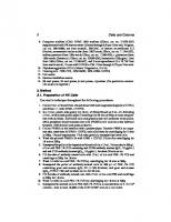
Franklin D. Roosevelt (FDR) served as the President of the United States of America from 1933 to 1945 (39). Over the course of his long political career (which began in 1910), FDR was photographed thousands of times and frequently appeared in short newsreels shown in movie theaters. By carefully staging these media opportunities, FDR was able to impart an image as a strong and resolute President during a time of economic depression and World War II. The general public was not aware that FDR was paralyzed from the waist down, that he had great difficulty walking any more than short distances, and that he often wore iron braces under his clothing. Most pictures of FDR show him seated, or if he is standing he can be seen holding on to something or someone to maintain his balance. Only three pictures are known to exist showing FDR in the wheelchair that he frequently used to get around when he was out of the public eye (see Fig. 1).

Fig. 1. US President Franklin D. Roosevelt was photographed thousands of times during his long political career. Most of the photographs show him seated, or if he was shown standing he was frequently holding onto someone or something. According to the FDR Library (112), Roosevelt’s paralysis was concealed (with the cooperation of the press) for political reasons, since at the time disabled persons were not considered able to perform the demanding responsibilities of elected office. Because the images the public routinely saw of Roosevelt did not hint of a physical limitation, the vast majority of the public was unaware that Roosevelt was paralyzed from the waist down (see Subheading 3.2). (a) Joseph Stalin (USSR), Franklin D. Roosevelt (USA), and Winston Churchill (UK) at the Tehran Conference, Teheran, Iran. November 29, 1943 (courtesy of the Franklin Delano Roosevelt Library website, Library ID 48-22 3715-107, Public Domain image). (b) Franklin D. Roosevelt in a wheelchair with his dog Fala in his lap, also pictured is family friend Ruthie Bie. Hyde Park, NY, February 1941 (courtesy of the Franklin Delano Roosevelt Library website, Library ID 73-113 61, Photographer: Margaret Suckley. Public Domain image).

1

Digital Images Are Data: And Should Be Treated as Such

5

Issues: Selectively presenting images that only tell one side of “the story” may be an engrained part of politics, but the expectation for scientists is that we will be unbiased and truthful. If we only show other people the pictures we want them to see, then the viewers will most likely reach the interpretation that we want them to have. What if our interpretation is wrong? It may be a poorly kept secret that most published images are somewhat less than “representative,” but is this right? What would happen to the quality of science if we only showed our most compelling images to our project leaders, lab group, or collaborators? 3.3. “Artistic” Changes to an Image Can Unintentionally Alter the Factual Content and/or a Viewer’s Interpretation of the Image

In 1994, television sports commentator and former American football player OJ Simpson was accused of, among other things, murdering his wife. He was later acquitted of the charges. Shortly after Mr. Simpson’s arrest, the Los Angeles Police Department provided a booking photograph to the media. On June 27, 1994 Newsweek ran the image almost unchanged as its cover photo, but Time magazine’s graphic artist significantly darkened the image to make it “more artful, more compelling” (40). The African-American community expressed outrage (41), because they perceived that Time had made Mr. Simpson look more sinister (42). To underscore the power of the images, few people complained about Newsweek’s bold headline “Trail of Blood,” while Time’s less prejudicial headline “An American Tragedy” was ignored (see Fig. 2).

Fig. 2. US sports and television personality OJ Simpson was arrested and accused of murdering his wife in June 1994. He was later acquitted of the charges. Newsweek and Time magazines both used the same Los Angeles Police Department booking photograph on the covers of the June 27, 1994 issues of their respective magazines. The heavily manipulated Time magazine cover (c) was seen by many as making Mr. Simpson appear more “sinister” (42) (see Subheading 3.3). (a) Original public domain image as found at the Washington Post website (113). (b) Color adjusted to more closely resemble the Newsweek cover. (c) Multiple image manipulations were performed to have the image more closely resemble the Time cover. To color match the images, regions were sampled from an image of the respective magazine covers (not shown) and the original image (a) was adjusted to match using the hue/saturation tool in Adobe Photoshop® CS3 to create the derivative images (b, c). The right image (c) was then colorized using the hue/saturation tool, the curves tool was used to darken the image, then a Gaussian blur (radius = 2.0) was applied, followed by setting the overall gamma to 0.85 in the levels tool to darken the image further, then selecting the background and lightening it using a gamma of 1.5. Photograph provided to the press on June 17, 1994 by the Los Angeles Police Department, Los Angeles, CA. Time magazine’s legal department would not grant permission for the magazine cover to be reproduced here.

6

D.W. Cromey

Issues: We need to be very cautious about manipulating an image so that it will better convey the message that we want to present. How should we make clear to readers that the manipulations performed on digital images are appropriate and scientific? 3.4. Photo-Illustrations That “Look” Real Are Misleading

Composite images are a staple of celebrity magazine covers. Occasionally news magazines have used realistic looking composites, with tiny disclaimers inside the magazine. For example, US media personality Martha Stewart spent 5 months in Federal prison on an insider stock trading charge. In March 2005, Newsweek magazine portrayed Ms. Stewart on their cover even before she was released from prison by digitally pasting an earlier image of Martha’s head onto another woman’s body (43). The composite was briefly described on page 3 of the magazine. The National Association of Press Photographers called the Newsweek cover a major ethical breach (44). Governments with something to prove have sometimes used composite images. In July of 2008 the Iranian government provided an image to the press that gave the impression of a successful launch of four Shahab-3 medium range ballistic missiles. The New York Times quickly determined that the image provided by Iran had been manipulated using “cloning” to give the impression that all four missiles had successfully launched. The analysis by The New York Times was confirmed by the discovery later of another image taken at the launch that showed only three missiles were successfully launched (45). Even prestigious scientific journals have occasionally stumbled when using composite images. A letter to the editor of the scientific journal Nature accused the publisher of a “deceptive” composite image that was featured on the cover of the August 2, 2007 issue (46). The Editor later apologized, stating “The cover caption should have made it clear that this was a montage” (47). Issues: The public “rolls their eyes” at manipulated images in tabloid newspapers and celebrity magazines, but they have higher expectations for scientists. Are composite images with disclaimers appropriate in science?

4. Before the Image Is Captured: Appropriate Image Acquisition Strategies

Bias is a far greater problem in science than is often acknowledged (48, 49). If images will be analyzed to create numerical data (size, shape, count, etc.), they need to be acquired in a systematic and well-defined manner (50). Systematic would include sufficient numbers of images, since there is always a certain amount of error in image analysis and analysis of enough structures will ensure that the error is small. Well-defined simply means that the images should be of the structures being measured, but selected in a manner that

1

Digital Images Are Data: And Should Be Treated as Such

7

reduces the operator’s own bias. Images are data and should, therefore, be subject to the same statistical treatment as all other scientific experiments. If the images will be used primarily for illustrative purposes, it is still best to take a number of images (51). Users should study the sample meticulously to allow the sample to provide the answer to the research question, rather than searching for an image field that best documents their hypothesis. The captured images can be examined later in the lab and it may be that further examination will provide a different interpretation of the data. The only way to accurately describe the differences seen in images of different treatment groups is to be very familiar with the appearance of the normal, untreated samples. To acquire appropriate and high-quality images it is important to make sure that the instrument used for the acquisition has been calibrated and properly aligned (52, 53). In addition, users need to understand the instrument’s capabilities, as well as its limitations. If images were acquired with different acquisition settings, it is important to communicate this to all the members of the lab, since changes in settings can affect the appearance of the image and possibly its interpretation.

5. How Digital Image Data Are Stored 5.1. Scientific Digital Images Are Data That Can Be Compromised by Inappropriate Manipulations

The underlying premise of image publication and ethics guidelines is that a digital image is data and that the data should not be manipulated inappropriately. Image data can represent intensity data acquired from a microscope CCD camera, or complex preprocessed information that comes from an Atomic Force Microscope or a Magnetic Resonance Imaging (MRI) scanner. Photographic film is an analog form of image capture, in that the information in the image is continuously variable. Digital imaging is a technique that samples the incoming data into discrete units called picture elements (pixels) that are presented as part of an array or grid. The scale of the pixels needs to be well matched to the resolution of the image capture instrument to ensure correct sampling and to avoid artifacts (see Fig. 3). The pixel in a digital image contains or represents a good deal of information. Each pixel has: ●

XY positional information relative to the rest of the grid that makes up the image.

●

Intensity information, presented as a numerical value within a range described as bit depth (e.g., 8 bit grayscale = 256 shades, 24 bit color = 16.7 M colors). This numerical information can represent data other than the amount of light being gathered

8

D.W. Cromey

Fig. 3. Digital images are a representative sampling of real life at discrete points (pixels). To ensure that the image correctly captures all the smallest details in the specimen, the Nyquist/Shandon theories suggest a minimum of 2× oversampling of the smallest resolvable element, with 2.4–2.8× oversampling suggested by some (55). Failure to adequately oversample can cause aliasing artifacts. Image (b) shows correct sampling and image (c) shows the same field undersampled. Note that in image (c) it is no longer possible to accurately count the number of visible in situ hybridization spots (see Subheadings 5.2, 5.3, 6.9, and 6.10). (a) Image captured at 2,048 × 2,048 pixels representing a field of view of 225 by 225 μm. The image was cropped to fit the page. (b) 2× enlargement of the field represented by the white box. Enlarged using Adobe Photoshop® CS3’s nearest neighbor resampling algorithm. (c) 2× enlargement of the same area, but taken from an image (not shown) that was captured at 512 × 512 pixels to represent the same field of view. Enlarged in the same manner as (b). Ciona intestinalis embryos, in situ hybridization stain, image captured with a Zeiss LSM 510 confocal microscope. These images are used by permission of Ella Starobinska and Dr. Bradley Davidson, University of Arizona.

by a detector. Intensity information may be used to represent forces, height, wavelength, etc. ●

A voxel (volume element) is a pixel with a z dimension, representing a volume. Information defining the voxel is usually stored in the metadata.

Many scientific images have associated metadata (data about data) that can store additional information. If the instrument does not capture these data automatically, it should be recorded manually. These data could include: ●

Information about the spatial, temporal, or spectral scale that was used to record each pixel. It is from this information that scale bars or other scalar references can be created. For many types of acquisitions, this includes a z dimension.

●

Acquisition settings used by the instrument to record the data (objective lens, magnification information, xyz stepper

1

Digital Images Are Data: And Should Be Treated as Such

9

motor positions, filter wheel positions, illumination source, gain settings, etc.). ●

The date and/or time that the data was acquired.

●

The operator who captured the image data.

Many scientific instruments save data in proprietary image file formats, with the Laboratory for Optical and Computational Instrumentation (LOCI, University of Wisconsin) Bio-Formats project supporting a growing list of 115 different formats (54). The proliferation of file formats is due to one of two reasons: most image formats were not designed to store complex metadata, and/ or a format was needed that was capable of storing complex multidimensional data (xyztλ). The correct acquisition of a digital image involves a number of considerations. 5.2. Sampling (See Subheadings 6.9 and 6.10)

●

Because digital images are a product of sampling, at least two to three times oversampling (e.g., Nyquist/Shandon) of the smallest resolvable elements in the image is required to avoid the possibility of artifacts (55, 56) (see Fig. 3). With some imaging techniques, this may include oversampling in the z dimension, as well as the x and y dimensions. Higher levels of oversampling have a benefit if the imaging technique has high light levels, but in low light situations higher levels of oversampling may reduce contrast and lower the S/N ratio to the point where the ability to resolve structures (e.g., Rayleigh criterion) is impaired (57).

●

If the image acquisition has a time dimension, temporal oversampling is also important. The “wagon wheel effect” (a form of temporal aliasing) has been known since the earliest days of movie making as a mismatch between the frames/s of the film and the rotational speed of a vehicle’s wheels (58, 59) (see Fig. 4).

Fig. 4. Temporal aliasing is a mismatch between the speed of the object and the speed of the camera (incorrect temporal sampling). The “wagon wheel effect” (also known as the “stroboscopic effect”) became familiar to viewers of Western movies as far back as the silent movie era (58). In the above illustration, the timing of each image is such that the wagon wheel has only rotated 94.5% of a turn (340°) per frame. When the video is played back, the wheel will appear to rotate in a clockwise direction, when in reality it is rotating counterclockwise (based on the indicated direction of travel, large arrow). Exploiting this artifact, a video could be created that showed an automobile obviously moving forward while the wheels appeared to be stationary, or a helicopter flying without the rotor turning (http://www.youtube.com/watch?v=Xhsf6vwSMc). Given the misleading possibilities of this artifact, it is important to know how quickly things are changing in a sample and to oversample correctly (see Subheadings 5.2 and 6.9). Dr. David Elliott, University of Arizona, provided technical assistance with this figure.

10

D.W. Cromey

Fig. 5. Rotating, as well as enlarging or reducing the image size (total number of pixels), causes the intensity values in an image to be resampled using interpolation (Merriam-Webster “to estimate values of (data or a function) between two known values” (114)). Rotating and/or resizing an image may be necessary for reporting the image data in a publication; however, this interpolation of the data should only be performed once on an image to avoid the compounding of interpolation artifacts (see Subheading 6.10). It is important to be very careful when using Adobe Photoshop®’s powerful image size dialog box, since it is very easy to accidentally resample an image with this tool (93). (a) A 6 × 6 pixel array. (b) A 15° rotation overlaid on the original image. (c) The result of the 15° rotation. (d) A 10 × 10 array is overlaid on the original image prior to enlarging the image. (e) The result of the 10 × 10 enlargement. Fifteen degree rotation performed using the Adobe Photoshop® CS3 Edit | Transform | Rotation tool. Enlargement performed using the Adobe Photoshop® CS3 Image Size dialog box, using the “bicubic smoother (better for enlargement)” resizing algorithm.

5.3. Digital Image Artifacts

●

In many cases, sampling at a higher bit depth can be beneficial, however much like over-magnifying an image (no additional resolution information), some noisy image acquisition techniques (e.g., confocal microscopy) do not warrant high bit depth images.

●

Wavelength (spectral) scanning should be correctly sampled using at least 2× the smallest resolvable element in the spectra. In practical application this can be difficult, especially in low light applications like fluorescence imaging.

●

Aliasing is the error that occurs when analog data is sampled incorrectly, or as a result of the interpolation that comes from resizing or rotating a digital image (see Figs. 3 and 5). James Pawley, editor of Handbook of Biological Confocal Microscopy says Aliasing may cause features to appear larger, smaller, or in different locations than they should be (60). An example would be the jagged line that appears when sampling a complex curved

1

Digital Images Are Data: And Should Be Treated as Such

11

Fig. 6. (a) Six by six pixel array (see Fig. 5a). Pixels have discrete intensity values, positional information within the array, and may imply a three-dimensional voxel (volume element). (b) The same array as (a) after a moderately aggressive brightness and contrast adjustment using ImageJ 1.43 m (115). (c) The same array as (a) after applying the Adobe Photoshop® CS3 sharpen filter. Graph: (key: light grey = (a), medium grey = (b), black = (c)). The graph shows the intensity values of the fourth row of pixels (arrow) in the images. The original image contains values that fit within the range of 0–255 (blackwhite). After the brightness and contrast adjustment, or the sharpening filter, a number of the intensity values have been truncated (asterisk) since they exceeded the 0–255 range, leaving just the maximum or minimum values. The relationship of these truncated values to those of the neighboring pixels has been lost (see Subheadings 6.1 and 6.5).

edge. Color aliasing artifacts can occur as well, particularly when sampling complex structures using a single chip color camera, since the color of any one pixel is based on the interpolation of color data from neighboring pixels. ●

Moiré is an image artifact produced when a repeated pattern is sampled at less than the Nyquist frequency, particularly when the sampling is performed with a pattern (e.g., the grid pattern of pixels on a CCD chip) (24, 61).

●

Bit depth saturation is often an operator-caused artifact, where the signal is truncated at the brightest or darkest ends of the spectrum (see Fig. 6). Any differences in the data that would have occurred outside of the range of the detector are lost in the truncated areas. This form of overly zealous adjustment is typically made during the image acquisition to suppress background or make the image appear more striking. Aggressive post-processing of images can also create this effect. A spike in the image’s intensity histogram (maps the frequency distribution of the pixels for the entire bit depth range) at the darkest or brightest values is an indication that some of the pixels in the image have been truncated (62).

●

Noise is present in most image acquisition systems. Some noise is sample-related, but the electronics of the image capture device also contribute to the overall noise levels (e.g., thermal

12

D.W. Cromey

noise, shot noise). Ideally, images should be acquired with a high signal-to-noise ratio, so that the effects of noise are minimized. In some instances (e.g., fluorescence imaging of live cells), that may not be possible. 5.4. Data Management

The US National Science Foundation is now requiring a two-page data management plan for all new grant applications (63, 64). It would not be surprising to see other US granting agencies follow suit. This raises the important issue of correctly storing the original data in its native file format. There are initiatives to develop open source software that will assist in organizing, tagging, storing, translating file formats, perform pre-configured image analysis routines, and secure sharing of data (65, 66). These programs require appropriate information technology resources and support. For the lab that does its own IT support, there needs to be a plan for organized storage of the original data and regular backups. Many labs have used CDs or DVDs as “read only” backups of their data, and while this has some appeal, optical media can be damaged and writable optical media’s use as reliable long-term storage is doubtful (estimated at 2–5 years) (67). Magnetic tape is estimated to have a 10–30-year lifespan, but even tape backups should be periodically tested (67). There are several good reasons for retaining the original data. Most of these fall under the heading of data provenance, which has been defined as Information about the source and history of particular data items or sets, which is generally necessary to ensure their integrity, currency, and reliability (68). ●

Any metadata stored in the original file format is retained.

●

Investigators can compare the final image used in a figure with the original image data to ensure that any manipulations performed were appropriate (69).

●

In the event that there is a question from a journal or granting agency about the image manipulations, the original data can be produced (70). It is important to note that online images (published or supplementary data) can be analyzed many years after publication (71).

●

The original data may be needed to satisfy regulatory requirements (e.g., CFR 21 part 11 (72, 73), HIPPA (74), Forensics (75, 76)) for maintaining the data.

Because the software to open older file formats can become obsolete or will no longer run on modern operating systems, exporting the data to a more standard format is often a wise precaution. Some software can export to the Open Microscopy Environment’s OME-TIFF specification (77); however, if this format is not available, the more common TIFF file format is recommended by the Microscopy Society of America (78). Other file

1

Digital Images Are Data: And Should Be Treated as Such

13

formats lack the bit depth for scientific images, or saving into the format performs a lossy type of compression on the image. TIFF is a quasi-standard file format (79) that supports large bit depths in grayscale and color and does not alter the exported bitmap data (see Subheadings 5.5 and 6.8). Scientists should not use the JPEG file format for image data, as this format’s lossy file compression alters the positional and intensity information of every pixel (see Subheading 6.8). 5.5. Manipulation of Digital Images Should Only Be Performed on a Copy of the Unprocessed Image Data File

When you begin your image manipulations, it is crucial to always use a copy of the original image. In most software it is far too easy to overwrite the original file with a manipulated image. Overwriting the original data with commercial image editing software (e.g., Adobe Photoshop®) can cause embedded metadata (e.g., nonstandard TIFF tags) to be lost or changed. The best practice is to open the file and immediately save a copy of the image, close the original file, and open the copy image. In recent years the issue of “self-plagiarism” has been raised when authors have reused image data that was previously published (80–82). Another issue of data provenance is tracking how a particular image was used in the past, so that reuse of the image does not occur without the appropriate permissions from the publisher or copyright holder of the original image. Good data management practices will go a long way to prevent this from occurring.

6. Post-processing Image processing (editing, manipulation) is a form of communication. As scientists, we need to be careful that our manipulations are helpful and do not hurt the communication of what is true in the image (see Subheading 3.3). Just because something can be done via image processing does not mean that it should be done. When editing an image, it is good to remember that serendipity has a wonderful role in science (83) and that a published image may mean something entirely different to a reader from outside of our specific field of expertise. To be clear, image processing is not a form of artistic expression; it is the mathematical manipulation of the underlying numbers in a digital image. Resist the urge to beautify scientific images (84), and remember that artistic changes can alter how others will interpret the image (see Subheading 3.3). Hard and fast rules that apply to every image-forming discipline are difficult to create (the National Academy of Sciences found this out (71, 85) when they were unable to agree on guidelines). The following guidelines are based on several decades of experience with microscopy and digital images (the numbers

14

D.W. Cromey

preceding the individual guidelines refer to the section of the text where it is discussed.) Ethical guidelines for the appropriate use and manipulation of scientific digital images (24, 86, 87) 5.1 Scientific digital images are data that can be compromised by inappropriate manipulations. 5.5 Manipulation of digital images should only be performed on a copy of the unprocessed image data file (Always keep the original data file safe and unchanged!). 6.1 Simple adjustments to the entire image are usually acceptable. 6.2 Cropping an image is usually acceptable. 6.3 Digital images that will be compared to one another should be acquired under identical conditions, and any post-acquisition image processing should also be identical. 6.4 Manipulations that are specific to one area of an image and are not performed on other areas are questionable. 6.5 Use of software filters to improve image quality is usually not recommended for biological images. 6.6 Cloning or copying objects into a digital image, from other parts of the same image or from a different image, is very questionable. 6.7 Intensity measurements should be performed on uniformly processed image data, and the data should be calibrated to a known standard. 6.8 Avoid the use of lossy compression. 6.9 Magnification and resolution are important. 6.10 Be careful when changing the size (in pixels) of a digital image. 6.1. Simple Adjustments Performed on the Entire Image Are Usually Considered an Acceptable Practice

While the reporting of certain basic image manipulations is not required, a better practice is to record the entire protocol of how the image was changed. Some software (e.g., ImageJ, Adobe Photoshop®, ImagePro®) have the ability to create an audit trail of image manipulations, but the function must be enabled by the user (88). The alternative is to manually document the protocol in a lab notebook. Careful adjustments of image brightness and contrast or a histogram stretch (e.g., levels tool) are usually considered non-reportable. Adjustment of image gamma, a non-linear operation, is considered a manipulation that should be reported by some journals and unnecessary to report by others (24, 89–91). Be aware that aggressive manipulation of images can over/under saturate the image, truncating the intensity data (see Subheading 5.3, Fig. 6), and may cause the apparent size of objects to change due to aliasing artifacts.

1

Digital Images Are Data: And Should Be Treated as Such

15

In labs that are sharing images among many computers, with different monitors (of varying age) and different operating systems (92), it is a worthwhile investment to purchase a monitor calibration device (approximately $200–300 USD) to ensure that everyone will be seeing the image with the correct image brightness and/or color. It should be noted that laptop computers running on battery power often dim the screen as a means of prolonging battery life. This change in screen brightness can affect how detail in the image is seen. Ambient lighting (e.g., exterior windows) can affect image brightness and color perception as well. Monitor calibration, in addition to attention to lighting, will ensure that adjustments made on one computer will appear the same on all the lab’s computers, and should improve the reproduction of the images in print. 6.2. Cropping an Image Is Usually Considered an Acceptable Form of Image Manipulation

Image cropping typically removes pixels from the outside edges of the image as a means to center an object of interest, or to permit the image to fit a defined space. It is important to consider the motivation for cropping. Will the cropped image improve the communication of unbiased scientific information, or will it change how the image is perceived by the viewer? Will the crop remove something that disagrees with the hypothesis being presented, or is the crop being performed to hide something in the image that cannot be explained? Be careful about how aggressively an image is cropped. To reproduce a bitmapped image in print, most journals require 300 pixels per inch. For example, a 512 × 512 image at 300dpi is only 1.7 by 1.7 in. in size and in many cases this may not be a large enough figure to show all the detail. Increasing the total number of pixels in the image using software (e.g., Photoshop’s dangerous “image size” dialog box (93)) usually gives the image an indistinct, or less crisp look, due to aliasing artifacts (see Subheading 6.10).

6.3. Digital Images That Will Be Compared to One Another Should Be Acquired Under Identical Conditions, and Any Postacquisition Image Processing Should Also Be Identical

This would include images intended for computerized analysis or images being assembled in a combined publication figure. A protocol for identical conditions would include: ●

●

Similar/identical sample preparation techniques. –

Ideally the sample preparation would occur at the same time; however in many studies this is not possible.

–

Be very careful with different lots of reagents (e.g., polyclonal antibodies).

The same instrument. –

Two different instruments with the same hardware do not always acquire identical images.

●

The acquisition conditions (settings) should be identical.

●

Post-processing of the images should be uniform (e.g., background subtractions, white level balancing).

16

D.W. Cromey

In many core facilities, it is the students and staff that acquire the bulk of the images. If someone who is unfamiliar with the instrument (i.e., post-doc, PI) will be interpreting the images, it is crucial that the acquirer of the data communicates with this person any differences in acquisition settings that were made. For example, small changes to the gain (signal amplification) and offset (black level) in a confocal microscope can greatly affect the final image data. Much like other composite images (see Subheading 3.4), if the images in a figure are presented as means of conveying similarities and differences in the outcomes of treatment, the assumption is made by the reader that they were acquired under similar conditions. 6.4. Manipulations That Are Specific to One Area of an Image and Are Not Performed on Other Areas Are Questionable

While dodging and burning of photographic prints was certainly done in the past, enhancing only selected areas in a scientific digital image is generally not allowed today. While rare, there may still be an appropriate rationale for enhancement of specific areas of an image in special cases, but it is mandatory that the manipulations be declared. High dynamic range (94) or extended depth of focus (95) images are useful techniques to overcome physical limitations in instrumentation (inability to capture the brightest and dimmest parts of a field of view in the same image, and inability to capture an in-focus image through the entire depth of a large three-dimensional object, respectively). These are computational techniques that combine data from multiple images into a single image. With appropriate explanation, these are acceptable techniques for scientific data.

6.5. Use of Software Filters to Improve Image Quality Is Usually Not Recommended for Biological Images

Software filters are typically a convolution kernel, a small array of mathematical functions that are applied to each pixel and the resulting change in the central pixel of the array is based on the kernel function and the values in neighboring pixels in the image. Since the values in the neighboring pixels will be different all throughout the image, the change created by the filter will not be the same in all areas (96). This is how a sharpening filter detects edges, based on localized changes in pixel intensity, with the effect being most pronounced in the edge area and less noticeable in areas where the intensity does not change significantly (see Fig. 6). Commercial image editing software (e.g., Adobe Photoshop®) does not provide access to the mathematical functions used in software filters. If commercial software is used, the software version number, filter name, and any additional settings should be carefully recorded. Although scientific image processing software may provide more information about the kernel used, or even allow the user to design their own kernel, these steps should also be carefully documented.

1

Digital Images Are Data: And Should Be Treated as Such

17

6.6. Cloning or Copying Objects into a Digital Image, from Other Parts of the Same Image or from a Different Image, Is Very Questionable

Composite images can be very misleading (see Subheading 3.4), even when they are explained in the figure legend. If two parts are added together, a white or black line should indicate the added piece. Adding an insert that shows a portion of the field at a higher magnification is appropriate, but it should be set off in a way that clearly shows that it is a different image. Use of cloning and copying to “clean up” or beautify an image is an invitation to trouble. These sorts of changes to an image are fairly easy to detect and they should always be declared in the figure legend. Failing to declare these sorts of changes may lead to the publication being rejected and could prompt further investigation of the author’s previously published papers. Commercial image editing software provides many options for retouching images. Almost all of these tools, in particular “auto” manipulation tools, should be avoided by scientists. If these tools are used, they should be documented as discussed previously (see Subheading 6.5).

6.7. Intensity Measurements Should Be Performed on Uniformly Processed Image Data, and the Data Should Be Calibrated to a Known Standard

Intensity measurements, particularly fluorescence intensities, are very difficult to do well (97). This is due, in part, to the difficulty in creating reproducible calibration standards (53). In addition, many instruments have known shortcomings that make the collection of reproducible data difficult (98). The data acquisition parameters and post-processing techniques need to be standardized, or the data are worthless. Mathematical analysis of images with pixels that have reached bit depth saturation (see Subheading 5.3) should be avoided to ensure accurate results (99). Densitometry of colorimetric stains (e.g., DAB, HRP) is easier to perform than fluorescence intensity measurements. Care should be taken with densitometry, since staining is not linear and the curve tends to flatten out at high staining densities (100, 101). Users should be careful about post-processing of images. Image filtering can introduce artifacts that may affect intensity and size measurements in unexpected ways (see Fig. 6).

6.8. Avoid the Use of Lossy Compression

There are several types of file size reduction schemas used with image files. TIFF images can use a form of the loss-less LZW (Lempel-Ziv-Welsh (61)) compression, which does not change the image data. It should be noted that LZW-TIFF files are not universally supported by image processing software. GIF images reduce file size by using a limited color palette (256 maximum), which can reduce the color or intensity information in the image. JPEG images reduce the file size by using the lossy discrete cosine function to reduce the high frequency information in the image. JPEG compression is particularly problematic, since it was designed to create changes that were not readily perceptible to the human eye (48). JPEG compression makes subtle changes in the color, intensity, and the location of the intensity, making it unsuitable for use with scientific images (48) (see Fig. 7). If JPEG must

18

D.W. Cromey

Fig. 7. The dangers of the JPEG file format. A TIFF image (a) was opened and saved as a JPEG file, then the JPEG was opened and saved as a JPEG a total of five times in a row (Adobe Photoshop® CS3’s “medium” JPEG setting, 5). Each time a JPEG file is saved, the compression algorithm is performed. The white box in the TIFF (a) image and the corresponding area in the JPEG image (d) were enlarged seven times using Adobe Photoshop’s® nearest neighbor resampling algorithm to show the compression artifacts (with a histogram stretch and gamma set to 1.5). Image (b) is the enlarged TIFF, and image (c) is the enlarged JPEG. Comparing image (a, d), there appears to be no visible change, but at the pixel level ((b) vs. (c)), the changes are very noticeable. The scatter plots illustrate the differences between the files. The plot compares the grey values of each pixel in both images. The TIFF images are identical, hence the straight line. The intensity values are quite different in the JPEG image. The gaps in the plots are due to an initial histogram stretch of the original TIFF image. The original TIFF file size is 204 kB, the first JPEG save is 36 kB and JPEG files 2–5 are all 35 kB. The Pearson’s correlation of TIFF vs. TIFF is 1.0, the correlation of TIFF vs. the first JPEG save is 0.991, with the correlation between subsequent JPEG saves being 0.99. The first JPEG save causes the biggest changes in the image and saves the most file space, and after that the subsequent saves degrade the image slightly each time. Saving the TIFF file one time at the highest JPEG quality factor (12, Adobe Photoshop®) reduced the file size to 123 kB and yielded a tighter, but not perfectly linear, scatterplot (data not shown). If JPEG is required, saving once at the highest quality factor makes the smallest change in the image (see Subheading 6.8). Confocal microscope image of cellular cytoskeleton (this figure was inspired by colleague Charles “Chip” Hedgcock, University of Arizona, and the colocalization technique was suggested by Dr. John Krueger, ORI).

be used (e.g., web pages, required by journal), the compression should only be performed one time on any image as the final step, and only with the highest quality setting (minimal artifacts). Be careful using JPEG, because every time the file is saved in this format the compression algorithm is performed. With each iteration of the file save, the JPEG artifacts compound one another, further degrading the image. On careful examination, lower quality factor JPEG images typically have an artifact of 8 × 8 pixel squares (96), also known as a macroblock (see Fig. 7c). In many cases, a more suitable alternative to JPEG is the loss-less PNG file format, although PNG does not support conversion to CYMK for printing (102). PNG is greatly preferred over JPEG when compressing figures that have small text or fine lines, since it does not blur the edges of these small items. Occasionally image data with a time or z dimension are converted to a video format. To keep the file size manageable, most

1

Digital Images Are Data: And Should Be Treated as Such

19

video file formats perform some form of compression. Many of the video formats use a variation of the discrete cosine transform that is used in JPEG images. While it is generally understood that video files use lossy compression, it is still important to carefully check the video to ensure that the software codec has not introduced misleading artifacts into the data. The codec name and the conversion settings used to create the video should be documented. Scientists should avoid using presentation software (e.g., Microsoft’s PowerPoint®) for assembling publication figures. The software may be familiar and available, but these programs are designed for images that will be shown on a projection screen at low resolution, not the 300 dpi needed to print bitmapped images or the 1,200 dpi needed for line art. Resizing images in PowerPoint® brings up the interpolation issues discussed below (see Subheading 6.10) and running the program’s file compression routine to reduce file size will perform some form of lossy compression (suspected to be JPEG) on every image in the file. The JCB will not accept images that have been manipulated by PowerPoint® (103). 6.9. Magnification and Resolution Are Important

Digital images are a product of sampling the data at discrete intervals. This sampling should be performed in a way that satisfies the Nyquist/Shandon criteria. Undersampling can lead to artifacts such as incorrect size, or very small elements being missed entirely, which is the result of aliasing artifacts such as moiré (spatial aliasing) and temporal aliasing. Oversampling can more closely approximate the information in the images, but concerns such as cost, low signal-to-noise in the image, and optical issues can limit the ability to sample at high levels of oversampling. Sampled images are acquired with information about the scale or size of each pixel in spatial (xyz), as well as temporal (T) and sometimes spectral (λ) dimensions. This information needs to be conveyed to the reader through the use of spatial scale bars, time stamps, or other scalar information. Any image manipulation that might change this important information must be done with care. Spatial scale bars are preferred over stating the calculated magnification in a figure legend because journals occasionally resize images in the process of publishing. The scale bar will resize proportionally with the image. While common in some fields, the practice of simply stating the microscope objective used to acquire the image does not factor in several other magnification factors that can be different with each microscope and is very imprecise. Correct magnifications can be calculated by taking and measuring images of a stage micrometer or other calibration standards. If structures are detected whose size is less than that of a microscope’s resolution limit, the structure’s apparent size will match the resolution limit (104). This is an artifact of the optics. Any measurements taken of these structures should keep this artifact in mind.

20

D.W. Cromey

6.10. Be Careful When Changing the Size (in Pixels) of a Digital Image

If the digital image captured by a microscope is a sampled image, then changing the total number of pixels in an image or reorienting the sample grid is a form of resampling the image (see Fig. 5). If an image is rotated in intervals of 90°, then the pixels are simply remapped. If the image size is changed by a power of two, the resampling mathematics is a fairly simple interpolation. If the image is resized or rotated at any other interval, a more significant form of interpolation must be performed in the software to estimate what the pixels would look like if the sampling grid had been that size or oriented at that angle. While rotating and/or resizing an image may be necessary for reporting the data in a publication, this interpolation of the data should only be performed once on an image to avoid the compounding of interpolation artifacts (analysis should only be performed on the un-interpolated image). This is usually not considered a reportable image manipulation, but it should be documented. Enlarging the image does not increase the resolution (Raleigh criterion) in the image; in fact this may make formerly crisp edges seem fuzzier due to aliasing artifacts that are introduced by the interpolation algorithm.

6.11. Reviewing the Processed Image

As mentioned earlier, the final product should be compared to the original image(s) to ensure that any manipulations performed were appropriate and do not alter the data. Senior authors have a particular responsibility for the work coming out of their lab (69). If there are suspicions that an image has been manipulated inappropriately, how can we tell? The JCB uses an experienced human editor to examine images, while other journals have used sophisticated image screening software (4, 105, 106). The only readily accessible resources for performing image forensics have been provided by the ORI (107). The ORI has several tools for examining suspect images that work in Adobe Photoshop® (see http://ori.hhs.gov/tools/). On a simpler level, users can examine the image’s intensity histogram for hints. Original, unprocessed images tend to have continuous histograms. Processed images frequently show common artifacts (gaps, spikes) that can suggest if the image is truly an original or if it has received some post-processing (62).

7. Going to Press As was mentioned earlier (see Subheading 2), some journals do not have a firm grasp on digital image requirements and their instructions to authors read like they were written by a graphic designer. Dealing with journals can lead to additional issues for authors.

1

Digital Images Are Data: And Should Be Treated as Such

21

7.1. High Bit Depth Images

High bit depth images (>8bit greyscale, or >24bit color) cannot be reproduced in print. Some form of downsampling of the bit depth needs to occur to be able to publish these images. This should be documented.

7.2. Line Art

Many journals request that line art (graphs, charts) be submitted as vector graphic files. Vector files use mathematical formulas to describe the lines and do not have pixels, so they can be printed at any size without aliasing artifacts. Line art that is not in vector file format is typically requested at 1,200 dpi so that the very fine lines print smoothly. Line art resolution is 16 times (4× the linear resolution) the total number of pixels (300 dpi) normally required to nicely reproduce a raster image. If your lab lacks the software or expertise to work with vector files, it is possible to zoom in on a chart (e.g., from Microsoft Excel®) and perform a series of screen captures on a high resolution monitor and then stitch the multiple images together in Photoshop.

7.3. RGB and CYMK

The process of printing takes a digital image that was usually captured and manipulated as grayscale or RGB color and converts it to a very different color space (often CYMK). The printing process cannot reproduce all the tones that are present in a digital image, particularly if the image is in color and the image uses the brightest reds or blues, and, to a lesser extent, green colors. The reproduction of color in print is highly dependent on the number and type of inks used by the printing press, as well as the type of paper used. It is baffling why journals expect scientists with little expertise in this highly technical area to optimally convert their images from the RGB color space to CYMK prior to submission. Fortunately, a number of journals have stepped away from color space conversion and now accept images in RGB (103, 108, 109).

7.4. File Compression Issues

Journals sometimes still ask for the digital image files to be sent as JPEG files. Inquire if they will take a TIFF image or a PNG file. If the journal insists on JPEG, perform this conversion as the very last item before submitting the image and do the conversion only at the highest possible quality factor to keep the artifacts to a minimum. Bitmapped images with fine lines or small text do not convert well to JPEG format. The lines and text lose their crispness. PNG is a better compressed image file format choice for images with fine lines and small text. It is also a good idea to check the file size of the proof PDF sent to you by the journal. The default image compression used by Adobe Acrobat is JPEG. Use the zoom features in your PDF viewer to examine the images (figures and line art) carefully. If you send the journal a document and image files totaling 8–10 MB, your PDF galley proof should not be a file that is less than 1 MB in size. Suggest that the journal change their PDF output settings from

22

D.W. Cromey

screen to print. This PDF conversion will still perform a JPEG compression; however it will be much less aggressive. If the journal agrees to make this change, your replacement PDF proof will be a larger file size and better quality.

8. Conclusions Once upon a time the darkroom technician acted as a “gate keeper” of image processing technology, but the photographic enlarger has been replaced by Adobe Photoshop® and other commercial image editing software. The tricky darkroom procedures that could be done by a few have now been replaced by digital tricks that can performed by almost anyone. Along the way we seem to have lost the distinction between appropriate and inappropriate image manipulations. While misconduct (fraud) is a concern in science (see Subheading 1), the bigger issue seems to be related to the lack of understanding of how to correctly manipulate digital images. Combine the excitement for a person’s research with a lack of understanding and one can see why the journals are still finding over-manipulated images (see Subheading 2) in spite of their detailed instructions to authors. One editor went as far as to admonish people to “stop misbehaving” (110). The first thing that needs to change is our mindset. We still tend to think of digital images as a “picture,” when in reality they are data. Pictures are artwork that can be changed to suit our desire for how they are presented to others, while image data are numerical and must be carefully manipulated in a way that does not alter their meaning. We need to ignore the pressure (peers and yourself) to beautify (19, 111) our images (see Subheading 3.3). Accurately communicating the truth is a fundamental issue in science (see Subheadings 3.1, 3.2, 3.3, and 3.4). Secondly, we need to develop the discipline of documenting all the manipulation steps performed on an image, as well as the software and version number used to perform the manipulations. This would include steps that ordinarily do not have to be reported. Other types of scientific experiments are documented in great detail in our notebooks. Shouldn’t our image manipulations be as well? If an “image is worth a thousand words” shouldn’t we be more careful with these data? Providing adequate information about the image manipulations performed is a protection against accusations of fraud. If a reviewer does not like a manipulation that was performed, the discussion now becomes a “difference of scientific opinion,” not an accusation. It is important to remember that online images and supplemental data can be checked for inappropriate manipulations many years after publication.

1

Digital Images Are Data: And Should Be Treated as Such

23

Lastly, we count on our colleagues to be fully truthful in reporting their results. Shouldn’t we return them the same favor? We also need to teach our colleagues and mentor the next generation of scientists in how to correctly work with digital images. These guidelines are a starting point for discussion and training, but when it comes to submitting your publications, follow the instructions to authors. If those are short on detail, refer to those found at the JCB.

Acknowledgements This work was supported in part by the Southwest Environmental Health Sciences Center (NIEHS ES006694); the Division of Biotechnology, Arizona Research Labs at the University of Arizona; the Arizona Cancer Center (NCI CA23074); and the University of Arizona Department of Cellular and Molecular Medicine. The views, opinions, and conclusions of this chapter are not necessarily those of the SWEHSC, NIEHS, AZCC, NCI, or the University of Arizona. References 1. Rossner M, Held MJ, Bozuwa GP et al (1998) Managing editors and digital images: shutter diplomacy. CBE Views 21:187–192 2. Rossner M, Yamada KM (2004) What’s in a picture? The temptation of image manipulation. J Cell Biol 166:11–15 3. Rossner M (2006) How to guard against image fraud. Scientist 20:24 4. Rossner M (2008) A false sense of security. J Cell Biol 183:573–574 5. Marris E (2006) Should journals police scientific fraud? Nature 439:520–521 6. Marcus A, Oransky I (2011) Stop the picture doctors. Lab Times 4–2011:35 7. Editorial Nature Cell Biology (2011) Combating scientific misconduct. Nat Cell Biol 13:1 8. Anderson C (1994) Easy-to-alter digital images raise fears of tampering. Science 263: 317–318 9. Taubes G (1994) Technology for turning seeing into believing. Science 263:318 10. McInnes SJ (2001) Is it real? Zool Anz 240: 467–469 11. Suvarna SK, Ansary MA (2001) Histopathology and the ‘third great lie’. When is an image not a scientifically authentic image? Histopathology 39:441–446 12. Krueger J (2002) Forensic examination of questioned scientific images. Account Res Policies Qual Assur 9:105–125

13. Pritt BS, Gibson PC, Cooper K (2003) Digital imaging guidelines for pathology: a proposal for general and academic use. Adv Anat Pathol 10:96–100 14. Editorial Nature Cell Biology (2004) Gel slicing and dicing: a recipe for disaster. Nat Cell Biol 6:275 15. Editorial Nature Cell Biology (2004) Images to reveal all? Nat Cell Biol 6:909 16. Guneri P, Akdeniz BG (2004) Fraudulent management of digital endodontic images. Int Endod J 37:214–220 17. Krueger J (2005) Confronting manipulation of digital images in science. Office Res Integr Newslett 13–3:8–9 18. Pearson H (2005) Image manipulation: CSI: cell biology. Nature 434:952–953 19. Nature Cell Biology Editorial (2006) Beautification and fraud. Nat Cell Biol 8:101–102 20. Nature Cell Biology Editorial (2006) Appreciating data: warts, wrinkles and all. Nat Cell Biol 8:203 21. Abraham E (2007) Update on the AJRCCM—2007. Am J Respir Crit Care Med 175:207–208 22. Nature Cell Biology Editorial (2007) Imagine. Nat Cell Biol 9:355 23. Krueger J (2009) Incidences of ORI cases involving falsified images. Office Res Integr Newslett 17–4:2–3

24

D.W. Cromey

24. Cromey DW (2010) Avoiding twisted pixels: ethical guidelines for the appropriate use and manipulation of scientific digital images. Sci Eng Ethics 16:639–667 25. Hwang WS, Ryu YJ, Park JH et al (2004) Evidence of a pluripotent human embryonic stem cell line derived from a cloned blastocyst. Science 303:1669–1674 26. Department of Health and Human Services (2005) Public Health Service Policies on Research Misconduct; Final Rule, (Public Health Service, Ed.) 42 CFR Parts 50 and 93. http://www.ori.dhhs.gov/documents/42_ cfr_parts_50_and_93_2005.pdf. Accessed 16 Sept 2011 27. Office of Research Integrity. Definition of Research Misconduct, http://ori.hhs.gov/ misconduct/de fi nition_misconduct.shtml . Accessed 16 Sept 2011 28. National Academies (U.S.). Committee on Science Engineering and Public Policy (2009) On being a scientist: a guide to responsible conduct in research, 3rd edn. National Academies Press, Washington, DC 29. Young JR (2008) Journals find fakery in many images submitted to support research. Chron Higher Ed, Washington, DC. http://chronicle.com/article/Journals-Find-Fakery-inMan/846/. Accessed 16 Sept 2011 30. Couzin J (2006) Scientific publishing. Don’t pretty up that picture just yet. Science 314:1866–1868 31. Abraham E, Adler KB, Shapiro SD et al (2008) The ATS journals’ policy on image manipulation. Am J Respir Cell Mol Biol 39: 499 32. Shattil SJ (2007) A digital exam for hematologists. Blood 109:2275 33. Caelleigh AS, Miles KD (2011) Biomedical Journals’ Standards for Digital Images in Biomedical Articles (presented at the Council of Science Editors annual meeting). http://scie n c e i m a g e i n t e g r i t y. o rg / w p - c o n t e n t / uploads/2010/04/CSEPoster-April20FINAL-AC-Edit1.ppt. Accessed 16 Sept 2011 34. Farid H (2011) Photo tampering throughout history, Fourandsix Technologies. http:// www.fourandsix.com/photo-tampering-history/. Accessed 16 Sept 2011 35. King D (2011) The commissar vanishes. The Newseum, Washington, DC. http://www. newseum.org/berlinwall/commissar_vanishes/. Accessed 16 Sept 2011 36. Oberg J (2011) Soviet Space Propaganda: Doctored Cosmonaut Photos, Wired.com, Condé Nast Digital. http://www.wired. com/wiredscience/2011/04/soviet-spacepropaganda/?pid=1177. Accessed 16 Sept 2011

37. Mackey R (2011) Newspaper ‘Regrets’ Erasing Hillary Clinton. In: The Lede. New York Times, New York. http://thelede.blogs. nytimes.com/2011/05/10/newspaperregrets-erasing-hillary-clinton/. Accessed 16 Sept 2011 38. Orwell G (1949) Nineteen eighty-four, a novel. Secker & Warburg, London 39. Franklin D (2011) Roosevelt, Wikipedia. http://en.wikipedia.org/wiki/Fdr. Accessed 16 Sept 2011 40. Meltzer B (1996) Digital photography: a question of ethics. Lead Learn Technol 23–4:18–21 41. Stanleigh S (1995) Where do we re-draw the line?, In: Ryerson Review of Journalism. Ryerson University School of Journalism, Toronto, Canada. http://www.rrj.ca/ m3693/. Accessed 16 Sept 2011 42. Carmody D (1994) Time responds to criticism over Simpson cover. New York Times Company, New York. http://www.nytimes. com/1994/06/25/us/time-responds-tocriticism-over-simpson-cover.html. Accessed 16 Sept 2011 43. Glater JD (2005) Martha Stewart Gets New Body in Newsweek. In: New York Times. New York Times Company, New York. http://www.nytimes.com/2005/03/03/ business/media/03mag.html. Accessed 16 Sept 2011 44. National Press Photographer’s Association (2005) NPPA Calls Newsweek’s Martha Stewart Cover “A Major Ethical Breach”. http://www.nppa.org/news_and_events/ news/2005/03/newsweek.html. Accessed 16 Sept 2011 45. Nizza M, Lyon PJ (2008) In an Iranian Image, a Missile Too Many. In: New York Times. New York Times Company, New York. http://thelede.blogs.nytimes. com/2008/07/10/in-an-iranian-image-amissile-too-many/. Accessed 16 Sept 2011 46. Nature (2007) Cover Image. Nature 448(7153) 47. Sincich L (2007) Cover story may obscure the plane truth. Nature 449:139 48. Russ JC (2004) Seeing the Scientific Image (parts 1–3). Proc R Microsc Soc 39(2):97– 114; (113):179–194; (114):267–281 49. Ioannidis JP (2005) Why most published research findings are false. PLoS Med 2:e124 50. Hyde DM, Tyler NK, Plopper CG (2007) Morphometry of the respiratory tract: avoiding the sampling, size, orientation, and reference traps. Toxicol Pathol 35:41–48 51. McNamara G (2006) Crusade for Publishing Better Light Micrographs—Light

1

52.

53.

54.

55.

56.

57.

58.

59.

60.

61.

62.

63.

Digital Images Are Data: And Should Be Treated as Such

Microscope Publication Guidelines. http:// home.earthlink.net/~geomcnamara/ CrusadeBetterMicrographs.htm. Accessed 16 Sept 2011 North AJ (2006) Seeing is believing? A beginners’ guide to practical pitfalls in image acquisition. J Cell Biol 172:9–18 Stack RF, Bayles CJ, Girard AM et al (2011) Quality assurance testing for modern optical imaging systems. Microsc Microanal 17:598–606 Supported Formats (2011) In: Bio-Formats. Laboratory for Optical and Computational Instrumentation (LOCI), University of Wisconsin-Madison. http://loci.wisc.edu/ bio-formats/formats. Accessed 16 Sept 2011 Pawley JB (2006) Points, pixels, and gray levels: digitizing image data. In: Pawley JB (ed) Handbook of biological confocal microscopy, 3rd edn. Springer Science + Business Media LLC, New York, NY, pp 59–79 Spring KR, Parry-Hill MJ, Long JC et al (2006) Spatial resolution in digital images. http://micro.magnet.fsu.edu/primer/java/ digitalimaging/processing/spatialresolution/. Accessed 16 Sept 2011 Spring KR, Fellers TJ, Davidson MW (2006) Resolution and contrast in confocal microscopy. http://www.olympusconfocal.com/ theory/resolutionintro.html. Accessed 16 Sept 2011 New York Times written in (1918) Why movie wheels turn backward; an explanation of the illusion and a suggested method for correcting it. In: Sunday (ed) New York Times. New York Times, New York. http://query.nytimes. com/gst/abstract.html?res=9A05E6DA143 EE433A25752C2A9619C946996D6CF. Accessed 16 Sept 2011 Purves D, Paydarfar JA, Andrews TJ (1996) The wagon wheel illusion in movies and reality. Proc Natl Acad Sci U S A 93:3693–3697 Pawley JB (2006) Fundamental limits in confocal microscopy. In: Pawley JB (ed) Handbook of biological confocal microscopy, 3rd edn. Springer Science + Business Media LLC, New York, NY, pp 20–42 Corporation M (1997) The Microsoft Press® computer dictionary, 3rd edn. Microsoft Press®, Redmond, WA Burger W, Burge MJ (2008) Histograms. In: Texts in Computer Science: Digital image processing. Springer, London, pp 37–52 National Science Foundation (2011) Chapter II—Proposal Preparation Instructions: Data Management Plan. http://www.nsf.gov/ pubs/policydocs/pappguide/nsf11001/ gpg_2.jsp#dmp. Accessed 16 Sep 2011

25

64. National Science Foundation (2011) Dissemination and sharing of research results. http://www.nsf.gov/bfa/dias/policy/dmp. jsp. Accessed 16 Sept 2011 65. Center for Bio-Image Informatics (2011) University of California—Santa Barbara. Bisque Database. http://www.bioimage. ucsb.edu/bisque. Accessed 16 Sept 2011 66. Open Microscopy Environment (2011) http://www.openmicroscopy.org/site . Accessed 16 Sept 2011 67. Blau J (2006) Do burned CDs have a short life span?, PC Magazine. http://www.pcworld. com/article/124312/do_burned_cds_have_a_ short_life_span.html. Accessed 16 Sept 2011 68. Searls DB (2005) Data integration: challenges for drug discovery. Nat Rev Drug Discov 4: 45–58 69. Alberts B (2010) Promoting scientific standards. Science 327:12 70. Melino G (2010) Policy and procedures on scientific misconduct. Cell Death Differ 17: 1805–1806 71. Committee on Ensuring the Utility and Integrity of Research Data in a Digital Age, National Academiy of Sciences (2009) Ensuring the integrity, accessibility, and stewardship of research data in the digital age. National Academies Press, Washington, DC 72. Tengowski MW (2004) Image compression in morphometry studies requiring 21 CFR Part 11 compliance: procedure is key with TIFFs and various JPEG compression strengths. Toxicol Pathol 32:258–263 73. Food and Drug Administration (2010) CFR—Code of Federal Regulations Title 21, Food and Drug Administration. http://www. accessdata.fda.gov/scripts/cdrh/cfdocs/ cfcfr/cfrsearch.cfm?cfrpart=11. Accessed 16 Sept 2011 74. Wikipedia (2011) Health Insurance Portability and Accountability Act. http://en.wikipedia. org/wiki/Health_Insurance_Portability_and_ Accountability_Act. Accessed 16 Sept 2011 75. Scientific Working Group Imaging Technology (2004) Best Practices for Documenting Image Enhancement, section 11 (Version 1.2 2004.03.04) 76. Scientific Working Group Imaging Technology (2010) Best Practices for Documenting Image Enhancement, section 11 (Version 1.3 2010.01.15). http://www.theiai.org/guidelines/swgit/guidelines/section_11_v1-3. pdf. Accessed 16 Sept 2011 77. Open Microscopy Environment (2011) OME-TIFF Overview and Rationale. http:// www.ome-xml.org/wiki/OmeTiff. Accessed 16 Sept 2011

26

D.W. Cromey

78. MacKenzie JM, Burke MG, Carvalho T, Eades A (2006) Ethics and digital imaging. Microsc Today 14–1:40–41 79. Wikipedia (2011) Tagged Image File Format. http://en.wikipedia.org/wiki/Tagged_ Image_File_Format. Accessed 16 Sept 2011 80. Guo H (2007) Retraction: Guo H. Complication of central venous catheterization. N Engl J Med 2007; 356: e2. N Engl J Med 356:1075 81. Le HQ, Chua SJ, Koh YW et al (2010) Growth of single crystal ZnO nanorods on GaN using an aqueous solution method (Retraction of vol 87, 101908, 2005). Appl Phys Lett 97:239903 82. (2011) Retraction: Jiang S, Alberich-Jorda M, Zagozdzon R, Parmar K, Fu Y, Mauch P, Banu N, Makriyannis A, Tenen DG, Avraham S, Groopman JE, Avraham HK. Cannabinoid receptor 2 and its agonists mediate hematopoiesis and hematopoietic stem and progenitor cell mobilization. Blood 2011;117(3):827– 838, Blood. doi:10.1182/blood-2011-06363325 83. Miano JM (2010) What is truth? Standards of scientific integrity in American Heart Association Journals. Arterioscler Thromb Vasc Biol 30:1–4 84. Editorial N (2006) Not picture-perfect. Nature 439:891–892 85. Kaiser J (2009) Scientific publishing. Data integrity report sends journals back to the drawing board. Science 325:381 86. Cromey DW (2001) Digital Imaging: Ethics. http://swehsc.pharmacy.arizona.edu/exppath/micro/digimage_ethics.php. Accessed 16 Sept 2011 87. Vollmer SH (2008) Online Learning Tool for Research Integrity and Image Processing. http://www.uab.edu/researchintegrityandimages/. Accessed 16 Sept 2011 88. Miles KD (2011) Integrity of Science Image Data Issues and emerging standards—Audit Tutorial, PI Outcomes. http://scienceimagei n t e g r i t y. o r g / w p - c o n t e n t / uploads/2010/04/Audit_Tutorial.pptx . Accessed 16 Sept 2011 89. Microscopy Society of America (2003) Position on ethical digital imaging. Microsc Today 11–6:61 90. Journal of Cell Biology (2011) Instructions for Authors. http://jcb.rupress.org/site/ misc/ifora.xhtml. Accessed 16 Sept 2011 91. Nature (2009) Editorial Policy: Image integrity and standards. http://www.nature.com/ authors/policies/image.html. Accessed 16 Sept 2011

92. Hall PA, Wixon J, Poulsom R (2011) The Journal of Pathology’s approach to publication ethics and misconduct. J Pathol 223: 447–449 93. Cromey DW (2002) Potentially the most dangerous dialog box in Adobe Photoshop™. http://swehsc.pharmacy.arizona.edu/exppath/resources/pdf/Photoshop_Image_ Size_dialog_box.pdf. Accessed 16 Sept 2011 94. Bell AA, Brauers J, Kaftan JN et al (2009) High dynamic range microscopy for cytopathological cancer diagnosis. Sel Top Signal Process J IEEE 3:170–184 95. Valdecasas AG, Marshall D, Becerra JM, Terrero JJ (2001) On the extended depth of focus algorithms for bright field microscopy. Micron 32:559–569 96. Russ JC (1998) The image processing handbook, 3rd edn. CRC Press, Boca Raton, FL 97. Zwier JM, Van Rooij GJ, Hofstraat JW, Brakenhoff GJ (2004) Image calibration in fluorescence microscopy. J Microsc 216:15–24 98. Pawley JB (2000) The 39 steps: a cautionary tale of quantitative 3-D fluorescence microscopy. Biotechniques 28(884–886):888 99. Bolte S, Cordelières FP (2006) A guided tour into subcellular colocalization analysis in light microscopy. J Microsc 224:213–232 100. Taylor CR, Levenson RM (2006) Quantification of immunohistochemistry— issues concerning methods, utility and semiquantitative assessment II. Histopathology 49:411–424 101. Bernardo V, Lourenco SQ, Cruz R et al (2009) Reproducibility of immunostaining quantification and description of a new digital image processing procedure for quantitative evaluation of immunohistochemistry in pathology. Microsc Microanal 15:353–365 102. (2011) PNG (Portable Network Graphics) Specification, Version 1.2–12. Appendix: Rationale. http://www.libpng.org/pub/ png/spec/1.2/PNG-Credits.html. Accessed 16 Sept 2011 103. Rossner M, O’Donnell R (2004) The JCB will let your data shine in RGB. J Cell Biol 164:11–13 104. Waters JC (2009) Accuracy and precision in quantitative fluorescence microscopy. J Cell Biol 185:1135–1148 105. Cidlowski JA, Haworth M (2008) Digital image integrity and RIGOUR. Mol Endocrinol 22:225 106. Pearson H (2006) Forensic software traces tweaks to images. Nature 439:520–521 107. Powell K (2006) Your own desktop crime lab. Nat Med 12:493

1

Digital Images Are Data: And Should Be Treated as Such

108. Schoenwolf GC (2005) Lost in (color) space? Dev Dyn 234:243 109. Pesanelli EJ (2005) Processing color figures: that was then, this is now. Physiol Genomics 22:127 110. Neill US (2006) Stop misbehaving! J Clin Invest 116:1740–1741 111. Editorial Nature Cell Biology (2009) Accurately reporting research. Nat Cell Biol 11:1045 112. Franklin D (2011) Roosevelt Presidential Library and Museum. Roosevelt Facts and Figures. http://www.fdrlibrary.marist.edu/ facts.html. Accessed 16 Sept 2011

27

113. (2010) Photoshop gone wrong: famous examples of doctored images. The Washington Post. http://www.washingtonpost.com/wpdyn/content/galler y/2010/09/22/ GA2010092202105.html. Accessed 16 Sept 2011 114. Interpolate (2011) Merriam Webster.com. http://www.merriam-webster.com/help/ citing.htm. Accessed 16 Sept 2011 115. Rasband WS (1997–2011) ImageJ, U. S. National Institutes of Health, Bethesda, Maryland, USA

Chapter 2 Epi-Fluorescence Microscopy Donna J. Webb and Claire M. Brown Abstract Epi-fluorescence microscopy is available in most life sciences research laboratories, and when optimized can be a central laboratory tool. In this chapter, the epi-fluorescence light path is introduced and the various components are discussed in detail. Recommendations are made for incident lamp light sources, excitation and emission filters, dichroic mirrors, objective lenses, and charge-coupled device (CCD) cameras in order to obtain the most sensitive epi-fluorescence microscope. The even illumination of metal-halide lamps combined with new “hard” coated filters and mirrors, a high resolution monochrome CCD camera, and a high NA objective lens are all recommended for high resolution and high sensitivity fluorescence imaging. Recommendations are also made for multicolor imaging with the use of monochrome cameras, motorized filter turrets, individual filter cubes, and corresponding dyes that are the best choice for sensitive, high resolution multicolor imaging. Images should be collected using Nyquist sampling and should be corrected for background intensity contributions and nonuniform illumination across the field of view. Photostable fluorescent probes and proteins that absorb a lot of light (i.e., high extinction co-efficients) and generate a lot of fluorescence signal (i.e., high quantum yields) are optimal. A neuronal immunefluorescence labeling protocol is also presented. Finally, in order to maximize the utility of sensitive widefield microscopes and generate the highest resolution images with high signal-to-noise, advice for combining wide-field epi-fluorescence imaging with restorative image deconvolution is presented. Key words: Epi-fluorescence, CCD camera, Light sources, Filters, Dichroic mirrors, Image collection, Objective lenses, Fluorophore, Fluorescent protein, Deconvolution, 3D rendering

1. Introduction Epi-fluorescence microscopy is a tool used in virtually all fields of the life sciences. The high specificity of immuno-fluorescent antibodies enables targeting of specific proteins of interest and even

Note: Company names and brands are mentioned throughout the chapter. This information is meant to facilitate scientists who are new to the field and wish to find out more information about the various components of the epi-fluorescence microscope. The authors in no way endorse specific products and apologize for any company who may have inadvertently been left out. Douglas J. Taatjes and Jürgen Roth (eds.), Cell Imaging Techniques: Methods and Protocols, Methods in Molecular Biology, vol. 931, DOI 10.1007/978-1-62703-056-4_2, © Springer Science+Business Media, LLC 2013

29

30

D.J. Webb and C.M. Brown

specific phosphorylation sites within proteins (1, 2). Advances in filter, mirror, and camera technologies continue to make optical microscopes increasingly sensitive with the ability to detect single fluorescent molecules (3–5). In addition, many possibilities for researchers have been created by the advances in fluorescent protein development and optimization. This has led to the generation of an array of fluorescent proteins with colors spanning the visible spectrum. These probes are available for multicolor live imaging of protein dynamics within single cells, tissues, and organisms (6–8). Lastly, innovations in fluorescent probes allow researchers not only to specifically label cellular organelles and substructures but also to observe protein function in living cells. For example, probes are available for measuring dynamic changes in the concentrations of small molecules such as calcium (9). Taken together, these tools enable studies of the architecture of the cell, of both intra- and intercellular molecular interactions, and of protein function to be carried out with amazing specificity. Combining the images collected on an epi-fluorescence microscope with state-of-the-art image processing and analysis software allows researchers to study the cell in ways that were once inaccessible. This chapter will present the epi-fluorescence microscope optical train (i.e., light path), details about the components within the light path, and recommendations for these components. The recommendations will focus on ways to develop the most sensitive epi-fluorescence microscope possible in order to minimize light damage to the sample and high background intensities due to autofluorescence and light scattering. Furthermore, immunofluorescence labeling will be discussed along with an optimized protocol for labeling neurons. Fluorescent probes and proteins will be briefly introduced and readers will be referred to more comprehensive reviews for additional details. Proper techniques for image acquisition, analysis, and processing will be presented including 3D imaging, image deconvolution, and 3D rendering of data.

2. The Fluorescence Light Path

The key to high resolution and high signal-to-noise (S/N) epifluorescence imaging is to be able to excite the sample with a specific color of relatively bright incident light, while having the capacity to separate and detect the much dimmer fluorescence being emitted from the sample. If the wavelength (i.e., color) of the incident excitation light is not well separated from the wavelength of the fluorescence, then there can be reflections of incident light off of optical surfaces (e.g., filters, mirrors, lenses) within the microscope. These reflections will increase the background intensity of the image decreasing S/N which will lead to reduced image quality.

2

Epi-Fluorescence Microscopy

31

The fluorescence microscope light path is made up of many components (Fig. 1a). Incident light from a lamp is focused through a collector lens system, which may include heat and neutral density (ND) filters. Infrared wavelengths from the light source can generate a great deal of heat when they are focused by the objective lens onto the specimen. ND filters, which uniformly attenuate most visible wavelengths of light, reduce incident lamp power and any potential photo-bleaching (Fig. 1b). The light source is aligned (if required) and the light passes through a diffuser to provide an even illumination across the microscope’s field of view. The field and aperture diaphragms are aligned and opened so that they are just larger than the field of view. This reduces stray incident light in the system that can lead to sample degradation and decreased S/N. A manual or automatic shutter should be present to block incident light when the sample is not being viewed. This will reduce photo-bleaching, and is essential for live cell timelapse imaging to reduce photo-toxicity. Some shutters are built into the microscope while other systems require external shutters between the lamp and the microscope stand (10) (Fig. 1b). The subsequent component in the optical train is the fluorescence filter cube (Fig. 1a, b). The first filter in the cube is the excitation filter (Fig. 1c). It is typically a band pass filter that selects a specific range of wavelengths of light from the white light source in order to excite the fluorophore of interest. For example, for EGFP excitation a 470/40 blue band pass filter could be used. The filter nomenclature gives the central transmitted wavelength (470 nm) followed by the band width (40 nm). Thus, the 470/40 filter will transmit light between 450 and 490 nm (Fig. 2a, solid line and solid line with open circles). Incident light then comes to a dichroic mirror (mounted at 45°), which is designed to reflect light below a certain wavelength and pass light above that same wavelength (Fig. 1c; Fig. 2a, dashed line and line with triangles). The selected excitation light is reflected off of the dichroic mirror and is directed at 90° towards the sample. For an inverted microscope, the incident excitation light travels up through the objective lens and is focused onto the sample. The fluorophores within the sample are excited and give off fluorescence. Some light energy is always lost during the fluorescence process, so the emission light is always of lower energy (longer wavelength) than the incident light (e.g., blue light is used to excite green probes). This shift to a longer wavelength is termed the Stokes shift of the fluorophore (11). Fluorescence will be emitted from the dye molecules within the sample in all directions. The emission light reaching the objective lens is focused down through the microscope and passes through the dichroic mirror (Fig. 1c). The final filter within the cube is the emission filter which is green for an EGFP cube (525/50), and is designed to both pass fluorescence emission and block any potential reflections from the incident light that may have passed through the dichroic mirror

32

Fig. 1. (a) Cut through of an Olympus IX81 fully motorized epi-fluorescence microscope showing details of the fluorescence light path. (b) Detailed view of the epi-illumination arm for the IX81 microscope showing components of the fluorescence light path. Images (a, b) are courtesy of Michael Davidson, Florida State University, National High Magnetic Field Laboratory, Tallahassee, FL. (c) Schematic of a fluorescence cube for EGFP imaging. Blue light is selected from the white incident light from the lamp using a blue band pass excitation filter. The blue light reflects off the dichroic mirror and is directed upwards to the objective lens then focused on the sample. Green emission light from the sample passes through the dichroic mirror and through a green band pass emission filter to the detector. The emission filter also reduces image background by rejecting any reflected blue incident light.

2

Epi-Fluorescence Microscopy

33

Fig. 2. (a) Filter transmission curves for EGFP cubes using either standard soft coated filters (HQ series) or hard coated filters (ET series) from Chroma Technology. (b, c) Cells stained with phalloidin AlexaFluor® fluorophore 488 (Invitrogen) were imaged on a Zeiss Axiovert 200 M microscope with a 63×/1.4 NA oil immersion lens and Axiocam HR camera at full resolution with 500 ms exposure times. Images were taken with either (b) the Zeiss soft coated 13 FITC; or the (c) Chroma Technology ET-GFP 49002 filter cube sets. The mercury lamp was attenuated to 5% power with neutral density filters. The image contrast, brightness, and gamma factor were all adjusted to the same levels for images displayed in (b, c). (d) Intensity profile from the white line shown in (b, c) for the hard coated ET (solid line) and soft coated HQ (dashed and dotted line) filter sets. The gamma factor was used to bring up dim features within the images so that they are visible by eye. Scale bar is 10 μm.

34

D.J. Webb and C.M. Brown

(Figs. 1c and 2a, dotted line and line with open squares). Most modern fluorescence microscopes are equipped with a multi-position filter cube turret so that multiple fluorescence cubes can be moved in and out of place rapidly. With motorized microscopes these turrets can be automated to facilitate multicolor image acquisition over time (10). Fluorescence emission is then either directed to the eyepieces generating an image on the retina of the observer or sent through another microscope port to a camera detector. The key components of the optical train and how to choose them appropriately will be discussed in detail in the following sections.

3. Components 3.1. Light Sources

(a) Tungsten-Halogen: An incandescent tungsten-halogen bulb (50–100 W) is placed inside of a reflective housing. Lamp intensity is controlled by varying the applied voltage on the bulb. These lamps are typically used for bright field applications but can be used for fluorescence imaging as well (12). Tungsten-halogen lamps use inexpensive bulbs that are long lasting and do not need to be aligned. In addition, for fluorescence live cell imaging there is reduced photo-toxicity due to the low incident light power and the lack of a UV light component. However, since there is no UV component, these lamps cannot be used to image blue dyes, and sometimes the power levels are not high enough to image weak fluorophores such as cyan fluorescent protein (CFP). (b) Mercury and Xenon Arc: The HBO mercury vapor arc lamp is commonly used for fluorescence microscopy. The lamp is a white light source, but the spectrum shows many bright intensity peaks. Thus, the power of the excitation light for different wavelengths is NOT uniform from the UV to the IR range of wavelengths (13). Bulbs are expensive, last only about 200 h, decay in brightness over time, and have to be disposed of in hazardous waste due to their mercury content. The bulbs also have to be precisely aligned in order to ensure an even illumination across the field of view. At lower magnifications there is typically nonuniform illumination, even if the lamp is well aligned, resulting in a field of view with a bright center. This nonuniformity should always be corrected for when performing quantitative imaging. Details on how to perform this correction will be presented later in this chapter. Arc lamps are intense and can be used to see even very dim fluorescent samples. Typically, it is best to attenuate these lamps using ND filters (to 1,500 h) and come with the reflector attached, so no bulb alignment is required. The light is coupled to the microscope by a liquid light guide, providing uniform excitation intensity across the microscope field of view. The liquid light guides do have to be replaced every couple of years. However, if there is an internal shutter within the light source, the life of the light guide can be extended. This would also negate the need for an internal shutter within the microscope. The metal halide lamp emission spectrum is similar to the mercury arc lamp, but the intensity between peak illumination bands is up to 50% brighter. This allows for access to the excitation of a broader range of fluorophores (10). (d) Light emitting diodes (LEDs): The most recent light source technology is based on LEDs. Commercial systems that are currently available include the Colibri™ (Carl Zeiss, Jena, Germany) (14), PrecisExcite™ (CoolLED Ltd., Hampshire, UK), LED4C (Thorlabs, Newton, NY), X-Cite® X-LED1 (Lumen Dynamics, Mississauga, ON), DM IL LED (Leica Microsystems, Wetzlar, Germany), and AURA light engine (Lumencor Inc., Beaverton, OR). Highly affordable systems can also be custom built with LEDs that are commercially available (15, 16). Essentially, the lamp consists of a number of discrete LED light sources each of a different color with relatively narrow bands of wavelengths. However, many of the LED sources in the green to yellow region of the spectrum are relatively broad (>50 nm) and do require excitation filters in order to avoid the excitation of multiple dyes with one LED. The LEDs can be turned on and off electronically within milliseconds. This eliminates the need for a mechanical shutter for the lamp. In many cases, excitation band pass filters are no longer required. The lamp brightness does not decay over time and ND filters are not needed since LED intensities can be precisely controlled electronically. LED lifetimes are on the order of 10,000 h and they are only turned on during image acquisition. LEDs eliminate the bleed through of unwanted wavelengths (e.g., UV, IR) found with arc lamps and filterbased wavelength selection; they do not produce heat and do

36

D.J. Webb and C.M. Brown

not require any alignment. The disadvantages are that systems directly coupled to the microscope often have only three to four different wavelength LEDs available at one time. Other systems combine seven to eight LEDs together making a white light source that can be coupled to the microscope with a liquid light guide. The LED power levels have been steadily increasing, making them suitable for photo-bleaching and photo-activation experiments. (e) Monochromator: The DeltaRAM X™ (Optical Building Blocks Corp.) and the RatioMaster™ (Photon Technology International, NJ) are commercially available monochromators with ~2 ms switching times between excitation wavelengths. These slit-based systems allow the width of the band pass to be adjusted giving a lot of flexibility so that virtually any dye excited from the UV to the visible range (250–650 nm) can be imaged with a few dichroic mirror sets. These systems eliminate the need for excitation filter wheels, making them ideal for rapid ratio imaging. Nonetheless, monochromators suffer from the same drawbacks as the light sources they use, which are typically Xenon Arc lamps. 3.2. Objective Choice

Phase contrast objectives should not be used in combination with fluorescence microscopy because the phase ring in the objective blocks some of the fluorescence emission light. DIC objectives are preferred when combined with fluorescence imaging. However, the DIC prism and analyzer should be removed from the light path during fluorescence imaging to avoid large losses in light throughput and resolution (17). The brightness (efficiency of transmission of excitation light and collection of emission light) of any objective lens is proportional to the numerical aperture (NA) of the lens to the fourth power and to the inverse of the magnification (M) squared (18, 19). Brightness ∝ (NA obj ) 4 / M 2 This should be taken into consideration when choosing between objective lenses. For example, a 60×/1.4 NA oil immersion lens will have a higher light throughput than a 100×/1.4 NA lens with the same resolving power. In fact, a 40×/1.2 NA water immersion lens will have ~20% higher light throughput than a 60×/1.4 NA lens at the expense of some resolution. Since the NA dependence is to the fourth power, even small changes in NA can lead to significant changes in lens brightness. For example, when comparing the intensities of the images collected in Figure 3 using three different 20x lenses, the 0.75 NA lens has the highest brightness (Fig. 3c) while the 0.5 NA lens collects only 40% of the relative signal (Fig. 3b) and the 0.4 NA lens only 23% (Fig. 3a). In general, the lowest magnification needed to see the features of interest should be used because higher magnification decreases

Fig. 3. Images of BPAE cell slide from Molecular Expressions labeled with DAPI, AlexaFluor® 488 Phalloidin, and MitoTracker® CMXRos. Images were collected on an Olympus IX71 microscope coupled with a mercury HBO lamp and using DAPI, FITC, and Texas Red BrightLine® hard coated filter sets (Semrock). Images were collected on a Retiga 2000R camera at full resolution with the same settings using three different 20× lenses. The lamp intensity was attenuated to 6%, with exposure times of 250 ms for DAPI, 1,000 ms for AlexaFluor® 488, and 500 ms for MitoTracker® used. Lenses used were (a) Plan 20×/0.4 NA; (b) UPlanFL N 20×/0.5NA; (c) UPlanSApo 20×/0.75NA. Images of the same sample as in (a–c) were collected using a 40×/0.6NA LWD, U PLAN FL lens with a coverslip thickness correction collar. Images were collected with the collar set correctly to 0.17 mm (d) or incorrectly to 1 mm (e). The image contrast, brightness, and gamma factor were all adjusted to the same levels for the images displayed in (a–c) as well as and for (d, e). The gamma factor was used to bring up dim features so they are visible within the images by eye. Scale bar is 10 μm.

38

D.J. Webb and C.M. Brown

brightness with a squared dependence. Ordinarily, plan-apochromatic lenses are recommended because they are corrected for field curvature, spherical aberrations, and chromatic aberrations. In other words, images are in focus in the center and at the edges of the field of view, there is little distortion when focusing through the sample, and focus differences between different colors are minimized. All high NA immersion objectives are corrected for imaging through a glass coverslip that is ~170 μm thick; therefore, it is important to mount samples using #1.5 coverslips and not the thinner #1 or thicker #2 coverslips. Some objectives actually have a correction collar that can be adjusted such that samples on glass or thick plastic tissue culture plates (~2 mm thick) can be imaged with the same lens. It is important to adjust the correction collar for the correct substrate thickness or images will be of low resolution and light throughput will be significantly reduced (Fig. 3d, e). If imaging more than a cell layer or two, it is also important to match the index of refraction of the media to the lens. For example, water immersion lenses when working with thick biological samples, because there is a reduction in spherical aberrations when imaging into tissue with a high water content (20). 3.3. Filter Choice

Traditionally, produce higher resolution images fluorescence filters and mirrors have been designed using “soft” coatings whereby layers of low-optical-index material are evaporated onto optical quality glass surfaces. Blocking and transmission of different wavelengths of light to different degrees depends on the thickness, number of layers, and the order that the different types of materials are coated onto the filter. These coatings are often made on colored glass to further block undesired wavelengths of light, but this causes a reduction in transmission of specific wavelengths as well. “Soft” coated filters are not very durable, are difficult to clean without damaging the coatings, and degrade over time due to exposure to high intensity light and humidity. Technologies for reliably producing “hard” coated filters by depositing metal-oxide films on optical quality glass have been developed (Chroma Technology—ET Series, Omega Optical—QMAX, Semrock—Brightline) (21, 22). These filters are very robust, do not degrade under normal conditions within the microscope, and are atomically flat thereby reducing nonspecific light scatter. Since the metal-oxide layer thickness can be precisely controlled, these filters have much better blocking and transmission properties as well as sharper cutoffs between blocking and transmission wavelengths (Fig. 2a, compare ET (Hard coated) with the HQ (Soft coated)). Images taken with traditional soft coated filters (Fig. 2b, d) are ~30% dimmer than images taken with exactly the same imaging conditions using a hard coated filter (Fig. 2c, d). Importantly, since the efficiency of fluorescence light transmission is nearing 100%, the incident lamp power can be reduced, minimizing photo-bleaching, photo-toxicity, and background. It is recommended to replace soft coated filters with “hard”

2

Epi-Fluorescence Microscopy

39

coated filters. The new filter sets can be mounted in existing filter cubes so the cost of upgrading is minimal. This is especially important for live cell applications in order to reduce photo-toxicity. For multicolor imaging, if time is not an issue, it is best to image each fluorophore separately with single fluorophore fluorescence cubes. If speed is an issue, or the filter turret is not motorized, then multiband mirrors can be used in place of dichroic mirrors. There are two main disadvantages when using multicolor cubes: (1) to avoid excitation and emission cross-talk between different dyes, the band pass filtering for both the excitation and emission filters has to be very narrow; (2) the coating on the multi-chroic mirror for excitation of one dye often reflects fluorescence emission from another dye. For example, red fluorescence is excited by green light, but some of the light coming from the green dye will also reflect off the mirror and will not be detected. Taken together, these factors result in multicolor cubes having a much lower light throughput. 3.4. Cameras

Charge-coupled device (CCD)-based cameras are most commonly used for high resolution fluorescence imaging. In general, color cameras should not be used for fluorescence imaging because they have lower resolution and lower sensitivity than monochrome cameras. Most color CCD cameras use a Bayer filter placed over the CCD pixel array making 25% of the pixels red, 50% green, and 25% blue. Therefore, much of the emitted light is not collected (Compare Fig. 4a, b) and the resolution is lower (Compare Fig. 4c, d). In this example, images were collected with exactly the same conditions, but with the color camera only ~12% of the blue light, ~20% of the green light, and ~11% of the red light is detected relative to the monochrome camera (Fig. 4). Therefore, it is preferable to use red, green, and blue filter sets, take three images on a monochrome camera, and use software to apply false color post-acquisition. There are many ways to automate multicolor imaging. For maximum sensitivity, it is best to put the different filter cube sets for each dye in a motorized microscope turret. For increased speed, a multiband dichroic mirror can be used in combination with motorized excitation and emission filter wheels. LED- or monochromator-based light sources can be used instead of excitation filter wheels. Liquid crystal filters (e.g., QImaging Corporation, Tucson, AZ) can be used to select for red, green, or blue emission; however, a lot of light is also lost. For maximal sensitivity and speed, there are color cameras equipped with three CCD chips and filters within the camera head to split the light to red, green, and blue components with minimal light loss and no resolution loss (e.g., ORCA-3CCD, Hamamatsu, Japan). Many of the high resolution scientific grade CCD cameras on the market are based on the Sony ICX285 sensor with 1,392 × 1,040, 6.45 × 6.45 μm pixels (e.g., Andor Technologies Clara; Hamamatsu OrcaER; Photometrics CoolSNAP ES2; QImaging Retiga EXi). This chip

40

D.J. Webb and C.M. Brown

Fig. 4. Images of the same sample collected on the same microscope as in Fig. 2. Images were captured with a Retiga 2000R monochrome (a, c) or color (b, d) camera at full resolution with a 60×/1.42 NA, PlanApoN objective. All images were collected with the same settings with the lamp intensity attenuated to 6% and exposures of 200 ms for DAPI, 500 ms for AlexaFluor® 488, and 50 ms for MitoTracker®. Images in (a, b) are presented with the same image display settings. The gamma factor is used to bring up dim features so they are visible within the images. Images in (c, d) are zoomed in areas of the images in (a, b). Images in (d) were further adjusted for brightness and contrast so they appear to have similar brightness when compared to (c) in order to provide a fair comparison of the image resolution. Scale bars are 10 μm.

2

Epi-Fluorescence Microscopy

41

has a quantum efficiency (QE) of 60–70% in the visible range meaning 60–70% of the photons that reach the camera will be detected. What differs between the manufacturers is the electronics surrounding the chip and the acquisition software. All cameras should be tested for a given application before a purchase is made. For high speed applications, electron multiplied (EM) CCD cameras are recommended. The EM-CCD sensor array includes an electron multiplication gain register that all pixel signals pass through before being read out, thus signal, but not read noise, is amplified. The top of the line EM-CCD cameras use back thinned sensors with >90% QE in the visible range (e.g., Andor Technologies iXON; Hamamatsu ImagEM; Photometrics Evolve; QImaging Rolera MGi Plus). There are also high resolution EM-CCD models with a 1,024 × 1,024 pixel array with 13 × 13 μm pixels; however, these chips are not back-thinned so the QE is in the 60–70% range (Andor Technology LucaEM; Hamamatsu ImageEM 1K; Photometrics Cascade II:1024). Nevertheless, if speed is not an issue, standard CCD sensors still have at least twice the resolution when compared to EM-CCDs. A nice option is to have a high resolution CCD camera on one detector port of the microscope for high resolution imaging and an EM-CCD on another detector port for high speed imaging. Devices are also available to split multiple colors of light onto the two halves/quarters of the CCD array allowing for simultaneous two/four color imaging (Dual-View, Quad-View—Photometrics, Tuzson, AZ), which is great for high speed applications. Cooling of cameras to 0°C or slightly below is usually significant for the exposure times used with biological samples. Cooling to below −30°C is typically not necessary as dark currents (caused by thermal noise) are not significant with exposure times of a few seconds or less. More information on cameras for fluorescence microscopy is also available (23–25). Finally, the latest development in camera technology is the advent of scientific CMOS (sCMOS) camera technology (Andor Technology—Fairchild Imaging—PCO.imaging sCMOS; Hamamatsu-Orca-Flash2.8). Early results suggest that these cameras have the potential to replace CCD devices with similar sensitivity, higher imaging speeds, lower noise, and higher resolution.

4. Fluorescence Probes and Immunofluorescence

Introduction to Fluorescence: This section will serve as a brief introduction to the process of fluorescence. Readers are referred to other publications for more in-depth discussions (11, 26, 27). Incident lamp excitation light is focused by the objective onto a

42

D.J. Webb and C.M. Brown

fluorescently labeled specimen. Fluorophores within the specimen absorb light energy and consequently enter the singlet excited state. The singlet excited state is unstable and therefore the molecules want to emit excess energy and relax back to the ground state. Some of the excited molecules can relax back to the ground state by emitting light energy in the form of fluorescence. Some energy is inevitably lost through vibrations of the molecule during this process, so emitted fluorescent light is always of lower energy, or longer wavelength, than the incident light. This process is termed the Stokes shift (11, 27) and allows for the separation of the excitation light and the emission light using filters. During epifluorescence microscope imaging, incident light is continuously exciting fluorophores within the specimen. Each fluorophore will cycle between the ground state and the excited state, repeatedly giving off many photons of light with each cycle. The quality of a fluorophore can be characterized by three fundamental properties: (1) the extinction co-efficient or the ability of the fluorophore to absorb light energy at a given wavelength; (2) the quantum yield or the percentage of absorbed light that produces fluorescence emission vs. other non-radiative processes (e.g., intersystem crossing, vibrational relaxation); and (3) the photo-stability of the fluorophore which is dependent on how stable the chemical structure of the dye is in the excited state. Optimization of all three of these properties is important; for example, a molecule may absorb a lot of light energy, but very little of it may result in fluorescence, or it may photo-bleach rapidly. In turn, if a molecule does not absorb a lot of light, but most of it results in fluorescence, and the molecule does not photo-bleach, it could be a very robust fluorophore. Most photo-bleaching occurs when excited molecules undergo intersystem crossing and enter a long lived highly reactive excited triplet state (11, 26, 27). A molecule in the triplet state can absorb a second photon of light, and this excess energy can induce chemical reactions between the dye and other molecules. Triple state reactions can cause the nonreversible destruction of the fluorophore so that it can no longer cycle between the ground and excited states and give off fluorescent light. Triplet state reactions can also cause the generation of oxygen radicals which in turn can cause the destruction of the fluorophore and/or cause photo-toxicity to living cells and tissues. The best way to combat photo-bleaching is to use a stable fluorophore that is not likely to enter the triplet state in combination with minimal light exposure. For fixed samples, photobleaching can be minimized by using mounting medium containing anti-fade reagents. An example of the importance of considering the extinction co-efficient, the quantum yield and the photo-stability of fluorophores is provided from the AlexaFluor® fluorophore series (Life Technologies–Molecular Probes). AlexaFluor® 633 is often a

2

Epi-Fluorescence Microscopy

43

fluorophore of choice because the excitation is well matched with the 633 nm LASER excitation found on many confocal systems. However, AlexaFluor® 633 has a relatively low quantum yield and photo-bleaches quite readily when compared to AlexaFluor® 647. In addition, the extinction co-efficient for AlexaFluor® 647 is 237,000, while for AlexaFluor® 633 it is 100,000; thus AlexaFluor® 647 absorbs ~2.4 times more light when compared to AlexaFluor® 633. Therefore, the AlexaFluor® 647 is a much better fluorophore even when using a 633 nm excitation source. 4.1. Fluorescent Proteins (FP)

The importance of green fluorescent protein (GFP) was recognized with a Nobel prize in 2008 for Osamu Shimomura who first isolated the protein (28), Martin Chalfie who first demonstrated that GFP could be used as a genetic tag (29), and Roger Y. Tsien who characterized the photochemistry and photophysics of GFP as well as extended the color palette, generating new FPs with an array of colors (30). These FPs can be characterized by the same three parameters as any fluorophore, namely absorption, quantum yield, and photo-stability. There are several reviews that discuss and compare the rapidly changing array of available fluorescent proteins (6, 8, 31–33). It is also important that the FPs are not causing protein–protein interactions via dimerization sites in the FP itself. Thus, monomeric versions of the proteins (e.g., mEGFP) should be used (34), and expression levels should always be kept low to avoid over-expression artifacts. Aside from EGFP, some of the brightest and most photostable FPs include mCitrine (35) or venus-YFP (36); killer orange (KO) (37); mCherry (8); and teal FP (TFP) (38), although this list is constantly evolving (39–41).

4.2. Fluorescent Probes and Biosensors

Thousands of fluorescent probes are commercially available, and it is not a trivial task to make the best choice for labeling cellular tissue. Publications are available, that provide advice about choosing the appropriate fluorescent probes (42, 43). Fluorescent probes are also available for many organelle and subcellular compartments (e.g., lysosomes—LysoTracker; Life Technologies), for measuring calcium concentrations (e.g., Fura-2AM, Premo-Cameleon; Life Technologies), for measuring intracellular pH (e.g., pH sensitive FPs (44), BCECF; Life Technologies), or for chloride ion concentrations (45). More sophisticated FP-based biosensor probes are also available for activation of the Rho family of proteins (46–48). Quantum dots are nanoparticles that are very photostable, absorb a lot of light, and have large fluorescence quantum yields. Recent developments have begun to solve some of the problems associated with the use of these heavy metal particles in living cells, and they are emerging as a useful fluorescence tool, particularly in the field of single molecule imaging (49, 50).

44

D.J. Webb and C.M. Brown

4.3. Immunofluorescence

5. Sample ImmunoFluorescence Staining Protocol

Immuno-fluorescence antibody availability has literally exploded over the last decade with commercial constructs available for thousands of proteins, including direct targets such as phospho-specific and kinase-specific antibodies (Biosource, Cell Signaling Technology, Affinity BioReagents). Immuno-fluorescence is particularly valuable for detecting endogenous proteins, which can serve as molecular markers in many cell types, including fibroblasts and neurons. In hippocampal neurons, immuno-fluorescence staining is especially useful for detecting synaptic proteins on both pre- and postsynaptic terminals. A commonly used presynaptic marker is the synaptic vesicle protein SV2, which is found in the presynaptic terminals of both excitatory and inhibitory synapses. The postsynaptic density (PSD) protein PSD-95 localizes to the postsynaptic side of the shaft and the spine excitatory endings. As such, it is an excellent marker for the PSD of excitatory synapses.

1. Fix cells grown in vitro on coverslips by incubating as follows: (a) Presynaptic Proteins: 4% paraformaldehyde (PFA)/4% sucrose in phosphate buffered saline (PBS) for 15 min at room temperature. (b) Postsynaptic Density Proteins: methanol at −20°C for 20 min. (c) PSD and EGFP Fluorescence: 1% PFA/4% sucrose in PBS for 3 min at room temperature, followed by methanol at −20°C for 10 min. 2. Rinse three times with PBS. 3. Permeabilize cells with 0.2% Triton X-100 for 5 min at room temperature. 4. Rinse three times with PBS. 5. Place coverslips in a humid environment to prevent them from drying out. To create a humid environment, wet Kimwipes can be placed in the incubation chamber. 6. Incubate with 100 μL of 20% goat serum at room temperature for 1 h to block nonspecific binding. 7. Dilute primary antibody in 5% goat serum at a dilution of 1:100. Note: This is a good starting concentration but lower or higher concentrations may be fine depending on the antibody. Always test a number of concentrations and use the lowest concentration that gives good specific binding and little nonspecific binding. 8. Incubate the coverslips with 100 μL of primary antibody for 1 h at room temperature or overnight at 4°C.

2

Epi-Fluorescence Microscopy

45

9. Rinse three times with PBS. 10. Dilute a fluorophore-conjugated secondary antibody 1:500 in 5% goat serum, and store in the dark. Again, the concentration of secondary antibody should be tested and the lowest concentration that gives good specific and minimal nonspecific labeling should be used. 11. Incubate the coverslip with 100 μL of secondary antibody for 1 h at room temperature. Do not incubate with secondary antibodies overnight, as it typically increases nonspecific binding without any significant improvement in specific binding. This may not be the case for thick tissue samples where it may take time for the secondary antibody to penetrate the tissue. 12. Rinse three times with PBS. 13. Place ~10 μL of mounting media containing an anti-fade agent (e.g., Aquamount; ThermoFisher) on a microscope slide and invert the coverslip onto the slide. Use a cotton swab to press down gently on the coverslip and direct any air bubbles to the edges. 14. Coverslips can be sealed with clear nail polish to prevent evaporation. However, there is evidence that the solvents in nail polish can alter the specimen integrity or the fluorescence of certain dyes. A more benign sealant is VALAP, which is a 1:1:1 mixture of Vaseline, lanolin, and paraffin. This mixture can be made by melting the three components in a beaker on a hot plate, letting it cool and then cutting it into small blocks. These blocks can be melted and dripped onto the edges of coverslips using a glue gun or soldering iron. A third option is to use a product called Twinseal available from Picodent, Wipperfurth, Germany. The yellow and blue components are mixed 1:1 and spread around the coverslip and left for 5 minutes to harden. 15. In general, a mounting media that cures and hardens is the best for specimen preservation (e.g., Shandon Immu-MountThermoFisher; CytoSeal-Edmund Scientific; Prolong GoldInvitrogen). Slides can be kept for weeks or months when stored in the dark at 4°C. Neurons were stained for synapses with an SV2 (Fig. 5a) primary antibody and AlexaFluor® 488 (Life Technologies) secondary antibody. Filamentous actin was stained with phalloidinTRITC (Fig. 5b). Phalloidin-TRITC was incubated in the same step as the primary anti-SV2 antibody after goat serum blocking. Phalloidin is commonly used to visualize dendritic spines since filamentous actin is abundant in these structures (Fig. 5b) (51, 52). Note: phalloidin staining does not work well with methanol fixation. For live cell work, transfection with plasmids for the membrane localized GAP-GFP protein conjugate (the palmitoylation and membrane targeting domain of neuromodulin (GAP-43)) provides a nice outline of dendrites and axons (53).

46

D.J. Webb and C.M. Brown

Fig. 5. Neurons were fixed with 4% paraformaldehyde/4% sucrose in phosphate buffered saline (PBS) for 15 min at room temperature and permeabilized with 0.2% Triton X-100 for 5 min at room temperature. (a) Cells were stained with a SV2 mouse monoclonal antibody (1:250 dilution) from the Developmental Studies Hybridoma Bank (The University of Iowa, Iowa City, IA) and anti-mouse Alexa Fluor® 488 (1:500 dilution). (b) Cells were co-stained with phalloidin-TRITC (1:250 dilution) from Sigma (St. Louis, MO) by incubating for 1 h at room temperature in the same step as the primary SV2 antibody. Neurons were imaged with a Retiga EXi CCD camera (QImaging, Surrey, BC) attached to an Olympus IX71 inverted microscope (Melville, NY) with a 60×, PlanApo/1.45 NA objective (Olympus). Image acquisition was controlled by MetaMorph software (Molecular Devices, Sunnyvale, CA) interfaced with a Lambda 10-2 automated controller (Sutter Instruments, Novato, CA). For SV2, an Endow GFP Band pass filter cube (excitation HQ470/40, emission HQ525/50, Q495LP dichroic mirror) (Chroma, Brattleboro, VT) was used. Phalloidin was imaged with a Chroma TRITC/Cy3 cube (excitation HQ545/30, emission HQ610/75, Q570LP dichroic mirror). Scale Bar is 10 μm.

2

6. Image Collection, Corrections, and Display 6.1. Collecting Images

6.2. Saving Images

Epi-Fluorescence Microscopy

47

When collecting fluorescence images, it is important that the camera settings are optimized. Camera pixels can be thought of as “buckets” that are filled up with photo-electrons. For fixed specimens, it is possible to use most of the dynamic range of the camera, namely for each image acquisition fill up each pixel nearly to capacity with photo-electrons. Under these conditions, high S/N images with many intensity values (i.e., gray levels) are generated. However, it is critical to make sure that no pixels, of the camera are saturated (over filled with photo-electrons). Saturated pixels no longer contain quantitative data. In addition, photons can spill over to neighboring pixels, affecting the quantitative nature of the intensity data within them as well (54). It is critical to make sure the camera and the objective resolutions match so that the pixel size is ~2–3 times higher than the resolution of the objective lens for a given wavelength. Set the exposure time to fill the camera dynamic range to ~75% with your brightest sample in order to leave room for sample variability. In general, it is better to use lower incident light powers and longer camera exposure times. This will increase the signal while reducing camera noise and fluorophore photo-bleaching. When imaging living samples light exposure needs to be reduced, so it is rare that the full dynamic range of the detector can be used. It is also important to let your incident light source warm up. You should use a fluorescent plastic test slide in order to measure the light source intensity during warm up and the intensity stability over time to ensure it does not vary during your experimental timeframe (55). Some light sources may need more time to warm up (mercury arc lamps), while others may not need to be warmed up at all (LED light sources). To perform accurate quantitative image analysis, it is crucial that images are saved in a format that maintains the raw data intact. Often software programs will default to formats such as .jpg which use compression algorithms that result in data loss. If a 12-bit camera has 4,096 gray levels, but the image is saved as an 8 bit image with 256 gray levels, a great deal of image detail will be lost, potentially losing the ability to differentiate between subtle changes in fluorescence intensity. In general, images should always be saved in the format of the software platform to retain the “meta” data about the image acquisition (e.g., exposure time, pixel size, objective used). Then, if need be, images can also be saved in .tif or .raw format for use in other software programs. Other image formats such as jpg, bmp, or png are useful for visualization but not for quantification. Always retain a copy of the original images when performing any data processing or analysis.

48

D.J. Webb and C.M. Brown

Fig. 6. Images of living CHO-K1 cells stably expressing paxillin-EGFP were collected with a CoolSNAP EZ camera with 2 × 2 binning on an Olympus IX71 microscope equipped with a 60×/1.45 NA oil immersion objective. Excitation was from a mercury lamp using a custom EGFP cube from Chroma Technologies (hq480/20×, z488rdc, hq525/50 m). (a) Image corrected for the background intensity of an ROI. (b) Image of the background intensity in a region of the sample with no cells collected with the same parameters as in (a). (c) Image corrected using a normalized background intensity image of (b), followed by subtraction of the average background intensity of an ROI with no cells. The brightness, contrast, and gamma factor are set to the same levels for (a, c), but were adjusted in order to visualize the background intensity in (b). Scale bar is 10 μm.

6.3. Correcting for Nonuniformity and Background

With any quantitative fluorescence imaging, it is important to do proper corrections for background intensities within the images (54). Simply taking the intensity of a region of interest (ROI) within the image where there are no cells and subtracting it from the image is often not sufficient. Mercury- or xenon-based light sources deliver a nonuniform illumination of the field of view. This results in a bright region in the center of the field of view with darker regions at the edges (Fig. 6a; background intensity values vary by 200–300 intensity units). To correct for this nonuniform incident light, an image should be acquired in a region of the sample where there are no cells (Fig. 4b), or by using a fluorescence plastic slide (Chroma Technology Corp; Rockingham, VT) that is the same color as the dye you are imaging (e.g., yellow-green if imaging EGFP). The fluorescent slide will give a better result because images will have higher S/N and will not add noise to the specimen images when performing corrections. Shading correction features within image processing software can be used to correct images. However, if these programs are not available the basic process is the following: (1) normalize the image of the fluorescent plastic slide and the image of the specimen by dividing by the maximum intensity and then multiplying a scale factor of 100 (8 bit images) or 1,000 (12 bit images) to maintain integer intensity values; (2) divide each normalized specimen image by the normalized background image to remove field nonuniformity. Ensure no pixel values read below 1; if they do, the scaling factor will need to be adjusted; (3) take the corrected specimen image and subtract the average intensity of an ROI where there are no cells from each pixel in the image (Fig. 4c). Background images should be taken for each color being acquired, and more importantly, for each objective lens being used. If these corrections are not done, cells in the center of the field will appear to have more fluorescent protein or dye than those at the edges, producing erroneous intensity information.

2

Epi-Fluorescence Microscopy

49

6.4. Image Display

Many of the problems with obtaining fluorescence images result from default image display settings within the acquisition or image processing and analysis software. Often images are displayed with auto-contrast on and samples that have very different intensities appear to have the same brightness. Other times, an image appears black, but the data are simply not filling up a large part of the dynamic range of the camera. This is often the case when taking images from a 12-bit camera in .tif format into Photoshop. The images are saved on the computer as 16-bit and therefore they appear black in Photoshop because most of the 16-bits are empty. This can be corrected by adjusting the image brightness and contrast so the data can be observed. Care must be taken, however, as Photoshop, unlike most scientific image analysis programs, will change the raw intensity data within the images when brightness and contrast are changed. The gamma factor is a nonlinear adjustment of the image intensity that can be useful when observing both bright and dim image features, such as actin filaments and soluble actin at the edge of the cell (54). When displaying images for figures it is best to use monochrome or grayscale look up tables (LUTs) as the human eye is not very sensitive to blue and red. Specialized rainbow, fire, or spectrum LUTs are very useful when trying to display subtle differences in intensity within or between images. When displaying images for publication, it is important to disclose any image manipulations including brightness, contrast, and gamma factor adjustments in the figure captions. It is also important to manipulate all images within a panel or sequence in the same way if the images are to be compared. Furthermore, all quantitative analysis must be done on the raw image data, not on images that have been manipulated.

6.5. Correcting for Excitation and Emission Cross-talk

As discussed above, there are many ways to collect multicolor image data. The method of choice depends on the hardware available and the need for sensitivity vs. speed. In all cases; for quantitative imaging it is critical to perform proper controls and correct for any excitation or emission cross-talk within the system. Excitation cross-talk occurs when a dye is excited by the same color of incident light as another dye. One common example is RFP or DsRed and EGFP, because RFP and DsRed absorb a substantial amount of light at 488 nm. Emission cross-talk is far more common and results from the fact that most organic dyes have a fluorescence emission curve with a long tail out into the red end of the visible spectrum. Therefore, cross-talk usually occurs from shorter wavelength dyes into the longer wavelength detector. In this case, the EGFP signal would be detected in the RFP imaging channel. Both types of cross-talk can be minimized by imaging dyes sequentially rather than simultaneously. However, if speed is required, this is not an option. In any case, images should be collected for control samples independently labeled for each dye as well as for unlabelled

50

D.J. Webb and C.M. Brown

cells to assess any contributions from cellular autofluorescence. Control images should be collected with exactly the same settings that are used during experimentation on multiple labeled samples. If no significant cross-talk is seen (e.g., no image in the RFP channel with a sample only containing EGFP), corrections may not need to be done. Otherwise, corrections are relatively straightforward. Take the EGFP and RFP example. A sample with EGFP alone is imaged for EGFP (green channel) and RFP (red channel). If there is significant emission cross-talk, there will be some signal in the RFP channel even though the sample does not contain RFP. The EGFP and RFP images should be corrected for field nonuniformity and background. Then, bright features within the EGFP image can be selected using the thresholding feature of any image analysis program. A mask of the EGFP staining can be created and the average intensity of these regions can be measured. This mask can then be transferred onto the RFP image and the average intensity of the emission cross-talk can be measured. Cells can also be manually outlined or several regions of interest can be drawn and the intensities can be averaged. This analysis should be done for 10–20 cells, and the average percentage of cross-talk can then be calculated. For instance, let’s say the cross-talk is high at 25%. For the experimental data, the corrected EGFP images should be multiplied by the cross-talk percentage and then this image should be subtracted from the corrected RFP image. In other words, 25% of the signal from the EGFP would be removed from the RFP image. These types of corrections need to be done for all of the fluorophores within a given experiment. Although it is preferable to use dyes that have well-separated excitation and emission spectra, in general, as long as control images are available, it is relatively straight forward to correct or “un-mix” the fluorescence signals (56).

7. 3D Imaging and Deconvolution When 3D imaging and deconvolution are applied to widefield images, they make the epi-fluorescence microscope a much more powerful research tool. In fact, widefield microscopes can be much more sensitive than confocal microscopes because out-of-focus light that is rejected by the confocal pinhole is detected (57). This combined with the use of highly sensitive CCD cameras (QE >60%) make the widefield microscope the preferred choice for low light applications, such as single molecule or livecell microscopy (58). Traditionally, two things have made image deconvolution difficult: (1) the requirement of powerful computers and hours of computation time; and (2) the need to wade through the many algorithms—published and proprietary—for performing image deconvolution. Recent improvements in computer power such as quad processors have helped to overcome the computing power

2

Epi-Fluorescence Microscopy

51

and time issues, while many references have been written to try and guide researchers through deconvolution algorithms (59–65). An introduction to the concepts and utility of deconvolution will be presented here, thus showing that a more affordable epi-fluorescence microscope can perform just as well as a laser scanning confocal microscope for many applications. Of course, for thick samples (>20–30 μm) where there is a high amount of light scattering and out-of-focus light, confocal microscopes will still be required. 7.1. Collecting 3D image series

When collecting a 3D image series, it is important to use the least amount of incident light required to achieve enough S/N in order to see the objects of interest. This is especially true if many image planes need to be imaged so that photo-bleaching is minimized. In general, to make the most of the imaging system, sampling in x, y, and z should be consistent with Nyquist sampling, or the sampling rate (pixel size) should be ~2.3× higher than the resolving power of the system (66). For example, when imaging with a 60×/1.4 NA oil immersion objective and 550 nm emission light, the resolution of the system is ~0.2 μm. Therefore, the pixel size in x and y should be ~90 nm. The resolution along the z-axis is typically ~3 times lower than in the image plane. Therefore, an image spacing of ~250 nm along the z-axis would be optimal for this objective lens. However, for image deconvolution the specimen is often oversampled with slightly higher x, y, and z-axis sampling. The specimen should be imaged in z to a distance equal to the depthof-field for the objective lens above and below the focal point (59). In practice, this distance can be estimated using a fast of live camera mode and moving the z focus to a position where the image minimum and maximum intensity values do not change between successive z-planes (59). For live cell imaging, undersampling along the z-axis will reduce photo-toxicity and help to maintain cell viability.

7.2. Image deconvolution

When imaging point sources through a microscope, the image that is measured is actually the result of light diffraction. As light from the point sources travels through the microscope, it spreads out due to diffraction so that sub-resolution objects within images appear to be much bigger than they are. Therefore, all sub-resolution objects will appear to be the same size within the image regardless of their actual size (62). Because the light is spread out by the optics of the system, the 3D image of a point source is termed the point spread function (PSF). The shape of the PSF is determined by the wavelength of light, the objective lens, the refractive index of the medium, and many other factors. Sub-resolution fluorescent microspheres can be used to measure the PSF of the microscope. This PSF can then be used to test the quality of the microscopes objective lens and to determine the microscope resolution (67). When a more complex fluorescently labeled specimen is imaged with the epi-flourescence microscope, the image that is generated can be

52

D.J. Webb and C.M. Brown

considered to be the sum of thousands or millions of PSFs generated by each fluorophore molecule. Due to the spreading out of the fluorescence light along the z-axis, there are contributions within each image plane from objects that are out-of-focus. This “blur” reduces the image S/N and contrast. Image deconvolution is essentially a mathematical technique whereby images are processed post acquisition in order to remove the “blur.” 7.3. Deblurring or Nearest-Neighbor Non-quantitative Deconvolution

Some deconvolution techniques are designed to work very quickly, generating “deblurred” images within seconds. These algorithms typically rely on the assumption that the out-of-focus light in the image plane is mainly derived from light coming from the two adjacent image planes, one above and one below. Out-of-focus light from other planes is assumed to be negligible. These algorithms remove the out-of-focus light by creating blurred images from the planes directly above and below a selected image plane and subtracting them from the in-focus image. These techniques use subtraction, so sensitivity is lost, and because they use estimates of the out-of-focus light and ignore light coming from other image, planes, they are only useful for visualization and are not quantitative (60, 61).

7.4. Quantitative Restorative Deconvolution

If the PSF of the optical system has been measured, then 3D image stacks can be de-convolved in order to make an estimate of what the actual specimen looks like before being convolved with the microscope optics (59–65). The basic process is an iterative one. The theoretical PSF is calculated, or the PSF of the microscope is measured using sub-resolution fluorescent microspheres. An initial estimate of what the specimen looks like is generated based on the resulting fluorescence image. This estimated image of the “object” is then mathematically convolved with the PSF to generate a “theoretical” image. This add quotes around theoretical theoretical image is then compared by statistical analysis to the actual image. This comparison is used to refine the “theoretical” image and the process is repeated difference between the “theoretical” image and the actual image reaches a user defined minimum (59–65). A choice has to be made with restorative deconvolution as to whether the algorithm operates using a theoretical PSF calculated from the optical properties of the microscope (i.e., objective lens, numerical aperture, x, y, z sampling frequency, color of light), or a PSF measured on the actual optical platform using sub-resolution (~100 nm) fluorescent microspheres. In general, if the measured PSF is of poor quality the theoretical PSF will give better results. However, there are subtle changes in the PSF for each objective lens, sample preparation, mounting media, and so on, and thus, a well-measured PSF will provide the most accurate results. It is important to collect the PSF using the same imaging conditions as for the sample. Therefore, measuring the PSF with microspheres in mounting media is not appropriate if images will be

2

Epi-Fluorescence Microscopy

53

collected from cells mounted in aqueous buffer. The optimal preparation is to make an unlabelled sample and place microspheres on the surface of the sample, for example, microspheres on top of a cellular monolayer. It is even better if microspheres are within the sample (i.e., inside the cell), but this can be difficult to do without introducing other artifacts, such as microsphere aggregation or accumulation in internal vesicles. Commercial software packages, such as Huygens software (Scientific Volume Imaging) and AutoQuant (Media Cybernetics), are available for performing restorative deconvolution. 7.5. Blind Deconvolution

Blind deconvolution is a modification of restorative deconvolution that minimizes the need to accurately measure the PSF of the microscope. In simple terms, the algorithm starts with a calculated theoretical PSF; however, during successive iterations not only is the original guess at the object modified, but the PSF itself is also modified. In a sense the PSF is determined from the specimen images themselves, or the PSF is “found” in the data (64). The images can even be broken up into small subsections for deconvolution so that different regions of the cell (e.g., cytosol vs. nucleus), which likely have different optical properties, can be treated separately. This type of localized PSF image restoration is not available using traditional restorative deconvolution software platforms. To ensure accurate image restoration, it is always advisable to have a specimen containing sub-resolution fluorescent microspheres in order to ascertain that the algorithms accurately restore the microsphere shape. One software platform that performs blind deconvolution is the AutoQuant AutoDeblur software (Media Cybernetics). Many standard image processing software packages use AutoQuant as their deconvolution solution including ImagePro Plus (Media Cybernetics), Imaris (Bitplane Inc.), and MetaMorph (Molecular Devices). Images of the nucleus, actin fibers, and mitochondria in BPAE cells were collected at high resolution with an oil immersion objective (Fig. 7). Maximum projections of nine images of the raw data, including the focal plane and four image planes above and below, are shown in the widefield panel (Fig. 7). These images were then deconvolved using AutoQuant X AutoDeblur software for widefield microscopes resulting in the maximum projections shown in the deconvolution panel (Fig. 7). Details within the nucleus are restored following deconvolution (Fig. 7a). All of the diffuse actin staining through the cell has been reassigned to the filamentous structures from where it originated, revealing beautiful high contrast actin filaments (Fig. 7b). Similarly, the mitochondrial staining is highly localized and the diffuse staining throughout the cell has been reassigned (Fig. 7c). An important benefit of restorative deconvolution is that out-of-focus light is not simply removed as it is with confocal microscopy, or with simple nearest neighbor deconvolution, but rather reassigned to the location from

54

D.J. Webb and C.M. Brown

Fig. 7. Images of (a) DAPI (Zeiss 49 DAPI cube; 250 ms), (b) phalloidin AlexaFluor® 488 (Zeiss 13 FITC cube; 400 ms), and (c) MitoTracker® Red CMXRos (Chroma Technology ET-Texas Red cube, 600 ms) taken on the same microscope with the same camera settings as in Fig. 2. The mercury lamp was attenuated to 5% power with neutral density filters. Z-axis images were taken every 0.1 μm for a total of 82 image frames. (a–c) Images are maximum projections of nine images centered about the focal plane for the raw widefield images (first column), and images deconvolved with AutoQuant X (third column). The second and third columns are displayed with the same brightness, contrast, and gamma factor settings to show the increase in S/N with deconvolution. The gamma factor was used to bring up dim features so they are visible in the images. The first column is displayed with enhanced brightness and contrast so that image resolution can be visualized. Scale bar is 10 μm.

2

Epi-Fluorescence Microscopy

55

Fig. 8. A color overlay of the maximum projection of the same data from Fig. 7 with blue (DAPI), green (actin phalloidin AlexaFluor® 488), and red (MitoTracker® Red) using AutoQuant X (Media Cybernetics) software for the (a) raw data and (c) deconvolved data. (a, c) also show x-z (bottom) and y-z (right side) axial profiles through the image stack emphasizing reduction in out-of-focus light following deconvolution. The same images were processed with Imaris 6.1.5 software (Bitplane Inc.) and 3D iso-surfaces were automatically produced from the (b) raw and (c) deconvolved images. Scale bar is 10 μm.

whence it originated. This results in deconvolved images that have a much higher S/N when compared to raw widefield data (compare intensity of second and third columns in Fig. 7a–c). The significant improvement of image quality and S/N with image deconvolution can also be seen in color overlays of the image data, once again comparing widefield (Fig. 8a) with deconvolved (Fig. 8c) images. In fact, 3D visualization software (Imaris, Bitplane Inc.) has a difficult time even generating iso-surfaces of widefield

56

D.J. Webb and C.M. Brown

data (Fig. 8b). In contrast, deconvolved data not only generates beautiful iso-surfaces (Fig. 8d), but these images can also be used to perform intensity analysis, as well as measurements of filament volumes and lengths. These types of measurements would be difficult to perform on the raw widefield data. As a cautionary note, deconvolved algorithms should always be thoroughly tested to ensure that no feature within the original data set is lost, no new features are generated and that quantitative relationships are maintained (e.g., if one cell is twice as bright as another before deconvolution, it should also be twice as bright after deconvolution) (59).

8. Conclusions Epi-fluorescence microscopy is an important tool for life sciences research enabling the visualization of cellular compartments and very specific cellular markers. Advances in microscope optics, filters, light sources, and cameras allow researchers to peer into the microscopic workings of cells, tissues, and organisms. The availability of an array of highly specific immuno-fluorescence agents as well as cellular markers, sensors, and fluorescent proteins will continue to light up the architecture and complex biochemical pathways that regulate cellular function. Improved sensitivity has enabled the use of epi-fluorescence microscopy on the most precious of tissues, for example, primary neurons, by immuno-fluorescence imaging and also live-cell imaging. When combined with restorative image deconvolution to generate beautiful high resolution quantitative images, the epi-fluorescence microscope can be a fundamental tool in any life sciences research lab.

Acknowledgements This work was supported by the McGill Life Sciences Complex Imaging Facility (CMB) and by grants GM092914 and MH071674 from NIH to DJW. Thank you goes out to the following people: Loralei Dewe formerly of Media Cybernetics and David Hitrys formerly of QImaging Corporation for their work performing the deconvolution of raw widefield images using AutoQuant X software for Fig. 7 and for generating the images used in Fig. 8a, b; Cory Glowinski formerly of Bitplane Inc. for generating the 3D iso-surfaces for Fig. 8c, d using Imaris Software; Adam Wegner for collecting the neuronal images in Fig. 5; Michael Davidson for providing the microscope and fluorescence illuminator figures in Fig. 1a, b; and Olympus Canada for providing the equipment in order to generate the images and Ji-Sook Lee for Figs. 2 and 4; Brady Eason and Ji-Sook Lee for critically reading the chapter.

2

Epi-Fluorescence Microscopy

57

References 1. Blaydes JP, Vojtesek B, Bloomberg GB, Hupp TR (2000) The development and use of phosphospecific antibodies to study protein phosphorylation. Methods Mol Biol 99:177–189 2. DiGiovanna MP, Roussel RR, Stern DF (2002) Production of antibodies that recognize specific tyrosine-phosphorylated peptides. Curr Protoc Cell Biol Chapter 16:Unit 16 16 3. Xu N, Xu M, Zhang YY (2005) Optical detection of single molecules in living cells. Sheng Li Xue Bao 57:271–277 4. Lang E, Baier J, Kohler J (2006) Epifluorescence, confocal and total internal reflection microscopy for single-molecule experiments: a quantitative comparison. J Microsc 222:118–123 5. Triller A, Choquet D (2008) New concepts in synaptic biology derived from single-molecule imaging. Neuron 59:359–374 6. Day RN, Schaufele F (2008) Fluorescent protein tools for studying protein dynamics in living cells: a review. J Biomed Opt 13: 031202 7. Giepmans BN, Adams SR, Ellisman MH, Tsien RY (2006) The fluorescent toolbox for assessing protein location and function. Science 312:217–224 8. Shaner NC, Steinbach PA, Tsien RY (2005) A guide to choosing fluorescent proteins. Nat Methods 2:905–909 9. Allen GJ, Kwak JM, Chu SP, Llopis J, Tsien RY, Harper JF, Schroeder JI (1999) Cameleon calcium indicator reports cytoplasmic calcium dynamics in Arabidopsis guard cells. Plant J 19:735–747 10. Dailey ME, Khodjakov A, Rieder CL, Swedlow JR, Andrews PD, Waters JC, Claxton NS, Olenych SG, Griffin JD, Davidson MW (2007) The automated microscope http://www. microscopyu.com/articles/livecellimaging/ automaticmicroscope.html 11. Wolf DE (2007) Fundamentals of fluorescence and fluorescence microscopy. Methods Cell Biol 81:63–91 12. Webb DJ, Donais K, Whitmore LA, Thomas SM, Turner CE, Parsons JT, Horwitz AF (2004) FAK-Src signalling through paxillin, ERK and MLCK regulates adhesion disassembly. Nat Cell Biol 6:154–161 13. Abramowitz M, Davidson MW (2003) Light sources for optical microscopy http://micro. magnet.fsu.edu/primer/anatomy/sources. html 14. Hohman B (2007) LED light source: major advance in fluorescent microscopy. Biomed Instrum Technol 41:461–464

15. Albeanu DF, Soucy E, Sato TF, Meister M, Murthy VN (2008) LED arrays as cost effective and efficient light sources for widefield microscopy. PLoS One 3:e2146 16. Cole RW, Turner JN (2008) Light-emitting diodes are better illumination sources for biological microscopy than conventional sources. Microsc Microanal 14:243–250 17. Frigault MM, Lacoste J, Swift JL, Brown CM (2009) Live-cell microscopy—tips and tools. J Cell Sci 122:753–767 18. Abramowitz M, Spring KR, Keller HE, Davidson MW (2002) Basic principles of microscope objectives. Biotechniques 33: 772–774; 776–778; 780–771 19. Keller HE (2006) Objective lenses for confocl microscopy. In: Pawley J (ed) Handbook of biological confocal microscopy, 3rd edn. Springer, New York, pp 145–161 20. North AJ (2006) Seeing is believing? A beginners’ guide to practical pitfalls in image acquisition. J Cell Biol 172:9–18 21. Standish B (2008) High performance with fluorescence optical filters. BioOptics World Vol 1 5:35–37 22. Erdogan T, Pradhan A, Mizrahi V (2003) Optical filters impact fluorescence fidelity. Biophotonics Int 10:34–38 23. Spring KR, Fellers TJ, Davidson MW. Introduction to charged-coupled devices (CCDs) http://www.microscopyu.com/ar ticles/ digitalimaging/ccdintro.html 24. Spring KR (2007) Cameras for digital microscopy. Methods Cell Biol 81:171–186 25. Tran P (2005) CCD cameras for fluorescence imaging of living cells. In: Goldman RD, Spector DL (eds) Live cell imaging: a laboratory manual. Cold Spring Harbor Laboratory Press, New York, pp 87–100 26. Tsien RY, Ernst L, Waggoner A (2006) Fluorophores for confocal microscopy: photophysics and photochemistry. In: Pawley J (ed) Handbook of biological confocal microscopy, 3rd edn. Springer, New York, pp 338–352 27. Lichtman JW, Conchello JA (2005) Fluorescence microscopy. Nat Methods 2:910–919 28. Shimomura O, Johnson FH, Saiga Y (1962) Extraction, purification and properties of aequorin, a bioluminescent protein from the luminous hydromedusan, Aequorea. J Cell Comp Physiol 59:223–239 29. Chalfie M, Tu Y, Euskirchen G, Ward WW, Prasher DC (1994) Green fluorescent protein as a marker for gene expression. Science 263:802–805

58

D.J. Webb and C.M. Brown

30. Shaner NC, Campbell RE, Steinbach PA, Giepmans BN, Palmer AE, Tsien RY (2004) Improved monomeric red, orange and yellow fluorescent proteins derived from Discosoma sp. red fluorescent protein http://www.invitrogen.com/site/us/en/home/References/ Molecular-Probes-The-Handbook.html. Nat Biotechnol 22:1567–1572 31. Day RN, Davidson MW (2009) The fluorescent protein palette: tools for cellular imaging. Chem Soc Rev 38:2887–2921 32. Tsien RY (2005) Building and breeding molecules to spy on cells and tumors. FEBS Lett 579:927–932 33. Goldman RD, Spector DL (2005) Live cell imaging: a laboratory manual. Cold Spring Harbor Laboratory Press, New York 34. Zacharias DA, Violin JD, Newton AC, Tsien RY (2002) Partitioning of lipid-modified monomeric GFPs into membrane microdomains of live cells. Science 296:913–916 35. Griesbeck O, Baird GS, Campbell RE, Zacharias DA, Tsien RY (2001) Reducing the environmental sensitivity of yellow fluorescent protein. Mechanism and applications. J Biol Chem 276:29188–29194 36. Nagai T, Ibata K, Park ES, Kubota M, Mikoshiba K, Miyawaki A (2002) A variant of yellow fluorescent protein with fast and efficient maturation for cell-biological applications. Nat Biotechnol 20:87–90 37. Karasawa S, Araki T, Nagai T, Mizuno H, Miyawaki A (2004) Cyan-emitting and orangeemitting fluorescent proteins as a donor/acceptor pair for fluorescence resonance energy transfer. Biochem J 381:307–312 38. Ai HW, Henderson JN, Remington SJ, Campbell RE (2006) Directed evolution of a monomeric, bright and photostable version of Clavularia cyan fluorescent protein: structural characterization and applications in fluorescence imaging. Biochem J 400:531–540 39. Kremers GJ, Gilbert SG, Cranfill PJ, Davidson MW, Piston DW (2011) Fluorescent proteins at a glance. J Cell Sci 124:157–160 40. Rizzo MA, Davidson MW, Piston DW (2009) Fluorescent protein tracking and detection: applications using fluorescent proteins in living cells. Cold Spring Harb Protoc 2009:pdb top64 41. Rizzo MA, Davidson MW, Piston DW (2009) Fluorescent protein tracking and detection: fluorescent protein structure and color variants. Cold Spring Harb Protoc 2009:pdb top63 42. Johnson ID (2006) Practical considerations in the selection and application of fluorescent probes. In: Pawley J (ed) Handbook of biological confocal microscopy, 3rd edn. Springer, New York, pp 353–367

43. The Molecular Probes Handbook—A Guide to Fluorescent Probes and Labeling Technologies 44. Patterson G, Day RN, Piston D (2001) Fluorescent protein spectra. J Cell Sci 114: 837–838 45. Jayaraman S, Haggie P, Wachter RM, Remington SJ, Verkman AS (2000) Mechanism and cellular applications of a green fluorescent protein-based halide sensor. J Biol Chem 275:6047–6050 46. Nalbant P, Hodgson L, Kraynov V, Toutchkine A, Hahn KM (2004) Activation of endogenous Cdc42 visualized in living cells. Science 305: 1615–1619 47. Kraynov VS, Chamberlain C, Bokoch GM, Schwartz MA, Slabaugh S, Hahn KM (2000) Localized Rac activation dynamics visualized in living cells. Science 290:333–337 48. Pertz O, Hahn KM (2004) Designing biosensors for Rho family proteins—deciphering the dynamics of Rho family GTPase activation in living cells. J Cell Sci 117:1313–1318 49. Jaiswal JK, Goldman ER, Mattoussi H, Simon SM (2004) Use of quantum dots for live cell imaging. Nat Methods 1:73–78 50. Michalet X, Pinaud FF, Bentolila LA, Tsay JM, Doose S, Li JJ, Sundaresan G, Wu AM, Gambhir SS, Weiss S (2005) Quantum dots for live cells, in vivo imaging, and diagnostics. Science 307:538–544 51. Allison DW, Gelfand VI, Spector I, Craig AM (1998) Role of actin in anchoring postsynaptic receptors in cultured hippocampal neurons: differential attachment of NMDA versus AMPA receptors. J Neurosci 18:2423–2436 52. Fischer M, Kaech S, Knutti D, Matus A (1998) Rapid actin-based plasticity in dendritic spines. Neuron 20:847–854 53. Liu Y, Fisher DA, Storm DR (1993) Analysis of the palmitoylation and membrane targeting domain of neuromodulin (GAP-43) by site-specific mutagenesis. Biochemistry 32:10714–10719 54. Brown CM (2007) Fluorescence microscopy— avoiding the pitfalls. J Cell Sci 120:1703–1705 55. Stack RF, Bayles CJ, Girard AM, Martin K, Opansky C, Schulz K, Cole RW (2011) Quality assurance testing for modern optical imaging systems. Microsc Microanal 17:598–606 56. Kraus B, Zeigler M, Wolff H (2007) Linear fluorescence unmixing in cell biological research. In: Méndez-Vílas A, Diaz (eds) Modern research and educational topics in microscopy. Formatex Microscopy Book Series, Badajoz, Spain, pp 863–873 57. Swedlow JR, Hu K, Andrews PD, Roos DS, Murray JM (2002) Measuring tubulin content in Toxoplasma gondii: a comparison of laserscanning confocal and wide-field fluorescence

2

58.

59.

60.

61.

62.

microscopy. Proc Natl Acad Sci U S A 99: 2014–2019 Swedlow JR, Platani M (2002) Live cell imaging using wide-field microscopy and deconvolution. Cell Struct Funct 27:335–341 McNally JG, Karpova T, Cooper J, Conchello JA (1999) Three-dimensional imaging by deconvolution microscopy. Methods 19:373–385 Swedlow JR (2007) Quantitative fluorescence microscopy and image deconvolution. Methods Cell Biol 81:447–465 Wallace W, Schaefer LH, Swedlow JR (2001) A workingperson’s guide to deconvolution in light microscopy. Biotechniques 31:1076– 1078; 1080; 1082 passim Murray JM (2005) Confocal microscopy, deconvolution, and structured illumination methods. In: Goldman RD, Spector DL (eds) Live cell imaging: a laboratory manual. Cold Spring Harbor Laboratory Press, New York, pp 239–279

Epi-Fluorescence Microscopy

59

63. Shaw PJ (2006) Comparison of widefield/ deconvolution and confocal microscopy for three-dimensional imaging. In: Pawley J (ed) Handbook of biological confocal microscopy, 3rd edn. Springer, New York, pp 453–467 64. Holmes TJ, Biggs D, Abu-Tarif A (2006) Blind deconvolution. In: Pawley J (ed) Handbook of biological confocal microscopy, 3rd edn. Springer, New York, pp 468–487 65. Wallace W, Schaefer LH, Swedlow JR, Fellers TJ, Davidson MW. Deconvolution in optical microscopy 66. Nyquist H (1928) Certain topics in telegraph transmission theory. Trans AIEE 47: 617–644 67. Cole RW, Jinadasa T, Brown CM (2011) Measuring and interpreting point spread functions to determine confocal microscope resolution and ensure quality control. Nat Protoc 6(12):1929–1941

Chapter 3 Live-Cell Migration and Adhesion Turnover Assays J. Lacoste, K. Young, and Claire M. Brown Abstract Fluorescence microscopy has revolutionized the way live-cell imaging is achieved. At the same time, it is also potentially harmful to a living specimen. Therefore, the specimen must be monitored for viability and health before, during, and after imaging sessions. Methods for monitoring cell viability and health will be discussed in this chapter. Another key to successful live-cell imaging is to minimize light exposure as much as possible. A summary of strategies for minimizing light exposure including maximizing the light throughput of the microscope and the sensitivity of light detection is presented. Various fluorescence microscopy techniques are presented with a focus on how the light is delivered to the sample (i.e., light density) and pros and cons for use with living specimens. The reader is also directed to other publications that go into these topics in more detail. Methods are described on how to prepare samples for single cell migration assays, how to measure cell migration rates (e.g., bright-field, semi-automated, and automated), and how to measure focal adhesion turnover rates. Details of how to correct images for background intensity and field-illumination uniformity artifacts for quantitative imaging are also described. Overall, this chapter will be helpful to scientists who are interested in imaging live specimens using fluorescence microscopy techniques. It will be of particular interest to anyone wanting to perform quantitative fluorescence imaging, and wanting to measure cell migration rates, and focal adhesion dynamics. Key words: Live cell, Cell migration, Photo-toxicity, Cell viability, Adhesion turnover, Adhesion dynamics

1. Introduction 1.1. A Bit of History

Microscopy has been present for hundreds of years and is now a part of most modern life sciences research projects (Nature Milestones in Light Microscopy, http://www.nature.com/milestones/milelight/index.html) (1). Initially, microscopy dealt with three things of prime importance: (1) magnification of the specimen, (2) resolving the specimen, and (3) generating contrast to discern the structure of the specimen that is being imaged. One route to achieve these three goals was electron microscopy, but this has to be done at the expense of the specimen’s life (i.e., on fixed

Douglas J. Taatjes and Jürgen Roth (eds.), Cell Imaging Techniques: Methods and Protocols, Methods in Molecular Biology, vol. 931, DOI 10.1007/978-1-62703-056-4_3, © Springer Science+Business Media, LLC 2013

61

62

J. Lacoste et al.

tissues). Fortunately, a parallel route compatible with live imaging was developed. With the emergence of molecular biology and modern genetics, tools were needed to image biological processes and fluorescence microscopy played a pivotal role in this. First, the development of fluorescent dyes, fluorochromes, and epi-fluorescence microscopes provided unprecedented high contrast, or detection of emitted light over a dark background, in light microscopy (2–4). Secondly, specificity a major novelty, was achieved by the development of immunofluorescence staining (5), fluorescent molecular probes (e.g., DAPI DNA stain (6)), and gene expression vectors encoding fluorescently labeled proteins (e.g., GFP) (7). Thirdly, the introduction of fluorescent molecules with nonoverlapping excitation and emission spectral properties opened the possibility of multiplexing the assays by combining different color labels (8). Lastly and most importantly, multiple colors of fluorescently labeled proteins (9), which together with a plethora of fluorescent markers, also made it possible to perform experiments in living samples (10, 11). Hence, fluorescence microscopy provided life scientists with a unique combination of possibilities for examining dynamic processes in real-time. Paradoxically, the fluorescence process itself can also be strongly incompatible with a living sample. Most cells are never exposed to light during their lifetime and fluorescence microscopy requires a strong light flux. Moreover, the fluorescence emission is intrinsically weak and the molecules can be fragile. Photo-chemical processes that result in photo-bleaching can also lead to the generation of free oxygen radicals, which can be photo-toxic to living cells and organisms (12). 1.2. Ways to Minimize Light Exposure

In order to perform successful live-cell experiments and collect reliable live-cell data under physiologically relevant conditions, the amount of light exposure must be minimized as much as possible. Chapter 2 by Webb and Brown (13) provides information about the epi-fluorescence microscope light path and ways to maximize light throughput and sensitivity. Light exposure can be reduced in many ways: (1) use transmitted light imaging whenever possible. Phase contrast and differential interference contrast (DIC) microscopy are wonderful techniques for watching living and unstained cells. Cell tracking can be done in a semi-automated way in order to calculate trajectories and speeds (10); (2) use the most stable fluorescent dyes available to minimize photo-bleaching, less phototoxicity, and therefore more cycles of fluorescence excitation and light emission. We will discuss enhanced-green fluorescent protein (EGFP) labeled cells, nuclear dyes, and MitoTracker; however, many other publications offer a more detailed discussion of livecell fluorescence dyes and proteins (9, 10, 14–16). In general, dyes with high absorption coefficients, quantum yields, and photostability are best; (3) neutral density filters can be used to minimize overall exposure of the sample to light, while specific filters can

3

Live-Cell Migration and Adhesion Turnover Assays

63

block damaging high energy ultraviolet (UV) light or heat causing infrared (IR) light (10, 11). Of course, choosing light sources that do not contain UV or IR wavelengths, such as light emitting diodes (LEDs) and lasers also reduces photo-damage; (4) use light sources that pulse which have been shown to reduce photo-bleaching (17– 20). These include IR lasers, pulsed visible lasers and some LED light sources; (5) using the more efficient hard-coated fluorescence filters that minimize the amount of excitation light needed, block more unwanted UV and IR light, and improve fluorescence light transmission (11); (6) use high numerical aperture objective lenses since they collect more fluorescence emission light (see Webb and Brown (13), Chapter 2); and (7) use the most sensitive detectors available. Electron multiplied charge coupled devices (EM-CCDs), especially the back-thinned versions, collect 70–95% of the emitted photons that reach the detector. However, the back-thinned versions have large pixels so they need to be coupled to the microscope using highly efficient magnifying optics for high-resolution imaging. Laser scanning confocals are now being equipped with newer photo-multiplier tube (PMT) technologies such as the Gallium-Arsenide-Phosphide (GaAsP) detectors that are helping PMTs catch up to the camera-based detectors (21), especially in the visible light range of wavelengths where they detect 40–45% of the light reaching the detector with reduced noise contributions compared to traditional PMTs. 1.3. Microscopy Platforms

Finally, the manner in which the fluorescence microscopy platform delivers the excitation light to the sample is important. In general, lower light densities will result in less photo-bleaching and less photo-toxicity: (A) confocal laser scanning microscopes (CLSMs) deliver light as a small focused spot that is raster scanned across the sample (22). This concentrated spot of light sits on a single region of the sample for a few microseconds and can lead to localized photo-toxicity; (B) resonant scanning confocals have somewhat alleviated this issue by scanning the laser beam much more quickly and therefore reducing the time the beam sits in any given spot (http://www.microscopyu.com/articles/confocal/resonantscanning. html). (C) wide-field microscopes spread the light over the entire field of view and are very efficient because most of the emission light is collected by the system. Because wide-field microscopes do not use any kind of aperture or pinhole, there is more out-of-focus light which causes haziness within the images, reducing image contrast, especially for thick samples (>30 μm). However, wide-field epi-fluorescence image stacks can undergo a mathematical image restoration process called deconvolution which reassigns the outof-focus light, producing high contrast 3D image stacks (see Webb and Brown (13), Chapter 2); (D) spinning disk confocal microscopes (SDCMs) give a low local dose of light relative to CLSMs because the laser excitation is spread out over the entire field of

64

J. Lacoste et al.

Fig. 1. Spinning disk confocal microscopy images of CHO-K1 cells stably expressing the focal adhesion adaptor protein paxillin conjugated to enhanced-green fluorescent protein (EGFP). EGFP was excited with a 491 nm laser. Images were collected using a 63×/1.4NA oil immersion lens on a Leica DMI6000B motorized inverted microscope (Wetzlar, Germany) coupled to a WaveFX spinning disk confocal (custom-modified Yokogawa CSU10 from Quorum Technologies, Guelph, ON), and detected with a Hamamatsu C9100-12 back-thinned EM-CCD camera (Hamamatsu City, Japan). Images from time points that are 15 min apart are shown. Images were corrected for background intensity and smoothed using a 2 × 2 lowpass filter to remove noise. Brightness, contrast, and the gamma factor were adjusted in MetaMorph software to the same settings for all images within the panel. Scale bars are 10 μm.

view giving lower local doses of light repeatedly for a longer period of time, and the excitation light is limited to the focal plane (23). SDCM light densities are orders of magnitude lower than CLSMs and each image location is sampled about 600 times per second (based on the disk spinning at 1,200 rotations per minute) giving rise to high signal-to-noise (S/N) data. Cell division is highly sensitive to cell health, so the fact that cells imaged in 3D over time using an SDCM migrate and divide shows that they are viable (Fig. 1); (E) swept field microscopes operate somewhere in between resonant scanners and spinning disk confocals with the light density intermediate between CLSMs and SDCMs. Swept field utilizes columnar optics to transform the laser beam point into a line that is swept across the sample by galvanometric mirrors (24, 25); (F) total internal reflection fluorescence (TIRF) microscopy is ideal for both live-cell imaging and studies of cell migration and adhesion. Similar to SDCMs, TIRF microscopes use a low dose of diffuse incident light intensity that illuminates the entire field of view. In addition, the excitation light is limited to a thin layer of ~100 nm from the microscope coverslip (26, 27), whereas for confocal techniques the focal volume is at least tenfold larger (~ 1 μm thick). Thus, relative to wide-field microscopy, TIRF microscopy provides high contrast images since out-of-focus light is virtually nonexistent (Compare Fig. 2a, b). Note from

3

Live-Cell Migration and Adhesion Turnover Assays

65

Fig. 2. Wide-field vs. TIRF microscopy images of CHO-K1 cells stably expressing the focal adhesion adaptor protein paxillin-EGFP. Images were collected with a 60×/1.45 NA oil immersion lens on an Olympus IX81 microscope coupled with a TIRF illuminator (Olympus Canada) on a CoolSNAP ES CCD camera (Roper-Photometrics) with no pixel binning and a pixel size of 0.108 μm. Excitation of EGFP was from the 488 nm laser line of a 200 mW argon ion laser at ~3% laser power with a 5 s exposure time. (a) A wide-field image was taken with the laser beam traveling straight through the sample. (b) A TIRF image was collected with the illuminator adjusted for the critical TIRF angle to produce an evanescent wave illumination. (c) A magnified region showing the TIRF image of one paxillin-EGFP expressing cell. (d) Intensity profile along the white line shown in (c) for the wide-field (solid line) and TIRF (dotted line) images. Note that the reduced background intensity in the TIRF image makes the adhesion intensity peaks stand out within the intensity traces. Scale bars are 10 μm.

the intensity profile along the white line (Fig. 2c) that the focal adhesion intensities are significantly brighter and the contrast is higher because of the lack of out-of-focus light from cytosolic proteins (Fig. 2d). Consequently, the cells are healthy and the cells migrate and divide during fluorescence imaging at 1 min intervals (Fig. 3); (G) programmable array microscopy (PAM) was developed in the late 1990s and uses a digital micro-mirror device to

66

J. Lacoste et al.

Fig. 3. Live-cell TIRF images demonstrating cell viability through cell division collected on the same microscope as in Fig. 2. Note that two cells round up, divide, and re-spread on the glass coverslip. Images were collected every minute with 2 × 2 pixel binning (0.216 μm pixels) and a 500 ms exposure time. Scale bars are 10 μm.

control the regions of the sample that are exposed to excitation light at any given time (28). This implies that the PAM can be programmed to perform in a similar manner to a spinning disk confocal or a swept field confocal. The main advantage of the PAM is that it also collects the out-of-focus light that is reflected off of the micro-mirror device making it more sensitive than other arraybased confocal techniques; (H) controlled light exposure microscopy (CLEM—not to be confused with correlated light electron microscopy) uses a feedback loop to vary the light exposure time of different regions of the sample (29, 30). Areas that are bright may only need a short exposure in order to collect enough S/N for that sample location. In turn, background regions of the sample do not need to be exposed to light at all. Overall, the light exposure to living samples is minimized, thus reducing photo-bleaching and photo-toxicity. Recently, the group of Tom Jovin combined PAM and CLEM showing the combined techniques significantly reduce photo-bleaching while maintaining high S/N images (31); and (I) stroboscopic illumination using pulsed LEDs (17), single photon (19), or multiphoton laser (18) light sources have been shown to reduce photo-bleaching of numerous fluorescence dyes. Computational theory supports the premise that there should be a reduction in bleaching when using pulsed light sources (20). Photo-bleaching is usually caused when an excited state molecule absorbs energy from a second photon of light. This can lead to the formation of an excited triplet state molecule that is highly reactive, can degrade (photo-bleach), and generate reactive oxygen species (photo-toxic). Pulsed light sources allow the molecule to relax back to the ground state before a second photon can be absorbed. Therefore, pulsing can limit photo-destruction which allows molecules to undergo more excitation-emission cycles, producing an increase of fluorescence intensity. Unlike the majority of assays used in research laboratories, live fluorescence microscopy imposes a unique requirement for monitoring sample viability before, during, and after experiments. In this chapter we will present methods for maintaining live, healthy samples to ensure that biological phenotypes are not artifacts of

3

Live-Cell Migration and Adhesion Turnover Assays

67

the technique itself. We will also present methods to prepare samples and measure quantitative and reproducible cell migration and adhesion turnover. This chapter will concentrate on imaging mammalian cells; however, most aspects can carry over to any living model system.

2. Materials 2.1. Cell Culture

1. CHO-K1 cells stably expressing paxillin-EGFP or transiently expressing another fluorescent protein fusion. Avoid highly over-expressing fluorescent proteins as much as possible (see Note 1). For techniques on constructing and expressing fluorescent protein fusions see articles by Spector et al. (32, 33). 2. DMEM Media (GIBCO 11885-084). Low glucose, with L-glutamine, with 110 mg/L sodium pyruvate, with pyridoxine hydrochloride. To a 500 mL bottle of medium, add 5 mL of nonessential amino acids (Gibco), 5 mL of Penicillinstreptomycin, 50 mL (10%) of fetal bovine serum, and 25 mM HEPES (N-2-Hydroxyethylpiperazine-N -2-Ethanesulfonic Acid) buffer (see Note 2). For stable fluorescent protein expressing cell lines, add 2.5 mL of G418 100 mg/mL stock of G418 (Geneticin, Gibco 11811-031). 3. Trypsin-EDTA (Gibco 25200056). 4. Round 60 mm diameter tissue culture plates.

2.2. Cell Viability Materials

Most dead cell markers rely on cell impermeable dyes that only label cells with a compromised plasma membrane. 1. Trypan Blue (Molecular Probes, 15250-061) is a visible blue dye that only penetrates dead cells. Cells can be trypsinized and suspended in a solution of Trypan Blue. The total number of cells and the number of dead cells can then be counted using transmission light microscopy. 2. Hoechst 34580 (Molecular Probes, H21486) will label all cell nuclei fluorescent blue, and membrane impermeable propidium iodide (PI, Molecular Probes, P1304MP) will label dead cells red. 3. LIVE/DEAD® Viability Kit (Molecular Probes L-3224). Livecells stain with green fluorescent calcein-AM, indicating intracellular esterase activity, and dead cells stain red with the cell impermeable ethidium homodimer-1. 4. Alamar Blue (Molecular Probes, DAL1025) provides both a visible (570 nm) and fluorescent (560 nm excitation, 590 nm emission) readout of cellular metabolic activity.

68

J. Lacoste et al.

2.3. Live-Cell Imaging Materials

1. DMEM medium without phenol red (see Note 3), or L-glutamine for live-cell imaging. Prepare as above, and also add 4 mM L-glutamine (Gibco 11054-020). 2. Glass bottom 35 mm dishes (World Precision Instruments, Sarasota, Florida, FD35-100). For other suppliers of glass bottom dishes see Lacoste et al. (11). 3. Fibronectin (Sigma Aldrich—F-0895). 4. Phosphate buffered saline (PBS) (Gibco 10010023). 5. MitoTracker Red CMXRos (Molecular Probes M-7512).

2.4. Image Analysis Tools

1. InSpeck Green (505/515) 2.5 μm diameter calibration microspheres (Molecular Probes, I7219) 2. Fluorescent plastic slides (Chroma Technology Corp., Bellows Falls, VT) 3. MATLAB (MathWorks, Natick, MA) 4. MetaMorph Software (Molecular Devices Inc., Sunnyvale, CA) 5. Microsoft Excel Software (Microsoft)

3. Methods 3.1. Before the Microscope: Cell Culture

Microscopy-based experiments start in the tissue culture room, well before the microscope imaging sessions. Rigorous tissue culture practices and a thorough understanding of the normal physiology and behavior of the cells to be used are required. Entire textbooks are devoted to this topic and anyone practicing tissue culture should consult them (34). A few basic points will be mentioned here. Cells in culture should be kept in log phase during growth (i.e., not split to extremely low densities nor allowed to overgrow so that cells are under stress). Antibiotics should be omitted as much as possible to avoid the development of resistance. For adherent cells, both overand under-trypsinization should be avoided (see Note 4). Use early passages of cell lines, and avoid environmental shock by minimizing time outside the incubator. Remember such equipment serves to provide the required temperature, humidity, and CO2 necessary for maintaining living and healthy cells. It is important to periodically verify the temperature and CO2 concentrations within the incubator by making measurements that are independent of those built into the incubation system. Buffering the tissue culture media with supplemental HEPES can help minimize the impact of transient CO2 loss (e.g., while passing cells or transporting them to the microscope). As with any supplement that is added to the tissue culture medium, it is important to verify that the addition of HEPES does not introduce any systematic effects on the normal physiology of the cells.

3

3.2. Monitoring Cell Health Before Imaging

Live-Cell Migration and Adhesion Turnover Assays

69

Cells in culture should be checked for viability and health before starting any live-cell experiments. Cells growing in 60 mm tissue culture plates can be examined in a number of different ways. 1. Cell morphology can be monitored using transmitted light microscopy techniques (e.g., DIC or phase contrast). If cells are forming many irregular plasma membrane bulges (i.e., cell blebbing), have large vacuoles and/or are not adhering well to the tissue culture plate, then they are likely under stress and probably in some stage of necrosis or apoptosis. For some examples, see Figs. 6 and 7 at http://www.microscopyu.com/ articles/livecellimaging/livecellmaintenance.html. 2. Contamination of cells with bacteria, mold, or yeast can be visualized when imaging cells (see Fig. 8 at http://www.microscopyu. com/articles/livecellimaging/livecellmaintenance.html ). Conversely, mycoplasma contamination is hard to detect visually so it is best to check all cells in the laboratory on a regular basis (e.g., using commercially available PCR-based detection kits). Cells should be tested every couple of months, or weeks depending on the usage of the tissue culture facility and on the frequency at which contamination is detected. If contamination exists, it is best to obtain new stocks of cells, although drugs are also available to decontaminate precious cell lines if uncontaminated stocks are not available (e.g., Ciprofloxacin). 3. Nonfluorescent cell viability markers such as Trypan Blue can be used to count the total number of cells and the number of dead cells that take up the dye because of a compromised plasma membranes. Fluorescent viability indicators typically have one dye that will label all cells, such as Hoechst 34580 and one that stains dead cells (e.g., PI). Some newer viability kits even have specific markers for live cells (calcein-AM indicating intracellular esterase activity) and dead cells (cell impermeable ethidium homodimer-1). More subtle markers for cell stress such as autophagy, apoptosis, or reactive oxygen species are also available (Molecular Probes, Promega). For example, Alamar Blue gives a visible and a fluorescence readout that is sensitive to the metabolic activity of cells (Molecular Probes). If the metabolic activity decreases, so do the visible and the fluorescence signals from the dye. The assay can be performed on living cells and tissues with no apparent adverse reaction from the cells, and it gives a linear response relative to cell number and cellular metabolic activity. 4. Healthy cells have a very dynamic mitochondrial network. During apoptosis, this network collapses into more numerous, enlarged, and isolated mitochondria. Therefore, dyes such as MitoTracker Red CMXRos can be used to visualize the mitochondria before, during, and after imaging the cells. However, take care to titrate the dyes so as to minimize any nonspecific changes in cellular physiology (11).

70

J. Lacoste et al.

3.3. Control Experiments

1. Cellular auto-fluorescence can vary widely between different cell types and tissues so experiments should be repeated under identical conditions with unlabeled cells to determine the extent of auto-fluorescence. 2. Images of a uniform sample such as a fluorescent plastic slide should be collected for all colors being imaged, in order to correct for any nonuniformity across the image field due to uneven fluorescence illumination (see Subheading 3.9, step 2 for more details). This is particularly important at lower magnifications and with lamp-based wide-field microscopes, but is also important when performing confocal microscopy (35). 3. For multicolor imaging, it is important to image multicolored fluorescence microspheres to determine if the various detection channels will lead to shifts in the pixel location of objects within the images. These shifts can be minimized by adjusting the alignment of the system (e.g., pinhole, cameras, mirrors, and filters) or the shift can be measured and compensated for during image processing (35). This is especially important when performing co-localization experiments.

3.4. Plating Cells for Migration and Adhesion Assays

1. Coat 35 mm glass bottom dishes with 2 μg/mL fibronectin for 60 min at 37°C, or overnight at 4°C. Rinse three times with PBS and store the coated dishes with ~2 mL of PBS in the refrigerator for up to 2 weeks (see Note 5). 2. Place 2 mL of imaging media (supplemented DMEM with no phenol red) into a fibronectin-coated 35 mm dish. 3. Maintain cells in culture in a state of exponential growth at all times. If cells are allowed to reach confluency, they will downregulate their cell migration-related proteins. As a result, when confluent cells are plated at a low density for imaging, they will not migrate due to the absence of the required proteins. 4. For 60 mm tissue culture plates: Wash the cells twice with 1 mL of trypsin-EDTA (Notes 4). Leave just enough residual trypsin to coat the bottom of the tissue culture plate. Place the plate in the incubator at 37°C for ~5 min. Gently tap the plate in the tissue culture hood to lift the cells off of the surface. Use 1 mL of imaging medium in a P1000 micropipette (see Note 6) to wash the cells off of the plate and suspend them. Pipette the suspended cells up and down gently a few times to break up any remaining cell–cell contacts. 5. Place 10 μL of suspended cell solution into a fibronectin-coated 35 mm dish. Mix the cells into the medium by moving the dish gently up and down, and then side to side. Do not mix the cells using a circular motion because they will pool at the edges of the dish. Inspect the cell density visually by using a transmitted light microscope with a 10× or 20× objective lens. Ensure that the cell density is sufficient to have several individual cells in the field

3

Live-Cell Migration and Adhesion Turnover Assays

71

of view of a 60× objective lens. If the density is too low, place another 10 μL of suspended cells into the dish and mix. If the density is too high, remove 1 mL of cells and media from the dish. Add 1 mL of fresh imaging media and mix (see Note 7). Alternatively, cells can be counted for this step. Start with 4 × 104 cells and adjust the cell count for an appropriate density. 6. Healthy cells will begin to spread almost immediately and will spread and start to migrate within 30–60 min (see Note 8). After 2–3 h, the cell motility tends to slow down as cells begin to develop mature adhesions with the fibronectin-coated substrate. 3.5. Live-Cell Imaging Conditions: Tissue Culture on the Microscope

The importance of maintaining proper conditions for live-cell imaging cannot be understated. 1. Temperature: A stage-top or microscope incubation enclosure should be used and should be turned on at least 1 h prior to experimentation. Some labs leave these systems on 24 h a day to avoid temperature instabilities. In fact, we have observed that a 1°C drop in temperature can stop the beating of mouse embryo hearts (unpublished observation). When using immersion objectives, it is important to also heat the objective lens; otherwise, it will act as a heat sink. Independently verify the temperature of the system occasionally and do not rely solely on the incubation equipment readout. Avoid temperature fluctuations resulting from ventilation within the room. 2. CO2 and pH: It is crucial to maintain cellular pH levels, and if possible, to maintain cells in a CO2 environment to maintain carbonate buffering of the medium. In fact, if the medium is not properly buffered, the mitochondrial network collapses within minutes. In addition, a small reduction of CO2 from 5 to 3.5% can halt HeLa cell division within minutes and initiate membrane blebbing shortly thereafter (unpublished observation). Wound healing experiments show that a reduction of CO2 (the 2 should be subscripted) from 5 to 4.5% impaired neuroendocrine-stimulated LNCap cell migration (unpublished observation). It is also important to have an independent measure of the CO2 concentration to verify the readout of the incubation chamber equipment. This is especially important if gas mixers are used with concentrated CO2 gas. 3. Humidity: The system needs to be maintained at high humidity to avoid evaporation of the medium and changes in osmolarity. Most systems bubble the CO2 gas through water to introduce humidified gas; however, in our experience, the addition of some other aqueous medium within the chamber is necessary. A simple solution is to put wet KimWipes or cotton balls within the chamber.

72

J. Lacoste et al.

3.6. Cell Migration Assay

1. The ideal way to measure cell migration trajectories is to track the center of the cell based on images collected with a 10× or 20× objective lens using a transmitted light technique such as phase contrast or DIC microscopy (10). Once the migration rate is known, the ideal image acquisition time will be two to three times faster than the velocity of migration. For example, if the cells are moving at 1 μm/min, then images should be taken every 20–30 s. There is no need to sample faster than this to determine migration speeds and trajectories. 2. Cell migration trajectories can also be measured using a 10× or 20× lens and a fluorescence marker, such as paxillin. Paxillin is a good cell marker because it is not a nuclear protein and therefore the nucleus of the cell will appear dark and can be easily tracked. Other cell markers such as free cytosolic EGFP or commercially available plasma membrane markers (Cell Mask, Molecular Probes) could also be used. Cell migration is very sensitive to light exposure, so verifying that migration speeds are similar with transmitted light and fluorescence excitation is a good indicator that the fluorescence light is not causing photo-toxicity. When using fluorescence, it is important to minimize the light exposure to the sample by using the largest time interval between successive images possible. For example, there is no need to image every 10 s if the cells are only moving at 0.2 μm/min. 3. Cell migration trajectories can also be measured in a fully automated fashion if nuclear markers are used (Fig. 4). Basically, cell nuclei are identified as bright spots within microscopy images and tracked (see further details in Subheading 3.8). However, it is important to be cautious when using any fluorescent probe within a living sample. Our previous studies show that using Hoechst 34580 as a marker results in a marked decrease in cell migration speeds and impaired cell division. (11). Therefore, it is crucial to verify cell migration measurements involving florescence markers against experiments conducted using transmitted light techniques.

3.7. Adhesion Turnover Assay

1. Objective Lens: For adhesion turnover assays, cells must be imaged at high resolution with an immersion objective lens, such as a 63×/1.4 numerical aperture (NA) oil immersion lens. High magnification and high NA lenses strongly focus excitation light onto the sample. Therefore, it is crucial to minimize the excitation light intensity as much as possible (see Webb and Brown, Chapter 2). In turn, high NA lenses also collect a large fraction of the fluorescence light emitted by the fluorophore so they are very efficient at collecting emission light. Avoid empty magnification, as higher magnification lenses are not as efficient at transmitting light. For example, if choosing between 60× and 100× objective lenses, both with an NA of 1.4, it is best to use the lower magnification lens for live-cell applications

3

Live-Cell Migration and Adhesion Turnover Assays

73

Fig. 4. Cell tracking and Rose plots. CHO-K1 cells were imaged on an Image Xpress Micro high content microscope system (Molecular Devices) using a 20×/0.75 NA Plan Apo objective lens. Images were collected using an EGFP-ET filter cube (Chroma Technology Corp) and a CoolSNAP-HQ camera (Photometrics) with 2 × 2 binning and a pixel size of 0.645 μm. The light source was a Xenon lamp and exposure times were 200 ms with images being collected every 5 min. (a) Cells were stained with a 1 μg/mL concentration of Hoechst (Molecular Probes) nuclear probe. (b) Cells were thresholded using the MetaXpress auto-threshold for light objects feature. (c) The center of each cell’s nucleus was tracked using the track objects module in MetaXpress. Tracks are shown for each of 3 cells over 150 min. Each point in the tracks represents the center of the nucleus for a single image frame. (d) MetaMorph object tracking requires the user to set up two tracking boxes. The inner box is representative of the size of the object (nuclei here) and the outer box is the region within which the nuclei will move during the subsequent image frame. (e) Rose plots were generated from the MetaMorph data using custom MATLAB code; however, any plotting software can be used. The time zero coordinates of the nuclear centers are assigned to x, y = 0, 0 and all successive coordinates are set relative to this starting point. Note that cells stained with Draq5 nuclear dye are more highly motile than those stained with the Hoechst dye.

74

J. Lacoste et al.

because of increased light throughput (see Webb and Brown (13), Chapter 2). 2. Temporal Sampling: As with cell migration assays, it is important to collect images for adhesion turnover on the appropriate time scale. If images are taken too often, then the sample is unnecessarily exposed to excess light. However, if images are taken at too large of a time interval, then the kinetics of turnover cannot be measured. According to Nyquist sampling theory, to properly reconstruct any signal, one must sample ~2–3 times as much as the required resolution (36). Therefore, if the adhesions are turning over every minute, the sampling should be every 20–30 s. If they are turning over every 5 min, then the sampling should be every 100–150 s. 3. Spatial Sampling: The spatial sampling of the cells and adhesions must also follow the Nyquist sampling recommendations. Sampling must be high enough to visualize the adhesions, but not so high that the adhesions are oversampled resulting in excess exposure of the sample to incident light. In general, with a 63× oil immersion lens and a standard CCD camera, binning the pixels 2 × 2 (adding up arrays of 4 pixels) provides high enough resolution (pixels = ~200 nm in diameter) for the adhesion turnover assay while keeping exposure times low and S/N high (Fig. 2a). For laser scanning confocal microscopes, there is often a tendency to oversample because the pixel size is only limited by how far the laser beam moves between data points, resulting in empty magnification that will not improve image quality (37). Not only will there be no improvement in resolution, but the laser beam will scan over the sample more slowly resulting in more photo-bleaching and photo-toxicity. For laser scanning confocal microscopes, a pixel size of ~200 nm is sufficient for the adhesion assay. 4. Wide-field Microscopy: Early studies measuring adhesion turnover were all conducted using the wide-field microscope, including the original work developing the adhesion turnover assay (38, 39). UV and IR blocking filters should be used with mercury and xenon light sources, and ND filters should be used to minimize the amount of incident light as much as possible. It is even recommended to use a tungsten lamp for the excitation light source as it does not produce any UV light, and the intensity of the lamp is much lower than the mercury and xenon light sources. In this case, UV, IR, and ND filters are not required and high S/N images of most fluorescent proteins can be generated (39). However, the tungsten lamp may not provide enough excitation light for imaging cyan fluorescent proteins and blue dyes. In general, low incident light powers ( ImageFF

(1)

Where Imagecorr is the corrected image, Imageraw is the collected image, is the average intensity of the flat-field correction image, and is the average intensity of a background region of Imageraw. The microsphere intensities within the corrected image (Fig. 5d) are much more uniform than those in the raw background corrected image (Fig. 5b). To more clearly see the intensity changes following image correction, magnified images of microspheres from four ROIs within the image (see ROIs in Fig. 5d) are shown (Fig. 5e). Note that intensities in bright regions (ROI2) slightly decrease following flat-field correction, significantly increase in dim areas (ROI1, ROI3), and change little in regions of moderate intensity (ROI4). These changes in intensity are more apparent in the combined intensity profile plot (Fig. 5f). Also note that the variability in the bead intensity is minimized following flat-field correction (a range of ~2,800 intensity units (4,300–7,100) before correction and ~1,100 (5,100–6,200) after correction) (Fig. 5f). 3. Adhesion intensities: TIRF microscopy is ideal for measuring adhesion assembly and disassembly because it is selective for the basal side of the cell, and the out-of-focus fluorescence is minimized due to the TIRF evanescent excitation field (Fig. 2).

Fig. 5. (Continued) time on an AxioHRm Camera with 0.3225 μm pixels. The flat-field image of the yellow-green fluorescent plastic slide (Chroma Technology Corp) was collected with 1% of the mercury lamp power and an exposure time of 64 ms. (a) Raw image collected on the microscope shown with a pseudocolor look up table to emphasize intensity differences across the image. (b) Same image as in (a) following the subtraction of a constant average background intensity measured in a region of the image devoid of microspheres. (c) Pseudocolor image of the fluorescent plastic slide collected for the flat-field correction. (d) Microsphere image fully corrected for background intensity and nonuniform field illumination based on Eq. 1. (e) Magnified images from the regions of interest (ROIs) shown in (b–d); pseudocolored to show subtle changes in microsphere intensities throughout regions across the images. (f) Intensity profiles from lines across the microspheres shown in ROI1-ROI4 from the background corrected and the fully corrected images. The intensity profiles from the four ROIs are shown on the same plot for simplicity. The solid line is the intensity profile from the background corrected “raw” images, and the dotted line is from the fully corrected image. The scale bar is 20 μm in (a–d) and 10 μm in (e).

80

J. Lacoste et al.

Paxillin-EGFP can be used as a marker to visualize both adhesion assembly (Fig. 6a) and disassembly (Fig. 6b). Corrected images are used for quantitative adhesion intensity measurements. The intensity for each adhesion is measured over time for a region of interest (ROI) outlining an adhesion relative to the intensity of a control ROI near the adhesion. The corrected intensity of the adhesion, Icorr (Eq. 2), is therefore the intensity of the adhesion ROI, Iadh (Black outline, Fig. 6c) minus the intensity of the control ROI, Icnt (White outline, Fig. 6c). Measurements were done semi-manually by moving the ROIs if the adhesions changed location within the cell during the image time series. I corr = I adh − I cnt

(2)

4. Turnover Rates: Adhesion assembly and disassembly rates can be determined from semi-log plots. For adhesion assembly, the natural log of the intensity of the adhesion (Icorr = I) relative to intensity of the adhesion at time point zero (Io) is plotted vs. time (Eq. 3). The slope of the plot is the assembly rate of the adhesion (Fig. 6d). For adhesion disassembly, the ratio is reversed to maintain positive log values. Therefore, the natural log of the intensity of the adhesion at time point zero (Io) relative to the adhesion intensity (I) is plotted vs. time (Eq. 4) and the slope of the curve is the disassembly rate (Fig. 6e). Assembly ln

I = rate * T + offset Io

Disassembly ln

Io = rate * T + offset I

(3)

(4)

Where I is the adhesion intensity, Io is the adhesion intensity at time zero, and T is the elapsed time. The offset of the curve should be approximately zero. In the example shown, the adhesion assembly rate is 0.11 min−1 and the adhesion disassembly rate is 0.09 min−1 (Fig. 6d, e). 3.10. Post-acquisition Monitoring of Cell Health

Monitoring cell health after performing imaging experiments is necessary to ensure that the observations made are not a result of the cellular response to light exposure. In fact, it has been shown that typical microscopy light doses for experimentation can have a lasting effect on yeast cell division (45). The same tests for cell health (Section 3.2) can be conducted following image acquisition. Cell morphology can be examined with phase or DIC microscopy. The viability of imaged cells can be compared to surrounding cells within the sample using visible or fluorescent viability markers or through the addition of a mitochondrial dye. Cell division can also be monitored for some time after experimentation to ensure cells that were imaged have the same proliferation properties as other cells within the sample.

3

Live-Cell Migration and Adhesion Turnover Assays

81

Fig. 6. Adhesion assembly and disassembly. TIRF live-cell imaging on the same microscope as described in Fig. 2. Images were collected every 2 min with 2 × 2 pixel binning (0.216 μm pixels) and a 500 ms exposure time. (a) Image frames showing adhesion assembly—see white arrows. (b) Image frames showing adhesion disassembly—see white arrows. (c) Image showing the analysis regions of interest (ROI) outlining a single adhesion (outlined in black) and a control region (outlined in white). (d) Semi-log plot for measuring the rate of adhesion assembly. (e) Semi-log plot for measuring the rate of adhesion disassembly. Scale bars are 10 μm.

4. Notes 1. Fluorescent protein (FP) clustering is a strong indication that cells are under stress. The clustering could be a stress response itself, or the stress could be caused by over-expression of the proteins, which then cluster. In general, protein expression levels should be kept as low as possible. RNAi knockdown of endogenous proteins followed by expression of FP constructs by an inducible promoter is recommended to ensure physiological levels of protein expression. One strategy to ensure low expression of FPs in transient transfection experiments is to keep the total DNA concentration constant (e.g., 1 μg/mL), while diluting the FP-specific plasmid with up to 90% of a prokaryotic expression plasmid that does not contain a FP. For example, use 0.1 μg of the FP plasmid and 0.9 μg of a Bluescript vector in 1 mL of transfection reagent. 2. Buffering of the imaging medium is important, especially if the cells will not be kept under a 5% CO2 environment. In the

82

J. Lacoste et al.

absence of CO2, we find that 25 mM HEPES is ideal for buffering medium when imaging CHO-K1 cells. A small reduction in concentration to 15 mM HEPES results in cell death between 12 and 24 h after the removal of CO2. Take care in using CO2-independent formulations because they could have adverse effects on the cells, such as inhibiting cell division. These conditions may be specific for CHO-K1 cells, so it is crucial to test all of the conditions, including the cell culture medium, on your cells with your imaging conditions to ensure viability (10). 3. Phenol red is fluorescent and can therefore cause high background fluorescence especially for wide-field epi-fluorescence experiments. Some serum proteins can also be highly autofluorescent. 4. Trypsinization is an enzymatic process by which surface proteins are stripped to allow detachment of cells from the container in which they are grown. Excessive exposure can be harmful to cells. Conversely, under-trypsinization is not recommended because over time less adherent cells in the population will be favorably selected, changing the properties of the model system. The amount of trypsin left on cells and the time in the incubator at 37°C may need to be adjusted for different cell types. 5. Coated dishes should only be stored for 2 weeks in the refrigerator. After this time fibronectin begins to degrade and lose its structural integrity, which is important for cell binding to the substrate. Immediately following purchase, the concentrated fibronectin solution should be aliquoted and stored in the freezer at −20°C. Concentrated aliquots can be thawed, diluted with PBS, and stored at 4°C for use within 2 weeks. 6. It is important to use a P1000 tip for this step. The small opening and gentle agitation when pipetting up and down breaks up the cells to ensure single cells are plated for imaging of cell migration and adhesion turnover. If a 1 mL plastic pipette is used with an automated pipette, the cells remain clumped making it difficult to find individual, isolated cells for imaging. 7. When cells are in suspension, they appear to be at a higher density than when they settle and adhere to the 35 mm dish. In general, we find it is best to overestimate the cell density at this step. 8. If cells do not spread well, but end up settling down as long spindle-shaped cells, this is an indication that the fibronectin coating has degraded and that there are few binding sites to which the integrin proteins can adhere. In this case, make fresh fibronectin-coated dishes with a fresh aliquot of fibronectin. 9. It is critical to measure flat-field correction images for each color being imaged. On wide-field microscopes, different

3

Live-Cell Migration and Adhesion Turnover Assays

83

dichroic mirrors will be used and will have different field nonuniformities. On laser-based systems, there can be a wavelengthbased dependence on the laser alignment. The magnitude of the difference between the different colors will depend on the spread of the wavelengths being used, the quality of the filters and mirrors, and the quality of the objective lens.

Acknowledgments Images for this chapter were collected at the McGill University Life Sciences Complex Imaging Facility funded by the Canadian Foundation for Innovation (CFI) and the Ministère du Développement économique, Innovation et Exportation—Québec (MDEIE) and the Cell Imaging and Analysis Network (CIAN), also funded by the CFI. Thank you to users and colleagues of CIAN, the McGill Imaging facility, MIA Cellavie, the Association of Biomolecular Resource Facilities, The Canadian Cytometry and Microscopy Association (CCMA) and corporate application scientists with whom we constantly interact. Thank you to everyone who read the chapter and gave us valuable constructive feedback. To Ji-Sook Lee for critical reading of the chapter. References 1. Clay RS, Court TH (1975) The history of the microscope. Holland Press, London 2. Clark G, Kasten FH (1983) History of staining, 3rd edn. Williams and Wilkins, Baltimore 3. Ellinger P, Hiert A (1929) Mikroskopische Beobachtungen an lebenden Organen mit Demonstrationen (Intravitalmikroskopie). Arch Exp Pathol Phar 147:63 4. Ploem JS (1967) The use of a vertical illuminator with interchangeable dichroic mirrors for fluorescence microscopy with incident light. Z Wiss Mikrosk 68:129–142 5. Coons AH, Kaplan MH (1950) Localization of antigen in tissue cells; improvements in a method for the detection of antigen by means of fluorescent antibody. J Exp Med 91:1–13 6. Kapuscinski J (1995) DAPI: a DNA-specific fluorescent probe. Biotech Histochem 70:220–233 7. Chalfie M, Tu Y, Euskirchen G, Ward WW, Prasher DC (1994) Green fluorescent protein as a marker for gene expression. Science 263:802–805 8. Yefenof E, Klein G, Jondal M, Oldstone MB (1976) Surface markers on human B and T-lymphocytes. IX. Two-color immunofluorescence studies on the association between

9.

10.

11.

12. 13.

14.

15.

ebv receptors and complement receptors on the surface of lymphoid cell lines. Int J Cancer 17:693–700 Shaner NC, Steinbach PA, Tsien RY (2005) A guide to choosing fluorescent proteins. Nat Methods 2:905–909 Frigault MM, Lacoste J, Swift JL, Brown CM (2009) Live-cell microscopy—tips and tools. J Cell Sci 122:753–767 Lacoste J, Vining C, Zuo D, Spurmanis A, Brown CM (2011) Optimal conditions for live cell microscopy and raster image correlation spectroscopy (RICS). In: Geddes CD (ed) Annual Reviews in Fluorescence 2010, Springer, New York Lichtman JW, Conchello JA (2005) Fluorescence microscopy. Nat Methods 2:910–919 Webb DJ, Brown CM (2012) Epi-fluorescence microscopy. In: Taatjes DJ, Roth J (eds) Methods in molecular biology. Springer, New York Day RN, Schaufele F (2008) Fluorescent protein tools for studying protein dynamics in living cells: a review. J Biomed Opt 13: 031202 Galdeen SA, North AJ (2011) Live cell fluorescence microscopy techniques. Methods Mol Biol 769:205–222

84

J. Lacoste et al.

16. Tsien RY (2005) Building and breeding molecules to spy on cells and tumors. FEBS Lett 579:927–932 17. Nishigaki T, Wood CD, Shiba K, Baba SA, Darszon A (2006) Stroboscopic illumination using light-emitting diodes reduces phototoxicity in fluorescence cell imaging. Biotechniques 41:191–197 18. Donnert G, Eggeling C, Hell SW (2007) Major signal increase in fluorescence microscopy through dark-state relaxation. Nat Methods 4:81–86 19. De AK, Goswami D (2009) A systematic study on fluorescence enhancement under single-photon pulsed illumination. J Fluoresc 19:931–937 20. Borlinghaus RT (2006) MRT letter: high speed scanning has the potential to increase fluorescence yield and to reduce photobleaching. Microsc Res Tech 69:689–692 21. Michalet X, Cheng A, Antelman J, Suyama M, Arisaka K, Weiss S (2008) Hybrid photodetector for single-molecule spectroscopy and microscopy. Proc Soc Photo Opt Instrum Eng 6862:68620F 22. Ockleford C (1995) The confocal laser scanning microscope (CLSM). J Pathol 176:1–2 23. Wilson T (2010) Spinning-disk microscopy systems. Cold Spring Harb Protoc 2010:pdb top88 24. Maddox PS (2008) Confocal imaging of cell division. Curr Protoc Cytom Chapter 12:Unit12 11 25. Wolleschensky R, Zimmermann B, Kempe M (2006) High-speed confocal fluorescence imaging with a novel line scanning microscope. J Biomed Opt 11:064011 26. Axelrod D (1981) Cell-substrate contacts illuminated by total internal reflection fluorescence. J Cell Biol 89:141–145 27. Axelrod D (2008) Chapter 7: total internal reflection fluorescence microscopy. Methods Cell Biol 89:169–221 28. Hanley QS, Verveer PJ, Gemkow MJ, ArndtJovin D, Jovin TM (1999) An optical sectioning programmable array microscope implemented with a digital micromirror device. J Microsc 196:317–331 29. Hoebe RA, Van der Voort HT, Stap J, Van Noorden CJ, Manders EM (2008) Quantitative determination of the reduction of phototoxicity and photobleaching by controlled light exposure microscopy. J Microsc 231:9–20 30. Hoebe RA, Van Oven CH, Gadella TW Jr, Dhonukshe PB, Van Noorden CJ, Manders EM (2007) Controlled light-exposure microscopy reduces photobleaching and phototoxicity in fluorescence live-cell imaging. Nat Biotechnol 25:249–253 31. Caarls W, Rieger B, De Vries AH, Arndt-Jovin DJ, Jovin TM (2011) Minimizing light expo-

32.

33.

34.

35.

36.

37. 38.

39.

40.

41.

42.

43.

44.

45.

sure with the programmable array microscope. J Microsc 241:101–110 Spector DL, Goldman RD (2010) Constructing and expressing fluorescent protein fusions. Cold Spring Harb Protoc 2010:pdb top87 Spector DL, Goldman RD (2010) Transfection of mammalian cells with fluorescent protein fusions. Cold Spring Harb Protoc 2010:pdb prot5517 Freshney IR (2005) Culture of animal cells: a manual of basic technique, 5th edn. Wiley-Liss, New York Stack RF, Bayles CJ, Girard AM, Martin K, Opansky C, Schulz K, Cole RW (2011) Quality assurance testing for modern optical imaging systems. Microsc Microanal 17:598–606 Nyquist H (1928) Certain topics in telegraph transmission theory. Reprint as classic paper in: Proc IEEE 90(2):617–644, Feb 2002 46 Brown CM (2007) Fluorescence microscopy— avoiding the pitfalls. J Cell Sci 120:1703–1705 Webb DJ, Parsons JT, Horwitz AF (2002) Adhesion assembly, disassembly and turnover in migrating cells—over and over and over again. Nat Cell Biol 4:E97–E100 Webb DJ, Donais K, Whitmore LA, Thomas SM, Turner CE, Parsons JT, Horwitz AF (2004) FAK-Src signalling through paxillin, ERK and MLCK regulates adhesion disassembly. Nat Cell Biol 6:154–161 Graf R, Rietdorf J, Zimmermann T (2005) Live cell spinning disk microscopy. Adv Biochem Eng Biotechnol 95:57–75 Nayal A, Webb DJ, Brown CM, Schaefer EM, Vicente-Manzanares M, Horwitz AR (2006) Paxillin phosphorylation at Ser273 localizes a GIT1-PIX-PAK complex and regulates adhesion and protrusion dynamics. J Cell Biol 173: 587–589 Zwier JM, Van Rooij GJ, Hofstraat JW, Brakenhoff GJ (2004) Image calibration in fluorescence microscopy. J Microsc 216:15–24 Wolf DE, Samarasekera C, Swedlow JR (2007) Quantitative analysis of digital microscope images. In: Methods in cell biology. Elsevier Inc, Vol 81, pp 365–396 Model MA, Blank JL (2008) Concentrated dyes as a source of two-dimensional fluorescent field for characterization of a confocal microscope. J Microsc 229:12–16 Carlton PM, Boulanger J, Kervrann C, Sibarita JB, Salamero J, Gordon-Messer S, Bressan D, Haber JE, Haase S, Shao L, Winoto L, Matsuda A, Kner P, Uzawa S, Gustafsson M, Kam Z, Agard DA, Sedat JW (2010) Fast live simultaneous multiwavelength four-dimensional optical microscopy. Proc Natl Acad Sci U S A 107:16016–16022

Chapter 4 Multifluorescence Confocal Microscopy: Application for a Quantitative Analysis of Hemostatic Proteins in Human Venous Valves Winifred E. Trotman, Douglas J. Taatjes, and Edwin G. Bovill Abstract Confocal laser scanning microscopy is commonly used to visualize and quantify protein expression. Visualization of the expression of multiple proteins in the same region via multifluorescence allows for the analysis of differential protein expression. The defining step of multifluorescence labeling is the selection of primary antibodies from different host species. In addition, species-appropriate secondary antibodies must also be conjugated to different fluorophores so that each protein can be visualized in separate channels. Quantitative analysis of proteins labeled via multifluorescence can be used to compare relative changes in protein expression. Multifluoresecence labeling and analysis of fluorescence intensity within and among human venous specimens, for example, allowed us to determine that the anticoagulant phenotype of the venous valve is defined not by increased anticoagulant expression, but instead by significantly decreased procoagulant protein expression (Blood 114:1276–1279, 2009 and Histochem Cell Biol 135:141–152, 2011). Key words: Multifluorescence, Confocal laser scanning microscopy, Immunofluorescence, Fluorescence intensity, Quantitative analysis

1. Introduction Confocal laser scanning microscopy is a unique form of fluorescence microscopy widely used in cell biology research. Unlike traditional wide-field fluorescence microscopy (3), confocal microscopy (4) relies on the of use lasers for the excitation of the fluorophore (this discussion refers to “point-scanning” systems, and not “spinning disk” systems, which of course can use white light for excitation). In addition, confocal microscopy uses point illumination and a pinhole aperture in a conjugate plane in front of the detector to

Douglas J. Taatjes and Jürgen Roth (eds.), Cell Imaging Techniques: Methods and Protocols, Methods in Molecular Biology, vol. 931, DOI 10.1007/978-1-62703-056-4_4, © Springer Science+Business Media, LLC 2013

85

86

W.E. Trotman et al.

eliminate out of focus light, and therefore, retain a sharp image at a single focal plane (4, 5). The high-resolution fluorescence images captured via confocal microscopy are more suitable for quantitative immunofluorescence as the non-specific out of focus light that cannot be accurately quantified is virtually eliminated. Visualization and quantification of the expression of multiple proteins in the same image requires the use of a multifluorescence technique (6). Multiple antibodies directed against different proteins must be produced in different host species, otherwise crossreactivity of antibodies will occur; of course, multiple antibodies from the same species may be employed if, for instance, biotin- and digoxigenin-labeled antibodies are used, but this topic is beyond the scope of this methods chapter. The antibodies are then added together in cocktail form and visualized after application of speciesappropriate secondary antibodies directly conjugated to different spectrally separated fluorophores. Using this multifluorescence technique, we labeled procoagulant von Willebrand factor (vWF) and anticoagulant proteins thrombomodulin (TM) and endothelial protein C receptor (EPCR) with spectrally separated fluorophores and imaged them in separate channels using confocal scanning laser microscopy. Semi-quantitative evaluation of vWF, TM, and EPCR immunolabeling was analyzed using MetaMorph Imaging Series 7.1 image analysis software (Molecular Devices, Sunnydale, CA). Fluorescence intensity was quantified in several regions within the same valve, as well as among valve specimens from different individuals. Due to extreme variances in fluorescence intensity among cases, which are not unusual when analyzing human tissues, detector gain settings needed to be adjusted among cases to avoid unquantifiable pixel saturation. Differences in relative fluorescence intensities among multiple cases could be compared by normalizing detector gain settings (7). This novel approach to quantitative multifluorescence microscopy allowed us to directly compare relative regional protein expression within and among human venous specimens. The quantification of immunofluorescence within and among valve specimens allowed us to further clarify that the anticoagulant phenotype of the venous valve is determined by significantly decreased procoagulant protein expression (1, 2). In this chapter we will present methods for multiple labeling of sections from paraffin-embedded tissue, followed by their evaluation by confocal scanning laser microscopy. Additionally, we will describe methods for computer-assisted semi-quantitative analysis of fluorescence intensity signals.

4

Multifluorescence Confocal Microscopy…

87

2. Materials 2.1. Reagents

1. Slide Pretreatment: Cell-Tak™ (BD Biosciences, San Diego, CA). For each slide, add 5 μL Cell-Tak™ onto glass and spread across slide with a glass Pasteur pipette rolling it on its side across the slide until the Cell-Tak™ is spread evenly. Allow slides to dry for approximately 10 min. Rinse slide in 70% ethanol for 1 min. Rinse in distilled water and air dry (see Note 1). 2. Wash Buffer (PBS): 10 mM phosphate buffered saline: Prepare 1 L of 100 mM stock of PBS. Add 2.76 g sodium phosphate monobasic and 14.1 g of sodium phosphate dibasic (anhydrous) to 500 mL of deionized water. Add 90 g of sodium chloride and bring the volume to 1 L. Adjust pH to 7.4. Dilute 1:10 for 10 mM PBS wash buffer. 3. Xylene: Aliquot 50 mL of 100% xylene (X3) and add to three coplin jars. 4. Ethanol: Aliquot 50 mL of 100% (X2), 95, 70, and 50% ethanol and add to coplin jars. 5. Formalin Fixative: 10% neutral buffered formalin. Prepare 1 L stock which can be stored at room temperature for up to 1 week without signs of bacterial contamination. 100 mL formaldehyde (37–40%), 900 mL distilled water, 4 g NaH2PO4, and 6.5 g Na2HPO4 (anhydrous). Mix to dissolve. 6. Blocking Buffer: 10% normal donkey serum (from secondary antibody host) and 0.1% bovine serum albumin (BSA) in 10 mM PBS. For 10 mL of blocking buffer, add 1 mL of donkey serum and 10 mg of BSA to 9 mL of 10 mM PBS. Solution is made fresh prior to each experiment (see Note 2). 7. Antigen retrieval: Prepare a 100 mM sodium citrate stock. Add 29.4 g of sodium citrate to 1 L of deionized water. Adjust the pH to 6.0. This stock can be stored at 4 °C until obvious signs of bacterial growth. Dilute 1:10 for working concentration of 10 mM sodium citrate. 8. DAPI (4,6-diamino-2-phenylindole hydrochloride): Used for labeling cell nuclear DNA. 9. Mounting medium: AquaPolyMount (Polysciences Inc., Warrington, PA) (see Note 3). 10. Nuclear label: (Mayer’s hematoxylin). Following routine deparafinization and rehydration, add slides to hematoxylin for a 10 min incubation. Rinse in running water for 5 min to clear hematoxylin. 11. Cytoplasmic label: (Mayer’s Eosin Y). After hematoxylin labeling and wash, counterstain with eosin for 15 s depending on

88

W.E. Trotman et al.

degree of counterstain desired. Dehydrate in 95% (X2) and absolute alcohols (X2) for 2 min each. Clear in xylene (X2) for 2 min each. Mount in Cytoseal-60 (Richard-Allan Scientific). 2.2. Equipment

1. Mictrotome: Tissue sections need to be cut from paraffin blocks using a microtome capable of cutting 5 μm thick sections. 2. Humidity chamber: These can be purchased or made in the lab (see Note 4). 3. Water bath: Antigen retrieval requires a 98 °C water bath (see Note 5).

2.3. Antibody Sources

1. Anti-Thrombomodulin: mouse monoclonal (DakoCytomation California, Inc.).

antibody

2. Anti-von Willebrand Factor: rabbit polyclonal antibody (DakoCytomation). 3. Anti-endothelial protein C receptor: goat polyclonal antibody (R&D Systems). 4. Donkey-anti-goat Alexa 647 (Invitrogen). 5. Donkey-anti-mouse Alexa 555 (Invitrogen) rabbit. 6. Donkey-anti- Alexa 488 (Invitrogen). 2.4. Software

1. MetaMorph Imaging Series 7.1 image analysis software (Molecular Devices, Sunnyvale, CA).

3. Methods 3.1. Tissue Processing and Sectioning

1. Collect greater saphenous veins from patients undergoing coronary artery bypass grafting. 2. Immediately following surgical removal, gently perfuse the specimens in an antegrade fashion with the donor’s heparinized blood and then immerse in a bowl of the same blood. 3. Fix the vein by perfusing each specimen in an antegrade fashion with 10% neutral buffered formalin to flush out the blood, and subsequently in a retrograde direction to shut the valve (see Fig. 1 for valve anatomy and blood flow direction). 4. Following vein perfusion, immersion fix specimens in 10% neutral buffered formalin for 24 h. Each vein must be fixed within 2–3 h of harvest. 5. Cut open fixed specimens longitudinally and pin open on a cork board to identify and isolate the valve (Fig. 2). Embed longitudinal segments taken from this region in paraffin.

4

Multifluorescence Confocal Microscopy…

89

Fig. 1. Cartoon illustrating saphenous vein valve anatomy. Depicted are the two valve leaflets, and the arrow illustrates the direction of blood flow.

Fig. 2. Photograph of freshly dissected and longitudinally sectioned human saphenous vein attached to a cork board. The two diaphanous valve leaflets are demonstrated at the ends of the dissecting needles.

90

W.E. Trotman et al.

6. Prepare several 5 μm sections for hematoxylin and eosin staining, as well as immunofluorescence labeling. Secure all paraffin sections on glass slides which have been pretreated with CellTak™ to ensure adherence. 7. Stain one of these sections with hematoxylin and eosin to check for intact valve endothelium. Use adjacent sections for subsequent immunofluorescence staining. 3.2. Multifluorescence Labeling Using Anti-Thrombomodulin, -EPCR, and -vWF 3.2.1. Deparaffinization and Rehydration of Tissue Sections

Xylene and ethanol are stored in coplin jars under a fume hood. 1. Xylene for 10 min (X3). 2. 100% Ethanol for 10 min (X2). 3. 95% Ethanol for 5 min. 4. 70% Ethanol for 5 min. 5. 50% Ethanol for 5 min. 6. Deionized water for 2 min (X2).

3.2.2. Antigen Retrieval

1. Preheat water bath to 98 °C with a coplin jar filled with 10 mM sodium citrate from 100 mM stock. It is important to put the coplin jar in the cool water bath to start, otherwise the glass will crack when put directly into a 98 °C water bath from room temperature. 2. Rinse slides in 10 mM PBS for 5 min. 3. Place slides in coplin jar in the water bath and heat at 98 °C for 10 min. 4. Remove coplin jar from water bath and place on bench top to cool for 15 min. 5. Rinse slides in 10 mM PBS for 5 min (X2).

3.2.3. Blocking Step

1. Place slides in humid chamber (see Note 6). 2. Add 200 μL of blocking buffer (10% normal donkey serum, 0.1% BSA in 10 mM PBS) to each slide, making sure to completely cover each tissue section with buffer. 3. Incubate slides for 1 h at room temperature in the humidity chamber.

3.2.4. Secondary Negative Control

For secondary negative control slides, pre-immune donkey serum should be left on the slides during primary antibody incubation. After washing in 10 mM PBS, a cocktail of species-appropriate fluorescence conjugated secondary antibodies is then added to the slides during secondary antibody incubation. This negative control slide is then used to set minimal threshold intensity values for semiquantitative analysis.

4 3.2.5. Primary Antibody Incubation: Each Primary Antibody Must Be Raised in Different Host Species for This Multifluorescence Technique

Multifluorescence Confocal Microscopy…

91

1. Tap off blocking buffer from slides by turning slide onto its side and tapping on bench top. Do not rinse blocking buffer off slides (see Note 7). 2. Prepare primary antibody cocktail (to include all primary antibodies), diluting antibodies in enough volume to completely cover each tissue section. Large tissue sections may require up to 200 μL of diluted antibody per slide to cover the entire section. 3. Apply primary antibody overnight at 4 °C to enhance staining intensities and to decrease non-specific background staining: Anti-thrombomodulin @ 2.5 μg/mL: anti-endothelial protein C receptor @ 5 μg/mL; anti-von Willebrand Factor @ 3 μg/mL.

3.2.6. Secondary Antibody Incubation: Use Secondary Antibodies Raised in the Same Host to Prevent Potential Interspecies Cross-Reactivity

1. Prepare secondary antibody cocktail in same volume as primary antibody mixture, using a different fluorophore conjugated to each of the host species of the primary antibodies. 2. Apply secondary antibody to tissue sections for 1 h at room temperature in the dark (see Note 8). All secondary antibodies are applied at a concentration of 4 μg/mL: donkey-anti-goat—Alexa 657; donkey-anti-mouse—Alexa 555; donkey-anti rabbit— Alexa 488. 3. Rinse slides in 10 mM PBS for 5 min (X3).

3.2.7. Labeling of Nuclei

1. Dilute DAPI (4,6-diamino-2-phenylindole hydrochloride) to 2 μg/mL in 10 mM PBS. 2. Apply 200 μL to each slide for 10 min at room temperature. 3. Rinse slides in 10 mM PBS for 5 min. 4. Rinse slides in deionized water for 3 min.

3.2.8. Application of Cover Slips and Slide Storage

1. Add a few drops of mounting medium onto a glass cover slip (see Note 9). 2. Place cover slip onto slide, applying minimal pressure to the cover slip to remove air bubbles and to create a tight seal. 3. Slides can now be stored in a slide box at 4 °C until analyzed (see Note 10).

3.3. Quantitative Fluorescence Imaging via Laser Scanning Confocal Microscopy 3.3.1. Confocal Settings

Capture images of immunostained slides with a Zeiss 510 META confocal laser scanning microscope (Zeiss MicroImaging, Thornwood, NY). Acquire all images in 12-bit multi-track mode to avoid fluorescence bleedthrough. Excite the DAPI signal with a 405 nm blue diode laser, the Alexa 488 with an argon ion laser, the Alexa 568 with a 543 nm helium neon ion laser, and the Alexa 647 with a 633 nm helium neon ion laser. Set the confocal pinhole

92

W.E. Trotman et al.

diameters for each channel to ensure equivalent optical section thickness (typically starting around 1 Airy Unit). Capture images with a ×25/0.8 NA multi-immersion objective lens. 3.3.2. Quantitative Analysis: Detector Gain Settings

To capture confocal images for intra-specimen quantitative analysis, all microscope settings must be held constant for each case throughout a series of images encompassing the valve and endothelium on the sinus and lumenal sides of the valve (see Note 11). To avoid saturation of pixels and allow for proper quantitative fluorescence analysis, detector gain may have to be adjusted between cases. The detector gain should be adjusted between cases so that each of the three fluorophore channels representing each antibody, respectively, has only one pixel of saturation. These gain adjustments must be made due to potentially large intensity differences between cases. Amplifier gain should be held constant for all antibodies.

3.4. Semi-Quantitative Computer-Assisted Image Analysis

Images are analyzed for intensity of immunoreactivity in successive steps using MetaMorph Imaging Series 7.1 image analysis software.

3.4.1. Determination of Minimal Threshold Value

Measure the intensity of the fluorophore-conjugated secondary antibodies alone. Intensity values below this minimal threshold value are defined as background. Pixel intensities greater than minimal threshold intensity are quantified and used for analysis of positive immunoreactivity.

3.4.2. Creation of a Reference Image

Open multichannel images as a set of four planes representing four separate fluorophores (Fig. 3). To merge all four fluorophores, create an overlay image, assigning different colors for each antibody (Fig. 4). Draw a region of interest on the newly created reference image to be transferred to individual fluorophore images for each fluorescence intensity measurement.

3.4.3. Measurement of Fluorescence Intensity

Perform fluorescence intensity measurements by selecting “integrated intensity” from the region measurements on the toolbar. The integrated intensity measurement is determined automatically in regions of interest by measuring all pixels with intensity values greater than the minimal threshold value indicated above. Integrated intensity calculated by MetaMorph is defined as the sum of the intensities of each pixel in the highlighted region of interest.

3.4.4. Percentage Conversion Technique

Intensity values are logged onto an Excel spreadsheet from which charts are created. For each antibody, compare arbitrary intensity units in each representative area within and between cases. For comparisons between cases where detector gain has been changed, a percentage conversion must be used throughout all cases (7).

4

Multifluorescence Confocal Microscopy…

93

Fig. 3. Confocal scanning laser microscopy images of paraffin sections from human saphenous vein illustrating fluorescence staining for DAPI ( blue), anti-von Willebrand factor (white), anti-EPCR (red ), and anti-thrombomodulin ( green). The multichannel images were separated into single channel images for semi-quantitative image analysis using the software package MetaMorph. An H&E image is also presented for morphological detail.

Fig. 4. Composite confocal scanning laser microscopy image illustrating immunostaining characteristics of the vein valve leaflet and adjacent vein lumen and valve sinus endothelial cells. Blue, DAPI; white, anti-von Willebrand factor; red, antiEPCR; green, anti-thrombomodulin.

94

W.E. Trotman et al.

For example, the detector gain was most commonly set at 635 while capturing images for anti-EPCR immunolabeling. To avoid saturation, and subsequently lead to unquantifiable pixels, the detector gain needed to be reduced to 620 for some samples. This adjustment was a 2.3% decrease in gain intensity. To normalize the fluorescence intensity (arbitrary integrated intensity units) for this case, the values were increased by 2.3% to match the values obtained for most of the images that were taken with the detector gain set at 635. These same adjustments were made for other cases where the detector gain was decreased to avoid unquantifiable pixel saturation.

4. Notes 1. Cell-Tak™ should be stored at 4 °C. Pretreated slides should be kept at 4 °C until use. Slides should be used within 2 weeks of treatment. 2. Store small aliquots of donkey serum at −20 °C. If the 10 mL stock is resuspended in deionized water and stored at 4 °C for longer than 1 week, it will start to show signs of bacterial contamination. 3. AquaPolyMount should be stored at 4 °C and warmed to room temperature before each use. 4. Any shallow flat bottomed storage container with lid of a reasonable size may be used. Place moist paper towels flat in the bottom of the dish. Break off ends of 1 mL serological pipettes and place them in pairs in the dish. Slides are then placed on top of the pipettes, preventing contact with the moistened paper towel. Once the lid is secure, the chamber will stay humid and prevent evaporation of reagents during incubation. 5. Before starting to deparaffinize and rehydrate the slides, fill a coplin jar with 10 mM sodium citrate for antigen retrieval and place it in water bath. Turn the water bath on and set the temperature for 98 °C, so it will be ready when the slides have been rehydrated. 6. The use of a humid chamber for overnight incubations is essential for preventing costly antibodies from drying out on the slide. Make sure that the lid is tightly sealed, preventing evaporation of the moisture. 7. After tapping the blocking buffer off of the slides, be careful not to rinse the slides in PBS as this negates the blocking effect. If this does happen, simply block again for the same amount of time.

4

Multifluorescence Confocal Microscopy…

95

8. Make sure to protect slides from light while in fluorophoreconjugated secondary antibodies. Place slides in a light-proof drawer under the bench top or cover the humidity chamber with aluminum foil. 9. Use no. 1-½ cover slips to match the requirements of the objective lenses used in confocal microscopy. 10. For quantitative immunofluorescence, all slides should be imaged within 1 week of preparation. Laser intensity fluctuates with time and the need for consistency is essential. 11. Only adjust gain settings between each case. For proper quantitative regional analysis within each case, gain settings should remain unchanged.

Acknowledgments The project described in this chapter was supported by Award Number 1S10RR019246 from the National Center for Research Resources (to DJT) for purchase of the Zeiss 510 META confocal scanning laser microscope. References 1. Brooks EG, Trotman WE, Wadsworth MP, Taatjes DJ, Evans MF, Ittleman FP, Callas PW, Esmon CT, Bovill EG (2009) Valves of the deep venous system: an overlooked risk factor. Blood 114:1276–1279 2. Trotman WE, Taatjes DJ, Callas PW, Bovill EG (2011) The endothelial microenvironment in the venous valvular sinus: thromboresistance trends and inter-individual variation. Histochem Cell Biol 135:141–152 3. Lichtman JW, Conchello J-A (2005) Fluorescence microscopy. Nat Methods 2:910–919

4. Conchello J-A, Lichtman JW (2005) Optical sectioning microscopy. Nat Methods 2:920–931 5. Amos WB, White JG (2003) How the confocal laser scanning microscope entered biological research. Biol Cell 95:335–342 6. Stern M, Taatjes DJ, Mossman BT (2005) Multifluorescence labeling techniques and confocal laser scanning microscopy on lung tissue. Methods Mol Biol 319:67–76 7. Sedgewick J (2007) Guidelines for a specific type of images. Scientific imaging with Photoshop: methods, measurements and output. New Riders, Berkeley, pp 44–74

Chapter 5 Colocalization Analysis in Fluorescence Microscopy Jeremy Adler and Ingela Parmryd Abstract The measurement of colocalization requires images of two fluorophores that are aligned, with no cross talk, and that the intensities remain within the response range of the microscope. Quantitation depends upon differentiating between the presence and absence of fluorescence, and measurements should be made within biologically relevant regions of interest. Co-occurrence can be measured simply by area or with the M1 and M2 coefficients, and should be compared to random distributions. Correlation analysis should use the Pearson and Spearman coefficients, which need to be measured by replicate based noise corrected correlation to eliminate errors arising from differences in image quality. Ideally, both co-occurrence and correlation should be reported. Key words: Colocalization, Co-occurrence, Correlation, Pearson correlation coefficient, RBNCC

1. Introduction The degree of colocalization is a description of the relative distribution of two fluorophores (1). Measurements can be made by comparing populations of pixels in images of both fluorophores. It is also possible to compare populations of objects, rather than pixels, which falls outside the scope of this chapter. The term colocalization is widely used and actually covers two quite different questions: 1. Are the fluorophores in the same place (co-occurrence)? 2. Is there a relationship between their intensities (correlation)? When describing patterns of distribution it is important to clarify whether co-occurrence or correlation is meant, or to report both (2). It is also important to fully describe all image processing and stay within ethical limits (3). Co-occurrence reports on the overlap between the fluorophores, measuring either the fraction of a region of interest (ROI) containing

Douglas J. Taatjes and Jürgen Roth (eds.), Cell Imaging Techniques: Methods and Protocols, Methods in Molecular Biology, vol. 931, DOI 10.1007/978-1-62703-056-4_5, © Springer Science+Business Media, LLC 2013

97

98

J. Adler and I. Parmryd

both fluorophores or, separately for each fluorophore the fraction of the total fluorescence found in common areas, the M1 and M2 coefficients. Correlation examines the relationship between the intensities of the fluorophores, using the Pearson, Spearman, and ICQ coefficients (4–6). Complete co-occurrence in the absence of correlation is possible and a strong correlation among co-occurring pixels can be found even when co-occurrence is rare. It is important to make measurements in biologically relevant regions of interest. If a pair of fluorophores is restricted to the nucleus, then reporting the co-occurrence over the whole cell is less informative. Similarly, if the distribution is restricted to the nucleus and is random, a correlation measurement covering the whole cell, and therefore including areas devoid of fluorescence, will be inappropriately high, since including a mass of pixels with low, but matched, intensities increases the measured correlation (4). This raises the question of how to define ROIs; using a third fluorophore is one possibility. An additional prerequisite for analysis is to differentiate between areas containing and areas devoid of fluorophore, which is usually achieved by intensity thresholding (7, 8). The accuracy of any measurement inevitably reflects the quality of the original data, in this instance the digital images. An overlap between the intensity range in background pixels and that of the pixels containing fluorophores makes intensity thresholding less reliable. Similarly, correlation measurements made between two sets of images of the same cell will differ if the quality of the images differs. This raises two important issues: (1) how to assess and standardize image quality and (2) whether a correction for measurements made from less than perfect images is possible. The measurement of colocalization of fluorophores can usefully be divided into two parts: (1) the acquisition of the images; and (2) the measurement of colocalization.

2. Materials Prepare slides with the relevant cells or tissue and fluorophores. All experimental groups should be processed concurrently, if possible, to ensure that differences in colocalization cannot be attributed to the experimental conditions and to variations in protocols or reagents. 2.1. Slides

1. Uniformly fluorescent slide, e.g., 92,001 autofluorescent plastic slides from Chroma, Inc., (Bellows Fall, VT, USA); (see Note 1). 2. Fluorescent microspheres with wide emission range covering that of fluorophore 1 and fluorophore 2 (Invitrogen Inc., Carlsbad, CA, USA).

5

Colocalization Analysis in Fluorescence Microscopy

99

3. Blank, specimen without either fluorophore. 4. Specimen with fluorophore 1 only. 5. Specimen with fluorophore 2 only. 6. Specimen with both fluorophores 1 and 2. 2.2. Imaging Systems

Two channels, one for each fluorophore, are required. Consecutive image acquisition is preferable. The following imaging systems meet these requirements: 1. Confocal microscope. 2. Multiphoton microscope. 3. Structured illumination microscope. 4. Widefield microscope (see Note 2). 5. Total internal reflection fluorescence microscope. 6. Stimulated emission depletion microscope.

2.3. Software

For co-occurrence and correlation, the following software packages may be used: 1. ImageJ (open source) with plugins Colocalization_Finder, Image Correlator, JACoP, and MBF. 2. Axiovision (Zeiss MicroImaging, Oberkochen, Germany). 3. CoLocalizer Pro (Colocalization Research Software) (see Note 3). 4. Huygens (SVI, Hilversum, The Netherlands). 5. ImagePro (Media Cybernetics, Bethesda, MD, USA). 6. Imaris (Bitplane, Zurich, Switzerland). 7. MetaMorph (Molecular Devices, Sunnyvale, CA, USA). 8. Slidebook (3I, Intelligent Imaging Innovations, Denver, CO, USA). 9. Volocity (Perkin Elmer, Waltham, MA, USA).

3. Methods 3.1. Choice of Fluorophores and Filters

1. Examine the excitation and emission spectra of the selected fluorophores (for instance, see http://www.spectra.arizona. edu; www.invitrogen.com; https://www.micro-shop.zeiss. com/?l=en&p=us&f=f), and make sure that, at least theoretically, the images formed in each channel will contain only photons from one fluorophore when using the chosen illumination (Fig. 1).

100

J. Adler and I. Parmryd

Fig. 1. The excitation and emission spectra of DAPI (4¢,6-diamidino-2-phenylindole) and Alexa Fluor-488 with excitation at 405 and 488 nm. Published spectra can be used to predict which combinations of fluorophores will be free from cross talk. The spectra suggest that the 405 nm excitation is not optimal for exciting DAPI, and that the 405 nm source can weakly excite Alexa Fluor-488. Whether both fluorophores would be excited in practice by 405 nm must be checked experimentally using the test slides with single fluorophores. It appears unlikely that the 488 nm line that is optimal for Alexa Fluor-488 would excite DAPI as well. The emission spectra show considerable overlap between DAPI and Alexa Fluor-488, due to the very long tail present in the DAPI emission. This overlap would be a problem if the 405 and 488 nm excitation lines were used concurrently, and the two images therefore need to be obtained sequentially using each excitation line individually. In practice it is always best to test the control slides, since the environment in vivo or in vitro differs from that used to obtain the published spectra. Consideration should be given to how light is handled within the microscope and to the properties of the emission filters and dichroics.

2. Check that the filters inside the microscope are appropriate for the selected fluorophores. Details of the filter specifications (excitation/emission) should be obtainable either from the filter or microscope manufacturer. 3.2. Microscope Setup

1. Check for even illumination. Record images from the uniformly fluorescent test slide. View images with a false color rather than a gray or monochromatic look up table (LUT). If the illumination is not uniform, the excitation source(s) should be checked and adjusted (see Note 4). 2. Check the alignment of the images. Use the test slide with fluorescent microspheres and acquire an image in each channel. Overlay the images (using for instance ImageJ) and check that they are precisely aligned and objectives with minimal chromatic aberration. If the images are not aligned, there are optical filter sets whose alignment is optimized (for instance, available from Chroma Inc., or Semrock Inc., Rochester, NY). It is also possible to align the images after acquisition. If there is chromatic aberration present in the microscope system, the alignment may differ across the imaging area.

5

Colocalization Analysis in Fluorescence Microscopy

101

3. Optimize image acquisition settings. Image the two slides containing single fluorophores, and establish the range of settings for acquiring images that fall within the response range of the system. Specifically, for an 8 bit image, no pixels should have values of 0 or 255. This is best seen with an over-range false color LUT. Record the gain, offset, exposure time etc. for each fluorophore. 4. Check for autofluorescence. Record images showing areas with the specimen and areas outside the specimen using the settings from step 3 in Subheading 3.2 with the unlabelled specimen. If no structure is apparent, then the presence of autofluorescence is not a problem. If structure is apparent, then either the sample preparation or the selection of fluorophores needs to be changed (see Note 5). 5. Optimize the illumination intensity. Co-occurrence and correlation analyses assume a linear relationship between the number of molecules of the fluorophore and the fluorescence signal (see Note 6). Test for overexcitation by acquiring an image, reducing the illumination, and acquiring a second image. Compare the two images: in the absence of saturation there will be a linear relationship between the intensities of homologous pixels in the two images. This relationship can be seen using a scattergram (for instance using the ImageJ “image correlator” plugin). Reduce the illumination to avoid saturation. 6. Check for potential cross talk and bleedthrough. The most basic requirement is that each of the images used to measure colocalization shows only the emission from a single fluorophore. This may not be the case if the excitation wavelength chosen for one fluorophore also excites the other fluorophore, and the range of wavelengths detected in each channel overlap with this range. This is checked by imaging the two slides with only a single fluorophore, while recording images in both channels using the settings from step 3 in Subheading 3.2. For each fluorophore, signal should be present in only one of the two channels. 3.3. Image Acquisition

1. Establish criteria for selecting or rejecting cells for analysis (see Note 7). 2. Blind the microscope operator to the experimental origin of the specimen if possible. This will eliminate any potential operator bias. 3. Make sure that the specimen has the same staining pattern throughout the slide by moving the stage and observing multiple fields of view. 4. Use the range of settings established in step 3 in Subheading 3.2, and acquire images of the specimens. Adjust the gain and offset of the detectors or the exposure time of a camera to maintain the intensities within the response range of the detectors/camera.

102

J. Adler and I. Parmryd

Fig. 2. Image Quality. Three images of the same specimen (6 μm fluorescent microspheres) are shown. The image on the right has been averaged over 64 scans, while the center and left images were obtained from single scans. Note that although the single scan images appear pixellated, the number of pixels in all the images is the same. The magnified area shown in the top left of each panel demonstrates that there is considerable variability between the images, indicating poor image quality.

5. Acquire images using the settings from step 3 in Subheading 3.2. Adjust the number of images averaged and the scan speed or, if using a wide field system, the exposure time until the images do not appear pixellated (Fig. 2); (see Note 8). 6. Select cells from the specimen by randomly moving the stage and imaging the cell nearest to the center of the field of view if it meets the criteria established in step 1 in Subheading 3.3. 7. Acquire pairs of images. Replicates of each image are necessary for correlation analysis using RBNCC. 3.4. Display of Colocalization

1. Overlay the images, using for instance the “Image Color Merge” channels in ImageJ. 2. Insert one image in the blue layer and display the second image in yellow by inserting it in both the red and green layers, yielding gray or white in areas of similar intensity (see Notes 9 and 10). 3. A binary display showing colocalized pixels is available in the ImageJ plugin “Colocalization_Finder.” 4. Scattergrams showing the relationship between the intensities in a pair of images are widely available, including the “Image Correlator” plugin in ImageJ (Fig. 3).

3.5. Measurement of Colocalization

3.5.1. Thresholding and Selection of an ROI

There are a substantial number of similar commercial software packages available for measuring fluorophore colocalization (see Subheading 2.3). User preference and available funds are suggested as issues determining the choice of the appropriate software package. 1. Threshold each channel to differentiate between the presence and absence of fluorescence. Simple thresholding tools are widely available, for instance Image/Adjust/Threshold in ImageJ.

5

Colocalization Analysis in Fluorescence Microscopy

103

Fig. 3. Scattergram presenting the overall relationship between the intensities of homologous pixels. For each pixel the intensities in the two channels are used as the coordinates for the scattergram, and the value at that location in the scattergram indicates the incidence of that combination. A perfect correlation would appear as a straight line passing through the origin (if the offset of the detector is accurately set). The slope is not important, since it reflects the gain setting for the two channels, but linearity and the spread are relevant. To select pixels above background, i.e., those with the fluorophore present, a threshold is set for each channel (th1 and th2).

2. Individual cells should be analyzed separately and, ideally, the operator should remain unaware of the experimental origin of the images being analyzed. 3. Select biologically relevant areas for measurement of colocalization: for instance, the entire cell, the plasma membrane, the nucleus, the cytoplasm, etc. ROIs can be created manually using the freehand selection, by thresholding, or from combinations of other ROIs. For instance, the cytoplasm can be obtained from the difference between the ROIs of an entire cell and its nucleus. ROIs may also be defined by thresholding images of additional fluorophores (see Notes 11 and 12). 3.5.2. Co-occurrence Analysis of Colocalization

Co-occurrence in its simplest form measures what fraction of the pixels in an ROI contains both fluorophores. The M1 and M2 coefficients indicate what fraction of the total fluorescence is found in common areas. 1. Use software to measure the common area as well as the M1 and M2 coefficients. An outline of the steps involved in obtaining co-occurrence measurements is shown in Fig. 4, and could be implemented in any image analysis package. 2. Compare the size of the area where the fluorophores are cooccurring with the area likely to be occupied if the fluorophores were distributed randomly. The area occupied by the binary images, Rfraction and Gfraction, can be used to obtain the expected occupancy: = Rfraction * Gfraction. If each fluorophore occupied

104

J. Adler and I. Parmryd

Fig. 4. Selection of a region of interest (ROI) and measurement of co-occurrence. Two channels (Red and Green) are shown and each channel is thresholded to differentiate between the presence and absence of fluorescence, producing a pair of binary images. The two binary images are combined, using a logical AND operation, to reveal common areas containing both fluorophores. The ROIs shown in the top right panel, the whole cell, and the nucleus, could be combined to select the cytoplasm. The ROIs might be selected manually, from the individual channels, from a combination of the channels, or from a third image of another fluorophore. Other biologically relevant ROIs might be the plasma and nuclear membranes. Co-occurrence by area can be measured for the whole cell by expressing the area of the combined thresholded image (areas in common) as a fraction of the area of the cell. Areas of binary images are obtained by measuring the mean intensity of the binary image. Co-occurrence by intensity (M1 and M2) requires the sum of the intensity for each fluorophore within the ROI and the sum of the intensity within the common area within the ROI.

50% of the ROI, then a random common distribution might be expected to be around 25%. Other randomization schemes are available within JACoP and MBF, which are large plugins that can be added to the ImageJ image analysis software. 3.5.3. Correlation Analysis of Colocalization

Correlation considers whether there is a relationship between the intensities within an ROI. The Pearson correlation coefficient is available within almost all commercial software and three ImageJ plugins (JACoP, MBF, Cocalization finder); the ICQ coefficient and Spearman rank coefficients are less widely available. We do not recommend use of the Mander’s Overlap coefficient (see Notes 11–14).

5

Colocalization Analysis in Fluorescence Microscopy

105

Fig. 5. Replicate based noise corrected correlation—Measurements of correlation that are independent of image quality. The schematic shows two images for each fluorophore (R1, R2 and G1, G2) and there are therefore four separate measurements of the red-green correlation. The measured correlation is taken to be the arithmetic mean of the four individual red-green correlations. Comparisons between the two sets of replicate images are used to assess image quality and the quality measurements for the two fluorophores are combined into a correction factor that is applied to the measured correlation between the fluorophores, producing a correlation between the fluorophores that is not underestimated due to the presence of image noise.

3.5.4. Replicate Based Noise Corrected Correlation Analysis of Colocalization

It is unfortunate that the measured correlation between two fluorophores depends upon the quality of both images and not solely on the underlying relationship between the fluorophores. Since we seek a measure of colocalization that only depends on the underlying relationship, the contribution of image noise must be eliminated. The trick is to utilize the measure of quality outlined in Subheading 3.2 as a correction to the measured correlation (Fig. 5). 1. Threshold the individual images manually approach described by Costes et al. (8) or those available within ImageJ (see Note 15). 2. Determine the quality by measuring the Pearson correlation coefficient between the two replicate images, A1 with A2 and B1 and B2 (see Note 16). 3. Combine the two self-correlation coefficients to obtain a correction factor.

106

J. Adler and I. Parmryd

4. Make the initial colocalization measurement by measuring Pearson correlation coefficients between A1-B1, A1-B2, A2-B1, and A2-B2 (see Note 17). 5. Calculate the arithmetic mean of the four between fluorophore correlations. 6. Use the correction factor to adjust the measured mean correlation coefficient and obtain a Pearson correlation coefficient that is independent of the quality of the images (see Note 18).

4. Notes 1. A uniformly fluorescent slide can be prepared with a layer of concentrated fluorophore sealed between a slide and coverslip. 2. If a widefield system is used for colocalization analysis, it should be complemented with image deconvolution. A widefield image contains the sum of the fluorescence from in focus and out of focus planes, so fluorophores in the nucleus would appear to colocalize with a fluorophore in the cytoplasm above or below the nucleus. Image deconvolution uses knowledge of the optical system to return the fluorescence to its point of origin and a widefield Z series becomes a series of in focus slices—the fluorophores in the nucleus and cytoplasm will no longer colocalize. Deconvolution also improves the quality of confocal images. 3. Although this software makes provision for using the co-occurrence and correlation coefficients discussed in this chapter, it uses undocumented image processing routines and should therefore be treated with caution. 4. If the illumination is uneven it may be possible to use only the central part or another uniformly illuminated subset of the imaging area. It is also possible to correct for uneven illumination using the image of the uniform sample; areas of the image that are poorly illuminated need to be scaled up and areas with above average illumination need to be scaled down. The rescaling can be achieved by dividing the images of the fluorophores by the image from the uniform slide. The uniform image requires a background subtraction, the intensity in the absence of illumination. 5. Autofluorescence differs between specimens, and may vary in intensity and spectra within an individual specimen. Moreover, it may also be altered by the sample fixation method. Autofluorescence is often lower at longer wavelengths, and thus choosing fluorophores in this part of the spectrum may reduce such problems. It is also possible to remove autofluorescence by

5

Colocalization Analysis in Fluorescence Microscopy

107

photobleaching prior to the addition of fluorophores. If the spectrum of the autofluorescence is known, a technique called spectral unmixing can be used to separate the fluorophores from each other and from autofluorescence. The use of bright fluorophores is recommended since they will have relatively stronger emissions than the autofluorescence, to the extent that autofluorescence becomes insignificant. 6. Linearity declines as illumination intensity increases. After emitting a photon and returning to the ground state, a fluorophore in strongly illuminated areas (at the point of focus) will be almost immediately re-excited. However, fluorophores in out of focus areas, that are more weakly illuminated, will fluoresce more as the illumination intensity is increased. 7. These criteria should be clearly stated in any publication. 8. The quality of a digital image can be assessed by visual inspection of the difference between consecutively acquired images by addressing the question whether pixels change as an image is reacquired, or simply by assessing whether individual pixels differ from their neighbors in a single image. 9. This differs from the more common combination of red and green to produce yellow. Red-green-yellow is unsatisfactory for people who have the most common forms of color blindness (9). 10. The display produced by overlaying images is sensitive to the acquisition settings and to changes in brightness and contrast of each channel. This means that the operator can produce white or gray color in any part of the image where both fluorophores are present. For co-occurrence this is less important, but for correlation the display can be deceptive. 11. There are large differences in the ease or even potential for selecting ROIs between different software. The MBF colocalization plugin allows the use of an ROI generated elsewhere. 12. Correlation measurements should only be attempted between pixels that include both fluorophores, since one simply cannot measure the relationship between something that is not there (10, 11). Generally, very few of the pixels within a carefully defined biologically relevant ROI are devoid of fluorescence. 13. The Manders Overlap coefficient is a confusing hybrid measurement with features of both correlation and co-occurrence (4). 14. Correlation measurements need to be restricted to an ROI. It is useful to define regions of interest within cells or tissues since the correlation in different organelles may be completely different and the existence of multiple relationships makes the readout meaningless. See ref. (4) for a discussion on how multiple relationships within an ROI affects the correlation coefficient.

108

J. Adler and I. Parmryd

15. The method described by Costes et al. sets a threshold using the reasonable assumption that pixels below the threshold will be uncorrelated and thus sets the threshold where the correlation is greater than zero. However, this method sometimes produces thresholds that exclude large numbers of pixels containing both fluorophores with intensities substantially above background. Moreover, this method will fail completely for fluorophores that show no correlation. 16. The Pearson correlation coefficient for a replicate set of images also serves as a positive control. The measured correlation between two images of the same specimen should be one (unity) and any deviation from this number is caused by image noise. 17. The method RBNCC (10) only applies to colocalization using the Pearson correlation and Spearman rank correlation coefficients. Measurements using the two Manders coefficients, M1 and M2, are affected both by noise and by the pixel size. Thus, when using these coefficients it is important to acquire images of high quality and only make comparisons between images with the same pixel size. 18. RBNCC generates accurate correlation coefficients from noisy images (12). This means that a time-course can be obtained from live cells without significantly bleaching the fluorophores and enhancing the phototoxicity, which can accompany prolonged long exposure times. In other words, image acquisition can be accomplished using lower levels of illumination, with a corresponding reduction in photobleaching and phototoxicity. The correction built into RBNCC will compensate for reductions in the signal caused by photobleaching.

Acknowledgements This work was supported by a grant from Signhild Engkvist’s Foundation. The authors declare that they are shareholders in the company, No More Noise. References 1. Manders E, Verbeek FJ, Aten JA (1993) Measurement of co-localisation of objects in dual-colour confocal images. J Microsc 169: 375–382 2. Adler J, Bergholm F, Pagakis SN, Parmryd I (2008) Noise and colocalization in fluorescence microscopy: solving a problem. Microsc Anal 22:7–10

3. Cromey DW (2010) Avoiding twisted pixels: ethical guidelines for the appropriate use and manipulation of scientific digital images. Sci Eng Ethics 16:639–667 4. Adler J, Parmryd I (2010) Quantifying colocalization by correlation: the Pearson correlation coefficient is superior to the Mander’s overlap coefficient. Cytometry A 77:733–742

5

Colocalization Analysis in Fluorescence Microscopy

5. Bolte S, Cordelieres FP (2006) A guided tour into subcellular colocalization analysis in light microscopy. J Microsc 224:213–232 6. Li Q, Lau A, Morris TJ, Guo L, Fordyce CB et al (2004) A syntaxin 1, Galpha(o), and N-type calcium channel complex at a presynaptic nerve terminal: analysis by quantitative immunocolocalization. J Neurosci 24:4070–4081 7. Dunn KW, Kamocka MM, McDonald JH (2011) A practical guide to evaluating colocalization in biological microscopy. Am J Physiol Cell Physiol 300:C723–C742 8. Costes SV, Daelemans D, Cho EH, Dobbin Z, Pavlakis G et al (2004) Automatic and quantitative measurement of protein-protein colocalization in live cells. Biophys J 86:3993–4003

109

9. Wong B (2011) Color blindness. Nat Methods 8:441 10. Adler J, Pagakis SN, Parmryd I (2008) Replicate-based noise corrected correlation for accurate measurements of colocalization. J Microsc 230:121–133 11. Barlow AL, Macleod A, Noppen S, Sanderson J, Guerin CJ (2010) Colocalization analysis in fluorescence micrographs: verification of a more accurate calculation of pearson’s correlation coefficient. Microsc Microanal 16:710–724 12. Bergholm F, Adler J, Parmryd I (2010) Analysis of bias in the apparent correlation coefficient between image pairs corrupted by severe noise. J Math Imaging Vis 37: 204–219

Chapter 6 A Time-Lapse Imaging Assay to Study Nuclear Envelope Breakdown Sunita S. Shankaran, Douglas R. Mackay, and Katharine S. Ullman Abstract Real-time imaging coupled with a permeabilized cell system presents a very versatile platform to visualize the dynamic and intricate nature of nuclear envelope breakdown, one of the major morphological changes of mitosis. Here, we describe such a strategy in which the plasma membrane of cells expressing fluorescently tagged nucleoporin POM121 and Histone H2B is permeabilized with digitonin. These cells are then incubated with mitotic Xenopus egg extract to create conditions that recapitulate the major events of mitotic nuclear remodeling seen in live-cell imaging, providing the opportunity to probe mechanisms and pathways that coordinate nuclear disassembly. Key words: Permeabilized cells, Live-imaging, Nuclear envelope, Xenopus egg extracts, GFP, POM121, Histone 2B mCherry

1. Introduction Nuclear envelope breakdown at mitosis involves the coordination of many events, including dispersal of nuclear pore complexes, disassembly of the nuclear lamina, and global remodeling of nuclear membranes (1, 2). The rapid nature of these processes makes them difficult to capture and interpret in static images, although important clues have come from analysis of fixed samples examined by light and electron microscopy (3–6). More recently, experimental systems amenable to tracking dynamics of these events have pushed our knowledge further forward (7–10). In some cases, the experimental system has been the Xenopus egg extract, in which mitosis can be triggered in a very synchronous manner, allowing nuclear envelope breakdown to be assessed at specific time points. A main advantage of this cell-free system is

Douglas J. Taatjes and Jürgen Roth (eds.), Cell Imaging Techniques: Methods and Protocols, Methods in Molecular Biology, vol. 931, DOI 10.1007/978-1-62703-056-4_6, © Springer Science+Business Media, LLC 2013

111

112

S.S. Shankaran et al.

its accessibility to biochemical manipulation. The addition of antibodies, interfering protein fragments, and small molecule inhibitors can be used to acutely block a particular pathway in order to probe its contribution. Another major strategy has been time-lapse imaging of intact cells that express a marker protein fused with green fluorescent protein or other variant. This approach has the advantage of yielding rich spatiotemporal information about the dynamics of specific events being tracked. Such a live-imaging experiment is shown in Fig. 1, which illustrates the rapid and dramatic nature of nuclear membrane rearrangements at the prophase to prometaphase transition. As with all techniques there are caveats to keep in mind. In cell-free systems, there is the possibility that cellular processes are not perfectly recapitulated, although the Xenopus egg extract system has been a reliable and rich source for discovery of fundamental mechanisms involved in cell cycle, DNA replication, nuclear transport, and more (11–14). When intact cells express a tagged protein, it is possible that the tag or the expression level alters the function of that protein or its environment. Certainly in the case of proteins targeted to the nuclear envelope, this latter point must be kept in mind as the over-expression of such proteins can lead to proliferation and deformation of the nuclear membranes (15, 16). When stable lines are selected, it is important to choose ones that do not have distortions in nuclear contour (Fig. 1). Overall, however, both cell-free and live-imaging approaches have been very useful in providing insight into mitotic remodeling of the nucleus. To learn more about how nuclear envelope breakdown is executed and regulated, we and others have been interested in combining the advantages of real-time cell-based imaging with the experimental manipulation possible in a cell-free system. Kutay and colleagues pioneered such a combined strategy to study the role of the small GTPase Ran in nuclear disassembly (7). To do so, they permeabilized the plasma membrane of cells expressing the inner nuclear membrane protein LAP2β fused to GFP and added mitotic (cytostatic factor arrested) Xenopus egg extract to induce nuclear envelope breakdown. In conjunction, they added fluorescently labeled dextran to track changes in nuclear permeability. Here, we detail a similar strategy, with some important differences (Fig. 2). Namely, we use a cell line expressing POM121-3GFP and histone H2B-mCherry, as this allows visualization of a marker of the nuclear pore complex itself during disassembly and simultaneously provides information on chromatin condensation, which confirms the presence of proper mitotic signaling. We also mix interphase and mitotic extracts to adjust the potency of the mitotic trigger, as slowing the process enables detailed changes of nuclear membrane dispersal to be studied.

Fig. 1. Live-imaging of nuclear envelope breakdown in intact cells. HeLa cells stably expressing POM121-3GFP were plated on a chambered cover glass slide. After ~16 h, the DMEM medium was aspirated and replaced with DMEM-F12 (which is buffered with HEPES and lacks phenol red) and the chamber was set up for live-imaging on a heated (37°C) automated microscope stage. DNA was visualized by adding DAPI, a cell permeable DNA dye, to the culture medium. Nuclear membrane remodeling and DNA condensation, two key features of early mitosis, were tracked to assess progression from interphase to prometaphase. Images were acquired using a ×60 objective in 3 min intervals. Scale bar, 10 μM.

114

S.S. Shankaran et al.

Fig. 2. Experimental set-up for real-time nuclear envelope breakdown assay.HeLa cells stably expressing POM121-3GFP (green) and HistoneH2B-mCherry (red) are plated and allowed to grow on a chambered cover glass slide for 16–24 h (see Subheading 3.2). The cells are then treated with digitonin, which preferentially permeabilizes the plasma membrane, leaving the nuclear membrane intact (see Subheading 3.4). To initiate mitotic conditions, Xenopus mitotic extract and energy mix (see Subheading 3.3) are added to the permeabilized cells. The chambered cover glass slide is then placed in a slide holder and imaged as described in Subheading 3.5. As mitosis progresses, the mCherry-labeled chromatin condenses and POM121-3GFP tracks nuclear membrane remodeling.

6

A Time-Lapse Imaging Assay to Study Nuclear Envelope Breakdown

115

2. Materials All solutions are prepared using autoclaved double-distilled or filtered water. All stock solutions except autoclaved 1 M sucrose are prepared and stored at room temperature. Working solutions are pre-mixed and stored temporarily at 4°C. 2.1. Solutions for Xenopus Egg Extract Preparation

1. Egg lysis buffer (ELB): 2.5 mM MgCl2, 50 mM KCl, 10 mM HEPES, 250 mM sucrose. Autoclave and adjust pH to 7.6. 2. Mitotic buffer: 240 mM β-glycerophosphate, 60 mM EGTA, 45 mM MgCl, 1 mM DTT, pH 7.3. 3. 1× MMR: 100 mM NaCl, 2 mM KCl, 1 mM MgSO4, 2 mM CaCl2, 0.1 mM EDTA, 5 mM HEPES, pH 7.8. 4. 2% cysteine—make fresh, dissolve in water, pH to 7.8–8.0 with NaOH. 10 mg/mL cycloheximide stock stored at 4°C (can be used for a few days). 5. 1 M DTT dissolved in DMSO, stored at −20°C; 5 mg/mL cytochalasin B, stored at −20°C; 5 mg/mL aprotinin and leupeptin stocks, stored at −80°C.

2.2. Cell Culture and Preparation

1. HeLa cell lines stably expressing POM121-3GFP and Histone H2B, cultured under standard conditions (DMEM, 10% FBS, and antibiotics used to maintain stable expression of integrated constructs). 2. Lab Tek II Chambered Coverglass #1.5 Borosilicate (8 well). 3. Prepare or purchase commercially prepared tissue-culture grade poly-L-lysine (0.01%) and fibronectin (10 μg/mL) solutions. 4. 1× PBS: 1.06 mM KH2PO4, 155.17 mM NaCl, 2.97 mM Na2HPO4-7H2O. Adjust pH to 7.4 and autoclave.

2.3. Preparing Reaction Mix for Nuclear Envelope Breakdown Assay 2.4. Reagents for Permeabilization

1. Make a master mix of energy regeneration reagents at a 1:1:2 (volume) ratio from the following stocks: ATP (0.2 M); creatine kinase (5 mg/mL); phosphocreatine (1 M). 1. Permeabilization buffer (PB): 20 mM HEPES, pH 7.3, 110 mM potassium acetate, 5 mM magnesium acetate, 0.5 mM EGTA, pH 8.0, 250 mM sucrose, 2 mM DTT. Prepare fresh each time, and store on ice. 2. Digitonin solution: from a stock solution of 10 mg/mL digitonin dissolved in DMSO (Calbiochem; see Note 1), make a fresh working solution of 40 μg/mL in 1× PB. Store on ice.

116

S.S. Shankaran et al.

3. Methods All steps are carried out at room temperature unless otherwise indicated. 3.1. Xenopus Egg Extract Preparation (17, 18)

1. Xenopus frogs are induced to lay eggs by a priming injection of 160 U human chorionic gonadotropin (HCG), followed ~7 days later with 500 U HCG. After the second injection, frogs lay eggs overnight into 100 mM NaCl. The eggs are collected the following morning in glass beakers. 2. After removing excess liquid, the eggs are dejellied in 2% cysteine solution for a total of 5 min (swirl and replace with fresh solution one to two times; 100 mL of 2% cysteine is used for 25 mL of eggs). 3. The cysteine is poured off and the eggs are washed three times with ¼ X MMR buffer and once with 1× MMR buffers. 4. The eggs are rinsed once with ELB (if preparing an interphase extract) or with Mitotic Buffer (if preparing a mitotic extract) and any eggs that are not clearly demarcated by light and dark hemispheres are removed with a plastic transfer pipette. 5. Rinse two times more with ELB/Mitotic buffer. In the last wash for interphase extract, use ELB supplemented with stocks of DTT (at 1:1,000) and cycloheximide (at 1:200 ratio). 6. The eggs are poured gently into a 15 mL round-bottom Falcon tube(s) and centrifuged in a clinical centrifuge set at 170 × g for 15 s, which compacts the eggs without breaking them. All excess buffer that collects on the top is then removed. 7. Aprotinin, leupeptin, and cytochalasin B are added to the top of the tube (at 1:1,000), which is then centrifuged in a Beckman JS 13.1 swinging bucket rotor at 15,680 × g for 15 min at 4°C. For interphase extracts, the rotor and centrifuge start at room temperature, whereas for mitotic extracts both are prechilled. 8. The yellowish/milky fraction, referred to as the S-fraction, immediately below a top layer of lipid is collected by puncturing the side of the falcon tube with an 18-gauge needle attached to a 10 mL syringe. The S-fraction is then transferred to a chilled 15 mL round-bottom falcon tube. 9. Aprotinin, leupeptin, and cytochalasin B are again added to the top surface and this tube is then centrifuged in Beckman JS13.1 rotor at 15,680 × g for 15 min at 4°C. 10. The lipid layer which collects on top is then carefully removed by suction and the remaining S-fraction is mixed well with glycerol to a final 5% volume. 11. The extract is aliquoted (~100 μL) and then flash frozen in liquid N2, followed by prolonged storage at −80°C. (see Note 2).

6

3.2. Plating Cells

A Time-Lapse Imaging Assay to Study Nuclear Envelope Breakdown

117

1. Add 500 μL of poly-lysine solution per well to the chambered coverglass (see Notes 3 and 4) and leave inside the cell culture hood. 2. After 5 min, aspirate the poly-lysine and add 500 μL of fibronectin solution. 3. After 10 min, aspirate fibronectin and wash with sterile 1× PBS at least three times. 4. Plate HeLa cells stably expressing POM121-3GFP and Histone H2B-mCherry (see Note 5) at 4–8 × 104 cells per well and culture for 16–24 h, with ~40–50% confluency being optimal for imaging (see Note 6).

3.3. Preparing Soluble Components for Addition to HeLa Cells in Imaging Chamber

1. Thaw egg extract tubes at room temperature on bench top. For mitotic conditions, interphase and mitotic extracts are mixed at a ratio of 60:40. 2. For each reaction, add 6 μL energy regeneration mix per 200 μL extract. 3. Aliquot samples into respective 1.5 mL tubes, supplement with recombinant protein/inhibitors as desired (see Note 7), and incubate for 10–30 min.

3.4. Digitonin Permeabilization

1. Incubate imaging chamber slide with cells on ice for 5 min. 2. Aspirate medium, add 500 μL of ice-cold PB for 5 min. 3. Aspirate PB and add 400 μL of ice-cold digitonin solution, incubate for 5 min on ice (see Note 8). 4. Aspirate digitonin and wash gently with 400 μL of ice-cold PB three times. 5. After the last PB wash, add Xenopus extract mixture.

3.5. Setting Up and Analyzing Time-Lapse Microscopy

1. Place a drop of oil on the ×60 oil immersion lens of an inverted fluorescence microscope equipped with an automated stage. Mount the imaging chamber and position it in the middle of the slide holder (see Fig. 2). The refractive index of the oil used is 1.518. 2. In each well of interest, select 2–4 fields of 6–10 cells (see Note 9). 3. In addition to positions being set in the XY plane, set a series of Z positions to be acquired above and below the plane of focus (see Note 10). 4. Set up the software (an analytical package such as softWorx) so that images are acquired at 5-min intervals for 4–5 h (see Note 11). 5. After images are acquired, create a montage of relevant time points (for example, see Fig. 3).

118

S.S. Shankaran et al.

Fig. 3. Real-time imaging of nuclear envelope breakdown in permeabilized cells.HeLa cells stably expressing POM121-3GFP and Histone H2B-mCherry were permeabilized and incubated under mitotic (left panels) or interphase (right panels) conditions. Cells incubated with mitotic extract exhibited nuclear envelope breakdown and chromatin condensation characteristic of mitosis as time proceeded; arrows indicate when a particular nuclear envelope is first observed to lose continuity. The exact kinetics depends on the potency and quality of the batch of mitotic extract. In contrast, cells incubated with interphase extract maintain stable morphology over time, although the nuclei enlarge somewhat over time likely due to ongoing import. Scale bar, 20 μM.

6

A Time-Lapse Imaging Assay to Study Nuclear Envelope Breakdown

119

Fig. 4. Quantification of nuclear envelope breakdown in permeabilized cells The cumulative percentage of cells displaying broken/discontinuous POM121-3GFP-labeled nuclear envelope is plotted in a graph. Error bars indicate mean ± SD of four independent experiments in which >40 cells were counted in total.

6. To quantify nuclear envelope breakdown and determine whether particular treatments have altered its kinetics, score nuclei (see Note 12) for the presence of broken/discontinuous nuclear rim staining as visualized by POM121-3GFP (Fig. 3 and see Note 13) and graph totals over time (Fig. 4).

4. Notes 1. Digitonin stock should be aliquoted and stored at −20°C, avoiding repeated freeze-thaw cycles. 2. The interphase and mitotic Xenopus egg extracts can be quality tested by immunoblotting to detect whether the cell cycle stages are robustly preserved. We track Nup153 and look for a shift to a slower migrating form in mitotic conditions, as well as phospho-Histone H3, which should be readily detected only in the mitotic extract. The ratio of interphase to mitotic extract is empirically determined for the purpose of the assay. While egg extract provides a robust and plentiful source of cell cycle staged material that works optimally at room temperature, the assay is amenable to other sources such as mammalian cell lysates as well. 3. Coating chamber slides with a mixture of polylysine and fibronectin solution enhances cell attachment. Different cell types and imaging chamber surfaces may require different combinations of surfactants for optimal cell adherence.

120

S.S. Shankaran et al.

4. With some microscope stages, only the middle four wells of the chambered coverglass can be used conveniently for imaging purposes. 5. The cell line used in Fig. 3 expresses POM121 tagged with three GFP moieties (19, 20) and Histone H2B-mCherry, for the reasons described in the Introduction. Other proteins, such as lamins, would also be interesting to tag and track using this method. One can also add soluble markers, such as fluorescently labeled proteins or dextrans of different sizes to track changes in nuclear permeability (9, 21). 6. Sufficient time in culture (at least 16–24 h) following plating onto the chambered coverglass slide is required for cells to spread and attach in order to prevent cell detachment during permeabilization. Cell numbers can be further optimized according to the requirements of the experiment. 7. To elucidate molecular pathways, this assay can be paired with small molecule enzymatic inhibitors or recombinant protein fragments that interfere with a particular protein function. In some cases, antibodies can also be used to block specific protein function. It may be necessary to pre-incubate the permeabilized cells with inhibitors as well. 8. Optimal digitonin concentrations are those that enable plasma membrane permeabilization while leaving the nuclear membrane intact. For every batch of digitonin and for different cell lines, both time and concentration should be tested and titrated to determine optimal conditions. We test the efficacy of the conditions by incubating permeabilized cells with interphase extract, energy mix, and rhodamine-labeled BSA-NLSconjugated import substrate. This should result in robust nuclear levels of import cargo if the plasma membrane is permeable and the nuclear membrane has maintained its integrity. 9. Restricting the distance between XY points prevents the ×60 lens from “whipping around” and thinning the oil layer, which in the course of time can lead to focal drift. 10. Z sections can be useful if the plane of focus for a cell changes. Reducing the number of fields (XY positions) will enable more Z positions to be imaged in the same given time frame. 11. Values for intensity of light and time of exposure for each required filter set are adjusted keeping in mind that imaging works optimally with lower light intensity for longer exposure intervals, to reduce phototoxicity and photobleaching. 12. Zooming in on original images on screen and alternative Z sections (not just the selected images in the montage) may be necessary to evaluate morphological changes. 13. Different parameters can be tracked and, depending on the stage affected by the experimental conditions, this might be

6

A Time-Lapse Imaging Assay to Study Nuclear Envelope Breakdown

121

necessary in the evaluation. For instance, rather than tracking discontinuity in the nuclear rim, clearance of POM121 from the chromatin surface could be scored.

Acknowledgements We thank Drs. Don Ayer, Einar Hallberg, Mary Dasso, and Maureen Powers for reagents and Drs. Mark Smith and Chris Rodesch and the University of Utah Fluorescence Microscopy Core Facility for assistance. Core facilities are supported in part by a grant (P30 CA042014) awarded to the Huntsman Cancer Institute. This work was funded by the National Institute of Health (grant R01 GM61275) and the Huntsman Cancer Foundation (to K.S.U.). D.R.M. is supported by an NIH Developmental Biology Training Grant (5T32 HD07491). References 1. Guttinger S, Laurell E, Kutay U (2009) Orchestrating nuclear envelope disassembly and reassembly during mitosis. Nat Rev Mol Cell Biol 10:178–191 2. Prunuske AJ, Ullman KS (2006) The nuclear envelope: form and reformation. Curr Opin Cell Biol 18:108–116 3. Cotter L, Allen TD, Kiseleva E, Goldberg MW (2007) Nuclear membrane disassembly and rupture. J Mol Biol 369:683–695 4. Georgatos SD, Pyrpasopoulou A, Theodoropoulos PA (1997) Nuclear envelope breakdown in mammalian cells involves stepwise lamina disassembly and microtubule-drive deformation of the nuclear membrane. J Cell Sci 110(pt 17):2129–2140 5. Beaudouin J, Gerlich D, Daigle N, Eils R, Ellenberg J (2002) Nuclear envelope breakdown proceeds by microtubule-induced tearing of the lamina. Cell 108:83–96 6. Salina D, Bodoor K, Eckley DM, Schroer TA, Rattner JB, Burke B (2002) Cytoplasmic dynein as a facilitator of nuclear envelope breakdown. Cell 108:97–107 7. Muhlhausser P, Kutay U (2007) An in vitro nuclear disassembly system reveals a role for the RanGTPase system and microtubule-dependent steps in nuclear envelope breakdown. J Cell Biol 178:595–610 8. Dultz E, Zanin E, Wurzenberger C, Braun M, Rabut G, Sironi L, Ellenberg J (2008)

9.

10.

11.

12.

13.

14.

15.

Systematic kinetic analysis of mitotic dis- and reassembly of the nuclear pore in living cells. J Cell Biol 180:857–865 Lenart P, Rabut G, Daigle N, Hand AR, Terasaki M, Ellenberg J (2003) Nuclear envelope breakdown in starfish oocytes proceeds by partial NPC disassembly followed by a rapidly spreading fenestration of nuclear membranes. J Cell Biol 160:1055–1068 Liu J, Prunuske AJ, Fager AM, Ullman KS (2003) The COPI complex functions in nuclear envelope breakdown and is recruited by the nucleoporin Nup153. Dev Cell 5:487–498 Murray AW, Kirschner MW (1989) Cyclin synthesis drives the early embryonic cell cycle. Nature 339:275–280 Blow JJ, Laskey RA (1988) A role for the nuclear envelope in controlling DNA replication within the cell cycle. Nature 332:546–548 Newmeyer DD, Forbes DJ (1988) Nuclear import can be separated into distinct steps in vitro: nuclear pore binding and translocation. Cell 52:641–653 Hetzer M, Meyer HH, Walther TC, BilbaoCortes D, Warren G, Mattaj IW (2001) Distinct AAA-ATPase p97 complexes function in discrete steps of nuclear assembly. Nat Cell Biol 3:1086–1091 Volkova EG, Kurchashova SY, Polyakov VY, Sheval EV (2011) Self-organization of cellular structures induced by the overexpression of

122

S.S. Shankaran et al.

nuclear envelope proteins: a correlative light and electron microscopy study. J Electron Microsc (Tokyo) 60:57–71 16. Polychronidou M, Hellwig A, Grosshans J (2010) Farnesylated nuclear proteins Kugelkern and lamin Dm0 affect nuclear morphology by directly interacting with the nuclear membrane. Mol Biol Cell 21:3409–3420 17. Higa MM, Ullman KS, Prunuske AJ (2006) Studying nuclear disassembly in vitro using Xenopus egg extract. Methods 39:284–290 18. Powers M, Evans EK, Yang J, Kornbluth S. (2001) Preparation and use of interphase

Xenopus egg extracts. Curr Protoc Cell Biol 11:11.10 19. Kihlmark M, Imreh G, Hallberg E (2001) Sequential degradation of proteins from the nuclear envelope during apoptosis. J Cell Sci 114:3643–3653 20. Mackay DR, Makise M, Ullman KS (2010) Defects in nuclear pore assembly lead to activation of an Aurora B-mediated abscission checkpoint. J Cell Biol 191:923–931 21. Lenart P, Ellenberg J (2006) Monitoring the permeability of the nuclear envelope during the cell cycle. Methods 38:17–24

Chapter 7 Light Sheet Microscopy in Cell Biology Raju Tomer, Khaled Khairy, and Philipp J. Keller Abstract Light sheet-based fluorescence microscopy (LSFM) is emerging as a powerful imaging technique for the life sciences. LSFM provides an exceptionally high imaging speed, high signal-to-noise ratio, low level of photo-bleaching, and good optical penetration depth. This unique combination of capabilities makes light sheet-based microscopes highly suitable for live imaging applications. Here, we provide an overview of light sheet-based microscopy assays for in vitro and in vivo imaging of biological samples, including cell extracts, soft gels, and large multicellular organisms. We furthermore describe computational tools for basic image processing and data inspection. Key words: Light sheet microscopy, In vivo imaging, Cell extracts, Quantitative developmental biology, Embryonic development, Image processing

1. Introduction Noninvasive three-dimensional imaging over time is indispensable for a quantitative understanding of biological processes at multiple scales, from molecular interactions to tissue morphogenesis (1–3). When confocal laser-scanning fluorescence microscopy (CLSM) emerged several decades ago, it provided means for noninvasive three-dimensional imaging of fixed as well as live specimens and, thus, quickly became a standard tool in many laboratories. However, the ever-increasing demand to image for longer periods of time and at higher spatiotemporal resolution is rapidly exposing the limitations of CLSM. The point-scanning implementation of CLSM is inherently slow and causes high levels of photo-bleaching and photo-toxicity, owing to the iterative use of non-selective excitation with high-power beams. Additionally, tissue penetration depth is relatively low. These issues inspired the development of nonlinear microscopy, specifically two-photon microscopy, which provided a substantial increase in the penetration depth and reduction in Douglas J. Taatjes and Jürgen Roth (eds.), Cell Imaging Techniques: Methods and Protocols, Methods in Molecular Biology, vol. 931, DOI 10.1007/978-1-62703-056-4_7, © Springer Science+Business Media, LLC 2013

123

124

R. Tomer et al.

Fig. 1. Light sheet-based microscopy. The central concept in light sheet-based microscopy is to illuminate the specimen in a single plane with a thin sheet of laser light and to record the fluorescence emitted by fluorophores in this thin section with a camera-based detection system oriented at a right angle to the light sheet. The optical sub-systems for illumination and detection are decoupled, which allows using separate objectives optimized for low numerical aperture (NA) specimen illumination and high-NA fluorescence detection. The light sheet is typically generated by scanning a pencil beam through the sample or by focusing a Gaussian beam along one direction into a sheet, using a suitable optical element such as a cylindrical lens.

photo-bleaching, albeit, at the expense of spatial resolution and imaging speed. In the last decade, Light Sheet Fluorescence Microscopy (LSFM) has emerged to fill the gap resulting from the limitations of CLSM and point-scanning two-photon microscopy. The key concept behind LSFM is sample illumination in a thin volume section from the side and fluorescence detection with an independent optical system at a right angle to the illumination axis (Fig. 1) (4, 5). This is in contrast to confocal microscopy and conventional wide-field microscopy, which typically use the same objective lens for illumination and detection. By illuminating only the in-focus plane, LSFM provides intrinsic optical sectioning and enables simultaneous detection of the fluorescence signal from an entire plane with highly efficient detectors. Thereby, LSFM combines several critical properties, including high acquisition speed, high signal-to-noise ratio, minimal levels of photo-bleaching, and good penetration depth. Moreover, sample preparation typically involves the use of spacious cylindrical compartments formed from thin plastic foils or low-concentration agarose cylinders for sample embedding, which represent a less stressful environment for live biological samples than the traditionally employed glass slide/coverslip (1). LSFM thus combines high-content dynamic imaging with a

7

Light Sheet Microscopy in Cell Biology

125

more physiological imaging environment and is therefore naturally well-suited for live imaging studies in cell biology and developmental biology (5–7). Here, we provide an overview of light sheet-based microscopy assays for in vitro and in vivo imaging of biological samples in cell biology and developmental biology. We focus in particular on cell extracts, soft gels, and large multicellular organisms. Since light sheet-based microscopy experiments typically yield large amounts of image data, we also describe computational tools for basic image processing and post-experiment data inspection.

2. Materials 2.1. Sample Preparation in Transparent Plastic Cylinders

1. Transparent plastic foil (bioFOLIE 25, Greiner Bio-One GmbH, see Note 1). A different type of plastic foil is also acceptable, as long as it has the following properties: refractive index matched to water (1.33), thickness of less than 50 μm, transparent, and nondisruptive to the imaging process. 2. Glass capillaries (Brand GmbH & Co KG). 3. Hot air welding apparatus (Unitherm K 5.8RS, Zinser Schweisstechnik GmbH).

2.2. Sample Embedding in Soft Agarose Gels 2.2.1. Specimen Embedding

1. Low melting temperature agarose (SeaPlaque Agarose, Lonza). 2. Glass capillaries (2.5 mm outer diameter, 2.0 mm inner diameter, 20 mm length). 3. Heating block (e.g., Thermostat Plus, Eppendorf). 4. Dissection microscope (e.g., SZX7 stereo microscope with SZX2-ILLT-1-5 LED illumination base, Olympus). 5. Petri dishes (e.g., cell culture dish, 100 mm × 20 mm). 6. Pipette and tips. 7. Microscope slides (e.g., SuperFrost Plus, Fisherbrand). 8. High-quality forceps (e.g., Dumont #5).

2.2.2. Drosophila Preparation and Live Imaging

1. Drosophila food vials. 2. Apple juice plates. 3. Yeast paste. 4. Drosophila mating cages. 5. Sieve. 6. Scalpels.

126

R. Tomer et al.

7. Sodium hypochlorite solution (bleach, Sigma-Aldrich). 8. 0.4% Low melting temperature agarose in tap water (see Subheading 2.2.1). 2.2.3. Zebrafish Preparation and Live Imaging

1. E3 medium: For 5 L 60× stock: 87.5 g of 5 mM NaCl, 3.8 g of 0.17 mM KCl, 14.5 g of CaCl2 × 2H2O, 24.5 g MgSO4 × 7H2O; set pH to 7.2 with NaOH; autoclave. 2. 0.4% Low melting temperature agarose in E3 medium (see Subheading 2.2.1). 3. Pronase (Sigma-Aldrich).

2.3. Light Sheet-Based Microscopy

We use scanned light sheet-based microscopes for live imaging (digital scanned light sheet microscopy, DSLM). Early implementations of fluorescence light sheet microscopy typically relied on stationary mechano-optics to create static laser light sheets for specimen illumination (4, 8, 9). This strategy is still used in many designs and is particularly useful when implementing miniaturized instruments (10, 11) or when performing high-speed 2D imaging, e.g., to record the beating heart in fish embryos (12). Scanned light sheet microscopy (5) introduced a new degree of freedom and enabled the implementation of advanced strategies to light sheetbased specimen illumination. In scanned light sheet microscopy, the specimen is illuminated from the side with a thin pencil beam that is rapidly scanned in one dimension to form a uniform laser light sheet. Using a two-axis scanner, one can furthermore quickly displace the entire light sheet and thereby perform 3D imaging without actually moving the specimen itself. Due to the intrinsic incoherence of the illumination process in scanned light sheet microscopy, light-scattering induced artifacts are greatly reduced if compared to imaging with static light sheets (13, 14). The scanned light sheet microscopy approach forms the basis for high-quality light sheet-based structured illumination (7), high-resolution imaging with “self-healing” Bessel beams (13, 15, 16) and efficient light sheet-based two-photon (2p) excitation (15, 17). A basic DSLM set-up, such as the instrument described in (5), consists of six sub-systems: (1) a light source, (2) a beam shaping device, (3) a scanning illumination/excitation system, (4) a specimen translating/rotating device, (5) a detection system, and (6) the electronics, electrical devices, computer, and the software. In contrast to standard fluorescence microscopes, e.g., conventional or confocal fluorescence microscopes, which use the same objective lens for excitation and emission detection, the DSLM excitation and fluorescence emission collection systems are operated independently. The complete DSLM illumination/excitation system (subsystems 1–3 above) consists e.g., of a multi-line argon krypton

7

Light Sheet Microscopy in Cell Biology

127

laser (e.g., Melles Griot, 35 LTL 835–230), an acousto-optical tunable filter (AOTF; e.g., AA Opto-Electronic, AA.AOTF.nC400-650nm-PV-TN) for laser wavelength selection and intensity control, a two-axis high-speed scan head (e.g., GSI Lumonics, VM500+), an f-theta lens (e.g., Sill Optics, S4LFT0061/065*), and a low-NA illumination objective lens (e.g., Carl Zeiss, PlanApochromat 5x/0.16) operated with a regular tube lens. The illumination/excitation objective lens is mounted on a piezo nanofocus (e.g., Physik Instrumente, P-725.CLQ), which can move the lens 400 μm along its optical axis. The specimen is placed inside a custom specimen chamber made e.g., from inert black Delrin. The specimen chamber features a temperature control system, which includes a temperature sensor inside the chamber and a heating foil attached below the chamber. Typically, long-working distance water-dipping objectives are used in the DSLM detection system (e.g., Carl Zeiss: Plan-Neofluar 2.5x/0.075, Fluar 5x/0.25, C-Apochromat 10x/0.45 W, PlanApochromat 20x/1.0 W, or Plan-Apochromat 63x/1.0 W) and mounted on a second independently operated piezo nanofocus. The detected light is filtered by long-pass filters (e.g., Semrock RazorEdge RU 488 LP, RU 568 LP, or RU 647 LP) mounted on a filter wheel (e.g., Ludl, 96A354), passes through a tube lens (e.g., Carl Zeiss, 164.5 mm focal length), and is recorded with a CCD camera (e.g., PCO AG, pco.2000). The illumination and detection sub-systems are complemented by a specimen positioning system, which consists of a set of three linear translation stages (e.g., Physik Instrumente, M-111K028) and one micro-rotary stage (e.g., Physik Instrumente, M-116. DG). The rotary stage with its customized port provides connectors for anodized aluminum specimen holders that hold glass capillaries and plastic syringes. The DSLM’s acquisition computer comprises a multi-core CPU (e.g., Intel Core 2 Quad Q6600, 2.4 GHz) and a highperformance hardware RAID controller (e.g., Promise, SuperTrak EX8350) with a multi-Terabyte RAID-0 disk array. Data transfer for up to two cameras is facilitated via a dual-camera-link controller card (e.g., National Instruments, PCIe-1430), which is installed in the acquisition computer as well. The other electronics controller cards are located in the DSLM electronics hub, which is attached to the computer via an Ethernet-linked bus extender (e.g., Hartmann Elektronik, StarFabric Bridge). The electronics hub includes the scan controller (e.g., GSI Lumonics, HC/3), a fourchannel stage controller (e.g., Physik Instrumente, C-843.41), two multi-channel I/O controllers (e.g., National Instruments, PCI-6733), and the custom mainframe relay system. The AOTF beam control unit (e.g., AA Opto-Electronic, AA.MOD.8C-C**75.158.24VDC) with an independent linear power supply (e.g., Kniel, CA 24.2,5), the dual-channel scanner drivers (e.g., GSI Lumonics, MiniSax) with dedicated linear power supplies (e.g., Kniel,

128

R. Tomer et al.

Fig. 2. Light sheet-based imaging of microtubule asters in egg extracts using transparent plastic cylinders. (a) Illustration (to scale) of the light sheet imaging arrangement. The detection lens in the central imaging chamber is immersed in water. The light sheet is focused into the chamber from the side and illuminates a thin volume section of the specimen. (b) The sample cylinder containing the egg extract is attached to a glass capillary and oriented parallel to gravity. The cylinder is located in front of the detection lens and can be moved along three dimensions via a set of linear miniature stages. The detector elements, including the microscope objective lens, are oriented at a right angle to the light sheet. The focal plane of the detection lens is coplanar with the light sheet. (c) The microtubule asters are polymerized in the egg extract inside the plastic cylinder. The cylinder has a diameter of approximately 2 mm and consists of a thin plastic foil with a thickness of 25 μm, which is gas-permeable but water-impermeable. The membrane has a high light transmittance at visible wavelengths and its refractive index is matched to the water in the imaging chamber. Due to the high viscosity of the egg extract, the polymerized asters can be kept in a stable position anywhere inside the sample cylinder. The distance between the cylinder’s surface and the recorded asters is typically on the order of 100 μm. Three-dimensional image data are recorded by moving the microtubule asters in small steps through the light sheet while simultaneously recording images with the CCD camera. Credits: Reprinted from Biophysical Journal, vol. 95, Keller et al., “Three-Dimensional Microtubule Behavior in Xenopus Egg Extracts Reveals Four Dynamic States and State-Dependent Elastic Properties,” 1474–1486, Copyright (2008), with permission from Elsevier.

CA 15.4) and the custom environmental control system for the specimen chamber are in a separate housing. The DSLM control software of our instrument described in (5) was developed in .NET framework 3.0 (Microsoft), using the programming language C# for user interface and high-level control layers and C++ for lower-level hardware communication. 2.4. Basic Image Processing

1. ImageJ (http://rsb.info.nih.gov/ij/) or Fiji (http://fiji.sc/ wiki/index.php/Fiji). 2. Matlab (The Mathworks Incorporated, http://www.mathworks. com).

3. Methods Light sheet-based microscopes often rely on long-working distance water-dipping objectives for fluorescence detection and, therefore, require sample immersion in an aqueous fluid (Fig. 2). Moreover, if specimens are subjected to multi-view imaging, they must be optically accessible for light sheet illumination and fluorescence detection from multiple angles (18). These two requirements often

7

Light Sheet Microscopy in Cell Biology

129

introduce challenges in the sample preparation. We developed protocols for live imaging of cell extracts, soft gels, and entire embryos embedded in agarose gels that fulfill these requirements and allow time-lapse data acquisition in a physiologically relevant context over long periods of time. 3.1. Sample Preparation Protocol for In Vitro Imaging of Cell Extracts and Soft Gels

3.1.1. Preparing Cell Extracts and Soft Gels in Plastic Cylinders

We developed a three-dimensional sample preparation technique in transparent plastic polymer cylinders for the observation of live specimens embedded in soft gels as well as the imaging of cytoskeletal filament dynamics in Xenopus laevis egg extracts (6, 19). Since these samples should not be directly exposed to the aqueous medium in the imaging chamber of the light sheet-based microscope, we are using thin plastic foils to create transparent isolated sample compartments. These plastic chambers were tested extensively in the context of live imaging of microtubule dynamic instability in small volumes of X. laevis egg extracts (10–20 μL). The light sheet can easily enter these chambers from any side, with the exception of a small angular range that is inaccessible due to a welding seam resulting from the production process (see Fig. 3). 1. Place a glass capillary in the middle of a rectangular piece of plastic foil with a size of about 50 mm × 100 mm, such that the capillary is oriented parallel to the long edges of the plastic foil. The capillary functions as a template for the cylindrical plastic chamber. Note that one side of the plastic foil is hydrophobic, whereas the other side is hydrophilic. Make sure that the glass capillary is placed on the hydrophilic side of the foil, such that this side will be the inner surface of the plastic cylinder. 2. Turn the foil over at one of the long edges, such that the foil encloses the glass capillary. 3. Use the hot air welding apparatus to form the seam of a plastic cylinder along the side of the glass capillary. Upon welding, the glass capillary can be removed. 4. Cut the approximately 100 mm long plastic cylinder into shorter pieces with a length of about 15 mm each. 5. Seal one end of each of these small cylinders by using the hot air welding apparatus. 6. Remove extra plastic foil at the two seams of each plastic cylinder with a pair of scissors. 7. Reinforce the welding seams by carefully dipping the plastic foil at each seam into clear silicone glue. 8. Glue the long seam of each plastic cylinder to a glass capillary. A photograph of a complete plastic cylinder including glass capillary is shown in Fig. 3. 9. Allow the glue to solidify for about 1 day before using the plastic cylinder in an imaging experiment.

130

R. Tomer et al.

Fig. 3. Sample preparation of egg extracts in transparent plastic cylinders. The photo shows a polytetrafluorethylen (PTFE) cylinder loaded with Xenopus laevis egg extract. The cylinder is formed using a 25-μm-thin transparent plastic foil. The bottom part and lateral part of the plastic cylinder are sealed by welding using hot air. The seams are reinforced by transparent silicone glue. The heat seals prevent contact of the silicone glue with the specimen inside the plastic cylinder. A glass capillary is glued to the cylinder with transparent silicone glue and acts as a sample holder in the light sheet microscope. A layer of mineral oil is added on top of the egg extract to prevent degradation by exposure to air. Scale: major tick mark spacing = 10 mm, minor tick mark spacing = 1 mm.

10. Prepare the egg extract or specimen in a soft gel mix and transfer it to the plastic cylinder using a laboratory pipette. 11. Add a thin layer of mineral oil on top of the egg extract or soft gel in order to prevent air contact and to reduce the rate of dehydration/degradation. 3.2. Sample Preparation Protocol for In Vivo Imaging of Drosophila and Zebrafish Embryos 3.2.1. Embedding Drosophila Embryos ( See Note 2)

1. Set up transgenic flies of interest in a cage with a grape juice plate at the bottom, ideally on the evening before the imaging experiment. On the next morning, replace the old plate with a fresh one containing a drop of yeast paste in the center, which acts as a stimulant of fly mating behavior. This ensures that the batch of fresh embryos is reasonably well synchronized. 2. Collect embryos by removing the plate from the cage. The embryonic chorion (eggshell) is optically less clear and therefore

7

Light Sheet Microscopy in Cell Biology

131

significantly affects image quality. It can be removed using common bleach, without compromising the viability of the embryos. For this purpose, first remove the yeast paste by carefully cutting out the piece of grape juice food substrate using a scalpel. Next, fill the plate with 50% bleach/H2O and leave it for appoximately 1 min with occasional shaking. The majority of embryos should start to float. Pour the embryos through a fine sieve, followed by several washes with tap water. Finally, collect the embryos in an agarose-coated Petri dish. An agarose coating of a few millimeters thickness is sufficient. 3. Select transgenic embryos of appropriate age under a dissection and fluorescence microscope. Use one arm of a forceps to lift the embryo from below. The embryo will stick at the tip of the forceps. Next, fill a 2.5 mm capillary with 0.4% melted agarose/ H2O (kept at 30 °C in a heating block) by dipping in a 1.5 mL Eppendorf tube. Since the agarose will start to solidify within about 20–30 s, the embryo has to be embedded quickly. 4. Place the capillary under a dissection microscope and put the embryo inside the agarose by inserting one arm of the forceps (with the embryo at the tip) into the capillary in a single quick move (preventing the embryo from being trapped at the agarose surface due to the high surface tension). The embryo should usually detach from the forceps tip. If not, gently tap the backside of the forceps on the capillary wall. The embryo can be oriented by moving the forceps tip around it, such that a flow is introduced in the surrounding agarose. 5. Store the embedded samples in tap water and proceed with imaging. 3.2.2. Embedding Zebrafish Embryos (See Note 2)

1. Set up fish mating tanks in the night. Remove tank dividers in the morning, and collect early stage embryos within an hour. Perform embryonic micro-injections, if needed. 2. Dechorionate embryos either manually or enzymatically. In brief, use a pair of forceps to hold the chorion with one forceps and tear open the chorion with the other forceps. Next, hold the chorion in a location opposite of the initial incision and gently push the embryo through the opening. Younger embryos are particularly fragile and require great care to avoid damage. Alternatively, an enzymatic treatment (Pronase) can be used to efficiently dechorionate larger amounts of eggs. 3. The dechorionated embryos are very sensitive to any manipulation. To minimize damage, use a glass capillary fitted in a pipette tip (by cutting the pipette tip’s end such that the capillary fits tightly, see Note 3) to transfer and embed embryos. First, transfer the embryo together with some medium to a microscope glass slide. Remove any excess medium, but leave enough to avoid air exposure. Gently pour a drop of 0.4%

132

R. Tomer et al.

Fig. 4. Light sheet-based imaging of a microtubule aster in X. laevis egg extract. (a) Single frame of the three-dimensional image stack. (b) Maximum-intensity projection of the three-dimensional image stack, which contains 68 planes at a 300 nm z-spacing. Microtubules oriented in parallel to the plane of observation appear dimmer than microtubules in a perpendicular orientation. Tubulin was labeled with TAMRA. Objective: Carl Zeiss Achroplan 100x/1.0 W. Scale: 10 μm. Credits: Reprinted from Current Opinion in Cell Biology, vol. 18, Keller et al., “Life Sciences Require the Third Dimension,” 117–124, Copyright (2006), with permission from Elsevier.

agarose/H2O (kept at 30 °C in a heating block) onto the embryo. Use the agarose-coated (by briefly dipping in agarose) glass capillary to gently pull up the embryo along with agarose. This should be performed under the dissecting microscope to avoid damaging the embryo. Note that it is generally difficult to orient the embryo using tools. Instead, simply push the embryo out and pull it in again until it comes to rest in the preferred orientation. 4. Store the embedded samples in E3 medium and proceed with imaging. 3.3. Light Sheet-Based Microscopy Imaging Protocol

Considering that, at the time of this writing, light sheet-based microscopes are non-commercial custom instruments, the precise steps in this section depend substantially on the specific implementation of the instrument. We will therefore only outline the basic procedure assuming a DSLM-like instrument, comparable to the microscope described in section 2.3 (see also (20)). 1. Carefully insert sample holder into the port of the rotary stage. Make sure that only a minimal amount of force is applied when locking the holder in the stage’s port. Try to support the rotary stage with the other hand when inserting and locking the holder. 2. Option 1 (imaging specimens in cell extracts and soft gels using plastic cylinders, Fig. 4): Move the plastic cylinder with the extract/gel in front of the detection objective’s lens (by moving the respective linear stage). Option 2 (imaging embryos in

7

Light Sheet Microscopy in Cell Biology

133

Fig. 5. Global cell tracking in zebrafish embryos with scanned light sheet microscopy. DSLM microscopy data (right half of embryo: animal view, maximum-intensity projection) and the subsequently reconstructed “digital embryo” (left half of embryo) with color-encoded cell migration directions. Time points: 289 minutes post fertilization (mpf) (a), 368 mpf (b), 599 mpf (c), 841 mpf (d). Color code: dorsal migration (cyan), ventral migration (green), toward or away from body axis (red or yellow), toward yolk (pink ). Objective: Carl Zeiss C-Apochromat 10x/0.45 W. Databases and high-resolution movies of the digital zebrafish embryo are available at http://www.digital-embryo.org. Credits: Reprinted from Science, vol. 322, Keller et al., “Reconstruction of Zebrafish Early Embryonic Development by Scanned Light Sheet Microscopy,” 1065–1069, Copyright (2008), with permission from AAAS.

agarose cylinders, Fig. 5): Move the end of the glass capillary with the specimen just above the detection objective’s lens (by moving the respective linear stage). If you are using an upright specimen positioning system, move the end of the glass capillary just below the detection objective’s lens. Carefully push the agarose cylinder out of the glass capillary, such that the specimen is located directly in front of the detection lens. 3. Point a cold light source at the sample chamber and activate the camera in order to locate the specimen. Use the linear and rotary stages to identify the volume of interest. 4. Deactivate the cold light source and switch to fluorescence mode (activate laser and laser scanner, enable fluorescence detection filter) in order to determine the optimal acquisition parameters, including exposure time, laser power, and z-range of the image stack. To achieve good z-sampling, the z-step size

134

R. Tomer et al.

(spatial interval between images in the z-stack) should be set to 50–70% of the central light sheet thickness. 5. Define the experiment parameters (considering options such as z-stack settings, time-lapse parameters, multi-view settings) and start image acquisition. 3.4. Basic Image Processing and Data Inspection in Light Sheet-Based Microscopy

The main data processing challenges the LSFM microscopist is facing routinely are as follows: ●

Large data sets in three and four dimensions must be stored and managed.

●

Images need to be deconvolved.

●

Image registration and fusion is necessary for multiview image reconstruction.

We typically use ImageJ (http://rsb.info.nih.gov/ij/) or Fiji (http://fiji.sc/wiki/index.php/Fiji), as well as Matlab (The Mathworks Inc., http://www.mathworks.com) as the main tools for LSFM image processing. 3.4.1. Deconvolution

The Lucy-Richardson (LR) method (21) has been successfully used for the deconvolution of LSFM images (5, 7). The main steps are given below: 1. Three-dimensional image volumes are imported into Matlab by sequentially reading individual two-dimensional frames from disk with the command imread. This constructs a threedimensional matrix representation in Matlab. 2. A PSF is defined. The PSF can either be experimentally determined by imaging a sub-pixel-sized fluorescent bead or theoretically calculated based on the imaging conditions. This PSF is also imported into (or calculated in) Matlab and represented as a three-dimensional matrix. 3. The built-in LR filter is executed using the command deconvlucy (see Note 4).

3.4.2. Image Registration and Fusion

Multiview imaging yields images that are spatially complementary and partially overlapping. By fusing these images, we eliminate anisotropy and produce a single enhanced image with better resolution and improved uniformity of image quality. This is especially important in the case of optically dense samples and comprises one of the major advantages of using LSFM. At the time of this writing, there are two main methods for LSFM data fusion. The first one (18) takes advantage of frequency information in the images, and performs simultaneous fusion and deconvolution. The steps involved in this process are: 1. Preprocessing of each view: This involves rescaling the axial dimension to obtain an isotropic dataset, followed by rotation

7

Light Sheet Microscopy in Cell Biology

135

to a reference frame, for example the orientation of the first view. Both steps can be accomplished by using bicubic interpolation either in ImageJ or Matlab. 2. Registration of all views (see Note 5): The above transformation is generally insufficient, and must be fine-tuned to maximize the overlap of all views. To register the views, only translation is considered, whose vectors are determined by cross-correlation, implemented using the fast Fourier transform. Registration depends on some minimal amount of overlap between the images. Since for some view pairs this overlap is not sufficient, this registration depends on a “running sum” approach. Adjacent views (which typically share the most overlap) are registered as a pair first. Their sum is then used as a registration target for the next adjacent view. After one round of this process, the views are fused by taking the weighted average of the registered views in Fourier space. The weights are given by the expected signal-to-noise ratio. This fused image is used, in a second stage, as the target for another round of registration. The process iterates until the registration corrections are less than a pixel. 3. Fusion combined with deconvolution (see Note 5): The registered images are convolved with the PSF (either experimentally determined or theoretically calculated, and normalized to integrate to unity), to produce a set of simulated images. Based on this set, correction coefficients are calculated using a regularized inverse filter. These coefficients are fused with the weighted average described above, and added to the estimate from the previous iteration to yield an updated estimate. The sample distribution is constrained to be non-negative and normalized, and is then compared to the previous one. If the change due to the update is sufficiently small, the fusion is complete; otherwise another iteration of deconvolution is performed. The regularization parameter needed in the inverse filtering step is optimized manually on a small region of the image. The second method, due to Preibisch et al. (22), requires fluorescent beads acting as fiducials to be present in the agarose gel. The main idea is that the bead locations are determined in a first step, and then the transformation that maximizes the overlap of all local bead constellations (point clouds) is estimated. This transformation is then applied to the original images. The method provides a fast and robust registration. Content-based fusion, combined with nonlinear blending gives the final fusion result. The code is made available through a Fiji plugin (http://pacific.mpi-cbg. de/wiki/index.php/SPIM_Registration).

136

R. Tomer et al.

4. Notes 1. The decision of using the 25-μm-thin bioFOLIE 25 instead of a thicker foil, such as the 50-μm-thin bioFOLIE 50, was based on an investigation of its optical properties and amenability for light microscopy assays. Light sheet-based microscopy recordings of small fluorescent beads in distilled water inside plastic cylinders constructed from both types of foils showed that the imaging quality inside the bioFOLIE 25 cylinders is only slightly affected by the foil, whereas the bioFOLIE 50 introduces significant optical aberrations and is clearly less wellsuited for biological imaging assays. 2. Embryos require great care to avoid damage. For specimen orientation, use forceps to move the agarose around the embryo. Also, embryos can get stuck at the surface of the liquid agarose. In such cases, discard the sample and start with a fresh one. 3. We typically use a glass capillary coated with agarose to transfer the specimens from the Petri dish to a microscopic slide. The agarose coating is applied by briefly dipping the capillary in liquid agarose. 4. The quality of the output image is sensitive to the accuracy of the PSF and to the number of LR iterations. Too few iterations would not provide a good reconstruction, too many introduce speckle artifacts. We found ten iterations to give good results for most experiments. The optimal number depends on the image signal-to-noise ratio. This has been taken into account in a program called AIDA (23), which determines the optimal convergence automatically. Moreover, in the absence of an accurate PSF, the CPU-expensive blind deconvolution strategy can be used (Matlab command deconvblind). In cases where the input images are too large to be held in memory at once, they can be divided into overlapping “slabs” and stitched together after deconvolution. 5. The registration and fusion are implemented in Matlab with the exception of the computation-intensive Fast Fourier Transform, which was implemented in Visual C# .NET (Microscoft Corporation). Further performance improvements are achieved by utilizing Intel Integrated Performance Primitives (Intel Corporation). The code can fuse time-lapse series of whole embryos over the course of a few days on a conventional desktop PC. For code availability see the original publication.

7

Light Sheet Microscopy in Cell Biology

137

Acknowledgement This work was supported by the Howard Hughes Medical Institute. References 1. Keller PJ, Pampaloni F, Stelzer EHK (2006) Life sciences require the third dimension. Curr Opin Cell Biol 18:117–124 2. Keller PJ, Stelzer EH (2008) Quantitative in vivo imaging of entire embryos with digital scanned laser light sheet fluorescence microscopy. Curr Opin Neurobiol 18:624–632 3. Khairy K, Keller PJ (2011) Reconstructing embryonic development. Genesis 49(7): 488–513 4. Huisken J, Swoger J, Del Bene F, Wittbrodt J, Stelzer EHK (2004) Optical sectioning deep inside live embryos by selective plane illumination microscopy. Science 305:1007–1009 5. Keller PJ, Schmidt AD, Wittbrodt J, Stelzer EHK (2008) Reconstruction of zebrafish early embryonic development by scanned light sheet microscopy. Science 322:1065–1069 6. Keller PJ, Pampaloni F, Stelzer EH (2007) Three-dimensional preparation and imaging reveal intrinsic microtubule properties. Nat Methods 4:843–846 7. Keller PJ, Schmidt AD, Santella A, Khairy K, Bao Z, Wittbrodt J, Stelzer EH (2010) Fast, high-contrast imaging of animal development with scanned light sheet-based structured-illumination microscopy. Nat Methods 7:637–642 8. Fuchs E, Jaffe J, Long R, Azam F (2002) Thin laser light sheet microscope for microbial oceanography. Opt Express 10:145–154 9. Voie AH, Burns DH, Spelman FA (1993) Orthogonal-plane fluorescence optical sectioning: three-dimensional imaging of macroscopic biological specimens. J Microsc 170:229–236 10. Engelbrecht CJ, Voigt F, Helmchen F (2010) Miniaturized selective plane illumination microscopy for high-contrast in vivo fluorescence imaging. Opt Lett 35:1413–1415 11. Turaga D, Holy TE (2008) Miniaturization and defocus correction for objective-coupled planar illumination microscopy. Opt Lett 33:2302–2304 12. Scherz PJ, Huisken J, Sahai-Hernandez P, Stainier DY (2008) High-speed imaging of developing heart valves reveals interplay of

13.

14.

15.

16.

17.

18.

19.

20.

21.

22.

23.

morphogenesis and function. Development 135:1179–1187 Fahrbach FO, Simon P, Rohrbach A (2010) Microscopy with self-reconstructing beams. Nat Photonics 4:780–785 Rohrbach A (2009) Artifacts resulting from imaging in scattering media: a theoretical prediction. Opt Lett 34:3041–3043 Planchon TA, Gao L, Milkie DE, Davidson MW, Galbraith JA, Galbraith CG, Betzig E (2011) Rapid three-dimensional isotropic imaging of living cells using Bessel beam plane illumination. Nat Methods 8:417–423 Fahrbach FO, Rohrbach A (2010) A line scanned light-sheet microscope with phase shaped self-reconstructing beams. Opt Express 18:24229–24244 Truong TV, Supatto W, Koos DS, Choi JM, Fraser SE (2011) Deep and fast live imaging with two-photon scanned light-sheet microscopy. Nat Methods 8(9):757–760 Swoger J, Verveer P, Greger K, Huisken J, Stelzer EH (2007) Multi-view image fusion improves resolution in three-dimensional microscopy. Opt Express 15:8029–8042 Keller PJ, Pampaloni F, Lattanzi G, Stelzer EHK (2008) Three-dimensional microtubule behavior in Xenopus egg extracts reveals four dynamic states and state-dependent elastic properties. Biophys J 95:1474–1486 Keller PJ, Stelzer EH (2010) Digital scanned laser light sheet fluorescence microscopy. Cold Spring Harb Protoc 2010:pdb.top78 Lucy LB (1974) An iterative technique for the rectification of observed distributions. Astron J 79:745–754 Preibisch S, Saalfeld S, Schindelin J, Tomancak P (2010) Software for bead-based registration of selective plane illumination microscopy data. Nat Methods 7:418–419 Hom EFY, Marchis F, Lee TK, Haase S, Agard DA, Sedat JW (2007) AIDA: an adaptive image deconvolution algorithm with application to multi-frame and three-dimensional data. J Opt Soc Am A 24:1580–1600

Chapter 8 Image-Based High-Throughput Screening for Inhibitors of Angiogenesis Lasse Evensen, Wolfgang Link, and James B. Lorens Abstract Automated multicolor fluorescence microscopy facilitates high-throughput quantitation of cellular parameters of complex, organotypic systems. In vitro co-cultured vascular cells form capillary-like networks that model facets of angiogenesis, making it an attractive alternative for anti-angiogenic drug discovery. We have adapted this angiogenesis assay system to a high-throughput format to enable automated image-based high-throughput screening of live primary human vascular cell co-cultures with chemical libraries for antiangiogenic drug discovery. Protocols are described for setup of a fluorescence-based co-culture assay, live cell image acquisition, image analysis of morphological parameters, and screening data handling. Key words: Angiogenesis, Co-culture, Retroviral vector transduction, Cell sorting, Fluorescent protein, High-throughput screening, High content screening, Automated fluorescence microscopy, Image analysis

1. Introduction The success of angiogenesis inhibitors to treat cancer has heightened interest in discovering new classes of compounds capable of ameliorating inappropriate blood vessel formation. To accomplish this, angiogenesis screening systems that adequately capture the complexity of new vessel formation while providing quantitative evaluation of the potency of these agents are required. Most in vitro angiogenesis assays are labor-intensive, impeding adaptation to high-throughput screening formats, or inadequately model the complex, multistep process of new vessel formation. We developed a high-throughput/high content image screening compatible endothelial-mural cell co-culture assay system that represents several steps of angiogenesis. Co-cultured primary human endothelial cells (EC) and vascular smooth muscle cells (vSMC) self-assemble into a network of tubular capillary-like structures enveloped Douglas J. Taatjes and Jürgen Roth (eds.), Cell Imaging Techniques: Methods and Protocols, Methods in Molecular Biology, vol. 931, DOI 10.1007/978-1-62703-056-4_8, © Springer Science+Business Media, LLC 2013

139

140

L. Evensen et al.

with vascular basement membrane proteins (1). The angiogenesis co-culture assay can be divided into a distinct VEGF-dependent migratory phase, where networks are established, followed by a quiescent phase, where stabilized networks remain viable for more than 3 weeks and exhibit resistance to anti-VEGF therapy. Candidate anti-angiogenic agents can be interrogated for their relative potency on immature and mature capillary-like networks by adding compounds at different time points. This chapter describes the EC-vSMC co-culture assay, automated fluorescence microscopy, image analysis, and data handling methods needed for high-throughput image-based identification of novel antiangiogenic agents. High content screening (HCS) was introduced in the late 1990s to combine the efficiency of high-throughput techniques with the ability of cellular imaging to collect quantitative data from complex biological systems (2). HCS allows the investigator to observe the reaction of a cell to an administered drug by multidimensional microscopy using spatially or temporally resolved methods. The level of biological complexity that can be addressed with HCS is outstanding among the various large scale approaches currently used in the drug discovery process. HCS allows for the incorporation of more predictive and more disease-relevant biological models into the drug discovery environment and hence is increasingly recognized as a key technology for eliminating unpromising compounds before they reach the expensive end of the drug development pipeline. Current algorithms can be readily applied for the automated extraction of multidimensional information from cellular images suitable to characterize many different phenotypic events which fall into four categories, namely fluorescence intensity changes, fluorescence distribution, morphology, and cell movement. Accordingly, HCS is ideally suited to systematically observe the phenotypic changes complex capillary-like networks undergo in response to chemical or genetic perturbation on a large scale in time and space.

2. Materials 2.1. Propagation of Primary Endothelial Cells and Vascular Smooth Muscle Cells

1. Human umbilical cord endothelial cells (HUVEC, Lonza Cat #C2517A). 2. Human pulmonary artery vascular smooth muscle cells (PA-vSMC, Lonza Cat #CC2581) (see Notes 1 and 3). 3. HUVEC; Endothelial cell basal medium EBM-2, #CC3156, EGM-2 bullet kit, #CC4176 (Lonza). 4. PA-vSMC; Smooth muscle cell basal medium SmBm-2, #CC3181, SmGm bullet kit, #CC4149 (Lonza).

8

Image-Based High-Throughput Screening for Inhibitors of Angiogenesis

141

5. Phoenix A retroviral packaging cells (Dr. Garry Nolan, Stanford University, USA) (3). 6. DMEM (Gibco) supplemented with 10% fetal bovine serum (FBS), 2 mM l-glutamine, 100 U/mL penicillin, and 100 μg/ mL streptomycin (all from Sigma-Aldrich). 7. Phosphate Buffered Saline (PBS): 137 mM NaCl, 2.68 mM KCl, 10 mM Na2HPO4, 1.76 mM KH2PO4. Dissolve in 1,600 mL ultrapure filtered water and adjust pH to 7.4 with HCl. Adjust total volume to 2,000 mL. 8. 0.1× Trypsin solution (0.025%): dilute standard 0.25% trypsin in PBS/EDTA solution (0.09 g/L EDTA in PBS). 2.2. Retroviral Vector Transfection (See Note 2)

1. 50 mM Chloroquine (Sigma), dilute in filtered ultrapure water. 2. 2 M CaCl2, dilute in filtered ultrapure water. 3. 5 μg/μL Proteamine sulfate (Sigma), dilute in filtered ultrapure water. 4. FBS: Standard quality EU approved (PAA Laboratories). 5. 2× HBS (3): Make a stock solution of 75 mM dibasic, anhydrous Na2HPO4 (5.32 g in 500 mL H2O). To 10 mL Na2HPO4, add 8.0 g NaCl and 6.5 g HEPES (sodium salt). Adjust final volume to 500 mL with H2O. Filter sterilize through a 0.2-μm nitrocellulose filter (Nalgene). Titrate to exactly pH 6.99 with 1 N HCl. Divide into aliquots and store up to 6 months at 4°C or up to 2 years frozen. Before using a new batch for the first time, the correct length of the bubbling time must be determined for precipitate formation. Test bubbling times between 2 and 20 s.

2.3. Compounds

1. PTK787/ZK (4) Novartis (Oncology Research, Novartis Institutes for BioMedical Research). 2. CHIR258 (5) Novartis (Oncology Research, Novartis Institutes for BioMedical Research). 3. Stock solutions of the test compounds were diluted in DMSO, deposited onto 96-well master stock plates (Nunc), transferred to multiple replica plates, and frozen at −80°C.

2.4. Microtiter Plates

1. 96-Well plates black (Beckton-Dickinson). 2. 96-Well half area plates (Greiner BioOne). 3. 96-Well plates with V-shaped bottoms (Nunc).

2.5. Hoechst and Propidium Iodide Staining

1. 1 μg/mL Propidium iodide (Sigma), dilute in filtered ultrapure water. 2. 10 μg/mL Hoechst 33342 (Sigma), dilute in filtered ultrapure water.

142

L. Evensen et al.

3. Methods 3.1. Propagation of Primary Endothelial Cells and Vascular Smooth Muscle Cells (T175 Flasks)

1. Aspirate cell medium. 2. Wash cells once with 10 mL of PBS. 3. Aspirate PBS. 4. Trypsinize cells with 8 mL 0.1× trypsin solution (2–3 min). Add an equal amount of the appropriate medium (8 mL) to terminate trypsinization. 5. Wash the cells off of the surface they were attached to by pipetting up and down three times, and collect them in one of the bottom corners of the flask. Transfer cells to a 50 mL falcon tube. 6. Centrifuge cells at 200 × g for 5 min. 7. Aspirate supernatant, but leave a small amount for resuspension of cells by flicking the tube until clumps are no longer observed. 8. Add 20 mL of the appropriate cell culture medium and transfer cells to a fresh T175 flask. 9. Incubate cells at 37°C, 5% CO2. 10. For passaging of cells every third day, seed two million cells per T175 flask in 20 mL of cell culture medium (see Notes 4–9). 11. Repeat the routine when cells reach 80% confluence.

3.2. Retroviral Vector Transfection 3.2.1. Transfection of Retroviral Packaging Cells (To Be Conducted in an BL-2 Cell Laboratory)

1. The day before transfection, seed 1.5 × 106 293T retroviral packaging cells (Phoenix A cells) in 1.5 mL of DMEM medium per well (6-well plate). 2. Allow the transfection reagents to equilibrate to room temperature. 3. Add 2 μL of 50 mM chloroquine to each well and swirl gently. 4. Use a 15 mL falcon tube for each transfection, and add 32 μL of 2 M CaCl2 to the bottom of the tube. 5. Add 1.5 μg of pCGFP (5) or pCtdTomato (6) plasmid DNA. 6. Add 250 μL H2O. 7. Add 2× HBS to reach a final concentration of 500 μL. 8. Bubble for approximately 10 s with the eject button fully depressed on a mechanical pipettor to disperse the DNA precipitate. 9. Using the same pipette, gently add the transfection mixture dropwise to the wells. 10. Return the transfected Phoenix A cells to the incubator for 6–8 h.

8

Image-Based High-Throughput Screening for Inhibitors of Angiogenesis

143

11. Aspirate the medium from the wells, replace with 2 mL of fresh DMEM medium, and return the cells to the incubator overnight. 12. The next day, aspirate the medium, add 2 mL EGM-2 supplemented with 10% FBS and transfer the cells to a 32°C incubator (5% CO2). 13. Harvest the retrovirus-containing supernatant 24 h following addition of EGM-2. 3.2.2. Infection of HUVEC

1. The day before infection, seed 2 × 105 HUVECs in 1.5 mL of EGM-2 per well in a 6-well plate. 2. Filter the harvested retroviral supernatant through a 0.45-μM filter. 3. Prepare the retroviral supernatant for infection by adding 2 μL of 5 μg/μL protamine sulfate. 4. Aspirate the medium from the HUVEC cells, add the retroviral supernatant and return the cells to the incubator overnight. 5. Infection is terminated by exchanging the retroviral supernatant with fresh medium. 6. Assay the cells for GFP expression by fluorescence microscopy at 48 h after infection.

3.2.3. FACS Sorting of GFP-Expressing HUVEC

1. Culture cells to about 80% confluence. 2. Add fresh medium to the cells 24 h prior to FACS sorting. 3. Trypsinize the GFP-expressing HUVECs as described in Subheading 3.1. 4. Resuspend the cells in 1,000 μL of PBS/2% FBS. 5. Sort the cells into a tube containing 1 mL of EGM-2/2% FBS using a cell sorter equipped with a 488 nm laser and bandpass 510/20 emission filter using purity settings. 6. Centrifuge cells at 200 × g for 5 min. 7. Plate the sorted cells into T25 flasks with 5 mL of complete EGM-2 (500,000 cells).

3.3. Co-culture Assay (See Notes 10–12)

1. Trypsinize and count the cells in a hemocytometer or equivalent. 2. To perform co-culture experiments, mix the cells at a 2.4:10 HUVEC–PA-vSMC ratio as required in a fresh 50 mL falcon tube: For example, 200 wells require 10 million PA-SMC and 2.4 million endothelial cells (use half the cell numbers for BioGreiner half area 96-well plates). 3. Mix the cell suspension by inverting the tube four to six times.

144

L. Evensen et al.

Fig. 1. The endothelial-mural cell co-culture assay is performed in uncoated microtiter plates. Co-seeding of endothelial cells and mural cells in microtiter plates leads to initiation of an autonomous self-organization of the two cell types; mural cells (invisible in the image) generate a confluent layer at the bottom of the well that endothelial cells (gray ) sit on top of. Heterogeneous mural cell–endothelial cell–cell contacts, growth factors expression (e.g., smooth muscle cell VEGF synthesis), and deposition of a collagen-rich basement membrane drive capillary-like network formation and stabilization. Automated image capture performed on a BD Pathway 855 BioImager enables montage imaging for a flexible field of view. GFP-expressing endothelial cells obviate the need to fix and stain co-cultures for visualization before imaging.

4. Centrifuge cells at 200 × g for 3–5 min. 5. Aspirate the supernatant to just above the cell pellet. 6. Flick the tube to resuspend the cells. 7. Add the volume of the appropriate cell medium (complete EGM-2) required for the experiment. For example, for 200 wells in 96-well plates, add 40 mL of EGM-2 (200 μL per well; for half area plates use 150 μL per well). 8. Mix the cells by inverting the tube four to six times and add 200 μL to each well in a 96-well plate with a dispenser pipette. 9. Centrifuge briefly at 200 × g (3 s) to ensure even distribution of cells in the wells. 10. Incubate the co-cultures at 37°C and 5% CO2 in a humidified atmosphere. 11. Capillary-like networks form within 72 h (see Fig. 1) and remain stable in culture for at least 3 weeks. To maintain cocultures for more than 72 h, exchange half (100 μL) of the EGM-2 medium every third day. 3.4. Hoechst and Propidium Iodide Staining

1. Add 1:1,000 dilution of 1 μg/mL propidium iodide and/or 10 μg/mL Hoechst 33342 (nuclei) to viable cell cultures. 2. Incubate for 10 min at 37°C, 5% CO2 in a humidified atmosphere. 3. Image cultures as described below using the appropriate filters (see Subheading 3.6).

8

Image-Based High-Throughput Screening for Inhibitors of Angiogenesis

3.5. Compound Addition to Co-cultures in 96-Well Plates

3.5.1. Manual Addition of Compounds (See Notes 17–21)

145

The co-culture assay is compatible with both manual compound addition and robotic liquid handling for large scale experiments using automated liquid handling (e.g., Agilent Technologies/ Velocity 11). Co-cultures are seeded manually as described using the Greiner BioOne plates. Cells are allowed to attach for 2–3 h before compound addition (see Notes 13–16). 1. Seed the co-cultures as described. 2. Prepare 96-well plates with V-shaped bottoms containing the control and test compounds dissolved in DMSO. 3. Using a multichannel pipette, dilute the compounds to 2× concentrations in a separate 96-well plate containing 100 μL of EGM-2 per well and mix thoroughly. 4. Remove 100 μL of the medium from the seeded co-cultures and substitute with 100 μL of EGM-2 containing 2× the compound concentrations. 5. When addition of the compounds 2–3 h post-seeding is desirable, co-cultures may be seeded in 100 μL of EGM-2 per well before the 100 μL EGM-2/2× compound mix is added 2–3 h later.

3.5.2. Robotic Compound Addition

1. Compounds are arrayed on a compound plate with V-shaped bottoms as 150× stock solutions. 2. To ensure thorough mixing of the compound in the cell cultures, 1 μL of the compound solution is taken up into the pipette from the compound plate followed by 50 μL of EGM-2 medium from the well in order to mix the compound with the cell culture medium in the pipette tip. 3. The pipette tips are emptied gently to avoid cell detachment. 4. Robotic compound addition is performed at room temperature. Co-cultures are viable and develop normally when kept outside the incubator for up to an hour.

3.6. Image Capture

Automatic live cell imaging of co-cultures is performed on a BD Pathway 855 BioImager using Attovision v1.6.2 software. Imaging of networks formed by HUVEC/GFP and PA-vSMC is performed as follows (see Note 11): 1. The imaging macro is set up with the following XY-positioning in each well to avoid overimaging in the center of the well and transient bleaching while adjusting autofocus settings: (a) X: 500. (b) Y: 0. 2. Autofocus is performed with specific binning 8. To bring cells into focus, a 60 μM z-stack is scanned with eight intervals using a GFP filter (excitation filter 488/10 and emission filter 520/35) and the Vollath F4 algorithm.

146

L. Evensen et al.

3. Image acquisition is performed using the same GFP filter and a 10× objective. Montage imaging (2 × 2 montage) is activated to enlarge the field of view. Typical acquisition settings are: Exposure time (0.11 s); Gain (208); and Offset (235). 4. Other filters used: (a) Propidium iodide: excitation filter 555/28 and emission filter 645/75. (b) Hoechst: excitation filter 380/10 and emission filter 435LP. (c) HUVEC/dsTomato cells: excitation filter 548/20 and emission filter 570LP. 3.7. Image Analysis (See Fig. 2)

To extract objects qualified to be identified as part of a cellular network from background, the following preprocessing steps are performed (see Notes 2, 22, and 23): 1. Background subtraction: 700. 2. Noise reduction filter: RB 25 × 25 (rolling ball). 3. Dilate 5 × 5. 4. Open 5 × 5. 5. Scrap objects below: 2,000 pixels. 6. Image thresholding: (a) Number of threshold steps: 2. (b) Offset percent: 8. 7. Cellular networks are measured with parameters tube total length (pixels) and tube total perimeter (pixels) using the tube formation algorithm of Attovision v1.6.2.

3.8. Data Analysis

The BD Pathway Bioimager outputs data as standard text files. Data are imported into the data analysis software BD Image Data Explorer and the following procedure is conducted: 1. Mark all the wells in individual plates and generate a plot with the desired parameter (tube total length or tube total perimeter). 2. BD Image Data Explorer generates a spread sheet where the data from individual plates are listed in separate columns. Calculate average values and standard deviations from each compound triplicate treatment. 3. Calculate the average value and standard deviation for DMSO control-treated wells. 4. Calculate the third standard deviation from the DMSO average. 5. Generate a plot for individual plates with average values for each triplicate treatment.

8

Image-Based High-Throughput Screening for Inhibitors of Angiogenesis

147

Fig. 2. Segmentation of fluorescent cellular objects and image analysis. Fluorescent cellular objects fulfilling the pixel size criteria are extracted from background using background subtraction and image-preprocessing filters. Segmented objects are highlighted and the total tube perimeter and total tube length in pixels is summed for all objects in the field of view. DMSO-treated co-cultures have normal tube formation. In a screening campaign compound-treated wells are normalized against the DMSO control. Compounds inhibiting (compound 1) or stimulating (compounds 2 and 3) network formation are quantified to have total tube perimeter and total tube length below or above the DMSO control. Compound-treated wells with tube total perimeter or total tube length more than three standard deviations away from the average DMSO control value are defined as screening hits.

6. A triplicate average value that is more than three standard deviations away from the DMSO control average value is defined as a hit. 7. Values from replicate plates with treated co-cultures are standardized for direct comparison in the same plot using the formula: (Tube total length single well − mean whole plate) / St dev whole plate

8. Calculate the mean for the entire plate using the desired parameter. 9. Calculate the standard deviation for the entire plate. 10. Apply the above formula for each triplicate average value. 11. Generate a plot including all plates in the experiment for direct comparison.

148

L. Evensen et al.

3.9. Z-Factor Calculation (See Fig. 3)

A 96-well plate containing 84 DMSO-treated (0.25%) and 12 CHIR258 (30 nM) co-cultures are incubated for 3 days and imaged as 2 × 2 montages. Average total tube lengths and standard deviations are quantified for the two treatment groups, and noise/ signal ratio calculations are performed using the formula: 1 − (3 × (SD NegCtrls + SD PosCtrls )) / (Avg NegCtrls − −Avg PosCtrls )

4. Notes 1. Each lot of cells is expanded 2–4 passages to establish several cryostocks. Cryostocks are used to seed cells for co-culture experiments and further expanded for a maximum of 8 (HUVEC) or 10 (PA-vSMC) passages. Each seed stock is tested in pilot co-culture assays; generally, intra-lot co-culture competence is stable. 2. To facilitate image analysis, early passage HUVEC cells (passage 2–3) are infected with a retroviral vector expressing a fluorescent protein: HUVEC cells used in screening experiments are transduced with a GFP expression construct (6) or alternatively dsTomato-expression construct (7). Be aware that dsTomato-expression gives a spotted fluorescence pattern that may affect image analysis, whereas GFP expression results in an even fluorescence throughout the cell. Experiments involving propidium iodide staining must be used in combination with a GFP expression construct. 3. Variability in VEGF-expression by different PA-vSMC lots affects co-culture assay competence (1). Hence, it is important to evaluate several PA-vSMC lots in pilot co-culture assays. 4. PA-vSMC divide more slowly than HUVEC, hence when preparing cells for large scale experiments it is recommended that the PA-vSMC culture is started 3 days before the HUVEC culture. This ensures enough cells of both types at the time point of seeding of co-cultures. 5. When starting a PA-vSMC culture in a T175 flask, never seed below 2 × 106 cells. When passaging PA-vSMC, split the 80% confluent cell culture 1:3 in three fresh flasks and continue to do this until the desired amount of PA-vSMC is obtained. 6. A PA-vSMC culture can be kept until a dense, wave-shaped culture is observed. At this point, the culture is at 80% confluence and should be passaged. 7. If the PA-vSMC culture is allowed to grow too dense, the cells may upon trypsination detach as cell clumps and perform less well in the co-culture assay. Distinguishing the appearance of

8

Image-Based High-Throughput Screening for Inhibitors of Angiogenesis

149

a 1

2

3

4

5

6

7

8

9

10

11

12

A

B

C

D

E

F

G

H

b

Z’-score 40000

Tube total length - Pixels

35000 30000 25000 20000 15000 10000 5000

3 6 9 12 15 18 21 24 27 30 33 36 39 42 45 48 51 54 57 60 63 66 69 72 75 78 81 84 87 90 93

0

Well number (96 well plate)

Fig. 3. z-Score calculation. Robustness of co-culture screening is ascertained by calculating a z-score, for the parameter tube total length. The z-score should be >0.2 to ensure reliable identification of hits in a compound screening campaign. Small variation in imaging data points from DMSO control-treated wells is a prerequisite for robust co-culture screening. (a) We seeded co-cultures in a 96-well plate; 84 wells (rows A–C and E–H, negative controls) were treated with DMSO and 12 wells were treated with CHIR258 to represent an active compound (row D, positive controls). (b) Average total tube lengths and standard deviations were quantified for the two treatment groups, and the noise/signal ratio was calculated. Very little variation in the data from the DMSO-treated wells was found and the average tube total lengths were around 30,000 pixels. Conversely, all CHIR258-treated wells were found to be below 10,000 pixels. The z-score was calculated as 0.68, indicating that inhibited phenotypes are well separated from normally developed networks.

overgrown cultures from optimal 80% confluence becomes apparent after a few rounds of PA-vSMC cultivation. 8. PA-vSMC may occasionally grow unevenly in the cell culture flasks with local regions of confluent cells. When observing this

150

L. Evensen et al.

phenomenon, it is recommended to passage the cells to obtain even spreading of the cells. 9. If PA-vSMC are seeded correctly, it should be clear from day to day that the cells have divided. If this is not observed, it is recommended that the cells are discarded and a new culture with fresh cells is started. 10. When exchanging the medium on seeded co-cultures, remove only half the volume of the cell medium in each well as this reduces the risk of detachment of co-cultures. 11. Double the amount of cells used in 96-well plates if the coculture assay is performed in 48-well plates; triple the amount of cells if it is performed in 24-well plates, etc. 12. HUVEC that have reached a maximum passage number, do not generate networks. Lack of network formation may also be due to PA-vSMC that does not support the process (e.g., lack of VEGF-expression). It is recommended that incompetent cells are discarded and fresh cell cultures are initiated. 13. For screening campaigns designed to identify inhibitors of network formation, compounds may be added at any time point between 2 and 3 h post-seeding and until ~50 h. 14. Networks are normally imaged at 72 h post-seeding, as at this time point the difference between normally developed networks and inhibited phenotypes is clearly detectable. 15. Shorter intervals may be evaluated, e.g., compounds are added at 48 h post-seeding and the co-cultures are imaged 72 h postseeding. 16. Co-cultures can be kept viable for at least 3 weeks by using low passage cells and exchanging the cell medium every third day. Compounds may therefore be tested on established mature networks at any time point beginning from day 6. 17. In a standard screening campaign, compounds are usually tested at a concentration of 10 μM. Compounds are dissolved in DMSO and distributed on 96-well plates with V-shaped bottoms as triplicates at 200× concentration (2 mM). 18. Using a multichannel pipette, 1 μL of a 2× compound concentration (e.g., 20 μM) is transferred to a separate 96-well plate containing 100 μL of EGM-2 in each well. 19. The 100 μL of EGM-2/2× compound mix is thoroughly mixed and transferred to cell cultures seeded in 100 μL of EGM-2. 20. Add the EGM-2/2× compound mix dropwise to reduce the risk of detachment of co-cultures. 21. The final compound concentration is 1× (10 μM) and the DMSO concentration is 0.5%.

8

Image-Based High-Throughput Screening for Inhibitors of Angiogenesis

151

22. During image segmentation, the pixel size of objects that should be included in image quantification may vary. The protocol in Subheading 3.8 is designed for identification of wells with clear inhibition of network formation. The aim may sometimes be to detect minor differences in network architecture and the object pixel size should be adjusted to meet the specific experiment criteria. 23. Our laboratory uses the BD Pathway 855 BioImager for automatic imaging and Attovison software for quantification of cocultures. However, for small scale experiments, manual fluorescent microscopes and any software able to quantify tube structures may be used. References 1. Evensen L et al (2009) Mural cell associated VEGF is required for organotypic vessel formation. PLoS One 4:e5798 2. Zanella F, Lorens JB, Link W (2010) High content screening: seeing is believing. Trends Biotechnol 28:237–245 3. Swift S et al (2001) Rapid production of retroviruses for efficient gene delivery to mammalian cells using 293T cell-based systems. Curr Protoc Immunol Chapter 10:Unit 10.17C 4. Wood JM et al (2000) PTK787/ZK 222584, a novel and potent inhibitor of vascular endothelial growth factor receptor tyrosine kinases, impairs vascular endothelial growth factor-induced

responses and tumor growth after oral administration. Cancer Res 60:2178–2189 5. Lee SH et al (2005) In vivo target modulation and biological activity of CHIR-258, a multitargeted growth factor receptor kinase inhibitor, in colon cancer models. Clin Cancer Res 11:3633–3641 6. Lorens JB et al (2000) Retroviral delivery of peptide modulators of cellular functions. Mol Ther 1:438–447 7. Shaner NC et al (2004) Improved monomeric red, orange and yellow fluorescent proteins derived from Discosoma sp. red fluorescent protein. Nat Biotechnol 22:1567–1572

Chapter 9 Intravital Microscopy to Image Membrane Trafficking in Live Rats Andrius Masedunskas, Monika Sramkova, Laura Parente, and Roberto Weigert Abstract Intravital microscopy is a powerful tool that enables imaging various biological processes in live animals. Here, we describe a series of procedures designed to image subcellular structures, such as endosomes and secretory vesicles in the salivary glands (SGs) of live rats. To this aim, we used fluorescently labeled molecules and/or fluorescently tagged proteins that were transiently transfected in the live animal. Key words: Intravital Microscopy, Salivary glands, Endocytosis, Exocytosis

1. Introduction Intravital microscopy (IVM) has been utilized primarily to image live animals at the tissue or the single cell level (1, 2). Although endosomes have been imaged in the kidney of live rats for short periods of time, the ability to perform subcellular imaging has been hindered by the motion artifacts due to respiration and the heartbeat (3, 4). Recently, we have developed some strategies to image subcellular structures in live rodents, thus opening the door to study cell biology in physiological conditions (1, 2, 4–7). As a model organ, we used the salivary glands (SGs) of live rats, which offer several advantages. First, they can be exposed by a relatively minor surgery and easily immobilized in order to minimize the motion artifacts that are detrimental to high-resolution imaging (5, 6). Second, SGs are amenable to both pharmacological and genetic manipulations making these organs ideal to study cellular processes at a molecular level. Indeed, molecules can be delivered to SGs through multiple routes: (1) via systemic injection, (2) via intra-organ injection, and (3) via the salivary ducts that can be Douglas J. Taatjes and Jürgen Roth (eds.), Cell Imaging Techniques: Methods and Protocols, Methods in Molecular Biology, vol. 931, DOI 10.1007/978-1-62703-056-4_9, © Springer Science+Business Media, LLC 2013

153

154

A. Masedunskas et al.

accessed from the oral cavity (5, 7). Specifically, this last route has been utilized to deliver plasmid DNA, enabling us to transiently express fluorescently tagged proteins (7). Since the most challenging part in IVM is the preparation of the animal, here we focus on the description of the basic surgical procedures that are utilized to expose and immobilize the SGs without compromising their function and to deliver probes to label subcellular compartments such as endosomes, secretory granules, and the Golgi apparatus. Our goal is to provide investigators who have minimal experience in surgical procedures and animal handling, with basic protocols to successfully perform IVM at a subcellular resolution.

2. Materials 2.1. Animals and Surgical Tools

1. Sprague–Dawley rats, 150–250 g body weight (Harlan Laboratories, Frederick, MD). 2. Anestethics: Isofluorane (Forane, 100 mL, Baxter, Deerfield, IL), Ketamine (Ketaved, 100 mg/mL, Fort Dodge Animal Health, Fort Dodge, IA), and Xylazine (Anased, 100 mg/mL Akorn, Decatur, IL) (see Note 1). 3. Vaporizer for isoflurane (Isolfuorane V 1.9) connected to a plexiglass restraining tube able to accommodate rats weighing up to 300 g (Braintree Scientific, Braintree, MA). 4. Eye lubricant: Neomycin/Polymyxin B (Bausch and Lomb, Tampa, Fl). 5. Downdraft table equipped with HEPA filter (Hazard Technology, Pasadena, MD). 6. Heat lamp, model HL1 (Braintree Scientific, Braintree, MA). 7. MicroTherma 2T Thermometer with RET-3 and IT-21 thermocouple probes (Braintree Scientific, Braintree, MA). 8. 70% Ethanol. 9. Sterile filtered normal saline. 10. Optical coupling gel: 0.3% Carbomer-940 (Snowdrift Farm, Tucson, AZ), 54.7 mg/mL D-Sorbitol, and Triethanolamine (pH 7.4), (see Note 2). 11. Surgical instruments: Operating scissors (11.5 cm straight); two #7 curved tip tweezers (one with blunt and one with sharper tips), disposable scalpel tips, scalpel holder, microscissors (World Precision Instruments, Sarasota, FL) (see Note 3). 12. 2% Lidocaine (Hospira, Lake Forest, IL). 13. Black Braided Silk suture # 4.0 (Deknatel, Triangle Park, NC). 14. Gauze sponges 2″ × 2″ (Tyco Healthcare, Gosport, UK).

9

Intravital Microscopy to Image Membrane Trafficking in Live Rats

155

Table 1 List of the fluorescent probes utilized to image membrane traffic and subcellular organelles in a live rat Fluorescent probe

Stock conc.

Store at (°C)

IV injection (mg/mL)

Intra-ductal

Intra-stromal

Hoechst 33342

10 mg/mL

4

0.02

–

–

FM1-43

20 mM

−20

–

200 μM

20 μM

Texas-Red DHPE

20 mM

−20

–

100 μM

20 μM

Cascade Blue 10 kDa dextran

25 mg/mL

4

–

1 mg/mL

50 μg/mL

Alexa 488 10 kDa dextran

10 mg/mL

4

–

1 mg/mL

50 μg/mL

Texas-Red 10 kDa dextran

25 mg/mL

4

–

1 mg/mL

50 μg/mL

Alexa 647 10 kDa dextran

10 mg/mL

4

–

1 mg/mL

50 μg/mL

Oregon G. 488 70 kDa dextran

10 mg/mL

4

0.4

–

50 μg/mL

Texas-Red 70 kDa dextran

25 mg/mL

4

0.4

–

50 μg/mL

FITC 500 kDa dextran

10 mg/mL

4

1

–

–

FITC 2,000 kDa dextran

10 mg/mL

4

2

–

–

Tetramethylrhodamine 2,000 kDa dextran

10 mg/mL

4

–

–

2.2. Fluorescent Probes

All fluorescent probes were purchased from Invitrogen, Carlsbad, CA. Stock concentrations and doses utilized are indicated in Table 1. The amount of probe delivered is adjusted for a 200 g rat and may need fine adjustments. Volumes of injections are: 500 μL for IV, 100 μL for intra-ductal, and 1 mL for intra-stromal delivery.

2.3. In Vivo Gene Delivery to Submandibular Salivary Gland

1. SZX7 Stereo microscope mounted on an adjustable arm (Olympus America, Center Valley, PA). 2. Custom-made stereotactic device for salivary duct cannulation (see Fig. 1a–c). 3. Polyethylene PE-5 cannula (Strategic Applications, Libertyville, IL) (see Note 4). 4. Histoacryl tissue adhesive (TissueSeal, Ann Arbor, MI). 5. 1 mL Plastic syringes. 6. 30 G 1/2 in. needle (Exelint, Los Angeles, CA). 7. Plasmid DNA purified from maxi-prep kit (Qiagen, Valencia, CA). 8. In vivo-jet PEI polyethyleneimine (PEI) (Polyplus Transfection, New York, NY).

156

A. Masedunskas et al.

Fig. 1. Animal preparation for intravital microscopy. (a–c) Cannulation of the Wharton’s duct. (a) Custom-made stereotactic device for cannulation. (b) Diagram showing the Wharton’s duct cannulation procedure. (c) Picture of an anesthetized rat, immobilized on the stereotactic device. Two PE-5 cannulae were inserted into the ducts. (d) Diagram of tail artery catheterization procedure. The tail artery is isolated, an incision is made, and PE-5 tubing is inserted. (e) Diagram showing the rat after SGs externalization surgery. The animal can be positioned for imaging either for upright or inverted configuration. (f–i) Setup for the upright configuration. (f) Custom-made animal stabilization stage with salivary gland (SG) holder. Lower panels show the details of SG holder. (g) Diagram showing the positioning of the animal for the upright configuration. Lower panel shows the insertion of the coverglass. (h) Diagram showing the animal in a side view on the stage. The objective equipped with a heater is brought on top of the coverslip covering the SG. (i) Picture showing the microscope in the upright configuration. Objective and heater are mounted onto an objective inverter. (j–l) Setup for the inverted configuration. ( j ) A round 40 mm cover slip secured to a 35 mm inverted dish holder stage insert is pictured. Plan-Apo 60x water-immersion objective is visible. (k) Diagram showing the 35 mm dish holder stage insert and a coverslip. (l) Diagram showing the positioning of the animal for the inverted configuration. The animal is stabilized by a suture holding the incisors and several bars holding down the neck and the thorax areas. These stabilization devices are held in place by masking tape.

2.4. Animal Holders and Positioning Devices

1. Custom-made immobilization stage (Fig. 1f). Alternatively, the stage can be assembled from components that are commercially available (Thorlabs, Newton, NJ): Aluminum Breadboard, 8″ × 8″ × 1/2″, ¼–20 Threaded (catalog # MB8), Mini-Series Swivel Post Clamp (catalog # MSWC), Cage Assembly Rods, 4″ Long, ∅6 mm (catalog # ER4), Thread Adapter, 1/4″-20 to #4-40 (catalog # MSA25) (see Note 5). 2. Custom-made submandibular salivary gland holder (see Fig. 1g and Note 5).

9

Intravital Microscopy to Image Membrane Trafficking in Live Rats

157

3. 22 mm × 22 mm glass coverslips, # 1.5 and # 0. 4. Stage insert for 35 mm dishes to accommodate a 40 mm glass coverslip (Olympus America, Center Valley, PA) (Fig. 1j–l) (see Note 5). 5. Glass 40 mm round coverslips, # 1.5 (Bioptechs, Butler, PA). 6. Custom-made salivary gland stabilizers for inverted configuration. 7. Objective warmer system (Bioptechs, Butler, PA). 8. Gauze sponges 4″ × 4″ (Tyco Healthcare, Gosport, UK) to be used as blankets. 9. Disposable Foot Warmers (Heat Factory, Vista, CA). 2.5. Microscope

1. IX81 inverted confocal microscope, equipped with a Fluoview-1000 scanning unit (Olympus America, Center Valley, PA) modified for multiphoton microscopy, as described in (8) (see Note 6). 2. Plan-Apo 60x, 1.2 NA, water-immersion objective (Olympus America, Center Valley, PA) (see Note 7).

3. Methods Subcellular structures can be labeled using different strategies, such as systemic delivery of fluorescent probes, transfection of fluorescently labeled proteins, or a combination of both. A flow chart of the procedures described hereafter is provided in Fig. 2. Salivary glands can be imaged using either an upright or an inverted microscope. The choice depends on the characteristics of the available microscope. The upright configuration requires the use of custom-made holders, whereas the inverted configuration requires particular care in immobilizing the animal. 3.1. Animals and Anesthesia

1. Rats are housed in a controlled environment in the local animal facility and 1 week prior to the experiments are moved and housed in the lab to acclimate (9). Water and food are provided ad libitum. 2. Weigh the animal prior to anesthesia. 3. Gently place the animal into the vaporizer chamber, and turn on the oxygen flow (800–900 mmHg). Set the Isofluorane level to 3% to proceed with the anesthesia induction (see Note 8). 4. Once the animal is unconscious, inject a mixture of 100 mg/ kg ketamine and 20 mg/kg xylazine (see Note 1) into the peritoneal cavity (25-gauge needle). 5. Observe the animal for signs of wakefulness and inject more anesthetic mixture as needed (75% of the initial dose within

158

A. Masedunskas et al.

Fig. 2. Flowchart of common experimental procedures for intravital microscopy. (a) Workflow for imaging only the transfected cells in vivo. (b) Procedures for imaging a combination of expressed fluorescent proteins and injected fluorescent probes. (c) Workflow for visualizing fluorescent probes introduced into the SG tissue. Note that the injection of the fluorescent probes can be performed while imaging.

45 min after the first injection and 50% every hour thereafter (see Note 9)). 6. Apply eye lubricant to prevent eye dryness. 7. Place the animal under the heat lamp or on a Foot Warmer pad. 8. Monitor the body temperature of the animals with the MicroTherma 2T Thermometer equipped with a RET-3 rectal temperature probe (see Note 10). 3.2. In Vivo Gene Delivery to Submandibular Salivary Gland

1. Secure the anesthetized animal into the stereotactic device with the mandibles wide open and the cheeks extended to the sides (Fig. 1b). The tongue should be folded towards the back of the mouth to expose the ductal orifices without obstructing the airways.

9

Intravital Microscopy to Image Membrane Trafficking in Live Rats

159

2. Incline the stereotactic device at approximately 45° and adjust the stereomicroscope to visualize the area below the tongue. 3. Focus on the two orifices of the Wharton’s ducts. They will appear as two small flaps of tissue in the center of the area under the tongue (Fig. 1b). 4. Use bent sharp #7 tweezers to grab the PE-5 cannula close to the tip (see Note 4). Gently push the orifice with the tip of the cannula until it gets inserted into the duct (see Fig. 1b and Note 11) 5. Once the Wharton’s duct is cannulated, apply a small drop of histoacryl tissue glue to the orifice, and let it dry. 6. Prepare the transfection mixture according to the PEI manufacturer’s instructions. Typically, efficient transfection is achieved by using 12–24 μg of DNA/gland in a final volume of 100 μL (see Note 12). 7. Aspirate the transfection mixture with a syringe (30-gauge needle) and make sure that no air bubbles are released when injecting the fluid. 8. Carefully connect the needle to the cannula without piercing the tubing. 9. Inject the transfection mixture gradually over a 5 min time period. 10. Remove the cannula and the syringe from the mouth and allow the animal to recover in the cage. A warm environment should be provided to facilitate the recovery and the animal should be monitored for at least 2 h. 11. Transfected cells can be visualized after 12–48 h either by excising the glands from euthanized animals or by performing IVM (see Subheadings 3.3 and 3.4 and Note 12). 12. The cannula can be also used to introduce fluorescent probes or pharmacological agents into the apical side of the epithelium of the SGs (see Note 13) (see Subheading 2.2 for probes and dilutions). 3.3. Insertion of the Catheter in the Tail Artery

1. This procedure should be performed before preparing the animal for imaging and requires minimal surgical procedures when compared with the catheterization of the femoral or the jugular vein. 2. Place the anesthetized animal on its back into the custommade immobilization stage (Fig. 1g). 3. Secure the tail by clamping it down with two screw-down clamps—one at the very base of the tail and another 4–5 cm further down the tail (Fig. 1d). 4. Clean the area with 70% ethanol. Carefully make a 3 cm incision along the midline of the tail with a scalpel, without cutting the

160

A. Masedunskas et al.

underlying arteries or veins. The cut should be deep enough to reach the connective tissue. Clean any bleeding with gauze and saline as needed. 5. With a sharp scalpel carefully cut the thin layer of white connective tissue covering the tail artery. This is best accomplished by sliding the edge of the scalpel underneath the connective tissue sheath and cutting it from below. Be careful not to damage the artery. 6. Now that the artery is accessible, use blunt bent tweezers to isolate the artery from the rest of the tail. This is accomplished by placing the tips of the tweezer under the artery and sliding them up and down. 7. Using a suture, tie off the lower part of the artery. This suture will be used to provide tension on the artery. 8. Prepare a 1 mL syringe with normal saline connected to a 20 cm PE-5 tubing (via a 30-gauge needle). The end of the catheter should be cut at a 45° angle. 9. Apply extra pressure to the clamp at the base of the tail to stop the blood flow to the artery. Extend the artery by pulling slightly on the suture and make a 45° angle incision, about 1/3 into the artery. 10. Apply several drops of 2% lidocaine solution to the area to dilate the artery. 11. Insert the catheter into the artery for about 1 cm and tie it with the suture. Make sure that the catheter is stable and well sutured to the tail, as some accidental pull on the catheter may dislodge it. 12. Release the clamps and inject 100–200 μL of saline. Saline should be injected every 30 min to ensure that the artery does not clog. 13. Now any fluorescent probe can be delivered to the systemic circulation (see Subheading 2.2 for probes and dilutions). 3.4. Animal Surgery and Positioning for Intravital Microscopy

1. Wipe down the ventral side of the neck area of the anesthetized animal with a gauze sponge soaked in 70% ethanol. Dry the excess of ethanol with a Kim wipe. 2. With dull tweezers lift up a small piece of skin at the midline, approximately at the lower side end of the masseter muscles and make a small incision (see Note 14). 3. Insert the scissors into the opening and separate the skin away from the underlying tissue by opening the scissor blades. Avoid damaging the underlying glandular tissue. Repeat this step several times until the scissors are free to move under the skin. 4. Using a pair of scissors excise a strip of loosened skin about 0.5 cm wide and 2 cm long.

9

Intravital Microscopy to Image Membrane Trafficking in Live Rats

161

5. With a syringe apply the optical coupling gel into the middle of the cut and wipe it towards the outside with sterile gauze. Use new gauze for each wipe to prevent introduction of hair or blood onto the glands. Repeat this procedure until all loose hairs are removed and bleeding has stopped. 6. Using #7 tweezers separate the connective tissue away from the submandibular gland all the way to the base of the gland (see Note 15). 7. If intra-stromal delivery of fluorescent probes is desired, the glands can be bathed in situ with pre-warmed probe solution (see Subheading 2.2 for probes and dilutions). 8. If setting up for intravital imaging in the upright configuration, follow the instructions below, otherwise skip to point #14. 9. Place a layer of gauze onto the custom-made immobilization stage. Cut the ends of a Foot Warmer packet to allow the air in. Place the packet onto the gauze and cover it with another piece of thin gauze (see Note 16). 10. Position the animal on its back on the stage and secure the salivary gland holder (Fig. 1f, g). Add some optical coupling gel inside the holder. 11. Position the body of the animal and the holder to minimize the angle between the body and the gland. This will prevent a reduction in the vascular flow. Place the gland into the holder with the ventral side of the gland facing up. 12. Insert the glass coverslip into the holder with gentle pressure so that the gland is stabilized. Avoid compressing the gland, which may result in restricting the blood flow (see Note 17). 13. Cover the animal with another layer of gauze and move the whole stage assembly onto the upright microscope stage (Fig. 1g–i). 14. For imaging in the inverted configuration, place the gauze and the Foot Warmer pack directly onto the microscope stage fitted with an 35 mm dish insert and a 40 mm coverslip (Fig. 1j, k). Cover the warming pack with a thin piece of gauze. 15. Place the animal on its side and onto the gauze with the warming pack. Position the animal with the submandibular salivary gland placed in the middle of the coverslip. 16. The animal has to be secured and stabilized in this position before immobilizing the gland (see Fig. 1l and Note 18). 17. Place a small piece of lens cleaning tissue over the gland. Extend the gland slightly and place a customized stabilizer over the gland. Tightly couple the stabilizer to the stage with masking tape (see Note 19). 18. Cover the animal with a gauze and image.

162

A. Masedunskas et al.

3.5. Imaging Parameters

1. The modality of imaging (inverted vs. upright and two-photon vs. confocal) should be chosen in advance. 2. Using epifluorescence illumination focus on the surface of the gland. If no fluorophores were injected, the glands could be visualized using a DAPI filter set to reveal the autofluorescence of the tissue. 3. Assess the health status of the tissue by visualizing the blood flow in the capillaries and then the overall morphology of the tissue. Signs of tissue damage include membrane blebbing, improper organelle aggregation, and sluggish motility of organelles or cells. 4. Assess the stability of the tissue either via epifluorescence or pre-scanning the selected area. A stable preparation is essential, since most of the motion artifacts cannot be removed or corrected in post-processing data analysis. If the preparation is not stable, adjustments are required. 5. Determine the scan speed (temporal resolution) and the duration of the time-lapse acquisition (see Note 20). 6. Determine the number of pixels acquired vs. the scan area zoom (spatial resolution) (see Note 20) 7. Determine the slice thickness by adjusting the pinhole (for confocal acquisition only). The idea is to find an acceptable balance between a good confocality effect and enough signal to form a clear image. Depending on the sample, we normally image using a theoretical optical slice thickness between 0.8 and 1.2 μm. 8. Determine the excitation laser power (see Note 21). 9. Adjust the detector settings to make sure that the intensities of the structures of interest fall within the dynamic range of the detectors. 10. Once all these parameters are set, imaging can be started. While imaging, drifting of the tissue in XY and Z may occur. This can be manually compensated by visually assessing the area and adjusting the scan area and Z position. The adjustments should be made gradually and by small increments to avoid motion artifacts. 11. Fluorescent probes can be introduced either into the circulation via tail artery catheter or into the ductal system via the cannulation of the Wharton’s duct as described earlier. 12. We have successfully observed a number of membrane trafficking events with this setup. For example, we followed endocytosis and endocytic vesicle fusion and probe trafficking through endosomal pathways (Fig. 3a) (2). In addition, compensatory endocytosis can be visualized by labeling the apical plasma membranes or the fluid phase (4). Exocytosis of the

9

Intravital Microscopy to Image Membrane Trafficking in Live Rats

163

Fig. 3. Imaging subcellular structures in live animals. (a) Endocytosis of fluorescently labeled dextran visualized in the salivary glands of live rats. Still images from a time-lapse are shown. Tail artery of an anesthetized rat was cannulated and connected to a syringe. First, the animal was injected with Hoechst dye to label the nuclei (time 00:00), and imaged in timelapse mode by using multiphoton microscopy. After 4:00 min a Texas-red 70 kDa dextran was injected (time 04:01) to image the endocytic process. Endocytic structures containing Texas-red 70 kDa dextran appeared within minutes after the injection and they increased in number and in size over time. Excitation wavelength 820 nm. Acquisition speed was 2 s per frame. Time is shown in minutes : seconds. Scale bar—20 μm. (b) Exocytosis of salivary protein-containing granules visualized in acinar cells of live rats. The Wharton’s duct of an anesthetized rat was cannulated and filled with Alexa 647–10 kDa dextran to label the acinar canaliculi (apical space in between the acinar epithelial cells). 0.1 mg/kg of Isoproterenol was injected subcutaneously into the animal to stimulate salivary secretion and 1 min later the time-lapse acquisition was started (time 00:00). The exocytic granules fused with the plasma membrane were filled with dextran (arrows). Excitation wavelength 633 nm. Acquisition speed was 220 ms per frame. Time is shown in minutes : seconds. Scale bar—5 μm. (c) Dynamics of the trans-Golgi network in salivary glands of a live rat. The Wharton’s duct of an anesthetized rat was cannulated and the glands were transfected with plasmid DNA encoding TGN38-RFP, a marker for the trans-Golgi network. The next day the salivary glands were imaged by confocal time-lapse mode. Fission events of TGN38RFP containing membranes can be observed. Excitation wavelength 561 nm. Acquisition speed was 2 s per frame. Time is shown in minutes : seconds. Scale bar—5 μm.

secretory granules can also be observed in the acinar cells upon stimulation with adrenergic agonists (Fig. 3b) (6). Lastly, a number of trafficking events such as the dynamics of the transGolgi network can be followed by transfecting the acinar cells with plasmid DNA (Fig. 3c).

164

A. Masedunskas et al.

4. Notes 1. Anesthetics are prepared fresh by diluting 100 mg/mL Xylazine to 20 mg/mL in normal saline and then mixing it with Ketamine. The amounts in the mixture are determined by the weight of the animal. 2. 0.3% Carbomer-940 gel is prepared by warming up 100 mL of ultra-pure water and dissolving 5.47 g of D-Sorbitol. Then 0.3 g of Carbomer-940 is added. The beaker should be covered and placed on stirring hot plate (lowest heat setting) for several hours or until all the carbomer clumps have completely dissolved. Lastly, Triethanolamine is added drop-wise while stirring gently until a pH of about 7.4 is reached. The gel is stored at 4°C (10). 3. Instruments should be cleaned and sterilized before use. 4. The cannulae should be cut at about 5 cm length with the tip beveled at a 45° angle. 5. The salivary gland holder should be mounted onto the immobilization stage. This setup is used for an upright imaging configuration, whereas a 35 mm dish stage insert is used for an inverted configuration. 6. If the cells to be imaged are located within the first 20–30 μm from the surface, use confocal laser-scanning microscopy, which achieves higher resolution than multiphoton microscopy (11). Multiphoton microscopy is used for imaging deeper into the tissue or to excite endogenous fluorescence (2, 5, 12) 7. High NA objectives have to be used for high-resolution imaging. A Plan-Apo 60x, 1.2 NA, water-immersion objective works exceptionally well in both confocal and multiphoton modalities. We also use a Plan-Apo 60x / 1.42 NA oil objective for confocal imaging at depths of up to 10 μm. 8. We find that the stress induced by administration of injectable anesthetics may induce some undesired effects, such as salivation. Therefore, we first induce anesthesia with isoflurane and then switch to injectable anesthetics. 9. Animals should be carefully monitored for signs for wakefulness, which may manifest as slight whisker movements and sensitivity to touch by a sharp object. To perform the sharp object test, extend one of the legs of the animal and touch the paw with light pressure using sharp tweezers. Muscle contraction would indicate that anesthesia has worn off. 10. Anesthesia induces hypothermia, which can adversely affect animal health, survival, and reproducibility of experiments.

9

Intravital Microscopy to Image Membrane Trafficking in Live Rats

165

Therefore, the body temperature should be monitored and heat should be provided to the animal as needed. The temperature is measured using a rectal probe and should be maintained around 37 ± 1°C by adjusting the heat provided. 11. The opening of the duct is roughly at the tip of the orifice. The tip should be probed gently to invert the orifice outside-in into the underlying mucosa. The beveled tip direction of the cannula can be rotated every few minutes, so that the orifice gets stretched evenly from different sides. Be careful not to apply too much pressure at once, as the mucosa can be ruptured, damaging the duct. Normally if the duct is damaged, bleeding will be observed from the injured mucosa. 12. As reported in (2), plasmid expression peaks at 12–24 h after transfection. Cells can be imaged in situ by IVM, or alternatively transfection can be tested in excised tissue. Freshly excised tissue is stable for about 30 min post-excision. This is especially useful for 3D stack acquisitions. Imaging time can be extended if the tissue is cooled to 4°C. 13. Longer cannulae (30 cm) can be used to deliver fluorescent markers or pharmacological agents. The infusion is driven by gravity with the syringe raised approximately 25 cm above the animal and opened to the atmosphere. For fluorescent probes, a solution of 100 μL is prepared at the concentrations listed in Table 1. 14. The skin should be cut so that the final opening starts near the base of the submandibular gland where the nerve, the duct, and the blood vessels connect the gland to the rest of the body. The resultant opening, after cleaning the wound area, should be oval in shape and measure roughly 1.5 × 2.5 cm. Both submandibular glands should be visible in the opening. 15. Using two bent #7 tweezers find the tip of the submandibular gland and grab the connective tissue a few millimeters away from the tip. Tear the tissue around the gland. Once the gland is exposed, gently separate the connective tissue from the gland. If bleeding occurs, wash the blood away immediately with normal saline. Make sure that all the connective tissues are separated and the gland is fully exposed. The degree of freedom will be important for the stabilization step. Prevent the surface of the gland from drying by applying optical coupling gel. 16. The heat intensity and duration of the Foot Warmer packs depend on the exposure to air oxygen. Cutting both ends and one side of the packet is sufficient to provide heat to the animal for several hours at reasonable intensity. The temperature of the animal should be monitored until results are reproducible.

166

A. Masedunskas et al.

17. The connection of the gland to the body should be loose and flexible, without much strain or harsh angles. The holder should be straight and tightly coupled to the immobilization stage to stabilize the glandular tissue. The stability may be improved by additional immobilization of the head and the thorax by stabilizing bars coupled to the stage. Blood flow should be assessed after placing the coverslip by examining the gland visually (it should retain a pink coloration). 18. Stabilization of the animal for inverted configuration is more challenging and requires several custom-made accessories. Most of them are modified from common labware. The accessories are coupled to the stage by masking tape, resulting in semi-rigid connections. These “devices” are then gently pressed against the most problematic areas of the body, such as the head and the thorax (Fig. 1l). 19. A gland stabilizer is cut from a piece of plastic and fitted with four spacers to accommodate the thickness of the submandibular gland (2–3 mm). Similar to the upright configuration, this stabilization should avoid inducing any sharp angles or tensions onto the gland. The blood flow should be inspected via epifluorescence microscopy immediately after stabilization to ensure viability of the tissue. 20. The settings for the spatial resolution are closely tied to the temporal resolution. Most membrane trafficking processes occur within a second (for example, endosomal fusion), requiring the highest possible scanning speed. We mostly use scanning speeds ranging from 200 ms up to 1 s per frame. We acquire about 10 pixels per micron in the sample, which yields about 100 nm pixels. This is well beyond the diffraction limit of the optics, and we find that some oversampling improves the final quality of the images. When high spatial and temporal resolution scans are required, high zoom of the scan area is used. For example, using a 60× objective, a 16× scan area zoom, and 128 × 128 pixel image will yield 0.103 μm/pixel spatial scale. With these settings, when pixel dwell time is set to 4 μs/ pixel, the resultant scan speed is close to 200 ms per frame. 21. The optimal laser power has to be empirically determined by performing a test acquisition for the required length. If signs of phototoxicity or photo-bleaching are observed, the power should be reduced.

Acknowledgements This research was supported by the Intramural Research Program of the NIH, National Institute of Dental and Craniofacial Research.

9

Intravital Microscopy to Image Membrane Trafficking in Live Rats

167

References 1. Amornphimoltham P, Masedunskas A, Weigert R (2011) Intravital microscopy as a tool to study drug delivery in preclinical studies. Adv Drug Deliv Rev 63:119–128 2. Weigert R, Sramkova M, Parente L, Amornphimoltham P, Masedunskas A (2010) Intravital microscopy: a novel tool to study cell biology in living animals. Histochem Cell Biol 133:481–491 3. Dunn KW, Sandoval RM, Kelly KJ, Dagher PC, Tanner GA, Atkinson SJ, Bacallao RL, Molitoris BA (2002) Functional studies of the kidney of living animals using multicolor twophoton microscopy. Am J Physiol Cell Physiol 283:C905–916 4. Sandoval RM, Kennedy MD, Low PS, Molitoris BA (2004) Uptake and trafficking of fluorescent conjugates of folic acid in intact kidney determined using intravital two-photon microscopy. Am J Physiol Cell Physiol 287: C517–526 5. Masedunskas A, Weigert R (2008) Intravital two-photon microscopy for studying the uptake and trafficking of fluorescently conjugated molecules in live rodents. Traffic 9: 1801–1810 6. Masedunskas A, Sramkova M, Parente L, Sales KU, Amornphimoltham P, Bugge TH, Weigert R (2011) Role for the acto-myosin complex in regulated exocytosis revealed by intravital microscopy. Proc Natl Acad Sci U S A 108(33): 13552–13557

7. Sramkova M, Masedunskas A, Parente L, Molinolo A, Weigert R (2009) Expression of plasmid DNA in the salivary gland epithelium: novel approaches to study dynamic cellular processes in live animals. Am J Physiol Cell Physiol 297:C1347–1357 8. Masedunskas A, Weigert R (2008) Internalization of fluorescent dextrans in the submandibular salivary glands of live animals: a study combining intravital two photon microscopy and second harmonic generation. Prog in Biomed Opt Imag—Proc of SPIE 6860:1605–7422 9. Peter B, Van Waarde MA, Vissink A, s-Gravenmade EJ, Konings AW (1995) Degranulation of rat salivary glands following treatment with receptor-selective agonists. Clin Exp Pharmacol Physiol 22:330–336 10. Rothstein EC, Nauman M, Chesnick S, Balaban RS (2006) Multi-photon excitation microscopy in intact animals. J Microsc 222: 58–64 11. Diaspro A, Sheppard CJR (2002) Two-photon microscopy: basic principles and architectures. In: Diaspro A (ed) Confocal and two-photon microscopy. Foundations, applications and advances. Wiley, New York 12. Zipfel WR, Williams RM, Christie R, Nikitin AY, Hyman BT, Webb WW (2003) Live tissue intrinsic emission microscopy using multiphoton-excited native fluorescence and second harmonic generation. Proc Natl Acad Sci U S A 100:7075–7080

Chapter 10 Imaging Non-fluorescent Nanoparticles in Living Cells with Wavelength-Dependent Differential Interference Contrast Microscopy and Planar Illumination Microscopy Wei Sun, Lehui Xiao, and Ning Fang Abstract Optical microscopy is a simple yet robust strategy to study live cellular processes. By changing the wavelength of the illumination light, different non-fluorescent nanoparticle probes can be identified and tracked dynamically inside crowded living cells with either differential interference contrast (DIC) microscopy or planar illumination microscopy (PIM). The translational and rotational dynamics of anisotropic nanoparticles can be readily extracted via the modified DIC microscope and the home-built PIM. In this protocol, the optimization procedures for DIC microscopy and PIM imaging are explained, and the sample preparation procedures to image non-fluorescent nanoparticles in living cells are described. Key words: Nanoparticle, Live cell imaging, Differential interference contrast microscopy, Planar illumination, Scattering, Plasmon resonance

Abbreviations APTES DIC fps LSPR NA PIM PLL QWP ROI

3-Aminopropyltriethoxysilane Differential interference contrast Frames per second Localized surface plasmon resonance Numerical aperture Planar illumination microscopy Poly-L-lysine Quarter wave plate Region of interest

Douglas J. Taatjes and Jürgen Roth (eds.), Cell Imaging Techniques: Methods and Protocols, Methods in Molecular Biology, vol. 931, DOI 10.1007/978-1-62703-056-4_10, © Springer Science+Business Media, LLC 2013

169

170

W. Sun et al.

1. Introduction As the basic building block of living organisms, a single cell is a complex machine containing lots of proteins, nucleic acids, and other biomacromolecules. What makes it more complicated is that each cell’s function and fate are heterogeneously determined by the varying concentrations and activities of these biomacromolecules. To uncover the underlying mechanisms of cell regulation, it is necessary to develop non-invasive and high-performance (superior detectability, high spatial and temporal resolution, and precise localization of molecular or nanoparticle probes) strategies to follow closely the dynamic processes involving target molecules and organelles in living cells (1). Fluorescence microscopy with a variety of configurations has been established as the main optical imaging tool for tracking biomacromolecules in living cells thanks to its chemical specificity and an extensive library of fluorescent probes. However, fluorescence microscopy is not without limitations, due to the nature of fluorescent probes. For instance, small organic fluorescent dye molecules can be photo-bleached quickly (within seconds), which limits their applications for long-term observations; conventional quantum dots have blinking effects that may preclude them from being used in dynamic tracking experiments (2). In the past decade, benefited from the explosive development of nanoscience and nanoengineering, a variety of nanoparticles have been made from metals, polymers, silica, other inorganic nanocrystals, and composites with core-shell structures. Many of these nanoparticles have been demonstrated to possess unique non-fluorescent optical properties for a wide range of applications, such as drug delivery, in vivo biosensing, and biomedical diagnostics and therapies (3–7). Compared to fluorescent probes, non-fluorescent nanoparticles generally have better photostability, allowing them to be tracked dynamically in optical microscopy techniques for long time periods (8). The key for sensitive detection of individual nanoparticles with a size of 1–100 nm in the cellular environment is to increase their signal yield and image contrast and to differentiate nanoparticle probes from the environment via spectrum discrimination. In this chapter, we provide the technical details of two recently developed optical microscopy techniques—wavelength-dependent differential interference contrast (DIC) microscopy and scattering-based planar illumination microscopy (PIM)—for non-invasive live-cell imaging with non-fluorescent nanoparticle probes, in particular, plasmonic gold nanospheres and nanorods. 1.1. Differential Interference Contrast Microscopy

DIC microscopy was first developed in the 1950s and incorporates several different versions (9). Most currently available DIC microscopes belong to the Nomarski-type and adopt a two-prism,

10

Imaging Non-fluorescent Nanoparticles in Living Cells…

A Polarizer/Analyzer

2nd Nomarski Prism

171

B c b

Objective

Specimen

a

Condenser

1st Nomarski Prism Polarizer Light source

Fig. 1. Optical components of a differential interference contrast (DIC) microscope and schematic light path. (a) Illumination light path. The arrows show the vibration directions of the light beam at different locations. (b) Imaging light path. Curves a, b, and c show the lateral distribution of the phase information for the light beams.

two-polarizer configuration. As shown in Fig. 1a, in an upright DIC microscope, the first polarizer and Nomarski prism lie below the condenser. The incoming illumination light is polarized by the first polarizer and then split by the first Nomarski prism into two orthogonally polarized beams that are mutually shifted by a small and typically sub-wavelength distance. Then the condenser directs the two beams to the microscope specimen where the sample places independent patterns of phase retardation to the two beams. The second Nomarski prism on top of the objective shifts the two orthogonally polarized beams back to overlay in the same lateral position (Fig. 1b). Then the two beams project their orthogonal vibration components to the vibration direction of the second polarizer and interfere with each other to generate the final amplitude contrast. The refractive index difference between the sample and its surrounding medium causes an optical path difference for the passing beams, which in turn gives rise to the final DIC image contrast. The images acquired in a DIC microscope appear to be pseudo 3D. DIC microscopes can detect objects much smaller than the theoretical diffraction limit of light, such as unstained microtubules of 25 nm in diameter (10) and noble metal nanoparticles of Load AFM Software (located at the bottom of pop-up window). (d) Click on Load AFM Software; the standard (basic) MFP3D-BIO “mode template” appears with accompanying “Holder” (Cantilever or Sample) panel and “Mode Master” panel. The “SmartStart Bus Recognition” feature will identify which type of cantilever holder is connected to the “Head”; panel usually pops up if no holder is recognized. (e) Choose desired imaging mode (or a personalized profile/ preference) from the “mode master”; if returning to continue with a saved experiment (*.pxp), then click on file > open experiment and continue from there. 8. Toggle the video camera window (and “Video Panel”) on: (a) Click on the camera (MFP3DXop v28up109) icon at bottom of screen.

13

Viewing Dynamic Interactions of Proteins and a Model Lipid Membrane…

273

(b) Go to input at the top of video window > click on “S-Video.” (c) Go to and click on “AFM Controls” > go to “Other” > click on “Video Panel.” 9. At this step, the following needs have to be verified before continuing. (a) Is the word “Ready” present in the lower left corner of the left monitor? (b) Is the “green” checkmark for “ARC Ready” present? (c) Is the “green” checkmark for “MFP-3D Ready” present? (d) Is the video camera window for viewing the cantilever displayed? (e) Are the following panels displayed? (i) Master Panel. (ii) Master Channel Panel. (iii) Sum and Deflection Meter Panel. (f) Affirmative responses to these questions indicate that the system is ready to continue. 10. Return to the BCH-45 acoustic hood enclosure to do the following: (a) Place a blank preparation/calibration specimen on the sample actuator staging (see Note 24). (b) Secure the specimen substrate support (i.e., glass specimen slide with a freshly cleaved mica disk) with two black magnets; one at each end of the glass slide (Fig. 4). (c) Place 200 μL of buffer on the freshly cleaved blank mica surface. (d) Place a bead of buffer on the cantilever holder’s triangular optical window until the cantilever (mounted probe) is submerged (Fig. 8d). (e) Next, grab the MFP-3D-BIO AFM “head assembly” from the “mounting platform” with both hands. (f) Steadily and vigilantly “flip” the “head assembly” (rightside up) with three support legs pointing down, maintaining an intact drop of buffer (Fig. 8e). (g) While tilting the front of the “head assembly” upward, align and lower the two back legs into their respective wells of the staging. (h) Once the back legs are in the wells, carefully lower the front leg into position (the front well), ensuring there is proper clearance to avoid damaging the probe and sample (Fig. 8f; see Note 25). (i) Once the legs are in place, check for head levelness using a small circular level.

274

A.S. Quinn et al.

(j) Initially, the probe should be positioned approximately 1.0 mm from the surface of contact. (k) Next, center the cantilever in “Live Video” window and optically align the “laser spot” on the cantilever. 11. Starting illumination for “Live Video” viewing: (a) Turn on the fiber optic light source. (b) Turn the dimmer (intensity) control clockwise (CW) to approximately 50%; “Live Video” window will be brighter with visible light on the sample and cantilever. 12. Cantilever (probe) location with adjustment of “Top View” focus and mirror: (a) Locate and center the cantilever tip in the on-screen video image by viewing the “Live Video” window and adjusting the two thumbscrews at the end of the head “tail” (Fig. 3). (b) Adjust the focusing ring on the “tail” of the MFP-3D-BIO AFM head for the sharpest image of the cantilever tip and chip. (c) Adjust the aperture diaphragm (knurled ring at fiber optic light entry location on the camera base) to improve contrast; readjustment of fiber optic light source via “Fiber Lite” control may be necessary. 13. “Laser Spot” Location, Alignment, and Maximization of “Sum and Deflection Meter” Values: (a) First, become familiar with the various thumb-wheel controls on the AFM head (Fig. 3). (i) LDX thumb wheel-moves laser spot along the length of cantilever. (ii) LDY thumb wheel-moves laser spot perpendicular to the length of cantilever. (iii) PD thumb wheel-centers the reflected laser beam on the head’s internal photo diode detector; this zero’s the cantilever deflection (see Note 26). (b) Second, locate “laser spot”; dynamic adjustment may be necessary to observe cantilever while simultaneously locating “laser spot”; laser should be nearby since cantilever chip is approximately mounted in the same location in the holder each time (especially when using the i-Drive holder that uses a proprietary probe). (c) Third, while viewing the “Live Video” screen, determine how the laser spot moves in relation to CW and counterclockwise (CCW) turn directions of the thumb wheels. (d) Moving the LDX thumb wheel CCW moves the “laser spot” from the chip base towards the probe tip, while

13

Viewing Dynamic Interactions of Proteins and a Model Lipid Membrane…

275

moving the LDY thumb wheel CCW moves up and down on the video screen (perpendicular to the cantilever). (e) Once the “laser spot” is located and positioned on the cantilever, fine alignment is accomplished by viewing the “Sum and Deflection Meter” window (make sure “Sum and Deflection Meter” status button in the upper right indicates “stop meter”) while slowly adjusting the thumb wheels to acquire changes in “Sum” reading. (f) Aligning the laser in one direction will cause the “Sum” value to go through a maximum with an abrupt drop-off at both sides; find the maximum by adjusting to the right and left of this cross-over point. (g) Turning the other thumb wheel will increase the “Sum” value slightly with an abrupt drop off at the end. (h) Next, minimize the “Deflection” value to “0” by turning the photo diode (thumb wheel) control, located just under “Sum” in the “Sum and Deflection Meter” window. (i) The “laser spot” should now be aligned. (j) Operator at this point in time can proceed to step 15 and image the blank/calibration gradient or continue with the next step. 14. Placement of sample specimen, i.e., pre-incubated β2GPI (see Note 27): (a) Raise the MFP-3D-BIO AFM “head assembly” front end by turning the front thumb wheel CW until there is ample clearance (approximately 4–5 mm is sufficient or 5–10 full turns of wheel CCW). (b) Pick up the head with legs pointing down and position (right-side up) on the “mounting platform” with legs in the respective wells. (c) Return to the AFM scanner stage, remove calibration substrate, and place the sample substrate (prepared mica on glass specimen slide) and secure with the two magnets; one on both ends of glass slide; add 50 μL of buffer to the approximate 150 μL meniscus of sample preparation (see Note 14). (d) Return to the “mounting platform,” grab the head with both hands and transfer the head back to the AFM scanner and place back legs first into leg wells, while keeping front of head angled upward. (e) Position hands as to support the front of head with thumbs and lower front leg carefully into the front leg well; double-check clearance. (f) Avoid destroying tip and sample; lower head back to within approximately 1.0 mm.

276

A.S. Quinn et al.

15. Set “Scan” Parameters in the “Master Panel” window (Fig. 9): (a) Click the tab “Main” (Fig. 9a). (b) Check “Delay Update” box. (c) Choose a “Scan Size” relative to sample “feature of interest” size. (d) Choose a “Scan Angle”; default is zero, however 90° is recommended since this results in less frictional buckling. (e) “Drive Amplitude” and “Drive Frequency” will be determined by the “Auto Tune” function. (f) Determine and input “Scan Rate” (we typically start at 0.3 Hz) (see Note 28). (g) Check “Save Images.” (h) Select a “Path”; type in a “Base Name” and “Note”—this ensures that all images will be saved with base file name, number, and assigned note. (i) Go to “Imaging Mode,” choose either “Contact Mode” or “AC Mode” (AC = tapping mode). (j) Choose “AC mode”; with i-Drive holder the mode is automatically selected. 16. “Tuning” the cantilever with i-Drive (Fig. 9; see Notes 20 and 29): (a) Click the tab “Thermal” (Fig. 9b) and set desired “sample size.” (b) Make sure head is retracted such that the probe is approximately 100–150 μm above surface—eliminates possibility of cantilever experiencing long range forces. (c) Adjust the deflection (PD) (Fig. 3a, b) on the AFM head so it reads approximately zero in the “Sum and Deflection Meter” panel (Fig. 9c). (d) Click “Do Thermal” button near bottom of panel; power spectrum comes into view (Fig. 9d2). (e) Click on the “Stop Thermal.” (f) Click on “Fit Guess”; Gaussian shaped curve (Fig. 9d1) near primary thermal resonant peak (Fig. 9d3) is displayed. (g) Click on “Try Fit”; Gaussian curve fits to the resonant peak. (h) Click the tab “Tune” and click “Auto Tune.” 17. Sum and deflection final check (Fig. 9c): (a) “Sum” should be greater than 6.00. (b) “Deflection” should be near zero; if not, adjust photodiode thumb wheel.

13

Meter / sqrt (Hz)

d

Viewing Dynamic Interactions of Proteins and a Model Lipid Membrane…

277

1

10−12 9 8 7 6 5 4 3

2

2

10−12 9 8 7 6 5

3

100 Hz

1 kHz

10 kHz

100 kHz

1 MHz

Fig. 9. Composite of monitor screenshots showing the parameters available to be set in the (a) “Main Tab” and the (b) “Thermal Tab” of Master Panel; the (c) Sum and Deflection Meter Panel presenting values of sum, deflection amplitude, phase, and Z-Voltage; and (d) a representative thermal graph with a “Guess fit” 1 Gaussian curve and “Try fit” over a thermal 2 power spectrum using the i-Drive. The i-Drive holder provides easy auto-tuning in fluids and 3 the open arrow indicates location where the auto tune will closely align with the thermal tune (see Notes 20 and 29).

278

A.S. Quinn et al.

(c) “Amplitude” should be approximately 1.00; if not, retune. (d) “Z-Voltage” should be 0.00. (e) “Engage” button should be visible. 18. Engagement of the sample (specimen; i.e., pre-incubated β2GPI on PSPC membrane): (a) Click “Engage” (starts electronics feedback loop) in the “Sum and Deflection Meter” window. (b) “Z-Voltage” should “rail” to 150 V; the “Z-Voltage” is the voltage applied to the “Z-piezo” (see Note 30). (c) Carefully lower the front of the head assembly by turning the front thumb wheel CW while watching the Z-Voltage number. (d) The continual CW turning of the wheel moves the cantilever tip towards the sample surface. (e) When the “Z-Voltage” reading (red bar) changes proceed very slowly; a chime will sound. (f) Continue turning the thumb wheel until the “Z-Voltage” reads approximately 70 V; in the “Z-Voltage” translation, “red” is good and “blue” is bad when imaging in contact mode (see Note 30). (g) Close and “latch” doors of the BCH-45 acoustic hood enclosure; now manual interaction with the instrument will cease. The tip is still above the sample surface and vibrations inherent in opening and closing the doors of the acoustic enclosure will not damage it. (h) Activate the “radio” button next to the “Set Point” voltage in the “Main Tab” of the “Master Panel” to link the “Hamster” control to the “Setpoint” value (see Note 31). 19. To initiate imaging, proceed with the following steps: (a) Click the “Do Scan” button (or “Frame Up” or “Frame Down”) on the “Main Tab” in the “Master Panel” window. (b) Upon imaging, four image data windows appear: height, Z-sensor, amplitude, and phase (see Note 32). (c) Observe the “blue” and “red” traces—they should closely overlap. (d) Continue imaging and fine-tune by making adjustments of the “Setpoint,” “Integral Gain,” and “Amplitude”; disregard “Proportional Gain” and set to zero (see Note 33). (e) The program will keep repeating scans (as well as saving every single scan) until operator indicates otherwise (see Note 34).

13

Viewing Dynamic Interactions of Proteins and a Model Lipid Membrane…

279

(f) When imaging parameters are maximized, continue capturing and saving (recommend both directions). (g) At this point while continually scanning and recording, dynamically add next desired component to the meniscus (i.e., HCQ) with a micropipette tip on a P20 and observe (Fig. 10). (h) Image for 1–2 h to fully capture molecular event(s). (i) Next, other subsequent constituent(s) can be added as above and dynamically recorded—i.e., CaCl2, then AnxA5 (Fig. 10). (j) Continue imaging and recording images as reaction events occur—time dependent. (k) Once desired images are captured, the live imaging is terminated by any one of the several commands (see Note 34). (l) At this point it is prudent to perform off-line analysis on selected images (Fig. 10c; see Note 35). 20. To Perform “Contact Mode” Imaging: (a) Click “Withdraw.” (b) Choose “Contact Mode” in the imaging mode field of the “Main Tab” of the “Master Channel.” (c) Click “Engage” in the “Sum and Deflection Meter” window. (d) As previously described for “AC Mode” imaging, lower the head while watching the “Z-Voltage,” hear the chime, and continue to approximately 70 V. (e) Continue imaging and fine-tune by making adjustments of the “Setpoint,” “Integral Gain,” and “Amplitude”; disregard “Proportional Gain” and leave at zero (see Note 33). (f) To change samples and/or cease imaging scan, click “Withdraw” or “Stop”; manually raise the front of the head assembly (approximately 3–5 mm) and load sample as previously described (see Subheading 3.5, step 14; see Note 27). 21. Terminating the imaging session and shutting down: (a) Withdraw and manually retract the tip by raising the head (approximately 4 mm above sample) with the front thumb wheel. (b) Turn “Fiber Optic Lite” control “Off,” then turn the “Fiber Optic Light” controller “Off.” (c) Turn “Laser Key” to the “Off” position. (d) Shut the program down.

280

A.S. Quinn et al.

Fig. 10. (a–c) Results of a control, dynamic imaging experiment with no antibody added; (a, b) shows β2GPI-HCQ complexes (white patches) with AnxA5 coalescing around their perimeters on a PSPC lipid membrane. (c) Cross-sectional height measurements of the β2GPI-HCQ complex ((b), black arrow) and AnxA5 ((b), white arrow). Previous captured images (not shown) for this experiment showed cofactor height of same ((b), white arrow) location to be 3.90 nm before addition of the HCQ drug. (a, b) are Z-sensor channel scans analogous to height scans with x-axis in μm and y-axis in nm providing more accurate heights measurements. (a) Square expanded image from a 35 × 35 μm original scan capture with superfluous features. (b) Same image area as (a) that was flattened with “Iterative” mask function prior to analysis (see Note 35).

(e) Move “Head” to “Mounting Platform” and remove “Cantilever Holder.” (f) Remove cantilever from holder. (g) Clean up (see Note 36).

13

Viewing Dynamic Interactions of Proteins and a Model Lipid Membrane…

281

4. Notes 1. All proteins used in the studies are tested for their purity with standardized western blotting and dot-blots (5–7). 2. HCQ is an anti-malarial compound that has been demonstrated to be an effective immunosuppressive medication in the management of systemic lupus erythematosus (SLE). Cohort studies had indicated that it may be effective in reducing thrombotic events as well as moderate evidence of preventing thrombosis (11). We have used AFM to determine whether the drug might protect the binding of AnxA5 from disruption by patient-derived aPL immunoglobulin G (IgG)-β2GPI complexes. A stock solution of HCQ was prepared with N-2hydroxyethylpiperazine-N-2-ethanesulfonic acid–buffered saline (HBS; 0.01 M N-2-hydroxyethylpiperazine-N-2ethanesulfonic acid, 0.14 M NaCl, pH 7.5) at 200 mg/mL and stored at 4°C (7). The stock HCQ was a gift of Dr Kirk Sperber, Mount Sinai School of Medicine. Indeed, we recently demonstrated that HCQ reduces the binding of aPL IgGβ2GPI complexes to PSPC planar membrane, and further that the drug can disintegrate the complexes (6). With the new MFP-3D-BIO AFM we have now successfully repeated these studies and will continue our molecular imaging studies of the aPL syndrome’s thrombotic events. 3. Always choose a substrate which is flatter than the molecule(s) of interest. Mica is a common rock forming mineral belonging to the silicate group that is formed from silicon and oxygen mixed with various elements and categorized by inherent crystalline structures. Mica has the propensity to cleave almost perfectly between atomic layers resulting in an exceptionally smooth atomically flat surface (12). This quality permits us to utilize mica as a testing platform to observe and analyze very small macromolecules, lipid membranes, and proteins interacting with the artificial membranes as well as with each other on deposited surfaces (13, 14). The quality and surface properties are dependent on the source of the mica. For example, ruby green natural muscovite cleaved mica has good optical clarity; higher quality of mica is linked to higher transparency. To maintain continuity of transparency when permanently securing (see Subheading 3.2, step 4) mica to the glass slide we use the mounting medium Permaslip (used in medical histology labs) that has an index refraction of 1.5. The mica we use is rated V-2 which indicates it to be clear and slightly stained with miniscule (very slight) air inclusions, nearly flat, and hard as classified in the table located at website http://www.2spi.com/ catalog/submat/chart.html. Even though V-2 is not considered

282

A.S. Quinn et al.

to be of the highest quality, it is reasonably sufficient for lipid vesicle depositions and corresponding studies. Muscovite’s innate abilities to change surface charge as a result of a change in solution pH, provides an adequate platform surface to accommodate a variety of specimens to study. 4. The “translucent” Scotch 3M Magic™ tape works the best for fresh cleaving of the mica; transparent scotch tape is too sticky and it is difficult to control its obviously aggressive cleaving, resulting in massive surface fracturing and many unwanted random chips. 5. The Asylum Research website http://www.rasy.com/ftp/ outgoing/manualette-v10.5.zip provides a manual specific for the MFP-3D-BIO, providing other operational pictures and supplemental information with greater detail. 6. The AVI-350/LP modular active vibration isolation system consists of a 216 lb 24 × 24 × 3 in. granite top plate (Standridge Granite Corporation, Santa Fe Springs, CA) situated on two isolation modules integrated with one electronics controller. The granite top plate is located just under the inverted microscope (Fig. 2k). The granite plate is thermally stable, showing no changes with fluctuations in temperature. Also, granite with a high resistance to chemical erosion is impervious to chemicals. Using no moving parts the slab will not outgas or present particulates, providing a cleaner environment for AFM work in an atmospherically controlled enclosure such as the BCH-45 acoustic hood enclosure. Granite is rated as having no degradation in performance after 10 plus years of use. For more information regarding the granite product go to website http://www.standridgegranite.com/. 7. A few specifics regarding the head are as follows: First, the MFP-3D-BIO AFM Head utilizes a laser or superluminescent diode (SLD) that emits at approximately 860 nm, and when coupled with a narrowband filter at the SLD source is conducive with AFMs incorporating optical capabilities of phase and fluorescence data overlays in registration with the same AFM topographical locations. SLDs significantly reduce data noise and the quantity of light emitted at detectable wavelengths. Earlier AFMs used red laser diodes for optical lever tracking and would appear in images acquired on an optical microscope, concurrently preventing the recognition of fluorophores that were excited or emitted within the wavelength range of the diode (15). Secondly, the head is accessorized with a “tail” with a “focus ring” and x,y-CCD camera translation for the top view optics. The two thumbscrews at the end of the “tail” are adjusted as necessary to keep the cantilever centered in the on screen S-video image. The “focus ring” is turned to bring the cantilever into focus. Lastly, one can purchase the MFP-3D

13

Viewing Dynamic Interactions of Proteins and a Model Lipid Membrane…

283

Head with the optional extender legs to enable increased z-height response to higher aspect specimens at a range greater than 40 μm. 8. The foremost difference between the MFP-3D-BIO AFM and the Bruker (formerly Veeco) BioScope AFM is the segregation of the x,y actuator and the z actuator—a design that separates them from the typical tube scanner arrangement of the BioScope. The close proximity of the x,y actuator on top of the z actuator in the tube scanner allowed increased electrical cross-talk, resulting in hysteresis and creep. The tube’s sweeping motion for x,y rasterizing at larger scan dimensions resulted in bowed images and more difficulty in obtaining section (height) measurements. Comparatively, the MFP-3D-BIO AFM incorporates the x,y scanning stage separate from the z scanner, which eliminates the coupling between the x,y plane and z motion. With the elimination of hysteresis and creep, x,y offsets and zooming are very precise in repositioning to scanned regions of interest. In addition, the bow effects are greatly reduced, providing easier quantification of topographical measurements. The MFP-3D-BIO is a closed-loop system requiring little to no calibration, compared to the older, open-loop AFM instruments, and utilizes LVDTs (Linear Variable Differential Transformers) to more accurately track the Z movements (Z-sensor) and x,y offsets. 9. The objective turret should always be retracted to its lowest vertical travel limit and the above base plate opening should be “on-center” before switching between objectives. A maximum of three objectives can be configured to the system at one time, and are installed leaving a space between them and capping the unused turret objective ports (×3). A 1.0 or 2.0 mm spacer beneath the low magnification objectives allows focusing high above a sample. In addition, the base plate is adjusted with spacers to allow clearance of high magnification objectives with short working distances. 10. There are three digital cameras integrated on our MFP-3DBIO AFM system (“Top view,” “Composite” and “Hamamatsu”) providing for a very flexible system to align or integrate optical microscopy (phase and/or fluorescent) with AFM topographical overlays. The primary use of the “Top view” camera is to image the probe for location and laser alignment. The “Top view” camera and fiber optic light source are exchanged for the “Phase” attachment (Phase Contrast Illumination module) when a phase contrast image from an area of interest having low contrast (i.e., cells in fluid) is to be captured; this image is acquired with either the composite (lower resolution) or the preferred Hamamatsu video camera (high resolution). The Hamamatsu camera is cooled by an

284

A.S. Quinn et al.

internal fan that can be toggled “on”/“off” outside the acoustical chamber with a software button; toggling the fan off eliminates obvious noise lines apparent during image capture. The Hamamatsu camera, together with either a ×40 or ×60 objective lens allows for the visual assessment of the cantilever and its probe apex. 11. The MFP-3D software running in Igor that controls the AFM is periodically being updated and improved to accommodate new components and operational features. The upgrade of an Igor Pro version needs to be compatible with the latest MFP-3D software (and not beyond it) that controls the AFM and integrated equipment options and accessories. Igor Pro is a technical computing software by Wavemetrics (http://www. Wavemetrics.com) and is regularly upgraded. Although MFP-3D software will operate on a range of Igor versions, it is possible that upgrading the Igor software could eventually cause the MFP-3D software to be impeded or halt operation. It is best to check with Asylum Research technical support when planning a software upgrade. 12. A 5 mmol/L phospholipid vesicle stock supply is prepared as previously described (5, 16). To validate their ability to form planar phospholipid bilayers, the extruded vesicles are added to an ellipsometer cuvette containing a “stirring bilayer buffer,” and the adsorption of the vesicles to the silicon slide is measured. The mass of the PS/PC bilayer should be no less than 0.35 μg/cm2 for AFM studies. 13. At post-thawing, ultrasonic sound waves through a bath and vial of water solutions surrounding a stock microtube of lipid vesicles appear sufficient for separating aggregated vesicles for sample preparations. To accomplish the sonication step we utilize a Branson B-22-4 Ultrasonic Bath Cleaner with 11 × 6 × 6 in. stainless steel chamber and drop-in perforated tray and small glass scintillation vial(s) (Fig. 1; (17, 18)). 14. Through trial and error, serial dilutions and various incubation times we established that a total volume of 150 μL for the preparation meniscus provided sufficient buffered solution to be incubated in a humidity chamber (successful incubations for several hours at room temperature and/or several days in a refrigerator without diminutive buffer volumes to properly cover the formed lipid membranes on the 0.5 in. mica substrates). The 150 μL was deemed optimal for subsequent addition of a component (maximum 15 μL) for overnight or longer incubation(s) with an intact meniscus remaining with no runoff over the edge of the mica disk; a volume greater than 160 μL greatly increases the chance of run-off occurring during incubations and transport.

13

Viewing Dynamic Interactions of Proteins and a Model Lipid Membrane…

285

15. The moisture chamber design is comprised of a reusable Pyrex glass petri culture dish set; the set-up is reverse of their normal use for culturing—the 150 × 20 mm set is flipped with the bottom dish used as the cover and the top used as the base dish with a moistened Whatman 150 mm filter circle and a 100 × 10 mm dish (bottom side up) on top of the filter (Fig. 6). The reason for using an outsized chamber to accommodate one substrate (resting on a smaller petri dish) preparation is to allow lengthy incubations while limiting evaporation of the solutions (19, 20). 16. We use a physiological concentration of free ionized calcium (1.25 mM CaCl2) for the forming of the homogenous lipid membrane and throughout the dynamic imaging experiment, unless indicated otherwise. For example, at times the CaCl2 concentration is increased to 2.0–3.0 mM to enhance the binding and formation of AnxA5 crystals (see Subheading 3.5, steps 19f–j; (9, 21, 22)). 17. A final component concentration is calculated based on the volume (μL) of meniscus vs. the addition of a known volume (μL) of a constituent (protein(s) and/or drug(s) of interest) of a known stock concentration. For example, the concentration for 5 μL of β2GPI (stock equals 0.33 mg/mL) that is incubated for a few hours at room temperature followed by overnight incubation at 4°C is calculated based on a meniscus volume of 150 μL. First, it is known that 5 μL is added to 150 μL meniscus resulting in a total meniscus volume of 155 μL. Second, 5 μL is divided by 155 μL to calculate a dilution factor of 0.032. Third, one multiplies 0.032 × 0.33 mg/mL to derive the actual concentration of 0.010645 or 0.0107 mg/mL in the meniscus (155 μL of buffer plus component) (Fig. 10). 18. Specific equipment should remain “On” at all times, unless indicated otherwise: the CPU, monitors, the ARC2 SPM (AFM) controller (indicated by green “On” light), the “Hamamatsu” camera controller (indicated by yellow “idle” light), the “Herzan” table stabilizer (located on the floor underneath TMC chamber), external terabyte hard drive, and the printer remain on to reduce the required warm-up time to stabilize the electronics. The foremost reason for leaving the electronics components on is to provide minimal equilibration time during experimentation startup. The AFM system has numerous cables connecting to various electronic equipment. The current is at a constant level and the equipment is thermally equilibrated; the only component to focus on stabilizing is the cantilever at the outset of an experimental imaging session. Specifically, keep the controller on at all times to keep the AFM electronics warm; a cold system requires several hours to warm up. Thermal drift becomes an annoyance during the span of warm up time.

286

A.S. Quinn et al.

19. The specimen, meniscus medium, and desired surface information will influence the choice of cantilever to use; the best way to become familiar with appropriate probes is to check the literature for what other investigators have utilized for similar AFM imaging experiments, together with information from vendors of AFM probes and accessories. Since the 1990s, the recommended cantilever for imaging bio-molecules in fluids is the short, narrow-legged silicon nitride (Si3N4) cantilever with a nominal spring constant of 0.32 N/m. Attached to the cantilever is a pyramidal probe of silicon or oxide-sharpened silicon. The apex varies in radii with the norm being 5–10 nm. Advancements in processing and manufacturing have resulted in higher quality probes compared to earlier versions (23). Interestingly, the 100 μm Si3N4 cantilever is still used extensively today; some are coated with gold, chromium/gold (CrAu), aluminum (Al), etc. to improve reflectivity and/or the level of reactivity with the sample surface. Others can be modified to accommodate specific cantilever holders, such as the i-Drive holder. When not in use, both probes and cantilever holders should be stored in an air-tight desiccator to ensure cleanliness. Always be aware of what coating is on the cantilever and how it might react to experimental imaging fluids. For example, Al coating is stable in water and ethanol, but becomes corrosive in an alkali solution such as in phosphate-buffered saline (PBS) at basic pH. It is recommended you use uncoated or Cr-Au coated cantilevers. 20. Although we have imaged successfully with the standard cantilever holder and a 100 μm Si3N4 probe (as well as various other types), we now routinely use the i-Drive holder with AR’s proprietary modified 100 μm Si3N4 probe (AR-iDrive-N01), where a small current flows through the cantilever legs in the vicinity of a magnetic field triggering a vibrational response and oscillates the cantilever for AC Mode imaging. This eliminates the mechanical coupling seen with a piezo shaker and a magnitude of associated resonance peaks in the power spectrum from the fluid and holder. Basically, the i-Drive allows more rapid tuning of the cantilever in solutions, providing an auto tune close to the thermal tune. The AR-iDrive-N01 probe has a spring constant of 0.09 N/m, resulting from a smaller leg thickness. Although the i-Drive holder uses the proprietary cantilever, it can also be used as a standard holder as well, and is easily switchable via the software. Handle the holder carefully, realizing the straight head screw is not metal and is more susceptible to damage, being soft and easily deformable. 21. Remove the unused longer cantilever (no laser spot focused on it) to insure smooth uninterrupted imaging; a longer cantilever that extends at a relatively great length in comparison to the

13

Viewing Dynamic Interactions of Proteins and a Model Lipid Membrane…

287

approximately 100 μm in length cantilever could bump into topographical protrusions causing periodic disturbances and resulting in suboptimal data acquisition. To remove the longer cantilever, use the tip from a pair of forceps to flex the cantilever upward and back until it breaks off. Be sure to remove the broken tip and any chip remnants of the break-off from the crystal window surface and/or blue platform. 22. More than one MFP-3D/Igor Pro software version can be installed on the AFM system. It can be a daunting task to learn enough code to utilize the Igor’s flexible user programmable interfaces that can accommodate numerous configurations. It is useful to contact Asylum Research technical support and utilize “Go Assist” to obtain their direct programming assistance for a multiple software version configuration. 23. The chime is integrated with the “Abort/Ready” button in the bottom tray of the screen display, and sounds at this point of software initialization to alert that the Igor Pro software (loaded first) is ready to accept a software request, i.e., “Load AFM Software” command. 24. There are several reasons to use an extra blank substrate support: (1) (dry) to more accurately adjust the cantilever’s probe tip towards the surface within the desired starting distance of 1.0 mm before engaging; (2) (wet) to check the tune quality of a cantilever in the solution that will be used during experimental imaging; (3) (wet) to check the quality of the physiological buffer for contaminants; and (4) to image briefly on the blank’s surface to reveal possible adhesions attributable to a contaminant on the probe. Additionally, commercial calibration gradients of known pitch, depth, and roughness are used to check the x,y actuator and z actuator sensitivities and accuracy. 25. While aligning and placing the MFP-3D-BIO AFM head legs into their respective wells, visually observe how close the probe is positioned above the sample; one should be conservative with respect to the original alignment—when in doubt, extend the front leg and/or back legs via thumb wheels to raise the head to a higher position. A dry run without buffer may be performed to align a closer proximity of the cantilever (see Note 24). 26. The thumb wheels are accompanied by graphic displays on the top of the AFM Head, indicating x and y directions and +/− positions (Fig. 3). 27. A fluid sample on a substrate needs to be mounted with a hydrophobic barrier around the sample (see Note 14) to retain the meniscus of fluid, preventing a leakage onto the glass slide and thus protecting the actuator’s electronic connections underneath from possible liquid damage. The imaging probe

288

A.S. Quinn et al.

“tip” needs to be presoaked and fully immersed in a small meniscus of the same solution that will be used for imaging the wet sample; this will minimize the opportunity for bubbles to form (Fig. 8d–f). As indicated during the described protocol (see Subheading 3.5, steps 14e, f), careful attention must be paid when lowering the head to fully submerge the cantilever with the attached probe tip into the sample fluid. A rapid and steady approach should be maintained to avoid a potential detrimental wicking of the fluid where the lipid surface is exposed to air (oxygen). 28. To scan slower than the 0.1 Hz per line lower limit, you can Type an Igor Hot key “Ctrl-J” to get the command line. Then type the basic code PVL(“ScanRate,”0.01). Speed of a scan (microns per second) is determined by the scan rate, size of scan, and how many scan points and scan lines within the indicated scan size. 29. For our most recent experiments, we have regularly used the i-Drive for imaging. “AC Mode” is automatically chosen when using i-Drive holder (Fig. 7b, c; see Note 20). The i-Drive provides expediently clean thermal and auto tunes which allow the potential implementation of Q-control, dual AC mode, and Phase imaging (24). With either holder a larger sample size number presents less noise and more definition in the power spectrum. Also, you can reset default resolution value of 5, but in doing so you alter the speed of the thermal tune—a lower number such as 3 is very good but slow and 7 is sufficient and fast, but generates a much noisier power spectrum. Remember to always set the deflection at “zero” volts when thermal tuning; if it is not, the software will warn you. When doing an auto tune with the standard cantilever, the natural tip frequency is determined based on parameter inputs by you for the “Auto Tune low” (kHz) number and “Auto Tune High” (kHz) number (probe manufacturers provide nominal range), “Target Amplitude” (volts) number and “Target Percent” (%) number; it is more daunting and time-consuming to obtain tunes in fluid with the standard cantilever holder. 30. The 150 V (red bar region) indicates the piezo is fully extended, and at −10 V (blue bar region) the piezo is fully retracted. During the acquisition of an image, the feedback loop initiates a shift of the Z-voltage. If the initial z-voltage is too close to either end (150 or −10 V) of the range, it is possible that the feedback loop will not function properly, adversely affecting the image quality. If the “Z-Voltage” does not reach 150 V upon clicking “Engage,” try adjusting the deflection value to zero (aligns laser to center of photodiode) and/or increase the drive amplitude. If these two options fail to present any feedback response, while imaging in AC mode, (1) recheck the

13

Viewing Dynamic Interactions of Proteins and a Model Lipid Membrane…

289

laser alignment, (2) redo thermal and auto tune, and (3) lower the probe closer to the surface, followed by repeating the auto tune function. Reengage, lower the head via the thumb-wheel approach, and continue until a “Z-Voltage” of approximately 70 V (ideal for AC and contact mode operation) is displayed; continue to set the Z-Voltage to −54 V (into the blue region) to compensate for soft flexible (thin-legged) cantilevers that lag and flex in fluids. This will accomplish a “soft approach” or slight retraction upon initial surface contact when the “Do Scan” command is activated (see Subheading 3.5, step 19). 31. The “Hamster” control adjusts and fine-tunes the “Setpoint” without using the keyboard to immediately reach the acceptable range of 50–90 V. Generally, it is best to engage at 70 V (see Note 30), which is in the mid-range, and typically the point where sensor noise is at its lowest level. 32. With the MFP-3D-BIO the user has access to four image data channels (signals) to display and record height (“Z-piezo” voltage signal and “Z-sensor”), amplitude (error signal), and phase signals. Additionally, each channel may be acquired in either one or both scanning directions. Essentially, the height (“Z-piezo” voltage, only) and amplitude channels are analogous to those of the first generation Veeco BioScope. The height signals with meaningful Z-scale data are the most important and provide a mechanism for accurate topographical measurements (i.e., surface roughness, structure peaks and undulations, horizontal distances, etc.). With the MFP-3DBIO it is recommended to collect the Z-sensor signal data, which are more precise. The more accurate “Z-sensor” (LVDT without non-linearities) essentially measures what is actually happening with respect to the non-linear “Z-piezo” response to a change in topography. The amplitude (error-correction) signal is excellent for visualizing the shape of a sample, and in identifying features for subsequent measurement in the height image mode. The phase signal provides information regarding the heterogeneity of a sample (25). Remember it is not necessary to acquire both forward and reverse directions, but imperative to collect all images in the same direction; trace and retrace images are not perfectly aligned with each other. While imaging, further assessment of surface structures can be accomplished with MFP-3D real-time 3D viewing. This image display is initiated by choosing AFM Analysis > 3D Surface Plot from the top of the menu bar, and selecting “Master ArGL Panel” display. Next, choose “New” tab > Surface > Real time > “Do it” command; other panel tabs offer a variety of control options to fine-tune the 3D display; any of the image data types can be displayed in real time 3D mode. 33. The “Setpoint” setvar controls the force applied by the probe to the sample. As with the BioScope AFM, the MFP-3D-BIO

290

A.S. Quinn et al.

AFM in AC mode requires a reduction in the “Setpoint” to increase the force applied, and conversely to increase that number to reduce applied force. The “Integral Gain” is used to establish good surface tracking; increase the “Integral Gain” until ringing appears in the image traces, then decrease the value until the ringing just disappears. The “Drive Amplitude” is adjusted to increase or decrease the amount of voltage applied to the shake piezo; for harder material specimens you can increase the number (i.e., 2 V), and for softer biological surfaces you can go with smaller values (typically, 0.7–0.9 V). Changing any setvar warrants adjustment of others. The “Proportional Gain” is a feedback gain often used with Z-range changes in a sample that have very large sharp topography features where the feedback loop needs to react very rapidly to the surface topography; this feature is typically not useful for most macromolecular imaging applications on the MFP-3DBIO since the response is out of the range of the AFM electronics. In other words, the frequency range of the scanner is below the range where the proportional gain would be a factor. Therefore, the proportional gain is of little concern and thus set to zero. 34. If data acquisition needs to be stopped during a scan (for instance, if the image appears substandard), click “Stop” or “Withdraw”; this automatically withdraws the tip and suspends the electronics feedback loop. However, the tip is physically still located at the surface. CAUTION: retract (remove) the tip from the surface manually to avoid damaging the probe tip before proceeding with corrective action(s). Clicking on “Last Scan” finishes and saves the current scan; note a prompt will appear to indicate after “Last Scan” directive to either automatically “withdraw” at this point or continue scanning without saving until further instruction. Terminated scans are not saved automatically—to save, click “Save Image.” 35. Typically, a captured image presents a different look than the real-time image due to artifacts caused by Z drifting, bowing, skipping, or vertical offsets between scan lines. A wide variety of off-line functions for image correction are typically employed prior to analysis. Most frequently used is flattening, plane-fit, contrast enhancement, and zoom in preparation for measurements. To investigate topographical height changes, consider the surface roughness or sectional analysis utility. In this chapter, images acquired with the MFP-3D-BIO were subjected to flattening and AR’s proprietary masking technique. Flattening alone can produce artifacts; however, the masking function produces images without flattening artifacts. The basic steps are as follows: (1) Place unflatten “Height Trace” image on the screen; (2) click “M” button (upper right of panel); (3) select “Flatten” Tab on pop-up “Modify” panel; (4) click on zero,

13

Viewing Dynamic Interactions of Proteins and a Model Lipid Membrane…

291

Fig. 11. Argyle 3D software rendering of dynamic control experiment with β2GPI and HCQ complex and coalescing AnxA5 on PSPC lipid membrane. No antibody has been added.

first or second order flatten (order depends on artifact(s)); (5) click on “Flatten”; (6) select “Mask” Tab—click on both the “inverse” and “Fill Mask” boxes; (7) select “Iterative” (calculation method); (8) click on “Calc Mask” button—features will have a red mask; and (9) return to the “Flatten” panel— re-flatten the image. Once the images are corrected, we apply the section analysis function to measure the initial and subsequent heights of the structures formed on the lipid planar membrane (Fig. 10). During the scanning procedure, cursory measurements may be made via the on-line analysis; the “Use Argyle” box needs to be “checked.” Also, post-imaging enhancements for display purposes are accomplished using Argyle software (Fig. 11). 36. Proper maintenance of the cantilever holder is crucial for clean image and force spectroscopy acquisitions, as well as for the long-term efficient operation of the instrument. At the conclusion of each experiment, remove the cantilever (seriously consider discarding since they are difficult to clean) in order to clean the holder. There are several ways in which to clean the cantilever holder, but we will describe that which we use: First, preferably while wearing gloves, gently rub the holder with soapy water; be sure not to scratch either the glass window on the “bottom” side of holder or the quartz window on the “top” side of the holder. Rinse thoroughly with deionized water. Next, rinse with 70% ethanol in filtered distilled water, to be followed by a final rinse with deionized water. To dry the holder, we use a moisture-free air supply. The top of the holder (the Kel-F polymer body part) can be immersed in ethanol and sonicated for approximately 2 min for a more thorough cleaning. Finally, expose the holder to a gentle plasma treatment for 30 s at 50 W and 0.15 Torr.

292

A.S. Quinn et al.

Acknowledgement(s) We are grateful for all the guidance and assistance provided by Asylum Research (http://www.AsylumResearch.com) in our transition to their MFP-3D-BIO AFM system. Special thanks to Biological/Applications Scientists Sophia Hohlbach and Nick Geisse; Software Engineers Bruce Wallace, Jason Bemis and Clint Callahan; and Terry Mehr (Director of Marketing Communications), Monte Heaton (EVP Marketing and Business Development; deceased) and Genette Dorney (Production Coordinator/Cantilever Sales). This project was supported in part by a grant from the National Institutes of Health/National Heart Lung & Blood Institute R01 HL061331, and by Award Number S10RR025498 (to DJT) from the National Center for Research Resources for purchase of the Asylum Research atomic force microscope. This chapter is dedicated to Edwin G. Bovill, M.D., upon the occasion of his retirement as Chairman of the Department of Pathology at the University of Vermont. References 1. Binnig G, Rohrer H, Gerber C, Weibel E (1982) Surface studies by scanning tunneling microscopy. Phys Rev Lett 49:57–61 2. Rand JH (2003) The antiphospholipid syndrome. Annu Rev Med 54:409–424 3. Meroni PL, Borghi MO, Raschi E, Tedesco F (2011) Pathogenesis of antiphospholipid syndrome: understanding the antibodies. Nat Rev Rheumatol 7:330–339 4. Rand JH, Wu X-X, Quinn AS, Taatjes DJ (2008) Resistance to annexin A5 anticoagulant activity: a thrombogenic mechanism for the antiphospholipid syndrome. Lupus 17:922–930 5. Rand JH, Wu X-X, Quinn AS, Chen PP, McCrae KR, Bovill EG, Taatjes DJ (2003) Human monoclonal antiphospholipid antibodies disrupt the annexin A5 anticoagulant crystal shield on phospholipid bilayers: evidence from atomic force microscopy and functional assay. Am J Pathol 163:1193–1200 6. Rand JH, Wu X-X, Quinn AS, Chen PP, Hathcock JJ, Taatjes DJ (2008) Hydroxychloroquine directly reduces the binding of antiphospholipid antibody-β2-glycoprotein I complexes to phospholipid bilayers. Blood 112:1687–1695 7. Rand JH, Wu X-X, Quinn AS, Chen PP, Hathcock JJ, Andree HAM, Taatjes DJ (2010) Hydroxychloroquine protects the annexin A5 anticoagulant shield from disruption by antiphospholipid antibodies: evidence for a

8.

9.

10.

11.

12.

novel effect for an old malarial drug. Blood 115:2292–2299 Montigny WJ, Quinn AS, Wu X-X, Bovill EG, Rand JH, Taatjes DJ (2006) Atomic force microscopy in the study of macromolecular interactions in hemostasis and thrombosis: utility for investigation of the antiphospholipid syndrome. In: Jena BJ, Horber JKH (eds) Force microscopy: applications in biology and medicine. Wiley, Hoboken, pp 267–286 Quinn AS, Wu X-X, Rand JH, Taatjes DJ (2012) Insights into the etiology of the antiphospholipid syndrome provided by atomic force microscopy. Micron 43(8):851–862 Gamsjaeger R, Johs A, Gries A, Gruber HJ, Romanin C, Prassl R, Hinterdorfer P (2005) Membrane binding of β2-glycoprotein I can be described by a two-state reaction model: an atomic force microscopy and surface plasmon resonance study. Biochem J 389: 665–673 Molad Y, Gorshtein A, Wysenbeek AJ, Guedj D, Majadla R, Weinberger A, Amit-Vazina M (2002) Protective effect of hydroxycholoroquine in systemic lupus erythematous. Prospective long-term study of an Israeli cohort. Lupus 11:356–361 Isaelachvilli JN, Alcantar NA, Maeda N, Mates TE, Ruths M (2004) Preparing contamination-free mica substrates for surface

13

13.

14.

15.

16.

17.

18.

Viewing Dynamic Interactions of Proteins and a Model Lipid Membrane…

characterization, force measurements, and imaging. Langmuir 20:3616–3622 Kawanishi N, Christenson HK, Ninham BW (1990) Measurement of the interaction between adsorbed polyelectrolytes: gelatin on mica surfaces. J Phys Chem 94:4611–4617 Richter RP, Brisson A (2004) QCM-D on mica for parallel QCM-D—AFM studies. Langmuir 20:4609–4613 Geisse NA (2010) Bioapplications of combined optical and AFM imaging techniques. BioPhotonics July/August:20–24 Andree HAM, Stuart MC, Hermens WT, Reutelingsperger CPM, Hemker HC, Frederik PM, Willems GM (1992) Clustering of lipidbound annexin V may explain its anticoagulant effect. J Biol Chem 267:17907–17912 Kim SH, Franses EI (2005) New protocols for preparing dipalmitoylphosphatidylcholine dispersions and controlling surface tension and competitive adsorption with albumin at the air/aqueous interface. Colloids Surf B Biointerfaces 43:256–266 Kim SH, Haimovich-Caspi L, Omer L, Talmon Y, Franses EI (2007) Effect of sonication and freezing-thawing on the aggregate size and size and dynamic surface tension of aqueous DPPC dispersions. J Colloid Interface Sci 311:217–227

293

19. Brian AA, McConnell HM (1984) Allogeneic stimulation of cytotoxic T cells by supported planar membranes. Proc Natl Acad Sci U S A 81:6159–6163 20. McConnell HM, Watts TH, Weis RM, Brian AA (1986) Supported planar membranes in studies of cell-cell recognition. Biochim Biophys Acta 864:95–106 21. Tait JF, Gibson D (1992) Phospholipid binding of annexin V: effects of calcium and membrane phosphatidylserine content. Arch Biochem Biophys 298:187–191 22. Richter R, Mukhopadhyay A, Brisson A (2003) Pathways of lipid vesicle deposition on solid surfaces: a combined QCM-D and AFM study. Biophys J 85:3035–3047 23. Taatjes DJ, Quinn AS, Lewis MR, Bovill EG (1999) Quality assessment of atomic force microscopy probes by scanning electron microscopy: correlation of tip structure with rendered images. Microsc Res Tech 44:347–352 24. Chen L, Yu X, Wang D (2007) Cantilver dynamics and quality factor control in AC mode AFM height measurements. Ultramicroscopy 107:275–280 25. Eaton P, West P (2011) AFM modes. In: Atomic force microscopy, 2nd edn. Oxford University Press, Oxford, p 49–81

Chapter 14 Mica Functionalization for Imaging of DNA and Protein-DNA Complexes with Atomic Force Microscopy Luda S. Shlyakhtenko, Alexander A. Gall, and Yuri L. Lyubchenko Abstract Surface preparation is a key step for reliable and reproducible imaging of DNA and protein-DNA complexes with atomic force microscopy (AFM). This article describes the approaches for chemical functionalization of the mica surface. One approach utilizes 3-aminopropyl-trietoxy silane (APTES), enabling one to obtain a smooth surface termed AP-mica. This surface binds nucleic acids and nucleoprotein complexes in a wide range of ionic strengths, in the absence of divalent cations and in a broad range of pH. Another method utilizes aminopropyl silatrane (APS) to yield an APS-mica surface. The advantage of APS-mica compared with AP-mica is the ability to obtain reliable and reproducible time-lapse images in aqueous solutions. The chapter describes the methodologies for the preparation of AP-mica and APS-mica surfaces and the preparation of samples for AFM imaging. The protocol for synthesis and purification of APS is also provided. The applications are illustrated with a number of examples. Key words: Atomic force microscopy, AFM, Mica functionalization, Surface chemistry, Silanes, Silatranes, DNA structure and dynamics, Protein-DNA complexes

1. Introduction The first results revealing reliable AFM imaging of long DNA molecules were reported in the early 1990s when a number of sample preparation methods were developed. The laboratory of Bustamante et al. (1) implemented the method of cationic treatment of mica (2). In this approach, the mica surface is treated with Mg2+ to increase the affinity of the negatively charged mica surface to DNA. Other metal cations such as Co2+, La3+, and Zr4+ can be used for mica pretreatment to obtain images of DNA (3). Later experiments showed that pretreatment of mica with cations was not necessary (4–7), as DNA adheres if Mg2+ cations are present in the buffer. In the laboratory of Z. Shao, an approach utilizing a modification of the well-known electron microscopic procedure

Douglas J. Taatjes and Jürgen Roth (eds.), Cell Imaging Techniques: Methods and Protocols, Methods in Molecular Biology, vol. 931, DOI 10.1007/978-1-62703-056-4_14, © Springer Science+Business Media, LLC 2013

295

296

L.S. Shlyakhtenko et al.

for imaging DNA was developed (8, 9). This method involves spreading DNA onto a carbon-coated mica substrate following cytochrome c denaturation at the air–water interface. The same group showed that DNA can be absorbed onto a supported cationic bilayer surface and imaged with AFM in aqueous buffers (10). The authors used densely and uniformly packed DNA filaments, enabling them to resolve a periodic lateral modulation of 3.4 ± 0.4 nm that was in concordance with the known pitch of the double helix. Gold substrates can also be activated by self-assembled monolayers of thiols for reliable imaging of DNA (11) and nontreated cover glass appeared to be a good substrate for binding chromatin, although the rinsing step (to remove unbound material and salt components) needed to be done gently and the dried sample had to be imaged immediately (12). Among these methods, the cation-assisted technique has become the most widely used due to the simplicity of sample preparation. However, the requirement for multivalent cations is mandatory, and therefore limits the range of experimental conditions to buffers with a defined concentration of cations. We (13–18 ) worked out a procedure for chemical functionalization of mica. A weak cationic surface is obtained if 3-aminopropyltriethoxy silane (APTES) is used to functionalize the mica surface with amino groups (AP-mica). The schematic for the chemical reaction of APTES with mica is shown in Fig. 1. As a result, functionalized surfaces remain positively charged at pH below

Fig. 1. Scheme for the reaction of APTES with mica. APTES reacts with hydroxyl groups on the mica surface formed spontaneously after the mica is cleaved.

14

Mica Functionalization for Imaging of DNA and Protein-DNA…

297

Fig. 2. APS-mica preparation. (a) Scheme for synthesis of 1-(3-aminopropyl)silatrane (APS, III) using APTES (I) and triethanolamine (II). APS: Molecular weight 232.36; molecular formula C9H20N2O3Si. (b) Scheme for reaction of APS (III) with mica surface. Similarly to APTES, APS reacts with hydroxyl groups on mica surface formed spontaneously after the cleavage. Three different stages of the reaction with the formation of adducts IV and V are shown. Note the last stage, exposure of APS-functionalized mica to water; it leads to dissociation of triethanolamine yielding product VI.

pKa values (pKa = 10.4) and are capable of binding to negatively charged DNA in the pH range of stable DNA duplexes. An analogous surface chemistry utilizes a more hydrolytically stable silatrane reagent 1-(3-aminopropyl) silatrane (APS) instead of silanes. Slow hydrolysis of the silatrane moiety allows one to avoid clumping and enable a smooth modification of the surface with amino groups achieving the results similar to vapor treatment. The schemes for the synthesis of APS and its reaction with the mica surface are shown in Fig. 2. The reaction with the surface (Fig. 2b) is apparently proceeding through several steps (phase 1–3) with eventual loss of triethanolamine molecule and covalent attachment of 3-aminopropyl siloxane group to mica. Both methods are robust and work reproducibly in various topographic studies involving DNA (19–32). The APS-mica methodology works reliably for force spectroscopy AFM applications (33–37). Sections below provide all specifics related to the preparation of both surfaces for AFM imaging.

298

L.S. Shlyakhtenko et al.

2. Materials 2.1. General Equipment and Supplies

1. A vacuum cabinet or desiccator for storing samples. A Gravity Convention Utility Oven (VWR) is recommended. 2. Plastic tubes, 15 mL. 3. Eppendorf tubes, 1.5 mL. 4. Plastic cuvettes. 5. Scissors. 6. Razor blade. 7. 2-L glass desiccators and vacuum line (50 mmHg is sufficient). 8. Pipettes with plastic tips for rinsing the samples. 9. Tweezers. 10. Gas tank with clean argon gas. Nitrogen gas can be used as well. 11. Vacuum distillation apparatus for distilling APTES. 12. Mica substrate. Any type of commercially available mica sheets (green or ruby mica) can be used. Asheville-Schoonmaker Mica Co (Newport News, VA) supplies thick and large (more than 5 × 7 cm) sheets (Grade 1) suitable for making the substrates of different thickness and sizes. 13. Deionized water filtered through 0.2-μm filter for mica functionalization and AFM sample preparation.

2.2. Reagents and Solutions

1. TE buffer solution: (20 mM Tris–HCl, pH 7.6, 1 mM EDTA) with 200 mM NaCl.

2.2.1. AP-Mica Preparation

1. 3-Aminopropyltriethoxy silane for re-distillation to ensure a reliable and reproducible AP-mica preparation. 2. N,N-diisopropylethylamine (DIPEA) for AP-mica preparation.

2.2.2. APS-Mica Preparation

1. 3-Aminopropyltriethoxy silane (APTES, TCI, USA) for APS-mica preparation. 2. Sodium hydroxide and triethanolamine for APS synthesis. 3. Methanol and toluene solvents for APS synthesis.

3. Methods 3.1. Synthesis of APS

The procedure described below is a modified version of our previously published method (38). We tested and verified that sodium hydroxide can be used as a catalyst instead of the previously

14

Mica Functionalization for Imaging of DNA and Protein-DNA…

299

recommended sodium metal. We also found that reproducibility and chance of crystallization after reaction completion substantially improve when precise stoichiometric amounts of triethanolamine and (3-aminopropyl) triethoxysilane are used. For this purpose, we recommend using a precision balance rather than graduated cylinders for measuring the volumes of these liquid reagents. The reaction is essentially quantitative and can be described by the scheme in Fig. 2a (see Notes 1 and 2). 1. Prepare the solution of sodium hydroxide in methanol (2 mg/ mL) by adding sodium hydroxide granules to the calculated amount of methanol and stirring for a prolonged period of time until all sodium hydroxide is completely dissolved. Sonication or moderate heat can accelerate the process (Caution: sodium hydroxide solid and solutions can cause burns to the eyes and skin! Do not heat in a closed vial!). 2. Add triethanolamine (14.92 g, 0.1 M) to a 250 mL roundbottom flask followed by 2 mL of sodium hydroxide solution in methanol (2 mg/mL). A precise equivalent amount of (3-aminopropyl) triethoxysilane (22.14 g, 0.1 M) is measured in a separate flask and added to the reaction mixture. Complete transfer of the reagent is assured by washing the flask with two portions of methanol (2 × 10 mL), and adding the methanol washes to the reaction mixture. 3. Place the reaction flask on a rotary evaporator (see Note 1); methanol is evaporated at 40°C under a moderate vacuum (100 Torr). This part of the process takes approximately 10 min. 4. Lower the vacuum gradually to 1 Torr; raise the temperature of the water bath to 60°C. Make sure that the flask is rotated constantly and the vacuum is applied slowly to avoid bumping. Ethanol that forms in the reaction is evaporated off. At the end of the reaction, the product solidifies to a crystalline mass (see Note 2). The crystallization starts spontaneously after approximately 30 min. The product forms quantitatively; the yield is 23.22 g of colorless solid material. The melting point is 86–90°C. We have shown that this product is suitable for the preparation of APS-mica. Traces of sodium hydroxide in the product do not affect the performance or pH of solutions for AFM. Transfer of the crude solid product from the reaction flask into a storage container may be difficult due to its hardness. 5. Save a small portion of the solid product (10–20 mg) for seeding crystallization. The rest of the solid product dissolved in hot methanol (15 mL) and diluted with toluene (150 mL). The mixture is partially evaporated to approximately 1/2 of the volume. If the product does not crystallize during evaporation,

300

L.S. Shlyakhtenko et al.

the solution is seeded with a small portion of the saved crude solid product, stirred and crystallized. Crystallization can be accelerated by sonication or stirring and spreading the seed crystals with a spatula. 6. Cool the mixture by placing the flask on ice. Crystals of the product form a slurry. 7. The solid material is collected by filtration using a medium porosity sintered-glass filter and vacuum suction, washed with two 20-mL portions of ice-cold toluene, and dried under vacuum. Avoid prolonged suction of air through the solid product after the filtration and wash steps. The solid product can absorb moisture from the air and melt. 8. The final product (11.3 g) is a colorless powder. APS prepared and purified by this method has a melting point (m.p.) of 91–94°C (open capillary tube); literature m.p. 87.2−87.9°C (sealed capillary tube) (US Patent 3,118,921). 1H NMR (DMSO-d6), ppm: 0.08–0.14 (2H, m, SiCH2); 1.1 (2H, br. s, NH2); 1.28–1.37 (2H, m, CH2); 2.37 (2H, tJ = 7.2 Hz, NCH2); 2.77 (6H, tJ = 5.9 Hz, NCH2); 3.59 (6H, t J = 5.9 Hz, OCH2). 9. The APS reagent should be stored refrigerated over a desiccant. The reagent demonstrated good performance in AFM after 3 years of storage under such conditions. 3.2. Mica Functionalization with APS

1. Prepare a 50 mM APS stock solution in deionized water and store it in refrigerator. The stock solution can be kept for more than a year at 4°C (see Note 3). 2. Dissolve the APS from the stock in a 1:300 ratio in water (e.g., 45 μL of the stock to 15 mL deionized H2O) to make the working APS solution for mica modification; it can be stored at room temperature for several days. 3. Cut both sides of the mica sheets to make strips of the needed size (typically 1.2 cm × 3 cm) and cleave the strips with a razor blade, or tape to make them as thin as 0.05–0.1 mm. Do not touch the cleaved mica surface (see Note 4). 4. Place the mica strips in appropriate plastic tubes. 5. Pour the working APS solution to cover the mica strip completely. 6. Leave the tubes/cuvettes on the bench for 30 min. 7. After 30 min discard the APS solution. 8. Rinse both sides of the mica with deionized water. 9. Completely dry both sides of the mica strips under argon flow. Put the dry mica strip into the clean dry cuvette for storage (see Note 5). The strips are now ready for the sample preparation. Additional storage in a vacuum for 1–2 h is recommended when the environment is humid.

14

3.3. Mica Functionalization with AP (Evaporation Method) 3.3.1 Vacuum Distillation of APTES

Mica Functionalization for Imaging of DNA and Protein-DNA…

301

1. Assemble the distillation apparatus (see Fig. 3). 2. Fill the distillation flask by no more than 2/3 of the volume with APTES. 3. Carefully insert the capillary tube into the distillation flask to prevent bumping during the distillation process. Put a piece of flexible tubing onto the inlet portion of the capillary. Insert a piece of thin wire inside the tubing and squeeze the tubing and the wire part with a clamp (see Fig. 3, left). This technique enables a fine control of the gas flow into the capillary tube and at the same time prevents complete closing of the inlet. 4. Connect the inlet to the argon or nitrogen line. 5. Slowly apply the vacuum and increase the temperature in the oil bath. Monitor the distillation process. Discard the first 10% of the distillate. Distillation will be complete when approximately 10% of the initial amount of APTES remains in the distillation flask. Boiling temperature depends on the vacuum.

Fig. 3. The scheme for the vacuum distillation apparatus of APTES. The distillation flask is immersed into the heated oil bath. A regular faucet aspirator (Nalgene) creates a necessary vacuum for the distillation process.

302

L.S. Shlyakhtenko et al.

Typically, the reagent distills at 103°C/20 mmHg. Refer to the boiling point calculators or Pressure–Temperature Nomograph when using other vacuums. The reference boiling point at atmospheric pressure is 217°C/760 mmHg. 6. Dispense the reagent into 1–2 mL screw cap vials, avoiding prolonged exposure to atmospheric moisture. The reagent showed good performance in AFM applications over 6 months when stored in frozen at −20°C. 3.3.2. Preparation of AP-Mica

1. Place two plastic caps (cut them from regular 1.5 mL plastic Eppendorf tubes) on the bottom of a 2 L desiccator. 2. Place the desiccator under vacuum, and fill it with argon. 3. As described in step 3 from Subheading 3.2, cut the mica sheets to the required size with scissors; you can use the sheets as large as 5 cm × 5 cm, cleaving the large thick sheets with a razor blade. A thickness of ~0.1 mm is recommended. 4. Place 30 μL of APTES into one plastic cap in the desiccator and 10 μL of DIPEA into the other cap. 5. Mount the sheets at the top of the desiccator. Clip each mica sheet at the edge with a metal binder paper clip, use a glass or plastic rod to hold the clips and mount the rod at the top of the desiccator. The design in Fig. 4 accommodates five mica sheets that can be modified simultaneously. 6. Close the lid and allow the functionalization reaction to proceed for 2 h at room temperature.

Fig. 4. Photo of the setup used for the preparation of AP-mica. The mica sheet (3), clipped with the paper clip, is mounted at the top on a plastic rod (4); the two plastic caps with APTES (1) and DIPEA (2) reagents are placed at the bottom of the desiccator.

14

Mica Functionalization for Imaging of DNA and Protein-DNA…

303

7. Open the lid, remove the caps with reagents, and purge the desiccator with argon gas for 2 min. 8. Leave the mica sheets for 1–2 days in the desiccator to cure. The AP-mica is then ready for the sample deposition (see Notes 6 and 7). 3.4. Sample Preparations for AFM Imaging

The sections below describe the procedures for the preparation of samples of DNA or protein-DNA complexes for AFM imaging. The procedures for AP-mica and APS-mica are similar; therefore, the type of functionalized mica is not specified unless it is required.

3.4.1 Sample Preparation for Imaging in Air

1. Prepare the solution of the sample (DNA, RNA, protein-DNA complex) in an appropriate buffer. The DNA concentration should be between 0.8 and 0.01 μg/mL, depending on the size of the molecules. The concentration 0.2 μg/mL is recommended for PUC plasmid DNA and higher concentrations (0.8 μg/mL) are recommended for smaller, 1 Kb DNA fragments. Concentrations as low as 0.01 μg/mL were used for imaging of lambda DNA (~50 Kb) (14).

Droplet Procedure

2. Cut the AP- or APS-mica substrates to a desired size (1 × 1 cm squares for the MultiMode (MM) AFM instrument) and place 5–10 μL of the solution in the middle of the substrate for 2 min. 3. Rinse the sample thoroughly with deionized water (2–3 mL per sample) to remove all buffer components. A 10 mL plastic syringe is useful for rinsing. Attach an appropriate plastic tip instead of a metal needle. 4. Dry the sample with clean argon gas. Additional drying of samples for an hour or two prior to imaging is recommended to ensure low tip adhesion. The samples can be stored in vacuum cabinets or desiccators filled with argon. The samples, as prepared, can be imaged many times provided that after imaging they are stored as described. Their shelf life is more than a month. The Immersion Procedure

This procedure is recommended if the deposition should be performed at strictly controlled temperature conditions (0°C or elevated temperatures). 1. Prepare the solution (DNA, RNA, nucleoprotein complexes) in an appropriate tube and pre-incubate for 10–20 min to allow the temperature to equilibrate. The recommended concentration of DNA is between 0.8 and 0.01 μg/mL, depending on the DNA size (see Subheading 3.4.1.1 above) (see Notes 9 and 10). 2. Immerse a piece of functionalized mica into the tube for a defined time (2–10 min) to allow the sample to adhere to the surface.

304

L.S. Shlyakhtenko et al.

3. Remove the mica strip, rinse with water thoroughly, and dry under argon flow as described above. The sample is then ready for imaging; however, it is recommended that the specimen be stored in a vacuum cabinet under argon for an hour to allow optimum sample drying. 3.5. AFM Imaging of the Samples

Two AFM microscopes, the MultiMode AFM system (BrukerNano/Veeco, Santa Barbara, CA) and the MFP3 (Asylum Research, Santa Barbara, CA) were our primary instruments employed. However, the procedures described below are general and can be adapted with minimal adjustments to any other AFM instrument (see Note 11).

3.5.1. Imaging in Air

AFM tips: For imaging in air, any type of tip with a spring constant of approximately 40 N/m and a resonant frequency between 300 and 340 kHz can be used. For example, Olympus silicon probes (Asylum Research, Santa Barbara, CA), with a spring constant of 40 N/m and a 300 kHz resonant frequency in air, work reliably in the Tapping/ Oscillating Mode imaging in air. Probes with similar characteristics are currently manufactured by a large number of other vendors. 1. Mount the sample prepared as per Subheading 3.4 on the AFM stage. 2. Tune the AFM probe to find its resonance frequency. 3. Adjust the drive amplitude; for the MultiMode AFM, 6–8 mV is typical. 4. Set the image size to 100 × 100 nm and start approaching the surface. 5. Gradually reduce the set point until the surface of the sample is clearly seen. Increase the scan size and acquire the images. Typical AFM images of DNA obtained with the use of the AP-mica procedure are shown in Fig. 5. These are images of supercoiled plasmid DNA (5.6 kB) deposited on AP-mica from the TE buffer solution (20 mM Tris–HCl, pH 7.6, 1 mM EDTA) with 200 mM NaCl. These images highlight a number of important features of the AP-mica procedure. First, the background is smooth, enabling unambiguous visualization of DNA (15, 17). Second, the concentration of DNA was adjusted in such a way that the molecules are spread over the surface with no overlap. Third, supercoiled DNA molecules have plectonemic morphologies with clearly separated supercoiled loops. Two of the three molecules in Fig. 5a are branched, which is typical for molecules of this size. It was shown that the morphology of supercoiled DNA depends on ionic conditions (17, 24) and these observations are fully consistent with the data obtained in solution. Mg2+ cations further increase interwinding of plectonemic molecules (17, 24), which is in agreement with

14

Mica Functionalization for Imaging of DNA and Protein-DNA…

305

Fig. 5. AFM images of supercoiled 5.6 Kb plasmid DNA deposited onto AP-mica. Images were acquired with the MultiMode AFM (Nanoscope III controller) operating in Tapping Mode.

experimental studies in solution (reviewed in ref. (26)). Thus, the AP-mica procedure preserves the structure of supercoiled DNA. It is recommended to use this technique to image global DNA conformations and the structure and dynamics of negatively supercoiled DNA, which is the natural state of DNA at physiological conditions and within cells. It is important to note that other sample preparation methods for AFM failed to obtain supercoiled DNA with such morphologies; therefore precaution should be taken when using these procedures (26). Figure 6 shows AFM images of DNA complexed with the single stranded DNA binding protein (SSB) obtained with the use of APSmica (39). Similar to AP-mica, the APS-mica surface appears smooth, enabling unambiguous identification of the samples. The protein appears as a bright spherical particle at the end of the DNA molecules. Such an arrangement is due to a special design of the DNA substrate in which a single stranded region (69 nucleotides) is located at one of the ends of the DNA duplex. The end-specific location of the protein confirms its highly specific binding to single stranded DNA. The SSB-DNA complex needs to be purified to obtain such high quality images and the procedure is described in (39).

306

L.S. Shlyakhtenko et al.

Fig. 6. AFM images of complexes of single stranded DNA binding protein (SSB) with DNA. The specially designed DNA substrate has a single stranded region (69 nucleotide) that binds the protein. The proteins appear as bright spherical features at one of the ends of the DNA substrate.

3.5.2. Imaging in Liquid

This mode of AFM imaging is attractive for two major reasons. First, imaging of the fully hydrated sample eliminates potential problems with the drying step. Second, imaging in liquid opens prospects for time-lapse visualization of sample dynamics and interactions. Importantly, due to AFM resolution at the nanometer scale, dynamics are observed at the single molecule level (see recent reviews in ref. (40–42) and references therein). Note in this regard, the advent and recent improvements of high-speed AFM, enabling the acquisition of the data at video rate (42–45). For imaging in liquid with a regular AFM, Si3N4, 100-μm-long probes (SNL, Bruker-Nano/Veeco, Santa Barbara, CA) with a spring constant approximately 0.06 N/m and a resonance frequency around 7–10 kHz are used. Tips with similar characteristics from other vendors are available. The protocols described below were developed with the use of MultiMode (MM) AFM (Bruker-Nano/ Veeco), but they can be adapted to any type of AFM. 1. Mount the tip on the tip holder. 2. Place the stage with the attached AP-mica or APS-mica substrate on the instrument stage. Mica pieces 1 × 1 cm work well for MM AFM. Double sticky tape can be used for gluing the modified mica substrate to the metal discs. However, if glue is used, glue the mica and cleave it prior to the functionalization step.

14

Mica Functionalization for Imaging of DNA and Protein-DNA…

307

The glue vapors react with the mica surface resulting in complete deterioration. 3. Use the video camera to find the tip and approach the surface manually, leaving a 500–1,000 μm gap between the tip and the surface. 4. Place a droplet of the prepared sample solution and readjust the spot position. The spot changes due to the difference in the refractive indexes of air and water; for MM AFM, 50 μL of the solution is sufficient to fill the gap. Note that due to the elevated hydrophobicity of AP-mica compared to bare mica, the spot does not spread; therefore, an additional O-ring is not required to keep the solution in place. 5. Find a resonance peak. Typically, it is quite a broad peak, around 7–10 kHz, for the MM AFM instrument. Follow the recommendations provided in the manual for determining the peak in fluid. 6. Start the computer controlled approach. Operate with the setpoint voltage and drive amplitude parameters to improve the quality of images. Minimize the drive amplitude. The number varies from tip to tip, but amplitudes as low as 10 nm or less and a scanning rate of ~2 Hz provide better quality pictures. Dried samples can be imaged in aqueous solutions as well. In this case, the procedure is similar, but instead of the sample solution, a buffer solution is placed on top of the substrate. Figure 7 shows the dynamics of the cruciform structure within a supercoiled DNA, detected with the use of time-lapse AFM and the AP-mica procedure (46). The arms of the cruciform are indicated in the images with arrows and they are positioned at ~60o on the initial image (a). Over time, one arm changes its position, becoming almost invisible in image (b) and almost parallel to

Fig. 7. Time-lapse AFM imaging of DNA cruciform dynamics captured in TE buffer with the use of AP-mica. The cruciform’s arms are indicated with arrows; the angle is ~60o in plate (a), one arm was in motion and is barely seen in plate (b), and both arms are almost parallel in plate (c). Images were acquired by the MultiMode AFM (Nanoscope IV) operating in Tapping Mode.

308

L.S. Shlyakhtenko et al.

Fig. 8. Time-lapse AFM imaging of the nucleosome unwrapping, with the use of APS-mica. Frames 1, 2, and 3 correspond to different times of the unwrapping process. Schematically, the structure of the nucleosome at each stage is indicated with insets. Images were acquired by the MultiMode AFM (Nanoscope IV) operating in Tapping mode.

another arm in image (c). A large-scale segmental dynamics of supercoiled DNA was observed in (17) with the use of the same AP-mica approach. Note numerous small bright dots on the background of the images. These are not present on dried samples and appeared due to hydrolysis and aggregation of adsorbed APTES molecules (17). This disadvantage of the AP-mica procedure is eliminated if APS-mica is used (e.g., (19, 20, 24, 41, 42, 47, 48) and references therein). Figure 8 illustrates the smooth feature of the substrate, enabling us to follow the dynamics of nucleosomes. Three frames show the images acquired at different times of the unwrapping process (see Note 12 for alternative procedures).

4. Notes 1. Although the APS synthesis can be performed in a roundbottom flask under vacuum with manual stirring, the best results are obtained using a rotary evaporator. 2. APS is typically crystallized as described above; however, both crystallized and non-crystallized reagents performed equally well in AFM experiments. 3. It is recommended to aliquot the APS stock solution (1 mL). The aliquots can be stored in a refrigerator (4°C) for more than a year. 4. Depending on the size of the mica strip, the plastic disposable 3-mL cuvettes or plastic 15 mL tubes are suitable for mica functionalization process and storage. 5. As prepared, the APS-mica sheets can be stored in dry (plastic tubes or cuvettes) in the argon atmosphere for at least a week.

14

Mica Functionalization for Imaging of DNA and Protein-DNA…

309

6. A dry argon atmosphere is crucial for obtaining AP-mica substrates suitable for AFM studies of DNA and proteinDNA complexes. Allow the gas to flow while the desiccator is opened. With such precautions, the AP-mica substrates can be stored in the desiccator and retain their activity for 2 weeks. See Fig. 4 illustrating the setup used in the lab for the AP-mica preparation. 7. Both procedures described in Subheadings 3.2 and 3.3 yield weakly charged cationic surfaces with a uniform distribution of the charge. 8. AP-mica vs. APS-mica. There is no difference between the substrates when the samples are imaged in air. However, APSmica is the preferred substrate for imaging in aqueous solutions. 9. DNA concentration: This parameter depends on the length of the molecules. If the molecules are as small as several hundred base pairs, the concentration of ~0.5–1 μg/mL is recommended to avoid intermolecular crossing. However, lower DNA concentrations are recommended for longer DNA molecules. For example, the concentration of lambda DNA (~48 kB), ~0.01 μg/mL, allowed us to image individual long DNA molecules without overlap (14). 10. DNA preparation: A very small amount of DNA is required for preparing the samples by the droplet procedure. Typically, 10 ng of DNA is sufficient for imaging plasmid DNA (~3 Kb long). Due to the fact that one band of DNA in agarose gels usually contains 100 ng of DNA, DNA extracted from the several bands is sufficient for the preparation of several samples. The gel purification procedure described in (47, 49) produces pure samples. 11. Imaging conditions: It is recommended to operate the instrument at the lowest possible drive amplitude. This recommendation is based on the following considerations. The oscillating tip transfers a large amount of energy to the sample. According to (17), the total energy applied to the sample by the oscillating tip can be as high as 10−16–10−17 J at 30 nm amplitude of oscillation. However, this value is almost three orders of magnitude lower if the microscope is operated at amplitude as low as ~3 nm. Such imaging conditions allow one to minimize the dragging effect of the tip, prevent damaging the tip, and enable one to acquire images with high contrast and facilitate the study of such dynamic processes as segmental DNA mobility or protein–DNA interactions (reviewed in ref. (42)). 12. Alternative procedures for AFM sample preparation: This chapter describes protocols for substrate preparation, utilizing chemical functionalization of mica, and outlines the major

310

L.S. Shlyakhtenko et al.

features of these methods. Other methods were developed, and among the techniques applied to AFM studies of DNA, the method based on using multivalent metal cation was proposed (1, 3, 50). This approach is attractive by the simplicity of the procedure, but the mandatory requirement for the presence of multivalent metal ions limits the use of the cationassisted method. Other problems with this method were identified and discussed in (26, 41). On the contrary, the AP-mica and APS-mica procedures are much more flexible. They do not require additional ions for DNA immobilization and they work in a broad range of ionic strengths, pH, and temperatures. Alternative AFM sample preparation techniques do not have these features.

Acknowledgements The authors thank the members of the Lyubchenko lab for their contribution to different parts of the paper and T. Zaikova for useful comments on the APS synthesis. The work is supported by grants to YLL from the DOE (DE-FG02-08ER64579), NATO (SfP 983204), NIH (P01 GM091743, 1R01 GM096039), the Nebraska Research Initiative (NRI), National Institutes of Health Grants (1P01GM091743-01A1 and 1 R01 GM096039-01A1), US Department of Energy Grant DE-FG02-08ER64579, National Science Foundation (EPS—1004094), and the Nebraska Research Initiative grant to Y.L.L. References 1. Bustamante C, Vesenka J, Tang CL, Rees W, Guthold M, Keller R (1992) Circular DNA molecules imaged in air by scanning force microscopy. Biochemistry 31:22–26 2. Brack C (1981) DNA electron microscopy. CRC Crit Rev Biochem 10:113–169 3. Thundat T, Allison DP, Warmack RJ, Brown GM, Jacobson KB, Schrick JJ, Ferrell TL (1992) Atomic force microscopy of DNA on mica and chemically modified mica. Scanning Microsc 6:911–918 4. Hansma HG, Vesenka J, Siegerist C, Kelderman G, Morrett H, Sinsheimer RL, Elings V, Bustamante C, Hansma PK (1992) Reproducible imaging and dissection of plasmid DNA under liquid with the atomic force microscope. Science 256:1180–1184 5. Bezanilla M, Manne S, Laney DE, Lyubchenko YL, Hansma HG (1995) Adsorption of DNA to mica, silylated mica, and minerals: character-

6.

7.

8.

9.

10.

ization by atomic force microscopy. Langmuir 11:655–659 Bustamante C, Rivetti C (1996) Visualizing protein-nucleic acid interactions on a large scale with the scanning force microscope. Annu Rev Biophys Biomol Struct 25:395–429 Bustamante C, Rivetti C, Keller DJ (1997) Scanning force microscopy under aqueous solutions. Curr Opin Struct Biol 7:709–716 Yang J, Takeyasu K, Shao Z (1992) Atomic force microscopy of DNA molecules. FEBS Lett 301:173–176 Yang J, Tamm LK, Tillack TW, Shao Z (1993) New approach for atomic force microscopy of membrane proteins. The imaging of cholera toxin. J Mol Biol 229:286–290 Mou J, Czajkowsky DM, Zhang Y, Shao Z (1995) High-resolution atomic-force microscopy of DNA: the pitch of the double helix. FEBS Lett 371:279–282

14

Mica Functionalization for Imaging of DNA and Protein-DNA…

11. Hegner M, Wagner P, Semenza G (1993) Immobilizing DNA on gold via thiol modification for atomic force microscopy imaging in buffer solutions. FEBS Lett 336:452–456 12. Allen MJ, Dong XF, O’Neill TE, Yau P, Kowalczykowski SC, Gatewood J, Balhorn R, Bradbury EM (1993) Atomic force microscope measurements of nucleosome cores assembled along defined DNA sequences. Biochemistry 32:8390–8396 13. Lyubchenko YL, Gall AA, Shlyakhtenko LS, Harrington RE, Jacobs BL, Oden PI, Lindsay SM (1992) Atomic force microscopy imaging of double stranded DNA and RNA. J Biomol Struct Dyn 10:589–606 14. Lyubchenko Y, Shlyakhtenko L, Harrington R, Oden P, Lindsay S (1993) Atomic force microscopy of long DNA: imaging in air and under water. Proc Natl Acad Sci U S A 90:2137–2140 15. Lyubchenko YL, Jacobs BL, Lindsay SM, Stasiak A (1995) Atomic force microscopy of nucleoprotein complexes. Scanning Microsc 9:705–724; discussion 724–707 16. Lyubchenko YL, Blankenship RE, Gall AA, Lindsay SM, Thiemann O, Simpson L, Shlyakhtenko LS (1996) Atomic force microscopy of DNA, nucleoproteins and cellular complexes: the use of functionalized substrates. Scanning Microsc Suppl 10:97–107; discussion 107–109 17. Lyubchenko YL, Shlyakhtenko LS (1997) Visualization of supercoiled DNA with atomic force microscopy in situ. Proc Natl Acad Sci U S A 94:496–501 18. Lyubchenko YL, Gall AA, Shlyakhtenko LS (2001) Atomic force microscopy of DNA and protein-DNA complexes using functionalized mica substrates. Methods Mol Biol 148:569–578 19. Shlyakhtenko LS, Potaman VN, Sinden RR, Gall AA, Lyubchenko YL (2000) Structure and dynamics of three-way DNA junctions: atomic force microscopy studies. Nucleic Acids Res 28:3472–3477 20. Lyubchenko YL, Shlyakhtenko LS, Potaman VP, Sinden RR (2002) Global and Local DNA Structure and Dynamics. Single molecule studies with AFM. Microsc Microanal 8:170–171 21. Yodh JG, Woodbury N, Shlyakhtenko LS, Lyubchenko YL, Lohr D (2002) Mapping nucleosome locations on the 208–12 by AFM provides clear evidence for cooperativity in array occupation. Biochemistry 41:3565–3574 22. Kato M, Hokabe S, Itakura S, Minoshima S, Lyubchenko YL, Gurkov TD, Okawara H,

23.

24.

25.

26.

27.

28.

29.

30.

31.

32.

33.

311

Nagayama K, Shimizu N (2003) Interarm interaction of DNA cruciform forming at a short inverted repeat sequence. Biophys J 85:402–408 Potaman VN, Bissler JJ, Hashem VI, Oussatcheva EA, Lu L, Shlyakhtenko LS, Lyubchenko YL, Matsuura T, Ashizawa T, Leffak M, Benham CJ, Sinden RR (2003) Unpaired structures in SCA10 (ATTCT)n. (AGAAT)n repeats. J Mol Biol 326:1095–1111 Shlyakhtenko LS, Gall AA, Filonov A, Cerovac Z, Lushnikov A, Lyubchenko YL (2003) Silatrane-based surface chemistry for immobilization of DNA, protein-DNA complexes and other biological materials. Ultramicroscopy 97:279–287 Lushnikov AY, Brown BA 2nd, Oussatcheva EA, Potaman VN, Sinden RR, Lyubchenko YL (2004) Interaction of the Zalpha domain of human ADAR1 with a negatively supercoiled plasmid visualized by atomic force microscopy. Nucleic Acids Res 32:4704–4712 Lyubchenko YL (2004) DNA structure and dynamics: an atomic force microscopy study. Cell Biochem Biophys 41:75–98 Tiner WJ Sr, Potaman VN, Sinden RR, Lyubchenko YL (2001) The structure of intramolecular triplex DNA: atomic force microscopy study. J Mol Biol 314:353–357 Kato M, McAllister CJ, Hokabe S, Shimizu N, Lyubchenko YL (2002) Structural heterogeneity of pyrimidine/purine-biased DNA sequence analyzed by atomic force microscopy. Eur J Biochem 269:3632–3636 Dahlgren PR, Karymov MA, Bankston J, Holden T, Thumfort P, Ingram VM, Lyubchenko YL (2005) Atomic force microscopy analysis of the Huntington protein nanofibril formation. Dis Mon 51:374–385 Lonskaya I, Potaman VN, Shlyakhtenko LS, Oussatcheva EA, Lyubchenko YL, Soldatenkov VA (2005) Regulation of poly(ADP-ribose) polymerase-1 by DNA structure-specific binding. J Biol Chem 280:17076–17083 Lushnikov AY, Potaman VN, Lyubchenko YL (2006) Site-specific labeling of supercoiled DNA. Nucleic Acids Res 34: e111; (111–117) Lushnikov AY, Potaman VN, Oussatcheva EA, Sinden RR, Lyubchenko YL (2006) DNA Strand Arrangement within the SfiI-DNA complex: atomic force microscopy analysis. Biochemistry 45:152–158 McAllister C, Karymov MA, Kawano Y, Lushnikov AY, Mikheikin A, Uversky VN, Lyubchenko YL (2005) Protein interactions and misfolding analyzed by AFM force spectroscopy. J Mol Biol 354:1028–1042

312

L.S. Shlyakhtenko et al.

34. Kransnoslobodtsev AV, Shlyakhtenko LS, Ukraintsev E, Zaikova TO, Keana JF, Lyubchenko YL (2005) Nanomedicine and protein misfolding diseases. Nanomedicine 1:300–305 35. Lyubchenko YL, Sherman S, Shlyakhtenko LS, Uversky VN (2006) Nanoimaging for protein misfolding and related diseases. J Cell Biochem 99:53–70 36. Krasnoslobodtsev AV, Shlyakhtenko LS, Lyubchenko YL (2007) Probing interactions within the synaptic DNA-SFII complex by AFM force spectroscopy. J Mol Biol 365:1407–1418 37. Shlyakhtenko LS, Yuan B, Emadi S, Lyubchenko YL, Sierks MR (2007) Single-molecule selection and recovery of structure-specific antibodies using atomic force microscopy. Nanomedicine 3:192–197 38. Lyubchenko YL, Shlyakhtenko LS, Gall AA (2009) Atomic force microscopy imaging and probing of DNA, proteins, and protein DNA complexes: silatrane surface chemistry. Methods Mol Biol 543:337–351 39. Shlyakhtenko LS, Lushnikov AY, Li M, Lackey L, Harris RS, Lyubchenko YL (2011) Atomic force microscopy studies provide direct evidence for dimerization of the HIV restriction factor APOBEC3G. J Biol Chem 286:3387–3395 40. Lyubchenko YL, Shlyakhtenko LS (2009) AFM for analysis of structure and dynamics of DNA and protein-DNA complexes. Methods 47:206–213 41. Lyubchenko YL (2011) Preparation of DNA and nucleoprotein samples for AFM imaging. Micron 42:196–206 42. Lyubchenko YL, Shlyakhtenko LS (2011) and Ando, T. Imaging of nucleic acids with atomic force microscopy, Methods 54:274–283

43. Yamamoto D, Uchihashi T, Kodera N, Yamashita H, Nishikori S, Ogura T, Shibata M, Ando T (2010) High-speed atomic force microscopy techniques for observing dynamic biomolecular processes. Methods Enzymol 475:541–564 44. Ando T, Uchihashi T, Kodera N, Yamamoto D, Miyagi A, Taniguchi M, Yamashita H (2008) High-speed AFM and nano-visualization of biomolecular processes. Pflugers Arch 456: 211–225 45. Ando T, Uchihashi T, Kodera N, Yamamoto D, Taniguchi M, Miyagi A, Yamashita H (2007) High-speed atomic force microscopy for observing dynamic biomolecular processes. J Mol Recognit 20:448–458 46. Shlyakhtenko LS, Potaman VN, Sinden RR, Lyubchenko YL (1998) Structure and dynamics of supercoil-stabilized DNA cruciforms. J Mol Biol 280:61–72 47. Lushnikov AY, Bogdanov A, Lyubchenko YL (2003) DNA recombination: holliday junctions dynamics and branch migration. J Biol Chem 278:43130–43134 48. Shlyakhtenko LS, Lushnikov AY, Lyubchenko YL (2009) Dynamics of nucleosomes revealed by time-lapse atomic force microscopy. Biochemistry 48:7842–7848 49. Shlyakhtenko LS, Gilmore J, Kriatchko AN, Kumar S, Swanson PC, Lyubchenko YL (2009) Molecular mechanism underlying RAG1/ RAG2 synaptic complex formation. J Biol Chem 284:20956–20965 50. Vesenka J, Guthold M, Tang CL, Keller D, Delaine E, Bustamante C (1992) Substrate preparation for reliable imaging of DNA molecules with the scanning force microscope. Ultramicroscopy 42–44(Pt B): 1243–1249

Chapter 15 Measuring the Elastic Properties of Living Cells with Atomic Force Microscopy Indentation Joanna L. MacKay and Sanjay Kumar Abstract Atomic force microscopy (AFM) is a powerful and versatile tool for probing the mechanical properties of biological samples. This chapter describes the procedures for using AFM indentation to measure the elastic moduli of living cells. We include step-by-step instructions for cantilever calibration and data acquisition using a combined AFM/optical microscope system, as well as a detailed protocol for data analysis. Our protocol is written specifically for the BioScope™ Catalyst™ AFM system (Bruker AXS Inc.); however, most of the general concepts can be readily translated to other commercial systems. Key words: Scanning probe microscope, Nanoindentation, Force spectroscopy, Mechanobiology, Cell mechanics, Young’s modulus, Stiffness, Elasticity

1. Introduction The mechanical properties of cells influence their ability to change shape, exert force (1), migrate (2, 3), and sense physical stimuli in their microenvironment (4–6), such as matrix stiffness and shear stress. Studies have also shown that changes in the mechanical properties of cells can serve as a biomarker for various diseases, including anemia (7), muscular dystrophy (8), pulmonary and cardiac diseases (9), and several types of cancer (8, 10–13). A number of tools have therefore been developed to measure the mechanical properties of living cells, including atomic force microscopy (AFM) indentation (14), micropipette aspiration (15, 16), particle tracking microrheology (17), and magnetic twisting cytometry (18). Of these, AFM is arguably the most widely used and versatile technique. In addition to measuring cellular mechanical properties, AFM can also be used to image cells through a variety of contrast mechanisms (19, 20), apply tensile forces to cells (21), and measure cellular contractile forces (22). Douglas J. Taatjes and Jürgen Roth (eds.), Cell Imaging Techniques: Methods and Protocols, Methods in Molecular Biology, vol. 931, DOI 10.1007/978-1-62703-056-4_15, © Springer Science+Business Media, LLC 2013

313

J.L. MacKay and S. Kumar Photodetector

La se r

314

Probe

Objective

Fig. 1. Schematic of an AFM indentation experiment depicting a probe with a pyramidal tip indenting a cell.

In AFM, piezoelectric actuators are typically used to control the x, y, and z position of a probe, which consists of a flexible cantilever with a micron-sized tip attached to a rectangular substrate (chip). When the probe is near a surface, attractive and repulsive forces between the tip and the sample cause deflection of the cantilever, which is tracked by a laser reflected off the back of the cantilever onto a position-sensitive photodiode detector. To measure the elastic modulus of a sample, the sample is indented by the probe, and the cantilever deflection is measured as a function of the probe’s z position (Fig. 1). The cantilever deflection is used to calculate the indentation force of the probe based on Hooke’s law, F = k × d where d is the cantilever deflection and k is the cantilever spring constant. The resulting force-vs.-indentation curve is then typically fit to the Hertz model, which was originally developed to describe the indentation of two elastic spheres (23) and has since been modified to describe the indentation of an elastic infinite halfspace by a small, rigid tip of defined geometry (24–26). From this fitted curve, the elastic modulus of the sample can be extracted. These force curves can be conducted in liquid and at ambient temperatures, which permits direct measurement of living cells and tissues. To locate cells and position the probe over specific subcellular locations, the AFM system is often integrated with an optical microscope, which can also be used to monitor cellular structure and function during the experiment. In this chapter, we provide a detailed protocol for measuring the elastic moduli of living cells, which includes calibration of the cantilever spring constant, acquisition of force curves on cells, and data analysis. Throughout the chapter, we include advice and troubleshooting tips based on our own experiences with these measurements. In Chapter 17 of the first edition of Cell Imaging Techniques: Methods and Protocols (27), Costa outlined methods for performing force measurements on cells using the original

15

Measuring the Elastic Properties of Living Cells…

315

BioScope™ AFM system from Veeco Instruments (now known as Bruker AXS Inc.). Here, we focus on the more recently developed BioScope™ Catalyst™ AFM system (Bruker AXS Inc.) and provide more specific, step-by-step instructions for acquiring single force curves on cells with the goal of calculating the average elastic modulus of a population of cells. Note that throughout this chapter we have indicated software commands by quotation marks (e.g., “initialize the stage”).

2. Materials

2.1. AFM System

The BioScope™ Catalyst™ AFM system is fully integrated with an inverted optical microscope to enable simultaneous force measurements and optical imaging. The open design of the AFM head permits a direct light path from the condenser to the optical objective for optimal phase contrast and differential interference contrast (DIC) imaging. The open design also facilitates the use of cell culture dishes and easy access to the sample. The following components are supplied with the AFM system: 1. BioScope™ Catalyst™ head. 2. Nanoscope V controller. 3. BioScope™ Catalyst™ Electronics Interface Box (“E-box”). 4. BioScope™ Catalyst™ baseplate with large NA sample holder plate. 5. EasyAlign™ for infrared laser alignment. 6. Joystick for controlling x, y, z motors. 7. Nanoscope software (version 8.10). 8. Probe holder for submersion in liquid. 9. Probe stand for securing probe holder while loading and unloading probes. 10. Magnetic sample substrate clamps. 11. Heater stage and controller (optional, see Note 1). 12. Petri dish perfusion cell (optional, see Note 1).

2.2. Additional Microscope Components

1. Nikon Eclipse Ti-E inverted light microscope (Nikon Instruments Inc., Melville, NY) with ×20 or ×40 Ph2 objective for phase imaging (see Note 2). 2. Controller for microscope shutters (e.g., Lambda 10-3, Sutter Instrument Company, Novato, CA). 3. Vibration isolation table.

316

J.L. MacKay and S. Kumar

4. Two computers: one with the Nanoscope software and AFM drivers installed and the other with the optical microscope software and drivers installed. 5. Digital camera (optional). 6. Fluorescence lamp (optional). 2.3. Additional Supplies

1. AFM probes appropriate for contact mode in fluid with spring constants around 0.01–0.2 N/m and a reflective coating on the back side of the cantilever (see Note 3). 2. Tweezers with non-scratching synthetic tips (e.g., Carbofib tweezers, Aven, Inc., Ann Arbor, MI) to avoid damaging the glass window on the liquid probe holder. 3. Standard 25 mm × 75 mm microscope slides. 4. Hydrophobic solution (OMS Opto Chemicals) to treat microscope slides (see Note 4). 5. Standard cell culture reagents. 6. Standard cell culture dishes (35 mm, 60 mm) or glass coverslips (see Note 5). 7. 50 mm glass-bottom Petri dishes (WillCo Wells). 8. Pipette. 9. Kimwipes® for cleanup.

3. Methods 3.1. Sample Preparation

1. Seed cells in cell culture dishes or on glass coverslips (see Note 5). We recommend seeding at a cell density that is sub-confluent but greater than 5,000 cells/cm2 to make locating cells easier and to reduce travel time between cells. 2. Allow cells to adhere and spread (2–24 h) prior to force measurements.

3.2. Cantilever Spring Constant Calibration

The actual spring constant of a cantilever can vary significantly from the nominal spring constant estimated by the manufacturer, and it is important to measure this value before each experiment. Various methods for measuring cantilever spring constants have been reviewed elsewhere (28, 29). We use the Thermal Tune method built into the Nanoscope software, which measures the thermal fluctuations of the cantilever as a function of time, calculates the power spectrum of the fluctuations, fits the chosen peak to a Lorentzian curve, and integrates under the curve to calculate the cantilever spring constant. This measurement should be conducted in air with a clean, dry cantilever, and it first requires

15

Measuring the Elastic Properties of Living Cells…

317

measurement of the “deflection sensitivity” (i.e., the conversion factor between cantilever deflection and photodetector voltage) on a material that is very stiff compared to the cantilever, such as glass or tissue culture plastic. 1. First turn on the computers and then turn on the Nanoscope V controller and the E-box. The optical microscope components should also be turned on. 2. Open the Nanoscope software, and under experiment type choose “contact mode in fluid.” This will turn the infrared laser on. Do not initialize the stage yet because the laser first needs to be aligned on the AFM probe. 3. Slide the probe holder for submersion in liquid onto the probe stand. Using tweezers with non-scratching synthetic tips (to protect the glass window on the probe holder), carefully pick up an AFM probe substrate by the sides (see Note 6) and place it on the probe holder with the tip facing up and with the cantilever of interest above the glass window. Push down on the probe stand to raise the spring-loaded clamp and slide the probe under the clamp so that the cantilever is in the center of the glass window. If there are additional cantilevers on the other end of the probe (under the clamp), they will likely be damaged and should not be used. 4. Stand the AFM head up vertically on the EasyAlign and slide the probe holder onto the z scanner. Lower the AFM head horizontally onto the EasyAlign (without liquid in the dish holder) so that the three legs on the head fit into the three dents in the EasyAlign. Turn the EasyAlign on and adjust the AFM head so that the cantilever is in view, adjusting the focus and brightness knobs as necessary. 5. Use the beam positioning knobs on the AFM head to move the laser spot onto the end of the cantilever (where the tip is located). Use the horizontal detector positioning knob (−H+) on the AFM head to set the horizontal deflection to 0 and the vertical detector positioning knob (−V+) to set the vertical deflection to a negative number (between −2 and −6 V). The laser sum should be a positive number greater than 2 and should be greatest when the laser is positioned on the cantilever (see Note 7). 6. With the AFM head still resting on the EasyAlign, follow the prompts in the Nanoscope software to “initialize the stage” and “wake up” the scanners. 7. Place a clean, dry microscope slide onto the sample holder plate on the microscope stage and secure the slide with the appropriate sample clamp. 8. Use the Navigation Menu in the Nanoscope software to ensure that the AFM head is near its highest position and then place

318

J.L. MacKay and S. Kumar

the head on the stage so that the three legs on the head fit into the three dents on the baseplate. 9. Use the optical microscope to focus on the top surface of the microscope slide. Using either the joystick or the Navigation Menu in the software, carefully lower the AFM head closer to the glass slide but still far enough away to be out of focus. If the z position of the AFM head is unclear, it is best to stay far away from the glass surface to avoid crashing the probe and z scanner; note that the greater the initial probe-sample separation distance, the more time will be needed to engage. 10. In the Scan Menu, set the scan size to zero and the deflection setpoint to around 1.5 V. Then in the Engage Menu, use the “slow engage” function to automatically bring the AFM head down to the surface. During this process, the scanner is set to scan mode and the AFM head is lowered to the surface until the vertical cantilever deflection reaches the specified deflection setpoint (see Note 8). Once the deflection setpoint is reached, the tip will start scanning the surface. The default engage settings can be used (“SPM engage step size” = 1 μm, “SPM withdraw step size” = 100 μm), or alternatively, we prefer to use an “SPM engage step size” of 5 μm to speed up the engagement process. 11. Once the probe is engaged at the surface, switch to the Ramp Menu and raise the AFM head 10 μm by going to “Microscope” in the menu bar and choosing “step motor” or by clicking the “step motor” icon in the RealTime Status Window. Be sure to check the box: “allow stage motion while engaged”. 12. Look through the optical microscope and check that the cantilever is in view. If necessary, temporarily raise the AFM head another 10–20 μm and adjust the stage using the baseplate positioning knobs (see Note 9). 13. In the Ramp Menu under the expanded view, choose the following settings: “ramp output” = Z, “ramp size” = 12 μm, “forward and reverse velocities” = 10 μm/s (which corresponds to 0.42 Hz), “number of samples” = 2,048, “Z-closed loop” = ON (see Note 10), “trigger mode” = relative, “data type” = deflection error, “trigger threshold” = 1–2 V (or about 50–100 nm), “start mode” = motor step, and “end mode” = retracted. Adjust the vertical deflection to be around −2 V (see Note 11), and then click the “single ramp” button in the toolbar to acquire a force curve on the glass slide (see Note 12). 14. In the graph, set channel 1 to “deflection error,” which plots the data as vertical deflection vs. z position. The extension part of the curve should have a flat baseline followed by a sharp, positive slope denoting deflection of the cantilever by the glass surface. The slope of this line gives the “deflection sensitivity”

15

Measuring the Elastic Properties of Living Cells…

319

Fig. 2. Screenshot from the Nanoscope software showing a magnified view of a force curve taken on a glass slide. The extension portion of the curve between the vertical dashed lines is used to calculate the “deflection sensitivity.” For clarity, the extension and retraction curves are labeled, and the font size for the axes has been enlarged.

in nm/V, which enables the vertical deflection value to be converted from volts to nanometers. Zoom into the sloped region of the curve by holding “Ctrl” and using the mouse to draw a box around the curve. Then click to the left or right of the graph to drag two red, dashed lines onto the graph and use these lines to mark the boundaries of the sloped region to be fit with a straight line (Fig. 2). Click the “update sensitivity” button in the toolbar to calculate the slope of the line and save this value. Click the magnifying glass button in the bottom left corner of the graph to zoom back out. 15. Bring the AFM head up at least 200 μm by clicking the “withdraw” button several times. Set both the vertical and horizontal deflections to 0 by adjusting the detector positioning knobs on the AFM head and click the “Thermal Tune” button in the toolbar. Do not change the laser beam position (see Note 13). 16. In the Thermal Tune Menu, check the box for “Lorentzian (Air),” choose the “thermal tune range” of 5–2,000 kHz, enter 1.144 for “deflection sensitivity correction” for v-shaped cantilevers or 1.106 for rectangular cantilevers, and then click the “acquire data” button. Zoom into the largest peak (which should be within the frequency range estimated by the probe manufacturer) and drag red lines onto either side of it to define the boundaries for fitting. Click “fit data” and “calculate spring constant” and then save this value. 3.3. Deflection Sensitivity Calibration in Water

Since the force measurements on cells will be conducted in liquid, the deflection sensitivity must first be recalibrated on a glass slide in water.

320

J.L. MacKay and S. Kumar

1. Place a 50 mm Petri dish in the dish holder of the EasyAlign and fill it with about 2–3 mL of deionized water. 2. Stand the AFM head up vertically on the EasyAlign and use a pipette to carefully place one or two drops of deionized water onto the probe. Carefully lay the AFM head down horizontally so that the tip holder is in contact with the water, but only partially submerged. Do not allow liquid to reach the electrical connections between the probe holder and the z scanner. 3. Turn the EasyAlign on and realign the laser onto the end of the cantilever if necessary. Set the horizontal deflection to 0 and the vertical deflection to around −6 V. 4. Add a few drops of water to the microscope slide (see Note 4) and place the AFM head onto the stage so that the probe contacts the water and forms a meniscus. 5. Wait a few minutes for the vertical deflection to stabilize (see Note 14), reset it to −6 V, and then perform a “slow engage” as in step 10 of Subheading 3.2. Switch to the Ramp Menu and raise the AFM head 10 μm using the step motor. 6. Follow steps 13 and 14 of Subheading 3.2 to update the “deflection sensitivity” in water and save this value. 7. Withdraw the AFM head at least 300 μm and place it horizontally on the EasyAlign so that the probe is in contact with the water in the dish (see Note 15). 3.4. Force Measurements on Cells

Since physically indenting a cell can stimulate rearrangements of the cytoskeleton and possibly alter cellular mechanical properties (30, 31), we recommend indenting each cell only once and assaying a large number of cells to account for both spatial heterogeneity within a cell as well as cell to cell heterogeneity across the population. 1. Place the cell culture sample on the microscope stage and secure it with the appropriate magnetic sample clamp. If the sample is on a coverslip, remove the coverslip from the cell culture medium, wick excess medium from the bottom of the coverslip with a Kimwipe®, place it on a microscope slide (preferably hydrophobic), and add a few drops of medium to the top of the coverslip. Do not add too much medium or it will run underneath the coverslip and cause it to float. 2. Carefully place the AFM head on the microscope stage so that the probe contacts the cell culture medium and forms a meniscus. If the sample is thick, first raise the AFM head further using the joystick or the Navigation Menu to avoid crashing the probe. 3. Repeat step 5 of Subheading 3.3 to engage on the surface and then use the joystick to position a cell under the AFM cantilever.

15

Measuring the Elastic Properties of Living Cells…

321

Fig. 3. Screenshot from the Nanoscope software showing a force curve taken on a living cell plotted as the vertical deflection (nm) vs. the z position of the probe (μm). The initial position of the probe is near Z = 0, and Z increases as the probe is lowered down to the cell during extension. Once the cantilever deflection reaches the deflection setpoint, the cantilever is retracted back to the initial z position. For clarity, the extension and retraction curves are labeled, and the font size for the axes has been enlarged.

When measuring the elastic modulus of a cell, the tip should be near the center of the cell but not above the nucleus. 4. In the Ramp Menu, change the “forward and reverse velocities” to 5 μm/s (which corresponds to 0.21 Hz), make sure the “Z-closed loop” is on, set the “trigger threshold” to about 100 nm, and click the “continuous save” button to save the data in a designated folder. 5. Click the “single approach” button to acquire a force curve (see Note 12). The curve should have a flat baseline with a smooth indentation (Fig. 3), and in the RealTime Status Window, the colored bar indicating how far the tip was extended should be green (see Note 16). 6. Use the joystick to move another cell under the AFM tip and continue taking force curves (see Note 17). Throughout the experiment, use the step motor to move the AFM head up and down as appropriate and adjust the vertical deflection to always be between −2 and −6 V. Be sure to raise the AFM head before moving to a different part of the sample in case the sample surface is not flat. If the cells are rounded or vary significantly in height, raise the AFM head between measurements to avoid scraping cells off the substrate and onto the AFM cantilever (see Note 18). If the probe has multiple cantilevers and one of the unused cantilevers hangs lower than the cantilever being used, that unused tip will drag along the surface. In this case, move along the sample in a zig-zag pattern to avoid indenting

322

J.L. MacKay and S. Kumar

cells that have already been touched by the low hanging tip. Alternatively, the longer cantilevers can be carefully sheared off with a tweezer prior to mounting the probe. 7. When ready to switch samples, withdraw the AFM head at least 300 μm and place it horizontally on the EasyAlign so that the probe is in contact with the water in the dish and repeat step 1 through step 6. 8. When finished for the day, stand the AFM head up vertically on the EasyAlign box and wick away excess liquid from the bottom of the probe holder with a Kimwipe®. Slide the probe holder off of the scanner and place it on the probe stand. 9. Use the tweezers with synthetic tips to carefully remove the probe from the probe holder and dip it in deionized water. Wick away excess water from the probe by touching the bottom of it to a Kimwipe® and then place it back in the probe container. We reuse probes several times until they appear dirty or their spring constants change significantly. 10. Clean the probe holder with water, dry it with a Kimwipe®, and place it back in its container. To decontaminate the probe holder, a 15% bleach solution can be used. 11. After exporting data (see Subheading 3.5), close the Nanoscope software and turn off the Nanoscope controller. The E-box can stay on. Turn off the microscope and its accessories, including the camera, light source, and shutter controller. 3.5. Data Analysis

We now outline the strategy for analyzing a single force curve in which we first plot the data, define the baseline and normalize the curve, calculate the contact point, and fit the data to a Hertz model for a pyramidal tip to calculate the elastic modulus (see Note 19). We use MATLAB® to analyze our data, but other programs capable of nonlinear least squares fitting should also work. 1. To export the data from the Nanoscope software, right-click on the files and choose to export as ASCII files. Choose “deflection error” for data type, “native” for units, and check the boxes for “extend” and “ramp” under the force curve options. The software will export each force curve as a separate text file with the first column containing the z position of the probe in nanometers (which starts at 0 and increases as the probe is lowered to the sample) and the second column containing the vertical deflection of the cantilever during probe extension in volts (see Note 20). 2. Import the data into MATLAB® as a 2 column matrix and multiply the second column by the “deflection sensitivity” (nm/V) measured in water to convert the vertical deflection from volts to nanometers.

15

Measuring the Elastic Properties of Living Cells…

323

3. Plot the z position data on the x-axis and the vertical deflection data on the y-axis. Define the baseline of the curve by choosing two points along the flat part of the curve, at least 2 μm apart, and calculate the slope of the line between these two points. Multiply the slope by the z position data and subtract these values from the vertical deflection data to straighten the curve so that the baseline is perfectly horizontal. 4. Calculate the average deflection along the baseline and subtract this value from the vertical deflection data to normalize the curve so that it starts at zero deflection. 5. Several methods have been developed to calculate the contact point, which is the z position of the probe when it first indents the cell (32). We use a formula from Domke and Radmacher (33, 34) in which two points of deflection are used to fit the indentation portion of the curve and to extrapolate back to where the deflection is near zero: cp =

(z 2 − d2 ) − (z1 − d1 )(d2 / d1 )n 1 − (d2 / d1 )n

where cp is the z position at the contact point, d1 and z1 refer to the vertical deflection and z position of the first data point to be fit, d2 and z2 refer to the vertical deflection and z position of the second data point to be fit, and n = 0.5 for a pyramidal/ conical tip (or n = 2/3 for a spherical tip). We have found that choosing vertical deflections around 5–15 nm for the first point and 100 nm for the second point (or the maximum deflection) gives good results. Overlay the contact point on a plot of the vertical deflection vs. the z position data to confirm that the point lies just before where the curve starts to slope upwards. 6. For each data point after the contact point, calculate the indentation force, F = k × d, and the indentation depth, δ = z − d, where k is the cantilever spring constant (N/m), d is the vertical deflection (nm), and z is the z position of the probe (nm). 7. Calculate the elastic modulus (E) of the cell by using a nonlinear least squares fitting method (e.g., lsqcurvefit) to fit the indentation force (F) to the Hertz model for a pyramidal tip (25): F =

3 E tan(α)δ 2 × 4 (1 − ν2 )

where δ is the indentation depth (nm), α is the tip half angle in radians (estimated by the probe manufacturer), and ν is the Poisson’s ratio of the cell, which is frequently assumed to be 0.5 but has been measured for some cell types to be around 0.37 (35, 36). Fit the data up to 1–2 μm of indentation into the cell and plot the fit against the experimental data to confirm that the fit is appropriate (see Note 21).

324

J.L. MacKay and S. Kumar

4. Notes 1. The BioScope Catalyst system has an optional heated stage that replaces the sample holder plate in the baseplate and a perfusion cell that enables circulation of both liquid and gas through the cell culture sample. While these features permit long-term culturing of cells during AFM experiments, both the heating and fluid circulation can introduce noise in the cantilever deflection. Therefore, for short experiments, we typically do not use these features and instead take measurements for no more than 30 min after the cells are removed from the incubator. For longer experiments, CO2-independent media can also be used. 2. When the Bioscope Catalyst head is placed on the microscope stage, the optical light path is partially blocked by the scanner. This can result in poor phase contrast, especially for the Ph1 phase rings that are typically used in ×10 and ×20 objectives. We have found that Ph2 phase ring objectives give good phase contrast, and we prefer to use a ×20 Ph2 objective (CFI Plan Apochromat DM20x, Nikon Instruments Inc., Melville, NY). Note that the phase ring should be aligned while the AFM head is engaged on a sample in liquid. 3. When choosing an AFM probe, it is important to consider the geometry of the tip because sharp tips can puncture the cell and thereby underestimate the elastic modulus. (On a force curve, a puncture event appears as an abrupt, sawtooth-like decrease in force during indentation.) Spherical tips, usually colloidal probes, are ideal for indenting cells (37), but are expensive if purchased commercially and can be difficult to assemble in the lab with consistent geometric and mechanical properties. We prefer to use the TR400PSA (OTR4) silicon nitride probes (Olympus), which have cantilevers with spring constants of 0.02 and 0.08 N/m and tetrahedral pyramidal tips with a 35° half angle. These tips are sharpened for imaging, but we do not usually experience cell puncture events. In the past, we preferred the DNP and MLCT silicon nitride probes (Veeco Instruments, now known as Bruker AXS Inc.), which were unsharpened with the same pyramidal tip shape, but the recent versions of these probes have sharper aspect ratios with pyramid half angles of 15–25°. 4. We have found that treating microscope slides with hydrophobic solution makes cantilever calibration in water easier by preventing the water from wetting the surface. Also, when cells are cultured on a coverslip that is then placed on top of a microscope slide, making the slide hydrophobic prevents liquid from running underneath the coverslip.

15

Measuring the Elastic Properties of Living Cells…

325

5. The Bioscope Catalyst has sample clamps that hold 35 and 60 mm cell culture dishes, 50 mm Petri dishes, and standard microscope slides. We do not recommend using 35 mm culture dishes, however, because the probe holder can collide with the walls of a small dish. For most experiments, we prefer to seed cells on 18 or 25 mm circular glass coverslips, which are placed on top of a microscope slide with a few droplets of medium before force measurements. For cells that are not well adhered to the substrate, we prefer to use 50 mm glass-bottom Petri dishes since transferring the coverslips and adding medium can dislodge the cells. Note that the surface area available for probing is limited by the range of XY stage movement to a square of 14 mm × 14 mm. 6. AFM cantilevers are fragile and will break if handled roughly. Grasp the probe substrate from the sides near the center and be careful not to flip or drop it. Visually inspect the probe before use to ensure that the cantilevers are clean and intact. 7. If the laser sum is low despite the laser being correctly positioned on the end of the cantilever, the mirrors that direct the laser onto the photodiode detector may be completely misaligned. Try turning both the horizontal and vertical detector positioning knobs from one extreme to the other until the laser sum increases and the vertical deflection can be set to a negative number between −2 and −6. 8. If the vertical deflection equals the deflection setpoint before the probe reaches the surface (which can happen due to noise fluctuations or drift), the software will assume that the surface has been reached and false engage. If this happens, set the vertical deflection to a more negative value and initiate “slow engage” again. 9. If the cantilever is still not in the field of view, raise the AFM head by clicking the “withdraw” button and place the head on the EasyAlign. Check to see that the baseplate is centered on the microscope and/or try repositioning the probe in the center of the glass window on the probe holder. 10. The “Z-closed loop” corrects for drift in the movement of the z piezo and should be on for all calibration steps and force measurements. While most of the ramp settings are saved after withdrawing and reengaging, the “Z-closed loop setting” is not and needs to be reset each time the probe is engaged. To check whether the “Z-closed loop” was on for previous measurements, check the “height sensor” data. If the “Z-closed loop” was on, the extension and retraction “height sensor” curves will be straight lines and overlapping. 11. The vertical deflection values range from −12 to +12 V, and it is important to stay within these boundaries for accurate results.

326

J.L. MacKay and S. Kumar

Since the vertical deflection becomes increasingly positive during a force measurement, the vertical deflection should be set to a negative number between −2 and −6 V. When the “deflection sensitivity” is first calculated in air, however, the vertical deflection should be set to −1 or −2 V to be near the value used when calculating the cantilever spring constant. 12. During a “single ramp,” the probe is lowered to the surface, raised up by the “ramp size,” and then lowered again until the “trigger threshold” is reached. This double tapping ensures that the probe always reaches the surface. In contrast, for a “single approach” the probe is lowered only once until the “trigger threshold” is reached or until the z scanner is fully extended. We use “single ramp” for cantilever calibration because it always produces an ideal force curve, but we prefer to use “single approach” for cell measurements to avoid contacting the cell more than once. 13. Each time the laser position is moved during the experiment, the “deflection sensitivity” must be recalibrated because the laser will be reflected onto the photodiode detector at a different angle. 14. When the probe is lowered onto a sample in liquid, the cantilever may maximally deflect and then rapidly relax back down. The vertical deflection often levels out after a few minutes, but it can continue to drift for 10–20 min. We usually wait only a few minutes before acquiring data and adjust the vertical deflection between measurements to account for drift if necessary. 15. Once the AFM probe is wet, always hold the AFM head horizontally to keep the probe wet and to prevent water from dripping near the electrical connections between the probe holder and the AFM head. Do not let the probe dry while sitting in the probe holder. When the water starts to evaporate, the surface tension generated between the probe and the probe holder may permanently bend the cantilevers. 16. The colored bar in the RealTime Status Window indicates how far the z scanner was extended when the tip contacted the surface. Green is ideal and means that the z scanner was in the middle of its range of extension when the tip contacted the surface, red means that the tip was either too close or too far from the surface (and these data should not be used), and yellow is in between. The positions of the two black horizontal lines on the colored bar indicate whether the AFM head should be moved up or down before the next measurement. If the lines are near the top of the bar, the tip is too close to the

15

Measuring the Elastic Properties of Living Cells…

327

surface and the AFM head should be moved up using the step motor. If the lines are near the bottom of the bar, the tip is too far from the surface and the AFM head should be moved down. If the colored bar is red and raising/lowering the AFM head does not help, check that the vertical deflection is between −2 and −6 V. 17. To work quickly, we view the sample through the microscope eyepiece (because this viewing window is larger than through the camera port) and control the Nanoscope software from that position using a wireless mouse. By doing this and by moving the sample to the next cell as early as possible (while the probe is still retracting from the previous force curve), we are able to attain 100–150 force curves in 30 min. 18. When cell debris accumulates on the AFM cantilever, it can interfere with the force measurements. When cell debris is visible, perform a force curve on glass to determine if it interferes with the measurement. To remove cell debris, gently lift the AFM head out of the liquid and then place it back down, repeating if necessary. 19. The Hertz model includes assumptions that the material being indented is isotropic, linearly elastic, and infinitely deep, none of which are strictly valid for a cell. Several modifications to the Hertz model have been developed to try to account for these limitations (38–41), but most researchers still use variations of the Hertz equations ((25, 26) for a pyramidal tip, (24) for a conical tip, (24) for a spherical tip). In addition, since calculating the contact point for soft samples can be difficult, at least one group has developed a strategy for analyzing force curves without needing to define a contact point (42). 20. While the data can be exported in “display units” to show the vertical deflection in nanometers instead of volts, we prefer to export the data as “native units” and to use the “deflection sensitivity” to convert the values ourselves. This is particularly important if the probe was changed during the experiment or if the “deflection sensitivity” was recalibrated. 21. We fit the data multiple times using a series of increasing indentation depths (e.g., 0.5, 1, 1.5, 2, 2.5 μm, etc.) and confirm that the elastic modulus for each of the fits is similar. Occasionally, the elastic modulus increases significantly with increasing indentation depth, which can indicate that the cell was too thin in that region and that the mechanical properties of the underlying substrate were detected. Alternatively, this has also been proposed to reflect nonlinear elastic behavior of the cell (27).

328

J.L. MacKay and S. Kumar

Acknowledgment This work was supported by grants to S.K. from the NSF (CMMI 0727420) and the NIH (1DP2OD004213, Director’s New Innovator Award, part of the NIH Roadmap for Medical Research; 1U54CA143836, Physical Sciences Oncology Center Grant). J.L.M. was supported in part by a Graduate Research Supplement (GRS) to Broaden Participation, in association with NSF CMMI 0727420. References 1. Wang N et al (2002) Cell prestress. I. Stiffness and prestress are closely associated in adherent contractile cells. Am J Physiol Cell Physiol 282:C606–C616 2. Nagayama M, Haga H, Kawabata K (2001) Drastic change of local stiffness distribution correlating to cell migration in living fibroblasts. Cell Motil Cytoskeleton 50:173–179 3. Park S et al (2005) Cell motility and local viscoelasticity of fibroblasts. Biophys J 89:4330–4342 4. Chowdhury F et al (2010) Material properties of the cell dictate stress-induced spreading and differentiation in embryonic stem cells. Nat Mater 9:82–88 5. Janmey PA, McCulloch CA (2007) Cell mechanics: integrating cell responses to mechanical stimuli. Annu Rev Biomed Eng 9:1–34 6. Solon J et al (2007) Fibroblast adaptation and stiffness matching to soft elastic substrates. Biophys J 93:4453–4461 7. Dulinska I et al (2006) Stiffness of normal and pathological erythrocytes studied by means of atomic force microscopy. J Biochem Biophys Methods 66:1–11 8. Jaalouk DE, Lammerding J (2009) Mechanotransduction gone awry. Nat Rev Mol Cell Biol 10:63–73 9. Ingber DE (2003) Mechanobiology and diseases of mechanotransduction. Ann Med 35:564–577 10. Lekka M et al (1999) Elasticity of normal and cancerous human bladder cells studied by scanning force microscopy. Eur Biophys J 28:312–316 11. Cross SE et al (2007) Nanomechanical analysis of cells from cancer patients. Nat Nanotechnol 2:780–783 12. Ochalek T et al (1988) Correlation between cell deformability and metastatic potential in B16-F1 melanoma cell variants. Cancer Res 48:5124–5128

13. Suresh S (2007) Biomechanics and biophysics of cancer cells. Acta Biomater 3:413–438 14. Tao NJ, Lindsay SM, Lees S (1992) Measuring the microelastic properties of biological material. Biophys J 63:1165–1169 15. Hochmuth RM, Evans EA (1982) Extensional flow of erythrocyte membrane from cell body to elastic tether. I. Analysis. Biophys J 39:71–81 16. Evans E, Yeung A (1989) Apparent viscosity and cortical tension of blood granulocytes determined by micropipette aspiration. Biophys J 56:151–160 17. Yamada S, Wirtz D, Kuo SC (2000) Mechanics of living cells measured by laser tracking microrheology. Biophys J 78:1736–1747 18. Wang N, Butler J, Ingber D (1993) Mechanotransduction across the cell surface and through the cytoskeleton. Science 260: 1124–1127 19. Radmacher M et al (1992) From molecules to cells: imaging soft samples with the atomic force microscope. Science 257:1900–1905 20. Radmacher M (2007) Studying the mechanics of cellular processes by atomic force microscopy. Methods Cell Biol 83:347–372 21. Benoit M et al (2000) Discrete interactions in cell adhesion measured by single-molecule force spectroscopy. Nat Cell Biol 2:313–317 22. Chaudhuri O et al (2009) Combined atomic force microscopy and side-view optical imaging for mechanical studies of cells. Nat Methods 6:383–387 23. Hertz H, Angew JR (1881) Ueber die Berührung fester elastischer Körper. J Reine Angew Math 92:156–171 24. Sneddon IN (1965) The relation between load and penetration in the axisymmetric boussinesq problem for a punch of arbitrary profile. Int J Engng Sci 3:47–57 25. Bilodeau GG (1992) Regular pyramid punch problem. J Appl Mech 59:519–523

15

Measuring the Elastic Properties of Living Cells…

26. Rico F et al (2005) Probing mechanical properties of living cells by atomic force microscopy with blunted pyramidal cantilever tips. Phys Rev E Stat Nonlin Soft Matter Phys 72:021914 27. Costa KD (2006) Imaging and probing cell mechanical properties with the atomic force microscope. Methods Mol Biol 319:331–361 28. Hutter JL, Bechhoefer J (1993) Calibration of atomic-force microscope tips. Rev Sci Instrum 64:1868–1873 29. Burnham NA et al (2003) Comparison of calibration methods for atomic-force microscopy cantilevers. Nanotechnology 14:1 30. Charras GT, Lehenkari PP, Horton MA (2001) Atomic force microscopy can be used to mechanically stimulate osteoblasts and evaluate cellular strain distributions. Ultramicroscopy 86:85–95 31. Charras GT, Horton MA (2002) Single cell mechanotransduction and its modulation analyzed by atomic force microscope indentation. Biophys J 82:2970–2981 32. Lin DC, Dimitriadis EK, Horkay F (2007) Robust strategies for automated AFM force curve analysis–-I. Non-adhesive indentation of soft, inhomogeneous materials. J Biomech Eng 129:430–440 33. Radmacher M, Domke J (1998) Measuring the elastic properties of thin polymer films with the atomic force microscope. Langmuir 14: 3320–3325 34. Schneider SW et al (2004) Shape and volume of living aldosterone-sensitive cells imaged with

35.

36.

37.

38.

39.

40.

41.

42.

329

the atomic force microscope. Methods Mol Biol 242:255–279 Shin D, Athanasiou K (1999) Cytoindentation for obtaining cell biomechanical properties. J Orthop Res 17:880–890 Trickey WR et al (2006) Determination of the Poisson’s ratio of the cell: recovery properties of chondrocytes after release from complete micropipette aspiration. J Biomech 39:78–87 Mahaffy RE et al (2000) Scanning probe-based frequency-dependent microrheology of polymer gels and biological cells. Phys Rev Lett 85:880 Matthewson MJ (1981) Axi-symmetric contact on thin compliant coatings. J Mech Phys Solids 29:89–113 Dimitriadis EK et al (2002) Determination of elastic moduli of thin layers of soft material using the atomic force microscope. Biophys J 82:2798–2810 Mahaffy RE et al (2004) Quantitative analysis of the viscoelastic properties of thin regions of fibroblasts using atomic force microscopy. Biophys J 86:1777–1793 Costa KD, Sim AJ, Yin FCP (2006) NonHertzian approach to analyzing mechanical properties of endothelial cells probed by atomic force microscopy. J Biomech Eng 128: 176–184 Carl P, Schillers H (2008) Elasticity measurement of living cells with an atomic force microscope: data acquisition and processing. Pflugers Arch 457:551–559

Chapter 16 Atomic Force Microscopy Functional Imaging on Vascular Endothelial Cells Lilia A. Chtcheglova and Peter Hinterdorfer Abstract One of the challenging tasks in molecular cell biology is to identify and localize specific binding sites on biological samples with high spatial accuracy (in order of several nm). During the past 5 years, simultaneous topography and recognition imaging (TREC) has become a powerful AFM-based technique for quick and easy high-resolution receptor mapping. In this chapter, we provide a flavor of TREC application on vascular endothelial cells by describing the detailed procedures for all stages of the experiment from tip and sample preparations through the operating principles and visualization. Key words: Vascular endothelial cells, VE-cadherin, F-actin, Atomic force microscopy, Simultaneous topography and RECognition imaging

1. Introduction The real-time visualization and quantification of receptor binding sites on cell surfaces remains a fundamental challenging task in molecular cell biology (1). This can be achieved by common techniques such as immunostaining or by sophisticated optical techniques such as single-molecule optical microscopy (2), near-field scanning optical microscopy (NSOM) (3, 4), or stimulated emission depletion microscopy (STED) (5). The lateral resolution in these studies ranges from a few tens of nanometers (30–60 nm) to ~200 nm (e.g., diffraction limit). Despite the fast time resolution in optical studies, no topographical data are attainable. Electron microscopy (EM), another technique that is broadly used by biologists, provides nanometer resolution, but requires dried samples and lacks biochemical specificity. In contrast, atomic force microscopy (AFM) (6), which represents a scanning probe microscopy (SPM) technique, allows nanometer spatial (topographical)

Douglas J. Taatjes and Jürgen Roth (eds.), Cell Imaging Techniques: Methods and Protocols, Methods in Molecular Biology, vol. 931, DOI 10.1007/978-1-62703-056-4_16, © Springer Science+Business Media, LLC 2013

331

332

L.A. Chtcheglova and P. Hinterdorfer

resolution studies of functional biological molecules and cells at physiological conditions and with moderate sample preparation protocols. With the recent development of simultaneous Topography and RECognition (TREC) technique, it becomes possible to quickly and easily obtain maps of binding sites with the lateral accuracy of several nm across a variety of surfaces, as has been demonstrated on model receptor-ligand pairs (7, 8), remodeled chromatin structures (9), protein lattices (10), and on isolated red blood cell (RBC) membranes (11). It appears highly profitable to explore a new generation of microscopes containing a rich combination of highly sensitive spectroscopy/microscopy methods and modes, to investigate cellular systems of complex composition, organization, and processing in space and time. In this chapter, we present the detailed procedure demonstrating how the TREC technique is exploited to locally identify vascular endothelial (VE)-cadherin binding sites on gently fixed microvascular endothelial cells from mouse myocardium (MyEnd) cells (12). VE-cadherin belongs to the widespread family of cadherins, trans-membrane glycoproteins, which are known to be crucial for calcium-dependent homophilic cell-to-cell adhesion (13). VE-cadherin is located at intercellular junctions of essentially all types of endothelium where VE-cadherin molecules are clustered and linked through their cytoplasmic domain to the actin-based cytoskeleton (13–15). The cadherin cis-dimer, which is formed by association of two extracellular domains in physiological Ca2+concentration (1.8 mM), represents a basic structural functional unit to promote a homophilic bond between cells (16–19).

2. Materials 2.1. AFM System

1. 5500 AFM (Agilent Technologies, Chandler, AZ, USA) equipped with a CCD camera. 2. PicoTREC and MAC Mode III boxes (Agilent Technologies, Chandler, AZ, USA). 3. Large AFM scanner, MAC bottom sample plate, standard nose cone for contact AFM mode, liquid flow-through cell and magnetically coated AFM cantilevers called as MAC Levers (Agilent Technologies, Chandler, AZ, USA) (see Note 1). 4. A vibration isolation platform to minimize vertical and horizontal mechanical vibrations of the microscope. We use a home-made isolation box, where the AFM is suspended from the ceiling using bungee cords. Another alternative would be placing the AFM on a slab of solid marble.

16

Atomic Force Microscopy Functional Imaging on Vascular Endothelial Cells

2.2. Coating of Recombinant VE-Cadherin-Fc Molecules to the AFM Tip

333

1. Chimeric protein consisting of the complete extracellular part of mouse VE-cadherin and Fc part of human IgG1 (kind gift from Prof. Detlev Drenckhahn, University of Würzburg, Germany) is secreted by stably transfected Chinese hamster ovary (CHO) cells and purified by affinity chromatography using protein A agarose (20) (see Note 2). 2. Hank’s Balanced Salt Solution (HBSS) containing 1.8 mM Ca2+ and Mg2+. 3. 3.3 mg home-made heterobifunctional PEG-crosslinker, 4-formylbenzoyl-NH-PEG27-CO-NHS abbreviated as aldehyde-PEG27-NHS (21, 22) (see Note 3). 4. Chloroform. 5. NaCNBH3: 1 M (dissolve 32 mg solid NaCNBH3 in 450 mL H2O, add 50 mL 100 mM NaOH) (see Note 4). 6. Ethanolamine hydrochloride, >99% (Sigma-Aldrich). 7. 1 M Ethanolamine hydrochloride in water, pH 9.6 preadjusted with NaOH 8. Molecular sieve, 0.4 nm (Merck, Germany). 9. DMSO (dimethylsulfoxide), ACS grade (Merck, Germany). 10. Ethanol, p.a. 11. Triethylamine, 99.5% (Aldrich). 12. Nitrogen gas. 13. Parafilm. 14. 100 mM NaOH. 15. Petri dish with diameter of 35 mm.

2.3. Components for the Cell Probes

1. MyEnd cells (23), the immortalized microvascular endothelial cells from mouse myocardium. The cells are immunopositive for VE-cadherin (12). 2. Growth medium: Dulbecco’s modified Eagle’s medium (DMEM) high glucose, 1% Penicillin/Streptomycin, and 10% fetal calf serum (FCS) (see Note 5). 3. Glass microscope slides with a diameter of 22 mm. 4. 0.2% Gelatin solution: 2% Gelatin from bovine skin dissolve in PBS (see Note 6). 5. 5% glutaraldehyde (GD) in HBSS with Ca2+ (dissolve 25% aqueous GD, EM grade) in HBSS with Ca2+, store in aliquots at −25°C. 6. Dulbecco’s Phosphate Buffered Saline (PBS) without Ca2+ and Mg2+ (PAA, Austria). 7. Petri dishes with diameter of 35 mm.

334

L.A. Chtcheglova and P. Hinterdorfer

3. Methods Cautions:

3.1. Attachment of VE-Cadherin-Fc Molecules onto the AFM Tip

–

Wear gloves and laboratory coat when handling all reagents and chemicals, use gas mask when working with toxic reagents such as glutaraldehyde, paraformaldehyde (PFA), NaCNBH3.

–

Additionally, all steps for the tip chemistry protocol (see Subheading 3.1) and cell fixation should be performed in the fume hood.

–

AFM measurements described here are designed to be used with a class II diode laser with an energy output of up to 1 mW of visible radiation at 670 nm. DO NOT stare into the laser beam.

–

MyEnd cells should be handled in an S2 safety level laboratory. Carry out all procedures at room temperature unless otherwise specified.

Attachment of ligand molecules onto AFM tips transforms them into biospecific molecular sensors. The attachment of ligands onto AFM tips via PEG chains is usually performed in three steps: (1) amino (–NH2) groups are produced on the tip surface, (2) heterobifunctional PEG chains are attached by one end to the amino group on the tip, and (3) a ligand molecule is coupled to another free functional end of the PEG linker. 1. For aminofunctionalization, 3.3 g of ethanolamine hydrochloride is dissolved in 6 mL of DMSO by heating to 60°C in a glass beaker (see Note 7). 2. After dissolving the entire solid, the beaker is removed and cooled down at room temperature. Molecular sieve beads (4 Å) are added to the mixture to form a monolayer, and a small thin glass slide (prewashed in ethanol and dried with nitrogen gas) is placed carefully on the top of the beads, taking care to avoid the formation of air bubbles (see Note 8). Dissolved air is removed by degassing in a desiccator using an aspirator vacuum for 30 min. 3. The cantilevers are rigorously washed with chloroform (3×), dried with nitrogen gas, and immersed in the ethanolamine hydrochloride/DMSO solution. The cantilevers are incubated in this solution overnight. 4. The tips are washed with DMSO (3×) and ethanol (3×) and gently dried with nitrogen gas (see Note 9). 5. For the attachment of PEG linker, 3.3 mg of NHS-PEG27Aldehyde is dissolved in 0.5 mL chloroform and transferred into a small glass reaction chamber.

16

Atomic Force Microscopy Functional Imaging on Vascular Endothelial Cells

335

6. Triethylamine (30 mL) is added and the cantilevers are carefully immersed in this solution at room temperature for 2 h. The reaction chamber is covered with an upside-down beaker to avoid chloroform evaporation. 7. After the reaction, the cantilevers are extensively washed in chloroform, dried with a gentle nitrogen stream, and put in a clean dry Petri dish, which is covered with Parafilm. The cantilevers are arranged in a circular manner such that the tips are in the center direction. 8. For the ligand coupling, a 50 mL aliquot of VE-cadherin-Fc stock solution (~0.5 mg/mL in HBSS with Ca2+, freshly thawed from −25°C) is mixed with 150 mL HBSS with Ca2+. The protein solution is pipetted onto the cantilevers as a drop to cover all tips with the liquid. 9. Immediately, 2 mL of 1 M NaCNBH3 (freshly prepared each time) is added and mixed carefully with a pipette. The reaction is carried out for 1–2 h. 10. Free aldehyde groups on the tips are inactivated by the addition of 5 mL of 1 M ethanolamine hydrochloride (pH 9.6 pre-adjusted with NaOH and stored in aliquots at −25°C) for 10 min. 11. Finally, the cantilevers are washed with HBSS with Ca2+ (AFM working buffer) (3×) and stored at 4°C until used (see Note 10). 3.2. Cell Preparation for AFM Measurements

1. Wash glass slides with 70% iso-propanol or ethanol and subsequently with distilled water or PBS, and place the glass slides in Petri dishes. 2. Cells are grown on gelatin-coated glass slides. For this, put 0.5–1 mL of 0.2% gelatin solution on the prewashed glass slides (step 1) and incubate for at least 20 min. 1–2 min before the deposition of the cell suspension, pump away the gelatin solution, and wash the glass slides (1×) with PBS. 3. When the cells have achieved the desired confluence state (~50%), “gently” fix them with GD (final concentration of GD in Petri dish is 0.5%) (24, 25). Warm up an aliquot with 5% GD, inject ~200 mL of 5% GD drop-wise into the Petri dish containing the cells (growth media volume of 2 mL), incubate for 30–60 min at 37°C, and finally wash (3×) with HBSS containing Ca2+. The fixed cells can be either immediately used for AFM measurements or stored at 4°C for several days (see Note 11).

3.3 Simultaneous Topography and RECognition Imaging

1. Connect the PicoTREC box according to the diagram illustrated in Fig. 1. 2. Turn on the AFM controller, MAC box, computer, lamps, and other major electronics and allow them to warm up for at least

336

L.A. Chtcheglova and P. Hinterdorfer

Fig. 1. Schematic of cable connections between PicoTREC box, MAC box, AFM Controller, and AFM Head Electronics box.

30 min in order to minimize the drift of electrical signals during the experiment. 3. Use the stepper motor to move the sample plate, ensuring that there is enough distance (1.5–2 mm) between the sample plate and the AFM scanner. This will prevent a sudden breakage of the AFM cantilever during the further mounting. 4. Prior to the mounting of a cell probe, place some reflective material, such as a gold-coated mica or aluminum sheet, onto the sample plate and cover it with a mica sheet. Mount the glass slide with fixed cells on the sample plate, carefully fix the liquid cell with two clips on the glass slide and fill it immediately with ~650 mL HBSS with Ca2+. Take care that the cells never dry out. Finally, mount the sample plate with the cell probe in the AFM. 5. Carefully mount the functionalized AFM cantilever on the AFM scanner, taking care that the cantilever will be not dried. 6. Orient the scanner, mount it onto the microscope stage, fix, and plug it in. Check with a CCD camera to ensure that the cantilever has not broken during the scanner mounting. If any air bubbles are observed, remove the scanner, carefully blot dry with the corner of a filter paper, and then repeat step 6. 7. Set up the instrument for MAC Mode. 8. Ensure that the TREC servo on the front of the PicoTREC box is in the OFF position. 9. Choose an appropriate calibration file for the AFM scanner.

16

Atomic Force Microscopy Functional Imaging on Vascular Endothelial Cells

337

Fig. 2. Typical amplitude-frequency (resonance or tuning) curve acquired in buffer (HBSS) with an MAC Lever. Tuning curves were recorded by varying the excitation frequency from 5 to15 kHz; tip-sample separation distance was 60 mm. A distinct resonance peak is obtained at ~9.3 kHz (using a cantilever with a nominal spring constant of 0.15 N/m). A frequency of ~8 kHz is used as excitation frequency for imaging (indicated by an arrow ).

10. Set one image channel to “Topography” (both in trace and retrace direction) and a second channel to “Aux In BNC” (both in trace and retrace direction) (see Note 12). 11. MACmode AFM has the advantage over acoustically driven cantilevers that the magnetically coated cantilevers are directly excited by an external magnetic field. This results in a sinusoidal oscillation with a defined resonance frequency. Perform a frequency sweep by tuning the functionalized MAC Lever far away from the sample surface (~60 mm), choose (Fig. 2) and set the starting drive amplitude (the amplitude meter on the MAC box should read ~6 V (MAC1.2 box) or ~1.5–2 V (MACIII box)) (see Note 13). 12. Perform a rough approach to the surface. Withdraw the tip and place the tip over a cell of interest with the help of the CCD camera. Adjust the drive signal to attain typically either ~6 V on the MAC1.2 box or ~1.5–2 V on the MACIII box. 13. Approach the sample surface and begin imaging a whole cell (typically at a scan size of ~60 × 60 mm2). Since VE-cadherin is cell specific and located at intercellular junctions (12, 26), collect AFM data on the contact region between adjacent cells. Topography images (Figs. 3 and 4a) typically illustrate complex filamentous networks with a wide range of forms, likely representing filaments of F-actin and some globular features as well.

338

L.A. Chtcheglova and P. Hinterdorfer

a

b

13 12 11 10

μm 14 13 12 11 10

9

9

8

8

7

7

6

6

5

5

4

4

3

3

2

2

1

1

0 0

2.5

0

5.0

50

7.5 100

10.0 nm

Topography flattened

Topography flattened

μm 14

0

μm 12.5 Sample@ 0.00V Scanned↓ →

0 0

2.5

5.0

25

7.5

50

75

10.0

12.5

μm

nm

Fig. 3. Typical AFM topographical images (a, b) recorded on gently fixed MyEnd cells.

a

b

0 0

250 100

500

750 200

1000

1250

300 A

1500

1750

nm

Sample@ 0.00V Scanned↓ →

nm 1900 1800 1700 1600 1500 1400 1300 1200 1100 1000 900 800 700 600 500 400 300 200 100 0

PicoPlus Aux flattened

Topography flattened

nm 1900 1800 1700 1600 1500 1400 1300 1200 1100 1000 900 800 700 600 500 400 300 200 100 0

0 0

250

500 0.05

750

1000

0.10

1250 V

1500

1750

nm

Sample@ 0.00V Scanned↓ →

Fig. 4. Simultaneously recorded Topography (left ) and RECognition (right ) images on vascular endothelial cells with VE-cadherin-Fc functionalized tip. RECognition map of VE-cadherin domains (black spots) represents an amplitude reduction due to a specific binding between VE-cadherin cis-dimers on the AFM tip and VE-cadherin molecules on the cell surface.

14. Consequently reduce the scanning area to ~2 × 2 mm2 (Fig. 4). Use a maximum lateral scan speed of ~3 mm/s; this will result in a total recording time of ~12 min per image (with a resolution of 512 lines per image). Scan using gain settings as high as possible, but without producing excessive noise. Start with a very low imaging force (high amplitude set-point so that the tip

16

Atomic Force Microscopy Functional Imaging on Vascular Endothelial Cells

339

slightly touches the surface; one can check this by opening the “real time cross-section” window and follow the topography cross-section in trace and retrace), and consequently reduce the amplitude set-point to get a fairly good overlay of trace and retrace cross-section lines. Try not to reduce the set-point further; this can cause a strong cross-talk of topography information into the recognition image (27). Setting the proper imaging amplitude is critical (27): it must be large enough to stretch the PEG linker, slightly deflect the cantilever as it oscillates over the target molecule, and detect the binding interactions. Nevertheless, the oscillation amplitude should remain small enough so that the binding does not rupture on each oscillation. Therefore, an imaging amplitude of ~8–15 nm (this typically corresponds to ~1.5–2.5 V on the amplitude meter of the MAC1.2 box) is recommended for TREC imaging (see Subheading 3.4 to determine the free oscillation amplitude in nm). Generally, the proper amplitude regime for the observation of recognition events differs from one functionalized cantilever to another, depending upon the length of the linker molecule, on the exact location of the linker molecule on the tip apex, and the size of the attached molecule. Therefore, actual settings will vary, and you might have to change the drive amplitude and approach again. 15. Recognition is observed as dark “hot” spots in the “Aux in BNC” image channel (Fig. 4 right). Normally the recognition maps of VE-cadherin domains remain unchanged during 1 h of continuous scanning. If no recognition signal is visible after adjusting the gains and amplitude after several frames of images, the functionalized MAC Lever may need to be replaced. It is recommended to functionalize as many MAC Levers as possible (a minimum of 5) to ensure at least one “good” MAC Lever for TREC imaging. 16. Perform the blocking experiment. Inject 5 mM EDTA very slowly (~50 mL/min) into the fluid cell while scanning the sample. The first scan after injection might not reveal immediate changes in the recognition map. After 2–3 scans, the recognition spots will practically disappear (Fig. 5 right) as the active VE-cadherin-Fc cis-dimers on the AFM tip dissociate in inactive monomers, thereby abolishing specific VE-cadherin transinteraction. After blocking experiments, simultaneously recorded topography images should remain unchanged (Fig. 5 left)—indicating that the blocking does not affect membrane topography (see Note 14). 17. To have an additional check on the specificity of the recognition events, the oscillation amplitude should be varied (27). A decrease of the amplitude should result in lower contrast of the recognition spots, since the linker is less stretched. An increase

340

L.A. Chtcheglova and P. Hinterdorfer

1800 1600 1400

nm 1800 1600 1400

1200

1200

1000

1000

800

800

600

600

400

400

200

200

0

0 0

500 100

1000 200

300

1500 A

nm Sample@ 0.00V Scanned↓ →

PicoPlus Aux flattened

Topography flattened

nm

0

0 0

500 0.05

1000 0.10

1500 V

nm Sample@ 0.00V Scanned↓ →

Fig. 5. Blocking experiment with 5 mM EDTA. Topography (left ) remained unchanged, whereas the recognition clusters practically disappeared in Ca2+-free conditions (right).

of the amplitude should lead to a sudden disappearance of the recognition spots, since the ligand is no longer able to bind continuously to the receptor’s binding sites. To perform such an experiment, vary the drive amplitude, but maintain the ratio of set-point amplitude to free amplitude. 3.4. Determination of the Free Oscillation Amplitude

The oscillation amplitude should be determined on solid surfaces such as mica or glass. 1. Open the spectroscopy window. Approach to the surface. Perform a complete amplitude-distance cycle (put Limit to OFF; control the z-piezo limits to not crash the tip) (Fig. 6). The distance between first contact and zero amplitude reflects the peak-to-peak amplitude of free oscillation, providing the ratio of nm/V conversion. 2. Adjust the drive signal and the set-point to attain a peak-to-peak set-point amplitude of ~8–15 nm (corresponds to ~1.5–2.5 V on the MAC1.2 box). This determined value of the amplitude is the proper setting, which should be used for TREC. 3. Withdraw the tip ~60 mm from the surface and determine the actual amplitude above the surface (~6 V on the MAC1.2 box).

3.5. Half-Amplitude Imaging (for Picoscan Software)

In contrast to the “normal” MAC mode imaging, where a peak-to-peak value of oscillating amplitude (A) is used as a feedback parameter, one can utilize the lower part of the oscillation (i.e., half-amplitude, A1/2) to drive a feedback loop to obtain the topography image. In contrast, the upper part of the oscillation is used

16

Atomic Force Microscopy Functional Imaging on Vascular Endothelial Cells

341

Fig. 6. Amplitude-distance curve acquired in buffer on a glass slide with an MAC Lever. Trace (light grey line ) and retrace (black line ) are collected using the same cantilever as in Fig. 2.

to create the recognition map. Thus, by using the half-amplitude feedback topographical images representing the correct height as the feedback, deviations of the oscillation amplitude due to recognition/adhesion events are not taken into account (27). 1. Turn the servo on the front of the PicoTREC box to the ON position. 2. Change to Contact mode in the AC mode panel. 3. Slowly decrease the amplitude set-point until the AFM tip is gently touching the surface again (amplitude set-point will be reduced by about 50% or less). 4. Set the gains as high as possible and continue to image in TREC mode like normal (see Note 15).

4. Notes 1. With MAC Mode, an MAC Lever is driven by an oscillating magnetic field. The magnetic field is applied directly to the MAC Lever from either above (Top-MAC) or below (MAC Stage) the cantilever. For Top-MAC Mode, use a special nose cone with a standard sample plate, and for MAC Stage, use a standard nose cone for contact mode with an MAC bottom sample plate.

342

L.A. Chtcheglova and P. Hinterdorfer

2. Protein solutions should conform to the following requirements: (a) Proteins should be as pure as possible (b) No serum samples (c) The protein solution should not contain other proteins or additives and stabilizers such as BSA (d) No sodium azide, no glycerol, no detergents (e) The buffer should not contain primary amines such as Tris 3. Whole protocol of aldehyde-PEG27-NHS synthesis consists of several steps (21). Briefly, in the first step, the commercial symmetric adduct O,O¢-bis(2-Aminopropyl)-poly(ethylene glycol) 1,500, NH2–PEG–NH2 (Fluka, Austria) (abbreviated as NH2– PEG–NH2) is reacted with glutaric anhydride and the asymmetric product NH2–PEG–COOH (N-glutaryl derivative of NH2–PEG–NH2) is isolated in pure form by three chromatographic steps (22). Then this general linker precursor is reacted with N-succinimidyl 4-formylbenzoate in chloroform/triethylamine to obtain aldehyde-PEG-COOH (21). In the last step, the terminal carboxyl (–COOH) is transformed into NHSester by activation with N,N,N¢,N¢-tetramethyl (succinimidyl) uranium tetrafluoroborate (TSTU) in N,N-dimethylformamide (DMF)/pyridine (21). 4. Caution: NaCNBH3 is toxic, and it must be used in a fume hood; additionally, wear a gas mask when weighing NaCNBH3. 5. Since FCS is no longer commercially available, it can be replaced by fetal bovine serum (FBS). 6. The gelatin solution should be prepared fresh each time. Heat a 2% gelatin solution in the water bath at 37°C for about 10 min, and dilute with PBS. We find that the final concentration of gelatin can be in the range of 0.2–0.5%. 7. We found that the aminofunctionalization in liquid phase sometimes leads to the significant loss of the magnetic layer of MAC Levers. Amino (–NH2) groups can be successfully produced on the tip by gas phase silanization with 3-aminopropyltriethoxysilane (APTES). For this, APTES is freshly distilled under vacuum. A desiccator (5 L) is flooded with argon gas to remove air and moisture. Next, two small plastic trays (e.g., the lids of Eppendorf reaction vials) are placed inside the desiccator, 30 mL of APTES and 10 mL of triethylamine are separately pipetted into the two trays, the AFM cantilevers are placed nearby on a clean inert surface (e.g., Teflon), and the desiccator is closed. After 2 h of incubation, APTES and triethylamine are removed, the desiccator is again flooded with argon gas for 5 min, and the tips are left inside for 2 days to “cure” the APTES coating.

16

Atomic Force Microscopy Functional Imaging on Vascular Endothelial Cells

343

8. Air bubbles can be removed by degassing the solution in a desiccator with aspirator vacuum for 30 min. 9. When the AFM tips are not used immediately for ligand binding, they can be stored in a desiccator under argon atmosphere at room temperature for several days. 10. We find that if the ligand functionalized AFM tips are not used immediately, they can be stored in HBSS with Ca2+ at 4°C for several weeks without any loss of binding activity of VE-Cadherin-Fc. 11. We find that the “gentle” cell fixation procedure with 0.5% GD did not practically affect the binding activity of VE-Cadherins (24, 25). However, for other cell receptors, an appropriate cell fixation method (concentration of fixative, time of fixation, etc.) should be determined. Using PFA solution can be an effective alternative. 12. RECognition data will be displayed in the “Aux In BNC” image window; for PicoView software users, this channel is called “CSAFM/Aux BNC.” Additional channels such as “Amplitude,” “Phase,” and “Deflection” would be helpful to control the quality of imaging. 13. Be aware that by using the bottom MAC plate, the generating magnetic field is not uniform. Place the MAC lever first where the magnetic field has a maximum value. Recognition imaging is performed best with a clean, strong resonance peak (~6 V on the MAC1.2 box). If the resonance peak is noisy or weak, replace the functional MAC lever. 14. In Ca2+-rich conditions, the previously blocked tip should regain its functionality. 15. TREC images represented here (Figs. 4 and 5) were collected by using half-amplitude technique. References 1. Hinterdorfer P, Dufrêne YF (2006) Detection and localization of single molecular recognition events using atomic force microscopy. Nat Methods 3:347–355 2. Schmidt Th, Schütz GJ, Baumgartner W, Gruber HJ, Schindler H (1996) Imaging of single molecule diffusion. Proc Natl Acad Sci U S A 93:2926–2929 3. Koopman M, Cambi A, de Bakker BI, Joosten B, Figdor CF, van Hulst NF, Garcia-Parajo MF (2004) Near-field scanning optical microscopy in liquid for high resolution single molecule detection on dendritic cells. FEBS Lett 573:6–10

4. Ianoul A, Street M, Grant D, Pezacki J, Taylor RS, Johnston LJ (2004) Near-field scanning fluorescence microscopy study of ion channel clusters in cardiac myocyte membranes. Biophys J 87:3525–3535 5. Willing KI, Rizzoli SO, Westphal V, Jahn R, Hell SW (2006) STED microscopy reveals that synaptotagmin remains clustered after synaptic vesicle exocytosis. Nature 440:935–939 6. Binnig G, Quate CF, Gerber C (1986) Atomic force microscope. Phys Rev Lett 56:930–933 7. Stroh CM, Ebner A, Geretschläger M, Freudenthaler G, Kienberger F, Kamruzzahan ASM, Smith-Gill SJ, Gruber HJ, Hinterdorfer

344

8.

9.

10.

11.

12.

13.

14.

15.

16.

L.A. Chtcheglova and P. Hinterdorfer P (2004) Simultaneous topography and recognition imaging using force microscopy. Biophys J 87:1981–1990 Ebner A, Kienberger F, Kada G, Stroh CM, Geretschläger M, Kamruzzahan ASM, Wildling L, Johnson WT, Ashcroft B, Nelson J, Lindsay SM, Gruber HJ, Hinterdorfer P (2005) Localization of single avidin-biotin interactions using simultaneous topography and molecular recognition imaging. Chemphyschem 6:897–900 Stroh C, Wang H, Bash R, Ashcroft B, Nelson J, Gruber H, Lohr D, Lindsay SM, Hinterdorfer P (2004) Single-molecule recognition imaging microscopy. Proc Natl Acad Sci U S A 101:12503–12507 Tang J, Ebner A, Badelt-Lichtblau H, Völlenkle C, Rankl C, Kraxberger B, Leitner M, Wildling L, Gruber HJ, Sleytr UB, Ilk N, Hinterdorfer P (2008) Recognition imaging and highly ordered molecular templating of bacterial S-layer nanoarrays containing affinity-tags. Nano Lett 8:4312–4319 Ebner A, Nikova D, Lange T, Haberle J, Falk S, Dubbers A, Bruns R, Hinterdorfer P, Oberleithner H, Schillers H (2008) Determination of CFTR densities in erythrocyte plasma membranes using recognition imaging. Nanotechnology 19:384017–384022 Baumgartner W, Schütz GJ, Wiegand J, Golenhofen N, Drenckhahn D (2003) Cadherin function probed by laser tweezer and single molecule fluorescence in vascular endothelial cells. J Cell Sci 116:1001–1011 Vincent PA, Xiao K, Buckley KM, Kowalczyk AP (2004) VE-cadherin: adhesion at arm’s length. Am J Physiol Cell Physiol 286:C987–C997 Hirano S, Nose A, Hatta K, Kawakami A, Takeichi M (1987) Calcium-dependent cellcell adhesion molecules (cadherins): subclass specificities and possible involvement of actin bundles. J Cell Biol 105:2501–2510 Yap AS, Brieher WM, Gumbiner BM (1997) Molecular and functional analysis of cadherinbased adherent junctions. Annu Rev Cell Dev Biol 13:119–146 Shapiro L, Fannon AM, Kwong PD, Thompson A, Lehmann MS, Grübel G, Legrand J-F, AlsNielsen J, Colman DR, Hendrickson WA (1995) Structural basis of cell-cell adhesion by cadherins. Nature 374:327–337

17. Brieher WM, Yap AS, Gumbiner BM (1996) Lateral dimerization is required for the homophilic binding activity of C-cadherin. J Cell Biol 135:487–496 18. Takeda H, Shimoyama Y, Nagafuchi A, Hirohashi S (1999) E-cadherin functions as a cis-dimer at the cell-cell adhesive interface in vivo. Nat Struct Biol 6:310–312 19. Chappuis-Flament S, Wong E, Hicks LD, Kay CM, Gumbiner BM (2001) Multiple cadherin extracellular repeats mediate homophilic binding and adhesion. J Cell Biol 154: 231–243 20. Baumgarther W, Hinterdorfer P, Ness W, Raab A, Vestweber D, Schindler H, Drenckhahn D (2000) Cadherin interaction probed by atomic force microscopy. Proc Natl Acad Sci U S A 97: 4005–4010 21. Ebner A, Wildling L, Kamruzzahan ACM, Rankl C, Wruss J, Hahn CD, Hölzl M, Zhu R, Kienberger F, Blaas D, Hinterdorfer P, Gruber HJ (2007) A new, simple method for linking of antibodies to atomic force microscopy tips. Biocunjug Chem 18:1176–1184 22. Riener CK, Stroh CM, Ebner A, Klampfl C, Gall AA, Romanin C, Lyubchenko YL, Hinterdorfer P, Gruber HJ (2003) Simple test system for single molecule recognition force microscopy. Anal Chim Acta 479:59–75 23. Golenhofen N, Ness W, Wawrousek EF, Drenckhahn D (2002) Expression and induction of the stress protein alpha-B-crystalline in vascular endothelial cells. Histochem Cell Biol 117:203–209 24. Chtcheglova LA, Waschke J, Wildling L, Drenckhahn D, Hinterdorfer P (2007) Nanoscale dynamic recognition imaging on vascular endothelial cells. Biophys J 93:L11–L13 25. Chtcheglova LA, Waschke J, Wildling L, Drenckhahn D, Hinterdorfer P (2010) AFM functional imaging on vascular endothelial cells. J Mol Recognit 23:589–596 26. Lampugnani MG, Dejana E (1997) Interendothelial junctions: structure, signaling and functional roles. Curr Opin Cell Biol 9: 674–682 27. Preiner J, Ebner A, Chtcheglova L, Zhu R, Hinterdorfer P (2009) Simultaneous topography and recognition imaging: physical aspects and optimal imaging conditions. Nanotechnology 20:215103–215121

Chapter 17 Porosome: The Secretory NanoMachine in Cells Bhanu P. Jena Abstract Cells synthesize and store within membranous sacs products such as hormones, growth factors, neurotransmitters, or digestive enzymes, for release on demand. As recently as just 15 years ago, it was believed that during cell secretion, membrane-bound secretory vesicles completely merge at the cell plasma membrane resulting in the diffusion of intravesicular contents to the cell exterior and the compensatory retrieval of the excess membrane by endocytosis. This explanation, however, failed to explain the generation of partially empty vesicles observed in electron micrographs following secretion. Logically therefore, in a 1993 News and Views article in the journal Nature, Prof. Erwin Neher wrote “It seems terribly wasteful that, during the release of hormones and neurotransmitters from a cell, the membrane of a vesicle should merge with the plasma membrane to be retrieved for recycling only seconds or minutes later.” The discovery of permanent secretory portals or nanomachines at the cell plasma membrane called POROSOMES, where membrane-bound secretory vesicles transiently dock and fuse to release intravesicular contents to the cell exterior, has finally resolved this conundrum. Following this discovery, the composition of the porosome, its structure and dynamics visualized with high-resolution imaging techniques atomic force and electron microscopy, and its functional reconstitution into artificial lipid membrane have provided a molecular understanding of cell secretion. In agreement, it has been demonstrated that “secretory granules are recaptured largely intact after stimulated exocytosis in cultured endocrine cells” (Proc Natl Acad Sci U S A 100:2070–2075, 2003); that “single synaptic vesicles fuse transiently and successively without loss of identity” (Nature 423:643–647, 2003); and that “zymogen granule exocytosis is characterized by long fusion pore openings and preservation of vesicle lipid identity” (Proc Natl Acad Sci U S A 101:6774–6779, 2004). It made no sense all these years to argue that mammalian cells possess an “all or none” mechanism of cell secretion resulting from complete vesicle merger at the cell plasma membrane, when even single-cell organisms have developed specialized and sophisticated secretory machinery, such as the secretion apparatus of Toxoplasma gondii, contractile vacuoles in paramecium, and different types of secretory structures in bacteria. The discovery of the porosome and its functional reconstitution in artificial lipid membrane, and an understanding of its morphology, composition, and dynamics, has resulted in a paradigm shift in our understanding of the secretory process in cells. Key words: Porosome, Fusion pore, Secretion, Membrane fusion

Douglas J. Taatjes and Jürgen Roth (eds.), Cell Imaging Techniques: Methods and Protocols, Methods in Molecular Biology, vol. 931, DOI 10.1007/978-1-62703-056-4_17, © Springer Science+Business Media, LLC 2013

345

346

B.P. Jena

1. Introduction For nearly half a century, the prevailing notion was that during cell secretion, membrane-bound secretory vesicles completely merge at the cell plasma membrane resulting in the diffusion of intravesicular contents to the outside and the compensatory retrieval of the excess membrane by endocytosis. This explanation of cellular secretion, however, contradicted the observation of partially empty vesicles in electron micrographs following secretion. Further, such an “all or none” mechanism of cell secretion by complete merger of secretory vesicle membrane at the cell plasma membrane leaves little regulation and control by the cell on the amount of content release. Furthermore, it made no sense for mammalian cells to utilize such “all or none” process of cell secretion, when even singlecell organisms have developed specialized and sophisticated secretory machinery, such as the secretion apparatus of Toxoplasma gondii, the contractile vacuoles in paramecium, or the various types of secretory structures in bacteria. Therefore in the 1960s, experimental data concerning neurotransmitter release mechanisms by Katz and Folkow (1, 2) advanced that limitation of the quantal packet may be set by the nerve membrane, in which case the size of the packet may actually correspond to just a fraction of the vesicle content (3, 4). Again, in 1993 in a News and Views article in the journal Nature (5), E. Neher noted “It seems terribly wasteful that, during the release of hormones and neurotransmitters from a cell, the membrane of a vesicle should merge with the plasma membrane to be retrieved for recycling only seconds or minutes later.” This conundrum on the molecular mechanism of cell secretion was finally resolved in 1996 ((6), published on-line ahead of print) following discovery of the “porosome,” a nanomachine at the cell plasma membrane and the universal secretory portal in cells. Porosomes are supramolecular lipoprotein structures at the cell plasma membrane, where membrane-bound secretory vesicles transiently dock and fuse to release intravesicular contents to the outside. In the past 15 years, the composition of the porosome, its structure and dynamics at nanometer resolution and in real time, and its functional reconstitution into artificial lipid membrane have been determined (6–42). Isolated live pancreatic acinar cells in near physiological buffer when imaged using atomic force microscopy (AFM) demonstrate the size and shape of the secretory vesicles called zymogen granules (ZG) lying immediately below the apical plasma membrane of the cell (43). Following stimulation of secretion, secretory products are released with no loss in vesicles (43). Furthermore, since porosomes in exocrine and neuroendocrine cells measure 100–180 nm, and only a 20–45% increase in porosome diameter is demonstrated following the docking and fusion of 0.2–1.2 μm in diameter secretory vesicles, it is concluded

17

Porosome: The Secretory NanoMachine in Cells

347

that secretory vesicles “transiently” dock and fuse, as opposed to complete merger at the porosome base, to release intravesicular contents to the outside. In agreement, it has also been demonstrated that “secretory granules are recaptured largely intact after stimulated exocytosis in cultured endocrine cells” (44); that “single synaptic vesicles fuse transiently and successively without loss of identity” (45); and that in the “zymogen granule (the secretory vesicle in exocrine pancreas) exocytosis is characterized by long fusion pore openings and preservation of vesicle lipid identity” (46). Microtubules have been recognized as the railroad for movement of organelles over long distances within the cell (>1 mm), whereas the actin system is responsible for transport over shorter distances, typically from tens to a few hundred nanometers. Thus, microtubule-dependent motors such as kinesin and kinesin-related proteins, and the superfamily of actin-dependent myosin motors, have all been implicated in intracellular organelle transport (47, 48). Myosin motors include the conventional myosin (myosin II) and a large group of unconventional myosins (myosin I, III, V, and VI). In recent years, the prime candidate for secretory vesicle transport in cells has been reported to be the class V of myosin motors (49–51). Myosin V is composed of two heavy chains that dimerise via a coiled-coil motif, located in the stalk region of the heavy chain (52). The heavy chain contains an amino-terminal actin-binding motor domain (52), followed by a neck region where up to six regulatory light chains can bind. The carboxy-terminus globular domain of the heavy chain is thought to mediate organelle-binding specificity (53). Interaction between the actin and the microtubule transport system seems to be a requirement for the correct delivery of intracellular cargo such as secretory vesicles (54–56). Studies have been undertaken to determine whether secretory vesicles in live cells remain free-floating, only to associate with the transport systems following a secretory stimulus, or whether they are always tethered. Studies using isolated live pancreatic acinar cells demonstrate that all secretory vesicles within the cell are tethered and not free-floating (57). Nocodazole and cytochalasin B disrupt much of this tether. Immunoblot analysis of isolated secretory vesicles further determines the association of actin, myosin V, and kinesin to them (57). These studies demonstrate for the first time that secretory vesicles in live pancreatic acinar cells are tethered and not freefloating, suggesting that following vesicle biogenesis they are placed on their own specific railroad track, ready to be transported to their final destination when required (57). Intuitively, this makes sense, since precision and regulation are the hallmarks of all cellular processes, and therefore would also hold true for the transport and localization of subcellular organelles within the cell. Using the cellular railroad system, once secretory vesicles dock at the porosome base following a secretory stimulus, the fusion of

348

B.P. Jena

membrane-bound secretory vesicles at the porosome base is mediated by calcium and a specialized set of three soluble N-ethylmaleimide-sensitive factor (NSF)-attachment protein receptors called SNAREs (58–62). In neurons, for example, target membrane proteins SNAP-25 and syntaxin (called t-SNAREs) present at the base of neuronal porosomes at the presynaptic membrane, and a synaptic vesicle-associated membrane protein (VAMP) or v-SNARE, are part of the conserved protein complex involved in membrane fusion and neurotransmission. In the presence of Ca2+, t-SNAREs and v-SNARE in opposing membrane bilayers interact and self-assemble in a ring conformation, to form conducting channels (63). Such self-assembly of t-/v-SNARE rings occurs only when the respective SNAREs are membrane-associated. The size of the SNARE ring complex is dependent on the curvature of the opposing lipid bilayers (64). Electron density maps and 3D topography of the SNARE ring complex suggests the formation of a leak-proof channel measuring 25 Å in ring thickness and 42 Å in height (65). Recently, our understanding of membranedirected SNARE ring complex assembly has greatly advanced, and SNARE ring size can now be mathematically predicted (65). X-ray diffraction measurements and simulation studies have further indicated that membrane-associated t-SNAREs and v-SNARE overcome repulsive forces to bring the opposing membranes closer to within a distance of approximately 2.8 Å (58, 66, 67). Calcium is then able to bridge the closely opposed bilayers, leading to the release of water from hydrated Ca2+ ions, as well as the loosely coordinated water at membrane phospholipid head groups, resulting in membrane destabilization and fusion (67). Other studies demonstrate that during cell secretion secretory vesicle swelling is required for the expulsion of intravesicular contents (43). Live pancreatic acinar cells in near physiological buffer imaged using AFM at high force (200–300 pN) reveal the size and shape of ZGs lying immediately below the apical plasma membrane of the cell. Within 2.5 min of exposure to a secretory stimulus, the majority of ZGs within the acinar cells swell, followed by secretion and the concomitant decrease in ZG size; there is no loss of secretory vesicles during and following secretion. These studies reveal for the first time in live cells intracellular swelling of secretory vesicles following stimulation of cell secretion and their deflation following partial discharge of vesicular contents (43). No loss of secretory vesicles is observed throughout the entire period of secretion, further demonstrating that transient fusion, and not a complete merger of secretory vesicles, occurs at the cell plasma membrane. Measurements of intracellular ZG size reveal that different vesicles swell to various capacities following a secretory stimulus. This differential swelling among secretory vesicles within the same cell may explain why following stimulation of cell secretion, some secretory vesicles demonstrate the presence of less

17

Porosome: The Secretory NanoMachine in Cells

349

vesicular content than others, reflecting variations between them in the amount of content discharged. To determine precisely the role of swelling in vesicle-plasma membrane fusion and in intravesicular content expulsion, an electrophysiological ZG-reconstituted lipid bilayer fusion assay has been employed (43, 63). The ZGs used in the bilayer fusion assays are first characterized for their purity and their ability to respond to a swelling stimulus, GTP. As previously reported (68, 69), exposure of isolated ZGs to GTP results in ZG swelling. Similar to what is observed in live acinar cells, it is found that each isolated ZG responds differently to the same swelling stimulus. This differential response of isolated ZGs to GTP has been further assessed by measuring percent change in volume of isolated ZGs of different sizes (43). ZGs in the exocrine pancreas range in size from 0.2 to 1.2 μm in diameter (68), though interestingly, not all ZGs are found to swell following a GTP challenge (43). Volume increases in most ZGs following GTP exposure fall between 5 and 20%; however, larger increases of up to 45% have been reported in vesicles ranging from 250 to 750 nm in diameter. In the electrophysiological bilayer fusion assay, immunoisolated porosome complexes from the exocrine pancreas are functionally reconstituted (14) into the lipid membrane of the bilayer apparatus, where membrane conductance and capacitance are continually monitored (43). Reconstitution of the porosome into the lipid membrane results in a small increase in capacitance, possibly due to the increase in membrane surface area. Addition of isolated ZGs (68) to the cis compartment of the bilayer chamber results in vesicle docking and fusion at the porosome-reconstituted lipid membrane, detected as a step increase in membrane capacitance. Even after 15 min of ZG addition to the cis compartment of the bilayer chamber, little or no release of the intravesicular enzyme α-amylase is detected in the trans compartment of the bilayer chamber. On the contrary, exposure of ZGs to 20 μM GTP induced swelling and results both in the potentiation of fusion as well as a robust expulsion of α-amylase into the trans compartment of the bilayer chamber observed using immunoblot assays. These studies demonstrate that during cell secretion, secretory vesicle swelling is required for the precise and regulated expulsion of intravesicular contents. This mechanism of vesicular expulsion during cell secretion may explain why partially empty vesicles are generated in cells following secretion. The presence of empty secretory vesicles could result from multiple rounds of fusionswelling-expulsion cycles which a vesicle may undergo during the secretory process, reflecting on the precise and regulated nature of this process. The discovery of the porosome, its functional reconstitution in an artificial lipid membrane, and an understanding of its morphology, composition, and dynamics has resulted in a paradigm shift in our understanding of the secretory process in cells and is discussed in this chapter.

350

B.P. Jena

2. Discovery of the Porosome Porosomes were first discovered nearly 15 years ago, initially in acinar cells of the exocrine pancreas (6). The resolving power of the light microscope is limited and dependent on the wavelength of used light and hence, 250–300 nm in lateral and much less in depth resolution can at best be achieved using light for imaging (although this diffraction-limited resolution has now been shattered by the so-called “super-resolution” techniques). Porosomes in exocrine pancreas and in neuroendocrine cells are cup-shaped supramolecular structures, measuring 100–180 nm at the opening and 25–45 nm in relative depth. However, at the nerve terminal or in astrocytes, the porosomes are an order of magnitude smaller cup-shaped structures, measuring just 10–17 nm at the opening to the outside. Due to the nanometer size of the porosome complex, it had evaded visual detection until its discovery using ultrahighresolution AFM (33, 70, 71). The development of the AFM (70) has enabled the imaging of live cell structure and dynamics in physiological buffer solutions, at nanometer to near angstrom resolution, in real time. In AFM, a probe tip microfabricated from silicon or silicon nitride and mounted on a cantilever spring is used to scan the surface of the sample at a constant force. Either the probe or the sample can be precisely moved in a raster pattern using an xyz piezodevice to scan the surface of the sample. The deflection of the cantilever measured optically is used to generate an isoforce relief of the sample (71). Force is thus used by the AFM to image surface profiles of objects such as live cells (6–11), subcellular organelles (43, 68, 69), and biomolecules (63–65), submerged in physiological buffer solutions, at ultrahigh resolution and in real time. For more details concerning AFM, please refer to the chapters by Quinn et al., Shlyakhtenko et al., MacKay and Kumar, and Chtcheglova and Hinterdorfer in this volume. Exocrine pancreatic acinar cells are polarized secretory cells possessing an apical and a basolateral end. This well-characterized cell of the exocrine pancreas synthesizes digestive enzymes which are stored within 0.2–1.2 μm in diameter apically distributed ZGs. Following a secretory stimulus, ZGs dock and fuse with the apical plasma membrane to release their contents to the outside. Contrary to neurons, where secretion of neurotransmitters occurs within milliseconds of a secretory stimulus, the pancreatic acinar cells secrete digestive enzymes over several minutes following stimulation, and therefore were chosen as a model system to dissect out the molecular steps involved in the secretory process. In the mid 1990s, AFM studies were undertaken on live pancreatic acinar cells to evaluate at high resolution the structure and dynamics of the apical region of the plasma membrane in both resting and stimulated cells. To our surprise and disbelief, isolated live pancreatic

17

Porosome: The Secretory NanoMachine in Cells

351

acinar cells in physiological buffer, when imaged using the AFM, revealed new cellular structures at the apical pole of the cell where secretion is known to occur. At the apical plasma membrane, a group of circular “pits” measuring 0.4–1.2 μm in diameter containing smaller 100–180 nm diameter “depressions” were identified (Fig. 1a–d). These depressions were subsequently named porosomes or secretory portals. Typically 3–4 depressions are found within each pit structure, and interestingly the basolateral cell membrane is found devoid of such pit and depression structures (6). Highresolution AFM images of depressions in live acinar cells further reveal a cone-shaped basket-like morphology, each cone measuring 15–35 nm in depth. Subsequent studies over the years demonstrated the presence of depressions in all secretory cells examined, including neurons (Figs. 1e, f and 2). Analogous to pancreatic acinar cells, examination of resting growth hormone (GH) secreting cells of the pituitary (9), and chromaffin cells of the adrenal medulla (8) also reveal the presence of pits and depressions at the cell plasma membrane. The presence of depressions or porosomes in neurons, astrocytes, β-cells of the endocrine pancreas, and in mast cells has also been determined, demonstrating their universal presence in secretory cells (18, 19, 24). Exposure of pancreatic acinar cells to a secretagogue results in a time-dependent increase (20–45%) in both the diameter and relative depth of depressions (Fig. 3). Studies demonstrate that depressions return to resting size on completion of cell secretion (6, 7). No demonstrable change in pit size is detected following stimulation of secretion (6). Enlargement of the depression diameter and an increase in its relative depth following exposure to a secretagogue correlates with secretion. Additionally, exposure of pancreatic acinar cells to cytochalasin B, a fungal toxin that inhibits actin polymerization and secretion, results in a 15–20% decrease in depression size and a consequent 50–60% loss in secretion (6). Results from these experiments suggested depressions to be the secretory portals in pancreatic acinar cells. Furthermore, these studies demonstrated the involvement of actin in regulation of both the structure and function of depressions. Similarly, depression in resting GH cells measures 154 ± 4.5 nm (mean ± SE) in diameter, and following exposure to a secretagogue, results in a 40% increase in depression diameter (215 ± 4.6 nm; p < 0.01), with no appreciable change in pit size (9). The enlargement of depression diameter during cell secretion and subsequent decrease accompanied by loss in secretion following exposure to actin depolymerizing agents (9) also suggested that they represent the secretory portal in GH cells. A direct determination that depressions are the secretory portals in cells, through which secretory products are expelled, was unequivocally demonstrated using immuno-AFM studies, initially in the exocrine pancreas (7) (Fig. 4), followed by studies in the GH cells of the pituitary (9). The localization at

Fig. 1. Porosomes, previously referred to as “depressions” at the plasma membrane in pancreatic acinar cells and at the nerve terminal. (a) AFM micrograph depicting “pits” and “porosomes” within at the apical plasma membrane in a live pancreatic acinar cell. (b) To the right is a schematic drawing depicting porosomes at the cell plasma membrane (PM), where membrane-bound secretory vesicles called zymogen granules (ZG) dock and fuse to release intravesicular contents. (c) A high-resolution AFM micrograph showing a single pit with four 100–180 nm porosomes within. (d) An electron micrograph depicting a porosome (red arrowhead) close to microvilli (MV) at the apical plasma membrane (PM) of a pancreatic acinar cell. Note the association of the porosome membrane ( yellow arrowhead ) and the zymogen granule membrane (ZGM) (red arrowhead) of a docked ZG (inset ). Cross section of a circular complex at the mouth of the porosome is seen. (e) The bottom left panel shows an electron micrograph of a porosome at the nerve terminal, in association with a synaptic vesicle (SV) at the presynaptic membrane (Pre-SM). Notice a central plug at the neuronal porosome opening. (f) The bottom right panel is an AFM micrograph of a neuronal porosome in physiological buffer, also showing the central plug at its opening. It is believed that the central plug in neuronal porosomes may regulate its rapid close-open conformation during neurotransmitter release. The neuronal porosome is an order of magnitude smaller (10–15 nm) in comparison to porosomes in the exocrine pancreas (figure represents a collage of images from our earlier publications (6, 10, 14)).

17

Porosome: The Secretory NanoMachine in Cells

353

Fig. 2. Structure and organization of the neuronal porosome complex at the nerve terminal. (a) Low resolution AFM amplitude image (Bar = 1 μm) (a) and high-resolution AFM amplitude image (Bar = 100 nm) (b) of isolated rat brain synaptosomes in buffered solution. (c) Electron micrograph of a synaptosome (Bar = 100 nm). (d) Structure and arrangement of the neuronal porosome complex facing the outside (top left), and the arrangement of the reconstituted complex in PC:PS membrane (top right ). Lower panels depict two transmission electron micrographs demonstrating synaptic vesicles (SV) docked at the base of a cup-shaped porosome, having a central plug (red arrowhead ). (e) EM, electron density, and 3D contour mapping demonstrates at the nanoscale the structure and assembly of proteins within the complex. (f) AFM micrograph of inside-out membrane preparations of isolated synaptosome. Note the porosomes (red arrowheads ) to which synaptic vesicles are found docked (blue arrowheads ). (g) High-resolution AFM micrograph of a synaptic vesicle docked to a porosome at the cytoplasmic compartment of the presynaptic membrane. (h) AFM measurements (n = 15) of porosomes (P, 13.05 ± 0.91) and synaptic vesicles (SV, 40.15 ± 3.14) at the cytoplasmic compartment of the presynaptic membrane. (i) Photon correlation spectroscopy (PCS) of immunoisolated neuronal porosome complex demonstrating a size of 12–16 nm. ( j ) Schematic illustration of a neuronal porosome at the presynaptic membrane, showing the eight ridges connected to the central plug (figure represents a collage of images from our previous publications (10, 12); Cell Biol Int 34:1129–1132, 2010).

354

B.P. Jena

Fig. 3. Porosome dynamics in pancreatic acinar cells following stimulation of cell secretion. (a) Several porosomes within a pit are shown at zero time, 5 and 30 min following stimulation of secretion. (b) Section analysis across three porosomes in the top panel is represented graphically in the second panel and defines the diameter and relative depth of each of the three porosomes. The porosome at the center is represented by red arrowheads. (c) The third panel is a 3D rendition of the porosome complex at different times following stimulation of secretion. Note the porosome as a blue cup-shaped structure with black opening to the outside, and part of a secretory vesicle (violet ) docked at its base via t-/v-SNAREs. (d) The bottom panel represents % total cellular amylase release in the presence and absence of the secretagogue Mas7 (blue bars ). Note an increase in porosome diameter and relative depth, correlating with an increase in total cellular amylase release at 5 min following stimulation of secretion. At 30 min following a secretory stimulus, there is a decrease in diameter and relative depth of porosomes and no further increase in amylase release beyond the 5-min time point. No significant changes in amylase secretion (green bars ) or porosome diameter were observed in control cells in either the presence or absence of the non-stimulatory mastoparan analogue (Mas17). High-resolution images of porosomes were obtained before and after stimulation with Mas7, for up to 30 min (modified figure from our earlier publication (6)).

depressions of gold-conjugated antibody to secretory proteins finally provided the first direct evidence that secretion occurs through depressions. Moreover, AFM micrographs demonstrating the specific localization of gold-tagged amylase-specific antibodies

17

Porosome: The Secretory NanoMachine in Cells

355

Fig. 4. Intravesicular contents are expelled to the outside through the porosome during cell secretion. (a, b) AFM micrograph and section analysis of a pit and two of the four depressions or porosomes, demonstrating enlargement of porosomes following stimulation of cell secretion in the acinar cell of the exocrine pancreas. (c) Exposure of live cells to gold-conjugated amylase antibody (Ab) results in specific localization of gold particles to these secretory sites. Note the localization of amylase-specific immunogold particles at the edge of porosomes. (d) AFM micrograph of pits and porosomes with immunogold localization demonstrated in cells immunolabeled and then fixed. Blue arrowheads point to immunogold clusters and the yellow arrowhead points to a depression or porosome opening (figure from our earlier publication (7)).

(ZGs contain amylase) at depressions following stimulation of cell secretion (7, 13) conclusively demonstrated depressions to be the secretory portal in these cells. Similarly, in somatotrophs of the pituitary gland, gold-tagged growth hormone-specific antibody found to selectively localize at the depression openings following stimulation of secretion (9), established these sites too, to be the secretory portals in GH cells. Over the years, the term “fusion pore” has been loosely used to refer to plasma membrane dimples that originate following a secretory stimulus or to the continuity or channel established between opposing lipid membranes during membrane fusion. Therefore for clarity, the term “porosome” was assigned to the depression structures at the cell plasma membrane. The porosome structure, at the cytosolic compartment of the plasma membrane in the exocrine pancreas ((14), Fig. 5) and in neurons ((10), Fig. 6), has also been determined at near nanometer resolution in live cells. To determine the morphology of porosomes at the cytosolic compartment of pancreatic acinar cells, isolated plasma membrane preparations in near physiological buffered solution have been imaged at ultrahigh resolution using the AFM. These studies reveal scattered circular disks measuring 0.5–1 μm in diameter, with inverted cup-shaped structures within (14). The inverted cups at the cytosolic compartment of isolated pancreatic plasma membrane preparations measure approximately 15 nm in height. On a number of occasions, ZGs ranging in size from 0.4 to 1 μm in diameter have been observed in association with one or more of the inverted cups, suggesting the circular

356

B.P. Jena

Fig. 5. AFM micrographs of porosomes within “pits” at the surface of the apical plasma membrane in live pancreatic acinar cells, and at the cytosolic compartment of an isolated pancreatic plasma membrane preparation. (a) Several circular “pits” (yellow arrowheads) with porosomes within (red arrowhead) are seen in this AFM micrograph of the apical plasma membrane in a live pancreatic acinar cell. (b) AFM micrograph of the cytosolic compartment of an isolated pancreatic plasma membrane preparation depicting a “pit” (yellow arrowheads) containing several inverted cup-shaped porosome structures (red arrowhead) within, associated with a ZG (blue arrowhead). (c) The “pit” and inverted porosomes in (b) are shown at higher magnification. (d) AFM micrograph of another “pit” with inverted porosomes within and associated ZG (Bar = 200 nm) (figure from our earlier publication (14)).

disks to represent pits, and inverted cups porosomes, in inside-out pancreatic plasma membrane preparations. To further confirm that the cup-shaped structures are indeed porosomes, where secretory vesicles dock and fuse, immuno-AFM studies have been performed. As mentioned earlier, target membrane proteins SNAP-23 (61, 72) and syntaxin (62) (t-SNARE) and secretory VAMP v-SNARE or VAMP (60) are part of the conserved protein complex involved in fusion of opposing bilayers in the presence of calcium (58, 66, 67). Since ZGs dock and fuse at the plasma membrane to release vesicular contents, it was hypothesized that if the inverted cups or porosomes are the secretory sites, then plasma membrane-associated t-SNAREs should localize at the structure.

17

Porosome: The Secretory NanoMachine in Cells

357

Fig. 6. Neuronal fusion pore distribution, size and structure. (a) shows the structure and distribution of fusion pores at the cytosolic compartment of a synaptosome. Inside-out synaptosome preparations when imaged in buffer using AFM demonstrate inverted 12–16 nm cup-shaped fusion pores, some with docked vesicles. Note one inverted cup-shaped fusion pore (green arrowheads ), with a docked synaptic vesicle (red arrowheads ), shown at higher magnification in “(b).” (b) AFM micrograph shows a 37 nm synaptic vesicle docked to a 14 nm fusion pore at the cytoplasmic compartment in the isolated synaptosomal membrane. (c) AFM measurement of the fusion pores (13.05 ± 0.91) and attached synaptic vesicles (40.15 ± 3.14) in the cytosolic compartment of the synaptosome membrane (n = 15). (d) Schematic illustration of a neuronal fusion pore showing the eight vertical ridges and a central plug. (e) PCS further demonstrates fusion pores measuring 12–16 nm (figure from our earlier publication (11)).

The t-SNARE protein SNAP-23 had previously been reported in pancreatic acinar cells (72). A polyclonal monospecific SNAP-23 antibody recognizing a single 23 kDa protein in immunoblots of pancreatic plasma membrane fraction, when used in immunoAFM studies, demonstrated selective localization to the base of the cup-shaped structures ((14); Fig. 7). These results confirm that the inverted cup-shaped structures in inside-out pancreatic plasma membrane preparations are indeed porosomes. The size and shape of the immunoisolated porosome complex has also been determined in exocrine pancreas ((14); Fig. 8), neurons ((10–12); Fig. 2), and astrocytes (73) using both negative staining EM and AFM. The immunoisolated porosome complex has further been structurally and functionally reconstituted into artificial liposomes and lipid bilayer membrane ((10–12, 14), Fig. 9). Transmission electron micrographs of pancreatic porosomes reconstituted into liposomes exhibit a 150–200 nm cup-shaped basket-like morphology, similar to their native structure observed in cells and when co-isolated with a ZG preparation (14). To test the functionality of the isolated porosome complex, purified porosomes obtained from exocrine pancreas or neurons have been reconstituted in lipid membrane of the electrophysiological bilayer setup (EPC9) and exposed to isolated ZGs (Fig. 9) or synaptic vesicle preparations. Electrical activity of the porosome-reconstituted membrane

358

B.P. Jena

Fig. 7. Morphology of the cytosolic compartment of the porosome complex revealed in AFM studies on isolated pancreatic plasma membrane preparations. (a) This AFM micrograph of isolated plasma membrane preparation reveals the cytosolic compartment of a pit with inverted cup-shaped porosomes. Note the 600 nm in diameter ZG at the left hand corner of the pit. (b) Higher magnification of the same pit demonstrates the presence of 4–5 porosomes within (c). The cytosolic side of a single porosome is depicted in this AFM micrograph. (d) Immunoblot analysis of 10 and 20 μg of pancreatic plasma membrane preparations, using SNAP-23 antibody, demonstrates a single 23 kDa immunoreactive band. (e, f) The cytosolic side of the plasma membrane demonstrates the presence of a pit with a number of porosomes within, shown before (e) and after (f) addition of the SNAP-23 antibody. Note the increase in height of the porosome base revealed by section analysis (bottom panel ), demonstrating localization of SNAP-23 antibody to the base of the porosome (figure from our earlier publication (13)).

as well as the transport of vesicular contents from the cis to the trans compartments of the bilayer chambers when monitored demonstrated that the lipid membrane-reconstituted porosomes are indeed functional (10, 14), since in the presence of calcium, isolated secretory vesicles dock and fuse to transfer intravesicular contents from the cis to the trans compartment of the bilayer chamber. ZGs fused with the porosome-reconstituted bilayer as demonstrated by an increase in capacitance and conductance and

17

Porosome: The Secretory NanoMachine in Cells

359

Fig. 8. Electron micrograph from negatively stained preparation and AFM micrographs of immunoisolated porosome complex from the exocrine pancreas. (a) Negatively stained electron micrograph of an immunoisolated porosome from solubilized pancreatic plasma membrane preparations, using a SNAP-23-specific antibody. Note the three rings and the ten spokes that originate from the innermost small ring. This structure represents the protein backbone of the porosome complex. The three rings and the vertical spikes are also observed in electron micrographs of intact cells and in porosomes co-isolated with ZGs (Bar = 30 nm). (b) Electron micrograph of the porosome complex depicted in “(a),” and (c) an outline of the structure presented for clarity. (d–f) AFM micrographs of isolated porosome complex in near physiological buffer (Bar = 30 nm). Note the structural similarity of the complex, imaged both by TEM (g) and AFM (h). The TEM and AFM micrographs are superimposable (i) (figure from our earlier publication (14)).

a time-dependent transport of the ZG enzyme amylase from cis to the trans compartment of the bilayer chamber. Amylase was detected using immunoblot analysis of the buffer in the cis and trans compartments of the bilayer chambers, using immunoblot analysis. In the pancreas, chloride channel activity present in the reconstituted porosome complex is critical to porosome function, since the chloride channel blocker DIDS inhibits porosome function (Fig. 9). Similarly, the structure and biochemical composition of the neuronal porosome and the docking and fusion of synaptic vesicles at the neuronal porosome complex have also been demonstrated. AFM, EM, and electron density measurements followed by contour mapping, and 3D topography of the neuronal porosome,

Fig. 9. Lipid bilayer-reconstituted porosome complex is functional. (a ) Schematic drawing of the bilayer setup for electrophysiological measurements. (b) Zymogen granules (ZGs) added to the cis compartment of the bilayer fuse with the reconstituted porosomes, as demonstrated by an increase in capacitance and current activities, and a concomitant time-dependent release of amylase (a major ZG content) to the trans compartment of the membrane. The movement of amylase from the cis to the trans compartment of the chamber was determined by immunoblot analysis of the contents in the cis and the trans chamber over time. (c) As demonstrated by immunoblot analysis of the immunoisolated complex, electrical measurements in the presence and absence of the chloride ion channel blocker DIDS indicate the presence of chloride channels in association with the complex (figure from our earlier publication (14)).

17

Porosome: The Secretory NanoMachine in Cells

361

have further provided an understanding of the arrangement of proteins at nanometer resolution within the complex ((12), Fig. 9). Results from these studies demonstrate that proteins at the central plug of the porosome interact with proteins at the periphery of the complex, conforming to its eightfold symmetry (Fig. 2d, e). Furthermore, at the center of the porosome complex representing the porosome base, where synaptic vesicles dock and transiently fuse, SNARE proteins are assembled in a ring conformation. In neurons, the SNARE ring is composed of merely three SNARE pairs (74, 75) having a 1–1.5 nm in diameter channel, for the express release of neurotransmitters from synaptic vesicles via the porosome to the synaptic cleft. These studies demonstrate that porosomes are permanent structures at the presynaptic membrane of nerve terminals, where synaptic vesicles transiently dock and fuse to release neurotransmitters. Photon correlation spectroscopy (PCS) of isolated porosome complexes further confirms that neuronal porosomes measure on average 14–15 nm (Fig. 2i). In PCS measurements, the size distribution of isolated porosome complexes is obtained from plots of the relative intensity of light scattered by particles of known sizes and a calculation of their correlation function. Negative staining EM performed using low electron dose in a Tecnai 20 electron microscope operating at 200 kV demonstrated that proteins at the central plug of the porosome complex interact with proteins at the periphery of the structure (12). Similar to AFM micrographs, approximately eight interconnected protein densities are observed at the lip of the porosome complex in electron micrographs (Fig. 2). The eight interconnected protein densities are also connected to the central plug, via spoke-like structures. Electron density and contour maps, together with resultant 3D topology profiles of the porosome complex, provide further details of the circular arrangement of proteins and their connection to the central plug via distinct spokes (Fig. 2e). The contour map of proteins within the neuronal porosome complex has been determined using published procedures (76–79). These results have demonstrated the arrangement of proteins at the nanometer scale within the neuronal porosome complex. The next level of understanding of this supramolecular structure requires electron crystallography of isolation complexes, which are currently in progress. Studies demonstrate that the porosome complex constitutes: SNAP, syntaxin, the cytoskeletal proteins actin, α-fodrin, and vimentin, calcium channels β3 and α1c, together with the SNARE regulatory protein NSF (13, 14). Chloride ion channels ClC2 and ClC3 have also been identified as part of the porosome complex, and as previously stated, are critical for porosome function. Isoforms of the various other proteins identified within the porosome complex have been demonstrated using 2D-BAC gels electrophoresis. For example, three isoforms each of the calcium ion channel and

362

B.P. Jena

vimentin are found in porosomes. Using yeast two-hybrid analysis and immunoisolation, studies confirm the presence and direct interaction between some of these proteins with t-SNAREs within the porosome complex (80). In addition to these proteins, studies report that the neuronal porosome assembly requires membrane cholesterol (11). Results from recent studies (11) demonstrate a significant inhibition in interactions between porosome-associated t-SNAREs and calcium channels following depletion of membrane cholesterol. Since calcium is critical to SNARE-induced membrane fusion, the loss of interaction between SNAP-25, Syntaxin-1, and calcium channels at the neuronal porosome complex would seriously compromise or even abrogate neurotransmission at the nerve terminal. In summary, these studies demonstrate porosomes to be permanent supramolecular lipoprotein structures at the cell plasma membrane, where membrane-bound secretory vesicles transiently dock and fuse to release intravesicular contents to the outside. Porosomes may therefore be considered the universal secretory nanomachines in cells (15–42). In recent years, there has been a flurry of research in the field and a number of papers from several laboratories investigating the porosome in different cell types, both in their native and disease states (40, 42, 80–84), such as porosome in the sensory hair cell (83) and in RBL-2H3 and BMMC cells (85). Clearly, these findings could not have advanced without highresolution imaging techniques such as the AFM, and therefore this powerful tool has greatly contributed not just to the discovery of the porosome but to a new understanding of the cell. The AFM has enabled the determination of live cellular structure-function at subnanometer to angstrom resolution, in real time, contributing to the birth of the new field of NanoCellBiology. Future directions will involve an understanding of the protein distribution and their arrangement at atomic resolution in the porosome complex. Determination of the atomic structure of the neuronal porosome complex is under way using electron crystallography.

Acknowledgement The author thanks the many students and collaborators who have participated in the various studies discussed in this article. Support from the National Institutes of Health (USA), the National Science Foundation (USA), and Wayne State University is greatly appreciated.

17

Porosome: The Secretory NanoMachine in Cells

363

References 1. Katz B (1962) The transmission of impulses from nerve to muscle and the subcellular unit of synaptic action. Proc Roy Soc B 155:455–479 2. Folkow B, Häggendal J, Lisander B (1967) Extent of release and elimination of noradrenalin at peripheral adrenergic nerve terminal. Acta Physiol Scand Suppl 307:1–38 3. Folkow B, Häggendal J (1970) Some aspects of the quantal release of the adrenergic transmitter. In: Springer-Verlag Bayer symposium, vol II. Springer, Berlin, pp 91–97 4. Folkow B (1997) Transmitter release at the adrenergic nerve endings: total exocytosis or fractional release? News Physiol Sci 12:32–35 5. Neher E (1993) Secretion without full fusion. Nature 363:497–498 6. Schneider SW, Sritharan KC, Geibel JP, Oberleithner H, Jena BP (1997) Surface dynamics in living acinar cells imaged by atomic force microscopy: identification of plasma membrane structures involved in exocytosis. Proc Natl Acad Sci U S A 94:316–321 7. Cho S-J, Quinn AS, Stromer MH, Dash S, Cho J, Taatjes DJ, Jena BP (2002) Structure and dynamics of the fusion pore in live cells. Cell Biol Int 26:35–42 8. Cho S-J, Wakade A, Pappas GD, Jena BP (2002) New structure involved in transient membrane fusion and exocytosis. Ann N Y Acad Sci 971:254–256 9. Cho S-J, Jeftinija K, Glavaski A, Jeftinija S, Jena BP, Anderson LL (2002) Structure and dynamics of the fusion pores in live GH-secreting cells revealed using atomic force microscopy. Endocrinology 143:1144–1148 10. Cho WJ, Jeremic A, Rognlien KT, Zhvania MG, Lazrishvili I, Tamar B, Jena BP (2004) Structure, isolation, composition and reconstitution of the neuronal fusion pore. Cell Biol Int 28:699–708 11. Cho WJ, Jeremic A, Jin H, Ren G, Jena BP (2007) Neuronal fusion pore assembly requires membrane cholesterol. Cell Biol Int 31:1301–1308 12. Cho WJ, Ren G, Jena BP (2008) EM 3D contour maps provide protein assembly at the nanoscale within the neuronal porosome complex. J Microsc 232:106–111 13. Jena BP, Cho S-J, Jeremic A, Stromer MH, Abu-Hamdah R (2003) Structure and composition of the fusion pore. Biophys J 84:1–7 14. Jeremic A, Kelly M, Cho S-J, Stromer MH, Jena BP (2003) Reconstituted fusion pore. Biophys J 85:2035–2043

15. Jena BP (2011) Porosome: the universal secretory portal in cells. Biomed Rev 21:1–15 16. Jena BP (2010) Secretory vesicles transiently dock and fuse at the porosome to discharge contents during cell secretion. Cell Biol Int 34:3–12 17. Jena BP (2009) Functional organization of the porosome complex and associated structures facilitating cellular secretion. Physiology 24:367–376 18. Jena BP (2009) Porosome: the secretory portal in cells. Biochemistry 49:4009–4018 19. Jena BP (2008) Porosome: the universal molecular machinery for cell secretion. Mol Cells 26:517–529 20. Jena BP (2007) Secretion machinery at the cell plasma membrane. Curr Opin Struct Biol 17:437–443 21. Jena BP (2006) Cell secretion machinery: studies using the AFM. Ultramicroscopy 106:663–669 22. Jena BP (2005) Cell secretion and membrane fusion. Domest Anim Endocrinol 29:145–165 23. Jena BP (2005) Molecular machinery and mechanism of cell secretion. Exp Biol Med 230:307–319 24. Jena BP (2004) Discovery of the porosome: revealing the molecular mechanism of secretion and membrane fusion in cells. J Cell Mol Med 8:1–21 25. Jena BP (2003) Fusion pore: structure and dynamics. J Endocrinol 176:169–174 26. Jena BP (2002) Fusion pores in live cells. News Physiol Sci 17:219–222 27. Holden C (1997) Early peek at a cellular porthole. Science 275:485 28. Wheatley DN (2004) A new frontier in cell biology: nano cell biology. Cell Biol Int 28:1–2 29. Anderson LL (2004) Discovery of a new cellular structure—the porosome: elucidation of the molecular mechanism of secretion. Cell Biol Int 28:3–5 30. Singer MV (2004) Legacy of a distinguished scientist: George E. Palade. Pancreatology 3:518–519 31. Craciun C (2004) Elucidation of cell secretion: pancreas led the way. Pancreatology 4:487–489 32. Anderson LL (2006) Discovery of the ‘porosome’; the universal secretory machinery in cells. J Cell Mol Med 10:126–131 33. Hörber JKH, Miles MJ (2003) Scanning probe evolution in biology. Science 302:1002–1005

364

B.P. Jena

34. Allison DP, Doktyez MJ (2006) Cell secretion studies by force microscopy. J Cell Mol Med 10:847–856 35. Anderson LL (2006) Cell secretion—finally sees the light. J Cell Mol Med 10:270–272 36. Jeftinija S (2006) The story of cell secretion: events leading to the discovery of the ‘porosome’—the universal secretory machinery in cells. J Cell Mol Med 10:273–279 37. Jeremic A (2008) Cell secretion: an update. J Cell Mol Med 12:1151–1154 38. Labhasetwar V (2007) A milestone in science: discovery of the porosome—the universal secretory machinery in cells. J Biomed Nanotechnol 3:1 39. Leabu M (2006) Discovery of the molecular machinery and mechanisms of membrane fusion in cells. J Cell Mol Med 10:423–427 40. Paknikar KM, Jeremic A (2007) Discovery of the cell secretion machinery. J Biomed Nanotechnol 3:218–222 41. Paknikar KM (2007) Landmark discoveries in intracellular transport and secretion. J Cell Mol Med 11:393–397 42. Siksou L, Rostaing P, Lechaire JP, Boudier T, Ohtsuka T, Fejtova A, Kao HT, Greengard P, Gundelfinger ED, Triller A, Marty S (2007) Three-dimensional architecture of presynaptic terminal cytomatrix. J Neurosci 27: 6868–6877 43. Kelly M, Cho WJ, Jeremic A, Abu-Hamdah R, Jena BP (2004) Vesicle swelling regulates content expulsion during secretion. Cell Biol Int 28:709–716 44. Taraska JW, Perrais D, Ohara-Imaizumi M, Nagamatsu S, Almers W (2003) Secretory granules are recaptured largely intact after stimulated exocytosis in cultured endocrine cells. Proc Natl Acad Sci U S A 100:2070–2075 45. Aravanis AM, Pyle JL, Tsien RW (2003) Single synaptic vesicles fusing transiently and successively without loss of identity. Nature 423:643–647 46. Thorn P, Fogarty KE, Parker I (2004) Zymogen granule exocytosis is characterized by long fusion pore openings and preservation of vesicle lipid identity. Proc Natl Acad Sci U S A 101:6774–6779 47. Kuznetsov SA, Langford GM, Weiss DG (1992) Actin-dependent organelle movement in squid axoplasm. Nature 356:722–725 48. Schroer TA, Sheetz MP (1991) Functions of microtubule-based motors. Annu Rev Physiol 53:629–652 49. Evans LL, Lee AJ, Bridgman PC, Mooseker MS (1998) Vesicle-associated brain myosin-V

50.

51.

52.

53.

54.

55.

56.

57.

58.

59.

60.

61.

can be activated to catalyze actin-based transport. J Cell Sci 111:2055–2066 Rudolf R, Kögel T, Kuznetsov SA, Salm T, Sclicker O, Hellwig A, Hammer JA III, Gerdes H-H (2003) Myosin Va facilitates the distribution of secretory granules in the F-actin rich cortex of PC12 cells. J Cell Sci 116:1339–12348 Varadi A, Tsuboi T, Rutter GA (2005) Myosin Va transports dense core secretory vesicles in pancreatic MIN6 beta-cells. Mol Biol Cell 16:2670–2680 Cheney RE, O’Shea MK, Heuser JE, Coelho MV, Wolenski JS, Espreafico EM, Forscher P, Larson RE, Mooseker MS (1993) Brain myosin-V is a two-headed unconventional myosin with motor activity. Cell 75:13–23 Reck-Peterson SL, Provance DW Jr, Mooseker MS, Mercer JA (2000) Class V myosins. Biochim Biophys Acta 1496:36–51 Hirschberg K, Miller CM, Ellenberg J, Presley JF, Siggia ED, Phair RD, Lippincott-Schwartz J (1998) Kinetic analysis of secretory protein traffic and characterization of golgi to plasma membrane transport intermediates in living cells. J Cell Biol 143:1485–1503 Rudolf R, Salm T, Rustom A, Gerdes H-H (2001) Dynamics of immature secretory granules: role of cytoskeletal elements during transport, cortical restriction, and F-actin-dependent tethering. Mol Biol Cell 12:1353–1365 Manneville J-B, Etienne-Manneville S, Skehel P, Carter T, Ogden D, Ferenczi M (2003) Interaction of the actin cytoskeleton with microtubules regulates secretory organelle movement near the plasma membrane in human endothelial cells. J Cell Sci 116:3927–3938 Abu-Hamdah R, Cho W-J, Hörber JKH, Jena BP (2006) Secretory vesicles in live cells are not free-floating but tethered to filamentous structures: a study using photonic force microscopy. Ultramicroscopy 106:670–673 Jeremic A, Kelly M, Cho J-H, Cho S-J, Horber JKH, Jena BP (2004) Calcium drives fusion of SNARE-apposed bilayers. Cell Biol Int 28:19–31 Malhotra V, Orci L, Glick BS, Block MR, Rothman JE (1988) Role of an N-ethylmaleimidesensitive transport component in promoting fusion of transport vesicles with cisternae of the Golgi stack. Cell 54:221–227 Trimble WS, Cowan DW, Scheller RH (1988) VAMP-1: a synaptic vesicle-associated integral membrane protein. Proc Natl Acad Sci U S A 85:4538–4542 Oyler GA, Higgins GA, Hart RA, Battenberg E, Billingsley M, Bloom FE, Wilson MC

17

62.

63.

64.

65.

66.

67.

68.

69.

70.

71.

72.

73.

Porosome: The Secretory NanoMachine in Cells

(1989) The identification of a novel synaptosomal-associated protein, SNAP-25, differentially expressed by neuronal subpopulations. J Cell Biol 109:3039–3052 Bennett MK, Calakos N, Schller RH (1992) Syntaxin: a synaptic protein implicated in docking of synaptic vesicles at presynaptic active zones. Science 257:255–259 Cho S-J, Kelly M, Rognlien KT, Cho J, Hörber JK, Jena BP (2002) SNAREs in opposing bilayers interact in a circular array to form conducting pores. Biophys J 83:2522–2527 Cho WJ, Jeremic A, Jena BP (2005) Size of supramolecular SNARE complex: membranedirected self-assembly. J Am Chem Soc 127:10156–10157 Cho WJ, Lee J-S, Ren G, Zhang L, Shin L, Manke CW, Potoff J, Kotaria N, Zhvania MG, Jena BP (2011) Membrane-directed molecular assembly of the neuronal SNARE complex. J Cell Mol Med 15:31–37 Jeremic A, Cho WJ, Jena BP (2004) Membrane fusion: what may transpire at the atomic level. J Biol Phys Chem 4:139–142 Potoff JJ, Issa Z, Manke CW Jr, Jena BP (2008) Ca2+-Dimethylphosphate complex formation: providing insight into Ca2+ mediated local dehydration and membrane fusion in cells. Cell Biol Int 32:361–366 Jena BP, Schneider SW, Geibel JP, Webster P, Oberleithner H, Sritharan KC (1997) Gi regulation of secretory vesicle swelling examined by atomic force microscopy. Proc Natl Acad Sci U S A 94:13317–13322 Cho S-J, Sattar AK, Jeong EH, Satchi M, Cho J, Dash S, Mayes MS, Stromer MH, Jena BP (2002) Aquaporin 1 regulates GTP-induced rapid gating of water in secretory vesicles. Proc Natl Acad Sci U S A 99:4720–4724 Binnig G, Quate CF, Gerber CH (1986) Atomic force microscope. Phys Rev Lett 56:930–933 Alexander S, Hellemans L, Marti O, Schneir J, Elings V, Hansma PK (1989) An atomic resolution atomic force microscope implemented using an optical lever. J Appl Phys 65:164–167 Gaisano HY, Sheu L, Wong PP, Klip A, Trimble WS (1997) SNAP-23 is located in the basolateral plasma membrane of rat pancreatic acinar cells. FEBS Lett 414:298–302 Lee J-S, Cho W-J, Jeftinija K, Jeftinija S, Jena BP (2009) Porosome in astrocytes. J Cell Mol Med 13:365–372

365

74. Cho W-J, Shin L, Ren G, Jena BP (2009) Structure of membrane-associated neuronal SNARE complex: implication in neurotransmitter release. J Cell Mol Med 13: 4161–4165 75. Mohrmann R, de Wit H, Verhage M, Neher E, Sørensen JB (2010) Fast vesicle fusion in living cells requires at least three SNARE complexes. Science 330:502–505 76. Ludtke SJ, Baldwin PR, Chiu W (1999) EMAN: semiautomated software for highresolution single-particle reconstructions. J Struct Biol 128:82–97 77. Frank J, Radermacher M, Penczek P, Zhu J, Li Y, Lasjadj M, Leith A (1996) SPIDER and WEB: processing and visualization of images in 3D electron microscopy and related fields. J Struct Biol 116:190–199 78. Goddard TD, Huang CC, Ferrin TE (2005) Software extensions to UCSF Chimera for interactive visualization of large molecular assemblies. Structure 13:473–482 79. Pettersen EF, Goddard TD, Huang CC, Couch GS, Greenblatt DM, Meng EC, Ferrin TE (2004) UCSF Chimera—a visualization system for exploratory research and analysis. J Comput Chem 25:1605–1612 80. Elshennawy WW (2011) Image processing and numerical analysis approaches of porosome in mammalian pancreatic acinar cell. J Am Sci 7:835–843 81. Savigny P, Evans J, McGarth KM (2007) Cell membrane structures during exocytosis. Endocrinology 148:3863–3874 82. Matsuno A, Itoh J, Mizutani A, Takekoshi S, Osamura RY, Okinaga H, Ide F, Miyawaki S, Uno T, Asano S, Tanaka J, Nakaguchi H, Sasaki M, Murakami M (2008) Co-transfection of EYFP-GH and ECFP-rab3B in an experimental pituitary GH3 cell: a role of rab3B in secretion of GH through porosome. Folia Histochem Cytobiol 46:419–421 83. Drescher DG, Cho WJ, Drescher MJ (2011) Identification of the porosome complex in the hair cell. Cell Biol Int Rep 18(1):e00012 84. Okuneva VG, Japaridze ND, Kotaria NT, Zhvania MG (2011) Neuronal porosome in the rat and cat brain: electron microscopic study. J Tcitologiya (in press) 85. Zhao D, Lulevich V, Liu F, Liu G (2010) Applications of atomic force microscopy in biophysical chemistry. J Phys Chem B 114:5971–5982

Chapter 18 Stereology and Morphometry of Lung Tissue Christian Mühlfeld, Lars Knudsen, and Matthias Ochs Abstract This chapter deals with the stereological quantification of structural characteristics of the lung. The aim of design-based stereological methods is the unbiased and efficient estimation of structural features without making any assumptions on the underlying nature of the biological sample. The methods are based on rigorous sampling of location and orientation, the application of appropriate test systems, and the controlling of the precision of the estimates. Here, we describe the workflow from the fixation of the lung over the processing of the tissue samples to gaining estimates on the structural properties of the lung. Specifically, this chapter deals with methods for estimating the reference volume, sampling location, and sampling orientation, estimating volumes and surface areas of alveolar compartments, estimating total alveolar number, performing stereology at light and electron microscopic level, and dealing with technical problems such as tissue shrinkage. The procedures are illustrated using a worked example from the authors’ own laboratory. Key words: Design-based stereology, Sampling, Disector, Transmission electron microscopy, Lung, Alveoli

1. Introduction The structure of the mammalian lung directly reflects its main function: to provide a large surface area and a thin diffusion barrier for efficient gas exchange. Quantitative alterations in either the available surface (decrease) or the thickness of the barrier (increase) will result in functional impairment, e.g., in emphysema or fibrosis. Thus, quantitative assessment of lung structure is essential for a thorough understanding of its function in health and disease. Parameters characterizing lung structure may be 3-dimensional (global volume, e.g., of alveolar septal tissue or of acinar airspace; mean particle size, e.g., of alveoli or alveolar epithelial type II cells (AE2C)), 2-dimensional (surface area, e.g., of alveolar epithelium or inner membrane of AE2C mitochondria), 1-dimensional

Douglas J. Taatjes and Jürgen Roth (eds.), Cell Imaging Techniques: Methods and Protocols, Methods in Molecular Biology, vol. 931, DOI 10.1007/978-1-62703-056-4_18, © Springer Science+Business Media, LLC 2013

367

368

C. Mühlfeld et al.

(length, e.g., of conducting airways or blood vessels; barrier thickness, e.g., of alveolar septae or blood-air barrier constituents), or 0-dimensional (number, e.g., of alveoli, AE2C or surfactantcontaining lamellar bodies of AE2C). Such quantitative structural data can be input into formal statistical analyses, e.g., when comparing different study groups, and are therefore an essential part of biomedical research. Measurement of structure is termed morphometry. While morphometric data can sometimes be obtained directly (e.g., measuring waist circumference of a human), there are certain cases in which this can only be done indirectly. The microscopic study of the lung’s internal structure is such a case. Here, not the whole organ but only sections from samples of it can be analyzed under the microscope. Thus, the methodology of measuring lung structure has to solve the inherent problems of size reduction (i.e., obtaining representative samples) and dimension reduction (i.e., obtaining meaningful 3-D data based on measurements on nearly 2-D thin microscopic sections). The method of choice in these cases is stereology. Stereology, as a theory a branch of stochastic geometry, can be defined for practical purposes as “the science of sampling structures with geometric probes” (1). It provides tools for obtaining representative tissue samples (i.e., randomized for position and, if necessary, for spatial orientation) for microscopic analysis and for obtaining quantitative parameters by applying simple geometric test systems (e.g., sets of test points or test lines) onto microscopic sections. By this, the measurements are reduced to simple counts of events created by the “interaction” of the test system with the structures present in the section (e.g., points fall on alveolar septal tissue or lines intersect alveolar epithelium). Thus, when lung morphometry is the aim, stereology provides the means. Current stereological methods are characterized by the absence of any assumptions on the nature of the structure under study (e.g., shape, size, spatial distribution, or spatial orientation). They are therefore theoretically unbiased by design (design-based stereology) (see Note 1). Although unbiasedness is a built-in property of design-based stereological methods, special attention has to be paid to other potential sources of bias in biomedical studies, such as tissue deformation arising from improper specimen fixation and processing. The structural dimensions and morphological details of cells and tissues as measured under the microscope have to reflect the in vivo situation as close as possible. The lung—with its constantly changing volume and its air content of over 80% at full inflation—is particularly challenging in this regard. Standardized fixation protocols based on strictly controlled conditions that produce consistent results in time and space are an essential prerequisite for valid lung morphometry (2). Although a gold standard of

18

Stereology and Morphometry of Lung Tissue

369

physiological lung fixation does not exist, several protocols that may be considered as “silver standards” can be used (see refs. (3–5)). Introductory (6, 7) as well as more in-depth textbooks of stereology (8) are available. Morphometry of the lung by means of stereology has a long and successful tradition (9–11). Recent developments in design-based stereology have been incorporated to study the lung under physiological and pathological conditions (12–20). The current state-of-the-art in lung stereology is summarized in an official research policy statement of the American Thoracic Society and the European Respiratory Society (21). This chapter presents methods and protocols for lung stereology at the light and electron microscopic level. We will focus on the gas exchange (parenchymal) region of the lung.

2. Materials 2.1. Basic Microscopy Equipment 2.1.1. Sample Preparation

The following media and buffers are based on a protocol starting with specimens fixed with a multi-purpose fixative containing 4% paraformaldehyde, 0.1% glutaraldehyde in 0.2 M Hepes buffer (see Note 2). 1. Embedding in methacrylate (see Note 3): 0.15 M Hepes buffer, 0.1 M sodium cacodylate buffer, 1% osmium tetroxide in 0.1 M sodium cacodylate buffer (see Note 4), half-saturated water-uranyl acetate solution, a graded acetone series (70%, 80%, 90%, 100%), glycol methacrylate (e.g., Technovit 7100), embedding mould. 2. Embedding in paraffin: 0.15 M Hepes buffer, graded ethanol series (70%, 80%, 90%, 100% ethanol) 1:1 ethanol:xylol, 100% xylol, paraffin oil, paraffin, embedding mould (see Note 5). 3. Embedding in epoxy resin: 1.5% glutaraldehyde and 1.5% paraformaldehyde in 0.15 M Hepes buffer, 0.15 M Hepes buffer, 0.1 M sodium cacodylate buffer, 1% osmium tetroxide in 0.1 M cacodylate buffer, half-saturated water-uranyl acetate solution, a graded acetone series (70%, 80%, 90%, 100%), epoxy resin (e.g., araldite), embedding mould. 4. Microtomes for paraffin, methacrylate, and epoxy resin sectioning. 5. Glass slides for LM sections. 6. Orcein staining solution: 0.5 g of 0.2% orcein dissolved in 250 mL 70% ethanol and 1.5 mL concentrated hydrochloric acid. 7. Toluidine blue staining solution: 1 g toluidine blue dissolved in 100 mL distilled water and 2.5 g sodium hydrogen carbonate.

370

C. Mühlfeld et al.

For staining, the stock solution should be diluted to 0.1% toluidine blue. 8. Grids for TEM sections. 9. Uranyl acetate and lead citrate. 2.1.2. Microscopes

1. Light microscope for bright field or fluorescence microscopy with space for two or more slides (see Note 6). 2. Objective lenses should include low power magnification (e.g., ×1.25) and a range of higher magnification levels (e.g., ×10, ×20, ×40, ×63 oil immersion, ×100 oil immersion). 3. Digital camera. 4. Image analysis and storage software (see Note 7). 5. Transmission electron microscope with digital camera, as well as software for image analysis and storage.

2.2. Specific Stereology Equipment

1. Agarose (preferably low melting variety).

2.2.1. Sample Preparation

3. Area sampling grid (see Note 9).

2. Tissue slicer with sharp knives (see Note 8). 4. Point grid. 5. Isector moulds or orientator clocks (see Note 10). 6. Random number table. 7. Beaker glass with water. 8. Balance. 9. Device to maintain the lung under water (see Note 11).

3. Methods Starting material are lungs having been fixed chemically in toto by airway instillation or vascular perfusion. A prerequisite for stereological analyses is a measure of the reference volume, in this case the lungs. 3.1. Reference Volume

Two basic methods may be used to measure/estimate the lung volume (see Note 12).

3.1.1. Fluid Displacement

1. Remove all structures that do not belong to the reference volume (e.g., extrapulmonary airways, esophagus, extrapulmonary vessels, etc.) from the lungs and ligate the extrapulmonary airways as close to the hilum as possible. 2. Place the beaker glass with water on the balance and adjust the device to prevent the lung from rising up to the water surface; tare the balance.

18

Stereology and Morphometry of Lung Tissue

371

3. Lift the device out of the water, place the lungs into the water and lower the device so that the lungs are completely submerged and the device is in the same initial position. The device and the specimen must not touch the wall or the bottom of the beaker glass. 4. Note the weight change and calculate the volume by dividing the measured weight by the density of water (22). 3.1.2. Cavalieri Principle

The following procedure is suitable for a lung approximately the size of a rodent lung. For smaller or larger lungs (such as a neonatal mouse or pig lung, respectively), other devices for sectioning the lungs need to be used (such as a vibratome or an organ knife, respectively). 1. Remove all structures that do not belong to the reference volume (e.g., extrapulmonary airways, esophagus, extrapulmonary vessels, etc.) from the lungs. 2. Place the lungs into a mould. 3. Prepare 4% fluid agarose, allow it to cool down to less than 50°C, pour it over the lungs, and let it harden (see Note 13). Make sure that the lungs are completely surrounded by agarose. 4. Place the agarose-embedded lungs in a tissue slicer and section the lungs from apex to base (or vice versa) with a defined section thickness (t) and place the resulting slices in a row. Always orient the same side of the slices up or down; this results in one slice at the beginning or the end having a natural instead of a cut surface. 5. Place a rectangular point grid (with a defined area surrounding each point, so-called area per point, a(p)) randomly onto the slices so that they are completely covered. Count the number of points (P) hitting the cut surface of the slices (see Note 14). 6. Calculate the volume of the lungs by the following formula: V (lung) = a (p) × ∑ P × t

3.2. Sampling of Tissue Blocks (Location)

The aim of the sampling procedure is to allow every part of the lungs an equal chance of being represented in the analysis. Thus, in each step when the fraction of the reference volume that is being analyzed is reduced, an appropriate sampling technique needs to be applied. An efficient and reliable way to do this is referred to as systematic uniform random sampling, which is described in detail below (23). It should be noted, however, that there are several other sampling methods, e.g., fractionator, smooth fractionator (24, 25), stratified sampling, which may prove to be particularly useful for a specific scientific question (see Note 15). Here, we assume that the sampling procedure serves to provide an unbiased

372

C. Mühlfeld et al.

sample for three different purposes: methacrylate-, paraffin-, and epoxy resin-embedded samples. 1. If the reference volume has been measured by fluid displacement, process the lungs according to Subheading 3.1.2, steps 3 and 4 of the Cavalieri method. 2. Arrange the slices in their natural order (beginning with the first and ending with the last or vice versa) in a row and number them. 3. Three systematic uniform random sets of slices are determined by a random start between 1 and 3 and a constant sampling interval of 3. Assign one of the numbers between 1 and 3 randomly to each of the embedding procedures. Example: A total of 11 slices was sectioned. The random number assigned to glycol methacrylate is 2, to paraffin is 1, and to epon is 3. Then slices 2, 5, 8, and 11 are sampled for methacrylate, slices 1, 4, 7, and 10 are sampled for paraffin, and slices 3, 6, and 9 are sampled for epon embedding. 4. In case of large lungs and epoxy resin embedding, the slice may be too large to be embedded as a whole. In these cases, a subsampling of the slices needs to be performed. Place an area sampling grid on the section and define how many specimens you would like to sample. Choose a random number k between 1 and n where n is the ratio between the number of possible samples, i.e., grid areas hitting lung tissue, and the desired number of samples. Starting with this random number take every nth specimen that is sampled by a grid area. Example: 20 sampling areas of the grid hit the lung slices; you would like to obtain at least 5 samples for epoxy resin embedding. 20/5 = 4. A random number between 1 and 4 is chosen, e.g., 3, then every fourth area is sampled: 3, 7, 11, 15, 19. 3.3. Sampling of Tissue Blocks (Orientation)

3.3.1. Isector

Estimation of surface area or length requires the orientation of the sections to be isotropic uniform random (or at least the combination of the section and the test grid, see Note 16). In studies on the gas exchange region of the lungs, it is safe to assume global isotropy, whereas studies on the bronchial tree or larger blood vessels require the disorientation of the samples. Although not required for the stereological measurements described in the course of this chapter, we will shortly explain the use of two basic techniques to randomize the orientation, viz., the isector for small samples (26) and the orientator for larger samples (27). 1. Embed the samples in small spherical moulds and allow the embedding medium to harden (see Note 17). 2. Roll the spheres containing the samples on a table and pick them up at some random stop point.

18

Stereology and Morphometry of Lung Tissue

373

3. Embed the spheres containing the samples in the final embedding medium in the same orientation. 4. Every central section of this sample will be isotropic uniform random. 3.3.2. Orientator

1. Place the sample on a uniformly divided f clock (e.g., 1–99) (see Note 18). 2. Choose a random number between 1 and 99, which determines the angle in which the sample is to be cut; cut the sample at the given angle. 3. Place the sample with the cut surface down on a cosineweighted q clock (e.g., 1–99). 4. Again, choose a random number between 1 and 99. Cut the sample along the angle given by the random number. 5. The newly generated surface is isotropic uniform random in 3D and so will be every section parallel to this surface.

3.4. Processing and Embedding

3.4.1. Paraffin Embedding

The following section compiles an exemplary protocol for each of the three different embedding media. It is gratuitous to say that a large number of protocols exist, and each of them may be equally useful for the purpose. 1. Place the samples subsequently in: (a) 70% ethanol for 12 h. (b) 70% ethanol for 40 min. (c) 80% ethanol for 40 min. (d) 90% ethanol for 40 min. (e) 100% ethanol for 40 min twice. (f) 1:1 ethanol/xylol for 40 min twice. (g) Xylol for 30 min twice. (h) Paraffin oil for 30 min twice. (i) 1:1 paraffin oil/paraffin (42°C) for 30 min twice. (j) Paraffin (42°C) for 30 min twice. 2. Embed samples in paraffin at 60°C.

3.4.2. Glycol Methacrylate Embedding (Here: Technovit 7100)

1. Place the samples subsequently in: (a) 0.15 M Hepes buffer for 5 min twice. (b) 0.1 M sodium cacodylate buffer for 5 min three times. (c) 1% osmium tetroxide in 0.1 M sodium cacodylate for 2 h. (d) 0.1 M sodium cacodylate buffer for 5 min four times. (e) Distilled water for 5 min twice. (f) Half-saturated watery uranyl acetate for 16–20 h (exclude light).

374

C. Mühlfeld et al.

(g) Distilled water for 5 min five times. (h) 70% acetone for 10 min twice. (i) 80% acetone for 10 min twice. (j) 90% acetone for 10 min twice. (k) 100% acetone for 10 min three times. (l) 1:1 acetone/Technovit 7100 base liquid for 2 h. (m) Technovit 7100 base liquid plus hardener I overnight. 2. Embed the samples in a medium containing Technovit 7100 base liquid plus hardener I and II at room temperature (1 h) and at 37°C (1 h). If not fully polymerized allow the blocks to harden overnight at room temperature. 3.4.3. Epoxy Resin Embedding (Here Araldite)

1. Place samples in 1.5% glutaraldehyde, 1.5% paraformaldehyde in 0.15 M Hepes buffer for 2 h. 2. Follow steps (a)–(k) of glycol methacrylate embedding (Subheading 3.4.2). 3. Incubate the samples twice for 2 h in 1:1 acetone/araldite. 4. Incubate the samples overnight in pure araldite. 5. Embed the samples in araldite and polymerize at 60°C for at least 48 h.

3.5. Measurements 3.5.1. Light Microscopy

1. Prepare thin sections from the methacrylate-embedded samples (1–1.5 mm thick) and mount them on a glass slide. 2. Stain sections with toluidine blue.

Alveolar Septal and Airspace Volume, Alveolar Duct Airspace Volume

3. Sample fields of view (FOV) at an objective lens magnification of ×10 or ×20 (see Note 19). 4. Project a rectangular point grid onto the FOV (see Note 20). 5. Count the number of points hitting the alveolar septa (P(alvsep)), alveolar airspace (P(alvair)), and alveolar duct airspace (P(ductair)) which together comprise points on lung parenchyma. Also, count the number of points hitting nonparenchymatous regions of the lung (P(nonpar)). 6. Estimate the volume fractions of the alveolar septa (VV (alvsep/lung)), the alveolar airspace (VV (alvair/lung)), the duct airspace (VV (ductair/lung)), and the total parenchyma (VV (par/lung)) from the following equations (see Note 21): ⎛ alvsep ⎞ P (alvsep) VV ⎜ = ⎝ lung ⎟⎠ [P (alvsep) + P (alvair ) + P (ductair ) + P (nonpar )] ⎛ alvair ⎞ P (alvair ) VV ⎜ = ⎝ lung ⎟⎠ [P (alvsep) + P (alvair ) + P (ductair ) + P (nonpar )]

18

Stereology and Morphometry of Lung Tissue

375

⎛ ductair ⎞ P (ductair ) VV ⎜ = ⎝ lung ⎟⎠ [P (alvsep) + P (alvair ) + P (ductair ) + P (nonpar )] ⎛ par ⎞ [P (alvsep) + P (alvair ) + P (ductair )] VV ⎜ = ⎟ lung P ( alvsep ) + P (alvair ) + P (ductair ) + P (nonpar )] ⎝ ⎠ [

7. Calculate the total volume of these compartments by multiplying the volume fraction by the total lung volume as assessed by fluid displacement or Cavalieri principle (see Subheading 3.1). Alveolar Epithelial Surface Area

Here we describe the estimation of alveolar surface area at the light microscopic level. We would like to mention that this parameter strongly depends on the resolving power of the microscopic system, i.e., estimations of alveolar surface area using the electron microscope will yield higher results than light microscopic measurements. 1. Prepare thin sections from the methacrylate-embedded samples (1–1.5 mm thick) and mount them on a glass slide. 2. Stain sections with toluidine blue. 3. Sample FOV at an objective lens magnification of ×20 or ×40. 4. Project a grid with equally sized line segments of known length lT onto the FOV. 5. Count the number of intersections (I (alvepi)) of the line segments with the alveolar epithelium (see Note 22) and the number of endpoints of the line segments (PL (par)) hitting lung parenchyma. 6. Calculate the surface density of the alveolar epithelium related to the parenchyma as the reference volume (SV (alvepi/par)) by the following equation: ⎛ alvepi ⎞ ⎛ alvepi ⎞ SV ⎜ = 4×I ⎜ ⎝ par ⎟⎠ ⎝ l T × PL (par ) ⎟⎠ (see Note 23). 7. The total surface area of the alveolar epithelium (S(alvepi, lung)) is given by the following equation: ⎛ par ⎞ ⎛ alvepi ⎞ S (alvepi ,lung ) = S V ⎜ ×VV ⎜ × V (lung ) ⎟ ⎝ par ⎠ ⎝ lung ⎟⎠

Alveolar Number

The background of alveolar number estimation is far beyond the scope of this chapter. Readers should refer to ref. (28–30). 1. Generate a row of consecutive thin sections of defined thickness (here: 1.5 mm) from the methacrylate-embedded samples (see Note 24). 2. Choose the first and the fourth section and mount them in parallel on one glass slide. This pair of sections is considered a

376

C. Mühlfeld et al.

physical disector with a height (h) of 4.5 mm (distance from the top of the first to the top of the fourth section) (see Note 25). 3. Perform an elastic fiber stain, e.g., orcein for staining the alveolar opening rings. 4. Sample FOV at ×20 using systematic uniform random sampling on the first section. Note that the FOV consists of two corresponding images, one from each section. 5. Project an unbiased counting frame with a defined area a(frame) onto the disector pair (see Note 26). 6. Compare the two corresponding images and count bridges (B) defined as a complete juncture between the edges of two alveolar septa leading to a closure of the alveolus. As the alveolar entrance is surrounded by a ring of elastic fibers, the edges of these rings appear as dark stained profiles (alveolus open). Count in both directions, meaning that bridges on both images have to be taken into consideration (see Note 27). 7. Count the total number of counting frames n falling on the reference volume (see Note 28). 8. The numerical density of alveoli per unit reference volume (parenchyma) is given by the following equation: ⎛ alv ⎞ B NV ⎜ = ⎟ ⎝ par ⎠ [2 × n × a ( frame) × h] 9. The total number of alveoli per lung is obtained by multiplication of the numerical density by the reference volume: ⎛ alv ⎞ N (alv, lung ) = N V ⎜ × V (par , lung ) ⎝ par ⎟⎠ Alveolar Size: NumberWeighted Mean Volume

1. Determine the total volume of alveolar airspace per lung V(alvair, lung) as mentioned above. 2. Compute the number-weighted mean volume ( (v N (alv)) ) of alveoli using the following equation: ⎛ alvair , lung ⎞ . vN (alv) = V ⎜ ⎝ N (alvair , lung ) ⎟⎠

Alveolar Size: VolumeWeighted Mean Volume

Determination of the volume-weighted mean volume of alveoli is based on the method of point-sampled intercepts (24). As larger alveoli have a greater chance of being analyzed by the point sampling process, this parameter is termed volume-weighted. This parameter also reflects heterogeneity in the distribution of alveolar volumes. The number- ( v N ) and the volume-weighted ( v N ) mean volumes are related to each other by the equation: v V = v N × (1 + CVN2 ) with CVN being the coefficient of variation.

18

Stereology and Morphometry of Lung Tissue

377

The theoretical background is beyond the scope of this chapter so that readers are referred to refs. (31, 32). 1. Perform an elastic fiber stain, e.g., orcein to facilitate identification of the alveolar entrance rings. 2. Sample FOV at an objective lens magnification of ×10. 3. Project a test point located in the center of a test line on each FOV. 4. If the test point hits an alveolar lumen, perform a measurement along the test line from one wall of the alveolus to the other (li). Should the alveolar opening towards the alveolar duct be visible, a partitioning is needed. Draw a straight line between the dark stained elastic fibers located at the free edges of the septal walls, indicating the entrance to the alveolus. Perform a measurement from this entrance to the alveolar wall along the test line. 5. Apply the following equation to estimate the volume-weighted 1 n π mean volume of the alveoli: v V (alv) = ∑ li3 . n i =1 3 3.5.2. Transmission Electron Microscopy Volume of Different Cell Types of Alveolar Septa

1. Prepare ultrathin sections from the epoxy resin-embedded tissue blocks and stain them with uranyl acetate and lead citrate to enhance the contrast. 2. Stabilize the sections in the TEM at low magnification for approximately 15 min. (see Note 29). 3. Sample FOV within sections by systematic uniform random sampling at a magnification of ×3,000 to ×10,000 depending on your specific question (see Note 30). If the whole or part of an alveolar septum appears in the FOV, acquire an image and save it. 4. Project a point grid onto the FOV and count the number of points hitting different septal cell types, capillary lumen (lum), and extracellular matrix (ECM). For example, the volume of alveolar epithelial type I and type II cells (AE1C and AE2C, respectively), of endothelial cells (EC) and interstitial cells (IC), is subject of the study. 5. Estimate the volume fraction of each cell type. For example the volume fraction of AE2C is calculated by: ⎛ AE 2C ⎞ P (AE 2C ) VV ⎜ = . ⎝ alvsep ⎟⎠ [P (AE 1C )) + P (AE 2C ) + P (EC ) + P (IC ) + P (lum) + P (ECM )]

6. The total volume of AE2C is then calculated by: ⎛ par ⎞ ⎛ AE 2C ⎞ ⎛ alvsep ⎞ V (AE 2C , lung ) = Vv ⎜ × Vv ⎜ × Vv ⎜ × V (lung ) ⎝ alvsep ⎟⎠ ⎝ par ⎟⎠ ⎝ lung ⎟⎠

(see Note 31).

378

C. Mühlfeld et al.

3.5.3. Paraffin

Paraffin embedding should only be used when the question makes this necessary, e.g., immunohistochemical labeling of particular structures. One major disadvantage is the considerable tissue shrinkage that occurs in paraffin (see Note 5). Another disadvantage is the greater section thickness compared with methacrylate sections because over-projection may cause different results (see Note 32). However, if it is indispensable to use paraffin sections, one tissue block should be used for estimation of volume shrinkage. In the following we describe how to carry out the estimation of volume shrinkage assuming similar shrinkage for all structures. For additional information on this important topic, the reader may refer to Dorph-Petersen et al. (33). 1. During the sampling, one tissue block has to be chosen randomly and the volume needs to be determined with great care, e.g., by fluid displacement. This is the volume before embedding (V(pre)). 2. Next, assume the alveolar surface area has been estimated from the other paraffin-embedded tissue. To correct this for the volume shrinkage, we need information on the volume of the separately embedded tissue block after embedding. 3. Use a well-calibrated microtome and section the tissue block exhaustively. For example, in the case of a tissue block with a length of 1 mm perpendicular to the section plane and a microtome advance of 5 mm, a total of 200 sections will be generated. 4. Perform a systematic uniform random sampling on these sections. For example, mount every tenth section on a glass slide starting with a randomly chosen section between 1 and 10. 5. Use the Cavalieri estimator to estimate the volume of the sections (V(sections)) according to the equation given in Subheading 3.1.2. 6. The volume of the tissue block after embedding (V(post)) is estimated by multiplying V(sections) by the reciprocal of the fraction of sections used for the Cavalieri; in this case one tenth of the sections was used, so V(post) = 10*V(sections). 7. The degree of shrinkage (d(shr)) is estimated by the following formula: d (shr) = [V (pre) − V (post)]/V(pre) 8. To correct alveolar surface area estimations, the following formula has to be applied (see Note 33): S (alvepi , lung )corr = S (alvepi , lung ) × (1 − d (shr ))1/3

18

3.6. A Case Study

Stereology and Morphometry of Lung Tissue

379

Surfactant protein D deficient mice spontaneously develop a chronic inflammation within lung parenchyma. Qualitative analysis of the lung structure raised the question whether this inflammation is associated with the development of pulmonary emphysema. To substantiate these qualitative findings with quantitative data, a design-based stereological assessment was performed. 1. Lungs were fixed by airway instillation applying a constant pressure of 25 cm H2O and the following fixation solution: 1.5% glutaraldehyde and 1.5% paraformaldehyde in 0.15 M Hepes buffer. 2. Using the fluid displacement method, the total lung volume was determined: V(lung) = 1.06 cm³. 3. Lungs were embedded in 4% agarose gel. Using a tissue slicer, the lungs were cut into 2 mm thick slices. Starting with a random number (in this case 2), every second slice was sampled, resulting in a total number of 4 tissue slices. 4. Each tissue slice was embedded in glycol methacrylate resulting in a total of 4 tissue blocks. 5. From each block, sections were cut. The first and the third section of a consecutive row were mounted on one glass slide. The section thickness was 1.5 mm. An orcein staining was performed. 6. A systematic uniform random area sampling was carried out by a computer assisted stereology tool to obtain representative FOV at different levels of light microscopic magnification. 7. Using a ×5 lens, a point grid consisting of 4 units (1 encircled point and 8 non-encircled points forming a unit of 3 × 3 points) was superimposed on each FOV. All points hitting nonparenchyma were counted whereas only the encircled points were used for counting points on parenchyma (Fig. 1). This simplification was derived from a pilot study showing that 85–90% of total lung volume was parenchyma. Table 1 shows the counting results. As per group only the encircled points were used for parenchyma, the points falling on parenchyma were multiplied by 9. The volume fraction of parenchyma within the lung was VV(par/lung) = P(par)/(P(par) + P(nonpar)) = 963/1,067 = 0.90. 8. Using sampled FOV within lung parenchyma and a ×20 objective lens, volume fractions of alveolar and ductal airspaces as well as septal wall tissue were estimated by means of point counting. In addition, line segments including a test point at each end were used for intersection counting with the alveolar epithelium (Fig. 2). The total length of the line segment IT was 70.94 mm, thus, the length per point was 35.47 mm. Table 2 shows the respective data.

380

C. Mühlfeld et al.

Fig. 1. Volume estimation. A point grid with 36 points, 4 of which are encircled, is projected on a micrograph of a toluidine blue-stained section. For estimation of the volume of nonparenchyma (N), each point hitting non-parenchymatous structures is counted, here 2 of 36. For estimation of the volume of parenchyma (P), only encircled points hitting parenchymatous structures are counted, here 2 of 4. Scale bar = 200 mm.

Table 1 Count data for the analysis of parenchymal and nonparenchymal volume Tissue block

Number of FOV

P (par)

P (nonpar)

1

8

26 × 9

30

2

12

31 × 9

28

3

9

27 × 9

25

4

7

23 × 9

21

∑

36

107 × 9

104

18

Stereology and Morphometry of Lung Tissue

381

Fig. 2. Surface area estimation. A grid consisting of 9 points and 2 line segments is projected on a micrograph of a toluidine blue-stained section. The points are used for estimation of alveolar (A, here 4 of 9) and ductal (D, here 4 of 9) airspace as well as alveolar septa (S, here 1 of 9) by counting the number of points hitting these compartments. For estimation of the alveolar surface area, intersections of the line segments with the alveolar surface (arrowheads, here 6) and the number of end points of the line segments hitting parenchyma (L, here 4 of 4) are counted. Length of line segment = 70 mm.

Table 2 Count data for the analysis of parenchymal compartment volumes and alveolar surface area Tissue block FOV

P(alvair) P(ductair) P(alvsep) PL(par) I(alvepi)

1

30

136

64

36

54

60

2

24

116

70

16

47

43

3

26

81

65

16

39

39

4

24

77

56

31

39

32

∑

104

410

255

99

179

174

382

C. Mühlfeld et al. ⎛ alvair ⎞ P (alvair ) VV ⎜ = = 410 / 764 = 0.54 ⎝ par ⎟⎠ [P (alvsep) + P (alvair ) + P (ductair )] ⎛ ductair ⎞ P (ductair ) VV ⎜ = = 255 / 764 = 0.33 ⎝ par ⎟⎠ [P (alvsep) + P (alvair ) + P (ductair )] ⎛ alvsep ⎞ P (alvsep) VV ⎜ = = 99 / 764 = 0.13 ⎝ par ⎟⎠ [P (alvsep) + P (alvair ) + P (ductair )] ⎛ alvepi ⎞ ⎛ alvepi ⎞ 174 = 4×I ⎜ = 4× = 549cm −1 SV ⎜ [70.94 μm × 179] ⎝ par ⎟⎠ ⎝ lT × PL (par ) ⎟⎠

By multiplication with the reference volume, fractions or densities were converted into absolute values: ⎛ alvair ⎞ ⎛ par ⎞ V (alvair , lung ) = VV ⎜ × VV ⎜ × V (lung ) ⎟ ⎝ par ⎠ ⎝ lung ⎟⎠ = 0.54 × 0.90 × 1.06cm 3 = 0.52cm 3 ⎛ par ⎞ ⎛ ductair ⎞ V (ductair , lung ) = VV ⎜ × VV ⎜ × V (lung ) ⎝ par ⎟⎠ ⎝ lung ⎟⎠ = 0.33 × 0.90 × 1.06cm 3 = 0.31cm 3 ⎛ par ⎞ ⎛ alvsep ⎞ × V (lung ) × VV ⎜ V (alvsep, lung ) = VV ⎜ ⎟ ⎝ par ⎠ ⎝ lung ⎟⎠ = 0.13 × 0.90 × 1.06cm 3 = 0.12cm 3 ⎛ par ⎞ ⎛ alvepi ⎞ × VV ⎜ × V (lung ) S (alvepi , lung ) = SV ⎜ ⎝ par ⎟⎠ ⎝ lung ⎟⎠ = 549cm −1 × 0.90 × 1.06cm 3 = 524cm 2

9. Using a ×20 lens, corresponding pairs of FOV from the first and third section of a consecutive row were sampled to obtain physical disectors. The disector height was 3 mm. Counting frames were superimposed on the corresponding image pairs and bridges were counted (Fig. 3). The area per counting frame was: a(frame) = 11,512 mm². Table 3 shows the counting data. The numerical density of alveoli was determined: ⎞ ⎛ alv ⎞ ⎛ B 96 NV ⎜ =⎜ = ⎟ ⎟ ⎝ par ⎠ ⎝ 2 × n × a ( frame) × h ⎠ [2 × 225 × 11, 512 mm 2 × 3 mm] = 6,177,130/cm 3

The total number of alveoli was: ⎛ par ⎞ ⎛ alv ⎞ × VV ⎜ × V (lung ) N (alv, lung ) = N v ⎜ ⎟ ⎝ par ⎠ ⎝ lung ⎟⎠ = 6,177,130 cm −3 × 0.90 × 1.06cm 3 = 5, 892, 982

18

Stereology and Morphometry of Lung Tissue

383

Fig. 3. Alveolar number estimation. The first (left) and third (right) sections of a consecutive row of 1.5 mm sections are used (disector height 3 mm). Counting frames consisting of an exclusion (solid line) and inclusion line (dashed line) are projected on a disector-pair of micrographs of orcein-stained sections. Alveoli which are open in one of the images and closed in the other image are counted (arrowheads, here 3). Counting events hitting the exclusion line are not counted (arrow). Additionally, the number of right upper corner points of the left counting frame hitting the parenchyma is counted (asterisk), here 1 of 1. Scale bar = 100 mm.

Table 3 Count data for the analysis of alveolar number Tissue block

n(frames)

B

1

78

35

2

64

27

3

24

4

4

59

30

∑

225

96

The number-weighted mean volume was: ⎛ V (alvair , lung ) ⎞ 0.52cm 3 vN (alv) = ⎜ = = 88, 240 mm 3 ⎟ N ( alv , lung ) 5, 892, 982 ⎝ ⎠

4. Notes 1. Recently it has been shown that under certain circumstances the underlying nature of the structure of interest may not fulfil the theoretical requirements necessary for unbiased stereological estimation (34). 2. The use of a certain fixative is often influenced by lab traditions. In any case, the choice of fixative depends on the purpose. If TEM is used, the fixative should contain glutaraldehyde in sufficient amount; when immunocytochemical techniques are being applied, glutaraldehyde may

384

C. Mühlfeld et al.

have to be avoided. Similarly, different buffers have several advantages and disadvantages which may influence the choice. The proposed multi-purpose fixative has delivered a good compromise between preservation of lung (ultra)structure and antigenicity in our hands. 3. The use of methacrylate for stereology in contrast to more frequently used techniques such as paraffin or cryostat sections has the following reasons: (1) The small thickness of the sections fulfils the axiom that we are looking at a 2D plane through a 3D structure; (2) this limits over-projection effects; (3) there is only minimal volume shrinkage of lung tissue prepared according to the above-mentioned protocol (Subheading 3.4) (see Note 5) and therefore usually no need to correct for shrinkage. 4. The use of osmium tetroxide as a fixative in light microscopy is justified by our experience that differential tissue deformation occurred during methacrylate embedding in lung tissue when the osmium was omitted. Differential tissue deformation means that certain cells were swollen whereas other structures were not; this effect could be avoided by the use of osmium tetroxide. 5. Paraffin is usually not recommended for stereological purposes because a strong and unpredictable degree of tissue shrinkage occurs during processing and embedding. As a result, the data depend on the degree of shrinkage which, of course, may be different between experimental groups, e.g., control vs. emphysematous lungs with altered elastic properties. If paraffinembedded tissue must be used, e.g., for detection of a certain cell type by immunohistochemistry, the data need to be corrected for tissue shrinkage. One notable exception is number estimation in a fractionator sampling design where tissue deformation does not matter (see Note 15). 6. Some of the stereological tools require the use of parallel sections which may either be collected on one or separate slides. It is therefore desirable to have space for more than one slide. 7. Although most of the stereological tools do not necessarily require the use of specific stereology software, its use simplifies many of the procedures (sampling, application of test systems, compensating for sectioning artifacts, computations, etc.). Several commercial systems are available (in alphabetic order): Bioquant Stereology Toolkit (Bioquant Image Analysis Corporation, Nashville, TN, USA); newCAST (Visiopharm, Horsholm, Denmark); Stereo Investigator (Microbrightfield, Williston, VT, USA); Stereologer (Stereology Research Center, Tampa, Florida, USA). We have been using the newCAST system and its precursor CAST for several years.

18

Stereology and Morphometry of Lung Tissue

385

Our reference to computer-based stereology tools is therefore— naturally—based on our experience with this specific system. 8. The tissue slicer may contain a set of razor blades or be used with a set of cardboard cutters. Tissue slicers may be selfdesigned or purchased from a manufacturer. 9. An area sampling grid allows for unbiased sampling of tissue blocks. A grid consisting of squares or circles is placed over the cut tissue slices. Samples are chosen following the principles of systematic uniform random sampling. Whenever the area of a chosen square or circle hits lung tissue, a tissue block is taken (see Fig. 2 in ref. (21)). 10. Isector moulds with varying diameters can be easily generated, e.g., by embedding metal spheres (ask your local bike trader) in silicone, incising the silicone, and removing the spheres. Orientator clocks can be copied from the scientific literature on this topic. 11. This device can be made from a piece of stainless steel wire. A small spiral-like basket made of such steel attached to a laboratory stand can be used to submerge the lungs under water (4). 12. Fluid displacement is based on buoyancy. Although the Cavalieri principle appears to be more time-consuming than the fluid displacement method, it can be easily integrated into the sampling process, thus causing minimal extra effort. For very small lungs such as neonatal mice lungs, the fluid displacement method may be biased by small air bubbles or retention of fixative to the pleural surface or the lobar fissures. For large lungs (e.g., dogs or humans), the Cavalieri method is also preferable because it allows a volume estimate in a state free of residual tissue elasticity, and thus closer to the dimensions of the embedded tissue samples on which the microscopic measurements will be performed (29, 35). Furthermore, nondestructive estimation of subcomponent volumes (e.g., coarse non-parenchyma) is also possible with the Cavalieri method. If there is no time for the point counting during the sampling process, one may take a digital photograph of the lung slices with a ruler for calibration, which allows for convenient volume estimation at a later time point. In these cases, the area per test point, a(p), needs to be corrected for magnification of the photograph. When using the Cavalieri principle, the coefficient of error can be estimated to calculate how large the contribution of the methodological imprecision to the overall observed variability is. 13. The agarose provides stability to the lung and facilitates the sectioning. The agarose, however, should not be hotter than 50°C, as this may lead to structural artifacts and reduce antigenicity; therefore, low-melting agarose is the preferred material.

386

C. Mühlfeld et al.

14. In general, counting of 100–200 points from 8 to 10 sections per animal provides an efficient and unbiased estimate of total lung volume. 15. The fractionator and the smooth fractionator techniques are useful when the number of particles is investigated (e.g., the number of cells of a specific type). The basic principle is that at each level when the fraction of the tissue designated for further analysis is reduced, this is documented. For example, one third of the blocks are sampled. Then, from each block every tenth section is used. Finally, in each section 20% of the tissue is investigated. Thus, the fraction f from which the data are generated is f = 1/3 × 1/10 × 1/5 = 1/150. The number of particles estimated in the given fraction then needs to be multiplied by the reciprocal of the fraction, in this case 150, to provide the total number within the sample. One of the main advantages of this method is that tissue shrinkage is of no concern. Of course, fractionator sampling can be combined with volume, surface, and length estimations if, in addition, the volume of the organ has been measured. 16. In those cases where it is necessary to keep track of the orientation of the tissue, e.g., trachea, so-called vertical sections can be generated. For vertical sections, different test systems have to be used for surface area (cycloid test system) and length (projectional test planes) estimations (36). 17. In principle, isectors can be generated in each embedding medium. Samples designated for paraffin embedding may be pre-embedded in agarose gel in the isector moulds prior to processing. For other purposes, the samples need to be embedded in epoxy resin or methacrylate within the isector mould. This usually requires a second flat embedding procedure of the isectors in blocks suitable for sectioning with a microtome. 18. It is unnecessary to lose precious tissue during the orientator procedure. If the sample is embedded in agarose gel or gelatin, the sections can be placed outside the specimen through the gel. Thus, no tissue is lost during the disorientation. 19. Sampling of FOV is facilitated by the use of a motorized microscope stage and stereology software. After delineating the region of interest and defining the step length between FOV, the desired fraction of the area that is to be sampled, the software proceeds to systematic uniform randomly sampled FOV. 20. The number of points (or line segments, etc.) a grid consists of needs to be designed by the investigator. In general, a number of 100–200 points per parameter and animal distributed over four or five separate tissue blocks are sufficient to provide a precise estimate. The point grid should be designed accordingly.

18

Stereology and Morphometry of Lung Tissue

387

For example, we may have five sections from independent tissue blocks. The structure of interest is supposed to have a volume fraction of, say 20% of the reference volume. This value can be taken from the literature or estimated in a pilot study. If we use a point grid consisting of 5 points, each FOV will contribute approximately 1 point, so we would need approximately 30 FOV from each section to end up with approximately 150 counting events. The stereology software helps you to design a point grid adjusted to your needs. If you take images manually, you may use the free web-based Java-applet tool STEPanizer (http://www.stepanizer.com/) to project test grids onto your images (37). 21. It is useful to use the following notation for stereological parameters. V = volume, S = surface, L = length, N = number. Densities are related to the respective reference volume by an index, e.g., VV. In brackets, give the name (or the abbreviation) of the structure and the reference volume in which the structure is contained. For densities use “/,” for total values “,”: the volume fraction of parenchyma in the lung is noted VV(parenchyma/lung); the total volume is V(parenchyma, lung). 22. If a line intersects an alveolar septum, it intersects the alveolar epithelium on each side of the septum which means that 2 intersections need to be counted. 23. The general equation for surface area estimation is S = 2I/L T with I being the number of intersections of test lines with the surface and LT being the total length of test line corrected for magnification hitting the reference volume. The latter can be estimated by counting the number of endpoints of the line segments of length lT hitting the reference volume. If both points of one line segment (e.g., the left and the right) are counted, then each line segment is counted twice. Therefore, the total length of the test line segments is calculated by LT = lT*P/2. 24. In many cases the optical disector (one thick section with optical planes) is more efficient than the physical disector. In the case of alveoli, the optical disector is hardly practicable because of the complexity of the counting events. 25. The height of the disector depends on the size of the object. In general, 30–40% of the size of the smallest particles is a useful disector height. For alveoli, disector heights of 3 mm for mice, 4.5 mm for rats, and 9 mm for humans can be recommended as safe (because no objects are “lost” between the sections) and efficient (reasonable number of counting events). 26. The unbiased counting frame (see Fig. 3) is composed of two inclusion and two exclusion lines. If a structure of interest lies within the counting frame or touches the inclusion line it is counted; if it touches the exclusion line (or its extensions!) it

388

C. Mühlfeld et al.

must not be counted (38). Note that the counting frame has to be surrounded by a guard area which is necessary for unequivocal identification of objects extending the dimensions of the counting frame. 27. To make sure no counting event is forgotten or overseen, one should adhere to a simple procedure. One of the sections, e.g., the left one, is used as the so-called sampling section, i.e., look for open alveoli in this section. The other section, e.g., the right one, is the so-called look-up section, i.e., look for bridges in this section. Afterwards, the sampling section is used as the look-up section and vice versa (i.e., counting in both directions). 28. The number of counting frames hitting the reference volume can be determined by using one of the four corners of the counting frame, e.g., the upper right corner, as a “representative” of the counting frame area. A counting frame is only counted if this corner hits the reference volume. The counting of counting frames and the counting of alveoli are independent estimations. Therefore, the counting frame is used for estimation of alveoli if it contains alveoli—irrespective of whether the frame itself is counted or not. 29. It is very useful to expose the sections to the electron beam for 15 min at a low magnification (e.g., ×150) as this stabilizes the sections making it easier to take artifact-free images. 30. Currently there is no stereology software for electron microscopes available making it necessary to gather the FOV manually. Several TEMs provide information on the position of the section. This can be used to sample the section systematic uniform randomly. Go to a position outside the specimen, then move the section in predefined step lengths meander-wise. 31. Cascade sampling (see Fig. 3 in ref. (12)) is an efficient way to combine estimations from different levels of magnification. Of course, at each level of the cascade, systematic uniform random sampling must be applied. Care should be taken that the different reference structures finally match; i.e., that the structure of interest at a lower magnification level (e.g., alveolar septum within parenchyma at light microscopy), which becomes the reference structure at a higher magnification level (e.g., cell types within alveolar septum at electron microscopy), is defined consistently. 32. In stereology it is generally stated that 3D data are obtained from 2D sections, although the data are generated from physical or optical sections which naturally consist of a volume that increases the thicker the section is. The thickness of the sections can affect the results when opaque (LM) or electron dense (EM) structures limit the recognition of less opaque or

18

Stereology and Morphometry of Lung Tissue

389

electron dense structures. This may lead to overestimations (Holmes effect). 33. The exponent for d(shr) depends on the dimension of the parameter that has to be corrected. For number, the exponent is 3/3 = 1, for length it is 2/3, for surface area it is 1/3, and for volume it is 0/3 = 0, for volume it is 0/3 = 0.

Acknowledgements Over the years, we have made friends with many stereologists in the world. We wish to thank them for the great time and discussions we enjoyed together. We would also like to thank the DFG and the SNF for financial support of our projects throughout the last years. References 1. Weibel ER, Cruz-Orive LM (1997) Morphometric methods. In: Crystal RG, West JB, Weibel ER, Barnes PJ (eds) The lung: scientific foundations, 2nd edn. Lippincott-Raven, Philadelphia, pp 333–344 2. Weibel ER, Limacher W, Bachofen H (1982) Electron microscopy of rapidly frozen lungs: evaluation on the basis of standard criteria. J Appl Physiol 53:516–527 3. Weibel ER (1984) Morphometric and stereological methods in respiratory physiology, including fixation techniques. In: Otis AB (ed) Techniques in the life sciences, part 1: respiratory physiology. Elsevier, Ireland, pp 1–35 4. Fehrenbach H, Ochs M (1998) Studying lung ultrastructure. In: Uhlig S, Taylor AE (eds) Methods in pulmonary research. Birkhäuser, Basel, pp 429–454 5. Mühlfeld C, Rothen-Rutishauser B, Vanhecke D et al (2007) Visualization and quantitative analysis of nanoparticles in the respiratory tract by transmission electron microscopy. Part Fibre Toxicol 4:11 6. Howard CV, Reed MG (2005) Unbiased stereology: three-dimensional measurement in microscopy, 2nd edn. Garland Science/BIOS Scientific, Abingdon 7. Mouton PR (2011) Unbiased stereology: a concise guide. Johns Hopkins University Press, Baltimore 8. Baddeley A, Vedel Jensen EB (2005) Stereology for statisticians. Chapman and Hall, Boca Raton

9. Weibel ER, Gomez DM (1962) Architecture of the human lung: use of quantitative methods establishes fundamental relations between size and number of lung structures. Science 137:577–585 10. Weibel ER (1963) Morphometry of the human lung. Academic, New York 11. Weibel ER (2001) Why measure lung structure? Am J Respir Crit Care Med 163:314–315 12. Ochs M (2006) A brief update on lung stereology. J Microsc 222:188–200 13. Nyengaard JR, Gundersen HJ (2006) Sampling for stereology in lungs. Eur Respir Rev 15:107–114 14. Ochs M (2006) Stereological analysis of acute lung injury. Eur Respir Rev 15:115–121 15. Hyde DM, Miller LA, Schelegle ES et al (2006) Asthma: a comparison of animal models using stereological methods. Eur Respir Rev 15:122–135 16. Fehrenbach H (2006) Animal models of pulmonary emphysema: a stereologist’s perspective. Eur Respir Rev 15:136–147 17. Hsia CCW (2006) Quantitative morphology of compensatory lung growth. Eur Respir Rev 15:148–156 18. Woodruff PG, Innes AL (2006) Quantitative morphology using bronchial biopsies. Eur Respir Rev 15:157–161 19. Weibel ER, Hsia CCW, Ochs M (2007) How much is there really? Why stereology is essential

390

20.

21.

22.

23.

24.

25. 26.

27.

28.

29.

C. Mühlfeld et al. in lung morphometry. J Appl Physiol 102:459–467 Knudsen L, Ochs M (2011) Microscopy-based quantitative analysis of lung structure: application in diagnosis. Expert Opin Med Diag 5:319–331 Hsia CCW, Hyde DM, Ochs M et al (2010) An official research policy statement of the American Thoracic Society/European Respiratory Society: standards for quantitative assessment of lung structure. Am J Respir Crit Care Med 181:394–418 Scherle W (1970) A simple method for volumetry of organs in quantitative stereology. Mikroskopie 26:57–60 Mayhew TM (2008) Taking tissue samples from the placenta: an illustration of principles and strategies. Placenta 29:1–14 Gundersen HJ, Bagger P, Bendtsen TF et al (1988) The new stereological tools: disector, fractionator, nucleator and point sampled intercepts and their use in pathological research and diagnosis. APMIS 96:857–881 Gundersen HJ (2002) The smooth fractionator. J Microsc 207:191–210 Nyengaard JR, Gundersen HJ (1992) The isector: a simple and direct method for generating isotropic, uniform random sections from small specimens. J Microsc 165:427–431 Mattfeldt T, Mall G, Gharehbaghi H et al (1990) Estimation of surface area and length with the orientator. J Microsc 159:301–317 Sterio DC (1984) The unbiased estimation of number and sizes of arbitrary particles using the disector. J Microsc 134:127–136 Ochs M, Nyengaard JR, Jung A et al (2004) The number of alveoli in the human lung. Am J Respir Crit Care Med 169:120–124

30. Hyde DM, Tyler NK, Putney LF et al (2004) Total number and mean size of alveoli in mammalian lung estimated using fractionator sampling and unbiased estimates of the Euler characteristics of alveolar openings. Anat Rec 277A:216–226 31. Gundersen HJ, Jensen EB (1985) Stereological estimation of the volume-weighted mean volume of arbitrary particles observed on random sections. J Microsc 138:127–142 32. Fehrenbach A, Ochs M, Wittwer T (1999) Stereological estimation of the volume weighted mean volumes of alveoli and acinar pathways in the rat lung to characterise alterations after ischaemia/reperfusion. J Anat 194:127–135 33. Dorph-Petersen KA, Nyengaard JR, Gundersen HJ (2001) Tissue shrinkage and unbiased stereological estimation of particle number and size. J Microsc 204:232–246 34. Mühlfeld C, Weibel ER, Hahn U et al (2010) Is length an appropriate estimator to characterize pulmonary alveolar capillaries? A critical evaluation in the human lung. Anat Rec 293:1270–1275 35. Yan X, Polo Carbayo JJ, Weibel ER, Hsia CC (2003) Variation of lung volume after fixation when measured by immersion of Cavalieri method. Am J Lung Cell Mol Physiol 284:L242–L245 36. Baddeley AJ, Gundersen HJ, Cruz-Orive LM (1986) Estimation of surface area from vertical sections. J Microsc 142:259–276 37. Tschanz SA, Burri PH, Weibel ER (2011) A simple tool for stereological assessment of digital images: the STEPanzizer. J Microsc 243:47–59 38. Gundersen HJ (1977) Notes on the estimation of the numerical density of arbitrary profiles: the edge effect. J Microsc 111:219–223

Chapter 19 A Novel Combined Imaging/Morphometrical Method for the Analysis of Human Sural Nerve Biopsies for Clinical Diagnosis Michele A. vonTurkovich, Marilyn P. Wadsworth, William W. Pendlebury, and Douglas J. Taatjes Abstract Nerve Morphometry is one tool employed in the clinical assessment of peripheral sural nerve pathological abnormalities. A new method is presented in this chapter incorporating an unbiased approach to quantitative sural nerve evaluation. Using conventional epoxy embedded nerves processed for electron microscopy, confocal microscopy, and interactive digital assessment, this method produces a rigorous, accurate reproducible record for use in clinical diagnosis. Key words: Nerve, Morphometry, Confocal, Image analysis, Quantitation

1. Introduction From a clinical perspective, in the analysis of sural nerve biopsies, information regarding involvement of large vs. small myelinated fibers may be of critical importance, not only for accurate diagnosis, but also for guidance regarding appropriate therapy. Studies by Dyck et al. (1) provided evidence that results of myelinated fiber diameter and density analyses in sural nerve cross-sections are consistent among human normal controls. They concluded that nerve morphometry may elucidate which components of the nerve are affected in patients with peripheral neuropathy. The method described in this chapter attempts to provide an unbiased protocol for the assessment of diagnostic sural nerve neuropathy. The method employs systematic uniform random sampling (SURS), which begins with a random start location, then samples subsequent areas, in a regular pattern, following a predetermined interval. Since measuring and counting all profiles within every Douglas J. Taatjes and Jürgen Roth (eds.), Cell Imaging Techniques: Methods and Protocols, Methods in Molecular Biology, vol. 931, DOI 10.1007/978-1-62703-056-4_19, © Springer Science+Business Media, LLC 2013

391

392

M.A. vonTurkovich et al.

fascicle of a nerve biopsy transverse section is time-consuming, numerous studies have been performed to determine the stereological sampling method that best eliminates bias while closely estimating parameters of interest. Conclusions vary concerning what percentage of the cross-sectional area must be analyzed to closely estimate the actual data obtained by measuring every profile within every fascicle of the nerve bundle, and which sampling method should be used to efficiently eliminate bias. The sampling scheme described here, based on the conclusions of Kaplan et al. (2), uses more frequent, small, unbiased counting frames (3) until 200 profiles are measured, whenever possible. Semi-thin cross-sections are evaluated for myelinated fiber profile (MFP) diameter and their density within the endoneurium using semi-automated, interactive image analysis with MetaMorph software and Microsoft Excel. The morphometric parameters measured include MFP area and count, and the endoneurium reference area (RA). The result of the analysis will be a distribution histogram for the derived values of MFP equivalent circle diameters (see Note 1) and their estimated density (expressed as the number per millimeter squared of endoneurium). We anticipate that the introduction of this method into diagnostic neuropathology may provide a more unbiased assessment of sural nerve pathology, and therefore aid in clinical diagnoses and treatment. Moreover, the methodology described in this chapter may also be relevant for the characterization of experimental models of peripheral neuropathy. The precise measurements allowed by the morphometric technique described in this chapter increase the comparative relevance of experimental models to the human condition.

2. Materials 2.1. Tissue Procurement

1. Millonig’s phosphate buffer, 0.1 M pH 7.2: sodium phosphate, monobasic (NaH2PO4·H2O) 1.8 g, sodium phosphate, dibasic, heptahydrate (Na2HPO4·7H2O) 23.25 g, sodium chloride (NaCl) 5.0 g, distilled H2O to make 1,000 mL. Dissolve and adjust pH to 7.2 (4). 2. 3.6% glutaraldehyde/Millonig’s phosphate buffer: 7.2 mL EM-grade glutaraldehyde (purchased as a 50% solution), 92.8 mL Millonig’s phosphate buffer. Mix well and store at 4°C (4, 5). This solution can be stored refrigerated for at least 6 months (see Notes 2 and 3). 3. Dental wax. 4. Razor blade. 5. Non-sterile 000 silk suture. 6. Glass weight.

19 A Novel Combined Imaging/Morphometrical Method for the Analysis…

393

7. A 15 mL tube with screw cap containing 3.6% glutaraldehyde in Millonig’s phosphate buffer. 8. Disposable gloves. 9. Micro curved forceps. 2.2. Tissue Processing

1. Aluminum foil. 2. Test tube rack. 3. 4–15 mL plastic tubes with caps. 4. Beem capsules with labels for tissues. 5. 2 glass vessels which hold 250 mL of water. 6. Bench paper for blotting. 7. Solvent proof marking pen. 8. Disposable pipettes. 9. Wooden applicator tips. 10. Ethanol, 35 mL per sample. 11. Propylene oxide, 25 mL per sample. 12. Millonig’s phosphate buffer, 30 mL per sample. 13. 4% osmium tetroxide (OsO4) stock solution: 2 g osmium tetroxide dissolved in 50 mL distilled water overnight. Store this solution at 4°C in a refrigerator which only stores osmium-based reagents (see Notes 4 and 5). 2% osmium tetroxide working solution: dilute 4% stock solution to 2% with Millonig’s phosphate buffer. Allow 4 mL of working solution per sample. 14. Kitty litter (in the event of an OsO4 spill). 15. Vegetable oil (in the event of an OsO4 spill). 16. Spurr’s Resin: 10 g ERL-4221 (cycloaliphatic epoxide resin), 10 g DER (736 epoxy resin), 26 g NSA (nonenyl succinic anhydride, EM grade), 0.4 g DMAE (2-dimethylamino ethanol) (6). While using personal protective equipment including a lab coat, gloves, and a face mask, measure and mix resins in a disposable beaker on a laboratory balance in a fume hood. Mix thoroughly using a tongue depressor. This should yield approximately 45 mL of Spurr’s resin, which may be prepared ahead of time and frozen at −20°C in screw-top plastic tubes. Be careful to prevent moisture from entering into the resin. All unused resin and resin-contaminated dry waste should be wrapped in foil and allowed to polymerize in a 70°C oven overnight prior to disposal.

2.3. Tissue Block Sectioning

1. Reichert-Jung ultramicrotome. 2. Glass knife with attached boat.

394

M.A. vonTurkovich et al.

3. Coated slides for optimal section adherence (we use Trubond 380 from Tru Scientific, Bellingham, WA). 4. Single edge razor blade. 5. Transfer loop. 6. Pelco HP1 Heat Pen (Ted Pella, Redding, CA). 2.4. Staining

1. 1% aqueous P-phenylenediamine (Sigma Chemical Company, St. Louis, MO) (see Note 6). Filter before each use (#42 Whatman filter paper) and store at room temperature for up to 2 weeks. 2. Coplin jar. 3. Number 1.5 glass coverslips (see Note 7). 4. Forceps. 5. Resin-based mounting media. 6. Gauze.

3. Methods 3.1. Tissue Procurement

Sural nerve biopsies should be chemically fixed as soon as possible following removal from the patient to ensure optimal morphology for histology and subsequent electron microscopy. Immediately after excision from the patient, the biopsy is placed on salinemoistened gauze and transported to the Surgical Pathology cutting room. A screw cap 15 mL tube is prepared with the patient’s label and accession number. The nerve biopsy is placed on dental wax and kept moist with saline while portions for the different analyses are cross-sectioned with a razor blade (see Fig. 1a, b). Each end of a longer portion (for the electron microscopic and morphometric analysis) is tied with a piece of silk suture thread and a glass weight is attached to the suture thread on one end (see Fig. 2a and Note 8). Immerse and suspend the specimen in 3.6% glutaraldehyde/Millonig’s phosphate buffer with the glass weight down, but not touching the bottom of the vial, to provide some gentle tension (see Fig. 2b) and secure the top thread with the screw cap. Fix the biopsy in this aldehyde solution for 2 h at 4°C. The remaining tissue portions will be processed for histology and frozen section immunolabeling and will not be described further.

3.2. Tissue Processing

Tissue processing chemically stabilizes the cellular constituents through fixation to preserve the morphology. The sample is then dehydrated and infiltrated with plastic resin to enable thin sectioning. 1. The tissue is fixed as described above and then washed in Millonig’s phosphate buffer three times for 5 min each. All

19

A Novel Combined Imaging/Morphometrical Method for the Analysis…

395

Fig. 1. (a) The nerve biopsy is placed on dental wax and kept moist with saline while portions are cut with a razor blade. (b) One of the 1.5 cm portions will be preserved in 3.6% glutaraldehyde in Millonig’s phosphate buffer, then further divided for analyses.

Fig. 2. (a) One portion of the nerve is tied on each end by suture silk, (b) weighted by a glass bead and immersed into a 15 mL centrifuge tube containing fixative. The cap secures the top suture, keeping the weight from touching the bottom of the tube. This portion will be further divided, after fixation, into 1 mm3 cross-sections for morphometric and electron microscopic analysis. The remainder is reserved for teased fiber analysis.

solution changes should be disposed of through hazardous waste. 2. Postfix the nerve biopsy in 2% osmium tetroxide in Millonig’s buffer for 2 h at room temperature on a rotator in a fume hood. 3. Wash in Millonig’s buffer three times for 5 min each. 4. The following schedule is used to infiltrate and embed a specimen using a 1,000 W laboratory grade microwave oven, such as a

396

M.A. vonTurkovich et al.

BP-110 (Microwave Research Applications, Laurel, MD) or equivalent (7). Use approximately 4 mL of solution for each step and microwave the sample, solution, and tube in 200 mL of cold tap water for each solution change (see Notes 9 and 10). Solution

Microwave time

Power control

Ethanol, 35%

1 min 35s

Medium low

Ethanol, 50%

1 min 35s

Medium low

Ethanol, 70%

1 min 35s

Medium low

Ethanol, 85%

1 min 35s

Medium low

Ethanol, 95%

1 min 35s

Medium low

Ethanol, 100% (5×)

1 min 35s

Medium low

Propylene Oxide (4×)

1 min 35s

Low

Propylene Oxide/Spurr’s 3:1

1 min 35s

Low

Propylene Oxide/Spurr’s 1:1

1 min 35s

Medium low

Propylene Oxide/Spurr’s 1:3

1 min 35s

Medium low

Spurr’s (100%)

1 min 35s

Medium low

5. Place the tissue into capsules with fresh resin and polymerize in a 70°C oven overnight. 3.3. Glass Knife Preparation

3.4. Block Sectioning

Glass knives are routinely used in ultramicrotomy and should be made according to the manufacturer’s instrument recommendations. We use 45 degree angle knives, broken from glass strips 6.4 mm × 25 mm × 400 mm and attach 6.4 mm boats from Electron Microscopy Sciences (EMS, Hatfield, PA) with nail polish. 1. Cut semi-thin sections 0.50–0.75 μm thick with a fresh glass knife. Trim away excess Spurr’s resin from the block face with a single edge razor blade. Make sure the final sections are free of knife marks. Use a heat pen to flatten out the compression from sectioning before transferring with a loop to a pre-cleaned, coated glass slide. 2. Collect several sections per slide. 3. Bake sections for 1 h at 70°C to ensure section adherence.

3.5. Thick Section Staining

Before proceeding with imaging and morphometric analysis, the stained thick sections must be reviewed by a pathologist to assess preservation and orientation suitability. 1. Filter 1% aqueous P-phenylenediamine (#42 Whatman filter paper).

19

A Novel Combined Imaging/Morphometrical Method for the Analysis…

397

2. Stain slides for 1–3 h at room temperature. The stain and contaminated dry waste should be disposed of as hazardous waste. 3. Rinse gently with running tap water for 10 min. 4. Differentiate and dehydrate one time with 95% ethanol for 10–15 min. Monitor this procedure through a light microscope since the stain will fade if left too long in this reagent. 5. Air dry and mount with a size 1½ coverslip and a resin based mounting medium using gauze to wick away any excess solution. 3.6. Confocal Microscopy Imaging

Images are acquired with a Zeiss 510 META confocal microscope (Carl Zeiss MicroImaging, LLC, Thornwood, NY). This confocal is equipped with an inverted microscope and four lasers, including a 25 mW 405 blue diode laser, a 30 mW argon gas laser with four selectable laser lines including 458, 477, 488, and 514, a 1 mW 543 helium neon gas laser, and a 5 mW 633 helium neon gas laser. The tiling will employ the 1 mW 543 helium neon gas laser. After first optimizing the image acquisition in channel mode, a low magnification automated image tiling is activated which subdivides a region of interest in a grid array without image stitching within the array. This tiling array will provide a complete overview of the sural nerve cross-section. For the final array (although a tiling array can be used at any magnification), we have selected a ×100 Plan Apochromat objective lens with a 1.4 numerical aperture. We have found the ×100 tiling provides more tiles within a fascicle with finer detail. The final tile array image will be displayed as one single image in an 8 bit (0–256) gray level scale. The display of this tile array will be shown reduced, for example, to 25% or lower to accommodate monitor display, but can be zoomed in to the original 100% pixel resolution for data analysis. 1. Turn on the confocal microscope system, which will include a mercury lamp, laser assembly, CPU, monitor, microscope, and electronics box. 2. Open the LSM510 software; “Scan new images” and “Expert mode” should be selected. 3. In the “Acquire” menu, select the laser dialog box and turn on the 543 laser. 4. Open the “Microscope” and “Stage” dialog boxes. In the “Microscope” dialog box, select the ×10 objective. For an inverted microscope, the objective will rotate into place and be raised into the work mode. Make sure both the slide and the objective are clean. If necessary, remove the objective and inspect it under a dissecting microscope to ensure it is free of debris. In the “Stage” dialog box, drop the objective down by selecting the “load” icon so that a slide can be safely placed on the stage

398

M.A. vonTurkovich et al.

without scratching the lens. Whenever a slide is placed on, or removed from the stage, the objective must be in the “load” mode. 5. Mount the slide onto the stage with the coverslip facing the objective. Select the “work” icon to move the objective up to the focus plane. In the “Microscope” dialog box, choose “Transmitted Light” “ON” (intensity 1–2) and no filters. Select the “VIS” icon from the main “Acquire” toolbar. Find a section on the slide that is well attached, unwrinkled, and stained well, without crystal artifact. Capture a single, low magnification ×10 image which will be used to measure the areas of whole fascicles and for determining the sampling scheme. Save the image. 6. Assign a number to each of the fascicles, for example, in a clockwise direction around the section. This can be done on a print-out of the image, or with the overlay tool in the LSM software. If using the overlay tool for numbering, the image must be saved by selecting “Export,” as image type “Contents of image window,” “single plane,” and as file type “tif” to retain the overlay information (see Fig. 3a). 7. Go to www.random.org and generate a random number (RN) between 1 and the total number of fascicles. The result will be the first fascicle to tile. Renumber the remaining fascicles, choose another random number between 1 and the remaining number of fascicles. The result is the second fascicle to tile. Continue with this system until all fascicles have been chosen and ordered for imaging.

Fig. 3. (a) Image of whole nerve cross-section, with fascicles numbered. (b) Whole tiled image of first fascicle (fascicle #3) chosen by random number start. Each tile retains its 100% pixel resolution (1,024 × 1,024) captured with a ×100 oil immersion objective lens. Numbers indicate systematic uniform random sampling (SURS) results. Scale bar = 200 μm (a); 50 μm (b).

19 A Novel Combined Imaging/Morphometrical Method for the Analysis…

399

8. Center the first fascicle to image in the field of view. Select the “load” mode and remove the slide. 9. Rotate the ×100 objective into place and again drop the objective into load mode. If your objective is a DIC objective, the DIC slider can be removed from the objective since the intent is to capture a simple grayscale image. 10. Put a drop of fluorescence free immersion oil (Zeiss Immersol 518F, Carl Zeiss MicroImaging) on the coverslip and secure the slide with clips to hold the slide when tiling. In the “Stage” dialog box, select the “work” icon to move the objective up to the focus plane. Bring the image sharply into focus and perform Koehler illumination (see Note 11). 11. From the “Acquire” menu open the “Configure” and “Scan” dialog boxes. In “Configure,” select “Channel Mode” and “Single Track.” Select “Channel D” at the bottom of the dialog box and uncheck any other detectors selected. In the “Scan” window, select “Mode,” then frame size 1,024 × 1,024 with no line/frame averaging, 8 bit (in a tile scan, the program defaults to this even if 12 bit is selected), single scan direction, a zoom factor of 1, and a scan speed of 5 or 6. Then select the “Channels” page from the “Scan” window and activate the 543 laser excitation wavelength at 80%. Click the “XY Continuous” button, fine focus for the laser, and adjust the channel settings for gain and offset using the range indicator to more accurately monitor the intensity changes. The range indicator is found on the image toolbar in the artist palate icon. It will pseudocolor any pixels with an intensity value near 0 (black) as blue and any pixels with an intensity value near 255 (white) as red. All other pixel values are displayed in grayscale. Care should be taken when adjusting the detector gain and offset to avoid pixel intensities in the red or blue range. 12. Once the gain and offset parameters are optimally set, in the “Scan” dialog box select “Mode,” then frame size 128 × 128 with no line/frame averaging, 8 bit, single scan direction, and a zoom factor of 1 and the fastest scan speed allowed. In the “Stage” dialog box, set the estimated number of tiles to cover the fascicle, the stage speed to 1, then Start. View the results and click on the “move to” box in the stage control dialog box and move the white box on the tiled image to the estimated center of the section. Adjust the tile numbers either in the x or y dimension to include the entire nerve fascicle. Repeat if necessary until the fascicle is completely represented and centered. 13. For a final tile scan, reset the frame size to 1,024 × 1,024 and scan speed to 6 or 7. Click Start from the “Stage” dialog box. When the tiling is finished, save the image with sample identification and fascicle order in the file name (first, second, etc.) (see Note 12) (see Fig. 3b). Capture a tiled image for every fascicle, again including its order in the file name.

400

M.A. vonTurkovich et al.

3.7. MetaMorph Image Analysis

Analysis is performed using MetaMorph offline software version 7.7.3 64 bit (Molecular Devices, Sunnyvale, CA). Interpretation of the morphometric analyses of sural nerve biopsies will be performed by the requesting pathologist. MetaMorph software will read the calibration information directly from the LSM image as the calibration is calculated from the objective magnification, pixel size, and zoom factor included in the “meta data” file header. 1. Open the MetaMorph software and go to Edit-Preferences. In “Preferences,” select the “Measure Objects” tab and select “Measure all regions” and “Log summary data on single line.” 2. Select “Measure” menu, and “Region Measurements” to configure measurement and logging choices: Include: All regions Configure Tab: Select “Disable All” then check “Region Label,” “Image Name,” and “Area” Display and Log: check “Region Measurements Only” Check “Log Image Calibration” Check “Log Column Titles” Select “Open Log”: Log measurements to: Dynamic Data Exchange (DDE)-OK Export Log Data Dialog Box Application: Microsoft Excel Sheet name: Sheet1 Starting Row: 1 Starting Column: 1 OK (see Note 13) 3. Open the low magnification LSM image of the entire nerve biopsy cross-section. The calibration should load automatically. Always check the bottom of the screen to be sure the correct calibration file has been loaded. Using the “Trace Region” tool, measure each fascicle area. Log to spreadsheet. View the logging results, save the spreadsheet, and minimize this screen area. 4. Open a tiled LSM image of the first fascicle to analyze. Using the random number generator, locate and center the first tile to be analyzed. Select the “Rectangular Region” tool and create a rectangular region defining this tile (8,100 μm2 for a 1,024 × 1,024 tile using a ×100 lens), or go to the region tool properties and under region size, type in pixel dimensions to match the image acquisition resolution (e.g., 1,024 × 1,024). Then, with the “Rectangular Region” tool activated, click on the upper left corner of the tile and it will be outlined automatically. Set zoom to 33%.

19 A Novel Combined Imaging/Morphometrical Method for the Analysis…

401

Fig. 4. (a) First fascicle with grid overlays. The center box of each 9 × 9 grid overlay functions as the unbiased counting frame for each tile within which to measure endoneurial/reference area (RA) and the area of each allowed MFP. (b) Center box of the grid overlay, as the unbiased counting frame from the fifth ROI/tile, with allowed MFPs traced. Scale bar = 50 μm (a); 10 μm (b).

5. With rectangular region activated (pulsing border), go to the “Display” menu-“Graphics”-“Grid.” Set values in “Draw Grid” dialog box to draw 3 × 3 boxes on “Selected Image,” with a line thickness of 3, Color 255. Click “Draw Grid.” Delete active region. 6. A grid with nine boxes will be overlaid on this ROI. Measurements will be made in the center box, which will function as the unbiased counting frame, while the surrounding eight boxes will be used as the guard area (see Note 14) (see Fig. 4 and 5). The term “counting frame” is referencing only the center box of the grid overlay. 7. Locate all tiles within which to analyze by determining the sampling interval (see Note 15). Carefully size and place a rectangular region over each of these tiles. Set zoom to 33% and repeat step 5 to place a grid overlay on each region/tile of interest (ROI). 8. After all ROIs in this image have a grid overlay, “Clear All Regions” in Regions menu, leaving the grid overlays. 9. Return to first grid overlay, set zoom to 75%, centering the counting frame (center box). Trace the region defining the reference area of the ROI, which will be either the entire center box (rectangular Region tool), or only the area containing endoneurium (Trace Region tool). Using the borders of the center box as an unbiased counting frame, trace allowed MFPs (see Notes 16 and 17) (see Fig. 5).

402

M.A. vonTurkovich et al.

Fig. 5. The rules of the unbiased counting frame dictate that a profile is counted if it lies completely inside the frame and if it touches or crosses the inclusion line (green). A profile is not counted if it touches or crosses the exclusion line (red). If a profile touches both lines, the exclusion line rule prevails. Scale bar = 10 μm

10. In Region Measurements, select the Measurements tab to view the area measurements. Click “F9: Log Data.” If there are no MFPs within the reference area, log this area anyway. The reference area (RA) and the area of each MFP will be logged to the spreadsheet. View the Excel sheet for proper logging (see Notes 18 and 19) (see Table 1). Save, then minimize. Clear all regions before moving to the next ROI. Also, in the “Region Measurements” window, in “Configure” tab, uncheck “Log Image Calibration” and “Log column Titles,” as these are not necessary for the subsequent measurements. 11. Zoom out and go to the next ROI. Repeat steps 9 and 10 for all ROIs in the first fascicle. Sample and analyze the remaining fascicles, in previously determined order. 3.8. Excel Calculations and Display

The final display of data is in the form of a column chart representing the frequency distribution of the MFP diameters. Calculation of the density of MFPs (#/mm2) is also important for pathology interpretation. The following steps describe the calculation of the equivalent circle diameter derived from the MFP areas (Table 2), the formatting of the data in preparation for display as a histogram, and the calculation of the density of the MFPs (Table 3).

19

A Novel Combined Imaging/Morphometrical Method for the Analysis…

Table 1 Example spreadsheet showing partial analysis before any modifications to the spreadsheet Image name

Region label

Area

92-005N 10x

1

46,406

92-005N 10x

2

70,482

92-005N 10x

3

30,014

92-005N 10x

4

42,736

92-005N 10x

5

29,816

Image name

Region label

Area

92-005N 100x firstfasc

1

8

92-005N 100x firstfasc

1

898

92-005N 100x firstfasc

2

74

92-005N 100x firstfasc

3

72

92-005N 100x firstfasc

4

42

92-005N 100x firstfasc

5

13

92-005N 100x firstfasc

6

113

92-005N 100x firstfasc

7

41

92-005N 100x firstfasc

1

66

92-005N 100x firstfasc

1

704

92-005N 100x firstfasc

2

7

92-005N 100x firstfasc

3

98

92-005N 100x firstfasc

1

898

92-005N 100x firstfasc

2

18

92-005N 100x firstfasc

3

87

92-005N 100x firstfasc

4

5

92-005N 100x firstfasc

5

2

92-005N 100x firstfasc

6

66

92-005N 100x firstfasc

7

8

92-005N 100x firstfasc

8

22

92-005N 100x firstfasc

9

18

92-005N 100x firstfasc

10

14

403

Table 2 Spreadsheet showing a partial analysis, after some modifications to the spreadsheet. MFP areas have been shifted to the right and reference area region labels have been changed for clarity

a b

Image name

Region label

Area (mm2)

Total fascicular area analyzed # of MFPs (mm2) analyzed

92-005N 10x

First fasc

46,406

2,574

17

6%

6,604

92-005N 10x

Sec fasc

70,482

92-005N 10x

Third fasc

30,014

92-005N 10x

Fourth fasc

42,736

92-005N 10x

Fifth fasc

29,816

Total

219,454

2,574

17

1.2%

6,604

Reference areaa (mm2)

% Fascicular # of area analyzed MFPs/ (mm2) mm2

MFP areab (mm2)

Image name

Region label

92-005N 100x firstfasc

RA1

8

92-005N 100x firstfasc

RA2

898

92-005N 100x firstfasc

2

74

92-005N 100x firstfasc

3

72

92-005N 100x firstfasc

4

42

92-005N 100x firstfasc

5

13

92-005N 100x firstfasc

6

113

92-005N 100x firstfasc

7

41

92-005N 100x firstfasc

RA3

66

92-005N 100x firstfasc

RA4

704

92-005N 100x firstfasc

2

7

92-005N 100x firstfasc

3

98

92-005N 100x firstfasc

RA5

92-005N 100x firstfasc

2

18

92-005N 100x firstfasc

3

87

92-005N 100x firstfasc

4

5

92-005N 100x firstfasc

5

2

92-005N 100x firstfasc

6

66

92-005N 100x firstfasc

7

8

92-005N 100x firstfasc

8

22

92-005N 100x firstfasc

9

18

92-005N 100x firstfasc

10

14

n/a

n/a

898

See note 19 for detailed explanation of spreadsheet modification for this column. If no MFP was present in the reference area, values reported as ‘’n/a”.

19 A Novel Combined Imaging/Morphometrical Method for the Analysis…

405

1. Create a new column to the right of the MFP area column labeled “MFP Equivalent Circle Diameter (μm).” Insert a formula for the equivalent circle diameter for each MFP (see Note 20) (8) The formula to enter in the formula bar is: =SQRT (Area/3.14159)*2. 2. Delete the empty cells in the equivalent diameter column in preparation for generating a histogram. 3. Next to the equivalent diameter column, create a new column labeled “Fiber Diameter (μm).” Enter the values for bin ranges from 0 to the largest value, spread evenly between 21 bins. These numbers represent the intervals required for the Histogram tool to use for distributing the input data. (Excel can automatically create a set of evenly distributed bins between the minimum and maximum values of the input data, without having been sorted first, but in some cases, you may want to define the bins yourself.) The spreadsheet is now formatted properly to use the Histogram tool (see Table 3). 4. Under the “Data” tab, in the “Analysis” group, select “Data Analysis” (see Note 21). 5. In the “Analysis Tools” box, select “Histogram,” and then “OK.” 6. Under “Input,” in the “Input Range” box, enter the cell reference for the range of “Equivalent Diameter” values. 7. Under “Input,” in the “Bin Range” box, enter the cell reference for the range of fiber diameters that define bin ranges. 8. If column labels were included when the input and bin range data were chosen, select the “Labels” check box. 9. Under “Output options,” to insert a new worksheet in the current workbook and paste the output table starting at cell A1 of the new worksheet, select “New Worksheet Ply”; insert a name in the “New Worksheet Ply” box. 10. Under “Output options,” to generate an embedded histogram chart with the output table, select the “Chart Output” check box. Select “OK.” 11. After the bin and frequency table is generated, select any of the text and change the default labels. When selecting the histogram, use the design, layout, and format options of the “Chart Tools” to change the display of the chart. 12. Add any other data required on the report (see Fig. 6) such as: ●

Density of myelinated fibers (#/mm2).

●

Percent of fascicular area analyzed.

406

M.A. vonTurkovich et al.

Table 3 A partial spreadsheet after a complete analysis

Image name

Region label

Area (mm2)

Myelinated Total fascicular # of MFPs % Fascicular fiber density area analyzed (mm2) analyzed area analyzed (#/mm2)

92-005N 10x First fasc

46,406

2,574

17

6%

6,604

92-005N 10x Sec fasc

70,482

4,388

38

6%

8,660

92-005N 10x Third fasc

30,014

7,472

41

25%

5,487

92-005N 10x Fourth fasc 42,736

3,119

23

7%

7,375

92-005N 10x Fifth fasc

2,792

27

9%

9,669

219,454 20,345

146

9%

7,176

29,816

Total

Reference area (mm2)

MFP area (mm2)

Equivalent diameter (mm)

Fiber diameter (mm)

Image name

Region label

92-005N 100x firstfasc

RA1

8

10

0

92-005N 100x firstfasc

RA2

898

10

1

92-005N 100x firstfasc

2

74

7

1

92-005N 100x firstfasc

3

72

4

2

92-005N 100x firstfasc

4

42

12

3

92-005N 100x firstfasc

5

13

7

3

92-005N 100x firstfasc

6

113

3

4

92-005N 100x firstfasc

7

41

11

5

92-005N 100x firstfasc

RA3

66

5

5

92-005N 100x firstfasc

RA4

704

11

6

92-005N 100x firstfasc

2

7

3

7

92-005N 100x firstfasc

3

98

2

7

92-005N 100x firstfasc

RA5

9

8

92-005N 100x firstfasc

2

18

3

8

92-005N 100x firstfasc

3

87

5

9

92-005N 100x firstfasc

4

5

5

10

92-005N 100x firstfasc

5

2

4

10

92-005N 100x firstfasc

6

66

0

11

92-005N 100x firstfasc

7

8

0

12

92-005N 100x firstfasc

8

22

0

12

92-005N 100x firstfasc

9

18

0

13

92-005N 100x firstfasc

10

14

0

898

19 A Novel Combined Imaging/Morphometrical Method for the Analysis…

407

Histogram

Frequency

40 30 20

Frequency 10

or e

19

M

17

15

13

11

9

7

5

3

1

0

Fiber Diameter (µm) Fig. 6. Excel final report displaying the frequency distribution data as a column chart.

4. Notes 1. Absent a perfect transverse section of myelinated nerve fibers, measurements of the two dimensional areas of profiles, used to derive the diameter of an equivalent circle, is the best method of estimating the diameter of myelinated nerve fibers. This estimation method was evaluated for accuracy, precision, and bias by Karnes et al. (8), and summarized in the book chapter by Dyck et al. (1), pp. 524–526. 2. Glutaraldehyde is a highly toxic chemical. Read the material safety data sheet (MSDS) before handling glutaraldehyde. Personal protective equipment including gloves and face shield should be used when handling glutaraldehyde and all preparations should be carried out in a fume hood. The liquid and dry waste should be collected separately, tagged, and disposed of according to institutional hazardous waste disposal guidelines. 3. A glutaraldehyde-specific spill kit should be readily available in the event of a spill. The kit should contain glutaraldehyde neutralizing pads (Kem-Safe, Kem Medical Products Corp., Farmingdale, NY) to neutralize and absorb the glutaraldehyde. All waste should be disposed of through hazardous waste disposal, even if neutralized. 4. Osmium tetroxide is extremely toxic and requires special handling. All operations must be carried out in a properly functioning hood using personal protection equipment, including lab coat, gloves, and face shield. Read the MSDS before handling osmium tetroxide and avoid any contact with the liquid or vapor. Kitty litter and vegetable oil should be available

408

M.A. vonTurkovich et al.

to neutralize and absorb any accidental spills. Any liquid to be discarded should be disposed of in glass waste bottles according to your institution’s hazardous waste disposal guidelines and labels should include the chemical concentration, “highly hazardous material” and “inorganic acid.” Waste bottles should contain vegetable oil to neutralize the osmium tetroxide and should be stored in the osmium refrigerator until pick-up. Any contaminated dry waste (such as gloves, pipettes, bench paper) should also be bottled separately and stored in the osmium refrigerator until disposal through hazardous waste. 5. Osmium tetroxide is packaged in 1 g scored ampoules. Use a 4 × 4 in. glassine weigh paper and fold in half to make a crease. Open paper up and place the ampoule in the center of the crease and roll the paper around it. Snap the ampoule with gentle force. Loosen the roll slightly and gently slide the contents (including glass) into a container containing 50 mL distilled water. Repeat with second ampoule. Secure cap and allow the osmium to dissolve overnight. When in aqueous solution, the solution color should be pale green. Pale brown solutions should be discarded. 6. Phenylenediamine is extremely toxic. Use only in the hood with personal protection including lab coat, gloves, and face shield. Read the MSDS before use and follow your institutional guidelines for hazardous waste disposal. Collect solid and liquid waste separately. 7. Coverslips are available in a variety of thicknesses. A microscope objective lens engraved with 0.17 coverslip thickness requires a size 1½ coverslip (range of 0.16–0.19 mm thickness) for optimal resolution. 8. Carefully tie the suture squarely across the nerve cross-axis as close to the ends as possible to maintain a gently stretched and uncompressed center for morphological analysis. 9. Caps are screwed on the tubes loosely when exposed to microwave processing to allow venting. Dry the tube each time after removing it from the water bath, before removing the cap, to prevent moisture from seeping into the tubes. 10. Solution amounts (4 mL), use of a cold water bath, microwave times, and power settings were determined through empirical trials in which an attempt was made to keep the temperature of the sample and solvent solutions at less than 40°C, below the boiling point of propylene oxide. 11. The image should look sharp and clear through the objective. If not, remove the objective and examine under a dissecting microscope for any dirt or debris. Lenses should be cleaned very gently with high purity cotton swabs and optical cleaning solutions only. Clean lenses and proper Koehler illumination

19 A Novel Combined Imaging/Morphometrical Method for the Analysis…

409

have a critical impact on the evenness of the illumination across the acquisition field. 12. An alternative widefield image acquisition can be used for analysis, using either an automated stage tiling if available, or a grid defined multiple image tile equivalent. To accomplish this, a low magnification image of the fascicle is taken and overlayed with a grid array, where a single grid square within the array is equivalent to the field capture of a ×100 image. Using the low magnification image as a reference, images can be acquired at ×100, row by row, beginning with the upper left corner, reading left to right, by moving the stage manually until the next grid area is represented. Images are acquired using an 8-bit grayscale density. The slide and optics must be inspected for cleanliness and Koehler Illumination performed before beginning this procedure. Often a “subtract background” feature is available in imaging software which allows a background subtraction of any dirt in the optical path. This is accomplished by acquiring an image in a blank area of the slide and using the background subtraction feature of the software to subtract this image from the sample image. Images can be analyzed using SURS ordering principles, by live monitor analysis software, or by acquiring sequential areas, then selecting their order by SURS for static analysis later. 13. If logging data to an existing spreadsheet, go to Log menu— Set Logging Row and Column dialog box to continue logging data to a partially completed analysis. 14. A profile should be counted if it lies completely inside the frame and if it touches or crosses the inclusion line (green). A profile is not counted if it touches or crosses the exclusion line (red). If a profile touches both lines, the exclusion line rule prevails. While deciding which profiles to exclude, it must be assumed that the exclusion lines extend as shown in the colored counting frame (see Fig. 5). The guard area consists of the other eight boxes overlaid on the tile. It allows profiles partially outside the frame to be measured and ensures that they won’t be measured twice in an adjacent frame. 15. Generate a random number between 1 and the total number of tiles from each fascicle. The result will be the first tile to analyze in each fascicle. In normal nerves, sampling every second (skip one) tile results in sampling 150–200 fibers. If, upon visual inspection, the nerve appears to have a depletion of MFPs, a counting frame in every tile may have to be analyzed to achieve the desired 200 measurements. If the random number start dictates beginning in a tile beyond the first row of tiles, sampling should continue to the end, then return to the top row, until the beginning tile is reached.

410

M.A. vonTurkovich et al.

16. A WACOM graphics tablet (Wacom Intuos, Wacom Technology Corporation, Vancouver, WA) and stylus can be used for finer control and also to minimize fatigue while tracing. 17. Automated bordering of MFPs by thresholding can be time saving, but many factors (image focus, quality of stain, and gray level histogram, among others) can quickly render thresholding more time-consuming than manual tracing. If the image quality is sufficient for thresholding, the Integrated Morphometry Analysis tool can log multiple object measurements with the calculated equivalent diameter measurement and total area measurement. In this scenario, the “total area” should be selected which will measure not only the thresholded region but the unthresholded hole within the MFP. Filters can be set within the object measurement preferences to establish limiting parameters, such as “greater than or equal to” or “between.” Unwanted thresholding on MFPs can also be deselected by double clicking (a preference selection). 18. When the Excel spreadsheet is connected to the MetaMorph software, it will not log an entry into a cell twice; therefore, if you delete a line of data, the program will skip a line when adding the next data entry. The spreadsheet can be reformatted after it is disconnected from the MetaMorph software. 19. For clarification of area values after logging, change the first region label to “RA1” (Reference Area #1), for example. All other regions logged for this ROI refer to MFP areas. Next, move the cells containing values for MFP areas into their own column to the right. Label this new column “MFP area (μm2).” Change the “Area” column title to “Reference Area (μm2)” (see Table 2). Each time a new data set is logged, label its first region as “RA #,” and move MFP area values to the right. Save the data each time. 20. Equivalent Diameter-the diameter of a circle with the same Area π 21. If “Data Analysis” tool is not present, click the “Microsoft , then click “Excel Options” and “Add-Ins.” Office button” In the “Manage” box, click “Excel Add-ins,” and “Go.” In the “Add-Ins available” box, do one of the following: area as the region. Calculated as 2

●

To load the Analysis ToolPak, select the “Analysis ToolPak” check box, then “OK.”

●

To include Visual Basic for Applications (VBA) functions for the Analysis ToolPak, select the “Analysis ToolPak— VBA” check box, and then “OK.”

If “Analysis ToolPak” or “Analysis ToolPak—VBA” is not listed in the “Add-Ins available” box, click “Browse” to locate. If a message appears indicating that the Analysis ToolPak is not currently installed on the computer, click “Yes” to install.

19

A Novel Combined Imaging/Morphometrical Method for the Analysis…

411

Acknowledgement The project described in this chapter was supported by Award Number 1S10RR019246 from the National Center for Research Resources (to DJT) for purchase of the Zeiss 510 META confocal scanning laser microscope. References 1. Dyck PJ, Giannini C, Lais A (1993) Pathologic alterations of nerves. In: Dyck PJ (ed) Peripheral neuropathy. W. B. Saunders Company, Pennsylvania, pp 514–595 2. Kaplan S, Geuna S, Ronchi G, Ulkay MB, von Bartheld CS (1999) Calibration of the stereological estimation of the number of myelinated axons in the rat sciatic nerve: a multicenter study. J Neurosci Method 187(1):90–99 3. Gundersen HJG (1977) Notes on the estimation of the numerical density of arbitrary particles: the edge effect. J Microsc 111:219–223 4. Hayat MA (1981) Fixation for electron microscopy. Academic, New York, NY

5. Hayat MA (1986) Basic techniques for transmission electron microscopy. Academic, San Diego, CA 6. Hayat MA (1970) Principles and techniques of electron microscopy. CRC Press, Boca Raton, FL 7. Boon ME, Kok LP (1989) Microwave cookbook in pathology. Couloumb Press Leyden, Leiden, Netherlands 8. Karnes JL, Robb R, O’Brien PC et al (1977) Computerized image recognition for morphometry of nerve attribute of shape of sampled transverse sections of myelinated fibers which best estimates their average diameter. J Neurol Sci 34:43

Chapter 20 Correlative Light–Electron Microscopy as a Tool to Study In Vivo Dynamics and Ultrastructure of Intracellular Structures Elena V. Polishchuk, Roman S. Polishchuk, and Alberto Luini Abstract Correlative light–electron microscopy (CLEM) is a very effective technique that combines live-cell imaging and immuno-electron microscopy for ultrastructural morphological characterization of dynamic intracellular organelles. The use of green fluorescent protein (GFP)-tagged chimeras allows the user to follow the movements and/or behavior of intracellular structures in a live cell and to fix it at the moment of interest. The subsequent immuno-electron microscopy processing can then reveal the three-dimensional architecture of the same structure, together with precise recognition of the GFP-labeled protein. The process resembles the taking of a high-resolution snapshot of an interesting live scene. Considering that CLEM is a very useful but technically demanding and time-consuming technique, accurate protocols will be helpful to simplify the work of scientists who are willing to apply this method for their own purposes. Here, we present a detailed protocol that describes all of the “tricks” and know-hows involved in carrying out the crucial steps of a CLEM experiment. Key words: Correlative light–electron microscopy, Green fluorescent protein, Live-cell imaging, Paraformaldehyde–glutaraldehyde fixation, Immuno-electron microscopy, Gold enhancement, Gridded coverslips, Resin embedding

1. Introduction Correlative microscopy began decades ago when morphologists started to compare structural features of cells or tissues at both the light and the electron microscopy (EM) levels (1). A few studies in fixed specimens even showed how exactly the same structure looks under both light and electron microscope (2, 3). A decisive step forward, however, took place about 12 years ago, as a consequence of the pervasive use of green fluorescent protein (GFP)-based video microscopy and of the revolutionary effects this technique had in biology. Or rather, it took place when it became frustratingly Douglas J. Taatjes and Jürgen Roth (eds.), Cell Imaging Techniques: Methods and Protocols, Methods in Molecular Biology, vol. 931, DOI 10.1007/978-1-62703-056-4_20, © Springer Science+Business Media, LLC 2013

413

414

E.V. Polishchuk et al.

clear that the limited resolution of light microscopy was a major limitation of GFP-based imaging, at least in the (many) cases in which the crucial structural changes occur beyond the resolving power of light. It thus became clear that some form of super resolution was needed, and correlative light–electron microscopy (CLEM) was conceived to move beyond this resolution barrier: this was provided by the integration of GFP-based video microscopy with the huge resolving power of EM. The first description of this technique was reported by Polishchuk et al. (4) in a study that demonstrated that transport carriers operating between the Golgi complex and the plasma membrane differ from the “expected” small round vesicles. Instead, these transport organelles appeared as significantly larger structures with a complex tubular–saccular architecture. Later on, using the same technique, the dynamics and three-dimensional (3D) ultrastructure of transport carriers that operate at the endoplasmic reticulum (ER)-to-Golgi interface and in the Golgi-to-endosome route were characterized (5, 6). In 2002, Oorscht et al. extended the application of CLEM to the cryosectioning technique (7), and then they improved and applied this method in 2008 to examine the kinetics and localization of the lysosomal membrane protein LAMP1 (8). In all of these above-mentioned studies, the individual intracellular structures were observed under the light microscope before being chemically fixed for their ultrastructural EM characterization. Modern fixation protocols usually preserve the ultrastructure quite well. However, under certain conditions, some fine structure details can indeed be lost (9). To avoid this, Verkade and colleagues proposed a new tool to rapidly freeze an object of interest at the end of its in vivo observation, by using high-pressure freezing (10, 11). They used this technique with endocytic tracers to monitor the dynamics and structure of multi-vesicular bodies and the fusion of endosomal structures (11). Among the various improvements to the CLEM technique (of which there are too many to review here), we believe that the generation of hybrid probes (i.e., probes that can be visualized by both light microscopy and EM) is of particular significance. An example is the photoconversion of GFP fluorescence into an electron-dense signal (12), designated as the GFP recognition after bleaching (GRAB) technique. Based on GFP bleaching and photooxidation of 3,3¢-diaminobenzidine into an electron-dense precipitate, this GRAB technique allowed to characterize the distribution of N-ace tylgalactosaminyltransferase-2-GFP within the Golgi stack (12). However, due to the low photooxidation potential of GFP, this method failed to achieve broad applicability. To circumvent this problem, a new fluorescent flavoprotein with exceptional photooxidation properties, known as miniSOG (mini Singlet Oxygen Generator), was engineered from Arabidopsis phototropin 2. MinSOG can be fused to proteins instead of GFP, and therefore,

20

Correlative Light–Electron Microscopy as a Tool to Study In Vivo Dynamics…

415

provides a novel opportunity for CLEM improvement (13). The initial use of miniSOG-tagged proteins (such as actin, histone 2B, connexin43, SynCAM, to name but a few) allowed efficient correlation of different intracellular structures at the light and electron microscopy levels, with very specific labeling, excellent preservation of ultrastructure, and high electron contrast. Despite the extensive evolution of CLEM (10), its original recipe optimized in our laboratory certainly remains a simple and reliable way to a single intracellular event of interest (e.g., see Fig. 1). Having said this, our protocol contains a large number of critical steps that we would like to communicate with this chapter. Here, we present our CLEM procedure that comprises the following stages (see Fig. 2): (1) DNA transfection; (2) observation of structures labeled with GFP in live cells; (3) fixing and immunolabeling for EM, followed by embedding in EPON resin; (4) identification of the cell of interest in the resin block and attachment of the special EPON-made capsule as a support for the flat MatTek surface; (5) thin section preparation; (6) EM analysis; and (7) 3D-reconstruction.

2. Materials 1. 35 mL Glass grid-bottomed dishes (MatTek CorporationP35G-2-14-C-grid). 2. HEPES: 200 mM, pH 7.3. 3. Paraformaldehyde (PFA): 4% solution in 200 mM HEPES, pH 7.3. Weigh out 4 g PFA and add to 100 mL of 200 mM HEPES in a glass beaker with a magnetic stirring bar, and warm to about 70°C. Stir for a maximum of 10 min to obtain a clear/ transparent solution; adjust to a final volume of 100 mL with the 200 mM HEPES. Filter the solution with a piece of soft filter paper using a funnel. Store at 4°C. 4. Mixture of 4% PFA and 0.05% glutaraldehyde (GA). To 10 mL of 4% PFA solution in 200 mM HEPES (pH 7.3) in a plastic container, add 62.5 mL of 8% GA to obtain a mixture with the required final concentrations. 5. Phosphate-buffered saline, (PBS, pH 7.4), containing NaCl, KCl, Na2HPO4, KH2PO4. 6. Blocking/permeabilization solution: 0.5% BSA, 0.1% saponin, 50 mM NH4Cl in PBS. Weigh out 0.5 g BSA, 0.1 g saponin, 0.27 g NH4Cl. Add these to PBS, to a final volume of 100 mL. 7. Primary polyclonal antibody against GFP (Abcam, Cat N AB 290-50).

Fig. 1. Example of Correlative light–electron microscopy (CLEM) for analysis of the ultrastructure of green fluorescent protein (GFP)-GGA1 transport carriers. (a) HeLa cells were transfected with a plasmid encoding GFP-GGA1, incubated for 30 min with TRITC-dextran (to discriminate between endocytic and biosynthetic structures), and imaged using confocal fluorescence microscopy. The area of interest (outlined by the box corresponding to the inset) contains GFP-GGA transport carriers that were fixed during the acquisition of the time-lapse sequence (numbered as 1–3; indicated by arrows). (b) Sequence of time-lapse frames (B1–B4) shows the movements of the three transport carriers shown in (a) and inset, from the juxtanuclear area towards the cell periphery. The cell of interest was quickly fixed during the course of observation (B4), and all three of these transport carriers were found again (see inset in (a)). (c) The cells were then prepared for immunogold EM with an anti-GFP antibody. This low magnification EM image shows the same cell and the same area of interest (box) as in (a). (d) Appearance of these three transport carriers labeled with an anti-GFP antibody, as shown in four serial thin sections (D1–D4). The white arrowhead, the black arrow, and the white arrow indicate the same three transport carriers shown in the box and inset in (a) (numbered from 1–3, respectively). (e–g) Higher magnification of all three of these transport carriers allows the clathrin coat at their surface to be appreciated. (h, i) Three-dimensional reconstructions of two of these GFP-GGA1-containing transport carriers (numbers 1 and 3), which correspond to structures 1 and 3 indicated in (a–e) and (g).

20

Correlative Light–Electron Microscopy as a Tool to Study In Vivo Dynamics…

417

Fig. 2. The stages of CLEM. Illustration of the sequence of the main steps during the CLEM procedure. small arrows indicate the structure of interest, while long arrows display transition from one step of the procedure to the other. For further details, see main text.

8. Anti-rabbit Fab¢ fragment complexed to 1.4 nm gold particles (Molecular Probes, Cat N 2004 anti-rabbit nanogold). 9. Gold enhancement (Nanoprobes, Cat N 2113, GoldEnhancement for EM). 10. Phosphate buffer: 100 mM, pH 6.8. Prepare solution A as 200 mM dibasic sodium phosphate. Weigh 35.61 g Na2HPO4·2H2O and dissolve it in 1 L water. Prepare solution B as 200 mM monobasic sodium phosphate. Weigh 31.21 g NaH2PO4·2H2O and dissolve it in 1 L water. Mix 24.5 mL of solution A with 25.5 mL of solution B, and make up to a total volume of 100 mL with water. 11. Osmium tetroxide (OsO4): 2% solution in water. 12. Potassium ferrocyanide (K4(Fe(CN)6)·3H2O): 3% solution in water. 13. Thiocarbohydrizide (CH6N4S): 1% solution in water. 14. Uranyl acetate (UO2(CH3COO)2·2H2O): 0.5% solution in water. 15. Ethanol (C2H5OH): 100%.

418

E.V. Polishchuk et al.

16. Epoxy resin (EPON): add 33.6 g EPON (Fluka, Cat N 45345), 21.0 g dodecenyl succinic anhydride (DDSA; Fluka, Cat N 45346), and 16.8 g methyl nadic anhydride (MNA; Fluka, Cat N 45347) together in a test tube. Heat the tube in an oven for 2–3 min at 60°C, and mix gently. Add 0.96 g of 2,4,6-Tris(dimethylaminomethyl)phenol (DMP-30; Sigma, Cat N 45348) and mix gently. EPON aliquots can be frozen and stored at −20°C before use. 17. Slot grids covered with carbon-formvar supporting film, Cu-slots (Electron Microscopy Science-FCF 2010-Cu-slots). 18. Pick-up perfect loop (Agar, Cambridge, England). 19. Tweezers. 20. Diamond knife. 21. Hydrofluoric acid: 40%. 22. Special EPON-made resin blocks. Prepare EPON resin blocks before starting the CLEM procedure. Fill the embedding capsules (Polyscience, Inc., no. 08408-50) with fresh EPON and polymerize in an oven at 60°C for 24 h.

3. Methods 3.1. Cell Transfection, Observation, and Fixation

1. CLEM starts with placing the cells of interest into the 35-mm glass grid-bottomed Petri dishes, from MatTek (see Note 1). 2. The day after seeding the cells, they are transfected with the GFP-tagged chimera of interest. Alternatively, stably transfected cell lines can also be used for CLEM. 3. The following day, observe the expressing cells, or the stable cell line under the light microscope, which allows acquisition of time-lapse series of images (see Note 2). 4. Draw the position of the cell of interest on the map available from MatTek. Grab the image with the cell position on the MatTek grid in phase contrast and fluorescence channels. 5. Video record the structure of interest until the moment you want to analyze it further by EM. For this, fix the cells with 1 mL of the mixture of 4% PFA and 0.05% GA in 200 mM HEPES (pH 7.3). To achieve fastest possible fixation, add the fixative mixture with a pipette directly into the culture medium. Make sure that the cell of interest does not change its position in the Z-axis and the structure of interest remains in the focal plain during the fixation (see Note 3). Stop taking time-lapse images as soon as the intracellular structures stop moving (see Note 4). Carefully change the solution by adding 2 mL of the formaldehyde–glutaraldehyde fixative, and leave the cells

20

Correlative Light–Electron Microscopy as a Tool to Study In Vivo Dynamics…

419

for 10 min at room temperature. After that, “wash” the cells once with 4% buffered paraformaldehyde, and continue fixation of the cells with 4% buffered paraformaldehyde for 30 min. 3.2. Immunolabeling

1. Wash the cells three times with PBS. 2. Incubate the cells with blocking/permeabilization solution (0.5% BSA, 0.1% saponin, 50 mM NH4Cl), for 20–30 min. 3. Add the antibody against GFP, diluted 1:250 in blocking/permeabilization solution. 200 mL of antibody solution are enough to cover the center of the petri dish. Incubate the cells with the primary antibody for 1 h at room temperature, and then overnight at 4°C. 4. The day after, wash the cells six times with PBS. 5. Add the secondary antibody, anti-rabbit Fab¢ fragment complexed to 1.4 nm gold particles (diluted 1:50 or 1:100 in blocking/permeabilization solution), and incubate for 2 h. 6. Perform the gold enhancement reaction to increase the size of the 1.4 nm gold particles. The GoldEnhance mixture is prepared immediately before use. Gold Enhancement reaction

3.3. Embedding

–

Mix one part (e.g., three drops) of component A (enhancer, green cap) with one part (e.g., three drops) of component B (activator, yellow cap), and wait for 10 min.

–

Add one part (e.g., three drops) of component C (initiator, magenta cap).

–

Add one part (e.g., three drops) of component D (buffer, white cap). Three drops of each solution are enough for one 35-mm petri dish from MatTek.

–

Add the mixture to the cells for 7–10 min. Observe the cells using conventional bright field light microscopy. As soon as the cells change color to violet-grey, stop the reaction by washing the cells three times with PBS. This is very important to achieve gold particles with homogeneous size and to avoid their aggregation into big clumps. Successful Gold Enhancement procedure is indicated by a violet-grey color of the cells.

1. Wash the cells three times with PBS. 2. Postfix the cells with 1% OsO4 in 100 mM phosphate buffer (pH 6.8) for 25–30 min on ice. 3. Wash the cells three times with water. 4. Cover with 1% aqueous thiocarbohydrizide for 5 min. 5. Wash the cells three times with water. 6. Add a mixture of 2% aqueous OsO4 and 3% aqueous potassium ferrocyanide (1v:1v) for 25 min.

420

E.V. Polishchuk et al.

7. Wash the cells three times with water. 8. Add 0.5% uranyl acetate and leave overnight at 4°C. 9. Wash the cells six times with water. 10. To dehydrate the specimens, pass them sequentially through 50%, 70%, and 90% ethanol for 10 min each, and then in 100% ethanol three times for 10 min each. 11. Add an EPON—100% ethanol mixture (1v:1v) to the cells and infiltrate for 2–4 h at room temperature. 12. Infiltrate with EPON mixture for 2–4 h at room temperature (see Note 5). 13. Finally, polymerize the specimens in an oven at 60°C for 24 h. 14. It is important to note that after the addition of EPON and resin polymerization, the coordinated grid on the glass bottom of the MatTek dish is not visible anymore. To observe your cells on the grid again, the glass should be removed with hydrofluoric acid. Take a plastic beaker with a few mL of 40% hydrofluoric acid and with the use of tweezers put the MatTek dish inside the hydrofluoric acid for 30 min. After that take the MatTek dish away from the beaker (always using tweezers), wash it in 200 mM HEPES buffer and then in water, clean it with a piece of soft paper, and dry it. A replica of the coordinated grid will be visible again at the surface of the resin at the bottom of the MatTek dish. 15. After dissolving the glass, the special EPON-made resin block (see Materials) has to be attached to the region of interest where your cell is located (see Fig. 2). First use a conventional inverted microscope to locate the cell on the grid. While observing the cell of interest under the microscope, put a mark near the cell on the surface of the resin in the MatTek dish using a STABILO OHPen universal marker. Then add the drop of resin onto the top of the mark, and stick the EPON block on to it, placing it at the top of the drop. 16. Polymerize this adjusted MatTek dish with the attached EPON block for an additional 24 h in an oven at 60°C. 3.4. Sectioning

1. Check whether the EPON block and resin in the MatTek dish are copolymerized attached, and start to section the cell of interest according to the instructions for the ultramicrotome (e.g., Leica). For this, first break the wall of the MatTek dish with pliers and try also to remove excess resin attached to the EPON block (always using the pliers). Be careful not to touch and damage the area of interest. 2. Place the resin block into the holder of the ultramicrotome and examine it under a stereomicroscope. When the position of the

20

Correlative Light–Electron Microscopy as a Tool to Study In Vivo Dynamics…

421

cell is found, trim a pyramid. Try initially to prepare quite a large pyramid with the cell of interest at its center. 3. By rotating the glass-knife stage, align the bottom edge of the pyramid parallel to the knife-edge. Bring the sample as close as possible towards the glass knife, but do not touch the surface of the pyramid. 4. Adjust the gap (which is visible as a bright band-shadow, if all three of the lamps of an ultramicrotome are switched on) between the knife-edge and the surface of the sample. The gap has to be identical in width between the uppermost and lowermost edges of the sample during the up and down movement of the resin block. 5. When you are sure of the correct orientation of the pyramid, trim the resin to make the surface of the pyramid smaller. The length of the pyramid should be less than 0.5 mm and its height less than 0.1 mm. The top and the bottom sides of the pyramid should be as parallel to each other as possible to obtain a straight ribbon of serial sections. 6. Align your pyramid and diamond knife again. Then start to cut serial sections at 70 nm nominal thickness. Try not to lose the first sections, since they are very important for the identification of the structure of interest. 7. Pick up the consecutive ribbons of the serial sections with slot grids. 3.5. Serial Section Analysis and 3D Reconstruction

1. Place the slot grid with the first serial sections under the electron microscope and find the cell of interest using the traces of the coordinates. 2. After identification of the cell of interest, try to find the structure of interest that was observed under the confocal microscope, and take photos of this structure in the subsequent serial sections. 3. Using the software for 3D reconstruction (e.g., Amira), align the images of the organelle of interest and then construct a 3D model according to the software instructions.

4. Notes 1. The cells should not overgrow and thereby mask the gridded coverslip of the MatTek dish. Hence, sparse cell density is recommended for the best observations. 2. Before observation, it is very important to clean the bottom of the MatTek dish with 100% ethanol. Otherwise, dirt might

422

E.V. Polishchuk et al.

obscure the coordinates of the grid. If the grid is not well visible with the 60× oil immersion lens, switching to the 10× or 20× objectives may be helpful. 3. Use of a hardware-automated focus device helps to keep the structure and the cell of interest in place during the fixation step of the CLEM procedure. 4. Immediately after addition of the fixative, the GFP fluorescence will decay significantly. Therefore, it is important to increase the CCD (or photomultiplier) gain as soon as the GFP signal starts to decrease. 5. It is important to use EPON for embedding since both Spurr and Araldite resin react with the plastic of the culture dish.

Acknowledgements We would like to thank C.P. Berrie for critical reading of the manuscript. This work was supported by Telethon grant GTF08001. References 1. Wouters CH, Ploem JS (1987) Light and scanning electron microscopy in a combined instrument. In: Hayat MA (ed) Correlative microscopy in biology. Academic, London, pp 23–57 2. Svitkina TM, Verkhovsky AB, Borisy GG (1995) Improved procedures for electron microscopic visualization of the cytoskeleton of cultured cells. J Struct Biol 115:290–303 3. Takizawa T, Suzuki K, Robinson JM (1998) Correlative microscopy using FluoroNanogold on ultrathin cryosections. Proof of principle. J Histochem Cytochem 46:1097–1102 4. Polishchuk RS et al (2000) Correlative lightelectron microscopy reveals the tubular-saccular ultrastructure of carriers operating between Golgi apparatus and plasma membrane. J Cell Biol 148:45–58 5. Mironov AA et al (2003) ER-to-Golgi carriers arise through direct en-bloc protrusion and multistage maturation of specialized ER exit domains. Dev Cell 5:583–594 6. Polishchuk RS et al (2006) Ultrastructure of long-range transport carriers moving from the trans-Golgi network to peripheral endosomes. Traffic 7:1092–1103 7. Oorscht V, de Wit H, Annaert WG, Klumperman J (2002) A novel flat-embedding method to

8.

9.

10.

11.

12.

13.

prepare ultrathin cryosections from cultured cells in their in-situ orientation. J Histochem Cytochem 50:1067–1080 van Rijnsoever C, Oorschot V, Klumperman J (2008) Correlative light-electron microscopy (CLEM) combining live-cell imaging and immunolabelling of ultrathin cryosections. Nat Methods 5:973–980 Dahl R, Staehelin LA (1989) High-pressure freezing for the preservation of biological structure: theory and practice. J Electron Microsc Tech 13:165–174 Brown E et al (2009) Studying intracellular transport using high-pressure freezing and correlative light–electron microscopy. Semin Cell Dev Biol 20:910–919 Verkade P (2008) Moving EM: the rapid transfer system as a new tool for correlative light and electron microscopy and high throughput for high-pressure freezing. J Microsc 230:317–328 Grabenbauer M et al (2005) Correlative microscopy and electron tomography of GFP through photooxidation. Nat Methods 2:857–862 Shu X et al (2011) A genetically encoded tag for correlated light and electron microscopy of intact cells, tissues and organisms. PLoS Biol 9:e1001041

Chapter 21 Photooxidation Technology for Correlative Light and Electron Microscopy Claudia Meisslitzer-Ruppitsch, Clemens Röhrl, Carmen Ranftler, Herbert Stangl, Josef Neumüller, Margit Pavelka, and Adolf Ellinger Abstract Correlative microscopic approaches combine the advantages of both light and electron microscopy. Here we show a correlative approach that uses the photooxidation capacity of fluorescent dyes. Through illumination with high energetic light, the chromogen diaminobenzidine is oxidized and stable deposits are formed at the sites of the former fluorescent signals, which after osmification are then visible in the electron microscope. The potential of the method is illustrated by tracing the endocytic pathway of three different ligands: the lipid ceramide, high density lipoproteins, and the lectin wheat germ agglutinin. The ligands were labeled either with BODIPY or Alexa dyes. Following cell surface binding, uptake, and time-dependent intracellular progression, the route taken by these molecules together with the organelles that have been visited is characterized. Correlative microscopic data are recorded at various levels. First, by fluorescence and phase contrast illumination with the light microscope, followed by the analysis of semithin sections after photooxidation, and finally of thin sections at the ultrastructural level. Key words: Correlative microscopy, DAB-photooxidation, Alexa Fluor dyes, BODIPY

1. Introduction Correlative microscopical methods, boosted by instrumental developments, new probes, and methodical refinements, have become en vogue over the last decade (1–17). Traditionally, light and electron microscopical investigations are done in separate experiments, reproducing comparable experimental conditions. The results are then recorded, merged, and in a further step correlated with each other. Historically, a milestone in the development of correlative light and electron microscopy dates back to the early 1980s of the last century, when A. R. Maranto reported “about a technique for directly visualizing Lucifer yellow-injected neurons with the electron microscope” (18). Since then, a variety Douglas J. Taatjes and Jürgen Roth (eds.), Cell Imaging Techniques: Methods and Protocols, Methods in Molecular Biology, vol. 931, DOI 10.1007/978-1-62703-056-4_21, © Springer Science+Business Media, LLC 2013

423

424

C. Meisslitzer-Ruppitsch et al.

of light microscopical imaging modalities have been combined with different aspects of electron microscopy. The common goal of the different approaches is the imaging of the same object at low and high resolutions and thus to use the advantages of both imaging modalities, covering a scale from micrometer to nanometer. Here we concentrate on “correlative light—electron microscopy”—CLEM—defined as combining light microscopy (LM) and electron microscopy (EM) of samples of fixed cells (reviewed in ref. (19)) to localize fluorescent signals after photooxidation in the EM. This approach allows the analysis of the same molecules following conversion of fluorescent signals into stable, electron dense precipitates by oxidation of the chromogen 3,3¢-diaminobenzidine tetrahydrochloride (DAB; Fig. 1). The underlying photooxidation reaction is based on the excitation of free oxygen radicals that form upon illumination of the fluorochromes with high energetic light (3, 4, 8). After osmium staining, oxidized DAB appears as fine granular deposits at the sites of former fluorescent signals (18). Using qualified fluorochromes as reactive oxygen emitters, which is a central requirement that determines the success of the method, the technique can be effectively used for correlative light and electron microscopic studies (4, 7, 20–22). A number of suitable fluorochromes have been summarized (23, 24). In this chapter, the method is illustrated through the analysis of the endocytic pathways of three molecules/particles, the lipid ceramide (Cer; Fig. 2), high density lipoproteins (HDL), and the plant lectin wheat germ agglutinin (WGA). BODIPY (BODIPYCer) and two Alexa dyes, Alexa568 (HDL-Alexa Fluor568) and Alexa555 (WGA-Alexa Fluor555), were used as fluorochromes. After addition to the cell culture medium, the binding, uptake, and intracellular progression of these molecules are identified by their fluorescent signals in the LM and after photooxidation by DABdeposits in both the LM and EM.

2. Materials 2.1. Minor Equipment

2.2. Major Equipment

General laboratory items such as gloves, work coats and masks, miscellaneous glass and plastic ware, adjustable pipettes, glass filtration device, filter paper, pH test strips, Beem capsules (polyethylene molds), Parafilm, and fine point tweezers for manipulation of the coverslips should be available. 1. Cell culture equipment. 2. Inverse light microscope equipped with bright field and phase contrast and the respective filter combinations for fluorescence microscopy (FITC, TRITC).

21

Photooxidation Technology for Correlative Light and Electron Microscopy

425

Fig. 1. The figure outlines the central steps of the photooxidation procedure. In the first row, the general scheme starts with the in vivo labeling of the cell cultures (endocytic uptake of the respective markers), followed by chemical fixation at defined uptake times. After the photooxidation step, with the conversion of the fluorescence signal into DAB-deposits, embedding and cutting of the different sections, these are analyzed in the LM and EM or processed for electron tomography and 3D-reconstruction. The middle part (second and third row) shows freshly fixed cultures in phase contrast compared to their fluorescence signals, which are taken before the onset of the illumination. Illumination then is accompanied on one hand by bleaching of the fluorescence, and on the other hand by precipitation of oxidized DAB. Ice crystals aside the objectives indicate necessary cooling during this step (see Note 18). The lower panel shows the final step of embedding of the cell cultures, with the coverslips now being put upside down on the resin. The Beem capsules should be slightly overfilled, in that the cell monolayers are well embedded within the resin. After polymerization, the coverslips are removed by repeated cycles of warming/cooling (touching the surface with liquid nitrogen and/or 60°C hot water). Afterwards, the cell monolayers are exposed at the surface of the resin ready for microtomy.

3. Transmission electron microscope including auxiliary infrastructure for fixation, embedding, polymerization, and ultramicrotomy. 4. Fume hood. 5. Ultrasonic bath. 6. Magnetic stirrer. 2.3. Reagents

1. BODIPY-ceramide (BODIPY®-FL-C5-ceramide conjugated to BSA). 2. WGA-Alexa Fluor555.

426

C. Meisslitzer-Ruppitsch et al.

Fig. 2. Localization of BODIPY-Cer in human endothelial cells. Cell culture was pre-incubated with BODIPY-Cer at 4°C for 15 min, warmed to 37°C, and incubated for 30 min. The lipid rapidly accumulated in the perinuclear Golgi region (a). After photooxidation, DAB deposits mark distinct Golgi regions: stacked Golgi cisternae as well as vesiculo-tubulo-cisternal membrane compartments of the trans-Golgi network (b).

3. HDL-Alexa Fluor568. 4. Phosphate-buffered saline (PBS); purchased as tablets or prepare 1 L 10× PBS (see Note 1). 5. Sodium dihydrogen phosphate·2H2O (sodium phosphate monobasic dihydrate; NaH2PO4·2H2O). 6. Di-sodium hydrogen phosphate·2H2O (sodium phosphate dibasic dihydrate; Na2HPO4·2H2O). 7. Tris (hydroxymethyl) aminomethane (TRIS; 2-amino-2(hydroxymethyl)-1,3-propanediol; H2NC(CH2OH)3); 0.05 M Tris–HCl buffer pH 7.4 (see Note 2). 8. Cacodylic acid sodium salt (sodium cacodylate; dimethylarsinic acid sodium salt trihydrate (CH3)2AsO2Na.3H2O; see Note 3). 9. Veronal sodium salt (5,5-diethylbarbituric acid sodium salt; C8H11N2NaO3; see Note 4). 10. Sodium acetate (acetic acid sodium salt; CH3COONa). 11. HEPES buffer 10 mM 4-(2-hydroxyethyl)-1-piperazinethansulfonic acid (see Note 5). 12. Glutaraldehyde (Pentane-1,5-dial; OHC(CH2)3CHO); electron microscopy grade 25% (see Note 6). 13. Paraformaldehyde (PFA) (polyoxymethylene; (CH2O)n; extra pure; see Note 7). 14. FA-GA-PBS fixative: 4% formaldehyde (FA)—0.5% glutaraldehyde (GA)—in PBS (see Note 8). 15. Osmium tetroxide (OsO4); crystalline or 2% and 4% solutions in H2O (see Note 9). 16. Potassium ferrocyanide (potassium hexacyanoferrate(II) trihydrate; K4[Fe(CN)6)·3H2O; see Note 10).

21

Photooxidation Technology for Correlative Light and Electron Microscopy

17. 3,3¢-Diaminobenzidine tetrahydrochloride (NH2)2C6H3C6H3(NH2)2.4HCl; see Note 11).

427

(DAB;

18. Graded series of ethanol (see Note 12). 19. Epon 812 (Glycid ether 100; 1,2,3-Propanetriol glycidyl ether); Epoxy resin of low viscosity (see Note 13). 20. 2-Dodecenylsuccinic acid anhydride (DDSA; C16H26O3); Epon hardener. 21. Nadic methyl anhydride (NMA; methylnorbornene-2,3-dicarboxylic anhydride); Epon hardener. 22. 2,4,6-Tris(dimethylaminomethyl)phenol (DMP-30); accelerator for epoxy polymerization. Alternatively: Epoxy Embedding Medium kit. 23. Cells: Cultures of established cell lines are used in the experiments (HepG2 human hepatocarcinoma cells; WI-38 human fetal lung fibroblasts; Hs68 human foreskin fibroblasts; HUVEC human umbilical vein endothelial cells; all obtained from the American Type Culture Collection—ATCC). 2.4 .General Processing of Cell Cultures

ATCC-human cell lines are cultured according to standard protocols (see Note 14). 24–48 h after seeding, they are in a subconfluent state being equally usable for LM and EM investigation. Model molecules/particles are added to the culture medium either at 4°C for pulse labeling or at 37°C for continuous uptake. For pulse labeling, coverslips with adhered cells are placed in Petri dishes with precooled medium for surface binding. After 15 min binding, labeled cultures are shortly rinsed in medium, replaced in Petri dishes with fresh medium, and incubated at 37°C for defined periods. Uptake and cellular progression of the molecules is stopped by rinses in cold buffer and immediate fixation. The flowchart outlines the sequence of steps from the incubation of the cell cultures with fluorescent probes up to the preparation of sections for LM and EM. Take pictures for correlation of the experiment at these stages (see Note 19).

3. Methods Wear gloves and protective coats throughout; pay attention to the safety instructions, especially when working with toxic, mutagenic, and/or biologic materials. Waste has to be collected according to the respective safety constraints/instructions. 3.1. BODIPY-Ceramide Photooxidation

1. Seed cells on coverslips 24–48 h before the onset of the experiments (see Notes 14 and 15). 2. Cool down subconfluent cell cultures to 4°C for pulse labeling.

428

C. Meisslitzer-Ruppitsch et al.

3. Transfer coverslips with cell monolayers into fresh 3.5 cm diameter Petri dishes. 4. Place 100 mL BODIPY-Cer solution on top of coverslips and incubate at 4°C for 15 min. Optional: Add Bodipy-Cer at 37°C for continuous uptake (see Note 16). 5. Rinse several times with cold cell type-specific medium. 6. Place coverslips in dishes with fresh medium. 7. Incubate for indicated periods in culture medium at 37°C. 8. Stop uptake of BODIPY-Cer by washing coverslips in cold PBS. 9. Fix cells by placing the coverslips in Petri dishes with cold 4% FA + 0.5% GA in PBS at 4°C for 45 min (see Note 8). 10. Parallel to the fixation of the samples, prepare the DAB solution, filter, and store it at 4°C in the dark (see Note 11). 11. Wash cells in PBS. 12. Place coverslips with labeled and fixed cells in fresh Petri dishes and wash again with Tris–HCl buffer. 13. Pre-incubate with DAB/Tris–HCl buffer in the dark (cover with aluminum foil) for 15 min at room temperature. 14. Replace DAB solution with 1 mL fresh DAB/Tris–HCl buffer and close the Petri dish. 15. Put the closed Petri dish with the samples into a 10 cm diameter Petri dish and cover/surround with crashed ice. 16. Put the Petri dishes together on an inverted light microscope and center the sample. 17. Illuminate for 20 min using a FITC filter set (see Notes 17 and 18). 18. Wash cells in 0.05 M Tris–HCl buffer pH 7.4. 19. Wash cells in dH2O. 20. Postfix with 1% osmium-ferrocyanide for 15 min. Osmiumferrocyanide is freshly prepared before use by mixing aqueous 2% OsO4 and 3% potassium ferrocyanide 1:1 (see Notes 9 and 10). 21. Dip coverslips into dH2O. 22. Postfix with 1% veronal acetate-buffered OsO4 for 30 min (see Note 9). 23. Dehydrate in graded series of ethanol (see Note 12). 24. Embed in Epon. 25. Polymerize the resin. 26. Cut semithin and thin sections (see Note 22).

21

Photooxidation Technology for Correlative Light and Electron Microscopy

3.2. WGA-Alexa Fluor555 Photooxidation

429

1. Seed cells on coverslips 24–48 h before the onset of the experiments (see Notes 14 and 15). 2. Cool down subconfluent cell cultures to 4°C for pulse labeling. 3. Transfer coverslips with cell layers into fresh 3.5 cm diameter Petri dishes. 4. Place 100 mL WGA-Alexa Fluor555 solution on top of coverslips and incubate at 4°C for 15 min. Optional: Add WGAAlexa Fluor555 at 37°C for continuous uptake (see Note 20). 5. Rinse several times with cold cell type-specific medium. 6. Place coverslips in dishes with fresh medium. 7. Incubate for indicated periods in the cell culture medium at 37°C. 8. Stop uptake of WGA-Alexa Fluor555 by washing in cold PBS. 9. Fix cells by placing coverslips in Petri dishes with cold 4% FA + 0.5% GA in PBS at 4°C for 45 min (see Note 8). 10. Parallel to the fixation of the samples, prepare the DAB solution, filter, and store it at 4°C in the dark (see Note 11). 11. Wash cells in PBS. 12. Place coverslips with labeled and fixed cells in fresh Petri dishes and wash again with Tris–HCl buffer. 13. Pre-incubate with DAB/Tris–HCl buffer in the dark (cover with aluminum foil) at room temperature for 15 min. 14. Replace DAB solution with 1 mL fresh DAB/Tris–HCl buffer and close the Petri dish. 15. Put the closed dish with the samples into a 10 cm diameter Petri dish and cover/surround with crashed ice. 16. Put the Petri dishes together on an inverted light microscope and center the sample. Illuminate for 20 min using a TRITC filter set (see Notes 17 and 18). 17. Wash cells with 0.05 M Tris–HCl buffer pH 7.4. 18. Wash cells in dH2O. 19. Postfix with 1% osmium-ferrocyanide for 15 min. Osmiumferrocyanide is freshly prepared before use by mixing aqueous 2% OsO4 and 3% potassium ferrocyanide 1:1 (see Notes 9 and 10). 20. Dip coverslips into dH2O. 21. Postfix with 1% veronal acetate-buffered OsO4 for 30 min (see Note 9). 22. Dehydrate in graded series of ethanol (see Note 12). 23. Embed in Epon. 24. Polymerize the resin. 25. Cut semithin and thin sections (see Note 22).

430

C. Meisslitzer-Ruppitsch et al.

3.3. HDL-Alexa568 Photooxidation

1. Seed cells on coverslips (see Notes 14 and 15). 2. Isolate HDL from plasma of normolipidemic humans by sequential flotation ultracentrifugation (25, 26). Optional: aspirate medium, wash twice with PBS and incubate with medium containing lipoprotein-deficient serum (lpds) prepared from FBS instead of FBS overnight (see Note 21). 3. Label HDL with Alexa Fluor568 using the Alexa Fluor568 protein labeling kit according to the manufacturer’s instruction. 4. Wash cells twice with pre-warmed (37°C) PBS. 5. Incubate cells with HDL-Alexa Fluor568 diluted in serum-free medium containing 2 mg/mL fatty acid-free bovine serum albumin (faf-BSA). HDL concentration is cell type-dependent, use 5–50 mg/mL (see Note 21). 6. Incubate for indicated periods at 37°C. 7. Wash three times with PBS. 8. Fix cells by placing coverslips in 3.5 cm diameter Petri dishes with 4% FA + 0.5% GA in PBS at 4°C for 45 min (see Note 8). 9. Wash cells in PBS and prepare for DAB-photooxidation experiments. 10. Place coverslips with labeled and fixed cells in new Petri dishes and wash again with 0.05 M Tris–HCl buffer pH 7.4. 11. Parallel to the fixation of the samples, prepare the DAB solution (1 mg/mL DAB in Tris–HCl buffer), filter, and store it at 4°C in the dark (see Note 11). 12. Pre-incubate with DAB/Tris–HCl buffer in the dark (cover with aluminum foil) at room temperature for 30 min. 13. Replace DAB solution with 1 mL fresh DAB/Tris–HCl buffer and close the Petri dish. 14. Put the closed dish with the samples into a 10 cm diameter Petri dish and cover/surround with crashed ice. 15. Put both Petri dishes on an inverted microscope and center the sample. 16. Illuminate for 20 min using a TRITC filter set (see Notes 17 and 18). 17. Wash cells in 0.05 M Tris–HCl buffer pH 7.4. 18. Wash cells in dH2O. 19. Postfix with 1% aqueous osmium-ferrocyanide for 15 min. Osmium-ferrocyanide is freshly prepared before use by mixing aqueous 2% OsO4 and 3% potassium ferrocyanide 1:1 (see Notes 9 and 10). 20. Dip coverslips into dH2O.

21

Photooxidation Technology for Correlative Light and Electron Microscopy

431

21. Postfix with 1% veronal acetate-buffered OsO4 for 30 min (see Note 9). 22. Dehydrate in graded series of ethanol (see Note 12). 23. Embed in Epon. 24. Polymerize the resin. 25. Cut semithin and thin sections (see Note 22).

4. Notes 1. PBS: prepare 1 L 10× PBS as follows: 500 mL dH2O; add 2.76 g sodium phosphate monobasic and 14.1 g sodium phosphate dibasic. Add 90 g of sodium chloride and fill up with dH2O to 1 l; adjust pH to 7.4. For 1× PBS, dilute 1:10 with dH2O and control/adjust pH again. 2. Tris–HCl buffer: 0.05 M, pH 7.4: Prepare a 0.2 M stock solution of 2.423 g Tris (hydroxymethyl) aminomethane in 100 mL dH2O. Add 25 mL stock solution and 40 mL 0.1 N HCl and fill to 100 mL with dH2O. Control/adjust pH again. The solution may be irritating to eyes and skin. 3. Cacodylate buffer: Prepare a 0.1 M solution. Dissolve dimethylarsinic acid sodium salt trihydrate (CH3)2As(=O)ONa to a final concentration of 0.1 M in dH2O; the pH is adjusted to 7.4 with 2 N HCl. 4. Veronal acetate buffer: Solution A: White powder; dissolve 14.7 g sodium 5,5-diethylbarbiturate and 9.7 g sodium acetate in 500 mL dH2O. Solution B: dissolve 42.5 g NaCl in 500 mL dH2O. 5. HEPES buffer: 1 M HEPES buffer solution [4-(2-Hydroxyethyl) piperazine-1-ethanesulfonic acid) is diluted with 1× Hanks buffered salt solution (HBSS) to a final concentration of 10 mM (HBSS/HEPES solution). 6. Glutaraldehyde (GA) is usually employed alone (0.5–4%) or mixed with formaldehyde. It tends to polymerize rapidly at pH values > 7.5. Such polymers together with impurities (arsenic, cyanide) might introduce artifacts. Therefore, fresh dilutions of purified stock solutions (“EM” grade or equivalent; mostly 25%, filled under N2) are used. Purified GA remains stable if stored at 4°C or below, at low pH of ~ 5.0 and under oxygenfree conditions. Diluted, alkaline solutions might be stored in the refrigerator for up to 1 week, and aliquots probably indefinitely in a freezer. Fixation should be done below 10°C. GA was not classifiable as a human carcinogen. Because of its lower vapor pressure, GA is less likely to be inhaled.

432

C. Meisslitzer-Ruppitsch et al.

It appears to be slightly less toxic than FA except for intravenous or ocular exposures. Nevertheless, although it is a weak allergen, the vapors may act as an irritant to the airway mucosa. 7. Formaldehyde (FA) is freshly prepared from paraformaldehyde (PFA; white powder), which is the condensation reaction product of formaldehyde with a typical degree of polymerization of 8–100 units. It is depolymerized to formaldehyde solution by water in the presence of an alkaline solution or heat (heat PFA to 60°C in water containing the salts that buffer the solution to pH 7.2–7.6; hydrolysis of the polymers is catalyzed in alkaline solution); very pure formaldehyde solutions are obtained in this way. Add 4 g of PFA powder to 100 mL distilled water in 250 mL Erlenmeyer flasks and heat under constant stirring to 60°C. The white powder will dissolve after reaching this temperature; continue with stirring until the milky solution becomes clear. Remove the flask from the heating plate, cool to room temperature, and filter the solution. Wear a mask when weighing PFA and never look from above into the beaker while heating. PFA should be handled in a fume hood using gloves. The fixation effect mainly is based to its reactions with proteins; carbohydrates, lipids, and nucleic acids are trapped in a matrix of cross-linked proteins, but are not chemically changed by FA unless fixation lasts for several weeks. There is sufficient evidence in humans for the carcinogenicity of formaldehyde; thus PFA is a suspected carcinogen as well. There is further consistent evidence of irritation of eyes, nose, and throat; high levels of FA may cause asthmatic reactions by an irritant mechanism and finally FA is one of the commoner causes of contact dermatitis and thought to act as a sensitizer of the skin. 8. FA-GA-PBS fixative: 4% FA—0.5% GA in PBS; mix the 4% FA-solution with the adequate amount of 25% GA (25 mL 4% FA + 0.5 mL 25% GA). The solutions are made fresh each time and chilled prior to use. Alternatively, a 4% FA stock solution can be kept frozen in small aliquots for long periods. 9. Osmium tetroxide (OsO4): EM-laboratories processing a large number of probes will use crystalline OsO4, otherwise commercially available 2% or 4% aqueous solutions are recommended. Add 1 g OsO4 crystals to 50 mL dH2O and allow dissolving. If required, ultrasonicate the OsO4-containing vial to loosen crystals from the glass. For 1% veronal acetate-buffered OsO4, mix 20 mL solution A, 7 mL solution B (see Note 4), 22 mL 0,1M HCl, and 50 mL 2% OsO4 together. The solution is stored at 4°C until use. For 1% Osmium-ferrocyanide, mix aqueous 2% OsO4 and 3% potassium ferrocyanide (1v:1v) and prepare freshly before use. Wear protective gloves, clothing, as well as eye and face protection. It is very toxic when inhaled, in

21

Photooxidation Technology for Correlative Light and Electron Microscopy

433

contact with skin, and if swallowed. Use as small amounts as possible. 200 mL per coverslip are adequate. Note! You must wear gloves and work in the fume hood. 10. Potassium ferrocyanide is used to reduce the oxidation state of OsO4 and probably forms a stable complex. This method accentuates the electron density of certain cell structures, notably membranes or filaments. The distinct membrane contrast facilitates the evaluation of overall cell architecture and in combination with veronal acetate-buffered OsO4 should lead to high contrast of both membranes and DAB-reaction products. Potassium ferrocyanide is harmful for the environment; it may cause harmful long-term effects in the aquatic systems. 11. Diaminobenzidine (DAB): Use prepackaged units; so risks during handling and contamination of materials are reduced to a minimum. Prepare the working solution (1 mg/mL DAB in 0.05 M Tris–HCl buffer, pH 7.4) directly before use by adding 10 mg DAB to 10 mL of 0.05 M Tris–HCl buffer (pH 7.4) and mix gently until dissolved. Filter and keep the clear and brownish solution in the dark and cold. Use one part for preincubation, the other part for incubation during illumination of the samples. Use fresh DAB solution at the beginning of the illumination; renew the solution after 10–15 min if necessary. Waste has to be collected according to the respective safety constraints/instructions. 12. Ethanol: A graded series of ethanol is used for specimen dehydration. Since the cell monolayers are transferred without propylene oxide and propylene oxide-resin mixtures, respectively, directly into the resin, it is advisable to dry the 100% ethanol by adding molecular sieve pellets. 13. Epon 812: Epon A: 62 mL Epon 812 substitute and 100 mL docecenyl succinic acid anhydride (DDSA); Epon B: 100 mL Epon 812 substitute and 89 mL NMA; mix together 10 mL Epon A and 15 mL Epon B; add 0.5 mL 2,4,6-Tri(dimethylaminomethyl) phenol (DMP-30) just prior to use. 14. Cell cultures: Cells are cultured according to standard procedures in modified Eagles medium (MEM) supplemented with 10% fetal bovine serum (FBS), 2 mM L-glutamine, 1% nonessential amino acid solution (NEAA), and 1% Penicillin/ Streptomycin or in Endothelial cell basal medium (MV) with low serum and supplement mix completed with 1% Antibiotic/ Antimycotic solution. The cultures are kept at 37°C in a humidified atmosphere of 95% air and 5% CO2. Place four of the round coverslips on the bottom of 3.5 cm diameter Petri dishes filled with 3 mL medium and 1 × 105 cells. Sowed cell number is adjusted to the cell type in that they reach 80%

434

C. Meisslitzer-Ruppitsch et al.

confluence 48 h after seeding, a density equally suitable for the LM and EM investigation. 15. Coverslips are defatted and sterilized before use as cell culture carriers. Clean coverslips with acetone followed by 70% ethanol and sterilize for 3 h at 200°C. 16. BODIPY-C5-Ceramide-BSA labeling: Prepare a 0.5 mM stock solution by dissolving 5 mg BODIPY-Cer in 150 mL dH2O. Aliquots should be stored at −20°C. Prepare a 2.5 mM solution by diluting the 0.5 mM stock solution 1:200 in 1× HBSS/10 mM HEPES buffer. Cells are washed twice with icecold HBSS/HEPES buffer and incubated up to 30 min with the BODIPY-Cer solution at 4°C, rinsed several times with ice-cold medium, and further incubated in medium for indicated periods at 37°C. For continuous uptake, cells are incubated with the BODIPY-Cer solution in medium for indicated periods at 37°C without preincubation at 4°C. 17. Illumination is done with a HBO 100-W high pressure mercury vapor lamp under an inverted microscope (Nikon Eclipse TE300) using a 40× objective (NA 0.60) and adequate filter sets (FITC, TRITC). The illuminated area corresponds to the visual field and corresponds to ~ 2 mm diameter for the 10× objective (NA 0.25). It is slightly more than 500 mm diameter for the 40× objective (NA 0.6). Assuming 50–80% confluence and a supposed average fibroblast size of 50 × 20 mm, approximately 50 cells will be illuminated. Troubleshooting: Fixative induced fluorescence. During fixation, aldehydes react with tissue components and generate fluorescent products, which mostly are uniformly distributed within the cells. In the case of FA, the autofluorescence is low; it is stronger with GA and increases with duration and temperature of fixation. Our standard fixation protocol revealed well-preserved ultrastructure with negligible background fluorescence. If autofluorescence is too strong, it can be quenched with reagents such as ammonium chloride, sodium borohydride, or glycine. 18. Reactive oxygen species, originating during illumination, have been implicated in the photooxidation reaction already more than two decades ago (23). Displacing oxygen in the working solution by argon, CO2, or N2 or inhibiting oxygen access, all hindered the reaction. On the other hand, a positive effect of oxygen was shown by flooding the working solutions with oxygen during illumination (27). Thus, providing an exogenous oxygen source might be favorable particularly if working with thick samples. In our incubation conditions, the effect of flooding with oxygen was negligible, maybe due to favorable surface to volume ratios of the medium and permanent cooling during illumination. To increase the temperature-dependent saturation

21

Photooxidation Technology for Correlative Light and Electron Microscopy

435

point of dissolved oxygen, the illumination reaction should be run at< 5°C. In water, the oxygen saturation is 13.09 mg/L at 4°C and only 6.72 mg/L at 37°C. 19. Photodocumentation: Cell cultures should be routinely photodocumented at distinct stages of the experiment as indicated in the flow chart. It is advisable to document overviews in phase contrast and fluorescence to show the general phenotype and the specific staining pattern of the culture; higher magnifications should display the structures of interest at the highest LM level; document the cell culture after illumination (photo-bleached areas) and corresponding regions after DAB-precipitation. Document ideal EM situations and go back to the various LM levels; this can be easily done using various finder grids for allocating corresponding regions in the LM and EM. 20. WGA-Alexa Fluor555 labeling: WGA-Alexa Fluor555 is prepared as 33 mg/100 mL solution by dissolving 5 mg WGA in 5 mL cell type-specific medium followed by an 1:3 dilution in culture medium just before use. Stock solutions may be stored at −20°C. Cells are washed twice with ice-cold HBSS/HEPES buffer and incubated up to 30 min with the WGA-Alexa Fluor555 solution at 4°C, rinsed several times with ice-cold medium, and are further incubated in medium for indicated periods at 37°C. For continuous uptake, cells are incubated with the WGA solution in medium for indicated periods at 37°C without preincubation at 4°C. 21. HDL-Alexa Fluor568 labeling: HDL is recovered from plasma by a serial ultracentrifugation at a density of 1.21 g/mL (25) and the apolipoprotein part of HDL is covalently labeled with Alexa Fluor568 (22). Cells are seeded on coverslips on day 0, washed twice with PBS, and reefed with cell type-specific medium containing 10% lpds on day 1. On day 2, cells are incubated with 50 mg/mL HDL-Alexa Fluor568 diluted in medium containing 2 mg/mL faf-BSA at 37°C for 15 min to 3 h. 22. Preparation of semithin/thin sections: Because of the relative small thickness of cell monolayers, sometimes ranging from less than one to only a few micrometers in peripheral cell regions, try to cut thin sections (80 nm) first and use thicker, purple to blue sections (“semithin sections”) for LM inspection.

Acknowledgements The authors gratefully acknowledge the skilful technical assistance of Mag. Beatrix Mallinger and Mrs. Regina Wegscheider and thank Mr. Ulrich Kaindl for his valuable help with the artwork.

436

C. Meisslitzer-Ruppitsch et al.

References 1. Brown E et al (2009) Studying intracellular transport using high-pressure freezing and correlative light electron microscopy. Semin Cell Devel Biol 20:910–919 2. Cortese K, Diaspro A, Tacchetti C (2009) Advanced correlative light/electron microscopy: current methods and new developments using Tokuyasu cryosections. J Histochem Cytochem 57:1103–1112 3. Giepmans BNG (2008) Bridging fluorescence microscopy and electron microscopy. Histochem Cell Biol 130:211–217 4. Grabenbauer M et al (2005) Correlative microscopy and electron tomography of GFP through photooxidation. Nat Methods 2:857–862 5. Jahn KA et al (2009) Correlative fluorescence and electron microscopy: an elegant tool to study the actin cytoskeleton of whole-mount (breast) cancer cells. J Microsc 235:282–292 6. McDonald K (2009) A review on high-pressure freezing preparation techniques for correlative light and electron microscopy of the same cells and tissues. J Microsc 235:273–281 7. Meisslitzer-Ruppitsch C et al (2008) Electron microscopic visualization of fluorescent signals in cellular compartments and organelles by means of DAB-photoconversion. Histochem Cell Biol 130:407–419 8. Meisslitzer-Ruppitsch C et al (2009) Photooxidation technology for correlated light and electron microscopy. J Microsc 235: 322–335 9. Mironov AA, Beznoussenko GV (2009) Correlative microscopy: a potent tool for the study of rare or unique cellular and tissue events. J Microsc 235:308–321 10. Nikonenko I et al (2005) Application of photoconversion technique for correlated confocal and ultrastructural studies in organotypic slice cultures. Microsc Res Tech 68:90–96 11. Plitzko JM, Rigort A, Leis A (2009) Correlative cryo-light microscopy and cry-electron tomography: from cellular territories to molecular landscapes. Curr Opin Biotechnol 20:83–89 12. Robinson JM, Takizawa T (2009) Correlative fluorescence and electron microscopy in tissues: immunocytochemistry. J Microsc 235:259–272 13. Sartori A et al (2007) Correlative microscopy: bridging the gap between fluorescence light microscopy and cryo-electron tomography. J Struct Biol 160:35–45 14. Schwarz H, Humbel BM (2007) Correlative light and electron microscopy using immunola-

15.

16.

17.

18.

19.

20.

21.

22.

23.

24.

25.

26.

27.

beled resin sections. Methods Mol Biol 369:229–256 Spiegelhalter C et al (2010) From dynamic live cell imaging to 3D ultrastructure: novel integrated methods for high pressure freezing and correlative light-electron microscopy. PLoS One 5(e9014):1–12 van Driel LF et al (2007) Fluorescent labeling of resin-embedded sections for correlative electron microscopy using tomography-based contrast enhancement. J Struct Biol 161:372–383 Vogels IMC, Hoeben KA, Van Noorden CJF (2009) Rapid combined light and electron microscopy on large frozen biological samples. J Microsc 235:252–258 Maranto AR (1982) Neuronal mapping: a photooxidation reaction makes Lucifer yellow useful for electron microscopy. Science 217:953–955 Mironov AA, Polishchuk RS, Luini A (2000) Visualizing membrane traffic in vivo by combined video fluorescence and 3D electron microscopy. Trends Cell Biol 10:349–353 Deerinck TJ et al (1994) Fluorescence photooxidation with eosin: a method for high resolution immunolocalization and in situ hybridization detection for light and electron microscopy. J Cell Biol 126:901–910 Lübke J (1993) Photoconversion of diaminobenzidine with different fluorescent neuronal markers into a light and electron microscopic dense reaction product. Microsc Res Tech 24:2–14 Röhrl C et al (2010) Characterization of endocytic compartments after holo-high density lipoprotein particle uptake in HepG2 cells. Histochem Cell Biol 133:261–272 Sandell JH, Masland RH (1988) Photoconversion of some fluorescent markers to a diaminobenzidine product. J Histochem Cytochem 36:555–559 Sosinsky GE et al (2007) Markers for correlated light and electron microscopy. Methods Cell Biol 79:575–591 Krieger M (1986) Isolation of somatic cell mutants with defects in the endocytosis of lowdensity lipoprotein. Methods Enzymol 129:227–237 Schumaker VN, Puppione DL (1986) Sequential flotation ultracentrifugation. Methods Enzymol 128:155–170 Kacza J, Härtig W, Seeger J (1997) Oxygenenriched photoconversion of fluorescent dyes by means of a closed conversion chamber. J Neurosci Methods 71:225–232

Chapter 22 Electron Microscopy of Endocytic Pathways Carmen Ranftler, Peter Auinger, Claudia Meisslitzer-Ruppitsch, Adolf Ellinger, Josef Neumüller, and Margit Pavelka Abstract Detailed insight into the fine structure and 3D-architecture of the complex and dynamic compartments of the endocytic system is essential for a morpho-functional analysis of retrograde traffic from the cell surface to different intracellular destinations. Here, we describe a cytochemical approach for electron microscopic exploration of endocytic pathways with the use of wheat germ agglutinin (WGA) in combination with either conventional chemical fixation or ultrafast physical fixation of the cells by high pressure-freezing. Horseradish peroxidase-labeled WGA endocytozed by human hepatoma cells for various periods of time served as a marker. Its intracellular routes were visualized by means of diaminobenzidine oxidation either done conventionally after chemical fixation or in living cells prior to physical fixation. The latter protocol permits the combination of peroxidase-catalyzed cytochemistry with high pressure-freezing (HPF), which is state of the art for ultrastructural studies of complex and dynamic organelles at high spatial and temporal resolutions. The technique yields distinct cytochemical reactions and excellently preserved fine structures well qualified for detailed electron microscopic and 3D-studies of the complex endocytic architectures. Key words: Endocytosis, Endocytic compartments, Golgi apparatus, Trans-Golgi network, DABcytochemistry, High pressure-freezing

1. Introduction Endocytosis plays a key role in cell physiology and pathology. It is involved in numerous cell functions including the regulation of cellular traffic and transport, motion, nutrition, defense, and the maintenance of cellular homeostasis. Endocytosis is also involved in several pathological conditions, such as trafficking of toxins and the response to cellular stress ((1–7), for review ref. (8)). The endocytic routes involve different, very complex, and dynamic compartments, such as early sorting and recycling endosomes, late endosomes, multivesicular bodies, lysosomes, the trans-Golgi network (TGN), and other compartments of the Golgi apparatus.

Douglas J. Taatjes and Jürgen Roth (eds.), Cell Imaging Techniques: Methods and Protocols, Methods in Molecular Biology, vol. 931, DOI 10.1007/978-1-62703-056-4_22, © Springer Science+Business Media, LLC 2013

437

438

C. Ranftler et al.

Detailed insight into the transport steps from the cell surface to the various and functionally interrelated intracellular destinations is essential for the understanding of physiologic and pathologic retrograde traffic routes, the assessment of effects of drugs, and for the development of strategies for targeted drug delivery (9–11). One of the great challenges in this field is the correlation of the fine structural architecture with molecular cell biologic research to unravel the machineries and regulatory mechanisms of retrograde traffic. The techniques described in this article represent one approach for a detailed fine structural exploration of early and late endocytic compartments. Here, horseradish peroxidase (HRP)-labeled wheat germ agglutinin (WGA) is internalized by HepG2 hepatoma cells for different periods of time and visualized by diaminobenzidine (DAB) oxidation, which leads to the formation of an electron dense precipitate well visible in the electron microscope. WGA is a plant lectin that binds N-acetyl-glucosamine and sialic acid residues of glycans (12). After binding to cell surface glycans, it is endocytozed mainly via clathrin-coated vesicles and taken up in large amounts. Depending on the internalization time, different structures such as early and late endosomes, multivesicular bodies, lysosomes, the TGN, and other compartments of the Golgi apparatus are reached by WGA (13–15) as can be visualized by the dense DAB-reaction product (see Fig. 1).

Fig. 1. (a, b) show various early and late endocytic compartments in human hepatoma cells after 30 min WGA-HRP internalization as visualized by electron dense DAB precipitates that were generated either in vivo prior to HPF (a) or after glutaraldehyde fixation (b). Complex endocytic compartments (long arrows ) frequently consisting of a multivesicular vacuolar part (asterisk in a) and multiple domains with different appendices are localized near the cell surface (a) or close to the Golgi apparatus (b). Extended endocytic trans-Golgi networks are visible in both panels. As can be seen in (a), reactions are lacking at the cell surface because of the treatment with ascorbic acid by which extracellular DAB oxidation is avoided and cells are protected from becoming walled by reaction products. GA Golgi apparatus, TGN trans-Golgi networks, N nucleus.

22

Electron Microscopy of Endocytic Pathways

439

Since HRP retains its catalytic activity after aldehyde fixation, the DAB oxidation is usually performed after chemical fixation. An improvement of the method was achieved by introducing a protocol for peroxidase-DAB-cytochemistry of living cells at 4°C, based on procedures originally used for cell fractionation (16) and immunocytochemical studies of endosomes by whole-mount electron microscopy (17), and by combining this protocol with high pressurefreezing (HPF) (18). HPF permits both ultrafast immobilization of dynamic cellular processes such as endocytosis and excellent fine structural preservation (for review, ref. (19)). Our combined cytochemicalHPF technique is very suitable for studies of the complex endocytic architectures and 3D-analyses by electron tomography.

2. Materials 2.1. Reagents

1. II Phosphate buffered saline (PBS); purchased as tablets. 2. Tris (hydroxymethyl) aminomethane (TRIS; 2-amino-2(hydroxymethyl)-1,3-propanediol; H2NC(CH2OH)3); 0.05 M Tris–HCl buffer, pH 7.4. 3. Cacodylic acid sodium salt (sodium cacodylate; dimethylarsinic acid sodium salt trihydrate; (CH3)2AsO2N2.3H2O); 0.1 M cacodylate buffer pH 7.4. 4. Veronal sodium salt (5,5-diethylbarbituric acid sodium salt; C8H11N2NaO3). 5. Sodium acetate (acetic acid sodium salt; CH3COONa). 6. HEPES-buffer 1 M (4-(2-hydroxyethyl)-1-piperazinethansulfonic acid). 7. Glutaraldehyde (pentane-1,5-dial; OHC(CH2)3CHO); electron microscopy grade 25%. 8. Osmium tetroxide (OsO4); crystalline. 9. Potassium ferrocyanide (potassium hexacyanoferrate (II) trihydrate; K4(Fe(CN)6)·3H2O). 10. 3,3¢-Diaminobenzidine tetrahydrochloride (NH2)2C6H3C6H3(NH2)2.4HCl).

(DAB;

11. Graded series of ethanol. 12. Epon 812 (glycid ether 100; 1,2,3-propanetriol glycidyl ether); epoxy resin of low viscosity. 13. 2-Dodecenylsuccinic acid anhydride (DDSA; C16H26O3); Epon hardener. 14. Nadic methyl anhydride (NMA; methylnorbornene-2,3dicarboxylic anhydride); Epon hardener. 15. 2,4,6-Tris(dimethylaminomethyl)phenol (DMP-30); accelerator for epoxy polymerization.

440

C. Ranftler et al.

2.2. Media and Solutions

1. Cell culture medium for HepG2 cells: Minimum Essential Medium with Eagle salts (MEM) containing 10% Fetal Bovine Serum (FBS), 2 mM L-glutamine, and 1% Non-essential Amino Acid Solution (NEAA) (see Note 1). 2. WGA-HRP solution: First, prepare a stock solution of 100 mg/100 mL WGA-HRP (Sigma) in double distilled water (ddH2O) and ultrasonicate. Then, dilute the stock solution with complete culture medium to a final concentration of 33 mg/100 mL (see Note 2). 3. Glutaraldehyde fixative: Dilute 25% glutaraldehyde (electron microscopy grade, stored at 4°C) to 2.5% with 0.1 M cacodylate buffer (pH 7.4) (see Note 3). 4. DAB solution for use after glutaraldehyde fixation of cells: Dissolve DAB (3,3¢-diaminobenzidine tetrahydrochloride) in 0.05 M Tris–HCl buffer (pH 7.4) by ultrasonication to obtain a final DAB concentration of 0.5 mg/mL. Afterwards, filter the solution through filter paper (Whatman grade 2). Prepare the DAB solution immediately prior to use and keep in the dark. 5. HEPES-buffered culture medium: Dilute 1 M HEPES-buffer solution in culture medium to a final molarity of 20 mM. Prepare the buffer immediately prior to the experimental procedure and warm it to 37°C. 6. DAB solution for in vivo use before HPF of cells: Dissolve 70 mM NaCl and 50 mM L-ascorbic acid in ddH2O. Add 1 M HEPES-buffer to a final concentration of 20 mM. Set the pH to 7.0–7.2. Then, add DAB to a final concentration of 1.5 mg/ mL. After ultrasonication and filtering the solution through filter paper (Whatman grade 2), check the pH value again and adjust the osmolarity to 300 mOsmol/kg with crystalline NaCl. Prepare the DAB solution immediately prior to use and keep it at 4°C in the dark (see Note 4). 7. Hydrogen peroxide solution: Dilute 30% hydrogen peroxide solution (medical extra pure, stabilized) to 1% in ddH2O (see Note 5). 8. Aqueous osmium tetroxide solution: Dissolve the content of sealed ampulle of osmium (VIII) oxide (OsO4) in ddH2O to a final concentration of 2%. Store the solution at 4°C until use (see Note 6). 9. Osmium-ferrocyanide solution: Dissolve potassium hexacyanoferrate (II) trihydrate to a final concentration of 3% with ddH2O and store at ambient temperature. Before use, mix it with an equal volume of 2% aqueous osmium tetroxide. 10. Buffered osmium tetroxide solution: Prepare solution A by dissolving 7.35 g veronal sodium salt and 4.85 g sodium acetate (anhydrous, pro analysis grade) in 250 mL ddH2O. Prepare

22

Electron Microscopy of Endocytic Pathways

441

solution B by dissolving 21.25 g NaCl in 250 mL ddH2O. To prepare a 1% OsO4 solution, mix 20 mL of solution A, 7 mL of solution B, 22 mL of 0.1 M HCl, and 50 mL of 2% aqueous osmium tetroxide. Store the solution at 4°C until use. 11. Preparation of the epoxy resin for embedding: Mix 131 mL glycid ether 100 (Epon 812), 50 mL DDSA, and 89 mL methylnadic anhydride (MNA) under gentle stirring. Afterwards, add 5.4 mL DPM-30 and mix well under gentle stirring. Let the resin mixture sit for 30 min, aliquot it in small glass bottles, freeze and store it at −20°C. 12. Uranyl acetate solution: Dissolve uranyl acetate dihydrate to a final concentration of 1% in ddH2O. Store it at room temperature until application. 13. Lead citrate solution: Dissolve 1.33 g lead (II) nitrate and 1.76 g sodium citrate in 30 mL ddH2O, mix well, and leave it for 30 min before addition of 8 mL 1 M NaOH. Afterwards, add ddH2O to a final volume of 50 mL and ultrasonicate the solution until the salts are completely dissolved. Store the solution at ambient temperature until use. 14. PBS: Dissolve pre-packed units in an appropriate volume of ddH2O yielding 0.01 M phosphate buffer, 0.0027 M potassium chloride, and 0.137 M sodium chloride. Adjust the pH to 7.4. 15. OTE-solution: Dissolve OTE powder (Oolong tea extract, purchased from Nisshin EM Co. Ltd. Tokyo, Japan) in PBS pH 7.4 to a final concentration of 0.2%. 2.3. Equipment

An HPF machine such as HPM 010 from BAL-TEC (Principality of Liechtenstein), sapphire discs (3 mm diameter, BAL-TEC), and a cryo substitution machine such as Leica AFS system (Leica Microsystems) are required. Furthermore, general laboratory items such as gloves, work coats and masks, miscellaneous glass and plastic ware, adjustable pipettes, glass filtration device, filter paper, pH test strips, Beem capsules (polyethylene molds), Parafilm, and fine point tweezers for manipulation of the coverslips should be available as well as equipment required for cell culture, resin embedding of the cells, the preparation of ultrathin sections, and an transmission electron microscope.

3. Methods 3.1. General Cell Culture Procedures

Human HepG2 hepatoma cells and other normal and tumor cell lines (all from American Type Culture Collection) were grown under conditions recommended by the supplier. The cell cultures were used at 60–80% confluency for the experiments, usually 48 h

442

C. Ranftler et al.

Fig. 2. Arrangement of different cell culture surfaces for both glutaraldehyde fixation and HPF in one experimental assay. This ensures that identical cell cultures can be concomitantly fixed with the two different methods.

after seeding. Cells were grown on different types of surfaces depending on the experimental procedure, i.e., on glass coverslips for DAB oxidation after chemical fixation or on sapphire discs placed onto glass coverslips for in vivo DAB oxidation and HPF (see Fig. 2). Sapphire discs were cleaned by placing them in 70% and 96% ethanol followed by immersion in cell culture medium (each step lasted for at least 15 min). Glass coverslips (13 mm diameter) were wiped with acetone and sterilized by dry heat sterilization (200°C for 3 h). For better adhesion, glass coverslips and sapphire discs were covered under sterile conditions with a droplet of culture medium until it had evaporated. This was advantageous to hold the sapphire disc and the glass coverslip together. 3.2. WGA Internalization

1. Transfer glass coverslips or sapphire discs with the grown cells into fresh Petri dishes (35 mm diameter) prior to the experiment. If HPF is used for cryofixation, two glass coverslips each with one sapphire disc on top are placed in one Petri dish (see Fig. 2). 2. For WGA-uptake, add the diluted (33 mg/mL) WGA-HRP carefully in 100 mL drops onto the glass coverslips and sapphire discs. Due to the surface tension, the WGA solution will remain on the coverslips or discs. 3. Incubate the cultures at 37°C in a humidified atmosphere of 95% air and 5% CO2 for various periods of time such as short periods of 2, 3, 5, 10, and 15 min and longer periods of 30, 60, 90, 120, and 180 min.

3.3. DABCytochemistry after Glutaraldehyde Fixation

1. For fixation, transfer the cells grown on glass coverslips into a 24-well plate and cover them with 1 mL/well of 2.5% glutaraldehyde in 0.1 M cacodylate buffer for 60–120 min at 4°C. 2. Subsequently, wash the cells on the glass coverslips three times with 0.1 M cacodylate buffer before storing them overnight in 2 mL of 0.1 M cacodylate buffer at 4°C. 3. On the next day, incubate the glass coverslips in 1 mL/well in the DAB solution described in Subheading 2.2, item 4 for

22

Electron Microscopy of Endocytic Pathways

443

15 min. Then, add 2 m L of 1% hydrogen peroxide and continue the incubation for another 30 min. The incubation is performed at ambient temperature in the dark and with gentle shaking. 4. This is followed by three rinses with ddH2O and incubation with 0.5 mL/well of osmium-ferrocyanide solution for 15 min at 4°C. 5. Following three rinses with ddH2O, the cells on the coverslips are fixed in 0.5 mL/well 1% veronal acetate buffered OsO4 solution for 4 h at 4°C. 6. Then, discard the 1% OsO4 and add 1 mL/well of 70% ethanol for 60–90 min at room temperature. 7. Subsequently, perform three cleaning steps with 70% ethanol and transfer the glass coverslips with the cells into a fresh 24-well plate for overnight storage in 70% ethanol at 4°C. 8. Dehydrate the cells in a graded series of ethanol starting with 70% followed by 80% and 96% ethanol and finally in two changes of 100% ethanol each at least for 10 min. 9. Embed the samples with complete epoxide resin mixture. For this, glass coverslips are placed with the cells facing toward the resin on Beem capsules completely filled with resin. For resin polymerization, transfer the Beem capsules in an incubator at 40°C for 48 h and then at 60°C for further 48 h (see Note 7). 10. Remove the glass coverslips by treatment with liquid nitrogen and/or 60°C warm water. 11. Trim the Epon block and prepare ultrathin sections (80 nm) according to standard protocols. Place the ultrathin sections on copper grids and let them dry for at least 60 min at 40°C. 12. For section staining, cover the grids for 5 min with a droplet of 1% uranyl acetate, jet-rinse with ddH2O, and place the grids on a droplet of ddH2O for 5 min. Then, incubate the grids with 8% lead citrate for 1 min, wash three times with ddH2O, and place the grids for 5 min on a droplet of ddH2O. Finally, blot the grids on filter paper (Whatman grade 2) and let them dry at 40°C for at least 1 h before analyzing them in the electron microscope (see Note 8). 3.4. DABCytochemistry In Vivo Prior to Fixation

1. Remove the WGA-containing culture medium from the Sapphire disc/glass coverslip doublet and cover them with 2 mL/Petri dish of 20 mM HEPES-buffered culture medium for 30 min. 2. To start the in vivo DAB-reaction, remove the 20 mM HEPESbuffered culture medium and replace it with 2 mL/PD of the DAB solution described in Subheading 2.2, item 6 and incubate the cells for 15 min at 4°C in the dark.

444

C. Ranftler et al.

3. Then, add 50 mL of 1% hydrogen peroxide (final concentration 0.025%) to the DAB solution and mix by gently rocking the PD. Incubate for 30 min at 4°C in the dark. 4. This is followed immediately by HPF and/or chemical fixation. 3.5. High PressureFreezing and Freeze Substitution 3.5.1. High PressureFreezing

1. Prepare the HPF machine (the protocol refers to the use of the BAL-TEC HPM 010 high pressure-freezing machine). 2. Place spacers and sapphire discs into the specimen holder as follows (see Fig. 3). Position the special aluminum spacer (500 mm) into the specimen holder, place one sapphire disc (cells facing upwards) into the specimen holder, put the copper spacer (50 mm, hole grid) on the sapphire disc, add a drop of culture medium on the specimen, place a second sapphire disc (cells downwards) into the specimen holder, and finally position the special aluminum spacer (500 mm) into the specimen holder. 3. Close the specimen holder. 4. Start the HPF process. 5. Store the specimens in liquid nitrogen.

3.5.2. Freeze Substitution

1. Precool the cryo substitution machine to −90°C. 2. Prepare the substitution medium by dissolving 0.4 g uranyl acetate in 10 mL acetone by ultrasonication at room temperature followed by the addition of 0.1 g OsO4. 3. Place this substitution medium into the cryo substitution chamber and cool down to −90°C. 4. Place the frozen specimens into injection bottles (10 mL), put these into the cryo substitution chamber, and let them adjust to −90°C. 5. Pipette cold substitution medium into the injection bottles (about 3 mL each).

Fig. 3. Schematic drawing of a sapphire disk “sandwich” with the cell cultures on the sapphire discs facing each other.

22

Electron Microscopy of Endocytic Pathways

445

6. Start the freeze substitution at −90°C for 8 h. Then, raise the temperature to −60°C within 30 min and continue freeze substitution at −60°C for 8 h. Raise the temperature to −30°C within 30 min and continue with freeze substitution at −30°C for 8 h. These steps are automatically controlled by the cryo substitution machine. 7. Raise the temperature to 0°C manually; this lasts about 10 min. 8. Remove the injection bottles from the cryo substitution machine, let the samples warm up to ambient temperature and allow the substitution medium to penetrate the specimens for 2 h. 9. Rinse the sapphire discs in acetone. 10. Place the sapphire discs into Petri dishes (35 mm) filled with about 3 mL of epoxide resin mixture. 11. Infiltrate for 2 h. 12. Transfer the sapphire discs into silicone embedding molds and place them vertically. 13. Fill up with epoxide resin mixture. 14. For polymerization, incubate the samples for 48 h at 40°C followed by 24 h at 60°C.

4. Notes 1. Optionally, 1% Antibiotic Antimycotic Solution or 1% PenicillinStreptomycin is added to the cell culture medium. 2. The stock solution can be stored at −20°C. The diluted WGAHRP solution should be prepared immediately prior to use and kept at 37°C until application. 3. Glutaraldehyde tends to polymerize rapidly at pH values > 7.5. Since polymers might introduce artifacts, freshly prepared dilutions of purified stock solutions (“EM” grade or equivalent; mostly 25%, filled under N2) should be used. Purified glutaraldehyde remains stable, when stored at 4°C or below at low pH (~ 5.0) and under oxygen-free conditions. Fixation should be done at 4°C. 4. Ascorbic acid is added to the DAB solution to prevent that DAB oxidation takes place at the surface of the cells. Otherwise, the cells would become walled by reaction products. 5. Because of the risk of serious damage to skin and eyes, wear gloves and use eye and face protection. 6. Because of the slow solution process, it takes several days until OsO4 is completely dissolved. For this reason, it is

446

C. Ranftler et al.

recommended to prepare the aqueous OsO4 solution at least 4–5 days before use. Osmium tetroxide is very toxic; wear gloves and a protective coat; use eye and skin protection and work under the fume hood. 7. It is important to let the epoxy resin thaw completely at room temperature. Since it is a very viscous solution, incubation for approximately 15 min at 60°C is helpful to increase the fluidity of the resin. This reduces the risk of formation of air bubbles during filling the resin into the Beem capsules. However, due care should be taken not to exceed this time and temperature since it could provoke a premature start of the polymerization process. 8. In recent experiments, we tried to gain experience with Oolong Tea Extract (OTE, Nisshin EM Co. Ltd. Tokyo, Japan) to be used instead of uranyl acetate (20). Our tests revealed results comparable to those obtained with uranyl acetate, when we worked with 0.2% OTE-solution in PBS, pH 7.4, and used incubation times of 20 min. Because of the good experience and to avoid the handling with uranyl acetate, we decided to increasingly use OTE instead of uranyl acetate in future experiments.

Acknowledgements The authors gratefully acknowledge the excellent technical assistance of Mag. Beatrix Mallinger, Mrs. Regina Wegscheider, Mr. Ulrich Kaindl, and Mr. Thomas Nardelli. Parts of this work were supported by the “Fonds zur Förderung der wissenschaftlichen Forschung” (FWF) grant P20116. References 1. Sannerud R, Saraste J, Goud B (2003) Retrograde traffic in the biosynthetic-secretory route: pathways and machinery. Curr Opin Cell Biol 15:438–445 2. Maxfield FR, McGraw TE (2004) Endocytic recycling. Nat Rev Mol Cell Biol 5:121–132 3. Sandvig K, van Deurs B (2005) Delivery into cells: lessons learned from plant and bacterial toxins. Gene Ther 12:865–872 4. Bonifacino JS, Rojas R (2006) Retrograde transport from endosomes to the trans-Golgi network. Nat Rev Mol Cell Biol 7:568–579 5. Johannes L, Popoff V (2008) Tracing the retrograde route in protein trafficking. Cell 135:1175–1187

6. Pavelka M, Neumüller J, Ellinger A (2008) Retrograde traffic in the biosynthetic-secretory route. Histochem Cell Biol 129:277–288 7. Anitei M, Wassmer T, Stange C, Hoflack B (2010) Bidirectional transport between the trans-Golgi network and the endosomal system. Mol Membr Biol 27:443–456 8. Doherty GJ, McMahon HT (2009) Mechanisms of endocytosis. Annu Rev Biochem 78: 857–902 9. Rajendran L, Knolker HJ, Simons K (2010) Subcellular targeting strategies for drug design and delivery. Nat Rev Drug Discov 9:29–42 10. Weissenböck A, Bogner E, Wirth M, Gabor F (2004) Binding and uptake of wheat germ

22

11.

12.

13.

14.

15.

Electron Microscopy of Endocytic Pathways

agglutinin-grafted PLGA-nanospheres by Caco-2 monolayers. Pharm Res 21:1917–1923 Wang C, Ho PC, Lim LY (2010) Wheat germ agglutinin-conjugated PLGA nanoparticles for enhanced intracellular delivery of paclitaxel to colon cancer cells. Int J Pharm 400:201–210 Goldstein IJ, Poretz RD (1986) Isolation, physicochemical characterization, and carbohydratebinding specificity of lectins. In: Liener IE, Sharon N, Goldstein IJ (eds) The lectins: properties, functions, and applications in biology and medicine. Academic, Orlando, pp 33–247 Pavelka M, Ellinger A, Debbage P, Loewe C, Vetterlein M, Roth J (1998) Endocytic routes to the Golgi apparatus. Histochem Cell Biol 109:555–570 Vetterlein M, Ellinger A, Neumüller J, Pavelka M (2002) Golgi apparatus and TGN during endocytosis. Histochem Cell Biol 117: 143–150 Vetterlein M, Niapir M, Ellinger A, Neumüller J, Pavelka M (2003) Brefeldin A-regulated retrograde transport into the endoplasmic reticulum

16.

17.

18.

19.

20.

447

of internalised wheat germ agglutinin. Histochem Cell Biol 120:121–128 Courtoy PJ, Quintart J, Baudhuin P (1984) Shift of equilibrium density induced by 3,3´-diaminobenzidine cytochemistry: a new procedure for the analysis and purification of peroxidase-containing organelles. J Cell Biol 98:870–876 Stoorvogel W, Oorschot V, Geuze HJ (1996) A novel class of clathrin-coated vesicles budding from endosomes. J Cell Biol 132:21–33 Ellinger A, Vetterlein M, Weiss C, MeisslitzerRuppitsch C, Neumüller J, Pavelka M (2010) High-pressure freezing combined with in vivoDAB-cytochemistry: a novel approach for studies of endocytic compartments. J Struct Biol 169:286–293 Cavalier A, Spehner D, Humbel B (2009) Handbook of cryo-preparation methods for electron microscopy. CRC Press, Boca Raton Sato S, Adachi A, Sasaki Y, Ghazizadeh M (2008) Oolong tea extract as a substitute for uranyl acetate in staining of ultrathin sections. J Microsc 229:17–20

Chapter 23 Morphological Analysis of Autophagy Keisuke Tabata, Mitsuko Hayashi-Nishino, Takeshi Noda, Akitsugu Yamamoto, and Tamotsu Yoshimori Abstract Autophagy is a bulk intracellular degradation process that is ubiquitous in eukaryotic cells and helps to recycle nutrients from catabolites by degrading proteins, lipids, and glycans, including organelles. Since autophagy has divergent physiological roles in cancer, infection, immunity, and other processes, it is important to accurately analyze autophagic activity. In this chapter, we describe methods that can be used to monitor autophagy in cultured mammalian cells by immunostaining and using fluorescently tagged autophagy-related proteins such as GFP- or mRFP-GFP-tandem-tagged proteins as well as electron microscopic methods, including electron tomography and immuno-electron microscopy. Key words: Autophagy, LC3, Tandem fluorescent-tagged LC3, Immunostaining, Electron microscopy, Transmission EM, Electron tomography, Immuno-EM

1. Introduction 1.1. The Process of Autophagy

Autophagy is a basic cellular activity and enhanced when cells suffer from stress such as nutrient depletion. During the process of autophagy, a sac-like membraneous structure, the so-called isolation membrane (also named phagophore) engulfs a portion of the cytoplasm or another substrate such as organelles (see Fig. 1) (1–3). This type of autophagy is called macroautophagy. Afterwards, a double-membrane circular structure, called the autophagosome, is formed when the ends of the isolation membrane fuse with each other. Autophagosomes subsequently fuse with lysosomes and this results in the formation of autolysosomes. As a consequence, the inner autophagosome membrane and the engulfed substrates are degraded by lysosomal enzymes. During the process of autophagosome formation, numerous autophagy-related proteins (Atgs) are involved (see Fig. 1) and thus can be used to visualize and analyze autophagic activity.

Douglas J. Taatjes and Jürgen Roth (eds.), Cell Imaging Techniques: Methods and Protocols, Methods in Molecular Biology, vol. 931, DOI 10.1007/978-1-62703-056-4_23, © Springer Science+Business Media, LLC 2013

449

450

K. Tabata et al.

Fig. 1. Schematic diagram of autophagosome formation in mammalian cells. A protein complex, which includes Atg5, Atg12, and Atg16L, associates with the membranes of small membrane sacs, recruits LC3-II to the membrane, and initiates membrane elongation. The membranes grow into the isolation membrane and eventually mature into autophagosomes in approximately 10 min. The Atg5 complex dissociates from the membrane just before or right after membrane fusion yielding the autophagosome, while LC3 remains associated with the autophagosome membrane. Fusion of lysosomes with autophagosomes results in the formation of autolysosomes. Concomitantly, LC3-II sheds form the outer membrane whereas LC3-II and the inner membrane become digested.

1.2. Strategy to Analyze Autophagy

LC3 is the mammalian homologue of yeast Atg8 and the most widely used marker for autophagy. When autophagy is induced, LC3-I forms, which is dispersed in the cytoplasm. Then, LC3-II results from conjugation with phosphatidylethanolamine (PE), which translocates to the isolation membrane and autophagosome membrane (3, 4). Few LC3-positive puncta are found under nutrient-rich conditions, while such puncta increase during starvation following nutrient depletion. Thus, counting the number of LC3 puncta is the first step in assessing autophagy. LC3 puncta can be visualized by immunostaining with anti-LC3 antibody or using a GFP-tagged LC3 (see Subheadings 3.3, 3.4, and 3.5). If the number of LC3 puncta decreases during autophagy induction, then this potential defect in autophagosome formation could be examined by observing Atg5, Atg12, or Atg16L puncta (see Fig. 2). These Atgs are markers of the isolation membrane (3, 5). Upon nutrient starvation, Atg5 is conjugated to Atg12 and translocated from the cytosol to the isolation membrane. The Atg5-12 conjugate immediately dissociates from membranes after autophagosome formation is complete. Atg5 also interacts noncovalently with Atg16L. Atg16L localizes to the isolation membrane together with the Atg5-12 conjugate during autophagosome formation. The significance of the Atg5-12 and Atg16L complex in autophagosome formation has been shown in studies using knockout cell lines of Atg5 or Atg16L. Therefore, these proteins are reliable isolation membrane markers and can be visualized by

e

as

re

ec

D

Normal

Number of Atg5/ Atg16L puncta

ct

ef fe

e

as

re

Normal

ec

D

sections 3.3 to 3.5

No effect ?

o

N c

In

Autophagic degradation assayed by immunoblotting (e.g. p62 level)

Defect of LC3 lipidation?

Number of Atg5/ Atg16L puncta

sections 3.3 to 3.5 re

e as

Decrease (Accumulation of p62 level)

al

rm

no

Ab

al

m

or

N

m or

al

Defect of the degradation step in lysosomes

Decrease

Increase

Defect of autophagosome formation

EM analysis Number of Isolation membrane, autophagosome, autolysosome

section 3.7

Induction of autophagosome formation

Defect of the fusion step autophagosomes ↑ between autophagosomes and autolysosomes ↓ lysosomes

N

Defect of autophagosome formation

EM analysis Number of Isolation membrane, autophagosome, autolysosome

section 3.7

Increase (decrease of p62 level)

EM analysis Morphology of autophagosome

section 3.7

Autophagic degradation assayed by immunoblotting (e.g. p62 level)

e

as

re

ec

D

EM analysis Number of autophagosome, autolysosome

section 3.7

Fig. 2. Strategy of autophagy analysis by microscopy. To examine the effects of various conditions on autophagy, LC3 puncta or isolation membrane marker proteins can be visualized by immunofluorescence. The methods used to observe LC3 and isolation membrane markers are described in Subheadings 3.3, 3.4, 3.5. The effects of autophagosome maturation can be addressed as discussed in Subheading 3.6. EM is a powerful tool to examine autophagy. Conventional transmission EM (TEM), electron tomography, and immuno-EM techniques are described in Subheading 3.7.

Number of LC3 puncta

sections 3.3 to 3.5

In

e

as

e cr

% of colocalization (GFP-) LC3/LAMP1

tfLC3 (ratio of colocalized puncta/mRFP puncta)

section 3.6

se ion ea at cr tur a (m

In

) ct

fe

de

Protein degradation assay by immunoblotting

23 Morphological Analysis of Autophagy 451

452

K. Tabata et al.

immunostaining or expressing GFP-tagged proteins (see Subheadings 3.3, 3.4, and 3.5). An increased number of LC3 puncta raises two possibilities; one is enhanced autophagy, and the other is disrupted autophagosome maturation or degradation. To examine the latter possibility, one can monitor tandem fluorescent-tagged LC3 (tfLC3) or the colocalization of GFP-LC3 with LAMP1, a lysosomal membrane marker (see Subheading 3.6). Enhanced autophagosome formation can be confirmed by visualizing the isolation membrane with Atg5, Atg12, or Atg16L (see Subheadings 3.3, 3.4 and 3.5). If autophagosome maturation is disrupted, there are three possibilities that can be addressed. First, autophagosome formation may be incomplete. With this possibility, it is likely that incomplete autophagosomes accumulate in cells and are visible by electron microscopy (see Subheading 3.7). The remaining possibilities are a defect in autophagosome–lysosome fusion, and/or lysosomal dysfunction. Electron microscopy is a valuable tool to distinguish these possibilities by examining whether autolysosomes (lysosomes containing autophagic substrates) can be observed in cells (see Subheading 3.7). 1.3. Electron Microscopy

Electron microscopy (EM) is indispensable to study autophagy and its mechanism. Conventional transmission EM (TEM) provides excellent morphological details such as the number of isolation membranes, autophagosomes, or autolysosomes independent of other methods. In addition, electron tomography and immuno-EM have greatly impacted studies on autophagy. Electron tomography is a powerful tool to obtain 3D information on intracellular membrane structures at a high resolution (6, 7). Immuno-EM can combine molecular and ultrastructural studies by detecting protein localization at the nanometer level. For instance, LC3 immunoEM can clearly discriminate autophagic membranes from other membranes such as endosomes. Here, we describe electron tomography in addition to conventional EM methods. We also briefly introduce immuno-EM using pre-embedding nanogold gold labeling followed by silver intensification. The details of the pre-embedding immuno-EM using nanogold gold and silver intensification method are described elsewhere and will not be covered in this review (8). The guidelines that were proposed by Mizushima et al. (9) and Klionsky et al. (10) to monitor autophagy are also useful. Together with other methods such as immunoblotting with antibodies, we will be able to determine how autophagy is affected under specific conditions.

23

Morphological Analysis of Autophagy

453

2. Materials and Reagents 2.1. Cells

2.2. Cell Culture

Mammalian cells (e.g., HeLa, A549, MCF7, mouse embryonic fibroblasts (MEFs), and NIH3T3) are maintained in growth medium under 5% CO2 at 37°C. Negative controls: Atg5 knockout MEFs, Atg7 knockout MEFs, Atg3 knockout MEFs, Atg16L knockout MEFs. 1. Growth medium: Dulbecco’s modified Eagle’s medium (DMEM; D6546, Sigma, St Louis, MO) containing 10% fetal bovine serum supplemented with 4 mM L-glutamine. 2. Starvation medium: Earle’s balanced salt solution (EBSS; E2888, Sigma, St Louis, MO). 3. Coverslips: Coverslips (Matsunami glass; 12-mm diameter round, NO. 1 S thickness) are sterilized using a dry-heat sterilizer. If necessary, collagen-coated coverslips are prepared by immersing in 0.1 mg/mL collagen (Nitta gelatin, Cell matrix Type I-C) for 2 h at room temperature (RT) followed by rinses with phosphate-buffered saline (PBS). For electron microscopy, we recommend Cell desk LF1 low autofluorescence 13.5-mm diameter plastic coverslips (Sumitomo Bakelite, Tokyo, Japan) (see Note 1).

2.3. Autophagy Inhibitors

1. Wortmannin: Stock solution of 100 mM wortmannin is prepared in dimethyl sulfoxide (DMSO). A working solution is prepared by diluting the stock solution 1:1,000 in growth or starvation medium (see Note 2). 2. E64d and pepstatin A: E64d (4321-v, Peptide Institute, Inc.) and pepstatin A (4397-v, Peptide Institute, Inc.) are prepared as 50 mg/mL or 25 mg/mL stock solutions, respectively, in DMSO. Both inhibitors are added to the growth or starvation medium at a final concentration of 50 ng/mL (see Note 3). 3. Bafilomycin A1: Bafilomycin A1 is added to the growth or starvation medium at a final concentration of 100 nM (see Note 4).

2.4. Transfection

Cells were transiently transfected using Lipofectamine 2000 Reagent (Invitrogen, Eugene, OR) according to the manufacturer’s protocol.

2.5. Antibody Sources

LC3 antibody: rabbit polyclonal LC3 antibody (PM036, MBL, Naka-ku, Nagoya). Atg12 antibody: rabbit polyclonal Atg12 antibody (#2011S, Cell Signaling) (see Note 5). LAMP1 antibody: mouse monoclonal LAMP-1 antibody (H4A3, Santa Cruz).

454

K. Tabata et al.

2.6. Immunofluorescent Microscopy

1. 10× PBS (pH 7.2) (for 1 L): Add 14.4 g of sodium dihydrogenphosphate dihydrate (Na2HPO4), 2.4 g of potassium dihydrogenphosphate (KH2PO4), 2 g of potassium chloride (KCl), and 80 g of sodium chloride (NaCl) to distilled water (dH2O). Bring the volume to 1 L, and then adjust the pH to 7.2. For 1× PBS, dilute the 10× PBS 1:10 with distilled water. Both solutions are stable at RT. 2. 10% (w/v) Paraformaldehyde solution (PFA): Add ~45 mL of Milli-Q water to 5 g of paraformaldehyde powder (Nacalai Tesque, Kyoto, Japan) and heat to 60°C. Add a few drops of 1.0 N NaOH under stirring in a draft chamber until the solution clears. Adjust the volume of the solution to 50 mL with Milli-Q water. This solution should be used within 24 h (see Note 6). 3. 4% (w/v) Paraformaldehyde solution: Mix 4.0 mL of 10% paraformaldehyde solution with 3.3 mL of PBS (3×) and 2.7 mL of Milli-Q water. This solution should be used within 24 h. 4. 50 mM NH4Cl in PBS: Add 0.27 g of ammonium chloride to 100 mL 1× PBS. 5. Digitonin stock solution: 50 mg/mL digitonin is dissolved in DMSO and stored at −20°C. For use, dilute the stock solution 1:000 with PBS. 6. Gelatin/PBS solution: Dissolve 0.1% (w/v) gelatin in PBS and autoclave. 7. SlowFade Gold antifade reagent: SlowFade Gold antifade reagent (S36936) is purchased from Invitrogen (Eugene, OR).

2.7. Electron Microscopy 2.7.1. Conventional TEM

1. 0.1 M Sodium phosphate buffer, pH 7.4 (PB): prepare 1.0 L of 3× (0.3 M) stock solution with 8.9 g of NaH2PO4·2H2O and 87.0 g of Na2HPO4·12H2O. Autoclave the solution and store at RT. Prepare a working PB solution by diluting one part of the stock solution with two parts Milli-Q water and adjust the pH if necessary with NaOH. 2. 2.5% (w/v) Glutaraldehyde solution: Dilute one part of 25% aqueous glutaraldehyde solution (EM grade) (Electron Microscopy Sciences, Hatfield, PA) with nine parts of 0.1 M PB (see Note 6). 3. OsO4 (TAAB Laboratories Equipment, Berks, UK): the 2% aqueous stock solution should be stored separately from other reagents (see Note 6). 4. OsO4-potassium ferrocyanide solution: Dissolve ferrocyanide powder to a final concentration of 1% (w/v) in 1% (w/v) OsO4 in PB immediately before use. 5. Graded series of ethanol solutions: 30%, 50%, 70%, 90%, and 100% (v/v) ethanol.

23

Morphological Analysis of Autophagy

455

6. Epoxy resin mixture (TAAB Laboratories Equipment, Berks, UK): Mix 24.5 mL of epon 812, 15.0 mL of dodecenyl succinic anhydride (DDSA), 13.5 mL of methyl nadic anhydride (MNA), and 0.75 mL of 2,4,6- tri (dimethylaminomethyl) phenol (DNP-30) (see Note 7). 7. Silicon rubber flat embedding mould (Dosaka EM Co., Kyoto, Japan). 8. Bioden mesh cement (0.25% neoprene solution in toluene, Ohkenshoji Co., LTD., Tokyo, Japan). 9. Veco specimen grid (200 mesh, copper) (Electron Microscopy Sciences Hatfield, PA). The EM grids are coated with Bioden mesh cement by placing the grids on filter paper (Whatman Grade No.2) and dropping the mesh cement onto the grids. 10. 2% (w/v) Aqueous uranyl acetate solution. 11. Lead citrate solution (Sigma, St Louis, MO). 12. Diamond Knife (Ultra 45, Diatome AG, Biel, Switzerland). 13. Ultramicrotome (Ultracut N, Reichert-Jung Optische Werke, Vienna, Austria). 14. Transmission electron microscope. 2.7.2. Electron Tomography

1. Formvar solution: Dissolve 1 g of polyvinylformal (Tokyo Kasei Kogyo Co., Tokyo, Japan) in 1,2-dichloroethane (Wako Pure Chem., Osaka, Japan) and bring the volume to 100 mL. Store the solution in a desiccator. 2. Copper 2 × 1 mm slot grids or reference pattern grids (100 mesh) (Electron Microscopy Sciences, Hatfield, PA) (see Note 8). 3. Filter paper, qualitative, grade 2 (Whatman, Maidstone, UK). 4. Glass Coplin staining jar (Electron Microscopy Sciences, Hatfield, PA). 5. 10 nm or 15 nm Colloidal gold (BBInternational, Cardiff, UK).

2.7.3. Immuno-EM Using Pre-embedding Nanogold Intensification

1. Saponin (Nacalai Tesque, Kyoto, Japan). 2. Bovine serum albumin (BSA, Sigma-Aldrich, St Louis, MO). 3. Normal goat serum (Vector Laboratories, Burlingame, CA). 4. Cold water fish skin gelatin (Sigma-Aldrich, St Louis, MO). 5. Permeabilization/blocking solution: PB containing 0.1% (w/v) saponin, 10% (w/v) BSA, 10% (v/v) normal goat serum, and 0.1% (w/v) cold water fish skin gelatin. 6. Primary antibody raised against the protein of interest. 7. Nanogold Fab¢ conjugates (Nanoprobes, Yaphank, NY): IgG Fab¢ fragment from goat anti-mouse IgG, anti-rabbit IgG, or anti-rat IgG complexed to 1.4 nm colloidal gold particles.

456

K. Tabata et al.

8. PBS containing 50 mM glycine. 9. PBS containing 1% (w/v) BSA. 10. GoldEnhance EM kit (Nanoprobes, Yaphank, NY). 11. 1% (w/v) Aqueous sodium thiosulfate solution. Prepare this solution immediately before use.

3. Methods 3.1. Cell Culture

The day before the experiment, plate cells on coverslips in 6-well dishes containing growth medium and incubate at 37°C in a CO2 incubator for 18–24 h.

3.2. Autophagy Induction

1. Remove the culture medium and wash twice with PBS prewarmed at 37°C. 2. For amino acid and serum starvation, cells are incubated in EBSS. For nutrient-rich conditions, culture cells in growth medium. These cells are incubated for 1–4 h depending on the cell line (e.g., 1 h for MEFs and 4 h for A549 cells). Add inhibitors to the culture medium as required.

3.3. Immunofluorescence

1. After inducing autophagy, wash the cells on coverslips once with PBS. 2. Fix cell by adding 1 mL of 4% PFA into each well and incubate for 15 min at RT. 3. Wash cells twice with PBS. 4. Quench free aldehyde groups by adding 1 mL of 50 mM NH4Cl in PBS and incubate for 10 min at RT. 5. Wash cells twice with PBS. 6. Permeabilize cells by adding 1 mL of 50 mg/mL digitonin in PBS into each well and incubate for 10 min at RT. 7. Wash cells twice with PBS. 8. Block cells by adding 1 mL of gelatin in PBS into each well and incubate for 30 min at RT. 9. Incubate cells on coverslips with 30 ml of primary antibody diluted in 0.1% gelatin/PBS (e.g., 1,000-fold diluted LC3 antibody) for 60 min at RT. 10. Wash cells three times with PBS. 11. Incubate cells with 30 mL of the appropriate secondary antibody diluted in 0.1% gelatin/PBS (1:500–1:1,000) for 40–60 min at RT. 12. Wash cells three times with PBS.

23

Morphological Analysis of Autophagy

457

13. Mount coverslips on glass slides using 5 mL of Slowfade Gold antifade regent. Remove the excess reagent with filter paper. 14. Seal coverslip and glass slide using nail polish. 15. Store at 4°C in a black box. 3.4. Microscopy

Observe the specimens with an epifluorescent microscope or confocal laser scanning fluorescent microscope equipped with appropriate lenses, e.g., 63 ×/1.40 and 100 ×/1.34 or 1.40.

3.5. Monitoring GFP-LC3

GFP-LC3, in addition to immunofluorescence with LC3 antibody, is useful to monitor autophagy. However, GFP-LC3 due care should be taken in the interpretation of the results (see Note 9).

3.5.1. Method of Monitoring GFP-LC3

The following method is used to transiently express GFP-LC3. If stably expressing cells are required, apply standard protocols with G418 and select clonal cell lines. 1. The day before transfection, plate the appropriate number of cells in 6-well dishes and culture for 18–24 h. 2. Transfect the cells with a GFP-LC3 plasmid using for instance Lipofectamine 2000 (11668–019, Invitrogen) according to the manufacturer’s instructions. 3. Replate the cells on coverslips that have been placed on the bottom of the dish so that they will be 50–60% confluent at the time of the experiment. Collagen-coated coverslips may be useful if cell adhesion is low. Then, incubate the cells for 18–24 h. 4. Follow Subheading 3.3, steps 2 and 3. 5. Wash the cells once with PBS. 6. Follow Subheading 3.3, steps 13–15.

3.6. Analysis of Autophagosome Maturation 3.6.1. Monitoring tfLC3

3.6.2. Colocalization of GFP-LC3 and LAMP1

To examine whether autophagosome maturation is disrupted, we examine mRFP-GFP tfLC3 (11). To observe tfLC3, follow the procedure described in Subheading 3.5. GFP signals are attenuated in acidic and degradative environments after autophagosome– lysosome fusion. On the other hand, mRFP is resistant to the lysosomal environment. Therefore, GFP-negative and mRFP-positive puncta can be observed while GFP-positive and mRFP-negative puncta cannot be observed in principle (see Note 10). We can investigate the effects on autophagosome maturation by counting the number of puncta and comparing the ratio of colocalized puncta and mRFP puncta. Autophagosome maturation can be examined by monitoring the colocalization ratio between GFP-LC3 and LAMP1. Follow the procedure described in Subheadings 3.3 and 3.5. GFP-LC3 signals are attenuated in lysosomes due to acidification and degradation.

458

K. Tabata et al.

Thus, cells should be treated with lysosomal enzyme inhibitors such as E64d and pepstatin A to monitor colocalization. We often use HeLa and A549 cell lines that stably express GFP-LC3. 3.7. Electron Microscopy

1. Culture cells on LF1 plastic coverslips in a 24-well plate containing 0.5 mL of culture medium per well.

3.7.1. Conventional TEM

2. Remove the culture medium, wash cells with 1 mL of PBS per well for a few seconds and then fix the cells with 0.5 mL of 2.5% buffered glutaraldehyde solution for 1 h at RT.

Cell Culture and Fixation

3. Wash cells in PB three times for 10 min, and then postfix the cells in 0.5 mL OsO4 -ferrocyanide in PB for 60 min at RT in a draft chamber (see Note 11). Embedding in Epoxy Resin

1. Wash cells in 1 mL of Milli-Q water three times for 1 min and then dehydrate the cells at RT in 1 mL of a graded series of ethanol solutions (30%, 50%, 70%, and 90%) and then twice in 100% ethanol for 10 min. 2. Incubate cells in 0.5 mL of a 50% (v/v) epoxy resin/ethanol mixture for 30 min at RT. 3. Incubate cells in 0.5 mL of epoxy resin mixture two times for 1 h at RT. 4. Fill the cavities in the silicon rubber flat embedding mould with epoxy resin mixture. Cut off the bent edge of a LF1 coverslip using scissors and cover the cavity with the coverslip with the cell side down. Polymerize the samples for 2 days at 60°C. 5. Prepare dummy blocks by filling cavities in an embedding capsule mould with epoxy resin mixture and polymerize them for 2 days at 60°C.

Ultrathin Sectioning

1. After the epoxy resin polymerizes, remove the LF1 coverslip from the epoxy resin block using tweezers. 2. Find the region of interest in the block under a light microscope and cut the portion of the block using a hole punch. 3. Mount the piece of the block with the cells face up on a dummy Epoxy block using instant bonding super glue. 4. Cut 70–80-nm thick sections in the plane of the cell layer using an ultramicrotome equipped with a diamond knife and pick them up on Bioden mesh cement-coated copper EM grids. 5. Stain sections with 2% uranyl acetate solution for 1 h and briefly wash them three times in Milli-Q water. 6. Stain sections with lead citrate solution for 12 min and then briefly wash them three times in Milli-Q water. 7. Observe the ultrathin sections under a TEM. Figure 3 shows a micrograph of nutrient-starved MEF containing autophagosomes and autolysosomes.

23

Morphological Analysis of Autophagy

459

Fig. 3. An electron micrograph of a nutrient-starved mouse embryonic fibroblast. The autophagosome (AP) is a double-membrane structure containing intact cytoplasm, while the autolysosome (AL) is a single membrane structure containing electron dense material that is being degraded. M mitochondria. Scale bar, 1 mm. 3.7.2. Electron Tomography Preparation of Formvar and Carbon-Coated Grids (see Note 12)

1. Make grids (2 × 1 mm copper slot grids or reference pattern grids) sticky by quickly immersing them in a 1% formvar solution in an Eppendorf tube using tweezers. Place the grids on filter paper and allow to dry. 2. Fill a 500 mL glass beaker with distilled water. Warm the water to approximately 40°C. 3. Immerse a clean glass slide in a 1% formvar solution in a glass Coplin staining jar. Remove the glass slide and allow it to air dry for a few minutes. 4. Curve the surface of the formvar-coated glass slide using the tip of tweezers. 5. Float a formvar film by immersing the formvar-coated glass slide with the curved surface face up in the beaker of warm water. Blow on the surface of the glass slide immediately before immersion to help detach the formvar film. 6. Place grids sticky side down on the floating formvar film using tweezers. 7. Scoop the floating film quickly with parafilm-wrapped coverslips or slides. 8. Dry grids in a desiccator overnight. 9. Coat the grids with carbon using a carbon coater and store grids in a desiccator.

Ultrathin Sectioning

1. Embed culture cells in epon after fixation as described for conventional TEM.

460

K. Tabata et al.

2. Cut 200 nm thick sections in the plane of the cell layer using an ultramicrotome. 3. Stain sections with a 2% (w/v) uranyl acetate solution and lead citrate solution as described for conventional TEM. 3D Tomographic Reconstruction and Modeling

1. Incubate sections on a drop of gold particles for 2 min at RT and then remove the excess gold colloid with filter paper. Label the other surface of the sections with gold particles colloid as described above (see Note 13). 2. Mount sections in a tilt-rotate specimen holder and observe them with a transmission electron microscope at an accelerating voltage of 200 kV. 3. Collect tilt series data for each section around two orthogonal axes (1 intervals over ±60° for each axis) using a CCD camera (see Note 14). After the first tilt series is complete, rotate the grid by 90° and collect the second tilt series. 4. Generate a tomogram from the collected tilt series using 3D tomographic reconstruction software. The IMOD software package (12) is freely available and widely used for electron tomography of various biological samples. The software can be downloaded from http://bio3d.colorado.edu/imod/ (see Note 15). 5. Align each tilt series separately using 20–40 gold particles, which are placed on both surfaces of the section. Compute each set of aligned tilt into a single-axis tomogram using the R-weighted back projection algorithm and then merge the two single-axis tomograms to produce the dual-axis tomogram (13). In addition, dual-axis tomograms computed from adjacent serial sections can be aligned and joined to increase the reconstructed volume. 6. Generate a 3D model from the reconstructed tomogram using 3dmod, the graphic component of the IMOD software package (12). Trace the portion of each object that is visible in one tomographic slice in the reconstructed region as a “contour” overlaid on the image (see Note 16). Trace the object through adjacent slices to assure that all compartments associated with that object are included in the model (see Note 17). 7. Adjust the Z-scale of modeled objects (see Note 18). Calculate the correction factor by dividing the section thickness by the calculated tomographic volume (number of tomographic slices multiplied by the pixel size) and apply to the Z-scale. 8. Once the 3D model is complete, connect the contours across the sections by generating a triangle mesh from the contour data to view the surface of each object. The resulting 3D model of an autophagosome in nutrient-starved NIH3T3 cells is shown in Fig. 4 (6).

23

Morphological Analysis of Autophagy

461

Fig. 4. A 3D tomographic reconstruction of a forming autophagosome. A 3D model of the forming autophagosome generated from two adjacent serial 200-nm thick sections shows that a subdomain of the ER (blue) encircles the isolation membrane (IM; yellow ). White color indicates vesicular tubular clusters (VTC) that are visible in the vicinity of the IM (a). A 3D model of the boxed region in (a) shown in a different orientation depicts the connection between the IM and the associated ER (b). Red arrowheads indicate a membrane extension. Images show 1.5 nm tomographic slices of the boxed region in (a), and depict the IM (black arrow ), whose edge (red arrowhead) is connected to the associated ER (black arrowhead) (c). Numbers indicate the depth of the tomographic slices. Scale bars, 100 nm in (a), and 50 nm in (b, c).

3.7.3. Immuno-EM Using Pre-embedding Nanogold Intensification Fixation and Permeabilization of Cultured Cells

1. Cells are cultured on LF1 plastic coverslips in a 24-well plate containing 0.5 mL of culture medium per well. 2. The culture medium is removed, and the cells are washed with 1 mL of PBS per well for a few seconds and then fixed with 0.5 mL of 4% paraformaldehyde for 0.5–2 h at RT (see Note 19). 3. The cells are washed three times for 5 min each in 1 mL of PB.

462

K. Tabata et al.

4. The cells are permeabilized with 0.5 mL of PB containing 0.25% (w/v) saponin for 30 min at RT and washed once with 1 mL of PB for 1 min. 5. The cells are stored in the 24-well plate in PB at 4°C until use. Immunogold Labeling

1. The fixed and permeabilized cells are incubated with 0.5 mL of blocking solution for 30 min. 2. The blocking solution is removed and replaced with 0.2 mL of primary antibody in blocking solution at a concentration similar to that used for immunofluorescence. The samples are incubated in a moist chamber overnight at 4°C. 3. The cells are washed six times for 10 min each with 1 mL of PB containing 0.005% (w/v) saponin. 4. The cells are incubated in a moist chamber with 0.2 mL of nanogold Fab¢ conjugates (1:500 dilution) in blocking solution for 2 h at RT. 5. The cells are washed six times for 10 min each with 1 mL of PB containing 0.005% saponin followed by a 10 min wash in 1 mL of PB. 6. The immunogold-labeled cells are fixed with 0.5 mL of 1% glutaraldehyde in PB for 10 min at RT. 7. The immunogold-labeled cells are washed three times for 5 min in 1 mL of PBS containing 50 mM glycine, followed by three 5 min washes in 1 mL of PBS containing 1% BSA and three 5 min washes in 1 mL of Milli-Q water. 8. The gold intensification solution is prepared immediately before use by mixing one part of solution A with five parts of solution B in an Eppendorf microcentrifuge tube. After 5 min, one part of solution C and of solution D are added to the Eppendorf tube and the solution is mixed (see Note 20). 9. The immunogold-labeled cells are incubated in 0.1 mL of the gold intensification solution at RT for 2 min (see Note 20). 10. The gold intensification solution is removed and the cells are incubated in 0.5 mL of freshly prepared 1% aqueous sodium thiosulfate solution for a few seconds and then washed in 1 mL of Milli-Q water three times for 1 min.

Post-fixation, Embedding, and Ultrathin Sectioning

Postfix cells with OsO4, embed them in Epon, and doubly stain the ultrathin sections with uranyl acetate and lead citrate solution as described for conventional TEM. Figure 5 shows an immuno-EM micrograph of nutrient-starved NIH3T3 cells expressing GFPDFCP1 (6). Gold-enhanced gold particles (small arrows) show GFP-DFCP1.

23

Morphological Analysis of Autophagy

463

Fig. 5. Immuno-EM micrographs of nutrient-starved NIH3T3 cells expressing GFP-DFCP1. GFP-DFCP1 was detected using a rabbit anti-GFP antibody and a pre-embedding nanogold gold intensification procedure. The isolation membrane (IM, arrowheads) and endoplasmic reticulum (ER, arrows) form an omegasome-like structure. Both the IM and ER are labeled by enhanced gold particles (small arrows ). Scale bars, 200 nm.

4. Notes 1. LF1 coverslips can be easily removed from the epoxy resin block after embedding, making them an ideal surface for cell growth. The coverslips are packed in a sterilized 24-well plate. Remove the black spacer on the coverslips in a clean ventilator. LF1 coverslips have a bent edge and can easily be removed from 24-well plates using tweezers. The coverslips can be placed in a 24-well plate, cell side up, containing the fixation, wash, and dehydration solutions. 2. Wortmannin is a specific, covalent inhibitor of phosphatidylinositol 3-phosphate (PI3P) kinase. Autophagosome formation is inhibited with 100 nM wortmannin. 3. E64d and pepstatin A are protease inhibitors that preferentially inhibit lysosomal degradation of autophagic substrates. 4. Bafilomycin A1 is a V-ATPase inhibitor that inhibits lysosomal degradation of autophagic substrates. 5. The rabbit polyclonal Atg12 antibody (mouse specific) detects endogenous Atg12. The Atg16L antibody can also be used as a marker of the isolation membrane (5, 14). 6. Paraformaldehyde and other chemicals used for fixation, postfixation, and staining are hazardous. These solutions should be prepared and used in a fume hood. Protective glasses and gloves should be worn. 7. Epoxy resin mixture can be stored in syringes sealed with Parafilm for 1 month in a freezer.

464

K. Tabata et al.

8. Both slot grids and reference pattern grids are convenient to handle and to acquire dual-axis tilt series. 9. Note of caution about over-expressing GFP-LC3: Highly expressed GFP-LC3 is prone to form aggregates, which is sometimes incorrectly recognized as autophagosomes (15). We recommend using a stable cell line to reduce GFP-LC3 expression. It is important to include proper negative controls such as cells treated with wortmannin and/or knock out cells for autophagy-related genes such as Atg5 or Atg7 to exclude false-positive results. An LC3 G/A mutant whose carboxy terminal is changed from glycine to alanine is also a valuable negative control (16). 10. Note of caution about expressing tfLC3. Cells that stably express tfLC3 may contain red-only puncta even under nutrient-rich conditions. This may be the result of two features. First, RFP-fluorescence is not quenched as easily as GFPfluorescence in lysosomes. Secondly, autophagy constitutively occurs during cell propagation even under nutrient-rich conditions. Therefore, transient tfLC3 expression is recommended. If needed, a tfLC3 plasmid can be co-transfected with other plasmids. As a negative control, cells treated with wortmannin are useful to distinguish between autophagosomes labeled with tfLC3 and LC3 aggregates (see also Note 2). 11. Potassium ferrocyanide enhances the contrast of the membranes and clarifies cellular ultrastructures. 12. It is important to make formvar film on grids thicker than usual so that it will not be broken by the electron beam during the collection of the tilt series. 13. Gold particles on both surfaces of the section are used as fiducial markers to align the tilt series. 14. The tilt series can be automatically acquired using a specific program mounted on a CCD camera-controllable PC. 15. ETomo tutorial for IMOD (http://bio3d.colorado.edu/ imod/doc/etomoTutorial.html) is helpful to familiarize users with the reconstruction process of dual-axis tomography. 16. Before modeling an object, the operator should study it throughout its entire volume to make an initial assessment of its connectivity. Start modeling at a slice within the dataset where the object is most distinct. 17. The image slicer tool of 3dmod can be used to display and analyze tomographic slices extracted from the tomogram in any position or tilt around the x-, y-, or z-axis. This tool is useful to study the morphology of the connecting and nonconnecting structures.

23

Morphological Analysis of Autophagy

465

18. The initial exposure to the electron beam causes the plastic section to collapse to a certain degree (17). Thus, to obtain accurate proportions to display the models and numerical data, a correction factor in the Z-scale needs to be applied to stretch the resulting models to the thickness of the original section analyzed. 19. If the immunolabeling signal is weak for cells that were fixed for 2 h with a 4% paraformaldehyde solution, reduce the fixation time to 20–30 min. However, shorter fixation time occasionally results in poor ultrastructural preservation. 20. To obtain greater particle intensification, mix one part of solution A and one part of solution B. After 5 min, add one part each of solutions C and D. The manufacturer’s instructions mention solution B as a stabilizing reagent for the gold intensification reaction. Greater particle intensification is also obtained with longer incubations (e.g., 3–5 min).

Acknowledgements This work was supported in part by Special Coordination Funds for Promoting Science and Technology of the Ministry of Education, Culture, Sports, Science and Technology (MEXT) of Japan, and by the Takeda Science Foundation. References 1. Yoshimori T (2004) Autophagy: a regulated bulk degradation process inside cells. Biochem Biophys Res Commun 313:453–458 2. Mizushima N et al (2008) Autophagy fights disease through cellular self-digestion. Nature 451:1069–1075 3. Mizushima N, Yoshimori T, Ohsumi Y (2011) The role of Atg proteins in autophagosome formation. Annu Rev Cell Dev Biol 27:107–132. doi:10.1146/annure-cellbio-092910-154005 4. Kabeya Y et al (2000) LC3, a mammalian homologue of yeast Apg8p, is localized in autophagosome membranes after processing. EMBO J 19:5720–5728 5. Mizushima N et al (2003) Mouse Apg16L, a novel WD-repeat protein, targets to the autophagic isolation membrane with the Apg12Apg5 conjugate. J Cell Sci 116:1679–1688 6. Hayashi-Nishino M et al (2009) A subdomain of the endoplasmic reticulum forms a cradle for autophagosome formation. Nat Cell Biol 11: 1433–1437

7. McIntosh R, Nicastro D, Mastronarde D (2005) New views of cells in 3D: an introduction to electron tomography. Trends Cell Biol 15:43–51 8. Yamamoto A, Masaki R (2010) Pre-embedding nanogold silver and gold intensification. Methods Mol Biol 657:225–235 9. Mizushima N, Yoshimori T, Levine B (2010) Methods in mammalian autophagy research. Cell 140:313–326 10. Klionsky DJ et al (2008) Guidelines for the use and interpretation of assays for monitoring autophagy in higher eukaryotes. Autophagy 4:151–175 11. Kimura S, Noda T, Yoshimori T (2007) Dissection of the autophagosome maturation process by a novel reporter protein, tandem fluorescenttagged LC3. Autophagy 3:452–460 12. Kremer JR, Mastronarde DN, McIntosh JR (1996) Computer visualization of three-dimensional image data using IMOD. J Struct Biol 116:71–76

466

K. Tabata et al.

13. Mastronarde DN (1997) Dual-axis tomography: an approach with alignment methods that preserve resolution. J Struct Biol 120:343–352 14. Itakura E et al (2008) Beclin 1 forms two distinct phosphatidylinositol 3-kinase complexes with mammalian Atg14 and UVRAG. Mol Biol Cell 19:5360–5372 15. Kuma A, Matsui M, Mizushima N (2007) LC3, an autophagosome marker, can be incorporated into protein aggregates independent of

autophagy: caution in the interpretation of LC3 localization. Autophagy 3:323–328 16. Tanida I et al (2008) Consideration about negative controls for LC3 and expression vectors for four colored fluorescent protein-LC3 negative controls. Autophagy 4:131–134 17. Luther PK, Lawrence MC, Crowther RA (1988) A method for monitoring the collapse of plastic sections as a function of electron dose. Ultramicroscopy 24:7–18

Chapter 24 Cytochemical Detection of Peroxisomes and Mitochondria Nina A. Bonekamp, Markus Islinger, Maria Gómez Lázaro, and Michael Schrader Abstract Peroxisomes and mitochondria are essential subcellular organelles in mammals. Interestingly, recent studies have elucidated that these highly dynamic and plastic organelles exhibit a much closer interrelationship than previously assumed. Peroxisomes and mitochondria are metabolically linked organelles, which are cooperating and cross-talking. They share key components of their division machinery and cooperate in antiviral signaling and defense. As peroxisomal alterations in metabolism, biogenesis, dynamics, and proliferation have the potential to influence mitochondrial morphology and functions (and vice versa), there is currently great interest in the detection of both organelles under different experimental conditions. Here, we present protocols used successfully in our laboratory for the dual detection of peroxisomes and mitochondria in cultured mammalian cells. We address double immunofluorescence and fluorescencebased techniques as well as reagents to investigate organelle dynamics, morphological alterations, and organelle-specific targeting of proteins. In addition, we describe the application of diaminobenzidine cytochemistry on cultured cells to specifically label peroxisomes in ultrastructural studies. Key words: Peroxisome, Mitochondria, Organelle dynamics, Organelle cross-talk, Protein import, DAB cytochemistry, Protein targeting, Immunofluorescence, Fluorescent proteins, Cell culture

1. Introduction Peroxisomes and mitochondria are dynamic subcellular organelles, which—surprisingly—show a much closer interrelationship than previously anticipated (1, 2). Besides metabolic cooperation and cross-talk in the turnover of fatty acids and reactive oxygen species (ROS) (3), peroxisomes and mitochondria cooperate in antiviral signaling and defense (4). Furthermore, a novel vesicular trafficking pathway from mitochondria to peroxisomes has been discovered (5, 6). In addition, peroxisomes and mitochondria share key components of their division machinery, which appears to be an evolutionary conserved strategy among organisms (7, 8). Functional loss Douglas J. Taatjes and Jürgen Roth (eds.), Cell Imaging Techniques: Methods and Protocols, Methods in Molecular Biology, vol. 931, DOI 10.1007/978-1-62703-056-4_24, © Springer Science+Business Media, LLC 2013

467

468

N.A. Bonekamp et al.

of these proteins inhibits peroxisomal and mitochondrial fission resulting in elongated organelle morphology (2). These morphological alterations have led to the discovery of a novel lethal disorder with defects in both peroxisomal and mitochondrial division (9). As peroxisomal alterations in metabolism, biogenesis, dynamics, and proliferation have the potential to influence mitochondrial morphology and functions (and vice versa), there is currently great interest in the concurrent detection of both organelles under different experimental conditions. This chapter provides detailed information on methods and strategies used successfully in our laboratory for the dual detection of peroxisomes and mitochondria in cultured cells. We present double immunofluorescence and fluorescence-based techniques as well as reagents to document organelle dynamics, morphological alterations, and organellespecific targeting of proteins. We also describe the application of diaminobenzidine (DAB) cytochemistry on cultured cells to specifically label peroxisomes in ultrastructural studies.

2. Materials 2.1. Culturing of Mammalian Cells

2.2. Equipment and Reagents 2.2.1. Labeling of Peroxisomes and Mitochondria by Immunofluorescence

HepG2 or COS-7 cells are maintained in Dulbecco’s modified Eagle’s medium (DMEM) supplemented with 10% fetal calf serum and 100 units/mL each of penicillin and streptomycin at 37°C in a 5% CO2-humidified incubator. 1. A humid environment is necessary to prevent evaporation of reagents during prolonged incubations. Inexpensive humidity chambers can be created by putting a moistened filter paper into the lid of a cell culture dish or multi-well plate. 2. The following electroporator systems have been successfully used: Easyject Plus (Peqlab, Erlangen, Germany); BTX ECM 630 (BTX Harvard Apparatus, Holliston, MA, USA). 3. 10× PBS (for 1 L): Weigh 80 g of NaCl, 2 g of KCl, 14.4 g of Na2HPO4 × 2H2O, and 2 g of KH2PO4. Bring volume to 1 L, followed by adjustment of the pH to 7.4. For 1× PBS, dilute 1:10 with distilled water (dH2O) and adjust pH to 7.4 if necessary. Both solutions are stable at room temperature (RT). 4. PBS-PFA fixative: 4% paraformaldehyde (PFA), 1× PBS. PFA should be handled under a fume hood and glove protection is required. Weigh 4 g of PFA and add to 100 mL of 1× PBS in an Erlenmeyer flask. Close the flask with aluminum foil and heat solution under stirring at 60°C until PFA dissolves. Control temperature with a bar thermometer. If required, add a drop of 1 N NaOH to completely dissolve the PFA. When the solution has become clear, remove flask from the heating

24

Cytochemical Detection of Peroxisomes and Mitochondria

469

plate, cool to RT, filter through Whatman filter paper, and adjust pH to 7.4. This solution is made fresh every time and used at RT. 5. Triton X-100: 0.2% Triton X-100, 1× PBS. Weigh 0.02 g of Triton X-100 and add to 10 mL of 1× PBS. Carefully shake the tube until Triton X-100 is completely dissolved. Avoid producing a lot of foam prior to use. This solution is stored at 4°C and used at RT. 6. 1% Bovine serum albumin (BSA)/PBS: 10 mg/mL BSA, 1× PBS. Store solution at 4°C or aliquot and freeze. This solution is stable until evidence of bacterial growth. 7. Mowiol mounting medium for immunofluorescence: to prepare Mowiol stock, dissolve 12 g of Mowiol 4-88 powder (Calbiochem/Merck, Darmstadt, Germany) in 40 mL of 1× PBS by stirring overnight at RT. The next day add 20 mL of glycerol and stir overnight. Centrifuge the viscous solution for 1 h at 18,500 × g (Beckman Avanti Centrifuge J-251, rotor JA 25.50) to pellet any remaining undissolved Mowiol crystals. Dissolve a few crystals of sodium azide in the supernatant to avoid bacterial contamination and aliquot stock. Store at 4°C. To prepare the working solution, mix 3 volumes of Mowiol stock with 1 volume of n-propyl-gallate stock (anti-fading reagent) and store at 4°C. This solution is stable for 4–6 weeks. 8. 2.5% n-propyl-gallate stock (anti-fading reagent): Dissolve 0.625 g of n-propyl-gallate in 12.5 mL 1× PBS (neutralize pH to dissolve n-propyl-gallate). Add 12.5 mL of glycerol and stir overnight at RT. Directly add fresh reagent to Mowiol working solution. Store the solution protected from light at 4°C. This solution is stable for 4–6 weeks and should be replaced when it turns brownish. Prolonged storage can lead to crystal formation within the solution. Do not try to redissolve, but avoid to pipet crystals. 9. HEPES-buffered saline (HBS) buffer for electroporation (21 mM HEPES, 137 mM NaCl, 5 mM KCl, 0.7 mM Na2HPO4, 6 mM dextrose): Weigh 0.5 g of HEPES, 0.8 g of NaCl, 0.037 g of KCl, 0.01 g of Na2HPO4, and 0.108 g of dextrose. Bring volume to 100 mL with dH2O and adjust pH to 7.15. 10. Mitotracker Red-CMX-ROS stock solution: dissolve 1 vial (50 μg; Invitrogen, Carlsbad, CA, USA) in 94 μL of DMSO for a stock solution of 1 mM. This solution can be stored at −20°C. A 300 nM staining solution is prepared by diluting 3 μL of the Mitotracker Red-CMX-ROS stock solution in 10 mL of Krebs-HEPES buffer. 11. Krebs-HEPES buffer (140 mM NaCl, 5.9 mM KCl, 1.2 mM MgCl2, 15 mM HEPES, 10 mM glucose, 2.5 mM CaCl2, pH

470

N.A. Bonekamp et al.

7.4). To prepare 500 mL of Krebs-HEPES buffer, weigh 4.091 g of NaCl, 0.220 g of KCl, 0.122 g of MgCl2 × 6H2O, 1.787 g HEPES, 0.139 g of CaCl2, and 0.993 g of glucose. Bring volume to 500 mL with dH2O and adjust pH to 7.4. 2.2.2. DAB-Staining of Peroxisomes for Electron Microscopy

1. Ultramicrotome, e.g., Reichert Ultracut E (Leica, Bensheim, Germany), knifemaker, e.g., Leica EM KMR2 and glass stripes, diamond knife. 2. BEEM® capsules size 3 (SPI supplies/Structure Probe, Inc., West Chester, PA, USA), copper grids, e.g., G100–G200 (Gilder Grids, Grantham, UK). 3. Reagents: 25% glutaraldehyde stock solution, PFA, sucrose, osmium tetroxide (sealed ampules, Sigma), maleic acid, NaOH, PBS, 3,3¢diaminobenzidine (DAB, Sigma), 30% H2O2 stock solution (Merck), ethanol (absolute), methacrylic acidhydroxypropylester (HPMA, Fluka). 4. Epoxy embedding medium (replacement for Epon-812, Fluka), Epoxy embedding medium hardener DDSA (2-Dodecenyl-succinyl-anhydride), Epoxy embedding medium hardener MNA (Methyl-nadic-anhydride), Epoxy embedding medium accelerator DMP-30 (2,4,6-TrisDimethylaminomethyl-Phenol) (all from Fluka). Prepare the Epoxy mixture while performing the ethanol dehydration. Mix 8.1 g MNA, 6.1 g DDSA, and 13 g Epoxy embedding medium, stir for 30 min. Then add 0.375 mL of DMP-30 and stir for another 30 min before use. 5. 0.05 M Teorell-Stenhagen (TS) buffer stock: 0.05 M H3PO4, 0.057 M boric acid, 0.035 M citric acid, 0.345 M NaOH, pH 10.5. 6. Alkaline DAB medium: 0.2% DAB, 0.15% H2O2, 0.01 M TS buffer. To prepare 10 mL, dissolve 20 mg DAB in 5 mL dH2O, add 2 mL of 0.05 M TS buffer stock solution and add 0.05 mL 30% H2O2. Adjust pH to 10.5 and bring volume to 10 mL with dH2O. This solution is made fresh prior to each use. 7. 2% Uranyl acetate in 0.05 M sodium maleate buffer, pH 5.2.

2.3. Controls

2.4. Antibody Sources and DNA Constructs

Specificity controls should be performed to assess the level of general background (i.e., incubation with secondary antibodies only). Controls using isotype control antibodies or pre-immune serum from the same species as the primary antibody may also be applied to validate the specificity of staining results. 1. PMP70: rabbit polyclonal PMP70 antibody (e.g., Affinity Bioreagent, Golden, CO, USA). 2. TOM-20: mouse monoclonal TOM20 antibody Transduction Laboratories, Franklin Lakes, NJ, USA).

(BD

24

Cytochemical Detection of Peroxisomes and Mitochondria

471

3. Catalase: sheep polyclonal catalase antibody (The Binding Site, Birmingham, UK). 4. MnSOD: mouse monoclonal MnSOD antibody (Alexis/ Axxora, San Diego, CA, USA). 5. ATP synthase beta: mouse monoclonal ATP synthase beta antibody (Abcam, Cambridge, UK). 6. GFP-PTS1 construct (10). 7. DsRed2-Mito construct (Clontech/Takara Bio Europe, Saint Germain-en-Laye, France).

3. Methods 3.1. Dual Labeling of Peroxisomes and Mitochondria 3.1.1. Immunofluorescence Labeling of Membrane Proteins

1. Remove the culture medium and briefly wash the cells with 1× PBS to remove serum proteins. Take care that the cells never get dry during the experimental procedure. 2. Fix the cells immediately with fresh 4% PFA for 20 min at RT (see Note 1). 3. Wash samples three times in 1× PBS for 2 min. 4. Permeabilize the cells with 0.2% Triton X-100 in 1× PBS for 10 min at RT (see Note 2). 5. Wash samples three times in 1× PBS for 2 min. 6. Block in 1% BSA in 1× PBS for 10 min at RT (see Note 3). 7. Wash samples three times in 1× PBS for 2 min. 8. Using forceps, place the coverslips in a humid chamber (cellside up!). Apply minimal forces, as the coverslips will break very easily (see Note 4). 9. Apply antibodies diluted in 1% BSA/1× PBS (rabbit polyclonal anti-PMP70, 1:200; mouse monoclonal anti-TOM20, 1:200). Apply carefully without making air bubbles and ensure that the cells on the coverslip are completely covered by the antibody solution. In most instances, we apply primary antibodies for 1 h at RT. Antibody dilutions can be prepared before the experiment or during the fixation period. Keep the antibodies on ice prior to use (see Notes 5 and 6). 10. Wash samples three times in 1× PBS for 2 min. 11. Incubate cells with fluorophore-conjugated secondary antibodies diluted in 1× PBS for 1 h at RT (e.g., Donkey-antiRabbit-Alexa488, Donkey-anti-mouse-TRITC). During the incubation, the humid chamber should be covered (e.g., with aluminum foil or a box) to avoid exposure to room light and potential photobleaching of the fluorophores. Keep the antibody dilutions on ice and in the dark prior to use.

472

N.A. Bonekamp et al.

Fig. 1. Dual localization of peroxisomes and mitochondria in mammalian cells. (a, b) Immunofluorescence microscopy of peroxisomes and mitochondria in COS-7 cells. Cells were stained with antibodies to PMP70, a peroxisomal membrane protein (a), and to mitochondrial TOM20, an outer membrane transporter (b) (kindly provided by Inês Castro). Peroxisomes exhibit spherical and elongated morphologies (a), whereas mitochondria have a tubulo-reticular appearance (b). Cytochemical localization of peroxisomal catalase (c, d) was performed according to the alkaline DAB method. Note the strong DAB labeling in rat hepatoma WIFB9 cells (d) and the weaker staining in human hepatoblastoma HepG2 cells (c), which is due to differences in the catalase content of peroxisomes. Peroxisomes (Po) and mitochondria (Mi) are often found in close contact with the endoplasmic reticulum (ER). Nu nucleus; sER smooth endoplasmic reticulum; rER rough endoplasmic reticulum. Bars, 10 μm (a, b), 100 nm (c, d).

12. Wash samples three times in 1× PBS for 2 min (see Note 7). 13. Apply a drop of Mowiol 4-88 on a glass microscope slide. Glass slides should be clean and dust-free. Label the slides with a waterproof marker or pencil (see Note 8). 14. Using forceps dip the coverslip briefly into dH2O and remove excess water by holding a piece of filter paper close to the rim of the coverslip. 15. Quickly place the coverslip (cell-side down!) onto the drop of Mowiol 4-88 on the glass slide. Avoid enclosing air bubbles underneath. Using the tips of the forceps, minimal pressure can be applied to the top of the coverslip to remove air bubbles. Remove excess Mowiol 4-88 (see Note 9). 16. Put slides in a lightproof slide box and let Mowiol 4-88 dry for 2–3 h. Store slides at 4°C in the dark until analysis (see Note 10) (see Fig. 1a, b).

24 3.1.2. Immunofluorescence Labeling of Matrix Proteins

Cytochemical Detection of Peroxisomes and Mitochondria

473

1. Wash cells (grown on coverslips) with 1× PBS and place them in 4% PFA for 20 min at RT. 2. Wash samples three times in 1× PBS for 2 min. 3. Permeabilize cells with 0.2% Triton X-100 in 1× PBS for 10 min at RT (see Note 2). 4. Wash samples three times in 1× PBS for 2 min. 5. Block in 1% BSA in 1× PBS for 10 min at RT. 6. Wash samples three times in 1× PBS for 2 min. 7. Place the coverslips in a humid chamber (cell-side up!). 8. Apply antibodies diluted in 1% BSA/1× PBS (sheep polyclonal anti-catalase, 1:200; mouse monoclonal MnSOD, 1:200; or mouse monoclonal anti-ATP synthase, 1:200) and incubate for 1 h at RT (see Note 11). 9. Wash samples three times in 1× PBS for 2 min. 10. Incubate cells with fluorophore-conjugated secondary antibodies (e.g., donkey-anti-rabbit-Alexa488, donkey-anti-mouseTRITC) diluted in 1× PBS for 1 h at RT. 11. Wash samples three times in 1× PBS for 2 min. 12. Rinse coverslips with dH2O. 13. Mount coverslips (cell-side down!) on a glass slides using Mowiol 4-88.

3.1.3. Organelle-Specific Targeting of Expressed Fusion Proteins

Whereas cell-permeable dyes for in vivo staining of mitochondria have been developed (e.g., Rhodamin 123, MitoTracker; see Subheading 3.1.4), comparable reagents are still missing for peroxisomes. An alternative method to simultaneously detect peroxisomes and mitochondria in mammalian cells is therefore the co-expression and localization of fusion proteins with organellespecific targeting information. Several constructs encoding for GFP- or DsRed-tagged peroxisomal or mitochondrial fusion proteins are commercially available (see Table 1). GFP (or DsRed) bearing a peroxisomal targeting signal 1 composed of amino acids SKL at the very C-terminus (GFP-PTS1) is commonly used to label the peroxisomal matrix (10, 11). DsRed2-Mito (and analogues, see Table 1), carrying the N-terminal mitochondrial targeting signal (MTS) derived from the subunit VII of human cytochrome c oxidase, is frequently applied for labeling of the mitochondrial matrix. In our hands both constructs have proven to be excellent labels in a variety of cell lines (including patient fibroblasts) for both fixed and live cell applications. The proteins emit a bright fluorescence that is relatively resistant to photobleaching in live cell applications and is applicable for multicolor labeling. For dual staining of both organelles (fixed or live cell imaging), GFP-PTS1 and DsRed2-Mito can be co-transfected into mammalian cells using either chemical transfection (e.g., PEI transfection,

474

N.A. Bonekamp et al.

Table 1 Selection of plasmids for subcellular localization of peroxisomes and mitochondria Plasmid

Color (emission)

Excitation (nm)

Emission (nm)

Source

pDsRed2-peroxi

Red

558

583

Clontech-Takara Bio Europe

mKate2-peroxi

Far Red

588

633

Evrogen

pmPhiYellow-peroxi

Yellow

525

537

Evrogen

GFP-PTS1

Green

488

509

Wiemer et al. (10) Koch et al. (11)

pDsRed2-mito

Red

558

583

Clontech-Takara Bio Europe

HcRed-mito

Far red

588

618 ±4

Clontech-Takara Bio Europe

pKate2-mito

Far Red

588

633

Evrogen

pPhi-Yellow-mito

Yellow

525

537

Evrogen

pTagCFP-mito

Cyan

458

480

Evrogen

pTagGFP2-mito

Green

483

506

Evrogen

pTagRFP-mito

Red/orange

555

584

Evrogen

pTagYFP-mito

Yellow

508

524

Evrogen

pTurbo-FP602-mito

True red

574

602

Evrogen

pTurbo-GFP-mito

Green

482

502

Evrogen

pTurbo-RFP-mito

Red/orange

553

574

Evrogen

an easy and low-cost method, calcium-phosphate precipitation, or lipofectamine) or electroporation. The latter method can result in high transfection rates and usually requires non-adherent cells (e.g., suspension cultures or trypsination of adherent cells). However, a dish electrode for in-dish transfection of adherent cells is as well available (BTX Harvard Apparatus). 1. For transfection by electroporation, grow COS-7 or HepG2 cells to 90% confluence on an area of 75 cm2 (1×107 cells). 2. Harvest the cells by trypsination and centrifuge at 500 × g for 3 min. 3. Wash the cells in 10 mL of HBS solution, centrifuge as above, and resuspend the cell pellet in 0.5 mL HBS. 4. Transfer the sample to a 0.4 cm gap, sterile electroporation cuvette containing 10 μg of GFP-PTS1 and 10 μg of MitoDsRed DNA and mix quickly by pipetting (see Note 12).

24

Cytochemical Detection of Peroxisomes and Mitochondria

475

5. Place the cuvette in the electroporator and perform the electroporation using the following settings: 230 V (use 250 V for HepG2 cells), 1,500 μF, 129 Ω, 25–30 ms duration (see Note 13). 6. After electroporation, immediately resuspend the cells in 1 mL of complete medium. Discard the viscous foam produced during electroporation. Dilute and plate the cells on coverslips, e.g., in 6-well plates (2×105 cells/well) and incubate for 24–48 h. Coating of the coverslips/dishes with poly-l-lysine or collagen can improve attachment (see Note 14). 7. Wash the cells briefly with 1× PBS and immediately fix with 4% PFA as described (see Subheading 3.1.1). 8. Wash samples three times in 1× PBS. 9. Rinse the coverslip briefly with dH2O and mount on glass slides for microscopic analysis. Alternatively, steps 7 and 8 can be omitted and the motile and dynamic behavior of peroxisomes and mitochondria can be monitored in vivo by life cell imaging. This requires specific equipment (inverted microscope, heated microscope stage, temperature and CO2 control, life cell imaging chamber to insert either round coverslips or glass bottom dishes). In the last couple of years, fluorescent probes and vector variants have been engineered to study key functional properties of both mitochondria and peroxisomes. The membrane-permeant dye JC-1 for example has been widely used to study mitochondrial membrane potential. Recently described vector variants enable the in vivo measurement of, e.g., the redox state (roGFP2), H2O2 levels (HyPer), or the selective induction of ROS (KillerRed) in peroxisomes and mitochondria (see Table 2). Combined expression of mitochondrial and peroxisomal variants of these vectors is of special interest to further investigate the cooperation of the organelles, e.g., in ROS signaling. 3.1.4. Detection of Mitochondria Using Mitochondrion-Selective Probes

A spectrum of cell-permeable dyes that allow live cell staining of mitochondria, such as tetramethylrosamine, Rhodamine 123, or Mito-Tracker dyes, is commercially available (from, e.g., Invitrogen). They are incubated with living cells, pass the plasma membrane and sequester within mitochondria in a short time, but exhibit different inherent properties. Uptake and equilibration of the cationic fluorescent dye Rhodamine 123, for example, is very quick (a few minutes); however, it is washed out of mitochondria upon loss of membrane potential (and is thus sensitive to changes in mitochondrial respiration/activity and fixation) and emits fluorescence over a broad spectrum limiting multicolor labeling. Some limitations can be overcome by members of the Mito-Tracker family. The red fluorescence of MitoTracker Red-CMX-ROS is both resolved

Green

Green

Red

Green

pHyPer-mito (-po*)

pCase12-mito

pKillerRed-mito (-po*)

roGFP2-mito roGFP2-peroxi

Red Green Green

No/red

pKindling—Red-mito

HaloTag (excitation/ emission depends on ligand used) TMR ligand Oregon Green ligand R110 direct ligand

Color

Plasmid

555 496 502

400 (ox) 490 (red)

585

516

516

580/580

Excitation (nm)

Table 2 Plasmids for functional applications

585 516 527

509

610

491

420/500

600/600

Emission (nm)

Multicolor imaging experiments using a single construct (e.g., spatial and temporal protein traffic)

Measurement of local redox potential

Promega, Huybrechts et al. (27)

Hanson et al. (26) Ivashchenko et al. (25)

Evrogen; * peroxisomal variant: Ivashchenko et al. (25)

Evrogen

Measurement of intraorganellar Ca2+ Light-induced generation of reactive oxygen species

Evrogen; *peroxisomal variant: Gehrmann and Elsner (24)

Evrogen

Source

Detection of submicromolar H2O2 concentrations in cell culture

Photo-activatable GFP-like protein that switches from a nonfluorescent to a red fluorescent form upon green light irradiation

Special characteristics

476 N.A. Bonekamp et al.

24

Cytochemical Detection of Peroxisomes and Mitochondria

477

from the green fluorescence of other probes and also retained in the mitochondria after fixation, allowing for versatile use in both live cell and fixed cell studies as an alternative to mitochondrial antibodies (see Note 15). 1. Wash the cells (grown on coverslips) with 1× PBS. 2. Incubate the cells with MitoTracker Red-CMX-ROS staining solution (300 nM in Krebs-HEPES buffer) in the incubator at 37°C for 30 min. 3. Wash the cells with fresh Krebs-HEPES buffer. 4. Mount the coverslip in a chamber suitable for fluorescence microscopy. The excitation/emission wavelengths for MitoTracker Red-CMX-ROS are 578/599 nm. 3.1.5. Cytochemical Detection of Peroxisomes in Cultured Cells

Whereas mitochondria can be unmistakably identified in routine transmission electron microscopy because of their characteristic double membrane and cristae structures, peroxisomes are easily confused with other single-membrane bound, granular organelles such as primary lysosomes or endosomes. For specific labeling and identification of peroxisomes, the peroxidatic activity of their prominent marker enzyme catalase can be exploited. The enzymes’ capability to oxidize DAB at a highly alkaline pH to an electrondense reaction product has been used to specifically stain peroxisomes in many tissues or cells (12–15) (see Fig. 1c, d). As this method is still the most suitable general staining technique for peroxisomes in electron microscopy, we describe a protocol which has been adapted for the staining of peroxisomes in cultured cells. A modified DAB staining procedure performed at a slightly acidic pH can be used for the detection of cytochrome C oxidase activity and thus, the staining of mitochondria (16, 17). Besides catalase, peroxisomes house a variety of oxidases with different metabolic functions. Their presence and amount in the peroxisomal matrix can be highly variable depending on the tissue and cell type investigated, even among neighboring cells in one tissue. The cerium capture technique (originally introduced by Briggs and colleagues in 1975) turned out to be a valuable and specific cytochemical staining method for the detection of the enzymatic activities and variations of several peroxisomal oxidases, depending on the substrate used, in ultrastructural studies (18). In principle, the cerium technique can be applied for the detection of any H2O2-producing enzyme, since this reaction by-product oxidizes cerium to yield electrondense complexes, presumably cerium perhydroxide, which can be visualized by electron microcopy. Accordingly this technique is as well applicable for the detection of H2O2-producing oxidase activities in other subcellular compartments such as mitochondria. In line with this, the method has been used to map the localization of, e.g., the mitochondrial enzymes monoamine oxidase (19) and dihydroorotate oxidase (20).

478

N.A. Bonekamp et al.

1. Grow HepG2 cells to appropriate density in plastic culture dishes (35 × 10 mm) or on glass coverslips in 24-well plates. 2. Aspirate the culture medium and directly fix with 4% PFA in 1× PBS, pH 7.4 containing 0.05% glutaraldehyde and 2% sucrose for 1 h at RT. 3. Rinse with 1× PBS and fix for another 30 min with 1.5% glutaraldehyde in 1× PBS. 4. Rinse three times with 1× PBS. 5. For the cytochemical visualization of catalase activity in peroxisomes, pre-incubate the cells for 30 min at 37°C in alkaline DAB medium without H2O2. Then add fresh DAB medium containing H2O2 and incubate for 1 h at 37°C (see Notes 16 and 17). 6. Rinse three times with 1× PBS and postfix in 1% aqueous osmium tetroxide in dH2O for 1 h at RT (see Note 18). 7. Remove osmium tetroxide and wash three times with NaHmaleate buffer, pH 5.2. Incubate in 2% uranyl acetate in NaHmaleate buffer for 30 min at 4°C. 8. Wash again three times in 1× PBS, pH 7.4 and dehydrate in a series of graded ethanol (75%, 85%, 95% and absolute ethanol). The samples are incubated in each ethanol three times for 15 min. 9. Prepare the Epoxy mixture while performing the ethanol dehydration. 10. Incubate the samples two times for 15 min in HPMA and once for 15 min in the following HPMA/Epoxy mixtures: 2 parts HPMA/1 part Epoxy; 1 part HPMA/1 part Epoxy; 1 part HPMA/2 parts Epoxy (30 min). Add pure Epoxy mixture, change two times, and incubate overnight at 37°C (see Note 19). 11. Polymerize at 60°C for 24 h. If the cells are grown on coverslips, remove them from the dish and mount them on inversed, Epoxy-filled BEEM® capsules, where the conical part was cut off. 12. After hardening, break the plastic dishes, saw the Epoxy resin into small pieces and mount on preprepared Epoxy-pieces with unpolymerized Epoxy mixture (see Note 20); let polymerize again for 24 h at 60°C. When coverslips are used, simply remove the glass part from the Epoxy resin by emersion in liquid nitrogen. 13. Cut ultrathin sections on an ultramicrotom, transfer sections to copper grids, and stain with alkaline lead citrate for 30 s to 1 min (see Fig. 1c, d).

24

Cytochemical Detection of Peroxisomes and Mitochondria

479

4. Notes 1. Fixation with ethanol or methanol only is not recommended, as it interferes with peroxisome morphology (21). Some primary antibodies, however, do not work after PFA fixation. In those cases, a combined PFA-methanol fixation can be performed. Cells are first fixed with 4% PFA as indicated, washed three times with 1× PBS, and are afterwards post-fixed (and permeabilized) with 100% methanol (−20°C) for 5 min. A further permeabilization step is not required. In addition, denaturing methods to expose hidden antigens in PFA-fixed cultured cells can be applied (22). 2. Instead of Triton X-100, cells can be permeabilized with 2.5 μg/mL digitonin in 1× PBS for 5 min at RT. This is recommended for the localization of some peroxisomal membrane proteins, e.g., Pex11pβ, which is lost during Triton X-100 permeabilization. In contrast to Triton X-100, digitonin does not permeabilize the peroxisomal or the mitochondrial membrane (differential permeabilization). Only epitopes accessible on the cytosolic surface of the organelle membranes will be detected. This differential permeabilization potential can be further exploited to unravel the topology of membrane spanning proteins (23). For the detection of matrix proteins, permeabilization with Triton X-100 is recommended. 3. Instead of 1% BSA, blocking of free aldehyde groups can be performed with 1% glycine in 1× PBS. 4. Cells grown on coverslips can be incubated with antibodies cell-side up in uni- or multi-well plastic dishes. Alternatively, coverslips can be placed cell-side down on a drop of antibody solution applied on Parafilm. 5. Antibody dilutions should be optimized using recommended concentrations as a guideline. A dilution series of all primary and secondary antibodies can be performed. 6. Primary antibody incubations can also be performed at 4°C overnight in a refrigerator or a cold room. In urgent cases, antibody incubations can be performed at 37°C for 30 min in an incubator. In both cases, evaporation of the antibody solution should be minimized (e.g., by covering with Parafilm or by increasing the volume of the antibody solution applied). 7. At this step, cellular nuclei can be stained by incubating the cells with Hoechst Dye or DAPI for 1–3 min followed by rinsing in 1× PBS or dH2O. DAPI is excited at a wavelength of 405 nm. 8. If necessary, glass microscope slides can be cleaned with 70% ethanol, dried, and cleaned with (lense) paper.

480

N.A. Bonekamp et al.

9. Excess Mowiol 4-88 can be removed either by aspiration with a vacuum pump using a Pasteur pipette or plastic pipette tip or, less elegant, by using a piece of filter paper. Do not leave mounting medium on top of the coverslip as it gets dry and disturbs microscopic observation. 10. Proper mounting in Mowiol 4-88 (containing fresh n-propylgallate as antifading reagent) and proper storage at 4°C in the dark can protect the samples for several months or even years. 11. Elongated peroxisomal membrane domains can be devoid of peroxisomal matrix proteins under certain conditions. Furthermore, catalase expression may vary depending on the cell type and cell lines selected. 12. Instead of GFP-PTS1 or DsRed2-Mito, other peroxisomal or mitochondrial proteins can be co-expressed to study their targeting or effect on organelle morphology, dynamics, or biogenesis. Besides wild-type proteins, mutated versions can as well be used to gather functional information. Electroporation can also be used to introduce siRNA to silence specific peroxisomal or mitochondrial proteins (11). When tagged fusion proteins are generated, it is advisable to ensure that tagging at either the N- or the C-terminus is not interfering with proper targeting (e.g., by blocking the signal sequence). Expression of some peroxisomal and mitochondrial membrane proteins can result in organelle clustering and aggregation. 13. Electroporation of mammalian cells typically requires optimization of various parameters that affect cell uptake and cell viability (e.g., electroporation medium, cell type and number, voltage, capacitance, resistance). It is advisable to test and optimize transfection efficiency. 14. If desired, cell lines stably expressing the fusion proteins of interest can be generated by using plasmids containing a resistance gene for antibiotic selection, e.g., for neomycin/G418. The use of moderate, eukaryotic promoters (e.g., murine ROSA26) instead of viral promoters such as CMV helps to retain the construct in the absence of selection medium. 15. Before selecting a mitochondrion-selective probe, you have to decide if you require a fast label (minutes compared to hours of vector expression), multicolor labeling (e.g., Rhodamine 123 vs. MitoTracker), and a fixation-resistant dye. 16. The intensity of the DAB staining is highly dependent on the peroxisomal catalase content. The method works very well with rodent cell lines derived from kidney or liver, and also with human HepG2 (hepatoblastoma) cells used in this protocol. In contrast, COS-7 cells house peroxisomes with magnitudes of lower catalase activities and are therefore not suitable for DAB staining. We suggest to test for significant catalase

24

Cytochemical Detection of Peroxisomes and Mitochondria

481

activity in cellular homogenates before adapting the technique to a new cell line. 17. Alternatively, the cells can be carefully scraped off the dishes after DAB staining, centrifuged, and further processed as a cell pellet. 18. Alternatively, cells can be post-fixed with 1% K4Fe(CN)6— reduced osmium tetroxide for 1 h at RT. Incubation with uranyl acetate is then omitted. This is recommended when the DAB staining for catalase is very strong in the cells used (see Note 16). 19. The use of propylene oxide instead of HPMA will dissolve the plastic material of the dishes. 20. After contrasting, the cells appear as a dark layer in the polymerized resin. This allows mounting the cells in a horizontal or vertical position to the cutting axis. This may be especially of interest when polymorphic cells or cells derived from polarized epithelia are investigated.

Acknowledgements We would like to thank H. D. Fahimi (University of Heidelberg, Germany) for stimulating discussions and B. Agricola (University of Marburg, Germany) for excellent technical support. This work was supported by the Portuguese Foundation for Science and Technology (FCT) and FEDER (PTDC/BIA-BCM/099613/2008, PTDC/SAU-OSM/103647/2008, SFRH/BD/37647/2007 (to N.A.B.), SFRH/BPD/74428/2010 (to M.I.), SFRH/ BPD/37725/2007 (to M.G. L)), and the University of Aveiro. References 1. Camoes F et al (2009) Organelle dynamics and dysfunction: a closer link between peroxisomes and mitochondria. J Inherit Metab Dis 32: 163–180 2. Schrader M (2006) Shared components of mitochondrial and peroxisomal division. Biochim Biophys Acta 1763:531–541 3. Wanders RJA, Waterham HR (2006) Biochemistry of mammalian peroxisomes revisited. Annu Rev Biochem 75:295–332 4. Dixit E et al (2010) Peroxisomes are signaling platforms for antiviral innate immunity. Cell 141:668–681 5. Braschi E et al (2010) Vps35 mediates vesicle transport between the mitochondria and peroxisomes. Curr Biol 20:1310–1315

6. Neuspiel M et al (2008) Cargo-selected transport from the mitochondria to peroxisomes is mediated by vesicular carriers. Curr Biol 18: 102–108 7. Delille HK, Alves R, Schrader M (2009) Biogenesis of peroxisomes and mitochondria: linked by division. Histochem Cell Biol 131: 441–446 8. Nagotu S, Veenhuis M, van der Klei IJ (2010) Divide et impera: the dictum of peroxisomes. Traffic 11:175–184 9. Waterham HR et al (2007) A lethal defect of mitochondrial and peroxisomal fission. N Engl J Med 356:1736–1741 10. Wiemer EA et al (1997) Visualization of the peroxisomal compartment in living mammalian

482

11.

12.

13.

14.

15.

16.

17.

18.

19.

N.A. Bonekamp et al. cells: dynamic behavior and association with microtubules. J Cell Biol 136:71–80 Koch A et al (2004) Peroxisome elongation and constriction but not fission can occur independently of dynamin-like protein 1. J Cell Sci 117:3995–4006 Fahimi HD (1968) Cytochemical localization of peroxidase activity in rat hepatic microbodies (peroxisomes). J Histochem Cytochem 16: 547–550 Fahimi HD (1969) Cytochemical localization of peroxidatic activity of catalase in rat hepatic microbodies (peroxisomes). J Cell Biol 43: 275–288 Hirai K (1968) Specific affinity of oxydized amine dye (radical intermediates) for heme enzymes: study in microscopy and spectrophotometry. Acta Histochem Cytochem 1:43 Novikoff AB, Goldfischer S (1968) Visualization of microbodies for light and electron microscopy. J Histochem Cytochem 16:507 Novikoff AB, Goldfischer S (1969) Visualization of peroxisomes (microbodies) and mitochondria with diaminobenzidine. J Histochem Cytochem 17:675–680 Seligman AM et al (1968) Nondroplet ultrastructural demonstration of cytochrome oxidase activity with a polymerizing osmiophilic reagent, diaminobenzidine (DAB). J Cell Biol 38:1–14 Angermüller S (1989) Peroxisomal oxidases: cytochemical localization and biological relevance. Prog Histochem Cytochem 20:1–65 Fujimoto T, Inomata K, Ogawa K (1982) A cerium method for the ultracytochemical

20.

21.

22.

23.

24.

25.

26.

27.

localization of monoamine oxidase activity. Histochem J 14:87–98 Angermuller S, Loffler M (1995) Localization of dihydroorotate oxidase in myocardium and kidney cortex of the rat. An electron microscopic study using the cerium technique. Histochem Cell Biol 103:287–292 Schrader M, Krieglstein K, Fahimi HD (1998) Tubular peroxisomes in HepG2 cells: selective induction by growth factors and arachidonic acid. Eur J Cell Biol 75:87–96 Peranen J, Rikkonen M, Kaariainen L (1993) A method for exposing hidden antigenic sites in paraformaldehyde-fixed cultured cells, applied to initially unreactive antibodies. J Histochem Cytochem 41:447–454 Schrader M et al (1998) Expression of PEX11beta mediates peroxisome proliferation in the absence of extracellular stimuli. J Biol Chem 273:29607–29614 Gehrmann W, Elsner M (2011) A specific fluorescence probe for hydrogen peroxide detection in peroxisomes. Free Radic Res 45: 501–506 Ivashchenko O et al (2011) Intraperoxisomal redox balance in mammalian cells: oxidative stress and interorganellar cross-talk. Mol Biol Cell 22:1440–1451 Hanson GT et al (2004) Investigating mitochondrial redox potential with redox-sensitive green fluorescent protein indicators. J Biol Chem 279:13044–13053 Huybrechts SJ et al (2009) Peroxisome dynamics in cultured mammalian cells. Traffic 10: 1722–1733

Chapter 25 Histochemical Detection of Lipid Droplets in Cultured Cells Michitaka Suzuki, Yuki Shinohara, and Toyoshi Fujimoto Abstract Cells store excess lipid as esters in the form of triglycerides and cholesterol esters. Most lipid esters are compartmentalized in globular structures called lipid droplets. Here we describe several methods of detecting lipid droplets by fluorescence microscopy. Lipid droplets can be visualized either by staining the lipid ester core using fluorescent dyes or by labeling lipid droplet-specific proteins using antibodies. The intracellular distribution of lipid droplets can be analyzed without much difficulty by these methods, but care must be taken to avoid certain pitfalls. Key words: Lipid droplet, Fluorescence microscopy, Lipid ester, ADRP, BODIPY, Oil red O, Nile red

1. Introduction Lipid droplets (LDs) occur in many kinds of cells. LDs were previously considered to be static lipid depots, but recent studies have revealed that they are dynamic organelles engaged in various critical cellular activities, including membrane biogenesis and cell signaling (1, 2). LDs are globular in shape and consist of a core of lipid esters with a surface lined by a phospholipid monolayer. The size and number of LDs varies significantly depending on cell type. The white adipocyte usually has one large LD that may be larger than 100 μm in diameter. Other cell types may contain several LDs, with diameters in the lower micrometer range. When challenged with fatty acids, or in pathological conditions such as liver steatosis, the number and size of LDs increase significantly in non-adipocytes. Fluorescence microscopy is an easy and convenient method to study the dynamic changes of LDs. For fluorescent detection, LDs can be labeled in three different ways. The first is to use highly hydrophobic fluorescent dyes that are preferentially incorporated

Douglas J. Taatjes and Jürgen Roth (eds.), Cell Imaging Techniques: Methods and Protocols, Methods in Molecular Biology, vol. 931, DOI 10.1007/978-1-62703-056-4_25, © Springer Science+Business Media, LLC 2013

483

484

M. Suzuki et al.

into LDs. This method is generally applied to cells after chemical fixation. The second method is to introduce fatty acid analogs with a fluorescent moiety to living cells. The analogs are converted to lipid esters and stored in LDs, thus making the LDs fluorescent. These two methods stain the LD core occupied by lipid esters. The third method is to label LD-specific proteins using antibodies; shown here is a method to label adipocyte differentiation-related protein (ADRP; also called adipophilin or perilipin 2), which is expressed prevalently in non-adipocytes. These methods can be performed relatively easily, but several pitfalls exist that may cause artifacts. Detailed methods and cautions to avoid artifacts are described in the this chapter.

2. Materials 2.1. Solutions

1. 0.5 M sodium phosphate buffer (PB): Dissolve 57.8 g of sodium phosphate dibasic (anhydrous; Na2HPO4) and 11.4 g of sodium phosphate monobasic (anhydrous; NaH2PO4) in an appropriate volume of distilled water (dH2O) and bring the volume to 1 L. The pH should be at 7.4 without further adjustment. This solution is stable at room temperature (RT). 2. Formaldehyde solution: Add 6 g of paraformaldehyde to 100 (or another appropriate volume) of dH2O and heat the solution to 55–60°C with vigorous stirring. The solution should become clear when hot; this may be helped by adding a few drops of 1 N sodium hydroxide. Do not heat the solution above 65°C (see Note 1). Cool to RT and adjust the volume with dH2O to 100 mL to make a 6% formaldehyde solution. If precipitates remain, filter the solution using filter paper. Because formaldehyde is a carcinogen, the above procedures should be performed in a fume hood. The solution can be stored at 4°C for up to 1 week. 3. Buffered 3% formaldehyde: Mix 2 mL of 0.5 M PB, 5 mL of 6% formaldehyde, and 3 mL of dH2O. This solution has to be made fresh before use. 4. Buffered mixture of 3% formaldehyde and 0.025% glutaraldehyde: Add an appropriate amount of glutaraldehyde (25–70%; EM grade) to buffered 3% formaldehyde. 5. Phosphate-buffered saline (PBS): Dissolve 8 g of sodium chloride (NaCl), 0.2 g of potassium chloride (KCl), 1.1 g of sodium phosphate dibasic (anhydrous; Na2HPO4), 0.2 g of potassium phosphate monobasic (anhydrous; KH2PO4), and 0.2 g of sodium azide (NaN3) in 1 L of dH2O. The pH should become 7.4 without further adjustment. This solution is stable at room temperature (RT).

25

Histochemical Detection of Lipid Droplets in Cultured Cells

485

6. Tris-buffered saline (TBS), pH 8.2: Dissolve 8 g of sodium chloride, 0.2 g of potassium chloride, 6 g of Tris base, and 0.2 g of sodium azide in an appropriate volume of dH2O. After adjustment of pH with 1 N hydrochloric acid (HCl), bring the volume to 1 L with dH2O. The solution is stable at RT. 7. 50 mM NH4Cl: Dissolve 0.27 g of NH4Cl in 100 mL PBS. Use a freshly prepared solution. 8. 1 mg/mL sodium borohydride (NaBH4): Dissolve sodium borohydride in TBS. This solution must be prepared immediately before use. 9. 0.01% digitonin in PBS: Dissolve 10 mg of digitonin in 100 mL PBS with vigorous stirring. 10. 0.1, 1, and 3% bovine serum albumin (BSA) in PBS: Dissolve an appropriate amount of BSA in PBS. The solution is stable at 4°C, but check for bacterial growth before use. 11. Mowiol mounting solution (3): Mix 2.4 g of Mowiol 4-88 and 6 g of glycerol; then add 6 mL of dH2O and leave at RT for several hours. Add 12 mL of 0.2 M Tris–HCl buffer (pH 8.5) and heat to 50°C for 10 min with intermittent mixing. Centrifuge at 5,000 × g for 15 min and dissolve 1,4-diazabicyclo (2.2.2) octane (DABCO) in the supernatant to a final concentration of 2.5%. Store aliquots at −20°C. The solution is stable for a few weeks at RT. 2.2. Fluorescent Dyes

1. 4,4-di fl uoro-1,3,5,7,8-pentamethyl-4-bora-3a,4a-diaza- s indacene (BODIPY493/503) (4): To prepare a stock solution, dissolve 1 mg of BODIPY493/503 in 1 mL of 100% ethanol. The solution must be kept at −20°C and protected from light. Dilute 1:500 in PBS immediately before use. 2. Nile red (5): An appropriate amount of Nile red powder is added to 100% acetone to make a saturated solution. The solution must be kept at −20°C and protected from light. Dilute 1:1,000 in the Mowiol mounting medium or in PBS immediately before use. 3. Oil red O (6): Add 0.42 g of Oil Red O to 120 mL isopropanol and stir overnight at RT. Filter using filter paper (e.g., Advantec No. 2) and add 90 mL of dH2O to the filtrate. Keep the solution overnight at 4°C. Filter again using filter paper and store the solution at RT for up to 6 months. Filter, using paper with a fine mesh (e.g., Advantec No. 5C), immediately before use. 4. 4,4-difluoro-5-(2-thienyl)-4-bora-3a,4a-diaza-s-indacene-3dodecanoic acid (BODIPY558/568 C12 (Invitrogen, D-3835)): To prepare a stock solution, dissolve 1 mg of BODIPY 558/568 C12 in 1 mL of 100% ethanol. The solution must be kept at −20°C and protected from light. Dilute 1:2,000 in the culture medium immediately before use.

486

M. Suzuki et al.

2.3. Antibodies

1. Mouse anti-human ADRP antibody (PROGEN, 610102). 2. Anti-mouse IgG antibody conjugated to an appropriate fl uorochrome. Fluorochromes emitting green fluorescence by B excitation (e.g., FITC, Cy2, Alexa488) and those emitting orange to red fluorescence by G-excitation (e.g., rhodamine, Cy3, Alexa568) are commonly used.

2.4. Equipment

Incubation with antibodies can be done in a humid chamber made from a plastic culture dish (10 cm in diameter). Wet filter paper is adhered to the lid and small drops of antibody solution are placed on a sheet of Parafilm in the bottom. Plastic 12-well culture plates are useful for dye staining and rinsing of cells cultured on glass coverslips.

2.5. Controls

Omission of the primary antibody is used as a negative control for immunolabeling. As the mouse anti-ADRP antibody (PROGEN) recognizes both human and rat molecules but not mouse ADRP, mouse cells may be used to check antibody specificity. Critical control methods do not exist for dye staining, but LDs in ordinary cells should be spherical and gross distortion may indicate problems in the staining procedure.

3. Methods Cells cultured on glass coverslips are used for the methods described below. The procedures are performed at RT unless specified otherwise. 3.1. Staining of LDs in Fixed Cells

1. Fix cells with buffered 3% formaldehyde for at least 15 min (see Note 2).

3.1.1. BODIPY 493/503

2. Rinse with PBS three times. 3. Incubate with the diluted BODIPY at least 15 min in the dark.

493/503

solution in PBS for

4. Rinse with PBS three times. 5. Mounting on a glass slide. Put a drop of Mowiol solution on the glass slide and apply the coverslip, cell culture side down. The non-cell side of the coverslip should be wiped with a Kimwipe before being placed onto the mounting medium. Drain excess mounting medium and leave the specimen to dry for at least 30 min until firmly glued. 6. Store specimens in a lightproof box until microscopic observation (see Note 3). 7. Observe under a fluorescence microscope with a filter set for B excitation (used for FITC, Cy2, Alexa488, or GFP) (Fig. 1a) (see Note 4). The excitation and emission wavelengths of BODIPY 493/503 are 493 and 503 nm, respectively.

25

Histochemical Detection of Lipid Droplets in Cultured Cells

487

Fig. 1. Double labeling of LDs and adipocyte differentiation-related protein (ADRP) in Huh7 cells. (a) Cells were immunolabeled for ADRP after fixation using a Cy3-conjugated secondary antibody and then stained for LDs by BODIPY493/503. ADRP (red) is observed around spherical LDs (green). (b) Cells were cultured with BODIPY558/563 C12, fixed and immunolabeled for ADRP using an Alexa488-conjugated secondary antibody. ADRP (green) and LDs (red) are seen in the same manner as in (a) but in opposite colors. Scale bars, 10 μm. 3.1.2. Nile Red

1. Fix cells with buffered 3% formaldehyde for at least 15 min (see Note 2). 2. Rinse with PBS three times. 3. Mount on a glass slide with the Mowiol solution containing Nile red (see Note 5). Alternatively, incubate with the Nile red solution in PBS for at least 10 min in the dark and then rinse three times in PBS. 4. Store specimens in a lightproof box until microscopic observation. 5. Observe under a fluorescence microscope. Nile red emits fluorescence over a broad range of wavelengths, but observation with a filter set for B excitation (used for FITC, Cy2, Alexa488, or GFP) gives the best LD image (7) (see Note 6).

3.1.3. Oil Red O

1. Fix cells with a buffered mixture of 3% formaldehyde and 0.025– 0.25% glutaraldehyde for at least 15 min (see Notes 2 and 7). 2. Rinse three times with PBS.

488

M. Suzuki et al.

3. Treat with 1 mg/mL sodium borohydride in TBS for 10 min to quench autofluorescence caused by glutaraldehyde (see Note 8). 4. Rinse three times with PBS. 5. Incubate in 60% isopropanol for 2–3 min. 6. Incubate with the Oil Red O solution for 30 min. 7. Rinse three times with 60% isopropanol. 8. Rinse three times with PBS. 9. Mount on a glass slide as described in Subheading 3.1.1. 10. Observe under a fluorescence microscope with a filter set for G excitation (used for rhodamine, Cy3, Alexa568, or RFP). 558/568

3.2. Staining of LDs in Live Cells

1. Incubate cells in culture medium containing BODIPY C12 for 30–60 min (see Note 9).

3.2.1. BODIPY 558/568 C12

2. Replace culture medium with fresh not containing the dye and incubate for 30 min. 3. Observe cells live. Alternatively, fix cells with buffered 3% formaldehyde (see Note 2) and mount them on a glass slide as described in Subheading 3.1.1. 4. Observe under a fluorescence microscope with a filter set for G excitation (used for rhodamine, Cy3, Alexa568, or RFP) (Fig. 1b). The excitation and emission wavelengths of BODIPY 558/568 C12 are 558 and 568 nm, respectively.

3.3. Immunolabeling of ADRP

1. Fix cells with a buffered 3% formaldehyde and 0.025% glutaraldehyde for 15 min (see Note 10). 2. Rinse three times with PBS. 3. Treat in 50 mM NH4Cl in PBS for 10 min to quench residual aldehydes. 4. Rinse three times with PBS. 5. Treat with 1 mg/mL sodium borohydride in TBS for 10 min to quench autofluorescence caused by glutaraldehyde (see Note 8). 6. Rinse three times with PBS. 7. Permeabilize cells with 0.01% digitonin in PBS for 30 min (see Note 10). 8. Rinse three times with PBS. 9. Treat in 3% BSA in PBS for 10 min to block nonspecific binding. 10. Rinse three times with PBS. 11. Incubate with mouse anti-ADRP antibody (diluted 1:5) in PBS containing 1% BSA for 30 min at 37°C. 12. Rinse three times with 0.1% BSA in PBS for 5 min.

25

Histochemical Detection of Lipid Droplets in Cultured Cells

489

13. Incubate with a fluorochrome-conjugated anti-mouse IgG antibody diluted in PBS containing 1% BSA for 30 min at 37°C. 14. Rinse three times with 0.1% BSA in PBS for 5 min. 15. Mount on a glass slide as described in Subheading 3.1.1. 16. Observe under a fluorescence microscope with a filter set appropriate for the fluorochrome used for labeling (Fig. 1). 3.4. Double Labeling of LDs with Fluorescent Dye and ADRP

1. Fix cells with a buffered 3% formaldehyde and 0.025% glutaraldehyde for 15 min (see Note 10).

3.4.1. Double Labeling using BODIPY 493/503

3. Treat in 50 mM NH4Cl in PBS for 10 min to quench residual aldehydes.

2. Rinse three times with PBS.

4. Rinse three times with PBS. 5. Treat with 1 mg/mL sodium borohydride in TBS for 10 min to quench autofluorescence caused by glutaraldehyde (see Note 8). 6. Rinse three times with PBS. 7. Permeabilize with 0.01% digitonin in PBS for 30 min (see Note 10). 8. Rinse three times with PBS. 9. Treat in 3% BSA in PBS for 10 min to block nonspecific antibody binding. 10. Rinse three times with PBS. 11. Incubate with mouse anti-ADRP antibody diluted 1:5 in 1% BSA in PBS for 30 min at 37°C. 12. Rinse three times with PBS containing 0.1% BSA for 5 min. 13. Incubate cells with Cy3-conjugated anti-mouse IgG antibody diluted in PBS containing 1% BSA for 30 min at 37°C (see Note 11). 14. Rinse three times in PBS containing 1% BSA for 5 min. 15. Rinse three times with PBS for 5 min. 16. Incubate cells with the BODIPY least 15 min in the dark.

493/503

solution in PBS for at

17. Rinse with PBS three times. 18. Mount on a glass slide. 19. Observe under a fluorescence microscope with appropriate filter sets (Fig. 1a). 3.4.2. Double Labeling Using BODIPY 558/568 C12

1. Incubate cells in culture medium containing BODIPY C12 for 30–60 min (see Note 9).

558/568

2. Replace culture medium with fresh one not containing dye and incubate cells for 30 min.

490

M. Suzuki et al.

3. Fix with buffered 3% formaldehyde for 15 min. 4. Rinse three times with PBS. 5. Treat in 50 mM NH4Cl in PBS for 10 min to quench residual aldehydes. 6. Rinse three times with PBS. 7. Permeabilize cells with 0.01% digitonin in PBS for 30 min (see Note 10). 8. Rinse three times with PBS. 9. Treat in PBS containing 3% BSA for 10 min to block nonspecific antibody binding. 10. Rinse three times with PBS. 11. Incubate with mouse anti-ADRP antibody diluted 1:5 in PBS containing 1% BSA for 30 min at 37°C. 12. Rinse three times with PBS containing 0.1% BSA for 5 min. 13. Incubate with Alexa488-conjugated anti-mouse IgG antibody diluted in PBS containing 1% BSA for 30 min at 37°C (see Note 11). 14. Rinse three times with PBS containing 0.1% BSA for 5 min. 15. Mount on a glass slide as described in Subheading 3.1.1. 16. Observe under a fluorescence microscope with appropriate filter sets (Fig. 1b).

4. Notes 1. Formaldehyde decomposes when heated to a higher temperature. While heating, place a bar thermometer in the solution and constantly monitor the temperature. 2. Fixation can be extended to overnight, or even for several days, if immunolabeling of proteins is not intended. Long fixation does not visibly effect the staining intensity of LDs. 3. Specimens need to be observed within a few days of preparation. Dyes do not covalently bind to lipid esters in LDs and only partition there due to hydrophobicity. Thus, staining of LDs may progressively fade with concomitant increase of background fluorescence over several days. 4. Avoid a long time observation as fl uorescence of BODIPY 493/503 bleaches rapidly. It is also advisable to capture images without extensive observation. BODIPY 493/503 may emit red fl uorescence under G excitation after observation by B excitation ( 8 ) . This must be avoided when double labeling is performed using dyes for G excitation

25

Histochemical Detection of Lipid Droplets in Cultured Cells

491

(e.g., Cy3, rhodamine). Always capture red (e.g., Cy3, rhodamine) images fi rst by G excitation before taking BODIPY 493/503 photos by B excitation. 5. Rinsing is not necessary in this procedure as Nile red emits fluorescence only in hydrophobic environments like LDs and not in aqueous media (7). 6. Nile red is difficult to use in double labeling due to its wide emission range. 7. Isopropanol in the Oil red O staining solution tends to change LD morphology (9). This distortion is reduced by using glutaraldehyde in the fixative. 8. Sodium borohydride bubbles when dissolved in TBS. Use the solution immediately after preparation. 9. BODIPY 558/568 C12 stains LDs only after conversion to lipid esters. The time required to make a sufficient amount of lipid esters may vary depending on the cell type and the culture conditions. 10. ADRP is not labeled well when cells are fixed with formaldehyde alone and permeabilized with Triton X-100 (10). Either permeabilization with digitonin or use of a fixative containing glutaraldehyde is necessary for efficient labeling. 11. Fluorochromes conjugated to the secondary antibody need to have excitation and emission wavelengths compatible with the dye used for LD staining. For double labeling with BODIPY 493/503 , use fluorochromes for G excitation (e.g., rhodamine, Cy3, Alexa568, etc.), and for double labeling with BODIPY 558/568 C12, use those for B excitation (e.g., FITC, Cy2, Alexa488). References 1. Fujimoto T et al (2008) Lipid droplets: a classic organelle with new outfits. Histochem Cell Biol 130:263–279 2. Fujimoto T, Parton RG (2011) Not just fat: the structure and function of the lipid droplet. Cold Spring Harb Perspect Biol 3:a004838. doi:10.1101/cshperspect. a004838 3. Harlow E, Lane D (1988) Antibodies: a laboratory manual. Cold Spring Harbor Laboratory Press, New York 4. Gocze PM, Freeman DA (1994) Factors underlying the variability of lipid droplet fluorescence in MA-10 Leydig tumor cells. Cytometry 17: 151–158 5. Greenspan P, Mayer EP, Fowler SD (1985) Nile red: a selective fluorescent stain for intracellular lipid droplets. J Cell Biol 100: 965–973

6. Koopman R, Schaart G, Hesselink MK (2001) Optimisation of oil red O staining permits combination with immunofluorescence and automated quantification of lipids. Histochem Cell Biol 116:63–68 7. Greenspan P, Fowler SD (1985) Spectrofluorometric studies of the lipid probe, nile red. J Lipid Res 26:781–789 8. Ohsaki Y et al (2010) A pitfall in using BODIPY dyes to label lipid droplets for fluorescence microscopy. Histochem Cell Biol 133: 477–480 9. Fukumoto S, Fujimoto T (2002) Deformation of lipid droplets in fixed samples. Histochem Cell Biol 118:423–428 10. Ohsaki Y, Maeda T, Fujimoto T (2005) Fixation and permeabilization protocol is critical for the immunolabeling of lipid droplet proteins. Histochem Cell Biol 124:445–452

Chapter 26 Environmental Scanning Electron Microscopy in Cell Biology J.E. McGregor, L.T.L. Staniewicz, S.E. Guthrie (neé Kirk), and A.M. Donald Abstract Environmental scanning electron microscopy (ESEM) (1) is an imaging technique which allows hydrated, insulating samples to be imaged under an electron beam. The resolution afforded by this technique is higher than conventional optical microscopy but lower than conventional scanning electron microscopy (CSEM). The major advantage of the technique is the minimal sample preparation needed, making ESEM quick to use and the images less susceptible to the artifacts that the extensive sample preparation usually required for CSEM may introduce. Careful manipulation of both the humidity in the microscope chamber and the beam energy are nevertheless essential to prevent dehydration and beam damage artifacts. In some circumstances it is possible to image live cells in the ESEM (2). In the following sections we introduce the fundamental principles of ESEM imaging before presenting imaging protocols for plant epidermis, mammalian cells, and bacteria. In the first two cases samples are imaged using the secondary electron (topographic) signal, whereas a transmission technique is employed to image bacteria. Key words: Bacteria, Hydrated, STEM, ESEM, Plant epidermis, Stomatal pores, Mammalian cells, Native state, Surface imaging

1. Introduction In any electron microscope the electron gun must be kept in high vacuum (10−7 to 10−9 Torr). In a conventional scanning electron microscope (CSEM) the whole microscope column is kept at high vacuum, including the specimen in the sample chamber. This necessitates specimen fixation, dehydration, and critical point drying such that the specimen is stable in the high vacuum environment (3). It is also necessary to metal coat the specimen to prevent insulating samples from charging under the electron beam. The critical difference with CSEM, is therefore that in an environmental scanning electron microscope (ESEM) a low vacuum (0.1–50 Torr

Douglas J. Taatjes and Jürgen Roth (eds.), Cell Imaging Techniques: Methods and Protocols, Methods in Molecular Biology, vol. 931, DOI 10.1007/978-1-62703-056-4_26, © Springer Science+Business Media, LLC 2013

493

494

J.E. McGregor et al.

Fig. 1. A schematic diagram of the environmental scanning electron microscopy (ESEM) graduated pressure column. Pressures range from very high vacuum conditions of 10−7 Torr at the electron gun to 10 Torr in the specimen chamber. Although the Pascal (N/m) is the SI unit for pressure, for the subatmospheric pressures in the ESEM, Torr is a more convenient unit with values typically ranging from 1 to 20 in the specimen chamber. 1 Torr is equivalent to 1 mm of mercury and 133.3 Pa. Atmospheric pressure is 760 Torr.

of gas, typically water vapor) is maintained in the specimen chamber. This is achieved by differentially pumping the microscope column, which is divided into regions separated by small pressure limiting apertures. This produces a graduated vacuum from the specimen to the gun as shown schematically in Fig. 1. Ionizing collisions between electrons and the gas molecules in the specimen chamber create positive ions which are attracted onto the sample, neutralizing the specimen charge. It is therefore possible to image insulating samples without the need for metallic coating. The presence of water vapor in the chamber also means that a high relative humidity can be maintained in the microscope chamber such that samples can be imaged in a hydrated state without the need for fixation, dehydration, or critical point drying. Further details of the instrument and its operation can be found in Donald (4) and Stokes (5). In what remains of this section we highlight two aspects of ESEM imaging fundamental to the use of the protocols outlined in the following sections.

26

Environmental Scanning Electron Microscopy in Cell Biology

495

Fig. 2. The phase diagram for pure water. At conditions corresponding to points above the 100% relative humidity line, the vapor is unsaturated and evaporation of any liquid water will occur. If pressure and temperature conditions fall below this line, the vapor is saturated and water will condense out.

Correctly controlling the chamber conditions is critical when attempting to image hydrated specimens as the appropriate relative humidity is necessary to prevent excessive evaporation from, or condensation onto, the sample. The relative humidity at any given temperature can be calculated as the ratio of the pressure of water vapor in the chamber, to the saturated vapor pressure (SVP) at that temperature (empirically derived SVP values are tabulated in, for example (6)). Relative humidity is therefore a strong function of specimen temperature and it is vital that the temperature in the ESEM chamber is carefully controlled. This is done using a cooling stage which relies on the solid state “Peltier effect.” The relationship between pressure, temperature, and relative humidity can be used to produce a phase diagram, delineating different thermodynamic regimes. The phase diagram for pure water is shown in Fig. 2. At conditions corresponding to points above the 100% relative humidity curve, the vapor is unsaturated and liquid water will evaporate from the specimen. If pressure and temperature conditions fall below this line, the vapor is saturated and water will condense onto the sample. Curves representing lower constant humidities may also be drawn onto such diagrams and can be used to define stable pressure and temperature conditions for specimens in the ESEM chamber. As the samples are not simply composed of pure water, the equilibrium relative humidity will certainly be less that 100%. However the exact value is sample dependent. In general it may be best to proceed cautiously by selecting the lowest temperature that the sample can tolerate, calculating

496

J.E. McGregor et al.

the theoretical pressure corresponding to perhaps 95% relative humidity and then finding, by small adjustments, the pressure at which water begins to visibly condense. It is worth noting that for most systems the temperature set on the cooling stage may not correspond perfectly with the temperature at the surface of the specimen due to thermal transfer effects (7). Furthermore users may observe that condensation onto the sample is associated with an increase in sample temperature; this results from the liberation of latent energy due to the change of state. Consideration must also be given as to how the desired pressure is achieved. During the pumpdown sequence, the ambient air (pressure of 760 Torr) which is in the sample chamber when the door is closed, must be removed and replaced by water vapor at the appropriate pressure. This is achieved by pumping the chamber down to a certain pressure and then flooding it with water vapor. In this way, the dry air is replaced by water vapor. However, such a pumpdown sequence exposes the sample to both evaporative and condensing conditions which, if uncontrolled, may be damaging. Cameron and Donald (8) described the pumping sequence mathematically and optimized the procedure based on two criteria. Firstly, the sample should finish the sequence at equilibrium with saturated water vapor above it; secondly, evaporation and condensation should be minimized. The protocols described in the following sections adopt these optimized pumpdown procedures unless otherwise stated. Once the chamber has been pumped down to the desired pressure the sample can be imaged. The electron beam interacts with the specimen producing a variety of signal types which may be collected using the appropriate detector and used to generate an image. In the following sections secondary electrons (SE) (a surfacesensitive signal) are used to image plant tissue and mammalian cells, whereas transmitted primary beam electrons (a signal sensitive to compositional contrast) are used to image bacteria. The source of the electrons used in imaging is the same as for CSEM. Secondary electrons (SE) are emitted from the sample surface due to the action of the energetic (primary) beam electrons. They provide topographic contrast (5), with peaks emitting more SE and hence appearing bright, whilst troughs appear dark. SE images of the microlandscape therefore make intuitive sense. By convention, SE are classified as electrons with energies less than 50 eV (9) and as such they can only escape from a shallow region of the surface; this means that SE images offer high resolution. The techniques outlined in Subheadings 3.1 and 3.2 use a “needle detector,” developed by Toth and Baker (10) for SE imaging at gas pressures in excess of 15 Torr. A positive bias of 800 V is applied to a needle shaped electrode. The tip of the needle should be positioned at the same height as the final pressure limiting aperture, around 10 mm away from the beam axis. The electric field strength around a sharp edge can be extremely high (11) and this

26

Environmental Scanning Electron Microscopy in Cell Biology

497

Fig. 3. A schematic diagram of the gaseous amplification cascade around the needle detector. Ionizing collisions mean that many electrons are derived from the original one.

configuration produces an intense ionization cascade in a region to one side of the beam axis, which extracts and amplifies the SE signal despite the presence of gas scatterers. The needle detector and gaseous amplification cascade are represented schematically in Fig. 3. By using ESEM in combination with a transmitted electron detector, the ESEM-STEM (scanning transmission electron microscopy) technique, makes it possible to probe beneath the surface of hydrated, unprepared samples. This technique is discussed in Subheading 1.3 with reference to imaging bacterial specimens. In STEM images of unaltered bacteria, contrast arises from differences in mass-thickness, whether natural in origin (e.g., plastic accumulations in Cupriavidus necator (12), hematite crystals in magnetotactic bacteria or the gap between a bacterium’s inner and outer membrane) or artificial (dehydration-induced collapse). For bacteria which have not been metal-coated, an SE and an ESEM– STEM image look similar, with STEM typically being much sharper and having increased contrast (see Figs. 11 and 14). In what remains of this section, we introduce three basic sample types and the specific examples that feature in the protocols described in Subheadings 2 and 3. Supporting notes can be found in Subheading 4 and the safe handling of live biological material in the microscopy lab is considered in the Appendix. 1.1. ESEM Imaging of Plant Tissue

Plant surface tissues, with their thick cell walls and waxy cuticles, represent relatively robust, dehydration-resistant samples and as such are well suited to ESEM imaging. By studying the changes in water content of Allium cepa (onion) cells held in the ESEM chamber

498

J.E. McGregor et al.

at a range of humidities, Zheng et al. (2) established that without the electron beam, plant cells could be maintained in a hydrated, viable state if the chamber humidity was above 90%. With the electron beam on, viability is dependent on the imaging parameters of the instrument. The protocol for imaging the epidermis of Tradescantia andersonia described in Subheadings 2.1 and 3.1 was developed to allow a sequence of secondary electron images of closing stomatal pores to be produced (see Note 1). As such the sample temperature and pressure are relatively high, and electron doses low, but it should be noted that many variations are possible depending on the sample and the aim of the experiment. Here we describe aspects of the imaging protocol; for details of stomatal closure experiments, consult McGregor and Donald (13). 1.2. ESEM Imaging of Mammalian Cells

To image hydrated samples, it is necessary that surface water is removed by evaporation in order to expose the top surface of the object of interest. In the case of mammalian cells, removing this liquid layer leads to a loss of membrane integrity. This means that ESEM imaging of live mammalian cells is not possible (14). As this precludes imaging dynamic cellular processes, little is lost by fixing these samples. Fixation is known to stabilize cells for imaging, protecting against any damage resulting from the chamber conditions (15). Although the samples are fixed, they are not metal coated or dehydrated, as they would be for CSEM, but rather the water vapor present in the ESEM sample chamber maintains a humid environment and provides an alternative charge neutralization mechanism. The mammalian cells protocol presented in Subheadings 2.2 and 3.2 is based around the authors’ experiences imaging human monocyte-derived macrophages and an oligodendrocyte/dorsal root ganglion (DRG) coculture. These cells were chosen as test subjects as they exhibit many delicate membrane structures vulnerable to preparation damage.

1.3. ESEM–STEM Imaging of Bacteria

It is possible to image bacteria unfixed in the ESEM as they are more resistant to the challenging environment of the chamber, most likely due to their thick cell walls which confer better resilience to osmotic shock than the finer cell membrane of the mammalian cell. However, there are a number of factors which can damage bacterial cells during imaging, so conditions must be carefully controlled. It should be noted that although samples can be imaged live, it may be challenging to observe dynamic processes in these samples for two reasons: (1) at the low temperatures necessarily used to maintain humidity, it is likely many biological process will be very slow, and (2) bacteria are imaged in pure water with no oxygen or carbon dioxide, so they will be both starved and lacking essential gases. The protocol described in Subheadings 2.3 and 3.3 focuses on ESEM–STEM imaging but SE imaging is also possible (see Note 2).

26

Environmental Scanning Electron Microscopy in Cell Biology

499

2. Materials In the following section the chemicals, equipment, and microscope accessories needed to image each of the three sample types are listed separately. 2.1. ESEM Imaging of Plant Tissue

1. Needle detector or gaseous secondary electron detector (GSED). 2. Peltier cooling stage. 3. A metal plate attachment for the Peltier cooling stage, large enough to accommodate the leaf. 4. Large adhesive carbon pads. 5. A sharp razor blade or scalpel. 6. A suitable plant, ideally located close to the imaging facility to minimize tissue transfer time.

2.2. ESEM imaging of Mammalian Cells

1. Needle detector or GSED. 2. Peltier cooling stage and appropriate metal sample mounting stub. 3. Standard 0.01 M, pH 7.4 phosphate buffered saline (PBS) solution. This can be bought as a 10× concentrated stock solution or in tablet form to which the appropriate amount of distilled water should be added. 4. 4% Glutaraldehyde fixative solution. To produce 100 mL of 4% glutaraldehyde solution, add 8 mL of 50% stock glutaraldehyde (purchased) to 92 mL of PBS. 5. Distilled water. 6. Pipette. 7. Suitably sized glass coverslips or other sample substrate.

2.3. ESEM–STEM Imaging of Bacteria

1. The work described in this section uses an ESEM–STEM detector manufactured by FEI Company, but a home built version may be assembled from a Peltier stage and a backscattered electron detector—this is described in more detail in ref. (16). 2. Copper TEM grids (see Note 3) with a rectangular mesh of 300 lines per inch or greater and coated with unbroken carbon film, are needed as substrates for the imaging the sample. 3. Benchtop centrifuge. 4. Eppendorf tubes. 5. Distilled water. 6. 0.1–2.5 μL adjustable pipette with fine-pointed disposable plastic tips. The tips should be of the aerosol barrier type (known as filter tips) to prevent contamination.

500

J.E. McGregor et al.

7. 70% Ethanol. 8. Appropriate means for sample handling and waste disposal (see Appendix).

3. Methods The following sections outline step-by-step instructions for users who wish to use the ESEM technique to image plant tissues, mammalian cells, or bacteria, respectively. 3.1. ESEM Imaging of Plant Tissue 3.1.1. Prepare the Microscope and Cooling Stage

3.1.2. Prepare the Tissue

1. Ensure that the microscope chamber is set up to operate in wet mode and the needle detector or GSED is in place. 2. Fit the large metal cooling plate on the Peltier stage (see Note 4). 3. Attach an adhesive carbon pad (see Note 5) to the cooling stage and set the desired temperature. For dynamic experiments, a temperature similar to the ambient growth conditions for the plant may be advantageous. A compromise must be struck as at higher temperatures higher pressure of water vapor are necessary to maintain a high relative humidity and this can degrade the image quality. In the stomatal closure experiments from which this protocol is drawn, a temperature of 7°C was used. Stabentheiner et al. (17) work at 5°C degrees and if static morphology is of principle interest there is no reason why the sample may not be cooled further provided that the tissue does not begin to freeze. 1. Tradescantia andersonia was used in the experiments described here. 2. Cut the section of the epidermis that will be imaged, minimizing the area of cut mesophyll that will be exposed to the partial vacuum (see Note 6). Using a sharp blade minimizes structural damage to the tissue. 3. Transfer the cut tissue as quickly as possible to the adhesive carbon tab on the cooled specimen stage. The setup in the microscope chamber is demonstrated in Fig. 4.

3.1.3. Pumpdown and Final Pressure

1. A final water vapor pressure of 7.3 Torr should be achieved using a custom pumpdown procedure developed by Cameron and Donald (8) to minimize sample evaporation (see Subheading 1). 2. Theoretically the optimum pumpdown sequence for our sample at 7°C involves eight cycles between a lower pressure of 7.3 Torr and an upper pressure of 12.6 Torr. A final pressure of 7.3 Torr of water vapor produces a relative humidity of 97%

26

Environmental Scanning Electron Microscopy in Cell Biology

501

Fig. 4. Chamber setup. An annotated CCD image of the interior of the ESEM chamber. The stage may be tilted to better expose the topography.

for specimens cooled to 7°C. A variety of final pressure and temperature conditions have been explored by other authors (see Note 7). 3. As discussed previously, high relative humidity achieved by low temperature and low pressure conditions is likely to be favorable for imaging, particularly at low voltage, whereas high relative humidity generated by higher temperature, higher pressure conditions is potentially more suited to dynamic experiments on active cells, such as imaging stomatal movements. The chamber conditions necessary to maintain a sample in a suitable condition for imaging is highly sample dependent (see Note 8) (17). 3.1.4. Imaging

1. All the experiments described here were conducted using an FEI XL30 FEG ESEM and involved detecting the secondary electron (SE) signal which provides topographic contrast. 2. The needle detector, developed by Toth and Baker (10) and capable of imaging at high gas pressures, is used to collect this SE signal. 3. An accelerating voltage of 3–10 kV is recommended; the beam voltage should be as low as possible, determined by the instrument performance, particularly if sample viability is an important factor (see Note 9). Two example images are presented in Fig. 5 and 6.

3.1.5. Beam Damage Considerations

1. It is important to ensure that the features observed are not artefactual i.e., a result of damage due to the beam or the chamber conditions. It is good practice to compare the final image of the area of interest with the initial images and to image a region of epidermis not previously scanned for comparison.

502

J.E. McGregor et al.

Fig. 5. A secondary electron image of a closed Tradescantia stomatal pore in a region of elongated epidermal cells close to a vein.

Fig. 6. A secondary electron image of a single Tradescantia stomatal pore, partially open. The stage is tilted to enhance the topographic contrast.

2. Beam damage can be minimized by lowering the beam voltage (see Note 10), lowering the magnification or blanking the beam between images if a time sequence is needed. Working quickly is advantageous to minimize any structural changes to an uncoated sample. An example of a beam damaged sample in presented in Fig. 7.

26

Environmental Scanning Electron Microscopy in Cell Biology

503

Fig. 7. An example of characteristic beam damage to plant surface tissue; the epidermal cells exposed to the beam appear deflated. Beam voltage 10 kV, spotsize 3 (calculated probe current 130 pA).

3.2. ESEM Imaging of Mammalian Cells

1. Cells should be cultured using the appropriate protocol and seeded onto a small glass coverslip (see Note 11).

3.2.1. Cell Culture and Fixation

2. Fix these cells for 1 h in 4% glutaraldehyde (see Note 12). If the cells need to be stored or transported to the imaging facility, transfer them to PBS.

3.2.2. Sample Preparation

1. The cells are gently rinsed with distilled water before being placed on the Peltier cooling stub. This rinsing prevents salt crystallization obscuring the sample details as the surface liquid evaporates. 2. The coverslip should be entirely in contact with the cooling stub and may be fixed with an adhesive carbon tab if necessary. 3. The temperature of the Peltier stage should be set to a few degrees Celsius (typically in the range 1–4°C) and the sample allowed to cool.

3.2.3. Reaching Imaging Pressure

1. An optimal pumpdown procedure was developed by Cameron and Donald (8). The chamber pressure must be cycled between an appropriate upper and lower water vapor pressure eight times in order to replace the air in the chamber solely with the water vapor needed for imaging. 2. The upper and lower pressures are dependent on the sample temperature. For 3°C, the optimal values are 5.5 Torr and 9.8 Torr (or at 1°C, this would be 4.8 Torr and 8.5 Torr). 3. A final pressure of 4.3 Torr was found to be appropriate for MDM cells, which corresponded to a relative humidity of 75% (see Note 13) at 3°C.

504

J.E. McGregor et al.

Fig. 8. An ESEM image of an MDM cell showing fine detail including filopodia. The cell was fixed in 4% glutaraldehyde and rinsed in deionized water before imaging; temperature 1°C, vapor pressure 1.9 Torr (39% RH), beam voltage 5 kV, FEI spotsize 5 (calculated current 1.57 nA).

3.2.4. Imaging Parameters

1. When the sample chamber has achieved the desired pressure, switch on the electron beam and reduce the working distance. 2. Keep the sample close to the aperture, which should ideally be fitted with a cone to reduce the electron path length through the imaging gas. 3. To focus, examine a small feature at high magnification. It is advantageous to use a relatively slower scan rate over a reduced scan area during this process. 4. Correct any astigmatism in the image at this point. 5. The optimal imaging parameters for any sort of ESEM imaging are highly sample specific; the accelerating voltage and beam current (referred to as spotsize in FEI microscopes) should be varied to achieve the maximum contrast and maximum resolution (see Note 14). The optimum imaging conditions for fixed human MDMs, in terms of image quality, were approximately 0.4–1.6 nA, 4–7 kV (14). 6. Beam damage, particularly at high magnifications (see Note15), is another important imaging consideration; therefore, it may be desirable to lower the beam voltage whilst adjusting the beam current to maintain an acceptable signal to noise ratio. 7. Fixed samples can be imaged for extended periods of time (e.g., 1 h) with limited changes in morphology due to chamber conditions, provided beam damage is kept to a minimum. Some example secondary electron images of fixed mammalian cells are presented in Figs. 8 and 9.

26

Environmental Scanning Electron Microscopy in Cell Biology

505

Fig. 9. An ESEM image of an oligodendrocyte contacting a bundle of dorsal root ganglion axons; temperature 5°C, vapor pressure 5.5 Torr (85% relative humidity), beam voltage 5 kV, FEI spotsize 4 (calculated current 398 pA).

3.3. ESEM–STEM of bacteria

1. Culture the bacteria using the appropriate protocol—ideally in liquid medium, although agar plates can be used.

3.3.1. Cell Culture and Resuspension

2. If using colonies on agar, extract sufficient quantities of bacteria and resuspend them in water. Five 2 mm colonies in 0.6 mL of water should be suitable.

3.3.2. Washing Procedure

1. Remove any solutes from the bacterial suspension. This is essential; otherwise, the sample will be obscured by salt crystals during ESEM–STEM imaging. 2. This procedure is based on Escherichia coli cultured in LB medium for 16 h. 0.5 mL of culture medium is spun in a desktop centrifuge at 17,000 × g for 1 min (see Note16). 3. The supernatant should be removed and replaced with sterile distilled water (SDW) (see Note 17). This washing procedure should be carried out a further three times, to ensure complete removal of all solutes. 4. The resulting suspension of bacterial culture medium should then be diluted with SDW or concentrated down by one more centrifugation to a level of 107 to 108 colony-forming units per mL. For reference, one 2 mm E. coli colony on agar removed to LB medium and cultured for 16 h at 37 º C will need diluting by approximately a factor of two. 5. Too high a concentration of bacteria will result in multilayer clusters which in turn provide poor image quality, whereas too low a concentration will result in difficulty finding specimens to image.

506

J.E. McGregor et al.

Fig. 10. Image of a TEM grid inside the FEI Wet STEM detector’s sample holder (see Fig. 11 for the entire assembly) along with an example of the droplet size required for imaging.

Fig. 11. Image of the packaged FEI Wet STEM detector assembled and with a TEM grid inside. 3.3.3. Sample Placement

1. Install the Wet STEM detector in the ESEM chamber. 2. Place a carbon film-coated TEM grid (with the film facing upwards) in the ESEM—STEM detector’s sample holder. 3. Dispense a 0.3 μL droplet of cleaned bacteria suspension in the middle of the TEM grid, as shown in Fig. 10. 4. The closed sample holder is fitted in the STEM detector and Peltier stage as pictured in Fig. 11. 5. The detector is represented schematically in Fig. 12.

3.3.4. Reaching Imaging Pressure

1. To keep samples hydrated, set the temperature to 1°C. 2. Set the final pressure to 5 Torr and purge six times from 6 to 9 Torr (see Note 18). 3. Four droplets of water may be placed on the microscope stage (18) to reduce evaporation from the sample during pumpdown (see Note 19).

26

Environmental Scanning Electron Microscopy in Cell Biology

507

Fig. 12. A schematic diagram showing the important components of a Wet STEM detector and their relative positioning. The sample on its TEM grid is held in thermal contact with a temperature-controlled copper arm while suspended over a semiconductor detector crystal.

4. When the microscope has finished purging, reduce the pressure to 4 Torr to expose the bacteria. At these conditions the final relative humidity will be 82%. This procedure is found to evaporate sufficient water to expose the bacteria for imaging, but is not so harsh as to induce collapse. 5. Under some circumstances it may be instructive to deliberately collapse the bacterium (see Note 20). 6. Once the bacteria are sufficiently exposed, they may then be imaged. 3.3.5. Imaging Parameters

1. The accelerating voltage used for ESEM-STEM is higher than the normal SEM operating voltage of 5–10 kV. A beam energy in the range of 20–30 keV was found to provide the best balance between contrast (see Note 21) and resolution loss due to beam spreading within the sample (see Note 22). 25 kV has been used for the example images presented here. 2. As the samples being imaged are unfixed and in a high humidity environment, the probe current was set relatively low to reduce beam damage (19) (see Note 23). Spot size 3 on an FEI XL30 field-emission ESEM and a 30 μm final aperture are used, corresponding to a (calculated) probe diameter of 3 nm and a measured beam current of 150 pA. 3. An example ESEM–STEM image of a hydrated bacterium is presented in Fig. 13.

3.3.6. Beam Damage Considerations

1. As for all biological material imaged in the ESEM, it is advisable to image using minimum exposure methods to reduce the dose to the sample. 2. These techniques include focusing and stigmating on unimportant features on the grid, navigating to the point of interest at low magnification and fast scan, then zooming in and taking one slow-scan image.

508

J.E. McGregor et al.

Fig. 13. A bright-field ESEM–STEM image of a hydrated Escherichia coli bacterium (4 Torr, 1°C). A double-membrane structure around the edges of the bacterium (indicated by the arrow) is visible in this image. This image was taken at 25 kV and with a beam current of 150 pA. 3.3.7. Microscope Decontamination

1. After working with live bacteria the instrument should be cleaned (see Note 24). 2. Clean the interior of the microscope and any accessory components (e.g., Wet STEM detector) with 70% ethanol. 3. Put the microscope into high vacuum mode to inactivate any remaining organisms. 15 min of high vacuum is sufficient to inactivate the hazard group 1 organism E. coli DH5α; however, longer times and more stringent safety precautions may be needed for different or higher risk microorganisms. Safe handling of biological samples in the microscopy lab is discussed in greater detail in the appendix.

4. Notes 1. If you intend to image the closure of stomatal pores, some additional steps are necessary. Firstly, to ensure that the stomata are open, transfer the plant to a high humidity, high light environment for 1–2 h. Once the first images of open pores are taken, the temperature of the sample stage may be increased to accelerate stomatal closure as required by the user. Images can then be taken at the desired time intervals with the appropriate steps taken to minimize beam damage. For further details of this protocol please consult McGregor and Donald (13). 2. Users wishing to conduct SE imaging of bacteria may wish to adopt the sample preparation and washing procedures presented

26

Environmental Scanning Electron Microscopy in Cell Biology

509

in Subheadings 3.3.1 and 3.3.2. A small (e.g., 30 μL) droplet of this bacterial suspension should then be placed on a glass coverslip and cooled following the steps presented in Subheading 3.2.2 (excluding the first point) of the mammalian protocol. Pumpdown and imaging should then proceed as described in Subheadings 3.2.3 and 3.2.4. The final relative humidity should exceed 50% and humidity should not be reduced below this level during imaging. This corresponds to a pressure of 2.8 Torr at 3°C. Imaging time should be kept to less than 20 min (as counted from reaching final relative humidity conditions) as after this time, bacterial viability starts to fall . This effect is independent of the relative humidity, provided that it is above 50%. After 20 min damage can be observed in the development of more flattened bacterial morphologies and surface wrinkling. 3. Copper cytotoxicity is not a problem for these studies. If the use of copper does pose potential problems, it is possible to use formvar on gold (20). 4. The cooling plate should be made of a material of high thermal conductivity. A copper plate was used in this case. For very large plates it is likely that the temperature at the periphery will not be equal to that close to the Peltier chip and therefore the relative humidity will be lower than anticipated at these peripheral locations. 5. The protective film covering the adhesive carbon tab should not be removed while the stage is being cooled as it is likely that the temperature the stage is set to will be below the dew point of the air in the microscope room. Consequently droplets of water vapor will condense on the stage and carbon tab causing it to lose its adhesive properties if it is not covered. Remove the film immediately prior to introducing the tissue sample. 6. The plant used in our studies was Tradescantia andersonia, a monocot with waxy grass-like leaves and viscous sap. We suspect that the cut edge sealed as the viscous sap dried into a plug during pumpdown. We also experimented with dicotyledonous plants using small leaves cut at the stem (21). To protect the tissue from excessive water loss during pumpdown the cut stem was sealed in a pipette tip, blocked at the end and filled with degassed water. The stem was sealed in with blue tac and the seal wrapped with parafilm. It was important to eliminate any air in the pipette tip; otherwise, the water would escape through any holes created when the expanding gas forces its way out into the partial vacuum. 7. Stabentheiner et al. (17) established that dehydration-resistant samples (see Note 8) can be imaged in hydrating conditions (5°C, 4–6 Torr) without any structural changes for up to 30 min. These authors also explored the use of ESEM with low gas pressures (under 1 Torr) and without sample cooling; this

510

J.E. McGregor et al.

is referred to as low vacuum (LV) ESEM. The relative humidity during LV experiments was under 5%. Whilst secretion products and dehydration-sensitive plant tissues are rapidly dehydrated and altered in these conditions, epidermal cells and trichomes could be observed for up to 15 min. 8. Stabentheiner et al. (17) examine the suitability of ESEM for a range of plant tissue samples. Surface tissues typically have impermeable cuticles and thick cell walls. Leaf surfaces and trichomes together with associated epicuticular waxes and inorganic surface layers therefore represent examples of dehydrationresistant samples. More dehydration-sensitive plant tissues were also examined to assess how they responded to ESEM investigation. Callus cells, cultured in high humidity conditions have thin cell walls and thin cuticles. If the samples were maintained in hydrating conditions (“wet ESEM” 5°C, 4–6 Torr), the surface layer of fluid obscured the surface detail. On evaporating this layer however, the cells collapsed (17). This is similar to the response of mammalian cells to ESEM imaging (14). Stigmatic tissue is also desiccation sensitive; however, the surface of these cells is covered in a secretion layer (proteins and lipids) which offers some protection. Stabentheiner (17) also reports that ESEM is unsuitable for imaging epicuticular waxes in either LV or wet ESEM mode due to melting and poor contrast. 9. Viability of Allium cepa cells has been shown to be strongly dependent on the imaging parameters selected (2). The total dose to the sample could be reduced by reducing the magnification, beam current, imaging time, etc. The total acceptable dose was observed to vary strongly with accelerating voltage, with striking increases in survival probability associated with lowering the beam voltage. Taking a typical low voltage imaging protocol as an example, after 30 min of imaging at ×8,000 magnification with a 5 KV beam, 70% of cells remained viable (2). 10. To reduce free radical damage Royall et al. (18), suggest that lowering the beam voltage is favorable, even if this means increasing the current to maintain an adequate signal to noise ratio. Whilst lowering the accelerating voltage is in general an attractive solution to beam damage problems, it is worth noting that lower voltage beams are less penetrating and can concentrate energy in the surface tissue and therefore may be more damaging in some circumstances. 11. In these experiments glass coverslips were used but a conductive substrate may be preferable. Indium tin oxide (ITO) has been suggested as this is both electrically conductive and optically transparent. Transparency is advantageous if the samples will be imaged using transmission light microscopy. Previous authors (22) have suggested silicone wafers, chips, or metallic

26

Environmental Scanning Electron Microscopy in Cell Biology

511

foils (coated in Matrigel or similar) may be a suitable conductive substrate for cells undergoing ESEM imaging. However, in the authors’ experience no visible evidence of sample charging was observed when imaging mammalian cells on glass. Smaller glass coverslips are advisable to ensure that the material fits on the cooling stage; regions of the coverslip overhanging the sample stub will not be cooled as effectively and will undergo dehydration damage. 12. In preliminary studies involving ESEM imaging of an oligodendrocyte (mouse) and DRG cell (rat) coculture (23), it seemed that fixation in glutaraldehyde offered more resistance to beam damage than paraformaldehyde fixation. 13. This final pressure need not be prescriptive as the appropriate relative humidity is highly sample dependent. Stokes et al. (24) observed that relative humidities in the range of 50–85% are generally most suitable for imaging the biological samples they studied, although lower relative humidities can be withstood by cells after fixation. Selecting a very low relative humidity increases the chance of sample damage, particularly shrinkage over time. 14. The resolution in the ESEM is very sample dependent, and necessarily lower than that achieved with metal coated samples as the penetration depth of the beam into materials with low atomic number (i.e., carbon-based biological material, membranes, cytoplasm, etc.) is much higher. The resulting larger interaction volume and greater escape depth leads to a loss of resolution for uncoated biological specimens (5). When attempting to improve the resolution, lowering the beam voltage can be advantageous as this lowers the interaction volume and localizes the signal to the surface layers. To achieve an acceptable signal to noise ratio at low voltage given the degree of scattering caused by the water vapor molecules, the beam current should be increased. However a very large beam current or scanning “spotsize” may ultimately impose a limit on resolution itself. 15. In the case of human MDMs, beam damage manifests itself as membrane blebbing and mass loss. Bubbling of the Matrigel coating on coculture coverslips was also observed. It can be helpful to focus and optimize beam conditions on an area of the sample which is not of significant interest. It is prudent to minimize high magnification imaging and beam exposure time of the areas interest on the specimen as this will reduce the likelihood of beam damage artifacts. 16. If imaging the bacterial flagellae is of interest, the bacteria should be centrifuged with less force for a longer time period. The washing protocol described here resulted in very few flagellae visible in E. coli samples.

512

J.E. McGregor et al.

17. Whilst bacteria, with their thick cell wells, are not as susceptible to osmotic shock as mammalian cells, they are nevertheless subject to structural changes following exposure to a distilled water environment. As the protocol here involves removal of the bacteria from the culture medium and resuspension in distilled water, imaging should be carried out as soon as possible after resuspension. Clear structural changes to bacteria which were stored for 5 h in SDW were observed, whilst bacteria imaged after only 2 h of storage were indistinguishable from fresh bacteria. We conclude that although the sample should ideally be imaged as soon as possible, there is a 2 h time window in which imaging can take place before the effects of osmotic damage become apparent. 18. While the original work by Cameron & Donald (8) purged for longer, the sample droplet was found to be still present after only six cycles and so any further purging was deemed unnecessary. 19. The water droplets evaporate preferentially as they are uncooled. This can be seen by observing the sample in the microscope during pumpdown using the inbuilt CCD detector. This additional step prevents rapid loss of surface water from the sample droplet in the early stages of the pumpdown and gives significant improvements in the level of sample viability after imaging. 20. Dehydration-driven collapse can be used as a form of contrast enhancement (25). To do this, do not use any temperature control, set the final pressure to 1 Torr, and purge five times from 2 to 9 Torr. This has the effect of collapsing the bacterium around its most structurally sound elements: potentially around the cytoskeleton (26), or in the case of the bacterium Cupriavidus necator around large plastic granules (12). An example of E. coli bacteria subjected to dehydration-induced collapse is presented in Fig. 14. 21. In STEM ESEM imaging contrast is generated by Rutherford scattering which scales with the reciprocal of the square of incident beam energy. 22. Beam spreading, which degrades the resolution, increases as the incident beam energy is decreased. 23. The authors observed two main effects of irradiation. Firstly, at high humidity and relatively low levels of irradiation, water accumulated around the imaged bacterium. A possible explanation for this may be that the beam ionizes the sample and grid, making it hydrophilic and thus causing it to condense water from the chamber atmosphere. This extra water will then obscure the bacteria and cause a noticeable drop in image quality. Secondly, physical damage to the imaged bacterium may occur, particularly at high magnifications. This beam damage usually manifests itself as mass-loss in the scanned area (corresponding to a lightening of the scanned region in bright-field

26

Environmental Scanning Electron Microscopy in Cell Biology

513

Fig. 14. E. coli bacteria imaged under dehydrating conditions (1 Torr, 20°C). The bacteria have collapsed into two dense regions at the poles (indicated by the arrow), connected by a thinner dense band running down the length of the cell. This image was taken at 25 kV and with a beam current of 150 pA.

Fig. 15. The effect of beam irradiation on E. coli bacteria held under hydrating conditions (4 Torr, 1°C). The area highlighted within the box was irradiated for 1 min with a 25 kV beam (2,500 electrons per second per nm2).

conditions) in some cases accompanied by localized areas of extreme ablation. An example of the characteristic beam damage caused by scanning a reduced area of the bacterium is shown in Fig. 15. 24. Traditional disinfectants like Virkon should not be used as they leave a salt residue as they evaporate which would contaminate the ESEM.

514

J.E. McGregor et al.

Acknowledgements The authors wish to thank T. W. Fairhead, D. J. Stokes, D. Waller, J. N. Skepper, A. Grant, Z. Wang, C. ffrench-Constant, A .A. R.Webb, P. J. Franks, and A. Luzhynskaya for their involvement with the development of these techniques.

5. Appendix: Safe Handling of Biological Samples in the Microscopy Lab

These protocols draw on the authors’ experience working with E. coli bacteria and monocyte-derived macrophages. Category 1 samples are defined in as being unlikely to cause human disease.

5.1. Handling Category 1 Samples 5.1.1. Mammalian Cells

Cells were prepared in appropriate laboratory conditions. Well plates containing cells in culture were sealed with sealing tape and samples were then sealed inside a box for transport to the microscopy suite. Gloves were used for sample handling and sample boxes were kept closed when not in use. Glass slides were removed from the well plate and placed into the microscope for imaging using tweezers. Tweezers were then soaked in 70% alcohol. Any spills were wiped up with tissue then cleaned with 70% alcohol. Any areas such as the sample holder which came into contact with samples were also cleaned with 70% alcohol after use. Gloves, tissue for cleaning, and any remaining samples were sealed in plastic bags and transported back to the in-house Category 1 biolab for disposal through the normal methods (autoclaved before disposal). Where samples were to be retained for further investigation after imaging, they were returned to a clean well plate after removal from the microscope with tweezers, which was subsequently sealed for transport as already described and transported back the Category 1 biolab for further analysis

5.1.2. Bacteria

Bacteria were prepared in appropriate laboratory conditions. Samples were sealed in falcon tubes which were then sealed inside a further plastic container for transport to the microscopy suite. Handling was broadly similar to that described above. However, liquid samples had to be transferred by pipette from the falcon tube to a glass slide or TEM grid for imaging. Here, care was taken not to create aerosols and pipette tubes or tips were disposed of with other waste after use, as described above.

26

5.2. Handling Category 2 Samples

Environmental Scanning Electron Microscopy in Cell Biology

515

This section draws on the authors experience in handling C. jejuni bacteria, which can carry a significant health risk and are categorized as a Category 2 sample. Category 2 materials require more care in their handling and use as they can cause human disease and may be a hazard to employees; however is unlikely to spread to the community and there is usually effective prophylaxis or treatment available. The main method used to minimize the risk of infection is the use of extremely low numbers of cells—for microscopy only very small numbers of individual cells are required. However, suitable care was also required in the transport, handling, and disposal of these samples. Samples were prepared in an appropriately classified laboratory. Before using any samples, 1 day was spent there training the microscopist in the preparation and handling of these samples in order to improve techniques. Samples were prepared in this laboratory and were then double boxed and placed inside a plastic container sealed with biohazard warning tape for transport to the microscope suite where imaging would take place. Here, appropriate equipment for the handling of the materials had already been assembled. Before opening the sample, the door to the room was closed and a biohazard warning sign placed on the door. No one else was allowed to enter the room whilst experiments were taking place. A blue lab coat (elasticated at neck and cuffs) was worn while handling samples along with latex gloves. Samples were restricted to a small area of the room, working on a clear surface next to the microscope chamber. 2% Virkon solution and 70% alcohol were available at all times for cleaning as well as an antibacterial alcoholbased handwash for use between sample handling events. Samples remained sealed at all times, except when a small amount of sample was being removed for imaging. In these cases, the sample would be opened and a small quantity removed using a pipette and placed onto a glass slide already in place in the microscope, taking care not to make aerosols. Filter top pipette tips were used and these were disposed into a marked biohazard waste bin after removal from the microscope, as were gloves used during sample handling. Great care was taken to avoid cross contamination using best handling practices. If there were any spillages, they were wiped up with tissue and placed into the biohazard bin, then cleaned with 2% Virkon solution (if outside the microscope) or alcohol (if inside the microscope). All equipment was cleaned with 2% Virkon solution after use and the interior of the microscope was cleaned with alcohol. All equipment was stored sealed into a specially labeled box. The biohazard waste bin was swabbed with alcohol, double bagged and sealed using cable ties, marked with biohazard warning tape and returned to the laboratory for disposal.

516

J.E. McGregor et al.

References 1. Danilatos GD (1993) Introduction to the ESEM instrument. Microsc Res Tech 25:354–361 2. Zheng T, Waldron KW, Donald AM (2009) Investigation of viability of plant tissue in the environmental scanning electron microscopy. Planta 230:1105–1113 3. Goldstein JI, Newbury DE, Echlin P, Joy DC, Fiori C, Lifshin E (1981) Scanning electron microscopy and X-ray microanalysis. Plenum Press, New York 4. Donald AM (2003) The use of environmental scanning electron microscopy for imaging wet and insulating materials. Nat Mater 2:511–516 5. Stokes DJ (2008) Principles and practice of variable pressure/environmental scanning electron microscopy (VP-ESEM). Wiley, Chichester, UK 6. Haynes WM (2011) (ed) CRC handbook of chemistry and physics, CRC Press, Boca Raton, Florida 7. Tai SSW, Tang XM (2001) Manipulating biological samples for environmental scanning electron microscopy observation. Scanning 23:267–272 8. Cameron RE, Donald AM (1994) Minimizing sample evaporation in the environmental scanning electron-microscope. J Microsc 173: 227–237 9. Philips Electron Optics (1996) Environmental scanning electron microscopy: an introduction to ESEM. Robert Johnson Associates, El Dorado Hills, California 10. Toth M, Baker FS (2004) Secondary electron imaging at gas pressures in excess of 15 torr. Microsc Microanal 10(suppl2):1062–1063 11. Jackson JD (1999) Classical electrodynamics, 3rd edn. Wiley, New York 12. Thomson NM, Channon K, Mokhtar NA, Staniewicz L, Rai R, Roy I, Sato S, Tsuge T, Donald AM, Summers D, Sivaniah E (2011) Imaging internal features of whole, unfixed bacteria. Scanning 33:59–68 13. McGregor JE, Donald AM (2010) ESEM imaging of dynamic biological processes: the closure of stomatal pores. J Microsc 239:135–141 14. Kirk SE, Skepper J, Donald AM (2009) Application of environmental scanning electron microscopy to determine biological surface structure. J Microsc 233:205–224

15. Collins SC, Pope RK, Scheetz RW, Ray RI, Wagner PA, Little BJ (1993) Advantages of environmental scanning electron microscopy in studies of microorganisms. Microsc Res Tech 25(398):405 16. Bogner A, Jouneau PH, Thollet G, Basset D, Gauthier C (2007) A history of scanning electron microscopy developments: towards “wetSTEM” imaging. Micron 38:390–401 17. Stabentheiner E, Zankel A, Polt P (2010) Environmental scanning electron microscopy (ESEM)—a versatile tool in studying plants. Protoplasma 246:89–99 18. Royall CP, Donald AM (2002) Optimisation of the environmental scanning electron microscope for observation of drying of matt waterbased lacquers. Scanning 24:305–313 19. Royall CP, Thiel BL, Donald AM (2001) Radiation damage of water in environmental scanning electron microscopy. J Microsc 204: 185–195 20. Guthrie S (2008) Exploration of the use of ESEM for the study of biological materials. PhD thesis, University of Cambridge 21. McGregor JE (2010) Imaging dynamic biological processes. PhD thesis, University of Cambridge 22. Mestres P, Putz N, Laue M (2003) Applications of ESEM to the study of biomedical specimens. Microsc Microanal 9(suppl3):490–491 23. McGregor JE, Wang Z, ffrench-Constant C, Donald AM (2010) Microscopy of myelination. In: Mendez-Vilas A, Diaz Alvarez J (eds) Microscopy: science, technology, applications and education, 2nd edn. Formatex Research Center, Badajoz, Spain, pp 1185–1195 24. Stokes DJ, Rea SM, Best SM, Bonfield W (2003) Electron microscopy of mammalian cells in the absence of fixing, freezing, dehydration, or specimen coating. Scanning 25:181–184 25. Staniewicz L, Donald AM, Stokes DJ, Thompson N, Sivaniah E, Grant A, Bulmer D, Anjam Khan CM (2011) The application of STEM and in-situ controlled dehydration to bacterial systems using ESEM, Scanning. doi: 10.1002/sca.21000 26. Graumann PL (2007) Cytoskeletal elements in bacteria. Annu Rev Microbiol 61:589–618

Chapter 27 Environmental Scanning Electron Microscopy Gold Immunolabeling in Cell Biology Francesco Rosso, Ferdinando Papale, and Alfonso Barbarisi Abstract Immunogold labeling (IGL) technique has been utilized by many authors in combination with scanning electron microscopy (SEM) and transmission electron microscopy (TEM) to obtain the identification/ localization of receptors and antigens, both in cells and tissues. Environmental scanning electron microscopy (ESEM) represents an important tool in biomedical research, since it does not require any severe processing of the sample, lowering the risk of generating artifacts and interfere with the IGL procedure. The absence of metal coating could yield further advantages for our purpose as the labeling detection is based on the atomic number difference between nanogold spheres and the biological material. Using the gaseous secondary electron detector, compositional contrast is easily revealed by the backscattered electron component of the signal. In spite of this fact, only few published papers present a combination of ESEM and IGL. Hereby we present our method, optimized to improve the intensity and the specificity of the labeling signal, in order to obtain a semiquantitative evaluation of the labeling signal. In particular, we used a combination of IGL and ESEM to detect the presence of a protein on the cell surface. To achieve this purpose, we chose as an experimental system 3T3 Swiss albino mouse fibroblasts and galectin-3. Key words: Immunogold labeling, Environmental scanning electron microscopy, Surface protein detection, Silver enhancement reaction

1. Introduction The development of immunochemical techniques is one of the emerging fields in biological and medical sciences. Colloidal gold labeling techniques were first introduced by Faulk and Taylor (1) when they absorbed anti-salmonella rabbit gamma globulins to gold particles for one-step identification and localization of salmonella antigens. Gold particles may be conjugated to primary antibodies for one-step identification of antigens, but are more usually employed as secondary antibody labels.

Douglas J. Taatjes and Jürgen Roth (eds.), Cell Imaging Techniques: Methods and Protocols, Methods in Molecular Biology, vol. 931, DOI 10.1007/978-1-62703-056-4_27, © Springer Science+Business Media, LLC 2013

517

518

F. Rosso et al.

In some instances, the identification of cellular components with immunogold labeling (IGL) by scanning electron microscopy (SEM) was restricted due to difficulties in resolving the particles and charging of non-sputtered specimens under the electron beam (2). Improved resolving power of SEM instruments, the use of backscattered electron (BSE) imaging, and deposition of cells directly onto metal stubs with carbon coating have greatly improved this situation and the method is now considered to be extremely sensitive and specific, giving rapid analysis of protein distribution over wide areas of cells and tissue structures (3, 4). The introduction of the environmental scanning electron microscope (ESEM), working in gaseous atmosphere, represented a new perspective for many researchers in the biological field. ESEM is a relatively new technique that makes it possible to examine practically any material, including biological tissues, wet or dry, insulating or conducting, because it allows the introduction of a gaseous environment into the specimen chamber. The choice of tissue processing procedures is fundamental for efficient detection and quantification of target antigens in cells by IGL electron microscopy. Many steps from conventional SEM preparation protocols, although attempting to preserve sample ultrastructure, also affect the native antibody binding activity of the antigen under study (5) and can interact negatively with the immunolabeling process. Many monoclonal antibodies work well only against fresh antigens but they recognize still those mildly fixed (6). Glutaraldehyde can often cause collapse of antigens, whilst all aldehyde fixatives produce charged residues that are responsible both for antibody electrostatic interactions and silver precipitation. On the other hand, osmication and dehydration can cause loss of gold nanoparticles. Although a great number of biomedical samples have been analyzed using ESEM, in many works the authors have reported their difficulties in dealing with wet samples (7, 8) and still used one or more steps from conventional SEM sample preparation protocols. In our experimental work on cell cultures and tissues, we obtained high-resolution ESEM images on natural samples that underwent only a mild fixation (9, 10). In ESEM, a gaseous detection device enables images to be obtained by secondary electrons (SE). This signal is mixed with the BSE image to provide strong material and morphological contrast. As there is no need for conductive coating of biological material, immunophenotypic characterization of cells can be achieved by staining with colloidal gold (conjugated antibodies) followed by silver enhancement reaction to enlarge gold particle dimensions, thereby providing a better signal also at low magnification. SE imaging (generated by inelastic collisions) is the main method for examining structural characteristics of specimens, while

27

Environmental Scanning Electron Microscopy Gold Immunolabeling in Cell Biology

519

BSE (generated by elastic collisions) imaging offers less resolution power but reveals compositional differences. Because of the nonconductive nature of biological specimens, ESEM imaging of colloidal gold stained samples offers a very strong contrast signal due to SE-BSE mixed components, thus making it very simple to identify the immunopositive cells in the microarchitecture of the tissue (11). Here, we present an optimized method that employs the combination of ESEM and IGL techniques to the high-resolution identification/localization of specific proteins on the cell surface. Furthermore, we have tested the reliability and the advantages of a semiquantitative analysis for the interpretation of specific marker labeling patterns. This kind of approach has been followed previously in many TEM-based studies (12, 13), but rarely in SEM/ ESEM (14, 15). In other words, we want to achieve a full exploitation of ESEM advantages in the biological field through the possibility of imaging the sample after minimum processing while keeping it highly hydrated. For this protocol development, we chose to study galectin-3, a protein currently under study in our laboratory. Galectin-3 is a glycoprotein predominantly located in the cytoplasm, although it has also been detected in the nucleus, on the cell surface, or in the extracellular environment, suggesting a multifunctionality of this molecule. Its extracellular location on the cell surface and in the extracellular milieu indicates its participation in cell–cell and cell– matrix adhesion (16).

2. Materials 1. Anti-galectin-3 mouse monoclonal antibody (mouse monoclonal IgG, 1 mg/mL, Affinity BioReagents). 2. Nanogold1—anti-Rabbit IgG (80 mg/mL; Nanoprobes, Yaphank, NY). 3. LI Silver Enhancement Kit (Molecular Probes, Invitrogen). 4. Bidistilled water (18.2 mΩ). 5. Glass coverslips (TAAB, Berks, U.K). 6. PBS buffer without calcium and magnesium (Euroclone). 7. TBST buffer: 20 mM Tris–HCl, pH 7.5, containing 500 mM and 0.1% vol/vol tween-20. 8. Methanol (SIGMA-ALDHRICH).

520

F. Rosso et al.

3. Methods 3.1. Galectin-3 Immunogold Labeling

Here we describe the galectin-3 IGL on 3T3 Swiss albino mouse fibroblasts, but this method can be used for other cell membrane epitopes as well (see Note 1): 1. Swiss 3T3 cells seeded at 1×104 cell/well are grown for 1 day on glass discs (see Note 2). 2. Rinse cells two times with PBS (preheated at 37°C) and fixed for 3 min with pure methanol precooled at −20°C. 3. Wash samples twice with TBST for 5 min each. 4. Block samples with 1% normal serum and 5% nonfat dried milk in TBST for 40 min. 5. Wash samples two times with TBST for 5 min each. 6. Incubate samples for 1 h at room temperature with anti-galectin-3 antibody diluted 1/400 in 5% nonfat dried milk diluted in TBST. 7. Wash samples three times with TBST for 5 min each. 8. Incubate samples for 1 h at room temperature with anti-mouse nanogold conjugated antibody diluted 1/600 in 5% nonfat dried milk diluted in TBST. 9. Wash samples three times with TBST for 10 min each.

3.2. Silver Enhancement Reaction

The silver enhancement reaction offers the possibility to stain the antigen with small particles, and then to enlarge their diameter to more easily detectable size. In presence of silver ions and a reducing agent, such as hydroquinone, gold particles act as catalysts to reduce silver ions to metallic silver, that is deposited onto the gold. The main advantage of silver enhancement procedure is the possibility of EM observation at relative low magnification and evaluation of marker localization in different cell surface areas (17–19). Silver enhancement protocol: 1. Wash samples three times with bidistilled H2O. 2. Mix compound A (initiator) with compound B (enhancer) in the dark. 3. Incubate samples with mix solution from step 2 for 10 min at 4°C, in the dark. 4. Remove the old solution and repeat step 3. 5. Wash the samples three times with bidistilled H2O.

3.3. Environmental Scanning Electron Microscopy

We use an FEI Quanta 200 electron microscope (FEI-Co., The Netherlands). Samples are imaged in ESEM mode operating at 15 kV, using a Peltier Stage and gaseous secondary electron detector (GSED).

27

Environmental Scanning Electron Microscopy Gold Immunolabeling in Cell Biology

521

Fig. 1. ESEM-IGL immunolabeling of anti-galectin-3 on 3T3 Swiss albino mouse fibroblast surface. (a) low magnification image (×6,000); (b) high magnification image (×12,000).

The chamber parameters are adjusted to 4°C temperature and 3.60 Torr pressure to achieve a relative humidity of 60%. Experiments are carried out in triplicate, and low and high magnification images are recorded. Importantly, no critical point drying or alcohol dehydration is carried out before ESEM observation. Figure 1 shows typical results of surface anti-galectin-3 immunostaining in 3T3 Swiss albino mouse fibroblast cells imaged by the ESEM-IGL method. 3.4. Image Analysis

Nanoparticle size and number evaluation is performed with XT Image Analysys Software (S.I.S F.E.I Co., The Netherlands). Nanoparticle size is calculated using the “arbitrary distance” measuring option. Nanoparticle count is performed using the “touch-count” option on the database images, choosing ten randomly selected cell surface areas of 10 μm2 for each experiment (see Note 3). High magnification images (×12,000, working distance 7.5 mm) are used to provide the ability to distinguish label nanoparticles from precipitates, both for size and shape over large sample areas.

4. Notes 1. To evaluate a specific cell membrane epitope, primary and secondary antibody concentrations must be optimized to minimize background signals. Briefly, to achieve an optimal image absent nonspecific signal, perform preliminary experiments using combinations of primary and secondary antibody concentrations on negative control preparations (cells not expressing the epitope). Select as upper limits the primary and

522

F. Rosso et al.

secondary antibody concentrations that yield no signal. Then, use these concentrations for the IGL method on cell samples. 2. Coverslips for light microscopy can be used as a cell growth substrate. It is important to seed the cells a few days before the experiment (the timing varies depending on cell types used) in order to obtain 70–80% semi-confluence. If the cells require a specific substrate for growth (i.e., collagen, fibronectin, etc.), cover the glass slides with the appropriate substrate prior to seeding the cells. 3. Grid square area can be selected as a function of cell surface morphology and marking intensity. For example, if the cell surface is rough and/or presents a high degree of marking, it is more appropriate to select a grid with a reduced square area (3 or 5 μm2). In contrast, if the cell surface is flat and/or presents a low degree of marking, select an enhanced surface square area (15 or 20 μm2).

Acknowledgement This research has been funded through the Ministry of Instruction, University and Research (MIUR), number 200734RMKE: Validation of molecular markers and technology innovation in environmental scanning electron microscopy (ESEM) for the clinical and prognostic setting of clonal proliferative thyroid lesions. References 1. Faulk W, Taylor G (1979) An immunocolloid method for the electron microscope. Immunochemistry 8:1081–1083 2. Hoyer LC, Lee JC, Bucana C (1979) Scanning immunoelectron microscopy for the identification and mapping of two or more antigens on cell surfaces. Scan Electron Microsc 3:629–636 3. De Harven E, Leung R, Christensen H (1984) A novel approach for scanning electron microscopy of colloidal gold labelled cell surfaces. J Cell Biol 99:53–57 4. Williams TE, Nagarajan S, Selvaraj P, Zhu C (2001) Quantifying the impact of membrane microtopology on effective two-dimensional affinity. J Biol Chem 276:13283–13288 5. Bendayan M (1995) Colloidal gold postembedding immunocytochemistry. Prog Histochem Cytochem 2:1–159 6. Polok JM, Van Noorden S (1986) Immunocytochemistry: modern methods and applications, 2nd edn. John Wright, Bristol

7. Martinez-Alvarez C, Tudela C, PerezMiguelsanz J, O’Kane S, Puerta J, Ferguson MW (2000) Medial edge epithelial cell fate during palatal fusion. Dev Biol 220:343–357 8. Mestres P, PutzN LaueM (2003) Applications of ESEM to the study of biomedical specimens. Microsc Microanal 9:490–491 9. Muscariello L, Rosso F, Marino G, Giordano A, Barbarisi M, Cafiero G, Barbarisi A (2005) A critical overview of ESEM biological applications. J Cell Physiol 205:328–334 10. Rosso F, Marino G, Muscariello L, Cafiero G, Favia P, D’Aloia E, D’Agostino R, Barbarisi A (2006) Adhesion and proliferation of fibroblasts on plasma-deposited nanostructured fluorocarbon coatings: evidence of FAK activation. J Cell Physiol 207:636–643 11. McMenamin PG, Djano J, Wealthall R, Griffin BJ (2002) Characterization of the macrophages associated with the tunica vasculosa lentis of the rat eye. Invest Ophthalmol Vis Sci 43:2076–2082

27

Environmental Scanning Electron Microscopy Gold Immunolabeling in Cell Biology

12. Ramandeep DKL, Raje M (2001) Optimization of immunogold labeling TEM: an ELISA based method for rapid and convenient simulation of processing conditions for quantitative detection of antigen. J Histochem Cytochem 49:355–367 13. Soltys BJ, Andrews DW, Jemmerson R, Gupta RS (2001) Cytochrome-c localizes in secretory granules in pancreas and anterior pituitary. Cell Biol Int 25:331–338 14. Tomczok J, Sliwa-Tomczok W, Klein CL, Bittinger F, Kirkpatrick CJ (1994) Application of immunogold labelling for light and electron microscopic localization of endothelial leukocyte adhesion molecule 1 (ELAM-1) on cultured human endothelial cells. Micron 25:257–266 15. Muscariello L, Rosso F, Marino G, Barbarisi M, Cafiero G, Barbarisi A (2008) Cell surface protein detection with immunogold labelling in

16.

17.

18.

19.

523

ESEM: optimisation of the method and semi-quantitative analysis. J Cell Physiol 214(3):769–776 Krezslak A, Lipinska A (2004) Galectin-3 as a multifunctional protein. Cell Mol Biol Lett 9:305–328 Hayat MA (1989) Colloidal gold: principles, methods and applications, vols 1 & 2. Academic, San Diego Namork E, Heier HE (1989) Silver enhancement of gold probes (5–40 nm): single and double labeling of antigenic sites on the surfaces imaged with backscattered electrons. J Electron Microsc Tech 11:102–108 Cafiero G, Papale F, Grimaldi A, Rosso F, Barbarisi M, Tortora C, Marino G, Barbarisi A (2011) Immunogold labelling in environmental scanning electron microscopy: applicative features for complementary cytological interpretation. J Microsc 241(1):83–93

Chapter 28 High-Pressure Freezing for Scanning Transmission Electron Tomography Analysis of Cellular Organelles Paul Walther, Eberhard Schmid, and Katharina Höhn Abstract Using an electron microscope’s scanning transmission mode (STEM) for collection of tomographic datasets is advantageous compared to bright field transmission electron microscopic (TEM). For image formation, inelastic scattering does not cause chromatic aberration, since in STEM mode no image forming lenses are used after the beam has passed the sample, in contrast to regular TEM. Therefore, thicker samples can be imaged. It has been experimentally demonstrated that STEM is superior to TEM and energy filtered TEM for tomography of samples as thick as 1 μm. Even when using the best electron microscope, adequate sample preparation is the key for interpretable results. We adapted protocols for high-pressure freezing of cultivated cells from a physiological state. In this chapter, we describe optimized high-pressure freezing and freeze substitution protocols for STEM tomography in order to obtain high membrane contrast. Key words: High-pressure freezing, Sapphire discs, Freeze substitution, Scanning transmission electron microscopy

1. Introduction Transmission electron microscopic (TEM) tomography is a method to acquire three-dimensional data of biological samples at a nanometer scale resolution (1). Thereby, a small sample is tilted gradually in the TEM and images are recorded at different tilt angles. This procedure results in an image series which can be backprojected to obtain a three-dimensional model (2). In this chapter, we present a method for optimized sample preparation for scanning transmission electron microscopic tomography (STEM tomography). STEM is a type of TEM where no projective lenses are used for image formation, but the sample is scanned by a very fine focused electron beam (similar to surface scanning electron microscopy). Scattered electrons are recorded

Douglas J. Taatjes and Jürgen Roth (eds.), Cell Imaging Techniques: Methods and Protocols, Methods in Molecular Biology, vol. 931, DOI 10.1007/978-1-62703-056-4_28, © Springer Science+Business Media, LLC 2013

525

526

P. Walther et al.

with a detector below the sample and an image is formed on a monitor by integrating the signal over time. The potential of using STEM for tomography has been pioneered by Midgley et al. (3) for material sciences. STEM tomography has been introduced to the life sciences by Yakushevska et al. (4). They showed that with STEM tomography, contrast and signal to noise ratio of plastic embedded biological samples was considerably better as compared to conventional bright field TEM tomography, when using the same electron dose. STEM tomography is especially well suited for thick samples up to 1 μm (5) for several reasons. One is the possibility to use small convergence angles causing very large depth of focus (6). The more important reason, however, is chromatic aberration due to inelastically scattered electrons that is a limitation in TEM, but not in STEM (5). In the STEM imaging mode, the scattered electrons will not form an image, but eventually hit the detector. Since these electrons are not focused by lenses after having lost energy, chromatic aberration is not an issue and inelastically scattered electrons may also contribute to image formation. HohmannMarriott et al. (7) experimentally demonstrated that STEM is superior to TEM and energy filtered TEM when it comes to tomography of 1 μm thick samples. Even the best microscopic imaging method, however, can only image structures that are retained during specimen preparation. In this chapter, we describe preparation protocols based on high-pressure freezing, freeze substitution, plastic embedding, and thin sectioning that can be applied to many different biological systems and offer new approaches for correlative microscopy. Some recent improvements of the method include the release of new high-pressure freezing machines, use of sapphire discs without aluminum cover for correlative microscopy (8, 9), and stronger membrane contrast by adding water to the substitution medium (10, 11). The goal of the presented protocols is to record three-dimensional subcellular structures in a life-like situation using the better contrast and the possibility to work with thicker sections, provided by STEM tomography.

2. Materials 2.1. Reagents and Disposables

1. Sapphire discs Two different types of sapphire discs (Engineering Office M. Wohlwend GmbH, Sennwald, Switzerland) are used as support for the different types of cells in culture or for cells in suspension that are attached to the discs before high-pressure freezing. The standard discs (for protocol see Subheading “High Pressure Freezing of Adherent Cells Using Aluminum Sapphire Sandwiches”) had a thickness of 0.05 mm and the new discs

28

High-Pressure Freezing for Scanning Transmission Electron Tomography…

527

(for protocol see Subheading “High Pressure Freezing of Adherent Cells Using Sapphire Gold Sandwiches”) had a thickness of 0.16 mm, so that they can also serve as coverslips for standard light microscopes for correlative microscopy. After use, the 0.16 mm thick sapphire discs could usually be cleaned and recycled. For correlative microscopy, we used 0.16 mm thick sapphire discs with a coordinate system (Engineering Office M. Wohlwend GmbH, Sennwald, Switzerland) that are pretreated as described above. 2. Aluminum planchette 3 mm aluminum planchettes with depressions of different depth between 50 μm and 300 μm are used for high-pressure freezing (Engineering Office M. Wohlwend GmbH, Sennwald, Switzerland). (For protocol see Subheading “High Pressure Freezing of Adherent Cells Using Sapphire Gold Sandwiches,” no aluminum discs are used). 3. Copper grids Bare copper grids with parallel grid bars in one direction only, diameter 3.05 mm, 300 bars per inch, (Plano GmbH, Wetzlar, Germany) are used for STEM tomography. 4. Poly-L-lysin Copper grids are coated with Poly-L-Lysin (Sigma-Aldrich, St. Louis, USA) to attach the thick sections and the colloidal gold particles. 5. Colloidal gold particles 15 nm colloidal gold particles (Aurion, Wageningen, The Netherlands) are used as fiducial markers. 6. 1-Hexadecene The cavities within the sample are filled with 1-Hexadecene (Merck, Darmstadt, Germany). (Except for protocol see Subheading “High Pressure Freezing of Adherent Cells Using Sapphire Gold Sandwiches”). 7. Freeze substitution media The standard freeze substitution medium consists of acetone (VWR International GmbH, Darmstadt, Germany) with 0.2% osmium tetroxide (Merck KGaA, Darmstadt, Germany), 0.1% uranyl acetate (Merck KGaA, Darmstadt, Germany), and 5% of water for good membrane contrast. Samples treated with this medium are then embedded in Epon (Fluka Chemie AG, Buchs, Switzerland). Epon is mixed with 2-propanol (Merck KGaA, Darmstadt, Germany). 2.2. Equipment

1. Glow discharge device For glow discharge of the carbon-coated sapphire discs, an Edwards High vacuum device (Leica Microsystems, Wetzlar, Germany) is used. Other devices may work as well.

528

P. Walther et al.

2. Carbon coating device We use a BAF 300 (Balzers, Principality of Liechtenstein) freeze etching device for carbon coating. Other carbon coating devices from other suppliers may work as well. 3. High-pressure freezer We use a Wohlwend Compact 01 high-pressure freezing device (Engineering Office M. Wohlwend GmbH, Sennwald, Switzerland). Other high-pressure freezing devices on the market are Leica EM HPM100, Leica EM PACT2 and Leica EM SPF (self pressurized freezer) (Leica Microsystems, Wetzlar, Germany), and Abra HPM 010 (Abra Fluid AG, Tucson, USA). 4. Freeze substitution device We use a homemade freeze substitution device. Commercial devices are supplied by Leica EM AFS2 (Leica Microsystems, Wetzlar, Germany) and RMC FS-7500 (Spectra Services, Ontario, NY, USA). 5. Oven for polymerization and for baking the carbon foil We use an oven from Memmert GmbH & Co.KG, Schwabach, Germany. Other devices may work as well. 6. Ultramicrotome We use ultramicrotomes from the type Ultracut (Leica Microsystems, Wetzlar, Germany) equipped with diamond knifes from Diatome (Biel, Switzerland). Competitive equipment is offered by RMC (Spectra Services, Ontario, NY, USA). 7. Plasma cleaning device For plasma cleaning of the tomographic section to prevent contamination, we use either the Solarus Model 950 (Gatan, Inc. Pleasanton, CA, USA) or the Binder Plasma Cleaner TP218 (Binder Labortechnik, Hebertshausen, Germany). Other devices may work as well. 8. Electron microscope We use a TITAN 300/80 electron microscope (FEI, Eindhoven, The Netherlands) equipped with a field emission gun, a scan generator, and a Fischione high angle annular dark field detector (Fischione, Export, PA, USA). There are reports that microscopes equipped with LaB6 cathodes can also be used for STEM tomography. Other suppliers that may have competitive equipment are Jeol (Tokyo, Japan), Hitachi (Tokyo, Japan), and Zeiss (Carl Zeiss SMT, Oberkochen, Germany). Tomograms are recorded with a Fischione single tilt specimen holder (Fischione, Export, PA, USA). 9. Tomogram acquisition software For tomogram acquisition, we use the software Xplore 3D (FEI, Eindhoven, The Netherlands). A competitive acquisition software, serialEM, has been developed by David Mastronarde (12). It is freeware and can be implemented into the software of most commercially available electron microscopes.

28

High-Pressure Freezing for Scanning Transmission Electron Tomography…

529

10. Digital data processing For tomogram reconstruction, we use the IMOD software package (13). This easy to use software works on all popular platforms (PC, Mac, Unix) and can be downloaded as freeware from the IMOD Web site (http://bio3d.colorado.edu/imod/) maintained by the main developer David Mastronarde. For segmentation and data display, we use either IMOD or Amira (Visage Imaging, Inc. San Diego, CA, USA).

3. Methods 3.1. Cell Cultures on Sapphire Discs

1. Clean the sapphire discs by ultrasonication for 15 min each in 60% sulphuric acid, soap water, and twice in absolute ethanol, and allow to dry. 2. Coat the discs with approximately 20 nm carbon and dry them for 8 h or overnight in an oven at 120 °C to increase the carbon film’s stability. We do coating by electron beam evaporation in an old freeze etching device. Coating by using the carbon wire technique should work as well. In order to discern top from bottom of the disc, we scratch the number “2” into the carbon coat, using sharp tweezers. 3. Sterilize the discs by exposing them to UV light. 4. Carefully immerse the coated sapphire discs in medium and seed the cells on top. (The carbon coat must not come off during this protocol).

3.2. High-Pressure Freezing

The described protocols are optimized for a Wohlwend HPF Compact 01 high-pressure freezer (Engineering Office M. Wohlwend GmbH, Sennwald, Switzerland). They will work as well for the new Wohlwend HPF Compact 02. The sample holders are similar to the holders used in the high-pressure freezers Leica EM HPM100 and the ABRA HPM 010, therefore we assume that the presented protocols will also work with these machines. The Leica EM PACT2 as well as the Leica EM SPF use a different technical principle and the presented protocols may need adaptations.

3.2.1. High-Pressure Freezing of Adherent Cells

Cells grown on sapphire discs can be frozen according to two different protocols described thereafter.

High-Pressure Freezing of Adherent Cells Using Aluminum Sapphire Sandwiches

1. Clamp a 50 μm thick sapphire disc with the cells grown on it between two aluminum planchettes so that the cells are protected in a 100 μm cavity on one planchette as described (11). 2. Fill the cavities with hexadecene as introduced and described ( 14 ) .

530

P. Walther et al.

High-Pressure Freezing of Adherent Cells Using Sapphire Gold Sandwiches

1. Mount a 50 μm gold spacer ring (diameter 3.05 mm, central bore 2 mm; Plano GmbH, Wetzlar, Germany) in between two 160 μm thick sapphire discs with the cells grown on them, similar to the protocol introduced by Hawes et al. (8). 2. High-pressure freeze these sandwiches without aluminum planchettes and without the use of hexadecene.

3.2.2. High-Pressure Freezing of Cells in Solution High-Pressure Freezing of Cells in Solution Using Capillaries

This protocol has been introduced by Hohenberg et al. (15) and it works well with bacteria, yeast cells, and other eukariotic cells, as long as the cells do not aggregate, so that they can be sucked into the capillary tubes. 1. Make a pellet of the cells in an Eppendorf tube. Do not discard the excess medium. 2. Cut the capillaries to a length of 50 mm. 3. Under a binocular, dip the capillaries into the pellet so that the capillaries get filled with cells. 4. Put the capillaries into a plastic Petri dish that is filled with hexadecane. 5. Use a sharp scalpel to cut the capillaries to a length of 2 mm that fits into the 150 or 200 μm depression of the aluminum planchette. 6. Add a second planchette, with its flat side toward the capillary, so that the total depression is 150 or 200 μm. 7. High-pressure freeze this sandwich.

High-Pressure Freezing of Cells in Solution Using Aluminum Sapphire Sandwiches

This protocol has been developed by Eberhard Schmid. It has the advantage that embedded cells are lined up in parallel to the sapphire disc, making sectioning easier. 1. Put a glow discharged sapphire disc under a binocular. 2. Use a small pipette to add a droplet of cell solution onto the sapphire disc. 3. Wait a few seconds until some of the cells have settled onto the sapphire disc. But cells must not dry! 4. Clamp this sapphire disc in between aluminum planchettes as described above, using hexadecane as a filler. 5. High-pressure freeze this sandwich.

3.2.3. High-Pressure Freezing of Tissue

1. Cut a small piece of tissue that fits into the aluminum planchettes, as fast as possible. Alternatively, small pieces of tissue can be obtained by needle biopsy (16). 2. Fill the aluminum cups with hexadecene and close the cups so that the central depression is not wider than 200 μm. 3. High-pressure freeze this sandwich.

28

High-Pressure Freezing for Scanning Transmission Electron Tomography…

3.2.4. High-Pressure Freezing of Prefixed Infectious Material

531

When high-pressure freezing from a physiologically defined state, it is essential that the living sample is transported to the high-pressure freezing apparatus. For safety reasons, this is probably not allowed when the sample is infectious. Our high-pressure freezer at Ulm University is situated in an S2 laboratory. This allows us to work with S2 classified systems such as human cytomegalovirus, if we have permission. When such a permission does not exist, samples must be prefixed with 2% of glutharaldehyde before high-pressure freezing and freeze substitution (17). In this case, obviously, samples are not immobilized by fast freezing, but by chemical fixation and the structures look clearly different from samples immobilized by high-pressure freezing (18). In our hands, however, structural preservation is still superior to classical chemical fixation and dehydration at ambient temperatures. 1. Chemically fix the infectious material with, e.g., 2% of glutaraldehyde in adequate buffer. 2. Do not wash prior to high-pressure freezing, since the glutaraldehyde works as a cryo-protectant and helps to prevent ice crystal formation during freezing. 3. Perform high-pressure freezing according to one of the protocols described above.

3.3. Freeze Substitution, Embedding, and Sectioning

There are a number of freeze substitution machines commercially available. In addition, McDonald and Webb (19) published a protocol for an easy to improvise homemade freeze substitution device. The freeze substitution protocol described in this chapter is performed as published by our group (9, 10). The substitution medium consists of acetone with 0.2% osmium tetroxide, 0.1% uranyl acetate, and 5% of water for good contrast of the membranes. The substitution medium can be prepared as follows: 1. Solve osmium tetroxide in water to obtain a 4% solution (w/v) at room temperature. 2. Solve 6 mg of uranyl acetate in 300 μL of this 4% osmiumtetroxide water solution at room temperature. 3. Add 5.7 mL of acetone to this solution at room temperature, fill the solution to Eppendorf cups (1 mL in each), and put them to the precooled freeze substitution device (−90 °C or colder). 4. Usually, the sandwiches need to be opened in liquid nitrogen with a scalpel cooled with liquid nitrogen. Wait until the temperature of the substitution medium has reached −90 °C, then carefully open the Eppendorf tubes with the substitution medium and add the samples. The sapphire discs can usually be removed from the aluminum holders. 5. Raise the temperature of the freeze substitution machine from −90 °C to 0 °C over a period of 17 h. (In our hands it turned

532

P. Walther et al.

out that the exact temperature and time regime is not critical. We obtained very similar result when warming up the samples over a period of 4 h. This is in agreement with observations published by other groups (8, 19)). 6. Keep samples at room temperature for 1 h and then wash twice with water-free acetone. 7. Embed samples stepwise in Epon (polymerization at 60 °C within 72 h). In our lab usually propanol-Epon mixtures are used for stepwise embedding, preventing solving and redistribution of uranium during embedding. After polymerization, the sapphire discs can be removed from the Epon by cooling in the vapor above liquid nitrogen. 8. Cut semi thin sections with an ultramicrotome (we used a Leica Ultracut UCT) using a diamond knife (we used a Diatome, Biel, Switzerland with an angle of 35° to minimize squeezing artifacts). The section thickness depends upon the question to be solved. The thinner the section, the better the resolution. We could, however, demonstrate that in a 500 nm thick section, the two leaflets of the bilayer can still be resolved when using STEM tomography, so that we consider 500 nm a useful thickness for many applications (9). 9. Collect sections on bare copper grids with parallel grid bars in one direction only, to prevent the grid bars from hiding the biological structures at high tilt angles (grids for tomography, diameter 3.05 mm, 300 bars per inch, Plano GmbH, Wetzlar, Germany). For tomography, it is essential that the sections are mounted as flat as possible. It turned out to be rather difficult to attach the relatively thick sections on the grid bars. Therefore, coat the copper grids with poly L-lysine (10% in water) before attaching the sections. Warm the grids with the sections on it to a temperature of 60 °C on a heating table to flatten the sections. Afterwards, coat the sections again with poly-L-lysine to attach the 15 nm colloidal gold particles (Aurion, The Netherlands) on both sample sides. These gold particles serve as fiducial markers for the calculation of the tomograms. In many cases it is advantageous to coat the mounted sections with 5 nm carbon from both sides by electron beam evaporation to increase electrical conductivity and mechanical stability. Improving electrical conductivity helps to reduce mass loss caused by ionization due to inelastic scattering (20). Also drift is reduced when electrical conductivity is enhanced by carbon coating. 10. Before imaging the samples in the electron microscope, use a plasma cleaner for about 5 s to clean the samples. This tremendously helps to prevent contaminations by the scanned electron beam. The common explanation for this is that the surfaces

28

High-Pressure Freezing for Scanning Transmission Electron Tomography…

533

are covered with carbohydrates that diffuse over the sample surface. When hit by the electron beam, the carbohydrates are ionized and bind to the surface and build up a contamination layer. By plasma cleaning the sample, these carbohydrates are removed permanently. 3.4. STEM Tomography

For STEM tomography, we use a 300 kV field emission STEM (Titan 80-300 TEM, FEI, Eindhoven) with an annular dark field detector (Fischione, Export, PA, USA) with a camera length of 301 mm. We record tilt series (−72° to +72°; 2° increment) with an illumination time of 18 s per 1,024×1,024 pixel image. So, a total of 73 images per tomogram is recorded. We use either the “convergent beam mode” with a semi convergence angle of 10 mrad, or the “parallel beam mode” with a very small semi convergence angle of 0.58 mrad as outlined in Biskupek et al. (6). It has been reported that using the bright field instead of the dark field signal is advantageous (7). In our system, however, bright field imaging is currently not possible for technical reasons (Fig. 1).

3.5. Tomogram Reconstruction and Visualization

For tomogram reconstruction, we use the IMOD software (13). Tomograms are reconstructed by weighted back projection (WBP) or by simultaneous iterative reconstruction technique (SIRT) with 25 iterations using the standard settings of the IMOD software package version 4.1.2. For segmentation and data display, we use the AMIRA or the IMOD software.

4. Notes The presented tomography method by tilting a semi thin section in the electron beam and reconstructing the data to a three-dimensional tomogram is currently challenged by block face methods. These methods work on the principle of classical SEM, imaging the trimmed blockface of a stained and resin embedded sample, and then gradually remove some resin before taking the next picture. Resin is removed either by focused ion beam (21) or by ultra thin sectioning using an ultra microtome in the SEM (22). These methods have the advantage that the process can be iterated many times and, therefore, much larger volumes can be analyzed than with STEM tomography, where section thickness is limited to about 1 μm, as explained above. The ultrastructural resolution of STEM tomography is, however, still considerably better, especially in X and Y direction.

534

P. Walther et al.

Fig. 1. (a) shows an overview and (b) a higher magnification of two tomograms of an M2 macrophage 5 days after infection with the endotheliotropic HCMV strain TB40E at moi 5. Secondary envelopment of the viral capsids takes place in the assembly complex in the cytoplasm of an infected cell. The arrows depict the same viral particle in the three section planes. MTOC: microtubule organizing center. Section thickness is 570 nm as measured in the microscope.

Acknowledgment We thank Li Wang, Ulm University for providing the sample shown in the figure. References 1. Baumeister W (2004) Mapping molecular landscapes inside cells. Biol Chem 385: 865–872 2. Hoppe W et al (1974) Three-dimensional reconstruction of individual negatively stained

yeast fatty-acid synthetase molecules from tilt series in the electron microscope. Z Physiol Chem 355:1483–1487 3. Midgley PA, Weyland M, Thomas JM, Johnson BFG (2001) Z-Contrast tomography: a tech-

28

4. 5.

6.

7.

8.

9.

10.

11.

12.

High-Pressure Freezing for Scanning Transmission Electron Tomography…

nique in three-dimensional nanostructural analysis based on Rutherford scattering. Chem Commun 10:907–908 Yakushevska AE et al (2007) STEM tomography in cell biology. J Struct Biol 159:381–391 Aoyama K et al (2008) STEM tomography for thick biological specimens. Ultramicroscopy 109:70–80 Biskupek J et al (2010) Optimization of STEM tomography acquisition—a comparison of convergent beam and parallel beam STEM tomography. Ultramicroscopy 110:1231–1237 Hohmann-Marriott MF et al (2009) Nanoscale 3D cellular imaging by axial scanning transmission electron tomography. Nat Methods 6:729–731 Hawes P et al (2007) Rapid freeze-substitution preserves membranes in high-pressure frozen tissue culture cells. J Microsc 226:182–189 Höhn K et al (2011) Preparation of cryofixed cells for improved 3D ultrastructure with scanning transmission electron tomography. Histochem Cell Biol 135:1–9 Walther P, Ziegler A (2002) Freeze substitution of high-pressure frozen samples: the visibility of biological membranes is improved when the substitution medium contains water. J Microsc 208:3–10 Buser C, Walther P (2008) Freeze-substitution: the addition of water to polar solvents enhances the retention of structure and acts at temperatures around −60 °C. J Microsc 230:268–277 Mastronarde DN (2005) Automated electron microscope tomography using robust prediction of specimen movements. J Struct Biol 152:36–51

535

13. Kremer JR, Mastronarde DN, McIntosh JR (1996) Computer visualization of three-dimensional image data using IMOD. J Struct Biol 116:71–76 14. Studer D, Michel M, Müller M (1989) High pressure freezing comes of age. Scanning Microsc Suppl 3:253–268 15. Hohenberg H, Mannweiler K, Müller M (1994) High-pressure freezing of cell suspensions in cellulose capillary tubes. J Microsc 175:34–43 16. Shimoni E, Müller M (1998) On optimizing high-pressure freezing: from heat transfer theory to a new microbiopsy device. J Microsc 192:236–247 17. Welsch S et al (2009) Composition and threedimensional architecture of the dengue virus replication and assembly sites. Cell Host Microbe 5:365–375 18. Walther P, Wang L, Höhn K (2011) The structure of mitochondria, a study using high-pressure freezing and STEM tomography. Microsc Microanal 17(suppl 2):206–207 19. McDonald KL, Webb RI (2011) Freeze substitution in 3 hours or less. J Microsc 243:227–233 20. Walther P et al (1995) Double layer coating for high resolution low temperature SEM. J Microsc 179:229–237 21. Knott G, Rosset S, Cantoni M (2011) Focussed ion beam milling and scanning electron microscopy of brain tissue. J Vis Exp 53:2588. doi: 10.3791/2588 22. Denk W, Horstmann H (2004) Serial blockface scanning electron microscopy to reconstruct three-dimensional tissue nanostructure. PLoS Biol 2:e329

Chapter 29 MALDI Imaging Mass Spectrometry for Direct Tissue Analysis Stephan Meding and Axel Walch Abstract MALDI (Matrix-Assisted Laser Desorption/Ionization) Imaging mass spectrometry is a powerful new method for analyzing the spatial distribution of molecules in tissues. Several different classes of cellular constituents such as proteins, peptides, lipids, and small molecules can be analyzed in situ while maintaining the morphological integrity of the tissue. This allows a correlation of the morphology with the previously acquired molecular patterns. By this, specific molecules can be clearly assigned to their cellular origin. Here, we will present a protocol for the analysis of proteins in tissues which are either native or alcoholfixed and paraffin-embedded. Key words: MALDI Imaging, Imaging mass spectrometry, In situ proteomics, Tissue proteomics, Morphology-based tissue analysis

1. Introduction MALDI (Matrix-Assisted Laser Desorption/Ionization) Imaging (mass spectrometry) is a recently developed and steadily improved method for analyzing the spatial distribution of molecules in situ in tissues (see Fig. 1) (1–4). The spatial distribution of several classes of cellular constituents can be analyzed, for example the distribution of proteins and lipids (5, 6) and of small molecules such as pharmaceuticals (7, 8). Proteins can be analyzed in two ways. Either they are digested before analysis and their peptides are measured (9–13) or intact proteins and naturally occurring protein fragments of up to 25 kDa are analyzed (14–18). With special preparation protocols, proteins of up to 70 kDa can be measured (19). By MALDI Imaging the distribution of molecules within a single tissue can be assessed with a lateral resolution as good as 20 μm (15). Mostly, MALDI Imaging is used as a screening

Douglas J. Taatjes and Jürgen Roth (eds.), Cell Imaging Techniques: Methods and Protocols, Methods in Molecular Biology, vol. 931, DOI 10.1007/978-1-62703-056-4_29, © Springer Science+Business Media, LLC 2013

537

538

S. Meding and A. Walch

Fig. 1. Principle of MALDI (Matrix-Assisted Laser Desorption/Ionization) Imaging mass spectrometry. A matrix-coated tissue section is spot-wise analyzed in a mass spectrometer. After the MALDI Imaging measurement, the tissue section is histologically stained. This allows a histology-driven analysis of the proteomic pattern acquired by mass spectrometry.

method for identifying specific markers which correlate with clinical endpoints. For example, in cancer research a series of patient samples is analyzed with MALDI Imaging. Afterwards, the resulting spectra patterns are correlated with clinical endpoints in order to identify molecular markers. A major challenge in the analysis of tissues is their complexity. Tissues are comprised of a multitude of different cell types and extracellular components. However, MALDI Imaging can cope with this tissue complexity since it analyzes it in a spatially resolved manner (see Fig. 2). The histology and thus the underlying morphological features of each sample can be taken into account during the analysis. So, only spectra which truly reflect the tissue components of interest can be selected for later analysis (20, 21). Here, we will present a protocol for MALDI Imaging of whole proteins on sections from native or alcohol-fixed and paraffinembedded (22) tissues.

2. Materials All solutions unless stated differently are of pro analysis grade. 2.1. Tissue Preparation

For tissue preparation, standard equipment of histological laboratories is needed. Staining dishes should be used to wash the slides. Additionally, a cryostat microtome for cutting frozen sections from

29

MALDI Imaging Mass Spectrometry for Direct Tissue Analysis

539

Fig. 2. MALDI Imaging mass spectrometry of a colon cancer sample. The overall spectra (bottom) of mucosa (green) and carcinoma (red) show a multitude of differentially expressed m/z species. In this case 49 differentially expressed masses (p < 0.05) could be identified. The expression pattern of two differentially expressed masses (asterisk) is visualized (top). The two m/z species are superimposed onto the hematoxylin- and eosin-stained section (m/z 6,691: green, mucosa; m/z 6,978: red, carcinoma). The visualization allows a straightforward correlation of the expression pattern with the tissue morphology.

native tissue samples and a standard microtome for alcohol-fixed and paraffin-embedded tissues are needed. 1. MALDI Imaging Germany).

slides

(Bruker

Daltonics,

Bremen,

2. Poly-lysine solution: 500 μL poly-lysine, 500 μL deionized water, 1 μL NP40. 3. Water-based Tipp-Ex. 2.2. Matrix Application

1. Sinapinic acid matrix: 10 g/L sinapinic acid (Sigma-Aldrich) in acetonitrile:water (3v:2v) with 0.2% trifluoroacetic acid (Applied Biosystems, Carlsbad, USA). 2. ImagePrep spray device (Bruker Daltonics, Bremen, Germany).

2.3. MALDI Imaging Mass Spectrometry Measurement

1. Table top scanner with a 35 mm film strip holder. 2. Protein standard: dissolve Protein Calibration Standard I (Bruker Daltonics, Bremen, Germany) in 125 μL acetonitrile:water (1v:2v) with 0.1% trifluoroacetic acid. Make 10 μL aliquots and store at −20°C. 3. Mass spectrometer suitable for and adjusted to MALDI Imaging (for instance the Autoflex or Ultraflex series by Bruker Daltonics, Bremen, Germany) and the FlexImaging software (Bruker Daltonics).

540

S. Meding and A. Walch

2.4. Tissue Staining

1. Eosin solution: 1 g/L Eosin Y disodium salt in water. 2. Mayer’s hematoxylin Germany).

solution

(Carl

Roth,

Karlsruhe,

3. Formalin solution, 10%, neutral, buffered. 2.5. Data Analysis

1. Light microscope scanner with an optical zoom factor of 20×. 2. Analysis software: ClinProTools (Bruker Daltonics, Bremen, Germany) is essential, additional statistical software either openSource, such as R (R Foundation for Statistical Computing), or commercial ones, such as SAS/STAT (SAS, Cary, USA) and S-Plus (Tibco Software, Palo Alto, USA), are beneficial.

3. Methods 3.1. Tissue Preparation

1. For better tissue adherence, coat the MALDI Imaging slide with poly-lysine. For this, put a droplet (20 μL) of poly-lysine solution on the MALDI Imaging slide close to one of its edges, streak it out with a Drigalski spatula, and dry the slide on a hot-plate (80°C) (see Note 1). 2. Label the MALDI Imaging slide at the upper right corner with Tipp-Ex (see Note 2). 3. Label a microscopy slide with the name or identification number of the tissue specimen (see Note 3).

3.1.1. Section Preparation from Native Tissues

1. Set the cryostat microtome temperature to −16 to −25°C depending on the tissue type. Transfer the tissue sample from the liquid nitrogen storage to the cryostat microtome on dryice. Put the MALDI Imaging slide placed in a slide holder into the cryostat microtome. Fill a 50-mL tube with deionized water and store it on ice. 2. Mount the tissue sample onto a precooled specimen disc. For this, place a specimen disc onto the quick-freeze shelf of the cryostat microtome, put a droplet of ice-cold deionized water with a Pasteur pipette on the specimen disc, wait a few seconds to let the water cool down further and then press the tissue onto the specimen disc holding it with a forceps (see Note 4). 3. Cut sections at a thickness of 12 μm. 4. Mount the tissue section onto the labeled microscopy slide. 5. Mount the consecutive section onto a MALDI Imaging slide. For good tissue adherence pre-warm the slide at the site of tissue application before mounting the tissue. Do this by pressing your thumb to the backside of the slide. Dry the tissue section

29

MALDI Imaging Mass Spectrometry for Direct Tissue Analysis

541

Fig. 3. Tissue section for MALDI Imaging with teach marks for co-registration. Three teach marks are needed for co-registration. In order to reduce the offset to a minimum, the teach marks should be the corners of a triangle covering the tissue section as displayed here in grey.

after mounting in the same way. Afterwards, keep the slide in the cryostat microtome (see Note 5). 6. Remove the MALDI Imaging slide from the cryostat microtome and let the condensation water evaporate (see Note 6). 7. Wash the MALDI Imaging slide in 70% and 100% ethanol for 1 min each. 8. Remove the slide from the ethanol, wipe off the remaining liquid from the backside and the edges of the slide. Then, airdry the slide in a vertical position. 9. Apply teach marks to the MALDI Imaging slide using Tipp-Ex. The teach marks will be used for later co-registration of the tissue with its reflected light scan image before the measurement and for co-registration of the tissue with its virtual microscopy scan after measurement. Three teach marks are needed for co-registration. Ideally, the three teach marks would form a triangle covering the tissue section (see Fig. 3). 10. Scan the MALDI Imaging slide with a table top slide scanner at 2,400 dpi. 3.1.2. Section Preparation from Alcohol-Fixed and Paraffin-Embedded Tissues

1. Store the alcohol-fixed and paraffin-embedded tissue for 30 min at 4°C. Fill the water-bath of the microtome with deionized water and set the temperature to 45°C. Mount the tissue onto the block holder of the microtome (see Note 1). 2. Cut sections at a thickness of 3.5 μm and transfer them to the water-bath. 3. Mount a tissue section on the labeled microscopy slide. 4. Mount the consecutive section onto the MALDI Imaging slide. 5. Dry the tissue sections for 1 h at room temperature. 6. Incubate the tissue section twice for 10 min in xylene. 7. Rinse for 5 min each with isopropanol, 100%, 95%, 70%, and 50% ethanol.

542

S. Meding and A. Walch

8. Dry for 10 min on a hot-plate (40°C). 9. Remove the slide from the ethanol, wipe of the liquid residue from the backside and the edges of the slide. Then, air-dry the slide in an upright position. 10. Apply teach marks to the MALDI Imaging slide using Tipp-Ex. The teach marks will be used for later co-registration of the tissue with its reflected light scan image before the measurement and for co-registration of the tissue with its virtual microscopy scan after measurement. Three teach marks are needed for co-registration. Ideally, the three teach marks would form a triangle covering the tissue section (see Fig. 3). 11. Scan the MALDI Imaging slide with a table top slide scanner at 2,400 dpi. 3.2. Histological Staining of Tissue Sections on Microscopy Slides 3.2.1. Native Tissues

1. Fix for 15 min in formalin solution. 2. Rinse for 30 s with deionized water. 3. Stain for 1 min with hematoxylin. 4. Rinse for 2 min with tap water. Place the staining dish under the tap and let water flow constantly into the dish (see Note 7). 5. Stain for 1 min with eosin. 6. Rinse for 30 s each with 70%, 90%, 100% ethanol and finally isopropanol. 7. Rinse twice for 1 min with xylene. 8. Remove the slide from the xylene. Put a drop of mounting medium onto an adequately sized coverslip, place it over the tissue section and gently press to remove excess mounting medium and air bubbles (see Note 8). 9. Put the slide into a drying chamber (60°C).

3.2.2. Alcohol-Fixed and Paraffin-Embedded Tissues

1. Incubate the tissue section twice for 10 min in xylene. 2. Rinse for 1 min each with isopropanol, 100%, 95%, 70%, and 50% ethanol. 3. Perform steps 3–9 described in Subheading 3.2.1.

3.3. Matrix Application

1. Set up the spray device. Use the cleaning program to wash the spray head with methanol. Wipe clean the inner chamber of the spray device and put a plain microscopy slide at the slide position. Adjust the spray power using sinapinic acid matrix. For this, set the spray power and modulation to the exact values as indicated in the matrix spraying program. The spraying should cover the whole slide evenly at an intermediate intensity (see Note 9).

29

MALDI Imaging Mass Spectrometry for Direct Tissue Analysis

543

2. Replace the microscopy slide with the MALDI Imaging slide. Make sure that the empty glass is above the sensor of the spray device. Start the spraying program (see Note 10). 3. Remove the MALDI Imaging slide after the matrix application is finished and clean the spray device with methanol using the cleaning program. 3.4. MALDI Imaging Mass Spectrometry Measurement

1. Clean the left and right edge (1–2 mm) of the MALDI Imaging slide with an ethanol-soaked wipe and place it into the slide adapter. 2. Wipe clean a small spot adjacent to the tissue. Apply 0.5 μL of protein standard and 0.5 μL of matrix solution onto the cleared spot and let it dry. Load the MALDI Imaging slide into the mass spectrometer. 3. Select a mass range of 2,500–25,000 m/z, a sampling rate of 0.1 GS/s and linear positive mode (see Note 11). 4. Create a new imaging file in the FlexImaging software. Co-register the tissue and its light scan image by using the teach marks. 5. Select the measurement region with FlexImaging software. Select the lateral resolution of the measurement (usually between 50 and 200 μm) and select the imaging method (see Note 12). 6. Calibrate the mass spectrometer using the spotted protein standard. 7. Adjust the laser intensity and the detector sensitivity in order to optimize the signal to noise ratio by making test shots on the tissue. 8. Save the method and the analysis file and start the measurement. Use a batch runner for consecutive measurement of several analysis files.

3.5. Histological Staining of Tissue Sections After MALDI Imaging Mass Spectrometry

1. Rinse-off the matrix by incubating in 70% ethanol.

3.6. Data Analysis

1. Scan the stained MALDI Imaging slide with a microscopy slide scanner.

2. Perform steps 2–9 described in Subheading 3.2.1.

2. Open the measured analysis file and co-register the light image scan with the virtual microscopy scan. 3. Try to revisualize the peaks within the tissue and identify peaks which correlate with the particular histological features.

544

S. Meding and A. Walch

4. Create Regions of Interest according to the histological features of the tissue and export the spectra (see Note 13). 5. Load the spectra into the ClinProTools software. 6. For further analysis several approaches can be undertaken: –

A cluster analysis can be undertaken.

–

The different regions of a single sample can be statistically compared.

–

Different samples can be compared statistically. For examples of statistical analyses we refer to the articles listed in the references section.

4. Notes

1. Be careful to always use the conductive side of the MALDI Imaging slides. 2. Water-based Tipp-Ex has proven best suited since it is not dissolved during the whole preparation process. 3. The microscopy slide will be for a single section of the tissue sample. By this, the tissue can be microscopically checked before MALDI Imaging measurement. 4. We recommend using water instead of mounting reagents since mounting reagents tend to suppress MALDI signals due to their polymeric nature. 5. Make sure that the tissue is thoroughly dried. The tissue section will slightly change its opaqueness during drying. Dry until no more changes occur. 6. The evaporation can be accelerated by gently applying a cold air-flow to the backside of the slide. This can be done with a hair-dryer with the heating element switched off and the airflow set to minimum. 7. Rinse until an intense blue color occurs. 8. Be careful to avoid air bubbles underneath the coverslip. 9. A normal spray plate can be used 15–20 times. 10. Check several times during the spraying program whether the spray intensity is still at the initial level. 11. The mass spectrometer has to be adjusted to MALDI Imaging by the manufacturer. Use FlexControl and FlexImaging for setting up the mass spectrometer. 12. The laser focus is adjusted by the manufacturer. Therefore, check with the manufacturer which laser focus is suitable for which lateral resolution. The imaging method is also

29

MALDI Imaging Mass Spectrometry for Direct Tissue Analysis

545

provided by the manufacturer. We accumulate 200 shots per measurement spot. 13. For basic data analysis, the ClinProTools software is well suited. For more refined analyses, other statistical software, such as R, should be used. For this, the data has to be loaded into ClinProTools and then exported as a CART file.

Acknowledgements AW acknowledges the financial support by the German Federal Ministry of Education and Research (BMBF) within the SysTec Initiative (IMAGING, 0315508A), the MoBiMed Initiative (EndoMed, 01EZ0803) and the MoBiTech Initiative (MALDIAMK, 01IB10004E). References 1. Heeren RMA et al (2009) Imaging mass spectrometry: hype or hope? J Am Soc Mass Spectrom 20:1006–1014 2. Schwamborn K, Caprioli RM (2010) MALDI imaging mass spectrometry–painting molecular pictures. Mol Oncol 4:529–538 3. Seeley EH, Caprioli RM (2011) MALDI imaging mass spectrometry of human tissue: method challenges and clinical perspectives. Trends Biotechnol 29:136–143 4. Balluff B et al (2011) MALDI imaging mass spectrometry for direct tissue analysis: technological advancements and recent applications. Histochem Cell Biol 136:227–244 5. Amstalden van Hove ER et al (2010) Multimodal mass spectrometric imaging of small molecules reveals distinct spatio-molecular signatures in differentially metastatic breast tumor models. Cancer Res 70:9012–9021 6. Burnum KE et al (2009) Spatial and temporal alterations of phospholipids determined by mass spectrometry during mouse embryo implantation. J Lipid Res 50:2290–2298 7. Marko-Varga G et al (2011) Drug localization in different lung cancer phenotypes by MALDI mass spectrometry imaging. J Proteomics 74:982–992 8. Prideaux B et al (2011) High-sensitivity MALDI-MRM-MS imaging of moxifloxacin distribution in tuberculosis-infected rabbit lungs and granulomatous lesions. Anal Chem 83:2112–2118 9. Djidja MC et al (2009) MALDI-ion mobility separation-mass spectrometry imaging of glucose-regulated protein 78 kDa (Grp78)

10.

11.

12.

13.

14.

15.

16.

in human formalin-fixed, paraffin-embedded pancreatic adenocarcinoma tissue sections. J Proteome Res 8:4876–4884 Groseclose MR et al (2008) High-throughput proteomic analysis of formalin-fixed paraffinembedded tissue microarrays using MALDI imaging mass spectrometry. Proteomics 8: 3715–3724 Gustafsson JO et al (2010) Citric acid antigen retrieval (CAAR) for tryptic peptide imaging directly on archived formalin-fixed paraffinembedded tissue. J Proteome Res 9: 4315–4328 Lemaire R et al (2007) Direct analysis and MALDI imaging of formalin-fixed, paraffinembedded tissue sections. J Proteome Res 6: 1295–1305 Stauber J et al (2010) On-tissue protein identification and imaging by MALDI-ion mobility mass spectrometry. J Am Soc Mass Spectrom 21:338–347 Balluff B et al (2010) Classification of HER2/ neu status in gastric cancer using a breastcancer derived proteome classifier. J Proteome Res 9:6317–6322 Lagarrigue M et al (2010) Revisiting rat spermatogenesis with MALDI imaging at 20 μm resolution. Mol Cell Proteomics 10:M110 005991 Meistermann H et al (2006) Biomarker discovery by imaging mass spectrometry: transthyretin is a biomarker for gentamicininduced nephrotoxicity in rat. Mol Cell Proteomics 5:1876–1886

546

S. Meding and A. Walch

17. Rauser S et al (2010) Classification of HER2 receptor status in breast cancer tissues by MALDI imaging mass spectrometry. J Proteome Res 9:1854–1863 18. Yanagisawa K et al (2003) Proteomic patterns of tumour subsets in non-small-cell lung cancer. Lancet 362:433–439 19. Franck J et al (2010) MALDI mass spectrometry imaging of proteins exceeding 30,000 daltons. Med Sci Monit 16: BR293–BR299

20. Deininger SO et al (2008) MALDI imaging combined with hierarchical clustering as a new tool for the interpretation of complex human cancers. J Proteome Res 7:5230–5236 21. Rauser S et al (2010) Approaching MALDI molecular imaging for clinical proteomic research: current state and fields of application. Expert Rev Proteomics 7:927–941 22. Ergin B et al (2010) Proteomic analysis of PAXgene–fixed tissues. J Proteome Res 9: 5188–5196

INDEX A Adhesion turnover assay ..............................................61–83 Adipocyte differentiation-related protein (ADRP) ........ 484, 486–491 AFM. See Atomic force microscopy (AFM) Alexa Fluor dyes ................. 46, 100, 424–426, 429, 430, 435 Alveoli .......................367, 368, 376, 377, 382, 383, 387, 388 Angiogenesis ...........................................................139–151 Annexin A5 (Anx A5) .............. 260, 261, 279–281, 283, 291 Anti-phospholipid antibody syndrome ............................260 Anx A5. See Annexin A5 (Anx A5) Apoptosis............................ 69, 193, 195–197, 200, 201, 205 Atomic force microscopy (AFM) ............259–291, 295–310, 313–327, 331–343, 346, 348, 350–359, 361, 362 Autofluorescence ......30, 49, 70, 77, 101, 106, 162, 192, 434, 453, 488, 489 Automated fluorescence microscopy................................140 Autophagy ......................................................... 69, 449–465

Charge-coupled device (CCD) camera ............ 7, 39, 41, 46, 50, 64, 65, 74, 75, 127, 128, 174, 175, 177, 182, 189, 192, 282, 332, 336, 337, 460, 464 CLEM. See Correlative light-electron microscopy (CLEM) Clinical diagnostics..................................................391–410 Co-culture ................................ 139, 140, 143–145, 147–151 Colocalization...............................18, 97–108, 452, 457–458 Confocal laser scanning microscopy ....................85–95, 164 Contact mode atomic force microscopy.................. 276, 278, 279, 289, 316, 317, 341 Co-occurrence ......................97–99, 101, 103–104, 106, 107 Correlation ....................................18, 97–99, 101–108, 135, 201, 353, 361, 415, 427, 438, 539 Correlative light-electron microscopy (CLEM) ......413–435 Correlative microscopy ............................ 413, 423, 526, 527 Cytometry ....................................................... 187–206, 313 Cytoplasm ....................................... 103, 104, 106, 190, 191, 195, 196, 200, 201, 248, 449, 450, 459, 519, 534

D

B Bacteria.......................................... 69, 87, 94, 346, 469, 485, 496–500, 505–509, 511–515, 530 Beta-2-glycoprotein I ......................................................260 BODIPY (BODIPY-Cer)............... 424–428, 434, 485–491

C Cantilever ................................................259, 260, 263–265, 269–276, 278, 280, 282, 284–289, 291, 314, 316–327, 334–337, 339, 341, 342, 350 Cavalieri principle ........................................... 371, 375, 385 Cell culture ............................................67, 68, 82, 115, 117, 125, 142–145, 148–150, 175, 176, 180, 181, 184, 214, 250, 315, 316, 320, 324, 325, 424–427, 429, 434, 435, 440–442, 444, 445, 453, 456, 458, 459, 468, 476, 486, 503, 505, 518, 529 Cell cycle ...................112, 119, 193, 195–199, 201, 204, 205 Cell extracts ............................................. 125, 129–130, 132 Cell mechanics ........................................................313, 320 Cell migration .....................................................61–83, 133 Cell secretion ...........................................................345–362 Cell sorting ..............................................................143, 188 Cell tracking ............................. 62, 72, 73, 76, 133, 174, 184

DAB-cytochemistry ................................ 439, 442–444, 468 DAB-photooxidation ...................................... 424–426, 430 Deconvolution ..........................30, 50–56, 63, 106, 134–136 Design-based stereology ..........................................368, 369 Dichroic mirrors ........................... 31, 32, 36, 39, 46, 83, 189 Differential interference contrast (DIC) microscopy ........................... 62, 72, 80, 169–185 Digital image .................... 1–23, 98, 107, 222, 223, 236–238 Disector ....................................................376, 382, 383, 387 DNA ........................................... 62, 81, 112, 142, 154, 190, 214, 295–310, 415, 470–471, 474 DNA structure and dynamics .......................... 305, 307, 308 3D rendering .....................................................................30 Drosophila .........................................125–126, 130–132, 247

E Elasticity ............128, 313–327, 376, 377, 384, 385, 515, 519 Electron microscopy (EM) ..........................61, 66, 111, 176, 221, 331, 353, 357, 359, 361, 371, 388, 394, 396, 413–435, 437–446, 452–456, 458–463, 470, 477, 493–515, 517–522, 525 Electron tomography .......................425, 439, 451, 452, 455, 459–461, 525–534

Douglas J. Taatjes and Jürgen Roth (eds.), Cell Imaging Techniques: Methods and Protocols, Methods in Molecular Biology, vol. 931, DOI 10.1007/978-1-62703-056-4, © Springer Science+Business Media, LLC 2013

547

CELL IMAGING TECHNIQUES 548 Index Embryonic development .................................................133 Endocytic compartments .................................................438 Endocytosis ..............................162, 163, 180, 346, 437–439 Environmental scanning electron microscopy (ESEM) .............. 493–515, 517–522 Enzyme kinetics .............................................. 188, 202–204 Epi-fluorescence ...................................... 29–56, 62, 82, 174 Ethics ...........................................................6, 7, 14, 97, 154 Exocytosis .........................................................162, 163, 347

F F-actin ............................................................................. 337 Filters .........................................9, 30, 62, 99, 115, 127, 141, 154, 162, 172, 189, 222, 261, 298, 336, 394, 415, 424, 440, 455, 468, 484, 499, 526 Fluorescence ....................................................10, 30, 62, 85, 97–108, 117, 123, 140, 164, 170, 187, 248, 264, 316, 370, 399, 424, 451, 468, 483 Fluorescence in situ hybridization (FISH) .....................191, 198–199, 204 Fluorescence intensity ...............................17, 47, 66, 86, 92, 94, 140, 190, 192–194, 198, 201, 202, 204 Fluorescence microscopy .....................29–56, 62, 63, 66, 70, 85, 97–108, 123, 124, 126, 131, 140, 143, 170, 184, 370, 416, 424, 477, 483, 486–490 Fluorescent protein ....................................30, 34, 43, 48, 56, 62, 64, 67, 74, 81, 112, 148, 158, 188, 413, 416 Fluorophore ................................... 31, 33–35, 39, 41–44, 47, 50, 51, 72, 85, 86, 91, 92, 97–108, 124, 162, 282, 471, 473 Force spectroscopy ...................................................291, 297 Freeze substitution....................444–445, 526–528, 531–533 Frozen tissue sections .......................217, 219, 221–224, 247

G Galectin-3 ............................................................... 519–521 Gene delivery .......................................... 155–156, 158–159 Glycol methacrylate embedding ..............................373–374 Gold enhancement ..................................................417, 419 Golgi apparatus ............................................... 154, 437, 438 Green fluorescent protein (GFP).......................... 43, 45, 46, 62, 64, 112, 120, 143–146, 148, 188, 413–416, 418, 419, 422, 450, 452, 457, 458, 462–464, 471, 473, 474, 476, 480, 486, 487 Gridded coverslips ...........................................................421

H High content screening (HCS) .......................................140 High pressure-freezing ............................................444–445 High throughput screening .....................................139–151 Histochemical detection ..........................................483–491 Histone 2B mCherry ........................112, 114, 117, 118, 120 Human umbilical vascular endothelial cell (HUVEC) ...................................... 140, 143, 145–146, 148, 150, 427

Hydrated ......................................... 217, 250, 260, 306, 348, 494, 495, 497, 498, 506–508, 519 Hydroxychloroquine ........................................................261

I Image analysis................................................2, 6, 12, 47, 49, 50, 68, 86, 88, 92–94, 103, 104, 140, 146–148, 187, 192, 204, 370, 384, 392, 400–402, 521 Image collection ...............................45–50, 74, 79, 175, 176 Image processing .......................................13–17, 22, 30, 48, 53, 70, 76, 97, 106, 125, 128, 134–135, 182 Imaging mass spectrometry .....................................537–545 Immuno-electron microscopy ................................. 451, 452, 455–456, 461–463 Immunofluorescence....................................... 30, 41–45, 62, 86, 90, 95, 194, 195, 451, 456–457, 462, 468–473 Immunogold labelling (IGL) .......................... 462, 517–522 Immunostaining .........................93, 201, 331, 450, 452, 521 Infrared laser.....................................214, 216, 217, 315, 317 In situ proteomics ............................................................214 Intravital microscopy ...............................................153–166 In vivo Imaging ............................................... 125, 130–132 Isector ...............................................370, 372–373, 385, 386

L Laser capture microdissection (LCM)............. 204, 213–255 Laser scanning cytometry (LSC).............................187–206 LC3 .......................................... 450, 452, 453, 456–458, 464 Light sheet microscopy............................................123–136 Light sources .......................... 34–41, 47, 56, 63, 66, 74, 182 Lipid droplet ...........................................................483–491 Lipid ester ................................................483, 484, 490, 491 Live cell imaging .......................................34, 51, 64, 66, 68, 71, 75, 81, 145, 170, 180–182, 473 Lung .................................................176, 248, 367–389, 427

M MALDI Imaging mass spectometry .......................537–545 Mammalian cells .............................................. 67, 119, 254, 346, 450, 453, 468, 472, 473, 480, 496, 498–500, 503–505, 510–512, 514 Manipulation .............................................. 1–3, 5–9, 12–17, 19, 20, 22, 49, 112, 131, 153, 238, 441 Mechanobiology ..............................................................313 Membrane trafficking ..............................................153–166 Mica functionalization.............................................295–310 Micronucleus ...........................................................196–197 Microscopy ........................................................... 10, 29–56, 61, 85–95, 97–108, 111, 123–136, 140, 153–166, 169–185, 196, 214, 259–291, 295–310, 313–327, 331–343, 346, 369, 394, 413–435, 437–446, 451, 470, 483, 493–515, 517–522, 525, 540 Mitochondria ................................................. 53, 69, 71, 80, 194, 200, 201, 205, 367, 459, 467–481 Molecular profiling ..................................................214, 217

CELL IMAGING TECHNIQUES 549 Index Morphology based tissue analysis ....................................537 Morphometry .......................................... 367–389, 391, 410 Multifluorescence ........................................................85–95 Multiphoton microscopy ................................. 157, 163, 164

Protein-DNA complexes .........................................295–310 Protein import .................................................................467 Protein targeting ...................................... 468, 473–475, 480 PSF. See Point spread function (PSF)

N

Q

Nanogold ...................417, 452, 455–456, 461–463, 519, 520 Nanoindentation .............................................................313 Nanoparticle ...................................... 43, 169–185, 518, 521 Nanostring...............................................................213–255 Native state ......................................................................493 Nerve .................165, 346, 350, 352, 353, 361, 362, 391–410 Neuron ............................................ 30, 44–46, 56, 196, 247, 348, 350–353, 355, 357, 359, 361, 362, 423 Neuropathy ..............................................................391, 392 Nile red .............................................................485, 487, 491 Nuclear envelope .....................................................111–121 Nucleolus ......................................................................... 198 Nucleus .......................................53, 72, 73, 76, 98, 103, 104, 106, 112, 188, 190, 191, 194–198, 201, 203, 321, 438, 472, 519

Quantitation ...................................................... 97, 139, 391 Quantitative analysis ......................49, 85–95, 192, 198, 519 Quantitative developmental biology ................................125

O Objective lenses ...........................................8, 31, 32, 36, 47, 48, 51, 52, 63, 70–73, 77, 78, 83, 92, 95, 124, 126–128, 132, 133, 189, 284, 370, 374, 375, 377, 379, 397, 398, 408 Oil red O ..................................................485, 487–488, 491 Organelle cross-talk .........................................................467 Organelle dynamics .........................................................468 Orientator......................................... 370, 372, 373, 385, 386

P Pancreatic acinar cell.................346–348, 350–352, 354–357 Paraffin sections................................................... 90, 93, 378 Paraformaldehyde-glutaraldehyde fixation ............. 418, 438, 440, 442–443, 499, 511 Pearson correlation coefficient ......................... 104–106, 108 Permeabilized cells .................................. 114, 118–120, 462 Peroxisome ..............................................................467–481 Phopshoprotein ............................................... 213, 217, 218 Phosphatidylcholine ........................................................259 Phosphatidylserine ..........................................................261 Photooxidation ................................................ 414, 423–435 Planar illumination microscopy (PIM)....................169–185 Plant epidermis................................................ 498, 500, 501 Plasmon resonance .................................. 169, 172, 173, 181 Point spread function (PSF) ........................ 51–53, 134–136 POM121 ..................................................112–115, 117–121 Porosome ................................................................. 345–362 Pre-analytical variablity ...................................................217 Protein .....................................................29, 62, 85–95, 112, 140, 154, 170, 187, 213–255, 259–291, 295–310, 332, 346, 379, 413, 430, 449, 468, 484, 510, 518, 537

R RBNCC. See Replicate based noise corrected correlation (RBNCC) Reference volume ............. 370–372, 375, 376, 382, 387, 388 Replicate based noise corrected correlation (RBNCC) ........................................ 99, 102, 108 Resin embedding ..............................372, 374, 377, 441, 533 Resolution ......................................... 7, 30, 63, 86, 123, 153, 170, 192, 260, 331, 346, 397, 414, 424, 452, 496, 518, 525, 537 Retroviral vector transduction .................................141–143 RNA .................................................200, 201, 213–255, 303

S Salivary glands ..........................153, 155–159, 161, 163, 164 Sampling .........................................................4–5, 7–11, 19, 20, 51, 52, 74, 75, 77, 133, 368, 370–373, 376–379, 384–386, 388, 391, 392, 398, 401, 409, 543 Sapphire discs ...........................441–445, 526, 527, 529–532 Scanning probe microscope (SPM) ........................ 259, 264, 285, 318, 331 Scanning transmission electron microscopy (STEM) .................................497–500, 505–508, 512, 525–528, 532, 533 Scattering .............................................. 18, 30, 38, 126, 170, 173–175, 184, 189, 190, 192, 199, 355, 361, 497, 511, 512, 518, 525, 526, 532 Serial section analysis ......................................................421 Silanes ............................................................................. 297 Silatranes ......................................................................... 297 Silver enhancement reaction ....................................518, 520 Simultaneous Topography and RECognition imaging (TREC) ........................... 332, 335–341 SNAREs................................... 348, 354, 356, 357, 361, 362 Spinning disk microscopy ..................................................75 SPM. See Scanning probe microscope (SPM) Spring constant............................................... 286, 304, 306, 314, 316–319, 322–324, 326, 337 STEM. See Scanning transmission electron microscopy (STEM) Stereology ................................................................ 367–389 Stiffness ................................................................... 313, 317 Stomatal pores ................................................. 498, 502, 508 Surface chemistry ............................................................297 Surface imaging ...............................................................493

CELL IMAGING TECHNIQUES 550 Index Surface protein detection .................................................517 Systematic uniform random sampling (SURS) ..............371, 376–378, 385, 388, 391, 398, 409

T Tandem fluorescent-tagged LC3 (tfLC3) ....... 452, 457, 464 Tapping mode (AC Mode) atomic force microscopy ............................. 276, 305, 307, 308 TEM. See Transmission electron microscopy (TEM) TGN. See Trans-Golgi network (TGN) Thrombosis ..................................................... 204, 260, 281 Time-lapse imaging........................... 31, 111–121, 192, 418 TIRF (Total internal reflectance fluorescence) microscopy ....................64–66, 75, 77, 79, 81, 99 Tissue .............................................. 30, 62, 86, 98, 115, 123, 153, 188, 213, 314, 367–389, 392, 413, 434, 477, 496, 518, 530, 537–545 Tissue heterogeneity ........................................................213 Tissue proteomics ............................................................538 Trans-Golgi network (TGN) .................. 163, 426, 437, 438 Transmission electron microscopy (TEM) .....................359, 370, 377, 383, 451, 452, 454–455, 458–460, 462, 477, 497, 499, 506, 507, 514, 519, 525, 526, 533

TREC. See Simultaneous Topography and RECognition imaging (TREC)

U UV laser 214, 216, 225, 226, 231

V Vascular endothelial cells .........................................331–343 Vascular smooth muscle cells (vSMC).....................139–142 VE-cadherin ...........................................................332–335, 337–339, 343 vSMC. See Vascular smooth muscle cells (vSMC)

X Xenopus egg extracts ................111, 112, 115, 116, 119, 128

Y Young’s modulus ...............................314, 315, 321–324, 327

Z Zebrafish embryo ....................................................130–133 Zymogen granule .................................... 346, 347, 352, 360