Vibrations, Dynamics and Structural Systems [2 ed.] 9058092216, 9789058092212
This textbook is the student edition of the work on vibrations, dynamics and structural systems. There are exercises inc
221 79 38MB
English Pages 602 [603] Year 2000
Cover
Half Title
Title Page
Copyright Page
Dedication
Preface to Second Edition
Preface to First Edition
Table of Contents
Chapter 1: Introduction
1.1 Introduction
1.2 Brief History of Vibrations
1.3 Comparison Between Static and Dynamic Analysis
1.4 D’Alembert’s Principle
1.5 Some Basic Definitions
1.6 Dynamic Loading
1.7 Finite Element Discretization
1.8 Response of the System
1.9 Types of Analysis
1.10 Linear and Nonlinear Vibration
References
Chapter 2: Free Vibration of Single Degree of Freedom System
2.1 Introduction
2.2 Equation of Motion of Single Degree of Freedom (SDF) System
2.3 Free Undamped Vibration of the SDF System
2.4 Free Damped Vibration of SDF System
2.5 Free Vibration with Coulomb Damping
2.6 Energy Method and Free Torsional Vibration
2.7 Logarithmic Decrement
References
Exercise 2
Chapter 3: Forced Vibration of Single Degree of Freedom System
3.1 Introduction
3.2 Response of Damped Systems to Harmonic Loading
3.3 Rotating Unbalance
3.4 Reciprocating Unbalance
3.5 Whirling of Rotating Shafts
3.6 Vibration Isolation and Transmissibility
3.7 Energy Dissipation by Damping
3.8 Equivalent Viscous Damping
3.9 Self-Excited Vibrations
3.10 Vibration Measuring Seismic Instruments
3.11 Response of Structures Due to Transient Vibration
3.12 Response of the SDF System to a General Type of Forcing Function
3.13 Dynamic Load Factor and Response Spectrum
3.14 Response Due to Periodic Forces
3.15 Response Due to Nonperiodic Excitation
3.16 Relationship Between Complex Frequency Response Function and Unit Impluse Response Function
3.17 Support Motion
3.18 Response of SDF Systems Related to Earthquakes
3.19 Techniques for Analysing Earthquake Response
References
Exercise 3
Chapter 4: Numerical Methods in Structural Analysis: Applied to SDF Systems
4.1 Introduction
4.2 Direct Integral Techniques
4.3 Numerical Evaluation of Duhamel’s Integral
4.4 Numerical Computation in Frequency Domain
References
Exercise 4
Chapter 5: Vibration of Two Degrees of Freedom System
5.1 Introduction
5.2 Free Vibration of Undamped Two Degrees of Freedom Systems
5.3 Torsional Vibration of Two Degrees of Freedom System
5.4 Forced Vibration of Two Degrees of Freedom Undamped System
5.5 Vibration Absorber
5.6 Free Vibration of Two Degrees of Freedom System with Viscous Damping
5.7 Coordinate Coupling
5.8 Free Vibration of Damped Two Degrees of Freedom System
References
Exercise 5
Chapter 6: Free Vibration of Multiple Degrees of Freedom System
6.1 Introduction
6.2 Equations of Motion of MDF Systems
6.3 Free Undamped Vibration Analysis of MDF Systems
6.4 Orthogonality Relationship
6.5 Eigenvalue Problem
6.6 Determination of Absolute Displacement of Free Vibration of MDF Systems
6.7 Eigenvalue Solution Techniques
6.8 Dunkerley’s Equation
6.9 Holzer Method
6.10 Transfer Matrix Method
6.11 Myklestad Method
6.12 Stodola’s Method
6.13 Matrix Deflation Procedure
6.14 Rayleigh’s Method
6.15 Rayleigh-Ritz Method
6.16 Subspace Iteration Method
6.17 Simultaneous Iteration Method and Algorithm
6.18 Geared Systems
6.19 Branched Systems
6.20 Reduction Methods for Dynamic Analysis
6.21 Component Mode Synthesis Method
6.22 Lagrange’s Equation
References
Exercise 6
Chapter 7: Forced Vibration Analysis of Multiple Degrees of Freedom System
7.1 Introduction
7.2 Mode Superposition Method for the Determination of Response of MDF System
7.3 Mode Acceleration Method for the Determination of Response of MDF System
7.4 Response of MDF Systems Under the Action of Transient Forces
7.5 Damping in MDF Systems
7.6 Response of MDF Systems to Support Motion
7.7 Earthquake Spectrum Analysis of Structures Having MDF Systems
7.8 Use of Response Spectra for Designing MDF Systems
7.9 Direct Integration for Determining Response of MDF Systems
7.10 Complex Matrix Inversion Method for Forced Vibration Analysis of MDF Systems
7.11 Frequency Domain Analysis of MDF Systems by Modal Superposition for Harmonic Loads
7.12 Frequency Domain Analysis of Direct Frequency Response Method
References
Exercise 7
Chapter 8: Free Vibration Analysis of Continuous Systems
8.1 Introduction
8.2 Vibration of Strings
8.3 Free Longitudinal Vibration of a Bar
8.4 Free Torsional Vibration of the Shaft
8.5 Free Flexural Vibration of Beams
8.6 Free Flexural Vibration of Simply Supported Beam
8.7 Free Flexural Vibration of Beams with Other End Conditions
8.8 Free Flexural Vibration of Beams with General End Conditions
8.9 Orthogonality Properties of Normal Modes
8.10 Effect of Rotary Inertia on the Free FLexural Vibration of Beams
8.11 Free Vibration of the Shear Beam
8.12 Effect of Axial Force on the Free Flexural Vibration of Beams
8.13 Free Vibration of Beams Including Shear Deformation and Rotary Inertia Effects
8.14 Collocation Method for Obtaining Normal Modes of Vibration of a Continuous Systems
8.15 Rayleigh’s Quotient for Fundamental Frequency
8.16 Rayleigh-Ritz Method for Determining Natural Frequencies for Continuous Systems
8.17 Vibration of Membranes
8.18 Transverse Vibration of Rectangular Thin Plates
References
Exercise 8
Chapter 9: Forced Vibration of Continuous Systems
9.1 Introduction
9.2 Forced Axial Vibration of Bars
9.3 Forced Vibration of the Shear Beam Under Ground Motion Excitation
9.4 Forced Vibration of Flexural Member
9.5 Forced Transverse Vibration of Uniform Damped Beam
9.6 Forced Vibration of Flexural Member Subjected to Ground Motion Excitation
9.7 Response of Beams Due to Moving Loads
References
Exercise 9
Chapter 10: Dynamic Direct Stiffness Method
10.1 Introduction
10.2 Continuous Beam
10.3 Method Analogous to Classical Methods in Statical Analysis
10.4 Dynamic Stiffness Matrix in Bending
10.5 Dynamic Stiffness Matrix for Flexural and Rigid Axial Displacements
10.6 Dynamic Stiffness Matrix of a Bar Undergoing Axial Deformation
10.7 Dynamic Stiffness Matrix of a Bar Subjected to Axial and Bending Deformation
10.8 Beam Segments with Distributed Mass Having Shear Deformation and Rotary Inertia
References
Exercise 10
Chapter 11: Vibration of Ship and Aircraft as A Beam
11.1 Introduction
11.2 Shift in Stiffness Matrix
11.3 Added Mass of a Ship
11.4 Flexibility Matrix Method for Determining Natural Frequencies of a Free-Free Beam in Vertical Vibration
11.5 Flexibility Matrix Method for the Analysis of Coupled Horizontal and Torsional Vibration
11.6 Numerical Examples
References
Exercise 11
Chapter 12: Finite Element Method in Vibration Analysis
12.1 Introduction to the Finite Element Method
12.2 Torsional Vibration of Shafts
12.3 Axial Vibration of Rods
12.4 Flexural Vibration of Beams
12.5 Vibration of Timoshenko Beams
12.6 lnplane Vibration of Plates
12.7 Flexural Vibration of Plates
12.8 Flexural Vibrations of Plates Using Isoparametric Elements
12.9 Periodic Structures
References
Exercise 12
Chapter 13: Finite Difference Method for the Vibration Analysis of Beams and Plates
13.1 Introduction to the Finite Difference Method
13.2 Central Difference Method
13.3 Free Vibration of Beams
13.4 Free Vibration of Rectangular Plates
13.5 Semianalytic Finite Difference Method for Free Vibration Analysis of Rectangular Plates
13.6 Semianalytic Finite Difference Method for Forced Vibration Analysis of Plates
13.7 Spline Finite Strip Method of Analysis of Plate Vibration
References
Exercise 13
Chapter 14: Nonlinear Vibration
14.1 Introduction
14.2 Perturbation Method
14.3 Step-by-Step Integration
References
Chapter 15: Random Vibrations
15.1 Introduction
15.2 Random Process
15.3 Probability Distributions
15.4 Ensemble Averages, Mean and Autocorrelation
15.5 Stationary Process, Ergodic Process and Temporal Averages
15.6 Power Spectral Density
15.7 Relationship Between Autocorrelation Function and Power Spectral Density
15.8 Random Response of SDF Systems
15.9 Random Response of MDF Systems
15.10 Response of Flexural Beams Under Random Loading
15.11 Finite Element Random Response of Plates
References
Exercise 15
Chapter 16: Computer Programme in Vibration Analysis
16.1 Introduction
16.2 Computer Programme for Forced Vibration Analysis
16.3 Computer Programme for Random Vibration Analysis
16.4 Computer Programme for Free Vibration Analysis of Framed Structures
16.5 Computer Programme for Free Vibration Analysis of Ships by Flexibility Matrix Method
16.6 Computer Programme for the Free Vibration Analysis of Plates
References
Appendix A: The Stiffness Matrix
A.1 Stiffness Matrix
A.2 Direct Stiffness Method
Appendix B: Table for Spring Stiffness
Index
Recommend Papers


![Modern Trends in Structural and Solid Mechanics 2: Vibrations [1 ed.]
1786307154, 9781786307156](https://ebin.pub/img/200x200/modern-trends-in-structural-and-solid-mechanics-2-vibrations-1nbsped-1786307154-9781786307156.jpg)


![Structural Dynamics Theory And Applications [1 ed.]
0673980529, 9780673980526](https://ebin.pub/img/200x200/structural-dynamics-theory-and-applications-1nbsped-0673980529-9780673980526.jpg)


![Vibrations, Dynamics and Structural Systems [2 ed.]
9058092216, 9789058092212](https://ebin.pub/img/200x200/vibrations-dynamics-and-structural-systems-2nbsped-9058092216-9789058092212.jpg)
File loading please wait...
Citation preview
VIBRATIONS, DYNAMICS AND STRUCTURAL SYSTEMS
Vibrations, Dynamics and Structural Systems (SECOND EDITION)
Madhujit Mukhopadhyay Indian Institute of Technology Kharagpur India
Boca Raton London New York
CRC Press is an imprint of the Taylor & Francis Group, an informa business
A BALKEMA BOOK
Published by: CRC Press/Balkema P.O.Box 447, 2300 AK Leiden, The Netherlands e-mail: [email protected] uk www.balkema.nl, www.tandf.co.uk, www.crcpress.com © 2000 by Taylor & Francis Group, LLC CRC Press/Balkema is an imprint of Taylor & Francis Group, an informa business No claim to original U.S. Government works ISBN 13: 9789054107286 (hbk) ISBN 13: 9789058092212 (pbk) This book contains information obtained from authentic and highly regarded sources. Reasonable efforts have been made to publish reliable data and information, but the author and publisher cannot assume responsibility for the validity of all materials or the consequences of their use. The authors and publishers have attempted to trace the copyright holders of all material reproduced in this publication and apologize to copyright holders if permission to publish in this form has not been obtained. If any copyright material has not been acknowledged please write and let us know so we may rectify in any future reprint. Except as permitted under U.S. Copyright Law, no part of this book may be reprinted, reproduced, transmitted, or utilized in any form by any electronic, mechanical, or other means, now known or hereafter invented, including photocopying, microfilming, and recording, or in any information storage or retrieval system, without written permission from the publishers. For permission to photocopy or use material electronically from this work, please access www. copyright.com (http://www.copyright.com/) or contact the Copyright Clearance Center, Inc. (CCC), 222 Rosewood Drive, Danvers, MA 01923, 978-750-8400. CCC is a not-for-profit organization that provides licenses and registration for a variety of users. For organizations that have been granted a photocopy license by the CCC, a separate system of payment has been arranged. Trademark Notice: Product or corporate names may be trademarks or registered trademarks, and are used only for identification and explanation without intent to infringe. Visit the Taylor & Francis Web site at http://www.taylorandfrancis.com and the CRC Press Web site at http://www.crcpress.com
The book is dedicated to the memory of The Late Professor Bidhu Ranjan Sen
PREFACE TO SECOND EDITION
Considerable changes have been made in the second edition of the book. A large number of new topics have been introduced spread over most of the chapters. To mention some of them: Brief History of Vibrations, Free Vibration of Damped Two Degrees of Freedom System, Reduction Methods in Dynamic Analysis, Component Mode Synthesis Method, Frequency Domain Analysis for MDF Systems, Vibration of Strings and Vibration of Membranes. The chapter on "Finite Element Method in Vibration Analysis" has been thoroughly revised. New items now dealt with in the chapter are: Axial Vibration of Rods, Linear Rectangular Element and Flexural Vibration of Plates using lsoparametric Element. The topic on "Periodic structures" is now introduced as also "Finite Element Analysis of Periodic Structures". Another new addition is the "Spline Finite Strip Analysis of Plate Vibration". The chapter on "Computer Programme in Vibration Analysis" is thoroughly modified. It now includes three computer programmes - 'Free Vibration Analysis of Space Frames', 'Vibration Analysis of Ships by the Flexibility Matrix Method' and 'Free Vibration Analysis of Orthotropic Plates using Isoparametric Quadratic Plate Bending Element'. Professor P. Venkateswara Prasad of S.V.H. College of Engineering, Machilipatnam, Andhra Pradesh pointed out some mistakes in the first edition of the book which are mostly of the form of printer's devil. The author profusely thanks Professor Prasad for his efforts. He also thanks Professor V.K. Manicka Selvam for seeking clarification about certain topics. The typing and composition of the camera - ready copy have been done by Messrs Asoke Das, Prabir Sinha and Parimal Kumar Ray under the overall supervision of the later. The author is thankful and grateful to them, specially to Mr. Ray for sitting before the PC day in and day out. The author is highly indebted to Mr. Chinmoy Mukherjee for preparing the drawings. The author expresses his deep appreciations, thanks and gratitude to his research student Sushanta Chakraborty for going meticulously through the proofs.
Kharagpur April 2000
Madhujit Mukhopadhyay
PREFACE TO FIRST EDITION
Structures and machines are subjected to loads which are truly speaking dynamic in nature. In order to analyse these systems in their true perspective, the dynamic nature of loading should be taken into account. This leads to computational problems except for the simple systems. The advent of digital computers circumvented some of them. During the last two decad~s the subject of vibration and dynamics of structural and mechanical systems has undergone significant development. The analysis and design of the systems taking into account the dynamic forces in both the deterministic as well as random sense have made considerable advancement. The existing books on the subject mainly deal with one of the two following aspects: 1) Vibration of Mechanical Systems 2) Structural Dynamics Though basic principles and solution techniques are same for both the above topics, they primarily differ in their application areas. The main objective of the book is to present these aspects in a unified and integrated manner. The material of the book has been developed during teaching/related courses in the Civil Engineering and Naval Architecture Departments of the Indian Institute of Technology, Kharagpur. Starting from basic concepts, the reader is acquainted with more advanced topics in a gradual manner. The manuscript of the book has been typed by Ashish Choudhuri and Manindra Chandra Debnath. The necessary drawings have been prepared by Chinmoy Mukherjee. The author is grateful to all of them. He thanks his wife Ratna and his sons Devdoot and Anubrati for their patience and forebearance shown during the preparation of the manuscript. The financial assistance granted by the Quality Improvement Programme Cell at Indian Institute of Technology, Kharagpur is gratefully acknowledged. The author will be grateful to his readers if any mistake in the book is brought to his notice or for any suggestion regarding the book they may think fit. Kharagpur August 1989
MADHUJIT MUKHOPADHYA Y
Contents vii ix
Preface to second edition Preface to first edition
Chapter 1
INTRODUCTION 1.1
1.2 1.3 1.4 1.5 1.6 1.7 1.8 1.9 1.10
Chapter 2
4
5 5 9 IO 11 11
12 12
FREE VIBRATION OF SINGLE DEGREE OF FREEDOM SYSTEM 2.1 2.2 2.3 2.4 2.5 2.6 2.7
Chapter 3
l 2
Introduction Brief History of Vibrations Comparison between Static and Dynamic Analysis D' Alembert's Principle Some Basic Definitions Dynamic Loading Finite Element Discretization Response of the System Types of Analysis Linear and Nonlinear Vibration References
Introduction Equation of Motion of Single Degree of Freedom (SDF) System Free Undamped Vibration of the SDF System Free Damped Vibration of SDF System Free Vibration with Coulomb Damping Energy Method and Free Torsional Vibration Logarithmic Decrement References Exercise 2
FORCED VIBRATION FREEDOM SYSTEM 3.1 3.2
OF
SINGLE
DEGREE
Introduction Response of Damped Systems to Harmonic Loading
14 14 17 26 33 35 43 47 48
OF 56 56
xii
3.3 3.4 3.5 3.6 3.7 3.8 3.9 3.10 3.11 3.12 3.13 3.14 3.15 3.16
3.17 3.18 3.19
Chapter4
Rotating Unbalance Reciprocating unbalance Whirling of Rotating Shafts Vibration Isolation and Transmissibility Energy Dissipation by Damping Equivalent Viscous Damping Self-excited Vibrations Vibration Measuring Seismic Instruments Response of Structures due to Transient Vibration Response of the SDF System to a General Type of Forcing Function Dynamic Load Factor and Response Spectrum Response due to Periodic Forces Response due to Nonperiodic Excitation Relationship between Complex Frequency Response Function and Unit lmpluse Response Function Support Motion Response of SDF Systems Related to Earthquakes Techniques for Analysing Earthquake Response References Exercise 3
NUMERICAL METHODS IN STRUCTURAL ANALYSIS : APPLIED TO SDF SYSTEMS Introduction 4.1 Direct Integral Techniques 4.2 Numerical Evaluation of Duhamel's 4.3 Integral Numerical Computation in Frequency 4.4 Domain References Exercise 4
65 67 69 70 74 78 79 82 86 89 92 93 101
104 105 107 110 114 115
124 124 137 142 146 147
xiii Chapters
VIBRATION OF TWO DEGREES OF FREEDOM SYSTEM 5.1 5.2 5.3 5.4 5.5 5.6 5.7 5.8
Chapter6
Introduction Free Vibration of Undamped Two Degrees of Freedom Systems Torsional Vibration of Two Degrees of Freedom System Forced Vibration of Two Degrees of Freedom Undamped System Vibration Absorber Free Vibration of Two Degrees of Freedom System with Viscous Damping Coordinate Coupling Free Vibration of Damped Two Degrees of Freedom System References Exercise 5
FREE VIBRATION FREEDOM SYSTEM 6.1 6.2 6.3 6.4 6.5 6.6 6.7 6.8 6.9 6.10 6.11 6.12 6.13 6.14 6.15 6.16 6.17
OF
MULTIPLE
150 150 154 155 156 161 162 · 164 169 169
DEGREES
Introduction Equations of Motion of MDF Systems Free Undamped Vibration Analysis of MDF systems Orthogonality Relationship Eigenvalue Problem Determination of Absolute Displacement of Free Vibration of MDF Systems Eigenvalue Solution Techniques Dunkerley's Equation Holzer Method Transfer Matrix Method Myklestad Method Stodola's Method Matrix Deflation Procedure Rayleigh's Method Rayleigh-Ritz Method Subspace Iteration Method Simultaneous Iteration Method and Algorithm
OF 174 174 177 178 180 181 186 187 190 194 201 206 214 217 219 221 222
xiv
6.18 6.19 6.20 6.21 6.22
Geared Systems Branched Systems Reduction Methods for Dynamic Analysis Component Mode Synthesis Method Lagrange's Equation References Exercise 6
223 224 226 231 237 239 240
Chapter 7
FORCED VIBRATION ANALYSIS OF MULTIPLE DEGREES OF FREEDOM SYSTEM 7 .1 Introduction 246 7 .2 Mode Superposition Method for the Determination of Response of MDF System 246 7.3 Mode Acceleration Method for the Determination of Response of MDF System 250 7.4 Response of MDF Systems under the Action of Transient Forces 252 7.5 Damping in MDF Systems 257 266 7.6 Response ofMDF Systems to Support Motion 7.7 Earthquake Spectrum Analysis of Structures having MDF Systems 269 7.8 Use of Response Spectra for Designing MDF 271 Systems 7.9 Direct Integration for Determining Response of MDF Systems 275 7 .10 Complex Matrix Inversion Method for Forced Vibration Analysis of MDF Systems 279 7.11 Frequency Domain Analysis of MDF Systems by Modal Superposition for Harmonic Loads 280 7.12 Frequency Domain Analysis of Direct Frequency Response Method 282 284 References Exercise 7 284
Chapter 8
FREE VIBRATION ANALYSIS OF SYSTEMS Introduction 8.1 Vibration of Strings 8.2 Free Longitudinal Vibration of a Bar 8.3
CONTINUOUS
289 289 295
xv
8.4 8.5 8.6 8.7 8.8 8.9 8.10 8.11 8.12 8.13 8.14 8.15 8.16 8.17 8.18
Chapter9
Free Torsional Vibration of the Shaft Free Flexural Vibration of Beams Free Flexural Vibration of Simply Supported Beam Free Flexural Vibration of Beams with Other End Conditions Free Flexural Vibration of Beams with General End Conditions Orthogonality Properties of Normal Modes Effect of Rotary Inertia on the Free Flexural Vibration of Beams Free Vibration of the Shear Beam Effect of Axial Force on the Free Flexural Vibration of Beams Free Vibration of Beams Including Shear Deformation and Rotary Inertia Effects Collocation Method for Obtaining Normal Modes of Vibration of a Continuous Systems Rayleigh's Quotient for Fundamental Frequency Rayleigh-Ritz Method for Determining Natural Frequencies for Continuous Systems Vibration of Membranes Transverse Vibration of Rectangular Thin Plates References Exercise 8
FORCED VIBRATION OF CONTINUOUS SYSTEMS 9.1 Introduction Forced Axial Vibration of Bars 9.2 Forced Vibration of the Shear Beam under 9.3 Ground Motion Excitation 9.4 Forced Vibration of Flexural Member Forced Transverse Vibration of Uniform 9.5 Damped Beam 9.6 Forced Vibration of Flexural Member subjected to Ground Motion Excitation Response of Beams due to Moving Loads 9.7 References Exercise 9
299 302 304 306 308 314 317 320 322 324 327 331 333 336 339 345 345 349 349 352 355 359 360 362 365 366
xvi
Chapter 10
Chapter 11
Chapter 12
DYNAMIC DIRECT STIFFNESS METHOD 10.l Introduction 10.2 Continuous Beam 10.3 Method Analogous to Classical Methods in Statical Analysis 10.4 Dynamic Stiffness Matrix in Bending 10.5 Dynamic Stiffness Matrix for Flexural and Rigid Axial Displacements 10.6 Dynamic Stiffness Matrix of a Bar Undergoing Axial Deformation 10.7 Dynamic Stiffness Matrix of a Bar subjected to Axial and Bending Deformation 10.8 Beam Segments with Distributed Mass Having Shear Deformation and Rotary Inertia References Exercise 10 VIBRATION OF SHIP AND AIRCRAFT AS A BEAM l l.l Introduction l l.2 Shift in Stiffness Matrix Added Mass of a Ship 11.3 l l.4 Flexibility Matrix Method for Determining Natural Frequencies of a Free-free Beam in Vertical Vibration Flexibility Matrix Method for the Analysis l l.5 of Coupled Horizontal and Torsional Vibration Numerical Examples l l.6 References Exercise 11
371 371 374 376 382 385 386 390 395 395 397 397 398
400 405 409 412 412
FINITE ELEMENT METHOD IN VIBRATION ANALYSIS Introduction to the Finite Element Method 414 12. l 414 12.2 Torsional Vibration of Shafts Axial Vibration of Rods 418 12.3 12.4 Flexural Vibration of Beams 421 Vibration of Timoshenko Beams 424 12.5 429 12.6 lnplane Vibration of Plates 436 12.7 Flexural Vibration of Plates 12.8 Flexural Vibrations of Plates using Isoparametric Elements 438
xvii
12.9
Periodic Structures References Exercise 12
446 457 459
Chapter 13
FINITE DIFFERENCE METHOD FOR THE VIBRATION ANALYSIS OF BEAMS AND PLATES Introduction to the Finite Difference Method 13.1 462 13.2 Central Difference Method 462 of Beams Free Vibration 464 13.3 466 13.4 Free Vibration of Rectangular Plates Semianalytic Finite Difference Method for 13.5 Free Vibration Analysis of Rectangular Plates 468 Semianalytic Finite Difference Method for 13.6 471 Forced Vibration Analysis of Plates Spline Finite Strip Method of Analysis of 13.7 Plate Vibration 474 References 484 485 Exercise 13
Chapter 14
NONLINEAR VIBRATION 14.1 Introduction 14.2 Perturbation Method 14.3 Step-by-Step Integration References
Chapter 15
RANDOM VIBRATIONS 15.1 Introduction 15.2 Random Process 15.3 Probability Distributions 15.4 Ensemble Averages, Mean and Autocorrelation 15.5 Stationary Process, Ergodic Process and Temporal Averages 15.6 Power Spectral Density 15.7 Relationship between Autocorrelation Function and Power Spectral Density Random Response of SDF Systems 15.8 15.9 Random Response of MDF Systems 15.10 Response of Flexural Beams under Random Loading
486 487 490 495 496 496 497 501 504 507 508 511 514 519
XVIII
15.11
Chapter 16
Appendix
Appendix INDEX
Finite Element Random Response of Plates References Exercise 15
COMPUTER PROGRAMME IN VIBRATION ANALYSIS 16.1 Introduction 16.2 Computer Programme for Forced Vibration Analysis 16.3 Computer Programme for Random Vibration Analysis 16.4 Computer Programme for Free Vibration Analysis of Framed Structures 16.5 Computer Programme for Free Vibration Analysis of Ships by Flexibility Matrix Method 16.6 Computer Programme for the Free Vibration Analysis of Plates References
521 525 526
529 529 530 532 552 559 572
A: A.I A.2
THE STIFFNESS MATRIX Stiffness Matrix Direct Stiffness Method
573 574
B:
TABLE FOR SPRING STIFFNESS
581 582
CHAPTER 1
INTRODUCTION 1.1 INTRODUCTION
Majority of today's structures is subjected to load which varies with time. In fact, with the possible exception of dead load, no structural load can really be considered as static. However, in many cases the variation of the force is slow enough, which allows the structures to be treated as static. For highrise buildings subjected to wind and earthquake, offshore platforms surrounded by waves, aeroplanes flying through storms, vehicles moving on the road, reciprocating engines, rotors placed on the floor and many other categories of loading, the dynamic effect associated with the load must be accounted for in the proper evaluation of safety, performance and reliability of these systems. Many of the structures such as buildings, slab-beam bridges, ship etc., are designed on the basis of static or pseudo-static analysis. The main reason for so doing lies in the simplicity of these analyses. A dynamic analysis of structures is much more involved and time consuming than an equivalent static analysis. Structures thus designed have been found to be safe, though no idea could be obtained from this as to the extent of its safety as also to its actual behaviour. The analysis of vibration problems in machines follows a similar approach. The torsional vibrations of shafting systems with its gearing arrangement, the vibration of turbine blades, the whirling of rotating shafts and various other related problems have assumed added significance. The effective working condition of these mechanical systems, keeping them free from critical conditions associated with vibration, can only be achieved from a thorough understanding of the vibration analytical procedures. With high speed digital computers at the disposal of the analyst, and the tremendous advancement made in the analytical and numerical procedures, more accurate representation of the structural behaviour due to dynamic loads, as also the study of more complex problems related to machine vibrations have now become possible. As such, many of the structures which could not have been conceived in terms of its length and breadth even three decades ago, have become a reality today. Large systems having internal intricacies and huge dimensions are now daringly attempted. The increasing interest in the vibrations and dynamics of structures and machines is thus only natural.
2
Vibration, Dynamics and Structural Systems
1.2 BRIEF HISTORY OF VIBRATIONS During the period of development of basic science in Greece, the birth of vibration theory and its subsequent growth was a natural process. The Ionion School of natural philosophy introduced the scientific methods of dealing with natural phenomena. Vibration theory was initiated by Pythagoras in the fifth century B.C. By establishing a rational method of measuring sound frequencies, Pythagoras quantified the theory of acoustics. He conducted several experiments with hammers, strings, pipes and shells for determining fundamental frequency. He proved with his hammer experiments that natural frequencies are system properties and they do not depend on the magnitude of excitation. [1.1), [l.2]. Aristotle and his Peripatetic School founded mechanics and developed an understanding between statics and dynamics. The basics were attempted to be implanted on fundamental philosophical ideas, instead of empirically founded axioms. [l.3] In the Hellenistic period there were substantial engineering developments in the field of mechanical design and vibration. The pendulum as a time and vibration measuring device, was known in antiquity to the extent that by the end of first millenium A.O., it was used by astronomers as a vibrating and perhaps, time measuring device. Galileo experimented with pendulum in the seventeenth century. He observed that there exists a relationship between the length and the frequency of a pendulum. He further noticed that the density, tension, frequency and length of a vibrating string are related to each other. The relationship between sound and vibration of mechanical system was understood for a long time, but Galileo was the first to prove that pitch is determined from the frequency of vibration. In the development of vibration theory, Taylor, Bernoulli, D' Alembert, Euler, Lagrange, Duhamel, Hertz and Fourier are the names to· conjure with. Thomas Young was the first to show how important dynamical effect of load can be [l.4]. Poncelet demonstrated analytically that a suddenly applied load produces twice the stress the same load would produce if applied gradually. From experiments, Savart noted the mode shapes from the study of nodal lines in aelotropic circular plates. He also coined the term fundamental for the lowest natural frequency and harmonics for the other. The concept of the principle of linear superposition of harmonics was put forward by Bernoulli. Coulomb carried out theoretical and experimental studies of torsional oscillation of a metal cylinder suspended by a wire in 1784. By covering a plate with fine sand, Chladni proved the existence of nodal lines for various modes of vibration. The French Emperor Napoleon was very impressed by Chladni' s experiments. At his suggestion, the French Academy announced in 181 I a prize for the problem of deriving a mathematical theory of plate vibrations. In response to it, Sophie Germain, a French lady proposed a solution, but was denied the prize due to an incorrect computation of the variation of a particular integral.
Introduction
3
The Academy proposed the subject again in 1813. Though the error previously mentioned was rectified by now, but Germain failed to give a satisfactory explanation of an assumption. So the prize again eluded her. When the Academy proposed the subject once more, Germain did finally win the prize in the third attempt in 1816, though the judges comprising of Legendre, Laplace and Poisson were still far from being happy. Poisson treated her as an inferior novice in the company of giants. Though the differential equation of plate vibration was correctly derived by Germain, but she made mistakes in boundary conditions which were corrected by Kirchhoff in 1850. Lord Rayleigh wrote his classic book on the theory of sound [ l .5] which is still being treated with great respect. Rayleigh introduced the concepts of generalised forces and generalised coordinates, the treatment of which proved advantageous to engineers. In his method an approximation is made of the suitable form of the type of motion for obtaining natural frequencies of complicated systems. The famous Rayleigh's method is based on the principle of conservation of energy for conservative systems. This idea of calculating natural frequencies directly from the energy consideration, without taking recourse to the differential equations of vibration was later utilised by Ritz. The so called Rayleigh-Ritz method is now a very popular approach for studying not only vibrations, but in solving problems in elasticity, theory of structures, nonlinear mechanics and other branches of physics. Euler and Bernoulli derived the differential equation of a vibrating beam undergoing small deflections. Kirchhoff investigated the vibration of bars of variable cross-section and found 'exact' solution for certain cases. Duhamel proposed a general method for analysing the forced vibration of elastic plates. This method was also used by Saint Venant in studying lateral forced vibration of beams. One of the first problems in which the importance of studying vibrations was recognised by engineers was that of torsional vibration of propeller shafts of steamships. Frahm was the first to investigate the problem theoretically and experimentally. Approximate methods have been introduced for studying beam problems of non-prismatic sections. One such idea of successively approximating the integration of differential equations was introduced by Vianello, who used it for calculating buckling load of struts. Its extension to vibration problems was made by Stodola. The whirling of a shaft carrying a disc was first investigated by Foppl. Investigation on two-span beam had been carried out theoretically and experimentally by Ayre, Ford and Jacobsen. Timoshenko included the shear deformation and rotary inertia in his beam vibration problem to yield an improved theory of beam vibration. Similarly, Mindlin contributed greatly to propose an improved theory of plate vibrations.
4
Vibration, Dynamics and Structural Systems
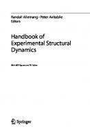
Mathematical theory of nonlinear vibration was developed towards the end of last century [1.6]. Duffing and Van der Pol were the first to propose definite solutions in nonlinear vibrations. Taylor introduced the concept of correlation function in 1920 and Wiener and Khinchin the spectral density in 1930s [ I. 7, 1.8]. These opened new vistas for laying down the theory of random vibrations [1.9-1.12]. A number of monographs on the topic are now available. Vibrations and structural dynamics have made rapid strides in last few decades. The advent of computer has brought in a revolution in this area like many others. As a result of which new numerical techniques have been developed, out of which the finite element method has proved to be most versatile [1.13]. These newly developed methods of analysis permits the structural analyst to formulate the increasingly complex problems [1.13]. 1.3 COMPARISON BETWEEN STATIC AND DYNAMIC ANALYSIS The prime difference between static and dynamic analysis lies in the interpretation of the load considered. Dynamic means time-varying. As such, time is the additional parameter in the dynamic analysis. What is the difference between the two regarding the interpretation of forces? A block resting on the ground is shown in Fig.I.I. The ground reactions can be evaluated for the following conditions from elementary knowledge of statics: (a) (b) (c)
When the block is at rest, When the block is on the verge of incipient motion, When it is moving with a uniform velocity.
w
Fig. 1.1. A block resting on the ground.
The forces that may arise in the above three conditions have been indicated in Fig. l. l. If the block now starts moving with acceleration a, then it will experience an inertia force which is equal to mass times acceleration. By applying Newton's second law, one obtains P-R=ma (1.1)
Introduction
5
It is the acceleration of the body which converts the problem into a dynamic one.
1.4 D'ALEMBERT'S PRINCIPLE The above example of the accelerating body can be considered as an equilibrium problem. The state of equilibrium is referred to as dynamic equilibrium. The principle .that is adopted for its solution is known as D'Alembert's principle. Equation ( 1.1) is rewritten in the following form
P-R-ma = 0 Equation (1.2) can be conceived as an equation of equilibrium, i.e.
(1.2)
L Fx = 0
which means that in addition to the real forces acting on the body, a fictitious force -ma acting opposite to the line and direction of motion is considered (Fig. 1.2), ma
w
P----•
Fig. 1.2. Application of D'Alembert's principle.
For the solution of problems of dynamics, the inertia force, which is mass times the acceleration opposite to the direction of motion is to be incorporated in the freebody diagram in addition to all impressed forces. This is known as D'Alembert's principle. Structural dynamics and machine vibrations have their basic input to the fundamental theory of vibration. To start with, let us look into some basic definitions. 1.5 SOME BASIC DEFINITIONS When an elastic system is acted upon by an externally applied disturbance, it will respond by oscillating to and fro. 1.5.1 Vibration and Oscillation
If the motion of the body is oscillating or reciprocating in character, it is called vibration if it involves deformation of the body. In case the reciprocating motion involves only the rigid body movement without involving its deformation, then it is called oscillation. The motion of a pendulum is simple
6
Vibration, Dynamics and Structural Systems
harmonic oscillation and so is the case of a ship if considered as a rigid body moving over waves. 1.5.2 Free Vibration Vibration of an elastic system may be initiated by the application of the external force, which may subsequently be withdrawn. The resulting vibration, where no external force is present is referred to as free vibration. 1.5.3 Forced Vibration
If the external force is considered to be operative during the vibratory motion of the body, such a motion is referred to as forced vibration. 1.5.4 Damping For all practical structures, resistance is encountered during vibration. As a result of which, the amplitude will not remain constant, but will gradually go on reducing with time in case of free vibration, till a time will come when all the motion will be damped out. Damping forces may depend on the vibrating system, as also on factors outside it. Damping in a system arises due to the internal friction of the material, or due to drag effects of surrounding air or other fluids, in which a structure is immersed. The exact representation of them involves difficulties. However, as to its nature, damping is of following four types: (a)
Structural damping,
(b)
Viscous damping,
(c) (d)
Coulomb damping, and Negative damping.
Structural damping is due to the internal molecular friction of the material of the structure, or due to the connections inherent in a structural system. Viscous damping occurs in a system vibrating in a fluid. The damping force in this case is proportional to the velocity and is given by F0
where
x=velocity =
=ex
(l.3)
dx and c is the damping constant. dt
Coulomb damping, also known as dry friction, occurs when the motion of the body is on a dry surface. The damping force is given by F0
=µ N
(l.4)
where µ is the coefficient of kinematic friction and N is the normal pressure of the moving body on the surface.
Introduction
1
Negative damping is a very special case, when the system is such that damping adds energy to the system instead of it being dissipated. As such, amplitude increases progressively in such cases. It occurs in the wires of transmission line tower. In this book, damping will be considered to be of viscous type unless otherwise specified.
1.5 .5 Degrees of Freedom Any mass can undergo six possible displacements in space - three translations and three rotations (about an orthogonal axis system). However, it happens with most systems that they are allowed to move in certain directions, while their movements in other directions are constrained. The minimum number of coordinate systems required to indicate the position of the mass at any instant of time is referred to as the degrees of freedom. A cantilever column with a concentrated weight at the top is shown in Fig. 1.3. If one is interested in studying the axial vibration, then one coordinate in the y-direction is sufficient to describe the motion. The system then has a single degree of freedom. If one is interested only in the flexural vibration of the structure, then the x-coordinate displacement describes the motion and the system still is of single degree of freedom. But if one intends to study the axial and flexural vibration in a combined manner, then the problem at hand becomes a two-degree of freedom system (the x and y displacements of the mass). Depending on the independent coordinates required to describe the motion, the vibratory system is divided into the following categories: (a)
Single degree of freedom system (SDF system),
(b) (c)
Multiple degrees of freedom system (MDF system), Continuous system.
yt I
-x
weight
Fig. 1.3. A cantilever column with a concentrated weight at the top.
If a single coordinate is sufficient to define at any time the position of any point in the system, it is referred to as a single degree of freedom system (Fig. 1.4).
8
Vibration, Dynamics and Structural Systems
( a)
( b)
Fig. 1.4. Single degree of freedom system.
m4 m3 m m,
7
\ ;,
. - _____ . ._
I
....
I
I
I.,,. ,, ✓
/ I
BEAM MODEL
( b)
( C)
Fig. 1.5 Multiple degrees of freedom system
Fig. 1.6 A continuous system
If more than one independent coordinate is required to define at any instant the position of different points in the system, it is referred to as multiple degrees of freedom system. A few examples of multiple degrees of freedom system have been shown in Fig. 1.5. If a system requires three independent coordinates as shown in Fig. l.5(a) and l.5(d), it is called three degrees of freedom system. The mass of a system, such as the beam of Fig. 1.6 may be considered to be distributed over its length, in which case the mass is considered to have infinite degrees of freedom. Such a system is referred to as a continuous system.
Introduction
9
1.6 DYNAMIC LOADING Dynamic load is that in which its magnitude, direction or position vary with time. Almost all structures are subjected to dynamic load sometime or other during its lifespan. They are the result of various manmade and natural causes. The particulars of the load with time vary for different sources from which they are generated. Some common types of influences resulting in the disturbance are due to initial conditions, applied actions and support motions. A few cases of dynamic loads acting on different systems are shown in Fig. 1. 7. In general the deterministic loading that act on different systems can be divided into two basic categories: periodic and nonperiodic. In periodic loading the variation of the load is same in each cycle. The simplest periodic loading is a simple harmonic motion. For the rotor, the reciprocating engine and the ship of Fig. l. 7, the dynamic load is periodic. The form of periodic loading varies from simple sine or cosine curves to more complex shapes. The bridge, the frame, the offshore tower and the building of Fig. 1. 7 are subjected to non periodic loading.
(e) BLAST
LOADING ON FRAME
(a) ROTOR MOUNTED ON A BED PLATE
:T, ':A
(b) VEHICULAR A BRIDGE
LOAD OVER
~~F(t)
(1) WAVE LOADING ON OFFSHORE TOWER
t
(c) RECIPROCATING
ENGINE
-\---..______7
c:::J
c::::J
t::]
c::::J
c:::J
c::::J
(g) EARTH~UA~E FORCES ON BUILDING
(d) PROPELLER FORCES AT THE STERN
Fig. 1.7 Dynamic loads on different systems
10
Vibration, Dynamics and Structural Systems
Again, the form of the loading for these cases varies. The blast loading of Fig. l. 7 (e) is of short duration, whereas the wave and earthquake loading of Fig. 1.7 (0 and 1.7 (g) are having a much longer tenure. Due to the characteristics of these loadings, the mathematical treatment is different for different cases. 1.7 FINITE ELEMENT DISCRETIZATION One of the initial steps to be followed in the finite element analysis is the discretization of the model. For framed structure the discretization is obvious, as one member is considered at a time which is the discrete element. However, for the sake of analysis, the joint may be artificially created by considering a joint at any point of the member. The tapered beam of Fig.1.8 is divided into four elements. Fig. 1.8 shows the beam consisting of four elements and 5 joints. A joint or a node is defined as the intersection of two or more elements, a support point or a free end. For the analysis of one-dimensional structures, the choice of the element is obvious in many cases. For example, the portal frame of Fig. l.9 has 3 elements and 4 joints/nodes. In this case the choice of the element is obvious, as each member (naturally occurring) is considered as an element.
• 2
3
5
4
Fig. 1.8 A tapered beam with elements
2
'3
0
CD 4
Fig. 1. 9 A portal frame
Introduction 11
Fig. 1.10 (a) A discretized plate
Fig. 1.10 (b) Discretized ship
When we focus our attention to two and three-dimensional structures such as plates and shells we immediately face difficulty with the choice of discretization, as no obvious choice exists. In such cases, like conventional onedimensional structures which are considered as an assemblage of structural elements interconnected at their intersections, the continuum is assumed to consist of imaginary divisions. Thus the real continuum is divided into a finite number of discrete elements as shown in Fig 1. IO. The continuum is considered as an assemblage of these 'finite elements'. 1.8 RESPONSE OF THE SYSTEM The dynamic load applied to the system not only p.-oduces certain motions, but also cause certain associated stresses, strains, reactions, etc. The term response of a system indicates any of the above effects produced by the dynamic load. More commonly, however, the dynamic response indicates the displacement time history. 1.9 TYPES OF ANALYSIS Dynamic load being defined as a time varying load, the structural response to dynamic loading is also time varying or dynamic. For the evaluation of the response due to the dynamic load, there are basically two different approaches: deterministic and random.
12
Vibration, Dynamics and Structural Systems
If the records of the dynamic load and the corresponding responses are taken many times under identical conditions, and both the records obtained are alike in all cases, then the vibration is said to be deterministic. In this, the analyst has perfect control over all the variables related to the problem. If the records of the dynamic load and the corresponding responses are taken many times, when all other conditions under the control are maintained the same, but the records are found to differ continually from each other, then the vibration is said to be random. This unpredictability associated with the input and output of the problem is referred to as randomness. The degree of randomness depends on the understanding of the effects of different parameters involved and the ability to control them. Chapter 15 of the book deals with random vibration, whereas the treatment in other remaining chapters are deterministic vibration.
I. IO LINEAR AND NONLINEAR VIBRATION If the basic components associated with the vibration analysis, such as the spring, mass and the damper behave linearly, then the emanated vibration is referred to as linear vibration. In this case the differential equation of motion is linear. On the other hand if one or more of the basic components behave in a nonlinear manner, the resulting vibration is said to be nonlinear vibration. In this case the analyst·will have to deal with nonlinear differential equation of motion. It may be mentioned that the linear analysis of vibration is more straight forward, whereas the nonlinear analysis of vibration is more mathematically involved.
References 1.1
M. R. Cohen and I. E. Drabkin, A Source Book on Greek Science, Harvard University Press, Cambridge, 1958
1.2
A. D. Dimarogonas, The origins of vibration theory, Journal of Sound and Vibration, V. 140, No. 2, 1993, pp. 181-189
M. G. Evans, The Physical Philosophy of Aristotle, The University of New Mexico Press, Albuquerque, 1964 1.4 S. P. Timoshenko, History of Strength of Materials, McGraw-Hill, New York 1953 1.5 J. W. Strutt [Lord Rayleigh], The Theory of Sound, Dover, 1945. 1.6 F. Dinca and C. Theodosin, Nonlinear and Random Vibration, Academic Press Inc., 1973.
1.3
Introduction 13
1.7 1.8 1.9
S. H. Crandall and W. D. Mark, Random Vibration in Mechanical Systems, Academic Press, New York, 1963. J. D. Robson, Random Vibration, Edinburgh University Press, Edinburgh, U. K., 1964. D. E. Newland, An Introduction to Random Vibrations and Spectral Analysis, Longman, London, 1975.
1.10 R.W.Clough and J. Penzien, Dynamics of Structures, McGraw-Hill Inc., 1993 1.1 I S.O. Rice, Mathematical Analysis of Random Noise, Dover Publications, New York, 1954 1.12 J.S. Bendat, Principles and Applications for Random Noise Theory, John Wiley & Sons, New York, 1966 1.13 0. C. Zienkiewiez and R.L. Taylor, The Finite Element Method, Vol I & Vol II, Fourth Edition, McGraw-Hill Book Company, UK, 1989 1.14 L. Meirovitch, Computational Methods in Structural Dynamics, Sijthoff and Nordhoff, The Netherlands, 1980
CHAPTER2
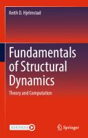
FREE VIBRATION OF SINGLE DEGREE OF FREEDOM SYSTEM 2.1 INTRODUCTION The simplest physical system is one having single degree of freedom. Almost all practical systems are much more complex than this simple model. However, for obtaining an approximate idea about vibration characteristics, some of the systems are at times reduced to that of a single degree of freedom, such as the water tower of Fig. 2. 1.
(a)WATER TOWER
(b)SIMPLIFIED TOWER
Fig. 2. 1. A water tower model
In some cases such as seismic instruments, this model is sufficient for the necessary study. Single degree of freedom systems may be translational or rotational. The rotational problems related to the torsional vibration of elastic systems are of considerable importance. In this chapter, we shall deal with free vibrations of these systems, whose motion can be described by a single coordinate [2.1 - 2.10]. 2.2 EQUATION OF MOTION OF SINGLE DEGREE OF FREEDOM (SDF) SYSTEM Consider the single bay portal frame of Fig. 2.2. The masses of the columns are considered to be small in comparison to the mass of the girder, and they are
Free Vibration Analysis of Single Degree of Freedom System
mass, m
1===:;:::=====1- ex te rna I
15
1orce
external 1orce lne,rtia force -
,L
re storing 1orce damping 1orce
(b) FREE BODY DIAGRAM
dashpot, damping constant., C (a) A RIGID FRAME
Fig. 2.2. A portal frame and its free body diagram
neglected in the analysis. Further, the girder is assumed to be infinitely rigid, so that the stiffness of the system is provided only by columns. The entire motion may be determined once the mass centre of the girder is known. When the frame vibrates in the horizontal direction, the forces associated with the motion are the inertia forces connected with the mass of the body, the restoring force provided by spring elements (the spring constant can be determined from the properties of the column and the boundary conditions), the damping force provided by the damper and the external force. A machine mounted on a spring is shown in Fig. 2.3. The damping in the system is indicated by the dashpot. When the machine undergoes vertical motion, the forces acting on its mass are indicated in Fig. 2.3(b). Again in the machine, the forces that act are the inertia force, the spring force, the damping force and the external force. From the above examples it is seen, that for studying the vibration of any system, the following are the four elements of importance: (a) (b) (c) (d)
The inertia force, The damping force, The restoring force, and, The exciting force.
If the external force is zero, the resulting vibration is called the free vibration. In such cases, if damping is present in the system, it is called free damped vibration and if damping is absent in the system, it is called free undamped vibration. The two systems mentioned above, can be idealised in the form of springmass system as shown in Fig. 2.4. All structures can be reduced to systems consisting of combinations of springs, masses and dashpots and is an idealisation in a convenient form of the actual structure.
16
Vibration, Dynamics and Structural Systems
external 1orce
external force
t
t
___,__1
----.y
l
mass, m
Spring elements, sti11nus K L~'----t--~
inertia 1orce Spring 1orc e Damping 1orce Dash pot, damping coe11icient c
I
! (b) FREE BODY
DIAGRAM
(a) MACHINE
Fig. 2.3. A spring mounted machine and its freebody
-
F(t)
m
X
(a) SPRING MASS SYSTEM -F(tl Restoring 1orce::kx
Inertia 1orce::mx
Damping 1orce:: ex
(bl FREE BODY DIAGRAM
Fig. 2.4. A spring-mass- dashpot system
The only independent coordinate of the spring-mass system of Fig. 2.4 is the x-directional translation and the displacement will simply be given by x,
"l/
2X]
dx) and accelerat10n . . x = dt) x··[ = ddt 2 ve Ioc1ty
•
The mert1a . . "1orce of th e mass 1s .
mx , the damping force is ex and the spring force is kx. The external force acting on the system is F(t). Applying D'Alembert's principle and considering equilibrium of all the forces in the x-direction, the general equation of motion for the SDF system is mx+cx+kx=F(t)
(2.1)
Free Vibration Analysis of Single Degree of Freedom System
17
The solution of Eq. (2. 1) gives the response of the mass to the applied force in the SDF system. 2.3 FREE UNDAMPED VIBRATION OF THE SDF SYSTEM When the case of free undamped vibration is considered, F (t)
=0
and
c = 0 in Eq. (2. 1) and the resulting equation becomes
or
mi+kx=O
(2.2)
x+ p 2 x=O
(2.3)
2 k p =-
where
m
The solution of Eq. (2.3) is assumed as follows (2.4)
x= Ae;. 1
Substituting x and its derivatives from Eq. (2.4) to Eq. (2.3), yields
A.?..2 e;. 1 + p 2 Ae;. 1 = 0 ;t =±ip
or The solution of Eq. (2.3) then is
x=A1eip1 +A2e-ip1
or
x
= A 1 (cos pt+ i sin pt)+ A 2 (cos pt -
i sin pt)
(2.5)
Rearranging the terms of Eq. (2.5), yields x = C 1 cos pt+ C 2 sin pt
(2.6)
where C 1 and C 2 are constants. The factors cos pt and sin pt are periodic functions. As such the motion is periodic and it repeats itself after a certain interval of time. pT = 2n , then Since
T= 2;=2nf¥
(2.7)
This time interval T is called the period of undamped free vibration. The number of times that the motion repeats itself in one second is called natural frequency of vibration f f
=~
= 2~ ~:
(2.8)
18
Vibration, Dynamics and Structural Systems
The parameter p can now be given a physical significance, since
2n p=-=2nf
(2.9)
T
p is called the circular or angular frequency of vibration. The vibratory motion represented by Eq. (2.6) is a harmonic motion. The constants C 1 and C 2 can be determined from the initial conditions of the motion.
If at t
= 0, x = x 0
and
x= x0 , then applying the initial conditions (2.10)
Therefore, the equation of motion becomes .
Xo
x = x 0 cos pt+ Assuming, x 0
= AcosE and x
Xo p
(2.11)
smpt
p
. = AsrnE,
Eq. (2.11) becomes
= AcosE cos pt+ AsinE sin pt (2.12)
x=Acos(pt-E) By squaring and adding the assumed values of x 0 and 2
x0
it can be shown that
·2
Xo
A= x 0 + P2
(2.13)
Thus, the resulting motion is simple harmonic, having an amplitude A and phase difference E. It has been shown graphically in Fig. 2.5. X
Fig. 2.5. Simple harmonic motion
Free Vibration Analysis of Single Degree of Freedom System
19
Similarly, the phase difference e is given by tane =___:Q_
(2.14)
PXo
Example 2.1
A weight W = 15 N is vertically suspended by a spring of stiffness k N/mm. Determine the natural frequency of free vibration of the weight.
I j,
ce-L -.r-
=2
K(yst .. y)
- - - - . - - 1Y,t
(bl
(o)
y STATIC
1
EQ.UUBRIUM
1ir--Posir~-.---
(c)
Fig. 2.6. Example 2.1 A vertically suspended weight W attached to a spring of stiffness k is shown in Fig. 2.6. Due to the application of the weight W, the spring will have vertical deflection, which is given by
w
Yst
=k
(2.15)
The spring will vibrate about its mean position, which is the static equilibrium position. The freebody diagram of the weight, when it is displaced by y during free vibration is shown in Fig. 2.6(c). Applying D'Alembert's principle, one gets
W y+k(ys1 +y)-W=O g
(2.16)
Substituting Ysr from Eq. (2.15) to Eq. (2.16), we get
W y+W+ky-W=O g
or
w .. ky = 0 -y+ g
(2.17)
or
y+p2y=O
(2.18)
where
2 kg p=-
w
20
Vibration, Dynamics and Structural Systems
The natural frequency is given by f=..f!_=_l
211:
{kg"
(2.19)
211:fw
Substituting y sr from Eq. (2.15) into Eq. (2.19), we get
/=2~!-f
(2.20)
Putting the numerical values of Wand k, we get f
=-1 ✓ 2x9810 =5.51 27t
15
Hz (cycles/s)
Example 2.2
A mass mis attached to the midpoint of a beam of length L (Fig. 2.7). The mass of the beam is small in comparison to m. Determine the spring constant and the frequency of the free vibration of the beam in the vertical direction. The beam has a uniform flexural rigidity El. The deflection at the centre of a simply supported uniform beam of length L and flexural rigidity El subjected to a load P at midspan is given by PL3 8=-48£1
L/2
L/2
Fig. 2.7. Example 2.2 Therefore, from definition, the stiffness which 1s the force required to produce unit displacement, becomes k
= P = 48El 8
L3
The natural frequency of the massless beam is given by f =-1 =-1 ✓ 48El 2n v--;;; 2n mL3
/k
Free Vibration Analysis of Single Degree of Freedom System
21
Example 2.3
Calculate the natural angular frequency in sidesway for the frame of Fig. 2.8 and also the natural period of vibration. If the initial displacement is 25 mm and the initial velocity is 25 mm/s, what is the amplitude and displacement at t = ls? If the horizontal deflection is o at the top of a member fixed at both ends, then the moments and forces developed at the supports is shown in Fig. 2.8{b). For such a member, the stiffness is 12E/ / L3 for a unit displacement at the top support. For the frame of Fig. 2.8(a), there are two vertical columns connected by a rigid beam. The freebody diagram of the beam with restoring forces is shown in Fig. 2.8(c).
Total restoring force in the columns = (KAB + Kev) x. The stiffnesses of two columns AB and CD in this case can be conceived as two springs connected in parallel. The equivalent stiffness in the columns therefore, is = 12(El)AB + 12(E/)cv
k eq
L3
AB
L3
CD
where LAB and Lev are the lengths of the members AB and CD. Putting the numerical values k
eq
12x30xl0 12 12x30x 10 12 =----+----=1,063,125 N/mm (1000) 3 (800) 3
Therefore, the natural angular frequency is given by p = ✓ keq = m
1063125x9810 = 18 _645 rad/s 30xl0 6
The time period is given by
2n
2n
T=-=--=0.337 s p 18.645 The system can be idealised into a spring-mass system and the equation of motion is given by Eq. (2.11 ).
xo sm. pt
x = x 0 cos pt + -
p
= 25 cos 18.645 t + ~ sin 18.645t 18.645 = A cos(l8.645t -e)
22
Vibration, Dynamics and Structural Systems
8
w:: JOx106t.i
C
(al
1'ZE16
7-..J
12El6
~ 6El6 -2-
7--
( b) L
Fig. 2.8. Example 2.3
where
A= (25) 2 + ( -25- ) 18.645
2
= 25.04 mm
The amplitude, of the motion is 25.04 mm E =
tan-I Xo
= tan - 1
PXo
[Eq. (2.14)]
25 = 0.054 rad 18.645x 25
At t = ls, the displacement is given by X
=25.04 COS (18.645 -
0.054) = 24.21 mm
Example 2.4
A multibay bent is shown in Fig. 2.9, where the girder is considered to be infinitely stiff and the uniform columns are assumed to have negligible mass in comparison to total mass M of the girder. Determine the period of free horizontal vibration.
Free Vibration Analysis of Single Degree of Freedom System
Tot.al mass= M
rLi
3El6
L2 ' \
B 0
0
in
El
F
D
-:
23
~ I
El
I I
3El6 -3-
El
0
'°
C
I
L El
I I I
I
I
L
I
A
(a)
(b)
E
Fig. 2.9. Example 2.4
Like the previous example, the equivalent stiffness of the columns is to be determined first. The columns CD and EF have one end hinged and the other end fixed. For such cases, the stiffness for a unit displacement at the top is 3El I L3 , where L is the length of the member. Therefore, the equivalent stiffness of the columns is
The period of free horizontal vibration then is
/M
T = 21r /,;- = 21r ~keq
Ma3
ffa3
- - - = 15.86 -_0.157El El
Example 2.5
Find the natural frequency of the system shown in Fig. 2.10. The mass of the beam is negligible in comparison to the suspended mass. E=2.lx10 5 N/mm In addition to the flexible beam which provides a spring action, there is a spring attached to the mass. In this the deformation of the central mass is equal to the sum of the deformations of the beam at the centre and the attached spring. The beam can be replaced by a spring k1 of stiffness 48El I L3 , where El is the flexural rigidity of the beam and L, its length. Two springs in this case is said to be connected in series (Fig. 2.lO(c)), which can be replaced by an equivalent spring having stiffness keq . Due to a unit force, the deformation in both the cases will be identical. For the equivalent spring. the deformation due
24
Vibration, Dynami.:s and Structural Systems
to unit force is 1I keq and for the two springs, they are 1/ k1 and 1/ k 2 . Therefore
1
1
1
keq
k1
k2
-=-+-
=
k
or
eq .. 3000mm • 1
k1 k2 k1 + k2
I
6000mm (a)
~□
µ00mnJ
(b) Cross-
section
~:40N/m
~
(d) Equivalent
( c)
system
Fig. 2.10. Example 2.5
Substituting numerical values for the problem
I = __.!__ X (100) (150) 3 = 28,125,000 mm 4 12 k = 48x2.lxl0 5 x28125000 =l3l 2 _5 N/mm I
k eq
(6000) 3
= 1312.5x40 =38.82N/mm 1312.5 + 40
The natural frequency of the system is
f =-1 ~keq =-1 2n m 21r
38.82x9810 = 2 1.962 Hz 20
Example 2.6
A mass m1 hangs from a spring having stiffness k. A second mass m2 drops through a height h and sticks to mass m1 without rebound (Fig. 2.11). Determine the subsequent motion.
Free Vibration Analysis of Single Degree of Freedom System
m1
!.___ _.,jStatic eqlJilibri um T rY,
mass m1
25
of
ml ----.static equilibrium of
Fig. 2.11. Example 2.6 The velocity of mass m2 just before impact is given by
vi= 2gh Applying the principle of conservation of momentum, if
y0 is the initial
velocity of the combined mass (m 1 + m 2 ) , then (m1 + mz) Yo
or
= m2 V2
. m2·/iih
Yo=
m1 + m2
After impact, the combined mass (m 1 + m 2 ) will vibrate about the static equilibrium position of (m 1 + m 2 ) . At the instant of impact, the mass m1 is at its static equilibrium position. Therefore, the initial displacement is equal to the distance between static equilibrium position of mass (m 1 + m 2 ) and the static equilibrium position of mass m1 alone. Thus
The minus sign has been put in the above expression, as the initial displacement is in the negative direction. Therefore, the equation of motion is given by (Eq. 2.11)
Yo sm . pt
y = Yo cos pt + -
Now
p
26
Vibration, Dynamics and Structural Systems
Substitution of the values of y0 , j, 0 and p in the above equation, we get
If the above equation is to be expressed with reference to the static equilibrium position of mass m1 , then a shift of axis is needed and the resulting equation becomes
2.4 FREE DAMPED VIBRATION OF SDF SYSTEM From Eq. (2.1 ), it follows that the equation of motion for free vibration for a damped SDF system is (2.21)
mx+cx+kx=O
Equation (2.21) is a linear differential equation of second order and can be solved by using standard procedure. The general solution of the equation can be assumed in the following form
x
= Ae"'
(2.22)
Substituting x and its time derivatives from Eq.(2.22) into Eq.(2.21) and rearranging the terms, we get
AJ.2 e"' + ~ Ak;. 1 + ~ Ae;. 1 = 0 m m or where
J.2 + 2nJ. + p 2 = 0 C
.
2
(2.23)
k
n = - and p = -
2m
m
Equation (2.23) is a quadratic equation and its solution is given by (2.24) Relative values of n and p will govern the resulting solution. Three cases may arise and they are discussed below one after another.
Free Vibration Analysis of Single Degree of Freedom System
27
Case I. Overdamped system (n > p)
Roots A.1 and A. 2 of Eq.(2.24) are real and negative when n is greater than p. The solution of the equation is x = A1eAi 1
+ A2 e,½r
(2.25)
The solution is shown graphically in Fig. 2.12. The solution does not contain any periodicity; as such it does not represent a vibratory motion. The roots of Eq. (2.24) are unequal and two terms on the right hand side represt;nt motions which decay exponentially at two different rates. The motion associated with root ,1.1 predominates only for a short time, which however goes on decreasing in an exponential manner with time. In this case, the viscous resistance of the body is so large that when it is displaced from the equilibrium position, it only creeps back to that position. The displacement finally vanishes as t approaches infinity. This system is known as overdamped system. Case II. Critically damped system (n = p)
When n = p, roots A.1 and A.2 of Eq. (2.24) are real, negative and equal, that is, repeating.
Fig. 2.12. Overdamped motion The solution of Eq. (2.21) is (2.26) where A. 1 = A. 2
=A .
The displacement of the mass reaches zero asymtotically with time for this case, as shown in Fig. 2.13. The damping in the system is great enough not to set up oscillatory motion. The system is known as critically damped system. At critical damping, damping coefficient c is given by C
= 2mp
(2.27)
28
Vibration, Dynamics and Structural Systems
X
Fig. 2.13. Critically damped motion
The damping coefficient in other cases is expressed in terms of a certain percentage of critical damping. For a structure having 10 percent of critical damping, it will have a damping coefficient c given by c =(0.1) 2mp =0.2 mp
(2.28)
Case Ill. Underdamped or Damped system (n < p) Roots
.11-1
and
.11- 2
are complex when n is less than p, and they are given by A.· 1, 2
= - n +. _ 1 vIp 2 -
n2
(2.29)
The solution of Eq. (2.21) will be
(2.30)
or
x
. 122
= A 1e -nt e •,JP- -n- t
. 122 + A e -nt e -•,JP-n-1 2
or or
x=e-n'( C cos'1p 1
2
-n 2 t+C 2
sin.Jp 2 -n 2 r)
(2.31)
where C 1 and C 2 are constants, which can be determined from initial conditions. This system is known as underdamped or simply damped system of vibration.
If at t
= 0, x == x 0
and
x= x0 , then putting these conditions in Eq. (2.31 ), we get
Free Vibration Analysis of Single Degree of Freedom System
x=e-n'[xo cos v,p
2
,p
-n 2 t+ nxo / 2 +xo2 sin V -n
vP
2
-n 2
tl
29
(2.32)
The variation of the displacement of the damped system with time given by Eq. (2.32) is shown in Fig. 2.14. The amplitude of vibration goes on decreasing in an exponential manner - the reduction in magnitude for each successive cycle gives a measure of the damping in the system. As can be seen from Eq.(2.32), the damped frequency of vibration is given by (2.33)
Fig. 2.14. Damped motion
Time period for damped free vibration is T _ d -
2n
(2.34)
-Jp2-n2
Equation (2.34) reveals that the damped time period is more than the undamped time period, but n is usually a small quantity in comparison top. This increase is a small quantity of second order. Therefore, for all practical purposes, it can be assumed with sufficient accuracy that a small viscous damping does not affect the period of vibration. Timewise variation of the displacement for different systems have been shown in Fig. 2.15, so that a relative idea of the displacements in different cases can be obtained.
30
Vibration, Dynamics and Structural Systems
Example 2.7
A mass l kg is attached to the end of a spring with a stiffness 0. 7 KN/111.m. Determine the critical damping coefficient. The stiffness of the spring is k = 0.7 KN/mm= 700 N/mm. The natural angular frequency is
p=
/k = vfioo v-;;; 1-1- = 26.46 rad/s
At critical damping
n=p ~=26.46 2m c = 26.46 x 2 x l = 52.92 Ns/m
or or Displacement X
Fig. 2.15. All possible SDF systems
Example 2.8 A mass, spring and dashpot attached to a rigid bar is shown in Fig. 2.16. Write the equation of motion. Determine the natural frequency of damped free oscillation and critical damping coefficient. b
a
•1
l
K
(a)
l>',
~BC
( b)
t I
Fig. 2.16. Example 2.8
(c)
Free Vibration Analysis of Single Degree of Freedom System
31
The bar AC being rigid, the point B where the mass and the dashpot is attached and the end C where the spring is attached will undergo different displacements and they are related. From similar triangles, it can be shown that b Y1 =-y
a During oscillation, the forces acting on the system are the inertia force
(a)
my , the
damping force cy and the spring force ky 1 • Taking moment about A [Fig. 2.16(c)], yields
m_ya + cya + ky 1b = 0
(b)
Substituting y 1 from Eq. (a) into Eq. (b), we get
my+ cy + k(!!..
r
a;
=0
y
(c)
Equation (c) can be written as follows
y + 2ny + p 2 y = 0 where
n = _!:_ and p 2 2m
(d)
=!:.._(!!..)2 m a
Equation (c) is of the same form as Eq. (2.21), except that k is replaced by
k ( !!..)2 \, a The natural frequency of damped oscillation is
At critical damping n=p
_:_=!!.. /k
or
2m
a
v;;;
or
Example 2.9 A piston of mass 5 kg is travelling inside a cylinder with a velocity of 15
mis and engages a spring and damper as shown in Fig. 2. 17. Determine the maximum displacement of the piston after engaging the spring-damper.
32
Vibration, Dynamics and Structural Systems
How many seconds does it take? The mass has an initial velocity. Referring to Eq. (2.32) C 175 n=-=--=17.5 2m 2x5
p=
ff
=
✓ 3~
= 24.295 rad/s
The displacement of the spring is given by x
= e -nr ( C1 cos.J p 2 -
t
n 2 + C 2 sin .J p 2
-
n2
t)
15m/sec
m:Skg
C:175Nsec/m
Fig. 2.17. Example 2.9
The velocity is given by
x=-ne-n 1 ( C1 cos ✓p 2 -n 2 t +C 2 sin.Jp 2 -n 2
t)
+ exp(-nt).Jp 2 -n 2 (-C 1 sin.Jp 2 -n 2 t+C 2 cos.Jp 2 -n 2 t) At t = 0, x = 0 and
x = 15
Putting these initial conditions in the above expressions for velocity and displacement, yields C1 = 0 and
C2
= 0.875
Therefore, the expression for displacement reduces to x = 0.815e-n 1 sin.J p 2 - n 2 t
Maximum displacement will occur when t = T 4 t = 0.045 s
Free Vibration Analysis of Single Degree of Freedom System
33
The maximum displacement is x
=0.875 e- 17 -5 xo.04s sin(17.85 x0.045) =0.277 m
2.5 FREE VIBRATION WITH COULOMB DAMPING So far we have considered viscous damping. However, the damping resulting from the friction of two dry surfaces gives constant damping force and the resulting damping is referred to as Coulomb or dry friction damping. A practical example of it is the friction of two dry surfaces as occurs in riveted joints.
A SDF system with Coulomb friction is shown in Fig. 2.18. The damping force FO is equal to the product of the normal force N and the coefficient of friction µ and is independent of the velocity. For a single degree of freedom system, the equation of motion will be (2.35)
mx+kx±F0 =0
~ mx
Fo fN ( b)
( a)
Fig. 2.18. Coulomb damping
The ± sign is arising due to the fact that the damping force is always opposite to that of the velocity and in the differential equation of motion, each sign is valid for half-cycle intervals. Or in other words
mx + F O + kx mx - FO + kx
o}
(2.36)
FO sgn (.i) / k
(2.37)
=0 =0
for for
.i > .i < 0
The solution ofEq. (2.35) is x
where p 2
k
=-
m
= A cos pt + B sin pt -
and A and Bare constants.
34
Vibration, Dynamics and Structural Systems
If ac t
= 0, x = x 0
and
x= 0
then
A= x 0
-
Fo sgn (x) and B = 0 k
On substitution of the values of A and B, Eq. (2.37) becomes
x=[x0
Fo sgn(x)lcospt+ Fo sgn(x)
-
k
k
_J
(2.38)
For the first half-cycle (pt = n), the displacement is X
=-
Xo
+ 2 FD sgn (x) k
Hence, the decrease in amplitude is 2
F
____!!.._
k
per half-cycle.
(2.39) The amplitude
change per cycle for free vibration with Coulomb damping then is 4 FO It k may further be noted from Eq. (2.38), that the time period for the free vibration with Coulomb damping is same as the undamped case. The resulting motion is plotted in Fig. 2.19. A characteristic feature of the response is that, the amplitude decays in a linear manner and not exponentially as in the case of viscous damping.
Example 2.10 For the SDF system of Fig. 2.18, determine the coefficient of friction if a tensile force P( = mg) elongates the spring by 6 mm. The initial amplitude of x 0 = 600 mm reduces to 0.8 of its value after 20 cycles. The spring stiffness in given units is
p k=6 For a SDF system with Coulomb damping, the amplitude reduces in each cycle by 4Fo . k Therefore 20 X 4 FD = 600 X 0.2 k or
F0 k
=
120 80
Free Vibration Analysis of Single Degree of Freedom System
or
FD
120 120 P k =x80 80. 6
=-
P 4
1 P 4
= - =-
35
(P will be the normal reaction).
Therefore, the coefficient of friction is 1/4. The variation of the displacement is shown in Fig. 2.19.
Fig. 2.19. The variation of displacement
2.6 ENERGY METHOD AND FREE TORSIONAL VIBRATION Using the principle of conservation of energy, natural frequencies of vibrating systems can be conveniently determined. For a mechanical vibrating system, the energy is partly kinetic and partly potential. The kinetic energy TE is associated with the velocity of the mass and the potential energy U is due to the strain energy stored in the spring. Thus. TE + U ::: Total mechanical energy = constant
(2.40)
Therefore, the rate of change of energy is zero. Mathematically
!!:_ (TE + U) = 0 dt
(2.41)
The equation of motion of the spring-mass system of Fig. 1.4 can be derived from energy consideration. The kinetic energy of the mass is given by TE
= ½m.x 2
(2.42)
The potential energy of the system is due to strain energy stored in the spring (Fig. 2.20) and is given by
36
Vibration, Dynamics and Structural Systems
(2.43)
F
II
...u
~ OI
C
I,.
Q.
~ IQ.:~~~~~"-------1~X
x Spring displacement
Fig. 2.20. Force - displacement relation
Substituting Eqs. (2.42) and (2.43) into Eq. (2.41), we get
(.!. mi:2 + .!_2 k.x2) = O
!}___ dt 2
or
l 2... . 0 -m xx+-l k2 xx=
or
mx+kx=O
2
(2.44)
2
(2.45)
Equation (2.45) is same as Eq. (2.2). 2.6.1 Torsional Vibration of the SDF System Applying the above energy principle, the free vibration equation for the torsion of the shaft can be derived. A vertical shaft with a disc attached at its lower end is shown in Fig. 2.21. The mass moment of inertia of the shaft is neglected in the analysis. Let p be the mass density of the material, / P be the mass moment of inertia of the disc, D be the diameter of the disc, d be the diameter of the shaft, L be the length of the shaft, and t be the thickness of the disc, then 4W p=-nD2tg 4W nD 4 WD 2 Ip =pJ 0 · t = - - - • - - t = - n D 2 tg 32 8g
(2.46)
(2.47)
Free Vibration Analysis of Single Degree of Freedom System
37
Fig. 2.21. Torsional vibration where J0 is the polar moment of inertia of the disc. In free torsional vibration of the shaft, the spring stiffness is provided by the shaft and it is given by nd 4 G k=-32L
(2.48)
· where G is shear modulus of elasticity of the material of the shaft.
If (/J be the angular displacement at any instant of time, the kinetic energy of the system is (2.49) The corresponding potential energy, is nothing but the strain energy in the spring and is given by U=
f' kt/) d(/J = -21 kt/)
2
(2.50)
0
Substituting the values of TE and U from Eqs. (2.49) and (2.50) respectively into Eq. (2.41), we get
!!_ (]._ IP~ 2 + ]._ kl/) 2 ) dt
or
2
2
=0
lp(/J+k(/J=O
(2.51)
Equation (2.51) is the free torsional vibration equation of the shaft. Equation (2.51) is similar to Eq. (2.2), and its solution is given by (/J = 2 +c2,,02
Substituting the value of Yin Eq. (3.31), we get
(3.32)
Now
2
C
W
cw I k = cw I mp = 2 · - - = 2 · n Ip · w Ip= 2TJ' 2m p 2
Therefore, Eq. (3.32) becomes _Fr._o =
F0
✓ 1+(2TJ() 2 ✓ (1-TJ2)2
(3.33)
+( 2TJ02
The ratio of the transmitted force to the applied force Fr0 I F0 , is defined as the transmissibility. The plot of this ratio with varying ri for different values of~ has been shown in Fig. 3.11. One of the main concerns for a designer is the reduction of the force transmitted to the foundation, i.e. to isolate the vibration. Figure 3.11 indicates that all the curves cross at TJ = .fi, . The transmitted force
is greater than the applied force for TJ < .fi. and less than the applied force for
TJ > .fi. _Therefore, the reduction of the transmitted force may be accomplished by adjusting the stiffnesses, such that TJ > .fi..
72
Vibration, Dynamics and Structural Systems
2
.210 "- u.
fi
2
3
'1F
Fig. 3.11 Variation of _L with 1J
Fo
Machine
k
C
y50 sinc.,t
Foundation
Fig. 3.12 Machine with support motions
3.6.1 Transmissibility Due to Support Motions Let us consider the case of a machine vibrating due to movable support [Fig. 3.12] and the harmonic motion of the support is given by
Ys = Yso sinwt
(3.34)
The equation of motion of the machine of mass m is given by
my+cj,+ky=cj,s +kys
(3.35)
Assuming Ys, from Eq. (3.34) into Eq. (3.35), one obtains
my+ cy + ky = cy sow cos wt + ky sow sin Wt or
(3.36)
There is a phase lag a between support motion and the existing force vector, given by the right hand side of Eq. (3.36).
Forced Vibration of Single Degree of Freedom System
73
If the solution is assumed as y = Y sin (wt - ), then from Eq. (3.13)
y
J1+(":
r
[,-r:rr•r2-; :r Y,ok
or
--,================== mp2
(3.37)
or
In this case, YI y so the ratio of the mass displacement to support displacement is known as the transmissibility. Comparing Eq. (3.37) with Eq. (3.33), the transmissibility for both force and motion is identical. Example3.6
A vertical single-cylinder diesel engine, of 500 kg mass is mounted on springs with k = 200 kN/m and dampers with ~ = 0.2. The rotating parts are well balanced. The mass of the equivalent reciprocating parts is IO kg and the stroke is 200 mm. Find the dynamic amplitude of the vertical motion, the transmissibility and the force transmitted to the foundation, if engine is operated at 200 rpm. The magnitude of the unbalanced force is F0 = mew 2 200x2n 20'/r m= IOkg,e= IOOmm=0.1 mand w = - - - = - - rad/s 60 3
(20n)
Therefore, F0 =lOxO.lx - 3-
2
=438.65 N
k = 200,000 Nim C
= 2 X 500 X 0.2 X
200•OOOO = 4000 Nm/s 500
74
Vibration, Dynamics and Structural Systems
The dynamic amplitude is 438.65
Xmax
=--;::================
[200.~-IOf~)']' +( 2~)' 4~x
= 2.06 X 10 - 3 m
Natural frequency of the system is 200,000 = 20 rad/s 500
p=
r,
207! =-p =- =1.047 3x20 (J)
Transmissibility is given by Eq. (3.33) as
.J 1+ ( 2 X 0.2 X 1.047 ) 2 =--;::============== .J {1- 1.047 2 ) 2 + ( 2 X 0.2 X 1.047) 2 The force transmitted to the foundation is Fr= 2.523
43 8.65 = 1106.71 N. X
3.7 ENERGY DISSIPATION BY DAMPING We have seen in the earlier section that the amplitude of motion goes on reducing with each successive cycle in damped free vibration. This suggests the occurrence of a loss of energy. For viscous damping, the damping force is F0
=ex
(3.38)
Let us assume the displacement of the spring-mass system as
= A sin ( pt - E)
(3.39)
x = Ap cos ( pt - E)
(3.40)
dx= xdt
(3.41)
X
and the velocity is Further,
Forced Vibration of Single Degree of Freedom System
75
The energy dissipated by viscous damping in one such cycle is given by
f
Ed = F0 dx =
2ir p
2ir p
0
0
f (ex) dx = f (cx)xdt
2ir p
f
=
e · (Ap) 2 cos 2 (rot -e)
dt
0
or, We know that p
(3.42)
Ed =new A 2
ff
=
and e = 2(
..r,;;;;,. Substituting these values in Eq. (3.42)
yields (3.43)
>, O'I
'-
cu
C
UJ
A
X
Fig. 3.13 Energies in viscous damping
The energy dissipated is proportional to the square of the amplitude of motion (Fig. 3.13). If we consider the steady state of vibration with the external force F(t) = F 0 sin rot, then the input energy of the external force per cycle is 2ir p
Ee=fF(t)dx= fF(t)xdt 0
2ir
f [F p
=
0
sin rot ][pA cosro (pt -e) ]dt
0
=nF0 Asine
(3.44)
76
Vibration, Dynamics and Structural Systems
Thus, Eq. (3.44) reveals that the energy due to the external force is proportional to the displacement amplitude. Using Eq. (3.19), we can show that sin E
= 2( ( w ) Ak p
(3.45)
Fo
Combining Eqs. (3.44) and (3.45), we get
Ee= 2n( w kA 2 p
(3.46)
Eqs. (3.43) and (3.46) reveal that energy dissipation in steady-state vibration is due to various damping in steady-state vibration. The graphical representation of energy dissipation in viscous damping is performed as follows. The velocity of motion is expressed as X
= WA cos(w t -E) =±WA .J1-sin 2 (Wt-£) =±.JA 2 -x 2
(3.47)
The damping force is related to displacement x as follows
Fd = ex = ± cw .J A2 - x 2
(3.48)
Eq. (3.48) is rearranged as (3.49) Eq. (3.49) is represented by an ellipse shown in Fig. 3.14. The loop of the curve is known as hysteresis loop, the area inside gives an estimate of the dissipated energy.
A
(a)
(b)
Fig. 3.14 Hysteresis loop (a) viscous damper, (b) spring and viscous damper in parallel
Forced Vibration of Single Degree of Freedom System
77
It may be of some interest to investigate the total resisting force Fs +Fd =kx+cw.JA 2 -x 2
(3.50)
where Fs is the strain energy of the spring. The graphical representation ofEq. (3.50) is shown in Fig. 3.14(b). In this case the hysterisis loop gets rotated. From Eq. (3.50) it is evident that loop area is proportional to w, which suggests that the hysteresis loop will not be formed, instead a single-value curve will appear if the harmonic load is applied slowly enough (i.e., w =0 ). We now look into two measures of damping. Specific damping capacity and the specific damping factor. Specific damping capacity is defined as the energy loss per cycle, Ed divided by the peak potential energy U · (Ed IV) and
KA2 U=-. 2 The specific damping factor, also known as the loss factor or loss coefficient is defined as the damping energy loss per radian Ed /211: divided by the peak potential energy U, (3.51) These two measures of damping are useful in comparing damping capacity of materials. Example 3.7
Prove the following
From Eq. (3.43)
Therefore, Example3.8:
Prove the following relations
78
Vibration, Dynamics and Structural Systems
From the previous example, we have obtained
(o/J
Ed = 4ns p U
(a)
Now, the logarithmic decrement 8 is given by
8
=2n,
(b)
Combining Eqs. (a) and (b), we get
~=w(;)
3.8 EQUIVALENT VISCOUS DAMPING We have seen in Section 3.2 that the amplitude of vibration reduces due to the presence of damping and its major influence remains within the band 0.5 ::s; T/ ::s; 1.5 . At resonance, the damping considerably limits the amplitude of motion. For the condition of resonance (w Ip= 1), the amplitude given by Eq.(3.14) reduces to A= F0 2ks
= F0 p 2 = F0 k2m = F0 2knp
2kmcp
cp
(3.52)
In the above equation, concept of equivalent damping may be introduced to approximate the resonant amplitude. The equivalent damping Ceq can be obtained from Eq (3.42) by equating the energy dissipated by viscous damping to that of the actual damping force (will be of nonviscous type) undergoing harmonic motion
Ed
=n CeqPAz
where Ed is the value of the energy associated with the particular value of damping force. 3.8.1 Example 3.9 A mass moving through a fluid experiences a damping force that is proportional to the square of the velocity. Determine C eq for these forces acting on a system undergoing harmonic motion of amplitude A and co. Fine! also its resonant amplitude. Assuming harmonic motion, the time is measured from the position of largest negative displacement, the displacement is given by
Forced Vibration of Single Degree of Freedom System
79
x=-A cos wt The damping force is expressed as
Fd =±a, .x2 where negative sign is considered with positive
x and vice versa.
The energy dissipated per cycle is 2,r
f FD du= f Fd x dt w
Ed
=
0 ,r
f (ax
!O
=2
2)
x dt
0
f sin
,r/w
=2aw 2 A 3
3
wt dt
0
=~aw 2 A 3 3 The equivalent viscous damping is given by 2A3 nCeq wA 2 =~aw 3
or,
C
eq
8 =-awA 3n
From Eq. (3.52) substituting c = Ceq, we get
A= F0 cp
=
3nF0
8apAa
or,
3.9 SELF-EXCITED VIBRATIONS
We have seen that the external dynamic loading acting on the system are independent of the response of the system, such as the displacement, velocity and acceleration. But there are certain systems where the external dynamic load is a function of the motion itself. Such systems are called self-excited vibrating systems. Typical examples of this category are the flutter of aeroplanes, aerodynamic vibration of bridges, the shimming of automobile wheels and flowinduced vibrations.
80
Vibration, Dynamics and Structural Systems
Self-excited vibrations may be linear or nonlinear. If the vibration causes an increase in energy of the system, the amplitude will go on increasing and the system will become dynamically unstable. Only a convergence of the displacement of the motion or its steady behaviour with time will result in a dynamically stable system. As an example, let us consider a viscously damped single d.o.f. linear system subjected to an internal force which is function of velocity. The equation of motion with usual notation is given by
mx + ex + kx = F0 x
(3.53)
Eq. (3.53) when rearranged is given by (3.54) Substituting an assumed solution x
= Ae;. 1
where A is a constant in Eq. (3.54),
we get,
;.,2 + (c-Fo) x+~=O m
(3.55)
m
which leads to the following solution ). i 2
·
= -( c - Fo ) ± ( c - Fo 12 2m
\
2m
)
k m
(3.56)
For positive damping c > F0 • This will result in a vibrating system similar to damped free vibrations and the system will remain stable. Let us investigate the possibility of negative damping. In this case, c > F0
•
Three cases arise.
Case I:
;:or> :l
(C
(3.57)
In this case, both A.1 and ). 2 are real and positive. The solution ofEq. (3.54) is (3.58) The system is unstable, as the solution indicates a diverging nonoscillating motion.
Forced Vibration of Single Degree of Freedom System
81
Case II
(3.59) In this case, both ;t 1 and ;t 2 are real, equal and positive. The system is unstable, as it indicates a diverging non-oscillating motion.
r
Case l/1
(c;:o
2
(f)
3.10 VIBRATION MEASURING SEISMIC INSTRUMENTS An engineer may be interested to measure any one or all the three quantities of interest in the motion of a vibrating body. They are the displacement, the velocity and the acceleration. Suitable instruments have been developed to measure each of the above quantities. Principles associated with the instrument is essentially based on the spring-mass system. An idealised system for the measurement is shown in Fig. 3.16. The base is undergoing a motion y = y 0 sin wt . As a result of which spring-mass system vibrates. If the displacement of the mass mis x(t), then the equation of motion is
mi+c(x-y)+k(x- y)=O
(3.63)
The relative displacement between the mass and the vibrating body is z = x - y, then Eq. (3.63) becomes
Forced Vibration of Single Degree of Freedom System
83
m(x-y)+c(x-j,)+k(x-y)=-my mz + d: + kz = - myoW 2 sin wt
or
_r
m
C
k
(3.64)
k
2
2
Fig. 3.16. An idealized system
Equation (3.64) is similar to Eq. (3.1) and its steady-state solution is 1 . my0w 2 z=--·----:=======Stn(Wt-(/)) k
✓ O-r,2)2+(lr,()2
(3.65)
I
3-0
,,_
c;!...
...~ .f
I I I l
2.0
...+
~I ~
1-0
2 3 FREQ.UENCY RATIO, l7.
(a)
Fig. 3.17 Variation of Zand
and
q, is given by Eq. (3.llb).
with rJ
4
5
84
Vibration, Dynamics and Structural Systems
Equation (3.65) can be written as T/2 z = v0 --;::====== sin (wt - I/>) ✓ (l -T/2 )2 + (2T/')2
Plot of
.
(3.66)
TJ 2 / ✓ 0-TJ 2 ) 2
+(2,,,)2 against T/ for various values of ,has been
shown in Fig. 3.17. Based on Eq. (3.66), two instruments have been developed. They are given below. 3.10. l Vibrometer
Vibrometer is an instrument for measuring displacements of the vibrating body.
From Fig. 3.17, it is clear that for
T/»l,TJ 2 / ✓ (l-TJ 2 ) 2
+(2T/0 2
tends to be unity and the phase angle 1/) tends to 180°. As such for T/ >> l, Eq. (3.66) becomes z=-y 0 sinwt
(3.67)
Therefore, the relative displacement directly measures the base displacement, which in fact is the objective. To obtain high values of fl, the natural frequency of the spring-mass system has to be of a very low order in comparison to the exciting frequency, preferably one-third to one-half of the lowest frequency to be recorded. In order to obtain a low natural frequency, the system should have a large mass and soft spring. This will entail in a large static displacement. Damping is induced in the system to reduce transient vibrations. The instrument is sensitive and delicate. Vibrometers are rarely used, other than for seismological measurements. 3.10.2 Accelerometers Basically vibrometers and accelerometers are similar in appearance. The main difference lies in the stiffness of the spring of both instruments. Accelerometers record the acceleration of the body. If T/ td
(3.94)
where Tis the time period. td For the rectangular pulse, two responses corresponding to T
= -1
10
and
!..!!... = ~ have been shown in Fig. 3.25. It can be seen that the response increases T 4 with the increase of td IT. Maximum response for varying td IT has been plotted for a rectangular pulse in Fig. 3.26. The ratio of the duration of the pulse to the natural period is the important parameter. So to read the maximum response for a given load function, one needs to know the natural period of the system. However, the chart does not include damping. Maximum dynamic load factor usually corresponds to the first peak response, where the damping existing in structures does not decrease it appreciably. As such, damping in the system will not have any significant effect.
Forced Vibration of Single Degree of Freedom System
93
~0,-__.L.L+--f-LL-.-f-.J.J---.J'----,-J---t 0
-1 -2L-----L---'---_.__
___.'-----'
Fig. 3.25 Time variation of DLF for a rectangular pulse
2.0
RECTANGULAR LOAD 1-6
rt)
r,o
"0 ,.2
E
;;: ..J
0
td-(t}
0-8
0L-L......,..L...._.__,__,_....._........_..._._."--....._..L...._.__._.__._.LJ..J. 0-1 0-2 0-5 ,.o 2 5 10 0-05
td/T
Fig. 3.26 Time variation of (DLF)max for a rectangular pulse
3.14 RESPONSE DUE TO PERIODIC FORCES Forces acting on different systems is often periodic. Any periodic force can be resolved into a series of harmonic components. We start by introducing real Fourier series and studying the response of the system to periodic forces [Fig. 3.27]. 3.14.1 Real Fourier Series Consider a periodic function F(t) of period T. This function can be separated into harmonic components by means of a Fourier series expansion. The periodic function F(t) is given by
F (t) =
00
00
n=I
n=I
a + Lan cosnwt + Lbn sin nwt 0
(3.95)
94
Vibration, Dynamics and Structural Systems
F(t)
t
Fig. 3.27 Periodic force
where
=-21! =fundamental frequency
w
T
a0
= 1/T
T+,
f F (t) dt '
T+,
an =2/T
f F(t)cos(nwt)dt
(3.96)
'
T+,
bn=2/T
where -r is any arbitrary time.
f F(t)sin(nwt)dt '
Though the Fourier series of F(t) contain an infinite number of terms, in practice the expression is truncated to contain a relatively small number of terms. Example 3.13
Find the Fourier series representation of the periodic force of Fig. 3.28. Draw the frequency spectrum for the waveform of the figure. The function F(t) is given by the expression
I
F(t) = A sin Wot
I
2n where w 0 = -r Different constants of the Fourier series can be evaluated as follows:
a0 = 1/-r
f' F (t) dt 0
Forced Vibration of Single Degree of Freedom System
T
= 1/ 'l'
T/2
f A Is.in w t Idt = 21 f A sin w t dt 'l'
0
0
=
95
0
0
= 2A
2A [-coswot]T/2 Wo'l'
1C
0
F(t)
SINE CURVE
o._____....,,;L-----,;...L..------L-----t 2
2
Fig. 3.28 Example 3.13
bn
= 2/'l'
f F(t) sinnWot dt T
0
f A Isin Wot IsinnWot dt T
= 2/r
0
=0 2
an = -
f A Isinw t j cosnw t dt T
0
0
'l' 0
4 T/2
=-
'l'
.
f A smw t cosnw t dt 0
0
0
2 T/2 =-A [sin (n + l)w 0 t -sin (n -l)w 0 t] dt 'l'
f 0
-2A [cos(n + l)n (n + l)w 0
= -'l'-
-
cos(n -1)1! (n - l)w 0
-
1 1 (n + l)w 0 + (n - l)w 0
l
For odd values of n, n + 1 and n - 1, the above expressions are zero. For even values of n, the value of an is given by
96
Vibration, Dynamics and Structural Systems
~ F(t)
4A
...... .........
0•5
...... ...
...... .......
......
-...... _____ _
1---L---'---'----'--------+--C:c...::.-===---nw
0
Fig. 3.29 Plot of 1C F(t)l 4A Vs w
Therefore
=
F(t)=a 0 +
L
ancosnw 0 t
n;2,4 ...
or
. 2A F(t)=-+ 1C
4A ( L= --
n =2.4
1C
l ) cosnw t 0 2n - l
(3.97)
where even values of n should be used. It may be noted that a 0 is included in Eq. (3.97). The frequency spectrum of the plot given by Eq. (3.97) has been shown in Fig. 3.29. 3.14.2 Response of SDF System to Periodic Forces Represented by Real Fourier Series The sine and cosine terms alternately present in the Fourier series representing the periodic force can be combined in the following form
F (t) =
L Fn sin (nw
0t
(3.98)
- an)
This force when considered to be applied to the SDF system, each harmonic component is assumed to act separately, and the final response is obtained by the superposition of the harmonic components. Thus, the response of individual component is given by Eq. (3.13), as Fn Im . [3 (3.99) Xn =-;::=========SID (Wnt 2 - w~)2 + (2n'wn)2
.J(p
n)
Forced Vibration of Single Degree of Freedom System
97
where, Wn
and
=nw 0
n'=c/2m
The steady-state response is given by
x = I, xn (t)
(3.100)
n
Example 3.14 A SDF system having a natural frequency p is subjected to a square wave excitation of Fig. 3.30. Determine the steady-state response of the undamped system. Take p = 8w F(t)
-
Al----~
T/2
T
t -A ,_ ______ ..,___ _
_,J
Fig. 3.30. Square wave
The Fourier series representation of the square wave excitation can be shown to be F (t)
t... -1);
4A ~ =--;;n=
(
sin (nwt)
(3.101)
Taking the nth term of Eq. (3.101), the response to SDF system is given by Eq. (3.13), after neglecting damping (3.102)
Therefore, the steady-state response given by Eq. (3.100) is (3.103)
For the present problem p = 8w . Therefore, Eq. (3.103) becomes
98
Vibration, Dynamics and Structural Systems
(3.104)
The excitation spectra and the response spectra has been plotted in Fig. 3.31 l'iKxn 4A
"-FnCt)
,;,.(a) EXCITATION
~)RESPONSE SPECTRA
SPECTRA
0-388
u>
3c.>
Sc.l
7c.,
91Al
0-609 0-328
wn
Wn
-0-418
Fig. 3.31. Excitation and response spectra
3.14.3 Complex Fourier Series A periodic function F(t) can be represented in the following form in terms of complex quantity F(t)=
Li=
Cneinwr
(3.105)
2n where w = - is the fundamental frequency. T The value of Cn can be obtained as
C
n
=_!_ T
f F(t)e-inwr dt
T+,
(3.106)
T
Therefore
C0
I
=T
f F (t) dt = average value of F(t)
T+r T
In this form of Fourier series, the coefficients are generally complex and for real functions, C_n is the complex conjugate of Cn. Example 3.15
Determine the complex Fourier series expression for the square wave of Fig. 3.30.
Forced Vibration of Single Degree of Freedom System
99
The coefficient of the complex Fourier series expression is determined as follows:
f Ae-mwt dt +-l f -Ae-mwt dt
l
T 12.
T
O
en =-
.
T
T
_
T/2
= ~ [- e-inwT/2 + l + e-inwT
_ e-inwT/2]
mwT A [l 2 -inn: =--~e +e - 2n:in]
in2n
Further e-inn:
= cosnn -
i sin nn
=
1 when n is even
l
(3.107)
- 1 when n is odd
Therefore
= iA
]= -
[2e-inn: -1- e-i 2n:n liA when n is odd. 2nn. nn Substitution of the value of en in Eq. (3.105) yields en
(3.108)
3.14.4 Response of SDF System to Periodic Forces Represented by Complex Fourier Series For a SDF system subjected to _an exciting force F0 eiwr , the equation of motion is (3.109) The steady-state solution of the SDF system is assumed in the complex form as follows x = H (w) F0 eiwt
(3.110)
H (w) is termed as complex-frequency-response function. Substituting the value of x and the necessary derivatives from Eq. (3.110) into Eq. (3.109), we get
H(w)=------mw2 +icw +k
100 Vibration, Dynamics and Structural Systems
(3.111)
or
(3.112)
Therefore, the response of individual component of C n einwr is given by (3.113) Applying the principle of superposition, the total steady-state response is given by
= ~
X
H (nw)
en einwt
(3.114)
n=-oo
Example 3.16
Determine the response of an undamped SDF system for an excitation in the nature of a square wave of Fig. 3.30, by using complex Fourier series. Given p = 8w . Also, draw the response spectra. For a square wave excitation, the complex Fourier series is given by Eq. (3.108) as 2iA F() t --1r
~ £...
n =1,3, ...
1 n
-e
inwt
The complex frequency response function is given by
=
H (nw)
Now
s =0 and p =8w .
Therefore H (nw) =
H·:)}{2(•:) II k
(3.115)
II k
1-(~)
2
Therefore, total response is given by [Eq. (3.114)] (3.116)
Forced Vibration of Single Degree of Freedom System IOI
or
x(i)
=
X
n = I, 3, ...
n
(3.117)
einwt
Ixn I= IH (nw) Fn (w) I
where
2A
The sketch of
Ixn I is given in Fig. 3.32.
1
-7
-3
_,
Fig. 3.32 Plot of (n k lxn
9
3
5
7
n
I/ 2A) Vs n
3.15 RESPONSE DUE TO NONPERIODIC EXCITATION In many physical problems such as earthquake and wave loading, the period of forcing function cannot be observed. As such they are non-periodic. For this class of problems, Fourier transform method is used. Further, for certain category of problems, it is more convenient to perform frequency domain analysis than time domain analysis. The Fourier series concept can be extended to incorporate the nonperiodic loading. An arbitrary non-periodic loading is shown in Fig. 3.33. The coefficient Cn of this loading is given by Eq. (3.106) can be obtained in the interval O < t < T, if it is made periodic as shown by the dotted line. However, this repetitive loading has been assumed to be imaginary and can be eliminated by extending the loading period to infinity. So the Fourier series expression is reformulated to take into account this infinite time range.
102 Vibration, Dynamics and Structural Systems
F(t)
-T
--
,
,
.... ' T
-2
... __ , , T
2
,, .... , 3T
T
' t
Fig. 3.33 Non-periodic loading
Use the notation defined below: 1
ro 0
T
2n
(3.118)
-=-
As T approaches infinity, ro O = 2n tends to zero. Hence each component of the T series is nearly equal to the adjacent one. In other words, the smallness of the quantity
2n
(n+l)ro 0 -nw 0 = -
T
I ~
(3.119)
is limited by the size of T. The difficulties of this procedure could be removed by introducing minor adjustments, that is 6.ro =ro 0 = -
and
nw,
~
2n
(3.120)
nAw : .
Further, introducing the notation F(nw 0 ) = TCn
or
6.ro · F(nro 0 ) = 2nCn
(3.121)
Equations (3.106) and (3.105) can be written as F(ron)=TCn
=
f F(t)exp(-iront)dt
T/2
(3.122)
-T/2
and
F (t)
6.ro
=-
2n
L"" F (wn) exp (iront)
n=-oo
(3.123)
Forced Vibration of Single Degree of Freedom System 103
It may be noted that limits of the integral are arbitrary, so long its one complete period is considered. Now, we consider the loading period to be tending to infinity, which suggests that the frequency increment w tends to dw . The discrete frequencies wn becomes a continuous function of w .
Thus, in the limit, the Fourier series expression ofEq. (3.123) becomes the following Fourier integral 1
F(t)=-
f F(w)eiwr dw
00
(3.124)
2n _
00
Equation (3.122) can be written as
f F(t)e-iwrdt
00
F(w)=
(3.125)
F (w) is called the Fourier transform of F(t) and may be directly evaluated
from Eq. (3.125). In general, F (w) is complex, but F(t) is real. F (- w) is the complex conjugate of F(w). Two Fourier integrals given by Eqs. (3.124) and (3.125) are known as Fourier transform pairs. Example 3.17
For the rectangular forcing function of Fig. 3.34, determine the Fourier transform. F (t) A
T
T
Fig. 3.34 Example 3.17
Fourier transform of the forcing function is given by
f F(t)e-iwr dt 00
F(w) =
=
f Ae-iwr dt
T
-T
- t
104 Vibration, Dynamics and Structural Systems
= ~ A [e-iwT _ eiwT] l(J)
2A. w
T
=-smw
= 2AT (
si:;r)
The response of a SDF system as from Eq. (3.110) is given by (3.126)
x=H(w)F(t)
Substitution of F(t) from Eq. (3.124) into the above equation, yields
f H(w)F(w)eiwrdw 2n _
1 x(t)=-
00
(3.127)
00
Fig. 3.35 Variation of F(w) with
(3.128)
or where
OJ
X(w) = H(w)F(w)
(3.129)
3.16 RELATIONSHIP BETWEEN COMPLEX FREQUENCY RESPONSE FUNCTION AND UNIT IMPULSE RESPONSE FUNCTION For a unit impulse applied at t = 0, the response from Eq. (3.89) is given by x(t) = sin pt mp
(3.130)
Forced Vibration of Single Degree of Freedom System I05
f F (t) dt = 1 00
In this case
For a damped system the response due to unit impulse is given by h(t)=
1 exp(-nt)sin,Jp 2 -n 2 t m,J P2 - n2
(3.131)
This response function is known as unit impulse response function. This response function describes the response of the system in time domain, whereas the complex frequency response function describes its response in the frequency domain. By the definition of unit impulse, the Fourier transform of the unit impulse is given by
f F(t)e-i{J}I dt=l 00
F(w)=
Therefore x(t)
f H(w)F(w)ei{J}I dw 2n _
= h(t) =-
l
00
00
or
h(t)
=-
l
f H(w)e;w, dw
00
2n _
(3. 132)
00
h(t) is thus the inverse Fourier transform of H (w) and therefore
=f 00
H(w)
h(t)e-iwt dt
(3.133)
Thus, h(t) and H (w) are Fourier transform pairs. 3.17 SUPPORT MOTION Determination of the response of the system due to movement of the support rather than the application of external force constitutes an important class of problems. Due to earthquake, the supports of the structure move. The analysis due to these effects can be performed by the displacement approach or the acceleration approach. Let us consider both the approaches one after another. 3.17.1 Displacement Approach Consider the frame of Fig. 3.36 subjected to support motion xs: The beam of the frame is considered to be rigid and having total mass m. The mass of the
106 Vibration, Dynamics and Structural Systems
column is negligible. The system is assumed to be undamped. The equation of motion is (3,134) mx+k(x-xs)=O or
(3.135)
mx+kx=kxs TOTAL MASS: m
i=:::;:======::::::::a===~-x I I
I I
I I(
I I
'
2 /
I I I
I
I
-X5
Fig. 3.36 A portal frame
Before proceeding further, Eq. (3.91) is modified. Let F ("t) = Ftf (-r), where F1 is the amplitude of the force and f ('t) time function. Noting that xsc = F1 I k, Eq. (3.91) is rewritten as
f f('t)sinp(t-'t)d't t
x=xscP
(3.136)
0
Equation (3 .135) is of the following form mx + kx = F(t)
(3.137)
If we assume that the support displacement is sinusoidally varying with time, then xs = xso sin wt, and solution of Eq. (3.135) can be obtained from Eq.(3.136)
f sin t
x = XsoP
WT
sin p (t -
T)
d-r
0
or
x=x oP
2[
sin Wt p2 -(1)2
s
w sin pt
-p
p2 -(1)2
l
(3.138)
(3.139)
The displacement of the mass, which is of interest to us is the relative displacement and is given by _
_
z - X - Xs - XsO(l)
sin wt
2 [
p
2
-(1)
p sin pt 2 2 (l) p -(1)
2 - -
l
(3.140)
Forced Vibration of Single Degree of Freedom System 107
3.17 .2 Acceleration Approach The response of the structure due to support motion can also be obtained, if the input to the problem is the.support acceleration rather than the displacement. Here the support acceleration is given by (3.141)
Xs = Xso fa (t)
where xso is the amplitude and fa (t) is the time function. Equation (3 .134) is rewritten as
m.x+k(x-x.)=0
+ k(x- x.) =- m.xs
.or
m(x- x.)
or
mz + kz =- m.xs =- mx.ofa (t)
(3.142)
where z = x- y
fa (t) = time function for support acceleration
x.0 =
amplitude of support acceleration.
Equation (3.142) is identical to Eq. (3.137), if F1 of the forcing function is replaced by - m.x.0 • Therefore, the general solution for the relative motion is
z =-
••
Xso
p
I
J fa('t) sin p(t -
't) dt
(3.143)
0
if the system starts at rest. The effect of damping can similarly be incorporated. 3.18 RESPONSE OF SDF SYSTEMS RELATED TO EARTHQUAKES A SDF system is represented by three constants-the mass m, the stiffness k and damping c. They are combined for the case of viscous damping into two constants p and n. The quantity of interest due to earthquake for this system is its displacement, velocity and acceleration, specially their maximum values. If the earthquake treated on a deterministic basis is the input, then curves can be prepared indicating maximum values of these quantities for the given disturbance, having prescribed values of m, k and c. These diagrams are called response spectrum. Thus, the response spectrum is a graph indicating the maximum responses of all SDF systems, due to the given disturbance. The abscissa of the spectrum is the natural frequency of the system and the ordinate is the maximum response. Thus, in order to determine the response for the particular input, we need to know only the natural frequency of the SDF system, of whose response we are interested. This can be illustrated with an example. Let us consider the ground acceleration as shown in Fig. 3.37(a). The corresponding ground displacement obtained by integrating twice the ground
l08 Vibration, Dynamics and Structural Systems
acceleration has been shown in Fig. 3.37(b). The spectra for maximum relative displacement and maximum absolute acceleration are to be obtained.
(a)
I-
td
.1
t
2.0 >(
0
E 1,5
_o'
...
,.o
..I
e
0-5 0·5
-,.o
1,5
2,5
2.0
td
p-
T
1011
2011
3011
4011
5011
P-
Fig. 3.37 Response due to the earthquake
Equation (3.143) is rewritten as ..
z =-
t
Xso
p2
pf
fa('t) sinp(t-'t) d't
0
or
z = - is~ (DLF) 0 p
(3.144)
Therefore
IZmax I= - Xs~ (DLF)a,max p
(3.145)
It can easily be shown that maximum relative displacement Zmax, and maximum absolute acceleration are directly related. At the instant of time when the relative displacement is maximum, absolute acceleration is also maximum.
Forced Vibration of Single Degree of Freedom System 109
Therefore, from Eq. (3.134) mxmax •• Xmax
or Substituting the value of
Zmax
(3.146)
+ kzmax = 0 2
(3.147)
= - P Zmax
from Eq. (3.145) into Eq. (3.147) we get
I I= Xmax
(3.148)
X s0 (DLF) a, max
Based on the ground acceleration of Fig. 3.37(a) t f (t)=l-td
a
for
t$td
(3.149)
Therefore (DLF)a =pf [1-_!_)sinp(t-r)dr
for
tStd
(3.150)
td
(3.151)
td
0
which on integration gives sin pt t (DLF) a = 1 - cos pt + - - - ptd
td
for
t
$
(DLF)a = -1-[sin ptd - sin p(t - td )]- cos pt
(3.152)
ptd
For different values of td IT, (DLF)a, max has been plotted in Fig. 3.37(c). If x50 =g and td =O.l, then the variation of the maximum relative displacement with the natural frequency has been plotted in Fig. 3.37(d) and the curve of maximum absolute acceleration versus natural frequency has been plotted in Fig. 3.37(e). Figures 3.37(d) and (e) give some interesting reading. From Eq. (3.145), it can be seen that as p approaches zero, (DLF) a, max also approaches zero.
Therefore,
Zmax
approaches, zero,
becomes indeterminate. However, it can be shown that as p Zmax
approaches maximum ground motion.
The results of the response spectra at two extreme values of natural frequencies can be physically explained. A very high value of natural frequency indicates a very stiff structure. The structure with a high value of p will move more or less as a rigid body, and the mass will move more or less wholly with
110 Vibration, Dynamics and Structural Systems
the ground, so that the maximum relative displacement is nearly zero and the absolute maximum acceleration of the mass approaches the maximum ground motion. Similarly, a very low value of natural frequency indicates a very flexible structure. Therefore, due to ground motion, the mass remains more or less stationary, while the ground moves below it. The relative displacement, of· the mass, therefore, becomes nearly equal to the ground displacement, and the maximum acceleration of the mass becomes negligible. 3.19 TECHNIQUES FOR ANALYSING EARTHQUAKE RESPONSE Unfortunately, the records obtained from the earthquake are not as simple as the one indicated in Fig. 3.37(a). The accelerograph of the earthquake having amplitudes and periods varying with time indicate a random movement. The acceleration associated with ground movement has all three components. However, the horizontal component of it is most important, as it has the most · damaging effect for the majority of the structures. So far very few records of earthquakes have been obtained. Only during the last three decades, earthquake records are taken on a more systematic basis in some countries. Still, their number is not sufficient to be used for statistical purposes. So, prediction of future earthquake at a place becomes problematic. However, past earthquake recordings have indicated that they all follow a particular pattern. As such, the same trend can be assumed for future earthquakes. Due to the limited extent of data available on earthquake motions, a simplified approach is adopted in design. A standard earthquake may be assumed for this purpose. If one is interested in determining the response on the · basis of this earthquake, one has to numerically integrate the record to compute DLF. However, numerical integration of the earthquake records is time consuming. For design purposes, some standard spectra are adopted. In IS 1893, the acceleration and velocity spectra based on studies of four strongest earthquakes have been indicated. To take into account the seismicity of various zones, the ordinates of the spectra are to be multiplied by a coefficient specified in the table of the code. The magnitude of this coefficient depends on a number of factors. They are the magnitudes, duration, form of the expected earthquake, distance of the place from the expected earthquake, soil conditions and the The average velocity and deformation characteristics of the structure. acceleration curves of ground motions adopted by IS 1893 have been given in Fig. 3.38. If Sv is the value of the maximum relative velocity as given by the
velocity spectra, then the following relationship is valid
Forced Vibration of Single Degree of Freedom System 111
40 >
"'
►-
30
!::
u
9.., > "
.., -.E" ".., -" >
0-02
o,os
~o
Q,10
I!)
Q.20
c(
.40
10
c(
1-2 UNDAMPED
1-6
2.0
2,4
2,8
PERIOD IN SECONDS
800 0
"'z'
y:O
0
~er.;;
...w L,J
u u
c( L,J
..
600
"
-
E ~
400 0-02
I!)
c(
200
" L,J
~
0
0-05 0,10 0·20 0-40 0-0
0-4
0,8 UNDAMPED
1.2
,. 6
2.0
2-4
2-8
PERIOD IN SECONDS
SI.No.
Location and Date
Magnitude
Multiplying Factor
1
El centro, California May 18, 1940
6.7
2.7
2
El centro, California
6.5
1.9
Dec. 30, 1934 3
Olympia, Washington April 13, 1949
7.1
1.9
4
Taft, California July 21, 1952
7.7
1.6
Fig. 3.38. Velocity and acceleration spectra
(3.153)
112 Vibration, Dynamics and Structural Systems
The above relations are only approximate, but are fairly accurate for design purposes. Eqs. (3.153) are derived as follows for the undamped cases. The relative velocity is given by . . . d ( d z=x-y=x-y ) =-z
dt
(3,154)
dt
l
Substituting the value of z from Eq. (3.153) into Eq. (3.154), one obtains
z= -d [ dt
.. x,o p
f la ('r) sin p (t - 't) d'r I
0
J
= - ..!._ x,o [Pfa (-r) cos p(t p
(3.155)
(3.156)
-r) d-r
0
As S v indicates the maximum value of relative velocity
=
Sv-=zmax .
[s
(3.157)
X.,ofa(-r)cosp(t--r)d-r]
()
max
The maximum value of the integrand of Eq. (3.157) remains unchanged if sine term is replaced by the cosine term. Therefore
sv
Zmax = -
p
. (3.158)
Further, noting the relations given by Eqs. (3.147) and (3.158), the following relation can be derived (3.159) Example 3. I 8
Determine the base shear in all columns and base moment in fixed end column of the structure shown in Fig. 3.39 for a horizontal earthquake motion for 2 percent viscous damping. The columns may be assumed to be massless and the horizontal girder may be assumed to be rigid. Assume uniform ground motion at the foot of the columns. Use average acceleration curves of Fig. 3.38. The structure is assumed to be located in a zone for which the coefficient of seismicity is 0.4. The stiffness of two extreme columns will be same and they are given by
The stiffness of the two inside columns will be same and they are given by
Forced Vibration of Single Degree of Freedom System 113
7500 N/m
10m
FOR All MEMBERS E=- 2.1x10 11 N/m2
-5 m 4
1 0 : 2.7x10
Fig. 3.39 Example 3.18
Therefore, total stiffness of the system is given by k
=[ 2 2712 + 264x 3 ]x2x10 X
= 5.30625 X 10 6
11
x2.7x10- 5 Nim
Nim
Total mass is given by m = 75 00 X 27 = 20 663.27 kg
9.8 ' Therefore, the undamped angular frequency of the system is given by 5.30625x10 6 20663.27
- - - - - = 16.02
p=
rad/s
Time period is given by T
=-27t =-21t- =0.392 s p
16.02
Based on T = 0.392, I;= 0.02 and coefficient of seismicity given as 0.4, the ground acceleration is given by [from Fig. 3.38] Xmax
=Sa =270 X 0.4 =108 cm/s 2
114 Vibration, Dynamics and Structural Systems
From Eq. (3.153), the maximum relative displacement is given by
z
S
max
108
= -p 2 =- - - - = 0.421 cm 16.02xl6.02 0
Base shear in column (l) = Base shear in column (4) 12£/0 = - - 3 - X Zmax
L
= 12x2xl011 :2.7xl0- 5
x0.4 2 lxl0_ 2
3
= 10,104 N
Base shear in column (2) = Base shear in column (3) 3£1 0 = - 3 - X Zmax
L
= 3 X 2 X 10 11 ~ 2. 7 X 10 - 5
X
0.4 2 l X lO _ 2
4
= 1065.66 N Base moment for column (1) or (4) is M
= 6x2xl0 11 x2.7x10- 5 x0.42 lxl0-2 9
= 15156 Nm
References 3.1
R.A. Anderson, Fundamentals of Vibration, McMillan Co., New York, 1967.
3.2
J.M. Biggs, Introduction to Structural Dynamics, McGraw-Hill Book Inc., New York, 1964.
3.3
R.W. Clough and J. Penzien, Dynamics of Structures, 2nd Edition, McGraw-Hill Book Inc., New York, 1993.
3.4
Roy R. Craig, Jr., Structural Dynamics, John Wiley & Sons, 1981.
3.5
J.P. Den Hartog, Mechanical Vibrations, Fourth Edition, McGraw-Hill Book Inc., 1956.
3.6
D.G. Fertis, Dynamics and Vibrations of Structures, John Wiley & Sons, New York, 1973.
Forced Vibration of Single Degree of Freedom System 115
3.7 3.8 3.9
L.S. Jacobsen and R.S. Ayer, Engineering Vibrations, McGraw-Hill Book Inc, 1958. L. Meirovitch, Elements of Vibration Analysis, McGraw-Hill Book Inc., New York, 1975. W.T. Thomson, Theory of Vibration with Applications, Prentice Hall, New Jersey, 1972.
3.10 M. Paz, Structural Dynamics Theory and Computations, Second Edition, CBS Publication and Distribution, New Delhi, 1983.
EXERCISE3 3.1
A machine weighing 600 N is supported by springs of stiffness k = 20 N/mm and has a damper attached, whose coefficient is c = 0.010 N-s/mm. A harmonic force of amplitude 20 N is applied by the machine. Determine the maximum and resonant amplitudes of steady-state vibration.
3.2
With the help of a harmonic-loading machine, the mass, damping and stiffness of a SDF system can be determined. But for so doing, it has to be operated twice at two different frequencies. If for a single bay portal, the machine was operated at frequencies w1 = 20 rad/s and w2 = 30 rad/s with a force amplitude of 2.5 kN, the response amplitude and phase relationships measured for the two cases were x1
= 3.34 x 10- 3 mm
x 2 =6.94x10- 3 mm 3.3
3.4
and
1
= 14°
and ()> 2 =52°
Determine the mass, stiffness and damping of the SDF system. For the basic SDF system of Fig. 2.4, m = 500 kg, k = 5000 N and c = 100 N s/mm. If the system is started from rest, determine the static displacement after 4 cycles. A viscously damped mass of 2 kg undergoes a resonant amplitude of 1.4 m with a period of 0.25 s when subjected to a harmonically excited force of 25 kg. Determine the damping coefficient.
3.5
If for problem I, the harmonic force has a frequency of 5 Hz, what will be the percentage increase in the amplitude of forced vibration when damping is removed?
3.6
A SDF system having viscous damping has a spring of stiffness 500 Nim. When the weight is displaced and released, the period of vibration is 2 s and ratio of successive amplitudes is 4 to I. Determine the amplitude of
116 Vibration, Dynamics and Structural Systems
the motion and the phase-angle when a force F = 4 sin 4t is applied to the system. 3.7
The mass of a SDF system is subjected to a force Co>2 sin wt. Allowing viscous damping, obtain an expression for steady-state forced vibration. Also, determine the value of w, at which the amplitude is maximum, in terms of damping ratio.
3.8
A harmonic motion \S applied to the system shown in the figure. Derive the equations of motion.
r
C
-·r
iY
b
.I .
l'e=•OTOR
SHAFL
FULCRUM
1-
e sinr.lt
Prob. 3.8
o,m
J
Prob. 3.9
A 15 kg rotor has an unbalance of 3 x 10- 3 kgm. Neglecting the mass of the shaft, find the amplitude of vibration and force at each bearing for a 20 mm diameter shaft. 3.10 Assuming a shaft to be simply supported between bearings, determine the lowest critical speed if a solid disk of mass 5 kg is keyed to the centre of the shaft. The diameter of the shaft 3 mm and the distances between bearings 200 mm. 3.11 An aircraft radio weighing 110 N is to be isolated from engine vibrations in the frequency range between 20 Hz and 40 Hz. What statical deflection must the isolators have for 85% isolation? 3.9
3.12 Turbines run through dangerous speed at resonance each time they started or stopped when they are made to operate at critical speed. Assuming the critical speed wn to be reached with amplitude p 0 , determine the equation for the amplitude building with time for an undamped system. 3.13
A water rotating eccentric weight exciter is used to produce forced vibration of a spring supported mass, as shown in the Fig. When the speed of rotation is varied, a resonant amplitude of 0.50 cm is recorded. When the speed of rotation is increased considerably beyond the resonant frequency, the amplitude tended to be constant at 0.75 cm. Determine the damping factor of the system.
Forced Vibration of Single Degree of Freedom System 117
M
k
2
Prob. 3.13 3.14 A vertical single cylinder engine of 600 kg mass is mounted on springs having total stiffness k = 150 kN/m and dampers with ~ = 0.2 . The engine is balanced. The mass of the equivalent rotating parts is 10 kg and the stroke is 150 mm. Determine, (a) the dynamic amplitude of vertical motion, (b) the transmissibility and (c) the force transmitted to the foundation, if the engine is operated at 500 rpm. 3.15 A 50 kg motor is supported on four equal springs, each having stiffness of 4.5 kN/m. The motor has a radius of gyration equal to 200 mm. The motor operates at a speed of 1200 rpm. Find the transmissibility for vertical and torsional vibrations. MOTOR
Prob. 3.15
3.16 Sources of vibration in the range of 200-300 Hz are to be isolated from an equipment of mass 15 kg and having insignificant damping. What will be the specification of the spring, if 50 per cent isolation is to be achieved? 3.17 A machine of mass 40 kg is supported by springs having static deflection 1.5 mm. A portion of the machine rotating at the rate of 600 rpm has a static unbalance of 280 kN. Assuming the damping ratio of 0.2, determine the transmissibility of forces . . 3.18 Determine equivalent viscous damping for Coulomb damping ..
118 Vibration, Dynamics and Structural Systems
3.19 Determine the expression for power developed by P = P0 sin (ffit + ) acting on a displacement x = A sin ffit.
a
force
3.20 An accelerometer with damping ~ = 0.70 is used to measure a periodic motion with the displacement given by the equation x = A sin p 1t + B sin p 2t
3.21
A vehicle idealised as shown, is moving over a surface having a sine curve having an amplitude Y5 , and wave length /. Determine the transmissibility of the motion. y
m
Prob. 3.21
3.22 An instrument is attached to a rubber mounting having a static deflection of 3.6 mm. The supporting structure vibrates at a frequency of 30 Hz. Determine the percentage reduction in the transmitted support motion. 3.23 A machine of mass 400 kg is supported on springs with a statical deflection of 5 mm. If the machine has a rotating unbalance of 0.2 kgm, determine the force transmitted to the floor at 1000 rpm. 3.24 Write the equation for the force vibration of a single - DOF system in terms of the loss factor T'f at resonance. 3.25
ff .
A viscously damped spring-mass system is initially at rest. If the system is actuated by a harmonic force of frequency w = p =
determine the
equation of its motion. 3.26 Two gears at two ends are being driven by an electric motor placed centrally on the shaft. If the torque experienced by the rotor is T = T0 cos wt, determine the resulting torsional vibration. The ends may be assumed to be changed for the purpose of the analysis. The following values are assumed:
Forced Vibration of Single Degree of Freedom System 119
= 200 Nm, w = 100 Hz , 10 =mass moment of whole of the rotor= 0.08 kgm2, T0
diameter of the shaft == 0.032 m, length of the shaft on the either side of the motor = 0.45 m,
3.27
G =shear modulus of the shaft =0.8 x 10 11 Nlm 2 A vibrating system with a moving base has a mass of 400 kg, a spring of stiffness 50,000 Nim and a damper whose damping constant is not known. It has been found that when the amplitude of support vibration is 3 mm at the natural frequency of the supported system, the amplitude of the vibration of the mass is 12 mm. Determine (1) the damping constant of the system, (2) the dynamic force amplitude at the base and (3) the amplitude of the mass relative to the base.
3.28 The radial clearance between the stator and the rotor of a variable-speed electric motor is 1 mm. The mass of the rotor is 30 kg and its unbalance (me) is 7.5 kg-mm. The rotor is centrally placed between the two bearings, that is, the bearings are 1 m on either side of the rotor. The operating speed of the machine varies between 600 and 6000 rpm. Assuming negligible damping, determine the shaft diameter so that the rotor is always clear of the stator at operating condition. 3.29 An accelerometer can measure vibrations in the range of 0 to 50 Hz. The maximum error that is likely to occur in the measurement is 1 percent. The suspended mass m is 0.1 kg. Find the spring stiffness and damping coefficient of the accelerometer. 3.30 A velometer has a damping ratio ~ = 0.5 and a natural frequency of 25 Hz. Determine the lowest frequency of vibration of the vibrating body so that the error of measurement of velocity is 1%. 3.31 A spring-mass system has a spring constant 4000 Nim. It is subjected to a harmonic force of amplitude 50 N and frequency 4 Hz. The amplitude of the forced vibration of the mass is 20 mm. Find the value of m. 3.32 Determine the ratio of the maximum amplitude to resonant amplitude for a viscously damped system when it is subjected to steady state vibration in harmonic force. 3.33 A machine weighing 30,000 N exerts a harmonic force of 3000 N amplitude, at 10 Hz at its supports. After installing the machine on a spring-type isolator, the force exerted on the support is reduced to 300 N. Determine the spring stiffness k. 3.34 Determine the response of a viscously damped system to the step function shown in the figure.
120 Vibration, Dynamics and Structural Systems
t
t
0
Prob. 3.34
3.35
Determine the response of the SDF system having m, k and c as the mass, stiffness and damping due to a periodic force shown 4n Fig. 3.28. 3.36 Determine the response of an undamped SDF system, subjected to a periodic loading shown in the figure.
. t
Prob. 3.36
3.37 If the displacement for the support point for a spring-mass system is given in Fig. 3.30 [change F(t) for x,(t)], determine the relative motion and absolute motion of the mass. 3.38 Obtain the Fourier series representation of the function given in the figure.
~-~-~----~----t.
0
T
..2
T
3T
T
Prob. 3.38
3.39 Determine the response of a spring-mass system having viscous damping due to the linearly increasing force as shown in the figure.
Forced Vibration of Single Degree of Freedom System 121
F(t)
t Prob. 3.39
3.40
An undamped SDF system is subjected to a base acceleration as shown in the figure. Determine the response spectrum of z.
Y
Yo t
Prob. 3.40
3.41
If the frame of Fig. 3.36 is subjected to a support motion as shown in the
figure, determine the relative motion.
lC
50
l
2
Prob. 3.41
122 Vibration, Dynamics and Structural Systems
3.42 The displacement amplitude A(x = A cos(rot - (/>) of an SDF system due to harmonic force is known for two excitation frequencies. At ro = ro 0 , A = 125 mm; at ro = 5ro 0 , A = 0.5 mm. Estimate the damping ratio of the
system. 3.43 A weight W placed on a barge is to be raised by a crane. The stiffness of the crane boom is Kc. Determine the equation of motion if the extended point on the boom is given a displacement x = Vt.
Prob. 3.43
3.44 A machine component vibrates with a frequency of 60 Hz. If an accelerometer having negligible damping and having weight and spring constant of 6 N and 150 N/mm indicates a total travel of 8 mm, what are the maximum amplitude and maximum acceleration of the machine component? 3.45 The natural frequency of a vibrometer is 30 rad/s. When it is used to record the vibration of a machine component, the reading obtained was 2 mm, at operating frequency of 150 rad/s, ~ = 0.02. What is the maximum displacement? 3.46 Based on response spectra of Fig. 3.34, determine the maximum displacement and base shear for a SDF system having m = 50 kg, k = 800 N/mm and c = 20 Ns/mm. 3.47 An undamped system having m, k and c experiences a base acceleration as shown in the figure. The initial conditions are all zero. Derive expressions for maximum relative displacement and maximum absolute acceleration.
Forced Vibration of Single Degree of Freedom System 123
Prob. 3.47
3.48 An automobile is moving over a multispan elevated roadway supported at every 30 metres. Due to long-term creep the roadway has become a wavy surface with 150 mm deflection of the middle of each span. The profile can be assumed as sinusoidal with an amplitude of 75 mm and length of 30 m. When fully loaded, the weight of the automobile is 18 kN. The effective stiffness of the automobile suspension is 14000 Nim and the damping ratio of the system is 0.4. Determine (a) the amplitude of the vertical motion, (b) when the vehicle is travelling at 60 km/hr and the speed of the vehicle that would produce a resonant condition. 3.49 For a SDF viscously damped system, show that the energy dissipated per cycle is given by
n F. 2 =- - -277( ~w =_o_ ---k
(1- 1J 2) 2 + (Z1Js)2
3.50 A machine component is vibrating with the motion y = 0.5 sin 30nt + 1.0 sin nt Determine the vibration record that would be obtained with an accelerometer having~= 0.15 and w = 1000 Hz.
CHAPTER4
NUMERICAL METHODS IN STRUCTURAL DYNAMICS: APPLIED TO SDF SYSTEMS 4.1 INTRODUCTION The analysis of SDF systems requires the solution of the differential equation. For simple cases of forcing functions, the solution of the equation can be obtained in closed bound form. However, the dynamic loading obtained from the records for many practical cases is not easily mathematically amenable and as such numerical procedures are to be applied for obtaining the solution. In time domain analysis, the numerical techniques can be classified as follows: (I)
Direct integration techniques
(2)
Numerical evaluation of the Duhamel's integral.
In direct integration techniques, the basic differential equation of a SDF system is integrated us.ing a step-by-step procedure [4.1 - 4.6]. The equations in this case are not transformed to any other form. In the case of Duhamel's integral, The numerical numerical integration is performed over the integrand. procedures are much more general than the rigorous approach, which are of limited usefulness due to severe restrictions imposed on it by practical problems. 4.2 DIRECT INTEGRATION TECHNIQUES In direct integration techniques, the time interval is divided into a discrete number of steps .1t apart. The solution is attempted at each time step, i.e. the differential equation is solved progressively from given or known initial conditions. Shorter the time step, the more accurate is the solution. A few of the direct integration techniques are given below. 4.2.1. Finite Difference Method The central difference scheme is adopted here. Time span under consideration is divided into n equal time intervals .1t( = Tin). The solution is obtained in a progressive manner from time t = 0 tot = T, in the time instants 0, .1t, 2.1t, 3 .1t, ... , i.1t, ... , T. Let x;, i; and i; be the displacement, velocity and acceleration respectively, at the time instant i!::.t.
Numerical Methods in Structural Dynamics 125
These terms, expressed in finite difference form are
= ~ (x;+i
X;
11t
+ X;_ 1 )
- 2x;
(4.1) (4.2)
Also
X·I =-1-(x. 211( I+ I -x./- i)
and
(4.3)
From Eqs. (4. l) and (4.3), it can be shown that X;+l
l .. /1 2 = X; + X;. /1t + Z X; t
(4.4)
x;+i
= 2x;M + x;_,.
(4.5)
Equations (4.1) to (4.5), together with the differential equation of motion are used for obtaining the necessary numerical solution. Initiation of the computation is dependent on the initial acceleration. Two conditions are encountered. 4.2. l. l When the Initial Acceleration is not zero We start with subscript l to indicate initial conditions. It is assumed that the initial acceleration remains constant during the first interval. Based on this assumption, the following relations can be written:
x2 =x, .x 2 = x1/1t
(4.6)
l .. A 2 x 2 = - x 1ut
and
2
The last two equations of Eq. (4.6) are derived from the integration of the acceleration terms. For example
JJ x.
!,,t
x2 =
0
t
1
dd Az t t = -l x.. 1 ut 2
0
(4.7)
The acceleration x 1 to be used in the above equation is obtained from the equation of motion. However, this is dependent on the initial velocity and the initial displacement. The equation of motion can be rewritten in the following form:
x =J_F(t)-_::_x _.!:__x l
m
l
m
l
m
l
(4.8)
126 Vibration, Dynamics and Structural Systems
The quantities x 2 and .i- 2 are determined from Eq. (4.6), which are substituted
x2. Based on the known values of x 2, .i- 2 and x2, the
into Eq. (4.8) to obtain
displacement x 3 is obtained for the next time step from Eq. (4.4) and .i-3 from Eq. (4.5). The process is repeated for other time steps. satisfactory solution, the time interval ~t < T/10.
In order to obtain
4.2.1.2 When the Initial Acceleration is zero When the initial acceleration is zero, Eq. (4.6) cannot be used, as the iterative process cannot be started. As such, recourse has to be taken to a new assumption. In this case, the acceleration in the first interval is assumed to vary linearly. Referring to Fig. 4.1 x2
=
f f (xi 0
+ x2
0
- xi
~t
t ldr dt )
(4.9)
or
(4.10)
Similarly
I:
t
..1
.I
Fig. 4.1 Linear variation of acceleration
With
x1
= 0, Eqs. (4.8) (4.9) and (4.10) are to be solved by trial and error, to
evaluate the necessary quantities to start with. Then the procedure indicated in Art. 4.2.1.1 is to be followed. Both the above cases have been dealt with in the examples given below.
Numerical Methods in Structural Dynamics 127
Example 4.1 Solve numerically the differential equation for a SDF system starting from rest with the force applied on it, as shown in Fig. 4.2. The equation of motion for the SDF system of Fig. 4.2(a) is given by
or
2.x + 2000x
= F(t)
x = _!_ F (t) -
lOOOx
2
(a)
Time period of the system is T = 2n
2 = 0.1987 s /m = 2n ✓ 2000 VT
~•••·· mrl
~
~ (a) F (t) in N
1 00 - - - - - - - - -
0,10
0,14
tin sec
(b)
Fig. 4.2 Example 4.1
Time interval L1t is chosen as !it =J...x0.1987
10
=0.02s
Another criterion is very important for selecting the time interval, i.e. time interval should be such that it should represent the variation of the load with time and should be capable of taking into account the sudden change in the loading function. In the present problem with the time interval of 0.02 s, the time stations occur at sudden breaks of the load function at t = 0.10 sand 0.14 s. The initial acceleration can be obtained from Eq. (a) above, given in Fig. 4.2(b). Noting that x 1 = x1 = 0
128 Vibration, Dynamics and Structural Systems
..
x1
I =- x50-1000x0=25
From Eq. (4.4),
X2
= ~ x 25 x (0.02 )2 = 0.005 and
from Eq. (4.6),
x2 = 25 X 0.02 = 0.5.
2
2
Therefore at t = 0.02 ..
x2
I =-
2
X
60 - l000x 0.005 = 25
At t = 2 x 0.02. x 3 and i 3 be obtained from Eqs. (4.4) and (4.5) X3
= 0.005 + 0.5 X 0.02 + ~ X 25 X (0.02 )2 = 0.02 2
x3 = 2 X 25 X 0.02 + 0 = I Similarly, from Eq. (a), at t = 2 x 0.02 ..
x3
I =-x70-1000x0.02=15 2
At t = 3 x 0.02 x4
= 0.02 + l X 0.02 -f ~ X 15(0.02) 2 = 0.043
x4
= 2x 15 X 0.02 + 0.5 = I.I
2
and the process is repeated and results up to t = 0.14 s is presented in the Table 4.1 Table 4.1 Response Evaluation by Finite Difference Method ls
F(t)
X
0
50
0
0
25
X
X
0.02
60
0.005
0.5
25
0.04
70
0.02
1.0
15
0.06
80
0.043
I.I
-3.00
0.08
90
0.0644
0.8
-19.40
0.10
100
0.0765
0.024
-26.52
0.12
87.5
0.0717
-1.037
-27.95
0.14
75
0.0454
-2.155
-7.87
Numerical Methods in Structural Dynamics 129
Example 4.2
The equation of motion for a spring-mass system is 0.4 x + 64x = F(t), where the excitation force is shown in Fig. 4.3. The system starts at rest. Using finite difference method, determine the response. F(t) 100
5
t
Fig. 4.3 Example 4.2
Time period of the system is given by T = 2n
/m {oA" = 0.497 =0.5 VT = 2n V64
s
Time interval selected is !it = ___!__ T = 0.05 s 10 Given, x 1 = .:i: 1 = 0 and the equation of motion is rewritten as X
= 2.5F{t) - I 60x.
(a)
From Eq. (4.9), at t = 0.05 X2
=_!_.x2(0.05) 2 =0.0004J7.x2 6
(b)
and from Eq.(a), t = 0.05
x2 = 2.5 X 10 -
160x 2
or
(c)
Solving Eqs. (b) and (c), we get X2
= 0.011
x2 = 26.79
x = _!_x26.79 x 0.05-= 0.670
From Eq.(4.10),
2
At t = 2 x 0.05 s, from Eq. (4.4) X3
= 0.011 + 0.670 X 0.05 + _!_ (26.79 )(0.05)2 2
= 0.0780
130 Vibration, Dynamics and Structural Systems
From Eq. (4.5),
x3 =2 X 26.79 x 0.05 + 0 =2.679.
From Eq. {a),
i 3 = 2.5 x 20 - 160 x 0.0780 = 37.52
and the process is repeated as given in Example 4. l. 4.2.2 Linear Acceleration Method One of the basic techniques for computing numerically the response of a SDF system is the linear acceleration method. As the name indicates, the acceleration here is assumed to vary linearly. Some of the numerical methods developed later derives its base from the linear acceleration method. Referring to Fig. 4.4 and assuming the acceleration to vary linearly, the acceleration between time stations i and i+ 1 can be approximated. i;+i - i; (t _-,,.) x=x;+--6.r
( 4.11)
I
,x
I.,
I
I I
Fig. 4.4 Variation of acceleration
The velocity at any instant of time is t.1
x;+i
=
x; + fx dt 0
or
.
X; + I
. f .+
=X; +
61 [ O X;
.. .. X;+J -X; /':,.t
]
(t - t;) dt
(4.12) Similarly, the displacement at time to Eq. (4.9)]
t;+i
can be derived [an expression similar
Numerical Methods in Structural Dynamics 131
X;+1
=
X;
.
&2 [··
+ x;t1t + 6
X;+J
Eqs. (4.12) and (4.13) indicate that the values of on X; + 1, which in tum is related to
X; + 1 and
.. ]
(4.13)
+ 2x;
X;+i
and
X;+i
are dependent
.x; + 1through tne equation of motion.
Thus, respective values at any time instant is to be evaluated in an iterative manner. Various schemes may be adopted for the iterative procedure. Some are given below:
= X;
(1)
By assuming
(2)
A linear variation of acceleration is assumed in two successive time intervals.
X;+i
The assumed value of
X;+J
is substituted into Eqs. (4.12) and (4.13), along with
the already computed values of values of x; + 1 and
X;,
.x;
and X;, to obtain X; + 1 and
X; + 1 .
These
.x; + 1 are, substituted into the equation of motion, to obtain
X; + 1 • If this value of i; + 1 does not tally with the previous value of i; + 1 , then the process is to be repeated with the new value of X; + 1 • This is to be continued till two successive values of X; + 1 agree within reasonable limits. This method is demonstrated in the following example. Example 4.3
Solve the problem of Example 4.1 (given in Fig. 4,2) by the linear acceleration method. The equation of motion for this problem is
x = _!_ F(t )- lO00x
(a)
2
X;
= X; = 0
and
L\t
= 0.02s
Then substituting these values into Eqs. (4.12) and (4.13), we get
.x2 =0 + _!_ X 0.02 X 2 X 25 = 0.5 2
132 Vibration, Dynamics and Structural Systems
x 2 =O+o+..!..x(o.02) 2 [2x25+25]=0.005
and
6
Substituting the above values x 2 and
.x 2
into Eq. (a), gives
X2 = 30 - 1000 x 0.005 = 25 The value
.x 2
is identical to the assumed value. Therefore, calculation may be
started for the next time step, i.e t = 2 x 0.02 s. Let
x2 = x3 = 25.
Then from Eqs. (4.12) and (4.13)
x3 = x2 + ..!._ (x2 + x3 )L\t 2
=0.5 + ..!..(2 X 25)x 0.02 =1.0 2
and
x 3 =x2
+x 2 L\t+..!..(2x2 +x3 )(M)2 6
= 0.005 + 0.5 X 0.02 + ..!._ (2 X 25 + 25)(0.02)2 6 =0.02 From Eq. (a),
x3 = 35 -
1000 x0.02 = 15
.x3 does not tally with the assumed value of 25. Now, assuming .x3 = 15, the above steps are repeated.
This value of
x3
= 0.005 + 0.5 x0.02 + ..!..(2x 25 + 15)x0.02 2 6
= 0.0193
.x3 =35-lO00x0.0193=15.7 Two successive values of x3 differ somewhat. Assume x3 == 15.7 . .x 3 = 0.5 + ..!..(25 + 15.7)x 0.02 = 0.907 2
l 6
x 3 = 0.005 + 0.5 X 0.02 + -(2 X 25 + 15.7)x 0.02 2 = 0.0194
Numerical Methods in Structural Dynamics 133
x3 =35- lO00x0.0194 =15.6 Iteration may be continued if higher accuracy is desired, and once the satisfaction of the value is obtained, one proceeds on to the next time step. 4.2.3 Runge - Kutta Method There are various methods available for the numerical solution of the differential equation. One of the popular methods in this direction is the RungeKutta method. The equation of motion of a SDF system is a second-order differential equation. In Runge-Kutta method, a second-order differential equation is to be reduced to two first-order equations. The equation of motion of the SDF system is given by
x = _!__[F(t )- kx -ex]= J(x,x,t)
.x =
m
(4.14)
Let us put y. Then the above equation can be expressed in the form of following two first order equations.
x=y
(4.15)
y =J(x,y,t)
Assuming h = At, both x and y can be expressed in the terms of Taylor's series as
x=x- +(dx) I dt i
h+[d2xl !!:_+······ dt 2
y=y. +(dy) I dt i
h+[d2yl !!:_+······ dt 2
2
.
I
2
(4.16)
.
I
The expressions of Eq. (4.16) can be replaced in terms of the average slope by neglecting higher order derivatives
x=x-I +(dx) dt . h 1av
y = Y· +(dy) I
dt .
(4.17)
h
'av
By using Simpson's rule, the average slope in the interval h becomes, (4.18)
134 Vibration, Dynamics and Structural Systems
Runge-Kutta method is very much similar to the preceding computations except the middle term of Eq. (4.18) is split into two terms and the computation of t, x, y, and/ at point i is as follows: t
y=x
X
Tl =t;
X1 =X;
h T2 =t-+l 2
h X2 =x;+Y12
h T3 = t-+l 2
= X;+Yz2 X4 = X;+Y3h
T4 =t;+ h
Y=y;
h
X3
J=y=x
Yz
h
F1 =J(T1,X1,Y1) F 2 =f(T2,X 2,Yi)
h
F3
= Y;+F1 2
= Y;+F2 2 Y4 = Y;+F3h Y3
=J(T3,X3,Y3)
F4 =J(T4,X4,Y4 )
The above quantities are used in the recurrence formula given below : h 6
X;+i =x; +-[Y1 +2Y2 +2Y3 +Y4 ] Y;+1
= Y;
(4.19)
h
+-[Fi+ 2Fz + 2F3 + F4] 6
The second term on the right hand side of Eq. (4.19) of the two equations are average values of dx and dy respectively. dt dt Example4.4
Solve Example 4.1 by Runge-Kutta method. The equation of motion i_s
y = x, then
Let
y = J(x,t)= .!.F(t)-lOOOx 2
With h = 0.02, the following table is calculated.
t1
t2
t 0 0.1 0.1 0.2
X 0 0 0.0025 0.0060
y= X 0 0.25 0.30 0.75
f
25 30 32.5 34
Numerical Methods in Structural Dynamics 135
x 2 and y 2 can be calculated as follows : X2
0.02 l ) = 0 +6-.\0 + 0.5 + 0.6 + 0.75 = 0.00617
0.02 y2 =0+ - (25+60+65+34 ) =0.547 6
The process is continued.
4.2.4 Newmark's fl-Method Newmark's scheme of numerical integration is an extension of acceleration methods and the derivation of the basic equations is essentially those given in Art. 4.2.2. However, the method is somewhat more general and can be applied to a nonlinear system as well [4.4]. The step-by-step solution procedure is as follows: (I) The quantities at t;+i is to be evaluated on the basis of known values of X;,X;
(2)
(3)
and j\.Assume the value of i;+i ·
Compute X;+l =X;
+[(1-8)i;
Xi+l =X;
+.X;Af+(½-/3
Based on the values of
X;+i
(4.20)
+8i;+1]~t
};~t +/3Xi+l(Af)
and
2
X;+i
(4.21)
2
in step (2), a new
i;+i
is computed
(4.22) (4) Steps (2) and (3) are repeated, beginning with a newly computed value of i;+i, or with an extrapolated value, until satisfactory convergence is attained. With 8 = .!.. and
2
/3 = .!.., Eqs. (4.20) and (4.21) reduce to Eqs. (4.12) and (4.13) 6
respectively, corresponding to the linear acceleration method. Newmark has suggested that a choice of
f3
1 between - and 4
sufficiently satisfactory and accurate value ( with 8 = .!.. 2
). The
/3 = .!.. corresponds to a parabolic variation of the acceleration. 6
.!.. 6
will give
value
of
136 Vibration, Dynamics and Structural Systems
In Newmark's ,8-method, equilibrium conditions at time station (i+ 1) is considered, unlike the finite difference method, where the equilibrium is considered at time i. A great elegance of the method lies, in that no starting procedures are needed, since displacements, velocities and accelerations at time t;+i are expressed in terms of same quantities at time t; only. Greater accuracy and faster convergence in this method are attained by shortening the period flt/I'. Example 4.5 Compute the response of the SDF system, which is initially at rest by Newmark's ,8-method. The data in consistent units are as follows: k
=72,
m
=8,
~
=0.1
and
F(t)
= 480 t.
The natural angular frequency of the system is
p=R=3 p = 0.1 X 3 = 0.3 21C 21C T=-=-=2.0944s p 3 Assume, At
t
llT
=0. IT =0.2 s, /3 =-1 6
=0, x 1 = 0, x1 =0
and
and 8
.x1 =0,
=-1 2
further, F(t)
=0 at t =0 (a)
X2
(b)
= 0.0067 X2
From equation of motion [Eq. (4.16)) ..
X2
F2(t)
= -- -
m
96 .. = 8
X2
2r~·
k
':il"X2 --X2
- 06" . X2 -
m
9 X2
(c)
Substituting x 2 and .i-2 from Eqs. (a) and (b) into Eq. (c) gives
x2 = 10.71, x2 =1.071
and x 2 = 0.072.
Solution of equations as presented above is not general, which would have been the case had the solution been obtained by successive approximation.
Numerical Methods in Structural Dynamics 137
At
t = 2 x 0.2.
Let
.x3 = x2 = 10.71
.i-3 = 1.071 + .!..[10.71 + 10.71) x 0.2 = 3.213 2 1 1 x 3 = 0.072 + 1.071 x 0.2 + - xl0.71 x0.2 2 +-x 10.71 x 0.2 2 = 0.5 3 6 X3 =24-0.6X3.213-9 X 0.5 =17.572 and Then,
Let
.X3 = 17.572 .i-3 = 1.071 + .!..[10.71 + 17.572)x0.2 = 3.899 2
1
1
x3 = 0.072 + l.07lx0.2 +- xl0.71 x0.2 2 +-x 17.572 x0.2 2 = 0.546 3 6 and
.x3 = 24 -
0.6 X 3.899 - 9 x0.546 = 16.746
A new iteration is to be performed with continued.
.x3 = 16.746
and steps are to be
4.3 NUMERICAL EVALUATION OF DUHAMEL'S INTEGRAL The response of a SDF system subjected to a general type of forcing function, as given by Duhamel's integral is as follows [Eq. (3.91)).
x(t)=
f F(-r) sinp(t--r)d-r o mp
(3.91)
For practical cases, this integral is .to be evaluated numerically, as F(-r:) is such that analytical solutions become difficult to obtain. The form of Eq. (3.91) is not suited well for numerical evaluation. If we use this expression as it stands, then the values of x and i obtained from the previous instants are not required for computing x and x at any time instant, and fresh computations for the previous instants are required at any time instant. The procedure, thus demands an impractically large number of computations [4.5). This is explained with the help of an example of a SDF system, in consistent units m = 2, p = 31.6, x 0 = 0, x0 = 0, At = 0.02 and the forcing function is shown in Fig. 4.2(b ). At
t=t 1 =A-r:=0.02
Fo . x 1 =-sm pt 1 Ar mp
138 Vibration, Dynamics and Structural Systems
50 sin(31.6x0.02)x0.02=0.00932 2x31.6
= At
t=t 2 =2A't'=0.04
x2
=
rf2 o
F (r) .
- - sm p (t mp
r) dr
= - 1-[F0 sin pt 2 Ar+ F1 sin pt 1 Ar] mp = - 1- [ 50 sin(31.6 x 0.04)x 0.02 + 60x sin (31.6 x 0.02) 63.2 X 0.02 ] = 0.026 It is clear from the above calculation that the value of
X;
is not utilised in
evaluating x 2 • So the previous value is not utilised and this involves a lengthy calculation. For efficient numerical integration, Eq. (3.91) is recast in a different form. Equation (3.91) is rewritten as x(t)=
f o
•
=
F(r) [sin pt cos pr -cos pt sin pr] dr mp I
r
pt f F (r) cos pr dr - cos pt f F (r )sin pr dr mp o mp o
Sm
or
x(t) = A(t) sin pt - B(t) cos pt
(4.23)
where
1 r A(t) = - f F(r) cosprdr mp o
(4.24)
1 / B(t) = - f F (r) sin prdr mpo
(4.25)
Thus the evaluation of x(t) is primarily numerical integration of A(t) and B(t). This can be done by various means. Here we adopt Simpson's rule. The variation of the displacement with time is of interest. Time is divided into a number of equal intervals, each of duration A't', and the response at these sequences of time is to be evaluated. It must be noted that though the time interval is Ai; the response is obtained at 2Ar, time intervals, if Simpson's rule is adopted.
Numerical Methods in Structural Dynamics 139
Applying Simpson's rule, numerical integration of Eq. (4.24) is t:J,:r [ A(t) = A(t - 2A-r) + - F(t - 2A-r) cosp(t - 2A-r) 3mp
+ 4F (t - A-r) cos p (t - A-r) + F (t) cos pt]
(4.26)
A(t - 2 A't") is the value of the integral at time instant (t - 2 M) obtained by the summation of the proceeding values. B(t) of Eq. (4.25) can be numerically integrated in a similar manner.
The procedure is explained with the help of an example. Example 4.6 A tower of Fig. 4.5 is subjected to a dynamic load. Evaluate numerically by Duhamel's integral its response. F(t) in kN
K:40,2 kN/mm2 0,1 s.ec
Fig. 4.5 Example 4.6
The frequency of vibration is given by _ ~_ p-,rw-
2n
40.2x9810 _ 29 94 di 440 . ra s
2n
T =-=--=0.02ls p 29.94
The time increment chosen for the numerical integration is A't" = 0.01 s. The calculation has been presented in a tabular form and is given in Table 4.2. Calculation as presented can be continued up to 't" = 0.1 s. After that, when internal force is not acting, A and B become constant values. But the motion still remains harmonic, as is given by Eq. (4.23).
140 Vibration, Dynamics and Structural Systems
Table 4.2 Numerical Integration of Duhamel's Integral 'l'
F (-r)
cosp'l'
sinp'l'
s
Evaluation of A (2)x(4)
Multiplier
(5)x(6)
M*
A
(7)
(8)
(9)
(l)
(2)
(3)
(4)
(5)
(6)
0.00
0
0
l.O
0
l
0.01
44
0.295
0.956
42.06
4
16~24
0.02
88
0.564
0.826
72.69
l
0.03
132
0.782
0.623
82.23
4
0.04
176
0.931
0.365
64.24
l
72.69} 328.92 64.24
l
0 0.0006 0.0006 0.0012 0.0018
Evaluation of B (2)x(3)
Multiplier
( lO)x(l l)
f'lB*
B
(10)
(l l)
(12)
(13)
(14)
0
I
12.98
4
51.92 0 49.63 412.88 163.86
49.63
I.
103.22
4
163.86
I
ll
(9)x(3)
(l4)x(4)
(15) - (16)
(15)
(16)
(17)
0
0
0
0
0.0002
0.00034
0.00016
0.00018
0.0018
0.00168
0.00066
0.00102
0.0002 0.0016
*M and t:,,.B have been calculated by summing up the three consecutive values of the previous . .m b rac ket an d mu Itip . Iymg . 1t . by -t:,,.-r column as given -. 3mp
4.3.1 Numerical Evaluation of Damped System by Duhamel's Integral The Duhamel' s integral for a damped system is governed by
x (t)
=-
1-
mpd
f
F(-r) e-, P }=A[/]{t/)}
(6.12)
[D]{tf>) =A[/] {ti>}
(6.13)
= [K] - I [M]
Equation (6.13) is in the form of a typical eigenvalue problem. Equation (6.13) contains a set of a homogeneous equations in {tf>} with A as unknown. The quantities A or 1/p2 are called eigenvalues or characteristic values. The vector {tf> ) is called the characteristic vector or the eigenvector or the modal vector. One of the various approaches of obtaining the solution is to make the following determinant as zero. (6.14) The determinant when expanded gives a polynomial of degree n. Thus ;.n +c1;.n-l +c2;.n-2 +···+Cn-1A+Cn =0
(6.15)
Solution of the polynomial equation known as characteristic equation or frequency equation given by Eq. (6.15) will yield n values of A. Once 11.s are determined, next tf>s are to be obtained. It may be noted that unique solutions of q>s do not exist. We obtain only ratios among tf>s. In other words, there exists for each mode, a unique solution for (n -1) of the tf>s, if we assign an arbitrary value to one of them. Before we embark upon the solution techniques of eigenvalue problem, let us look into the orthogonality relationship. 6.4 ORTHOGONALITY RELATIONSHIP For a MDF system, let p, and p s , be two natural frequencies and {tf>
(rl}
and {t/> (s)) be the corresponding modal vectors. Applying Eq. (6.8) for the above two frequencies, the following equations are obtained
- p; [M]{t/) - p; [M]{tf>
{O}l
+ [K]{t/) (r)} = (s)} + [K]{q> (s)) = {OJ
(r)}
Premultiplying the first of Eq. (6.16) by {'1> get
(s)
(6.16)
f and the second by {'1> f, we
for the first natural frequency and
/2) and ?>
for the second natural frequency. According to the orthogonality relationship given by Eq. (6.21), we get
m
,1,0l,1,(2)
1'1'!
'l'j
+m
,1,0J,1,(2) _
2'1'2
'1'2
-
0
(6.22)
Multiplying both sides of Eq. (6.22) by - a 2eiPi I eiPi I pf, we get - (m1apf eiP1' · ?> )(aeiP2t
·?>)- (m2apf eiP1t · ? )(aeiP2t · ;,1>) = 0 (6.23)
We know from Eq. (6.6), that (6.24) Substituting these values of x 1, x 2 and their differentiations
x\
and
x2 ,
Eq. (6.23) can be written as .. (I)
m1X1
(2)
. X1
.. (I)
(2)
+ m2X2 X2
=
0
where the following interpretations are made inertia force of mass m 1 for the first mode,
(6.25)
180 Vibration, Dynamics and Structural Systems
xf >
=
displacement of mass m1 for the second mode,
= m 2 X··(I) 2
inertia force of mass m 2 for the first mode and
x?>
=
displacement of mass
m2 for the second mode.
Equation (6.25) can thus be interpreted as the work done by the inertia forces occurring in the first mode, in going through the displacements of the second mode, and is equal to zero. We know from elementary mechanics that if the line of action of the force and displacement is orthogonal, the work done by the force is equal to zero. Equation (6.25) reveals that normal modes are orthogonal. Thus, this is known as orthogonality relationship. Another physical interpretation of the orthogonality is described in the following: The equivalent static force acting at the rth mode [F(r)} =[K] l(r))aeip,t
(6.26)
and the corresponding displacement in the s-th mode is {x(s))
= { (s))a/Pst
(6.27)
The work done by the equivalent static force m r-th mode in undergoing displacement in the s-th mode is W
= [( {(/J(r) })T [K]{(/J (s)i] a2 /P,t /Ps 1
(
6 .28 )
which is zero due to the orthogonality relation given by Eq. (6.20). Thfirefore, another interpretation of orthogonality properties is that the work done by the equivalent static forces in the r-th mode in undergoing displacement in the s-th mode is zero [6.2] 6.5 EIGENVALUE PROBLEM For the solution of the eigenvalue problem, the most direct approach is to compute the zeroes of the characteristic polynomial and then obtain eigenvectors for each root of A. The value of the determinant l[D]-A[/]I in Eq. (6.14) involves a computation, which if the size of the determinant is large, may lead to roundoff errors. Hence, when the size of [D] is large, the determination of the roots of the determinant is not attempted. For the general case, no explicit formulas are available for computation of roots of f ().) given by Eq. (6.15), if the degree of the polynomial is larger than four. As such, various methods have been developed for the solution of the problem. As the problem demands the determination of the roots of the polynomial, the proposed methods are basically iterative in nature. However,
Free Vibration of Multiple Degrees of Freedom System 181
for the economic evaluation of the eigensystem, [M] and [K] matrices may be suitably modified. The various methods which have been proposed can be broadly divided into four groups. They are: (l) vector iteration method, (2) transformation method, (3) determinant search method and (4) other methods. 6.6 DETERMINATION OF ABSOLUTE DISPLACEMENT OF FREE VIBRATION OF MDF SYSTEMS The equations of motion for the MDF systems given by Eq. (6.4) are coupled equations. To obtain the absolute displacement of the masses, these equations are to be solved. In its present form, the solution of the equations is difficult. As such, these sets of equations are uncoupled by the use of principal or normal coordinates. From Eq. (6.4), it is revealed that a MDF system having n degrees of freedom is represented by n equations based on n independent coordinates of the masses. In Eq. (6.4), coordinates have been chosen as the displacements of the masses from their static equilibrium position. This choice has been made, because it is convenient. However, any other set of independent coordinate system can be chosen as well. By a proper selection, it is always possible to select a set of coordinates, such that the coupling of the equation can be removed, as a result of which each equation will contain one independent variable. Thus n sets of coupled equations are reduced to n sets of independent equations. Coordinates which enable the equations to be solved independent of one another, each of which has its own amplitude. frequency and phase angle are called principal coordinates or normal coordinates. The equation of transformation is given by (6.29)
{x} =[]{g}
where
[]= [{(l)} {(2)} ......... ~(n)})
i.e. each column of [] represents one normal mode and
g} is
the principal
coordinate. Equation (6.8) is rewritten as
- p 2 [Ml{> 1/ Pi ,then
Eq. (6.49) becomes l
(6.50)
- 2 =d11 +d22 P1
Equation (6.50) is known as Dunkerley's equation. Equation (6.49) can be extended to systems with n masses and it will assume the following form l - 2 :d11 +d22 P1
+ ... +dnn =
n
L d;;
(6.51)
i=I
Dunkerley's equation gives a lower bound to the fundamental frequency. From Eq. (6.13), it is seen that (6.52)
Free Vibration of Multiple Degrees of Freedom System 189
for a lumped mass system, where /;; is the influence coefficient, that is, it denotes the deflection at i due to a unit force applied at i. The quantity d;; can be given a physical meaning. If we set all the masses of the system to zero except mi, the system becomes a single degree of freedom system, having a natural frequency given by (6.53) Substituting Eqs. (6.52) and (6.53) into Eq. (6.51), Dunkerley's equation is expressed as follows: 1
1
1
1
- 2 = - 2 +-2-+ .. ·+-2P1 P11 P22 Pnn
(6.54)
Example 6.3
Estimate the fundamental frequency of torsional vibration by Dunkerley's equation, for the system having two discs fixed to the shaft as shown in Fig. 6.4. 101 J
10l
Fig. 6.4 Example 6.3
The influence coefficients corresponding to 0 1 and 0 2 are L !11=GJ lOL
/22=-
GJ
Then the natural frequencies of the shaft having only the first disc or a second disc is given by 1
- 2 =J;;l=
P11
IL GJ
_1_ = / 22 IO/= 100/L Pii GJ
190 Vibration, Dynamics and Structural Systems
From Dunkerley's equation, we get
1 _ 1 + 1 _ IL + lO0IL _ lO l IL 2 -
P1
2
2
GJ
P22
P11
GJ
GJ
or, fundamental frequency is given by 2
Pi
=_l_ GJ =0.0099 GJ 101 IL
IL
6.9 HOLZER METHOD Holzer method falls under the determinant search technique. The method can be applied to rectilinear or angular motions for damped or undamped systems. The method is best suited for systems where the components are arranged along a basic axis. The method starts by assuming a trial frequency. Displacement of unit amplitude is assumed at one end, and the forces and the displacements of different masses are then calculated in a progressive manner. If the force or the displacement at the other end is compatible with the conditions prevailing there, the assumed frequency is one of the natural frequencies of the system. The calculation steps can be presented in a systematic tabular form, and the method can be easily programmed in a computer. The method is explained for the spring-mass system of Fig. 6.5. c 1orce
Assume a frequency p and a displacement x 1 = 1.0 at the top. The inertia · m1 p 2 . J ( mx-•• _ p 2 m A e ipt -_ · o f mass m1 ts p 2 m 1x 1• 1"f x 1 -_ A1e ipt 1s 1 1
assumed). Deformation of the spring, k 1 due to this force is m p2
_1_=l-x2
k1
or
(6.55)
Similarly, the inertia force of mass m2 is m 2 p 2 x 2 • Considering the equilibrium of two masses m 1 and m2 as shown in Fig. 6.5(b), the following relation can be written
or
(6.56)
Free Vibration of Multiple Degrees of Freedom System 191
x 3 can be obtained from Eq. (6.56). The procedure can be repeated. Thus, for the ith mass
(6.57)
(a)
Fig. 6.5 Spring-mass system of n masses
The displacements of all the masses can thus be obtained. If the frequency assumed is correct, then x n + 1 = 0 for the system of Fig. 6.5. The procedure is to calculate xn + 1 corresponding to the assumed frequency and a plot similar to
I
Fig. 6.3, except that instead of [D] - A[/]
I, it would be xn + 1 • The frequencies
which correspond to xn + 1 equal to zero, will be the natural frequencies of the system. The displacements at different levels will give the corresponding mode shapes.
Example 6.4 A three-storey frame with rigid beams is shown in Fig. 6.6. Determine the natural frequencies and mode shapes. Assuming x 1 = 1 and a trial frequency of p = 3 rad/s, top beam inertia force is
The displacement at the second beam level [Eq. (6.44)] is X
2
=l- 18x10 4 1500x103
0.88
The displacement at the third beam level is [from Eq. (6.45)]
192 Vibration, Dynamics and Structural Systems
X4
= 0.6544 -
32 3
1500x 10
(20000 + 20000 X 0.88)
=0.6544
m 1: 2000 kg )½=1500kN/m
¾=1500kN/m
,, .,,
,, ..,
Fig. 6.6 Example 6.4
Similarly, the base displacement is given by X4
= 0.6544 -
32 1500xl0
3
(20000 + 20000 X 0.88 + 20000 X 0.6544)
=0.3503 m From the calculation made, it is seen that with p = 3 rad/s, displacements at different beam levels are all positive and for a base motion of 0.3503 m amplitude, produces a vibration amplitude of 1.0 m at the top. It suggests that p = 3 rad/s is less than the first mode natural frequency. As next trial, we assume p = 4 rad/s, and the calculation steps are repeated. Both these calculations are presented in tabular form below. p p2
3 9
4 16
X1
=1.0
X2 2
F1 =m1p X1
1.0 X 10⁴ 1.0 32x 104 18
= 1- F1 I k1
F2 =F1
+p
2
x2m2
0.88 33.84 X 10⁴ 0.7867 57.17 X 104
X3
F3
= X2
- F2 / k2
= F2 + m3X3p 0.6544 45.62 X 10⁴ 0.4055 70.14 X 104
X4
=X3 -
F3
f k3
2
0.3503 - 0.062
The calculation can thus be continued for varying values of p and for each assumed value of p, xn + 1 is calculated. The variation of xn + 1 with p is plotted
Free Vibration of Multiple Degrees of Freedom System 193
in Fig. 6.7. The values of p, where
xn + 1
is zero correspond to the natural
frequencies of the system. For this example p 1 = 3.85 rad/s,
p 2 = 10.8 rad/s
and
p 3 = 15.61 rad/s
"n.,., 1
.o
Fig. 6.7 Variation of xn+l withp
The corresponding mode shapes are given as
1
1.00! , { values in terms of other 5 can be substituted in Eq. (6.13) and it can then be rearranged. Neglecting the first modified equation, this will give rise to (n - 1) independent equations for a n-degree of freedom system.
Free Vibration of Multiple Degrees of Freedom System 207
This reduced_ matrix is known as the sweeping matrix, as this sweeps out
1
component. Matrix iteration as mentioned earlier can then be carried out with this matrix of size (n - 1) x (n - 1), to obtain the second natural frequency and the second mode shape. Same procedure is to be repeated for other natural frequencies and mode shapes. Example 6.9
Determine the natural frequencies and mode shapes for the framed structure shown in Fig. 6.17. The floor is considered to be absolutely rigid.
H· m
m
•3
•2
m
K
m
., m
(b)
K
(al
Fig. 6.17 Example 6.17
The equivalent spring-mass system of the framed structure has been shown in Fig. 6.17(b ). The mass and the stiffness matrices of the problem based on the coordinate system are
[M]a[~ ; !lam[~
I ~]
-2k and
4k
-2k By performing the matrix inversion of [K], we obtain
[8 5 2]
[K]- 1 =1- 5 5 2 6k 2 2 2 Therefore
8 5 1 [5 [D]=[Kr 1 [M]=-
5
~lm[~ ~ ~]=!!!....[!
6k 2 2 2
0 0 1
6k 2
208 Vibration, Dynamics and Structural Systems
The matrix iteration can now be started by assuming a trial vector {1/))T = {1 1 1}
Therefore
8 5 [ !!!... 5 5 6k 2 2 Next,atrialvectorof {1/>}r ={1.0 0.8 0.4}is assumed and the next iteration is carried out. :
8 5 2l ll.Ol [ 5 5 2 0.8 = : 2 2 2 0.4
ll2.8l 0.77 9.8 = 12~:m ll.OOl 4.4 0.34
It may be noted that for the second iteration, the assumed {I/>} and the derived {1/)} are much closer. The process is continued for a few more iterations. Thus, after a few iterations, it can be shown that
8 5 [ !!!... 5 5 2l 2 ll.000l 0.759 = : 6k 2 2 2 0.336
ll2.47l 9.47 = 12 ·::7 m ll.OOOl 0.759 4.19 0.336
Therefore }. =-1-= 12.467m I 2 6k P1
or
2 6k Pi = 12.467m
or
p 1 =0.6951-f
and the first mode shape is given by
1 l
1.00 {1/>(l)}= 0.759 0.336
Next, the second natural frequency and the second mode shape is to be calculated. Considering the first and the second mode, the following is the orthogonality relationship.
m11/>il)'1>?> +m21/>t'1>?> +m31/>t'1>?> =0
(a)
Free Vibration of Multiple Degrees of Freedom System 209
I/Jj 1>of the first
rriode in Eq. (a) and the
1/J?) = - 0.7591/Jf) - 0.3361/J?)
(b)
Substituting the values of 1/) 1, 1/Jil) and values of the masses, we get
Writing Eq. (6.13) in expanded form and omitting superscript 2 for convenience, we get
(c)
Substituting the values of 1/)1 from Eq.(b) into Eq.(c) and arranging the different terms
1.0721/) 2 + 0.6881/)3
= - }. (0. 7591/) 2 + 0.3361/)3 ) x -6k m
6k
1.21/) 2 + 0.321/)3 = Al/) 2 xm
(d)
6k
0.481/) 2 + 1.331/)3 = Al/)3 x -
m
Considering the last equation given by Eq. (d) and writing them in matrix form, we get m [
1.2
6k 0.48
0.32] {1/>2 }- ;. {1/>2 } 1.33 1/> 3 1/)3
Performing matrix iterations given earlier, we obtain m [
1.2
6k 0.48
0.32] {l} m {1.52} m {1.00} 1.33 1 = 6k 1.81 = 6k x l.S 2 1.19
Performing a few more iterations, we obtain !!!_ [ 1.2 6k 0.48
0.32] {1.00} = 1.66 lm {1.00} 1.33 1.44 6k 1.44
(e)
210 Vibration, Dynamics and Structural Systems
Substituting the values of and q,J3> from Eqs.(i) and (i) into the last equation given by Eq. (d), we get .!!!:_ x 2 [0.398 - 0.966 + l] (/Jj 3) = A3(/Jj 3)
6k
0.864.!!!:.. "'( 3) =). 3"'(33) 6k 3
or
).
or
3
=_l_ =0.864m Pi
or
p3
Third mode shape is given by
6k
ff
l ll
=2.635
j
0.398 {q,( 3)} = - 0.966
which on normalisation gives
{q,( 3)} =
1.000
1.000
- 2.427 2.512
The mode shapes for the framed structure have been shown in Fig. 6.18. Example 6. JO
For a simply supported beam having uniform flexural rigidity EI and span L as shown in Fig. 6.19, determine the first natural frequency by Stodola's method. The total mass of the beam is M and the mass per unit length is m. The beam is divided into four equal segments.
1st. mode shape
2nd. mode shape
3rd. mode shape
Fig. 6.18 Mode shapes of Example 6.9
212 Vibration, Dynamics and Structural Systems
mo
A L/4
m,
m2
I
t
A
m3
I
1 L/4
J
I
L/4
◄
L
Fig. 6.19 A simply supported beam
The beam is divided into four equal segments. As such, the masses indicated in Fig. 6.19 will assume the following values ml
M
m1 =m2 =m3 = - = -
4
ml
and
4
M
mo =m4 = s = s
The equivalent spring-mass model for this problem is complicated. So the most convenient approach to this problem is through the use of influence coefficients. The forces involved in a normal mode are the inertia forces. Total deflection at any point on the beam will be considered to be same as the deflection at that point due to individual inertial force. If the deflections at 1, 2 and 3 are Yi. y2 and y 3 , then the following equations can be written on this basis. Y1 : - f11m1~1 - f12m2?2 - f13m3~: Y2 - - fi1m1Y1 - f22m2Y2 - f23m3y3
l
(a)
Y3 = - f31m1Y1 - IJ2m2Y2 - fJ3m3Y3
n
where fJ 1,f12, etc., are influence or flexibility coefficients. Equation (a) can be written in matrix form as follows:
fnr
Ji =- !21
[f.
!22
f23
f31
f32
f33
Y3
or
{y} =-[F][M]ly)
or
-[D]{y}={y}
!12
0 0
0 mz
o 0
0
m3
lr'l Y2
(b)
Y3
where [D]=[F][M] The following solution is assumed {y)=aeipt{cp)
(c)
Substituting {y} and {y} from Eq.(c) into Eq.(b), we get [DJ{}=~{} =A{}
p
(d)
Free Vibration of Multiple Degrees of Freedom System 213
1 where il=-
P2
Now, the elements of [F] and [Ml matrices are to be generated. The mass matrix for this lumped case is a diagonal matrix, which is given below: M 4
[M]=
0
0
0
0 M 4
0
0 M
=: [~ ~ ~i O O 1
4
The elements of [F] matrix are as follows:
2.33L3
3L3
/i 1 = f 33 = 256£1 ; / 13 = / 31 = 256£1 ; 3.67L3 f 21 = /12 = /32 = /23 = 256 El Therefore
[3.00 3.67 2.33] 3.67 5.33 3.67 256EI 2.33 3.67 3.00 3
[F] = _L-
[D] =[F][M] = ML3
1024£1
[~:~~
;:;;
~::~i
2.33 3.67 3.00
We can now start the matrix iteration
jl.Ol
j
l l
3 [3.00 3.67 2.33] 1.0 = ML3 12.67 9.0 ML 3.67 5.33 3.67 1024£1 1024£1 2.33 3.67 3.00 1.0 9.0
=
l.
9ML311.0 4l l024EI 1.0
After a few more iterations, the following will be the value of
El 2 p 1 =97.32-3 ML
P?
214 Vibration, Dynamics and Structural Systems
It is interesting to note that the exact solution for the fundamental frequency of the beam problem, by considering it as a continuous system is p2 1
= :,r4 El= 97.41 ~ ML
ML3
6.13 MATRIX DEFLATION PROCEDURE The natural frequencies and higher modes for a multiple degrees of freedom system can be obtained by using Gram-Schmidt orthogonalisation and matrix deflation procedures. By inverse iteration, A and {} will always converge to the first mode. In the sweeping matrix technique given in the previous article, the lower modes are eliminated by using orthogonality relationship. In Gram-Schmidt orthonormalisation, we use orthogonality relationship in a different way. We choose the second mode shape {il given by lil = {J-a{ 0 ll
(6.94)
and the value of a is such that {i) is orthogonal to {(I) } . Therefore {(]) }r [M] {f} = {0} {Ol
or
f [M][{} -
a {Ol}] = {OJ
{(]) }r[M] {}
a=----{)
or
{(]) }r[M] {Ol}
(6.95)
Substituting a. from Eq. (6.95) into Eq. (6.94), we obtain lil={}- {(l)}{(l)}T[M] {} {Ol )r[M]{o>}
(6.96)
One can now use {fl as the starting vector instead of {} and the convergence to the second mode is thus achieved. In order to determine { } by inverse iteration, we must remove both {< 1>}
and
{< 2 >}
as shown below (6.97)
In order to determine a 1 and a 2 , the orthogonality relationships can be used as demonstrated above. The procedure may be repeated for other higher modes. However, if the iteration is carried out with {il, then due to round-off errors,
{ (l) } may be reintroduced in the trial vectors. Therefore, the
Free Vibration of Multiple Degrees of Freedom System 215
modification as given by Eq. (6.83) or (6.96) is to be made for each cycle of iteration. It is more convenient to work on a modified matrix
l
[D]{f} = [D].([/]- {(I) }T {(/>()) }[M] {} { (I)}
This new dynamical matrix [D][S] does not contain any first-mode component, and this is expected to automatically converge to the second mode. Example 6.11
Determine the second natural frequency and the second mode shape of the problem of Example 6. 7 by matrix deflation method. The first mode shape is given by
l
l.000) {(/>(!)} = 0.759 0.336
To determine an appropriate starting iteration vector, we are required to deflate the unit full iteration vector {4>< 1>}
{)
(6.99)
The maximum kinetic and potential energies can be written as Tmax
=½ {.x}~ax [M] {.xlmax
U max
=2 {xlmax [K] {xlmax
I
r
(6.100) (6.101)
Substituting values of{x} and {.x} from Eq. (6.99) into Eqs. (6.100) and (6.101), we get
(6.102)
218 Vibration, Dynamics and Structural Systems
(6.103) Equating the maximum energies of the system, we get (6.104) The above method is referred to as Rayleigh's method. As it is always possible to make a fairly reasonable estimate of the fundamental mode shape. Rayleigh's method gives a good idea about the fundamental frequency. The method is upper bound.
Example 6.12 Determine by Rayleigh's method, the fundamental frequency of the system shown in Fig. 6.17. A reasonably good estimate for the fundamental mode of MDF system, is the shape obtained by applying a static load proportional to the mass, or the mass moment of inertia of the system. Based on this concept, the following is the mode shape for the given problem
11.00)
{(/)} = 0.80 0.40
{(/)} can be obtained with the value of Example 6. 7. Therefore
1
X1
IP?> 1PY)
IPjl)
X2
;I ;2
(6.105)
=
IP!k)
IP!I)
xn
;k
A reduced number of normal coordinates which is k has been chosen. Equation (6.105) can be written as {x} =[]{;}
nxl
nxk
(6.106)
kxl
The kinetic and potential energies for the MDF system is given by T = ½ {~} T []7 [M](]{~
}l
U =½{;}T[f[K][]{;}
(6.107)
The generalised masses and stiffnesses associated with {;} are [M] =[]7[M] [Jl [K] =[]7[K](]
(6.108)
The generalised inertia and elastic forces are given by
{Flet =-
{a;au} =-[K]{;}
The work done by virtual displacement due to external forces is given by
(6.109)
220 Vibration, Dynamics and Structural Systems
8w =8{x)T{F)=8{;)T[f{F)
The generalised external force is given by
(6.110)
{Fl=[f[F]
The equations of motion of the system is given by
L F = -[M] {~-} -[.K]{;} + {F} = {OJ
(6.111)
[M] and [K] will be diagonal matrices only for the normal modes. As in this procedure, the calculations are based on the assumption of mode shapes, it is quite likely that Eq. (6.111) will be in coupled form. However, a good choice of assumed mode shapes will make off-diagonal terms relatively small. For free vibration of the system, the following solution is assumed {;}={A}sinpt (6.112) Substituting the solution assumed in Eq. (6.112) into Eq. (6.111), the equation of motion becomes
(6.113) Solution of eigenvalue problem given by Eq. (6.108) will yield the eigenvalues.
Example 6. I 3 For the problem given in Example 6.9, determine the first two natural frequencies by Rayleigh-Ritz method, assuming first two mode shapes. Th_e first two mode shapes are assumed as
1.00
[]= [ 0.80
0.40
T
l
1.00 -0.80 -1.20
lgl
}f,;
01 0][1.0 0 0.8 - 1.0 0.8 ] . 0 1 0.4 - 1.2 ; 2
=-ts1 2
Similarly, the potential energy is given by
U=.!_{;1 ;2}[1.0 2
~!k l
0.8 0.4]1_2;k 1.0 - 0.8 -1.2 0
_ 2k
l
Ql[l.Q J.Q ]{;I} 0.8 -0.8 ;
-2k 5k
0.4 -1.2
2
Free Vibration of Multiple Degrees of Freedom System 221
For free vibration, we obtain from Eq. (6.118) the following eigenvalue problem 2 [ k [0.88 - 0.4]- p m [ 1.80 - 0.12]] - 0.4 11.12 - 0.12 3.08
{gg2 = {o}0 1}
On solution of the characteristic equation, the following values of natural frequencies are obtained p 1 =0.695ff,p 2
=l.9ff
The above values are very close to those obtained in Example 6.9. One of the problems the analyst may face by applying Rayleigh-Ritz method to the MDF system is in approximating the mode shapes of the structure. The application of this method to continuous systems poses lesser difficulties and is thus more extensively used for those cases. The point that is to be noted in Rayleigh-Ritz method is that, instead of one mode shape at a time as assumed in Stodola's method, a number of mode shapes is assumed simultaneously. This fact is taken into consideration in the most practical method of solving large system structural vibration problems, that is subspace iteration method. For more details of subspace iteration method, see Bathe and Wilson [6.9]. 6.16 SUBSPACE ITERATION METHOD Subspace iteration method is one of the most powerful vector iteration method [6.9 - 6.11]. The steps to be followed in the method are described below. 1) Start with a trial vector [o]i having q columns where q > p For x = 1, 2, ..... , iterate the following (a) [K]
[sL1 =[M] [O]r
(6.114)
(b) Perform the following calculations: -r [Klr+l =[Olr+dK][o]r+l
(6.115a)
-r [Mlr+l =[Olr+l [M][olr+l
(6.115b)
(c) Solve the following reduced eigenproblem [Klr+l [Qlr+l =[Mlr+l [Qlr+l [Alr+l
(6.116)
222 Vibration, Dynamics and Structural Systems
for q eigenvalues [A],+ 1 (a diagonal matrix) and eigenvectors [Q] ,+ 1 (d) An improved approximation to the original system can be calculated as follows (6.117)
{8} r+l =[8],+l [Q],+l
The eigenvalues [A],+ 1 and eigenvectors [8], + 1 converge to the lowest eigenvalues and eigenvectors as r ➔ oo • The first step in the subspace iteration method is the selection of starting vector [8] 1 • For details, the reader may refer to References 6.13, 6.14 and 6.15. 6.17 SIMULTANEOUS ITERATION METHOD AND ALGORITHM Simultaneous iteration method is similar in technique to subspace iteration method. [6.12] In this method [K] is decomposed as [K] = [L]
(6.118)
[Lf
where [L] is a lower triangular matrix. Using Eq. (6.115), the free vibration equation (6.118) can be written as
{[Lr' [M] ( [Lr' or
r} {[Lf
{8}}=
[A]= {
[Lr' [M] ([Lr'
(6.119) (6.120)
[A]{x}=A{x}
where
½[Lf {8}
r}
{x}=[Lf {8}
1 P2
A=-
The procedure for solving Eq. (6.120) by the simultaneous iteration method is summarised as follows: 1.
Set a trial vector [U] and orthonormalise it
2.
Back substitute [L] [X] = [U]
3.
Multiply [Y] = [M ][X]
4.
Forward substitute [Lf [V] = [Y]
5.
Form [B] = [Uf [V]
Free Vibration of Multiple Degrees of Freedom System 223
6.
Construct [T]sothat tu =land tij =-2bijl[b;; -bij +S(h;; -bij) 2 ] where S = sign of (h;; - bij)
= [U] [T]
7.
Multiply [W]
8.
Perform Schmidt orthonormalisation to derive [U]
9.
Check tolerance [U] - [U]
10. If not satisfactory, go to step 2.
6.18 GEARED SYSTEMS Two shafts are connected by a gear as shown in Fig. 6.20(a). The speed ratio of shaft 2 to shaft l is n. The system can be reduced to an equivalent shaft.
1,~
K1
l
K2
~1,
n2K2
□-~'
(a)
1,~
K1
( b)
Fig. 6.20 Geared systems
If the rotations of two shafts at the gear are 0 1 and 0 2 , then 0 2
= n01 •
The kinetic energy of the system is given by l ·2 l ·2 T=-1 10 1 +-/ 2 0 2 2 2 or
l ·2 l 2 ·2 T=-1 101 +-l 2 n 0 1 2 2
(6.121)
Thus the disc 2 with reference to disc l has an equivalent inertia, which is n 2 I 2 • The potential energy of the system is
(6.122) or
224 Vibration, Dynamics and Structural Systems
The equivalent stiffness of shaft 2 with reference to shaft 1 is n 2 k 2 • The equivalent single shaft system has been shown in Fig. 6.20(b). Thus the rule to be followed for the geared system is, multiply all stiffness and inertias of the geared shaft by n 2 , where n is the speed ratio of the geared shaft to the reference shaft. In dealing with multispeed systems, it is convenient to transform the system into one of constant speed using suitable equivalent masses and stiffness coefficients. 6.19 BRANCHED SYSTEMS Branched systems are frequently encountered in engineering. Their examples include ship shafting installations, either as twin-screw or as twinengine systems, drive shaft and the differential of an automobile. By forming equivalent stiffnesses and inertia, branched systems can be reduced to the form of one-to-one gears, as shown in Fig. 6.21.
gear ratio n 1
gear ratio n2 K3
lzl:F===~ Fig. 6.21 Branched systems
The following steps are required for the calculation of natural frequency of the branched system of Fig. 6.21 by Holzer method: (a) (b)
Start with an assumed frequency p. It is always preferable to start from the branched end of a system. Assume an amplitude of the upper branch, say 0 6 = 1. Let us convert every stiffness and inertia with respect to the left hand shaft, which is the reference shaft. 2
2
2
2
I 6e = n, I 6' I 4e = n, I 4' I 5e = n2 I 5' I 2e = n2 I 2
K2e =nfk2,K3e =nik3
(c)
Applying Holzer's method (6.123)
Free Vibration of Multiple Degrees of Freedom System 225
(6.124) (d)
Assume 0 5
= 1.
Applying Holzer's method (6.125)
0 2 is related to 03 of the centre gear. Therefore, - =1- [ 1 /5p2] -, 03 - - =03 n2
(e)
In most cases,
03
(6.126)
k3
will differ from
if;. Therefore, a new value of 05
is to
be assumed. Let this value be
05
=
'0ii; =0o
(6.127)
Computation is again started from the lower branch.
e,=e,(iTherefore
1 :,']
0; =!!1.[1- /5p2 n2
k3
l
(6.128)
(6.129)
Substituting the value of 0 5 from Eq. (6.128) and using the relation given in Eq. (6.126), Eq. (6.129) becomes
-, 03 -, 0 3 = if; x0 3 =0 3
(6.130)
Now we obtain a unique value of rotation of the centre gear, whether we move from the lower brarich or the upper branch. (f)
Then torques from the two branches are transferred to the single line part of the system. Total torque becomes
T = (n12 16 · l + n220 l 5 o + n120 l 4 4 + n220 l 2 2 + l 30 3) P 2
(6.131)
Substituting 0 4 = ni03 and 0 2 = n 20 0 into Eq. (6.131 ), yields 2 2 22 2 T = (n 1 16 • l + n2 I 50 0 + n 1 14 0 3 + n2I 20 0 + 130 3) p
(6.132)
226 Vibration, Dynamics and Structural Systems
(g)
The rotation of disc / P, is given by
-
T
(6.133)
01 =03 - -
k1
(h)
Resulting torque at the far end is
T,xr
=T + I1p201
(6.134)
If the correct frequency has been assumed, then T,x, will be zero. Steps (a) to (h) are to be followed based on one assumed frequency of p.
6.20 REDUCTION METHODS FOR DYNAMIC ANALYSIS An analysis of the free vibration problem can be performed by solving the following eigenvalue problem (6.135) The direct method of generating [K] and [M] matrices is suited only to problems of smaller size. For bigger size problems advantage is taken of the fact that [K] and [M] are symmetric and banded for structural problems. These matrices may be stored in half-band and to save further storage space in skyline form. As most eigenvalue solvers are increasingly expensive (takes time of solution proportional to n3 where n is the number of degrees of freedom), better methods have been sought which would take less time. It is desirable to apply methods in which the size of these matrices are reduced so that more economic solution of the eigenvalue is obtained. Two such methods will be discussed here. They are Guyan's reduction method of dynamic analysis [6.13, 6.14] and the component mode synthesis method [6.15, 6.16]. 6.20.1 Static Condensation Total degrees of freedom of the superelement is separated into two groups, namely the retained degrees of freedom and the internal degrees of freedom. Accordingly, the matrices may be split into submatrices [K] =
[[K],, [K];,
[K],;]; [K];;
{x}={{x},} {x};
and
{F}={{F},} {F};
(6.136)
where subscripts r and i correspond to retained and internal degrees of freedom respectively. [K],, is the stiffness matrix associated with the retained joint displacements
[K],; is the stiffness matrix associated with the retained displacements developed by unit values of internal displacements
Similarly, [K];, and [Kl;; can be defined.
Free Vibration of Multiple Degrees of Freedom System 227
[K] is symmetric, therefore [K] ir = ( [K] ri) T
From Eq. (6.136), two matrix equations can be written
[K]rrlx}r +[K]r;{x}; ={F}r
(6.137a)
[K];r{x}r +[K];;{x}; ={F};
(6.137b)
Adjusting the terms of Eq. (6.137b), we get
{X}; =[KJ; 1{F}; -[KJ; 1[K];rlx}r
(6.138)
Eliminating {x}; from Eq. (6.137a) using Eq. (6.138), we get
[K]red {x} r = {F} red
(6,139)
where
[K]red = [K]rr - [K]ri [K];7 1 [Kl;,
(6.140)
and
{P}red ={P}r -[K]ri [K];7 1 {F};
(6.141)
[K],ed is the reduced stiffness matrix of the structure. {P} red is the reduced load matrix. 6.20.2 Guyan's Reduction Method of Dynamic Analysis In this case it is assumed that the same static relationship between retained and internal degrees of freedom remains valid in the dynamic problem. We rewrite Eq. (6.138) for an unloaded structure, that is, {F}; = {0}
=[W]{x) r
(6.142)
[W] = -[KJ;7 1 [Kl;,
(6.143)
{x};
where
In dynamic analysis in order to ascertain the correct relation between internal and retained d.o.f., [W] matrix of Eq. (6.142) would have to be specified from the dynamic displacement pattern, which is not known a priori. [W] should also be time dependent. In order to use the reduction method as in static analysis, the normal approximation is to make [W] as the static displacements obtained in the internal d.o.f (also termed as slave d.o.f.) {x};, when an otherwise unloaded structure is given unit displacement in the retained d.o.f (also termed as master d.o.f.). Or in other words it means that an approximation is introduced which depicts that {x}; will get a static deformation pattern imposed from {x) r on an otherwise unloaded structure. The mass and damping matrices can be reduced by the same relationship. [W] is called as the influence matrix, since it relates the displacements at internal degrees of freedom to the retained d.o.f. The dynamic equilibrium equation is given by [M]{x} + [C]{x} + [K]{x)
={F (t))
(6.144)
228 Vibration, Dynamics and Structural Systems
Partitioning Eq. (6.144) yields [ [M],,
[M]ir
[M],;]{{x},} [[C],, [M];; {.x}; + [C];,
[C]ri]{{.x},} [C];; {.x};
{{x} r} {r{F},}
+ [[K],, [K],;] = [K];, [K]ii {x}; {F};
(6.145)
Eq. (6.142) may be written in another way; {x}=
[[/]] {x},=[H]{x}, {{x},} = {x}; [W]
(6.146)
[H]=[[/]] [W]
(6.147)
Therefore,
From Eq. (6.146), we get (6.148) Premultiplying both sides ofEq. (6.144) by 8 {x}T and using Eq. (6.148) yields
8 {x)~ ([Hf[M][H]{.x}, +[Hf [C][H]{.x}, [Hf [K][H]{x),) =8 {x}~ [Hf {F (t)}
(6.149)
From Eq. (6.149) we get I
[Mlred
{xi,
+[C],ed {.x}, +[K],ed {x), ={Fired
(6.150)
where [Mlred =[Hf[M][H], [K],ed =[Hf[K][H]
[Clred =[Hf[C][H]
and
{F},ed =[Hf {F}
(6.151)
Combining Eqs. (6.147) and (6.151), yield [M],ed =[M],, +[Wf[M];, +[M],;[W]+[Wf[M];;[W]
(6.152a)
[Cl red= [C],, + [Wf [C];, + [C],;[W] + [Wf [C]ii[W]
(6.152b)
[K],ed =[K],, +[Wf[K];,
(6.152c)
{Fl red= {F), + [Wf {R};
(6.152d)
The expression for the reduced stiffness matrix given by Eq. (6.152c) is identical to that given by Eq. (6.140), which is obtained by static condensation of the stiffness matrix.
Free Vibration of Multiple Degrees of Freedom System 229
If [M] and [CJ matrices are diagonal, then [M],ed and [C],ed given by Eqs. (6.152a) and (6.152b) are considerably simplified, since all off-diagonal elements of the matrices will be zero.
This approach is known as master-slave reduction technique. The method is also termed as the static condensation of the dynamic problem. Now, if the displacements corresponding to internal degrees of freedom are to be retracked, then (6.153) Similarly, the velocities and accelerations if needed to be retracked is given by
and
{.iL =-[K];; 1[K];,{.i}, =[W]{.i},
(6.154)
=-[K];;1 [K];, {x) r =[W]{x) r
(6.155)
{x};
If there is no damping and no load, then Eq. (6.150) reduces to [M ],ed {x), + [K],ed {x), = {0}
(6.156)
Eq. (6.156) indicates an eigenvalue problem.
Example 6. I 4 Use the reduction method to eliminate x2 from the equations of motion of the system shown in Fig. 6.22
Fig. 6.22 Example 6.14
The equation of motion for free vibration is given by
From the second equation of motion, we get after neglecting the inertia term -k.xl +2kx2 -k.x3 =0
which yields
230 Vibration, Dynamics and Structural Systems
Therefore,
1:+
1
0
-
1
-
0
0
1
2
2
{;J
Therefore,
[M]red
= =
[K]red
[Hf [M][H]
mk 2 m+-4k 2
k 2m 4k 2
k 2m 4k 2
mk 2 m+-4k 2 m 4
=
15~
=
[Hf [K] [H]
=
5m 4
k2 2k-2k
k2
-2k
k2
k2 2k-2k
-2k
=
1:~
-½i 3k 2
It is suggested that the master degrees of freedom should be chosen in the region of high flexibility and slave degrees of freedom in regions of high stiffness [6.17, 6.18]. Reference [6.19] describes automatic procedure for this. According to Ref. 6.17, retained (master) and internal (slave) d.o.f. can be selected on the basis of ratio of diagonal terms of [K] and [M] matrices of Eq. (6.144). Those d.o.f. which yield the largest values of the ratio K;; IM;; are selected as slave d.o.f.
Free Vibration of Multiple Degrees of Freedom System 231
Attempts have been made to reduce the error inherent in the static consideration method applied to dynamic problems. A dynamic consideration method has been proposed which is as follows [6.20] To start the process, an approximate value is assigned to the first eigenvalue pf , then the dynamic condensation is applied to the dynamic matrix [Di]= [K]-
pf [M],
and then solving the reduced eigenvalue problem to
determine the first and second eigenvalues
Pi
and
pj . Next
condensation is applied to the dynamic matrix [D 2 ] = [K]-
the dynamic
Pi [M] to reduce Pi are calculated.
the problem and the second and third eigenvalues pf and The procedure is repeated with one exact eigenvalue and an approximation of next eigenvalue calculated at each step. 6.21 COMPONENT MODE SYNTHESIS METHOD In this section another technique for reducing a number of degrees of freedom is introduced. The method is known as component mode synthesis method, substructure analysis or building block approach. These methods are very suitable for solving very large structural dynamics problems. This will prove to be useful for structures having natural components, for example, building with a surrounding soil and the space shuttle orbitor with its payloads. Like the substructure method of static analysis, instead of catering large number of equations at one time, a set of smaller size problems are to be encountered in this method. A complete structure is divided into a number of substructures (component), each of which is idealised as a finite element model. Total number of degrees of freedom in each substructure is reduced by modal substitution. All the components are then assembled together and the complete structure is analysed. In the following, two types of component mode synthesis methods will be discussed. They are the fixed interface method and the free interface method. 6.21.1 Fixed Interface Method Fig. 6.23 shows a clamped-clamped beam which has been divided into two substructures, I and II. The substructure has been idealised into finite elements. Let the total displacements of each substructure is given by {x} s. Total displacements are partitioned into two parts, that is (6.157)
where subscript I refers to internal nodes and subscript B refers to boundary nodes which are common to two or more substructures at the boundary.
232 Vibration, Dynamics and Structural Systems
~] q
l
!)
1 (~ c, q p 1
.,
2
(a)
p
l
11
(b)
(c)
t
Fig. 6.23 Clamped-damped beam divided into two substructures
Using Eq. (6.28), Eq. (6,157) is rewritten
{x}s = {{xb} = [[]N {x}B
(6.158)
[0]
(6.159)
or,
Considering interface boundaries fixed, an eigensolution of the following equation will give []N matrix (6.160) [Klu is the stiffness matrix found by internal nodes (without considering boundary nodes). Similarly, [M]u is the appropriate portion of [Mf. []N are general coordinates related to the natural modes of the substructure.
[lc the constrained modes of the substructure is physically explained as each column representing the values at the internal nodes for a unit value of one of the degrees of freedom at an interface boundary mode. They are obtained from the following equation [K]u {x} 1
+ [K] 18 {x} 8
= {0}
(6.161)
which gives
{x} 1 =-[K]; 1 [K] 18 {x} 8 =[]c{x} 8
(6.162)
Both fixed interface and constrained modes are shown in Fig. 6.24 The energy expression for each substitution is given by Ts =.!.(({x}s)7[M]s {x}s) 2
(6.163)
Us = .!. ( lN [Klu [Cl>]N
Diagonal matrices can be formed accordingly.
(6.174)
234 Vibration, Dynamics and Structural Systems
[K] matrix can be positioned as follows [K]s = [[K]u [K]Bl
[K]IB] [K]BB
(6.175)
It can be shown that -
[K]BB = [K)eB -[K]Bl ([K]u)
-1
(6.176)
[K],B
Eq. (6.176) indicates that internal nodes have been eliminated by static condensation. If the contributions of two substructures shown in Fig. 6.24 are added, it yields (6.177) (6.178)
(6.179)
where
and [K] = [
[K]~N
~O~
[O]
[K]NN
[0]
[0]
[0] [0] [K]kB
l
(6.180)
(6.181)
+ [K]iB
Subscripts 1 and 2 indicate the substructure number. The equation of motion of the complete structure is
[M] {g·} + [K] {; }= {0}
(6.182)
Once Eq. (6.182) is solved, the displacements of each substructure can then be found from Eq. (6.1). The method is very elegant and possesses good convergence characteristic with the increase of number of component modes. 6.21.2 Free Interface Method
Free Vibration of Multiple Degrees of Freedom System 235
In the free interface method, the following transformation is used for reducing the number of degrees of freedom in a substructure (6.184)
[]N
is obtained from the solution of the eigenvalue problem of the
substructure (6.185) Free interface modes of substructure 1 of Fig.6.23 are shown in Fig. 6.25. [- 1[J1 {;N }2
(6.199)
Therefore, (6.200) where (6.201) and
Free Vibration of Multiple Degrees of Freedom System 237
[TJc =[
-]7 [M][cl>]
1
X 20000 [ 0
=
l
1.000 - 2.427 -1.1572 2.512
[cl>]= 0.7594 - 0.8047
l
l.000 0.7594 0.3361 1.000 -0.8047 -1.1572 1.000 - 2.427 2.512
ol ol0 [0.7594 1.000
0 0 1
1.000 1.000 -0.8047 - 2.427 0.3361 -1.1572 2.512
l
Forced Vibration Analysis of Multiple Degrees of Freedom System 249
=['r ['~
[]T {F(t))
l. lro,.,,l
0 00 2.9867 0 13.200
X
20000
=
0.7594 0.3361 1.000 -0.8047 -1.1572 1.000 -2.427 2.512
=
!
Pcoswt) Pcoswt
0 0
={F} coswt
Pcoswt
The rth equation for this harmonic excitation is [from Eq. (7.5)] •.
F
2
; ; + pr ; r = _!
m,
(a)
COS (J)t
Steady state solution of Eq. (a) is
; = r
F,coswt
(b)
m,(p;-w2)
The displacement at the top level is [Eq. (7.9)] X1
=
:t
(c)
'P1(r) ; ,
r=I
Let us first write the expression for x; (t) for all the modes and then we shall take out the terms for the necessary truncation Xi
(t)
=
1.0(Pcoswt) 20000xl.6896x(1924.733-w 2 ) 1.0(Pcoswt)
+-----'----'----
],=l r=2 r=3
20000x2.9867 (14437.2-w 2 ) 1.0 (P cos Wt)
+--------20000xl3.2 (27889-w 2 ) Say
C
X1 0
(t)
Pcoswt
For different values of w, the values of Co has been shown in the following table for different values of r.
250 Vibration, Dynamics and Structural Systems
Values of Co r= 1 (I)=
0
w = 0.5 Pt W
= 1.3 P2
-
r= 2
1.5375 X 10- 8
1.6535
2.059 x 10- 8
2.17
X
X
r=3
10- 8
10- 8
- 2.9972 X 10· 9
1.3167 X 10· 9
1.667 X 10- 8 2.1838
X
10- 8
- 1.9119 X 10· 9
For ro = 0 and ro = 0.5 p 1 , a two-mode solution is reasonably accurate. But for
ro = 1.3 p 2 , for obtaining correct solution, all modes must be considered. In this case, the frequency of the external force w is between the second and third natural frequency of the system. As such, the contribution of both the second and the third mode is very important in this case. From this, we may generalise that if the frequency of the external forcing function lies between two particular natural frequencies of the system, the modes in the vicinity of that frequency are important. When the truncation of mode shapes is to be considered, this aspect should be borne in mind. 7.3 MODE-ACCELERATION METHOD FOR THE DETERMINATION OF RESPONSE OF MDF SYSTEM In mode superposition method, many modes are needed to obtain an accurate solution. Total number of modes needed for a desired degree of accuracy can be further reduced by the application of mode-acceleration method, as the method possesses better convergence characteristics. The equations of motion of an undamped MDF system is given by
[M]{x}+ [K]{x }= {F(t))
(7.1)
The mode superposition solution {x} is given by Eq. (7.9). N
x1(t)= L J'
1924.733x 3.3792 X 10 4
p~ =14400
=0.015 m.
~3.11
=-0.00022 m
-16.285 X lo' 27889 X 26.4 X 104
pf= 27889
= 0.003775 m
- 28.6425 X 10' ~,. = 14400x5.2684xl04
~1st
9.752x 10'
pf = 1936
~~
ci1
"'"'
!Jl !Jl
N
;:!
~
"'
~
;:!
"'~
'">l ;;i
.Q,
~;;i
% ~
~
.Q,
),.
5 i" ~-
~
g·
~
~
;::i
256 Vibration, Dynamics and Structural Systems
-O,Olm
Fig. 7.3 Variation of displacement
The maximum force developed at the first mass is P 1 = k 1 (x 2 -x 1 )
= k,
L (ipy> -t/)?) )tst (DLF),
= k1
[(ipf> -ip[ >);,.,
+
1
1
(DLF)1 +
(ipf> -ip[2> ~2s, (DLF)2
(ip?> - ti>? ~3s, (DLFh]
= k1 [(-0.2406)(0.0150) (DLF )1 + (-1.8047) (-0.003775) (DLF)2 + (-3.427)(-0.00022)(DLF)3] or,
P 1 = k 1 [ (-0.00361) (DLF)1 + (0.0068l)(DLF)2 + (0.00075)(DLF)3 ]
In order to determine the maximum value of P 1, the same procedure as mentioned for the determination of maximum x 2(t) may be followed. An upper bound of maximum force at the second mass is given by
(Pi Lax $; 16 x IO7 [(0.00361) ( DLF )1, max + (0.00681 ){ DLF )2, max + (0.00075){DLF)3,max] kN For the given loading function (DLF)1, max= 1.12, (DLF)z, max= 1.53 Therefore
and
(DLF)3, max= 1.68
(P1 )max $;16 X IO 7 [{ 0.00361)(1.12) + (0.00681)(1.53 )+ (0.00075)(1.68 )] $;2,515,600
kN
Forced Vibration Analysis of Multiple Degrees of Freedom System 257
A root mean square of the maximum values for each mode may be more realistic. The root mean square value for this particular problem corresponding to maximum (DLF) in each mode is rms of P2 = 16 X 10\} (0.0036 X 1.12)2
+(0.0068 X 1.53}2 +(0.0007 X
1.68)2
= 1,799,533.3 kN 7.5 DAMPING IN MDF SYSTEMS It is very difficult to know the nature of damping by any theoretical means. Experimental investigation has not done much to throw sufficient light on damping of different systems. The arrangement of dampers and the coefficients that are to be considered are perplexing problems even today. As such, treatment of damping is always based on simplifying assumptions. Equations of motion for a damped MDF system are given by
[M]{x}+[c]{x}+[K]{x}= {F(t)}
(7.20)
The displacements are expressed in terms of normal coordinates
{x }= [ ]{{}
(7.21)
Substituting {x} and its derivatives into Eq. (7.20) and then pre-multiplying by [ ]7, we get
[
Y [M ][ Jk }+ [ Y [C] [ J{~ }+ [ Y [K ][]{{}= [ Y {F (t)}
(7 .22)
It is assumed that the frequencies and mode shapes obtained from undamped free vibration analysis is valid, even when damping is present in the system. This is reasonably true for systems having small values of damping. Using the orthogonality relation ofEqs. (6.21) and (6.29), Eq. (7.22) can be written as
[ Y [M ][
lk }+ [ Y [c ][ lk }+ [ Y [M ][ ](p
2
]{;}= [ lT {F (t)} (7.23)
[]7 [M] [] is a diagonal matrix. In order to uncouple Eq. (7.22), it is assumed that the orthogonality condition applies to damping as well, i.e.
{(r)j [c l{(sl}={o} and
[
Y [c][ ]= [ Y [M][ ][2p{)
(7.24) (7.25)
Combining Eqs. (7.23) and (7.25), we get
[ Y [M ][ J(k }+ [2p( J{~ }+ ~2 ]{{ }) = [ Y{F (t)}
(7.26)
The rth equation of Eq. (7.26) is given by
m,(f+2p,~,t+p;{,)= J,
(7.27)
258 Vibration, Dynamics and Structural Systems
Converting the damping matrix into diagonal form suggests that a reasonable percentage of critical damping is assumed in each mode. It is not only convenient, but also physically reasonable to assume damping in this form, than trying to evaluate the elements of [C] matrix. The final values of the displacements are obtained by substituting the solution of g, from Eq. (7.27) into Eq. (7.21). Example 7.4 For the two-storeyed frame with viscous damping shown in Fig. 7.4, compute the displacement at the top storey. m2 : 1
c2 :
Ki: 500
0-335
Pcos47tt
c, = 0•700
K1 :1000
Fig. 7.4 Example 7.4
The natural frequencies and mode shapes for the free undamped vibration is to be obtained.
[M]=[l.O0 1.0OJ
and
[ K ] = [ 1500 - 500] -500 500
The free vibration equation is [ 500 [ ~ 1 ~
J-p
1
2
[~
~]}
{!:}= {~}
The frequencies and mode shapes are found to be p 1 = 17.11
[ ]
and
P2
= 41.32
= [1.000
1.000 ] 2.414 -0.414
[] r [M ][]= [1.000
1.000 ] [ 1 0] [1.000 1.000 ] 2.414 -0.414 0 1 2.414 -0.414
= [6.~27
l.~71]
Forced Vibration Analysis of Multiple Degrees of Freedom System 259
[C] = [
1.035 -0.335] -0.335 0.335
[ct>]T [C][ct>] = [1.000
2.414 ] [ 1.035 -0.335] [1.000 1.000 ] 1.000 - 0.414 -0.335 0.335 2.414 -0.414
= [ l.~70 l.~70 ] {F(t)}= {
p cos4m} 0
ct> F t =[1.000 2.414 ] {Pcos4m} [ ] { ( )} 1.000 -0.414 0
= Pcos4mt} Therefore, Eq. (7.27) for this problem for r = 1 is as follows: 6.827~1 +l.37g 1 +292.75x6.827; 1 =Pcos 4m
(a)
Before, we proceed further, let us check the damping ratio for this mode ; =
= 0.00586 1.3 7 2x6.827xl 7.11
Equation (a) is written after dividing both sides by 6.827 as .. . . p ; 1 + 0.2; 1 + 292.75; 1 = - - cos4m 6.827 Therefore, for steady-state vibration
(b)
p J! ':>1
6·827 cos 4m .J(292.75-(4rc) 2 +(2x0.2x4rc)2
J
p =---cos4rc 1737.67
Similarly 1.171~·2 +l.37g 2 +1707.34xl.171; 2 =Pcos4m or
.. . Pcos4m ;2 +1.17;2 +1707.34;2 = - - 1.171
(c)
260 Vibration, Dynamics and Structural Systems
For steady-state vibration
p
~ 2
1.1 71 .J(1707.34-(41r) 2
-
p
= -2200
)2 +(2xl.17x4n) 2
cos4m
cos4m
Therefore, the displacement at the top storey level X1 = ip/l) ~I+
'Pi2\;2
p
p
= --=
cos4m + - - cos 4m 1737.67 2200 p
970.85
cos4nt
7.5.1 Conditions for Damping Uncoupling In the derivation of uncoupled damped equation, Eq. (7.20), it is assumed that the normal coordinate transformation, Eq. (7.21) that has been used to uncouple the inertial and elastic forces also uncouples the damping forces, Eq. (7.23). This results in transforming the damping matrix in terms of modal damping ratio. However, there are situations where the principle of superposition cannot be applied for the dynamic response analysis so that damping matrix cannot be expressed by damping ratios, rather the damping matrix expressed explicitly, needed in such cases. The cases are (a) nonlinear responses, for which the mode shapes are not fixed, but are changing with changes of stiffness and (b) analysis of linear system having nonproportional damping. The easiest approach to formulate a proportional damping matrix is to treat it as proportional to either the mass or the stiffness matrix, because the undamped mode shapes are orthogonal with respect to each other. Thus, the damping matrix can be expressed as [C]
= a[M],
[CJ
= /J[K]
(7.28 a, b)
in which proportionality constants a and /J have units of sec- 1 and sec, respectively. The left hand equation of Eq. (7.28) is mass proportional damping and the right hand equation of Eq. (7 .28) is stiffness proportional damping For Eq. (7.28 a)
or,
Forced Vibration Analysis of Multiple Degrees of Freedom System 261
a
(,=2p,
or,
(7.29 a)
Similarly, for Eq. (7.28 b)
c, = P{(,)}7 [Kl{(,)}
(7.29 b)
From Eq. (6.29) R. 2 c,=,-,p,m,
or,
(,=
or,
PP,
(7.29 c)
2 Typical variations of mass and stiffness-proportional damping ratios are shown in Fig. 7.5. In practice it has been found that mass proportional damping can represent friction damping whilst stiffness proportional damping can represent internal material damping. Some typical values of modal damping ratios are 0.01 for small diameter piping systems to 0.07 for bolted joints and reinforced concrete structures. If all modal damping ratio can be estimated, it is not necessary to form the damping matrix. The values of (, are substituted into Eq. (7 .27) .
.,
p
Fig. 7.5 Mass and stiffness-proportional damping
Eq. (7.29 a) and (7.29c) reveal that for mass proportional damping, the damping ratio is inversely proportional to the frequency, while for stiffness proportional damping it is directly in proportion with the frequency. In dynamic analysis, contribution of all n modes are involved, though only a few modes are included in the uncoupled equations of motion. Thus when the significant modes span over a wide range, neither of the above types are suitable
262 Vibration, Dynamics and Structural Systems
for the dynamic analysis of MDF system, as the relative amplitudes of different modes will be seriously distorted by the inappropriate damping ratios.
Fig. 7.6 Rayleigh damping
An improvement is obvious if the damping is assumed to be proportional to a combination of the mass and the stiffness matrices and is given by [C]=a[M]+/3[K] (7.30) This is called Rayleigh damping [Fig. 7.6]. From Eq. (7.29), it is evident that Rayleigh damping leads to the following relationship between damping ratio and frequency,
S
r
=_!!__+ f3 Pr 2pr 2
(7.3 I)
Now, it is apparent that the two Rayleigh damping factors, a and f3, can be evaluated by the solution of a pair of simultaneous equations if the damping ratios r and s associated with two specific frequencies Pr and Ps are known. Writing Eq. (7 .31) for each of these two cases and expressing the two equations in matrix form leads to
s
s
(7.32)
and the solution is
[_1 Pr
(7.33)
Forced Vibration Analysis of Multiple Degrees of Freedom System 263
In order to evaluate a and /3, information about the variation of the damping ratio with frequency is required, detailed information of which is seldom available. It is usually assumed that the same damping ratio applies to both control frequencies, i.e., ( r = ( s = ( . In this case, then
2( {Pr Ps} {a}= /3 Pr+ Ps
(7.34)
I
In applying this proportional damping matrix derivative procedure in practice, it is recommended that Pr be generally taken as the fundamental frequency of the MDF system and Ps be set among the higher frequencies of the modes that contribute significantly to the dynamic response. The derivation ensures that the desired damping ratio is obtained from these two modes ( ( r = ( s = 0 , then as shown in Fig. 7 .5, modes with frequencies between these two specified frequencies will have somewhat lower values of damping ratio, while all modes with frequencies greater than Ps will have damping ratios that increase above ( monotonically with frequency. The end result is that the responses of very high frequency modes are effectively eliminated by their high damping ratios. Example 7.5 For the structure of Example 7.1, define an explicit damping matrix such that the damping ratio in the first and third modes will be 5 per cent of critical.
l;:H::::J
=
½[43.~72 167
l:l
4:::2]
~-:~:-4}
{;} = { 4 _7
or, Hence,
~
[C]=3.474[~ ~ix20000+ 0 0 1
l
-2
4.74xl0- 4 x8xl0 7
145320 _ 75840 o = [ -75840 221160 -75840 0 - 7840 259080
x [-~ 4 0 -2
Ns/m
It is interesting to determine the damping ratio this matrix will yield in the second mode
264 Vibration, Dynamics and Structural Systems
(2 = _!_ [ l 120.155] {~} 2 120.155 /J = 0.0429 =4.29%
Hence, even though the first and third damping ratios were specified, the resulting damping ratio of the second mode will have a reasonable value. 7.5.2 Extended Rayleigh Damping The mass and stiffness matrices used to formulate Rayleigh damping are not the only matrices to which the free-vibration mode-shape orthogonality conditions apply. However, there are other matrices formed from mass and stiffness matrices which also satisfy the orthogonality conditions. In general, the damping matrix may be of the form (7.35) where i can be anywhere in the range - a < i < a and the summation may include as many terms as desired. The damping matrix of Eq. (7.30) can be obtained as a special case of Eq. (7.35). By taking two terms corresponding to i =0 and i = I in Eq. (7.35), we obtain the damping matrix given by Eq. (7.30). With this form of damping matrix it is possible to compute the damping coefficients necessary to provide uncoupling of a system having any desired degree of damping ratios in any specific number of modes. For any mode r, the modal damping matrix is (7.36)
If [CJ given by Eq. (7.35) is substituted in the expression for
er, we obtain (7.37)
}= p; [M ]{(/) (r)})
Now, using ([ K ]{(/) (r)
and performing several algebraic operations, we can show that the damping coefficient associated with any mode r may be written as -
~
-
2r
2i-
Cr=£.Jai Pr mr= ':>rPrmr
(7.38)
from which
I
~
z;
Sr =-2-4,J a; Pe.
(7.39)
Pr ;
Eq. (7.39) may be used to determine constants ai for any desired value of modal damping ratios corresponding to any specified number of modes. For example, to evaluate these constants specifying the first four modal damping ratios ~1 , ~ 2•
Forced Vibration Analysis of Multiple Degrees of Freedom System 265
~ 3 and 1;.i, we may choose i = 1, 2, 3, 4. In this case, _Eq. (7.39) gives the following system of equations
pf pf p~
p~
pj
p~
p~
Pl
(7.40)
In general, Eq. (7.40) may be written symbolically as
{, }= _!_ [Q ]{a} 2
(7.41)
where [Q] is a square matrix having different powers of the natural frequencies On solving Eq. (7.41), yields (7.42) Finally, the damping matrix is obtained after the substitution of Eq. (7.42) into Eq. (7.35) Fig. 7.7 illustrates the relationship between damping ratio and frequency that would result from this matrix. To simplify the figure, it has been assumed was specified for all four frequencies; however that the same damping ratio each of the damping ratios could have been specified arbitrarily. p 1 is the fundamental frequency and p4 is intended to approximate the frequency of the highest mode that contributes significantly to the response, while p 2 and p 3 are spaced about equally within the frequency range. It is evident in Fig. 7.7 that damping ratio remains close to the desired value , throughout the frequency range, being exact at four specified frequencies and ranging slightly above or below at other frequencies. It is important to note however, that the damping increases monotonically with frequency for frequencies above p 4 _ This has the effect of excluding any significant contribution from any modes with frequencies much greater than p 4 _ This has the effect of excluding any significant contribution from any mode with frequencies much greater than p 4 _ Thus these modes need not be included in the response superposition. An even more important point to note is the consequence of including only three terms in the derivation of the viscous damping matrix in Eq. (7.35). In that case three simultaneous equations equivalent to Eq. (7.40) would be obtained and the resulting damping ratio-frequency relation obtained after solution is shown in Fig. 7.7(b). As required by the solution of the simultaneous equation, the desired damping ratio is obtained exactly at the three specified frequencies and is approximated well at intermediate frequencies. However, the serious defect of this result is that the damping decreases monotonically with frequencies increasing above p 3 and negative damping is indicated for all highest
f
266 Vibration, Dynamics and Structural Systems
modal frequencies. This is an unacceptable result because the contribution of the negatively damped modes would tend to increase without limit in the analysis, but certainly would not do so in actuality. The general implication of the observation is that extended Rayleigh damping may be used effectively only if an even number of terms is included in the series expression.
LU ·a. E o
O
I
I
I
I
I I
I I
I
I I
I
P1
P2
P3
P4
Frequency- p
Frequency-p
(a) FOUR TERM SOLUTION
(bl THREE TERM SOLUTION
Fig. 7.7 Extended Rayleigh damping
7.6RESPONSE OF MDF SYSTEMS TO SUPPORT MOTION The equations which have been developed for the response of SDF systems to ground motion can be extended to MDF systems. The equations of motion for a structure subjected to ground motion is given by
[M]{z}+ [C]{z}+ [K]{z}=
- [M]
{x,}
(7.43)
where z represents the relative displacement of the mass with respect to the ground and xs is the ground acceleration. Let us assume the solution in terms of normal coordinates as usual. {z} = []{;}
(7.44)
Substituting {z} from Eq. (7.44) into Eq. (7.43) and pre-multiplying both sides by [f , it can be shown as demonstrated in the previous sections that it results in a series of uncoupled differential equations. For the response due to support motion, the rth equation will be ·•
•
2
;,+2p,(,;,+p,;,
fyr =--=m,
(7.46)
where
and
(7.45)
m, = i
j=I
mj
(q,}'))2
(7,47)
Forced Vibration Analysis of Multiple Degrees of 'Freedom System 267
From Eq. (7.44), the displacement of the ith mass is Z;
(7.48)
=itpi(r)gr r=l
Solution ofEq. (7.45) is
f mrPdr /yr exp[-prs'r(t-i-)]sinpdr(t-i-)d-r
gr= -
(7.49)
0
where Pdr is the damped natural frequency in the rth mode. Substituting gr from Eq. (7.44), and /yr and mr from Eqs. (7.46) and (7.47) respectively, into Eq. (7.48), we get
~ m .q,(r) n
= - ~ q,.(r)
Z·
~
l
'
r=I
.£.J11 j=I
I -
n ( \2 Lmj c/>)')J Pdr
('
X
Jo
s
(-r)
j=I
exp [-Pr' r (t-T )] sin Pdr (t-T) dT
(7.50)
f mjc/>}r)
The quantity
B,
= ---'----mj (}rlf j=I
i
is called the mode participation factor.
j=I
From Eqs. (3.128) and (3.132), it is known that the spectral displacement of the rth mode is
z~lx = syl = 1-Pdr1-I X (-r )exp(- Pr Sr (t-T ))sin Pdr (t-T )d-r I 5
max
=-
where
x50
Xs; l(DLFt,rlmax
(7.51)
Pr
is the maximum amplitude of the ground motion.
Example 7.6 A two storeyed bent is shown in Fig. 7.8. Compute the displacements at the floor levels due to the motion of the support as shown. The natural frequencies for this bent are 9.00 rad/s and 23.5 rad/s respectively. The mode shape matrix is
268 Vibration, Dynamics and Structural Systems
l.00
[]= [ l.59
l.00] -1.06
¾
m1 :5250kg
(a)
(b)
Fig. 7.8 Example 7.6
Let us next compute the mode participation factors. They are
81
=
f m/1>)1)
=
j=l
±mi
(t1>Y) [
= 0 _783
(5250)xl.00+(3160)xl.57 2
5250x(l.O0 ) +(3160 )x(l.57)
2
j=l
Similarly
=
B 2
(5250)(1.00)+ (3160)(-1.06) = 0 _216 (5250 )(1.00 )2 + (3160 )(-1.06 )2
The dynamic load factor is determined as follows:
(DLF)u,r =pr
f J(r)sinpr(t-r)dr
= pr Jo1 sin WT sin pr (t -T) dr =p 2 [ sin wt - w - sin Prt r p; -w2 Pr p; -w2
l l
1. w smprt . =2 ( smwt-l-~ Pr
p;
For the first normal mode, when r = 1 (DLF) 0
·
1
=
4n sin 9t) 1 2 (sin 4m 9 1 _ (4n)
92
= -1.053 (sin 4n t -
0.535 sin 23.5t)
Forced Vibration Analysis of Multiple Degrees of Freedom System 269
Similarly, (DLF
t
2
= 1.400 (sin 4m -0.535 sin 23.5t)
Therefore, Z;
= (2)
m)tl>flf
m·ti> (3)
m)t/>;3))
1.000 -0.804 - 1.157 - 0.961
1.000 0.646 1.339 3.027
1.000 - 2.462 2.580 1.118
1.000 6.061 6.656 13.717
J
J
B =- 0 ·961 =-0.317 2 3.027
J
J
B = ~ = 0.082 3 13.717
*As all masses are same and there are same masses in both the numerator and the denominator, which cancel out, they are taken as unity in this table for simplicity.
The values of spectral ground acceleration and spectral ground displacement are then determined from Fig. 3.35, considering 5 per cent damping in each mode.
274 Vibration, Dynamics and Structural Systems
s(r)
s(r) d
a
Mode
T,
1
1.227
1150
47.50
2
0.467 0.336
1650 1900
9.16
3
mm/s 2
mm
5.44
Applying Eq. (7.53), the relative displacement with respect to the ground for each storey is determined.
z(1)
Mass
z(2)
I
=]=
0.406 -0.475] 0.707 -0.467 0.904 0.024 1.000 1.000
r
Also determine the torque between the first and the second discs. Solve the problem by mode superposition method. Also determine the necessary values using mode-acceleration method. Compare the values obtained from both the methods. 7 .8
Figure shows a structural steel beams with E = 205 x 109 N/m2• I = 400 cm 4 , L = 400 cm and m = 10 kg/m. Determine the displacement response of the system to a suddenly applied force of 400kN applied at the left mass. ml
ml
3
T
Prob. 7.8
7.9
Lumped mass representation of a uniform beam having flexural rigidity El is shown. Determine the displacements of the masses due to constant force P acting on them. ,Y, 2m
~
1.
l
• 'F
~-
tY2 m
•tF
~
~
Prob.7.9
7.10 An idealised building is excited by ground motion x = X cos wt. Find the steady state shear force at the base, considering only the response in the fundamental mode.
Forced Vibration Analysis of Multiple Degrees of Freedom System 287
-",
2m
K
2m
-"2
2K -"J JK -"4 4K
2m 4m
Prob. 7.10
7.11. A reinforced concrete chimney idealised as lumped mass cantilever is subjected at the top level to a step force F(t) = 4500 kN with m = 7000 kg-sec.2/cm. El= 2.305 x 10 10 kN-m2. Solve by any numerical technique the equations of motion after transforming them to the first two modes by the lower acceleration method with l:lt = 0.1 s. F (t.)
(kN)
4500
t Prob. 7.11
7.12 For the system whose spring-mass-damper representation is shown in the figure, the different quantities have the following values:
k1 =1000,
F/t) =P1 coswt,
k 2 =500,
m=l
Cz =0.05
Determine the response of the masses. X2
X,
~ ~
~
m
C
.
~
m
C
C
Prob. 7.12
7.13
Find the steady-state response of the system shown in the figure.
288 Vibration, Dynamics and Structural Systems
Prob. 7.13
7.14 For the Prob. 7.3, determine the base shear by using spectral diagrams of Fig. 3.35. Assume 2 percent critical damping.
CHAPTERS
FREE VIBRATION ANALYSIS OF CONTINUOUS SYSTEMS 8.1 INTRODUCTION Structures analysed so far have been treated as discrete systems. The structures have been idealised and for convenience of computation, simplifying assumptions have been introduced and as such results obtained can only be treated as approximate. But they are, however, sufficiently accurate for most practical purposes. Increase of structural discretisation will entail an increase of degrees of freedom and this will improve the accuracy of the results. For all systems, the mass of the members are continuously distributed. As such, specifying the displacement at every point in the system will require infinite number of coordinates. The system in this case is assumed to have infinite degrees of freedom. For such cases the mass is inseparable from the elasticity of the system. Continuous models of vibrating systems are indeed more realistic because the structural properties are distributed rather than concentrated at discrete points. The price however to be paid for increased realism is the increased complexity. The reason as to why the practical structures are reduced to discrete system, is due to the fact that the analysis of continuous system is much more involved. The argument is similar to that applied to the static analysis, in which for a somewhat redundant structure, solutions obtained by classical methods are very tedious and for such cases, matrix or finite element analysis is to be preferred. However, there are certain applications where modelling the system on the basis of distributed parameter may be justified. In this chapter, the continuous system has been discussed. The equation of motion is a partial differential equation for continuous systems. In the treatment of the entire chapter, it has been assumed that the material is elastic, homogeneous and isotropic. 8.2 VIBRATION OF STRINGS Study of vibration of strings will be helpful in understanding the dynamic behaviour of strings. The free body diagram for a section of the displaced string is shown in Fig. 8. l. In this figure T(x) is the tension in the string, f (x, t) is the applied force per
290 Vibration, Dynamics and Structural Systems
unit length and m(x) is the mass per unit length. Considering the equilibrium of
l
vertical forces (for small displacements, where sin0 ""0 ), we get
ar(x) ( T(x)+~d.x
J(ay a 2y ax+ ax2 d.x
ay a 2y +f(x,t)d.x-T(x)ax =m(x)d.x at2 (8.1)
(a)
I I I I I
g T{x)
x
+
ily ,.! (~)dx ax ax ilx
dx
( bl
Fig. 8.1 Free-body diagram of the string
Ignoring second order effects, Eq. (8.1) reduces to
a[
a]
a
2
T(x)2- + f(x,t)=m(x)-f d.x ax at
(8.2)
If the string is uniform and the tension is constant, Eq. (8.2) reduces to
a2y a2y T(x)-2 + f(x,t)=m(x)2 ax at
(8.3)
If f (x, t) = 0, we get the free vibration equation (8.4)
Free Vibration Analysis of Continuous Systems 291
This can be written as wave equation.
a2 y 1 a2 y ox 2 =;r ot 2
where c =
.JT Im =
(8.5)
velocity of wave propagation.
In order to find natural modes of vibration of a string, the free vibration Eq.
(8.5) is to be solved by separation of variables as y (x, t) =
(8.6)
Y (x) q (t)
Substituting Eq. (8.6) into Eq. (8.2) and setting f (x, t) = 0 , yields
.!!__ [T(x) Y'(x) q(t)] = m(x) Y(x) ij(t)
(8.7)
1 d - - - - [ T ( x ) Y'(x)] =!I=- p 2 m(x) Y(x) dx q
(8.8)
dx
or,
If we carefully look into Eq. (8.8), we will notice that the space dependent variables are on one side of the equation and the time dependent variables are on the other side. Eq. (8.8) can be written as d , - -[T (x) Y (x)] dx
= p 2m(x) Y(x)
(8.9)
When the string is uniform and the tension is constant, Eq. (8.9) becomes d2Y p2 -+-Y=O 2 dx c2
(8.10)
d2 _!J_+ p 2 q=O dt 2
(8.11)
The solution of Eqs. (8.10) and (8.11) are Y(x)=Acospx +Bsin px C
(8.12)
C
q(t) = C1 cos pt+ C 2 sin pt
(8.13)
Therefore, the general solution of the equation is y (x, t)
=( A cos
P: +
B sin :x
),I
.61,1,
-"
-22-4
'
~L
-L
. 2..61,
C: 2-45
C:2.l,5
.c===:--,.J
1/
~ C = 3-56
~
-~
-776
-L
-L
-L
I/
.11,7
C:::7.96
-.. : : : :; --
.,.-=::::-,,.I
_551,
C = 7-95
.l,l,0
C = 9-82
~
. 500
-L .132
J-=1---==--~t
/
-868
C:9.82
-500
-359
-L
-102
C:16·6
1..--.J =~
-6!12 -38"
.,.......J
-L
-308
~I
-616
=
C: 19-2
~
.906 -61,l,
-L -356 .09"
C:::19-2
1
.61,1
.5 .278
'
-L
-L
~
-L
C::: 28.l,
l,.....j I, -=> ~
.765 .529 -233 .0777
~= 28.l,
- 7 ~ 1 -2~
C::: 31-8
I= ~ f
!~-k
·927 -723 .500 -277 .03 l,
C:31-8
.122
, ~ I - ~ 1-=--~-1 ~ ,~-=Lhf
C:3-56
C=-560
.226
a ~ 1 -==-"
-L
I~, I
Table 8.4 Natural frequencies of uniform beams -L
-:=:-t
-L
.773 .S91.IIJ9 .227
-L
i-
-20
w
-L
L-1 '--' C = 1,7.5
C: 1,3.3
.,.....J ~I,......!......_.L.....,I'
. 810 .619 -"29.237 .063
C = 1,3.3
-L
7 -l-l
-762 .571 -381 .190
-L
-~,
~I
,
►
.9',0 .771, .591.l,(!l.?27 -060
C:l,7.5
~LI.J_LI
f
.I,()
l-_l
.80 .60
.....,,1
C :::JJ_._§_
'C>\.
f-21 .500 .277 -0725 1.-J k---,..1
~
Ul
-
~
"' ~ "'~
C ;.::
S·;.::
~
~
~ i;;·
is
),.
;:,
5·
""i:l
"'$
'">l
316 Vibration, Dynamics and Structural Systems
Combining Eq. (8.137) with either Eq. (8.135) or Eq. (8.136), we get
f EI d£U2Y, ~dK=O £U2 2
L
d2
(8.138)
0
Equations (8.137) and (8.138) are known as orthogonality conditions for normal modes for flexural vibrations of beams. If the beam is uniform, Eqs.(8.137) and (8.138) reduce to
f Y,Ys dK = 0 L
0
f d£U2Y, L
0
2
2
d Y. dK £U2
=O
(8.139)
Example 8.3
Find the general solution of free vibration of a simply supported beam, if all the masses of the beam are given a uniform velocity v. The general solution of the vibrating beam is y(x, t)
=
i:
m=l
sin mm (Am cos Pmt + Bm sin Pmt) L
(a)
The initial conditions of the problem are
dy =V dt Let us substitute the first condition from Eq. (b) into Eq. (a), to give
at
t = 0,
y(x, t) = 0,
-
(b)
Multiplying both sides by sin nm and integrating with respect to x throughout L the length of the beam, we get . mm . nm ,i_ sm--sm-tu= 0
L
L
Using orthogonality relationship given by Eq. (8.137), we get An
l(
sin n~
YdK = 0
(c)
Free Vibration Analysis of Continuous Systems 317
or or
(d)
Substituting second condition from Eq. (b) into Eq. (a), we get V
=
L Pm (Bm) sin mm L
(e)
Multiplying both sides of Eq. (e) by sin nm and integrating with respect to x L
throughout the length of the beam, we get
. mm . nm dx fo v sin nmL dx = L PmBm fo sm--sm-L L L
L
m
Using the orthogonality relationship given by Eq. (8.137), we get 2 mr
L
- v = Pn Bn 4
or
for
2
n = l, 2, 3, ....
V
Bn = - for n=l,2,3, .... nn Pn Therefore, the general solution for transverse displacement is y(x, t) = 4v
. mnx . L -I- sm-sm Pmt 00
m=l,3,5, ...
Now
& There1ore
m
y ( x, t ) = 4 v
4 ✓pAL -
El
(g)
L
mnpm
P =(mn)2
(f)
✓ pAL4 EI
~
1
,t.,, -3 m=l,3,5, ... (mn)
. mm sm . Pmt sm-L
(h)
8.10 EFFECT OF ROTARY INERTIA ON THE FREE FLEXURAL VIBRATION OF BEAMS The displacement of a fibre located at a distance z from the axis of the beam is given by [Fig. 8.13]
ay
u=-z-
ax
(8,140)
The displacement u is a function of y. As y varies with time, u also varies with time. Further, u also varies with the distance of the fibre from the axis. As such, = 2 u I 2 ) . Therefore, a crossthe axial fibres will have acceleration
u( a at
sectional area dA of length dx will have an inertia force equal to pdA dx u. On substitution of the value of u from Eq.(8.140)
318 Vibration, Dynamics and Structural Systems
a3
Inertia force = pd.A dx z - ;
dx dt
Just as we have in the case of beam bending, along with the normal force in the fibre at a particular distance z above the neutral axis, there will be an equal normal force but in the opposite direction, at the same distance below the neutral axis. As this normal force is time dependent, this will give rise to a time dependent moment, which is given by
MR=
f p dx z
d3y
(8.141)
--dA
2
dx dt 2
A
I
I
__J__z___
I
~
dx
I I
,-,-I \I "'!'-
'
qJ =
'
ay ax
I
j
Fig. 8.13 Rotation of an elemental beam
The second moment of the area is I=
fz
2
dA
(8.142)
A
(8.143)
Therefore The effect of this couple is included in Eq. (8.76) and it becomes
iJM dx
iJ 3 y iJx iJt 2
-=V+pl--
(8,144)
Substituting M from Eq. (8.77) into Eq. (8.143), and then differentiating both sides with respect to x, we get (8,145)
Free Vibration Analysis of Continuous Systems 319
Combining Eqs.(8.74) and (8.145) and assuming w = 0, we get
a2 [Ea2y) a2y a4y I- =-pA-+pl---
-
ox2
ot 2
ox 2
Equation (8.146) is written as
:, [EI ~;) =- pA[
ox 2 0 t 2
!:i -,, ax~•;,,]
(8.146)
(8.147)
where r 2 = !_, r is the radius of gyration of the cross-section. A. The additional term introduced in Eq. (8.147) due to the effect of timedependent couple of the axial fibres of the beam is referred to as rotary or rotatory inertia. For free vibration, we assume (8.148) y (x, t). = Y (x) sin (pt - a) Substituting y from Eq. (8.148) into Eq. (8.147), and assuming the beam to be uniform, we get
d 4-Y-_p A p El dx4
2[y -r 2-ddx2-Y) 2
(8.149)
Equation (8.149) is rewritten as 4
Y=A.4[r-r2 ddx2Yl
d dx4
2
(8.150)
where ,1,4 = pAp 2
(8.151)
The solution of Eq. (8.150) is as follows: Y = C1 sin kx + C2 coskx + C3 sinh k'.x + C 4 cosh k'.x
(8.152)
EI
Substituting Yfrom Eq.(8.152) into Eq.(8.150) gives the following relationship (8.153)
Example 8.4
A freely vibrating simply supported uniform beam is considered. Determine the effects of rotary inertia. Let the span of the beam be L and the flexural rigidity of the beam be El. The boundary conditions of the beam are:
320 Vibration, Dynamics and Structural Systems
at x and
= 0,
at x
Y
= L,
d 2Y and - - = 0 d.x2
=0 Y
=0
and
(a)
d 2Y - - =0
(b)
dx2
Substituting the conditions given by Eq. (a) in Eq. (8.152), we get (c)
and on substitution of condition given by Eq. (b) into Eq. (8.152), finally gives the frequency equation as sin kl= 0
(d)
which gives mr kl = - - , L
n = 1, 2, 3, ....
(e)
Replacing the value of k from Eq. (e) into the first of Eq. (8.153) gives
k4
)_4 =
l + r2k2
or
p
2
EI (
= pA
4
k l+r 2 k 2
(f)
l
We know that the angular frequencies of an elastic simply supported beam without rotary inertia effect is [Eq. (8.95)] _ 2
Pn
=
n 4 n 4 EI pAL4
(g)
Now, combining Eqs. (e), (f) and (g), we get
2- -2(
p -Pn 1-
n2r2n2
L2
+
n4r4n4
L4
_,,,
)
(h)
The rotary inenia is thus a function of r/L. Its effect is most prominent in short and stocky beams and in higher modes of vibration. 8.11 FREE VIDRA TION OF THE SHEAR BEAM For short and sturdy beams, the contribution of the shear force towards the total deflection of the beam is not negligible. In this section, let us limit our study only to the transverse shear effect. Though the shear force is the rate of change of bending moment, the effect of bending moment is not considered in the following analysis. Similarly, the rotary inertia effect is also ignored. The
Free Vibration Analysis of Continuous Systems 321
beam which is analysed on the basis of transverse shear only, is referred to as shear beam. Consider a shear beam of length L, shown in Fig. 8.14. Let us consider an infinitesimal element of length dx at a distance x from the origin. Let y, be the transverse deflection at that section and V is the shear force at the left hand end. Then, we may write V = µAG
oy,
(8.154)
ox
where µ is called the shape factor and it depends on the shape of the crosssection. A is the cross-sectional area and G is the shear modulus of elasticity.
If the beam is vibrating due to its own mass, then considering the dynamic equilibrium, the following equation results [Fig. 8.14(b)]
oV =pA o2y,
ax
(8.155)
ai 2
where p is the mass density of the material of the beam and A is the crosssectional area.
I
~~.:....~~•. + x
· •1•dx •1
~
.... -.
y
~
-._.__
------. ..... ________ __,:
L (a)
ay
.itAG-5
ax
x
ay 5 a ay µ.AG-+- (.M,AG-)dx
fQ! ; f -
I
•1
ax
ax
PA-1.J.. dx at2
(b)
Fig. 8.14 (a) A shear beam and (b) its freebody diagram
Combining Eqs. (8.154) and (8.155) for a uniform shear beam, we get
µAG a2Ys = pA a2Ys
ox 2
or
where
A.2
ot 2
°ox
a2Ys 2 Ys = 2 at 2
;i? = µG p
(8.156)
(8.157)
322 Vibration, Dynamics and Structural Systems
Equation (8.156) is of the same form as Eq. (8.43), derived for free longitudinal vibration of bars. The general solution of Eq. (8.156) is Ys (x, t) = (C1 sinm + C 2 cosm) (C3 sin pt+ C 4 cos pt)
(8,158)
where C 1 and C 2 are constants, which depend on the end conditions of the beam. C 3 and C 4 are also constants, but they depend on the initial conditions. 2
a2=]!_
(8,159)
;i_2
For a cantilever uniform shear beam, the end conditions are at at
and
X
= 0,
x = l,
ys
=0
dy5 I dx
=0
}
(8,160)
Substituting Ys from Eq. (8.158) into the conditions given by Eq. (8.160), we get (8,161)
C2 =0
and the frequency equation becomes (8.162)
cosaL = 0 Solution of Eq. (8.162) gives
a=
(2n -1)
2L
n,
n
= 1, 2, 3, ...
(8.163)
Substituting the value of a from Eq. (8.159) into Eq. (8.163), gives
p
= (2n -
2L
1)
1C
✓ µG ' p
n
= 1, 2, 3, ...
(8.164)
The general solution of the equation becomes Ys
= sinm(C3 sin pt+ C 4
cos pt)
(8,165)
8.12 EFFECT OF AXIAL FORCE ON THE FREE FLEXURAL VIBRATION OF BEAMS In practical problems, a beam undergoing flexural vibration may be subjected to an axial tension or compression. Freebody diagram or an element of length dx of a beam has been shown in Fig. 8.15. The beam is subjected to an axial tension N, which is supposed to be constant throughout the length for small deflection of the beam. The shear deformation and rotary inertia effects have not been considered in the present derivation.
Free Vibration Analysis of Continuous Systems 323
y
.!Y_ dx
ax
Fig. 8.15 Freebody diagram of a beam Considering the dynamic equilibrium of the forces acting on the element the following equation results
2 pA a Y dx=-(v+ dV dx)+v+N(e+ ae dx)-Ne at 2 ax OX or
or
pA a 2y =- av +N aex ax ax ot 2
a
o
2y 2y av pA-=--+Not2 ax ax 2
(8.166)
Combining Eqs. (8.76), (8.77) and (8.166), we get (8.167) For a uniform beam, Eq. (8.167) becomes
pA a2y at 2 or
= - El o4y ox 4
+ N o2y ox 2
pA 02 y + El a4 y - N a2 y ot 2 ax 4 ax 2
=0
(8.168)
The sign of N will have to be reversed, if axial compression is applied. Example 8.5 Determine the natural frequency of a uniform, simply supported beam subjected to an axial compression.
324 Vibration, Dynamics and Structural Systems
The solution is assumed as
Yn (x, t) = C sin nm sin(pnt -a)
(a)
L
Substituting solution given by Eq. (a) in Eq. (8.157), we get
El ( or
L - N L) - pApn = 0 nn
)
Pn = (nn) 2
[
4
l-
(
nn
\2
2 2NL2
n n EI
2
·1 - EI2 pAL
(b)
n = 1, 2, 3, ...
when N = 0, Eq. (b) reduces to the case of a simply supported beam. The effect of axial compression is to reduce the natural frequency, and the axial tension will increase the natural frequency of the beam. The fundamental frequency is
Pi =n
l
N - - EI -[ 1-Ne, pAL4
(c)
2
where N er = n ; 1 is the critical buckling load for the member. L
8.13 FREE VIBRATION OF BEAMS INCLUDING SHEAR DEFORMATION AND ROTARY INERTIA EFFECTS Le/y,,, y, and y be the bending, shear and total deflection of beams, then Y = Yb + Y.,
(8.169)
dyb dy_, (8.170) dx dx The bending and shear deformation effects have been considered separately and the total effect is considered to be the summation of the two. Some of the equations derived earlier are written as and
dy
-=-+dx
V=µAGdy.,
(8.154)
ax av= pA a y 2
dx
(8.155)
dt 2
M = - El d2yb
ax
2
(8.77)
Free Vibration Analysis of Continuous Systems 325
Negative sign has been put in Eq. (8.77), because positive direction of y is upwards. Again
aM =V+pl a3yb ax ax a1 2
(8.144)
l
Combining Eqs. (8.154), (8.169) and (8.170) for a uniform beam, we get
- µAG a2Ys
or
= pA[a2yb + a2Ys
(8.171)
ar 2 ar 2 a2y a2y s = µAG _ a2y_s pA--b + pA _ _ a1 2 a1 2 ax 2 ax 2
(8.172)
Combining Eqs. (8.169), (8.154), (8.77) and (8.144), we get
Ela3yb +µAGay. -pl a3yb =0 ax 3 ax ax a1 2
(8.173)
Equations (8.172) and (8.173) form a pair of coupled equations in Yb and Ys· They can be combined into a single equation in y
a4y pA a2y ax 4 + El at 2
[P -
P2
P ) a4y a4y E + µG ax 2 at 2 + µEG at 4
=O
(8.174)
Equation (8.174), which includes the shear deformation and rotary inertia effects is known as Timoshenko beam equation. The equations are sometimes derived in terms of total deflection y and the bending slope 1/f. Eq. (8.173) can be rewritten as follows
a"' ( ay ) a "' El ax2 + µAG -ax -1/f = pl -a1-2 2
2
(8.175)
Equation (8.172) is rewritten as
µAG[a 2 Y -
ax 2
a"']= pA azy2 ax a1
(8.176)
Eliminating 1/f from Eqs. (8.175) and (8.176) results in Eq. (8.174). Eliminating y from Eqs. (8.175) and (8.176) results in 4 4 2 4 a2 "'- - [ pl+-pE1) -a "' 0 Ea l -"'+ p A -"' - +p- 1 -a = 4 2 2 2 ax at µG ax at µG at 4
(8.177)
326 Vibration, Dynamics and Structural Systems
Example 8.6
Determine the natural frequencies of a beam simply supported at both ends, by including the shear deformation and rotary inertia effects. The solution of Timoshenko beams with arbitrary boundary conditions is somewhat difficult. The only beam problem which can be solved somewhat easily, is the one having both ends simply supported. The boundary conditions are same as those used in elementary beam theory that is at
x = 0,
y=0
and
and at
x= L,
y=0
and
After eliminating the time function from Eq. (8.176) by considering the total solution as a product of two functions of space and time, we get d 4 Y _ ;.,4 y
dx 4
+;.,4,2 (l +_!_I d Y +;.,s,4 (_!_ ly = 0 2
µG ) dx 2
(a)
µG )
and ,2 = .!_ . EI A The simply supported beam mode shape is assumed as follows:
where
).4 = mp2
nroc Yn (x)= A s. m (b) L Equation (b) satisfies all the boundary conditions of the problem. Therefore, the shear deformation and the rotary inertia do not have any effect on the mode shape of the uniform simply supported beam. Substituting Yn from Eq.(b) into Eq. (a), we get
(n:J-).4 _;.,4n2(:r(1+ :a )+;.,8,4(µ~ )=o
(c)
Substituting the values of ). and r in Eq. (c), we get 4
l [(E +µG)n n µGA] ---+- p
p --
p
2
L2
2
I
2
n= +µGEn --4
p2L4
4
O
(d)
Depending on the geometrical and material properties of the beam, n frequencies can be calculated from Eq. (d). The natural frequencies have been plotted for three values of EI µG in Fig. 8.16. It is seen in the figure, that the correction due to shear deformation and rotary inertia increases with mode number and decreases with the increase of slenderness ratio.
Free Vibration Analysis of Continuous Systems 327
g11 ,.,
0-8
~ l10-4 II.I
a:
IL.
N
K
N
C
0-2 0 .____.__....,__......___,__ 0 0-2 0-4 0-6 0-6
_,___,.J.
,.o
,.2
~ {¼ Fig. 8.16 Effect of geometric and material properties on natural frequencies
8.14 COLLOCATION METHOD FOR OBTAINING NORMAL MODES OF VIBRATIO~ OF A CONTINUOUS SYSTEM The integral equation of motion is to be formed first. The equation is derived on the basis of the flexibility function. The flexibility coefficient f ij is the displacement at point i due to a unit load placed at point j. In the case of continuous systems, the term coefficient is replaced by function, as here we deal with infinite number of points. The flexibility function f (x, ;) represents the displacement at x due to a unit load applied at ; . Consider an element of the beam of infinitesimal length d; at a distance ; from the origin (Fig. 8.17). For free vibration case, it is the inertia force which only acts and its magnitude is equal to - pAy d;, where p is the density and A is the cross-sectional area. Therefore, the displacement dy at x resulting from the inertia force of this infinitesimal element is dy(x, t) =- f(x, ;) pA(;) y(;, t) d;
Fig. 8.17 An infinite beam element
(8,178)
328 Vibration, Dynamics and Structural Systems
Now, considering all the infinitesimal elements and their contributions towards total displacement at x is
=- f l
y(x, t)
f (x, g) pA(g) y(g, t) dg
(8.179)
0
The influence function should satisfy the end conditions of the problem. Assuming that variables can be separated in the solution y (x, t) =
(8.180)
Y (x) q(t)
Substituting y(x, t) from Eq. (8.180) into Eq. (8.178), we get Y(x)
ij(t)
f f(x,g)pA(g)Y(;)d;
q(t)
--------=-l
(8.181)
0
If certain function of xis equal to a certain function oft, then both will be equal
to a constant. Choosing p2 as the constant
f f(x,;)pA(;)Y(;)d; l
Y(x)=p 2
(8.182)
0
and
ij
+ p 2q = 0
(8.183)
Equation (8.183) is equivalent to the differential equation [Eq.(8.82)]. The solution will consist of infinite sets of eigenvalues and the corresponding set of eigenfunctions Y(x). In the method of collocation, we reduce the problem to a finite number of equations of motion. Let us divide the beam into (n + 1) stations, marked as x 0 , x 1, x 2 , ••• , xn. We shall satisfy the equations of motions at n points; between the points, however, the equation of motion in general will not be satisfied. Let us take the case of a cantilever beam, as shown in Fig. 8.18. At x = 0, Y (0) = 0 and f (0, ;) = 0. Substituting them in Eq. (8.182), gives 0 = 0 in generalised coordinates; 8 s is described by
Y (x) =
n
L /3; (x) · O;
(8.184)
i=I
in which the shape function /J; (x) must satisfy /3; (x) = 0 and Substitution ofEq. (8.184) into Eq. (8.182) leads to
t •{/1,(x,)- t p2
f (x, ~)pA(~)/1, (~) d~] = 0
tJ; (x) = 0. (8.185)
Free Vibration Analysis of Continuous Systems 329
r(x,> r(x2> rx3)
r{n)
1:t::=~========~ Fig. 8.18 A collocating beam
There will be n equations based on Eq. (8.183). The equations will be homogeneous. As discussed for the case of lumped mass system, n eigenvalues and n eigenvectors can be calculated. Let J;i be the flexibility coefficient for the station x;, xi [f (x;, x j )] • The integrand on the left hand side is approximated as follows:
f f(x;,~)pA(~)Y(~)d~= L wjfijpAjYj L
n
0
j=I
(8.186)
where A(xj) = Aj and Y(xj) = Yj and wi is a weighing factor. Therefore, Eq. (8.186) can be written as
y;
L wj /;j pAJj n
= p2
(8.187)
j=I
Equation (8.186) written in matrix form becomes
(8.188)
or
{Y} = p 2 [F]p[A][w]{Y}
(8.189)
Equation (8.189) is an eigenvalue problem, which on solution will given natural frequencies and n mode shapes.
330 Vibration, Dynamics and Structural Systems
Example 8.7
Determine the fundamental frequency of a cantilever beam by dividing it into three equal parts, that is, by considering four stations by the method of collocation.
l l
The flexibility influence coefficients associated with points 1, 2 and 3 are (Fig. 8.19) 3
[2 165 288
[F] =-L- 5 162£/ 8
28 54
Numerical integration is done by the trapezoidal rule. According to trapezoidal rule, the weighting numbers are 1 0
0
[w] = ~ [ 0 1 0 0 0 1/2
r, r2 r3
~t!_-i!_+~~-x 3
J
3
y Fig. 8.19 Example 8.7
Since the beam is uniform, we can write
[A]=A[~ r ~] Therefore, from Eq. (8.188)
Free Vibration Analysis of Continuous Systems 331
or,
: 2
1:: l Y3
= : 8~~:
[!
:l 1:: l
1: 1 8 28 27
Y3
The eigenvalues and eigenyectors can be solved by any suitable procedure. For determining the fundamental frequency, we adopt matrix iteration procedure. 4
pAL
[! l: l:i 1~]
or,
1~~i llpAL 1~::) 4
l '~l .r-818 l .r-~l 4l '~l .r338 l .r-~l 4
5 [2 16 14 --5 486£/ 8 28 27 pAL4
4
= pAL = 486 £/ 1 486 £/ 63
486 £/ 8 28 27
5 pAL4 [2 16 14 --5 486£/ 8 28 27
3.182 5.727
= pAL
3.334
= pAL
136.090 486 £/ 251.725
144.682
486 £/ 267.861
6.167
5.727
= 40 ·81 PAL 486 £/
= 43338 pAL 486 £/
3.334 6.167
3.338
6.180
If we stop at this stage and determine the natural frequency, then 1 43.338pAL4 pf = 486EI or The exact value for the problem is
p 1 = 3.516
4
8.15 RAYLEIGH'S QUOTIENT FOR FUNDAMENTAL FREQUENCY Rayleigh's method presented for lumped mass is extended here for continuous systems, for determination of fundamental frequency. It is based on the principle of conservation of energy, that is, the maximum potential energy is equal to the maximum kinetic energy. For a beam, the strain energy is given by
-J EI [a2 _ i ]dx 2 ox
UE = 1
L 0
2
(8.190)
332 Vibration, Dynamics and Structural Systems
and the kinetic energy is given by TE :::::
_!_ 2
fp
2
(8.191)
d y ) dx
A(
cit
0
The deflection y(x, t) is expressed as y(x, t)::::: Y (x) sin (pt - a)
Therefore
and
2
• 2 1 L EI ( -d 2 Y ] sm Ue:::::-f (pt-a)dx 2 20 dx
1 L Te:::::--p 2 f pAY 2 sin 2 (pt-a)dx 2 0
Equating the maximum values of U E and
TE ,
f EI ( dxd 2
2
o
2
(8.194)
dx
p :::::----L
2
(8.193)
we get
; ]
f pAY
(8.192)
(8.195)
dx
0
If there are a number of springs and masses located at different points in the continuous beam, then
f EI(ddx 2
;)
2
dx+
i
ki(¥;)2
o i=I p :::::-L-~-~--m----2
f pAY2 dx + L m; (Yi )2 O
(8.196)
i=l
If for a particular mode, the mode shape Y(x) is known exactly, then Eq. (8.196) will give the exact natural frequency for that particular mode.
Example 8.8 Find the fundamental frequency for a uniform, simply supported beam by assuming the static deflection curve. The static deflection curve for the simply supported beam due to its own weight is
Free Vibration Analysis of Continuous Systems 333
Therefore
J pA(Y)
2
dx = pA ( pAg )
2
24EI
0
J (L x - 2Lx 3
3
+ x 4 ) 2 dx
0
A(pAg) 2 124£9 - p 24EI 2520 _
d 2 Y =pAg (-12Lx+l2x 2 ) dx 2 24EI
f El L
(
2 )2dx = El ( pAg )2 fL (-12Lx + 12x 2 ) 2 dx
d ;
dx
0
24EI
0
.
2 L
= 144E/ ( pAg ) 24EI = 144' El ( pAg 30 24EI
J (x
2 -
Lx) 2 dx
0
)2 Ls
Therefore
p2 =
144 EI
pAg
30
24E/ 9(
pAL
pAg -24EI
)2
2
Ls
= 144 124 -2520
30
X
2520 ~ = 97548 ~ 124 pAL4
pAL4
or which is very close to the exact value of p =9.8696
4
8.16 RAYLEIGH-RITZ METHOD FOR DETERMINING NATURAL FREQUENCIES OF CONTINUOUS SYSTEMS In Rayleigh-Ritz method, the deflection curve Y(x) is assumed in the form of a finite series Y (x) =
L C;ef>; (x) n
i=l
(8,197)
334 Vibration, Dynamics and Structural Systems
where 1/J; (x) is any function that satisfies the boundary conditions of the problem and C; is a parameter. Substituting Eq. (8.197) into Rayleigh's quotient in Eq. (8.195), we obtain
p
2
f =
0
El
jt i=l
2
C; d ~· dx
2 )
t pA!t. c,~,r L L n
n
i=l
j=I
C;Cj
dx
dx
[L
d 2,t,
d 21/J.
dx
dx
J EI--:!'f- ·-i' dx O
t, t, c,c; [t
l
=--------------
pAM;
(8.198)
dx] (8.199)
or
where L
mij =
J pA=[l or
f==[N]{X)e
where
[N]=[(1-:)
and
{Xle = {
:J
(12.4)
:]
(12.5) (12.6)
[N] is called the interpolation matrix, or the shape function matrix. The equivalent stress-strain relationship of the shaft is
T =GJ o}
( 12.25)
I
where
.A.=P2
Equation (12.25) is a typical eigenvalue problem and its solution procedures have been discussed in Chapter 6. Example 12.1
A uniform shaft having one end fixed and the other end free is divided into two equal elements (Fig. 12.2). Determine the natural frequency in free torsional vibration. Tz,~3.
___., . . . _)_ ___.+~-l.--"t_1__~...1~-J-t,,____,T,,Gl1
~
Fig. 12.2 Example 12.l
After assembling the two elements, the structure stiffness matrix is [ K ] 2GJ =- [
L
I -IJ 2
-1
418 Vibration, Dynamics and Structural Systems
and the total mass matrix is given by
[MJ=~~[~ !]
[K]
_1
[2 l]IL[2 12 1
L [M] = 2GJ 1 1
l]
IL [5 56] 2
4 = 24GJ 3
On solution of the eigenvalue problem, the natural frequency squared are 2 GI p = 2.597 -=--T
IL
and
GJ 31.687 -=--T IL
If the system is subjected to forced vibration and damping is included in the system, Eq. (12.23) is modified as [M]{X} + [C]{X} + [K]{X} = {P}
(12.26)
If the system has viscous damping, then the damping matrix of an element will be [Cle =
L
f
(12.27)
[NJ7 µ[N] dx
0
where µ , is some numerical value of viscous damping. Equation (12.27) is identical to Eq. (7.20). As such when the structure stiffness, damping and mass matrices, as also the dynamic loading matrix have been formed, the procedure of analysis is same as that presented in Chapter 7. In the following, we limit ourselves to the derivation of element stiffness matrix and element consistent mass matrix, for different types of structural elements. The assembly of these elements can be done in the same manner as given in Appendix A and the necessary analysis can be performed as per Chapter 6 or 7, depending on the problem. 12.3 AXIAL VIBRATION OF RODS A rod element of Fig. 12.3 has two nodes at two ends
1
2o
1~
'
·------+t=-----♦2
x:-o
Fx,j
5::-1
x::o
~=1
Fig 12.3 Axial element
The unknown displacements at each end are the axial displacements, X, and X2• The displacement function in terms of non-dimensional coordinate ~ is given by
Finite Element Method in Vibration Analysis 419
(12.28) where a 1 and
a 2 are constants (12.29)
or The nodal values are
{i:}=[: ~l]{:J {:J=[: -/rl {;:}
or
(12.30)
Combining Eq. (12.29) and (12.30), we get
f = u = [1 ;] or
1 ~ 1]-I {XX: } [1 (12.31)
f =u=[N]{X}e
where
[N]
= [(1- ;)
(1 + ;)]
(12.32)
For the axial element shown in Fig. 12.3, the energy expressions are T, =
½Jp A ii
2
(12.33)
dx
-a
U,
2 f EA ( au ) dx 2 -a ax
=_!_
(12.34)
p is the mass density of the rod element, E is the modulus of elasticity and A is the cross-sectional area. Substituting Eq. (12.32) into Eq. (12.33), yields Te
or
=.!_{X}~ pAa 2
f [Nf [N]d; {X}e I
(12.35)
-I
T,
1
.
T
=2 {X},
.
[M], {X},
(12.36)
f [Nf [N] d;
(12.37)
where [M),
= pAa
I
-I
420 Vibration, Dynamics and Structural Systems
Combining Eq. (12.32) and Eq. (12.37), yields the explicit value of the consistent mass matrix [M le which is
[2 l]
= pAa
[M]
3
e
I
(12.38)
2
Now, let us look into strain energy expression of Eq. (12.34). Combining Eq. (12.34) and Eq. (12.31), yields
f EA
= _!_
U
2-
e
I
)2 a d~
_I ( iJu a2
i)~
=21 {X}eT [K]e {X}e
(12.39)
where
(12.40)
Example 12.2 For the rod shown in the Fig. 12.4, determine the lowest frequency by the finite element method by considering it as an element.
,~-----------•2 x:O
X
:L
Fig. 12.4 A rod
The boundary condition indicates that the displacement at the left hand support is zero. Nodes l and 2 have been indicated in Fig. 12.4 at two ends. Based on Eq. (12.38) and (12.40), the eigenvalue problem is
[2 l] {
pAa 3 l
2
l -I] {
X 1 } = A EA [ X2 2a -1
l
Now, X 1 = 0, therefore
pAa . 2X 2 = A EA X 2 3 2a or,
l A
2
EA
= p = 2a 2
•
3 2pA
X1} X2
Finite Element Method in Vibration Analysis 421
or,
or,
12.4 FLEXURAL VIBRATION OF BEAMS Consider a uniform beam element of length L, cross-sectional area A and mass density p . Modulus of elasticity of the material of the beam is E and I the second moment of the area. The unknown displacements of this element are the deflection and the rotation at two ends - they total four in all. The displacement function is represented by the deflection equation. The slopes can be obtained by differentiating the deflection. The displacement function is given by {f}=w=a 1 +a 2 x+a 3 x 2 +a 4 x 3
where
(12.41)
a 1 and a 2 are constants
(12.42)
or
(12.43)
{/} = [C] {a}
or
Though lf1 indicates a single quantity, the matrix notation of lf1 is given for the sake of generality. Based on Eq. (12.41) and its derivative, the nodal displacements can be written as [Fig. 12.5].
or
l~J[i
0
0 0 L2
L
1 2L
11[]
(12.45)
{X}e =[A] {a}
F,
-x,
F3-X3
F,-,,d
J·
L
(12.44)
Jt,:
Fig. 12.5 Beam element
422 Vibration, Dynamics and Structural Systems
Combining Eqs. (12.43) and (12.45), we get (12.46)
{f} = w=[N]{X}e
where
[NJ=
[N]=[C][Ar 1
[(I_ 3:: 2;' )( 2t +
x_
+ ~: ) ( 3:,' _
2;' ) (
o
Y(Xo)*O
~------
I
I
t/l1 -
2 1/lo+f/1_1
t/l1 -
2 1/lo +t/l-1
I I
t/l1- 2 t/lo+t/J_1
(13.44) in which the 1/)/s are the standard local splines and the i; 's are the amended local splines. The amended scheme is given in Table 13.2. It may be mentioned that there are other possibilities of the amended scheme. The reader may check the amended splines by substituting I/>; 's from Eq. (13.43). 13.7.2 Displacement Functions Let us consider the formulation of rectangular plates only. A typical plate strip is shown in Fig. 13.10 which is rectangular. The width of the strip is b and length is a which is divided into m sections, a knot is placed on each section. Let
[t/>d
and [t/) 3 ] be B3
-
spline representations for the displacements w of the
nodal lines i and j respectively (m-sections) and
[q,2 ]
and [t/)4 ] be Brspline
representations for the rotations 0 of nodal lines i and j, respectively (m
Finite Difference Method for the Vibration Analysis of Beams and Plates 477
sections), 1 -1'
m-1
and {w i } be
,
w 1-
,
m
w 1-
m+I
]7
displacement
[0; ,0; ,0; , 0; ,
T .. •,
0 1-
]7
-I
O
,
I
0 1-
m
,
2
0 1-
m+I
parameter
and [w.
J -I'
vectors
W· W- W· ...... 10' 11' 12' '
corresponding to tp1 and tp 3 , respectively, and {0;} and rotation
the
m-1
the
W· W· W· ...... WWW]7 10' 11' 12' ' 1m-l' 1m' 1m+I
[W·
w 1-
{ W; }
0;
m-1
,0; ,0; m
m+I
parameter ]
[0 1-_ 1 , 0 1-0 , 0 1-1 , 0 1-2 ,
and
vectors ...... ,
corresponding to tp 2 and tp4 respectively. Then, with a
cubic polynomial interpolation in the x-direction, the displacement function for the strip will be Section-knots
a Typical strip
x/ ~h~h~h~hl
m s.ections.
Fig 13.10 Typical strip
(13.45)
where N 1 =l-3x 2 +2x 3 , N 2 =x(l-2x+x 2 ) N 3 =(3x 2 -2x 3 ), N 4 =x(x 2 -x)
(13.46)
and
x = x I b . In concise matrix form, {/} = [N] [] {X}e
13.7.3 Strain-Displacement Relationship The strain-displacement relationship is
(13.47)
478 Vibration, Dynamics and Structural Systems
{e} =
a2 w ax 2 a2 w ay2 a2 w 2--
=
r-[N'] 0
r~ll
0 -[NJ
0 o
0
2[N']
0
[ct>'J {8le
(13.48)
[ct>']
axay
(13.49) [N'J =
a\
ax
[NJ=[-: b
o-
-;.(1-
2:x), ~(2 - 3x), b b
[ct>'J =
aay Cct>J,
2:x), ~(1b
3x)]
(13.50)
(13.51, 52)
[ct>'J = ~[ct>J
ay2
In matrix form {e} =[B]{8}.,
(13.53)
13.7.4 Stiffness Matrix The stiffness matrix [K] for an orthotropic plate strip may be worked out by hand and expressed in an explicit form as follows, [K] =
l
J [Bf [DJ [BJ d (area)= J [[ct>f, [ct>'f, [ct>'f]
,-[N'f O
O
-[Nf
0
[-c:']7 0
0
-
[~f 0
O llD)C
D1
O
D1
Dy
2[N')7
0
0
~ j[c::1]
2 [NY
0] 0
Dxy
d (area)
[ct>']
~~:~ ~ 0
l[c:
[C5 ]
111 dy
[ct>']
Finite Difference Method for the Vibration Analysis of Beams and Plates 479
=
f {[f[Ci] []+ [f [C3][ .. ] + [*f [C ][] a
2
0
(13.54)
f [N*f Dx [N .. ] dx,
[Ci)=
[Cz] =
Di [N] dx,
0
0
f [Nf Di [N .. ]dx,
f [Nf Dy[N]dx, b
b
[C 3 ]=
f [N .. f b
b
[C 4 ]=
0
0
[C5]
=
f [NY Dxy [N'] dx b
(13.55)
0
Dx Y, DY etc., being the usual orthotropic plate constants. The integrations in Eq. (13.55) can be worked out explicitly since only simple polynomials are involved while the integrations for the coupling matrices
f /k) JI) dy in Eq. (13.54) may be reduced to summation operations of the integrals f /k) JI) dy over a typical segment. Such segment integrals have a
0
also been tabulated explicitly. Table 13.3 Values of cross-sectional integrations of two standard B3 - splines,
(I) sij
(2)
Section
L4 Section
L3 Section
L2 Section
L1
Section
Section
Section
Section
L1
L2
L3
L4
1
60
129
20
J
(I)
(Zl dy
1
h 36
x-x60
933
1188
129
129
1188
933
60
20
129
60
1
140
480 Vibration, Dynamics and Structural Systems
Table 13.4 Values of cross-segmental integrations of standard B3 - spline and its first derivative
oi S;j
"'(2)
Section
L4
Section
L3
Section
L2
Section
Li
f (/> (I)
; 2 )
dy
Section
Section
Section
Section
Li
L2
L3
L4
- l
-38
-71
-10
- 18
- 183
- 150
-9
9
150
183
18
10
71
38
l
l
l
20
36
x-x-
Table 13.5 Values of cross-segmental integrations of the first derivatives of standard B3 - splines,
"';I) S;j
1/>;2) Section
L4
Section
L3
Section
L2
Section
Li
f1/>;I) 1/>; 2 dy >
Section
Section
Section
Section
Li
L2
L3
L4
-3
-36
21
18
-36
-87
102
21
21
102
-87
-36
18
21
-36
-3
1
1
10
36h
x-x--
Finite Difference Method for the Vibration Analysis of Beams and Plates 481
Table 13.6 Values of cross-segmental integrations of standard B3 - spline and its second
f q,;1 'i'>czi dy >
q'>(I) SiJ
'l'>c2) Section
L4
Section
L3
Section
L2
Section
L1
Section
Section
Section
Section
L1
L2
L3
L4
3
66
99
12
6
-33
-132
-21
- 21
- 132
-33
6
12
99
66
3
I
I 36h
x-x-IO
Table 13.7 Values of cross - segmental integrations of the second derivatives of standard B1 - splines,
'l'>c1i SiJ
'l'>c2i Section
L4
Section
L3 Section
L2
Section
L,
f 'i'>c1i 'i'>c2i dy
Section
Section
Section
Section
L,
L2
L1
L4
6
0
- 18
12
0
- 18
36
- 18
- 18
36
- 18
0
12
- 18
0
6
I
x--
They are given in Tables 13.3 - 13.7 The explicit value of stiffness matrix is given in Table 13.8 [ 13.15]
36h 3
1 [Kl= 420b3
J
,, . =
j ,,r •1 dy.
O
1,1 =
D, bi D, bi D, +156 b• D, + 2016 b 2 D,,
5040 -504 -504
D, D, D,
O
+4 b" + 224 b 4 D,,
D,
+22 b' D, + 168 b 3 D,, 1680 bi D, -56 b• D, -56 b• D,
2520 b -462 b 3 -42 bl
bi bi
O
1522
168
0
+156 b• + 2016 b 2
-504
5040 -504
b2 b2
b' bl
+ 13
+42
+42
12,, /322 1422
b bl bl
-2520
b• +54 - 2016 b 2
+504
+504
-5040
/122
15,2
12,, 13,, 14,,
11,,
1233 /333 14 33
/133
1523
/423
1223 /323
1123
/313 14,3 1413
/113 12,3
D, D, D., 14 33
D,
D, D, D, D, D,, D, D, D, D, D,, D,
j ,,;' •1 dy. 131 = j ,,r •i dy. ,.; = j ,,;' •i dy. 1,1 = j ,,;r ,;r dy
O
/411
/311 /411
1211
Jill
Bending stiffness matrix of rectangular strip
Table 13.8
b• b• b"
-56 -56 +4
+ 224 b 4
bl
b' bl
b bl bl
1680
-168
+462 +42 -22
-2520
-56 b 4
b bl bl
D, D, D, D, D,, D, D, D, D, D,,
D,,
D, D, -42 D, - 13 b' D, + 168 b 3 D,, 840 b2 D, +14 b 4 D, + 14 b 4 D, -3 b" D,
2520 -42
15 ..
13.. 14..
12 ..
11 ..
/534
/234 1334 /434
/134
/424 15,.
12,. 13,.
11,.
14,. 15,.
13,.
12,.
II,.
+>-
§
~
i
r
l
fa·
j"
i::!
c::r-
;s;
N
00
Finite Difference Method for the Vibration Analysis of Beams and Plates 483
13.7.5 Consistent Mass Matrix of the Plate Strip A consistent mass matrix is formulated on the basis of lateral displacement w. The displacement is given by Eq. (13.45) (13.56)
[N mwl is defined by Eq. (13.45) to (13.47). The acceleration components of this point is given by (13.57) The components of the inertia force of a small elements of volume dV at that point is given by {/1 }
= pdV {w} = pdV[Nmwl {X}e
(13.58)
where p is the mass density of the plate material. Applying virtual work principles, we get {X}!° {F1 }
=
f (dF/ {F
1}
(13.59)
V
where {F1 } is the nodal inertia force parameters. Combining Eqs. (13.56), (13.58) and (13.59), yields {XieT {F,)
=
f {dXel
T
·· [Nmwl T pdV[NmwHX}e
(13.60)
V
Eq. (13.60) can be written as
{F,}=p
f [Nmwf[NmwldV{X}e =[M]e {X}e
(13.61)
where (13.62)
[M]e for a plate strip of uniform thickness t is given below when rotational displacements are included
ff ([Nmw1:x [Nmw1, x +[Nmwl;y [NmwJ,Jdxdy + pt ff [N mwf [N mwl dx dy (13.63) 3
[M]e =
~~
484 Vibration, Dynamics and Structural Systems
References
13.1
P.C. Wang, Numerical Methods in Structural Mechanics, John Wiley & Sons, 1980.
13.2 F. Schied, Numerical Analysis, Schaum Series, McGraw-Hill, 1968. 13.3 E.V. Krishnamoorthy and S.K. Sen, Computer Based Numerical Algorithms, 2nd Edition, Affiliated East-West Press, 1998. 13.4 R. Ali, Finite difference methods in vibration analysis, Shock and Vibration Digest, V.15, No. 1, 1983, pp 3-7. 13.5 F.B. Hilderbrand, Introduction to Numerical Analysis, McGraw-Hill, 1976. 13.6 M.G. Salvadori and M.L. Baron, Numerical Methods in Engineering, Prentice-Hall, New Jersey, 1952. 13.7 M. Mukhopadhyay, A semianalytic solution for free vibration of rectangular plates, Journal of Sound and Vibration, V.60, 1978, pp. 71-85. 13.8 M. Mukhopadhyay, Free vibration of rectangular plates with edges having different degrees of rotational restraint, Journal of Sound and Vibration, V.73, 1979, pp. 459-458. 13.9 M. Mukhopadhyay, Vibrational analysis of elastically restrained rectangular plates with concentrated mass, Journal of Sound and Vibration, V.113, 1987, pp. 547-558. 13.10 M. Mukhopadhyay, A semianalytic solution for free vibration of annular sector plates, Journal of Sound and Vibration, V.63, 1979, pp. 87-95. 13.11 M. Mukhopadhyay, Free vibration of annular sector plates with edges having different degrees of rotational restraints, Journal of Sound and Vibration, V.73, 1981, pp. 275-279. 13 .12 A. W. Leissa, The free vibration of rectangular plates, Journal of Sound and Vibration, V.31, 1973, pp. 257-273. 13.13 Y.K. Cheung, Finite Strip Method in Structural Analysis, Pergamon Press, 1976. 13.14 Y.K. Cheung, S.C. Fan and C.Q. Wu, Spline finite strip in structural analysis, Proceedings of the International Conference on Finite Element, Shanghai, China, 1982, pp. 704-709. 13.15 S.C. Fan and Y.K. Cheung, Flexural vibrations of rectangular plates with complex support conditions, Journal of Sound and Vibration, V.93 (1), 1984, pp. 81-94. 13.16 W.Y. Li, Y.K. Cheung and L.G. Tham, Spline finite strip analysis of general plates, Journal of Engineering Mechanics Division, ASCE, V.112, 1986, pp. 43-54.
Finite Difference Method for the Vibration Analysis of Beams and Plates 485
13.17 Abdul Hamid Sheikh, Linear and Nonlinear Analysis of Stiffened Plate Structures under Static and Dynamic Loading by the Spline Finite Strip Method, Ph.D. Thesis, Indian Institute of Technology, Kharagpur, 1995.
EXERCISE /3
13.1
13.2
Using finite difference method, determine the fundamental frequency of the uniform beam shown in the figure, by dividing the beam into four equal parts. A simply supported square plate with mesh division is shown in the figure. Determine the fundamental frequency. Take advantage of the symmetry about both axes.
,----- - - - ---- --- ----' I I
A
/' L
(a)
~
I
El
L
{b)
Prob. 13.1 13.3 13.4 13.5
I l
I
:t---f=-3--+:-~-~ I
I I I
,t---+=--+---=-zl----1
:~--t"1__1,...___,_ __. I I
I
. ·-- - ----------------I
'
Prob. 13.2
Write a computer program for free vibration analysis of plates using semi-analytic finite difference method. Write a computer program for steady-state vibration analysis of plates in harmonic excitation, using semi-analytical finite difference method. Derive the equations related to the forced vibration analysis of plates by the semianalytic finite difference method, when the forcing function is not harmonic.
CHAPTER 14
NONLINEAR VIBRATION 14.l INTRODUCTION In all the preceding chapters, we have discussed different linear systems. All the differential equations that have been formed and dealt with so far, whether a single equation in the case of SDF system or a set of coupled equations in the case of MDF system, are linear. But there are certain vibration phenomena, which cannot be predicted by the linear theory. The vibration of a string, the belt friction drive, the shimming of automobile wheels and the inclusion of nonlinear damping are some of the examples of nonlinear vibration. [14.1-14.5] The principle of superposition does not hold good for nonlinear systems. If the excitation to a system is trebled, it does not mean that the response will also be trebled. Thus the Duhamel's integral cannot be applied to determine the response of these SDF systems. Another characteristic of nonlinear system is that, it can have more than one equilibrium position, whereas a linear system can have only one equilibrium position. Nonlinear problems are classified into two categories: geometric nonlinearity and material nonlinearity. So far we have dealt with small strains, Certain assumptions in the derivation have been introduced to make the problem linear. But accurate representation of the displacement may involve geometric nonlinearity. For instance, membrane stresses in the neutral surface which are neglected in the beam analysis, may reduce displacements significantly, though the value of the displacement may remain quite small. These types of problems are also referred to as large deflection problems, and this will result in nonlinear equations. There is another class of problem, where the stress-strain relationship of the material of the structure is not linear. For a material like steel, the stressstrain relation is linear up to yield point, but beyond it, the curve deviates from linearity. So, for a structure made of steel, if an analysis is to be carried out beyond yield point, it will involve the nonlinear material behaviour. For certain other materials, the stress varies in a curvilinear manner with the strain. Nonlinear vibration problems can be solved by a number of methods: ( l) The Method of Direct Integration. (2) Graphical methods such as the Phase Plane Method, Pell's Method, Isoclinic Method, etc.
Nonlinear Vibration 487
(3) Analytical Methods, such as the Method of Iteration, the Method of Perturbation, the Method of Fourier series, the Method of Harmonic Balance, The Variation of Parameter Method, etc. (4) Numerical Methods such as Step-by-Step Integration, Wilson 0 Method,
Runge-Kutta Method, Newmark's Method etc. In the following, we deal with some of the above methods. 14.2 PERTURBATION METHOD When the parameter associated with the nonlinear term of a differential equation is small, the perturbation method can be successfully applied. The proposed solution in this method is expressed in terms of a power series, which consists of a generating solution and added corrective terms. Example 14.1 A taut spring with a centrally attached mass mis shown in Fig. 14.l. The spring has an initial tension T0 • The tension in the spring is assumed to be linear with its elongation. Determine the equation of motion of the spring. Also determine by the perturbation method the response of the system in free vibration. p(t)
Fig. 14.1 Example 14.1
The tension in the string is
T;To+( A:)o
(a)
where AE is the axial rigidity of the string and 8 is its elongation. From Fig 14.1
l,+8 or
;,JL2 + y2
8; ✓L2 +y2-L
From the freebody diagram in Fig. 14.1, the equation of motion is found to be
}:,FY; my
(b)
488 Vibration, Dynamics and Structural Systems
p(t)- 2Tsin0 =
or
my
(c)
where
(d)
Combining Eqs. (a) to (d), we get
mY
+2[r +( A:)j,JL'+ y2 - L)] [,/L': y'] = 0
p(t)
(e)
For small displacements y 5 The spring at yield point= 5, therefore Af4=5-5=0 We assume
x5 =0.24, so that
Af 4 = 0
x5 = 0.692 + .!._ (0.24 + 0.24) x 0.1 = 0.716 2
X5
and
= 0.110 + 0.692 X 0.1 + .!._ (2 X 0.24 + 0.24) (0.1) 2 = 0.1804 6
As the maximum F5 = 5 corresponding to
So the assumed value of
x5
f~ Y
is correct.
The above steps can be repeated for other time instants. The pattern of the response curve expected is shown in Fig. 14.4. X
(t,)
t Fig. 14.4 Response curve
The method can be easily extended to MDF systems. Nonlinear vibration has been discussed very briefly in this chapter. The main purpose is nothing beyond mere introduction of the topic. A number of textbooks are available on the subject, which may be consulted for further details [14.1 - 14.5).
Nonlinear Vibration 495
References 14.l
W.J. Cunnigham, Introduction to Nonlinear Analysis, McGraw-Hill, New York, 1958.
14.2 F. Dinca and C. Theodosin, Nonlinear and Random Vibration, Academic Press, 1973. 14.3 N. Minorsky, Nonlinear Oscillations, D. Van Nostrand, New Jersey, 1962. 14.4 J.J. Stoker, Nonlinear Vibration, Interscience Publishers Inc., New York, 1950. 14.5 N.V. Butenin, Elements of the Theory of Nonlinear Oscillations, Blaisdell Publishing Co., New York, 1965.
CHAPTER 15
RANDOM VIBRATIONS 15.l INTRODUCTION During the last three decades, a great deal of activity has taken place in studying the loads acting on the structure in a realistic manner and the necessary response thereof. The analytical methods during this period have made tremendous strides and a need has been felt to account for the load in its truer perspective. The dynamic loads which have been considered in all the previous chapters, have fixed or definite values of amplitude, frequency, period and phase. But for many cases, such as wave forces on offshore structures, earthquake effects on buildings, bridges and dams, air pressure on aeroplanes and vibration of ships in rough seas, there is an uncertainty involved with the exactness of the loading parameters. These uncertainties are related to the random time functions. The input to the problem, that is the loading, is rather complex and extremely irregular in many cases. Exact mathematical representation of them is practically impossible. The only rational way to deal with such cases is to treat them as random process, so that the loading can be treated in a probabilistic sense. The input being random, the response of the structure will also be random. [15.1 - 15.7] 15.2 RANDOM PROCESS Based on the behaviour of the parameters, a process may be categorised into the following two types: deterministic process and random process. If an experiment is conducted a number of times under identical conditions and the records obtained are always alike, then the process is termed as deterministic. If an experiment is conducted a number of times, maintaining the variables identified by the experimenter same in all cases, but the output or records continually differ from each other, then the process is said to be random. The degree of randomness in a process depends on, ( l) the understanding of the variable parameters associated with the experiment and (2) the ability to control them. The wave elevation at a given location is intended to be measured as a function of time. The wave elevation at certain wind speed, duration, etc.,
Random Vibrations 491
obtained at different times is shown in Fig. 15.1. The striking feature of these records is that, they are not identical. Thus, based on macroscopic parameters such as wind direction, speed, duration, etc., the wave elevation at a given location cannot exactly be predicted. The wave generation is therefore treated as a random process. Each of the wave elevation record is called a sample function. Total number of records together is referred to as an ensemble. To form a rational basis of the understanding of the random process, concepts of probability is used.
t :t, Fig. 15.1 Variation of wave elevation with time
15.3 PROBABILITY DISTRIBUTIONS We consider infinitely many sample functions, each of which consists of a continuous function oft. At a particular value t = t; the value of X(t) from each of the three samples x = -
00
0
00
15.9 RANDOM RESPONSE OF MDF SYSTEMS Complex structures have multiple degrees of freedom. The random response analysis of these structures can be carried out in the frequency domain. There are two approaches to the problem. 15.9.l Complex Matrix Inversion Method The equation of motion for a system having n degrees of freedom is given by Eq. (6.4), which is reproduced with usual notations
[M] {x} + [C] {x} + [K] {x} = {F(t)}
(6.4)
Let us assume {x(t)) and {F (t)) as stationary random processes, with zero mean value.
Random Vibrations 515
Talcing Fourier transform ofEq. (6.4), we get ([K]
+ iw[C] -w 2 [M]) {X (W)} = {F (W)}
(15.51)
where w is the frequency of vibration. Equation (15.51) is written as [A]{X} = {F}
(15.52)
where [A] is a complex matrix of order n x n.
+ i [B']
[A]= [B']
where [B'] and [B'] are real square matrices of the same order as that of [A]. Solution ofEq. (15.51) is {X(w)} = [Ar 1 {F(w)} = [Z] {F}
[Z] = [Y'] + i[Y']
and where
[Y']
= ([B'] + [B'] [B'r 1 [B'])- 1 [B'] [B'r 1 [Y'] = [B'r 1 [B'] [Y']- [B'r 1
(15.53) (15.54) (15.55a) (15.55b)
It is assumed in Eqs. (15.55a) and (15.55b) that [B'] is a non-singular matrix. Writing the ith equation of Eq. (15.53) n
X;=LZifF/
(15.56)
j=l
Based on the relation of Eq. (15.56), we can write the complex conjugate of Xm as
.
n
~
..
Xm=£.J Zm1F1
(15.57)
I=!
Forming the product of Eqs. (15.56) and (15.57) and dividing both sides by T and talcing limits as T ➔ oo , we get (15.58) Equation (15.58) can be interpreted in terms of cross-spectral density of the responses and the generalised forces, which is written as (15.59)
S x. x can be separated into real and imaginary part as follows: ,m
s:.x =Realpartof Sx.x , m l m
516 Vibration, Dynamics and Structural Systems
L L n
=
n
j =I I =I
(Y;1 Y~1 + YJ
Y;1 ) s~j Fi
- s;j F1 - (Y;j Y~1 - Y;1 Y;1 >s~j F1
(15.60b)
Likewise, taking the combination of i's and m's, we can form the crossspectral density matrix [S xx] . In order to determine the mean square value of a
x;
displacement < > , we pick up the diagonal element of [S xx] and integrate over the entire frequency range. The frequencies are discretised in this method and the procedure mentioned requires the inversion of matrices at each frequency step. As such, the method demands a high computer time. 15.9.2 Normal Mode Method We have seen in Chapters 6 and 7 that the displacement in a multiple degrees of freedom system, can be expressed in terms of the normal coordinates. {x} = []{~} (15.61) where [] is the modal matrix and {~} is the normal coordinate. Multiplying both sides of Eq. (6.4) by [f and using Eq. (15.61), we obtain
Equation (15.62) is written as follows: (15.63) It is assumed that [M] , [C] and [ K] are diagonal matrices. This aspect has been discussed in Chapters 6 and 7. The ith equation from the set given by Eq. (15.63) will have the form (15.64) The complex frequency response function is given by (15.65)
Random Vibrations 517
The direct and cross-spectral densities of the generalised forces are (15.66) It may be noted from Eq. (15.66) that the direct spectral densities are real and the cross-spectral densities are complex. The spectral densities of the generalised modal coordinates are given by an equation similar to Eq. (15.59)
Su. (f) = Hi H; S JJ. (f) I
J
I
J
(15.67)
Combining Eqs. (15.66) and (15.67), we get (15.68) The spectral densities in terms of the original coordinate system can be related to modal spectral densities as follows: (15.69) Sometimes it is convenient to note the following relationship
s~r~s (/) = s;r ~s (/)
for
r 'F- s
(15.70)
Using the relation given by Eq. (15.70), Eq. (15.69) is rewritten for direct spectral densities as
where Re{ } denotes the real part of the function. Further, for most practical problems, second term on the right hand side of Eq. (15.71) may be neglected. Substituting Su.(/) from Eq. (15.68) into Eq. (15.69), will give the element I
J
S x. x. (f) of the spectral density matrix. I
J
Computing all such elements, the
spectral density matrix can be written as [S xx (f)] = [][H (/)][f [S FF (f)][][H (f)][f
(15.72)
Once the spectral densities are obtained, the mean square value of the response can be derived by following the same procedure as mentioned earlier.
518 Vibration, Dynamics and Structural Systems
Example 15. 7
A two-degree of freedom system model is shown in Fig. 15.10. The natural frequencies and mode shapes for the system based on the coordinate system of the figure are [p2} =
{1}3 !:._m
and []=
[1 1] 1 -1
~ K
K
m
K
m
Fig. 15.IO Example 15.7
Determine the power spectral density function S x
x
I I
corresponding to random
displacement x 1 , when the excitation is a single stationary random process F1 (t) with a white noise S0 • Also determine the stationary mean square value of
E[Xi2J. The mass matrix is
[M]=[~ :] [f[M][]=[: ~1][~ :][: _\]=m[~ ~] [f [K][] =[f[M][][p 2 ] =m [~
~]: [~
~}=
k [~ ~]
Assume that F1 (t) and F2 (t) are acting on the masses. Then from Eq. (7 .4), we get
~]{t}={;:~::}
2m[~ ~Ht)+2k[~ Two uncoupled equations are
2m4· +2k~ = F (t) 2m4" +6k~ = F (f) 1
1
2
2
1
2
(a)
(b) (c)
(d)
Random Vibrations 519
1
H2(w)= 6k-2mw
1
2
=
1
(3k 2)= 2m(pi-W 2) 2m -;;;- w
(e)
p 1 and p 2 are the two natural frequencies of the two-degree of freedom system SF. F. ""S0 11
and SF.12 F. =SF. F. =SF. F. 21 22
=0
Therefore, from Eq. (15.66) S1111 =S 0
and
S1z 11 =S 1112 =S1z1z =0
From Eq. (15.68), we get SM = H 1 (w) 2 S 0 ,
S~1~2 = H 1 (W) H; (W) S 0
and From Eq. (15.69), we get
I
S1 x1 (w) = H 1 (w)l 2 S 0
+ H 1 (w) H;(w) S0 + H;(w) H 2 (w) S0 + IH 2 (w) j2 S0 (f)
Substituting all the necessary values of H 1(w) etc., in Eq. (f), we get
sx1x1 (W)=_!__g__[ 1 4m2 (pf-W2)2
+
2 (pf-w2)(p?-w2)
+
1 (p?-w2)2
l
(g)
Therefore, the mean square value of x 1 is
.. E[Xf]= f s1xl(w)dw=
00
15.10 RESPONSE
OF FLEXURAL BEAMS UNDER RANDOM LOADING The relative displacement of a uniform flexural beam to ground motion excitation is given by [Eq. (9.57)] as L
f Yr dx Z(x,t)=- L Yr(x) 2 f Ys(t-0)hj (0)d0 f Y/ dx ..
t
r=I
-oo
0
(15.73)
520 Vibration, Dynamics and Structural Systems
where hi(0) is given by Eq. (3.131) and
y8 (t) is the ground acceleration.
Further, it may be noted that as the process is random stationary, the shift of origin has been made in the integral ofEq. (15.73). The autocorrelation function at any·location x of [Rzz (x, -r)] is given by Rzz (x, -r) = E[z (x, t) z (x, t
+ -r)]
(15.74)
y8 is assumed to be random stationary. Using
The ground acceleration
Eqs. (15.73) and (15.74), we get L
L
L L Yi (x) Yk (x) i
~
00
Rzz (x, -r) =
i
J Yi (X1) dx1 J yk (x2) dx2
00
J Y] )7 [M] [cl>]= ( [1]*0 Do
i = 1, no. of blocks
Call
FORCE (* to form nodal force spectral density matrix*)
co = co block (I) co= co(start) Do j = 1, nstep (i) Call Bw (• to form [H (co)]*) Do K = 1, no. of equations Call MULT (* to Multiply [«1>)7 [H (ro)] [«1>)7 for one row*) Write results on file End Do Call DISPEC (* to calculate the displacement spectra at desired points from the inputs of file *) Call STRSPC (* to calculate stress spectra *) co:=co +step End
Do
End
Do
Return End
532 Vibration, Dynamics and Structural Systems
16.4 COMPUTER PROGRAMME FOR FREE VIBRATION ANALYSIS
OF FRAMED STRUCTURES A computer programme in FORTRAN is presented in Table 16.3 for the free vibration analysis of space frame structures, having six degrees of freedom per node - three transactions and three rotations. The notations and different steps in the computer programme have been explained with the help of comment cards. Table 16.3 gives the main programme along with a number of subroutines. GSTIF and GMASS are the overall mass matrix and overall stiffness matrix of the framed structure. ESTIF of the main programme is the element stiffness matrix in local coordinates. The elements of ESTIF matrix are generated with the help of the subroutines ELST. They are then pre and post multiplied by the transpose of the transformation matrix TRA and the transformation matrix respectively, to yield the elements of ESTG matrix. It may be noted that ESTG matrix in the main programme is the element stiffness matrix in global coordinates bearing local numbering. The elements of the transformation matrix are generated in subroutine TRAN. ESTG matrix for the individual element is assembled into GSTIF matrix. It may be noted that while ESTG matrix is a square matrix, GSTIF is a matrix of single array. The purpose of subroutine CRUNCH and SEARCH is to reduce the size of GSTIF matrix, eliminating the zero elements lying in the extreme ends of the band in rows. There is yet another purpose of CRUNCH . It labels the diagonal elements of the overall stiffness matrix. As GSTIF is arranged in a single array, this label is indicated by KIND in the main programme, which is referred to as pointer vector. The boundary restraints have been taken into account by inserting a very high number in the diagonal element of the stiffness matrix corresponding to thilt restraint. The eigenvalue problem is solved on the basis of total degrees of freedom. As mentioned in Chapter 6, there are a large number of methods available for the solution of eigenvalue problem. As only the first few natural frequencies are of interest, it is desirable to apply a technique which will serve this purpose. The natural frequencies and mode shapes are determined with the help of subroutine RSUSIV. It is based on the simultaneous iteration method of Corr and Jennings [6.12]. The listing of the subroutine is given in the computer programme of Table 16.3. All the output statements are in the main programme. Table 16.3 Computer Programme for the Free Vibration Analysis of Space Frame
*
PROGRAMME FOR FREE VIBRATION ANALYSIS OF SPACE FRAMES parameter (ielt•SO,inod•50,ntdf•inod*6,inh•50) parameter (ibh•25,itdf•ntdf*ibh) cammon /a/ ntv,nhh,gatif(itdf),gmaaa(itdf),gload(ntdf),kind(ntdf),
Computer Programme in Vibration Analysis 533
>mind(ntdf) ccmaon /b/ nod(ielt,2) ,xg(inod) ,YV(inod) ,zg(inod) ccmaon /c/ area(ielt),ixx(ielt),iyy(ielt),izz(ielt) diman■ ion e■tif(12,12),tra(12,12),-■ (12,12),e ■tg(12,12) diman■ ion
nodlod(inod),load(inod,6),nbd(inb,7) freq(20)
diman■ ion
title(15)
character
an■ *2
diman■ ion
real ixx,iyy,izz,len,load,length
open(l,fil••'frame.in') op-(2,fil•••frame.out•) 150 151 152 153 15, 155 156 157 158 159 160 161 162 163
16' 165 166 167 168
fo:r:mat(15a,) fo:r:mat(/,'Young■ Nodulu ■
fo:r:mat(/'lllo. of
••••• •
•1-t ■ ••••• •
•,g12.,,/'Den■ ity ••••• •
•,i5,/'No. of
•,g12.,) •,i5) Area
nod••·····•
fo:r:mat(/'Cro■■ -Sectional Propertie■ ',/'Bl-nt
\ > :txx :tyy :tzz',/(i5,,g12.,)) fo:r:mat(/'Nodal Connectivity',/'Bl-t Nodal >Connectivity',/(i5,5x,2i8)) fo:r:mat(/'Nodal Coordinate ■ ',/'Node x-cor Y-Cor > z-cor',/(i5,3g15.6)) fo:r:mat(/'lllo. of boundary point■ •••••• • •,i5) \ fo:r:mat(/'Bounary Code■ ',/'Nod• Boundary Code■ ',/(i3,7x,6i2)) fo:r:mat(/'No. of load■ acting on the ■tructure •••••• • •,i5) fo:r:mat(/'Node■ on which load i ■ acting and it ■ magnitude',/ >(i3,6g10.,)) fo:r:mat(/"l'otal d.o.f in the ■tructure ••••• • •,i5,/'Balf Bandwidth > ••••• • ',i5) fo:r:mat(/'Bl-t Stiffn••• llatrix',/(6g12.,)) fo:r:mat(/'Bl-t Ila■■ llatrix',/(6g12.,)) fo:r:mat(/'verall Stiffne■■ llatrix•,/(6g12.,)) fo:r:mat(/'Overall Load llatrix',/(6g12.,)) fo:r:mat(/'Overall Ila■■ llatrix',/(6g12.,)) fo:r:mat(/'lllodal Di ■plac-t ■ ',/(i,,6g12.,)) fo:r:mat(/'Natural Prequenci•■ ',/(i3,5x,g12.,)) fo:r:mat(a2) print *,'Do you want to carry Static
Analy■ i ■ ?
> or Y. •
print *,'Bl•• Pr•• Vibration read 168,an■
Analy■ i ■ i ■
:tf
ye ■
enter: y
carried out•
read (1,150)title write(2,150)titl•
*
Specify the material properti•• read(l,*)emod,den■
write(2,151)emod,d-■
•
Specify the no. of element ■ and nod•• in th• read ( 1, *) nela, nnod write(2,152)nela,nnod
*
Specify the properti•• of th• •1-t ■ read(l,*)(area(iel),ixx(iel),iyy(iel),izz(iel),iel•l,nela)
■tructure
write(2,153)(iel,area(iel),ixx(iel),iyy(iel),izz(iel),iel•1,nela)
*
Specify the nodal connectivity of th•
•1-nt ■
534 Vibration, Dynamics and Structural Systems
read(1,*)((nod(ie1,ind),ind•1,2),ie1•1,nelm) write(2,154)(iel,(nod(iel,ind),ind•1,2),iel•1,nelm) *
Specify the nodal coordinates read(l,*)(xg(ind),yg(ind),zg(ind),ind•l,nnod) write(2,155)(ind,xg(ind),yg(ind),zg(ind),ind•1,nnod)
*
Specift the no. of bounary nodes read(l,*)nbp write(2,156)nbp
*
Specify the boundary codes if(nbp.ne.O)then print *,'Spec~fy boundary codes• read(l,*)((nhd(ibp,ind),ind•l,7),ibp•l,nbp) write(2,157)((nhd(ibp,ind),ind•1,7),ibp•1,nbp)
endif
if(ana.eq.•y•.or.ana.eq.'Y')then Specify the loads acting on the mambera read(l,*)nload read(l,*)(nodlod(ild),(load(ild,ind),ind•l,6),ild•l,nload) write(2,158)nload write(2,159)(nodlod(ild),(load(ild,ind),ind•1,61,ild•1,nload)
endif
ntv•nnod*6
nbh•O do iel•l,nelm do in •1,2 do jn •1,2 nbl • aha(nod(iel,in)-nod(iel,jn)) if(nbl.gt.nbhlnbh•nbl enddo enddo •nddo nbh•(nbh+1)*6 write(2,160)ntv,nbh *
Calculation of stiffness
and-••
-trices of the • 1 - t a
do 101 iel•l,nelm xl•xg(nod(iel,1)) x2•xg(nod(iel,2)1 yl•yg(nod(iel,1)1 y2~(nod(iel,2)1 zl•zg(nod(iel,111
z2•zg(nod(iel,2))
len • aqrt((x1-x2)*(x1-x2)+(y1-y2)*(y1-y2)+(z1-z2)*(z1-z2)1 call elat(iel,emocS,len,eatifl call tran(iel,x1,x2,y1,y2,z1,z2,len,tra) call t_tkt (iel, eatif, tra, eatg)
Computer Programme in Vibration Analysis 535
if(an•.eq.•y•.or.an•.aq.'Y'l go to 103 call elma•(iel,4erul,len,-•l do iro,,,,1,12 e•tg(irow,irow) • e•tg(irow,irow)+alpha•-•(irow,irowl enddo
103
if(iel.aq.l)then write(2,1&1l (e•tg(itg,itg),itg•l,12) enclif
*
.
A■ •eably
of B l - t Stiffne•• llatrix
if(iel.eq.l)then write(2,1&2) RATIC BLBIIEIIT
C
c***********************************************************************
* *
dimen■ ion g■ tif(3300000), ■tifo(24,24),a■ at(24,24),rgd(5,5)
,
■ fd(8), ■ fde(8), ■ fdz(8), ■ fder(8), ■ fdzr(8),xg(8),yg(8),zx(8),
zy(8), ■ tiff(24,24),ama ■ o(3300000),elmaa(24),nod(40,8)
c c
dimension kind(6000),mind(6000),bh(5,24) ain(y)•dain(y) coa(y)•dcoa(y)
C
ab& (yy) •dab& (yy)
c
aqrt(zz)•daqrt(zz)
c*********************************************************************** C C C C
a b
t
dx,dy,
C
dl,dxy
C
■x,ay
C C C C
C C C C C C
C C C C C C C
length along x-axis length along y-axi ■ thickness of the plate
flexural properties of the plate ■hear rigidities of the plate pr Poi ■■on•a ratio -1,eyl aizea of the finite el-■nt in the x and y-diractiona phai angle between aide ■ in degrees (•90 for rectangle) nx,ny me ■h division■ in the x and y-diractiona a coda given for typical boundary conditions nbon nq no. of Gau■■ points in the evaluation of stiff nn no. of nodes in the ■1-nt nfree degrees of fraadam par node total degree ■ of fraadam of the entire plate nt nelm total number of ■1-nt ■ nbh half-band width of the overall atiffna ■ a metrix nanp total degrees of fraadam par ■1-nt dxz partial derivative of x with respect to zi dyz partial derivative of y with respect to zi partial derivative of x with respect to eta dxe dye partial derivative of y with respect to eta zac the value .of the jacobian
Computer Programme in Vibration Analysis 561
C
4mc
C
~
C
■ !4
■ f4• ■ f4•
C C
D04
C C
rv4
C
a ■at
C
■tiff
C
g■tif
C
-■o •lllla•
C
...
C
xg
C C
yg
llY
C
rho
C
4erivative of the ab.ape function with re■pect to x 4erivative of the ab.ape function with re■pect toy ab.ape function partial 4erivative of the ab.ape function with re■pect to :oi partial 4erivative of ■f4 with re ■pect to eta global number of D04•• of the • 1 - t rigi4ity -trix part of the • 1 - t ■tiffne ■■ -trix • 1 - t ■tiffn••• -trix in global coor4inat•• overall ■tiffne•• -trix overall-•• -trix ■1-t - • • -trix ■ -coor4inate of the • 1 - t y-coor4inate of the • 1 - t noz:aali ■.O. x-coor4inate noz:aali ■.O. y-coor4inate - • • 4en■ity of the -t•rial
c************************************************************************** nrq4 no. of eig-value required. C c**************************************************************************
op-
(7,file••i ■ofreein•)
open
(8,file••i ■ofre-t•)
foz:aat (2x, 6gl3.6) foz:aat(l6i5)
100 101
c*************************************************************************** c
input 4ata file an4 their out
■tart ■
c****************************************************************************
105
read. (7,*) a,b,phai,rho,t read. (7, *) nx,ny,nn,nfree,nt,nbh,nq,nrq4 rea4(7,*) nbonl,nbon2,nbon3,nbon,,n■ymx,n■ym;y read. (7, *) 4x,4y,41,4xy, ■x,. ■y,pr nenp•nn*nfr•• nellllanx*ny
c••••••••••••••••••*••••••••••••••••••••••••••••••••••••••••••••••••••••••••
c***************************************************************************
•
writ• (8,*) 'l'UB Vl:BRA'l'IOII AIIALYSIS or OR'l'BO'l'ROPIC PLA'l'BS' writ• (8,*) •usIHO ISOPAR»IB'l'RIC QUAI>RA'l'IC BDIDIHO BLBIIBll'l'' write (8,*) ' A B PIIAI RHO 'l'BICK' write (8,100) a,b,phai,rho,t write (8,*) • nx ny nn nfree nt nbh nq nelm nenp nrq4 • write (8,101) nx,ny,nn,nfree,nt,nbh,nq,nelm,nenp,nrq4 write (8, *) 'nbonl nbon2 nbon3 nbon, n■ymx n■ym;y' writ• (8,101) nbon1,nbon2,nbon3,nbon,,naymx,n■ym;y write (8,*) • 4x dy 41 4xy ■x ■y' write (8,100) 4x,4y,41,4xy, ■x, ■y
c**************************************************************************** c**************************************************************************** output of the given 4ata over C c****************************************************************************
nt• nfree*(((nn/2-l)*nx+nnt,)*ny+(nn/,)*nx+l) nbh• nfree*((nn/2-l)*nx+(nn/2+1)) ntot• nbh*nt-nbh*(nbh-1)/2 phai• 3.l,15927*phai/90.0
c**************************************************************************** c
autcaatic -•h generation
■ tart ■
c****************************************************************************
c****************************************************************************
nx21•2*nx+l nxl•nx+l 4o 10 ii•l,nelm nxi-(ii-1)/nx
562 Vibration, Dynamics and Structural Systems
4o 1, i•l,3 1,
15 10
50
DOd(ii,i) • mc21*nxi+nxl*nxi+2*(ii-nx*nxi)+i-2 DOd(ii,,) • mc21*(nxi+l)+nxl*nxi+(ii-nx•nxi)+1 DOd(ii,8) •DOd(ii,,) - 1 4o 15 i•5,7 k•i-, DOd(ii,il• (mc21+nxl)*(nxi+1)+2*(ii-nx*nxi)+2-k continue write(I,*) • node number•• 4o 50 ii•l,nel.m write (8,*) • The • 1 - t number.•, ii write (8,101) (DOd(ii,il,i•l,1111) continue
c****************************************************************************
c**************************************************************************** C
autcaatic -•h generation over
C
generation of rg4 -trix atart•
c••••••••••••••••••••••••••••••••••••••••••••••••••••••••••••••••••.,..•••••••• c****************************************************************************
23
4o 23 i•l,5 do 23 :1•1,5 rgd(i,:l)•0.0 rgd(l,1) • 4x rg4 (1,2)• 41 rg4(2,1) • 41 rg4(2,2) •dy rg4(3,3)• 4xy rfll1(',') - rg4(5,5) • •Y
c**************************************************************************** c generation of the rgd -trix over c****************************************************************************
c•••••••••••••••••••••••·••••••••••••••••••••••••••••••••••••••••••••••••••••• 12
do 12 i•l,nenp 4o 12 j•l,nenp atiff(i,:l)•0.0
c•••••••••••••••••••••••••••••••••••••••••••••••••••••••••••••••••••••••••••• C •1-nt coordinate info~tion i• preacribed c**************************************************************************** divx•nx divyany exl•a/divx eyl•b/divy xg(l) • eyl*coa(phai) xg(2) • exl/2.0+xg(l) yg(ll • eyl*ain(phai) yg(2) • yg(l) xg(3) • exl+xg(l) yg(3) • yg(l) xg(') • exl+xg(l)/2.0 yg(') • yg(l)/2.0 xg(5) - ex1 yg(5) • o.o xg(6) • exl/2.0 yg(6) • o.o xg(7) • o.o yg(7) • o.o xg(I) • xg(l)/2.0 yg(B) • yg(l)/2.0 zx(l)•-1.0 zy(l)•l.0 zx(2)•0.0
Computer Programme in Vibration Analysis 563
sy(2)•1.0 sx(l)•l.0 sy(3)•1.0 sx(f.)•1.0 sy(f.)•0.0 sx(5)•1.0 sy(5)•-1.0 sx(6)•0.0 sy(6)•-1.0 sx(7)•-1.0 sy(7l•-1.0 sx(l)•-1.0 sy(ll•0.0
c••••••••••••••••••••••••••••••••••••••••••••••••••••••••••••••••••••••••• c
e l - t •tiffne•• -trix generation •tart•
c•••••••••••••••••••••••••••••••••••••••••••••••••••••••••••••••••••••••••• do 16 i•l,nq do 16 j•l,nq
call gacuv(i,j,si,eta,hi,hj,nq)
c************************************************************************* c gacuv i ■ a •ubrou.tine to fetch gau•• point value• ba•ed on the C number
c
of integration point• raquired
c****************************************************************************
call aha.pa (si,eta,sx,sy,•fd,•fdr,•fds,•fdsr,•f4e, ■ f4er, *bb,sac,xg,yg,nn,nenp,nfree,e1-•,rho) do 2, ...1,nenp do 2f. n•l,nenp if (n-m) 2f.,611,611 611 a•at(m,n) • 0.0 do 2, 1•1,5 do 2f. k•l,5 a■at(m,n) • a•at(m,n)+bb(l,m)*rgd(l,k)*bb(k,n)*sac 2f. continue 16 continue do 620 i•l,nenp do 620 j•l,nenp 620 •tiff(j,i) • •tiff(i,j) c**************************************************************************** C C C
c****************************************************************************
c**************************************************************************** a••embly of overall
C
•tiffne ■•
-trix in
■ ingle
array
•tart ■
C
c****************************************************************************
do 120 i • 1,ntot 120 200
g•tif(i) • 0.0
do 200 iim • 1,nelm call a• ■-(iim,lll>h,•tiff,nod,g■tif,nenp,nelm,nn,nfree) continue
c**************************************************************************** C C
a• ■embly
of overall •tiffne•• matrix over
C
c****************************************************************************
do 30 ij•l,nt kind(ij)•0 mind(ij)•ij
564 Vibration, Dynamics and Structural Systems
-■o(ij)•0
30
4o 125 iia-1,nelm call aaa■ (iim,nn,nfree,nelm,nod,elma■ ,-■o) 125 continue write(8,*) ' the overall ■tiffn••• -trix• call crunch (nt,Dbh,ntot,v■tif,kind) c**************************************************************************** C
fitting of boundary
C
condition■
C
c**************************************************************************** 114•0 nx21•nfree*(nx+nx)+1 call bound (nbon1,1,nx21,nfr•••v•tif,kin4,n4) 114•1 call bound (nbon2,nx21,nt,nxf,v■tif,kin4,n4) nin•nxf-nfree+l n■t • nt-nx21-nfr•• call bound (nbon2,nin,n■t,nxf,v■tif,kin4,n4) 114•0 n■t • n■t+2 call bound (nbon3,n■ t,nt,nfree,v■tif,kin4,n4) 114•1 call bound (nbon4,1,n■ t,nxf,g■ tif,kin4,n4) nx21 • nx21+ nfr•• n■ t•nt-nxf+l
call bound call
(nbon4,nx21,n■t,nxf,v■tif,kin4,n4)
r8u■ iv(nt,nrqd,g■tif,kin4,-■o,min4,bd,nfr•••W)
■ top
end
c************************************************************************ C
main p r o g r - •114•
C C
c*************************************************************************
c************************************************************************* SIIAPB SUBROU'l'J:NB J:S GJ:VBN BBLOW
C C
c**************************************************************************
* •
1
517
518
■ubroutine
■hape
(zi,eta,zx,zy, ■ fd, ■fdr, ■ fdz, ■ fdzr,afde,afder,
bb,zac,xg,yg,nn,nenp,nfree,elmaa,rho) dimenaion afd(8),afde(8),afdz(8),afder(8),afdzr(8),afdr(8), bb(5,24),zx(8),zy(81,xv(8),YV(8),elma ■ (24l
do 1 i•l,nn elmaa(il•0.0 awa-0.0 4o 517 k•l,7,2 ziz• zi*zx(k) etaz• eta*zy(k) afd(k)• (1.0+ziz)*(l.0+etaz)*(ziz+etaz-1.0)/4.0 afdz(k)• (1.0+etaz)*zx(k)*(2.0*ziz+etaz)/4.0 afde(k)• (1.0+ziz)*zy(k)*(2.0*etaz+ziz)/4.0 4o 518 11•2,6,4 etaz•eta*zy(ll) afd(ll)• (1.0-zi*zi)*(l.0+etaz)/2.0 afdz(lll• -zi*(l.0+etaz) afde(lll• (1.0-zi*zi)*zy(ll)/2.0 4o 519 kk•4,8,4 ziz• zi*zx(kk) ■ fdz(kkl• zx(kk)*(l.0-eta*eta)/2.0
Computer Programme in Vibration Analysis 565
-eta*(l.0+sis) (1.0+sis)*(l.0-eta•eta)/2.0 do 520 ii•l,5 do 520 jj•l,nenp bb(ii,jj)•0.0 dxs•0. c!ys•0. dxe•0. c!ye•O. do 521 ij•l,nn dxs• dxs+ ■ fds(ij)*xg(ij) ■fde(kk)•
519 520
■fd(kk)•
d.y■• c!ys+ ■fds(ij)*yg(ij)
dxe•
dxe+■ fde(ij)*xg(ij)
--t
dye• dye+ 521
■ fde(ij)*yg(ij)
continue
sac• dxs*dye-d.ys*dxe sac•ab■ (sac)
call ( ■fd,sac,hi,hj,rbo, ■ua,elaa■ ,nn) do 50 ij•l,nn 50
elaa■ (ijl•elaa■ (ij)*rbo/ ■ua
dxsi•dye/sac d.ysi•-c!ye/sac dxei•-dxe/sac dyei•dxs/sac
do 522 ii•l,nn
k•nfree*ii-2 dmc•
■fds(ii)*dxsi+ ■fde(ii)*d.ysi
~ ■ fds(ii)*dxei+ ■ fde(ii)*c!yei
bb(l,k+l)• -dmc bb(2,k+2)•-dny bb(3,k+ll•-dny bb(3,k+2)•-dmc bb(,,k)• dmc bb(,,k♦ll• - ■fd(ii)
522
bb(5,k)• 4ny bb(5,k+2) •- ■ fd(ii)
return
end
c*******************************•••••••••••••••••••••••••••••••••·•·•••••••
c************************************************************************ '1'110 POIIIT
C
causs
Dl'l'SGRATIOR
c•••••••••••••••••••••••••••••••••••••••••••••••••••••••••••••••••••••• 10 20 30 ,o 50 60 70 80 90 100
■ubrollti11■ gacuv (i,j,si,eta,hi,hj,nq) if(nq-2) 70,10,70 if(i-1) 30,20,30 si • -0.577350269189626 hi • 1.0 go to si • 0.577350269189626 hi • 1.00 if(j-1) 60,50,60 eta• -0.577350269189626 hj • 1.0 go to 170 eta• 0.577350269189626 hj • 1.0 go to 170 if(i-1) 90,80,90 si • -0.77,5566692,1,83 hi 0.555555555555556 go to 120 if(i-2) 110,100,110 d • 0.0 hi • 0.888888888888889
,o
566 Vibration, Dynamics and Structural Systems
go to 120 0.77,5966692,1,13 110 ai hi 0.555555555555556 120 if(j-1) 1,0,130,1,0 130 eta• -0.77,5966&92,1,13 hj 0.555555555555556 go to 170 1'0 if(j-2) 160,150,160 150 eta• o.o hj 0.888888888888889 go to 170 160 eta• o.77,5966&92,1,13 hj 0.555555555555556 170 return end
c•••••••••••••••••••••••••••••••••••••••••••••••••••••••••••••••••••••• smmotJTIID ASSl:11
C
c*********************************************************************** ■uhrou.tine a■■-(iim,nbh, ■tiff,nod., ■tifo,DC1P,nelm,nn,nfree) d~■ ion ■tifo(l), ■tiff(DeJ!P,Denp), nod.(,0,8)
ii•iim
do 55 i•l,nn
iii • nod.(ii, i) iil•iii-1 -nfree*iil m-free*(i-1) do 55 j•l,nn jjj•nod.(ii,j) jjl•jjj-1 n•nfree*jjl nj• nfree*(j-1) do 50 k•l,nfree aai-♦k
35 ,o ,5
aai-1 imi-m+k do 50 1•1,nfree nn:I• n+l jnj• nj+l if (nnj .gt.ad) go to 50 if < au-nbhl 35,35,,o kjj• -•(-♦ 1)/2+nnj Jckj•kjj ·go to ,5 Jckj•nbh* (nbh+l) /2 lrow •
dimen■ ion ■f4(1),elma■ (1),-■o(1),no4('0,8)
4o 55 i•l,nn
jj•(nod(ii,i)-l)*nfree+l
-■o(jj)•-■o(jj)+elaa■ (i)
55
continue return end
c**************************************************************************** c
end of
■v.broutine caa■
c****************************************************************************
101 20 102 103 100
■v.broutine output (n4,n,nrq4,value,vector,ier,m) r-1 value(1),vector(n4,a) 4o 100 in•l,nrqd write(S,101)' eig-value for mode(',in,•)•,value(in) write(&,*)' the eig-fvector■ are• thatay• write(&,*)' w thetax foraat (i5,g15.5) 4o 20 ij•l,n,.5 write(8,102)(vector(i,inl,i• ij,ij+2) continue write(8,103)' error code(ier) • •,ier foraat(5i5) format (2x,6g13.5) continue return end
c•••• ... ••••••••••••••••••••••••••••••••••••••••••••••••••••••••••••••••••••• c•••••••••••••••••••••••••••••••••••••••••••••••••••••••••••••••••••••••••••
'1'110 l'ODl'l' QMJSS Ill'l'IIORATIOIII C c***************************************************************************
gacuv (i,j,si,eta,hi,hj,nq) if(nq-2) 70,10,70 if(i-1) 30,20,30 si • -0.577350269189626 hi • 1.0 go to ,o si • 0.577350269189626 hi 1.00 if(j-1) 60,50,60 eta• -0.577350269189626 hj 1.0 go to 170 eta• 0.577350269189626 hj 1.0 go to 170 if(i-1) 90,80,90 si • -o.11,5566692,1,13 hi 0.555555555555556 go to 120 if(i-21 110,100,110 si • o.o hi • 0.888888888888889 go to 120 si o.11,5966692,1,13 hi 0.555555555555556 if(j-1) 1,0,130,1,0 ata • -o.11,5966692,1,13 ■v.broutine
10 20 30 ,o 50 60 70 ao 90 100 110 120 130
568 Vibration, Dynamics and Structural Systems
hj
•
0.555555555555556
go to 170
1,0 if(j-2) 160,150,160 150 eta• 0.0 hj • 0.881888888888889 go to 170 160 eta• 0.776596669261683 h:I 0.555555555555556 170 rat= ad
c••••••••••••••••••••••••••••••••••••••••••••••••••••••••••••••••••••• ASllmLY DI SltlrL:oa: l'ORN
C
c••••••••••••••••••••••••••••••••••••••••••••••••••••••••••••••••••••• IIUllroutine a••-1(iela,Dl:)h,e•tif,D04,g•tif,nfr-> ~ i o n e•tif(60,60),D04(1000,8),g•tif(3300000) DDPl"I
c
DDPl"DO of D04 per ~ r / e l - t 4o 60 i•l,nnpa
ig•(D04(iela,i)-l)"nfree
4o 60 ii•l,nfree
35
mai•ig+ii -1-1 Uli•(i-l)*nfree+ii 4o 60 :1•1,mipa jp(D04(ieJ.a,:ll-l)*nfree 4o 60 :1:1•1,nfree nnj•jg+jj :ln:1•(::l-l)*nfree+:1:1 if(nn::I .gt.aai)go to 55 if(aai-Dl:)h)35,35,60 k::l::t-•(-♦ l)/2+nnj
kk::l•kjj go to 65 60 kk::f•Dl:)h*(Dl:)h+l)/2
lrow-(--Dl:)h♦l)*Dl:)h+nnj--1
kk::l•kk::l+lrow 65 continue g•tif(kk:ll•g•tif(kkj)+e•tif(Uli,jnj) 55 continue 60 continue cwrite(*,*)'kk:l••,kkj ret= ad
c••••••••••••••••••••••••••••••••••••••••••••••••••••••••••••••••••••••• c••••••••••••••••••••,mroutine czimc:h*********************************** IIUllroutine czimc:h(npt:, Dl:)h, ntot, gatif, kind.) 41-naion ak(3300000),g•tif(3300000),kin4(6000) i•t•l iad•0 4o 10 H•l,Dl:)h h(:l:l*(:1:1-1))/2 4o 2 ii•l,:1:1 ak(ii)•g•tif(i+ii) 2 continue call •earch(ak,:1:1,i•t,iad,g•tif) kind.(:l::ll•iad 10 continue 4o 20 ::l::f•Dl:)h+l,apt i•i+Dl:)h 4o 6 ii•l,Dl:)h ak(ii)•g•tif(i+ii) , continue call •earch
continue
i ■t•i ■t+icount
return end
c******************************************************************** c******************************************************************** C ■ubroutine bound ■tart ■ C
c******************************************************************** ■ubroutine bound (nbon,i,:l,k, ■tifo,kind,nd) diman■ ion ■tifo(l)
5
rigi4•1.0e20 go to 1,0,30,20,10,5), nbon+l do 7 ii•i,:f,k ■tifo(kind(ii+nd))•rigid ■ tifo(kind(ii+,-nd))•rigid
7
10
continue return do 15 iiai,:l,k ■tifo(kind(ii+nd))•rigid ■ tifo(kind(ii+2))•rigid
15 20
continue go to do 25 ii•i,:l,k
,o
■tifo(kind(ii))•rigid
■tifo(kind(ii+l))•rigid ■tifo(kind(ii+2))•rigid ■tifo(kind(ii+,-nd))•rigid
25 30
continue go to do 35 ii•i,:f,k
,o
■tifo(kind(ii))•rigid ■tifo(kind(ii+l+nd))•rigid
35
,o
continue continue return end
c************************************************************************** end of bound C c**************************************************************************
570 Vibration, Dynamics and Structural Systems
Table 16.10 Input data of plate problem Input data for th• plat• probl1. 1. 6 6 8 1 1 1 1. 1.
90. 100. 0.01 3 399 69 2 2 1 0 0 0.3 0.35 35000 35000 0.3
Table 16.11 Out of the plate problem output data for th• plate problPREE VIBRATION ANALYSIS OF ORTHOTROPIC PLATES USING ISOPARAlll!:TRIC QUADRATIC BENDING ELBMENT Length and Width of the Plate: 1.000 PHAJ: • 90.00 Denaity of th• Material 100.0 Thickne•• of the Plate• 0.1000B-01
1.000
No. of diviaiona in x- and y- direction•• No. of nod•• per •1-nt • 8 No. of d.o.f. per node a 3 Total d.o.f. of the plates 399 Half Bandwidth• 69 No. of gauaa point•• 2 No. of el-nta • 36 No. of d.o.f. per el-nt = 24 No. of required frequenci•• = 2
6
6
Boundary Condition•: nbonl nbon2 nbon3 nbon4 naymx naymy1 1 1 1 0 0 Rigidity Component• dy dx 1.000 1.000 0.3500B+05 El-nt Nodal The e l - n t 1 2 The el-.nt 3 4 The el-nt 5 6 The el-nt 7 8 The el-nt
Connectivity no. 1 15 23 3 no. 2 16 25 5 no. 3 17 27 7 4 no. 9 18 29 no. I 5
dl 0.3000
dxy
0.3500
22
21
14
24
23
15
26
25
16
28
27
17
BX
0.3500B+05
BY
Computer Programme in Vibration Analysis 571
9 The 11 The :.ill The 23 The 25 The 27 The 29 The 31 The 41
The 43 The 45 The 47 The 49 The 51 The 61 The 63 The 65 The 67 The 69 The 71
The 81 The 83 The 85 The 87 The 89 The 91 The 101 The 103 The
10 19 11 e l - n t no. 12 13 20 e l - n t no. :z:z 23 35 e l - n t no. 24 25 36 element no. 26 27 37 element no. 28 29 38 element no. 31 30 39 element no. 40 32 33 element no. 42 43 55 element no. 45 44 56 element no. 57 46 47 element no. 48 49 58 element no. 51 59 50 element no. 52 53 60 element no. 75 62 63 element no. 65 76 64 element no. 67 77 66 element no. 69 78 68 element no. 70 71 79 element no. 72 73 80 element no. 82 83 95 element no. 84 85 96 element no. 87 97 86 element no. 89 98 88 element no. 91 99 90 element no. 92 93 100 element no. : 102 103 115 element no. : 104 105 116 element no. :
31 6 33 7 43 8 45 9 47
10 49 11 51 12 53 13 63
30
29
18
32
31
19
42
41
34
44
43
35
46
45
36
48
47
37
50
49
38
52
51
39
62
61
54
64
63
55
66
65
56
68
67
57
70
69
58
72
71
59
82
81
74
84
83
75
86
85
76
88
87
77
90
89
78
92
91
79
102
101
94
104
103
95
106
105
96
108
107
97
110
109
98
112
111
99
122
121
114
124
123
115
14
65 15 67 16 69 17 71
18 73 19 83 20 85 :.ill 87
:z:z
89 23 91 24 93 25 103 26 105 27 107 28 109 29 111 30 113 31 123 32 125 33
572 Vibration, Dynamics and Structural Systems
105 106 107 117 The el-nt no. : 107 108 109 118 The el-nt no. I 109 110 111 119 The el-nt no. : 111 11:1 113 1:10
1:17
1:16
1:15
116
1:18
1:17
117
130
129
118
13:1
131
119
34
1:19 35 131 36 133
The Eigenvalues Are Mode
1
2
Eigenvalue 19.727364 49. 346203
References
16.1 16.2 16.3
16.4
16.5
K.J. Bathe, Finite Element Procedures in Engineering Analysis, Prentice Hall of India Pvt. Ltd., New Delhi, 1990. W.H. Press, S.A. Teukolsky, W.T. Vellerling and B.P. Flannery, Numerical Recipes, 2nd Edition, Cambridge University Press, 1994. R.B. Corr and A. Jennings, A simutaneous iteration algorithm for symmetric eigenvalue problems, International Journals for Numerical Methods in Engineering, V.10, 1976, pp. 647 - 663. K.J. Bathe and S. Ramaswamy, An accelerated subspace iteration methods, Computer Methods in Applied Mechanics and Engineering, V.23, 1980, pp. 313 - 331. J.H. Wilkinson, QR - algorithm of local symmetric matrices with multiple eigenvalues, Computer Journal, V.8, 1965, pp. 88 - 89.
APPENDIX A
THE STIFFNESS MATRIX A. 1 STIFFNESS MATRIX The degrees of freedom of the structure is first identified. It is referred to as the number of independent joint displacements of the structure. The intersections or interconnections between individual elements of the structure are called joints or nodes. Displacements corresponding to each degree of freedom, referred to as nodal displacements, are numbered and positive directions are assumed. In order to evaluate the elements of the stiffness matrix, the structure is assumed to deform corresponding to a unit value of one of the nodal displacements, while all other displacement are restrained. The forces at all the required points are evaluated. The process is repeated for a unit value for each nodal displacement. The formation of the stiffness matrix is explained with the help of an example. The continuous beam of Fig. A. l, has two degrees of freedom numbered 8 1 and 8 2 . Referring to Fig. A.l(b), joint B is allowed to rotate by unity in the counterclockwise direction (i.e. positive direction, see Fig. A.2) while joint C is kept fixed. The moment developed at B due to unit rotation at B is termed as Ku, and the moment induced at C due to this displacement is K21 Note that there is a relation of the labels 1 and 2 in K11 and K21 to joint displacements 8 1 and
Oz.
(b)
(a) A
(c)
Fig. A. l A continuous beam
574 Vibration, Dynamics and Structural Systems
(bl
Fig. A.2 Sign convention
In order to determine K 11 the contribution from both the members AB and BC is to be taken into account. Referring to Fig. A .. 3, Ku
= 4EI
+ 4EI
L
and
K21
L
~
Y'"""
L
2EI =-L
4EI ~'.I-A---=-----=--_-_-_----,.:..il\-~~B
= 8EI
y2
1
4E~l---L-~=--l