Urban Heat Stress and Mitigation Solutions: An Engineering Perspective 9780367493639, 9780367493677, 9781003045922
This book provides the reader with an understanding of the impact that different morphologies, construction materials an
259 122 32MB
English Pages [431] Year 2021
Cover
Half Title
Title Page
Copyright Page
Contents
Contributors
Preface
Part I: Physical processes and outdoor comfort in urban areas
1. Understanding heat and mass transfer at the urban scale
Introduction
The different scales of the urban heat island
The urban energy balance
The role of surface properties
The role of wind
The role of vegetation
The role of anthropogenic heat emissions
The human energy balance outdoors
The mean radiant temperature
The role of urban geometry and orientation
The role of trees and vegetation
The role of the surface albedo
Conclusions
References
2. An overview of microclimate simulation tools and models for predicting outdoor thermal comfort
Introduction
Bioclimatic indices
Outdoor thermal comfort models
Fanger's approach
Klima Michel Model
Munich Energy Balance Model for Individuals (MEMI)
The OUT_SET* model
Universal Thermal Climate Index (UTCI)
Software and simulation tools
SOLENE-Microclimate
ERA5-HEAT (Human thErmAl comfort)
Parallelised Large-Eddy Simulation Model
Urban Weather Generator
Urban Multi-scale Environmental Predictor
RayMan
ENVI-met
Conclusions
References
3. Measuring and assessing thermal exposure
Introduction
Metrics, measures, and indicators for characterising thermal exposure
Thermal comfort indices
Thermal stress and thermal sensation
Health impact
Cumulative thermal exposure
Methods for monitoring and characterising thermal exposure at various scales
Global scale
City scale
Street scale
Building scale
Human scale
Conclusions
References
4. Thermal comfort in the outdoor built environment: the role of clothing
Introduction
Physical parameters influencing thermal comfort in the outdoors
The evolution of clothing characteristics as a function of climate
Thermal resistance of clothing
Preferences for thermal resistance of clothing
Conclusions
References
5. Potential effects of anthropometric variables on outdoor thermal comfort
Introduction
Preliminary information about Outdoor Thermal Comfort
Methodology
Monitored conditions and survey sample
Data analysis
Results
Raw data
Statistical significance
Empirical model
Concluding remarks
Notes
References
Part II: Urban energy modelling
6. Urban form and climate performance
Introduction
Urban form as the main driver of local microclimate
Urban form and solar radiation absorption
Urban form and longwave radiation emission
Urban form and air flow in the urban canopy layer
Indirect correlations between urban form and microclimate
Urban geometry descriptors to assess climate performance
The urban canyon model
The local climate zones classification
Urban canopy parameterisation
Climate performance of urban form: the role of compactness and vertical density
Parametric analysis using urban weather generator
Quantitative relationships between geometrical descriptors and UHI intensity
Compactness and vertical density as indicators of the climate performance of urban form
Validity of the results
Conclusions
References
7. Including weather data morphing and other urban effects in energy simulations
Introduction
Building performance simulation
Weather data
Local climate zones and urban tissues categories: clustering representative samples
Site-specific thermal modelling
Weather file morphing strategies
Coupling building and atmospheric models: simulation engines and aspects to be modelled
Urban temperatures and urban heat island
Weather file morphing with urban weather generator
Assessing the input parameters for UWG simulation
Outputs generated by UWG
Other urban effects to be accounted in building energy simulations
Shadows
Long-wave radiant heat transfer
Natural ventilation and other air-flow-related issues
Urban green simulation
Example of a modelling chain of urban weather generator and TRNSYS simulation
Urban weather generator simulation
TRNSYS simulation
Results
The use of BPS for mitigation and adaptation strategies evaluation
Conclusions
References
8. The climate-related potential of natural ventilation
Introduction
Methodologies to define the natural ventilation climate potential
Simplified morphed urban approaches
A method to assess ventilative cooling potential in the Mediterranean Basin
Results and discussion
Applicability maps
Discussion
Conclusions and limitations
References
9. Different approaches to urban energy modelling
Introduction
Urban building energy modelling
Statistical bottom-up models
Physics-based bottom-up models
Geospatial techniques in bottom-up approaches
Urban-scale energy modelling
Integrated urban-scale energy modelling tools
Co-simulation urban-scale energy modelling tools
Conclusions
References
10. Low carbon heating and cooling strategies for urban residential buildings — a bottom-up engineering modelling approach
Introduction
Worldwide efforts for reducing the housing sector energy demand
Top-down and bottom-up methods
Existing bottom-up models
Framework and process for bottom-up engineering modelling
Archetype approach and archetypical buildings
A case study of bottom-up engineering archetype approach
Background of the case study
The method
Residential archetypes
The household categories
The built form
The construction age
Simulation and aggregation
EUI for different residential archetypes
The average heating and cooling EUI of the different construction age groups
Stock total floor area calculation and construction age distribution
Total residential floor area
Construction age distribution under the four future projection scenarios
Weather adjustment
Evaluating retrofit measures
Conclusions
Acknowledgements
References
11. Definition, modelling, and performance evaluation of energy distribution networks of prosumers
Introduction
Defining an energy distribution network of prosumers: grid configurations and regulations
The grid infrastructure and topological configuration
The normative scenario
Modelling techniques
Performance evaluation: key drivers for the improvement
Technology aspects
Economic aspects
Environmental aspects
Social aspects
Conclusions
References
Part III: Adaptation and mitigation measures
12. Cool materials in buildings. Roofs as a measure for urban energy rehabilitation
Introduction
Five decades of cool materials
Structure and objectives
Case study
Roof materials: an analysis of the international construction market
Radiative behaviour of roof materials
Roof materials in the Metropolitan Area of Mendoza
Identifying roofing materials by means of satellite remote sensing
Calculation of the roof-envelope ratio (RE ratio)
Energy saving potential by cool roof implementation in the Metropolitan Area of Mendoza
Simulation model of the urban microclimate
Roof surface temperatures
Energy demand for cooling
Energy savings estimation for the assessed housing typology
Conclusions
Acknowledgements
Notes
References
13. Building greenery systems
Introduction
The multi-functionality of building greenery systems
Greenery systems as passive tools for energy savings at the building level
Green roofs
Vertical greenery systems
Multiple effects of greenery for passive energy savings
The shade effect
The direct cooling effect
The insulation effect
The wind barrier effect
Research on building greenery systems
Research on green roofs
Mediterranean climate
Other climates
The role of the vegetation cover
The role of the substrate and its thermal features
Research on vertical greenery systems
Measured performance in summer
Measured performance in winter
The effect of the orientation
Correlation between thermal performance and LAI
Contribution of building greenery systems to reducing the urban heat island effect
Conclusions and future research trends
Acknowledgements
References
14. Thermochromic and retro-reflective materials
Introduction
Thermochromic materials classification
Conventional thermochromic materials
Inorganic thermochromic materials
Organic thermochromic materials
Nano-scale thermochromic materials
Quantum dots
Plasmonics
Photonic crystals
Application of thermochromic materials
Retro-reflective materials: classification
Characterisation of retro-reflective materials
Experimental facilities
Application of retro-reflective materials
Conclusions and future developments
References
15. Urban green infrastructures for climate change adaptation: a multiscale approach
Introduction
Urban trees and their cooling mechanisms
Shade cooling
Transpiration cooling
Simulating the impacts of climate change on ecosystem services (cooling) of urban trees
Thermal comfort provision by urban green infrastructure measures
Conclusions
References
Part IV: Towards a resilient urbanscape
16. Environmental valuation and the city perspectives towards the circular economy
Introduction
Economic and sociological features of circular economy
The three surpluses triangle: strong and weak sustainability
Input
Output
The three surpluses as social value
Urban and territorial issues. Social system and environment
Urban and environmental valuation and planning
Life cycle thinking
Life cycle assessment
Life cycle cost
LCA and LCC for the economic and environmental assessment of UHI mitigation interventions
LCA for UHI mitigation interventions
LCC for UHI mitigation interventions
Co-benefit generated by GHG control policies
Co-benefits on human health
Co-benefits on ecosystem quality
Benefits on climate change
Co-benefits on resources
Conclusions
References
17. Urban energy poverty
Introduction
Definition of energy poverty
Main factors determining falling into energy poverty
Role of income, energy price, and climate for falling into energy poverty
Health and social disease
Health diseases
Social diseases
The building: envelope and technical systems
Energy poverty: heating poverty and cooling poverty
Typical countermeasures to energy poverty
Conclusion
References
18. Planning criteria for nature-based solutions in cities
Introduction
Green and blue nature-based solutions in cities
Urban greenery
New forms of urban agriculture
Blue infrastructure and sustainable urban drainage systems
Key planning criteria for integrating nature-based solutions in cities
Land use
Land cover
Fragmentation
Landownership
Urban morphology
Walking and cycling mobility
Local residents
Type of users
Users' preferences
Legal and planning framework
Suitability, accessibility and viability
Suitability
Accessibility
Viability
Conclusions
References
19. The colour of heat: visualising urban heat islands for policy-making
Introduction
The use of colours in infographics and maps
Colour schemes rules
Colour schemes for urban heat island visualisations
Satellite imagery for UHI visualisation in arid climates: the case of Jeddah (Kingdom of Saudi Arabia)
LANDSAT 8 for land surface temperature detection
Operational steps to estimate land surface temperature in GIS environment
The City of Jeddah
Comparative analysis of climatic performance for vernacular urban patterns and new developments
UHI visualisations: from static images to web-powered interactive maps (Bologna and Antwerp examples)
Conclusions: towards an equity-focused approach to UHI
Acknowledgements
References
Index
Recommend Papers


![Urban Heat Island (UHI) Mitigation: Hot and Humid Regions [1st ed.]
9789813340497, 9789813340503](https://ebin.pub/img/200x200/urban-heat-island-uhi-mitigation-hot-and-humid-regions-1st-ed-9789813340497-9789813340503.jpg)


- Author / Uploaded
- Vincenzo Costanzo
- Gianpiero Evola
- Luigi Marletta
File loading please wait...
Citation preview
URBAN HEAT STRESS AND MITIGATION SOLUTIONS AN ENGINEERING PERSPECTIVE Edited by Vincenzo Costanzo, Gianpiero Evola, and Luigi Marletta
Urban Heat Stress and Mitigation Solutions
This book provides the reader with an understanding of the impact that different morphologies, construction materials and green coverage solutions have on the urban microclimate, thus affecting the comfort conditions of urban inhabitants and the energy needs of buildings in urban areas. This book covers the latest approaches to energy and outdoor comfort measurement and modelling on an urban scale, and describes possible measures and strategies to mitigate the effects of the mutual interaction between urban settlements and local microclimate. Despite its relevance, only limited literature is currently devoted to appraising—from an engineering perspective—the intertwining relationships between urban geometry and fabrics, energy fluxes between buildings and their surroundings, outdoor microclimate conditions, and building energy demands in urban areas. This book fills this gap by first discussing the physical processes that govern heat and mass transfer at an urban scale, while emphasizing the role played by different spatial arrangements, manmade materials and green infrastructures on the outdoor microclimate. The first chapters also address the implications of these factors on the outdoor comfort conditions experienced by pedestrians, and on the buildings’ energy demand for space heating and cooling. Then, based upon cutting-edge experimental activities and simulation work, this book demonstrates current and forthcoming adaptation and mitigation strategies to improve the urban microclimate and its impact on the built environment, such as cool materials, thermochromic and retroreflective finishing materials, and green infrastructures applied either at a building scale or at the urban scale. The effect of these solutions is demonstrated for different cities worldwide under a range of climate conditions. Finally, the book opens a wider perspective by introducing the basic elements that allow fuel poverty, raw materials consumption, and the principles of circular economy in the definition of a resilient urban settlement. Vincenzo Costanzo is currently a Researcher at the Department of Civil Engineering and Architecture (DICAR) at the University of Catania, Italy. He holds a PhD in energetics, focusing on building and environmental physics. Gianpiero Evola is Associate Professor of building physics at the Department of Electric, Electronic and Computer Engineering (DIEEI) at the University of Catania, Italy. He holds a PhD in building physics. Luigi Marletta is Professor of building physics at the Department of Electric, Electronic and Computer Engineering (DIEEI) at the University of Catania, Italy.
Urban Heat Stress and Mitigation Solutions An Engineering Perspective
Edited by Vincenzo Costanzo, Gianpiero Evola, and Luigi Marletta
First published 2022 by Routledge 2 Park Square, Milton Park, Abingdon, Oxon OX14 4RN and by Routledge 605 Third Avenue, New York, NY 10158 Routledge is an imprint of the Taylor & Francis Group, an informa business © 2022 selection and editorial matter, Vincenzo Costanzo, Gianpiero Evola and Luigi Marletta; individual chapters, the contributors The right of Vincenzo Costanzo, Gianpiero Evola and Luigi Marletta to be identified as the authors of the editorial material, and of the authors for their individual chapters, has been asserted in accordance with sections 77 and 78 of the Copyright, Designs and Patents Act 1988. All rights reserved. No part of this book may be reprinted or reproduced or utilised in any form or by any electronic, mechanical, or other means, now known or hereafter invented, including photocopying and recording, or in any information storage or retrieval system, without permission in writing from the publishers. Trademark notice: Product or corporate names may be trademarks or registered trademarks, and are used only for identification and explanation without intent to infringe. British Library Cataloguing-in-Publication Data A catalogue record for this book is available from the British Library Library of Congress Cataloging-in-Publication Data Names: Costanzo, Vincenzo, 1987- editor. | Evola, Gianpiero, editor. | Marletta, Luigi, editor. Title: Urban heat stress and mitigation solutions: an engineering perspective / edited by Vincenzo Costanzo, Gianpiero Evola and Luigi Marletta. Description: Abingdon, Oxon; New York, NY: Routledge, [2022] | Includes bibliographical references and index. Identifiers: LCCN 2021009171 (print) | LCCN 2021009172 (ebook) | ISBN 9780367493639 (hbk) | ISBN 9780367493677 (pbk) | ISBN 9781003045922 (ebk) Subjects: LCSH: Municipal engineering. | Urban heat island. | City planning. | Temperature control. | Energy conservation. | Architecture and climate. Classification: LCC TD160.U69 2022 (print) | LCC TD160 (ebook) | DDC 628--dc23 LC record available at https://lccn.loc.gov/2021009171 LC ebook record available at https://lccn.loc.gov/2021009172 ISBN: 978-0-367-49363-9 (hbk) ISBN: 978-0-367-49367-7 (pbk) ISBN: 978-1-003-04592-2 (ebk) Typeset in Goudy by MPS Limited, Dehradun
Contents
Contributors Preface
viii xvii
PART I Physical processes and outdoor comfort in urban areas
1
1 Understanding heat and mass transfer at the urban scale
3
VINCENZO COSTANZO, GIANPIERO EVOLA, AND LUIGI MARLETTA
2 An overview of microclimate simulation tools and models for predicting outdoor thermal comfort
21
M AUR IZIO DETO MM A SO , AN TO N I O G A GL IA N O, AN D FRA NCESCO N OC ER A
3 Measuring and assessing thermal exposure
40
NEG IN NA ZARI AN A ND L ES LI E NO R F OR D
4 Thermal comfort in the outdoor built environment: the role of clothing
62
F ER DINAN DO S A LA T A A N D F ED ER IC A RO SSO
5 Potential effects of anthropometric variables on outdoor thermal comfort
78
EDUA RDO KRÜ GE R , L UÍ S A ALC A N TA RA RO SA , AND EDUA RDO G RAL A D A C U N HA
PART II Urban energy modelling 6 Urban form and climate performance AG NESE SALVATI
95 97
vi
Contents
7 Including weather data morphing and other urban effects in energy simulations
118
M ASSIMO PA LM E AN D AG NES E SA LVA T I
8 The climate-related potential of natural ventilation
139
GIA CO M O CH I E S A
9 Different approaches to urban energy modelling
162
M IROSLA VA K A V GI C
10 Low carbon heating and cooling strategies for urban residential buildings — A bottom-up engineering modelling approach
188
RU NM ING Y A O AN D SH A N ZH OU
11 Definition, modelling, and performance evaluation of energy distribution networks of prosumers
213
ALB ERT O F I C HE R A A ND ROS A RI A VO LPE
PART III Adaptation and mitigation measures
231
12 Cool materials in buildings. Roofs as a measure for urban energy rehabilitation
233
NO ELIA L ILI AN A AL CH APA R, M A RÍ A F LO RENCI A COLL I, AND ERICA NOR M A C OR RE A
13 Building greenery systems
253
JULIÀ COMA AN D G A B RI E L PER EZ
14 Thermochromic and retro-reflective materials
274
F EDERICO R OS S I, M A T THE O S SAN TA M O U RI S, S AM IR A G ARSH ASB I, MA R TA C A R DI NA LI, A ND A LESS IA DI G IUS EPP E
15 Urban green infrastructures for climate change adaptation: a multiscale approach STEPH AN PAU L EI T , TE R ES A Z Ö LC H, SA B RI N A ER LW EI N , ASTRID R EISC H L , MO HA M MA D RA H M A NN , HAN S PRE TZSC H, A ND TH OM AS R Ö TZ E R
301
Contents
vii
PART IV Towards a resilient urbanscape
323
16 Environmental valuation and the city perspectives towards the circular economy
325
M ARIA RO SA T R OV A TO A ND SALV A TO R E G IU FFR IDA
17 Urban energy poverty
350
KRISTIA N F ABB RI
18 Planning criteria for nature-based solutions in cities
368
RICCAR DO P RIV I TE R A A ND D A NI ELE LA RO SA
19 The Colour of Heat: Visualising Urban Heat Islands for policy-making
385
CARM ELO IGNA CC O L O
Index
405
Contributors
Noelia Liliana Alchapar: Architect (2004), PhD in Science - Renewable Energy Area (2015). Specialist in Sustainable Design of the Human Habitat (2013). Assistant Researcher at the National Scientific and Technological Research Council (CONICET) of Argentina. Her research activity is focused on the energy efficiency of building materials and in urban cooling for sustainable planning of cities. The main objective is to generate strategies for mitigation and adaptation to global climate change. On this theme, research projects have been financed by national and international agencies. Their results have been published in national and international scientific journals and in proceedings of international conferences. Marta Cardinali is a third-year PhD Student of Energy and Sustainable Development at CIRIAF (Interuniversity Research Center on Pollution and Environment “Mauro Felli”). She graduated in building engineering and architecture at the University of Perugia. Her research interests mainly deal with Urban Heat Island mitigation techniques, outdoor human thermal comfort, solar and radiative features of building materials, high-reflective coatings and retro-reflective materials. Giacomo Chiesa is an Assistant Professor (tenure) in architectural technology at Politecnico di Torino. His research focuses on technological innovation, sustainable design, and bioclimatic architecture; passive/hybrid cooling; and ICT/IT integration in the building sector. Chiesa is an author of more than 100 publications, local unit manager of two H2020 projects, and technical manager of one of them. Currently studies the relation between free-running buildings and energy performance, the influence of different level of smartness on useractivation and the climatic potential of low-energy techniques in response to urban environments and climate change. He teaches both architecture and engineering courses. María Florencia Colli: Geographer (2012). She has worked in the municipal public sector in the Directorate of Planning, Territorial Control and Environment (2013 to 2018). Currently a PhD Student in engineering—Civil Environmental Mention—and master’s student in environmental and territorial management.
Contributors ix Research Fellow at the National Council of Scientific and Technological Research (CONICET) of Argentina. Her research focuses on the study of urban climate and in the generation of spatial data as a tool for energy and environmentally sustainable planning of urban areas. The results have been published in national scientific journals and in proceedings of international conferences. Julià Coma is a Postdoctoral Researcher at the University of Lleida. His academic background includes a bachelor’s degree in technical architecture (2011), a master’s degree in applied sciences in engineering (2012), and an international PhD in engineering and information technologies from the University of Lleida (2016). His research areas include green infrastructure (green roofs and vertical greenery systems) when implemented on building skins as passive energy saving systems and educational innovation in the building sector. He also conducts research on building information modelling (BIM), 3D modelling of green walls, and building energy simulation analysis in Energy Plus. Erica Norma Correa: Chemical Engineer, PhD in Science—Renewable Energy Area. Tenured Researcher at INAHE, CONICET—National Council for Scientific and Technical Research—and Professor at UTN National Technological University, Argentina. Her research is focused on the energy and environmental sustainability of cities, especially the assessment of the efficiency of diverse heat island mitigation strategies in arid zones urban contexts. On this theme, research projects have been developed and PhD thesis directed. Their results have been published in scientific journals and proceedings of congresses on the subject. Vincenzo Costanzo, MEng in architectural engineering and PhD in energetics at the University of Catania (Italy). Costanzo is a visiting PhD Student at Victoria University of Wellington (New Zealand), visiting lecturer at Chongqing University (China), research fellow at the University of Reading (UK), and currently a member of the building physics research group at the University of Catania. He has been involved in various international research projects such as REELCOOP, LoHCool, IEA Task 59, and H2020 project e-SAFE. He authored several journal papers and book chapters on the topics of building energy efficiency, building performance simulation, thermal and visual comfort, and daylighting. Eduado Grala da Cunha: Architect (UFPel, 1994), with master’s degree in architecture (UFRGS, 1999) and a doctorate in architecture (UFRGS, 2005). Associate Professor at Federal University of Pelotas (Universidade Federal de Pelotas—UFPel). Research interests: thermal performance and energy efficiency. Maurizio Detommaso has a degree in building engineering and architecture and a second-level master in “Networks for the Energy Efficiency and Sustainability” at the University of Catania. Since 2019, he is a PhD Student in “Evaluation
x Contributors and Mitigation of Urban and Territorial Risks” at the University of Catania, after several years of research scholarship concerning “Energy and environmental analysis of green roofs” and “Mitigation of Urban Heat Island phenomenon”. He is an author of 25 articles published in international journals and 25 conference proceedings. The main areas of research are buildings energy efficiency, building thermal comfort, and urban microclimate analysis. Alessia Di Giuseppe is a second-year PhD Student of energy and sustainable development at CIRIAF (Interuniversity Center for Research on Pollution and the Environment “Mauro Felli”). She is a biology nutritionist, graduated in food and human nutrition science at University of Perugia. Her research interests include technologies for the sustainability of food production, life-cycle assessment, albedo monitoring, and high-reflective and retro-reflective materials. Sabrina Erlwein is a PhD Candidate at the Chair for Strategic Landscape Planning and Management at the Technical University of Munich. She has studied geography and environmental planning in Marburg, Utrecht and Munich and has work experience as a city planner. Her research interest lies in investigating the possibilities of adapting the climate of growing cities through urban greenery and in interdisciplinary city planning. Gianpiero Evola, MEng, Associate Professor of building physics at DIEEI. He earned his PhD in “Building Physics” at the University of Palermo, Italy. His research activity is mainly focused on the analysis and optimization of solarassisted heating and cooling systems, the dynamic thermal simulation of buildings, the development of mathematical models for calculating the transient response of the building envelope, and the use of renewable energies in buildings. He is the author of five book chapters, 50 papers published in international peer-reviewed journals, and about 80 papers published in national and international conference proceedings. Kristian Fabbri, architect. Consultant in building energy performance, energy services, indoor environmental quality, and Adjunct Professor in building simulation at the University of Bologna. Consultant of the Emilia-Romagna Region (Public Bodies), SMEs trade and professional organizations. His research interests include human behaviour, indoor and outdoor comfort, energy poverty, heritage buildings, and building energy performance. He published several research articles in international journals and books such as “Indoor thermal comfort perception”, “Historic Indoor Microclimate of the Heritage Buildings”, “Building a Passive House”, and “Urban Fuel Poverty”. Personal website: www. kristianfabbri.com Alberto Fichera is Full Professor of thermodynamics and heat transfer at the University of Catania. His main research interests are numerical heat transfer and energy management. Among the most recent projects, he participated in ASTUTE, funded by the European Commission and Intelligent Energy Executive Agency (2006–2009); GRaBS, funded by the European Commission
Contributors xi (2008–2011); and SPECIAL co-funded by European Union’s Intelligent Energy Europe (IIE) programme and led by Town and Country Planning Association (2012–2016). He has held the position of deputy rector for didactics since 2019. He has authored more than 160 papers published in peer-reviewed journals and proceedings of national and international conferences. Antonio Gagliano is an Associate Professor of environmental applied physics at the University of Catania. He gives academic courses on environmental applied physics, applied acoustics, and environmental control techniques. He is the author of more than 130 articles published in international journals and conference proceedings. His research activity mainly deals with energy efficiency in buildings, building acoustics, environmental acoustic, air pollution, renewable energy (solar thermal, photovoltaic, wind, and biomass), energy policy, HVAC plants, fluid-dynamic analysis of ventilated building components, heat transfer, and thermal comfort. Samira Garshasbi is a scientia PhD Student of high-performance architecture at UNSW, working on her PhD thesis on development of Quantum Dots (QDs) coatings for urban overheating mitigation. Her main research interests include development of advanced coatings including NIR-reflective materials, fluorescent materials, and thermochromic materials to fight urban overheating. She is currently working on a project together with researchers from five other international research institutes including CSIC (Spain), NUS (Singapore), Politecnico Di Torino (Italy), California State Polytechnic University Pomona (USA), and Graz University of Technology (Austria) on development of temperature-sensitive quantum dots coatings for adaptive building envelopes. Salvatore Giuffrida is a Researcher of appraisal and evaluation at the University of Catania where he holds the course of economics and environmental valuation in the degree in architecture. His scientific interests concern the evaluation of urban regeneration programs and historical building fabrics, environmental evaluation, and the real estate market analysis. He has participated in numerous national and international conferences, some of which he was chairman and member of the scientific-organizing committee. He is the author of several publications of national and international interest. He is a member of the editorial committee of the journals “Sustainability” and Valori e Valutazioni. Carmelo Ignaccolo is a PhD Candidate in city design and development at MIT, DUSP, and an adjunct assistant professor of digital technologies for urban design at Columbia University GSAPP. He is particularly interested in applying data-visualization and mapping techniques to reveal spatial narratives that can materialize invisible trends, systems, and phenomena in cities and broader territories. Carmelo holds a five-year master’s degree in building engineering-architecture from Catania University and a postgraduate degree in architecture and urban design from Columbia University GSAPP. At
xii
Contributors Columbia, he was awarded a Fulbright fellowship and the GSAPP prize for excellence in urban design for the 2016/2017 academic year.
Miroslava Kavgic is a Mechanical Engineer with an M.Sc. and PhD in environmental design and engineering from the University College London in the United Kingdom. Dr. Kavgic has over 15 years of research, development, and industrial experience in sustainable building design and energy modelling. Her research approach explores all phases of the built environment's life cycle through an interdisciplinary approach to investigate and understand how to make buildings more efficient, sustainable, comfortable, and affordable. Dr. Kavgic has worked primarily in building physics, specializing in physicsbased energy modelling techniques, novel building materials and systems, indoor environmental quality, and advanced control strategies. Eduardo Krüger: (PhD in Urban and Regional Planning) Civil engineer (UCP, Petrópolis, 1998), with master’s degree in energy planning (COPPE/UFRJ, Rio de Janeiro, 1993) and a doctorate in architecture (Leibniz Universität Hannover, Germany, 1998). He is a Full Professor at the Federal University of Technology from the State of Paraná/Brazil (Universidade Tecnológica Federal do Paraná—UTFPR). Research interests: climatology, civil engineering, and architectural engineering. Daniele La Rosa is an Associate Professor of urban and environmental planning at the Department Civil Engineering and Architecture of the University of Catania (Italy). He teaches spatial planning and urban design in building engineering MSc course at the University of Catania. His research topics include sustainable planning, ecosystem services, GIS applications for urban and landscape planning, environmental indicators, environmental strategic assessment, land use science, and landscape studies. Luigi Marletta, MEng, Full Professor of environmental physics at DIEEI. He has focused his research work on renewable energy systems, energy engineering systems, and building physics. He was also responsible of various research projects of national and regional interest. Negin Nazarian is a Scientia Lecturer (Assistant Professor) at UNSW Built Environment, Associate Investigator at the ARC Centre of Excellence for Climate Extremes, and leader of the Climate-Resilient Research lab, a multidisciplinary group focusing on urban climate research using innovative methodologies. Negin is an urban climatologist with great interest in urban climate sensing, modelling, and data analytics aiming to tackle urban heat and air quality challenges. Dr. Nazarian is a graduate of the University of California San Diego and before joining UNSW in 2020, was the SMART Scholar at the SingaporeMIT Alliance. Francesco Nocera is an Associate Professor of building physics and building energy systems at University of Catania, key analysis expert for European Polytechnical University (Bulgaria), honorary member of National Association for
Contributors xiii the Thermal and Acoustic Insulation, member of “Evaluation and Mitigation of Urban and Territorial Risks” PhD course, rector’s delegate for UN Sustainable Development Solutions Network, responsible of Energetic Sustainability and Environmental Control lab, and co-author of more 115 indexed scientific papers on buildings energy analysis, environmental thermofluid dynamics, natural lighting, environmental and building acoustics, indoor and outdoor comfort, and renewable energy. Leslie Norford is a Professor of building technology at MIT. His research and teaching focus on reducing building energy use and associated resource consumption and emissions. Major research projects include fault detection and optimal control of HVAC equipment, low-energy dehumidification, natural ventilation of buildings, and indoor and ambient air quality. He has studied interactions of buildings with the electricity grid and with the urban environment, emphasizing the impact of buildings on urban climate, thermal comfort, and resilience to extreme heat events. Active internationally, he has worked in Abu Dhabi, China, India, Pakistan, Russia, Singapore, and the UK. Massimo Palme is a Materials Engineer; PhD in architecture, energy, and environment; professional degree in data science; and Associate Professor, Catholic University of the North, Antofagasta, Chile. Since 2006, he has developed research on the topics of building simulation, sustainability of urban environment, and climate change mitigation and adaptation. President of the International Building Performance Simulation Association for Chile and secretary of the International Landscape Ecology Association, Massimo is author of about 100 publications and he has been funded in Ecuador and Chile to develop research projects as principal investigator. He has been a visiting researcher at several Universities in Italy, Brazil, Ecuador, and Japan. Stephan Pauleit holds the Chair for Strategic Landscape Planning and Management in the Technical University of Munich’s School of Life Sciences, Freising, Germany. Prior to this, he has held positions at Wye College, UK; University of Manchester, UK; and University of Copenhagen, Denmark. He investigates how planning of green infrastructure can meet the challenges of global urbanisation by improving quality of life in cities, reducing the ecological footprint, and promoting climate resilience. At present, Stephan Pauleit is the co-director of the “Centre for Urban Ecology and Climate Adaptation” at the Technical University of Munich. Gabriel Pérez is an Associate Professor and Researcher at the University of Lleida. His academic qualifications include a PhD in research in energy and environment for architecture from the Polytechnic University of Catalonia (2010) and a degree in agricultural engineering from the University of Lleida (1995). His main areas of research include urban green infrastructure (specifically the use of green roofs, green walls, and green facades to provide ecosystem services at both the building and urban levels), the use of recycled and sustainable materials in
xiv
Contributors
sustainable construction, life cycle assessment (LCA) in the building sector and building information modelling (BIM) methodologies. Hans Pretzsch received his PhD in forest growth and yield science and biometrics at Ludwig-Maximilians-Universität München and his Dr. h. c. at Czech University of Prague. He has been Full Professor of forest growth and yield science at Technical University of Munich/Germany since 1994 and is responsible for the network of long-term experimental plots in Bavaria which date back to 1870. For the past 25 years he focused on general principles of tree and stand growth in forests and urban areas, on growth modelling, and diagnosis of growth disturbances. Riccardo Privitera is Research Fellow in urban and spatial planning at the Department of Civil Engineering and Architecture, University of Catania (Italy). He holds a PhD degree in urban planning and taught urban design as a lecturer in architecture MSc programme. He is member of the Italian Centre of Urban Planning Studies, visiting academic researcher at the University of Sheffield (UK), and visiting professor at the University of Alexandria (Egypt). His scientific interests include non-urbanised areas planning, urban green infrastructures, climate change adaptation and mitigation strategies, ecosystem services, urban morphology analysis, real estate development processes, and transfer of development rights. Mohammad Rahman is an urban ecologist, and his major interest revolves around the quantification of ecosystem services provided by the urban greenspaces, i.e. cooling, human thermal comfort at outdoor settings, runoff reduction, carbon sequestration across scales and climate, and built environment gradient. Currently, he is working as a Research Associate at the chair for Strategic Landscape Planning and Management, Technical University of Munich, Germany. He was a Humboldt Fellowship awardee (2015–18), and also worked as a research associate at the University of Hull, UK. He did his PhD in urban ecology from the University of Manchester, UK. Luísa Alcantara Rosa: Architect (UFPel, 2018), Master’s Student at UFPel. Federico Rossi is a Full Professor of applied physics at the University of Perugia. He has held courses in applied physics, energetics, thermo-technical systems, and solar systems. His research interests include applied thermodynamics focused on renewables and sustainable hydrogen technologies: production storage and utilization, hydrate-based technologies, and fuel cells. Rossi’s research activities include energy efficiency concerning optimization of building skin and new strategies for urban heat island mitigation: high-reflective and retro-reflective materials. He is a principal investigator for a PRIN 2017 project and is author of six patents and of more than 230 publications. Federica Rosso is Postdoctoral Research Fellow in architectural technology at the University of Rome “Sapienza” (Italy), Dept. of Civil, Construction and Environmental Engineering. She received the M.Sc. in architectural
Contributors xv engineering and the PhD in architectural and urban engineering. She has been a Visiting Research Scholar at New York University, Tandon School of Engineering (USA). Her research interests are related to passive strategies to reduce energy consumptions in buildings and improve outdoor thermal comfort in urban areas; her works on these topics have appeared in international scientific journals, such as Building and Environment, Construction and Building Materials, Energy and Buildings, Renewable energy, and Sustainability. Thomas Rötzer has been working on ecosystem modelling for more than 20 years. His research deals with the growth dynamics of forest ecosystems and urban tree systems at tree, stand, and landscape level. His focus is on the effects of climate change on plant growth and the adaptation of cities by changing green structures. He is Deputy Head of the Center for Urban Ecology and Climate Adaptation. He published more than 150 peer-reviewed articles and book chapters. Ferdinando Salata is currently a Researcher at the University of Rome “Sapienza” (Italy), Department of Astronautical Engineering, Electrical and Energy (DIAEE). In the last few years, he studied urban microclimate and outdoor thermal comfort, energy demand optimization of buildings, energy and reliability optimization of conditioning and lighting systems, natural ventilation in buildings, CHP systems, desalination through absorption machines, and thermal conductivity in soils. He is a member of the Academic Board of the PhD in energy and environment at DIAEE and member of International Advisory Board of the Sustainable Cities and Society Journal, Thermal Science Journal, Journal of Daylighting, Atmosphere Journal, and Journal of Solar Energy Research Updates. Agnese Salvati is a Research Fellow in Resource Efficient Future Cities at the Institute of Energy Futures at Brunel University London. She has a joined PhD degree in architecture, energy, and environment from the Barcelona School of Architecture (UPC) and in engineering-based architecture and urban planning from Sapienza University of Rome. Her research work focuses on the interrelationships between urban morphology, urban microclimate, and building energy performance. She participated in various research projects including the IEA EBC Annex 80 on Resilient cooling of buildings, the UK EPSRC project Urban Albedo, the EU projects ReCO2St, and the Spanish project MUM: Mediterranean Urban Morphology. Mattheos Santamouris is a Scientia Professor of high-performance architecture at UNSW; past professor at the University of Athens, Greece; and visiting professor at Metropolitan University London, Tokyo Polytechnic University, Seoul University, and National University of Singapore. He is a past president of the National Center of Renewable and Energy Savings of Greece; editor in chief of the Energy and Buildings Journal; past editor in chief of the Advances Building Energy Research; associate editor of the Solar Energy
xvi
Contributors
Journal; member of the Editorial Board of 14 journals; and editor and author of 14 international books published by Elsevier, Earthscan, Springer, etc. Maria Rosa Trovato is an Assistant Professor in appraisal and evaluation at the University of Catania. Her scientific interests concern the evaluation of urban regeneration programs and historical building fabrics, environmental evaluation, and the real estate market analysis. She has participated in numerous national and international conferences, in some of which she was chairman and member of the scientific-organizing committee. She is the author of several publications of national and international interest. She is a member of the editorial committee of the journals Sustainability, Valori e Valutazioni and book series—The Landscapecultural Mosaic, and topic board of the Land and Environments MPDI journal. Rosaria Volpe is an Assistant Professor of applied thermodynamics and heat transfer at the University of Catania. Her research interests include renewable energy technologies, energy management, computational fluid dynamics, biomass, and carbon capture and storage. She has been awarded “Young Researcher Award Certificate of Merit 2017”. She is the lead researcher of a project funded by the European Commission and the Italian Ministry of Education on the topic of biomass exploitation in urban areas. She authored several publications in international journals. She is a member of the Editorial Boards of “Energies—MDPI” and “Developments in the Built Environment—Elsevier”. Runming Yao is a fellow of the Chartered Institution of Building Services Engineers (FCIBSE), a member of the American Society of Heating, Refrigerating and Air Conditioning Engineers (ASHRAE), a fellow of the Chartered Institute of Building (FCIOB), and a fellow of the Higher Academy (FHEA). She is Professor of the Sustainable Built Environment at the University of Reading and Chongqing University. She has broad research interests with focuses on energy efficiency and indoor environmental quality in buildings. Shan Zhou is a PhD Candidate at Chongqing University. Her research interests are energy efficiency and indoor environments. Teresa Zölch is an environmental scientist and since 2018 has been working for the environmental department of the City of Munich. Her work focuses the fields of urban climate and climate adaptation, e.g. within the research project “Green City of the Future”, together with the Technical University of Munich (TUM). Before, she worked on climate adaptation research at the Climate Service Center in Hamburg and was the chair for Strategic Landscape Planning and Management at TUM. In 2017, she finished her PhD on green infrastructure planning for the regulation of heat and heavy rain events.
Preface
The study of the urban thermal environment has recently raised particular interest in the scientific community because of its implications for many different areas such as energy use in buildings, outdoor thermal comfort, air pollution, and urban ecology. All these issues contribute to determining the quality of life in urban areas, and their deterioration ends up in the so-called urban heat stress. Cities also play a key role in determining the global warming trend, since about 55% of world population lives and works in metropolitan areas, and more than 60% is expected to do so by 2030. Human activities release large amounts of heat in the urban boundary layer, thus giving rise to the so-called Urban Heat Island (UHI) effect, that is to say the increase in air temperature values in cities if compared to those achieved in the surrounding rural areas. Despite its relevance, only limited literature is currently devoted to appraise—on an engineering basis—the intertwining relationship among urban geometry and fabrics, energy fluxes between the buildings and their surroundings, outdoor microclimate conditions, and buildings’ energy demand in urban areas. This book aims at collecting the academic and practical expertise of renowned scholars who have recently investigated urban microclimate and its relationship with energy performance of buildings and liveability of the urban built environment. The book addresses the most recent approaches for energy and outdoor comfort modelling at urban scale, and describes possible measures and strategies to mitigate the mutual interaction between urban settlements and local microclimate. In particular, Part I aims at discussing the physical processes that govern heat and mass transfer at urban scale, while emphasizing the role played by different spatial arrangements, building materials and green infrastructures on the outdoor microclimate and its thermal perception by pedestrians. This preliminary framing takes into account the effects of anthropometric features, climate conditions and clothing habits on thermal perception, and presents the most commonly used tools and indices for quantifying outdoor thermal comfort. Once the reader has gained a good understanding of the main physical processes taking place in urban areas—and the way they can be measured and quantified—Part II introduces various modelling techniques currently used by the research community to simulate the effects of urban form on the urban
xviii
Preface
microclimate, including the prediction of urban air temperatures and windinduced natural ventilation effects. This section includes results from case studies based either on computer simulations or experimental measurements. Then, current and innovative adaptation and mitigation measures for improving urban microclimate are thoroughly dealt with in Part III. These include cool materials, thermochromic and retro-reflective finishing materials, green infrastructures, and building greenery systems. This section aims at providing information about their effectiveness, while also suggesting suitable design criteria. Finally, Part IV contributes to providing a wider perspective to the above mentioned issues, which are contextualised in the context of circular economy and resilient city concepts. This section also includes information on how to reduce fuel poverty and raw materials consumption, planning criteria for nature-based mitigation solutions, and a final discussion concerning the usefulness of GIS-based colour maps in monitoring urban heat stress and planning mitigation measures. The content of the book is fully in line with the Special Report on Global Warming, released in 2018 by the Intergovernmental Panel on Climate Change (IPCC): keeping global warming below the threshold of 1.5°C—with reference to pre-industrial levels—is of utmost importance in order to reduce global and regional climate changes and minimize their impact on humans. The editors hope this contribution will provide the reader with a broad view of the many phenomena involved—ranging from urban physics to urban planning and valuation—and of their mutual relationships, while referring to the wide literature referenced for detailed studies.
Part I
Physical processes and outdoor comfort in urban areas
1
Understanding heat and mass transfer at the urban scale Vincenzo Costanzo, Gianpiero Evola, and Luigi Marletta University of Catania (Italy)
Introduction The evaluation of urban settlements and their local climate has received increasing attention starting from the 19th century, when a strong urbanisation process took place because of the new industrialised society. The study of the urban thermal environment has raised particular interest because of its implications on the energy use in buildings, human comfort, air pollution, and urban ecology. In this sense, the pioneering work of Howard, who conducted the first-ever systematic urban climate study in London [1], laid the basis for what is now recognised as the Urban Heat Island (UHI) effect, i.e. the warmer air temperatures experienced in urban areas if compared with those of the undeveloped (rural) surroundings. The increase in the air temperature contributes to worsening the liveability of urban areas, thus determining the so-called urban heat stress. However, an outstanding contribution to urban heat stress also comes from the radiant heat emitted by built-up outdoor surfaces and received by the human body. This contribution is again higher than in rural areas, where the absence of dark and impermeable manmade surfaces, along with the presence of vegetation, would significantly reduce the ground surface temperature and the radiant energy emitted (or reflected) to the human body. The scientific community has agreed on the correlation between extreme heat stress and mortality: indeed, the human body is not able to manage the excessive exposure to heat, and its reduced ability to cool down can result in dehydration, circulatory collapse, and eventually death. With the aim of understanding urban heat stress, this chapter describes the physical phenomena that affect the urban energy balance and the human energy balance, by taking into account all the relevant climatic, morphometric and thermal properties of urban areas. This paves the way to a discussion of the possible mitigation strategies and their effectiveness.
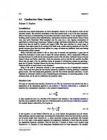
The different scales of the urban heat island The understanding of the UHI effect involves different scales of analysis, both spatially and temporally. In particular, three urban climate scales are usually involved in the establishment of the UHI effect (see Figure 1.1):
4 Vincenzo Costanzo et al.
Figure 1.1 Schematics of the various scales for thermal stress: (a) mesoscale, (b) local scale, (c) microscale.
•
The microscale, where individual buildings, trees and other manmade constructions create an urban canopy that extends in height from the street level to the tallest building (so-called urban canopy layer, UCL) and horizontally for about hundreds of metres
Understanding heat and mass transfer 5 •
•
The local scale, made up of similar houses and urban contexts, extending from one to several kilometres horizontally and up to the roughness sublayer (RSL) in height. The RSL, which extends up to a few building heights, is the air volume where the turbulence effects, originated by manmade surfaces, mainly take place. Within a local climate zone, many different microscales coexist, which implies a great variability in the urban climate and the corresponding perceived heat stress The mesoscale, which includes various local scales horizontally and extends up to the urban boundary layer (UBL) vertically. The UBL extends from the top of the canopy layer up to the mixing layer and is characterised by the fact that its height depends on diurnal cycles. During daytime the UBL is typically well mixed because of the turbulence originated by rough and warm urban surfaces (with a typical extension of more than one kilometre), while during the night it shrinks to hundreds of metres
According to this classification, heat islands can be regarded as a phenomenon occurring at the urban surfaces scale (surface UHI), at the canopy layer scale (canopy-layer UHI) and at the boundary layer scale (boundary-layer UHI), respectively [2]. Surface UHI is usually measured using land surface temperatures (TS) derived from remote thermal sensing, which provide an opportunity to characterise this phenomenon at various temporal (diurnal, seasonal and annual) scales [3,4]. However, the currently available resources used for deriving TS do not have a high spatiotemporal resolution because of satellite technical constraints and due to disturbance from cloud cover [5]. Satellite derived TS data have been used also for calculating air temperature (TA) in the UCL of cities with the support of limited meteorological observations through a statistical regression between TA and TS [6]. However, the published relationships between TA and TS remain empirical, and a general relationship has yet to be found [3,4]. For this reason, but also because the high air temperature experienced by pedestrians within the canopy layer can lead to reduced mental and physical performance and to physiological and behavioural changes [7], the canopy-layer UHI remains the most widely studied effect. The main causes of the canopy-layer UHI are: • • •
• • •
Decreased long-wave radiation loss to the sky at night (atmospheric window), due to the presence of buildings and other obstructions Increased sensible heat storage due to the use of materials with high thermal admittance (e.g. concrete, asphalt, brick) Increased absorption of short-wave radiation due to the increased reflec tions from the surrounding surfaces, especially if they are covered with lowalbedo materials Decreased evapotranspiration from pervious surfaces, water bodies, and vegetation, due to their reduced presence in urban areas Increased anthropogenic heat production Decreased convective heat transport due to reduction in wind speed
6 Vincenzo Costanzo et al.
The urban energy balance The diurnal variation of the UHI effect at the canopy layer is marked and confirmed by numerous experimental studies [8–10]: during daytime, the urbanrural temperature difference is usually small (below two degree Celsius) or even negative (i.e. a cool island effect may arise) in dense settlements or in presence of tall buildings, mainly because of the beneficial shading effect on urban surfaces. On the contrary, after sunset and until sunrise, the reduced cooling rates in cities determine noticeably higher air temperatures within the UCL than in the rural surrounding areas (so-called rural boundary layer, RBL). The main cause of this diurnal pattern lies in the dynamic nature of the energy balance at the urban scale, as determined by the heat transfer from every surface (e.g. walls, pavements, water bodies, and vegetation) to the air. According to the original Oke’s formulation, this energy balance can be simplified by considering a fictitious volume delimited on top by the UCL height [11]. Under these hypotheses, the energy balance poses: Q + QF = QH + QE + QS + QA
(W )
(1.1)
Here Q* is the all-wave net radiation flux, QF is the anthropogenic heat flux, QH and QE are the turbulent sensible and latent heat fluxes, ΔQS is the net storage of heat in the urban fabric and ΔQA is the net horizontal advection heat flux. This last term indicates the horizontal transport of heat and moisture and should be taken into account when horizontal temperature gradients are ex pected within the city (e.g. when the fictitious volume considered for the energy balance is adjacent to a different local climate zone or to a rural area). The next subsections discuss how the terms of the energy balance equation are linked (both directly and indirectly) with various urban and climate features. The role of surface properties The rough nature of urban surfaces, along with their high temperatures under sunlight exposure, promotes turbulent mixing during daytime while during nighttime slightly unstable or neutral conditions are typically experienced. This way, sensible convective fluxes (QH) are released from surfaces for most hours of the day and the main consequence is a warming of the outdoor air. This process is however influenced by several factors, and in particular by those that determine the amount of solar radiation received by the surface, such as the orientation of the building envelope, the geometry of the buildings and their surroundings [12]. It is interesting to note how the share of the net all-wave radiation flux Q* that is converted into a convective heat flux has been found rather constant, and in the range of 35–45% for a variety of cities, geographic locations, and climates [13]. This share is even more variable in relation to the heat stored by
Understanding heat and mass transfer 7 urban fabrics (ΔQS), for which the amount of the converted radiation flux is found in the range of 20–55%. The main factors affecting the absorption of short and long-wave radiation are two optical surface characteristics, i.e. albedo and thermal emissivity. They account respectively for the amount of solar radiation reflected by a surface and the amount of radiant heat released by it. Furthermore, the thermal admittance is another key parametre that measures a material’s ability to absorb heat from, and release it to, a space over time, due to a unit temperature fluctuation. Finally, the wind striking various urban surfaces affects the amount of heat released by convection to the air, as marked turbulence effects can increase the rate of heat transfer. This is usually expressed by the convective heat transfer coefficient (CHTC): this is a peculiar property for each urban surface, whose determination can be made either experimentally for a selected number of re presentative cases, or numerically via computational fluid dynamics (CFD) models [14,15]. CHTC values increase when the buildings become taller because of their strong sensitivity to wind speed, and can reach values even higher than 40 W∙m−2∙K−1 on the façades of high-rise isolated buildings [15]. The role of wind The wind flow through the city is contrasted by drag forces exerted by urban surfaces, trees and various objects within (e.g. cars and street furniture). These drag forces are balanced by a net momentum transfer between the upper RSL and the lower UCL due to differences in wind velocities. When buoyancy effects are not taken into account, the mean wind velocity profile above the RSL is logarithmic with the height z and is usually expressed as follows [2]: u(z) =
u z d ln k z0
(m s 1)
(1.2)
Here, u* is the friction velocity (m∙s−1), k is the von Karman constant typically taken as 0.40, d is the displacement height (m), and z0 is the roughness length (m). The friction velocity is a proxy of the surface shear stress and is closely linked with the roughness length, an empirical length-scale representation of a sur face’s roughness on wind flow, while the displacement height is the distance from the ground at which wind velocity is null. This formulation has been widely used when representing cities in regional and mesoscale models, and treats the single city as a lower boundary condition for the undisturbed flow above it. Recent approaches improved the predictive performance of the log law at the district scale by using urban statistical para metres such as the average building height, the ratio of built area and frontal area to total area (so called “plan area density” and “frontal area density” indices) to better define z0 and d parametres [2].
8 Vincenzo Costanzo et al. (1.2) holds if no buoyancy occurs. However, thermal processes within the UCL are usually not negligible, especially when the UHI phenomenon takes place. In particular, the heat storage of urban surfaces produces an increase in air temperature and an upward sensible heat flux that can extend over the night. If large scale (synoptic) winds are weak or absent, the established airflow also includes a convergent horizontal inflow from the rural area to the urban area at the lower heights, with a divergent outflow (from the urban area to the rural area) at the upper heights [16]. This circulation scheme depends on the size of the city, the UHI magnitude and the orographic features nearby (e.g. mountains, valleys, or the presence of the sea) [2]. In such circumstances, simplified models such as the logarithmic law fail to account for these complex interacting phenomena and one needs to resort either to CFD models or to difficult and expensive direct measurements through helicopters, balloons, or remote sensing techniques. In the end, the effect of wind patterns on human thermal comfort is twofold: first, wind contributes to convective cooling of the human body and thus re duces the risk of heat stress [17,18]. Secondly, the advection of air at the local scale can alter the overall thermal environment as described above and affects a city’s ventilation by mitigating the urban thermal environment [19], while also dispersing airborne pollutants as reported by Fan et al. who calculated a reduced time of around four hours to completely mix and disperse pollutants emitted in an idealised urban area when the approaching wind speeds are higher than a typical average value of 3 m·s−1 [20]. The role of vegetation Vegetation contributes to regulate the urban microclimate through three main mechanisms that involve all the terms shown in (1.1), both directly and in directly. In fact, vegetation can produce significant shading to various urban surfaces and as such has the potential to reduce the net all-wave radiation flux Q* and the amount of heat stored by urban surfaces (ΔQS). Trees can also modify the airflow pattern around buildings by significantly reducing the wind speed and the air pressure at the façades (windbreak action). This in turn would decrease both the rate of convective heat transfer and the rate of adventitious air that infiltrates through cracks in the building envelope, eventually reducing the amount of energy used for space heating and cooling. For instance, Liu and Harris found out that shelterbelt trees reduce by more than a half the convective heat transfer coefficient over a building façade, with predicted energy savings in the annual heating needs by 18% in Scotland [21]. The use of various plants, as well as the adoption of pervious surfaces, can directly lower the outdoor air temperature through the endothermic nature of evapotranspiration processes, thus affecting the latent heat flux QE in the energy balance reported in (1.1). The physical processes behind evapotranspiration mechanisms are mainly two, and concern both the soil and foliage layers. In fact, under the action of air temperature, relative humidity, wind, and solar
Understanding heat and mass transfer 9 radiation, the soil releases water vapour to the air by evaporation. Further, plants absorb water from the soil through the roots and convoy it in liquid form to the leaves where the photosynthesis process takes place. The stomata, which are tiny pores located in the leaves and in some stems, release water vapour to the air because of this endothermic mechanism. The combination of evapora tion and plant transpiration results in the evapotranspiration process, which locally increases air humidity and reduces the dry-bulb air temperature [22]. Given the complexity of the phenomena involved, apart from a few purely experimental studies limited to appraise single effects induced by vegetation, the majority of researchers rely on CFD simulations calibrated with on-site measurements [23]. The role of anthropogenic heat emissions Anthropogenic heat encompasses various sources of heat generated by human activities (e.g. waste heat from buildings, industries, and cars) and then released to the urban outdoor air [24]. Anthropogenic heat fluxes (QF) are difficult to measure, so they are usually estimated via an inventory-based approach or an energy balance closure ap proach [25]. Inventory approaches can either use large-scale aggregated data that are then downscaled to smaller spatiotemporal units (e.g. local and hourly), or use energy consumption data estimated at smaller scales (e.g. building and road scales) to be scaled up. The former approach is based on utility energy consumption and empirical traffic count data, while the latter uses building energy modelling. In any case, both methods typically assume that the total energy consumption converts to waste heat emissions in the form of a sensible heat flux, although contributions to heat storage and latent heat fluxes are also possible in principle. As an alternative to the inventory approach, the use of long-term micro meteorological measurements can enable estimates of the anthropogenic heat fluxes as the residual term in (1.1), under the assumption that ΔQS equals zero in a yearlong cycle. In any case, anthropogenic heat gains show a seasonal trend and they are usually larger in winter than in summer. According to estimates made before 1980, they were assumed to range, on average and with respect to the urban footprint, between 20 and 40 W∙m−2 in summer and between 70 and 210 W∙m−2 in winter, and to follow a daily pattern with two recognisable peaks [26]. A first peak is observed in the morning between 6 a.m. and 9 a.m. when people wake up and go to work, while the second one occurs in the late afternoon (between 5 p.m. and 7 p.m.) when people finish working. A more recent research, instead, shows that anthropogenic heat gains are nowadays significantly higher due to increasing energy use, especially because of the extensive use of air conditioning in summer [27]. As an example, a study of the most densely populated and energy-intensive urban regions in Tokyo (Japan) has found levels as high as 400 W∙m−2 in
10
Vincenzo Costanzo et al.
summer and up to 1590 W∙m−2 in winter [28]. Considering Tokyo’s overall daily energy balance, it was found that anthropogenic heat gain was equal to about 40% of the incoming solar energy in summer and 100% in the winter.
The human energy balance outdoors Thermally comfortable outdoor spaces contribute to improving wellbeing in urban areas because they encourage outdoor activities and foster the fruition of outdoor common areas, thus enhancing socialisation. Furthermore, thermally comfortable outdoor spaces reduce health issues related to severe heat stress, especially in the hot season. As highlighted in the previous section, the increase in the outdoor air tem perature compared to close-by rural areas, known as Urban Heat Island effect, contributes to the heat stress in urban areas. Indeed, the human body experi ences convective heat transfer to the outdoor air, whose intensity per unit body surface can be assessed through (1.3): q c = h c (Ts
Ta)
(W m 2)
(1.3)
Here, hc is the convective heat transfer coefficient (CHTC) for the clothed human body, which mainly depends on the wind velocity. In the summer, the body surface temperature Ts is normally close to — and actually slightly higher than — the ambient air temperature Ta: this means that the convective heat flux usually leaves the human body and thus helps removing internal heat, especially in windy conditions and apart from particularly hot days. On the contrary, the net radiant heat flux between the human body and the surrounding environment is an incoming term, due to the solar radiation and to the high temperature of sunlit surfaces, and thus plays a key role in defining the intensity of heat stress for pedestrians. Measuring the radiant heat experienced by the human body is not easy, since one should be able to take into account all the terms that contribute to the radiant field. As reported in Figure 1.2, one should separate the short-wave and the long-wave radiant loads: the former is related to the solar radiation hitting the human body, and the latter is associated with the thermal radiant emission from all the objects “seen” by the human body (ground, buildings, trees, and other urban furniture). The thermal radiant emission from the objects depends on their surface temperature and their or ientation relative to the human body, which can be described through the view factor (also known as surface factor or form factor). The sky vault is also involved in the long-wave radiant heat exchange with the human body, and this contribution is highly relevant in open areas where buildings do not significantly reduce the sky view factor. As far as short-wave radiation is concerned, direct solar radiation hits the human body only when this is not in the shade, whereas the contribution of the diffuse solar radiation is always relevant in the daytime. Finally, the (direct and diffuse) solar radiation
Understanding heat and mass transfer
11
Figure 1.2 Main contributions to the radiant heat load for a pedestrian in outdoor spaces.
can be reflected by the surrounding surfaces proportionally to their albedo, and then hit the human body. Formally, the calculation of the radiant heat absorbed by the clothed human body can be conducted through (1.4) [29]:
qr =
n bL
j =1
Fj
j
T 4j
Long wave radiation emitted by surrounding objects
+
n bS
j =1
Fj 1
jS
Ij +
Diffusely reflected short wave radiation
fb I
(W m 2)
(1.4)
Solar radiation hitting the body
Here, one can recognise the Stefan-Boltzmann constant σ = 5.67 W∙m−2∙K−4 and the absorption coefficient αb for the clothed human body, that is to say the fraction of incident radiation that is absorbed (and not reflected) on the body surface: its standard values are αbS = 0.7 and αbL = 0.97 for solar (short-wave) and infrared (long-wave) radiation, respectively. Both sums extend to the n isothermal surfaces seen from the body, while Fj are the corresponding view factors, which usually refer to a standing person and depend on the position of the person in the open space. Each surface in the radiant environment has its own temperature (Tj), short-wave absorption coefficient (αjS) and thermal
12
Vincenzo Costanzo et al.
emissivity (εj); the latter can be usually set to 0.95 for the greatest part of the building materials and the objects in the urban environment, such as the trees. Finally, Ij is the solar irradiance measured on the surface plane, which is then diffusely reflected. The last term in (1.4) indicates the solar radiation directly hitting the human body: this term depends on the solar irradiance measured on a surface perpen dicular to the sun ray (I*), multiplied by the surface projection factor (fp) of the body surface exposed to solar radiation [29]. Even if the contribution of the short-wave radiation is dominating for a person standing in sunny areas, it has been shown that — on average — 70% of the radiant energy is absorbed by a standing body in the form of long-wave radiation during daytime [29,30]. Indeed, on the one hand the solar radiation hitting a pedestrian significantly varies with time, and is controlled by the azimuth and the zenith angles of the sun relative to the horizon [31]; in Mediterranean and tropical climates its peak value can approach 900 W∙m−2 at noon, but is much lower during the other hours. The contribution of the diffusively reflected short-wave radiation is almost one order of magnitude lower, because of the generally low albedo of the urban surfaces. On the other hand, the long-wave radiation reaching a pedestrian shows little variation with time, and remains almost constant in open squares. The long-wave radiation coming from the ground has been found to be between 450 W∙m−2 and 700 W∙m−2, according to the ground temperature and emissivity, and constantly higher than the long-wave radiation coming from buildings and sky vault [31,32]. This demonstrates the importance of accurately addressing either the calculation or the field measurement of long-wave radiation. The mean radiant temperature The most used approach to quantify the effects of a complex radiant environ ment relies on the introduction of an equivalent temperature called mean radiant temperature (TMRT). The great advantage of this approach is that this temperature-like index can be combined to the other environmental parametres (namely dry-bulb air temperature, humidity and wind velocity) in order to assess the overall thermal comfort. In relation to a human body placed in a given environment, the mean radiant temperature is defined as the “temperature of an imaginary uniform enclosure in which the radiant heat transfer from the human body equals the radiant heat transfer in the actual non-uniform enclosure” [33], being “uniform” that en closure having all walls at the same surface temperature. This definition was originally conceived for indoor spaces, but it applies also to outdoor spaces. Once the radiant heat load on the human body is known, e.g. by means of (1.4), the TMRT can be derived through the following relationship, where εb = 0.97 is the standard value for the thermal emissivity of the clothed human body:
Understanding heat and mass transfer TMRT =
13
0.25
qr
273.15
(°C)
(1.5)
b
Several studies have demonstrated that, on clear and calm summer days, TMRT is the meteorological parametre with the highest influence on the human energy balance [34,35]. Indeed, TMRT is a very good predictor of both heat stress and heat-related mortality [32]: according to some authors, a positive correlation holds between the daily maximum TMRT and the heat-related risk of mortality, with a threshold value of 59.4°C that should not be exceeded, especially for aged people [36]. The literature proposes several different methods to derive the mean radiant temperature based on measured data. While the use of a globe-thermometre is most suitable in indoor spaces, in open urban areas the preferred methodology consists in measuring separately the solar and the infrared radiant fluxes reaching the human body from six different perpendicular directions (the four cardinal points plus the upper and lower directions). To this aim, six pyrano metres and six pyrgeometres are mounted on a suitable rack at 1.1 m above ground. In this case, (1.4) can be conveniently written as [35]: qr =
6 bL
j =1
Fj qjL +
6 bS
j =1
Fj qjS
(W m 2)
(1.6)
Here, qjL and qjS are respectively the measured long-wave and short-wave ra diant fluxes. In case of a standing person, the view factor relative to the four cardinal points is F = 0.22, while F = 0.06 can be used for the upper and lower direction [29]. Further details about the ways to measure the outdoor mean radiant temperature are discussed in Chapter 3 of this book. The mean radiant temperature in outdoor spaces can also be derived by means of numerical models involving large urban areas, which is now possible thanks to the increased computational power. In this case, the radiant fluxes appearing in (1.6) are simultaneously evaluated over a grid of points usually defined at 1.1 m above ground, thus providing a view of the time and spatial variation of TMRT over an urban area. Apparently, this is undoubtedly a step ahead if compared to the experimental derivation of TMRT for a single point, and makes it possible to investigate the effect of potential mitigation strategies to reduce heat stress in a city. However, software tools rely on simplifications to describe the physical phenomena con tributing to the radiant field experienced by pedestrians. For instance: • • •
Multiple reflections over building façades are neglected. The sky vault is normally described as an isotropic emitting body. An uniform average albedo is attributed to all vertical surfaces in the entire domain.
14
Vincenzo Costanzo et al.
•
The influence of wall inertia and insulation on their outdoor surface temperature is neglected. The influence of wind velocity on surface temperature is neglected.
•
Gál and Kántor recently presented a comprehensive study about the reliability of three well-known software tools for the calculation of TMRT in urban areas, by comparing the simulated results to experimental measurements [37]. They highlighted that significant inaccuracies may occur, and that there is a ten dency to overestimate TMRT in shaded areas, while underestimating it in sunny areas. However, according to the authors, the required level of accuracy for the calculation of the mean radiant temperature in the outdoor environ ment can be taken equal to the accuracy requirements accepted by the ISO 7726 Standard for thermal stress evaluation in workplaces, that is to say ±5°C [38]. Hence, software tools can be reliably used for assessing outdoor radiant heat stress as long as their inaccuracy keeps below this threshold. Further information about the software tools available for the simulation of the radiant field in the outdoors can be found in Chapter 2 of this book. The role of urban geometry and orientation Many urban features may influence the radiant heat balance in the outdoor environment, thus positively or negatively affecting the heat stress experienced by pedestrians. Understanding how different urban settings modify the spatial variation of the mean radiant temperature can provide valuable implications for climate-responsive urban design and planning: it is then essential that archi tects, engineers, and urban planners have a clear understanding of these con nections, in order to avoid any choices — both at building scale and at urban scale — that may exacerbate heat stress. According to Chen et al. [39], the mean radiant temperature in the outdoor environment is primarily determined by building geometry and orientation, street layout, albedo of façades and ground surface, and availability of vegetation cover. However, it is has been found that building geometry and vegetation play the most significant role, whereas surface albedo only plays a minor role. The following sub-sections will provide detailed information about these issues, with some examples coming from the literature. In unshaded open spaces, direct solar radiation hits pedestrians in the day time. They also receive long-wave radiant heat from the sky vault and from the ground, the latter being hot due to the absorbed solar radiation. In these open areas, the long-wave radiation emitted from the vertical surfaces has no effect on the radiant heat balance for the human body, due to the very low view factor; similarly, the short-wave radiation reflected by the façades hardly reaches the human body. In densely built spaces, e.g. inside an urban canyon, shaded areas occur, where pedestrians can avoid being hit by direct solar radiation. The ground surface is also partially in the shade, hence cooler, and this reduces the long-wave radiant
Understanding heat and mass transfer
15
load in the daytime; however, in the nighttime, the radiant losses to the sky vault are minor, due to the low sky view factor, and the ground keeps warm. Moreover, the vertical surfaces here play a more important role than in un shaded open areas, due to the high view factor with the human body: sunlit façades may overheat, especially if they have a dark colour, thus contributing to increase the long-wave radiant heat load. This suggests that densely built urban areas show a great spatial variability in the TMRT. Indeed, several authors reported that the difference in TMRT between sun-exposed and shaded areas reaches up to 25°C or 30°C at noon [30,39,40]. According to Lindberg et al., the variation in TMRT over different ground surfaces at sunlit locations is very small if compared with the difference between unshaded and shadowed locations (38.2°C at 4 p.m.) [32]. During clear and warm summer days, the highest TMRT values are found in paved open squares and near sunlit walls at noon: this is due to the high direct and reflected short-wave radiation combined with long-wave radiation emitted from the neighbouring sunlit surfaces [39,41]. The orientation and the shape of street canyons can also have a significant impact on street-level radiant heat load. Actually, solar access in a street canyon increases in case of small height-to-width (H/W) ratios; during the summer, the duration of solar access is twice as long in a north-south oriented street as in an east-west oriented street when H/W is between 0.5 and 3.5 [42]. However, sig nificant variations in the radiant heat load with the street orientation occur only when H/W < 1 in north and mid-European cities, and H/W < 2 in south European cities [41]. The worst configuration is the E–W canyon, since in this case the northern side of the canyon (i.e. the walls facing south) is almost con stantly sunlit [39]. As an example, Evola et al. found out that in E–W canyons in southern Italy (H/W = 1.14) TMRT = 54°C at noon in summer for a point at 1 m from the south-oriented façade, while TMRT = 48.5°C in the middle of the street [43]. At higher H/W ratios, street orientation has a minor effect. Unlike the great spatial variability of the mean radiant temperature in urban areas, the outdoor air temperature may vary by no more than 3°C within a city, with a minor impact on the heat stress for pedestrians. This suggests that TMRT is the most important parametre to capture the intra-urban variation in outdoor thermal comfort conditions. The role of trees and vegetation When dealing with radiant heat stress, the main advantage of planting trees in urban areas is that they cast shadows on otherwise unshaded surfaces. This reduces the direct impact of solar radiation on pedestrians, while also reducing the ground temperature, hence the long-wave radiant load in the daytime. In the winter, this effect can be detrimental for outdoor thermal comfort, thus deciduous species should be preferred. Of course, trees are more effective at improving summer heat stress when they are planted in open areas, where building shade is absent [44]. More in detail,
16
Vincenzo Costanzo et al.
trees should be placed in wide streets with low H/W ratio and in E–W oriented streets close to the south-facing walls. Moreover, they should be arranged in clusters, because a group of trees is more effective than isolated trees at reducing the mean radiant temperature [45]. As far as grass is concerned, it provides low ground surface temperature thus reducing the long-wave radiant flux, but it actually brings little improvement to the thermal environment compared to using trees [46]. The role of the surface albedo The albedo of urban surfaces has contrasting effects on the radiant heat load experienced by pedestrians. On the one hand, a high albedo value reduces the amount of short-wave radiant flux absorbed by a built surface, which in turn keeps its temperature relatively low, i.e. close to the ambient air temperature, even in case of a sunlit surface. Hence, the long-wave radiant flux released by the surface to the environment — and to the pedestrians — keeps low. On the other hand, the solar radiation that is not absorbed by the surface is then re flected to the environment, contributing to an increase in the radiant load for pedestrians. Consequently, the mean radiant temperature in outdoor spaces is almost insensitive to the albedo of the surrounding vertical surfaces, and the use of cool materials (i.e. high albedo plasters) has only a minor — and frequently adverse — impact on outdoor heat stress if compared to the effect of shade and vegetation [47]. High albedo pavements in sunlit areas even increase the mean radiant temperature by several degrees [48].
Conclusions This chapter provides the reader with the fundamentals concerning urban physics, with an insight on various urban-scale phenomena that affect humans’ thermal comfort outdoors. Particular emphasis is given to the UHI effect, a phenomenon that implies a raise in the air temperature within cities compared to surrounding rural areas. This is mainly determined by the synergic action of dense urban morphology, use of impervious and highly absorbing construction materials, and the heat emission from various anthropogenic activities (e.g. transportation and waste heat from buildings mechanical systems). The high concentration of dark and impermeable manmade surfaces in urban areas, as well as the reduced sky view factor due to urban canyons geometry, also implies an increased radiant heat load for pedestrians. This last aspect is predominant in the human balance and can be quantified by various metrics such as the mean radiant temperature and the Universal Thermal Climate Index, as thoroughly discussed in Chapters 2 and 3 of this book. As an example, the mean radiant temperature can easily reach values higher than 59.4°C, a commonly accepted threshold over which the heat-related risk of mortality significantly increases for elderly people. This chapter allows the
Understanding heat and mass transfer
17
reader to have a clear understanding of all the physical phenomena justifying heat stress, and suggests a series of mitigation strategies that will be further investigated in the subsequent chapters of this book.
References [1] L. Howard, The Climate of London Deduced From Meteorological Observations, Cambridge Library Collection — Earth Science, Cambridge, UK, 2012. [2] M. Roth, Urban heat islands, in: H.J.S. Fernando (Ed.), Handbook of Environmental Fluid Dynamics, Systems, Pollution, Modeling, and Measurements, Vol. 2, CRC Press, New York (US), 2013. [3] J.A. Voogt, T.R. Oke, Thermal remote sensing of urban climates, Remote Sensing of Environment 86 (2003) 370–384. doi:10.1016/S0034-4257(03)00079-8. [4] D. Zhou, J. Xiao, S. Bonafoni, C. Berger, K. Deilami, Y. Zhou, S. Frolking, R. Yao, Z. Qiao, J.A. Sobrino, Satellite remote sensing of surface urban heat islands: Progress, challenges, and perspectives, Remote Sensing 11 (2019) 1–36. doi:10.3390/ rs11010048. [5] Q. Weng, P. Fu, F. Gao, Generating daily land surface temperature at Landsat re solution by fusing Landsat and MODIS data, Remote Sensing of Environment 145 (2014) 55–67. doi:10.1016/j.rse.2014.02.003. [6] M. Pichierri, S. Bonafoni, R. Biondi, Satellite air temperature estimation for monitoring the canopy layer heat island of Milan, Remote Sensing of Environment 127 (2012) 130–138. doi:10.1016/j.rse.2012.08.025. [7] G.W. Evans, Environmental Stress, Cambridge University Press, Cambridge, UK, 1982. [8] J. Niu, J. Liu, T. Cheung Lee, Z. Lin, C. Mak, K.T. Tse, B. Sin Tang, K.C.S. Kwok, A new method to assess spatial variations of outdoor thermal comfort: Onsite monitoring results and implications for precinct planning, Building and Environment 91 (2015) 263–270. doi:10.1016/j.buildenv.2015.02.017. [9] M. Zinzi, E. Carnielo, B. Mattoni, On the relation between urban climate and energy performance of buildings: A three-year experience in Rome, Italy, Applied Energy 221 (2018) 148–160. doi:10.1016/j.apenergy.2018.03.192. [10] A. Salvati, H. Coch Roura, C. Cecere, Assessing the urban heat island and its energy impact on residential buildings in Mediterranean climate: Barcelona case study, Energy and Buildings 146 (2017) 38–54. doi:10.1016/j.enbuild.2017.04.025. [11] T.R. Oke, The urban energy balance. Progress in Physical Geography: Earth and Environment 12(4) (1988) 471–508. doi:10.1177/030913338801200401. [12] J. Bouyer, C. Inard, M. Musy, Microclimatic coupling as a solution to improve building energy simulation in an urban context, Energy and Buildings 43 (2011) 1549–1559. doi:10.1016/j.enbuild.2011.02.010. [13] M. Roth, Review of urban climate research in (sub)tropical regions, International Journal of Climatology 27 (2007) 1859–1873. doi:10.1002/joc.1591. [14] A. Hagishima, J. Tanimoto, K.I. Narita, Intercomparisons of experimental con vective heat transfer coefficients and mass transfer coefficients of urban surfaces, Boundary-Layer Meteorology 117 (2005) 551–576. doi:10.1007/s10546-005-2078-7.
18
Vincenzo Costanzo et al.
[15] T. Defraeye, B. Blocken, J. Carmeliet, Convective heat transfer coefficients for ex terior building surfaces: Existing correlations and CFD modelling, Energy Conversion and Management 52 (2011) 512–522. doi:10.1016/j.enconman.2010.07.026. [16] Y. Fan, Q. Wang, S. Yin, Y. Li, Effect of city shape on urban wind patterns and convective heat transfer in calm and stable background conditions, Building and Environment 162 (2019) 106288. doi:10.1016/j.buildenv.2019.106288. [17] S. Saneinejad, P. Moonen, T. Defraeye, J. Carmeliet, Analysis of convective heat and mass transfer at the vertical walls of a street canyon, Journal of Wind Engineering and Industrial Aerodynamics 99 (2011) 424–433. doi:10.1016/j.jweia.2010.12.014. [18] Y. Toparlar, B. Blocken, P. Vos, G.J.F. Van Heijst, W.D. Janssen, T. van Hooff, H. Montazeri, H.J.P. Timmermans, CFD simulation and validation of urban mi croclimate: A case study for Bergpolder Zuid, Rotterdam, Building and Environment 83 (2015) 79–90. doi:10.1016/j.buildenv.2014.08.004. [19] L. Yang, Y. Li, City ventilation of Hong Kong at no-wind conditions, Atmospheric Environment 43 (2009) 3111–3121. doi:10.1016/j.atmosenv.2009.02.062. [20] Y. Fan, J.C.R. Hunt, Y. Li, Buoyancy and turbulence-driven atmospheric circulation over urban areas, Journal of Environmental Sciences 59 (2017) 63–71. doi:10.1016/ j.jes.2017.01.009. [21] Y. Liu, D.J. Harris, Effects of shelterbelt trees on reducing heating-energy consumption of office buildings in Scotland, Applied Energy 85 (2008) 115–127. doi:10.1016/j.apenergy.2007.06.008. [22] T.E. Morakinyo, A.A. Balogun, O.B. Adegun, Comparing the effect of trees on thermal conditions of two typical urban buildings, Urban Climate 3 (2013) 76–93. doi:10.1016/j.uclim.2013.04.002. [23] G. Kang, J.J. Kim, W. Choi, Computational fluid dynamics simulation of tree effects on pedestrian wind comfort in an urban area, Sustainable Cities and Society 56 (2020) 102086. doi:10.1016/j.scs.2020.102086. [24] L.M. Gartland, Heat Islands. Understanding and Mitigating Heat in Urban Areas, EarthScan, London (UK), 2008. [25] C. Park, G.W. Schade, N.D. Werner, D.J. Sailor, C.H. Kim, Comparative estimates of anthropogenic heat emission in relation to surface energy balance of a subtropical urban neighborhood, Atmospheric Environment 126 (2016) 182–191. doi:10.1016/ j.atmosenv.2015.11.038. [26] H. Taha, Urban climates and heat islands: Albedo, evapotranspiration, and an thropogenic heat, Energy and Buildings 25 (1997) 99–103. doi:10.1016/s03787788(96)00999-1. [27] S.M. Khan, R.W. Simpson, Effect of a heat island on the meteorology of a complex urban airshed, Boundary-Layer Meteorology 100 (2001) 487–506. doi:10.1023/A: 1019284332306. [28] T. Ichinose, K. Shimodozono, K. Hanaki, Impact of anthropogenic heat on urban climate in Tokio, Atmospheric Environment 33 (24–25) (1999) 3897–3909. doi:10.1016/S1352-2310(99)00132-6. [29] N. Kántor, J. Unger, The most problematic variable in the course of humanbiometeorological comfort assessment — The mean radiant temperature, Central European Journal of Geosciences 3 (2011) 90–100. doi:10.2478/s13533-011-0010-x. [30] K.K.L. Lau, C. Ren, J. Ho, E. Ng, Numerical modelling of mean radiant temperature in high-density sub-tropical urban environment, Energy and Buildings 114 (2016) 80–86. doi:10.1016/j.enbuild.2015.06.035.
Understanding heat and mass transfer
19
[31] S. Manavvi, E. Rajasekar, Estimating outdoor mean radiant temperature in a humid subtropical climate, Building and Environment 171 (2020) 106658. doi:10.1016/ j.buildenv.2020.106658. [32] F. Lindberg, S. Onomura, C.S.B. Grimmond, Influence of ground surface char acteristics on the mean radiant temperature in urban areas, International Journal of Biometeorology 60 (2016) 1439–1452. doi:10.1007/s00484-016-1135-x. [33] American Society of Heating, Refrigerating and Air-Conditioning Systems, Chapter 1: Psychometrics, Handbook Fundamentals, S.I., ASHRAE, Atlanta, (US), 2013. [34] F. Ali-Toudert, H. Mayer, Numerical study on the effects of aspect ratio and or ientation of an urban street canyon on outdoor thermal comfort in hot and dry climate, Building and Environment 41 (2006) 94–108. doi:10.1016/j.buildenv.2005.01 .013. [35] H. Mayer, P. Höppe, Thermal comfort of man in different urban environments, Theoretical and Applied Climatology 38 (1987) 43–49. doi:10.1007/BF00866252. [36] S. Thorsson, J. Rocklöv, J. Konarska, F. Lindberg, B. Holmer, B. Dousset, D. Rayner, Mean radiant temperature — a predictor of heat related mortality, Urban Climate 10 (2014) 332–345. doi:10.1016/j.uclim.2014.01.004. [37] C.V. Gál, N. Kántor, Modeling mean radiant temperature in outdoor spaces: A comparative numerical simulation and validation study, Urban Climate 32 (2020) 100571. doi:10.1016/j.uclim.2019.100571. [38] ISO 7726:1998, Ergonomics of the Thermal Environment: Instruments for Measuring Physical Quantities, International Organization for Standardization (ISO), Geneve (Switzerland), 1998. [39] L. Chen, B. Yu, F. Yang, H. Mayer, Intra-urban differences of mean radiant tem perature in different urban settings in Shanghai and implications for heat stress under heat waves: A GIS-based approach, Energy and Buildings 130 (2016) 829–842. doi:10.1016/j.enbuild.2016.09.014. [40] H. Lee, J. Holst, H. Mayer, Modification of human-biometeorologically significant radiant flux densities by shading as local method to mitigate heat stress in summer within urban street canyons, Advances in Meteorology 2013 (2013) 312572. doi:10.1155/2013/312572. [41] S. Thorsson, D. Rayner, F. Lindberg, A. Monteiro, L. Katzschner, K.K.L. Lau, S. Campe, A. Katzschner, J. Konarska, S. Onomura, S. Velho, B. Holmer, Present and projected future mean radiant temperature for three European cities, International Journal of Biometeorology 61 (2017) 1531–1543. doi:10.1007/s00484-01 7-1332-2. [42] C. Ketterer, A. Matzarakis, Human-biometeorological assessment of heat stress re duction by replanning measures in Stuttgart, Germany, Landscape and Urban Planning 122 (2014) 78–88. doi:10.1016/j.landurbplan.2013.11.003. [43] G. Evola, V. Costanzo, C. Magrì, G. Margani, L. Marletta, E. Naboni, A novel comprehensive workflow for modelling outdoor thermal comfort and energy demand in urban canyons: Results and critical issues, Energy and Buildings 216 (2020) 109946. doi:10.1016/j.enbuild.2020.109946. [44] A.M. Coutts, E.C. White, N.J. Tapper, J. Beringer, S.J. Livesley, Temperature and human thermal comfort effects of street trees across three contrasting street canyon environments, Theoretical and Applied Climatology 124 (2016) 55–68. doi:10.1007/ s00704-015-1409-y.
20
Vincenzo Costanzo et al.
[45] J.K. Thom, A.M. Coutts, A.M. Broadbent, N.J. Tapper, The influence of increasing tree cover on mean radiant temperature across a mixed development suburb in Adelaide, Australia, Urban Forestry & Urban Greening 20 (2016) 233–242. doi:10.1 016/j.ufug.2016.08.016. [46] M.W. Yahia, E. Johansson, S. Thorsson, F. Lindberg, M.I. Rasmussen, Effect of urban design on microclimate and thermal comfort outdoors in warm-humid Dar es Salaam, Tanzania, International Journal of Biometeorology 62 (2018) 373–385. doi: 10.1007/s00484-017-1380-7. [47] E. Erell, D. Pearlmutter, D. Boneh, P.B. Kutiel, Effect of high-albedo materials on pedestrian heat stress in urban street canyons, Urban Climate 10 (2014) 367–386. doi:10.1016/j.uclim.2013.10.005. [48] M. Taleghani, U. Berardi, The effect of pavement characteristics on pedestrians’ thermal comfort in Toronto, Urban Climate 24 (2018) 449–459. doi:10.1016/ j.uclim.2017.05.007.
2
An overview of microclimate simulation tools and models for predicting outdoor thermal comfort Maurizio Detommaso, Antonio Gagliano, and Francesco Nocera University of Catania (Italy)
Introduction In the last decades, researchers are witnessing an increasing interest among public opinion and global communities regarding outdoor environmental comfort. The number of studies about mitigation strategies for the Urban Heat Island (UHI) phenomenon and the effect of climate change in urban areas has considerably increased, as well as those aimed to assess the effectiveness of urban planning strategies (e.g. implementation of vegetation and building orientation) on the urban microclimate and the outdoor comfort [1]. Actually, indoor thermal comfort is a well-established discipline. However, the outdoor environment is far more complex than the indoor environment because of the wide spatial and temporal variations of meteorological variables, hence the need to define suitable models and indices to assess the outdoor thermal comfort. Such models usually refer to a standing person and take into account how human body exchanges heat with the surroundings, according to the mechanisms thoroughly discussed in Chapter 1 of this book. This chapter briefly discusses some of the main models for the evaluation of the outdoor thermal comfort in urban areas, by also showing principles and features of the main related thermal indices. Then, it presents a description of the main software tools nowadays available to simulate the urban microclimate and to calculate the above-mentioned outdoor comfort indices. For each software tool, the chapter aims to highlight the main advantages and drawbacks, while also providing hints about their reliability according to the existing literature.
Bioclimatic indices The outdoor comfort models and the related indices can be divided into the following three main groups [2]:
22
Maurizio Detommaso et al.
•
Indices based on the human’s energy balance, which account for the interrelation among metabolic activities, clothing, environmental parameters and human thermal perception. They include COMFA (COMfort Formula), ETU (Universal Effective Temperature), ITS (Index of Thermal Stress), PMV (Predicted Mean Vote), PET (Physiological Equivalent Temperature), PT (Perceived Temperature), OUT_SET* (Standard Effective Temperature for outdoor), SET (Standard Effective Temperature), and UTCI (Universal Thermal Climate Index) Empirical indices, which are expressed as linear regressions of data derived from field studies and surveys defining the perceived human comfort for a specific climate or location. They include Actual Sensation Vote (ASV), Thermal Sensation (TS), and Thermal Sensation Vote (TSV) Indices based on linear equations defining the comfort as a function of the thermal environmental variables and namely air temperature, wind speed and relative humidity. Among these indices one can list Apparent Temperature (AT), Discomfort Index (DI), Environmental Stress Index and (ESI) and Physiological Strain Index (PSI), Effective Temperature (ET), Humidex (H), Heat Index (HI), Cooling Power Index (PE), Relative Strain Index (RSI), Wet Bulb Globe Temperature Index (WBGT), and Wind Chill Index (WCI)
•
•
Thermal indices based on energy balance enable quantification of thermal sensation considering the human variables and the urban microclimate. Empirical indices are intended to describe the thermal perception of humans and the environmental factors acting on their thermal behaviour. Finally, the indices based on linear equations can be useful either for meteorological forecasting or for mapping of thermal comfort trends over the time [3]. The above-mentioned indices can also be categorised as direct, empirical, and rational indices [4]. Direct indices rely on direct measurements of environmental variables, obtained by using integrated measurement devices that model a human body, or by combining measured meteorological parameters using an algebraic weighted expression [4]. By contrast, empirical indices are developed by exposing people to different environmental conditions (e.g. in a climate chamber) and measuring physiological parameters such as heart rate or rectal temperature. Finally, rational indices formalise the heat exchange mechanisms of the human body to yield its heat balance equation. They can refer either to equilibrium conditions or to transient conditions, and can even account for changing activities. The physiological state of a person results from regulation mechanisms taking place in the body in response to environmental conditions. The regulation mechanisms are simulated with different complexity in one-node, two-node, multi-node, and multi-element models [5]. Several indices based on the concept of reference environment calculate the air temperature that would result in an equivalent effect for a person as the actual environment does, the equivalent effect being defined differently for each
Overview of microclimate simulation tools
23
index (e.g. the core temperature or the physiological response are equal in both environments). The great proliferation of these indices is a clear sign of the interest within the scientific community to quantify the effect of climatic and thermal environmental variables on the human body. Temperate climate emerges as the most studied condition, followed by studies referring to arid, cold, and tropical climates, while very few studies refer to polar environments.
Outdoor thermal comfort models This section describes the main models used by the scientific community to assess outdoor thermal comfort. Most of these models are implemented in the software tools discussed in the second part of this chapter. Fanger’s approach Fanger developed a comfort theory based on human body heat transfer that led to defining the PMV (Predicted Mean Vote) and the PPD (Predicted Percentage of Dissatisfied) [6]. Later on, this theory became the basis for indoor thermal comfort standards, such as ISO 7730:2005 [7] and ASHRAE 55:2010 [8], and for developing models of outdoor thermal comfort. The PMV was introduced to predict the thermal sensation of a person through a heat balance equation based on six variables (i.e. dry-bulb temperature, mean radiant temperature, air velocity, relative humidity, metabolic activity and clothing insulation). PMV values vary on a scale from −3 (cold) to +3 (hot), where PMV = 0 corresponds to neutral conditions. The PMV should be used to predict the general thermal sensation and degree of discomfort of people exposed to moderate thermal environments when the main parameters are within a specified range (e.g. air temperature between 10°C and 30°C, as highlighted in the ISO Standard 7730:2005 [7]). Applying the Fanger’s theory for estimating outdoor thermal comfort when temperatures are higher than 34°C involves a thermal sensation above the highest rate of +3 [9]. Thereby, when a person experiences “very hot” or “extremely hot” sensation outdoors the seven-point scale is not sufficient. In order to consider wider variations of outdoor climate conditions, a few studies used a nine-point thermal sensation scale as an extension of ASHRAE sevenpoint scale, from −4 (very cold) to +4 (very hot) [10]. PMV > 4 can be attained in the hours of maximum solar radiation in hot summer days. Klima Michel Model Jendritzky et al. [11] managed to adjust Fanger’s model and make it applicable to complex outdoor conditions by adding outdoor radiation. Their model takes into account the direct and diffuse short-wave radiation and the longwave radiation fluxes originating from the ground, building surfaces and free atmosphere [12].
24
Maurizio Detommaso et al.
This approach, also known as the “Klima Michel Model”, was devised to estimate an integral index for the thermal component of climate and does not provide any description of thermal body conditions [13]. In this model, the sweat rate is a function of metabolic activity only and it does not include the effects due to weather conditions [14]. More widely applicable are the models that enable to predict the “real values” of thermal quantities of the body, i.e. skin temperature, core temperature, sweat rate or skin wetness. To this purpose, it is necessary to take into account all basic thermoregulatory processes like the constriction or dilation of peripheral blood vessels and the physiological sweat rate [14]. As an output of the Klima Michel Model, the Perceived Temperature (PT) represents the air temperature of a reference environment where the perception of heat and/or cold would be the same as under the actual conditions. In such reference environment, the mean radiant temperature equals the air temperature, the wind velocity is reduced to a slight draught and the relative humidity is fixed to 50% [15]. The PT refers to a standardised sample human (male, 35 years old, height 1.75 m, weight 75 kg), walking at 4 km per hour on a horizontal plane, with internal heat production of 172.5 W, and clothing insulation varying between 0.5 clo (summer) and 1.75 clo (winter) [16–18]. Munich Energy Balance Model for Individuals (MEMI) The Physiologically Equivalent Temperature (PET) is based on a thermophysiological heat-balance model called “Munich Energy Balance Model for Individuals” (MEMI) [14]. It was developed to explicitly compare the actual outdoor environmental conditions with equivalent indoor conditions, thus making it possible to evaluate comfort in the outdoor environment in terms of indoor standards. The reference person has a working metabolism of 80 W (light activity) in addition to basic metabolism and 0.9 clo (clothing insulation). MEMI calculates the physiological sweat rate as a function of skin average temperature and core temperature [19,20], and offers an analytical solution of the human energy balance for steady-state conditions, while also avoiding temporal integration compared to transient models. In the MEMI model, the mean clothing temperature, mean skin temperature, and sweat rate depend also on climatic conditions. Separate calculations for the heat fluxes from body surface parts that are covered or uncovered by clothing are carried out as well [14]. The OUT_SET* model The index OUT_SET* was developed for adapting the indoor comfort index SET to the outdoor environment [21]. This index provides physiological representation of outdoor human thermal comfort and stress across almost unlimited combinations of air and mean radiant temperatures, humidity, air velocity, clothing thermal insulation, and metabolic rate.
Overview of microclimate simulation tools
25
For the body’s surface area participating to the radiant heat exchange, the outdoor mean radiant temperature OUT_MRT is calculated taking into account the amount of outdoor irradiation absorbed by the body and by subtracting the outgoing fluxes [21,22]. Experimental results indicate that the OUT_MRT slightly overestimates absorbed solar radiation by about a quarter for clothing insulation of 0.25 clo [21]. Universal Thermal Climate Index (UTCI) Outdoor thermal indices based on a steady-state energy balance of the human body (e.g. PMV, PT, and PET) are not appropriate for assessing short-term exposure in the outdoor environment [20]. To overcome this shortcoming, the UTCI is stated as an equivalent ambient temperature of a reference environment that produces the same physiological response in a reference person as in the actual environment [23]. The reference person has a body surface area of 1.85 m2, a body weight of 73.4 kg and body fat content of 14% [24,25]. The UTCI reference environment considers a wind velocity of 0.5 m ∙ s−1 observed at 10 m above the ground, the mean radiant temperature equal to the air temperature and relative humidity of 50%. The metabolic rate, that is of 2.3 met (135 W), is higher than that used by the PET and SET* models. The calculation of the UTCI is based on a multi-node model for human thermoregulation, consisting of 12 body elements comprising overall 187 tissue nodes. Compared with the two-node models, multi-node models simulate the human body with higher detail, predicting both overall and local physiological responses. The variables under analysis include mean skin temperature, body core temperature, and different forms of heat loss, leading to an extensive polynomial expression with 210 coefficients. The UTCI is classified into ten thermal stress categories — from extreme cold stress to extreme heat stress — that correspond to a specific set of human physiological responses to the thermal environment. Further information about the main thermal comfort indices is summarised in Table 2.1, while Table 2.2 reports the different thermal sensations and physiological stress levels for the main thermal comfort indices.
Software and simulation tools There are many effective measures and strategies to mitigate heat stress in urban areas, whose effectiveness can be properly investigated through numerical models that combine many microclimatic parameters to estimate the thermal sensation of people. Nowadays, tools for simulating project scenarios are increasingly available and updated, allowing for the reproduction of complex urban areas. Table 2.3 reports the most used software tools for predicting the indices discussed so far, while later a brief description of each tool is given.
26
Maurizio Detommaso et al.
Table 2.1 Main models and thermal indices used to assess outdoor thermal comfort Year Index
Reference
1970 PMV
Fanger [6]
1981 PMV (extended version) 1986 SET*
1999 PET
2000 PT
Model type
Notes
Steady-state energy PMV scale: from −3 to +3 balance (One- Metabolic rate: 46–232 node model) W ∙ m−2 (0.8–4 met) Clothing thermal resistance: 0–0.310 m2 K ∙ W−1 (0–2 clo) Ambient air temperature: 10–30°C Mean radiant temperature: 10–40°C Air velocity: 0–1 m ∙ s−1 Jendritzky and Klima-Michel PMV scale: from −4 to +4 Nubler [12] Model (OneMetabolic rate: 172.5 W ∙ m−2 node model) Weight: 75 kg Gagge Transient Energy SET*scale (°C): SET* < 17; et al. [26] Balance (Two17 ≤ SET ≤ 37; SET* > 37 node model) Air Temp. = Mean Radiant Temp. Relative humidity: 50% Air velocity: 0.15 m ∙ s−1 Clothing thermal resistance: 0.6 clo Metabolic rate: 1.0 met The same mean skin temperature witnessed as the person in the actual complex environment Höppe [14] Munich Energy PET scale (°C): PET < 4; 4 ≤ Balance model PET ≤ 41; PET > 41 for individuals Air Temp. = Mean (Two-node Radiant Temp. model) Air temperature: 20°C Air velocity: 0.1 m ∙ s−1 Vapour pressure in the air: 12 hPa Relative humidity: 50% Metabolic rate: 80 W ∙ m−2 Clothing thermal resistance: 0.9 clo Jendritzky Klima-Michel PT scale (°C): PT < − 39, −39 et al. [15] Model (Two< PT < 38, PT > 38 node model) Relative humidity: 50% Metabolic rate: 135 W ∙ m−2 Clothing thermal resistance: 1.75 clo (winter), 0.5 (summer) (Continued)
Overview of microclimate simulation tools
27
Table 2.1 (Continued) Year Index
Reference
Model type
Notes
2001 UTCI
Jendritzky et al. UTCI-Fiala model UTCI scale (°C): UTCI < − [27,28], Fiala (Multi-node 40; −40 < UTCI < 46; et al. [24] model) UTCI > 46 Air Temp. = Mean Radiant Temp. Metabolic rate: 2.3 met Walking speed: 1.1 m ∙ s−1 Air velocity: 0.5 m ∙ s−1 (10 m above ground). Relative humidity: 50%
Table 2.2 Thermal sensations and physiological stress levels used in main bioclimatic indices Thermal sensation
PMV (-) SET* (°C)
PT (°C)
PET (°C) UTCI (°C) Physiological stress
Very hot
>+4
≥38
≥41
>37
>46 38÷46
Hot
+3
34÷37
32÷38
35÷41
32÷38
Warm
+2
30 ÷34 26÷32
29÷35
26÷32
Slightly warm Comfortable
+1
20÷26
23÷29
0÷20
18÷23
9 ÷26
Slightly cool
−1
−13÷0
13÷18
0÷9
Cool
−2
Cold
0
17÷30
140 W∙m−2 0% if solar radiation on window is < 120 W∙m2
26°C
18°C (15°C at night)
ON: 0–24
ON: 6–22
6–22
Occupancy 0–24
Shading masks in TRNSYS were defined by two angular values for azimuth and inclination of the obstacle from the middle of the façade. The shading provided by the urban environment was obtained by modelling the same regular array used in UWG. Surface convective heat transfer was obtained from (7.5) and (7.6) for hor izontal and vertical surfaces, respectively [26]: h c,hor = 9. 42 + 3. 68· v (W m
2
K 1)
(7.5)
h c,ver = 8. 18 + 2. 28·V (W m
2
K 1)
(7.6)
The air change per hour (ACH), i.e. the relation among the volumetric air flow rate and the space volume, was calculated by and Excel sheet as a function of the average air speed, the wind direction and the geometry of the urban area. Calculation follows the selection strategy described in [28]. Once the average wind velocity in the canyon is calculated, which is nor mally reduced by around 20–50% if compared to undisturbed values, the original wind directions from the weather file were used to determine the pressure coefficients and the air ACH. Windows are by default placed on opposite façades for family houses and on two perpendicular façades for each apartment in multifamily buildings. The excel computation is conducted hourly in an integrated manner within the TRNSYS simulation studio project. Finally, the equation used for ACH calculation, according to Grosso [38], was qv = vw
|c+p n i =1
cp |
( ) 1 c i2 A i2
(m3 s 1),
(7.7)
where qv is the air flow (m3∙s−1), vw is the average air speed at window height (m∙s−1), cp are the pressure coefficients at inlet and outlet openings (nondimensional), ci are the discharge coefficients of the openings (nondimensional), and Ai are the net opening areas (m2). Index i indicates the progressive opening position between the inlet and the outlet zones. Alternatively, air flow can be directly inserted in TRNSYS as mass flow, or
132
Massimo Palme and Agnese Salvati
Figure 7.4 Cooling loads for test building in Rome and Antofagasta. From Salvati et al. [ 30].
computed by TRNFLOW component of TRNBUILD from pressure coefficients, discharge coefficient, and average wind speed. Results Figure 7.4 shows the cooling loads for two simulated buildings in different urban environments of both cities. The effects were incorporated sequentially in the simulation: the impact of shadows was addressed first, then the UHI intensity was added using the UWG weather file, then the long-wave correction was performed and finally the impact of urban wind on the hourly ACH was added too. First of all, one can observe that different climate regions determine a dif ferent sensitivity of the building energy behaviour to urban effects: in Rome (Mediterranean temperate climate), shadows and UHI effects are quite ba lanced, while in Antofagasta (arid climate) shadows seem to play a more im portant role than the UHI effect. This is in agreement with existing literature on UHI in arid climates and reflects also the lower average temperature and higher solar radiation in Antofagasta than in Rome. Long-wave radiant heat
Including weather data morphing 133 transfer and wind effects are always present and in some cases they are very important to determine the final energy performance of urban buildings. The results also indicate that urban morphology determines the final cooling energy demand of urban buildings. Dense urban areas, with higher values of site coverage and façade-to-site ratios, such as Campo Marzio in Rome, will ex perience higher UHI intensity, which is only partially balanced by the beneficial effect of shadows. The presence of urban greenery contributes to lower the UHI effect, like in the case of Prati. In Antofagasta, denser urban environments (Coviefi and Centro) perform better, as observed. The worst urban fabrics, among the analysed sectors, are Corvallis and Jardines del Sur. Both environ ments are composed of family houses in a quite compact layout but with very low building height. The sector “Brasil”, which has the best performance in terms of cooling loads, is where the highest value of average building height is found across the city. Results are in accordance with the fundamental principles of bioclimatic architecture and urbanism as formulated for example by Olgyay [39] and Serra [40] many decades ago. In arid environments, shadows and compactness should be privileged, while in temperate environments a balance has to be reached among permeability (both at building and at city scale), vertical/horizontal development, sun access/protection, depending on the season. Expected results for hot-wet environments are a prevalence of UHI on shadows and the extreme importance of permeability to wind. Green infrastructure also plays a relevant role. Finally, in cold climates, where the heating load is the driver of the energy consumption, the orientation of buildings and urban fabrics following the sea sonal solar access is the key factor. However, in some cases overheating of buildings has been detected [41], even in winter, for high latitude environments, putting in evidence the relevance of cooling issues for the future.
The use of BPS for mitigation and adaptation strategies evaluation Some attempts have been done recently to correlate the different disciplines involved in developing and modelling mitigation strategies for urban heat stress and global warming. Most of these strategies have a scale of intervention ranging from urban blocks to the whole city, like the proposals of green-blue infrastructures [42,43], the use of available breezes and synoptic winds to cool the urban environment [44,45], the evaluation of cool materials for pavements [46], and the estimation of the benefits introduced by changes in transporta tion systems [47]. However, the influence of buildings performance on the anthropogenic heat release to the urban canyons [48] makes it necessary to evaluate the mitigation strategies also at the building scale. Adaptation is also important at this scale, since buildings that are better designed could be more flexible in facing warmer environments. Indeed, both concepts should be considered together, favoring those mitigation strategies that can be also adaptive [49,50].
134
Massimo Palme and Agnese Salvati
An example of how to perform BPS and contribute to a mitigation/adaptation plan for the whole city can be found in Litardo et al. [15]. Here, the effect of different mitigation strategies (city greening, cool materials for pavements and buildings’ roofs, changes in urban patterns) is assessed at both urban and building level. Cool roofs, green roofs, and even a green infrastructure able to produce shadows on buildings’ façades and roofs, are strategies that have a twofold mitigation effect: they reduce the urban temperatures (surface and air temperatures) and contribute to reduce the cooling loads of buildings, which means an increased effect in reducing urban temperatures. In some climate regions, the reduction of cooling loads can be counter balanced by an increase in heating loads. This effect would lead to a net zero effect on global warming mitigation. However, in terms of adaptation, it appears fundamental to privilege cooling loads reduction on heating loads reduction. It is a clear example of “adaptigation” [51]: a mitigation of both urban heat stress and global warming plus an adaptation to future conditions. BPS is a key factor in linking UHI mitigation and building energy efficiency strategies. Both downscaling of urban climate effects to the building level and upscaling of building-level energy results to the whole city (as performed for example in Palme et al. [12]) are processes that should be improved and con sidered in climate responsive urban planning.
Conclusions Urban climate and building energy performance are strictly correlated. Building behaviour influences the urban thermal environment and exacerbates urban heat island. Urban effects influence also building performance in a pronounced way especially in summer when the first effect amplifies the second one: the more energy is used for air conditioning, the more the heat released to urban canyons. Performing BPS in urban contexts is a difficult task; however, it can be conducted following some of the strategies and approaches discussed in this chapter. The definition and calibration of urban weather files is a pending challenge for building scientists, as well as the formulation of an integrated theory of cities’ metabolism and energetic behaviour across different scales. Some attempts have been done to relate the different disciplines involved, with the objective to develop strategies and models to check the effectiveness of adaptation and mitigation strategies facing urban climate and the global warming. This chapter aims to be a useful guideline in developing heat miti gation studies including building scale effects. BPS, as shown, can be a powerful tool to test the efficacy of mitigation strategies, contributing to a better global understanding of urban microclimate design.
References [1] R.L. Wilby, A review of climate change impacts on the built environment, Built Environment 33(1) (2007) 31–45. doi:10.2148/benv.33.1.31.
Including weather data morphing 135 [2] W.E. Rees, The built environment and the ecosphere: A global perspective, Building Research & Infomation 27(4-5) (1999) 206–220. doi:10.1080/096132199369336. [3] United Nations, Department of economic and social affairs, sustainable develop ment, transforming our world: The 2030 Agenda for Sustainable Development, https://sdgs.un.org/2030agenda. [4] Y.N. Bahar, C. Pere, J. Landrieu, C. Micolle, A thermal simulation tool for building and its interoperability through the Building Information Modeling (BIM) platform, Buildings 3(2) (2013) 380–398. doi:10.3390/buildings3020380. [5] L. Toledo, P. Cropper, A.J. Wright, Unintended consequences of sustainable archi tecture: Evaluating overheating risks in new dwellings, Proceedings from the Passive and Low Energy Architecture Conference (PLEA), Los Angeles (US), July 2016. [6] M. Kolokotroni, X. Ren, M. Davies, A. Mavrogianni, London’s urban heat island: Impact on current and future energy consumption in office buildings, Energy and Buildings 47 (2012) 302–311. doi:10.1016/j.enbuild.2011.12.019. [7] C.S. Barnaby, D.B. Crawley, Weather data for building performance simulation, in: J.L.M. Hensen, R. Lamberts (Eds.), Building Performance Simulation for Design and Operation,1st ed., Routledge, London (UK), 2011, pp. 37–55. [8] ISO 15927-4:2005, Hygrothermal Performance of Buildings—Calculation and Presentation of Climatic Data—Part 4: Hourly Data for Assessing the Annual Energy Use for Heating and Cooling, International Organization for Standardization, Geneve (Switzerland), 2005. [9] F. Sanchez de la Flor, S. Álvarez, Modelling microclimate in urban environments and assessing its influence on the performance of surrounding buildings, Energy and Buildings 36(5) (2004) 403–413. doi:10.1016/j.enbuild.2004.01.050. [10] I.D. Stewart, T.R. Oke, Local climate zones for urban temperature studies, Bulletin of the American Meteorological Society 93(12) (2012) 1879–1900. doi:10.1175/BAMSD-11-00019.1. [11] A. Salvati, P. Monti, H. Coch Roura, C. Cecere, Climatic performance of urban textures: Analysis tools for a Mediterranean urban context, Energy and Buildings 185 (2019) 162–179. doi:10.1016/j.enbuild.2018.12.024. [12] M. Palme, L. Inostroza, G. Villacreses, A. Lobato, C. Carrasco, From urban climate to energy consumption: Enhancing building performance simulation by including the Urban Heat Island effect, Energy and Buildings 145 (2017) 107–120. doi:10.101 6/j.enbuild.2017.03.069. [13] M. Halkidi, Y. Batistakis, M. Vazirgiannis, On clustering validation techniques, Journal of Intelligent Information Systems 17(2–3) (2001) 107–145. [14] M. Palme, L. Inostroza, A. Salvati, Technomass and cooling consumption in South America: A superlinear relationship?, Building Research & Information 46(8) (2018) 864–880. doi:10.1080/09613218.2018.1483868. [15] J. Litardo, M. Palme, M. Borbor-Cordova, R.J. Caiza, J. Macias, R. Hidalgo, G. Soriano, Urban Heat Island intensity and buildings’ energy needs in Duran, Ecuador: Simulation studies and proposal of mitigation strategies, Sustainable Cities and Society 62 (2020) 102387. doi:10.1016/j.scs.2020.102387. [16] K. Perini, A. Chokhachian, S. Dong, T. Auer, Modeling and simulating urban outdoor comfort: Coupling ENVI-Met and TRNSYS by Grasshopper, Energy and Buildings 152 (2017) 374–384. doi:10.1016/j.enbuild.2017.07.061. [17] F. Salata, I. Golasi, R. de Lieto Vollaro, A. de Lieto Vollaro, Urban microclimate and outdoor thermal comfort. A proper procedure to fit ENVI-met simulation
136
[18]
[19]
[20]
[21] [22]
[23] [24]
[25]
[26]
[27] [28]
[29] [30]
[31]
[32] [33]
Massimo Palme and Agnese Salvati outputs to experimental data, Sustainable Cities and Society 26 (2016) 318–343. doi:1 0.1016/j.scs.2016.07.005. P.J. Crank, D.J. Sailor, G. Ban-Weiss, M. Taleghani, Evaluating the ENVI-met microscale model for suitability in analysis of targeted urban heat mitigation stra tegies, Urban Climate 26 (2018) 188–197. doi:10.1016/j.uclim.2018.09.002. N. Lauzet, A. Rodler, M. Musy, M.H. Azam, S. Guernouti, D. Mauree, T. Colinart, How building energy models take the local climate into account in an urban context — A review, Renewable & Sustainable Energy Reviews 116 (2019) 109390. doi:10.101 6/j.rser.2019.109390. C. Georgatou, D. Kolokotsa, Urban climate models, in: M. Santamouris, D. Kolokotsa (Eds.), Urban Climate Mitigation Techniques, Taylor & Francis, London (UK), 2016, pp. 175–194. M. Bruse, ENVI-met 3.0: Updated model overview, 2004. http://www.envi-met.net/ documents/papers/overview30.pdf. B. Bueno, L. Norford, J. Hidalgo, G. Pigeon, The urban weather generator, Journal of Building Performance Simulation 6(4) (2013) 269–281. doi:10.1080/19401493.2012 .718797. T.R. Oke, City size and the urban heat island, Atmospheric Environment 7(8) (1973) 769–779. doi:10.1016/0004-6981(73)90140-6 J. Mao, L.K. Norford, Urban weather generator: Physics-based microclimate simu lation for performance-oriented urban planning, in: M. Palme, A. Salvati (Eds.), Urban Microclimate Modelling for Comfort and Energy Studies, Springer Nature, Cham (Switzerland), 2021 (in press). J. Mao, Y. Fu, A. Afshari, P.R. Armstrong, L.K. Norford, Optimization-aided cali bration of an urban microclimate model under uncertainty, Building and Environment 143 (2018) 390–403. doi:10.1016/j.buildenv.2018.07.034. J. Mao, J.H. Yang, A. Afshari, L.K. Norford, Global sensitivity analysis of an urban microclimate system under uncertainty: Design and case study, Building and Environment 124 (2017) 153–170. doi:10.1016/j.buildenv.2017.08.011. TRNSYS Manual, vol. 5, Multizone Building modelling with Type 56 and TRNBuild. Energy Plus Engineering Reference, Chapter 3, Surface Heat Balance. https:// www.energyplus.net/sites/default/files/docs/site_v8.3.0/EngineeringReference/03SurfaceHeatBalance/index.html#outside-surface-heat-balance. P.W. O’Callaghan, S.D. Probert, Sol-air temperature, Applied Energy 3(4) (1977) 307–311. doi:10.1016/0306-2619(77)90017-4. A. Salvati, M. Palme, G. Chiesa, M. Kolokotroni, Built form, urban climate and building energy modelling: Case-studies in Rome and Antofagasta, Journal of Building Performance Simulation 13(2) (2020) 209–225. doi:10.1080/19401493.201 9.1707876. M. Santamouris, C. Georgakis, A. Niachou, On the estimation of wind speed in urban canyons for ventilation purposes — Part 2: Using of data driven techniques to calculate the more probable wind speed in urban canyons for low ambient wind speeds, Building and Environment 43(8) (2008) 1411–1418. doi:10.1016/j.buildenv.2007.01.042. S.E. Nicholson, A pollution model for street-level air, Atmospheric Environment 9(1) (1975) 19–31. doi:10.1016/0004-6981(75)90051-7. R.S. Hotchkiss, F.H. Harlow, Air Pollution Transport in Street Canyons, Report for: Office of research and monitoring U.S. Environmental Protection Agency, 1973.
Including weather data morphing 137 [34] R.J. Yamartino, G. Wiegand, Development and evaluation of simple models for the flow, turbulence and pollutant concentration fields within an urban street canyon, Atmospheric Environment 20(11) (1986) 2137–2156. doi:10.1016/0004-6981(86)903 07-0. [35] C. Ghiaus, F. Allard, M. Santamouris, URBVENT WP1 Final Report: Soft Computing of Natural Ventilation Potential, 2004. [36] M. Palme, R. Privitera, D. La Rosa, The shading effects of Green Infrastructure in private residential areas: Building Performance Simulation to support Urban Planning, Energy and Buildings 229 (2020) 110531. doi:10.1016/j.enbuild.2020.11 0531. [37] M. Palme, R. Privitera, D. La Rosa, G. Chiesa, Evaluating the potential energy savings of an urban Green Infrastructure through environmental simulation, Proceedings from the 16th Conference of the International Building Performance Simulation Association (IBPSA), Rome (Italy), 2–4 September 2019. [38] M. Grosso, Wind pressure distribution around buildings: A parametrical model, Energy and Buildings 18 (1992) 101–131. doi:10.1016/0378-7788(92)90041-E. [39] V. Olgyay, Design With Climate. Bioclimatic Approach to Architectural Regionalism, Princeton University Press, Princeton (UK), 1963. [40] R. Serra, Arquitectura y Climas, Gustavo Gili (Ed.), Barcelona (Spain), 1999. [41] M. Rakatonjanahari, F. Scholzen, D. Walmann, Summertime overheating risk as sessment of a flexible plug-in modular Unit in Luxembourg, Sustainability 12(20) (2020) 8474. doi:10.3390/su12208474. [42] K.R. Gunawardena, M.J. Wells, T. Kershaw, Utilising green and bluespace to mi tigate urban heat island intensity, Science of the Total Environment 584–585 (2017) 1040–1055. doi:10.1016/j.scitotenv.2017.01.158. [43] M.A. Ruiz, M.B. Sosa, E.N. Correa, M.A. Cantón, Design tool to improve daytime thermal comfort and nighttime cooling of urban canyons, Landscape and Urban Planning 167 (2017) 249–256. doi:10.1016/j.landurbplan.2017.07.002. [44] J. Yang, S. Jin, X. Xiao, C. Jin, J. Xia, X. Li, S. Wang, Local climate zone ventilation and urban land surface temperatures: Towards a performance-based and windsensitive planning proposal in megacities, Sustainable Cities and Society 47 (2019) 101487. doi:10.1016/j.scs.2019.101487. [45] H. Takebayashi, T. Tanaka, M. Moriyama, H. Watanabe, H. Miyazaki, K. Kittaka, Relationship between city size, coastal land use, and summer daytime air tempera ture rise with distance from coast, Climate 6(4) (2018) 84. doi:10.3390/cli6040084. [46] M. Santamouris, Using cool pavements as a mitigation strategy to tight urban heat island – a review of actual developments, Renewable & Sustainable Energy Reviews, 26 (2013) 224–240. doi:10.1016/j.rser.2013.05.047. [47] D. Sailor, L. Lu, A top-down methodology for developing diurnal and seasonal anthropogenic heating profiles for urban areas, Atmospheric Environment 38(17) (2004) 2737–2748. doi:10.1016/j.atmosenv.2004.01.034. [48] F. Salamanca, M. Georgescu, A. Mahalov, M. Moustaoui, M. Wang, Anthropogenic heating of the urban environment due to air conditioning, Journal of Geophysical Research: Atmosphere 119(10) (2014) 5949–5965. doi:10.1002/2013JD021225. [49] B.J. He, Towards the next generation of green building for urban heat island mi tigation: Zero UHI impact building, Sustainable Cities and Society 50 (2019) 101647. doi:10.1016/j.scs.2019.101647.
138
Massimo Palme and Agnese Salvati
[50] B. Stone, The City and the Coming Climate. Climate Change in the Places We Live, Cambridge University Press, Cambridge (UK), 2012. [51] A. Galderisi, G. Mazzeo, F. Pinto, Cities dealing with energy issues and climaterelated impacts: Approaches, strategies and tools for a sustainable development, in: R. Papa, R. Fistola (Eds.), Smart Energy in the Smart City, Springer Nature, Heidelberg (Germany), 2016.
8
The climate-related potential of natural ventilation Giacomo Chiesa Politecnico di Torino (Italy)
Introduction A continuous growth in cooling energy needs for buildings was underlined in recent decades. This trend is correlated to several causes, including: climate change, urban heat island phenomena, changes in comfort expectations and the diffusion of building design approaches that do not consider bioregionalism and climatic issues [1–3]. Nevertheless, in addition to these causes, the progressive increase of overheating phenomena in hyper-insulated buildings with perfect airtightness is generating increasing cooling needs. This trend is visible not only in summer, but also in thermal-neutral periods and in the central, hottest hours of the winter seasons [4,5]. Furthermore, the growth in cooling needs is corre lated to the increase in the global penetration of air conditioners in domestic and tertiary spaces, a trend that is underlined by several sources [6,7]. Given this general background, it is clear that the valorisation of alternative cooling strategies, such as ventilative cooling solutions, is essential to poten tially reduce the usage of mechanical systems under favourable environmental conditions, e.g. when external air temperatures are below internal ones. This was also underlined by the recent EPBD Directive [8] that highlights the need to also include in the energy performance of buildings all “passive techniques aiming to reduce the energy needs for heating or cooling (…) and for ventilation” to improve thermal comfort. Among passive and hybrid techniques, ventilative cooling refers to three main strategies: • • •
Comfort ventilation, i.e. improving thermal sensation by increasing the heat dissipation through the skin due to rising air velocities Environmental ventilation, i.e. dissipating internal heat gains by replacing internal air with cooler outdoor air Structural ventilation, i.e. activating thermal mass dissipation toward airflow exchanges such as in nocturnal structural ventilative cooling effects [9]
In ventilative cooling techniques, air-movement may be both naturally or mechanically activated, e.g. by fans. Natural air movement is due to differences
140
Giacomo Chiesa
in pressures generated by wind forces or by temperature gradients, i.e. the socalled stack effect [10]. This chapter focuses on natural ventilation and aims, in particular, to its local climatic applicability, being the potential application of passive techniques directly correlated to typical local weather conditions [11,12]. Furthermore, general considerations on urban applicability are discussed. This contribution concerns the early-design stages, i.e. building programming, with the aim to support the definition of potential local passive and low-energy solutions. In line with the climatic design methodology introduced in [13], this contribution follows a performance-driven design approach [14,15] and the correlated aspects for building space cooling suggested in [16]. The contribution is structured as follows: a first section describing different methodologies to define the climatic potential of natural ventilation; a short discussion on the impact that urban morphologies may have on ventilative potential; a sample application of the described early-design geo-climatic ap proach to a set of locations in the Mediterranean Basin.
Methodologies to define the natural ventilation climate potential The cooling potential of natural ventilation strategies is very location-specific, since it is connected with microclimate environmental conditions. Without aiming at defining a full review on this topic, this section describes different key performance indicators (KPIs) to define the geo-climatic ventilative cooling potential of a location. Amongst the various indicators, the adoption of cumulative degree-hour indices is well-recognised in several studies, as underlined in recent review papers [17,18] and in specific researches [19]. In particular, it is possible to mention the Climate Cooling Potential (CCP) [5,20]: this indicator analyses the difference between environmental temperature and the internal temperature of a “virtual” building space, assuming that the latter varies around a set-point temperature that is guaranteed by diurnal mechanical space cooling following a 24-h sinusoidal curve. A suggested set-point tempera ture of 24.5°C with an amplitude of ±2.5°C may be adopted, in line with thermal comfort suggestions for office spaces [21]. This method was used to map the CCP in Europe [20] and was recently applied in other studies, such as the mapping of the impact of climate change in the Iberian peninsula [22]. Additionally, the residual cooling degree days/hours (CDDres, CDHres) approach supports the calculation of the natural ventilation potential in cooling a “virtual” space [11]. It considers the reduction in local CDD/CDH indices due to wind—including the effect of air velocity variations on the perceived air temperature—and to daily-temperature variations. It is possible to refer in par ticular to the indices introduced in [23] considering the cooling potential of comfort ventilation (wind-driven)—see Equation (8.1) hereinafter—and
Potential of natural ventilation
141
environmental/structural cooling (temperature gradient)—see Equation (8.3) hereinafter. CDHres, w = n
(( 0
v, air )
en
c)
if (( if ((
en
v, air)
c)
en
v, air)
c)
>0 0
(°C) (8.1)
where ϑen is the environmental temperature, ϑc is the comfort temperature (e.g. using fixed set points or adaptive comfort models), Δϑv,air is the perceived air temperature decrease which is a function of air velocity derived from [24]. This effect, in line with the mentioned ASHRAE reference, is expected to be about 1.6°C for an air velocity of 0.5 m∙s−1 and 2.8°C for an air velocity equal to 1 m∙s−1, which are values consistent with the ones that may be defined using the method described in EN 15251:2008 Standard. Nevertheless, values may be in dividually regressed to define a reference equation for Δϑv,air—see Equation (8.2) [16]. v,air
= 2.319 (vwind frw) + 0.4816
(°C)
(8.2)
Here, frw is an internal air reduction factor to couple wind velocities with a “virtual” building effect, which is assumed equal to the average external opening discharge coefficient (e.g. 0.6 according to [9]). Furthermore, a limit in terms of air velocity is set to 1.5 m∙s−1 corresponding to an internal value around 1 m∙s−1 in order to avoid discomfort perception [24]. On the other hand, the residual cooling degree hours related to environ mental and structural cooling potential is based on Equation (8.3): CDHres, st . EF =
( day
nday, cd
en
c)
+
( nday, nc
en
c)
EF [only positive values]
(°C)
(8.3)
Here, the subscript “nday,cd” indicates the hours of the day where ϑen. > ϑc and “nday,nc” indicates the hours of the day where ϑen < ϑc (night cooling potential), while EF is an exploitation factor (0 − 1) simulating the effect of “realistic” cooling potential (e.g. indirectly including the effect of thermal masses). It is possible to set EF = 1 to define the maximum theoretical po tential. The cumulative calculation in Equation (8.3) may be limited to those days in which a positive residual cooling need is expected considering the extra-cooling from discharge. Nevertheless, a cumulative analysis may also be performed to calculate the theoretical dissipative potential of night ventilation over a given period (CDHres,diss). Unlike CDHres,st.EF, which assumes a daily charge-discharge balance in thermal masses, CDHres,diss de fines the whole potential dissipation in the selected calculation period, as suming EF = 1 and considering both positive and negative daily balances in
142
Giacomo Chiesa
Equation (8.3), in line with the approach used in other climatic indicators, e.g. the mentioned CCP. A compatible CDHres methodology was developed for other passive cooling technologies, e.g. including earth-to-air heat exchangers and direct evaporative cooling [25,26], to compare their geo-climatic potentials. This approach is vi able in contrasting climate change by defining the correlated expected statistical impacts on local potential of specific heating and cooling techniques [27]. Furthermore, it is also possible to estimate the cross-wind-driven ventilative cooling potential [28], by defining its possible heat dissipation on the basis of Equation (8.4): Qwind =
cs, hr
{ ( q w, h )
air
cair (CDH
)}/1000
c
(kWh)
(8.4)
Here, the subscript “cs,hr” refers to the hours in the cooling season (or to a specific calculation period), ρair (in kg∙m−3) and cair are the air density and heat capacity, and CDH is based on temperature differences between the environ mental air and the given comfort threshold (negative values only, expecting to stop ventilation when external air is not suitable to cool a space). Qwind re presents the sensible cooling dissipative potential in kWh and is negative. This value may be divided by the number of hours in order to define an average hourly dissipative potential (for all hours in the period or for the sole Controlled Natural Ventilation activation hours). Finally, in Equation (8.4)qw,h is the wind-driven hourly airflow rate defined as follows: q w, h =
vw cd A 0
cp 3600 if (
c
en )
if (
c
en )
act
2), due to perpendicular wind blowing effects, the wind near the ground level is drastically reduced [57,58]. A detailed approach, defining a procedure to estimate wind velocities in urban canyons, was developed during the URBVENT EU project [59]. In par ticular, the approach described in [60] adopts an algorithmic flowchart that, on the basis of geometrical canyon ratios and reference wind velocities and di rections, supports the adoption of empirical canyon models or advanced ex pressions to estimate the wind velocities in given canyons [61–63]. In addition to wind velocity, the potential of ventilative cooling in urban spaces is drastically influenced by changes in the typical temperature profiles, as discussed before. In case of early-design, it is possible to mention the urban weather generator (UWG) [64,65], which is able to morph the rural TMY based on urban parameters, by modifying ambient air temperatures and relative hu midity values and simulating urban impacts.
A method to assess ventilative cooling potential in the Mediterranean Basin This section is devoted to introduce and discuss a sample application able to analyse the geo-climatic potential of ventilative cooling in the Mediterranean Basin. To this aim, a set of reference points were produced in QGIS by selecting 100 locations representative of different climatic conditions in the area—see Table 8.1 reporting the reference location, coordinates, and Köppen-Geiger climate class for each value [66]. Each node was further translated to coordinates and, thanks to a selfdeveloped python script to define batch files, Typical Meteorological Years (TMYs) were produced by using the Meteonorm v.7 tool [67]. Such TMYs have an hourly time granularity and are based on the reference irradiation period 1991–2010 and on the temperature period 2000–2009. Once the reference (rural) TMYs were collected, the same were processed producing sample typical morphed urban weather files. This process is based on the adoption of the aforementioned [64,68,69] urban weather generator tool (UWG) [65]. This tool is able to morph temperatures and humidity values in an *.epw file on the basis of given simple city parameters [50,70] in order to simulate the potential effect of urban contexts on TMYs. For this chapter, an average building height of five
43.62° 37.92° 39.95° 36.83°
36.87° 39.17° 27.05° 37.9°
42.1° 19.1° Csa 41.42° 2.13° Csa 41.12° 16.87° Csa
33.82° 31.62° 36.72° 32.08° 32°
Ancona/Falconara Andravida Ankara Annaba
Antalya Arta Asyut Athinai/ Hellenkion Bar Barcelona City Bari
Bayrouth Bechar Bejaia/Soummam Benina Bet Dagan
35.48° −2.23° 5.07° 20.27° 34.82°
30.73° 21° 31.02° 23.73°
Csa BWh Csa BSh Csa
Csa Csa BWh Csa
Cfa Csa Csb Csa
36.18° 37.22° Csa 40.63° 8.28° Csa 36.85° −2.38° BSk
Aleppo/Neirab Alghero Almeria Airp.
13.52° 21.28° 32.88° 7.82°
36.98° 35.3° Csa 30.72° 20.17° BWh 41.92° 8.8° Csa
Adana Agedabia Ajaccio
Class
Lat/Long
Location
La Coruna Lisboa Luga/Qrendi (Malta) Madrid/Barajas Malaga Airp. Marseille Melilla Mersa Matruh
Izmir Kalamata Konya Kopaonik
Hon Hurguada Iraklion Istanbul/Goztepe
Gaziantep Genova Habib Bourguiba
Faro Firenze Gabes
Location
Class
27.17° 22.02° 32.56° 20.8°
15.95° 33.85° 25.18° 29.08° Csa Csa BSk Dfb
BWh BWh Csa Csa
40.45° 36.67° 43.43° 35.28° 31.33°
−3.55° −4.48° 5.22° −2.95° 27.22°
BSk/Csa Csa Csa BSk BWh
43.37° −8.42° Csb 38.72° −9.15° Csa 35.83° 14.43° Csa
38.43° 37.07° 37.98° 43.28°
29.13° 27.23° 35.33° 40.97°
37.02° −7.97° Csa 43.78° 11.25° Cfa 33.88° 10.1° BWh/ BSh 37.08° 37.37° Csa 44.42° 8.93° Csb 35.76° 10.75° BSh
Lat/Long
Class
43.37° −0.42° Cfb 42.73° 2.87° Csa 42.43° 14.2° Cfa
Lat/Long
Siracusa Sirte Souda/Khania Split/Marjan Tangier
Sidi-Barrani Silifke Sinop
37.07° 31.2° 35.48° 43.51° 35.73°
15.3° 16.58° 24.12° 16.43° −5.9°
Csa BWh Csa Csa/Cfb Csa
31.63° 25.4° BWh 36.38° 33.93° Csa 42.01° 35.16° Cfa
43.67° 10.38° Csa 41.13° −8.6° Csb 31.66° 35.96° BSh/ BWk Roma/Ciampino 41.8° 12.58° Csa Salamanca/Matacan 40.95° −5.5° Csb Santander 43.47° −3.82° Cfb Santa Maria Di 39.82° 18.35° Csa Leuca Sarajevo 43.87° 18.43° Cfb Sde Boqer BSRN 30.91° 34.78° BWh Sevilla 37.41° −5.9° Csa Shahat 32.82° 21.85° Csa
Pisa/S. Giusto Porto Queen Alia Intl
Pau Perpignan Pescara
Location
Table 8.1 The 100 selected locations (toponymal, coordinates, and Köppen-Geiger climate classification).
146 Giacomo Chiesa
Csa Cfa Csa BSk/ BWk 36.72° 3.25° Csa 34.68° 3.25° BSk 29.55° 34.95° BWh
31.12° 33.75° BWh 25.45° 30.53° BWh
Darel Beida Djelfa/Tletsi Eilat
El Arish El Kharga
33.57° 42.2° 39° 33.5°
Casablanca Chirpan Crotone Damascus
−7.67° 25.33° 17.07° 36.47°
39.25° 9.05° Csa 30.08° 31.28° BWh 40.13° 26.4° Csa
Cagliari Cairo Cannakkale
Class
Lat/Long
Location
Table 8.1 (Continued)
Paphos/Bafintl
Oran (Es Senia) Oujda/Angada Palmyra
Messina Misurata Montelimar/ Ancone Mugla Murcia/San Javier Napoli Nice
Location
Class
28.35° −0.8° 14.3° 7.2°
Csa BSk Csa Csb
35.63° −0.6° BSh 34.78° −1.93° BSk 34.55° 38.3° BWk/ BWh 34.71° 32.48° Csa
37.2° 37.78° 40.85° 43.67°
38.2° 15.55° Csa 32.32° 15.05° BSh 44.58° 4.73° Cfb
Lat/Long
Zadar Punta Mika
Udine/Rivolto Valencia Airp. Venezia/Tessera
Tozeur/Nefta Trieste Tripoli Intl Airp. Tunis
Thessaloniki Tirana Torino
Location
Class
8.1° 13.75° 13.15° 10.22°
BWh Cfb BSh Csa
44.13° 15.21° Csb
46.03° 13.18° Cfb/Cfa 39.5° −0.47° Csa/BSk 45.5° 12.33° Cfa
33.91° 45.65° 32.67° 36.84°
40.52° 22.97° Csa 41.33° 19.78° Csa 45.18° 7.65° Cfa
Lat/Long
Potential of natural ventilation 147
148
Giacomo Chiesa
floors (15 m) was selected with a site-coverage ratio of 0.5, a façade-to-site ratio of 0.85 and no vegetation. Further details about UWG settings can be found in Chapters 6 and 7 of this book. Buildings were assumed to be built before the 1980s (which influences the building thermal features—e.g. U-values, equipment, schedules—in line with international standard values—see also [71]), traffic parameters were defined in line with [72] and pavement parameters were set in line with UWG suggestions assuming an albedo of 0.1. Assuming the two weather databases, the first one with reference TMY files and the second one with urban-morphed files, a series of indicators for venti lative cooling potential are calculated for a cooling period ranging from June to August. The selected KPIs are: • • •
The climatic cooling potential (CCP) The % of reduction of local CDH due to gradient availability by calculating the CDHres-st and the CDHres,diss. The heat dissipation potential due to fictitious wind-driven ventila tion (Qw)
Firstly, the local cooling climate potential (CCP) is defined assuming the methodology mentioned in the previous section and detailed in literature [5]. This analysis is performed considering night cooling potential only—from 19:00 to 7:00—assuming that during daytime mechanical cooling systems are acti vated (as in setting for office spaces). Furthermore, the minimum difference between internal and external building temperature is set to 3°C. Secondly, the local climatic CDH is calculated assuming a reference base temperature of 25°C [73]. In parallel, the gradient availability CDHres-st is defined adopting EF = 0.7 in Equation (8.3), assuming a “virtual” building with a medium-to-high thermal mass [46]. Furthermore, the CDHres,diss is also calculated for the considered period. CDHres values are compared with the original CDH to evaluate the percentage of potential reduction in local degree hours due to the urban climate. Assuming a reference fictitious window height at 5 m from the ground, the wind velocity at the given point is calculated by using the power law function—(8.6)—for rural and urban sites according to each database. A maximum air velocity value of 1.5 m∙s−1 is assumed, considering that at higher velocities users are expected to reduce the airflow in confined spaces. The defined wind velocity at the given window height is used to calculate the cross-wind-driven ventilative cooling potential in heat dissipation (Qw) assuming that pressure differences vary in the domain {0.1; 0.3; 0.5; 0.7}. The discharge coefficient is set to 0.6 [29] and the opening area to 1 m2 so as to help designers in easily scaling the results. All calculations are performed using an author-developed python code. Furthermore, results are visualised through QGIS maps in order to compare geoclimatic ventilative cooling potential over the Mediterranean Basin. Figure 8.1 summarises the adopted methodological flowchart.
Potential of natural ventilation
149
Figure 8.1 The proposed methodological flowchart.
Results and discussion Applicability maps Figure 8.2 shows the distribution of the chosen set of locations classified ac cording to their original CDH25 in the assumed calculation period (from June to August) considering the rural TMY database (Figure 8.2a) and the fictitious urban-morphed database (Figure 8.2b). The map illustrates that the general distribution of CDH almost follows the local latitude, with highest values in desert and South Mediterranean locations. Urban cases show an increase in CDH, especially in terms of central CDH values—see in particular Figure 8.2c describing the variation between urban and rural data as percentage of original rural data. Figures 8.3a and 8.3b classify the local CCPd (daily CCP) respectively based on the reference database and the urban database. CCPd classes are based on the 9-class subdivision used for Europe in literature [20], assuming an equal interval of 20°C·h∙night−1 between classes. Southern-Mediterranean sites are characterised by a low CCPd potential, as it was expected considering the high local temperature profiles in the summer. A comparison between rural original files and urban ones demonstrates a decrease in CCPd potential in urban conditions. In particular, the number of locations in the lower class—from 0 to 20%—considerably increases, as shown in Figure 8.3b, while Figure 8.3c re ports the difference between urban and rural data as percentage of the original rural CCPd. Figure 8.4 shows the reduction in the original CDH on the basis of the re sidual CDHres,stEF (pie charts). Figure 8.4a relates to the rural database, while Figure 8.4b refers to the morphed urban database. Similarly, Figure 8.4c and 8.4d report the same analysis calculated on the basis of the CDHres,diss index. The latter case shows a higher potential for ventilative cooling, being based upon a seasonal balance and not including discharging on a daily basis. A general in crease in the residual discomfort is underlined for urban cases in both indicators.
150
Giacomo Chiesa
Figure 8.2 CDH25 distribution for the given set of locations considering rural (a), morphed-urban (b) TMYs, and difference between urban and rural data as a percentage of original rural CDH25 (c).
Finally, Figure 8.5 reports the climate-potential heat dissipation (averaged on the number of operation hours—see Figure 8.5a) considering a difference in pressure coefficients set to 0.1 (Figure 8.5b), 0.3 (Figure 8.5c), and 0.5, respectively (Figure 8.5d). This figure refers to the original TMYs, while Figure 8.6 reports the same analyses for urban-morphed cases. Values are classified according to nine
Potential of natural ventilation
151
Figure 8.3 CCPd classification for rural (a) and urban (b) databases. (c) Differences between urban and rural data expressed as percentage of original rural data.
classes, the firsts two with an interval of 0.5 kWh for low-potential locations, the following five using a 1 kWh step, while the last two classes with an interval of 2 kWh. The maps reported show an evident decrease in the heat dissipation po tential for urban spaces, considering on the one hand the increase in local tem peratures and on the other hand the reduction in wind velocities.
152
Giacomo Chiesa
Figure 8.4 Pie charts relating residual CDH and CDH turned to comfort by ventilative cooling for CDHres,stEF rural (a) and urban (b) conditions, and for CDHres,diss for rural (c) and urban (d) cases.
Potential of natural ventilation
153
Figure 8.5 Climate-potential of heat dissipation due to wind-driven ventilation—Rural cases. (a) number of activation hours in the assumed summer period; (b) mean dissipative potential (for activation hours) considering a ΔCp = 0.1; (c) equal to 0.3; and (d) equal to 0.5.
154
Giacomo Chiesa
Figure 8.6 Climate-potential of heat dissipation due to wind-driven ventilation—Urban cases. (a) number of activation hours in the assumed summer period; (b) mean dissipative potential (for activation hours) considering a ΔCp = 0.1; (c) equal to 0.3; and (d) equal to 0.5.
Potential of natural ventilation
155
Figure 8.7 Correlations between indices based on the rural (a) and urban (b) sample sets of TMYs.
Discussion A comparison between the different proposed indices is described by analysing their mutual correlation through polynomial second order regression lines. Figure 8.7 shows very strong R2 statistical correlations (>0.8 Rural; >0.91 Urban) between average daily Qw (calculated with ΔCp = 0.3) and CCPd — in both cases daily average values are produced considering all days in the period. Similar results are also underlined for all considered ΔCp values. Differently, limited correlations (>0.26 Rural, >0.44 Urban) are underlined when the average daily ΔCDH(res-st.) index is plotted as a function of Qw. Nevertheless, assuming the daily average ΔCDH(res,diss) (without limiting the potential to days with positive balance), a very strong correlation with both the CCPd and the Qw indices (>0.84 Rural, >0.91 Urban) is underlined. In fact, CCPd and Qw indices do not limit their dissipative potential to the days in which CDH balances are higher than zero, but rather analyse the hourly dissipative potential with respect to a given threshold. Similarly, the number of potential activation hours of ventilative cooling (favourable en vironmental temperatures) are statistically correlated (plotting on the x-axis the no. of act. hrs) to CCPd (>0.9 Rural, >0.93 Urban), Qw (>0.87 Rural, >0.92 Urban), and CDHres,diss (>0.93 Rural, >0.94 Urban) since all these indices are calculated on an hourly basis considering reference base temperatures. These outcomes are valid for both rural and urban cases, even though in urban-morphed climates statistical correlations are slightly stronger (please see Figure 8.7a and 8.7b, respectively). Finally, a sample representation of differences (rural-urban) in local geoclimatic ventilative potentials is reported in Figure 8.8. Such graphs show—for CCPd, CDH, CDHres,diss., and mean Qw values for activation hours (ΔCp = 0.3), respectively—the frequency distribution of locations with respect to the specific indicator. A general reduction in urban distributions is underlined, especially for the wind-dissipative cooling potential (Qw) index. The latter indicator includes, in fact, not only changes in temperatures but also in wind velocities.
Figure 8.8 Frequency distributions of locations with respect to CDDd (a), CDH and CDHres,diss (b), and Qw (average in activation hours) (c).
156 Giacomo Chiesa
Potential of natural ventilation
157
Conclusions and limitations This chapter presents a geo-climatic methodology to define the local climatic potential of ventilative cooling, and shows an application to the Mediterranean Basin. Amongst various indices available in the literature, CCPd can be used to analyse the cooling potential of night ventilation in buildings provided with daytime mechanical cooling (e.g. offices), while the CDHres indices family allows a comparison of different strategies and their climatic impact on the well-known DH/DD indices. In particular, CDHres,w is used to analyse the impact of winddriven environmental ventilation, CDHres,st.EF is suggested for structural cooling early-definition and CDHres,diss is adopted to emphasise dissipative effects of night ventilation. The Qw indices are used to define the local climatic potential of wind-driven ventilation in dissipating internal heat gains and may be also used to support early-design choices to maximise the natural ventilation potential. The calculated sample maps refer to a limited set of locations, while more comprehensive studies are planned for future research advancements. Nevertheless, this sample set of locations clearly shows that the ventilative cooling potential is location-specific and requires attentive climatic analyses in order to define, since the early-design phases, the correct bioregional approach to low-energy cooling. Furthermore, even though the considered fictitious city effect is limited to a simple case without the exploitation of a sensitivity analysis—that is under development and will be the object of future research—the morphed urban results show a discrepancy from the geo-climatic potential defined by using rural-based TMYs. Roughly speaking, in urban conditions a general increase in environmental temperatures was underlined: the temperature rise affects the CDH index, increasing the correlated discomfort intensity and virtual cooling needs. Furthermore, a slight decrease in the local ventilative cooling potential is underlined in several fictitious urban locations, where the differences between environmental and base temperatures were reduced in respect to rural TMYs. This change reduces the expected ventilative cooling benefit (cooling intensity) and defines a contraction in potential activation hours. This reduction effect is, however, non-homogeneous in all locations. The urban canopy also reduces the wind velocity by limiting the benefit underlined by wind-driven indicators (e.g. Qw). Building cooling energy needs may be negatively affected by the increase in the local air temperatures and the reduction of urban convection exchanges. The latter effect is expected, in particular, to increase building cooling needs, with a consequent higher po tential for heat dissipation through ventilation when external air is below the activation temperature threshold. Nevertheless, an increase in cooling needs in urban spaces are partially counterbalanced by the higher shading effect due to building density in com parison with rural sites. Furthermore, changes in pressure differences between opposite openings due to changes in the urban PAD (plan area density) are not included in this study, but are under investigation considering specific tools such as the mentioned CPcalc, CPcalc+, and CPcalc2.
158
Giacomo Chiesa
References [1] G. Chiesa, M. Grosso, D. Pearlmutter, S. Ray, Advances in adaptive comfort modelling and passive/hybrid cooling of buildings, Energy and Buildings 148 (2017) 211–217. [2] M. Santamouris, Cooling the buildings—past, present and future, Energy and Buildings 128 (2016) 617–638. doi:10.1016/j.enbuild.2016.07.034. [3] M. Santamouris, (ed.), Advances in Passive Cooling, Earthscan, London (UK), 2007. [4] F. Flourentzou, J. Bonvin, COOLINGVENT—Refroidissement par ventilation pour les bâtiments à basse consommation, rénovés ou neufs. IEA ECBCS Annex 62 on Ventilative cooling, OFEN, Geneva (Switzerland), 2017. [5] M. Kolokotroni, P. Heiselberg, IEA EBC Annex 62—Ventilative Cooling State-ofthe-Art Review, Aalborg University, Aalborg (Denmark), 2015. [6] Daikin Industries, Annual Report 2019. https://www.daikin.com/investor/data/ report/daikin_jar19.pdf. [7] M. Santamouris, (Ed.), Cooling Energy Solutions for Buildings and Cities, World Scientific, New Jersey (US), 2019. [8] Directive (EU) 2018/844 of the European Parliament and of the Council of 30 May 2018 Amending directive 2010/31/EU on the Energy Performance of Buildings and Directive 2012/27/EU on Energy Efficiency. [9] M. Grosso, (Ed.), Il raffrescamento passivo degli edifici, IV, Maggioli, Sant’Arcangelo di Romagna (Italy), 2017 (in Italian). [10] K. Terpager Andersen, Elementary of Buoyancy-Driven Ventilation, Aalborg University, Aalborg (Denmark), 2018. [11] G. Chiesa, Calculating the geo-climatic potential of different low-energy cooling techniques, Building Simulation 12 (2019) 157–168. doi:10.1007/s12273-018-04 81-5. [12] B. Givoni, Passive and Low Energy Cooling of Buildings, Van Nostrand Reinhold, New York (USA), 1994. [13] G. Chiesa, M. Grosso, An Environmental Technological Approach to Architectural Programming for School Facilities, in: A. Sayigh (Ed.), Mediterranean Green Buildings & Renewable Energy, Springer International Publishing, New York (US), 2017. doi:10.1007/978-3-319-30746-6_54. [14] UNI, Edilizia residenziale. Sistema tecnologico. Analisi dei requisiti, 1983 (in Italian). [15] UNI, Edilizia. Esigenze dell’utenza finale. Classificazione, 1981 (in Italian). [16] G. Chiesa, M. Grosso, Meta-design approach to environmental building program ming for passive cooling of buildings, in: A. Sayigh (Ed.), Sustainable Building for a Cleaner Environment, Springer International Publishing, New York. doi:10.1007/ 978-3-319-94595-8_24. [17] S. Carlucci, L. Pagliano, A. Sangalli, Statistical analysis of the ranking capability of long-term thermal discomfort indices and their adoption in optimization processes to support building design, Building and Environment 75 (2014) 114–131. doi:10.1 016/j.buildenv.2013.12.017. [18] S. Carlucci, L. Pagliano, A review of indices for the long-term evaluation of the general thermal comfort conditions in buildings, Energy and Buildings 53 (2012) 194–205. doi:10.1016/j.enbuild.2012.06.015.
Potential of natural ventilation
159
[19] M. Santamouris, D. Asimakopolous (Eds.), Passive Cooling of Buildings, James and James, London (UK), 1996. [20] N. Artmann, H. Manz, P. Heiselberg, Climatic potential for passive cooling of buildings by night-time ventilation in Europe, Applied Energy 84 (2007) 187–201. doi:10.1016/j.apenergy.2006.05.004. [21] EN 15251:2007, Indoor Environmental Input Parameters for Design and Assessment of Energy Performance of Buildings Addressing Indoor Air Quality, Thermal Environment, Lighting and Acoustics, Brussels (Belgium), 2007. [22] H. Campaniço, P.M.M. Soares, R.M. Cardoso, P. Hollmuller, Impact of climate change on building cooling potential of direct ventilation and evaporative cooling: A high resolution view for the Iberian Peninsula, Energy and Buildings 192 (2019) 31–44. doi:10.1016/j.enbuild.2019.03.017. [23] G. Chiesa, M. Grosso, Geo-climatic applicability of natural ventilative cooling in the Mediterranean area, Energy and Buildings 107 (2015) 376–391. doi:10.1016/ j.enbuild.2015.08.043. [24] ASHRAE, Handbook of Fundamentals, ASHRAE, Atlanta (US), 1989. [25] G. Chiesa, Climate-potential of earth-to-air heat exchangers, Energy Procedia 122 (2017) 517–522. doi:10.1016/j.egypro.2017.07.300. [26] G. Chiesa, N. Huberman, D. Pearlmutter, Geo-climatic potential of direct eva porative cooling in the Mediterranean Region: A comparison of key performance indicators, Building and Environment 151 (2019) 318–337. doi:10.1016/ j.buildenv.2019.01.059. [27] G. Chiesa, A. Zajch, Contrasting climate-based approaches and building simula tions for the investigation of Earth-to-air heat exchanger (EAHE) cooling sensi tivity to building dimensions and future climate scenarios in North America, Energy and Buildings 227 (2020) 110410. doi:10.1016/j.enbuild.2020.110410. [28] G. Chiesa, Climatic potential maps of ventilative cooling techniques in Italian cli mates including resilience to climate changes, IOP Conference Series on Materials Science Engineering 609 (2019) 032039. doi:10.1088/1757-899X/609/3/032039. [29] F. Allard, (Ed.), Natural Ventilation in Buildings: A Design Handbook—EC, ALTENER Programme, James and James (Science Publishers) Ltd, London (UK), 1998. [30] D. Cóstola, B. Blocken, J.L.M. Hensen, Overview of pressure coefficient data in building energy simulation and airflow network programs, Building and Environment 44 (2009) 2027–2036. doi:10.1016/j.buildenv.2009.02.006. [31] R. Ramponi, A. Angelotti, B. Blocken, Energy saving potential of night ventilation: Sensitivity to pressure coefficients for different European climates, Applied Energy 123 (2014) 185–195. doi:10.1016/j.apenergy.2014.02.041. [32] AIVC, Wind Pressure Workshop Proceedings, Brussels (Belgium), 1984. [33] M. Swami, S. Chandra, 3127—Correlations for pressure distribution on buildings and calculation of natural-ventilation airflow, ASHRAE Transactions 94(3112) (1988), 243–266. [34] G. Chiesa, M. Grosso, Python-based calculation tool of wind-pressure coefficients on building envelopes, Journal of Physics: Conference Series 1343 (2019) 012132. doi:10.1088/1742-6596/1343/1/012132. [35] M. Grosso, CpCalc+, Politecnico di Torino (Italy), 2001. [36] M. Grosso, CpCalc, Politecnico di Torino (Italy) & Berkeley University (USA), 1992.
160
Giacomo Chiesa
[37] M. Grosso, Wind pressure distribution around buildings: A parametrical model, Energy and Buildings 18 (1992) 101–131. [38] B. Knoll, J. Phaff, W. de Gids, Pressure simulation program. Proceedings from the Conference on Implementing the Results of Ventilation Research, Palm Springs, 18–22 September 1995. [39] F. Flourentzou, J. Bonvin, Energy performance indicators for Ventilative Cooling. Proceedings from the 2011 AIVC-Tightvent Conference, Brussels, 12–13 October 2011. [40] P. Heiselberg, IEA EBC Annex 62—Ventilative Cooling Design Guide, Aalborg (Denmark), OECD/IEA, Paris, France, 2018. [41] A. Belleri, M. Avantaggiato, T. Psomas, P. Heiselberg, Evaluation tool of climate potential for ventilative cooling, International Journal of Ventilation 17 (2018) 196–208. doi:10.1080/14733315.2017.1388627. [42] A. Belleri, G. Chiesa, IEA EBC—Annex 62, Ventilative Cooling potential tool. User guide - Version 1.0, 2018. [43] P. Warren, IEA EBC Annex 23—Multizone Air Flow Modelling (COMIS)—ISBN: 1902177155, 1996. [44] MIT, CoolVent Sofwtare, MIT (USA). 2014. [45] ESTIA, Dial+ Software, Lausanne (Switzerland), 2017. https://www.dialplus.ch/ [46] M. Grosso, WindChill Software, in: Il raffrescamento passivo degli edifici, Maggioli Editore, Santarcangelo di Romagna (Italy), 2011. [47] M. Palme, L. Inostroza, G. Villacreses, A. Lobato-Cordero, C. Carrasco, From urban climate to energy consumption. Enhancing building performance simulation by including the urban heat island effect, Energy and Buildings 145 (2017) 107–120. doi:10.1016/j.enbuild.2017.03.069. [48] A. Salvati, H. Coch Roura, C. Cecere, Assessing the urban heat island and its energy impact on residential buildings in Mediterranean climate: Barcelona case study, Energy and Buildings 146 (2017) 38–54. doi:10.1016/j.enbuild.2017.04.025. [49] M. Santamouris, Recent progress on urban overheating and heat island research. Integrated assessment of the energy, environmental, vulnerability and health im pact. Synergies with the global climate change, Energy and Buildings 207 (2020) 109482. doi:10.1016/j.enbuild.2019.109482. [50] A. Salvati, M. Palme, G. Chiesa, M. Kolokotroni, Built form, urban climate and building energy modelling: Case-studies in Rome and Antofagasta, Journal of Building Performance Simulation 13 (2020) 209–225. https://doi.org/10.1080/194 01493.2019.1707876. [51] E. Erell, D. Pearlmutter, T.J. Williamson, Urban microclimate designing the spaces between buildings, Routledge (UK), 2015. [52] T. Oke, Boundary layer climates, 2nd ed., Routledge, New York (US), 1987. [53] O. Sutton, The logarithmic law of wind structure near the ground, Quarterly Journal of the Royal Meteorological Society 62 (1936) 124–127. [54] D. Brunt, Physical and dynamical meteorology, 2nd ed., Cambridge University Press, Cambridge (UK), 1952. [55] D. Pearlmutter, P. Berliner, E. Shaviv, Evaluation of urban surface energy fluxes using an open-air scale model, Journal of Applied Meteorology 44 (2005) 532–545. doi:10.1175/JAM2220.1. [56] E. Ng, ed., Designing High-Density Cities for Social and Environmental Sustainability, Earthscan, London (UK), 2010.
Potential of natural ventilation
161
[57] F.T. DePaul, C.M. Sheih, Measurements of wind velocities in a street canyon, Atmospheric Environment (1967) 20 (1986) 455–459. doi:10.1016/0004-6981(86) 90085-5. [58] A. Kovar-Panskus, P. Louka, J.-F. Sini, E. Savory, M. Czech, A. Abdelqari, P.G. Mestayer, N. Toy, Influence of geometry on the mean flow within urban street canyons – a comparison of wind tunnel experiments and numerical simulations, water, Air and Soil Pollution: Focus 2 (2002) 365–380. doi:10.1023/A:1021308022939. [59] C. Ghiaus, F. Allard, (Eds.), Natural ventilation in the urban environment: Assessment and design, Earthscan, London (UK), 2005. [60] C. Georgakis, M. Santamouris, Wind and temperature in the urban environment, in: F. Allard, C. Ghiaus (Eds.), Natural Ventilation in the Urban Enrivonment Assessment and Design, Earthscan, London (UK), 2005. [61] R. Hotchkiss, F. Harlow, Air Pollution Transport in Street Canyons, US Environmental Protection Agency, Washington, D.C., 1973. [62] S.E. Nicholson, A pollution model for street-level air, Atmospheric Environment 9 (1975) 19–31. doi:10.1016/0004-6981(75)90051-7. [63] R.J. Yamartino, G. Wiegand, Development and evaluation of simple models for the flow, turbulence and pollutant concentration fields within an urban street canyon, Atmospheric Environment (1967) 20 (1986) 2137–2156. doi:10.1016/ 0004-6981(86)90307-0. [64] B. Bueno, L. Norford, J. Hidalgo, G. Pigeon, The urban weather generator, Journal of Building Performance Simulation 6 (2013) 269–281. doi:10.1080/19401493.2012 .718797. [65] UWG, Urban Weather Generator Software, MIT (US), 2016. [66] F. Rubel, M. Kottek, Observed and projected climate shifts 1901–2100 depicted by world maps of the Köppen-Geiger climate classification, Meteorologische Zeitschrift 19 (2010) 135–141. doi:10.1127/0941-2948/2010/0430. [67] Meteotest, Meteteonorm Handbook Part I, Meteotest AG, Bern (Switzerland), 2017. [68] B. Bueno Unzeta, Study and Prediction of the Energy Interactions Between Buildings and the Urban Climate, PhD Thesis, MIT, 2012. [69] B. Bueno Unzeta, An Urban Weather Generator Coupling a Building Simulation Program with an Urban Canopy Model, PhD Thesis, MIT, 2010. [70] G. Chiesa, M. Palme, Assessing climate change and urban heat island vulner abilities in a built environment, TECHNE—Journal of Technology for Architecture and Environment (2018) 237–245. doi:10.13128/TECHNE-22086. [71] J.H. Yang, The Curious Case of Urban Heat Island: A Systems Analysis, Master of Science thesis, MIT, 2016. [72] D.J. Sailor, A review of methods for estimating anthropogenic heat and moisture emis sions in the urban environment: Estimating anthropogenic heat and moisture emissions, International Journal of Climatology 31 (2011) 189–199. doi:10.1002/joc.2106. [73] J.M. Sameron, F.J. Sanchez, S. Alvarez, J.L. Molina, R. Salmeron, Climatic ap plicability of downdraught cooling in Europe, Architectural Science Review 55 (2012) 259–272.
9
Different approaches to urban energy modelling Miroslava Kavgic University of Ottawa (Canada)
Introduction Cities are one of the largest energy consumer groups and greenhouse gas (GHG) emitters. By 2050, approximately 70% of the world’s population is expected to live in urban areas [1]. Residential and commercial buildings account for more than 30% of global energy use [2]. Thus, the built environment offers con siderable potential for energy efficiency improvements and GHG emission re duction. Over the last decade, decision-makers have increasingly recognised that the transition toward a sustainable urban environment requires exploring various pathways with estimates of energy policies’ effectiveness to identify technical measures that considerably improve end-use efficiencies. One way to investigate possible pathways for city or district-wide building energy demand reductions is through modelling. Urban Building Energy Modelling (UBEM) is one of the most extensively used techniques to simulate the building stock demand by combining energy models for individual buildings into a district or city-level model [3–5]. Nowadays, a wide range of publicdomain and commercial simulation engines capable of performing engineering calculations with hourly or sub-hourly single-building energy demand simula tions are widely available. Although these comprehensive building modelling techniques predict building energy needs accurately, the difficulties occur when scaling up their predictions to a district or city scale, for the lack of models accounting for microclimatic effects or the role of energy supply and distribution networks [3,4]. Hence, the UBEM tools’ vital goal is to overcome these limitations by considering microclimate effects and other driving factors when calculating building energy consumption at the urban level. One approach to achieve this goal is to integrate UBEM tools with other tools that calculate the urban mi croclimate impacts. For instance, UBEM tools can be combined with geo graphical information systems (GIS) to support estimating and investigating spatial and temporal variations of urban building energy consumption [3–5]. Urban-scale energy modelling (USEM) represents another approach to urban energy modelling that has experienced substantial progress in recent years. USEM considers physical systems and phenomena, such as climatology, building
Approaches to urban energy modelling 163 physics, infrastructure requirements, user behaviour, urban morphology, local energy resource availability, land use, and transportation [4]. Because of the complexity of such problems arising from various scales, the simulation tools aimed at modelling urban-scale energy systems comprise specific sub-models. In this context, a sub-model emulates the behaviour of a subsystem within the urban context. The sub-models can be existing simulation engines or tailormade models/algorithms. Through the combination of different sub-models for estimating the performance of less complicated and manageable urban-scale energy systems, the USEM can accurately predict urban-scale energy use [4]. For example, there is an increasing understanding that urban energy systems should include both supply and demand side. Furthermore, urban microclimate impacts building stock energy demand. Thus, modelling of building energy use without considering the urban microclimate no longer suffices. This chapter provides a review of simulation environments for modelling building energy use at the city or district level, including the urban building energy modelling (UBEM) and the urban-system energy modelling (USEM). Particular attention is paid to physics-based bottom-up methods for predicting building energy consumption based on the physical characteristics of the buildings and thermodynamic principles that govern their interaction with the environment. The selection of USEM tools has been classified into two subcategories based on the sub-model interaction approach, including integrated and co-simulation modelling tools.
Urban building energy modelling Generally, there are two fundamental classes of modelling methods used to predict and analyse various aspects of overall building stock energy use and associated CO2 emissions: the top-down and bottom-up approaches [3]. Figure 9.1, derived from [6], schematically displays the general methodological philosophy behind the bottom-up and top-down models. It is also the case that some sophisticated models can combine components of both methods. The top-down modelling approach works at an aggregated level, typically aimed at fitting a historical time series of national energy consumption or CO2 emissions data. Such models investigate the inter-relationships between the energy sector and the economy at large and could be broadly categorised as econometric and technological top-down models. The econometric top-down models are primarily based on energy use relationships with variables such as income, fuel prices, and gross domestic product to express the connection between the energy sector and economic output. They can also include general climatic conditions, such as population-weighted temperature, for a nation. As such, the econometric topdown models often lack details on current and future technological options as they emphasise the macroeconomic trends and relationships observed in the past, rather than on the individual physical factors in buildings that can influence energy demand [7]. More importantly, the reliance on past energy–economy interactions might also not be appropriate when dealing with climate change issues where
164
Miroslava Kavgic
Figure 9.1 Top-down and bottom-up modelling approaches, adapted from [ 6].
environmental, social, and economic conditions might be entirely different to those previously experienced. They also have no inherent capability to model discontinuous changes in technology. Although the technological top-down models include a range of other factors that influence energy use (i.e. saturation effects, technological progress, and structural change), they are not described ex plicitly within the models [8]. In contrast, bottom-up methods are built up from data on a hierarchy of dis aggregated components that are then combined according to some estimates for their individual impact on energy usage. For instance, in the United Kingdom, the contribution from Victorian terrace housing might be weighted according to their prevalence in the stock. This implies that they may be useful for estimating how various individual energy efficiency measures the impact on CO2 emission
Approaches to urban energy modelling 165 reduction, such as by replacing one type of heating system with another. These models are often seen as a way to identify the most cost-effective options to achieve given carbon reduction targets based on the best available technologies and processes [9]. The bottom-up models work at a disaggregated level and thus need extensive empirical databases to support the description of each component [3]. Contingent upon the type of data input and structure, statistical and building physics-based (also called engineering) methods represent two distinct approaches applied in the bottom-up models to determine the energy consumption of spe cified end-uses [3]. Furthermore, linking bottom-up models and GIS can support estimating and investigating spatial and temporal variations of urban building energy consumption [3–5]. Table 9.1 summarises the benefits and limitations of statistical, physics-based, and GIS bottom-up modelling approaches. Statistical bottom-up models The statistical models typically take building energy use values from sample buildings to analyse the relationship between end-uses and total energy use. Thus, the bottom-up statistical methods used for urban energy modelling rely on historical data of the building energy use/external conditions and building characteristics to predict energy consumption [3]. Although the statistical models are similar to top-down regarding their ability to incorporate socio economic factors, they use more detailed and often disaggregated data, typically on individual buildings’ level of energy consumption data [3,5]. The bottom-up statistical methods can be broadly divided into regression analysis, conditional demand analysis, and neural network [5,10]. The regression analysis fits the relation between historical energy use and socioeconomic dri vers to predict future energy consumption [10,11]. Sensitivity analysis allows determining the most significant drivers’ influence, followed by goodness-of-fit tests to assess model performance. Although the regression analyses do not re quire detailed data about the building’s physical properties, a high amount of data is needed to develop the model. For example, Douthitt [12] developed a model that simulates the space heating energy use based on around 370 data records of fuel price, fuel consumption, climate conditions, and building pro totypes collected from Canada. The study reported a positive, statistically sig nificant correlation between energy consumption and the subsidies provided to low-income households. Similarly, Tonn and White [13] developed 30 different regression models to examine the relationship between electricity consumption and wood fuel use, equipment and lighting, and heating and indoor temperature in Hood River, Oregon. Their study also employed data obtained from 300-question surveys. The most important finding is that households with attitudes toward conservation prefer lower indoor temperatures and use less energy. Additionally, regression methods can also be suitable for assessing large building stock’s retrofit potential, as proposed by Walter and Sohn [14]. For example, Raffio [15] developed a re gression model with three “energy signature” coefficients, including weather
166
Miroslava Kavgic
Table 9.1 Benefits and limitations of statistical, physics-based, and GIS bottom-up modelling approaches Characteristics
Bottom-upstatistical
Bottom-upbuilding physics
GIS inbottomupapproaches
Benefits
• Include macroeco nomic and socio economic effects • Able to determine a typical end-use en ergy consumption • Easier to develop and use • Do not require de tailed data (only billing data and simple survey infor mation)
• Facilitate data merging from several databases • Increase in spatial resolution • Enable focusing on urban settings • Provide a reposi tory for storing and exchan ging data • Facilitate further analysis and com munication
Limitations
• Do not provide much data and flexibility • Have the limited capacity to assess the impact of en ergy conservation measures • Rely on historical consumption data • Require a large sample • Multicollinearity
• Describe current and prospective technol ogies in detail • Use physically measurable data • Enable policy to be more effectively targeted at energy consumption • Assess and quantify the impact of a different combina tion of technolo gies on delivered energy • Estimate the leastcost technological measure combina tion to meet given demand • Poorly describe market interactions • Neglect the rela tionships between energy use and macroeconomic activity • Require a large amount of tech nical data • Do not determine human behaviour within the model but by external as sumptions
• Often expensive and may be chal lenging to use • Different map projections and different scales of data • Relys on histor ical data • May rely on in complete and sometimes out of date/insufficient quality data
independent energy use, the building heating or cooling coefficient, and the building balance-point temperature for identifying building characteristics. Structures with high heating or cooling coefficients are an appropriate target for energy efficiency retrofits. Furthermore, to evaluate energy savings potential, the coefficients were used to examine how the building energy performance has de veloped over time and determine the average, best, and worst energy performers. Conditional demand analysis (CDA) is another regression-based method sui table for analysing large data sets and modelling building energy consumption. In
Approaches to urban energy modelling 167 contrast to traditional regression analysis, CDA performs regression analysis based on end-use appliances belonging to each building and requires comprehensive data about building characteristics (i.e. heating method, conditioned area, oc cupancy patterns) or appliance ownership and use. Owner surveys and utility data are typical sources of such detailed information. An early CDA approach by Parti and Parti [16] used a regression method to estimate residential appliances’ utili sation rate (e.g. dishwasher, freezer, and television) and evaluate the energy consumption level, based on the utility monthly electric billing data of 5,286 households. The CDA approach also allows estimating energy use at various scales. In this respect, Lafrance and Perron [17] applied a CDA regression method with electricity billing data, appliance information and other inputs, such as heating equipment, weather conditions, and water heater characteristics of 100,000 households, to analyse the electricity consumption of the residential sector in Quebec, Canada. The study suggests high dependence between elec tricity consumption and household dwelling types (i.e. single-family, duplexes, triplexes, buildings with four to nine and over 10 apartments). Artificial neural network models (ANN) are another statistical approach frequently used to model building energy consumption at the individual building and the city-scale by studying the relationship between a wide range of variables and parameters based on a large training dataset. For instance, Aydinalp [18] developed different ANN models for estimating energy use of appliances, lighting, and cooling based on 55 variables. The ANN models’ training set included energy consumption and metre data from 741 households, whereas the validation set included data from 247 homes. Aydinalp [19] further extended their model to predict space heating and domestic water heating energy use in Canada. Even though bottom-up statistical models can be used to model residential energy consumption, they do not provide much detail and flexibility. Therefore, they have a restricted capacity to evaluate the impact of a wide range of energy conservation scenarios [20]. For example, due to the lack of flexibility of the CDA method, the analysis of energy conservation measures on demand varia tion is often prohibited. Similarly, although the ANN method is suitable for evaluating energy consumption and the impact of socioeconomic factors [21], they are not adequate for defining energy conservation measures even though some applications exist [22]. Moreover, bottom-up statistical models are usually a yearly or monthly aggregated quantification with a firm reliance on historical consumption information. Physics-based bottom-up models Building physics or engineering methods are detailed models based on physics and traditional thermodynamic relationships [21]. Therefore, bottom-up en gineering models require data input composed of quantitative data on physi cally measurable variables such as the efficiency of space heating systems and their characteristics, information on the areas of the different dwelling
168
Miroslava Kavgic
elements (walls, roof, floor, windows, doors) along with their thermal prop erties (U-values), internal temperatures and heating patterns, ventilation rates, the energy consumption of appliances, number of occupants, weather, etc. [3]. Typically, bottom-up engineering simulations are deterministic and generally include a sample of houses representative of the national housing stock (i.e. archetypes or prototypes). Thus, after calculating each building archetype’s energy consumption, weighting factors are applied, based on the number of units or floor area of each archetype, to obtain the entire city or district energy consumption [23]. The combination of building physics and empirical data from housing surveys and other data sets, as well as assumptions about buildings operation, give modellers the means to estimate energy consumption in dwellings for the past, present, and future. By developing different scenarios, the bottom-up models appear to have the potential to assess the impact of specific carbon reduction measures on the overall energy demand [24]. Consequently, in Europe, bottomup building physics stock models are seen as useful tools for better-informed estimates of energy policies’ effectiveness. In recent years, a range of building physics-based residential stock models varying in complexity, data input requirements and structure have been de veloped and used to analyse the potential impact of different energy efficiency measures and scenarios. In the United Kingdom, for example, the most widely used physically based model for the calculation of domestic energy demand is BREDEM (The Building Research Establishment’s Domestic Energy Model) [25–28]. It con sists of a series of heat balance equations and empirical relationships to pro duce an estimate of the annual (BREDEM-12 [26]) or monthly (BREDEM-8 [27,28]) energy consumption of an individual dwelling. BREDEM, modified to varying degrees, has been extended to other physics-based residential energy use models, such as the Building Research Establishment’s Housing Model for Energy Studies (BREHOMES) developed by Shorrock and Dunster [29], the Johnston model [30], developed by Johnston, the UK Carbon Domestic Model (UKDCM) developed by Boardman et al. [31] as part of the 40% house pro ject, the DECarb model developed by Natarajan and Levermore [32], and the Community Domestic Energy Model (CDEM) developed by Firth et al. [33]. Although these models share the BREDEM framework, they differ in the disaggregation level, baselines used for estimating energy consumption, future scenarios, and uncertainty estimation. Table 9.2 summarises the main char acteristics of the five UK models. DECarb is a highly disaggregated model using a relational data set to de lineate 8064 unique combinations for six age bands. UKDCM similarly comprises over 20,000 dwelling types by 2050, defined by geographical areas, age classes, types of construction, number of floors, tenure, and construction method, with each category given an appropriate weighting to describe the overall carbon and energy profile for a given scenario. BREHOMES dis aggregates the housing stock into over 1000 categories, defined by built form,
Level of a data input requirement
Classification categories
400 dwelling types (defined by four age groups, 17 built forms, three tenures, and the ownership of central heating) Construction age, built – form type, tenure, central heating ownership, heating patterns Medium (national Medium (national statistics) statistics)
Steady-state Steady-state Annual energy Monthly energy consumption consumption and CO2 and CO2 emissions Two dwelling types 20,000 dwelling types (pre- and by 2050 post-1996)
Steady-state Annual energy consumption
Level of disaggregation (spatial resolution)
2003 BREDEM-9
Early 1990s BREDEM
Year Embedded calculation model Calculation method Data output and temporal resolution
Steady-state Annual energy consumption and CO2 emissions
Department of Civil and Building Engineering, Loughborough University, UK 2009 BREDEM-8
CDEM
Housing stock profiling 47 house archetypes, based on a 2-step derived from unique iterative method combinations of built form type and dwelling age
Steady-state Annual energy consumption
2007 BREDEM
The University of Bath, University of Manchester, UK
DeCarb
Medium (national statistics)
Low (defaults from national statistics)
(Continued)
Medium (national statistics)
Construction age, built Construction age, built Construction age, built form type, number of form type, insulation form type floors, floor area, level, etc. tenure, location
Environmental Change Institute (ECI), Oxford University, UK 2006 BREDEM-8
Building Research Ph.D. thesis, Leeds Establishment (BRE) Metropolitan University, UK
UKDCM
Developer
Johnston
BREHOMES
Name
Table 9.2 Comparative analysis of UK bottom-up models
Approaches to urban energy modelling 169
Two scenarios until 2020: a. Reference (business-as-usual) b. Efficiency
Time dimension (projections to the future)
Policy advice tool (used Policy advice tool by DEFRA)
Policy advice tool (Oxford)
Policy advice tool
With national energy statistics (DECC DUKES)
Application
With national energy statistics (DECC DUKES)
Comparison with regional statistics provided by BERR
Comparison with results obtained from BREHOMES –
With national energy statistics (DECC DUKES)
Comparison with results obtained from BREHOMES
City
National
DeCarb Back-cast scenario from 1970 to 1996 and UKCIP02 climate change scenarios and additional runs to test the BREHOMES, Johnston, and UKDCM scenarios National
UKDCM Three scenarios until 2050: a. Business-as-usual b. 44% emission re duction c. 25% emission re duction below 1990 levels
Three scenarios until 2050: a. Business-asusual b. Demand side c. Integrated
Johnston
Comparison with top-down data
Aggregation level of National data output (spatial coverage) Inter-model Extensive comparison
BREHOMES
Name
Table 9.2 (Continued)
With DEFRA aggregate domestic space heating consumption figure for 2001 Policy advice tool
Local sensitivity analysis, linearity, superimposition tests
National, City, Neighbourhood
Back-cast projections to 1970, future forecasts to 2005
CDEM
170 Miroslava Kavgic
Approaches to urban energy modelling 171 construction age, tenure, and central heating ownership. However, it uses a single composite dwelling to predict future trends in the overall stock, re sulting in simplified calculations [34]. CDEM aggregates annual energy con sumption of 47 house archetypes, derived from unique combinations of built form type and dwelling age. At the other end of the scale, the Johnston model has been constructed around only two “notional” dwelling types (before and after 1996). One of the main criticisms of models that function at relatively low dis aggregation levels is that the model provides only broad or indicative results for relative differences when comparing efficiency measures [32]. For instance, Johnston acknowledges that the two “notional” dwelling types approach hinders the exploration of reductions in energy consumption resulting from the selective upgrade or demolition of different age classes of the UK housing stock [30]. On the other hand, models that disaggregate the building stock to a high degree may not have sufficient supporting data for each category. Furthermore, although the disaggregation provides the opportunity to adjust numerous variables to fit na tional statistics over time better, having so many degrees of freedom in the model with relatively limited energy consumption records risks losing validity for its predictive power. Besides, different baselines, both in terms of the year and the external con ditions, are used for modelling energy consumption. The Johnston model (UKDCM) and DECarb have 1996 as their base year and projected scenarios to 2050. An earlier version of BREHOMES made technical projections from 1990 up to 2020 [29,35] and from 1993 to 2050 [36]. On the other hand, the CDEM model has been used only for estimating energy use in 2001 based on climate data between 1971 and 2000. Even though different future scenarios have been constructed within these studies, BREHOMES being the only model that considers energy-saving and costs from conservation measures hinders the comparison of various strate gies across models. On the other hand, all the models require various as sumptions to construct them. Nevertheless, of the five UK models, only CDEM investigated the relative influence of the uncertainties associated with the input variables on the results [33]. Firth et al. carried out extensive local sensitivity analysis and assigned sensitivity coefficients to the model’s primary input parameters. They found that heating systems’ characteristics and usage patterns (such as the thermostat temperature and hours of heating use), along with dwellings’ heat losses are highly determining factors of domestic space heating demand. For instance, a 10% increase in heating demand temperature leads to a 15.5% increase in the estimated CO2 emis sions. The authors also demonstrated that the effects on CO2 emissions of the assigned sensitivity coefficients might be added linearly to calculate re liable estimates of the cumulative impact of a series of uncertainties. From this, Firth et al. highlight the potential for constructing simpler domestic energy models functioning only with a set of limited input parameters and associated sensitivity coefficients.
172
Miroslava Kavgic
In addition to the BREDEM model, the physics-based approach has been followed by the Canadian Residential Energy End-Use Model (CREEM) to investigate the impact of various carbon reduction strategies included within two standards, the R-2000 [37] and NECH standard [38]. The CREEM comprises five prevailing types of dwellings: single-detached, single-attached (i.e. houses but with at least one wall shared with a neighbour), apartments (less than five-storey), high-rise apartments (five-storey and more), and mobile homes. It is used to conduct comparative techno-economic analysis for a wide range of building retrofit and fuel switching scenarios and cap ability to assess the energetic and emissions impact of changes to the building code [39]. The CREEM model’s main limitations are related to the omission of mid- and high-rise multi-family residential buildings (30% of Canadian residential stock) and older dwellings (pre-1967) in evaluating energy effi ciency policies. Another energy model is the regional North Karelia, Finland model devel oped to improve the quality and quantity of heating energy and emission data, especially beneficial for local decision-making authorities [40]. It comprises calculation units representing municipally aggregated groups of all buildings in the area clustered according to the building type, heat distribution means, primary heat/energy source and construction or refurbishment year. This model’s main limitations are the restriction in the supporting data on fuel use, such as biomass for space heating, which leads to significant assumptions in modelling energy and emissions scenarios. Secondly, as a steady-state physics model, it cannot address the temporal changes in demand that result from heating loads due to occupants, appliance usage and solar gains, which might be of particular value to local authorities. Bottom-up building physics stock models are used to explicitly determine and quantify the impact of different combinations of technological measures on delivered energy use and CO2 emissions, representing an essential tool for policymakers. However, there are several additional limitations associated with the models. The most critical shortcoming of all these models is their lack of transparency and quantification of inherent uncertainties [3,5]. The lack of publicly available detailed data on the models’ inputs, outputs, and underlying algorithms hinders any attempt to reproduce their outcomes. Besides, the re lative importance of variations in the input parameter on the predicted de mand outputs needs to be quantified [3]. Currently, models often fail to adequately deal with different energy demand aspects, particularly sociotechnical factors [3,4]. Some of them include the lack of knowledge about how people consume energy in their homes, how they use domestic technologies and how they react to dwelling changes resulting from energy performance measures [3]. Finally, the new generation of bottom-up building stock models should include multidisciplinary and dynamic approaches. For instance, they can improve the synergy in policy development on energy efficiency, comfort, and health.
Approaches to urban energy modelling 173 Geospatial techniques in bottom-up approaches With the advances in geographical information systems (GIS), the necessity for incorporating these techniques in studying building energy consumption is in creasing. Primarily this is because geospatial techniques allow withdrawing in formation regarding the geometry and typology of the existing buildings. Consequently, GIS can be integrated with bottom-up physics models to support estimating and investigating spatial and temporal variations of urban building energy consumption. For instance, Zhou and Gurney [41] combined their energy use model, eQUEST, with GIS techniques to model urban building energy use and carbon emissions for Indianapolis-Marion County. In their study, data sets such as building footprint and building parcel data enabled the investigation and visualisation of citywide building energy consumption along with its spatial and temporal variations. Gurney [42] further examined the spatial variation of the entire urban landscape of building emissions by modelling carbon emissions down to each building with the support of geospatial techniques. Davila et al. [43] developed an Urban Building Energy Model (UBEM) to estimate the citywide hourly energy demand at the building level. They used EnergyPlus to simulate energy use intensity for each building and combining it with geospatial techniques to calculate final building energy use and scale the energy use up to the city level. In practice, most of the GIS models deal poorly with semantic information acquisition. Incorporating building semantics and components into GIS can address this limitation, leading to semantic 3D city models [4]. Many urban building energy modelling tools have been developed in Germany based on the open semantic 3D city model CityGML [44]. Their principal focus is on the semantic definitions of all the objects (features) relevant for volumetric/geo metric description of existing buildings within a wide area and the relations between those features. Nouvel et al. [45] extended CityGML to CityGML Energy ADE Extension to increase the number of energy-relevant properties that the city model offers (i.e. physical materials, thermal zones, boundaries, and building occupant behaviour). Benner, Geiger, and Hafele [46] worked on further use and extension of the existing CityGML Energy ADE Extension through the framework of IBPSA Project 1 [47]. This collaborative project aims to create open-source software for the building and district energy systems’ design and operation based on three standards: IFC, Modelica, and CityGML. SimStadt is another tool based on the CityGML standard that uses CityGML Energy ADE Extension, allowing automated calculation of every building’s monthly energy demand [48]. As part of the work done in IBPSA Project 1, Remmen et al. developed a Python tool named TEASER to extract the geometric and semantic information of buildings from CityGML and generate the simulation model in Modelica by making use of the Modelica library AixLib [49]. Another web-based tool CityBES combines the interface OpenStudio Software Development Kit (SDK) and CityGML to manage the building energy simulations and represent the 3D building stock in cities [50]. OpenStudio SDK is an interface developed at the
174
Miroslava Kavgic
U.S. National Renewable Energy Laboratory (NREL) based on two dynamic simulation engines, EnergyPlus building simulation software and Radiance lighting simulation software. As a result, this interface facilitates an integrated whole-building energy simulation to generate sub-hourly load profiles for each building. Furthermore, CityBES simulates the surrounding structures as shading surfaces in EnergyPlus, allowing calculation of the Urban Heat Island (UHI) impact on building performance. The GeoJSON is another widely supported format with many generating and data editing tools, capable of transferring building properties with geographical data structures [51]. Moreover, NREL has developed an open-source framework called the OpenStudio City Modelling Framework based on OpenStudio SDK that uses GeoJSON file formats to up load building data [51].
Urban-scale energy modelling The computer simulation assessment of the real potential for energy savings in a city requires a holistic analysis of the entire system. The Urban-Scale Energy Modelling (USEM) at the neighbourhood or city level experienced considerable progress in recent years due to the growing interest in uses such as new strategies for urban energy demand and supply, planning development, or distribution network stability. The state-of-the-art multi-domain USEM tools capable of simulating a broad urban energy system, including different sub-models, dis tinguish from those limited to specific purposes or sub-parts of urban areas. The most relevant USEM tools belong to co-simulation and integrated modelling tools based on the relationship between different sub-models [4]. The cosimulation method combines characteristics from separate sub-models through the coupling at runtime (i.e. each time step) while preserving their character istics. The coupling strategies used in co-simulation architecture can be strong and weak based on the temporal data exchange and the iteration between the sub-models. The strong coupling scheme requires interactions that include sharing inputs among various simulation tools and linking outputs to another tool’s inputs to guarantee user-defined convergence criteria [52]. In contrast, there is no iteration between the coupled simulators in the weak coupling scheme, and coupled simulators utilise the coupling data obtained using only information from the preceding time step. On the other hand, the integrated method employs an altogether new, fully-integrated simulation environment through the assemblage of the required sub-models developed using the same programming language. Integrated urban-scale energy modelling tools This section introduces the most relevant integrated USEM tools comprising various building energy systems, energy supply infrastructure, control, and en ergy management systems and underlines their main characteristics. Table 9.3 summarises the most significant features of the reviewed tools.
Phys.
Endo
– –
–
✓
H, L, A, DHW –
Phys.
Endo
✓ ✓
✓
✓
H, C, V, L, A
Demand modelling method Endogenous/ Exogenous demand modelling Urban climate Building stock characterisation (location) Non-residential buildings Individual building use (archetypes, 3D) Building energy consumption
User behaviour ✓ impact on energy consumption
Robinson Baetens et al. [53] et al. [54]
IDEAS
Developer
CitySim
Best et al.
✓
H, C, L, A
✓
✓
– ✓
Endo
Phys.
✓
✓
✓4 ✓
Exo
1
✓
–
✓ –
Exo2
–
✓
–
–
H, E
✓
–
✓ –
Exo3
Phys.
Molitor et al. [59]
Platform with MESCOS BCVTB
Huber and UMEMNytschConsortium [57] Geusen [58] Phys. Phys.
UMEM project
H, C, E, L H, C, V, L, A H, C street
✓
–
– –
Exo1
Phys.
Bergerson Best et al. [55] et al. [56]
LakeSIM
Table 9.3 Reviewed USEM tools characteristics
–
H, E
✓
–
✓ –
Exo1
Polly et al. [61]
Bollinger and Evins [60] Phys.
1
-
(Continued)
H, C, E
✓
–
✓5 ✓
Exo
Phys.
URBANoptOpenDSSinteg ration
HUES
Approaches to urban energy modelling 175
Hourly
Hourly
6
Monthly
– *6 ✓ ✓
*
LakeSIM
Hourly
– – – ✓
Chiller, CHP, PV, GSHP
Best et al.
Hourly
✓ ✓ – ✓
PV, CHP, ST, W
UMEM project
Hourly
CHP, PV, ST, Chiller, Gas–boil er ✓ – – ✓7 Hourly
✓ ✓ ✓ ✓
PV, S
Platform with MESCOS BCVTB
Sub-hourly
✓ ✓ – ✓8
ST, S
HUES
Sub-hourly
✓ ✓ ✓
PV, S, GSHP
URBANoptOpenDSSinteg ration
Notes: Phys, Physics-based model; H, Heating; C, Cooling; V, Ventilation; A, Appliances; L, Lighting; E, Electricity; DHW, Domestic Hot Water; PV, Photovoltaics; S-Storage; W, Wind; ST, Solar thermal; GSHP, Ground-source heat pump; CHP, Combined Heat & Power; BIPV, Building Integrated Photovoltaics; HP, Heat Pump; CCHP, Combined Heating, Cooling, and Power.
Notes 1 Exogenous demand calculation from an energy modelling software (i.e. EnergyPlus, eQuest, or TRACE). 2 Buildings simulated with Modelica and EnergyPlus. 3 Buildings simulated with Modelica libraries. 4 Application of OpenFoam CFD software. 5 Use of Radiance software. 6 Future improvements of LakeSIM. 7 Matlab Control sequence for HVAC Systems and optimisation algorithms for electricity demand response control. 8 Utilisation of Aimms software.
– ✓ – ✓
✓ ✓ – ✓
District heating Electricity network Gas network Optimisation analysis Time scale
HP, BIPV
S,
PV, S, W, ST
IDEAS
Energy generation
CitySim
Table 9.3 (Continued)
176 Miroslava Kavgic
Approaches to urban energy modelling 177 The CitySim platform developed at Ecole Polytechnique Federale de Lausanne is a C++-based Graphical User Interface aiming to provide deci sion support for urban energy planners and stakeholders to minimise nonrenewable energy net use and greenhouse gas emissions [62]. The CitySim environment simulates and optimises multiple building models’ energy flows and their interdependent relationship with the urban climate. The platform utilises relatively simple resistance-capacitance models for building thermal demand [53,63] and is capable of dealing with single-zone and multi-zone scenarios. CitySim uses exogenous urban climate modelling while relying on hourly models for modelling building thermal performance, urban radiation, occupant behaviour, heating, ventilating and air-conditioning (HVAC) equipment, and energy conversion systems integrated into a single simula tion engine. Another computer programme capable of the simultaneous transient simu lation of thermal and electrical systems at both building and feeder levels is the IDEAS tool developed at KU Leuven [54]. The IDEAS tool incorporates all district energy system models in one simulation environment using the Modelica IDEAS Library that integrates multi-zone thermal building energy simulations, including building envelope, HVAC systems, and electric system simulations. The IDEAS platform also incorporates occupancy, lighting, and appliance use from stochastic occupant behaviour patterns. However, for ex tensive scenarios, the computation time increases significantly due to the complete integration into a single model. On the other hand, implementing different control objectives for the individual buildings is more straightforward in a fully integrated simulation environment than in a co-simulation between Modelica and other tools. The Lakeside Sustainable Infrastructure Model (LakeSIM) developed at Argonne National Laboratory aims to improve the decision-making process associated with large-scale urban developments by investigating the long-term impact of design decisions on energy and transportation demand [55]. LakeSIM employs the Energy Performance Standard Calculation Toolkit, based on the ISO 13790 Standards for predicting buildings’ monthly energy performance, to calculate the building stock energy demand and 3D modelling platform for urban environment visualisation. The tool’s further development will include adding agents to the building simulation to improve building occupancy dy namics and connect them to the transportation agents. At Stanford University, Best et al. [56] developed a model that generates supply and demand of heating, cooling, and electricity at a district level composed of a hundred buildings with a peak electrical demand of around 100 MW on an hourly scale. The model consists of three modules developed in the Python programming language: demand module, supply module and analysis, and optimisation module. The district demand is obtained by combining different individual demand profiles of building archetypes, si mulated by an energy modelling software or taken from real load profiles. Furthermore, the demand module calculates losses in the energy system and
178
Miroslava Kavgic
municipal street lighting electrical demand. The supply module employs a set of classes to define different types of energy supply objects. Lastly, the op timisation module aggregates the outputs from the supply module into per formance, cost, and community structure results before matching them with the building metadata collected in the demand module to find the most costeffective scenario. Co-simulation urban-scale energy modelling tools As previously mentioned, co-simulation or external coupling links sub-models to exchange information through the simulation [52]. The integration of dif ferent simulation programmes requires runtime infrastructure that takes care of the time and data distribution management. Table 9.3 provides the most sig nificant characteristics of the reviewed tools. The IEA Annex 60 framework, named “New generation computational tools for building and community energy systems based on the Modelica and Functional Mockup Interface Standards”, is an excellent showcase of the FMI application for a co-simulation in urban-scale energy modelling [64]. Urban multi-scale energy modelling (UMEM) project is another example of the FMI tool application through co-simulation between the previously introduced CitySim urban tool and the building simulation engine EnergyPlus [57]. The UMEM project aims to connect and co-simulate different scale models to achieve a more comprehensive analysis of the urban-scale energy systems. Thomas et al. [65] extended the CitySim solver through Design Performance Viewer and a plugin for Autodesk Revit software that allows creating an EnegyPlus model from the digital description of various built assets contained within the Building Information Model. This development enables exchanging simulation variables with the EnergyPlus model at each step, resulting in a more comprehensive urban model. Another advancement in the framework of UMEM includes a multiscale approach using the models developed in the open-source computational fluid dynamics (CFD) software package OpenFoam to determine the impact of the urban climate on the space conditioning demand of buildings [66]. Other work carried out within the UMEM framework by Miller et al. [67] includes im plementing a longwave radiation exchange between surfaces, first computed in CitySim and then implemented in EnergyPlus. Due to the CitySim’s more advanced radiation exchange calculations from a set of urban buildings, this approach enhances EnergyPlus simulation accuracy compared to the conven tional weather file method. Figure 9.2 illustrates the modules included by dif ferent studies in the UMEM project framework [67]. Another approach to the direct coupling of programmes for multi-domain city or neighbourhood simulations is the Building Controls Virtual Test Bed (BCVTB) middleware that manages the data exchange between various simula tors acting as clients. The BCVTB has a modular architecture based on Ptolemy II
Approaches to urban energy modelling 179
Figure 9.2 The UMEM project framework, adapted from [ 4].
software. Currently, BCVTB is connected to several programmes, including EnergyPlus, ESP-r, Radiance, Matlab, and Modelica tools for simulating energy systems. While BCVTB supports some calculation task parallelisation, no itera tion between the clients is possible within a time step. Although BCVTB is best known as a middleware for co-simulation, Huber and Nytsch-Geusen [58] have used it to develop a USEM environment capable of modelling an urban area composed of numerous thermal building simulations performed in EnergyPlus coupled to the comprehensive simulation of thermal energy generation plants and distribution networks carried out in the Modelica. Figure 9.3 presents the tools used for co-simulation in the USEM architecture developed by Huber and Nytsch-Geusen [58]. The MultiEnergy System COSimulator for City District Energy Systems (MESCOS) developed at RWTH Aachen University is a simulation platform focused on large-scale simulations using existing software packages within the co-simulation environment [59]. Through its runtime infrastructure that hosts interfaces for various simulators, MESCOS can simulate large urban end-uses, including building energy systems, energy supply infrastructure, and control and energy management algorithms. Figure 9.4 shows the tools used for cosimulation in MESCOS [59]. The Holistic Urban Energy Simulation (HUES) platform developed at ETH Zurich and Urban Energy Systems Laboratory Empa is another USEM tool that links three modules: (1) a dynamic building energy module for calculating the energy demands of individual buildings; (2) an energy system module for opti mising the operation of a district-level system; (3) an optimisation module
180
Miroslava Kavgic
Figure 9.3 Tools used for co-simulation in the USEM architecture, adapted from [ 4].
Figure 9.4 The tools used for co-simulation in MESCOS, adapted from [ 4].
consisting of a range of optimisation algorithms [60]. The HUES tool also in corporates modules such as a longwave radiation model, solar gain calculation model, and an electricity network model. Figure 9.5 presents a schematic re presentation of HUES architecture [60]. NREL is currently developing the open-source tool URBANopt using the OpenStudio City Modelling Framework that acts as the middleware layer be tween URBANopt, the building data collection and the EnergyPlus simulation engine to allow modelling at the individual building level [61]. Furthermore, NREL is developing a modelling environment that couples URBANopt and a simulation tool for power distribution systems, OpenDSS, allowing the assess ment of the district’s interaction with the grid. Figure 9.6 illustrates the tools used for co-simulation in URBANopt [61].
Figure 9.5 Schematic representation of HUES architecture, adapted from [ 60].
Approaches to urban energy modelling 181
182
Miroslava Kavgic
Figure 9.6 The tools used for co-simulation in URBANOpt, adapted from [ 4].
Conclusions Urban energy modelling is a robust technique that provides a pathway to test, analyse, and optimise various energy efficiency strategies and technologies. Thus, city- or district-level energy models are powerful tools to enable policy makers to make better-informed decisions about the scenarios for decarbonising urban energy systems and end-uses. Urban building energy modelling (UBEM) is a widely used technique to simulate building stock demand by combining energy models for individual buildings into a district city-level model. Bottomup physics-based (also referred to as engineering) models based on physical characteristics of the examined building stock and thermodynamic principles that govern their interaction with the environment are among the most ex tensively employed approaches for calculating building energy consumption. Although bottom-up engineering models can compute the building’s energy use in detail, the difficulties occur when scaling up their predictions to a district or city scale. For instance, these tools generally do not consider microclimatic effects and other driving factors when calculating building energy consumption at the urban level. On the other hand, there is an increasing understanding that urban energy systems should include both supply and demand sides of energy use. Furthermore, microclimate affects building stock energy use and models that fail to consider it no longer suffice. In this respect, the bottom-up engineering models hold the potential to eventually evolve towards integrating other urban energy systems into their simulations. One approach is to integrate engineering models with geospatial techniques to estimate and investigate spatial and temporal variations of urban building energy consumption. Urban-scale energy modelling (USEM) is a vital emerging tool for assessing city or district energy policies due to its ability to model complex urban-scale energy systems, such as climatology, building physics, infrastructure require ments, user behaviour, urban morphology, local energy resource availability, land use, and transportation through a set of desired sub-models. In this context, a sub-model emulates the behaviour of a subsystem within the urban context.
Approaches to urban energy modelling 183 Through the combination of different sub-models for estimating the perfor mance of less complicated and manageable urban-scale energy systems, the USEM tools can accurately predict urban-scale energy use. In particular, a bottom-up disaggregated approach that integrates modelling of building energy use, land use, and transportation through the microsimulation of individuals’ behaviour can lead to several new capabilities, such as predicting energy de mands of different consumers while considering their interdependences. Nevertheless, the future development of USEM environments faces several challenges. The first challenge lies in collecting data to develop the existing urban-scale models, including 3D city models. Secondly, assessing the impact of specific energy efficiency measures at an urban level using bottom-up engineering models may increase computing power due to the processing of a significant amount of technical data and the subsequent calculations. In particular, in tegrated USEM tools require a very high computing power for extensive scenarios because of the complete integration of specific uses into a single model. Additionally, numerous existing USEM tools only focus on building energy de mand and local energy generation by ignoring sub-models’ energy distribution and assuming guaranteed required energy on the district scale. Furthermore, the building energy sub-models should consider the inter-building effect in the urban environment, such as the radiant heat exchange between buildings. The possible solution to cope with some of these challenges in urban energy modelling includes using existing domain-specific tools in a co-simulation en vironment to develop new USEM tools. On the one hand, the co-simulation approach reduces the implementation and modelling effort by facilitating a collaborative model. On the other hand, it can increase the reliability due to the utilisation of established simulation packages for each sub-model. Therefore, future development of USEM tools should include the co-simulation of submodels of various subsystems and other driving factors of energy consumption within the urban context to evaluate the potential for energy savings in a city holistically.
References [1] United Nations, Population Division of the United Nations Department of Economic and Social Affairs (UN DESA): Revision of the World Urbanization Prospects, United Nations, 2018. [2] T. Abergel, B. Dean, J. Dulac, Towards a Zero-Emission, Efficient, and Resilient Buildings and Construction Sector: Global Status Report 2017, UN Environment and International Energy Agency, 2017. [3] M. Kavgic, A. Mavrogianni, D. Mumovic, A. Summerfield, Z. Stevanovic, M. Djurovic-Petrovic, A review of bottom-up building stock models for energy con sumption in the residential sector, Building and Environment 45(7) 1683–1697. doi:1 0.1016/j.buildenv.2010.01.021. [4] A. Sola, C. Corchero, K. Cetin, J. Salom, M. Sanmarti, Multi-domain urban-scale energy modelling tools: A review, Sustainable Cities and Society 54 (2020) 101872. doi:10.1016/j.scs.2019.101872.
184
Miroslava Kavgic
[5] L. Wenliang, Y. Zhou, K. Cetin, J..Eom, Y. Wang, G. Chen, X. Zhang, Modeling urban building energy use: A review of modeling approaches and procedures, Energy 141 (2017) 2445–2457. doi:10.1016/j.energy.2017.11.071. [6] IEA, Mapping the energy future: Energy modelling and climate change policy, in: Energy and Environment Policy Analysis Series, International Energy Agency/ Organisation for Economic Co-operation and Development, Paris, France, 1998. [7] MIT, Energy Technology Availability: Review of Longer Term Scenarios for Development and Deployment of Climate-Friendly Technologies, Massachusetts Institute of Technology Energy Laboratory, Cambridge, Massachusetts, USA, 1997. [8] D. Johnston, A Physically Based Energy and Carbon Dioxide Emission Model of the UK Housing Stock. Ph.D. thesis. Leeds Metropolitan University (UK), 2003. [9] N. Rivers, M. Jaccard, Combining top-down and bottom-up approaches to en ergy–economy modeling using discrete choice methods, The Energy Journal 26(11) (2005) 83–106. [10] S. Moghadam, C. Delmastro, S. Corgnati, P. Lombardi, Urban energy planning procedure for sustainable development in the built environment: A review of available spatial approaches, Journal of Cleaner Production 165 (2017) 811–827. doi:1 0.1016/j.jclepro.2017.07.142. [11] G. Fracastoro, M. Serraino, A methodology for assessing the energy performance of large scale building stocks and possible applications, Energy and Buildings 43 (2011) 844–852. doi:10.1016/j.enbuild.2010.12.004. [12] Douthitt R.A., An economic analysis of the demand for residential space heating fuel in Canada, Energy 14 (1989) 187–197. doi:10.1016/0360-5442(89)90062-5. [13] B. Tonn, D. White, Residential electricity use, wood use, and indoor temperature; an econometric model, Energy Systems Policy 12(3), 1988. [14] T. Walter, M. Sohn, A Regression-based approach to estimating retrofit savings using the Building Performance Database, Applied Energy 179 (2016) 996–1005. doi:10.1016/j.apenergy.2016.07.087. [15] G. Raffio, O. Isambert, G. Mertz, C. Schreier, K. Kissock, Targeting residential energy assistance, Proceedings from the ASME 2007 Energy Sustainability Conference, Long Beach (USA), 27–30 July 2007. [16] M. Parti, C.Parti, The total and appliance-specific conditional demand for elec tricity in the household sector, The Bell Journal of Economics 11(1) (1980) 309–321. doi:10.2307/3003415. [17] G. Lafrance, D. Perron, Evolution of residential electricity demand by end-use in Quebec 1979-1989: A conditional demand analysis, Energy Studies Review 6(2) (1994) 164–173. doi:10.15173/esr.v6i2.334. [18] M. Aydinalp, V. Ismet Ugursal, A.S. Fung, Modeling of the appliance, lighting, and space-cooling energy consumptions in the residential sector using neural networks, Applied Energy 71 (2002) 87–110. doi:10.1016/S0306-2619(01)00049-6. [19] M. Aydinalp, V. Ismet Ugursal, A.S. Fung, Modeling of the space and domestic hotwater heating energy-consumption in the residential sector using neural networks, Applied Energy 79 (2004) 159–178. doi:10.1016/j.apenergy.2003.12.006. [20] A.S. Fung, Modeling of National and Regional Residential Energy Consumption and Associated Greenhouse Gas Emissions. Ph.D. thesis, Dalhousie University (Canada), 2003. [21] M. Aydinalp-Koksal, V.I. Ugursal, Comparison of neural network, conditional demand analysis, and engineering approaches for modelling end-use energy consumption in the
Approaches to urban energy modelling 185
[22]
[23]
[24] [25]
[26]
[27]
[28]
[29]
[30]
[31] [32]
[33]
[34] [35]
[36] [37]
residential sector, Applied Energy 85 (2008) 271–296. doi:10.1016/j.apenergy.2 006.09.012. M. Krarti, J. Kreider, D. Cohen, P. Curtiss, Estimation of energy saving for building retrofits using neural networks, Journal of Solar Energy Engineering 120 (1998) 211–216. doi:10.1115/1.2888071. A. Ivancic, J. Lao, J. Salom, J. Pascual, Local energy plans-a way to improve the energy balance and the environmental impact of the cities: Case study of Barcelona, ASHRAE Transactions 110 (2004) 583–591. D. Wilson, J. Swisher, Exploring the gap: Top-down versus bottom-up analyses of the cost of mitigating global warming, Energy Policy 21 (1993) 249–263. C.M. Dickson, J.E., Dunster, S.Z. Lafferty, L.D. Shorrock, BREDEM: Testing monthly and seasonal versions against measurements and against detailed simula tion models, Building Services Engineering Research and Technology 17 (1996) 135–140. doi:10.1177/014362449601700306. B.R. Anderson, P.F. Chapman, N.G. Cutland, C.M. Dickson, G. Henderson, J.H. Henderson, P.J. Iles, L. Kosmina, L.D. Shorrock, BREDEM-12-model description: 2001 Update. Watford (UK), 2002. L.D. Shorrock, S. MacMillan, J. Clark, G. Moore, BREDEM 8, a monthly calcu lation method for energy use in dwellings: Testing and development, Proceedings from the building environmental performance’ ’91, London, 10–11 April 1991. B.R. Anderson, P.F. Chapman, N.G. Cutland, C.M. Dickson, S.M. Doran, G. Henderson, J.H. Henderson, P.J. Iles, L. Kosminat, L.D. Shorrock, BREDEM-8model description: 2001 Update. Watford (UK), 2002. L.D. Shorrock, J.E. Dunster, The physically-based model BREHOMES and its use in deriving scenarios for the energy use and carbon dioxide emissions of the UK housing stock, Energy Policy 25 (1997) 1027–1037. doi:10.1016/S0301-4215(97) 00130-4. D. Johnston, R. Lowe, M. Bell, An exploration of the technical feasibility of achieving CO2 emission reductions in excess of 60% within the UK housing stock by the year 2050, Energy Policy 33 (2005)1643–1659. doi:10.1016/j.enpol.2004.02 .003. B. Boardman, S. Darby, G. Killip, M. Hinnells, C. Jardine, S. Palmer, G. Sinden, 40% House, ECI, University of Oxford (UK), Oxford, 2005. S. Natarajan, G.J. Levermore, Domestic futures – which way to a low-carbon housing stock? Energy Policy 35 (2007) 5728–5736. doi:10.1016/j.enpol.2007.05 .033. S.K. Firth, K.J. Lomas, A.J. Wright, Targeting household energy-efficiency measures using sensitivity analysis, Building Research & Information 38 (2010) 25. doi:10.1080/ 09613210903236706. S. Natarajan, G.J. Levermore, Predicting future UK housing stock and carbon emissions, Energy Policy 35 (2007) 5719–5727. doi:j.enpol.2007.05.034. L.D. Shorrock, J.E. Dunster, Energy use and carbon dioxide emissions for UK housing: Two possible scenarios, in: Building Research Establishment, Information Paper 7/97, Watford (UK), BRE Press, 1997. L.D. Shorrock, J. Henderson, J.I. Utley, Reducing Carbon Emissions from the UK Housing Stock, Watford (UK), BRE Press, 2005. CHBA/NRCan, R-2000 Home Program Technical Requirement, Canadian Home Builders Association (CHBA) and Natural Resources Canada (NRCan), Ottawa, 1994.
186
Miroslava Kavgic
[38] NRC. The national energy code for housing. Draft 6.1, Canadian commission on building and fire codes, National Research Council, Ottawa, 1996. [39] Canadian Residential Energy End-use Data and Analysis Centre (CREEDAC), Development of Canadian Residential Energy End-Use and Emission Model, 2000. [40] J.P.A. Snakin, An engineering model for heating energy and emission assessment: The case of North Karelia, Finland, Applied Energy 67 (2000) 353–381. [41] Y. Zhou, K. Gurney, A new methodology for quantifying on-site residential and commercial fossil fuel CO2 emissions at the building spatial scale and hourly time scale, Carbon Manag 1 (2010) 45–56. doi:10.4155/cmt.10.7. [42] K.R. Gurney, I. Razlivanov, Y. Song, Y. Zhou, B. Benes, M. Abdul-Massih, Quantification of fossil fuel CO2 emissions on the building/street scale for a large U.S. City, Environmental Science and Technology 46(2012) 12194–12202. doi:10.1 021/es3011282. [43] C. Davila, C.F. Reinhart, J.L. Bemis, Modeling Boston: A workflow for the efficient generation and maintenance of urban building energy models from existing geos patial datasets, Energy 117(2016) 237–250. doi:10.1016/j.energy.2016.10.057. [44] G. Groger, L. Plumer, CityGML–interoperable semantic 3D city models, ISPRS Journal of Photogrammetry and Remote Sensing 71 (2012) 12–33. [45] R. Nouvel, R. Kaden, J.M. Bahu, J. Kaempf, P. Cipriano, M. Lauster et al. (2015b). Genesis of the citygml energy ADE, Proceedings from the International Conference CISBAT 2015 on Future Buildings and Districts Sustainability from Nano to Urban Scale, Lausanne, 9-11 September 2015. [46] J. Benner, A. Geiger, K.H. Hafele, Virtual 3D City model support for energy de mand simulations on city level–The CityGML energy extension, Proceedings from the 21st International Conference on Urban Planning, Regional Development and Information Society CORP–Competence Center of Urban and Regional Planning, 2016. [47] IBPSA, IBPSA Project 1. BIM/GIS and Modelica Framework for building and community energy system design and operation, 2019. [48] R. Nouvel, K.H. Brassel, M. Bruse, E. Duminil, V. Coors, U. Eicker, D. Robinson, SimStadt, a new workflow-driven urban energy simulation platform for CityGML city models, Proceedings from the International Conference CISBAT 2015 Future Buildings and Districts Sustainability from Nano to Urban Scale, Lausanne, 9–11 September 2015. [49] P. Remmen, M. Lauster, M. Mans, T. Osterhage, D. Muller. CityGML import and export for dynamic building performance simulation in modelica, Proceedings from the Building Simulation and Optimization Conference 2016 (BSO16), Newcastle, 11-14 September 2016. [50] Y. Chen, T. Hong, M.A. Piette, Automatic generation and simulation of urban building energy models based on city datasets for city-scale building retrofit analysis, Applied Energy 205 (2017) 323–335. doi:10.1016/j.apenergy.2017.07.128. [51] D. Macumber, K. Gruchalla, N. Brunhart-Lupo, M. Gleason, J. Abbot-Whitley, J. Robertson, B. Polly, K. Fleming, M. Schott, City scale modeling with openstudio, Proceedings from the SimBuild 2016 Conference, Salt Lake City, 10-12 August 2016. [52] M. Trčka, J.L.M. Hensen, M. Wetter, Co-simulation of innovative integrated HVAC systems in buildings, Journal of Building Performance Simulation 2 (2009) 209–230. doi:10.1080/19401490903051959.
Approaches to urban energy modelling 187 [53] D. Robinson, F. Haldi, P. Leroux, D. Perez, A. Rasheed, U..Wilke, CitySim: Comprehensive micro-simulation of resource flows for sustainable urban planning, Proceedings from the Building Simulation Conference, Glasgow, 27-30 July 2009. [54] R. Baetens, R. De Coninck, J. Van Roy, B. Verbruggen, J. Driesen, L. Helsen, D. Saelens, Assessing electrical bottlenecks at feeder level for residential net zeroenergy buildings by integrated system simulation, Applied Energy 96 (2012) 74–83. doi:10.1016/j.apenergy.2011.12.098. [55] J. Bergerson, R.T. Muehleisen, W.B. Rodda, J.A. Auld, L.B. Guzowski, J. Ozik, N. Collier, Designing future cities: LakeSIM integrated design tool for assessing short and long term impacts of urban scale conceptual designs, ISOCARP Review 11, 2015. [56] R.E. Best, F. Flager, M.D. Lepech, Modeling and optimization of building mix and energy supply technology for urban districts, Applied Energy 159 (2015) 161–177. doi:10.1016/j.apenergy.2015.08.076. [57] UMEM-Consortium, SCCER Future Energy Efficient Buildings & Districts (2014), http://www.sccer-feebd.ch/wp-content/uploads/703_UMEM_AAR-CCEM_20142.pdf. [58] J. Huber, C. Nytsch-Geusen 2011, Development of modeling and simulation stra tegies for large-scale urban districts, Proceedings from the 2011 Building Simulation Conference, Sydney, 14–16 November 2011. [59] C. Molitor, S. Gros, J. Zeitz, A. Monti, MESCOS—A multienergy system cosi mulator for city district energy systems, IEEE Transactions on Industrial Informatics, 10 (2014) 2247–2256. [60] L.A. Bollinger, R. Evins, HUES: A holistic urban energy simulation platfor for effective model integration, Proceedings from the International Conference CISBAT 2015 Future Buildings and Districts Sustainability from Nano to Urban Scale, Lausanne, 9–11 September 2015. [61] B. Polly, C. Kutscher, D. Macumber, M. Schott, S. Pless, B. Livingood, O. Van Geet, From zero energy buildings to zero energy districts, ACEE Summer study on energy efficiency in buildings, 2016. [62] E. Walter, J.H. Kämpf, A verification of CitySim results using the BESTEST and monitored consumption values, Proceedings from the 2nd IBPSA-Italy conference, Bozen-Bolzano, 4–6 February 2015. [63] J.H. Kampf, D. Robinson, A simplified thermal model to support analysis of urban resource flows, Energy and Buildings 39 (2007) 445–453. doi:10.1016/j.enbuild.2 006.09.002. [64] IEA, Annex 60: New Generation Computational Tools for Building and Community Energy Systems Based on the Modelica and Functional Mockup Interface Standards Homepage (2018). [65] D. Thomas, C. Miller, J. Kampf, A. Schlueter, Multiscale co-simulation of EnergyPlus and CitySim models derived from a building information model, Proceedings from the Bausim 2014 conference, Aachen, 22-24 September 2014. [66] V. Dorer, J. Allegrini, K. Orehounig, P. Moonen, G. Upadhyay, J. Kampf, J. Carmeliet, Modelling the urban microclimate and its impact on the energy demand of buildings and building clusters, Proceedings from the 13th Building Simulation Conference, Chambery, 26-28 August 2013. [67] C. Miller, D. Thomas, J. Kämpf, A..Schlueter, Long wave radiation exchange for urban scale modelling within a co-simulation environment, Proceedings from the CISBAT 2015 Conference Future Buildings and Districts Sustainability from Nano to Urban Scale, Lausanne, 9–11 September 2015.
10 Low carbon heating and cooling strategies for urban residential buildings — a bottom-up engineering modelling approach Runming Yao1 and Shan Zhou2 1
University of Reading (UK), Chongqing University (China) Chongqing University (China)
2
Introduction Climate change has become a global issue and attracted wide concern. In response to the global threat of climate change, the Paris Agreement was signed by about 190 parties in 2016 to stop climate change by limiting global warming below 2°C above pre-industrial levels, while striving to limit it even below 1.5°C. Under the current trend of increasing carbon emissions and global warming, governments of many different countries have set up their carbon reduction targets. For example, the United Kingdom has become the first major economy to set legally binding targets to bring all greenhouse gas emissions to net zero by 2050 [1]; the Chinese gov ernment has set its own goals of peaking the carbon dioxide emissions by 2030 [2] and turning carbon-neutral by 2060 [3]. In Europe, climate strategies and actions are released aiming to be climate-neutral by 2050 [4] and the same goals have been set by Japan [5] and South Korea [6]. Within this context, reducing energy consumption and carbon emissions have been topical. Globally, building energy consumption represents a substantial proportion of the total energy consumption. According to the International Energy Agency (IEA) report [7], the buildings and building construction sectors consume more than onethird of global final energy consumption and account for almost 40% of direct and indirect carbon emission. Due to the increasing building floor area and improved access to energy in developing countries, the building energy demand continues to rise. Among the various building types, residential buildings consume a large amount of energy accounting for 22% of global final energy demand [8]; space heating and cooling makes up a very high portion of residential building energy consumption. As examples, the domestic space heating and cooling account for 58% and 41% of urban and rural household energy consumption in China [9], while space heating represents 64% of domestic energy use in the United Kingdom and in the European Union (EU) [10]. The high consumption indicates a high
Low carbon heating and cooling strategies
189
potential for energy conservation. As a result, an insight into heating and cooling energy demand determinants is essential. Energy demand for heating and cooling has both behavioural and physical determinants. Behavioural determinants have limited or no relation with cli mate but are strongly related to households’ human factors such as the occu pancy patterns and comfort temperature settings. Behavioural determinants are associated with domestic appliances such as a cooker, microwave, oven, washing machine, fridge-freezer, kettle, television, dishwasher, etc. [11]. By contrast, physical determinants have high co-relation with climate and building design while low co-relation with people’s habits. More specifically, the determining factors of heating and cooling energy consumption include weather, building envelope features, energy system performance, thermal com fort requirements, and occupancy profiles. The energy demand is also related to personal preference and building occupancy.
Worldwide efforts for reducing the housing sector energy demand There exist many studies concerning the improvement of energy efficiency of buildings in different regions with various climates. In Europe, a series of projects were conducted such as DATAMINE (2006–2008) that aimed to broaden the knowledge of building stocks’ energy performance using a newlffigy launched “energy performance certificate”. Another example is the project “Typology Approach for Building Stock Energy Assessment” (TABULA) (2009–2012), a harmonised approach to categorise building stocks based on their energy-related characteristics by a widely used building typology scheme developed and im plemented in 13 European countries. The European project EPISCOPE (Energy Performance Indicator Tracking Schemes for the Continuous Optimisation of Refurbishment Processes in European Housing Stocks) (2013–2016) followed up aiming to conduct lower energy refurbishment in the European housing sector in a more transparent and effective way by developing targeted monitoring approaches, combined with scenario analyses and building typologies [12]. In the United Kingdom, the project CALEBRE (Consumer Appealing Low Energy technologies for Building REtrofitting) (2008–2013) made a contribu tion to expand the knowledge in support of the UK’s Government and industry goal of reducing the energy demand of the UK housing stock and address the domestic building energy refurbishment challenge. The key outcomes involved the effects of energy efficiency measures, improved building airtightness and envelope materials, improved heat pump technologies to allow ease of retro fitting, technology of vacuum glazing, and business case modelling [13]. In China, National Key Research and Development Programme “Solutions to Heating and Cooling of Buildings in the Yangtze River Region” (SSHCOOL) (2016–2020) was developed to provide integrated solutions to improve building thermal performance and system efficiency under the overall strategy of reducing total energy consumption and improving indoor thermal environments for a large area of China. The research showed the potentialities of strategies such as
190
Runming Yao and Shan Zhou
extending the non-heating/cooling period and the application of passive mea sures for new or refurbished residential buildings in the Yangtze River region with hot summer and cold winter climates [14]. Most of the previously referenced projects aim to provide evidence for the implementation of energy efficiency policies using detailed building thermal modelling and energy simulation. In recent years, due to the rapid urbanisation and the high potential of reducing energy consumption in urban areas, there appears a growing demand for detailed knowledge of energy consumption drivers at the stock level in order to provide a community or city scale information to policymakers. In this regard, urban building energy modelling (UBEM) has drawn a great deal of attention due to its availability to conduct robust and reliable building stock modelling (see also Chapter 9). For example, building characteristics, such as building envelope and energy systems, need to be re defined when drawing national and regional policies: in this case, UBEM can be used to estimate the present energy use intensity of the existing urban building stock and to have a reliable projection of the future situation to guarantee ef fective energy conservation policies within a city.
Top-down and bottom-up methods Broadly, building stock energy consumption models can be categorised into two distinct approaches, namely top-down and bottom-up approaches [15]. The terminology is defined by the hierarchal position of input data related to the building sector (Figure 10.1). The top-down models, including econometric and technological top-down models, consider the residential sector as an energy sink and does not pay at tention to individual buildings and end-users. They link building energy use with historic aggregated energy consumption and top-level variables including macroeconomic indicators (e.g. gross domestic product, unemployment and inflation), energy price, and climate conditions. Therefore, the energy con sumption of the housing stock can be regressed as a function of these variables. The top-down approach usually includes macroeconomic and socioeconomic effects along with technical characteristics of the building stock. Accordingly, the results cannot explain energy consumption in detail, but only on a more general level. The top-down approach is easier to use and does not require detailed data if compared with the bottom-up approach. However, top-down approaches rely on past energy consumption data and are unable to simulate future visions with the effects of new technologies or climate changes. As outlined by Swan and Ugursal [15], there are two types of bottom-up approaches, namely statistical and engineering modelling approaches, both based on calculating the energy consumption of individual or groups of buildings and then extrapolating these results to represent a region or a nation. The bottom-up statistical models, also called data-driven models, adopt different data mining and machine learning techniques such as neural network, condi tional demand analysis, and regression analysis to estimate the energy use of the
Low carbon heating and cooling strategies
191
Figure 10.1 Classification of energy consumption modelling approach for residential stock (modified after [ 15]).
stock for each specific end-use. This approach does not rely on the definition of a specific building type. Since the bottom-up engineering model is based on the building physics and engineering systems via a detailed thermal characterisation using a vast amount of data to perform thermal balance calculations, it can be categorised as a whitebox-based approach that requires the detailed measurable data and variables as the input data. The main input data include weather, building information, occupancy and behaviour patterns, system information, and thermal comfort requirement. Furthermore, the bottom-up engineering models can integrate the effects of energy saving measures on the building stock as a whole to flexibly measure energy saving strategies in detail and determine the energy consump tion of end-users. In addition, the future vision of building stock can be en visaged through such a modelling technique.
Existing bottom-up models The advantage of bottom-up approaches over top-down approaches is their ability to analyse energy demand by end-users and provide detailed techno logical interventions to improve energy efficiency for decision making. In recent years, a wide range of bottom-up building residential stock models have been developed aiming to enable policymakers to establish the long-term targets related to housing stock energy consumption and associated CO2 emissions. For example, the Building Research Establishment’s Domestic Energy Model (BREDEM) developed in the UK consists of a series of heat balance equations
192
Runming Yao and Shan Zhou
and empirical relationships to produce an estimate of the annual or monthly energy consumption of an individual dwelling. It is a key part of the energy rating method referred to as Standard Assessment Procedure (SAP) of dwell ings. The SAP method has been approved for calculating the design energy efficiency of buildings, and then used as a tool for Energy Performance Certification (EPC) [16]. The BREDEM modelling framework is not only widely applied in the United Kingdom for displaying asset energy ratings, but it has been used also for other purposes since its algorithms are very flexible. For example, a study developed an optimal energy strategy for housing refurbishment, specifically applied to highrise, multi-family blocks using “BREDEM 8” monthly calculation procedure. The performance of insulating measures, glazing options, ventilation strategies, and alternative heating systems were considered [17]. Another study in vestigated a policy implementation concerning the replacement of existing heating systems and found out that by 2050 the replacement of some 80% of current gas-fired systems would enable the United Kingdom to reduce by 80% carbon emissions in this sector when accompanied by simultaneous dec arbonisation of the electricity supply [18]. A study by Gupta and Irving [19] incorporated heat pumps and the associated elements into a modified BREDEM8 model to estimate cooling energy consumption and reflect performance of heat pumps. The results provided support for the UK government’s policy of sub sidising heat pump installations. The modelling process of every bottom-up approach has the common feature of feeding the input data into simulation tools according to the model’s re quirements. However, some listed steady-state models do not take into account properly the core elements influencing the energy consumption of the re sidential building stock. In steady-state models such as SAP, the monthly averaged weather data (e.g. outdoor temperature, wind speed and solar radiation) are used and the indoor temperature profile is standardised, thus oversimplifying the physical processes taking place [20–22]. By contrast, dynamic simulation modelling tools such as EnergyPlus, TRNSYS (Transient System Simulation Programme), or IES (Integrated Environmental Solutions), require hourly input data and can pro vide detailed information including inherent uncertainties (e.g. in the re presentativeness of the building types, form of construction and occupancy details), detailed high-resolution load profiles and climate change factors (such as global warming effects on decreased heating demand and increased cooling demand). Thus, energy conservation technologies including envelope insula tion, energy efficient boiler, ground/air source heat pump and solar systems as examples, can be assessed with numerical evidence of their usefulness.
Framework and process for bottom-up engineering modelling The building stock bottom-up engineering energy modelling can be further categorised into three techniques: distributions, samples and archetypes [15].
Low carbon heating and cooling strategies
193
Distributions technique use regional or national distributions of appliance ownership and usages and determines the end-use energy consumption with common appliance ratings. Since end-uses are typically calculated separately, this technique does not account for interactions amongst them. Sample techniques are defined to select existing buildings (not virtual ones) to be representative of a percentage of the whole stock [15]. The main issue of using samples is the choice of proper selection criteria. This approach usually obtains information on the existing building stock from the national statistical data of the population census and defines a matrix of the “number of apartments per building/construction period” [23]. The building characteristics and the representative buildings can then be identified from such a matrix. Archetypes technique uses reference buildings (archetype buildings) clustered according to certain characteristics (e.g. the construction year, size, and type of housing) to describe and classify the entire building stock. Archetype definitions can be developed for each major category of houses and these descriptions can be used as input data for energy modelling. By multiplying the energy-related results of each archetype by the number of houses represented by the archetype description, the estimated energy consumption can be scaled up to represent the regional or national housing stock. Archetype approach and archetypical buildings Archetypes are a statistical combination of the characteristics of the building stock, that is, archetypes are virtual buildings conceived by the four steps of segmentation, characterisation, quantification, and validation of the final energy demand for a reference year. First, the segmentation process determines the number of archetypes obtained from a combination of different parameters. The parameters of the building mainly include shape, height, function, geometry, and geospatial positions. Moreover, non-geometrical properties of buildings such as materials, technical systems, and occupancy, are defined to represent the energy consumption characteristics of the building stock. Then, each archetype is fully described (characterisation) based on a large amount of data obtained from extensive surveys or publicly available data. Afterwards, the archetypes are introduced with weighting coefficients (quantification) that quantify the distribution of the archetypes within the stock. Finally, the validation process compares the si mulation results with actual energy usage statistics [24]. The methodologies applied for archetype classification can be split into three main categories: de terministic classification, probabilistic classification, and cluster analysis [25]. Deterministic classification is the most frequently used approach in urban building energy modelling studies. Deterministic approach classifies buildings based on the factors influencing the theoretical energy use. These factors mainly include building function, construction age, building layout, and floor area. The building classification according to building function (e.g. residential, public, industrial, etc.) gives an insight into the energy usage profile, while construction
194
Runming Yao and Shan Zhou
age and refurbishment year indicate the building envelope materials and thermal performances. Moreover, depending on the availability of data, building heating, ventilation, and air-conditioning (HVAC) systems are additional factors accounted for. Readily available data from public or municipal data sets, e.g. geographical information system (GIS) data, can also be used in this approach [25]. Another method for archetype classification is probabilistic classification, where historic energy demand data are added as an auxiliary indicator. Therefore, the classification of buildings can be significantly improved by sta tistically identifying the parameters most relevant to real energy use intensity. Additionally, the uncertainty associated with deterministic methods which are based on the theoretical relationship between indicators and energy use can be reduced [25]. Finally, cluster analysis is a relatively new approach for urban building energy modelling. Data clustering is a well-known data mining method that provides unsupervised data classification based on similarities, such as patterns and re presentative elements. When the building inventory is classified by the clus tering method, the building features that affect the thermal behaviour of the building will be identified and converted into a cluster classifier. After the cluster is identified, the most representative case can be chosen as the selected archetype for a given cluster.
A case study of bottom-up engineering archetype approach In order to illustrate the bottom-up approach on a city level, a case study in Chongqing city, China, is selected [26]. The case study demonstrates how the approach can support low carbon heating and cooling policy development considering future scenarios of population growth, building replacement, and climate change. Background of the case study Chongqing is located in hot summer and cold winter (HSCW) zone of China as one of the pilot energy-saving cities selected by the Chinese government. At present, air-conditioners (ACs) are widely used for residential buildings for both heating and cooling with a mode of part-time-part-space, which means residents in this area usually use heating and cooling only when and where they stay [27]. The reason for using ACs as heating system in HSCW zone is heavily influenced by historical policy. In the 1950s, the Qinling–Huaihe Line was selected to be the boundary line based on weather condition and economic situation. Areas north of this line mainly include cold (C) and severe cold (SC) zones of China and are privileged with municipal central heating, while in area south of the Qinling–Huaihe Line, including the vast majority of HSCW zone, no detailed policy applies to support residential central heating or other heating methods (see Figure 10.2). However, the indoor thermal environments face the challenge
Low carbon heating and cooling strategies
195
Figure 10.2 Location of the Qinling–Huaihe Line and geographic dis tribution of the five climate zones in China (SC: severe cold zone; C: cold zone; HSCW: hot summer and cold winter zone; HSWW: hot summer and warm winter zone; M: mild zone).
of low indoor temperature in winter, and occupants suffer from uncomfortable indoor thermal conditions [27]. With steady economic growth and improvement of people’s living stan dards, people pursue more comfortable indoor environments, thus the energy demand of AC has kept increasing. In this regard, researchers and policy makers are studying the balance between improving indoor thermal comfort while meeting regional building energy efficiency targets [28]. As a result, the discussion of whether the northern China heating style (24 h) is applicable also in southern China is of great concern. To answer this question, the bottom-up modelling method with archetype techniques is used in this case study to aggregate the policy and technical strategies into the present scenario through insights into the current and future changes of the residential buildings stock. The method The framework of the case study is shown in Figure 10.3 with the main in formation of research steps and of input and output data. Energy modelling for Chongqing residential building stock involved a four-step process as follows: •
Step 1: based on household categories, built form, and the construction age of the residential stock under investigation, typical archetypes to represent the stock are identified
196
Runming Yao and Shan Zhou
Figure 10.3 Bottom-up engineering approach for residential building stock (modified after [ 24]).
•
•
•
Step 2: space heating and cooling energy consumption simulation and aggregation using EnergyPlus software. Computer simulation techniques are used to calculate space heating and cooling energy consumption (more specifically, energy use intensity) for different residential archetypes, to finally aggregate the average energy use intensity and carbon dioxide emissions for residential buildings of different construction age ranges and different archetypes Step 3: stock total floor area calculation and construction age distribution. Calculation of the total floor area of the stock and projections about possible future scenarios. Assigning the floor area into different construc tion age groups, by considering both the new construction and old buildings demolition Step 4: weather-adjusted space heating and cooling energy consumption for the entire stock. Collection of past real weather data and generation of “business as usual” future weather via the climate change world weather file generator tool. Heating and cooling degree-days to refine the estimation of space heating and cooling energy consumption of the stock for both past and future time points under different scenarios. Convert space heating and cooling energy consumption into carbon dioxide emissions using CO2 emission factors. Results are eventually validated with reference to various literature and national energy targets
Residential archetypes The household categories The household categories provide information about number of family members and of generations. Number of generations indicates elderly members above 60 years belonging to an individual family. Based on the census data, nine
Low carbon heating and cooling strategies
197
Table 10.1 The household structure distribution of Chongqing urban area Household categories
Number of generations
Number of people in a household
Household structure
Percentage of households
A B C D E
1 1 1 1 2
1 1 2 2 2
16.43% 4.86% 13.62% 4.40% 8.63%
F
2
3
G
2
4
H
3
4
J
3
5
One working One retired Two working [couple] Two retired [couple] One working single + one juvenile Two working [couple] + one juvenile Two working [couple] + two juveniles One retired single + two working [couple] + one juvenile Two retired [couple] + two working [couple] + one juvenile
26.26% 7.80% 5.58% 5.52%
household categories were selected and representative household structures and their corresponding percentage for each household category are summarised in Table 10.1. The maximum number of family members is five, covering 93% of all the family categories. With the information of family structure, the occupancy period can be de termined because the office workers/students will be at work/school during working hours while the retired elderly occupants are more likely to be at home. The duration of household occupation influences heating and cooling energy consumption dramatically since the most common usage mode in China for space heating and cooling is part-time-part-space as already mentioned. The built form As the multi-family residential building dominates the Chinese residential stock, the built form of Chongqing urban residential building is based on the individual household flat. The residential floor area per capita for Chongqing urban residents is 35 m2 [29]. Accordingly, the total floor area for each household category (F) was determined by floor area per capita (f) and average family members (P) as per (10.1). F = f P (m2).
(10.1)
The household shape is rectangular, which is the most common shape in China, while the window-to-wall ratios are defined in accordance with Chinese
198
Runming Yao and Shan Zhou
Table 10.2 Floor plans (the areas covered in blue slash pattern and yellow cross pattern are bedrooms and activity areas, respectively, while the white areas include kitchen, storage rooms, and toilets) Floor plan type
Floor plan
Total floor area (m2)
Corresponding household categories
I
35
A&B
II
70
C&D&E
III
105
F
IV
140
G&H
V
175
J
building design standards to be a maximum of 0.45, 0.35, and 0.4 for the south, east, and north façades, respectively. The detailed information for the selected typical floor plan types, including total floor area and its corresponding house hold categories, is shown in Table 10.2. The construction age The age band classification for residential buildings relies on the temporal se quence of Chinese standards JGJ 134-2001 and their updated version JGJ 1342010 “Energy efficiency design standard for residential buildings in the hot summer and cold winter zone”, which came into force in October 2001 and
Low carbon heating and cooling strategies
199
Table 10.3 Residential building envelope characteristics Vintage
Pre-2001 2002–2010 Post-2011
Envelope Wall
Window
U-value (W∙m−2∙K−1)
U-value (W∙m−2∙K−1)
Solar heat gain coefficient (–)
1.97 1.03 0.83
5.74 2.80 2.67
0.85 0.48 0.34
Air exchange rate (h−1)
2 1 1
August 2010, respectively. Three age bands were defined, namely pre-2001 (including 2001), 2002–2010 (including 2010), and post-2011 (including 2011), enabling the envelope thermophysical characteristics of residential buildings in different construction age bands to be defined. Thus, average space heating and cooling energy usage intensity (EUI) for different construction age can be derived through dynamic simulations with EnergyPlus (Table 10.3). After considering nine typical household categories with their built and considering three different construction ages, 27 residential archetypes have been generated. Simulation and aggregation EUI for different residential archetypes The input weather data source used for simulation purposes is Chinese Standard Weather Data (CSWD) for Shapingba, Chongqing, which is downloaded from the EnergyPlus website as the typical climate condition. For internal loads, the lighting density of residential buildings is defined as 6 W∙m−2 and the equipment density is defined as 4.3 W∙m−2 according to the national standard. Occupancy patterns are shown in Table 10.4 according to a study of Wang et al. [30] that considers both the common work timetable as well as the sleeping habits of residents. Lighting is turned on after 17:00 and equipment is operated if an awaken occupant stays in the room. For space cooling, air-conditioning units with a cooling efficiency EER = 2.3 are used taking national standards as reference again. The cooling period for Chongqing residential households was taken as 1st June to 30th September, with a cooling set point of 26°C. It is assumed that only activity areas (including the living room and study room) and bedrooms are cooled. Cooling is made available whenever the room is occupied during the cooling period. For space heating, the heating period was assumed to run from 1st December to 28th February, with a heating set point of 18°C. Since district heating is only available to the north of the country, two space-heating patterns were considered as follows:
0:00–8:00
8:00–12:30
Retired people’s bedroom O.S U Working/school people’s bedroom O.S U Retired people’s activity area U O.W Working/school people’s activity area U U Unoccupied (U), occupied with occupant(s) awake (O.W), occupied with
Room type
Table 10.4 Occupancy patterns of different room types 14:00–17:00
O.S U U U U U U U occupant(s) asleep (O.S)
12:30–14:00
U U O.W O.W
17:00–22:00
O.W O.W U U
22:00–24:00
200 Runming Yao and Shan Zhou
Low carbon heating and cooling strategies •
•
201
The northern China heating pattern: in this scenario, in which district heating is made available in Chongqing, the space heating pattern will be continuous for all rooms during the heating periods. The corresponding heat source for Chongqing urban residential buildings is assumed to be a gas boiler with an efficiency of 90% The HSCW heating pattern: the main space heating supply in residential buildings within the HSCW zone is heat pump air conditioning units with a heating efficiency (COP) of 1.9. As the current space heating usage pattern is part-time-part-space, only occupied activity areas (including the living room and study room) and bedrooms are heated only when the occupants of the room are actually awake
With the above-described input data, the EUIs for different residential arche types of the three construction ages are calculated respectively and presented in Figure 10.4. Here it is possible to see how older buildings (constructed before 2001) consume higher energy for space heating than the other two construction ages. Moreover, the EUIs for northern China pattern dramatically increased
Figure 10.4 The space heating and cooling energy use intensities for every archetype of Chongqing urban residential stock under the different heating scenarios: northern China (top) and HSCW (bottom) pattern.
202
Runming Yao and Shan Zhou
compared with the HSCW pattern, indicating a much higher energy demand if the residential buildings are continuously heated. The average heating and cooling EUI of the different construction age groups The above simulation has detailed results of heating and cooling EUIs for each household category of the three construction ages. In order to further compare the average heating and cooling energy use intensity of the different con struction age groups, the 27 household categories and the corresponding per centage of total floor area are aggregated into the three corresponding construction ages. Thus, the average space heating and cooling EUIs at each construction age were calculated. Moreover, as different energy structures are used for space heating in the two patterns, the primary energy consumption and CO2 emissions are calculated using Equations (10.2) and (10.3). S = EUI Ip (kWh)
(10.2)
C = EUI Ic (kgCO2)
(10.3)
Here, S is the source energy use intensity, EUI is the simulated energy use intensity and Ip is the source-to-site energy conversion factor. Furthermore, C is the carbon dioxide emission intensity, and Ic is the CO2 emission factor. The Ip values for electricity and natural gas are 3.167 and 1.084 [9], while Ic values for electricity and natural gas are 0.5257 kgCO2 ∙ kWh−1 and 56.1 kgCO2 ∙ GJ−1, respectively. The results reported in Figure 10.5 show that energy consumption and carbon emission dramatically increase in all the three construction age groups of the building in northern China pattern. The evidence suggests that the space heating pattern adopted in northern China is not suitable for application within the HSCW zone, if one considers the national goal of energy conservation and carbon emission reduction. Therefore, the current HSCW pattern should be encouraged to continue in the future. Stock total floor area calculation and construction age distribution After the comparison between different construction age groups and the northern and southern heating patterns, the urban residential stock floor area and construction age distribution in Chongqing are further used for calculating the total average EUI of the study area. Total residential floor area The past and existing urban residential floor areas for every year are calculated from the official Chongqing statistical yearbook. Together with the census data, the construction age distribution for Chongqing urban residential floor area is
Low carbon heating and cooling strategies
203
Figure 10.5 The space-heating-related EUI (top) and carbon dioxide emission intensity (bottom) under different heating patterns.
yielded. Furthermore, future floor area projections are predicted with the change of urban population and the future residential floor area per person. The sce narios of future residential floor area per person are 35, 40, 55, and 60 m2, respectively, in S1, S2, S3, and S4 in accordance with the prediction of Chinese national energy report [31] and the one from United Nations [32]. From Figure 10.6 it can be seen that the urban population is expected to slowly rise and then to stabilise in the future, and the forecast of the total area of residential buildings in Chongqing also maintains the same trend. Construction age distribution under the four future projection scenarios Along with the four different scenarios of increasing residential floor area and population presented above, construction age distribution is updated due to demolition of old buildings. With the average real life for urban buildings being around 30–40 years, the construction age distribution for the four future pro jection scenarios is drawn in Figure 10.7.
204
Runming Yao and Shan Zhou
Figure 10.6 The future urban residential floor area and population projections for Chongqing (based on data from [ 31,32]).
Figure 10.7 Age distribution of Chongqing urban residential floor area under four dif ferent scenarios (2010 and 2015 values are historical values used to stabilise the predictive model estimates).
Low carbon heating and cooling strategies
205
Weather adjustment Following the four different future scenarios of floor area per person, the stock average EUIs and carbon emissions of the four scenarios are calculated using Equations (10.4) to (10.6) HSEUI =
HAEUIx CAPx = EUI IC (kWh m 2)
(10.4)
CSEUI =
CAEUIx CAPx (kWh m 2)
(10.5)
CAPx =
FAx URFA
( )
(10.6)
Here, HSEUI and CSEUI are the stock average space heating and cooling EUIs under typical weather data; CAPx is the percentage of floor area constructed in age x; FAx is the floor area constructed in age x; URFA is the total urban residential floor area. The average space heating and cooling EUIs and related carbon dioxide emissions for the Chongqing urban residential stock at different time points have been calculated and presented in Table 10.5. The predicted heating EUI for the year 2015 generated from this model is 9.31 kWh∙m−2, which is close to the study by Wang et al. [30] at 9.8 kWh∙m−2 with variation of only −5%. The cooling EUI for the year 2015 generated from this model is 16.63 kWh∙m−2, which is within the cooling EUI range (between 9.3 kWh∙m−2 and 21.6 kWh∙m−2) from the study by Liu et al. [33]. Referring to the existing studies, the developed model can thus be considered accurate enough for drawing preliminary indications about the most suitable energy-saving strategies. However, outdoor climate variation has a very significant impact on space heating and cooling energy consumption, so the changing weather should also
Table 10.5 Stock average space heating and cooling EUIs and related carbon dioxide emissions with the stock construction age variation only Scenarios
S1 Heating Cooling S2 Heating Cooling S3 Heating Cooling S4 Heating Cooling
Electricity EUI (kWh∙m−2)
CO2 emissions (kg CO2∙m−2)
2010
2015
2020
2050
2010
2015
2020
2050
10.16 18.18 10.16 18.18 10.16 18.18 10.16 18.18
9.31 16.63 9.31 16.63 9.31 16.63 9.31 16.63
8.96 16.01 8.77 15.66 8.43 14.99 8.35 14.84
8.18 14.67 8.10 14.48 7.94 14.13 7.90 14.06
5.34 9.56 5.34 9.56 5.34 9.56 5.34 9.56
4.89 8.74 4.89 8.74 4.89 8.74 4.89 8.74
4.71 8.42 4.61 8.23 4.43 7.88 4.39 7.80
4.30 7.71 4.26 7.61 4.17 7.43 4.15 7.39
206
Runming Yao and Shan Zhou
be considered. The two indices, Heating Degree-Day (HDD) and Cooling Degree-Day (CDD), are used to measure the sum of the daily variation of the temperature below or above a certain threshold and to adjust the predicted heating and cooling energy demand. As CSWD weather data are based on historical series, the HDD18 and CDD26 for 2010 and 2015 are modified with historic real weather data measurements. Furthermore, the climate change world weather file generator tool, CCWorldWeatherGen [34], is used to generate the climate weather file for 2020 and 2050 starting from the 2010 and 2015 data. The HDD18 and CDD26 for 2010, 2015, 2020, and 2050 as well as in the CSWD typical year are presented in Table 10.6. Comparing to the CSWD typical year weather file, the historic real weather of 2010, 2015, and predicted weather of 2020 and 2050 have lower HDD values and higher CDD values. It is also noted that, in 2050, the CCD will reach 431.8, which is 2.36 times the value for the CSWD typical year. According to the changing HDD and CDD, space heating and cooling EUIs for Chongqing urban residential building stock considering the weather adjustment are calculated and shown in Table 10.7. Table 10.6 HDD18 and CDD26 for different weather conditions Weather data source
HDD18 (°C·day)
CDD26 (°C·day)
CSWD typical year 2010 2015 2020 2050
1102.7 1066.8 839.9 952.0 725.8
182.8 277.5 218.3 277.0 431.8
Table 10.7 Weather-adjusted average space heating and cooling EUIs for the building stock in 2050 Scenarios
S1 Heating Cooling Total S2 Heating Cooling Total S3 Heating Cooling Total S4 Heating Cooling Total
EUI (kWh∙m−2)
Carbon dioxide emission (kgCO2∙m−2)
2010
2015
2020
2050
2010
2015
2020
2050
9.83 27.60 37.43 9.83 27.60 37.43 9.83 27.60 37.43 9.83 27.60 37.43
7.09 19.86 26.95 7.09 19.86 26.95 7.09 19.86 26.95 7.09 19.86 26.95
7.74 24.26 32.00 7.57 23.73 31.30 7.27 22.71 29.98 7.21 22.49 29.70
5.38 34.65 40.03 5.33 34.20 39.53 5.23 33.38 38.61 5.20 33.21 38.41
5.17 14.51 19.68 5.17 14.51 19.68 5.17 14.51 19.68 5.17 14.51 19.68
3.73 10.44 14.17 3.73 10.44 14.17 3.73 10.44 14.17 3.73 10.44 14.17
4.07 12.75 16.82 3.98 12.47 16.45 3.82 11.94 15.76 3.79 11.82 15.61
2.83 18.22 21.04 2.80 17.98 20.78 2.75 17.55 20.30 2.73 17.46 20.19
Low carbon heating and cooling strategies
207
Evaluating retrofit measures As the current Chongqing urban residential building stock failed to perform well enough to achieve the 20 kWh∙m−2 space heating and cooling EUI goal, which is suggested by Ministry of Science and Technology of China to realise effective building energy savings [35], retrofit measures should be considered to improve its energy efficiency. As the space heating and cooling equipment in residential buildings are normally heat pump air conditioner units, retrofit measures using system optimisation are not applicable, so the retrofit measures considered are as follows: (1) Improving the thermal performance of the building envelope; (2) Improving HVAC equipment efficiency with a higher energy efficiency index for heat pump type air conditioners (annual performance factor, APF). Accordingly, four energy conservation retrofit scenarios are simulated as follows: • • •
•
Passive method (RE-1): building envelope meets the current HSCW 2010 standard, while the HVAC equipment efficiency stays unchanged Active method (RE-2): building envelope stays unchanged, while the HVAC equipment efficiency is improved to an APF = 3.5 [36,37] Passive and active integrated (RE-3): building envelope meets the current HSCW 2010 standard, while the HVAC equipment efficiency is improved to an APF = 3.5 [37] Passive and active integrated (RE-4): building envelope meets the current HSCW 2010 standard, while the HVAC equipment efficiency is improved to an APF = 4.0 [37]
The weather adjusted stock space heating and cooling energy consumption figures under different scenarios are presented in Figure 10.8. All four energy conserva tion retrofit scenarios show reductions in residential stock space heating and cooling energy consumption. Under S1 and S2 future residential building stock development scenarios and by applying the most prestige bundle of retrofit measures (RE-4), the future stock space heating and cooling energy consumption will be reduced from the 2015 levels. However, for scenarios S3 and S4, even the application of retrofit measures bundle RE-4 cannot stop the energy consumption increasing in the future. This further stresses the importance of limiting future increase of total residential floor area or the per person floor area available. The stock space heating and cooling related carbon dioxide emissions are 9.5 ∙ 109 kgCO2 and 9.2 ∙ 109 kgCO2, respectively, for 2010 and 2015, and 12.1–19.3 ∙ 109 kgCO2 and 18.2–29.9 ∙ 109 kgCO2 for 2020 and 2050 for the business-as-usual (BAU) scenarios. However, by applying the highest prestige bundle of retrofit measures (RE-4), the residential stock space heating- and cooling-related carbon dioxide emissions can be reduced to only 4.8–8.2 ∙ 109 kgCO2 for 2020 and 7.8–13.4 ∙ 109 kgCO2 for 2050. The space heating and cooling total energy saving/carbon dioxide emission reduction percentages for different retrofit scenarios compared to the businessas-usual scenario are shown in Table 10.8. The application of RE-1 can achieve
208
Runming Yao and Shan Zhou
Figure 10.8 The Chongqing urban residential stock space heating and cooling energy consumption (top) and carbon dioxide emissions (bottom).
Table 10.8 Space heating and cooling total energy saving/carbon dioxide emission re duction percentage of different retrofit scenarios Scenarios
S1 S2 S3 S4
2020
2050
RE-1
RE-2
RE-3
RE-4
RE-1
RE-2
RE-3
RE-4
17.2% 15.4% 11.7% 10.8%
37.0% 37.1% 37.1% 37.1%
47.9% 46.8% 44.5% 43.9%
60.7% 59.8% 58.1% 57.6%
9.8% 8.6% 6.4% 6.0%
35.8% 35.8% 35.8% 35.8%
42.1% 41.4% 40.0% 39.7%
57.2% 56.6% 55.6% 55.3%
Low carbon heating and cooling strategies
209
more than 10% energy savings and carbon reductions in 2020, and this figure is smaller in 2050 at less than 10%. RE-4 can achieve the highest energy con servation and carbon reduction with the reduction percentages varying from 57.6% to 60.7% in 2020 and from 55.3% to 57.2% in 2050.
Conclusions The case study of Chongqing city has demonstrated the application of the bottom-up approach to provide evidence and strategic guidance for policy makers. The main findings are as follows: •
•
•
•
The northern China space heating pattern, based on a centralised heating system continuously working, should not be considered in Chongqing as it would dramatically increase both primary energy consumption and carbon dioxide emissions from space heating usage. The urban residential floor area in Chongqing increased continuously from 2000 to 2015. Under four different future scenarios, the urban residential floor area in Chongqing is projected to become stable. The pre-2001 and 2002–2010 residential buildings will gradually undergo a demolition process, leading to an increasing percentage of post-2010 residential buildings that are more energy efficient. Energy conservation retrofit measures can significantly reduce total space heating and cooling EUIs and the intensity of carbon dioxide emissions to 17.16 kWh∙m−2 and 9.02 kg CO2 ∙ m−2 for the 2050 scenario, respectively. The space heating and cooling total energy saving/carbon dioxide emission reduction percentage for Chongqing urban residential stock can reach 55.3%–57.2% in 2050. Apart from the energy conservation retrofit measures, controlling the construction of new residential floor area, as well as the floor area available per capita, is important for lowering total stock space heating and cooling energy consumption and carbon dioxide emissions.
Acknowledgements Chapter authors would like to thank Dr Xinyi Li for her contribution in the case study.
References [1] GOV.UK, UK Becomes First Major Economy to Pass Net Zero Emissions Law, https://www.gov.uk/government/news/uk-becomes-first-major-economy-to-pass-netzero-emissions-law (Accessed October2020). [2] Central People’s Government of the People’s Republic of China, Enhanced Actions on Climate Change: China’s Intended Nationally Determined Contributions, http:// www.gov.cn/xinwen/2015-06/30/content_2887330.htm (Accessed October 2020).
210
Runming Yao and Shan Zhou
[3] P. Bakker, Beijing’s Climate Pledge Could Pave Way to Net-Zero Global Economy, http://global.chinadaily.com.cn/a/202010/15/WS5f878f6aa31024ad0ba7eb89.html (Accessed November 2020). [4] European Commission, Climate Strategies and Targets, https://ec.europa.eu/clima/ policies/strategies_en (Accessed October 2020). [5] National Public Radio, ‘A Decarbonized Society’: Japan Pledges To Be Carbon Neutral By 2050, https://www.npr.org/2020/10/26/927846739/a-decarbonizedsociety-japan-pledges-to-be-carbon-neutral-by-2050 (Accessed November 2020). [6] MSN, South Korea to Seek Carbon Neutrality by 2050, https://www.msn.com/enus/money/other/south-korea-to-seek-carbon-neutrality-by-2050-moon/ar-BB1at2QL (Accessed November 2020). [7] IEA, Buildings: A Source of Enormous Untapped Efficiency Potential, https:// www.iea.org/topics/buildings (Accessed October 2020). [8] IEA, Global Status Report for Buildings and Construction 2019, https://www.iea.org/ reports/global-status-report-for-buildings-and-construction-2019 (Accessed October 2020). [9] X. Zheng, C. Wei, P. Qin, J. Guo, Y. Yu, F. Song, Z. Chen, Characteristics of residential energy consumption in China: Findings from a household survey, Energy Policy 75 (2014) 126–135. doi:10.1016/j.enpol.2014.07.016. [10] Explained Eurostat Statistics, Energy Consumption in Households, https:// ec.europa.eu/eurostat/statistics-explained/index.php/Energy_consumption_in_ households#cite_note-1 (Accessed November 2020). [11] R. Yao, K. Steemers, A method of formulating energy load profile for domestic buildings in the UK, Energy and Buildings 37 (2005) 663–671. doi:10.1016/ j.enbuild.2004.09.007. [12] EPISCOPE, Monitor Progress Towards Climate Targets in European Housing Stocks Main Results of the EPISCOPE Project — Final Project Report — (Deliverable D1.2), https://episcope.eu/fileadmin/episcope/public/docs/reports/ EPISCOPE_FinalReport.pdf (Accessed November 2020). [13] D.L. Loveday, K. Vadodaria, Project CALEBRE: Consumer Appealing Low Energy technologies for Building REtrofitting - A summary of the project and its findings, https://www.lboro.ac.uk/microsites/enterprise/calebre/ (Accessed October 2020). [14] R. Yao, V. Costanzo, X. Li, Q. Zhang, B. Li, The effect of passive measures on thermal comfort and energy conservation. A case study of the hot summer and cold winter climate in the Yangtze River region, Journal of Building Engineering 15 (2018) 298–310. doi:10.1016/j.jobe.2017.11.012. [15] L.G. Swan, V.I. Ugursal, Modeling of end-use energy consumption in the residential sector: A review of modeling techniques, Renewable & Sustainable Energy Reviews 13 (2009) 1819–1835. doi:10.1016/j.rser.2008.09.033. [16] CIBSE, Energy Efficiency in Buildings: CIBSE Guide F, https://www.ihsti.com/ tempimg/538d075-CIS888614800315138.pdf. (Accessed October 2020). [17] M. Gorgolewski, Optimising renovation strategies for energy conservation in housing, Building and Environment 30 (1995) 583–589. doi:10.1016/0360-1323(95) 00011-T. [18] J. Yu, Q. Ouyang, Y. Zhu, H. Shen, G. Cao, W. Cui, A comparison of the thermal adaptability of people accustomed to air-conditioned environments and naturally ventilated environments, Indoor Air 22 (2012) 110–118. doi:10.1111/j.1600-0668.2 011.00746.x.
Low carbon heating and cooling strategies
211
[19] R. Gupta, R. Irving, Development and application of a domestic heat pump model for estimating CO2 emissions reductions from domestic space heating, hot water and potential cooling demand in the future, Energy and Buildings 60 (2013) 60–74. doi:10.1016/j.enbuild.2012.12.037. [20] G.M. Huebner, M. McMichael, D. Shipworth, M. Shipworth, M. Durand-Daubin, A. Summerfield, The reality of English living rooms – a comparison of internal temperatures against common model assumptions, Energy and Buildings 66 (2013) 688–696. doi:10.1016/j.enbuild.2013.07.025. [21] G.M. Huebner, M. McMichael, D. Shipworth, M. Shipworth, M. Durand-Daubin, A. Summerfield, Heating patterns in English homes: Comparing results from a national survey against common model assumptions, Building and Environment 70 (2013) 298–305. doi:10.1016/j.buildenv.2013.08.028. [22] T. Kane, S.K. Firth, K.J. Lomas, How are UK homes heated? A city-wide, sociotechnical survey and implications for energy modelling, Energy and Buildings 86 (2015) 817–832. doi:10.1016/j.enbuild.2014.10.011. [23] G. Dall’O’, A. Galante, M. Torri, A methodology for the energy performance classification of residential building stock on an urban scale, Energy and Buildings 48 (2012) 211–219. doi:10.1016/j.enbuild.2012.01.034. [24] V. Costanzo, R. Yao, X. Li, M. Liu, B. Li, A multi-layer approach for estimating the energy use intensity on an urban scale, Cities 95 (2019) 102467. doi:10.1016/ j.cities.2019.102467. [25] F. Johari, G. Peronato, P. Sadeghian, X. Zhao, J. Widén, Urban building energy modeling: State of the art and future prospects, Renewable & Sustainable Energy Reviews 128 (2020) 109902. doi:10.1016/j.rser.2020.109902. [26] X. Li, R. Yao, W. Yu, X. Meng, M. Liu, A. Short, B. Li, Low carbon heating and cooling of residential buildings in cities in the hot summer and cold winter zone - A bottom-up engineering stock modeling approach, Journal of Cleaner Production 220 (2019) 271–288. doi:10.1016/j.jclepro.2019.02.023. [27] H. Jiang, R. Yao, S. Han, C. Du, W. Yu, S. Chen, B. Li, H. Yu, N. Li, J. Peng, B. Li, How do urban residents use energy for winter heating at home? A large-scale survey in the hot summer and cold winter climate zone in the Yangtze River region, Energy and Buildings (2020) 110131. doi:10.1016/j.enbuild.2020.110131. [28] C. Du, B. Li, W. Yu, H. Liu, R. Yao, Energy flexibility for heating and cooling based on seasonal occupant thermal adaptation in mixed-mode residential buildings, Energy 189 (2019) 116339. doi:10.1016/j.energy.2019.116339. [29] Chongqing Minicipal Bureau of Statistics & NBS Survey Office in Chongqing, Chongqing Statistical Yearbook, China Statistic Press, Beijing (China), 2016. [30] Z. Wang, Z. Zhao, B. Lin, Y. Zhu, Q. Ouyang, Residential heating energy con sumption modeling through a bottom-up approach for China’s Hot Summer–Cold Winter climatic region, Energy and Buildings 109 (2015) 65–74. doi:10.1016/ j.enbuild.2015.09.057. [31] THUBERC, Annual Report on China Building Energy Efficiency, Beijing (China), 2017. [32] UN, 2014 Revision of the World Urbanization Prospects, https://www.un.org/en/ development/desa/publications/2014-revision-world-urbanization-prospects.html (Accessed December 2020). [33] L. Xiang, Q. Wannan, Z. Hualing, Energy consumption of residential under existing real state in Chongqing area, Refrigeration & Air Conditioning 96 (2014) 110–118.
212
Runming Yao and Shan Zhou
[34] SERG, Climate ChangeWorld Weather File Generator for World-wide Weather Data-CCWorldWeatherGen, http://www.energy.soton.ac.uk/ccworldweathergen/ (Accessed March 2020). [35] MOST, ‘Green Building and Building Industrialization’ Key Project 2016 Application Guide, http://service.most.gov.cn/sbzn/20160222/885.html. (Accessed October 2020). [36] G. Wu, G. Ding, T. Ren, A fast prediction method for maximum APF of heat pump type air conditioners based on a single group of experimental data, International Journal of Refrigeration 115 (2020) 126–138. doi:10.1016/j.ijrefrig.2020.03.016. [37] MOHURD, GB 21445-2013: Minimum Allowable Values of the Energy Efficiency and Energy Efficiency Grades for Variable Speed Room Air Conditioners (2013).
11 Definition, modelling, and performance evaluation of energy distribution networks of prosumers Alberto Fichera and Rosaria Volpe University of Catania
Introduction The building sector accounts for almost the 70% of the world’s energy de mand and is one of the major contributors to greenhouse gas emissions [1]. According to the projections of the United Nations, energy consumption and related emissions are expected to increase, given that the world’s po pulation living in urban areas will raise from the actual 55% to 68% before 2050 [2]. As part of the problem, cities are also part of the solution. Several regulations, directives, and best practises have been put into effect to foster energy sus tainability of built-up areas and promote mitigation actions for emissions’ re duction. Among these, the Directive 2018/44 of the European Union gave a common normative framework favouring the adoption of energy efficiency and decarbonisation measures for the European building stock [3]. In this Directive, one of the identified strategies drives to the installation either on or in buildings of autonomous energy production systems, the energy of which should come from renewable sources, such as solar (both photovoltaic and thermal), wind, biomass or, generally, from high-efficiency cogeneration systems. As a further benefit, the exploitation of renewable sources within the built environment contributes to the decrease of urban temperature, thus counterbalancing the urban heat island phenomenon [4]. Although highly advisable, the path towards sustainability is a non-trivial and challenging process. In fact, if on one side the diffusion of energy production systems resulted in a higher percentage of energy produced from renewable sources, nonetheless, it also led to the unpredicted emergence of local and in dependent energy communities, who forced the energy sector for a radical transformation. This fundamental shift can be attributed to a new class of energy actors: the prosumers. With a view of giving a concise but significant definition of prosumers, it could be stated that “prosumers are grid connected consumers who produce energy for self-consumption” [5] and, albeit partial, this definition unequivocally captures the magnitude of this change.
214
Alberto Fichera and Rosaria Volpe
Prosumers set the basis for a more affordable deregulated energy market, in which production and consumption are geographically localised in the same place. Despite remarkable, the gained energy independency is only one of the most revolutionary feature characterising these new market actors; indeed, above all, prosumers changed the way energy distribution has been so far conceived. In fact, beyond self-consuming the autonomously produced energy, they actively participate in the storage and distribution stages, thus contributing de facto to the decentralisation of the traditional and centralised grid configuration [6]. Prosumers affect the distribution layer from many viewpoints: regulations, eco nomic treatments, operation, management; even the topology of the energy transmission lines need to be redesigned to account for the impact of their au tonomous and private decisions [7]. This chapter focuses on residential prosumers, easily identified as buildings or single-family houses. More in detail, among the several features shaping each prosumers’ profile, the attention is here devoted to their energy distribution capabilities and the consequent impact on the main grid configuration. In the following paragraphs, a case-specific definition of prosumers with particular re ference to residential applications is proposed. Afterwards, the main grid to pological configurations arisen with the emergence of prosumers and the actual normative scenario are discussed. Finally, a brief overview of the most diffused modelling techniques and performance evaluation for energy distribution in urban areas are presented.
Defining an energy distribution network of prosumers: grid configurations and regulations The term “prosumer” is a portmanteau coined for digital and information in dustries. Lang et al. defined prosumers as “individuals who consume and produce value, either for self-consumption or consumption by others, and can receive implicit or explicit incentives from organizations involved in the exchange” [8]. The extension of this term to the energy sector derives from the diffusion of onsite generation technologies in residential areas [9]. As said, the installation of decentralised energy production systems allowed consumers to shift from merely passive actors to active energy suppliers, able not only to guarantee the satisfac tion of their own energy demands but also to store and distribute the exceeding production. Under these premises and adapting the above definition to the en ergetic context, prosumers can be defined as “subjects who consume and produce energy for self-consumption (and/or storage) and for the distribution to other interconnected individuals”. According to this definition, prosumers have the chance to share the own produced energy with both the main grid and a local network. With respect to this last option, they may decide to establish private connections for energy sharing, thus permitting the constitution of a local and decentralised network of energy exchanges. In the following, three main dis tribution scenarios, highlighting the most important features and changes for both the main grid and the local network of prosumers, are presented and discussed.
Energy distribution networks of prosumers 215
Figure 11.1 Prosumers and related energy segments.
The grid infrastructure and topological configuration Prior to the emergence of prosumers, the grid infrastructure typically consisted of four distinct segments: production, distribution, storage, and consumption. In the first time, prosumers installed autonomous energy production systems with the main aims of providing for their own energy needs and targeting cost-saving purposes. Later, it became clearer how their role could substantially influence not only the production segment of the energy supply chain, but more deeply the entire distribution layer. Indeed, as schematically represented in Figure 11.1, prosumers produce energy (rooftop PV systems, combined heat and power sys tems, to list some of the most diffused production technologies for residential applications), they self-consume it and, finally, they distribute the exceeding production to other requiring consumers and to the main grid or, eventually, they store it for further consumption or distribution. Their impact on the distribution can be considered as the most significant expression of the radical change undergone by the energy sector, in which the traditional and centralised distribution configuration has been re volutionised by private decisions. This affected the economic and manage ment of the energy distribution, regulations, energetic balances of the grid and, in a more meaningful way, the topological configuration of the entire distribution infrastructure. In the traditional grid architecture, control, operations, and management of the energy distribution are centrally coordinated to ensure reliability of the grid and security of supply. Although remaining highly centralised, the main grid acknowledges the existence of local and decentralised networks in which prosumers have the chance to share the own produced energy [7]. Depending on the connections of the local energy networks, different distribution configurations arise. In this chapter, three main distribution topologies are discussed:
216
Alberto Fichera and Rosaria Volpe
Figure 11.2 Topological distribution configuration of prosumers connected to the main grid.
• • •
Prosumers connected to the main grid (absence of local distribution network) Prosumers connected to the local decentralised network (no connection with the main grid) Prosumers connected to both the main grid and the local network (hybrid configuration)
The first analysed distribution configuration is shown in Figure 11.2, the most simple among the three above listed options. In Figure 11.2, prosumers are re presented as nodes with different size and position and the main grid is posi tioned on the top left for mere graphical purposes; transmission lines are depicted as red-dotted bidirectional links with random positioning on the area. As can be observed from Figure 11.2, prosumers are exclusively connected to the main grid, whilst local and private connections are not allowed. They have installed energy production systems and self-consumed the amount of energy necessary to satisfy their own energy needs; exceeding production is released to the grid. From the perspective of the main grid, this configuration calls for a central control coordinating operations and distribution along the already
Energy distribution networks of prosumers 217
Figure 11.3 Topological distribution configuration of prosumers connected only to the local network.
existing energy transmission lines. This grid organisation is simple and well consolidated; however, it does not guarantee for sufficient flexibility when planning the inclusion of local and decentralised energy distribution units [10]. From the viewpoint of prosumers, the participation to the energy market has only the main aim of producing energy for self-consumption and obtaining competitive retail prices for the exceeding energy released to the grid. In fact, in this configuration, prosumers do not actively manage their production, still under the control of the main grid. The second identified topological distribution configuration is shown in Figure 11.3 and is typical of micro-grids operating in islanded mode. The solid blue lines represent the private links established among prosumers for energy sharing. In this case, prosumers of the local energy distribution network autonomously coordinate operation and management issues bypassing the main grid. This approach increases the autonomy and competitiveness of prosumers, now able to provide energy for the network to which they belong. However, as highlighted by Bandeiras et al., this configuration presents some major challenges: optimal coordination of data is more complex due to the lack of a central controller and
218
Alberto Fichera and Rosaria Volpe
Figure 11.4 Topological distribution configuration of prosumers connected to both the main grid and the local network.
data sharing among several users prejudice security [10]. Finally, individual and egoistic behaviours pointing at higher economic advantages could arise among prosumers, thus compromising the overall performance of local distribution. For all the above-mentioned reasons, this configuration usually maintains a certain rate of dependency from the main grid, necessary to guarantee optimal stability of the local network. The third and last option is a hybrid topological configuration, in which prosumers are connected to the local distribution network (solid blue lines) while maintaining the traditional transmission lines with the main grid (dotted red lines). This configuration is represented in Figure 11.4 and is the most suitable solution to avoid the disadvantages listed for the two previous options. This configuration ensures for a higher reliability of the supply, since it guarantees for the satisfaction of energy demands of prosumers if their auton omous production is not sufficient to cover the entire energy demand of the local network [11]. In addition, this also helps in light of the increasing trend of the energy demand in residential areas and the consequent environmental concerns that could not be adequately satisfied only through the autonomous and decentralised network [10]. The hybrid configuration still sees a relevant
Energy distribution networks of prosumers 219 presence of the main grid control, but also guarantees flexibility with respect to the prosumers’ decisions. The normative scenario The discussion on the normative framework in the field of energy production from renewable sources or from cogeneration systems begins with the release of Directive 2004/8/EC, aiming at the promotion of cogeneration to target the objectives of the Kyoto Protocol [12]. This directive recognised that the diffu sion of cogeneration systems (although not yet at the residential level) could significantly affect the internal energy market competition. With respect to final users, the directive only specified the need for providing all measures and sup port to guarantee transparency. Going forward, Directive 2006/32/EC focused on the need for promoting energy incentives for consumers, especially those belonging to the public sector [13]. The directive also fostered the establishment of best practises with the main scope of improving energy efficiency measures at all level of the energy supply chain: distribution, operators, and retail sale companies. Again, final consumers are considered as mere “passive” entities, to whom security of supply has to be ensured. These two directives were repealed from Directive 2012/27/EU on energy efficiency [14]. As declared, this directive set the basis for targeting the wellknown 20% threshold in energy efficiency before 2020 and 32.5% before 2030. Moreover, it established rules and requirements necessary “to remove barriers in the energy market”. In this direction, the European Union pushed for the pro motion of policies encouraging the installation in buildings of small-scale energy production systems based on the exploitation of renewable sources or on co generation. Therefore, energy users, especially at the domestic and residential level, could take advantages from incentives and subsidies favouring the installation of these systems. However, apart from the energy used for selfconsumption, the exceeding part had to be released to the main grid. The energy management had to be coordinated from the central grid operator, who applied competitive tariffs for dynamic pricing and ensured for the removal of any financial barriers to the consumer participation in “system efficiency”. Later in 2016, the European Union recognised the fundamental role of consumers in targeting energy efficiency goals in a communication entitled “Clean Energy for All Europeans” and acknowledged buildings as key parts in accomplishing an efficient and low-emission energy strategy [15]. In this Communication, consumer-centred actions are delineated to boost the decen tralisation of energy production and distribution in cities. The willingness of putting consumers at the centre of the energy strategy became clearer in a subsequent study, in which the term “prosumer” finally appears in an official document of the European Union [16]. This study aimed at investigating bar riers, policies, subsidies, taxation, and future trends characterising the role of prosumers in each EU member state. More in details, this study identified four main objectives that are reported below:
220 • • • •
Alberto Fichera and Rosaria Volpe Investigation on the most diffused energy production technologies installed by residential prosumers Evaluation of the main barriers or incentives pushing a consumer to become a prosumer, with a deep focus on the participation in the energy market Assessment of regulation and financial taxation for each member state Delineation of projections for 2030 under the current regulation regime
Most of these aspects are deepened in the Directive 2018/844, amending the previous Directive 2010/31/EU on the energy performance of buildings and Directive 2012/27/EU on energy efficiency [3]. In detail, Directive 2018/844 established a common framework for buildings’ renovation, including the chance for installing renewable energy production systems in smart buildings connected to a high-communication network. Finally, the recent release of Directive 2019/944 can be considered as a first and peculiar step towards the effective regulation of prosumers’ participation in the electricity market [17]. This directive paves the way for the empowering of consumers in the energy distribution grid, focussing on the need to provide them with adequate tools and knowledge for real-time information on the network to which they belong and in which they operate. In this sense, prosumers can be effectively involved in a fair competition process and “take full advantage of the opportunities of a liberalised internal market for electricity” [17].
Modelling techniques The modelling of energy distribution among prosumers is a complex and multifaceted subject, extensively and diversely studied by the specialised literature in the field. The choice of the modelling approach depends on the scale of ap plication, on the technological equipment and even on the operation of the distribution network. Energy distribution for connected prosumers is usually analysed by deepening technological and operational issues. In the specialised literature, valuable contributions addressed either the optimal design of single production tech nologies [18] or the optimal combination of a set of distributed energy tech nologies [19]. With respect to operation, the modelling of decentralised networks takes into account two main distribution options: the energy-hub mode and the distributed mode. The first option provides for prosumers whose operations are managed by a central controller, i.e. the energy hub, coordinating any interactions within the local distribution network and between the local network and the main grid. According to the second option, instead, prosumers’ decisions are independent from any form of central control and coordination. Jing et al. optimised the design and dispatch of a local distribution network in both energy-hub and distributed mode [20]. The authors selected a business area with 60 buildings located in Shanghai with the aim of minimising the overall project costs of a newly built network compared to a traditional baseline in vestment scenario. Simulations were conducted by dividing the area into
Energy distribution networks of prosumers 221 clusters, from two to twelve. In the energy hub mode, the cost saving potential highly depends on the number of clusters: generally, over eight clusters, cost savings around 42–43% compared with the traditional configuration can be identified. Higher cost performances are achieved for buildings connected in a distributed mode: in this case, the fewer are the clusters, the higher is the cost saving (from a minimum of 45% to almost 49%). Authors also studied the optimal length of the network; it is evidently shorter for larger clusters considering that fewer buildings imply less connections. Moreover, in the distributed mode the total length of the network decreased due to many standalone buildings. Moving forward, local energy communities can be described focussing on the optimal network design or on the optimal energy management for interacting households [21]. Niemi et al. analysed optimised scenarios of on-site generation for prosumers connected to the grid, presenting Helsinki (wind power) and Shanghai (PV systems) as reference case studies [22]. In Helsinki, wind power can cover from 5% to 32% of the yearly electricity demand. However, these percentages are limited from power transmission constraints. Higher penetra tion, i.e. from 40% to 200%, can be achieved by favouring the electricity-toheat option and by exploiting the local district heating network. In Shanghai, the amount of energy from PV power used for self-consumption is around 21% of the annual electricity demand, with its maximum beyond 30% when enabling distribution. Apart from technological or operational issues, discussion on planning tools and strategies has been extensively applied to the distribution context in order to evaluate the cost-optimal electricity systems characterised by a high pene tration of renewables [23] or, more generally, considering multi-energy microgrids [24]. A valid support for decision makers derived from studies comparing planning tools with respect to the scale of application (district/urban) and to the intensity of the energy fluxes characterising a local network [25]. The transition towards decentralised energy communities implies the re thinking of the grid infrastructure for energy sharing among prosumers. Several authors dealt with this topic, either focusing on the mere distribution aspect [26] or trying to find optimised trade-offs for the energy shared with the grid and other prosumers [11] and including the position of storage systems within the grid [27]. Among these studies, Liu et al. demonstrated that inserting batteries in distribution networks characterised by multiple energy flows in creases the rate of self-consumption among prosumers and facilitates the in teraction between electricity and heat networks [28]. Finally, high interest is devoted to the topic of energy trading among prosumers in micro-grids. Different approaches range from peer-to-peer trading [29–31] to sensitivity analyses aiming at the examination of how and to what extent electricity prices could affect the overall system’s efficiency [32]. The profitability of interconnected prosumers is also deepened considering the implications of different subsidies for incentivising distribution [33] and including frequency containment reserves [34].
222
Alberto Fichera and Rosaria Volpe
Above all, it is unquestionable that the most diffused and adopted modelling technique consists of optimisation models, especially when dealing with dis tribution issues in decentralised networks. Objective functions can be for mulated to find the optimal distribution technology minimising costs or emissions [35,36] or to define management and operation issues affecting the heating, cooling, and electricity network for a selected neighbourhood [37]. The optimal trade-off can also involve the selection among different suitable distribution technologies and the relative optimisation of the network of en ergy exchanges [38]. Optimisation models are powerful tools, but their com putational complexity rises exponentially at the increase of variables involved in the problem. This becomes clearer when aiming at designing the optimal configuration of the links along which energy exchanges among prosumers take place. In this case, in fact, the optimal solution can be easily determined in case of small clusters (typically not above one hundred buildings), but becomes significantly complex if the scale of application increases up to the neighbourhood or district level. The need for modelling larger areas with a significant number of energy interactions calls for different approaches, which could provide near-optimal solutions in shorter computational times. In this direction, agent-based models are widely adopted in the literature, especially when modelling interactions among autonomous entities pursuing egoistic decisions [39]. More specifically, agent-based models are a class of computational evolu tionary tools able to highlight the impact of agent’s private decisions on a specific system or environment. This feature makes agent-based models suitable for the simulation of energy distribution among interacting prosumers. As a first step, the application of the agent-based theory to the energy field requires the modelling of prosumers as agents. Agents usually pursue personal objectives: in the case of prosumers connected to a local network, the maximisation of their profit could be one of the major reasons pushing prosumers to exchange the produced energy. Some of their successful applications dealt with balance pro blems of the grid [40] or management strategies [41]. Local distribution networks should be designed considering not only the production potential of the built area, but also the physical distance among interacting prosumers. It has been demonstrated that distribution is enhanced by planning the insertion of PV potential corresponding to the 20–30% of the electricity demand of the area and allowing short distances of connection, typically around 50 m, for energy ex changes [42]. Other studies included policy implications [43] and financial role of prosumers within the energy markets [44], also comparing central and au tonomous negotiation [45].
Performance evaluation: key drivers for the improvement The performance of urban energy distribution networks depends on several factors. The most important drivers have been reported in Figure 11.5 and refer to the distribution technology (and related aspects), operation and management
Energy distribution networks of prosumers 223
Figure 11.5 Drivers for the performance evaluation of the distribution network.
issues, environmental concerns, costs, and social aspects. These aspects should be included into the analysis to obtain a complete framework of the perfor mances of any local energy distribution network. In the following, each of the above-listed drivers is discussed. It is worth pointing, however, that a proper performance evaluation has to consider not only the single impact of drivers, but also their joint influence. Technology aspects Taking into consideration the impact of technological issues for any energy dis tribution network entails the specification of different levels to which this concept applies. In this respect, the following three main aspects can be identified: • • •
Energy production system Auxiliary energy storage system Grid infrastructure
Among the different energy production technologies available on the market, PV systems are certainly the most diffused, especially when referring to re sidential prosumers. Therefore, they are selected as reference technology for the
224
Alberto Fichera and Rosaria Volpe
following discussion. Improvements of this technology can be achieved by en hancing the module output power of traditional PV panels or by commercia lising advanced technologies, such as those based on nano-materials [9]. With respect to the second aspect, it is worth noting that batteries are fre quently coupled to PV systems reducing the disadvantages deriving from the mismatch between users’ demand and production. The most competitive technologies are lithium-ion and lead-acid batteries, whose diffusion is expected to increase in the near future due to both price decrease and the availability of national subsidies targeted for the adoption in the residential sector [46]. Leadacid batteries are more common within the power-grid context and have a lower cost of investment; however, the lithium-ion technology is more affordable (higher lifetime, low maintenance) and is proving to be more adapted for re sidential applications [47]. Their diffusion within the distribution networks is crucial also with respect to the chance that prosumers have not only to store the produced energy for self-consumption but also to store it for further distribution within the network to which they belong [48]. Finally, technological performances depend on the grid infrastructure en abling the energy sharing among prosumers. In fact, the on-site production of energy significantly reduces energy losses along transmission lines and pipelines, thus contributing to higher performance of the overall distribution. Actually, reductions around 83% in terms of peak power losses have been estimated for local distributors [49]. As highlighted, proper models, algorithms, and control procedures have been proposed from the current literature in order to achieve the optimal or near-optimal grid configuration permitting the distribution among prosumers. Economic aspects The effectiveness of an energy distribution network of prosumers should be evaluated with respect to the profitability of the investment. In other words, costs and revenues should be properly taken into account for any decision. Costs typically refer to installation (including the costs for the auxiliary components, such as inverter, module, and controller in the case of PV panels), operation and maintenance [9]. To these cost items, the economic investment for batteries should be eventually considered. For instance, it is well known that the cost of installation of PV has shown a constant decrease over the last decades; this also entails the residential sector, even if the size of the installed PV systems at the residential level cannot take full advantage from economies of scales. Another important decisional factor is the retail price for energy sold to the grid or distributed within the local network. In accordance with actual regulations, in fact, prosumers usually choose to maximise self-consumption rather than opting for the distribution of their exceeding production, because of non-convenient tariffs for energy exchange. Proper policies and benefits should be made avail able in order to encourage energy interactions among prosumers and allow for the constitution of a local network of energy trading [9].
Energy distribution networks of prosumers 225 Finally, the amount of energy sold to the grid and to other consumers with respect to the amount produced should be considered in the analysis as well. It is unquestionable that prosumers yield only a limited advantage from the in stallation of autonomous energy production systems for the exclusive private use: in fact, the energy production from these systems is highly restricted to a limited period of the day or it has a high dependence from seasons, location, orientation (in the case of solar systems). Therefore, the mismatch between production and consumption cannot be easily reduced. As said, this can be partially solved by coupling batteries to the production systems in order to gain the chance for further distribution in different periods, i.e. shifted with respect to the period of production, and thus realising further revenues. In a distribution network, in fact, prosumers gain a higher value from their investments not only for the higher amount of energy that they can self-consume (due to the in troduction of batteries) but also because they can account for a higher reliability of the distribution, ensured also by distributive storage systems. Environmental aspects The most important normative bodies and governments worldwide have pushed towards the adoption of energy production systems from renewable sources and proposed incentives and subsidies encouraging energy distribution among pro sumers. Actually, ensuring for a higher production from autonomous and de centralised producers could be the real asset on mitigation measures. The decision of prosumers to be involved can arise from the gained awareness on climate change issues; energy production from renewable sources is a sus tainable choice for both the producer and the community. Prosumers are con scious of the fact that the partial displacement of fossil sources for energy production contributes to the emissions’ reduction, improves air quality, and reduces water consumption, to list some of the advantages deriving from the adoption of renewable sources in residential areas [9]. However, an exhaustive environmental analysis should include other aspects than the mere calculation of the emissions avoided. Indeed, as highlighted by the European Union, prosumers’ decisions are also affected by the environ mental impact of purchases [16]. In this sense, in order to have a reliable eva luation, a deep analysis should be conducted to determine to what extent technological equipment purchases and distribution lines rearrangement con tribute to the emissions. Social aspects As highlighted by Campos and Marin-Gonzalez, prosumerism is the expression of an entire community to act as a democratic and unique subject [50]. The decision of becoming prosumers is highly driven by financial objectives, such as cost savings or profit making. However, beyond the economic factors, there are other reasons motivating this shift.
226
Alberto Fichera and Rosaria Volpe
Although unpredictable, immaterial drivers have a substantial role in pushing a consumer to participate in the energy production and distribution markets. The International Energy Agency identifies some of the most important factors affecting this decision and, consequently, affecting the constitution and per formance of the arising distribution network [9]. Among these, significant in fluence have the desire for self-sufficiency, interest in technology, gained status, and prestige of adopters. To some extent, the desire for self-sufficiency reflects the willingness of consumers to be independent from third parties and to control their energy usage [9]. In addition, this allows autonomous decisions with re spect to the distribution or storage of their own produced energy. The con sciousness of being part and reason of a radical change is an equally important factor for subjects who aim at highlighting their social status and prestige within their communities [9]. A further crucial element can be identified in the imitation factor: it has been demonstrated that prosumers tend to be concentrated in specific clusters, i.e. that the adoption of renewable energy-based production systems is more diffused in specific geographical areas [51]. Actually, a consumer is encouraged to become a prosumer if other people in the neighbourhood have decided for this shift. In this sense, imitating neighbours is a way to express the willingness to being part of the community and to contribute to its economic and social development.
Conclusions Building-integrated renewable energy systems represent an effective and viable strategy to both reduce emissions and mitigate the urban heat island effect, two crucial aspects for a sustainable development of cities. The diffusion of renewable sources within the built environment also implies a re-thinking of the traditional energy distribution paradigm. Taking lessons and drawing inspiration from the scientific literature on this field, this chapter dis cussed the state-of-art definition, modelling, and performance evaluation of prosumers connected to a local energy distribution network. It is unquestionable that the transition towards a deregulated energy market is already in place. As highlighted, this entails all segments of the energy supply chain, from produc tion to distribution, storage, and consumption. Prosumers’ decisions affect all the listed segments. Energy production changes insofar as it is no longer ex clusive domain of fossil-fuelled power stations, but it is accomplished in or on buildings, i.e. in proximity to the point of consumption. Distribution and storage sectors evolved towards a more decentralised or, at least hybrid, configuration, in which the role of private decisions of prosumers cannot be longer neglected. Consumption is characterised by a gained awareness on their own energy trends and a more conscious use of the energy produced. As emerges from the brief discussion conducted in this chapter, prosumers are crucial to target the energy efficiency and decarbonisation of urban areas, especially in the long-term. However, it is worth pointing that, while the
Energy distribution networks of prosumers 227 technological level is mature enough to sustain this shift, the normative fra mework is still inadequate to support these ambitious goals. Therefore, a sub stantial effort is required to policymakers in order to guide the realisation of a liberalised energy market in which real-time decisions of prosumers are effec tively considered as economic parties from the grid operator and their partici pation to the energy distribution fully acknowledged.
References [1] R.K. Pachauri, L.A. Meyer, Climate Change 2014: Synthesis Report. Contribution of Working Group I, II and III to the Fifth Assessment Report of the Intergovernmental Panel on Climate Change, IPCC, Geneva (Switzerland), 2014, 169. [2] United Nations, Department of Economic and Social Affairs, Population Division. World Urbanization Prospects: The 2018 Revision, New York (US), 2019, 126. [3] European Commission, Directive (EU) 2018/844 of the European Parliament and of the Council Amending Directive 2010/31/EU on the Energy Performance of buildings and Directive 2012/27/EU on Energy Efficiency, 30 May 2018. [4] V. Masson, M. Bonhomme, J.-L. Salagnac, X. Briottet, A. Lemonsu, Solar panels reduce both global warming and urban heat island, Frontiers in Environmental Science 2(14) (2014) 1–10. doi:10.3389/fenvs.2014.00014. [5] K.E.A. Petrick, I.-R.O. Agent, Remote prosumers—preparing for deployment (REMOTE PROSUMERS), IEA Implementing Agreement for Renewable Energy Technology Deployment (IEA-RETD), Utrecht (Netherlands), 2015, 101. [6] V.M.J.J. Reijnders, M.D. van der Laan, R. Dijkstra, Energy communities: A Dutch case study, in: F. Sioshansi (Ed.), Behind and Beyond the Meter, Academic Press, Cambridge (MA), 2020, 137–155. [7] A. Fichera, M. Frasca, V. Palermo, R. Volpe, Application of the complex network theory in urban environments. A case study in Catania, Energy Procedia 101 (2016) 345–351. doi:10.1016/j.egypro.2016.11.044. [8] B. Lang, R. Dolan, J. Kemper, G. Northey, Prosumers in times of crisis: Definition, archetypes and implications, Journal of Service Management (in press) (2020). doi:10.1108/JOSM-05-2020-0155. [9] IEA-RETD, Residential Prosumers—mac_avoidhyphen/> Drivers and Policy Options (Re-prosumers), IEA — RETD, Renewable Energy Technology Deployment, 2014. [10] F. Bandeiras, E. Pinheiro, M. Gomes, P. Coelho, J. Fernandes, Review of the co operation and operation of microgrid clusters, Renewable and Sustainable Energy Reviews 133 (2020) 110311. doi:10.1016/j.rser.2020.110311. [11] A. Fichera, M. Frasca, R. Volpe, The centralised energy supply in a network of distributed energy systems: A cost-based mathematical approach, International Journal of Heat and Technology 35 (2017) S191–S195. doi:10.18280/ijht.35 Sp0127. [12] Directive 2004/8/EC of the European Parliament and of the Council of 11 February 2004 on the Promotion of Cogeneration Based on a Useful Heat Demand in the Internal Market and Amending Directive 92/42/EEC, 2004. [13] Directive 2006/32/EC of the European Parliament and of the Council of 5 April
228
[14]
[15] [16] [17]
[18]
[19]
[20]
[21]
[22]
[23]
[24]
[25] [26] [27]
[28]
[29]
Alberto Fichera and Rosaria Volpe 2006 on Energy End-Use Efficiency and Energy Services and Repealing Council Directive 93/76/EEC, 2006. Directive 2012/27/EU of the European Parliament and of the Council of 25 October 2012 on Energy Efficiency, Amending Directives 2009/125/EC and 2010/30/EU and Repealing Directives 2004/8/EC and 2006/32/EC, 2012. European Commission, Brussels 30.11.2016, Communication from the Commission “Clean Energy For All Europeans”, COM(2016) 860 Final, 2016. European Commission, Study on “Residential Prosumers in the European Energy Union” JUST/2015/CONS/FW/C006/0127, Framework Contract EAHC/2013/CP/04, 2017. Directive (EU) 2019/944 of the European Parliament and of the Council of 5 June 2019 on Common Rules for the Internal Market for Electricity and Amending Directive 2012/27/EU, 2019. A.M. Humada, M. Hojabri, H.M. Hamada, F.B. Samsuri, M.N. Ahmed, Performance evaluation of two PV technologies (c-SI and CIS) for building in tegrated photovoltaic based on tropical climate condition: A case study in Malaysia, Energy and Buildings 119 (2016) 233–241. doi:10.1016/j.enbuild.2016.03.052. Z. Zhou, P. Liu, Z. Li, W. Ni, An engineering approach to the optimal design of distributed energy systems in China, Applied Thermal Engineering 53 (2013) 387–396. doi:10.1016/j.appthermaleng.2012.01.067. R. Jing, M. Wang, Z. Zhang, X. Wang, N. Li, N. Shah, Y. Zhao, Distributed or centralised? Designing district-level urban energy systems by a hierarchical approach considering demand uncertainties, Applied Energy 252 (2019) 113424. doi:10.1016/ j.apenergy.2019.113424. J. Leithon, S. Werner, V. Koivunen, Cost-aware renewable energy management: centralised vs. distributed generation, Renewable Energy 147 (2020) 1164–1179. doi:10.1016/j.renene.2019.09.077. R. Niemi, J. Mikkola, P.D. Lund, Urban energy systems with smart multi-carrier energy networks and renewable energy generation, Renewable Energy 48 (2012) 524–536. doi:10.1016/j.renene.2012.05.017. C. Gaete-Morales, A. Gallego-Schmid, L. Stamford, A. Azapagic, A novel frame work for development and optimisation of future electricity scenarios with high penetration of renewables and storage, Applied Energy 250 (2019) 1657–1672. doi:1 0.1016/j.apenergy.2019.05.006. A. Ehsan, Q. Yang, Scenario-based investment planning of isolated multi-energy microgrids considering electricity, heating and cooling demand, Applied Energy 235 (2019) 1277–1288. doi:10.1016/j.apenergy.2018.11.058. S. Ferrari, F. Zagarella, P. Caputo, M. Bonomolo, Assessment of tools for urban energy planning, Energy 176 (2019) 544–551. doi:10.1016/j.energy.2019.04.054. Y. Parag, B.K. Sovacool, Electricity market design for the prosumer era, Nature Energy—Perspective 1 (2016) 16032. doi:10.1038/nenergy.2016.32. S. Korjani, A. Facchini, M. Mureddu, G. Caldarelli, A. Damiano, Optimal posi tioning of storage systems in microgrids based on complex networks centrality measures, Scientific Reports 8 (2018) 16658. doi:10.1038/s41598-018-35128-6. X. Liu, Z. Yan, J. Wu, Optimal coordinated operation of a multi-energy community considering interactions between energy storage and conversion devices, Applied Energy 248 (2019) 256–273. doi:10.1016/j.apenergy.2019.04.106. K. Siozios, A framework for supporting energy transactions in smart-grid environ ment, in: K. Siozios, D. Anagnostos, D. Soudris, E. Kosmatopoulos (Eds.), IoT for
Energy distribution networks of prosumers 229
[30]
[31]
[32]
[33]
[34]
[35]
[36]
[37]
[38]
[39]
[40]
[41]
[42]
[43]
[44]
Smart Grids: Design Challenges and Paradigms, Springer Nature, (Switzerland), 2019, pp. 282. K. Kusakana, Optimal peer-to-peer energy management between grid connected prosumers with battery storage and photovoltaic systems, Journal of Energy Storage 32 (2020) 101717. doi:10.1016/j.est.2020.101717. Z. Li and T. Ma, Peer-to-peer electricity trading in grid-connected residential communities with household distributed photovoltaic, Applied Energy 278 (2020) 115670. doi:10.1016/j.apenergy.2020.115670. C. Cristea, M. Cristea, I. Birou, R.A. Tirnovan, Economic assessment of gridconnected residential solar photovoltaic systems introduced under Romania’s new regulation, Renewable Energy 162 (2020) 13–29. doi:10.1016/j.renene.2020.07.130. M.G. Fikru, C.I. Canfield, A generic economic framework for electric rate design with prosumers, Solar Energy 211 (2020) 1325–1334. doi:10.1016/j.solerner.2020.1 0.014. J.C. Hernandez, F. Sanchez-Sutil, F.J. Munoz-Rodriguez, C.R. Baier, Optimal sizing and management strategy for PV household-prosumers with self-consumption/ sufficiency enhancement and provision of frequency containment reserve, Applied Energy 277 (2020) 115529. doi:10.1016/j.apenergy.2020.115529. D.C. Alvarado, S. Acha, N. Shah, C.N. Markides, A technology selection and operation (TSO) optimisation model for distributed energy systems: Mathematical formulation and case study, Applied Energy 180 (2016) 491–503. doi:10.1016/ j.apenergy.2016.02.013. C. Weber, N. Shah, optimisation based design of a district energy system for an ecotown in the United Kingdom, Energy 36 (2011) 1292–1308. doi:10.1016/j.energy.2 010.11.014. S. Bracco, G. Dentici, S. Siri, DESOD: A mathematical programming tool to op timally design a distributed energy system, Energy 100 (2016) 298–309. doi:10.1016/ j.energy.2016.01.050. E.D. Mehleri, H. Sarimveis, N.C. Markatos, L.G. Papageorgiou, A mathematical programming approach for optimal design of distributed energy systems at the neighbourhood level, Energy 44 (2012) 96–104. doi:10.1016/j.energy.2012.02.009. J.M. Gonzalez de Durana, O. Barambones, E. Kremers, L. Varga, Agent based modeling of energy networks, Energy Conversion and Management 82 (2014) 308–319. doi:10.1016/j.enconman.2017.03.018. D.D. Sharma, S.N. Singh, J. Lin, Multi-agent based distributed control of dis tributed energy storages using loading data, Journal of Energy Storage 5 (2016) 134–145. doi:10.1016/j.est.2015.12.004. A.K. Mbodji, M. Ndiaye, P.A. Ndiaye, Decentralised control of hybrid electrical system consumption: A multi-agent approach, Renewable and Sustainable Energy Reviews 59 (2016) 972–978. doi:10.1016/j.rser.2015.12.135. A. Fichera, A.V.R. Pluchino, A multi-layer agent-based model for the analysis of energy distribution networks in urban areas, Physica A 508 (2018) 710–725. doi:1 0.1016/j.physa.2018.05.124. S. Bellekom, M. Arentsen, K. van Gorkum, Prosumption and the distribution and supply of electricity, Energy Sustainability and Society 6 (2016) 22. doi:10.1186/s13 705-016-0087-7. I. Lopez-Rodriguez, M. Hernandez-Tejera, Infrastructure based on supernodes and software agents for the implementation of energy markets in demand-
230
[45]
[46]
[47]
[48]
[49]
[50]
[51]
Alberto Fichera and Rosaria Volpe response programs, Applied Energy 158 (2015) 1–15. doi:10.1016/j.apenergy.2 015.08.039. D. Ye, M. Zhang, S. Sutanto, Decentralised dispatch of distributed energy resources in smart grids via multi-agent coalition formation, Journal of Parallel and Distributed Computing 83 (2015) 30–43. doi:10.1016/j.jpdc.2015.04.004. S. Speidel, T. Braeunl, Leaving the grid — the effect of combining home energy storage with renewable energy generation, Renewable and Sustainable Energy Reviews 60 (2016) 1212–1224. doi:10.1016/j.rser.2015.12.325. S.P. Ayeng’o, T. Schirmer, K.P. Kairies, H. Axelsen, D.U. Sauer, Comparison of offgrid power supply systems using lead-acid and lithium-ion batteries, Solar Energy 162 (2018) 140–152. doi:10.1016/j.solener.2017.12.049. A. Fichera, A. Pluchino, R. Volpe, Modelling energy distribution in residential areas: A case study including energy storage systems in Catania, Southern Italy, Energies 13 (2020) 3715. doi:10.3390/en13143715. G.P. Harrison, A. Piccolo, P. Siano, R. Wallace, Exploring the tradeoffs between incentives for distributed generation developers and DNOs, IEEE Transactions on Power Systems 22(2) (2007) 821–828. doi:10.1109/TPWRS.2007.895176. I. Campos, E. Marin-Gonzalez, People in transitions: Energy citizenship, prosu merism and social movements in Europe, Energy Research & Social Science 69 (2020) 101718. doi:10.1016/j.erss.2020.101718. R. Volpe, M. Frasca, A. Fichera, L. Fortuna, The role of autonomous energy pro duction systems in urban energy networks, Journal of Complex Networks 5 (2017) 461–472. doi:10.1093/comnet/cnw023.
Part III
Adaptation and mitigation measures
12 Cool materials in buildings. Roofs as a measure for urban energy rehabilitation Noelia Liliana Alchapar, María Florencia Colli, and Erica Norma Correa National Scientific and Technological Research Council (CONICET), Mendoza (Argentina)
Introduction Urban warming has become one of the main environmental challenges [1]. It is produced by city growth and by some features of design and materiality fre quently dissociated from local climate conditions. Moreover, urban warming is constantly intensified by the global effects of climate change. In the last decades, there has been a growing concern about global energy demand due to the exponential increase in its consumption. Nearly 40% of all world final energy consumption is attributable to buildings across the public and private sector [2]. Nowadays, space cooling processes for buildings account for a considerable share of the world´s energy consumption. Global and local climate change, in combination with projected population growth and economic de velopment, are expected to greatly increase future energy demand for cooling, thus making it the dominant energy component. Santamouris designed a pre dictive model for future cooling energy consumption in both residential and commercial sectors [3]: in the scenarios proposed for 2050, the demand for cooling energy is expected to increase by up to 750% in the residential building sector and by 275% in the commercial building sector. New cooling technologies have emerged as mitigation and adaptation stra tegies that seek to improve thermal response of urban environments to current impending environmental challenges. Amongst them, cool materials or “highly reflective” ones represent an environmentally friendly passive technology that contributes to energy and environmental efficiency within cities, since they reduce the demand for energy to cool indoor spaces while also improving urban microclimate by reducing surface and air temperatures in cities. Cool materials are characterised by high solar reflectance and high infrared emittance. Solar reflectance or albedo (ρ) is the measure of a surface´s ability to reflect incident solar radiation, considering reflection specular for direct solar radiation and hemispheric for the diffuse components. It is measured on a scale of 0 to 1, or 0% to 100%. Infrared emittance (ε) is a measure of the ability of a surface to
234
Noelia Liliana Alchapar et al.
release absorbed heat through longwave radiant emission: it determines the intensity with which a surface radiates energy, compared to a black body op erating at the same temperature. Infrared emissivity is measured on a scale of 0 to 1. If a surface with high albedo and high infrared emittance is exposed to solar radiation, it will have a lower surface temperature when compared to a similar surface with lower values of the properties mentioned previously. Therefore, the application of a cool material on the envelope of a building, would reduce the penetration of heat towards the interior and on an urban scale so contribute to lower ambient air temperature [4]. Five decades of cool materials For decades, numerous investigations have shown that cool materials have a great impact on outside air temperatures, on the intensity of urban heat islands, on building energy consumption and city comfort. In the 1970s, pioneering studies demonstrated the potential of increased roof albedo to reduce snowmelt in the state of Alaska [5]. In the 1980s, research was conducted by the Departments of Energy in California and Tennessee to assess “solar radiation control coatings” on rooftops. This study found that energy costs decreased when these coatings were used. In the ’90s, studies carried out by Taha [6] in the Energy and Environment Division of Lawrence Berkeley Laboratory, University of California, demon strated that the application of cool materials on roofs could decrease their surface temperature by up to 35°C in relation to a roof with conventional technology during clear and sunny days in the state of California. Akbari and Taha [7], evaluated the potential of using high albedo materials in combination with vegetation to modify the microclimate of the cities of Toronto, Edmonton, Montreal and Vancouver in Canada. Studies indicated that a 30% plant cover increase coupled with a 20% albedo increase could rise heating energy demand by approximately 10% in urban houses and 20% in rural houses, while cooling energy demand could be reduced by 40% and 30%, respectively. Later, Rosenfeld [8] estimated 20–40% direct energy savings when increasing the roof albedo of a commercial building. Through simulations, they also cal culated that the indirect effects of large-scale solar reflectance changes would double the direct savings. Studies by Sailor [9] presented three-dimensional meteorological models to analyse the potential impact of urban surface mod ifications on Los Angeles Basin´s local climate. By increasing albedo levels in downtown Los Angeles by 0.14 and by an average of 0.08 throughout the basin, maximum summer temperatures decreased by as much as 1.5°C. The results of these simulations demonstrated a 5% to 10% reduction potential on urban energy demand and air pollution. Parker and Barkaszi [10] estimated the impact of reflective high-performance roofs on energy consumption for air conditioning over a period of three years, in a series of homes in Florida, USA. The ex periment recorded average electricity savings of 19% in homes, ranging from 2% to 43%. Cooling energy reductions depend on the initial level of insulation and
Cool materials in buildings 235 albedo of the roofs, as well as on the location of the air duct system and the size of the air conditioning equipment. Trainings carried out by Bretz and Akbari [11] examined albedo degradation of high-performance roofs due to exposure and dirt accumulation over time in the states of California and Florida. In 70% of the evaluated roofs, the greatest magnitude of the ageing effect of the coatings occurred within the first year of application and even within the first two months of exposure. In the 21st century, environmental and energy problems have become more evident originating a greater interest in investigating the scope, limitations, and potential of high solar reflectance materials as a global warming adaptation and mitigation measure. According to these studies, the main benefits of cool roofs can be summarised in five main points: • • • • •
Reduction of the heat gain of buildings: the temperature of a reflective cool roof is generally similar to outdoor daytime ambient temperature [12] Savings in energy consumption for cooling due to a lower demand in the use of air conditioning during the summer period [13] Improvements in indoor thermal comfort conditions in buildings without air conditioning [14] Increased durability of roofing materials due to less thermal fatigue and less UV degradation, leading to lower material maintenance costs [15] Mitigation of up to 2°C in the heat island effect due to a lower heat transfer to the surrounding ambient air [4]
Policies for implementing cool roofs are presented in the form of building codes, public awareness programmes, and discount and incentive programmes. Since 1999, various building energy efficiency standards have been widely used in North America, motivating the adoption of credits for the application of cool roofs, such as: ASHRAE 90.1 [16], ASHRAE 90.2 [17], the International Energy Conservation Code and California’s Title 24 [18]. The standards have been analysed and summarised in a study developed by Akbari and Levinson [19]. Due to the energy crisis in the state of California, the “Cool Roof” project developed by the United States Department of Energy was presented in 2001. This measure promoted the widespread application of cool roofs in most com mercial buildings, which has now been extended to residential buildings as well.1 In 2008, the European Commission within the framework of the Intelligent Energy Europe Programme (IEE) joined the “Cool Roofs”2 initiative, aimed to develop and implement an action plan to promote this technology in countries within the European Union. In 2010, the Global Cool Cities Alliance (GCCA) was formed to accelerate a worldwide transition to cooler and healthier cities by increasing the albedo of roof and floor surfaces. The official members of the working group are the governments of India, Japan, Mexico, South Africa, and the United States. On the Asian continent, most of the members of the Asia-Pacific Economic Cooperation (APEC) do not have specific regulations related to cool roofs.
236
Noelia Liliana Alchapar et al.
With the exception of Japan, no other APEC member in Asia or Oceania particularly supports Cool Roof implementation [20]. Something similar hap pens in Latin America, where cool roof systems have not became a widespread energy efficiency technology yet [21]. In Latin America, excepting Mexico, there is a lack of information on the integration of policies and planning activities to achieve energy efficient and resilient buildings and constructions [22]. However, the increase in energy price and the progressive withdrawal of energy subsidies have given rise to a series of initiatives that can potentially act as a vehicle for the introduction of policies that promote the application of cool roofs. For example, in 2014, a member of the Cool Roofs and Pavements Working Group of the Global Superior Energy Performance Initiative (GSEP) within the Clean Energy Ministry (CEM) in Mexico, designed a cool roof action plan for residential and non-residential buildings [23]. The study, based on simulations, was carried out in seven cities covering the country´s six climatic zones. The results showed the great potential of cool roofs as an adaptation measure to the environmental demands of Mexican cities. This plan demonstrated that in creasing roof albedo level to 0.9 in residential and non-residential buildings would produce reductions in annual cooling loads for all selected cities. The greatest reduction in the annual cooling load would occur in buildings located in very dry climates (such as Hermosillo) while the lowest decrease would occur in cities with a temperate sub-humid climate (such as Mexico City). Following this direction, the scientific-technological sector of Latin American countries is working on generating knowledge to join the cool roof initiative widely spread in the EU and US. Investigations by Alchapar [24] in Argentina and Brazil demonstrated that the application of cool roofs constitutes an efficient strategy to reduce urban temperatures and mitigate some of the warming effects of climate change through global cooling. Their studies ob served urban air temperature reductions by up to 3.5°C in the city of Mendoza, Argentina (dry temperate climate), and by up to 4.5°C in the city of Campinas, Brazil (humid temperate climate). This work was carried out through the construction of theoretical models that modified the albedo level of the building envelope, the percentage of the urban forestation area and building height. Other research carried out by Alchapar and Correa [25] in Mendoza, Argentina, indicated that for every 10% increase in roofing and pavement albedo, a de crease by 0.75°C in outdoor air temperature occurs, and on the contrary every 10% increase in façades raises outdoor air temperature by 0.5°C in buildings higher than 12 metres. In terms of Mean Radiant Temperature, all scenarios that increase surface albedo are likely to increase the radiant temperature, especially in high-density scenarios where overheating occurs due to trapped radiation in the urban canyon. Thus, the application of cool materials to rooftops is always an effective strategy in order to reduce the costs of cooling a city; however, the mitigation potential on façades is strongly conditioned by the geometric variables of the
Cool materials in buildings 237 urban profile [26]. Han observed that high-reflective coatings in façades within a deep urban canyon increase mutual reflections among buildings due to the solar irradiation trapped at street level, producing serious problems of thermal and visual discomfort [27]. This phenomenon is known as the “Inter Building Effect” [1,28]. In this context, cities with emerging economies need to focus on studies that comprehensively investigate the relationship between economic cost and en vironmental/energy benefit associated with the widespread application of cool materials. This would generate the bases to support the development of policies and/or energy efficiency incentives. Structure and objectives This chapter seeks to advance in the optic and thermal characterisation of roofing materials and in the evaluation of energy benefits associated with their application. This research has been carried out in the Metropolitan Area of the city of Mendoza, Argentina. To achieve these objectives, three stages of analysis are proposed: (i) survey of optical and thermal performance of available roofing materials in the international construction market; (ii) identification of roofing materials by means of satellite remote sensing in the Metropolitan Area of Mendoza; and (iii) estimation of the energy saving potential derived from cool roof application in this area.
Case study The study was conducted in the Metropolitan Area of Mendoza (MAM), Argentina, (32° 54ʹ 48″ S, 68° 50 ʹ 46″ W) because it is the most important urban nucleus in western South America [29]. Made up of six municipalities including the provincial capital city, Mendoza´s total population exceeds one million, concentrating most of the population and activities of the region. The extension of the urban area advances on a reduced surface conditioned by the physical-geographical characteristics of a desert. For this reason, the central area is highly densified with homogeneous and segregated socio economic characteristics, which are dispersed, fragmented, configuring a discontinuous, disordered space. Its structure responds to a multi-nodal model of cities and territories that are related to the compact historic centre through highly concentrated and congested flows of people, mobility, and communication [29]. Mendoza´s Metropolitan Area has an open urban geometry, consisting of wide, heavily forested road channels and a pyramidal structure in relation to the distribution of high buildings in the city. It is a complex urban zone composed of different types of roofing materials, pavements, and urban vege tation. The city has an area of 168 km2, where 22% (36.71 km2) is composed by buildings and 78% (131.29 km2) of the surface consists of vegetation, bare soil, and asphalt.
238
Noelia Liliana Alchapar et al.
Correa carried out investigations to determine the intensity and characteristics of the heat island effect in the city of Mendoza [30,31]. The results of these studies show that with different frequency and intensity the phenomenon of the heat island is verified in all the seasons. The maximum urban heat island intensity oscillates between 8°C and 10°C, with a modal value of 6°C. The highest values are registered at night (between 10 p.m. to 8 a.m.) in the summer: this increases summer energy consumption by approximately 20% due to the cooling needs for indoor conditioning. These studies also show that the air temperature in the city generally follows the trend of the solar radiation on the façade more exposed, so from the point of view of the bioclimatic conditioning of the spaces it is advisable to work on the façades shading and on their surface properties. According to Köppen´s classification, the climate of the city is desert, BWk type [32] with 218 mm of annual precipitation, 1.7 m ∙ s−1 annual wind speed (at 10 m height) and southeast direction. During summer period, the city registers 1077.7 W ∙ m−2 maximum solar irradiance and 11.5% relative humidity. The mean air temperature is 25.1°C, with maximum of 38.1°C and minimum of 12.7°C. During winter period, it registers 717.7 W ∙ m−2 maximum solar irra diance and 51.3% relative humidity. The mean air temperature is 11.6°C, with a maximum of 25.0°C and a minimum of –0.2°C. According to the 2010 National Census on the Advances of Civil Engineering on Population, Homes and Houses, the predominant roofing materials in the province are: asphalt or membrane (265,817 homes); zinc sheet (72,329 homes); flooring tile or slab (63,655 homes); slate or roof tile (43,472 homes); asbestos cement or plastic sheet (4873 homes); cardboard sheet (891 homes); others (35,645 homes). Thus, 79% of Mendoza´s houses have membrane, zinc sheet, or roof tiles over the roof. For the energy evaluation, Cementista neighbourhood, a social neighbour hood located in the district of Las Heras (northwest of Mendoza) was selected as the study area (32° 54′ 48″ S, 68° 50′ 46″ W). According to the National Institute of Statistics and Censuses, INDEC 2010,3 Las Heras is the second most populated district in Mendoza: therefore, it is an area with great potential for urban rehabilitation due to its continuous expansion and future growth. Cementista neighbourhood is located in an area of low urban density with morphological and material characteristics that are representative of the pro vince´s Metropolitan Area. Regarding the morphological configuration, the area is characterised by having: rectangular blocks, street width ranging between 16 and 20 metres, 3 metres wide sidewalks and an average building height of 3.2 metres. The ratio of building height to street width (H/W aspect ratio) is between 0.15 and 0.19, built area represents 80% of the study area and 13% is covered by urban for estation, mainly of the morus alba species [33]. The façades are predominantly made of stone and brick cladding, or grey and beige painting. The average albedo of the façades is 0.25. The fairways are made of cement and the roofing materials are predominantly terracotta tile, with an average albedo of 0.35. A generalised use of red calcareous pedestrian pavement was found, with an average albedo of 0.30. This group of pedestrian pavements represents 80%
Cool materials in buildings 239 of all the sidewalks within the Metropolitan Area of Mendoza. The vehicular pa vement is made of concrete with a mean albedo value of 0.25 [34].
Roof materials: an analysis of the international construction market Radiative behaviour of roof materials In this section, the results of the survey on available roofing materials in the international construction market are statistically assessed according to their optical and physical performance in relation to the exposure period: new ma terials and three-year aged ones. To perform the statistical analysis, the fol lowing databases are consulted: • • •
EU Cool Roofs: http://www.coolroofs-eu.eu Cool Roofs Rating Council: http://www.coolroofs.org/products/search.php Energy Star roof products: http://downloads.energystar.gov/bi/qplist/roofs_ prod_list.pdf
The geographical scope of the databases mainly refers to countries from the European Union and North America. Due to this, a series of widely diffused roofing materials was added to the analysis in order to incorporate materials of traditional Latin American technology. The radiative characterisation of these materials was carried out by Alchapar [35], Alchapar and Correa [36], and Alchapar [21]. The total sample unit is comprised of 3106 roofing materials available on the international market under new material conditions and 2894 aged materials after three years of exposure to weather conditions. This detailed description of thermo-energetic behaviour and its availability in the construction market provides a solid database to perform parametric evaluations with simulation models. The set of analysed roofing materials has an initial albedo ranging between 0.03 and 0.94 (mean value: 0.47), and between 0.03 and 0.87 (mean value: 0.44) after ageing. Infrared emittance registers a range between 0.05 and 0.98 (mean value: 0.86) in new materials and between 0.1 and 0.99 (mean value: 0.85) after three years of exposure. If we consider that a material must have an albedo greater than 0.65 to be considered a cool roof [37,38], the behaviour of the only cool materials has an initial albedo ranging between 0.35 and 0.94 (mean value: 0.81 and modal value: 0.87), and between 0.38 and 0.87 (mean value: 0.70 and modal value: 0.70) after ageing. Infrared emissivity of cool materials registers a range between 0.81 and 0.97 (mean value: 0.88 and modal value: 0.90) in new materials, and between 0.74 and 0.97 (mean value: 0.88 and modal value: 0.90) after three years of exposure. These data show the im portance of scrutinising albedo behaviour with ageing, while thermal emissivity is much more stable. Therefore, the focus should be on the ageing rate of solar
240
Noelia Liliana Alchapar et al.
Figure 12.1 Radiative behaviour of roofing materials.
reflectance of roofing materials, even more if considering that albedo is re sponsible for the increase in the maximum surface temperatures of a material exposed to solar radiation. Figure 12.1 describes the optical behaviour of the sampling unit. The abscissa axis reports the solar reflectance, while the ordinate axis shows the infrared emissivity. This diagram shows that 31.1% (968) of the evaluated materials in initial condition and 25.1% (727) of the aged materials behave as cool selective ma terials, that is, they are classified as cool materials due to their high albedo and high infrared emittance. 63.0% (1956) of new materials and 68.6% (1984) of aged materials act as absorptive, that is, they have low albedo and high infrared emittance. A much lower percentage are selective hot (4.7% (146) of new materials and 5.6% (163) of aged). Furthermore, 1.2% (36) of new materials and 0.7% (20) of aged materials show reflective behaviour, that is, high albedo and low infrared emissivity. From these data, it could be inferred that the efforts of roofing material manufacturers should focus on the development of materials and compounds that raise the albedo of the large percentage of materials clas sified as absorptive, this could mean a great benefit to reduce urban thermal loads on a global scale.
Cool materials in buildings 241
Roof materials in the Metropolitan Area of Mendoza Identifying roofing materials by means of satellite remote sensing This section describes the method used to identify and differentiate the various materials used in the roof surfaces of the Metropolitan Area of Mendoza, Argentina. The objective is to determine, on a city scale, the current reflectance of roofing materials and the magnitude of the energy benefits that could derive from an albedo increase. The methodology was based on performing a Supervised Classification of roofing materials based on their individual spectral signature. To this aim, Sentinel 2 A platform satellite images from the Earth Explorer of the USGS (United States Geological Survey) were used due to their wide territorial and temporal coverage of the area, ensuring the possibility of re plication. For the processing and classification of images, “Bonn” QGIS 3.2 software was used. To reduce possible uncertainties due to the projection of shadows from the tree canopy on roofs, the analysed images correspond to 30 July 30 2018 (winter in the Southern Hemisphere) at 02:43:13 UTC. These images were projected by Posgar System 07 Argentina Belt 2. In a first stage, a radiometric and atmospheric calibration was carried out followed by a Supervised Classification based on the availability of training areas, that is, areas with known categorisation. This classification allowed the generation of a characteristic spectral response for each image. In order to extract roof pixels from the imagery, a roof covering vector file of the Metropolitan Area of Mendoza generated by the General Directorate of Cadastre was used as a previously processed layer of image cut (mask layer) to remove free spaces and roads. Through the semi-automatic classification plugin, supervised classification was applied to the clipper of roofs. The defined cate gories were: membrane (black), tile roof (grey), and zinc sheet (white), which are the predominant roofing materials in the study area. According to Figure 12.2, training areas were selected for each material based on knowledge and certainty that the selected covers are from materials within the predefined categories (membrane, roof tile, or zinc sheet). In this phase, the database of spectral signatures is created to identify unknown pixels. The result of the process is a raster in which each pixel has been assigned the colour of that category and the unclassified areas are assigned the colour white. The distribution of roofing materials resulting from the supervised classification showed that 74% of roofs are membranes, 13% are zinc sheets, and 13% are tiles (see Figure 12.2). Thus, the city of Mendoza shows great possibilities to increase albedo levels on low slope roofing by applying high-performance reflective paints. Calculation of the roof-envelope ratio (RE ratio) The energy saving potential in residential buildings derived from the extensive application of cool roofs is closely associated to the roof surface percentage in
242
Noelia Liliana Alchapar et al.
Figure 12.2 Roofing material maps of the Metropolitan Area of Mendoza.
Cool materials in buildings 243 relation to the total building envelope, a relationship named Roof-Envelope ratio (RE ratio). The RE ratio indicator for each building of Metropolitan Area was calculated with a cartographic software, QGIS. A total 608,000 records were processed (see Figure 12.3), corresponding to the total number of buildings in the Metropolitan Area of Mendoza (Source: General Directorate of Land Registry and Cadastre). The results of the analysis indicate that 50% of the buildings show RE values ranging between 0.21 and 0.395, with an average of 0.30. In Cementista Neighbourhood, 50% of the roof surfaces cover between 22” and 40% of the total envelope surface, with an average of 34% and external values between 5% and 60%. Therefore, in terms of building morphology, Cementista Neighbourhood is a representative case of the percentage because it presents a very similar range of RE ratio to the total Metropolitan Area of Mendoza.
Energy saving potential by cool roof implementation in the Metropolitan Area of Mendoza Simulation model of the urban microclimate In the following section, we propose the evaluation of the cool roofs potential to reduce surface temperatures and consequently reduce building energy consump tion through the construction of an Urban Building Energy Model (UBEM) [39]. The study was conducted during summer time because of the extreme weather conditions in the selected area (Cementista Neighbourhood). The urban scale study was carried out by means of the Urban Weather Generator software (UWG v4.1) developed by Bueno [40]. UWG is a model of urban microclimate that integrates urban geometry and features, anthropogenic heat emission, and rural climatic conditions. The simulation generated from the UWG model explains the underlying mechanisms that drive the impact of the urban heat island effect and the interactions between the elements of the urban meteorological system [41]. By using rural climate data as input and a parametric description of the re ference area, the UWG model calculates hourly air and surface temperature of urban envelope elements — floors, roofs, and walls — within an urban area. Further details about the settings and the reliability of UWG can be found in Chapters 3 and 7 of this book. With the purpose of obtaining the environmental performance of Cementista neighbourhood, a fixed sensor was placed within the study area. The sensor recorded air temperature and relative humidity values during January 2014 every 15 minutes. The records, corresponding to January 14, 15, and 16, indicate a maximum daytime solar irradiance of 1079 W ∙ m−2 (at 14:00 hours). The urban maximum air tem perature is 41.0°C (at 16:00 hours) while the minimum air temperature is 25.6°C and mean air temperature is 32.8°C. The air temperature curve calculated with the UWG model registered a very good fit. Further details can be found in Alchapar [42]. For the UWG model analysis, eight scenarios that modify the albedo of roof materials by 10% each were proposed, covering a range of solar reflectance between 0.2 and 0.9.
244
Noelia Liliana Alchapar et al.
Figure 12.3 Roof-envelope ratio distribution in Metropolitan city and Neighbourhood (Cementista).
Cool materials in buildings 245 Roof surface temperatures UWG model output shows that the scenario with an albedo level of 0.9 has the lowest roof surface temperature, registering an average surface temperature of 30.1°C and a maximum value of 39.6°C. The scenario with an albedo level of 0.2 is the one that reaches the highest surface temperatures on the roofs with an average of 37.4°C and a maximum of 56.9°C. That is, the scenario with 0.9 roof albedo level is 17.3°C cooler than the scenario with an albedo level of 0.2 during the hottest hours. For every 10% increase in the albedo level on the roof, the average surface temperature decreases by 1°C and the maximum surface temperature by between 1.6°C and 2.8°C. From these results, it can be deduced that the impact in sectors with low albedo roofs is much more significant. The calculation of the reduction in surface temperature produced by the increase in albedo is a valuable tool to evaluate the impact of new interventions and de termine specific policies to make cooling energy consumption more efficient. Energy demand for cooling In order to determine the energy savings derived from cool roofs, the energy demand for cooling in Cementista Neighbourhood’s houses was estimated. To this aim, a typical semi-detached house, with a roof albedo ranging from 0.2 to 0.9 (eight scenarios), was assessed during summertime. It is well known that dynamic simulation tools (DOE-2, Energy Plus) can effectively predict the energy consumption for air conditioning in buildings. However, the use of these tools requires a detailed building description [43,44]. Since this study aims at providing a first estimation of the cool roofs advantages over the building stock of a large area (pre-design stage), a simplified tool based on a steady state energy balance was chosen (PREDISE freeware). This freeware software calculates the average indoor temperature and the energy fluxes that a building exchanges with the environment through all its exposed surfaces under steady state conditions. Additionally, PREDISE freeware serves as support to be used by other de tailed programmes through its independence from commercial applications [45]. It was developed by the INENCO research group, the Science depart ment at the National University of Salta, Argentina (download link: http:// www.unsa.edu.ar/alejo/predise/). This simplified assessment was used in other studies in order to predict quickly the effects of various variables related to the features of buildings and/or urban spaces over the energy demand for cooling of buildings [46,47]. PREDISE requires a geographical, meteorological, building, and internal heat gain database to work properly. The geographical data identify the study site (Metropolitan Area of Mendoza), while the meteorological data are similar to the ones used for obtaining the UWG simulation results. Moreover, building data include the material characteristics of all the exposed surfaces (roof, walls, windows, and doors). The input parametres and values of the PREDISE database are presented in Table 12.1.
246
Noelia Liliana Alchapar et al.
Table 12.1 PREDISE database parametres and values. Geographical data Meteorological data
Building data
Housing typology scheme
Latitude Altitude (m.a.s.l) Albedo (–) Outdoor maximum temperature (°C) Outdoor average temperature (°C) Horizontal solar radiation (MJ ∙ m−2) Building volume (m3) Building area (m2) Roof area (m2) Wall area (m2) Door area (m2) Window area (m2) Height (m) Foundation perimetre (m) Door material Roof material Wall material U-value roof (W ∙ m−2 ∙ K−1) U-value wall (W ∙ m−2 ∙ K−1) U-value windows (W ∙ m−2 ∙ K−1) Air infiltration (renovations per hour) Indoor comfort temperature (°C) North orientation
−32.5° 746 0.2 Defined by the study site Defined by the study site Defined by the study site 375 80 80 125 2.2 9 3 41.2 Wood concrete slab and polystyrene (0.25 m thick) solid brick (0.20 m thick) 0.36 2.25 3.5 2 25 South orientation
Energy savings estimation for the assessed housing typology Figure 12.4(a) shows the amount of heat transferred from the roof to the indoors according to the proposed albedo values. It can be seen that the daily heat exchanged diminishes in a linear proportion with the increase of albedo values. Besides, this figure describes the difference between external and internal roof
Cool materials in buildings 247
Figure 12.4 Effectiveness of the col roofs for different albedo values in the considered housing typology. (a) Heat flux transferred from the roof to the indoors, (b) temperature difference between external and internal roof surfaces, (c) de crease in cooling energy needs.
248
Noelia Liliana Alchapar et al.
surfaces Figure 12.4(b), which decreases when roof albedo increases, as it was expected, but in this case, not in a continued linear proportion but in a major proportion when roof albedo is higher than 0.6. This highlights an inflexion point in roof behaviour, showing that materials that have roof albedos higher than 0.6 are better to improve roof performance and reduce cooling energy consumption. The results indicate that, on average, for all house orientations considered in the simulated urban grid, the change in roof albedo produces an approximate 2.5% decrease in cooling energy consumption for every 10% increase in roof albedo Figure 12.4(c). For the analysed house typology, if albedo changes from 0.2 to 0.9 it is possible to save up to 17% of the consumed cooling energy.
Conclusions This chapter explores different aspects of the implementation of cool roofs on a global scale and particularly in the Metropolitan Area of Mendoza. The ob jective is to evaluate its potential as a strategy for mitigating urban heat island and saving energy in homes associated with the decrease in the demand for cooling. The conclusions were structured according to the three axes of analysis raised in the introduction. The first thematic axis sought to identify the diversity and availability of roofing materials in the international construction market through their optical and thermal characterisation. The results, obtained from the statistical analysis of a sample of more than 6000 roofing material technologies available in the American and European markets, showed that 31% of the surveyed materials can be classified as cool materials due to their high albedo and high thermal emissivity. On the other hand, 63% of the surveyed sample represented ab sorptive materials since they registered a high infrared emittance but their al bedo level was below 0.65. This information suggests the need to develop further materials that incorporate more reflective products in the solar range, while also promoting their energy certification. In the second thematic axis, progress was made in the knowledge of dis tribution and frequency of use of roofing materials in the city of Mendoza, Argentina. Through digital tools for satellite processing, the different roof materials in the Metropolitan Area of Mendoza were identified. This evaluation made it possible to state that the highest percentage of roofs (74%) are covered with an aluminised membrane on their surface. This material offers great pos sibilities for improvement because it is possible to increase the level of re flectivity of the roof by applying coatings or paints on its surface. The third axis allowed the identification of the energy benefits associated with the application of cool roofs in a social neighbourhood of the city of Mendoza, Argentina. For this purpose, a building morphological indicator, called RE ratio, which established the relationship between the roof area and the envelope area in Mendoza, was designed. This indicator determined that roofs represent a 30%, on average, of the total building envelope area. Consequently, Cementista
Cool materials in buildings 249 Neighbourhood was selected as a representative case since it registered a RE re lationship similar to the morphological characteristics of the Metropolitan Area of Mendoza. For this purpose, eight theoretical urban models were built with different albedo level on the roof surface. The results showed that raising the roof albedo level from 0.2 to 0.9 decreases maximum roof surface temperature by 17°C. The modification on the surface temperature of the roofing materials had a direct impact on the building energy consumption of the studied sector. Findings de rived from this estimate indicated that the change in roof albedo produces a decrease of approximately 2.5% in cooling energy consumption every 10% in crease in roof albedo. For the analysed type of house, if the albedo is increased from 0.2 to 0.9, preliminary simulations carried out with the PREDISE freeware software showed that it is possible to save up to 17% of the cooling energy. It is worth mentioning that these results were calculated in a housing typology that has an efficient roofing solution (insulation thickness = 0.10 m). Therefore, in roofing technologies with less insulation, energy savings will be greater. The efficiency of the cool materials technology to mitigate the heat island is conditioned by complex urban and environmental factors, which include building characteristics, urban morphology, relative position in front of the sky vision, geographical locations, local climate, etc. This research demonstrated the potential of the implementation of cool roofs as a solution towards building energy efficiency without incurring in additional economic cost. However, the extensive use of cool materials in urban envelope can cause a counterproductive effect: cool façades and cool pavements increase the mean radiant temperature perceived by pedestrians, thus emphasising urban heat stress and discomfort for the inhabitants. Therefore, it is strongly recommended that urban policies regulate the potential environmental impacts that reflecting surfaces cause within an urban environment, as well as analysing the individual mitigation potential of each material. Further contributions are necessary to guide future policies and programmes aimed at the massive application of cold roofs, especially in cities where cool roof systems are still not a mature and widely used energy efficient technology.
Acknowledgements This work was supported by the National Agency for Scientific and Technological Promotion – ANPCyT—of Argentina, through the Fund for Scientific and Technological Research—FONCyT (PICT2017-3248 and PICT2018-2080).
Notes 1 https://coolcalifornia.arb.ca.gov/roof-history 2 https://coolroofcouncil.eu/ 3 Instituto Nacional de Estadísticas y Censos, INDEC (2010). Censo nacional de población, hogares y viviendas. Argentina. Access (17/11/2020): https://www. indec.gob.ar/indec/web/Nivel4-CensoNacional-1-2-Censo-2010
250
Noelia Liliana Alchapar et al.
References [1] N. Nazarian, N. Dumas, J. Kleissl, L.K. Norford, Effectiveness of cool walls on cooling load and urban temperature in a tropical climate, Energy and Buildings 187 (2019) 144–162. doi:10.1016/j.enbuild.2019.01.022. [2] European Commission, Financing the energy renovation of buildings with cohesion policy funding, 2014. doi:10.2833/18766 [3] M. Santamouris, Cooling the buildings — past, present and future, Energy and Buildings 128 (2016) 617–638. doi:10.1016/j.enbuild.2016.07.034. [4] M. Santamouris, A. Synnefa, T. Karlessi, Using advanced cool materials in the urban built environment to mitigate heat islands and improve thermal comfort conditions, Solar Energy 85(12) (2011) 3085–3102. doi:10.1016/j.solener.2010.12.023. [5] R. Berg, W. Quinn, Use of light colored surface to reduce seasonal thaw penetration beneath embankments on permafrost, Proceedings from the 2nd International Symposium on Cold Regions Engineering, 1978. [6] H. Taha, D. Sailor, H. Akbari, High-Albedo materials for reducing building cooling energy use, Technical Report, 1992. doi:10.2172/7000986. [7] H. Akbari, H. Taha, The impact of trees and white surfaces on residential heating and cooling energy use in four Canadian cities, Energy 17(2) (1992) 141–149. doi:1 0.1016/0360-5442(92)90063-6. [8] A.H. Rosenfeld, H. Akbari, S. Bretz, B.L. Fishman, D.M. Kurn, D. Sailor, H. Tahaet, Mitigation of urban heat islands: Materials, utility programs, updates, Energy and Buildings 22(3) (1995) 255–265. doi:10.1016/0378-7788(95)00927-P. [9] D.J. Sailor, Simulated urban climate response to modifications in surface albedo and vegetative cover, Journal of Applied Meteorology 34(7) (1995) 1694–1704. doi:10.11 75/1520-0450-34.7.1694. [10] D.S. Parker, S.F. Barkaszi, Roof solar reflectance and cooling energy use: Field re search results from Florida, Energy and Buildings 25(2) (1997) 105–115. doi:10.1016/ s0378-7788(96)01000-6. [11] S.E. Bretz, H. Akbari, Long-term performance of high-albedo roof coatings, Energy and Buildings 25(2) (1997) 159–167. doi:10.1016/S0378-7788(96)01005-5. [12] M. Zinzi, Cool materials and cool roofs: Potentialities in Mediterranean buildings, Advances in Building Energy Research 4(1) (2010) 201–266. doi:10.3763/aber.2 009.0407. [13] A.L. Pisello, M. Santamouris, F. Cotana, Active cool roof effect: Impact of cool roofs on cooling system efficiency, Advances in Building Energy Research. 7(2) (2013) 209–221. doi:10.1080/17512549.2013.865560. [14] C. Romeo, M. Zinzi, Impact of a cool roof application on the energy and comfort performance in an existing non-residential building. A Sicilian case study, Energy and Buildings 67 (2013) 647–657. doi:10.1016/j.enbuild.2011.07.023. [15] A. Synnefa, M. Santamouris, Advances on technical, policy and market aspects of cool roof technology in Europe: The Cool Roofs project, Energy and Buildings 55 (2012) 35–41. doi:10.1016/j.enbuild.2011.11.051. [16] ASHRAE Standard 90.1:2004, Energy Standard for Buildings Except Low-Rise Residential Buildings, American Society of Heating, Refrigerating and AirConditioning Engineers, Atlanta, GA (US), 2010. [17] ASHRAE Standard 90.2:2007, Energy-Efficient Design of Low-Rise Residential Buildings, American Society of Heating, Refrigerating and Air-Conditioning Engineers, Atlanta, GA, 2007.
Cool materials in buildings 251 [18] California Energy Commission, Energy Efficiency Standards for Residential and Nonresidential Buildings, Sacramento, CA (US), 2001. [19] H. Akbari, R. Levinson, Evolution of cool-roof standards in the US, Advances in Building Energy Research 2(1) (2008) 1–32. doi:10.3763/aber.2008.0201. [20] J. Philip, W.W.M. Thu, Cool roofs in APEC economies: Review of experience, Best Practices and Potential Benefits, Technical Report, Building System & Diagnostics PTE Ltd, Singapore, 2011. https://www.apec.org/Publications. [21] N.L. Alchapar, M.F. Colli, E.N. Correa, Albedo quantification using remote sensing techniques. Cool roof in the metropolitan area of Mendoza-Argentina, IOP Conference Series: Earth Environmental Science 503 (2020) 012035. doi:10.1088/1 755-1315/503/1/012035. [22] GlobalABC/IEA/UNEP, GlobalABC Regional Roadmap for Buildings and Construction in Latin America 2020-2050, Technology Report, IEA, Paris, 2020. www.iea.org/ reports. [23] G.D.S. Alvarez, B. Shah, F. Rubin, H. Gilbert, I.M. Domínguez, K. Shickman, Assessing energy savings from ‘Cool Roofs’ on residential and non-residential buildings in Mexico, Project Report, 2014. doi:10.13140/RG.2.1.1930.9041. [24] N.L. Alchapar, C.C. Pezzuto, E.N. Correa, L. Chebel Labaki, The impact of dif ferent cooling strategies on urban air temperatures: The cases of Campinas, Brazil and Mendoza, Argentina, Theoretical and Applied Climatology 130(1–2) (2017) 35–50. doi:10.1007/s00704-016-1851-5. [25] N.L. Alchapar, E.N. Correa, The use of reflective materials as a strategy for urban cooling in an arid ‘OASIS’ city, Sustainable Cities and Society 27 (2016) 1–14. doi:1 0.1016/j.scs.2016.08.015. [26] J. Yang, Z.-H. Wang, K.E. Kaloush, Environmental impacts of reflective materials: Is high albedo a ‘silver bullet’ for mitigating urban heat island?, Renewable and Sustainable Energy Reviews 47 (2015) 830–843. doi:10.1016/j.rser.2015.03.092. [27] Y. Han, J.E. Taylor, A.L. Pisello, Toward mitigating urban heat island effects: Investigating the thermal-energy impact of bio-inspired retro-reflective building envelopes in dense urban settings, Energy and Buildings 102 (2015) 380–389. doi:1 0.1016/j.enbuild.2015.05.040. [28] M.J. Gavira, G. Pérez, C. Acha, A. Guerrero, Thermochromic mortar façade coating: Impact on the building energy performance, Informes de la Construcción 72 (2020) 558. doi:10.3989/ic.69899. [29] M.V. Furlani, El Área Metropolitana Gran Mendoza. Análisis de tendencias glo bales, factores endógenos y modelos de gestión del desarrollo urbano, Revista Iberoamericana De Estudios Municipales 3 (2011) 63–92. https://ri.conicet.gov.ar/ handle/11336/95056 [30] E.N. Correa, Isla de calor urbana. El caso del Área Metropolitana de Mendoza, Universidad Nacional de Salta, 2006. [31] E.N. Correa, C. De Rosa, G. Lesino, Isla de calor urbana. Distribución espaciotemporal de temperaturas dentro del Área Metropolitana de Mendoza, Avances en Energías Renovables y Medio Ambiente 10 (2006) 121–128. [32] M. Kottek, J. Grieser, C. Beck, B. Rudolf, F. Rubel, World map of the KöppenGeiger climate classification updated, Meteorologische Zeitschrift 15(3) (2006) 259–263. doi:10.1127/0941-2948/2006/0130. [33] M.B. Sosa, E.C. Cantaloube, M.A. Canton, Urban form and outdoor thermal beha vior. A study for reduce the urban heat island in an arid city, Estudios del Habitat 15(2) (2017) 1–12. https://revistas.unlp.edu.ar/Habitat/article/view/3723/4011.
252
Noelia Liliana Alchapar et al.
[34] N.L. Alchapar, E.N. Correa, M.A. Cantón, Solar reflectance index of pedestrian pavements and their response to aging, Journal of Clean Energy Technologies 1(4) (2013) 281–285. doi:10.7763/jocet.2013.v1.64. [35] N.L. Alchapar, Materiales de la envolvente urbana. Valoración de su aptitud para mitigar la isla de calor en ciudades de zonas áridas, Master Thesis, Universidad Nacional de Salta, 2015. [36] N.L. Alchapar, E.N. Correa, Aging of roof coatings. Solar reflectance stability ac cording to their morphological characteristics, Construction and Building Materials 102(1) (2016) 297–305. doi:10.1016/j.conbuildmat.2015.11.005. [37] A. Synnefa, A. Dandou, M. Santamouris, M. Tombrou, N. Soulakellis, On the use of cool materials as a heat island mitigation strategy, Journal of Applied Meteorology and Climatology 47(11) (2008) 2846–2856. doi:10.1175/2008JAMC1830.1. [38] B. Urban, K. Roth, Guidelines for Selecting Cool Roofs, US Department for Energy, Washington, DC (US), 2010. [39] F. Johari, G. Peronato, P. Sadeghian, X. Zhao, J. Wid, Urban building energy modeling: State of the art and future prospects, Renewable and Sustainable Energy Reviews 128 (2020) 109902. doi:10.1016/j.rser.2020.109902. [40] B. Bueno, L. Norford, J. Hidalgo, G. Pigeon, The Urban Weather Generator, Journal of Building Performance Simulation 6(4) (2013) 269–281. doi:10.1080/19401493.2012 .718797. [41] J.H. Yang, The Curious Case of Urban Heat Island: A Systems Analysis, University of Toronto, Toronto, ON (Canada), 2016. [42] N.L. Alchapar, C. Pezzuto, S. Ballarini, E.N. Correa, Reference weather data se lection in urban weather generator model, Proceedings from 35th International Conference on Passive and Low-Energy Architecture (PLEA), La Coruna, Spain, 1–3 September 2020. [43] T. Maile, M. Fischer, V. Bazjanac, Building energy performance simulation tools a life-cycle and interoperable perspective, Working Paper, Center for Integrated Facility Engineering, Stanford University, Stanford (UK) 2007. [44] E. Rodrigues, A.R. Amaral, A.R. Gaspar, A. Gomes, M.C. Gameiro da Silva, C.H. Antunes, GerAPlanO − a new building design tool: Design generation, thermal assessment and performance optimization, Proceedings from the Energy for Sustainability 2015 Conference, Coimbra, Portugal, 14–15 May 2015. [45] A. Hernández, PREDISE. Un novedoso y práctico programa de evaluación térmicade edificios, Avances en energías renovables y medio ambiente 6(2) (2002) 61–66. www.unsa.edu.ar/alejo/predise/#link1 [46] M.B. Sosa, E.N. Correa, M.A. Cantón, Urban grid forms as a strategy for reducing heat island effects in arid cities. Sustainable Cities and Society 32 (2017) 547–556. doi:10.1016/j.scs.2017.05.003. [47] M.B. Sosa, E.N. Correa, M.A. Cantón, Neighborhood designs for low-density social housing energy efficiency: Case study of an arid city in Argentina. Energy and Buildings 168 (2018) 137–146. doi:10.1016/j.enbuild.2018.03.006.
13 Building greenery systems Julià Coma and Gabriel Perez University of Lleida (Spain)
Introduction Building greenery systems are a set of innovative construction systems that make it possible to incorporate vegetation into the building envelope, not only contributing to a more efficient use of urban space but also providing multiple ecosystem services at both the building and citywide levels. Thus, beyond their invaluable aesthetic and landscape value, building greenery systems such as green roofs and vertical greenery systems contribute to the quality of the urban environment in many different ways. They reduce the urban heat island (UHI) effect, capture pollutants and reduce CO2 emissions, improve the control of water runoff, decrease urban noise, support biodiversity, activate the economy by creating jobs and stimulate urban agricultural pro duction, and improve the health of the population thanks to the psychological effects associated with having access to nature [1]. At the building level, these systems also improve thermal and acoustic insulation properties; they protect the buildings’ materials from the influence of weather while raising their value by improving their aesthetics [1]. With the certainty that most of these benefits are interrelated, the aim of this chapter is to explore the multi-functionality of building greenery systems, highlighting the ways these systems improve the urban microclimate and mi tigate the urban heat island (UHI) effect. Furthermore, considering the high level of variability in the provision of these benefits when working with living organisms (plants), this topic leads to exciting research challenges that scientists are currently addressing under different climates. The valuable data and con clusions obtained will allow for the future consolidation of these systems as a suitable mitigation strategy and for the improvement of the urban environment towards the sustainable cities of the future. The second part of this chapter explores a set of the most advanced research carried out in recent years relating to the quantification of the use of greenery on buildings as a tool for energy saving and UHI mitigation.
254
Julià Coma and Gabriel Perez
The multi-functionality of building greenery systems The use of green infrastructures (GI) at the urban level, and especially in buildings, has recently become popular because of the multiple benefits they provide to the urban environment. Nowadays there are many definitions to describe green infrastructures and the benefits they offer (also known as ecosystem services). Depending on the typology of GI and on the field of their implementation (urban, peri-urban and rural), they can widely contribute to different ecosystem services. Therefore, to con tinue within the scope of this chapter, we will explore these GI benefits in the urban environment when applied as building envelopes. John Dover [2], drawing from his own expertise as well as from an extensive literature review on GI in buildings and in urban environments, suggested the following outline of meaning: Green infrastructure is the sum of an area’s environmental assets, including stand-alone elements and strategically planned and delivered networks of highquality green spaces and other environmental features including surfaces such as pavements, car parks, driveways, roads and buildings (exterior and interior) that incorporate biodiversity and promote ecosystem services. Figure 13.1 illustrates some examples of urban green infrastructure, including the systems integrated into the building skin — that is, green roofs and walls. With more than 54% of the world’s population living in urban areas (a percentage expected to rise to 66% by 2050, especially in the European Union, where it already amounts to 66% [3]), GI systems have become successful tools for providing multifunctional benefits at ecological, economic and social levels in the same spatial area through natural solutions [4]. GI development in urban
Figure 13.1 Examples of GI in urban areas: (a) Double-skin green façade, Barcelona, Catalonia (Spain); (b) roof orchards on the Architecture and Landscape Building at the University of Greenwich in London, UK; (c) intensive green roof, London, UK; (d) rain garden in Lleida, Catalonia (Spain).
Building greenery systems
255
areas is one way to help offset the losses caused by ecosystem fragmentation over the years due to urbanisation, industrialisation and the continued expansion of grey infrastructure [5]. These systems could also respond to the European objectives set in the 2030 Climate and Energy Framework [6], focused on promoting energy efficiency in buildings and industry, also by incorporating nature-based solutions into built environments and reducing greenhouse gas emissions. At the same time, GI also positively contributes to multiple Sustainable Development Goals (SDGs) with a direct impact on Clean Water and Sanitation (SDG 6), Affordable and Clean Energy (SDG 7), Sustainable Cities and Communities (SDG 11), Climate Action (SDG 13), and Life on Land (SDG 15) [7]. Apart from helping to maintain a healthy environment and contributing significantly to achieving many European Union and United Nations key policy objectives, GI can provide many direct benefits to society and wildlife, the so-called ecosystem services (ESs) [8]. To meet the needs of a rapidly expanding population, humans have altered ecosystems more rapidly and extensively in the last 60 years than in any com parable period in history. Thus, in 2000, the United Nations called for a largescale ecosystem assessment. The international work programme known as the Millennium Ecosystem Assessment (MA) [9] was designed to assess the con sequences of ecosystem change for human well-being and the scientific basis for mitigation and conservation actions. The first publication of the MA was the book entitled Ecosystems and Human Well-being [10], which offers an overview of the project, describing the conceptual framework, defining its scope and providing a baseline of understanding that all participants need to move forward. The MA defines ecosystem services (ESs) as the benefits people gain from ecosystems and classifies them into the following four primary categories: • • • •
Provisioning services — products obtained from ecosystems Regulating services — benefits obtained from the regulation of ecosystem processes Cultural services — the non-material benefits obtained from ecosystems Supporting services — the necessary services for the production of all other ESs
Later, with a similar objective and to better understand the economic value of ESs and the tools that consider this value, The Economics of Ecosystems and Biodiversity (TEEB) [11] proposed an extended classification with 24 ecosystem services sorted into the categories previously established by the MA (Table 13.1). The concept of ESs and the TEEB initiative are very useful as they provide a framework for classifying the global natural capital and help to mainstream the values of biodiversity and ecosystem services into decision-making at all levels by following a structured approach to valuation. This helps policymakers and other stakeholders to analyse the wide range of potential benefits provided by ecosystems and biodiversity,
256
Julià Coma and Gabriel Perez
Table 13.1 Classification of the 24 different ecosystem services sorted by MA categories Provisioning services
Regulating services
• • • •
• Local climate regulation • Habitats for species • Air quality regulation • Carbon sequestration/ • Maintenance of genetic storage diversity • Moderation of extreme events • Wastewater treatment regulation of water flows • Erosion prevention • Maintenance of soil fertility • Pollination biological control • Maintenance of life cy cles of migratory species
Food Raw materials Fresh water Medical resources • Genetic resources • Ornamental resources
Habitat/supporting services
Cultural services • Recreation and mental and phy sical health • Tourism • Aesthetic appre ciation and inspiration for culture, art and design • Spiritual experi ence and sense of place • Information for cognitive devel opment
demonstrate their values in economic terms and capture those values in decisionmaking. However, GI in the built environment is a relatively new concept and the lack of quantitative and qualitative analysis, as well as the complexity involved in identifying adequate indicators to assess its multifunctional benefits (ecological, economic and social), hinders the possibility of creating adequate policies and in itiatives to promote its eventual implementation and long-term durability [4]. Regarding GI systems and their main ESs related to both buildings and urban environments, Table 13.2 shows their attributes and some examples of their direct and indirect benefits for the human being. Within this context, when GIs are incorporated into building envelopes (as green roofs and vertical greenery systems), they not only represent useful tools for addressing overall energy consumption and CO2 emissions, but can also deliver many of the abovementioned ecosystem ser vices [2]. Indeed, GI systems benefit buildings directly, making them more energy efficient, improving aesthetics and increasing indoor comfort by controlling shade and lighting. In addition, the indirect urban benefits of incorporating these systems into building envelopes include pollution control, the enhancement of biodiversity, the improvement of human health, the improved visual built environment, better urban drainage and a higher quality of life in cities as places to live [12].
Greenery systems as passive tools for energy savings at the building level As explained previously, at the building level, there are two ways to incorporate green infrastructures: firstly, green roof (GR) systems, which have been studied
Building greenery systems
257
Table 13.2 The main ecosystem services provided by green infrastructure when applied in buildings and urban environments, adapted from [2] Aspect
Attributes
Visual Pollution Control
Aesthetics, screening Water, light, noise, air pollution
Examples
Improved visual environment Removes PM10 (and below) from air; absorbs nitrogen oxides, ozone, VOC; acts as a heavy metal sink Climate Control Reduced heat-related Provides shade against UV-related mortality, heat island, and cancer, cardiovascular mortality, heatstroke, etc.; reduces air and wind; improved air circulation and climate surface temperature; provides change mitigation fresh air Sustainable Reduced runoff and flash Reduces risk, economic losses, trauma Urban flooding and distress, and processing costs Drainage Energy Efficiency Reduced air conditioning and Insulates buildings; provides shelter heating costs against drafts; shades windows Biodiversity Wildlife habitat, wildlife Provides breeding habitat, food and corridors and stepping other resources; promotes dispersal; stones reduces extinction risks Human Health Exercise (walking, running, Reduces costs to health providers green gym), pollution through reduced admissions, abatement, de-stressing, improved mental health, faster socialisation, recreation recovery Formal and informal education, skills Education Study and experience of wildlife, schools, ranger through volunteering, hobbies services, volunteering (photography, bird watching, etc.) Food Production Allotments, gardens, orchards, Improved diet, community bonding, roofs, walls education, biodiversity, exercise Transport Alternative movement Reduces road congestion and exposure corridor for cyclists and to pollution; provides safer routes pedestrians and a more relaxed setting Economics Property prices, inward Improves staff morale and retention investment, tourism, and reduces sick leave; attracts improved business/shopping businesses; units let faster and fewer environment voids
and used for more than fifty years around the world, and secondly vertical greenery systems (VGSs). Green roofs Nowadays, there are two established approaches toward green roofs (GRs), namely extensive and intensive systems, although an intermediate “semiintensive” solution also appears in the literature [13]. This general classification derives from their multilayer structure that comprises, from the top to the bottom, the following layers: vegetation, substrate, filter, water drainage-storage, protection and water retention and finally root barrier and waterproofing layer.
258
Julià Coma and Gabriel Perez
Table 13.3 Green roof typologies and main features Parameter
Extensive
Weight at maximum 50–150 kg ∙ m−2 water capacity Substrate layer 6-m 20 cm thickness Plant typologies Succulent, herbaceous and grasses Slope 350 kg ∙ m−2
10–25 cm
>25 cm
Herbaceous, grasses and shrubs