Test File
364 14 934KB
English Pages 160 Year 1984
Recommend Papers
![English Grammar. Test File : учебное пособие [3, исправленное ed.]
9785949622643](https://ebin.pub/img/200x200/english-grammar-test-file-3-nbsped-9785949622643.jpg)


File loading please wait...
Citation preview
Test File Based on Obsolete 13 December 1983 Version of LATEX Manual Leslie Lamport Created 7 July 1984 Run March 4, 2005 c Copyright 1984
Preface This is still a preliminary version of the LATEX manual. In the final version, this preface will thank those who have helped me. The people who have helped me so far, by their comments on an earlier version or by their help in getting LATEX running, are: Todd Allen, Robert Amsler, David Bacon, Stephen Barnard, Daniel Brotsky, David Fuchs, Richard Furuta, Andrew Hanson, Arthur Keller, Donald E. Knuth, Kenneth Laws, Tim Morgan, Mark Moriconi, Oren Patashnik, Martin Reges, Lynn Ruggles, Michael Spivak, and Gio Wiederhold. (Please let me know if your name was inadvertently omitted from this list.) You can join this select list by giving me your comments and suggestions on the following topics. • This manual. Let me know about any errors, omissions, or things that aren’t clear. • LATEX itself. People obviously will complain about bugs, but I’d also like to know about anomalies such as poor page breaking, and about anything else that LATEX does or doesn’t do which you find surprising. To all you early users of LATEX, good luck. Those who come after you will appreciate your efforts. Menlo Park December 1983
iii
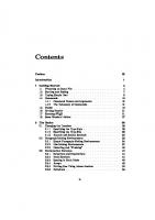
Contents Preface
iii
Introduction
1
1 Getting Started 1.1 Preparing an Input File . . . . . . . . . . 1.2 Starting and Ending . . . . . . . . . . . . 1.3 Typing Simple Text . . . . . . . . . . . . 1.4 Commands . . . . . . . . . . . . . . . . . 1.4.1 Command Names and Arguments 1.4.2 The Taxonomy of Commands . . . 1.5 Modes . . . . . . . . . . . . . . . . . . . . 1.6 Getting Fancier . . . . . . . . . . . . . . . 1.7 Running LATEX . . . . . . . . . . . . . . . 1.8 Some Words of Advice . . . . . . . . . . .
. . . . . . . . . .
. . . . . . . . . .
. . . . . . . . . .
. . . . . . . . . .
. . . . . . . . . .
. . . . . . . . . .
. . . . . . . . . .
. . . . . . . . . .
. . . . . . . . . .
. . . . . . . . . .
. . . . . . . . . .
4 4 7 8 10 10 15 19 21 21 27
2 The Basics 2.1 Changing the Typeface . . . . . . . . . . . . . . 2.1.1 Specifying the Type Style . . . . . . . . 2.1.2 Specifying the Type Size . . . . . . . . . 2.1.3 Accents and Special Symbols . . . . . . 2.2 Paragraph-Making Environments . . . . . . . . 2.2.1 Simple Paragraph-Making Environments 2.2.2 List-Making Environments . . . . . . . 2.2.3 Centering and “Flushing” . . . . . . . . 2.3 Mathematical Formulas . . . . . . . . . . . . . 2.3.1 Subscripts and Superscripts . . . . . . . 2.3.2 Math Symbols . . . . . . . . . . . . . . 2.3.3 Spacing in Math Mode . . . . . . . . . . 2.3.4 Arrays . . . . . . . . . . . . . . . . . . . 2.3.5 Putting One Thing Above Another . . . 2.3.6 Delimiters . . . . . . . . . . . . . . . . .
. . . . . . . . . . . . . . .
. . . . . . . . . . . . . . .
. . . . . . . . . . . . . . .
. . . . . . . . . . . . . . .
. . . . . . . . . . . . . . .
. . . . . . . . . . . . . . .
. . . . . . . . . . . . . . .
. . . . . . . . . . . . . . .
. . . . . . . . . . . . . . .
. . . . . . . . . . . . . . .
29 29 29 30 32 33 34 37 40 42 44 44 48 49 52 53
iv
. . . . . . . . . .
. . . . . . . . . .
v
2.4
2.5
2.6
2.3.7 Mathematical Miscellany . . . . . . . . . . 2.3.8 Changing Typeface and Style . . . . . . . . 2.3.9 What to Do When Nothing Works . . . . . Text That Migrates . . . . . . . . . . . . . . . . . 2.4.1 Footnotes . . . . . . . . . . . . . . . . . . . 2.4.2 Figures, Tables, and Other Floating Bodies 2.4.3 Marginal Notes . . . . . . . . . . . . . . . . Sectioning . . . . . . . . . . . . . . . . . . . . . . . 2.5.1 The Sectioning Commands . . . . . . . . . 2.5.2 Table of Contents, Etc. . . . . . . . . . . . 2.5.3 The Appendix . . . . . . . . . . . . . . . . The Title Page . . . . . . . . . . . . . . . . . . . .
3 Doing It Yourself 3.1 Defining Things . . . . . . . . . . . . . . . . . 3.1.1 Commands . . . . . . . . . . . . . . . 3.1.2 Lengths . . . . . . . . . . . . . . . . . 3.1.3 Counters . . . . . . . . . . . . . . . . 3.2 Spaces and Boxes . . . . . . . . . . . . . . . . 3.2.1 Spaces . . . . . . . . . . . . . . . . . . 3.2.2 Boxes . . . . . . . . . . . . . . . . . . 3.3 Line and Page Breaking . . . . . . . . . . . . 3.3.1 The \\ Command . . . . . . . . . . . 3.3.2 Line Breaking . . . . . . . . . . . . . . 3.3.3 Page Breaking . . . . . . . . . . . . . 3.4 Formatting it Yourself . . . . . . . . . . . . . 3.4.1 The tabbing Environment . . . . . . 3.4.2 The tabular and array Environments 3.4.3 The picture Environment . . . . . . 3.4.4 The list Environment . . . . . . . . 3.4.5 Verbatim . . . . . . . . . . . . . . . . 3.5 Changing the Style . . . . . . . . . . . . . . . 3.5.1 The Page Layout and Document Style 3.5.2 Page Styles . . . . . . . . . . . . . . . 3.5.3 Style Parameters . . . . . . . . . . . . 3.6 Using Raw TEX . . . . . . . . . . . . . . . . .
. . . . . . . . . . . . . . . . . . . . . .
. . . . . . . . . . . . . . . . . . . . . .
. . . . . . . . . . . . . . . . . . . . . .
. . . . . . . . . . . .
. . . . . . . . . . . .
. . . . . . . . . . . .
. . . . . . . . . . . .
. . . . . . . . . . . .
. . . . . . . . . . . .
. . . . . . . . . . . .
. . . . . . . . . . . .
54 55 56 57 57 59 64 66 66 67 69 69
. . . . . . . . . . . . . . . . . . . . . .
. . . . . . . . . . . . . . . . . . . . . .
. . . . . . . . . . . . . . . . . . . . . .
. . . . . . . . . . . . . . . . . . . . . .
. . . . . . . . . . . . . . . . . . . . . .
. . . . . . . . . . . . . . . . . . . . . .
. . . . . . . . . . . . . . . . . . . . . .
. . . . . . . . . . . . . . . . . . . . . .
71 71 71 73 76 78 78 80 86 86 87 90 91 92 96 100 108 110 111 111 112 114 118
4 Two-Column Text 5 Getting Bigger 5.1 Doing it in Parts . . . . . . . 5.2 Index and Glossary . . . . . . 5.3 Cross References . . . . . . . 5.4 Bibliographies and Citations .
120 . . . .
. . . .
. . . .
. . . .
. . . .
. . . .
. . . .
. . . .
. . . .
. . . .
. . . .
. . . .
. . . .
. . . .
. . . .
. . . .
. . . .
. . . .
. . . .
. . . .
122 122 126 127 128
vi 5.5 5.6
Auxiliary Files . . . . . . . . . . . . . . . . . . . . . . . . . . . . 130 Interaction . . . . . . . . . . . . . . . . . . . . . . . . . . . . . . 132
6 Errors 6.1 About Errors . . . . . . 6.2 LATEX’s Error Messages 6.3 TEX’s Error Messages . 6.4 LATEX Warnings . . . . 6.5 TEX Warnings . . . . .
. . . . .
. . . . .
. . . . .
. . . . .
. . . . .
. . . . .
. . . . .
. . . . .
. . . . .
. . . . .
. . . . .
. . . . .
. . . . .
. . . . .
. . . . .
. . . . .
. . . . .
. . . . .
. . . . .
. . . . .
. . . . .
. . . . .
. . . . .
134 134 136 139 142 142
A Document Styles
144
B The Bibliography Database
145
C Making Slides
146
List of Figures 1.1
The file myfile.tex. . . . . . . . . . . . . . . . . . . . . . . . . .
22
2.1 2.2 2.3
A Sample Figure. . . . . . . . . . . . . . . . . . . . . . . . . . . . The first half of a two-in-one figure. . . . . . . . . . . . . . . . . The second half of a two-in-one figure. . . . . . . . . . . . . . . .
60 61 61
3.1 3.2 3.3 3.4
A grand example. . . . . . . . . . . . . Input for a Grand Example. . . . . . . Points and their coordinates. . . . . . \put (1.4,2.6){\line(3,-1){4.8}}
vii
. . . .
. . . .
. . . .
. . . .
. . . .
. . . .
. . . .
. . . .
. . . .
. . . .
. . . .
. . . .
. . . .
. . . .
. 98 . 99 . 100 . 103
List of Tables 2.1 2.2 2.3 2.4 2.5 2.6 2.7 2.8 2.9 2.10 2.11
Accents. . . . . . . . . . . . Foreign Symbols . . . . . . Variant Greek letters. . . . Binary Operation Symbols. Relation Symbols . . . . . . Arrow Symbols . . . . . . . Miscellaneous Symbols . . . Variable-sized Symbols. . . “Log-like” Functions. . . . . Math Mode Accents. . . . . Delimiters. . . . . . . . . .
. . . . . . . . . . .
. . . . . . . . . . .
viii
. . . . . . . . . . .
. . . . . . . . . . .
. . . . . . . . . . .
. . . . . . . . . . .
. . . . . . . . . . .
. . . . . . . . . . .
. . . . . . . . . . .
. . . . . . . . . . .
. . . . . . . . . . .
. . . . . . . . . . .
. . . . . . . . . . .
. . . . . . . . . . .
. . . . . . . . . . .
. . . . . . . . . . .
. . . . . . . . . . .
. . . . . . . . . . .
. . . . . . . . . . .
. . . . . . . . . . .
. . . . . . . . . . .
33 33 45 45 45 46 46 47 48 53 54
Introduction LATEX is a computer program for generating many kinds of printed documents. You type in your text and some commands to say how you want it formatted, and LATEX does the rest. For example, typing \chapter{Getting Started} produced the chapter heading on page 4, complete with chapter number, and the table of contents entry on page iv. Even the page references in the preceding sentence were generated by LATEX; as I’m typing this, I don’t know on what page things will appear.1 Of course, LATEX also does the obvious things, like deciding where to start a new line or a new page. LATEX is a version of Donald Knuth’s TEX typesetting system, but it is much easier to use than the standard version of TEX. This manual tells you everything you need to know to generate most documents; no prior knowledge of TEX is required. The first thing you probably want to know about LATEX is how it’s pronounced. I won’t tell you because I believe that pronunciation should be determined by usage rather than fiat. TEX is usually pronounced teck, so lah-teck, lah-teck, and lay-teck are logical choices. Since logic doesn’t have much to do with such things, lay-tecks is also a possibility. However, pronouncing it as “L. A. TEX” is definitely frowned upon. LATEX was inspired by Brian Reid’s Scribe system While many ideas were stolen directly from Scribe, LATEX does not attempt to emulate Scribe. A primary goal of a document preparation system like Scribe or LATEX is to separate the specification of the document’s logical structure from the specification of how it is to be printed. I typed \chapter{Getting Started} to specify the beginning of a new chapter, a chapter being a logical component of the document. LATEX decided how this logical structure is to be translated onto the printed page—i.e., by starting a new page, printing a chapter number followed by the chapter name in large type, etc. 1 And
...
I produced this footnote by typing
will appear.\footnote {And I produced this footnote by ...
1
}
You tell LATEX how it should print things like chapter headings by specifying the document style. LATEX provides several standard document styles for you to choose from. You can easily change some aspects of the document style, such as producing a larger indentation at the beginning of a paragraph, or using Roman instead of Arabic numerals in the chapter number. Using the standard document styles with suitable modifications, most people will like the way LATEX typesets their papers, reports and books. There will always be special cases that no standard document style can handle. For example, the standard LATEX document styles aren’t well suited for typesetting the Old Testament. Fortunately, you can design your own document style. Unfortunately, it’s not easy to do; you have to know a lot about TEX, and you have to read the LATEX Document-Style Designer’s Guide, which has not yet been written. I expect there to be a few hardy souls who design new document styles and make them available to other LATEX users. A document style created for typesetting the Old Testament can be used by someone else to typeset the New Testament. However, most users will be happy with document styles designed by others. A document style tells LATEX how to print logical structures like chapters and enumerated lists. However, no document style can know about all possible logical structures. A recipe is a logical component of a cookbook, but none of the standard document styles knows about recipes. There’s no \recipe command that’s analogous to the \chapter command; you have to tell LATEX how to print your recipe. LATEX has commands for specifying exactly how something is to be printed—what type style to use for the list of ingredients, how to number the cooking steps, etc. You can even define your own \recipe command. While LATEX provides simple commands for typesetting things the way you want them, these commands are not as powerful as the more complicated ones provided by TEX. Since LATEX is a version of TEX, you can use almost all the ordinary TEX commands in LATEX. So, if you find yourself trying to do something that you can’t in LATEX, you can read The TEXbook by Donald Knuth to learn how to use the ordinary version of TEX. TEX was designed especially for typesetting mathematics, and it has many powerful commands for producing complicated mathematical formulas. If your documents contain only a few formulas, you’ll be able to get by with the LATEX commands and a little fudging. If they contain many formulas, then you’ll probably want to read the parts of The TEXbook that talk about typesetting mathematics. If you are a mathematician, or a mathematician’s typesetter, you should find out about AMS-TEX, a version of TEX specially made for mathematicians. There will also be a version called LAMS-TEX that combines the features of LATEX and AMS-TEX. Producing a document with LATEX is a lot different from typing it directly. Your input file is filled with lots of funny commands, and you can’t see exactly what the printed output will look like. Various document-production programs
2
have been developed that are a lot easier to use—programs that show you on the screen what your document will look like when it’s printed. These are sometimes called “what you see is what you get” formatting systems, so I’ll call them “WYSIWYG systems”. If these WYSIWYG programs are so easy to use, why did Knuth bother to implement TEX, and why did I compound the foolishness by implementing LATEX on top of it? There are two reasons why someone should use LATEX instead of a WYSIWYG program. The first is that it produces better quality output. The quality of typesetting done by TEX is comparable to that of a book publisher, so your LATEX output will look as good as an ordinary typeset book or journal. This is not true of any WYSIWYG system that I know about. The second and more important reason for using LATEX is the enormous flexibility that it provides. In the words of Brian Reid, these WYSIWYG systems are “what you see is all you’ve got” formatters. They can produce exactly what you see on your screen, but that’s all they can do. With LATEX, by changing a few declarations, you can completely change the appearance of your document. The same text may appear first in a short note, then as a chapter of a final report, and again as a journal article. Each time, it should be formatted differently. Even if your document will be printed only once, you may change your mind about how you want it formatted. With a WYSIWYG program, you’d have to reformat it yourself each time. With LATEX, you just change some declarations. When casually reading this manual, it may seem like the names “TEX” and “LATEX” have been used interchangeably. However, the careful reader will note that I have tried to distinguish between standard TEX and those features provided by LATEX. This distinction is important only when you read The TEXbook, where you will learn that most of the LATEX commands you have grown to know and love are not part of standard TEX. Before telling you how to use LATEX, I need to tell you how to use this manual. Chapter 1 tells you everything you have to know to start using LATEX. You should read it very carefully, and finish reading it before doing anything else. The rest of the manual is a reference book; you can turn to it when you come to something that you don’t know how to do. Chapter 1 tells you how to find what you need.
3
Chapter 1
Getting Started 1.1
Preparing an Input File
Your input to LATEX is a text file. On most computers, file names have two parts separated by a period, like always.iys. The first part of your input file’s name can be anything, but the second part should be tex. I’ll use myfile.tex as my standard example input-file name, but you can use any name you like. I assume that you know how to prepare a file with a text editor, so I’ll just tell you what should go into the manuscript file, not how to get it there. First, however, I’ll mention some important things about text files that you may not be aware of. A text file is a string of characters. There are two kinds of characters, printing and nonprinting ones. The printing characters are all those characters like q , % or = that light up phosphors on the screen, or put ink on the paper when the file is printed. All the rest are nonprinting characters. The nonprinting characters are just as real as the printing ones, and it’s important to know about them. When you look at a text file, it appears to be a series of lines composed of characters and horizontal spaces, the characters usually being grouped into words. The lines and spaces are actually produced by certain nonprinting characters that are in the file. The spaces between words are most often the result of space characters that are put into the file when you hit the space bar on your keyboard. In this manual, I’ll usually denote space characters by blank spaces, just like they appear on your terminal’s screen. However, when I want to emphasize that there’s a space character present in the input file, I’ll use the symbol to denote that character. Unlike an ordinary character such as q , it’s often hard to tell whether you’ve typed one or two space characters. Fortunately, you don’t have to worry about that. LATEX treats any number of consecutive characters just the same as a single one. There’s another key on your terminal that produces empty space on the
4
CHAPTER 1. GETTING STARTED
5
screen or printed page: the tab key. Hitting this key enters a nonprinting character called tab that acts like one or more space characters. LATEX treats a tab character exactly the same as a character. Since one is the same as several to LATEX, you never have to worry about whether that blank space on your screen is caused by a tab character or some characters. I usually won’t mention the tab character, but everything I say about will apply to tab as well. Your file is broken into a series of lines by a nonprinting character called ☎ carriage return that appears between the lines. I will use ✛✆as the name for ☎ this carriage return character.1 The ✛✆characters were probably entered in your file by hitting the key marked return on your terminal. Just like a q or a , ☎ ☎ a ✛✆is a full-fledged character. Most of the time, TEX treats a ✛✆as if it were a , but you’ll see that there are cases when this isn’t true. There’s one other nonprinting character that you might find in your file: the new-page character, sometimes called Control-L. If your text editor has a command for starting a new page, it probably works by putting a new-page character in the file. TEX treats a new-page character as if it were a blank line. Text files can also contain some weird nonprinting characters, like the one that makes your terminal beep. Those characters don’t belong there; TEX will come to a grinding halt if it finds one. Fortunately, it’s hard to get such characters into your file, so you needn’t worry about them. There are a number of funny printing characters hiding in the corners of your keyboard that you may find yourself typing for the first time when you prepare LATEX input. First and foremost is the \ character (pronounced “backslash”). It should not be confused with the more familiar / character, as in 1/2. You’d better practice typing the \ because you’ll use it a lot. Every LATEX command begins with a \. In typing the input for this chapter, I’ve used the \ characters about as often as the letter d. Your keyboard should have three kinds of bracketing pairs: parentheses ( and ), square brackets [ and ], and curly braces { and }. LATEX makes special use of the square brackets and curly braces. There should be three quote characters on your keyboard: ", ’ and ‘. You can forget about the " (double quote); you won’t need it at all. The ’ is called “right quote” and the ‘ is called “left quote” for reasons that will soon be obvious. The ’ is probably in a prominent position on the keyboard, perhaps over the 7; it may look more like ′ or on your screen. The ‘ is probably squirreled away in a corner, and may appear on your screen as ` . Among the printing characters, the following ten play a special role in TEX and are called special printing characters, or simply special characters. # $ % & ~ _ ^ \ { } 1 On many computer systems, a carriage return is really two characters—a plain carriage return and a line feed. This is of no concern, since TEX treats them as a single character.
CHAPTER 1. GETTING STARTED
6
While you’re perusing your keyboard, it would be a good idea to pick them out. The first four are everyday symbols that you’re familiar with. The tilde character ~ is probably hidden at the edge of your keyboard; the caret ^ may be denoted by a ↑ ; the underscore _ sometimes appears on the screen as a ←. You might want to paint these ten special character keys red because they are the characters that have a special meaning to TEX. Whenever you put one of these characters into your file, you’re doing something special. The remaining printing characters are called the ordinary printing characters. They are the upper- and lowercase letters, the ten digits 0 . . . 9 and the following. . : ; , ? ! " ‘ ’ ( ) [ ] < > - = + / * | @ Note that uppercase and lowercase letters are distinct characters. Don’t confuse the uppercase letter O (oh) with the digit 0 (zero). Also, don’t confuse the letter l (the lowercase el ) with the digit 1 (one). The only characters that should appear in your file are the ordinary and ☎ , tab and newspecial printing characters and the nonprinting characters , ✛✆ page. Some terminals have a variety of keys with strange characters etched on them. Pressing one of these keys usually issues a command to your editor without putting the strange character in the file. However, some of them may put weird characters in your file. TEX does not like such characters and will either complain bitterly or do strange things if it finds one in an input file. If your keyboard happens to have a key labeled ≤ , you will be tempted to try to produce 1 ≤ 2 by typing 1≤2. Don’t, unless you’ve been assured by a local expert that it works; otherwise, it probably won’t. It’s easy enough to generate a ≤ with ordinary LATEX commands. To get a document formatted properly, you have to tell LATEX what you want. This involves a lot of typing. Being a fast typist helps, but it’s still quite a chore. For example, a boldface word like bold is produced by typing {\bf bold}, which means typing six characters besides the four in bold. All these extra characters can add up to a lot of extra work. Fortunately, a good text editor like EMACS can be customized to reduce the amount of typing required. In my own personal version of EMACS, typing a single control character produces {\bf } and leaves the cursor just before the }. Typing {\bf bold} takes only two extra keystrokes (the second to move past the }) instead of six. This special EMACS command, together with a bunch of similar ones, saves me a lot of work. If you can’t do this with an editor available on your computer, you should complain. A good text editor can also help you avoid errors. The easiest error to make in your input is to leave out a curly brace. TEX expects braces to come in matched pairs and gets very unhappy when they don’t. With my editor, a single keystroke generates a pair of braces, so I can’t forget to type the closing }. There’s also a command that checks the entire file for unmatched braces, in
CHAPTER 1. GETTING STARTED
7
case I accidentally deleted a single brace. Adding these commands to my editor eliminated 90% of my TEX errors.
1.2
Starting and Ending
Your input file starts with commands to tell TEX how you want your document formatted—how wide the text should be, how sections are to be numbered, and so on. You may eventually want to decide all this yourself, but to start out, you’ll choose some standard format. The first part of the format is called the page layout. Your own computer installation will have its own selection of page layouts, but there should be a standard one called normal. To use it, you begin your file with the command \pagelayout{normal} The \pagelayout command specifies the dimensions of things on the page, such as the height and width of the text. The second part of the format that you must specify is called the document style. It determines such things as how sections are numbered and where figures are placed. Two standard document styles are report and article. The major difference between them is that the largest division in the report style is the chapter, each chapter starting on a new page, while the largest division in the article style is the section, where a section need not start on a new page. Both styles have sections, subsections and subsubsections. To choose the article document style, the second command in your file will be: \documentstyle{article} You can, of course, obtain the report style by typing report instead of article. The \pagelayout and \documentstyle commands are then followed by a \begin{document} command. After this comes the actual text of the document. The file ends with the command \end{document} The \begin{document} and \end{document} will make more sense to you later. For now, just remember that they have to be there, and concentrate on the important stuff—the text that generates the printed output. So, you just need to know that your file looks like this: \pagelayout{normal} \documentstyle{article} \begin{document} ... your text goes here ... \end{document}
8
CHAPTER 1. GETTING STARTED
1.3
Typing Simple Text
Producing simple text is easy; you can pretty much type what comes naturally. The rest is done for you. For example, the preceding two sentences were obtained by typing Producing simple text is easy; you can pretty much type what comes naturally. The rest is done for you. TEX ignored how many spaces I put between words—it treats any number of ☎ consecutive characters like a single . It also considers a ✛✆to be the same as a and does its own line breaking. A new paragraph is begun by leaving one or more blank lines—in other ☎ ☎ characters containing at least two ✛✆ ’s. A words, by any sequence of ✛✆and new paragraph is normally indented, but the indentation can be suppressed by typing \noindent at the beginning of the paragraph. Below is a list of other things that come up frequently in simple text. Quotes: Double quotes are produced by typing two ‘ characters for the left quotes and two ’ characters for the right quotes. For example, typing ‘‘quote’’ produces “quote”. You get single quotes, as in ‘single’ by typing single ‘ and ’ characters, as in ‘single’. The observant reader will note that I use the logical rather than the conventional method of mixing quotation marks and punctuation, writing “this”, and not “this.” “This”, being my own personal preference, is not a LATEX policy. You can type ‘‘this’’, or ‘‘that,’’ to produce “this”, or “that,” as you prefer. Dashes: TEX provides three sizes of dash: -, –, and —. They are produced by typing one, two, or three - characters, respectively, as in three sizes of dash: -, --, and ---. A minus sign, as in 4 − 2 = 2, is not the same as a dash. If you’re using a minus sign, then you’re writing a mathematical formula and you should refer to Section 2.3 on page 42. Space after periods: TEX tries to put a little extra space after a sentenceending period, but not after a period that doesn’t end a sentence. However, TEX is rather simple-minded, and it thinks that a period ends a sentence unless it follows an upper-case letter. This works most of the time, but look what happens if you type: Euclid et al. proved I + I = II. TEX produces
Meanwhile ...
9
CHAPTER 1. GETTING STARTED
Euclid et al. proved I + I = II. Meanwhile . . . thinking that the period after al ends a sentence, and the period after II doesn’t. To force TEX to do the right thing, you should type: Euclid et al.\
proved ... II\mbox{}.
Meanwhile ...
The \ tells TEX to make an ordinary space, and the \mbox{} separates the upper-case I from the period. Special characters: All of the ordinary printing characters listed on page 6 produce more or less what you’d expect them to. For example, typing + produces +, and typing [ produces [ . However, the ten special characters # $ % & ~ _ ^ \ { } have special meanings for TEX. The following six can be produced by typing a \ in front of them: # $ % & { } For example, typing \$20 yields $20. The other four special characters are used so seldom in text that LATEX doesn’t provide such a simple method of generating them. How to obtain them, as well as a host of other symbols, is explained in in Sections 2.1.3 and 2.3.2. Preventing line breaks: TEX produces nice, neat, justified paragraphs from your ragged input, hyphenating words if necessary. Sometimes it breaks a line where you don’t want it to. For example, it looks bad if I refer to page 28, and the line is broken between the “page” and the “28”. You can prevent this from happening by typing page~28. The ~ acts like a single , except that it prevents TEX from breaking the line there. Don’t leave a space before or after the ~ ; it will produce an extra space in the document. Comments: Sometimes you may want to leave little notes to yourself in the input file that you don’t want printed. Typing % tells TEX to ignore everything ☎ else on the current line, including the ✛✆at the end. For example, you might type as what’s his name% Look up the name! showed in 1976. to produce as what’s his nameshowed in 1976. However, the next time you’ll remember that the % causes TEX to ignore the ☎ ✛✆as well as the text, and you’ll type name % . You’ll also remember this if you ever want to end a line in your input file without putting space in the output.
CHAPTER 1. GETTING STARTED
10
Now that you know how to enter ordinary text, you’ll want to structure your text in units—sections, subsections and subsubsections if you’re using the article style, or chapters, sections, subsections and subsubsections if you’re using the report style. I’ve already mentioned that this chapter was begun by typing the command \chapter{Getting Started} and you can probably guess that the following section was begun with \section{Commands} The \subsection and \subsubsection commands are similar. You can find more information about these and other sectioning commands in Section 2.5 on page 66. Warning: Don’t try putting any LATEX commands in the name of a chapter or (sub[sub])section before reading Section 2.5. There are still a few more things you’d probably like to add, such as a title page and a table of contents. After finishing this chapter, you’ll be able to find and read the sections in later chapters that tell you how. Although you’ll eventually want to do that, you should probably start out the easy way—by copying from a friend. Given a LATEX input file, it’s pretty simple to figure out which commands create the title page, and what you have to change to generate your name instead of his. In fact, the friendly people who install LATEX on your computer system should also provide some sample input files for you to browse through.
1.4
Commands
To type fancier text, you have to issue LATEX commands. Before learning about what the commands do, you should learn their syntax and taxonomy. The material in this section may seem abstract and unmotivated, but knowing it will make it easier for you to understand how commands work. Your effort now will be amply rewarded in a little while. I will illustrate the general rules by using some specific commands as examples. Don’t worry about what these commands do; for now we’re just interested in the syntax. The commands themselves are explained in later chapters.
1.4.1
Command Names and Arguments
A LATEX command begins with the command name, which consists of a \ followed by either (i) a string of letters or (ii) a single nonletter. Here are some of the commands you’ve encountered so far. \bf
\mbox
\noindent
\begin \$
CHAPTER 1. GETTING STARTED
11
Another useful command is \today, which causes LATEX to produce today’s date—that is, the date on which you ran your file through LATEX. Here’s how I can tell you that this edition of this chapter was generated on March 4, 2005. Here’s how ... was generated on \today. Most command names are of the first kind, having of a string of letters. TEX regards lowercase and uppercase letters as completely different, so \large, \Large and \LARGE are three different commands. Most LATEX command names have only lowercase letters; the exceptions are generally like the three “large” commands, where uppercase letters are used to distinguish otherwise identicallyspelled commands. (As you’ll see in Section 2.1.2, \LARGE is larger than \Large, which is larger than \large.) If you write \$one, TEX knows that this is a \$ command followed by the text one because the only command names having nonletters are two-character names like \$. However, if you write \todayone , TEX wouldn’t think that this is the command \today followed by the text one . Instead, it regards it as a command named \todayone, and since there’s no such command, it will report an error. You have to tell TEX where a command name ends by putting a nonletter after it. You can write \today1 or \today one or \today-one, since 1, and - are nonletters. The most common way to end a command name is with a , so TEX ignores all spaces following a command name. However, this can cause trouble, since typing \today
was a sunny day.
produces March 4, 2005was a sunny day. Leaving more spaces after the \today won’t help—TEX treats any series of spaces the same as a single space. You can get TEX to stop ignoring spaces by typing {}. I can tell you that March 4, 2005 was a sunny day by typing either of the following: \today{} was a sunny day \today {} was a sunny day. The special character commands like \$ and \# are exceptions to this rule; spaces are not ignored after these commands. Typing \$ .99 produces $ .99. Many commands have arguments, which are enclosed in curly braces. For example, when you type \mbox{xyz}, xyz is the argument of the \mbox command. Typing \mbox{} gives \mbox a null argument. If a command takes more than one argument, each one is enclosed by curly braces. \parbox is a command taking two arguments, so you type
CHAPTER 1. GETTING STARTED
12
\parbox {2in}{A Parbox} to give a \parbox command whose first argument is 2in and whose second argument is A Parbox . Don’t worry about what these commands mean; just observe the syntax. Spaces after the command name are ignored, but you must not leave any spaces between arguments. Some commands have one or more optional arguments, an optional argument being enclosed in square brackets. The \parbox command has an optional argument that may appear before the other two, so \parbox [t]{2in}{A Parbox} has the optional argument t and with the same two mandatory arguments as before. The place where an optional argument comes is fixed; for \parbox it can come only right after the command name. TEX will be very confused if you try to put it somewhere else, like between the two mandatory arguments. There should be no space between any two arguments, whether they’re optional or mandatory. Some LATEX commands have a variant form indicated by writing a * at the end of its name. The variant form is also called the *-form. For example, there’s a \chapter* command that works just like the \chapter command except that it doesn’t add a chapter number or a table of contents entry. 44 % of the cases. You now know how to write commands in the normal 99 100 Let’s learn what surprises the other .56% has to offer. Optional arguments provide two kinds of surprises. Consider a command like \item that has one optional argument and no mandatory ones, so you can type either \item[foo] or \item foo. In the first case foo is the argument of the \item command, and in the second case it is the text that follows the command. Now, what happens if we want to type an \item command followed by the text [foo]? If we type \item [foo], TEX ignores the space and considers foo to be the argument. To prevent this, we must type \item{}[foo] or \item {}[foo]. The {} tells LATEX to stop looking for an optional argument as well as telling it to stop ignoring spaces. Now suppose we want to make not foo but [foo] the optional argument of the \item command, with the square brackets as part of the argument. If we type \item[[foo]], LATEX will take [foo to be the argument, enclosed by the first [ and the first ], and it will regard the second ] as part of the text following the \item[[foo] command. Once again, curly braces come to the rescue. If we type \item[{[foo]}], then LATEX will interpret {[foo]} as argument; the extra curly braces will do no harm. This trick must be used whenever there’s a [ in the text that could be mistaken for the left bracket delimiting an optional argument. The *-commands provide a related surprise. Although we think of the * as part of the command name, TEX actually regards it as an optional argument. Unlike the ordinary optional arguments that are enclosed by square brackets,
CHAPTER 1. GETTING STARTED
13
you can leave spaces between the * and the following argument. Thus, any of the following is acceptable:
CHAPTER 1. GETTING STARTED
14
\chapter*{Introduction} \chapter* {Introduction} \chapter *{Introduction} If a command with no mandatory arguments has a *-form, then we have the same problem, and the same solution, as with the \item command. One such command is \\ . To follow the plain \\ command with a * as part of the text, we must use a {}—typing \\ {}* instead of \\ * . LATEX would interpret \\ * as the *-form of the command. These problems are actually quite rare. Most of the time, you just have to know the following rules. • Command names begin with \. • Spaces following a command name are ignored, except for the specialcharacter commands like \$ . Use {} to make TEX stop ignoring spaces. • The variant form of a command has a * at the end of the name. • Mandatory arguments are enclosed by curly braces {}. • Optional arguments are enclosed by square brackets []. • There must be no spaces between arguments. There are a few minor exceptions to some of these rules, but you’ll hardly notice them. They are all as benign as the exception to the first rule that you’ve already encountered: the ~ command. To avoid rare but unpleasant surprises, you should also remember these exceptional situations. • Use {} if a [ can be mistaken for the beginning of an optional argument. • A ] that’s part of an optional argument must be inside braces. • Use {} if a * can be mistaken for a variant-command indicator. There’s one more little thing you might like to know about command arguments. It’s not important, but it can save you a bit of typing. An argument need not be enclosed in braces if it consists of either a single command name or a single letter or digit. If the second argument of a \parbox command is the single command \today, then you can type either of the following: \parbox {2in}\today \parbox {2in}{\today} However, if the argument is \mbox{\today}, then you must use braces because the \parbox’s argument then consists of a command name plus argument rather than just a command name.
CHAPTER 1. GETTING STARTED
1.4.2
15
The Taxonomy of Commands
There are five classes of LATEX commands. Understanding the differences among these classes will enable you to use the commands properly and will help you to remember individual commands. Text-Producing Commands A text-producing command places a piece of text in the document. The actual text is usually specified by an argument, as in the \mbox command. There may be other arguments that specify how the text is to be formatted; the argument that specifies the text is almost always the last argument. Sometimes, as in the \today command, there is no text-specifying argument because LATEX decides what text to insert. An important subclass of text-producing commands are the space-producing commands. The “text” they produce consists of blank space, an argument specifying how much blank space. Most text-producing commands put their text at the current position in the document. There are two cases in which the text may appear elsewhere: • Footnotes appear at the bottom of the page. • Marginal notes are placed in the margin, like the one on the right.
Figures and tables may also be moved from where they appear in the input file, but they’re not made with text-producing commands. Environments Text-producing commands are designed for formatting short pieces of text. To format a large piece, you use an environment. An environment begins with a \begin command and ends with a matching \end command. The above itemized list was produced with an itemize environment, which I typed as follows. \begin{itemize} \item Footnotes appear ... \item Marginal notes ... \end{itemize} The environment is begun with the \begin{itemize} command and is ended with the \end{itemize}. The stuff between these two commands is not an argument. Don’t worry now about what goes between the \begin and the \end commands; just remember that the itemize environment has no arguments. Some environments do have arguments. These arguments appear as extra arguments to the \begin command. For example, there’s an array environment, used to make arrays in mathematical formulas, with a single mandatory argument. Typing
This is an example of a marginal note.
CHAPTER 1. GETTING STARTED
16
\begin{array}{llr} ... \end{array} creates an array environment whose argument is llr . Environment arguments can be mandatory or optional. Just remember that the environment’s arguments become additional arguments to the \begin, and all the rules given in Section 1.4.1 apply. Environments can be nested in the obvious way. For example, figures are made by the figure environment. To make a figure that contains an itemized list, you type: \begin{figure} ... \begin{itemize} ... \end{itemize} ... \end{figure} In fact, your entire document is produced by a document environment—that’s what the \begin{document} and \end{document} commands are for. Each environment has rules about what other environments may appear inside it. For example, the document environment can’t contain another document environment, so you’ll only have one \begin{document} command in your file. \begin and \end commands have to come in matched pairs, just like curly braces. Forgetting an \end is a common error that your text editor should help you avoid. Mine produces a matching \begin–\end pair with a single command. A few environments have *-forms. For example, if you’re producing twocolumn output, the figure environment makes a figure that’s one-column wide and the figure* environment makes a two-column-wide figure. To use the figure* environment, you type \begin{figure*} ... \end{figure*} Notice that the * becomes part of the environment name. It does not act like an optional argument, as in ordinary commands. Declarations A declaration is a command that causes TEX to change the way it’s doing things. For example, the \bf command tells TEX to start using boldface type, as I just did by typing ... using \bf boldface type, as I just did by ... Note how TEX typeset everything after the \bf command in boldface. How did I get TEX to stop using the bold typeface and revert to its normal typeface? For the answer, you first have to understand the concept of nesting. As TEX processes your input, it can best be thought of as traveling through the levels of a subterranean building. TEX starts out at street level. Every time it encounters a { or a \begin , TEX goes down a flight of stairs to the next lower level, and every time it encounters a } or an \end it goes up a flight of
CHAPTER 1. GETTING STARTED
17
stairs to the next higher level. Thus, it remains underground from the time it hits your \begin{document} command until it reaches the \end{document}. Every time TEX descends a flight of stairs, it paints on them what led it down those steps, painting either a { or a \begin command, and covering over anything that what was previously painted there. When it next ascends those steps, it must have been directed to do so by the corresponding } or \end . If it had painted \begin{itemize} on the steps, it can only be directed up them by an \end{itemize}, not by a } or an \end{figure}. Thus, you can’t type \begin{figure} {
... \end{figure} } is wrong!
because the \end{figure} would cause TEX to try walking up a flight of steps painted with a { . The braces that enclose an argument are somewhat different from other braces. In almost all cases, the braces enclosing an argument of a LATEX command cause TEX to go down a flight of steps to start processing the argument, and back up the steps when it’s through. So, when TEX encounters the command \mbox{arg}, it’s at a lower level when processing the arg than it is before and after the command. As explained in Section 3.1.1, when you define your own commands, you can choose whether or not the argument braces should cause TEX to change levels. A declaration normally stays in effect as long as TEX remains at or below the current level. As soon as TEX returns to the next higher level, it forever forgets about the declaration. The region in which a declaration is in effect is called its scope. We can produce a single bold word by typing {\bf bold} because the scope of the \bf declaration ends with the right brace. The following input shows how TEX reacts to a \bf declaration, assuming that it begins when TEX is producing output in a Roman typeface. This is Roman. {Still Roman. \bf Start boldface \begin{itemize} ... boldface ... \end{itemize} Still boldface.} Back to Roman. {Still Roman.} One declaration can be superceded by a countermanding declaration. The \bf declaration in our example superceded a prior declaration that told TEX to use a Roman typeface. The \bf declaration can in turn be superceded by another typeface declaration, such as \it , which tells TEX to use an italic typeface. Adding an \it command to the previous example gives the following. This is Roman. {Still Roman. \bf Start boldface \begin{itemize} ... boldface. \it Start italic ... \end{itemize} Back to boldface.} Back to Roman. {Still Roman.}
CHAPTER 1. GETTING STARTED
18
Note that the \end{itemize} ends the scope of the \it command, but leaves TEX within the scope of the \bf . Any declaration can be used as an environment—you just remove the \ to get the environment name. For example, you can type \begin{bf} A bold sentence.\end{bf} The environment is the scope of the \bf command, so this is equivalent to typing {\bf A bold sentence.} You should use the bf environment when one or more paragraph are all in boldface, since you’ll probably find it hard to keep braces matched properly when they’re far apart. Some environments make changes within them that supersede declarations made outside the environment. These will be mentioned when the environment is explained. Some declarations are global, meaning that they remain in effect even when TEX climbs above its current level. These are generally declarations whose effects you would not expect to end with the current environment. For example, page numbering is outside the province of environments and normal scoping, so a declaration like \pagenumbering{roman}, which causes LATEX to number the current page i, the next page ii, and so on, is global. Page-Breaking and Line-Breaking Commands This is a small class of commands that tell TEX where to end a page or a line, or where not to end it. Indirect Commands This class is a mixed bag of commands that have one thing in common: they don’t have any direct effect on TEX’s output. For example, Section 2.5 describes an indirect command for adding a table of contents entry with the current page number. Executing it has no effect on what is produced during the current execution—TEX probably generated the table of contents before seeing the command. However, the next time you run your file through LATEX, the entry will magically appear in the table of contents. An indirect command is sometimes placed right in the middle of a paragraph, usually between words. When this happens, you’re faced with the question of whether to leave a space on each side of the command, or to attach the command to one of the two adjoining words. Usually it makes no difference. However, sometimes you may wind up with an extra space between the words, or, less often, with no space between them. When that happens, it will be obvious what you should do to correct the situation. However, by the time you see your output, you’ll probably have forgotten all about the indirect command and all
CHAPTER 1. GETTING STARTED
19
you’ll see is the extra space. When that happens, remember to look at the input to see if there’s an indirect command causing the problem. An extra space is removed by attaching the command to either of the adjacent words. A missing space is usually corrected by adding a space before the command.
1.5
Modes
When TEX is processing your input text, it is always in one of three modes: • Paragraph mode • Math mode • Left-to-right mode, called LR mode for short. TEX changes mode only when it goes up or down a staircase to a different level, though not all level changes produce mode changes. Mode changes occur only when entering or leaving an environment, or when TEX is processing the argument of certain text-producing commands. The description of each environment and text-producing command describes whether it causes a mode change. Paragraph mode is the most common; it’s the one TEX is in when processing ordinary text. In that mode, TEX breaks your text into lines and breaks the lines into pages. TEX is in math mode when it’s generating a mathematical formula—you’ll learn about that in Section 2.3. Before getting to LR mode, I must explain a bit more about how TEX processes text. As I explained in Section 1.1, the input to TEX is a string of characters. TEX’s output is a sequence of pages, each page consisting of a sequence of lines and vertical spaces, and each line consisting of a sequence of characters and horizontal spaces. To distinguish the printed representation of a character from the input character, I will call the former a glyph. Thus, the character t in your input file might generate any one of the following glyphs in the printed output. t t
t
t
In paragraph mode, TEX translates each ordinary printing character into ☎ the corresponding glyph and translates and ✛✆characters into horizontal spaces—except when they end a paragraph. TEX regards each string of glyphs as a word, and it breaks the text into lines of words, with space between them. If necessary, it will hyphenate words to keep the spaces between them from getting too large. Text-producing commands generate glyphs and/or spaces. Typing \today today (March 4, 2005) produces exactly the same sequence of glyphs and spaces as typing March 4, 2005
CHAPTER 1. GETTING STARTED
20
TEX could start a new line between the day and the year. However, some textproducing commands produce a box , which is a chunk of text that TEX treats exactly like a single glyph. One such command is \mbox. Typing \mbox{no way} tells TEX to make a box with “no way” inside it. Just looking at the output, there’s usually no way of knowing that I used an \mbox command instead of simply typing no way . However, the output is a lot different to TEX. TEX regards the box produced by a \mbox command as if it were a single glyph, so the command \mbox{no way} produces something that looks to TEX like no way There’s no way that TEX can split no way across two different lines, just as there is no way for it to split the glyph A into two pieces. So, if you want keep TEX from splitting something across lines, just use the \mbox command to put it in a box. Now let’s return to LR mode. The canonical example of when TEX is in LR mode is while it is processing the argument of an \mbox command. In LR mode, as in paragraph mode, TEX considers the output that it produces to be a string of words with spaces between them. However, unlike paragraph mode, TEX keeps going from right to left; it never starts a new line in LR mode. Even if you put a hundred words into an \mbox, TEX would keep typesetting them from left to right inside a single box, and then complain because the resulting box was too wide to fit on a line. TEX is in LR mode when it starts making a box with an \mbox command. You can get it to enter a different mode inside the box—for example, you can make it enter math mode to put a formula in the box. There are also several text-producing commands and environments for making a box that put TEX in paragraph mode. The box made by one of the commands or environments will be called a parbox, named after \parbox, the exemplar of these commands. When TEX is in paragraph mode while making a box, it is said to be in inner paragraph mode. Its normal paragraph mode, which it starts out in, is called outer paragraph mode. There are some things, like making footnotes, that TEX can do in outer paragraph mode but not in inner paragraph mode. I’ll warn you about them as we go along. While we’re on the subject of boxes, I should mention that sometimes you’ll want to make a great big box and stick it on its own line. If you leave a blank line before and after the box, TEX will view it as if it were a one-character paragraph. However, remember that you must use a \noindent command if you don’t want the paragraph indentation.
CHAPTER 1. GETTING STARTED
1.6
21
Getting Fancier
Section 1.3 told you how to produce simple output. Most of the rest of this manual is about how to produce fancier output. The purpose of this section is to help you find what you need. The first place to look for something is in the table of contents. Suppose you want to write theorems and would like an environment to format them for you. Scanning through the table of contents quickly reveals that Section 2.2.1 is the place to look. However, you shouldn’t go right there. The information in this manual is tree-structured. Section 2.2.1 is a subsection of Section 2.2.1, which is a subsection of Section 2.2. Before reading Section 2.2.1, you should read the introduction to Section 2.2 and the introduction to Section 2.2.1. The introduction to a section is everything from the beginning of the section until the beginning of its first subsection, so the introduction to Section 2.2.1 starts at the beginning of that section and ends at the beginning of Section 2.2.1.1. To use a command or environment, you may have to understand other things about LATEX. I assume that you know everything in this chapter—especially the material in Section 1.4 and 1.5. When knowledge of other material is required, I will tell you where to find that material. The introduction to each section tells you what’s in that section. If you think you might need a paragraph-making environment, but don’t know what kind, you should read the introduction to Section 2.2. If the table of contents doesn’t help, you might can try the index. However, the index is designed to help you find information about a specific topic like footnotes, not to tell you what features LATEX provides. Chapter 2 contains the more elementary commands—the ones you’re likely to use right away. The environments and commands of this chapter generally allow LATEX to handle the formatting, under the control of the document style. Chapter 3 contains commands and environments that allow you to control exactly how things are formatted, as well as commands for changing documentstyle parameters. Chapter 4, which discusses two-column output, should really be part of Chapter 3. However, I wanted to show you an example of two-column output, and it’s hard to produce just part of a chapter in that format. Chapter 5 describes commands that you won’t need until you start producing larger documents. These include commands for splitting your input into several files, and cross-referencing commands. Finally, Chapter 6 will help you cope when something goes wrong.
1.7
Running LATEX
You now know how to prepare an input file; it’s time to learn how to run LATEX on that file. Let’s suppose that you’ve created an input file named myfile.tex, you’ve checked that there are no unmatched curly braces, and you’re ready to
CHAPTER 1. GETTING STARTED
22
\pagelayout{normal} \documentstyle{article} \begin{document} Look at this \begin{simple} error. And at this \parbox{nasty} one. Is there a little town in Wales called Llegharffysloughlarwaghaurllysgnforghallyl? \end{document} Figure 1.1: The file myfile.tex. run it and see what happens. I’d like to tell you that your file will sail through LATEX and produce beautiful output, but the chances of that happening on the first try are rather slim. Your input file will almost certainly contain errors, so you must be prepared to deal with them. To give you some idea of what you’ll run into, we’ll try the short input shown in Figure 1.1. Note that it has two errors: there’s a spurious \begin{simple} command, and the \parbox command is missing one of its mandatory arguments. The first thing we must do is start the LATEX program. On my computer, I ☎ , but you may have to type something else on yours. do this by typing latex✛✆ It all depends upon what operating system you’re using. LATEX starts by typing **, which is its way of asking for the name of the input file. Since our file is ☎ . LATEX then types out named myfile.tex, we respond by typing myfile✛✆ the following bunch of junk. (It may type something a little different on your computer.) This is TeX, Tops-20 Version 1.0 (preloaded format=lplain 84.02.07) (PS:MYFILE.TEX.4 LaTeX Version 2.0 - Release 7 Feb 84 (PS:NORMAL.PLO.2 Page Layout ’normal’ -- version of 21 Mar 1984. ) (PS:ARTICLE.STY.65 Document Style ’article’. Version 1.0 - released 8 Jun 1984 ) No file myfile.aux.
We needn’t worry about any of this, it’s just LATEX’s way of saying hello. The first time you run LATEX on your system, it’s a good idea to check that the version number it types is 2.0. If it isn’t, then the version of LATEX you’re running is different from the version described in this manual, and you should ask a local expert if there are any important changes that you should know about.
CHAPTER 1. GETTING STARTED
23
The ‘No file myfile.aux’ message appears the first time we run LATEX on myfile.tex. Afterwards, a file named myfile.aux will appear in our directory. As explained in Section 5.3, the file myfile.aux is used to implement LATEX’s automatic cross-referencing feature. Since we’re not doing any cross-referencing, this file is totally useless. If we don’t delete it, then the next time we run the file through LATEX, that message will be replaced by: (PS:MYFILE.AUX.1 )
The next thing that LATEX types is much more important; it’s the error message for the spurious \begin{simple} command. Before we look at it, I should explain the precise relation between LATEX and TEX. Most of the commands that you use are LATEX commands, which means that they were defined by me in terms of more primitive TEX commands. LATEX makes some effort to catch errors, but it won’t catch them all. (It would slow LATEX down too much to do a lot of error checking.) If LATEX misses an error, TEX will probably catch it. Unfortunately, it will appear to TEX as an error in one of the TEX commands that I wrote that implements the LATEX command you typed. Keeping all this in mind, let’s look at what’s typed out when the \begin{simple} command is encountered. LaTeX error. See LaTeX manual for explanation. Type H for immediate help. ! Environment simple undefined. \@latexerr ...for immediate help.}\errmessage {#1} \endgroup l.4 Look at this \begin{simple} error. ?
The first two lines of this message tell us that we’re in luck—the error was detected by LATEX before any lower-level TEX errors occurred. The next line, beginning with the ! , is called the error indication line. It tells us what the problem is. Section 6.2 gives a list of all LATEX-generated error indications, and tells you how to find out exactly what caused them. In this case, the problem is simple—there’s no such environment as simple. After the error indication line, there is a bunch of stuff that will be quite meaningless to you and should be ignored. (If you’re curious, you’ll have to read The TEXbook to find out what it all means.) After it comes a pair of lines called the error locator, followed by a line containing only a question mark. In this message, the error locator begins with l.4. The error locator tells us how much of our input TEX had read when the error was discovered. The l.4 says that the error was found when processing the fourth line of our input. Following the l.4, TEX types input line four, split into two lines. Where the split occurs tells us exactly how far TEX had gotten when it discovered the error—the first line showing what TEX had read and the second line showing what it hadn’t. In this case, the error was discovered right
CHAPTER 1. GETTING STARTED
24
after TEX read the \begin{simple} command. An error locator might consist of a single line followed by a blank line, meaning that TEX had read everything on the line before finding the error. The error locator might also be completely blank, indicating that TEX discovered the error when it was processing a blank input line. The final line of the message, the one consisting of the question mark, tells us that TEX has stopped and is waiting for us to tell it what to do. We’ll accept ☎ . It responds with the following helpful LATEX’s offer of help and type H✛✆ message. Your command was ignored. Type I to replace it with another command, or to continue without it. ?
The question mark at the end again tells us that TEX has stopped and wants us to type something. Since there’s nothing that we want to replace the ☎ \begin{simple} command with, we’ll just type ✛✆and let LATEX proceed. The next message we get is caused by the error in the \parbox command. ! Missing number, treated as zero.
n n asty \@iparbox ...true $\vcenter \fi \fi \fi {\hsize #2 \@parboxrestore #3}\if@pbo... l.5 And at this \parbox{nasty} o ne. ?
The absence of the ‘LaTeX Error’ at the beginning tells us that the error was detected by TEX instead of LATEX. TEX’s error-handling mechanism doesn’t know anything about LATEX commands, so we can’t expect much help from the the error indicator line. Some common TEX error indicators and their causes are listed in Section 6.3, so you can try looking there for help. You can also ☎ type H✛✆ and see what advice TEX gives you, but most of the time it won’t be too helpful. Right now, let’s see what we can discover by ourselves. As usual, we can ignore everything between the error indicator and the error locator. The error locator tells us that the error was detected right after TEX read the o that followed the \parbox command. As this example shows, TEX can go past the point where the real error is before it discovers that something is wrong. Fortunately, it didn’t go very far, and we have the incorrect \parbox command displayed before us. Unfortunately, there’s nothing we can do about it now. At this point, you may be tempted to stop LATEX, correct the errors, and try again. Don’t. You should always let LATEX go as far as it can in your file before giving up. Whenever you find one error there are probably several more
CHAPTER 1. GETTING STARTED
25
beyond it, so you should find as many as you can each time you run LATEX. To ☎ . We then get the following error message. let LATEX continue, we type ✛✆ ! Illegal unit of measure (pt inserted).
n n asty \@iparbox ...true $\vcenter \fi \fi \fi {\hsize #2 \@parboxrestore #3}\if@pbo... l.5 And at this \parbox{nasty} o ne. ?
Once again, this message was generated by TEX rather than LATEX, so we can ignore everything but the error locator. It tells us that TEX hasn’t gotten any further; it’s at the same place in our input where it was the last time. TEX found something else wrong when processing the incorrect \parbox command. ☎ Undaunted, we type ✛✆and carry on. TEX next types the following message. Overfull \hbox (68.3333pt too wide) in paragraph at lines 5--5 []\tenrm nastyo \hbox(6.19444+1.94444)x0.0 .\hbox(0.0+0.0)x40.0 .\tenrm n .\tenrm a .\tenrm s .\tenrm t .etc.
This is a warning message rather than an error message. There’s no questionmark line, so TEX is still running. The fact that it’s warning us about something at “lines 5--5” gives us a clue that the problem was probably caused by the bad \parbox command, and the presence of the word “nasty”, the argument of that command, in the message confirms our suspicions. TEX is telling us that our incorrect \parbox command produced some bad-looking output, which isn’t surprising. The next thing that TEX types is the following: Overfull \hbox (1.94412pt too wide) in paragraph at lines 7--9 []\tenrm Is there a lit-tle town in Wales called Llegharffys-lough-lar-waghau-r llysgn\hbox(6.94444+1.94444)x340.0, glue set - 1.0 .\hbox(0.0+0.0)x40.0 .\tenrm I .\tenrm s .\glue 3.33333 plus 1.66666 minus 1.1111 .\tenrm t .etc.
CHAPTER 1. GETTING STARTED
26
This is also a warning—in fact, the same kind of “Overfull \hbox” warning we saw above. You’ll see a lot of these warnings. They happen when TEX can’t find a good way to break a paragraph into lines, so it gives up and leaves a line sticking out in the margin. Section 3.3.2 on page 87 tells you how to deal with this problem. Another warning you’re likely to see is an ‘Underfull \vbox’ message. It occurs when TEX can’t find a good place to start a new page. You needn’t worry about this warning, but you should check Section 3.3.3 on page 90 if, when you look at the output, you’re not happy with TEX’s page breaking. Other warning messages are explained in Chapter 6. While we’ve been pondering this message, LATEX has continued processing the input file, printing: [1] (PS:MYFILE.AUX.2)
TEX typed the [1] right after producing the first page of output. Had there been a second page, it would have typed [2] immediately after that page was produced. Of course our tiny file produced only a single page, but you should pay attention to those numbers when you’re running LATEX; they’ll help you correlate the error messages on your terminal with the printed output. The ‘(PS:MYFILE.AUX.2)’ can be ignored, but it does tell you that TEX has reached your \end{document} command and is now finishing up. TEX’s final words to us are: Output written on PS:MYFILE.DVI.2 (1 page, 392 bytes). Transcript written on PS:MYFILE.LST.2.
They tell us that the output was written on a file called myfile.dvi, and that everything TEX typed out on our terminal plus some additional information was also written on the file myfile.lst. We didn’t bother writing down all the error information that was typed because it will be waiting for us on this “.lst” file. We’ve finished running LATEX, but we still haven’t seen our output. At the moment, it’s just sitting on the file myfile.dvi. We have to run some other program to actually print it. Exactly how this is done depends upon your particular computer system, so you’ll have to ask a local expert what to do next. In this example, things went pretty smoothly. Even though there was a nasty error (the missing \parbox argument), we could get TEX to continue past ☎ it by typing ✛✆after the two error messages. A single error can easily generate five or ten error TEX messages. Sometimes TEX gets so confused by an error that it either won’t go any further, producing error after error with the same error locator, or else it starts thinking that almost everything is an error. If that happens, you’ll have to correct the error and rerun TEX in order to get ☎ any further. The best way to stop LATEX after an error is to type I \stop✛✆ in response to its question mark. If that just produces another error message,
CHAPTER 1. GETTING STARTED
27
☎ ; this will always cause TEX to quit. TEX will produce then you should type X✛✆ a .dvi file with the output that was generated so far, as well as a .lst file with all the error messages. TEX may stop without any error message, simply typing a *. The most likely cause of this is a missing \end{document} command, but other errors can also ☎ . If that doesn’t work, have this result. If it happens, you should type \stop✛✆ you’ll have to stop TEX by whatever means your operating system provides for halting uncooperative programs. Even experienced LATEX users are sometimes mystified by an error. When that happens to you, the most important thing to remember is
DON’T PANIC. Instead, turn to Chapter 6 to find out what to do.
1.8
Some Words of Advice
A major goal of LATEX is to allow you to change the way your document is formatted by changing a few declarations without having to change the text itself. However, no matter how much one tries, changing the format may require some changes to the text. You can change the width of your lines with a single declaration, but, if you make the lines too narrow, you may have to change some things that no longer fit on a single line. The proper use of LATEX allows you to minimize the number of changes that have to be made to your text when you reformat it. When you tell LATEX how to print a recipe, you’ll probably specify how far the list of ingredients should be indented from the left margin. You could give the distance in inches, but you might have to change that distance if you changed the line width. A better method would be to specify the distance as a certain fraction of the line width, so the same LATEX commands would produce the right indentation regardless of the line width. An even better way to avoid having to change the text of your recipes when changing the format is to define a \recipe command, using the \newcommand command described in Section 3.1.1. That way, you just have to change the definition of the \recipe command to change how every recipe is printed; you never have to change the individual recipes. Whenever your document contains a special class of objects like recipes, you should define a command to generate them. This will usually save you a lot of typing, since you don’t have to repeat the formatting commands every time. However, even if it doesn’t, you should still define a command to generate these objects because that makes it easier to change how they are formatted. Defining a command \hoare so that
CHAPTER 1. GETTING STARTED
28
\hoare{P}{S}{Q} produces {P } S {Q} doesn’t save any typing. But, if you decide that there should be more space in the expression, so it looks like {P } S {Q} then only the definition of \hoare has to be changed; you don’t have to change every occurrence of the notation. The experienced LATEX user makes extensive use of its command-defining features. Another thing the experienced LATEX user does is avoid wasting his time and his computer’s time running LATEX over and over again with the same input. Documents, except for very short ones, are written a little bit at a time. You’ll naturally want to see LATEX’s output as you produce the input. However, after you write the first ten pages and get LATEX to print them for you, it’s silly to keep regenerating those ten pages every time you write some more input. It’s especially silly to wait while LATEX processes those ten pages again in order to find the errors in your new input. You should always run LATEX on new input by itself, without any of the old input. Only after there are no more errors in the new input should it be added to the old. If it’s fairly short, then the entire document might be processed by LATEX every time you add new text. For a larger document, you should use the methods described in Section 5.1 to avoid this reprocessing.
Chapter 2
The Basics This chapter describes the basic text-producing commands, environments and declarations. Most of these commands specify the logical structure of the text and leave the formatting to LATEX. However, commands for telling LATEX what typeface to use and how to do some simple formatting, like centering text, are also included. Remember that, as described in Section 1.4.2, any declaration can be used as an environment.
2.1
Changing the Typeface
As I explained in Section 1.5, TEX translates an ordinary printing character like A into a glyph. Whether it’s translated into the glyph A or the glyph A depends upon the typeface. You specify a typeface by giving the size and the style. For example, this sentence is printed in 10-point italic. The 10-point is the size, a point being a unit of length used by printers, and italic is the style. A typeface is also called a font.
2.1.1
Specifying the Type Style
Below is a list of the type styles available with LATEXand the declarations for obtaining them. They work like the \bf command for generating boldface, which you’ve already seen in Section 1.4.2. Note that, like \bf, the type-style declaration commands all have two-letter names. \rm: Roman. This is an example of the Roman typeface; it is the typeface ordinarily used by LATEX. \it: Italic. This is an example of the italic typeface. \bf: Boldface. This is an example of the bold typeface.
29
CHAPTER 2. THE BASICS
30
\sl: Slanted. This is an example of the slanted typeface. \sf: Sans serif. This is an example of the sans serif typeface. \sc: Small caps. This is an example of the small caps typeface. \tt: Typewriter. This is an example of the typewriter typeface. The \rm command may seem useless, since Roman is what you get when you don’t specify any other typeface. However, you can type {\rm word} to make just the “word” appear in Roman in the middle of a boldface or italic sentence. There’s one little trick you should know when using the italic and slanted fonts in order to produce the finest quality output. Examine closely the word didn’t , which I produced by typing {\it did}n’t. Notice how the slanting d of did bumps into the n of n’t . To prevent this, you have to add some extra space after did . The \/ command adds just the right amount of extra space. You type {\it did\/}n’t to produce did n’t , which looks much nicer. It’s a good idea to use the \/ whenever switching back from an italic or slanted typeface to an upright one like Roman. The one exception is that you shouldn’t put the \/ right before a period or comma. Warning: If you use a type-style-changing command in math mode, then the scope of that command should end before TEX “climbs the stairs” leading it out of math mode. What this means is that any style-changing command like \bf in a math formula should always be enclosed in curly braces that lie within the formula.
2.1.2
Specifying the Type Size
The Normal Type Size Printers specify type size in points, where 24-point type is twice as big as 12point type. The ordinary text of most books is, like this manual, set in 10-point type. It looks quite normal in a book, but you may find it rather small for your ′′ own reports and papers—especially if they’re printed on standard 8 12 × 11′′ paper. You might want to consider 11-point or 12-point type, illustrated in the following two paragraphs.
This paragraph is set in 11-point type. You can get LATEX to set your entire document in this size type by choosing an 11-point document style. This is done by specifying the 11pt substyle for the document style you’ve chosen. For example, you type \documentstyle{article,11pt} in place of the ordinary \documentstyle command to get the elevenpoint version of the article style, and similarly for the report style. Make sure that there are no spaces in the argument.
CHAPTER 2. THE BASICS
31
This paragraph is set in 12-point type. You can get your entire document set in this type size by choosing the 12pt substyle for the document style you’ve chosen. The 11pt and 12pt document substyles may change the line width and other parameters to produce a more aesthetically pleasing document. You shouldn’t judge these type sizes by these two paragraphs, since they were produced with parameters chosen for 10-point type. Instead of specifying a substyle as part of the same \documentstyle command, as in \documentstyle{report,12pt} you can make it a separate \documentstyle command, writing \documentstyle{report} \documentstyle{12pt} The main style command, in this case report, must come before the substyle command. Additional Type Sizes The document style defines the normal type size. LATEX provides the following commands for producing text with different type sizes within the document. Here is what they produce in a 10-point document style; they will usually produce correspondingly larger type in an 11-point or 12-point document style. \normalsize: This is an example of the normal type size. \large: This is an example of the large type size. \Large:
This is an example of the Large type size.
\LARGE:
This is an example of the LARGE type size.
\huge:
This is a huge type size.
\small: This is an example of the small type size. \footnotesize:
This is an example of the footnotesize type size. It is the type size normally used in footnotes.
\scriptsize:
This is an example of the scriptsize type size. It is the type size normally used in subscripts and superscripts.
\tiny:
This is an example of the tiny type size. It is the smallest type size provided.
CHAPTER 2. THE BASICS
32
Each of these size-changing declarations switches to the Roman type style. Thus, if TEX is currently using the \normalsize type size, we have: {\bf normal boldface {\large large Roman} back to normal boldface } Because the information needed to generate each typeface takes up valuable room inside TEX, not all type styles are available in all sizes. Different computer systems may provide a different selection of typefaces. However, all styles should be available in the \normalsize, \small and \large sizes. If you request a typeface that’s not available, LATEX will produce an error with the following error indication. ! Typeface not available. Warning: If you want to typeset one or more entire paragraphs in a different type size, then you must be sure to end the scope of the size-changing declaration after the blank line that ends the last paragraph in that size. For example, you should type \begin{large} Beginning of large typeface paragraph ... ... end of large typeface paragraph. \end{large} Omitting the blank line before the \end{large} command will produce funnylooking output. Warning: Don’t issue a size-changing command in math mode. If you want to use a different type size for an entire mathematical formula, then put the entire formula in the scope of the size-changing command. If you want part of a formula to be in a different type size, then use an \mbox in the formula and put the size-changing command inside the \mbox.
2.1.3
Accents and Special Symbols
Accents TEX enables you to generate any kind of accent you’re likely to need. Table 2.1 shows how to do it. The letter o is used in the table, but you can replace it with any other letter. These accents work properly with all the usual type styles except for the typewriter (\tt) style. They can’t be used in that style. The letters i and j need special treatment because they should lose their dots when accented—typing \’{i} produces ´ı . The commands \i and \j produce a dotless i and j , respectively, so typing \’{\i} gives ´ı .
33
CHAPTER 2. THE BASICS Type \‘{o} \’{o} \^{o} \"{o} \~{o}
to get o ` o ´ o ˆ o ¨ o ˜
Type \={o} \.{o} \u{o} \v{o} \H{o}
to get ¯o o˙ ˘o ˇo ˝o
Type \t{oo} \c{o} \d{o} \b{o}
to get o⁀ o o¸ o. o ¯
Table 2.1: Accents. Type \oe \OE \ae \AE
to get œ Œ æ Æ
Type \aa \AA \o \O
to get ˚ a ˚ A ø Ø
Type \l \L \ss
to get l L ß
Table 2.2: Foreign Symbols Symbols Table 2.2 shows how to make some of the special symbols used by Western languages other than English. These commands can appear in paragraph and LR modes. However, they won’t work when a typewriter (\tt) type style is in effect. There are a large number of mathematical symbols that can be used only in math mode. These are described in Section 2.3.2. TEX also provides five special symbols that can be used in any mode: Type \dag \ddag
2.2
to get † ‡
Type \S \P
to get § ¶
Type \copyright
to get c
Paragraph-Making Environments
This section describes LATEX environments for producing various kinds of paragraphs, used for quotations, poetry, etc. In all these environments, a blank line begins a new paragraph. This causes the appropriate amount of interparagraph vertical space to be inserted. The first line of a paragraph is indented in some environments, but not in others. The output generated by a paragraph-making environment starts on a new line, as does the output that follows the environment. Whether you should leave blank lines before and after the environment depends upon the logical structure of the document. Leave a blank line before the \begin command unless the environment is logically part of the same paragraph as the preceding text; leave a blank line after the \end command unless it is logically part of the same
CHAPTER 2. THE BASICS
34
paragraph as the following text. LATEX will automatically format the output to express this logical relationship. For example, it will put a normal paragraph indentation at the beginning of the following text if and only if there is a blank line after the environment. In some paragraph-making environments, like verse, you want to specify when to end a line and begin a new one. The standard command for telling LATEX to end a line is \\. Spaces before and after the \\ command have no effect. See Section 3.3.1 on page 86 for a complete description of this command, including variants for adjusting the interline spacing and preventing page breaking. The \\ command has both a *-form and an optional argument, so remember the anomalies discussed in Section 1.4.1. The \\ command separates lines; it is not used after the last line of the environment. Two successive \\ commands should never appear with no intervening text. To produce get a blank line, you must make a line with invisible text, as is produced by a \mbox{} command. A paragraph-making environment can be used only in paragraph mode, and TEX is in paragraph mode while processing it. Even in the centering and “flushing” environments of Section 2.2.3, in which you normally use the \\ command to end lines, TEX is in paragraph mode and will break a line for you if it’s too large. If TEX started in outer paragraph mode, then it’s still in outer paragraph mode inside the environment. Paragraph-making environments can be nested within one another, except where explicitly noted otherwise. Warning: Most of these environments should not be used in a parbox except in the minipage environment. The only ones that can be used in an ordinary parbox are the theorem environments of Section 2.2.1 and the centering and flushing environments of Section 2.2.3,
2.2.1
Simple Paragraph-Making Environments
The following environments are defined in terms of a general list environment that is described in Section 3.4.4 on page 108. If they don’t do what you want, the general the list environment will. Quotations LATEX provides two standard environments for quotations: the quotation environment and the quote environment. Here is a sample of a quotation. This is a quotation. Note that the margins are indented on the left and the right, the text is justified at both margins, and there is a paragraph indentation. Leaving a blank line produces a new paragraph like this one. It was produced by typing
35
CHAPTER 2. THE BASICS
\begin{quotation} This is a quotation. Note ... paragraph indentation.
that ...
Leaving a blank line produces ... \end{quotation} The quote environment is similar, but paragraphs are not indented. Verse The verse environment is designed for poetry, though you may find other uses for it. You can produce a masterpiece like There is an environment named verse Whose features some poets will curse. For instead of making Them do all line breaking, It allows them to put too many words on a line when they’d rather be forced to be terse. by typing the following input \begin{verse} There is an environment named {\tt verse} \\ Whose features some poets will curse. For instead of making\\ Them do {\it all\/} line breaking,\\ It allows them to put too many words on a line when they’d rather be forced to be terse. \end{verse} As usual, TEX ignores where you break lines in your input. You tell it to start a new output by line typing \\ . Since TEX is in paragraph mode, leaving a blank line starts a new paragraph, which in this case leaves some extra vertical space and starts a new line. You don’t use a \\ command after a line that ends a paragraph. Theorems, Lemmas, Etc. If you’re writing mathematics, you’ll probably want to include some theorems. You’d like to type
CHAPTER 2. THE BASICS
36
\begin{theorem} All theorem numbers are interesting. \end{theorem} to produce something like the following. Theorem 1 All theorem numbers are interesting. I can’t anticipate the assortment of theorem-like statements that you will want in your document. You might want lemmas numbered the same as theorems, so Lemma 5 follows Theorem 4, or you might want them numbered separately. You might want propositions numbered within chapters, or numbered consecutively from the beginning. In addition to theorems, lemmas and propositions, you might want to number definitions, axioms, assertions, conjectures, wild guesses, and so on. Rather than trying to force some particular style on you, LATEX provides a \newtheorem command that lets you define your own theorem-like environments. Suppose you want an environment called guess to produce something like: Conjecture 1 All conjectures are interesting. You define such an environment with the command \newtheorem{guess}{Conjecture} This causes your conjectures to be numbered consecutively from the start of the document. If you want them numbered consecutively within sections, you type \newtheorem{guess}{Conjecture}[section] The same input as before then produces the following. Conjecture 2.2.1 All conjectures are interesting. This is Conjecture 2.2.1 because it’s the first conjecture in Section 2.2. To get your conjectures numbered within chapters instead of sections, you’d type: \newtheorem{guess}{Conjecture}[chapter] Finally, suppose you want another environment named hunch that is numbered the same as the guess environment, but is labeled Hunch rather than Conjecture. You define this hunch environment by typing: \newtheorem{hunch}[guess]{Hunch} The input
37
CHAPTER 2. THE BASICS
\begin{hunch} Some interesting conjectures are numbered. \end{hunch} then produces the following. Hunch 2.2.2 Some interesting conjectures are numbered. It is Hunch is number 2.2.2 because it is the first hunch or guess environment after Conjecture 2.2.1. This is all summarized below. numbered within
✠ \newtheorem{guess}{Conjecture}[section] ❍ ❨❍ ✒ ❍ printed label environment name ❅ ✠ ❅ ❘ \newtheorem{hunch}[guess]{Hunch} ✒ same numbering as
Remember the discussion in Section 1.4.1 about not letting a [ be confused with an optional argument. The numbering of an environment defined with the \newtheorem command is controlled by a counter having the same name as the environment. Counters are discussed in Section 3.1.3, which tells you how to change both the values of individual theorem numbers and the way those numbers are printed—for example, to get theorems numbered I, II, III, etc. The \newtheorem command is a global declaration—one whose scope does not end when TEX “climbs the stairs” to a higher level. You can put the \newtheorem command anywhere before the environment is used, but it must come after the \documentstyle command. The natural place for it is before the \begin{document} command.
2.2.2
List-Making Environments
LATEX provides environments for making three different kinds of lists, which are described below. Like the simple paragraph-making environments described above, they are defined using the general list environment of Section 3.4.4 on page 108. If none of these three list-making environments does what you want, the generic list environment will. In all of these environments, each list item including the first is begun with an \item command. A blank line within an item begins a new paragraph of that item. Blank lines between items have no effect. Each item in a list environment is marked with a label. For example, in an enumerate environment, the label is the item number. The \item command has a single optional argument, which specifies how the item is to be labeled. If that
CHAPTER 2. THE BASICS
38
argument is missing, then the default label is used—for example, the number in an enumerate environment. You normally use the default labels in the itemize and enumerate environments and specify the labels in the description environment. Enumerated Lists Here are some of the things you should know about enumerated lists. 1. An enumerated list, like this one, is created with the enumerate environment. 2. Enumerations can be: (a) Nested within one another, up to four levels deep. (b) Nested within other paragraph-making environments. 3. Each item of an enumerated list begins with an \item command. This enumerated list was created by the following input. \begin{enumerate} \item An enumerated list, like ... \item Enumerations can be: \begin{enumerate} \item Nested within one another ... \item Nested within other ... \end{enumerate} \item Each item of an ... \end{enumerate} The indentation of the input is for clarity only, TEX pays no attention to how many spaces you type—one space is as good as a hundred. However, it’s a good idea to format your input like this because it can help you catch missing \end commands. The numbering in an enumerate environment is controlled by the enumerate counter. See Section 3.1.3 to find out how to change its value to circumvent the default numbering—for example, to begin with item number 7. Itemized Lists The itemize environment works the same way as the enumerate environment. Thus, replacing enumerate by itemize in the example from the preceding section yields the following. • An itemized list, like this one, is created with the itemize environment.
CHAPTER 2. THE BASICS
39
• Itemizations can be: – Nested within one another, up to four levels deep. – Nested within other paragraph-making environments. • Each item in an itemized list begins with an \item command. Descriptions The description environment is used to make labeled lists like the following. Gnat: A very small animal that causes no end of trouble in the North Woods. It should be avoided at all costs. Gnu: A very large animal that causes no end of trouble in crossword puzzles. It should be avoided at all costs. Armadillo: A medium-sized animal having a medium-sized Texas city named after it. This list was created with the following input text. \begin{description}{Armadillo:} \item[Gnat:] A very small animal ... \item[Gnu:] A very large animal ... \item[Armadillo:] A medium-sized animal ... \end{description} Observe how the optional argument of the \item command produces the label. The description environment has a single mandatory argument, which should be the widest item label. More precisely, the argument of the environment should be the same as the argument of the \item command that produces the widest label. LATEX doesn’t look ahead when processing a description environment, so it needs the argument to tell it to leave enough space for an Armadillo: when making the label Gnat: . The argument of the description environment provides the default label, which you get if you omit the \item command’s optional argument. Thus, in the above example, I could have typed \item instead of \item[Armadillo:]. This makes it easy to use the description environment to make itemized lists with your own choice of tick marks. TEX is in LR mode when processing the argument of an \item command. It places the text of the label at the left of a box of the appropriate width. See Section 3.2.1 to find out how to move the text elsewhere in the box.
40
CHAPTER 2. THE BASICS
2.2.3
Centering and “Flushing”
LATEX allows you to create a paragraph consisting of lines that are centered like these two. You can also create a paragraph with lines that are flushed right to the right-hand margin like these or a with a series of lines that are flushed left to the left-hand margin like these. They are created with the center, flushright, and flushleft environments, respectively. For example, the last one was produced by typing \begin{flushleft} flushed left to the \\ left-hand margin like these. \end{flushleft} As usual, a new line is started with the \\ command. These three environments can be nested with other paragraph-making environments in reasonable ways. For example, You can put a flushright environment inside a quote. by typing \begin{quote} \begin{flushright} You can put\\ a flushright environment \\ inside a quote. \end{flushright} \end{quote} This is useful because, unlike most of the other paragraph-making environments, the centering and flushing environments don’t change the margins. To understand what makes some nestings unreasonable, you need to know that the \item command does not actually produce the label. Instead, it causes the label to be attached as an appendage to the first piece of text that follows it. Thus,
41
CHAPTER 2. THE BASICS
\begin{itemize} \item The following is reasonable. \begin{center} It produces a centered paragraph within the item. \end{center} \item \begin{center} This is unreasonable. It puts the item label in a strange place. \end{center} \end{itemize} As with all paragraph-making environments, TEX is in paragraph mode when processing these environments, so it will break any line that’s too long. The centering and flushing environments work by making certain magical declarations to change how TEX makes paragraphs. These declarations are available by themselves as the LATEX commands \centering, \raggedleft and \raggedright. Instead of using the flushright environment, the above example could have been made using a \raggedleft command as follows. \begin{quote} \raggedleft You can put\\ a flushright environment \\ inside a quote. \end{quote} Remember the following correspondence between the environments and the declarations: environment center flushright flushleft
↔ ↔ ↔
declaration \centering \raggedleft \raggedright
These declarations are particularly useful inside parboxes. For example, \parbox{3in}{\raggedright Suite 123 \\ 4567 Ave. of the Armadillos \\ Gnu York, G.Y. } produces a parbox with three lines moved flush against the left-hand margin of the box. You could also use these declarations in ordinary paragraphs, but there is seldom any need to. Remember that the declarations work by changing the way TEX forms a paragraph. To have any effect, their scope must include the blank line that ends the paragraph.
42
CHAPTER 2. THE BASICS
Warning: You can put any of these three environments inside a parbox. However, if they appear at the beginning or end of the parbox, then they produce an extra vertical space above or below it, respectively. Section 3.2.1 on page 78 tells you how to insert a negative space to cancel this extra space. However, most of the time you’ll want the centered or flushed text to fill the entire parbox, so you can use the declarations instead of the environments.
2.3
Mathematical Formulas
If you type x+y=z in paragraph or LR mode, you get x+y=z . While this may look acceptable, it doesn’t look nearly as good as the formula x + y = z that TEX produces in math mode. You want TEX to be in math mode when it’s generating mathematical formulas. There are three environments that put TEX in math mode: math, displaymath and equation. The math environment is for formulas that appear right in the text, like the expression x2 + y 2 . The displaymath environment is for formulas that appear on their own line, like φxy =
d2 x dx dy
The equation environment is the same as the displaymath environment except that it adds an equation number: z=
n X
x2i .
(2.1)
i=1
It is equation number 2.1 because it’s the first equation environment in Chapter 2. The report document style numbers equations this way; the article style numbers them consecutively from the beginning of the document. Other document styles may number equations differently. As explained in Section 5.3, I can symbolically label Equation 2.1 by inserting the command \label{eq-sum} in the equation environment, and refer to Equation 2.1 by typing and refer to Equation~\ref{eq-sum} by typing You can replace eq-sum by the label of your choice. The math environment can be used in both paragraph and LR mode, but the displaymath and equation environments can be used only in paragraph mode. The math and displaymath environments are used so often that they have the following short forms: \( . . . \) instead of \begin{math} . . . \end{math} \[ . . . \] instead of \begin{displaymath} . . . \end{displaymath}
CHAPTER 2. THE BASICS
43
In fact, the math environment is so common that it has an even shorter form: you can type $ . . . $ instead of \( . . . \) The shorter forms are easier to type, but they make it easier to forget one of the delimiters. I recommend letting the size of the formula determine which form you use, reserving the shorter forms for shorter formulas. For example, you might type: $x+y$
and
\( 2a + 3b + 4c + 5d + 26z \),
using the regular \begin–\end form for really long formulas. Most of what goes into a math formula is typed just the way you would expect. The ordinary printing characters do what you’d expect them to in math mode. Typing x+1=y-2 (pronounced “tab”), the subsequent text will begin at tab stop 3—that is, at the beginning of column 4. Another \> command takes us to tab stop 4, which is the beginning of column 5, and so on. The line is ended by the \\ command, which is described, along with its optional argument and *-form, in Section 3.3.1 on page 86. Thus, typing gnu \> gneisses \> \> gnarl \\ u \> e \> g produces the following two lines in the tabbing environment. gnu gneisses u e g
gnarl
Again, remember that the vertical lines are only for clarity; they are not produced by the tabbing command. Although I aligned the input to make it easier to read, TEX paid no attention. As usual, it doesn’t matter whether you type one space or fifty. If you put more text in a column than will fit, then the next \> command may move the current position to the left in order to put it at the next tab stop. For example, the first \> command after gneisses in the above example moved took us to tab stop 4 (about where the second s began, and the next \> took us to tab stop 5. This is not the way the tab key on a typewriter works; you can overwrite text with a \> command. The left margin of the next and all following lines is moved one tab stop to the right by the command \+ , and is moved one tab stop to the left by the command \- . Tab stops are set using the \= command. The easiest way to think of this command is that it is the same as \> except the appropriate tab stop is set so that the \> has no effect. More precisely, if this command appears in the text of column i, it sets tab stop i to the current text position and begins column i + 1. Thus, typing \begin{tabbing} gnomon \= agnostic \= arma\= dillo \= gnash \=
94
CHAPTER 3. DOING IT YOURSELF
\+\+ \\ gnu \> gneisses \> u \> e \> g \end{tabbing}
\> gnarl \\
produces the following. gnomon agnostic armadillo gnash gnu gneisses gnarl u e g Note the effect of spaces in this example. Commands like \= and \> ☎ “gobble up” spaces—that is, and ✛✆ characters—that follow them, but spaces that precede them do count. You should not put blank lines in a tabbing environment. When using the tabbing environment, you’ll often find that you want to set tab stops without producing text. This is done with the command \kill, which is just like \\ except that it throws away the current line instead of producing output for it. The effect of any \= , \+ or \- in that line remains. Thus, replacing the first \\ in the above example by \kill produces the output of the preceding example on page 3.4.1. Unlike \\ , the \kill command has no optional argument or *-form. The \< command allows you to put something to the left of the local left margin without changing the margin—that is, without having to use \+ and \- commands. A \< command at the beginning of a line has the effect of moving the current text position one tab stop to the left without changing the current margin. You can use as many \< commands in a row as you want, as long as you don’t try to go past tab stop 0, but they must appear at the beginning of the line. With the above commands, it is easy to get text flushed left at the beginning of a column. However, you may want text flushed right at the end of a column. This can be done with the \’ command. This command moves everything that you have typed so far in the current column—everything starting from the most recent \> , \< , \’ , \\ , or \kill command—to the right of the previous column, flush against the current column’s tab stop. The command leaves you positioned once again at the beginning of the current column. To see how it works, let’s once again assume that the current left margin is at tab stop 2. Typing a \> b \>c \> d dillo:\’ a \> \> ma\’ c produces the following. a dillo: a
b c ma c
d
\\
95
CHAPTER 3. DOING IT YOURSELF
The \’ command doesn’t push the text right up against the tab stop, but leaves some space between the text and the tab stop. The space left by the \’ to the right of the text is the value of the length command \tabbingsep. It can be set at will with the commands of Section 3.1.2. The \’ command allows you to put text flushed right against any tab stop, including tab stop 0. (Putting text to the left of tab stop 0 may cause it to extend into the page margin.) However, it can’t move text to the right of the last column because there’s no tab stop there. The \‘ command moves all the the text that follows it, up to the \\ or \end{tabbing} command that ends the line, to the right margin of the tabbing environment. There must be no \> or \’ command between the \‘ and the command that ends the line. Remember that \’ moves text to the left and \‘ moves text to the right. These commands make it easy to put text at the left or right of any column. Getting text centered in a column isn’t as easy, but it can be done using the boxmaking and length commands of Sections 3.2.2 and 3.1.2. However, centering text in a column is quite simple with the tabular environment, so perhaps that’s what you should be using if you need centered columns. Finally, you may want to change your tab stop settings for a few lines and then return to the original settings. If you type a \pushtabs command, all the tab stop settings you then make disappear when you type \poptabs, reverting to their previous settings. You can nest \pushtabs and \poptabs commands in the obvious way. However, every \pushtab in the tabbing environment must have a corresponding \poptab. Warning Each column entry in a tabbing environment is a separate LR box. This means that TEX is in LR mode when it is processing each entry. Declarations in a tabbing environment are local to the entry in which they appear. More precisely, the scope of any declaration extends only up to the next tabbing command, where the tabbing commands are the following: \> \< \= \pushtabs
\+ \\\ \poptabs
\kill \’ \‘ \end{tabbing}
Since each column entry is a separate LR box, any environment begun in one entry must be ended in the same column. Thus, no environment can contain any of the above tabbing commands unless it contains the entire tabbing environment. Warning: In Section 2.1.3 on page 32, you learned that the commands \‘ , \’ and \= are used for producing accents. However, when inside a tabbing environment, they are the tabbing commands described in this section. This means that they can’t be used to produce accents in a tabbing environment. This will seldom be a problem. However, if you need to put “Sous´e” in a tabbing environment, you use a \savebox command outside the environment to save the “Sous´e”, and put a \usebox where you want it to go. (The \savebox and \usebox commands are described in Section 3.2.2.)
CHAPTER 3. DOING IT YOURSELF
96
Outside the tabbing environment, the \- command affects TEX’s linebreaking algorithm, as described in Section 3.3.2. The only time TEX will be breaking lines for you inside a tabbing environment is in a parbox, and \- , \’ , \‘ , and \= have their ordinary paragraph-mode meanings inside a parbox.
3.4.2
The tabular and array Environments
The tabular and array environments are almost identical, so most of Section 2.3.4 applies to both of them. You should turn to page 49 and read that section if you haven’t already done so. You should also read about the \\ command in Section 3.3.1 on page 86. The following are the only differences between the tabular and array environments. • The tabular environment can be used in any mode, the array environment can be used only in math mode. • TEX is in LR mode when processing the entries of a tabular environment, and in math mode when processing the entries of an array environment. • TEX is in LR mode when processing an @-expression of a tabular environment, but in math mode when processing an @-expression of an array environment. In practice, these differences mean that you should use an array environment only for mathematical formulas, and otherwise use the tabular environment. Both environments produce a box. In Section 2.3.4, you learned about the following items in an array or tabular environment’s argument: r
l
c
@{ ... }
(Don’t forget the restrictions on what can go into an @-expression.) There are three more things that can go into the argument. A | produces a vertical line between columns. You can put as many |’s in a row as you want—for example, writing ||| puts three vertical lines between columns. A *-expression allows you to repeat a portion of an argument an indicated number of times. Writing *{7}{r|l|} is equivalent to writing r|l|r|l|r|l|r|l|r|l|r|l|r|l| which is seven copies of r|l| . You can nest one *-expression inside another in the obvious way.
CHAPTER 3. DOING IT YOURSELF
97
You may want a single entry in a tabular environment to have several rows of text. You can do this by placing a \parbox command in the entry. (See Section 3.2.2 on page 83 for an explanation of parboxes.) However, you can let every entry in a column be a parbox by using a p-expression in the environment argument. For example, the input \begin{tabular}{lp{1in}} First Item: & This is a rather tiny parbox \\[.1in] Second Item: & This is another tiny parbox \end{tabular} \] produces the following First Item:
This is a rather tiny parbox
Second Item:
This is another tiny parbox
Note that the “argument” of the p-expression is the width of the parbox. You can use a p-expression in an array as well as a tabular environment, but you’d rarely do so. Also, recall what I said in Section 3.3.1 about the amount of space left by a \\[...] command and note how much space the \\[.1in] actually produced. Warning: In a parbox created by an ordinary \parbox command, \\ has its normal meaning of “start a new paragraph in the parbox”. This is not true of the parbox created by a p-expression, where \\ has the meaning of “start a new line in the tabular or array environment”. A | in the environment’s argument puts a vertical line through the entire environment. Sometimes you may want to put a vertical line in just a single entry. This is done with the \vline command. An \hline command puts a horizontal line across all columns of a tabular or array environment. This command can appear only right after a \\ command or right after the environment’s \begin command. You can make an entry that spans several columns with a \multicolumn command. The command \multicolumn{3}{|c|}{wide entry} creates an entry, with the text “wide entry”, that spans three columns. This three-column entry is formatted according to the specifier |c| , so the wide entry is centered in it and there are vertical lines on either side of the threecolumn space. The second argument of a \multicolumn command may contain anything that can appear in a tabular environment’s format, except that there may be at
CHAPTER 3. DOING IT YOURSELF
98
AT&T Common Stock Year Price Dividend 1973 46-51 $2.87 4 40-53 3.24 5 45-52 Gr: Nt: 3.40 1.73 6 51-59 .95a a (first quarter only) Figure 3.1: A grand example. most one c, l or r. (If there is none, then the third argument is ignored.) This argument replaces the items for the corresponding columns from the tabular or array environment’s argument, which may include | items and @-expressions. (We don’t have to worry about *-expressions because they’re expanded into the requisite number of copies of their argument.) This raises the following question: to what column does a | or an @-expression in the environment’s argument belong? The answer is given by the following rule: Every column after the first is begun by a c, l or r. Thus, the tabular environment argument |c|l@{ : }lr| comprises the four columns |c| , l@{ : } , l , and r| . (Of course, the first column may also begin with a c, l or r.) A \multicolumn command to span a single column serves to override the normal entry positioning for that column. The command \multicolumn{1}{c}{entry} causes the single-column entry to be centered in its column, regardless of what positioning the environment’s argument specifies for that column. Most of these features are illustrated in the grand example of Figure 3.1, which was produced by the input shown in Figure 3.2. (See Section 2.3 for an explanation of the $ and ^ , Section 3.2.2 for the \makebox command, and Section 3.2.2 for the \parbox command.) There should be some more space at the bottom of the “Gr:” and “Nt:” subcolumns. It can be added by putting a strut at the end of one of the \parbox arguments. (See page 85 for an explanation of struts.) When making a complex table like this, you’ll usually have to add some final touches like that to get it just right. Warning: Each entry in a tabular or array environment is a separate box. Declarations are local to the entry in which they appear. More precisely, the scope of any declaration extends only up to the next & or \\ . No environment can contain either of these commands unless it contains the entire tabular or array environment.
CHAPTER 3. DOING IT YOURSELF
\begin{tabular}{||r|c|r||} \hline \multicolumn{3}{||c||}{AT\&T Common Stock} \\ \hline \multicolumn{1}{||c|}{Year} & Price & \multicolumn{1}{c||}{Dividend} \\ \hline 1973 & 46-51 & \$2.87 \\ \hline 4 & 40-53 & 3.24 \\ \hline 5 & 45-52 & \parbox[t]{.25in}{\raggedright Gr: \\ 3.40} \vline{} \parbox[t]{.25in}{\raggedright Nt: \\ 1.73} \\ \hline 6 & 51-59 & .95\makebox[0pt][l]{$^{a}$}\\ \hline \multicolumn{3}{l}{$^{a}$(first quarter only)} \end{tabular} Figure 3.2: Input for a Grand Example.
99
100
CHAPTER 3. DOING IT YOURSELF
y ✻ s (2,1.4)
1.4 (-1.8,1) s
1
-1.8
✛
unit length
✲
2
✲ x
Figure 3.3: Points and their coordinates.
3.4.3
The picture Environment
The picture environment allows you to create just about any kind of picture you want containing text, lines, arrows and circles. You tell LATEX where to put things in the picture by specifying their coordinates. A coordinate is a number that may have a decimal point and a minus sign—a number like 5, 2.3 or -3.1416. A coordinate specifies a length in multiples of the unit length \unitlength, so if \unitlength has been set to 1cm, then the coordinate 2.54 specifies a length of 2.54 centimeters. You can change the value of \unitlength anywhere you want, using the commands of Section 3.1.2 on page 73, but strange things will happen if you try changing it inside the picture environment. A position is a pair of coordinates, such as (2.4,-5), which specifies the point with x-coordinate 2.4 and y-coordinate -5. Coordinates are specified in the usual way with respect to an origin, which is normally at the lower-left corner of the picture. Note that when a position appears as an argument, it is not enclosed in braces; the parentheses serve to delimit the argument. Figure 3.3 illustrates how points are located by their coordinates. The picture environment has one mandatory argument, which is a position. It specifies the size of the picture. The environment produces a rectangular box with width and height determined by this argument’s x- and y-coordinates. (Recall the discussion of boxes in Section 1.5.) The picture environment also has an optional position argument, following the size argument, that can change the origin. (Unlike ordinary optional arguments, this argument is not contained in square brackets.) The optional argument gives the coordinates of the point at the lower-left corner of the picture (thereby determining the origin). For example, if \unitlength has been set to 1mm, the command
CHAPTER 3. DOING IT YOURSELF
101
\begin{picture}(100,200)(10,20) produces a picture of width 100 millimeters and height 200 millimeters, whose lower-left corner is the point (10,20) and whose upper-right corner is therefore the point (110,220). When you first draw a picture, you will omit the optional argument, leaving the origin at the lower-left corner. If you then want to modify your picture by shifting everything, you just add the appropriate optional argument. The environment’s mandatory argument determines the nominal size of the picture. This need bear no relation to how large the picture really is; LATEX will happily allow you to put things outside the picture, or even off the page. The picture’s nominal size is used by TEX in determining how much room to leave for it. Everything that appears in a picture is drawn by the \put command. The command \put (11.3,-.3){ ... } puts the object specified by “...” in the picture, with its reference point at coordinates (11.3,-.3). The reference points for various objects will be described below. The \put command creates an LR box, so you should review the discussion of LR boxes in Section 3.2.2 on page 81. You can put anything in the text argument of the put command that you’d put into the argument of an \mbox and related commands of Section 3.2.2. When you do this, the reference point will be the lower left corner of the box. The \makebox command, and the related \framebox and \savebox commands, have special forms designed for use in with pictures. The command \makebox(20,30){ ... } forms a box 20 units (multiples of \unitlength) wide and 30 units high. As with the ordinary \makebox command, there is an optional argument to specify the position of the object in the box. However, both the vertical and horizontal positions can be specified. With no argument, the object is centered vertically and horizontally. An optional argument, following the position argument, can consist of one or two of the following letters: t: Moves the item to the top of the rectangle. b: Moves the item to the bottom. l: Moves the item to the left. r: Moves the item to the right. The letters can appear in either order. When a position isn’t specified, centering is assumed. Thus,
102
CHAPTER 3. DOING IT YOURSELF
\put(25,-4.5){\makebox(10,20)[tl]{gnu}} makes a box of width 10 units and height 20 units, with “gnu” at the top left corner, and places that box with its lower left corner at coordinate position (25,-4.5). The \framebox and \savebox commands are analogous. This version of \framebox command differs from the ordinary one described in Section 3.2.2 in two respects: • No extra \fboxsep space is left between the frame and the box contents. The command \framebox(100,30)[r]{gnu} produces something like gnu
• The thickness of the lines in the frame is not determined by \fboxrule, but is equal to the width of line produced by other picture commands, as described below. You can use the \savebox command inside or outside a picture environment; just remember that it’s a declaration with normal scoping rules. It takes LATEX a long time to draw a pictures, especially if they have slanted lines in them, so it’s a good idea to use \savebox commands whenever the same object appears in different pictures, or in different places within the same picture. However, a saved box also uses TEX’s valuable memory space, so you should not save pictures any longer than you need to. The space used by a saved box is reclaimed when TEX leaves the scope of the \savebox declaration. If you’ve saved a picture in storage bin 7, you can unsave it, reclaiming its space, with the command \sbox7{} which puts an empty box in bin 7. There is another command in the \makebox “family” that is designed only for use in a picture environment. This is the \dashbox command, which draws a dashed box like gnu This was drawn with the command \dashbox {5}(30,20)[t]{gnu}
103
CHAPTER 3. DOING IT YOURSELF y P ✲ ✻ PPP ✛ 3 PrP 2.6 P PP p0 P ✻ PP PP PP PP 1 PP PP PP PP PP PP P❄ P PP PP PP PP PP PP P r p1 PP ✛ ✲ P 4.8 ✲x
1.4
Figure 3.4: \put (1.4,2.6){\line(3,-1){4.8}} Note that it has an extra argument at the beginning, which specifies the width of each dash. This command produced a rectangle of width 30 units and height 20 units, drawn with dashed lines, where the length of each dash is 5 units. A dashed box looks best when the width and the height are both multiples of the dash length. As with any box, the reference point of the dashed box is its lower left corner, so a \put(3,-.2) command will put that corner of the box at the point (3,-.2). Anything that you could normally put inside an LR box can be used as the argument for a \put command. In addition, the following objects are designed especially for use with the \put command. Lines: The way you’d probably like to draw a line is by specifying the two endpoints. That would work fine if LATEX could draw a line with any arbitrary slope. Unfortunately, LATEX can draw lines with a fixed, though large, choice of slopes. Specifying the endpoints of a line wouldn’t work very well because, with a fixed collection of slopes, LATEX can’t draw a line through any two points. Therefore, LATEX provides the following \line command for specifying the slope and the length of a line. You may find it a little hard getting used to this command, but it’s the best one I could think of for drawing lines with LATEX. You draw a line by writing a command of the form \put(x0 ,y0 ){\line(x,y){len}} where (x0 ,y0 ) specifies the starting point, (x,y) specifies the slope, and len specifies its length, as I’ll now explain. (See Figure 3.4 for an example that illustrates this explanation.) Let p0 be the point with coordinates (x0 , y0 ). Starting at p0 , move x units to the right and y units up to find the point p1 . In other words, p1 has coordinates (x0 + x, y0 + y)
CHAPTER 3. DOING IT YOURSELF
104
Note that moving right a distance of −2 units means moving 2 units to the left, and similarly for a negative vertical distance. The line drawn by this command will lie along the straight line through p0 and p1 . The line will start at p0 and go in the direction of p1 . To determine its length, there are two cases: x 6= 0: This means that the line is nonvertical. In this case, the line extends len units of distance horizontally to the right or left of p0 (depending upon whether x is positive or negative). x = 0: This means that the line is vertical. In this case, the line extends len units of distance above or below p0 (depending upon whether y is positive or negative). Note that len, which must be a nonnegative number, always specifies a horizontal distance except in the case of a vertical line, in which case the horizontal distance is zero so you must specify the vertical distance. It equals the length of the line, as measured along it, only for horizontal and vertical lines. Since only a fixed number of slopes are available, there are only a limited number of values that x and y can assume. They must both be integers (numbers without decimal points) lying between −6 and +6. Moreover, they can’t have any common divisors bigger than one. In other words, x/y must be a fraction in its simplest form, so you can’t have x = 2 and y = −4, you must use x = 1 and y = −2 instead. The following are all illegal arguments of a \line command: (1.4, 3), (3,6), (0,2), and (1,7). LATEX draws slanted (neither horizontal nor vertical) lines using a special typeface whose glyphs consist of small line segments. This means that there is a smallest slanted line that it can draw—its length is about 10 points, or 1/7-inch. If you try to draw a smaller slanted line, LATEX will print nothing. Also, since it has to print lots of line segments to make up a line, LATEX takes a long time to draw slanted line segments. This doesn’t apply to horizontal or vertical lines, which can be draw to any length in essentially the same amount of time. Arrows: LATEX provides a \vector command for drawing arrows, which works exactly like the \line command. In the notation used to describe the \line command, the tail of the arrow is at point p0 and the tip of the arrowhead is at p1 . This is true even if the arrowhead is longer than the distance from p0 to p1 . In particular, the command \put(10,20.5){\vector(2,3){0}} which specifies an arrow of length zero, puts an arrowhead having slope (2,3) with its tip at the point (10, 20.5). LATEX can’t draw arrows with as many different slopes as it can lines. The x and y values of the \vector command’s argument must lie between −4 and +4, inclusive. Remember that, as in the \line command, the values of x and y that specify the slope must have no common divisor.
CHAPTER 3. DOING IT YOURSELF
105
stacks: The \shortstack command produces a stack of objects, just like a one-column tabular environment. (See Section 3.4.2 for a description of that environment.) In fact, the command \shortstack {x \\ yy \\ zzz} acts pretty much like an abbreviation for \begin{tabular}[b]{c} x \\ yy \\ zzz \end{tabular} producing
x yy zzz
If you look closely, you’ll note that there’s a little less space between the items than the tabular environment produces, which makes \shortstack better suited for use in a picture. The \shortstack command normally centers each item horizontally in the stack. By adding an optional l or r argument, you can get them to be flushed left or right in the stack, as in x yyyy zzzzzzzz which I produced by typing \shortstack[r]{x \\ yyyy \\ zzzzzzzz} The \shortstack command makes a box. As usual, the reference point of that box is its lower-left corner, so its the position of this corner that the \put command specifies. You can use this command outside the picture environment, but you’ll seldom have any need to. circles: LATEX provides a \circle command for drawing circles. The command \put(24,35){\circle{10}} draws a circle whose diameter is 10 units and whose center is at the point (24,35). More precisely, its diameter will be as close to 10 units as LATEX can achieve with the fixed collection of circles that it can draw. At the moment, the largest circle in its repertoire is ✬✩ ✫✪
but there may be a larger circles available in the version of LATEX that you are using.
106
CHAPTER 3. DOING IT YOURSELF
The \circle* command draws solid circles like ✉ . LATEX can’t draw solid circles as big as its larger open circles, but you’d have little need for such big solid circles. Ovals and Curved Corners: An oval is a rectangle with rounded corners. The command \put(100,20){\oval(50,30)} draws an oval 50 units wide and 30 units high, rounding the corners as much as possible to produce something like✛ ✘ ✚
✙
with its center at the point (100,20). An optional argument allows you to choose any half or quarter of the oval. For example the command \put(100,20){\oval(50,30)[tr]}
✘
produces
It is positioned just as before, with the center of the oval at position (100,20). The optional argument bl would produce the bottom-left quadrant, r would produce the right half, b the bottom half, and so on. In all cases, the reference point is the center of the complete oval. Framing: The \framebox command allows you to put a frame of a fixed size around an object. However, sometimes you’d like the size of the object to determine the size of the frame. This is what the \fbox command of Section 3.2.2 does, but that command leaves extra space around the object that you usually don’t want in a picture. LATEX therefore provides the \frame command, which works very much like the \fbox command except it doesn’t leave any extra space. Thus, typing \frame{\shortstack{a \\ b}} produces
a b
LATEX provides two standard thicknesses for the lines in a picture—thin and thick. They are obtained with the declarations \thinlines and \thicklines, respectively. The default is the thickness specified by \thinlines. LATEX also allows you to choose the thickness of horizontal and vertical lines yourself with the \linethickness command. Writing
CHAPTER 3. DOING IT YOURSELF
107
\linethickness{.4mm} will make all horizontal and vertical lines .4mm thick. However, it will not affect the thickness of slanted lines and circles. You will therefore get strange results if you give an \oval command after setting the line thickness with a \linethickness command, since the straight lines and the rounded corners may have different thicknesses. These three commands are ordinary declarations, and can be used at any time. There’s one more picture-drawing command that doesn’t provide any new abilities, but does make some things a lot easier. It is used when you’re putting the same object in a regular pattern across the picture. The \multiput command has the following form: \multiput(x,y)(∆x,∆y){n}{obj } It is equivalent to the n commands \put(x,y){obj } \put(x + ∆x,y + ∆y){obj } \put(x + 2∆x,y + 2∆y){obj } ... \put(x + (n − 1)∆x,y + (n − 1)∆y){obj } Thus, it puts n copies of the specified object into the picture, starting at position (x, y) and stepping the position by (∆x, ∆y) units each time. Don’t use a \multiput with n greater than about 100, or TEX may run out of room. That’s all there is to it, so you can let your creative imagination run wild. Before you do, I will offer some advice based upon my experience. I suggest using a small unit length, like a 1pt or 1mm, so you seldom have to worry about decimals. You should lay out your figure on “graph” paper, so you know how everything fits. However, if I’m connecting things with lines or arrows, I find it best to determine the actual positions of objects by calculation rather than from the picture. For example if I draw a box with \put(100,20){\framebox(30,15){...}} and want to draw an arrow from the middle of its right side, then a simple calculation shows that I should have \put(130,27.5){\vector ...} This type of calculation is especially important because of the limited choice of line slopes that LATEX provides. When using slanted lines, I find myself basing the positions of boxes upon where slanted lines can go.
CHAPTER 3. DOING IT YOURSELF
3.4.4
108
The list Environment
LATEX uses a general list environment to define most of the paragraph-making environments of Section 2.2. The list environment produces a list of items, each of which is begun by the \item command described in Section 2.2.2 on page 37. The list environment has two arguments. The first specifies how items should be labeled when no argument is given to the \item command. This argument is a piece of text that is inserted in a box to form the label. The text is normally left-justified in the box, but you can change that by inserting one or more \hfill commands, as described in Section 3.2.1. Items are numbered by using the list counter, which is incremented by every \item command that does not have an argument. See Section 3.1.3 on page 76 for an explanation of how to generate numbers from a counter. For example, writing \begin{list}{(\alph{list})}{...} creates a list whose items are labeled (a), (b), etc. The second argument of the list environment contains commands to change the spacing parameters for the list. When this argument is evaluated, the spacing parameters have been given default values. Any spacing parameters not changed by the commands in this argument will retain their default values. The spacing parameters are all length commands, which can be changed by the commands of Section 3.1.2 on page 73. Below is a list of these parameters. \topsep: The extra vertical space inserted between the first list item and the preceding paragraph. If the list environment is preceded by a blank line, then its default value is the value of \topsep in the surrounding environment. At the outermost document environment, \topsep equals \parskip, one of the parameters described in Section 3.5.3. If the list environment is not preceded by a blank line, then the default value is \topsepcorrection times the value of \topsep of the enclosing environment. The parameter \topsepcorrection is a number such as .75 or 1, and can be changed by the \renewcommand command of Section 3.1.1. \itemsep: The extra vertical space between successive list items. Its default value is the same as for \topsep. \parsep: The extra vertical space between paragraphs within an item. Its default value is the smaller of the following two lengths: \parsep of the enclosing environment and the default value of \topsep. At the outermost document environment, the value of \parsep equals the value of \parskip.1 1 There is actually some extra “stretchiness” in \parskip that is not in \parsep, but that shouldn’t concern you.
CHAPTER 3. DOING IT YOURSELF
109
\leftmargin: The horizontal distance between the left margin of the enclosing environment and the left margin of the list. It must be nonnegative. Its default value depends upon the nesting level of the list environment. For an outermost list, the default value is \leftmargini, for the next level it’s \leftmarginii, and so on up to \leftmarginvi. Lists can be nested at most six levels deep. You can change the values of \leftmargini through \leftmarginvi at any time, but the sensible place to do so is before the \begin{document} command. Note that changing these values will affect the itemize and enumerate environments as well. \rightmargin: The horizontal distance between the right margin of the enclosing environment and the right margin of the list. It must be nonnegative. Its default value is 0in. \listparindent: The amount of extra indentation added to the first line of every paragraph of an item after the first. It is not added to the the first line of the item. Labeled lists usually have listparindent equal to 0cm, which is its default value. Note that its value may be negative. \itemindent: The amount of extra indentation added to the beginning of each item. This indentation is added before the label. Its default value is 0mm. \labelsep: The space between the end of the label box and the text of the item. It may be negative. Its default value is determined by the document style. \labelwidth: The normal width of the box that contains the label. It must be nonnegative. Its default value is \leftmargin−\labelsep—in other words, just large enough so the left edge of the label box is flush with the left margin of the enclosing environment. Note that the distance between the bottom of the list and the following text is not specified by any parameter. If there is no blank line following the \end{list}, then the vertical space below the list will be the same as the vertical space above it. If there is a blank line following the \end{list}, then the interparagraph space of the enclosing environment is used. The item’s label is normally placed in a box of width \labelwidth, with its right edge a distance of \labelsep to the left of the item’s left margin. However, if the label is wider than \labelwidth, then it will be placed in a larger box, and the box allowed to extend further than normal to the right. In other words, the left edge of the box will be a distance \labelwidth+\labelsep to the left of the item’s left margin, and there will be a \labelsep space to the right of the label. You can define your own paragraph-making environment with the \newlist command. A command of the form \newlist{mylist}{larg1 }{larg2 }{iarg}
CHAPTER 3. DOING IT YOURSELF
110
defines a \begin{mylist} command to be equivalent to \begin {list}{larg1 }{larg2 }iarg and makes \end{mylist} synonymous with \end{list}. The iarg argument is most often used to add an \item command to the beginning. Every one of LATEX’s paragraph-making environments that indents the margin is defined in terms of the list environment. For example, the quote environment, in which paragraphs are unindented and the right margin is indented the same as the left can be defined as follows. \newlist{quote}{}{\setlength{\rightmargin}% {\leftmargin}}{\item[]} (Remember the use of % to start a new line without adding a space, as explained in Section 1.3 on page 8.) The verse environment uses negative values for \itemindent and \listparindent. The right combination of parameters will provide any kind of list-making environment you’re likely to want.
3.4.5
Verbatim
The verbatim environment is a paragraph-making environment that gets LATEX to print exactly what you type in. For example, typing produces the following: \begin{verbatim} Look, Ma! Special characters: % $ & # \ ~ ^ _ { } \end{verbatim} produces the following: Look, Ma! Special characters: % $ & # \ ~ ^ _ { }
☎ The verbatim environment turns LATEX into a typewriter, with ✛✆and characters having the same effect that they would on a typewriter. Every character in a verbatim environment produces itself; even the \ acts like an ordinary printing character. The only thing that you can’t put inside a verbatim environment is the character string \end{verbatim} There’s also a \verb command that typesets its argument in “verbatim mode”. For example, a sentence like this one containing \#{}$% can be typed as
CHAPTER 3. DOING IT YOURSELF
111
... this one containing \verb+\#{}$%+ can be ... In this example, the argument of the \verb command is \#{}$% , the +’s serving to delimit the argument. You can use any ordinary printing character instead of + to delimit the argument. (See page 6 in Section 1.1 if you don’t remember what the ordinary printing characters are.) The verbatim environment and the \verb command have *-forms that differ only in that they cause a space to print like “ ” instead of just leaving a blank space. For example, I can print {x + y} by typing \verb*"{x + y}" Be careful to include the \end{verbatim} or matching argument delimiter for the \verb command. If you forget it, LATEX may process the rest of your document, including the \end{document}, as part of the verbatim text. Needless to say, the result would be disastrous. Warning: You cannot put a verbatim environment or a \verb command in an argument of any other command. For example, \mbox{x + \verb"\verb!${}#!" + y} is wrong won’t work right.
Warning: A tab character is not the same as a space in a verbatim or \verb ☎ command. Also, you should not put a ✛✆in the argument of a \verb command.
3.5
Changing the Style
Many aspects of the way LATEX formats your document can be “tweaked” by commands to choose different style options and to change parameters. This section describes how it’s done.
3.5.1
The Page Layout and Document Style
Recall that your document begins with a \pagelayout command followed by a \documentstyle command. The \pagelayout command defines the page layout—where things are placed on the page. A page of output consists of three units: the head, the text and the foot. The head and foot are used for page numbers and various things that people like to put at the top and bottom of pages, such as the title of the current chapter. The text consists of everything that comes directly from your manuscript file, including figures and footnotes. The pagelayout command specifies the size of each of these three units and where they go on the page. It determines the size of the \textwidth and \textheight lengths, which are the dimensions of the text on the page. (See Section 3.1.2.)
CHAPTER 3. DOING IT YOURSELF
112
The argument of the \pagelayout command consists of the name of the chosen layout plus one or more options, separated by commas. Executing the command causes LATEX to read a special command file that sets the appropriate parameters. The normal page layout will be on a file named normal.plo on some system directory. If you can find a copy of this file, browsing through it might be informative. The standard version of most page layouts is designed for documents that will be printed on just one side of the paper. Most formats have a twoside option for documents that are printed on both sides, like real books. For example, the command \pagelayout{normal,twoside} selects the normal page layout with the twoside option. After your \pagelayout command comes the \documentstyle command to specify the document style. I’ve already discussed the standard document styles. The command \documentstyle{article} causes LATEX to read a file named article.sty from a system directory, which is a special command file that sets certain parameters and defines some stylespecific commands, such as sectioning commands. This file is of interest only to confirmed TEX hackers; ordinary people should not attempt to look at it. Like page layouts, document styles can have options. The 11pt and 12pt style options, which choose an 11-point and 12-point type size, are discussed in Section 2.1.2 on page 30. You should check with your local expert to find out what other options are available.
3.5.2
Page Styles
The page layout determines the size and position of the page’s head and foot. The page style determines what goes in them. The page style changes at various points in a document. For example, the title page has no page number, and the first page of a chapter has a different head and foot from the rest of the text. Fortunately, you don’t have to worry about these changes; LATEX handles them automatically. However, there are certain points in the manuscript, usually when you’re beginning a new part of the document, where you may want to tell LATEX to change the page style—for example, when you begin the table of contents or go from the introduction to the main body of the text. Also, you can override LATEX’s choice of page style if you disagree with it. The \pagestyle and \thispagestyle commands are used to change the page style. They are the same except that the \pagestyle command changes the style from the current page on, while \thispagestyle changes it only for the current page, reverting afterwards to the style specified by the preceding
CHAPTER 3. DOING IT YOURSELF
113
\pagestyle command. However, be careful if you execute a style-changing command in the middle of a page, because you and TEX may have different ideas about what the “current page” is when it is processing your command. You will seldom have any trouble, though, if you put the style-changing command between paragraphs, with a blank line before and after it. The argument of the \pagestyle or \thispagestyle command specifies the page style. What page styles are available will depend upon the document style. Below are some standard options that will be available in many document styles. plain: Just a plain page number. empty: Produces empty heads and feet—no page number. headings: Puts running headings on each page. The document style specifies what goes in the headings; there may be other options that provide different kinds of headings. myheadings: You specify what is to go in the heading. The command \head{Gnus} tells LATEX to make “Gnus” the text of the heading. For two-sided printing, you can give an optional l or r argument to indicate that the heading should go on the left- or right-hand page. Thus, \head[l]{Gnats} \head[r]{Gnus} will make “Gnats” the heading on left-hand pages and “Gnus” the heading on right-hand pages. These commands change the heading starting with the current page. They specify only the text of the headings; the document style determines the type style and where the page number goes. Warning: The restrictions on what can go into the optional argument of a sectioning command, described in Section 2.5.1 on page 66, apply to the argument of a \head command. Remember that the pagestyle command changes the style starting with the current page. If you want the headings page style to begin after the introduction, starting with the first chapter, then the correct sequence of commands is: ... ending our introduction. \newpage \pagestyle{headings} \chapter{Armadillos I Have Known}
CHAPTER 3. DOING IT YOURSELF
114
The \chapter command may need to know what page style is in effect in order to set up the headings, so it is preceded by the \pagestyle command. The headings page style won’t take effect until the second page of the chapter because \chapter executes a \thispagestyle command that takes precedence. Although the document style determines where the page number goes, you get to decide what the number looks like. The \pagenumbering command allows you to change the numbering style and reset the page number to one. You can write \pagenumbering{arabic} for arabic numbering and \pagenumbering{roman} for Roman numerals. Section 3.1.3 provides additional options.
3.5.3
Style Parameters
In this section are listed all the style parameters that you might want to use or change, except some that are described elsewhere. They are all lengths, unless otherwise specified. Any restrictions on where they can be changed are stated; otherwise they can be changed at will. The phrase “initial declaration only” means that the parameter can be changed only before the \begin{document} command. Remember that a length which TEX regards as one inch may not appear as exactly one inch on the printed page. The output device may provide a uniform magnification of all lengths. Page Layout Parameters The parameters that specify distances from the physical edge of the page should not be taken literally, since they measure the distance from where TEX thinks the physical edge of the page should be, not where your output device thinks it is. \topmargin: The distance from the top of the physical page to the pages’s head. Initial declaration only. \oddsidemargin: The distance between the left side of the page and the text’s normal left margin. For two-sided printing (specified by the twoside page-layout option), it applies only to odd-numbered (right-hand) pages, otherwise it applies to all pages. Initial declaration only. \evensidemargin: Same as \oddsidemargin except used for even-numbered pages in two-sided printing. Initial declaration only.
CHAPTER 3. DOING IT YOURSELF
115
\headheight: Height of the head—the box at the top of the page that holds the running head. Initial declaration only. \headsep: The vertical distance between the bottom of the head and the top of the text. Initial declaration only. \footheight: Height of the foot—the box at the bottom of the page that may hold the page number. Initial declaration only. \footskip: The vertical distance between the bottom of the last line of text and the bottom of the foot. Note difference between \footskip and \headsep. Initial declaration only. \textheight: The height of the text on the page, excluding the head and foot. Initial declaration only. \textwidth: The normal width of the text. Initial declaration only. \columnwidth: The width of the current column. In single-column text it equals \textwidth, but it will be different in two-column text. Do not change. \columnsep: The distance between the two columns in two-column text. It can be changed before the \begin{document} command, or before a command that switches from one-column to two-column style. \columnseprule: The width of the rule between columns on two-column pages. Its normal value is zero. \footnotesep: The height of a strut placed at the beginning of every footnote. (See page 85 of Section 3.2.2 for a discussion of struts.) \marginparwidth: The width of a marginal note. \marginparsep: The horizontal space between the margin and the marginal note. \marginparpush: The minimum amount of vertical space that LATEX will leave between two marginal notes. Float Parameters The following parameters are the float-placement constraints mentioned in Section 2.4.2. Changes made to these parameters before the \begin{document} command apply from the first page on. Changes made after the \begin{document} take effect on the next page, not the current one. topnumber: The maximum number of floats allowed at the top of a page. This is a counter, so it can be changed by the commands of Section 3.1.3.
CHAPTER 3. DOING IT YOURSELF
116
\topfraction: The maximum fraction of the page that can be occupied by floats at the top of the page. The value .25 specifies that the top quarter of the page may be devoted to floats. It is changed with the \renewcommand command of Section 3.1.1. bottomnumber: Same as topnumber except for the bottom of the page. \bottomfraction: Same as \topfraction except for the bottom of the page. totalnumber: The maximum number of floats that can appear on a single page, irrespective of their positions. It is a counter. \textfraction: The minimum fraction of a text page that must be devoted to text. The other 1 − \textfraction fraction may be occupied by floats. It is changed with \renewcommand. \floatpagefraction: The minimum fraction of a float page that must be occupied by floats. This limits the amount of blank space allowed on a float page. It is changed with the \renewcommand command. dbltopnumber: The analogue of topnumber for two-column floats (in two-column style). \dbltopfraction: The dbltopnumber analogue of \topfraction for two-column floats. \dblfloatpagefraction: The analogue of \floatpagefraction for two-column float pages. The following parameters control the space left between and around floats. Their values are rubber lengths, so you should not change them unless you’ve read Chapter 12 of The TEXbook. You can effectively change their values by controlling the amount of space you put in each float. \floatsep: The distance between floats that appear at the top or bottom of a text page. \textfloatsep: The distance between the floats appearing at the top or bottom of a page and the text on that page. \intextsep: The vertical space placed above and below a float that is put in the middle of the text with the h float-placement option. \dblfloatsep: Same as \floatsep except for double-width floats on a twocolumn page. \dbltextfloatsep: Same as \textfloatsep except for double-width floats on a two-column page.
CHAPTER 3. DOING IT YOURSELF
117
Paragraph-Making Parameters See also the parameters used by the list environment, described in Section 3.4.4. \parskip: The extra vertical space added between paragraphs. It should be a “rubber” length, so don’t try changing it unless you have read Chapter 12 of The TEXbook. \parindent: The horizontal indentation added at the beginning of a paragraph. \baselineskip: The normal distance from the bottom of one line of a paragraph to the bottom of the next line. Should only be changed locally. If you want to change its value for the entire document, see \mainbaselineskip. \mainbaselineskip: The value of baselineskip for the \normalsize type size. Should be changed only before the \begin{document} command. \parstretch: A “rubber” length whose natural length is zero. It is used to provide the vertical stretch between paragraphs and items in a list. Don’t change it unless you’ve read Chapter 12 of The TEXbook. \linewidth: The width of the current line. It will differ from \columnwidth only when inside a list environment, or one of the environments defined in terms of the list environment. Box Parameters \fboxrule: The thickness of the lines in the frame produced by the \framebox and \fbox commands. \fboxsep: The space between the frame and the text that it’s framing in the \framebox and \fbox commands. Table of Contents Parameters \begintableofcontents: A command that produces the heading for a table of contents. It must include all the necessary formatting commands. It is changed with the \renewcommand command of Section 3.1.1. \beginlistoffigures: The analogue of \begintableofcontents for the list of figures. \beginlistoftables: The analogue of \begintableofcontents for the list of tables.
CHAPTER 3. DOING IT YOURSELF
118
tabbing, tabular, and array \tabbingsep: The distance to the left of a tab stop moved by the tabbing environment’s \’ command. \arraycolsep: Half the width of the space left between columns in an array environment. \tabcolsep: Half the width of the space left between columns in a tabular environment. \arrayrulewidth: The width of the rule created in a tabular or array environment by a | in the argument, an \hline command, and a \vline command. \doublerulesep: The horizontal distance between the two vertical rules created by a || in the argument of a tabular or array environment.
3.6
Using Raw TEX
With LATEX, you can format things any way you like, but it may not be as easy as you’d like. LATEX will print a recipe exactly the way you want it, but it may not allow you to define a \recipe command that does it all automatically. For that, you may have to delve into The TEXbook and learn to use the more primitive TEX commands. However, before you do that, be sure it’s worth it. You can format a lot of recipes in the time it takes you to learn how to write that \recipe command. LATEX has been carefully planned so its commands fit together into a single system. Many compromises have been made to ensure that a command will work properly when used in any reasonable way with other LATEX commands. It may not work properly when used with raw TEX commands. Every effort will be made to correct errors found in LATEX. However, I will not even look at an error unless every command in the input that produced it is either listed in the index of this manual or defined using a command listed in the index. In other words, you’re on your own when you use raw TEX. Now that I’ve disclaimed all responsibility, I’ll give you some idea of what you can do without getting into trouble. A good general rule is not to mix LATEX commands with plain TEX commands. More precisely, you shouldn’t combine a LATEX command with any TEX commands that might modify parameters it uses. For example, it would be foolish to think you could use a TEX \hangindent command or modify \hsize inside one of LATEX’s list environments. You should not modify any parameters that are used by LATEX’s \output routine, except as specified in this manual. In particular, you should forget about most of what’s in Chapter 15 of The TEXbook. However, LATEX does
CHAPTER 3. DOING IT YOURSELF
119
obey all of TEX’s conventions for the allocation of registers, so you can define your own counts, boxes, etc. with the normal TEX commands. Most of the TEX commands described in The TEXbook have been retained in LATEX, even though they may not officially be part of LATEX. The exceptions are commands used only in TEX’s standard \output routine, and certain commands that have been replaced by more powerful LATEX commands, such as the tabbing commands in Chapter 22 of The TEXbook. A few TEX commands have been displaced by LATEX commands of the same name—for example LATEX’s \end command is completely different from TEX’s. There are also a few of TEX’s commands that have been given slightly different definitions. For example, LATEX’s \input command works with the LATEX convention of enclosing its argument in braces, as well as with the TEX convention of omitting the braces.
Chapter 4
Two-Column Text Normally, LATEX produces onecolumn output, like you’ve seen in all the preceding chapters of this manual. LATEX also can generate a two-column format like the one used in this chapter. There is a twocolumn document style option that you should use if your entire document is going to be in a twocolumn format. You can also print just part of your document in two-column style by using the \twocolumn command. The \twocolumn declaration causes LATEX to start a new page and begin producing two-column output. More precisely, the \twocolumn command executes the \clearpage command described in Section 3.3.3, which prints all outstanding figures and tables before starting the new page. The \twocolumn command has an optional argument for producing a fullpage-wide heading at the top of the new page. The argument is typeset in a two-column-wide parbox. Thus, you could reproduce the formatting of the first page of the index, page ??, with the command \twocolumn[\large INDEX] Of course, that’s done for you by the
theindex environment. The \chapter command also makes a two-columnwide chapter title. The command \onecolumn is the inverse declaration, executing a \clearpage command and producing one-column output. LATEX does everything pretty much the same when producing twocolumn output as when producing onecolumn output. The handling of figures and tables in two-column format is discussed in Section 2.4.2 on page 64. Marginal notes are handled in the obvious way, since there’s only one margin where the note may appear. The page-breaking commands described in Section 3.3.3 on page 90 work differently in two-column format, the \newpage and \pagebreak commands starting new columns rather than new pages. format. However, the \clearpage and \cleardoublepage commands begin new pages as usual. When you do a \clearpage in two-column format, LATEX does not even out the columns for you.1 If you want the columns on a partially-filled 1 This this would be very difficult because there might be footnotes or other migrating text on the page.
120
CHAPTER 4. TWO-COLUMN TEXT
121
page to be the same height, you’ll have needn’t worry about them if your ento insert a \newpage command in the tire document is in two-column format. appropriate place. If the column break should come inside a paragraph, you’ll have to do some fiddling. The new column should start with a \noindent command to suppress the paragraph indentation. The easiest way to make sure that the last line is filled out to the right margin is to put an \hfill command between every word on the last line. (See Section 3.2.1 for an explanation of this command.) Needless to say, this is something you should do only when producing the very final output. LATEX puts a vertical line between the columns in two-column format. This width is the value of the length command \columnseprule, which is normally zero, making the line invisible. You can use the commands of Section 3.1.2 to set it to a nonzero value. However, LATEX always extends this line to the bottom of the page, regardless of how long the columns are. This will look funny, and probably require manual touching up, if the text doesn’t go all the way to the bottom of the page. The \twocolumn command does not change any document-style parameters. Some parameters, like the paragraph indentation, may have to be changed for two-column format. See Section 3.5.3 on page 114 for a list of all possibly relevant parameters. TEX will also have a hard time finding good places to break lines when the lines are so short, so you’ll probably want to use the \sloppy declaration, described in Section 3.3.2, when producing two-column output. The twocolumn document-style option makes all these changes for you, so you
Chapter 5
Getting Bigger A large document presents problems to both you and your reader. In preparing the document, you have the problem of breaking it into manageable pieces. Your reader has the problem of finding his way around the document. LATEX helps solve your problem with commands that incorporate a number of different files into a single document, and allow you to choose which of them to process on any single execution of LATEX. It helps solve your reader’s problem by providing commands for cross-referencing—letting one part of the document point to another. You’ve probably noticed the many cross-references of the form see Section 2.4.1 on page 57. There are are two other kinds of cross-references used in this manual: indexing and bibliographic citation. All the numbers in these cross-references—section, page and citation numbers—were generated by LATEX using commands described in this chapter. The following sections describe how to break your document into parts and how to produce the various forms of cross-referencing. Section 5.5 describes exactly how this is done, and explains why things work the way they do. You should consult this section if any surprises occur when using these features. Another feature that is especially useful for large documents is the ability to interact with LATEX while it is processing your input. Section 5.6 describes how this is done.
5.1
Doing it in Parts
A large document requires a large amount of input. It is inefficient to handle this input as a single large file; it’s much better to split it into several smaller files. LATEX provides two ways in which you can do this. Regardless of how
122
CHAPTER 5. GETTING BIGGER
123
many separate files you use, there is always one file that is the main file. This is the file whose name you give to LATEX—the one we’ve been calling myfile.tex. The simplest way to split your input into different files is with the \input command. The command \input{gnu} in your main file causes LATEX to insert the contents of the file gnu.tex right at the current spot in your manuscript.1 LATEX acts as if the \input{gnu} command were removed from the main file and replaced by the contents of the file gnu.tex. Of course, LATEX doesn’t actually change your input files. The file gnu.tex could also contain an \input command, calling another file that could contain another \input command, and so on. In addition to allowing you to split your input into convenient-sized chunks, the \input command also makes it easy to use the same input in two or more documents. Although you’ll seldom recycle text in this way, you might develop a library of declarations that you use in many different documents. As you develop your own style of using LATEX, you’ll define a number of commands that you use in all your documents. You can write a single file, perhaps called mycmds.tex, containing the \newcommand declarations (see Section 3.1.1) that define these commands, as well as any other declarations you always use, and then put an \input{mycmds} command in every main file. The file mycmds.tex can even include the \pagelayout and \documentstyle commands, and you can begin your main file with \input{mycmds}. In the course of preparing a document, you’ll often find yourself changing only small parts of it and wishing you could get LATEX to produce only those pages that had changed, without having to process the entire input file again. With a little care, it’s possible to get LATEX to process any single page of your document by itself. This involves using the \noindent command of Section 1.3, the page-breaking commands of Section 3.3.3, and the renumbering commands of Section 3.1.3. (You’ll also want to use the \nofiles command of Section 5.5 when you do this.) It would be nice if LATEX could do all that for you, allowing you to process only the page containing the changes. LATEX can’t because, in general, it’s not possible. Adding one word to the first page could force the last word from that page onto the following page, creating a ripple effect that changes every page in the document. However, LATEX does provide a mechanism for splitting your manuscript into pieces and processing the pieces separately as you revise them. The \include command works like the \input command described above in that the command \include{gnu} 1 To
maintain compatibility with standard TEX, LATEX allows you to leave out the braces around the file name, but there’s no good reason to do so.
CHAPTER 5. GETTING BIGGER
124
tells LATEX that the file gnu.tex should be inserted here. However, it’s possible to tell LATEX not to process the file gnu.tex, but to step all the counters it uses for numbering things, so subsequent text is processed as if file gnu.tex had been processed. (See Section 3.1.3 on page 76 for a discussion of counters.) To process only part of your document, you put an \includeonly command in your main file, before the \begin{document} command. The argument of the \includeonly command is a list of file names, which are the only \include’d files that LATEX will process. Suppose your input file contains the command \includeonly{gnu,gnat,gnash} When LATEX comes to the command \include{gnat} it will read in the file gnat.tex as usual. However, when it comes to the command \include{rmadlo} it will not read the file rmadlo.tex because rmadlo was not in the argument of the \includeonly command. Instead, LATEX will increment all appropriate counters so the following text will be treated exactly as if the file rmadlo had been processed. Section 5.6 on page 132 describes how you can get LATEX to ask you what files to include, so you don’t have to keep changing the \includeonly command in your main file. This sounds too good to be true, and it is. LATEX can’t perform magic, and the following restrictions apply to the \include command. 1. The text in the \include’d file and the text that follows the \include command must begin on new pages. More precisely, LATEX executes a \clearpage command (described in Section 3.3.3) immediately before and after executing the \include command. (Remember that two \clearpage commands in a row are the same as a single one, so \include’ing an empty file is equivalent to executing a single \clearpage.) You will usually put one or more complete chapters on a single \include’d file. 2. An \include’d file must not contain an \include statement. Thus, if your input file has an \include{gnu} command, then the file gnu.tex may not contain any \include commands. However, gnu.tex may contain \input commands. 3. An \include command may not precede the \begin{document} command.
CHAPTER 5. GETTING BIGGER
125
Remember that everything in your main file is always processed. If your main file does not have an \includeonly command, then all the \include’d files are processed. If your main file contains the command \includeonly{} then all \include’d files are skipped. The \includeonly command has no effect on \input commands; an \input command always causes the specified file to be processed. (Of course, an \input in an \include’d file is executed only if that file is processed.) Warning: Don’t put any spaces in the argument of an \include or \includeonly command. LATEX doesn’t perform magic, so it can’t know how many page or section numbers to skip for a file it has never processed it. LATEX uses a very simple algorithm for setting its counters when it skips an \include’d file, and it can produce incorrect numbering. A complete explanation of this algorithm is given in Section 5.5 on page 130. A simple description of how it works is contained in the following example. Suppose your main file contains \include{gnus} \chapter{Gnats} and has an \includeonly command that doesn’t include gnu, so LATEX will skip this \include’d file. Suppose also that the last time LATEX actually processed the file gnu.tex, the output it produced ended in Chapter 5 on page 37. The \chapter{gnats} command will then begin Chapter 6 on page 38. This will be true even though you’ve added several chapters that produced 47 more pages of output before the \include command. LATEX will correctly skip over \include’d files so long as an \include’d file is always reprocessed whenever there is any change to the document before that \include statement. Of course, the only changes that matter are ones that can affect the numbering. Minor modifications that don’t add or delete chapters and don’t change the number of pages cause no problems. What you’ll probably find is that when you’re working on a large manuscript, you’ll make each chapter a separate part. In the early drafts, you’ll be satisfied with seeing each chapter by itself and won’t worry about getting the page numbers to match properly. At some point, you’ll put it all together and process the whole manuscript. Then, you’ll work on individual chapters, processing each one separately. Since it takes a long time for LATEX to process a long manuscript, you’ll keep processing individual chapters by themselves until the numbering gets too far out of line, whereupon you’ll run LATEX on the entire document.
CHAPTER 5. GETTING BIGGER
5.2
126
Index and Glossary
Creating an index or a glossary is not easy, and no completely automatic system will do a very good job of it. LATEX doesn’t even try; all it does is write a file containing the information you’ll need to do it yourself. If your input file is myfile.tex, then the index information will be written on the file myfile.idx. When you want an item to appear in the index, you write a command like \index{A. A. Dillo} in the text to which the index entry should point. If LATEX decides to produce an index file for you, it will write the line \indexentry{A. A. Dillo}{37} on the .idx file, telling you that the item appeared on page 37. If the item appears on page xxxvii, it will write \indexentry{A. A. Dillo}{xxxvii} The \index command does not produce any text. If you want to index an appearance of the word “gnat”, you’ll have to type something like gnat\index{gnat} See Section 3.1.1 on page 71 to find out how you can avoid having to type gnat twice. Although you’ll be putting \index commands in your document as you write it, you won’t want to produce an index until the document is finished. LATEX won’t write an .idx file unless you put a \makeindex command in your input file. This command should go before the \begin{document}. Section 5.5 on page 130 describes in more detail exactly when the .idx file is produced. LATEX provides the theindex environment to make an index for you. This environment produces two-column pages, as described in Chapter 4. Each main index entry is begun by an \item command. A subentry is begun with \subitem, and a subsubentry is begun with \subsubitem. Thus, a complex entry might look like \item gnus 24, 37, 233 \subitem good, 38, 234 \subsubitem very, 235 \subitem bad, 39, 236 Blank lines between entries are ignored. An extra vertical space is produced by the \indexspace command, which is usually put before the first entry starting with a new letter. The procedure for making a glossary is completely analogous. Instead of the \index command you use a \glossary command, and instead of \makeindex
CHAPTER 5. GETTING BIGGER
127
you write \makeglossary. The glossary file is named myfile.glo instead of myfile.idx, and LATEX writes \glossaryentry instead of \indexentry. However, there is no environment for glossaries that corresponds to the theindex environment. You’ll have to format the glossary yourself.
5.3
Cross References
When I tell you to see the discussion of ordinary printing characters on page 6 in Section 1.1, you can be sure that if you turn to page 6 you’ll find that discussion there. This is because you’re not depending upon my care in getting things right, but on LATEX’s automatic cross-referencing facility. I began the preceding paragraph with ... characters on page~\pageref{ordinary-char} in Section~\ref{ordinary-char}, you can be sure ... In Section 1.1, in input that produced the discussion of ordinary printing characters on page 6, there appeared the command \label{ordinary-char} The \pageref command produces the page number where the corresponding \label command occurred, and the \ref produces the section number. (See Section 1.3 for an explanation of what the ~ is doing there.) The argument of the \label command can be any string of ordinary printing characters. As usual, upper-case and lower-case letters are considered to be different characters; \ref{gnu} does not refer to \label{Gnu}. It’s safest to stick to a single case, either upper or lower, for all your labels. You can use the \ref command to refer to anything that LATEX numbers for you, such as equations and item numbers. The \label command causes its argument to label the innermost numbered environment that contains it. Thus, if you put a \label{gnu} command inside Theorem 2.7, then \ref{gnu} produces “2.7”, and if you put it inside item 3(b) of an enumeration, then the \ref command produces “3(b)”. If the \label command is not within any numbered environment, then it labels the most recent \chapter, \section, \subsection, or \subsubsection command. As explained in Section 2.4.2, it is the \caption command that numbers a figure or table. To label a figure or table, you should put the \label command inside the figure or table environment, right after the caption. A \ref or \pageref command can precede the corresponding \label command. LATEX accomplishes this by writing the information it needs on an auxiliary file having the extension .aux. If your main file is named myfile.tex, then LATEX will produce an auxiliary file named myfile.aux. Moreover, for every \include’d file gnu.tex, it will generate an auxiliary file named gnu.aux. (See Section 5.1 above for a discussion of \include’d files.)
CHAPTER 5. GETTING BIGGER
128
A \ref or \pageref command always produces the numbers that were right the last time the corresponding \label command was processed. If the input has been changed, then these may not be the correct values. When it’s wrapping things up, LATEX will type a warning message if an incorrect number may have been produced by a \ref or \pageref command. If you receive this warning, you must run your file through LATEX again to get things right. In practice, when putting the finishing touches on a document, the last few changes you make will seldom change any cross references, so you’ll hardly ever have to make an extra pass just for the cross references. LATEX also warns you about undefined and multiply-defined labels. If you work hard at it, you can create a \label and corresponding \pageref that LATEX cannot handle correctly. The probability of doing that by accident is too small to worry about. The \nofiles command, described in Section 5.5 below, suppresses the writing of the auxiliary files. However, LATEX always tries to read your .aux file, and produces a warning message if it doesn’t find it. This was the cause of the No file myfile.aux. message we saw in our example on page 25 of Section 1.7. Since LATEX makes cross referencing so easy, you may be tempted to go overboard. Each \label command uses up some of TEX’s string space, so it’s a good idea to label only what you actually reference. Remember also that page references are rare in technical documents; they are used in this manual to help you browse through it without reading the whole thing. When using symbolic names for cross-referencing, it’s easy to forget what name you’ve assigned to a section or figure. You can generate a list of your symbolic names and what they refer to by running LATEX with a special input file named lablst.tex. This file will be on some system directory, and you’ll have to consult a local expert to find out how to run LATEX on it. When LATEX processes the lablst file, it will ask you to type in the name of the input file whose cross-references you want listed, and the name of the document style used by that file.
5.4
Bibliographies and Citations
To produce the citation [?], I typed \cite{knuth-tex82} The argument of the \cite can be any string of ordinary printing characters. (See page 6 in Section 1.1 to find out which the ordinary printing characters are.) I also had to tell LATEX that knuth-tex82 should refer to The TEXbook, giving it all the information appearing in the bibliography entry on page ??.
CHAPTER 5. GETTING BIGGER
129
Eventually, it will be possible to put your bibliography information into one or more bibliography database files. Putting the command \bibliography{mamls,gnats} will cause the bibliography to appear at that point, with the information to construct the bibliography coming from the database files named mamls.bib and gnats.bib. If the command \cite{Knuth:gnus} appears in your text, then an entry labeled Knuth:gnus must appear in one of these two database files. This automatic bibliography feature will work as follows. Suppose your input file is named myfile.tex. (If your input is split into several files, as described in Section 5.1, this is the main file.) When LATEX processes the input, it records the argument of every \cite command as well as the argument of the \bibliography command on the .aux file or files it produces. (See Section 5.5 for a complete discussion of .aux files.) When you’re ready to produce the bibliography, you will run a special program called BIBTEX, which will produce a file named myfile.bbl containing the LATEX input that generates the bibliography. The next time you run LATEX on your file myfile.tex, executing the \bibliography command will cause LATEX to read in the file myfile.bbl and produce the bibliography. The format of the bibliography database files will be described in a later edition of this manual. It will be compatible with the format used by Scribe for its .bib files [?]. A database file will consist of a set of reference entries, each one containing the data needed to create a bibliography entry—author, title, year of publication, and so on—but no information about how the entry is to be formatted. The formatting of the bibliography will be specified by a LATEX \bibstyle command. For example, the command \bibstyle{ieee} might specify that the bibliography entries be formatted in the style used by the IEEE in its publications. The \bibstyle command can go anywhere in your input file. That’s the way things will work eventually; for now, you’ll have to create your own bibliography using the thebibliography environment. This environment is very much like the description environment described in Section 2.2.2 on page 37. Its argument is a copy of the longest reference name or number—e.g., 99. or [Knuth82]. Each bibliography entry is begun with a \bibitem command instead of an \item command. The \bibitem command has a mandatory argument containing the label by which the reference is cited. For example, I created the bibliography entry [?] on page ?? by typing \bibitem{knuth-tex82} Knuth, Donald ... and referred to that entry by typing
CHAPTER 5. GETTING BIGGER
130
\cite{knuth-tex82} Note how this caused the bibliography entry to receive a number. If I wanted it to be labeled as something like “[Knuth83]”, I would have added an optional argument to the \bibitem command as follows: \bibitem[{[Knuth83]}]{knuth-tex82} Knuth, Donald ... Recall that, as discussed in Section 1.4.1, you have to put braces around an optional argument that contains a right square bracket. The \bibitem command defines the reference number produced by a \cite command in exactly the same way that a \label command defines the number produced by a \ref command, which was explained in Section 5.3 above. See also Section 5.5 below for a more complete explanation.
5.5
Auxiliary Files
LATEX can produce quite a few files when processing your input. You can keep it from producing many of them by putting a \nofiles declaration before the \begin{document} command. The ones that are of primary interest to us here are the .aux files, which are used to implement LATEX’s \includeonly command and most of its cross-referencing features. Before describing how this is done, I will list all of the files that LATEX can produce if your main file is myfile.tex and you have an \include’d file named part.tex, and under what circumstances it is produced. myfile.dvi: The output file. It is always produced. myfile.lst: The file containing everything that TEX printed on your terminal and then some. It is always produced. myfile.idx: A list of all index entries produced by \index commands. This file is produced only if there is a \makeindex command and no \nofiles command. myfile.glo: A list of all glossary entries produced by \glossary commands. This file is produced only if there is a \makeglossary command and no \nofiles command. myfile.toc: Generates the table of contents. This file is produced only if there is a \tableofcontents command and no \nofiles command. myfile.lof: Generates the list of figures. This file is produced only if there is a \listoffigures command and no \nofiles command. myfile.lot: Generates the list of tables. This file is produced only if there is a \listoftables command and no \nofiles command.
CHAPTER 5. GETTING BIGGER
131
myfile.aux: Described below. It is produced unless there is a \nofiles command. part.aux: Described below. It is produced only if part.tex is processed and there is no \nofiles command. In addition to these, nonstandard document styles could produce other files, such as one for a list of programs. Since a list of programs would be handled the same as a list of figures, I will ignore this possibility. We now come to the gory details of what gets put on the .aux files, and how this data is used. You don’t really need to know any of this, and I suggest that you leave everything in LATEX’s hands and not read any further. If you run LATEX twice on the entire input, the output from the second run will have all the right numbering—assuming you didn’t forget any \label commands or bibliography entries. However, if you want to understand why LATEX sometimes messes up the numbering when you’re making changes and processing only part of the input, then read on. A data item is written on an .aux file whenever any of the following are encountered in the text. • An entry for the table of contents, list of figures or list of tables. This data item contains the complete entry and whether it is a table of contents entry or one of the other two kinds of entry. • A \label command. The data item contains the argument of the \label command. • A \bibitem command. The data item contains the command’s mandatory argument. • A \cite, \bibliography, or \bibstyle command. This data item is used only by the BIBTEX program. Any of these items may be found on either the main file’s .aux file (the file myfile.aux) or on an \include’d file’s .aux file (the file part.aux), depending upon whether the command that generated that item was encountered in the main file or in the \include’d file. Note that as far as the auxiliary files are concerned, text inserted with an \input command logically belongs to the file containing that command. Whenever LATEX encounters an \include command, it writes the name of the \include’d file on the main .aux file. If LATEX processes this file, upon reaching the end of the file, it writes the current values of all counters on the \include’d file’s .aux file. This describes when everything is written on the auxiliary files, and will explain why funny things happen if you stop a LATEX execution in the middle. If you stop LATEX by responding to a ? with an X or a I\stop, as described
CHAPTER 5. GETTING BIGGER
132
in Section 1.7, then the new .aux files will be written for the main file and for every \include’d file whose processing was begun. (The .lst file will tell you if TEX has begun processing an \include’d file.) If you stop LATEX by using an operating system command, the best thing to do is to use your system’s directory commands to see when the .aux files were written. Having written the .aux files, when does LATEX read them? LATEX reads the previously-written version of the main .aux file when it executes the \begin{document} command. It then tries to read the .aux file of every \include’d file mentioned on the main file’s .aux file. It types a warning message whenever it fails to find an .aux file. The information it reads at this time is used to determine what each \ref, \pageref and \cite command will produce. Even though a \ref{gnu} command comes after the \label{gnu} command, LATEX will still use the information from the .aux file, which could be obsolete, in generating the output for the \ref{gnu}. It is while processing the \begin{document} command that LATEX warns you if two \label commands or two \bibitem commands had the same argument. (A \label command and a \bibitem command may have the same argument.) LATEX reads the newly-written main .aux file and the latest version of every \include’d file’s .aux file when it executes the \end{document} command. It does two things at this time: • It writes the .toc, .lof, and .lot files (if they should be written). • It checks if the values assigned to any cross-referencing label have changed, and types a warning if it has. You now know more than you wanted to about how LATEX handles auxiliary files. This information is of hardly any use, and will only serve to reassure you that LATEX is doing what it’s supposed to when the cross-referencing commands surprise you.
5.6
Interaction
When creating a large document, it’s easy to forget about things, so you may want to leave notes for yourself. The use of the % for comments was described in Section 1.3. However, this kind of passive comment is easy to overlook. Therefore, LATEX provides the \typeout command for printing messages on your terminal when LATEX processes your file. Executing the command \typeout{Don’t forget to revise this!} prints the message Don’t forget to revise this!
CHAPTER 5. GETTING BIGGER
133
on your screen, and puts it in the .lst file. Sometimes it is useful to be able to change something from the keyboard when running LATEX without changing your input file. For example, you might want to enter an \includeonly command without putting the command in your file. Processing the command \typein{Enter ‘includeonly’, turkey!} causes LATEX to type out Enter ‘includeonly’, turkey! \@typein=
☎ . The text that you and then wait for you to enter some text followed by a ✛✆ type will then be processed exactly as if it had appeared in the input file right where the \typein command appeared. The command \typein [\turkeyed]{Enter included file names.} is similar, except instead of processing the text you type, LATEX defines the command \turkeyed to be equivalent to that text. You might follow the \typein command with \includeonly{\turkeyed} Had you responded to the \typein command by typing ☎ gnat,gnu✛✆
then that \includeonly command would be equivalent to \includeonly{gnat,gnu} Warning: The argument of a \typeout or \typein command should contain only ordinary printing characters and space characters. Commands in the argument will produce strange results.
Chapter 6
Errors You should look at this chapter when you get an error or warning message that you can’t cope with. The first time the instructions given in Section 1.7 for dealing with errors prove inadequate, you should read the following section. The other sections of this chapter should be used for finding out about what specific error messages or warnings mean.
6.1
About Errors
In Section 1.7, you learned first aid for dealing with errors. That material will get you through the more common simple errors. Here, you’ll find out what to do when things are more serious. First of all, let’s return to the question of finding out where the error occurred. Remember that TEX’s error messages include an error locator that starts with a line number. Most of the time, the line number is something like “l.4”, meaning that the error was found when processing the fourth line from the beginning of the file. However, if your text editor allows you to break your file into pages, then the line number might be something like “p.3,l.4”, which indicates the fourth line of the third page of the file. If your input is all on a single file, then the error locator unambiguously identifies where TEX thinks the problem is. However, if you’re using the commands of Section 5.1 to split your input into several files, then you need to know what file the error is in. TEX uses the following device to tell you what file it’s processing. Whenever it starts processing a file, it prints a ( followed by the file name, and when it finishes processing a file it types a ) . For example, suppose TEX types the following. ...\ (MYFILE.TEX.13 [1] [2] [3] (PART.TEX.4 [4] [5]) [6] ! Undefined control sequence.
134
135
CHAPTER 6. ERRORS
l.249 \newpag ?
The first ( and file name tells us that TEX began processing the file myfile.tex. (Don’t worry about the extra stuff attached to the file name; it will depend upon the operating system and isn’t of much interest.) After producing the first three pages of output, it began processing part.tex. After producing the next two pages of output, it finished processing part.tex and resumed processing myfile.tex. While it was producing output page 7, when it was processing line 279 of the file myfile.tex, TEX found an error. (In this case, it was a misspelled \newpage command.) This tells you you where TEX thinks the error is, but how do you figure out where it really is? In most cases, the error is right where TEX tells you it is. However, if you can’t see anything wrong with the input right there, then the problem may lie elsewhere. If the error was found by LATEX, then you can look up the error-indication message in Section 6.2 on page 136 to find out what went wrong. If the error was found by TEX, then Section 6.3 on page 139 might list the error message and help you figure out what caused it. If this doesn’t help, then you’ll have to wait until LATEX has finished so you can return to the text editor and look at your input file. To find the cause of a mysterious error, you should scan backwards from the point where TEX found the error. Here is a list of common mistakes to check for. • Improperly matching braces. • A missing math-mode delimiter—one of the commands \[
\]
\(
\)
$
• A missing \end command. • A missing command argument. • A [ in the text begin mistaken for an optional argument. • Trying to do something in LR or math mode that can be done only in paragraph mode. • Trying to do something in paragraph or LR mode that can be done only in math mode. If looking at the input doesn’t help, look at the output. If you were able to use the \stop command to stop LATEX, then you will have output right up to the point where it stopped. By examining the last part of the output very carefully, you can often figure out exactly where things started going wrong, which may provide the necessary clue.
CHAPTER 6. ERRORS
136
When all else fails, you can isolate the error by dividing your input into small pieces and running them through LATEX separately. In this way, you can very quickly isolate the error to a very small section of text, which should be enough to enable you to see what the problem is. If, after discovering the LATEX command that caused the error, you still don’t see anything wrong there, go back and read the section of this manual that describes that command. Then, if you still don’t see what’s wrong, consult a local expert.
6.2
LATEX’s Error Messages
Here is a complete alphabetical list of LATEX’s error indicators, together with their causes. ! Bad \line or \vector argument. The first argument, which specifies the slope, of a \line or \vector command is illegal. Look up the constraints on this argument in Section 3.4.3 on page 100. ! Bad math environment delimiter. You either have a \] or \) command without a corresponding \[ or \( , or else you’ve used a \[ or \( in math mode. The problem is probably that your math mode delimiters don’t match, but it could also be caused by unbalanced braces. ! Bad use of \\. You issued a \\ command between paragraphs in paragraph mode, where the command makes no sense. ! \begin{...} ended by \end{...}. LATEX has found an \end command that doesn’t match the corresponding \begin command. You probably misspelled the environment name in the \end command, have an extra \begin, or else forgot an \end, ! Command name ... already used You are trying to use a \newlist, \newtheorem, \newcommand or \newlength command to define a command name that is already defined. You’ll have to choose a new command name, or else, in the case of \newcommand, switch to a \renewcommand. ! Counter too large. LATEX is trying to number something greater than 26 with a letter. You’re either making a very long list, or else you’ve been messing around with counter values. ! Environment ... undefined. You have issued a \begin command for a nonexistent environment. You probably misspelled the environment name. !
Float(s) lost.
CHAPTER 6. ERRORS
137
You put a figure or table environment or a \marginpar command inside a box—for example, by placing it a footnote. Remember that such migrating text can be used only in outer paragraph mode. LATEX probably discovered this long after it passed the offending environment or command, so you may have to check quite a ways back through your input to find where you made the error. LATEX has lost one figure, table or marginal note. However, the one it lost is not necessarily the one that was put in the wrong place. !Illegal character in preamble. You have an illegal character in the argument of an array or tabular environment, or in the second argument of a \multicolumn command. ! Missing \begin{document}. LATEX tried to produce output before encountering a \begin{document} command. If you didn’t forget the \begin{document}, then there’s something wrong in your input file before that command. The problem may be a stray character or an error in some declaration—for example, omitting the braces around an argument or forgetting the \ in a command name. ! Missing p-arg in preamble. You have a p not followed by an expression in braces in the argument of an array or tabular environment, or in the second argument of a \multicolumn command. ! Missing @-exp in preamble. You have an @ character not followed by an @-expression in the argument of an array or tabular environment, or in the second argument of a \multicolumn command. ! \newnumbering of ... illegal You’re using a \newnumbering command to try to change the numbering of something that you can’t. You’re probably trying \newnumbering{enumerate}{...} which isn’t allowed. Reread Section 3.1.3 on page 76. ! No such counter. You have specified a nonexistent counter in a \setcounter, \addtocounter or \newnumbering command. This was probably a typing error. ! Not in outer par mode. You had a figure or table environment or a \marginpar command in math mode or inside a box. Remember that a command to produce migrating text can be used only in outer paragraph mode. ! \pushtabs and \poptabs don’t match. LATEX found a \poptabs with no matching \pushtabs, or has come to the \end{tabbing} command with one or more unmatched \pushtabs commands.
CHAPTER 6. ERRORS
138
! Tab overflow. A \= command has exceeded the maximum number of tab stops that LATEX permits. If you really need them, you might be able to convince a local expert to modify LATEX so it allows more tab stops. ! There’s no line here to end You are using a \newline or \\ command in paragraph mode between paragraphs, where the command makes no sense. ! This is a LaTeX bug. This shouldn’t happen. If it does, then there’s an error in LATEX itself and you should call an expert for help. Save the input that generated the error, so we can find out exactly where LATEX went wrong. ! Too deeply nested. You have more than six list environments or more than four enumerate environments nested within one another. Environments such as quote and verse count as list environments. ! Too many unprocessed floats. LATEX has run out of room to store figures, tables and marginal notes. This probably means that you have put a huge number of figure or table environments or \marginpar commands on a single page. It may also be caused by giving optional placement arguments to figure or table environments, or setting the float-placement parameters, in such a way that the figures and tables can’t be put anywhere. Try moving some of your figure and table environments further back in your input. ! Two-column float on one-column page. You have given a figure* or table* environment when LATEX is not producing two-column output. ! Typeface not available. You are trying to use a typeface that is not available in your system’s version of LATEX—probably some exotic type style in an unusual size. You might be able to persuade the local wizards to create a new version of LATEX with that typeface, but you can probably live without it. ! Undefined tab position. You are using a \> , \+ , \- , or \< command to try to step to a nonexistent tab position. ! \< in mid line. You are using a \< command in the middle of a line in a tabular environment. The \< command may appear only at the beginning of a line.
CHAPTER 6. ERRORS
6.3
139
TEX’s Error Messages
Here is an alphabetical list of some of TEX’s error messages and what may have caused them. ! Double subscript. There are two subscripts in a row in a mathematical formula—i.e., you typed something like x_{2}_{3} , which makes no sense. If you meant x23 , then you should have typed x_{2_{3}} . ! Double superscript. There are two superscripts in a row in a mathematical formula—i.e., you typed 3 something like x^{2}^{3} , which makes no sense. If you meant x2 , then you should have typed x^{2^{3}} . ! Extra alignment tab has been changed to \cr. You are trying to put too many column entries into a single row in an array or tabular environment. In other words, there were too many &’s before the end of the row. ! Extra }, or forgotten $. Your braces or $’s don’t match properly. You’ve probably forgotten a { or $ somewhere. ! I can’t find file ‘...’. TEX couldn’t find the input file that you asked for. You can get this as a result of typing in the wrong file name when you start LATEX, or specifying a nonexistent input file with an \input or \include command. When this error occurs, TEX will type Please type another input file name: and wait for you to type the correct file name. ! Illegal unit of measure (pt inserted). If you just got an ! Illegal number, treated as zero. message, then this is part of the same problem. If not, it means that LATEX was expecting a length as an argument and it got a number instead. The most common cause of this error is writing 0 for a length of zero instead of writing ☎ 0in . In this case, you can type ✛✆and your output should be all right. However, the error can also be caused by omitting a mandatory argument. ! Illegal parameter number in definition of ... . This is probably caused by a \newcommand or \renewcommand command in which you used an argument number that’s bigger than the number of arguments—for example, you might have put a #3 in the second mandatory argument after specifying that the command you’re definiting should have only two arguments.
CHAPTER 6. ERRORS
140
If the “...” in the error indicator is \@gtempa, then you’ve probably put a # in the argument of a \label command. ! Misplaced alignment tab character &. You’ve used the special character & in ordinary text. You probably meant to type \& . ! Missing control sequence inserted. You have probably typed a \newcommand, \renewcommand or \newlength command whose first argument is not a command name. ! Missing number, treated as zero. TEX was probably in the middle of executing a LATEX command that expected either a number or length as an argument and didn’t get one. Perhaps you omitted a mandatory argument, or a square bracket in your text was mistaken for the beginning of an optional argument. ! Missing { inserted. ! Missing } inserted. TEX has gotten confused somewhere along the line. These error messages often occur after the point where the incorrect input is. ! Missing $ inserted. TEX probably a command that can be used only in math mode when it wasn’t in math mode. The commands of Section 2.3 are designed for making mathematical formulas and must be used in one of the math environments. Remember that TEX is not in math mode when it begins processing the argument of a box-making command, even if that command is in a math environment. This error also occurs if TEX encounters a blank line when it’s in math mode. ! Not a letter. You may have put something in the argument of a \hyphenation command that doesn’t belong there. ! Paragraph ended before ... was complete. You have a blank line in a command argument where it doesn’t belong. You probably forgot the right brace at the end of an argument. ! TeX capacity exceeded, sorry [...]. TEX has just run out of space and aborted its execution. Before you panic, remember that the least likely cause of this error is that TEX doesn’t have the capacity to process your document. You probably made some error that caused TEX to keep chasing its tail until it ran out of room. The end of the error indicator tells you what kind of space TEX ran out of. The following are the cases in which you there’s a reasonable chance that you actually exceeded TEX’s capacity. box memory size: You may be creating so complicated a page of output that TEX can’t hold all the information needed to generate it. Such complicated
CHAPTER 6. ERRORS
141
output can be produced by large tabbing, tabular, array and picture environments. TEX’s space may also be filled up with figures and tables waiting for a place to go. To find out if you’ve really exceeded TEX’s capacity, put a \clearpage command in your file right before the place where TEX ran out of room and try running it again. If it doesn’t run out of room with the \clearpage command there, then you did exceed its capacity. If it still runs out of room, then there’s probably an error in your file. What can you do if you have run TEX out of room? TEX always processes a complete paragraph before deciding where to start a new page. Inserting a \newpage command may save the day by letting TEX write out the current page without having to process the part of the paragraph that goes on the next page. If the problem is caused by accumulating figures and tables, you can try to prevent them from accumulating—either by moving them further back in the document or by trying to get them to come out sooner. See Section 2.4.2 on page 62 to find out how to do this. exception dictionary: You have used \hyphenation commands to give TEX more hyphenation information than it has room for. hash size: You ran TEX out of room by defining too many command names and/or using too many cross-referencing labels. pool size: You probably ran TEX out of room by using too many cross-referencing labels and/or defining too many new command names. More precisely, the labels and command names that you defined have too many characters, so you can try using shorter ones. However, before assuming that this is the case, make sure you didn’t forget a right brace on the argument of a counter command like \setcounter, or in a \newtheorem or \newlist command. ! Text line contains an invalid character. Your input contains one of those weird characters that I warned you about in Section 1.1.
! Undefined control sequence. ☎ You probably spelled a command name incorrectly. In this case, if you type H✛✆ , TEX will tell you how to type in the correct command, but you’ll still have to change your input file later. TEX may also produce this message in the middle of executing a LATEX command. This probably means that there’s a LATEX command in the wrong place—for example, an \item command that’s not inside a list environment. Another possibility is that you left out the \pagelayout or \documentstyle command. ! Use of ... doesn’t match its definition. If the “...” is a LATEX command, then it’s probably one of the commands for
CHAPTER 6. ERRORS
142
drawing pictures described in Section 3.4.3, and you probably used the wrong syntax for specifying an argument. If it’s \@array that doesn’t match its definition, then you have put something you shouldn’t have in an @-expression in the argument of an array or tabular environment. Otherwise, I don’t know what you might have done wrong; you’ll have to figure it out yourself. ! You can’t use ‘macro parameter character #’ in ... mode. You’ve used the special character # in ordinary text. You probably meant to type \# .
6.4
LATEX Warnings
LATEX’s warning messages all begin with LaTeX Warning: Below is an alphabetical list of all such warning messages and what they mean. Citation ‘...’ on page ... undefined. The symbolic citation name in a \cite command was not defined by a \bibitem command. Label ‘...’ multiply defined. Two \label or \bibitem commands had the same argument the last time LATEX processed your input. Label(s) may have changed. Rerun to get cross-references right. The numbers printed by \ref, \pageref or \cite commands may be wrong. Marginpar on page ... moved. A marginal note had to be moved down on the page to avoid printing on top of a previous marginal note. It will therefore not line up with the place in the text where the \marginpar command appeared. Oval too small. An \oval command specified an oval so small that LATEX can’t draw small enough quarter-circles to put in its corners, so it had to draw a funny-looking oval. Reference ‘...’ on page ... undefined. The argument of a \ref or \pageref command was not defined by a \label command. If you don’t understand why it wasn’t, see Section 5.5 on page 130.
6.5
TEX Warnings
You can tell a TEX warning message because it’s not an error message, so TEX doesn’t stop running, and it doesn’t begin with “LaTeX Warning:”. Below is an alphabetical list of some of TEX’s warnings.
CHAPTER 6. ERRORS
143
Overfull \hbox ... See Section 3.3.2 on page 87. Overfull \vbox ... Because it couldn’t find a good place for a page break, TEX put more on the page than it should. See Section 3.3.3 on page 90 for how to deal with page-breaking problems. Underfull \hbox Check your output for extra vertical space. If you find some, it was probably caused by a problem with a \\ or \newline command—for example, having two \\ commands in succession. This warning can also be caused by inserting a \linebreak command. Underfull \vbox See Section 3.3.3 on page 90.
Appendix A
Document Styles A description of the various document styles will appear here. In addition to various options for the article and report styles, there will also be other document styles like letter. Suggestions for document styles are welcome.
144
Appendix B
The Bibliography Database A description of how to make a bibliographic database file—a .bib file—will go here.
145
Appendix C
Making Slides There will be a special version of LATEX, called SLITEX, that can be used to make make slides for overhead projectors. SLITEX produces pages of output, just the way LATEX does. However, these pages are formatted so they can be copied onto transparencies to make slides. SLITEX provides a simple mechanism for making color slides, which are produced by generating a separate page for each color on the slide, copying each page onto a transparency of the appropriate color, and then overlaying the colored transparencies.
146
Index ’, 5, 8 ’,in math mode, 43 *, 12, 27 **, 22 *-expression, in array or tabular argument, 96 *-form, 12 *-form of float environments, 64 .aux file, 23, 127 .aux files, 130 .dvi file, 26, 130 .glo file, 130 .idx file, 126, 130 .idx file, producing, 126 .lof file, 68, 130, 132 .lot file, 68, 130, 132 .lst file, 26, 130, 132 .lst file, putting things in, 133 .plo file, 112 .sty file, 112 .toc file, 67, 130, 132 [, 5 &, 49 “$, 43 ], 5 ‘, 5, 8 “Log-like” functions, 48 Paragraph-Making Parameters, 117 11-point type, 30 11pt, 112 11pt substyle, 30 12-point type, 31 12pt, 112 12pt substyle, 31
0, 6 1, 6 accents, 32 appendix, 69 arguments, 10, 72 armadillo, 39, 41 array environment, 15, 49, 52, 78, 86, 91, 96, 137, 139, 141, 142 array environment, parameters, 118 arrays, 49 arrows, in a picture, 104 article document style, 7, 10, 30, 66 article document style, appendix, 69 article document style, equation numbering in, 42 article document style, float-placement in, 62 article documentstyle, figure numbering in, 61 aux files, 129 auxiliary file, 127 b, 51, 101 b float-placement position, 62 backslash, 5 badness, 90 bibliography, 128 bibliography database file, 129 bibtex, 131 blank line, 32 blank lines, 94 blank lines, before and after environments, 33 blank page, 91
147
INDEX
blobs, rectangular, 84 boldface, 6, 16, 29 bottom of line, 74, 85 bottomnumber, 116 box, 20 box, centered on its own line, 80 box, moving text around in, 79 boxes, 80 boxes, making with frames, 82 braces, 5, 14, 30 braces,matching, 6 brackets, 5
148
counters, printing their values, 77 cross references, 127 cross-referencing, 23, 122 cross-referencing labels, using too many, 141
dashes, 8 database file, 129 dbltopnumber, 116 declaration, global, 37 declarations, 16 declarations as environments, 18 defining length commands, 75 c, 49 delimiter, unmatched, 54 calligraphic symbols, 44 delimiters, 53 caret, 6 depth, changing apparent, 85 carriage return, 5 description environment, 38, 39, 79 carriage return, in tabbing environment, descriptions, 39 94 display math style, 55 case, 127 displaymath environment, 42, 55 center environment, 40, 86 document environment, 16 centered, 95 document style, 2, 7, 65, 109, 112, 113 centering, 40 document style parameters, for two-column centering a box, 80 format, 121 centering, array column, 49 document style, 11-point, 30 circles, 105 document styles, new, 2 citations, 128 document substyle, 30, 31 cm, 73 dots, 55 column, 92 dots, filling space with, 80 columns, evening in two-column for- double-column, see two-column, 120 mat, 120 dvi file, 90 comma, 30 el, 6 command classes, 15 ellipsis, 55 command-names, 10 em, 73 commands, 10 commands, entering from keyboard, 133 emacs, 6 empty page style, 113 commands, latex versus tex, 23 enumerate counter, 38, 77, 78 commands,defining, 27 enumerate environment, 37, 38, 77 comments, 9, 132 enumerate environment, changing left contents files, 68 margin, 109 control-l, 5 enumerate environments, nested too deeply, coordinate, 100 138 counter command, 141 environment, 15 counters, 37, 76, 124
149
INDEX
environment arguments, 15 Environments, 15 environments, paragraph-making, 33 equation environment, 42, 55 equation numbering, 42 error indication line, 23 error locator, 23, 134 errors, 22, 134 ex, 73 figure environment, 16, 60, 137, 138 figure placement, 62 figure* environment, 16, 64, 138 figures, 15, 16, 59, 91 figures, labeling, 127 file names, 4 float page, 62 float pages, 91 float parameters, 115 float placement, 62 float placement specifier, 62 float-placement constraints, 63, 115 float-placement parameters, 138 floats, 59 flushing, 40 flushing, in a tabbing environment, 94 flushleft environment, 40, 86 flushleft, array column, 49 flushright environment, 40, 86 flushright, array column, 49 font, 29 footnote counter, 59, 78, 84 footnotes, 15, 20, 57 footnotes, in minipage, 84 footnotes, parameter, 115 foreign symbols, 33 formulas, 42 fractions, 55 galley, 59 glo, 127 global declarations, 18 glossary, 126 glyph, 19
glyphs, 86 gnat, 39 gnu, 39, 41 Greek letters, 44 Greek letters,variant, 44 h float-placement position, 62 headings page style, 113 height, changing apparent, 85 horizontal braces, 52 horizontal line in math mode, 52 horizontal lines, in tabular or array environment, 97 horizontal space,adding, 78 hyphenation, 19, 88 hyphens, 88 i, dotless, 32 i,dotless, 53 IEEE, 129 indentation,paragraph, 8 index, 126 index entry, 126 index file, 126 index subentry, 126 index subsubentry, 126 index, using, 21 indirect commands, 18 initial declaration, 114 inner paragraph mode, 20 input file, 4 input, entering from keyboard, 133 interaction, 132 interline spacing, 34 invisible text, 34 italic, 17, 29 italic, upper-case Greek, 44 item label, 37 itemize environment, 15, 38 itemize environment, changing left margin, 109 itemized lists, with your choice of tick marks, 39 j, dotless, 32
150
INDEX
j,dotless, 53 keyboard, 44 knuth, 2, 3 Knuth, Donald E., 1 l, 6, 49, 101 l, shortstack argument, 105 l, argument of makebox, 81 labeled lists, 39 lablst.tex, 128 left quote, 5 left-to-right mode, 19 lemmas, 35 length, 73 length command, 74 letter document style, 144 library of declarations, 123 line breaking, 8, 9, 26, 87 line breaking, preventing, 9, 89 line breaking, with , 86 lines, horizontal, 85 lines, thickness in a picture, 106 lines, vertical, 85 list counter, 77, 108 list environment, 34, 37, 77, 92, 108 list environments, nested too deeply, 138 list of figures, 61, 67 list of figures, .aux file entry for, 131 list of tables, 61, 67 list of tables, .aux file entry for, 131 lists, 37, 108 logical structure, 1 lower-case, 127 lowering text, 85 LR box, 95 LR mode, 19, 39, 42, 75, 80, 85, 95 macro expansion, 73 main file, 123 making boxes of a specified width, 81
marginal note, moved, 142 marginal notes, 15, 64 marginal notes, in two-column format, 120 marginal notes, parameters, 115 math environment, 42, 55 math environments, short forms, 42 math italic, 56, 80 math mode, 19, 42, 44, 50 math mode, type-size changing, 32 math mode, type-style changing, 30 math style, 55 mathematical formulas, 42 medium space in math mode, 48 messages, generating, 132 minipage, 34 minipage environment, 58, 83, 84 minipage environment, footnotes in, 57 minipage environment, nesting, 84 minus sign, 8 mm, 73 modes, 19 mpfootnote counter, 76, 78, 84 myfile, 22 myfile.tex, 4, 21, 123, 126, 127 myheadings page style, 113 negative space,adding, 78 negative thin space in math mode, 48 nesting, 16 nesting environments, 16 nesting of paragraph-making environments, 34 nesting, of paragraph environments, 40 new-page character, 5 nonprinting characters, 4 normal page layout, 7, 112 null delimiter, 54 O, 6 oh, 6 one, 6 one-column text, 120 one-sided printing, 65
INDEX
151
operating system, 22 pictures, 100 optional arguments, 12 plain page style, 113 ordering of floats, 64 point, 73 ordinary printing character, 29 points, 30 ordinary printing characters, 6, 9 position, 100 ordinary printing characters,in math mode, printing characters, 4 43 programs, 60 origin, 100 pronunciation, 1 outer paragraph mode, 20, 57, 58, 137 pt, 73 ovals, 106 question mark, 23 overfull quotation environment, 34 hbox, 26, 87 quotations, 34 overlining, 52 quote characters, 5 p float-placement position, 62 quote environment, 34, 110, 138 p-expression, 97 quotes, 8 page breaking, 26, 90, 143 r, 49, 101 page breaking, preventing, 34 r, page counter, 77 shortstack argument, 105 page layout, 7, 111 raising text, 85 Page Layout Parameters, 114 rectangular blobs, 84 page numbering, 18, 77, 114 reference points, 101 page style, 112 page-breaking commands, in two-column reid,brian, 1, 3 report document style, 7, 10, 91 format, 120 report document style, appendix, 69 pages, in input file, 134 report document style, equation numparagraph, 8 bering in, 42 paragraph indentation, suppressing, 8 paragraph mode, 19, 34, 42, 80, 83, 86 report document style, figure-placement in, 62 paragraph-making environments, in a report document style, float-placement minipage, 84 in, 62 parbox, 20, 57, 60, 64, 96 report documentstyle, figure numberparbox in tabular environment, 97 ing in, 61 parbox, paragraph-making environments right quote, 5 in, 34 rigid length, 74 parboxes, 41 roman, 16, 29 parentheses, 5 Roman type style, 56 parsep, 108 roots, 55 parts, 122 rubber lengths, 74, 116 percent, 9, 110, 132 rule boxes, 84 period, 30 period, space after, 8 picture environment, 57, 92, 100, 141 sans serif, 30 scope, 17 picture environment, reusing, 82
INDEX
scribe, 1, 129 script math style, 55 scriptscript math style, 55 sectioning command, 78 sectioning commands, 10, 66 simple text, 8 single-column, see one-column, 120 size,type, 29 slanted, 30 slitex, 146 small caps, 30 space, 8, 48, 49 space character, 4, 8 space, after command, 72 space, around a float environment, 61 space, around an indirect command, 18 space, between array columns, 50 space, in math mode, 48 space, in verbatim, 110 space-producing commands, 15 spaces, 11 spaces, in math mode, 43 spaces, in tabbing environment, 94 spacing, 78 spacing, figures and tables, 116 special character commands, 14 special characters, 9, 92 special printing characters, 5 special symbols, 33, 51 square brackets, 12 square root, 55 stairs, 16 stopping latex, 26 stopping latex, effect on .aux files, 131 storage bins, 82 stretchable lengths, 79 string space, 128 strut, 85 style parameters, 114 style, math, 55 style, type, 29 subscripts, 44, 55 subscripts, double, 139 superscripts, 44, 55
152
superscripts, double, 139 symbolic labeling of equations, 42 symbolic names, making list of, 128 symbols,math, 44 symbols,nonmath, 33 t, 51, 101 t float-placement position, 62 tab, 5, 93 tab stop, 92 tab, in verbatim, 111 tabbing commands, 95 tabbing environment, 86, 91, 92, 141 tabbing environment, parameters, 118 table, 91 table environment, 60, 137, 138 table of contents, 18, 61, 67 table of contents parameters, 117 table of contents, .aux file entry for, 131 table of contents, using, 21 table* environment, 64, 138 tables, 15, 59, 91 tables, labeling, 127 tabular environment, 78, 86, 91, 96, 105, 137, 139, 141, 142 tabular environment, parameters, 118 terminal, 6 tex, 1, 118 TEX macros, 73 texbook, 2, 23 text editing, 16, 44 text math style, 50, 55 text-producing commands, 15, 19 textfraction, 116 textheight, 111 the paragraph indentation, in two-column format, 121 thebibliography environment, 129 theindex environment, 120, 126 theorems, 21, 35 thick space in math mode, 48 thin space in math mode, 48 tilde, 6, 9, 127
153
INDEX
title page, 69 titlepage environment, 69 topnumber, 115 totalnumber, 116 two-column floats, 64 two-column output, 16 two-column text, 120 two-sided printing, 65, 91 twocolumn document style option, 120 twoside, 112 type size, 29, 30 type style, 29 type styles, 32 typeface, 29 typeface, unavailable, 138 typefaces, in math mode, 56 typesetting mathematics, 2 typewriter, 32, 33 typewriter typeface, 30 Underfull hbox message, 89 underlining, 52 underscore, 6 upper-case, 127 variable-sized math symbols, 47 variant commands, 12 variant Greek letters, 44 verbatim, 110 verbatim environment, 92, 110 verbatim* environment, 111 verse, 35, 138 verse environment, 35, 86, 110 vertical line, between columns, 121 vertical lines, in tabular or array environment, 96 vertical positioning of arrays, 51 vertical spacing, 79 warning message, 25 warning, marginpar moved, 64 weird characters, 5 what you see is what you get, 3
wide accents, 53 WYSIWYG systems, 3 zero, 6 zero length, 73 zero-width boxes, 82