System Modelling and Simulation 8122423868, 9788122423860, 9788122429244, 8122429246

Citation preview

This page intentionally left blank

Copyright © 2009, New Age International (P) Ltd., Publishers Published by New Age International (P) Ltd., Publishers All rights reserved. No part of this ebook may be reproduced in any form, by photostat, microfilm, xerography, or any other means, or incorporated into any information retrieval system, electronic or mechanical, without the written permission of the publisher. All inquiries should be emailed to [email protected]

ISBN (13) : 978-81-224-2924-4

PUBLISHING FOR ONE WORLD

NEW AGE INTERNATIONAL (P) LIMITED, PUBLISHERS 4835/24, Ansari Road, Daryaganj, New Delhi - 110002 Visit us at www.newagepublishers.com

PREFACE

Almost half a century has passed since System Analysis emerged as an independent field in Physical Sciences. Number of books and research papers has appeared in the literature and a need is felt to have a systematic one to the study of the subject. The basic techniques of Modeling and Simulation are now being taught in undergraduate engineering courses, and its applications in various engineering subjects require detailed studies. Similarly its application in “Weapon Systems Performance Analysis” is very essential and has also been discussed in the book. Although no claim has been made about the comprehensiveness of this book, yet attempt has been made to make this treatise useful to engineers as well as scientists, especially defence scientists. The present book is the output of my thirty years of work in the field of Armament and System Analysis and also during my tenure in Institute of Engineering and Technology, Bhaddal, where this subject is being taught at various levels. Most of the chapters in the book are based on the papers published by the author in various technical journals. In order to make the analysis easier to understand, basic mathematical techniques have also been discussed. It is not possible to do full justice to the subject in one small book. But I have tried to condense as much material in this book as possible. I will not say that this treatise is exhaustive, yet it may give quite insight into the subject. In the end I will like to acknowledge my friend and colleague Sh. Yuvraj Singh, Scientist E., Aeronautical Development Establishment, Bangalore, who was part of my team—Center for Aeronautical System Studies and Analysis, Bangalore and had been quite helpful in preparing this monograph.

V.P. Singh

This page intentionally left blank

CONTENTS Preface 0 . WHAT IS A SYSTEM 1 . MODELING AND SIMULATION 1.1 PHYSICAL MODELS 1.2 MATHEMATICAL MODELS 1.2.1 Static Mathematical Models 1.2.2 Costing of a Combat Aircraft 1.2.3 A Static Marketing Model 1.2.4 Student Industrial Training Performance Model 1.3 COMPUTER MODELS 1.3.1 Runway Denial using BCES Type Warhead 1.3.2 Distributed Lag Models—Dynamic Models 1.4 COBWEB MODELS 1.5 SIMULATION 1.5.1 Monte Carlo Simulation 2 . PROBABILITY AS USED IN SIMULATION 2.1

2.2 2.3

BASIC PROBABILITY CONCEPTS 2.1.1 Sample Point 2.1.2 Sample Space 2.1.3 Event 2.1.4 Universal Set 2.1.5 Set Operations 2.1.6 Statistical Independence 2.1.7 Mutual Exclusivity 2.1.8 The Axioms of Probabilities 2.1.9 Conditional Probabilities DISCRETE RANDOM VARIABLE EXPECTED VALUE AND VARIANCE OF A DISCRETE RANDOM VARIABLE 2.3.1 Some Theorems on Expected Value

v 1– 7 9 – 25 10 12 13 13 15 16 18 18 19 20 23 24 27– 64 28 28 28 28 29 29 30 30 31 32 33 33 34

viii

Contents 2.3.2 Variance 2.3.3 Some Theorems on Variance 2.4 MEASURE OF PROBABILITY FUNCTION 2.4.1 Central Tendency 2.4.2 Median 2.5 SOME IMPORTANT DISTRIBUTION FUNCTIONS 2.5.1 Cumulative Distribution Function 2.5.2 Uniform Distribution Function 2.5.3 Binomial Distribution Function 2.5.4 Poisson’s Distribution 2.6 CONTINUOUS RANDOM VARIABLE 2.7 EXPONENTIAL DISTRIBUTION 2.7.1 Gamma Distribution Function 2.7.2 Erlang Density Function 2.8 MEAN AND VARIANCE OF CONTINUOUS DISTRIBUTION 2.9 NORMAL DISTRIBUTION 2.9.1 Properties of Normal Distribution Curve 2.9.2 Cumulative Density Distribution Function of Normal Distribution 2.9.3 An Experiment for the Demonstration of Normal Distribution Function 2.9.4 Example of Dispersion Patterns 2.9.5 Estimation of Dispersion 2.10 CIRCULAR PROBABLE ERROR (CEP) AND THE PROBABLE ERROR (PE) 2.10.1 Range and Deflection Probable Errors 2.10.2 Probability of Hitting a Circular Target APPENDIX 2.1

3 . AN AIRCRAFT SURVIVABILITY ANALYSIS 3.1 3.2 3.3

3.4 3.5 3.6

SUSCEPTIBILITY OF AN AIRCRAFT THREAT EVALUATION SUSCEPTIBILITY ASSESSMENT (MODELING & MEASURES) 3.3.1 Aircraft Detection and Tracking 3.3.2 Probability of Detection 3.3.3 Infra-red, Visual and Aural Detection VULNERABILITY ASSESSMENT VULNERABILITY DUE TO NON-EXPLOSIVE PENETRATOR 3.5.1 Case of Multiple Failure Mode CASE OF NON-REDUNDANT COMPONENTS WITH OVERLAP 3.6.1 Area with Overlap and Engine Fire 3.6.2 Redundant Components with no Overlap 3.6.3 Redundant Components with Overlap

4 . DISCRETE SIMULATION 4.1

GENERATION OF UNIFORM RANDOM NUMBERS 4.1.1 Properties of Random Numbers

35 35 36 36 36 37 37 38 39 44 46 48 49 50 51 52 53 53 55 56 56 58 59 60 63

65–78 66 68 68 70 70 71 71 72 75 76 77 77 78 79–108 80 81

Contents

4.2

ix 4.1.2 Congruential or Residual Generators 4.1.3 Computation of Irregular Area using Monte Carlo Simulation 4.1.4 Multiplicative Generator Method 4.1.5 Mid Square Random Number Generator 4.1.6 Random Walk Problem 4.1.7 Acceptance Rejection Method of Random Number Generation 4.1.8 Which are the Good Random Numbers? TESTING OF RANDOM NUMBERS 4.2.1 The Kolmogrov-Smirnov Test 2

4.2.2 chi-square (χ ) Test 4.2.3 Poker’s Method 4.2.4 Testing for Auto Correlation 4.3 RANDOM VARIATE FOR NON-UNIFORM DISTRIBUTION 4.4 NORMAL RANDOM NUMBER GENERATOR 4.4.1 Central Limit Theorem Approach 4.4.2 Box-Muller Transformation 4.4.3 Marsaglia and Bray Method 4.5 APPLICATIONS OF RANDOM NUMBERS 4.5.1 Damage Assessment by Monte Carlo Method 4.5.2 Simulation Model for Missile Attack APPENDIX 4.1 APPENDIX 4.2 APPENDIX 4.3 APPENDIX 4.4 APPENDIX 4.5 5 . CONTINUOUS SYSTEM SIMULATION 5.1 5.2

82 83 83 84 85 87 89 89 89 90 91 93 94 96 97 98 98 98 99 100 103 104 106 107 108 109 –130

WHAT IS CONTINUOUS SIMULATION ? MODELING OF FLUID FLOW 5.2.1 Equation of Continuity of Fluids 5.2.2 Equation of Momentum of Fluids 5.2.3 Equation of Energy of Fluids 5.3 DYNAMIC MODEL OF HANGING CAR WHEEL 5.4 MODELING OF SHOCK WAVES 5.4.1 Shock Waves Produced by Supersonic Motion of a Body 5.5 SIMULATION OF PURSUIT -EVASION PROBLEM 5.6 SIMULATION OF AN AUTOPILOT 5.7 MODELING OF PROJECTILE TRAJECTORY APPENDIX 5.1

109 110 110 112 112 113 115 116 118 120 121 123

6 . SIMULATION MODEL FOR AIRCRAFT VULNERABILITY 6.1 MATHEMATICAL MODEL

131–158 132

x

Contents 6.2

SINGLE SHOT HIT PROBABILITY ON N-PLANE 6.2.1 Single Shot Hit Probability 6.2.2 Probability of Fuse Functioning 6.3 VULNERABILITY OF AIRCRAFT DUE TO DA-FUSED AMMUNITION 6.4 PROBABILITY OF LANDING IN CASE OF PROXIMITY FUZED SHELL 6.4.1 Determination of RL 6.4.2 Probability of Detection by Radar 6.5 VULNERABILITY OF THE AIRCRAFT BY VT-FUZED AMMUNITION 6.5.1 Energy Criterion for Kill 6.6 EXPECTED NUMBER OF FRAGMENT HITS ON A COMPONENT 6.7 PENETRATION LAWS 6.8 CUMULATIVE KILL PROBABILITY 6.9 DATA USED APPENDIX 6.1 APPENDIX 6.2

133 136 136 136 138 140 142 142 143 143 148 149 149 153 155

7 . SIMULATION OF QUEUING SYSTEMS 7.0 SYMBOLS USED 7.1 KENDALL’S NOTATION 7.2 PRINCIPLE OF QUEUING THEORY 7.3 ARRIVAL OF K CUSTOMERS AT SERVER 7.3.1 Exponential Service Time 7.4 QUEUING ARRIVAL-SERVICE MODEL 7.5 SIMULATION OF A SINGLE SERVER QUEUE 7.5.1 An Algorithm for Single Queue-single Server Model 7.5.2 Infinite Queue-infinite Source, Multiple-server Model 7.5.3 Simulation of Single Queue Multiple Servers

159 –196 161 162 162 165 167 167 172 175 184 188

8 . SYSTEM DYNAMICS

197–208

8.1 8.2 8.3 8.4 8.5 8.6 8.7 8.8

EXPONENTIAL GROWTH MODELS EXPONENTIAL DECAY MODELS MODIFIED EXPONENTIAL GROWTH MODEL LOGISTIC MODELS MULTI- SEGMENT MODELS MODELING OF A CHEMICAL REACTION 8.6.1 Second Order Reaction REPRESENTATION OF TIME DELAY A BIOLOGICAL MODEL

9 . INVENTORY CONTROL MODELS 9.1 INFINITE DELIVERY RATE WITH NO BACKORDERING 9.2 FINITE DELIVERY RATE WITH NO BACKORDERING 9.3 INFINITE DELIVERY RATE WITH BACKORDERING

198 199 200 202 203 204 205 205 206 209 – 228 210 213 215

Contents 9.4 9.5

FINITE DELIVERY RATE WITH BACKORDERING PROBABILISTIC INVENTORY MODELS 9.5.1 Single-period Models 9.5.2 Single-period Model with Zero Ordering Cost 9.6 A STOCHASTIC CONTINUOUS REVIEW MODEL APPENDIX 9.1

xi 218 219 219 220 222 227

10. COST - EFFECTIVENESS MODELS 229 –239 10.1 COST-EFFECTIVENESS STUDY OF A MISSILE VS AIRCRAFT 229 10.2 LIFE CYCLE COST OF AN AIRCRAFT 230 10.3 LIFE CYCLE COST OF A MISSILE 231 10.3.1 Research and Development (RD) Costing for Each System and Subsystem 232 10.3.2 Initial Investment Costing 232 10.3.3 Costing of Annual Operations 234 10.4 COST-EFFECTIVENESS STUDY OF A MISSILE VS AIRCRAFT 235 10.5 DATA REQUIRED 235 10.5.1 Ground Targets 236 10.5.2 Weapon Characteristics 236 10.5.3 Aircraft Flight Time for Mission 236 10.5.4 Weapon Delivery and Navigation Accuracy 236 10.6 COST OF ATTACK BY AIRCRAFT 237 10.7 COST OF ATTACK BY MISSILES 237 10.8 EFFECT OF ENEMY AIR DEFENCE 237 APPENDIX 10.1 239 BIBLIOGRAPHY

241

INDEX

245

This page intentionally left blank

123456789 123456789 123456789 123456789 123456789 123456789 123456789 123456789

0

WHAT IS A SYSTEM

System modeling and computer simulation, recently has become one of the premier subject in the industry as well as Defence. It helps an engineer or a scientist to study a system with the help of mathematical models and computers. In other words, one can say, system simulation is nothing but an experiment with the help of computers, without performing actual experiment. It saves lot of money which is required, if we actually perform experiments with the real system. Present book, “System Modeling and Simulation” has been written by keeping engineering students as well as scientists especially defence scientists in mind. Earlier this manuscript was prepared only for the use of defence scientists which has now been extended to other engineering applications. Modeling of a weapon system is just an application of basic techniques of modeling and simulation, which are being discussed in chapter two and four. After my superannuation from Defence Research & Development Organisation, briefly called DRDO in 2000, when I joined the Punjab Technical University, and taught this subject to B. Tech and M. Tech students, the manuscript was rewritten, so that it should be useful to engineering students too. Although many of the examples have been taken from target damage, yet care has been taken to include other examples, from marketing, and mechanical engineering and other related subjects. My intentions are that this book should prove itself as a complete manual for system simulation and modeling. That is the reason, that basic subjects required for modeling and simulation, such as probability theory, numerical methods and C++ have also been included and discussed wherever required. Wherever possible, computer programmes have been given with the output. First question the user of this book can raise is, after all what is a system1? We give here a popular definition of what a system is? A broader definition of a system is, “Any object which has some action to perform and is dependent on number of objects called entities, is a system”. For example a class room, a college, or a university is a system. University consists of number of colleges (which are entities of the system called university) and a college has class rooms, students, laboratories and lot many other objects, as entities. Each entity has its own attributes or properties. For example attribute of a student is to study and work hard. Each college in itself can be treated as a complete system. If we combine few of these objects, joined in some regular interactions or 1. Technical terms in italics are indexed at the end of the book.

2

System Modeling and Simulation

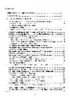
inter-dependence, then this becomes a large system. Thus we can say university is a large system whereas college is a system. This means, each system can be divided into blocks, where each block is in itself a complete and independently working system (Fig. 0.1). When these blocks are combined, depending on some interdependence, they become entities of a larger system. An aircraft for example, is another example of a system. It consists of a cockpit, pilot, airframes, control system, fuel tank, engines etc. Each of these blocks can in itself be treated as a system and aircraft consisting of these interdependent blocks is a large system. Table 0.1 gives components of a system (say college) for illustrations purpose. Does a system also has some attributes? I will say yes. Systems broadly can be divided into two types, static system and dynamic system. If a system does not change with time, it is called a Static System and if changes with time, it is called a Dynamic System. Study of such a system is called System Analysis. How this word originated is of interest to know. COLLEGE

RAW STUDENTS

DEPARTMENTS

CLASS ROOMS

CANTEEN

LABS

PLAY GROUND

CONFERENCE HALL

HOSTELS

GRADUATE

W/SHOPS

Fig. 0.1: College as a system.

While looking at these systems, we see that there are certain distinct objects, each of which possesses some properties of interest. There are also certain interactions occurring in the system that cause changes in the system. A term entity will be used to denote an object of interest in a system and the term attributes denotes its properties. A function to be performed by the entity is called its activity. For example, if system is a class in a school, then students are entities, books are their attributes and to study is their activity. In case of the autopilot aircraft discussed below, entities of the system are gyroscope, airframe and control surfaces. Attributes respectively are gyroscope setting, speed and control surface angles. Activity of the aircraft is to fly. Banks et al., (2002) has defined state variables and events as components of a system. The state is defined as collection of variables necessary to describe the system at any time, relative to the objectives of the study. An event is defined as an instantaneous occurrences that may change the state of the system. But it is felt, entities are nothing but state variables and activity and event are similar. Thus there is no need of further bifurcation. Sometimes the system is effected by the environment. Such a system is called exogenous. If it is not effected by the environment, it is called endogenous. For example, the economic model of a country is effected by the world economic conditions, and is exogenous model. Aircraft flight is exogenous, as flight profile is effected by the weather conditions, but static model of the aircraft is endogenous. A class room in the absence of students, is endogenous. As mentioned earlier study of a system is called System Analysis. How this word “System Analysis” has cropped up? There is an interesting history behind this.

What is a System

3

After second world war (1939–1945), it was decided that there should be a systematic study of weapon systems. In such studies, topics like weapon delivery (to drop a weapon on enemy) and weapon assignment (which weapon should be dropped?) should also be included. This was the time when a new field of science emerged and the name given to it was “Operations Research”. Perhaps this name was after a British Defence Project entitled “Army Operations Research” [19]*. Operations Research at that time was a new subject. Various definitions of “Operations Research” have been given. According to Morse and Kimball [1954], it is defined as scientific method of providing executive departments with a quantitative basis for decisions regarding the operations under one’s control. According to Rhaman and Zaheer (1952) there are three levels of research : basic research, applied research and operations research. Before the advent of computers, there was not much effect of this subject on the weapon performance studies as well as other engineering studies. The reason being that enormous calculations were required for these studies, which if not impossible, were quite difficult. With the advent of computers, “Computerised Operations Research” has become an important subject of science. I have assumed that readers of this book are conversant with numerical methods as well as some computer language. Table 0.1: Systems and their components System

Entities

Attributes

Activities

Banking

Customers

Maintaining accounts

Making deposits

Production unit

Machines, workers

Speed, capacity, break-down

Welding, manufacturing

College Petrol pump

Teachers, students Attendants

Education To supply petrol

Teaching, games Arrival and departure of vehicles

History of Operations Research has beautifully been narrated by Treften (1954). With the time, newer and newer techniques were evolved and name of Operations Research also slowly changed to “System Analysis” [17]. Few authors have a different view that “Operations Research” and “System Analysis” are quite different fields. System Analysis started much later in 1958–1962 during the Kennedy administration in US (Treften, FB 1954). For example, to understand any system, a scientist has to understand the physics of the system and study all the related sub-systems of that system. In other words, to study the performance evaluation of any system, one has to make use of all the scientific techniques, along with those of operations research. For a system analyst, it is necessary to have sufficient knowledge of the every aspect of the system to be analysed. In the analysis of performance evaluation of a typical weapon as well as any other machine, apart from full knowledge of the working of the system, basic mathematics, probability theory as well as computer simulation techniques are used. Not only these, but basic scientific techniques, are also needed to study a system. In the present book our main emphasis will be on the study of various techniques required for system analysis. These techniques will be applied to various case studies with special reference to weapon system analysis and engineering. Modeling and simulation is an essential part of system analysis. But to make this book comprehensive, wherever possible, other examples will also be given. Present book is the collection of various lectures, which author has delivered in various courses being conducted from time to time for service officers and defence scientists as well as B. Tech * Number given in the square bracket [1], are the numbers of references at the end of this book. References however are in general given as author name (year of publication).

4

System Modeling and Simulation

and M. Tech students of engineering. Various models from other branches of engineering have also been added while author was teaching at Institute of Engineering and Technology, Bhaddal, Ropar in Punjab. Attempt has been made to give the basic concepts as far as possible, to make the treatise easy to understand. It is assumed that student, reading this book is conversant with basic techniques of numerical computations and programming in C++ or C language. But still wherever possible, introductory sections have been included in the book to make it comprehensive. As given earlier, Simulation is actually nothing but conducting trials on computer. By simulation one can, not only predict the system behaviour but also can suggest improvements in it. Taking any weapons as an example of a system, lethal capabilities of the weapon which are studied by evaluating its terminal effects i.e., the damage caused by a typical weapon on a relevant target when it is dropped on it, is also one of the major factor. There are two ways of assessing the lethal capabilities of the weapons. One is to actually drop the weapon on the target and see its end effects and the other is to make a model using a computer and conduct a computer trial, which simulates the end effects of the weapon on the target. Conducting trials on the computers is called computer simulation. Former way of conducting trial (actual trials) is generally a very costly affair. In this technique, cost of the weapon as well as target, are involved. But the second option is more cost effective. As an example of a conceptually simple system (Geofrey Gordon, 2004), consider an aircraft flying under the control of an autopilot (Fig. 0.2). A gyroscope in the autopilot detects the difference between the actual heading of aircraft and the desired heading. It sends a signal to move the control surfaces. In response to control surfaces movement, the aircraft steers towards the desired heading.

θi DESIRED HEADINGS

GYROSCOPE

ε

CONTROL SURFACES

AIRFRAME

θο ACTUAL HEADING

Fig. 0.2: Model of an autopilot aircraft.

A factory consisting of various units such as procurement department, fabrication and sale department is also a system. Each department of the factory, on which it depends, is an independent system and can be modelled independently. We have used the word “modelled” here. What is modeling, will be discussed in chapter one of this book. Scientific techniques used in system studies can also broadly be divided into two types: 1. Deterministic studies and 2. Probabilistic studies Deterministic studies are the techniques, where results are known exactly. One can represent system in the form of mathematical equations and these equations may be solved by analytic methods or by numerical computations. Numerical computations is one of the important tools in system analysis and comes to rescue the system analyst, where analytical solutions are not feasible. In case of study of damage to targets, knowledge of shock waves, fragments penetration, hollow charge and other allied studies is also required. Some of the topics have been introduced in this book for the purpose of broader horizon of the student’s knowledge.

What is a System

5

Apart from the two types of studies given above, system can be defined as (i) Continuous and (ii) Discrete. Fluid flow in a pipe, motion of an aircraft or trajectory of a projectile, are examples of continuous systems. To understand continuity, students are advised to refer some basic book on continuity. Examples of discrete systems are, a factory where products are produced and marketed in lots. Motion of an aircraft is continuous but if there is a sudden change in aircraft’s level to weather conditions, is a discrete system. Another example of discrete system is firing of a gun on an enemy target. It is important to conduct experiments to confirm theoretically developed mathematical models. Not only the experiments are required for the validation of the theoretical models but various parameters required for the development of theoretical models are also generated by experimental techniques. For example to study the performance of an aircraft, various parameters like drag, lift and moment coefficients are needed, which can only be determined experimentally in the wind tunnel. Thus theory and experiment both are complementary to each other and are required for correct modeling of a system. In case of marketing and biological models in place of experiments, observations and trends of the system over a time period, are required to be known for modeling the system. This issue will be discussed in chapter eight. The aim of this book is to discuss the methods of system analysis vis a vis an application to engineering and defence oriented problems. It is appropriate here to make reference to the books, by Billy E. Gillett (1979), Pratap K. Mohapatra et al., (1994) and Shannon (1974), which have been consulted by the author. Layout of the book is arranged in such a way that it is easy for the student to concentrate on examples of his own field and interest. Our attempt is that this book should be useful to students of engineering as well as scientists working in different fields. Layout of the book is as follows: In chapter one, basic concepts of modeling and simulation are given. Number of examples are given to illustrate the concept of modeling. Also different types of models are studied in details. In chapter two, basic probability theory, required for this book has been discussed. Probability distribution functions, as used in modeling of various problems have been included in this chapter. Wherever needed, proof for various derivations are also included. Application of probability theory to simple cases is demonstrated as examples. Although it is not possible to include whole probability theory in this book, attempts have been made to make this treatise comprehensive. Chapter three gives a simple modeling of aircraft survivability, by overlapping of areas, using probability concepts developed in chapter two. It is understood that projection of various parts on a plane are known. This chapter will be of use to scientists who want to learn aircraft modeling tools. However engineering students, if uncomfortable, can skip this chapter. Simulation by Monte Carlo technique using random numbers, is one of the most versatile technique for discrete system studies and has been dealt in chapter four. The problems which cannot be handled or, are quite difficult to handle by theoretical methods, can easily be solved by this technique. Various methods for the generation of uniform random numbers have been discussed. Properties of uniform random numbers and various tests for testing the uniformity of random numbers are also given. Normal random numbers are of importance in various problems in nature, including weapon systems. Methods for generating normal random numbers have been discussed in details. Study of different types of problems by computer simulation technique have been discussed in this chapter. Here simulation technique, and generation of different types of

6

System Modeling and Simulation

random numbers is studied in details. Computer programs in C++ for different techniques of random number generation are also given. Chapter five deals with the simulation and modeling of Continuous Dynamic Systems. Problem becomes slightly complex, when target is mobile. Problem of mobile targets and surface to air weapons, will be studied in chapter six. A study of vulnerability of aerial targets such as aircraft will be discussed. Simulation and modeling can not be learnt without working on practical problems. Therefore number of examples have been worked out in this chapter. A case study of aircraft survivability has been given in chapter six. Aircraft model discussed in chapter three was purely on probability concepts. But present model is a simulation model, where all the techniques developed in first five chapters has been utilised. What is the probability that an aircraft will survive when subjected to ground fire in an enemy area, has been studied in this model. This model involves mathematical, and computer modeling. Concept of continuous and stochastic modeling has also been used wherever required. Simulation of manufacturing process and material handling is an important subject of Mechanical Engineering. Queuing theory has direct application in maintenance and production problems. Queuing theory has been discussed in chapter seven. Various applications on the field of manufacturing process and material handling have been included in this chapter. There are various phenomena in nature which become unstable, if not controlled in time. This is possible only if their dynamics is studied and timely measures are taken. Population problem is one of the examples. Nuclear reaction is another example. This type of study is called Industrial dynamics. Eighth chapter deals with System Dynamics of such phenomena. Various cases of growth and decay models with examples have been discussed in this chapter. One of the pressing problems in the manufacturing and sale of goods is the control of inventory holding. Many companies fail each year due to the lack of adequate control of inventory. Chapter nine is dedicated to inventory control problems. Attempt has been made to model various inventory control conditions mathematically. Costing of a system is also one of the major job in system analysis. How much cost is involved in design and manufacturing of a system is discussed in tenth chapter. Cost effectiveness study is very important whether procuring or developing any equipment. In this chapter basic concepts of costing vis a vis an application to aircraft industry has been discussed.

EXERCISE 1. Name several entities, attributes, activities for the following systems. • A barber shop • A cafeteria • A grocery shop • A fast food restaurant • A petrol pump

What is a System

2.

3.

7

Classify following systems in static and dynamic systems. • An underwater tank • A submarine • Flight of an aircraft • A college • Population of a country Classify following events into continuous and discrete. • Firing of a gun on enemy • Dropping of bombs on a target • Tossing of a coin • Flow of water in a tap • Light from an electric bulb.

‰‰‰

This page intentionally left blank

Modeling and Simulation

9

12345678 12345678 12345678 12345678 12345678 12345678 12345678 12345678

1

MODELING AND SIMULATION

Term Modeling and Simulation is not very old and has become popular in recent years. But the field of modeling and simulation is not new. Scientific workers have always been building models for different physical scenarios, mathematically as well as in laboratories. Here question arises, what is the basic difference between modeling and simulation? In fact, there is very thin border line between the both. In fact, physical models can not be called simulation, but mathematical models can be called simulation. Similarly computer simulation can not be given name of modeling but mathematical simulation can be called modeling. Model of a system is the replica of the system, physical or mathematical, which has all the properties and functions of the system, whereas simulation is the process which simulates in the laboratory or on the computer, the actual scenario as close to the system as possible. In fact, a modeling is the general name whereas simulation is specific name given to the computer modeling. Models can be put under three categories, physical models, mathematical models and computer models. All of these types are further defined as static and dynamic models. Physical model is a scaled down model of actual system, which has all the properties of the system, or at least it is as close to the actual system as possible. Now-a-days small models of cars, helicopters and aircraft are available in the market. These toys resemble actual cars and aircraft. They are static physical models of dynamic systems (cars, helicopters and aircraft are dynamic systems). In wind tunnel, scaled down models of an aircraft are used to study the effect of various aerodynamic forces on it. Similarly before the construction of big buildings, scaled down models of the buildings are made. Well known laws of similitude are used to make the laboratory models. All the dimensions are reduced with respect to some critical lengths (Sedov LI, 1982). Figure 1.1 gives different types of models. These types will be studied in details in the coming chapters. While building a model certain basic principles are to be followed. While making a model one should keep in mind five basic steps.

• • • • •

Block building Relevance Accuracy Aggregation Validation

System Modeling and Simulation

10

A model of a system can be divided into number of blocks, which in itself are complete systems. But these blocks should have some relevance to main system. For example, let us take an example of a school. Class rooms are blocks of the school. Aim of the school is to impart education to students and class rooms are required for the coaching. Thus relevance of class rooms (blocks) with school is coaching. Interdependency is the one of the important factor of different blocks. Each block should be accurate and tested independently. Then these blocks are to be integrated together. Last is the validation i.e., this model is to be tested for its performance. For validation following methods can be used.

• If the model is mathematical model, then some trivial results can be run for verifications. • If experimental results are available, model can be checked with these experimental results. In the following sections, we will discuss in details the various types of models as shown in Fig. 1.1. MODEL

PHYSICAL

STATIC

MATHEMATICAL

DYNAMIC

NUMERICAL

STATIC

ANALYTICAL

COMPUTER

DYNAMIC

STATIC

DYNAMIC

NUMERICAL

SYSTEM SIMULATION

Fig. 1.1: Different types of models.

1.1 PHYSICAL MODELS Physical models are of two types, static and dynamic. Static physical model is a scaled down model of a system which does not change with time. An architect before constructing a building, makes a scaled down model of the building, which reflects all it rooms, outer design and other important features. This is an example of static physical model. Similarly for conducting trials in water, we make small water tanks, which are replica of sea, and fire small scaled down shells in them. This tank can be treated as a static physical model of ocean. Dynamic physical models are ones which change with time or which are function of time. In wind tunnel, small aircraft models (static models) are kept and air is blown over them with different velocities and pressure profiles are measured with the help of transducers embedded in the model. Here wind velocity changes with time and is an example of dynamic physical model. A model of a hanging wheel of vehicle is another case of dynamic physical model discussed further.

Modeling and Simulation

11

Let us take an example of hanging wheel of a stationary truck and analyze its motion under various forces. Consider a wheel of mass M, suspended in vertical direction, a force F(t), which varies with time, is acting on it. Mass is connected with a spring of stiffness K, and a piston with damping factor D. When force F (t), is applied, mass M oscillates under the action of these three forces. This model can be used to study the oscillations in a motor wheel. Figure 1.2 shows such a system. This is a discrete physical static model. Discrete in a sense, that one can give discrete values F and observe the oscillations of wheel with some measuring equipment. When force is applied on it, which is a function of time, this discrete physical static model becomes dynamic model. Parameters K and D can also be adjusted in order to get controlled oscillations of the wheel. This type of system is called spring-mass system. Load on the beams of a building can be studied by the combination of springmass system. Mathematical model of this system will be studied in coming chapters.

Fig. 1.2: Suspended weight attached with spring and piston.

Let us consider another static physical model which represents an electric circuit with an inductance L, a resistance R, and a capacitance C, connected with a voltage source which varies with time, denoted by the function E (t). This model is meant for the study of rate of flow of current as E (t) varies with time. There is some similarity between this model and model of hanging wheel. It will be shown below that mathematical model for both is similar. These physical models can easily be translated into a mathematical model. Let us construct mathematical model of system describing hanging wheel. Using Newton’s second law of motions, system for wheel model can be expressed in the mathematical form as

M where x

dx d2 x + Kx = KF(t) + D 2 dt dt

...(1.1)

= the distance moved,

M = mass of the wheel, K = stiffness of the spring, D = damping force of the shock absorber. This system is a function of time and is a dynamic system. Equation (1.1) cannot be solved analytically and computational techniques can be used for solving the equations. Once we interpret the results of this equation, this becomes a dynamic mathematical model of the system. Physical model

12

System Modeling and Simulation

can also be used to study the oscillations by applying force F, and measuring the displacement x of the model. Values of K and D can be changed for required motion with minimum oscillations. This equation will be discussed in the section on Mathematical models in section 1.2. Equation of electrical circuit given above can be written as Lqɺɺ + Rqɺ +

E (t ) q = C C

. Here the q is the electric current. In this equation if we say q = x, L = M, R = D, E = F and K = 1/C, then one can easily see that this equation is similar to (1.1).

R

L

I C

E(t)

Fig. 1.3: Static circuit of an electrical system.

Thus same mathematical model, by using different constants can give solution for hanging wheel as well as electrical circuit.

1.2 MATHEMATICAL MODELS In section 1.1 we have seen, how a physical model can be converted to mathematical model. Most of the systems can in general be transformed into mathematical equations. These equations are called the mathematical model of that system. Since beginning, scientists have been trying to solve the mysteries of nature by observations and also with the help of Mathematics. Kepler’s laws represent a dynamic model of solar system. Equations of fluid flow represent fluid model which is dynamic. A static model gives relationships between the system attributes when the system is in equilibrium. Mathematical model of a system, in equilibrium is called a Static Mathematical Model. Model of a stationary hanging wheel equation (1.1) is a dynamic mathematical model, as equations of the model are function of time. This equation can be solved numerically with the help of Runge-Kutta method. It is not possible to find analytic solution of this equation and one has to adopt the numerical methods. We divide equation (1.1) by M and write in the following form (Geofrey Gordon, 2004)

d2 x dx 2 + 2ζω + ω 2 x = ω F (t ) dt 2 dt

...(1.2)

where 2ζω = D / M and ω 2 = K /M. Expressed in this form, solution can be given in terms of the variable ωt. Details of the solution of this equation will be given in chapter five on continuous models. Expressed in this form, solution can be given in terms of the variable ωt , where ω is the frequency of oscillation given by

ω2 = 2π f and f is the number of cycles per second.

Modeling and Simulation

13

We can integrate equation (1.2) using numerical techniques. It will be shown that wheel does not oscillate for ζ ≥ 1 .

1.2.1 Static Mathematical Models Mathematical model of equation (1.2) involves time t, and is thus dynamic model. If mathematical model does not involve time i.e., system does not change with time, it is called a static mathematical model of the system. In this section, we will discuss few static mathematical models. First of the model is for evaluating the total cost of an aircraft sortie, for accomplishing a mission. Costing is one of the important exercise in System Analysis, and is often required for accomplishing some operations. Second case has been taken from the market. A company wants to optimize the cost of its product by balancing the supply and demand. In a later section, this static model will be made dynamic by involving time factor in it. A student training model, in which marks allotted to students are optimized, is also presented. 1.2.2 Costing of a Combat Aircraft This section can be understood in a better way after chapter ten. But since this problem falls under static modeling, it is given here. Students of engineering can skip this section if they like. In this model we assume that a sortie of fighter aircraft flies to an enemy territory to destroy a target by dropping the bombs. Now we will construct a mathematical model to evaluate the total cost of attack by aircraft sortie to inflict a stipulated level of damage to a specified target. This cost is the sum of (a) Mission cost of surviving aircraft, (b) Cost of aborted mission, (c) Cost of killed aircraft/repair cost, (d) Cost of killed pilots, and (e) Cost of bombs. Here surviving aircraft mean, the number of aircraft which return safely after attacking the enemy territory. Aborted mission means, aircraft, which could not go to enemy territory due to malfunctioning of aircraft. Meaning of other terms is clear. (a) Mission cost of surviving aircraft In order to evaluate these costs, we have to know, how many aircraft have survived after performing the mission and how many have been killed due to enemy firing. Let N be the total number of aircraft sorties which are sent on a mission, then N = Nw / [Nb . p . p1 (1 – pa) (1 – pb) (1 – pc)]

...(1.3)

where Nw Nb p p1 pa pb pc

= = = = = = =

number of bombs required to damage the given target up to the specified level, number of bombs per one aircraft sortie, survival probability of aircraft in enemy air defence environments, weapon reliability, abort probability before reaching the target, abort probability on account of not finding the target, abort probability due to failure of release mechanism.

It is assumed that the various probabilities in equation (1.3) are known based on earlier war experience. Due to various reasons, it is quite possible that some of the aircraft are not able to perform mission during operation, and thus abort without performing the mission. To take such aborted aircraft into account, let Na, Nb and Nc be the number of aircraft aborted due to some malfunctioning, due to missing

14

System Modeling and Simulation

the target and due to failure of weapon release mechanism respectively. Then Na, Nb and Nc are given as follows: Na = N . pa Nb = N . (1 – pa ) pb ...(1.4) Nc = N . (1 – pa ) (1 – pb ) pc In equation (1.4), Nb is the product of aircraft not aborted due to malfunctioning i.e., N (1 – pa) and probability of abort due to missing the target ( pb ). Same way Nc is evaluated. Since Na number of aircraft have not flown for the mission, we assume, that they are not subjected to enemy attrition. Then total number of aircraft going for mission is N1 = N – Na = N (1 – pa )

...(1.5)

Nb and Nc are number of aircraft being aborted after entering into enemy territory and thus are subject to attrition. Therefore total number of aircraft accomplishing the successful mission is N – Na – Nb – Nc Out of which surviving aircraft are given as Ns = p(N – Na – Nb – Nc ) or by using (1.4) in the above equation, Ns = p .N [1 – pa – (1 – pa ) pb – (1 – pa ) (1 – pb ) pc ] ...(1.6) There are another category of surviving aircraft (given by equation (1.4)) which have not been able to accomplish the mission. Amongst these Na aircraft aborted before entering the enemy territory and are not subject to attrition, where as Nb and Nc category have attrition probability p, as they abort after reaching near the target. Let these aircraft be denoted by Nas. Then ...(1.7) Nas = Na + ( Nb + Nc ) . p Therefore total number of survived aircraft is Ns + Nas Once number of survived aircraft is evaluated, we can fix a cost factor. This is accomplished as follows. If the acquisition cost of an aircraft, whose total life in H hours is C, then the life cycle cost of the aircraft, is given by C (1 + k) where k is the cost factor for computation of life cycle cost which includes cost of spares and maintenance, operation etc., and strike-off wastage during its life. Value of cost for computation of life cycle cost which includes cost of various aircraft is given in Appendix 10.1. The cost of the surviving aircraft for the assigned mission, and have performed the mission is given by C1 = (C (1 + k) Ns t/H),

...(1.8)

where t is mission sortie time in hours.

(b) Cost of aborted mission (C2 ) The number of surviving aborted aircraft as given in equation (1.7), are Nas. Thus the total cost of such aborted aircraft is N a C (1 + k ) . t a p .Nb .C (1 + k ) .tb p . Nc . C (1 + k ) .tc + + ...(1.9) C2 = H H H

Modeling and Simulation

15

where ta, tb, tc are the sortie time taken in each of the aborted cases mentioned above. Timings ta, tb and tc are input data and is based on the war estimates and total sortie time t of the aircraft. For example tc = t as in this case the aircraft had reached the target but could not release the weapon due to failure of firing mechanism. Similarly tb can also be taken as equal to t as aircraft has flown up to the target but could not locate it.

(c ) Cost of killed aircraft Let Nk be the total number of killed aircraft given by Nk = (N – Na) . (1 – p) and tj is the life already spent by Nj-th aircraft, then the total cost of killed aircraft is given by C3 =

p C Csow  1 +  ∑ Nj ( H − tj ) H C j =1

...(1.10)

where Nk = N1 + N2+ …+ Np and the terms Csow / C in above equation has been taken due to the reasons that when an aircraft which has spent a life of tj hours is lost, partial cost of spares, fuel, and maintenance is not lost. Only loss in this case is C + Csow. Thus if we assume that all the aircraft are new i.e., tj = 0, we have,

Csow    C3 = N k C 1 + C 

...(1.11)

It is to be noted that in this equation only cost due to strike-off wastage is taken out of cost factor k. This is because cost of spares and maintenance is not assumed as gone when an aircraft is killed.

(d) Cost of killed pilots Let p2 be pilot survival probability of killed aircraft. Then the cost of the killed pilots is given by ...(1.12) C4 = (1 – p2) int (Nk ) . Cp where Cp is the cost of killed pilot and int (Nk) means integer part of Nk. Cost of pilot is based on the total expenditure of giving him training and compensation involved in case of his death. (e) Cost of bombs If Cb is the cost of a bomb, then the total cost of bombs is given by N w Cb ...(1.13) p1 where Nw are the total number of bombs required to damage the target and p1 is the reliability that bomb will function.

C5 =

Thus the total cost of the attack by aircraft to inflict a stipulated level of damage to a specified target is the sum of all the individual costs defined above and is given by ...(1.14) Ca/c = C1 + C2 + C3 + C4 + C5

1.2.3 A Static Marketing Model In order to illustrate further, we take one more example of static mathematical model. Here we give a case of static mathematical model from industry. Generally there should be a balance between the supply and demand of any product in the market. Supply increases if the price is higher. This is because shopkeeper gets more commission on that product and tries to push the product to the customers even if quality is not excellent. Customer generally feels that more cost means better quality. But on the other hand demand decreases with the increase of price. Aim is to find the optimum price with

16

System Modeling and Simulation

which demand can match the supply. Let us model this situation mathematically. If we denote price by P, supply by S and demand by D, and assuming the price equation to be linear we have D = a – bP S = c + dP

...(1.15)

S = D In the above equations, a, b, c, d are parameters computed based on previous market data. Equation S = D says supply should be equal to demand so that market price should accordingly be adjusted. Let us take values of a = 500, b = 2000, c = –50 and d =1500. Value of c is taken negative, since supply cannot be possible if price of the item is zero. In this case no doubt equilibrium market price will be a−c 550 = = 0.1571 P = b+d 3500 and S = 186 Price

0.25

Demand

Supply Demand

Supply

Price

Price

0.20 0.15 0.10 0.05 0

100

200

300 400 Quantity

Fig. 1.4: Market model.

500

Quantity

Fig. 1.5: Non-linear market model.

In this model we have taken a simplistic linear case but equation (1.15) may be complex. In that case solution may not be so simple. More usually, the demand and supply are depicted by curves with slopes downward and upward respectively (Fig. 1.5). It may not be possible to express the relationships by equations that can be solved easily. Some numerical or graphical methods are used to solve such relations. In addition, it is difficult to get the values of the coefficients of the model. Observations over the extended period of time, however, will establish the slopes (that is values of b and d ) in the neighbourhood of the equilibrium points. These values will often fluctuate under the global and local economic conditions.

1.2.4 Student Industrial Training Performance Model For engineering students, six months training in industry is a part of their course curriculum and is compulsory. It has been observed that training marks allotted to students from industrial Institutions, vary drastically, irrespective of the academic record of the student. Nature of project offered and standard of training institutions pay a very dominating role in these criteria. Due to this sometimes, very good students, who are supposed to top the University exam, can suffer with no fault on their part. A model to optimize the industrial marks which are about 40% of total marks is presented below. Let M be the marks allotted by industry and M the optimized marks.

Modeling and Simulation If

17

m mac mext m int mind

= = = = =

average result of the college. % average marks of student in first to six semester. % marks of training given by external expert. % marks given by internal evaluation. % average marks given by industry for last two years.

wac wext wint wind

= = = =

weight weight weight weight

factor factor factor factor

of of of of

academic. external marks. internal marks. industry.

Then,

M = M + wac (mac – m) + wext (mext – m) + wint (mint – m) – wind (mind – m) minus sign to industry is because it is assumed that good industry does not give high percentage of marks. Weight factors are as follows: wac = 0.5 wext = 0.25 wint = 0.125 wind = 0.125 m

= 0.8 (say)

(I) Case Study (Good Student) M = 0.75 mac = 0.95 mext = 0.9 mint = 0.95 mind = 0.6 Then,

M = 0.75 + 0.5 × (0.15) + 0.25 × (0.10) + 0.125 × (0.15) – 0.125 × (0.6 – 0.8) ⇒

M = 0.75 + 0.075 + 0.025 + 0.019 + 0.025

∴

M = 0.894

(II) Case Study (Poor Student) M = 0.95 mac = 0.50 mext = 0.6 mint = 0.5 m ind = 0.9

18

System Modeling and Simulation Then, M

= 0.95 + 0.5 × (0.5 – 0.8) + 0.25 × (0.6 – 0.8) + 0.125 × (0.5 – 0.8) – 0.125 × (0.9 – 0.8)

⇒

= 0.95 + 0.15 – 0.05 – 0.034 – 0.0125

M

∴ M

= 0.70

Model can be used for upgrading or down grading (if required) the industrial marks.

1.3 COMPUTER MODELS With the advent of computers, modeling and simulation concepts have totally been changed. Now all types of stochastic as well as continuous mathematical models can be numerically evaluated with the help of numerical methods using computers. Solution of the problem with these techniques is called computer modeling. Here one question arises, what is the difference between mathematically obtained solution of a problem and simulation. Literal meaning of simulation is to simulate or copy the behavior of a system or phenomenon under study. Simulation in fact is a computer model, which may involve mathematical computation, computer graphics and even discrete modeling. But Computer oriented models which we are going to discuss here are different from this. One can design a computer model, with the help of graphics as well as mathematics, which simulates the actual scenario of war gaming. Let us assume, we have to model a war game in which missile warheads are to be dropped on an airfield. Each warhead is a cratering type of warhead which makes craters on the runway so that aircraft can not take off. This type of warhead is also called Blast Cum Earth Shock (BCES) type of warhead.

1.3.1 Runway Denial using BCES Type Warhead First requirement of air force during war time, is to make the enemy’s runway unserviceable, so that no aircraft can take off or land on it. It has been observed that during emergency, a modern fighter aircraft like F-16, is capable of taking off even if a minimum strip of 1000m × 15m is available. Thus in order that no where on airstrip, an area of 1000m × 15m is available, bombs which create craters on the runway are dropped by the aircraft or missile. This model was first developed by the author, when a requirement by army was sent to Center for Aeronautical System Studies and Analysis, Bangalore to study the cost-effectiveness of Prithvi vs. deep penetrating aircraft. Prithvi is a surface to surface missile, developed by Defence Research and Development Organization. Blast Cum Earth Shock warhead (BCES ), generally used against runway tracks is capable of inflicting craters to the tracks and making them unserviceable. These types of warheads earlier used to be dropped on runway in the pattern of stick bombing (bombs dropped in a line). In this section a simulation and mathematical model for the denial of an airfield consisting of runway tracks inclined at arbitrary angles, using BCES type of warheads has been discussed. A Static model of airfield: In this section we construct a static model of an airfield. An airfield consisting of three tracks (a main runway denoted by ‘RW’ and a taxi track denoted by ‘CW’ and another auxiliary runway denoted by ‘ARW’ ) is generated by computer using graphics (Fig. 1.6). The airfield consists of one runway (3000 × 50m), a parallel taxi track (3000 × 25m) and an auxiliary runway normal to both (2500 × 50m). This model is developed to simulate the denial of runway by dropping bombs on it. The denial criterion of the airfield is that, no where on the track, a strip of dimensions 1000 × 15m, which is sufficient for an aircraft to take off in emergency, is available. To check whether this track (1000 × 15) square meters is available or not, an algorithm has been developed by Singh et al., (1997) devising a methodology for checking the denial criterion.

Modeling and Simulation

19

SAMPLE DMAI

Fig. 1.6: A typical airfield, showing runways and DMPIs (black sectors).

To achieve this, we draw certain areas on the track so that if atleast one bomb falls on each of these areas, 1000 meters will not be available anywhere on the three tracks. These areas are called Desired Mean Areas of Impact (DMAI ), and have been shown as black areas in Fig. 1.6. Desired Mean Points of Impact (DMPIs) and strips are chosen in such a way that, if each strip has at least one bomb, no where a strip of dimensions 1000m × 15m is available. Number of strips Ns of effective width Ws in a DMAI is given by,

if Wd = W  1,  Ns =   2W  ...(1.16) int  W + 2r  + 1, otherwise d b  where W, Wd , rb are the width, denial width respectively of the RW and lethal radius of the bomblet. Monte Carlo computer model of airfield denial has been discussed by Singh et al., (1997) and is given in chapter four.

1.3.2 Distributed Lag Models—Dynamic Models The market model, discussed in section 1.2.3 was straight forward and too simplistic. When model involves number of parameters and hefty data, one has to opt for computer. Models that have the properties of changing only at fixed intervals of time, and of basing current values of the variables on other current values and values that occurred in previous intervals, are called distributed lag models [Griliches, Zvi 1967]. These are a type of dynamic models, because time factor is involved in them. They are extensively used in econometric studies where the uniform steps correspond to a time interval, such as a month or a year, over which some economic data are collected. As a rule, these model consists of linear, algebraic equations. They represent a continuous system, but the one in which data is only available at fixed points in time. As an example, consider the following simple dynamic mathematical model of the national economy. Let, C be consumption, I be investment, T be taxes, G be government expenditure and Y be national income.

20

System Modeling and Simulation Then C = 20 + 0.7(Y − T )  I = 2 + 0.1Y   T = 0 + 0.2Y   Y =C + I +G All quantities are expressed in billions of rupees.

...(1.17)

This is a static model, but it can be made dynamic by picking a fixed time interval, say one year, and expressing the current values of the variables in terms of values of the previous year. Any variable that appears in the form of its current value and one or more previous year’s values is called lagged variables. Value of the previous year is denoted by the suffix with-1. The static model can be made dynamic by lagging all the variables, as follows;

C = 20 + 0.7(Y−1 − T−1 )  I = 2 + 0.1Y–1   ...(1.18) T = 0.2Y−1   Y = C−1 + I−1 + G−1  In these equations if values for the previous year (with –1 subscript) is known then values for the current event can be computed. Taking these values as the input, values for the next year can also be computed. In equation (1.18) we have four equations in five unknown variables. It is however not necessary to lag all the variable like it is done in equation (1.18). Only one of the variable can be lagged and others can be expressed in terms of this variable. We solve equation for Y in equation (1.17) as Y = 20 + 0.7(Y – 0.2Y ) + I + G = 20 + 0.56Y + I + G Y = 45.45 + 2.27(I + G)

or Thus we have,

I = 2.0 + 0.1Y–1

  Y = 45.45 + 2.27( I + G )  T = 0.2Y   C = 20 + 0.7(Y − T )

...(1.19)

In equations (1.19) only lagged parameter is Y. Assuming that government expenditure is known for the current year, we first compute I. Knowing I and G, Y and T for the current year is known, and thus C is computed from the last equation. In this problem, lagged model is quite simple and can be computed with hand calculator. But national economic models are generally not that simple and require long computations with number of parameters.

1.4 COBWEB MODELS In section 1.2.3, a simple static model of marketing a product had been discussed. In that model two linear equations for demand D and supply S were considered. Aim was to compute the probable

Modeling and Simulation

21

price and demand of a product in the market subject to a condition that supply and demand should be equal. But supply of the product in the market depends on the previous year price, and that can be taken as lagged parameter. Thus equations (1.15) become D = a – bP S = c + dP–1 D = S Model 1 P 0 = 30

...(1.20)

Model 2 P0 = 5

a = 12

a = 10.0

b = 30

b = 0.9

c =

1.0

c = –2.4

0.9

1.2

In the equations (1.20), values of parameters a, b, c, and d can be obtained by fitting a linear curve in the data from the past history of the product. We assign some initial value to the product say P0 and find S from second equation of (1.20). Thus S and D are known and first equation of (1.20) gives us new value of P. Using this value of P as initial value, we repeat the calculations and again compute P for the next period. If price converges, we say model (1.20) is stable. Let us take two examples and test whether these models converge or not. Table 1.1: Cobweb model for marketing a product

Model 1

Model 2

i

P

i

P

0

–0.533333

0

7.11111

1

0.382667

1

4.2963

2

0.355187

2

8.04938

3

0.356011

3

3.04527

4

0.355986

4

9.71742

5

0.355987

5

0.821216

6

0.355987

6

12.6828

7

0.355987

7

–3.13265

8

0.355987

8

17.9546

9

0.355987

9

–10.1618

10

0.355987

10

27.3268

We have given a small program to find the value of P on the next page.

22

System Modeling and Simulation

Program 1.1: Program for Cobweb Model for Marketing a Product # include void main (void) { double po, a,b,c,d,s,q,p; int i; ofstream outfile; outfile.open(“vps”); cout >po >>a>>b>>c>>d; cout