Stochastic Aspects of Classical and Quantum Systems: Proceedings of the 2nd French-German Encounter in Mathematics and Physics, held in Marseille, ... 1, 1983 (Lecture Notes in Mathematics, 1109) 9783540139140, 3540139141

Citation preview

Lecture Notes in Mathematics Edited by A. Dold and 8. Eckmann

1109 Stochastic Aspects of Classical and Quantum Systems Proceedings of the 2nd French-German Encounter in Mathematics and Physics, held in Marseille, France, March 28 - April 1, 1983

Edited by S. Albeverio, Ph. Combe and M. Sirugue-Collin

Springer-Verlag Berlin Heidelberg New York Tokyo 1985

Editors

Sergio Albeverio Mathematisches Institut, Ruhr-Universitat 4630 Bochum, Federal Republic of Germany Philippe Combe Universite d'Aix-Marseilie II Luminy Marseille, France Madeleine Sirugue-Collin Universite de Provence, Marseille, France

AMS Subject Classification (1980): 60GXX, 60HXX, 60JXX, 81FXX; 34 BXX, 35JXX, 35XX, 73XX, 76XX, 81G20, 82XX, 85XX ISBN 3-540-13914-1 Springer-Verlag Berlin Heidelberg New York Tokyo ISBN 0-387-13914-1 Springer-Verlag New York Heidelberg Berlin Tokyo Library of Congress Cataloging in Publication Data. Main entry under title: Stochastic aspects of classical and quantum systems. (Lecture notes in mathematics; 1109) 1. Stochastic processes-Congresses. 2. Quantum theory-Congresses. I. Albeverio, Sergio. II. Combe, Philippe, 1940-. III. Sirugue-Collin, M. (Madeleine), 1936-. IV. Series: Lecture notes in mathematics (Springer-Verlag); 1109. 0A3.L28 no. 1109 510 s 85-2652 [QC20.7.S81 [530.1'592] ISBN 0-387-13914-1 (U.S.) This work is subject to copyright. All rights are reserved, whether the whole or part of the material is concerned, specifically those of translation, reprinting, re-use of illustrations, broadcasting, reproduction by photocopying machine or similar means, and storage in data banks. Under § 54 of the German Copyright Law where copies are made for other than private use, a fee is payable to "Verwertungsgesellschaft Wort", Munich.

© by Springer-Verlag Berlin Heidelberg 1985 Printed in Germany Printing and binding: Beltz Offsetdruck, Hemsbach 1Bergstr. 2146/3140-543210

Preface In recent years it has been realized by research workers in many different research areas that the traditional rather strict separation between deterministic and stochastic phenomena had to undergo a profound revision. Systems that used to be described and interpreted purely in classical deterministic terms have turned out to have essential stochastic features, and there have been on the other hand serious efforts to give a classical interpretation to some basic stochastic phenomena. As an example of the former we might mention the detailed study of simple dynamical systems exhibiting "strange attractors", as an example of the latter we think of the efforts to construct mechanical models of diffusion processes and hence, via stochastic mechanics, of quantum phenomena. The present workshop, the second in a series of Encounters between mathematicians and mathematical physicists operating in France and in the Federal Republic of Germany, was organized around a central subject belonging to the above area of interactions between classical and probabilistic descriptions of certain "chaotic" natural phenomena. The relation between quantum theory and classical mechanics has many different aspects. Some of the contributions of this volume are concerned with this study. In recent years methods of functional integration and probabilistic techniques have been used to derive asymptotic expansions in Planck's constant for!various quantum mechanical quantities, the coefficient in the expansion being describable_in terms of classical mechanics (like e.g. in the work of Jona-Lasinio, Martinelli and Scoppola, based on methods of Ventzell and Freidlin; many references in this area are given in the Albeverio-Arede contribution to the Proceedings of the Como '83 Conference "Quantum Chaos", Ed. G. Casati, J. Ford, Plenum). The present volume contains new contribution to the subject by Azencott and Doss, which in particular unifies and extends by probabilistic technique results previously obtained separately for the Schrodinger and heat equations. A study of quantum stochastic differential equations, in connection with a problem of quantum statistics, starting from the corresponding classical limit is presented in the contribution by von Waldenfels. This paper gives a bridge between traditional probabilistic techniques in quantum theory and the new field of "quantum probability", in which there has been much activity in recent years. Yet another aspect of the relations between classical mechanics and quantum theory is covered by the investigations around Nelsons's stochastic mechanics. Stochastic mechanics provides a truly stochastic formulation of quantum mechanics. The relevant stochastic differential equation can in turn be looked upon as an equation describing approximatively an underlying classical dynamical system. The problem of justifying this "diffusion approximation" is analyzed in the contribution by Diirr, who more generally discusses basic results obtained by himself and others, in recent years,

IV

on deriving mechanical models for stochastic motions of "test particles" moving in a classical fluid (the problem of the "hydrodynamical limit"). In the contribution by Levy the inherent chaotic behaviour of classical nonlinear systems ("strange attractors") mentioned at the beginning is exhibited

through a detailed study of

the ergodic properties of a simple map of the plane. The "diffusion approximation" of classical mechanics already mentioned in connection with Dlirr's contribution is used in the paper by Albeverio, Blanchard and

which develops on one

hand a stochastic model for the formation of planetary systems and on the other hand discusses a class of singular solutions of hydrodynamic equations (in the limit of vanishing pressure). Various forms of the relations between quantum mechanics and stochastic processes appear in the contribution by Albeverio, Blanchard, Gesztesy and Streit which gives probabilistic expressions for the scattering length in potential scattering. Results concerning certain inequalities for Gaussian measures with connections with problems of electrostatics and statistical mechanics are discussed in the paper by Badrikian. Other aspects of the relation between classical mechanics, quantum theory and probability theory are discussed in the contribution by Bertrand-Rideau who find expressions for the time evolution of quantum observables in terms of stochastic integrals involving a single Poisson process. Another topic of central interest in solid state physics and mathematical physics in recent years ist the study of the spectral properties of elliptic second order

differential operators with random or quasi periodic coefficients, in

particular Schrodinger operators with random or quasi periodic potentials. The spectral properties of such Hamiltonians are quite different from those of Hamiltonians with potentials vanishing at infinity and give rise to many new interesting problems. The present contributions by Bentosela, Kirsch, Lima, Moussa-Bessis and Wihstutz are in this area. In his lecture Bentosela studies analytically and numerically the spectrum of a class of one-dimensional Schrodinger operators with bounded or random or deterministic periodic potentials and a linear term (electric field). He proves in particular that the presence of the linear term transforms pure point spectrum into purely absolutely continuous spectrum, and discusse 0), ve r i f Lant

la

condition initiale : 1/J(o,x)

(0.2)

Ici

tI

f(x)

s(x»

est Ie Laplacien usuel,

fonctions

a valeurs

dans

h

est la constante de Planck,

f et s

deux

m.

L'etude du comportement de

ljI

lorsque

h

tend vers zero permet l'interpreta-

tion de la mecanique classique comme limite de la mecanique quantique et a ete abcrdee par de nombreux auteurs (A1beverio et Krohn

[lJ,

Elworthy, Truman [8J,

(1 D

entre autres). Les methodes utilisecs (phase stationnaire appliquee

a "l'integrale de Feynmann") a l'approche que

presentent de serieuses difficultes techniques, contraircment

nous proposons ici qui permet de traiter aisement des situations nouvelles : en particulicr, les votentiels que nous considerons ne sont pas necessairement des transformees de Fourier de mesures bornees mais peuvent avoir des singularites

a

1a frontierc de l'ouvert

W ou bien ctre des polynomes, verifiant certaines

conditions, de degre aussi eleve que l'on veut (Cf. Ie paragraphe (4.29».

2

Cette approche est basee sur l'idee de la representation probabiliste de (Doss

C6J)

W

et presente des analogies avec la methode de Laplace pour des inte-

grales de Wiener (Azencott

[3],

[8],

Elworthy­Truman

Schilder

Elle permet, de la meme faeon, de considerer Ie cas ou differentiel d'ordre Z situations ou

6

a coefficients

(10).

6 est un operateur

non constants, y compris bon nombre de

n'est pas elliptique mais, par exemple, hyperbolique.

(cr. Azencott, Bellaiche, Doss [4J). 1. LES HYPOTHESES ET LA REPRESENTATION PROBABILISTE DE Soit D

D l'ouvert de {x + ,I[

y

ou

W

defini par:

=

x

(xl' ... ,xn) E W et

On va supposer que Ie potentiel

et les donnees initiales

V

f,s

verifient les

hypotheses de regularite suivantes V,f,S

(1.1)

admettent des prolongements analytiques (notes

dans l'ouvert

(croissance moderee de

(1.2)

Pour chaque pDsitives ait

1,c Z'c 3,

d

iii) !f(x + I [ y) ou

Ily II Iv)

1,d Z,d3

ImV(x + I [ y)

i)

=

V,f,s

a

l'infini).

xoc.W, on peut trouver un voisinage c

Sup

j=l, ... ,n

I

ly.1 J

V,f,s)

D.

U de x

telles que, lorsque

c 1 + d 1 Ily

o

(x,y)

Ir

+ IV(x + I [ y)

I

avec, de plus :

exp(c

3

+ d

3

lIy If)

et des constantes decrit

U x lRn, on

3

W'

Notons que,

iii)sont satisfaites alors la condition T et h Soit

=

dans ]Rn.

(0, TJ D' apres (6J (Bt

E

\

est automatiquement verifiee pour

Ie mouvement Brownien usuel, issu de zero,

a valeurs

(hypotheses legerement differentes ici), on a Ie :

[6J) :

Theoreme (Doss,

(1. 3)

iv)

WI.

assez petits, uniformement sur B

W, si les conditions i), ii),

etant un ouvert borne inclus dans

Sous les hypotheses (1.1) et (1.2), il existe une solution forte unique (ljJ(t,x»(t,xh':.[o,r]xw

1jJ =

suivante:

(O,T]

sur On

=

1jJ

D,

x

du pr obLeme (0.1), (0.2)

(ljJ(t,x»(t,x)

e [o,rJxw

analytique en

ce

qui ve r i f i e la condition

prolonge en une fonction de classe

(xE'.D).

x

a, de plus, la representation probabiliste suivante ljJ(t,x)

(1. 4)

si

= E{f(x +

,I1h B

t) exp

(-s(x + vTIl B t ) +

f:

V(x + vTIl B)du)

J}

(t,x)E(o,T] xD.

Remarque : Pour faire Ie lien entre les hypotheses (1.2) et celles, plus faibles, de

[6J,

phe

g

noter que la representation integrale de Cauchy pour une fonction holomorpermet de propager des majorations du type :

Ig(x + ,I[ y) de

I

exp (c + d Ily

If),

en des majorations ana Logues pour les derivees

g.

2. UNE ETUDE HEURISTIQUE PRELIMINAlRE :

Soit

(t,x)'

sur

[O,TJ, a

sur

(O,T].

[O,T)

x W et

n=

T] ,:IRn), i: espace des fonctions continues

valeurs dans ]Rn, nulles en zero, muni de 1a norme uniforme

Introduisons la fonctionnelle differentiable sur

(2.1) de sorte que, en posant (2.2)

("

..11,

(t,4)

devient:

n

definie par

4

eu

B

est la trajectoire de

(B ) u

Considerons la fonctionnelle X(w) " X(W) "

I f:

X de fl

sur

CO,T). [0, + , on0 VOlt que Sl IE{r£

­1

P

+ -1 • 1 q

'/

q

p > 1

12

A COut

R > 0, on peut done associer

R' et

C > 0

tels que, si

C 6

C,

alors : (1•• 18)

.

tf[O,T],

Soit

2)

et

y

Soit

I

ou

£

1 sur

@,C],

=

= E{Ie;

a

C""

0,

si

support compact telle que

2e, •

lui

R' exp(-

pain. On

£

Rj

e;

°

1,

It

et (4,t8)

+ E{Ie;

I

1jJ( t ,x) = E {I }

est donne e par (4.17).

une fonction de classe

1jJ(t,x)

la so l.ut ion du p rob l eme (0.1), (0.2)

un chemin defini par la formule (4.12). On a

Yu

e = vb

avec

!

( (t , x)

=

(\IJ( t, x)

K,

entraine

2)'

La demonstration du Theoreme (4.2) montre que

I

i £

S) Xe;(t)

ou

£

est donnee par (4.15) et (4.19)

sr

£jIB

2C, on voit qu'il existe

I° (l-v)dv 1

[cxp CI Soit

t
a et tout rearrangement gaussien S = S(T,u) , on a :

(Si C est un sous-ensemble de E, dC designe sa frontiere). Demonstration: Remarquons d'abord que pour tout borelien C de E, en vertu de la relation (si d(x,C) designe la distance de x a c) d(x,dC) donc :

ac

=

sup(d(x,C) ; d(x,C

+ B(r)

a

c

c

d(x,C)

+ B(r»\CC]UdC.

deux disjoints :

YE(dC+B(r)-yE(C)

aB

-

sup(d(x,Cl-

[(C + B(r»'C]U[(C

Et puisque les ensembles sont deux Appliquons cette egalite

c

-

YE(C + B(r) -YE(C) +YE(C

(en tenant compte de YE(dB) = 0), et

a

c

S(B).

On obtient

et

yE(S(B) + Br) - yE(S(B» + yE(S(B)c + B(r»

c

+ B(r»-yE(C).

- yE(S(B)c)

28

= YE(dBc) = o.

Maintenant, du fait que YE(dB) On en deduit C

B

•

YE(SB) = YE(SB) = yE(B) = yE(B) et des egalites analogues concernant

En outre on a vu que SeA + B(r))::»S(A) + B(r)

VAG

Donc :

C

et une inegalite analogue par B

•

D'ou Ie resultat.

Donnons deux applications de ce resultat. Theoreme 2 Soit B un ferme de R

(au

n

dont la frontiere satisfait la condition (c)

designe la densite de Y par rapport n

a

la mesure de Lebesgue sur

JRn) et 6 designe "l'aire" de dB. Demonstration : Soit S un n-rearrangement dans R unitaire). Ici YE(d(SB))

=

a

n

a

(relativement

un vecteur u

car S(B) est un demi-espace ferme. D'apres Ie lemme 2

on a :

Par consequent 1 lim (dF + B(r)) 2 r-e-O

lim

1

Y ( S(F) + B(r)).

r r-+() 2

n

Or cette derniere limite, se calcule facilement elle est egale

a C.Q.F.D.

Theoreme 3 Soit S un rearrangement gaussien dans R

n

p une fonction JRn - ) JR Lipschi

tzienne et p* sa rearrangee. On a l'inegalite Demonstration

JJRn II grad

p 11

2

dy

n

JJRn II grad

p* 11

2

do . n

On a vu que p* est Lipschitzienne, donc grad p* existe pour presque

tout x. Soit A l'epigraphe de p, A* celui de p* ; on a vu que A* sont negligeables. Si

I

=

I.(A) et que dA et dA*

est la symetrisation dans JRn x JR associee

a

SeT x JR,u)

29 D'apres Ie lemme 1, dA* etant negligeable, on deduit :

Vr >

Yn+ 1 (dA + Bn+ 1 (r»

0

Yn+ 1 (dA* + Bn+ 1 (r»

Done aussi

fdA \fn +1 do (ou

fA* I£n+1

0* est "I' aire" sur dAie. Ce qui s' exprime encore par : 2(X)J) 2 fJRn exp (- [llfl2 + p (1 +llgrad p(x)11

1

?

dx 1

2 + P(X)])(1 +llgrad p*(x) 11 )2 dx .

fJRn exp

L'inegalite ei-dessus etant vraie pour tout p lipsehitzienne, on ¥a l'appliquer Ep

(E > 0), compte tenu de ee que (Ep)*

=

a

EP* ; on a done pour tout E > 0 1

2 2(x)]) 2 2 + E P (1 + E I!grad p(x)11 )2

fJRn exp(-

dx 1

fJRn

exp (-

2

2) 2 2 211 2 grad p* (x ) 11 dx . [II x I 1 + E p*2 (x)]) (1 + E

D'ou l'on deduit que pour tout E> 0, l'integrale : exp(-

2

1

2 E p2(x»

(1 + E211grad p Cx) 11 2 )2 - 1 E

estsuperieure

a

dx

2

l'integrale analogue ou p a ete remplaee par

p*.

Faisant tendre Evers zero on obtient l'inegalite eherehee. Remarque : Ce resultat, a ete beaueoup ameliore par EHRHARD

[2]

lui-meme qui a de-

montre que, sous les memes hypotheses sur p pour toute fonetion F eonvexe eroissante sur R+ et tout borelien B de JR on a :

f

{p*G.B}

F ( II grad p II) dy

n

f

{PE.B}

F ( II grad p* II ) dy

n

N°3 - Rearrangement de "eondensateurs" Soient A et B deux ouverts non vides de JRn tels que AC.B. On de s i grie par s(A,B) l'ensemble des fonetion p: JRn ---> JR - pest lipschitzienne - p(x) - p(x)

o "Ix f

B

possedant les proprietes suivantes

30 GEHRING et SARVAS ant considere l'expression : C(A,B) = inf UI !grad pI1

2

dx; pE.i;(A,B)}

Nous allons, avec EHRHARD considerer la quantite : C(A,B) = inf {flIgradpi1

2

dY

pc£ i;(A,B)}

n

et nous en donnerons une borne inferieure. Soit ma.,intenant S = oS(T,u) un rearrangement gaussien dans R F'.

A* = SeA)

,B*

f\

S(B)

n

; et soit

, p* = S(p) et A*C. B*. D'apres ce que l'on a vu

p

also compact.

wri t ten:

00

x) and

, satisfies:

sup x,YEb Then

where N

-I

,r,m,..... Replacing V' (t )

(I), it can be proved that the kernel of

Kn(x,y)

E- 1

E:

lim

r­.""

1S

sup

xeR

F

V

l

V' U X(l!) F

V'

,r,m

is

as it can be also

{r (V(x + r ) ­ Vex ­ r»! = 0

based on the Liouville method to calculate the asymptotic form of the

solutions of the equation

35

(- ::2 + Fx + VeX») f(x) : Ef(x) Introducing the new variable tion

g ,defined by

s(x):

JX

(E + Fy - V(y» 1/2dy

B(s(y»:

one finds the func-

g(s(x»: f(x)

o

g"(S) + B(s) g'(s) + g(s) where

(3)

(4 )

(E + Fy - V(y)l/2 . (E + Fy - V(y»

Then defining a new function h(s)

g Cs )

h 1

exp (2

it is easy to verify that

h

by

j

s B(u)du) So

satisfies (5)

h"(s) + (I + Q(s) h Cs ) : 0 with

(

]

Q(s) : 2;

then solutions of (5) as 1S e g ± (s) : e±

then and f

(s)

e

:I:iJxxo

S

i

(F - v' (s»2 E + Fs -yes) + VII(S} ±is (1+0(1» look like e + 0(1) )

+ Fs --::-V(sf)

9/4 (

(E + Fy - V(y» 1!2 dy

1/4

E + Fxo - V(xo)\ ( E + Fx - Vex)

1

(1 + O(J) )

All the solutions of (3) can be written in the form k]

r 5:0

(E + Fy - V(y» 1/2 dy + k)J[l J1/\1+0(1» ;k l f- 0 E + Fx - Vex)

and it is easy to prove that no function of this form can lie in

II -

L 2(a,

+ 00)

WANNIER RESONANCES

Since many years there were controversies about the existence,in the periodic case,of sharp resonances, also called Wannier states by physicists. What can be the origin of such resonances ? Unlike in the Stark atomic problem we start with an Hamiltonian H : B V (x + a) : V (x), which has purely absOlutely continuous spectrum. p

p

Bloch functions are particular solutions of the differential equation 2 f'{x) : Ef(x) which have the property (- d 2 + V (x) dx p they give uS the kernel of the unitary operator 2(R) 2(N U : L L x B) ; ke B (Brillouin zone)

»)

(Uf) (n,k)

SY n0 X) f(x)dx R

1f' nk (x

+ a)

V (x) p

,

36

who diagonalises

Let us call H + Fx B

P

n

H B

the spectral projection of

on the

n

th

band. We can decompose

in the following manner interband term

l.n (P nHBPn

+ FP

n

x P ) n

+

FL,P n,n n n#n'

y

xP, n

intraband term

UF

It is easy to prove that

J

tCn (k)} __ {(En (k ) + E

nv j

. = j Fa +

2Tr/a

0

n

x P

ri

) C (k)} n loa E (k) dk n

x U-

l

=

' so the intraband operator is

i

the spec trum of which are the eigenvalues

'--v---J In general these eigenvalues will be dense on

R

turbation theory when we add the interband term.

•

So it is difficult to do a per-

We get a small divisor problem

That is the reason why we restrict ourselves to the semi-infinite crystal. The model we use to calculate numerically the resonances is a Kronig-Penney model N

- v;

I

n=O

b (x -en

+

o

+ Fx

x

N is of the order of 300. We calculate explicitly the Green function

G(x,y,E)

and look at its poles.

We

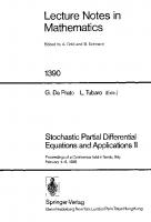
found several quasi-ladders of sharp resonances (see fig. 1). J) We show that some of these resonances are stable as

N

increases so we can

real-

ly say that they are semi-infinite cr¥stal resonances. 2) The realoarts

of the

nth

quasi ladder resonances verify

1

I

I

The imaginary parks are related to = 2a (where G is the k(E) dE n GIl. st st ili n n gap in particular the resonances belonging to the 1 ladder and 1 plateau ve3)

rify

1

37

F _

0

4) We calculate the Schrodinger solutions for energies corresponding at the resonances and find they are "located" in space regions which are determined by the tilted bands (see Fig. 2)

600

450

300

150

750

To observe a resonance,the length a£ the region in which the crystal is per­

Remark

feet has to be larger than the region the resonance needs to live i.e. scattering length is 3 0 and 1 = lOA then

,6E

we must have 10 4 F F> TO-s = I 0 VI em) .

If we are in a superlattice

toE

I

or

AE.t F

F> -1- (for instance if

is much smaller (.t.E j

_

tion band splits into several minibands,then much smaller

1£ =

the 10eV

meV) because the conducF

can be used.

Following Avron ideas we have also look the field dependence of the widths (see Fig. 3).

The large oscillations we observe are interpreted using a simple model barrier

and are discussed in terms of the

c/.. n

[see reLit.]

III ­ RESONANCES IN DISORDERED SYSTEMS IN THE PRESENCE OF AN ELECTRIC FIELD In march 83 appeared in Physical Review Letters a paper by Soukoulis, Jose, Economou, Ping­Sheng in which they study the transmission coefficient using the model L + [.

VAlli) &(x

- n) -

Fx

n=l where

V

n

is a random variable with rectangular probability distribution W2 48F

W

• They

found numerically

w2

-Li8F

They also say that there axi s t solutions which behave like 'r(L) = L so for W2 I they become normalizable. Notice that in the case V is fields such that 48F > 2 sufficiently regular these eigeniunctions don't exist (see our theorem).

38 With the same model we began recently to look at the resonances. There is no doubt there are very sharp resonances. They are exponentially small with F

, and it seems to us that here should be a structure like several "ladders".

It

is not impossible we find a transition i.e. a field strengh for which the width changes abruptly.

REFERENCES

I. F. BENTOSELA, R. CARMONA, P. DUCLOS, B. SIMON, B. SOUILLARD, R. WEDER

Carom. Math. Phys. 88 (1983) 387-397

2. F. BENTOSELA, V. GRECCHI, F. ZIRONI. J. Phys. C 15 (1982) 7119-7131 3. J. AVRON.

Ann. Phys. 143 nOI (1982) 33-53

4. F. BENTOSELA, V. GRECCHI, F. ZIRONI.

Phys. Rev. Lett. 50, nOI (1983) 84-86

5. C. SOUKOULIS, J. JOSE, E. ECONOMOU, PING-SHENG Phys. Rev. Lett. 50, nO 10 (1983) 764-766

a,

" "

"

.. ..

.

""

o

....

.....

.....

""

. ." .

.....

'" "

..

8 10-

8

FIG. I. Some plateaus of RelE} the first and second ladder

FIG. 3./- 1 behavior of three resonances in the third reg lou followed by continuity.

AN INTRINSIC APPROACH TO THE EVOLUTION OF QUANTUM OBSERVABLES IN TERMS OF STOCHASTIC PROCESSES ON PHASE SPACE J. BERTRAND and G. RIDEAU C.N.R.S - E.R. 177 Laboratoire de Physique theorique et mathematique Universite Paris VII - Tour 33-43 - 1er etage 2, place Jussieu - 75251 PARIS CEDEX 05 - FRANCE.

1.

INTRODUCTION In Quantum Mechanics, the evolution of a system is descri-

bed either in terms of wave functions or in terms of observables. In a set of works initiated by Maslov and Chebotarev [1]-[4], the evolving wave function has been written as a mean value with respect to a stochastic jump process, defined by the interaction potential when it is the Fourier transform of a bounded measure. Such a description can be extended to the evolution of quantum observables. Yet, this will require the use of two independent stochastic processes. On the contrary, working directly on the equation satisfied by some well adapted representative of the observables, we can

expect to derive more

tractable expressions. Beside its own interest, such a study would be especially valuable for application to field theory where Heisenbero representation is mainly used. Indeed, we have derived in a previous work [3]formulas analogous to Maslov's for a laroe family of Weyl symbols related to quantum observables. To this end, we used a Dyson expansion, which meant awkward computation even though the free hamiltonian was only a function of momentum. Here, we avoid systematically working with the perturbation series. We notice that, in some cases, the integro differential equations satisfied by the Weyl symbol or by its Fourier transforms (with respect to q or (q,p)

) can be formally solved by a standard

procedure using expectations on suitable stochastic processes. This works, in particular, when the free hamiltonian is equal to

+

or to a harmonic oscillator hamiltonian. But the general theory of stochastic calculus cannot be applied directly since the coefficients of the associated stochastic equations do not verify a

40

global Lipshitz condition and furthermore, the functionals are not even bounded. Thus, our main work consists of giving proofs specifically adapted to our problem in order to justify riaorously the formal expressions. To make the paper self­contained, we recall in § 2 the main results of Gihman and Skorohod L5]on the extension of stochastic calculus to Poisson processes. Then we give our notations in § 3. In § 4 and in § 5, we treat separately the two cases of hamiltonians

since the

required proofs are different. These results appeared in a shortened form in (6) .

2. PRELIMINARY REMARKS ON STOCHASTIC CALCULUS (according to Gihman and

2.1 Stochastic integral with respect to a Poisson measure. Let

(.n.. \ Ot..

of

) '§l

and ' \

) be a probability space,

a measure on

Definition A Poisson measure

on

the Borel

.

... lR )( [o)Tl

is an integer valued

random measure such that (2.1)

v(B,lle) ...

) At:.

(2.2) If

£

[o/T]

,has a Poisson distribution with

te.) llt. : E '" (eo ,lll:.) = l't \8) lit:

parameter

...

B1> .•.

riable s -.J teo,

are pairwise disjunct, then the random va1

AI:.)

are mutually independent.

This can be visualized by thinking of the number of events occur ina in

v

as giving

and characterized by coordinates

belonging to B. To define stochastic intearals with respect to

v

in the

same way as Ito's integral with respect to brownian process, we need some conditions of non­anticipation and independence on cisely, let \

1

IJ'" ­algebras of

Ot..

(2.3) for any B

t:. 1i: [0,,1 ,

the random measure

.

,

v .

More pre­

be a fixed non decreasing family of sub

v

must be such that :

the random variables

"\,I(B,[o,I:])

are

'Sft: -

measurable (2.4) the family

\V (B ll.I:, C+61:.]),lll:.>o

cr ­alqebras (2.5)

SIl.... 'Ttldu.)

IX)

J

is independent of the

41

Now, let \f:.!l. .. /R'" (2.6)

x

[O,T]

is

..

IR'" be a measurable function such that

-measurable

(2.7)

with probability 1.

IX)

The stochastic integral

1J.. . T

(2.8)

ell)

-V

=ItT)

is defined as the limit in probability of step function approximations. Besides linearity in (2.9)

E

(2.10)

E\

, this integral has the following properties

lTJw...

ff

.. IR

+E Examples

tI

E\

..

dl:

\2/ 'F 1 g

t

1) The process N wi th parameter t: T((IR....) .

is an ordinary Poisson process

"tll) =JJ. to

2) The process

t) TC

has constant trajectories except

· . f or Jumps at t h e same tlmes as the a b ove POlsson process.

This process is used by Maslov

(11 to solve Schrodinger equation.

2.2 Generalized Ito formula The stochastic integral (2.8) defines a stochastic process with stochastic differential given in the one-dimensional case by (2.11)

dl(b)=

1

It Ito's calculus has been extended by Gihman and Skorohod differentials. Namely, let

[5J

to such

be the process defined by

(2.12 )

where

is an

-measurable random function such that

E

;.

J1 t

l:

(2.15)

J

+

o

c

We shall assume that ti )

(2.16)

for some constant L, (ii) R >

a local Lipshitz condition holds, ie for arbitrary there is a constant CR (2.17)

2.

+

J

a

such that 2

l\

CR

I

2-

J

l Whenever CR is independent of R, we shall speak of a global Lipshitz condition.

43 Under these conditions, one can assert that equation (2.14) has a

unique solution which is right continuous with probability 1 and ve-

rifies the relation (2.18 )

2.4 Generator of the process and Kolmogorov's backward equation Now, we shall assume that the coefficients in equation (2.14) satisfy (2.16) and a global Lipshitz condition. Let

denote the solution equal to

for s

t. It is a Markov

process with transition probability

P (t J

j 1)

Definition.

B) =

E

B} ) B

The generator As of the process

E. oj(

(2.19 )

(t l ) ) \::'_t.

-

is defined by

i

A is computed in two steps. a) Let

-1

be the process defined by an equation analo­

gous to (2.14) but with i(­:I)

replaced by the constant

in all coeffi-

cients. Then, the global Lipshitz condition leads to the result (2.20)

b) Applying formula (2.13) to compute performing the limit t'­t

and

0, one obtains the value of the generator.

More precisely, one can state Theorem I.

If

f

has bounded continuous partial derivatives of first

order and if is a solution of (2.14) satisfying (2.16) and (2.17) with C independent of R, then R

The above hypotheses imply that if g is a function with bounded continuous first derivative, the function

44

E. has the same property. Then we can derive a Kolmogorov backward equation along the same lines as in the brownian case. The precise statement reads : Theorem II.

If g has continuous bounded first derivative and if

is the same as in theorem I, then

is differentiable in

E

'Sff:

, has bounded continuous derivatives and

satisfies

with boundary condition

Remark

It must be noted that for processes without brownian component,

the generalized Ito formula requires the existence, boundedness and continuity of the first derivatives only.

3. DEFINITIONS AND NOTATIONS

Let A be a quantum observable operator. The inverse Weyl rule associates to it a "function" A(q,p) called the Weyl symbol of A and defined formally by

where Q,P are canonical quantum operators. Any operator equation can thus be written in terms of Weyl symbols. In particular, if H(q,p) is the symbol of the hamiltonian operator H, the evolution equation

A

.

L = _L ll-lll\{tl] ell: -\;.. becomes

(3.2)

eH.

i; !botl

Pe.

A

;9 )A(qB)PBlt)\ B

"'rp" = I'

45 We assume H has the form : (3.3) where Ho is the free hamiltonian and V is the Fourier transform of a bounded measure (3.4)

v (0.,1' ) = J..J L1J,

As is well known

)d'X.) 4't f \ 2. i. 1'(

-+':>C.

a positive measure

f') } f(dy,dx) and a real function

(y,x) exist such that

(3.5)

The hermiticity of V implies

-

J

=J

I

ck ) i(- '(1/-

for any measurable function f. Together with the function A(q,p,t), we shall use the Fourier transforms defined by : (3.6)

(3.7)

According to (3.1), A(q,p)

is not necessarily a function. But, the

above formulas also make sense with distributions. We shall find out in due time what conditions have to be imposed upon these objects.

In this section, we consider the following hamiltonian (4.1)

where the potential V(q,p) has the form (3.4), ho(p) with polynomial growth and h

1

..,

is a C -function

(p) is a derivable bounded function veri-

46

fying together with its first derivatives a uniform Lipschitz condition. The evolution equation (3.2) is most conveniently written in terms of (3.6). Thus we have:

(4.2)

where

­R.. (p...

a (4.3)

:t

.e,.(p­1\t.q,)

""k. (C\)f): We associate to this equation a stochastic process with initial value Let \'" t d11 c:lx

IE.)

ck.)

1R'l)( Z2l( lO)IJ

I Eo

= ±

be a random Poi sson measure def ined on

1

,where

with mean value given by

The first two components of

are defined by the following sys-

tem of differential equations :

dO. (-:I) ""

-

) ?(­:») cb -

:v,.'r:.

=­+

(4.4)

j

po

ck) e l d.o)

­1\1:..

The coefficients verify conditions (2.16) and (2.17) globally provided the integral

is finite.

The component

is defined by a stochastic differential

...

(4. 5)

+'\\.

J\

JfE. ...

2.lt'X. (pI"') ...

(9 ("'»f'l2.(V:") t

are finite. Yet

is not bounded and before proceeding to the deriva-

tion of the associated Kolmogorov equation, we need two lemmas. Lemma

: Let us assume that the moments

for p

D,1, ... n and g(p) is a

P'1'=l2lt{

are finite

function growing no faster than Ipln

47 at infinity : C(-1+

\f'\"')

Then we have the inequality

Proof.

Due to the assumed finiteness of the moments of

f

'

Ito's

formula can be applied : %

-J

- catf:!:.

'T\t

1\

(1:)

et"l:.

('tJ)

:!:.1lt.

l::

.0

-t

4

\f(tt-q

=to 2.'T\.

-

(1:)

± T{t. qil:l1:»)}

Jc!X)

1:I)

c:h)

Then we perform a Taylor expansion of g to order n about

(-')_t)

+(/,\_l:.)i.

+ Y.

I:

""t'

-t.

It.-I

.

':t

1(1..

£.1

""!

-

'I(t.

±"t\t

l;:»)-

The result follows from the behaviour of

tra-

to write:

\

C1

+

4!

EI

-+ C-1

and .e..(l')

and use the boundedness of

(-c)

,,"" \"''''

(p ± tt1. q)

I

at infinity by an itera-

tion procedure. Now, let us consider the function IN

(4.7)

)

where

=.e.

jl '"

d(C\lf )

is a function bounded and continuous together with its

first derivatives. Since z is complex, F does not satisfy the assumptions in theorem I, § 2. Yet, to prove that it belongs to the domain of the

S

-process infinitesimal generator, it is sufficient to establish

the following lemma . Lemma 2:

Let

..

be the stochastic process obtained from (4.4)

and (4.5) by substituting their initial values for the processes in the right-hand sides. Under the conditions of Lemma 1, we have:

48

(4.8)

Proof.

with constants C and C'. The general theory (§2.4, eq.

(2.20)

) applies to the second term and

gives the required limit. For the first one, we have :

where K depends on 1mz. But, from the definitions : \:.'

S

'&,=1:. t\:.')-

-

1

l:

J\

(91 f')}

dt:

\:'

l;

+

-

t

Jf 1:'

+

(

-" -

E."t

ld...e ) !old'!:.)

l:

so that, applying lemma , and taking into account the Lipschitz property of hI, (p), we get: 2

"f'I

1

\1'tI_1)

(-1-+ Ipl -

Therefore

\:'_t_o

_

(t:.'_t(

,=0

which completes the proof. Then we set (4.9)

...u..(\:.,q IV

)

=E e.

1('"'

.\

i-'b F ('1IP , t

Q.

IV

)

49

Since u(t,q,p,z) has the same property as function (4.7), it belongs to the domain of the

-process infinitesimal generator and the result

of theorem II holds. Thus we can state Theorem III.

Let us assume that

h e is a C" _ function growing no faster than

IpI'"

,

h 1 is a bounded function whose first derivative verifies Lipshitz condition

- ¢

(y,x) is a real function and

j

that the integral 2 2

P

a global

f(dy,dx) a positive measure such

I(y,x) f(dy,dx)

is finite for I(y,x) =

,4.2

2

(y,x),x ,

x y and Iy\ ' 0 p n. Then, the function defined by

satisfies

oF\C\

I

O\:.

(4.11 )

P ,I:.)

+

L. \ Eo l \.

1\

to("

-\0 Eo

l(t..;) -

E."t.."

_1. L.

p-\0

J

l..

(f

F

1

I

-0

!!.

aq

9)} F (2\ )P t) l

F(q,r,t:)

p) 1:)

"" .!. o (A.. )ck ) L Eo e... 4>( ,'X) + 2, ""

t: t

Z: E.-t tp-t

_2.

2.

2

£,(t..

F (3). Let us pause to give an example. Example 1: Assume we have particles randomly spread through JRd number of particles in a bounded set A by a random measure that the mumber of particle

w

We measure the

(A). This simply means

in A is random, but for fixed w this number

is a

where a is the Dirac measure x i at x and the t:i(w) are the random positions of the particles. Imagine that anyone (point) measure in the variable A. Thus

w

=

La t: () w

of the particles produces a potential f(·-t:i(w»

around its position t:i(w), then the

total potential is given by: V (x) w

=

(dy) w

(5)

72

which is just a (fancy) way of writing the sum over all V will be stationary if w x

w

is stationary in the sense

w(A) ;

of course we have to make some assumption both on

and the function f appearing in

the (5) • Let us define C the unit cell of the lattice zd. by o' JRd

and {f

i

I

tz

jo;;;x. max (2.d/2)

k

(iii) see [19]

The random field V

w is

metrically transitive if the random variable

and

are independent if the distance between A and B is large enough. A random measure

of particular importance for several applications is the Poisson

random measure. This measure is characterised by (i)

(I· I

(A) ; k}) ; IAl w k

k

e- 1AI

(8)

denotes Lebegue measure)

and (ii)

Example 2:

and

are independent if A and B are disjoint.

Let K be a connected compact Riemannian manifold. Let

denote

Brownian motion on K and let F be a nonflat function with values in [0.1]. Then defining: V (x) ;

w

x

(w))

x E JR

we obtain a metrically transitive random process. It is this potential for which Gol'sheid. Molcanov and Pastur proved [13] point spectrum and Molcanov [26] (see also Carmona

[6J).

pure

obtained exponential localization of the eigenstates

73

Example 3:

In this example we consider almost periodic functions as potentials V.

Those functions are not random at all. But it is useful in the present context instead of the a.p. function V itself to consider a "random" element of its hull. Let us be more precise: A function f (CbOR d), the bounded continuous functions is called almost periodic if the closure in the uniform norm of {f Iy ( Y d). (f (x) := f(x-y» is compact in CbOR Y d We call Q = {fyly the hull of the almost periodic function f. Defining f f 0 f = f and extending this operation by continuity to the whole hull we equip y z y+z Q with a group structure. It is easy to see that with this group structure and the f uniform topology Q becomes a (compact)topological on Q there exists f f a finite measure v that is invariant under the group operation. This measure is unique up to constant factors and is called the Haar measure. We may normalize it so that v(Qf) for any

B(uf),v) is a probability space. Defining = f' we obtain a group of measure preserving transformation which can be =

1. Thus (u

proved to be ergodic. Now we define the random potential V

:=

for all

(U

is easily seen to be metrically transitive. In this sense we can consider

c

almost periodic potentials as random ones.

zd-metricallY transitive potentials Beside the class of metrically transitive random potentials there is an other class of random potentials of physical interest. For these operators we assume:

(u, T ,p) there is a group {T.}. 1 1

1') On

(

Zd of measurable measure preserving

transformations. 2') We have VT.w(x)

=

Vw(x-x

1

(9)

i) d

where the {xi}i(Zd form a d-dimensionallattice inJR .

3') {Ti}i (Zd is ergodic. We will call a potential satisfying 1') and 2') Zd-stationary. If furthermore 3') is valid we speak of a Zd-metrically transitive potential. Again we discuss examples: Example 4: Let {x

be a lattice with unit cell Co and let {q.}. 1 1 1,} P random field on Zd and f (L ) for p > max(2,d/2)

I

V (x) w

If E(lq

o

I)

i (zd
1 for d

=

(i.e. V satisfies Assumption A). w 1 D Then the measures vA (w,·) converge weakly as n n is independent of w. n

T!CT

2 p

+

=

2:

for d> 2) P

00

to a measure v (.) that

The distribution function ND(A) of \)D is given by fullfills:

D. at all the continuity points of N

d

79 The limit measure v

D

D

is called the density of states measure of H N is called the w' D (integrated) density of states. To call N the density of states is clearly an abuse D of language since this term should be used for the density of the measure v provided D there exists one. Nevertheless we will eventually follow the practice to refer to N as the density of states. The existence of the density under stronger assumption was first proven in the pioneering works by Benderskii -Pastur

[3]

and Pastur [29],

and in Nakao [27] • The stated theorem is essentially due to Kirsch-Martinelli [17] . However in this reference only a slightly weaker notion of convergence is proven to hold. Proof of the Theorem:

We give the proof in some details, but restrict ourselves to

3. More informations can be found in [17] .

dimension d

Let A' ,A" be closed hypercubes in JRd with non intersecting interiors, define A = A' U A", then

(15) Thus the stochastic process FA (w):

=

D

N (W,A) is superadditive.

A

Let us briefly consider (15).

aA the boundary of A may be strict ly smaller than aA 1

Thus the domain

:0

of

st.",

in general is larger than the direct

1

HD 1)

since we require more restrictive boundary conditions in the latter case. Applying the mini-max-principle we obtain (15). 1

To show that

D

N

An

n

(w,x) converges we apply the superadditive ergodic theorem in

the version of Akcoglu and Krengel [1] A,

TAl 1

n

.This theorem tell us that for fixed

D N (w,A) converges P-almost surely provided A

sup n

n

1

TTl IAnl

D

E (N A (w, A)) < n

Moreover we have lim n--+oo

rX=T n

n

We will argue (16) for d

(16)

00

(W,A)

sup n

1

TD n

D

E(N (W,A) A

a. s ,

n

3. By the Cwikel-Lieb-Rosenbljum bound the number of

negative eigenvalues N(H) of the Schrodinger operator H = H + V is bounded above o d 2 by Iv-(X) I / dx , V- being the negative part of V (see e.g. Reed-Simon IV[32] ).

C·f

By mini-max principle N(H

+ (V

s c

-A)

w

o

f

A n

[v

w

(x) -

'l d / 2 1\

X{ V (x ) < A} ( x ) d x

w

(X is the characteristic function of the set A). A Therefore:

80

1

D

TD

d/2

E(N1\ (W,A»;:; C E( Ivw (0) - A I X{V (0) n n w


1 whether v is a continuous measure. For discrete versions of random Schrodinger operators there are much more results in this direction (see Craig-Simon [9] , Wegner [34], Constantinescu-Frohlich-Spencer

[ 7]). For d

=

1 Avron-Simon proved that v is a continuous measure or equivalently N is a

continuous function. More precisely they proved that any atom of v, i.e. any point of discontinuity of N, necessarily is an eigenvalue of H of infinite multiplicity. Those eigenvalues easily can be excluded for d

= 1

by ODE methods.

The above continuity result was improved by Craig-Simon [8] . Those authors proved that (for d=1) the density of states is log-Holder continuous, i.e. for E,E' with IE-E' I

2

there exists a constant C such that IN(E) - N(E')

I

C

5) The asymptotic behaviour of the density of states In this section we study the behaviour of the density of states for high and low energies. It turns out that for high energies the random potential does not playa significant role, i.e. the density of states N(A) behaves like the one of the free Hamiltonian at + 0 0 . For low energies we have to distinguish two cases: 1) l::= inf CJ(H ) = - 00 and I I ) l: = O. w Other values of l: can be reduced to the second case. In both cases the density of

states has a tendency to decay exponentially fast near l: while the density of states of the free Hamiltonian decays as a power near The behaviour of N(A) near :

l: = O.

was already investigated by Pastur [29J. The results

given here are extensions of Pastur's results, the proofs however are quite different. The exponential falloff of N near l:

0 was stated by Lifshitz [25]on the basis of

physical arguments. The behaviour of N near l:

=

-d/2 0 as e- CA ,C

>

0 is therefore

called the Lifshitz behaviour. Nakao [27] and Pastur [30] gave rigorous proofs for the Lifshitz behaviour in the example of Poisson distributed sources (see example 1 in section 2). Using DonskerVaradhan techniques those authors were able even to compute the constant C appearing in the exponent above. The behaviour of the density of states for large energies 2 d). Let us start with the density of states N (\) of the free Hamiltonian H =-6 on L OR o

0

86 As one would expect it is possible to compute N explicitely: o(\) N (\)

(21T)d

o

Where

T

(24)

\d/2

=

denotes the volume of the unit ball in Rd. This result is due to Weyl. (An

d enlighting proof can be found in Reed-Simon IV, XIII. 15 [

J.)

Turning now to N(\) we recall from Corollary 2 of Theorem 2:

3). From this estimate we read off that

(Remember that we assume d N(\) • sup n

ri:1

D\d/2

(\»

n

=

0 N (\) o

n

for arbitrary \. For large \ we even have: Theorem 6: If the potential V satisfies Assumption B then w N (A) lim _0_ _ lim N(\) \ __ \d/2 \__ \ d/2 Proof: From section 4 we know that for arbitrary s>O N

V s(Ho)A + bA(s,V w) W1A in the sense of quadratic forms. This implies

By the mini-max principle we obtain from this (1-s) \n(H

N - bA(s,V oA) w)

N \n(HA(w»

(l+s) thus: (N )N ( o A

\-bA(S,V) ) 1 + \+b,(s,V) (

H

1 + s

+ bA(s,V

w)

D

w)

(25)

D

N

N

D

where (No)A (resp. NoA) is the number of eigenvalues of (Ho)A (resp. HoA) less than \. Using Proposition 2 in Reed-Simon IV, XIII.15 [32 N ( ) _ 011

m

C TAT

(1+]AI(d-D/d

s

N

o(ll)

11

(d-D/2)


k

0 and moreover E( IV (0) I )

In N(A) ::; B

w


_1_).

1\ Vw(x)+aA dx

F1\ (a,A»

1+a

J 1\ Vw (x)+aA A

A dx) =: M(a,A). V (x)+aA w

E(J

=

C

0

is easy to check that F1\ satisfies the assumption of Theorem[16]in the Appendix. Hence Theorem 16 tells us that: It

p(

1 TAT

whenever

F1\(a,A) >

e

-cl1\1

> M(a,A). C may depend on

and A.

By dominated convergence: lim+ M(a,A) = lim+ E(J

1.70

1.70

J

V (x)=o w

dx)

V

(x) w A

C

o

+a

dx)=-!.E(j{xE:CIV(x) a

0

We set p := E(I{xE:C IV (x ) = o w Now we choose a such that

£ a


0 S1nce 0 (i.e. a> ---1

-p

Now we choose A so small that M(a,A)




Clx[-a for large Ixl

(a

> d) and P(qo =0) < 1, then

_MA-d/(a-d)

(37)

e

for a suitable M> 0 and small A (;;; 0). Remark: If a < d+2 the convergence to zero In (37) is faster than that one in (36). Proof: We discuss only the case d ;;; 3. Let us define q.(w) = min (qi (w), 1) and f(x) r, Then N(A)

min

(f (x ) , 1) •

N(A), N being the density of states of H w Thus we may assume without loss of generality that qi (w)

1 and f(x)

H

0

+ V w

1

In section 4 we stated that N(A)

E(IVw(O) - Al

d/ 2

X{V (O) 0: 4 d

e( with C

s

d

t - C4t d / a ) A,- a-d >

a-d

e -C s

;';

0 where we have chosen t

Finally we get N(A) ;'; C Ad/ 2 e- CS 1

an appropriate way.

d - a-d A

o

The next theorem provides us with a lower bound to N(A) for

for independent identically distributed qi' We suppose that f(x) Let us define F(t)

=

clxl- a for large Ixl with a P(qo;';

>

d.

t ) ,

Theorem 1S: (L)

N(A)

(Li )

If a ;;; d+2 then

d Q 2" 2 N(A) ;;; C' A eCilnF(C3A) A 1

for suitable constants C (resp. C" 1,C 2,C 3 Remark: If we suppose that P(qo

=

Z' C)

C

>

0) > 0 we again have that

o.

96 1

0 < lim A+O

Ad/ 2

1 Ad/ 2

s lim

In N(A)

A+O

In N(A)
i(E) WEJ (i) If the sets

-n

iCE)

+

)

=

EP T

iCE)

C.A

-i

.E

P

is small enough, this

•

(l-p) Log(l/E) / Log A , we get

n W)

(A (E»

J(i) , i

1

T

C.E

T

•

were empty, we should be finished. This is not the

case but a similar but more careful analysis gets rid of these sets, and allows to derive the result. As noticed before, we get Corollary IV.2

The foliation described in Theorem 111.2 exist lJ-a.c

By the invariance of lJ{xEQ

I ml (W+ (x»

on

Q

lJ , and by the same arguments as in Th. 4

< c}

l:

nEJN

Some easy consequences of Theorem 7 can be derived. Corollary IV. 3

V

For

kElZ

For

xEQ

o

ABSOLUTE CONTINUITY IN THE UNSTABLE DIRECTION The absolute continuity of the conditional probabilities of

lJ

along the

unstable foliation with respect to the Lebesgue measure, here briefly called UAC, is the following property. Let

¢

be the set of unstable fibers of WE ¢

We Q and

Q, id est

V xEW , W = W+(x)

110

The induced sub

a-algebra

of

and the quotient measure

B(n)

of

is

is simply the restriction of

to

By general theorems (cf. [II] e.g.) we know that there exists a of probability measures every

IW)

(conditional probabilities) on

has support on

W, and for

A E B(n) ,

Theorem V.I

, !W) m where W W. In fact we can prove more

For

u (.[ W)

,

,

u

n

(.1 W)

=

m W

m is the normalized I-dim W

mj,

, it is straightforward to see that for

Because of the explicit construction of nEJN

=

B(n), such that

=

We say we have UAC if for any Lebesgue measure on

unique family

+

Note that the restriction

of

has

to

finite support. To prove the theorem is enough to show that

f

=

IDW(f)

. Let

f E

Suppose that, for some topology

T

and that

Then, we have weak convergence of

is compact for

T

= lim

and we can write

n-+=

n

of

, the function

(f) = lim n-+=

f

mW(f)

W + mW(f)

=

f

is continuous ( +)

mW(f) du + (W)

+

to

and the

result follows from the uniqueness of the desintegration. A natural topology on

is the Hausdorff topology given by the following

distance between closed sets d(A,B)

sup inf dist(x,y) + smp inf dist(x,y) • xEA yEB xEB yEA

is not compact for this topology ; but the weak convergence can be obtained under weaker assumptions small values of n

£

) , nEJN

£

Prokhorov's theorem says that it is sufficient to find, for ,

a compact set

are bounded by

£

£

•

c

such that the quantities

Corollary IV.3, by eliminating the smallest elements of pact set.

£

This can be done (for details, see [4]) using in order to get a com-

111

VI

ERGODIC PROPERTIES The following theorem is the key of the ergodic properties of

Theorem VI. I

Let

f

be a mesurable function,

unstable manifolds. Then

f

is

a subset of

n ,

constant along stable and

constant.

We summarize the proof. Let F

T.

x,y E n

= 0 , such that, on

and let n\F , f

f

be a measurable function

is constant along stable and

unstable manifolds. We show that, f(x)

2

(x,y) E n

fey) , for

By the hyperbolicity we can

exhibit two quadrilaterals

Q(x)

and

mited by pieces of stable anA unstable fibers such that the endpoints of outside

Q(x) , those of

W+(y)

outside

Q(x) . TnQ(y)

N such that, for

n> N , TnQ(y)

F , we could write

W+(x)

and

almost surely, one can

F

has zero

TnW+(y) , thus zero length on these segments and that

find

zED(P[W+(x) ,TnW+(y)J)\F

so that

= f(Tny) • We can with no restriction suppose k k+n so that we get as well, for and n> N , f(T x) = f(T y). fey) = f(T

-N

W­(x)

f(Tny) = f(x).

f(x) = fez) = f(P(z»

Thus,

are

is stretched in the unstable direction, and crosses

By the UAC and Theorem 111.4, it is possible to prove that expectations on

W­(x)

TnW+(Y) n W­(x) i ¢ . If we were sure that this intersection

transversally, so that is not contained in

deli-

Q(y) .

By the topological mixing, there is an integer intersects

Q(y)

F

invariant,

N

x) = f(T y) = f(x).

Corollary VI. 2

is ergodic T) is a K­automorphism

To prove the ergodicity, it is enough to show that, for I , such that

xfn

f

lim n-> ,y,!) oil

G(

f, y, r)

La forme la plus simple de relier

est une matrice

Mo

2 x 2

V; 0

GUf 'Y'f)-1

(4)

inversible.

L'enonce du theoreme suivant montre que Ie programme de conjugaison n'est pas realisable sous cette forme simple, mais qu'il l'est, si on Ie modifie sur deux points :

. La conjugaison se fait avec torsion de la fonction

2 . La conjugaison relie une valeur de l'energie pour lenodele libre

a

une energie differente du modele perturbe. Bien que ce decalage de

123

-la

c(

dans l'enonce du Theoreme- soit parfaitement continu des parametres,

sa valeur explicite n'est pas connue. De plus, la conjugaison n'est pas realisable pour toute valeur de l'energie.

v

Theoreme 1 . Supposons que que

9

est holomorphe dans

r[I';;

r

T + i [-r, +r] ,

r> 0

et

verifie la condition diophantienne (ll) specifiee plus bas.

1.> o ,

Alors il existe des constantes appartient

a

un ensemble de Cantor

K

c

0

, Y E:'lr

r-j

et

et

It" ')

B

3

teHes que si avec

iI vII { on a (5)

Les fonctions G : Kx'lr

-

---.

x DjI

0 2

We first recall the well known three term linear relation between successive ortho. . . Is P . I s [10] • For conven1ence gona I polynom1a we w1l1 use the orthonormal polynom1a

defined by(see equation 9): P

(h ) -1/2 P n n

n

n

(25)

Then we have:

v'if----:n+ I Pn+ I (x ) = x Pn (x )

-

IRn Pn- I (x)

(26)

where h n = RI ..• R The coefficients R will be described in the next section. n, n The equation (26) can be equivalently written as an eigenvalue equation in matrix form:

H where

=

x

(27)

is an infinite dimensional vector with components:

n

P(x),n=O, 1,2, ,.,

(x)

(28)

n

and H is an infinite dimensional tridiagonal matrix, with elements: H.

0, I, 2,

1 .

J+ ,J

All other elements of H vanish, From (27) we see that

.,. ,

(29)

is a quasieigenvector of

H with eigenvalue x. The fundamental property (13) may also be expressed in an operator form: H satisfies a renormalization group transformation property: HD = D(H

2

- A)

(30)

142

where D is a decimation operator defined as: (31 )

Let us describe shortly the properties of H[14]: i) the spectrum of H is invariant under the map T and its two inverses: -1

±

T± (x)

IX+"""T

(32)

0

ii) The spectral measure relative to the special vector ¢, defined by ¢n

= 0no'

introduced in section II. Therefore we have (as in

is nothing but the measure equations: 3 , 4, 5):

I

G(z)

(33)

•

s iii) When A

2, the spectrum is nothing but the whole interval [-2, +2J and we

have +2

f

G(z)

(34)

z - x

-2

iv) When A > 2, the spectrum of H

the set

K

of points E(O), where:

+

a

a.1

±1 (35)

v) K is a Cantor set of Lebesgue measure zero

[8]

K may be more precisely described

as follows: let S be the largest fixed point of T(x): (36)

1(-s)[, then in each We start from [-S, +sJ and we remove the segment JT(-1)(-S), T... remalnlng lnterva I we remove

-1

JT±(-1)

a T_(-1)() -S, T±

-1

+

a T+ (-s)[, and so on. The

end points of the removed segments are preimages of the point -So What is left after

an infinite number of stepsis just K.

vi) The representation (35) is a well adapted coding of K and the action of T is +

expressed on the sequences of sign a as the usual shift S:

143

(37)

I

Similarly we express the action of T- :

(38) -I

-+

T± (E(O» Using the

coding, we can identify the measure

as the coin tossing probability

measure: f(E(Oo' Therefore we see that

°1 , °2

.•. »

• (39)

has no atomic parts and the action of T on the spectrum has

the ergodicity properties of a Bernoulli shift. We therefore have an explicit example of an operator with spectrum on a Cantor set and purely singular continuous spectral measure. In fact one can show that the spectral measure defined in (33) is also the density of states, that is the limit of the density of eigenvalues

obtained by successive truncations of increasing order of

the infinite dimensional matrix H. V. ALMOST PERIODICITY AND BEHAVIOUR OF THE STATES We first give explicit expressions for the coefficients R in (26) and (29). n Using (30) we get the following recursion relation[2,3] R

o

=

0

(39) R

n

A careful analysis of these relations allows to prove recursively[2] that for

o

< R

2n

.2.

R

A-I

A > 2: (40)

+

2n 1

< A

(41)

R

(42)

s

More difficult is the proof that in equation (42) the limit k going to infini-

144

ty is obtained unformly with respect to p and s. A rather easy recursive argument shows that for

[ 14]

A > 3 :

A IRo 2k+ s - Rs I :5.k . (A - 2) This argument can be extended

[ IS]

(43)

to complex values of A large enough in modulus and

for A real slightly bigger than 2. The statement that (42) holds uniformly with res. equ1valent . . almost per10 . d 1C i [16] pect to S 1S to the statement that the sequence R 1S . n Therefore we can expand R in a Fourier like series: n

00

R

n

I

2 q - l-l

I

r

(2in 1T (2p+I)\ exp \ ) \ 2q

p,q

q=O p=o

(44)

Let us mention now some properties of the states. The high n behaviour is governed by the Lyapunov exponent y(x)

It can be proven

[17 14]

'

lim n->oo

[ 17]

2n

(x ) + ljJ2 n+ 1 (x )

.en

"

1jJ2(x) 0

-I

ljJ2(X)

\

)

(45)

1

that y(x) satisfies: 2y(x)

=

(46)

y(T(x»

which proves that y vanishes on the spectrum

[14] .

The behaviour of the stamscan also be studied directly using the renormalisation group equation (14) or (30). This procedure, similar to the one used in Ref. 18, gives the following results for A > 2: i) outside the spectrum, ljJn(x) increases exponentially because ljJn2 k(x) , '. , OUtS1. d e t h e spectrum. an d Tk ( x ) goes to 1nf1n1ty as ( x ) kd when x 1S ii) inside the spectrum we use for n even: (47)

and for

n odd: (48)

So we can decrease the order n and prove recursively the following bound for 2

k- 1

< n < 2 k: (49)

145

This recursive arguments uses inequalitv (41)and the fact that the spectrum K is ineluded in the segments [-s,

-x

u

:\ s],

where

S is given in (36).

Therefore we have an exnlicit polynomial increasing bound on the spectrum. Let us now emphasize the following fact, On the spectrum we have: (50) However, when k goes to infinity the sequence Tk(x) is ergodic on the spectrum. Therefore the sequences

have fully chaotic behaviour of a precise type related

to the Bernoulli shift above mentioned. Although the complete behaviour remains to [19]

be analysed

, and

.

should not be excluded a priori, that the chaotic behaviour k

could be atributed to the sampling (p2 ), we assert that our model is the only almost periodic discrete one in which such an explicit statement on the states can be made when the spectrum is singular continuous, VI.PHYSICAL CONTEXT The Schrodinger equation with a quasiperiodic potential arises in many physical problems usually referred as incommensurate structures, for example the properties of crystals in magnetic fields[20]. The discrete version of the quasiperiodic Schrodinger equation is best represented by the popular "Almost Mathien Equation": +

+ II cos (em + S)

(51)

which is expected to have localized solution for large wand non localized solution [21,22,23] '" . h f or sma 11 W • A 1S then exnected to at W ; I. However t e . . . h l' d' . . b (24) muc more comn has een proven that for some a Liouville

numbers) a singular continuous spectrum arises for any non vanishing W •

This very difficult problem, related to the Kolmogorov-Arnold-Moser theory, has been subjected to many works in the recent years (see for instance the references quoted in [23]). One of the most obscure problem is the behaviour of the states of a Hamiltonian

with purely singular spectrum. Our model is an attempt to answer to this

question. There

an other useful property of our model: the renormalization group equa-

tion (30,13). Therefore it is not surprising to meet similar problems in physical systems with built in scaling properties. The simplest example is the vibrational spectrum of fractal structures[25,26) which in some cases is also a Cantor set similar to the one we have considered here. However the snectral measure may be different and is usually a pure point one, dense in a Cantor set. One interesting physical question is the low excitation spectrum which can be studied

using a functional equation approach

similar to equation (4). We refer to works on transformation on real variables [27,28) and complex

.

[29 J

for further developments.

146

REFERENCES D. Bessis, M.L. Mehta, P. Moussa, C.R. Acad. Sci. Paris 293, Ser. I, 705-708 (1981) [2]

D. Bessis, M.L. Mehta, P. Moussa, Letters. Math. Phys.

123-140 (1982)

[3]

M.F. Barnsley, J.S. Geronimo, A.N. Harrington, Comrnun. Math. Phys. 88, 479-501 (1983)

[4]

M.F. Barnsley, J.S. Geronimo, A.N. Harrington, Bull. Amer. Math. Sbc. (1982)

[5]

D. Bessis, P. Moussa, Comrnun. Math

[6]

G. Julia, J. Maths.

2,

381-384

Phys. 88, 503-529 (1983)

Ser. 7 (Paris), 47-245 (1918)

P. Fatou, Bull. Soc. Math. France, 47, 161-271 (1919); 48 33-94 (1920); 48 208-314 (1920) [7]

A. Douady, Systemes Dynamiques Holomorphes, Semina ire Bourbaki n0599, November 1982

[8]

H. Brolin,Ark. Mat.

[9]

N.I. Akhiezer, The Classical Moment Problem, Oliver and Boyd, Edmburgh 1965, see p. 85-86

103-144 (1965)

[10] G. Szego, Orthogonal polynomials, Amer. Math. Soc. Colloquim publications, 23 (1939) -[II] M.F. Barnsley, J.S. Geronimo, A.N. Harrington, to appear in Ergodic Theory and

Dynamical Systems.

[12] R.L. Adler, T.J.

Rivlin, Proc. Am. Math. Soc.,

[13] T.S. Pitcher, J.R. Kinney, Ark. Mat.,

12,

794-796 (1964)

25-32 (1968)

[14] J. Bellissard,D. Bessis, P: Moussa, Phys. Rev. Lett. 49, 701-704 (1982) [15] G.A. Baker, D. Bessis, P. Moussa, to appear in proceedings of the Vllth Conference on Mathematics and Physics, Boulder, Colorado, August (1983) [16] H. Bohr, Almost periodic functions, Chelsea New York (1951) [17] D.J. Thouless, J. Phys. C,

2,

77-81 (1972)

[18] D.J. Thouless, Q. Niu, J. Phys. A,

1911-1919 (1983)

[19] M. Kohmoto, Y. Dono, Cantor Spectrum for an almost periodic Schrodinger Equation and a Dynamical Map, Illinois University at Urbana Preprint (1983) [20] P.G. Harper, Proc. Phys. Soc. London, Sect A, 68, 874-878 (1955) [21] S. Aubry, G. Andre, Ann. Israel Phys. Soc.,

1,

[22] E. Dinaburg, Ya.G.Sinai, Funct. Anal. Appl.

133-164 (1979) 279-289 (1976)

[23] J. Bellissard,R. Lima, D. Testard, Comrnun. Math. Phys., 88, 207-234 (1983) B. Simon, Advances in Appl. Maths., [24] J. Avron

1,

463-490 (1982)

, B. Simon, Bull. Amer. Math. Soc.,

81-85 (9182)

[25] E. Domany, B. Alexander, D. Bensimon, L.P. Kadanoff, Phys: Rev. (1983)

28, 3110-3123

R. Ramrnal, Phys. Rev. B28, 4871-1873 (1983) [26] R. Ramrnal, G. Toulouse, J. Phys. Lettres, Paris, 44, L13-L22 (1983) [27] B. Derrida, J.P. Eckmann, A. Erzan, J. Phys. A,

893-906 (1983)

[28] S. Alexander, R. Orbach, J. Physique Lettres, Paris, 43, L625-L631 (1982) R. Ramrnal, T. Lubensky, G. Toulouse, J. Phys. Lettres, Paris, 44, L65-L71 (1983)

147

[29] D. Bessis, J.S. Geronimo, P. Moussa, Complex dimensionality on fractal structures Saclay SPhT, Preprint (v983), to appear in J. Phys. Lettres Paris D. Bessis, J.S. Geronimo, p. Moussa, Mellin transform associated with Julia sets and physical applications,Saclay SPhT Preprint (1983) to appear in J. Stat. Phys.

ON THE ABSENCE OF BREAKDOWN OF SYMMETRY FOR THE PLANE ROTATOR MODEL WITH LONG RANGE UNBOUNDED RANDOM INTERACTION

P. PICCO Centre de Physique Theorique CNRS - LUMINY - CASE 907 F-13Z88 MARSEILLE CEDEX 9 (FRANCE) ABSTRACT We study the plane rotator model with Hamiltonian where

Jxy

for different pair (x.y)

_ 1:. Jxy cosC8x- y) z Xfy !x_y\3+-(

are independent symmetric unbounded random

variables. It is proved that for almost all J, all Gibbs states riant by rotation.

p(J)

are inva-

INTRODUCTION A spin glass is a dilute magnetic alloy where magnetic impurities are diluted in a non magnetic metal. It is believed that the physical behavior of such systems comes from a spin-spin interaction of the impurities which is long range and rapidly oscillating. It appears that this oscillating property, which is

essen-

tial to produce a spin glass, can be -modelled, according to the ideas of Edwards and Anderson

ri) ,by

a spin system in which the interaction potential

Jxy

are random

variable. Let< .)(J)

denote expectation with respect to a Gibbs state correspond-

ing to a given configuration of the interaction potential

Jxy. Let

E denote

expectation with respect to the random variable J. Since the mean magnetization E t in the physical literature by E(= expectation value). Then [F(t),F*(S)] = Llg\1 2e- i w\(t-S)

(8)

:= k(t-s)

[F (t) ,F (s)]= [F* (t) ,F* (s)] = 0 EF(t) F*(s) = L(lH(w

o+w\))

Ig\1 2e- i w\(t-S)

EF(t)F(s) = EF*(t)F*(s) = O. In this context the Wigner-WeiBkopf approximation is equivalent to replacing k(t)

in (8) by a multiple of a 6-function and

by

The physical validity of this assumption shall be discussed later. With these assumptions

(8) becomes

[F (t) ,F* (s)] = -il6 (t-s)

(9)

EF (t) F * (s) = (1+ )y 6 (t - s ) where we have listed the non-trivial relations only . In order to interprete equation (1) turn to the classical limit T -+

together with (4) and (9) we

or, e qu Lv a Le n t.Ly b -+

00

j

00.

In order to

get a well-defined limit, we let y approach zero in such a way that Then (9)

goes to a constant, e.g.

(10)

reads

[F (t), F* (s)] = 0 EF (t) F* (s) = 0 (t-s)

So F(t)

is nothing but classical complex white noise. Then (1)

ther with (4) and (10)

toge-

is a classical stochastic differential equation

on the unitary group U(2), whose solution is a process with independent, stationary increments. So a completely well understood objekt. Nevertheless a difficulty arises. The equation (1), together with (4) and (10), is not uniquely defined. We have to prescribe in what sense it has to be understood, e.g. Ito or Stratonovich. The same problem arises in the quantum case. In a previous paper [6] Equation (1) was solved in a modified Ito sense. Here we want to solve it in the sense of Stratonovich. This means that we want to calculate at first U(t) for a finite heat bath (!AI

« f (0)

is hermitian

v

fk v (t) f

(t) dt

(0)

->

­00

and +00

f -. (t) f 2

­00

Then for f

1,f 2EL

t ->

ff

1

;;;t

C(w

2

(t) dt

­s­

2ReKf (0)

(ill)

w

dt2dtlf2(t2)fl (t 1)Yk

2,w 1,+)ff 1

(s)f

v

w

2(t 2)b 1 (t

2(s)ds

and

ff ->

C(w

2,w 1,­J!f 1

where the constants C(w

(s)f

2(s)ds

2,w 1,±)

are given by the table

1))

165

b

w

w

2

b

1

±

C(W

1,W 2

b b*

b b*

± ±

a a

b

b*

+

(1 +B) K

b b*

b*

(1+B) iZ

b b*

b

' ±)

+

BiZ BK

For e.g. t

II 1

:> t

dt2dtlf2(t2)fl(tlhk

(l+B)

co

+=

dUk (u) v o

_00

I

I

v'

d s f , (s) f

2

B(b(t 2)b*(t 1)) (s+u)

as the second integral is a Co(m) -function with respect to u. Theorem 1.1

Assume that

is a sequence of integrable, hermi-

tian functions such that

I

o

k

v

(t)f(t)dt

Kf(o)

and that Ilk v

f to )

o

for any fEC

o

(m) .

Let f 1, ..• ,f 2m be real L 2(m) -functions. Let n be a permutation of 1 , ... ,2m. Then for v 00

converges to c n (1 ) , rr (2) ... C rr (2m -1) , n (2m)

!

sl-'"

Is: ds 1·· .dsmf n (1) (sl)fn (2) (sl) ... f n (2m-1) (sm)fn(2m) (sm) -sm

with c n(2k-1) ,n (2k)=c(wmax(n (2k-l) ,n(2k)) ,wf.dn(n(2k-1)n(2k) ,sgn(n(2k)-n(2k-1))

' ±) is given by the table above.

where C(W

2,W 1

Proof:

The proof of the theorem is very similar to the proof of theo-

rem 1 in [4] p.222 which treats a special case. We refer to that proof. It proceeds in four steps. The first step has already been done. The

166

second step is rather analogous if we observe that by the uniform bounded theorem the integrals flk v (t)!dt stay bounded. The third step is quite straight forward. In order to establish the forth step we have to prove essentially that

dt for

1dt 2dt 3dt 4

­+ 0

continuous of compact support. The left side is ;:;llf21L1lf41Iooflkv(t) [d t

Iff f 1 (t 1)f3(t3) t ;,t 1 2;:;t 3 Ikvl (t3­t1ldt1dt2dt3

= const

+00

f

du,u'lkv!(u)

o

f

dsf

1(slf 3(s+u)­+

0

by the assumption of theorem as the integrand with respect to u is a continuous function of compact support vanishing at the origane.

§ 2.

Statement and proof of the theorem

Fix a finite set A, by simplicity let us assume that

and a function

A­+g(A). We identify w and A. The noise F(tl is given by (cf. (0.3)) A ­iAt (1) F(t) = L g(A)e B A "EA The operators B" and are realized on the symmetric tensor space whose completion is the Fock space (cf [ 6 ]§3). A, n= (n,,) "EA' n" , !}E2Z+ T

s

Let e, be defined by (e,l =0, ­" r:»; \1 A BAI!}>

InA

B:I!}

In A+1

On the Weyl algebra C*­algebra

\1

then as usual

generated by

or alternatively on the

of bounded operators on

is defined by (3 )

or (4)

with

L(1 - z ) IA I)

nA

I cp I!}>

n

(5)

Choose

x d and put A1=A, A2=_A* and define

the Gaussian state

167

(6)

The differential equation for the finite heat bath (7)

: t U(t) = A(t)U(t)

is solved in proposition 2.1. Proposition 2.1

For fET

series

(8)

s(cr

l:

U(t,s)f

(9)

1

0

and t,sElli we have convergence of the

In(t,s)f

n=O

with

A)0cr d

(t,s)

In (t,s) The operator U(t,s) can be extended in a unique way to a unitary operad tor from F(cr )0cr onto itself. It describes a time evolution, i.e. U (t,t) = 1

(10)

U(t,s)

= U{s,t)*

U(t,s)U(s,r) = U(t,r) for all r,s,tElli. Proof:

(c f ,

(6) lemma 3.1) Hn

Then A(t) maps H into H and one has n n+ 1 IIA(t)fll;;; C/n+1 Ilfll for fEHn. Then for fEH

n

IIIk{t,s)fll;;;

k (t­s)k /{n+1) ... (n+k)

This proves the convergence of the series. Let f,gEH

n

and consider

­

l:

k, Ji,

l:

«Ik(s,t)f,IJi,(s,r)g>­-{1 , ... ,n} and where (26)

2M,lji =J

o lji

(lIdT i k)fl(Tl,1) .. ·f 1(Tl,m 1)

f

n

(T

n, 1)

... f

n

(T

n,m n )

w wn YB«A(T ,m ) ... A(T )) 1 18I • • • I8I(A(T n,m ) .•• A(T n , 1)) ) 1 1 1,n n Fix now lji and the associated numbers m ••. ,m and the associated n 1, We want to calculate

mapping

(v) lm 2M 'l'

l'

v-+ oo

'

Expanding like in (24) we have

174

Call

An6

=

Tl n A 6=

and observe that rem 1.1. Then (27)

lim

6 ' commute for different k and

and .p(v)

2M , IjJ

=I (A6( 0 GVZ is the operator in L2(IR ) with kernel defined for Imz E

function in

1 eiVZlx-yl GVZ(x,y) = 4n Ix-yl

by

k,k' E IR 3

Let now

by (see e.g.

(j)

k,2

¢

(2n) -3

r

J IR 3

dx e

-ik.x

V(x)

tp

(2.2)

(x,k' )

is the solution of (2.1). If follows then that

a uniformly continuous function of TI 0 ,

i p. (v e

-1

f(k,p,q)

p,qEIR

,)

I

by

t(k) u e i q . )

(u G v + 1)-1 k is such that

3

(2.5)

being the scalar product in

L

2(IR3

(H - k 2 ) -1 = G - G v t (k ) u G ' k k k 2

3

where H is the Hamiltonian defined in L (IR ) by -f::" -+- V in the sense of quadratic forms ([ 1]). Moreover, t(k) exists as a uniformly 3 1 / 2, l / 2 2 norm continuous operator in L (IR ) , for a :,> Re k :'> 6 Lm k?: 0, for any interval

[0:,13] c

(see [1]). Thus also

(O,oo)\E

f(k,p,q)

is

well defined for such values of k, its restriction to Ipl = Iql = k being equal [3], [4], [5] to the on-shell scattering amplitude f (k,w,w ') with w " p/lpl,

w' "q/lql

f(k,w,w') = _(4n)-1 -(4n)

It follows from (2.4) and

fIR3 dx

-1

(v e

w " pi I pi, w'

(2.5)

e- i k wx V(x)

ipx

, t(k) u e

iqx 1[' )llpl=lql=k

H

that

o

(one obtains a zero-energy eigenvalue of 2

tion

3

E L (IR) u G

v

o

s.t.

II

u

G

0

u Go v

=

and

H

VII " H S

+

o.

We say

if there exists a func-

_ Go v

is a well-defined bounded operator in

bert-Schmidt kernel since

k

has a zero-energy resonance or a zero-energy u G v in L 2(IR 3 ) has the eigenvalue

bound state if the operator -1

(2.6)

- q/ I q I •

We are interested in the study of these quantities when (see [ 6 ], [ 7 l ) that

V E R

(f

2

3

E L (IR ). Note 3 2(m ) with HilL A

implies that the Hilbert-Schmidt norm

\ 1/2 I I ) (4n)-1\,dXd Y I v(x)lv(y) Ix-yi2

is finite. We shall now assume that V is such that there is no zero--energy resonance or zero-energy bound state. This is the "generic case", see [ 8 ], [9]. The assumption is in particular satisfied if in this case

u = v

and

I

that

u Go v = v Go v

V?: 0, since

is a positive operator which

).

212

does not have the eigenvalue generic case where f (r k , sp , e q )

It is shown in [7] that in the i:; such that e 2b l' I V(·) E R for some b > 0

V

-1.

is analytic in

in a neighborhood of zero

E

f(Ek,Ep.Eq) =_(41T)-1(v,(u Go v + l)-lu) + i

(.!1T)-2 c k Iv , (u G

v + 1)-lu)2

o

(2.7)

+ (41T1-1 iE(pxv, (u Go v + l)-lu) -

( 41T1 - 1 it: (v,

G

(u

v + 1) -1

o

q

xu) + 0 ( E 2

) •

Moreover, under the same assumption one has the analytic expansion for the on-shell scattering operator

S(k)

S(Ek) = 1 + (21Ti)-1(Ek) (v,(u G

o

-

where

2-1

(81T) '(Ek)

2

with kernel given by (2.3):

v+l)

-1

(v,(uGov+l)

u)(Yo")Y o -1

u)

2

(2.8)

(Y,.)Y o 0

Yo(w) _ (41T)-1/2 Y1 (w) -

(41T 3/ 2) -1

Jdx

wx v(x)

(.,.)

being the scalar product on 3 sphere in IR .

(U

L

Go v + 1)

2 (S 2 , d w) ,

-1

s2

u(x) being the unit

Remark: A weakening of the assumption e 2a l· 1 V(·) E IR to (1+ Ixl)n 3 l V(x) E L ( I R ) , V E R is possible with the same result as asymptotic expansions in

E,

up to an order determined by

n. This has been

discussed first in the spherically symmetric case, see e.g. [10], and in the non spherically symmetric case in [ 8], [11]. For V ERn L l ( I R 3 ) the scattering length in the generic case is by definition, see [7], [12], the quantity (2.9) which gives the leading term in the expansion (2.7) fur leading term for

S(Ek) - 1

f

and the

in the expansion (2.8). It is useful to

derive another expression for the scattering length, using (2.6). In fact, from (2.7) a = -lim E+O

(2.9) we get

f(Ek, Ep, Eq)

213

and from

(2.6)

r

a = lim (4n)-1 E-+O J]R3

dx e-iEkwx V(x)

(2.10)

As we remarked above for this it suffices that

V ERn L l ( IR ) 3

and

that there is no zero-energy resonance or zero-energy bound state. Remark: In fact, the analysis of [ 7], [12] shows that the same holds with (2.9) replaced by lim (4 n ) - 1 (v, (u Go v + 1 + E+O Po

E:) -

1 (1 - Po) u)

being the projection onto the eigenspace of u Go v to the eigen2 -1 in L ( ]R3 ) , even if H has a zero-energy eigenvalue.

value

We shall now study the expression (2.10). is for any k such that k 2 ¢ E the unique solution of the Lippman - Schwinger equation (2.1) for

a·e· x

(see e.g.

[1]). Assume now

case. Then there is a unique solution which obeys E L 2 (]R 3 ) . Let (2.1) for T(k,k')

k

¢

E • By

(2n) -3

k E]R3

f

]R3

rIR3

¢

E i.e. the generic

0

¢

E

we have that

k' = 0, i.e.

e -ikx

Taking now

T(O,O) = (2n)-3

0

of the Lippman - Schwinger be the unique solution of

(2.2) and the fact that

is given by (2.2) also for

T(k,O) for all

2

(x)

k = 0

we get

dx V(x)

J

On the other hand, T(Ek, Ek') = f(Ek, k/lkl, k' Ilk' I) for all 3 k,k' E IR with jkl= Ik'i k 2 ¢ E, and by (2.7) we have in the generic case lim E-+O

f(Ek,Ep,Eq)

But lim T(Ek,Ek) = T(O,O) E+O (see [2], XI.6).

since

k -+ T(k,k)

is continuous for

k

2

¢

E

Thus we get a = (4n)-1

Jr

]R3

dx V(x)

(2.11)

214

where

is the unique solution of the Lippman-Schwinger equation

(2.1) for

k

Theorem 2.1 Let

O.

=

V ERn L

We summarize the results in the following.

l(JR3)

where

R

is the Rollnik class and assume the

generic case. Then the scattering length is given by

with

r

(4lT)-1

a =

dx V(x)

J JR3

(4lT)-1 (v, (u G v + 1)-1 u) a I/ 2 v = IVI u = sign V v

Go

(2.12 ) and where

is

the unique solution of the zero energy Lippman-Schwinger equation = 1which satisfies E L 2(JR3). Under the additional assumption

e2blxlv(x) E R

for some

b > 0 , we have that the off- and

on-shell scattering amplitudes and the S-matrix have analytic expansions ( 2. 7), (2. 8) in the energy, with leading terms given by a . 3. Probabilistic Expressions for the Scattering Length Let

,-:(s), s E [0,00)

JR3, started at

be the Wiener process in

0

and

normalized to have diffusion coefficient V2 i.e. for any t s 0, W(t) - ,,,(s) is Gaussian with mean zero, covariance E([W(t) _W(s)]2) 6(t-s), such that W(t 2)-W(s2) is independent of hJ(t l) -W(sl) for all t 2 s2 tl sl and W(O) = O. E means expectation with respect to the underlying Wiener measure P We have chosen the covariance

=

such that the infinitesimal generator is

6

rather than

as for

the standard Wiener process, in order to keep the same normalization as in Sect. 2. Let

be a real measurable function of x E JR3 such is a well defined self-adjoint operator in L 2(JR3), oo as closure of its definition on C ( I R3 ) in the sense of sums of forms, o t . lower bounded and such that for a .e. XI e -!0 dsV(W(s)+x) 1S a well-de-

that

H = -

6

V

+ V

fined

Ll(dP)-function. Sufficient conditions for this are well-known, e.g., V 0 J V E Ll (JR3) or more generally, as shown by Simon, V l oc is a sum of finitely many Vi ' each one either of the form i) V.1 bounded from below and or ii) V.

1

=

f.

1

JR3 onto for some

0

lT i

,

lTi

l (JR3) V. E L lac 1

some linear function from

JR)1 with sup ( x

f

p > )1/2, see

[13] ,

dy

If. (x-i-y) Ip) lip 1

[ 1 4] •


3/2

V E R)

(note that then

e has a continuous solution 11

00

- esslim 11 x -Too

11

11 = 11

in

L

oo

00

-

r

J IR 3

dy G

11

3)

[14],

[15],

[16], [17] such that

(x-y) V(y) 11 (y) .

0

Conversely, any solution of (3.1) in If

(IR

exists and is finite and

(x )

11 = 11

-tH

one has in addition that

3

00

L (IR)

(3.1) satisfies

e

-tH

11=11

then there is a zero-energy resonance or zero-energy bound state of H, in the sense of Section 2, i.e. a solution E L 2 ( IR3) of UGovG Thus, if there is no zero-energy resonance or zero00

= 0

energy bound state then =

J

1 -

11

0

00

and the equation

dy Go(x-y)

3

(3.2)

V(y)

IR has a solution

= 11/11

00

this solution satisfies

oo E L ( IR3). Note that for V E L l(IR 3 )nLQORh ,qi3 E L 2 ( IR ) and hence coincides with

the unique solution of the Lippman-Schwinger equation (2.1) for k = O. 3) V E LP ( IR n Lq ( I R 3 ) with p and q as above we have moreover that if a solution 11 0 of e- t H11 = 11 is non negative In the general case

then 11 > 0 and 11 o -tH 0 constants, of e 11

is the unique solution, modulo multiplicative 11.

It is also known that necessary and suffioo t H11 e= 11 in L with

cient conditions for having a solution of

ess inf 11>0 (which is the case if there is no zero-energy resonance) are

13 00 '" sup E(e t,x

-f;

ds V(W(s)+x) )

and [ 1 ], [13] , [14] , ess sup

11/11

00

Soo

sup 11 s ess ess inf 11


3/2 a

> 0

00

(3.5)

3

By FUbinisTheorem this can also be written as a

=

(47T)-1 E

[J

3 dx v(x)e- fo ds V(W(s)+x) ] .

(3.6)

JR

We summarize the results in the fo11owinq Theorem 3.1.

Assume that

V E L l(IR3) n Lq(IR 3)

for some

q > 3/2

and that there is no zero energy resonance or zero-energy bound state. Then we have the following expression for the scattering length, in terms of the p0tential and expectation with respect to the Wiener measure

a = (47T) -1

E[e-f;dS V(W(s)+x)]

The quantity

is strictly

bounded uniformly by the finite number the unique solution in ess lim

=

Loo ( IR 3)

sup t,x

of the equation

1. It is also the

e-tHIj)

=

solution of the equation

x-+ oo

unique under the specification

continuous, ds V(W(s)+x)] and is

Ij)

oo

E L

( IR

3)

or

Ij)

satisfying =

1-G oVIj)

217

Remark: For

V

E[e- f: d S V(W(s)+x)]

0,

has the probabilistic inter-

pretation of total expected killing under the killing measure for the Wiener process started at B c IR 3 , we h ave B

a

=

1 4n

fB

x.

If

XB

V

'Bx

dx E (e -Tx B), Wlt it h

by the process started at

V(y)dy

for some Borelset th e t ilme spen t

' In

x

We now remark that we have also \p(x)

lim t-++ oo g ( t,x)

with

w i.t.h

V+

g (t ,x)

t - f OOd S V-l- (Iv (s) +x) -, _ E Le - f 0 ds V (W (s) +x) e t J

r

the posi ti ve part of

for almost all

V

I

(3.7)

by monotone convergence from he lON'

x

Since

lim g(t,x) - g(oo,x) exists for a.e x t-+ oo rian theorem (see [18]) that for any a > 0 H(a,x)

we have by

a

Taube-

a t g(t,x) - a Jroodt e-

(3.8)

o

exists and moreover lim a ....O

g (oo,x)

E(a,x)

(3.9)

monotonically from below. Thus we get \p(x)

E[e lim

a+O

-fOOds V(W(s)+x) 0

a

]

r+ OO

J'

dt. e-

at

g(t,x)

and from (3.6) and FUbinistheorem using we have

a =

(3.10)

0

(4 n ) -1 lim a Joo 0.t e -at [

«-o

(4n)-1 lim ai-O

J3

l(IR 3)

J3 IR

dx V (x)

and

dx V (x) g (t , x) ]

IR

0

a

V E L

g (a,x),

g(t,x)fl (3.11)

218

= 1 dt

where

e-

at

(3.12)

g(t,x)

o

is the Laplace transform of g(t,x). Hence we have proven the following Proposition 3.2. Let E [e

lim g(t,x)

- 1 dsV(W(s)+x) 0

]

lim a a+O

t700

be as in Theor. 3.1, then

dte 1 0

-!Xt

g(t,x),

lim ag(a,x) a+O with g(t,x), g(a,x) given by (3.7) and (3.12), resp. For the scattering length a we have a = (4rr)-1 lim a 1 dt ea+O 0

at

[

13

dxV(x)g(t,x)]

JR

= (4rr) -1 lim a 13 dxV(x)g(a,x). a+O

Now let y(t,x)

=E

0

J dsV(W(s)+x)

JR

o

[e

].

For simplicity we assume V i:: a (but it is not difficult to extend the arguments to non necessarily positive V in the above class). We have lim

y(t,x)

t->«>

= y(oo,x) =

(313)

By a Tauberian theorem we then have that for a r(a,x) _

a

f

dt e- a t

a

>

(3.14)

y(t,x)

o

exists and lim

(3.15)

r(a,x) =

It is not difficult to show, using iterations and analyticity, that

r (a, • )

vr (a, .) ,

1 - G

ila with G

iv"U

(3.16)

r I x-y 1 -ya

(x-y ) = _e-;--.,---._

4rrlx-y[

From (3.16) we get by integration, using

f

[1 - r(a,xJ dx

=

1 V(x)

13

JR

dx G

iFa:

1 a

(x-y) = -

(3.17)

r(a,x)dx

From (3.15), (3.17) and dominated convergence we have lim 1[1 - r(a,x)]dx

a+O

hence from (2.12)

lim 1 V(x) r(a,x)dx

a+O

=

J V(x)W(x)dx

(3.18)

219 1

Ie

lim I [1 - f(a,x)]dx 4TI lim J {a dt [l­y(t,x)]}dx (3.19) 41f a+O a+O 0 But 0;; y(t,y) ;;1, and exchanging by Fubini­Tonelli's theorem the order of integration

a

we e'et a

00

lim a I dt e ­at {j [1 ­y(t,x) [dx} 41f a+O 0

(3.20)

Using again a Tauberian theorem (see e.g. a

(41T)­1 lim 1 t ....+ oo t

=

(41f)­1 lim t .... oo

Remark: have

t ­J ds V(W(s)+x)

r

1 t

dx [ 1 ­ y ( t , x) ]

JJR3

Since V E Lq(JR3) for some q(JR3) = and hence

rewrite Eq.

=

> 0

0

dx ] 1 ­ E (e

q > 3/2

(3.21)

we

and

-1

V =

this implies

)]

in the sense of distributions.

E L

Moreover, since

a

f IR 3

[18]) we get then

a.e .. Hence we can

(3.6) in the form

(41T)­lE [JdX IR

(x)

e

-1

­f;ds

(\'l(s)+x )

1 J

(3.22)

)

3

which involves only expectation with respect to t!1e c'liener measure and the distributional

LOO­solution

of

O.

We summarize the above observations in the following Theorem 3.3.

Under the same assumptions as in Theorem 3.1 we have t!1at

the scattering length is also given by the following expressions a

=

(41T)­1 lim a. 0.+0

where

f

3 dx V (x )

A

y(o.

,x) )

IR

y(a,x) ­ J+OO 0 dt e ­at y(t,x)

is the Laplace transform of

y(t,x)­

220

E[e

-ftdS V(W(s)+x) 0

a

JIR3 d x l

(4n) -1 lim 1 t-++ oo t

=

L> y (t,x)]

and

a = (4n)-1

\P

with

Err

L JIR3

a