Statistical Computing Environments for Social Research 0761902694, 9780761902690
The nature of statistics has changed from classical notions of hypothesis testing, towards graphical and exploratory dat
267 106 11MB
English Pages 256 [260] Year 1996
Recommend Papers


![Statistical Procedures for Agricultural Research [Hardcover ed.]
0471870927, 9780471870920](https://ebin.pub/img/200x200/statistical-procedures-for-agricultural-research-hardcovernbsped-0471870927-9780471870920.jpg)
![Statistical Tools for Epidemiologic Research [1 ed.]
0199755965, 9780199755967](https://ebin.pub/img/200x200/statistical-tools-for-epidemiologic-research-1nbsped-0199755965-9780199755967.jpg)


File loading please wait...
Citation preview
ATISTIGAL
=.
COMPUTING ENVIRONMENTS
ron] G0) G7 AN RESEARCH Robert Stine lela. editors
|
Digitized by the Internet Archive in 2022 with funding from Kahle/Austin Foundation
https://archive.org/details/statisticalcompu0000unse_jOro
STATISTICAL SME SapiNits ENVIRONMENTS FOR SOCIAL aa) Ne
NOTTS \..
pit
TiS *
Te
cos Aa AAS
AAS
=
.
= —
-
a
P
=
'
om
>
a
Port
ae
JkIJOS “Yr
2
>
an
a
ep
ae Foe) foe tS Sefer ioed|2 =
=
=
ae) =>
a
;
# -
.
>
STATISTICAL GeMEOSMRNE ENVIRONMENTS mor: SOCIAL RESEARCH Robert
Stine
Tommaso editors
SAGE Publications International Educational and Professional Publisher Thousand Oaks London New Delhi
Copyright © 1997 by Sage Publications, Inc.
All rights reserved. No part of this book may be reproduced or utilized in any form or by any means, electronic or mechanical, including photocopying, recording, or by any information storage and retrieval system, without permission in writing from the publisher.
For information address: SAGE Publications, Inc. 2455 Teller Road Thousand Oaks, California 91320
E-mail: Crd Tees eev ue cmog
FF
SAGE Publications’ ia
,
6 Bonhill Street,
London EC2A,4PU
,
|
3
5S
=
%
|
1 i
ek
SE )
4*
7 &
i
B
%
g
19 9?
United Kingdom SAGE Publications India Pvt. Ltd. M-32 Market Greater Kailash I New Delhi 110 048 India
Printed in the United States of America Library of Congress Cataloging-in-Publication Data Main entry under title: Statistical computing environments for social research / editors, Robert Stine, John Fox.
cn ps Includes bibliographical references (p. _)and index. ISBN 0-7619-0269-4 (cloth: acid-free paper). — ISBN 0-7619-0270-8 (pbk.: acid-free paper) 1. Social sciences—Statistical methods—Computer programs. I. Stine, RobertA. II. Fox, John, 1947—
HA32.5678 1996 300€.285—dc20
96-9978
This book is printed on acid-free paper.
POR
IS09
“10h O87
16. &
et
Production Editor: Gillian Dickens oo...
fr
T US
,
eel
Contents
. Editors’ Introduction ROBERT STINE and JOHN FOX
PART 1: COMPUTING
ENVIRONMENTS
. Data Analysis Using APL2 and APL2STAT
a
JOHN FOX and MICHAEL FRIENDLY
. Data Analysis Using GAUSS and Markov
4]
J. SCOTT LONG and BRIAN NOSS
. Data Analysis Using Lisp-Stat
66
LUKE TIERNEY
. Data Analysis Using Mathematica ROBERT A, STINE
89
. Data Analysis Using SAS
108
CHARLES HALLAHAN
. Data Analysis Using Stata LAWRENCE
126
C. HAMILTON and JOSEPH M. HILBE
. Data Analysis Using S-Plus
152
DANIEL A. SCHULMAN, ALEC D. CAMPBELL, and ERIC C. KOSTELLO
PART 2: EXTENDING
LISP-STAT
. AXIS: An Extensible Graphical User Interface for Statistics
175
ROBERT STINE
10. The R-code: A Graphical Paradigm for Regression Analysis
193
SANFORD WEISBERG
TE ViSta: A Visual Statistics System
207
FORREST W. YOUNG and CARLA M. BANN
Index
232
About the Authors
247
Editors’
Introduction
ROBERT STINE JOHN FOX
1.1
OVERVIEW
The first—and larger—part of this book describes seven statistical computing environments: APL2STAT, GAUSS, Lisp-Stat, Mathematica, S, SAS, and Stata. The second part of the book describes three
innovative statistical computing packages—Axis, R-code, and Vista— that are programmed using Lisp-Stat. Statistics software has come a long way since the days of preparing batches of cards and waiting hours for reams of printed output. Modern data analysis typically proceeds as a flowing sequence of interactive steps, where the next operation depends upon the results of previous ones. All of the software products featured in this book offer immediate, interactive operation in which the system responds directly to individual commands—either typed or conveyed through a graphical interface. Indeed, the nature of statistics itself has changed, 1
2
STATISTICAL COMPUTING
ENVIRONMENTS
FOR SOCIAL RESEARCH
moving from classical notions of hypothesis testing toward graphical, exploratory modeling which exploits the flexibility of interactive computing and high-resolution displays. All of the seven computing environments make use of some form of integrated text/program editor, and most take more or less sophisticated advantage of window-based interfaces. What distinguishes a statistical computing environment from a standard statistical package? Programmability. The most important difference is that standard packages attempt to adapt to users’ specific needs by providing a relatively small number of preprogrammed procedures, each with a myriad of options. Statistical computing environments, in contrast, are much more programmable. These environments provide preprogrammed statistical procedures—perhaps, as in the case of S or Stata,
a wide range of such procedures—but they also provide ming tools for building other statistical applications. Extensibility. To add a procedure to a traditional statistical requires—if it is possible at all—a major programming a language, such as C or Fortran, that is not specifically towards statistical computation.
Programming
programpackage effort in oriented
environments,
in con-
trast, are extensible: a user’s programs are employed in the same manner as programs supplied as part of the computing environment.
Indeed,
the
programming
language
in which
users
write
their applications is typically the same as that in which most of the environment is programmed. The distinction between users and developers becomes blurred, and it is very simple to incorporate others’ programs into one’s own. Flexible data model. Standard statistical packages typically offer only rectangular data sets whose “columns” represent variables and whose “rows” are observations. Although the developers who write these packages are able to use the more complex data structures provided by the programming languages in which they work, these structures—arrays, lists, objects, and so on—are not directly accessible to users of the packages. The packages are geared towards processing data sets and producing printed output, often voluminous printed output. Programming environments provide much greater flexibility in the definition and use of data structures. As a consequence, statistical computing in these environments is primarily transformational: output from a procedure is more frequently a data structure than a printout. Programs oriented towards transforming data can be much more modular than those that have to produce a final result suitable for printed display.
EDITORS’
INTRODUCTION
3
These characteristics of statistical computing environments allow researchers to take advantage of emerging statistical methodologies. In general, nonlinear adaptive estimation methods have gradually begun to replace the simpler traditional schemes. For example, rather than restrict attention to the traditional combination of normally distributed errors and least-squares estimators, robust estimation leads to estimators more suited to the non-Gaussian features typical of much real data. Such robust estimators are generally nonlinear functions of the data and require more elaborate, iterative estimation. Often, however, standard software has not kept pace with the evolving methodology— try to find a standard statistics package that computes robust estimators. As a result, the task of implementing new procedures is often the responsibility of the researcher. In order to use the latest algorithms, one frequently has to program them. Other comparisons and evaluations of statistical computing tools appear in the literature. For example, in a discussion that has influenced our own comments on the distinction between packages and environments, Therneau (1989, 1993) compares S with SAS. Also, in a
collection of book reviews, Baxter et al. (1991) evaluate Lisp-Stat and
compare it with S. Researchers who do not expect to write their own programs or who are primarily interested in teaching tools might find the evaluation in Lock (1993) of interest.
1.2
SOME
BROAD
COMPARISONS
All of the programming environments include a variety of standard statistical capabilities and, more importantly, include tools with which to construct new statistical applications. APL2STAT, Lisp-Stat, and GAUSS are built upon general-purpose interactive programming languages—APL2, Lisp, or a proprietary language. Because these are extensible programming languages that incorporate flexible data structures, it is relatively straightforward to provide a shell for the language that is specifically designed to support statistical computation. The chapters that describe these environments discuss how a shell for each is used. Because of their expressive power, APL2 and Lisp are particularly effective for programming shells, as illustrated for LispStat in the three chapters that comprise the second part of the book.
4
STATISTICAL COMPUTING
ENVIRONMENTS
FOR SOCIAL RESEARCH
In keeping with the evolution of their underlying languages, LispStat and APL2STAT encourage object-oriented programming and offer objects that represent, for example, plots and linear models. One must keep in mind, though, that both of these object systems are customized, nonstandard implementations. Given the general success of object-oriented programming, it is apparent that this trend will sweep through statistical computing as well, and the two chapters offered here give a glimpse of the future of statistical software. (The S package is also moving in this direction.) In addition, Lisp-Stat possesses the most extensive—and extensible—interactive graphics capabilities of the seven products, along with powerful tools for creating graphical user interfaces (GUIs) to statistical software. To illustrate the power and promise of these tools for the development of statistical software, we have included three chapters describing statistical packages that are written in Lisp-Stat. GAUSS, like the similar MatLab, is a matrix manipulation language that possesses numerous intrinsic commands for computing regressions and performing other statistical analyses. Because so many of the computing tasks of statistics amount to some form of matrix manipulation, GAUSS provides a natural environment for doing statistics. Its specialization to numerical matrices and PC platforms provides the basis for GAUSS’s well-known speed. Many users of GAUSS see it as a tool for statistics and use it for little else. In contrast, relatively few Mathematica
users do data anal-
ysis. Mathematica is a recent symbolic manipulation language similar to Axiom, Derive, MACSYMA, and Maple. As shown in the accompanying chapter, one can use Mathematica as the basis for analyzing data, but its generality makes it comparatively slow. None of the other computing environments, however, comes with its ability to simplify algebraic expressions. Although S incorporates a powerful programming language with flexible data structures, it was designed—in contrast to Lisp or APL— specifically for statistical computation. Most of the statistical procedures supplied with S are written in the same language that users employ for their own programs. Originating at Bell Laboratories (the home-away-from-home of John Tukey and the home of William Cleveland), S includes many features of exploratory data analysis and modern statistical graphics. It is probably the most popular computing tool
EDITORS’
INTRODUCTION
5
in use by the statistical research community. As a result, originators of new statistical methods often make them available in S, usually with-
out cost. S-plus, a commercial implementation of S, augments the basic S software and adapts it to several different computing platforms. Stata is similar in many respects both to S and to Gauss. Like S, Stata has a specifically statistical focus and comes with a broad array of built-in statistical and graphical programs. Like Gauss, Stata has an
idiosyncratic programming language that permits the user to add to the package’s capabilities. SAS, of course, is primarily a standard statistics package, offering a wide range of preprogrammed statistical procedures which process self-described rectangular data sets to produce printouts. Most SAS users employ the package for statistics, although SAS has grown to become a data~-management tool as well. SAS originated in the days of punch cards and batch jobs, and the package retains this heritage: one can think of the most current window-based implementations of SAS as consisting of a card-reader window; two printer windows (for “listing” and “log” output), and a graphics screen. There is even an anachronistic CARDS statement for data in the input stream. But SAS is programmable in three respects: (1) the SAS data step is really a simple programming language for defining and manipulating rectangular data sets; (2) SAS incorporates a powerful (if slightly awkward) macro facility; and (3) the SAS interactive matrix language (IML), which is
the focus of the chapter on SAS in this book, provides a computing environment with tools for programming statistical applications which can, to a degree, be integrated with the extensive built-in capabilities of the SAS system. Table 1.1 offers a comparison of some of the features of the seven computing environments. This table includes the suggested retail price for a DOS or Windows implementation, an indication of platforms for which the software is available, the time taken for several
common computing tasks, and several programming features. All of the programs are available for DOS or Windows-based personal computers. The table indicates if the software is available for Macintosh and Unix systems. The timings, supplied by the editors and authors of the chapters in this book, were taken on several different machines (all 486 PCs) and may not, therefore, be wholly comparable. Moreover, it is our experience that particular programs can perform
6
STATISTICAL COMPUTING
ENVIRONMENTS
FOR SOCIAL RESEARCH
TABLE 1.1 Comparison of the Seven Statistical Computing Environments in Terms of Price for
a DOS/Windows
Implementation; Availability
on Alternative Platforms; Speed for Several Computing Tasks on a 66-MHz 486 Machine; and Some Programming Features Mathe-
Feature
Price’
APL2STAT
Lisp-Stat
matica
Gauss
S-plus
Stata
SAS
$0/$630°
$0
$795
$495
$1450
$338/944
$3130 +$1450°
Available for Mac
{e)
e
e
fo)
fe)
Unix
°
°
e
°
e
e
e
4.2 8) 4 11.8
4.1 1.4 ii! 0.6
el 0.7 , ely: — xB),
(1)
f=
where the function p measures the lack of fit at the 7th observation, y; is the dependent-variable value, and x; is the vector of values of
the independent variables. (For clarity, this notation suppresses the potential dependence of p on x;; the function p can be made to depend on x; to limit the leverage of observations.) The fitting criterion of robust regression generalizes the usual least-squares formulation in which p(y — x’B) = (y — x’B)*. With suitable assumptions, we can differentiate with respect to B in (1) and obtain a set of equations that
generalizes the usual normal equations,
5 oy; — 1B) = 0,
(2)
i=1
where
= dp/dB. The function w is known
as the influence function
of the robust regression (not to be confused with the influence values computed in regression diagnostics). One must resort to a very general minimization program to solve (2) directly. A clever trick, however, converts this system to a more tractable form and reveals the effect of the influence function. In particular, assume that we can write w(e) = eW(e) so that (2) becomes a
weighted least-squares problem, oy. €;X;W;
—
0,
(3)
iil
where €; = y; — x/B is the ith residual and w; = W(é;) is the associated weight. The weights are clearly functions of the unknown coefficients, leading to an apparent dilemma: the weights w; require the coefficients B, and the coefficients require the weights. The most popular method for resolving this dilemma and computing B is iteratively reweighted least squares. The essential idea of this
EDITORS’
INTRODUCTION
ale
approach is simple: start the iterations by fitting an ordinary leastSquares regression, that is, treat the weights as constant, wr = =! and solve for B from (3). Label the initial uate of B as Bo. Given Bo, a new, data-dependent set of weights is ws = W(y; — x/Bo). Returning to (3), the new set of weights defines a new vector of estimates, say
B,. The new coefficients lead to a newer set of weights, which in turn give rise to a still newer set of estimates, and so forth. Typically, the influence function y is chosen so that the weight function W down-weights observations with large absolute (standardized) residuals. Least squares aside, the most popular influence functions are the Huber and the biweight, for which the weight functions are,
respectively,
We)
=
if
Beek
Lie
emelssr 1:
and
(Lene
W3(e) = | 0,
Poem leh
ls
(el coy ts
Qualitatively, the Huber merely bounds the effect of outliers, whereas the biweight eliminates sufficiently large outliers. Because robust regression reduces to least squares when W(e) = 1 for all e, least squares does not limit the effect of outliers. As defined, neither of these weight functions is practical, because both ignore the scale of the residuals. In practice, one evaluates the weight for an observation with residual €; as w; = W(é;/cs), where c is a tuning constant that controls the level of robustness and s is a measure of the scale of the residuals. A popular robust scale estimate is based on the median absolute deviation (MAD) of the residuals,
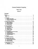
s = MAD/0.6745. Division by 0.6745 gives an estimate of the standard deviation when the error distribution is normal. For the robust estimate of B to be 95% efficient when sampling from a normal population, the tuning constant for the weight function is c = 1.345 for the Huber (equivalent to 1.345/0.6745 ~ 2 MAD’s), and c = 4.685 for the biweight (equivalent to 4.685/0.6745 ~ 7 MAD’s). Figure 1.1 shows a plot of the Huber and biweight functions W;, and Ws defined with these tuning constants.
2
STATISTICAL COMPUTING
ENVIRONMENTS
FOR SOCIAL RESEARCH
Biweight
eaipetsy
(Oey
ee)
2558
Ome
Figure 1.1. Biweight and Huber Robust-Regression Weight Functions
A remaining subtle feature of programming a robust regression is deciding when to terminate the iterations. It can be proven that iterations based on the Huber weight function must converge. Those for the biweight, however, may not: One need not obtain a unique solution to (2) when using the biweight. Keeping the potential for divergence in mind, iteration proceeds until the fitted regression coefficients are unchanged, to some acceptable degree of approximation, from one iteration to the next. Programming a robust regression within the confines of a statistics package presents some interesting challenges. First, one must be able to use the coefficients estimated by the initial regression in subsequent computations,
and then be able to program
a sequence
of
weighted least-squares regressions that terminates when some condition is satisfied. Second, one must decide how
much
flexibility to
permit in the choice of estimators. Because the choice of the influence function is crucial, one might decide to let this function also be an argument of the computing procedure. Users can then program their own influence functions rather than be restricted to a limited domain of choices. Table 1.1 shows the environments that have this degree of flexibility.
BOOTSTRAP RESAMPLING
As previously noted, bootstrap resampling provides an alternative to asymptotic expressions for the standard errors of estimated regression coefficients. The method assesses sampling variation empirically
EDITORS’
INTRODUCTION
13
by repeatedly sampling observations (with replacement) from the observed data, and calculating regression coefficients for each of these
bootstrapped samples. One can build the bootstrap samples for a regression problem in two ways, depending upon whether the model matrix X is treated as
fixed or random. Denote the data for the ith observation as (y;, X;). The procedure for one iteration of the random-X bootstrap is: R1. Form a set of random integers, uniformly distributed on 1,...,n, and
label these {i{, ..., 15}. That is, sample with replacement n times from the integers 1,..., n.
R2. Build a bootstrap sample of size n defined as y* = [Yir, eae Ye | and xX* =
[x;+, Saree
|
R3. Compute the associated regression estimates from y* and X*. In the case of least squares these would be B* = (X*X*)"!X*y*.
The procedure to use if X is treated as fixed is first to compute the residuals {€;,..., €,,} from the original fitted model. The bootstrap for
fixed-X is then:
F1. Same as R1.
F2. Compute y* = XB + e*, where e* = (Ej... 5 Ex)’ F3. Same as R3, but with X* = X.
In either case, one repeats the calculation B times, forming a set of bootstrap replications {B*,..., 8%} of the original estimates. This collection provides the basis for estimating standard errors and confidence intervals. Thus the bootstrapping task involves drawing random samples, iterating a procedure (the robust regression), and collecting the coefficients from each of the bootstrap replications. The sequence of tasks is very similar to that in a traditional simulation, but in a simulation samples are drawn from a hypothetical distribution rather than from the observed data.
KERNEL DENSITY ESTIMATION
Kernel density estimation is a computationally demanding method for estimating the shape of a density function. Given a random sample Z,, Z),...,Z, from some population, the kernel estimator of the
14
STATISTICAL COMPUTING
FOR SOCIAL RESEARCH
ENVIRONMENTS
density of the Z’s is the function P = 1yo fn)
K(=4),
z—Z,;
(4)
where /t is termed the smoothing constant, s is an estimate of scale, and K is a smooth density function (such as the standard normal), called
the kernel. While the choice of the kernel K can be important, it is h that dominates the appearance of the final estimate: the larger the value of h, the smoother the estimate becomes. The optimal value of h depends on the unknown density, as well as on the kernel function. Typically, programs choose ht so that the method performs well if the
population is normally distributed. Stine’s chapter uses Mathematica to derive the optimal value for / in this context. The calculation of the kernel density estimator offers many of the computing tasks seen in the other problems, particularly iteration and the accumulation of iterative results. In practice, f is evaluated at a grid of m positions along the z-axis, with this sequence of evaluations plotted on a graph. At each position z, the kernel function is evaluated for each of the observations and summed as in (4), producing a total of mn evaluates of K. Obviously, it is wise to choose a kernel that can
be computed quickly and that yields a good estimate. A particularly popular choice is the Epanechnikov kernel,
3
K,(z) =
——(1-
Al
a —
5)
0,
fon
z
Epona
(5)
otherwise.
This kernel is optimal under certain conditions. As with the influence function in robust estimation, kernel density estimation requires an estimate of scale. Here the popular choice is to set
~ foe interquartile inter til =e), ee rnin(
7
1.349
(6)
where * = )°;(Z;—Z)*/(n—1) is the familiar estimate of variance. Di-
vision by the constant 1.349 = 2 x 0.6745 makes the interquartile range a consistent estimator of o in the Gaussian setting. Finally, one can ex-
EDITORS’
INTRODUCTION
lS
ploit the underlying programming language to allow the smoothing kernel to be an input argument to this procedure.
1.5
STATISTICS
PACKAGES
BASED
ON LISP-STAT
The several statistical computing environments described in the first part of this book vary along a number of dimensions that affect their use in everyday data analysis. In one respect, however, Lisp-Stat distinguishes itself from the others. All of these computing environments encourage users to create new statistical procedures. But by providing tools for building user interfaces, along with tools for programming statistical computations, Lisp-Stat is uniquely well suited to the development of new and innovative statistical packages. What we mean by a “package” in this context is a program, or related set of programs, that mediates the interaction between users and data. Traditional statistical programs, such as SAS, SPSS, and Minitab,
are packages in this sense. Developing a package in Lisp-Stat entails several advantages, however:
e The package can take advantage of Lisp-Stat’s substantial built-in statistical capabilities. You do not have to start from scratch. ¢ Because Lisp-Stat provides tools for the development of graphical interfaces, the cost of experimentation is low. ¢ A package can easily itself be made extensible, both by the developer and by users. Lisp-Stat’s programming capabilities and object system encourage this type of open-ended design.
The three Lisp-Stat-based statistical packages described here—Axis, R-code, and Vista—all
make
extensive use of the GUI-building
and
object capabilities of Lisp-Stat, but in quite different ways. Of the three packages, R-code’s approach is the most traditional: users interact with their data via drop-down menus, dialog boxes, and a variety of “plot controls.” The various menus, dialogs, and controls are, however, very carefully crafted, and the designers of the package have taken pains to make it easy to modify and extend. The result is a data-analysis environment that is a pleasure to use, and one that incorporates state-of-the-art methods for the graphical exploration of regression data.
16
STATISTICAL COMPUTING
Axis offers many
ENVIRONMENTS
of the same
FOR SOCIAL RESEARCH
statistical methods
as R-code,
but
presents the user with a substantially different graphical interface. Here, for example, it is possible to manipulate variables visually by moving tokens that represent them. Axis also includes a very general mechanism for addressing features in the underlying Lisp-Stat code by permitting users to send arbitrary “messages” to objects. Like R-code, Axis incorporates tools to facilitate additions. Vista uses the graphical-interface tools of Lisp-Stat in the most radical manner, not only to control specific aspects of a data analysis, but also to represent visually—and in alternative ways—the data-analysis process as a whole. Vista accomplishes these representations by developing simple, yet elegant, relationships between the functions that are employed to process data and various elements of visual displays, such as nodes and edges in a graph. Although it remains to be seen whether these visualizations of the process of data analysis prove productive, it is our opinion that the ideas incorporated in Vista are novel,
interesting, and worth pursuing. We believe that it is no accident that Vista also includes tools for extension: this style of programming is encouraged by the object orientation of Lisp-Stat. 1.6
HOW TO ACQUIRE THE STATISTICAL ENVIRONMENTS
COMPUTING
APL2STAT and the freeware TryAPL2 interpreter are available by anonymous ftp from watservl.waterloo.edu. The APL2STAT software is in the directory /languages/ap]/workspaces in the files a2stry20.zip (for use with TryAPL2) and a2satf20.zip (for use with APL2/ PAS): The TryAPL2 software is in the directory /languages/ap]/tryap12. The
commercial APL2/PC interpreter may be purchased from APL Products, IBM Santa Teresa, Dept. M46/D12T,
P.O. Box 49023, San Jose,
CA 95161-9023. GAUSS may be purchased from Aptech Systems Inc., 23804 SE Kent-Kangley Road, Maple Valley, WA 98038. Lisp-Stat is available by anonymous ftp from umnstat.stat.umn.edu. Mathematica may be purchased from Wolfram Research Inc., 100 Trade Center Drive, Champaign, IL 61820-7237. S-plus may be purchased from Statistical Sciences Inc., 1700 Westlake Ave. N., Seattle, WA 98109.
EDITORS’
INTRODUCTION
7
SAS may be purchased from the SAS Institute Inc., SAS Campus Drive, Cary, NC 27513:
Stata may be purchased from Stata Corporation, 702 University Dr. East, College Station, TX 77840.
Axis may be obtained by anonymous
ftp from compstat.wharton
.upenn.edu. It is located in the directory pub/software/1isp/AXIS. R-code, version 1, for DOS/Windows
and Macintosh computers, is
included with Cook and Weisberg (1994). The Unix implementation
of the package, and information about version 2, may be obtained via the World-Wide Web at http: //www.stat.umn.edu/~rcode/index.htm1.
R-code is licensed to purchasers of Cook and Weisberg’s book. Vista may be obtained by anonymous ftp from www.psych.unc.edu. REFERENCES Baxter, R., Cameron,
M., Weihs, C., Young, F. W., & Lubinsky, D. J. (1991). “Lisp-Stat:
Book Reviews.” Statistical Science 6 339-362.
Cook, R. D., & Weisberg, S. (1994). An Introduction to Regression Graphics. New York: Wiley. Duncan, O. D. (1961). “A Socioeconomic Index for All Occupations.” In A. J. Reiss, Jr., with O. D. Duncan, P. K. Hatt, & C. C. North (Eds.), Occupations and Social Status.
(pp. 109-138). New York: Free Press. Fox, J. (1991). Regression Diagnostics. Newbury Park: Sage. Fox, J., & Long, J. S. (Eds.) 1990. Modern Methods of Data Analysis. Newbury Park: Sage. Lock, R. H. (1993).
A Comparison of Five Student Versions of Statistics Packages. Amer-
ican Statistician 47 136-145.
Therneau, T. M. (1989, 1993). manuscript.
A Comparison of SAS and S. Mayo Clinic. Unpublished
@
—
Pas
'
u
»
_
ond
© ,
c=
See
AG
Va
NE
©
. -~
¢
es
ee
eas :
oa
Aas
QT.
ee
LINEAR_MODEL LAST_LM
'PRESTIGE+INCOME+EDUCATION'
The LINEAR_MODEL function takes a symbolic model specification as a right argument. The syntax is similar to that in SAS or S. A more
DATA ANALYSIS
USING APL2 AND APL2STAT
31
PRESTIGE
EDUCATION
1.minister 2.railroad_conductor 3.railroad_engineer
Figure 2.1. A Scatterplot Matrix for Duncan’s Occupational Prestige Data NOTE: The highlighted points were identified interactively with a mouse.
complex model could include specifications for interactions, transformations,
or nesting, for example.
Because both
INCOME and
EDUCATION
are quantitative variables, a linear regression model is fit; character variables (e.g., a REGION variable with values 'East', 'Midwest', etc.) are
treated as categorical, and dummy regressors are suitably generated to represent them. APL2STAT also makes provision for ordered-category data. Rather than printing a report, the LINEAR_MODEL function returns a linear-model object; because no name for the object was specified, the function used the default name LAST_LM. This object contains the following slots (for brevity, most are suppressed):
382
COMPUTING
ENVIRONMENTS
8> SLOTS 'LAST_LM' PARENT MRE COEFFICIENTS COV MATRIX RESIDUALS FITTED VALUES RSTUDENT HATVALUES COOKS D
We could retrieve the contents of a slot directly, using the GET function, but it is more natural to process LAST_LM using functions meant for linear-model objects. PRINT, for example, will find an appropriate method to print out a report of the regression: 9> PRINT GENERAL
'LAST_LM' LINEAR MODEL: Coefficient CONSTANT ~6.0647 INCOME 0.59873 EDUCATION 0.54583 df Regression
SS
2
Residuals 42 Total 44 R-SQUARE = 0.82817 Source CONSTANT INCOME EDUCATION
PRESTIGE+INCOME+EDUCAT ION ie p 4.2719 Taig 0.16309 0.11967 5.0033 0.00001061 0.098253 5.5554 1.7452E6 Std.Error
SS Hee 4474.2 5516.1
F
p
36181
101.22
0
7506.7 43688 SE = 13.369
N = 45
i ia 1
df AY 2 42
i; 2.0154 25.033 30.863
p 0.16309 0.00001061 1.7452E6
Likewise, the INFLUENCE_PLOT function plots studentized residuals against hatvalues, using the areas of plotted circles to represent Cook’s D influence statistic. The result is shown in Figure 2.2, where the la-
beled points were identified interactively. 10> INFLUENCE_PLOT
'LAST_LM'
eS 2
ae
aGcz
§°t
eas
eQ720 'QO
a
Q
ag.
O
Co 0
el
(g)
ae
0
10FJ jo pezyuapnys s[enpisey S,ULIUNG UOISSaIBZIY Aq sanyeajzeZ] V }O[g aanBry °Z'Z
GaAZILNaGnALsS
IWNGISa¥
1
' ' ' ' ' ! ' ' ' '‘ ‘ ' ' ' ‘ ‘ H
ie
@
! '
'
'
SSeS 1 ' ' ' ' ' ' '
-anqeayey aBLIOAL JY} SAU} a4} PUL ITM} ye aTe SaUTT [PITAGA dU} ‘ZF PUL O1EZ JO S[ENPISaI pezyUapn}s je are sauT] feyUOZTIOY sy], ‘“esnow e YIM ATaATeIA}UT peyquept o1am sjutod pajeqey ayy “uoTssar8a1 oy} UT adUENTUT Jo sMsvour e /ONSHRIs G SOOD 0} [euOHsOdord are sapdIID ay} JO seare OUT, “ALON SANTWA LVH
33
COMPUTING
34
ENVIRONMENTS
This analysis (together with some diagnostics not shown here) led us to refit the Duncan regression without ministers and railroad conductors: 1l> OMIT
'minister'
'railroad_conductor'
12> 'NEW_FIT'! LINEAR_MODEL 'PRESTIGE+INCOME+EDUCATION' NEW_FIT 13> PRINT 'NEW_FIT' ION GENERAL LINEAR MODEL: PRESTIGE+INCOME+EDUCAT Coefficient Std.Error t p 0.086992 “1.7546 3.6526 6.409 CONSTANT Ap ShvAlests! Pasles 0.12198 0.8674 INCOME 0.0017048 3.3645 0.09875 0.33224 EDUCATION
The OMIT function locates the observations in the observation-names vector and places corresponding zeroes in the observation-selection vector ASELECT. (APL2STAT functions and operators use ASELECT to determine which observations to include in a computation; observations
corresponding to entries of one are included and those to entries of zero are not.) Notice that we explicitly name the new fitted model NEW_FIT to avoid overwriting LAST_LM. The income coefficient is substantially larger than before, and the education coefficient is substan-
tially smaller than before.
2.3
PROGRAMMING (AND BOOTSTRAPPING) REGRESSION IN APLe
ROBUST
APL2STAT includes a general and flexible function for robust regression, but to illustrate how programs are developed in APL2, we write a robust-regression function that computes an M-estimator using the bisquare weight function. To keep things as simple as possible, we bypass the general data handling and object facilities provided by APL2STAT. Similarly, we do not make provision for specifying alternative weight functions,
scale estimates,
tuning constants,
and con-
vergence criteria, although it would be easy to do so. A good place to start is with the bisquare weight function, which
written in APL in the following manner:
may be simply
DATA ANALYSIS
USING APL2 AND APL2STAT
35
VWT+BISQUARE Z [1] WTe(1>]Z)x(1-z*2)*2 [2] Vv The monadic function | in APL2 is absolute value, * is exponentiation, and the relational function > returns 1 for “true” and 0 for “false.” In addition to the weight function, we require a function for weighted least-squares (WLS) regression: VBeWT
WLS
YX3;Y3X
| Ye=TOS i2eexXel I 2NX [3]
WT+WT*0.5
[4] Be(YxWT)BXx[1] WT Ey
¢ The function WLS takes weights as a left argument and a matrix, the first
column of which is the dependent variable, as a right argument. ¢ The first line of the function extracts the first column of the right argument, ravels this column into a vector (using ,), and assigns the result to Y; the
second line extracts all but the first column, assigning the result to X. ¢ The square roots of the weights are then computed, and the regression coefficients B are calculated by ordinary least-squares regression of the weighted Y values on the weighted Xs. The domino or quad-divide symbol (@) used dyadically produces a least-squares fit. (Used monadically, this symbol returns the inverse of a nonsingular square matrix.)
Our robust-regression function takes a matrix right argument, the first column
of which is the dependent variable, and returns regres-
sion coefficients as a result: VB+ROBUST [1]
YX;ITERATION;LAST_B;X;Y
Ye, IT liZyyx
D2
xe wx
[3]
Be YX
[4]
ITERAT IONRNDN (2,2) 1.91837 0.72441 -1.25045 -1.63685
Here and later we show computer code and output in the typewriter font. The » indicates that the command was entered by the user, with
the results generated by GAUSS. You can move around the screen with arrow keys, modify commands, and rerun them. The results of computations can be saved to matrices in memory, which can then be used for additional computations. Printed results can be spooled to an output file that can be examined and edited. As you work interactively, you can save commands to a file that can be edited and rerun. In edit mode, you enter commands
with an ASCII editor. With few
exceptions, you can enter the same commands that you might enter in command mode. The difference is that you save a series of commands to a disk file that can be executed all at once and then edited and rerun at a later time. For complex work or program development, you will usually work in edit mode. From
either command
or edit mode,
you can access
on-line help
by pressing alt-h, which largely reproduces the 2-volume, 1,600-page manual. MATRICES VERSUS DATA SETS
Matrices are two-dimensional arrays of numbers that are assigned names and kept in memory. For example, the command a=RNDN(2,2) creates a 2 x 2 matrix of random normal numbers and assigns this matrix to the variable that is stored in memory. Data sets are stored
COMPUTING
44
ENVIRONMENTS
on disk either in data file format, which allows many variables to be stored in a single file, or in matrix file format, which stores a single
matrix. Data sets must be read into matrices before they can be analyzed with matrix commands. If an entire data set will not fit into memory all at once, it can be read and processed in pieces. Thus statistical procedures are not limited by the amount of data than can be held in memory. The DATALOOP command applies GAUSS matrix commands to in disk files. For example, if you had the vectors x1, x2, and x3 in memory, you could construct a new variable such as newl = SQRT(x1./x2) + LN(x3). If you wanted to apply this transformation to the variables x1, x2, and x3 in the disk file mydata, you would create a new data set, say mydata2, with the commands!
variables
DATALOOP
mydata
MAKE newl ENDATA;
mydata2;
= SQRT(x1./x2)
+ LN(x3);
DATALOOP also includes features for selecting cases and variables. DATALOOP is an extremely powerful feature that allows you to use the full power of GAUSS to construct new variables and modify data sets.
INTRINSIC VERSUS EXTRINSIC COMMANDS
Intrinsic commands are internal to GAUSS and always available for use. Examples are the command
columns
of a matrix, and
MEANC, which takes the mean of the INV, which takes the inverse of a matrix.
Extrinsic commands are constructed from intrinsic commands and/or other extrinsic commands. GAUSS’s flexibility comes from the way that extrinsic commands can be seamlessly integrated into the system. You can add new commands
to accomplish the mundane
(e.g., a
command to change DOS directories) or the complex (e.g., a new interface to GAUSS). For example, we can create the command absmeanc to take the mean of the absolute values of a vector of numbers: PROC absmeanc(x) ; RETP(MEANC(ABS(x))); ENDP;
DATA ANALYSIS
USING GAUSS
AND MARKOV
45
You would save the code to disk as a source file and tell the GAUSS library where the file is located. The first time you use an extrinsic command, the source file is automatically read and compiled. Unless you clear memory
or leave GAUSS,
extrinsic commands
remain
in
memory after their first use. Thus you can use extrinsic commands in exactly the same way as you use intrinsic commands. GAUSS comes with a large run-time library of extrinsic commands including procedures such as ordinary least squares and numerical integration. In our examples, we often use extrinsic commands that are not part of the run-time library. To avoid confusion, all commands that are included with GAUSS are capitalized (e.g., OLS, MEANC), whereas the names of variables or procedures we create are in lowercase (e.g., x1, absmeanc).
VECTORIZING
GAUSS’s power comes from its rich set of matrix commands; its speed comes from the speed with which it manipulates matrices. Thus, when
programming,
you should
use matrix
operations rather
than looping through a series of scalar operations. For example, to compute the mean of the 100 numbers in a column vector x, you could either write a program similar to that used in most programming languages: i ee
EO uae Os DOSUNDIESTe=—
total
= total
1005
+ x[i];
mete 1s ENDO;
mean
= total/i;
or use the matrix command more than 100 times faster.
mean
= MEANC(x). The matrix approach is
GRAPHICS
GAUSS includes a graphics programming language referred to as Publication
Quality Graphics
(PQG).
PQG
produces
noninteractive
46
COMPUTING
ENVIRONMENTS
graphs that use an extremely high 4190 x 3120 pixel resolution. Programs are included for scatterplots, line plots, box and whisker plots,
contour plots, and 3D scatterplots. Using the programming language, you can customize plots nearly any way you want or construct new
types of graphics.
3.2
APPROACHES
In this section, we
TO USING
GAUSS
use multiple regression to illustrate the different
ways you might use GAUSS. Data from Duncan (1961) are used for regressing occupational prestige on income and education. We assume that the data are saved in a GAUSS file named named prestige, income, and education.
USING THE EXTRINSIC COMMAND
duncan, with variables
OLS
The simplest way to compute a regression is with GAUSS’s extrinsic command 0LS. This command takes three variables as input: the name of the data set, the name of the dependent variable, and a vector with
the names of the independent variables. For example, » CALL OLS("duncan,"
"prestige",
"income"|"educ")
where "income"|"educ" is a 2x 1 vector stacking income on top of "educ".
This command produces the following results as seen in Figure 3.1. You can have OLS return results to matrices in memory with the command » {vnam,m,b,stb,vc,stderr,sigma,cx,rsq,resid,dwstat}
= OLS("duncan","prestige","income"|"educ") The same results are returned to the screen but, in addition, the estimated coefficients are returned to the matrix b, the standardized coefficients to the matrix stb, and so on.? These matrixes are then available
for further manipulation.
10D
deg
peztpzepueys
ajeutjsg”
872SSTS0 S672v9d0
|a|< qoza
000°0 000°0 £9T 0
9T6TS8°0 TO8LE8 0 zea
€S7860 L996TT TV6TLZ
St
v9
‘Te ans81y
STQetzeA
onda AWOONT LNYLSNOO
0 0 9-
pEssrs €€L86S £99790
mei)el
TPIOL
:saseo PTIPA
*SS
:pezenbs-y
:sS Tenptsey
SCY
ajeultqs”
ONE
LB9EP
878 °0
669° 90SL
Ee”
0 0 VY
paepueqs
Juepusedeq :@TQetazeA
TPSSSSs TEEOO'S SIOLVsLs
eanTeA-
:4s0 Jo z027z9 pas :poezenbs-1zeqy :wopeerjy JO seerzbeq
*a JO AATTTQeqoid
YaTM
0028° LSadd
000°0 69 facie cv aS
47
48
COMPUTING
ENVIRONMENTS
GAUSS COMMANDS
FROM THE COMMAND
LINE
You could also compute the regression results from the command line by writing a simple program for regression. Assume that the matrices prestige,
income, and educ contain the Duncan
data. We would
compute the regression results in the following steps. First, we assign the data to the matrices y and x to make later formulas simpler. The ONES command adds a column of ones for the intercept. The ~ is the horizontal concatenation operator that combines the vectors into a matrix. > y = prestige
» nobs = ROWS(prestige) >» x = ONES(nobs,1)~income~educ » nvar = COLS(x)-1
Standard formulas for least squares are entered in an obvious way: » > » »
bhat = INVPD(x’x)*x’y resid = y - x*bhat s2 = (resid’resid) / (nobs-nvar) covb = s2*INVPD(x’x)
To compute the t values, we need to take the square roots of the diagonal of the covariance matrix: » seb = SQRT(DIAG(covb) )
> t = bhat
./ seb
This last line includes the command °. /” illustrating that when a command is preceded by a period, the operation is applied to each element of the matrix individually. Thus A./B would divide a;; by b; for all elements. The command A/B, without the period, would divide the matrix A by the matrix B—that is, AB~!. Results can then be printed,
where the ’ transposes a column into a row: » b’ -6.0647
0.5987
0.5458
DATA ANALYSIS
USING GAUSS
AND
MARKOV
49
The obvious limitation of this approach is that each time you want to run a regression, you must reenter each line of code. The solution is to construct a procedure that becomes an extrinsic command. CREATING A REGRESSION PROCEDURE
It is very simple to take the commands used previously to construct the procedure myols: 1. PROC(6) .
= myols(y,x,xnm);
LOCAL bhat,covb,xpxi,resid,nobs,s2,nvar, seb,t,prob, fmt,omat;
3. 4. See Gon
nobs = ROWS(y); x = ONES(nobs,1)~x; nvar = COLSCx)—1. Xpxa (= sINVPD(xX4x)
7 8.
Did Gea XD Xe OCay = resid = y - x*bhat;
9. s2 = (resid’resid) / (nobs-nvar); LOE COVDE——S2 XN xis 11. seb = SQRT(DIAG(covb)); i2eptte= bhat ./ sebs 13. prob = 2*CDFTC(ABS(t) ,nobs-nvar); 14. print “Variable Estimate StdErr t-value 15... HG
print. Ane
17.
omat
18.
CALL
19.
RETP(bhat,seb,s2,covb,t,prob);
20.
Prob”;
SAA”, SR Oates See TO) ocals
peeer Nie Ona eae I eam o eeSom Tato Ans = (“CONSTANT” |xnm)~bhat~seb~t~prob; PRINTFM(omat,0~1~1~1~1, fmt) ;
ENDP;
Line 1 defines the procedure myols as taking three values for input and returning six matrices to memory. y is a vector containing observations for the dependent variable. x is a matrix containing the independent variables. xnm contains names to be associated with the columns of x to be used to label the output.* Line 2 lists the variables to be used.
These are called local variables because procedure and are not available to the ishes running. Lines 3 through 13 are discussion. Lines 14 through 18 format returns the matrixes
they are only available to the user after the procedure finself-evident given our earlier and print the results. Line 19
bhat, seb, s2, covb, t, and prob so that they can
50
COMPUTING
ENVIRONMENTS
be used for further analysis. With myols, the regression could be computed with the command » {bhat,seb,s2,covb,t,prob} = = myols(prestige, income~educ, “INCOME” |“EDUC”)
The results are as follows: Variable
Estimate
StdErr
t-value
CONSTANT INCOME EDUC
-6.0647 0.5987 0.5458
4.2719 0.1197 0.0983
-1.420 5.003 Bp o0
Prob
0.1631 0.0000 0.0000
With obvious substitutions, regressions with other variables could be computed. USING MARKOV
AND GAUSSX
Our first three approaches make you feel like you are a programmer rather than a data analyst working in an interactive environment. If your analysis is simply running a few regressions, there would be few advantages to these approaches. In response to the difficulty in using GAUSS for routine data analysis, enhancements to GAUSS have been developed that provide a more accessible interface: GAUSSX and Markov. GAUSSX
(Econotron
Software
1993b)
includes
a wide
variety of
econometric procedures including ARIMA, exponential smoothing, static and dynamic forecasting, generalized method of moments estimation, nonlinear 2SLS and 3SLS, Kalman
filters, and nonparamet-
ric estimation. Although GAUSSX allows you to access any GAUSS command, it is menu driven and acts as a shell that isolates you from the GAUSS command line. You can work in GAUSSX without knowing how to use GAUSS. With GAUSSX, you would run our sample regression with the commands create (u) 1 45; open; fname=duncan; ols (d) prestige c income end;
educ;
DATA ANALYSIS
These commands
would
USING GAUSS AND MARKOV
ail
be submitted, with results returned to the
screen. Markov (Long 1993) takes a different approach to the same end.5 Markov is designed so that you can use GAUSS as if Markov were not there. You are limited only in that you cannot use the memory that Markov requires or use the names of variables and procedures used by Markov. Markov adds new commands that make life simpler. To run our sample regression, the following commands would be entered: » » » >»
set dsn set lhs set rhs go reg
duncan prestige income educ
Results are left in predefined matrices. For example, the regression estimates are placed in the matrix _b and the standardized coefficients are placed in —stdb. COMMENTS
A common feature of all of these approaches is that key results are both printed and returned to matrices in memory. These matrices can be manipulated with other GAUSS commands. Suppose you were running a logit with the coefficients returned to the vector _b. You could compute the percentage change in the odds for a unit change in the independent variables with the code 100*(exp(_b)-1). The ability to
easily manipulate the results of analyses is an extremely useful feature of GAUSS. 3.3,
ANALYZING
OCCUPATIONAL
PRESTIGE
This section begins a more realistic analysis of the occupational data using a combination of GAUSS and Markov commands.® We begin with descriptive statistics to make sure our variables are in order. This is done by specifying the data set and running the means program with Markov: » set
dsn
>» go means
duncan
De
COMPUTING
ENVIRONMENTS
This generates the output Variable
Mean
Std
INCOME EDUC PRESTIGE
41.8667 52.5556 47.6889
Dev
24.4351 29.7608 31.5103
Minimum
Maximum
Valid
7.000 7.000 3.000
81.000 100.000 97.000
45.00 45.00 45.00
Missing
0.00 0.00 0.00
While the results look reasonable, a scatterplot matrix is a useful way
to check for data problems. Because graphics procedures in GAUSS plot matrices that are in memory, we use the Markov command » read
from
duncan
to read the vectors income, educ, and prestige from disk into memory. The read command illustrates the difference between programming
in GAUSS and working in GAUSS enhanced by Markov. In GAUSS, the functions of the read command are accomplished with the code OPEN fl = duncan; x = READR(f1,100);
income = x[.,2]; educt="xiie3 prestige = x[.,4]; CLOSE(f1);
This is an awkward way to accomplish a routine task and illustrates that GAUSS is fundamentally a programming language. Without a supplemental package such as Markov or GAUSSX, you end up debugging GAUSS code to accomplish the mundane and repetitious. With the data in memory, we specify the variables to plot and execute a Markov procedure for a scatterplot matrix: » set x income
educ
prestige
>» go matrix
This produces Figure 3.2. in which each panel is a scatterplot between two variables. For example, the panel in row 1, column 2 plots INCOME
against EDUC. In this figure, several observations stand out as potential outliers that might distort the results of OLS regression. Consequently,
DATA ANALYSIS
USING
7.0
100.0
GAUSS
AND
MARKOV
53
97.0
INCOME 3.0 100.0
7.0
81.0
.
3
ace
PRESTIGE
7.0
81.0
3.0
97.0
Figure 3.2. Scatterplot Matrix of Duncan Data
when we run our regression, we save regression diagnostics to the file duncres: » >» > >»
set set opt go
lhs prestige rhs income educ resid duncres reg
The reg procedure produces a variety of descriptive statistics, measures of fit, and tests of significance. The key results are as follows:
Variable
OLS Estimate
Std Error
CONSTANT INCOME EDUC
6.064663 0.598733 0.545834
4.271941 0.119667 0.098253
t-value
-1.42 5.00 5.56
2-tailed Prob
0.163 0.000 0.000
Cor With Dep Var
Std Estimate
‘
A 0.46429 0251553"
0.83780 0.85192
54
COMPUTING
ENVIRONMENTS
Residuals and predicted values are saved to the file duncres as specified by the command opt resid duncres. Among other things, this file includes predicted values in the variable hat and studentized residuals in the variable rstudent. A quick scatterplot of these is generated with the Markov commands » >» » »
read from duncres set x hat set y rstudent
go quick
The quick procedure that produced Figure 3.3 is designed for “quick and dirty” plots without customization. For presentation, graphics can be highly customized.
For example,
we can add specific ranges, tic marks, and labeling. In presenting these commands, we do not precede each line by a chevron and end each line with a semicolon. This reflects a move to edit mode in which we
3.41
rstudent
00 oO
0.0118
0.2813 hat
Figure 3.3. Quick Plot of Studentized Residuals
DATA ANALYSIS
USING GAUSS
AND MARKOV
50
construct a command
file that can be saved, modified, and rerun as the results become refined. Setex set
nats
y rstudent;
opt xrange
0 .3;
opt yrange
-4 4;
opt xticsize 0.10; opt yticsize 2; opt grid on; label x Hat Values; label y Studentized
Residuals;
go Xy;
This produces the plot Showing how to add trates that the plotting grammer. To reproduce
in Figure 3.4. plot options in GAUSS without Markov illusfacilities in GAUSS are designed for the proFigure 3.4. using standard GAUSS commands,
t 1
i.
i
r
Residuals Studentized
fae;
0.1
0.2 Hat
Values
Figure 3.4. Refined Plot of Studentized Residuals
0.3
56
COMPUTING
ENVIRONMENTS
you would use the commands graphset; _psymsiz = .5; MUTESO5 Sho la) 2
ytics(-4,4,2,0); splotsiz = 6A; eporidsael|0¢ xlabel (“Hat Values”); ylabel(“Studentized Residuals”); AHilewiel = oils call xy(hat,rstudent);
Although these commands are difficult to use for routine work, they should be viewed as part of a graphical programming language. As such, they are very powerful. It is clear from Figure 3.4—however it is produced—that outliers may be a problem and that robust procedures are appropriate. This provides an opportunity to illustrate how to program in GAUSS. 3.4
PROGRAMMING
IN GAUSS
When programming in GAUSS, you move among three components: the command screen, in which you interactively enter commands and see output; the editor, in which you can construct command files that either from the editor or from the command line;
can be executed
and the output file containing results. A typical programming session involves testing parts of your program from command mode, adding these lines to a program in the editor, executing the program, and examining the results in the output file. This section shows how you can program GAUSS to compute nonstandard statistical procedures. The code is designed to be as simple as possible and excludes tests for problems in the data that you might normally include.
M-ESTIMATION
Very simply, the idea of M-estimation is to assign smaller weights to observations with larger residuals, thus making the results robust to outliers. A variety of weight functions can be used. We use Huber’s
DATA ANALYSIS
USING GAUSS
AND
MARKOV
57
weight function, which is defined as aie!
Weiler Ven
for |u| < 1.345
for |u| > 1.345
(1)
Estimation proceeds by iterating through four steps: 1 . Estimate 8 by weighted least squares (WLS). 2 . Calculate the residuals r. 3. Compute a scale estimate § = median( auak|r|) 0. 4 . Obtain new weights w().
Iterations continue until convergence is reached. To implement this algorithm, the first step is to write a procedure for WLS: PROC(2)
= wls(y,x,wt);
LOCAL
wy,wx,bwls,resid;
wy = y.*SQRT(wt); wx = x.*SQRT(wt); bwls = INVPD(wx’wx) *wx’wy; resid = y - x*bwls; RETP(bwls,resid); ENDP;
The weights are contained in the vector wt, which is then used in the standard way to compute the WLS estimate bwls. Residuals resid are the difference between the observed and expected values. With this procedure,
the command
{bwls,resid}=wls(prestige,
educ~income,wt)
computes the WLS estimates of the effects of prestige on education and income with weights wt. We use wis in the four steps of the M-estimation algorithm. Comments are contained within /* */: 1. PROC(1) 2.
LOCAL
= mest(y,x); wt,bold,bnew,resid,nobs,nvar,shat,tol,
pctchng;
/* define constants tol = 0.000001; Dom Pw
nobs = ROWS(y); x = ONES(nobs,1)~x;
and set up the data */
58
COMPUTING
7.
ENVIRONMENTS
wt = ONES(nobs,1); petehng— 100;
8 9.
bnew
= 9999999;
10.
/* iterate until
11. We. sh. 14.
DO UNTIL pctchng < tol; bold = bnew; { bnew,resid } = wls(y,x,wt); shat = MEDIAN(ABS(resid))/.6745;
15.
wt = resid/shat;
16.
wt
=
%change in estimate
< tol */
(ABS(wt) .1.345) .*
(1.345. /ABS(wt))); 17.
pctchng
Ste
19. 20s
= MAXC(ABS((bold-bnew) ./bold)) ;
ENDOE
RETP(bnew); ENDPs
Weights wt are initially set to one, which results in OLS estimates for start values. Lines 11 through 18 repeatedly compute WLS estimates until the new estimates change by less than pctchng percent, which is computed in line 17 as the maximum value of the absolute value of the percentage change from the old to the new estimates. Line 16 needs elaboration because it involves a standard trick in GAUSS. Re-
call from Equation (1) that the weight is to be set to 1 if the absolute value is less than 1.345. This is tested for each observation with the code
(ABS(wt) . nrep; PWDY OND sel = 1 + TRUNC(RNDU(nobs,1)*nobs); yboot = ydata[sel,.]; xboot = xdata[sel,.]; b = mest(yboot,xboot); bboot = bboot|b’; irep = irep + 1; .
ENDO;
. . . . ea .
bboot = TRIMR(bboot,1,0); sdboot = STDC(bboot); bmest = mest(prestige, income~educ) ; “M-EST” bmest’; SDaesdboote: “EST/SD” bmest’./sdboot’;
Most of the work is done in lines 7 through 14, where we loop nrep times. Uniform random numbers are drawn in line 8 to select which rows of our original data we want to use in the current iteration.
The selected rows are used to create a bootstrap sample in the next
60
COMPUTING
ENVIRONMENTS
two lines. The bootstrap sample is passed to mest. The resulting Mestimates are accumulated in the 100 x 3 matrix bboot. After we have completed all bootstrap iterations, the dummy values placed at the top of bboot are “trimmed” with TRIMR before the standard deviations of the estimates are computed with STDC. Line 17 computes the Mestimates for the full sample, before the results are printed: M-EST SD EST/SD
-7.11072 PAA. -2.45951
0.70149 We tl7Asil 4.08771
As an indication of GAUSS’s
0.48541 Oi SZ 3.66380
speed, these 100 iterations took 5.4 sec-
onds on an 80486 running at 66 MHz.
KERNEL DENSITY ESTIMATION OF THE SAMPLING
DISTRIBUTION
Our bootstrapping resulted in 100 estimates of each parameter, which can be used to estimate the sampling distribution of the estimator. If estimates were plotted, the empirical distribution would be
lumpy reflecting the small number of estimates being plotted. A density estimator can be used to smooth the distribution (see Fox 1990, pp. 88-105). We have n observations b; that we want to smooth. Consider a histogram with bars of width 2h. Instead of counting each observation in an interval as having equal weight in determining the height of the bar, density estimation weights each observation by how far it is from the center of the bar, with more distant values receiving smaller weights. We use the Epanechinkov kernel for weighting
Keys
eae (1= =) for |z| < /5 4/5
0 Oversimplifying
&
otherwise
a bit, the density estimator
takes a particular inter-
val or window of data, weights the observations relative to how far they are from the center of the interval, and uses the weighted
sum
to determine the density at that point. In Markov, the density estimates for the bootstrap would be computed simply with the com-
DATA ANALYSIS
mand
{sx,sy,winsiz}
USING GAUSS
AND
MARKOV
61
= smooth(b), where sx and sy contain the coordi-
nates to be plotted and winsiz is the size of the window. To implement this procedure in GAUSS, we first create a procedure to divide a range of values into npts parts that will be used to define
the windows for density estimation:’ PROC
seqas(strt,endd,npts);
LOCAL
siz;
siz = (endd-strt) /npts; RETP(SEQA(strt+0.5*siz,siz,npts)); ENDP;
Second, we construct a procedure that computes the function K(z): PROC epan(z); LOCAL
a,t;
t = (ABS(z) .< SQRT(5)); a = CODE(t,SORT(5) |1); RETP(t.*((0.75)*(1-(0.2) .*(z*2))./a)); ENDP;
These procedures are used by the procedure density to compute the coordinates for the smoothed distribution. density takes as input the values to be smoothed and the number of points to be computed for the density function. The procedure is PROC
(2) = density(y,npts);
LOCAL
smth,sy,std,xloc,yloc,i,nrows,t;
sy = SORTC(y,1); /* sort the data */ std = MINC((sy[INT(3*ROWS (sy) /4)]Fe PWD
sy [INT(ROWS (sy) /4)])/1.34|STDC(sy)) s
5.
smth = 0.9*std*(ROWS(sy)*(-0.2));
6.
xloc
fee
yL0Ge=—x1l0G;
8.
nrows
= seqas(MINC(y) ,MAXC(y),npts) ; = ROWS(y);
Cie St ce phe DOO WH LEs
11. 12. ie
joa
iA
ENDO?
15. 16.
:
68
COMPUTING
ENVIRONMENTS
ss (e& i 7)
3
The expression (+ 1 2) given to the interpreter is a standard compound Lisp expression: a function symbol, +, followed by two arguments and enclosed in parentheses. The system responds by evaluating the expression and returning the result. Arguments can themselves be expressions: S(t 25
(2a
aed)
The interpreter evaluates a function call recursively by first evaluating all argument expressions and then applying the function to the argument values. Expressions can also consist of numbers or symbols: —
pi
. 14159
(+ pi 1) .14159 Vv ee WV VPV x error:
unbound
variable
-X
An error is signaled if a symbol does not have a value. A few procedures, called special forms, act a bit differently. A LispStat special form used for assigning a value to a global variable is def: > (def x (normal-rand
10))
X
> xX (-0.2396
1.03847
-0.0954114
.
.
+9)
The special form def evaluates its second argument but not its first. Another useful special form is quote, used to prevent an expression from being evaluated:
DATA ANALYSIS
USING LISP-STAT
69
> (quote (+ 1 2)) (+ 1 2) Sa le?) (+ 1 2)
A single quote ’ before an expression is a shorthand notation for using quote explicitly. Some additional special forms are introduced as they are needed. With this brief introduction, we can begin to use some of the built-
in Lisp-Stat functions to examine the Duncan occupational status data set. Suppose the file duncan.1sp contains the Lisp-Stat expressions (def (def (def (def
occupation ’("ACCOUNTANT" "AIRLINE-PILOT" income ’(62 72... .)) education ’(86 76... .)) prestige ‘(82 83 .. .))
. . .))
We can read in this file using the load function. The function variables provides a list of the variables created during this session using def: > (load "duncan") 3; loading "duncan.1|sp" > (variables) (EDUCATION
INCOME
OCCUPATION
We can start with some
PRESTIGE
univariate
X)
summaries
of one of the vari-
ables, say the income variable: > (mean income) 41.8667 > (standard-deviation 24.4351 > (fivnum income) (7 21 42 64 81)
income)
The function fivnum returns the five number summary needed for a skeletal box plot: the minimum, and the maximum.
first quartile, median, third quartile,
70
O
OF
anB1y “LF
O2
068
oot
suUTeISORSTPY JO ay}
QUIOSUT
09
SeTqetAeA UT dy}
40 02 09
ULdUNG]
00
O
TeUOHedNdd_Q SN}zeISge}eqJas
uoneonp”
O0t;08
ee O2
OF
08
osso1g
O09
OOT
re
DATA ANALYSIS
USING LISP-STAT
WY
The histogram function produces a window containing a histogram of the data. Histograms of the three variables produced by the expressions (histogram (histogram (histogram
income) education) prestige)
are shown in Figure 4.1. Each histogram would appear in its own window. A menu can be used to perform various operations on the histograms such as changing the number of bins. In addition, the histogram function returns a histogram plot object. This object is a software representation of the plot that can be used, for example, to change the plot’s title, add or remove data points, or add a curve to the plot. Section 3 illustrates the use of plot objects to add simple animations to some plots. To begin an analysis of the relation between prestige, income, and
education, we can look at two scatterplots. The function plot-points is used to produce a scatterplot. To see what variations and options are available, we can ask for help for this function: > (help ‘’plot-points) PLOT-POINTS Args: (x y &key (title
[function-doc] "Scatter Plot") variable-labels point-labels symbol color) Opens a window with a scatter plot of Y vs X, where X and Y are compound number-data. VARIABLE-LABELS and POINT-LABELS, if supplied, should be lists of character strings. TITLE is the window title. The plot can be linked to other plots with the link-views command. Returns a plot object.
Keyword arguments listed after the &key symbol are optional arguments that can be supplied in any order following the two required arguments x and y, but they must be preceded by a corresponding keyword, the argument symbol preceded by a colon. We can construct scatterplots of education against income and prestige against income as
ie
COMPUTING
ENVIRONMENTS
> (plot-points income education :variable-labels ’("Income" :point-labels occupation)
"Education")
# > (plot-points income prestige svariable-labels
:point-labels #
The resulting plots are shown in Figure 4.2(a). Most of the points in
the education-against-income plot fall in an elliptical pattern. There are three exceptions—two points below and one point above the main body of points. Using the plot menus, we can link the plots, turn on point labels, and then select the three outlying points in the educationagainst-income plot. The corresponding points in the prestige-againstincome plot are automatically highlighted as well as shown in 4.2(b). Ministers have very high education and prestige levels for their income, whereas railroad engineers and conductors have rather low ed-
ucation for their levels of income. For the conductors, prestige is also low for their income level. Linking is a very useful interactive graphical technique. Linking can be used, as it is used here, to examine where points outlying in one plot are located in other linked plots. It can also be used to examine approximate conditional distributions by selecting points in one plot with values of a variable in a particular range and then examining how these selected points are distributed in other linked plots. Linking several two-dimensional plots is thus one way of gaining insight into the higher dimensional structure of a multivariate data set. Based on these plots, a regression analysis of prestige on income and education is likely to be well determined in the direction of the principal component of variation in income and education, but the orthogonal component of the fit might be sensitive to the three points identified in the plots. This can be confirmed with a three-dimensional plot of the data produced by spin-plot.
(spin-plot
(list income education prestige) :variable-labels ’("I" "E" "p") :point-labels occupation)
DATA ANALYSIS a
USING LISP-STAT
=
73
¥
P|
8
MINISTER (se:] oo
"
sararkg
S
°
Sa ae |
“5
°
pe)
wo
°
5
ue ee
;
r
; , RR-CONDUCTOR ,RR-ENGINEER
: .-)
oOo
°
N
=
0
20
40
60
80
100
Income b
oO oO 4
°
,MINISTER
°
oOo
64%
°°?
=
°
oo
3 oo
°
,RR-ENG INEER
x
mn
°
»
n
°
°
, RR-CONDUCTOR
°
one
Guns
oO N
oe
0
20
40
60
80
100
Income
Figure 4.2. Linked Plots of Two Variable Pairs With Outlying Points in the Education Against Income Plot Highlighted
74
COMPUTING
ENVIRONMENTS
The plot can be rotated to show
two views
of the point cloud, one
orthogonal to the education-income diagonal and one along the diagonal. These views are shown in Figure 4.3. After this preliminary graphical exploration, a regression model can
be fit using the regression-model
> (def m (regression-model
(list
function:
income
education)
prestige :predictor-names
Least
‘("Income" "Education"))) Estimates:
Squares
Constant Income Education
-6.06466 0.598733 0.545834
R Squared: Sigma hat: Number of cases: Degrees of freedom:
0.828173 13.369 45 42
The function fits the model, prints sion model object as its result. This the variable m and can be used for Objects, such as this regression returned by the plotting functions, sending them messages using the provides some information on the
> (send REGRESS Normal Help is
(4.27194) (0.119667) (0.0982526)
a summary, and returns a regresmodel object has been assigned to further examination of the fit. model object and the plot objects can be examined and modified by send function. The :help message messages that are available:
m :help) ION-MODEL-PROTO Linear Regression Model available on the following:
tiowooO wItdOoO aexog ee en |
US
aexoo
trewoo0
wItdOO
d OM], ‘€'p BANBIy ye URSUNG] ay} JO SMarA [PUOISUSUTTC-seTYL PoweIo
75
76
COMPUTING
ENVIRONMENTS
:ADD-METHOD :ADD-SLOT :BASIS :CASE-LABELS : COEF-ESTIMATES :COEF-STANDARD-ERRORS :COMPUTE :COOKS-DISTANCES .
As an example, the coefficient estimates shown in the summary can be obtained using > (send m :coef-estimates)
(-6.06466
0.598733
0.545834)
A first step in examining the sensitivity of this fit to the individual observations might be to compute the Cooks’s distances and plot them against case indexes: > (plot-points #
Figure 4.4 shows the resulting plot with the four most influential points highlighted. These points include the three already identified as well as the reporter occupation. At this point, it would be useful to go back and locate the reporter point in the plots used earlier. One way to do this is to use the function name-list to construct a scrollable list of the occupations, link the name list plot, and then select the reporter entry in the name list.
4.3,
WAITING
LISP FUNCTIONS
Because the Duncan data set contains some possible outliers, it might be useful to compute a robust fit. Currently, there are no tools for robust regression built in to Lisp-Stat, but it is easy for a user to add such tools using the Lisp language. This section outlines a rather minimalist approach designed to reflect what might be done as part of a data analysis. A complete system for robust regression would need to be designed more carefully and would be more extensive. The systems
DATA ANALYSIS
USING LISP-STAT
Ta,
\o
o
, MINISTER
s Oo
c °
,RR-CONDUCTOR
i REPORTER
0
10
20
, RR-ENG INEER
30
40
50
Figure 4.4. Plot of Cooks’s Distances Against Case Index for the Linear Regression of Prestige on Income and Education
for fitting linear regression models and generalized linear models in Lisp-Stat provide examples of more extensive systems. To begin, we need to select a weight function and write a Lisp function to compute the weights. Weights are usually computed as w(r/C), where r is a scaled residual, C is a tuning constant, and w is
a weight function. We use the biweight function
(= x)
at elt
UX ee otherwise with a default tuning constant of C = 4.685.
78
COMPUTING
ENVIRONMENTS
The expression (defun
biweight
(x)
(* (- 1 (4 (pmin (abs x) 1) 2)) 2))
defines a Lisp function to compute the biweight function. The special form defun is used to define functions. The first argument to defun is the symbol naming the function, the second argument is a formal parameter list, and the remaining arguments are the expressions in the body of the function. When
the function is called, the expressions in
the body are evaluated sequentially and the result of the final expression is returned as the function result. In this case, there is only one expression in the function body. The function robust-weights defined by (defun robust-weights (m &optional (c 4.685)) (let* ((rr (send m :raw-residuals)) (s (/ (median (abs rr)) .6745))) (biweight (/ rr (**c™s)))))
computes the weights for a regression model using the biweight function and the raw residuals for the current fit. This function accepts a value for the tuning constant as an optional argument; if this argument is not supplied, then the default value of 4.685 is used. This function definition uses the let* special form to establish two local variables, rr and s. This special form establishes its bindings sequentially so that the variable rr can be used to compute the value for the scale estimate s. To implement an iterative algorithm, we also need a convergence criterion. The maximal relative change in the coefficients is a natural choice; it is computed by a function defined as (defun max-relative-error
(x y)
(max (/ (abs (- x y)) (pmax
(sqrt machine-epsi lon)
(abs y)))))
The function robust-loop implements the iteratively reweighted leastsquares algorithm:
DATA ANALYSIS
(defun robust-loop
(m &optional
(epsilon (limit
USING LISP-STAT
79
.001)
20))
(send m :weights nil) (let ((count 0) (last-beta nil) (beta (send m :coef-estimates) ) (rel-err 0)) (loop (send m :weights (robust-weights m)) (setf count (+ count 1)) (setf last-beta beta) (setf beta (send m :coef-estimates) ) (setf rel-err (max-relative-error beta last-beta) ) (if (or (< rel-err epsilon) (< limit count)) (return (list beta rel-err count))))))
First this function uses the expression (send m :weights
nil) to remove
any weights currently in the model. Then it uses a let expression to set up some local variables. The let special form is similar to let* except that it establishes its bindings in parallel. The body of the let expression is a loop expression that executes its body repeatedly until a return is executed. The setf special form is used to change the values
of local variables;
def cannot be used because
it affects
only global variables. To avoid convergence problems, the function imposes a limit on the number of iterations. The result returned on termination is a list of the final parameter list, the last relative error value, and the iteration count.
Having defined our robust regression functions, we can now apply them to the Duncan data set: > (robust-loop ((-7.41267
m)
0.789302
0.419189)
0.000851588
11)
The algorithm reached the convergence criterion in 11 iterations. The estimated income coefficient is larger and the education coefficient is smaller than those for ordinary least squares.
COMPUTING
80
ENVIRONMENTS
RR-ENG INEER Sn |
CMe)
O90
°
°
°o
eo
0
©
A
°
°
So°0
60
6»
29
P56
5
,
°
ig
°
oO
°
°
Ww
Oo
A
e
bs
RR-CONDUCTOR , REPORTER
Oo N Oo
MINISTER oO
®
0
10
20
30
40
50
Figure 4.5. Plot of Weights From Robust Fit Against Case Indexes
After executing the robust fitting loop, the regression model object m contains the final weights of the algorithm. We can plot these weights against case indexes to see which points have been downweighted: (plot-points (iseq 45) (send m :weights) :point-labels occupation)
The result is shown in Figure 4.5. The three lowest weights are for ministers, reporters, and railroad conductors; the weight for railroad
engineers is essentially one. To assess the variability of the robust estimators, we can use a very simple form of bootstrap in which we draw repeated samples of size 45 with replacement from our data and compute the robust estimates
DATA ANALYSIS
for these
samples.
The
expression
USING LISP-STAT
(sample x n t) draws
81
a random
sample of size n from a list or vector x. The final argument t indicates that sampling is to be done with replacement. Omitting this argument or supplying nil implies sampling without replacement. The function robust-bootstrap defined as (defun
robust-bootstrap
(m &optional (nb 100) (epsilon ((n (send m :num-cases)) (k (- (send m :num-coefs) (send m :x)) ~~ Oe (send m :y)) nee (result nil) (i-n (iseg n))
(let*
.01)) 1))
(i-k (iseq k))) (dotimes
(i nb)
(let ((s (sample i-n n t))) (send m :x (select x s i-k)) (send m :y (select y s)) (send m :weights nil) (push (first (robust-loop m epsilon)) result))) (send m :x x) (send m :y y) (send m :weights nil) (transpose result)))
performs this simple bootstrap and returns a list of lists of the sampled values for each coefficient: (def bs (robust-bootstrap
m))
We can then look at five number summaries: > (fivnum
(first
(-15.6753
-9.11934
bs))
> (fivnum
(second
-7,46313
-5.43951
1.26937)
0.875396
1.31214)
0.515034
0.850496)
bs)) 0.787972
(0.257142
0.647229
> (fivnum
(third bs))
(0.051893
0.365448
0.431528
COMPUTING
B82
ENVIRONMENTS
Taking the income coefficients as an example, we could also compute means and standard deviations: > (mean
(second
bs))
0.754916
> (standard-deviation
(second
bs))
0.183056
The mean is below the median, suggesting some downward
skewness
in the bootstrap distribution. The median of the bootstrap sample is very close to the robust estimate of the income coefficient. Both the mean and the median of the bootstrap sample are higher than the OLS estimate. The standard deviation of the bootstrap sample, which can serve as an estimate of the standard error of the robust coefficient estimate, is 50% larger than the estimated OLS standard error in the
regression summary. We can also compute a kernel density estimate of the bootstrap distribution of the income coefficients: > (def p (plot-lines
(kernel-dens
(second
bs))))
Figure 4.6. shows the result. The ordinary least-squares coefficient is at approximately the 20th percentile of the bootstrap distribution: > (mean
(if-else
(“Kernel Density of Education”, PlotStyle-> Dashing/@{{.01,.01}, {202,01}, 1.040507) )) -Graphics-
The option PlotStyle in this example determines the length of the dashes. Dashing[{x,y}] produces dashes of length x separated by spaces of length y. The operator /@ maps the function Dashing over the list of sizes. The option is thus the list {Dashing [{.01,.01}], Dashing[{.02,.01}], Dashing [{.04,.01}] so that, for example, the
roughest kernel estimate kdEducl appears with short dashes. Only with h = 1 do three groups appear, apparently an artifact of setting h too small. The larger values of h, including hy», suggest two groups. It is known, however, that in bimodal problems the optimal width h,,, determined by the Gaussian assumption is too large, and this question of the number of modes deserves further attention. 5.5
FITTING
A REGRESSION
MODEL
Fit is the basic line-fitting function of Mathematica. Fit has an unusual syntax that differs from most regression software and requires some time to get used to it. For example, to fit the regression of Prestige on Income and Education, the first argument of Fit is a list of observations, each having the value of Prestige last. The second argument of Fit specifies how to use the values for each observation as labeled symbolically by the third argument. The dependent variable, which is last in each observation list, is not named. Fit returns a polynomial that can be manipulated. For example, we can extract various coefficients. In[34]:=
linFit
= Fit[Transpose[{INCOME,
EDUCATION,
{inc,
PRESTIGE}],
{1,inc,edu},
edu}]
Outl34]=
-6.06466
+ 0.545834
In[35]:=
Coefficient[linFit,
Out[35]=
0.545834
edu
edu]
+ 0.598733
inc
98
COMPUTING
ENVIRONMENTS
A similar command m[36];=
Out[36] =
fits a second-order model with an interaction.
PRESTIGE}], ose[{ INCOME, EDUCATION, quadFit = Fit[Transp {l,inc,edu, inc*2, edu*2, inc*edu },{inc, edu}] 2 - 0.0243761
-0.856207 0.967453
edu
+ 0.00745087
edu
+
inc
2
-0.00577384
edu inc - 0.000869464
inc
The output of Fit lacks the standard statistics so that we cannot tell whether any coefficients are significant or whether the added quadratic terms improve the fit. We
can, however,
take a good look at the fitted model.
Plotting
functions make it easy to draw the regression surface and display it with the observed data. The following command draws quadFit using a gray-scale coloring to indicate the height of the surface. The plot is named surf. In[37]:=
surf = Plot3D[{quadFit, GrayLevel[quadFit/100]}, {inc,0,100}, {edu,0,100}, AxesLabel->{“Income”, “Prestige” }];
“Education”,
The next command uses graphics primitives to construct a plot that shows the data for Income, Education, and Prestige as oversize points in
three dimensions. Combining this plot with surf produces the images in Figures 5.2(a) and 5.2(b). In[38]:=
pts = Show[Graphics3D[{PointSize[.025], Point /@Transpos INCOME, EDUCATION, e[{
In[39]:=
partA = Show[surf,pts]; partB = Show[ partA, ViewPoint->{-2,-2,-1}] -Graphics3D-
PRESTIGE}]}
Out[39]=
J];
Figure 5.2(a) shows the surface and data from the default viewpoint; the surface is transparent. Figure 5.2(b) is from a viewpoint looking
up the surface from below the origin; this view makes it clear which
DATA ANALYSIS
USING MATHEMATICA
2]e)
100 e
Prestige
Income
Figure 5.2a. Initial View of the Estimated Quadratic Regression Surface and Data
points are above and which are below the surface. Mathematica can build an animated sequence of rotations from such three-dimensional figures, but it generally lacks the ability to dynamically rotate images (with the exception of certain workstation implementations). The plots in Figures 5.2(a) and 5.2(b) make it clear that the curvature in quadFit is weak, but we need some
test statistics to confirm
these visual impressions. To obtain these, another Mathematica package includes the function Regress that provides more comprehensive results (albeit quite a bit more slowly than Fit). The syntax of Regress is the same as that of Fit. Its output is a list of rules that include various statistics. In[41]:= In[42]:=
Out[42]=
1 inc edu
RSquared
Estimate -6.06466 0.598733 0.545834
-> 0.828173,
SE 4.27194 0.119667 0.0982526
TStat -1.41965 5.00331 5.55541
AdjustedRSquared
PValue , 0.16309 0.0000105 0
-> 0.819991,
100
COMPUTING
ENVIRONMENTS
Educatiog
Prestige
Figure 5.2b. View Up the Regression Surface From Below the Origin, Showing Points Above and Below the Fit
EstimatedVariance
->
178.731,
ANOVATable
DoF
SoS
MeanSS
Model Error
2 42
36180.9 7506.7
18090.5 WS. 783i
Total
44
43687 .6
->
FRatio 101.216
PValue} 0
The coefficients of both Income and Education are statistically significant. A similar command reveals that R? = 0.837 for the quadratic fit and that the partial F test for the added coefficients is not significant. Regress produces further output if so directed by optional arguments. The following commands generate the scatterplot of the residuals on the fitted values shown in Figure 5.3. The OutputList option adds fitted values and the residuals to the results of Regress. Replacement
rules extract these from
the list regr into a form
plotted with ListPlot. In[43]:=
regr = Regress[Transpose[{ INCOME, EDUCATION,
PRESTIGE}],
{1,
inc,edu},
edu}, OutputList->{PredictedResponse, FitResiduals}]; In[44]:=
res
= PredictedResponse
fit = FitResiduals
/. regr;
/. regr;
{inc,
more
easily
DATA ANALYSIS
USING MATHEMATICA
101
Fit
Residuals
-30
e
Figure 5.3. Residuals Plotted on Fitted Values From the Linear Regression of Prestige on Income and Education
In[46]:=
Out[46]=
ListPlot[ Transpose[{res, fit}], AxesLabel->{‘“Residuals”, “Fit”}] -Graphics-
Although this plot does not indicate a problem with the fitted model, other regression diagnostic plots reveal the distorting influence of outlying occupations (e.g., Fox 1991).
5.6
BUILDING
A ROBUST
REGRESSION
Although Regress can do the weighted least-squares calculations needed to compute robust estimates by iteratively reweighted least squares, its generality makes it too slow for our ultimate bootstrapping task and it becomes necessary to write our own weighted least-squares program. The following robust regression uses the biweight influence function that is identical to BiweightKer but for the
missing normalization factor. In[47]:=
Biweight
[x_]
:=
If[Abs[x]SameCoefQ]
Out[57]=
{-7.41267,
0.789303,
ols,
20,
0.419188}
The third argument to FixedPoint is a limit on the maximum number of iterations (20 in this case). Because the biweight need not converge, such a limit is crucial. For later use, it is convenient to collect these commands into a single function.
The definition of the subroutine
next within
RobustRegress
closely resembles that of NextEst. In[58]:=
RobustRegress[X_,Y_, maxit_:20] := Module [ {next, ols,e,s, Xt = Transpose[X]}, next b= lee == (Ser—aVeoeXeebs s = Median[ Abs[e] ]/0.6745; WTS = Biweight[ e / (4.685 s) ]; Inverse[Xt . (WIS X)] . (Xt .
(WTS Y)) )s OS = Wonwercsayes 6 2d) 5 O88 o WHR FixedPoint[next, ols, maxit, SameTest->SameCoefQ]
de
The results for this function are quite close to our previous calculations. The small differences are due to the different starting values for the iterations. In[59]:= Out[59]=
To
see
RobustRegress[X,Y] {-7.41267,
the
LabeledListPlot
weights
from
0.789302,
0.419189}
assigned
to the
Graphics‘Graphics.
observations,
Its syntax
we
can
is identical
use
to
104
COMPUTING
ENVIRONMENTS
that of ListPlot except that it expects a third element for each observation—its label. To keep the plot from getting cluttered, the next command
filters the occupation labels, selecting those for which
the robust weight is less than 0.6. This command uses a so-called pure function to filter the labels and illustrates a popular style of programming with Mathematica. The plot produced by LabeledListPlot appears in Figure 5.4.
{WIS. Out[60]
=
Tl0LE}
SE
|
CONCUCEORNCON tid CLO
Instmance=agentsmsusn >
In[61]:= Outl61]=
reporter,
ee
>
minister,
3
>
>
>
>
>
>
>
>
ese >
>
Bn
lami ainsi
ndechinus >
>
a
anne tema
}
LabeledListPlot[Transpose[{Range[1, 45], WTS, labels}],PlotLabel->“Robust Weights”] -Graphics-
Range[a,b] produces the integer list {a,a+l, . . . ,b}. A thorough analysis would consider why ministers, for example, receive such low weight in the robust regression (see, eo Fox gah): Robust lheeee
’
©% 20%
Weights
Sen
e
ave
eo5e
eer,
758
econtractcmmachinist einsurance_agent
ereporfEpnductor
10
20
30 40 Figure 5.4. Labeled Weights From the Robus t Regression Plotted on Case Number Indicating Downweighted Occupation s
DATA ANALYSIS
5.7
BOOTSTRAP
USING MATHEMATICA
105
RESAMPLING
Although it possesses many advantages over ordinary least squares, robust regression has its own weaknesses. Aside from the need for iterative computation, expressions for the standard errors of the robust estimators are complex and not very accurate in small samples. Bootstrap resampling offers an alternative method that, although demanding yet more computation, tends to be more reliable in practice. Bootstrap estimates rely on sampling with replacement from the observed data. The function Random makes this quite easy to do. For example, a sample of 10 integers drawn with replacement from the collection {1,2,3,4,5} is In[62]:=
Table[
Random[Integer,{1,5}],
Guiatevstas
seh, Gh
ihe TA Shee
{10}]
ile Sh, V5 SH
Resample uses Random to generate the indexes for sampling with replacement from a given list. In[63]:=
Resample[n_]
:= Table[Random[Integer, {1,n}],{n}]
To bootstrap the robust regression of Prestige on Income and Education, we simply Resample the rows of the matrix X and vector Y defined at In[49]. Doing 100 iterations may take a while, but the Table function makes it quite easy to program. In[64J:=
bsCoefs = Table[index = Resample[45]; RobustRegress[X[[index]], Y[{[index]], 10],{100} ];
The second argument of Table gives the number of times (here 100) to repeat the calculations specified by the commands given as the first argument. To make the calculations faster, the robust regression was limited to 10 iterations (it still takes quite a while). The means and standard deviations of the bootstrap estimates allow us to estimate the bias and standard error of the robust estimates. The analysis is easier if we first transpose bsCoefs into three lists of 100 values. Either Table (using an iterative style) or Map (functional)
produces the needed summaries.
106
COMPUTING
In[65]:= In[66]:=
ENVIRONMENTS
bsCoefs
= Transpose[
bsCoefs
Table[ Mean[ bsCoefs[[i]] 0.737704,
];
], {1,3}
Outl66]=
{-6.93025,
In[67]:= Out[67]=
Map[StandardDeviation, bsCoefs] {3.03126, 0.192809, 0.156091}
]
0.458941}
Because the means of the bootstrap replications are similar to the observed robust estimates, the bootstrap suggests no bias. The standard deviations imply that the robust slope estimates are more variable than the least-squares estimates, whose standard errors are .12 and .098, respectively.
A kernel density estimate conveys the shape of the distribution of the robust estimates. The density estimates of the two slopes appear together in Figure 5.5, with the kernel for the slopes of Income in black and that for the slopes of Education in gray. Both densities are asymmetric due to the presence of highly influential observations. In[68]:=
kInc = KernelDensity[ bsCoefs[[2]] ]; kEduc = KernelDensity[ bsCoefs[[3]] ];
Kernel
Of24F0ts
Density
0 er Ura
Estimates
amVe
Sheena
Figure 5.5. Kernel Density Estimates From the Bootstrap Replica tions of the Robust Slopes (Education in gray, Income in black)
DATA ANALYSIS
In[69]:=
Out[69]=
5.8
USING MATHEMATICA
107
Plot[ {kInc[x], kEduc[x]},{x,0,1.5}, PlotStyle->{GrayLevel[0], GrayLevel[.5]}, PlotLabel->“Kernel Density Estimates” ] -Graphics-
DISCUSSION
Mathematica offers a very different computing environment for data analysis. Before choosing to compute in this environment, one must address a fundamental question: Do the symbolic computing capabilities offered by Mathematica make up for its slow speed and lack of interactive graphics? No other environment considered in this issue comes with its capabilities for symbolic mathematics, but none is
as slow as Mathematica either. Current versions of Mathematica also place considerable demands on the memory and CPU of the host system. One should keep in mind, though, that Mathematica runs on a
great many systems, and it is quite easy to use a workstation to per-
form the calculations while letting a PC manage the user interface. Perhaps the optimal compromise is to use Mathematica in conjunction with a statistics package. For example, Cabrera and Wilks (1992) show how to link Mathematica with S. With this combination, one can
reserve Mathematica for algebraic tasks such as finding h,,, and use S for regression and interactive graphics.
REFERENCES Belsley, D. A. 1993. “Econometrics ¢ M: A Package for Doing Econometrics in Mathematica.” Pp. 300-43 in Economic and Financial Modeling With Mathematica, edited by H. Varian. New York: Springer-Verlag. Cabrera, J. F. and A. R. Wilks. 1992. “An Interface From S to Mathematica.” Mathematica Journal 2:66-74.
Fox, J. 1991. Regression Diagnostics. Newbury Park, CA: Sage. Maeder, R. 1991. Programming in Mathematica, 2nd ed. Redwood City, CA: AddisonWesley. McNeil, D. 1973. Interactive Data Analysis. New York: Wiley. Silverman, B. W. 1986. Density Estimation. London: Chapman & Hall.
Wolfram, $. 1991. Mathematica: A System for Doing Mathematics by Computer, 2nd ed. Redwood City, CA: Addison-Wesley.
Data Analysis Using SAS CHARLES HALLAHAN
6.1
INTRODUCTION
At one time, SAS stood for Statistical Analysis System. Today, the acronym is offically uninterpretable, and SAS is promoted as the “SAS System for information delivery.” A recent count shows that the SAS System consists of at least 22 separate but integrated products ranging from the original Base SAS to SAS/ENGLISH, a natural language interface to SAS. This article considers only the statistical computing features of SAS. Whereas the SAS System has been broadening its scope over the years, the statistical component has been keeping pace, and SAS remains one of the most comprehensive statistical packages on the market. SAS’s MultiVendor Architecture design allows SAS to run on mainframes, minicomputers, UNIX workstations, and personal computers. The latest release is SAS 6.11, which I am currently using on
an IBM PS/2 under OS/2 warp. 108
DATA ANALYSIS
USING SAS
109
SAS has a very active user community. SAS Users Group International (SUGI) annual meetings have been held for the past 21 years. Regional groups such as the Northeast SAS Users Group (NESUG) and local groups such as the DC SAS Users Group in the Washington, DC, area, hold regular meetings at sites across the United States,
Europe, and Asia. The Bitnet listserv discussion group SAS-L (crossposted to Usenet newsgroup comp.soft-sys.sas) provides a worldwide forum for SAS-related topics. For the purposes of this article, statistical programming is taken to mean the programming of algorithms for data analysis not directly available as a command or procedure in SAS. The examples to be discussed—M-estimation, bootstrapping, and kernel density estimation—are all directly unavailable in SAS; I have recently started using SAS/INSIGHT, which does include kernel density estimation, however. In my opinion, the matrix language IML, possibly coupled with the SAS macro facility, is the most appropriate way in SAS to implement such statistical algorithms. For general data manipulation, most programming tasks can be accomplished in the SAS DATA step. In general, statistical analysis in SAS would take advantage of the extensive choice of preprogrammed procedures: GLM for general linear models, GENMOD for generalized linear models,
CATMOD
for various
addition to SAS/STAT, rate products
SAS/IML
categorical models,
and so forth. In
which contains these procedures, the sepa(matrix
language),
SAS/ETS
(econometric
modeling), SAS/QC (quality improvement), SAS/OR (mathematical programming), SAS/LAB (guided data analysis), SAS/PH (clinical trials analysis), and SAS/ INSIGHT (graphical EDA and GLIMs) form the family of SAS statistical tools. SAS jobs can be executed either in batch mode or interactively under the control of the Display Manager. The primary windows in interactive mode are the PROGRAM EDITOR and the LOG and OUTPUT windows. The PROGRAM EDITOR window features a fullscreen configurable editor. SAS statements in the PROGRAM EDITOR window are executed by either entering the “submit” command on a command line, hitting a predefined function key, or clicking on a popup menu. The LOG window echos the program statements and issues appropriate messages, warnings, or errors in a noticeable red color. Procedure output appears in the OUTPUT window. Special windows
110
COMPUTING
ENVIRONMENTS
such as the OPTIONS, KEYS, and TITLES windows are also available.
An exception to the command line interface for SAS is SAS/INSIGHT, which has a menu-based, point-and-click graphical interface.
6.2
BRIEF ILLUSTRATION
This section illustrates a typical SAS program by analyzing the Duncan occupational prestige data. An SAS program consists of a sequence of DATA and PROC (procedure) steps. The DATA step is needed to import data from an external source, usually in ASCII format, and convert the data to an SAS format as a prerequisite for processing by an SAS PROC. Data transformations and assignment of variable properties, such as formats and labels, are also carried out in a DATA step. The SAS data set becomes input for SAS statistical and graphical procedures. For the Duncan data, the objective is to predict an occupation’s prestige rating based on the explanatory variables income and education. The first step of identifying the files is system dependent. On a PC, suppose that the subdirectory containing the SAS file is c:\mydir. The libname statement specifies the SAS library to contain the SAS data set. libname
saslib
A DATA
'c:\mydir';
step begins with the keyword
DATA. I capitalize certain
words for emphasis, but SAS is not case sensitive. Several statements
can appear on the same line, and a single statement can run for multiple lines. DATA saslib.duncan; infile 'c:\mydir\duncan.dat'; label occup = 'name of occupation’;
length occup $ 35.; input
occup
income
educ
prestige;
Note that each SAS statement ends with a semicolon. It is necessa ry to specify the length of the character variable occup as 35. Otherwise, the default number of characters stored is 8. The result is a read-write
DATA ANALYSIS
USING SAS
111
loop being executed until an end-of-file indicator is reached. Because the SAS data set has a two-level name,
saslib.duncan,
it becomes
a
permanent file. The SAS data set can now be used as input to PROC REG for regression analysis. PROC REG data = saslib.duncan; model prestige = income educ;
Various options extend the output for to reproduce the graph on page 38 of studentized residuals versus hatvalues proportional to Cook’s D, the necessary REG and saved.
each procedure. For example, Fox (1991), a bubble plot of with the size of each bubble statistics are requested from
PROC REG data = saslib.duncan; id occup; model prestige = income educ / r influence; output out = saslib.regdiags cookd = cookd h = hat rstudent = rstudent;
A basic line-printer plot of studentized residuals versus hatvalues can be obtained by adding the statement plot rstudent.
* h.;
The id statement labels each observation with the value of the variable occup, making listed output easier to read. Residual analysis and influence diagnostics are requested as options to the model statement. Finally, an output data set, saslib.regdiags,
is created and contains,
along with the variables in the input data set, the quantities needed for the bubble plot. As would be expected, there are many options available for graphics output. The goptions, title, and axis statements are available to
enhance the resulting plot. The SAS/GRAPH procedure GPLOT and the bubble statement produce the plot. PROC GPLOT
data
= saslib.regdiags;
bubble rstudent*hat vaxis
= axis2
= cookd / haxis = axisl
frame
bcolor
= black;
112
COMPUTING
ENVIRONMENTS
An excellent source
for producing
statistical graphs with SAS
is
Friendly (1991).
With further work using the SAS/GRAPH batch-mode annotate facility, the graph could be enhanced to identify the large bubbles (Figure 6.1; see Friendly 1991, pp. 242-5).
Graphics output can be displayed on the screen, saved in an SAS catalog for later replay, sent directly to a printer or plotter, or written to a file for import into other programs (e.g., WordPerfect). PROC REG makes it unnecessary to do any statistical programming in SAS to produce standard regression diagnostics. However, it may be instructive to introduce IML by replicating the diagnostic statistics computed by REG in the matrix language. IML is discussed in more detail in the next section. What follows is a bare-bones IML program, just a sequence of matrix calculations. Each line can be entered and executed immediately,
or the whole program can be executed at one time. The formulas in the program can be found in Belsley, Kuh, and Welsch (1980). Comment lines begin with an asterisk.
CHHD e300
0.00
0.05
0.10
0.15
0.20
0.25
Diagonal of Hat Matrix
Figure 6.1. Bubble Plot: Studentized Residuals Versus Hatvalues
NOTE: The areas of the bubbles are proportional to Cook’s D influence statistic.
0.20
DATA ANALYSIS
PROC IML; use saslib.duncan;
read all
var
n = nrow(educ); y = prestige;
x = j(n,1,1)
* read
{prestige
data
into
USING SAS)
113
matrices;
educ income};
* number of observations; up y and x for regression;
* set
||income
||educ;
k = ncol(x); * number of parameters; XN (Xe =X) xe beta = xx*y; yhat = x*beta; r= y - yhat; s2 = ssq(r)/(n-k); hdiag = vecdiag(x*xx); s2_i = ((n-k)*s2 = r#r/(1-hdiag))/(n-k-1); rstand = r/(sqrt(s2*(1-hdiag))); cookd = (rstand#rstand/k)#(hdiag/(1-hdiag)); rstudent = r/(sqrt(s2_i#(1-hdiag))); print rstand rstudent cookd hdiag;
These program statements are straightforward representations of the corresponding matrix algebra equations. Note that a*b is the usual matrix multiplication and that a#b is elementwise multiplication. The IML program produces exactly the same results as does REG with the advantage of having all calculations under user control.
6.3.
INTRODUCTION
TO PROGRAMMING
IN SAS
Programming in SAS is generally carried out via the DATA step and SAS macro language. The more specialized task of statistical programming is best achieved with the matrix language, SAS/IML. IML, a separate SAS product, replaced PROC MATRIX, once a part of Base SAS, several years ago.
The only data object in IML is an m x n matrix whose values are either numeric or character. A matrix can be directly defined, as in the 2 x 3 matrix x ={1 2 3, 4 5 6}. Matrix elements are referenced by square brackets; for example, x12 = x[1,2] selects the element in row 1 and column 2, x1 = x[1,] selects the first row of x, and x2 = x[,2]
selects the second column of x. The usual matrix arithmetic operators are +, -, *, and
follows:
‘ for transpose. Operators specific to matrices are as
114
COMPUTING
ENVIRONMENTS
1. Elementwise operators; for example, z = x/y yields z[i,j]
yyliso = XPisdty
2. Subscript reduction operators; for example, x[+,] yields column sums of x and x[,:] yields row means ofx.
3. Concatenation operators; for example, x||y is horizontal concatenation.
Of course, matrices must be conformable for the various operations. Standard
control
structures
such
as DO-WHILE,
IF-THEN/
ELSE,
and START/FINISH for module definition are supported, along with a library of Base SAS functions and specialized matrix operations (SVD, Cholesky factors, GINV, etc.). Functions for eigenvalues of nonsymmetric matrices and nonlinear optimization were added in version 6.10. The program DIAGNOSE.PGM listed earlier is not, as currently written, a general program. It works only for a specific data set and variables in that data set. An IML program could be generalized in two ways, either by use of the SAS macro language or IML modules. Whereas modules are peculiar to IML, the SAS macro language considerably extends the flexibility of SAS and is applicable in any SAS
program. This article is not the place to go into much detail on the SAS macro language. However, to give some idea of how it works, suppose we wanted to generalize DIAGNOSE.PGM to handle any SAS data set and regression modei consisting of variables in that data set and to allow as an option whether or not the model has a constant term. The skeleton of the SAS macro would be *MACRO
diagnose(depvar, indvars,dsn=_last_,
const=YES); body of macro *MEND
diagnose;
The special symbol % signals the SAS supervisor, the primary inter-
preter of SAS code, that what
follows
should
be passed
off to the
SAS macro processor. The macro is called diagnose and has four parameters; the first two are positional and the last two keyword . The
DATA ANALYSIS USING SAS
115
advantage of keyword parameters, which must appear last in the argument list, is that they can be assigned default values. For example, the default model includes a constant term, as specified by const=YES in the %MACRO statement. The special SAS variable _last_ holds the value of the last SAS data set created. The four parameter names—depvar, indvars, dsn, and const—define (local) SAS macro variables whose val-
ues within the macro are referenced by prefixing the symbol & to the macro variable name. For example, the original DIAGNOSE.PGM specified the SAS data set with the statement use
saslib.duncan;
This statement will be replaced in the macro by use &dsn;
The macro diagnose could be written as %MACRO
diagnose(depvar,
PROC
use &dsn; read all var n = nrow(y);
{&depvar}
read
{&indvars}
%IF
all
.
var
%UPCASE(&const)
BSIR(K %MEND
indvars,dsn=_last_,const=YES)
;
IML;
into y;
into x;
= YES
%THEN
= J(fsl,ty [1 xs)
. rest
of statements
exactly
as
before
diagnose;
The SAS macro processor generates regular SAS code by resolving macro variables and evaluating macro functions. It is necessary to use the %STR function when adding a constant term to the x matrix so that the semicolon following the x is interpreted as the end of the IML statement
x = j(n,1,1)
|| x; and not as the terminating
symbol for
the macro statement %IF. An invocation of the macro that would reproduce the earlier results for the Duncan data set is %di agnose(prestige, income
educ,dsn=saslib.duncan)
116
COMPUTING
ENVIRONMENTS
OSE.PGM An alternative way within IML to generalize DIAGN would be to define an IML module. ule is
The structure of an IML mod-
argument
START module_name(...optional
TRISTE oo NIE
body of module FINISH;
Modules are executed with either the RUN or the CALL statements. A module with no arguments has all its variables treated as global variables;
otherwise
its variables
are local to the module.
A GLOBAL
option is available on the START command to declare specific variables to be global. An IML module can act as a function and return a single value (which, of course, could be an m x n matrix) by including the statement RETURN(variable_name);
in the module. An IML module may
also return results through its argument list. Compiled modules, as well as matrixes, can be permanently saved in an IML storage catalog with the STORE command and retrieved with the LOAD command. IML modules, as currently implemented, have two shortcomings. First, keyword arguments, as in the macro language, are not allowed. If a module is defined with n arguments, then exactly n arguments must be passed each time the module is invoked. The assignment of default values is not as straightforward as it is in the macro language. A way around this problem is to define a separate module without arguments whose sole purpose is to define a set of global variables with the default values. This situation arises, for example, when develop-
ing a set of flexible plotting routines. It is natural to specify a large number of default values for axes characteristics, fonts, size of char-
acters, plot symbols, and so forth. A particular module then only a relatively small number of arguments, whereas a GLOBAL ment on the START command for the module provides access to predefined default values. The second shortcoming is that only matrices are allowed guments,
not other modules.
An example, discussed
needs stateall the as ar-
later, where
it
is important to pass a module as an argument to another module is kernel density estimation. Suppose kde is the name of a user-defined
DATA ANALYSIS
USING SAS
117
module to perform kernel density estimation and kfun is a character matrix holding the name of a specific kernel function to use. For example, kfun = 'gauss', where gauss is the name of a user-defined function to evaluate the Gaussian kernel. In a loop within kde, it is necessary to evaluate the kernel at a point x, effectively gauss(x). This can be accomplished with apply(kfun,x). The IML function apply has as its first
argument the name of an existing module (kfun evaluates to gauss), and the remaining arguments
of apply are the necessary arguments
for that module.
6.4
PROGRAMMING
EXAMPLES
This section discusses three specific examples of nonstandard tasks to illustrate the programming features of SAS/IML: (i) M-estimation of the Duncan regression model described in section 2, (ii) bootstrap-
ping the M-estimator in part (i) to obtain bootstrap estimates of the standard errors for the regression coefficients based on 100 bootstrap samples, and (iii) kernel density estimates, including graphs, of the bootstrapped samples obtained in part (ii).
M-ESTIMATION
The same notation as in the editors’ introduction is used here for robust regression. One form of robust regression is p(r) = |r|, least absolute value (LAV) regression. Earlier releases of SAS had a PROC LAV in their Supplemental Library of user-contributed procedures, but there is not a general PROC ROBUST. The SAS/STAT manual has an example in which PROC NLIN provides robust estimates, but it may not be as general as one would like. There is also an example
in the IML manual illustrating regression quantiles (LAV is a special case) using the IML function 1p for linear programming. Algorithms
to calculate
M-estimators
are iterative, and
there are
several choices—for example, the method of modified residuals and iteratively reweighted least squares (IRLS; see Thisted 1988, pp. 149-51, for a short discussion). An IML module
M_EST
is now
defined, which allows either the
modified residuals or IRLS algorithms. Pseudo code for M_EST is
COMPUTING
118
ENVIRONMENTS
1. Get initial estimate bO. 2. Calculate current residuals r = y — x DO. 3. Calculate scale parameter s = MAD(r)/.6745. 4. If modified residuals, then regress W(r/s) * s on x to get chg_beta. else do calculate weights w = V(r/s)/r
perform weighted regression of r on x to get chg_beta. end 5. If not converged, then calculate new beta, b0 = b0 + chg_beta and go tOr2: In IML, the MAD function is defined as MAD(x)
= abs(x-median(x))[:];
A function module is needed for each V function (e.g., HUBER) where
the global variable c is the tuning constant. start HUBER(z) global (c); pz = z#(abs(z)c) return(pz) ;
-
c#(z= $3500, title "Occupational title"
the data have been saved
1950"
to the Stata-format
file
duncan.dta, we can retrieve them at any later time by typing use duncan. To view a variable list and labels: describe Contains data from duncan.dta Obs: 45 (max= 19778)
Vars: 4 (max= 99) Width: 37 (max= 200) 1. title str34 %34 s 2. income 3. educate 4. prestige Sorted by:
byte byte byte
%9.0g %9.0g %9.0g
Duncan (1961) SEI dataset 9 Jun 1995 15:11 Occupational title % males earning >= $3500, 1950 % males who are HS graduates * excellent or good prestige
We can modify our data in many different ways, such as replacing earlier values or generating new variables from logical or algebraic expressions, and merging or appending multiple data sets. Explicit case-number subscripts can be specified with variabl es when needed; for example, income[5] equals the value of income for the data set’s fifth case.
DATA ANALYSIS
7.4
USING STATA
131
A FIRST LOOK AT THE DATA
Our common analytical task involves replicating Duncan’s regression of prestige on income and educate. Today we have better tools than those that were available to Duncan. How does this change our approach, or shed new light on old data? One recent trend has been the increasing use of exploratory and graphical techniques. A stem-and-leaf display reveals the markedly bimodal distribution of educate: stem
educate
Stem-and-leaf
plot
o*| 7
1* 2* 3* 4* 5* 6* 7* 8* 9* 10*
for educate
(% males
who
are
HS graduates)
| 579 | 002235566889 | 02249 | 457 | 056 | | 1246 | 2446667 | 012378 |0
The two modes correspond to blue- and white-collar jobs. Although less starkly bimodal, the distributions of prestige (Figure 7.2) and income also reflect this two-class structure. For comparison, Figure 7.2
superimposes on the histogram of prestige a Gaussian curve having the same mean and standard deviation. More formal normality checks available in Stata include hypothesis tests based on skewness and kurtosis,
e.g., sktest
varname,
and
also quantile-normal
plots, qnorm
varname. A scatterplot matrix (Figure 7.3) provides a quick look at the bivariate distributions. In the prestige-income plot at lower left, one occupation has much higher prestige than we might expect, given its income value. To obtain a simple scatterplot matrix, we type graph followed by a variable list, a comma, and the option matrix:
graph
income
educate prestige,
matrix
132
COMPUTING
ENVIRONMENTS
10 .
on
|
Frequency
04
is
20
d
iS
60
40
% excellent
or
good
‘
_=
100
BO
prestige
Figure 7.2. Histogram of Prestige, With Superimposed Normal Curve
A general syntax of “command variable list, option(s)” is followed by most Stata commands. Most Stata graphs involve the versatile graph command, which has many possible options. A symbol( ) option controls what plotting symbols appear. symbo1(0)
calls for large circles, and symbol(d)
small dia-
monds, for instance. Multiple y variables could be plotted with different symbols, or connected in a variety of ways including line segments, step functions, smooth curves, or error bars. symbol ([varname])
causes values of the variable varname to appear as plotting symbols. Thus the command graph
prestige
income,
symbol([title])
draws a scatterplot with values of title (occupational title) as plotting symbols, similar to that shown in Figure 7.4. This graph reveals that the high prestige/low income occupation is “minister.” Toward the lower right of Figure 7.4, another occupation, “railroad conductor,” stands out for its unusual combination of low prestige and higher income.
DATA ANALYSIS
0
50
USING STATA
100
Ab eh ae ee
ora
ace®
income
>= $3500,
:
°
% males earning
°
Speman
1950
aera.
400
a
a
°
ge°
i °
ave
SE
°
o
et
oe?
e
ent
el
oct
o
ice
%
e.
ae
@o
50 +
ae
oe
a Q9
educate
eves:
% Males
°
)
*
ao
Bi)
pee
who
are
Sees
HS graduates
S
L 60
F 20
AN
;
g
5” Syme a
7 80
Leo
°
Sc
a
133
°
% 2
cease
ore °
e
a
=
oo
0 °
ot
° a” ones : ) cia ee a 2 Ses o
28°
20
¢
ay
°
oe
a
p restige g
% excellent or
ee
good prestige
-59
cat
‘
oa og
40
ee % wae
60
,
-9
BO
4
5p
£00
Figure 7.3. Scatterplot Matrix Showing Bivariate Distributions of Income, Educate, and Prestige
To regress prestige on income and education, repeating Duncan’s analysis: regress prestige
income
df
Source
Model
educate
| 36180.9458 | 7506.69865
2 42
Number of obs = 45 F(2, 42) = 101.22 Prob > F = 0.0000 R-squared = 0.8282
MS 18090.4729 178.73092
Adj
4-----------------------------
| 43687.6444
44
Std income
educate
. 5987328 - 5458339 -6.064663
ser
. 1196673 .0982526 4.271941
R-squared
Root MSE
992.90101
t 5.003 5.555 -1.420
= 0.8200
= 13.369
P>|t|
[95% Conf.
Interval]
0.000 0.000 0.163
.3572343 3475521 -14.68579
=. 8402313 ~=.7441158 2.556463
134
COMPUTING
ENVIRONMENTS
100 7
physician se minister
Remgh; GAR
onmscomntankad sony JARRE EARS instructor
bui Baatrimprcartt renters in the public schools Pailroad
engin
neLACR A ndAaRhY 90vEPDNE electricy@horter
50-4
Manager
of a small
store
n
poakkBRbbRenen
Daaghehe
an a daily
newspaper
;
a ci
RCL
nt
Pailroad
conductor
carrier
mail
carpenter ?
in
plumber
machi te Sane e§- EP ea PED: ony
barber
excellent good %ar prestige
coareArenant See nuck=drdy
streetcar motorman
a store
pestaied tometer ee shoe-shiner (al =I
0
20 % males
40 earning >=
$3500,
60 1950
80
Figure 7.4. Scatterplot of Prestige Versus Educate, With Occupation Titles Used as Plotting Symbols
The regression finds that income and educate together explain about 83% of the variance in prestige. Next we can obtain predicted values, residuals, and diagnostic statistics through Stata’s predict command: predict predict predict
yhat e, resid D, cooksd
predict creates variables derived from the most recent regression. Its general syntax is “predict new variable, option,” where the option specifies what kind of new variable should be created—in this example, predicted y values (no option specified), residuals (resid) and Cook’s D (cooksd). predict (or its close relative fpredict) can gener-
ate many of the diagnostic statistics described in Belsley, Kuh, and
DATA ANALYSIS
USING STATA
135
Welsch (1980) or Cook and Weisberg (1982)—studentized residuals, hat diagonals, DFBETAS, DFFITS, and so forth. predict also works with ANOVA/ANOCOVA, robust regression, and other methods. Similar commands
will generate predicted values, residuals, and di-
agnostic statistics after virtually any Stata model Ipredict after logistic regression). Cook’s distance or D measures
estimation
(e.g.,
how much the ith case influences
the vector of estimated regression coefficients. Rawlings (1988, p. 269) suggests that a Cook’s D value larger than 4/n indicates an influential observation. Stata’s system variable _N automatically stores the number of observations in a data set, and using this we discover that by Rawlings’ criterion, the Duncan data contain three influential cases:
list title prestige yhat D if D > 4/_N
6. 9. reporter 16.
on a daily railroad
title minister newspaper conductor
prestige 87 52 38
yhat 52.35878 81.53799 57.99738
D .5663797 .0989846 .2236412
Two of these occupations, minister and railroad conductor, were noticed earlier (Figure 7.4). The third, reporter on a daily newspaper, like railroad conductor has lower prestige than one would predict based on income and educate. Figure 7.5 shows a residual versus predicted values plot, in which the data points’ areas are proportional to Cook’s D. The most influential occupations stand out as large circles. Minister, at top center, has the largest positive residual; reporter, at
bottom right, has the largest negative residual.
7.5
ROBUST
REGRESSION
Visual inspection and diagnostic statistics, as just demonstrated, help in identifying influential cases. We could repeat our analysis without such cases simply by adding an if qualifier to the regression command: regress prestige
income
educate
if
D < 4/_N
136
ENVIRONMENTS
COMPUTING
as
© O
Ais
O
9
Oo Lol 3
o
°
2 in
Cy
schere
fon)
=!
:
e
°
°
:
age 2)
=
o
°
:
i
20 °
®
°
O
OLS
predicted
prestige
Figure 7.5. Residuals Versus Predicted Values Plot, With Symbol Areas Proportional to Cook’s D
Note that if works the same way with regress as it does with list or most other Stata commands. Outlier deletion using if requires allor-nothing decisions, however, based on an arbitrary cutoff. Robust regression offers a more efficient alternative: smoothly downweighting the outliers, with lower weights given to cases farther from the center.
Stata’s built-in robust regression method is an M-estimator employing iteratively reweighted least squares. The first iteration begins with ordinary least squares (OLS). Next, weights are calculated based on
the OLS residuals, using a Huber function. After several Huber iterations, the weight function shifts to a Tukey biweight, tuned for 95%
Gaussian efficiency. This combination of Huber and biweight methods was suggested by Li (1985). Stata’s version estimates standard errors and tests hypotheses using the pseudovalues approach of Street, Carroll, and Ruppert
(1988), which
does not require Gaussian
or even
symmetrically distributed errors. See Hamilton (1991, 1992) for more
DATA ANALYSIS
USING STATA
137
about this method, including Monte Carlo evaluations of its relative
efficiency and standard errors. The program that implements
these
calculations
is an
ASCII
file about 150 lines long, named rreg.ado. Programmers can study rreg.ado, or hundreds of other Stata .ado (automatic do) files, directly.
Although physically rreg.ado exists as a distinct file, this distinction is transparent to a data analyst. A single command invokes robust regression: rreg prestige Huber Huber Huber Biweight Biweight Biweight Biweight
income
educate
iteration iteration iteration iteration iteration iteration iteration
maximum difference maximum difference maximum difference maximum difference maximum difference maximum difference maximum difference Biweight iteration HP maximum difference WY CONDO Biweight iteration 9: maximum difference Robust regression estimates
in weights = in weights = in weights = in weights = in weights = in weights = in weights = in weights = in weights = Number of obs
.60472035 .16902566 .04468018 .29117224 .09448567 .1485161 .05349079 .01229548 .00575876 = 45
(25 AYA) Se e778) PrObe>a ees O 0000
prestige
| Coef.
StdshErn.
income educate -cons
| .8173336 | .4048997 | -7.49402
.1053558 .0865021 3.761039
oot 7.758 4.681 -1.993
P>|t|
[95% Conf.
0.000 0.000 0.053
.6047171 .2303313 -15.0841
Interval] 1.02995 - 579468 .0960642
| rreg’s output table resembles that for OLS regression seen earlier— including an asymptotic F test but not R* or sums of squares statistics, which would be misleading. Similar consistency in command syntax and output format is maintained to the extent reasonable across all Stata’s model-fitting procedures. Thus, with any of them, one knows where to look for coefficients, standard errors, tests, and intervals.
Furthermore, one knows that adding if qualifiers and options such as rreg prestige
income
educate
if educate
> 50,
level (90)
138
COMPUTING
ENVIRONMENTS
50, will restrict the analysis to those cases with educate greater than the of instead s interval nce confide 90% and print a table containing default 95%. The robust regression iteratively downweights observations having large residuals. Three occupations previously noticed received weights below .3: railroad conductor (.18), reporter on a daily news-
paper (.17), and minister (0). With a weight of zero, minister has effectively been dropped. We now have two alternative regression equa-
tions (standard errors in parentheses):
regress
predicted prestige = —6.1 + .60 income + .55 educate (4.3) (.12)
rreg
predicted prestige
(.10)
= —7.5 + .82 income + .40 educate
(3.8) (.11)
(1) (2)
(.09)
Given normally distributed errors, rreg should be almost as efficient
as regress (OLS).When error distributions have heavier-than-normal tails, rreg tends to be much more efficient than OLS. Residual distri-
butions in the sample at hand exhibit lighter-than-normal tails, however, so it is not surprising that rreg here has only slightly smaller estimated standard errors than regress. The most notable contrast between (1) and (2) is that the OLS equa-
tion accords roughly equal importance to income and educate as predictors of prestige, whereas robust regression finds income about twice as important. The OLS equation is, to a surprising degree, influenced by a single occupation: minister. This occupation has fairly high prestige (87), and a relatively large proportion
(84%) of ministers
are high-
school graduates; but only 21% have high incomes. We might conclude from this that education without income can still yield high prestige. However, if we set ministers aside, as done by robust regression, then income assumes dominant importance. Since the prestige of ministers derives partly from their identification with the sacred,
unlike the other more worldly occupations in these data, setting ministers aside as unique makes some substantive sense as well. Besides rreg, Stata provides a second regression method with high resistance to y-outliers. This is quantile regression or greg, which in
its default form predicts the conditional median (or .5 quantile) of
DATA ANALYSIS
USING STATA
139
the y variable. It belongs to a class the robustness literature has variously termed least absolute value (LAV), minimum absolute deviation (MAD), or minimum L1-norm estimators. Instead of minimizing a sum of squared residuals, greg minimizes the sum of absolute residu-
als. Like robust regression, quantile regression in Stata is implemented by ado-files. The command syntax for greg resembles that for regress, rreg, and most other Stata model-fitting procedures: qreg prestige
income
educate
Iteration
1: WLS
sum of weighted
Iteration Iteration Iteration Iteration Iteration Iteration
1: 2: 3: 4: 5: 6:
of of of of of of
sum sum sum sum sum sum
abs. abs. abs. abs. abs. abs.
weighted weighted weighted weighted weighted weighted
Median Regression Raw sum of deviations Min sum of deviations
Coef.
deviations deviations deviations deviations deviations deviations deviations
1249 415.9771
(about
Err.
t
Std.
=
435.45438 = = = = = =
448.85635 420.65054 420.1346 416.71435 415.99351 415.97706 Number
of obs =
Pseudo
R2
P>|t|
prestige
|
a
ee
SEES
income educate _cons
| .7477064 | .4587156 | -6.408257
.1016554 .0852699 4.068319
45
41)
jE35 5m 000 0.000 5.380 0.123 -1.575
[95% Conf.
= 0.6670
Interval]
ee
.5425576 .2866339 -14.61846
.9528553 .6307972 1.801944
This gives us a third regression equation: qreg
predicted prestige
= —6.4 + .75 income + 46 educate (4.1) (.10) (.09)
(3)
qreg agrees generally with rreg, that income predicts prestige better than educate does.
7.6
BOOTSTRAPPING
Both rreg and qreg, by default, estimate standard errors through meth-
ods that are asymptotically valid given normal or nonnormal, but independent and identically distributed, errors. Monte Carlo work
COMPUTING
140
ENVIRONMENTS
ed even suggests that the rreg standard-error estimates remain unbias
here. The qreg in samples much smaller than the n = 45 considered
stically standard errors, on the other hand, sometimes appear unreali low compared with the variation seen in small-sample Monte Carlo nd experiments. To deal with this problem, Stata provides a comma , default By for quantile regression with bootstrapped standard errors. atory bsqreg performs only 20 bootstrap repetitions—enough for explor
work, but not for “final” conclusions. More stable standard-error es-
timates require at least 200 bootstrap repetitions. Bootstrapping this median regression 200 times takes about one and a half minutes on a
66-MHz 486: bsqreg prestige
income
educate,
rep(200)
Median Regression, bootstrap(200) SEs Raw sum of deviations 1249 (about 41) Min sum of deviations 415.9771
prestige SS
ee
| Coef.
Stdeu enc.
ee! +----------
income educate _cons
~~~
| .7477064 | -4587156 | -6.408257
ee
.1426557 .1196385 3.457354
tc
P>|t|
45
Number
of obs
=
Pseudo
R2
= 0.6670
[95% Conf.
Interval]
nee
5.241 3.834 -1.854
0.000 0.000 0.071
.4598156 .2172753 -13.38548
The median regression coefficients’ bootstrap standard
1.035597 .7001558 .5689656
errors, based
on a technique called data resampling (which does not impose the assumption of identical error distributions at all values of x), are larger than the theoretical estimates given earlier. Stata does not presently supply bootstrap options for regress and rreg, so these require a small amount of programming effort. Stata does, however,
have
a generic bootstrap
command,
bstrap.
Unlike
most Stata commands, bstrap looks for a user-defined program telling it exactly what bootstrapping task to perform. We therefore must begin by defining such a single-purpose program, which we shall name bootreg.
bootreg
performs
robust
regression
with
the Duncan
data,
and stores coefficients on income and educate as new variables named Bincome and Beduc. This program, typed using any text editor, is saved as an ASCII file named bootreg. ado:
DATA ANALYSIS define bootreg Ue meeee a global S_1 "Bincome
USING STATA
141
program
Beduc"
exit
} rreg prestige
post
income
‘1’ _b[income]
educate,
iterate(25)
_b[educ]
end}
Bootstrapping for other purposes may require only slight modifications of the bootreg.ado format. The user need change only the definition name in line 1 (bootreg), the name of created variables in line 3 (Bincome, Beduc), the command line (rreg ... iterate(25)), and
the bootstrap outcomes which this program will post or add into the new
data set (_b[income], _b[educate]).2 The internal mechanism
by
which bstrap calls this program, and by which the program’s results are passed back to bstrap, need not concern most users. Iterative reweighting methods such as rreg occasionally fail to converge, and instead bounce back and forth indefinitely between two or more sets of weights. In ordinary data analysis, the researcher will notice such failures and think about how to resolve them. Often, a small
change in the tuning constant suffices. In bootstrap or Monte Carlo simulations, however, failure to converge presents a nuisance that can hang
up the experiment. To short-circuit such trouble, analysts can limit the maximum
number of iterations by adding an iterate( ) option to the
rreg command, as illustrated in the bootreg program given earlier. This option limits the robust regression iterations, not the bootstrap. Two hundred bootstrap repetitions (i.e., 200 repetitions of the recently defined command bootreg) are now accomplished through the Stata command
bstrap:
bstrap bootreg,
Variable
| Obs
ete lean ae eee ee
Bincome | 200 Beduc
rep(200)
| 200
leave
Mean a
a
Std. Dev. a
Min ers, one
Max cs
ol
.8173336
.2184911
18314
1.353468
.4048997
.1659067
-.0927046
.8444723
The leave option instructs Stata to leave the new data set, with 200 bootstrap estimates of the coefficients on income and educate, in active
142
COMPUTING
ENVIRONMENTS
memory. That is, the original (Duncan) data have now been cleared
and replaced by a new data set of bootstrap coefficient estimates. These bootstrap estimates, which we analyze in the following section, could also be saved as a separate data file. 7.7,
KERNEL
DENSITY
ESTIMATION
Kernel density estimation, a method for approximating the density function from an empirical distribution, is implemented in Stata through ado-file kdensity.ado. This is flexible and easy to use. To get a plot similar to that at the top left in Figure 7.6, we need type no more than kdensity
Bincome
kdensity options include storing the kernel density estimates, controlling the number of points at which the density estimate is evaluated,
specifying the halfwidth of the kernel, and specifying the kernel function. Seven kernel functions are built in: biweight, cosine, Epanech-
nikov, Gaussian, Parzen, rectangular, and triangular.
The top left plot in Figure 7.6 used kdensity’s defaults. These include the Epanechnikov kernel function estimated at 50 points. Since we did not specify the halfwidth, Stata supplied a value for us. This value is stored as a macro named S_3, which we can ask to see using a display command: display
$S$_3
-08527289
Macros are names that can stand for strings, program-defined results, or user-defined values. $S_3 denotes the contents or definition
of global macro S_3. Stata’s default halfwidths, in this example .085, would be optimal if a Gaussian kernel were applied to Gaussian data. When the data contain influential observations, bootstrapping often yields a bi- or multimodal distribution of estimates. Such is the case with Bincome, graphed in Figure 7.6. But kdensity’s default halfwidth seems to over smooth Bincome and conceal its bimodality. The top right and lower left plots in Figure 7.6, using narrower halfwidth s
AQtsusg ajtsuag
ha
desysjoog
uorssaiZay
iH
Aysueqsyo[g yo
TeMTE“ZUR
"ADA
moj Jeulay suolpun
BJPWTIES
ré
ainBryq ‘9°Z Jeurley
SLOIUtE
Spee
rs
TSUU8>
S}BWTAISZ
SUYOSUBdS
oz0'0
euoourg
ae
BWOIUTE
ore
‘s}yusHyJe0D Buls—y
TBUUB>
SWOOUTg
ees
YIPTAITEY = SBO'D
Taudsay
= URDTMETEY
‘ACATUYSeUNdy YIPRARTAY =
[Tauday
‘AONTUUOSUAdS UPtAeTeY = GOO
QhO'O
Aqysuan
143
Jworayiq
S3EWT3635
a3ewt3s35
SYIPIMJTRH 10
COMPUTING
144
ENVIRONMENTS
of .04 and .02, more clearly reveal the shape of this distribution. The bottom
right plot, based on a biweight kernel with halfwidth
Review
window,
.085,
appears similar to the Epanechnikov kernel with halfwidth .04. Fox (1990) suggests that data analysts adjust the halfwidth experimentally until satisfied with the balance of smoothness and detail. Stata’s from which
we
can
recall and edit previously is-
sued commands, makes such experimentation easy. For example, a plot similar to the one at top right in Figure 7.6 requires an option setting the halfwidth as .04: kdensity Bincome,
w(.04)
To get the next plot (halfwidth .02), we just recall this command and replace the 4 with a 2. Figure 7.6 illustrates Stata’s ability to combine multiple graphs into one image. 7.8
PROGRAMMING
IN STATA
Stata commands and programming are closely interconnected. Many seemingly intrinsic commands (such as rreg and kdensity) turn out to be programs written in Stata’s proprietary language. In preceding sections, we saw the program bstrap call program bootreg, which in turn called rreg, which itself called the intrinsic hardcoded Stata command
regress. These linkages are fast and transparent to a data analyst who just performs bootstrapping, but they illustrate how Stata programmers can use other programs as components in ones they wish to design. Stata programming is facilitated by the manner in which Stata procedures routinely store their results in macros. For example, we have seen that regress temporarily stores regression coefficients as -b[varname], values
and standard errors as _se[varname]. It also stores such as the number of observations, _result(1); the residual sum
of squares, _result(4); the root mean
squared
error,
_result(9), and
so forth. These are all program-defined macro results. User-written programs can likewise store output as macros, if desired. One may also create macros to store temporary information within a program
routine. Local macros create variables that exist only within the pro-
gram defining them; global macros define variables that can be used
DATA ANALYSIS
USING STATA
145
between programs and called subroutines. Stata manuals provide details on creating and using macros. Programs are designed to meet a particular need, whether for a single statistic not supplied with the usual Stata output, or for a com-
plete new statistical procedure. Stata’s matrix algebra capabilities allow building models nearly from scratch. For instance, a user could write his or her own linear regression routine in matrix form. Another important feature is the built-in maximum likelihood algorithm, which offers choices of various optimization methods and the capability to build multiple-equation models and models employing ancillary parameters. The available tools permit one to create nearly any statistical model imaginable, or to accomplish a wide variety of datamanagement tasks. Many of the programs included with Stata today originated with users who wished to expand the package to meet their individual needs. Such users typically submit their work to either the Stata Technical Bulletin, a journal dedicated to Stata programming, or to StataList, an Internet listserver used by Stata users and Stata Corporation developers alike to ask questions, submit programs, disseminate information,
and discuss
Stata-related
material.
These two vehicles
have resulted in the remarkable growth of the Stata package over the past several years. The next section shows how to write a Stata program that calculates the trimmed means of one or more variables. This example, though quite simple, should provide some feel for the ease and power of Stata programming.
7.9
A PROGRAMMING
EXAMPLE:
TRIMMED
MEANS
The “10% trimmed mean” is the mean of a variable following the elimination of observations beyond the 10th and 90th percentiles. Trimmed means provide efficient estimates of center for symmetrical but heavytailed distributions, since, unlike ordinary means, they are unaffected
by the most extreme values. Stata does not automatically supply a trimmed mean, but we can easily write a program for this purpose. The intrinsic command summarize varname, detail calculates detailed summary statistics, displaying them on screen but also storing some
COMPUTING
146
as macros
ENVIRONMENTS
named
_result().
Our
example
will use
three
of these
macros:
_result(3) = mean _result(8) = 10th percentile
_result(12) = 90th percentile The trimmed mean of varname can be found in two steps: summarize once to obtain 10th and 90th percentiles, then summarize a second time to get the mean of values within this range. The necessary commands
are summarize
varname,
summarize
varname
detail
if varname
> _result(8)
& varname
< _result(12)
After the second command, the trimmed mean will be displayed on screen and also unobtrusively be stored as the local macro _result(3).
The next step is building a more general trimmed-mean program. The following commands,
typed into a file named
tmean.ado, define a
program called tmean that performs the calculations and displays their outcome: program define tmiean version 4.0 quietly summ ‘1’,
quietly display
detail summ ‘1% if ‘1’ > _result(8) "Trimmed mean =" _result(3)
& ‘1’ < _result(12)
end
The first line of code tells Stata that called tmean. Once this program has been able as a Stata command just like any vides information regarding the version program—in
we are defining a program defined, tmean becomes availother. The second line proof Stata required to run the
this case, version 4.0 or higher.
When it executes a program, Stata automatically stores any argu-
ments (such as variable names) that we typed on the command line after the program’s name as local macros named 1, 2, and so on. Left
DATA ANALYSIS
USING STATA
147
and right single quotes around a local macro name cause the substitution of that macro’s contents for the name (as we saw earlier, a $ sign performs this function with global macros). Thus the line quietly
summ
‘1’, detail
tells this program to quietly (without screen
output) summarize the first variable listed on the command line following the tmean command. Internal Stata commands may be shortened to the fewest characters needed to uniquely identify that command. For example, summarize may be shortened to sumn. The fourth line uses the results produced in line 3. It summarizes the same variable, but this time constraining analysis to only those values between the 10th and the 90th percentiles. Stata automatically defines new macros to store the most recent command results. The fifth line simply displays the resulting mean after printing the words “Trimmed mean =”. The newly defined command tmean, applied to Duncan’s education variable, gives us: tmean
educate Trimmed mean = 52.55882
This works, but it is not very refined. We might enhance our program to allow for calculation on a list of one or more variables, as well as provide for a nicer display. We can also save the results as user-defined global macros, usable by other programs. Lines beginning with * are comments, which we could embed anywhere to explain what a program is doing. With these enhancements, the program becomes *lversion 1.0: 11-8-95, Program * one or more variables. program define tmean version 4.0 local varlist "req ex"
parse parse
to calculate
the trimmed
mean
of
WwrX*n70
“*varlist*, parse(™") iv=—L display _n in green -col(1) "Variable" _col(20) "Trimmed Mean" display in green -col({i) *=---+---- " _col(20) "------------ : locale
while
Seed
quietly quietly
l=
summ summ
wu
{
‘1’, detail ‘1’ if ‘1’ > tresult(8)
&)°17"
, the user can enter expressions that are then evaluated, with the results printed to the screen: >1+3
The user can save the result of an expression by assigning it to a named variable: > some.data
10 * some.data
40 > some.data 4
Unless specifically deleted or reassigned, objects are always available for further operations. The persistence of objects—even across computing sessions—is an unusual feature of S.
DATA ANALYSIS
USING S-PLUS
155
The output of a function can also be assigned to an object: > sqrt.out
sqrt.out
10
Arguments to functions can be expressions, objects, or the output of other functions: > Sgrt(23 + 2) 5 > sqrt(some.data) 2 > sqrt(sqrt(some.data) ) 1.414214
The S-plus interpreter processes commands line by line. In typical use, results from expressions are saved for input into subsequent expressions. Data analysis in S-plus often proceeds as a series of gradual steps, enabling the user to check the results along the way. For example, to begin an analysis of Duncan’s occupational prestige data, we could calculate some summary
statistics:!
> Income inc.sumry inc.sumry Min. 1st Qu.
7 21 42 41.87
The mean
Median
Mean
3rd Qu.
Max.
64 81
and the median are close to each other, and the first and
third quartiles are roughly evenly spaced from the median, indicating that the distribution is relatively symmetrical.
156
8.3
COMPUTING
ENVIRONMENTS
EXTENSIBILITY
For many users, the large number of preprogrammed functions renders programming unnecessary. Getting the most out of S-plus, however, requires users to program their own functions. Programming basics are introduced here, with more complicated examples later. Continuing the univariate analysis of the Duncan data, one might want to compute the standard deviations of the variables. Although S-plus has a variance function, it does not have a function to compute standard deviations directly: > variance.edu
sqrt (variance. edu) 29.76083
Even more simply, > sqrt (var(Education) ) 29.76083
These steps can be repeated each time a standard deviation is needed, or a permanent reusable standard deviation function can be created:? sdev Income[3]
# Income of the third 75 > Income[1:10] # Income for first 62 72 75 55 64 21 64 80 67 72
Occupation ten Occupations
158
ENVIRONMENTS
COMPUTING
> some.data
Income[some.data] subscript
an object
as a
55
The colon is the sequence operator, and so the expression 1:10 produces a vector subscript consisting of the integers from 1 to 10. One frequent use for subscripting is to recode data. Suppose, for example, that the value for the 43rd element of Education was miscoded as 200 rather than 20. Then, to fix the error,
> Education[43]
duncan.mat
duncan.mat[1:10,
“Income” ]
[ye 72 Tiley Fay Moyel 27 Levels t8t0) ows yi
Here “Income” is surrounded by quotes to differentiate the column labeled Income from the object named Income. The ability to assign names to the dimensions of an array (discussed further later) is a unique and convenient feature of S. Data frames and lists are more complex data objects supported by S-plus. Data frames are like matrices but allow both numeric and nonnumeric vectors as columns. Data frames were introduced in New S, but not all functions have been updated to handle them. To use data stored as a data frame in an older function requires the transforming
DATA
ANALYSIS
USING
S-PLUS
159
function as.matrix to “coerce” the data into a matrix: > duncan. frame
is.data.frame(duncan. frame) if
> 1s.matrix(as.matrix (duncan. frame) ) iL
The commands is.data.frame and is.matrix are functions to test the type of an object. Lists are the most general objects in S in that their elements can be completely heterogeneous. For example, a single list could contain a character vector, three matrices, a data frame, and another list.
Because of their generality, statistical procedures often return their output as lists. Elements of lists are referenced by name (following a $) or by position (within double brackets). Suppose, for example, that the coefficients of a regression are stored in the first position of the list regression.object under the name coef; the coefficients can be referenced as regression.object$coef or as regression.object[[1]].
8.5
INTERACTIVE
AND
DYNAMIC
GRAPHICS
The ability to produce customized, publication-quality graphs is one of the great strengths of S-plus. Although there is no magic formula for eliminating the tedious iterations it takes to get a graph to look just right, one happy result of doing that work within S-plus is that as the data change, a new graph can be generated simply by rerunning the same set of commands. Graphics commands to the interpreter produce immediately visible effects in a display window. The user can therefore continually check results interactively while building up a figure. For example, to examine the two-way relationship between Income and Prestige in the Duncan data: > plot(Income,
Prestige)
The simple scatterplot produced by this command is shown in the upper left panel of Figure 8.1.° By default, S-plus labels the axes with
160
COMPUTING
ENVIRONMENTS
the arguments to plot. Other plotting defaults are context sensitive. For example, the text and point sizes are automatically scaled down for the quarter-panel figure. The scatterplot has an elliptical pattern with a few anomalous points. Having previously created a character vector called Occupations, the identify command
allows the user to label points on
the figure using a mouse: > identify(Income,
Prestige,
Occupations)
These labeled occupations are shown in the upper right panel of Figure 8.1. Ministers have high prestige but low income, and the two railroad occupations have among the highest incomes but only midlevel prestige. The labels placed on the figure are an example of an overlay; identify does not create a new plot. In the lower left panel, a smooth curve is calculated by the lowess function and overlaid on the scatterplot by the lines function: > lines(lowess(Income,
Prestige) )
Note that the lowess curve is approximately linear. Other kinds of overlays include regression lines, text, or even other plots. The lower right panel of the figure is completed by calling the title function > title(“Scatterplot of prestige against income + with anomalous points highlighted and
lowess
line”)
S-plus also has the ability to explore higher order relationships through dynamically linked plots: > brush(duncan.mat,
hist=T)
The resulting plot, shown in Figure 8.2, contains several different sec-
tions. On the upper left are the three pairwise scatterplots. Underneath
@Wodu| OV
02
08
JOONpUCD WY
08
09
09
awoou|
Ov
8woodu|
Ov
02
e
30)8|UjW
02
snf{g-s ut ydersy e Jo uoy -ejouuy pure juaurdojaaaq aatsserZ01g ay} SuULMOYS ‘eUTODUT JsUTeBSY a8yse1q JO s}o[d1a}RdS ‘“T'g aN31y
09
°
10)S}UjW
02
02 Ov
08
10}9NpUuoD WY
Ov
oul] $seMoj e pue payybyyBjy syujod snojewoue UyJM eWOdU! JsujeBe eByseid jo JojdseneoS
09
eBbyseld
ebyseid
08
Jo}ONpuoD YH
e
Je)s;ujwW
ool
oor
eBbnseld eByseid
09 os ool oF os 08
oor
@Woou}
162 Graph
COMPUTING
ENVIRONMENTS Help =
Options
RR conductor
ony
ec
Income
Education
Figure 8.2. Brush Plot of Prestige, Education, and Income
the scatterplots are histograms of all three variables, obtained by specifying the option hist=T. (Optional arguments to a function are usually given with an equals sign.) To the right of the top scatterplot is the three-dimensional point cloud. The user can rotate and spin the point cloud to investigate the data. All of these subplots are dynamically linked; with the mouse, the user can select a point in any part of the display and it will be highlighted in all of the plots. The effect of highlighting an observation on the histograms is to remove the observation from the distributions. We adjusted the point cloud until three points clearly stood out. The large highlighted block represents ministers. As seen in the earlier scatterplot, ministers’ prestige is not in line with their income. It is clear here that ministers’ income is also low for their education, but
theiz prestige is commensurate with their education. The two railroad occupations have much higher income than expected based on their education.
DATA ANALYSIS
8.6
OBJECT-ORIENTED
FEATURES
USING S-PLUS
163
OF S-PLUS
It may at first appear that using S-plus is confusing because of the number of different kinds of objects (e.g., arrays, functions, lists, data frames)
and
because
of the several
modes
of data
(e.g., numeric,
character). Part of the difficulty stems from the ongoing development of S-plus toward a more object-oriented language combined with the relative unfamiliarity of terms associated with this style of programming (e.g., classes, methods). In practice, however, the increasing number of different kinds of objects makes S-plus easier to use. S-plus determines an object’s relevant characteristics (such as mode and class) without the direct intervention of the user. Data ob-
jects carry sets of attributes—which normally remain invisible to the user—describing their structure and providing additional information. For example, matrices have a dimension attribute, which itself is
a vector of length two, and an optional “dimnames” attribute holding row and/or column labels. The attributes of objects in S-plus make them self-describing. S-plus supports true object-oriented programming in which the “method” by which a generic function processes an object is determined by the class of the object. For example, when the generic summary function is called with an argument of class Im (a linear model
object), the specific method
function
summary.1m is automati-
cally invoked to process the argument. Many other classes of objects also have specific summary methods. Moreover, a user can create a new object class along with methods specific to that class. If no specific method is available for a particular class, then a method may be “inherited” from another class as specified in the class attribute of the object being processed.
8.7
REGRESSION
ANALYSIS
OF DUNCAN'S
DATA
New S introduced a modeling language to facilitate the development of statistical models. Use of this language is restricted to the arguments of certain modeling functions. The syntax is straightforward: The tilde symbol connects the left- and right-hand sides of an equation and means “is a function of.” A linear regression model such as g = f(u, v, w) = bu + bv + bzw is written as g ~ u + Vv + W. Variables
164
COMPUTING
ENVIRONMENTS
may be either preexisting S-plus objects or valid S-plus expressions, but they must be either factor, categorical, or numeric objects. The modeling language is quite flexible and is capable of expressing models with dummy regressors, interactions, nesting, and so on. An OLS regression for the Duncan data is produced by the 1m (linear model) function:
> regl.out summary (regl.out)
Call:
Im(formula
= Prestige
~
Residuals: Min 1Q Median -29.54 -6.417 0.6546 Coefficients:
Value Std. (Intercept) Income Education
-6.0647 0.5987 0.5458
Income
+ Education)
3Q
Max
6.605
34.64
Error
t-value
Pr(>|t|)
4.2719 0.1197 0.0983
-1.4197 5.0033 Boo o4
0.1631 0.0000 0.0000
Residual standard error: 13.37 on 42 degrees freedom Muitiple R-Squared: 0.8282 F-statistic: 101.2 on 2 and 42 degrees of freedom, the p-value is 1.1lle-016 Correlation of Coefficients:
(Intercept) Income Education
-0.2970 -0.3591
Income -0.7245
of
DATA ANALYSIS
USING S-PLUS
165
The results indicate positive partial relationships of occupational prestige to income and education, but the graphical analysis of the previous section indicated the possibility of outliers in the data. A check on the analysis is provided by the command > regl.diagnostics
Ims.out reg2.out reg2.out$coef (Intercept) Income Education -7.241423
0.8772736
0.3538098
The effect is to make the income coefficient much larger and the education coefficient much smaller. Weights produced by LMS regression are binary, and the cases with zero weights can be found by subscript-
ing: > Occupations[Ims.out$wt == 0] “minister” “reporter” “conductor”
There are three M-estimation options in S-plus. The easiest to use is the robust feature of the glm function. This function fits generalized
166
COMPUTING
ENVIRONMENTS
linear models (including linear models with Gaussian errors, linear logit models, probit models, log-linear models, and so on); glm uses
the same modeling language as does Im. The robust option of glm uses the Huber weight function with a tuning constant set for 95% efficiency when the errors are normally distributed. With a bit of work, either the weight function or the tuning constant can be changed. The command is > reg3.out reg3.out$coef (Intercept) Income Education -7.145792 0.699746
0.4870792
The income coefficient is larger and the education coefficient is smaller than those in the original OLS analysis, but the changes are not as great as those for LMS. Again, we want to see which cases are downweighted the most. Because M-estimation produces continuous weights, a plot will be most useful. Figure 8.3 shows the results of plotting the weights against observation indexes; observations having weights less than one were labeled with the identify command. The three points assigned zero weight by the LMS regression also have the lowest weights here, but the weight accorded to railroad conductors is not very different from those for a number of other occupations. Notice that railroad engineers are weighted to one.
8.8
ADVANCED
PROGRAMMING
EXAMPLES
BOOTSTRAPPING
The small sample size of the Duncan data set makes it unwise to rely on the asymptotic normality and asymptotic standard errors of the robust regression coefficients. Bootstrapping, then, is a natural way to generate coefficient standard errors and to construct confidence intervals. S-plus does not include a preprogrammed bootstrap function, but several members of the user community have filled this gap by providing general-purpose bootstrap functions through StatLib. For
DATA ANALYSIS
USING S-PLUS
167
* coal miner
* carpenter
*
owner ofa factory employing 100
-
streetcar motorman
» mall carrler
Weights clerk ina store
RR conductor
°
« + building contractor
* trained machinist
+ Insurance agent
* reporter
* minister
Index
Figure 8.3. Weights From M-Estimation of the Regression of Occupational Prestige on Income and Education
example, S-plus implementations of many of the programs in Efron and Tibshirani (1993) are located there.
Writing code for a specific bootstrap problem is often as easy as using a general function. To bootstrap the robust coefficients,
> rob.coefs rob.inc.dens
Leol
anyOnyj—d
“SISSI-1L
PES HLIM
40 SISA TYNY
jOPOL AOAAZ | =PoL aDuNnesS
sisATeuY UOIsseIsay oy} Jo Woday ‘OTTL anstq
-S3NHIYHA
Fo 289Er Od ° 90S2 S608) Gt saupnbs-jo-wns
Ta00HW
(wopaaa4, yo saaubag [Sespo jo swaquniy
IS31 =P Cp
y
"¢HdOUde SHH) POY owBis ‘paupnbs Yy paysn!Py
paupnbs
ef" z3"
‘Lid 40 AYBWWNS
UO! POSS SWOIuU |
eon
gs 'o o9°O
We]
yUpYSUoy
BpPOwlzpSsy
u04
YalaWbdbd
sjdizjny
1pad sop asuodsay - |SPOW
asuodsay
SALKWILSS
uoissaubey
:Sa|quiaby (S38;qbolupp)
Ss]qoiupy
90° 9-
LSHAT>
aBbi,seaug
¢SSYWNOS
sisfjpouy
CUOlPOOINPA Bwosu,) (36135844) 361 }S844q97-934y
Hioday 84S!
223
224
= STATISTICAL COMPUTING
ENVIRONMENTS
FOR SOCIAL RESEARCH
values, fit values, residuals (raw, studentized, and externally studen-
tized residuals), leverages, and Cook’s distances. While the fit is very significant, we keep in mind that it may be due to the outliers we noted in the data visualization. Thus, we turn to a visualization of the
model to see if this is the case. The Visualize Model item produces the visualization spreadplot shown in Figure 11.11. This spreadplot has six windows. Of these, four are specialized scatterplots and two are lists of variable names and observation
labels. The OLS Regression
scatterplot plots the ob-
served response values against the predicted values, along with the superimposed regression line. It shows the overall regression, as well as residuals from the regression (shown indirectly as deviations perpendicular to the line). The residuals are directly shown in the Residuals1 plot, which plots fit values against residuals. Ideally, the Linear Regression point cloud should be narrow
(showing strong re-
gression), and both the regression and residuals point clouds should be linear and without outliers. The two Influence plots are designed to reveal outliers. They will appear as points that are separated from the main point cloud. These two plots reveal four points that may be outliers. They have been selected and labeled. Since the plots are linked, the selected points are shown in all windows, with labels. We see that these four points
include the three points that looked like outliers in the raw data (Figure 11.8) plus the “Reporter” job. Looking back at the raw data, we see that reporters have a rather high education level, but only average income and prestige. Spinning the data’s spinplot also reveals that the reporter job is on the edge of the main swarm of points.
ROBUST REGRESSION
We now turn to robust multiple regression. First, we added the code presented by Tierney (in this volume) to ViSta’s regression module, as discussed in Section 11.5. Then we performed the analysis by clicking on the Iterate button located in the Regression plot. Clicking there presents a choice of two iterative regression methods, one for robust regression, the other for monotone regression. Choosing the robust option, and specifying ten iterations, produces the visualization shown
oO
7?
oo
ie
On
Re
&
= Ee
4
@F
Be $10
ee
Bb
olyedo7 = (]
Be
68
*
igi
861 88 89 payiipald aBiysaid
YY Cs sls
Le ; on
a
fs
(=
pre
to
2 iy ae
SS Jo}INPUOD
| 8@
SIUJa}
Stku-h
afilnsald
89
.
m
at J “5 g Jaysiut =] = nS
z
a gon
yoidpeaids uorssei8ay-Ieeur] “TL IL aan3ry
uo
Ep ©
2
a
mb
as
CF]
uv =
BS eo
os o i2
a4 z
ae
Be
* a
>
ayelay]
a
2B oc Ob
$10
Ge
Bo 8
Gb
98
7
re
a6
Jo};INPUGD
yaqsaayipta
98
661
Jaysiul
Weldsfiud
|ooyIs
JayIFal
ajes|3m JanJom
Jadaax7009
Jabeuey
a
8/3 yy
OUIYIELY +S
UPI} JaauiGug
Ja}uadied
JAdED juaby aqueinsu sayode@’,3104s HLalD
[BL
Jaxueg
asoys
JopINpues yy Bpig Jo,9e1};u09 fil}oIe4 Jaumo
soyanpuoy
Jaauibug
payIpasd afiingasig
49
yy?
yy
SIHH-A
9 0
*
@9
uy
YY
Jays!Ulld
paygipald a6iysaid
*
:
8iheSL a0Gh
uolyEIOT [9
$10
*
Jafimey JayxeyJapun Jaauigug pints
+$1}U30
J0$$as0Jd
uone07GQ
ON +$!/9N
|
uoissaibay
Jaystuitd
+S$1WWAYI
$lxu-A [] = Wol}BI07 CF]
| aduanjul
$10
SUOIJeMIasgg
aWogu) uolpeanpy
Sajqeueg 10)3Ipaid
229
5
a
cr
E
226
STATISTICAL COMPUTING
ENVIRONMENTS
FOR SOCIAL RESEARCH
in Figure 11.12. This visualization has the same plots as for the linear regression, plus a Robust Weights plot. This plot shows the iterative history of the weights assigned to each observation. First, we see that the estimated weight values have stabilized. Second, we see that three
of the outliers we have identified (Minister, Reporter, and RR Conduc-
tor) have been given low weight. In addition, the Cook‘s distances in the Influence 1 plot show that RR Conductor has the highest Cook’s distance, and the leverages in the Influence 2 plot show that RR Engineer is the only observation with high leverage. Noting, however, that the scale of the Influence 1 plot is much smaller than it was before the robust-regression iterations, we conclude that the only outlier remaining after the robust iterations is RR Engineer, which still has high leverage. There is slight, but unimportant, change in the residuals and regression plots. LINEAR REGRESSION WITH OUTLIERS REMOVED
On the basis of the robust regression, we removed the four apparent outliers from the data set. This was done by displaying the observation-labels window and removing the names of the outliers. We then used the Create Data item to create a new data set with these outliers removed. Finally, we analyzed these data by regression analysis. These steps can also be done by typing: (remove-selection (select-observations “("Minister" "Reporter" "RR Engineer" (create-data "JobSubset") (regression-analysis :response "Prestige" :predictors ’("Education" "Income"))
"RR Conductor") ))
Once this ordinary linear-regression analysis is completed, the workmap looks like Figure 11.13. The report of this analysis (which we do not present) shows that the squared correlation has increased to .90, showing that the fit in the original analysis was not due to the outliers. All fit tests remain significant. The visualization of the OLS analysis of this subset of the Duncan data is shown in Figure 11.14. First, we note that there are no unusual residuals or leverage values. Second, we see that there is one unusual Cook’s distance, for “Tram
UI Jaauibug
UOIZEI07
s}ybiam
ad
Jo}INpued
a1
yy
uolssaibay
payaipaid sald abn
al 88
ysnaoy
ab
89
SIKU-A
ae
CF]
@
oe
ab
UOIZEIO)
@9
abisaid
olye907[9
@&8
a+FJ3+1
aal
sjenpisay L
Fal
ysnqoy
saGesanay ysngoy
661 48 89 Bb Be @ a6iysasg payIipaid ¥$nqgoy
uotssar8ay-sngoy yojdpeaids
a $30UE}$I9 $4009 3$nqgoy
69 O $/ENpisay
BF Mey
82
8
Be
uolssaihay
aan31y "ZLIL
a
ysndou
Bb
ab
a
@9
89
yy
C]
aduanijuy Z
IHd-A
oo
uoseI07(|
@8
DaddIDald said Bi; |
Jaxueg Jadaayyoog Jajzuadies
Jaauibuqz
aGlysaid payIipaid ysnqoy
$1HH-A
3/9 UBMs}
yy JoyINpUED
aol
UOIZEIO] CL]
3104s
|!EL
G8
L 86 96 Fa co @B s}UuBblam uolpeniasaqa
oB
ysnqoy
[]
Jaded W131 aIUeInsu|
filo}2e4 jooygs Bpig aso
ied
aduanyjul |
}UaGy
JaydbalJoyIeJ}uoD Jaumo Jafieuey)
at ysnqoy
ey,
928
STATISTICAL COMPUTING
ENVIRONMENTS
FOR SOCIAL RESEARCH
vista WorkMap
REG-Jobsubset
Figure 11.13. Workmap After Analyzing the Subsetted Duncan Data
Motorman,” but in comparison to the linear-regression analysis of the entire data (Figure 11.11), the Cook’s distance value is relatively small (note the change in scale of the y-axis). Thus, we conclude that the subset of data probably does not contain any outlying observations.
MONOTONIC
REGRESSION
Having satisfied ourselves that the subsetted data no longer contains outliers, we
turn our investigation to the linearity of the rela-
tionship between the response and the predictors. This is done using the MORALS (multiple optimal regression using alternating least squares) technique proposed by Young, de Leeuw, and Takane (1976). MORALS is quite similar to the more recently proposed ACE (alternating conditional expectations) techniques proposed by Brieman and
661 68 69 Bb Be BG afiysaidg pazIipaid $10
Gb
861 Be $10
°
OUP
safesane7 $10
Jaqieg Japuaieg aous
peyesqns—jojdpeaids eyeq
69 68 661 payI!pald aflysald
IL Gb
$ldb-A
UEWIO}
uotssaiZey-1esury]
G@
661 aBiysaig
filozIe4 JaxJom YPUWIOOL-) WEIL ond Jang
aan81q “PETIT
68
$4009 $10
IREL
89
UO!}Eed07 C]
68
aduanyul Z
89
SEQ |203
payipaid a61}$add
Gb Iipasdpay
}SAUIYIELY Jed URWJIEday
GF
@
Be
Be $10
Jaulys }UNBIEysaY HOOD
suoleaiasgg UBIZEPS
$10
coe
UPWIOPOL)
16 C]
@
UO!IPEINPZ
aWOdU|
JaUlW Jang Jaquinid
ae
SI@
WEIL,
$9IUE}$!IO
slhb-A
co
sjenpisay |
al
aduanyuy |
Ps
68
°
aBiysald
69
WEIL
@
Gb
uose207—9 J s1KU-A UPWIOFOL)
UOIyed07] C]
Be
ae!
uoissaibay
10)91Ipaid Sajgeueg
Fy
@
uolse707
$10
‘Udtth
Bt Bois 2 $/ENPIsay MEY $10
229
230
= STATISTICAL COMPUTING
ENVIRONMENTS
FOR SOCIAL RESEARCH
Friedman (1985). As implemented in ViSta, MORALS monotonically transforms the response variable to maximize the linearity of its relationship to the fitted model. Specifically, it solves for the monotone transformation of the response variable and the linear combination of the predictor variables which maximize the value of the multiple correlation coefficient between the linear combination and the monotonic transformation. The monotonic regression is done by clicking on the linearregression plot’s Iterate button (see Figure 11.14), and specifying that we wish to perform ten iterations of the monotonic-regression
method. When these iterations are completed, the report (not shown) tells us that the squared correlation has increased (it cannot decrease) to .94, and that all fit tests remain significant. Thus, there was not much improvement in fit when we relaxed the linearity assumption. The visualization is shown in Figure 11.15. We see that the regression plot, which is of primary interest, has a new, nonlinear but monotonic line drawn on it. This is the least-squares monotonic-regression line. Comparing this to the least-squares linear-regression line (the straight line) allows us to judge whether there is any systematic curvilinearity in the optimal monotonic regression. We judge that there does not seem to be systematic curvilinearity. The visualization also contains a new
RSquare/Betas plot, which shows
of the value
of the squared
multiple
the behavior, over iterations, correlation
coefficient,
and
of
the two “beta” (regression) coefficients. This plot shows that we have
converged on stable estimates of the coefficients, and that the estimation process was well-behaved, both of which are desirable.
Finally,
we note that the two influence plots and the residuals plot have not changed notably from the linear results shown in Figure 11.14 (although there is some suggestion that “Plumber” is a bit unusual). All of these results lead us to conclude that the relationship between the linear combination of the predictors and the response is linear, as we had hoped. If this analysis revealed curvilinearity, we would proceed to apply an appropriate transformation to the response variable, and to repeat the above analyses using the transformed response. As a final step, we may wish to output and save the results of the above analysis. This is done with the Create Data item, which produces a dialog box that lets the user determine what information will be placed in new data objects. Figure 11.16 shows the workmap that
aGlysaig
Gt
papiipasd
6s
82 BG1G8 Boaree
uolssaibay
UPWWUIO}POLY
WEIL
oO J}Ela}|
auoyougy
6 Be-
6S|
sH-A
©
Be
Bl
Gjenpisay
Mey
uolssasGay
8
Gite
IL SUP
uolyeI07
UOIZEYS ‘Udd}h
fisozae4 Jaxjom
JaulLy |209 WEIL YEWIOFOL) WEL Jang Hon Jang
SBD
}SAUIYIELY UBWJIEday
UEIDI}I3819
Jajyuadies
9104S HII
UEWIOOM Jes PED
Jaquinid?
Be BF 89 B2lG8188 auo}yougLy payIpaig afilpsasd
UOI}EI07
Be-&
Bc188188
auoyouopy paydipasid aflysasd
Jaqieg
Sie}
uorssaiZay-oruojouoyy peyjesqns—jo[dpeaids uedunqd eyeq
safesana] auojyouoly
aan814q L “STE
6B
6@t
Sab
sl4d-a
auop,ouoLy payipaid aGlysaid
3UO}OUOL
8
$4009
@c-
SlI416
Be Gb 69
JaqQuinid
CF]
Be-&
°
661
WEIL
89 68 aflysaid
YPWIOVOLY
UONZEIO7
Ge
s1at-A
a)
aduanyuy |
yoise301
ind
auojouo;
uolye201
sej}ag/asenbs-y
9
Sebco
$9IUE}$IQ
cB $UOIZEIS}|
86 96 Pa sPyagsasenbs me
suoleniasgg
auoyoudp)
e-
231
232
STATISTICAL COMPUTING
ENVIRONMENTS
FOR SOCIAL RESEARCH
viSta WorkMap
Figure 11.16. Workmap After Creating Output Data Objects
results when the user chooses to create two data objects, one containing fitted values (scores) and the other containing regression coefficients. These data objects can serve as the focus of further analysis within ViSta, or their contents can be saved as data files for further
processing by other software.
11.5
ADDING
ROBUST
REGRESSION
TO ViSta
When we were asked to write this chapter, ViSta did not perform robust regression. It did, however, have a module
for univariate re-
viSta: A VISUAL STATISTICS SYSTEM
233
gression which would perform both linear and monotonic regression. Thus, we had to modify our code to add robust-regression capabilities to ViSta. The
code
regression
was
added
code, which
by taking Tierney’s he had
written
(this volume)
to demonstrate
how
robustrobust
regression could be added to Lisp-Stat, and modifying it so that it would serve to add robust regression to ViSta. The fundamental conversion step was to change Tierney’s robust-regression functions to become robust-regression methods for ViSta’s regression object (whose prototype is morals-proto). Thus, Tierney’s biweight and robust-weights functions become the following methods for our already-existing morals-proto object: (defmeth morals-proto
Cot
:biweight
(x)
(pmine(abs 2x) ht )82),),.2).)
(defmeth morals-proto :robust-weights (&optional (let* ((rr (send self :raw-residuals)) (s (/ (median (abs rr)) .6745)))
(send self
:biweight
(c 4.685))
(/ rr (* c s)))))
Comparing these methods to Tierney’s functions shows that we have only changed the first line of each piece of code. We made similar changes to the other functions presented by Tierney. Since ViSta is entirely based on object-oriented programming (see Young 1994; Young and Lubinsky 1995), this conversion added the new robust-regression
capability, while carrying along all of the other capabilities of the system (such as workmaps, guidemaps, menus, etc.). Of course, once Tierney’s code had been modified, we then had to
modify ViSta’s interface so that the user could use the new code. This involved modifying the action of the visualization’s Iterate button so that it would give the user the choice of robust or monotonic regression (originally, it only allowed monotonic-regression iterations). We also had to add another plot to the visualization, and modify dialog boxes, axis labels, window titles, and other details appropriately. While these modifications took the major portion of the time, the basic point remains. We could take advantage of the fact that ViSta uses Lisp-Stat’s object-oriented programming system to introduce a new analysis method by making it an option of an already-existing analysis
234
STATISTICAL COMPUTING
ENVIRONMENTS
FOR SOCIAL RESEARCH
object, and we did not have to recode major portions of our software.
Furthermore, we did not have to jump outside of the ViSta/Lisp-Stat system to do the programming. No knowledge of another programming language was required. Finally, since ViSta is an open system, statistical programmers other than the developers can also take advantage of its object-oriented nature in the same way.
11.6
CONCLUSION
ViSta is a visual statistics system designed for an audience of data analysts ranging from novices and students, through proficient data analysts, to expert data-analysts and statistical programmers. It has several seamlessly integrated data-analysis environments to meet the needs of this wide range of users, from guidemaps for novices, through workmaps and menu systems for the more competent, on through command lines and scripts for the most proficient, to a guidemap-authoring system for statistical experts and a full-blown programming language for programmers. As the capability of computers continues to increase and their price continues to decrease, the audience for complex software systems such as data-analysis systems will become wider and more naive. Thus, it is imperative that these systems be designed to guide users who need the guidance, while at the same time be able to provide full dataanalysis and statistical programming power. As we stated at the outset, our guiding principle is that data analyses performed in an environment that visually guides and structures the analysis will be more productive, accurate, accessible, and satisfying than data analyses performed in an environment without such visual aids, especially for novices. However,
we understand
that vi-
sualization techniques are not useful for everyone all of the time, regardless of their sophistication. Thus, all visualization techniques are optional, and can be dispensed with or reinstated at any time. In addition, standard
nonvisual
data-analysis methods
are available. This
combination means that ViSta provides a visual environment analysis without sacrificing the strengths of those standard system features that have proven useful over the years. We that it may be true that a single picture is worth a thousand
for datastatistical recognize numbers,
Vista:
A VISUAL STATISTICS SYSTEM
235
but that this is not true for everyone all the time. In any case, pictures and numbers give the most complete understanding of data. REFERENCES Bann, C. M. (1996a). “Statistical Visualization Techniques for Monotonic Robust Multiple Regression.” MA Thesis, Psychometrics Laboratory, University of North Carolina, Chapel Hill, NC. Bann, C. M. (1996b), “ViSta Regress: Univariate Regression with ViSta, the Visual Statis-
tics System.” L. L. Thurstone Psychometric Laboratory Research Memorandum (in preparation). Brieman, L., & Friedman, J. H. (1985). “Estimating Optimal Transformations for Multiple Regression and Correlation.” Journal of the Amerian
Statistical Association, 77,
580-619. Duncan, O. D. (1961). “A Socioeconomic Index of All Occupations.” In A. J. Reiss, O. D. Duncan, P. K. Hatt, & C. C. North (Eds.), Occupations and Social Status. (pp. 109-138). New York: Free Press.
Faldowski, R. A. (1995). “Visual Component Analysis.” Ph.D. Dissertation, Psychometrics Laboratory, University of North Carolina, Chapel Hill, NC.
Lee, B-L. (1994). “ViSta Corresp: Correspondence Analysis With ViSta, the Visual Statis-
tics System.” Research Memorandum 94-3, L. L. Thurstone Psychometric Laboratory, University of North Carolina, Chapel Hill, NC.
McFarlane, M. & Young, F. W. (1994). “Graphical Sensitivity Analysis for Multidimensional Scaling.” Journal of Computational and Graphical Statistics, 3, 23-34. Tierney, L. (1990). Lisp-Stat: An Object-Oriented Environment for Statistical Computing & Dynamic Graphics. New York, Wiley. Young, F. W. (1994). “ViSta—The Visual Statistics System: Chapter 1—Overview; Chapter 2—Tutorial.” Research Memorandum 94-1, L. L. Thurstone Psychometric Laboratory, University of North Carolina, Chapel Hill, NC.
Young, F. W. & Lubinsky, D. J. (1995). “Guiding Data Analysis With Visual Statistical Strategies.” Journal of Computational and Graphical Statistics, 4(4), 229-250. Young, F. W., Faldowski,
R. A., & McFarlane,
M. M. (1993). “Multivariate
Statistical
Visualization.” In C. R. Rao (Ed.), Handbook of Statistics, Volume 9 (pp. 959-998).
Amsterdam: North Holland. Young, F. W., & Smith, J. B. (1991). “Towards a Structured Data Analysis Environment:
A Cognition-Based Design.” In A. Buja, & P. A. Tukey, (Eds.), Computing and Graphics in Statistics, Volume 36 (pp. 253-279). New York: Springer-Verlag.
Young, F. W., de Leeuw, J., & Takane, Y. (1976). “Multiple and Canonical Regression With a Mix of Quantitative and Qualitative Variables: An Alternating Least
Squares Method With Optimal Scaling Features.” Psychometrika, 41, 505-530.
iM
eer
“
:
zh
aPepaeeru>,
38
=@"
plan
oy
ua” pn"
4c
deg
me
(inte!
458
4
;
:
uyAny
ed
ewehtah))
ene
:
=
eg nt
tbr
gil
es
tO
q ag
a
“rie
vd ip G
Wan
7?
oy et
at Ss dm
|
etaleven. ‘iPins
ae p
\fge
7
é ,
t=
*
Le
oe e
a Bei oa
Te
eo
é
a
of
“ot
ere
=