Stanford Introduction to Robotics Lecture Notes CS223A

Citation preview

Lecture Notes (CS223A)

Introduction to Robotics

Oussama Khatib and Krasimir Kolarov Stanford University

Winter 2016-17

ii

c ⃝2017 by Khatib and Kolarov

iii

Foreword Robotics is an exciting and dynamic field with a long history. The first introduction of the term ”robot” referring to fictional automation dates of 1921 and is attributed to Karel Chapek. There are descriptions of automata and mechanisms going back to 1st Century A.D. 1961 marks the year when the first programmable robotic manipulator, the Unimate, was deployed to perform industrial operations. Today, there are many millions of robots in operation and production, in a variety of fields, including industrial automation and manufacturing, construction, medical applications, security and surveillance, entertainment, household applications and many others. Significant driver for progress in robotics have been advances in space and underwater research, as well as the need of autonomous work in dangerous and hazardous environments. All major Universities and most of the large electronics companies have advanced research labs, designing next generation robotics and automation technology. Wide availability of low cost computational, memory and sensory resources, facilitates fast development and prototype of new manipulator devices and capabilities. There is a large variety of automation applications and devices designed and deployed to perform those applications. Those devices are built upon common basic mechanics and mathematics principles, which are the fundamentals of robotics manipulation. This text introduces these common notions and formulations. The material in the text has been used in the introductory course on Robotics at Stanford University, California, since 1990. The text describes the basic model and technique for control of robot systems. The first chapter Spatial Description introduces the notions of links, joints, base and end-effector of a robotic manipulator. The text uses the terms robot and manipulator interchangeably. The manipulator is described as a sequence of rigid body links, that are connected together via joints. The first link of the manipulator (the base) is fixed in the environment of the robot. The last link (the end-effector) is the part that interacts with the other objects in the environment (e.g. a gripper). The chapter introduces several sets of spatial parameters that describe the position and the orientation of the configuration of the manipulator structure. A number of different transformations between those parameters are extensively discussed The next chapter Direct Kinematics defines the position and the orientation of the end-effector with respect to the parameters describing the manipulator

iv structure. That relationship is defined as forward kinematics of the manipulator. The chapter introduces the notion of frames associated with each link, and propagates the frame representation along the chain from the base of the manipulator to the end-effector. The result is a mathematical representation that calculates the exact configuration of the end-effector given the position and orientation of each of the links in the chain. The Inverse Kinematics chapter solves the inverse problem. It derives formulas that calculate the position and orientation of each link in the chain that results in a given position and orientation of the end-effector. Since the corresponding formulas involve trigonometric equations, the inverse kinematics might not be solvable in closed form, or there might be multiple solutions corresponding to the same end-effector representation. The corresponding discussion in the Chapter introduces the notion of workspace of the manipulator and discusses several different types of workspace. The next chapter The Jacobian addresses the velocities of the manipulator. It introduces the notion of the Jacobian which describes mathematically the relation between the joint velocities and the end-effector velocities. After discussing the cases of linear and angular motion, the chapter derives the formulas for the Jacobian by propagating the velocities representation along the chain from the base to the end-effector. The discussion includes the notion of static forces and their propagation along the chain, which also results in a Jacobian representation. Different forms of Jacobian are introduced and discussed along with kinematic singularities of the manipulator. Having developed the relationships describing the Kinematics, the chapter on Dynamics introduces two alternative representations of the dynamics of a manipulator. While kinematics deals with the static structure of the manipulator, the dynamics representation uses the Jacobian model to describe the motion of the links and end-effector of the manipulator, when there are torques applied to the motors. The Newton-Euler method isolates each link, analyzes all forces (including the inertial forces) acting on it, and propagates those along the kinematic chain. The notions of linear and angular momentum and inertia tensor are introduced and derived. The other representation of the dynamics uses the Lagrange formulation. The Lagrange approach uses the Kinetic energy and the Potential energy of the mechanism to build the equations of motion. The chapter derives the mass matrix, centrifugal, coriolis and gravity forces of the manipulator, and combines all in one representation.

v The next chapter Trajectory Generation introduces approaches to planing a path for the manipulator in environment with obstacles. A path is defined as a sequence of configurations for the end-effector, that allow for the manipulator to be moved from a starting position and orientation to a goal position and orientation. The path (or trajectory) can be described as a sequence of linear segments, linear segments with parabolic blends, cubic splines, higher degree polynomials, trigonometric functions or others. The planning can also be done in the space of the manipulator’s joints (Joint Space) or the space of motion of the end-effector (Configuration Space). There are a number of new techniques for collision avoidance and motion planning. The last chapter of the text addresses the issue of Manipulator Control, where all the previous discussion comes together in the notion of control of the manipulator to achieve particular task. The discussion starts with the notion of PID Controllers (proportional, integral, derivative controllers) which are widely used, basic control loop feedback mechanisms. That general control structure is then discussed, for dynamic decoupling and control of joint motions (Joint Space Dynamic Control). Finally the Cartesian Space Dynamics Control presents the basics of the task-oriented operational space control, which provides dynamic decoupling and direct control of the end-effector motions. The discussion includes conservative, dissipative and nonlinear systems, disturbance rejection and stability issues. The Appendix summarizes some commonly used trigonometric relationships.

vi

Contents Foreword

iii

1 Spatial Description 1.1

1.2

1.3

1

Manipulator Structure . . . . . . . . . . . . . . . . . . . . . .

1

1.1.1

Generalized Coordinates . . . . . . . . . . . . . . . . .

2

1.1.2

Joint and Operational Coordinates . . . . . . . . . . .

4

1.1.3

Position and Orientation of Rigid Bodies . . . . . . . .

5

1.1.4

Rotation Matrix . . . . . . . . . . . . . . . . . . . . . .

7

Transformations . . . . . . . . . . . . . . . . . . . . . . . . . .

9

1.2.1

Pure Rotation Transformation . . . . . . . . . . . . . . 10

1.2.2

Pure Translation Transformation . . . . . . . . . . . . 11

1.2.3

General Transformation . . . . . . . . . . . . . . . . . 12

1.2.4

Homogeneous Transformation . . . . . . . . . . . . . . 13

1.2.5

Transforms as Operators . . . . . . . . . . . . . . . . . 15

1.2.6

Inverse Transforms . . . . . . . . . . . . . . . . . . . . 18

1.2.7

Transform Multiplication . . . . . . . . . . . . . . . . . 19

1.2.8

The Transform Equation . . . . . . . . . . . . . . . . . 20

Configuration Representations . . . . . . . . . . . . . . . . . . 21 1.3.1

Direction Cosines . . . . . . . . . . . . . . . . . . . . . 22

1.3.2

Euler and Fixed Angle Representation . . . . . . . . . 24 vii

viii

CONTENTS

1.4

1.3.3

Inverse of an Orientation Representation . . . . . . . . 27

1.3.4

Equivalent Angle - Axis Representation . . . . . . . . . 29

1.3.5

Euler Parameters . . . . . . . . . . . . . . . . . . . . . 31

Exercises . . . . . . . . . . . . . . . . . . . . . . . . . . . . . . 34

2 Direct Kinematics

39

2.1

Introduction . . . . . . . . . . . . . . . . . . . . . . . . . . . . 39

2.2

Link Description . . . . . . . . . . . . . . . . . . . . . . . . . 39

2.3

Conventions for First and Last Link . . . . . . . . . . . . . . . 42

2.4

Attaching Frames to Links . . . . . . . . . . . . . . . . . . . . 44 2.4.1

Example: RRR Manipulator . . . . . . . . . . . . . . . 48

2.4.2

Example: RPRR Manipulator . . . . . . . . . . . . . . 49

2.5

Propagation of Frames . . . . . . . . . . . . . . . . . . . . . . 51

2.6

Kinematics of Manipulators . . . . . . . . . . . . . . . . . . . 54

2.7

Direct Kinematics

2.8

Exercises . . . . . . . . . . . . . . . . . . . . . . . . . . . . . . 59

3 Inverse Kinematics

. . . . . . . . . . . . . . . . . . . . . . . . 56

67

3.1

Introduction . . . . . . . . . . . . . . . . . . . . . . . . . . . . 67

3.2

Closed Form Solutions . . . . . . . . . . . . . . . . . . . . . . 68

3.3

Pieper’s Solution . . . . . . . . . . . . . . . . . . . . . . . . . 72

3.4

Existence of Solution . . . . . . . . . . . . . . . . . . . . . . . 75

3.5

Workspace of the Manipulator . . . . . . . . . . . . . . . . . . 77 3.5.1

3.6

3.7

Example: PRR Manipulator . . . . . . . . . . . . . . . 79

Number of Solutions . . . . . . . . . . . . . . . . . . . . . . . 80 3.6.1

Example: PUMA Robot . . . . . . . . . . . . . . . . . 82

3.6.2

Example: Stanford Scheinman Arm . . . . . . . . . . . 82

Exercises . . . . . . . . . . . . . . . . . . . . . . . . . . . . . . 84

CONTENTS

ix

4 The Jacobian

91

4.1

Introduction . . . . . . . . . . . . . . . . . . . . . . . . . . . . 91

4.2

Differential Motion . . . . . . . . . . . . . . . . . . . . . . . . 92

4.3

4.4

4.2.1

Example: RR Manipulator . . . . . . . . . . . . . . . . 93

4.2.2

Example: Stanford Scheinman Arm . . . . . . . . . . . 94

Basic Jacobian . . . . . . . . . . . . . . . . . . . . . . . . . . 97 4.3.1

Example: Ep , Er . . . . . . . . . . . . . . . . . . . . . 98

4.3.2

Relationship: Jx and JO . . . . . . . . . . . . . . . . . 98

Linear/Angular Motion . . . . . . . . . . . . . . . . . . . . . . 100 4.4.1

Pure Translation . . . . . . . . . . . . . . . . . . . . . 100

4.4.2

Pure Rotation . . . . . . . . . . . . . . . . . . . . . . . 101

4.4.3

Cross Product Operator and Rotation Matrix . . . . . 102

4.4.4

Example: Rotation About Axis Z . . . . . . . . . . . . 104

4.5

Combined Linear and Angular Motion . . . . . . . . . . . . . 105

4.6

Jacobian: Velocity Propagation . . . . . . . . . . . . . . . . . 106

4.7

Jacobian: Explicit Form . . . . . . . . . . . . . . . . . . . . . 107 4.7.1

Example: Stanford Scheinman Arm . . . . . . . . . . . 111

4.7.2

Jacobian in a Different Frame . . . . . . . . . . . . . . 113

4.8

Kinematic Singularities . . . . . . . . . . . . . . . . . . . . . . 114

4.9

Jacobian at Wrist/End-Effector . . . . . . . . . . . . . . . . . 116 4.9.1

Example: 3 DOF RRR Arm . . . . . . . . . . . . . . . 117

4.10 Static Forces . . . . . . . . . . . . . . . . . . . . . . . . . . . . 119 4.10.1 Force Propagation . . . . . . . . . . . . . . . . . . . . 119 4.10.2 Example: 3 DOF RRR Arm . . . . . . . . . . . . . . . 122 4.10.3 Virtual Work . . . . . . . . . . . . . . . . . . . . . . . 124 4.11 More on Explicit Form: Jv . . . . . . . . . . . . . . . . . . . . 125 4.11.1 Stanford Scheinman Arm Example . . . . . . . . . . . 126 4.11.2 pin Derivation . . . . . . . . . . . . . . . . . . . . . . . 128 4.12 Exercises . . . . . . . . . . . . . . . . . . . . . . . . . . . . . . 129

x

CONTENTS

5 Dynamics

141

5.1

Introduction . . . . . . . . . . . . . . . . . . . . . . . . . . . . 141

5.2

Newton-Euler Formulation . . . . . . . . . . . . . . . . . . . . 143

5.3

5.4

5.2.1

Linear and Angular Momentum . . . . . . . . . . . . . 144

5.2.2

Euler Equation . . . . . . . . . . . . . . . . . . . . . . 145

5.2.3

Inertia Tensor . . . . . . . . . . . . . . . . . . . . . . . 147

Lagrange Formulation . . . . . . . . . . . . . . . . . . . . . . 150 5.3.1

Explicit Form of the Mass Matrix . . . . . . . . . . . . 152

5.3.2

Centrifugal and Coriolis Forces . . . . . . . . . . . . . 154

5.3.3

Example: 2-DOF RP Manipulator . . . . . . . . . . . . 158

5.3.4

Example: 2-DOF RR Equations of Motion . . . . . . . 161

Exercises . . . . . . . . . . . . . . . . . . . . . . . . . . . . . . 164

6 Trajectory Generation

173

6.1

Introduction . . . . . . . . . . . . . . . . . . . . . . . . . . . . 173

6.2

Joint Space vs. Cartesian Space Planning . . . . . . . . . . . . 174

6.3

Path Planning With Polynomial Trajectories . . . . . . . . . . 177

6.4

Planning with Intermediate Points . . . . . . . . . . . . . . . 182

6.5

Straight Paths With Parabolic Blends . . . . . . . . . . . . . . 183

6.6

Generalized Path Planning . . . . . . . . . . . . . . . . . . . . 188

6.7

Exercises . . . . . . . . . . . . . . . . . . . . . . . . . . . . . . 189

7 Manipulator Control

195

7.1

Introduction . . . . . . . . . . . . . . . . . . . . . . . . . . . . 195

7.2

Passive Natural Systems . . . . . . . . . . . . . . . . . . . . . 199

7.3

7.2.1

Conservative Systems . . . . . . . . . . . . . . . . . . . 199

7.2.2

Dissipative Systems . . . . . . . . . . . . . . . . . . . . 201

Passive-Behavior Control . . . . . . . . . . . . . . . . . . . . . 204

CONTENTS

xi

7.3.1

Nonlinear Systems . . . . . . . . . . . . . . . . . . . . 208

7.3.2

Motion Control . . . . . . . . . . . . . . . . . . . . . . 209

7.4

Disturbance Rejection . . . . . . . . . . . . . . . . . . . . . . 210 7.4.1

Control Gain Limitations . . . . . . . . . . . . . . . . . 213

7.4.2

Integral Control . . . . . . . . . . . . . . . . . . . . . . 213

7.5

Actuation System . . . . . . . . . . . . . . . . . . . . . . . . . 214

7.6

PD Control for Multi-Link Systems . . . . . . . . . . . . . . . 215

7.7

7.8

7.6.1

Stability of PD Control . . . . . . . . . . . . . . . . . . 217

7.6.2

Joint Space Dynamic Control . . . . . . . . . . . . . . 219

Operational Space Control . . . . . . . . . . . . . . . . . . . . 221 7.7.1

Operational Space Dynamics . . . . . . . . . . . . . . . 223

7.7.2

Operational Space Dynamic Control . . . . . . . . . . 224

Exercises . . . . . . . . . . . . . . . . . . . . . . . . . . . . . . 225

A Trigonometry

235

B Solution to some exercises

237

Chapter 1 Spatial Description 1.1

Manipulator Structure

A manipulator is a mechanical structure consisting of rigid bodies, or links, connected together through joints. The manipulator part that most interacts with the surrounding environment, the last body in the manipulator’s structure, is called the end-effector. The end-effector can vary, based on the manipulator’s specific task, e.g. a mechanical gripper, a tool or a vacuumoperated positioning device. The first part of the manipulator, the base, is typically fixed in the environment. The manipulator’s configuration is defined by its joints’ positions. Each configuration of the manipulator corresponds to a unique configuration of end-effector. The end-effector’s configuration can be described by the the effector’s position and orientation. The model describing the relationships between the manipulator configuration and the end-effector configuration is called the forward kinematics of the manipulator. This chapter focuses on the forward kinematics of manipulators. A main assumption in this chapter is that each joint has just one degree of freedom (1 DOF). There are two distinct types of joints: prismatic joints that provide linear motion between links and revolute joints that provide rotational motion (see Figure 1.1). The number of joints of the manipulator is denoted by n. Configuration Description 1

2

CHAPTER 1. SPATIAL DESCRIPTION

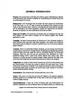
Figure 1.1: General manipulator. In general, a manipulator has n joints and n + 1 links (including the base and the end-effector). It’s configuration is determined by a set of configuration parameters. There are a variety of ways to select these parameters. One approach is to attach a frame to the manipulator’s fixed base and then locate the moving links by vectors with respect to that frame, as illustrated in Figure 1.2. Since the configuration of a rigid body can be described by 3 vectors locating 3 different points of the body, this would result in a 9-parameter representation for each link. This is not an efficient approach, as it would require 9 × n parameters for describing the configuration of the n moving links. The next section introduces a particular set of parameters, called generalized coordinates, that provides a minimal configuration representation.

1.1.1

Generalized Coordinates

Generalized coordinates for a manipulator are a set of independent configuration parameters. The number of DOFs of the manipulator is determined by the number of generalized coordinates needed to describe it. The first task is to determine the number of degrees of freedom of a manipulator with n + 1 links and n joints (or alternatively the number of generalized coordinates needed to describe it). Start by disassembling the manipulator. This generates n + 1 rigid bodies, of which 1 is fixed to the ground and n are completely free to move. The task

1.1. MANIPULATOR STRUCTURE

3

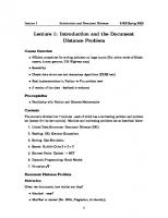
Figure 1.2: Generalized coordinates. now is to describe their configuration in space. The configuration of a rigid body in space can be described by six parameters: three parameters for the position of a point on the body and three parameters for describing the body’s orientation. A full configuration of a system with n free moving bodies can be described with 6 × n parameters.

Rigid bodies can move with respect to each other. However, in the manipulator these motions are constrained because the bodies are connected. The connections through joints introduce constraints on the motion of the rigid bodies. Re-assemble the manipulator by serially connecting the rigid bodies with the joints. Each joint has 1 DOF allowing a single motion – revolute or prismatic. Thus each joint introduces 5 constraints on the motion of the free rigid bodies. The connections introduce 5 × n constraints on the system’s motion. The number of generalized parameters that describe the system’s configuration is the difference between the number of parameters for all free rigid bodies and the number of constraints introduced by the joints, or 6×n−5×n=n . This is also the system’s DOF. Thus a manipulator with n joints, has n DOF and requires n generalized coordinates to describe its configuration. Joints are either prismatic or revolute. A prismatic joint i results in a linear (translational) motion that is measured as a displacement di between the two neighboring links. A revolute joint i results in a rotational motion that would be measured with an angle θi between the corresponding links. A common

4

CHAPTER 1. SPATIAL DESCRIPTION

coordinate qi can be used to denote both types of coordinates associated with linear motion and rotational motion. The type of a joint i is determined by a binary parameter ϵi defined as ! 0 for a revolute joint θi ; (1.1) ϵi = 1 for a prismatic joint di . The i-th joint can be then described by the coordinate qi , defined as q i = ϵi θi + ϵi d i

(1.2)

where ϵi = 1 − ϵi

The coordinates q1 , q2 , . . . , qn provide a minimal set of parameters for describing the manipulator configuration. This is the set of generalized joint coordinates. The representation of the configuration of the end-effector of the manipulator is discussed in the next section.

1.1.2

Joint and Operational Coordinates

Figure 1.3: Three-DOF revolute mechanism. Consider the mechanism shown in Figure 1.3. This is a planar mechanism where the manipulator’s links are moving in the plane of the paper and the

1.1. MANIPULATOR STRUCTURE

5

joints’ axes are perpendicular to that plane. The three links with three revolute joints are described by the parameters θ1 , θ2 and θ3 , defined as the angles between the axes of the consecutive links (including the ground described by axis X). These 3 parameters uniquely describe the system’s configuration. The 3 parameters are the three joint coordinates of the system and the space defined by θ1 , θ2 and θ3 is called the joint space of the manipulator. A point in that space defines a configuration of the mechanism. Inversely, every configuration of the mechanism is represented by a point in the joint space. There is another space that defines the configuration of the end-effector, i.e. its position and orientation. For example the position can be described by the position of the point at the end-effector in the plane (x, y). The orientation of can be described by the angle α between the X axis of the fixed base and the vector connecting the base point O and the end-effector point. The end-effector configuration in the example above is defined by the 3 coordinates (x, y, α). The general case of spatial manipulators, will require three Cartesian coordinates, x, y, and z to represent the position of the end-effector, and three other coordinates, e.g. three angles α, β, and γ, to represent its orientation. The end-effector position and orientation coordinates provide a description of the manipulator task or operation and are called task coordinates, or operational coordinates1 . While the joint coordinates describe the configuration of the entire manipulator, the task or operational coordinates describe the configuration of the end-effector. The next objective is to establish the relationships between these coordinates.

1.1.3

Position and Orientation of Rigid Bodies

Several concepts are needed to develop the relationships between the manipulator and the end-effector coordinates. The first one is position of a point in space. A point in space can be described as a vector locating this point with respect to some origin or reference point, O. Once the point O is fixed, a point P in 1

by extension to the position, these coordinates are sometimes called Cartesian coordinates.

6

CHAPTER 1. SPATIAL DESCRIPTION

⃗ , representing the position of space can be described by the vector p = OP this point with respect to O, as illustrated in Figure 1.4.

Figure 1.4: Position of a point. It is important to distinguish between the vector p and its components. The vector p represents the position of point P with respect to origin O. Its components are determined by the frame with respect to which this vector is evaluated. These components vary from frame to frame. Consider the frame denoted by {A} in Figure 1.5, with unit vectors XˆA , YˆA , and ZˆA . The ˆ. denotes that these are unit vectors. A point P described by p will have in frame {A} the components (pXA , pYA , pZA ). A description in a different frame will have a different set of coordinates. The components of p in frame {A} will be denoted by the column matrix A p. This is ⎞ ⎛ˆ XA · P A P = ⎝ YˆA · P ⎠ ZˆA · P

(1.3)

The position of a rigid body is described by the position of a point fixed in that rigid body. For example, in Figure 1.5 the vector A p describes the position of the point P fixed in the rigid body. The orientation of the rigid body can be described in many different ways. They all involve defining the orientation of a frame {B} fixed in the rigid body with respect to some reference frame {A}. The frame origin of frame {B} is selected to coincide with the point P described above. This frame is fixed with respect to the rigid body and will move as the rigid body moves.

1.1. MANIPULATOR STRUCTURE

7

Figure 1.5: Rigid body configuration. The frame {A} is fixed in the environment. Modeling the orientation requires a description of the position and orientation of frame {B} with respect to frame {A} . This is done in the next section using the four vectors A p, A XB , A YB , A ZB .

1.1.4

Rotation Matrix

The relationship between different descriptions of a vector relies on the notion of rotation matrices . A rotation matrix A B R describes the orientation of frame {B} with respect to frame {A}. In this notation, the leading subscript B and superscript A point to the two frames involved in this transformation. The columns of the rotation matrix are simply the three unit vectors of frame {B} expressed in frame {A}. If rij are the elements of this matrix, the rotation matrix is given by ⎡ ⎤ r11 r12 r13 *A + A ˆ B A YˆB A ZˆB ⎣ ⎦ (1.4) X B R = r21 r22 r23 = r31 r32 r33 ˆ B in {A} are given by the dot product of X ˆB The components of vector X ˆ ˆ ˆ with the vectors XA , YA , and ZA .

8

CHAPTER 1. SPATIAL DESCRIPTION ⎡ˆ ˆ ⎤ XB . XA A ˆ ˆ B .YˆA ⎦ ⎣ XB = X ˆ B .ZˆA X

(1.5)

Similarly A YˆB and A ZˆB are computed and the rotation matrix is written in the following form ⎡ˆ ˆ ˆ A ZˆB .X ˆA⎤ XB .XA YˆB .X A ˆ B .YˆA YˆB .YˆA ZˆB .YˆA ⎦ ⎣X BR = ˆ B .ZˆA YˆB .ZˆA ZˆB .ZˆA X

(1.6)

Note that the dot products above are not expressed in any particular frame – the dot product computation can be performed in any frame with respect to which both vectors are expressed. An important property of this matrix is that the rows of this matrix are the components of the three unit vectors of frame {A} expressed with respect to frame {B}

Figure 1.6: Simple rotation of a frame.

A BR

=

*A

ˆB X

Aˆ YB

⎡B ˆ T ⎤ XA + Aˆ B ˆ T ⎦ = B RT ⎣ = ZB YA A B ˆT Z A

(1.7)

1.2. TRANSFORMATIONS

9

This property is illustrated in the example of Figure 1.6, where frame {B} ˆ axis is obtained from frame {A} by a 90 degrees rotation about the X ⎞ ˆT 1 0 0 ← BX A A ⎝0 0 −1⎠ ← B Yˆ T BR = A 0 1 0 ← B ZˆAT ⎛

(1.8)

As can be seen, the rotation matrix from frame {B} to frame {A} is equal to the transpose of the rotation matrix from frame {A} to frame {B} A BR

T =B AR

Since the inverse of the rotation matrix describing {B} with respect to {A} is the matrix describing {A} with respect to {B}: A −1 BR

A T =B AR = BR

Thus the inverse of a rotation matrix is equal to its transpose A −1 BR

T =A BR

This is a general property of orthonormal matrices (a matrix with orthogonal unit columns and rows). The quantities defined so far allow for the description of frames. A frame describes the position and orientation of a rigid body. It is defined by the ˆ B , A YˆB and A ZˆB and the vector that locates the origin three unit vectors A X of the frame. The notation used for this vector is A pBorg - the origin of frame {B} expressed in frame {A}. Thus a frame is the set of four vectors A ˆ ˆB , A ZˆB , A pBorg (see Figure 1.7). A frame {B} will be represented by XB , A Y, A pBorg . {B} = A BR

1.2

Transformations

The task is to describe the end-effector configuration with respect to the manipulator’s base. That requires to establish the relationships between descriptions in different frames attached to different links along the manipulator’s structure.

10

CHAPTER 1. SPATIAL DESCRIPTION

Figure 1.7: Frame description.

1.2.1

Pure Rotation Transformation

In the example in Figure 1.8, a point P is defined by the vector connecting it to the origin of frame {A}. The components in {A} of this vector will be different from those computed with respect to frame {B}, having the same origin.

Figure 1.8: Mapping between frames. The coordinates of the vector p in {A} are the dot products of vector p with the unit vectors XA , YA , and ZA . The dot product computation can be done in any frame, in particular in frame {B}

1.2. TRANSFORMATIONS

11

⎛B ˆ B ⎞ ⎛B ˆ T ⎞ XA XA . p A B B B ⎝ ⎝ ⎠ ˆ p= YˆAT ⎠ B p YA p = B ˆT B ˆ B ZA ZA p

(1.9)

Using the definition of the rotation matrix, yields A

B p=A BR · p

(1.10)

This establishes the relationship between the description of a vector p expressed with respect to a frame {B} to its description with respect to a frame {A}, having the same origin. Notice the arrangement in this notation of the leading sub- and superscripts. The leading superscript of p matches the subscript of the rotation matrix. This arrangement is very effective when dealing with more complex chain multiplication.

1.2.2

Pure Translation Transformation

Figure 1.9: Translation of frames. So far the relationships for transformations involve pure rotation of frames. Figure 1.9 shows an example where a frame {B} is translated with respect to frame {A} without rotation. This motion can be described by the vector

12

CHAPTER 1. SPATIAL DESCRIPTION

denoting the position of the origin of frame {B} with respect to the origin of frame {A}, pBorg/OA .

Consider an arbitrary point P in the space. This point can be described with respect to frame {A} (vector pOA ) or frame {B} (vector pOB ). This situation is different than before, because now there are two different vectors describing the position of the same point. In the rotation case, the same vector is described in two different frames. A translation operation is a mapping that transforms a vector describing some point with respect to some origin point to a vector describing that same point with respect to another origin point. The difference between the two vectors is exactly the vector describing the position of the origin of the frame {B} with respect to the origin of frame {A}, pBorg/OA , and thus pOA = pOB + pBorg/OA

(1.11)

As before this vector relationship can be expressed in any frame (in particular with respect to frame {A}).

Figure 1.10: General Transformation.

1.2.3

General Transformation

A general transformation involves both a frame rotation and a translation of the rotated frame, as illustrated in Figure 1.10. The general transformation can be implemented by first performing a rotation to make the axes of the two frames parallel, and then translating them. The resulting relationship is

1.2. TRANSFORMATIONS

A

13

B A pOA = A B R pOB + pBorg/OA

(1.12)

The next section rewrites this equation in a matrix form that can be very useful for uniform fast numerical computations.

1.2.4

Homogeneous Transformation

The general transformation in equation 1.12 can be written in a compact form that is more suitable for compound transformations and propagation of description between links. This is called the homogeneous transformation, which is obtained by augmenting the relationship of equation 1.12 by one dimension. A 4 × 4 matrix is formed, where the primary blocks are the 3 × 3 A rotation matrix and the pBorg /OA . The last row of the 4 × 4 * + position vector A matrix is 0 0 0 1 . The vectors p and B p are also augmented by 1 to make them 4-dimensional vectors. The resulting equation is .A

/ . A pOA BR = 0 0 0 1

A

pBorg/OA 1

/ .B

pOB 1

/

(1.13)

The homogeneous transformation matrix matrix will be denoted by A B T and the above relationship can be written as A

B pOA = A B T(4×4) pOB

(1.14)

The homogeneous transform combines both the rotation of {B} to {A} and the translation of the origin of {B} with respect to {A}. This transform represents one of the basic tools for the kinematics of mechanisms. Example The example depicted in Figure 1.11 illustrates this* concept. + The origin of frame {B} in the figure is translated to a position 0 3 1 with respect to frame {A}. The goal is to find the homogeneous transformation * + between the two frames in the figure. If a point P is defined as 0 1 1 in frame {B}, what is the vector describing this point with respect to frame {A}.

14

CHAPTER 1. SPATIAL DESCRIPTION

Figure 1.11: Example of homogeneous transform. The matrix A B T is formed as defined earlier using the rotation matrix and the given translation vector. The result is ⎡

1 ⎢ A ⎢0 BT = ⎣ 0 0

⎤ 0 0 0 0 −1 3⎥ ⎥ 1 0 1⎦ 0 0 1

(1.15)

Since p in frame {B} is ⎡ ⎤ 0 ⎢ 1⎥ B ⎥ p=⎢ ⎣ 1⎦ 1 the vector p in frame {A} can be computed using the relationship A B B T p, ⎡ ⎤ 0 ⎢ 2⎥ A ⎥ p=⎢ ⎣ 2⎦ 1

(1.16)

A

p =

(1.17)

1.2. TRANSFORMATIONS

1.2.5

15

Transforms as Operators

The transforms presented above allow us to change the descriptions of points in space from one frame to another. However, these transforms can be also viewed as operators acting on points that change their locations in the space. In that case, rotations and translations will be described as operators moving one point into another point, with respect to the same frame.

Figure 1.12: Rotation: changing description. Consider first the rotation matrix. As illustrated in Figure 1.12, the rotation matrix facilitates change of the description of a point P from one frame {B} to another frame {A}. This is A

B p=A BR p

(1.18)

In Figure 1.13, the rotation matrix is acting on a vector locating a point P1 and transforming it into a different vector locating a different point P2 through a rotation the X axis. The rotation matrix in this case is treated as a rotation operator about the x axis. In the general case, this operator can act about an arbitrary vector k with an angle θ. Applying the rotation operator to vector p1 produces another vector p2 . The corresponding relationship is: p2 = Rk (θ) p1 A rotation about the X axis, for example, is given by

(1.19)

16

CHAPTER 1. SPATIAL DESCRIPTION

Figure 1.13: Rotational operator. ⎤ 1 0 0 Rx (θ) = ⎣0 cos θ − sin θ⎦ 0 sin θ cos θ

(1.20)

⎡ ⎤ ⎤⎡ ⎤ 0 0 1 0 0 p2 = RX (θ)p1 = ⎣0 0.8 −0.6⎦ ⎣2⎦ = p2 = ⎣1⎦ 2 1 0 0.6 0.8

(1.21)

⎡

* + If p1 was given as 0 2 1 and the rotation was of an angle 37o the resulting vector would be : ⎡

Consider next the translation as an operator. In the previous interpretation of translation, a point P2 (see Figure 1.14) is described as a vector pOA with respect to the origin of frame {A}, or pOB with respect to the origin of frame {B}. Here the same point is described with two different vectors and the relationship is: pOA = pOB + pBorg

(1.22)

When viewed as an operator, a translation Q (Q : P1 → P2 ) moves a point P1 (described by vector p1 ) into a point P2 (described by vector p2 ) p2 = p1 + Q

1.2. TRANSFORMATIONS

17

Figure 1.14: Translation operator. In this case two different points are described with two different vectors. These vector equations can be expressed in any frame. In a matrix form, the homogeneous transform is p2 = TQ p1 where

⎡

1 ⎢0 TQ = ⎢ ⎣0 0

0 1 0 0

⎤ 0 qx 0 qy ⎥ ⎥ 1 qz ⎦ 0 1

(1.23)

(qx , qy , qz ) are the components of the vector Q. Note that these are the only variables in the representation of the translational operator. In the general case, the rotational operator and translational operator are combined in a general transformation operator, T, defined below similarly to the homogeneous transform:

p2 =

2

3 RK (θ) Q p1 0 0 0 1

The operator T acts on p1 to produce p2 ,

(1.24)

18

CHAPTER 1. SPATIAL DESCRIPTION

p2 = T p1 This representation constitutes the third interpretation of the homogeneous transformation. The first one is a description of a frame. The second is a transform mapping that changes the description of a point in space. The third is a transform operator that moves points in space. The next section defines the inverse of a transformation.

1.2.6

Inverse Transforms

To compute the inverse of a generalized transform, consider inverses of the rotation and translation transforms. A seen earlier, the inverse of a rotation is simply given by the transpose of that rotation, R−1 = RT .

Figure 1.15: Inverse transform. For a pure translation, the inverse is given by the same vector with an opposite sign. As illustrated in Figure 1.15, pBorg/OA = −pAorg/OB .

The presence of both translation and rotation in the homogeneous transform slightly complicates the inverse problem. In particular the inverse of the transform is not equal to its transpose because this 4 × 4 matrix is not orthonormal (T −1 ̸= T T ).

The inverse of a homogeneous transformation matrix . A / A R p Borg/O A B A BT = 0 0 0 1

(1.25)

1.2. TRANSFORMATIONS

19

is the matrix

A −1 BT

=

B AT

.

/ . B T A −A B R . pBorg/OA AR = = 0 0 0 0 0 0 1 A T BR

B

/ pAorg/OB 1 (1.26)

The rotation part in the above equation comes directly from the inverse of the rotation matrix, while the translation part represents the vector defining the origin of frame {A} expressed with respect to the origin of frame {B}. The minus sign comes from the inverse of the translation, while the preT multiplication by A is needed to express the vector in the same frame BR {B}.

The next step is to propagate the transform descriptions along the kinematic chain.

1.2.7

Transform Multiplication

The transformation from one frame to another as well as its inverse was described previously. Those transformations can be combined to propagate from some far away frame (attached to the end-effector of the manipulator) to the base frame (attached to the fixed ground). Assume that there are three frames {A}, {B} and {C} and the transformations from {B} to {A} and from {C} to {B} are known. What is the new compound transformation from frame {C} to frame {A} (see Figure 1.16)? The result is very simple - it is just the multiplication of the two transformation. Express first: B

C p=B CT p

(1.27)

B A B C A C p=A BT p = BT C T p = CT p

(1.28)

and A

Thus A CT

B =A BT C T

(1.29)

20

CHAPTER 1. SPATIAL DESCRIPTION

Figure 1.16: Compound transformation.s The 4 × 4 matrix representing the transformation from {C} to {A} is A CT , which is the product of the 4 × 4 matrices representing the two given transB formation A B T and C T . Since matrix multiplication is not commutative, one has to pay special attention to the order in which the matrices are multiplied. The matrix A C T can be written explicitly as: A CT

1.2.8

=

.A

B B RC R

A B B R pCorg

0 0 0

1

+ A pBorg

/

(1.30)

The Transform Equation

As described earlier, a manipulator consists of many links starting from the fixed base and continuing through to the end-effector. There are frames associated with all those links and the parameters describing the frames can be propagated in order to build a transformation representing the end-effector frame {E} with respect to the fixed base frame {B}. The manipulators usually work in a real world environment with movable objects (e.g. a machine part that needs to be picked up) placed on top of fixed objects (e.g. a work table). There is a frame describing the work table, as well as a frame associated with the movable machine part. Typically the transformation between the manipulator base frame and the work table frame is known. This is also true for the transformation between the frames of the work table and

1.3. CONFIGURATION REPRESENTATIONS

21

the machine part. The goal is to calculate the transformation between the frame associated with the machine part that needs to be picked up by the manipulator and the end-effector’s frame.

Figure 1.17: Transform equation. This is done using a simple relationship called the transform equation. The idea is to start along the chain of bodies involved and move in the same direction, until getting back to the starting point. multipling all the transformations involved will obtain the identity transformation. In the notations of Figure 1.17: A U B C D U T BT C T DT A T

≡I

(1.31)

This equation allows extracting what is unknown. If for example UA T is C D needed, the matrix equation can be solved as UA T = UB T B C T D T A T . In terms D −1D of the transforms given in the figure UA T = UB T B AT. CT C T In the developments above, the type of parameters to describe position and orientation are not explicitly specified. Next section consideres some of those representations.

1.3

Configuration Representations

The end-effector position and orientation is completely defined by the (4 × 4) homogeneous transformation B E T . However, this representation involves a

22

CHAPTER 1. SPATIAL DESCRIPTION

large number of redundant parameters and a more compact representation of the end-effector configuration is needed. The position and the orientation of the end-effector (depicted in Figure 1.18), with respect to the base can be represented as

Figure 1.18: End-effector configuration. .

/ XP position X= XR orientation

(1.32)

There is a variety of sets of 3 parameters for position representations that can be used based on the task that the manipulator is performing. Examples include Cartesian coordinates of the end-effector (x, y, z), Cylindrical coordinates (ρ, θ, z) or Spherical coordinators (ρ, θ, φ) as depicted in Figure 1.19. Going from one representation to another is quite easy - there are well known explicit formulas for that purpose. The real problem comes with orientation representation. There is no universal agreement in the field of robotics as to what is the best orientation representation and each representation has advantages and shortcomings.

1.3.1

Direction Cosines

One orientation representation was introduced earlier - the rotation matrix. Using frames attached to the end-effector and the base, the orientation of the

1.3. CONFIGURATION REPRESENTATIONS

23

Figure 1.19: Describing the position of a point. end-effector can be described by the compound rotation matrix developed in the previous sections. The direction cosines representation is simply the set of nine parameters involved in the rotation matrix. This matrix can be written as: ⎡

⎤ r11 r12 r13 * + R = ⎣r21 r22 r23 ⎦ = r1 r2 r3 r31 r32 r33

(1.33)

⎡ ⎤ r1 x r = ⎣ r2 ⎦ r3 (9×1)

(1.34)

The columns of the rotation matrix can be concatenated and arranged in a 9 × 1 vector:

This is the direction cosines representation of the orientation. There are 6 constraints among these 9 parameters - 3 because the columns of the matrix are unit vectors and 3 because these vectors are perpendicular. |r1 | = |r2 | = |r3 | = 1

(1.35)

r1 .r2 = r1 .r3 = r2 .r3 = 0

(1.36)

and

24

CHAPTER 1. SPATIAL DESCRIPTION

Thus of these 9 parameters only 3 are independent. Clearly for most cases it is better to find a more compact representation.

1.3.2

Euler and Fixed Angle Representation

A very common selection of orientation parameters is the three-angle representations. There are many different choices for these angles.

Figure 1.20: Three angles representation. Consider the two frames {A} and {B} illustrated in Figure 1.20. Start from the configuration where {B} is coincident with frame {A}. To reach the final configuration of {B}, proceed in the following manner. First rotate about XA to achieve frame {B ′ }. Next there are two choices: (i) rotate with respect to one of the axes of {A} that are fixed, or (ii) rotate with respect to one of the axes of {B ′ }, obtained from the first rotation. Proceeding with respect to the axes of {A} obtains the so-called fixed angles representation. Proceeding with respect to the axes of {B ′ } and continuing with the new frames that are generate, will obtain the Euler angle representation. In fact these two

1.3. CONFIGURATION REPRESENTATIONS

25

representations are dual and for every fixed angle representation there is a corresponding Euler angle representation. A total of three rotations are needed with three angles α, β and γ. There are 12 possibilities for both the fixed and the Euler angle representations. The notation XY Z means the first rotation about axis X is followed by a rotation about Y and finally a rotation about axis Z. Naturally no alternatives need to be considered where there are two consecutive rotations about the same axis since they are equivalent to one rotation with the sum of the two angles. Consider for example the Z − Y − X-Euler angle representation, illustrated in Figure 1.21. Starting with frame {A} rotate about axis ZA of an angle α to obtain frame {B ′ }. The corresponding rotation matrix is A B ′ R = Rz (α). ′ Next rotate about the newly generated Y-axis of frame {B } of an angle ′ β and obtain the frame {B ′′ }. The rotation matrix here is B B ′′ R = Ry (β). Finally rotate about the axis X of {B ′′ } of an angle γ to obtain frame {B} ′′ A with a rotation matrix B B R = Rx (γ). The resulting matrix B R is simply the product A BR

=A B′ R

B′ B ′′ B ′′ R B R

or A BR

= RZ (α) RY (β) RX (γ)

Consider now the X − Y − Z-fixed angles representation. Fixed angle rotations can be best understood from the point of view of small instantaneous rotations. They also have an analog in aerospace engineering. Think in terms of airplane control with the Z-axis pointing vertically up and the Xaxis pointing in the direction of the flight. Then rotation about the Z-axes is yaw , rotation about the X-axes is roll and rotation about the Y-axes is pitch, as illustrated in Figure 1.22. The sequence now is: γ rotation about X of {A}, then a β rotation about Y of {A} and a α rotation about Z of {A}. The rotation about X of an angle γ is a rotation operator which acts on a vector v transforming it into Rx (γ)v. The result of the first operator is subject to the second rotation resulting in Ry (β)(Rx (γ)v), and finally from the third rotation leads to Rz (α)(Ry (β)(Rx (γ)v)). In summary RX (γ) : v → RX (γ)v

(1.37)

26

CHAPTER 1. SPATIAL DESCRIPTION

Figure 1.21: Euler angles (Z-Y-X).

RY (β) : (RX (γ)v) → RY (β)(RX (γ).v)

(1.38)

RZ (α) : (RY (β)RX (γ)v) → RZ (α)(RY (β)RX (γ)v)

(1.39)

Comparing this result with the Euler angle rotation obtained above, it is clear that the X − Y − Z-fixed angles rotation of angles (γ, β, α) is equivalent to the Z − Y − X-Euler angles rotations of angles (α, β, γ). This illustrates the duality principle mentioned above.

A BR

=A B RXY Z (γ, β, α) = RZ (α)RY (β)RX (γ)

(1.40)

1.3. CONFIGURATION REPRESENTATIONS

27

Figure 1.22: Fixed angles (X-Y-Z).

1.3.3

Inverse of an Orientation Representation

The end-effector position and orientation is determined by the compound homogeneous transformation B E T which will be computed as a function of joint angles through the so-called forward kinematics, as discussed in Chapter 2. The rotation part of this transformation B E R contains the information about the orientation of the end-effector. Given the elements rij of the matrix B E R, the problem is to extract from this matrix the parameters selected to represent the orientation. For the Euler angle representation the task is to find the three angles α, β and γ corresponding to the elements rij found from the forward kinematics (the propagation of the link parameters along the kinematic chain). For the ZY X Euler angle representation with angles α, β and γ, the matrix A B R is

⎤ ⎤ ⎡ cα.cβ cα.sβ.sγ − sα.cγ cα.sβ.cγ + sα.sγ r11 r12 r13 A ⎦ ⎦ ⎣ ⎣ B R = r21 r22 r23 = sα.cβ sα.sβ.sγ + cα.cγ sα.sβ.cγ − cα.sγ −sβ cβ.sγ cβ.cγ r31 r32 r33 (1.41) The abbreviation cα and sα above denote cos(α) and sin(α) and will be used extensively throughout the text. ⎡

There are 9 trigonometric equations with 3 independent parameters α, β and γ. In this case, β can be found from r11 , r21 and r31 ,

28

CHAPTER 1. SPATIAL DESCRIPTION 4 5 6 2 2 cos β = cβ = r11 + r21 2 2 → β = A tan 2(−r31 , r11 + r21 ) sin β = sβ = −r31

(1.42)

2 2 This assumes that r11 + r21 is not zero. Knowing β, one can find α from r21 and r11 , and γ from r32 and r33 , namely:

α = Atan2(

r21 r11 , ) cβ cβ

(1.43)

γ = Atan2(

r32 r33 , ) cβ cβ

(1.44)

7 8 The 2-argument Atan2(y, x) function computes tan−1 xy , and uses the signs of both x and y to determine the quadrant in which the resulting angle lies.

2 2 If r11 + r21 = 0, that means that cβ = 0, sβ = ±1 and the system is at a a singularity of the representation. Here it is for β = ±90o . In this case, the angles α and γ cannot be determined. The only expressions that can be determined are α + γ or α − γ. Namely, if cβ = 0, sβ = +1 then ⎞ ⎛ 0 −s(α − γ) c(α − γ) A ⎝0 c(α − γ) s(α − γ)⎠ (1.45) BR = −1 0 0

And if cβ = 0, sβ = −1 then ⎞ ⎛ 0 −s(α + γ) −c(α + γ) A ⎝0 c(α + γ) −s(α + γ)⎠ BR = 1 0 0

(1.46)

As an example, for the configuration shown in Figure 1.23, from RZY X (α, β, γ) it follows that α = 0, β = 0, γ = 90o

(1.47)

Formulas for finding the corresponding rotation angles can be similarly obtained for all Euler or fixed angle representations.

1.3. CONFIGURATION REPRESENTATIONS

29

Figure 1.23: Example of a Z-Y-X Euler rotation.

1.3.4

Equivalent Angle - Axis Representation

Thus far all rotations are about the primary axes of the frames attached to the objects. It can be shown that any rotation from one frame to another can be represented by a rotation about some axis with some angle θ. Given two frames {A} and {B} with a common origin (i.e. one frame can be rotated into the other), there is an axis K and an angle θ such that {B} can be obtained from {A} via a rotation about K of angle θ. This representation is called the equivalent angle - axis representation, which is illustrated in Figure 1.24.

Figure 1.24: Equivalent angle-axis representation. If kx , ky , and kz are the components of the unit vector k, the rotation matrix

30

CHAPTER 1. SPATIAL DESCRIPTION

about k with an angle θ can be represented by the vector k scaled by the angle θ as ⎡

⎤ θkX Xr = θk = ⎣ θkY ⎦ θkZ

(1.48)

To solve inversely for k and θ

⎤ kx kx vθ + cθ kx ky vθ − kz sθ kx kz vθ + ky sθ RK (θ) = ⎣kx ky vθ + kz sθ ky ky vθ + cθ ky kz vθ − kx sθ⎦ kx kz vθ − ky sθ ky kz vθ + kx sθ kz kz vθ + cθ ⎡

Here

(1.49)

vθ = 1 − cθ

(1.50)

⎤ r11 r12 r13 RK (θ) = ⎣r21 r22 r23 ⎦ r31 r32 r33

(1.51)

Given a rotation matrix ⎡

the corresponding angle is

θ = Arc cos(

r11 + r22 + r33 − 1 ) 2

(1.52)

and ⎡

⎤ r32 − r23 1 ⎣ A r13 − r31 ⎦ , singularity f or sin θ = 0 k= 2 sin θ r21 − r12

(1.53)

Note that this is a 3 parameter representation (two independent parameters for the unit vector k and one angle θ). Note also that for configurations where sin(θ) = 0, there will be a singularity of the representation. The next representation avoids such singularities.

1.3. CONFIGURATION REPRESENTATIONS

1.3.5

31

Euler Parameters

In some instances it is useful to derive a redundant representation, i.e. one that uses more than three parameters, but as few as possible (ideally four parameters). For examples three parameters in some cases are not enough to access some of the configurations of the manipulator in singularities. Alternatively, nine parameters (direction cosines) are far too many. Four parameters provide a minimal singularity-free representation.

Figure 1.25: Euler parameters representation. Euler parameters use a unit vector w with components (wx , wy , wz ) and a rotation about it of an angle θ (see Figure 1.25). The Euler parameters are ε1 = wx sin

θ 2

(1.54)

ε2 = wy sin

θ 2

(1.55)

ε3 = wz sin

θ 2

(1.56)

ε4 = cos

θ 2

The sum of the squares of these parameters is one,

(1.57)

32

CHAPTER 1. SPATIAL DESCRIPTION

|W | = 1,

ε21 + ε22 + ε23 + ε24 = 1

(1.58)

This normality condition shows that only three of the parameters are independent. The parameters (ε1 , ε2 , ε3 , ε4 ) define the unit hyper-sphere in four - dimensional space because of the Normality Condition. The rotation matrix associated with Euler parameters is ⎤ ⎡ ⎤ 1 − 2ε22 − 2ε23 2(ε1 ε2 − ε3 ε4 ) 2(ε1 ε3 + ε2 ε4 ) r11 r12 r13 ⎣r21 r22 r23 ⎦ = ⎣2(ε1 ε2 + ε3 ε4 ) 1 − 2ε21 − 2ε23 2(ε2 ε3 − ε1 ε4 )⎦ (1.59) r31 r32 r33 2(ε1 ε3 − ε2 ε4 ) 2(ε2 ε3 + ε1 ε4 ) 1 − 2ε21 − 2ε22 ⎡

The inverse problem for ε4 is easy to solve since the sum of the diagonal elements is 4 ∗ (ε4 )2 − 1 (using the Normality Condition), i.e. r11 + r22 + r33 = 3 − 4(ε21 + ε22 + ε23 ) = 4ε24 − 1

(1.60)

or ε4 =

1√ 1 + r11 + r22 + r33 2

(1.61)

The rest of the parameters are easily determined using ε4 in the denominator, i.e. ε1 =

r32 − r23 r13 − r31 r21 − r12 , ε2 = , ε3 = 4ε4 4ε4 4ε4

(1.62)

The only possible singularity occurs when ε4 = 0. The rest of the parameters can be computed similarly to ε4 above. For example ε1 can be found taking r11 − r22 − r33 , etc. Because of the normality condition, it is not possible for all four of the Euler parameters to be zero at the same time. Thus one of the εi ’s will be non-zero and an unique solution to the inverse problem can always be found. In fact the following is true: Lemma: For all rotations, at least one of the Euler parameters is greater than or equal to 1/2.

1.3. CONFIGURATION REPRESENTATIONS

33

A good approach is to find the maximal ε and use that to solve for the rest of the parameters. In particular, if ε1 = max {εi } i

(1.63)

then: ε1 =

1√ r11 − r22 − r33 + 1 2

(1.64)

ε2 =

(r21 + r12 ) 4ε1

(1.65)

ε3 =

(r31 + r13 ) 4ε1

(1.66)

ε4 =

(r32 − r23 ) 4ε1

(1.67)

Similarly, if ε2 = max {εi } i

(1.68)

then ε2 =

1√ −r11 + r22 − r33 + 1 2

(1.69)

If ε3 = max {εi } i

(1.70)

then ε3 =

1√ −r11 − r22 + r33 + 1 2

(1.71)

34

CHAPTER 1. SPATIAL DESCRIPTION

An alternative way to find the Euler parameters is by using the ZY X Euler angles from the formulas below: γ β α γ β α ε1 = sin( ) cos( ) cos( ) − cos( ) sin( ) sin( ) 2 2 2 2 2 2

(1.72)

γ β α γ β α ε2 = cos( ) sin( ) cos( ) + sin( ) cos( ) sin( ) 2 2 2 2 2 2

(1.73)

γ β α γ β α ε3 = cos( ) cos( ) sin( ) − sin( ) sin( ) cos( ) 2 2 2 2 2 2

(1.74)

γ β α γ β α ε4 = cos( ) cos( ) cos( ) + sin( ) sin( ) sin( ) 2 2 2 2 2 2

(1.75)

The next chapter defines a set of link-related parameters which will facilitate the derivation of the forward kinematic formulas for a general manipulator.

1.4

Exercises

Exercise 1.1. A vector A P is rotated about YˆA by ψ degrees and is subˆ A by φ degrees. Give the rotation matrix which sequently rotated about X accomplishes these rotations in the given order. What is the result if ψ = 30◦ and φ = 45◦ ? Exercise 1.2. A frame {B} is located as follows: initially coincident with a ˆ B by φ and then we rotate the resulting frame {A} we rotate {B} about X frame about YˆB by ψ degrees. Give the rotation matrix, A B R which will change B A the description of vectors from P to P . What is the result if ψ = 30◦ and φ = 45◦ ? Exercise 1.3. For sufficiently small rotations so that the approximations sinθ ≈ θ, cosθ ≈ 1, and θ2 ≈ 0 hold, derive the rotation matrix equivalent ˆ Start with Eqn (1.49) in the text to a rotation of θ about a general axis, K. for your derivation. Show that two infinitesimal rotations commute.

1.4. EXERCISES

35

Exercise 1.4. A frame {A} a frame {B}, we rotate {A} resulting frame such that the * position vector, 11.0 −3.0

is located as follows: initially coincident with about Z9B by −30◦ and then we translate the origin of the final frame can be expressed by a +T 9.0 with respect to {B}.

A (a) Compute the rotation matrices, B A R and B R.

(b) Compute A V , given a velocity vector B V = (c) Are A V and B V different vectors? Explain.

*

10.0 20.0 30.0

+T

.

A (d) Compute the homogeneous transformation matrices, B A T and B T .

(e) Compute A P , given a position vector B P = (f) Are A P and B P different vectors? Explain. (g) Is A V different from physical meanings).

A

*

10.0 20.0 30.0

+T

.

P ? Justify your answer(types of vectors and

Exercise 1.5. (a) Prove the Lemma stated in section 1.3.5 in Chapter 1 of the text. (b) Determine the Euler parameters ε1 , ε2 , ε3 , ε4 for the following rotation matrix: ⎡

⎢ R=⎣

− 21 1 2 √1 2

1 2 − 12 √1 2

√1 2 √1 2

0

⎤

⎥ ⎦.

ˆ and θ of this Exercise 1.6. (a) What are the equivalent axis and angle, K rotation matrix: ⎡

⎢ R=⎣

0 √1 2 − √12

√1 2 1 2 1 2

√1 2 − 12 − 12

⎤

⎥ ⎦.

(b) What are the Euler parameters ε1 , ε2 , ε3 , ε4 of R?

36

CHAPTER 1. SPATIAL DESCRIPTION

Exercise 1.7. (a) In robotics, free vectors are used to represent velocities of points, angular velocities of bodies, accelerations of points, forces, moments, etc. They are very important! Given a free vector B F = * +T 1 3 7 and given the transformation matrix ⎡

⎤ cos(π/3) − sin(π/3) 0 5 ⎢ sin(π/3) cos(π/3) 0 −2 ⎥ A ⎥ ⎢ BT = ⎣ 0 0 1 4 ⎦ 0 0 0 1

compute the free vector A F.

(b) On the other hand, we will also be dealing with vectors which are not free vectors — namely, position vectors for points. Given a position * +T vector A P = 1 3 7 in frame {A}, compute the coordinates of the position vector in frame {B} using the transformation matrix above. Exercise 1.8.

A (a) Given a transformation matrix B A T , find B T ⎡ ⎤ 1 0 0 1 ⎢ 0 cos(θ) − sin(θ) 2 ⎥ B ⎥ ⎢ T = A ⎣ 0 sin(θ) cos(θ) 3 ⎦ 0 0 0 1

(b) Given θ = 45◦ and B P =

*

4 5 6

+T

, compute A P .

Exercise 1.9. Given the following 3 × 3 matrix: ⎡ 1 ⎤ √ √1 0 2 ⎢ 2 1 ⎥ R = ⎣ − 21 √12 2 ⎦ 1 1 √ − 2 − 2 21 (a) Show that it is a rotation matrix. (b) Determine a unit vector that defines the axis of rotation and the angle (in degrees) of rotation. (c) What are the Euler parameters ε1 , ε2 , ε3 , ε4 of R?

1.4. EXERCISES

37

Exercise 1.10. Derive the formulas to calculate the X–Z–Y Euler angles from the given rotation matrix, R. In other words, express α, β, and γ in terms of rij ’s. Be specific about boundary cases. Use θ = Atan2(sθ, cθ). ⎡ ⎤ r11 r12 r13 R = ⎣ r21 r22 r23 ⎦ r31 r32 r33

Exercise 1.11. Derive the formulas to calculate the X-Z-X fixed angles from a given rotation matrix R. In other words, find formulas for α, β and γ in terms of the rij ’s such that R = RXZX (γ, β, α). ⎡

⎤ r11 r12 r13 R = ⎣ r21 r22 r23 ⎦ r31 r32 r33

Be specific about boundary cases, and be sure to use atan2(y, x) instead of atan(y/x). (Note: This is more than a difference in notation! )

38

CHAPTER 1. SPATIAL DESCRIPTION

Chapter 2 Direct Kinematics 2.1

Introduction

The spatial descriptions introduced in the previous chapter are independent of the structure of the manipulator. They calculate the position and orientation of the frame associated with the end-effector of a manipulator with respect to the frame associated with its fixed base. This chapter introduces a set of parameters specific to each manipulator. These parameters can be used to describe the rotational and translational motion of the joints which connect the links of the manipulator. The relationships between these parameters for neighboring links are established below. Propagating descriptions along the links of the manipulator derives its forward and inverse kinematic models.

2.2

Link Description

A manipulator consists of a chain of links from the base, which is typically fixed in the workspace, to the end-effector (the gripper that interacts with the environment). Consecutive links are connected by joints which exert the degree of freedom of the motion of the link. As pointed out in the previous chapter, only simple rotational and translational motion of the links will be considered. Each joint will have one degree of freedom (DOF) — rotational or translational. 39

40

CHAPTER 2. DIRECT KINEMATICS

Consider the i-th link in the kinematic chain. This link connects two joints. At the end of link i, there is an axis with respect to which the next link, i + 1 , is going to move. There is also an axis in the beginning of link i. Those two axes are lines in a three dimensional space. They are characterized by a common normal. This common normal has a length that is called link length. This is one of the parameters describing the link.

Figure 2.1: Link description. In Figure 2.1, ai−1 (the link length) denotes the length along the common normal from axis i − 1 to axis i. To define the relative position between two axes in space, in addition to the common normal, the angle between the axes needs to be computer. Draw a parallel line to axis i at the point where the common normal intersects the axis i − 1. The angle between this parallel line and axis i − 1, denoted by αi−1 , will be called link twist. This angle is measured in the right-hand sense about the vector defined by ai−1 directed from axis i − 1 to axis i along the common normal. Figure 2.1 illustrates this notation. Often in industrial robots there are consecutive axes that intersect at a point. For example, in the manipulator known as the Stanford Scheinman Arm, which is analyzed later, axes 2 and 3 intersect at a right angle. In this case,

2.2. LINK DESCRIPTION

41

the twist angle αi−1 is +90o or −90o . As shown in Figure 2.2, when there are intersecting axes, the definition of link twist will be free in terms of the direction of positive or negative. Alternatively, two consecutive axes can be parallel. This is the case in the example of the three-link planar manipulator that was used in the previous chapter. All three axes in that example are parallel and perpendicular to the plane of the manipulator. In that case, the link twist is 0o .

Figure 2.2: Intersecting joint axes. The link length and the link twist describe the configuration of a particular link in the kinematic chain. There are two other parameters that describe the connections between any two consecutive links. Link i − 1 is determined by its corresponding joints i − 1 and i. Consider the next link i in the chain. That link will have a link length, ai , and angle, αi . The distance along the line on axis i between the common normal for link i − 1 and the common normal for link i (between axes i and i + 1) is a parameter called link offset. It is denoted by di in this terminology. The angle between the two common normals mentioned above, measured about axis i, is the fourth parameter in the representation. It is called joint angle and it is denoted by θi . All parameters are depicted in Figure 2.3. The link length and the link twist are always constant since only rigid links are considered. However, the link offset and the joint angle can be either constant or variable. In particular, for a revolute joint i, the joint angle θi is

42

CHAPTER 2. DIRECT KINEMATICS

Figure 2.3: Relationship between links. variable, and the link offset di is constant. Alternatively, for a prismatic joint i, the link offset, di , is a variable, and the joint angle, θi , is constant. For the three-link planar manipulator from the previous chapter, all joint angles are variable. For the Stanford Scheinman Arm, one of the link offsets is a variable (along the prismatic joint). The next section describes a convention for assigning the values of the four link parameters for unique representation of the links. Those parameters determine the complete relationship between link i and i − 1. They will define the homogeneous transformation between those two links.

2.3

Conventions for First and Last Link

The first and the last links in the chain need special convention consideration. Clearly from the definition above, ai and αi depend on axes i and i + 1. They can be propagated along the chain as depicted in Figure 2.4. Thus having the axes in space will define a1 , a2 , . . . , an−1 , and α1 , α2 , . . . , αn−1 . There is a freedom in choosing a0 , α0 and an , αn . The convention is to try to assign

2.3. CONVENTIONS FOR FIRST AND LAST LINK

43

Figure 2.4: Frames propagation between links. zeroes to as many variables in the chain as possible. In particular, try to select a0 = α0 = an = αn = 0. This will determine how the frame attached to the base is selected. In other words, the frame {0} and frame {N } will be selected so that the parameters above are zeroes.

Figure 2.5: Revolute First Link. Similar considerations can be used for the two other parameters θi and di . By definition, these parameters depend on links i − 1 and i. Just as above θ2 , . . . , θN −1 and d2 , . . . , dN −1 are clearly defined. For link 1, there are two options: In Figure 2.5, if axis 1 is a revolute one,

44

CHAPTER 2. DIRECT KINEMATICS

select d1 = 0. In that case, θ1 is variable depending on the motion of axis 1.

Figure 2.6: Prismatic First Link. If axis 1 is prismatic (as in Figure 2.6), select θ1 = 0 since d1 is variable. Similarly if axis N is revolute, select dN = 0 and if it is prismatic, then θN = 0.

2.4

Attaching Frames to Links

These four parameters (αi , ai , θi , di ) describe the relationship between two links. They are called the Denavit-Hartenberg parameters. For each joint, three of these parameters will be fixed, and one will be variable. That variable is either θi if the joint is revolute or di if it is prismatic. The first two parameters provide the description of the link itself, and the next two describe the connection with the next link. A transformation between two successive links can be expressed in terms of these four parameters. The next step in the process is to attach frames to the links. By convention, select the origin for frame {i − 1} as the point at the intersection of the common normal between links i − 1 and i with the axis i − 1. Axis i − 1 itself will be used for the Zi−1 axis, and the Xi−1 points along the common normal from axis i − 1 to axis i. The Y-axis is selected to make a direct frame (Cartesian frame with the right hand rule).

2.4. ATTACHING FRAMES TO LINKS

45

Figure 2.7: Affixing frames to links. The frame consisting of Xi , Yi and Zi is defined in a similar fashion. From that definition, it can be seen that if joint i is revolute, the joint variable is the angle between Xi−1 and Xi . If it is prismatic, the distance di between Xi−1 and Xi along Zi is the variable. The assigned frames are depicted in Figure 2.7. When there are intersecting axes, there is a choice in assigning the directions. For example, Figure 2.8 illustrates the case when axes i and i + 1 are intersecting. In this case, take the perpendicular to both in the point of intersection and assign Xi along it in such direction that the angle is measured from axis i to i + 1 in a positive sense. The origin of the frame is at the intersection of the two axes. The first and the last link in the kinematic chain require special attention. Consider the first link of the mechanism with frame {0} attached to the fixed base. There are 2 possible cases: if the first joint is revolute (depicted in Figure 2.9), then frame {1} attached to link 1 rotates with respect to the fixed base. There is a choice in selecting the reference frame {0}. Select it in such way so that a0 = α0 = d1 = 0. Thus when θ1 = 0 → {0} ≡ {1} (the zero and the first frame coincide). This assignment will simplify the computations.

46

CHAPTER 2. DIRECT KINEMATICS

Figure 2.8: Frames on intersecting axes.

Figure 2.9: Frames on revolute first link. In some cases, however, frame {0} might be selected differently to facilitate measurements with respect to alternative fixed frames. If the first joint is prismatic (as pictured in Figure 2.10), choose frame {0} to be parallel to frame {1} with a displacement d1 between the origins. Thus a0 = 0, α0 = 0, θ1 = 0 . When d1 = 0, the two frames are coincident again, i.e. d1 = 0 → {0} ≡ {1}

(2.1)

The last link is handled similarly. If the last joint is revolute, set frame {n} so that dN = 0. Thus for θn = 0 → xn ||xn−1 (the axes are collinear) as in Figure 2.11.

2.4. ATTACHING FRAMES TO LINKS

47

Figure 2.10: Frames on prismatic first link.

Figure 2.11: Frames on last revolute link. If the joint is prismatic, as in Figure 2.12, select frame {n} so that θN = 0. Then if dN = 0, the two X- axes are again collinear. To summarize, Figure 2.13 introduces four parameters: Link Length ai is the distance between (Zi , Zi+1 ) along Xi . Link Twist αi is the angle between (Zi , Zi+1 ) about Xi . Link Offset di is the distance between (Xi−1 , Xi ) along Zi . Joint Angle θi is the angle between (Xi−1 , Xi ) about Zi . At any time, one of these four parameters will be variable, and the rest will be constant. These parameters are called the D&H (Denavit and Hartenberg) parameters. There is a simple procedure that can be followed to define the frame attachment along the kinematic chain. Start by defining the axes along the joints. Next, define the common normals. The origins of the frames go at the inter-

48

CHAPTER 2. DIRECT KINEMATICS

Figure 2.12: Frames on last prismatic link. sections of those normals with the joint axes as in Figure 2.14. The Z-axes of the frames point along the joint axes at each of the origins. The X-axes point along the common normals at each of the origins. The Y-axes are defined by the right-hand rule, perpendicular to the X and Z-axes at each of the origins.

2.4.1

Example: RRR Manipulator

Consider a simple example depicted in Figure 2.15 - a RRR (revolute-revoluterevolute) manipulator. This is a planar example with three joint variables θ1 , θ2 , θ3 , that describe the rotation about each of the axes. All Z-axes are perpendicular to the plane of the manipulator. The X-axes are along the common normals as denoted. The origins of frames {1}, {2} and {3} are at the joint axes and the Y-axes are defined so that the frames are direct. X3 is selected so that it is collinear with X2 for θ3 = 0 and X2 is selected to be collinear with X1 when θ2 = 0. Similarly, the origin of frame {0} coincides with the origin of frame {1}, and X0 is collinear with X1 when θ1 = 0. For clarity of the representation, the D&H parameters are arranged in a table, where for each link i the entries are: αi−1 , ai−1 , di and θi . The parameters are arranged in such order because that combination of parameters is used to compute the transformation matrix from frame {i} to frame {i − 1}.

2.4. ATTACHING FRAMES TO LINKS

49

Figure 2.13: Frames assignment.

i αi−1 ai−1 di 1 0 0 0 2 0 l1 0 3 0 l2 0

θi θ1 θ2 θ3

(2.2)

Since all Z-axes are parallel (perpendicular to the plane of the manipulator), α0 = α1 = α2 = 0. Choose frame {0} so that α0 = d1 = 0. Because all X-axes are in the same plane, d1 = d2 = d3 = 0. The joint angles θ1 , θ2 and θ3 are variables, and a1 and a2 are constants denoted by l1 and l2 in the example.

2.4.2

Example: RPRR Manipulator

Another more complicated example is described in the Figure 2.16. The mechanism in the Figure starts with a revolute joint (denoted by the truncated cylinder). The first joint is connected to the ground as denoted by the slanted marks on the first axis. The output of the first joint is itself an axis for the second joint which is prismatic. This is denoted by the two small triangles with a common vertex in the figure. This joint translates along

50

CHAPTER 2. DIRECT KINEMATICS

Figure 2.14: Frame attachment propagation. its axis. The third joint is revolute and perpendicular to the plane of the paper - it is denoted by the circle with a point in the middle (a top view of the joint). The output of the corresponding link is the fourth joint of the mechanism which is also revolute. At the end of the mechanism, there is a gripper (end-effector), the symbol of which is shown in the figure. Typically, a mechanism like this is given in some configuration. To describe it, assign frames, find the D&H parameters, and build the table for the mechanism. The frames positions are depicted in the figure. Note that axis Z3 is perpendicular to the plane of the paper and is represented as a point. Note also that there is freedom in the assignment of frame {1}, which is typically resolved by moving from link 0 to link 1 and assigning the Z-axis pointing upward. In this example, the origins O3 and O4 coincide because the third and the fourth axes intersect at that point (and are perpendicular). This configuration is sometimes called a wrist point, and it is very common for a number of manipulators. In addition to the four frames associated with the links, a frame 5 can be introduced at the end-effector point. This frame is selected so that its origin is at the point defined by the end-effector, and the corresponding frame is parallel to frame {4}. To complete the table of D&H parameters, introduce the distances L2 , L4 and L5 .

2.5. PROPAGATION OF FRAMES

51

Figure 2.15: RRR Manipulator.

i αi−1 ai−1 di θi 1 0 0 0 θ1 2 −90 0 d2 −90 3 −90 L2 0 θ3 4 90 0 0 θ4 5 0 L4 L5 0

(2.3)

If the axes were assigned alternatively (downward vs. upward), some of the angles in the D&H table would have been +90o rather than −90o . For every static configuration of the mechanism, a column in the table ca be added showing the values of the variables at that state (e.g. θ1 = 0, d2 = L1 , θ3 = 0, θ4 = 180o ). A useful exercise is to build the corresponding D&H table.

2.5

Propagation of Frames

The important role of the D&H parameters is in determining the transformation matrices between the frames. For link i − 1 with joints i − 1 and

52

CHAPTER 2. DIRECT KINEMATICS

Figure 2.16: RPRR Mechanism. i, draw frames {i − 1} and {i} as shown in Figure 2.17. That will determine αi−1 , ai−1 , di , and θi . These parameters will be used to calculate the (i−1) transformation matrix i T from frame {i} to frame {i − 1}. In order to compute this transformation matrix, three additional frames need to be introduced. First, translate frame {i} to frame {P } so that the origin of frame {P } lies on the common perpendicular of the axes i − 1 and i. The transformation TiP is a simple operator of translation Dz along the Z-axis with magnitude di . The second frame introduced is denoted by Q. This frame is the result of a simple rotation Rz about the axis Z at an angle θi so that the X-axis of frame {Q} is along the common perpendicular. The next step is to translate frame {Q} along the common perpendicular to a new frame {R} whose origin coincides with the origin of frame {i − 1}. This is a simple translation Dx along the X-axis at a distance ai−1 . Finally, rotate frame {R} into frame {i − 1} via a simple rotation Rx about the X-axis on an angle αi−1 . The compound transformation from frame {i} to frame {i − 1} is: i−1 i T

R Q P = i−1 R T QT P T i T

(2.4)

2.5. PROPAGATION OF FRAMES

53

Figure 2.17: Frames for manipulator kinematics. This matrix can be written as the product of the operators above, i.e i−1 i T (αi−1 , ai−1 , θi , di )

= Rx (αi−1 )Dx (ai−1 )Rz (θi )Dz (di )

(2.5)

Multiply the matrices corresponding to the simple rotations and translations about the major axes to get: ⎤⎡ 1 0 0 0 1 ⎥ ⎢ ⎢ i−1 ⎢0 cαi−1 −sαi−1 0⎥ ⎢0 i T = ⎣ 0 sαi−1 cαi−1 0⎦ ⎣0 0 0 0⎡ 1 0 cθi −sθi ⎢sθi cθi .⎢ ⎣0 0 0 0 ⎡

The final result is:

0 1 0 0 0 0 1 0

⎤ 0 ai−1 0 0 ⎥ ⎥ 1 0 ⎦ 0 ⎤ ⎡1 0 1 0 ⎢0 1 0⎥ ⎥⎢ 0 ⎦ ⎣0 0 1 0 0

0 0 1 0

⎤ 0 0⎥ ⎥ di ⎦ 1

(2.6)

54

CHAPTER 2. DIRECT KINEMATICS ⎡

⎤ cθi −sθi 0 ai−1 ⎢sθi .cαi−1 cθi .cαi−1 −sαi−1 −sαi−1 .di ⎥ i−1 ⎢ ⎥ T = i ⎣sθi .sαi−1 cθi .sαi−1 cαi−1 cαi−1 .di ⎦ 0 0 0 1

(2.7)

This is the principal formula describing the relationship between two successive frames using the link parameters.

2.6

Kinematics of Manipulators

Using the kinematic chain and the relationship from the previous section, compute the transformation from the end-effector to the base link 0 by multiplying the transformation matrices for the consecutive frames. 0 NT

−1 = 01 T 12 T...N T N

(2.8)

In the case of the Stanford Scheinman Arm, the frame attachment is illustrated in Figure 2.18. Note that the offset of the arm is denoted as d2 in the figure and it is NOT a variable. The six variables are θ1 , θ2 , d3 , θ4 , θ5 and θ6 . The wrist point is where the origins of frames {4}, {5} and {6} are located. The D&H table is given below. The overall transformation matrix is computed in the Appendix. αi−1 ai−1 di 1 0 0 0 o 2 −90 0 d2 3 90o 0 d3 4 0 0 0 o 5 −90 0 0 6 90o 0 0

θi θ1 θ2 0 θ4 θ5 θ6

(2.9)

The following set of equations depicts a representation for the final position and orientation of the mechanism as a function of the joint variables and parameters. The position is given in Cartesian coordinates, and the orientation is given by the direction cosines of the end-effector in frame {0}.

2.6. KINEMATICS OF MANIPULATORS

55

Figure 2.18: Frames on Stanford Scheinman’s arm.

⎡

⎤ C1 [C2 (C4 C5 C6 − S4 S6 ) − S2 S5 C6 ] − S1 (S4 C5 C6 + C4 S6 ) ⎢ S1 [C2 (C4 C5 C6 − S4 S6 ) − S2 S5 C6 ] + C1 (S4 C5 C6 + C4 S6 ) ⎥ ⎢ ⎥ ⎢ ⎥ −S2 (C4 C5 C6 − S4 S6 ) − C2 S5 C6 ⎢ ⎥ ⎢C1 [−C2 (C4 C5 S6 + S4 C6 ) + S2 S5 S6 ] − S1 (−S4 C5 S6 + C4 C6 )⎥ ⎥ ⎡ ⎤ ⎢ ⎢S1 [−C2 (C4 C5 S6 + S4 C6 ) + S2 S5 S6 ] + C1 (−S4 C5 S6 + C4 C6 )⎥ r1 ⎢ ⎥ . / ⎢ r2 ⎥ ⎢ ⎥ XR S (C C S + S C ) + C S S 2 4 5 6 4 6 2 5 6 ⎥=⎢ ⎥ =⎢ ⎥ ⎣ r3 ⎦ ⎢ XP C1 (C2 C4 S5 + S2 C5 ) − S1 S4 S5 ⎢ ⎥ ⎢ ⎥ XP S (C C S + S C ) + C S S 1 2 4 5 2 5 1 4 5 ⎢ ⎥ ⎢ ⎥ −S C S + C C 2 4 5 2 5 ⎢ ⎥ ⎢ ⎥ C 1 S2 d 3 − S1 d 2 ⎢ ⎥ ⎣ ⎦ S1 S2 d 3 + C 1 d 2 C2 d3 (2.10)

56

2.7

CHAPTER 2. DIRECT KINEMATICS

Direct Kinematics

Figure 2.19: Direct Kinematics Mapping. The representation discussed so far is known as the forward (or direct) kinematics of the mechanism. As depicted in Figure 2.19, it is a mapping between the joint space of dimension n and the task space of the manipulator of dimension m. The joint space is formed by all possible values for the joint variables. ⎡ ⎤ q1 ⎢ q2 ⎥ ⎢ ⎥ ⎢.⎥ ⎥ q=⎢ ⎢.⎥ ⎢ ⎥ ⎣.⎦ qn

(2.11)

qi = ε¯i θi + εi di

(2.12)

The parameters (qi ) represent angles (θi ) for revolute joints and displacements (di ) for prismatic joints. The common notation for the cases of revolute and prismatic joints is:

where

2.7. DIRECT KINEMATICS

57

/ 0 revolute joint εi = { 1 prismatic joint

(2.13)

ε¯i ≡ 1 − εi

(2.14)

.

In that notation,

The task space of the manipulator is formed by all possible values for the position and orientation of the end-effector of the manipulator. ⎡

⎤ x1 ⎢ x2 ⎥ ⎢ ⎥ ⎢ . ⎥ ⎥ x=⎢ ⎢ . ⎥ ⎢ ⎥ ⎣ . ⎦ xm

(2.15)

q = (q1 q2 ... qn )T

(2.16)

The relationship x = f (q) describes the forward kinematics. The corresponding task coordinates of the manipulator can be found, given the function f for any set of values for the joint variables. For a vector q

0 nT

= 0n T (q) defines the forward kinematics by transforming the end-effector position from the {n} frame to the {0} frame. The result can be written as: x = f (q)

(2.17)

This relationship is sometimes called the Geometric Model of the manipulator because it is determined solely by knowing the geometry of the manipulator. For the example considered earlier in Figure 2.20, the vector X(x, y, α) for the position and the orientation of the planar RRR manipulator is: ⎤ ⎡ ⎤ ⎡ l1 c1 + l2 c12 x x = ⎣ y ⎦ = ⎣ l1 s1 + l2 s12 ⎦ θ1 + θ2 + θ3 α

(2.18)

58

CHAPTER 2. DIRECT KINEMATICS

Figure 2.20: 3 DOF example. Note: The notation c12 denotes cos(θ1 + θ2 ). Similarly s12 = sin(θ1 + θ2 ). The orientation α of the end-effector is simply the sum of the joint angles θ1 + θ2 + θ3 (as expected for a planar mechanism). A unique position and orientation of the end-effector can be found using this representation, for any given set of joint variables q. Unfortunately, the inverse is not true. There are a number of possible values of q that will result in the same given x using the formulas above. Finding these values of q is the goal of the Inverse Kinematics method described next.

2.8. EXERCISES

2.8

59

Exercises

Exercise 2.1. Consider the PRR manipulator shown in Figure 2.21. Z 0 X4 Y4 L3

L2

Y0

Figure 2.21: (Exercise 2.1) PRR manipulator

i 1 2 3 4

αi−1

ai−1

di

θi

conf. shown d1 = d1 θ2 = −90◦ θ3 = 0 ◦ n/a

Table 2.1: (Exercise 2.1) D-H parameters. (a) The configuration of the manipulator shown above is when d1 = d1 , θ2 = −90◦ , and θ3 = 0◦ . Assign the frames {1}, {2}, and {3} consistent with the given configuration. Use the conventions studied in class. (b) Introduce appropriate D-H parameters where necessary and label them on the figure. (c) Fill in the table 2.1.

60

CHAPTER 2. DIRECT KINEMATICS

(d) Derive the forward kinematics (04 T ) of the manipulator. (e) What is the configuration of the manipulator when 0 P4ORG =

*

−L2 L3 d1

(f) Sketch the workspace of the manipulator. The joint limits are L2 = 2L3 = 0.5m, 0.5m ≤ d1 ≤ 1.0m, −180◦ ≤ θ2 ≤ 0◦ , and −90◦ ≤ θ3 ≤ 0◦ . Assume that the workspace is not limited by self-collisions. Exercise 2.2. Looking at equation (2.7) of the text, give a geometric interpretation of why t13 = 0. Hint: Consider what the third column represents; your answer should be only one or two sentences. Exercise 2.3. The following sketch represents a generic open, serial, kinematicchain. Here each kinematic joint connects to adjacent members. Assume that the relative displacement between adjacent members i − 1 and i are described by an operator Ti that is a 4x4 matrix whose elements are computed in a coordinate frame {A} fixed to the base of the chain. Now, if each member is displaced in sequence, starting from the free end, the displacement operator for the resultant total displacement of the free end will be given by T1 T2 T3 T4 . (Note: In this problem you are to use only displacements operators, not coordinate transformations)

Figure 2.22: (Exercise 2.3) Serial kinematic-chain However, if the displacements are done in the reverse order, ie. starting at the fixed end, and moving in the sequence 1, 2, 3, 4, then the operators T2 , T3 , and T4 no longer represent the actual displacements. Determine, in terms of the original Ti :

+T

?

2.8. EXERCISES

61

(a) The operator for joint 2, when its displacement is done after the displacement in joint 1. Let us call this operator T2′ (b) The operator for joint 3 when its displacement follows the displacement in joints 1 and 2 (from part (a)). Let us call this operator T3′ (c) The operator for joint 4 when its displacement follows the displacement in joints 1, 2 and 3 (from part (b)). Let us call this operator T4′ (d) Using your results for parts (a), (b) and (c), show that the resulting displacement operator for the free end is still T1 T2 T3 T4 Exercise 2.4. Consider the following RRP manipulator (figure courtesy of J. J. Craig):

Figure 2.23: (Exercise 2.4) RRP manipulator (a) Draw a schematic of this manipulator, with the axes of frames {0} through {3} labeled. Also, include the parameters θ1 , θ2 , a2 , and d3 on your schematic. Assume that in this diagram, the slider bar is parallel to the ground and that this is the configuration where θ1 = 0, θ2 = 90o . (b) Write down the Denavit-Hartenberg parameters for this manipulator, in the form of table 2.2:

i 1 2 3

ai−1

αi−1

di

θi

Table 2.2: (Exercise 2.4) D-H parameters. (c) Derive the forward kinematics for this manipulator — that is, find 03 T .

62

CHAPTER 2. DIRECT KINEMATICS

Figure 2.24: (Exercise 2.5) 2RP2R manipulator Exercise 2.5. Consider the following 2RP2R manipulator (figure courtesy of J. J. Craig): (a) Draw a schematic of this manipulator, with the axes of frames {0} through {5} labeled. Include all non-zero Denavit-Hartenberg parameters and the joint variables. Draw your schematic in the position where, as far as possible, the angles θi are in their zero positions. (b) Write down the Denavit-Hartenberg parameters for this manipulator, in the form of table 2.3:

i 1 2 3 4 5

ai−1

αi−1

di

θi

Table 2.3: (Exercise 2.5) D-H parameters. Exercise 2.6. For the 2-link manipulator shown below, the link transformations 0 T and 1 T were determined. Their product is: 1 2 ⎤ ⎡ c1 c2 −c1 s2 s1 l1 c1 ⎥ ⎢ 0 T = ⎢ s1 c2 −s1 s2 −c1 l1 s1 ⎥. 2 ⎣ s2 c2 0 0 ⎦ 0 0 0 1

2.8. EXERCISES

63

The frame assingments used are indicated below in the figure. Note that frame 0 is coincident with frame 1 when θ1 is 0. The length of the second link is l2 . Find an expression for the vector 0 Ptip which locates the tip of the arm relative to the 0 frame (figure courtesy of J. J. Craig).

Figure 2.25: (Exercise 2.6) 2-link manipulator Exercise 2.7. Consider the following PRR manipulator.

Figure 2.26: (Exercise 2.7) PRR Manipulator (a) Draw a schematic of this manipulator, with the axes of frames {0} through {3} labeled. Also, include the parameters d1 , a1 , θ2 , a2 and θ3 on your schematic. Assume that this diagram shows a configuration where θ2 = θ3 = 0. (b) Find the Denavit-Hartenberg parameters for this manipulator – that is, fill in the entries for the following table:

64

CHAPTER 2. DIRECT KINEMATICS i 1 2 3

ai−1

αi−1

di

θi

Table 2.4: (Exercise 2.7) D-H parameters (c) Derive the forward kinematics for this manipulator – that is, find the matrix 0T . 3 Exercise 2.8. Affix co-ordinate frames to the following linkages. (Fig. 2.27-2.29)

Figure 2.27: (Exercise 2.8) RRRPR manipulator

Figure 2.28: (Exercise 2.8) RPRR manipulator

2.8. EXERCISES

65

Figure 2.29: (Exercise 2.8) RRPP manipulator Exercise 2.9. For the 5-DOF arm in Fig. 2.30 derive the link parameters, put them in a table and derive the transform matrices 10 T , 21 T , 32 T , 43 T , 54 T . (Note: There is a twist of 90 degrees in magnitude between axes 1 and 2)

Figure 2.30: (Exercise 2.9)Five-DOF arm. Exercise 2.10. Can an arbitrary rigid body transformation always be expressed with four parameters {a, α, d, θ} using the form of equation (2.7)

66

CHAPTER 2. DIRECT KINEMATICS

Chapter 3 Inverse Kinematics 3.1

Introduction

Finding the inverse kinematics of a mechanism is a difficult task because of the multiplicity or non-existence of potential solutions. The formulas defining the direct kinematics typically involve trigonometric equations (when revolute joints are present). Solving these equations for the joint angles and the link offsets is not at all trivial. At the same time, solving the inverse kinematics is an important practical problem. Typically, the goal for the manipulator motion is defined in task coordinates. The corresponding joint variables trajectory for achieving this motion is to be computed fast, in real time. In the general case, consider the 6 DOF manipulator pictured in Figure 3.1 with joint variables q1 , q2 , . . . ., q6 . The forward kinematics is given by the transforma0 tion from the wrist frame {W } to the base frame {B} – B W T = 6 T (q1 , q2 , q3 , q4 , q5 , q6 ). The end- effector position XP and orientation XR form the vector .

/ XP x= = f (q) XR The inverse problem is to find q given form, this problem can be written as:

B T W

or x, or to find q = f −1 (x). In matrix

0 6 T (q1 , q2 , q3 , q4 , q5 , q6 )

67

(3.1)

=B WT

(3.2)

68

CHAPTER 3. INVERSE KINEMATICS

Figure 3.1: Base to Wrist frame kinematics. Since the right side of the equation is known (e.g. as numbers), the system has 12 equations with 6 unknowns (the joint variables). Of those 12 equations, only 6 are independent (3 for the position and 3 for the orientation). Thus, effectively, there are 6 equations with 6 unknowns. However, the equations are highly non-linear and involve trigonometric functions (if revolute joints are present). Typically, the system can have up to 16 solutions, but occasionally it can have no solutions at all. The next section illustrates the notion of multiple solutions with some examples.

3.2

Closed Form Solutions

There are two possible approaches for solving the general system described in the equation above - algebraic and geometric. They are illustrated in the example of the 3 DOF mechanism used throughout the previous chapter (see figure 2.20). Consider first the geometric solution. Using the cosine theorem in Figure 3.2, solve for the second joint angle θ2 . The equation: l12 + l22 + 2l1 l2 cos θ2 = x20 + y02

(3.3)

(x20 + y02 ) − (l12 + l22 ) 2l1 l2

(3.4)

gives cos θ2 =

3.2. CLOSED FORM SOLUTIONS

69

Figure 3.2: Geometric Solution example. which determines two solutions: θ2 and −θ2 . θ1 can be found similarly, i.e. from the cosine theorem l22

=

l12

+

(x20

+

and cos γ = Angle β can be computed from

y02 )

6 − 2l1 x20 + y02 cos γ

x20 + y02 + l12 − l22 4 2l1 x20 + y02

(3.5)

(3.6)

y0 x0

(3.7)

θ1 = β ± γ

(3.8)

tan β = The first joint variable, θ1 , is simply

depending on the sign of θ2 . Since θ1 and θ2 are already computed, θ3 is: θ3 = α0 − (θ1 + θ2 )

(3.9)

Overall there are two possible solutions, based on the two different values for θ2 .

70

CHAPTER 3. INVERSE KINEMATICS

Figure 3.3: Algebraic Solution example. The same problem can be solved using an algebraic approach depicted in Figure 3.3. The starting point is the relationship defining the forward kinematics 03 T ≡ B WT. This can be written explicitly as: ⎛

c123 −s123 ⎜s123 c123 ⎜ ⎝ 0 0 0 0

⎞ ⎛ 0 l1 c1 + l2 c12 cα0 −sα0 ⎟ ⎜ 0 l1 s1 + l2 s12 ⎟ ⎜sα0 cα0 ⎠=⎝ 0 1 0 0 0 1 0 0

⎞ 0 x0 0 y0 ⎟ ⎟ 1 0⎠ 0 1

(3.10)

The right side of this equation can be derived from the observation that the endeffector point is at a position (x0 , y0 ) with respect to the base frame, and at an angle α0 with the X0 axis of the base frame. The left side can be derived using the propagation of D&H parameters described in the previous chapter. Equating the elements (1,1) and (2,1) on both sides of the equation, obtains: cos(θ1 + θ2 + θ3 ) = cos α0 sin(θ1 + θ2 + θ3 ) = sin α0

5

⇒ θ1 + θ2 + θ3 = α0

(3.11)

To find θ1 and θ2 , use elements (1,4) and (2,4) of the matrix: l1 c1 + l2 c12 = x0 and

(3.12)

3.2. CLOSED FORM SOLUTIONS

71

l1 s1 + l2 s12 = y0

(3.13)

(x0 , y0 ) needs to be in the workspace of the manipulator, hence: −1 ≤ cos θ2 =

(x20 + y02 ) − (l12 + l22 ) ≤1 2l1 l2

(3.14)

From this relationship θ2 = A tan 2(±

4

1 − cos2 θ2 , cos θ2 )

(3.15)

Now use again equations 3.12 and 3.13 for θ1 rewritten as: (l1 + l2 c2 )c1 − (l2 s2 )s1 = x0 (l1 + l2 c2 )s1 + (l2 s2 )c1 = y0

5

(3.16)

which can also be written as k1 c 1 − k2 s1 = x0 k 1 s 1 + k 2 c 1 = y0

5

(3.17)

In the above formula, all terms depending on the variable θ2 in the functions k1 and k2 have been grouped together. An alternative representation for k1 and k2 is: 4 3 r = k12 + k22 2 k1 = r cos γ (k1 , k2 )− − − − −− → k2 = r sin γ tan γ = k2 /k1

(3.18)

Using that representation: x0 = r cos(θ1 + γ)

(3.19)

y0 = r sin(θ1 + γ)

(3.20)

Solving the last two equations for θ1 obtains: θ1 = A tan 2(y0 , x0 ) − A tan 2(k2 , k1 )

(3.21)

72

CHAPTER 3. INVERSE KINEMATICS

To complete the algebraic solution, θ3 can be found using the fact that θ1 +θ2 +θ3 = α0 . As in the geometric case, there are two possible solutions of the inverse kinematics problem determined by the two possible values for θ2 in the formulas above.

3.3

Pieper’s Solution

The same approach can be used to find the inverse kinematics solution for a general six DOF mechanism with the last three axes intersecting (see Figure 3.4). This solution is part of a class of solutions first derived by Pieper in his thesis work at Stanford University.

Figure 3.4: Pieper’s solution example. The last three frames of the mechanism have the same origin — point P = O4 . Consider the representations of the vectors from each of the other frames’ origins to the point O4 . Further, consider the case where the first three joints are revolute. In frame {1}, this vector is 1 p = 12 T (θ2 )2 p. In vector form, the representation can be written as: ⎡ ⎤ g1 ⎢ g2 ⎥ 1 ⎥ p=⎢ ⎣g 3 ⎦ 1

(3.22)

where gi = gi (c2 , s2 , fi ) are functions of θ2 and the remainder of the terms grouped in the expressions fi -s.

3.3. PIEPER’S SOLUTION

73

In frame {3}, the same vector is ⎤ a3 ⎢−sα3 .d4 ⎥ 3 ⎥ p=⎢ ⎣ cα3 .d4 ⎦ 1 ⎡

(3.23)

Since the coordinates of 2 p are only dependent on the variable θ3 ⎤ f1 (θ3 ) ⎢f2 (θ3 )⎥ 2 ⎥ p=⎢ ⎣f3 (θ3 )⎦ , 1 ⎡

2

p = 23 T (θ3 )3 p

(3.24)

and similarly ⎤ c 1 g 1 − s1 g 2 ⎢s1 g 1 + c 1 g 2 ⎥ 0 ⎥, p=⎢ ⎦ ⎣ g3 1 ⎡

0

p = 01 T (θ1 )1 p

(3.25)

These relationships are resolved moving forward along the chain. It is known that 0 p ≡ p . From there: 0 ⎤ ⎡ ⎤ x0 c 1 g 1 − s1 g 2 ⎣ s 1 g 1 + c 1 g 2 ⎦ = ⎣ y0 ⎦ g3 z0

(3.26)

5 c 1 g 1 − s1 g 2 = x0 θ if g1 and g2 are known s 1 g 1 + c 1 g 2 = y0 1

(3.27)

⎡ From the first two elements

Thus, once θ2 and θ3 are known, θ1 can be computed as θ1 = Atan2(y0 , x0 ) − Atan2(g2 , g1 ) The following relationships for θ2 ca be derived from the equations above:

(3.28)

74

CHAPTER 3. INVERSE KINEMATICS .

g 2 + g22 + g32 = x20 + y02 + z02 = r02 θ2 : { 1 g 3 = z0

/

(3.29)

Here gi = gi (c2 , s2 , f1 , f2 , f3 ). Those equations can be re-written as: (k1 c2 + k2 s2 )2a1 + k3 = r02

(3.30)

(k1 s2 − k2 c2 )sα1 + k4 = z0

(3.31)

where ki = ki (f1 , f2 , f3 ). θ2 can be found from these relationships if ki -s are known. θ2 can be eliminated by rearranging terms, then squaring and adding the two equations. The result is: θ3 : (r02 − k3 )2 s2 α1 + (Z0 − k4 )2 4a21 = 4a21 s2 α1 (k12 + k22 )

(3.32)

ki = ki (fi (c3 , s3 ))

(3.33)

where

Finally the transcendental equations for ki can be solved by using the method of Reduction to Polynomials. This method relies on a change of variable u = tan 2θ which reduces to: < θ cos θ = u = tan ⇒ { 2 sin θ =

1−u2 1+u2 2u 1+u2

=

(3.34)

Use this change of variables for θ3 and ki , and denote θ3 : ki = ki (u, u2 ). The result is: Au4 + Bu3 + Cu2 + Du + E = 0, with u = tan

θ3 2

(3.35)

There are a number of well known methods for solving 4th degree polynomials. Solving this equation for u, will then determine θ3 and hence ki . Working back along the chain solves for the rest of the parameters. The last three variables θ4 , θ5 and θ6 will be computed using the equation 06 R(Θ) ≡ R0 which can also be written as:

3.4. EXISTENCE OF SOLUTION

0 6 R(Θ)

= 01 R(θ1 )12 R(θ2 )23 R(θ3 )34 R(θ4 )45 R(θ5 )56 R(θ6 )

75

(3.36)

The first three matrices in the right side of the equation depend on the variables that were already computed. They can be grouped into one known term. The fourth matrix can be written as: 3 4 R(θ4 )

= 34 R|θ4 =0 RZ (θ4 )

(3.37)

and the overall equation can be expressed as: [04 R|θ4 =0 (θ1 , θ2 , θ3 )][RZ (θ4 )45 R(θ5 , θ6 )] = R0

(3.38)

Another way to write this equation is: R(θ4 , θ5 , θ6 ) = R0′

(3.39)

In that representation, all the known quantities (computed using θ1 , θ2 and θ3 ) have been moved to the right side of the equation. They have also been combined with matrix R0 to form the now known matrix R0′ on the right. The equation above can be solved for θ4 , θ5 and θ6 using the Euler Angle approach (among others). That completes the algebraic solution for the 6 DOF revolute manipulator using Pieper’s solution. Many commercial robots have a geometry that matches this configuration or are similarly designed to allow an explicit algebraic approach. When the algebraic or geometric approaches are not possible, the only option is to use Iterative Solutions to the inverse kinematics problem. However, there are a number of cases where a solution to the inverse kinematics problem does not exist. This is illustrated in the next section.

3.4

Existence of Solution

Since the kinematic equations are often described by trigonometric equations, these equations might not have a solution. Consider the following example: Figure 3.5 depicts a 3 DOF manipulator with all axes perpendicular to the surface of the paper at the points of the joints. The manipulator is drawn in some configuration.

76

CHAPTER 3. INVERSE KINEMATICS

Figure 3.5: Existence of solution example. The task is to move the manipulator to a certain final configuration at point (x0 , y0 ) and orientation α0 . Derive the forward kinematics equations as described by the matrix T30 . θ1 , θ2 and θ3 are the joint variables for the revolute joints. This transformation matrix can also be written in terms of the position and orientation of the end-effector as shown in the following equation: ⎛

c123 −s123 ⎜ s 0 ⎜ 123 c123 3T = ⎝ 0 0 0 0

⎞ ⎛ cα0 −sα0 0 l1 c1 + l2 c12 ⎜sα0 cα0 0 l1 s1 + l2 s12 ⎟ ⎟=⎜ ⎠ ⎝ 0 0 1 0 0 0 0 1

⎞ 0 x0 0 y0 ⎟ ⎟ 1 0⎠ 0 1

(3.40)

A solution exists when there are values for the joint variables θ1 , θ2 and θ3 that make these two matrices equal and possible. One condition that achieves this, is: (l1 − l2 )2 ≤ x20 + y02 ≤ (l1 + l2 )2

(3.41)

In this example, θ1 + θ2 + θ3 = α. If the condition above is satisfied, θ1 and θ2 can be found from the first two elements of the last column. That will be a solution to the inverse kinematics problem. The points that can be reached by the manipulator are depicted in Figure 3.6. In that figure, the center represents the fixed base of the manipulator. Consider first all the points in the inside circle with radius l1 − l2 . In this case l1 (the length of

3.5. WORKSPACE OF THE MANIPULATOR

77

Figure 3.6: Workspace of a manipulator. the first link) is larger than l2 (the length of the second link). None of the points in the inside circle can be reached geometrically by the manipulator. This conclusion can also be reached by looking at the forward kinematic expressions. In that case these points can not be reached with any solution.

3.5

Workspace of the Manipulator

The set of points that can be reached with the manipulator define the workspace of the manipulator. In the figure above, those points lie in the area enclosed by the large outside circle (with radius l1 + l2 ) and the small inside circle (with radius l1 −l2 ). For all other points, there is no solution to the inverse kinematics problem. An explicit assumption in the example above is that the links can rotate through a full 360o around their axes (by convention from −180o to +180o ). However, in practice, there are always joint limits defined by the mechanical design of the manipulator. For the example of our manipulator with joint limits defined as: 0 ≤ θ1 ≤ 180o

(3.42)

0 ≤ θ2 ≤ 180o

(3.43)

the workspace is the area about the highlighted region in Figure 3.7 (much more complicated than the case in Figure 3.6 and close to half of its workspace).

78

CHAPTER 3. INVERSE KINEMATICS

Figure 3.7: Workspace with joint limits. Even when there are inverse kinematics solutions for the manipulator (i.e. the workspace is not empty), there are still a number of interesting questions to consider. One of them is the question about the number of possible solutions. To analyze this topic better consider two types of workspace - Reachable and Dextrous workspace. The same point in the manipulator workspace can be reached via different configurations of the manipulator. Reachable workspace is the set of points that can be reached in at least one configuration of the manipulator. Conversely, dextrous workspace is the set of points that can be reached by any possible orientation of the end-effector. Obviously the dextrous workspace is a subset of the reachable workspace. Dextrous workspace is especially important in motion planning with obstacles. In that case certain positions need to be approached to and departed from with different orientations of the end-effector. Alternatively objects in the workspace need to be re-grasped for transportation. Consider the example of three links RRR manipulator in Figure 3.8 with lengths of the links l1 > l2 > l3 . The reachable workspace is the donut defined by the outside circle (with a center at the base of the manipulator and a radius l1 + l2 + l3 ) and the inside circle (with a center at the base of the manipulator and a radius l1 − l2 − l3 ). The dextrous workspace is the inside unshaded donut with center at the manipulator base and radius: l1 + l2 − l3 (for the outside circle) and l1 − l2 + l3 (for the inside circle).

3.5. WORKSPACE OF THE MANIPULATOR

79

Figure 3.8: Dextrous workspace example.

3.5.1

Example: PRR Manipulator

Consider the PRR planar manipulator in Figure 3.9. In the configuration shown, d1 = 8m and θ2 = θ3 = 0. Assuming the manipulator has the joint limits

0m ≤ d1 ≤ 8m 0 ≤ θ2 ≤ 180o −180o ≤ θ3 ≤ 180o the workspace for the end-effector position is shown in Figure 3.10. The area covered by this workspace can be computed as:

A = (upper semicircle) + (area of rectangle) + (lower semicircles) − (indentation) 1 1 1 2 (8) π + 8 · 16 + 2[ (3)2 π] − (2)2 π = 2 2 2 = 32π + 128 + 9π − 2π = (39π + 128)m2

80

CHAPTER 3. INVERSE KINEMATICS

Figure 3.9: Schematic of a PRR planar manipulator.

3.6

Number of Solutions

By definition, in the dextrous workspace, there are an infinite number of solutions for the inverse kinematics problem. However, even in the reachable workspace, there can be more than one configuration where the manipulator can reach a given point. In that case, it will be useful to be able to choose one of those solutions to work with. This choice is usually dictated by the rest of the problem setup. For example the goal can be to move from point A to point B in the workspace in Figure 3.11. In that case the manipulator configuration for point B can be chosen so that it is more easily and continuously reached from point A. Analytically, this is described by choosing the smaller distance between

and

> > C1 = >Θ(B1 ) − Θ(A) > > > C2 = >Θ(B2 ) − Θ(A) >

(3.44)

(3.45)

Another criteria for choice of solution can be to move smaller links or an assembly of links rather than to move large links.

3.6. NUMBER OF SOLUTIONS

81

Figure 3.10: Workspace of the PRR planar manipulator.

The question of the number of solutions for classes of manipulators has been studied heavily in the robotics literature. As a result, there are a number of theoretical results that determine the number of solutions for particular manipulators. For example, it has been shown that for a 6 DOF manipulator with revolute joints for which all the link parameters are non-zero, there are at most 16 possible solutions for the inverse kinematics problem. If one of the link parameters is zero, there can still be up to 16 solutions to the inverse kinematics. However if two of the link parameters are zero, there are at most 8 solutions, and if three of the parameters are zero, there are at most 4 possible solutions. It should be noted that these results are only for the number of solutions to the inverse kinematics; they do not reflect the range of motion of the manipulator.

A summary of some of these theoretical results is as follows: 6R manipulators have at most 16 solutions (some of them might be the same), 5RP manipulators have up to 16 solutions, 4R2P manipulators have at most 8 solutions, and 3R3P manipulators can have, at most, 2 solutions. In general, there can be 16, 14, 12, . . . , 2 possible solutions.

For in-parallel structures (which are not considered in this text), there can be up to 40 possible solutions.

82

CHAPTER 3. INVERSE KINEMATICS

Figure 3.11: Multiplicity of solutions.

3.6.1

Example: PUMA Robot

The number of solutions for the Puma robot are illustrated graphically in Figure 3.12, illustration courtesy of John Craig. There are 4 different manipulator solutions shown in the figure that achieve the same position and orientation of the end-effector. θ4 can be substituted with θ4 −180o and θ5 with −θ5 . Thus, there are 8 possible solutions for the manipulator, for:

3.6.2

θ4 → θ4 − 180o

(3.46)

θ5 → −θ5

(3.47)

θ6 → θ6 − 180o

(3.48)

Example: Stanford Scheinman Arm

For the Stanford Scheinman Arm , there are 2 possible configurations for the manipulator which are depicted in Figure 3.13. In general, a manipulator is considered solvable if all possible sets of solutions can be determined. All possible solutions at all possible points should be able

3.6. NUMBER OF SOLUTIONS

83

Figure 3.12: 8 solutions for a Puma manipulator.

Figure 3.13: 2 solutions for Scheinman arm. to be determined with one particular algorithm. It has been shown that 6 DOF open-chain mechanisms are solvable. There can be either a closed-form solution (an analytical one) or a numerical solution. The numerical solutions typically involve a certain degree of approximation and can be achieved by numerous possible approaches. This text concentrates on closed-form, explicit algebraic solutions to

84

CHAPTER 3. INVERSE KINEMATICS

the inverse kinematics problem. These solutions typically exist for a large class of mechanisms. In practice, almost all robots are specifically designed so that they have an explicit closed-form inverse kinematics solution. There are different sufficient conditions that can guarantee the existence of closedform solutions. This section described the case where the manipulator has three intersecting neighboring axes. Pieper and other researchers have shown that closedform solutions also exist when the intersecting axes are either prismatic or revolute. Furthermore, the three intersecting axes can be anywhere in the kinematic chain.

3.7

Exercises

Exercise 3.1. Assume that for a given manipulator, frames have been assigned to the links following the standard conventions. Given the transformation matrix from {i} to {i − 1} ⎤ ⎡ t11 t12 t13 t14 ⎢ t21 t22 t23 t24 ⎥ i−1 ⎥ ⎢ T = i ⎣ t31 t32 t33 t34 ⎦ t41 t42 t43 t44 use equation (2.6) to determine the D-H parameters ai−1 , αi−1 , di , θi in terms of the tjk ’s. Exercise 3.2. Consider the PRRP manipulator schematic shown in Figure 3.14. L2

z0

L3

x0

Figure 3.14: (Exercise 3.2) A PRRP manipulator. (a) Assuming no joint limits, sketch the workspace of this manipulator. Be sure to include dimensions in your drawing. Assume L2 > L3 .

3.7. EXERCISES

85

(b) Describe the (3D) dexterous workspace of this manipulator. (c) With no joint limits, if we are considering only the position of the end effector, how many inverse kinematic solutions are there (in general)? Explain briefly. (d) Imagine that we remove the first prismatic joint, so that the first revolute joint now rotates around the base. Repeat part (c) for such an RRP manipulator. (e) Imagine that we further modify the manipulator from part (d) by inserting another revolute joint between the two existing revolute joints, whose axis is oriented in the same direction as the other two. Repeat part (c) for such an RRRP manipulator. Exercise 3.3. Consider the RRR manipulator below in Figure 3.15. Assuming that the joint limits of this manipulator are 0 ≤ θ2 ≤ 180◦ and −90◦ ≤ θ3 ≤ 90◦ , sketch the workspace of this manipulator. Be sure to include a cross section with dimensions included.

x4 y4

1 z0,1

3

2 2

x 0,1

Figure 3.15: (Exercise 3.3) RRR manipulaor. Exercise 3.4. Sketch the reachable workspace envelopes for point A of the linkages in Fig. 3.16–3.20. Assume all the revolute joints have unlimitedrotation and

86

CHAPTER 3. INVERSE KINEMATICS

all the prismatic joints allow a displacement of ±L from the position shown. L represents 1/2 inch in the scale of the sketches. Which ones have identical workspaces (assuming appropriate link lengths)?

Figure 3.16: RPP manipulator (a).

Figure 3.17: PRP manipulator (b).

Figure 3.18: RPP manipulator (c).

Figure 3.19: RPP manipulator (d).

Figure 3.20: PPR manipulator (e).

3.7. EXERCISES

87

Exercise 3.5. In a manipulator where joints 4,5 and 6 are revolute with mutually intersecting axes and (the D-H parameters) α4 = 900 a4 = a5 = 0 α5 = 900 the inverse kinematics for the wrist are exactly the same as for the Z-Y-Z Euler angle. You can use this fact as a shortcut to determine θ4 ,θ5 and θ6 corresponding to the following matrix for 46 R. (If you do not want to use the shortcut, do the inverse kinematics directly from the linkage). Be sure to include all possible solutions if more than one value exists for any angle. ⎡

.93 4 ⎣ .07 R = 6 −.35

.07 .93 .35

⎤ .35 −.35⎦ .87

Exercise 3.6. Design a manipulator having the reachable workspace shown in Fig. 3.21.

Figure 3.21: (Exercise 3.6) Reachable workspace.

Exercise 3.7. Fig. 3.22 shows a linkages which is incorporated in several industrial manipulators. Axes 2 and 3 are parallel to each other and each of them is perpendicular to axis 1. The link dimensions and joint angle ranges are

88

CHAPTER 3. INVERSE KINEMATICS

l2 = 1, l3 = 1, −450 < θ1 < 450 ,

−450 < θ2 < 450 ,

−450 < θ3 < 450 (a) Sketch the workspace envelope of point P. (b) Find the volume of this workspace.

Figure 3.22: (Exercise 3.7) RRR manipulator. Exercise 3.8. A 6-dof manipulator has the link parameters shown in table 3.1 At a particular position of the manipulator the transformation matrix 06 T is equal to ⎞ −.0823 −.9964 0.0181 6.9290 ⎜ 0.9410 −0.0837 −0.3278 5.5890⎟ ⎟ ⎜ ⎝0.03282 −9.926 × 10−3 0.9445 1.0429⎠ 0 0 0 1 ⎛

3.7. EXERCISES

89 i 1 2 3 4 5 6

αi−1 00 200 −400 300 900 −900

ai−1 0 0 5 5 0 0

di 0 3 0 −2 0 0

θi θ1 θ2 θ3 θ4 θ5 θ6

Table 3.1: (Exercise 3.8) Parameters of a six-DOF manipulator. (a) Use Pieper’s Method to find the polynomial in tan(θ3 /2). What is the degree of the polynomial? Why? Find the roots of the polynomial and hence find all values of θ3 which satisfy the polynomial. (b) Pick the value of θ3 , which is nearest to +30o , and find all the values of θ2 . (c) Find the corresponding values of θ1 . (d) Compute the transformation of the matrix 03 T . (e) Compute the transformation of the matrix 06 T . Exercise 3.9. Consider the PRR manipulator show in Fig. 3.23. Derive the inverse kinematics for a given coordinates of the origin of the end-effector frame. How many solutions of the (position) kinematics equations can exist at most for a given point in the workspace. Z 0 X4 Y4 L3

L2

Y0

Figure 3.23: (Exercise 3.9) PRR manipulator

90

CHAPTER 3. INVERSE KINEMATICS

Exercise 3.10. A 2-DOF positioning table is used to orient parts for arc-welding. The forward kinematics which locate the bed of the table (link 2) w.r.t the base (link 0) are: ⎤ ⎡ c1 c2 −c1 s2 s1 l2 s1 + l1 ⎥ ⎢ s1 c2 0 0 0 ⎢ ⎥ 2T = ⎣ −s1 c2 s11 s2 c1 l2 c1 + h1 ⎦ 0 0 0 1

Given any unit direction fixed in the frame of the bed (link 2), 2 Vˆ , give the inverse kinematic solution for θ1 , θ2 such that the vector is aligned with 0 Zˆ (i.e. upwards). Are there multiple solutions? Is there a singular condition for which a unique solution can not be obtained? Exercise 3.11. Fig. 3.24 depicts two 3R mechanisms. In both cases, the three axes intersect at a point (note that over all configurations, this point remains fixed in space). The mechanism in figure A has link twist (αi ) of magnitudes 90 degrees. The mechanism in figure B has one twist of Φ in magnitude and the other of 180−Φ in magnitude.

Mechanism A can be seen to be in correspondence with Z −Y −Z Euler angles, and therefore we know that it suffices to orient link 3 (with arrow in figure) arbitrarily w.r.t the fixed link 0. Because Φ is not equal to 90 degrees, it turns out that mechanism B cannot orient link 3 arbitrarily. Describe the set of orientations which are unattainable with mechanism B. Note that we assume that all joints can turn 360 degrees (i.e. no limits) and we assume that the links may pass through each other if need be (i.e. workspace not limited by self-collision).

Figure 3.24: (Exercise 3.11) Two RRR mechanisms.

Chapter 4 The Jacobian

4.1

Introduction

The previous chapters established the mathematical models for the forward kinematics and inverse kinematics of a manipulator. These models describe the relationships between the static configurations of a mechanism and its end-effector. The focus in this chapter is on the models associated with the velocities and static forces of articulated mechanisms and the Jacobian matrix which is central to these models. Assuming the manipulator is at a given configuration, q, imagine that all its joints undertook a set of infinitesimally small displacements, represented by the vector δq. At the end-effector, there will be a corresponding set of displacements of the position and orientation x, represented by the vector δx. The goal in this chapter is to establish the relationship between δx and δq. By considering the time derivatives of x and q, this same relationship can be viewed as a relationship ˙ The relationship between x˙ and q˙ is described between the velocities x˙ and q. by the Jacobian matrix. Because of the duality between forces and velocities, this matrix is key to the relationship between joint torques and end-effector forces.

91

92

CHAPTER 4. THE JACOBIAN

Figure 4.1: A Manipulator.

4.2

Differential Motion

Consider the function f that maps the space defined by variable q to the space defined by the variable x. Both q and x are vector variables (n and m- dimensional resp.), related by ⎞ ⎞ ⎛ x1 f1 (q) ⎜ x2 ⎟ ⎜ f2 (q) ⎟ ⎟ ⎜ ⎟ ⎜ ⎜ .. ⎟ = ⎜ .. ⎟ ⎝ . ⎠ ⎝ . ⎠ ⎛

xm

(4.1)

fm (q)

Consider the effect of an infinitesimal motion of the relationship x = f (q). That can be written for each component of x and q resulting in the following set of equations for δx1 , δx2 , . . . , δxm as functions of δq1 , δq2 , . . . , δqn

∂f1 ∂f1 δq1 + · · · + δqn ∂q1 ∂qn .. . . = .. ∂fm ∂fm δxm = δq1 + · · · + δqn ∂q1 ∂qn δx1 =

(4.2)

(4.3)

4.2. DIFFERENTIAL MOTION

93

The above equations can be written in vector form as follows ⎡ ∂f1 ∂q1

⎢ δx = ⎣ ...

∂fm ∂q1

··· .. . ···

∂f1 ∂qn

⎤

.. ⎥ δq . ⎦

∂fm ∂qn

(4.4)

The matrix in the above relationship is called the Jacobian matrix and is function of q. J(q) ≡

∂f ∂q

(4.5)

In general, the Jacobian defines relationships between corresponding small displacements in different spaces. Dividing both sides of the relationship by small time interval (i.e. differentiate with respect to time) obtains a relationship between the velocities of the mechanism in joint and Cartesian space. x˙ (m×1) = J(q)m×n q˙ (n×1)

4.2.1

(4.6)

Example: RR Manipulator

Figure 4.2: A 2 link example. The Jacobian is a mxn matrix from its definition. To illustrate the Jacobian, consider the following example. Take a two link manipulator in the plane with revolute joints and axis of rotation perpendicular to the plane of the paper. First derive the positional part of a Jacobian. Start with the forward kinematics to derive

94

CHAPTER 4. THE JACOBIAN

the description of the position and orientation of the end-effector in Cartesian space with respect to the joint coordinates θ1 and θ2 .

x = l1 c1 + l2 c12

(4.7)

y = l1 s1 + l2 s12

(4.8)

The instantaneous motion of the position vector (x, y) produces a displacement δx = −(l1 s1 + l2 s12 )δθ1 − l2 s12 δθ2 δy = (l1 c1 + l2 c12 )δθ1 + l2 c12 δθ2

(4.9) (4.10)

Grouping the coefficients in front of δθ1 and δθ2 obtains a matrix equation which can be written as .

/ . /2 3 δx −(l1 s1 + l2 s12 ) −l2 s12 δθ1 δx = = δy (l1 c1 + l2 c12 ) l2 c12 δθ2

(4.11)

The 2x2 matrix in the above equation is the Jacobian, J(q). δx = J(q)δq

(4.12)

This matrix is a function of the vector q = (θ1 , θ2 ).

J≡

?

∂x ∂θ1 ∂y ∂θ1

∂x ∂θ2 ∂y ∂θ2

@

(4.13)

Now consider the differentiation w.r.t. time, and write the relationship between x˙ ˙ and q. x˙ = J(q)q˙

4.2.2

(4.14)

Example: Stanford Scheinman Arm

Consider, as an example, the Jacobian associated with the end-effector position of the Stanford Scheinman arm . The first three joint variables here are θ1 , θ2 and d3 . From the forward kinematics observe that the position of the end-effector as a function of θ1 , θ2 and d3 is:

4.2. DIFFERENTIAL MOTION

95

⎡

⎤ c 1 s2 d3 − s1 d2 x p = ⎣s1 s2 d3 + c 1 d2 ⎦ c 2 d3

(4.15)

Differentiating with respect to the joint vector (θ1 , θ2 , d3 , θ4 , θ5 , θ6 ) obtains the following Jacobian for the position of the end-effector.

⎛ ⎞ ⎡ −(s1 s2 d3 + c1 d2 ) c1 c2 d3 c1 s2 x˙ x˙ p = ⎝y˙ ⎠ = ⎣ (c1 s2 d3 − s1 d2 ) s1 c2 d3 s1 s2 0 −s2 d3 c2 z˙

⎡ ⎤ q˙1 ⎤ ⎢q˙2 ⎥ ⎥ 0 0 0 ⎢ ⎢q˙3 ⎥ ⎢ 0 0 0⎦ ⎢ ⎥ q˙4 ⎥ ⎥ 0 0 0 ⎢ ⎣q˙5 ⎦ q˙6

(4.16)

The position part is denoted as xp and the corresponding part of the Jacobian is denoted as Jp . x˙ p(3×1) = Jp(3×6) (q)q˙ (6×1)

(4.17)

The orientation part defines a Jacobian associated with the end-effector orientation representation, xr . x˙ r = Jr (q)q˙

(4.18)

In the example the orientation part is given in terms of direction cosines (r11 , r12 , . . . , r33 ). Differentiating those w.r.t. the joint variables obtains the Jacobian for this orientation representation. ⎤ r1 (q) xr = ⎣r2 (q)⎦ r3 (q) ⎡

⎛ ∂r ⎛ ⎞ 1 r˙ 1 ∂q1 ⎜ ∂r x˙ r = ⎝r˙ 2 ⎠ = ⎝ ∂q12 ∂r3 r˙ 3 (9×1) ∂q 1

··· ··· ···

(4.19) ⎛ ⎞

⎞ q˙1 ∂r1 ⎜q˙2 ⎟ ∂q6 ⎜ ⎟ ∂r2 ⎟ ⎜ .. ⎟ ∂q6 ⎠ ⎝.⎠ ∂r3 ∂q6 (9×6) q˙6 (6×1)

(4.20)

This is a 9×6 matrix because it uses the redundant direction cosines representation for the orientation. As time derivatives the relationship between q˙ and x˙r (the

96

CHAPTER 4. THE JACOBIAN

derivative of the orientation) is described by Jr (Jacobian of the orientation). Next, the position and the orientation part are put together below.

x˙ p = Jp (q)q˙

(4.21)

x˙ r = Jr (q)q˙

(4.22)

The above equations can be combined as 2

x˙ p x˙ r

3

2 3 Jp (q) q˙ = Jr (q)

(4.23)

This Jacobian is a 12 × 6 matrix. x˙ (12×1) = Jx (q)(12×6) q˙ (6×1)

(4.24)

Note that so far no explicit frame have been used to describe those quantities, i.e. these equations are valid for any common frame that the variables are described in. The above matrix is clearly dependent on the end effector representation. A different representation for the orientation or the position of the end-effector will result in a different Jacobian matrix. .

x x= p xr

/

x = f (q) −→ Jx =

∂f (q) ∂q

Typically, the position xp is represented by the three Cartesian coordinates of a point on the end- effector (x, y, z). Spherical or Cylindrical coordinates can also be used for that end-effector point and this will lead to a different Jacobian Jp . The orientation can be also described by different sets of parameters - Euler angles, direction cosines, Euler parameter, equivalent axis parameters, etc. Depending on the representation, the orientation component of the Jacobian will have different dimension - 9 × n for direction cosines, 4 × n for Euler parameters, 3 × n for Euler angles or angle-axis parameters. Here n is the number of degrees of freedom of the mechanism.

4.3. BASIC JACOBIAN

4.3

97

Basic Jacobian

There is an unique Jacobian that is associated with the motion of the mechanism. The Jacobian considered so far depends on the representation used for the position and orientation of the end-effector. Using spherical coordinates for the position and direction cosines for the orientation will result in a Jacobian (12 for 6 DOF robot) very different from the one that results from Cartesian coordinates for the position and Euler parameters for the orientation (7 × 6 matrix for a 6 DOF robot). In general, since it is defined as the differentiation of x = f (q) with respect to q, the Jacobian is dependent on the representation x of the end-effector position and orientation. Since the kinematic properties of a mechanism are independent of the selected representation, it is important for the kinematic model to also be representation-independent. The Jacobian associated with such a model is unique. This Jacobian will be called the basic Jacobian.

The basic Jacobian matrix establishes the relationships between joint velocities and the corresponding (uniquely-defined) linear and angular velocities at a given point on the end-effector. 2 3 v = J0 (q)(6×n) q˙ (n×1) ω (6×1)

(4.25)

Linear velocities are the time derivatives of the Cartesian coordinates of the endeffector position vector. However this is not the case for any orientation representation. For example the derivatives of the (α, β, γ) Euler angles are not the angular velocities. In fact angular velocities do not have a primitive function. No representation of the orientation has derivatives equal to the angular velocities. The angular velocity is defined as an instantaneous quantity. However, the time derivative of any representation of the orientation is related to the angular velocity. This is also the case for general position representation. These relationships are of the form x˙ p = Ep (xp )v

(4.26)

x˙ r = Er (xr )ω

(4.27)

Here x˙p is the time derivative of the position part of the end-effector representation and x˙r is the time derivative of the orientation part. The matrices Ep and Er are only dependent on the particular position or orientation representation of the end-effector. The Jacobian for the particular representation can be obtained as a function of the basic Jacobian using Ep and Er .

98

4.3.1

CHAPTER 4. THE JACOBIAN

Example: Ep , Er

Consider, for example, using Cartesian coordinates for the end-effector position and α − β − γ Euler angles for the end-effector orientation ⎛ ⎞ x ⎝ xp = y ⎠ z

(4.28)

⎛ ⎞ α ⎝ xr = β ⎠ γ

(4.29)

The corresponding matrices for Ep and Er are: ⎛

⎞ 1 0 0 Ep (xp ) = ⎝0 1 0⎠ 0 0 1 ⎛

− sα.cβ ⎜ sβ Er (xr ) = ⎝ cα sα sβ

cα.cβ sβ

sα − cα sβ

(4.30) ⎞ 1 ⎟ 0⎠ 0

(4.31)

As mentioned earlier Ep is the unit 3 × 3 matrix for that example.

4.3.2

Relationship: Jx and JO

The basic Jacobian, J0 , is defined as 2 3 v = J0 (q)q˙ ω

(4.32)

Denote Jv and Jω as the linear and angular velocity parts of this matrix. !

v = Jv q˙ ω = Jω q˙

Using the definitions of Ep and Er above

(4.33)

4.3. BASIC JACOBIAN

99

x˙ p = Ep v ⇒ x˙ p = (Ep Jv )q˙

(4.34)

x˙ r = Er ω ⇒ x˙ r = (Er Jω )q˙

(4.35)

and

derive the following relationships between Jp and Jr and the basic Jacobian’s components Jv and Jw . !

JX P = EP Jv JX R = ER Jω

(4.36)

The above relationships can also be arranged in a matrix form by introducing the matrix E(6×6) 2 3 2 32 3 Jp Ep 0 Jv Jx = = Jr 0 Er Jω

(4.37)

Using E, the relationship between Jx and the basic Jacobian J0 becomes Jx (q) = E(x)J0 (q)

(4.38)

2 3 v = J0 (q)q˙ ω

(4.39)

Ep = I 3 ; Jp = Jv

(4.40)

2 3 I 0 E= 0 Er

(4.41)

with

For the example above

and

100

4.4

CHAPTER 4. THE JACOBIAN

Linear/Angular Motion

This section further analyzes the linear and angular velocities associated with multi-body systems. Consider a point P described by a position vector p with respect to the origin of a fixed frame {A}. If the point P is moving with respect to frame {A}, the linear velocity of the point P with respect to frame {A} is the vector vP/A . As a vector, the linear velocity can be expressed in any frame - {A}, {B}, {C} with the coordinates A vP/A , B vP/A , C vP/A . The relationships between these coordinates, involve the rotation transformation matrices introduced earlier. Naturally if the point P is fixed in frame {A}, the linear velocity vector of P with respect to {A} will be zero.

Figure 4.3: Linear velocity.

4.4.1

Pure Translation

Consider now a pure translation of frame {A} with respect to another frame {B}. The linear velocity of point P with respect to {B} is vP/B . If vA/B represents the velocity of the origin of frame {A} with respect to frame {B}, the two vectors of linear velocities of point P with respect to {A} and {B} are related by vP/B = vA/B + vP/A

4.4. LINEAR/ANGULAR MOTION

101

Figure 4.4: Pure translation.

4.4.2

Pure Rotation

In order to analyze the rotation of a rigid body, define a point fixed in the body and an axis of rotation passing through this point. The body rotates about this axis and all the points along this axis are fixed w.r.t. this rotation. This rotation is described by a quantity called angular velocity, represented by the vector Ω. A point P on the rotating rigid body is moving with a linear velocity vP , which is dependent on the magnitude of Ω and on the location of P with respect to the axis of rotation. Different points on the rigid body will have different linear velocities. For a point O in the body selected along the axis of rotation, the position vector p measured from O to P will be perpendicular to the linear velocity vector vp . From mechanics considerations, the vector vp is also perpendicular to the axis of rotation and in particular to Ω (the angular velocity vector). The magnitude of vp is proportional to the magnitude of Ω (the rate of rotation) and to the distance to the axis of rotation, i.e. to the magnitude of p sin(φ) (as illustrated in Figure 4.5). Here φ is the angle between the axis of rotation and the position vector p. The following relationship can be derived vP = Ω × p

(4.42)

Using the definition of cross product operator, the above vector relationship can be described in the matrix form as 9 vP = Ω × p ⇒ vP = Ωp

(4.43)

102

CHAPTER 4. THE JACOBIAN

Figure 4.5: Rotational motion. Consider the components of the vectors Ω and p. ⎡

⎤ Ωx Ω = ⎣Ωy ⎦ Ωz

and

⎡ ⎤ px ⎣ p = py ⎦ pz

(4.44)

With the cross product operator, the linear velocity of a point P is ⎤⎡ ⎤ px 0 −Ωz Ωy 9 ⎦ ⎣ ⎣ py ⎦ 0 −Ωx vP = Ωp = Ωz pz −Ωy Ωx 0 ⎡

4.4.3

(4.45)

Cross Product Operator and Rotation Matrix

Consider the rotation matrix between a frame fixed with respect to the rigid axis 9 can be and frame moving with the rotated body. The cross product operator Ω expressed in terms of this rotation matrix. Consider a pure rotation about an axis with an angular velocity Ω. Let P be a point fixed in body B. Then the velocity of P in B is zero, i.e.

4.4. LINEAR/ANGULAR MOTION

103

Figure 4.6: Rotation and cross product.

vP/B = 0

(4.46)

The representations B p and A p of the position vector p in frames {A} and {B} are related by the rotation matrix A BR A

B p=A BR p

(4.47)

Differentiate w.r.t. time the above relationship A

A B ˙B ˙ p˙ = A BR p + BR p

Noting that the second term is equal to zero (since vP/B = 0), the relationship becomes A

˙B p˙ = A BR p

Transforming B p to A p by pre-multiplication of

A

p˙ =

A

p˙ =

A RT A R B B

= I, yields

A ˙ B A ˙ A TA B B R (I) p = B R (B R B R) p A ˙A T A B A ˙A T A B RB R (B R p) = (B RB R ) p

(4.48) (4.49)

The above relationship can be written in vector form for any rotating frame

104

CHAPTER 4. THE JACOBIAN

˙ Tp p˙ = RR

(4.50)

Observing that p˙ is linear velocity of vP obtains

4.4.4

9 = RR ˙ T Ω

(4.51)

Example: Rotation About Axis Z

Consider the rotation of frame about the axis Z of a fixed frame. Measured by the angle θ, the corresponding rotation matrix is ⎞ cθ −sθ 0 R = ⎝sθ cθ 0⎠ 0 0 1

(4.52)

⎛ ⎞ −sθθ˙ −cθθ˙ 0 R˙ = ⎝ cθθ˙ −sθθ˙ 0⎠ 0 0 0

(4.53)

⎞ ⎛ 0 −θ˙ 0 ˙ T = ⎝θ˙ 0 0⎠ R.R 0 0 0

(4.54)

⎛ ⎞ 0 Ω = ⎝0⎠ θ˙

(4.55)

⎞ 0 −θ˙ 0 9 = ⎝θ˙ 0 0⎠ Ω 0 0 0

(4.56)

⎛

The derivative w.r.t. time is

or

Clearly vector ω here is just

and it follows that ⎛

4.5. COMBINED LINEAR AND ANGULAR MOTION

105

Thus the relationship above is verified.

9 = RR ˙ T Ω

4.5

(4.57)

Combined Linear and Angular Motion

Consider now motions involving both linear and angular velocities, as illustrated in Figure 4.7.

Figure 4.7: Linear and angular motion. The corresponding relationship is:

vP/A = vB/A + vP/B + Ω × pB

(4.58)

In order to perform this addition, all quantities need to be expressed in the same reference frame. In frame {A} the equation is A

B A A B vP/A = A vB/A + A B R vP/B + ΩB × B R pB

(4.59)

106

CHAPTER 4. THE JACOBIAN

Figure 4.8: A spatial mechanism.

4.6

Jacobian: Velocity Propagation

In the case of several rigid bodies connected in a mechanism, the velocities need to be propagated from frame {0} to frame {n}. The linear and angular velocity at the end-effector can be computed by propagation of velocities through the links of the manipulator. The relationship between joint velocities and end- effector velocities can be established by computing and propagating linear and angular velocities from the fixed base to the end-effector. This provides an iterative method to compute the Basic Jacobian. Consider two consecutive links i and i + 1.

Figure 4.9: Velocity propagation.

4.7. JACOBIAN: EXPLICIT FORM

107

The angular velocity of link i + 1 is equal to the angular velocity of link i plus the local rotation of link i + 1 represented by Ωi+1 . ωi+1 = ωi + Ωi+1

(4.60)

This local rotation is simply given by the derivative θ˙i+1 of the angle of rotation of the link along the axis of rotation zi+1 . Ωi+1 = θ˙i+1 zi+1

(4.61)

For the linear velocity the expression is slightly more complicated. The linear velocity at link i + 1 is equal to the one at link i plus the contribution of the angular velocity of link i (ωi ×pi+1 ) plus the contribution of the local linear velocity associated with a prismatic joint (this is d˙i+l zi+1 ) if joint i + 1 was prismatic. vi+1 = vi + ωi × pi+1 + d˙i+1 zi+1

(4.62)

Use these equations and propagate them from the beginning to the end of the chain. If the computation of velocities is done in the local frame, the result will be obtained in frame {n}. The end-effector linear and angular velocities in the base frame are 2 0 3 20 v nR 0ω = 0

0 0R n

3 2n 3 v nω

(4.63)

˙ from which the basic Jacobian The above expressions are linear functions of q, can be extracted. This iterative procedure is suitable for numerical computations of the Jacobian. The procedure, however, does not provide a description of the special structure of the Jacobian matrix. The next section addresses this aspect and presents a method for an explicit form of the Jacobian.

4.7

Jacobian: Explicit Form

Consider a general mechanism and examine how the velocities at the joints affect the linear and angular velocities at the end-effector. The velocity of a link with respect to the proceeding link is dependent on the type of joint that connects them. If the joint is a prismatic one, then the link linear

108

CHAPTER 4. THE JACOBIAN

Figure 4.10: Explicit form of the Jacobian. velocity with respect to the previous link is along the prismatic joint axis, zi with a magnitude of q˙i . vi = zi q˙i

(4.64)

Similarly for a revolute joint the angular velocity is about the revolute joint axis with a magnitude of q˙i . Ωi = zi q˙i

(4.65)

The local velocity at each joint contributes to the end effector velocities. A revolute joint creates both an angular rotation at the end-effector and a linear velocity. The linear velocity depends on the distance between the end-effector point and the joint axis. It involves the cross product of Ωi with the vector locating this point. The angular velocity, Ωi is transferred down the chain to the end-effector. A prismatic joint j creates only a linear velocity vj that gets transferred down to the endeffector. The total contribution of joint velocities of the mechanism to the end-effector linear velocity is therefore

v=

n A i=1

[ϵi vi + ϵ¯i (Ωi × pin )]

(4.66)

4.7. JACOBIAN: EXPLICIT FORM

109

Similarly the end-effector angular velocity is the sum n A

ω=

ϵ¯i Ωi

(4.67)

i=1

Substituting the expressions of vi and Ωi from equations 4.64 and 4.65, obtains v=

n A i=1

[ϵi zi + ϵ¯i (zi × pin )]q˙i

ω=

n A

(4.68)

ϵ¯i zi q˙i

(4.69)

i=1

The end-effector velocity is: v = (ϵ1 z1 + ϵ¯1 (z1 × p1n ))q˙1 + (ϵ2 z2 + ϵ¯2 (z2 × p2n ))q˙2 + · · ·

(4.70)

⎡ ⎤ q˙1 ⎥ * + ⎢ ⎢ q˙2 ⎥ v = (ϵ1 z1 + ϵ¯1 (z1 × p1n )) (ϵ2 z2 + ϵ¯2 (z2 × p2n )) · · · . ⎢ . ⎥ ⎣ .. ⎦

(4.71)

or

q˙n

and it can be written as:

v = Jv q˙

(4.72)

where Jv is the linear motion Jacobian. Similarly the end-effector angular velocity is: ω = ϵ¯1 z1 q˙1 + ϵ¯2 z2 q˙2 + · · · + ϵ¯n zn q˙n

(4.73)

⎡ ⎤ q˙1 ⎢ + ⎢ q˙2 ⎥ ⎥ · · · ϵ¯n zn . ⎢ . ⎥ . ⎣.⎦ q˙n

(4.74)

or

* ω = ϵ¯1 z1 ϵ¯2 z2

110

CHAPTER 4. THE JACOBIAN

and it can be written as: ω = Jω q˙

(4.75)

where Jω is the angular motion Jacobian. Combining the linear and angular motion parts leads to the basic Jacobian !

v = Jv q˙ ω = Jω q˙

5

2 3 v → = J q˙ ω

(4.76)

2

(4.77)

or J=

Jv Jω

3

The equations provide the expressions for the matrices Jv and Jw . The derivation of the matrix Jv involves new quantities p1n , p2n , . . . , pnn that need to be computed. A simple approach to compute Jv is to use the direct differentiation of the Cartesian coordinates of the point on the end-effector ⎛ ⎞ x˙ ∂xP ∂xP ∂xP v = ⎝y˙ ⎠ = x˙ P = q˙1 + q˙2 + · · · + q˙n ∂q1 ∂q2 ∂qn z˙ B C ∂xP ∂xP ∂xP · · · ˙ = Jv q˙ v = ∂q1 ∂q2 ∂qn q

(4.78) (4.79)

For Jw it is sufficient to compute the z−vectors associated with revolute joints. Overall the Jacobian takes the form

J=

?

∂xP ∂q1

∂xP ∂q2

ϵ¯1 z1 ϵ¯2 z2

P · · · ∂x ∂qn · · · ϵ¯n zn

@

(4.80)

Note that ϵ is zero for a revolute joint and one for a prismatic one. To express the Jacobian in particular frame, it is sufficient to have all the quantities expressed in that frame. 0

J=

?

∂ 0 xP ∂q1 ϵ¯1 0 z1

∂ 0 xP ∂q2 ϵ¯2 0 z2

··· ···

∂ 0 xP ∂qn ϵ¯n 0 zn

@

(4.81)

4.7. JACOBIAN: EXPLICIT FORM

111

7 8 The components of 0 zi can be found as 0 zi = 0i Ri zi (i zi is of course 0 0 1 ). The angular motion Jacobian is defined by the last column of the rotation matrix. ⎛ ⎞ ⎛ X ⎝X ⎠ = ⎝ X 0

⎞⎛ ⎞ 0 X ⎠ ⎝ 0⎠ X 1 X

(4.82)

zi = 0i Rz

(4.83)

⎛ ⎞ 0 z = ⎝0⎠ 1

(4.84)

with

The overall Jacobian is then found as: 0

4.7.1

J=

2

∂ 0 ∂q1 ( xP ) ϵ¯1 (01 Rz)

∂ 0 ∂q2 ( xP ) ϵ¯2 (02 Rz)

··· ···

3 ∂ 0 ∂qn ( xP ) ϵ¯n (0n Rz)

(4.85)

Example: Stanford Scheinman Arm

The frames, the D&H parameters and the D&H table for the Sheinman Arm were introduced earlier in the text. The transformation matrices were calculated as: ⎡

c1 −s1 ⎢ s 0 ⎢ 1 c1 1T = ⎣ 0 0 0 0 ⎡

c2 −s2 ⎢ 0 1 ⎢ 0 2T = ⎣ −s2 c2 0 0 ⎡

1 ⎢ 2 ⎢0 3T = ⎣ 0 0

0 0 1 0

⎤ 0 0⎥ ⎥ 0⎦ 1

⎤ 0 0 1 d2 ⎥ ⎥ 0 0⎦ 0 1

⎤ 0 0 0 0 −1 −d3 ⎥ ⎥ 1 0 0 ⎦ 0 0 1

(4.86)

(4.87)

(4.88)

112

CHAPTER 4. THE JACOBIAN ⎡

c4 −s4 ⎢ 3 ⎢s4 c 4 4T = ⎣ 0 0 0 0

0 0 1 0

⎤ 0 0⎥ ⎥ 0⎦ 1

(4.89)

⎤ 0 0⎥ ⎥ 0⎦ 1

(4.90)

⎤ c6 −s6 0 0 ⎢0 0 −1 0⎥ 5 ⎥ ⎢ 6T = ⎣ s6 c 6 0 0⎦ 0 0 0 1

(4.91)

⎡

c5 −s5 ⎢ 0 4 ⎢ 0 5T = ⎣ −s5 −c5 0 0

0 1 0 0

⎡

Next, express each of the frames w.r.t. the {0} frame, and calculate the transformation matrices: ⎤ c1 c2 −c1 s2 −s1 −s1 d2 ⎢s1 c2 −s1 s2 c1 c 1 d2 ⎥ 0 ⎥ ⎢ 2T = ⎣ −s2 −c2 0 0 ⎦ 0 0 0 1

(4.92)

⎤ c1 c2 −s1 c1 s2 c1 d3 s2 − s1 d2 ⎢s1 c 2 c 1 s1 s2 s1 d3 s2 + c 1 d2 ⎥ 0 ⎢ ⎥ 3T = ⎣ ⎦ −s2 0 c2 d3 c 2 0 0 0 1

(4.93)

⎡

⎡

⎤ c1 c2 c4 − s1 s4 −c1 c2 s4 − s1 c4 c1 s2 c1 d3 s2 − s1 d2 ⎢s1 c2 c4 + c1 s4 −s1 c2 s4 + c1 c4 s1 s2 s1 d3 s2 + c1 d2 ⎥ 0 ⎥ ⎢ 4T = ⎣ ⎦ −s2 c4 s2 c 4 c2 d3 c 2 0 0 0 1 ⎡

⎤ X X −c1 c2 s4 − s1 c4 c1 d3 s2 − s1 d2 ⎢X X −s1 c2 s4 + c1 c4 s1 d3 s2 + c1 d2 ⎥ 0 ⎥ ⎢ 5T = ⎣ ⎦ X X s 2 s4 d3 c 2 0 0 0 1 ⎡

(4.94)

(4.95)

4.7. JACOBIAN: EXPLICIT FORM

113

⎤ X X c 1 c 2 c 4 s5 − s1 s4 s5 + c 1 s2 s5 c 1 d3 s2 − s1 d2 ⎢X X s1 c 2 c 4 s5 + c 1 s4 s5 + s1 s2 s5 s1 d3 s2 + c 1 d2 ⎥ 0 ⎥ ⎢ 6T = ⎣ ⎦ X X −s2 c4 s5 + c5 c2 d3 c 2 0 0 0 1 ⎡

(4.96)

The origin of frame {3} is the same as the one for {4}, {5} and {6}. The computation of the orientation is defined by the third column of the transformation matrices. The 6 × 6 Jacobian in this case can be formed using the information above.

J=

?

∂xP ∂q1 0z 1

∂xP ∂q2 0z 2

∂xP ∂q3

0

0 0z 4

0 0z 5

0 0z 6

@

(4.97)

The 3 × 1 representation of the third orientation vector is 0 (since it is a prismatic link). The rest of the matrix can be completed similarly as a function of 0 z , 0 z , . . . . , 0 z and ∂xP , ∂xP , ∂xP . These expressions can be easily calculated 1 2 6 ∂q1 ∂q2 ∂q3 using the transforms calculated before. The Jacobian, J, is ⎡

⎤ −c1 d2 − s1 s2 d3 c1 c2 d3 c1 s2 0 0 0 ⎢−s1 d2 + c1 s2 d3 s1 c2 d3 s1 s2 ⎥ 0 0 0 ⎢ ⎥ ⎢ ⎥ 0 −s d c 0 0 0 2 3 2 ⎥ ⎢ ⎢ ⎥ 0 −s 0 c s −c c s − s c c c c s − s s s + c s s 1 1 2 1 2 4 1 4 1 2 4 5 1 4 5 1 2 5 ⎢ ⎥ ⎣ 0 c1 0 s1 s2 −s1 c2 s4 + c1 c4 s1 c2 c4 s5 + c1 s4 s5 + s1 s2 s5 ⎦ 1 0 0 c2 s2 s4 −s2 c4 s5 + c5 c2 Of course, all quantities in this matrix are expressed in frame {0}. Note that the vertical dimension of the basic Jacobian depends on the number of DOF of the mechanism, while the horizontal one is six (3 for the position and 3 for the orientation).

4.7.2

Jacobian in a Different Frame

As mentioned above, the Jacobian may need to be expressed in different frames. The transformation matrix between two frames is B

J=

2B

AR

0

0 BR A

3

A

J

(4.98)

114

CHAPTER 4. THE JACOBIAN

Note that the rotation matrix B A R appears twice, once for Jv and once for Jω . In practice the best frame to compute the Jacobian is in the middle of the chain because that makes the expressions of the elements of the Jacobian least complicated. Moving to frame {0} can be done using the above transformation.

4.8

Kinematic Singularities

The work space of a manipulator generally contains a number of particular configurations that locally limit the end-effector mobility. Such configurations are called singular configurations. At a singular configuration, the end-effector locally loses the ability to move along or rotate about some direction in Cartesian space. Note that these singularities are related to the kinematics of the manipulator and are obviously different from the singularities of the representation discussed earlier (which uniquely arise from the type of the selected representation). For example the kinematic singularities for a 2 DOF revolute arm (see Figure 4.11) are the configurations where the two links are collinear. The end-effector cannot move along the common link direction. Another example of singularity is the wrist singularity, which is common for the Stanford Scheinman Arm and the PUMA. This is the configuration when axis 4 and axis 6 are collinear, the end-effector cannot rotate about the normal to the plane defined by axes 4 and 5. In such configurations, instantaneously the end-effector cannot rotate about that axis. In that case, while the joint velocities can vary, the resulting linear or angular velocity at the end effector will be zero. Since the Jacobian is the mapping between these velocities, the analysis of kinematic singularities is closely connected to the Jacobian. At a singular configuration, some columns of the Jacobian matrix become linearly dependent and the Jacobian losses rank. The phenomenon of singularity can then be studied by checking the determinant of the Jacobian, which is zero at singular configurations. det[J(q)] = 0

(4.99)

Consider again the example of the 2 DOF revolute manipulator illustrated in Figure 4.11.

4.8. KINEMATIC SINGULARITIES

115

Figure 4.11: Two-DOF example. The coordinates of the end-effector point can be derived from simple geometric considerations. x = l1 c1 + l2 c12

(4.100)

y = l1 s1 + l2 s12

(4.101)

2 3 −y −l2 s12 J= x l2 c12

(4.102)

This leads to the Jacobian 0

The Jacobian can be expressed in frame {1} to further simplify its expression. 1

J = 10 R0 J

with 0 1R

=

2

c1 −s1 s1 c 1

3

(4.103)

Thus: 1

J=

2

−l2 s2 −l2 s2 l1 + l2 c 2 l2 c 2

3

(4.104)

116

CHAPTER 4. THE JACOBIAN

The above expressions show how the manipulator approaches 7 a 8singularity as the angle θ2 goes to zero. When s2 = 0 the first row becomes 0 0 and the rank of the Jacobian is 1. 1

J=

2

0 0 l1 + l2 l2

3

(4.105)

Note that the determinant of the Jacobian does not depend on the frame where the matrix is defined. B

det[ J] = det

.B

AR

0

/ 0 A B R det[ J] A

(4.106)

Consider a small joint displacement (δθ1 , δθ2 ) from the singular configuration. The corresponding end-effector displacement (δx, δy) expressed in frame {1} is 21

δx 1 δy

3

=

2

0 0 l1 + l2 l2

32 3 δθ1 δθ2

(4.107)

Thus: 1

δx = 0

(4.108)

δy = (l1 + l2 )δθ1 + l2 δθ2

(4.109)

and 1

4.9

Jacobian at Wrist/End-Effector

The point at the end-effector where linear and angular velocities are evaluated varies with the robot’s task, grasped object, or tools. Each selection of the endeffector point corresponds to a different Jacobian. The simplest Jacobian corresponds to the wrist point. The wrist point is fixed with respect to the end-effector and the Jacobian for any other point can be computed from the wrist Jacobian. Consider a frame {e} at the end-effector located with respect to the wrist point (origin of frame {n}) by a vector pwe . The linear velocity, ve at the origin of {e} is

4.9. JACOBIAN AT WRIST/END-EFFECTOR

117

Figure 4.12: Jacobian at the end-effector.

ve = vn + ωn × pne

(4.110)

Since the angular velocity is the same at both points ({e} being fixed with respect to {n}): ! ve = vn − pne × ωn ω e = ωn 9 ne yields Replacing pne × by the cross product operator p 0

4.9.1

2 3 9 ne 0 I −0 p Je = Jn 0 I

(4.111)

(4.112)

Example: 3 DOF RRR Arm

Consider the 3 DOF revolute planar mechanism shown in Figure 4.13. The position coordinates of the end-effector wrist point are

xW

= l1 c1 + l2 c12

(4.113)

yW

= l1 s1 + l2 s12

(4.114)

and at the end-effector point they are:

118

CHAPTER 4. THE JACOBIAN

Figure 4.13: Three-DOF example.

xE

= l1 c1 + l2 c12 + l3 c123

(4.115)

yE

= l1 s1 + l2 s12 + l3 s123

(4.116)

The Jacobian in frame {0} for the wrist point is ⎡

JW

−l1 s1 − l2 s12 −l2 s12 ⎢ l1 c1 + l2 c12 l2 c12 ⎢ ⎢ 0 0 =⎢ ⎢ 0 0 ⎢ ⎣ 0 0 1 1

⎤ 0 0⎥ ⎥ 0⎥ ⎥ 0⎥ ⎥ 0⎦ 1

(4.117)

Use vector pW E in frame {0} to get the Jacobian at the end-effector : 2 3 9W E 0 I −0 p JE = JW 0 I

(4.118)

⎞ ⎤ ⎛ 0 0 l3 s123 l3 c123 9W E = ⎝ 0 0 −l3 c123 ⎠ = ⎣l3 s123 ⎦ ⇒ 0 p −l3 s123 l3 c123 0 0

(4.119)

0

The cross product operator is

0

pW E

⎡

4.10. STATIC FORCES

119

The Jacobian at point E is 0

Here:

2 3 20 3 20 3 9 W E 0 Jω(W ) 9W E Jv(W ) Jv(W ) − 0 p I −0 p JE = = 0J 0J 0 I ω(W ) ω(W )

9 W E 0 Jω(W ) −0 p

⎞ −l3 s123 −l3 s123 −l3 s123 l3 c123 l3 c123 ⎠ = ⎝ l3 c123 0 0 0 ⎛

(4.120)

(4.121)

The multiplications result in the the following 3 columns for the Jacobian associated with the linear velocity and the overall Jacobian follows. ⎤ −l1 s1 − l2 s12 − l3 s123 −l2 s12 − l3 s123 −l3 s123 ⎢ l1 c1 + l2 c12 + l3 c123 l2 c12 + l3 c123 l3 c123 ⎥ ⎥ ⎢ ⎥ ⎢ 0 0 0 0 ⎥ JE = ⎢ ⎢ 0 0 0 ⎥ ⎥ ⎢ ⎣ 0 0 0 ⎦ 1 1 1 ⎡

(4.122)

These results can be verified using the time derivatives of (x, y, z) as before.

4.10

Static Forces

Another application of the Jacobian is to define the relationship between forces applied at the end-effector and torques needed at the joints to support these forces. The relationship between linear velocities and angular velocities at the end-effector and the joint velocities were described so far. Consider now the relationship between end-effector forces and moments as related to joint torques. Denote by f and n the static force and moment applied by the end-effector to the environment. τ1 , τ2 , . . . , τn are the torques needed at the joints of the manipulator to produce f and n.

4.10.1

Force Propagation

One way to establish this relationship is through propagation of the forces along the kinematic chain, similar to the velocity propagation from link to link. In

120

CHAPTER 4. THE JACOBIAN

Figure 4.14: Static forces. fact, as seen later in considering the dynamics of the manipulator, velocities are propagated up the kinematic chain after which forces are propagated back in the opposite direction. During the propagation, the internal forces that are supported by the structure, are eliminated. This is done by projecting all forces at the joints. To analyze the static forces, imagine that the links of the manipulator are isolated into components, which can be treated as separate rigid bodies. For each rigid body, consider all forces and moments that act on it and then set the conditions to bring it to equilibrium. Consider the rigid body i (link i). In order for this rigid body to be at equilibrium, the sum of all forces and moments with respect to any point on the rigid body must be equal to zero. For link i: fi + (−fi+1 ) = 0

(4.123)

Select the origin of frame {i} for the moment computation. This leads to the equation ni + (−ni+1 ) + pi+1 × (−fi+1 ) = 0

(4.124)

The above two relationships can be written recursively as follows: fi = fi+1

(4.125)

ni = ni+1 + pi+1 × fi+1

(4.126)

4.10. STATIC FORCES

121

Figure 4.15: Force and moments cancelation. The components in these equations that will be transmitted to the ground through the structure of the mechanism, need to be eliminated. This is done by projecting the equations along the joint axis and propagating these relationships along the kinematic chain from the end-effector to the ground. These relationships are as follows: For a prismatic joint τi = fiT zi and for a revolute joint τi = nTi zi . For link n n n

fn = n f

(4.127)

nn = n n + n pn+1 × n f

(4.128)

and for link i i i

fi = ii+1 Ri+1 fi+1

(4.129)

ni = ii+1 Ri+1 ni+1 + i pi+1 × i fi

(4.130)

This iterative process leads to a linear relationship between end-effector forces and moments and joint torques. The analysis of this relationship shows that it is simply the transpose of the Jacobian matrix.

122

CHAPTER 4. THE JACOBIAN

Figure 4.16: Link equilibrium.

τ = JT F where F is the vector combining end-effector forces and moments. The above relationship is the dual of the relationship established earlier between the endeffector linear angular velocities and joint velocities. Similar equations were derived earlier for propagating angular and linear velocities along the links. These equations are ωi+1 = i+1 Ri i ωi + θ˙i+1 i+1 zi+1

(4.131)

vi+1 = i+1 Ri+1 (i vi + i ωi × i pi+1 ) + d˙i+1 i+1 zi+1

(4.132)

i+1 i+1

Starting from the first fixed link, propagate to find the velocities at the end-effector, and then extract the Jacobian matrix.

4.10.2

Example: 3 DOF RRR Arm

This example illustrates the method on the 3 DOF revolute manipulator used in this Chapter. For the linear velocity:

4.10. STATIC FORCES

123

Figure 4.17: Example of velocity propagation.

v P1

= 0

(4.133)

v P2

= vP1 + ω1 × P2

(4.134)

= vP2 + ω2 × P3

(4.135)

⎤ ⎤ ⎡ ⎤⎡ −l1 s1 0 −θ˙1 0 l1 c 1 = 0 + ⎣θ˙1 0 0⎦ ⎣l1 s1 ⎦ = ⎣ l1 c1 ⎦ θ˙1 0 0 0 0 0

(4.136)

v P3 or

0

v P2

⎡

and

0

v P3

0

v P3

⎤ ⎤ ⎡ 0 −1 0 −l1 s1 = ⎣ l1 c1 ⎦ θ˙1 + ⎣1 0 0⎦ (θ˙1 + θ˙2 )0 p3 0 0 0 0 ⎤ ⎤ ⎡ ⎡ −l1 s1 −l2 s12 = ⎣ l1 c1 ⎦ θ˙1 + ⎣ l2 c12 ⎦ (θ˙1 + θ˙2 ) 0 0 ⎡

(4.137)

(4.138)

The angular velocities are simple since they are all rotations about the Z-axis perpendicular to the plane of the paper.

124

CHAPTER 4. THE JACOBIAN

0

ω3 = (θ˙1 + θ˙2 + θ˙3 )0 z0

(4.139)

In matrix form

0

v P3

⎡

⎤⎡ ⎤ −(l1 s1 + l2 s12 ) −l2 s12 0 θ˙1 l2 c12 0⎦ ⎣θ˙2 ⎦ = ⎣ l1 c1 + l2 c12 0 0 0 θ˙3

(4.140)

and ⎤⎡˙ ⎤ θ1 0 0 0 0 ⎦ ⎣ ⎣ ω3 = 0 0 0 θ˙2 ⎦ 1 1 1 θ˙3

(4.141)

⎛˙ ⎞ 2 3 θ1 v ⎝ = J θ˙2 ⎠ ω θ˙3

(4.142)

⎡

which obtains the Jacobian:

This Jacobian is clearly the same as previously calculated using the explicit method.

4.10.3

Virtual Work

The relationship between end-effector forces and joint torques can be directly established using the virtual work principle. This principal states that at static equilibrium the virtual work of all applied forces is equal to zero. The virtual work principal allows to avoid computing and eliminating internal forces. Since internal forces do not produce any work, they are not involved in the analysis. Joint torques and end-effector forces are the sole applied or active forces for this mechanism. Let F be the vector of applied forces and moments at the end-effector, 2 3 f F= n At static equilibrium, the virtual work is

(4.143)

4.11. MORE ON EXPLICIT FORM: JV

τ T δq + (−F)T δx = 0

125

(4.144)

Note that the minus sign is due to the fact that forces at the end effector are applied by the environment to the end-effector. Using the relationship δx = Jδq yields τ = JT F

(4.145)

This is an important relationship not only for the the analysis of static forces but also for robot control.

4.11

More on Explicit Form: Jv

As shown earlier, the linear motion Jacobian Jv can be obtained from direct differentiations of the end-effector position vector. There is an explicit form for obtaining this matrix. The expression for the linear velocity was found in the form

v =

n A i=1

[ϵi zi + ϵ¯i (zi × pin )]q˙i

v = [ϵ1 z1 + ϵ¯1 (z1 × p1n )]q˙1 + [ϵ2 z2 + ϵ¯2 (z2 × p2n )]q˙2 + · · · + [ϵn zn + ϵ¯n (zn × pnn )]q˙n

(4.146)

(4.147)

and the corresponding Jacobian is * + Jv = ϵ1 z1 + ϵ¯1 (z1 × p1n ) · · · ϵn zn + ϵ¯n (zn × pnn ) q˙

(4.148)

In this form, Jv is expressed in terms of the zi vectors and pin vectors associated with the various links. Combining the linear and angular parts, the Jacobian J is

126

CHAPTER 4. THE JACOBIAN ⎛ ⎝

(ϵ1 z1 + ϵ¯1 z1 × p1n ) · · · (ϵn−1 zn−1 + ϵ¯n−1 zn−1 × p(n−1)n ) ϵn zn ϵ¯1 z1

···

ϵ¯n−1 zn−1

ϵ¯n zn

⎞

⎠.

(4.149)

To express this matrix in a given frame, all vectors should be evaluated in that frame. The cross product (zi × pin ) can be evaluated in frame {i}. Again, since the components in {i} of zi are independent of frame {i}, define ⎞ ⎛ 0 −1 0 Z9 =i 9 zi = ⎝1 0 0⎠ . 0 0 0 The components in frame {i} of cross product vectors (zi ×pin ) are simply (Z9 i pin ).

The components in the frame {i} of the vector pin are given in the last column of the transformation in T .

The expression in frame {0} of the Jacobian matrix, 0 J is given by ⎛0 ⎝

1 R(ϵ1 Z

+ ϵ¯1 Z91 p1n ) · · ·

0 R¯ 1 ϵ1 Z

4.11.1

0 n−1 R(ϵn−1 Z

+ ϵ¯n−1 Z9n−1 p(n−1)n )

0 ϵn−1 Z n−1 R¯

···

0 Rϵ Z n n 0 R¯ n ϵn Z

⎞

⎠.

(4.150)

Stanford Scheinman Arm Example

Apply the explicit form of Jv to the Stanford Scheinman arm. Setting the numerical values of ϵi results in the Jacobian as 0

J=

20

(z1 × p13 ) 0z 1

0 (z

2

× p23 ) 0z 2

0z

3

0

3

(4.151)

⎞ 0 s2 d3 s2 1 0 d2 ⎟ ⎟ 0 c 2 d3 c 2 ⎠ 0 0 1

(4.152)

0 0z 4

0 0z 5

0 0z 6

p13 is given in 13 T in frame {1} ⎛

c2 3 2 1 1 ⎜ p13 0 1 3R =⎜ 3T = ⎝−s2 0 0 0 1 0

4.11. MORE ON EXPLICIT FORM: JV

127

To express (z1 × p13 ) in frame {0}: 0

(z1 × p13 ) = 01 R.(1 z1 × 1 p13 )

(4.153)

The computation of i zi × i Pin in frame {i} is simply ⎞ ⎞⎛ ⎞ ⎛ ⎛ −py px 0 −1 0 (i zi × i p) = ⎝1 0 0⎠ ⎝py ⎠ = ⎝ px ⎠ 0 pz 0 0 0

(4.154)

For 1 z1 × i P13 , this computation is 1

and

1

p13

⎞ d3 s2 = ⎝ d2 ⎠ d3 c 2

z1 × 1 p13

⎛

⎞ −d2 = ⎝d 3 s 2 ⎠ 0 ⎛

(4.155)

(4.156)

In frame {0} this is ⎞ ⎞ ⎛ ⎞⎛ −c1 d2 − s1 s2 d3 −d2 c 1 s1 0 0 1 1 ⎝s1 c1 0⎠ ⎝d3 s2 ⎠ = ⎝−s1 d2 + c1 s2 d3 ⎠ 1 R( z1 × p13 ) = 0 0 0 0 1 ⎛

(4.157)

For 0 (z2 × p23 ), similarly:

2

and

p23

⎛ 1 0 ⎜ 0 = ⎣−d3 ⎦ ← 23 T = ⎜ ⎝0 0 0 ⎤

⎡

2

z2 × 2 p23

⎞ 0 0 0 0 −1 −d3 ⎟ ⎟ 1 0 0 ⎠ 0 0 1

⎛ ⎞ d3 =⎝0⎠ 0

(4.158)

(4.159)

128

CHAPTER 4. THE JACOBIAN

Since ⎞ c1 c2 X X 0 ⎝s1 c2 X X ⎠ 2R = −s2 X X ⎛

(4.160)

obtain ⎛

⎞ c 1 c 2 d3 0 2 2 ⎝s1 c2 d3 ⎠ 2 R( z2 × p23 ) = −s2 d3

(4.161)

⎞ ⎡ ⎤ ⎛ c 1 s2 0 0 z3 =← 03 R ⎣0⎦ = ⎝s1 s2 ⎠ c2 1

(4.162)

Finally z3 in frame {0} is

The Jacobian in frame {0} is, as expected, the same as the one derived earlier: ⎤ −c1 d2 − s1 s2 d3 c1 c2 d3 c1 s2 0 0 0 ⎥ ⎢−s1 d2 + c1 s2 d3 s1 c2 d3 s1 s2 0 0 0 ⎢ ⎥ ⎢ ⎥ 0 −s2 d3 c2 0 0 0 ⎥ ⎢ ⎢ ⎥ 0 −s 0 c s −c c s − s c c c c s − s s s + c s s 1 1 2 1 2 4 1 4 1 2 4 5 1 4 5 1 2 5 ⎥ ⎢ ⎣ 0 c1 0 s1 s2 −s1 c2 s4 + c1 c4 s1 c2 c4 s5 + c1 s4 s5 + s1 s2 s5 ⎦ 1 0 0 c2 s2 s4 −s2 c4 s5 + c5 c2 ⎡

There is yet another approach to compute the vectors pin discussed in the next section.

4.11.2

pin Derivation

The computation in frame {i} of the vector pin requires in T . However, this transformation is often not explicitly available, as only the matrices: 01 T , 02 T , ..., 0i T , ..., 0 T are computed. In this case, it is more efficient to express p in as n pin = xp − p0i .

4.12. EXERCISES

129

Figure 4.18: Computing pin . The vectors xp and p0i are expressed in frame {0}, 0 p0i is given in 0i T .

The computation of (0i R Z9 i pin ) that appears in (4.150) can then be replaced by (0i R Z9 i pin )

4.12

=⇒

(0i R Z9 0i RT ) (0 xp − 0 p0i ).

Exercises

Exercise 4.1. Consider the PPPRRR manipulator in Figure 4.19. Z7

Y7

X0

L2

L1

Z0

Y0

Figure 4.19: (Exercise 4.1 & 4.2) PPPRRR manipulator.

130

CHAPTER 4. THE JACOBIAN

(a) The configuration of the manipulator shown in Fig 4.19 is when θ4 = −90◦ , θ5 = 0◦ , and θ6 = 0◦ . Frame {7} is assigned by a pure translation of frame {6} by L2 in Z7 direction. Assign the frames {1} through {6} consistent with the given configuration. (b) Introduce appropriate D-H parameters where necessary and label them on the figure. (c) Derive the forward kinematics from the base to the wrist, 06 T . (d) Find the Jacobian relating joint velocities to the wrist point (The point where Z4 , Z5 and Z6 intersect) ’s linear and angular velocities in frame {0}. (e) Find the Jacobian relating joint velocities to the end-effector’s linear and angular velocities in frame {0}. (hint: use the result from (d)) (f) Find the singularities of this manipulator and explain the physical meaning of them. Exercise 4.2. Consider the PPPRRR manipulator in Figure 4.19 with L1 = L2 = 0. (a) Find J −1 . (b) Given x˙ = [1 1 1 1 1 1]T , find q. ˙ (c) Find [J T ]

−1

.

(d) Given τ = [1 1 1 1 1 1]T , find F . (e) Discuss your results from (a), (b), (c), and (d) when the manipulator goes to singularities. Exercise 4.3. Consider the RRR manipulator shown in Figure 4.20. (a) Assuming that the joint limits of this manipulator are 0 ≤ θ2 ≤ 180◦ and −90◦ ≤ θ3 ≤ 90◦ , sketch the workspace of this manipulator. Be sure to include a cross section with dimensions included. (b) Find the DH parameters for this manipulator. Remember to assign the interior frames of this manipulator using the conventions discussed in class. i αi−1 ai−1 θi di 1 2 3

4.12. EXERCISES

131 x4 y4

1 z0,1

3

2 2

x 0,1

Figure 4.20: (Exercise 4.3) RRR manipulator. (c) Derive the forward kinematics, 04 T , of this manipulator. (d) Find the basic Jacobian, J0 , for this manipulator. (e) Find 1 Jv , the position Jacobian matrix expressed in frame {1}. (f) Use the matrix that you found in (e) to find the singularities (with respect to linear velocity) of this manipulator. (g) For each type of singularity that you found in part (f), explain the physical interpretation of the singularity, by sketching the arm in a singular configuration and describing the resulting limitation on its movement. Exercise 4.4. Consider the RRR manipulator shown in Figure 4.21. Z4

Z0,Z1 out

X4

X0,1 1

1

1

Figure 4.21: (Exercise 4.4) RRR manipulator.

132

CHAPTER 4. THE JACOBIAN

(a) Find the DH parameters for this manipulator. Remember to assign the interior frames of this manipulator using the conventions discussed in class. i αi−1 ai−1 θi di 1 2 3 (b) Derive the forward kinematics, 04 T , of this manipulator. (c) Find the basic Jacobian, J0 , for this manipulator. (d) Find 1 Jv , the position Jacobian matrix expressed in frame {1}. (e) Use the matrix that you found in (e) to find the singularities (with respect to linear velocity) of this manipulator. (f) For each type of singularity that you found in part (f), explain the physical interpretation of the singularity, by sketching the arm in a singular configuration and describing the resulting limitation on its movement. Exercise 4.5. You are given that a certain RPR manipulator has the following transformation matrices, where {E} is the frame of the end effector. ⎡

c1 −s1 ⎢ s c1 0 ⎢ 1 1T = ⎣ 0 0 0 0 0 ET

⎤ ⎡ 0 c1 c3 −c1 s3 −s1 L1 c1 − s1 d2 ⎢ 0 ⎥ s c 1 L1 s1 + c 1 d2 ⎥ , 03 T = ⎢ 1 c3 −s1 s3 ⎦ ⎣ 0 −s3 −c3 0 0 1 0 0 0 1 ⎤ −s1 c1 s3 c1 c3 L1 c1 + L2 c1 c3 − s1 d2 c 1 s1 s3 s1 c 3 L1 s1 + L2 s1 c 3 + c 1 d2 ⎥ ⎥ 0 c3 −s3 −L2 s3 ⎦ 0 0 0 1

0 0 1 0 ⎡

⎢ =⎢ ⎣

⎤

⎥ ⎥, ⎦

Derive the basic Jacobian relating joint velocities to the end-effector’s linear and angular velocities in frame {0}. Exercise 4.6. Consider the planar 2-link RP manipulator in Figure 4.22 (picture shows configuration where θ1 = 0◦ ): (a) Find the origin of frame {2} expressed in terms of frame 0, that is 0 P2org .

4.12. EXERCISES

133 Z2

X2

d2

Z0, Z1 out X0, X1 a1

Figure 4.22: (Exercise 4.6) RP manipulator. (b) Give the 2x2 Jacobian that relates the joint velocities to the linear velocity of 0 P2org . (c) For what joint values is the manipulator at a singularity? Exercise 4.7. You are given two frames, {A} and ⎡ 0.866 −0.500 0.000 ⎢ 0.500 0.866 0.000 A ⎢ BT = ⎣ 0.000 0.000 1.000 0 0 0

{B}, related by: ⎤ 10.0 0.0 ⎥ ⎥ 5.0 ⎦ 1

An observer at the origin of frame {B} sees a rigid body P with position: * +T B P= 1 2 3 and measures the the 6 × 1 velocity vector of P to be: * +T B vP/B = −5.298 6.415 2.091 −3.798 7.832 −6.813

Meanwhile, an observer at the origin of frame {A} measures the 6 × 1 velocity vector of frame {B} to be: * +T A vB/A = 4.153 3.051 −8.743 0.000 −5.672 9.707

134

CHAPTER 4. THE JACOBIAN

What will be the 6 × 1 velocity vector of P from the perspective of the observer in {A}? Exercise 4.8. The kinematics of a 3R robot are given by ⎤ c1 c23 −c1 s23 s1 L1 c1 + L2 c1 c2 ⎢s1 c23 −s1 s23 −c1 L1 s1 + L2 s1 c2 ⎥ 0 ⎥ ⎢ 3T = ⎣ ⎦ s23 c23 0 L2 s2 0 0 0 1 ⎡

(4.163)

Find 0 J(θ) in the equation ⎡ ⎤ x˙ 0⎣ ⎦ y˙ z˙ 3

ORG

⎡˙⎤ θ1 0 ⎣ = J(θ) θ˙2 ⎦ θ˙3

Exercise 4.9. For the 4 revolute jointed manipulator shown in Fig. 4.23, find the Jacobian values of the angles α, β which correspond to singular values of the Jacobian matrix. (Note axes 2 and 3 are parallel and are perpendicular to axes 1 and 4). Solve this problem with joint 4 locked.

Figure 4.23: (Exercise 4.9) RRRR manipulator. Exercise 4.10. For the manipulator on Fig. 4.24 with frame {0}, {3}, {4} located ⃗ as shown, draw frame {1} and {2} verifying Table 4.1 and find 4 J(θ). ⃗ Comment: Be careful what are the components of the vector θ here.

4.12. EXERCISES

135

Figure 4.24: (Exercises 4.10 & 4.11) RRRR manipulator. i 1 2 3 4

αi−1 00 900 −900 00

ai−1 0 0 L2 0

di L1 0 0 d3

θi θ1 θ2 θ3 0

Table 4.1: (Exercises 4.10 & 4.11) D-H parameters. Exercise 4.11. Find the values of θ1 , θ2 and d3 for which the 4 J found in 4.10 becomes singular, classifying them as “boundary singularities” or interior singularities”. Do the same for 0 J and compare the results in term of singularities and complexity. Exercise 4.12. Let’s say that for a general 6-DOF robot we have available 0 Zˆ i and 0 P iorig for all i. That is, we know the values of the unit Z vectors at each link frame in term of the base frame, and also the location of the origins of all link frames in term of the base frame. Let’s also say that we are interested in the velocity of the tool point (fixed relative to link n) and we know 0 P tool also. Now, for a revolute joint, the velocity of the tool tip due to the velocity of joint i is given by 0 vi = θ˙i 0 Zˆ × (0 P tool − 0 P iorig ) (4.164) and the angular velocity of link n due to the velocity of this joint is given by

136

CHAPTER 4. THE JACOBIAN

0

ωi = θ˙i

0

Zˆi

(4.165)

The total linear and angular velocity of the tool is given by the sum of the 0 vi and 0 ω respectively. i Give equations analogous to (4.164) and (4.165) for the case of joint i prismatic, and write the 6 × 6 Jacobian matrix of an arbitrary 6-DOF manipulator in term of the Zˆi , Piorg and Ptool . Exercise 4.13. You are given an RRR manipulator in Figure 4.25 and its configuration (Table 4.2).

Figure 4.25: (Exercise 4.13) RRR manipulator. i 1 2 3 4

αi−1 0 900 0 0

ai−1 0 0 1 1

di 0 0 0 0

θi θ1 θ2 θ3 0

Table 4.2: (Exercise 4.13) D-H parameters of the RRR manipulator. (a) Find the Jacobian Matrix 4 J of the linkage shown in Fig. 4.25 and table 4.2 . Also find the Jacobian in frame 2 and frame 0. Your answer should be 3 by 3 matrices of the form.

4.12. EXERCISES

137

V4ORG

⎛˙ ⎞ θ1 = J ⎝θ˙2 ⎠ θ˙3

(b) Verify your answer for 4 J of part (a) by deriving it using the force propagation technique. (c) When the linkage in Fig. 4.25 is in a position specified by θ1 = 100 , θ2 = −200 and θ3 = 400 , it applies a force F (see Fig. 4.25). 0

F =

*

−12 11.7 −3

+T

Find the required joint torques in order to apply this force

Figure 4.26: (Exercise 4.14) RRP manipulator. Exercise 4.14. (a) For the manipulator in Fig. 4.26, find the vector 0 PORG in terms of the joint variables and link parameters. (Hint: you could write down the elements of 0 PORG directly, using geometric intuition, without grinding through the T.) (b) Differentiate this vector with respect to time.

138

CHAPTER 4. THE JACOBIAN i 1 2 3 4

αi−1 0 900 0 0

ai−1 0 0 0 0

di 0 3 d3 l

θi θ1 θ2 0 0

Table 4.3: (Exercise 4.14) D-H parameters of the RRP manipulator. (c) Write the results of part (b) in the form ⎛˙ ⎞ θ1 0 0 ⎝ V4 = J θ˙2 ⎠ θ˙3

Figure 4.27: (Exercise 4.15) RP manipulator. Exercise 4.15. A 2-DOF RP manipulator (Polar with offset) Given . / θ θ= 1 θ2 0

P2ORG

⎤ A1 c1 − d2 s1 = ⎣A1 s1 + d2 c1 ⎦ 0 ⎡

4.12. EXERCISES

139

Give the 2 × 2 Jacobian, 0 J(θ), in the equation . / .0 / ˙ θ˙ 0 X 0 = J(θ) ˙ 1 ˙ Y 2 d2 2 ORG

Give a value of θ where the device is at singularity

ORG

140

CHAPTER 4. THE JACOBIAN

Chapter 5 Dynamics 5.1

Introduction

The study of manipulator dynamics is essential for both the analysis of performance and the design of robot control. A manipulator is a multi-link, highly nonlinear and coupled mechanical system. In motion, this system is subjected to inertial, centrifugal, Coriolis, and gravity forces, which can greatly affect its performance in the execution of a task. If ignored, these dynamics may also lead to control instability, especially for tasks that involve contact interactions with the environment. Our goal here is to model the dynamics and establish the manipulator equation of motion in order to develop the appropriate control structures needed to achieve robot’s stability and performance. There are various formulations for modeling the dynamics of manipulators. This chapter discusses a recursive algorithm based on the Newton-Euler formulation, and presents an approach for the explicit model, based on Lagrange’s formulation. These two methodologies are similar to the recursive and explicit approaches presented earlier for the kinematic model and the Jacobian matrix. In the Newton-Euler method, the analysis is based on isolating each link and considering all the forces acting on it. This analysis is similar to the previous study of static forces, which led to the relationship between end-effector forces and joint torques, i.e. τ = J T F. The difference is that now the inertial forces acting on the manipulator links will also need to be accounted for. For link i, consider the forces fi and fi+1 , and the moments ni and ni+1 acting at joints i and i + 1. Since the link is moving, the inertial forces associated with this

141

142

CHAPTER 5. DYNAMICS

Figure 5.1: Link’s dynamics. motion will be considered. Let Fi and Ni be the inertial forces corresponding to the linear motion and angular motion respectively, expressed at the center of mass of the link. These dynamic forces are given by the equations of Newton (linear motion) and Euler (angular motion), mi v˙ Ci = Fi Ci

I ω˙ i + ωi × Ci Iωi = Ni

(5.1)

(5.2)

where mi and Ci I are the link’s mass and its tensor of inertia at the center of mass. Similarly to the earlier static analysis, recursive force and moment relationships can be developed, and internal forces and moments can be eliminated by projection on the joint axis, τi =

!

nTi Zi for a revolute joint fiT Zi for a prismatic joint

(5.3)

The Newton-Euler algorithm consists of two propagation phases. A forward propagation of velocities, accelerations, and dynamic forces. Backward propagation then eliminates internal forces and moments. Internal forces are transmitted through the structure. Lagrange’s formulation relies on the concept of energy, the kinetic energy K and the potential energy U of the system. The kinetic energy is expressed in terms of

5.2. NEWTON-EULER FORMULATION

143

the manipulator mass matrix M and the generalized velocities q˙ in the following quadratic form, 1 K = q˙ T M q˙ 2

(5.4)

Given the potential energy V , the Lagrangian is L=K −V

(5.5)

and Lagrange’s equations of motion are d ∂L ∂L ( )− =τ dt ∂ q˙ ∂q

(5.6)

where τ is the vector of applied generalized torques, i.e. it contains the joint torques from the revolute joints and the linear forces from the prismatic joints. Both formalisms, Newton-Euler and Lagrange, lead to the same set of equations, which can be developed in the form ¨+v+g =τ Mq

(5.7)

where g is the vector of gravity forces and v is the vector of centrifugal and Coriolis forces. These equations provide the relationship between torques applied to the manipulator and the resulting accelerations and velocities of the manipulator. Analysis of Lagrange’s equations shows that the coefficients involved in v can be obtained from M . This reduces the problem to finding M and g. The mass matrix M can be directly found from the total kinetic energy of the mechanism, and g can be determined simply from static analysis. This provides an explicit form of the equation of motion.

5.2

Newton-Euler Formulation

Newton’s equation provides a description of the linear motion. Euler’s equation, which describes the angular motion, involves the notion of angular momentum and the link’s inertia tensor.

144

CHAPTER 5. DYNAMICS

Figure 5.2: A particle’s dynamics.

5.2.1

Linear and Angular Momentum

Start with a simple particle. The kinetic energy of a particle with a velocity v is 1/2mv2 . Newton’s law gives the equation for the acceleration of the particle a with respect to an inertial frame, given an applied force F ma = F This equation can be also written in terms of the linear momentum, mv of this particle. The rate of change of the linear momentum is equal to the applied forces, d (mv) = F dt

Figure 5.3: Angular momentum computation.

(5.8)

5.2. NEWTON-EULER FORMULATION

145

To introduce the angular momentum , take the moment of the forces that appear on both sides of the above equation. The moment N of F with respect to some point O is the cross product of the vector p locating the particle and the vector F . Taking the moment with respect to the same point of the left hand side of the equation yields p × mv˙ = p × F = N

(5.9)

Consider the rate of change of the quantity p × mv, d (p × mv) = p × mv˙ + v × mv = p × mv˙ dt

(5.10)

d (p × mv) = N dt

(5.11)

This yields

The quantity p × mv is the angular momentum with respect to O of the particle. Thus the rate of change of the angular momentum is equal to the applied moment. This equation complements the one above for the rate of change of the linear momentum and the applied forces.

5.2.2

Euler Equation

The Euler’s equations can be developed by extending the previous result to the rigid body case. A rigid body can be treated as a large set of particles, and the previous analysis can be extended to the sum over this set. Consider the angular motion of a rigid body rotating, with respect to a given frame, about some fixed point O at an angular velocity ω. The linear velocity, vi , of a particle i of this rigid body is ω × pi . where pi is the position vector for the particle with respect to O. The angular momentum, Φ, of the rigid body – the sum of the angular momentums of all particles – is Φ=

A i

mi pi × (ω × pi )

(5.12)

Assume that the mass density of the rigid body is ρ. The mass mi can be approximated by the product of the density of the rigid body ρ by a small volume dv occupied by a particle. Integrating over the rigid body’s volume, V, we obtain

146

CHAPTER 5. DYNAMICS

Figure 5.4: Rigid body rotational motion.

Φ=

D

p × (ω × p)ρdv

(5.13)

V

Observing that ω is independent of the variable in this integral, and replacing p× ˆ , yields by the cross product operator p Φ=[

D

ˆ ρdv]ω −ˆ pp

(5.14)

V

The quantity in brackets is called the inertia tensor of the rigid body, I, hence I=[

D

ˆ ρdv] −ˆ pp

V

Finally, the angular momentum of this rigid body is Φ = Iω

(5.15)

Euler’s equations for the rotational motion with respect to some point O state that the rate of change of the angular momentum of the rigid body is equal to the applied moments ˙ = I ω˙ + ω × Iω = N Φ

(5.16)

5.2. NEWTON-EULER FORMULATION

147

Together with Newton’s law, these equations provide the description of the linear and angular motions for a manipulator, subjected to external forces.

5.2.3

Inertia Tensor

The inertia tensor I is defined by I=

D

ˆ ρdv −ˆ pp

(5.17)

V

ˆ can be written as (where I3 is the 3 × 3 identity matrix) The quantity −ˆ pp ˆ ) = (pT p)I3 − ppT (−ˆ pp

(5.18)

The inertia tensor is therefore I=

D

[(pT p)I3 − ppT ]ρdv

(5.19)

V

Consider a Cartesian representation for the position vector p, ⎡ ⎤ x p = ⎣y ⎦ z

(5.20)

The term in the integral is ⎡

⎤ y2 + z2 −xy −xz z 2 + x2 −yz ⎦ [(pT p)I3 − ppT ] = ⎣ −xy 2 −xz −yz x + y2

(5.21)

The inertia tensor I is represented by the matrix ⎡

⎤ Ixx −Ixy −Ixz I = ⎣−Ixy Iyy −Iyz ⎦ −Ixz −Iyz Izz where

(5.22)

148

CHAPTER 5. DYNAMICS

Ixx =

DDD

(y 2 + z 2 )ρdxdydz

(5.23)

Iyy =

DDD

(z 2 + x2 )ρdxdydz

(5.24)

Izz =

DDD

(x2 + y 2 )ρdxdydz

(5.25)

Ixy =

DDD

xyρdxdydz

(5.26)

Ixz =

DDD

xzρdxdydz

(5.27)

Iyz =

DDD

yzρdxdydz

(5.28)

Ixx , Iyy , and Izz are called the moments of inertia and Ixy , Iyz and Izx are called products of inertia. When the matrix I is diagonal, the diagonal moments of inertia are called the principal moments of inertia.

Parallel Axis Theorem Because of the symmetries generally found in rigid bodies, it is usually most efficient to compute the body’s inertia tensor with respect to its center of mass. and a set of axes aligned with the body’s principal geometric directions. If needed with respect to another point and axes, the inertia tensor can be obtained from the tensor computed at the center of mass through a translation and rotation transformation, determined by the parallel axis theorem. Assume that the inertia tensor has been computed with respect to the origin of frame {C} (at the body’s center of mass). Proceed as follows to find the inertia tensor with respect to the origin of another frame {A}, whose axes are parallel to those of {C}: Let pC be the vector locating point C in frame {A}. The parallel axis theorem states: A

I = C I + m[(pTC pC )I3 − pC pTC ]

(5.29)

5.2. NEWTON-EULER FORMULATION

149

Figure 5.5: Parallel axis theorem. If (xc , yc , zc ) are the Cartesian coordinates of point C in frame {A}, the relationships between the elements of the two tensors are A

2 Izz = C Izz + m(x2C + yC )

A

Ixy = C Ixy + mxC yC

(5.30)

(5.31)

The other elements follow by simple permutations of x, y, and z.

Rotation Transformation Consider the case where the inertia tensor needs to be expressed with respect to another frame rotated with respect to the rigid body frame. The angular momentum expressed in frame {A} is A

Φ = AI Aω

Express this quantity in a frame {B}, having the same origin as {A} and obtained by a rotation B A R, B

A B A A Φ=B AR Φ = AR I ω

where A

B B TB ω=A ω BR ω = AR

150

CHAPTER 5. DYNAMICS

thus B

A B T Φ=B A R I(A R

B

ω)

also B

Φ = BI

B

ω

finally B

A B T I = [B AR IAR ]

The relationship described above is a similarity transformation. For a general frame transformation involving both translation and rotation, proceed with a translation using the parallel axis theorem, and then apply the similarity transformation for the rotation.

5.3

Lagrange Formulation

Given a set of generalized coordinates, q, describing the configuration of a mechanism, there is a set of corresponding generalized forces, τ , acting along (or about) each of these coordinates. If the coordinate qi represents the rotation of a revolute joint, the corresponding force τi would be a torque acting about the joint axis. For a prismatic joint, τi is a force acting along the axis of the joint. Lagrange’s equations involve a scalar quantity L, the Lagrangian, which represents the difference between the two scalars corresponding to the kinetic energy K and the potential energy V of the mechanism, L=K −V

(5.32)

The Lagrangian, L is a function, of the generalized coordinates q and the gener˙ alized velocities, q. ˙ L = L(q, q) For an n DOF mechanism, the Lagrange formulation provides the n equations of motion in the following from

5.3. LAGRANGE FORMULATION

151

d ∂L ∂L ( )− =τ dt ∂ q˙ ∂q

(5.33)

Since the potential energy (due to the gravity) is only dependent on the configuration, these equations can be written as ∂K ∂V d ∂K ( )− + =τ dt ∂ q˙ ∂q ∂q

(5.34)

The first two terms define the inertial forces associated with the motion of the mechanism, and the third term represents the gradient of the gravity potential acting on it. This gradient is the gravity force vector. For a single mass m with a velocity v, the kinetic energy is 1/2(v T mv). In the case of a multi-link manipulator with a mass matrix M and generalized velocities ˙ the kinetic energy is the scalar given by the quadratic form , q, 1 K = q˙ T M q˙ 2

(5.35)

∂K ∂ 1 T ˙ = M q˙ = ( q˙ M (q)q) ∂ q˙ ∂ q˙ 2

(5.36)

Using this expression of K:

Differentiating with respect to time obtains: d ∂K ¨ + M˙ q˙ ( ) = Mq dt ∂ q˙

(5.37)

The inertial forces in the equation of Lagrange can be expressed as ⎡

⎤ ˙ q˙ T ∂M ∂q1 q ∂K 1⎢ d ∂K ⎥ .. ¨ + M˙ q˙ − ⎣ ( )− = Mq ⎦ . dt ∂ q˙ ∂q 2 ∂M T q˙ ∂qn q˙

(5.38)

This equation can be developed in the form ∂K d ∂K ¨ + v(q, q) ˙ ( )− = Mq dt ∂ q˙ ∂q

(5.39)

152

CHAPTER 5. DYNAMICS

where v is the vector of centrifugal and Coriolis forces given by ⎡

⎤ ˙ q˙ T ∂M ∂q1 q 1⎢ ⎥ .. ˙ = M˙ q˙ − ⎣ v(q, q) ⎦ . 2 ∂M T q˙ ∂qn q˙

(5.40)

Finally adding the inertial and gravity terms in the Lagrange equations, yields ˙ + g(q) = τ M (q)¨ q + v(q, q)

(5.41)

The vector of centrifugal and Coriolis forces can be expressed as ˙ = C(q)[q˙ 2 ] + B(q)[q˙ q] ˙ v(q, q)

5.3.1

(5.42)

Explicit Form of the Mass Matrix

The mass matrix M plays a central role in the dynamics of manipulator. In particular, the elements of the matrices B and C can be completely determined from this matrix.

Figure 5.6: Explicit form. Because of its additive property, the kinetic energy of the total system is the sum of the kinetic energies associated with its links.

5.3. LAGRANGE FORMULATION

K=

153 n A

Ki

(5.43)

i=1

The kinetic energy of a link has two components: one that is due to its linear motion, and the second due to its rotational motion. If the linear velocity of the center of mass of a link is vCi , and if the angular velocity of the link is ωi , the kinetic energy, Ki of this link is 1 T Ki = (mi vC v + ωiT ICi ωi ) i Ci 2

(5.44)

where ICi is the inertia tensor of link i computed with respect to the link’s center of mass, Ci . The linear velocity at the center vCi can be expressed as a linear ˙ Introducing a Jacobian matrix, Jvi , correcombination of the joint velocities, q. sponding to the linear motion of the center-of-mass of link i, the velocity vector vCi can be written as vCi = Jvi q˙

(5.45)

where J vi = [

∂pCi ∂q1

∂pCi ∂q2

···

∂pCi ∂qi

0 0 · · · 0]

(5.46)

In this matrix, the columns i + 1 to n in Jvi are zero columns, since the velocity vCi at the center of mass of link i is independent of the velocities of joint i + 1 to joint n. Similarly the angular velocity can be expressed as ωi = Jωi q˙

(5.47)

where * + Jωi = ε¯1 Z1 ε¯2 Z2 · · · ε¯i Zi 0 0 · · · 0

(5.48)

Using these expressions, the kinetic energy becomes n

K=

1A ˙ (mi q˙ T JvTi Jvi q˙ + q˙ T JωTi ICi Jωi q) 2 i=1

(5.49)

154

CHAPTER 5. DYNAMICS

Factoring out the generalized velocities, the kinetic energy can be expressed as n

A 1 K = q˙ T [ (mi JvTi Jvi + JωTi ICi Jωi )]q˙ 2

(5.50)

i=1

Equating this expression to the quadratic form of the kinetic energy leads to the following explicit form of the mass matrixM ,

M=

n A

(mi JvTi Jvi + JωTi ICi Jωi )

(5.51)

i=1

The mass matrix M is a symmetric positive definite matrix, i.e. mij = mji and q˙ T M q˙ > 0 for q˙ ̸= 0

5.3.2

Centrifugal and Coriolis Forces

Consider now the relationships between the matrices B and C with the matrix M . These relationships can be obtained from the development of equation 5.40 defining the vector of centrifugal and Coriolis forces ⎤ ˙ q˙ T ∂M ∂q1 q 1⎢ ⎥ .. ˙ = M˙ q˙ − ⎣ v(q, q) ⎦ . 2 ∂M T q˙ ∂qn q˙ ⎡

This equation involves time derivatives and partial derivatives of the elements mij of the matrix M . Denote by mijk the partial derivatives mijk ≡

∂mij ∂qk

(5.52)

The time derivative of an element mij is n

A dmij mijk q˙k = dt k=1

To simplify the development, consider the case of a 2 DOF manipulator. The mass matrix is

5.3. LAGRANGE FORMULATION

M=

2

155

m11 m12 m12 m22

3

(5.53)

The vector v of centrifugal and Coriolis forces is

v = M˙ q˙ −

. / 2 1 q˙ T Mq1 q˙ m ˙ 11 = m ˙ 12 2 q˙ T Mq2 q˙

⎡

2

m111 3 ⎢ 1 m ˙ 12 2m121 q˙ − ⎢ m ˙ 22 2 ⎣ T m112 q˙ m122 q˙ T

3 ⎤ m121 q˙ m221 3 ⎥ ⎥ ⎦ m122 q˙ m222

These expressions can be developed in the form .1

+ m111 − m111 ) 12 (m122 + m122 − m221 ) ˙ = v(q, q) + m211 − m112 ) 12 (m222 + m222 − m222 ) . / m112 + m121 − m121 [q˙ q˙ ] m212 + m221 − m122 1 2 2 (m111 1 2 (m211

/ . 2/ q˙1 + q˙22 (5.54)

Expansion in this form shows a pattern of grouping of coefficients that leads to the following representation of Christoffel symbols, 1 bijk = (mijk + mikj − mjki ) 2

(5.55)

Using these symbols the equation above can be written as: .

b b v = 111 122 b211 b222

/ . 2/ . / q˙1 2b112 + [q˙ q˙ ] q˙22 2b212 1 2

(5.56)

In this equation, the first matrix corresponds to the matrix C of the coefficients associated with centrifugal forces, and the second matrix represents the matrix B corresponding to the the coefficients of Coriolis forces. In this case of 2 DOF, the matrix C is of dimension (2 × 2) and B is (2 × 1). In the general case of n DOF, C is an (n × n) matrix, while B is of dimensions (n × (n−1)n ). Using these matrices, the vector v is 2 ˙ = C(q)[q˙ 2 ] + B(q)[q˙ q] ˙ v(q, q)

(5.57)

156

CHAPTER 5. DYNAMICS

[q˙ 2 ] is the symbolic representation of the n × 1 vector of components q˙i2 (square joint velocities), [q˙ 2 ]T = [q˙12 q˙22 q˙32 . . . q˙n2 ]T ˙ is the ( (n−1)n [q˙ q] × 1) vector of product of joint velocities 2 ˙ T = [q˙1 q˙2 q˙1 q˙3 . . . q˙1 q˙n q˙2 q˙3 q˙2 q˙4 . . . q˙2 q˙n . . . q˙(n−1) q˙n ]T [q˙ q] The general forms of the matrices B and C are ⎡

b1,11 ⎢ b2,11 ⎢ C(q) = ⎢ . ⎣ ..

b1,22 b2,22 .. .

bn,11 bn,22

and ⎡

2b1,12 ⎢ 2b2,12 ⎢ B(q) = ⎢ . ⎣ ..

2b1,13 2b2,13 .. .

2bn,12 2bn,13

⎤ · · · b1,nn · · · b2,nn ⎥ ⎥ .. .. ⎥ . . ⎦ · · · bn,nn

(5.58)

⎤ · · · 2b1,1n 2b1,23 · · · 2b1,2n · · · 2b1,(n−1)n · · · 2b2,1n 2b2,23 · · · 2b2,2n · · · 2b2,(n−1)n ⎥ ⎥ ⎥ .. .. .. .. .. .. .. ⎦ . . . . . . . · · · 2bn,1n 2bn,23 · · · 2bn,2n · · · 2bn,(n−1)n (5.59)

Because of the properties of the mass matrix, many of the elements bijk are zero. This symmetric, positive definite matrix represents the inertial properties of the manipulator with respect to joint motion. For instance, if joint 1 was revolute, m11 would represent the inertia (mass if it were prismatic) of the whole manipulator as it rotates about the joint axis 1. m11 is independent of the first joint, but varies with the configuration of the links following in the chain (q2 , q3 , . . . , qn ). Similarly m22 depends only on q3 , . . . , qn , and m(n−1)(n−1) depends only on qn . Finally mnn is a constant element. These properties result in a number of zero partial derivatives of the elements of the mass matrix, and leads to significant simplification of the elements involved in B and C. The gravity forces are the gradient of the potential energy of the mechanism. The potential energy of link i increases with the elevation of its center of mass. This energy is proportional to the mass, the gravity constant, and to the height of the center of mass. Vi = mi g0 hi + V0 (5.60)

5.3. LAGRANGE FORMULATION

157

Figure 5.7: Potential energy. Where V0 represents the potential energy at some reference level. The height is given as the projection of the position vector pCi along the gravity direction, Vi = mi (−g T pCi )

(5.61)

The potential energy of the whole manipulator is V =

A

Vi

(5.62)

i

Using the matrix Jvi , the gradient of the potential energy is

7 g = − JvT1

JvT2

⎛

⎞ m1 g ⎟ 8⎜ ⎜ m2 g ⎟ · · · JvTn ⎜ . ⎟ ⎝ .. ⎠

(5.63)

mn g

Direct Computation of g The gravity forces can be directly computed by considering the gravity at the link’s as weights acting at each link’s center of mass. The gravity forces can then be directly computed as the torques needed to compensate for these weights. This leads to g = −(JvT1 (m1 g) + JvT2 (m2 g) + · · · + JvTn (mn g))

(5.64)

158

CHAPTER 5. DYNAMICS

Figure 5.8: Gravity vector.

5.3.3

Example: 2-DOF RP Manipulator

The links of the RP manipulator shown in Figure 5.9 have total masses of m1 and m2 . The center of mass of link 1 is located at a distance l1 from the joint axis 1, and the center of mass of link 2 is located at the distance d2 from the joint axis 1. The inertia tensors of these links are ⎞ Ixx1 0 0 1 Iyy1 0 ⎠ ; and I1 = ⎝ 0 0 0 Izz1 ⎛

⎞ Ixx2 0 0 2 Iyy2 0 ⎠. I2 = ⎝ 0 0 0 Izz2 ⎛

The Mass Matrix M The mass matrix M can be obtained by applying equation 5.51 to this 2 DOF manipulator: T T T T M = m1 Jv1 Jv1 + Jω1 I1 Jω1 + m2 Jv2 Jv2 + Jω2 I2 Jω2 .

Jv1 and Jv2 are obtained by direct differentiation of the vectors: 0

pC1

⎤ l1 C1 = ⎣ l1 S1 ⎦ ; and 0 ⎡

0

pC2

⎤ d2 C1 = ⎣ d2 S1 ⎦ . 0 ⎡

5.3. LAGRANGE FORMULATION

159

Figure 5.9: Two-DOF RP manipulator. In frame {0}, these matrices are: ⎤ ⎡ −l1 S1 0 0 Jv1 = ⎣ l1 C1 0⎦ ; 0 0 This yields

T0 m1 (0 Jv1 Jv1 )

.

/ m1 l12 0 = ; 0 0

0

Jv2

⎤ −d2 S1 C1 = ⎣ d2 C1 S1 ⎦ . 0 0 ⎡

T0 (m2 0 Jv2 Jv2 )

.

/ m2 d22 0 = . 0 m2

The matrices Jω1 and Jω2 are given by * + * + Jω1 = ϵ¯1 z1 0 = and Jω2 = ϵ¯1 z1 ϵ¯2 z2 .

Joint 1 is revolute and joint 2 is prismatic. In frame {0}, these matrices are: ⎤ ⎡ 0 0 0 Jω1 = 0 Jω2 = ⎣0 0⎦ . 1 0

Noting that for this planar mechanism 1 Jω1 = 0 Jω1 and 1 Jω2 = 0 Jω2 yields T 1 1 (1 Jω1 I1 Jω1 )

Finally, the matrix M is

.

/ Izz1 0 = ; 0 0 .

T 2 2 (2 Jω2 I2 Jω2 )

.

/ Izz2 0 = . 0 0

/ m1 l12 + Izz1 + m2 d22 + Izz2 0 M= . 0 m2

160

CHAPTER 5. DYNAMICS

Centrifugal and Coriolis Vector v The Christoffel Symbols are defined as ∂mij 1 bi,jk = (mijk + mikj − mjki ); where mijk = ; with biii = biji = 0. 2 ∂qk For this manipulator, only m11 (see matrix M ) is configuration dependent – a function of d2 . This implies that only m112 is non-zero, m112 = 2m2 d2 .

Matrix B

/ . / 2b112 2m2 d2 B= = . 0 0

Matrix C

.

.

C=

Vector V

0 b211

/ . / b122 0 0 = . 0 −m2 d2 0

.

/ . /. / 2m2 d2 * ˙ ˙ + 0 0 θ˙12 V = . θ1 d 2 + 0 −m2 d2 0 d˙22

The Gravity Vector g T T G = −[Jv1 m1 g + Jv2 m2 g].

In frame {0}, the gravity vector is ⎤ ⎤ ⎡ ⎡ / / . . 0 0 −d S1 d C1 0 −l S1 l C1 0 2 2 1 1 0 ⎣−m2 g ⎦ ; ⎣−m1 g ⎦ − G=− C1 S1 0 0 0 0 0 0

and

0

Equations of Motion .

G=

.

/ (m1 l1 + m2 d2 )gC1 . m2 gS1

/. / m1 l12 + Izz1 + m2 d22 + Izz2 0 θ¨1 + 0 m2 d¨2 / . / . / . /. / . (m1 l1 + m2 d2 )gC1 τ 2m2 d2 * ˙ ˙ + 0 0 θ˙12 + = 1 θ1 d 2 + 2 ˙ m2 gS1 τ2 0 −m2 d2 0 d2

5.3. LAGRANGE FORMULATION

5.3.4

161

Example: 2-DOF RR Equations of Motion

Figure 5.10: 2-DOF RR equations of motion. The masses of the links are m1 and m2 . The center of mass for the first link is located on the second joint axis at a distance l1 from the fixed origin. The distance from the second joint axis to the center of mass of link 2 is denoted by l2 . The inertia tensors of the links are I1 and I2 . ⎛

⎞ Ixx1 0 0 1 Iyy1 0 ⎠ ; and I1 = ⎝ 0 0 0 Izz1

⎛ ⎞ Ixx2 0 0 2 Iyy2 0 ⎠. I2 = ⎝ 0 0 0 Izz2

Matrix M The mass matrix M is obtained by applying equation 5.51. T T T T M = m1 Jv1 Jv1 + Jω1 I1 Jω1 + m2 Jv2 Jv2 + Jω2 I2 Jω2 .

Compute Jv1 and Jv2 by direct differentiation of PC1 and PC2 .

0

pC1

⎤ l1 C1 = ⎣ l1 S1 ⎦ ; and 0 ⎡

In frame {0}, these matrices are:

0

pC2

⎤ l1 C1 + l2 C12 = ⎣ l1 S1 + l2 S12 ⎦ . 0 ⎡

162

CHAPTER 5. DYNAMICS

0

Jv1

This yields

T0 m1 (0 Jv1 Jv1 )

⎤ −l1 S1 0 = ⎣ l1 C1 0⎦ ; 0 0 ⎡

.

/ m1 l12 0 = ; 0 0

0

Jv2

⎤ −l1 S1 − l2 S12 −l2 S12 l2 C12 ⎦ . = ⎣ l1 C1 + l2 C12 0 0 ⎡

T0 (m2 0 Jv2 Jv2 )

.

/ m2 (l12 + l22 + 2l1 l2 C2 m2 (l22 + l1 l2 C2) = . m2 (l22 + l1 l2 C2) m2 l22

The matrices Jω1 and Jω2 are given by * + * + Jω1 = ϵ¯1 z1 0 = and Jω2 = ϵ¯1 z1 ϵ¯2 z2 .

Both joints are revolute. In frame {0}, these matrices are: 0

Jω1

⎤ 0 0 = ⎣0 0⎦ ; 1 0 ⎡

0

Jω2

⎤ 0 0 = ⎣0 0⎦ ; 1 1 ⎡

and since 1 Jω1 = 0 Jω1 and 1 Jω2 = 0 Jω2 , we have T 1 1 (1 Jω1 I1 Jω1 )

/ Izz1 0 ; = 0 0 .

T 2 2 (2 Jω2 I2 Jω2 )

.

/ Izz2 Izz2 = . Izz2 Izz2

Finally, the matrix M is .

/ m1 l12 + Izz1 + m2 (l12 + l22 + 2l1 l2 C2) + Izz2 m2 (l22 + l1 l2 C2) + Izz2 M= . m2 (l22 + l1 l2 C2) + Izz2 l22 m2 + Izz2

Centrifugal and Coriolis Vector v The Christoffel Symbols are defined as ∂mij 1 bi,jk = (mijk + mikj − mjki ); where mijk = ; with biii = biji = 0. 2 ∂qk

Matrix B

.

/ 1 2b112 B= ; b112 = m112 ; 0 2 . / −2l1 l2 m2 S2 B= . 0

5.3. LAGRANGE FORMULATION

163

Matrix C C=

.

0 b211

/ 1 b122 ; b211 = (−m112 ); andb122 = m122 ; 0 2 .

/ 0 −l1 l2 m2 S2 C= . l1 l2 m2 S2 0

Vector v .

/ . /. / −2l1 l2 m2 S2 * ˙ ˙ + 0 −l1 l2 m2 S2 θ˙12 V = . θ1 θ2 + 0 l1 l2 m2 S2 0 θ˙22

The Gravity Vector g T T G = −[Jv1 m1 g + Jv2 m2 g].

In frame {0}, the gravity vector is

⎤ ⎤ ⎡ ⎡ . / / 0 0 −l1 S1 − l2 S12 l1 C1 + l2 C12 0 ⎣ −l1 S1 l1 C1 0 ⎣ 0 −m2 g ⎦ ; −m1 g ⎦− G=− −l2 S12 l2 C12 0 0 0 0 0 0 .

and 0

.

/ [(m1 + m2 )l1 C1 + m2 l2 C12]g G= . m2 l2 C12g

Equations of Motion .

m1 l12 + Izz1 + m2 (l12 + l22 + 2l1 l2 C2) + Izz2 m2 (l22 + l1 l2 C2) + Izz2 m2 (l22 + l1 l2 C2) + Izz2 l22 m2 + Izz2 .

/ . /. / −2l1 l2 m2 S2 * ˙ ˙ + 0 −l1 l2 m2 S2 θ˙12 + + θ1 θ2 + 0 l1 l2 m2 S2 0 θ˙22 .

/ . / [(m1 + m2 )l1 C1 + m2 l2 C12]g τ = 1 . m2 l2 C12g τ2

/. / θ¨1 θ¨2

164

CHAPTER 5. DYNAMICS

5.4

Exercises

Exercise 5.1. Consider the RR manipulator in the figure 5.11. Assume that the first and second links are modeled as cylindrical bars with radii r1 and r2 , lengths L1 and L2 , masses m1 and m2 , and their center of mass located in the middle of the bars. Assume that all joints have zero mass and zero inertia. (a) Derive the equations of motion for this manipulator using the method of Explicit Form. Express the result in the form of equation (5.41) and (5.42). (b) When the manipulator is at rest (θ˙i = θ¨i = 0), find the minimum torques required to compensate gravity in any configuration. Justify your answer. (c) When the manipulator is at rest (θ˙i = θ¨i = 0), find the configuration(s) which requires minimum torques to compensate gravity. In other words, find θ1 and θ2 . Justify your answer.

Z0,1

Y2 m1

m2 X2 L2

X0,1 L1

Figure 5.11: (Exercise 5.1) RR manupulator. Exercise 5.2. Consider the following RRRR manipulator in Figure 5.12: It has the following forward kinematics and rotational Jacobian: ⎡

√

√

c12 c34 − √22 s12 s34 −c12 s34 − √22 s12 c34 ⎢ ⎢ s12 c34 √+ 22 c12 s34 −s12 s34√+ 22 c12 c34 0 4T = ⎢ 2 2 ⎣ 2 s34 2 c34 0 0

√

2 s √2 12 2 2√c12 2 2

0

√ 2c c − s12 (s3 − 1) + c1 √ 12 3 2s12 c3 + c12 (s3 − 1) + s1 s3 + 1 1

⎤ ⎥ ⎥ ⎥ ⎦

5.4. EXERCISES

165

⎡

0 0 ⎢ 0 Jω = ⎣ 0 0 1 1

√

2 2

0

√

2 2

√

2 2

⎤

⎥ 0 ⎦

√

2 2

Figure 5.12: (Exercise 5.2) RRRR manipulator. (a) Find the basic Jacobian Jo in the {0} frame, for the position q = [0, 900 , −900 , 0]T . (q is the vector of joint variables.) (b) A general force vector is applied to the origin of frame {4} and measured in frame {4} to be [0, 6, 0, 7, 0, 8]T . For the position in (a), determine the joint torques that statically balance it. (c) Consider the same configuration as above. A screw driver is gripped in the end-effector so that its tip is along Zˆ4 at a distance of 9 units of length from the origin of frame {4}. What is the force and torque the screw driver tip applies when the same joint torques that were determined in part (b) are applied? Exercise 5.3. In the derivation of the kinetic energy matrix, we found that the kinetic energy of a link i is given by Ki =

8 17 T TC mi vC v + ω I ω i i C i i i 2

166

CHAPTER 5. DYNAMICS

where mi is the mass of the link, vCi is the velocity of the center of mass of the link, ωi is the angular velocity of the link, and C Ii is the inertia tensor of the link expressed in some frame {C} attached to the center of mass. This equation doesn’t mention any specific frames, however. We know that, since it is a scalar quantity, kinetic energy shouldn’t change when we change our frame of reference. In this problem, we will show that the frames that we use to calculate the mass matrix don’t matter, as long as we’re consistent. (a) Assume that we have the linear velocity of the center of mass of link i expressed in some frame {A}; that is, you have A VCi . The contribution of the linear motion to the kinetic energy of this link with respect to {A} is A

1 T A Kvi = mi A vC v Ci i 2

Show that A Kvi = B Kvi for any frame {B}. (b) Assume that we have a frame {Ci }, located at the center of mass of link i, and that we have Ci Ii , the intertia tensor of the link expressed in {Ci }. Also, assume that we have Ci ωi , the angular velocity of the link, expressed in {Ci }. The contribution of the angular motion to the kinetic energy of this link with respect to {Ci } is Ci

Show that {Ci }.

Ci K ωi

=

Ci′ K ωi

Kωi =

1 Ci T Ci Ci ωi I i ωi 2

for any frame {Ci′ } that has the same origin as

The lesson to learn from this problem is that the kinetic energy of a link can be calculated by 8 17 A T A mi vCi vCi + Ci ωiT Ci Ii Ci ωi Ki = 2

where {A} is any stationary frame (we usually pick {0}), and {Ci } is any frame attached to the center of mass. You can apply this theorem to your calculations of the mass matrix, where you need to find A Jvi and Ci Jωi . Exercise 5.4. (a) Derive a formula that transforms an inertia tensor given in some frame {C} into a new frame {A}. The frame {A} can differ from frame {C} by both translation and rotation. You may assume that frame {C} is located at the center of mass.

5.4. EXERCISES

167 YC

{C} YA

XC

6

2

ZC

{A} XA

ZA

4

Figure 5.13: (Exercise 5.4 (b)) Uniform density box. (b) Consider, for example, the uniform density box shown below in Figure 5.13. It has mass m = 12kg, and dimensions 6 × 4 × 2. Frame {C} lies at the center of mass of the box, and the coordinate axes are lined up with the principal axes of the box. In other words, YC is aligned with the long axis of the box, and XC and ZC are aligned with the short axes of the box. First, compute the inertia tensor of the box in frame {C}. Note: When using a frame at the center of mass and along the principal axes, the inertia tensor for the box of uniform density becomes diagonal. It takes the form: C

⎡

I=⎣

m 2 12 (sy

+ s2z ) 0 0

0 m 2 2 (s 12 x + sz ) 0

⎤ 0 ⎦ 0 m 2 2 12 (sx + sy )

where sx , sy and sz are the dimensions of the box along the XC , YC and ZC axes, respectively. In this case, sx = 4, sy = 6, and sz = 2. (c) Given the transformation matrix from {C} to {A}: ⎡

⎢ ⎢ ⎢ A CT = ⎢ ⎢ ⎣

√1 2 √1 2

0 0

⎤ 0 1 ⎥ √1 0 1 ⎥ 2 ⎥ ⎥ 0 1 2 ⎥ ⎦ 0 0 1

− √12

use your formula from part (a) and your inertia tensor from part (b) to compute the inertia tensor of the box in frame {A}.

168

CHAPTER 5. DYNAMICS

Exercise 5.5. In this problem, we will walk through the process of finding the equations of motion for a simple manipulator from the Lagrange formulation. Consider the RP spatial manipulator shown in Figure 5.14. The links of this manipulator are modeled as bars of uniform density, having square cross-sections of thickness h, lengths of L1 and L2 , and total masses of m1 and m2 , with centers of mass shown. Assume that the joints themselves are massless. From the derivation in section 5.3 of the notes, we know that the equations of motion have the form: M (q)¨ q + C(q)[ q˙ 2 ] + B(q)[ q˙ q] ˙ + G(q) = τ where M is the mass matrix, C is the matrix of coefficients for centrifugal forces, B is the matrix of coefficients for Coriolis forces, and G is the vector of gravity forces. L1

h

YC1

Y0, Y1

Y2 L2 X0, X1 Z0, Z1

XC1

ZC1

d2

X2

Z2

Figure 5.14: (Exercise 5.5) An RP spatial manipulator. 1. For each link i, we have attached a frame {Ci } to the center of mass (in this case, frame {2} is the same as {C2 }). Compute kinematics for these frames: that is, calculate the matrices 0C1 T and 0C2 T . For a two-link manipulator, the mass matrix has the form M = m1 JvT1 Jv1 + m2 JvT2 Jv2 + JωT1 C1 I1 Jω1 + JωT2 C2 I2 Jω2 where Jvi is the linear Jacobian of the center of mass of link i, Jωi is the angular velocity of link i, and Ci Ii is the inertia tensor of link i expressed in frame {Ci }.

5.4. EXERCISES

169

(b) Calculate 0 Jv1 and 0 Jv2 . (c) Calculate

C1 J

ω1

and

C2 J

ω2 .

(d) Calculate C1 I1 and C2 I2 in terms of the masses and dimensions of the links. You may use the equations from section 6.3 of the textbook to help you. Be careful which measurements you use along the axes. (e) Calculate the mass matrix, M (q). To make your algebra easier, leave the inertia tensors in symbolic form until the end, i.e. ⎡ ⎤ Ixx1 0 0 C1 Iyy1 0 ⎦ I1 = ⎣ 0 0 0 Izz1 Now we need to calculate the centrifugal and Coriolis forces. This can be done mechanically by manipulating the Christoffel symbols, but that isn’t a very illuminating way to solve the problem. Instead, we will derive the form directly. (f) Beginning with the equation from p. 136 in the lecture notes, 1 v(q, q) ˙ = M˙ q˙ − 2


0 for the motion ; (v) L0 = L1 = L2 = 1 The coordinates of the points given in this problem are with respect to the fixed frame {0}. Exercise 6.5. If we are to avoid an obstacle in the workspace sometimes it is easier to plan path for the manipulator in Cartesian space. For the manipulator in Fig. 6.15, consider the task of going from point A(.62, .358, 1.7598) to point

192

CHAPTER 6. TRAJECTORY GENERATION

B(−.606, −.35, 2) via points E(.3674, .2121, 1.9899) and F (−.2778, −.1604, 2.1212). e.g around an obstacle. This time the robot uses a Cartesian controller and we want to compute the trajectory in the base frame of the robot. Using linear function with parabolic blends, generate a trajectory for the end-effector point in the base frame that satisfies the following condition: (i) the manipulator begins its motion at rest ; (ii) the manipulator comes to rest at the end of the motion (iii) the duration of each of the segment AE, EF and F B is 2s (iv) The magnitude of X¨C , Y¨C , and Z¨C , at all blend points is 4m/s2 Calculate all segment velocities, blend times and linear times. The coordinates of points are w.r.t the fixed frame. Exercise 6.6. We wish to move a single joint from θ0 to θf starting from rest, ending at rest, in time tf . θ0 and θf are given, but we wish to compute tf so ˙ ¨ that |θ(t)| < θ˙M AX and |θ(t)| < θ¨M AX for all t. where θ˙M AX and θ¨M AX are given positive constants. Use a single cubic segment, and give an expression for tf and for the cubic’s coefficients.

Figure 6.16: (Exercise 6.7) RRR manipulator.

6.7. EXERCISES

193 i 1 2 3

αi−1 0 900 0

ai−1 0 0 1

di 0 0 0

θi θ1 θ2 θ3

Table 6.1: (Exercise 6.7) D-H parameters of the RRR manipulator. Exercise 6.7. Consider the 3-DOF robot shown in Fig. 6.16 with parameters shown in Table 6.1. It performs a pick and place operation in which the endeffector point C has to move from point A(1, −1, 0) to point B(1, 1, −0.5) via point D(1, 0, 1). Assume that the robot is using a joint space controller and the path is to be planned in joint space. The whole motion from A to B of the endeffector must be completed in 5 s, with the first segment lasting 2 s and the second segment lasting 3 s. Use cubic polynomials to perform the trajectory generation for joint 3 in order to achieve the motion with the following conditions: (i) the manipulator is at rest at start of the motion ; (ii) the manipulator comes to rest at the end of the motion ; (iii) the velocity and acceleration of joint 3 are continuous at via point D ; (iv) θ2 > 0 for the motion ; No conditions are specified on the orientation of the object during motion. The coordinates of points are w.r.t the fixed frame. Exercise 6.8. An assembly station is set up within the workspace of the robot of exercise 6.8. For path planning purposes, the assembly station is considered to be a box of height 0.5m and width 0.4 m which robot must avoid. The robot performs the same task as in exercise 6.8 this time going from point A(1, −1, 0) to point B(1, 1, −0.5) via points C(1, −0.2, 0.75) and D(1, 0.2, 0.75). i.e. the robot goes over the assembly station. This time the robot has a Cartesian controller and we want to compute the trajectory in the base frame of the robot. Using linear function with parabolic blends, generate a trajectory for the end-effector point in the base frame that satisfies the following condition: (i) the manipulator begins its motion at rest ; (ii) the manipulator comes to rest at the end of the motion (iii) the duration of each of the segment AC, CD and DB is 3s

194

CHAPTER 6. TRAJECTORY GENERATION

(iv) The magnitude of X¨C , Y¨C , and Z¨C , at all blend points is 4m/s2 Calculate all segment velocities, blend times and linear times. The coordinates of points are w.r.t the fixed frame.

Chapter 7 Manipulator Control 7.1

Introduction

This chapter starts with a review of the basics of PID controllers. That is followed by a presentation of the general control structure for dynamic decoupling and control of joint motions. The discussion is completed with a presentation of the basics of the task-oriented operational space control, which provides dynamic decoupling and direct control of end-effector motions. Consider the task of controlling the motion of an n-DOF manipulator for some goal configuration defined by a set of desired joint positions. This task can be accomplished by selecting n independent proportional-derivative, PD, controllers that affect each joint to move from its current position to the goal position. Each of these controllers can be viewed as a spring-damper system attached to the joint. The spring’s neutral position corresponds to the goal position of the joint, as illustrated in Figure 7.1. Any disturbance from that position would result in a restoring force that moves the joint back to its goal position. During motion, the damper contributes to the stability of the system. These simple controllers are widely used in industrial robots to execute pointto-point motion tasks. However, these controllers are limited in their ability to perform motion tracking or any task that involves interaction with the environment. In motion, the manipulator is subjected to the dynamic forces acting on its links. By ignoring these forces, PD controllers are limited in their performance for these tasks. The control structures needed to address the dynamics of manipulator systems are presented in section 7.6.2. The discussion here focuses on independent PD controllers.

195

196

CHAPTER 7. MANIPULATOR CONTROL

Figure 7.1: Manipulator with springs and dampers. When the goal position is specified in terms of the end-effector configuration, the manipulator can be directly controlled at the end effector. Imagine placing a 3D spring-damper system at the end-effector itself, instead of the one placed at the joints. In that case the end-effector will be attracted to move to its goal position by the stiffness of the spring, and the stability of the motion will be provided by the damper. A more general way to think about this approach is to imagine the application of a force at the end-effector, as the gradient of some attractive potential field, whose minimum is at the goal position. In that case thers is a need to add some damping proportional to the velocity to stabilize the system at the goal position. To produce this type of control, it is necessary to be able to create a force at the end-effector, which must be produced by the actuators at the joints. This can be accomplished with the transpose of the Jacobian, which relates forces at the end-effector to corresponding torques at the joints. This allows direct control of the effector without requiring any inverse kinematics. The difficulty in practice with such controllers is their limited performance for motion control, since the dynamics of the manipulator are ignored. The incorporation of the dynamics for the end-effector control is discussed in section 7.7.1.

Control with Inverse Kinematics Typically robot control has the following structure Let xd be the desired position and orientation of the end effector. The inverse kinematics are used to find the corresponding desired joint position qd . This is a

7.1. INTRODUCTION

197

Figure 7.2: Potential Field for a manipulator. vector of desired positions for each joint that is transmitted to a set of independent controllers each of which is trying to minimize the error between the desired joint position and actual joint position. These controllers are simple PD or PID controllers. Because of the computational complexity of inverse kinematics, this approach is difficult to use for tasks involving real-time modifications of the endeffector desired position and orientation.

Control with Linearized Kinematics Another approach to the task transformation problem relies on the linearized kinematics and the use of the Jacobian and its inverse. This approach called resolved motion rate control was first proposed by Whitney in 1972. To a small joint space displacement δq corresponds a small end-effector displacement δx. Given δq, the corresponding displacement δx is given by δx = J(q)δq

(7.1)

When it exists, the inverse of the Jacobian allows the computation of the displacement δq that corresponds to a desired displacement δx, δq = J −1 (q)δx

(7.2)

If the manipulator task consisted of following a path of the end effector, this relationship can be used to continuously increment the joint position in accordance with small displacements along the end-effector path. At a given configuration q,

198

CHAPTER 7. MANIPULATOR CONTROL

Figure 7.3: Inverse kinematics robot control. the end-effector position and orientation is determined by the forward kinematics, x = f (q). Selecting a neighboring desired end-effector configuration xd results in a small end-effector displacement.

δx = xd − x The corresponding joint displacement δq can be established using the inverse of the Jacobian matrix.

δq = J −1 (q)δx From the current joint configuration q, this allows to compute the desired joint configuration qd as,

qd = q + δq In general, the task transformation problem involves, in addition, transformations of the end-effector desired velocities and accelerations into joint descriptions. Task transformations are computationally demanding and are difficult to carry out in real-time.

7.2. PASSIVE NATURAL SYSTEMS

199

-

-

-

Figure 7.4: Linearized kinematics robot control.

7.2

Passive Natural Systems

The behavior of a PD controlled mechanism has common characteristics with passive spring-damper systems. This section considers the mass-spring-damper system shown in Figure 7.5. The study of this natural 1 DOF system will provide the basis for the development of PD controllers.

Figure 7.5: Spring-mass system.

7.2.1

Conservative Systems

Consider a mass m connected to a spring of stiffness k. The position of the mass is determined by the coordinate x, and the neutral position of the spring is assumed at x = 0. The kinetic energy of this system is 1 K = mx˙ 2 2

200

CHAPTER 7. MANIPULATOR CONTROL

The potential energy of this system is due to the spring. The mass is subjected to the force f = −kx which is the gradient of the spring potential energy 1 V = kx2 2 The Lagrangian equation for this system is d ∂L ∂L ( )− =0 dt ∂ x˙ ∂x

(7.3)

This system is conservative, since the only force acting on it is a conservative force due to a potential energy. On the right hand side of Lagrange’s equation, the external force is zero. The total energy of the system is therefore constant. Thus this system is stable, but oscillatory. The equation of motion is m¨ x + kx = 0

(7.4)

The potential energy of the system can be set initially by pulling on the mass. The system will start with zero kinetic energy, its velocity will increase and the potential energy will be transfered into kinetic energy. At the neutral position, the potential energy becomes zero and the kinetic energy starts to transfer back into potential energy. As illustrated in Figure 7.6, the potential is set to some level. After its release, the mass oscillates between two positions with a frequency that depends on both k and m – higher frequency with higher stiffness and smaller mass. The natural frequency, ωn of this system is ωn =

H

k m

(7.5)

The equation of motion can be written in the form x ¨ + ωn2 x = 0 and the time response, x(t), of this system is

(7.6)

7.2. PASSIVE NATURAL SYSTEMS

201

Figure 7.6: System’s response.

x(t) = c cos(ωn t + φ)

(7.7)

where c and φ are constants depending on the initial conditions.

7.2.2

Dissipative Systems

In a real setting there is always some amount of friction acting on a mechanical system. Assume that the friction acting on the mass-spring is simply viscous, ffriction = −bx˙ With the friction, the Lagrange equation is d ∂L ∂L ( )− = ffriction dt ∂ x˙ ∂x

(7.8)

202

CHAPTER 7. MANIPULATOR CONTROL

The dissipative force ffriction appears now as an external force on the right hand side of the equation. This system is dissipative, and is described by the second order equation m¨ x + bx˙ + kx = 0

(7.9)

4 To analyze the characteristics of this system, divide the equation by m. k/m represents the natural frequency of the system and b/m represents the damping of the system. x ¨+

k b x˙ + x = 0 m m

(7.10)

The friction results in an oscillatory-damped behavior. As the friction coefficient b increases, the magnitude of oscillations decreases at a faster rate. If b was very large, the system will be over damped. It will never cross the zero axis, slowly moving toward the goal position. Between these two states, there is a criticallydamped behavior of the system. As will be seen, this behavior is quite desirable in the development of control systems. The analysis of the time-response of the system shows that the critically-damped state is reached when b = 2ωn m

Figure 7.7: Dissipative Systems.

(7.11)

7.2. PASSIVE NATURAL SYSTEMS

203

Treating the critically-damped state as a reference state, introduce a ratio describing the damping b/m with respect to its critical value when b/m = 2ωn . The natural damping ratio is defined as ξn =

b b = √ 2ωn m 2 km

(7.12)

The system is critically damped when ξn = 1, It’s over damped if ξn > 1, and oscillatory when ξn < 1. With ωn and ξn , the equation of motion is x ¨ + 2ξn ωn x˙ + ωn2 x = 0

(7.13)

The time-response of this system is x(t) = ce−ξn ωn t cos(ωn

4 1 − ξn2 t + φ)

(7.14)

Figure 7.8: Dissipative Systems Response. The exponential4 decreases with the damping ratio, and the frequency of oscillation is affected by ωn 1 − ξn2 . This quantity is defined as the damped natural frequency, ω = ωn

4 1 − ξn2

204

CHAPTER 7. MANIPULATOR CONTROL

When ξn = 1, the system is critically damped and there are no oscillations. The smaller ξn , the closer is the damped natural frequency is to the natural frequency. The period of the oscillations is √2Π 2 . ωn

1−ξn

Example Consider the simple example when m = 2.0; b = 4.8; k = 8.0. Since 6 4 √ k m

√b 2 km

ω = ωn

1 − ξn2 then ωn =

7.3

Passive-Behavior Control

= 2, ξn =

= 0.6 and ω = 2. 1 − 0.36 = 1.6.

The passive behavior of a natural system can be reproduced in the design of the robot controller. Consider a robot with 1-DOF prismatic joint, with mass m. The task is to move the robot from its current configuration, x0 , to a desired position xd . The actuation of this robot involves one force, f , acting on the prismatic link. The robot equation of motion is m¨ x=f

Figure 7.9: Simple goal control. The goal is to find the force f that accomplishes the task, while providing passive behavior. To achieve this behavior, select f to be conservative – the gradient of a positive potential function. For this task, the potential function will be designed to have a zero minimum at the desired position xd , V (x) =

!

0, x = xd V (x) > 0, x = ̸ xd

The simplest such function is the potential

7.3. PASSIVE-BEHAVIOR CONTROL

205

Figure 7.10: Potential function.

1 V (x) = kp (x − xd )2 2 The gradient of this potential is the conservative force f = −∇V (x) = −

∂V ∂x

Applying this control to the robot, leads to m¨ x=−

∂ 1 [ kp (x − xd )2 ] ∂x 2

(7.15)

The behavior of the controlled closed-loop system is m¨ x + kp (x − xd ) = 0

(7.16)

This behavior is identical to that already seen for the conservative mass-spring system. In this controlled system, however, the natural springiness, is reproduced by the parameter kp , which controls the artificial stiffness of the closed loop system. Under this control, the link will oscillate around the desired position xd , in similar fashion 4 to the mass-spring system. The frequency of this oscillation is determined by kp /m. This frequency represents the closed loop frequency, ω of the controlled system. With its conservative behavior, this system is stable. However, it is not asymptotically stable. Asymptotic stability can be achieved by the application of a

206

CHAPTER 7. MANIPULATOR CONTROL

dissipative force. This non-conservative force will appear on the right-hand side of Lagrange equation, d ∂L ∂L ( )− = τdissipative dt ∂ x˙ ∂x

(7.17)

The general condition for asymptotic stability is x˙ T τdissipative < 0,

for x˙ ̸= 0

(7.18)

Intuitively, the above condition implies that the dissipative forces are always acting to oppose the velocity. Choosing the dissipative force as fd = −kv x, ˙ the asymptotic stability condition for this system becomes x˙ T (−kv x) ˙ = −kv x˙ 2 < 0,

for x˙ ̸= 0

(7.19)

This condition is satisfied if kv > 0. The total control force becomes f = −kp (x − xd ) − kv x˙

(7.20)

where kp > 0 and kv > 0. This is simply the conventional proportional-derivative control. kp is position gain and kv is the velocity gain. The closed-loop system corresponding to this control is described by m¨ x + kv x˙ + kp x = kp xd

(7.21)

To determine the characteristics of this 2nd order system, divide the above equation by m and introduce the frequency and damping ratio, as proceeded with the massspring system. This leads to x ¨ + 2ξω x˙ + ω 2 x = ω 2 xd

(7.22)

with

ω2 = ξ =

kp m k 4v 2 kp m

(7.23) (7.24)

7.3. PASSIVE-BEHAVIOR CONTROL

207

where ω is the closed-loop frequency and ξ is the closed-loop damping ratio. Since these two parameters determine the response of the controlled system, first set ω and ξ to achieve the desired response. The position gain kp and the velocity gain kv can be then selected in accordance with the desired behavior. These are kp = mω 2

(7.25)

kv = m(2ξω)

(7.26)

The above expressions for kp and kv show that both of these gains are proportional to the mass m, given a selection of ω and ξ. For a system with unit mass, these gains would be given by

kp′ = ω 2

(7.27)

kv′

(7.28)

= 2ξω

kp′ and kv′ represent the position and velocity gains that correspond to a desired dynamic response for a unit-mass system. 1.¨ x = f′

with f ′ = −kv′ x˙ − kp′ (x − xd )

and the closed-loop behavior for the single unit-mass system is 1.¨ x + kv′ x˙ + kp′ x = kp′ xd Given the control gains for a desired behavior of a unit-mass system, the gains that provide the same behavior for an m-mass system are given by

kp = mkp′ kv = mkv′ and the control f of the m-mass system is m¨ x=f

with f = mf ′

These relationships play an important role in extending the analysis to systems with nonlinearities and larger numbers of degrees of freedom.

208

7.3.1

CHAPTER 7. MANIPULATOR CONTROL

Nonlinear Systems

Consider again the 1-DOF prismatic arm. A more realistic model of this system will include some amount of friction, which will be approximated by a nonlinear function of the position and velocity, i.e. b(x, x). ˙ The system is now described by the equation m¨ x + b(x, x) ˙ =f

(7.29)

If it was possible to model the friction b, this model could be used in the control of the system to compensate for this friction, and to control the resulting linearized system as before. The general structure for implementing this type of control is f = αf ′ + β

(7.30)

where β represents the portion of the control that compensates for the nonlinear forces acting on the system, and α is the mass of the system allowing the use of unit-mass system’s control design f ′ . Since both the mass and the nonlinearities in the system must be identified, α and β will only be estimates of these quantities. In the case of our system, α and β are

α = m 9 9 β = b(x, x) ˙

(7.31)

m¨ x + b(x, x) ˙ = mf 9 ′ + 9b(x, x) ˙

(7.33)

m 9 and 9b(x, x) ˙ are the estimate for the mass and friction of the system.

(7.32)

With perfect estimates, (m 9 = m, and 9b = b), the closed-loop behavior of this system will be described by the the unit-mass system controlled by f ′ 1.¨ x = f′ f ′ , the control input of the linearized unit-mass system, will be designed with kp′ and kv′ to achieve the desired behavior. This control structure is shown in Figure 7.11. The dotted block in this Figure represents the unit-mass system being controlled by f ′ with outputs x and x. ˙

7.3. PASSIVE-BEHAVIOR CONTROL

209

Figure 7.11: Non-linear control system.

7.3.2

Motion Control

The task discussed above concerned placing the robot at a desired position, xd . The system robot system m¨ x + b(x, x) ˙ =f is controlled by selecting

with

f = mf 9 ′ + 9b(x, x) ˙ f ′ = −kv′ x˙ − kp′ (x − xd )

where kp′ and kv′ are the PD control gains. With perfect estimates, the closed-loop behavior is described by 1.¨ x + kv′ x˙ + kp′ (x − xd ) = 0

(7.34)

A robot task may involve the tracking of a desired trajectory xd (t). In addition to the time-varying desired position, a trajectory tracking task generally involves the desired velocities and accelerations, i.e. x˙ d (t) and x ¨d (t). The robot control for this task will have an identical structure to the controller described above, with a new unit-mass control input, f ′ , designed for trajectory tracking

210

CHAPTER 7. MANIPULATOR CONTROL

f′ = x ¨d − kv′ (x˙ − x˙ d ) − kp′ (x − xd )

(7.35)

The closed-loop system is described by (¨ x−x ¨d ) + kv′ (x˙ − x˙ d ) + kp′ (x − xd ) = 0

(7.36)

This is a second order system in the error e = x − xd , e¨ + kv′ e˙ + kp′ e = 0

(7.37)

Figure 7.12: Error correction control. The trajectory tracking control system is shown in Figure 7.12. In addition to position and velocity feedback, trajectory tracking control involves an acceleration feed-forward component that allows the system to better anticipate changes on the desired trajectory.

7.4

Disturbance Rejection

The linear closed-loop behavior we have achieved relies on the assumption of exact estimates of the system’s parameters. The errors in these estimates, in addition to other un-modeled aspects of the system, all contribute to disturbance forces that could affect the performance and stability of the system. The effects of these disturbances can be minimized by appropriate selection of gains, kp′ and kv′ , involved in the unit-mass controller. The larger these gains are the better the disturbance

7.4. DISTURBANCE REJECTION

211

rejection of the system becomes. There are, however, various factors that limit the gains, as will be seen in section 7.4.1. Let us assume that all disturbances acting on the system can be represented by a single disturbance force fdist , that is directly acting at the input of system, as illustrated in Figure 7.13. In addition, this disturbance force will be assumed to be constant. The system’s equation of motion becomes m¨ x + b(x, x) ˙ = f + fdist

(7.38)

Figure 7.13: Disturbance rejection control. Using the control structure f = mf ′ + b(x, x) ˙ and the unit-mass control for trajectory tracking f′ = x ¨d − kv′ (x˙ − x˙ d ) − kp′ (x − xd ) The closed-loop behavior of the unit-mass system is e¨ + kv′ e˙ + kp′ e = For a desired position task,

fdist m

(7.39)

212

CHAPTER 7. MANIPULATOR CONTROL

f ′ = −kv′ x˙ − kp′ (x − xd ) The closed-loop behavior of the system is 1.¨ x + kv′ x˙ + kp′ (x − xd ) =

fdist m

Steady-State Error The steady-state error is determined by analysis of the closed-loop system at rest, i.e. when all derivatives are set to zero. This leads to the steady-state equation kp′ e =

fdist m

(7.40)

Then the steady-state error is e=

fdist fdist = ′ mkp kp

(7.41)

Thus high values of kp′ reduce the steady-state error. This also shows that heavy systems (with large masses) are less sensitive to disturbances.

Figure 7.14: One-DOF prismatic manipulator. Example Let us consider the 1-DOF manipulator shown in Figure 7.14. The manipulator is controlled to the desired position xd . The closed-loop behavior of this system is

7.4. DISTURBANCE REJECTION

213

m¨ x + kv x˙ + kp (x − xd ) = 0

(7.42)

Let us consider the application of a disturbance force, fdist , to this system, and let us find the new position of the manipulator. At rest, the steady-state equation is kp (x − xd ) = fdist and the manipulator is positioned at x = xd +

7.4.1

fdist kp

Control Gain Limitations

The higher kp is, the better the disturbance rejection becomes. However, control gains are limited by various factors involving structural flexibilities in the mechanism, time-delays in actuators and sensing, and sampling rates. An increase of kp results in an increase of the closed-loop frequency ω. As this frequency approaches the the first unmodeled resonant frequency, ωlow−resonant , the corresponding mode can be excited. It is thus important to keep ω well below this frequency. In addition, ω must be remain below the frequency corresponding to the largest time delay, ωlarge−delay . The frequency associated with the sampling rate, ωsampling−rate also imposes a limitation on ω. Typically ω is selected as

ω < ω < ω
0. A manipulator controlled with a set of independent PD controllers is stable, as the effect of these controllers is only to modify the manipulator’s potential energy, while providing the dissipation needed for asymptotic stability.

7.6.2

Joint Space Dynamic Control

While providing stability, a PD controller is limited in its performance as it ignores the dynamic coupling forces. High gains provide better disturbance rejection, but as mentioned earlier, control gains are limited by the system’s flexibilities, time delays and sampling rate. Dynamic decoupling and motion control of the robot system can be accomplished by a control structure that uses the manipulator dynamic model. The manipulator dynamics are described by ˙ + g(q) = τ M (q)¨ q + v(q, q)

(7.63)

220

CHAPTER 7. MANIPULATOR CONTROL

Based on this model, the control structure for dynamic decoupling and control is I(q)τ ′ + v 9 (q, q) ˙ +g 9(q) τ =M

(7.64)

I)τ ′ + M −1 [(v − v 9 ) + (g − g 9)] 1.¨ q = (M −1 M

(7.65)

1.¨ q = τ′

(7.66)

where 9. represents an estimate. Appling this control to the robot, the closed-loop behavior will be described by

With prefect estimates, the system is described by the unit-mass system

With a PD design, the control input for the unit-mass systems, τ ′ , is ¨ d − kv′ (q˙ − q˙ d ) − kp′ (q − qd ) τ′ = q

(7.67)

and the closed-loop system is ¨ + kv′ e˙ + kp′ e = 0 e

(7.68)

with e = q − qd The overall control system is shown in Figure 7.19. This structure provides decoupling and linearization of the robot system, rendering it as set of unit-mass systems, controlled by τ ′ . The control input to the decoupled system was selected as a set of simple PD controllers, but obviously other control designs can be used. The input to the control system shown in Figure 7.19 is the joint trajectory, qd , q˙d and q¨d . However, robot tasks are generally specified in terms of end-effector descriptions. In which case, the end-effector task must be first transformed into joint specifications.

7.7. OPERATIONAL SPACE CONTROL

221

Figure 7.19: Closed system diagram.

7.7

Operational Space Control

The operational space framework provides direct control of the end-effector motions, eliminating the need for task transformation. The problem of task transformation and joint coordination is yet more difficult for manipulation involving redundant mechanisms or multiple robots. The manipulation of an object, for example, by two robots, as illustrated in Figure 7.20, requires complex real-time coordination. This becomes unnecessary with the direct control of the manipulated object provided in the operational space approach.

Figure 7.20: Multiple arm manipulation. The basic idea in the operational space approach is to control the end effector by

222

CHAPTER 7. MANIPULATOR CONTROL

a potential function whose minimum is at the end-effector goal position. 1 Vgoal (x) = kp (x − xgoal )T (x − xgoal ) 2

(7.69)

The corresponding force, F, that must be created at the end is given by the gradient of this potential, F = −∇x Vgoal (x) This force will be produced by a torque vector at the joint of the robot, given simply by τ = JT F Other more complex behaviors can be simply created by the design of artificial potential functions to avoid joint limits, kinematic singularities, or obstacles. The Lagrange’s equation can be used to analyze the stability of this type of control: ∂(K − Vgravity ) d ∂K ( )− =τ dt ∂ q˙ ∂q

(7.70)

The control forces applied to the system are τ = J T (−∇x Vgoal )

(7.71)

τ = −∇q Vgoal

(7.72)

which can be rewritten as

and the controlled system becomes ∂(K − (Vgravity + Vgoal )) d ∂K ( )− =0 dt ∂ q˙ ∂q

(7.73)

This system is stable. The asymptotic stability requires the addition of damping forces, for instance Fd = −kv x˙

7.7. OPERATIONAL SPACE CONTROL

223

The corresponding torques are ˙ τd = J T (−kv x) and the Lagrange’s equation becomes ∂(K − (Vgravity + Vgoal )) d ∂K ( )− = τd dt ∂ q˙ ∂q The condition for asymptotic stability is q˙ T τd < 0

(7.74)

Replacing x˙ by J q˙ yields ˙ 0.

7.7.1

Operational Space Dynamics

The description of the dynamics at the end-effector requires first to select a set of generalized coordinates, x, that represent the end-effector position and orientation, e.g. (x, y, z, α, β, γ). The kinetic energy of the system can then be expressed as a ˙ quadratic form of the generalized velocities, x, 1 Kx = x˙ T Mx x˙ (7.75) 2 where Mx represents the mass matrix associated with the inertial properties at the end-effector. Let F be the vector of generalized forces corresponding to the generalized coordinates x. The end-effector equations of motion are ∂(K − V ) d ∂K ( )− =F dt ∂ x˙ ∂x which can be developed in the form

(7.76)

224

CHAPTER 7. MANIPULATOR CONTROL

¨ + vx (q, q) ˙ + gx (q) = F Mx x This equation is similar to the one obtained for joint space dynamics. In fact, joint-space and operational-space dynamics are related by simple relationships. First examine the kinetic energy. In terms of joint velocities, the kinetic energy of the system is 1 Kq = q˙ T M q˙ 2

(7.77)

where M is the joint space mass matrix. Expressing the fact that Kx = Kq establishes the relationship J T Mx J = M

(7.78)

Mx = J −T M J −1

(7.79)

which leads to

The relationship between the gravity force vectors g and gx is simply given by the transpose of the Jacobian matrix. g = J T gx The relationship between v and vx involves the time derivatives of the Jacobian ¨ + J˙x). ˙ In summary these relationships are matrix (¨ x = Jq

Mx = J −T M J −1

7.7.2

vx = J

−T

gx = J

−T

v − Mx J˙q˙ g

Operational Space Dynamic Control

The end-effector dynamics is described by the equation ¨ + vx (q, q) ˙ + gx (q) = F Mx x

(7.80) (7.81) (7.82)

7.8. EXERCISES

225

Figure 7.21: Operational Space diagram. The control structure for dynamic decoupling and motion control is Ix F′ + v 9x + g 9x F=M

(7.83)

1.¨ x = F′

(7.84)

where 9. represents an estimate. F′ is the input of the unit-mass system, For an end-effector trajectory following, F′ is ¨ d − kv (x˙ − x˙ d ) − kp (x − xd ) F′ = x

(7.85)

The operational space control structure is shown in Figure 7.21. Here, the trajectory is directly specified in terms of end-effector motion, xd , x˙d and x¨d .

7.8

Exercises

Exercise 7.1. Consider the planar manipulator in Figure 7.16 of the text. The corresponding equations of motion are given in section 7.6. Let m1 = 2, m2 = 1, and l1 = l2 = 1.0.

226

CHAPTER 7. MANIPULATOR CONTROL

(a) Assume the manipulator is moving the horizontal plane, so G(q) = ⃗0. If * +T * +T rad q = 0.2618 0.5236 radians, q˙ = ⃗0, and q¨ = 0.0 10.0 sec2 , what is the inertial coupling torque seen at joint 1? (b) With the manipulator still in the horizontal plane, assume that the joints * +T rad ⃗ are moving at constant velocity: q˙ = 1.5 −1.0 sec , q¨ = 0. At some point during the motion, the configuration is the same as in part (a). What is the disturbance torque at each joint due to centrifugal/coriolis forces at that instant? (c) Finally, return the manipulator to the vertical plane so that gravity forces are present. We will now apply motor torques which correspond to the PD controller: . / . / 100 0 10 0 τ =− (q − qd ) − q˙ 0 100 0 10 Once the manipulator has come to rest using this control law with some desired position, the actual position reading obtained from the joint posi* +T tion sensors is q = 0.2618 0.5236 radians. Treating the gravity as a disturbance force at this configuration, what is the steady state error? (d) What was the desired position of the manipulator from part (c)? Exercise 7.2. The equations of motion for the RR planer manipulator in Figure 7.22 is given as, . / . /. / . / . / τ1 4 + 2C2 1 + C2 θ¨1 −S2 (θ˙22 + 2θ˙1 θ˙2 ) (C12 + 3C1 )g = + + , τ2 1 + C2 1 C12 g θ¨2 S2 θ˙12 where the gravity is acting in the negative Y0 direction. The system is controlled with the following PD controller which uses a non-linear model-based portion with goal position (¨ qd = q˙d = 0) to critically damp the system at all times.

′

τ =− (a) Find α and β.

.

KV′ 1 0

τ = ατ ′ + β / . ′ 0 KP1 q˙ − ′ KV2 0

0 KP′ 2

/

(q − qd )

7.8. EXERCISES

227

θ2 Y0 θ1 X0

Figure 7.22: (Exercise 7.2) RR planar manipulator. (b) Find the minimum KP′ 2 such that it is guaranteed to have the steady-state error, e2 is less than or equal to 0.5% of the disturbance force, τdist2 in any configuration. Also, find the maximum steady-state error, e1 in terms of τdist1 when KP′ 1 = 400. Assume τdist1 = 2τdist2 . (c) Find corresponding KV′ 1 and KV′ 2 . (d) Find ω1 , ω2 , ξ1 , and ξ2 by using results from (b) and (c). (e) Finally, place the manipulator to the frictionless horizontal plane so that its XoYo plane is on a frictionless table and its Zo axis is pointing upward from the table. In other words, all links of the manipulator are lying on the table with their joint axes are vertical to the table surface. Since there is no friction, the manipulator is now floating on the table and the gravity is now acting on the negative Zo direction. Notice that the gravity has no effect on the manipulator in this setup since all links are supported by the frictionless table, i.e., G(q) = ⃗0. Once the manipulator has come to rest using this control law with some desired position, the actual position reading obtained from the joint position sensors is q = [0◦ 90◦ ]T . Treating the “no gravity” as a disturbance force at this configuration, what is the steady-state error if g = 9.81m/s2 ? (f) What was the desired position of the manipulator from part (e)?

228

CHAPTER 7. MANIPULATOR CONTROL

Exercise 7.3. Consider the 1-DOF system with equation of motion: f = ml2 θ¨ + v θ˙ + mlg cos(θ) We are using a control strategy which compensates for the non-linear part of the system and has a unit-mass linear controller for trajectory tracking: f

= αf ′ + β

α = ml ˆ 2 β = v θ˙ + mlg ˆ cos(θ) f ′ = θ¨d − kv′ (θ˙ − θ˙d ) − kp′ (θ − θd ) (where m ˆ is the estimate of the mass m of our system.) If there is an error in our mass estimate, given by ψ = m − m, ˆ then what is the resultant steady-state position error of the controlled system? Assume position error is given by e = θ − θd . Your answer should be in terms of ψ, m, ˆ l, kp′ , θ¨d , θ, and g. Exercise 7.4. Consider the 2-link RP manipulator shown in Figure 7.23: Its equations of motion were derived in the text and are shown here: τ1 = (m1 L21 + Izz1 + Izz2 + m2 d22 ) θ¨1 + 2m2 d2 θ˙1 d˙2 + (m1 L1 + m2 d2 )g cos(θ1 ) 2 τ2 = m2 d¨2 − m2 d2 θ˙1 + m2 g sin(θ1 ) The manipulator parameters have the following numerical values: L1 = 0.2m, m1 = 1.0kg, m2 = 0.8kg, Izz1 = 0.1kgm2 , Izz2 = 0.07kgm2 , and the range of d2 is between 0.5m and 1.0m. (a) The system is controlled by a joint-space dynamic decoupling control, τ = ατ ′ + β, which compensates the non-linear part of the system, decouples the dynamics, and tracks a desired trajectory (ie. position, velocity and ′ , acceleration) separately for each joint. Leaving only the feedback gains (kp1 ′ ′ ′ kp2 , kv1 , kv2 ) as symbols, give values for the matrix α, vector β, and vectors τ and τ ′ . Note: you should also leave the joint variables (θ1 , d2 ) and joint velocities (θ˙1 , d˙2 ) as symbols. ′ , k ′ , k ′ , k ′ such that the closed-loop (b) Find the values for the gains kp1 p2 v1 v2 system for joint 1 is critically damped with natural frequency of 20 rad/sec, and the closed-loop system for joint 2 is critically damped with natural frequency of 25 rad/sec.

7.8. EXERCISES

229

Figure 7.23: (Exercise 7.4 (a)-(c)) RP manipulator. (c) Consider the original equations of motion (ie. without a controller), when d2 = 0.6m. For joint 1, what is the effective inertia “seen” by the joint if we have gearing with ratio η = 5 and motor inertia Im = 0.004kgm2 ? Consider again the original system in Figure 7.24 (ie. no controller or gearing). You are given DH coordinate frames as shown below: The length from the center

Figure 7.24: (Exercise 7.4 (d)-(e)) RP manipulator. of mass of link 2 to the end-effector is L3 . In this case, the end-effector position in the plane is:

230

CHAPTER 7. MANIPULATOR CONTROL

0

Pend =

.

s1 (d2 + L3 ) −c1 (d2 + L3 )

/

(d) Use 0 Pend to compute the Jacobian for linear velocity at the end-effector in frame {0}. (e) Using your answer from part (d), the configuration θ1 = 45◦ , d2 = 0.6m, and assuming L3 = 0.2m, compute the system’s mass matrix Mx in frame {0} when the dynamics are written in terms of the operational space coordinates. Exercise 7.5. Consider the 1-DOF system described the equation of motion, 4¨ x + 20x˙ + 25x = f . (a) Find the natural frequency ωn and the natural damping ratio ζn of the natural (passive) system (f = 0). What type of system is this (oscillatory, overdamped, etc.) ? (b) Design a PD controller that achieves critical damping with a closed-loop stiffness kCL = 36. In other words, let f = −kv x˙ − kp x, and determine the gains kv and kp . Assume that the desired position is xd = 0. (c) Assume that the friction model changes from linear (20x) ˙ to Coulomb friction, 30sign(x). ˙ Design a control system which uses a non-linear modelbased portion with trajectory following to critically damp the system at all times and maintain a closed-loop stiffness of kCL = 36. In other words, let f = αf ′ + β and f ′ = x ¨d − kv′ (x˙ − x˙ d ) − kp′ (x − xd ). Then, find f ,α,β,f ′ ,kp′ and kv′ . Note that f is an m-mass control, and f ′ is a unit-mass control. Use the definition of error, e = x − xd . (d) Given a disturbance force fdist = 4, what is the steady-state (¨ e = e˙ = 0) error of the system in part (c)? Exercise 7.6. For a certain RR manipulator, the equations of motion are given by . /. / . / . / 4 + c2 1 + c2 θ¨1 −s2 (θ˙22 + 2θ˙1 θ˙2 ) τ1 + = 1 + c2 1 τ2 θ¨2 s2 θ˙12 (a) Assume that joint 2 is locked at some value θ2 using brakes and joint 1 is controlled with a PD controller, τ1 = −40θ˙1 − 400(θ1 − θ1d ). What is the minimum and maximum inertia perceived at joint 1 as we vary θ2 ? What are the corresponding closed-loop frequencies?

7.8. EXERCISES

231

(b) Still assuming that joint 2 is locked, at what values of θ2 do the minimum and maximum damping ratios occur? (c) Now assume that both joints are free to move, and that this system is controlled by a partitioned PD controller, τ = ατ ′ + β. Design a partitioned, trajectory-following controller (one that tracks a desired position, velocity and acceleration) which will provide a closed-loop frequency of 10 rad/sec on joint 1 and 20 rad/sec on joint 2 and be critically damped over the entire workspace. That is, let τ

′

= ¨θd −

.

kv′ 1 0

0 kv′ 2

/

( θ˙ − θ˙ d ) −

.

kp′ 1 0

0 kp′ 2

/

(θ − θd )

then find the matrices α and β and the vector τ , along with the necessary gains kv′ i and kp′ i . (d) If θ2 = 180◦ , what is the steady-state error vector for a given disturbance torque, τdist = [2 4]T ? Exercise 7.7. Consider the mass-spring system in Fig. 7.25: m = 2 kg k = 1 N/m b = 3 N.s/m

Figure 7.25: (Exercise 7.7) Mass-spring system. If perturbed from rest, are the motions of the block under-damped, over-damped or critically damped?

232

CHAPTER 7. MANIPULATOR CONTROL

Exercise 7.8. Design a trajectory following controller with the structure shown in Fig. 7.26 for a system with dynamics f = Ax2x¨ ˙ x + B x˙ 2 + C sin x such that errors are suppressed in a critically damped fashion over all configurations and the closed loop stiffness is KCL . (Give expressions for Kp , Kv , α, β).

Figure 7.26: (Exercise 7.8) PPP manipulator. Exercise 7.9. For the system shown in Fig. 7.27 the equations of motion are given by

Figure 7.27: (Exercise 7.9) RR planar manipulator.

7.8. EXERCISES

233

τ1 =m2 l22 (θ¨1 + θ¨2 + m2 l1 l2 c2 (2θ¨1 + θ¨2 ) + (m1 + m2 )l12 θ¨1 − m2 l1 l2 s2 θ˙22 − 2m2 l1 l2 s2 θ˙1 θ˙2 + m2 l2 gc12 + (m1 + m2 )l1 gc1 ,

τ2 =m2 l2 c2 θ¨1 + m2 l1 l2 s2 θ˙12 + m2 l2 gc12 + m2 l22 (θ¨1 + θ¨2 ).

Using the symbols in these equations, give explicit equations for computing the values of τ2 for a joint based controller which will. Use a model based control system as given by τ = ατ ′ + β to produce decoupled control with a servo law of the form τ ′ = θ¨d + Kv E˙ + Kp E with .

/ 100 0 Kp = 0 110

and

.

/ 29 0 Kv = 0 35

Give your results for the case where the joint angles and trajectories of each joint are respectively the straight line θ1 = 0.1 + 0.4t

and

θ2 = 0.6t

Exercise 7.10. Using our methodology, design a control system (i.e. give α, β, Kp , Kv ) for the following 2-DOF system: m1 x ¨1 + k1 x1 − k1 x2 = F1

m2 x ¨2 + (k1 + k2 )x2 − k1 x1 = F2 We desire critically damped response to errors and a closed loop stiffness of KCL = 100 for both degrees of freedom. Exercise 7.11. In order to implement a hybrid controller of the type in diagram 7.28 (including the omitted velocity loop), if the manipulator has 6 degree of freedom (in addition to the end-effector opening and closing), how many scalar quantities need to be measures? What are these scalar quantities and how are they usually measured? (i.e. what is the name of the primary piece of hardware associated with the measurement).

234

CHAPTER 7. MANIPULATOR CONTROL

Figure 7.28: (Exercise 7.11) Hybrid position/force controller.

Appendix A Trigonometry Basic Identities cos(θ) ≡ sin(90o − θ) 2

2

cos (θ) + sin (θ) ≡ 1

(A.1) (A.2)

Sums of Angles sin(A + B) ≡ sin(A) cos(B) + cos(A) sin(B)

sin(A − B) ≡ sin(A) cos(B) − cos(A) sin(B)

cos(A + B) ≡ cos(A) cos(B) − sin(A) sin(B)

cos(A − B) ≡ cos(A) cos(B) + sin(A) sin(B)

(A.3) (A.4) (A.5) (A.6)

Half-Angle Formulae A A sin(A) ≡ 2 sin( ) cos( ) 2 2 A A cos(A) ≡ cos2 ( ) − sin2 ( ) 2 2 2 tan( A2 ) tan(A) ≡ 1 − tan2 ( A2 )

(A.7) (A.8) (A.9)

If u = tan( A2 ), then: sin(A) ≡ cos(A) ≡

235

2u 1 + u2 1 − u2 1 + u2

(A.10) (A.11)

236

APPENDIX A. TRIGONOMETRY

Cosine and Sine Rules for Triangles For a triangle with vertices labeled A, B, and C, and corresponding sides labeled AB, BC, and CA: (CA)2 + (AB)2 − (BC)2 2(CA)(AB) sin(A) sin(B) sin(C) = = BC CA AB

cos(A) =

(A.12) (A.13)

Appendix B Solution to some exercises Chapter 1 1.2. X-Y Euler angles: ⎤ ⎤ ⎡ ⎤⎡ cψ 0 sψ cψ 0 sψ 1 0 0 A A ⎣ 0 cφ −sφ ⎦ ⎣ 0 1 0 ⎦ = ⎣ sφsψ cφ −sφcψ ⎦ B R = B Rx′ y ′ (φ, ψ) = Rx (φ)Ry (ψ) = −cφsψ sφ cφcψ −sψ 0 cψ 0 sφ cφ ⎡

⎤ ⎤ ⎡ c30◦ 0 s30◦ 0.8660 0 0.5000 A A ◦ ◦ ⎣ s45◦ s30◦ c45◦ −s45◦ c30◦ ⎦ = ⎣ 0.3536 0.7071 −0.6124 ⎦ B R = B Rx′ y ′ (45 , 30 ) = −0.3536 0.7071 0.6124 −c45◦ s30◦ s45◦ c45◦ c30◦ ⎡

1.9. (a) This can be done by proving that the matrix has orthonormal columns, ie. each column vector is a unit vector, and orthogonal to the other columns. The same principle applies to the rows. There are two ways to check this, and they amount to the exact same set of computations: either (i) check if RT R = I, or (ii) check that each column vector has unit length and that its inner product with any other column gives zero.

237

238

APPENDIX B. SOLUTION TO SOME EXERCISES Here is the first option in MatlabTM : % question 4(a) R = [0.7905 -0.3864 0.4752 0.6046 0.3686 -0.7061 0.0977 0.8455 0.5250]; R’*R The output is: 1.0000 0.0000 0.0000

0.0000 1.0000 0.0000

0.0000 0.0000 1.0000

(b) Apply equations 1.52, 1.53 of the Lecture Notes: % question 4(c) rot_angle_rad = acos( (R(1,1) + R(2,2) + R(3,3) - 1)/2 ); rot_angle_deg = rot_angle_rad*180/pi temp_axis = [R(3,2) - R(2,3) R(1,3) - R(3,1) R(2,1) - R(1,2)]; rot_axis = ( 1 / (2*sin(rot_angle_rad)) ) * temp_axis The answers are: angle = 70o , and axis =

*

0.8256 0.2009 0.5273

(c) Apply equations 1.61, 1.62 of the Lecture Notes: % question 4(b) e4 = 0.5*sqrt(1 e1 = ( R(3,2) e2 = ( R(1,3) e2 = ( R(2,1) -

+ R(1,1) R(2,3) ) R(3,1) ) R(1,2) )

+ / / /

R(2,2) ( 4*e4 ( 4*e4 ( 4*e4

+T

.

+ R(3,3)) ) ) )

The answers are: e4 = 0.8192, e1 = 0.4735, e2 = 0.1152, and e3 = 0.3024.

Chapter 2 2.1. (a) See Figure B.1

239 (b) See Figure B.1 (c) See Table B.1.

i 1 2 3 4

αi−1 0 −90◦ −90◦ 0

ai−1 0 0 L2 L3

di d1 0 0 0

θi 0 θ2 θ3 0

conf. shown d1 = d1 θ2 = −90◦ θ3 = 0 ◦ n/a

Table B.1: D-H parameters Z 0 Z 1 X2 X3 X4 Y4 L3

Y3

Θ3

L2

Y1 Z 2

Θ2

d1

Y0

Figure B.1: PRR Manipulator (d) 0 4T

0 1 2 3 1T 2T 3T 4T ⎡ 1 0 0 0 ⎢ 0 1 0 0 = ⎢ ⎣ 0 0 1 d1 0 0 0 1

=

⎤⎡

c2 −s2 ⎥⎢ 0 0 ⎥⎢ ⎦ ⎣ −s2 −c2 0 0

0 1 0 0

⎤⎡ 0 c3 −s3 ⎥ ⎢ 0 ⎥⎢ 0 0 0 ⎦ ⎣ −s3 −c3 1 0 0

⎤⎡ 0 L2 1 0 ⎥ ⎢ 1 0 ⎥⎢ 0 1 0 0 ⎦⎣ 0 0 0 1 0 0

⎤ 0 L3 0 0 ⎥ ⎥ 1 0 ⎦ 0 1

240

APPENDIX B. SOLUTION TO SOME EXERCISES ⎤ c2 c3 −c2 s3 −s2 c2 (c3 L3 + L2 ) ⎥ ⎢ −s3 −c3 0 −s3 L3 ⎥ =⎢ ⎣ −s2 c3 s2 s3 −c2 −s2 (c3 L3 + L2 ) + d1 ⎦ 0 0 0 1 ⎡

(e) 0

P4ORG

⎧ ⎤ ⎡ ⎤ c2 (c3 L3 + L2 ) −L2 ⎨ θ2 = ±kπ, wherek = 0, 1, 2, . . . ⎦ ⎦ ⎣ ⎣ −s3 L3 θ3 = (−π/2 ± 2kπ)or(3π/2 ± 2kπ) L3 = =⇒ = ⎩ −s2 (c3 L3 + L2 ) + d1 d1 = d1 d1 ⎡

(f) L2 = 2L3 = 0.5m, 0.5m ≤ d1 ≤ 1.0m, −180◦ ≤ θ2 ≤ 0◦ , and −90◦ ≤ θ3 ≤ 0◦ See Figure B.2

Top View X0

Y0

0.25

0.25

0.5 1.25

0.25

0.5 Z0

Z0 X0 Y0

Side View

0.25

1.0

0.25

Front View

Figure B.2: Cross-sections of workspace 2.2. The third column of the matrix is the z-axis of frame {i} expressed in the coordinates of frame {i − 1}, ie. i−1 Zˆi . Using DH conventions, the tranformation ˆ i−1 axis, so the x-coordinate between Zˆi and Zˆi−1 is only a rotation about the X i−1 i−1 ˆ ˆ of Zi will be zero just as it was for Zi−1 . 2.3.

241 (a) The first thing to recognize is that this entire question is based on displacement operators, not frame transformations – this concept was discussed Lecture Notes section 1.2.5, and is vital to solving this question. Now, when joint 1 moves it causes a displacement (given by T1 ) which affects the entire manipulator – including the rotation axes of joints 2, 3, and 4. To find the new rotation axis corresponding to joint 2, we use a similarity transform: T2′ = T1 T2 T1−1 (b) Joint 3 gets displaced first by joint 1 (T1 ), followed by joint 2 from part (a) (T2′ ). So when we do a similarity transform on T3 , we use the combined displacement matrix T2′ T1 . This means: T3′ = (T2′ T1 )T3 (T2′ T1 )−1 Using the answer from part (a) to substitute in for T2′ gives: T3′ = (T1 T2 )T3 (T1 T2 )−1 = T1 T2 T3 T2−1 T1−1 (c) The reasoning for this part is the same as before. Joint 4 gets displaced first by T1 , followed by T2′ , and T3′ . So when we do the similarity transform, we need to use T3′ T2′ T1 . This gives: T4′ = (T3′ T2′ T1 )T4 (T3′ T2′ T1 )−1 Plug in the results for T2′ and T3′ from parts (a) and (b) respectively, and then simplify: T4′ = (T1 T2 T3 T2−1 T1−1 T1 T2 T1−1 T1 )T4 (T1 T2 T3 T2−1 T1−1 T1 T2 T1−1 T1 )−1 = (T1 T2 T3 )T4 (T1 T2 T3 )−1 = T1 T2 T3 T4 T3−1 T2−1 T1−1 (d) First joint 1 moved, then joint 2 from part (a), then joint 3 from part (b), then joint 4 from part (c). The final displacement of the end effector is given by: Tf inal = T4′ T3′ T2′ T1 Plug in the expressions from the previous parts and simplify: Tf inal = (T1 T2 T3 T4 T3−1 T2−1 T1−1 )(T1 T2 T3 T2−1 T1−1 )(T1 T2 T1−1 )T1 = T 1 T2 T3 T 4

242

APPENDIX B. SOLUTION TO SOME EXERCISES

Chapter 3 3.1. From equation (3.6) we have: ⎡ cθi −sθi 0 ai−1 ⎢ sθ cα cθ cα −sα −sα i i−1 i−1 i−1 di i−1 ⎢ i i−1 i T = ⎣ sθ sα cαi−1 cαi−1 di i i−1 cθi sαi−1 0 0 0 1

Thus, matching components, we have

⎤

⎡

t11 ⎥ ⎢ t21 ⎥=⎢ ⎦ ⎣ t31 t41

t12 t22 t32 t42

t13 t23 t33 t43

⎤ t14 t24 ⎥ ⎥ t34 ⎦ t44

ai−1 = t14 αi−1 = atan2(sαi−1 , cαi−1 ) = atan2(−t23 , t33 ) θi = atan2(sθi , cθi )

di

= atan2(−t12 , t11 ) ! t24 /t23 if t23 ̸= 0 = t34 /t33 otherwise

3.3. A good procedure for these workspace problems is to spin the end-effector point around the full travel of the outermost joint, then to take the resulting set of points and spin it around the next joint, etc. For this manipulator, this results in a solid of revolution, whose cross-section is shown in Figure B.3.

Chapter 4 4.3. (a) See exercise 3.2. (b) i αi−1 ai−1 θi di 1 0 0 θ1 0 ◦ 2 90 0 θ2 0 3 0 2 θ3 0

243

3 2 1 5 solid of revolution around Z 1

Figure B.3: Cross-section of workspace (c) From the D-H equation, ⎡

c1 −s1 ⎢ c1 0 ⎢ s1 1T = ⎣ 0 0 0 0

0 0 0 0

⎤ ⎡ 0 c2 −s2 0 0 ⎥ ⎢ 0 ⎥ 1 0 0 −1 0 , T =⎢ ⎣ s2 0 ⎦ 2 c2 0 0 1 0 0 0 1

⎤

⎡

c3 −s3 ⎥ 2 ⎢ s3 c3 ⎥ , 3T = ⎢ ⎦ ⎣ 0 0 0 0

0 0 1 0

We also need the the offset from frame {3} to the end-effector frame {4}, which is a simple translation along x3 : ⎡

1 ⎢ 3 ⎢ 0 4T = ⎣ 0 0

0 1 0 0

0 0 1 0

⎤ 1 0 ⎥ ⎥ 0 ⎦ 1

As usual, we get the transformations by multiplying. We do the multiplications from left to right, as we’ll need these sub-results later when computing the Jacobian. ⎡

c1 c2 −c1 s2 s1 ⎢ 0 0 1 ⎢ s1 c2 −s1 s2 −c1 2 T = 1 T2 T = ⎣ s2 c2 0 0 0 0

⎤ 0 0 ⎥ ⎥, 0 ⎦ 1

⎤ 2 0 ⎥ ⎥ 0 ⎦ 1

244

APPENDIX B. SOLUTION TO SOME EXERCISES ⎤ c1 c23 −c1 s23 s1 2c1 c2 ⎢ s1 c23 −s1 s23 −c1 2s1 c2 ⎥ 0 0 2 ⎥, ⎢ 3 T = 2 T3 T = ⎣ s23 c23 0 2s2 ⎦ 0 0 0 1 ⎡ c1 c23 −c1 s23 s1 2c1 c2 + c1 c23 ⎢ 0 0 3 ⎢ s1 c23 −s1 s23 −c1 2s1 c2 + s1 c23 4 T = 3 T4 T = ⎣ s23 c23 0 2s2 + s23 0 0 0 1 ⎡

⎤ ⎥ ⎥ ⎦

(d) For xP , we use the position of the end-effector expressed in frame {0}, which is the last column of 04 T : ⎤ < 0 = 2c1 c2 + c1 c23 ∂ xP ∂ 0 xP ∂ 0 xP ∂q ∂q ∂q 0 0 1 2 3 xP (q) = ⎣ 2s1 c2 + s1 c23 ⎦ , J0 = ϵ¯1 0 z1 ϵ¯2 0 z2 ϵ¯3 0 z3 2s2 + s23 ⎤ ⎡ −s1 (2c2 + c23 ) −c1 (2s2 + s23 ) −c1 s23 ⎢ c1 (2c2 + c23 ) −s1 (2s2 + s23 ) −s1 s23 ⎥ ⎥ ⎢ ⎢ 0 2c2 + c23 c23 ⎥ 0 ⎥ ⎢ J0 = ⎢ ⎥ 0 s1 s1 ⎥ ⎢ ⎣ 0 −c1 −c1 ⎦ 1 0 0 ⎡

(e) This is accomplished by rotating 0 Jv , the top half of 0 J0 , by the matrix 1 R =0 R T : 0 1 ⎤ ⎤⎡ ⎡ −s1 (2c2 + c23 ) −c1 (2s2 + s23 ) −c1 s23 c 1 s1 0 1 Jv =10 R0 Jv = ⎣ −s1 c1 0 ⎦ ⎣ c1 (2c2 + c23 ) −s1 (2s2 + s23 ) −s1 s23 ⎦ 0 2c2 + c23 c23 0 0 1 ⎡ ⎤ 0 −(2s2 + s23 ) −s23 0 0 ⎦ = ⎣ 2c2 + c23 0 2c2 + c23 c23 (f) We need to take 1 Jv and find the values of θ1 , θ2 , θ3 for which the matrix is singular. We can do this by taking the determinant and setting it to zero: det(1 Jv ) = −(2c2 + c23 ) [−(2s2 + s23 )c23 + (2c2 + c23 )s23 ]

= −(2c2 + c23 )(−2s2 c23 + 2c2 s23 − s23 c23 + c23 s23 )

= −2(2c2 + c23 )(s23 c2 − c23 s2 ) = −2(2c2 + c23 )(s3 )

245 Setting the determinant equal to zero, we say that 1 Jv is singular (and therefore, the manipulator is at a singularity) when 2c2 + c23 = 0 or s3 = 0. (g) The quantity 2c2 + c23 is the distance of the end-effector point to the axis z1 . When this distance is zero, then joint 1 has no effect on the velocity of the end-effector. Since joints 2 and 3 can only effect velocities in their common plane of rotation, the end-effector cannot move in the y1 direction. (Figure B.4) When s3 = 0, the elbow joint is either straight out (θ3 = 0) or bent back on itself (θ3 = 180◦ ). In either case it is impossible for the end-effector to move in the x4 direction.

z0,1 z0,1

x 0,1 x 0,1

Figure B.4: Singular configurations of an RRR manipulator

4.5. For Jv , we simply differentiate the position of the end-effector expressed in frame {0}, which is the last column of 04 T . For Jω we take the z-vectors from 01 T and 03 T , and since joint 2 is prismatic, it doesn’t contribute. ⎡

⎤ −L1 s1 − L2 s1 c3 − c1 d2 −s1 −L2 c1 s3 c1 −L2 s1 s3 ⎦ Jv = ⎣ L 1 c 1 + L 2 c 1 c 3 − s 1 d 2 0 0 −L2 c3

⎤ 0 0 −s1 c1 ⎦ Jω = ⎣ 0 0 1 0 0 ⎡

246

APPENDIX B. SOLUTION TO SOME EXERCISES

Chapter 5 5.2. (a) 0

Jv =

E

∂ 0 Pe ∂q1

∂ 0 Pe ∂q2

∂ 0 Pe ∂q3

∂ 0 Pe ∂q4

F

where 0 Pe is from the 4th column of 04 T . Thus: 0

Jv

√ √ √ ⎤ −√ 2s12 c3 − c12 (s3 − 1) − s1 −√ 2s12 c3 − c12 (s3 − 1) −√2c12 s3 − s12 c3 0 = ⎣ 2c12 c3 − s12 (s3 − 1) + c1 2c12 c3 − s12 (s3 − 1) − 2s12 s3 + c12 c3 0 ⎦ 0 0 c3 0 ⎡

Plug in q = [0, 900 , −900 , 0]T , and join with 0 Jω (which was directly given to us) to get: ⎡

⎢ ⎢ ⎢ 0J = ⎢ ⎢ o ⎢ ⎢ ⎣

0 3 0 0 0 1

0 √0 2 2 0 0 0 √12 0 0 1 √12

0 0 0

⎤

⎥ ⎥ ⎥ ⎥ √1 ⎥ 2 ⎥ ⎥ 0 ⎦ √1 2

(b) We are given a 6 × 1 force/moment vector Fapp which is exerted on the robot. If the arm is statically balancing this, then we know that the robot must be exerting an equal and opposite force/moment vector at the origin of frame {4} (we can thank Sir Isaac Newton for that!). So we know that in the coordinates of frame {4}, the vector 4 F4 = −4 Fapp and we want to find the joint torques τ corresponding to 4 F4 . Recall that τ = J T F . To multiply F and J, however, they must be in the same frame. You can transform either the J from frame {0} to {4}, or transform F from frame {4} to {0}. Both give the same answer.

247

4

F4 = −4 Fapp = −[0, 6, 0, 7, 0, 8]T . 0 / R 0 0 4 4 F4 = F4 0 04 R τ

=

0 T0

J

F4

The final answer is: τ = − [18.707, 12.707, 16.485, 8.0]T (c) Let’s look at the free-body diagram (Fig B.5) of the screw-driver, with the left-end being at origin 04 and the screw-driver tip on the right. NOTE: In this diagram, we consider 3x1 force and moment vectors, so “F” represents the 3x1 linear force, NOT the combined 6x1 vector.

Figure B.5: Forces and torques acting on the screw-driver We must first choose an origin for our computations, and then apply static equilibrium. For this computation, the choice of origin is arbitrary! You should get the same answer regardless. Two sensible options are either the origin of frame {4}, or the tip {S} of the screw-driver. Let’s use the origin of frame {4}. Also, for simplicity we’ll express all our vectors using the coordinates of frame {4}. In static equilibrium, we know: ΣF = 0 and ΣN = 0. These give us:

F4 + (−Fs ) = 0 ⇒ Fs = F4

N4 + (−Ns ) + Ps4 × (−Fs ) = 0 ⇒ Ns = N4 +4 Ps × (−Fs ) The position 4 Ps is the position vector from origin {4} to the tip, so we know that: 4 Ps = [0, 0, 9]T . Meanwhile, from part (b), we that: F4 = −[0, 6, 0]T

248

APPENDIX B. SOLUTION TO SOME EXERCISES and N4 = −[7, 0, 8]T . If we first solve for Fs (using the upper equation), we can then use this value to solve for Ns in the lower equation. THUS: 4F

T s = −[0, 6, 0] 4 N = −[61, 0, 8]T s

5.4. (a) Solving this problem involves using the Parallel Axis Theorem to translate the inertia tensor to a frame at a different location, and a similarity transformation to rotate it into the new frame. These operations can be done in either order, as long as we’re careful that the vectors we use are expressed in the correct frame. However, it is definitely easier to do the rotation first. Assume that we have A C T , the transformation from frame {C} coordinates to frame {A} coordinates, which contains the rotation matrix A C R and the translation vector A pC which locates the origin of frame {C} with respect to {A}. Let’s first solve the problem by a rotation followed by a translation. Consider an intermediate frame {C ′ } which has the same origin as {C}, but whose axes are parallel to frame {A}. Using a similarity transformation (see p. 134-135 of Lecture Notes), we know that C′

′

C′

C T I =C C R IC R

However, since frame {C ′ } has the same orientation as frame {A}, we know ′ A that C C R =C R, so C′

A

C T I =A C R ICR

We now have the inertia tensor expressed in the intermediate frame {C ′ }. Since {C ′ } is parallel to {A}, we can use the Parallel Axis Theorem to ′ transform C I to A I. To use this theorem, we just need the vector A pC ′ that locates the center of frame {C ′ } with respect to {A}, expressed in frame {A}, which yields the formula * + ′ A I = C I + m (A pTC ′ A pC ′ )I3 − A pC ′ A pTC ′

where m is the total mass of the object and I3 is the 3 × 3 identity matrix. Since {C ′ } and {C} have the same origin, the vector A pC ′ is just A pC . ′ Substituting this value and our previous expression for C I yields: * A TA + A C A T A A T I =A C R I C R + m ( pC pC )I3 − pC pC

249 Equivalently, we could do this problem with a translation first, and then a rotation. To do that, we can define an intermediate frame {A′ }, which has the same origin as {A}, but whose axes are parallel to {C}. We can get the intertia tensor in the intermediate frame by using the Parallel Axis ′ Theorem. To use it, however, we need the vector A pC which locates the origin of frame {C} with respect to frame {A′ }, expressed in frame {A′ }. Using this formula with the vector expressed in frame {A} is incorrect. We ′ ′ C can get A pC by rotating A pC with A A R = A R, and then simplify: A′

E ′ F ′ ′ ′ I + m (A pTC A pC )I3 − A pC A pTC * + A T C A C A C A T = C I + m (C A R pC ) (A R pC )I3 − (A R pC )(A R pC ) E F TC A C A A T C T = C I + m A pTC (C R R p I − R( p p ) R 3 C A A A C C A *A T A + C C A A T C T = I + m pC pC I3 −A R( pC pC )A R

I =

C

Then, to get the inertia tensor in frame {A}, we can use a similarity trans′ formation to rotate A I: A

I = = =

A A′ A T A A′ A T A′ R I A′ R =C R I C R 7C * +8 A A A T C T A T I + m A pTC A pC I3 −C R CR A R( pC pC )A R C E F A A TA C A A T C T A T A C T A p p I − R( p p ) R R I R + m R 3 C C A C C A CR C C C

E F A T A C A A T C TA T + m (A pTC A pC )A RI R − R R( p p ) R R 3 C C C A C C A C * + A A C T A TA A A T I = A C R I C R + m ( pC pC )I3 − pC pC =

A C A T CR ICR

This is the same expression that we got from the other approach.

(b) Apply the given formula,we are given that m = 12, and from the diagram we see that: sx = 4, sy = 6, and sz = 2. So: C

⎡

I = ⎣ ⎡

12 2 12 (6

+ 22 ) 0 0

0 12 2 (4 + 22 ) 12 0 ⎤

40 0 0 = ⎣ 0 20 0 ⎦ 0 0 52

⎤ 0 ⎦ 0 m 2 2 12 (4 + 6 )

250

APPENDIX B. SOLUTION TO SOME EXERCISES

(c) Given the transformation matrix from {C} to {A}: ⎡ ⎤ √1 √1 − 0 1 2 ⎢ √12 ⎥ √1 0 1 ⎥ ⎢ 2 2 ⎢ ⎥ A ⎥ CT = ⎢ 0 1 2 ⎥ ⎢ 0 ⎣ ⎦ 0 0 0 1

use your formula from part (a) and your inertia tensor from part (b) to compute the inertia tensor of the box in frame {A}.

We apply the formula from part (a). In this case, from A C T , we know: ⎤ ⎡ 1 ⎡ ⎤ √ − √12 0 2 1 ⎥ ⎢ 1 1 √ √ A 0 ⎥ ⎢ ⎣ 1 ⎦ , p = R = 2 C C ⎦ ⎣ 2 2 0 0 1 The first part of the transformation (into ⎤ ⎡ 1 √ − √12 0 ⎡ 2 ⎢ √1 √1 A′ C A T 0 ⎥ ⎥⎣ ⎢ 2 I =A 2 C R ICR = ⎣ ⎦ 0 0 1

⎤ 30 10 0 A′ I = ⎣ 10 30 0 ⎦ 0 0 52 ⎡

To * Tcompute the parallel + (pC pC )I3 − pC pTC : ⎡ 1 T T ⎣ pC pC = 6, pC pC = 1 2

the intermediate frame {A′ }) is ⎡ 1 ⎤ ⎤ √ √1 0 2 2 40 0 0 ⎢ − √1 √1 0 ⎥ ⎥ 0 20 0 ⎦ ⎢ 2 2 ⎣ ⎦ 0 0 52 0 0 1

axis transformation, we need to find the matrix ⎤ ⎤ ⎡ 1 2 5 −1 −2 * + 1 2 ⎦ , (pTC pC )I3 − pC {pTC = ⎣ −1 5 −2 ⎦ 2 4 −2 −2 2

We now compute the entire transformation: * + T T A C A T I = A C R I C R + m (pC pC )I3 − pC pC ⎤ ⎤ ⎡ ⎡ 30 10 0 5 −1 −2 = ⎣ 10 30 0 ⎦ + 12 ⎣ −1 5 −2 ⎦ 0 0 52 −2 −2 2 ⎤ ⎡ 90 −2 −24 A 90 −24 ⎦ I = ⎣ −2 −24 −24 76

251 5.5. (a) The transformation 1C1 T is just a constant offset of L1 /2 along the x axis; the other transformations are found in the regular manner: ⎡

⎢ ⎢ s =⎢ 1 ⎣ 0 0

0 C1 T

1 2 L1 c 1 1 2 L1 s1

c1 −s1 0

⎤

⎥ ⎥ ⎥, 0 ⎦ 1

c1 0 0 1 0 0

0 C2 T

⎡

c1 −s1 0 L1 c1

⎤

⎥ c 1 0 L1 s1 ⎥ ⎥ 0 1 d2 ⎦

⎢ ⎢ s =⎢ 1 ⎣ 0 0

0 0

1

F or a two-link manipulator, the mass matrix has the form M = m1 JvT1 Jv1 + m2 JvT2 Jv2 + JωT1 C1 I1 Jω1 + JωT2 C2 I2 Jω2 where Jvi is the linear Jacobian of the center of mass of link i, Jωi is the angular velocity of link i, and Ci Ii is the inertia tensor of link i expressed in frame {Ci }. (b) Calculate 0 Jv1 and 0 Jv2 . These matrices are found directly by differentiating the last columns of 0Ci T : 0

J v1 =

E

∂ 0 p C1 ∂θ1

(c) Calculate

C1

Jω1 =

*

C1 J

ω1

ϵ¯1 C1 z1

0

F

and

0

⎡

⎢ =⎣ C2 J

+

− 12 L1 s1 0 1 2 L1 c 1

0

⎤

⎥ 0 0 ⎦ , J v2 = 0

E

∂ 0 p C2 ∂θ1

∂ 0 p C2 ∂d2

F

⎤ −L1 s1 0 = ⎣ L1 c 1 0 ⎦ 0 1 ⎡

ω2 .

⎤ 0 0 = ⎣ 0 0 ⎦, 1 0 ⎡

C2

Jω1 =

*

ϵ¯1 C2 z1 ε¯2 C2 z2

+

⎤ 0 0 =⎣ 0 0 ⎦ 1 0 ⎡

(d) The inertia tensor written at the center of mass of a uniform density rectangular solid is ⎡ m 2 ⎤ 2 0 0 12 (sy + sz ) C m 2 2 ⎦ 0 0 I=⎣ 12 (sx + sz ) m 2 2) (s + s 0 0 y 12 x

252

APPENDIX B. SOLUTION TO SOME EXERCISES where sx , sy and sz are the dimensions of the solid along the xC , yC and zC axes, respectively. Plugging in the values for our links yields

C1

C2

⎡

m1 2 6 h

I1 = ⎣

0 m1 2 12 (L1

0 0

⎡

+ h2 )

m1 2 12 (L1

0

m2 2 12 (L2

I2 = ⎣

0 0

+ h2 )

0 m2 2 12 (L2

0 0

+ h2 )

0

+

h2 )

⎤ ⎦

⎤ 0 0 ⎦ m2 2 6 h

(e) ⎡

⎤ Ixx1 0 0 C1 Iyy1 0 ⎦ I1 = ⎣ 0 0 0 Izz1 This just requires a bit of matrix algebra: 0 T0 J v1 J v1

JωT1 C1 I1 Jω1

M

M

=

=