Special and General Relativity: With Applications to White Dwarfs, Neutron Stars and Black Holes (Astronomy and Astrophysics Library) 0387471065, 9780387471068

Citation preview

lXAl LIBRARY

Series Editors:

ASTRONOMY AND ASTROPHYSICS LIBRARY G. Borner, Garching, Germany A. Burkert, Miinchen, German y W. B. Burton, Charlottesville, VA, USA and Leiden, The Netherlands M. A. Dopita, Canberra, Australia A. Eckart, Koln, Germany T. Encrenaz, Meudon, France E. K. Grebel, Basel, Switzerland B. Leibundgut, Garching, German y J. Lequeu x, Paris, France A. Maeder, Sauverny, Switzerland V. Trimble , College Park, MD, and Irvine, CA, USA

Norman K. Glendenning

Special and General Relativity With Applications to White Dwarfs, Neutron Stars and Black Holes First Edition

fd Springer

Norman K. Glendenning Laurence Berkeley National Laboratory Nuclear Science Division & Institute for Nuclear & Particle Astrophysics One Cyclotron Rd, MS 70R319 Berkeley, CA 94720 U.S.A.

Library of Congress Control Number: 2007921529 ISBN 10: 0-387-47106-5 ISBN 13: 978-0-387-47106-8

eISBN 10: 0-387-47109-X eISBN 13: 978-0-387-47109-9

Printed on acid-free paper. © 2007 Springer Science+Business Media, LLC All rights reserved. This work may not be translated or copied in whole or in part without the written permission of the publisher (Springer Science + Business Media, LLC, 233 Spring Street, New York, NY 10013, USA), except for brief excerpts in connection with reviews or scholarly analysis. Use in connection with any form of information storage and retrieval, electronic adaptation, computer software, or by similar or dissimilar methodology now known or hereafter developed is forbidden. The use in this publication of trade names, trademarks, service marks, and similar terms, even if they are not identified as such, is not to be taken as an expression of opinion as to whether or not they are subject to proprietary rights. Printed in the United States of America. 9 8 765 432 1 springer.com

I dedicate this book to my youngest child, Nathan

Preface There are magnificent tomes on General Relativity, the greatest of all being Gravitation by C. Misner, K. Thorne, and J. Wheeler, and Gravitation and Cosmology by S. Weinberg, both of which include some of the interesting historical context. Nevertheless, a smaller book that the covers the mathematics of curved spacetimes through to the development of the General Relativity-briefly but completely-and provides as well succinct chapters on White Dwarfs, Neutron Stars, Black Holes, and Cosmology, has been suggested by some who have read my earlier book on Compact Stars. I would like to mention as well a little known book by the great Paul Dirac. It will probably hold the distinction of being the briefest of all expositions of General Relativity alone. There are no applications to relativistic objects aside from black holes. Norman K. Glendenning Lawrence Radiation Laboratory One Cyclotron Road University of California Berkeley, California 94720

January 1, 2007

Contents Preface 1

2

3

Introduction 1.1 Compact Stars . 1.2 Compact Stars and Relativistic Physics 1.3 Compact Stars and Dense-Matter Physics

vii 1 2 5 6

.

Special Relativity 2.1 Lorentz Invariance . . . . . . . . . . . 2.1.1 Lorentz transformations 2.1.2 Time Dilation. . . . . . . . . . 2.1.3 Covariant vectors. . . . . . . . . . 2.1.4 Energy and Momentum 2.1.5 Energy-momentum tensor of a perfect fluid 2.1.6 Light cone. . . . . . . . . . . . . . . . . . .

. . . . . . .

. . . . . ..

General Relativity 3.1 Scalars, Vectors, and Tensors in Curvilinear Coordinates.. 3.1.1 Photon in a gravitational field 3.1.2 Tidal gravity . . . . . . . . . . . . . . 3.1.3 Curvature of spacetime 3.1.4 Energy conservation and curvature . . . . . . 3.2 Gravity . . . . . . . . . . . . . . . . . . . . 3.2.1 Einstein's Discovery . . . . . . . . 3.2.2 Particle Motion in an Arbitrary Gravitational Field 3.2.3 Mathematical definition of local Lorentz frames . 3.2.4 Geodesics................ 3.2.5 Comparison with Newton's gravity . 3.3 Covariance 3.3.1 Principle of general covariance . . . 3.3.2 Covariant differentiation. . . . . . . . . . .. 3.3.3 Geodesic equation from covariance principle . . 3.3.4 Covariant divergence and conserved quantities 3.4 Riemann Curvature Tensor . . . . . . . . . . . . . . . .

9 11 11 14 14 16 17 18 19 20 28 29 30 30 32 32 32 35 36 38 39 39 40 41 42 45

x

Contents

3.5 3.6

3.7 3.8 4

3.4.1 Second covariant derivative of scalars and vectors .. 3.4.2 Symmetries of the Riemann tensor . . 3.4.3 Test for flatness. . . . . . . . . . . . . 3.4.4 Second covariant derivative of tensors 3.4.5 Bianchi identities .. 3.4.6 Einstein tensor . . . Einstein's Field Equations . Relativistic Stars . . . . . . 3.6.1 Metric in static isotropic spacetime. 3.6.2 The Schwarzschild solution . 3.6.3 Riemann tensor outside a Schwarzschild star 3.6.4 Energy-Momentum tensor of matter . 3.6.5 The Oppenheimer-Volkoff equations . 3.6.6 Gravitational collapse and limiting mass . Action Principle in Gravity . . . . . 3.7.1 Derivations.... . .... Problems for Chapter 3

45 46 47 47 48 48 50 52 53 54 55 56 57 62 63 65 68

Compact Stars: From Dwarfs to Black Holes 70 4.1 Birth and Death of Stars. . . . . . . . . . . . 70 4.2 Aim of this Chapter . . . . . . . . . . . . . . . 78 79 4.3 Gravitational Units and Neutron Star Size. 4.3.1 Units 79 4.3.2 Size and number of baryons in a star . 82 4.3.3 Gravitational energy of a neutron star 84 4.4 Partial Decoupling of Matter from Gravity. 85 4.5 Equations of Relativistic Stellar Structure . . . 87 4.5.1 Interpretation.............. 87 90 4.5.2 Boundary conditions and stellar sequences. . 4.6 Electrical Neutrality of Stars 92 4.7 "Constancy" of the Chemical Potential. . . . . 93 4.8 Gravitational Redshift . . . . . . . . . . . . . 95 4.8.1 Integrity of an atom in strong fields 95 4.8.2 Redshift in a general static field 96 4.8.3 Comparison of emitted and received light 100 4.8.4 Measurements of M / R from redshift 100 4.9 White Dwarfs and Neutron Stars . . . . . . . . . 101 4.9.1 Overview . . . . . . . . . . . . . . . . . . . . . . .. 101 4.9.2 Fermi-Gas equation of state for nucleons and electrons 103 4.9.3 High and low-density limits . . . . . . . . 109 4.9.4 Poly tropes and Newtonian white dwarfs . . . . . .. 112 4.9.5 Nonrelativistic electron region. . . . . . . . . . . .. 116 4.9.6 Ultrarelativistic electron region: asymptotic white dwarf mass. . . . . . . . . . . . . . . . . . . . . . . . . .. 116

Contents

4.10

4.11 4.12 4.13 4.14 4.15 4.16 4.17 4.18 4.19

4.20 4.21 4.22

4.23 4.24

4.25

4.26

4.9.7 Nature of limiting mass of dwarfs and neutron stars 4.9.8 Degenerate ideal gas neutron star. . . . . . . . . . . Improvements in White Dwarf Models . 4.10.1 Nature of matter at dwarf and neutron star densities . 4.10.2 Low-density equation of state 4.10.3 Carbon and oxygen white dwarfs . . Temperature and Neutron Star Surface Stellar Sequences from White Dwarfs to Neutron Stars. Density Distribution in Neutron Stars . Baryon Number of a Star . Binding Energy of a Neutron Star Star of Uniform Density . Scaling Solution of the OV Equations Bound on Maximum Mass of Neutron Stars Stability . 4.19.1 Necessary condition for stability . 4.19.2 Normal modes of vibration: Sufficient condition for stability . Beyond the Maximum-Mass Neutron Star Hyperons and Quarks in Neutron Stars . First Order Phase Transitions in Stars . . 4.22.1 Degrees of freedom and driving forces 4.22.2 Isospin symmetry energy as a driving force 4.22.3 Geometrical phases. . . . . . . . . . . . . . 4.22~4 Color-flavor locked quark-matter phase (CFL) Signal of Quark Deconfinement in Neutron Stars . . . Neutron Star Twins 4.24.1 Particle populations in twins . 4.24.2 Test for stability . . . . . . 4.24.3 Formation and detection. . . . Black Holes . . . . . . . . . . . . . . . 4.25.1 Interior and exterior regions. 4.25.2 No statics within . 4.25.3 Black hole densities . 4.25.4 Black Hole Evaporation . . . . 4.25.5 Kerr Metric for Rotating Black Hole . . . . . . Problems for Chapter 4

5 Cosmology 5.1 Foreword . . 5.2 Units and Data 5.3 World Lines and Weyl's Hypothesis .. 5.4 Metric for a uniform isotropic universe 5.5 Friedmann-Lemaltre Equations . . . . 5.6 Temperature Variation with Expansion

xi

120 121 123 123 126 127 130 133 136 137 138 140 142 144 148 149 151 152 155 156 157 159 162 162 165 171 173 174 175 176 176 179 182 182 183 184

187 187 188 188 189 190 192

xii

Contents

5.7 5.8 5.9 5.10 5.11 5.12 5.13 5.14 5.15 5.16 5.17 5.18 5.19 5.20 5.21 5.22 5.23 5.24 5.25 5.26 5.27

Expansion in the Three Ages Redshift . . Hubble constant and Universe age Evolution of the Early Universe Temperature and Density of the Early Universe . Derivation of the Planck Scale Time-scale of Neutrino Interactions . Neutrino Reaction Time-scale Becomes Longer than the Age of the Universe . . . . . . . . . . . . . . Ionization of Hydrogen . . Present Photon and Baryon Densities Expansion Since Equality of Radiation and Mass Helium Abundance . Helium Abundance is Primeval . Redshift and Scale Factor Relationship . . Collapse Time of a Dust Cloud . . . . . . . . Jeans Mass . . . . . . . . . . . . . Jeans Mass in the Radiation Era . . . . . . Jeans Mass in the Matter Era Early Matter Dominated Universe Curvature Acceleration .

192 194 194 195 196 197 198 198 199 199 200 201 201 201 202 203 203 204 205 206 207

References

209

Index

217

1

Introduction "In the deathless boredom of the sidereal calm we cry with regret for a lost sun ..." Jean de la Ville de Mirmont, L'Horizon Chimerique.

Compact stars-neutron stars and white dwarfs-are the ashes of luminous stars. One or the other is the fate that awaits the cores of most stars after a lifetime of millions to billions of years. Whichever of these objects is formed at the end of the life of a particular luminous star, the compact object will live in many respects unchanged from the state in which it was formed. Neutron stars themselves can take several forms-hyperon, hybrid, or strange quark star. Likewise white dwarfs take different forms though only in the dominant nuclear species. A black hole is probably the fate of the most massive stars, an inaccessible region of spacetime into which the entire star may fall at the end of the luminous phase. Neutron stars are the smallest, densest stars known. Like all stars, neutron stars rotate-some as many as a few hundred times a second. A star rotating at such a rate will experience an enormous centrifugal force that must be balanced by gravity else it will be ripped apart. The balance of the two forces! informs us of the lower limit on the stellar density. Neutron stars are about 1014 times more dense than the average Earth density. Some neutron stars are in binary orbit with a companion. Application of orbital mechanics allows an assessment of masses in some cases. The mass of a neutron star is typically 1.4 - 1.5 solar masses, though some may be heavier: their radii are about ten kilometers. Into such a small object, the entire mass of our sun and more, is compressed. We infer the existence of neutron stars from the occurrence of supernova explosions (the release of the gravitational binding of the neutron star) and observe them in the periodic emission of pulsars. Just as neutron stars acquire high angular velocities through conservation of angular momentum, they acquire strong magnetic fields through conservation of magnetic flux 1GM m /

R 2 ~ mO? R ----+ G P ~ 4~ 0 2 (p = av. Density, 0 = angular frequency

2

Special and General Relativity

during the collapse of normal stars. The two attributes, rotation and strong magnetic dipole field, are the principle means by which neutron stars can be detected-the beamed periodic signal of pulsars. The extreme characteristics of neutron stars set them apart in the physical principles that are required for their understanding. All other stars can be described in Newtonian gravity with atomic and low-energy nuclear physics under conditions essentially known in the Iaboratory' Neutron stars in their several forms push matter to such extremes of density that nuclear and particle physics-pushed to their extremes-are essential for their description. Further, the intense concentration of matter packed into neutron stars with a typical radius of 10 km makes them fully relativistic stars describable only in General Relativity, Einstein's theory of gravity which describes the way the weakest force in nature arranges the distribution of the mass and constituents of the densest objects in the universe.

1.1

Compact Stars "With all reserve we advance the view that supernovae represent the transition from ordinary stars into neutron stars, which in their final stages consist of closely packed neutrons." W. Baade and F. Zwicky, 1933.

Stars like our Sun are, in the words of Sir Arthur Eddington, great furnaces that will burn for 12 billion years. In the late stages of burning, the Sun, as with all low-mass stars, will expel some of its outer layers of gas to form a nebula. Meanwhile, the core will sink into a white dwarf stage, a hot and dense object with no internal source of energy. It will cool slowly for billions of years and in time may even become crystalline. More massive stars, up to about 5 solar masses (5M 8 ) , will end their lives in a supernova explosion, which casts off most of the star. Under the attraction of gravity the inner shells will fall in a fraction of a second to form a dense neutron star about 20 kilometers across. The birth of a neutron star, if close enough-as in the case of the explosion of 1987 in the Large Magellanic Cloud-is signaled by an intense neutrino shower in addition to the light display. The explosion may illuminate the sky for many weeks before finally fading, as in the case of the 1054 event-the Crab Supernova. More massive stars, at the end of their luminous lives, sink into the oblivion of a black hole. 2Luminous stars evolve through thermonuclear reactions. These are nuclear reactions induced by high temperatures but involving collision energies that are small on the nuclear scale. In some cases the reaction cross-sections can be measured with atomic accelerators, while in others, measured cross-sections must be extrapolated to lower energy.

1. Introduction

3

The notion of a neutron star made from the ashes of a luminous star at the end point of its evolution goes back to 1933 and the study of supernova explosions by the German-born Walter Baade and the Swiss-born Fritz Zwicky working in astrophysics at the California Institute of Technology

[1]. The neutron had only been discovered a mere two years prior to Baade and Zwicky's insightful interpretation of supernovae. James Chadwick, working at the Cavendish Laboratory at Cambridge University discovered this electrically neutral cousin of the proton. Astrophysics was destined to change forever when neutron stars were eventually discovered by Joselyn Bell and Anthony Hewish at Cambridge in 1967 [2]. J. Robert Oppenheimer and G. M. Volkoff had already devised a theoretical model for such a star almost 30 years prior to the actual discovery [3]. We use "neutron star" in a generic sense to refer to stars as compact as described above. How does a star become so compact as neutron stars and why is there little doubt that they are made of many types of baryons and possibly have a core of quarks-the constituents of baryons? These are questions that we explore. During the luminous life of a star, part of the original hydrogen is converted in fusion reactions to heavier elements by the heat produced by gravitational compression. When sufficient iron-the end point of exothermic fusion-is made, the core containing this heaviest ingredient collapses and an enormous energy is released in the explosion of the star. Baade and Zwicky guessed that the source of such a magnitude as makes these stellar explosions visible in daylight and for weeks thereafter must be gravitational binding energy. This energy is released by the solar mass core as the star collapses to densities high enough to tear all nuclei apart into their constituents. The most famous such explosion was the one that produced the beautiful Crab Nebula. It was reported by the court astronomer to

the emperor of the Sung dynasty in 1054:-"1 bow low. 1 have observed the apparition of a guest star ... its color was an iridescent yellow ... ". The nebula is now about 10 light years across, and growing still, powered by the a rapidly rotating Crab pulsar The power emitted by the rotating magnetized pulsar is equal to 100,000 times the power emitted by our Sun. By a simple calculation one learns that the gravitational energy acquired by the collapsing core is more than enough to power such explosions as Baade and Zwicky were detecting. Their view as concerns the compactness of the residual star has since been supported by many detailed calculations, and most spectacularly by the supernova explosion of 1987 in the Large Magellanic Cloud, a nearby minor galaxy visible in the southern hemisphere. The pulse of neutrinos and photons observed in several large detectors carried the evidence for an integrated energy release over 41r steradians of the expected magnitude.

4

Special and General Relativity

The gravitational binding energy of a neutron star is about 10 percent of its mass. Compare this with the nuclear binding energy of 9 MeV per nucleon in iron which is one percent of its mass. We conclude that the release of gravitational binding energy at the death of a massive star is of the order ten times greater than the energy released by nuclear fusion reactions during the entire luminous life of the star. The evidence that the source of energy for a supernova is the binding energy of a compact stara neutron star-is compelling. How else could a tenth of a solar mass of energy be generated and released into the heavens in such a short time? Neutron stars are denser than was thought possible by physicists at the turn of the century. At that time astronomers were grappling with the thought of white dwarfs whose densities were inferred to be about a million times denser than the earth. It was only following the discovery of the quantum theory and Fermi-Dirac statistics that very dense cold matter-denser than could be imagined on the basis of atomic sizes-was conceivable. Prior to the discovery of Fermi-Dirac statistics, the high density inferred for the white dwarf Sirius seemed to present a dilemma. For while the high density was understood as arising from the ionization of the atoms in the hot star making possible their compaction by gravity, what would become of this dense object when ultimately it had consumed its nuclear fuel? Cold matter was known only in the atomic form it is on earth with densities of a few grams per cubic centimeter. The great scientist Sir Arthur Eddington surmised for a time that the star had "got itself into an awkward fix"-that it must some how re-expand to matter of familiar densities as it cooled, but it had no remaining source of energy to do so. The perplexing problem of how a hot dense body without a source of energy could cool persisted until R. H. Fowler "came to the rescue" 3 by showing that Fermi-Dirac degeneracy allowed the star to cool by remaining comfortably in a previously unknown state of cold matter, in this case a degenerate" electron state. A little later Baade and Zwicky conceived of a similar degenerate state as the final resting place for nucleons after the supernova explosion of a luminous star. The constituents of neutron stars - leptons, baryons and quarks - are degenerate. They lie helplessly in the lowest energy states available to them. They must. Fusion reactions in the original star have reached the end point for energy release-the core has collapsed, and the immense gravitational energy-converted to neutrinos and photons-has been carried away. The star has no remaining source of energy to excite the Fermions. Only the 3Eddington in an address in 1936 at Harvard University. 4Nucleons and electrons obey the Pauli exclusion principle, according to which each particle must occupy a different quantum state from the others. A degenerate state refers to the complete occupation of the lowest available energy states. In that event, no reaction and therefore no energy generation is possible-hence the name -degenerate state.

1. Introduction

5

Fermi pressure and the short-range repulsion of the nuclear force sustain the neutron star against further gravitational collapse-sometimes. At other times the mass is so concentrated that it falls into a black hole, a dynamical object whose existence and external properties can be understood only in the Theory of General Relativity.

1.2 Compact Stars and Relativistic Physics Classical General Relativity is completely adequate for the description of neutron stars, white dwarfs, and the exterior region of black holes as well as some aspects of the interior. 5 The second chapter briefly reviews Special Relativity and the next is devoted in detail to the mathematics of curved spacetimes and then to General Relativity. The goal is to rigorously arrive at the equations that describe the structure of relativistic stars-the Oppenheimer-Volkoff equations-the form taken by Einstein's equations for spherical static stars. Two important facts emerge immediately. No form of matter whatsoever can support a relativistic star above a certain mass called the limiting mass." Its value depends on the nature of matter but the existence of the limit does not. The implied fate of stars more massive than the limit is that either mass is lost in great quantity during the evolution of the star or it collapses to form a black hole. Black holes-the most mysterious objects of the universe-are treated at the classical level and only briefly. The peculiar difference between time as measured at a distant point and on an object falling into the hole is discussed. And it is shown that within black holes there is no statics. Everything at all times must approach the central singularity. Unlike neutron stars and white dwarfs, the question of their internal constitution does not arise at the classical level. They are enclosed within a horizon from which no information can be received. The ultimate fate of black holes is unknown. Luminous stars are known to rotate because of the Doppler broadening of spectral lines. Therefore their collapsed cores, spun up by conservation of angular momentum, may rotate very rapidly. Stellar rotation-its effects on the structure of the star and spacetime in the vicinity, the limits on rotation imposed by mass loss at the equator and by gravitational radiation, and the nature of compact stars that would be implied by very rapid rotation-is discussed in detail in reference [4]. Rotating relativistic stars set local inertial frames into rotation with respect to the distant stars. An object falling from rest at great distance toward a rotating star would fall-not toward its center but would acquire 5The density at which quantum gravity would be relevant is 1078 higher than found in neutron stars. 6The limiting mass is also sometimes referred to as the Chandrasekhar mass, or the Oppenheimer-Volkoff limit.

6

Special and General Relativity

an ever larger angular velocity as it approaches. The effect of rotating stars on the fabric of spacetime acts back upon the structure of the stars and so is a topic found in reference [4].

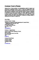
1.3 Compact Stars and Dense-Matter Physics The physics of dense matter such as in neutron stars is not as simple as the final resting place of neutrons imagined by Baade and Zwicky. The constitution of matter at the high densities attained in a neutron star-the particle types, abundances and their interactions-pose challenging problems in nuclear and particle physics. How should matter at supernuclear densities be described? In addition to nucleons, what exotic baryon species constitute it? Does a transition in phase from quarks confined in nucleons to the deconfined phase of quark matter occur in the density range of such stars? And how is the transition to be calculated? What new structure is introduced into the star? Do other phases like pion or kaon condensates playa role in their constitution? We do not have definitive answers to these questions. They are of intense importance to theorists and experimentalists alike: the purpose of building large particle accelerators at CERN is aimed at answering them. But perhaps some of the exotic states of matter envisioned by theorists can exist only in neutron stars. In some cases there are subtle signals that may be detectable [5]. In Fig. 1.1 we show a computation of the possible constitution and interior crystalline structure of a neutron star near the limiting mass of such

stars. Only now are we beginning to appreciate the complex and marvelous structure of these objects [7]. Surely the study of neutron stars and their astronomical realization in pulsars will serve as a guide in the search for a solution to some of the fundamental problems of dense many-body physics both at the level of nuclear physics-the physics of baryons and mesonsand ultimately at the level of their constituents-quarks and gluons. And neutron stars may be the only objects in which a Coulomb lattice structure (Fig. 1.1) formed from two phases of one and the same substance (hadronic matter) exists. We do not know from experiment what the properties of superdense matter are. However we can be guided by certain general principles in our investigation of the possible forms that compact stars may take. Some of the possibilities lead to quite striking consequences that may in time be observable. The rate of discovery of new pulsars, X-ray neutron stars, and other high-energy phenomena associated with neutron stars is astonishing, and was unforeseen a dozen years ago. White dwarfs are the cores of stars whose demise is less spectacular than a supernova-a more quiescent thermal expansion of the envelope of a lowmass star into a planetary nebula, and the subsidence of its central region

1. Int rodu ction M/ M 11 10

0

7

= 1.4

~~~~~~lo:n iC crust 1

9

8 7

E -'"

6 5

3

2

° FIGURE 1.1. A section t hro ugh a neutron star model t hat contains an inner sphere of pure quark mat ter surro unded by a crystalline region of mixed ph ase hadronic and qu ark mat t er. The mixed ph ase region consists of vari ous geomet rical objects of t he rare ph ase immersed in t he domin ant one labeled by h(ad ronic ) drops, h(adronic) rods, . . ., imme rsed in quark mat ter, t hrough to q( uark) drops . . . imme rsed in hadr onic matter. The particle compos ition of t hese regions is quarks, nucleons, hyp erons, and leptons. A liquid of neutron star matter containing nucleons and leptons sur rounds t he mixed ph ase. A t hin crust of heavy ions forms t he stellar surface [6J .

to form a whit e dwarf. (P lanetary nebul a is a misnomer inasmuch as it has nothing to do with a planet . Early ast ronomers interpret ed the centers of such object s, which are whit e dwarfs , as planets.) The const it uents of whit e dwarfs are nuclei immersed in an electron gas and therefore arranged in a Coulomb lattice because of the opposite elect rical cha rge of gas and nuclei. White dwarfs are supporte d against collapse by th e Fermi pressure of degenerate elect rons- while neutron stars-are supported by the Fermi pressur e of degenerate nucleons and by the repulsion of nucleons at close distance. Whi te dwar fs pose less severe and less fundamental probl ems t han neutron stars. The nuclei will comprise varying proportions of helium , car bon, and oxygen, and in some cases heavier elements like magnesium , depend ing on how far in t he chain of exot hermic nuclear fusion reactions t he precursor star burned before it was disrupted by instabiliti es leaving behind t he dwarf. Whi te dwarfs are barely relativistic.

8

Special and General Relativity

Of a vastly different nature than neutron stars are strange stars. Like neutron stars, strange stars, if they exist, are very dense, of the same order as neutron stars. However their very existence hinges on a hypothesis that at first sight seems absurd. According to the hypothesis, sometimes referred to as the strange-matter hypothesis, quark matter-consisting of an approximately equal number of up, down and strange quarks-has an equilibrium energy per nucleon that is lower than the mass of the nucleon or the energy per nucleon of the most bound nucleus, iron. In other words, under the hypothesis, strange quark matter is the absolute ground state of the strong interaction [8]. We customarily find that systems, if not in their ground state, readily decay to it. Of course this is not always so. Even in well known objects like nuclei, there are certain excited states whose structure is such that the transition to the ground state is hindered. The first excited state of 180Ta has a half-life of 1015 years, five orders of magnitude longer than the age of the universe! The strange-matter hypothesis is consistent with the present universe-a long-lived excited state-if strange matter is the ground state. The structure of strange stars is fascinating as are some of their properties. But that subject does not fall within the narrower aims of this book in laying down the General Theory of Relativity. The subject is treated in reference [4].

2

Special Relativity "If I pursue a beam of light with velocity c, I should observe such a beam ... at rest. [ie. the oscillation would be frozen]. However, there appears to be no such thing ... " A. Einstein at age 16 [as recalled many years later] "The views of space and time which I wish to lay before you have sprung from the soil of experimental physics, and therein lies their strength. They are radical. Henceforth space by itself, and time by itself, are doomed to fade away into mere shadows, and only a kind of union of the two will preserve an independent reality." H. Minkowski [9]. The principle of relativity in physics goes back to Galileo who asserted that the laws of nature are the same in all uniformly moving laboratories. The relativity principle, stated in the narrow terms of reference frames in uniform motion, referred to as inertial frames, implies the existence of an absolute space relative to which they move. The notion of the absoluteness of time goes back to time immemorial. A Galilean transformation assumes the absoluteness of both space and time: x'==x-a-vt,

y'==y,

z'==z,

t'==t-b.

(2.1)

Newton's second law Fx == m d2x / dt 2 is evidently invariant under this transformation if one assumes that force and mass are independent of the state of motion. However, in contrast to Galileo's principle, Einstein made the important distinction between reference frames that simply are in uniform motion, and those that are in uniform motion with respect to each other. This distinction makes all the difference in the world. In contrast to Newton's equations, Maxwell's equations do not take on the same form if subjected to a Galilean transformation whereas under a Lorentz transformation they do.' This fact led Einstein to the postulate that the speed of light, and every law of nature, is the same in all inertial (unaccelerated) systems. That is the historical role that light speed played in the discovery of Special Relativity, and the reason for the undoubted influence that the lSee, for example, Ref. [10] for the Lorentz invariant form of Maxwell's equations.

10

Special and General Relativity

Michelson-Morley experiment [11] had on the early acceptance of the theory. However, the underlying physics is quite different from how it appears in the historical development of the Special Theory. The speed of light need not have been postulated as an invariant. H. Minkowski (1849-1909) realized soon after Einstein's epochal discovery in 1905 that the spacetime manifold of our world is not Euclidean space but is pseudo-Euclidean and we call it the Minkowski Manifold having such a nature that dT2 == k 2 dt 2 - dx 2 - d y 2 - dz 2 is invariant in the absence of gravity. The constant k is a conversion factor between length and time. Minkowski's fundamental discovery was inspired by Einstein's theory, which was based on the postulate of the constancy of light speed. However, as Minkowski realized, the constancy of light speed is a consequence of the nature of the spacetime manifold of our universe. In other words, Special Relativity is a consequence of the local spacetime manifold in which we live [12, 13]. That the constancy of the speed of light is a property of the local spacetime manifold is clearly illustrated by a thought experiment proposed by Swiatecki [12, 13]. He shows that the invariance of the differential interval between spacetime events (sometimes called the proper time, or the Minkowski invariant), (2.2) can be verified (at least in principle) without resort to propagation of light signals, but with only measuring rods and clocks. And if it were technically feasible to perform the experiment with sufficient accuracy, k would be measured and its value would be found to equal c if indeed, the photon is massless, as we assume hereafter. As an historical note, we add that Voigt observed in 1887 that D¢ == 0 preserved its form under a transformation that differed from the Lorentz transformation by only a scale factor [14]. In fact we will see shortly that the d'Alembertian D is a Lorentz scalar. Consequently, (2.3) informs us that a disturbance described by a wave equation for a massless particle in Minkowski spacetime propagates with velocity c in vacuum as viewed from this and any other reference frame connected to it by a Lorentz transformation. Having now stressed that it is by assumption of zero mass for the photon that we can use light velocity c in the Minkowski invariant, we shall in the sequel make this assumption. Nevertheless, as a matter of principle, let us not loose sight of the fact that the invariance of the propertime is a property of the spacetime of the world we live in, and an empirical

2. Special Relativity

11

determination of the constant k appearing in it would find its values to be c, within experimental error.

2.1

Lorentz Invariance

The Special Theory of Relativity, which holds in the absence of gravity, plays a central role in physics. Even in the strongest gravitational fields the laws of physics must conform to it in a sufficiently small locality of any spacetime event. That was a fundamental insight of Einstein. Consequently, the Special Theory plays a central role in the development of the General Theory of Relativity and its applications.

2.1.1

LORENTZ TRANSFORMATIONS

The Lorentz transformation leaves invariant the proper time or differential interval in Minkowski spacetime

(2.4) as measured by observers in frames moving with constant relative velocity (called inertial frames because they move freely under the action of no forces). The Minkowski manifold also implies an absolute spacetime in which spacetime events that can be connected by a Lorentz transformation lie within the cone defined by dr == o. "Absolute" means unaffected by any physical conditions. This was the same criticism that Einstein made of Newton's space and time, and the one that powered his search for a new theory in which the expression of physical laws does not depend on the frame of reference, but, nevertheless, in which Lorentz invariance would remain a local

property of spacetime. ( Local in this context, means "in a sufficiently small region of spacetime".) We will develop General Relativity, which extends the relativity principle to arbitrary frames in a gravity-endowed universe, not just un-accelerated frames in relative uniform motion. Here we review briefly the Special Theory. A pure Lorentz transformation is one without spatial rotation, while a general Lorentz transformation is the product of a rotation in space and a pure Lorentz transformation. The pure Lorentz transformation is sometimes also referred to as a boost. For convenience, define

(2.5) (In spacetime a point, such as that above, is sometimes referred to as an event.) The linear homogeneous transformation connecting two reference frames can be written

(2.6)

12

Special and General Relativity

(We shall use the convenient notation introduced by Einstein whereby repeated indices are summed-Greek over time and space, Roman over space alone.) Any set of four quantities AfL (J-t == 0,1,2,3) that transforms under a change of reference frame in the same way as the coordinates is called a contravariant Lorentz four-vector,

(2.7) The invariant interval (also variously called the proper time, the line element, or the separation formula) can be written

(2.8) where TJfLv is the Minkowski metric which, in rectilinear coordinates, is

TJfLV

==

1

0

o

-1 0 0

o o

o

0

-1

0 0

o

o

(2.9)

-1

The condition of the invariance of dT2 is (2.10) Since this holds for any dx", dx f3 we conclude that the AfLv must satisfy the fundamental relationship assuring invariance of the proper time: (2.11) Transformations that leave dT2 invariant also leave the speed of light the same in all inertial systems; this is so because if dr == 0 in one system, it is true in all, and the content of dr == 0 is that dx]dt == 1 (with units c == 1). Let us find the transformation matrix AfL for the special case of a boost along the x-axis. In this case it is clear that Q

(2.12) and, moreover, that x/o and x/ 1 cannot involve x 2 and x 3 . So,

x/o == AOoxo + A01 X 1 x/ 1 == A 1 O+ A 1 1 , 0x

1x

(2.13)

with the remaining A elements zero. So the above quadratic form in A yields the three equations, 1 -1

o

(A°0)2 - (A10)2 (A01 ) 2 - (A11 ) 2 AOoAo1 - A10A 11 ·

(2.14)

2. Special Relativity

13

To get a fourth equation, suppose that the origins of the two frames in uniform motion coincide at t == 0 and the primed x-axis, x,l, is moving along xl with velocity v. That is, xl == vt is the equation of the primed origin as it moves along the unprimed x-axis. The equation for the primed coordinate is (2.15)

or

AIO== -AIIV.

(2.16)

The four equations can now be solved with the result,

Ao0-- Al1 -- 'VI AIO== AOl == -V1 A22 ==A33 == 1,

(2.17)

where 1

== (1 -

2)-1/2 V

== coshB,

V1

== sinhB,

v

== tanhB.

(2.18)

So X'D == xO cosh B- xl sinh B X,l == -x o sinh B + xl cosh B x,2 == x 2,x,3 == x 3 .

(2.19)

The combination of two boosts in the same direction, say VI and V2, corresponds to B == Bl + B2 • A boost in an arbitrary direction with the primed axis having velocity v == (vI, v 2 , v 3 ) relative to the unprimed is AOo == "Y

AO..J == »; == - .v j 1 AJ k == Akj == 8~ + (1- l)v jv k /y2

.

(2.20)

For a spatial rotation, say in the x-y plane, the transformation for a positive rotation about the common z-axis is x,l == Xl cosw + x 2 sinw x,2 == -Xl sinw + x 2 cosw x'D == z", x,3 == x 3 .

(2.21)

Transformation of vectors according to either of the above, or a product of them, preserves the invariance of the interval dT2 • For convenience they can be written in matrix form as

A==

cosh B - sinhB 0 0 - sinh B coshB 0 0 o 010 o 001

(2.22)

14

Special and General Relativity

R==

2.1.2

1 0 0

-sinw

0

0

0 cosw

0 sm ce cosw 0

0 0

0 1

(2.23)

TIME DILATION

Let there be two identical clocks at rest at x == O. The clocks tick at equal intervals dt. The propertime in this frame is

dr ==

J dt 2 -

dx 2 == dt .

(2.24)

An observer takes one of the clocks and moves away along the x-axis with velocity v. He sees the first clock at dx' == -v dt . The propertime expressed in his frame is

dr' ==

J dt,2 -

dx,2

== dt' ~

(2.25)

But the two events are connected by a Lorentz transformation and so their propertimes are the same. Consequently

dt' ==dt/~.

(2.26)

This expresses the dilation of time as measured by observers in uniform relative motion. The converse holds for length measurements.

2.1.3

COVARIANT VECTORS

Two contravariant Lorentz vectors such as

(2.27) and BfL may be used to create a scalar product (Lorentz scalar) A' . B'

== TJfLvA'fL B'v == TJfLV AfLaAV/3AaB/3 == TJa/3A aB/3 == A . B .

(2.28)

Because of the minus signs in the Minkowski metric we have

A . B == A 0 B O - A . B ,

(2.29)

and the covariant Lorentz vector is defined by

(2.30) A covariant Lorentz vector is obtained from its contravariant dual by the process of lowering indices with the metric tensor,

(2.31)

2. Special Relativity

15

Conversely, raising of indices is achieved by

(2.32) It is straightforward to show that

(2.33) where 6/1 == v

{I

if J-L == v 0 otherwise

(2.34)

is the Kroneker delta. It follows that

(2.35) The Lorentz transformation for a covariant vector is written in analogy with that of a contravariant vector:

(2.36) To obtain the elements of A; we write the above in two different ways,

(2.37) This holds for arbitrary A/1 so

A/1v -- TJ/1Q AQf3TJ f3v .

(2.38)

Using (2.33) in the above we get the inverse relationship

(2.39) Multiplying (2.38) by A/1a , summing on J-L, and employing the fundamental condition of invariance of the proper time (2.11) we find

(2.40) We can now invert (2.6) and find that A; is the inverse Lorentz transformation, (2.41) The elements of the inverse transformation are given in terms of (2.17) or (2.20) by (2.38). We have

Aaa == Ala == A 22 =

All == 1 , Aa1 == v1 , A 33 = 1.

(2.42)

16

Special and General Relativity

A boost in an arbitrary direction with the primed axis having velocity v == (VI, V 2, v 3 ) relative to the unprimed is Aoj

== 1, == A.o ==

Ajk

==

Aoo

J .

AkJ

vj

1,

.

== 6~

+ (1 -

l)v jv k /v2

(2.43) .

The velocity is a vector of particular interest and defined as uJ-t

==

dxJ-t dT .

(2.44)

Because dr is an invariant scalar and dx!' is a vector, uJ-t is obviously a contravariant vector. From the expression for the invariant interval we have

dr

dT==~dt,

v== dt

(2.45)

with r == (Xl, x 2 , x 3 ) ; it therefore follows that dt

u O == -

dT

(2.46)

== 1,

or uJ-t uJ-tuJ-t

1(1, vI, v 2 , v 3 )

,

UJ-t

== 1(1, -VI, -v 2 , -v 3 ) ,

1.

(2.47)

The transformation of a tensor under a Lorentz transformation follows

from (2.7) and (2.36) according to the position of the indices; for example, (2.48) We note that according to (2.11), the Minkowski metric TjJ-tv is a tensor; moreover, it has the same constant form in every Lorentz frame.

2.1.4

ENERGY AND MOMENTUM

The relativistic analogue of Newton's law F == ma is d 2xJ-t FJ-t==m-dT

(2.49)

dxJ-t dT .

(2.50)

and the four-momentum is pJ-t

== m

Hence, from (2.44) and (2.45) pO

== E == m1 p == mrtv .

(2.51)

2. Special Relativity

2.1.5

17

ENERGY-MOMENTUM TENSOR OF A PERFECT FLUID

A perfect fluid is a medium in which the pressure is isotropic in the rest frame of each fluid element, and shear stresses and heat transport are absent. If at a certain point the velocity of the fluid is v, an observer with this velocity will observe the fluid in the neighborhood as isotropic with an energy density E and pressure p. In this local frame the energy-momentum tensor is E

o o

o

000 p 0 0 0 p 0 0 0 p

(2.52)

As viewed from an arbitrary frame, say the laboratory system, let this fluid element be observed to have velocity v. According to (2.41) we obtain the transformation (2.53) The elements of the transformation are given by (2.42) in the case that the fluid element is moving with velocity v along the laboratory x-axis, or by (2.43) if it has the general velocity v. It is easy to check that in the arbitrary frame (2.54)

0--+----"'------'9---------+-----------, o 2 3

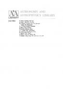
FIGURE 2.1. Future light cones at radial distances both inside and outside a black hole Schwarzschild radius r s == 2G M / c2 . The possible futures of any event at the vertex of each cone, lies within the cone. Light propagates along the cone itself. On the scale of distance relative to the Schwarzschild radius of the black hole, the cones narrow and are tipped toward the black hole. At the critical radius, the outer edge of the cone is vertical; not even light can escape. Within the black hole, light can propagate only inward, as with anything else. Future points in spacetime of a material particle at the vertex of a cone can lie only within the cone.

18

Special and General Relativity

and reduces to the diagonal form above when v ~ O. We have used the four-velocity u/-L defined above by (2.46). Relative to the laboratory frame it is the four-velocity of the fluid element.

2.1.6

LIGHT CONE

The vanishing of the proper time interval, dr ~ 0, given by (2.4) defines a cone in the four-dimensional space x!' with the time axis as the axis of the cone. Events separated from the vertex event for which the proper time, (or invariant interval) vanishes idr ~ 0), are said to have null separation. They can be connected to the event at the vertex by a light signal. Events separated from the vertex by a real interval dT2 > 0 can be connected by a subluminal signal-a material particle can travel from one event to the other. An event for which dT2 < 0 refers to an event outside the two cones; a light signal cannot join the vertex event to such an event. Therefore, events in the cone with t greater than that of the vertex of the cone lie in the future of the event at the vertex, while events in the other cone lie in its past. Events lying outside the cone are not causally connected to the vertex event.

3

General Relativity

"Scarcely anyone who fully comprehends this theory can escape its magic." A. Einstein "Beauty is truth, truth beauty-that is all Ye know on earth, and all ye need to know." J. Keats Ode on a Grecian Urn

General Relativity-Einstein's theory of gravity-is the most beautiful and elegant of physical theories. It is the foundation of cosmology-the subject that traces the evolution of the universe from its first intensely hot and dense beginning to its possible futures. 1 General Relativity is also the foundation for our understanding of compact stars. Neutron stars and black holes Can be understood correctly only in General Relativity as formulated by Einstein [15,16]. Dense objects like neutron stars could also exist in Newton's theory, but they would be very different objects. Chandrasekhar found (in connection with white dwarfs) that all degenerate stars have a maximum possible mass [17,18]. In Newton's theory such a maximum mass is attained only asymptotically when all Fermions, whose pressure supports the star, are ultra relativistic. Under such conditions, stars populated by the three heavy quarks-known as charm, truth, and beauty-would exist. However, such stars do not occur in Einstein's theory because the maximum-possiblemass star is not sufficiently dense, even at its center; therefore they cannot exist in nature. Einstein sought the answer to a question that must have seemed to his contemporaries, and all who preceded him, as of no consequence: What meaning is attached to the absolute equality of inertial and gravitational masses? If all bodies move in gravitational fields in precisely the same way, no matter what their constitution or binding forces, then this means that their motion has nothing to do with their nature, but rather with the na1 Einstein, himself, never did apply his theory to the evolution of the cosmos. Indeed, when he discovered the theory (1915), it was a canon of western thought that the world lasted from "everlasting to everlasting." Edwin Hubble's 1927 discovery of universal expansion shook that belief.

20

Special and General Relativity

ture of spacetime. And if spacetime determines the motion of bodies, then according to the notion of action and reaction, this implies that spacetime in turn is shaped by bodies and their motion. Beautiful or not, the predictions of theory have to be tested. The first three tests of General Relativity were proposed by Einstein, the gravitational redshift, the deflection of light by massive bodies and the perihelion shift of Mercury. The latter had already been measured. Einstein computed the anomalous part of the precession to be 43 arcseconds per century, in agreement with the measurement of 42.98 ± 0.04. A fourth test was suggested by Shapiro in 1964-the time delay in the radar echo of a signal sent to a planet whose orbit is carrying it toward superior conjunction/ with the Sun. Eventually agreement to 0.1 percent with the prediction of Einstein's theory was achieved in these difficult and remarkable experiments. It should be noted that all of the above tests involved weak gravitational fields. In testing General Relativity, the crowning achievement was the cumulative 20-year study by Taylor, Hulse and their colleagues of the Hulse-Taylor pulsar binary that was discovered in 1974. Their work yielded a measurement of 4.22663 degrees per year for the periastron shift of the orbit of the neutron star binary and a measurement of the decay of the orbital period by 7.60 ± 0.03 x 10- 7 seconds per year. This rate of decay agrees to less than 1% with careful calculations of the effect of energy loss through gravitational radiation as predicted by Einstein's theory [19]. A fuller discussion of these experiments and other intricacies involved in the tests of relativity can be found in the book by Will [20]. Since these early experiments, more accurate tests are being made by Dick Manchester and collaborators at Parkes Observatory in Australia, who have discovered a tighter orbiting pair of pulsars (neutron stars) - "We have verified GR to 0.1% already in two years" - ten times better than the early experiment." (Private communication: R. N. Manchester, 6/15/2005). The goal of this chapter is to provide a rigorous derivation of the Oppenheimer-Volkoff equations that describe the structure of relativistic stars. For this purpose we need to understand General Relativity.

3.1 Scalars, Vectors, and Tensors in Curvilinear Coordinates In the last chapter we dealt with inertial frames of reference in flat spacetime. We now wish to allow for curvilinear coordinates. Our scalars, vectors, and tensors now refer to a point in spacetime. Their components refer to the reference frame at that point. 2Superior conjunction refers to the situation when the Earth and the planet are on opposite sides of the Sun.

3. General Relativity

21

A scalar field S (x) is a function of position, but its value does not depend on the coordinate system. An example is the temperature as registered on thermometers located in various rooms in a house. Each registered temperature may be different, and therefore is a function of position, but independent of the coordinates used to specify the locations:

S'(x') == S(x).

(3.1)

A vector is a quantity whose components change under a coordinate transformation. One important vector is the displacement vector between adjacent points. Near the point x J1 we consider another, x J1 + da!', The four displacements dx!' are the components of a vector. Choose units so that time and distance are measured in the same units (c == 1). In Cartesian coordinates we can write the invariant interval dr of the Special Theory of Relativity, sometimes called the proper time, as

(3.2) Under a coordinate transformation from these rectilinear coordinates to arbitrary coordinates, x J1 -+ x'J1, we have (from the rules of partial differentiation)

a 'J1

dx 'J1- ~d aXV x.v

(3.3)

As always, repeated indices are summed. We can also write the inverse of the above equation and substitute for the spacetime differentials in the invariant interval to obtain an equation of the form (3.4)

where the gJ1V are defined in terms of products of the partial derivatives of the coordinate transformation. Depending on the nature of the coordinate system, say rectilinear, oblique, or curvilinear, or on the presence of a gravitational field, the invariant interval may involve bilinear products of different dx!", and the 9 J1V will be functions of position and time. The gJ1V are field quantities-the components of a tensor called the metric tensor. Because the gJ1V appear in a quadratic form (3.4), we may take them to be symmetric:

(3.5) In regions of spacetime for which the rectilinear system of the Special Theory of Relativity holds, the metric tensor gJ1V is equal to the Minkowski tensor (2.9). In fact, as we shall see, Special Relativity holds locally anywhere at any time. We shall refer to reference frames in which the metric is given by the Minkowski tensor as Lorentz frames.

22

Special and General Relativity

The invariant interval or proper time dr is real for a timelike interval and imaginary for a spacelike interval. 3 The notation proper time is seen to be appropriate because, when two events occur at the same space point, what remains of the invariant interval is dt. .. Any four quantities All that transform as dx!' comprise a contravariant vector (3.6) and (3.7) is its invariant squared length. It is obviously invariant under the same transformations that leave (3.2) invariant because the four quantities All form a four-vector like dx!', A covariant vector can be obtained through the process of lowering indices with the metric tensor:

(3.8) In terms of this vector, the magnitude equation (3.7) can be written as

(3.9) Let All and BIl be distinct contravariant vectors. Then All

+ >..BIl is also

a contravariant vector for all finite A. The quantity

is the invariant squared length. Because this is true for all >.., the coefficient of each power of >.. is also an invariant; for the linear term we find (3.10) where we have used the symmetry of 91l v . Thus, we obtain the invariant scalar product of two vectors: (3.11) To derive the transformation law for a covariant vector use the fact, just proven, that AIlBIl is a scalar. Then using the law of transformation of a contravariant vector (3.6), we have

A'

J-L

n» == A

x

0:

BO: == A 8 O: e» 0: 8x J-L '

'

(3.12)

3The opposite convention ds 2 = -dT 2 could also be employed. The interval ds is often referred to as the line element.

3. General Relativity

23

where A~ is the same vector as AJL but referred to the primed reference frame. From the above equation it follows that

a ax A )B'JL == 0 ( A'JL - ax'JL a .

(3.13)

Because BJL is any vector, the quantity in brackets must vanish; thus we have the law of transformation of a covariant vector,

A~

ax v

= 8x ,p,Av .

(3.14)

Compare this transformation law with that of (3.6). Let the determinant of gJLV be g, (3.15)

As long as g does not vanish, the equations (3.8) can be inverted. Let the coefficients of the inverse be called gJLv. Then find (3.16) Multiply (3.8) by gaJL and sum on

J-L

with the result (3.17)

or (3.18)

where 8~ is the Kroneker delta. Because this equation holds for any vector, we have (3.19) The two g's, one with subscripts, the other with superscripts, are inverses. In the same way as gJLV can be used to lower an index, gJLV can be used to raise one as in, (3.20)

Both g's are symmetric; (3.21)

The derivative of a scalar field S(x) == S'(x') with respect to the components of a contravariant position vector yields a covariant vector field and, vice versa:

as ax'JL

Ba"

as

ax'JL ax v .

(3.22)

24

Special and General Relativity

Accordingly, we shall sometimes use the abbreviations,

a aJ1 == -axJ1

and

a aJ1 == -aXJ1 ,

(3.23)

especially in writing Lagrangians of fields. In relativity it is also useful to have an even more compact notation for the coordinate derivative-the "comma subscript":

s == as ,J1 -

(3.24)

axJ1 .

The d'Alembertian, (3.25) is manifestly a scalar. Tensors are similar to vectors, but with more than one index. A simple tensor is one formed from the product of the components of two vectors, AJ1 BV. But this is special because of the relationships between its components. A general tensor of the second rank can be formed by a sum of such products: (3.26) The superscripts can be lowered as with a vector, either one index, or both, TJ1v

== gJ1aTav ,

T~

== Tva gaJ1 ,

TJ1v

== gJ1agvf3Taf3 .

(3.27)

Similarly, we may have tensors of higher rank, either contravariant with respect to all indices, or covariant, or mixed. The position of the indices on the mixed tensor (the lower to the left or right of the upper) refers to the position of the index that was lowered. If TJ-lV is symmetric, then TJt == T v J1 and it is unimportant to keep track of the position of the index that has been lowered (or raised). But if TJ1V is antisymmetric, then the two orderings differ by a sign. If two of the indices on a tensor, one a superscript the other a subscript, are set equal and summed, the rank is reduced by two. This process is called contraction. If it is done on a second-rank mixed tensor, the result is a scalar, (3.28) When TJ1V is antisymmetric, the contractions TJ1J1 and T~ are identically zero. The test of tensor character is whether the object in question transforms under a coordinate transformation in the obvious generalization of a vector. For example, (3.29) is a tensor.

3. General Relativity

25

In general, we deal with curved spacetime in General Relativity. We must therefore deal with curvilinear coordinates. Vectors and tensors at a point in such a spacetime have components referring to the axis at that point. The components will change according to the above laws, depending on the way the axes change at that point. Therefore, the metric tensors gj.LV' gJ-LV cannot be constants. They are field quantities which vary from point to point. As we shall see, they can be referred to collectively as the gravitational field. Because the formalism of this section is expressed by local equations, it holds in curved spacetime, for curved spacetime is flat in a sufficiently small locality. Because the derivative of a scalar field is a vector (3.22), one might have thought that the derivative of a vector field is a tensor. However, by checking the transformation properties one finds that this supposition is not true. We have referred invariably to the gJ-LV as tensors. Now we show that this is so. Let AJ-L, BV be arbitrary vector fields, and consider two coordinate systems such that the same point P has the coordinates xJ-L and x'J-L when referred to the two systems, respectively. Then we have I

ga,8

v A'a A ',8 == g AJ-L A V == g axJ-L ax A'a A ',8 J-LV J-LVax 'a ax . ',8

(3.30)

Because this holds for arbitrary vectors, we find

axJ-L ax v ga,8 == gJ-LV ax'a ax , ',8 I

(3.31)

which, by comparison with (3.14), shows that gJ-LV is a covariant tensor. Similarly gJ-Lv is a contravariant tensor: 9

la,8 _

- 9

j.LV

a 'a a 1,8 X

X

8xJ-L 8xv .

(3.32)

These are called the fundamental tensors. Of course, the above tensor character of the metric is precisely what is required to make the square of the interval dr 2 of (3.4) an invariant, as is trivially verified. Mixed tensors of arbitrary rank transform, for each index, according to the transformation laws (3.6, 3.14) depending on whether the index is a superscript or a subscript, as can be derived in obvious analogy to the above manipulations. Tensors and tensor algebra are very powerful techniques for carrying the consequences discovered in one frame to another. That the linear combination of tensors of the same rank and arrangement of upper and lower indices is also a tensor; that the direct product of two tensors of the same or different rank and arrangement of indices, A~:::B~:" == it:": is also a tensor; and that contraction (defined above) of a pair of indices, one upper, one lower, produces a tensor of rank reduced by two-are all easy theorems that we do not need to prove, but only note in passing. Of particular note,

26

Special and General Relativity

if the difference of two tensors of the same transformation rule vanishes in one frame, then it vanishes in all (i.e., the two tensors are equal in all frames). "The possibility of explaining the numerical equality of inertia and gravitation by the unity of their nature gives to the general theory of relativity, according to my conviction, such a superiority over the conceptions of classical mechanics, that all the difficulties encountered in development must be considered as small in comparison." A. Einstein [16] Eotvos established that all bodies have the same ratio of inertial to gravitational mass with high precision [21]. With an appropriate choice of units, the two masses are equal for all bodies to the accuracy established for the ratio. One might have expected such conceptually different properties, one having to do with inertia to motion (mI), the other with "charge" (me), in an expression of mutual attraction between bodies, to be entirely different. The relation between the force exerted by the gravitational attraction of a body of mass M at a distance R upon the object, and the acceleration imparted to it are expressed by Newton's equation, valid for weak fields and small material velocities: (3.33) Einstein reasoned that the near equality of two such different properties must be more than mere coincidence and that inertial and gravitational masses must be exactly equal: mr

== me == m.

(3.34)

The mass drops out! In that case all bodies experience precisely the same acceleration in a gravitational field, a == mj R 2 , where m is the mass of the accelerating body. A common acceleration due to gravity was presaged by Galileo's careful experiments performed centuries earlier. For all other forces that we know, the acceleration (a == F / m) is inverse to the mass. The equivalence of inertial and gravitational mass is established to high accuracy for atomic and nuclear binding energies." Moreover, as a result of very careful lunar laser-ranging experiments, the earth and moon are found to fall with equal acceleration toward the Sun to a precision of almost 1 part in 1013 , better than the most accurate Eotvos-type experiments on laboratory bodies. This exceedingly important test involving bodies of different gravitational binding was conceived by Nordtvedt [22]. The essentially null result establishes the so-called strong statement of equivalence 4 Eotvos' experiments on such diverse media as wood, platinum, copper, glass, and other materials involve different molecular, atomic, and nuclear binding energies and different ratios of neutrons and protons.

3. General Relativity

27

of inertial and gravitational mass: Free bodies-no matter their nature or constituents, nor how much or little those constituents are bound, nor by what force-all move in the spacetime of an arbitrary gravitational field as if they were identical test particles! Because their motion in spacetime has nothing to do with their nature, it evidently has to do with the nature of spacetime. Einstein felt certain that a deep meaning was attached to the equivalence; "The experimentally known matter independence of the acceleration of fall is .... a powerful argument for the fact that the relativity postulate has to be extended to coordinate systems which, relative to each other, are in non-uniform motion" [23]. This conviction led him to the formulation of the equivalence principle. The equivalence principle provides the link between the physical laws as we discern them in our laboratories and their form under any circumstance in the universe-more precisely, in arbitrarily strong and varying gravitational fields. It also provides a tool for the development of the theory of gravitation itself, as we shall see in the sequel. The universe is populated by massive objects moving relative to one another. The gravitational field may be arbitrarily changing in time and space. However, the presence of gravity cannot be detected in a sufficiently small reference frame falling freely with a particle under no influence other than gravity. The particle will remain at rest in such a frame. It is a local inertial frame. A local inertial frame and a local Lorentz frame are synonymous. The laws of Special Relativity hold in inertial frames and therefore in the neighborhood of a freely falling frame. In this way the relativity principle is extended to arbitrary gravitational fields. Associated with a given spacetime event there are an infinity of locally inertial frames related by Lorentz transformations. All are equivalent for the description of physical phenomena in a sufficiently small region of spacetime. So we arrive at a statement of the equivalence principle:

At every spacetime point in an arbitrary gravitational field (meaning anytime and anywhere in the universe), a local inertial (Lorentz) frame can be chosen so that the laws of physics take on the form they have in Special Relativity. This is the meaning of the equality of inertial and gravitational masses that Einstein sought. The restricted validity of inertial frames to small localities of any event suggested the very fruitful analogy with local flatness on a curved surface. Einstein went further than the above statement of the equivalence principle. He spoke of the laws of nature rather than just the laws of physics. It seems entirely plausible that the extension is true, but we deal here only with physics. The equivalence principle has great power. It is the instrument by which all the special relativistic laws of physics-valid in a gravity-free universecan be generalized to a gravity-filled universe. We shall see how Einstein

28

Special and General Relativity

was able to give dynamic meaning to the spacetime continuum as an integral part of the physical world quite unlike the conception of an absolute spacetime in which the rest of physical processes take place. In Einstein's own words

... it is contrary to the mode of thinking in science to conceive of a thing (the spacetime continuum) which acts itself, but which cannot be acted upon.[16]

3.1.1

PHOTON IN A GRAVITATIONAL FIELD

The trajectory of photons is bent by a gravitational field. Imagine a freely falling elevator in a constant gravitational field. Its walls constitute an inertial frame as guaranteed by the equivalence principle. Therefore, a photon (as for a free particle) directed from one wall to the opposite along a path parallel to the floor will arrive at the other wall at the same height from which it started. But relative to the Earth, the elevator has fallen during the transit time. Therefore the photon has been deflected toward the earth and follows a curved path as observed from a frame fixed on the Earth. Employing the conservation of energy and Newtonian physics, Einstein reasoned that the gravitational field acts on photons. Let a photon be emitted from Zl vertically upward to Z2, and only for simplicity, let the field be uniform. A device located at Z2 converts its energy on arrival to a particle of mass m with perfect efficiency. The particle drops to Zl where its energy is now m + mgh, where 9 is the acceleration due to the uniform field. A device at Zl converts it into a photon of the same energy as possessed by the particle. The photon again is directed to Z2. If the original (and each succeeding photon) does not lose energy (hv)gh in climbing the gravitational field equal to the energy gained by the particle in dropping in the field, we would have a device that creates energy. By the law of conservation of energy Einstein discovered the gravitational redshift, commonly designated by the factor Z and equal in this case to gh. The shift in energy of a photon by falling (in this case blue-shifted) in the earth's gravitational field has been directly confirmed in an experiment performed by Pound and Rebka

[24]. In the above discussion the equivalence principle entered when the photon's inertial mass (hv) was used also as its gravitational mass in computing the gravitational work. One can also see the role of the equivalence principle by considering a pulse of light emitted over a distance h along the axis of a spaceship in uniform acceleration 9 in outer space. The time taken for the light to reach the detector is t == h (we use units G == c == 1). The difference in velocity of the detector acquired during the light travel time is v == gt == gh, the Doppler shift Z in the detected light. This experiment, carried out in the gravity-free environment of a spaceship whose rockets produce an acceleration g, must yield the same result for the energy shift of the photon in a uniform gravitational field 9 according to the equivalence

3. General Relativity

29

principle. The Pound-Rebka-Snyder experiments can therefore be regarded as an experimental proof of the equivalence principle [24, 25]. We may regard a radiating atom as a clock, with each wave crest regarded as a tick of the clock. Imagine two identical atoms situated one at some height above the other in the gravitational field of the earth. Since, by dropping in the gravitational field, the light is blue-shifted when compared to the radiation of an identical atom (clock) at the bottom, the clock at the top is seen to be running faster than the one at the bottom. Therefore, identical clocks, stationary with respect to the earth, run at different rates according to their different heights above the earth. Time flows at different rates in different gravitational fields. An experiment carried out by J.e. Hafele and R.E. Keating tested a combination of time dilation in Special Relativity and the General Relativistic effect of differing gravitational field on the flow of time [26]. "During October 1971, four cesium atomic beam clocks were flown on regularly scheduled commercial jet flights around the world twice, once eastward and once westward, to test Einstein's theory of relativity with macroscopic clocks. From the actual flight paths of each trip, the theory predicted that the flying clocks, compared with reference clocks at the U.S. Naval Observatory, should have lost 40 ± 23 nanoseconds during the eastward trip and should have gained 275 ± 21 nanoseconds during the westward trip ... Relative to the atomic time scale of the U.S. Naval Observatory, the flying clocks lost 59±10 nanoseconds during the eastward trip and gained 273±7 nanosecond during the westward trip, where the errors are the corresponding standard deviations. These results provide an "unambiguous empirical resolution of the famous clock 'paradox' with macroscopic clocks." The different timelapse of the eastward and westward journeys of the clocks has to to with their motion relative to the Earth bound reference clock. The above experiment proves that the so-called "twin paradox" is not a paradox at all. The twins will have aged differently if they have had different trips in differing gravitational fields, one on the ground and one traveling in an airplane at a height above ground. Time dilation of Special Relativity is of different nature, having to do with differing speeds of the clocks, and is established in high-energy particle accelerators and routinely employed in designing experiments. We shall encounter both phenomena in later chapters.

3.1.2

TIDAL GRAVITY

Einstein predicted that a clock near a massive body would run more slowly than an identical distant clock. In doing so he arrived at a hint of the deep connection of the structure of spacetime and gravity. Two parallel straight lines never meet in the gravity-free, flat spacetime of Minkowski. A single inertial frame would suffice to describe all of spacetime. In formulating the equivalence principle (knowing that gravitational fields are not uniform and

30

Special and General Relativity

constant but depend on the motion of gravitating bodies and the position where gravitational effects are experienced), Einstein understood that only in a suitably small locality of spacetime do the laws of Special Relativity hold. Gravitational effects will be observed on a larger scale. Tidal gravity refers to the deviation from uniformity of the gravitational field at nearby points. These considerations led Einstein to the notion of spacetime curvature. Whatever the motion of a free body in an arbitrary gravitational field, it will follow a straight-line trajectory over any small locality as guaranteed by the equivalence principle. And in a gravity-endowed universe, free particles whose trajectories are parallel in a local inertial frame, will not remain parallel over a large region of spacetime. This has a striking analogy with the surface of a sphere on which two straight lines that are parallel over a small region do meet and cross. What if in fact the particles are freely falling in curved spacetime? In this way of thinking, the law that free particles move in straight lines remains true in an arbitrary gravitational field, thus obeying the principle of relativity in a larger sense. Any sufficiently small region of curved spacetime is locally flat. Such paths in curved spacetime that have the property of being locally straight are called geodesics.

3.1.3

CURVATURE OF SPACETIME

Let us now consider a thought experiment. Two nearby bodies released from rest above the earth follow parallel trajectories over a small region of their trajectories, as we know from the equivalence principle. But if holes were drilled in the earth through which the bodies could fall, the bodies would meet and cross at the earth's center. So there is clearly no single Minkowski spacetime that covers a large region or the whole region containing a massive body. Einstein's view was that spacetime curvature caused the bodies to cross, bodies that in this curved spacetime were following straight line paths in every small locality, just as they would have done in the whole of Minkowski (flat) spacetime in the absence of gravitational bodies. The presence of gravitating bodies denies the existence of a global inertial frame. Spacetime can be flat everywhere only if there exists such a global frame. Hence, spacetime is curved by massive bodies. In their presence a test particle follows a geodesic path, one that is always locally straight. The concept of a "gravitational force" has been replaced by the curvature of spacetime, and the natural free motions of particles in it are defined by geodesics.

3.1.4

ENERGY CONSERVATION AND CURVATURE

Interestingly, the conservation of energy can also be used to inform us that spacetime is curved. Consider a static gravitational field. Let us conjecture that spacetime is flat so that the Minkowski metric holds; we will arrive at

3. General Relativity

31

a contradiction. Imagine the following experiment performed by observers and their apparatus at rest with respect to the gravitational field and their chosen Lorentz frame in the supposed flat spacetime of Minkowski. At a height Zl in the field, let a monochromatic light signal be emitted upward a height h to Z2 == Zl + h. Let the pulse be emitted for a specific time dtl during which N wavelengths (or photons) are emitted. Let the time during which they are received at Z2 be measured as dt 2 • (Because the spacetime is assumed to be described by the Minkowski metric and the source and receiver are at rest in the chosen frame, the proper times and coordinate times are equal.) Because the field in the above experiment is static, the path in the zt plane will have the same shape for both the beginning and ending of the pulse (as for each photon) as they trace their path in the Minkowski spacetime we postulate to hold. The trajectories will not be lines at 45 degrees because of the field, but the curved paths will be congruent; a translation in time will make the paths lie one upon the other. Therefore dT2 == dt2 == dtl == dTl will be measured at the stationary detector if spacetime is Minkowskian. In this case, the frequency (and hence the energy received at Z2) is the same as that sent from Zl. But this cannot be. The photons comprising the signal must lose energy in climbing the gravitational field (see Section 3.1.1). The conjecture that spacetime in the presence of a gravitational field is Minkowskian must therefore be false. We conclude that the presence of the gravitational field has caused spacetime to be curved. Such a line of reasoning was first conceived by Schild [27, 28, 29].

32

Special and General Relativity

3.2 Gravity "I was sitting in a chair at the patent office at Bern when all of a sudden a thought occurred to me: 'If a person falls freely he will not feel his own weight.' I was startled. This simple thought had a deep impression on me. It impelled me toward a theory of gravitation." A. Einstein [30]

3.2.1

EINSTEIN'S DISCOVERY

Einstein's discovery of General Relativity is generally regarded as the greatest intellectual achievement of anyone man. I'm not sure how many people who subscribe to this view actually understand the theory and all of the mathematics that was needed to construct it. In this chapter we set it down for all who wish to see and follow it. Subtle is the Lord by Abraham Pais is a marvelous book that discusses the history of Einstein's struggles on the path to his discovery [31].

3.2.2

PARTICLE MOTION IN AN ARBITRARY GRAVITATIONAL FIELD

As we have seen, massive bodies generate curvature. Galaxies, stars, and other bodies are in motion; therefore the curvature of spacetime is everywhere changing. For this reason there is no "prior geometry". There are no immutable reference frames to which events in spacetime can be referred. Indeed, the changing geometry of spacetime and of the motion and arrangement of mass-energy in spacetime are inseparable parts of the description of physical processes. This is a very different idea of space and time from that of Newton and even of the Special Theory of Relativity. We now take up the unified discussion of gravitating matter and motion. The power of the equivalence principle in informing us so simply that spacetime must be curved by the presence of massive bodies in the universe suggests a fruitful way of beginning. Following Weinberg [32], or indeed, following the notion expressed by Einstein in the quotation above, we seek the connection between an arbitrary reference frame and a reference frame that is freely falling with a particle that is moving only under the influence of an arbitrary gravitational field. In this freely falling and therefore locally inertial frame, the particle moves in a straight line. Denote the coordinates by ~Q. The equations of motion are d2~Q

dT 2

== 0

,

(3.35)

and the invariant interval (or proper time) between two neighboring spacetime events expressed in this frame, from (2.8), is dT

2

== 7]Q{3d~Qd~{3.

(3.36)

3. General Relativity

33

The freely falling coordinates may be regarded as functions of the coordinates x Jl of any arbitrary reference frame-curvilinear, accelerated, or rotating. We seek the connection between the equations of motion in the freely falling frame and the arbitrary one which, for example, might be the laboratory frame. From the chain rule for differentiation we can rewrite (3.35) as

o

~ (8~a dXJl ) dr 8x/-L dr 8~a d2x/-L 8 2 ~a dx" dx" 8x/-L dT2 + 8x Jl8x V dT dT .

Multiply by 8x A / 8~a, and use the chain rule again to obtain

8x A 8~a

dx A

A

-==--.-==6 Jl dx» 8~a 8x Jl

•

(3.37)

The equation of motion of the particle in an arbitrary frame when the particle is moving in an arbitrary gravitational field therefore is

(3.38) Here r~v, defined by A r /-LV

8x A

82~a

== - - - - -

-

8~a

8x Jl8x V '

(3.39)

is called the affine connection. The affine connection is symmetric in its lower indices. The path defined by equation (3.38) is called a geodesic, the extremal path in the spacetime of an arbitrary gravitational field. We do not see here that it is an extremal, but this is hinted at inasmuch as it defines the same path of (3.35), the straight-line path of a free particle as observed from its freely falling frame. In the next section we will see that a geodesic path is locally a straight line. The invariant interval (3.36) can also be expressed in the arbitrary frame by writing d~a == (8~a / 8x/-L )dx Jl so that (3.40)

with 8~a 8~{j

9/-LV == 8x Jl 8x v TJa{j .

(3.41 )

In the new and arbitrary reference frame, the second term of (3.38) causes a deviation from a straight-line motion of the particle in this frame. Therefore, the second term represents the effect of the gravitational field. (To be

34

Special and General Relativity

sure, the connection coefficients also represent any other noninertial effects that may have been introduced by the choice of reference frame, such as rotation.) The affine connection (3.39) appearing in the geodesic equation clearly plays an important role in gravity, and we study it further. We first show that the affine connection is a nontensor, and then show how it can be expressed in terms of the metric tensor and its derivatives. In this sense the metric behaves as the gravitational potential and the affine connection as the force. Write r~v expressed in (3.39) in another coordinate system and use the chain rule several times to rewrite it:

x/J-L

_ax_fA _ax_p_a_ (_ax_a _a~_a) ax pa~a ax/J-L aX/vax a ax/A ax p[ax a axT a2~a a2x a~a] ax pa~a ax/v ax/J-L axTax + ax/J-Lax/v axa 2x p ax/A Bx" Bx" ax/A a ------r --axp Bx'!' ax/v TO' + -axp- -aX/J-Lax/v O"

0"

p

(3.42)

According to the transformation laws of tensors developed in Section 3.1, the second term on the right spoils the transformation law of the affine connection. It is therefore a nontensor. Let us now obtain the expression of the affine connection in terms of the derivatives of the metric tensor. Form the derivative of (3.31):

Take the derivatives and form the following combination and find that it is equal to the above derivative:

Multiply this equation by ~ and then multiply the left and right sides by the left and right sides, respectively, of the law of transformation (3.32), namely,

Use the chain rule and rename several dummy indices to obtain (3.43)

3. General Relativity

35

where the prime on {} means that it is evaluated in the x'J-l frame and the symbol stands for (3.44)

This is called a Christoffel symbol of the second kind. It is seen to transform in exactly the same way as the affine connection (3.42). Subtract the two to obtain

rA

[ J-lV

-

\ }]' == ~~~ 8 'A 8 T 8 a /\ { J-lV 8x p 8x'J-l 8x'V

[

p - {P }] rT ara

.

(3.45)

This shows that the difference is a tensor. According to the equivalence principle, at anyplace and anytime there is a local inertial frame ~Q in which the effects of gravitation are absent, the metric is given by (2.9), and r~v vanishes (compare (3.35) and (3.38)). Because the first derivatives of the metric tensor vanish in such a local inertial system, the Christoffel symbol also vanishes. Because the difference of the affine connection and the Christoffel symbol is a tensor which vanishes in this frame, the difference vanishes in all reference frames. So everywhere we find (3.46)

We use the "comma subscript" notation introduced earlier to denote differentiation (3.24). Sometimes it is useful to have the superscript lowered on the affine connection (3.47)

It is equal to the Christoffel symbol of the first kind

r l R).

(3.151)

This completes the derivation of the Schwarzschild solution of 1916 of Einstein's equations outside a spherical static star. It was the first exact solution found for Einstein's equations. The proper time is

dT2

M) de _ (1 _ 2~M)

( 1 _ 2~

-r 2d02 - r 2 sin 2 0 d¢2 ,

-1 dr2

(r > R)

where R, in this context, denotes the radius of the star. Let us summarize the Schwarzschild solution found above for r

gOo(r)

=

e2v (r )

=

911(r)==-e 2A(r) 922 (r) ==

-r 2 ,

(3.152)

> R:

(1- 2~M), (

2GM)-1 ,

==- 1 - -933 (r, 0) ==

r _r 2 sin 2 f) .

(3.153)

Notice that the Schwarzschild metric is singular at the radius

r == r s == 2GM/c2 ,

(3.154)

where we have reinserted c which by our usual convention we take as unity. This does not mean that spacetime itself is singular at that radius, but only that this particular metric is. Other nonsingular metrics have been found, in particular, the Kruskal-Szerkeres metric [40, 41]. However, further analysis shows that if rs lies outside the star where the Schwarzschild solution holds, then it is a black hole-no particle or even light can leave the region r < t s- This radius, rs, is called the Schwarzschild radius or singularity or horizon. But because the above metric holds only outside the star, r s has no special significance if it is smaller than the radius of the star. For then a different metric holds inside the star which does not possess a singularity. We come to this solution shortly.

3.6.3

RIEMANN TENSOR OUTSIDE A SCHWARZSCHILD STAR

If spacetime is flat, then the Riemann curvature tensor vanishes (Section 3.4.3). We are now prepared to address the converse (albeit not rigorously): if spacetime is curved, some components of the Riemann tensor are finite (which components, of course, will depend upon how convoluted spacetime is).

56

Special and General Relativity

The metric tensor and, indeed, the affine connection for the empty space outside a massive body were computed in the preceding section. We have seen in Section 3.1.3 that massive bodies curve spacetime. So we know that the Schwarzschild metric tensor refers to curved spacetime. Referring to the definition of the Riemann tensor (3.114) and the specific form that the affine connection takes for a static spherical star (3.141), we can compute

R610 == (v" + 2v,2 - v' A')e2(V-

A) .

(3.155)

Thus we exhibit at least one nonvanishing component of the Riemann tensor in the curved spacetime outside a Schwarzschild star. This suggests that Riemann is not identically zero in curved spacetime. An actual proof that if Riemann is finite then spacetime is curved requires the formulation of parallel transport, which we do not take up here. We declare, without rigorous proof, that the Riemann tensor vanishes if and only if spacetime is flat. Notice that, far from an isolated star where spacetime approaches flatness, Riemann approaches zero as it should.

3.6.4

ENERGy-MOMENTUM TENSOR OF MATTER

From the success of Newtonian physics in describing celestial mechanics and other weak gravitational field phenomena, we know that mass is a source of gravity. From the experimental verifications of the Special Theory of Relativity, we know that all forms of energy are equivalent and must contribute equally as sources of gravity. Normally, of course, it is mass that dominates, and the average mass density in the solar system and in the universe is very small; that is why Newtonian physics is so accurate under the typical conditions mentioned above. An essential aspect of Einstein's curvature tensor is that it automatically has vanishing covariant divergence (3.128). It is also a symmetric second-rank tensor. Accordingly, mass-energy-the source of the gravitational field-must be incorporated into a divergenceless, symmetric, secondrank tensor in flat space. As a tensor, it can be transcribed immediately to its form in an arbitrary spacetime frame by the general covariance principle. Such a tensor is the energy-momentum tensor. In the book Compact Stars [4] specific theories of dense matter are described from which we are able to explicitly construct the energy-momentum tensor of the theory. Here we are interested in the general form such a tensor takes. Frequently, matter may be regarded as a perfect fluid. The fluid velocity is assumed to vary continuously from point to point. The perfect fluid energy-momentum tensor in the Special Theory of Relativity can be expressed in terms of the local values of the pressure p and energy density E as in (2.54). The General Relativistic energy-momentum tensor can be written immediately using the Principle of General Covariance spelled

3. General Relativity

57

out on page 42: TMV

_pgMV + (p + E)UMUV , gMvUMU V == UvUv == 1 .

==

(3.156)

In the above equations, u M is the local fluid four-velocity (see 2.47) (3.157) The pressure and total energy density (including mass) are related by the equation of state of matter, frequently written in either form p

== p(E)

or

E

==

(3.158)

E(p)

where p and E are the pressure and energy density (including mass) in the local rest-frame of the fluid. In the next section we shall see how the equations for stellar structure involve these quantities and this relationship.

3.6.5

THE OPPENHEIMER-VOLKOFF EQUATIONS

We are now prepared to derive the differential equations for the structure of a static, spherically symmetric, relativistic star. For the region outside a star, we found that the vanishing of the Einstein tensor was equivalent to the vanishing of the Ricci tensor or the scalar curvature. This is not the case for the interior of the star. We need both the Ricci tensor and scalar curvature to construct the Einstein tensor. The general form of the metric for a static isotropic spacetime was obtained in (3.138). From Section 3.6.1 we find the scalar curvature, v gM R"v

R

fA'

2 == e -2v Roo - e -2), R 11 - -R2 r2 2

e- 2). { -2v "

+

A' - 4u' } + 2A, u, - 2v '2 - -22 + 4r

2

r2

r

r

(3.159)

.

It is more convenient to work with mixed tensors. For example, (3.160) is obtained with the results of Section 3.6.1 for a static isotropic field, namely,

o

go == gOvg

Ov

== goog 00 == 1 .

(3.161)

So using results obtained earlier in this section we can find that the components of the Einstein tensor are

58

Special and General Relativity

(3.162) Because of the assumption that the star is static, the three-velocity of every fluid element is zero, so

u/1 == 0

(/.1

(3.163)

~ 0),

according to (3.156). The energy-momentum tensor expressed as a mixed tensor, we have the nonzero components in the present metric,

To0 ==

E,

T/1/1 == -P

(J-L ~

0).

(3.164)

So the (00) component of the Einstein equations gives d r 2GOO = - dr {r(l - e- 2A(r»)} = kr 2To0 = kr 2f(r) .

(3.165)

This can be integrated immediately to yield

.:

e- 2A(r ) == 1 + -

r

Let us define

0

E(r)r2dr.

(3.166)

(3.167) and let R denote the radius of the star, the radial coordinate exterior to which the pressure vanishes. Zero pressure defines the edge of the star because zero pressure can support no material against the gravitational attraction from within. Denote the corresponding value of M(R) by M:=M(R).

(3.168)

Now comparing (3.72, 3.150, 3.151) we see that, to obtain agreement with the Newtonian limit, we must choose k == -87rG

(3.169)

and interpret M as the gravitational mass of the star. Therefore, M(r) is referred to as the included mass within the coordinate r. So Einstein's field equations can now be written (3.170) From the above, we have found so far that (3.171)

3. General Relativity

59

which agrees with (3.151), but now we see that gll(r) has the same form inside and outside the star although it is the included mass M (r), not the total mass, that appears in the interior solution. Having learned the constant of proportionality in Einstein's equations (3.170), let us now write out the field equations for a spherically symmetric static star, including the one we have already solved. In passing we note that our solution gives a relationship between the included mass M(r) at any radial coordinate and the metric function gll(r) or A(r), but we have yet to learn how to compute one or the other. The differential equations from (3.162) are

G11

2A') 2V')

1 - - --==-87rGE(r), 1 e -2;\ ( r2 r r2 e -2;\ ( -12 + - -12 == 87rGp(r) , r r r v/ e- 2A ( u" + v/ 2 - )../v/ + ~ = 81rGp(r) , G 22 == 81rGp(r) .

A')

(3.172) (3.173) (3.174) (3.175)

The last equation contains no information additional to that provided by those preceding it. To simplify notation, choose units so that G == c == 1. Solve (3.172) to find

(3.176) and (3.173) to find 2rv' == (1 + 81rr 2p )e2A - 1 .

(3.177)

Take the derivative of (3.177) and then multiply by r: 2rv'

Solve for

+ 2r 2v" =

[2r)..' (1 + 81rr 2p)

+ (161rr 2p + 81rr3p/)] e2A •

v'' using (3.177, 3.176): 2r 2v"

==

1 + (167rr 2p + 87rr 3p/)e 2;\ -(1 + 87rr2p)(1 - 87rr2E)e4 ;\

•

(3.178)

+~.

(3.179)

Square (3.177) to obtain the result 2r 2v/2 == ~(1

+ 87rr 2p)2e4 ;\ -

(1 + 87rr 2p)e 2 >'

The last four numbered equations provide expressions for A', u' , u"; and v/ 2 in terms of p, p/, E, and e2 ;\ the latter of which, according to (3.171), can be expressed in terms of the included mass. Therefore the metric can be eliminated altogether by substitution of the above results

60

Special and General Relativity

into the remaining field equation (3.174). After a number of cancellations, we emerge with the result

dp dr

[p(r) + t(r) ] [M(r) + 41fr 3p(r) ] r[r - 2M(r)]

(3.180)

This and equation (3.167) represent the reduction of Einstein's equations for the interior of a spherical, static, relativistic star. These equations are frequently referred to as the Oppenheimer-Volkoff equations. The stars they describe-static and spherically symmetric-are sometimes referred to as Schwarzschild stars. Notice that this metric becomes singular at

r == rs == 2GMjc2 ,

(3.181)

which is called the Schwarzschild radius (with c and G reinserted). The singularity in this metric is a feature of this metric, and there are other metrics in which it is seen that no singularity exists across the boundary of a black hole. To see the correspondence with Newton's equations for stellar structure, rewrite the above as, 2

dp E(r)M(r)[l + p(r)jE(r)][l + 47rr 3p(r)jM(r)] == - - - - - - - - - - - - - - - - - dr [1 - 2M(r)jr]

r -

(3.182)

The three terms in square brackets are the General Relativistic corrections to Newton. Given an equation of state (3.158), the stellar structure equations (3.167) and (3.180) can be solved simultaneously for the radial distribution of pressure, p(r), and hence for the distribution of mass-energy density E( r). Moreover, in any detailed theory of dense matter, the baryon and lepton populations are obtained as a function of density; hence the distribution of particle populations in a star can be found coincident with a solution of the Oppenheimer-Volkoff equations. It may seem curious that the expression (3.167) for mass has precisely the same form as one would write in nonrelativistic physics for the mass whose distribution is given by E( r). How can this be, inasmuch as we know that spacetime is curved by mass and mass in turn is moved and arranged by spacetime in accord with Einstein's equations? The answer is that (3.167) is not a prescription for computing the total mass of an arbitrary distribution t(r). There are no arbitrary distributions in gravity; rather t(r) is precisely prescribed by another of Einstein's equations (3.180) together with the equation of state, which relates E and p. As such, M comprises the mass of the star and its gravitational field. Because of the mutual interaction of mass-energy and spacetime, there is no meaning to the question "What is the mass of the star?" in isolation from the field energy. That is why we refer to M as the gravitational mass or the mass-energy of the star. It is the only

3. General Relativity

61

type of mass that enters Einstein's theory and is the only stellar mass to which we will refer in this book. Therefore, we shall generally refer to a star's mass as simply the mass without the adjective "gravitational" . Sometimes a so-called proper mass is defined. It appears nowhere in Einstein's equations and is an artifact. It is not measurable. It does make sense to inquire about the mass of the totality of nucleons in a star if they were dispersed to infinity. This mass is referred to as the baryon mass. The difference between gravitational mass and baryon mass, if negative, is the gravitational binding of the star. As we shall find, the gravitational binding is of the order of 100 MeV per nucleon in stars near the mass limit as compared to 10 MeV binding by the strong force in nuclei. Notice that, according to (3.180), the pressure is a monotonic decreasing function from the inside of the star to its edge because all the factors in (3.180) are positive, leaving the explicit negative sign. This makes sense. Any region is weighted down by all that lies above. We have assumed that the denominator in (3.180) is positive. Overall this is true of the earth, the Sun, and a neutron star. In fact, 2M/ R < 8/9 for any static stable star. It can also be shown that 2M(r)/r < 1 for all regions of a stable star [42]; so indeed we are justified in taking the denominator in (3.180) as positive. In (3.152) we saw a singularity in the Schwarzschild solution if a star lies within r == 2M. Such stars are highly relativistic objects called black holes. No light or particle can escape from within their Schwarzschild radius. A luminous star is highly nonrelativistic. A neutron star is relativistic. Newtonian gravity would not produce the same results as General Relativity. This fact is clear, given that 2M can be as large as ~R for a neutron star, which makes the denominator of (3.180) a large correction (as much as 9 instead of 1). We already have an expression for the radial metric function both inside and outside a star. It is sometimes useful to have the time metric function goo. No general expression for the solution can be obtained, as for gIl, (3.171). However using the latter in (3.177) we obtain a differential equation,

dv dr

M(r) + 47rr 3p(r) r[r-2M(r)]

(3.183)

The solution must match the exterior solution (3.151). This is easily accomplished. If v(r) is a solution, we can add any constant to it and still have a solution. We obtain the correct condition at R if we make the change

v(r) ----t v(r) - v(R) + ~

In(1 - 2:),

r < R.

(3.184)

We can start the integration at r == 0 with any convenient value of v(O), say zero.

62

Special and General Relativity

Alternately, once the OV equations have been solved so that p(r) and hence E(r) are known, one can find v(r) by integration of

1

dv dr

- p

dp

+ E dr

(3.185)

'

namely,

v(r) == -

i

T

1

dp

---d a p+ E r

+ constant,

v( 00) == O.

(3.186)

The Oppenheimer-Volkoff equations can be integrated from the origin with the initial conditions M(O) == 0 and an arbitrary value for the central energy density E(O), until the pressure p(r) becomes zero at, say R. Because zero pressure can support no overlying matter against the gravitational attraction, R defines the gravitational radius of the star and M(R) its gravitational mass. For the given equation of state, there is a unique relationship between the mass and central density E(O). So for each possible equation of state, there is a unique family of stars, parameterized by, say, the central density or the central pressure. Such a family is often referred to as the single parameter sequence of stars corresponding to the given equation of state.

3.6.6

GRAVITATIONAL COLLAPSE AND LIMITING MASS

In Newtonian physics, mass alone generates gravity. In the Special Theory of Relativity mass is equivalent to energy, so in General Relativity all forms of energy contribute to gravity. It is surprising that pressure also plays a most consequential role in the structure of relativistic stars beyond the role it plays in Newtonian gravity. Pressure supports stars against gravity, but surprisingly, it ultimately assures the gravitational collapse of relativistic stars whose mass lies above a certain limit. Pressure appears together with energy density in determining the monotonic decrease of pressure (3.180) in a relativistic star. Gravity acts to compress the material of the star. As it does so, the pressure of the material is increased toward the center. But inasmuch as pressure appears on the right side of the equation, this increase serves to further enhance the grasp of gravity on the material. Therefore, for stars of increasing mass, for which the supporting pressure must correspondingly increase, the pressure gradient (which is negative) is increased in magnitude, making the radius of the star smaller because its edge necessarily occurs at p == o. As a consequence, if the mass of a relativistic star exceeds a critical value, there is no escape from gravitational collapse to a black hole [43]. Whatever the equation of state, the one-parameter sequence of stable configurations belonging to that equation of state is terminated by a maximum-mass compact star. The mass of this star is referred to as the mass limit or limiting mass of the sequence. We see examples of this in the next chapter.

3. General Relativity

63

3.7 Action Principle in Gravity We arrived at Einstein's equations by noting the vanishing divergence of the Einstein curvature tensor and equating it to the energy-momentum tensor of matter as the source of the gravitational field. We did not comment on how the energy-momentum tensor might be obtained. In general, this tensor is not given but must be calculated from a theory of matter. In what frame should the theory be solved? Evidently in the general frame of the gravitational field. But this is an entirely different problem than is normally solved in many-body theory. We are accustomed to solving problems in nuclear and particle theory in flat spacetime (or even flat space) in which the constant Minkowski metric TJ /-LV appears, not a general and as yet unspecified field 9 /-LV (x). A tacit assumption is made in passing from the energy-momentum tensor in a Lorentz frame (2.54) to its form (3.156) in a general frame by means of the principle of general covariance, as was done in deriving the OppenheimerVolkoff equations of stellar structure. The local region over which Lorentz frames extend is assumed to be sufficiently large that the equations of motion of the matter fields can be solved in a Lorentz frame, that is, in the absence of gravity, and the corresponding energy-momentum tensor constructed from the solution for such a region. As we shall see in the next chapter, the local inertial frames in the gravitational field of neutron stars (and therefore for the less dense white dwarfs and all other stars) are actually sufficiently extensive that the matter from which they are constituted can be described by theories in flat Minkowski spacetime. We shall refer to such a situation as a partial decoupling of matter from gravity. In other words, the equations of motion for the matter and radiation fields can be solved in Minkowski spacetime. The solutions will provide the means of calculating the energy density and pressure of matter E and p throughout the star. But the general metric functions of gravity g/-Lv(x) reappear on the right side of Einstein's field equations in the energy-momentum tensor, (3.156), when referred to a general frame in accord with the principle of general covariance. Therefore the gravitational fields g/-Lv(x) still appear on both sides of Einstein's field equations, and matter in bulk shapes spacetime just as spacetime shapes and moves matter in bulk. However, the local structure of matter is determined only by the equations of motion in Minkowski spacetime. There are, theoretically, conceivable situations where the partial decoupling just described may not hold. In that case the equations of motion themselves contain, not the Minkowski metric tensor (a diagonal tensor with constant elements), but the general, spacetime-dependent, metric tensor. This is the fully coupled problem and obviously would be enormously difficult to solve. While we do not encounter this situation in this book (see as an example where strong coupling is used, Refs. [44, 45]), nonetheless it is worth seeing in symbolic form what the fully coupled problem looks

64

Special and General Relativity

like. The expectation that the stress-energy tensor should be obtained in general from a theory of matter by solving the field equations of the theory in a general gravitational field will be verified. It is also interesting to see Einstein's equations emerge from a variational principle. We employ the gravitational action principle. As in all cases, the Lagrangian of gravity ought to be a scalar. We have encountered the Ricci scalar curvature R == gJ-lV RJ-lv, and from it, as Hilbert did, the Lagrangian density can be formed (with a prefactor that can be known only in hindsight): 1

c9 ==--RN· 161rG

(3.187)

Here G is Newton's constant and 9 is the determinant of the metric gJ-lV, which is negative for our choice of signature for the metric. (Recall, for example, the Minkowski metric, or the Schwarzschild metric.) We also define the Lagrangian density (3.188) from the Lagrangian L m of the matter and radiation fields ¢. The total action is I

=

J

(1:'9

+ .em) d4 x .

(3.189)

The coupled field equations for the matter and metric functions emerge as the conditions that yield vanishing variation of the action with respect to all the fields-the gravitational fields described by gJ-lV and matter fields described by ¢. The manipulations are quite tedious and are relegated to the next section. The field equations obtained are

et.; et.; ocP - all- o(0ll-cP) = 0 , GJ-lV == -81rGTJ-lV ,

(3.190) (3.191)

where GJ-lV == RJ-lV - ~gJ-lV R is the Einstein tensor(3.129). The first of the field equations reduces to the familiar Euler-Lagrange equations in the limit of weak gravitational fields, ( weak gravity ) . One encounters the Euler-Lagrange equations in studying theories of dense nuclear matter [4]. The second are Einstein's field equations (3.170). The two are coupled through the metric tensor. The matter-radiation energy-momentum tensor that emerges from the variational principle is given by Til-V

==

_gil-V i ;

+ 2 °a L m . gJ-lV

(3.192)

3. General Relativity

65

The second term is

Combining these results yields the canonical form of the energy-momentum tensor in field theory (for example, see Ref. [10]) except that the Minkowski tensor is replaced by the general metric of gravity. Thus we have

7

tu.; VQa ~ T J-lV -- -g J-lvL m + ~ O(O/LcP)g 0'1-'

,

(3.193)

where the sum is over the various fields ¢ in L m . In this way we see how the equations couple all matter and gravitational fields, ¢( x), ..., gJ-lV (x) in the general case.

3.7.1

DERIVATIONS

We write down most of the steps in deriving the Einstein field and matterradiation equations from the variation of the action. The gravitational and matter fields will be subjected to arbitrary variations except the values and first derivatives will be kept constant on the boundaries. We concentrate on the gravitational part because that is the hardest. First, from (3.19) and (3.49) we readily obtain by differentiation,

Multiply by g{3v and sum on

lJ

to find (3.194)

Next, evaluate gJ-lv,aA + gJ-lV(A),a -gJ-lpr~aA- gVpr~aA

+ gJ-lV(A),a'

Use (3.102) to find (3.195) Now set

(J

== u and contract. After a cancellation of two terms, find, (3.196)

The above results can now be employed to rewrite the gravitational action (where, as usual, we set G == c == 1 whenever convenient); (3.197)

66

Special and General Relativity

From (3.122) define

V gIL (r~Vr~p - r~ar~p) V gIL (r~a,v - r~v,a) .

L M

(3.198)

With these definitions the scalar curvature becomes R==M-L.

(3.199)

Use (3.195) and (3.196) to find

==

MA

_(gILVA),vr~a

(gILVr~aA),v

(gILVr~vA),a

+ (gIL VA),ar~v·

(3.200)

The first two terms are perfect differentials and so contribute nothing under the integral because of the vanishing of the fields and their derivatives on the boundaries. After some manipulation, the remaining two terms are found to be 2LA. Consequently,

16nIg

=

J J

4

LAd x

gJLV

(r~vr~p - r~ar~p) A

4x

d

.

(3.201)

Now evaluate the variation, examining separately the two terms in the integrand. Use (3.102) and (3.196) to rewrite the variation of the first term;

me. Above the threshold up to the interesting condition that neutron and proton densities are equal (approximately so in nuclei), electrons are relativistic, and nucleons are nonrelativistic, k.: kp --21f r~ohr

(4.144)

or energy densities E

> pU == 5.4Z4 gjcm 3 .

(4.145)

The computed range for which the fully ionized nuclei occupy Coulomb lattice sites holds for He, C, 0, and Mg white dwarfs. Figure 4.10 shows the

130

Special and General Relativity

mass-radius relationship for carbon white dwarfs for an equation of state as computed in the manner described above. We note that the mass limits for the BPS and C equations of state are, respectively rv IM8 and r-;» 1.4M8 , which illustrates the dependence of gross properties of white dwarfs on their composition. The data on mass and radius of observed white dwarfs lies mostly to the right of the region where the two different types of dwarf sequences lie. Two types of measurements are shown. The circles show measurements from binaries (giving M) combined with redshift measurements (giving M / R) and are rather accurate. The squares are probably much less certain. Again, they involve the redshift measurement, but the other independent determination, this time of radius, is obtained through the less certain chain involving color and flux, distances as measured by parallax, and model atmospheres [77, 97]. There appear to be problems of two kinds in the comparison with theory. To begin, we note that the two curves should rather accurately bracket the theoretical expectations for cold dwarfs. The BPS curve corresponds to an equation of state consisting of a Coulomb lattice of varying nuclear species, depending on density, embedded in an electron gas. The nuclear species and the arrangement in a lattice represents the lowest energy state of electrically neutral matter in the white dwarf domain. Such an equation of state should yield a sequence of dwarfs more compacted than can be realized in nature given the evolution of the progenitors that produce white dwarfs. The carbon equation of state represents a lattice of carbon nuclei with free electrons. It is appropriate to a white dwarf produced before the endpoint of nucleosynthesis is reached in the evolution of its progenitor. As remarked earlier, essentially the same result for the equation of state is obtained for pure He and 0 stars as for C. The reason is simply that the result can be thought of as that of a polytrope with an electron to nucleon fraction of 1/2, and with the polytropic index changing continuously from the nonrelativistic value (5/3) to relativistic (4/3) from low to high density. So the equations of state differ only in the small lattice energy, and pressure in going from He to O. The import of this note is that all cold white dwarfs should lie in the band between the two curves of Fig. 4.10. They clearly do not. As discussed, mass measurements for most white dwarfs are not directly made as for binaries, but depend strongly on model-dependent inferences about the radii. Because the equation of state is derived in a physically dependable regime, the inferred mass or radius determinations or both are most likely inaccurate.

4.11

Temperature and Neutron Star Surface

The temperature of neutron stars falls below 1 MeV in 20 seconds so that we may consider them as cold on the nuclear scale [51]. However, close to the

4. Compact Stars

131

surface where the density is low, say below the neutron drip density (4.132) and still closer to the surface than this, temperature becomes important, at least as a matter of principle. In practice, the mass, radius and other such bulk properties can be accurately computed as if the star is cold, and this is the assumption made in the computation of the high-density equation of state (justifiably) and also for low densities as in the work of Baym et al. and of Harrison and Wheeler [93, 86]. On the other hand, for such matters as cooling and phenomena associated with the magnetosphere, the zero temperature assumption for the surface layer becomes questionable. We have already noted that because a neutron star is made from the processed material of a massive star at the endpoint of its evolution, the most bound nucleus Fe56 will be the dominant species at its surface. What is the nature of iron on and near the surface? We have noted that neutron stars are born with temperatures of about 1011 K and cool quickly to have surface temperatures of 108 K in a month and 106 K in less than a million years. The melting point of metallic iron at zero pressure is about 1,200 K and the boiling point is about 2,500 K. Certainly ordinary iron atoms cannot exist on the surface. Let us define the surface region as that extending outward from the point where the density corresponds to the neutron drip density. At that density, the space available to each ion is far smaller than the size of atoms, as we compute shortly. Atoms are completely ionized. We will show that the lattice energy (4.137) is far larger than the thermal energy kT, so the lattice is secure against melting. However, close to the surface, where the density is lower, ionization by pressure becomes less important than thermal ionization. On the surface itself, simple estimates are impossible. We make some crude estimates of conditions at several densities based on the preceding section by calculating the energy of a Coulomb lattice of iron nuclei (not atoms). First we consider matter at a depth within the star where the density is so high that atoms are fully ionized because there is insufficient room for atoms. Earlier we referred to the neutron drip density (page 125). It is a density occurring typically less than a kilometer from the surface, where some of the neutrons drip out of ionized atomic nuclei and join electrons as an interstitial gas. The energy density is given by (4.132). The corresponding baryon number density is Pdrip ~ 2.4

X

10- 4 fm- 3

,

(4.146)

obtained by dividing the energy density by the nucleon mass in grams. In the previous section we assumed that ionized atoms will form a Coulomb lattice. Here we want to compare the energy of the lattice with the thermal energy. From (4.143) we find the cell size corresponding to a Coulomb lattice of 26Fe56 (actually approximated as an A == 2Z nucleus for convenience), 3 x 26 ) R == ( 21r x 2.4 X 10-4

1/3

fm == 37 fm.

(4.147)

132

Special and General Relativity

We now use this to calculate the lattice energy of fully ionized iron. E

= lat

~ (26)2 x 1.44 MeV fm = 24 M V 10

37 fm

e

.

(4.148)

Because 1010 K ~ 1 MeV, the temperature of the star expressed in MeV after a month is 10- 2 MeV and in a million years 10- 4 MeV. So the Coulomb lattice at the depth of the drip density is not disturbed by the temperature; neither is it disturbed at greater depth where a Coulomb lattice can exist to the density at which nuclei dissolve into their constituents. Let us now enquire to what smaller density and lattice energy the temperature can also be ignored. To do this, let us find the density at which each nucleus is allotted a volume corresponding to the lowest Bohr orbit of iron. At that density the atoms must be fully ionized by virtue of the high density. Then compare the lattice energy with temperature. The Bohr radius for the lowest electron in iron is

li2 (liC)2 3 rz == - Z2 == 2 Z 2 == 2 x 10 fm. me e mec· e

(4.149)

Find the number density at which the cell radius R equals rz. It is 3Z 3 9 oz == -21rr - 3 == 2 X 10- fm- .

z

(4.150)

The corresponding energy density (obtained by multiplying by the nucleon mass) is EZ

== 3.4

X

106 gm/cm".

(4.151)

The corresponding lattice energy is 9 (Ze)2

E Lat == - - - - == 0.1 MeV. 10 r z

(4.152)

This is large compared to the temperature, either after a month and certainly after a million years. So, fully ionized iron nuclei can exist in a Coulomb lattice at densities in the crust even as low as p z, which is five orders of magnitude lower than the drip density. Down to this density, and possibly lower, the cold approximation is still good. Nearer the surface of the star, where atoms are not crushed, we have to consider the ionization energy. The binding of an electron in the lowest Bohr orbit in iron is B

Ze 2 == 1 X 10- 2 MeV. 2rz

== -

(4.153)

The total ionization energy must be less than Z == 26 times this or less than 0.3 MeV. This statement, however, is too vague to proceed. We use a well

4. Compact Stars

133

known approximation to the Thomas-Fermi binding energy of electrons in an atom [98, 99]. It is

B == 1.4

X

10- 5 Z2.39 == 3.4

X

10- 2 MeV.

(4.154)

This is not small compared to the temperature after a million years so atoms will not be fully ionized by heat at the surface. Will they form a Coulomb lattice as they did at higher densities? Is the lattice energy of partially thermally ionized iron atoms sufficiently large compared to surface temperature to sustain a lattice? The above questions cannot be answered by the means we have used. Both temperature and density (pressure) will influence the degree of ionization and the solidity or melting of the lattice. The lattice energy will be much smaller than the values computed above for the inner crust because the cell size, R, will be larger and the charge, Z', on the ion smaller than Z. Lattice melting is related to the ratio of lattice to thermal energy r Elat/T.19 However, it is not really known what value of r would correspond to the melting point. Temperature and pressure are so much greater on the surface and into the crust of a compact star than are attainable in the laboratory. So is the degree of ionization for atoms under immense pressure as compared to free atoms. The problem is one of atomic structure under conditions not attainable by laboratory experiment. We do not attempt such an estimate here. Instead we note that in a cold star with mass 1.5M8 and radius 10 km, the distance from the surface to the radius at which cold matter is fully ionized (4.151) is 76 cm. We conclude that the molten surface of a hot star is very thin and consists of fully ionized atoms.

=

4.12

Stellar Sequences from White Dwarfs to Neutron Stars

An approximate overall picture of the relative densities of white dwarfs and neutron stars is shown in Fig. 4.9, where the mass as a function of the central density is plotted. The BPS equation of state is used for white dwarfs up to the central density just above normal nuclear density marked as EO. The equations of state for He, C, or 0 white dwarfs or any mixture of these elements would each yield a somewhat different sequence with maximum masses as high as 1.4M8 . As explained earlier, white dwarfs do not correspond to a single sequence because of the individuality conferred on them by the particular evolution of their progenitors (page 103). White dwarfs become unstable above the Chandrasekhar mass because the chemical potential of the increasingly relativistic electrons rises along 19r

is estimated as

r-;»

170 MeV in Ref. [100].

134

Special and General Relativity

M==lM 0 ...--....

C'J

S o

4/3, is stationary at "Y == 4/3, and is a decreasing function for "Y < 4/3. So a necessary condition for the stability of polytropes is "Y

> 4/3.

(4.186)

The maximum in the mass is known as the mass limit, or limiting mass. White dwarf and neutron star sequences both have a limiting mass, but for different reasons that were discussed in Section 4.9.7.

4.19.2

NORMAL MODES OF VIBRATION: SUFFICIENT CONDITION FOR STABILITY

The only astronomically interesting objects are those that are not only in hydrostatic equilibrium, but are also stable against radial oscillations. Stars can vibrate, or ring, like most objects if perturbed. The vibration may either grow or be damped exponentially. To determine which, we solve for the eigenfrequencies of the normal radial modes of vibration. (Any other vibrations can be analyzed in terms of the normal modes.) We refer to the various methods described by Bardeen, Thorne, and Meltzer [121]. For the metric of a spherically symmetric star (3.137), the adiabatic motion of the star is expressed in terms of an amplitude un(r) of normal modes of vibration by (4.187) which denotes small perturbations in r. Here n is a mode index with n == 0

being the fundamental or nodeless mode. The quantities

Wn

are the star's

oscillatory eigenfrequencies. We want to find these eigen-frequencies for each equilibrium configuration of the stellar sequence under discussion. The eigenequation for un(r) which governs the nth normal mode-first derived by Chandrasekhar [91]-has the Sturm-Liouville form

d(dun) II dr + (Q +

dr

2) W Un == 0 ,

(4.188)

Wn

where the functions

rp

II

e(A+3v)r- 2

Q

_4e(.>.+3v)r- 3

~~

- 81Te 3(>,+v)r- 2 p

(f. + p) ,

+ e(>"+3v)r- 2 (f. + p)-l (~~) 2 ,

w r

e(3'\+v)r- 2

dlnp -dlnp

(E + p) ,

(E + p) dp

----

p

de

(4.189)

152

Special and General Relativity

are expressed in terms of the equilibrium configuration of the star. [Note that the last equality follows from (4.78)]. The quantities E, p, and dp/dr denote the energy density, the pressure, and pressure gradient as measured by a local observer. They are obtained from the Oppenheimer-Volkoff equations. The symbol r denotes the varying adiabatic index at constant entropy. The boundary conditions are Un r 3 at the star's origin and du n / dr == 0 at the star's surface. The second of these assures that the Lagrangian change/:' in the pressure at the surface is zero. Solving the eigenvalue equation leads (n == 0,1,2, ...) of the normal radial modes. to the frequency spectrum, A characteristic feature of the Sturm-Liouville equation is that the squared eigenfrequencies w; form an infinite discrete sequence, w5 < < w§ < .... If any of these is negative for a particular star, the frequency is purely imaginary and therefore any perturbation of the star will grow exponentially in amplitude of oscillation as e 1w1t . Such stars are unstable. As a consequence of the ordering of the eigenfrequencies and the fact that one mode of oscillation changes in stability at every stationary point (4.182) we may infer the following. If the fundamental mode (n == 0) becomes unstable at the maximum neutron star mass, and it does, then at the next minimum in the sequence, either stability is restored to the fundamental mode or the next (n == 1) mode becomes unstable, and so on. The changes in density that arise because of the radial vibrations may produce changes in the local particle populations. We have seen how the neutron to proton fraction varies with density in the ideal gas model in earlier sections of this chapter. In a more realistic model of dense matter, additional baryon species will be populated, or changes in the phase of matter may occur at specific densities such as quark deconfinement as discussed later in the chapter and in reference [4]. Such local changes might be thought to prevent, or at least complicate, the determination of the points in a stellar sequence for which a change between stability and instability occurs. However, this is not so. The period of vibration becomes infinitely long (21r /w) at the points where changes in stability occur (w == 0). Therefore the location of such points does not depend on the reaction rates. r-;»

w;

wI

4.20

Beyond the Maximum-Mass Neutron Star

Can superdense stars above the density found in neutron stars exist? The general belief is, or has been, that there are no stable configurations beyond the stable neutron stars [43]. The Oppenheimer-Volkoff equations provide the equilibrium configuration at each central density corresponding to an equation of state of cold matter. There are two density ranges for which 21The Lagrangian perturbation follows moving fluid elements in the perturbed and unperturbed configurations that correspond to one another. In contrast, Eulerian perturbations refer to changes at fixed points in space.

4. Compact Stars 25

3.5 - - . . - - - - - - - - - - - - - - .

3

15 2.5

o

~

-s.

0, but that beyond the limiting neutron star in density, all configurations are unstable to vibrational modes. Here we show that even the equation of state corresponding to the causal limit of Section 4.18 satisfies the conditional theorem of Wheeler et. al. Figure 4.20 illustrates two segments of the sequence corresponding to the causal-limit equation of state for which the slope is positive. The first segment represents the stable neutron stars. The second is the first in the infinity of segments that satisfy the necessary condition for stability but nonetheless are unstable. That all configurations above the limiting neutron star in density are unstable is shown in Fig. 4.21. 22 The squared frequency 22The function ¢ plotted in Fig. 4.21 has the sign of w 2 and is defined by ¢ == sgn(a) log[l + lal] where a == (wn / s- 1) 2.

154

Special and General Relativity

of the fundamental (nodeless n == 0) mode becomes negative at about 109 gjem" which terminates the stability of white dwarf configurations. The fundamental mode becomes stable again at rv 1.5 X 1014 gjcm3 , ushering in the stable neutron stars. The same mode becomes unstable at the limiting mass neutron star and remains unstable for all higher central densities. At each succeeding turning point in the mass as a function of central density, whether maximum or minimum, an additional vibrational mode becomes unstable, as illustrated for the n == 1 and n == 2 modes in Fig. 4.21. This is in accord with the "turning points theorem" stated on page 150. For those of the sequence shown in Fig. 4.20 with positive slopes that lie higher in central density than the stable neutron star sequence, the energy profile increases so steeply as the center of the star is approached that the star is unstable to radial vibrations. As the amplitude of a radial perturbation grows, the lowest (nodeless) mode may bring the central part of the star within its critical Schwarzschild radius when the amplitude of the vibration is sufficiently high. The core collapses, and then the rest of the star, with nothing to support it, follows. If this does not happen first, then in the outward motion of the vibration, the star may disassemble, or explode. One or the other is the fate of stars more dense than neutron stars if the equation of state is sufficiently smooth, as it might well be. 18 ~-------------. I

I I I

, ,, ,

(Y)

E

~

.E

16

,,

k)

0>

o

14 4--...,.-...,....----,-....,.-_ _~~_L....!

o

2

4

6

8

10

12

14

r (krn)

FIGURE 4.22. Mass-energy distribution of the stars at the two maxima of Fig. 4.20. Solid line refers to the first maximum. The star at the second maximum is not really a stable configuration over the long-term; because of the steep rise in density toward the center of the star, a slight perturbation of the star will cause it to collapse gravitationally to a black hole.

A comparison is made in Fig. 4.22 between the mass-energy distribution of a stable neutron star at the Oppenheimer Volkoff limit and that of the unstable star at the next maximum. The remarkably steep energy distribution in the second case is responsible for the instability described above

4. Compact Stars

155

and characterizes the distribution in all stellar configurations above the Oppenheimer-Volkoff limit for neutron stars for most equations of state.

4.21

Hyperons and Quarks in Neutron Stars

Although conceived of originally as stars made of neutrons, we have seen that taking account of beta equilibrium, neutron stars are not made purely of neutrons. Neutrons are no doubt the dominant particle species. But as the Fermi energy increases with density, other particle species are populated. At the simplest level, a neutron star could be thought of as an equilibrium admixture of neutrons, protons, and electrons, with an equal number of the latter two so as to preserve charge neutrality. But at higher density additional baryon species will be populated, namely the hyperons, as seen in Figure 4.23,and at sufficiently high density, quarks-which are normally confined in individual baryons and mesons-may be liberated in a larger macroscopic region of colorless quark matter. This topic is covered in detail in reference [4]; here we present some of the salient parts.

(Y) I

E

~

>-

+-' C/)

c

0.1

Q)

\J !o-

Q)

...0

E :J

c

0.01

"Q)

o, 0 "0-

0.001 0

2

4

6

8

10

(krn) FIGURE 4.23. Particle populations as a function of radial coordinate in a neutron star of mass 1.45M0 . Note that the neutron is dominant but hyperons form a significant part of the population.

When we considered a star made from neutrons, protons and electrons, we encountered the condition J-le + J-lp == J-ln for chemical equilibrium in connection with equation 4.83. Two of the chemical potentials are independent, and we may take them to be one for baryon charge number qb, and

156

Special and General Relativity

one for electric charge number qe (in units of the electron charge). Then each baryon, B, has a chemical potential, (4.190) (so that for the proton, Mp == Mn - Me, because the proton has opposite charge to the electron.) For the the negative muon, (4.191) Populations of hadrons in a neutron star near the maximum mass (of the particular model) are shown in Figure 4.23. However, depending on the unknown density at which quarks become deconfined, hadrons may becomes dissolved into their quark components. Therefore we add to the above discussion, the chemical potentials for the three quark flavors, which of course can be written in terms of the two independent chemical potentials Mn and Me, namely (4.192) The baryon and electric charge content of the quarks is reflected in the signs and factors appearing in the above expressions. The suffixes stand for the quark flavor-up, down, and strange. Figure 4.24 shows particle number density in a neutron star in which the core of 2 km. is purely quark, the intermediate region extending from 2 to 8 km is in the mixed phase of quarks and hadrons, and the outer two kilometers is purely hadronic, mostly made of neutrons with a small admixture of protons and electrons and negative muons. This figure serves to illustrate the rich particle structure of what we call neutron stars.

4.22 First Order Phase Transitions in Stars Generally, physicists think of a phase transition such as from water to vapor as being typical of a first order transition. In the real world it is far from typical. Its characteristics are: if heated at constant pressure, the temperature of water and vapor will rise to 100 C and remain there until all the water has been evaporated before the temperature of the steam rises. This is true of substances having one independent component (like pure water). The situation can, and usually is much more interesting for substances with two or more independent components [68]. Such a substance we refer to sometimes as a complex substance. Neutron stars are an example. The independent components are the conserved baryon and electric charge. Until about 1990, all authors forced stellar models into the mold of single-component substances by imposing a condition of local charge neutrality and ignoring the discontinuity in electron chemical potential at

4. Compact Stars

157

2 M I

M/M 8 = 1.45

E

~

>-

+-oJ

CJ)

c

0.1

Q)

"'0 ~

Q)

..0

E

:J

0.01

c

~

Q)

Q.

0 0... ~

0.001

0

2

3

4

5

6

7

8

9

10 11

r (krn) FIGURE 4.24. Particle populations in a neutron star of mass 1.45M8 as a function of radial coordinate including quarks. Note that three phases are present, pure quark matter in the center out to 2 km., a mixed quark-hadronic phase out to about 8 km., surrounded by hadronic matter.

the interface of two phases in equilibrium. This procedure cannot satisfy Gibbs criteria for phase equilibrium in complex systems. An altogether new phenomenon is found by solving the problem correctly: Indeed, a Coulomb

crystalline region involving the two phases in equilibrium could form, an idea that had not previously come to light [68].

4.22.1

DEGREES OF FREEDOM AND DRIVING FORCES

Two features can come into play in phase transition of complex substances that are absent in simple substances. The degree(s) of freedom can be seen in the following way. Imagine assembling a star in a pure phase (say ordinary nuclear matter) with B baryons and Q electric charges, either positive, negative or zero. (Of course, more precisely, we consider a typical local inertial region.) The concentration is said to be c == Q/ B . Now consider another local region deeper in the star and at higher pressure with the same number of baryons and charges, but with conditions such that the mixed coexistence phase occupies that part of the volume. Suppose the baryons and electric charges in the two phases are distributed

158

Special and General Relativity

such that concentrations in the two phases, labeled by '1' and '2', are (4.193) The conservation laws are still satisfied if (4.194) Why might the concentrations in the two phases be different from each other and from the concentration in the other local volumes at different pressure? Because the degree of freedom of redistributing the concentration may be exploited by internal forces of the substance so as to achieve a lower free energy. In a single-component substance there was no such degree of freedom, and in an n-component substance there are n - 1 degrees of freedom. In deeper regions of the star, still different concentrations may be favored in the two phases in equilibrium at these higher-pressure locations. So each phase in equilibrium with the other, may have continuously changing properties from one region of the star to another. (This is unlike the simple substance whose properties remain unchanged in the equilibrium phase, until only one phase remains.) The key recognition is that conserved quantities (or independent components) of a substance are conserved globally, but need not be conserved locally [68]. Otherwise, Gibbs conditions for phase equilibrium cannot be satisfied. Let us see how this is done. Gibbs condition for phase equilibrium in the case of two conserved quantities is (4.195) We have introduced the neutron and electron chemical potentials by which baryon and electric charge conservation are to be enforced. In contrast to the case of a simple substance, for which Gibbs condition-PI (M, T) == P2(M, T)-can be solved for M, the phase equilibrium condition cannot be satisfied for substance of more than one independent component without additional conservation constraints. Clearly, local charge conservation (q(r) == 0) must be abandoned in favor of global conservation (J q(r)q(r) == 0), which is after all what is required by physics. For a uniform distribution global neutrality reads, (4.196) where (4.197) Given T and X we can solve 4.195 and 4.196 for Mn and Me. Thus the solutions are of the form (4.198)

4. Compact Stars

159

300 - - - - - - - - - - - - . . . . , . . .

200

M

Maxwell

E '+-

>CD

-

Normal phase

~

Q.

100

O-+-~----r------r"------.

o

500

1000 3 G (MeV/fm )

1500

FIGURE 4.25. Solid line: equation of state for neutron star matter with a kaon condensed phase. (The situation is analogous for any phase transition in a complex substance, including the transition from hadronic matter to deconfined quark matter.) Regions of the normal nuclear matter phase, the mixed phase, and the pure kaon condensed phase are marked. Notice that the pressure changes monotonically through the mixed phase. Dashed line: The Maxwell construction with the typical constant pressure region does not satisfy equality of the electron chemical potential in the two phases.

Because of the dependence on X (0::; X ::; 1), all properties of the phases in equilibrium change with proportion, X, of the phases. This contrasts with simple (one component) substances. These properties are illustrated for the pressure in Figure 4.25. The behavior of the pressure is illustrated for two cases: (1) a simple, and (2) a complex substance. In the latter case, the pressure is monotonic increasing as a function of density or equivalently, position in the star, as proven above. This is in marked contrast to the pressure plateau of the simple (one component) substance. As a consequence of the monotonic behavior of the pressure, the mixed phase occupies a finite radial extent in the star. A constant pressure region, as in the phase transition of a simple substance where the pressure is constant in the transition region, is totally absent from the star, since it occupies a single radial point.

4.22.2

ISOSPIN SYMMETRY ENERGY AS A DRIVING FORCE

A well known feature of nuclear systematics is the valley of beta stability which, aside from the Coulomb repulsion, endows nuclei with N == Z the greatest binding among isotones (N + Z == const). Empirically, the form of

160

Special and General Relativity

300 - - r - - - - - - -

.:

- - -__--,

n+p+H~! i

I

M

E

Q)

-

~ 0..

i

n+p

'+-

); 100-

:

.I

200-

I II

I

/1

/

/

/ /

/

/

/

/

\ ! !//// /, .

/

! /

/

Hybrid

.I ///

/~~

V

/~Mixed-

O-t-.....----r--------------l I I o 500 1000 1500 3 E (MeV/fm ) FIGURE 4.26. Equation of state for matter in beta equilibrium for three hypothetical models of dense nuclear matter; (1): only neutrons and protons are present (n + p), (2): in addition to neutrons and protons, hyperons (H) are also present (n + p + H), (3): Hybrid denotes the equation of state for which matter has a low-density nuclear matter phase (below E ~ 200), an intermediate mixed phase of hadrons and quarks (up to

phase (above these phases.

E

~

E

~

1000), and a high-density quark

1000). Discontinuities in slope signal the transition between

the symmetry energy is

EN -

sy m

== E[(N - Z)/(N + Z)]2 .

(4.199)

Physically, this arises in about equal parts from the difference in energies of neutron and proton Fermi energies and the coupling of the p meson to the nucleon isospin current. Consider now a neutron star. While containing many nucleon species, neutron star matter is still very isospin asymmetricit sits high up from the valley floor of beta stability (4.199)-and must do so because of the asymmetry imposed by the large strength of the Coulomb force compared to the gravitational, which enforces charge neutrality on the star. We may define sample volumes V, small enough to be local inertial frames because the relative change in spatial metric is 10- 9 over a distance of 10 the order of 10 internucleon spacings [4]. Therefore all problems of the structure and composition of matter can be solved in Minkowski spacetime and the results used in the matter stress-energy tensor appearing in Einr-;»

4. Compact Stars

161

stein's equations. We examine such volumes of matter at ever-deeper depth in a star until we arrive at a volume where the pressure is high enough that some of the quarks have become deconfined; that both phases are present in the local volume. According to what has been said above, the highly unfavorable isospin repulsive asymmetry energy, depending on the isospin ((N - Z)/(N + Z)) of the nuclear phase of neutron star matter, can be lowered if some neutrons in the hadronic phase exchange one of their d quarks with a u quark in the quark phase that is in equilibrium with it. In this way the nuclear matter will become positively charged and the quark matter will carry a compensating negative charge, and the overall energy will be lowered. The degree to which the exchange will take place will vary according to the proportion, X, of the phases: Clearly a region with a small proportion of quark matter cannot as effectively relieve the isospin asymmetry of a large proportion of neutron star matter of its excess isospin as can a volume of the star where the two phases are in more equal proportion. We see this quantitatively in Figure 4.27 where the charge densities on hadronic and quark matter are shown as a function of proportion of the phases. 50---rr----------""T'1

0.4---r-------------,

'(

E

0.2

~

Total charge

>+-'

·05 c

Q)

](/)

0

"'0

\

-0 Q)

0)

m ..c -0.2

c co

o

Leptons

U

Quark matter

45

M/M 0=1.454

40

(Mixed phase region)

35 30

25 20 15 10

5

-0.4

--F---r----r----r---~-_____!

o

0.2

0.4

0.6

0.8

x FIGURE 4.27. Electric charge densities on hadronic and quark matter in the mixed co-existence phase, as a function of proportion of one phase compared to the other (X volume fraction of quark phase).

0---+-r-T"""T""T"'r""T""T'"T'"T'"'T"'''I''''"l"""r'''I'"''T""T''''T"'T''T'"T'''T'"T'''T''''T''''T"''T'''T'''''T"''T'''''I

2

3

4

5

6

7

8

r (krn)

FIGURE 4.28. Diameter D (bottom

and Spacing S (top) of the geometrical phases as a function of position in the co-existence region of the star.

162

Special and General Relativity

4.22.3

GEOMETRICAL PHASES

In equilibrium, the isospin driving force tends to concentrate positive charge on nuclear matter and compensating negative charge on quark matter. The Coulomb force will tend to break up regions of like charge while the surface interface energy will resist this tendency. The same competition is in play in the crust of the star where ionized atoms sit at lattice sites in an electron sea. For the idealized geometries of spheres, rods, or sheets of the rare phase immersed in the dominant one, and employing the Wigner-Seitz approximation (in which each cell has zero total charge, and does not interact with other cells), closed form solutions exist for the diameter D, and spacing 3 of the Coulomb lattice. The Coulomb and surface energy for drops, rods or slabs (d == 3,2,1) have the form: (4.200) where Cd and 3 d are simple algebraic functions of X. The sum is minimized by ES == 2Ec. Hence, the diameter of the objects at the lattice sites is (4.201) where their spacing is 3 == D /X 1 / d if the hadronic phase is the background or 3 == D/(l- X)l/d if the quark phase is background. Figure 4.28 shows the computed diameter and spacing of the various geometric phases of quark and hadronic matter as a function of radial coordinate in a hybrid neutron star. Figures 4.29 and 4.30 show the radial distribution of the geometric phases and their nature-either quark or hadronic matter-for stars of two different masses, respectively. In the higher mass star, the full complement of geometric phases exists-from a pure quark matter phase through all the geometric phases to pure hadronic matter. By contrast, in the lower mass, only two of the geometric mixed phases are present.

4.22.4

COLOR-FLAVOR LOCKED QUARK-MATTER PHASE

(CFL) Alford, Rajagopal and Wilczek have argued that the Fermi surface of the quark deconfined phase is unstable to correlations of quarks of opposite momentum and unlike flavor and form BCS (Bardeen-Cooper-Schriefer) pairs [122, 123]. Alford et. al. estimate a pairing gap of ~ r-;» 100 MeV. The greatest energy benefit is achieved if the Fermi surfaces of all flavors are equal in radius. This links color and flavor by an invariance to simultaneous rotations of color and flavor. The approximate energy density corresponding to the gap is E~-CFL

r-;»

C(k F ~)2

rv

50 . C MeV /fm 3 ,

(4.202)

4. Compact Stars 13 12

12

11

11

10

E ::::;.

13

M/M 0=1454

Ionic crust

9

8

8

7

M/M 0= 1.2 Ionic crust

10

9

6

163

E ::::;.

n. p , e, I-' superf lu id (7)

6 5

.:;" ","' .,"

4

-'-,

3

2

'::I'

0 ' 0,fb

,-\

'be,

'b:::--~

0'> .,0

/'(:."" 0

FIGURE 4.29, Pie section showing geometrical phases in star of high mass.

FIGURE 4,30. Pie section showing geometrical phases in star of low mass,

where C = 3/7[2 . This is another "drivi ng force" as spoken of above in addition to t he nuclear symmetry energy EN-sym . It acts, not to restore isospin symmetry in nuclear matter, but instead to favor color-flavor symmetry in the quark phase. Rajagopal and Wilczek [124] have argued t hat t he CFL phase , which is identically charge neutral and has this large pairing gap may preempt the possibility of phase equilibrium between confined hadronic matter and the quark phase; that any amount of quark matter would go into the charge neutral CF L phase (with equal numbers of u, d and s quarks, irrespective of mass) and that the mixed phase spoken of above would be absent . That the nuclear symmetry driving force would be overcome by t he color-flavor locking of the quark phase leaving the degree of freedom possessed by the twocomponent system unexploited . The discontinuity of the electron chemical potential in the two phases , hadronic and quark matter would be patched by a spherical interface separating a core of CFL phase in the star from the surrounding hadronic phase. For that conclusion to be true, a rather large surface interface coefficient was chosen by dimensional arguments. However, my opinion is that nature will make a choice of surface interface properties between hadronic and quark matter such t hat the degree of freedom of exchanging charge can be exploited by t he driving forces (here two in number as discussed below). This is usually the case. Physical systems generally have their free energy lowered when a degree of freedom (as

164

Special and General Relativity

spoken of above) becomes available. With two possible phases of quark matter, the uniform uncorrelated one discussed first, and the CFL phase as discussed by Rajagopal and Wilczek, there is now a competition between the CFL pairing and the nuclear symmetry-energy densities, and these energy densities are weighted by the volume proportion X of quark matter in comparison with hadronic matter in locally inertial regions of the star. That is to say, ECFL and Esym are not directly in competition, but rather they are weighted by the relevant volume proportions. It is not a question of "either, or" but "one, then the other". The magnitude of the nuclear symmetry energy density at a typical phase transition density of p 1/fm3 is r-;»

EN-sym

== 35[(N - Z)/(N + Z)]2 MeV/fm3 .

(4.203)

To gain this energy a certain price is exacted from the disturbance of the symmetry of the uniform quark matter phase in equilibrium with it, namely EQ-sym' As can be inferred from Figure 4.27, the price is small compared to the gain. On the other side, the energy gained by the quark matter entering the CFL phase was written above and is offset by the energy not gained by the nuclear matter because the CFL preempts an improvement in its isospin asymmetry. So we need to compare

(1 -

X)EN-sym -

X EQ-sym

-

[Esurf(X)

+ Ecoul(X)]

(4.204)

with X E~-CFL - (1 - X)EN-sym .

(4.205)

The behavior of these two lines as a function of proportion of quark phase X in a local volume in the star is as followsr'" The first expression for the net gain in energy due to the formation of a mixed phase of nuclear and uniform quark matter monotonically decreases from its maximum value at X == 0 while the second expression, the net energy gain in forming the CFL phase monotonically increases from zero at X == O. Therefore as a function of X or equivalently depth in the star measured from the depth at which the first quarks become deconfined, nuclear symmetry energy is the dominating driving force, while at some value of X in the range 0 < X < 1 the CFL pairing becomes the dominating driving force. In terms of Figure 4.29, several of the outermost geometric phases in which quark matter occupies lattice sites in a background of nuclear matter are undisturbed. But the sequence of geometric phases is terminated before the series is complete, and the inner core is entirely in the CFL phase. 23The behavior of the quantity in square brackets can be viewed in Figure 9.14 of reference [4],.2'nd ed.

4. Compact Stars

165

In summary, when the interior density of a neutron star is sufficiently high as to deconfine quarks, a charge neutral color-flavor locked phase with no electrons will form the inner core. This will be surrounded by one or more shells of mixed phase of quark matter in a uniform phase in phase equilibrium with confined hadronic matter, the two arranged in a Coulomb lattice which differs in dimensionality from one shell to another. As seen in Figure 4.27, the density of electrons is very low to essentially vanishing, because overall charge neutrality can be achieved more economically among the conserved baryon charge carrying particles. Finally, all this will be surrounded by uniform charge neutral nuclear matter with varying particle composition according to depth (pressure), (cf. Figure 4.29.)

4.23

Signal of Quark Deconfinement in Neutron Stars

Here we develop an signal of quark deconfinement in neutron stars that is, in principle, observable [5, 125]. The deconfined phase of hadronic matter called quark matter is believed to have pervaded the early universe and may reside as a permanent component of neutron stars in their dense highpressure cores [126, 127, 128, 129, 130, 131]. However no means of detecting its presence has been found because the properties of neutron stars and those with a quark matter core are expected to be very similar. Alternately, instead of looking to the properties of the star itself, we study the spin-down behavior of a rotating star with the realization that changes in internal structure as the star spins down will be reflected in the moment of inertia and hence in the deceleration. Pulsars are born with an enormous store of angular momentum and rotational energy which they radiate slowly over millions of years by the weak processes of electromagnetic radiation and a wind of electron-positron pairs [132, 133, 134, 135]. When rotating rapidly, a pulsar is centrifugally flattened. The interior density will rise with decreasing angular velocity and may attain the critical density for a phase transition. First at the center and then in an expanding region, matter will be converted from the relatively incompressible nuclear matter phase to the highly compressible quark matter phase. The weight of the overlaying layers of nuclear matter will compress the quark matter core and the entire star will shrink. The mass concentration will be further enhanced by the increasing gravitational attraction of the core on the overlaying nuclear matter. The moment of inertia thus decreases anomalously with decreasing angular velocity as the new phase slowly engulfs a growing fraction of the star. The decrease of moment of inertia caused by the phase transition is superposed on the natural response of the stellar shape to a decreasing centrifugal force occasioned by radiation loss. Therefore, to conserve angular

166

Special and General Relativity

6000

4000

s:

I

c 2000

5

10

15

r (krn)

FIGURE 4.31. Evolution of radial location (x-axis) between boundaries of various phases in a neutron star of given baryon number as a function of moment of inertia (y-axis), which is a decreasing function of time in a pulsar that is spinning down. Stellar mass is 1.42M0 for the nonrotating counterpart. Formation of a pure quark matter core occurs below I 107 km" (0 ~ 1400 radjs). Note the decrease of radius with time. See Ref. [7] for a description of spatial geometry in mixed phase. f',.)

n

momentum not carried off by radiation, the deceleration of the angular velocity must respond by decreasing in absolute magnitude and may actually change sign. The pulsar may spin up for a time, just as an ice skater spins up upon contraction of the arms before air resistance and friction reestablish spin-down. Such an anomalous decrease of the moment of inertia as described is analogous to the phenomenon of "backbending" in the rotational bands of nuclei predicted by Mottelson and Valatin and observed years ago [136, 137, 138]. The moment of inertia of a nucleus changes anomalously because of a change in phase from a nucleon spin-aligned phase at high angular momentum to a pair-correlated superfluid phase at low. The connection between the moment of inertia and the internal structure of a neutron star is shown in Fig. 4.31 and between moment of inertia and frequency in Fig. 4.32. The property of asymptotic freedom of quarks makes a phase change from confined to deconfined matter inevitable for sufficiently high energy density of hadronic matter. We have therefore referred to the transition as being from the confined to deconfined phase. However, it is apparent in our discussion and results, that the phenomenon we discuss is not unique to this particular transition. It is simply the most plausible in our view, but any phase transition in dense hadronic matter is interesting. Now we develop the appropriate measure for detecting the occurrence of

4. Compact Stars

167

110- - - - - - - - - - - - - - ,

105

c

0

(V)

'~

E

~

'00 c

100

75

J = 10

~

+-'

95

90 -+---~~-.....,...--...,...._----4 1325 1350 1375 1400 1425

[2 (rad/s)

FIGURE 4.32. Moment of inertia as a function of rotational angular velocity over the epoch during which an increasing central volume of the star is passing into the deconfined quark matter phase. The temporal development is from large to small I. Spin-up of the pulsar is clearly evident. An analogous phenomenon known as "backbending" is observed in the rotational properties of nuclei.

a phase transition and its envelopment of an increasing proportion of the mass and volume of the star with time. The production of electromagnetic radiation and a wind of relativistic pairs by the rotating magnetic field of the star exert a torque on the star which is characteristic of magnetic dipole radiation. The energy loss equation representing processes of multipolarity n is of the form

== .!!.- (~102) == _CO n +1 (4.206) dt dt 2 where n == 3 for magnetic dipole radiation. The rate of change of frequency is governed by dE

.

o=-

G [ 1'(0)0]-1 n 1(0) 1 + 21(0) O.

(4.207)

For low frequency or if changes in 1 are ignored this reduces to the usual form quoted in the literature. 0 == -Kon where K == GjI, (cf. Ref. [139, 140]). The dimensionless measurable quantity OOj02 is referred to as the "braking index". It would be equal to the intrinsic index n of the energy-loss mechanism (4.206) if the frequency were small or if the moment of inertia were a constant. However these conditions are not usually fulfilled and the measurable quantity is not constant. Rather it has the value n(O) ==

no 0 =n 2

3I'n + I"n 2 21 + 1'0

(4.208)

168

Special and General Relativity

where I' == dI / dO and I" == dI 2/ d0 2. The progression of the new phase through the central region of the star will be signaled by an anomalous value of the braking index, far removed from the canonical value of n. Because the pulsar rotational energy is coupled to weak processes, is small and none of the quantities in (4.208) will change appreciably over any observational time span. However the signal is carried in non-zero derivatives dI/ dO and dI 2/ d0 2; these are large during the phase transition epoch because of the progressive conversion of nuclear matter into compressible quark matter. As can be seen from (4.208), large derivatives of the moment of inertia will produce enormous deviations of the braking index from its canonical value while the region of the star occupied by quark matter is growing. Since the growth is paced by the slow spin-down of the pulsar, we will find that the signal is "on" over an extended epoch. The behavior of the moment of inertia in the critical frequency interval for our model star (which is described later) is shown in Fig. 4.32. As the pulsar evolves in time (decreasing I) the derivative dI/dO passes through two singularities, switching between +00 and -00 at each turning point of O. From (4.207) it is clear that the deceleration will pass through zero and change sign at both turning points becoming an acceleration in the central part of the'S'; the pulsar spins up for a time. Moreover, -I" has similar singularities as can be found from

n

n

20 _ I" == (dI) 3 d dO dI2·

(4.209)

Consequently n(O) goes to ±oo at the two turning points respectively as shown in Fig. 4.33. We have plotted the braking index as a function of I because I decreases monotonically with the time, unlike O. (The spin-up referred to above has nothing to do with the minuscule spin-up known as a pulsar glitch. The relative change in moment of inertia in a glitch episode is very small (~I / I ~ -~O/O 10- 6 or smaller) and approximates closely a continuous response of the star to changing frequency on any time scale that is large compared to the glitch and recovery interval. Excursions of such a magnitude as quoted would fall within the thickness of the line in Fig. 4.32.) A change in moment of inertia owing to a change in phase such as we have described is evidently a robust phenomenon. However, we cannot be sure that nature will respond as strongly as our model does. Backbending, as in Fig. 4.32, is an extreme response of the moment of inertia to the progression of a phase transition through the central region of the star. Instead, the transition of the moment of inertia from that of a neutron star (at high 0) to a hybrid star may be a single-valued function of O. However the transition between these two moments can still be marked by a large first derivative I' and a second derivative I" that is large and changes sign in the transition interval. In this case, the braking index will not swing between ±oo but nonetheless can attain large positive and negative values. r-;»

4. Compact Stars

169

n

Typically it is difficult to measure (and hence the braking index) because of timing noise. Only four braking indices are presently known. However, for a star that is passing through the phase transition epoch, the deceleration (4.207) is reduced markedly (even changing to acceleration). The second derivative must therefore be large in absolute magnitude through all but the central portion of the epoch where spin-up occurs. Consequently, the second derivative of frequency should be easier to measure for pulsars passing through the epoch than for typical pulsars. Hence, difficulty in measuring the second derivative may be used as a de-selection criterion. We estimate the plausibility of observing in the pulsar population a signal of the kind that we find in our calculation. Assume that neutron stars are created in a narrow mass window (as present evidence suggests). The duration over which the observable index is anomalous is ~T ~ -~n/n where ~n is the frequency interval of the anomaly. The range in which n is smaller than zero or larger than six (Fig. 4.33) is ~n ~ 100 rad/s. Take a typical period derivative of P 10- 16 sis to find ~T rv 105 years. The signal would endure for 1/100 of a typical active pulsar lifetime. Similarly we estimate that spin-up would last for about 1/6'th of that time. Given that more than 1000 pulsars are presently known 10 of these may be signaling the growth of a central region of new phase. r-;»

20

t

00

c

10 -

x

Q)

"'0

.f; 0> .~

0

--

-_...__

... ...

_... _... _... _... _...-

...

.s: co ~

co

-10 -00

-20

80

•

I

100

3

120

(km ) FIGURE 4.33. The braking index as a function of angular velocity signals by its large departures from n = 3 the progression of the deconfined phase in the stellar interior. The braking index would be identically 3 if it were not for the response of I to rotation, and in any case tends to 3 for low frequency (for magnetic dipole radiation). The duration of time over which the braking index differs significantly from its canonical value of 3, undergoing a discontinuity, is 108 years. Note the correspondence in moment of inertia I here and in Figure 4.32: The discontinuity of the braking index occurs at the central value of the backbend.

170

Special and General Relativity

We describe briefly the calculation. The equations describing the configurations of rotating stellar structures are solved for a sequence having the same baryon number but different rotational frequencies. The usual expression for the moment of inertia in General Relativity due to Hartle is not adequate for our purpose (see Ref. [141] equations (49) and (62)). Not only are effects of internal constitutional changes in the star absent but also absent are the effects of the alteration of the metric of spacetime by rotation, the dragging of local inertial frames, and even centrifugal flattening. Instead, to calculate the moment of inertia, we must use an expression that incorporates the above effects as derived by Glendenning and Weber [142, 143]. The stellar model is described as follows. Neutron star matter has a charge neutral composition of hadrons consisting of members of the baryon octet together with leptons when in the purely confined phase. The properties of such matter are calculated in a covariant mean field theory as described in Refs. [85, 144, 145, 146, 147, 148]. The values of the parameters that define the coupling constants of the theory are certain fairly well constrained properties of nuclear matter and hypernuclei as described in the references; (binding energy of symmetric nuclear matter B / A == -16.3 MeV, saturation density p == 0.153 fm- 3 , compression modulus K == 300 MeV, symmetry energy coefficient a sy m == 32.5 MeV, nucleon effective mass at saturation at == 0.7m and ratio of hyperon to nucleon couplings X a == 0.6, X w == 0.653 == x p that yield, together with the foregoing parameters, the correct A binding in nuclear matter [144]). Quark matter is treated in a version of the MIT bag model with the three light flavor quarks (m u == md == 0, tn.; == 150 MeV) as described in Ref. [68]. A value of the bag constant B 1 / 4 == 180 MeV is employed. (See Refs. [145, 68, 149] for a correct treatment of first order phase transitions in multi-component substances such as neutron star matter for which baryon and electric charge are the independent conserved charges.) Very little is known about the highdensity properties of matter and our calculation does not imply a prediction of the rotational frequency or stellar mass at which a phase transition will occur. Rather it shows what the signal could be if conditions are attained for the phase change. So far as we know, there is little difference in the properties of a neutron star that has no quark core and one that has already fully developed one. But a strong signal may be associated with the gradual conversion of matter from one phase into the other as the conversion is paced by the slow loss of angular momentum in the processes of electromagnetic radiation and electron-positron wind. The important observational features by which such an epoch could be identified are:

m:

(1) The braking index has a value far from the canonical value, possibly by orders of magnitude and can be of either sign. (2) The epoch over which the braking index is anomalous is long because

4. Compact Stars

171

pulsars spin down slowly under ordinary circumstances but even more slowly when 11'1 is large (see (4.207)). (3) The pulsar may be observed to be spinning up. (To avoid confusion with spin-up due to accretion, only isolated pulsars are relevant.) (4) Except for the central part of the spin-up era, the derivative is large and therefore easy to measure and so also is the braking index. (5) Difficulty in measuring can be used to deselect phase transition candidates. (6) An estimated 1/100 pulsars may be passing through the transition epoch.

n

n

Pulsar observations are still in their infancy. It takes a considerable timespan of data to measure the braking index. And many of the presently known pulsars have only recently been discovered. We conclude from our work that it is plausible that the phase transition signal can be observed. It would be a momentous discovery to find that a phase of matter that existed in the early universe inhabits the cores of some neutron stars.

4.24

Neutron Star Twins

Could there exist in nature additional stable regions of dense stars beyond neutron stars? At first sight the answer seems to be negative. What else is there to stabilize a higher density sequence than the generic neutron star? If the quark constituents of baryons are deconfined as predicted by the theory of the strong interaction (QeD and its property of asymptotic freedom [150]), then baryon Fermi pressure is simply replaced (not supplemented) by the Fermi pressure of quarks. No apparent new agent for stabilization occurs as a consequence of deconfinement. Indeed, deconfinement will soften the equation of state by the loss of the short-range repulsive interaction between nucleons and by the sharing of nucleon Fermi pressure among three low-mass quark Fermi seas. Generally, deconfinement is expected to terminate the neutron star sequence when quarks are deconfined from a sufficiently large amount of hadronic matter. Nevertheless, it is at least theoretically possible that a branch with higher density than normal neutron stars could exist. It may happen that, because of a phase transition, the equation of state is not sufficiently smooth as to obey the conditional theorem of Wheeler et al. [43]. Then there could exist non-identical twins of the same mass but different internal constitution than the canonical neutron stars [151]. We have investigated the possible existence of a third sequence of stable compact stars in the reference above and find that there are circumstances under which a third family does

172

Special and General Relativity 300 - , - - - - - - - - - - - - - - - ,

(V)

200

E ); ~

Q)

~ Q.

100

-Mixed---

O-+-~-......,.---~-----f

o

500

1000

1500

3 E (MeV/fm )

FIGURE 4.34. Equation of state of nuclear matter showing the pressure as a function of energy density in three phases: (1) low-density normal nuclear matter, (2) mixed phase of nuclear matter and quark matter, and (3) the high-density pure quark-matter phase. Neutron-star-matter has two independent components: they are baryon and electric charge [68]. The phase transition is first order. Consequently the pressure varies in the mixed phase rather than being constant, as in a one-component substance (such as pure water). Normal density of nuclear matter is 140 MeV/fm 3 and occurs in the first segment of this plot. exist: They are non-identical twins of the normal family, being denser and therefore having a particle population corresponding to that higher density. The equation of state for the sequence with maximum neutron star mass rv 1.42M8 , is shown in Fig. 4.34. The form is general for first order phase transitions of whatever origin in any substance with two or more independent components [68]. (For neutron stars the two independent components are electric and baryonic charge.) The three parts of the equation of state that are separated by discontinuities in slope correspond to (1) the pure quark-confined phase of nuclear matter, (2) the mixed coexistence phase of nuclear and quark matter, and (3) the pure deconfined quark matter phase. Features of the stellar sequence shown in Fig. 4.35 can be identified with features in the equation of state shown in Fig. 4.34. One can see that near the end of the mixed phase dp/ de becomes small; therefore also the adiabatic index, r, becomes small;

r == dlnp/dlnp == (p + E)/P' dp/dE.

(4.210)

Pressure, energy density, and baryon density are denoted respectively by E, and p. In the upper region of the mixed phase, the pressure is too weak a function of energy density to sustain stability: consequently the canonical neutron star family terminates. The weakening of the adiabatic

p,

4. Compact Stars

173

1.45 1.44 1.43 0

~