Research Practitioner's Handbook on Big Data Analytics 1774910527, 9781774910528

Citation preview

RESEARCH PRACTITIONER’S

HANDBOOK ON BIG DATA ANALYTICS

RESEARCH PRACTITIONER’S

HANDBOOK ON BIG DATA ANALYTICS

S. Sasikala, PhD

Renuka Devi D, PhD

Raghvendra Kumar, PhD Editor

First edition published 2023 Apple Academic Press Inc. 1265 Goldenrod Circle, NE, Palm Bay, FL 32905 USA 760 Laurentian Drive, Unit 19, Burlington, ON L7N 0A4, CANADA

CRC Press 6000 Broken Sound Parkway NW, Suite 300, Boca Raton, FL 33487-2742 USA 4 Park Square, Milton Park, Abingdon, Oxon, OX14 4RN UK

© 2023 by Apple Academic Press, Inc. Apple Academic Press exclusively co-publishes with CRC Press, an imprint of Taylor & Francis Group, LLC Reasonable efforts have been made to publish reliable data and information, but the authors, editors, and publisher cannot assume responsibility for the validity of all materials or the consequences of their use. The authors, editors, and publishers have attempted to trace the copyright holders of all material reproduced in this publication and apologize to copyright holders if permission to publish in this form has not been obtained. If any copyright material has not been acknowledged, please write and let us know so we may rectify in any future reprint. Except as permitted under U.S. Copyright Law, no part of this book may be reprinted, reproduced, transmitted, or utilized in any form by any electronic, mechanical, or other means, now known or hereafter invented, including photocopying, microfilming, and recording, or in any information storage or retrieval system, without written permission from the publishers. For permission to photocopy or use material electronically from this work, access www.copyright.com or contact the Copyright Clearance Center, Inc. (CCC), 222 Rosewood Drive, Danvers, MA 01923, 978-750-8400. For works that are not available on CCC please contact [email protected] Trademark notice: Product or corporate names may be trademarks or registered trademarks and are used only for identification and explanation without intent to infringe. Library and Archives Canada Cataloguing in Publication Title: Research practitioner's handbook on big data analytics / S. Sasikala, PhD, D. Renuka Devi, Raghvendra Kumar, PhD.

Names: Sasikala, S., 1970- author. | Devi, D. Renuka, 1980- author. | Kumar, Raghvendra, 1987- author.

Description: First edition. | Includes bibliographical references and index.

Identifiers: Canadiana (print) 20220437475 | Canadiana (ebook) 20220437491 | ISBN 9781774910528 (hardcover) | ISBN 9781774910535 (softcover) | ISBN 9781003284543 (ebook) Subjects: LCSH: Big data—Handbooks, manuals, etc. | LCSH: Big data—Research—Handbooks, manuals, etc. | LCSH: Data mining—Handbooks, manuals, etc. | LCSH: Electronic data processing—Handbooks, manuals, etc. | LCGFT: Handbooks and manuals. Classification: LCC QA76.9.B45 S27 2023 | DDC 005.7—dc23 Library of Congress Cataloging-in-Publication Data

CIP data on file with US Library of Congress

ISBN: 978-1-77491-052-8 (hbk) ISBN: 978-1-77491-053-5 (pbk) ISBN: 978-1-00328-454-3 (ebk)

About the Authors

S. Sasikala, PhD S.Sasikala, PhD, is Associate Professor and Research Supervisor in the Department of Computer Science, IDE, and Director of Network Operation and Edusat Programs at the University of Madras, Chennai, India. She has 23 years of teaching experience and has coordinated computer-related courses with dedication and sincerity. She has acted as Head-in-charge of the Centre for Web-based Learning for three years, beginning in 2019. She holds various posts at the university, including Nodal Officer for the UGC Student Redressal Committee, Coordinator for Online Course Development at IDE, President for Alumni Association at IDE. She has been an active chair in various Board of Studies meetings held at the institution and has acted as an advisor for research. She has participated in administrative activities and shows her enthusiastic participation in research activities by guiding research scholars, writing and editing textbooks, and publishing articles in many reputed journals consistently. Her research interests include image, data mining, machine learning, networks, big data, and AI. She has published two books in the domain of computer science and published over 27 research articles in leading journals and conference proceedings as well as four book chapters, including in publications from IEEE, Scopus, Elsevier, Springer, and Web of Science. She has also received best paper awards and women’s achievement awards. She is an active reviewer and editorial member for international journals and conferences. She has been invited for talks on various emerging topics and chaired sessions in international conferences.

Renuka Devi D, PhD Renuka Devi D, PhD, is Assistant Professor in the Department of Computer Science, Stella Maris College (Autonomous), Chennai, India. She has 12 years of teaching experience. Her research interests include data mining, machine learning, big data, and AI. She actively participates

vi

About the Authors

in continued learning through conferences and professional research. She has published eight research papers and a book chapter in publications from IEEE, Scopus, and Web of Science. She has also presented papers at international conferences and received best paper awards.

About the Editor

Raghvendra Kumar, PhD Raghvendra Kumar, PhD, is Associate Professor in the Computer Science and Engineering Department at GIET University, India. He was formerly associated with the Lakshmi Narain College of Technology, Jabalpur, Madhya Pradesh, India. He also serves as Director of the IT and Data Science Department at the Vietnam Center of Research in Economics, Management, Environment, Hanoi, Viet Nam. Dr. Kumar serves as Editor of the book series Internet of Everything: Security and Privacy Paradigm (CRC Press/Taylor & Francis Group) and the book series Biomedical Engineering: Techniques and Applications (Apple Academic Press). He has published a number of research papers in international journals and conferences. He has served in many roles for international and national conferences, including organizing chair, volume editor, volume editor, keynote speaker, session chair or co-chair, publicity chair, publication chair, advisory board member, and technical program committee member. He has also served as a guest editor for many special issues of reputed journals. He authored and edited over 20 computer science books in field of Internet of Things, data mining, biomedical engineering, big data, robotics, graph theory, and Turing machines. He is the Managing Editor of the International Journal of Machine Learning and Networked Collaborative Engineering. He received a best paper award at the IEEE Conference 2013 and Young Achiever Award–2016 by the IEAE Association for his research work in the field of distributed database. His research areas are computer networks, data mining, cloud computing and secure multiparty computations, theory of computer science and design of algorithms.

Contents

Abbreviations ..................................................................................................... xiii

Preface .................................................................................................................xv

Introduction....................................................................................................... xvii

1.

Introduction to Big Data Analytics............................................................. 1

Abstract................................................................................................................................ 1

1.1 Introduction................................................................................................................. 1

1.2 Wider Variety of Data ................................................................................................. 3

1.3 Types and Sources of Big Data ................................................................................... 4

1.4 Characteristics of Big Data ......................................................................................... 9

1.5 Data Property Types.................................................................................................. 16

1.6 Big Data Analytics .................................................................................................... 18

1.7 Big Data Analytics Tools with Their Key Features .................................................. 25

1.8 Techniques of Big Data Analysis .............................................................................. 32

Keywords........................................................................................................................... 42

References ......................................................................................................................... 42

2.

Preprocessing Methods.............................................................................. 45

Abstract.............................................................................................................................. 45

2.1 Data Mining—Need of Preprocessing ...................................................................... 45

2.2 Preprocessing Methods ............................................................................................. 49

2.3 Challenges of Big Data Streams in Preprocessing.................................................... 59

2.4 Preprocessing Methods ............................................................................................. 60

Keywords........................................................................................................................... 68

References ......................................................................................................................... 68

3.

Feature Selection Methods and Algorithms ............................................ 71

Abstract.............................................................................................................................. 71

3.1 Feature Selection Methods........................................................................................ 71

3.2 Types of Fs ................................................................................................................ 72

3.3 Online Fs Methods.................................................................................................... 78

3.4 Swarm Intelligence in Big Data Analytics................................................................ 79

3.5 Particle Swarm Optimization.................................................................................... 86

3.6 Bat Algorithm............................................................................................................ 86

x

Contents 3.7 Genetic Algorithms ................................................................................................... 89

3.8 Ant Colony Optimization.......................................................................................... 91

3.9 Artificial Bee Colony Algorithm............................................................................... 96

3.10 Cuckoo Search Algorithm......................................................................................... 99

3.11 Firefly Algorithm .................................................................................................... 100

3.12 Grey Wolf Optimization Algorithm ........................................................................ 103

3.13 Dragonfly Algorithm............................................................................................... 104

3.14 Whale Optimization Algorithm............................................................................... 108

Keywords......................................................................................................................... 109

References ....................................................................................................................... 109

4.

Big Data Streams ..................................................................................... 113

Abstract............................................................................................................................ 113

4.1 Introduction............................................................................................................. 113

4.2 Stream Processing................................................................................................... 114

4.3 Benefits of Stream Processing................................................................................. 118

4.4 Streaming Analytics ................................................................................................ 119

4.5 Real-Time Big Data Processing Life Cycle ............................................................ 119

4.6 Streaming Data Architecture................................................................................... 122

4.7 Modern Streaming Architecture.............................................................................. 128

4.8 The Future of Streaming Data in 2019 and Beyond ............................................... 129

4.9 Big Data and Stream Processing............................................................................. 130

4.10 Framework for Parallelization on Big Data ............................................................ 130

4.11 Hadoop.................................................................................................................... 134

Keywords......................................................................................................................... 153

References ....................................................................................................................... 154

5. Big Data Classification ............................................................................ 157

Abstract............................................................................................................................ 157

5.1 Classification of Big Data and its Challenges......................................................... 157

5.2 Machine Learning ................................................................................................... 159

5.3 Incremental Learning for Big Data Streams ........................................................... 179

5.4 Ensemble Algorithms.............................................................................................. 180

5.5 Deep Learning Algorithms...................................................................................... 188

5.6 Deep Neural Networks............................................................................................ 191

5.7 Categories of Deep Learning Algorithms ............................................................... 202

5.8 Application of Dl-Big Data Research ..................................................................... 212

Keywords......................................................................................................................... 215

References ....................................................................................................................... 215

Contents 6.

xi

Case Study ................................................................................................ 217

6.1 Introduction............................................................................................................. 217

6.2 Healthcare Analytics—Overview ........................................................................... 219

6.3 Big Data Analytics Healthcare Systems.................................................................. 231

6.4 Healthcare Companies Implementing Analytics..................................................... 240

6.5 Social Big Data Analytics ....................................................................................... 243

6.6 Big Data in Business............................................................................................... 255

6.7 Educational Data Analytics..................................................................................... 269

Keywords......................................................................................................................... 280

References ....................................................................................................................... 280

Index ................................................................................................................. 283

Abbreviations

ABC

Ant Bee Colony

ABC

Artificial Bee Colony

ACO

Ant Colony Optimization

AI

Artificial Intelligence

ANNs

Artificial Neural Networks

APIs

Application Programming Interfaces

BA

Bat Algorithm

BI

Business Intelligence

BMU

Best Matching Unit

CDC

Centers for Disease Control and Prevention

CHOA

Children’s Healthcare of Atlanta

CNNs

Convolutional Neural Networks

CT

Computed Tomography

DA

Dragonfly Algorithm

DBNs

Deep Belief Networks

DL

Deep Learning

EMRs

Electronic Medical Records

ETL

Extract–Transform–Load

FHCN

Family HealthCare Network

FS

Feature Selection

GA

Genetic Algorithms

GANs

Generative Adversarial Networks

GWO

Grey Wolf Optimization Algorithm

HDFS

Hadoop Distributed File System

HQL

Hive Query Language

Abbreviations

xiv

JSON

JavaScript Object Notation

KNN

K-Nearest Neighbor

KPIs

Key Performance Indicators

LR

Linear Regression

LSTMs

Long Short-Term Memory networks

MDP

Markov Decision Process

ML

Machine Learning

MLP

Multilayer Perceptron

NPCR

National Program of Cancer Registries

OFS

Online Feature Selection

OLAP

Online Analytic Processing

PSO

Particle Swarm Optimization

RBFNs

Radial Basis Function Networks

RBMs

Restricted Boltzmann Machines

ReLU

Rectified Linear Unit

RNNs

Recurrent Neural Networks

SI

Swarm Intelligence

SOMs

Self-Organizing Maps

SVM

Support Vector Machine

WOA

Whale Optimization Algorithm

Preface

Throughout the learning behavior among academicians, researchers, and students around the globe, we observe unprecedented interest in big data analytics. As decades pass by, big data analytics knowledge transfer groups have been intensively working on shaping various nuances and techniques and delivering them across the country. This would have not been possible without the Midas touch of researchers who have been extensively carrying out research across domains and connecting big data analytics as a part of other evolving technologies. This book discusses major contributions and perspectives in terms of research over big data and how these concepts serve global markets (IT industry) to lay concrete foundations on the same technology. We hope that this book will offer a wider connotation to researchers and academicians in all walks and on par with their ways of using big data analytics as a theoretical and practical style.

Introduction

With the recent developments in the digital era, data escalate at a rapid rate. Big data refers to an assortment of data that are outsized and intricate so that conventional database administration systems and data processing tools cannot process them. This book mainly focuses on the core concepts of big data analytics, tools, techniques, and methodologies from the research perspectives. Both theoretical and practical approaches are handled in this book that can cover a broad spectrum of readers. This book would be a complete and comprehensive handbook in the research domain of big data analytics. Chapter 1 briefs about the fundamentals of big data, terminologies, types of analytics, and big data tools and techniques. Chapter 2 outlines the need for preprocessing data and various methods in handling the same. Both text and image preprocessing methods are also highlighted. In addition to that, challenges of streaming data processing are also discussed. Chapter 3 briefs on various featured selection methods and algorithms, and research problems related to each category are discussed with specific examples. Chapter 4 describes the core methods of big data streams and the prerequisite for parallelization. This chapter also enlightens on the streaming architecture. Hadoop architecture is comprehensively mentioned with the components of parallel processing. Chapter 5 updates on the big data classification techniques, and various learning methodologies are explained with examples. To extend the same, deep learning algorithms and architectures are also briefed. Chapter 6 highlights application across verticals with research problems and solutions.

CHAPTER 1

Introduction to Big Data Analytics

ABSTRACT This chapter briefs about fundamentals of big data analytics, terminologies, types of data analytics, big data tools and techniques. The fundamentals of big data analytics extend into understanding the various types of big data, its 5V’s characteristics, and the sources of big data. The core types of big data analytics are explained with examples. Big data analytics refers to a group of tools and techniques that use new methods of incorporation to retrieve vast volumes of unknown knowledge from large datasets that are more complex, large-scale, and distinct from conventional databases. In recent times, various tools have been developed for deeper analytics and visualization. The commonly used big data analytics tools are discussed elaborately covering the key features, applications and highlighting the potential advantages. 1.1 INTRODUCTION The word “big data” applies to the evolution and application of technology that provide people with the right knowledge from a mass of data at the right moment; it has been growing exponentially in its culture for a long time. The task is not only to deal with exponentially growing data volumes but also with the complexities of increasingly heterogeneous formats and increasingly dynamic and integrated data management (Anuradha, 2015). Its meaning varies according to the groups that involve a customer or service provider. Research Practitioner’s Handbook on Big Data Analytics. S. Sasikala, PhD, D. Renuka Devi, & Raghvendra Kumar, PhD (Editor) © 2023 Apple Academic Press, Inc. Co-published with CRC Press (Taylor & Francis)

2

Research Practitioner's Handbook on Big Data Analytics

Big data, invented by the network giants, describes itself as a solution intended to allow anyone access to giant datasets in real time. It is difficult to exactly describe big data because the very notion of big differs from one field to another in terms of data volume. It does not describe a collection of technologies but describes a group of techniques and technologies. This is an evolving field, and the meaning shifts as we understand how to apply this new concept and leverage its value. Digital data generated is partly the product of the use of Internet-connected devices. Smartphones, laptops, and computers, therefore, relay information about their customers. Linked smart objects relay knowledge about the use of ordinary objects by the user. In addition to connected computers, information comes from a broad variety of sites: population data, climate data, science and medical data, data on energy use, and so on. Data include information on the location, transport, preferences, usage patterns, recreational activities, and ventures of users of smartphones, and so on. However, information about how infrastructure, machinery, and facilities are used is also available (Loshin, 2013). The amount of digital data is rising exponentially with the everincreasing number of Internet and cell phone users. In the last decade, the amount of data that one must contend with has risen to unprecedented heights and, at the same time, the price of data storage has systematically decreased. Private firms and academic organizations collect terabytes of data from devices such as cell phones and cars regarding the experiences of their customers, industry, social media, and sensors. This era’s challenge is to make sense of this sea of knowledge. This is where the study of big data comes into focus. Big data analytics primarily means gathering data from multiple sites, mixing it in a manner where researchers can consume it, and eventually providing data items that are beneficial to the business of the enterprise. The essence of big data analytics is the method of transforming vast volumes of unstructured raw data retrieved from multiple sites to a data product usable for organizations. It is important to use this knowledge for predictive forecasting, as well as for marketing and also involving many other uses. It would not be possible to execute this task within the specified time frame if it uses the conventional solution, since the storage and computing space will not be suitable for these types of tasks. To explain the meaning of big data, it has a clearer description. The more reliable version is given by Kim and Pries (2015):

Introduction to Big Data Analytics

3

Data that is vast in scale concerning the retrieval system, with several organized and unstructured data to be processed comprising multiple data patterns. Data is registered, processed, and analyzed from traffic flows and downloading of music, to web history and medical information, to allow infrastructure and utilities to deliver the measurable performance that the world depends on every day. If it just keeps hanging on to the information without analyzing it, or if it does not store the information, finding it to be of little use, it could be to the detriment of the organization.

These businesses manage all the things that they do on their website and use them to create income (Loshin, 2013; Anuradha, 2015) for overall improved customer experience, as well as for their benefit. There are several examples of these types of activities that are available and they are rising as more and more enterprises understand the power of information. For technology researchers, this poses a challenge to come up with more comprehensive and practical solutions that can address current problems and demands. The information society is now transitioning to a knowledge-based society. It needs a greater volume of data to extract better information. The knowledge society is a society in which data plays a significant role in the economic, cultural, and political arenas. Thus, big data analytics play a significant role in all facets of life. 1.2 WIDER VARIETY OF DATA The range of sites of data continues to grow. Internally based operating systems, such as enterprise resource planning and CRM applications, have traditionally been the main source of data used in the predictive analysis (Kim and Pries, 2015). However, the complexity of data sizes that feed into the empirical processes is increasing to expand information and understanding and to provide a broader spectrum of data sizes such as: • Data on the Internet (i.e., clickstream, social networking, connections to social networks). • Main (i.e., polls, studies, observations) study. • Secondary analysis (i.e., demand and competitive 1data, business surveys, customer data, organization data). • Data on positions (i.e., data on smart devices, geospatial data). • Picture evidence (i.e., film, monitoring, satellite images).

4

Research Practitioner's Handbook on Big Data Analytics

• Data on supply chain (i.e., electronic data interchange (EDI), distributor catalogs and prices, consistency data). • Information about devices (i.e., sensors, programmable logic controllers (PLCs), radio frequency (RF) devices, Laboratory Information Management System (LIMs), telemetry). The broad spectrum of data adds to problems in ingesting the data into data storage. The variation of details often complicates the transformation (or the transformation of data into a shape that can be utilized in the processing of analytics) and the computational calculation of data processing. Big data is considered a series of vast and dynamic datasets that are challenging to store and process utilizing conventional databases and data analysis techniques. Big data is obtained from both conventional and modern channels that can be used for study and review when accurately refined. Over time, organizations are rising and are often increasing rapidly with this knowledge produced by these organizations. The challenge is to provide a website that includes the entire data with a single, coherent view. Another task is to organize this knowledge in detail so that it makes sense and is beneficial. Big data is constantly generated from all around us. The processing of such an immense volume of data is the duty of social networking platforms and digital outlets. Sensors, mobiles, and networks are the key to how this massive volume of data is transmitted (Loshin, 2013). 1.3 TYPES AND SOURCES OF BIG DATA 1.3.1 TYPES OF DATA The overview of categories of data is presented in this section. 1.3.1.1 STRUCTURED DATA Data that is ordered in a predefined schema and has a fixed format is considered structured data (Figure 1.1). Examples of organized data provide data from conventional databases and archives such as mainframes, SQL Server, Oracle, DB2, Sybase, Access, Excel, txt, and Teradata. The

Introduction to Big Data Analytics

5

method of relational database management deals with mostly this kind of knowledge.

FIGURE 1.1

Structured data.

1.3.1.2 MULTISTRUCTURED DATA Multistructure data is unmodeled, it must be ordered, so it is overlooked even if there might be a schema. It can be learned from human and

Research Practitioner's Handbook on Big Data Analytics

6

computer experiences, which includes data on developing economies, e-commerce, and other third-party data, such as temperature, currency conversion, demographics, tables, etc. 1.3.1.3 METADATA Metadata is information that does not represent data but contains knowledge regarding the attributes and structure of a dataset. Metadata monitoring is important to the collection, storing, and interpretation of big data because it offers knowledge regarding the birth of data, as well as all its collection measures (Figure 1.2). Metadata allows managing data in certain situations. It can, for instance, maintain certain metadata regarding the resolution of the picture and the number of colors used. Of course, it will get this detail from the graphic image, at the expense of a longer loading period. Figure 1.2 shows the example of metadata and contains the details of the image, resolution, and other characteristics of the image.

FIGURE 1.2

Metadata.

Introduction to Big Data Analytics

7

1.3.1.4 UNSTRUCTURED DATA Unstructured data is considered unstructured data (Figure 1.3) and it is not possible to view such data using conventional databases or data structures. Social networking info pertains to these, such as chatter, text analytics, blogs, messages, mentions, clicks, marks, etc. The relationship between structured data (data that is easy to describe, index, and analyze) and unstructured data (data that tends to avoid easy classification, requires a lot of storage space, and is typically more difficult to analyze) is “level set” (Engelbrecht and Preez, 2020).

FIGURE 1.3

Unstructured data.

Unstructured data is content that lacks a predetermined data model or does not fit well into a relational database. Text-heavy unstructured data is common, but it may also contain information like hours, numbers, and statistics. The word semiorganized data is used to define structured knowledge that does not fall within a formal data model framework. However, tags that isolate textual elements include semistructured data, which requires the potential to implement hierarchies within the data.

8

Research Practitioner's Handbook on Big Data Analytics

• Every 2 years, the amount of data (all data, everywhere) doubles. • It is getting more open regarding its planet. As it grows more familiar with parting with data that used to feel sacred and confidential and thus are starting to acknowledge this. • The latest data were largely unstructured. Unstructured data accounts for almost 95% of the latest data, while structured data accounts for just 5%. • Unlike structured data, which continues to evolve more linearly, unstructured data tend to grow steadily. Unstructured material is vastly therefore underused. Imagine large reserves of oil or other natural resizes ready to be exploited that are only just lying there. As of now, that is the real status of unstructured records. Tomorrow would be a different story because there is a lot of profit to be created for clever people and businesses that can effectively exploit unstructured data. 1.3.2 SOURCES OF BIG DATA The various sources of big data are given in Figure 1.4. Social media: Large data firms such as Facebook and Google receive data from whatever operations they undertake. Facebook, Twitter, LinkedIn, journals, SlideShare, Instagram, chatter, WordPress, Jive, and so on are other examples. Public web: This includes Wikipedia info, healthcare, the World Bank data, economy, weather, traffic, and so on. Archives: This covers records with all materials, such as medical records, consumer communications, insurance reports, documents scanned, etc. Docs: Big data outlets provide documents in all format, like HTML, CSV, PDF, XLS, Word, XML, etc. Media: Images, videos, audio, live streams, podcasts, etc. Data storage: The different databases and file structures used to archive data, thus function here in this as a big data outlet. Machine log information: System data, device logs, audit logs, comprehensive CDR call histories, numerous smartphone applications, mobile positions, etc. Sensor information: Information from medical device-connected systems, road monitors, rockets, traffic surveillance software, video games,

Introduction to Big Data Analytics

9

home appliances, air-conditioning equipment, office buildings, etc. Thus, large data is a combination of data that is unstructured, organized, and multistructured.

FIGURE 1.4

Sources of big data.

1.4 CHARACTERISTICS OF BIG DATA Now that have set the groundwork for future debates, let us move on and speak about the first capabilities of big data. It must have more than one attribute, usually referred to as the five Vs in Figure 1.5 (Renuka Devi and Sasikala, 2020) for a dataset to be called big data. These five attributes of big data are used to help distinguish knowledge classified as big from other data sizes. Doug Laney initially described several of them in the early 2001 when he published an article explaining the effect on enterprise data warehouses of the scale, pace, and variety of e-commerce data.

Research Practitioner's Handbook on Big Data Analytics

10

FIGURE 1.5

Five Vs of big data.

To highlight the importance of all data with a low signal-to-noise ratio, veracity has been applied to this list. The use of big data aims to execute data collection in such a way that high-quality outcomes are generated in a timely fashion, supplying the organization with optimum value. 1.4.1 VOLUME Business statistics in previous years applied only to the details provided by their workers. Now, as the use of technology increases, it is not just employee-generated data but also machine-generated data used by businesses and their customers. Also, people are sharing and uploading too much material, images, photographs, tweets, and so on, with the growth of social networking and other Internet tools. Just imagine, the population of the planet is 7 billion, and nearly 6 billion of them have mobile phones. There are many sensors in the cell phone itself, such as a gyro-meter, which generates data for each event and is now being collected and analyzed (Saltz et al., 2020). From Table 1.1, numerous machine memory

Introduction to Big Data Analytics

11

sizes are mentioned to offer an understanding of the conversions between different devices. TABLE 1.1

Memory Sizes.

1 bit

Binary digit

8 bits

1 byte

1024 bytes

1 KB (kilobyte)

1024 KB

1 MB (megabyte)

1024 MB

1 GB (gigabyte)

1024 GB

1 TB (terabyte)

1,024 TB

1 PB (petabyte)

1024 PB

1 EB (exabyte)

1024 EB

1 ZB (zettabyte)

1024 ZB

1 YB (yottabyte)

1024 YB

1 brontobyte

1024 brontobytes

1 geophyte

In the big data sense, as we speak about volume, it is a large quantity of data concerning the computing method that cannot be obtained, stored, and analyzed using conventional methods. It is data at rest that is already gathered and data that is continuously often produced by streaming. Take Facebook, for example, they have 2 billion active users who share their status, images, videos, feedback on each other’s messages, interests, dislikes, and several more things constantly using this social networking platform. A daily 600 TB of data is absorbed into the Facebook servers, as per the statistics given by Facebook. Figure 1.6 shows the graph below which displays the details that occurred in previous years, the present scenario, and where it will be going in the future (Michael and Miller, 2013). We take another example of an airplane with a helicopter. For every hit of flight time, one statistic indicates that it produces 10 TB of data. Now think of how the volume of data produced will exceed several petabytes per day, involving thousands of flights per day (Michael and Miller, 2013).

Research Practitioner's Handbook on Big Data Analytics

12

FIGURE 1.6

Data growth.

The volume of data produced in the last 2 years is equivalent to 90% of the data ever made, per 1.2 years, the world’s data doubles. One study further states that by 2020, 40 zettabytes of data will be produced. Not that long ago, it was deemed a challenge to produce such a large volume of data as the cost of storage was very high. But now, when the cost of storage is declining, it is no longer a problem. Solutions such as Hadoop and numerous algorithms that assist in ingesting and analyzing this immense volume of data often render it as look resourceful. Velocity is the second feature of big data. Let us explore what it is. 1.4.2 VELOCITY Velocity is the pace at which the data is produced, or how rapidly the data arrives. It may term its data in motion in simpler terms. Imagine the sum of data every day received from Twitter, YouTube, or other social networking platforms. They must store it, process it, and be able to recover it somehow later. Here are a few explanations of how data is growing rapidly: • On each trading day, the New York stock exchange collects 1 TB of data.

Introduction to Big Data Analytics

13

• One-hundred and twenty hits of videos are posted per minute to YouTube. • Data created by modern vehicles; thus approximately 100 sensors are available to track each item from fuel and tire pressure to obstacles around it. Every minute, 200 million emails are sent. • With the example of developments in social networking, more knowledge indicates more revealing details regarding groups of citizens in various territories. Figure 1.7 indicates the number of time people spent on common websites for social networking. Based on these user habits, imagine the frequency of data produced. This is merely a snapshot of what is going on out there. The period over which data can make sense and be useful is another component of velocity. Over time, will it age and reduce the value, or will it remain worth permanently? This is also critical since it can confuse one, if the data ages and loses validity over time, so maybe over time. It addressed two features of big data so far. Variety is the third one. Now let us explore it.

FIGURE 1.7

Velocity of data.

Research Practitioner's Handbook on Big Data Analytics

14

1.4.3 VARIETIES The review of the classification of data is done in this portion. It may be data that is organized or unstructured. For the knowledge that has a predefined schema or which has a data model rather with predefined columns, data forms, and so on, structured data is chosen, on the other hand, unstructured data has none of these attributes. Figure 1.8 provides a long list of records, such as papers, addresses, text messages from social media, photographs, still photos, audio, graphs, and sensor performance from all forms of computer-generated records, computers, RFID marks, computer logs, and GPS signals from mobile phones, and more. In distinct chapters, in this novel chapter, we are learning more information regarding structured and unstructured data.

FIGURE 1.8

Data variation.

Let us take one example, 30 billion pieces of content are posted on Facebook every month. There are 400 million messages sent every day. Every month, 4 billion hits of videos are viewed on YouTube. These are both indicators of the production of unstructured data that needs to be processed, either for a stronger customer interface or for the businesses themselves to produce sales. Veracity is the fifth feature of big data. 1.4.4 VERACITY This particular characteristic deals with knowledge ambiguity. It could be due to low data quality or also because of data noise. It is human behavior to say that knowledge given to us is not always trusted by us. This is one of the main factors that reveal that the evidence they use for decision-making is not trusted by one in three company leaders.

Introduction to Big Data Analytics

15

Before analysis and decision-making, it can be considered in a way that velocity and variety are dependent on clean data, whereas veracity is the opposite of these characteristics as it is derived from data uncertainty. The sources of data veracity are presented in Figure 1.9.

FIGURE 1.9

Veracity—sources.

To remove confusion, the biggest problem is that they do not have time to clean up streaming data or high-speed data. Machines and sensors produce data such as event data, and if it is hesitant to clean and process it first, the data can lose importance. So, taking account of confusion, it must process it as is. Veracity is all about misunderstanding and how much confidence one has with data, so it might be that it must redefine trustworthy data with a particular meaning while using it in terms of the sense of big data. It is, in my view, the way it uses data or analyzes it to make decisions. It affects the importance and effect of the decisions it makes because of the faith one has in its data. Now let us look at the fifth big data characteristic, which is uncertainty.

Research Practitioner's Handbook on Big Data Analytics

16

1.4.5 VALUE In terms of large data, this is the most significant vector, but it is not especially synonymous with big data, and it is equally valid with small data, too. Now it is time to determine if it is worth storing the data and investing in storage, either on-premises or in the cloud, after resolving all the other Vs, length, velocity, variety, variability, and veracity, which requires a lot of time, commitment, and energy. One aspect of value is that before we can use it to give valuable information in return, we must store a huge amount of data. Earlier, it was lumbered with enormous costs by storing this volume of data, but now storage and recovery technology are so much less costly. One wants to be sure that the data gives value to its organization. To satisfy legal considerations, the study must be done. 1.5 DATA PROPERTY TYPES 1.5.1 QUALITATIVE AND QUANTITATIVE PROPERTIES There are two main types of properties (Table 1.2): • Qualitative properties are properties that can be detected, but with a numerical outcome, they cannot be evaluated or calculated (Tsai et al., 2015). To describe a given subject in a more abstract way, including even impressions, opinions, views, and motivations, it uses this type of property. This gives a subject breadth of comprehension but also makes it more challenging to examine. It regards this form of property as unstructured. The measurement is nonstatistical if the data type is qualitative. • Qualitative characteristics ask (or answer) why? • Numbers and statistical equations rely on quantitative properties and can be measured and computed. It regards this kind of property as organized and statistical. How much is questioned (or answered) by quantitative properties? Yeah, or how many? Its characteristics can be interpreted as quantitative data on a specific subject. If the characteristic of the property is qualitative, it can be converted into a quantitative one by supplying the numerical details of

Introduction to Big Data Analytics

17

that characteristic for statistical analysis (Saltz et al., 2020; Michael and Miller, 2013). TABLE 1.2

Qualitative and Quantitative Properties.

Factor

Qualitative

Meaning

The data in which the classification The data which can be measured of objects is based on attributes and and expressed numerically properties

Quantitative

Analysis

Nonstatistical

Statistical

Type of data

Unstructured

Structured

Question

Why?

How many or how much?

Used to

Get an initial understanding

Recommends final cause of action

Methodology

Exploratory

Conclusive

1.5.2 DISCRETE AND CONTINUOUS PROPERTY The discrete and continuous properties are given in Table 1.3. • Discrete is a category of statistical data that can only assume a fixed number of different values and lacks an underlying order often. Often recognized as categorical, since it has divisions that are different, intangible. • Continuous is a category of statistical knowledge that within a specified range will assume all the possible values. If an infinite and uncountable range of values may be taken from a domain, then the domain is referred to as continuous. TABLE 1.3

Discrete and Continuous Properties.

Factor

Discrete

Meaning

This applies to a vector that It refers to a vector that considers considers the number of the number of various values to be independent values to be finite infinite and uncountable

Continuous

Represented by

Lines separated

Points linked

Values (provenance)

By counting, values are collected

Values are gained by measuring

Values (assume)

Distinct or distinct values

For the two values, every meaning

Classification

Nonoverlap

Overlapping over

18

Research Practitioner's Handbook on Big Data Analytics

1.6 BIG DATA ANALYTICS Big data typically applies to data that extends traditional databases and data mining techniques’ usual storage, retrieval, and computational power. Big data requires software and techniques as a resistance that can be used to evaluate and derive trends from large-scale data (Goul et al., 2020). Study of organized data progresses due to the variety and speed of the data that are manipulated. Therefore, the large range of data suggests that the structures in place would be able to aid in the processing of data and are no longer adequate to interpret data and generate reports. The research consists of efficiently identifying the associations between the data across a spectrum which is constantly shifting the data to aid in the utilization of it. Big data analytics relates to the method by which vast datasets are gathered, processed, and are evaluated to uncover numerous trends and useful knowledge. Big data analytics refers to a group of tools and techniques that use new methods of incorporation to retrieve vast volumes of unknown knowledge from large datasets that are more complex, large-scale, and distinct from conventional databases. It mainly focuses on overcoming new issues or old problems in the most productive and reliable way possible. 1.6.1 TYPES OF BIG DATA ANALYTICS Big data is the compilation of large and dynamic databases and data types, including huge numbers of data, social network processing applications for data mining, and real-time data. A vast volume of heterogeneous digital data remains where, in terms of terabytes and petabytes, massive datasets are measured (Saltz et al., 2020). The various types of analytics are discussed below (Figure 1.10). 1.6.1.1 DESCRIPTIVE ANALYTICS This consists of posing the question: What’s going on? (Figure 1.11) It is a preliminary step in the collection of data that provides a historical dataset. Methods of data mining coordinate knowledge and help discover

Introduction to Big Data Analytics

19

trends that provide insight. Descriptive analytics offers potential patterns and probabilities and provides an understanding of what could happen in the future.

FIGURE 1.10

Types of analytics.

FIGURE 1.11

Descriptive analytics.

20

Research Practitioner's Handbook on Big Data Analytics

1.6.1.2 DIAGNOSTIC ANALYTICS It consists of answering the question: why did it come about? (Figure 1.12) Diagnostic analytics search for a problem’s root cause. To assess whether anything happens, it is included. This form seeks to recognize the origins of incidents and actions and understand them.

FIGURE 1.12

Diagnostic analytics.

1.6.1.3 PREDICTIVE ANALYTICS It consists of answering the following question: What is going to happen? (Figure 1.13) To foresee the future, it uses past evidence. Forecasting is all around it. To evaluate existing data and build simulations about what might happen, predictive analytics utilizes multiple tools, such as data mining and artificial intelligence. 1.6.1.4 PRESCRIPTIVE ANALYTICS It includes posing the question: What is to be done? (Figure 1.14) It is committed to determining the best step to take. Descriptive analytics

Introduction to Big Data Analytics

21

includes past evidence and what could happen are anticipated through predictive analytics. To identify the right answer, prescriptive analytics utilizes these criteria.

FIGURE 1.13

Predictive analytics.

FIGURE 1.14

Prescriptive analytics.

22

Research Practitioner's Handbook on Big Data Analytics

1.6.1.5 DECISIVE ANALYTICS A set of techniques for visualizing information and recommending courses of action to facilitate human decision-making when presented with a set of alternatives. 1.6.1.6 STREAMING ANALYTICS Streaming analytics is the real-time analytics, where the data are collected from sensors or devices (Figure 1.15). This kind of analytics help us to identify and understand the pattern of data being generated and can provide immediate analytics and solutions.

FIGURE 1.15

Streaming analytics.

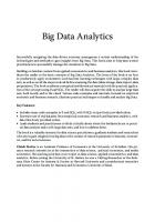
1.6.1.7 LOCATION ANALYTICS Location analytics involved much with geographical location analysis (Figure 1.16).

Introduction to Big Data Analytics

23

The key features are as follows: – Enhance business system with location-based predictions with the geographical analysis. – Maps are used for visual analytics and locate the targets groups. – Spatial analytics—combining geographical information systems with another type of analytics. – Explore the temporal and special patterns to locate specific activities or behavior. – Rich data collection: combines consumer’s demographic details, map, lifestyle, and other socio-environmental factors. – Presence of maps/GPS on all electronic gadgets.

confirmed cases Dec 31

May 31

deaths Source: World Health Organization Data may be incomplete for the current day or week

Dec 31

FIGURE 1.16

May 31

Jun 30

Sep 30

Dec 31

Mar 31

Jun 30

Sep 30

Dec 31

Mar 31

August 17, 2020 1,811,779 Confirmed Cases -78,815 Weekly Decrease -4.14% Weekly Change

Location analytics.

Source: World Health Organization covid cases.

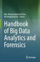
1.6.1.8 WEB ANALYTICS This type of analytics is based on the usage of websites and interactions (Figure 1.17).

Research Practitioner's Handbook on Big Data Analytics

24

The main features are as follows: – Now: the study of the behavior of web users. – Future: the study of one mechanism for how society makes decisions. – Example: behavior of web users: • Number of people clicked on a particular product or webpage. • The user location, usage of website duration, total number of sites visited and the user interface experience of the website. • What can this type of analytics tell us? • Aid in decision making and presenting the inferred information. – Commercially, it is the collection and analysis of data from a website to determine that aspects of the website achieve the business objectives.

FIGURE 1.17

Web analytics.

1.6.1.9 VISUAL ANALYTICS This type of analytics leverages the visualization techniques for presenting complex problems into simpler one (Figure 1.18).

Introduction to Big Data Analytics

25

1.7 BIG DATA ANALYTICS TOOLS WITH THEIR KEY FEATURES Big data analytics program is commonly used to evaluate a broad data collection virtually. These software analytical methods help to recognize emerging developments in the industry, consumer expectations, and other data (Husamaldin and Saeed, 2020). The cutting-edge big data analytics techniques have been the cornerstone to achieving effective data processing with the increase in big data volume and tremendous development in cloud computing. It will review the top big data analytics platforms and their main function.

FIGURE 1.18

Visual analytics.

Research Practitioner's Handbook on Big Data Analytics

26

1.7.1 BIG DATA ANALYTICS TOOLS 1.7.1.1 APACHE STORM Apache Storm is a large data computing system that is open sources and free. Apache Storm is also an Apache product that supports every programming language with a real-time application for data stream processing. It includes a distributed framework for real-time, fault-tolerant processing, with capabilities for real-time computation. About topology configuration, storm scheduler manages workload with multiple nodes and works well with the Hadoop Distributed File System (HDFS). Features • The transmission of 1 million 100-byte messages per second per node is calculated. • Storm to guarantee that the data device is processed at least once. • Great scalability in horizontal terms. • Fault-tolerance built-in. • Auto-reboot for crashes. • Clojure-written writing. • Fits with the topology of a direct acyclic graph. • Output files are in the language of JavaScript Object Notation (JSON). • Real-time analytics, log analysis, ETL, continuous computing, distributed RPC, deep learning have numerous use cases. 1.7.1.2 TALEND Talend is a tool for big data that simplifies and automates the integration of big data. Native code is generated by its graphical wizard. It also supports convergence with big data, master data processing, and data consistency tests. Features Streamlines large data with ETL and ELT. • Achieve the pace and size of the spark. • Expedites the switch to real-time.

Introduction to Big Data Analytics

27

• Handling various sizes of info. • Provides multiple connections under one roof, allowing it to tailor the solution according to its needs. • By creating native code, Talend big data platform simplifies the usage of MapReduce and Spark. • Smarter accuracy of data with machine learning and analysis of natural languages. • To speed up big data projects, Agile DevOps. • Streamline all the processes in DevOps. 1.7.1.3 APACHE COUCHDB It is an open-sources, cross-platform, document-oriented NoSQL database that strives to render a modular design simple to use and manage. It is written in Erlang, a competition-oriented script. In JSON records, Couch DB stores data that can be downloaded electronically or queried using JavaScript. With fault-tolerant storage, it provides distributed scaling. Through specifying the Couch Replication Protocol, it facilitates accessing data. Features • CouchDB is a database with a single node that functions like every other database. • It enables a single logical database server to be run on any number of computers. • The ubiquitous HTTP protocol and the JSON data format are used. • Inserting, updating, retrieving, and deleting documents is quite simple. • It should convert the JSON file into different languages. 1.7.1.4 APACHE SPARK Spark is also a very popular and open-source analytics platform for big data. Spark has over 80 operators at the highest level to render parallel applications simple to create. In a broad variety of organizations, it is used to process massive datasets.

28

Research Practitioner's Handbook on Big Data Analytics

Features

• It helps to operate an application in the Hadoop cluster, in memory up to 100 times faster and on disc 10 times faster. • It provides fast-processing lighting. • Sophisticated analytics help. • Integration capacity with Hadoop and current Hadoop data. • In Java, Scala, or Python, it provides optimized APIs. • In-memory data processing capabilities are supported by spark, which is far quicker than the disc processing leveraged by MapReduce. • Furthermore, spark operates on both cloud and on-prem HDFS, OpenStack, and Apache Cassandra, bringing another degree of flexibility to the business’s big data operations. 1.7.1.5 SPLICE MACHINE It is an analytics platform for large data. Their architecture, including AWS, Azure, and Google, is scalable across public clouds. Features • It can scale from a few to thousands of nodes dynamically to allow applications at every scale. • Each query to the distributed HBase regions automatically evaluates the splice machine optimizer. • Reduce management, deploy more rapidly, and decrease the risk. • Create, evaluate, and deploy machine learning models by consuming fast streaming data. 1.7.1.6 PLOTLY Plotly is a platform for visualization that helps users to build web-sharing maps and dashboards. Features • Convert some details easily into eye-catching and insightful graphics.

Introduction to Big Data Analytics

29

• It offers fine-grained knowledge regarding data provenance to audited industries. • Via its free city plan, Plotly provides unregulated public file hosting. 1.7.1.7 AZURE HDINSIGHT It is a cloud-based spark and Hadoop operation. It offers cloud offerings of big data in two types, regular and luxury. It provides the company with an enterprise-scale cluster for operating the big data workloads. Features • With an industry-leading SLA, efficient analytics. • It provides protection and control for enterprise-grade. • Safe computer properties and apply for access and compliance measures on-site to the cloud. • For developers and researchers, a high-productivity platform. • Integration of leading technologies for efficiency. • Without buying new hardware or paying other up-front expenses, deploy Hadoop in the cloud. 1.7.1.8 R R is a computer language and free software, and figures and images are computed here. The R language is popular for the development of statistical software and data analysis among statisticians and data miners. Many statistical tests are provided by the R Language. Features • R is often used to facilitate wide-scale statistical analysis and data visualization along with the JupyteR stack (Julia, Python, R). JupyteR is one of the fit commonly used big data visualization software, 9000 plus Comprehensive R Archive Network algorithms and modules that enable any analytical model running it to be composed in a convenient setting, modified on the go, and examined at once for the effects of the study. Language R is as follows: • Within the SQL server, R will run.

Research Practitioner's Handbook on Big Data Analytics

30

• • • • • • • •

On all Windows and Linux servers, R runs. Apache Hadoop and Spark Helps R. R is incredibly compact. R scales effortlessly from a single test computer to large data lakes on Hadoop. Effective facility for data handling and retrieval. It offers a collection of operators, in specific matrices, for calculations on arrays. This offers a cohesive, organized set of data processing large data resizes. It offers graphical data processing facilities that view either on-screen or hardcopy.

1.7.1.9 SKYTREE Skytree is a tool for big data analytics that empowers data scientists to build more precise models more quickly. It provides accurate models of predictive machine learning that are quick to use. Features • Algorithms strongly flexible. • Computer scientists’ artificial intelligence. • It helps data scientists to grasp and interpret the reasoning behind ML decisions. • Fast to use the interface or assists in programmatically using Java. SkyTree. • Interpretability of model. • It is intended to resolve robust predictive concerns with data preparation capabilities. • GUI and programmatic access 1.7.1.10 LUMIFY Lumify is considered a platform for visualization, big data fusion, and analytics. It allows users with a suite of analytical options to uncover links and explore relationships in their results.

Introduction to Big Data Analytics

31

Features

• It offers some automated formats for both 2D and 3D graph visualizations. • Connects research between graph organizations, mapping systems integration, geospatial research, multimedia analysis, collaboration in real-time across a collection of projects or workspaces. • Relevant intake processing and design components for textual information, photographs, and videos are included. • This space mechanism helps it to arrange work into a variety of tasks or workspaces. • It is focused on tested, scalable large data technologies that are focused on • Supports the ecosystem centered on the cloud. It fits for Amazon’s AWS well. 1.7.1.11 HADOOP The long-standing big data analytics leader is recognized for its capabilities for large-scale data processing. Thanks to the open-source big data system, it has low hardware specifications and can operate on-premises or in the cloud. The key advantages and characteristics of Hadoop are as follows: • Hadoop Distributed File System, targeted at HDFS (Huge-Scale Bandwidth). • An extremely configurable large data analysis model—(MapReduce). • A Hadoop resources control resources scheduler—(YARN). • The required glue to enable modules from third parties to function with Hadoop (Hadoop Libraries). It is intended to scale up from Apache Hadoop, a distributed file system, and big data handling program platform. Using the programming model MapReduce, it processes datasets of large data. Hadoop is an open-source application written in Java that offers support for cross-platforms. This is, without a doubt, the top big data platform. Hadoop is employed by over half of the Fortune 50 firms. Some of the major names like single servers on thousands of computers for Amazon Web services, Hortonworks, IBM, Intel, Microsoft, Twitter, etc.

32

Research Practitioner's Handbook on Big Data Analytics

Features • Enhancements to authentication when using HTTP proxy servers. • Hadoop compliant file system effort definition. • Help for extended attributes in the POSIX-style file system. • It creates a strong atmosphere that is well-tailored to the theoretical needs of a developer. • This adds versatility to the collection of data. • It makes it easier to process data more rapidly. 1.7.1.12 QUBOLE Qubole data service is an autonomous and all-inclusive big data platform that manages, learns, and optimizes its use on its own. This helps the data team to focus instead of maintaining the platform on company performance. Warner music community, Adobe, and Gannett are among the very, very few popular names that use Qubole. Revulytics is the nearest rival of Qubole. 1.8 TECHNIQUES OF BIG DATA ANALYSIS A collection of numbers or characters is raw data or unprocessed data. For the extraction of decision-based material, data is sampled and analyzed, while expertise is extracted from a significant amount of experience in the subject (Hazen et al., 2014). Wherever an entity or atmosphere alters, sensory experience exists. Social knowledge, the creation of rules, practices, beliefs, rituals, social functions, icons, and languages, offers citizens the skills and behaviors they need to engage in their own cultures. Phenomena in theory end up suggesting that what is perceived as the foundation of truth. Phenomena are also understood to be phenomena that appear or that human beings witness. A phenomenon can be an observable attribute and occurrence of matter, electricity, and the motion of particles in physics. Data on actual phenomena may be viewed as perception or knowledge. Geographical evidence is thus known as an observation of physical and human spatial phenomena. Geographical big data processing is targeted at investigating the complexities of geographical reality (Russom, 2011).

Introduction to Big Data Analytics

33

The characteristics of large data analysis are derived from the characteristics of large data in the form of data structural collection and structural analysis. Therefore, in Figure 1.19, six big data analytics approaches are suggested.

FIGURE 1.19

Two theoretical breakthroughs and six techniques in big data analytics.

1.8.1 ENSEMBLE TECHNIQUE Ensemble data processing, also known as multidataset processing or multialgorithm analysis, is performed on the whole data array or a large volume of data. Big data is defined as the entire data collection without any sampling purpose. What does the entire kit entail? Data from resampling, classified and unlabeled data, previous data, and subsequent data can all be used loosely. The term “ensemble” is understood in the context of ensemble learning in machine learning, the ensemble approach in statistical mechanics, and the Kalman ensemble filtering in data assimilation (Dey et al., 2018). The whole data is sometimes split into three sections, that is, training data, test data, and validation data, in supervised learning and image

34

Research Practitioner's Handbook on Big Data Analytics

recognition. The picture classifier is learned and applied to the test data using training data. Lastly, the findings of picture classification are checked by ground reality. Generally, on training data rather than test data, the classifier produces reasonable output. To accomplish a tradeoff between the complexity of the model and the classification outcome on training data, ensemble analysis is used to produce the global optimum result on the whole set of training data, test data, and validation data. Structural risk minimization is used in support vector machine learning to address the problem of overfitting, that is, the learning model is closely adapted to the particularities of training data but badly applicable to test data. 1.8.2 ASSOCIATION TECHNIQUE Big data is typically obtained without special methods for sampling. Since data developers and data users are typically somewhat different, the causeand-effect relationships hidden in scientific data are not clear to individual data consumers. The set theory, that is, the theory about participants and their relationships in a set, is general enough to deal with data analysis and problem-solving. In certain cases, the big data association (Wiech et al., 2020) is linked to the relationship of set members. Association research is critical for multisiting, multitype, and multidomain data processing. Data mining with association rule algorithms, data association in goal monitoring, and network relation research are all examples of connection research. There are two elements of association law, an antecedent (if) and a consequent (if) in the Apriori algorithm of association rules mining (then). Through analyzing data and using the support and trust criteria to identify the value of relationships, association guidelines are developed to define certain if/then patterns. Help is a metric that indicates how many items are available in the purchasing catalog. Trust is a measure of how much it has been found that the if/then claims are valid. Association rules mining is an example of transaction data calculation of conditional likelihood P (consequent/antecedent). However, unlike the asymptotic study of mathematical estimators, the usefulness of the rules relating to mined associations depends only on the thresholds of assistance and trust that users manually provide (Stucke and Grunes, 2016).

Introduction to Big Data Analytics

35

Typically, numerous sensors are used in object detection and multiple objects are traveling in a dynamic setting. Three associations of calculation (observation) data association, goal state association, and goal-tomeasurement association need to be studied to define and monitor goals. The most probable future goal position calculation is used to adjust the goal’s state estimator to enable the tracking device to work properly. A distance function from the expected state to the observed state is the likelihood of the given calculation is right. Kalman filtering is a time-varying recurrent estimator or filtering of a time series that is ideal for processing data streams in real-time. Kalman filtering, also known as linear quadratic estimation or trajectory optimization, is a time-based algorithm that produces estimates of unknown states (variables) from a set of noise-disturbed measurements (observations) that tend to be more reliable than single-calculation methods. The covariance of state error and operator of state prediction is regarded as stochastically and deterministically as state associations. Similarly, the covariance and observation operator of measurement loss are considered stochastically and deterministically as measurement relations (Mithas et al., 2013). In a way, the association of data and the pace of big data is defined by the Kalman filtering. Social people and social interactions form a social network of social networking. Concepts and logical connections constitute a cognitive network of natural language or mental models. The associations of networks, often called connected data, are typically formalized by social ties and logical relations. The network, in essence, is a topological construct. The network relation defines the community or community, which may also be considered an alliance. The interaction in big data is essentially known to be the partnership in set theory. Associations are formalized as advanced partnerships as metrics are allocated. Statistical connections and geometric relation, for example, are correlations eventually assigned to the probability metric and geometric metric. 1.8.3 HIGH-DIMENSIONAL ANALYSIS Big data implies a large variety of data. The mathematical space (object) dimension is defined as the minimum number of coordinates required to specify any point within it, and the vector space dimension is defined as

36

Research Practitioner's Handbook on Big Data Analytics

the number of vectors on any space basis or the number of coordinates required to specify any vector in mathematics. The material dimension is a property of the material that is independent of the space in which it is embedded. The dimension refers to the number of points of view from which the physical world can be discerned. Classical mechanics explains the physical world in three dimensions. Starting from a certain point in space, the basic ways in which to pass are up/down, left/right, and forward/backward. Concerning time, the equations of classical mechanics are symmetric (Elahi, 2019). Time is directional in thermodynamics, concerning the second thermodynamic theorem, which specifies that the entropy of an independent system never decreases. Such a structure progresses naturally into a thermodynamic equilibrium of maximum entropy states. Multidimensional analysis for a sample (realization) of multiple random variables is available in statistics and econometrics. In classical multivariate review, high-dimensional statistics analyze data whose scale is greater than certain measurements. Even the data vector component can be greater than the sample size in certain implementations. Usually, in big data analysis, the curse of dimensionality emerges. Once the dimensionality increases, the space volume increases so rapidly that the data available become sparse. This sparsity will lead to the statistical error of significance and the dissimilarity between objects in high-dimensional space when handling traditional data algorithms. This paradox does not exist in low-dimensional space; however, it only occurs in high-dimensional space, which is known as the dimensionality curse. Using distance or variance metrics, dimension reduction is a way of minimizing the number of random variables by choosing a subset of the original variables (called subspace) to conserve the volatility of the original variables as much as possible. There exist linear and nonlinear transforms of dimension reduction. The primary component analysis, for example, is a linear transformation of dimension reduction. 1.8.4 DEEP ANALYTICS Today, the amount of evolving data is high enough for difficult training on artificial neural networks. In the meantime, multicore CPU, GPU, and FPGA high-performance computing systems dramatically decrease the

Introduction to Big Data Analytics

37

training period of deep artificial neural networks. Typical artificial neural networks are dynamically enhanced in such cases, with hidden layers of latent variables, and so-called deep learning, as opposed to shallow learning, is created. It is often assumed that as its understanding grows rich, human awareness of the natural world is rising deeper. The opportunity for deep research is to discover the dynamic structural properties of big data. Via deep research, unobservable variables, secret factors, secret hierarchies, contextual associations, and the dynamic distribution of random variables can be identified. The latent Dirichlet allocation models, the deep Boltzmann machine, the deep belief net, the hidden Markov model, and the Gaussian mixture model typically exist. Multilayered artificial neural networks are used to create deep learning architectures. In a general artificial neural network, there are numerous nonlinear neuron processing units (activation units), such as the sigmoid function. Different neurons from each layer are viewed as multiple variables in principle. Deep analysis is considered as a deterministic (or stochastic) translation function from input to output. Theoretical mechanisms for developing multilayered artificial neural networks can be used as theoretical approximation models, data-fitting functions, and maximum likelihood estimators. In complex data modeling, the multilayered artificial neural network, which has multiple layers, multiple variables, and nonlinear activation units, is very successful. However, for deep learning of some dynamic functions, there are no universal theories of approximation available so far. The output of different architectures, which are not always tested on the same datasets, cannot be compared all together. In multivariate multilayered neural networks that are completely connected or sparsely linked, multiple parameters must be determined, including the number of layers, the number of units per layer, the weights, and thresholds of each activation unit. By finding a maximal answer to the data appropriate function or mathematical estimator, this will increase the issue of ill-posed problems and low measurement performance. Overfitting and expensive computing time are typical outcomes of the complicated paradigm. To solve these fitting issues, regularization techniques are developed. To boost the performance, several numerical algorithms have been developed, such as pretraining, concave-to-convex approximation, and computing the gradient on several training datasets at once.

38

Research Practitioner's Handbook on Big Data Analytics

1.8.5 PRECISION METHODS Precision is the resolution of the representation, which is often determined by the number of decimal or binary digits. Accuracy is the similarity of a calculation to the true value of numerical analysis. Instead of detail and accuracy, bias and heterogeneity are included in the statistics. Bias is the amount of inaccuracy, and heterogeneity is the quantity of imprecision. In fact, the truth of a series of calculation outcomes is the average’s closeness to the actual (true) value, and accuracy is the consistency of a set of results. Ideally, with measures all like and closely grouped around the true meaning, a measuring system is both exact and reliable. A measuring method, one or both, maybe exact but not exact, is reliable but not precise. Increasing the sample size usually improves precision when an experiment involves a systemic mistake but does not boost precision. The removal of systemic errors increases precision but does not modify accuracy. A precision review is used from the viewpoint of data utility and data accuracy to determine the veracity of data. 1.8.6 DIVIDE-AND-CONQUER TECHNIQUE Divide-and-conquer is a mathematical methodology for improving problem-solving efficiency and the speed at which large data is analyzed. Divide-and-conquer analysis is used to recursively separate a problem into two or three subproblems in the stage of division, until they become simple enough to be solved automatically in the stage of conquest. When both subproblems have been solved, they are combined into a single answer to the main problem. Distributed computing, such as cloud computing and distributed information computing, can be thought of as divide-and-conquer in space, whereas parallel computing (multicore computing and cluster computing) can be thought of as divide-and-conquer in time. In terms of unstructured data and time limits, steam generation and realtime computing are a divide-and-conquer calculation. From the perspectives of virtualized networks and culture of mind, cloud computing and interactive information computing are more akin to divide-and-conquer computing. In a shared-memory multiprocessor, high-performance concurrent processing utilizes parallel algorithms, whereas distributed algorithms are

Introduction to Big Data Analytics

39

used to coordinate a large-scale distributed machine. In multiprocessor computers, divide-and-conquer analysis is quickly executed, and separate subproblems may be executed on different processors. By transmitting messages between the processors, information is shared. To solve a query, concurrent computation requires several computational elements concurrently. This is done by splitting the issue into different components such that each processing component will perform the algorithm component concurrently with the others. The processing components may be complicated, requiring the resizing of multiple processors and many networked computers, such as a single computer. After frequency scaling hit a ceiling, multicore systems became more prevalent and concurrent algorithms became widespread. A multicore processor is a single-chip processor with multiple processing units (cores). The main memory of a parallel computer is either shared memory (all processing elements share a common address space) or distributed memory (each processing element has its own local address space). Parallel processing is a method of computing in which many operations are carried out at the same time, allowing complicated problems to be broken down into smaller bits and solved at the same time. Parallel computing is made up of many layers of bit, instruction, input, and task parallelism. These subtasks will then be performed by the processors concurrently and mostly cooperatively. OpenMP is one of the most frequently used shared memory application programming interfaces (APIs) in programming languages, although the message passing interface is the most frequently used API for message-passing applications. A concurrent computation programming framework is MapReduce in the machine cluster. Concerning data organized in (key, value) pairs, the map and reduce functions of MapReduce are both specified. All maps may be done in tandem, providing that each mapping process is independent of the others. At the same time, all outputs of the map operation which share the same key are presented to the same reducer. Then, the reduce function is added to and category in parallel. However, MapReduce differs from relational databases in that it lacks a structural data schema and allows for quick evaluation of B-tree and hash partitioning techniques, and it is mostly used for simple or one-time retrieval tasks (Elahi, 2019).

40

Research Practitioner's Handbook on Big Data Analytics

The data processing date, time constraints, and time validity are all important in real-time computation. A real-time database is a database system that manages constantly changing workloads using real-time computation. This differs from traditional databases of permanent records in that it remains mostly intact over time. A stream is a series of data or a sequence of operations. Nonstructural data and infinite-size continuous data are other terms for streaming data. Unlike archived data, stream data is usually a real-time, read-only sequence. For the streaming data portion, incremental update, and Kalman filtering, the time window of data processing has implications for the data sampling rate and underlying temporal similarity of windowed data. Both nodes are on the same local network in cluster computing and use identical hardware. A computer cluster is a community of computers strongly coupled that operate tightly together such that they can be viewed as a single computer in certain respects. Multiple standalone computers linked by a network are comprised of clusters. Nodes are shared around globally and administratively dispersed networks of grid computing, and they utilize more heterogeneous hardware. The most distributed method of parallel computing is grid computing, and it allows the use of machines that connect across the Internet to operate on a given topic. In distributed computing, a problem is divided into several operations, each of which is resolved by one or more machines that communicate by exchanging messages, and each computer has its own private memory (distributed memory). Computational structures are referred to as devices or nodes. A distributed structure of databases consists of locations that are closely connected and do not share physical components. The distribution is translucent, that is, as though it were one abstract structure, consumers can communicate with the system. Also, transactions are open, ensuring that each transaction must preserve the credibility of the database across several databases. Cloud computing, also known as on-demand computing, is a form of Internet-based computing that delivers pooled processing services and data to computers and other devices on-demand, allowing for ubiquitous, on-demand access to a common pool of configurable computing resources. Compared to conventional parallel computing methods, cloud computing offers the resizes and technology to create data/computation-intensive

Introduction to Big Data Analytics

41

parallel applications at far more accessible rates. Virtualization is the primary supporting technology for cloud computing. Virtualization software splits a real computer machine into one or more “virtual” units, each of which can be used and managed to perform computing tasks. Service-oriented architecture concepts are used in cloud computing to help consumers break down problems into services that can be integrated to provide a solution. According to numerous models, cloud-computing companies provide their “packages,” which shape a stack, that is, infrastructure, platform, and software as a service. The human–machine–environment interface mechanism can be loosely conceptualized in distributed intelligence computing to be a mechanism of agents. Individuals’ rationality is limited by the intelligence available, the tractability of the judgment question, the cognitive limitations of their brains, and the time available to make the decision, according to Simon’s theory of bounded rationality. A rational agent is one who has simple expectations, models ambiguity using variables’ expected values or functions, and frequently chooses the action with the best-expected effect for himself from among all possible actions. Something that makes choices, usually a human, computer, or software, maybe a logical agent. An intelligent agent is an autonomous entity that observes and acts on an environment utilizing actuators by sensors and guides its behavior toward achieving objectives. Intelligent agents can often learn to accomplish their objectives or use intelligence. 1.8.7 GEOGRAPHICAL BIG DATA METHODS Six big data analytics methods are still applicable for spatial big data. The unique thing about spatial big data is the spatiotemporal association, such as geometric associations, mathematical similarities, and semantic connections, compared to general big data. Geometrical calculation research, human spatial data analysis, and physical spatial analysis may be loosely grouped into spatiotemporal data analysis. The artificial planet, smart planet, and earth simulator analytics are partially suggested by three kinds of study. The human–machine–environment scheme is gradually being encountered in digital form through the creation and implementation of device

Research Practitioner's Handbook on Big Data Analytics

42

and communication technology. A vast amount of spatial data, such as satellite imagery of earth observation and data from the mobile Internet, is gathered jointly or independently. In certain instances, independent of technology domains and sampling methods, spatial big data is virtually the whole data collection. Ensemble data processing is commonly applied to large data in geography. Geometrical relations, mathematical associations, and semantic relations are classified into spatiotemporal relations. Space and time in mathematics may be formalized into geometric quantities. Measurement modification in surveying, for example, is the least square measurement of angles, corners, and elevations of geometrical features (parameters). The duration is scaled by the velocity of objects “motion, such as heavenly bodies” timing objects and atom clocks. Currently, for a vast number of georeferenced details, physical and human geographical phenomena are detected utilizing different survey tools. In the modern environment, the machine digitally tracks topographical observation and geographical phenomenon sensing, and geometrical interaction analysis in geographical big data analytics is stressed. KEYWORDS • • • • • • •

big data structured data unstructured data volume velocity variety veracity

REFERENCES Andrejevic, M.; Gates, K. Big Data Surveillance: Introduction. Surveillance Soc. 2014, 12 (2), 185–196. Anuradha, J. A Brief Introduction on Big Data 5Vs Characteristics and Hadoop Technology. Procedia Comput. Sci. 2015, 48, 319–324.

Introduction to Big Data Analytics

43

Dey, N.; Hassanien, A. E.; Bhatt, C.; Ashit, A.;Satapathy, S. C., Eds. Internet of Things and Big Data Analytics toward Next-Generation Intelligence; Springer: Berlin, 2018; pp 3–549. Elahi, I. Scala Programming for Big Data Analytics: Get Started with Big Data Analytics Using Apache Spark; Apress, 2019. ISBN: 9781484248102. Engelbrecht, E. R.; Preez, J. A. D. Introduction to Quasi-open Set Semi-supervised Learning for Big Data Analytics, 2020. Goul, M.; Sidorova, A.; Saltz, J. Introduction to the Minitrack on Artificial Intelligence and Big Data Analytics Management, Governance, and Compliance, 2020. Hazen, B. T.; Boone, C. A.; Ezell, J. D.; Jones-Farmer, L. A. Data Quality for Data Science, Predictive Analytics, and Big Data in Supply Chain Management: An Introduction to the Problem and Suggestions for Research and Applications. Int. J. Product. Econ. 2014, 154, 72–80. https://searchbusinessanalytics.techtarget.com/definition/big-data-analytics https://www.sas.com/en_in/insights/analytics/big-data-analytics.html Husamaldin, L.; Saeed, N. Big Data Analytics Correlation Taxonomy. Information 2020, 11 (1). Kankanhalli, A.; Hahn, J.; Tan, S.; Gao, G. Big Data and Analytics in Healthcare: Introduction to the Special Section. Inform. Syst. Front. 2016, 18 (2), 233–235. Kim, H.; Pries, R. D. Big Data Analytics; Auerbach Publications, 2015. ISBN: 9781482234527. Loshin, D. Big Data Analytics; Morgan Kaufmann, 2013. ISBN: 9780124186644. Michael, K.; Miller, K. W. Big Data: New Opportunities and New Challenges [Guest Editors’ Introduction]. Computer 2013, 46 (6), 22–24. Mithas, S.; Lee, M. R.; Earley, S.; Murugesan, S.; Djavanshir, R. Leveraging Big Data and Business Analytics [Guest Editors’ Introduction]. IT Professional 2013, 15 (6), 18–20. Renuka Devi, D.; Sasikala, S. Feature Selection and Classification of Big Data Using MapReduce Framework. In Intelligent Computing, Information and Control Systems. ICICCS 2019. Advances in Intelligent Systems and Computing; Pandian, A., Ntalianis, K., Palanisamy, R., Eds., Vol. 1039; Springer, Cham, 2020. Russom, P. Big Data Analytics. TDWI Best Practices Report, Fifth Quarter 2011, 19 (4), 1–34. Saltz, J.; Sidorova, A. Goul, M. Introduction to the Minitrack on Artificial Intelligence and Big Data Analytics Management, Governance, and Compliance. In Proceedings of the 53rd Hawaii International Conference on System Sciences, 2020. Stucke, M. E.; Grunes, A. P. Introduction: Big Data and Competition Policy. Big Data and Competition Policy; Oxford University Press, 2016. Tsai, C. W.; Lai, C. F.; Chao, H. C.; Vasilakos, A. V. Big Data Analytics: A Survey. J. Big Data 2015, 2 (1), 1–32. Wiech, M.; Boffelli, A.; Elbe, C.; Carminati, P.; Friedli, T.; Kalchschmidt, M. Implementation of Big Data Analytics and Manufacturing Execution Systems: An Empirical Analysis in German-Speaking Countries. Production Planning & Control, 2020; pp 1–16.

CHAPTER 2

Preprocessing Methods ABSTRACT This chapter outlines the need for preprocessing data and various methods in handling the same. Both text and image preprocessing methods are also highlighted. As the data are collected from various resources, it might contain discrepancies and inconsistencies in data representation. To overcome the same, the pre-processing methods used are data cleaning, data integration, data transformation, data reduction and data transformation. The various pre-processing algorithms under each category are discussed with a neat procedure and examples. The challenges of big data stream processing are also highlighted. At the end of the chapter text and image pre-processing methods are discussed with examples for clear understanding. 2.1 DATA MINING—NEED OF PREPROCESSING Before we discuss the challenges in data mining, let us understand the life cycle of Machine Learning (ML) process. The life cycle of any ML starts with data gathering or data acquisition. This is presented in Figure 2.1. “Data” is vital for any data analytics process. Understanding data and preparing the data for further analytics is indeed considered to be a crucial step in mining. A core collection of (García et al., 2016) approaches are called as “data preprocessing,” which is applied before the analytics process. This is the part of the knowledge discovery (Zaki and Meira, 2014). Research Practitioner’s Handbook on Big Data Analytics. S. Sasikala, PhD, D. Renuka Devi, & Raghvendra Kumar, PhD (Editor) © 2023 Apple Academic Press, Inc. Co-published with CRC Press (Taylor & Francis)

Research Practitioner's Handbook on Big Data Analytics

46

FIGURE 2.1

Life cycle.

As the data are collected from various resources, it might contain discrepancies and inconsistencies in data representation. Streaming data are collected at a very fast rate across verticals. When this kind of scenario emerges, it is obvious that an enhanced mechanism is required to handle them effectively. Thus, preprocessing algorithms have been proposed by various researchers. The objective of any algorithm is to: •

• •

Handle—real-time data ○ Real-time data consists of noise ○ Incomplete information ○ Errors ○ Outliers Handle—streaming characteristics of data Handle—scalability issues

Preprocessing Methods

47

Issues and Challenges Most of the common problems are listed below: • Incomplete data • Error due to manual typing • Inconsistent data • Raw data format • Mismatch in representing numerical values • Data-type error • Crashed file • Irrelevant data Incomplete Data Not all data are complete; some datasets will have junk values or incomplete information. Different approaches are proposed for handling those types of issues. First, we have to explore the causes of the missing data and find the reasons behind that. This is usually identified from the following perspectives: • The random nature of missing is that the missed data has no relation with any of the data points present in the dataset. There is no dependency of missed value with the rest of the data present. The entry is simply missed out or not captured that is why it is not recorded. • Second perspective is that, still the random nature of value is missing but it has some relevance with the existing data. Some point of relevancy exists between them. Some values are purposely missed out based on the other data values. • In the third one, there is a complete dependency that exists and apparently the data is omitted. The missed values can be treated for all aforesaid cases. If no relevance exists, we can very well omit the data, but if there is relevance then deletion and omission can lead to anomalies. When we try to delete records that may less represent a particular class in the entire dataset. Another possible method is to replace the missed value with some other value based on statistical measure. Error Due to Manual Typing Data inconsistency arises when the user commits a typo error. For example, entering string values in the numeric data field or appending some special

48

Research Practitioner's Handbook on Big Data Analytics

characters to the numeric value. To change this, either remove the special character or transform the non-numeric into numeric field. Inconsistent Data The variations in the data are called as “inconsistency.” This is considered to be a major issue in preprocessing. For example, the same value is represented in two different forms but the meaning of both the terms is same. For example, zero or 0 is the same, but different representations for the same field lead to inconsistency. For the entire datasets, the unique way of representation has to be followed for the same field. Providing more than one value to a single column also leads to inconsistency. Raw Data Format Data in all forms can be collected for analytics. When we collect the data in raw format, make sure that in which format it is to be represented. For example, Date of birth is represented in many formats, therefore decide on which format (dd/mm/yyyy or mm/dd/yyyy) that the date has to be represented in the dataset. Always check and verify the same for inconsistencies. Mismatch in Representing Numerical Values Numerical data can be expressed in various metrics like grams or kilograms, temperature in Celsius or Fahrenheit. The common representation of units is decided and it is uniformly represented across the dataset. Data-type Error Human error or incorrect representation of data can lead to inconsistency. The data representation is verified and checked before the analytics process. Crashed File When we try to import some files into native formats, the file may get crashed because of software we use for conversion. File manipulation is the biggest issue when we try to convert one file format into another. Irrelevant Data Some of the gathered data may contain sensitive information (like password, pin number, etc.), those data should be eliminated before the process.

Preprocessing Methods

49

2.2 PREPROCESSING METHODS The various types of preprocessing methods are given in Figure 2.2.

FIGURE 2.2

Overview—preprocessing methods.

2.2.1 DATA CLEANING Cleaning of data is done by replacing the missed data with some values, removing noisy elements, detecting outliers, and inconsistencies. The objective of this process is to enhance the quality of data. The quality of data degrades when they are incorrectly represented. The noisy data reduces the accuracy of the ML model that leads to poor performance. Various reasons for unclean data are listed below: • • • • •

Data missing—absence Violation of rule or representation error Data integrity Data mismatch or represented in various format for the same column Wrong usage of primary keys

2.2.2.1 MISSING VALUE Once the missing values are identified, it should be handled. Several techniques are available to handle the missing data, but the appropriate

50

Research Practitioner's Handbook on Big Data Analytics

method is chosen based on the datasets. The other factors like specific domain, data mining process is also taken for consideration. The ways of handling missed data are: • Ignore—Missing data is completely ignored. That is the row with the missing value is deleted. Deletion should not result in poor performance. This is very tedious and a time-consuming process. This method is not considered for large- scale problems. The deleted row should not completely ignore the significant features. • Constant—Replace the missed value with a constant. For example, zero or NULL can be used to replace the missed values all over the dataset. Global hard encoding, one-to-one mapping techniques are existing for this purpose. • Mean—Mean of the column values is used for replacing the null values. For example, if the salary column has the missed value, the mean of all salaries can be calculated and replaced uniformly to all the null values. Statistical measures can also be employed. • Forward/backward fill—The preceding or succeeding values of the specific columns are used. • Algorithm—Use specific an algorithm for predicting the missed value. Algorithms The overview of the algorithm used for handling “missing value” is presented below: • Statistical Method ○ Ignoring method—List-wise deletion, Pairwise deletion ○ Missing data model—Maximum Likelihood, Expectation Maximum Algorithm • Machine Learning Method ○ Imputation Techniques ▪ Mean and Median ▪ Regression ▪ Multiple imputation ▪ k-Nearest Neighbor ▪ k-means ▪ Fuzzy k-Mean

Preprocessing Methods

51

2.2.2.2 NOISY DATA Noisy data can arise during typo error, data collection from sensors/ devices, and so on. For example, erroneous encoding for female is “E” instead of “F,” negative value for the numeric field where it has to be positive (Salary = −20000) and so on. Noisy data are well handled by the binning techniques. The given data is sorted and separated into number of bins. Partitions of the bins are done with equal width and height. Once they are segregated, smoothening is applied. In this way, outliers are identified and removed. Box-plot method is also very helpful in identifying the outliers. The various types of noises are depicted in Figure 2.3.

FIGURE 2.3

Types of noises.

From Figure 2.3, we can infer the following: Class noise occurs when the output class label is incorrect (Mislabeled) and attribute noise occurs when there is an attribute error/missing value error. The various filters are used to remove the noises, • • •

Ensemble-based filtering Iterative-based filtering Metric-based filtering

52

Research Practitioner's Handbook on Big Data Analytics

The list of other approaches is presented in Figure 2.4.

FIGURE 2.4 Noise filter algorithms.

2.2.2 DATA INTEGRATION Integration means collations of data from various sources. The format of data is either structured, unstructured, or semistructured. The data source can be of a single type or heterogeneous. When we gather data from multiple sources the following issues may arise. They are the following: • Merging different schema formats into combined format is a challenging task. For example, the Employee name is “empname” in database, the same column is represented by “Ename” in another schema definition. When we integrate, we have to resolve this issue and establish a single representation for the employee’s name column. • Data representation in different formats is verified and uniform representation is devised. For example, weights are represented by grams or kilograms. The conflict has to be resolved and appropriately represented. • When we integrate, there is a possibility that the same feature is repeated, leading to redundancy issues.

Preprocessing Methods

53

2.2.3 DATA TRANSFORMATION This is conversion of data into other forms, like aggregation or generalization of datasets. They are the following: Normalization Normalization is a scaling technique that transforms the data into rage between 0 and 1. But the originality of the data remains the same even though after transformation. This method is applied when the attributes are on different scales. The widely used methods are as follows: • • •

Z normalization Min–max normalization Mean normalization

Z Normalization Z normalization is also called “standardization.” This can done by the following equation: x−µ Z= σ Z = standard score

x = observed value

μ = mean of the sample

σ = standard deviation of the sample

Min–Max Min–max scales the given value into a range [0,1]. The equation is given as x′ =

x − min( x) max( x) − min( x)

Min and max are the minimum and maximum value in the dataset, respectively. Mean The mean of the values is used in the equation. And the transformations is done by the equation x′ =

x − average( x) max( x) − min( x)

Research Practitioner's Handbook on Big Data Analytics

54

2.2.4 DATA REDUCTION Data reduction is done when the dataset is large, and not all the features are significant for data analysis. Thus, reduction allows selecting only the optimal features by reducing the total number of features significantly. This way reduction enhances the mining process with only imperative features. Let us discuss the techniques of reduction as follows: • • •

Data cube aggregation Dimensionality reduction Data compression

2.2.4.1 DATA CUBE AGGREGATION Aggregation means combining the data in a simpler form. For example, if the dataset contains sales data for a year, but only a quarterly sales report is to be presented then we can collate the three months data into one. We can summarize and present the data. 2.2.4.2 DIMENSIONALITY REDUCTION This is the process of removing features, thereby reducing the dimensions of the dataset. The methods used for the selection process are forward selection, backward selection, and so on. When the features are reduced, make sure that it should not eliminate important ones. Forward Selection Forward selection starts with an empty set, features are added incrementally to form the final subset (Figure 2.5). Backward Selection In this method, all the given attributes are taken into consideration. At every iteration, the features are removed one by one thus producing the condensed subsets (Figure 2.6).

Preprocessing Methods

FIGURE 2.5

Forward selection.

FIGURE 2.6

Backward selection.

55

Feature Selection Feature selection (FS) is to select the significant features thereby reducing the extraneous and superfluous features with the objective to enhance the performance of machine learning model (Hall and Smith, 1998). The derived subsets have to maintain the originality and properly describe the characteristics of the given dataset.

56

Research Practitioner's Handbook on Big Data Analytics

The FS process may introduce generalizations and overfitting issues. Generally, in big data analytics, FS plays a vital role because reducing the feature space is an important and challenging task. 2.2.4.3 DATA COMPRESSION Compression is the process of reducing the size of the features for the sake of the mining process. It can be either lossy or lossless. In the lossy approach, the quality is compromised during the compression process, wherein lossless preserves the quality of data after compression. Lossless Compression Encoding approaches are commonly used for lossless compression. This algorithm maintains the precise form of the original data even though they are converted into another form. Lossy Compression Transformation techniques such as wavelet transformation, principal component analysis are employed for compression. The compressed data may vary from the original but useful for analysis for large-scale problems. 2.2.5 DATA DISCRETIZATION For any data analysis, domain and type of data should be known before applying any data-mining algorithms. The types of data such as categorical, nominal, and discrete must be handled in a specific way. For example, the categorial value is considered important in node split-up in a decision tree. If the data is continuous in nature, then discretization of data is done priorly before the induction process begins. This is done by splitting the attributes in a range of continuous values and giving them separate labels for the same. This way it is used to make the mining process easier. From the example given in Figure 2.7, the age attribute values are split into three groups and each group is given labels to identify. The discretization types are top-down and bottom-up. The techniques for discretization are given below:

Preprocessing Methods

57

• Histogram—It is a plot that represents the frequency distribution of data in continuous form. The distribution of data is depicted in such a way that we can understand the distribution pattern very well. • Binning—The continuous data is divided into number of bins • Cluster analysis—Grouping the similar data together • Decision tree analysis—Building decision tree based on the node split-up criterion • Partitioning datasets—Equal width and depth partitioning

FIGURE 2.7

Discretization process.

2.2.6 IMBALANCED DATA—OVERSAMPLING AND UNDERSAMPLING The class imbalance (López et al., 2013) occurs in data mining, where there is less representation of records for a particular class. If it is not treated may give rise to overfitting or underfitting difficulties. The analysis results of the imbalanced datasets are quite often biased toward the negative class, and then ultimately model prediction may result in higher misclassification error rate. The datasets that contain more samples are called majority class and less representation of any class is called as a minority. The cost of misprediction is complex in minority classes compared with majority classes. Multiclass imbalance can happen when a dataset represents all the instances that belong to one of many target classes. It is the combination of several minority and majority classes.

Research Practitioner's Handbook on Big Data Analytics

58

To overcome this issue, resampling methods are employed for suitable data balance. Resampling is achieved by shuffling and rearranging the given datasets to maintain the balance. Sampling techniques are categorized as undersampling and oversampling (Tanha et al., 2020). The two methods available (Figure 2.8) for class imbalance issues are: • Undersampling—Subset of features are created by removing the majority features • Oversampling—Features are created by replicating the existing (minority) features

FIGURE 2.8

Undersampling and oversampling.

Undersampling is applied to reduce the number of occurrences of majority classes. The advantage of this method is less computational complexity and less memory requirements. Random sampling is one of the commonly used methods for handling undersampling. The disadvantage of undersampling is that sometimes removal of data instances might remove the significant records as well. Oversampling is done by replicating some data instances in such a way that class balance is maintained. The main advantage of this method is that we retain all the records at the same time; repetition might lead to computational complexity. The simplest method of oversampling is random oversampling which randomly chooses the minority class instances and duplicates them. The disadvantage of this method is overfitting. Oversampling is applied to minority classes by SMOTE (Synthetic Minority Oversampling Technique). SMOTE technique handles the

Preprocessing Methods

59

imbalance between majority and minority classes and also removes noise (Pan et al., 2020). When SMOTE (Figure 2.9) is applied, the synthetic samples are generated for minority classes. The working procedures are as follows: Procedure • A random data from the minority class is chosen • The k-nearest neighbors from the data point are created • Synthetic data is generated between a random point and one of the nearest neighbor points • This procedure is repeated for the number of times, until we have an equal proposition of minority and majority classes

FIGURE 2.9

Synthetic minority oversampling technique.

2.3 CHALLENGES OF BIG DATA STREAMS IN PREPROCESSING The fundamental characteristics of Big Data are already presented in Chapter 1. To extend the same, the challenges of preprocessing methods for big data streams are discussed in this section. Various preprocessing

Research Practitioner's Handbook on Big Data Analytics

60

approaches for handling big data have been proposed. The challenges are outlined below, • Conventional approaches are mostly full batch loading of features, but streaming features are incremental; they have to be processed immediately once they are gathered. Automated approaches are indeed required to process the features as soon as they arrive and fine-tune the parameters as well. • Importantly, all the updation has to be synchronized with the model. Otherwise, the predictive model cannot accommodate the changes made upon the arrival of new features. • To apply this change to the machine learning model, increment learning approaches have been proposed for updating the induction model incrementally (Renuka Devi and Sasikala, 2019). The most of the contributions for preprocessing methods in big data analytics is based on MapReduce, Apache Spark, Flink (García et al., 2016) Twister, (Massively parallel feature selection) MPI, and MATLAB. The feature selection methods are elaborately discussed in Chapter 3. The various preprocessing methods for big data streams processing are presented in Figure 2.10. Most of the approaches are based on parallel MapReduce-based system distributed across the nodes. 2.4 PREPROCESSING METHODS 2.4.1 TEXT PREPROCESSING METHOD The main components of text preprocessing are: • • • •

Tokenization Normalization Substitution Noise—removal

Tokenization Tokenization is a process of dividing the given texts into number of smaller parts called “tokens.” The large sentence taken for preprocessing is divided into number of sentences, then sentences are further split into a number of words. Further analytics is applied to the smaller token. This is

Preprocessing Methods

61

also called as “token analysis” or segmentation. Segmentation is preferred when larger texts are taken for analysis. The process of tokenization is presented in Figure 2.12.

FIGURE 2.10

Overview of big data preprocessing algorithms.

62

Research Practitioner's Handbook on Big Data Analytics

FIGURE 2.11

Text preprocessing method.

FIGURE 2.12

Tokenization.

Normalization Converting the texts into a form of uniformity is called “Normalization.” Stemming and lemmatization are the basic steps of normalization. Stemming is applied to remove the affixes from the word. For example, if

Preprocessing Methods

63

the word is “Travelling,” after stemming the word “Travel” is derived. Lemmatization is to form the lemma of the word given. The other methods are converting into upper/lower case, removal of punctuation/stop words, white space removal and numbers removal, and so on. The following example (Figure 2.13), the raw text forms are normalized into a meaningful form.

FIGURE 2.13 Normalization.

Noise Removal Noise removal is the process of removing the unnecessary elements from the given text. This is imperative in text analytics, and problem-specific. When we analyze tweets, it is obvious that the tweeted text may contain hashtags or some special characters. Those characters have to be treated and removed because they may lead to noise. Let us explain with an example (Figure 2.14), noisy input is converted into stemmed word that still contains the meaningless form. When the noise is removed or cleaned before the stemming process, it will result in a proper lemma form.

64

FIGURE 2.14

Research Practitioner's Handbook on Big Data Analytics

Noise removal.

2.4.2 IMAGE PREPROCESSING METHOD The objective of image processing is to enhance the image. This is done by removing the distortions and noises. The broad categories of image preprocessing techniques are pixel transformation, geometric transformations, filtering, segmentation, and image restoration. Pixel Transformation Pixel transformation changes the brightness of the pixels based on the properties of the image. The output of the transformation depends only on the input. Image transformations include contrast adjustment, color correction, and brightness adjustment. Enhancing the contrast of the pixels is really significant in the field of medicine, vision, speech recognition, video processing, etc. The types

Preprocessing Methods

65

of brightness transformations are brightness corrections and gray-scale transformation. The commonly applied operations are Gamma correction, sigmoid stretching, and histogram equalization. Gamma Correction Gamma correction is applied to individual pixels when the objects present in the image are not clear (Figure 2.15). The correction is nonlinear transformation to the pixels present. This is represented by the equation γ

 I  o  =  × 255  255 

FIGURE 2.15

Gamma correction.

Sigmoid Sigmoid or logistics function is applied for contrast adjustment (Figure 2.16). This statistical equation is given as:

66

Research Practitioner's Handbook on Big Data Analytics

f ( x) =

1 1+ e −tx

g( x, y ) =

1 1+ e(c*(th− fs( x, y )))

The adjusted image is g(x, y), c = contrast factor, th = threshold, and the input image is fs(x, y).

FIGURE 2.16

Sigmoid.

Preprocessing Methods

67

When we change the contrast factor, the images change accordingly. Histogram A histogram is a common enhancement technique used in most of the applications. The advantage of this method is its compatibility. It can be applied to all types of images and shows enhanced performance. The histogram method employs a nonlinear transformation function to map the intensity of the input and output pixel. The equalization is applied using a function P(N)= number of pixels with intensity/total number of pixels. The equalization transformation is shown in Figure.2.17.

FIGURE 2.17

Histogram equalization.

Research Practitioner's Handbook on Big Data Analytics

68

KEYWORDS

• • • • • • •

machine learning preprocessing data cleaning normalization data integration data transformation data reduction

REFERENCES Roy, A.; Rafael, M. O.; Cruz, R. S.; George, D. C. Cavalcanti. A Study on Combining Dynamic Selection and Data Preprocessing for Imbalance Learning. Neurocomputing 2018. Chen, F.; Jiang, L. A Parallel Algorithm for Data Cleansing in Incomplete Information Systems Using Mapreduce. In 10th International Conference on Computational Intelligence and Security (CIS); Kunmina: China, 2014; pp 273–277. del Río, S.; López, V.; Benítez, JM.; Herrera F. On the Use of Mapreduce for Imbalanced Big Data Using Random Forest. Inf. Sci. 2014, 285, 112–137. Dubey, A. K.; Kumar, A.; Agrawal, R. An Efficient ACO-PSO-Based Framework for Data Classification and Preprocessing in Big Data. Evol. Intel. 2020. García, S.; Ramírez-Gallego, S.; Luengo, J. Big Data Preprocessing: Methods and Prospects. Big Data Anal. 2016, 1, 9. https://doi.org/10.1186/s41044-016-0014-0 Hall, M. A.; Smith, L. A. Practical Feature Subset Selection for Machine Learning, 1998; pp 181–191. https://machinelearningmastery.com/what-is-imbalanced-classification/ https://medium.com/@limavallantin/dealing-with-data-preprocessing-problemsb9c971b6fb40 https://sci2s.ugr.es/noisydata https://serokell.io/blog/data-preprocessing https://towardsdatascience.com/data-preprocessing https://towardsdatascience.com/having-an-imbalanced-dataset-here-is-how-you-can-solve-it1640568947eb https://www.geeksforgeeks.org/data-reduction-in-data-mining/ https://www.kdnuggets.com/2017/12/general-approach-preprocessing-text-data.html https://www.kdnuggets.com/2019/04/text-preprocessing-nlp-machine-learning.html https://www.mygreatlearning.com/blog/introduction-to-image-preprocessing/ https://www.tutorialspoint.com/big_data_analytics/big_data_analytics_lifecycle.htm

Preprocessing Methods

69

Tanha, J.; Abdi, Y.; Samadi, N.; Razzaghi, N.; Asadpour, M. Boosting Methods for Multi-Class Imbalanced Data Classification: An Experimental Review. J. Big Data 2020, 7, 70. López, V.; Fernández, A.; García, S.; Palade, V.; Herrera F. An Insight into Classification with Imbalanced Data: Empirical Results and Current Trends on Using Data Intrinsic Characteristics. Inf. Sci. 2013, 250, 113–114. Meena, M. J.; Chandran, K. R.; Karthik, A.; Samuel, A. V. An Enhanced ACO Algorithm to Select Features for Text Categorization and Its Parallelization. Expert Syst. Appl. 2012, 39 (5), 5861–5871. Pan, T.; Zhao, J.; Wu, W.; Yang, J. Learning Imbalanced Datasets Based on SMOTE and Gaussian Distribution. Inf. Sci. 2020, 512, 1214–1233. Park, SH.; Ha, YG. Large Imbalance Data Classification Based on Mapreduce for Traffic Accident Prediction. In 8th International Conference on Innovative Mobile and Internet Services in Ubiquitous Computing (IMIS); Birmingham, 2014; pp 45–49. Ramírez-Gallego, S.; García,S.; Mourino-Talin, H.; Martínez-Rego, D.; Bolon-Canedo, V.; Alonso-Betanzos, A.; Benitez, JM.; Herrera F. Distributed Entropy Minimization Discretizer for Big Data Analysis under Apache Spark. In IEEE TrustCom/BigDataSE/ ISPA, Vol. 2; IEEE: USA, 2015; pp 33–40. Renuka Devi, D.; Sasikala, S. Online Feature Selection (OFS) with Accelerated Bat Algorithm (ABA) and Ensemble Incremental Deep Multiple Layer Perceptron (EIDMLP) for Big Data Streams. J. Big Data 2019, 6, 103. Shi, W.; Zhu, Y.; Huang, T. et al. An Integrated Data Preprocessing Framework Based on Apache Spark for Fault Diagnosis of Power Grid Equipment. J. Sign. Process Syst. 2017, 86, 221–236. Triguero, I.; del Río, S.; López, V.; Bacardit, J.; Benítez, J. M.; Herrera, F. ROSEFW-RF: The Winner Algorithm for the ECBDL’14 Big Data Competition: An Extremely Imbalanced Big Data Bioinformatics Problem. Knowl-Based Syst. 2015, 87, 69–79. Zaki, M. J.; Meira, W. Data Mining and Analysis: Fundamental Concepts and Algorithms; Cambridge University Press: New York, 2014.

CHAPTER 3

Feature Selection Methods and Algorithms ABSTRACT In this chapter, various feature selection methods, algorithms, and the research problems related to each category are discussed with specific examples. From the diverse sources, data have been gathered, which might contain some anomalies. The voluminous feature sets are combined with pertinent, extraneous, and misleading features during data collection. Feature selection is mainly employed for substantial feature selection with importance. The basic types of feature selection methods used are filter, wrapper, embedded and hybrid. In addition to the basic methods, the online feature selection methods are also highlighted with the use of swarm intelligence based algorithms. 3.1 FEATURE SELECTION METHODS As we have already discussed in the previous chapters, data volume has been increasing at a rapid pace, thus the numbers of features/attributes are exponentially increased. Number of research interests and approaches have been proposed by scholars and research communities. From the diverse sources, data has been gathered, which might contain some anomalies. The voluminous feature sets are combined with pertinent, extraneous, and misleading features during data collection. The scalability issue is well addressed by several feature selection (FS) methods with big data technology.

Research Practitioner's Handbook on Big Data Analytics

72

FS is mainly employed for substantial FS with importance. The new challenge is added upon the prevailing methods, since the big data challenge is added upon the scenario. The big data FS methods are aimed at not only significant FS, also irrelevant feature exclusion. The collected data sets are fed into the Machine Learning model for analysis, not all the features contribute to this process. Even though the best features are selected from a huge pool of data, the high dimensionality will generate scalability glitches. Feature exclusion can considerably improve the performance of the model and decrease the time complexity. The advantages of FS are discussed below: • Complex models are not desirable for analysis, where simple model is considered for better analytics with significant features. • Time factor is vital for any data analytics because it is proportionally related to cost factor. Reduced time complexity can lead to faster prediction with affordable cost. • FS is intended to avoid overfitting problems. The noisy variables having less prediction capability are removed during the FS process, so the generalization of the model can be significantly improved. • Sometimes, highly correlated features will provide similar information. Removal of those features will enhance the model prediction with less noise factor. In addition to FS, feature engineering and dimensionality reduction are the terms related to this process. Feature engineering is to create a new set of features from the available features, whereas dimensionality is involved with reducing the number of features or completely transforming the features into low dimension. 3.2 TYPES OF FS FS are classified into three procedures based on the technique on which features are selected. They are the following: 1. 2. 3. 4.

Filter Wrapper Embedded Hybrid

Feature Selection Methods and Algorithms

73

Filter methods are classifier independent. The wrapper method is feedback based which works each time the performance of the model is taken into consideration. Embed method employs the combination of filter and wrapper method, and it combines the advantages from both the methods for improved accuracy. 3.2.1 FILTER METHOD This approach is model independent and classifier independent. The features are selected based on the factor correlation. Correlation exhibits the connectivity between the input and output variables. The features with the highest correlation value are considered as the best feature and chosen for building the model either classification or regression (see Figure 3.1). The advantage of this method is enhanced computation time with tolerant to overfitting problems.

FIGURE 3.1

Filter method.

Research Practitioner's Handbook on Big Data Analytics

74

Filter methods are further split into univariate and multivariate. Univariate is applied on single feature and ranked accordingly. The single feature mapping is applied, and rank is generated individually based on some criteria. The process is given below: • •

Rank the features based on certain criteria. Select the highest ranked feature.

The drawback of this method is that it may select a redundant feature, because the correlation between the features is completely ignored. To overcome this type of problems, multivariate is applied on the entire features, considering the features are correlated with each other based on some relevance. The basic filter methods are constant, quasi-constant, and duplicated (Figure 3.2).

FIGURE 3.2

Basic filters.

Correlation filter methods are, namely, Pearson correlation coefficient, Spearman’s rank correlation coefficient, and Kendall’s rank correlation coefficient. Pearson correlation coefficient This is a known measure used in most of the machine learning models. The linear relationship between the variables is represented between 1 and −1. The positive correlation is represented by the value 1 and negative correlation is represented by −1. If there is no relationship between the

Feature Selection Methods and Algorithms

75

variables then the value zero is assigned. Before we apply this method, certain assumptions are established and they are the following: • The variables are considered to be normally distributed. • There exists a relation between the variables, represented by straight lines. • The feature points are distributed around the regression line equally. The equation is represented below as rx y =

∑ ∑

n i =1

(xi − x ) ( yi − y)

∑

n n 2 i =i 1 = i 1

r xi x̅ yi y̅

(x − x )

( yi − y) 2

= correlation coefficient = values of the x-variable in a sample

= mean of the values of the x-variable

= values of the y-variable in a sample

= mean of the values of the y-variable

Spearman’s rank correlation coefficient This method is applied for nonparametric tests, which is used to associate with the degree of correlation. The score of the variables ranges between +1 and ˗1. It also establishes monotonic associations whether they are linearly correlated or not. The equation is presented below: ρ = 1−

6 ∑ di2

n (n 2 −1)

ρ = Spearman’s rank correlation coefficient di = difference between the two ranks of each observation

n = number of observations

Kendall’s rank correlation coefficient This is the another nonparametric test-based measure, which explores the ordinal relationship between the variables. The measure takes the value between the range +1 and −1. When it is applied on the discrete variables, positive values are given when the rank is similar and negative score is given for dissimilar rank between variables.

Research Practitioner's Handbook on Big Data Analytics

76

The equation is represented below as: τ=

2( nc − nd ) n(n −1)

where nc and nd are concordant and discordant with size n, respectively. Other methods Chi-squared and ANOVA The statistical methods like ANOVA and chi-square are generally used to test for the categorical variables. The correlation score is generated between categorical variables with the specification that it should be only suitable for nonnegative variables. Similar to this method, ANOVA scores the dependency between the variables, with assumption that they are normally distributed and establishes the linearity between the variables. 3.2.2 WRAPPER METHOD Wrapper-based approach is a kind of feedback analysis, where FS is applied to the subset of features, and model is trained and accuracy is measured (see Figure 3.3). Based on the previous results, we tend to add the feature or remove it from the datasets. This process is iterative to achieve a promising accuracy with the selected features.

FIGURE 3.3

Wrapper method.

Feature Selection Methods and Algorithms

77

The generalized process is given below: • Employ search method for a subset ○ Forward – Select the features by adding one after the other ○ Backward – From the given features set, remove one by one ○ Exhaustive – Combination of all methods ○ Bi-directional – Employs both forward and backward method • Develop a Machine Learning Model—based on the subsets formed. • Evaluate a model. • Iterate the above process until the condition is arrived. The iterative process must be stopped when the performance of the model degrades/performance of the model increases, and the selected features are substantial features are selected for model building. 3.2.3 EMBEDDED METHOD It takes and combines all the advantages of both the filter and wrapper methods.

FIGURE 3.4

Embedded method.

The generalized step of this method is given (Figure 3.4) below: • Form a subset of features. • Create and train the model.

Research Practitioner's Handbook on Big Data Analytics

78

• •

Derive the feature importance between the variables/score. Remove the nonredundant features.

The most commonly used embedded methods are regularization and tree-based methods. L1, L2, and L1/L2 are the regularization methods used. Tree-based method uses random forest for FS, where information gain/entropy is calculated for FS decision. The major advantage of this method is that, • • •

faster, accurate, and prone to overfitting.

3.2.4 HYBRID This method is the combination of taking advantages from all the previous methods for the FS process. The feedback from the previous learning experience coupled with the ranking of the features. Advantages • fast • accurate • scalability • enhanced computational complexity 3.3 ONLINE FS METHODS Streaming FS is called “Online Feature Selection (OFS),” involved with real-time analytics. This is vital for stream data mining. The FS process is to select the significant features from streams of incoming data then the machine learning model is formed based on the selected features (Al Nuaimi and Masud, 2020). Most of the conventional systems access all the features at once (Single Batch) before the analytics process. When we consider the real-time applications, not all the features are available at the beginning, because of the streaming nature the instances may arrive at different intervals of time. To address this issue, there should be a mechanism required for updating the instances and the induction model. OFS processes the instances on the fly.

Feature Selection Methods and Algorithms

79

The streaming FS challenges are (Wang et al., 2014) • When all the instances are available at the beginning of the model building. • When instances arrive at an irregular interval—partial learning of instances. • When instances are streaming nature. Most of the FS methods are based on batch processing mode (offline mode). OFS methods are used to process the features online as they arrive (Devi et al., 2019). In data stream mining (Stefanowski et al., 2014), this approach is used to select the significant features to create a model with enhanced prediction accuracy. Several approaches have been suggested in recent literatures for streaming features selection, such as maintaining the constant number of selected features even though the features arrive one at a time (li et al., 2017). The streaming feature grouping approach is proposed for selecting the small number of significant features from Big Data (Al Nuaimi and Masud, 2020). The 5Vs of big data characteristics have presented challenges of streaming FS. The social network-based OFS approach is applied for FS in processing the social text streams (Tommasel and Godoy, 2018). The social data is highly complex and voluminous. The classification of text streams is really a challenging task here. 3.4 SWARM INTELLIGENCE IN BIG DATA ANALYTICS The metaheuristic methods are generally used for large-scale optimization problems. Evolutionary computation methods/nature-inspired approaches are employed for Big Data analytics problems. Compared with conventional algorithms, swarm intelligence (SI)-based methods provide enhanced and optimal FS (Sasikala and Devi, 2017). The advantage of this method is search capability and feature space exploration with randomness. These methods are well suited for optimal FS. Some of the methods (Rostami et al., 2021) are Genetic Algorithms (GAs), Ant Colony Optimization (ACO), Particle Swarm Optimization (PSO), Ant Bee Colony (ABC), and Bat Algorithm (BA). Some of the algorithms are detailed in this section.

80

Research Practitioner's Handbook on Big Data Analytics

The SI is the algorithm derived from the collective population of individuals, also called the nature-inspired techniques. The key aspect of any nature-based approaches is to provide optimal solution by exploring and searching the solution space. The key element is population, which consists of a group of possible solutions spread across the solution space. In contrast with the single-point algorithm, this is entirely a populationbased algorithm. The conventional approaches are primarily focused upon handling the collected data with the predefined statistical methods (Yang et al., 2020). When the perception of big data came into effect because of huge data accumulations, thus complexity of the conventional analytics approaches has been increased. Therefore, novel optimization algorithms are employed in the place of conventional types. The optimization algorithms are generally preferred because of its scalability and the efficacy to encounter the other V’s of Big Data characteristics (Cheng et al., 2013). There is a paradigm shift from the conventional approach to data-driven approach. Most of the present-day scenarios in the domain of data sciences are very well handled by optimization problems. The conventional types force the problem to be presented in the continuous and differentiable methods, which is tuned into a complex procedure when the scalability is higher. So, it is always beneficial to use the optimization algorithms. There are two kinds of heuristics approaches. Simple heuristics approach is dependent on a specific problem (problem specific) and metaheuristic approach is independent of problem, having the ability to handle large-scale problems, providing multiple solutions. SI is a kind of metaheuristics algorithm. 3.4.1 ELEMENTS OF SI The basic (Kennedy, 1995) element of SI is “Swarms”. The general characteristics are shown in Figure. 3.5. SI algorithms consist of a given population of candidate solutions that are grouped together. They are randomly placed in the population, not in any particular order. Every individual element is considered as the potential solution that is to be optimized for every iteration. The iteration is the number of steps required to repeat the process, so that for every iteration there is a tendency of generating good solutions. This process is repeated

Feature Selection Methods and Algorithms

81

until it reaches the stopping criterion or good solution. The solutions are guided at every iteration to move forward for betterment.

FIGURE 3.5

Elements of swarm intelligence.

Research Practitioner's Handbook on Big Data Analytics

82

The outline of the algorithm is presented in Figure.3.6.

FIGURE 3.6

Outline of SI algorithm.

As already mentioned, the algorithm iterates for the specific number of times. For every time, the fitness function is calculated for a time t. Over the time t + 1, the solution improves considerably. The updating process is a kind of mapping one population to another represented by f(). Population(pt) changes into pt+1 for every step of iteration. 3.4.2 SI AND BIG DATA ANALYTICS Among the various SI algorithms, the most common ones are PSO algorithm and ACO algorithm. Both the algorithms are commonly used for single or multiobjective problems. The applications of SI algorithms are widespread, especially in large-scale clustering or classification, FS problems, and solving many big data problems. The sandwich of both SI and Big data Analytics (Cheng et al., 2016) is given below (Figure 3.7). Big data analytics is envisioned for large data handling with reduced time complexity. When the complexity of the data and pattern increases, the objective of solving those problems is also increased along with time complexity.

Feature Selection Methods and Algorithms

FIGURE 3.7

83

SI and big data analytics.

The objective of optimization is to provide multiple solutions within a given time period. The solutions can be several or local solutions. These kinds of multiobjective, scalability problems are well handled by SI algorithms merged with big data techniques. The following section addresses this issue. The preview of this is depicted in Figure. 3.8.

FIGURE 3.8

SI-big data.

84

Research Practitioner's Handbook on Big Data Analytics

Handling large data requires a quick scan to the entire search space. This is a population-based sampling technique where the entire solution space is searched and explored for optimal solution. As per the rule of metaheuristic concepts, the sampling is done from the massive population. The representative solution is obtained from the large population when we use SI-based strategy. Thus, we could provide the best solution for large-scale problems. When this approach is coupled with MapReduce, the scalability and time complexity problems are being solved in a more competent way. Even though the optimization performs well (Cheng et al., 2013)sometimes its performance may deter when the dimension of the population space is increased exponentially. Thus, efficient search strategies must be devised to explore all possible solutions. Dynamic data changes at a rapid rate. Most social media data are dynamic in nature, such as twitter, facebook, and Instagram. The usage of the Internet has been increased at a rapid rate, thus data rate is escalating at a rapid speed with volume. This problem is a kind of nonstationary. The real-time streaming big data analytics are used to solve this kind of issue. SI algorithms solve both stationary and nonstationary problems. The various uncertainties that might arise in optimization problem are discussed below: • Handle noisy data and computing fitness function for the same. • Optimization might deviate from the optimal point of solution. • The approximation is done sometimes. The fitness functions suffer with approximation due to external parameters. • Difficult to track the optimum when it changes over the particular point. The uncertainties can be challenged by the SI—multiobjective optimization algorithms. The functionalities are given below: • To reduce the distance between nondominated to the optimal solution. • Solutions should be distributed uniformly. • Series of values should be enclosed by nondominated solutions. The various SI-based algorithms are presented below:

Feature Selection Methods and Algorithms

FIGURE 3.9

85

SI algorithms.

3.4.3 APPLICATIONS The applications of SI-based algorithms across the verticals, social network analysis, scheduling, gene sequencing, resource allocation, facial recognition, and image segmentation. Social network analysis is primarily involved in connecting the people across networks. To explore connected community patterns and preference, this kind of analytics plays a vital role. The community detection algorithms have been proposed based on SI algorithms (Lyu et al., 2019) to explore the community structures in a network of complex structure. In addition to the above-mentioned application, it extends to disperse power/energy systems and consumer-demand analysis. Biological gene sequencing problems are very well addressed by SI. Protein structure design is considered as an optimization problem. Cloud service resource allocation (Cheng et al., 2017) problem is effectively handled by this approach. Natural Language processing (Abualigah et al., 2018) applications have also been proposed.

86

Research Practitioner's Handbook on Big Data Analytics

3.5 PARTICLE SWARM OPTIMIZATION Particle swarm optimization (PSO) is a stochastic, metaheuristic population-based algorithm developed by Dr. Kennedy (Kennedy, 1995). The social behavior of birds or fish schooling was great inspiration for the development of this algorithm. The problem-solving approach is inspired from the problem-solving nature of birds when they are in search of food. The social behaviors are impersonated by PSO for finding optimal solutions. The initial version of the approach has been changed considerably over the year to accommodate recent research challenges and variations in the basic weight adjustment, inertia, velocity, and other hybrid methods are proposed. Functionality and components of Algorithm The algorithm starts with searching for a particle or a solution, which is called “swarms”. As the general rule of any population-based algorithm is searching and moving forward for the better solution for each iteration. The fitness function is applied on every particle. The two terms are important here: one is local best (lbest) and global best (gbest). The lbest and gbest are evaluated for each iteration, and the particle is attracted toward the global best position (Zhang et al., 2014). The process flow of the algorithm is presented in Figure.3.10. The algorithms start with initializing the particle along with velocity and position. The fitness function is calculated for each randomly distributed particle. Gbest and lbest are interchangeably updated according to fitness value and swapped with the positions. At the end of each iteration, the position is updated along with the velocity. The objective function is either to maximize or minimize to reach the optimum. Wide range of optimization methods are available, but they are problem dependent. Depending upon the features count they might vary and applied accordingly. To find the best fit, the optimization method is chosen accordingly. 3.6 BAT ALGORITHM Bat algorithm (BA) is one of the optimization algorithms based on the echolocation characteristics of the bats. All the nature-inspired algorithms

Feature Selection Methods and Algorithms

87

try to mimic the functionality of nature. Sane way, how bat emits sound and recognizes the prey in the path and acts accordingly. Bats when they fly, emit a sound pulse. The echo is sensed by bats when the prey or object is recognized in the path. In this way, the identification is made even in the complete darkness. The same functionality is stimulated by the algorithm to achieve optimal solution.

FIGURE 3.10

PSO process flow.

Research Practitioner's Handbook on Big Data Analytics

88

The outline of the algorithm is given below: 1. Bat discover food and prey using echolocation. 2. Every bat has velocity vei, with a feature position fpi with freqmin fixed frequency, λ varying wavelength and A0 loudness. The pulse emission rate varies betweener ∈ [0,1]. The wavelength is modified accordingly. 3. The loudness is from A0 to Amin. Based on the steps explained, the algorithm generates possible optimal solutions by exploring the search spaces. The frequency ranges between freqmin, freqmax corresponds to the wavelength [λmin, λmax]. The velocity and frequency are updated by the following equations (Akhtar et al., 2012), freqi =freqmin + ( freqmax − freqmin ) β t i

t −1 i

ve = ve

t i

+ ( fp − fp* ) freqi t i

t −1 i

= fp fp

t i

+ ve

β ∈ [0,1] = random vector drawn from a uniform distribution The flow of the process is presented in Figure 3.11:

FIGURE 3.11

BA—process.

(3.1) (3.2) (3.3)

Feature Selection Methods and Algorithms

89

3.7 GENETIC ALGORITHMS

Genetic algorithm (GA) is based on a mathematical model (Holland et al., 1975;Goldberg, 1989) of optimization. This is a heuristic-based optimization approach, where elements of the population try to provide enhanced solutions. The algorithm mainly consists of three sections. The outline of the algorithm is presented below: Step 1: Solutions are represented by a string or sequence of real values. The vector is formed with all these elements together. Step 2: For every iteration, solutions are modified by means of mutation or crossover mechanism, at a single point or multiple points. Crossover is applied to the parent solution to produce the new solution. But mutation is applied for single or multiple points of solution. Step 3: The objective function, that is, fitness function is evaluated for each solution. Higher value of the function is preferred for maximization problems. Best solutions are compared and chosen at every iteration. The process of the algorithm is presented in Figure 3.12.

FIGURE 3.12

GA components.

Research Practitioner's Handbook on Big Data Analytics

90

The basic components of GA (Figure 3.6) are the following: Population Chromosomes Gene Allele

The given set of possible solutions A single individual possible solution Is the position of the element Is the gene value

The above-mentioned procedure is the basics for all GA algorithms. All the biological and genetics-based approaches are based on GA only. When compared with general biological science, genes evolve, mutate, and adapt to the environment. The state diagram is depicted in Figure 3.13.

FIGURE 3.13

State diagram.

Figure 3.13 outlines the entire flow of the process. The process is iterated until the stopping condition is reached. The crossover and mutation

Feature Selection Methods and Algorithms

91

are done for swapping and forming a new best solution. The objective function is used for evaluation. The first step is to form the population. To enhance the diversity of the population, the population is randomly distributed. Fitness function is applied upon each individual element of the population. Once the function lists the value, the element with highest score is considered for selection. The commonly used fitness methods are rank-based assessment. After the selection, the solutions with the highest value are combined and proceeded for the next iteration. When the number of selected solutions reaches half of the total number of given solutions, the crossover mechanism is applied on them to generate new solutions. This process of combining features, for example, if two selected solutions are combined to form double the features of offsprings to form a new solution. The uniform crossover method checks upon whether the featured are formed from a single parent or another one. The disadvantage of crossover method is that sometimes it might generate the solution very much similar to that of a parent causing low diversity of the population. To combat this issue, mutation operator is applied (Figure 3.14). Thus, the entire process of fitness evaluation, selection, crossover, and mutation is repeated for a number of times until we achieve the optimal solution. 3.8 ANT COLONY OPTIMIZATION The ant colony optimization (ACO) methodology was devised by Marco Dorigo in 1990. The ant’s nature-inspired algorithm used the food-seeking behavior of the ants for simulation of the algorithm. The seeking nature and finding and gathering aspect of the ants were taken for research. First, this methodology was used to solve the traveling salesman problem. Later, it extended its applications on various research areas, particularly hard optimization problems. Ants are community-dependant and prefer to live in a group than an individual. The interaction between them is possible through sense, sound, and pheromone. The pheromone is a chemical secreted by the ants during communication and interaction among them. The trails formed by them gives a clue to the rest of ants to follow the path. Normally they are sensed by others to follow. This phenomenon is stimulated for real-time applications as well.

Research Practitioner's Handbook on Big Data Analytics

92

FIGURE 3.14

Crossover and mutation.

The foundations of this methodology are the following: • • •

To follow and perceive the path—to search for food. Multiple paths are found. The selected path should be shortest one.

To start with, ants generally move toward a path in search of food in a random manner. The search is random, because all the possibility of reaching the food is explored and found. The path is established like a line between their location and source of food.

Feature Selection Methods and Algorithms

93

Every time when the ants move, they leave the pheromone deposit on the path based on the food quality and amount. Thus, the trails paths are selected based on the probability of getting the food source. The other factors like concentration of pheromone, the shortest distance is also taken for consideration. The inferences from Figure 3.15 are discussed below.

FIGURE 3.15

ACO—path.

Consider the first one, there was no pheromone on the path between colony and food source. This is the initial stage. The probability of the pheromone is residual in this case. The path is not explored and searched. The second stage, where food source is available, and the path is to be explored. The two paths curved and straight ones are considered for the search. Equal probability of searching for food is done. It is found that the longer path is curved one compared to the straight path that is shorter. In the next stage, the selection of the path is done with a probability function. The shortest path is considered to be the best one, because of distance and also pheromone concentration. The selection of the shortest path is finalized with high probability value. At the final stage, when more ants do follow the shortest path because of high concentration of pheromone and the probability of choosing the longest path is discarded completely. Thus, the entire colony moves toward the optimal shortest and concentrated path for food.

Research Practitioner's Handbook on Big Data Analytics

94

The process flow is shown in Figure 3.16.

FIGURE 3.16

Process flow—ACO.

The process flow diagram shows how the optimal solution is arrived at. Two factors are considered here: • The updating of pheromone value—The value is updated at every point of movement from one location to another. The ant density and quantity are changed accordingly. • Cycle of the process—The updation is done for all ants when they complete their travel.

Feature Selection Methods and Algorithms

95

Algorithm – Initialize Trail – Do White (Stopping Criteria Not Satisfied) – Cycle Loop • Do Until (Each Ant Completes a Tour) – Tour Loop • Local Trail Update • End Do • Analyze Tours • Global Trail Update – End Do The optimized path arrives when the pheromone is updated with transition probability in the search space by a simple mathematical formula. The fitness function is measured and global fitness value is generated for ants very similar way how the general optimization algorithm works. The search is iterative and continuous, checking the fitness score. If the fitness score is high, move the ants to that location else start the new search in the random space for discovering a new path. The search is local and global based. It is represented in the following equation: Pk (t ) =

tk (t )

∑

n

t (t )

j =1 j

P is the probability function. For a region k, n is the total number of ants and r is the rate of evaporation. t is the total pheromone at a region k. The path of the ants is depicted as a graph of paths (Figure 3.17). The graph is made up of edges, nodes/vertices, and paths. The source and nest of the ants are nodes. The path connects the food source and ants. Path traversal is implemented through a weighted graph. The weights are nothing but the pheromone scores, associated with every path of the traversal. The outline of various optimization problem where ACO is used are presented in Figure 3.18. Applications • Telecommunication networks • Cloud-load balancing • Genomics

Research Practitioner's Handbook on Big Data Analytics

96

• • •

Routing and scheduling Dynamic applications Large scale FS problems

FIGURE 3.17

Graph—ACO.

1. Stochastic vehicle routing problem (SVRP) 2. Vehicle routing problem with pick-up and delivery (VRPPD) 3. Group-shop scheduling problem (GSP) 4. Nursing time distribution scheduling problem 5. Permutation flow shop problem (PFSP) 6. Frequency assignment problem 7. Redundancy allocation problem 8. Traveling salesman problem (TSP) FIGURE 3.18

ACO optimization methods.

3.9 ARTIFICIAL BEE COLONY ALGORITHM Artificial bee colony (ABC) is one of the metaheuristic methods devised by Karaboga 2014) for various optimization problems. The life of bees

Feature Selection Methods and Algorithms

97

is stimulated by this algorithm. The components of these algorithms (Tereshko and Loengarov, 2005) are discussed below: •

• •

•

Foraging BEES—They search for good sources of food. ○ Employed ○ Unemployed—Onlookers, Scout Food Sources—Checks nearer to hives Behavior ○ Self-organized ○ Collective Feedback ○ Positive—To check for good sources and accept it ○ Negative—Reject the sources of food

The swarm of bees is assigned a task for searching food (Figure 3.19). They find the sources by means of cooperation between them. The intelligent behavior of the bees is the fundamental approach here. The bees that are employed searching food try to save the location in memory, and later it is shared to onlooker bees.

FIGURE 3.19

Food search—ABC.

98

Research Practitioner's Handbook on Big Data Analytics

The duty of onlooker bees is to select the good food from the list of information shared by employed bees. The fitness function or objective function is evaluated for the different sources of food found by the employed bees. Higher the fitness value, the source is taken for consideration, thus avoiding the low-quality foods. When the employed bees are exhausted in search for food, they are turned into scout bees. The scout bees are hired for searching new sources, when found food sources of low quality. The location where the optimal source is found, it is considered as the possible solution. The objective function is evaluated and iterated for a number of times to achieve an optimal solution. The initial vectors are assigned with values that are changed accordingly when they move toward the optimal solution by searching mechanisms thus avoiding the poor solutions. The total number of employed bees is equal to the number of solutions. The general scheme of the ABC algorithm is as follows:

FIGURE 3.20

ABC algorithm.

Feature Selection Methods and Algorithms

99

Applications

• Large-scale clustering problems. • Training feedforward neural networks. • Sensor-based classification. • Electrical engineering optimization problems. • Power flow controller—Distributed energy systems. • Multiobjective optimization problem. • Load balancing. • FS. 3.10 CUCKOO SEARCH ALGORITHM The cuckoo search algorithm is a metaheuristic algorithm (Yang, 2009; Yang and Deb, 2014) used for resolving optimization problems (Joshi et al., 2017). This is inspired by the cuckoo and entirely portrays and simulates the characteristics of cuckoo bird. The intelligent aspect of cuckoo is to lay eggs in host bird’s nest, and remove the other eggs to upsurge the hatching. Parameter tuning is the key aspect of the algorithm. Certain hyperparameters are tuned in such a way that it would enhance the algorithm’s efficacy. The cuckoo search for food is supported by a random walk (levy flights). The random walk is represented by the graph of Markov Chain. The search position is moved to a position based on the current location and transition probability. The search capability further can be expanded by levy flights. Levy flights are the way they search for a food in a random fashion. The movement or the path they take depends on the current position and probability of steps (probability distribution function). Each cuckoo is considered as the potential solution for the given problem. At the end of each iteration, the improved solution is generated and is substituted with the formerly generated solution. So, when the iterations are completed, we accomplish a good solution for the complex problem. Certain considerations are outlined in this algorithm, which are as follows: • Nests have one egg each. • For complex problem, more than one egg is placed in the nest. • Nests are randomly chosen and eggs are placed (cuckoo’s egg as new solution) • No of eggs = No of potential solutions.

100

Research Practitioner's Handbook on Big Data Analytics

• Fitness function is applied, the nest with the highest fitness will be given a priority. • The total number of the host’s nest is a constant. • The probability of host’s bird to identify the misplaced egg will be from zero to one. • Based on the probability, the host either will remove the egg or nest. The applications of cuckoo search algorithm in various domains are listed below: • • • • • • • • • • •

Np hard problems. FS. Neural Network—Training. Design optimization. Speech analytics. Engineering Applications. Image Processing. Health care (ECG). Wireless Networks. Robotic Path. The generalized algorithm is given in Figure 3.21.

3.11 FIREFLY ALGORITHM Firefly algorithm is another SI-based algorithm, inspired on the fireflies’ characteristics. The mode of communication between them is signaled by flashes. The primary objective of the fireflies is that to flash and attract each other (Xin-She Yang, 2009). The fundamental characteristics are the following: • Fireflies attract each other irrespective of their sex (considered all flies are unisex). • The attractiveness is proportional to the brightness (shorter the distance, higher the brightness) • The attractiveness is inversely proportional to the distance. • Fireflies are attracted only for higher brightness. • Fitness function is applied for calculating the brightness level. • For optimization problems, brightness is proportional to the fitness function.

Feature Selection Methods and Algorithms

FIGURE 3.21

101

Cuckoo search algorithm.

The generalized algorithm is specified in Figure 3.22. The standard algorithm begins with the initialization step, where the flies are randomly populated. Each fly is associated with light intensity. The intensity of the light gives the level of brightness and the flies are fascinated by the bright light. The movement of the flies is based on this intensity level and the positions are updated. The objective function (fitness function) is applied to

102

Research Practitioner's Handbook on Big Data Analytics

each fly. The local best solution is compared with global best and replaced according. This process is iterative until the maximum generation is achieved.

FIGURE 3.22

Firefly algorithm.

Feature Selection Methods and Algorithms

103

The algorithm is very well suited for parallel implementation. Many research studies have proposed parameter tuning because of slower convergence and local optimum problems. The basic algorithm is primarily projected for noncontinuous problems; hence the parameters should be fine-tuned for a continuous problem. The adjustments of parameters are suggested (Khan et al., 2016) below: • Parameter Changes ○ Change the parameters updating mechanism of the algorithm is same. • Mechanism Changes ○ Propose novel update mechanism/function. ○ Use hybrid methods, mutation operators. • Search Space Changes ○ Use probability distribution function. The Firefly algorithm is simple and easy to implement. The various applications are listed below: • • • • •

FS. Big data optimization. Engineering. Text classification. Wireless sensor networks.

3.12 GREY WOLF OPTIMIZATION ALGORITHM Grey wolf optimization (GWO) is one of the metaheuristics methods used for resolving optimization problems. The grey wolf procedure is extensively used for major optimization problems for its added advantages. The algorithm is extensively used for large-scale problems (Faris et al., 2018) and flexibility in handling complex problems. The optimal convergence is achieved through sustaining the proper balance between exploration and exploitation. Grey wolves are considered as topmost predators and occupy the highest level in the hierarchy in the food chain and they live as a group. The GWO stimulates the hunting behavior of them. The classifications of grey wolves are alpha, omega, beta, and delta. The alpha wolves are mainly involved in decision-making, search, and hunting

104

Research Practitioner's Handbook on Big Data Analytics

operations. Others merely follow them. The group hunting behavior is characterized as the following: • • •

Search for prey and track. Encircle the prey, and stop the movement of the prey. Finally, attack mode.

The replications of the same behavior and hunting characteristics are depicted as mathematical model. As mentioned above, the alpha wolves are decision maker, they are considered as the best solution to the optimization problem. The optimization is directed by alpha, omega, beta, and delta parameters. The positions of the grey wolves are updated at each iteration, thus an optimal solution is reached. The outline of the algorithm is presented in Figure 3.23. The standard algorithm gives the best solution over the number of iterations. However, the parameters can be enhanced and fine-tuned. The encircling mechanism leverages the functionality that can be also be extended for high dimension space. Also, there is a possibility of integrating mutation and evolutionary operators. Applications • Global optimization • FS • Engineering applications • Prediction modeling • Image segmentation • Clustering applications 3.13 DRAGONFLY ALGORITHM Dragonfly algorithm (DA) is SI-based metaheuristic optimization algorithm (Mirjalili, 2016) stimulated by the swarming behavior of dragonflies. Nature-enthused algorithm is used for solving variety of optimization problems (Meraihi et al., 2020). Dragonflies are a smaller insect that hunts for prey like ants and bees. The algorithm is based on the static and dynamic swarming features of the flies (Baiche K et al., 2019). The static and dynamic swarms are the phase where exploration and exploitation of swarm begins. The static

Feature Selection Methods and Algorithms

105

swarm behavior is to fly in one direction and divert from enemies. The dynamic nature of flies to form a small group and fly over an area in search of food (Figure 3.24).

FIGURE 3.23

Grey wolf algorithm.

Research Practitioner's Handbook on Big Data Analytics

106

FIGURE 3.24

Swarming behavior.

The basic ideologies of these algorithms (Figure 3.25) are presented below: • • • • •

Separation—Collision is avoided. Alignment—Fly at their own speed in line with others. Cohesion—Tendency to move toward the center point of swarm. Attraction—Toward the food source. Distraction—Divert from opponents.

The algorithm is presented below:

1. 2. 3. 4.

Initialize the population Calculate the fitness function for each fly Update the source of food, other parameters like radius If neighboring fly exists, then update the velocity and position of the fly otherwise update the velocity 5. Update the new positions and boundaries 6. Repeat the steps 2 to 5 until the maximum iteration is reached. The applications are extensive across verticals. They are FS, resource allocation, routing problems, ANN-training, image segmentation, optimization, MLP networks, optical filters, medical image processing, intrusion detection, energy optimization, RFID networks, and healthcare sector.

Feature Selection Methods and Algorithms

FIGURE 3.25

Swarm patterns.

107

108

Research Practitioner's Handbook on Big Data Analytics

3.14 WHALE OPTIMIZATION ALGORITHM Whale optimization algorithm (WOA) (Mafarja and Mirjalili, 2017) is the new algorithm developed under the group of metaheuristics optimization. The algorithm is grounded on the bubble net hunting technique of whale’s hunting behavior. It is widely used for engineering problems and other applications because of its simplicity, right balance between exploration and exploitation, less hyper parameters, robustness, and the convergence of the algorithm is fast (Rana et al., 2020). The basic components of the algorithm are the following: • Encircle: Prey is encircled when the location is found by the whales. The search space is unknown at the beginning of the search. The assumption is made in such a way that the present solution is considered as “prey” and the position of other agents is updated accordingly. • Exploitation: Bubble net attacking method—The position of the whale follows the spiral path to attack the prey. • Exploration: Search for prey—The search agents are updated with new positions of best search agent. The generalized procedure is given below: 1. Initialize the whale positions, and they are randomly set. 2. Generate an objective (fitness function) for each candidate. 3. The probability is found and the positions are updated based on that value. (helix-shaped movement). 4. One component of each whale is changed with a probability. 5. Repeat steps 2 to 4, until a termination condition is met. 6. Report the best solution. Applications • Classical Engineering problems—Bar design, beam design, and so on, • Power systems • Robotics • Optimization techniques • Navigation radar • Machine learning

Feature Selection Methods and Algorithms

• •

109

Neural network Civil engineering

KEYWORDS • • • • • • •

swarm intelligence big data particle swarm optimization ant colony optimization genetic algorithm feature selection bat algorithm

REFERENCES Abualigah, L. M.; Khader, A. T.; Hanandeh, E. S. A New Feature Selection Method to Improve the Document Clustering Using Particle Swarm Optimization Algorithm. J. Comput. Sci. 2018, 25, 456–466. Akhtar, S.; Ahmad, A. R.; Abdel-Rahman, E. M. A Metaheuristic Bat-Inspired Algorithm for Full Body Human Pose Estimation. In Ninth Conference on Computer and Robot Vision 2012; pp 369–375. Al Nuaimi, N.; Masud, M. M. Online Streaming Feature Selection with Incremental Feature Grouping. Wiley Interdiscipl. Rev. Data Mining Knowl. Discov. 2020, 10 (4), e1364. Baiche, K.; Meraihi, Y.; Hina MD.; Ramdane-Cherif, A.; Mahseur M. Solving Graph Coloring Problem Using an Enhanced Binary Dragonfly Algorithm. Int. J. Swarm Intell. Res. (IJSIR) 2019, 10 (3) 23–45. Cheng, S. et al. Cloud Service Resource Allocation with Particle Swarm Optimization Algorithm. In BIC-TA 2017. CCIS; He, C., Mo, H., Pan, L., Zhao, Y., Eds., Vol. 791; Springer, Singapore, 2017; pp 523–532. Cheng, S.; Shi, Y.; Qin, Q.; Bai, R. Swarm intelligence in Big Data Analytics. In IDEAL. LNCS; Yin, H. et al., Eds., Vol. 8206; Springer, Heidelberg, 2013; pp 417–426. Cheng, S.; Zhang, Q.; Qin, Q. Big Data Analytics with Swarm Intelligence. Ind. Manage. Data Syst. 2016. Eberhart; Russell; Kennedy, J. Particle Swarm Optimization. In Proceedings of the IEEE International Conference on Neural Networks; Citeseer, 1995. Faris, H.; Aljarah, I.; Al-Betar, M.A. Grey Wolf Optimizer: A Review of Recent Variants and Applications. Neural Comput. App. 2018, 30, 413–435.

110

Research Practitioner's Handbook on Big Data Analytics

Goldberg, D. E. Genetic Algorithms in Search. Optimization, and Machine Learning, 1989. http://www.scholarpedia.org/article/Ant_colony_optimization https://heartbeat.fritz.ai/hands-on-with-feature-selection-techniques-an-introduction1d8dc6d86c16 https://towardsdatascience.com/ https://towardsdatascience.com/the-inspiration-of-an-ant-colony-optimization-f377568ea03f https://www.analyticsvidhya.com/ https://www.geeksforgeeks.org/introduction-to-ant-colony-optimization/ https://www.neuraldesigner.com/blog/genetic_algorithms_for_feature_selection https://www.tutorialspoint.com/genetic_algorithms/genetic_algorithms_fundamentals.htm Joshi, A. S.; Kulkarni, O.; Kakandikar, G. M.; Nandedkar, V. M. Cuckoo Search Optimization-a Review. Mater. Today Proc. 2017, 4 (8), 7262–7269. Karaboga, D.; Gorkemli, B.; Ozturk, C.; Karaboga, N. A Comprehensive Survey: Artificial Bee Colony (ABC) Algorithm and Applications. Artif. Intell. Rev. 2014, 42 (1), 21–57. Khan, W. A.; Hamadneh, N. N.; Tilahun, S. L.; Ngnotchouye, J. M. AReview and Comparative Study of Firefly Algorithm and Its Modified Versions. Optim. Algorithms-Methods App. 2016, 281–313. Lyu, C.; Shi, Y.; Sun, L. A Novel Local Community Detection Method Using Evolutionary Computation. IEEE Trans. Cybernet. 2019. Mafarja, M.M.; Mirjalili, S. Hybrid Whale Optimization Algorithm with Simulated Annealing for Feature Selection. Neurocomputing 2017, 260, 302–312. Meraihi, Y.; Ramdane-Cherif, A.; Acheli, D. Dragonfly Algorithm: A Comprehensive Review and Applications. Neural Comput App. 2020, 32, 16625–16646. Mirjalili S. Dragonfly Algorithm: A New Metaheuristic Optimization Technique for Solving Single Objective, Discrete, and Multi-Objective Problems. Neural Comput. App. 2016, 27 (4), 1053–1073. Rana, N.; Latiff, M. S. A.; Abdulhamid, S. M. Whale Optimization Algorithm: A Systematic Review of Contemporary Applications, Modifications and Developments. Neural Comput. App. 2020, 32, 16245–16277. Rostami, M. et al. Review of Swarm Intelligence-Based Feature Selection Methods. Eng. App. Artif. Intell. 2021, 100, 104210. Sasikala, S.; Devi, D. R. A Review of Traditional and Swarm Search Based Feature Selection Algorithms for Handling Data Stream Classification. 2017 Third International Conference on Sensing, Signal Processing and Security (ICSSS). IEEE, 2017; pp 514–520. Stefanowski, J.; Cuzzocrea, A.; Slezak, D. Processing and Mining Complex Data Streams. Inf. Sci. 2014, 285, 63–65. Tereshko, V.; Loengarov, A. Collective Decision Making in Honey-Bee Foraging Dynamics. Comput. Inf. Syst. 2005, 9 (3), 1. Tommasel, A.; Godoy, D. A Social-Aware Online Short-Text Feature Selection Technique for Social Media. Inf. Fusion 2018, 40, 1–17. Wang, J.; Zhao, P.; Hoi, S. C. H.; Jin, R. Online Feature Selection and Its Applications. IEEE Trans. Knowl. Data Eng. 2014, 26 (3), 698–710. Yang, J. et al. Swarm Intelligence in Data Science Applications, Opportunities and Challenges. In Advances in Swarm Intelligence; Tan, Y., Shi, Y., Tuba, M., Eds.; Lecture Notes in Computer Science; Springer: Cham, 2020.

Feature Selection Methods and Algorithms

111

Yang, X. S. Firefly Algorithms for Multimodal Optimization. In Stochastic Algorithms: Foundations and Applications; Watanabe, O., Zeugmann, T., Eds., Vol. 5792; Lecture Notes in Computer Science; Springer: Berlin, Heidelberg, 2009. Yang, X. S.; Deb, S. Cuckoo Search: Recent Advances and Applications. Neural Comput. App. 2014, 24 (1), 169–174. Yu, K.; Wu, X.; Ding, W; Pei, J. Scalable and Accurate Online Feature Selection for Big Data. ACM Trans. Knowl. Discov. Data (TKDD) 2016, 11 (2), 1–39. Zhang, Y.; Balochian,S.; Agarwal, P.; Bhatnagar,V.; Housheya,O J. Artificial Intelligence and Its Applications. Math. Problems Eng. 2014, 840491.

CHAPTER 4

Big Data Streams ABSTRACT In this chapter, the core methods of big data streams and the prerequisite for parallelization are highlighted. This chapter also discusses about the streaming architecture with an example of Apache Kafka and the benefits of stream processing. Here the fundamentals of the streaming process, its need, and how it performs are discussed briefly. Various real time streaming platforms are listed in this chapter. To comprehend the same, Hadoop architecture is comprehensively explained with the components of parallel processing. The future trends in streaming data is also highlighted that leads to new research challenges. 4.1 INTRODUCTION Big data streaming is a rapid progression that facilitates a seeker to extract real-time information from any big data. The knowledge obtained from this process thoroughly depends on the rate in which the data are streamed in real time. Big data streaming initiates a rapid data stream that is gathered and stored continuously (Hirzel et al., 2018). It is a systematic technique that consumes massive streams of real-time data and renders information and patterns that can be utilized for varied purposes. Unless and until you store big data on any specified drive, a constant stream of unstructured data will keep directing to the memory for review. This kind of massive storage becomes possible through a server cluster.

114

Research Practitioner's Handbook on Big Data Analytics

In the process of streaming big data, pace counts the most. When the value of results is not subjected to a rapid process, it will eventually decline over time. Timely processing becomes a perplexing task for technical specialists to come up with data stream processing without a server. Now many e-business sectors employ innovative processing tools in big data streaming. This has created a huge demand for technical specialists who are resourceful in providing serverless big data streaming. Here the fundamentals of the streaming process, its need, and how it performs are discussed briefly. Further, it continues with the way to compose quick and scalable software for the distributed stream processing in