Remote Sensing of Urban Green Space 9811956928, 9789811956928
This book presents a systematic study of urban green space remote sensing from multi-dimensional and multi-scale. On the
258 110 14MB
English Pages 253 [254] Year 2023
Foreword
Acknowledgements
Introduction
Contents
1 Introduction
1.1 The Connotation of Urban Green Space
1.1.1 Concepts from Foreign Researchers
1.1.2 Concepts from Chinese Researchers
1.1.3 The Connotation of Urban Green Space
1.2 Scientific Significance of Urban Green Space Remote Sensing
1.2.1 Research Significance of Urban Green Space Remote Sensing
1.2.2 Application Values of Urban Green Space Remote Sensing
1.3 Difficulties and Solutions of Current Research
References
2 Remote Sensing Data Preprocessing Technology
2.1 Brief Introduction of Experimental Area
2.1.1 Experimental Area in Székesfehérvár, Hungary
2.1.2 Experimental Area in Tianjin, China
2.2 Data Preprocessing Technology
2.2.1 Orthocorrection and Splicing of Multi-spectral Image
2.2.2 Multi-source Remote Sensing Image Registration Technology
2.2.3 Extraction Technology of Ground Object Height Information Based on LiDAR
2.2.4 Classification Technology Based on Street View Data
2.3 Conclusion
References
3 Extraction Technology of Urban Vegetation Information with Remote Sensing
3.1 Extraction Technique of Two-Dimensional Urban Vegetation Information
3.1.1 Research Status
3.1.2 Research Methods
3.1.3 Results of Experiment
3.1.4 Conclusion
3.2 Extraction Technique of Three-Dimensional Structure Parameters of Urban Vegetation Canopy
3.2.1 Research Status
3.2.2 Research Methods
3.2.3 Results of Experiment
3.2.4 Conclusion
References
4 Measurement Technology of Two-Dimensional Urban Green Space
4.1 Research Status
4.2 Research Methods
4.2.1 Urban Green Space Measurement Based on Area Method
4.2.2 Urban Green Space Measurement Based on Grid Method
4.2.3 Urban Green Space Measurement Based on Buffer Method
4.2.4 Urban Green Space Measurement Based on Moving Window
4.3 Results of Experiment
4.3.1 Urban Green Space Measurement Based on Area Method
4.3.2 Urban Green Space Measurement Based on Grid Method
4.3.3 Urban Green Space Measurement Based on Buffer Method
4.3.4 Urban Green Space Measurement Based on Moving Window
4.4 Conclusion
References
5 Measurement Technology of Three-Dimensional Urban Green Space
5.1 Construction of Urban Green Space Measurement Model in Building Scale
5.1.1 Research Status
5.1.2 Research Methods
5.1.3 Results of Experiment
5.1.4 Conclusion
5.2 Construction of Urban Green Space Distribution Measurement Model in Vertical Perspective
5.2.1 Research Status
5.2.2 Research Methods
5.2.3 Results of Experiment
5.2.4 Conclusion
References
6 Construction Technology of Multi-scale Perception Model of Urban Green Space
6.1 Construction of Building-Scale Urban Green Space Perception Model
6.1.1 Research Status
6.1.2 Research Methods
6.1.3 Results of Experiment
6.1.4 Conclusion
6.2 Construction of Floor-Scale Urban Green Space Perception Model
6.2.1 Research Status
6.2.2 Research Methods
6.2.3 Results of Experiment
6.2.4 Conclusion
6.3 Construction of Street-Scale Urban Green Space Perception Model
6.3.1 Research Status
6.3.2 Research Methods
6.3.3 Results of Experiment
6.3.4 Conclusion
References
7 Evaluation Technology of Urban Green Space with Remote Sensing
7.1 Research Status
7.1.1 Research Status of Urban Green Landscape Patterns
7.1.2 Research Status of Comprehensive Evaluation of Ecological Benefits of Urban Green Space
7.2 Research Methods
7.2.1 Urban Object Information Extraction Based on LiDAR and Multi-spectral Data
7.2.2 Analysis of Urban Objects Spatial Characteristics Based on Moving Window
7.2.3 BGEI Model Based on Moving Window
7.3 Results of Experiment
7.3.1 Urban Object Information Extraction Results
7.3.2 Analysis of Urban Objects Spatial Characteristics Based on Moving Window
7.3.3 Urban Building Green Environment Evaluation Result Based on Moving Window
7.4 Conclusion
References
Afterword
Recommend Papers


![Space remote sensing of subtropical oceans: proceedings of COSPAR Colloquium on Space Remote Sensing of Subtropical Oceans [1st ed]
9780080428505, 0-08-0428-509](https://ebin.pub/img/200x200/space-remote-sensing-of-subtropical-oceans-proceedings-of-cospar-colloquium-on-space-remote-sensing-of-subtropical-oceans-1st-ed-9780080428505-0-08-0428-509.jpg)


File loading please wait...
Citation preview
Qingyan Meng
Remote Sensing of Urban Green Space
Remote Sensing of Urban Green Space
Qingyan Meng
Remote Sensing of Urban Green Space
Qingyan Meng Aerospace Information Research Institute Chinese Academy of Sciences Beijing, China
ISBN 978-981-99-0702-1 ISBN 978-981-99-0703-8 (eBook) https://doi.org/10.1007/978-981-99-0703-8 © The Editor(s) (if applicable) and The Author(s), under exclusive license to Springer Nature Singapore Pte Ltd. 2023 This work is subject to copyright. All rights are solely and exclusively licensed by the Publisher, whether the whole or part of the material is concerned, specifically the rights of reprinting, reuse of illustrations, recitation, broadcasting, reproduction on microfilms or in any other physical way, and transmission or information storage and retrieval, electronic adaptation, computer software, or by similar or dissimilar methodology now known or hereafter developed. The use of general descriptive names, registered names, trademarks, service marks, etc. in this publication does not imply, even in the absence of a specific statement, that such names are exempt from the relevant protective laws and regulations and therefore free for general use. The publisher, the authors, and the editors are safe to assume that the advice and information in this book are believed to be true and accurate at the date of publication. Neither the publisher nor the authors or the editors give a warranty, expressed or implied, with respect to the material contained herein or for any errors or omissions that may have been made. The publisher remains neutral with regard to jurisdictional claims in published maps and institutional affiliations. This Springer imprint is published by the registered company Springer Nature Singapore Pte Ltd. The registered company address is: 152 Beach Road, #21-01/04 Gateway East, Singapore 189721, Singapore
Foreword
As a senior space researcher, I am very pleased to see that over the past 60 years China’s aerospace field has achieved rapid development, thanks to the concerted efforts of several generations of China’s space scientists. Now China is well on its way to a space power, which was initiated by the launch of Dongfanghong satellite, made frog-leap development by the launch of Shenzhou manned spaceflight, and the launch of Chang’e lunar exploration project marked a milestone. As for China’s high-resolution earth observation system and Beidou navigation system, we must prove that we can make full use of our space power. I sincerely hope by making good use of our satellites for various fields, we can serve our country’s development better, make environment healthier and people’s lives better. China’s social economy develops rapidly, but China is also facing challenges of frequent environmental problems. Among so-called ‘Urban maladies’, for example, urban green space is decreasing, impervious surface is increasing, urban heat island is aggravating, air, soil and water pollution are constantly emerging, while urban livability is declining. Therefore, China proposes to build ‘Beautiful China’, ‘Ecocity’ and ‘Smart City’, where satellite remote sensing will play an irreplaceable role. I affirm that China’s satellite system engineering will be ‘perceptible, computable, operable and achievable’. As I have also said that remote sensing should benefit both urban and rural areas, The book Remote Sensing of Urban Green Space is a good practice of this philosophy. The book, as a summary of the latest research results of Prof. Meng Qingyan’s research team, presents a systematic study on urban vegetation from multiple perspectives, analyzing its two-dimensional and three-dimensional characteristics, identifying its natural features as well as its impact on a livable urban environment at fine scale or city’s scale. The book has provided practical application as well as important reference for urban planning, landscaping, environmental protection and urban fine management. Professor Meng Qingyan and his research team have developed the remote sensing of urban green space into an emerging discipline remote sensing. The author systematically summarizes many years’ research achievements forming this monograph. Remote Sensing of Urban Green Space is a comprehensive, systematic and multidimensional study of urban vegetation from the perspective of remote sensing, with a v
vi
Foreword
goal to promote the development of urban environment and to enrich the connotation of urban landscape ecology. I sincerely congratulate the publication of the monograph and wish the discipline of ‘remote sensing of urban green space’ a faster and better development. I hope that more experts and scholars concern and boost the development of remote sensing of urban green space as an important application direction of satellite remote sensing, so that China’s satellite remote sensing will move from industrial application to regional and mass application, and realize the dream of China’s space power as soon as possible.
April 2022
Jiadong Sun Academician of Chinese Academy of Sciences Beijing, China
Acknowledgements
Supported by the Textbook Publishing Center of University of Chinese Academy of Sciences. Remote Sensing of Urban Green Space Textbook Series of University of Chinese Academy of Sciences (Graduate Level) (YJC0705006).
vii
Introduction
City is a complex ecosystem, and also a living organism in a sense, which is composed of natural elements such as water, soil, air, biology and artificial elements such as roads and buildings. The exchange of material, energy and information is generated continually. Vegetation is the core component of urban ecosystem, which plays an important role in improving urban environment. With the rapid development of urbanization in China, ‘urban problem’ such as urban environment pollution is becoming increasingly serious. Meanwhile, China is vigorously promoting ecological progress, building a beautiful China and pushing forward a new type of urbanization, with emphasis on ecological, green and sustainable development. In this context, it is more important and urgent to analyze, measure and evaluate urban vegetation from multiple perspectives. Therefore, we propose and develop the research direction of urban green space remote sensing, and now refine the research achievements to form the book. The book has been awarded the only Gold Medal in the field of Urban Environmental Sciences of the 10th Qian Xuesen Urban Research, the National Science and Technology Academic Works Publication Fund, and selected as one of the top ten Remote sensing events in China in 2020. Remote sensing of urban green space means to study urban green space from multi-dimensional, comprehensive vegetation types, physiological and ecological parameters, three-dimensional spatial distribution characteristics and other spatial scales. Taking urban livability as the starting point, to study the extraction technologies of two- and three-dimensional vegetation structure parameters based on multi-source data. Then carry out the evaluation of urban green space remote sensing modeling and validation, explore the quantitative configuration relationship between urban green space and building, model adaptability, urban green space mechanism and ecological benefit, thus forming system, pushing forward the development of urban green space remote sensing research direction and technological process. The rapid development of Earth Observing System (EOS) in China has provided a new perspective and technology platform for urban vegetation research. China’s high-resolution earth observation system and civil space infrastructure are under
ix
x
Introduction
comprehensive construction. Satellites have been launched into space one after another, carrying a variety of payloads and improving their spatial and temporal resolution. Laser Rader and oblique photography have become important carriers to promote urban vegetation research from two-dimensional to three-dimensional observation. Therefore, the research and development of urban green space remote sensing research is expected to mine more effective information through multisource remote sensing technology, realize the purpose of observing urban vegetation more accurately, faster and more systematically, and provide effective services for urban environmental monitoring, landscaping, improvement of human settlement environment and urban fine management. The book introduces studying urban vegetation systematically from multidimension, multi-perspective, multi-angle and multi-scale. The book will introduce two-dimensional methods such as Area method and Grid method as well as several three-dimensional methods of measuring urban green space. Multi-perspective refers to measure the quantity, quality and individual perception of urban vegetation. Multiangle refers to not only scientifically measure natural attributes of urban vegetation, but also analyze social attributes of urban vegetation’s contribution human settlements. Multi-scale refers to analyze the evolution characteristics of vegetation in fine scale, medium scale and large scale. On the whole, the book emphasizes the systematicness, integrity and practicability of urban green space remote sensing research. The book pursues systematicness and practicability at the technical level. As to systematicness, we elaborate the urban vegetation classification, two-dimensional parameters extraction, three-dimensional information extraction, multi-dimensional measurement of human perception, urban vegetation evaluation, space optimization configuration, regional adaptability analysis, etc, thus establishing a complete system of remote sensing technology of urban green space. As to practicability, we expect to emphasize the idea of ‘remote sensing + multidisciplinary’, that is, to push forward the multidisciplinary research from views of remote sensing, ecology, environment, etc. Moreover, multi-source data are used including multi-spectral data, multi-spatial resolution data, airborne LiDAR data, street view data, etc. Then, we can improve the generalization and operation level of techniques. The thematic technological process will be introduced in each chapter, and some examples are provided to improve the practicability. Urban green space remote sensing is an important part of urban land surface environment remote sensing. We take remote sensing of urban land surface environment as the research field, and focus on remote sensing in urban green space, urban thermal space, urban grey space and urban humidity. Research on urban thermal space includes urban heat island retrieval, driving effect analysis, simulation, anthropogenic heat emission and industrial capacity reduction infrared remote sensing monitoring. The research on urban grey space includes fine classification and change detection of urban objects, fine extraction of 2D/3D urban buildings, road networks, impervious surface, buildup area and function area, etc. Research on urban humidity includes
Introduction
xi
urban water extraction and water quality monitoring. Furthermore, urban livability remote sensing is carried out. Then, the systematic and complete remote sensing technology system of urban land surface environment is constructed to provide technical support for urban environment monitoring and urban fine management. The book is a systematic summary of our research group’s achievements in the past ten years, tries to be innovative in exploring new ideas, new methods and new applications of urban vegetation remote sensing. There are seven chapters. Chapter 1 briefly introduces the connotation, scientific significance, application values of urban green space, difficulties and solutions in the research. Chapter 2 introduces the experimental area and data preprocessing technology. Chapter 3 introduces the extraction methods of two-dimensional and three-dimensional information of urban vegetation. Chapter 4 introduces the space measurement technology of two-dimensional urban green space. Chapter 5 introduces the measurement technology of three-dimension urban green space. Chapter 6 introduces the construction techniques of urban green space perception measurement model from scales of buildings, building floors and streets. Chapter 7 introduces the evaluation techniques of urban green space remote sensing. Chapter 1 was written by Meng Qingyan, Sun Yunxiao, Zhang Jiahui and Liu Miao. Chapter 2 was written by Meng Qingyan, Yang Jian, Li Xiaojiang, Wang Yongji and Guo Jing. Chapter 3 was written by Meng Qingyan, Liu Miao, Zhang Jiahui, Sun Yunxiao, and Liang Yan. Chapters 4 and 5 were written by Li Xiaojiang, Zhang Jiahui, Liu Yuqin, Liu Miao and Wu Jun. Chapter 6 was written by Li Xiaojiang, Meng Qingyan, Sun Yunxiao and Zhang Jiahui. Chapter 7 was written by Wu Jun, Sun Yunxiao, and Chen Xu. The drafts were sorted out by Meng Qingyan, Sun Yunxiao, Chen Xu, Zhang Jiahui and Wang Xuemiao. The book was translated by Meng Qingyan, Wang Xuemiao, Chen Minjia, Chen Ruiying, Qi Junnan. The book is funded by National Natural Science Foundation of China (The Research on the Multi-perspective Evaluation of Urban Green Space Based on Remote Sensing and Street View Data, 42171357, Study on Urban Green Space Index model Based on Airborne LiDAR Data, 41471310), National Major Special Scientific And Technological Plan Project (Demonstration system for scientific research and application of high-resolution earth surface systems, 30-Y30B13-9003-14/16), Hainan Major Science and Technology Project (Key Technologies and Applications of Ecological Resource Supervision in Hainan Province based on Space-based Big Data, ZDKJ2019006). Sincerely thanks to China’s ‘two bombs and one satellite medal’ and ‘state medal’ winner Jiadong Sun, academician of Chinese Academy of Sciences for writing the Foreword. Thanks to Prof. Tamas Jancso from University of Obuda, Hungary for providing the precious data. The book also gets supports from Profs. Xingfa Gu, Guoliang Tian, Tao Yu, and Associate Professors Yulin Zhan, Chunmei Wang, and Dr. Shufu Liu from Aerospace Information Research Institute (AIR), Chinese Academy of Sciences. The book is a collaborative effort of the author’s research group, and sincerely thanks to all the researchers and graduate students’ hard work.
xii
Introduction
The book is based on author’s research achievements in recent years, a modest spur to induce other scientists and amateurs to come forward with valuable contributions. Remote sensing of urban green space is a new direction of remote sensing, which is still in the developing stage and has some imperfections. There may be some errors due to the limited ability and research background of the author. comments and suggestions are always welcomed.
January 2022
Qingyan Meng Professor of Aerospace Information Research Institute Chinese Academy of Sciences Beijing, China
Contents
1 Introduction . . . . . . . . . . . . . . . . . . . . . . . . . . . . . . . . . . . . . . . . . . . . . . . . . . . 1.1 The Connotation of Urban Green Space . . . . . . . . . . . . . . . . . . . . . . . . 1.1.1 Concepts from Foreign Researchers . . . . . . . . . . . . . . . . . . . . 1.1.2 Concepts from Chinese Researchers . . . . . . . . . . . . . . . . . . . . 1.1.3 The Connotation of Urban Green Space . . . . . . . . . . . . . . . . . 1.2 Scientific Significance of Urban Green Space Remote Sensing . . . . 1.2.1 Research Significance of Urban Green Space Remote Sensing . . . . . . . . . . . . . . . . . . . . . . . . . . . . . . . . . . . . . . . . . . . . . 1.2.2 Application Values of Urban Green Space Remote Sensing . . . . . . . . . . . . . . . . . . . . . . . . . . . . . . . . . . . . . 1.3 Difficulties and Solutions of Current Research . . . . . . . . . . . . . . . . . . References . . . . . . . . . . . . . . . . . . . . . . . . . . . . . . . . . . . . . . . . . . . . . . . . . . . . .
1 1 1 2 2 3
2 Remote Sensing Data Preprocessing Technology . . . . . . . . . . . . . . . . . . . 2.1 Brief Introduction of Experimental Area . . . . . . . . . . . . . . . . . . . . . . . 2.1.1 Experimental Area in Székesfehérvár, Hungary . . . . . . . . . . . 2.1.2 Experimental Area in Tianjin, China . . . . . . . . . . . . . . . . . . . . 2.2 Data Preprocessing Technology . . . . . . . . . . . . . . . . . . . . . . . . . . . . . . 2.2.1 Orthocorrection and Splicing of Multi-spectral Image . . . . . 2.2.2 Multi-source Remote Sensing Image Registration Technology . . . . . . . . . . . . . . . . . . . . . . . . . . . . . . . . . . . . . . . . . 2.2.3 Extraction Technology of Ground Object Height Information Based on LiDAR . . . . . . . . . . . . . . . . . . . . . . . . . . 2.2.4 Classification Technology Based on Street View Data . . . . . 2.3 Conclusion . . . . . . . . . . . . . . . . . . . . . . . . . . . . . . . . . . . . . . . . . . . . . . . . References . . . . . . . . . . . . . . . . . . . . . . . . . . . . . . . . . . . . . . . . . . . . . . . . . . . . .
9 9 9 11 11 12
3 Extraction Technology of Urban Vegetation Information with Remote Sensing . . . . . . . . . . . . . . . . . . . . . . . . . . . . . . . . . . . . . . . . . . . 3.1 Extraction Technique of Two-Dimensional Urban Vegetation Information . . . . . . . . . . . . . . . . . . . . . . . . . . . . . . . . . . . . . . . . . . . . . . . .
4 5 6 8
17 21 22 25 26 27 27
xiii
xiv
Contents
3.1.1 Research Status . . . . . . . . . . . . . . . . . . . . . . . . . . . . . . . . . . . . . . 3.1.2 Research Methods . . . . . . . . . . . . . . . . . . . . . . . . . . . . . . . . . . . 3.1.3 Results of Experiment . . . . . . . . . . . . . . . . . . . . . . . . . . . . . . . . 3.1.4 Conclusion . . . . . . . . . . . . . . . . . . . . . . . . . . . . . . . . . . . . . . . . . . 3.2 Extraction Technique of Three-Dimensional Structure Parameters of Urban Vegetation Canopy . . . . . . . . . . . . . . . . . . . . . . . 3.2.1 Research Status . . . . . . . . . . . . . . . . . . . . . . . . . . . . . . . . . . . . . . 3.2.2 Research Methods . . . . . . . . . . . . . . . . . . . . . . . . . . . . . . . . . . . 3.2.3 Results of Experiment . . . . . . . . . . . . . . . . . . . . . . . . . . . . . . . . 3.2.4 Conclusion . . . . . . . . . . . . . . . . . . . . . . . . . . . . . . . . . . . . . . . . . . References . . . . . . . . . . . . . . . . . . . . . . . . . . . . . . . . . . . . . . . . . . . . . . . . . . . . . 4 Measurement Technology of Two-Dimensional Urban Green Space . . . . . . . . . . . . . . . . . . . . . . . . . . . . . . . . . . . . . . . . . . . . . . . . . . . . . . . . . 4.1 Research Status . . . . . . . . . . . . . . . . . . . . . . . . . . . . . . . . . . . . . . . . . . . . 4.2 Research Methods . . . . . . . . . . . . . . . . . . . . . . . . . . . . . . . . . . . . . . . . . . 4.2.1 Urban Green Space Measurement Based on Area Method . . . . . . . . . . . . . . . . . . . . . . . . . . . . . . . . . . . . . 4.2.2 Urban Green Space Measurement Based on Grid Method . . . . . . . . . . . . . . . . . . . . . . . . . . . . . . . . . . . . . . 4.2.3 Urban Green Space Measurement Based on Buffer Method . . . . . . . . . . . . . . . . . . . . . . . . . . . . . . . . . . . . 4.2.4 Urban Green Space Measurement Based on Moving Window . . . . . . . . . . . . . . . . . . . . . . . . . . . . . . . . . . 4.3 Results of Experiment . . . . . . . . . . . . . . . . . . . . . . . . . . . . . . . . . . . . . . . 4.3.1 Urban Green Space Measurement Based on Area Method . . . . . . . . . . . . . . . . . . . . . . . . . . . . . . . . . . . . . 4.3.2 Urban Green Space Measurement Based on Grid Method . . . . . . . . . . . . . . . . . . . . . . . . . . . . . . . . . . . . . . 4.3.3 Urban Green Space Measurement Based on Buffer Method . . . . . . . . . . . . . . . . . . . . . . . . . . . . . . . . . . . . 4.3.4 Urban Green Space Measurement Based on Moving Window . . . . . . . . . . . . . . . . . . . . . . . . . . . . . . . . . . 4.4 Conclusion . . . . . . . . . . . . . . . . . . . . . . . . . . . . . . . . . . . . . . . . . . . . . . . . References . . . . . . . . . . . . . . . . . . . . . . . . . . . . . . . . . . . . . . . . . . . . . . . . . . . . .
28 29 38 49 50 50 51 61 64 65 67 67 68 68 69 71 75 76 76 78 79 83 89 89
5 Measurement Technology of Three-Dimensional Urban Green Space . . . . . . . . . . . . . . . . . . . . . . . . . . . . . . . . . . . . . . . . . . . . . . . . . . . 91 5.1 Construction of Urban Green Space Measurement Model in Building Scale . . . . . . . . . . . . . . . . . . . . . . . . . . . . . . . . . . . . . . . . . . . 91 5.1.1 Research Status . . . . . . . . . . . . . . . . . . . . . . . . . . . . . . . . . . . . . . 91 5.1.2 Research Methods . . . . . . . . . . . . . . . . . . . . . . . . . . . . . . . . . . . 93 5.1.3 Results of Experiment . . . . . . . . . . . . . . . . . . . . . . . . . . . . . . . . 104 5.1.4 Conclusion . . . . . . . . . . . . . . . . . . . . . . . . . . . . . . . . . . . . . . . . . . 133
Contents
5.2 Construction of Urban Green Space Distribution Measurement Model in Vertical Perspective . . . . . . . . . . . . . . . . . . . . 5.2.1 Research Status . . . . . . . . . . . . . . . . . . . . . . . . . . . . . . . . . . . . . . 5.2.2 Research Methods . . . . . . . . . . . . . . . . . . . . . . . . . . . . . . . . . . . 5.2.3 Results of Experiment . . . . . . . . . . . . . . . . . . . . . . . . . . . . . . . . 5.2.4 Conclusion . . . . . . . . . . . . . . . . . . . . . . . . . . . . . . . . . . . . . . . . . . References . . . . . . . . . . . . . . . . . . . . . . . . . . . . . . . . . . . . . . . . . . . . . . . . . . . . . 6 Construction Technology of Multi-scale Perception Model of Urban Green Space . . . . . . . . . . . . . . . . . . . . . . . . . . . . . . . . . . . . . . . . . . 6.1 Construction of Building-Scale Urban Green Space Perception Model . . . . . . . . . . . . . . . . . . . . . . . . . . . . . . . . . . . . . . . . . . . 6.1.1 Research Status . . . . . . . . . . . . . . . . . . . . . . . . . . . . . . . . . . . . . . 6.1.2 Research Methods . . . . . . . . . . . . . . . . . . . . . . . . . . . . . . . . . . . 6.1.3 Results of Experiment . . . . . . . . . . . . . . . . . . . . . . . . . . . . . . . . 6.1.4 Conclusion . . . . . . . . . . . . . . . . . . . . . . . . . . . . . . . . . . . . . . . . . . 6.2 Construction of Floor-Scale Urban Green Space Perception Model . . . . . . . . . . . . . . . . . . . . . . . . . . . . . . . . . . . . . . . . . . . 6.2.1 Research Status . . . . . . . . . . . . . . . . . . . . . . . . . . . . . . . . . . . . . . 6.2.2 Research Methods . . . . . . . . . . . . . . . . . . . . . . . . . . . . . . . . . . . 6.2.3 Results of Experiment . . . . . . . . . . . . . . . . . . . . . . . . . . . . . . . . 6.2.4 Conclusion . . . . . . . . . . . . . . . . . . . . . . . . . . . . . . . . . . . . . . . . . . 6.3 Construction of Street-Scale Urban Green Space Perception Model . . . . . . . . . . . . . . . . . . . . . . . . . . . . . . . . . . . . . . . . . . . 6.3.1 Research Status . . . . . . . . . . . . . . . . . . . . . . . . . . . . . . . . . . . . . . 6.3.2 Research Methods . . . . . . . . . . . . . . . . . . . . . . . . . . . . . . . . . . . 6.3.3 Results of Experiment . . . . . . . . . . . . . . . . . . . . . . . . . . . . . . . . 6.3.4 Conclusion . . . . . . . . . . . . . . . . . . . . . . . . . . . . . . . . . . . . . . . . . . References . . . . . . . . . . . . . . . . . . . . . . . . . . . . . . . . . . . . . . . . . . . . . . . . . . . . . 7 Evaluation Technology of Urban Green Space with Remote Sensing . . . . . . . . . . . . . . . . . . . . . . . . . . . . . . . . . . . . . . . . . . . 7.1 Research Status . . . . . . . . . . . . . . . . . . . . . . . . . . . . . . . . . . . . . . . . . . . . 7.1.1 Research Status of Urban Green Landscape Patterns . . . . . . 7.1.2 Research Status of Comprehensive Evaluation of Ecological Benefits of Urban Green Space . . . . . . . . . . . . 7.2 Research Methods . . . . . . . . . . . . . . . . . . . . . . . . . . . . . . . . . . . . . . . . . . 7.2.1 Urban Object Information Extraction Based on LiDAR and Multi-spectral Data . . . . . . . . . . . . . . . . . . . . . 7.2.2 Analysis of Urban Objects Spatial Characteristics Based on Moving Window . . . . . . . . . . . . . . . . . . . . . . . . . . . . 7.2.3 BGEI Model Based on Moving Window . . . . . . . . . . . . . . . . . 7.3 Results of Experiment . . . . . . . . . . . . . . . . . . . . . . . . . . . . . . . . . . . . . . . 7.3.1 Urban Object Information Extraction Results . . . . . . . . . . . . 7.3.2 Analysis of Urban Objects Spatial Characteristics Based on Moving Window . . . . . . . . . . . . . . . . . . . . . . . . . . . .
xv
134 134 135 138 142 142 145 145 146 147 153 155 155 158 162 164 168 168 169 170 181 204 204 207 207 207 208 209 210 214 217 220 220 224
xvi
Contents
7.3.3 Urban Building Green Environment Evaluation Result Based on Moving Window . . . . . . . . . . . . . . . . . . . . . . . . . . . . 230 7.4 Conclusion . . . . . . . . . . . . . . . . . . . . . . . . . . . . . . . . . . . . . . . . . . . . . . . . 236 References . . . . . . . . . . . . . . . . . . . . . . . . . . . . . . . . . . . . . . . . . . . . . . . . . . . . . 236 Afterword . . . . . . . . . . . . . . . . . . . . . . . . . . . . . . . . . . . . . . . . . . . . . . . . . . . . . . . . 239
Chapter 1
Introduction
This chapter mainly introduces the connotation of urban green space, the scientific significance and application value of urban green space remote sensing research. We finally summarize the existing problems, solution ideas and the overall technical design of remote sensing of urban green space.
1.1 The Connotation of Urban Green Space 1.1.1 Concepts from Foreign Researchers Foreign scholars discuss urban green space, urban greenness, urban open space, etc. from different perspectives. Urban Green Environment (URGE) projects from European Union (EU) defines urban green space as an area within a city covered by vegetation, directly used for recreational activities, and has a positive impact on the Urban Environment with convenient accessibility from the perspective of ecological service function [1]. Open Space Act in the United Kingdom defines urban open space from the perspective of spatial distribution relationship of topographical objects as ‘Any enclosed or unenclosed sites without buildings inside or with less than 1/20 area occupied by buildings and others for parks, recreation, or unused space’ [2]. American scholars emphasize the natural characteristics of environmental space and defines green open space as ‘Regions that remain natural landscape in a city or restored natural landscape such as recreational sites, conserved sites, scenery spots or land left from the city construction’ [3]. Japanese planning department defines urban open space from views of city planning as ‘Spared land without building coverage except city’s roads, rivers, canals and other public construction sites.’ The definition mainly emphasizes the green space uncovered by buildings [4].
© The Author(s), under exclusive license to Springer Nature Singapore Pte Ltd. 2023 Q. Meng, Remote Sensing of Urban Green Space, https://doi.org/10.1007/978-981-99-0703-8_1
1
2
1 Introduction
As in all these definitions, there is not a uniform definition of urban green space. However, the connotations emphasize its natural attributes and illustrate landscape patterns from views of spatial distribution characteristics and emphasize its opening features. These definitions mainly illustrate functions of ecological service and highlight its contribution to the improvement of living conditions of urban residents and livability of cities.
1.1.2 Concepts from Chinese Researchers Chinese scholars discuss connotations of urban green space from different perspectives. Urban green planning and construction divides urban green space into six categories according to types, which are public urban green space, green space in residential area, green space belonging to companies, green buffer, productive plantation area and landscape. Li et al. [5] emphasizes its ecological system characteristics and defines it as ‘A type of artificial or natural ecological system based on soil, dominated by vegetation, featured on human disturbance and has symbiosis with biological communities, which is also a green space network includes city garden, city forest, Mumluk urban agriculture, waterfront green space and three-dimensional space greening’. Che and Song [6] reckons from views of landscape ecology that ‘Urban green space is area in a city which remain natural landscape or has restored natural landscape. It is a comprehensive embodiment of urban natural and humanity landscape, and it is an ecological space which reflects most the ecology of a city. Urban green space is a crucial part of urban landscape which includes various types of gardens, green space in residential area, green space in companies, road greening, farmland, forests, shelter forest, scenic spots and urban unused area having a good vegetation coverage’. Chang et al. [7] defines urban green space according to ecological activities and service functions as ‘Urban regional space which is composed of green vegetation with photosynthesis and environmental elements such as light, soil, water, air, etc. and has multiple functions such as life supporting, social service and environment conservation’. It is obvious that Chinese scholars usually study urban greenness from views of fine classification of urban green space. They focus on the depiction of structures and functions of urban greenness.
1.1.3 The Connotation of Urban Green Space In the above discussion, scholars from China and abroad usually explain urban greenness from the views of composition, structure, function, etc. and in two-dimensional space only. Moreover, researches on urban green space characteristics from views of
1.2 Scientific Significance of Urban Green Space Remote Sensing
3
city livability is not sufficient. Therefore, taking multidisciplinary background and multiple attributes of urban green space into account, it is of great importance to define urban green space clearly and boost related research. We define Urban Green Space as the area covered by vegetation and with certain ecological service benefits within the urban scope, mainly including urban forest, urban grassland, street trees, parks and wetlands, etc., which has a positive impact on the urban environment, has convenient accessibility, and is more prominent in its three-dimensional characteristics. Remote Sensing of Urban Green Space quantitatively measures the quantity, quality and humanistic perception of urban green space from multi-dimension and multi-scale based on multi-source remote sensing data, and then realizes comprehensive evaluation of urban vegetation structure and function, including urban green space measurement, perception and evaluation, etc. Urban green space measurement refers to quantitative retrieval of spatial distribution of urban vegetation and vegetation characteristics such as two-dimensional, three-dimensional spatial structure and eco-physiological parameters, then analyze the quality and quantity of urban vegetation and its ecological benefits. Urban green space perception refers to the multi-dimensional and multi-scale measurement of residents’ visual perception of urban vegetation and its spatial characteristics. Urban green space evaluation refers to evaluating the urban green space quality and livability contribution, taking the multidimensional information of urban vegetation, buildings and their configuration relationship into account. Urban green space measurement, perception and evaluation are important parts of urban ecosystem service function and quality evaluation. Urban vegetation is multidimensional, and urban green space emphasizes its threedimensional traits and highlights the spatial distribution in horizontal scale, structure characteristics of height dimension based on the space configuration relationship between urban green and other objects. As to the function, urban green space emphasizes spatial configuration characteristics of urban vegetation and other features. As to spatial patterns, it highlights the study of spatial characteristics and functions of urban green space from the perspective of three-dimensional observation based on the urban vegetation classification and measurement with remote sensing, in order to make the research more objective and closer to the real living environment.
1.2 Scientific Significance of Urban Green Space Remote Sensing China is pushing forward the new type of urbanization, the construction of ‘beautiful China’ and ‘Eco-city’. Dynamic monitoring of cities and guaranteeing the quality of urban ecological living environment are taken as prior themes. It has great scientific significance and application values to research on remote sensing of urban green
4
1 Introduction
space and evaluate urban green space from multi-dimension, multi-angle and multiscale based on the urban livability.
1.2.1 Research Significance of Urban Green Space Remote Sensing Urban green space remote sensing is an important research direction with bright prospect. It includes modeling urban green space based on multi-dimension and multi-scale remote sensing datasets, exploring the functioning mechanism of urban green space, forming a systematic and perfect research direction and technical process to realize scientific evaluation of urban green space remote sensing. It can deepen and broaden the urban vegetation’s connotation and quantitative remote sensing research and of important scientific value. Urban green space remote sensing provides a new perspective for exploring the operational mechanism of urban environment and has a great potential for urban development. Considering vegetation type and three-dimensional spatial distribution characteristics, urban green space remote sensing investigate urban vegetation from multi-dimension, provides urban vegetation classification, and eco-physiological parameters retrieval. The extraction of urban vegetation three-dimensional information is helpful to reveal the interaction relationship between vegetation-citizenbuilding, and promote the breakthrough of the theory and mechanism of vegetation remote sensing, which is an effective extension of quantitative remote sensing of urban vegetation. With the diversified development of remote sensing observations, emerging technologies such as light detection and ranging (LiDAR) and street view imaging are becoming important carriers to promote the development of vegetation research. Based on the multi-source data such as optical data, LiDAR and street view data, urban green space remote sensing explores the technological advantages of satellite remote sensing, aerial remote sensing and near-Earth remote sensing to promote the urban vegetation research from two-dimensional to three-dimensional observation. It also provides an in-depth analysis of the relationship among vegetation, buildings, floors and streets under the “people’s perspective”, which provides a new perspective for probing urban environmental operation mechanism. Research on urban green space remote sensing can enhance the development of earth system science. As an indispensable part of the biosphere, urban green space is the maintainer of urban natural space which plays an important role in energy recycling and interactions between different spheres. It is also crucial to regulating local microclimate, ensuring the integrity and continuity of urban natural ecological processes and improving the living environment. Therefore, it is a quantitative remote sensing of urban green space, supporting the exploration of earth system science effectively.
1.2 Scientific Significance of Urban Green Space Remote Sensing
5
Urban green space remote sensing has already been a new field in urban environment remote sensing. Aiming at the urban livability, urban vegetation is studied from multiple dimensions, multiple angle and multiple scale. Studying the spatial extension and human perception of three-dimensional greenness and modeling remote sensing evaluation of urban green space will promote the interdisciplinary of remote sensing, environment, ecology, etc.
1.2.2 Application Values of Urban Green Space Remote Sensing Urban green space remote sensing has great application values for urban livability. Traditional greenland area method, grid method, etc. are not able to measure the spatial difference of citizens’ exposure to urban green space objectively. It is important to construct a systematic technology method system of urban green space remote sensing, and gradually use it in urban vegetation monitoring, landscaping, environmental planning, human settlement environment improvement and urban refined management. The quality and spatial distribution of urban greenness landscape not only relates to the working and living environment of citizens, but also determines the quality of urban scene visual construction. Urban residents are paying more and more attention to the contribution of urban green space to human settlements. Scientifically and objectively reflecting the spatial distribution characteristics of urban greenness and describing the urban green space environment from a new perspective can guide the urban green layout more reasonably and fairly, so that residents can better enjoy the benefits of green space in their work, life and travel, and support cities’ sustainable development. The research achievements of urban green space can be fully used in urban environment monitoring and conservation as well as landscape planning and quality evaluation. They can also enrich the evaluation system of urban greening, provide valuable evaluation indexes for urban landscape planning, and an important reference for evaluating distribution and ecological functions of urban green space from view of livability. As an important factor in representing the spatial distribution relationship between urban green space and buildings, urban green space evaluation index scientifically reflects the spatial distribution characteristics of urban green environment and environment livability. It describes urban green environment from a new perspective, can help the construction of eco-cities. With the gradual maturity of applications and processing techniques of highresolution satellite remote sensing images, there will be a new boom in research on dynamic changes of urban development. Urban green space remote sensing can play an important role in environmental protection, residential construction, gardening
6
1 Introduction
and other industries. It can provide effective support and service for eco-city assessment, urban architectural planning, municipal management, landscape greening, green asset assessment and digital city construction.
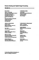
1.3 Difficulties and Solutions of Current Research ➀ Research on three-dimensional characteristics of urban vegetation has become a promising field. However, urban vegetation remote sensing is usually limited to vegetation information extraction. The organic combination of threedimensional structural information of vegetation and quantitative retrieval of eco-physiological parameters is still not enough. ➁ There are many studies on urban green space classification, mostly focusing on the urban vegetation area and distribution measurement. The relationship between urban green space and buildings has been studied, but the multi-scale perception of urban green space from the perspective of urban livability is still less. ➂ Urban vegetation evaluation mostly aims at the ecological benefits of large-scale urban vegetation, mostly takes the urban vegetation area as the main index. There are few studies on urban green environmental quality evaluation from three-dimensional perspective. ➃ Further researches on adaptability of urban green space model in different cities or different regions in the same city need to be conducted. It is of great theoretical significance and application values to analyze the adaptability of urban green space model in different cities or regions and improve its practicability. ➄ The extraction of three-dimensional urban green information based on LiDAR has been carried out. Street-scale environmental survey using street-view data has just started. The research on urban green space perception combining satellite data, LiDAR and street-view data is less. In summary, remote sensing of urban green space has just started. There are lots of basic theoretical and technical issues to be solved in the field. The book attempts to mine the data potential of multi-source satellite data, LiDAR and street view data. Taking Székesehérvár, Hungary, and Tianjin, China as research areas, the research extracted urban buildings and vegetation information based on object-oriented classification method and maximum inter-class distance method, and then the modeling of urban green space remote sensing is carried out. Finally, we conduct the validation of urban green space index model by comparing the adaptability of the model in different cities and different regions in the same city to construct a complete technical system of urban object classification, multi-dimensional vegetation information extraction, green space measurement, multi-scale perception, remote sensing evaluation, and promote the development and improvement of urban green space remote sensing research direction (Fig. 1.1).
1.3 Difficulties and Solutions of Current Research
Multi-spectral image
7
Street view data
LiDAR
Image processing (Székesfehérvár, Hungary/Tianjin, China) Classification of urban objects
Information extraction of vegetation structure
Urban vegetation
2-D information
Urban vegetation
3-D information
Measurement model construction of urban green space
2-D measurement method
3-D measurement method
Area method
Urban green space measurement model in building scale
Grid method Buffer method Moving window method
Urban green space measurement model in vertical perspective
Perception model construction of urban green space Building-scale urban green space perception model
Floor-scale urban green space perception model
Street-scale urban green space perception model
Evaluation model construction of urban green space Fig. 1.1 Chapter system of Remote Sensing of Urban Green Space
8
1 Introduction
References 1. GOODIER J. Encyclopedic dictionary of landscape and urban planning[J]. Reference Reviews, 2011, (2): 40–57. 2. TURNER T. Open space planning in London: from standards per 1000 to green strategy[J]. Town Planning Review, 1992, 63(4): 365–385. 3. LI Y. The change of urban green space and its impact on eco-environmental effects: A case study in Shanghai[D]. Shanghai: Fudan University, doctor degree, 2012. 4. SHEN D, XIONG G. About urban green open space[J]. Urban Planning Forum, 1996, 6: 7–11. 5. LI F, WANG R. Evaluation and ecological planning of urban green space service[M]. Beijing: China Meteorological Press, 2006. 6. CHE S, SONG Y. Extract of the remote sensing message of urban green space landscape— Shanghai City as the case study[J]. Urban Environment & Urban Ecology, 2001, 14(2): 10–12. 7. CHANG Q, LI S, LI H. Research progress on urban green space[J]. Chinese Journal of Applied Ecology, 2007, 18 (7): 1640–1646.
Chapter 2
Remote Sensing Data Preprocessing Technology
With the development of remote sensing technology, remote sensing images are becoming increasingly convenient. Different types of remote sensing images have different advantages in urban green space research. This chapter mainly introduces the characteristics and preprocessing methods of multi-spectral high-resolution data, LiDAR point cloud data, Quickbird image data, etc. Apart from these, the latest street view map, a type of real time map service, provides 360° panoramic views of cities, streets or others. The service provides users the maps with an immersive browsing experience. Street view data has gradually become the data source of urban green space research due to its similarity to pedestrian perspective and low acquisition cost. At the end of this chapter, we will introduce the objects classification techniques and characteristics of street view data.
2.1 Brief Introduction of Experimental Area The main experimental area in the book is Székesfehérvár, Hungary and Tianjin, China. The experimental area includes regions both in China and abroad, which is representative. Moreover, the high-resolution image and street view data ensure the accuracy and universality of the results and enable the research methods and conclusions to be widely applied.
2.1.1 Experimental Area in Székesfehérvár, Hungary Székesfehérvár is located in the Middle-Transdanubian region of Hungary at 47°06' 48.60'' N–47°13' 50'' N, 18°20' 15'' E–18°30' 33.5'' E. It is the ninth largest city in Hungary, with a population of 101,973 people (2010). Székesfehérvár is situated around 65 km southwest from Budapest. The climate is continental, which is frigid © The Author(s), under exclusive license to Springer Nature Singapore Pte Ltd. 2023 Q. Meng, Remote Sensing of Urban Green Space, https://doi.org/10.1007/978-981-99-0703-8_2
9
10
2 Remote Sensing Data Preprocessing Technology
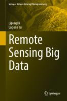
Fig. 2.1 The architectural composition and landscape of Székesfehérvár
and dry in winter while hot and rainy in summer. The average temperature is 14 °C, and the precipitation varies from 400 to 700 mm per year. Székesfehérvár is situated near Danube River in a flat area adjacent to the great plain to the east and Mediterranean to the south. Buildings in Székesfehérvár has typical western characteristics, developing from opening individual space to high altitude. The architectural layout and landscape of Székesfehérvár is shown in Fig. 2.1. The 1 km2 study area is located at the border between the downtown area and the suburbs. Here we chose districts including part of the downtown area and the residential area as study area (Fig. 2.1), which was helpful for validating the proposed index model. The minimum, maximum and standard deviation value of building height in the study area are 0.18 m, 46.22 m and 6.46 m, respectively. Furthermore, those of building height in downtown are 0.18 m, 46.22 m and 3.83 m, respectively. Those of building height in residential area are 0.2 m, 36.88 m and 10.27 m, respectively. In downtown and residential area, the mean values of building height are respectively about 9 m and 14 m. The population in the downtown is about 1,650 and that of residential area is about 1,460. Multi-source high resolution data and LiDAR point cloud data are used in the experimental area. The flight mission was launched on 30 May 2008, by the German company TopoSys. These two types of data can be recorded simultaneously by the airborne RC20 analog frame camera with a focal length of 153 mm. The spatial resolutions of multi-spectral and LiDAR point cloud data are respectively 0.5 m and 1 m. More detailed data are listed in Table 2.1.
2.2 Data Preprocessing Technology Table 2.1 The system parameters of TopoSys
11
Data
Parameter information
Multi-spectral and LiDAR point cloud data
Spatial resolution RGBI: 0.5 m Spatial resolution LiDAR: 1 m Horizontal accuracy 3m
NDVI>Threshold
Segmentation map
Coarse building map
Yes
Vegetation map
Overlap
Buildings map
DSM
Building height model
Canopy height model
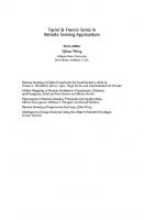
Fig. 5.1 Technical workflow of urban surface information extraction
Set the grayscale of an image to be L(G = 1, 2, . . . , L),, ni indicates the number of pixels with grayscale i. The total number of pixels in the image is: N = n1 + n2 + · · · + n L =
L ∑
ni
(5.1)
i=1
In the above formula, p(i) indicates the probability of occurrence of a pixel with a grayscale i in the image. Normalize the histogram: p(i ) =
ni N
(5.2)
Obviously, L ∑
p(i ) = 1
(5.3)
i=1
Using the grayscale T as the threshold, the pixels in the image are divided into two categories according to the grayscale T : C1 = {1 − T } and C2 = {T + 1 − L}, then the probability of occurrence of the two types is:
5.1 Construction of Urban Green Space Measurement Model in Building Scale
w1 = Pr (C1 ) =
T ∑
p(i )
95
(5.4)
i=1
w2 = Pr (C2 ) =
L ∑
p(i )
(5.5)
i=T +1
w1 + w2 = 1
(5.6)
Obviously, The grayscale mean values of the two classes are shown below: ∑T ∑T ∑T ∑T in i i=1 in i i=1 i p(i ) i=1 i p(i ) = u 1 = ∑i=1 = = ∑ ∑ T T T w1 i=1 n i i=1 N p(i ) i=1 p(i ) ∑L ∑L ∑L ∑L in i i p(i ) +1 i p(i ) +1 in i u 2 = ∑i=T = ∑ L i=T +1 = ∑i=T = i=T +1 L L w2 i=T +1 n i i=T +1 N p(i ) i=T +1 p(i )
(5.7)
(5.8)
The grayscale means value of the entire image: ∑L u1 =
i=1
N
in i
=
L ∑
i p(i )
(5.9)
i=1
The grayscale mean square deviation of the entire image is expressed as follows: ∑L u1 =
i=1 (i
∑ − u)2 n i = (i − u)2 p(i ) N i=1 L
(5.10)
For an image, u and σ 2 is constant and independent of threshold T. The variance between the two classes is defined as: ( ) σ = w1 u 1 − u 2 + w2 (u 2 − u)2
(5.11)
The basic idea of the OTSU’s method is to use the gray-scale histogram of the image to dynamically determine the optimal segmentation threshold of the image with the largest variance between the target and the background. That is, when the variance between the classes reaches the maximum, the corresponding gray-scale value is the best threshold [8]. The larger the variance between the target and the background, the greater the difference between them. When some of the targets are misclassified into the background or part of the background is divided into the target, the difference between the two parts will be smaller. Therefore, the greater the variance between them, the smaller the probability of misclassification will be.
96
5 Measurement Technology of Three-Dimensional Urban Green Space
(2) Rough classification of vegetation Because different vegetation types have similar spectral properties, it is difficult to distinguish them using multi-spectral data alone. The DSM can be obtained from LiDAR data to identify trees and grassland with similar spectral characteristics. According to the obtained vegetation mask and DSM, the vegetation canopy height can be obtained by multiplying the two. Through field investigation and research in study area, it is considered that the vegetation above 2 m is trees, the vegetation with height between 0.4 m and 2 m is shrubs, and the vegetation with height less than 0.4 m is grassland. Based on empirical knowledge, the classification rule above is formulated to classify vegetation types roughly. (3) Image Segmentation Image segmentation is the key in understanding and recognizing images. With the improvement of the resolution of remote sensing images, the internal spectral difference of same type features increases, making the pixel-based classification method unable to meet the needs of accurate information extraction [9]. The object-oriented classification method provides a new research direction for information extraction of high-resolution remote sensing images, whose core lies in image segmentation [10]. Image segmentation is a process of delineating an image into homogeneous polygons related to objects on the ground, and it is the foundation for further image analysis and interpretation when using object-oriented classification method [11]. At present, remote sensing image segmentation methods can be divided into two major categories, namely knowledge-based segmentation method and pixel-based segmentation method [12]. Segmentation method based on pixel values can be subdivided into three categories: histogram-based segmentation techniques (threshold segmentation, etc.), neighborhood-based segmentation techniques (edge detection, region growth, etc.), and watershed segmentation algorithm [13]. The watershed algorithm regards the image as a terrain surface, with the elevation corresponding to the gray-scale value. The local minimum corresponds to the valley bottom, the largest corresponds valley peak, and the watershed line divides the image into several basins developed from the valley bottom [14]. The watershed algorithm proposed by Vincent and his group is a mathematical nonlinear segmentation algorithm [15]. The traditional watershed algorithm is sensitive to noise and often causes oversegmentation. In this section, an improved watershed algorithm based on Sobel operator is used to extract edge features, whose core is to control over-segmentation by using labeled images [16, 17]. Image segmentation flow chart of multi-spectral images is shown in Fig. 5.2. First, the Sobel operator is used to extract image edge features. Then, the edge feature is segmented by moving threshold method to get the labeled image [18, 19]. Finally, the edge image obtained by Sobel operator is reconstructed according to the labeled image, and then the final segmentation image is obtained by watershed segmentation algorithm. There is only one parameter used to control the size of the smallest dividing unit in the segmentation algorithm, which is a fixed value for most
5.1 Construction of Urban Green Space Measurement Model in Building Scale
97
Multi-spectral image
Band 1
Band 2
ę
Band n
Sobel operator
Gradient feature
Labeled image
Watershed segmentation algorithm
Image segmentation results Fig. 5.2 Image segmentation approach of multi-spectral images
applications. In the experiment, the optimal parameters are selected through repeated manual tests. Code of label image algorithms is shown in Code 5.1. Code 5.1 Code of label image algorithms commentminsz: the minimum acceptable marker size commentG: input gradient image std = StandardDeviationOf (G) mean = MeanOf (G) threshs[11] = −1 to 0 step 0.1 fori = 1 to 11 { thresholdLevel = mean + threshs[i] × std thresholdImage = GTI(thresholdLevel,G)
98
5 Measurement Technology of Three-Dimensional Urban Green Space
markerImage[i] = GCRGT(minsz) regionNumber[i] = NOR(markerImage[i]) } maxIndex = FindMaxValue(regionNumber) returnmarkerImage[maxIndex] comment GTI(•): GetThresholdImage comment GCRGT(•): GetConnectedRegionsGreaterThan comment NOR(•): NumberOfRegions (4) Rough extraction of buildings Buildings have similar spectral features with roads and other artificial surfaces, so it is hard for us to identify them through spectral information only. However, buildings have certain height information that is different from other man-made features such as roads and squares. With the help of LiDAR data, which contains the elevation of surface features, a height map of buildings was obtained. First, using the green distribution map as an image mask, the nongreen information was extracted. Then, according to hands-on experience and field investigation, in the area nongreen information with a height higher than 3 m was defined as a building, and the rough extraction of the building was finished. (5) Building boundary smoothing The building distribution map extracted using the threshold method has a large number of spots, which are not building information, and the outline of the extracted building is not clear. To this end, based on the building map and segmentation map of the multi-spectral image, the vote rule was used to improve the precision of the building information. Specifically, every object in the segmentation map was tested by calculating the ratio between the number of building pixels in every object and the total number of pixels in every object. If the ratio was higher than 50%, then the object was defined as a building [16]. 2. LAI retrieval based on radiative transfer model PROSAIL In this section, the sensitivity analysis of physiological and biochemical parameters of the model is first carried out. Variable and fixed parameters of the model are determined by sensitivity analysis results and referring to the typical feature spectrum base, and then we built a look-up table (LUT) of the canopy LAI in research area. For LAI retrieval, only search operations are needed to identify the parameter combinations that yield the best fit between LUT spectra and measured data (Fig. 5.3).
5.1 Construction of Urban Green Space Measurement Model in Building Scale
Sensibility analysis of model
PROSAIL model
Parameters determined Building Look up table(LUT)
99
Field measurement
LAI reference
Cost function LAI inverted
Validation
Fig. 5.3 Approach of LAI retrieval
3. BNGI modeling in building scale Based on the previously calculated vegetation information, building information and LAI of research area, combined with the vegetation type buffer zone map and the high building distribution map, the single building is used as the research scale to establish its buffer zone. Calculate the ratio of green area, vegetation type buffer zone, building area and high building area to the buffer zone of the single building. Finally, assign the weights of each parameter and BNGI distribution map of research area is obtained by overlapping [20, 21]. The construction process of BNGI is shown in Fig. 5.4.
Fig. 5.4 The construction process of BNGI
100
5 Measurement Technology of Three-Dimensional Urban Green Space
Fig. 5.5 Conceptual Model of BNGI
The neighborhood of a building refers to the area with the same characteristics around the building, such as houses and greening conditions. This section defines the area as the buffer of a single building (including the building itself) with a buffer size of 20 m. BNGI shows the distribution of green space around buildings in the city. Because it is to analyze the features based on neighborhood, neighborhood is defined as a spatial concept here. Figure 5.5 shows the conceptual model of building neighborhood green index (BNGI). Based on neighborhood level, urban vegetation characteristics can be divided into total amount of green space and degree of proximity to green space and building parameters can be divided into building density and building height. Total green space refers to the percentage of green space per unit area, usually defined as UGI. Different types of green areas provide the environment with different quantity of ecological benefits. We define the proximity to different types of green areas as proximity to green. Urban residents are close to different types of vegetation and enjoy different benefits. (1) Building sparsity Building sparsity in the study is the percentage of non-building area in the buffer zone of a single building. The layer is not identical with GI layer as it also takes into account the open spaces without vegetation as non-built-up area. In the buffer zone of a single building, a higher building density means more impervious surfaces, and the residents in the zone share less quality and quantity of urban green space. Therefore, the distribution of buildings in the zone will indirectly affect quantity of the urban green space residents enjoyed. Likewise, a lower building density means more green areas and open spaces, and the residents in the zone share a higher quality and quantity of urban green space. Here, the ratio between the building proportion in the buffer zone of a single building and the area of the buffer zone of a single building was defined as a negative impact factor—building density. As the factor is negative, a higher building density means less contribution to the Building Neighborhood Green
5.1 Construction of Urban Green Space Measurement Model in Building Scale
101
Index. A lower building density means a higher building sparsity, so it contributes more to the Building Neighborhood Green Index. The formula for building sparsity is as follows: / Building Sparsity = 1.0 − Abuild Abuffer
(5.12)
where Abuild is the building proportion in the buffer zone of each single building, Abuffer is the area of buffer zone of each single building (including its own area). (2) High-rise sparsity High building sparsity (hereafter high-rise sparsity) in the study is the percentage of non-high built-up area in the buffer zone of a single building. Considering the different parts of each single building, the average height was calculated first. In the buffer zone of a single building, tall buildings are usually obstacles to the green space around them and have a negative effect. Here, the sparsity of high buildings was considered as another factor affecting the Building Neighborhood Green Index. In order to simplify the process, buildings taller than the mean height of all buildings in the study area were defined as high-rise buildings. Buildings shorter than the mean height of all buildings in the study area were considered low-rise buildings. Here, the ratio between the high-rise building proportion in the buffer zone of a single building and the area of buffer zone of single buildings was identified as another negative impact factor—density of high-rise buildings. Likewise, as the factor is negative, a higher density of high-rise buildings means less contribution to the Building Neighborhood Green Index. So here we define the difference between the value 1.0 and the high-rise density as high-rise sparsity. The formula for high-rise sparsity is: / High - rise Sparsity = 1.0 − AH - build Abuffer
(5.13)
where AH-build is the high-rise proportion in the buffer zone of each single building, and Abuffer is the area of buffer zone of each single building (including its own area). (3) UGI Urban Green Index (UGI) is the percentage of the green area in the buffer zone of a single building. A green distribution map was used in the calculation of UGI. The specific calculation formula is as follows: / UGI = Agreen Abuffer
(5.14)
where Agreen is the green proportion in the buffer zone of each single building, and Abuffer is the area of buffer zone of each single building (including its own area). (4) Proximity to green Ecological characteristics of different vegetation types are not consistent, that is, radiation efficiency is not the same in a certain region on different vegetation types. The
102
5 Measurement Technology of Three-Dimensional Urban Green Space
ecological benefits of different vegetation types are closely related to physiological and biochemical processes of vegetation such as photosynthesis and transpiration. Therefore, the involvement of physiological and biochemical parameters of the vegetation such as LAI and biomass can help better calculate the urban green space index and evaluate the urban green space. In this section, the LAI of vegetation in the study area is calculated and divided into three levels, namely, Level 1 (LAI ≤ 1), Level 2 (1 < LAI < 3) and Level 3 (LAI ≥ 3). Such classification can better reflect vegetation growth and ecological benefits than simple classification of vegetation types (tree, shrub, grassland). At the same time, the adjacent area of different vegetation types is defined as a vegetation benefit radiation area. Different vegetation types also have different benefits. The radiation area of different vegetation types refers to the establishment of buffer zones of corresponding vegetation types, and the buffer distance is set as 20 m. In the single building buffer zone, the ratio between the sum of the ecological benefit radiation area of different vegetation types and the area of the single building buffer zone is defined as the green space radiation benefit of the single building. The formula is as follows: ∑
Proximity to green =
W j × Pj
(5.15)
j=1, 2, 3
where Pj (j = 1,2,3) is the ratio between the area of neighborhood vegetation and the buffer zone area of single buildings in the buffer zone of a single building, and Wj is the relative weight of each neighborhood vegetation in the buffer zone of a single building. (5) Weighting and overlay The ecological benefits of urban green space shared by residents are affected by many different factors including vegetation distribution and building distribution. In this section, four influencing factors, GI, green space radiation benefit, building sparsity and high building sparsity, are mainly considered. The value of BNGI changes within the range from 0 to 1, the calculation formula is BNGI =
i=1,2,...,n ∑
W j × Pi j
(5.16)
j=1,2,...,4
where BNGI is the Building Neighborhood Green Index of the ith building, Pij is the value of jth parameter in ith building including UGI, proximity to green, building sparsity, and high-rise sparsity; Wj is the relative weight of the jth parameter, corresponding to 0.27, 0.25, 0.18 and 0.30, respectively, where j = 1 to 4; i = 1 to n, representing there are n single buildings. 4. Validation of the BNGI model UGI concentrates only on percentage of green in an urban area but BNGI addresses the spatial distribution of urban green space and their interlinking with urban structures, as well as the vertical dimension of structures and their impact on urban green
5.1 Construction of Urban Green Space Measurement Model in Building Scale
103
space. Statistical analysis of BNGI distribution characteristics in different regions will help us to better understand the quality and quantity of urban green space that residents are sharing and the difference in the BNGI distribution in different regions. The distribution of buildings in the study area was irregular. Specifically, some regions had high-rises but high building sparsity, and some regions had low-rises but low building sparsity, while others had high-rises and low sparsity. We did not directly perceive whether Building Neighborhood Green Index reflects the urban green space distribution effectively, and we were not able to decide whether Building Neighborhood Green Index has an advantage over the traditional Green Index according to the above situation. Therefore, different characteristic regions were classified according to the building distribution characteristics, the building function characteristics, and the Urban Green Index (e.g., UGI and BNGI) classification. The statistical characteristic values including the mean, median, and standard deviation of UGI and BNGI were calculated and compared to visualize the difference between the UGI and the BNGI approaches (Fig. 5.6). 5. Adaptability Analysis of BNGI Model Tianjin was selected as the validation area, and research area was divided into different areas according to the building distribution and UGI value. The mean, median, and standard deviation of BNGI were compared in different areas of the same city, based on which we evaluated the adaptability of BNGI to verify its regional adaptability (Fig. 5.7).
UGI/BNGI
Area 1
Area 2
Mean
Area 3
Median
Standard deviation
Better urban green space index
Fig. 5.6 Workflow of model validation
Area 4
104
5 Measurement Technology of Three-Dimensional Urban Green Space Different characteristic areas in the same city
High-rise high-spasity area
Comprehensive area
High-rise low-spasity area
Numerical zone 1 Numerical zone 2
Residential area Low-rise high-spasity area Low-rise low-spasity area
Different cities
Numerical zone 3 Commercial area
Numerical zone 4
Fig. 5.7 Workflow of model adaptability validation
5.1.3 Results of Experiment 1. Extraction results of vegetation and buildings 105 (1) Results of vegetation extraction and type discrimination In NDVI image, non-vegetation area is dark, while vegetation area is highlighted. Due to the bimodal distribution of vegetation and non-vegetation on the NDVI histogram, it is simple and effective to extract the vegetation information based on the NDVI image using OTSU’s method. Here, OTSU is used to determine the optimal threshold and extract vegetation information. Figure 5.8 is NDVI distribution map of research area, and Fig. 5.9 shows the NDVI histogram and optimal threshold 0.27. It can be seen from the histogram that the optimal threshold lies between the two peaks of the histogram. Figure 5.10 shows the vegetation distribution map of research area obtained from threshold calculation. A map grid was set up on the vegetation distribution map, and 121 test samples were randomly selected at the grid intersection. The distribution map of test samples is shown in Fig. 5.11. We determined the attribution of each test sample by visual interpretation and verified the accuracy of vegetation information extraction. The accuracy of vegetation distribution map was verified up to 95% by uniform selection of test samples. Accuracy validation result is shown in Table 5.1. The vegetation types are roughly classified based on the vegetation classification rules mentioned above, and rough vegetation classification result is shown in Fig. 5.12. (2) Result of building information extraction Using the method described above to extract buildings in research area, the rough extraction results of the buildings are shown in Fig. 5.13. The final extraction result of the building is obtained by voting method for further smoothing. Figure 5.14 shows Sketch of building extraction effect, from which it
5.1 Construction of Urban Green Space Measurement Model in Building Scale
Fig. 5.8 NDVI distribution map of research area
Fig. 5.9 NDVI histogram and optimal threshold
105
106
5 Measurement Technology of Three-Dimensional Urban Green Space
Fig. 5.10 Vegetation distribution map of research area
can be seen that the outline of the building is clearly depicted and there is no spot, indicating that the method can well integrate different resolution LiDAR data and multi-spectral aerial images for building extraction. The method is applied to the entire area, and the building distribution map in research area are shown in Fig. 5.15. A map grid was set up on the building distribution map, and 121 test samples were randomly selected at the grid intersection. The distribution map of test samples is shown in Fig. 5.16. We determined the attribution of each test sample by visual interpretation and verified the accuracy of building information extraction. The accuracy of building distribution map was verified higher than 98% by uniform selection of test samples (Table 5.2). Based on the extracted buildings and DSM, the building height model can be obtained by multiplying the building distribution map with the corresponding DSM. Considering the different heights of different parts of each single building, we simplified the process, where the height of a single building is the average height of each part of it, thus obtained the height map of buildings (Fig. 5.17). 2. LAI retrieval result According to the sensitivity analysis of PROSAIL parameters, we found that LAI, ALA, Cab, Car, Cw, and Cm had obvious effects on canopy spectral reflectance in the
5.1 Construction of Urban Green Space Measurement Model in Building Scale
107
Fig. 5.11 Vegetation distribution map of test samples
Table 5.1 Accuracy validation result (vegetation) Extracted object
Number of test samples
Number of Number of false correctly extracted extracted validation points validation points
Extraction accuracy/(%)
Vegetation
121
114
95
7
visible light region, especially LAI, ALA, and Cab. Table 5.3 reported the maximum and minimum values for each of the six ’free’ model parameters. The approximate maximum and minimum values of LAI, ALA, Cab, Car, Cw, and Cm were selected in agreement with the existing literature. Here, the leaf structural parameter was set to 1.4, and the solar zenith angle, observing zenith angle, and relative azimuth angle were set according to the observation information when the image was produced. The hot spot value was set to 0.01. Therefore, there were six parameters of the PROSAIL model affecting the canopy spectral reflectance, including LAI, ALA, Cab, Car, Cw, and Cm. Finally, the changed and fixed parameter values were all taken into the PROSAIL model to simulate the canopy spectral reflectance, and we built a LUT
108
5 Measurement Technology of Three-Dimensional Urban Green Space
Fig. 5.12 Rough vegetation classification result Fig. 5.13 Rough extraction results of buildings
5.1 Construction of Urban Green Space Measurement Model in Building Scale
Fig. 5.14 Sketch of building extraction effect
Fig. 5.15 Building distribution map in research area
109
110
5 Measurement Technology of Three-Dimensional Urban Green Space
Fig. 5.16 Building distribution map of test samples
Table 5.2 Results of accuracy validation (building) Extracted object
Number of test samples
Number of Number of false correctly extracted extracted validation points validation points
Extraction accuracy/(%)
Buildings
121
118
98
3
of the canopy LAI. The canopy spectral reflectance includes blue band reflectance, green band reflectance, red band reflectance, and NIR band reflectance. Range of parameters for PROSAIL model is shown in Table 5.3. The canopy reflectance calculated by PROSAIL model is a point data without spatial scale. For the response of the image sensor in the effective band is different, the spectral response function of the sensor should be considered, which is the foundation of matching the simulated canopy reflectance with the image reflectance. Formula 5.17 and 5.18 are used to calculate the effective wavelength of the sensor and the reflectance of the sensor in the corresponding band:
5.1 Construction of Urban Green Space Measurement Model in Building Scale
111
Fig 5.17 Height map of buildings in research area
Table 5.3 Range of parameters for PROSAIL model Abbreviation in model/Unit
Parameter
Range
Step
LAI
Leaf area index
(0, 7)
0.25
LAD ( ) Cab/ µg · cm−2 ) ( Car/ µg · cm−2
Mean leaf inclination angle
(5, 85)
10
Leaf chlorophyll content
(0, 50)
5
Leaf carotenoid content
(0, 10)
2.5
Equivalent water thickness
(0, 0.02)
0.005
Cw/cm ( ) Cm/ g · cm−2
Dry matter content
(0,0.02)
0.005
N
Leaf structural parameter
1.4
–
SL
Hot spot size
0.01
–
λeffective =
∑ λ (λRes(λ)) ∑ λ Res(λ)
ρsensor (λ) = ρ mod (λeffective )
(5.17) (5.18)
112
5 Measurement Technology of Three-Dimensional Urban Green Space
where Res(λ) is the value of spectral response function, ρsensor (λ) is the reflectance of image sensor and ρmod (λ) is canopy reflectance simulated by PROSAIL model. Modify the PROSAIL source code, input parameter values and effective wavelength of each band according to the above model and execute the PROSAIL model circularly to construct the LUT. The data of each row in the LUT are LAI, LAD, Cab, Car and reflectance of blue, green, red and near infrared bands generated by the model, totaling 190,080 rows. Table 5.4 shows part of the data in LUT. Using the radiative transfer model, a LUT is built through forward calculations. For the retrieval, only search operations are needed to identify the parameter combinations that yield the best matching between LUT spectra and measured. To find the solution to the inverse problem for a given canopy spectra, for each modeled reflectance spectra of the LUT, the COST between measured and modeled spectra is calculated as: Table 5.4 Part of the data in LUT LAI
LADFa
Cab
Car
Blue
Green
Red
NIR
0.00
5.00
0.0000
0.0000
0.309830
0.307312
0.313268
0.330208
0.00
5.00
0.0000
0.0000
0.283635
0.286463
0.291890
0.307187
0.00
5.00
0.0000
0.0000
0.261473
0.268171
0.273170
0.287156
0.00
5.00
0.0000
0.0000
0.242438
0.251963
0.256610
0.269533
0.00
5.00
0.0000
0.0000
0.309828
0.307306
0.313231
0.329945
0.00
5.00
0.0000
0.0000
0.283634
0.286458
0.291858
0.306960
0.00
5.00
0.0000
0.0000
0.261472
0.268166
0.273142
0.286957
0.00
5.00
0.0000
0.0000
0.242437
0.251958
0.256585
0.269357
0.00
5.00
0.0000
0.0000
0.309827
0.307299
0.313195
0.329682
0.00
5.00
0.0000
0.0000
0.283632
0.286452
0.291827
0.306733
0.00
5.00
0.0000
0.0000
0.261471
0.268161
0.273114
0.286758
0.00
5.00
0.0000
0.0000
0.242436
0.251954
0.256561
0.269181
0.00
5.00
0.0000
0.0000
0.309825
0.307292
0.313159
0.329420
0.00
5.00
0.0000
0.0000
0.283631
0.286446
0.291795
0.306506
0.00
5.00
0.0000
0.0000
0.261470
0.268156
0.273087
0.286559
0.00
5.00
0.0000
0.0000
0.242435
0.251949
0.256536
0.269005
0.00
5.00
0.0000
2.5000
0.094127
0.307312
0.313268
0.330208
0.00
5.00
0.0000
2.5000
0.091137
0.286463
0.291890
0.307187
0.00
5.00
0.0000
2.5000
0.088319
0.268171
0.273170
0.287156
0.00
5.00
0.0000
2.5000
0.085659
0.251963
0.256610
0.269533
0.00
5.00
0.0000
2.5000
0.094126
0.307306
0.313231
0.329945
0.00
5.00
0.0000
2.5000
0.091137
0.286458
0.291858
0.306960
5.1 Construction of Urban Green Space Measurement Model in Building Scale
COST =
n (I I) ∑ I j I j Iρ mod − ρCCD I
113
(5.19)
i=1 j
j
where ρ mod is measured reflectance at wavelength j, ρCCD is the modeled reflectance at the same wavelength in the LUT, and n is the number of wavebands. Figure 5.18 shows the LAI retrieval result. By comparison and analysis, we found that the points of maximum LAI value in the retrieval result corresponded to densely vegetated areas in the image, and the points of minimum LAI value in the retrieval result corresponded to sparsely vegetated areas. According to the physical model used, most studies showed that the PROSAIL model has high accuracy in retrieval of LAI. Through the comparative analysis of the vegetation height model and the LAI retrieval results in research area, it is found that the high value of LAI retrieval mostly appears in the tree area. The low value mostly appeared in the grass area, indicating that the LAI retrieval result is convincing, which provides a basis for urban green space research. Comparison of LAI and vegetation rough classification result is shown in Fig. 5.19.
Fig. 5.18 LAI retrieval result
114
5 Measurement Technology of Three-Dimensional Urban Green Space
Fig. 5.19 Comparison of LAI and vegetation rough classification result
5.1 Construction of Urban Green Space Measurement Model in Building Scale
115
3. Modeling Result of BNGI According to the urban BNGI modeling method, the distribution map of building sparsity, high-rise sparsity, UGI and proximity to green are obtained. It can be seen from Fig. 5.20 that the sparsity of buildings in commercial area is relatively low, whereas the sparsity in residential area is relatively high. High buildings distribution map is shown in Fig. 5.21. It can be seen from Fig. 5.22 that the buildings in the commercial area are generally high, and high-rise sparsity is lower; buildings in residential area are relatively low, and the high-rise sparsity is high. UGI distribution map is shown in Fig. 5.23. Distribution map of proximity to green is shown in Fig. 5.24. The four parameters are weighted and overlapped to obtain BNGI distribution map of research area, as shown in Fig. 5.25. It can be seen from Fig. 5.25 that high values of BNGI were mainly associated with more green such as in residential area, and low values of BNGI were mainly
Fig. 5.20 Building sparsity map
116
5 Measurement Technology of Three-Dimensional Urban Green Space
Fig. 5.21 High buildings distribution map
distributed in commercial area where the population and high-rise sparsity were low. Meanwhile, the underlying surface was mainly composed of cement and asphalt, and the green coverage was sparse. 4. Validation of the BNGI model By statistically analyzing the distribution characteristics of BNGI in each feature area, we can better understand the benefit of urban green space and its distribution in different areas. The distribution characteristics of buildings in research area is uneven. There are some areas with high-rise low-sparsity, some with low-rise low-sparsity, and high-rise high-sparsity. Therefore, according to building height, building density, the different functional characteristics of buildings and the value of UGI/BNGI, research area is divided into different areas. The mean, median, and standard deviation of UGI and BNGI were compared in these regions, based on which we evaluated the difference and reliability of UGI and BNGI. According to the distribution difference, we validated the newly constructed index BNGI. (1) Overall analysis of the distribution pattern of BNGI The urban green space spatial distribution map based on UGI and BNGI are shown in Fig. 5.26.
5.1 Construction of Urban Green Space Measurement Model in Building Scale
117
Fig. 5.22 High-rise sparsity map
Distribution ranges of the traditional UGI and BNGI were both within the value ranging from 0 to 1 and the numerical distribution was not uniform. The value of the traditional UGI was relatively low and the value of BNGI was relatively high. This situation might be resulted from the two different models. The factors considered in the BNGI model were more comprehensive, so the low value of BNGI would not be too low. But the factor considered in the traditional UGI model was merely green distribution, so when there was no green area, the UGI was zero. Generally, both UGI and BNGI can reflect the overall situation of the real urban green space spatial distribution. (2) Research area dividing according to building function In terms of the building function, we classified the study area into three regions including district with mixed functions, residential area and commercial area. The mean, median, and standard deviation of UGI and BNGI were compared in these three regions. BNGI map in different functional zones are shown in Fig. 5.27. The statistical characteristics of BNGI and UGI in different functional zones are shown in Table 5.5. We can find that the mean, standard deviation, and median distribution trend in the three functional zones are similar, which demonstrate the urban green space
118
5 Measurement Technology of Three-Dimensional Urban Green Space
Fig. 5.23 UGI distribution map
evaluation of the two kinds of urban green space indices are basically the same, indicating that BNGI can reflect the overall situation of the real urban green space spatial distribution. The BNGI histograms of the above three regions are shown in Fig. 5.28. According to the histograms, we found that in the mixed-use district the proportion values 0.6– 0.8 were highest in the range 0 – 1, up to 51.86%, and the proportion values 0.4–0.6 were in second place at 31.65%. In the residential area, the proportion values 0.6 – 0.8 were highest in the range 0–1, up to 81%, whereas the other groups were all flat. In the commercial area, the proportions of groups from 0.2 to 0.8 were balanced, reaching about 30%. The results showed that the BNGI in residential area was relatively high and the BNGI in commercial area was relatively low. We could also find that the standard deviation in the residential area was lowest and the standard deviation in commercial area was highest, which indicated that the change rate of BNGI in the residential area was steady, whereas, the change rate of BNGI in commercial area was most fluctuant. This might result from having less green vegetation and an uneven distribution of green areas in commercial area. The median and mean values of BNGI in the residential area were highest, which indicated that the degree of urban green
5.1 Construction of Urban Green Space Measurement Model in Building Scale
119
Fig. 5.24 Distribution map of proximity to green
space residents sharing was highest in the residential area and lowest in commercial area. The degree of urban green space residents shared in the mixed-use district was in second place. (3) Research area dividing according to building distribution In terms of the building distribution characteristics, we classified the study area into three regions including high-rise low-sparsity, low-rise low-sparsity, and high-rise high-sparsity, as shown in Fig. 5.29. The mean, median, and standard deviation of UGI and BNGI were compared in these three regions, the results of which are shown in Table 5.6. We found that urban green space evaluation of the two kinds of urban green space indices were basically the same, indicating that BNGI can reflect the overall situation of the real urban green space spatial distribution. The BNGI histograms of the above three regions were shown in Fig. 5.30, demonstrating that in the high-rise low-sparsity area the proportion values 0.6–0.8 were highest in the range 0–1, up to 40%, and the proportion values 0.4–0.6 were in second place at 31%. In low-rise low-sparsity and high-rise low-sparsity areas, the proportion values 0.4–0.6 were matched, up to 30%, and the proportion values 0.6– 0.8 were matched, up to 60%. The results showed that the BNGI in the high-rise low-sparsity area was relatively low and the BNGI in the low-rise low-sparsity and
120
5 Measurement Technology of Three-Dimensional Urban Green Space
Fig. 5.25 BNGI distribution map
high-rise high-sparsity areas were relatively high. Table 5.5 showed that the median and mean value in the high-rise low-sparsity area was the lowest and standard deviation was highest, meaning the degree to which residents enjoying urban green space was worse here. Both neighborhoods high-rise low-sparsity and low-rise low-sparsity areas were equal in terms of amount of green as per mean UGI values, namely, if areas were judged based on UGI and remote sensing images alone, both of them were equal in terms of urban green quality. But when assessed using BNGI, the high-rise low-sparsity area had a lower mean value of BNGI, 0.56, as compared with that of the low-rise low-sparsity neighborhood, 0.62. It expressed the effect of nearness to green areas and urban density on quality of green areas in urban neighborhoods. (4) Research area dividing according to urban green space indices classification For the sake of simplicity and ease of interpretation, the values of BNGI and UGI were both categorized in four equal intervals. By analyzing the distribution proportions of four different classes of urban green space index in different characteristic regions, we could more clearly compare the distribution characteristics of BNGI and UGI. The statistics are shown in Table 5.7. The distribution of BNGI in different building zones was focused on the range from 0.5 to 1.0, whereas the distribution of UGI was focused on the range from 0 to
5.1 Construction of Urban Green Space Measurement Model in Building Scale Fig. 5.26 Urban green space spatial distribution map based on UGI and BNGI
(a) UGI distribution map
(b) BNGI distribution map
121
122
5 Measurement Technology of Three-Dimensional Urban Green Space
(a) BNGI map in research area
(b) BNGI map in residential area
(c) BNGI map in commercial area
Fig. 5.27 BNGI map in different functional zones
Table 5.5 Statistical characteristics of BNGI and UGI in different functional zones
Zones
Statistics characteristics
BNGI
UGI
District with mixed function
Mean
0.57
0.24
Standard deviation
0.20
0.17
Median
0.62
0.24
Residential area
Mean
0.65
0.31
Standard deviation
0.15
0.12
Median
0.67
0.32
Mean
0.51
0.24
Standard deviation
0.22
0.20
Median
0.50
0.18
Commercial area
0.5 (see Table 5.7). In the range from 0 to 0.25 of various neighborhoods especially, BNGI in different characteristic regions was far lower than UGI, which indicated that the factors considered by the UGI model were more unilateral and the factors considered by the BNGI model were more comprehensive. The BNGI model not only took green distribution into account, but also considered the proximity to green and building distribution in the study area. As a whole, the value of BNGI was higher than that of UGI. Moreover, BNGI was more effective at expressing the urban green space distribution. Specifically, the gap between BNGI and UGI was smaller in area under low green quality of the range from 0 to 0.5 in the high-rise low-sparsity area than those in the high-rise high-sparsity and low-rise low-sparsity areas. This means that the BNGI model describes the effect of urban density. 5. Adaptability analysis of BNGI model The BNGI plays an important role in characterizing the spatial distribution of urban green space and the comfortless of human settlements. The adaptability of BNGI
5.1 Construction of Urban Green Space Measurement Model in Building Scale
(a) Histogram of BNGI in the district with mixed functional buildings
123
(b) Histogram of BNGI in the residential area
(c) Histogram of BNGI in the commercial area
Fig. 5.28 BNGI histograms in different functional zones
(a) building zones in research area
(b) BNGI map in zone with high-rise and lowsparsity
(c) BNGI map in zone with low-rise and lowsparsity
(d) BNGI map in zone with high-rise and highsparsity
Fig. 5.29 BNGI distribution in different characteristic building zones in research area
124
5 Measurement Technology of Three-Dimensional Urban Green Space
Table 5.6 Statistical characteristics of the urban green space index in different building zones
Zones
Statistics characteristics BNGI UGI
High-rise low-sparsity
Mean
0.55
0.25
Standard deviation
0.21
0.19
Median
0.59
0.23
Mean
0.63
0.25
Standard deviation
0.15
0.13
Median
0.66
0.26
0.59
0.25
Standard deviation
0.19
0.14
Median
0.65
0.26
Low-rise low-sparsity
High-rise high-sparsity Mean
(a) BNGI histogram in the high-rise low-sparsity
(b) BNGI histogram in the low-rise low-sparsity
(c) BNGI histogram in high-rise high-sparsity
Fig. 5.30 BNGI histogram in different building zones
in different areas and different background environments is analyzed, which lays a foundation for its practical application. Model adaptability is used to assess the model’s adaptation to the research environment. It is indispensable for model analysis, assessment and screening. This section is achieved by comparing and analyzing the adaptability of BNGI model in two cities with different characteristics.
5.1 Construction of Urban Green Space Measurement Model in Building Scale
125
Table 5.7 Distribution Characteristics of UGI/BNGI Values Index category
High-rise high-sparsity (n = 117)
Low-rise low-sparsity (n High-rise low-sparsity = 72) (n = 86)
BNGI/(%)
BNGI/(%)
UGI/(%)
UGI/(%)
BNGI/(%)
UGI/(%)
[0, 0.25]
0
41.03
0
44.29
1.16
51.16
(0.25, 0.5]
9.40
55.56
8.33
51.43
29.07
36.05
(0.5, 0.75]
80.34
3.42
73.61
4.29
54.65
11.63
(0.75, 1]
10.26
0.01
18.06
0.01
15.12
1.16
Total
100
100
100
100
100
100
From the layout of the building space, Chinese architecture is a closed group space pattern, which is spread on the ground. From the residence to the palace, no matter what kind of building, it is almost the same, similar to the “Courtyard Dwellings” model. Western architecture is an open, single-space pattern that is developing at a high altitude. If Chinese architecture occupies the ground, then Western architecture takes up the sky space. The distribution pattern of buildings in Székesfehérvár is a typical western example. Taking Tianjin area with Chinese characteristics in the distribution of buildings as the research area, the adaptability study of the BNGI model was carried out. According to building distribution and green space indices classification, research area is divided into sub-areas, and BNGI is evaluated by comparing the mean, standard deviation and median value of different green space indices in different zones of the city to verify model adaptability. (1) Building sparsity According to the building information extraction method based on image segmentation illustrated in Sect. 5.1.2, the building information is extracted from the research area of Tianjin, which is shown in Fig. 5.31. According to the definition of building sparsity, the building sparsity map in research area is calculated by using the obtained building information. From the results shown in Fig. 5.32, it can be seen that the building sparsity in the eastern and northern parts of the research area is lower than that in the southwestern part. It can also be seen from the building distribution map in Fig. 5.31 that the building density in the southwestern part of the research area is relatively low. (2) High-rise sparsity According to the building height information extraction method based on image segmentation and LiDAR data as described in Sect. 5.1.2, the building height information is extracted from the Tianjin research area. High building distribution map is shown in Fig. 5.33. According to the definition of high-rise sparsity, the high-rise sparsity in Tianjin area is calculated by using the information of high buildings, and the results are shown in Fig. 5.34. It can be seen that the high-rise sparsity of the entire research area is generally high, that is, the high building density of research area is generally low.
126
5 Measurement Technology of Three-Dimensional Urban Green Space
Fig. 5.31 Building distribution map in Tianjin research area
Fig. 5.32 Building sparsity map in Tianjin research area
5.1 Construction of Urban Green Space Measurement Model in Building Scale
Fig. 5.33 High buildings distribution map in Tianjin research area
Fig. 5.34 High-rise sparsity map in Tianjin research area
127
128
5 Measurement Technology of Three-Dimensional Urban Green Space
(3) UGI According to the vegetation information extraction method based on NDVI and the OTSU method described in Sect. 5.1.2, the vegetation information is extracted from the Tianjin research area, are shown in Fig. 5.35. According to the definition of UGI, using the acquired vegetation information, the UGI distribution map in Tianjin is calculated, shown in Fig. 5.36. It can be seen that the UGI value in research area is concentrated in the range of 0–0.6. At the same time, except for the area of the southwest with high value of building sparsity and some area with high-rise sparsity, the distribution pattern of green space is generally uniform. (4) Proximity to green According to the vegetation LAI retrieval method based on radiative transfer model PROSAIL described in Sect. 5.1.2, the LAI retrieval was performed in Tianjin area. The result is shown in Fig. 5.37. According to the definition of proximity to green, using the obtained LAI, the distribution map of proximity to green of Tianjin research area is calculated. The result is shown in Fig. 5.38. It can be seen that the vegetation LAI in research area is higher in the northeast and the south, and higher in areas with high high-rise sparsity.
Fig. 5.35 Vegetation distribution map
5.1 Construction of Urban Green Space Measurement Model in Building Scale
Fig. 5.36 UGI distribution map in Tianjin research area
Fig. 5.37 LAI retrieval result in Tianjin research area
129
130
5 Measurement Technology of Three-Dimensional Urban Green Space
Fig. 5.38 Distribution map of proximity to green in Tianjin research area
(5) BNGI The spatial distribution map of urban green space in research area was calculated by the newly constructed BNGI model, as shown in Fig. 5.39. The spatial distribution pattern of urban green reflected by BNGI could be seen. The spatial distribution pattern of urban green was consistent with the actual environmental conditions. The high values of BNGI were mainly associated with more green such as in residential area, and low values of BNGI were mainly distributed areas where the population and high-rise sparsity were low. Meanwhile, the underlying surface was mainly composed of cement and asphalt, and the green coverage was sparse. (6) Adaptability analysis In order to study whether the newly constructed BNGI model is applicable to Tianjin research area, the model is used to calculate the spatial distribution pattern in Tianjin research area, and the validation is carried out to judge the model’s adaptability. In terms of the building distribution characteristics, we classified research area into three regions including high-rise low-sparsity, low-rise low-sparsity, and high-rise high-sparsity, as shown in Fig. 5.40. The statistical eigenvalues of BNGI in these three regions are calculated, as shown in Table 5.8. As can be seen from Table 5.8, UGI distribution shows that green space is most widely distributed in low-rise high-sparsity areas. BNGI is the largest in low-rise high-sparsity areas, which is consistent with UGI. In the low-rise high-sparsity area,
5.1 Construction of Urban Green Space Measurement Model in Building Scale
131
(a) UGI distribution map
(b) BNGI distribution map
Fig. 5.39 Urban green space spatial distribution map based on UGI and BNGI in Tianjin research area
132
5 Measurement Technology of Three-Dimensional Urban Green Space
Fig. 5.40 Different characteristic building zones in research area Table 5.8 Statistical characteristics of the urban green space index in different building zones of Tianjin Zones
UGI
BNGI
Mean
Standard deviation
Median
Mean
Standard deviation
Median
High-sire high-sparsity
0.3072
0.1320
0.3162
0.5437
0.0963
0.5389
Low-rise high-sparsity
0.3680
0.1208
0.3417
0.5847
0.0839
0.5653
Low-rise low-sparsity
0.3073
0.1051
0.3156
0.5094
0.0526
0.5037
5.1 Construction of Urban Green Space Measurement Model in Building Scale
133
Table 5.9 Spatial Distribution Characteristics of UGI/BNGI Values Index category
High-rise high-sparsity (n = 156)
Low-rise low-sparsity (n Low-rise high-sparsity = 194) (n = 244)
BNGI/(%)
BNGI/(%)
UGI/(%)
UGI/(%)
BNGI/(%)
UGI/(%)
[0, 0.25]
0
34.62
0
24.23
0
17.62
(0.25, 0.5]
33.33
58.33
47.94
71.65
12.3
64.34
(0.5, 0.75]
64.74
7.05
52.06
4.12
82.38
18.04
(0.75, 1]
1.93
0
0
0
5.32
0
Total
100
100
100
100
100
100
the median and mean value is the highest and standard deviation is lowest, meaning the degree to residents share urban green space is best. At the same time, the mean value of UGI is equal in high-rise high-sparsity area and low-rise low-sparsity area, while the mean value of BNGI is 0.5437 in high-rise high-sparsity area and 0.5094 in low-rise low-sparsity area. It shows that under the same green space (UGI is equal), because of the influence of building distribution and the nearness to green areas, the results of BNGI are different, which is more in line with the actual situation, indicating that BNGI has advantages over UGI. For the sake of simplicity and ease of interpretation, the values of BNGI and UGI are both categorized in four equal intervals. By analyzing the distribution proportions of four different classes of urban green space index in different characteristic regions, we can more clearly discuss whether the BNGI model is suitable for Tianjin research area. The statistics are shown in Table 5.9 The results of BNGI are more realistic and reliable. Specifically, unlike the distribution ratio of the two indices in the high-rise high-sparsity area and the low-rise low-sparsity area, in the low-rise high-sparsity area, the gap between the proportion of UGI in (0, 0.5) and that of BNGI in (0, 0.5) has increased. This indicates that BNGI takes into account the distribution of buildings, so it distributes less in low value area and larger in high value area. In summary, the newly constructed BNGI model can objectively reflect the spatial distribution pattern of urban green space in research area. Therefore, the model has applicability in the Tianjin research area.
5.1.4 Conclusion In this section, aiming at the problems that the traditional urban green space index model and grid method only consider urban green space distribution, and the validation of urban green space index model is difficult to develop. Based on multi-source remote sensing data, BNGI model is proposed, which is based on building scale and takes into account green space area, proximity to green, building sparsity and highrise sparsity to achieve a two-dimensional to three-dimensional research perspective
134
5 Measurement Technology of Three-Dimensional Urban Green Space
transformation. Secondly, the definition and calculation methods of the four indicators are introduced in detail, including the establishment of the buffer of single building and weight determination of each parameter. Finally, the model validation and adaptability analysis at different scales are carried out. It is found that the index can truly reflect the distribution pattern of urban green space and can provide model input and reference basis for livability evaluation of urban human settlements.
5.2 Construction of Urban Green Space Distribution Measurement Model in Vertical Perspective Urban vegetation plays an important role in improving urban environment and promoting human health. However, with the urbanization, the contradiction between the urban housing construction and green space resources configuration has become increasingly prominent. It is particularly important to rationally plan the spatial layout of green space. How to objectively evaluate the distribution pattern and configuration relationship of urban green space in the process of urbanization is of great significance to promote sustainable urban development. With the continuous development of large cities’ buildings at high altitudes, vertical three-dimensional greening has become a developing trend. The traditional plane observation and evaluation methods can no longer meet the needs of urban planners in three-dimensional greenness space configuration. Airborne lidar technology has the advantage of automatic and high precision stereo scanning, which makes it possible to obtain three-dimensional spatial information of urban objects, and also provide a new way for people to analyze urban green space layout from multiple angles and multiple dimensions. Based on airborne LiDAR and aerial image data, this section extracts three-dimensional information of vegetation and buildings in research area. Through vertical stratified sampling of urban space, the configuration quantity of green space and building at different sampling heights is calculated, and the vertical space configuration features of different functional areas and architectural feature areas are compared.
5.2.1 Research Status With the acceleration of urbanization, the contradiction between urban residential construction and the allocation of green space resources becomes increasingly prominent, so it is particularly important to rationally plan the spatial layout of green space. How to objectively evaluate the distribution pattern and allocation relationship of urban greenness space in the process of urbanization is of great significance to maintain the sustainable development of urban regions.
5.2 Construction of Urban Green Space Distribution Measurement Model …
135
Traditional urban green space configuration survey methods include area method, buffer method and grid unit method [22]. Researchers obtained the overall greening situation of study area by counting the distribution ratio of green space in different scales (whole area, buffer range or grid unit) [23–25]. However, this kind of method cannot indicate the spatial distribution characteristics of urban green space relative to buildings, and the description of green structure only stays at the two-dimensional level. With the continuous deepening of people’s understanding of urban green space function and the enrichment of remote sensing observation methods, more researchers have carried out research on urban green space configuration from the perspective of the relationship between residents and green space. It is mainly evaluated by calculating the number (area or volume) of urban green space and the distance between buildings and green space [1, 20, 26, 27]. Although many studies have realized three-dimensional observation of urban green space based on remote sensing, the spatial analysis of green space is still in the two-dimensional perspective, so that the true three-dimensional spatial configuration evaluation has not yet been realized. The differences of tree height and crown height of different tree species will inevitably lead to different distribution patterns of urban green in the vertical direction. In addition, the height of buildings is different, and the combination of the two will further lead to spatial differentiation in vertical configuration. Therefore, how to quantify the greening level at different height and the quantity configuration relationship between green space and buildings is the key issue in this section. In this section, Székesfehérvár is chosen as research area. The three-dimensional structure information of vegetation and buildings is extracted by airborne LiDAR data and aerial imagery, and the configuration quantity and layout characteristics of green space and building space on the corresponding height level are investigated by vertical spatial height sampling method [28]. The vertical space is divided according to the quantitative relationship between the spatial configurations of green space and buildings, then compare and statistically analyze the vertical space configuration characteristics of different functional areas. By analyzing the correlation between the building and the structure of building group, a series of urban green space layout optimization are proposed to provide decision-making basis for urban greening construction and refined management.
5.2.2 Research Methods 1. Three-dimensional information extraction of urban objects The study mainly investigates the number and spatial configuration of urban vegetation and buildings. Extracting the three-dimensional structure information of buildings and crowns is the premise of the study. The process of extracting canopy information includes: Canopy height model (CHM) generating, individual treetop
136
5 Measurement Technology of Three-Dimensional Urban Green Space
identification and canopy structure parameters retrieval. First, NDVI was calculated based on the red and near-infrared bands of aerial images, and the optimal segmentation threshold of NDVI was determined by using the maximum inter-class variance algorithm to extract vegetation information. Then the vegetation binary mask image is superimposed to the digital height model to obtain the tree canopy height model, where the digital height model is the difference between DSM and DTM. The treetop is always located at the center of canopy; Thus, we used a local maximum filter algorithm to detect treetops. Then possible treetops are extracted by comparing the sliding filter with CHM with a variable window size with canopy height. In order to obtain crown height, crown diameter and other canopy structure parameters, it is necessary to recognize the crown projection boundary based on CHM and the treetop identification results. In this study, the spoke wheel operator is applied to delineate canopy boundary, and canopy structure parameters are calculated according to the ratio of the maximum cross-sectional height to crown diameter (Sect. 3.2 for details). By setting elevation threshold, buildings are extracted from DEM after vegetation mask. After statistics and geometric calculation, the height, area and volume of single building are obtained. Because of the Baroque style of Hungarian buildings, there are often spires, meaning that different parts of each single building are not at the same height. In order to facilitate the model analysis, the height of each single building is set to be the average height of the single building. 2. Calculating elevated landscape The elevated landscapes are formed by the intersection of urban objects with spaced cutting planes. The cuboid building is displayed as a series of overlapping rectangles after being elevated. These rectangles belonging to the same building also have the same shape with equal area. Thus, the topmost cross sections for each building can be determined by rounding off the building height to the nearest sampling height and the bottommost ones exist on the 1st elevated urban landscape for every building. Between them the vertical cross sections are discontinuously situated on each layer. However, the calculation for ellipsoidal canopy is more complex due to the fact that canopies are generally irregular in shape and do not rise from the ground like buildings. As elevating canopy landscape is linked with their specific geometric structures and locations in a spatial layout, we compute these quantitative relations based on a simplified geometric model with calculated structural parameters in Sect. 3.2 as follows: [ ] (h − h c )2 2 , h = 0, 0.5, 1, 1.5, . . . (5.20) Sh = πa 1 − c2 where, S h refers to the cross-sectional area of the crown at the height h, a is the radius of the crown, c is the half-length crown height, and hc is the height off the ground when the cross-sectional area of the crown is the largest. Figure 5.41 is the Geometric sketch of canopy structure parameters. Through vertical stratified sampling in urban space, the sampling area of buildings and crowns on different height planes was obtained.
5.2 Construction of Urban Green Space Distribution Measurement Model …
137
Fig. 5.41 Geometric sketch of canopy structure parameters
3. Method for analyzing vertical features In this section, the number of configurations is represented by the sum of the building cross-sectional area and the sum of crown cross-sectional area at different sampling heights, and the distribution difference is represented by the quantitative relationship between the two areas in the vertical direction. Relevant research shows that urban housing construction and greening configuration are in a process of matching, and the relative quantity relationship between them is an important indicator for studying the spatial distribution of urban green space. In view of the increasing importance of the balance between construction land and green space, this section regards the quantitative balance of the two as the critical point, divides the height layer whose crown cross-section area is less than building cross-section area into green-deficient layer, and the height layer whose crown cross-section area is larger than building cross-section area into green-sufficient layer. Green-deficient layers may exist at the full height of the city, or may exist only in individual height ranges, indicating that the number of green spaces in this height range is less than that of other height range. The relatively saturation layer indicates the proportion of green space at this height is equivalent to that of building space, and the number of green spaces is more abundant than that at other height. According to the different purposes of building function in research area, typical representative sample areas are selected: residential and commercial areas. From the perspective of configuration quantity and structure, the vertical distribution characteristics of green space and building space are compared and analyzed, as well as the vertical distribution characteristics of green-sufficient layer and green-deficient layer in different functional areas. In order to explore the correlation between the spatial structure of buildings and the distribution of green-deficient layer, the residential and commercial areas are further divided into high-rise high-density area, high-rise lowdensity area, low-rise high-density area and low-rise low-density area according to the height and density of buildings. By counting the number and proportion of building located in green-deficient layers in different building feature areas, we analyzed the main causes of green-deficient layers from the perspective of building structure, and
138
5 Measurement Technology of Three-Dimensional Urban Green Space
then gave the layout optimization suggestions on improving urban vertical greening configuration.
5.2.3 Results of Experiment 1. Vertical distribution characteristics of green space and building space The sum of the cross-sectional areas of green space and building space at all sampling height is separately calculated, and the vertical distribution curves of green space and building space are obtained (Fig. 5.42). Figure 5.42a shows calculation results of green space configuration quantity of residential and commercial areas. Figure 5.42b shows the calculation results of building space configuration quantity of residential and commercial areas. It can be seen from Fig. 5.42 that the green space curve shows the parabolic shape of “increase first and then decrease”, which is caused by the ellipsoid shape of tree crown. It can be seen from Fig. 5.42a that the green space of the commercial area and the residential area is concentrated in the range of 1.5–19.5 m, and the peak area appears near the height of 8 m. The two curves are similar in shape, indicating the vertical configuration structure of green space in commercial and residential area is similar. However, the maximum area ratio of green space in residential area is 0.42, which is higher than that in commercial area of 0.3, indicating that the green space of the residential area is more dominant in configuration quantity. The building space curve shows the basic form of gradual decline. As can be seen from Fig. 5.42b, the height of the buildings in the commercial area can reach 18.28 m, which is equivalent to the height of 6 floors, and lower than the 30.05 m of the residential area (that is, the height of 10 floors). According to statistics, the area under building space curve in each height interval shows that nearly 94.6% of the building space in commercial area is below 12 m in height (that is, the height of 4 floors), while the percentage of residential area is 64.6%. It shows that commercial area is mainly
(a) green space
(b) building space
Fig. 5.42 Vertical distribution curves of green space and building space
5.2 Construction of Urban Green Space Distribution Measurement Model …
(a) commercial area
139
(b) residential area
Fig. 5.43 Vertical space configuration results in different functional areas
distributed with low buildings, and the residential area are mainly distributed with high buildings. Comparing the area ratio of buildings at a height of 0 m (i.e., the ratio of building area to the total area of each area), the building density of the commercial area is 41.5%, and the building density of the residential area is only 16.8%, indicating that the building density of commercial area is more intensive than that of residential area. In summary, the commercial area is a high-intensity development area of the city center, which is characterized by a large density of buildings and mostly lowrise buildings. The residential area is a low-intensity development area dominated by residences, and there are a certain number of high-rise buildings, but the density is relatively low compared with the commercial area. 2. Comparison of vertical configuration characteristics in different functional areas The difference in the configuration structure and the number of configurations between building and green space will result in different combinations of configuration curves, resulting in different distribution characteristics of green-sufficient layer and green-deficient layer in the vertical space. Figure 5.43a, b show the vertical space configuration results for commercial and residential area, respectively. As shown in Fig. 5.43, the green-sufficient layer of the commercial area is concentrated in the range of 8.89–19.16 m, and the building space below 8.89 m (i.e., 1–3 building layers) are all located in the green-deficient layer, indicating that the green space configuration in the low building height range of the commercial area is less. There are two reasons for this: First, the buildings density in the commercial area is large, resulting in a limited open space for greening, so the green space is at a lower level in the number of configurations. Furthermore, it is caused by the misalignment of the vertical distribution structure of building space and green space. According to the area under building space curve in each height interval, there is 83.5% of building space distribution in the height range of 0–8.89 m in commercial area, but only 27.7% of green space is located in this height range. In summary, the lack of green space configuration and the vertical configuration structure are two factors, which together lead to uneven distribution of the overall greening of commercial area in the vertical direction.
140
5 Measurement Technology of Three-Dimensional Urban Green Space
The green-deficient layer of residential area is concentrated in the near-surface building layer (height ≤3.93 m, i.e., 1 floor) and high-altitude building layers (height ≥17 m, six floors and above). Compared with commercial area, the lower proportion of low-altitude green-deficient layer in residential area is mainly due to the lowdensity building structure in residential area, indicating that reasonable building quantity and building density can improve the lack of green space in low floors to a certain extent. Due to the larger average building height of residential area, many high-altitude buildings layers lack of green space of the same height, resulting in a lack of green space at high altitude. The reason for the high-altitude green-deficient layer is mainly limited by the growth conditions of vegetation. When the ground greening conditions cannot meet the high-altitude demand, it is necessary to enhance a high-altitude greening configuration. 3. Relationship between green-deficient layer and building structure In order to further analyze the influence of the height and density of building on the distribution of green-deficient layer, based on the division of building characteristic area, the proportion of building space in the green-deficient layer and green-sufficient layer in different building feature areas is calculated respectively. The statistical results are shown in Table 5.10. Statistical results of commercial area show that the number of building space located in green-deficient layer is similar to that in green-sufficient layer in the highrise area, but in low-rise area, the proportion of green-deficient layer is significantly higher than that of green-sufficient layer, indicating that the low-rise buildings are the main source that constitutes a green-deficient layer. By comparing the different density areas in the low-rise area, it is found that 91.2% of the building space in low-rise high-density area is located in green-deficient layer, accounting for 57.8% of the total number. It shows that the low-rise, high-density building structure is the dominant factors causing the distribution of green-deficient layer in commercial area. In summary, the following optimization approaches are given: ➀ Starting from the spatial configuration structure of green space, improving the low-altitude, multi-level composite greening configuration ratio, improving the “low-altitude green scarcity” caused by the single vertical configuration structure. ➁ Starting from the number of green space configuration, increase the overall number of green space configuration in research area, and increase the proportion of the green-sufficient layer of the commercial area by balancing the quantity of green space and building space. ➂ Starting from the spatial configuration structure of building space, provide more open space for greening facilities construction through reducing the development intensity of commercial area. The statistical results of residential area show that, in the four characteristic areas, the number of building space located in green-sufficient layer is greater than that in green-deficient layer in varying degrees. For the four characteristic areas, by comparing the proportion of the number of building space located in green-deficient layer in the total number of building space, the order of the proportion of building
63.4
8.1
100
Low-rise high-density
Low-rise low-density
Total
82
7.5
57.8
1.9
3.1
High-rise low-density
18
0.6
5.6
1.2
100
5.9
18.8
62.3
13
14.8
25.4
High-rise high-density
10.6
Total/%
41.2
2.5
6.6
28.7
3.4
Green-deficient layer/(%)
Residential area
Green-deficient layer/(%)
Total/(%)
Green-sufficient layer/(%)
Commercial area
Feature type
Table 5.10 Proportion of the building space in different building feature areas
58.8
3.4
12.2
33.6
9.6
Green-sufficient layer/(%)
5.2 Construction of Urban Green Space Distribution Measurement Model … 141
142
5 Measurement Technology of Three-Dimensional Urban Green Space
space located in green-deficient layer is obtained, that is, high-rise high-density area 5.5), indicating that the street view data are in the range of (0 ~ 5.5) and (>5.5), the larger the vertical imaging range, the smaller the calculation result of green view index. The difference in canopy height of street trees makes the perception degree obtained from street view data different at different vertical viewing angles, thus explaining the difference of green view index based on different pitch lens parameters. Figure 6.34 shows the differences of green view index distribution between two street scenes under different pitch parameter settings. The first set of street view data shows that the green view index is too small due to the increased Pitch perspective: When Pitch = 0°, the green view index of the viewing position is 0.52 according to the calculation formula of parameter 1. When Pitch = 45°, the green view index of the viewing position is 0.12. After the weighted average of the calculation results from various perspectives, the final result is too small. The second set of street view data shows that the green view index is higher due to the increased Pitch angle of view, which is also caused by the difference in the canopy height of street trees. The above analysis shows that the difference in Pitch calculation results caused by different pitch parameters is due to the different distribution of street tree crown heights in different street scenes, and a single Pitch collection perspective cannot objectively
6.3 Construction of Street-Scale Urban Green Space Perception Model
185
Fig. 6.34 Differences of green view index distribution between two street scenes under different pitch parameter settings
and completely restore the green view index difference caused by the difference of the inner part of street tree morphology. In order to further refine the street tree morphology that causes deviations in the green view index, and the effect of Pitch lens parameters on green view index under different street scene characteristics, the green view index of street tree obtained by different pitch parameters is divided into four levels according to the numerical values(5.5), combined with the type map of the study area segmentation generated based on street tree shape (Fig. 6.25), compare the green view index of different error levels. The proportion in the characteristic road sections with different street tree shape distributions, so as to analyze the distribution characteristics of the sample points with numerical differences. The distribution ratio of green view index error caused by Pitch parameter among the four road section types is shown in Table 6.4. Comparing the proportion of green view index of different error levels in the characteristic road sections of different street tree shape distribution, we can find that: ➀ The sample points with large numerical values caused by Pitch parameter (that is, the error levels are in the range of 5.5) are concentrated in the small-crown small-spacing sections, followed by the small-crown large-spacing sections. In combination with in-situ street image inspections, it was found that the average height of sidewalk trees with smaller crowns mostly floats near the head-up viewing angle, that is, the main body of the canopy is concentrated in the field of view with Pitch = 0°. The chance of increase is greater, and the proportion of the map is increased. When only the green viewing rate of Pitch = 0°is calculated, the calculation result is generally large for the roadside tree section with a small crown width, especially in the small-spacing section. As a result, the calculation result of green view index in the pedestrian perspective is overestimated. In the visible area of Pitch = 45°, the distribution ratio of green area of the “altitude” canopy is very low. After weighting of the calculation formula, the green view index result under the original single pitch perspective is reduced. The reduction is even more severe. This shows that the expansion of the vertical viewing angle will have a small impact on the final green vision result and makes the calculation result of green view index of the road section of small-crown road more objective.
6.3 Construction of Street-Scale Urban Green Space Perception Model
187
In summary, compared to the single vertical imaging range of parameter 1, parameter 2 can more comprehensively and completely obtain the side elevation information of different types of street trees, and further reflect difference in the green view index caused by factors such as crown height and crown width. (2) Effect of FOV parameters on green view index The FOV parameter determines the field of view of image, which essentially represents zoom. The smaller the number, the higher the level of zoom. By controlling the other lens parameters (Heading, Pitch) to be fixed, the study compares the two methods based on parameter 2 and parameter 3 to calculate the green view index calculation result, so as to explore the effect of FOV parameters on green view index model. The difference between the two lens settings is that the FOV of parameter 2 is 60, which represents a small and limited field of view. While the allowable maximum of parameter 3’s FOV is 120, which represents the maximum field of view that can be obtained by a single street view image, indicating that the street view data obtained based on parameter 3 has a wider imaging range in the horizontal and vertical directions. See Table 6.5 for FOV parameter lens settings. The numerical difference between the calculation results based on different lens parameters reflects the effect of the FOV parameter on the green view index model. The numerical difference distribution map and histogram of parameter 2 and parameter 3 are calculated as the input of error source analysis. The error histogram of calculation results of different FOV parameters is shown in Fig. 6.35 (the calculation result of parameter 2 minus the result of parameter 3). Table 6.5 FOV parameter lens settings Parameter
Location
2
Latitude and longitude of sample points
3
Size
Heading/(°)
FOV/(°)
Pitch/(°)
300 × 200
0, 90, 180, 270
60
0, 45
300 × 200
0, 90, 180, 270
120
0, 45
60.0
Fig. 6.35 Error histogram of calculation results of different FOV parameters
Percentage/%
50.0 40.0 30.0 20.0 10.0 0.0 5.5
188
6 Construction Technology of Multi-scale Perception Model of Urban …
Comparing the numerical differences obtained from the calculation results of green view index based on the two FOV lens parameters, it can be seen that the change of the FOV field of view will cause the horizontal and vertical imaging range of street view data to change, which will cause the deviation of green view index calculation results. According to the statistical results of the histogram of numerical differences, the calculation results of green view index at the location of most of the sample points in the study area became smaller after the FOV field angle increased (0 ~ 5.5 and > 5.5). There were 360 sampling points in the whole area, only 43 points’ green view index of parameter 3 is greater than the result of parameter 2. The error distribution is mainly concentrated in the range of (0 ~ 5.5) and (>5.5), indicating that the increase of field of view of street view data imaging will result in the calculation result of green view index to be small. Due to the difference in the imaging field of view of the same street tree morphology, the perception degree of street trees obtained in the street view data at different FOV is different, which explains the calculation result difference of green view index based on different FOV lens parameters. Figure 6.36 shows the green view index distribution difference between two street scenes under different FOV parameter settings. The first set of street view data shows that the green view index is too small due to the increase of field of view: When the lens parameters Pitch = 0° and FOV = 60°, according to the calculation formula of parameter 2, the green view index of the viewing position 0.80; when FOV = 120°, because the enlarged field of view includes non-green information such as roads and sidewalks, the green view index at this viewing position is reduced to 0.27. According to the calculation formula of parameter 2, for the two viewing angles, after the weighted average of the following calculation results, the result is eventually small. The second set of street view data shows that the green view index is too large due to the increase in the FOV. It is also caused by the change in the imaging field of view, which causes a small amount of green that has not been acquired to enter the field of view. The above analysis shows that the difference in the FOV calculation results caused by the difference in FOV parameters is due to the horizontal and vertical extension of FOV, and the small FOV acquisition field angle is susceptible to the sparse random distribution of street trees. The effect of “seeing trees but not forests” has resulted in extreme values. In order to further study the effect of FOV changes on green view index under different street scene characteristics, the green view index of street trees obtained from different FOV parameters was divided into four levels (5.5), combined with the section map of the study area generated based on the street tree morphology division (Fig. 6.25), to compare the proportion of green view index of different error levels in the characteristic road sections of different street tree morphology distribution. In order to analyze the distribution characteristics of the sample points with numerical differences, the distribution ratio of green view index error caused by FOV parameter among the four road section types is shown in Table 6.6.
6.3 Construction of Street-Scale Urban Green Space Perception Model
189
Fig. 6.36 Differences in green view index distribution between two street scenes under different FOV parameter settings
Table 6.6 Distribution ratio of green view index error caused by FOV parameters among the four road section types Index category
Large-crown small-spacing section (n = 39)/%
Large-crown large-spacing section (n = 77)/%
Small-crown small-spacing section (n = 153)/%
Small-crown large-spacing section (n = 91)/%
Total (n = 360)/%
5.5
5.0
5.8
10.8
10.3
31.9
Total
10.8
21.4
42.5
25.3
100.0
Comparing the proportion of green view index of different error levels in the characteristic road sections of different street tree shape distribution, we can find that: ➀ Sample points with large numerical values caused by FOV parameter (that is, the error levels are in the intervals of 5.5) exist on each of the four road sections, indicating that the increase in the field of view has different effect on them. A comparison of in-situ street view image inspections on different road sections found that when the street trees on both sides of the street is constant, as the field of vision increases, the proportion of green areas in the entire image will decrease. Specifically, when Pitch = 0°, non-green information such as motor vehicle, roads and sidewalks will occupy a certain proportion of the map; when pitch = 45°, the increase in the field of view will cause street view data to include too much sky into the field of view. In addition to the primary cause of the decrease in the proportion of perception degree of street trees, the sparse distribution of street trees will also cause the green view index to be small. The sparseness of the street tree distribution means that the distance between adjacent crowns is random. For observer positions sampled at equal intervals, the mismatch between the two distances can easily cause extreme values, such as: the lens just captures the complete crown of a tree or just Failure, which affects the result reliability. When the field of view becomes larger, the distribution of street trees in the neighborhood is displayed in the street view data, which will help reduce the extreme deviation caused by the random distribution of street trees. It is especially suitable for green view index calculation of road sections with small crowns and sparse distribution. In summary, compared to the small field of view imaging range of parameter 2, the lens setting of parameter 3 is more comprehensive for the spatial sampling of street scenes, the omission rate is lower, and it is less susceptible to the random distribution of street trees. The green view index measurement of the plant distance section is more reliable. In addition, the increase of the field of view indicates that there is a phenomenon of repeated coverage of the same scene in adjacent imaging perspectives, which makes the green view index in each direction begin to approach,
6.3 Construction of Street-Scale Urban Green Space Perception Model
191
the internal difference of the green view index obtained in different directions is reduced, and the average calculation method is more meaningful. (3) Effect of Heading parameter on green view index The Heading parameter indicates the shooting direction of the camera. 90°, 180°, 270°, and 0° (360°) represent the orientation of the four lens directions of east, south, west, and north, respectively. By controlling other lens parameters (Pitch, FOV) to be fixed, the research compares the calculation results of green view index based on the two methods of parameter 2 and parameter 4, so as to explore the effect of Heading parameters on green view index. The difference between the two lens settings is that the Heading parameter of parameter 3 only covers the four directions of east, south, west, and north, while the heading parameter of parameter 4 covers the six directions of horizontal orientation, namely 0°, 60°, 120°, 180°, 240°, 300°, which means that the street view data based on parameter 4 is more densely sampled in the horizontal direction and the scene coverage is greater. See Table 6.7 for the heading parameter lens settings. The numerical difference of the calculation results obtained according to different lens parameters reflects the effect of the heading parameter on green view index model. The numerical difference distribution map and histogram of parameter 2 and parameter 4 are calculated as the input of error source analysis. The error histogram of calculation results of different heading parameters is shown in Fig. 6.37 (Parameter 2 calculation result minus parameter 4 result). Table 6.7 Heading parameter lens settings Parameter Location
Heading/(°)
FOV/(°) Pitch/(°)
Latitude and longitude 300 × 200 0, 90, 180, 270 60 of sample points 300 × 200 0, 60, 120, 180, 240, 300 60
Fig. 6.37 Error histogram of calculation results of different Heading parameters
Percentage/%
2 4
Size
0, 45 0, 45
50 45 40 35 30 25 20 15 10 5 0 5.5
192
6 Construction Technology of Multi-scale Perception Model of Urban …
Comparing the calculation results of green view index based on the two heading lens parameters, the difference of sampling direction and frequency in the horizontal direction during the data acquisition cannot only affect the scene coverage of street view data, but also change the imaging perspective due to the lens orientation. It will change the distribution ratio of perception degree of street trees in the street view data, leading to deviations of green view index. According to the histogram of numerical differences, there is no significant difference in the green view index calculation results of nearly 86.1% sample points in the study area, which basically fluctuates in the interval of −5.5 ~ 0 and 0 ~ 5.5. Among 360 sample points in the whole area, there are only 50 deviations in the calculation results of green view index after increasing the sampling frequency. It proves that the increase of the sampling frequency of street view data in the horizontal direction will cause a small change of green view index. The study shows that the same street tree morphology changes the green area obtained in the street view data due to the change of imaging perspective, and the phenomenon is closely related to road direction. In order to further explain the difference of green view index based on different heading parameters, Fig. 6.38 shows the differences in green view index distribution between two different street scenes at different imaging angles. The first set of street view data shows that the green view index is too small due to the change of imaging angle: Parameter 4 splits the orientation of heading lens by replacing the images shot with east orientation with 60° and 120° orientation images (Heading = 90°). For north–south roads, this means that the imaging angle of the street facing one side is replaced by two oblique angles of left and right. According to the calculation formula of parameter 2, the green view index is 0.83 when heading = 90°; when multi-view imaging is adopted, the green area of the sidewalk trees that should occupy the full frame is reduced due to the “perspective shrinkage” principle, which makes the green view index at this position decreased to 0.32. The second set of street view data shows that the green view index is too high due to the change of imaging perspective: For east–west roads, the forwardview perspective when traveling is replaced by the oblique perspective that reflects information on both sides of road. Because the forward-view perspective displays mostly road information and some distant sidewalk greens, the street view data after perspective conversion more reflects the neighborhood sidewalk trees distributed on both sides of road, making it appear green. The proportion of the picture frame is much higher than the front view angle. According to the calculation formula of parameter 4, after the weighted average of the calculation results under the two squint angles of view, the result is too large. In order to further study the effect of Heading lens parameters on green view index under different street scene characteristics, the green view index of street trees obtained from different Heading parameters was divided into four levels (5.5), combined with the classification map of the study area based on the street tree morphology division, and comparing the proportion of the green view index of different error levels in the characteristic road sections of street tree morphology distribution, so as to analyze the numerical difference, Table
6.3 Construction of Street-Scale Urban Green Space Perception Model
193
Fig. 6.38 Differences in green view index distribution between two different street scenes at different imaging angles
194
6 Construction Technology of Multi-scale Perception Model of Urban …
Table 6.8 Distribution ratio of green view index error caused by Heading parameter among the four road section types Index category
Large-crown small-spacing section (n = 39)/%
Large-crown large-spacing section (n = 77)/%
Small-crown small-spacing section (n = 153)/%
Small-crown large-spacing section (n = 91)/%
Total (n = 360)/%
5.5
0.8
2.2
3.3
2.5
8.9
Total
10.8
21.4
42.5
25.3
100.0
6.8 shows the distribution ratio of the green view index error caused by Heading parameter among the four road section types. Comparing the proportion of green view index of different error levels in the characteristic road sections of different street tree shape distributions, we can find that: ➀ The sample points with larger value caused by changing the Heading parameter (i.e. the error level is in the range of −5.5 and −5.5 ~ 0) are concentrated in the small-crown large-spacing section, followed by the large-crown large-spacing section. Combined with the in-situ street view image, it is found that different pitch parameters cause different effects of heading parameters on green view index, and the main data source that causes the road section with small crown to be larger is pitch = 0° perspective. As mentioned earlier, the change of acquisition frequency of street view data in horizontal direction will make the lens direction deviate, which will lead to the change of imaging perspective. For the smallcrown large-spacing section, when the camera shoots the scenes on both sides of the street with the positive view angle, the green view index level is often low. When the positive view angle is divided into the inclined view angle for imaging, the neighborhood street trees along the road will be acquired by the camera, and the multiple arrangement and distribution of the street trees will eventually lead to the increase of the green view index calculation results. In different places, the main data source causing the green view index of sample points magnified in the large-crown large-spacing section comes from pitch = 45°. The reason is that parameter 4 taking the high frequency sampling mode, is more likely to obtain the missing green quantity of large crown street trees under the low sampling frequency. Therefore, for the large-crown large-spacing section, the increase of the proportion of green area in the map caused by the change of sampling frequency is the main reason for the larger calculation result of green view index. The results show that the multi perspective calculation model cannot only better highlight the visual perception differences of pedestrians, improve the internal stability of the model when calculating the green view index of high plant distance road section, but also largely avoid the omission of road trees, and
6.3 Construction of Street-Scale Urban Green Space Perception Model
195
improve the ability to obtain randomly distributed high-altitude crown, then the calculation results of large-crown large-spacing section can be more accurate. ➁ The sample points (i.e. the error level is in the range of 0 ~ 5.5 and >5.5) with small value caused by changing the Heading parameter are concentrated in the small-crown and small-spacing section, followed by the large-crown and smallspacing section. Combined with the in-situ street view image inspection, it is found that for the road sections with dense street trees, when the street view lens takes the scene on both sides of the street with a positive perspective, the green view index level is often higher, and the increase of non-positive sampling perspective caused by the increase of sampling frequency will lead to the map ratio decrease of distant crown due to the “perspective contraction” effect. After multi-directional weighted average, the calculation results are smaller, and the reduction effect on the road section with small crown is more serious. The results show that the increase of sampling frequency can effectively distinguish the internal differences caused by different crown sizes under dense distribution and make the calculation results of green view index more practical. In conclusion, compared with the low-frequency sampling method of parameter 2, the lens setting of parameter 4 is more comprehensive in spatial sampling of street scenes, and the omission rate of effective green area is lower. At the same time, it can further reflect the difference of green view index caused by distribution density, crown size and other factors. The specific performance is to improve the stability of green view index calculation results of high plant distance road section. In order to avoid the probability of missing “green quantity at high-altitude” in the data acquisition process, the difference of green view index caused by different crown sizes in dense road sections can be distinguished in a more effective way. (4) Effect of observation perspective on green visible area Pedestrians’ perception of street greening during walking is different from the aerial view of traditional remote sensing images. Therefore, traditional measurement and observation methods cannot be directly applied to evaluate the ecological benefits of greening generated by visual contacting. The study is to carry out quantitative research on visual quality of street landscape from the visual intuition of pedestrians. In order to further verify the advantages of the green visible area model in restoring the stereoscopic visual effect of street greening level under the perspective of pedestrians, the study selects three typical perspectives according to different Observation perspectives: top view, side view and pedestrian perspective. The average and standard deviation of the calculation indexes in different sections based on these three observation perspectives were counted and compared. The detailed description of observation perspective indicators is shown in Table 6.9. The calculation of CPA and CSA is based on the LiDAR data-based tree crown three-dimensional structure information extraction method discussed in Chapter 3. According to the definition of the CPA, using the obtained canopy structure parameters, the CPA of individual plant is calculated, and the CPA sum of street tree canopies
196
6 Construction Technology of Multi-scale Perception Model of Urban …
Table 6.9 Detailed description of observation perspective indicators Index category
CPA CSA
Observation perspectives
Visual distance
Visual obstruction
Top view
None
50 m buffer zone
Side view
pedestrian perspective
√
√ √
CVA
√
Horizontal angle normalization
100 m buffer zone
Visual range √
√
√
√
√
located within the visible range of each sample point is obtained. The calculation of CSA is to calculate the side area of individual plant’ s canopy, and obtain the side area sum of street tree canopy within the visible range of each sample point. The CSA refers to the green visible area without horizontal perspective normalization. It is to calculate the canopy visible area from pedestrians’ perspective by using the obtained canopy structure parameters and the spatial positional relationship between the observer and street trees, and to obtain the CVA sum of street tree canopy located within the visible range of each sample point. Table 6.10 shows the statistical results of indicators under different observation perspectives in different sections. The biggest difference between the green visible area calculation method proposed here and the traditional metric index is that the traditional method usually treats the urban vegetation into planar patches, and the new method measures the visible area of street tree of pedestrian side view based on the visual scene analysis. Comparing the statistical results of the calculated indicators in different sections from three observation perspectives, it can be found that the distribution pattern of green visible area of urban street trees reflected by the three indicators is relatively consistent, and the high value mainly distributes in some road types with higher green quantity, such as the section with large crown width and low plant spacing. The low value mainly distributes in the road location with less vegetation coverage Table 6.10 Statistical results of indicators under different observation perspectives in different sections Street type
Statistical value
CPA/m2
CSA/m2
CVA/m2
Large-crown small-spacing section (n = 39)
Mean value
139.3
204.8
186.5
Standard deviation
40.9
48.1
44.6
Large-crown large-spacing section (n = 77)
101.0
151.9
112.9
Standard deviation
33.6
37.6
35.4
Mean value
73.1
127.9
80.6
Small-crown small-spacing section (n = 153) Small-crown large-spacing section (n = 91)
Mean value
Standard deviation
32.1
39.2
36.2
Mean value
41.8
57.7
46.4
Standard deviation
21.8
24.2
18.1
6.3 Construction of Street-Scale Urban Green Space Perception Model
197
and sparse vegetation, such as the section with small crown width and high plant spacing. It shows that the more absolute the number of street trees existing near the observation point and the larger the distribution area, the more opportunities for pedestrians to visually perceive the street trees. Comparing the average statistical results of CPA and CSA in different sections, it can be found that the value of CPA based on the overhead view is low, while the value of CSA based on the side view is higher. Due to the perspective difference, the distribution area of canopy around observation point with high green visible area is low in the study area, indicating that the higher green distribution area does not mean that pedestrians can perceive more green landscape by visual contact. At the same time, CPA and CSA differ in their ability to reflect the difference in the tree canopy width from the side-view perspective. The specific performance is as follows: For the road sections with larger crowns, the difference between CPA and CSA is larger. The reason is that the ratio of crown diameter and crown height of different tree species are not fixed, which results in the same canopy area but different crown heights, making the green visible area different from the side view. The above results show that the two-dimensional distribution information of vegetation is not enough to reflect the true pedestrian perception to street greening, which is likely to cause a serious underestimation of green visible area of street trees. The difference between CVA and CSA is that CVA further considers the effect of pedestrian’s ’lookup’ on green visible area, that is, the difference in height between pedestrian and canopy makes canopy’s lower edge more easily acquired by pedestrian’s sight. The specific performance is that the statistical results of CVA in different sections are different to some extent than CSA. It shows that CVA can restore the real scene of street tree crown in pedestrian perspective to the maximum extent, and without considering the effect of distance factor, the observation perspective of green visible area model can better obtain the difference of green area visibility of pedestrian in side-view perspective. (5) Effect of visual distance on green visible area The total urban green space does not mean that the pro-green demand in the residents’ daily life is satisfied, that is, the uneven spatial distribution of urban green space resources will have an impact on greening obtained truly from the pedestrians’ perspective. Pedestrians’ perception of street greening during the walking process mainly adopts visual contact, and the uneven distribution of street trees will cause different visual effect of the same street tree to the distance. In order to further verify the advantages of green visible area model in restoring the stereoscopic visual effect of street greening level, the study compares the average and standard deviation of green visible area calculation results in different sections obtained by CVA without distance correction and normalized by FOV according to whether the model considers the distance factor. The detail description of CVA and green visible area is shown in Table 6.11. Table 6.12 shows the statistical results of the indicators in different sections. Comparing the statistical results of CVA and green visible area in different road sections, the green visible area calculation result normalized by FOV perspective is
198
6 Construction Technology of Multi-scale Perception Model of Urban …
Table 6.11 Detailed description of CVA and green visible area Index category
CVA Green visible area
Observation perspectives
Visual distance
Visual obstruction
Top view
pedestrian perspective
None
√
√
50 m buffer zone
Side view
√
Horizontal angle normalization
100 m buffer zone
√
Visual range √ √
Table 6.12 Statistical results of CVA and green visible area in different sections Street type
Statistical value
CVA/m2 Green visible area/m2
Large-crown small-spacing section (n = Mean value 186.5 39) Standard deviation 44.6
54.5
Large-crown large-spacing section (n = 77)
112.9
39.4
Standard deviation
35.4
17.5
Small-crown small-spacing section (n = Mean value 153) Standard deviation
80.6
31.6
36.2
18.4
Small-crown large-spacing section (n = 91)
Mean value
46.4
8.6
Standard deviation
18.1
6.9
Mean value
20.2
much lower than that of the CVA. This is because the green visible area model not only considers the distribution area and quantity of street trees, pedestrian’s elevation perspective, but also the relative position of pedestrian observation point and street tree. The farther the street tree is from the observation point, the more it will be reflected in the imaging effect of pedestrian’s eyes. It shows that the side view area of street tree is larger, and the closer it is to the pedestrian, the more significant the effect on the green visible area. For roads with similar green distribution, the spatial distribution and relative position relationship with pedestrians will directly affect pedestrians’ visual perception of street greening. The green visible area model makes full use of the advantages of airborne LiDAR data in restoring the threedimensional scene of ground object, and maximizes the area occupied by the street tree green landscape on both sides of the road in the pedestrian’s field of view, so that it not only has the ability to distinguish the number of street trees at street level, but also can truly reflect the impact of uneven distribution of street trees on green visible area, and more objectively restore the difference in visual effects. (6) Effect of sight obstruction on green visible area The farther the street tree is from the observation point, it will not only affect the visible area of greening under pedestrian’s perspective due to the phenomenon of “perspective shrinkage”, but also the probability of line-of-sight occlusion between pedestrians and street trees. In order to further validate the green visible area model
6.3 Construction of Street-Scale Urban Green Space Perception Model
199
in restoring the stereoscopic visual effect of street greening level from pedestrians’ perspective, the study selected three kinds of observation range according to the difference of line-of-sight obstruction: 50 m buffer, 100 m buffer and visual domain range. The average and standard deviation of calculation indexes in different sections based on these three observation ranges were counted and compared. The detailed description of indicators under different visual obstruction is shown in Table 6.13. Table 6.14 gives the statistical results of these indicators in different sections. Comparing the mean and standard deviation of these three indicators under different observation ranges, the green visible area calculation results under the 50 m Table 6.13 Detail description of indicators under different visual obstruction Index category
Observation perspectives
Visual distance
Visual obstruction
Top view
None
50 m buffer zone √
Green visible area (50 m) Green visible area (100 m) Green visible area
Side view
pedestrian perspective √
Horizontal angle normalization √
√
√
√
√
100 m buffer zone
Visual range
√
√
Table 6.14 Statistical results of three indicators in different sections Street type Large-crown small-spacing section (n = 39) Large-crown large-spacing section (n = 77)
Statistical value
Green visible area Green visible area (50 m)/m2 (100 m)/m2
Mean value
38.1
58.7
54.5
8.6
25.6
20.2
26.7
57.3
39.4
6.4
23.9
17.5
18.3
37.2
31.6
6.0
18.6
18.4
Standard deviation Mean value Standard deviation Mean value
Green visible area/m2
Small-crown small-spacing section (n = 153)
Standard deviation
Small-crown large-spacing section (n = 91)
Mean value
8.9
28.5
8.6
Standard deviation
2.9
12.7
6.9
200
6 Construction Technology of Multi-scale Perception Model of Urban …
Table 6.15. Distribution characteristics of the two indicators in different road sections. Index category
Large-crown Large-crown small-spacing large-spacing section (n = 39)/% section (n = 77) /%
Small-crown small-spacing section (n = 153) /%
Small-crown large-spacing section (n = 91) /%
Green visible area
Green visible area
Green visible area
Green view index
Green visible area
Green view index
Green view index
Green view index
[0,0.05]
13.4
17.7
38.3
20.5
24.2
22.7
66.3
58.9
(0.05,0.15]
40.1
40.2
47.1
53.5
49.0
48.0
30.8
39.1
(0.15,0.25]
38.2
36.8
21.3
23.8
25.0
28.0
2.9
2.0
8.3
5.3
3.3
2.2
1.8
1.3
0.0
0.0
(0.25,1]
buffer range are lower than that under the visual range in each road section type, but the numerical difference between the sections is obvious, indicating that the smaller buffer range can reflect the distribution of street trees in the neighborhood of the observation point. The calculation results of green visible area under 100-m buffer range are generally higher than that under visual range, and the numerical difference between the road sections cannot reflect the real distribution of actual street trees, indicating that the unreasonable expansion of observation range will lead to calculation results cannot represent the greening level of street scenes from pedestrians’ perspective. When examining the observation points with low green visible area in the study area, it was found that there were a certain number of street trees around some observation points. According to the building distribution map, it was shown that these locations were mostly surrounded by buildings. Although the number of street trees is sufficient, if it is blocked by buildings and does not appear in pedestrian’s field of view, it will still cause the green visible area at a low level. It also explains the numerical difference of green visible area under different observation ranges in the statistical table. The above analysis shows that since pedestrian’s field of view is easily constrained by buildings on both sides of road, in addition to the conversion of pedestrian’s perspective and occlusion of pedestrian’s line of sight cause the internal difference between green visible area and street tree distribution. Here, the green visible area model eliminates the invisible street tree in the field of view analysis phase, which is more reasonable than the traditional method of constructing the buffer. 4. Adaptability analysis of street-scale street tree perception degree model (1) Adaptability analysis of road section divided by street tree morphology According to the results of three-dimensional structure information extraction of canopy based on LiDAR data, as well as the crown size and distribution density characteristics of street trees, the streets in the study area are divided into four types of road sections, and the distribution of four road section types is obtained. The
6.3 Construction of Street-Scale Urban Green Space Perception Model
201
distribution characteristics of the calculated results from two data sources under different types of road sections are calculated, as shown in Table 6.15. By comparing the numerical distribution intervals of two indicators under the four road section types, it is found that green visible area based on airborne LiDAR data has the same spatial distribution trend as the green view index based on street view data, and the distribution proportion is the same. The green visible area of street tree with the small crown width and the high plant spacing section is the lowest, which is lower than the overall level of the study area, while the value range of the large crown width and low plant spacing section is the highest, indicating that the pedestrians walking in the section are more likely to enjoy the visual ecological benefits brought by street greening. The analysis results show that there is a certain correlation between street tree perception degree and its quantity and distribution density. When the absolute number of street trees existing near the observation point and the distribution area are larger, the opportunity for pedestrians to visually perceive the street tree increases. It indicates that the evaluation results obtained by the two indexes can all distinguish the effect of the morphology and distribution difference of canopy on the green visible area, and objectively reflect the fairness of pedestrians’ visual contact with the street greenness as a whole. The difference of the distribution proportion between the two indexes under different road sections indicates that there is a difference in the model adaptability on calculating green visible area of different street scenes. Comparing the performance of the two methods in extreme cases, we can see that the green visible area is higher than the green view index. This is because the crown extraction based on geometric restoration is more regular than the result based on image classification, so the recognition integrity rate of the visible street tree is higher. The height of plant distance indicates that the distribution of street trees is sparse and random. Comparing the statistical results of different crown sizes of high plant distance road section, it is found that the distribution proportion of green view index in the middle level (corresponding green view index is 0.05–0.25) is lower, and the distribution trend extends to the extreme value, which indicates that the green view index can better represent the effect of different crown shapes and visual distance on the calculation of green view area, highlighting the internal differences of the results and of better separability. Comparing the statistical results of the two models on the road section with large crown distribution, it can be seen that due to the limitation of the street view camera angle, the high-altitude crown at the close location has not been completely obtained, so the corresponding green view level is seriously underestimated. In conclusion, the green view index model based on image classification method has certain advantages in the evaluation of green visible area of street trees in the large-crown large-spacing section, while the green visible area model based on 3D modeling method has good adaptability in the large-crown small-spacing section, small-crown small-spacing section and small-crown larger-spacing section.
202
6 Construction Technology of Multi-scale Perception Model of Urban …
(2) Adaptability analysis of road section divided by building distribution According to the building three-dimensional structure information extraction results based on LiDAR data, the height distribution map and building density distribution map of the study area are calculated. According to the building height and density characteristics, the streets in the study area are divided into four types of road sections (high-rise high-density section, high-rise low-density section, low-rise high-density section, and low-rise low-density section). Four types of road sections are obtained, and the distribution characteristics of the perception degree of street trees calculated from two data sources under different types of road sections are calculated, as shown in Table 6.16. The results show that there is a certain correlation between the visibility of green area of street tree and the number and distribution density of buildings. When the absolute number of buildings near observation points is more and the distribution of adjacent streets is denser, the probability of sight obstruction caused by building occlusion is greater for pedestrians. It is shown that the evaluation results obtained by using two kinds of data sources can objectively measure the green visibility of street trees actually acquired by pedestrians under road scene, and the spatial distribution characteristics of visual contact probability. The density of buildings mainly affects the visibility of green area of street trees from two aspects: ➀The dense distribution of buildings indicates that it occupies a large proportion of land in the neighborhood of road, resulting in the limited planning area of vegetation, making the number of street trees at a disadvantage in configuration, so as to reduce the opportunities for pedestrians to perceive street trees. ➁The dense distribution of buildings means that the adjacent buildings are closer, the building occlusion is more serious, and the field of vision of pedestrians is more easily blocked by buildings, resulting in the low contribution of street trees distributed behind the buildings to the perception degree of street trees. Comparing the performance of the two indexes in different road sections, it shows that the buildings’ height has little effect on the perception degree of street trees. It is because the origin of pedestrian’s line of sight is low and the average road width is small, there is almost no case that the top of the tree behind the building is higher than the extension line of view. The statistical results show that the green visible area of the sparsely distributed sections of buildings are generally lower than the green view index through in-situ street view images analysis, it is found that a few tree crowns not completely covered by buildings are removed in the field of view analysis stage and are well preserved in the street view classification results. The results show that the green visible area method based on three-dimensional modeling method is weak in the interpretation of irregular crown shape, and the green view index model based on image classification method can more accurately reflect the green view area of irregular street trees uncovered by buildings. In conclusion, the green view index model based on street view data has certain advantages in the green visibility area calculation of street trees in the evaluation of sparsely distributed road sections of buildings. While the green visible area model
27.5
17.0
28.1
16.9
4.6
(0.05, 0.15]
(0.15, 0.25]
(0.25, 1]
4.8
50.8
50.4
8.7
25.5
41.2
24.6
9.7
29.3
40.8
20.2
Green view index (%)
High-rise low-density sections (n = 185)/% Green visible area (%)
Green view index (%)
High-rise high-density sections (n = 44)/%
Green visible area (%)
[0, 0.05]
Index category
1.2
18.5
21.0
59.3
Green visible area (%)
1.1
18.9
18.8
61.2
Green visible area (%)
Low-rise high-density sections (n = 95)/%
13.8
24.7
42.6
18.9
Green view index (%)
14.5
30.6
38.7
16.2
Green visible area (%)
Low-rise low-density sections (n = 37)/%
Table 6.16 Distribution characteristics of perception degree of street trees in different sections (Road sections divided according to building distribution)
6.3 Construction of Street-Scale Urban Green Space Perception Model 203
204
6 Construction Technology of Multi-scale Perception Model of Urban …
based on airborne lidar data has more adaptability in the high densely distributed road sections of buildings and low densely distributed road sections of buildings.
6.3.4 Conclusion In this section, aiming at the deficiency of quantitative research on visual quality of street landscape, starting from the visual intuitive feeling of pedestrians, based on street view data and lidar data, the visualization degree and spatial distribution difference of street tree in street scene are quantitatively described, and the authenticity and adaptability of two models of street tree green view index and green visible area in different characteristic streets are analyzed. The object-oriented interpretation method of street view data can automatically and accurately process massive street view data. In addition, after the effect of lens parameters on the calculation results of green view index is clarified, more scientific and comprehensive calculation results of green view index will be obtained by using the appropriate street view data. By making full use of lidar data for fine scale modeling of tree crown structure, a new visual greenness index method is proposed to evaluate street greenness visualization. The method simulates the real scene of the surrounding trees in the range of pedestrians’ visual field. The results show that the method can be used to distinguish the perceived amount of green degree in different places, and the objective measurement of street green degree is provided It is an effective method to perceive the visual scene of street green. The street green view index model and LiDAR based green visible area model of street trees can be used for urban street greening construction planning and evaluation, providing scientific basis for urban ecological construction.
References 1. RIDDER K, ADAMEC V, BAÑUELOS A. An integrated methodology to assess the benefits of urban green space [J]. Science of the Total Environment, 2004, 334:489-497. 2. PAULEIT S, ENNOS R, GOLDING Y. Modeling the environmental impacts of urban land use and land cover change-a study in merseyside, UK [J]. Landscape and Urban Planning, 2005, 71(2-4): 295-310. 3. OUMA Y O, JOSAPHAT S S, TATEISHI R. Multiscale remote sensing data segmentation and post-segmentation change detection based on logical modeling: theoretical exposition and experimental results for forestland cover change analysis [J]. Computers and Geosciences, 2008, 34(7): 715-737. 4. HOFMANN P, STROBL J, NAZARKULOVA A. Mapping green spaces in Bishkek-how reliable can spatial analysis be [J]. Remote Sensing, 2011, 3(6): 1088-1103. 5. HECHT R, MEINEL G, BUCHROITHNER M F. Estimation of urban green volume based on last pulse lidar data at leaf-off aerial flight times[C]//Proceedings of 1st EARSeL Workshop on Urban Remote Sensing, 2006: 2–3. 6. HU Z, HE X, LU Q. Green space accessibility research based on GIS: Taking Shenyang as an example [J]. Journal of Shenyang Jianzhu University(Natural Science), 2005, 21(6): 671–675.
References
205
7. JI Y, LI B. Research on the green space accessibility of Xuzhou city based on Geoprocessing [J]. Jiangsu Agricultural Sciences, 2012, 40(10): 341-343. 8. MAO Q, LUO S, MA K. Research advances in ecological assessment of urban greenspace [J]. Acta Ecologica Sinica, 2012, 32(17): 5589-5600. 9. LI S, WANG L, DONG N. Simulation of urban small-area population space-time distribution based on building extraction: Taking Beijing Donghuame subdistrict as an example [J]. Journal of Geo-information Science, 2013, 15(1): 19-28. 10. FENG T, GONG J. Investigation on small-area population estimation based on building extraction [J]. Remote Sensing Technology and Application, 2010, 25(3): 323-327. 11. ZHANG Z, ZHOU Y, LI Q. An estimation method of dynamic population within an urban local area [J]. Journal of Geo-information Science, 2010, 12(4): 503-509. 12. JENSEN R, GATRELL J, BOULTON J. Using remote sensing and geographic information systems to study urban quality of life and urban forest amenities[J]. Ecology and Society, 2004, 9(5): 301-303. 13. ZHOU X, WANG Y. Spatial-temporal dynamics of urban green space in response to rapid urbanization and greening policies[J]. Landscape and Urban Planning, 2011, 100(3): 268-277. 14. JIM C. Y. Green-space preservation and allocation for sustainable greening of compact cities[J]. Cities, 2004, 21(4): 311-320. 15. ZHOU X, RANA MMP. Social benefits of urban green space: a conceptual framework of valuation and accessibility measurements[J]. Management of Environmental Quality: An International Journal, 2012, 23(2): 173–189. 16. SAMET J M, SPENGLER J D. Indoor environments and health: moving into the 21st century[J]. American Journal of Public Health, 2003, 93(9): 1489-1493. 17. TYRVÄINEN L, SILVENNOINEN H, KOLEHMAINEN O. Ecological and aesthetic values in urban forest management[J]. Urban Forestry and Urban Greening, 2003, 1(3): 135-149. 18. NUTSFORD D, PEARSON A L, KINGHAM S. An ecological study investigating the association between access to urban green space and mental health[J]. Public Health, 2013, 127(11): 1005-1011. 19. STILGOE J R. Gone barefoot lately[J]. American Journal of Preventive Medicine, 2001, 20(3): 243-244. 20. MALLER C, TOWNSEND M, PRYOR A. Healthy nature healthy people: ’contact with nature’ as an upstream health promotion intervention for populations[J]. Health Promotion International, 2006, 21(1): 45-54. 21. CHIESURA A. The role of urban parks for the sustainable city [J]. Landscape and Urban Planning, 2004, 68(1): 129-138. 22. BHATTARAI B, OJHA H R. Distributional impact of community forestry: who is benefiting from Nepal’s community forests [J]. NepalNet, 2001. 44(2):155-167. 23. LARGO-WIGHT E, CHEN W W, DODD V. Healthy workplaces: the effects of nature contact at work on employee stress and health[J]. Public Health Reports, 2011, 126 (Sup 1):124. 24. TRENBERTH L, DEWE P, WALKEY F. Leisure and its role as a strategy for coping with work stress[J]. International Journal of Stress Management, 1999, 6(2): 89-103. 25. KAPLAN R. The role of nature in the context of the workplace[J]. Landscape and Urban Planning, 1993, 26(1): 193-201. 26. ULRICH R S. Visual landscapes and psychological well-being[J]. Landscape Research, 1979, 4(1): 17-23. 27. KENNEDY R, BUYS L, MILLER E. Residents’ experiences of privacy and comfort in multistorey apartment dwellings in subtropical brisbane[J]. Sustainability, 2015, 7(6): 7741-7761. 28. FULLER R A, GASTON K J. The scaling of green space coverage in European cities[J]. Biology Letters, 2009, 5(3): 352-355. 29. GARRITY S R, VIERLING L A, SMITH A M S. Automatic detection of shrub location, crown area, and cover using spatial wavelet analysis and aerial photography[J]. Canadian Journal of Remote Sensing, 2008, 34(sup2): 376-384. 30. MAAS J, VERHEIJ R A, GROENEWEGEN P P. Green space, urbanity, and health: how strong is the relation[J]. Journal of Epidemiology and Community Health, 2006, 60(7): 587-592.
206
6 Construction Technology of Multi-scale Perception Model of Urban …
31. TILT J H, UNFRIED T M, ROCA B. Using objective and subjective measures of neighborhood greenness and accessible destinations for understanding walking trips and bmi in seattle, Washington[J]. American Journal of Health Promotion, 2007, 21(4s): 371-379. 32. WITTEN K, HISCOCK R, PEARCE J. Neighbourhood access to open spaces and the physical activity of residents: a national study[J]. Preventive Medicine, 2008, 47(3): 299-303. 33. SCHÖPFER E, LANG S, BLASCHKE T. A green index incorporating remote sensing and citizen’s perception of green space[J]. International Archives of Photogramm, Remote Sensing and Spatial Information Sciences, 2005, 37(5): 1-6. 34. LIU Y, MENG Q, ZHANG J. An effective Building Neighborhood Green Index model for measuring urban green space[J]. International Journal of Digital Earth, 2016, 9(4): 387-409. 35. NICHOL J, WONG M S. Modeling urban environmental quality in a tropical city[J]. Landscape and Urban Planning, 2005, 73(1): 49-58. 36. LANG S, SCHÖPFER E, HÖLBLING D. Quantifying and qualifying urban green by integrating remote sensing, gis, and social science method[M]. Petrosillo I, Müler F, Jones K B, et al. Use of Landscape Sciences for the Assessment of Environmental Security. Netherland: Springer, 2008: 93–105. 37. GUPTA K, KUMAR P, PATHAN S K. Urban neighborhood green index–a measure of green spaces in urban areas[J]. Landscape and Urban Planning, 2012, 105(3): 325-335. 38. YANG J, ZHAO L, MCBRIDE J. Can you see green? assessing the visibility of urban forests in cities[J]. Landscape and Urban Planning, 2009, 91(2): 97-104. 39. DRAVIGNE A, WALICZEK T M, LINEBERGER R D. The effect of live plants and window views of green spaces on employee perceptions of job satisfaction[J]. Hort Science, 2008, 43(1): 183-187. 40. LI X, ZHANG C, LI W. Assessing street-level urban greenery using google street view and a modified green view index[J]. Urban Forestry & Urban Greening, 2015, 14(3): 675-685. 41. ZHANG J, MENG Q, SUN Y. Study on urban green view index [J]. Journal of Geo-information Science, 2017, 19(6): 838-845. 42. BERLAND A, LANGE D A. Google Street View shows promise for virtual street tree surveys[J]. Urban Forestry & Urban Greening, 2017, 21(Complete):11–15. 43. LI X, RATTI C, SEIFERLING I. Quantifying the shade provision of street trees in urban landscape: A case study in Boston, USA, using Google Street View [J]. Landscape and Urban Planning, 2018, 169: 81-91. 44. SEIFERLING I, NAIK N, RATTI C. Green streets−quantifying and mapping urban trees with street-level imagery and computer vision [J]. Landscape & Urban Planning, 2017. 165: 93-101. 45. BRANSON S, WEGNER J D, HALL D. From Google maps to a fine-grained catalog of street trees [J]. ISPRS Journal of Photogrammetry & Remote Sensing, 2018, 135: 13-30. 46. LI X, RATTI C. Mapping the spatial distribution of shade provision of street trees in Boston using Google Street View panoramas [J]. Urban Forestry & Urban Greening, 2018, 31: 109-119. 47. LIM K, TREITZ P, WULDER M. LiDAR remote sensing of forest structure [J]. Progress in Physical Geography, 2003, 27(1): 88-106. 48. ZHANG J, MENG Q, ZHANG Y. Walking with green scenery: Exploring street-level greenery in terms of visual perception[C]//2016 IEEE International Geoscience and Remote Sensing Symposium, 2016: 1768–1771. 49. ZHANG J. Visibility assessment of urban street-level greenery using street view imagery and LiDAR [D]. Beijing: University of Chinese Academy of Sciences, 2017.
Chapter 7
Evaluation Technology of Urban Green Space with Remote Sensing
Based on high-precision urban information of buildings and vegetation retrieved from multi-spectral remote sensing and LiDAR, the two-dimensional and threedimensional spatial distribution characteristics of urban buildings and vegetation are analyzed by moving window method. The urban building green environment index (BGEI) model is established based on the four indexes: vegetation coverage index (VCI), vegetation aggregation index (VAI), building coverage index (BCI) and building aggregation index (BAI). The adaptability of the model was validated in four functional areas (residential area, commercial area, cultural area and leisure area) to provide reference for the evaluation of urban green space based on remote sensing.
7.1 Research Status Scholars have recognized the importance of urban green space and carried out numerous evaluation research. Most of early scholars and urban planners used subjective methods to evaluate urban green space, including questionnaire survey and so on. The objective evaluation method mostly adopts the spatial analysis technology based on remote sensing and GIS. The evaluation contents include green landscape pattern, green space ecological benefits and so on.
7.1.1 Research Status of Urban Green Landscape Patterns In the field of land use and landscape ecology, scholars in China and abroad mostly use landscape metrics to evaluate the impact of spatial distribution pattern, mode and state of construction land and non-construction land on ecological process, surface biophysical properties and land cover change. Mackey et al. [1] retrieved © The Author(s), under exclusive license to Springer Nature Singapore Pte Ltd. 2023 Q. Meng, Remote Sensing of Urban Green Space, https://doi.org/10.1007/978-981-99-0703-8_7
207
208
7 Evaluation Technology of Urban Green Space with Remote Sensing
the urban vegetation index and surface albedo with remote sensing images to study the relationship between urban green space landscape change and spatial pattern of urban heat island and found that urban green space could significantly mitigate urban heat island effect. Oliveira et al. [2] took Lisbon as an example to demonstrate the effect of urban green space on decreasing urban temperature and found that it could improve its contribution capacity by improving the landscape pattern of urban green. Thani et al. [3] analyzed the impact of urban landscape on temperature. Georgi et al. [4] took Chania as an example to discuss how urban green space affected regional microclimate through transpiration to improve urban environment. Connors et al. [5] developed the relationship between urban landscape characteristics and urban surface temperature in three different functional areas with 2.4 m remote sensing images and ASTER temperature products, which indicated that urban impervious surface and urban green space could explain the spatial distribution of temperature more reasonably. Clergeau et al. [6] emphasized that in urban landscape research and urban planning, scale issues should be paid more attention. Jari et al. [7] discussed the methods and significance of urban green space planning and protection from the perspective of ecological service function. Marc et al. [8] found that urban impervious surface had an impact of about 70% on urban surface temperature by studying the relationship between heat island effect and land surface biodiversity in 38 cities of United States.
7.1.2 Research Status of Comprehensive Evaluation of Ecological Benefits of Urban Green Space Based on the relationship between the structure and function of urban green space, scholars from different countries began systematic research on urban green space and carried out a lot of field work and established a variety of comprehensive evaluation models. In United States, American Forests (1996) proposed a method of urban ecological evaluation and developed a CITYgreen function module based on ArcView GIS software with 3S technology. The module is used to evaluate the ecological benefits of urban green space and guide urban planning. CITYgreen takes the ecological benefits of urban green space in reducing urban air pollution, absorbing CO2 , purifying water quality and intercepting urban runoff into account. At present, more than 200 cities use CITYgreen for urban environmental analysis and evaluation, which has achieved great social and economic benefits. In addition, U.S. Forestry Administration developed the i-Tree model in 2006, which has been widely used in urban forest research in North American countries. In Europe, Ridder et al. [9] established a set of evaluation model of urban green space benefit that suitable for European region, by taking European cities as the research object. Pauleit et al. [10] took British cities as examples, obtained land use change through high-precision remote sensing images, established a set of urban temperature model, hydrological
7.2 Research Methods
209
model and biodiversity model, and studied the ecological effects of urban green space. Some Chinese scholars have also carried out comprehensive evaluation research on the ecological benefits of urban green space. Li et al. [11] established an ecological benefit evaluation and prediction model of urban green space with GIS technology. The model takes the urban green space coverage, per capita green space area, CO2 , SO2 , Cl2 and other pollutant emissions, vegetation types, tree age, perennial wind speed and direction and other factors into account. Hu [12] established a comprehensive evaluation index system of urban green space from the perspective of social, economic and environmental benefits of urban green space, and comprehensively evaluate the ecological benefits of different types of urban green space in Tianjin based on AHP decision analysis and fuzzy evaluation methods. Based on Shanghai greenland data, Liu [13] used the factor analysis method to construct a quantitative model of green space structure information-Greenland Structure Index (GSI) model, studied the quantitative relationship between GSI and ecological effects, and the establishment of urban green space visualization information base based on GSI model was explored. Wang et al. [14] combined remote sensing, GIS technology, computer supervised classification with visual interpretation, obtained urban green space type information in Beibei District of Chongqing, and used fuzzy evaluation model to grade ecological benefits of different types of green land. Fei et al. [15] comprehensively judged the ecological functions and social functions of Tai’an public green space by using multi-level fuzzy comprehensive evaluation method based on the different urban green space types in Tai’an City. The results show that the eco-efficiency rating standard of urban green space in Tai’an City is good. Wang et al. developed an objective and quantitative urban green space evaluation index— —Green Environmental Benefit Index (GEBI) for the evaluation of Beijing based on investigating the impact of urban green space type and landscape pattern on its thermal environmental benefits [16]. In general, the current research mostly assesses urban green space environment with urban green space area as the main parameter. Considering the vegetation types and height attributes, there are few studies on the comprehensive analysis of urban green space environment from the perspective of three-dimensional space. The evaluation of green space mostly focuses on its ecological benefits and landscape pattern, and there are few studies on the evaluation of green environment from the perspective of urban human settlement.
7.2 Research Methods Based on multi-spectral remote sensing and LiDAR to obtain high-precision urban buildings and vegetation information, a remote sensing evaluation model of urban green environment was constructed. Specifically include:
210
7 Evaluation Technology of Urban Green Space with Remote Sensing
➀ Based on LiDAR and multi-spectral high-resolution remote sensing image, the urban vegetation and building plane and height information are retrieved with combining pixel-based and object-oriented method. ➁ The moving window method is used to measure four factors, including twodimensional coverage and three-dimensional aggregation of urban vegetation and buildings. ➂ Based on the two-dimensional coverage and three-dimensional aggregation of urban vegetation and buildings, the evaluation criteria were established and weighted, a urban green environment remote sensing evaluation model based on moving windows was constructed. ➃ The urban green environment remote sensing evaluation model is applied to four functional areas——residential area, commercial area, cultural area and leisure area to verify its adaptability and practicability. The overall technology roadmap is shown in Fig. 7.1.
7.2.1 Urban Object Information Extraction Based on LiDAR and Multi-spectral Data (1) Urban vegetation information extraction Previous studies used parameter threshold segmentation method to divide cities into vegetation and non-vegetation areas. Since the vegetation is strongly reflected in the near-infrared region and strongly absorbed in the red band, NDVI is widely used to distinguish vegetation from non-vegetation. Vegetation mapping using NDVI method is the main method for large-scale vegetation remote sensing mapping, which has been widely used in city scale. The calculation formula of NDVI is: NDVI = (NIR − RED)/(NIR + RED)
(7.1)
where RED and NIR are the reflectance of red and near-infrared bands respectively. Figure 7.2 shows the NDVI image of research area. The vegetation is highlighted, while the NDVI of the non-vegetation area is obviously smaller, making NDVI based vegetation extraction simple and effective. However, in high-resolution images, the shadows of tall objects are more common, while the NDVI threshold method often classify the non-vegetation of the shaded areas into vegetation by mistake. In order to extract the vegetation information of the shadow area, the GNVDI can be constructed by using green band and near infrared band in the multi-spectral remote sensing image. (See Chap. 3 for details) GNDVI = (NIR − GREEN)/(NIR + GREEN)
(7.2)
7.2 Research Methods
211
Data input and preprocessing Multispectral remote sensing data
LiDAR
Image preprocessing
Image preprocessing
NDVI
GNDVI
Threshold α
Threshold β
Intermediate parameter
Method demonstration
DSM
Image segmentation
2-D distribution of Height distribution of urban green space urban green space
2-D distribution of buildings
Urban green space area Urban green space height
Grid method
Threshold γ
Height distribution of buildings
Building area
Building height
Moving window method
Buffer method
Research on urban green space measurement method based on moving window method
Moving windows(N×N)
Method application Vegetation distribution map
Vegetation type map (Trees/shrub/grasslands)
Building distribution map
Building height map
Vegetation coverage index
Vegetation aggregation index
Building coverage index
Building aggregation index
BGEI
Evaluation criteria
2-D evaluation results of vegetation
3-D evaluation results of vegetation
2-D evaluation results of buildings
Weighting Building green environment index evaluation model
Fig. 7.1 Overall technology roadmap
3-D evaluation results of buildings
212
7 Evaluation Technology of Urban Green Space with Remote Sensing
Fig. 7.2 NDVI image of research area
Figure 7.3 shows the GNDVI image of research area. The vegetation is bright and most of the non-vegetation areas are relatively dark. However, some colored roofs show higher brightness and are easily misclassified into vegetation. Figure 7.4a–c shows the effect of GNDVI on non-vegetation information in the shadow area. Figure 7.4a is a true color composite image of the original image. The red circle shows the shadow of the vegetation on the water surface, the blue circle shows the shadow of the vegetation on the road. Figure 7.4b is the NDVI image of the corresponding area. The NDVI value in the red circle and the blue circle is relatively bright, similar to the NDVI value of the vegetation. Figure 7.4c is the GNDVI map of the corresponding area, and GNDVI value of the shadow in the red circle and the blue circle is relatively dark, having a significant difference from the GNDVI values of vegetation. Figure 7.5 shows the effect of GNDVI on color roofs. Figure 7.5a is a true color composite of the original image, and the circle is the color roof. Figure 7.5b shows the NDVI of corresponding area. The NDVI value in the circle is darker, which is significantly different from the vegetation NDVI. Figure 7.5c is the GNDVI diagram of corresponding area. The GNDVI value in the circle is relatively bright, which is close to the vegetation GNDVI value, so it is difficult to distinguish. In order to obtain high-precision vegetation distribution map, this study fully integrates the characteristics of NDVI to distinguish vegetation from colored roof and
7.2 Research Methods
213
Fig. 7.3 GNDVI image of research area
Fig. 7.4 The effect of GNDVI on non-vegetation information in the shadow area
characteristics of GNDVI to distinguish vegetation and non-vegetation information in shadow area. The multi-parameter threshold method is used, it means that the threshold values of NDVI and GNDVI are taken separately, and the intersection of the two is obtained (see Formula 7.3) to get a better vegetation distribution map. ∫
NDVI = (NIR − RED)/(NIR + RED)α GNDVI = (NIR − GREEN)/(NIR = GREEN)β
(7.3)
214
7 Evaluation Technology of Urban Green Space with Remote Sensing
(a)
(b)
(c)
Fig. 7.5 The effect of GNDVI on color roofs
Over repeated trials, the final threshold α of GNDVI was determined to be 0.1, and the final threshold β of GNDVI was 0.1. (2) Urban building information extraction The building extraction methods used in this chapter are detailed in Chap. 5.
7.2.2 Analysis of Urban Objects Spatial Characteristics Based on Moving Window Using the two-dimensional, three-dimensional information of urban vegetation and buildings retrieved from LiDAR data and multi-spectral remote sensing images, this section aims to study the distribution characteristics of urban vegetation and buildings based on moving window method. Results show that the measurement method is more precise and can reflect the urban green space more accurately. Analysis method of spatial characteristics of urban ground objects is shown in Fig. 7.6. y1. Analysis of spatial characteristics of urban vegetation (1) Urban vegetation coverage measurement The difference in the configuration relationship between urban buildings and green space reflects the difference in residents’ enjoyment of urban green ecological service function. Vegetation fraction refers to the percentage of green space in a unit area [17, 18], reflecting the probability of residents contacting vegetation within the study area. The Vegetation Coverage Index (VCI) refers to the percentage of vegetation area of the total area in the moving window, which was used as the result of urban two-dimensional green measurement. Statistics show that the majority of urban residents have an expected distance of less than 100 m for urban green space, which has also become the theoretical basis for urban green space planning and layout decisionmaking in China and abroad [19]. Therefore, this section sets the moving window
7.2 Research Methods 2-D vegetation information
215 Vegetation height information
2-D building information
Building height information
Threshold Vegetation type map Moving window method
Area ratio
Weighting
Area ratio
Sum of heights
Vegetation coverage index
Vegetation aggregation index
Building coverage index
Building aggregation index
Different function areas
Different numerical ranges
Fig. 7.6 Analysis method of spatial characteristics of urban ground objects
edge length L/2 = 50 m. The two-dimensional distribution image of urban vegetation obtained by NDVI and GNDVI above is used to calculate VCI. The specific calculation formula is as follows: VCl = Areagreen /Areaall
(7.4)
where, Areagreen represents the vegetation area in the moving window, and Areaall represents the total area of the moving window. (2) Urban vegetation aggregation measurement Urban vegetation has ecological functions such as cooling, humidification, noise reduction, and air purification, which can effectively improve the surrounding environment and eco-environment quality. Trees, shrubs and grassland are the main types of urban vegetation. The ecological benefits of different vegetation types are different, and the contribution to urban green environment is also different. Schematic diagram of urban vegetation types is shown in Fig. 7.7. At the same time, the ecological benefits of urban vegetation have a certain scope. The study shows that the ecological benefits of urban vegetation decrease with the increase of horizontal distance, and the effect is no longer obvious beyond 20 m [20]. Therefore, the edge length of the moving window is L/2 = 20 m. The calculation formula of VAI is as follows:
216
7 Evaluation Technology of Urban Green Space with Remote Sensing
Fig. 7.7 Schematic diagram of urban vegetation types
∑
i=n,j=n
VAI(i,j) =
wk × height(i, j)
(7.5)
i=1,j=1
where, W k shows the contribution weight of different vegetation types. According to research results of Ong [21], the contribution ability of grassland, shrub and tree is 0.1, 0.3 and 0.6 respectively [22]. height(i, j) is the height attribute value of vegetation with coordinates(i, j). 2. Analysis of spatial characteristics of urban buildings The spatial distribution characteristics of urban buildings directly reflect the quality of living environment in local urban areas. This section uses the moving window method to analyze the two-dimensional and three-dimensional spatial distribution characteristics of urban buildings. (1) Building coverage measurement Building is an important part of a city. Timely acquisition of the spatial distribution and coverage of buildings can help to evaluate urban living environment scientifically, promote the optimal configuration of land use, and provide reference for scientific planning such as transportation and communications [23, 24]. At the same time, the fragmentation of urban green space landscape is greatly affected by the building
7.2 Research Methods
217
density. The denser the buildings, the higher the fragmentation of urban green space landscape [25]. In the moving window centered on building research unit, the denser the buildings, the lower the probability that the urban residents perceive the urban green, and the worse the ecological benefits of urban vegetation. Therefore, Building Coverage Index (BCI), the ratio of the distribution area of buildings in the moving window centered on the target building to the total area of the moving window is used to analyze the distribution characteristics of urban buildings in two-dimensional plane. The edge length of the moving window is L/2 = 50 m [26]. BCl = Areabuilding /Areaall
(7.6)
In the formula, Areabuilding refers to the two-dimensional distribution area of buildings within the moving window, and Areaall refers to the total area of the moving window. (2) Three-dimensional building aggregation measurement Urban buildings have a significant impact on the airflow field and pollutant diffusion. Studies have shown that building height and density affect the urban local thermal environment by changing the sunshine environment in the nearby area [27]. While studying the two-dimensional characteristics of urban buildings, it is necessary to comprehensively consider the height attributes of buildings and analyze the degree of urban building aggregation. Spatial three-dimensional information better reflects the degree of urban building aggregation than two-dimensional information. This study uses the sum of the heights of urban buildings in the 20 m area around the building research unit as a reference indicator. The specific calculation formula of Building Aggregation Index (BAI) is as follows: ∑
i=n,j=n
BAI =
wp × height(i, j)
(7.7)
i=1,j=1
where, wp = 1 when the coordinates (i, j) are covered by buildings, otherwise, wp = 0. height(i, j) is the height attribute value of a building unit with coordinates (i, j).
7.2.3 BGEI Model Based on Moving Window In order to accurately describe the environmental quality of urban buildings, some scholars attempted to establish a relationship model between urban vegetation and residential environment [28]. The relational model mainly adopts buffer setting and weight assignment, and finally gets the evaluation results by weighting. The simple buffer method establishes a buffer of a certain distance centering on the building and
218
7 Evaluation Technology of Urban Green Space with Remote Sensing
Fig. 7.8 Schematic diagram of vegetation and building space configuration
calculates the urban vegetation area in the buffer as the building green environment metric. The improved buffer method, such as Schöpfer et al. [29] constructed a series of rings spaced 10 m apart with the center of each building in the research area as the center of the circle, and calculated the urban vegetation area within each ring. Then set the weight value of the vegetation contribution in each ring to obtain the urban vegetation perception of the single building, which was taken as a quantitative indicator of the urban greenness environment around the building. Li Xiaojiang uses the ratio of urban vegetation area, LAI, RVI in a certain buffer zone to the perimeter, side area, volume of the building object as the green environment index of the building unit [22]. In order to express the distribution relationship between urban vegetation and buildings in detail, Gupta et al. [30] evaluated the four indicators, Green Index, proximity to green, built-up density and height of structures. Chapter 5 of the book uses four indicators, UGI, proximity to green, building sparsity, and high-rise sparsity when modeling BNGI in building scale. Schematic diagram of vegetation and building space configuration is shown in Fig. 7.8 and technological process of urban building green environment assessment is shown in Fig. 7.9. This section refers to Chap. 5 and Gupta’s modeling method, and makes full use of the three-dimensional spatial information of urban vegetation and buildings to measure the four indicators of urban vegetation coverage, vegetation aggregation, building coverage and building aggregation based on the moving window method, and then uses the analytic hierarchy process to establish an evaluation system to evaluate the urban building green environment [31]. BGEI model is shown in Fig. 7.10 in detail. For vegetation fraction, when the VCI in the moving window is (0, 0.20], (0.20, 0.40] (0.40, 0.60], (0.60, 1.0], it indicates that the probability of contact with green space around buildings is low, general, relatively high and high, and the evaluation criteria are set at 0.25, 0.5, 0.75 and 1.0, respectively. For vegetation aggregation, when the VAI in the moving window is (0, 10000], (10,000, 20000], (20,000, 40000] and (40,000, 70000], it indicates that the people around the building can enjoy the ecological benefit of urban green is poor, general, good and very good. The evaluation criteria are set at 0.25, 0.5, 0.75 and 1.0, respectively.
7.2 Research Methods
2-D vegetation information
219
Vegetation height information
2-D building information
Building height information
Moving window
Vegetation coverage index
Vegetation aggregation index
Building coverage index
Building aggregation index
Evaluation criterion
2-D evaluation results of vegetation
3-D evaluation results of vegetation
2-D evaluation results of buildings
3-D evaluation results of buildings
Weighting Mask with building area Building green environment index(BGEI) Fig. 7.9 Technological process of urban building green environment assessment
For building coverage, when the BCI in the moving window is [0, 0.15), [0.15, 0.30), [0.30, 0.45), [0.45, 0.60), it indicates that the distribution of other buildings around the building are scattered, general, dense and very dense, and the chance of contacting urban green space is high, general, low and very low, respectively. The evaluation criteria are set at 1.0, 0.5 and 0.25, respectively. For building aggregation, when the BAI in the moving window is [0, 20,000), [20000, 40,000), [40000, 60,000) and [60000, 130,000), it shows that the distribution of other buildings around the building are mostly open, moderate, relatively dense
220
7 Evaluation Technology of Urban Green Space with Remote Sensing Two dimensional plane distribution characteristics
Vegetation coverage index
Urban vegetation
Building coverage index
Urban buildings
BGEI
Vegetation aggregation index
Building aggregation index
Distribution characteristics of height information
Fig. 7.10 BGEI model
and dense, and the evaluation criteria are set at 1.0, 0.75, 0.5 and 0.25, respectively. The evaluation criteria of the four impact factors are shown in Table 7.1. BGEI refers to the distribution characteristics of urban vegetation and buildings in a two-dimensional plane and three-dimensional space in a certain area around a building. The urban building green environmental assessment index is constructed by combining the grading standards of the analytic hierarchy process. The specific calculation formula is as follows: ∑
i=n, j=4
BGEI =
wj × Pi j
(7.8)
i=1, j=1
In the formula, Pi j represents the value of VCI, VAI, BCI and BAI within the moving window centered on the target building, and wj shows the weight of the four impact factors, respectively 0.27, 0.25, 0.18 and 0.30. j represents four impact factors, and i represents n building research objects.
7.3 Results of Experiment 7.3.1 Urban Object Information Extraction Results (1) Urban vegetation information extraction results The final threshold of NDVI is 0.1 and that of GNDVI is 0.1 after repeated experiments. Based on GNDVI and NDVI, high-precision information extraction of urban vegetation in the research area is realized. Vegetation distribution map of research area is shown in Fig. 7.11.
7.3 Results of Experiment
221
Table 7.1 The evaluation criteria of the four impact factors Sequence number
Parameters
Subsection
Value (Pij)
Evaluation result
1
VCI
(0.0, 0.20]
0.25
Low probability of contact with green space
(0.20, 0.40]
0.5
General probability of contact with green space
(0.40, 0.60]
0.75
Relatively high probability of contact with green space
(0.60, 1.0]
1.00
High probability of contact with green space
2
3
4
VAI
BCI
BAI
(0.0, 100000] 0.25
Poor ecological benefits of vegetation
(10,000, 20000]
0.5
General ecological benefits of vegetation
(20,000, 40000]
0.75
Good ecological benefits of vegetation
(40,000, 70000]
1.0
Very good ecological benefits of vegetation
[0.0, 0.15)
1.0
Buildings are relatively scattered
[0.15, 0.30)
0.75
General building density
[0.30, 0.45)
0.50
Buildings are densely distributed
[0.45, 0.60)
0.25
Buildings are very dense
[0, 20,000)
1.0
Most of the buildings are low buildings
[20000, 40,000)
0.75
General height of surrounding buildings
[40000, 60,000)
0.50
High building aggregation
[60000, 130,000)
0.25
Very high building aggregation
In order to verify the accuracy of extracting urban vegetation based on NDVI and GNDVI, a grid is set on the vegetation distribution map, and 144 validation points are randomly selected at the grid intersection (as shown in Fig. 7.12). In the study, the visual interpretation method was used to determine the attribution of each sample point to verify the accuracy of urban vegetation information extraction. Accuracy validation results are shown in Table 7.2. Urban vegetation type distribution map is further obtained (as shown in Fig. 7.13). On the basis of extracting the two-dimensional plane distribution map of urban vegetation by using different spectral characteristics of multi-spectral data, DSM is obtained from LiDAR data, and the urban vegetation height can be obtained by mask processing. Vegetation height map is shown in Fig. 7.14.
222
7 Evaluation Technology of Urban Green Space with Remote Sensing
Fig. 7.11 Vegetation distribution map of research area
Fig. 7.12 Vegetation information extraction validation point distribution map
7.3 Results of Experiment
223
Table 7.2 Accuracy validation results Object
Index
The number of sample points
Correctly classified sample points
Misclassified sample points
Extraction accuracy (%)
Vegetation
NDVI
144
129
15
89
Vegetation
NDVI&GNDVI
144
131
13
91
Fig. 7.13 Urban vegetation type distribution map
Fig. 7.14 Vegetation height map
224
7 Evaluation Technology of Urban Green Space with Remote Sensing
Fig. 7.15 Two-dimensional Distribution Map of Buildings
(2) Urban building information extraction result Two-dimensional and height distribution map of buildings in the research area was extracted, as shown in Figs. 7.15 and 7.16 respectively. Two-dimensional distribution map of buildings and vegetation can be obtained based on the extraction results of urban vegetation and buildings, as shown in Fig. 7.17.
7.3.2 Analysis of Urban Objects Spatial Characteristics Based on Moving Window (1) Urban vegetation spatial features analysis results The VCI distribution map is obtained according to the urban vegetation spatial feature measurement method mentioned in 7.2.2, as shown in Fig. 7.18. Based on the two-dimensional plane information of urban buildings retrieved from LiDAR data and multi-spectral data, the VCI distribution map is masked to obtain the VCI distribution map of buildings, which reflects the probability of urban residents contacting green space, and also reflects the rationality of the two-dimensional distribution of urban green space. In areas with dense buildings, the probability of urban residents contacting urban green space is lower, and the larger the area of single buildings, the lower the probability. However, in areas with scattered buildings, the
7.3 Results of Experiment
Fig. 7.16 Height Distribution Map of Buildings
Fig. 7.17 Two-dimensional distribution map of buildings and vegetation
225
226
7 Evaluation Technology of Urban Green Space with Remote Sensing
Fig. 7.18 VCI distribution map
probability of urban residents contacting urban green space is higher. Similarly, the measurement result of VAI is shown in Fig. 7.19. The VAI distribution map after building mask is shown in Fig. 7.20.
Fig. 7.19 VAI distribution map
7.3 Results of Experiment
227
Fig. 7.20 VAI distribution map after building mask
The VAI distribution map reflects the ecological benefit output ability of urban green space to building objects, and also reflects the three-dimensional spatial distribution characteristics of urban green space. From Fig. 7.20, it shows that in areas with dense buildings, buildings have fewer opportunities to enjoy the ecological benefits of urban vegetation. And in areas with sparse buildings, the three-dimensional green benefit of buildings depends on the coverage ratio of surrounding urban surface types and vegetation types. (2) Analysis of building spatial characteristics The BCI distribution map is obtained based on the spatial analysis method of buildings (as shown in Fig. 7.21): The two-dimensional plane information of urban buildings based on LiDAR and multi-spectral data is used to mask the BCI distribution map to obtain the BCI distribution map after building mask (as shown in Fig. 7.22). In the same way, the BAI distribution map and BAI distribution map after building mask are obtained (as shown in Fig. 7.23 and Fig. 7.24 respectively).
228
7 Evaluation Technology of Urban Green Space with Remote Sensing
Fig. 7.21 BCI distribution map
Fig. 7.22 BCI distribution map after building mask
7.3 Results of Experiment
Fig. 7.23 BAI distribution map
Fig. 7.24 BAI distribution map after building mask
229
230
7 Evaluation Technology of Urban Green Space with Remote Sensing
7.3.3 Urban Building Green Environment Evaluation Result Based on Moving Window Based on the BGEI model construction method in 7.2.3, the classification maps of each evaluation index in the research area are obtained (as shown in Figs. 7.25, 7.26, 7.27, 7.28, 7.29 and 7.30). According to the functional characteristics of the research area, four typical functional areas, residential area, commercial area, leisure area and cultural area in the study area were extracted (as shown in Fig. 7.31), and the evaluation indexes and statistical results of each functional area were obtained, as shown in Fig. 7.32, 7.33, 7.34, Table 7.3, 7.4. According to the function of the buildings, by comparing their BGEI and UGI, we can find that BGEI has similar distribution characteristics with UGI, that is, the building green environment quality of commercial area is the worst, lower than the overall level of the study area; there is not much difference between residential areas and leisure areas in building green environment quality, which is higher than the overall level of the study area. BGEI can truly reflect the spatial distribution of urban green space in the study area. At the same time, the standard deviation of BGEI is larger than UGI, indicating that the evaluation results obtained from BGEI can better show the difference in the green environment quality between different functional area. The BGEI in the study area is graded and counted. When BGEI is at [0,0.40), [0.40,0.55), [0.55,0.65), [0.65,0.80), [0.80,1.0), respectively indicates that the green
Fig. 7.25 VCI classification map
7.3 Results of Experiment
Fig. 7.26 VAI classification map
Fig. 7.27 BCI classification map
231
232
7 Evaluation Technology of Urban Green Space with Remote Sensing
Fig. 7.28 BAI classification map
Fig. 7.29 BGEI distribution map
7.3 Results of Experiment
233
Fig. 7.30 BGEI classification map
(a) residential area
(b) commercial area
(c) leisure area
(d) cultural area
Fig. 7.31 BGEI distribution of different functional areas
environment around the building unit is very poor, poor, general, preferable and good. Statistical analysis of BEGI and UGI shows that in the residential area, the proportion of BGEI and UGI in general level is quite different. There are 32% of UGI value are in general level, while the proportion of BGEI is only 14%. The values of BGEI are mostly distributed in preferable and good levels, account for 29% and 25% respectively. In the commercial area, the distribution proportion of BGEI decreases gradually with the increase of level, and the proportion is 0.39, 0.21, 0.14, 0.15, and 0.11 in turn. In the leisure area, the distribution characteristics of UGI and BGEI in five levels are quite different. For example, the proportion of UGI in very poor level is 0.17, while that of BGEI is only 0.05. And the values of BGEI are mostly distributed in general and preferable levels, account for 28% and 31% respectively. The BGEI in the cultural area shows that the building green environment quality is
234
7 Evaluation Technology of Urban Green Space with Remote Sensing
Fig. 7.32 VCI distribution map of buildings in different functional areas
Fig. 7.33 BGEI contrast among functional areas
7.3 Results of Experiment
235
(a) residential area
(b) commercial area
(c) leisure area
(d) cultural area
Fig. 7.34 Distribution characteristics of BGEI in functional areas Table 7.3 Comparison of statistical results between UGI and BEGI Functional area
UGI
BGEI
Mean
Standard deviation
Mean
Standard deviation
Research area
0.34
0.13
0.59
0.24
Residential area
0.37
0.14
0.66
0.19
Commercial area
0.27
0.11
0.43
0.31
Leisure area
0.39
0.16
0.61
0.23
Cultural area
0.45
0.12
0.71
0.17
Table 7.4 Distribution characteristics of UGI and BEGI in functional areas Green space environmental quality
Residential area
Commercial area
Leisure area
Cultural area
UGI
BGEI
UGI
BGEI
UGI
BGEI
UGI
BGEI
Very bad
0.15
0.17
0.33
0.39
0.17
0.05
0.02
0.04
Poor
0.16
0.15
0.30
0.21
0.15
0.21
0.22
0.06
General
0.32
0.14
0.21
0.14
0.28
0.29
0.24
0.19
Preferably
0.20
0.29
0.06
0.15
0.21
0.31
0.25
0.34
Good
0.17
0.25
0.10
0.11
0.19
0.14
0.27
0.37
Total
1.00
1.00
1.00
1.00
1.00
1.00
1.00
1.00
236
7 Evaluation Technology of Urban Green Space with Remote Sensing
generally higher than the general level, and the proportion of BGEI in preferable and good levels are 0.34 and 0.37, respectively, while the proportion of UGI distributed in 5 levels is slightly average.
7.4 Conclusion In this chapter, based on LiDAR and multi-spectral remote sensing image data, the high-precision two-dimensional and three-dimensional information of urban buildings and vegetation was retrieved. Moving window method is applied to the spatial configuration research of urban green space and buildings. Vegetation coverage, vegetation aggregation, building coverage and building aggregation measurement factors are retrieved respectively. Based on them, BGEI evaluation model is constructed. Compared with UGI, BGEI has more advantages and regional applicability, which can be applied in urban green space evaluation [32].
References 1. MACKEY C W, LEE W, SMITH R B. Remotely sensing the cooling effects of city scale efforts to reduce urban heat island[J]. Building & Environment, 2012, 49(3): 348-358. 2. OLIVEIRA S, ANDRADE T, VAZ T. The cooling effect of green spaces as a contribution to the mitigation of urban heat: a case study in Lisbon[J]. Building & Environment, 2011, 46(11): 2186-2194. 3. THANI S K S O, MOHAMAD N H N, ABDULLAH S M S. The influence of urban landscape morphology on the temperature distribution of hot-humid urban center[J]. Procedia-Social and Behavioral Sciences, 2013, 85: 356-367. 4. GEORGI J N, DIMITRION D. The contribution of urban green spaces to the improvement of environment in cities: a case study of Chania, Greece[J]. Building & Environment, 2010, 45(6): 1401-1414. 5. CONNORS J P, GALLETTI C S, CHOW W T L. Landscape configuration and urban heat island effects: assessing the relationship between landscape characteristics and land surface temperature in Phoenix, Arizona[J]. Landscape Ecology, 2013, 28(2): 271-283. 6. CLERGEAU P, JOKIMÄKI J, SNEP R. Using hierarchical levels for urban ecology[J]. Trends in Ecology & Evolution, 2006, 21(12): 660-661. 7. JARI N, SANNA R, TARJA S. Using the ecosystem services approach for better planning and conservation of urban green spaces: a Finland case study[J]. Biodiversity and Conservation, 2010, 19(11): 3225-3243. 8. MARC L, LAHOUARI B, RUTH D. The consequences of urban land transformation on net primary productivity in the United States[J]. Remote Sensing of Environment, 2004, 89(4): 434-443. 9. RIDDER K, ADAMEC V, BAÑUELOS A. An integrated methodology to assess the benefits of urban green space[J]. Science of the Total Environment, 2004, (334/335): 489–497. 10. PAULEIT S, ENNOS R, GOLDING Y. Modeling the environmental impacts of urban land use and land cover change-a study in Merseyside, UK[J]. Landscape & Urban Planning, 2005, 71(2–4): 295-310. 11. LI M, ZHOU L, MAO L. Urban greenbelt ecological benefits evaluation and prediction model based on RS & GIS technology[J]. Environmental Monitoring in China, 2003, 19(3): 48-51.
References
237
12. HU D. An approach to the assessment on multi-benefits of urban green space[J]. Urban Environment & Urban Ecology, 1994, 7(1): 18-22. 13. LIU X. Study on ecological effects of urban green space in Shanghai based on GSI model[D]. Shanghai: Fudan University, 2012. 14. WANG S, ZHOU T, CHEN X. Acquisition of urban green space information and evaluation of ecological benefit based on RS and GIS[J]. Journal of Anhui Agricultural Sciences, 2011, 39(27): 16980-16982. 15. FEI X, ZHANG Z, GAO X. Fuzzy evaluation for the function of public green space based on RS and GIS[J]. Science of Surveying and Mapping, 2010, 35(1): 154-155. 16. Wang X, Meng Q, Zhang L. Evaluation of urban green space in terms of thermal environmental benefits using geographical detector analysis[J]. International Journal of Applied Earth Observation and Geoinformation, 2021,105. 17. HUR M, NASAR J L, CHUN B. Neighborhood satisfaction, physical and perceived naturalness and openness[J]. Journal of Environmental Psychology, 2010, 30(1): 52-59. 18. LESLIE E, SUGIYAMA T, IERODIACONOU D. Perceived and objectively measured green of neighborhoods: are they measuring the same thing[J]. Landscape & Urban Planning, 2010, 95(1): 28-33. 19. CHEN S. Urban parks accessibility research based on network analytic[D]. Harbin: Harbin Institute of Technology, 2013. 20. LIN Y, HAN X, WU X. Ecological field characteristic of green land based on urban green space structure[J]. Acta Ecologica Sinica, 2006, 26(10):3339-3346. 21. ONG B L. Green plot ratio: an ecological measure for architecture and urban planning[J]. Chinese Landscape Architecture, 2003, 63(4): 197-211. 22. LI X. Study on urban green space indices based on multi-source remotely sensed data[D]. Beijing: University of Chinese Academy of Sciences, 2013. 23. CHENG C, YU X, GUO S. Analysis of the crowd degree of building for communities based on high spatial resolution remote sensed images[J]. Acta Scientiarum Naturalium Universitatis Pekinensis, 2005, 41(6): 875-881. 24. ZHAO H, RAO H, ZHANG Z. The research about urban buildings based on high resolution images [J]. Geomatics & Spatial Information Technology, 2008, 31(6): 27-30. 25. LIU C, ZHANG M. Landscape defragmentation trends of urban forests under different building densities[J]. Journal of Northwest Forestry University, 2012, 27(5): 266-271. 26. NAZARKULOVA A, STROBL J, HOFMANN P. Green spaces in Bishkek – a satellite perspective[J]. Proceedings of the Fourth Central Asia GIS Conference-GISCA’10, 2010, 5: 27–28. 27. YE Z. Relation between neighborhood with dense high-rises and thermal landscape using remote sensing[D]. Beijing: Capital Normal University, 2009. 28. LIU P. Introduction to environmental science[M]. Beijing: Higher Education Press, 2004, 20-50. 29. SCHÖPFER E, LANG S, BLASCHKE T. A green index incorporating remote sensing and citizen’s perception of green space[J]. International Archives of Photogrammetry., Remote Sensing and Spatial Information Sciences, 2005, 37(5): 1–6. 30. GUPTA K, KUMAR P, PATHAN S K. Urban neighborhood green index-a measure of green spaces in urban areas[J]. Landscape & Urban Planning, 2012, 105(3): 325-335. 31. WU J. Assessing urban green environment based on moving window[D]. Beijing: University of Chinese Academy of Sciences, 2016. 32. MENG Q, CHEN X, SUN Y. Urban building green environment index based on LiDAR and multispectral data[J]. Chinese Journal of Ecology, 2019, 38(10): 3221-3227.
Afterword
—struggling time, striving team As the book is going to be published, my mind is filled with a myriad of thoughts. Looking back the past twelve years, I am proud of our research efforts on the remote sensing of urban green space as well as the research results which will be presented on this book. The fact that I chose the urban green space remote sensing as one of my research focuses was inspired by my graduate student LI Xiaojiang who chose this as his research direction in 2010. At the start of 2014, our research team was built, and joined by SUN Yunxiao, ZHANG Jiahui, wujun, LIU Yuqin, CHEN Xu, LIANG Yan, WANG Xuemiao, Chen Xu, Qi Junnan, among many other students and colleagues. Thanks to the joint efforts of my team members during the past 12 years, now the team has expanded to nearly 30 members, and the remote sensing of urban green space has developed into an emerging discipline. Although having gone through wind and rain, I realize more about the enrichment of struggle, joy of scientific research, growth of graduate students and striving of the team! The remote sensing of urban green space features multi-disciplines, among which remote sensing is expected to provide a problem-solving approach in the study of urban green space. However, due to the limitation of my knowledge and research background, our research is still has a long way to go to become a well-developed discipline and I hope this book will benefit the discipline development. I also hope more experts and scholars, industry practitioners, and urban vegetation researchers join to drive the development of the remote sensing of urban green space. My thanks firstly go to my research team who contribute greatly to the book. My gratitude extends to senior scientists from various fields for their concerning and suggestions for the book. My deep gratitude comes to my family for their great support on me and my research for so many years.
© The Editor(s) (if applicable) and The Author(s), under exclusive license to Springer Nature Singapore Pte Ltd. 2023 Q. Meng, Remote Sensing of Urban Green Space, https://doi.org/10.1007/978-981-99-0703-8
239
240
Afterword
Thousands of feelings and experiences are integrated into the book! There is no pity that we have probed and worked hard during the past time. The struggling time is unforgettable forever and the striving team is appreciated sincerely!
July 2022
at the Chinese Academy of Sciences Olympic Science Park