Relativistic Quantum Mechanics: With Applications In Condensed Matter And Atomic Physics 0521562716, 9780521562713
This graduate text introduces relativistic quantum theory, emphasizing important applications in condensed matter physic
731 137 24MB
English Pages 610 [609] Year 1998
0
1
2
3
4
Recommend Papers


![Relativistic and Non-Relativistic Quantum Mechanics: Both at Once (Undergraduate Lecture Notes in Physics) [1st ed. 2023]
3031370724, 9783031370724](https://ebin.pub/img/200x200/relativistic-and-non-relativistic-quantum-mechanics-both-at-once-undergraduate-lecture-notes-in-physics-1st-ed-2023-3031370724-9783031370724-i-4855245.jpg)
![Relativistic and Non-Relativistic Quantum Mechanics: Both at Once (Undergraduate Lecture Notes in Physics) [1st ed. 2023]
3031370724, 9783031370724](https://ebin.pub/img/200x200/relativistic-and-non-relativistic-quantum-mechanics-both-at-once-undergraduate-lecture-notes-in-physics-1st-ed-2023-3031370724-9783031370724.jpg)


![High Magnetic Fields: Applications in Condensed Matter Physics and Spectroscopy (Lecture Notes in Physics, 595) [2001 ed.]
354043979X, 9783540439790](https://ebin.pub/img/200x200/high-magnetic-fields-applications-in-condensed-matter-physics-and-spectroscopy-lecture-notes-in-physics-595-2001nbsped-354043979x-9783540439790.jpg)

File loading please wait...
Citation preview
2-- 5l- \
This graduate text introduces relativistic quantum theory, emphasizing its important applications in condensed matter physics. Basic theory, including special relativity, angular momentum and particles of spin zero are first reprised. The text then goes on to discuss the Dirac equation, symmetries and operators, and free particles. Physical consequences of solutions including hole theory and Klein's paradox are considered. Several model problems are solved. Important applications of quantum theory to condensed matter physics then follow. Relevant theory for the one-electron atom is explored. The theory is then developed to describe the quantum mechanics of many electron systems, including Hartree-Fock and density functional methods. Scattering theory, band structures, magneto-optical effects and superconductivity are amongst other significant topics discussed. Many exercises and an extensive reference list are included. This clear account of relativistic quantum theory will be valuable to graduate students and researchers working in condensed matter physics and quantum physics.
Marrnara Onlversitesl KOtiiphane ve DokOmantasyon Dalre Ba~kanhgl
111111111 11111111111111111111111111111111111111111
*M0038435*
Relativistic Quantum Mechanics
11' t
RELATIVISTIC QUANTUM MECHANICS WITH APPLICATIONS IN CONDENSED MATTER AND ATOMIC PHYSICS
Paul Strange Keele University
"f
.f
,.~
[
-CAMBRIDGE-' -{JNIVERStfY P:R:ESS
f)
I
7 Lt·
()
I', ' L--\'" :
~ 1-1-
1~9 J
CAMBRIDGE UNIVERSITY PRESS Cambridge, New York, Melbourne, Madrid, Cape Town, Singapore, Sao Paulo Cambridge University Press The Edinburgh Building, Cambridge CB2 2RU, UK Published in the United States ofAmerica by Cambridge University Press, New York www.cambridge.org Information on this title: www.cambridge.org/9780521562713 © Cambridge University Press 1998 This publication is in copyright. Subject to statutory exception and to the provisions of relevant collective licensing agreements, no reproduction of any part may take place without the written permission of Cambridge University Press. First published 1998
A catalog1le record/or this publication is available from the British Library Library a/Congress Cataloguing in Publication data Strange, Paul, 1956Relativistic quantum mechanics I Paul Strange. p. cm. Includes bibliographical references and index. ISBN 0 521562716 1. Relativistic quantum theory. I. Title. QCI74.24.R4S87 1998 530.12-dc21 97-18019 CIP ISBN-13 978-0-521-56271-3 hardback ISBN-IO 0-521-56271-6 hardback ISBN-13 978-0-521-56583-7 paperback ISBN-IO 0-521-56583-9 paperback Transferred to digital printing 2005
T.e. Marmara Onive~itesi KOWphane ve DokLinl~I(J:i;a;von DairEf Ba:,;ka nll 91 •.
Dt.MiRBA~ NO:j ~'-r35
Dedication
Unlike so many other supportive families, mine did not proof-read, or type this manuscript, or anything else. In fact they played absolutely no part in the preparation of this book, and distracted me from it at every opportunity. They are not the slightest bit interested in physics and know nothing of relativity and quantum theory. Their lack of knowledge in these areas does not worry them at all. Furthermore they undermine one of the central tenets of the theory of relativity, by providing me with a unique frame of reference. Nonetheless, I would like to dedicate this book to them, Jo, Jessica, Susanna and Elizabeth.
• '!:'""
vii
Contents
Preface
xv
1.1 1.2 1.3 1.4 1.5 1.6 1.7
The Theory of Special Relativity The Lorentz Transformations Relativistic Velocities Mass, Momentum and Energy Four-Vectors Relativity and Electromagnetism The Compton Effect Problems
1 2 7 8 14 15 18 21
2 2.1 2.2 2.3 2.4 2.5 2.6 2.7 2.8 2.9 2.10 2.11 2.12 2.13 2.14
Aspects of Angular Momentum Various Angular Momenta Angular Momentum and Rotations Operators and Eigenvectors for Spin 1/2 Operators for Higher Spins Orbital Magnetic Moments Spin Without Relativity Thomas Precession The Pauli Equation in a Central Potential Dirac Notation Clebsch-Gordan and Racah Coefficients Relativistic Quantum Numbers and Spin-Angular Functions Energy Levels of the One-Electron Atom Plane Wave Expansions Problems
23 24 29 30 33 35 38 41 46 50 51 58 60 62 63
3 3.1
Particles of Spin Zero The Klein-Gordon Equation
64 65
1
IX
x
Contents
3.2 3.3 3.4 3.5 3.6 3.7 3.8 3.9
Relativistic Wavefunctions, Probabilities and Currents The Fine Structure Constant The Two-Component Klein-Gordon Equation Free Klein-Gordon Particles/Antiparticles The Klein Paradox The Radial Klein-Gordon Equation The Spinless Electron Atom Problems
4
The Dirae Equation The Origin of the Dirac Equation The Dirac Matrices Lorentz Invariance of the Dirac Equation The Non-Relativistic Limit of the Dirac Equation An Alternative Formulation of the Dirac Equation Probabilities and Currents Gordon Decomposition Forces and Fields Gauge Invariance and the Dirac Equation Problems
99 100 103 109 111 118 121 123 125 127 128
5.4 5.5 5.6 5.7 5.8
Free Particles! Antiparticles Wavefunctions, Densities and Currents Free-Particle Solutions Free-Particle Spin Rotations and Spinors A Generalized Spin Operator Negative Energy States, Antiparticles Classical Negative Energy Particles? The Klein Paradox Revisited Lorentz Transformation of the Free-Particle Wavefunction Problems
130 130 131 133 139 142 145 150 152 154 156
6 6.1 6.2 6.3 6.4 6.5 6.6 6.7 6.8 6.9
Symmetries and Operators Non-Relativistic Spin Projection Operators Relativistic Energy and Spin Projection Operators Charge Conjugation Time-Reversal Invariance Parity ~P/!r Angular Momentum Again Non-Relativistic Limits Again Second Quantization
157 158 160 162 165 167 168 171 175 176
4.1 4.2 4.3 4.4 4.5 4.6 4.7 4.8 4.9 4.10 5 5.1 5.2 5.3
67 72
73 77
85 88 91 98
Contents
xi
6.10 6.11 6.12
Field Operators Second Quantization in Relativistic Quantum Mechanics Problems
186 189 198
7
Separating Particles from Antiparticles
7.1 7.2 7.3 7.4 7.5 7.6
The Foldy-Wouthuysen Transformation for a Free Particle Foldy-Wouthuysen Transformation of Operators
199 200 203 206 214 216 226
Zitterbewegung
Foldy-Wouthuysen Transformation of the Wavefunction The F-W Transformation in an Electromagnetic Field Problems
8
One-Electron Atoms
8.1 8.2 8.3 8.4 8.5 8.6 8.7
The Radial Dirac Equation Free-Electron Solutions One-Electron Atoms, Eigenvectors and Eigenvalues Behaviour of the Radial Functions The Zeeman Effect Magnetic Dichroism Problems
9
Potential Problems
9.1 9.2
9.6 9.7
A Particle in a One-Dimensional Well The Dirac Oscillator The Non-Relativistic Limit Solution of the Dirac Oscillator Expectation Values and the Uncertainty Principle Bloch's Theorem The Relativistic Kronig-Penney Model A One-Dimensional Time-Independent Dirac Equation A Potential Step A One-Dimensional Solid An Electron in Crossed Electric and Magnetic Fields An Electron in a Constant Magnetic Field An Electron in a Field for which IEI = clBI Non-Linear Dirac Equations, the Dirac Soliton Problems
10
More Than One Electron
10.1 10.2 10.3 10.4
The Breit Interaction Two Electrons Many-Electron Wavefunctions The Many-Electron Hamiltonian
9.3 9.4
9.5
227 228 231 233 243 248 254 261 263 264 269 269 271 276 280 283 283 286 289 295 298 309 311 315 317 318 322 329 333
~,
7"f'
\
I xii 10.5
I
Contents
10.15 10.16 10.17 10.18
Dirac-Hartree-Fock Integrals Single-Particle Integrals Two-Particle Integrals The Direct Coulomb Integral The Exchange Integral The Dirac-Hartree-Fock Equations The One-Electron Atom The Many-Electron Atom Koopmans' Theorem Implementation of the Dirac-Hartree-Fock Method Introduction to Density Functional Theory Non-Relativistic Density Functional Theory The Variational Principle and the Kohn-Sham Equation Density Functional Theory and Magnetism Density Functional Theory in a Weak Magnetic Field Density Functional Theory in a Strong Magnetic Field The Exchange-Correlation Energy Relativistic Density Functional Theory (RDFT) RDFT with an External Scalar Potential RDFT with an External Vector Potential The Dirac-Kohn-Sham Equation An Approximate Relativistic Density Functional Theory Further Development of RDFT Relativistic Exchange-Correlation Functionals Implementation of RDFT
334 336 337 339 341 345 346 348 351 352 363 365 370 374 374 376 380 386 387 389 391 395 397 398 400
11
Scattering Theory
11.1 11.2 11.3 11.4 11.5 11.6 11.7 11.8 11.9 11.10 11.11 11.12 11.13 11.14 11.15 11.16
Green's Functions Time-Dependent Green's Functions The T -Operator The Relativistic Free-Particle Green's Function The Scattered Particle Wavefunction The Scattering Experiment Single-Site Scattering in Zero Field Radial Dirac Equation in a Magnetic Field Single-Site Scattering in a Magnetic Field The Single-Site Scattering Green's Function Transforming Between Representations The Scattering Path Operator The Non-Relativistic Free Particle Green's Function Multiple Scattering Theory The Multiple Scattering Green's Function The Average T -Matrix Approximation
407 408 411 412 413 416 418 420 426 428 433 435 437 440 443 447 450
10.6
10.7 10.8 10.9 10.10 10.11 10.12
10.13 10.14
7'f
,1
Contents
11.17 The Calculation of Observables
xiii
The Band Structure The Fermi Surface The Density of States The Charge Density Magnetic Moments Energetic Quantities 11.18 Magnetic Anisotropy The Non-Relativistic Limit, the RKKY Interaction The Origin of Anisotropy
452 452 456 457 461 462 465 467 472 475
12 12.1 12.2 12.3 12.4 12.5 12.6 12.7 12.8 12.9 12.10 12.11
Electrons and Photons Photon Polarization and Angular Momentum Quantizing the Electromagnetic Field Time-Dependent Perturbation Theory Photon Absorption and Emission in Condensed Matter Magneto-Optical Effects Photon Scattering Theory Thomson Scattering Rayleigh Scattering Compton Scattering Magnetic Scattering of X-Rays Resonant Scattering of X-Rays
480 481 483 485 494 497 505 509 511 514 522 533
13
Superconductivity Do Electrons Find Each Other Attractive? Superconductivity, the Hamiltonian The Dirac-Bogolubov-de Gennes Equation Solution of the Dirac-Bogolubov-de Gennes Equations Observable Properties of Superconductors Electrodynamics of Superconductors
536 537 539 542 544 547 551
13.1 13.2 13.3 13.4 13.5 13.6
The Uncertainty Principle
556
Appendix B The Confluent Hypergeometric Function Relations to Other Functions B.1
559 560
Appendix C
Spherical Harmonics
562
Appendix D
Unit Systems
567
Appendix E
Fundamental Constants
569
Appendix A
References
570
Index
585
1
,1
Preface
I always thought I would write a book and this is it. In the end, though, I hardly wrote it at all, it evolved from my research notes, from essays I wrote for postgraduates starting work with me, and from lecture handouts I distribute to students taking the relativistic quantum mechanics option in the Physics department at Keele University. Therefore the early chapters of this book discuss pure relativistic quantum mechanics and the later chapters discuss applications of relevance in condensed matter physics. This book, then, is written with an audience ranging from advanced students to professional researchers in mind. I wrote it because anyone aiming to do research in relativistic quantum theory applied to condensed matter has to pull together information from a wide range of sources using different conventions, notation and units, which can lead to a lot of confusion (I speak from experience). Most relativistic quantum mechanics books, it seems to me, are directed towards quantum field theory and particle physics, not condensed matter physics, and many start off at too advanced a level for present day physics graduates from a British university. Therefore, I have tried to start at a sufficiently elementary level, and have used the SI system of units throughout. When I started preparing this book I thought I might be able to write everything I knew in around fifty pages. It soon became apparent that that was not the case. Indeed it now appears to me that the principal decisions to be taken in writing a book are about what to omit. I have written this much quantum mechanics and not used the word Lagrangian. This saddens me, but surely must make me unique in the history of relativistic quantum theory. I have not discussed the very interesting quantum mechanics describing the neutrino and its helicity, another topic that invariably appears in other relativistic quantum mechanics texts. However, as we are leaning towards condensed matter physics in this book, there are sections on topics such as magneto-optical effects and xv
I
XVI
Preface
magnetic anisotropy which don't appear in other books despite being intrinsically relativistic and quantum mechanical in nature. In the end, what is included and what is omitted is just a question of taste, and it is up to the reader to decide whether such decisions were good or bad. This book is very mathematical, containing something like two thousand equations. I make no apology for that. I think the way the mathematics works is the great beauty of the subject. Throughout the book I try to make the mathematics clear, but I do not try to avoid it. Paraphrasing Niels Bohr I believe that "If you can't do the maths, you don't understand it." If you don't like maths, you are reading the wrong book. There are a lot of people I would like to thank for their help with, and influence on, my understanding of quantum mechanics, particularly the relativistic version of the theory. They are Dr E. Arola, Dr P.J. Durham, Professor H. Ebert, Professor W.M. Fairbairn, Professor J.M.F. Gunn, Prof B.L. Gyarify, Dr R.B. Jones, Dr P.M. Lee, Dr lB. Staunton, Professor J.G. Valatin, and Dr W. Yeung. Several of the examples and problems in this book stem from projects done by undergraduate students during their time at Keele, and from the work of my Ph.D students. Thanks are also due to them, C. Blewitt, H.J. Gotsis, O. Gratton, A.C. Jenkins, P.M. Mobit, and E. Pugh, and to the funding agencies who supported them (Keele University physics department, the EPSRC, and the Nuffield foundation). There are several other people I would like to thank for their general influence, encouragement and friendship. They are Dr T. Ellis, Professor M.l Oillan, Dr M.E. Hagen, Dr P.W. Haycock, Mr 1 Hodgeson and Mr B.O. Locke-Scobie. I would also like to thank R. Neal and L. Nightingale of Cambridge University Press for their encouragement of, and patience with, me. Finally, my parents do not have a scientific background, nonetheless they have always supported me in my education and have taken a keen interest in the writing of this book. Thanks are also due to them, R.J. and v.A. Strange. I hope you enjoy this book, although I am not sure 'enjoy' is the right word to describe the feeling one has when reading a quantum mechanics textbook. Perhaps it would be better to say that I hope you find this book informative and instructive. What I would really like would be for you to be inspired to look deeper into the subject, as I was by my undergraduate lectures many years ago. Many people think quantum mechanics is not relevant to everyday life, but it has certainly influenced my life for the better! I hope it will do the same for you.
. ,';,":
,'
1 The Theory of Special Relativity
Relativistic quantum mechanics is the unification into a consistent theory of Einstein's theory of relativity and the quantum mechanics of physicists such as Bohr, Schrodinger, and Heisenberg. Evidently, to appreciate relativistic quantum theory it is necessary to have a good understanding of these component theories. Apart from this chapter we assume the reader has this understanding. However, here we are going to recall some of the important points of the classical theory of special relativity. There is good reason for doing this. As you will discover all too soon, relativistic quantum mechanics is a very mathematical subject and my experience has been that the complexity of the mathematics often obscures the physics being described. To facilitate the interpretation of the mathematics here, appropriate limits are taken wherever possible, to obtain expressions with which the reader should be familiar. Clearly, when this is done it is useful to have the limiting expressions handy. Presenting them in this chapter means they can be referred to easily. Taking the above argument to its logical conclusion means we should include a chapter on non-relativistic quantum mechanics as well. However, that is too vast a subject to include in a single chapter. Furthermore, there already exists a plethora of good books on the subject. Therefore, where it is appropriate, the reader will be referred to one of these (Baym 1967, Dicke and Wittke 1974, Gasiorowicz 1974, Landau and Lifschitz 1977, Merzbacher 1970, and McMurry 1993). This chapter is included for revision purposes and for reference later on, therefore some topics are included without much justification and without proof. The reader should either accept these statements or refer to books on the classical theory of special relativity. In the first section of this chapter we state the fundamental assumptions of the special theory of relativity. Then we discuss the Lorentz transformations of time and space. Next we come to discuss velocities, momentum and energy. Then lr~.CQ
1 ...
"
.." :'.:.
~".:--: ;: :~: ~~.f·~::/~~)~~'~'BY
~i
2
1 TIle Theory of Special Relativity
we go on to think about relativity and the electromagnetic field. Finally, we look at the Compton effect where relativity and quantum theory are brought together for the first time in most physics courses. 1.1 The Lorentz Transformations
Newton's laws are known to be invariant under a Galilean transformation from one reference frame to another. However, Maxwell's equations are not invariant under such a transformation. This led Michelson and Morley (1887) to attempt their famous experiment which tried to exploit the noninvariance of Maxwell's equations to determine the absolute velocity of the earth. Here, I do not propose to go through the Michelson-Morley experiment (Shankland et al. 1955). However, its failure to detect the movement of the earth through the ether is the experimental foundation of the theory of relativity and led to a revolution in our view of time and space. Within the theory of relativity both Newton's laws and the Maxwell equations remain the same when we transform from one frame to another. This theory can be encapsulated in two well-known postulates, the first of which can be written down simply as ( 1) All inertial frames are equivalent.
By this we mean that in an isolated system (e.g. a spaceship with no windows moving at a constant velocity v (with respect to distant stars or something)) there is no experiment that can be done that will determine v. According to Feynman (1962) this principle has been verified experimentally (although a bunch of scientists standing around in a spaceship not knowing how to measure their own velocity is not a sufficient verification) .. Here, we are implicitly assuming that space is isotropic and uniform. The second postulate is (2) TIlere exists a maximum speed, c. If a particle is measured to have speed c in one inertial frame, a measurement in any other inertial frame will also give the value c (provided the measurement is done correctly). That is, the speed of light is independent of the speed of the source and the observer.
The whole vast consequences of the theory of relativity follow directly from these two statements (French 1968, Kittel et al. 1973). It is necessary to find transformation laws from one frame of reference to another that are consistent with these postulates (Einstein 1905). Consider a Cartesian frame S in which there is a source of light at the origin. At time t = 0 a spherical wavefront of light is emitted. The distance of the wavefront
I
1.1 The Lorentz Transformations z
zz
z
z'
oo'}-----xx'
3 z'
xx'
yy' (b)
(a)
(e)
Fig. 1.1. (a) At t = t' = 0 the two frames are coincident and observers 0 and 0' are at the origin. At this time a spherical wavefront is emitted. (b) At a time t > 0 as viewed by an observer stationary in the unprimed frame. Observer 0 is at the centre of the wavefront. (c) At a time t' > 0 as viewed by an observer stationary in the primed frame. Observer 0' is at the centre of the wavefront. Note that in (b) and (c) it is not possible for the observer not at the centre of the wavefront to be outside the wavefront.
from the origin at any subsequent time t is given by x2 +
l
+z2 = c2~
(1.1)
Now consider a second frame S' moving in the x-direction with velocity v relative to S. Let us set up S' such that its origin coincides with the origin of S at t' = t = 0 when the wavefront is emitted. Now the equation giving the distance of the wavefront from the origin of S' at a subsequent time t' as measured in S' is (1.2) So, at all times t, t' > 0, observers at the origin of both frames would believe themselves to be at the centre of the wavefront. However, each observer would see the other as being displaced from the centre. This is illustrated in figure 1.1. It can easily be seen that a Galilean transformation relating the coordinates in equations (1.1) and (1.2) does not give consistent results. A set of coordinate transformations that are consistent with (1.1) and (1.2) is
x-vt x' - --;:=== v2jc 2'
)1-
y' =y,
z' = z,
(1.3a)
4
1 The Theory of Special Relativity
and the inverse transformations are x=
x' + vt'
V1- v /e 2
y = y',
z
=
z',
(1.3b)
2'
These equations are known as the Lorentz transformations. Under these transformations the interval 8 defined by 82
= (et'f -
x'2 - y,2 _ z'2
= (et)2 -
x2 -
y2 - z2
(1.4)
is a constant in all frames. It is conventional to adopt the notation 1 'Y - -,====
- V1-v 2 /e 2 '
f3
= v/e
(1.5)
Equations (1.3) lead to some startling conclusions. Firstly consider measurements of length. If we measure the length of a rod by looking at the position of its ends relative to a ruler, then if in the S frame the rod is at rest we can measure the ends at Xl and X2 and infer that its length is L = X2 - Xl. Now consider the situation in the primed frame. The observer will measure the ends as being at points x~ and Xz and hence L' = Xz - x~. We want to know the relation between these two lengths. The rod is moving at velocity -v in the x-direction relative to the observer in S'. To find the length this observer must have measured the position of the ends simultaneously (at t'o) in his frame. So, considering the first of equations (1.3b) we have (1.6) Subtracting these equations leads directly to L'
= Xz - x~
=
V(l- v2/e2)(x2 - xd = V(l- v2/e2)L
(1.7)
This is the famous Lorentz-Fitzgerald contraction and is illustrated in figure 1.2. It shows that observers in different inertial frames of reference will measure lengths differently. The length of any object takes on its maximum value in its rest frame. Let us emphasize that nothing physical has happened to the rod. Measuring the length of the rod from one reference frame is a different experiment to measuring the length from another reference frame, and the different experiments give different answers. The process of measuring correctly gives a different result in different inertial frames of reference. The above description of Lorentz-Fitzgerald contraction depended crucially on the fact that the observer in S' performed his measurements of
5
1.1 The Lorentz Transformations z
z'
L' =L/y
f========-.. . .
L
-1)
}-------x'
x
L
y
L' =L/'Y
(a)
(b)
Fig. 1.2. Here are two rods that are identical in their rest frames with length L. In (a) we are in the rest frame of the lower rod. The upper rod is moving in the positive x-direction with velocity v and is Lorentz-Fitzgerald contracted so that its length is measured as Lfy. In (b) we are in the rest frame of the upper rod and the lower rod is moving in the negative x-direction with velocity -v. In this frame of reference it is the lower rod that appears to be Lorentz-Fitzgerald contracted.
the position of the end points simultaneously. It is important to note that simultaneous in S' does not mean simultaneous in S. So the fact that the light from the ends of the rod arrived at the observer in S' at the same time does not mean it left the ends of the rod at the same time. This is trivial to verify from the time transformations in equations (1.3). Next we consider intervals of time. Imagine a clock and an observer in frame S at rest with respect to the clock. The observer can measure a time interval easily enough as the time between two readings on the clock (1.8) Now we can use the Lorentz time transformations to find the times t'2 and t'1 as measured by an observer in S' again moving with velocity v in the x-direction relative to the observer in S: , t1 - (XIV/C 2) (1.9) t1 = , v2 /c 2
)1-
We can subtract one of these from the other to discover how to transform time intervals from one frame to another: " t2 - t1 (1.10) t2 - t1 = = y(t2 - tr) 2 2 v /c
)1-
.6
1 The Theory of Special Relativity
where we have set X2-XI = O. This is obviously true as the clock is defined as staying at the same coordinate in S. What we have found here is the time dilation formula. The time interval measured in S' is longer than the time interval measured in S. Another way of stating the same thing is to say that moving clocks appear to run more slowly than stationary clocks. This, of course, is completely counter-intuitive and takes some getting used to. However, it has been well established experimentally, particularly from measurements of the lifetime of elementary particles. It is also responsible for one of the most famous of all problems in physics, the twin paradox. Next, let me describe a thought experiment that one can do, which demystifies time dilation to some extent, and shows explicitly that it arises from the constancy of the speed of light. Consider a train in its rest frame S as shown in the top diagram in figure 1.3 (with a rather idealized train). Light is emitted from a transmitter/receiver on the floor of the train in a vertical direction at time zero. It is reflected from a mirror on the ceiling and the time of its arrival back at the receiver is noted. The ceiling is at a height L above the floor, so the time taken for the light to make the return journey is 2L t=(1.11) c
Now suppose there is an observer in frame S', i.e. sitting by the track as the train goes past while the experiment is being done, and there is a series of synchronized clocks in this frame. This is shJwn in the lower part of figure 1.3. The observer in S' can also time the light pulse. Using Pythagoras's theorem it is easy to see from the figure that when the light travels a distance L in S, it travels a distance (L 2 + (!vi')2)1/2 in S', and it goes the same distance for the reflected path. So the total distance travelled as viewed by the observer in S' is d = 2(L2 + (!vt')2)1/2
But the velocity of light is the same in all frames. So d2 c2t'2 = 4L2 + v 2t'2
(1.12)
(1.13)
Rearranging this , t
=
2L 2L Y = yt (c 2 _ v2)1/2 =
c
(1.14)
Thus if the clock in the train tells us the light's journe.y time was t, the clocks by the side of the track tell us it was yt > t. Se, to the observer at the side of the track, the clock in S will appear to be running slowly. Equation (1.14) is exactly the same as equation (1.10) wbich was obtained directly from the Lorentz transformations.
1.2 Relativistic Velocities
7
s
b
L
s L
~ Ut'
Q
Q
I
G
~u
/2
Q
Q
Q
Q
Q
Q
Q
Fig. 1.3. Thought experiment illustrating time dilation, as discussed in the text. The upper figure shows the experiment in the rest frame of the train and the lower figure shows it in the frame of an observer by the side of the track.
Equations (1.3) are easy to derive from the postulates, and easy to apply. However, their meaning is not so clear. In fact they can be interpreted in several ways. Depending on the circumstances, I tend to think of them in two ways. Firstly, a rather woolly and obvious statement. At low velocities non-relativistic mechanics is OK because the time taken for light to get from the object to the detector (your eye) is infinitesimal compared with the time taken for the object to move, so the velocity oflight does not affect your perception. However, when the object is moving at an appreciable fraction of the speed of light, the time taken for the light to reach your eye does have an appreciable effect on your perception. Secondly, a rather grander statement. Let us consider space and time as different components of the same thing, as is implied by equations (1.1) and (1.3). Any observer (Observer 1) can split space-time into space and time unambiguously, and will know what he or she means by space and time separately. Any observer (Observer 2) moving with a non-zero velocity with respect to Observer 1 will be able to do the same. However, Observer 2 will not split up time and space in the same way as Observer 1. Observers in different inertial frames separate time and space in different ways! 1.2 Relativistic Velocities Once we have the Lorentz transformations for position and time, it is an easy matter to construct the velocity transformation equations. As before,
I
8
1 The Theory of Special Relativity
we have a frame S in which we measure the velocity of a particle to have three components ux ,. uy and Uz . Now let the frame S' be moving with velocity v relative to S in the x-direction. We can write the Lorentz transformations (1.3) in differential form: A
I
oX -
dx - vdt v2/c 2'
dy
- )1-
dz
'
= dz,
dt'
=
I
= dy, 2
(1.15)
dt - (dxv/c ) v2 /c 2
)1-
Now velocity in the x-direction in the S frame is given by dx/ dt and in the S' frame by dx ' / dt' , and similarly for the other components. So we simply divide each of the space transformations in (1.15) by the time transformation, and divide top and bottom of the resulting fraction by dt to obtain I
U X
Ux-V
=----:-;::-
1- vux /c 2
(1.16a)
(1.16b)
Equations (1.16) enable us to find the velocity of an object in any other Lorentz frame given its velocity in one such frame (see figure 1.4). These equations are certainly consistent with the postulate that c is the ultimate speed. If, for example, we substitute U x = c in (1.16a) it is trivial to see that u~ = c as well for any value of v, the relative velocity of the frames. If, instead of choosing our photon velocity parallel to the relative motion of the frames, we choose it in an arbitrary direction, the magnitude of the velocity as measured in the S' frame also works out as c. However, the angle the photon makes to the axes of S as measured in S is, in general, different to the angle it makes to the axes of S' as measured in S'. 1.3 Mass, Momentum and Energy
Perhaps the most famous equation in the whole of physics, and certainly one of the most important and fundamental in the theory of relativity, is the equivalence of mass and energy described by (1.17) where m is the mass of a particle as measured in its rest frame. It is also known that, for photons with zero rest mass, the energy E and frequency
9
1.3 Mass, Momentum and Energy z
z
z·
ll-U
- - _ . 11,,:'
-u ---------~
l-11xU/C
llx' =llx -
U
(Galilean)
r---r-----------x· x
r------x y
= - x - - 2 (Lorentz)
y
(a)
z
z
z·
\J ' , u;c'=-u
lly =lly{1-u/c,on )
lly
-u
X
y
x
y (b)
x'
y'
Fig. 1.4. Velocity transformation between different frames. (a) The upper left frame contains a particle moving at velocity Vx ' In the upper right figure the dashed line indicates the velocity in the primed frame· found from a Galilean transformation and the full line indicates the velocity from a Lorentz transformation using (1.16a). (b) In the lower left figure we have a particle moving parallel to the y-axis of an unprimed frame. Its velocity as viewed from a frame moving in the x-direction relative to the unprimed frame has components in both the x' and y' directions. v are related by
he (1.18) A where p and A are the photon momentum and wavelength respectively. Putting these two equations together, the total energy of any free particle is given by (1.19) E =hv
= - =pe
Obviously these statements do not constitute a derivation of (1.19). For a full discussion of the origin of this equation the reader should refer to standard texts on relativity. Equation (1.19) is usually developed for a
10
1 The Theory of Special Relativity
single particle. However, if we have a collection of particles and observe them in a frame S, we can measure their energy E and the magnitude of the vector sum of their momenta p and we can form the quantity E2 - p2c2• The same thing can be done again in a frame S', and we find (1.20)
This is not just a statement about the rest mass of the particles because there is no necessity for them all to be at rest in the same frame. The quantity on both sides of equation (1.20) is described as being relativistically invariant, i.e. it doesn't change under a Lorentz transformation. Compare equation (1.20) with the fundamental definition of an interval given by (1.4) which is also a Lorentz invariant. From equation (1.19) it can be shown that both the energy and mass as measured in a frame moving with velocity v are given in terms of their rest frame values by E(v)
= ./
mc 2 2
V 1- v jc
2
= ymc
2
( 1.21)
and m(v)
111
--==== =ym
J1
(1.22)
v2 jc 2
where v = Ivl. Equation (1.22) is the inertial property of a body moving with velocity v such that the momentum is given by p = m(v)v = ymv
(1.23)
E = m(v)c 2
(1.24)
and
It is not immediately clear that equations (1.21-1.23) are consistent with (1.19). The easiest way to prove this is to substitute (1.22) and (1.23) into (1.19) and we find
(1.25)
Taking the square root of this gives (1.21) directly. Note that now velocity and momentum are no longer proportional to each other as they are in classical mechanics. The velocity is bounded by -c < v < c, but the momentum can take on any value -00 < p < 00. In figure 1.5 we show the relativistic momentum and the classical momentum
1.3 Mass, Momentum and Energy
11
3.0 ...---..,.--...,.----,--,..----.----,-----.,..----..,.--...,.----.,
2.5
2.0
.z o
1.5
R.
1.0
0.5
0.2
0.4
0.8
0.6
1.0
1.2
1.4
1.6
1.8
2.0
vie Fig. 1.5. Graph showing the classical mv momentum (full line) and the relativistic momentum (dotted line) given by equation (1.18). The momentum is divided by mc, where In is the rest mass, so the plotted numbers are independent of the rest mass of the particle. Note the agreement between the two curves at low velocities.
as a function of velocity. Clearly they agree at low velocities but diverge strongly when the velocity becomes an appreciable fraction of c. The velocity of a particle in terms of its energy and momentum is pc 2
(1.26)
v=E:
It is easy to see that this has the correct non-relativistic limit. As c -+ we have
pc2 V = Vp 2c 2 + m 2c4
-
pc2 mc2J1 + p2jm2c4 ~ m(1
00
P + p2j2m2c2)
p
(1.27)
~-=V
m
Newton's laws are still valid within a relativistic framework. By direct substitution of equation (1.23) we can define a relativistic force
F = dp = d dt dt
mv 1 - v2 j c2
J
and by integrating this over· a path we can define work as K = mc2(y -1)
(1.28)
(1.29)
12
"'I
1 The Theory oJ Special Relativity
I
!
Now to ensure that we are on the right track it is useful to take the nonrelativistic limit of some of these equations to make sure they correspond to the quantity we think they do. Firstly, let us look at the total energy, as given by equation (1.21): E(v) =
me 2
V1 -v /e 2
=
me2(1- v2/e 2)-1/2
2
1
(1.30) 3v4 /8e 4 ) = me2 + -mv 2 - 3mv 4 /8e 2 2 This is just the rest mass energy plus the kinetic energy in the nonrelativistic limit. Rest mass energy does not appear in non-relativistic physics and only corresponds to a redefinition of the zero of energy. So, we have correctly found the non-relativistic limit of the total energy. In a similar way we find the non-relativistic limit of K as ~ me2(1
+ v2/2e 2 -
K = !mv 2 2
(1.31a)
This, of course, is the kinetic energy as we expect. Let us consider the first correction to this due to relativistic effects. It is (1.31b)
This expression will be useful in interpreting the non-relativistic limit of our relativistic wave equations in later chapters. In figure 1.6 we can see the classical (full line) and relativistic (lower dotted line) expressions for kinetic energy plotted as a function of velocity. This illustrates rather clearly the agreement between the two up to velocities of order 0.5e, and the continually increasing divergence between them as v - ? e. We also include on this figure the total energy of equation (1.21) (upper dotted· line) directly. Clearly, from equation (1.19), this must take on the value me2 when the particle is at rest. Energy and momentum become united in special relativity in the same way as space and time. The energy-momentum Lorentz transformations in one dimension are I Px -vE/e2 I I (1.32) Py = Py, pz = Pz, Px= 1- v2 /e 2
V
'
The conservation of momentum and energy unite into one law, which is the conservation of the four-component energy-momentum vector. At this stage we should recall that mass and energy also are no longer separate concepts. A photon moving in the x-direction has E =hv,
Px
= h/).. = hv/e
(1.33)
13
1.3 Mass, Momentum and Energy 5
-I;
4
"C,)
+ +. + + +.
3
~
t.
........
~2
0.2
0.4
0.6
O.B
1.0
1.2
1.4
1.6
1.B
2.0
vie Fig. 1.6. Graph showing the classical kinetic energy (full line) and the relativistic kinetic energy (or work) (dotted line) given by equation (1.29). Note the agreement between the two at low velocities. Also shown is the total relativistic energy including the rest mass energy (crosses). All energies in this figure are divided by mc2, where m is the rest mass, thus making the plotted numbers independent of the rest mass of the particle.
and substituting these into the last equation of (1.32) gives hv' = hv - vhv / c = hv )1- v 2 /c 2
v(1-
1 - v/ c v/c)(1 + v/c)
(1.34a)
i.e. v' =
V
(1-V/C)1/2 1 +v/c
(1.34b)
This is the well-known formula for the Doppler effect. If a source of radiation is emitting at frequency v we can use (1.34) to tell us the frequency detected by an observer travelling at velocity v relative to the source. For a relativistic effect this has a surprising number of mundane applications. It is the physics underlying the change in pitch in the sound of a train passing you as you stand on a railway station platform. It is also used to measure the speed of motor vehicles by the police. In physics perhaps its most important uses are astrophysical where the famous red shift enables us to estimate stellar and galactic relative velocities. Finally in this section we mention briefly the problem of defining a relativistic centre of mass. We will not do any mathematics associated
14
1 The Theory of Special Relativity
with this, but just point out the problem. Consider two particles (A and B) of equal mass (in their rest frames), moving uniformly towards each other. We can certainly imagine sitting in a frame of reference in which they move with equal and opposite velocities, and the point at which they collide will be the centre of mass. That will surely be the centre of mass frame. Now consider the same situation from the rest frame of particle A. In that frame A has mass m, but particle B has mass ym, from (1.22), and so the centre of mass is closer to B than to A. An observer in the rest frame of B will see A as having the greater mass and so will think that the centre of mass is nearer to A. Obviously these two points of view cannot be reconciled and we are left with the conclusion that the centre of mass depends upon the inertial frame in which observations are made. 1.4 Four-Vectors
Next we will discuss four-vectors (see Greiner 1990 for example). They are a familiar concept in relativity, and do provide a very neat way of writing down equations. However, they are used sparingly in this book. There are two reasons for this. They are only a mathematical nicety, and for people inexperienced in using them they can obscure the physical meaning of the equations they represent. Furthermore, they are not used much in the condensed matter physics literature. On the other hand, 4-vectors are very much used in many applications of relativity and an understanding of them is undoubtedly useful. Therefore they are introduced here and used occasionally in this book. To really understand 4-vectors and the mathematical advantage gained from them, the reader should go through the work in this book that uses 4-vectors and then redo it without 4-vector notation. A 4-vector is defined as a set of four quantities that can be written in four component form such as r = (x, y, Z, et). Other familiar examples of 4-vectors are the energy-momentum 4-vector pf1 = (px,py,pz,E/e), the 4-current Jf1 = (lx, Jy, J z , ep) with p the charge density, and the vector potential Af1 = (Ax,Ay,Az, 0 we have j = 1- 1/2. There are two values of K for every value of l. Finally note that any integer value of K is permissible except K = O. Let us operate with K on 1p(r)
K
1p
(r) = ( }-z + ~ LXA- iLy) (1pt(r») = -nK (1pt(r») Lx+iL y -Lz+n 1p!(r) 1p!(r)
(2.89)
Writing (2.89) out in component form
{L z + n)1pt
+ {Lx - iLy)1p! = -nK1pt
(-L z + n)1p! + (Lx
+ iLy)1pt =
(2.90a)
-nK1p!
(2.90b)
It turns out that (2.90b) is just a multiple of (2.90a), so we only need to work with one of them. We can use equations analogous to (2.10) for orbital angular momentum to solve these, and we obtain f(r)[(I
+ ml + 1)(1- mll]1/2Y/,,1
= g(r)(-K - ml -1)Y/,,1
(2.91)
Here the spherical harmonics cancel, and this relation shows us that the radial parts of 1pt and 1p! only differ from one another by a constant. For K < 0 equation (2.91) gives (l
For
K
+ ml + 1)1/2f(r) =
(1- m1l1/2g(r)
(K = -1- 1)
(2.92a)
> 0 we have (K = I)
(2.92b)
Equations (2.92) show that for a particular set of quantum numbers, the radial parts of the eigenfunctions defined in (2.85) are the same except for a simple multiplicative factor. So we can write 1p(r) = fer)
Cl y1ml(r) ( C2 y / III +1(r)
)
(2.93)
We have the relative sizes of Cl and C2 from (2.92), but their absolute values depend upon the normalization. Let us define the normalization by
J
1J'r(r)1J't(r) + 1pI(r)1J'!(r)dr = 1
(2.94)
There is still some arbitrariness in this integral because we can choose the values of the constants C and the radial part of the wavefunction in
i
'
!
'-I
2 Aspects of Angular Momentum
50
I
equation (2.93) in an infinite number of ways and still satisfy (2.94), but the usual and the most intuitively sensible choice is (2.95) and hence Icd
2
+ IC212
(2.96)
1
Comparison of (2.96) and (2.92) gives
_(1 +21 + +1 1) 1nl
_(1-1n1)1/2 21 + 1 '
Cl = -
(
1+ 1nl + 21 + 1
1/2
C2 -
Cl -
1)
_(121 + 1
1nl) 1/2
1/2
'
C2 -
(K < 0)
(K > 0)
These are more symmetrically written in terms of mj rather than are shown in that form in table 2.2, later in this chapter.
(2.97a)
(2.97b) ml
and
2.9 Dirae Notation
In this section we introduce a shorthand method of writing down quite complicated mathematical formulae. We have not used Dirac notation so far in this book, but in fact it is very intuitive and you can probably guess what the shorthand means, even if you haven't met it before. Dirac notation has several advantages. It is both concise and precise, and also rather general. For example one can write down a matrix element without stating what space it is written in. Hence it tends to take us from the particular to the general. We will use Dirac notation in the following section and in several subsequent ones, so let us define it now. A wavefunction is a four-component column and is written (2.98a)
and (2.98b)
Itp) is sometimes called a state vector. Another label is that (tp I is known as a bra, and Itp) is known as a ket. We can take a scalar product of (2.98a and b): (4)ltp)
=
j(4)itp1
+ 4>itp2 + 4>;tp3 + 4>4tp4)dz
(2.99)
i !
2.10 Clebsch-Gordan and Racah Coefficients
51
where z just represents the space in which we are working - it could be position or momentum, for example. The normalization integral is
(tpltp) = 1 and an expectation value for an operator (0) = (tpIOltp) =
(2.100)
0 is written
J
tptOtpdz
(2.101)
Finally, if tpn represents one of a complete set of eigenfunctions, we can write (2.102) n
This is about all we need to know about Dirac notation. The ket Itp) can represent any type of wavefunction. It could be a very complicated many-body wavefunction or one of the simple one-electron type. 2.10 Clebsch-Gordan and Racah Coefficients
The coefficients Cl and C2 in the above section are examples of the ClebschGordan coefficients. These are coefficients that we come across when trying to add angular momenta. This is not a book about angular momentum, so this section contains only a short description of the Clebsch-Gordan coefficients and the relations between them that we will require in this book. This section follows the work of Rose (1957) and readers are referred there or to one of the many other good books on the quantum theory of angular momentum (e.g. Edmonds 1957, Tinkham 1964) for a more thorough discussion. Suppose we have two particles, each with an angular momentum that obeys commutation relations like (2Ab). Another possibility for which the same formalism is applicable is when we have a single particle whose angular momentum is defined as a sum of two parts, spin and orbital for example. In each case both angular momenta obey eigenvalue equations like equations (2.5). The eigenfunctions are defined by (2.103a) (2.103b) (2.104a) A
nlh
J 2ztph
t:
nlh
= inh/1tph
(2.104b)
Now we are going to define the total angular momentum
J JI +J2
(2.105)
52
2 Aspects of Angular Momentum
and we want to add the angular momenta in such a way that the total angular momentum operator .1 also obeys angular momentum commutation relations and eigenvalue equations like (2.103) and (2.104). Firstly let us point out some simple properties that .1 must have. If we add together two angular moment a their z-components must just behave additively, so mj = mit + mho Now we know that (2.106) So, the maximum value that mj can take on is jl be the maximum possible value of j. That is,
+ h, and this must also (2.107)
This is consistent with our understanding of the addition of vectors. If we just add the vectors .11 and .12 together it is easy to see from drawing simple vector diagrams that the values j can take on are j =
Ih -hi, Ih-hl+l, U1-hl+2," ·,j1 +h-2,h+h-l,h+h (2.108a)
This is known as the triangle condition. We also have
(2.108b) Equations (2.103) and (2.104) describe the two-component system in a way in which the wavefunctions are completely uncoupled. Let us define a new representation in which the two angular momenta are coupled via (2.109) The coefficients C are the Clebsch-Gordan coefficients. Clearly they require six numbers in the brackets to be fully defined, although we shall see below that not all these numbers are independent. There is a bewildering number of different symbols and notations used for the Clebsch-Gordan coefficients. We stick with the one used by Rose (1961). There is also a variety of names for them in the literature, including 'vector addition coefficients' and 'Wigner coefficients'. Let us apply the z-component of the operator in (2.105) to both sides of (2.109). This immediately yields
o
(2.110)
The wavefunctions in equation (2.110) are linearly independent quantities, and therefore it is the coefficients that must vanish. Indeed the
i .1-
53
2.1 0 Clebsch-Gordan and Racah Coefficients
(2.111) and we can suppress one of the quantum numbers in (2.109) to give C(hhj;mhmhmj) = C(jlhj;mh mh(mjl +mh))
= C(jlhj;mj- mh,mh)
(2.112)
In the last step in (2.112) the sixth quantum number is understood to be the sum of the fourth and fifth quantum numbers. Hence we can write (2.113) The eigenfunctions in (2.103) to (2.113) are all orthonormal to one another. If we assume that both j and j' are found from the same initial values of hand h we have (lp;ljllp;:j) =
LL mh
C(jlhj;mj - mh,mh)C(jlhj';mj - mj2,mj)
mJ~
X ( lp;:rlllh
L L C(hhj; mj IIIh
mJ~
=L
C(jlhj;mj
IIp;?-mJ~ )
(
lp
~h IIp;~4) =
mh, mh)C(hhj'; mj - mj2' mj2)b lllh ,III bllljlllj J2 mh,mh)C(jlhj';mj - mh,mh)bmjmj
IIIh
(2.114)
= bjj1bmj,mj
i.e.
L C(hhj;mj -
mh,mh)c(hhj' ;mj - mh,mjJ
= CJjjl
(2.115)
11112
This is a useful orthogonality relation obeyed by the Clebsch-Gordan coefficients. There exists an inverse transformation to (2.113). The easiest way to prove this is to write it down and then proceed to show that it leads to (2.113). The inverse is (2.116)
2 Aspects of Angular Momentum
54
Next we multiply (2.116) by C(hhj' ;mj -mhmh) and sum over mjr
=
2: 2: C(hhi'; mj -mh' mjJC(hhj; mj -mh, mh)tp7 j
=
j
I1lh
~ tp7 (2: C(hhi'; mj j
]
mh, mjJC(hhj; mj - mh, mh))
mh
"' l: I1lj = " ~ tpjI1lj Ujj' = tpj'
(2.117 )
j
We see that (2.116) leads to (2.117) which is identical to (2.113). The reason for writing (2.116) is that it leads to another useful orthogonality relation. Multiplying (2.116) by itself and taking matrix elements we obtain
(2.118)
Using the orthonormality of the eigenfunctions, we can reduce this to
2: C (jlhj;mj
(2.119)
j
Equations (2.115) and (2.119) are useful orthogonality relations obeyed by Clebsch-Gordan coefficients. There also exist formulae for finding the coefficients directly. These are unwieldy and only an extremely devoted fan of Clebsch-Gordan algebra would evaluate them by hand, but they can be used to calculate the coefficients on a computer, which may be useful for large values of the quantum numbers. The first of these was inflicted on us by Wigner (1931), as described by Rose (1957): C(hhj;mlm2m)
=
(2j + 1)1/2 bm(1Il1+1Il2)
(j -m)!(j + m)!(jl + h - j)!(j + h - h)!(h + j - h)! ) ( x (j1 mt}!(h + ml)!(h - m2)!(h + m2)!(h + h + j + 1)!
x~
(-1)Jl+h+11l2(j+h+ml-Jl)!Ul-ml+Jl)! ) ( Jl!(j+m-Jl)!(j+h-h-Jl)!(Jl+h h-m)!
1
2:
(2.120)
55
2.10 Clebsch-Gordan and Racah Coefficients
and the second by Racah (1942): C(hhj;m1 m2m ) =
0, W takes on the same value as for x < 0, of course. However, for x > 0, it is made up of (something like) a rest mass energy, a potential energy and a kinetic energy. Now, let us stop to consider this result in conjunction with (3.83). Imagine what happens as we increase Vo from 0. At first, it appears that everything behaves properly: as W2 2 m2c4 , K is imaginary, and so we have propagating solutions. The first change comes when Vo 2 W - mc2 . When the potential reaches this point, K is zero, and as the potential rises, K becomes real, so we have total reflection of the· wave by the barrier, as one would expect. However, as Vo approaches W, the difficulties start. The probability density approaches zero, and indeed becomes negative, even though Itpl2 does not. Also, we can see from (3.89) that K takes on a maximum value of the Compton wavevector as Vo approaches W. This is not the only peculiar thing that happens. One's quantum mechanical intuition (a notoriously unreliable thing) leads one to believe that, as Vo increases, the penetration into the barrier will become less and less, although the wave will continue to be totally reflected. This is not the case according to the equations above. As Vo increases above W, K decreases, so the wave can penetrate further into the barrier. The final nail in the coffin of one's intuition is hammered home when Vo has increased to so large a value that Vo > W + mc2• At that stage K becomes imaginary, and in this limit of a barrier large compared with all other energies in the problem, including the energy of the incident particles, we have a propagating solution inside the barrier! Let us summarize our results so far.
3.6 111e Klein Paradox
87
Vo < W - mc 2 : K is imaginary leading to propagating solutions, i.e. the particle goes over the· top of the barrier. 2 < Vo < W: K is real and increases in this range, so there is ID W - mc total reflection at the barrier. The probability density in this region of potential is positive but decreasing, i.e. the particle hits the barrier and is reflected from it. 2 ID W < Vo < W + mc : K is still real but decreases in this range. The probability density in the barrier is negative, i.e. there is still reflection at the barrier, but something peculiar is happening inside the barrier. • Vo > W + mc2 : K becomes imaginary again, so reflection at the barrier does not necessarily occur. There are wave-like solutions of the KleinGordon equation on both sides of the barrier. ID
To try to understand this apparently lunatic state of affairs, it helps to calculate the probability current density for x > 0 in the Vo ~ co case. The current is given by the right hand side of equation (3.30). If we put the wave function (3.88) into this with ik' = K, it is easy to see that j
_ Ilk'ltpf
(3.90)
111
For a very large potential and x > 0 the current is in the negative xdirection. It looks like a beam of particles coming in from -co to zero. However, since p < 0, we interpret this as a beam of antiparticles being emitted from x = 0 and propagating towards x = co. This enables us to interpret our negative probability density to some extent. We can say that a negative probability for finding a particle is equivalent to a positive probability for finding the antiparticle. Of course, a negative probability still doesn't make sense, but at least we understand why the definition of probability is breaking down and we can give (3.83) a sensible meaning by multiplying the right hand side by e and calling it a charge density. We are able to go further still. There have been no restrictions imposed on R or T. Let us force the wavefunctions and their first derivatives to be continuous at x = O. As in the non-relativistic case this gives us l+R= T ik(l - R)
= -KT
(3.91a) (3.91b)
These are easy enough to solve for Rand T: R=ik+K ik-K
(3.92a)
T=~
(3.92b)
ik-K
88
3 Particles of Spin Zero
Now let K ~ ik' with k' positive as we only have particles incident from the left, and look what happens: k+k' R = k _ k' > 1
(3.93a)
2k T=k_k,>1
(3.93b)
From these equations it looks as if there is more wave reflected and more wave transmitted than is actually incident in the first place. The only way that all these apparent contradictions can be reconciled is if there are particle/antiparticle pairs created at the barrier. The created antiparticles find a barrier that is repulsive to particles but attractive to themselves. We can ask what minimum energy of the barrier is necessary to create a particle/antiparticle pair. Clearly, this will be when they both have zero kinetic energy. For a particle on the left of x = 0 in figure 3.3 this will be mc2• For an antiparticle on the right of x = 0 it will be mc2 - VD, so the minimum possible size of barrier to create a particle/antiparticle pair is given by (3.94) Actually this analysis leaves several questions unanswered. We are using a single-particle theory, and as soon as we can have creation of particles the theory becomes suspect. To treat the problem properly we should really include the electrostatic attraction between the particles and antiparticles. How does the probability of creation of a particle/antiparticle pair affect the potential seen by the incident particle? Is it actually necessary to have an incident particle for the creation to take place? These questions expose the inadequacy of the theory presented here and lead to quantum field theory, which is beyond the scope of this book. 3.7 The Radial Klein-Gordon Equation
As for the Schrodinger equation, if we want to discuss the quantum mechanics of atoms, it is convenient to express the Klein-Gordon equation in spherical polar coordinates (Baym 1967). We assume that the potential is dependent only on the radial distance away from some origin (Corinaldesi and Strocchi 1963) V(r) = V(r)
(3.95)
and then the Klein-Gordon equation is
(W - V(r))2 + n2c2v2 -
m2c4 ) 1p(r) = 0
(3.96)
'/
3.7 The Radial Klein-Gordon Equation
89
Now, in spherical polar coordinates
n2 =1- -a (2r -a ) .+ v
r2 ar
ar
a (. sm 0-a ) r2 sin 0 ao ao 1
2
1 a +---=-r2 sin2 0 a(p2
(3.97)
As readable a derivation as you can get of this horrible operator is given by Eisberg and Resnick (1985). We adopt the same procedure as in the non-relativistic case to find the radial component of this equation: we separate the wavefunction into three functions, each dependent on just one of the coordinates 1p(r,O,(p) = R(r)0(0)(cp)
(3.98)
Note that cp here has nothing to do with the function cp defined· in equation (3.44). That cp was a component of the two-component K1einGordon equation and does not appear in this section. The cp here is the usual angular coordinate in spherical po1ars. Substituting (3.97) and (3.98) into (3.96) gives a messy equation. After some juggling we are left with 2 1 ( W - V)2r2 sin 0 . 2 a (2 a ) R(r)0(0) 1i2c2 + sm 0 ar r ar + 2 22 . a (. a) m c 2 . 2 ) 1 a ( cp) smO smO - y r sm 0 R(r)0(0)=-(cp) acp2 aO aO
(3.99)
Here we have an equation where cp does not appear on the left hand side and rand 0 do not appear on the right hand side. The only way this equation can be valid for all values of r, 0 and cp is if both sides of (3.99) are equal to a constant. We set this constant equal to mf and then 2 a ( cp) = -m 2("') acp2 I 'f'
(3.100)
Substituting from equation (3.100) back into (3.99) followed by some trivial manipulations gives (W - V(r»2r2 c2
1i2 a 2aR(r) + R(r) ar r mf1i2
222
ar - mer
1i 2 1 a . a0(0) = sin20 - 0(0) sin 0 ao sm 0ae
(3.101)
We can use the same trick again. The left hand side of (3.101) has no o dependence and the right hand side has no r dependence. In parallel with the non-relativistic case we set both sides of this equation equal to a constant 1(1 + 1)1i2• There is no loss of generality in this choice, as we have not placed any restrictions on 1 at this stage. However, substituting
90
3 Particles of Spin Zero
this into (3.101) gives
a0 (0) ~0(0) - _1_~ sinO 2
= l(l + 1)0(0) (3.102) sin 0 sin 0 ao ao Equations (3.100) and (3.102) for the angular parts of the wavefunction are precisely the same as those obtained when the radial Schrodinger equation is derived. Therefore the angular part of the wavefunction for a Klein-Gordon particle in a central potential must be the same as that for a Schrodinger particle. That is, equations (3.100) and (3.102) are the defining equations for the spherical harmonics, and so the angular parts of the wavefunctions are the spherical harmonics. Simple properties of the spherical harmonics are discussed in appendix C. This means that all the discussion about the angular dependence· of the one-electron atom wavefunctions in non-relativistic quantum theory books carries over directly to the relativistic atom if the electron spin is ignored. Polar diagrams showing the directional dependence of the probability densities for the spinless electron atom can be drawn which are exactly the same as in non-relativistic quantum mechanics, so we do not need to reproduce them here. A good example of such diagrams is given by Eisberg and Resnick (1985). All the discussion of chemical bonding (Pettifor 1995) that follows from these diagrams also follows in the relativistic case. Where relativity has its effect is in the radial part of the wavefunction. The radial Klein-Gordon equation is 2
(W - V(r))2r2 aR(r) -'-----::-"-'-'-+ -/i- -ar2 -2 R(r) ar
c
ar
r = 1(1 + 1)'1:2 ,1
(3.103)
l(l ~ 1)) R(r)
= 0 (3.104)
2 2 2
m c
.
and a little rearrangement gives 2 a R(r) ar2
+ ~ aR(r) + r
ar
(W -/i c
22 V(r))2 _ m c 2 2 /i 2
Equation (3.104) is the relativistic generalization of the familiar radial Schrodinger equation. Together equations (3.100), (3.102) and (3.104) are all that is required to completely describe a Klein-Gordon particle in a spherical potential. It is instructive to examine the similarities and differences between equation (3.104) and the radial Schrodinger equation 2 a R(r) ar2
+ ~ aR(r) + r
ar
2m (E _ V(r) _ l(l + 1)) R(r) /i 2 r2
0
(3.105)
Clearly the derivative terms and the term containing the orbital angular momentum quantum number are identical in both equations. In the Schrodinger equation it is the l(l + 1) term that determines the behaviour
,{
3.8 The Spinless Electron Atom
91
of the wavefunction near the origin (it is large as r ~ 0). In the KleinGordon case for a Coulomb potential the V(rf term will also be of order l/r2 and hence will also affect the behaviour close to the origin. The total energy /potential term appearing in the radial Klein-Gordon equation is quadratic because of the existence of the antiparticles. We can still take the positive or negative square root to find the energy eigenvalues. So, from these two statements, it appears that the existence of antiparticles may affect the behaviour of the spin-zero electron wavefunction close to the origin. Finally, the Compton wavevector term in (3.104) is a correction for the rest mass energy.
3.8 The Spinless Electron Atom In this section we work through an example application of the radial Klein-Gordon equation (3.104). It should come as no surprise that the example we choose is the Coulomb potential. There are good reasons for this. Firstly, it is the straight relativistic generalization of the Schrodinger case. The results of this section, when compared with the non-relativistic case, will show the effect on the energy levels of the fact that the orbiting particle actually obeys relativistic kinematics. Secondly, in a later chapter we examine the 'real' one-electron atom. The only difference between that case and the present one is that there the electron has spin 1/2 whereas here it does not. Hence a comparison of that result with those in this section is a direct measure of the effect of spin on the energy levels. So, by going to the spinless electron atom as an intermediate step between the non-relativistic and the relativistic single-electron atom, we are able to separate the effects of spin from the effects of relativistic kinematics on the wavefunctions and energy levels. We will not go further than determining the energy levels and lowest eigenfunctions of the spinless electron in a central coulombic field as we discuss the calculation of observables for the hydrogen atom in chapter 8. The model is a negatively charged spinless electron in orbit around an infinitely massive positively charged source of potential. Obviously the negatively charged electron will feel a potential V(r)
Ze 2 4neor
= ---
(3.106)
Let us substitute this into (3.104) and multiply out the brackets. o2R(r) or2
+
2oR(r) r a;:-
+ ( -'lI(W2 - - m22) c i2 c2
2 2 1(I+l)-Z a + 2WZa)R()_0 r r2 'licr
(3.107)
3 Particles of Spin Zero
92
where (J, is the fine structure constant. This looks very complicated. We can simplify it by collecting together constants: iJ2R(r) 01'2
+ ~ oR(r) + (F + 2H + G) R(r) = l'
or
1'2
l'
0
(3.108)
where the replacements are the obvious ones. Next we change our space variable using
p = 21'--/ F
(3.109)
This may look unusual as it contains the square root of an apparently negative number. However, we are considering bound states, so W must be less than the rest mass energy, and therefore W2 - m2c4 must also be less than O. Hence F < 0 and we are really taking the square root of a positive number. Making this change of variable in (3.108) gives 02R(p) op2
+ ~ oR(p) + p op
(_! + 4
H
p--/ F
+.Q.) R( ) p2 p
=
0
(3.110)
Now this equation is in a form where we can begin to solve it. We know the wavefunction has to tend to zero as p -7 00, so let us try the solution R(p) = e- p/ 2u(p)
(3.111)
Calculating the necessary derivatives of (3.111) and putting them into (3.110) leaves o2u(p) op2
+ (~-1) p
ou(p) op
+ (HI FP -1 P
+.Q.) u(p) = 0 p2
(3.112)
The next step is to expand u(p) as a power series in p: (3.113) v=O
Doing the necessary differentiations and substituting for u(p) in (3.112) enables us to compare coefficients of particular powers of p and obtain a recursion relation for the coefficients a v • av =
(s+v
-HIFP)av-l
(s + v)2
+s +v +G
(3.114)
If we set v = 0 in this equation and we know that av-l = 0 for v = 0 (by definition), then the only way to avoid having av = 0 for all v (which would mean the particle didn't exist) is for the denominator of (3.114) to be zero as well. This is achieved if s(s + 1) = -G = 1(1 + 1) - Z2(J,2
(3.115)
3.8 The Spinless Electron Atom
93
Furthermore, we know that the wavefunction must be finite (or zero) at infinity, otherwise it would be unnormalizable. Hence there must be some value of v (which we call n') for which the bracketed part of the numerator in (3.114) is zero. This will ensure that an' and all subsequent values of av are zero. The value of n' is defined by s+n'+1-H/~ F=O
(3.116)
Hence we can substitute from (3.116) and (3.115) into (3.114) to put it in the more succinct form v-n'-1 + 2s+ 1)a v-
av = v ( v
1
(3.117a)
A general av is given in terms of ao by av =
(-1)Yn'!(2s+ 1)! ao (n'-v)!v!(v +2s+ 1)!
(3.117b)
Now ao is the oIily part of the wavefunction that remains unspecified. It can be chosen arbitrarily. Later on the wavefunction can be normalized and that will eliminate the arbitrariness. For now, we leave this parameter undefined. Now we can collect together our results from (3.111), (3.113), (3.116) and (3.117) to write our radial wavefunction as R() -p/2 s~ (-1Yn'!(2s + 1)! v p =e aop ~(n'-v)!v!(v+2s+1)!P
(3.118)
The value of s can be determined from the indicial equation (3.115). This is a quadratic for s which can be evaluated in the usual way to give s=
+«1 + !)2 -
Z2 ct2)1/2 - !
(3.119)
There are two possible solutions here. We are only interested in the positive one, as the negative one wi1llead to the wavefunction in (3.118) diverging at the origin. If we take the non-relativistic limit of (3.119) we find s = 1 in agreement with the Schrodinger case. It doesn't take long to convince oneself that (3.118) can be written as R(p) = e- p/ 2 aopS M(-n',2s+2,p)
(3.120)
where M(a,b,x) is a confluent hypergeometric function whose properties are discussed in appendix B, and we have used equation (B.2). M(a, b, x) is a finite polynomial only if a is a negative integer. Indeed, in this case, M is proportional to a Laguerre polynomial (Abramowitz and Stegun 1972). This is another good place to examine the non-relativistic limit. In this limit the fine structure constant is zero, so from (3.115) we can see that s must be an integer. From (3.116) we see that this means there will only be acceptable solutions when _H2 / F is an integer. In that case
3 Particles of Spin Zero
94
the wavefunction becomes a Laguerre polynomial, which is the correct limit. That -n' has to be a negative integer in the relativistic case forces the series (B.2) to be finite. This is required for the wavefunction to be normalizable. This restriction also leads to the quantization condition for the energy. We can obtain the relativistic energy levels from (3.116). Neither s nor _H2 / F has to be an integer in this case. Inserting the definitions of F, G and H from (3.108) into (3.116), and carrying out some tedious algebra we obtain
W n, =
(1
+ Z 20:2/(n' + ((l +
mc2 1/2)2 _ Z20:2)1/2
+ 1/2)2)1/2
(3.121)
This is not a very transparent form for the energy eigenvalues. However, by repeated use of the small x expansion (1
+ x)P =
1 + px + pep -1) x 2 +...
2!
(3.122)
we find (3.123)
where
n = n' + I + 1
(3.124)
is the relation between n' and the usual principal quantum number n. If you check equation (3.123), take care, it is very easy to lose terms you should retain (I speak from experience). . Equation (3.124) looks a bit odd. We don't expect n to depend on I as directly as this. Indeed our experience of the periodic table implies this would be an unreasonable (stupid) conclusion. Equation (3.124) is a bit misleading in this respect as n' is itself defined in terms of I. If we consider (3.116) and substitute for s from equation (3.115) and n' from equation (3.124) we obtain the correct relation between nand 1. They only occur together in the relativistic corrections to the non-relativistic energy eigenvalues. The first term in equation (3.123) is the familiar Rydberg form for the energy levels of hydrogen. The second term here is the correction to the Rydberg term to order 1/c2• Outside the brackets the prefactor of the second term is simply the square of the Rydberg energy divided by mc2 . In the non-relativistic formula the energy of a one-electron atom is independent of the I quantum number. Hence the energy of all I-shells for a given value of n are degenerate. We see that this is not the case for the relativistic theory. This degeneracy is lifted and the I-shells for a given n have different energies. However, the 21 + 1 degeneracy associated with the ml quantum number remains. The relativistic correction to the
3.8 TIle Spinless Electron Atom
95
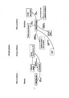
energy enters equation (3.123) at the l/c 2 level. Therefore we expect the separation between levels with the same n and different 1 to be very small compared with the separation between levels of different 1l. Figure 3.4 is a schematic diagram of the energy levels in the spinless electron atom calculated relativistically. The energy levels from the nonrelativistic theory are shown on the right of the figure. An atomic number of Z = 64 is chosen because we want Z to be large to maximize relativistic effects. However, if Zex. > 1 + 1/2, the denominator of (3.121) is imaginary. This occurs at Z = 69 for s-electrons so we cannot go above that. value. The energy levels of the one-electron atom do not split as implied by figure 3.4 when observed experimentally. This is clear evidence that something is omitted from the description of the atom in this section. In chapter 8 we will see that the missing physics is the spin. In figures 3.5a, band c we show the radial part of the wavefunction calculated from equation (3.118). Also drawn on these diagrams are the equivalent non-relativistic radial wavefunctions. Note that the figures show r R(r) rather than the wavefunction itself. There is good reason for this. We have actually glossed over a subtle point, as to mention it at the time would have distracted from the thread of the mathematics. Consider equation (3.119) for 1 = 1,2,3,' .. ,00: it is necessary to take the positive square root to get s positive. However, for 1 = 0, we find that s is negative whichever square root we take, which means that the wavefunction (3.120) is divergent at the origin. This does not matter provided that it does not diverge faster than l/r. What does matter is that the radial probability density does not diverge. To calculate any observable we have to do an integral in spherical polar coordinates involving something like the product of two wavefunctions. In this integral we always multiply by the infinitesimal volume r2 sin 0 drdOdcf>. As long as the wavefunction diverges less rapidly than l/r as r -+ 0, there will be no divergence in observables. The Is wavefunction tends to zero as r -+ 00, has a maximum at r = s/.J F, and decreases a little before rising to infinity as r -+ 00. Indeed any 1 = 0 wavefunction behaves similarly close to the origin. It is this divergence that is caused by the radial equation being quadratic in the potential, as mentioned when we compared equations (3.104) and (3.105). So the divergence is, indirectly, due to the existence of the negative energy states. There is one other intriguing limit of the above theory which we have not discussed. Although no one-electron atom exists with Z > 69, there is no limit on Z in the above theory. However, consider again equation (3.119) for s. If Z ex. > 1 + 1/2 we have to take the square root of a negative number and s becomes complex. The real part of pS is then p-l/2 which diverges as p -+ O. What happens in this case is that the
n
d
E(eV)
-2232 -2238 -2250
d
E(eV)
0,1.2.3,4
2S
-2226
0.1.2,3
I.
-3479
n
-un -2511 -349.5 -3.517
-3572 -4059
O,IJ
-6185
0,1
-13917
-6249
-6377 -7$14
-14371
-18461
-5.5669
- 89696
Fig. 3.4. On the left hand side are the relativistic energy levels of the single spinless electron atom with Z =64. Each level is labelled by its quantum numbers n and I, and its degeneracy is labelled d. The energies in electronvolts calculated from equation (3.121) are also shown. On the right hand side are the non-relativistic energy levels with the same labels for comparison.
3.8 The Spinless Electron Atom
'.
(a)
0.6
97
(b)
§
:;:;
o c
..2
.................
./
-0.1
III
>
~
/,/'
-02
......../
..
......./ .~
-0.3
2
3
4
5
6
7
8
9
---'
-0.4 L . - _ L . . - _ L . . - - . l L - - . l _ - . l _ - - ' 20 25 30 10 15 o 5
10
Radial distance
Radial Distance
0.35 . - - - , - - - - , - - - - , - - - - . . , , - - - - , : - - - ,
(c)
0.30
025
c
o ~ 0.20
c
.2 III
~ 0.15
0.10 0.05
5
10
15
20
25
30
Radial distance
Fig. 3.5. The Is (a), 2s (b), and 2p (c) wavefunctions (times r) of the Z = 64 spinless electron atom (full line), and their non-relativistic counterpart (dashed line). Distance is measured in units of the Compton wavelength and the wavefunction is calculated in relativistic units to emphasize the effects of relativity (see appendix D).
attractive Coulomb potential is so large that the kinetic energy of the orbiting electron (or the zero point energy in the n = 1 case) is insufficient to prevent it spiralling down into the nucleus. For I = 0 this means that the attractive potential energy must have fallen to less than half the rest mass energy at a distance of one Compton wavelength from the nucleus. To treat such atomic systems properly it is necessary to consider other factors as well, such as the finite extent of the nucleus. Now that we have evaluated the eigenvalues and eigenfunctions for the spinless electron atom, it seems a shame to stop here and not calculate some observable quantities. We will do this for the real hydrogen atom,
98
3 Particles of Spin Zero
but we don't do it for this case for two reasons. Firstly, although we have derived an expression for the wavefunction in equation (3.120), we have not normalized it. The integration involved in the normalization is a very messy calculation. Secondly, we are going to calculate observables for the single-electron atom later on and it would be a duplication of effort for minimal extra insight. Therefore we will cease our description of a spinless particle in a fixed central Coulomb field here. There is no such thing as a spinless electron, so the results described here are only of use for comparison with the non-relativistic case and with the relativistic one-electron atom including spin. However, with only the masses changed, the formalism described here could be applied to a an atom composed of a negative pion (which has spin zero) in a central Coulomb potential. One can conceive of creating such an atom (West 1958). 3.9 Problems (1) Show that the Klein-Gordon equation is Lorentz invariant.
(2) In this chapter we have considered only interactions between particles that are electromagnetic in nature and distinguish between particles and antiparticles. Derive a Klein-Gordon equation for scalar interactions that treat particles and antiparticles alike. (3) A spinless electron atom is placed in a constant magnetic field which is parallel to the x-axis. Derive an expression for the splitting of the energy levels due to the field. (4) Equation (3.59) enables us to calculate the antiparticle wavefunction, given a particle wavefunction for spin-zero particles. Explain how electrically neutral particles fit into this picture. Is the theory capable of differentiating between particles such as the nO which are their own antiparticle and the KO which are neutral, but have another quantum number reversed in the antiparticle (in this c.ase the strangeness)? (5) Find the eigenvectors of the radial Klein-Gordon equation (equation (3.104)) for a potential defined by
v-- { -vo 0
rsR r>R
where Vo is a positive number. Find an expression that determines the eigenvalues.
4 The Dirac Equation
In the previous chapter we discussed the direct relativistic generalization of the Schrodinger theory of quantum mechanics. It was shown that this leads to the Klein-Gordon equation from which some fundamental physics follows. Spin does not appear in either the Schrodinger or the KleinGordon theory. Indeed, the Klein-Gordon equation is only appropriate for particles with spin zero. Most of the particles encountered in everyday life (not that one actually encounters many fundamental particles in everyday life) are not spin zero. The most common ones, the neutron, proton and electron, all have spin 1/2. In this chapter we find the equation to describe particles with spin 1/2 and explore its properties. From the title of this chapter you will not be surprised to learn that it is known as the Dirac equation. The Dirac equation is more general than anything that has gone before, and therefore cannot really be derived. Much of the rest of this book involves looking for solutions of the Dirac equation under various circumstances. Although the Dirac equation cannot really be derived from anything learnt up to the present level, some plausibility arguments for its existence can be given and a couple of these are presented in the first section. As in the Schrodinger theory, it is very useful to be able to write the Dirac equation in Hamiltonian form. This is also discussed in the first section. Much of the theory of spin-1/2 particles is written in terms of 4 x 4 matrices. In other textbooks there are several representations of the Dirac matrices. Throughout this book we use a common one, which is the most convenient for our purposes. The properties of these matrices and a brief mention of their relation to other representations is given in the second section. A relativistic quantum theory is not much use unless the fundamental equation looks the same in any Lorentz frame of reference. Therefore in the third section we show explicitly that the Dirac equation is Lorentz invariant and how it can be transformed from one frame to
99
100
4 The Dirae Equation
another. Next we take the non-relativistic limit of the Dirac equation and show that this leads to the Pauli equation already mentioned in chapter 2. We can correct the Pauli equation to order 1/e2 and see that this yields some extra terms in the Pauli Hamiltonian. The non-relativistic limit is very instructive as it predicts the magnetic moment of the electron, and also we learn that this leads to the spin-orbit coupling so beloved by physics students everywhere. A less familiar form of the Dirac equation is then derived, which was first used in the theory of [3-decay, but has not found much application in condensed matter physics. Here we derive it for later use in our discussion of a single electron in a constant magnetic field. After that we show how the probability density and current are defined in Dirac theory. This leads to a natural method of normalizing the Dirac four-component wave function. Next we consider the Gordon decomposition, which is a method of separating the probability density and current into a part similar to that for Klein-Gordon particles and a part arising from the internal state of the particle. Finally we consider a particle in an electromagnetic field and explain how the Dirac equation can be used to find the forces on such a particle. Hence we are able to display explicitly the connection between relativistic quantum theory and the classical theory of electromagnetism. The review article by Feshbach and Villars (1958) covers a lot of the material presented in this chapter. 4.1 The Origin of the Dirae Equation In this section we present two origins of the Dirac equation, one based on symmetry arguments and the other on energetic considerations. The Lorentz transformations unite time and space into a single fourdimensional quantity. The basic equation underlying relativistic quantum theory must reflect this unity, implying that there must be complete symmetry between the time and space parts of the equation. Clearly the Schrodinger equation does not satisfy this constraint because it is first order in the time derivatives and second order in the space derivatives. Let us assume that, like the Schrodinger equation, the Dirac equation will be linear in the time derivatives. Therefore it must also be linear in space derivatives. It is certainly desirable for the principle of superposition to hold in relativistic quantum theory, so we have to constrain the equation to be linear. We know from classical relativity that the energy of a free particle is given by (4.1)
If we make the operator substitutions in (4.1), p -+ p = -;11\1 and W -+ W = il1a Iat, and have them operate on a wavefunction, we find the
,l
101
4.1 The Origin of the Dirae Equation Klein-Gordon equation 2
(
2 2
8- m e ) V2 - 1- 1p(r t)=O e2 8t2 li 2 '
(4.2)
If we insert a plane wave 1p(r, t) = exp(i(p' r - Wt)/Ii), this equation reduces to (4.1). For a wave equation describing a spin 1/2 particle we must also be able to substitute in a free-particle solution to obtain (4.1). Above we have insisted on several necessary constraints on the form of the Dirac equation. Within these constraints let us allow the equation to be as general as possible. We allow the wavefunction to have N components where the value of N is as yet unspecified. Now we express the time derivative of one component of 1p(r, t) in the most general way conceivable (Dirac 1928a,b, Bjorken and Drell 1964)
!e 81pi(r, t) 8t
_ _ ' " ~ ~ 81p1l _ ime ~ p_ ( ) L....J L....J iX ,,1I 8k Ii L....J 1,/l1p1l r, t k=x,Y,z 11=1
(4.3)
11=1
The left hand side of this equation is the time derivative of one element of 1p(r, t). The first term on the right hand side is a sum over all possible spatial derivatives of all components of the wavefunction and the second term on the right hand side is a linear combination of all the components of 1p(r, t). We have inserted the constants into equation (4.3) for the sole reason that they make the equation dimensionally correct. The factor i has been included in the final term with no loss of generality as the iX~ /ls and Pi,/lS have not yet been defined. Equation (4.3) looks a little compiicated, but we can make it look rather more simple by writing it in matrix form. If we let 1p(r, t) be a column vector with N elements then iX~1I and Pi,/l are, in general, elements of an N x N matrix. Furthermore, the sum over k in the first term on the right of (4.3) just amounts to a dot product. So the iX~1l , can be written as a vector ~ and (4.3) becomes
- 1p (r t ) t) - -ime p 'Ii'
-181p(r,t) = -~- . V1p (r e
8t
(4.4)
The tilde over ~ and P indicates that they are matrices. Next let us make the usual replacement p -+ liV /i and multiply the whole equation through by eli/i. We end up with
ili :t 1p(r, t) = H1p(r, t) = (eii'
p+ pme2 )1p(r, t)
(4.5)
This is one of the familiar forms of the Dirac equation. Of course, the ii and p matrices are still undefined. The Dirac matrices will be discussed in detail in the following section. Next we are going to arrive at the Dirac equation in·}a."1"ather more •
... ._.'l ...
: \:>~'-"'-.-:~ "-~ '::~i;'f/~~~;;;;;'~~~~'D1\ c~(!::
4 The Dirae Equation
102
straightforward manner which will also give us some clues about the properties of the Dirac matrices (Dirac 1958). Consider equation (4.1). To obtain a linear equation we write the square root of it in the following way (without worrying about the sign ambiguity when we take a square root): W = vp2e2 + m2e4 = (x' pc + {Jme 2 (4.6) Here, (X and {J have to be such that when we square (4.6) we arrive back at (4.1). Clearly, {J has to be a scalar and (X has to be a vector so that both terms on the right hand side of this equation are scalars. Let's square this explicitly. W 2 = «x. pc + {Jme 2)«X . pc + {Jme 2)
+ a~p~e2 + a;p;e2 + p{Jme 3 + {J(X . pme 3 + {J2m 2e4 +e 2«a xay + ayax)pxpy + (aya z + azay )pypz + (azax + axaz )pzPx) = a~p~e2
(x.
For this to be consistent with (4.1) we require that a2x = a2y = a2z = {J2 I
(4.7)
(4.8a)
and (4.8b) (4.8e)
In words, this means that the squares of the (x and {J operators have to be equal to the identity operator, and all components of (x and {J have to anticommute with each other. Provided these conditions can be met, it is clear that (4.6) is a valid way of writing the energy. Furthermore, if we make the usual operator substitutions in (4.6), we obtain equation (4.5), which was derived from symmetry and Lorentz invariance considerations. No numbers exist that can satisfy (4.8a, b and c) simultaneously. However, it turns out that there are matrices that do so. Therefore we have again found that the Dirac equation is a matrix equation. Finally, let us sum up what has been achieved in this section. Two plausibility arguments have been used to derive an equation of motion for a spin-1/2 particle, equation (4.5). Both these arguments led us to the same equation (I wouldn't have presented them if they had not) which is written in terms of some unknown quantities ii and p. By considering the energy of a free particle we have found some constraints that must be obeyed by these quantities. These are given by equations (4.8). Next we will separate the Dirac equation into time-dependent and time-independent parts, and hence derive the Hamiltonian form of the Dirac equation. In relativistic theory, time and space variables are linked
4.2 The Dirac Matrices
103
in a way that they are not in non-relativistic theory. It is not so clear, intuitively, that separating time and space makes sense. In fact it does, because the Dirac equation, like the Schrodinger equation, contains only a first order time derivative. Let us take the equation in the form of (4.5) in :t 1p(r, t) = c(-iM· V + pmc)1p(r, t)
(4.9)
We have already seen that & and 13 are N x N matrices. Let us pre-empt ourselves just a little and state that they are, in fact, 4 x 4 matrices. In that case the wavefunction in (4.9) must, in general, be a 4-vector. Let us write it in the form 1p(r t) = 1p(r)e-iWt / 1i = ,
(:~~~~) 1p3(r)
e- iWt / fi
(4.10)
tp4(r)
Substituting this into (4.9) and doing the time differentiation gives (4.11) H1p(r) = (c& . P+ pmc 2)tp(r) = W1p(r) Equation (4.11) defines the Hamiltonian for a free particle. W is the energy eigenvalue again. Instead of equation (4.10), we could have chosen the solution 1p(r, t) = 1p(r)eiWt / fi • In that case, we would have obtained an equation that looked like (4.11) except that on the right hand side W would be replaced by - W. Such a wavefunction would represent either a particle going backward in time or a particle in a negative energy state, like those we didn't think too much about when we took the square root in equation (4.6). 4.2 The Dirac Matrices Equations (4.8) are constraints on the Dirac matrices. Our task now is to find the matrices that satisfy them. We require four matrices, all of which anticommute with one another. The matrices we have seen before that describe spin are the Pauli matrices of equation (2.29). It would be satisfying if the & and 13 could be written in terms of the Pauli matrices. Unfortunately the Pauli matrices are 2 x 2 and the maximum possible number of anticommuting 2 x 2 matrices is three. It is necessary to go to 4 x 4 matrices to find four that anticommute (Rose 1961, Feynman 1962, Baym 1967). We will not derive a set of matrices satisfying the rules above, rather we will write them down and leave their verification as an exercise. There are actually several important sets of matrices in relativistic quantum theory, and we will write them down here and discuss their properties. It turns out that we can write the matrices in a representation in which the Pauli
104
4 The Dirae Equation
spin matrices play a role, and that is the representation we select. Firstly the identity matrix and
p:
14 =
U -e'
p=
(~
~)1 - 0 R) °01 0
0 1 0 0 0 1 0 0
0
0 0 -1 0
~) -e'
o
(4.12a)
-~2)
0
-1
(4.12b)
Henceforth we will label the identity matrix 1 whether it is 2 x 2 or 4 x 4. Which it is should be obvious from the context. Next the a-matrices:
CXX =
CXy =
CXZ =
° D~U,
0 0 1 1 0 0 0 0 0 i -i 0 0 1 0 0 0 0 -1 0
0
~)
° n~uY ° ° ~1) o ~U
0
G
~) ~)
az
(4. Ba)
(4.13b)
(4.13c)
0
Equations (4.12) and (4.13) are the matrices that appear in the Dirac equation (4.5) in what is known as the 'standard representation'. Check for yourself that conditions (4.8) hold and also show that
p-l-ai p=-ai-
(4.14)
The 4 x 4 Pauli spin matrices are also widely used. They are
a4x =
1 0 0)
o o
0 0 0 1 010
G G
-i
a4y =
0 0 0
oo
=
0) O.
o -l 0
(a x
0)
ax
0
=
(ay 0
3)
ay
(4.15a)
(4.15b)
,{
105
4.2 The Dirac Matrices
~) (~
1
0 0 -1 0 ( 001 0 0 0 -1
o
(4.l5c)
=
Again, from now on we will not differentiate in the notation between the 2 x 2 and the 4 x 4 Pauli matrices. The matrices (4.15) obey (4.16) . Furthermore, they have angular momentum commutation rules (4.17) where Cijk 0 unless i f j f k, Cijk = 1 if ijk = xyz or cyclic permutations thereof, and Cijk = -1 otherwise. The anticommutators are (4.18) One further very useful property of both the a-matrices and the a-matrices also arises from being able to write them in terms of the Pauli matrices. If A and B are arbitrary vectors, then ii . A ii . B = A . B + io- . A x B 0- . A 0- . B
= A . B + io- . A x
B
(4.l9a) (4.19b)
The a-matrices are called odd because they have non-zero elements only in the top right and the bottom left quadrants. The a-matrices, on the other hand, are called even, because they have non-zero elements only in the top left and bottom right quadrants. It is not hard to convince oneself that p commutes with all even matrices and anticommutes with all odd matrices. This is a property we will make full use of when it comes to separating the particle and antiparticle states in chapter 7. There are commutation relations between the a- and the a-matrices which will be useful later. We leave it to the problems for the reader to prove that
[ihad {O'i,aj}
=
(4.20a)
0
=0
ii x ii = 2io-
ifj
(4.20b)
(4.21)
One further set of relativistic matrices is very often defined. They are the ,),-matrices. There are several slightly differing definitions of the ,),-matrices in the literature. We select a definition in agreement with that of Feynman (1962) and Bjorken and Drell (1964) for Y1 to Y4 and a slightly different
4 The Dimc Equation
106
definition for }is (Rose 1961) because that simplifies our derivation of the radial Dirac equation later. The definitions are
( -1~ gl0
(
~ ~) (-~x ~) =
0 0
~o ~i ~0 ~i)=( ~ 0
-(Jy
0 0
-i
0) o 00 01 -1 ~1 ~ ~ ~
(~ ~ o
0
0
(0 =
-0-z
o-z)
-1
-1
(4.22c)
(4.22d)
-1
~ 0~ ~10 ~1) = (0_ -01 ) 0 -f
(o
(4.22b)
0
~) = (~ ~f)
gl 0
o-Y)
0
0
(
(4.22a)
0
(4.22e)
0
Several other conventions may be found in the literature for }is, but the one above is most convenient for our purposes. One form of the Dirac equation was written down in equation (4.5). If we premultiply it by iP llic, it becomes
-a
-{3 act lp(r, t) =
(A imC-) f lp(r, t) y. \I +!i
(4.23) .
Now if we define the 4-vectors \Ill =
~ = (~ ~ ~ !~) axil
(4.24)
ox' ay' OZ' cat '
we can write the Dirac equation in the rather succinct form
(~Y"V" + iIke) w(r,') ~ 0
(4.25)
where kc is the Compton wavevector. The y-matrices also obey some anticommutation rules. It is easy to verify that i=/=j
(4.26)
,(
4.2 The Dimc Matrices
107
All the anticommutators of the first four y-matrices can be described by the matrix elements gij •. (4.27) where gij is the fundamental tensor of equation (1.38). The matrix anticommutes with all the other y-matrices, i.e.
{Y5, Yi} = Y5Yi + YiY5 = 0 but commutes with all the
li,-
Y5
(4.28a)
and IT-matrices (4.28b)
for all i. Triple products of the y-matrices can also be taken and more relationships between them are found:
Y5Y1 Y5Y3
= =
iY2Y3Y4, iY1 Y2Y4,
Y5Y2 = -iY3Y4Y1 Y5Y4 = iY1 hY3
(4.29)
Sixteen matrices are required to form a complete set of 4 x 4 matrices. Such a complete set can be formed from the y-matrices. These are given by equations (4.22), (4.12a) and (4.29), and the products Y1Y2, Y1Y3, Y2Y3, Y1Y4, Y2Y4 and Y3Y4. Any 4 x 4 matrix can be written as a linear combination of these sixteen matrices. The matrices (4.12) and (4.13) were written down because they obey the conditions (4.8). However, they are not the only matrices that could have been deduced. Any matrix related to (4.12) and (4.13) by the transformations
a' =
sas- ,
P' = SPS- 1
1
(4.30)
also satisfies (4.8). This can be verified trivially by substitution. If we use such a representation in the Dirac equation we have lp
--1
= S
lp
,
(4.31)
and the Dirac equation becomes
. alp' zn-at = H
A"
•
lp
-
alp
-
A
-
= znS-at = SHS
-1' lp
-
A
= SHlp
(4.32)
and cancelling the S gives us back the Dirac equation in the original representation. We can ask what effect the different representations of our matrices and wavefunctions will have on the calculation of observables. Here we have to pre-empt ourselves and assume we already know how to calculate expectation values with 4-vector wavefunctions; there will be further discussion of this in section 4.6. In the new representation we
4 The Dirae Equation
108
assume an operator 0 can be written as a matrix and its expectation value is given by
Jtp/tO/v/dr JtptstsOS-lStpdr = JtptStSOtpdr JtptOtpdr =
=
(4.33)
In the last step here we have assumed that the matrix S is unitary. We can turn this argument round and say that if observables are going to be independent of our matrix representation (as they must be) then the allowable representations are related to the standard representation by the transformations (4.30) and (4.31) provided S is unitary. Next we will do a particular example of the unitary transformation above. This is done by stating a transformation matrix and using that to transform the Cl-, {3- and a-matrices from one Lorentz frame to another (Baym 1967). As a represents spin, an angular momentum, and the product of two vectors, we can assume it transforms as a second rank tensor, like the electromagnetic field. Therefore we will show how to transform one of the matrices and then complete the transformation of the Dirac matrices by analogy with the electromagnetic field transformation already described in chapter 1. The Lorentz transformation matrix for this case is
Ti =
exp(~ . 0/2)
(4.34a)
exp(-~ . 0/2)
(4.34b)
and so
Ti- 1 =
Here we have the primed frame moving with velocity v relative to the unprimed frame. The vector 0 lies in the direction of this velocity and has magnitude is given by u = tanh-l~, e
(v = Ivl)
(4.35a)
and hence (4.35b)
Let us take the x-axis as the direction of the relative velocity, and firstly let us transform uz • u~ =
Tju z Ti- 1 =
exp(~' 0/2)uz exp(-~' 0/2) = exp(~' o)uz
(cosh u + ~. usinh u)uz = cosh u(l + ~. utanh u)uz = (1 - v2/ e2)-1/2(uz + ~ . (v / e)uz ) =
(4.36)
where we have used the commutation relations (4.20) and the series representation of the hyperbolic functions. A little further algebra gives _/
(u z - iv?J.y/e)
az =
(l-v 2/c 2)1/2
(4.37)
4.3 Lorentz Invariance of the Dirac Equation
109
This is indeed analogous to the transformation of the electromagnetic field given by equation (1.58), and verifies our choice (4.34). Similar analyses can be done for all components of 0- and ~ and the analogy with the electromagnetic field holds for all components. Hence the Dirac matrices are components of the second rank tensor J!V =
a
0 az ( _ay -irix
-az 0
ax -iriy
ay -ax 0 -iriz
iriX) iriy iriz 0
(4.38)
and so the Lorentz transformations of the l/.- and p-matrices can be written as (aJ!V)' = faJ!vf- t (4.39) where f is given by equation (4.34). We have not actually proved that the l/.- and a-matrices transform like this, because the transformation (4.34) was written down without proof. However, we have shown that everything works out nice and consistently provided that (4.34) is a valid description of the Lorentz transformation properties of the Dirac matrices. Finally we need to see how to transform p. This is also straightforward because p anticommutes with ~, and we find -,
p=
p-pv'~/c (1- v2 /c 2 )1/2
(4.40)
From the above, the transformation properties of the y-matrices can easily be deduced, and I leave this to you in the problems. Note that the original transformation defined by (4.34) has the same form as the rotation operator described in section 2.2. 4.3 Lorentz Invariance of the Dirac Equation
Above we have postulated, but not proven, the existence of the Dirac equation. The best we have been able to do is give some plausibility arguments for its existence. Clearly, under such circumstances, it is necessary to verify that the equation behaves correctly before using it in a problem solving role. One property the Dirac equation must have is that it takes the same form in all inertial frames (Dirac 1958, Baym 1967). Any equation for which this is not true would be of very limited applicability. To prove that the Dirac equation is invariant under a Lorentz transformation we first have to recall some formulae from chapter 1. We have already defined the y-matrix 4-vector (equation (4.24)) and the energymomentum 4-vector (above equation (1.35)). Their scalar product (as defined by equation (1.37)) can easily be taken and must, obviously, give a scalar. Let us take the square of this scalar product and see what the
4 The Dime Equation
110
result is. To do this we also rewrite the y-matrices in terms of the p-matrices. 2
Cyllpll) =
lI.-
and
2 2 wj3 2 (PW le - Pii' p) = (PW le) - -(Pii + iiP)' p + (Pii' p)
e
=
W 2 /e 2 -
p2 =
m2e2
(4.41)
where we have used equation (4.19) and the relations between the Dirac matrices (4.8). The quantity m in equation (4.41) is the rest mass of our particle. This is the same in any Lorentz frame. So, taking the square root of (4.41), we see that yllpll
= (j3w le - j3ii' p) = +me
(4.42)
Thus we have shown that this scalar product is Lorentz invariant. If we label quantities in one Lorentz frame with a prime and quantities in another without a prime we have
p'W'le - P'ii' . p' = j3w le - Pii' P
(4.43)
Now let us write the Dirac equation (4.9) in the primed reference frame:
Ii
a
-
. v' + p'me)tp(r', t')
i1i at' tp(r', t') = e( iii'
(4.44)
The next step is to make the usual operator substitutions in (4.43):
aP 111at' -"f:
p-,lie _, '0' -at· v i
_
-
a-
P- 1/1'f:
at
P- -at· eli -
i
'0
(4.45)
v
We can now multiply (4.44) by P' and substitute for the operators from (4.45) into (4.44). Then multiplying through by P gives a result that is identical to (4.9) if (r', t') represents the same space-time point as (r, t). The primed quantities r' and t' are related to rand t via a simple Lorentz transformation. The argument above shows that the Dirac equation takes on the same form in all Lorentz frames. However, it would soon become clear that (4.44) is not the most convenient way of writing the Dirac equation in the new frame. This is because the lI.- and p-matrices take on different forms in different frames. It turns out to be more convenient if we keep the matrices the same in all frames. In that case, the wavefunctions have to differ between frames. As is shown in section 4.2, the Dirac matrices in one frame are related to those in any other frame via a transformation of the type (4.30). If we premultiply (4.44) by i3' and use these transformations we get - - - - 1i1i at' a tp(r,"t) TiPT i
=
e
(Iii TiPT - --i- 1 TiiiT - - -1 , ) i . V + me
tp(r," t)
(4.46)
.(
4.4 The Non-Relativistic Limit of the Dimc Equation Now if we premultiply this by [J Tji11 ~, tp'(r', t') =
1
111
we obtain
(c~ fl· V' + [Jmc 2 )
tp'(r', t')
(4.47)
where (4.48) Thus equation (4.47) is a representation of the Dirac equation for which the matrices fl and [J are the same in all frames. We have simply transformed to a representation where the difference in the matrices between frames is replaced by a difference in the wavefunctions between frames. The wavefunction in the primed frame is related to the wavefunction in the unprimed frame by equation (4.48). This shows that we can write the Dirac equation in a form such as (4.9) and it will be valid in any frame. The change in the wavefunction between one frame and another will be taken care of by changes in the potentials. 4.4 The Non-Relativistic Limit of the Dirac Equation
Another property we require of the Dirac equation is that it have a reasonable non-relativistic limit. It would be difficult to justify putting an equation at the heart of relativistic quantum theory if its non-relativistic limit did not make sense. In this section, then, we will give a detailed account of how to take this limit, and discuss the results obtained. Following Baym (1967), we start by writing down the Dirac equation in the presence of an electromagnetic field. We state without proof that this can be done in the same way as for the Schrodinger equation with the simple addition of the scalar potential and the replacement it -+ it - eA. In the penultimate section of this chapter we derive some results for particles in electromagnetic fields which confirm this procedure. Our Dirac equation becomes 'f;. otp(r, t) (4.49) In ot where V(r) is related to the electric field E and the scalar potential via E = -V(r) and V(r) = e(r). We are going to proceed with the following strategy. Firstly, we look at the non-relativistic limit of (4.49). Secondly, relativity has a natural small parameter in it, l/c, and we consider corrections to the non-relativistic limit to order 1/ c2• Equation (4.49) is rather abstract in itself and it is difficult to have any physical intuition about its solutions and properties. However, the corrections to the non-relativistic limit are amenable to direct physical interpretation. One feature of equation (4.49) worthy of note at this stage is that the external vector potential couples directly to fl which is associated with
4 The Dirae Equation
112
internal degrees of freedom of the particle described by the 4-vector wa vefunction. To take the non-relativistic limit of (4.49) we write 1p(r, t) as 1p(r t) ,
= (4)(r, t))
(4.50)
x(r, t)
where 4> and Xare both two-component quantities. Substituting (4.50) into (4.49) and using the definition of the a-matrices (4.13) we find
- eA(r)) . ux(r, t) + (V(r) + me c (~V - eA(r)) . u4>(r, t) + (V(r) - me
ili a4>~:, t) = e ili ax~~ t) =
(~V
2
)
4>(r, t)
(4.51a)
2
x(r, t)
(4.51b)
)
We will require these equations shortly. Now, recall the solution of the freeparticle Dirac equation (4.10). In the non-relativistic limit this becomes 1p(r, t) = 1p(r)e-iWt / iz ~ 1p(r)e-im c'lt/iz
(4.52)
and this is a solution of ili a1p~:, t)
~ me 21p(r, t)
(4.53)
Therefore, the lower component of equation (4.50) obeys
. ax(r, t)
zli
at
~
2
me x(r, t)
(4.54)
Now we go back to (4.51b) and substitute for the time derivative from (4.54). As e is large we ignore terms of order cO and lower, and we obtain x(r, t)
=
1 2me
(IiTV - eA(r)). u4>(r, . t)
(4.55)
This equation tells us about the relative sizes of 4> and x. Evidently, the term in brackets is a measure of the momentum of the particle. Classically this would be given by mv. This is divided by the 2me outside the brackets. The m cancels and we are left with X being of order v / e times 4>, so X is called the small component of the wavefunction and 4> is called (you guessed it) the large component. Now that we have an expression for X in terms of 4> we can substitute it into (4.51a) to remove X from that equation and hence make it easier to solve. Clearly this is the right way round to proceed. From the above we see that X --t 0 in the extreme non-relativistic limit, so we would not obtain anything useful by deriving a non-relativistic expression for 4> and substituting that into (4.51b). Eliminating X from (4.51a) gives .lia4>(r,t) 1 at = 2m
z
((IiTV - eA(r)·(1 ) _)2) 4>(r,t +(V(r)+me2)4>(r,t)
(4.56)
,{
4.4 The Non-Relativistic Limit of the Dirac Equation
113
This can be simplified using (4.19b)
(
(~V -
eA) . a) 2 4J =
(~V -
eA) 2 4J - elia . (V x A + A x V)4J
=
(iIi V -
eA
)2 4J - elia . B4J A
(4.57)
Putting this back into (4.56)
. a4J(r,t) zli at =
(1 (Iii 2m
V - eA(r)
)2 -
eli _ 2 2m (J • B(r) + VCr) + mc 4J(r, t) A
.)
(4.58) This is the Pauli equation which we. have already encountered as a description of spin-1/2 particles in an electromagnetic field in chapter 2. It differs from the previous version of equation (2.55) in the mc2 term. This only amounts to a redefinition of the zero of energy. Equation (4.58) is a very pleasing result. Not only does it show that the Dirac equation has the correct non-relativistic limit, but also the magnetic moment of the electron has fallen out of this formalism - we have not had to put it in, as is done ad hoc in the non-relativistic theory.
eli
f1 = 2m
(4.59)
This was a major success for the Dirac theory of the electron. All the usual non-relativistic theory of atomic spectroscopy, the anomalous Zeeman effect and the interpretation of the Stern-Gerlach experiment follow from this result. Before the discovery of the Dirac equation such experiments were understood on the basis of a spin which could only be postulated rather arbitrarily. It would be pleasing to be able to say that equation (4.58) also predicts the magnetic moment of the proton and neutron - after all, they are also spin-1/2 particles. However, this cannot be true for the neutron because it is uncharged, and it is also untrue for the proton. This failure is rather instructive. It is a first indication that protons and neutrons are composite particles, made up of three quarks (each of which is a spin1/2 particle). Quarks should obey the Dirac equation, and their magnetic moment may be deduced from an equivalent expression to (4.58). In fact the gyromagnetic ratio g of a neutron turns out to be -3.8, and that of a proton is +5.6, compared with g = 2 for the electron obtained from equation (4.59). The proton and neutron feel the strong nuclear force which is mediated by gluons, and to describe their properties fully requires a more complete theory taking into account the gluon field. We can continue the analysis above to find the lowest order relativistic corrections to the Pauli equation. Adding and subtracting 2mc2x(r, t) to
4 The Dirae Equation
114
the right hand side of (4.51b) and a little rearranging gives
1
x(r, t) = -2 (~V - eA(r)) . G(r, t)
(p -
eA(r)))) 4>(r, t)
eA(r)) . E(r, t)4>(r, t)
(4.66)
In the last step here we have used the Pauli equation to lowest order and have made liberal use of the identity (4.19). So our Pauli equation with corrections to order 1/ c2 is
ili
a4>(r, t) a t
1 m
= -2
(Ii
~V l
- eA(r)
)2 4>(r, t) -
eli _ -2 (1' B(r)4>(r, t) A
111
1 + (V(r) + mc2)4>(r, t) - - 8 3 2 (p - eA(r))4 4>(r, t)
mc
- 4 e~ 2 a . (E(r, t) x (p - eA(r))) 4>(r, t) mc ilie - -4 2 2 P . E(r, t)4>(r, t) mc
(4.67)
4 TIle Dirae Equation
116
One might think that this was the end of the story, we have found the Pauli equation and (4.67) is the Pauli equation with relativistic corrections to order 1/e2• Unfortunately this is not the end, and the reason is that the final term in (4.67) is not hermitian. This means it is not guaranteed to have real eigenvalues, which is disastrous for a Hamiltonian. The Dirac equation (4.49) is hermitian, so the non-hermiticity came about because of the approximations we have made. Let us assume that the solution to equation (4.49) was correctly normalized (we will discuss how to normalize a 4-vector wavefunction in a later section; here you should just accept that it can be done). So, using (4.50)
j tpt(r, t)tp(r, t)dr = j(4Yt (r, t)4Y(r, t) + xt(r, t)x(r, t))dr = 1 However, 4Y is defined in terms of X in equation (4.54), so 2 xt(r, t)x(r, t) = 4Yt(r, t)4 2 - eA(r)) 4Y(r, t) me I
~ (~v
(4.68)
(4.69)
but this expression for X is correct only to order v2 / e2, and so the normalization integral remains constant only to within terms of that order. Thus, in the non-relativistic limit, the integral we want to be constant is
j 4Yt (r,t) (1+ 4: e (~v_eA(r))2) 4Y(r,t)dr= 1 2 2
(4.70)
i.e. ignoring terms of order v4 / e4 (4.71a)
where A
_
(
M- 1+
(qv - eA(r))2) 8me 22
(4.71b)
All this tells us that the non-relativistic limit of the Dirac wavefunction needs to be renormalized. The correct non-relativistic wavefunction is related to the non-relativistic limit of the relativistic wavefunction by
E(r, t) =
(1 + 8m~e2 (~v - eA(r)) 2) 4Y(r,
t)
(4.72)
So we really require a wave equation for E(r, t) rather than the one we have got for 4Y(r, t). To obtain this we premultiply each term of (4.67) by Mand take it through the equation. Luckily this commutes with most of the terms in (4.67). However, it does not commute with the time derivative or VCr). Some algebra (quite a lot really) shows that if we work out the
4.4 TIle Non-Relativistic Limit of the Dirac Equation
117
commutator and add to it the non-hermitian term from the Hamiltonian (4.67) (after taking out a common factor 1/8m2c2 ) we obtain
([ (~V - eA(r)) (itl :t 2,
=
V(r))
1+ 2inep· E(r, t)) cfJ(r, t)
(4.73)
-n2V 2 V(r)cfJ. c ;: Q)
u
0.0
:;:; C
?- -0.5 lL.
IV~ I I
",\ l'
A{\
A:\
{\f\
n,/'..
~ t~'; lA ,\ A,: I I"
rn• :.•• \ ,; i,I.I::.
;,i.:::
.'
III
' '111,
'\/ \'J,v. '\,: :":.:1\. . /\/\~ :. "
I-
Q) Q) l-
f\:\
,/1, I
f\f\
I I
I\~. ,:,','
Ii
I I
(.::
1' / /1
I
\1,1f 1-:. ',.,::
\,,',
i: ~:
:
:-:
I'
:::.:: v. l:\;I.
l\j :,' I ~.
t\J
! !~.,:
I -i
I::
: :
i "!
: :
: I
v·d v\J Vi! vii v\! Vi) vij Vi! -1.0 I-1.5 0
10
5
20
15
25
30
35
40
45
50
Distance (Compton wavelengths) 1.5
c: 0 :;:; 0 c:
.... ::J
1.0
,,"" ,, , ,
0.5
..
Q)
> c ;: Q)
,
0.0
u
I-
?-c -0.5
·. ·.
Q) Q) l-
lL.
-1.0
,
,
'
I rr
, ,, ,,, ,, ,, , ,, , ,, , ' , "','
:;:;
(b) ..,·., i\ ,'.'.. ,....., , ,,· , ,,· ,, ,,, , , , , .,,, ·· ··,, ···, ·,,, ,·,,· ,,,, , · ,, ,, ·. , · .,,,, ,,,, ,,,, ,,,, ··,,,, .,, ··,, ,,, ,,,,, ., ,,,, ., .,,, ·,,, ,,, ·,,,, ,,·,· .,, , ., , · , ,, , , , · ...,, : ·,, .,
.
I,
"
, , ~
\:
,
""
' , "'1
-1.5 0
1000
2000
3000
4000
5000
Distance (Compton wavelengths)
Fig. 5.1. (a) The free-particle wavefunction for a particle with momentum like where ke is the Compton wavevector. The full lines are the real part of the large and small components of the wave function, the dotted lines are the imaginary part. (b) Same as (a) but the particle momentum is lilao where ao is the first Bohr radius. The structure of the small components is invisible on this scale. The figures are drawn using relativistic units.
138
5 Free Pm·ticles/ Antiparticles
Let us look at the non-relativistic limit of the wavefunctions (5.23). In this limit W -)0 mc 2 and Px, py -)0 0 so
(5.26a)
(5.26b)
This is the expected result. In the non-relativistic limit the bottom two components of the wavefunction disappear, and therefore it becomes possible to do quantum mechanics including spin with two components to the wavefunctions rather than four, i.e, we have recovered the Pauli formalism discussed in chapter 2. Because of the limit described by (5.26) the upper two elements of the wavefunction are known as the large component and the lower two are known as the small component. To calculate any measurable quantities we need to evaluate the expectation values of operators. An even operator will couple the two large components together and the two small components together, and the effect of the small components will be overwhelmed. However, an odd operator will couple the large and small components together, which will be a purely relativistic effect. So, if we want to see relativistic effects in nature, we should look at observables described by an odd operator. (See the discussion of magnetic dichroism . in chapter 12 for example.) As we have seen, the Pauli operator for the spin of an electron (~u) is insufficient to fully describe spin within Dirac theory. The Pauli operator is only appropriate when the momentum is zero or parallel to the particles spin. This can easily be seen if we write the eigenvalue equation explicitly (5.27) The upper component of this behaves appropriately, but Uz does not commute with u . p unless p is in the z-direction. So, a sensible question to ask is, 'What is the spin operator for a free particle moving in some general direction?' Much of the rest of this section is devoted to deriving the answer to this question. We will do this in two ways. Firstly, we will write down the spin eigenfunctions in the usual way and then rotate them using spin rotation matrices. Secondly, we will define a generalized spin operator, which is valid for any direction of the electron spin.
5.3 Free-Particle Spin
139
Rotations and Spinors
In this section we will show explicitly what happens to a spin or when we rotate the coordinate system and hence the axis of quantization. This is a fairly straightforward task, but we can use the results in chapter 6 when we discuss spin projection operators. The strategy in this section will be as follows. Firstly, we will recall the Pauli spinors. Secondly, we will use the Pauli spin matrices to define a rotation operator for spinors which is closely akin to previously defined rotation operators (equation (2.22)). Thirdly, we will apply the rotation operator on a Pauli spin or explicitly to confirm that it describes the rotation we expect. In chapter 2 we defined the Pauli spinors X-
l/2
=
(~)
(5.28)
which form a complete set in spin space (fors = 1/2), so any wavefunction for a spin-1/2 particle can be written as a linear combination of them. (P =
L
(5.29)
tplllsXllls
IIIs=±l/2
where tpllls contains all the space, time and energy dependence, etc., of the wavefunction. In the above discussion we have implicitly assumed that the spin is quantized along the z-direction, so Sz is diagonal with eigenvalues +tz/2. Let us rotate the axes, so that S is diagonal in another direction. In section 2.2 we have seen that rotation operators can be written in terms of angular momentum operators. Let us write down the rotation operator in terms of spin anguiar momentum by analogy with equation (2.22) (5.30) Now (} here is an angle of magnitude (J about an axis n. We know that be written in terms of the Pauli matrices, so writing (5.30) as an infinite series (which is the only way it can be understood), we have
S can
A
i(Jn . a
R=1--2-+
i 2(J2(n . a)2
2x2!
i 3(J3(n . a)3
-
2x3!
+ ...
(5.31)
nis a unit vector that n. a raised to any even power is the unit matrix. Therefore when it is raised to any odd power it must be either plus or minus the unit matrix. Inserting this into equation (5.31) tells us that R can be equal to exp( +i8 /2). We can combine both signs of the exponent into one operator
It follows immediately from equation (4.19) and the fact that
5 Free Particles/Antiparticles
140
if we write it as a diagonal matrix:
(eiO/2 R0 A
(5.32)
So this matrix operating on a spinor rotates it through an angle (} around the direction defined by fi. Let us illustrate this explicitly with an arbitrary spinor X of the form (5.29) which we rotate to make spinor X' using (5.32)
iB
I
X
Now, as
0) (a)b = RX
iO
) (e /2 a ) ( e /2 = a' b' = e- iB /2 b = 0 (
e- iO / 2
(5.33)
A
S is diagonal along some arbitrary direction q, we can write (5.34a)
where qs are the eigenvalues. Writing equation (5.34a) in matrix form gives us
n( qz. 2 qx + zqy
qx-iqy) (a)=qs(a) -qz b b
Next, let us premultiply (5.34) by (5.32) and note that ~ (eiO/2 2 0
o. )
e- zB /2
(qz qx + iqy
( eiBo/2
iO
qx - iqy ) (e- /2 -qz 0
iO 0) (a) ( e e- iO / 2 b = qs 0
/2
(5.34b)
RtR 1. So
0) x 0) (a)b e-iO / 2 .
e zB /2
(5.35)
Using the associative property of matrices we can multiply out the first three matrices on the left hand side of this equation and then we use the definition (5.33) to obtain
n(
2:
qz (qx + iqy)e-iB
(qx - iqy)e -qz
iB
)
I
I
X = qsX
(5.36)
Expanding the complex exponentials as trigonometric functions gives
e-
11 ( qz. q- cos iq_ sin -qz 2 q+ cos e- iq+ SIll e
e) X = qsX I
I
(5.37a)
with q- = qx - iqy,
q+ = qx + iqy
(5.37b)
But we know the equations that represent a rotation about the z-axis from simple trigonometric arguments:
= qx cos e+ qy sin e q~ = -qx sin e+ qy cos e q~ I
qz = qz
(5.38)
5.3 Free-Particle Spin
141
So we can substitute from (S.38) and (S.37b) into (S.37a) and we find
n("
"2
q~
qzf
+ iq~
'f) qxf - lqy _q~
f -
(S 39) .
f
X - qsX
Equation (S.39) is the same as (S.34b), but written with respect to a rotated set of axes. This formalism and example show that, given a Pauli wavefunction and an arbitrary direction 4, we can form the operator nO' . 4/2 according to (S.34a) which gives us the component of the spin along the direction 4. If we premultiply this equation by R we find it corresponds to a rotation of both the spin direction and 4 by an angle e. However, as they have both been rotated by the same angle, the component of spin along 4 should be unaffected by the rotation. This is verified by the fact that qs is the same in equations (S.34b) and (S.39). None of this is very surprising. Now let us pursue this line of thought further. We can find the eigenvalues qs by explicit solution of equation (S.34b). This is a simple simultaneous equation and will have non-trivial solutions if
qz - ~qs qx - ii y 1=0 qx + lqy -qz - Jiqs This can be solved: recalling that 4 is a unit vector, we have
I
n42qs2 = qz2 + ( qx -
.)( lqy qx
.) + lqy = qz2 + qy2 + qx2 = qA2 = 1
(S.40)
(S.41)
Hence qs = +n/2. Now that we have the eigenvalues in (S.34b) we can find the corresponding eigenvectors. It is more convenient to work in spherical polar coordinates, so qx = sin ecos 4>, qy = sin esin 4> and qz = cos e, where and 4> are now the usual angles in spherical polar coordinates. If the normalization condition for the spinors is chosen as
e
lal 2 + Ibl 2 =
1
(S.42)
it is straightforward to show that satisfactory solutions are
+
X =
(e-eic/J/2 sincosee/2/2) ' icfJ 2 /
e e
_ (_e- ic/J/2 sin /2) X = eic/J/2 cos /2 '
qs =
n/2
(S.43a) (S.43b)
The relative phases here have been chosen so as to give the most symmetric form to (S.43), but other choices are equally valid. Equations (S.43) are the expressions we were looking for. They allow us to write the twocomponent wavefunctions relative to a set of axes other than the direction along which we quantize their spin. Furthermore, they are orthonormal, and in the limit that e = 4> ..... 0 they become the usual spinors of equation (S.28).
142
5 Free Particles/Antiparticles A Generalized Spin Operator
To set up a generalized spin operator we are going to construct an arbitrary operator with specific properties, and then show that it is an operator which differentiates between the two spin states. It is central to this argument to recall that if an operator commutes with the Hamiltonian it represents a constant of the motion. Consider any unit vector r. Let us evaluate the commutator [iT . 1', E] = [iT . 1', di . p] = 2icri . I' x
So this commutator is zero if I' and commutator
P
(5.44)
p are parallel. Now let us evaluate the
[,BiT' 1', E] = [,BiT . 1', cri' p] = -2c,BYsr . p
(5.45)
This commutator is zero if I' and p are perpendicular. Equations (5.44) and (5.45) are not obvious, but can be verified easily (and tediously) by writing out the matrices explicitly. Now we are in a position to define a coordinate frame in terms of directions relative to the momentum. We can define appropriate operators along these directions to give us an operator that commutes with the Hamiltonian. Let us define the coordinate system with one axis defined by a unit vector in the direction of the momentum p and the other two by unit vectors 1'1 and 1'2. These are guaranteed to be perpendicular to one another if we define them by the relations (5.46) Such a coordinate system is illustrated in figure 5.2. Using it and the . commutators (5.44) and (5.45) we can define a generalized spin operator
s= ~(iT . pp + ,BiT . 1'11'1 + ,BiT . 1'21'2)
(5.47)
In conjunction with (5.44) and (5.45) this automatically gives us (5.48) As we have already seen, in the non-relativistic limit we need only consider the upper two components of the wavefunction. So in this limit, we can neglect the ,Bs in (5.47) and then S clearly reduces to the Pauli form. Now that we have set up this operator, we need to operate with it on the eigenfunctions (5.23) and see that it does indeed produce the right eigenvalues. Initially we have to do this component by component.
5.3 Free-Particle Spin
143
z
h
P j-------x
y
-
Fig. 5.2. The coordinate system used to define the generalized spin operator. The particle's motion is in the direction p, and £1 and £2 are defined in equations (5.46).
W = (
+ mc2) 1/2 2W
( ii· rlx±1/2 ) -icpiH? X±1/2 W+mc-
(S.49a)
where we have made use of equations (4.19) and (S.46). Similarly
ii'r2 UWl =
(
ii . pUiW =
(
W+mc 2W W
2) 1/2 ( ii· r2X±1/2 ) . _. lcpa'rt, X±1/2
(S.49b)
( ii· PX±1/2 ) • cPP ±1/2 W+iiiC2 X
(S.49c)
+ mc2) 1/2 2W
W+mc-
Combining (S.49a,b and c) according to the definition of S in equation (S.47) and taking the z-component of the resulting expression gives
S UWl z
=
~ (W + I11C 2
2W
2
1
) 1: (
(ii' ppz + ii . r1r1z + ii· r2r2z)X±! ) w+cpmc2 (pz + iii . r2r1z iii . 1'1 r2z )X±!
(S.SO) The upper component of (S.SO) is easy to simplify. Each term is just the component of ii along one of the axes and then we take the z-component of that. So this just becomes o-zX±1/2 = +X±1/2. Next we consider the
144
5 Free Particles/Antiparticles
lower component of (S.SO). This is rather more difficult to interpret. We need to look at the XI / 2 and X- I / 2 cases separately really, but we will only worry about XI/2 and leave the other case to the problems (aren't you grateful ?). For any vector r we have q . rxl/2
=(
rz.
)
+ lry
rx
(S.Sl)
Using this in the expression for the lower component of (S.SO) gives szuj =
fi (W +mc 2" 2W
2
XI/2
1 (
) 'i
~. 2 W+mc
A
.A
A
) pz
+ lr2y)rl z -
(l«r2x
A
.A
A
(rl x + lrl y )r2Z))
(S.S2)
(because the z-components of the terms in rl and r2 cancel). Now i«r2x
+ ir2y)rlz -
(rl x + irly)r2z)
= i(rl x r2)y + (1'1 x r2h = Px + ipy
(S.S3)
and substituting this back into (S.S2) gives A
szuj =
fi W + mc2 2" ( 2W )
1/2
XI/2
(~XI/2) W+mc-
(S.S4a)
That is,
~uj
Szuj =
2
(S.S4b)
and if we do the same thing for X- I / 2 we find SzU! =
-~U! 2
(S.S4c) .
We have obtained the results (S.S4) regardless of the value of the momentum. This tells us that the z-component of 8 takes on the same value whatever the momentum. The operator 8 has been normalized so that the eigenvalues of Sz are +fi/2. The expectation value of 82 can be calculated for the states UjW. We have to evaluate
J t8 1p
2
1pdr
The volume integral just gives us a volume which cancels with the in (S.23). Hence we are left with
(82 )rW =
r~ «(UjWI(q . p)2I Ujw) + (UjWI(,Bq . f l )2I U jw) + (UjWI(,Bq . 6fl UjW))
(S.SS)
l/.JVs (S.S6)
,{
5.4 Negative Energy States, Antiparticles
145
The fJ-matrix commutes with the (j-matrices and we can use (4.19) to write the three matrix elements on the right hand side of (5.56) as the expectation values p2, ft2 and 6 2. The square of a unit vector is just unity, and the expectation value of unity is one. SO 2 112 A2 A2) (A 2) 311 (SA2) tW = 4((P (5.57) ) + (rl + r2 ) = 4 This shows that the square of the spin operator we have defined in (5.47) has the expected length 3/4 (in units of 112). Furthermore we have seen that this operator may be used to distinguish between the plane wave functions (5.23), pointing along the +z-direction for ljJt and along the -zdirection for 1jJ!. This differentiation between the two cases is the origin of the phrases 'spin up' and 'spin down' frequently encountered in n6nrelativistic quantum mechanics and condensed matter physics, particularly in magnetism. As you have seen, the mathematical justification for that picture of the electron's spin is fairly complicated. However, it is necessary to understand spin at the level at which it is treated here to realize the limitations of that model. The functions (5.23) are eigenvectors of the S operator, and they have different eigenvalues. Obviously, this means that they must be orthogonal to one another; I leave it as an exercise for the reader to verify this. Finally, let me mention that the choice of the z-direction as the axis of quantization is arbitrary, but is motivated by convention and by the fact that the (j z-matrix is the only one of the (j-matrices that is diagonal. Hence the mathematics is simplest in this case. 5.4 Negative Energy States, Antiparticles In our solution of the free-particle Dirac equation we found the relative values of the coefficients Ul, U2, U3, and U4 in equations (5.10). Following this we took the right hand expression in (5.11) to give us the ratio Ut/U4. There was no reason to select this expression, we could just as easily have taken the central formula (Baym 1967). Had we done this we would have replaced equation (5.13) by the following
C(PX - iPY)) 1jJ!
ljJt
et:.
et:.
(
~
exp(i(p' r - Wt)/I1)
(5.58a)
W-mc 2
(C(PX~iP~)) exp(i(p·rW-mc o
Wt)/n)
(5.58b)
5 Free Pm·ticles/ Antiparticles
146
This pair of solutions is as valid as the pair given by equation (S.13). It is easy to see that one set of solutions may be obtained from the other simply by multiplying by a constant factor. Surprisingly, despite this, the two sets of solutions are definitely not equivalent. To show this explicitly we take the example of ut from (S.13a) and obtain the coefficient in (S.S8a) simply by multiplying by c(Px - ipy)
(S.S9)
where we have used (S.12). It appears that one solution is just a simple multiple of the other, but this is not the case. The easiest way to see this is to examine these solutions in the particle rest frame as we did for the particles in equation (S.17), i.e. when Px = py = p2 = O. We find
! V (p) et:.
vt( ) et:.
p
c(Px - ipy) ) 0 (
0
~
(0) 0 0
W -mc2
(c(px ~ iPY )) W - mc2 o
(S.60a)
-2mc2
~
(
~
-2mc 2 0
)
(S.60b) .
Here we have had to take the negative square root of the expression for the energy to get non-trivial solutions. In equations (S.17) we took the positive square root. So the states described by having the large part of the wavefunction in the lower half of the four-component wavefunction have negative energies. The real origin of this property is equation (S.12) for the energy. It has both a positive and a negative square root. We could get one solution from the other in (S.S9) because we used (S.12) which contains no information about sign of the energy. Now we have found all four independent solutions of the free-particle Dirac equation. There are positive and negative energy solutions and two possible spin directions.
,/
5.4 Negative Energy States, Antiparticles
147
Let us be absolutely clear about what we mean here:
'PJ
~ (D e-IW'I' ~ spin-up positive energy state in its rest frame.
'Pj
~ G) e-'W'I' ~ spin-down positive energy state in its rest frame.
'Pj
~
(r)
e'w 'I'
~ spin-up negative energy state in its rest frame.
'P~ ~ (D e,w'I' ~ spin-down negative energy state in its rest frame. The magnitudes here are arbitrary because they depend on the normalization. Note that in 1pJ we could have the third component of the 4-vector non-zero and still have an eigenfunction of Sz defined by equation (5.16) with eigenvalue n12. Similarly we could have the first component of 1pJ non-zero. Furthermore we could have the fourth component of 1p~ and the second component of 1p~ non-zero and still have an eigenfunction of Sz with eigenvalue -nI2. By studying the derivation of our plane wave solutions in section 5.2 it can be seen that motion in the z-direction would correspond to the introduction of these components. However, motion in the x- and y-directions leads us to a situation in which our wavefunction is no longer an eigenfunction of Sz. This shows unambiguously that, with this operator, we can really only define the spin parallel or anti parallel to the particle's momentum, and reveals the need for the generalized spin operator defined by equation (5.47). The normalized eigenfunctions for the negative energy states in a general frame are 1pi-
=
Vi(p)exp(i(p· r + Wt)ln)
= _1
.Jf7
(W + me2)1/2 (- ~ X1/2) exp(i(p. r + W+mc
2W
X1/2
Wt)/n)
(5.61a)
5 Free Particles/Antiparticles
148
tp!- = V!(p) exp(i(p . r + Wt)/Ii)
(W + mc JV 1
=
2W
2
) 1/2
(_~
W~~l/~
-1/2)
exp(i(p· r + Wt)/Ii) (5.61b)
where W is a positive energy. Clearly, there will be some interpretational difficulties with the negative energy states. Here we mention a couple of the problems. In the same way as was discussed for a Klein-Gordon particle, any negative energy state has lower energy than any positive energy state, so if a negative energy state is empty a positive· energy particle should be able to decay down into it, emitting a photon. Indeed it should be able to continue doing this forever, with the only restrictions being the usual angular momentum selection rules. Obviously, any reasonable, consistent view of nature cannot allow the universe to disappear up its own posterior like this, and anyway the photons emitted as the particles disappear down to -co are not observed. In (5.25) we have written the current operator for a particle. In this equation we can take W as the negative square root and the velocity of the particle is then in the opposite direction to its momentum, clearly an idea that requires a lot of justification. These difficulties were resolved by Dirac (1928b). One simply assumes that in a vacuum all the negative energy states are filled with electrons and all the positive energy states are empty, as illustrated schematically in figure 5.3. This is where we have to qualify our earlier statement that electrons must have W > mc2 . For -mc2 < W < mc2 we have a forbidden energy region, because the minimum energy any electron can have is its rest mass energy. Below this region down to -co are all the filled negative . energy states, and above the region up to +co are states available for standard positive energy electrons to occupy. In this scheme the Pauli exclusion principle automatically explains why there are no transitions to negative energy states. Now, suppose a negative energy electron is excited to a positive energy state. This will give a positive energy electron, but it will leave a hole in the 'sea' of negative energy states. The absence of a negative energy state will look the same as the existence of a positive energy state of the same mass. For electrons, the absence of the electronic charge will be equivalent to a charge of equal magnitude and opposite sign. This also means that the particle's velocity and momentum are parallel to one another. It is necessary to be careful in defining the spin of the hole. The absence of tpJ will leave us with a hole that has apparent spin down, and the absence of tp; will leave us with a hole of spin up.
,I
149
5.4 Negative Energy States, Antiparticles Allowed positive energy region Particle
me
2
w=o----me
2
$/Il/lIIlI!!/!IIlII/!IIlIIl
Antiparticle
Allowed negative energy region
(a)
(b)
Fig. 5.3. (a) The energetically forbidden region of width 2mc2 separating the positive and negative energy states. This figure represents the vacuum with the shading indicating that the negative energy sea is filled. (b) Same as (a), but here a negative energy particle has been excited up to an empty state in the positive energy continuum. This creates a positive energy particle and the hole left behind is identified as the antiparticle.
If this picture is correct, relativistic quantum theory is predicting the existence of particles with very specific properties relative to the electron (or any other spin-1/2 particle). Such a particle was discovered, after the predictions of Dirac (1928b), by Anderson (1933) and dubbed the positron. Undoubtedly, this prediction was one of the greatest triumphs of relativistic quantum theory, but it raises as many questions as it answers. There is something unsatisfactory about this description of nature because the particle/antiparticle symmetry inherent in the Dirac equation is broken in an unexplained manner. A more pressing problem this leaves us with is how to describe a vacuum properly. It appears to require very elaborate electrodynamics for a complete explanation, as any applied field should shift the negative energy states and hence polarize the vacuum. As there is an infinite number of these negative energy states the polarization of the vacuum should be infinite (Schwinger 1948, 1949, Tomonaga 1946). As an example of this, consider a single electron in a vacuum. This electron has charge e and it will repel the nearby electrons that fill the negative energy states. So, in effect, it polarizes the vacuum around itself, making the surrounding area positive. If the charge density of the electron is Pe(r) and the charge density of the polarized vacuum is py(r) then any macroscopic measurement of the electronic charge is going to see the sum of the electronic charge and the positive vacuum polarization !(Pe(r) + py(r»dr = e. However if some test charge could get inside the
lS0
5 Free Particles/Antiparticles
radius of the vacuum polarization it would see the electronic charge as greater than e. Of course, the test charge would itself polarize the vacuum and so the problem is not as simple as stated here. Nonetheless, the effect of vacuum polarization can be observed. In hydrogen, the I = 0 wavefunctions get very close to the nucleus, and a small correction to their energy levels occurs, owing to the vacuum polarization. So, although the discovery of antiparticles was one of the great successes of relativistic quantum mechanics, it was also the beginning of the end, and showed that the single-particle picture was insufficient even for the simplest problems. This and other considerations led to the development of quantum field theory, which is beyond the scope of this book. This does not mean we can say no more about antiparticles, but it does mean we have to be careful not to overstep the bounds of validity of relativistic single-particle quantum mechanics which we are discussing in much of this book. Equations (S.61) give the wavefunction for the negative energy electron states. However, this is not the real particle and the correctly normalized wavefunctions for a positive energy positron are tpbW =
+
2) 1/2 ( X±1/2 ) 7u w;;nc _ -yV ( _~X±1/2
exp(i(-p' r - Wt)/h) (S.62a)
W+mc
while the negative energy positron states are
tp~!)
1 ( W
=
+ JV
+ mc2 ) 1/2 ( ~!!c2 X±1/2 )
2W
X±1/2
exp(i(-p' r + Wt)/h) (S.62b)
where W is defined as being positive, i.e. it is the magnitude of the energy and p represents the true momentum of the particle, which we have chosen . as opposite to that of the negative energy state of (S.61) for consistency within the hole theory. These wavefunctions are identical to the freeelectron wavefunctions, as they should be. There is no difference between the Dirac equation for a free positron and the Dirac equation for a free electron. The charge has no effect on their properties as long as there are no fields present. The sign outside the wavefunction is an arbitrary phase factor which cannot be observed, of course, but which is left because it appears again when we discuss charge conjugation in chapter 6. 5.5 Classical Negative Energy Particles?
There is nothing quantum mechanical about equation (S.12) - it does not contain h so one can ask whether negative energy particles can be created in non-quantum mechanics. Our experience is that antiparticle creation cannot occur in a situation that is governed by classical relativity
5.5 Classical Negative Energy Particles?
Negative energy states
151
Positive energy states
Fig. 5.4. The potential barrier of height 2mc 2 and width 2mc2 / eEo used in our discussion of particle/antiparticle pair production. A negative energy particle tunnels through the barrier to become a positive energy one and to leave behind an antiparticle.
and mechanics. Here we are going to make a handwaving estimate of the production rate of particle/antiparticle pairs assuming the process can be described as tunnelling through a potential barrier: Such a view is suggested by our analysis of the Klein paradox earlier and by the picture we have of antiparticles being the hole in the negative energy sea of electrons that is left behind after a particle has been excited through the forbidden zone, as shown in figure 5.3. Referring to figure 5.4, we require a potential barrier with height (in energy) sufficient to create a particle/antiparticle pair: it must be of height at least 2mc2• For the purposes of this argument let us assume that this potential barrier is due to a constant field given by Eo. This assumption will not materially affect our argument. We also have to separate the particle/antiparticle pair by a distance x so that they do not instantly annihilate. When the particle travels a distance x in the field Eo the drop in potential energy (increase in kinetic energy) is given by eEox. Let us take the distance it is necessary to separate the particle/antiparticle pair as the distance required for the drop in potential energy to be equal to the rest mass energy. We could take another numerical factor times the rest mass energy, but that will not qualitatively affect our answer. So eEox = 2mc 2 • I would like to thank Professor J.M.F. Gunn for bringing this argument to my attention.
(5.63)
152
5 Free Particles/Antiparticles
or 2mc 2 eEo
(5.64)
X=--
The particle is excited from one side of the barrier (in the sea of negative energy states). It has to tunnel through the barrier of height 2mc2 and width 2mc2 / eEo. Once on the other side it is the particle and the hole it leaves behind is the antiparticle. The pair creation rate is equal to the tunnelling rate for the particle through the barrier. This single-particle tunnelling rate is given in many quantum theory textbooks (Gasiorowicz 1974) as
T'
DC
exp
(-2
~ (V -
E)a)
(5.65)
where the barrier has height V and width 2a. Our only task is to calculate (5.65) for the particle. If we set E = 0 as we have no incident particle and substitute in our values of the barrier height and width we find 2
2
2) 2m mc- ) = exp (4mc T 2 ex. exp ( -2 -(2mc - - -) 112 eEo eA.CEo
(5.66)
In (5.66), AC is the Compton wavelength. Now the point has been made, there will not be significant creation of particle/antiparticle pairs unless the potential changes by a significant fraction of the rest mass energy over a distance of order the Compton wavelength. This simple argument is in extremely good agreement with the much more sophisticated quantum field theory calculation (Itzykson and Zuber 1980) which gets the same functional form as equation (5.66), but replaces the factor 4 by n. Everything in (5.66) is a constant; let us expand AC and write it as (5.67) Now if we take the classical limit 11 ~ 0, the rate of creation of particle/antiparticle pairs tends to zero. So, if the universe were governed by classical relativistic mechanics, antiparticles might have existed since the beginning, but they could not have been created since then. 5.6 The Klein Paradox Revisited
In chapter 3 we solved the Klein-Gordon equation for a particle incident upon a potential step. For large enough values of the potential step, we found propagating solutions which do not occur in non-relativistic theory. Here we re-examine the same problem with an incident spin-1/2 particle
5.6 The Klein Paradox Revisited
153
v=vo ,-------------------------
w
rv\!V\I\J\r
v=o------------------~
z= 0
Fig. 5.5. The potential barrier problem that is solved to illustrate the Klein paradox for the Dirae equation. The particle wavefunetion is found for all possible positive values of Vo relative to W.
to see how the Klein paradox arises from the Dirac equation (Bjorken and Dre111964, Greiner 1990). Our one-dimensional potential is
zo
V(z) = 0 V(z) = Vo
(5.68)
This is illustrated in figure 5.5. We have chosen our one dimension as the z-axis this time as that means the incident particle can be an eigenfunction of the Sz-operator. We will not solve this problem at z = 0, rather we will solve for z < 0 and z > 0 and match the solutions at z = O. In fact, we have already done the hard work to solve the Dirac equation for this potential. On the left hand side of the barrier we have the free-particle solution (5.69)
and for the transmitted wave the solution is just that of a free electron rigidly displaced by energy Vo, so to the right of the barrier we have 1p(r) = T (
,~
)
eiP2zZ/n
(5.70)
W- Vo+mc 2
o
with (5.71)
1S4
5 Free Particles/Antiparticles
Note that we have defined the incident particle as being spin up. There can be no spin flip at the barrier because then the second and fourth components of the wavefunction would be non-zero while the first and third were zero. There would then be no non-trivial way of matching the wavefunctions at z = O. We have to conserve current and so we can match the solutions (S.69) and (S.70) at the boundary. The top row of the 4-vector equation gives
1+R= T
(S.72a)
2 1 _ R = P2z ( W + me ) T Plz W - Vo + me2
(S.72b)
and the third row yields
These are simultaneous equations for Rand T and can be solved straightforwardly to give
T =
+ me2) Vo + me 2 ) + P2z(W + me2)
(S.73a)
+ me2 ) - P2z(W + me2 ) + me2) + P2z(W + me2)
(S.73b)
2plz(W - Vo Plz-(W -
R _ Plz(W - Vo - Plz(W - Vo
Now, equation (S.71) leads us to exactly the same conclusions as we found in the Klein-Gordon case. There are several important regions of size of potential and the interpretation of them is given below equation (3.89). The transmission and reflection coefficients are given by equations (S.73). We see from (S.73b) that provided Plz and P2z are both positive (as they should be for particles incident from the left) we may for very large potential barriers find R < -1 and hence IRI2 > 1, i.e. more wave . reflected than incident again. The transmission coefficient T can also become greater than one and again this can only be understood on the basis of the creation of particle/antiparticle pairs at the boundary. What has happened here is that when the potential becomes Vo > 2me2 the negative energy electrons are displaced in energy by a sufficient amount for them to be taken out of the vacuum and the holes left behind in the barrier are the antiparticles, i.e. the field is sufficiently strong to force the vacuum to decay. 5.7 Lorentz Transformation of the Free-Particle Wavefnnction
In this section we take the wavefunction for a free particle moving in some general direction and perform a Lorentz transformation on it to move into the particle's rest frame (Baym 1967). This is simply an example showing
5.7 Lorentz Transformation of the Free-Particle Wavefunction
155
how to do the Lorentz transformations described in the previous chapter. From (4.34) a Lorentz transformation acting on a wavefunction is A-I
tp(r', t')
f
=
tp(r, t)
(5.74)
where A
f
= exp(& . u/2)
(5.75)
M
(5.76a)
with u = tanh- 1
c
(5.76b)
Here v is the velocity of the primed frame as measured by an observer in the unprimed frame, and u is the magnitude of the vector u in the direction of v. Using (5.75) we can rewrite (5.74): tp(r', t') = exp( -& . u/2)tp(r, t)
(cosh(u/2) - &. Usinh(u/2))tp(r, t) (5.77)
Now, some elementary identities of the hyperbolic functions can be used to write tp (r,") t = =
((COShU+1)1/2 2 - IX_ . u (COShU-1)1/2) 2 tp (r, t ) A
Y+ 1)1/2 _ (Y _1)1/2) tp(r, t) (( -2- - IX . u -2A
(5.78)
The explicit form we are going to use for the wavefunction is that of equation (5.23), so tp' =
_1_
J2V
((y + 1)1/2 _ &. u(y _1)1/2)
(W + mc2) 1/2 2W
x (
_Xnls ) ei(por-Wt)/Ii CuoPXnl s
(5.79)
w+niC2 where we have used the shorthand that tp' is the wavefunction in the new frame. Now the term in the exponent is a Lorentz invariant, as can be seen by taking the 4-vector scalar product of the Lorentz energy-momentum transformations with the Lorentz space-time transformations. Equation (5.79) can be simplified if we recall that this is a free particle and so its total energy is given in terms of y by equation (1.21). Also we write the IX-matrices in terms of the 2 x 2 Pauli spin matrices using (4.13). We also require equation (4.19) to show that G' pG' U= p. This is because the velocity and the momentum vectors are (obviously) parallel and uis a
156
5 Free Particles/Antiparticles
unit vector. After a little algebra we have ,
1·
lp -
--
- 2JVy
(
((Y + l)Xms ) ~XlIls
p -
-
me
IIlc(y+l} (~XIllS)) (j.
(5.80)
fiXlIls
The lower terms in (5.80) cancel immediately, because p times the unit vector fi is just the vector p. It takes a little more work to simplify the upper term, but if we substitute for the momentum from p2e2 = W 2 -m2e4 and use equation (1.21) again we end up with lp' =
}vy (X~!S)
ei(p·r-Wt}/i'i
(5.81)
The wavefunction lp' is still normalized. Its normalization simply represents the effect of Lorentz-Fitzgerald contraction along its direction of motion in the same way as we saw for the Klein-Gordon particle. Comparison of this equation with (5.23) shows that (5.81) just represents a free spin-up particle in its rest frame, i.e. p = o. In this section we have shown how to perform a Lorentz transformation on a wavefunction. We have actually chosen a transformation to the particle rest frame which works out rather easily. As we have never specified the velocity of the particle, the question of how we chose the rest frame as the one to which we were transforming is rather subtle. The answer lies in the definition of the energy of the moving particle. We wrote W = yme 2 where m is actually the rest mass, the mass as viewed in the frame to which we are transforming. To transform to some arbitrary frame would require us to write the energy in the untransformed frame in terms of quantities measured in the new frame. 5.8 Problems
(1) Solve the Dirac equation for a particle that is free to move along the zaxis only. Find all four solutions and show that they are eigenfunctions of both the Sz operator and the pz operator. (2) For a positive energy, free-particle wavefunction show that the expectation values of Pand ~ are
(~) =!
e (3) Verify that the free-particle eigenfunctions of equation (5.23) are indeed orthogonal to one another. (4) Starting from equation (5.50) verify equation (5.54e). (5) Starting from the wavefunction for a stationary free particle, perform a Lorentz transformation of the type described in section (5.7) to find the wavefunction of the particle in the frame of reference of an observer moving with velocity v relative to the particle.
6 Symmetries and Operators
In this chapter we are going to discuss some rather esoteric topics. Despite this nature they are of fundamental significance in relativistic quantum theory and have profound consequences. Clearly we could discuss a lot of topics that routinely occur in non-relativistic quantum theory under such a chapter heading. We will not do this, but only consider topics of specific importance in relativistic quantum theory. We will start this chapter by introducing a new type of operator known as a projection operator. This is an operator that acts on some wavefunction and projects out the part of the wavefunction corresponding to particular properties. In particular there are energy projection operators which can project out the positive or negative energy part of a wavefunction and spin projection operators which (surprise surprise!) project out the part of the wavefunction corresponding to a particular spin direction. Such operators form an essential part of the theory of high energy scattering. We will not be using them much in our discussion of scattering because our aim there is towards solid state. applications. For further discussion of projection operators, the books by Rose (1961), Bjorken and Drell (1964) and Greiner (1990) are useful. Secondly, we will look at some symmetries that occur in the Dirac equation. The symmetries we will consider are charge conjugation, timereversal invariance, parity and combinations of them. Matrix operators representing these symmetries will be discussed and we will show how this leads to the Feynman view of the negative energy states as representing antiparticles moving backwards through time (Feynman 1949). Thirdly, we will return to the topic of angular momentum. This follows on from our discussion in chapter 2. There we looked at angular momentum in the Pauli theory. Here we will generalize that work to a four-component representation of angular momentum in preparation for our discussion of the relativistic one-electron atom. Next, we will repro157
158
6 Symmetries and Operators
duce a simple argument relating the relativistic and non-relativistic kinetic energy operators for a particle in a magnetic field. Finally a major section of this chapter is devoted to many-body theory. Clearly this is something we have to know about for a description of the electrons in condensed matter. In this chapter we look at formal aspects of the theory only; we will apply the theory in several later chapters. Here it will be necessary to revise non-relativistic theory, before we introduce the relativistic formulation. We will introduce second quantized operators and discuss their properties and applications. Then we will relate them to the Dirac field operators, and show how to generalize non-relativistic theory to describe relativistic particles. Finally we will see how this enables us to develop a more consistent interpretation of the negative energy states and antiparticles, which removes the requirement to introduce an infinite number of negative energy electrons to maintain the single-particle picture. 6.1 Non-Relativistic Spin Projection Operators
A spin projection operator is defined as an operator that acts as follows. If we have a general wavefunction containing both spin-up and spin-down character, a spin projection operator acting on that wavefunction will give us the part of the wavefunction corresponding to one spin direction and will filter away the part of the wavefunction corresponding to the other spin direction. The term spin projection operator should not be confused with the operator (f . q. This latter operator, when used in an expectation value expression, just gives the average value of the spin (plus or minus a factor 11/2) along the direction q. From the discussion in chapter 5 it is very easy to see what operator we should use to project out the spin character of a particle described by a spinor. Let us define the operators first, then show that they do project out one particular spin and then discuss their properties. The projection operators are (6.1a) (6.1b)
In chapter 5 we saw that the eigenvalues of (f . q are +1. If the eigenvalue of (f. q is +1 then p+ has eigenvalue +1 and P- has eigenvalue 0, and vice versa if the eigenvalue of (f • q is -1. So we are claiming that, as (f . q is the operator whose eigenvalue is the value of the spin (in units of n/2) along the direction q, P+ operating on an arbitrary spinor will project out the spin parallel to q from that spinor and P- will project out the spin antiparallel to q.
6.1 Non-Relativistic Spin Projection Operators
159
To show that this is so, let us take a spin or X and operate on it with the projection operators (6.1). The result of this operation is an eigenfunction of iT . q, i.e, it is a state whose spin is purely along q.
iT· q!(1 + iT· q)x = !(iT . q + (iT' q)2)X
iT· qP+X =
!(iT' q+ l)X = +lP+X = +lXi
iT . qP-X = iT . q!(1 =
(6.2a)
iT . q)x = !(iT . q - (iT . q)2)X
!(iT . q -l)X = -lP-X = -X!
(6.2b)
Here the unit matrix is understood to multiply any terms where it is necessary and we have used equation (4.19) again. We have defined these operators in (6.1) and shown that they are spin projection operators by proving that when operating on an arbitrary spinor they give an eigenfunction of iT· q. Now, let us look at some other simple properties of these operators. Firstly, it is trivial to see that (6.3)
The mathematical term for this property is idempotent. Furthermore, there is no overlap between the two operators as p+p- = p-p+ = 0
(6.4)
Finally, as p+ projects out one spin direction and P- projects out the other, adding up the results of both operations should give us the original wavefunction back: (p+
+ P-)x =
(!(1
+ iT· 0) + !(1 -
iT ·o))X = X
(6.5)
as required. Finally we note from (6.2) and (6.4) that p+X!
= p-Xi = 0
(6.6)
In many experiments it is necessary to detect the spin of a particle. Imagine we have a detector that will sense whether an incident particle is parallel or anti parallel to some direction q. Let us write the wavefunction of the incident particle as (» =
L
lPl(r)x"
(6.7)
Il=j,!
We can project out the component of (» parallel (antiparallel) to q using P+(P-). The fraction of the particles that the detector sees as being parallel (antiparallel) to q will be F±q
=
I (}>t(r)P±(}>(r)dr I (}>t(r)(}>(r)dr
(6.8)
160
6 Symmetries and Operators
and, obviously, if we substitute in the operators we find p+q _ P_q =
J lpt(r)lpj(r)3 r - J lpI(r)lp!(r)dr J lpt(r)lpj(r)dr + J lpI(r)lp!(r)dr
(6.9)
This is a quantity often measured in experiments that involve either the electron or photon polarization. What we have considered up to this point in this chapter is the nonrelativistic spin projection operator. We now go on to look at how this formalism generalizes to the relativistic case. 6.2 Relativistic Energy and Spin Projection Operators
It turns out to be convenient to consider the energy projection operators rather than the spin projection operators first. These work in an analogous way to the spin projection operators described above. If we operate with the positive energy projection operator, the part of the wavefunction corresponding to negative energies is removed, and if we operate with the negative energy projection operator, the positive energy part is removed. We will illustrate the energy projection operators using the free particle wavefunctions of chapter 5. For the positive energy states the wavefunction is of the form (equation (5.23)) lp(r, t) = U(p)ei(p·r-Wt)/ti
(6.10a)
and for the negative energy states (c.f. equation (5.61)) lp(r, t) = V(p)ei(p·r+Wt)/ti
(6.10b)
Now, let us define the operators (with the square root always positive)
r=
a;. p+ pmc (p2
r±
+ m2c2)1/2
(6.11) .
!(1 + t)
(6.12)
r
Note that the numerator of is the total energy operator (divided by c), so it can be replaced by ilia/act (from the Dirac equation). Now we can operate on the states described by (6.10) with
r:
rU(p)ei(p'r-Wt)/ti
_
=
1 i1i~ U(p)ei(p.r-Wt)/ti c(p2 + m2c2)1/2 at
1 WU(p)ei(p'r-Wt)/ti = U(p)ei(p'r-Wt)/ti (c 2p2 + m2c4)1/2
(6.13a)
and similarly rv (p )ei(p'r+ Wt)/ti
_ V (p )ei(p·r+ Wt)/ti
(6.13b)
6.2 Relativistic Energy and Spin Projection Operators
161
and from this it is obvious that r+U(p)ei(p'r-Wt)/1i = U(p)ei(p.r-Wt}/Ii
(6.14a)
t-U(p)ei(p.r-Wt)/Ii = 0
(6.14b)
t+V(p)ei(p'r+Wt)/1i = 0
(6.14c)
t-V(p)ei(p'r+Wt)/1i = V(p)ei(p.r+Wt)/1i
(6.14d)
So, if we have a wavefunction that is some linear combination of positive and negative energy states, operating on it with t+ will project out of the wavefunction only those states that have positive energy. Similarly twill project out only those states that have negative energy. These energy projection operators have the following properties:
t+t- = t-t+ = 0,
(6.15)
We can conclude from this section that the energy projection operators are written in an analogous way to the non-relativistic spin projection operators and their properties are very similar. As we saw in chapter 5 it is difficult to define the spin of an electron in a general state of motion. It was shown in section 5.3 that the spin of a moving electron can only be defined simply in the directions parallel and antiparallel to its motion. If we define the particle spin in these directions then the relativistic spin projection operator can be defined simply in analogy with the non-relativistic case as (6.16a) (6.16b)
where (j are now the 4 x 4 Pauli spin matrices and q is a unit vector in the direction of the particle motion. For the general spin operator of equation (5.47), the projection operator becomes rather more complicated (Rose 1961).
By combining (6.12) and (6.16) we have obtained a set of operators which will project out spin and energy components of the wavefunction. To state that explicitly: ptr+ operating on a wave function will give us the positive energy spin-up part of the wavefunction, pt r+ gives us the spin-down positive energy part, ptr- gives the spin-up negative energy part and finally pt r- gives the spin-down negative energy part. We have chosen the free particle/antiparticle wavefunctions here. These form a complete set, so any wavefunction can be written as a linear combination of them. In principle, therefore, the energy and spin projection operators can be used on any wavefunction.
162
6 Symmetries and Operators 6.3 Charge Conjugation
In chapter 5 we saw that the existence of negative energy states is a prediction of the Dirac equation and that there emerges from this the hole theory where an antiparticle is interpreted as the absence of a negative energy particle. Mathematically, we could just as easily have started with the Dirac equation for the positron and constructed electrons as the absence of negative energy solutions to that equation. Clearly this symmetry is present in the Dirac equation and in this section we put that symmetry on a more formal mathematical basis. Let us start by writing down the Dirac equation for an electron in an electromagnetic field, i.e. equation (4.49) ili atp~:, t) = (ca.
(~V
- eA(r, t») + ,Bmc + V(r») tp(r, t) 2
(6.l7a)
Of course, this has negative energy solutions. Now, let us write down the Dirac equation for a positron in the same electromagnetic field. Obviously the sign of the charge of the particle differs so the sign of the term in the vector potential is reversed. The mass is still positive so the rest mass energy term in the Hamiltonian does not change. Finally, if the electron finds a potential attractive the positron with opposite charge will find it repulsive and vice versa, so the term in the scalar potential also reverses sign. We are left with i1i atp~~r, t) = (ca.
(~V + eA(r, t») + ,Bmc2 -
V(r») tpc(r, t)
(6.17b)
where tpc(r, t) is known as the charge conjugate· state. This equation describes the positron. On the hole theory we identify an antiparticle as the absence of a negative energy state. Therefore there must be a oneto-one correspondence between the negative energy solutions to (6.17a) and the positive energy solutions to (6.17b). Our aim now is to find an operator that will transform (6.17a) into (6.17b) and that will also transform (6.17b) back into (6.17a). We have to change the sign of the terms in the electromagnetic field and retain the sign in the terms for the kinetic energy, rest mass energy and time dependence of the wavefunction. The first step is to take the complex conjugate of (6.17a) and multiply by -1. This gives
'Ii atp*(r, at t) = (-* (IiiV + eA(r,t)) -
11
Cry;
•
/3-* me 2 - V(r) ) tp *(r,t)
(6.18)
The next step is to postulate the existence of a non-singular matrix which we shall call C. We will premultiply (6.18) by this and insert C- 1C, the
6.3 Charge Conjugation
unit matrix, into the middle. Recalling that
163
p is real gives
inC0tp*(r, t) =
ot
C (Cii*.
(~v+eA(r,t») -pmc2
Vcr») C- 1Ctp*(r,t)
(6.19)
Now it is simply necessary to find the matrix C. In order to satisfy the condition that (6.19) be equivalent to (6.17b) we must require that C satisfies the following: CPC- 1 =-p
Cii*C- -1 = ii,
(6.20)
A matrix that is consistent with (6.20) for all components of ii and is non-singular (all its eigenvalues are non-zero and its inverse exists) is C
=
0 0 0 0 0 -1 ( 1 0
0 -1 0 0
1)
0 0 0
=
.-_ l{3C1. y
(6.21)
Note that we have just written this matrix down, we have not proved it uniquely satisfies all the necessary conditions. The matrix is its own inverse, which is a desirable property, because if we perform charge conjugation twice we expect to return to the original Hamiltonian and particle. If we perform the matrix multiplications in equation (6.19) explicitly we find
in :t Ctp*(r, t)
(Cii'
(~v + eA(r») + pmc2 -
Vcr») Ctp*(r, t)
(6.22)
and making the identification (6.23)
gives us back equation (6.17b). Thus, by devising the operator ~=take the complex conjugate and premultiply by ipay , we have discovered a mathematical way of transforming (6.17a) into (6.17b). Let us check that the relation between the electron and positron wavefunctions implied by the above discussion is consistent with the freeparticle wavefunctions we wrote down explicitly in chapter 5. Labelling the electron (tp) and positron (tpc) wavefunctions i (!) for spin up (down) and +(-) for positive (negative) energy solutions, and lumping all the constants into one and calling it A we have, for a spin-up positron
(6.24a)
6 Symmetries and Operators
164
(.
(
i1 '
me
2
w=o me
2
,
>
)
~
(b)
(a)
Fig. 6.1. (a) The (more or less) filled sea of negative energy electrons. A negative energy electron can be excited to positive energy states as shown. The hole left behind is the positron. (b) The charge conjugation operation shows that (mathematically) we could equally well consider the positron as the fundamental particle. A negative energy positron could be excited up to the positive energy states and the hole left behind would correspond to an electron.
and similarly for the spin-down positive energy electron
~lP!+ = CA* (
c0 1_ W!mc2
-~ W +me
)*
e-ip ·r / Ii = -A
(~) W~~lc2 1 0 .
e- ip ·r / Ii
= -lPb(6.24b)
Here we have used the fact that A is real. This operator replaces a negative . energy spin up (down) solution of (6.l7a) with a positive energy spin-down (up) solution of (6.17b) and vice versa. So we can use this operator within the hole theory to give us the wavefunction for the antiparticle, if we know the wavefunction for the negative energy particle. From this analysis we see that the antiparticle has the same mass as, but opposite charge, momentum, spin and energy to, the particle, which is what we would expect within the hole theory. Now that we have discovered a one-to-one mapping between the negative energy electrons and the positrons we can broaden our definition of the negative energy sea of electrons. We can see that an electron in a positive energy state is entirely equivalent to a positron in its equivalent negative energy state. There is a symmetrized sea of electrons and positrons which exist side by side. This is illustrated in figure 6.1. Mathematically there is no reason for assuming the electron is the fundamental
6.4 Time-Reversal Invariance
165
particle. In the theory, both electron and positron have equal status. From the point of view of an observer on earth there appears to be an imbalance between the amount of matter and antimatter in the universe. However, it is very difficult to verify whether there is actually an imbalance if we consider the universe as a whole. This symmetry of charge conjugation also tells us that the motion of an electron in a field (A(r), VCr)) is identical to the motion of a positron in a field described by (-A(r), - V(r)). Some readers may find this unsurprising. Indeed it is what would be expected on the basis of classical physics. The remarkable thing is that the positrons are actually predicted to have specific properties from charge conjugation and the hole theory. Clearly their discovery, with these properties, is one of the great successes of theoretical physics. 6.4 Time-Reversal Invariance
The physical meaning of time-reversal invariance is not quite so selfevident as that of charge conjugation. Perhaps the easiest way to think about it is to consider running a film of some simple physical process, involving electrons, forwards and backwards. It isn't strictly necessary to consider only electrons, but let's keep things as simple as we can. We can run the film forwards and we will see events occurring that are describable within the Dirac theory. Now, if we run the film backwards we will see all the events running backwards in time. Time-reversal invariance holds . true if the dynamics underlying the time-reversed behaviour can also be described by the Dirac equation. Time-reversal invariance is bound to be embodied in the Dirac equation if we can find some mathematical transformation that can be performed which leaves the Dirac equation invariant when we change t ~ -to The correct time-forward Dirac equation for a particle in an electromagnetic field is equation (6.17 a). We can ask what this becomes if t ~ -t = t. Obviously the term that contains t will change sign and the t in the argument of the wavefunction will become t. Under time reversal r ~ r' and m ~ m' so there is no change to the momentum and rest mass terms. The potential VCr) will remain the same (like charges repel and unlike charges attract regardless of the direction of time). However, the vector potential A(r) reverses its sign if we reverse the direction of time. This is because the vector potential is generated by moving charges and the direction of motion of these charges will be reversed if time changes direction. So, the Dirac-like equation describing the time-reversed situation is (6.25)
6 Symmetries and Operators
166
This is not the same as the Dirac equation (6.17a). So, now we are looking for an operation that will transform (6.25) into (6.17a). Let's not beat about the bush. To do this we take the complex conjugate of (6.25) and premultiply by T
0 0)
=-
0 -i i 0 0 0 0 0 0 -i ( o 0 i 0
.__
= -lCXxCX z
(6.26)
This matrix is its own inverse, which is a useful property because we also require that it transform from the time-reversed state back to the time-forward state, as two time reversals must land you back in the timeforward state again. Let us perform this operation on equation (6.25):
a-
*
,
in at' Ttp (r, t ) =
f (ca*. (-~v+eA(r,t')) +p*mc2 + V(r)) f-lftp*(r,t')
(6.27)
Now, it is easy to verify that
fa*f- 1 = -a,
(6.28)
and if we make the identification (6.29) equation (6.27) takes the same form as equation (6.17a). So, our full time-reversal operator is: g-=take the complex conjugate and premultiply by the 4 x 4 matrix f and let t ~ t! = -to This operation leaves the Dirac . equation invariant. Following the same route as we took in the case of the charge conjugation operator, let us act on a free-particle wavefunction with the time-reversal operator to see what we get. We wi11limit ourself to a particle moving in the z-direction only, for reasons which will become clear soon. The spin-up and spin-down free-particle wavefunctions for this case are given by equation (5.23) with Px = py = 0, and again we will lump all the constants together into A. Now we operate on these wavefunctions with the time-reversal operator.
6.5 Parity
167
So a spin-up particle is mapped onto a spin-down particle with opposite momentum and vice versa. The i and -i multiplying the final expressions in (6.30a) and (6.30b) are phase factors. When included in an expectation value expression they disappear. If such a phase factor does occur and the Hamiltonian is invariant under time reversal, then the energy eigenstates occur in time-reversed pairs. This is known as Kramers degeneracy. If we had included the x- and y-components of momentum in this example we would have got into difficulties with the definition of the spin direction of a moving electron again. For electromagnetic interactions we have shown that if we film a physical process described by the Dirac equation, we can run the film backwards and we will still see a process that can be described by the Dirac equation. The particles in the time-forward case will be described by a wavefunction tp(r, t) and those in the time-reversed case by tpT(r, t'). So, time-reversal invariance is an intrinsic symmetry of the Dirac equation, and therefore Dirac particles must have this symmetry. This operation was first introduced by Wigner (1932). 6.5 Parity
The parity operator acting on a wavefunction or equation transforms the position coordinate to its negative, i.e. r -+ -r = r'. This operation is often described as taking a mirror image, although it is not really that. A plane mirror only inverts coordinates perpendicular to itself, whereas to get the parity operation we require a rotation about the normal to the mirror as well. To describe this symmetry we proceed in exactly the same way as we have for the charge conjugation and time-reversal symmetries. We will write down the Dirac equation after a parity operation and then find the operator that transforms the result back into the usual Dirac form. After a parity operation the scalar potential remains the same, whereas the vector potential changes sign. This is a consequence of its vector nature. Of course, the momentum operator also changes sign and we have
in atpP (;', t) a
=
(ca. (-~V' + eA(r', t)) + ,Bmc2 + v(r')) tpp(r', t)
(6.31)
The signs of V and A(r) have only changed if we measure them with respect to the untransformed set of space coordinates. If we measure them
168
6 Symmetries and Operators
with respect to the parity-inverted coordinates we would expect to get back the original Dirac equation (6.17 a). Now let us define the matrices P-
=
i 0 0 0 i 0 o 0 -i ( o 0 0
0) 0 0
= 'pl
~
p- -1
-i
=
( -i 0 0 0 ) 0 -i 0 0 0 0 i 0 0 0 0 i
= _ 'pl
(6.32) Now, an operator that transforms (6.31) into the form of (6.17a) is just premultiply by
P:
i1i :tptp(r/, t) = P
(c~. (i1iV' + eA(r/, t)) + pmc2 + V(r /)) p-1Ptp(r, t) (6.33)
and it is straightforward to see that p~p--1 =_~,
(6.34)
and making the identification
tpp(r/, t) = Ptp(r, t)
(6.35)
we have obtained (6.17a) as intended. So the full parity operator is 9= ---+ -r = r' and premultiply by P. We have shown that the Dirac equation is invariant under the operation of inverting space. Any physical process described by the Dirac equation can be looked at in a mirror (a special mirror that inverts all three dimensions) and that process is also describable by the Dirac equation. The inverse is also true, we can use the parity operator to describe the unreflected events in the reflected coordinate system. Next we ask what effect the parity operator has on the free-particle wavefunction. There is really no need to write this out explicitly. It is clear that replacing r by r' in the free-particle wavefunction (5.23) and premultiplying by P will give a phase factor· multiplying a wavefunction for a free particle with the same spin and opposite momentum. Let r
6.6 ~9g-
In the above three sections we have examined the charge conjugation, time-reversal and parity operators individually. In fact there is further insight to be gained into the symmetry of Dirac particles if we combine them, so in this section we consider them together. Consider first the Dirac equation for an electron and act on it with the parity operator. This will give us back the Dirac equation with r replaced with r/. Acting on this with the charge conjugation operator gives
i1iatpp~;r/,t) = (c~. (~VI +eA(r/,t)) +pmc2 -
V(r /)) tppc{r/,t) (6.36)
6.6 ~&g-
169
Now let us write down the Dirac equation for the positron. . atpc(r, t) (_ at = C~·
In
(nTV + eA(r, t)) + pmc - 2
)
(6.37)
V(r) tpc(r, t)
and we operate on this equation with the parity operator. This gives
inatpc~;r',t) =
(Cii'
(~V'-eA(r',t)) +Pmc2 -v(r'»)tpcp(r',t)
(6.38)
But (6.38) is identical to (6.36), so the space-inverted positron is the charge conjugate of the space-inverted electron, or, put mathematically, the charge conjugation operator and the parity operator commute. Now let us look at what happens if we operate on the Dirac equation for the negative energy solutions with all three of these operators:
~&g-(Cii' (p -
eA(r, t))
+ pmc2 + V(r, t»)(~&g-)-l~&g-tp(r, t) = -W~&g-tp(r, t)
(6.39)
where W is defined as being positive. First, consider the wavefunction . .&~g-tp(r, t) = &~(''ttp*(r, t'» = &(C(ifi.xfi.ztp*(r, t'))*) = &(iPfi.y(-ifi.xfi.ztp(r, t'))) = iP(iPfi.y(-ifi.xfi.ztp(r', t'»)
.- - - tp (") - (' = liXyiXxiXz r , t = -Y5tp r , t') = tprf&'ff (' r , t')
(6.40)
With this substitution (6.39) becomes
~&g-(Cii' (p -
eA(r, t»)
+ pmc2 + v(r»)g--l&-l~-ltprf&,ff(r" = -Wtprf&,ff(r',t')
t') (6.41)
Now, we already know that the time-reversal operator and the parity operator will give us the same Hamiltonian as appears in (6.41) with r replaced by r' = -r and t replaced by t' = -to We also know from earlier that the charge conjugation operator acting on this Hamiltonian will give us the Hamiltonian with the signs of the terms in the kinetic energy and rest mass reversed, but those in the potentials remaining the same. If we then multiply through by -1, (6.41) becomes (Cii'
(~V' + eA(r', t'») + pmc2 -
v(r'») tprf&,ff(r', t')
=
W tprf&,ff(r', t')
(6.42) What does this mathematics mean? You may well ask. We have started with the Dirac equation for a negative energy electron and by using these symmetries we have ended up with (6.42) which is the Dirac equation for a positron, but r' and t' are of opposite sign to rand t. So, using the ~&g we have transformed a negative energy electron into a positive energy
6 Symmetries and Operators
170
Table 6.l. Symmetry of various operators and physical quantities under charge conjugation, time reversal, parity and CfJ& ff. Symmetry
CfJ
Operator i'
+
;;
i'xp
+ +
v
e
A(r) (r) ii
= V(r)j e
;;CfJff
+
P p
ff
+ + +
iJ
+ +
+
+
+
+
+
+
+
+ + + + + +
positron moving backwards in space-time. This view of the positron is fundamental, but is really only a model, and forms the basis of the positron theory formulated by Stlickelberg (1941) and Feynman (1949). Let us check this by evaluating 1fJ0'[JJg-(r', t') using (6.40): "
-
"
1fJ0'[JJg-(r ,t ) = -Ys1fJ(r ,t ) = A ( =
A
(
_
0 1_) (
I 0
+1/2 X-
~ ±1/2 W+mc
~2X ±1/2) I W+mc ei(P'r'-Wt )/fi X±1/2
X
)
i(p·r'-Wt/)/fi
e
(643) .
This is the required result: comparison with (5.61) shows that we have indeed transformed a positron into a negative energy electron moving . backwards in space and time. One application of this view of antiparticles is the following. Equation (6.42) can be taken as an equation for a positron in a negative Coulomb potential. All the theory of the relativistic one-electron atom (which we examine in chapter 8) can be gone through for the antiparticle one-electron atom, i.e. a positron in the field of an antiproton. Equation (6.42) predicts that the spectrum associated with the antimatter one-electron atom will be identical to that for the usual one-electron atom. If it is not, the ~f;;g- symmetry is broken, with fundamental consequences for our view of nature. The creation of such antimatter atoms and measurement of their spectra is a very sensitive test of this symmetry (Baur et al. 1996). For the reader's convenience, in table 6.1 there is a summary showing how various operators and physical quantities behave under the charge conjugation, parity and time-reversal operations and ~f!J!T. You should
171
6.7 Angular Momentum Again
note that we have proved these symmetries only for particles experiencing electromagnetic interactions. Lee and Yang (1957) showed that these individual symmetries don't necessarily hold in interactions governed by the weak nuclear force. However, lCiJ g- is still a valid symmetry in that case. It has been shown that if we only assume Lorentz invariance and the fact that spin-1/2 particles obey Fermi-Dirac statistics whereas spinzero particles obey Bose-Einstein statistics, lCiJ g- invariance is guaranteed (Ludders 1954). 6.7 Angular Momentum Again
In chapter 2 we discussed angular momentum within non-relativistic spin theory in some detail. Now that we have derived and examined the Dirac equation, it is time to think about angular momentum again, in particular its generalization to a 4 x 4 theory and, hence, its implications for Dirac particles. This, of course, will find much application when we come to discuss atoms. We are going to consider angular momentum in a slightly non-standard way. Usually authors discuss matrix angular momentum in terms of the well-known properties of the operators. Here we are going to write out the matrices explicitly. Although this is cumbersome, it is instructive to do it once. The first step is to write down the full Dirac Hamiltonian in matrix form as we will want to refer to it several times later in this section: 0 c(Pz - eAz) c(p_ - eA_) ) V + mc2 0 V + mc2 c(p+ - eA+) -c(pz - eA z ) H= c(pz - eA ) c(p_ - eA_) V - mc2 0 z ( c(p+ - eA+) -c(pz - eA z ) 0 V - mc2 A
(6.44)
where P± = Px + ipy and A± = Ax + iAy and where we have omitted the dependence of the potentials on the coordinate for brevity. Next we write the angular momentum operators in matrix form. The orbital angular momentum is simply the usual operator multiplied by the identity matrix: Lx = (ypz - zpy)14,
Ly
(zPx - xPz)14,
Lz = (xPy - YPx)14 (6.45)
The spin operators have already been defined in 2 x 2 matrix form in equation (2.30). The 4 x 4 form of Sz was applied in chapter 5. In full the 4 x 4 spin operator takes on the unsurprising form A
1'1
Sx = "2ax,
A
1'1
Sy = "2 ay ,
A
1'1
Sz = "2az
(6.46)
where the ai are the 4 x 4 a-matrices of equation (4.15). Now we can define the total angular momentum operator (6.47)
172
6 Symmetries and Operators
and, of course, this can be written in terms of the spin and orbital angular momentum. For ilh.:J.strative purposes we will write the total angular momentum components out in full matrix form
o AA
o
Ii
AA
xpy - ypx -:2
o o
Xpy - YPx + :2li
o
o o o
o
XPy - YPx -:2
AA
AA
AA
AA
) 1i
(6.48a) A
Jx =
(
1'1/2
1'1/2
YPz -ZPy
0
y-
(
iIi/2 0
o
o o
YPz -ZPy
-ili/2 zPx -xpz
o o
o ZPX -xpz
J _
o
YPZ -zpy
1'1/2
o o
o
(6.48b)
o
zPx -xpz iIi/2
)
(6.48c)
-ili/2 zpx -xpz AA
AA
Before examining the properties of these matrix operators in relation to the Dirac Hamiltonian we should first confirm that they are correct representations by checking that they obey the commutation relations of equation (2.4b). Here we will evaluate one such commutator explicitly and it will be apparent that the others will follow by cyclic permutation of the indices. From the definitions above it is straightforWard to see that if we multiply them one way (being careful to keep the operators in the correct order at all times) we get
txf,y + i~2 iliL 2
AA_
JxJy
-
(
0 0
- ilif+
A
LA xy LA _
ili
2
4 A
o o
(6.49a)
"li2
A
LxLy+T
0 0
iliL 2
and if we multiply them the other way we find _ifiL+ 2
(LyLx-T .. rn' JyJx =
ifiL
-2-
0 0
A
A
0 0
ili2
LyLx+T 0 0
A
o0
ili2
A
LyLx-T ifiL
-2-
)
ifiL+ --2A
A
ili2
LyLx+T
(6.49b)
6.7 Angular Momentum Again
173
Subtracting these two gives the commutator between lx and ly:
[lx,]y] = lXly - lylx
~ ~ ~ ~
2
(~
i1i 0 0 1 0 + 2 0 o 0 0 1 0 Ii = i1iLzI + i1i2,az = i1i(Lz + Sz) = i1iJz
=
A
A
[Lx, Ly]
(
A_
A
)
A
o -1
oo
o 1 o o
0) 0 0
-1
A
(6.50)
An exactly analogous piece of mathematics will give the corresponding results for [ly,lz] and [lz,lx]. So these matrix representations of the angular momentum operators clearly do obey the required commutators. It is now just a matter of matrix multiplication and use of the positionmomentum commutator to show that
[l;,H] =0
(6.51)
where i = X,Y,Z. So total angular momentum commutes with the Dirac Hamiltonian and hence is a constant of the motion. When this commutator is evaluated it is easy to see the necessity of including the spin and orbital angular momenta to get something that commutes with H. In fact we find (6.52)
Using these commutators and equation (2.4a) proves that total angular momentum is conserved in the fully relativistic quantum theory. However, spin angular momentum and orbital angular momentum are not conserved separately, as we found previously for Pauli theory with spin-orbit coupling. The next step is to write the J2 operator in matrix form:
A2 A2 A2 A2 J =Jx+Jy+Jz
=
(A 1iax LX+T
)2 + (ALY+T 1iay )2 (A 1iaz )2 + LZ+T
- +LA yay - +LAza-) = LA2+1i2(-2+-2+-2)+1i(LA 4 ax ay az xax z =
f,2 + 1iL. (j + 3:
2
(6.53)
where we have used the facts that (j and L commute and the square of all the Pauli matrices is the identity matrix. Now, we know from chapter 2 that the eigenvalues of the total angular momentum operator are of the form j(j + 1)1i2• Next we define a new operator K such that
A2
A2
K = J
1i 2
+4
(6.54)
6 Symmetries and Operators
174
and the eigenvalues of this are (6.55) and so (6.56) In chapter 2 we defined an operator K, and the more awake reader may realise that (6.56) is simply the 4 x 4 equivalent of equation (2.87). From (6.53) and (6.54), and using the fact that (it' L)2 is not, as you might expect from (4.19), equal to L2 because the components of L do not commute, we find that A
K
2
=
2
2
+ IiL . it + Ii 2 = L2 - IiL . it + 2liL . it + Ii 2 (it . L)2 + 2liL . it + 1i2 = p2(iT . L + 1i)2 (6.57) A
= J
1i +"4
A
= L
2
A
A
A
A
Here the pis not strictly necessary, but it is included by convention. Equation (6.57) is an alternative expression for K (see equation (2.86)). This operator is of fundamental importance in spherically symmetric problems, and naturally one thinks of atoms in this context. It can be seen immediately from (6.56) that the eigenvalue K can take on all integral values except zero. Indeed K as the eigenvalue of (6.56) has exactly the same relation to the other quantum numbers as those described in equations (2.126) and (2.127). The eigenvalue is chosen as negative for consistency with equation (2.87). For completeness we will write K as a matrix operator:
K=
P(iT· L + Ii) =
L
+Ii
L+
( o o
L_ -Lz + Ii
0
0) ~
0
0 - Lz - Ii
- L_
0
-L+
Lz-Ii
A
(6.58)
Now let us verify some commutators. Firstly a simple one: using (6.51) it is easy to see that
[J2,fi]
=
J 2H - HJ 2 = J[J,H] - [H,J]J [K2,H] = [J2+li 2/4,H] =0
= 0
(6.59)
(6.60)
It is not straightforward to show that
[K,H] =0
(6.61)
but this commutator is equal to zero, and if you don't believe it, feel free to work it out from equations (6.44) and (6.58). It is a long mathematical
6.8 Non-Relativistic Limits Again
175
proof (I recommend you believe it). Finally, from the definition of K it is obvious that A2 (6.62) [K,J ] = [K,Jz] = 0 A
A
A
All these commutators prove two things: firstly, that )2, }z and K all represent quantities that are constants of the motion; secondly, eigenfunctions of the Hamiltonian are also eigenfunctions of these operators. When we come to discuss the relativistic hydrogen atom all these operators will be of central importance. 6.8 Non-Relativistic Limits Again Let us write down the Dirac Hamiltonian for a free particle (yet again)
H = c& . P+ pmc2
(6.63)
Now, suppose that the particle described by this Hamiltonian experiences a perturbation due to some electromagnetic effect. This may be an interaction with a photon or entering some region where it experiences a magnetic field. The effect on the eigenvalues and eigenvectors of H of such an occurrence may be calculated using perturbation theory. The perturbation Hamiltonian is found in the usual way by letting
p --+ p-
eA
(6.64)
where A is the vector potential associated with the perturbation. Inserting this into (6.63) gives us the perturbation Hamiltonian
H' =
-ec&' A
(6.65)
This does not look like the more familiar non-relativistic expression. The Schrodinger Hamiltonian for a free particle is A 1 A2 Hs = 2m P
(6.66
)
and putting (6.64) in here, the Schrodinger perturbation Hamiltonian is e = 2 (A, P+ P. A) (6.67) m where we are assuming the vector potential is small so the term in A2 can be ignored. The question that arises is how (6.65) and (6.67) can possibly describe the same thing. In the Schrodinger case the Hamiltonian is quadratic in the momentum operator and when the perturbation is added, terms linear in the momentum operator are carried through into the perturbation. However, the relativistic Dirac Hamiltonian is linear in momentum, so no terms containing the momentum operator carry through into the perturbation.
Hs
176
6 Symmetries and Operators
Certainly, one can resolve this difference by going through the involved mathematics required to take the non-relativistic limit of the Dirac equation described in chapter 4, or by performing a Foldy-Wouthuysen transformation as described in chapter 7. However, there is a simple hand-waving kind of argument which can get us from (6.65) to (6.67) directly. We start by remembering that A is a position dependent vector field whereas fi is just a 4 x 4 matrix containing simple numbers, so they obviously commute with one another. We also have to recall that cfi is the velocity operator V, so e
+ A· cfi) ':'(v . A + A . v) 2 (p' A + A· p) (6.68) 2 2 m As required, this is identical to the right hand side of (6.67). We have taken the non-relativistic limit in deriving (6.68) because we have used a non-relativistic formula for the momentum operator p = my. ecfi' A = ':'(cfi' A
6.9 Second Quantization
In this section we will discuss the creation and annihilation operators for bosons and fermions, although it is the latter with which we will be principally concerned in subsequent chapters. Much, if not all, of the first part of this section could equally well be presented in a text on non-relativistic quantum theory. Our strategy will be as follows. We will introduce some general concepts in many-body theory and see how they lead us to postulate the two different kinds of particles, bosons and fermions. Then we will discuss bosons and fermions separately. After that we will do some more general work with second quantized operators. This will lead naturally to field operators. Among the many good books on this subject are those by Baym (1967) and Merzbacher (1970). Only in the final section will we see how this formalism is modified when applied to relativistic systems (see Sakurai (1967) for example). Creation and annihilation operators act on a many-body wavefunction which is written in Fock space (where?). Such wavefunctions are called state vectors. Fock space is a mathematical space which contains all possible state vectors (so that's consistent then). These are a rather different way of writing wavefunctions to that which we have been using. State vectors are a way of writing general many-body wavefunctions in a manageable way using Dirac notation. They look like this: nl , 112, 113 , '" ,', 11' •.• )
1
(6.69)
This is actually a wavefunction with some subtle assumptions underlying it. It postulates some operator, often, but not necessarily, a Hamiltonian A with eigenvalues Ai. Equation (6.69) states that there are 111 particles with eigenvalue AI, 112 with eigenvalue A2, and ni particles with eigenvalue Ai.
6.9 Second Quantization
177
Such a wavefunction assumes that the many-body system it describes can be written as some sort of sum of single-particle behaviour. i.e. it assumes that in the many-body system the particles retain a lot of their single-particle identity. This is by no means obvious in quantum mechanics. Equation (6.69) is a particularly easy way to write a manybody wavefunction because all the position and time dependence as well as constants and normalization are suppressed. Particular examples of Fock space wavefunctions are as follows. The vacuum state is written as (6.70)
10,0," ,,0) = 10)
i.e. it contains no particles in any states. However, with our picture of the vacuum as a sea of filled negative energy states, some modification of this definition will be required later. Single-particle states are 10,0, ... ,0, lli
= 1,0,0, ... ,0) = IAi)
(6.71)
Here there is a single particle in quantum state i and none in any other state. We can see that the space of all single-particle wavefunctions is a very small subset of the whole Fock space. Now we are going to define the second quantized operators ai and at. The first of these is known as an annihilation operator. It takes a many-body system with ni particles in the itb state and relates it to the many-body system with ni - 1 particles in the jtb state. The operator at is known as a creation operator. It relates the many:-body system with ni particles in the jtb state to the many body system with n; + 1 particles in the jtb state. In both cases the number of particles in all other states remains constant, i.e. a-1nl z , n2 , n3 , ... ' n· h ... ) a!llll 1 ,
= klnl , 112 , n3 , ... , 1 n- -
112 , 113 , ••• ' 11h ••• ) =
1, ... )
(6.72)
plnl , n2 , n3 , ... , 111 + 1, ... )
(6.73)
where k and p are, as yet, unknown constants. One very important feature of this approach to the quantum mechanics of many-body systems is how a unitary transformation from one basis to another is made. To see this explicitly let us introduce a second operator B with eigenvalues Bj and occupation numbers mj- Then the transformation from the m to the n basis is written as (6.74) j
j
178
6 Symmetries and Operators
where the transformation coefficients Cij form a unitary matrix:
L CikCkj
= CJij
(6.75)
k
Of course in writing (6.74) we have used the fact that the eigenfunctions of both A and B form a complete set. A transformation like (6.74) does not change the vacuum state. However, a state that is a one-particle state in the basis of eigenfunctions of A is, in general, not a one-particle state in the basis of eigenfunctions of B. It is perfectly possible, though, to introduce single-particle creation and annihilation operators in the latter representation in exactly the same way as was done for the former: (6.76)
b!lm1 I ' m2 , 1113 , ... ' nlh ... ) = p'Im1 , 1112 , m3 , . _. ,mI + 1, - -.)
(6.77)
For single-particle states atlO) -10 " c"IO " c·-b~IO) i , ... ,nI = 1" 0 ... ) = ' L....t I J ' ... ' nJ = 1" 0 ... ) = ' L....t IJ J j
j
(6.78) and this is only satisfied if (6.79a)
al = LcijbJ j
and we can take the hermitian adjoint of this equation to give (6.79b)
ai = LC;jbj j
Equations (6.79) have been shown to hold for single-particle states only, but we will assume that they hold over the whole of Fock space. Now a creation operator only acts on one quantum state within the Fock space wavefunction. Therefore, if we were to act with two creation operators on different single-particle states we would expect the state we end up with to be independent of the order in which we apply the operators; the only thing that might change is the normalization, so for the particular states I and 111 we expect
at a~lll, 111) = Aalatl1, m)
(6.80)
Now we can use (6.79a) to transform this into the basis of eigenfunctions of B. This gives
(at a~1 - Aa~lat)ll, m) = L Clpc11lq(bbb~ - Ab~bb)lp, q) p,q
=0
(6.81)
6.9 Second Quantizatioll
179
As the transformation coefficients are arbitrary, except for the constraint of unitarity, this is only satisfied if
b~b4 - Ab4b~ = 0
(6.82a)
Of course, we could just as easily have switched round the subscripts in (6.80) and then we would have arrived at b4bt - Abtb4 = 0
and m (6.82b)
This can be substituted into (6.82a) to give t btb p q
= A2btpbtq
(6.83)
and so (6.84)
A= +1 Substituting A = +1 back into (6.80) gives us immediately t t - ama/ t t -- 0 a/am
(6.85a)
and the hermitian adjoint of this is (6.85b) A similar argument can be made to give a/ah, - ah, a/ = (\m
(6.85c)
If, instead, we allow the solution A = -1 in (6.80) we have a;ah, + ala;
=0
(6.86a)
and the hermitian adjoint of this is a/am
+ ama/ =
(6.86b)
0
and as previously (6.86c) So the operators with A = +1 commute and those with A = -1 anticommute. This argument implies that there are two different types of particle. Those that obey (6.85) are known as Bose-Einstein particles or bosons for short, those that obey (6.86) are called Fermi-Dirac particles or fermions for short. For a system of bosons in equilibrium at temperature T with chemical potential J1. the fraction of particles in the quantum state with energy W i is 1
!(Wi
-
J1.) =
e(Wj-J.L)/kBT
1
(6.87)
6 Symmetries and Operators
180
and for fermions the same quantity is 1 f(Wj - /1) = e(Wi-jl)/kBT
(6.88)
+1
With our understanding of the commutation relations for the creation and annihilation operators for bosons and fermions we can now assign consistent values to the constants k and p in (6.72) and (6.73). Let us consider bosons first. Equations (6.72) and (6.73) can be written ajlnl, n2, n3, ... , nj, ... ) = Jililnl, n2, 113, ... ,11j - 1, ... )
annl, 112, 113,···, nj,···)
=
(6.89)
Vnj + 11111. 112, 113,···, 11j + 1,···)
(6.90)
and the commutation rules can immediately be seen. We haven't proved (6.85c) but with the definitions (6.89) and (6.90) we have
(ajar - ar aal·· ., 11j,···) = aj V 11j + 11 ... , nj + 1, ... ) - ar Jilil ... , 11j - 1, ... ) = V11j =
+ 1V11j + 11···, n,···) -
JiliJiliI···, nj,···)
I· .. , 11j, ... )
(6.91)
which is consistent with (6.85c). Now, aj is the hermitian conjugate of ar and so if I'll) is a general many-body wavefunction we can write ('Plajarl'P) = (al'Plal'P) = (ajal'PI'P) Next consider the operator
N=
(6.92)
al aj acting on an arbitrary state vector
NI· .. n· ... ) = at a·l· .. n· ... ) = at rn:1··· '"1 , n· - 1 ... ) - rn:atl··· j , 11· - 1 ... ) - n·I·· .. n· ... ) ,
h
I
-
I
,
h i "
,,'"1
I
,
-
I
I
,
,
h
(6.93)
So the operator N is a number operator, it tells us the number of particles in the i th quantum state. The existence of this operator was implied by our representation of the wavefunction in the form (6.69). With the definitions we have so far we can see that any boson manybody state in Fock space can be constructed by repeated operation of the creation operators on the vacuum state: 1111,112,···,nj,···) =
(aIyll (a1)n 2
~ ...
(al)ni
r;;-:j ···10,0,···,0,···) (6.94) " 11 1. " n2 • " 111 • Creation and annihilation operators that act on different states do not interfere with one another, as shown by the commutation relations (6.85). It doesn't matter which order we perform the operations in equation (6.94). Now let us move on to consider the creation and annihilation operators for fermions. There are two important differences from the boson case.
r;;:f
6.9 Second Quantization
181
Firstly, any state can only be occupied by one particle. Hence ni in the state vector can only take on the values 0 and 1. Secondly, the operators anticommute, which leads to the antisymmetric nature of the many-fermion wavefunction. It would be useful to see explicitly how this antisymmetry comes about. By analogy with equation (6.94) we can build up a state vector for a many-fermion system by repeated operation of the fermion creation and annihilation operators Inl,n2,··· ,ni,···) = (aI)'I'(a~)n2 ... (a[)'li .. ·10,0,··· ,0,···)
(6.95)
with ni always equal to zero or one. The factorials in (6.94) are not present here because ni! is always one. Using the anticommutation relations (6.85) it is immediately clear that if we interchange the order of any two of the creation operators in (6.95) the sign of the wavefunction on the left hand side is changed, so the antisymmetry is built in. Let us see how this works for simple cases. Firstly consider the simplest case, a single particle state. The creation and annihilation operators acting on such a state are
aIIO)
= 11),
ad1)
= 10),
all1) = adO)
=0
(6.96)
This is easy, it is just the same as (6.89) and (6.90) for bosons. As there is only one particle there is no need to worry about antisymmetry. For two particles the situation is a bit more complicated. Inside the state vector we call the left hand state 1 and the right hand state 2. There are four possible states, and the creation and annihilation operators acting on them are aIIO, 0) = 11,0), aIIO, 1) = 11,1), alI1,0) = all1, 1) = 0 ali1, 1) = 10,1), alI1,0) = 10,0), adO, 1) = alIO,O) = 0
(6.97a) (6.97b)
a~IO,O)
(6.97c) (6.97d)
= 10, 1),
a~11,0)
= -11,1), a!IO, 1) =
a211, 1) = -11,0), a210,1)
= 10,0),
a211,0)
a~11, 1)
= 0
= a210,0) = 0
As you can see we have defined some negative signs here. This has been done to maintain the antisymmetry. The second equation in (6.97c) could be said to come from a~11,0) = a~aIIO,O) which is (6.95) for two particles with the operators reversed. That is why it has a negative sign. The negative signs also have to be consistent so the sign in the first equation of (6.97d) is there because it must undo the work of the equivalent creation operation in the second of (6.97c). Antisymmetry of the two-fermion state can be demonstrated explicitly by taking the state 11,1) and removing the particle in state 1 using al. The particle in state 2 is removed from state 2 and put in state 1 using aI a2. The first particle is then placed back in
6 Symmetries and Operators
182 . . h at , I.e. state 2 WIt 2
Of course, this could also be done the other way round. We could remove the particle from state 2, move the particle from state 1 to state 2 and put back the remaining particle in state 1. This gives the same result as (6.98). You might think that the operation defined in (6.98) should yield the same result as
but it doesn't. The reason for the lack of a sign change is that (6.99) represents the operation of removing a particle from state 1, removing a particle from state 2 and then putting the same particle back into state 2, and finally putting the original particle back into state 1 - that is, removing the electrons and putting them back into their original states. When using these operators for fermions it is very important to make sure that the order in which the operations are performed corresponds to the physical system you are trying to describe. A rule of thumb is that you continue to work with the same particle unless the operator cannot operate on it in its present state, then you go back to the most recently operated on particle that you can. Of course you are always subject to the restriction that no state can ever contain two or more particles. Finally here, we will consider the three-state system without going into all the mathematical detail of the two-state system above. The wavefunction must change sign if we interchange any two particles regardless of whether the third state is filled or empty. So, in analogy with the case above, we can write the following: atlO, 1,0)
=
-11,1,0),
aliI, 1,0)
=
-10,1,0)
a!IO,O, 1) = -10,1,1),
a210, 1, 1) = -10,0,1)
aIll,O,O) =-11,0,1),
a311,0, 1) = -11,0,0)
(6.100)
All other single creation or annihilation operators acting on the threeparticle state either give zero or the appropriate state multiplied by +1. Again we will see what happens if we interchange two particles. If we interchange particles in states 1 and 2 the interchange operator is identical to the two-particle case. a! at a2all1, 1,0) = -a!aI a210, 1,0) = -a!aIIO, 0, 0) = -a!ll,O,O) = -11,1,0)
(6.101a)
183
6.9 Second Quantization
Now, if the third state is filled we must still get the antisymmetry emerging. Let us see if that works: a1aIa2atl1, 1, 1)
a1aIa210, 1, 1)
= -a1aII0, 0, 1)
= -a11 1,0, 1) = -11,1,1)
(6.101b)
So it works again. It can be seen immediately that cyclic permutation of the subscripts 1, 2 and 3 will yield the same result. If you have time, try doing the same thing for other pairs of particles or with the operator with the subscripts reversed a1aIa2al. If you don't have time, do it anyway. For four or more particles, working out which operators acting on which state vectors have negative prefactors becomes complicated. In condensed matter we are usually working with the order of 1023 particles, so working it out becomes impossible and is pointless. Useful quantities are usually written in terms of several creation and annihilation operators. For fermions the number operator for the number of particles in a single particle state i is given by (6.102)
and the operator for the total number of fermions in the system is (6.103) Now we will go on to consider a few more of the general properties of second quantized operators. In particular we will see how to use them to calculate some useful quantities. The simplest case is an observable which can be regarded as the sum of single-particle observables. An example might be the total mass of the system. Anyway, operators representing such observables can be written using the number operator and singleparticle eigenvalues as (6.104)
This can be transformed to the b representation above using equations (6.79). Let us do this explicitly:
It =
LAialai = LAi LCiqb~ LC~rbr = Lb~br LCiqAiCir i i q r q,r i
= Lb~br L(BqIAi)Ai(A;jBr) q,r
i
=
Lb~br(BqIAIBr) q,r
(6.105)
with (6.106)
184
6 Symmetries and Operators
being just a definition which we use to keep the equations as short as possible. Operators like these are the simplest imaginable. Let us go one step further and consider additive two-particle operators, the obvious example being any two particles' interaction such as their mutual potential energy. The total potential energy operator is the sum of the individual two-particle potential energy operators. If Vij is the matrix element of the potential energy operator for two particles, one in state i and the other in state j, the operator representing the total potential energy is (6.107) The quantity Pij = NiNj - Nil)ij is known as the pair correlation function. In a gas of fermions there is a tendency for the particles to avoid one another, because of the Pauli exclusion principle. The pair correlation function can be used to give a theoretical measure of this. Physically it tells us the probability of finding a particle in state j if we know there is an electron in state i. Using the Fermi-Dirac operator commutation relations we can see from (6.107) that (6.108) So
v=
~ ~araJajaiVij
(6.109)
I,J
or, if we want to transform to the b representation. (6.110) . where
(p, rlVprqslq,s) = L(BpIAi}(AdBq) Vij(BrIAj}(AjIBs)
(6.111)
iNi
For the potential energy operator we must have Vij = Vji and so
(p, rlVlq, s) = (r, plVls, q)
(6.112)
A matrix element such as this can be represented diagrammatically as shown in figure 6.2. Now let us just briefly consider the type of problem for which a second quantized approach is appropriate. It will often be useful in a system where we have both localized and itinerant electrons. Imagine we have an atom whose outer electronic shell is partially filled and highly degenerate.
6.9 Second Quantization
185
r
p
v
q
s
Fig. 6.2. Illustration of a two-particle matrix element.
The obvious example is a rare earth atom with its partially filled f -shell. A Hartree-Fock type of calculation can be carried out and the singleelectron energy levels C; can be found. These are fully occupied up to some energy and above that they are unoccupied. The energy of the atom is described by the Hamiltonian occ
fIo
Lc;ar a;
(6.113)
;=1
Now suppose we immerse this atom in a system of free electrons. The freeelectron energy bands will fill up to the Fermi energy, and free electrons may drop into the localized states. However, there is an energy barrier to this, which is the Coulomb repulsion of the electrons already localized on the atom. This can be represented by a term in the Hamiltonian
fIe =
~ .~. Uijara;aJaj = ~ .~. U;/I;nj 1,},lr}
(6.114)
1,},lr}
Here Uij represents the Coulomb repulsion between an electron in state i and one in state j. This is multiplied by the relevant number operators, and summed over all possible states. We can see that the Coulomb repulsion increases by some factor proportional to Uij every time another electron is put into the localized state. Thus the energy necessary to add in another electron rises until we get to a position where the energy required would raise the localized level above the Fermi energy. At that point no further electrons can drop into the localized state. So, the occupation number of the localized state depends upon the Coulomb repulsion, as well as the single-particle properties that were calculated originally. The Hamiltonian fI = fIo + fIe is known as the Hubbard or Anderson-Hubbard Hamiltonian and finds application in many areas of condensed matter physics. It is the simplest imaginable way of including some electron-electron correlations into condensed matter theory.
186
6 Symmetries and Operators
6.10 Field Operators
In what we have covered so far on the topic of second quantization we have made an enormous assumption. We have assumed that the manybody system we have, and the operator used to define the state vector, have discrete eigenvalues. This is OK if we are working with particles in bound systems, but in many situations this is not the case and we need to consider the possibility that the single-particle basis we use is a continuous one. Probably the most familiar example of such a basis is the usual position coordinate r. We will only be concerned with this case and will use it as our example throughout. The normalization condition that we use is (r'lr") = c5(r' - r")
(6.115)
The second quantization formalism can be transcribed to the continuous case quite straightforwardly, the principal difference being that the occupation number representation in Fock space is no longer much use. Because we have a continuous variable, rather than a discrete one, the creation and annihilation operators are now represented as cpl(r) and CPi(r) respectively. The operator cpl (r) creates a particle in the quantum state labelled by i at position rand cp;(r) destroys a particle in state i at position r. The CPiS are continuous operators with position and are called field operators. The commutation and anticommutation relations obeyed by these operators are the same as in the discrete case for both bosons and fermions. For brevity we will unite these into a single set of relations cpj(r")CPi(r') = 0
(6.116a)
cpl(r')cp}(r") + cp}(r")cpl(r') = 0
(6.116b)
cp;(r')cp }(r") ± cP }(r")CPi(r') = c5(r' - r")c5ij
(6.116c)
CPi(r')cpj(r")
where the upper signs refer to fermions and the lower ones refer to bosons. Now suppose we want to define some many-body state. It may be written down in terms of the field operators as IrI, iI; r2, i2; ... ; r'b ill) =
~cP~ (rt}cpt (r2) ... cpt (rll)l'¥(O»)
"n
(6.117)
From the commutation relations (6.116) we can see immediately that for bosons this state is symmetric under the interchange of any two particles, whereas for fermions it is antisymmetric under such an interchange. Equation (6.117) describes a localized state with a particle in state iI at point r1, a particle in state i2 at r2 etc. This state automatically has the right symmetry because of the anticommutation relations of the field
6.1 0 Field Operators
187
operators. A full n-particle state is given by a coherent superposition of these localized states: (6.118) where 1p(rl, r2,·· ., rn) is the spatial part of the many-body wavefunction. Equations (6.117) and (6.118) may be regarded in the following way. The field operators create localized particles at the points rI, r2, ... , rn. These are then multiplied by the relative phase 1p(rI, r2, ... , rn). The integration completes the many-particle state by defining it over all space. Here again, the correct symmetry is guaranteed. Now, let us go on to see how we use the field operators in the evaluation of observables. The number operator is
J
n= 2;: cP; (r)cpi(r)dr
(6.119)
I
For a continuous system we can define operators in the same way as for the discrete case. An operator representing an observable that may be regarded as a sum of single-particle terms can be written analogously to (6.105) as
si =
2; JJcP; (r')(r', iIAlr",j)cpj{r")dr'dr"
(6.120)
IJ
where the matrix element within the integral is a matrix element of the single-particle operator A with single-particle wavefunctions. For additive two-particle operators we can make a direct generalization of equation (6.109) to give "Y =
~
t; JJJJcp; (r')cp}(r") (r', i, r", jl Vir"', k, r"", 1) CPk(r"')cp/(r"")dr' dr" dr'" dr""
(6.121)
Again the matrix element on the right hand side here is a matrix element of a two-particle operator over two pairs of single-particle states. This is all rather esoteric, so let us consider these operators in a bit more detail by doing a specific example. We will work in a basis of non-relativistic plane waves as they are by now very familiar and are particularly simple to work with. The field operator for such a state creates a plane wave at position r. We take the spatial parts of our wavefunctions in the form
1p(r)
-1e-ip'r/Ii
JV
(6.122)
188
6 Symmetries and Operators
Now, a field operator creates a particle with spin s at point r which is in a superposition of these states, i.e. cpI(r)
=
]v ~ e-ip'r/lia~s
(6.123a)
and the hermitian conjugate of this equation is m (r) '/'s
=
~ eip·r/lia JV7 ps
_1_
(6.123b)
The single-particle part of these field operators should be regarded only as an amplitude and phase multiplying the appropriate creation or annihilation operator. We can invert (6.123a) by multiplying each side by eiPI'r/1i and integrating over all space. This is completely straightforward and gives at = _1_ /eiPI'r/limt(r)dr PIS JV '/'s
(6. 124a)
and similarly for (6.123b) a
PIS
= _1_ /
JV
e-ipI'r/lim (r)dr '/'s
(6. 124b)
Now the kinetic energy of a system of particles may be regarded as the sum of the kinetic energies of the single particles. So using equation (6.104) we may write the total kinetic energy operator as (6.125)
Now we can substitute (6.124) directly into this expression to give
T = ~! 2::: /
/ peip.r/lipe-ip'r' /licpI(r)cps(r')dr' dr _1_ 2:::/1 (~veiP.r/ll) (-.ilv'e-iP'r'/Ii) cpI(r)cps(r')dr'dr 2mV ps 2m V ps
=
l
2
=
il --2 m
2:::
/
vcpI (r)Vcps (r)dr
l
(6.126)
s
where the rand r' integrations have separated immediately and we have carried out an integration by parts. Similarly if we don't do the integral in equation (6.119) we have the number density operator at a point r (6.127)
6.11 Second Quantization in Relativistic Quantum Mechanics
189
The remarkable thing about equations (6.126) and (6.127) is that they look identical to the single-particle expression for the expectation values of these operators. We can look at this the other way round, in manybody theory, single-particle wavefunctions have become operators which create and annihilate particles, while single-particle expectation values have generalized to become operators for the corresponding many-body observables. This is the historical reason for the name 'second quantization'. We will utilize this formalism extensively when we come to discuss many-electron systems in chapter 10. 6.11 Second Quantization in Relativistic Quantum Mechanics
Up to the present our discussion of second quantized operators could equally well have appeared in a text on non-relativistic quantum theory. Here we will generalize the previous discussion to a relativistic framework. Using the arguments above, the total Hamiltonian for a system of free relativistic Dirac particles may be postulated to be (6.128) Now, the operator in brackets here is a 4 x 4 operator, implying, in analogy with the single-particle picture, that the Dirac field operator is a four-component quantity. So we need to understand what is meant by this. The discussion at the end of the previous section, describing the field operators as creation or annihilation operators multiplied by a plane wave, gives us the clue as to how to proceed. Consider the free-particle wavefunction of equations (5.23). It will be convenient to change the notation slightly and write U and V as a single symbol UU). We will return to the original notation shortly. Now we can write the free-particle wavefunctions as (6.129a)
and for the negative energy states (5.61) gives (6.129b)
In the previous section we had to sum our field operators over spin states. Here we will sum over both spin and positive/negative energy states. Our
6 Symmetries and Operators
190
field operators are then (6. BOa)
(6. BOb)
The operators aWlt and aWl create and annihilate a particle in the state with momentum p and index j. Note that in this relativistic theory we explicitly allow the creation and annihilation operators to have a time dependence, which we will evaluate below. Firstly we substitute (6.130) into (6.128) giving
fI =! !LLaWltUUlt(p)e-;por/\c.x. p+ pmc2 )x V
p
j
L L a~')UU'l(p')e;P'or/lidr p'
= L
j'
L b pp' W' UUlt (p) UU'l (p')aWlt a~'l
(6.131)
p,p' j,j'
where we have operated on the right hand plane wave with the Hamiltonian to obtain its energy and the momentum delta function has arisen from the integration over r. From chapter 5 we know that
L
UUl(p)U(j'lt(p) = 14
(6.132)
j
The first of these enables us to simplify the Hamiltonian to a level where the terms have a very clear meaning: (6.133) where we have used the fact that the energy of a plane wave is positive if j = 1,2 and negative if j = 3,4. Equation (6.133) makes good sense. It is the energy of the positive energy states multiplied by the number of those states minus the modulus of the energy of the negative energy states multiplied by the number of those, so it is clearly the total energy written as the sum of the energies of the individual particles. With the Hamiltonian in this form, the time dependence of the creation and annihilation operators
6.11 Second Quantization in Relativistic Quantum Mechanics
191
can be derived straight away from Heisenberg's equation of motion. aaVl(t) at
=
aa(jlt (t) p
at
~ [H
_~1i W a (jl( ) p t
j = 1,2
= +~ WaVl(t)
j= 3,4
(jl()] =
1i' a p t
i
i
= -[H, a(jlt(t)] = +- Wa(jlt(t) 1i p 1i p = -~ Wa(jlt(t) 1i p
(6. 134a)
j
= 1,2
(6. 134b)
j= 3,4
from which we immediately deduce that aVl(t) = aVl(O)e-iWt/1i
j = 1,2
(6. 135a)
aVl(t) = aVl(O)e+iWt/1i
j = 3,4
(6.135b)
aVlt(t) = aVlt(O)e+iWt/1i
j = 1,2
(6.135c)
aVlt(t) = aVlt(O)e-iWt/1i
j= 3,4
(6. 135d)
It is common practice to move this time dependence from the a, at s to the
plane wave part of the field operators. The second quantized operators are then set to their value at t = O. If we do this equations (6.130) can be rewritten as IO,···, 1)
(6.157)
]
It is now time to stop the rather relentless mathematics and start thinking
about what this formulation of many-body quantum mechanics means. Firstly consider the spin operators acting on the single-particle state in (6.154) and (6.157). Equation (6.154) tells us that for an electron with spin up we need the electron state to be an eigenvector of fi z with eigenvalue +1 and for an electron with spin down the electron state must be an eigenvector of fiz with eigenvector -1. On the other hand for a positron to have spin up we must have it in a state that is an eigenvector of fiz with eigenvalue -1 and for it to be spin down it must have eigenvalue + 1. This is rather similar to the hole picture of antiparticles developed in chapter 5. There the absence of a negative energy state with spin s was interpreted as an antiparticle with spin -so Hence, the present formalism is completely consistent with the earlier hole theory. This is exactly what we might have surmised from our definition of the positron creation and annihilation operators in (6.141). You may well be asking yourselves why I bothered to introduce this positron operator. Up to that point we had described positrons as holes in the negative energy sea of electrons. OK, that is not a very elegant theory, but we haven't actually found anything wrong with it, have we? Well, there are several things wrong with that interpretation of the theory although . we have not really pointed them out. The most damning evidence against this theory is as follows. The hole theory conserves electrons. If we create a positron we do it by exciting a negative energy electron up to a positive energy state. So a positron is an electron that is missing, and if we create a positron we necessarily create a positive energy electron as well. If we can find an example where a positron is created without an associated electron, the hole theory is sunk. In fact such an example is very easy to find. Positron beta-decay involves the following nuclear reaction p ~ n+€+
+v
A positron is created, but where is the electron that used to occupy the now vacated negative energy state? It isn't there. The second major objection to the hole theory is more philosophical. In earlier chapters we have tried to cling to a single-particle interpretation
6.11 Second Quantization in Relativistic Quantum Mechanics
197
of the' Dirac wavefunction (in fact we will continue to do this in some later chapters as well). However, we have also been forced to contradict this by introducing the sea of negative energy electrons - we have had to introduce an infinite number of electrons to maintain the single-electron picture. This is surely not a satisfactory state of affairs. Even the positron picture we have introduced with the vacuum as a base state is not yet satisfactory, although it does have many desirable features. Consider the Hamiltonian (6.147) and the total charge operator (6.148). Clearly they both behave as they should under most circumstances. If we add either an electron or a positron to a system we increase the total energy by an amount W. If we add an electron the charge (with e negative) decreases by one unit of lel, and if we add a positron it increases by one unit of le\. However, look at what happens when we apply these operators to the vacuum state:
HIO,··· ,0)
=
LL P LL
W
(aV>taV> + bV>tbV> -1) 10,··· ,0)
j=1,2
=
W(O + 0 - 1)10, .. ·,0) = -0010, .. ·,0)
(6.158)
P j=1,2
Q=
eLL (+1)10,··· ,0) = +0010,··· ,0)
(6.159)
p j=1,2
The reason for the appearance of these infinities is that we have removed the negative energy sea without removing its infinite negative energy or charge. It is necessary to do this, of course, and it can be done easily by redefining our zeroes of energy and charge so that we can rewrite the Hamiltonian and total charge operators as
H= L
L
W
(aVHaV> + bVHbV»
(6.160)
p j=1,2
Q= eLL (aVHaV>
(6.161)
p j=1,2
The momentum and spin operators (6.149) and (6.150) are unaffected by this redefinition. The positron operators have been introduced because the hole picture is not satisfactory for the reasons stated above. However, in condensed matter physics we are almost invariably interested in electromagnetic interactions where the number of electrons is conserved. Under these circumstances the hole picture of antiparticles can often be usefully applied.
198
6 Symmetries and Operators
6.12 Problems (1) Show that the product of two commuting projection operators is
another projection operator; (2) Operate with the charge conjugation operator on the wavefunction of a free electron (including its time dependence) with negative energy in its rest frame, Interpret your solution. (3) Derive the parity operator for the Pauli equation. Show that a term proportional to (i . E in the Pauli equation would violate both parity and time-reversal invariance. (4) Electrons are fermions and hence their creation and annihilation operators obey commutators (6.86). In the standard BCS theory (Bardeen et al. 1957) of superconductivity electrons pair up and the operators Ck = a-kLakj,
4 = akja_kL
are important. Here k represents the wavevector of the electron and the arrow is its spin direction. Find the commutators [ck, Ck'], ct,]
[4,
and [4,Ck'], What does this tell you about the electron pairs? (5) Prove the anticommutation relation (6.146).
7 Separating Particles from Antiparticles
As we have seen, in the non-relativistic limit, a Dirac particle (one with spin 1/2) is well described by the Pauli equation with a two-component wavefunction. The lower two components of the wavefunction become negligible in the non-relativistic limit if we are considering particles and the upper two if we are considering antiparticles. Clearly, this is as it should be. In the non-relativistic limit the particles and antiparticles separate. The question that then naturally arises is whether we can find a transformation in which the particles and antiparticles are separated for any value of the momentum. Foldy and Wouthuysen (1950) have shown that such a representation is possible. Furthermore, this representation is instructive and gives profound insight into the nature of Dirac particles. Therefore we shall discuss it in detail. To understand how to find a representation in which we can eliminate two components of the wavefunction it is necessary to understand why the Dirac equation requires a four-component wavefunction in the first place. The reason is in the a-matrices. They are odd matrices. By this we mean that the top left and bottom right quadrants are zero and the top right and bottom left quadrants are non-zero. Therefore, the term cii . p in the Hamiltonian connects particle and antiparticle parts of the wavefunction. This means it is necessary to look for a representation in which the terms in the Hamiltonian that contain odd matrices are small. The FoldyWouthuysen (F-W) transformation is a very successful attempt to do this. Indeed, as we shall see later, it leads to the familiar Pauli equation and the relativistic corrections to it. All books on relativistic quantum theory contain a section on the F-W transformation, so any such books in the references may be consulted for another point of view on this subject. In fact the F-W transformation for free particles looks rather different from that for particles in a field. For free particles it is an exact analytical transformation, but for particles in a field it is an expansion in powers 199
7 Separating Particles from Antiparticles
200
of 1/mc2 which is only correct up to the order chosen. It turns out to be most convenient and least confusing to treat these two cases separately. 7.1 The Foldy-Wouthuysen Transformation for a Free Particle Before going on to the F-W transformation, let us consider separating the upper and lower components of the wavefunction in a way that one might first think of, and show that it does not work. Firstly we write down the time-independent form of the free-particle Dirac equation (ca· p + pmc2 )tp(r) = Wtp(r)
(7.1)
Now we could try replacing tp(r) by !(l + p)tp(r) where I is the identity matrix. The lower two components of the wavefunction are forced to be zero. However, this cannot work because !(I + p)tp(r) is not a solution of (7.1). To see this, premultiply each side of (7.1) by !(1 + P). The right hand side works out all right, but one has to recall the commutation relations for the a-matrices with I and p. The as commute with I but anticommute with p. So when we commute through we find !ca . p(1 - p)tp(r) + pmc 2 !(l + p)tp(r)
= W!(1 + p)tp(r)
(7.2)
Each term in (7.2) is a 4-vector. In the last two terms, only the upper two components of the 4-vector are non-zero because the bottom half of the 4 x 4 matrix !(I + P) is zero. In the first term, because of the change of sign in front of p, the lower two components are the ones that are non-zero. Thus the upper and lower components are not de coupled by this transformation. This little calculation illustrates two things. Firstly, it is necessary to be a good deal more subtle than this to de couple the upper and lower components of the wavefunction, and secondly, it is the symmetry of the a-matrices that leads to the relativistic wavefunctions being four-component, rather than two-component, objects. Now let us look at the F-W transformation. The Dirac equation is
in atp(r) at
(ca·
P+ pmc 2 )tp(r) =
Htp(r)
(7.3)
We want to make a transformation of the type tp'(r) = Stp(r)
= eiUtp(r)
(7.4)
This transformed wavefunction fulfils the equation .1i atp '(r) r = 1 1-HA, tp '()
at
where
nau at
(7.5)
(7.6)
7.1 The Foldy-Wouthuysen Transformation for a Free Particle
201
The truth of this is easily substantiated by substituting (7.6) and (7.4) into (7.5) and seeing that it reduces to (7.3). We are only going to be interested in the case when au lot = 0, so only the first term on the right hand side of (7.6) remains. Obviously, if we transform the Hamiltonian and wavefunction this way, we will also have to transform any other quantities we use, in particular, other operators. The next step is to choose a form of U such that exp(iU) separates the positive and negative energy solutions of (7.1); It was our heroes, Foldy and Wouthuysen, who achieved this. They suggested UFW =
1 -Ii . P -1 ( Iplc ) -:-13"1 tan " l IHI +me2 1p
(7.7)
and 2-
IHI + me + ef3li . P - -'---i."--;:-,,--'---=[2IHI(IHI + me2)]1/2 A
±iUFW _
e
(7.8)
To develop a transformation as complicated as this to give extra understanding of the nature of Dirac particles was an astonishing feat. That (7.8) follows from (7.7) is not immediately obvious. Indeed the mathematics for getting from (7.7) to (7.8) is rather subtle. Therefore we reproduce it here in detail. e±iUFlV
=
=
(+13 Ii Ptan-1
( "Iple )) Ipl IHI +me2 .-IX·p pc I ) ) -" tan-1 ( I" A cos ( -lf3-IAI 2 IHI+me p • . .-IX pc _A• P tan-1 (IAI)) + lsm (-lf3-IAI " 2 P IHI+me
exp
A
•
(7.9)
Next a subtlety occurs. If we expand cos 0 as a series we only obtain even powers of O. It is easy to see that (131i . p/lpI)2 = '-I from equation (4.19) and, since _i2 = -1, when we expand the cosine term in (7.9) (-i131i . p/lpl)n will always give the unit matrix. Now if all even powers of (-i13li· p/lpl) are one, it follows that all odd powers must be (-i13li· p/lpl), so in the series expansion of the sine term in (7.9) this will come outside the summation and leave us with e±iUFlV
1i = cos [tan- 1 ( A Iple 2 )] + 13 ~ psin [tan-1 ( "Iplc 2 .)] IHI + me Ipl IHI + me T r (7.10) ..... .. ~ :;~-'~:J ~ Jr!~~l'~~~f~~~t=t8i ~,-;;
•
#
~..
; J.',
'-t:,.·~.. ~~.:;: :,-~'~~;'
~
;r.fltnmr;te.S\·'L;1)
. ". ;" .>; F; ::~~;-:; l~ :-: (i! ! 6 ~
7 Separating Particles from Antiparticles
202
For simplicity let
x=
tan- 1 (
Iplc ) IHI +mc2
(7.11)
A
Therefore tanX = sinX = Iplc cos X IHI + mc 2
(7.12)
A
But from sin2X .
SIll X
=
+ cos2X =
1, and (7.12), it can be seen that
Iplc
cos
AI'
(p2c2 + (IHI
+ mc2)2)2
X
=
2 H +mc A
(p2c2 + (IHI
I
+ mc2)2)2
(7.13)
Substituting these back into (7.10), and remembering that IHI = Vp 2c2 + m2 c4
(7.14)
soon leaves us with (7.8). It is important to remember that IHI is an operator. The next thing to do is prove that (7.15) This is fairly easily done: 2
A
=
-
2-
IHI + mc + cf3a . p IHI + mc - cf3a . p A A -"A-.-A---(2IHI(IHI + mc2))1/2 (2IHI(lHI + mc2))1/2 (IHI + mc2 f - (c13a' p)2 p2c2 + 2m 2c4 + 21Hlmc2 + c2p2
iUFlv -iUFW _
e
e
A
-
(2IHI(IHI
+ mc2 ))
21~12 ~ 21Hlmc2 (2IHI(IHI + mc2 ))
-
(2IHI(IHI
+ mc2 ))
= 1
(7.16)
where we have made copious use of (7.14). This is the required result. There is one further point to note about this transformation. Obviously a commutator of two operators A and 13 after they have been transformed to the F-W representation is [e iUFlV Ae-iUFlv , eiUFlv 13e-iUFw ]
= eiUFlV [A, 13]e-iuFW
(7.17)
i.e. the commutator of the transformed operators is equal to the transform of the commutators. This result will prove useful in the next section. So, to summarize what we have done so far, we have postulated the transformation (7.8) with UFW given by (7.7). We have shown that these definitions of U FW are consistent with one another and we have verified (7.15). This proves that this transformation has the necessary mathematical properties and we are now ready to go ahead and use it.
7.2 Foldy-Wouthuysen Transformation of Operators
203
7.2 Foldy-Wouthuysen Transformation of Operators
The next stage in our exploration of the Foldy-Wouthuysen formalism is to examine the way in which some of the important operators transform. Henceforth we shall label operators in the following way. Operators in the standard representation prior to a F-W transformation will just have a standard hat (0). Operators in the F-W representation after an F-W transformation will be labelled with a hat and a subscript FW (OFW). Let us start with the free-particle Hamiltonian. This is the key operator to consider. When transformed according to (7.6) it should display the separation of particles and antiparticles. Obviously it takes the form
H
2 IHI + mc2 + c,Bii . P _ 2 IHI + mc - c,Bii . P (2IHI(IHI + mc2»1/2 (c(X • P + f3mc ) (2IHI(IHI + mc2»1/2 A
FW =
-
(7.18)
The most reliable way of finding a simple form of HFw is to write everything out in explicit matrix form and multiply out the matrices that way. The relevant matrices are
IHI + mc2 IHI + mc2 + c,Bii' P=
(
_
°A
IHI + mc
+cpz +cp+
H = (cii . P+
=
2
+cp_ +cpz
mc ,Bmc2 )
±cpz +cp+ IHI +mc2
0
~
2
( cpz cp+
0
2
mc cp_ -cPz
o
cpz cp+ -mc2 0
CP_)
-cPz 0
(7.l9b)
-mc2 Here we have used the standard notation P± = Px + ipy. Now the transA
A
formation (7.18) is just a matter of multiplying out the matrices defined in (7.19) in the right order. It takes several pages of algebra, and it is very easy to make mistakes (believe me, I speak from experience). Therefore, I suggest you either do not do it, or, if possible, set it as an exercise for anyone who particularly irritates you. Anyway, one eventually finds
(7.20)
This is an interesting result (honest): the Hamiltonian in this representation is diagonal. Equation (7.5) with H' given by (7.20) now has separable solutions. The upper (lower) two components represent the positive (negative) energy states. If we write lp'(r) = '(r),
at
=-
IHA IX'(r )
(7.22)
Rather than go on to discuss the implications of this result we are going to continue looking at the transformations and postpone the discussion until all the necessary mathematical results have been obtained. Next we will consider the momentum operator p. This is a very easy operator to transform because it commutes with IHI and hence commutes with exp(+iUFW). This is trivial to see. In equation (7.8) we note that exp( +iUFW) contains constants and the momentum operator, in particular it does not contain the position operator, so p is bound to commute with it. Therefore the F-W transform of the momentum operator is the momentum operator itself, i.e. (7.23)
Now we will look at the F-W transformation of the position operator. This is a rather more difficult thing to get right, so we write out the derivation in a nauseating amount of detail. In this derivation we require the following commutator [F(p), r]
~V • PF(A) P
(7.24)
1
where Vp is the momentum space gradient operator. Using (7.14) and (7.24) we have
P: i
r.
[I HI r] = ~
,
A
2
(7.25)
IHI
The F-W transformation for the position operator is A IHI + mc2 + c13a· p A IHI + mc2 - c13a· p rFW = (2IHI(IHI + mc2))1/2 r (2IHI(IHI + mc2))1/2
(7.26)
Now, using (7.25) we have r(lHI
+ mc2 - c13a· p) -
(IHI
+ mc2 - c13a· p)r =
ili (p:2 - c13a) (7.27) IHI
7.2 Foldy-Wouthuysen Transformation of Operators
205
We can substitute (7.27) into (7.26) to get the messy looking expression
rFw =
(IHP + IHlmc2)1/2 A
1
2
A
r 2
2(IHI + IHlmc )
~
(IHI 2+ IHlmc2)1/2 (lHI + mc2+ cT3~ . p)(i11cT3~ - ilic2p/lill) A
(7.28)
The first term of this expression can be found using (7.24):
H 2 H 2 1/2 (I I + I Imc)
1
A
r
21HI + mc2 r + 2ilHI IHI2 + IHlmc 2 lipc
A
(IHI 2+ IHlmc2)1/2
=
2
(7.29) Next we must multiply out the brackets in the second term of (7.28). This becomes quite involved. However, if we use the identity (4.19) we can simplify the resulting expression a little to A
A
rFW = r -
ilicT3~
lic2(icT3(~ . p)p - (iT x p)IHI)
21HI +
21H12(IHI + mc2)
(7.30)
This is a mind-bogglingly complicated form for a position operator. Sadly, it is the price that we have to pay for diagonalizing the Hamiltonian. There are several other important operators that can be transformed into the F-W representation. We will not go through the mathematics again, but leave that as an exercise for the reader. Here we merely quote the results. The velocity operator is given by A
_
iUFW _ -iUFW
VFW - e
c(Xe
=
_ C(X
+ c2{3- p IHI A
-A- -
c3(-(X, p P A)A
IHI(IHI+ mc2)
-A,,----:;A:----''--''--
(7.31)
The angular momentum operator is fairly simple: LFW
= eiUFW(r x p)e-iUFW = rFW
P
(7.32)
:2p:
(7.33)
x
and finally the spin operator becomes
S FW
= eiUFW Ii~ x ~ e-iUFW = ~ (iT + icT3~ x p _ (iT x P») 4i 2 IHI IHI(lHI + mc2)
We are now in a position to discuss some of the physics of this transformation. A question that occurs is why we ever work in representations in which the particles and antiparticles are mixed when this representation exists in which they are not. The answer to this is twofold. Firstly, although the Hamiltonian and momentum operators are fairly simple in this representation, no other operators are, so calculating any observables becomes a daunting task. The second reason we don't work in this representation will be apparent when we transform the wavefunction later.
206
7 Separating Particles from Antiparticles
The fact that working in the F-W representation is mathematically complex does not mean we cannot learn from it. Indeed there is profound insight to be gained from a consideration of the form of the operators above. We develop this line of thought further in the next section.
7.3 Zitterbewegung Let us consider the velocity operator. Up to now we have been working with an implicit contradiction which we have deliberately failed to point out. This concerns the non-relativistic limit of the velocity operator. In the non-relativistic Pauli theory the velocity operator is
v=p/m
(7.34)
whereas in the Dirac theory it is given by A
V
i
A
.A.
= 1j[H,r] = e~
(7.35)
In the former case the velocity can take on any value, but in the latter case the eigenvalues must be between +e, from the central postulates of relativity. Every non-zero element of the matrix operator (7.35) is of magnitude e. Despite this it is conceivable that (7.34) and (7.35) could represent the same quantity at low velocities. Consider how (7.35) works. The a-matrices are odd matrices. So, when placed in an expression for an expectation value, they multiply the large component of one wavefunction by the small component of the other. Now we have seen (below equation (4.55)) that the small component is of order v/2e of the large component. If the wavefunctions are normalized then the large component of the wavefunction is of order 1, so in the expectation value expression (taking the x-component of velocity as our example) we can use the order of magnitude argument (v x)
j 1pteax1pdx = j 1 or
1\,- -
2,2", I\, 'f'1
leA '" + -~ -Wc '" ~kc '" 0 + -'f'2 'f'1 + -'f'2 = r r r
(S.24a)
A°c/>2 + leAc/>1_ ~WCc/>2_ ~kCc/>1 =0 (S.24b) or r r r Let us change to a dimensionless variable p = 2Ar and then we have (S.2Sa) (S.2Sb)
We have now got these equations into a form in which they can be solved, but this is still not simple. There is no nice well-defined function that is the solution of these equations. We have to solve them by substituting in a power series in p and then equating powers of p: 00
c/>1(p) = pS
L
!Xmpm
(S.26a)
fJ l1Ip
(S.26b)
m=O 00
c/>2(p)
=
pS
L 111=0
l1l
8.3 One-Electron Atoms, Eigenvectors and Eigenvalues
235
There should be no confusion between the coefficients IXm and the IXmatrices. The IX-matrices do not appear in section 8.3 and the IX coefficients appear nowhere else. Putting (8.26) into (8.25) is straightforward. Then if we compare coefficients of equal powers of p in each term we find the following recursion relations for the IX and P coefficients.
~kc)
( K+T
Pm(m + s) =
Pm
~kc) Wc~ IXm + -).-Pm ( -K + T
(8.27a)
(8.27b)
For m > 0 this determines all the IX and P coefficients in terms of lXo and Po. However, as yet we do not know these, nor do we know the correct value of s. To find the latter we let m = 0 in equations (8.27). Then, by definition, from (8.26), IXm-l = 0 and we have a pair of simultaneous equations for lXo and Po. These equations will have a non-trivial solution if the determinant of the coefficients is equal to zero. (8.28) i.e.
w~e 2 ?---=K -ekb ).2 ).2 But, by definition,
).2
= kb -
(8.29)
W~ and so we are left with
S=+JK2_~2
(8.30)
The usual argument for taking the positive square root is because the wavefunctions (8.26) must be regular at the origin. This is not actually the case. The wavefunctions may diverge as r - t 0 provided they do not do so faster than as l/r. As a factor r2 is always included when we do an integral in spherical polar coordinates to calculate an observable, the observable will still take on a finite value. It is necessary to take the positive square root in (8.30) because that ensures the wavefunctions are always square integrable. The next stage in this analysis is to find IXm in terms of IXm-l and Pm in terms of Pm-l. This can be done using equations (8.27). Rearranging (8.27b) gives us
Pm
-
K -
~kcl).
Wc~/).-m-s
-
K -
~kcl).
n' -m
(8.31)
where we define n' = (Wc~/).)-s. The astute reader may guess the reason for making this definition. If not, it will soon become clear. We can use
8 One-Electron Atom8
236
(8.31) in (8.27a), and some simple algebra leads to n'-m am-l m(2 8+m )
(8.32)
We now have am in terms of am-b but m just represents an arbitrary term in the expansions (8.26). Using (8.32) but reducing m by one means we can find am-l in terms of am-2. This process can be continued down to ao to give us m (11' -1)(11' -2)···(11' -m) am = (-1) ao (8.33) m!(28 + 1)(28 + 2)··· (28 + m) We can also use (8.31) to eliminate am and am-l in (8.27a). This gives us an expression for Pili in terms of Pm-l Pm =
n' -m+ 1 m(28 + m) Pm-l
(8.34)
and hence _ 1111 11'(11' -1)···(11' -m+ 1) Pili - (- ) m!(28 + 1)(28 + 2)··· (28 + m) Po
(8.35)
Now the only quantities we don't know are ao and Po. However, these are known in terms of each other from (8.31):
P0=
K-
eke/).
n'
(8.36)
ao
Now we can take an arbitrary value for, say, ao and then all am and Pili are known in terms of it. The arbitrariness can be removed later by our choice of normalization. Indeed the fact that the normalization is unspecified is the reason that the indeterminacy remains in the wavefunctions. To find the wavefunctions, we first substitute (8.33) and (8.35) into (8.26). 00
I
I
,,
I
~
I
, ,,
v.l
,,
I
-0.3
0.0 ••••••••
_----------------------------------------~~~.------
....Q.4
L-_.l...-_.L.-_..1.-_-'--_-'-_-'
o
5
10
15
20
25
Distance (Compton wavelengths)
30
.
....Q.l '--_'--_.1..-_-'--_-'--_-'-----'
o
5
10
15
20
25
30
Distance (Com~ton wavelengths)
Fig. 8.4. (a) to (d) The relativistic 1s1/2, 2s1/2, 2p1/2, and 2p3/2 wavefunctions (times r) in the one-electron atom with Z = 92 as a function of distance from· the nucleus. In each case the full line is the large component, the short dashed line is the small component and the long dashed line is the non-relativistic (a) Is, (b)2s, (c)2p1/2 (d)2p3/2 wavefunction. The wavefunctions for (a) to (d) are given by equations 8.53 a and b; c and d; e and /; and g and h respectively.
• If K > 0: the number of nodes in !K(r) exceeds the number of nodes in gK(r) by one.
These rules can easily be confirmed by inspection of the eigenfunctions in figures 8.4a to d which show all the radial wavefunctions for the principal quantum numbers n = 1,2 and spin-angular quantum numbers K = -1,1, and -2. These figures illustrate another noteworthy pointin the comparison between the relativistic and non-:-relativistic quantum theory of atoms. In these figures, the peak of the large component of the relativistic
8.4 Behaviour of the Radial Functions
245
wavefunction lies closer to the nucleus than that of the non-relativistic wavefunction. This fact implies that the screening of the nucleus by the electrons is more efficient in relativistic theory, a fact that is confirmed by more sophisticated calculations on multielectron atoms. Equations (S.40) look exceedingly complicated, but they can be simplified to some extent. Incorporating a factor of l/n' into 0:0 enables us to rewrite (S.40) in the following form
0:ox
fK(r) = 2A(ke - Wc)I/2e- Ar (2Ar)5- 1 (n'M(I- n',2s + 1,2Ar) - (le - eke/ A)M(-n',2s + 1,2Ar))
(S.52a)
0:ox
gK(r) = 2A(ke + Wc)I/2e- Ar (2Ary- 1 (n'M(1 - n', 2s + 1, 2Ar) + (le - eke/ A)M(-n', 2s + 1,2Ar))
(S.52b)
These wavefunctions are not often written out explicitly in their full, normalized form, therefore we will write down explicit expressions for the lowest few eigenfunctions of the one-electron atom here For the Is state
_ (2A)5+1/2 (k g (r ) - (2ker{2s + 1))1/2 e fer) =
(
+
m
)1/2 5-1 -Ar(b b) ere 0 + lr
(2A)5+1/2 (k IXT )1/2 5-1 -).r( ) ao + aIr 2ker{2s + 1))1/2 e - yye r e
(S.53a)
(S.53b)
For the 2s state I
k ( ) _ (2A)25+1 c(2S + 1)(ke + wc)) 2 5-1 -Ar(b gr 2Wc( 2We + ke)r(2s + 1) reo
+
b) lr
(S.53c)
I
2A)25+1kc(2S + 1)(ke - wc)) 2 5-1 -Ar( ) f( r ) = - ( 2Wc( e+ e)r(2s+1) r e ao+alr 2W k
(S.53d)
For the 2pl/2 state I
k ) = (2A)25+1 c(2S + 1)(ke + wc)) 2 5-1 -Ar(b + b r ) g (r 2Wc( 2We _ ke)r(2s + 1) reo l
(S.53e)
I
2A)2s+1kc(2S + 1)(ke - wc)) 2 5-1 -Ar( ) f( r ) = r e ao + aIr ( 2Wc( 2We _ ke)r(2s + 1)
(S.53!)
8 One-Electron Atoms
246
Table 8.1. Parameters defining the eigenfunctions of the one-electron atom for the principal quantum numbers n = 1 and n = 2. Orbital
1s
2s
2pl/2
2p3/2
n
1
2
2
2
n'
0
1
1
0
K
-1
-1
1
-2
0
0
1
1
7
1
1
0
2
s
(1 _ ,2)1/2
(1- e)1/2
(1 _ ,2)1/2
(4 - e)1/2
Wc
sAl,
,kU2A
,k~/2A
sA!,
ao
1
.ill:. +1 kc
.ill:. kc
1
al
0
(1+~)
l (1 - ~) 2s+1 kc
0
ho
1
l!:'.c. kc
(l!:'.c. kc -1)
1
hi
0
_22s+1 (1+~) kc
2-(1-~) 2s+l kc
0
and for the 2p3/2 state _ (22y+1/2 (k g (r ) - ( 2kcr{2s + 1))1/2 c
+
m
(22)5+1/2 (k _ f( r ) -- - ( cr{2s + 1))1/2 c 2k
)1/2 5-1 -Ar(b
ere
m
b') 0 + 11
)1/2 5-1 -Ar(
ere
ao
+ a1 r
(8.53g)
)
(8.53h)
The values of the quantum numbers and the required parameters for each orbital are given in table 8.1. They can easily be evaluated using equation (8.30) and the definitions of 2 and n'. Equations (8.53) were obtained from (8.52) simply by substitution of the quantum numbers and normalization using the standard integral (8.54)
8.4 BehaviouI' of the Radial FU1lctions
247
(Gradshteyn and Ryzhik 1980) where r{v) is the standard gamma function (Abramowitz and Stegun 1972). All the g(r) and f(r) with 11oo
3ao 2
=-
(8.60)
This is exactly the result obtained in the non-relativistic case. However, as s < 111:1 the expectation value in the relativistic case is less than in the non-relativistic case. This reinforces the point made earlier that screening is more efficient in relativistic quantum theory. 8.5 The Zeeman Effect The Zeeman effect is the observed splitting into several components of the spectral lines of an atom when it is placed in a steady magnetic field. For small fields the splitting is proportional to the applied field. The nonrelativistic theory is divided into two, the normal Zeeman effect which
8.5 The Zeeman Effect
249
can be described within a classical model of the atom, and the anomalous Zeeman effect which requires the existence of spin for a satisfactory theoretical description. As we have seen, spin is a relativistic quantity and so the anomalous Zeeman effect is, on a fundamental level, a relativistic effect, although it is possible to 'fix up' non-relativistic quantum theory to describe both effects without any reference to relativity. The fully relativistic theory of the Zeeman effect unites the normal and anomalous effects into a single theory. As in the non-relativistic case, we treat the Zeeman effect using first order perturbation theory (Rose 1961). Indeed, working through this treatment is a very good exercise, as much research in relativistic quantum theory is based on perturbation methods. As stated in the introduction, the Zeeman effect is easier to treat relativistic ally than non-relativistic ally. This is because the effect of a magnetic field on the Hamiltonian is to make the replacement p -+ p - eA where A is the vector potential associated with the applied field. In nonrelativistic quantum mechanics the Hamiltonian depends upon momentum squared (p2/2m) whereas in the relativistic theory the dependence is linear. As one does perturbation theory A is assumed to be small. In nonrelativistic theory this smallness is invoked to ignore the term in A2 to make the problem tractable. In relativistic quantum theory this approximation becomes unnecessary. We will examine the Zeeman effect for the case of the principal quantum number n = 1,2 and the orbital angular momentum quantum number I = 0, 1 for the one-electron atom with Z = 64. If Ho is the Hamiltonian for the electron in the atom with zero applied field and H' is the perturbation, then the full Hamiltonian may be written
H = Ho + H'
(8.61)
and for the special case of a constant applied field the vector potential can easily be written in terms of the magnetic field, giving A
H
I
ec = -ecfl . A = -fl .r x B 2
(8.62)
Now, let us make life easy for ourselves and, in accordance with convention, define the z-axis as being the direction in which the uniform field is applied. In that case we can rearrange equation (8.62) using standard vector identities as (8.63) with B = IBI = B z • The next thing to do, which is left as an exercise, is to work out the commutators [J2, H] and [.Jz,H]. One finds that the full Hamiltonian does not commute with J2, but does commute with .Jz. This tells us that the perturbation may mix states of different total angular
8 One-Electron Atoms
250
momentum, but that matrix elements only exist between states with the same value of mj. Matrix elements for the perturbation are
(8.64)
where we have used equation (4.13) for the et-matrices. These matrix multiplications are straightforward, and lead immediately to a fairly simple expression for the matrix elements
{ro
Jo
IIljt tpK
H'
IIlj d tpK' r
__ ieBc R1l HlIlj 2 K,K' K,K'
(8.65)
-
where we have separated radial and angular integrals (8.66a)
(8.66b)
Here n represents the principal quantum number. In equation (8.66a) ;; are the 2 x 2 Pauli matrices, as we have omitted the zeros in the leading diagonal of (8.64), enabling us to reduce the dimensions of the equations from 4 x 4 to 2 x 2. The angular integrals are familiar from other areas. of quantum mechanics and we evaluate them below. With the earlier definition of XS it is easy to see that
X-S ,
S ayX
.( l)l_S-S =1 - 2 X
(8.67)
Next we recall the definitions of the spin-angular functions in equation (2.131a). Using them with (8.67) it is straightforward to see that (8.66a)
becomes
H~:K' =
i
(8311:) ~
1 ..
(
X
1 1
-11-,1.
1
1
C(l21,111j-2'2)C(l21,mj+2'-2) l. +C(l 21;111j
j dQY/ IIlr~* Y Yr -1 1
IIlj+!
l_l)C(-l'l-" . . _ll)jdn.ylIlj+!*ylylllr!) 2' 2 21,m] 2' 2 .l.t. / 1 I'
(8.68)
8.5 The Zeeman Effect
251
The integrals over spherical harmonics in (8.68) are standard and often appear in quantum mechanics. They determine selection rules in many electronic transitions. They are given in appendix C and lead to
H;:~ = i (2(~I;:
L
:))
I
2
C(I'11;O,O)x
(8.69)
C([~j; mj - s, s)C(1' ~j'; mj + s, -s)C(1' 11; nlj + s, -2s)
s
This expression determines which states need to be included in our perturbation theory. From it and the properties of the Clebsch-Gordan coefficients it is apparent that H;~ is zero unless
[ l' = ±1
j' - j = 0,+1, [' + [ is even,
[
['
0, ±2
Finding numerical values for H:n~ is now just a matter of looking up the Clebsch-Gordan coefficients in tables 2.1 and 2.2. Doing this eventually leads to values for the elements diagonal in K of (8.70a)
and for the elements with different values of K but the same value of [ we have for positive K
.
Hili)
-
1(,-1(-1 =
(([ + 1)2 _ m~)1/2 2 ] l 2[ + 1 . •
(8.70b)
Some coupling is non-zero between orbitals with different values of [, for example states with the same value of mj in the s1/2 and d 3/ 2 orbital have non-zero matrix elements. However, these are usually well separated in energy and can be neglected. The radial integrals in equation (8.66b) can also be done analytically. This is a long and tedious calculation which provides little extra insight. so it is not reproduced here. It is useful, however, to have the result of the radial integral for one case as it will be used later to illustrate the non-relativistic limit of the formalism discussed here. For simplicity we choose the diagonal 1s term which reduces to the simple form R(1s)
-1,-1
= -~ kc
(s + !) 2
(8.71)
It is straightforward to put the quantum numbers into equations (8.70) and insert these into (8.65) to find the matrix elements of the radial functions.
252
8 One-Electron Atoms -58.90....----r----.--.,-----,,---,
-58.95 I-
-59.15 '--_--1._ _- ' -_ _- ' - - _ - - - ' ' - - _ - - ' 0.0 2.0 4.0 6.0 8.0 10.0
Magnetic field (kilo-relativistic units)
Fig. 8.5. The Zeeman effect in the Is state of the one-electron atom with Z = 64. The energy is calculated from equations (8.43) and (8.72) and then the electron rest mass energy is subtracted.
In general we then have to set up and solve a secular determinant in the matrix elements. However, for s-states there is only one value of K and the determinant is 1 x 1. So E
m' J=
WIl
2eBc RIl
.
11m'] - 1-3 - -,-
(8.72)
where the -1 subscript emphasizes that W Il also depends on the quantum number K. The only difference between the splitting of the 1s and the 2s energy levels is in the radial integral. Clearly the splitting is linearly proportional to the applied field and the mj = 1/2 and mj = -1/2 levels are moved an equal energy in opposite directions away from the unperturbed level. Zeeman splitting of the 1s level of the one-electron atom with Z = 64 is shown in figure 8.5 as a function of applied field. On the figure the energy scale has had the electron rest energy subtracted from it. The Zeeman effect for the 2s level is included in figure 8.6. For 2p3/2 states with Imjl = 3/2 there is no coupling with the j = 1/2 state simply because j = 1/2 has no Imjl = 3/2 state. Again the secular determinant is 1 x 1 and substituting in the quantum numbers gives E±3/2 _ W2 - 2eBc R(2p) -
-2
+ -5-
-2,-2
(8.73)
8.5 The Zeeman Effect
253
-13.50 .-------r---,..---.,.------,..------,
-15.50 L - _ - - 1 ._ _-1-_ _. . L - _ - - - J L - _ - - - I 10.0 4.0 6.0 B.O 2.0 0.0
Magnetic field (kilo-relativistic units)
Fig. 8.6. The Zeeman effect in the 2s (long dashes) and 2p (short dashes) states of the one-electron atom with Z = 64. The energy is calculated from equations (8.43), (8.72), (8.73) and (8.76) and then the electron rest mass energy is subtracted. Note that the 2s and 2pl/2 levels are degenerate in zero field. This occurs because (8.43) depends on IKI rather than K.
For the mj = +1/2 case the mathematics is slightly more difficult. In this case there is the possibility of coupling between the 2pl/2 and 2p3/2 levels. Therefore our secular determinant becomes 2 x 2:
I
wl + (lP~jIH'llP~j) -
E
(8.74)
(lP~iIH'llP~j)
The matrix elements here can easily be evaluated using (8.65) as 2eBc R(2p) . (lPlnljlH'1 lPlnlj) -_ -311 mJ
(8.75a)
nlj IH'I nlj ) __ 4eBc R(2p) m. (lP-2 lP-2 15 -2-2 J
(8.75b)
nlj) = ( nlj IH'I nlj) = eBc (lPlnlj IH'I lP-2 lP-2 lPl 6
(~_ ~) 1/2 R(2p) 4 m 1-2 J
(8.75c)
The determinant (8.74) is a quadratic which can be solved in the usual
254
8 One-Electron Atoms
way for W. We end up with a fairly dreadful looking expression.
2 2 21 (2 W 1 + W_ 2 + 3eBcRl,l11lj -
m'
E ) =
2 + (( W_2 2 2 2
+
2
W1 -
4 15 eBcR-2,-2 mj
32 eBcRl,l11lj -
4 )2 15 eBcR-2,-2 mj
e B c (9
4 -11lj2) R21,-2 )1/2)
9
(8.76)
This is rather complicated: it has two solutions for each value of 11lj, one corresponding to the level that has been split off from the 2pl/2 level and one corresponding to the level split off from the 2p3/2 level. It is easy to see in (8.76) that the correct limit is reached as B - ? O. Depending on which sign of the square root we take, we get either of the unperturbed j = 1/2 or j = 3/2 levels. Equation (8.76) will be valid as long as B is 'small', as we have used perturbation theory. Small here means small compared with the next higher energy scale in the problem. In this case that is the spin-orbit splitting of the 2p levels. Figure 8.6 shows the splitting of the 2s and 2p energy levels as a function of applied field. Our final task is to check that in the non-relativistic limit the equations above reduce to the familiar ones for the anomalous Zeeman effect. This is rather difficult in general and so we content ourselves with examining the limit of the 1s level. In equation (8.71) we have evaluated the radial matrix element for the 1s electrons. Substituting this into (8.72) gives (8.77)
1"1, so for
this case
W- 1 + gsftCOonj = W_ 1 + gsf.J.B B11lj
(8.78)
Now, in the non-relativistic limit, ~ - ? 0 and so s (s + 1/2) = 3/2. Hence (8.77) becomes m'
E } =
W1
-1
+ lieBcmj mc
=
1
r..
-?
1
This is the usual expression for the anomalous Zeeman effect (see Eisberg and Resnick (1985), for example). The g-factor associated with spin has 2, as we expect because there is no orbital angular come out as gs momentum for the 1s state. The usual expression for the Larmor frequency COL given by equation (2.53) has also dropped neatly out of this formalism. Thus, for the 1s state at least, we can see that the familiar form of the anomalous Zeeman effect can be found easily in the non-relativistic limit. 8.6 Magnetic Dichroism
In this section we are going to discuss magnetic dichroism which is a purely relativistic effect. Essentially this is the dependence of the probability of
8.6 Magnetic Dichroism
255
some electronic transition on the state of polarization of the incident photon. The mathematics of this section is rather similar to that for the Zeeman effect, but it is somewhat more difficult. Nonetheless, this is a very important topic as dichroism is the basic physics underlying magnetooptical effects such as Faraday rotation and the Kerr effect, and dichroism in the single-electron atom is a model that can be solved analytically. Therefore we are going to go through it in detail. This section follows the work of lenkins and Strange (1993). For dichroism to occur in an atom it is necessary to break the spherical symmetry of the atom in some way. We have already done this. In the previous section on the Zeeman effect we selected a particular direction in space using a magnetic field. As we are already familiar with it let us break the spherical symmetry this way. We will illustrate dichroism in a one-electron atom in a magnetic field. We will consider an electron being excited by an incident photon of the right energy from the Is state up to the 2p 3/2 and 2pl/2 states. The transition probability is given by the Fermi's golden rule Tfi =
2n
A
2
T1(fIH'li)1 n(E)
(8.79)
where n(E) is the density of states available for the final state, H' represents the perturbation felt by the system due to the photon, and f and i represent the final and initial states respectively. Note that we have assumed this equation is valid in relativistic theory, we have not derived it. In fact it can be derived purely within relativistic quantum theory and this is shown explicitly in chapter 12. We need to evaluate the matrix element (fIH'li) =
J
tp;jt (r)H'tp::j(r)dr
(8.80)
We saw in the previous section that a magnetic field couples states with the same value of mj and 1, but different values of K. Therefore the perturbed wavefunction must be written IlIIj( ) _ """"' IIIj (gK,K'(r)x:! ) r - ~ aK K' .f () mj K' ' I K,K' r X-K'
tpK
_ IIIj ( - aK,K
gK,K(r)x~j ) + IIlj (gK,-K-l (r)X:~_l ) ·fK,K () IIIj aK- K- 1 · ( ) IIIj r X-K ' I f K,-K-l r XK+l
(8.81)
I
Here we assume the unperturbed wavefunctions are normalized. The a~~ are determined from perturbation theory in a standard way with the assumption that the perturbed wavefunction is also normalized to unity. We omit the explicit derivation of this form for the perturbed wavefunction, as it distracts from the main thrust of this discussion. Each
256
8 One-Electron Atoms
radial wavefunction has to be labelled by three quantum numbers now. Firstly there is mj as before, secondly there is the left K which labels the state the electron would be in in the absence of a magnetic field, thirdly there is the right K which is the character of that particular component of the wavefunction. The left hand K therefore has a dominant K contribution and a secondary contribution from the -K - 1 state. The perturbative part of the Hamiltonian is given by
H' =
(8.82)
-eca;' A
Here A is the vector potential associated with the incident photon. As is well known, electromagnetic radiation consists of oscillating electromagnetic fields which satisfy the wave equation. From Maxwell's equations it is easy to see that the vector potential associated with electromagnetic radiation also takes the form of a plane wave. Hence equation (8.82) takes the form (8.83) where EA. is a vector describing the state of polarization of the photon. The next step is to make the dipole approximation. This involves assuming that the interaction between the electron and the photon is weak and so we can make the following simplification:
_ q2r2 e'q -r = 1 + iq . r - 2
+ ... ~ 1
(8.84)
Now we are going to calculate the matrix element (8.80) twice, once for incident right circularly polarized (RCP) and once for incident left circularly polarized (LCP) radiation. We can substitute (8.81), (8.83) and (8.84) into the matrix element (8.80) to get A
(fIH 'Il') = - 'lec (nlj aK,K
J
nlj (r )fnl 1.2 gK,K Ki
ji ( )Hnlj.nlji r K,-Ki dr
(8.85) where the limits on all the integrals are 0 and 00. The quantum numbers with subscript i refer to the initial state, other quantum numbers refer to the final state. Note that, as in the Zeeman effect, only cross terms in f and g occur because the a-matrices are always off-diagonal. The H~:!~~2
8.6 Magnetic Dichroism
257
contain all the angular integrals and their general form is (8.86) where we have reduced the 4 x 4 nature of the equations to 2 x 2 in the same way as in the Zeeman effect. The reason for choosing the Is state as the initial state is twofold. Firstly it is the natural one, being the ground state for hydrogen. Secondly, and more pragmatically, it has K = -1 and there is no state with -K - 1. Hence only the first term in the expansion (8.81) remains. Therefore we only have to label it with one value of K. For the excited 2p levels there is no such simplification. Let us evaluate these angular parts of the matrix elements. We have to do this separately for right and left circularly polarized incident radiation. For LCP and RCP respectively we have E-
=
1 . .fi(I, -l, 0),
(8.87)
where we have assumed the wavevector of the incident radiation points along the z-axis, parallel to the applied field. Equation (8.86) is analogous to (8.66a) in that they both determine selection rules, but the integral (8.86) is different (and somewhat easier to do). Therefore we can expect the selection rules to differ from those for the Zeeman effect. Substituting for the spin-angular functions gives
,
Hmpllj _ KK'
-
'2C(11J·'m._!!)C(1'1J·"m.+1_1)
V~
2')
22
2')
2
2
J
1, ['
1
yl/lj-2yl1lj+2dQ [
(8.88a)
for LCP and
,
l/lj,m j _ Fi2C(11" . + 1 _ 1)C(1'1 ". . _ !!) H KK' - V~ 2J,m) 2 2 2J ,111) 22
J
, 1 yl1lj + 1 2 yl/lj2dQ
[
['
(8.88b)
for RCP radiation. The angular integrals here are given in appendix C and we have H/Ilj,l1Ij = KK'
'2C(l 1J"
V~
111' -
2')
1 1)C(1' 1J" . 111'. + 1 22
2'
J
(8.89a)
2
for LCP. For RCP we find l/lj,mj _ Fi2C(11" H KK' - V~ 2J,111j
+ 21 -
1 )C(l' 1 . , . ,
2
1
2J ,111j - 2
+ 21)U[,I'U mrl1l j,-l l:
l:
(8.89b)
Here is the first sign of the magnetic dichroism. The two polarizations of the absorbed wave give a matrix element with different selection rules. We can substitute this into equation (8.85) to give an expression for the matrix
8 One-Electron Atoms
258
element for the transition of interest. Let us develop some shorthand to simplify subsequent equations: (8.90a) (8.90b)
(8.91a)
(fIH'li)RCP
=
-J2iecx
l '. (C(l . 2J, mj -
+ 21 -
. C(-/l2J111j
+ 21 -
l '. + C(l 2J, Inj -
1 )C(-l 1 . .
2
'. C(-ll2J,11lj
i2Ji, Inji -
1 1) 11lj1llji s: s: 2' 2 R2 K,K,K;ul,l;u!:1l1lj,-l
1 )C(l 1 . .
1 1) 11lj1llji s: s: 2' 2 R1 K,K,K;Ul,i;U!:1l1lj,-l 1.. 1 1 )R211lj1llj; s: s: + 21 - 21 )C(-[i2Ji, mji - 2' 2 K,-K-l,K;ul,l;U!:1l1lj,-l 1 .. 1 1 )Rl l1ljlllj ; s: s: ) + 21 - 21 )C(li2Ji,11lji - 2' 2 K,-K-l,K;u7,I;u!:1l1lj,-l (8.91b)
2
i2Ji,l1lji -
where we have used obvious notation and !1l1lj mj - 11lji. The j in the first Clebsch-Gordan coefficient of each term refers to the second K index of the radial integrals. Equations (8.91) are complicated enough. If we had used an initial state other than the s-state there would be eight rather than four terms in each of (8.91a and b). These equations look rather· less forbidding if we insert the numbers explicitly for the Clebsch-Gordan coefficients. If we excite a Is electron we have li = 0, ji = 1/2, Ki = -1 and li = 1, and two possible values of Inji = ±1/2. These two have to be treated separately. If we label the initial state by its Ki and 11lji values and the final state by the K and 111j values they would have in zero field, we have six non-zero matrix elements for 1s to 2p transitions:
(-2, ~IH'I-l, -~)LCP =
iec
Ji ! -! Fi ~ -! 2 ! -! ) ( T R2 ':2,1,-l + 'Y2Rl.::.'2,1~_l - 3R2-=-'2,":2,-1
2iec R2 B (- 2'231 H 'I - 1'21) LCP -- -.j3 -2,-2,-1 A
(8.92a)
(8.92b)
259
8.6 Magnetic Dichroism
(S.92c)
(S.92d) (S.92e)
(S.92f) In any real experiment a photon would be fired in at the appropriate energy, but we would be unable to tell whether it had excited the mji = -1/2 or the mji = 1/2 electron. Let us assume that an incident photon is equally likely to excite each of these electrons, and that there is no interference between these processes. Then we can just add the square of (S.92a) to that of (S.92b) and the square of (S.92d) to that of (S.92e) to get the transition rates to the 2p3/2 levels. If we assume the density of states in (S.79) is a b-function for the hydrogen atom we have expressions for the 1s ~ 2p 3/2 transition rate for each polarization. 2 2
T LCP -_ 2ne1i c
~(E.
U
1-
Er.) f
+ ,1W
X
( ( 2 R2M
J3
-2,-2,-1
~ R2!:;:i
)2
2,-1
n
(8.93a)
(S.93b)
and similar expressions (with the first subscript on R1 and R2 changed from -2 to 1) for the 1s ~ 2p1/2 transition. In general these two expressions are different, and the difference has two origins. Firstly the sign of I I R2':~':2,_1 is different for each case; secondly, in general, the radial matrix elements are different for each value of the mj quantum numbers although
8 One-Electron Atoms
260
0.4.-----r---r----r-----,...----...,
0.3
E
0.2
Ul
'0 L.. ..c u
1:5
0.1
0.0, _ _ _ _ _ _ _ __
-0.1 ' - - - - - ' - - - - ' - - - - ' - - - - - - ' - - - - ' 3 2 4 5 o
Magnetic field (MT esla)
Fig. 8.7. Magnetic X-ray dichroism in the one-electron atom with Z = 64 as a function of applied magnetic field for excitation from the Is to the 2pl/2 level (lower line) and 2p 3/2 level (upper line).
even for heavy atoms this is likely to be a small effect. If there were no magnetic field present the first two terms on the right hand side of (S.93a and b) would disappear and the sign difference would disappear. Except at very large fields, where the perturbation theory breaks down anyway, (S.93a and b) will be dominated by the terms in 1L2,-2,-1. In general, finding the radial matrix elements is a numerical problem, although it can be done analytically for the one-electron atom. This is a time consuming and tedious task which we leave as an exercise for the reader. Now we are in a position to define the magnetic dichroism as D=
T RCP
fi T fiRCP
_
T LCP fi
+ TfiLCP
(S.94)
It is meaningless to define dichroism of individual energy levels, so in (S.94) i means an average of all nlj values within the initial state multiplet
and f means an average over all nlj in the final state multiplet. This assumes the applied field is small so the frequency profile of the incident beam is such that it cannot resolve the individual energy levels within a multiplet. The results of a calculation of the dichroism for a one-electron atom with atomic number Z = 64 and for excitations from the 1s level to the 2pl/2 and 2p3/2 levels are shown in figure S.7.
8.7 Problems
261
Non-relativistically, the difference between the matrix elements Rl,l,-l and 1L2,-2,-1 disappears. In fact the non-relativistic limit is difficult to examine here because as c -+ r:t:) the small component of the wavefunction disappears and all the radial integrals of (8.90) disappear as well. The reason for this is the off-diagonal nature of the a-matrices in the perturbation (8.82). Furthermore (8.82) is mathematically very different to the non-relativistic perturbation H' = -(e/2m)(p' A+ A· p) + (e 2/2m)A2, although in chapter 6 we showed an argument relating the relativistic and non-relativistic forms of the perturbation (see equation (6.68». Although we have only looked at the single-electron atom, dichroism occurs in real permanent magnets, and measurement of the difference in absorption rate for LCP and RCP X-rays is an important probe of the magnetic properties of materials. The calculation performed above reproduces some of the dichroic behaviour found in real materials. In particular we see that dichroism is proportional to the applied field. In a real material the magnetic field is a way of representing the exchange interaction due to other electrons, and is much more complicated than the constant field used above. Nonetheless the proportionality still holds. In figure 8.10 the dichroism changes sign depending on whether we excite to the 2pl/2 or the 2p3/2 state. It is also observed in real materials that the states we excite to (or from) have a characteristic effect on the overall sign of the dichroism. Again in solids it is more complicated because we excite to an energy band rather than to a single orbital. In chapter 13 we show how to calculate dichroic effects in real materials.
8.7 Problems (1) Evaluate the commutators [J2, H] and [.Jz , H], where H is given by equation (8.61). (2) The selection rules for right and left circularly polarized radiation are given by equations (8.89). Derive a selection rule for linearly polarized light. How could linear dichroism arise? (3) If the total energy of an electron in a one-electron atom is greater than mc2 we have a scattering state rather than a bound state. Solve the radial Dirac equation for such a state. (4) Calculate the shift in the 2p energy levels of the one-electron atom, to first order in perturbation theory, if the atom is placed in a weak electric field (the Stark effect). (5) Screening of the nucleus by electrons may be modelled by multiplying the bare Coulomb potential by e-w where J1 is a small number. Use first order perturbation theory to estimate the effect this might have on the energy levels of the one-electron atom.
262
8 One-Electron Atoms
(6) Find the solutions of the radial Dirac equation for a spherical flat potential well: V(r) = -Vo
=0 where Vo is positive.
R r>R r 5,
9 Potential Problems
I believe that physicists gain much of their physics intuition from solving simple model problems explicitly. Apart from the hydrogen atom, this is something that is not often done in relativistic quantum theory books (except the book by Greiner (1990)). In this chapter we set up and solve five simple models that have exact analytical solutions. Furthermore, they are all related to well-known non-relativistic counterparts, and most find application in many areas of physics, particularly solid state physics. These relationships will be pointed out and where appropriate we will also mention the applications and consequences of the models. There are very few models in quantum mechanics that yield exact solutions, hence any that do are of fundamental interest, the hydrogen atom being, perhaps, the most famous example. The hydrogen atom with the potential V(r) = -Ze2j4neor is unique in that it can be solved analytically classically and in both non-relativistic and relativistic quantum theory, with and without spin. This has been discussed in detail in chapters 3 and 8. The five examples we choose to consider here are the following. Firstly we will solve the Dirac equation for an electron in a one-dimensional well, a relativistic generalization of the non-relativistic particle in a box problem. Secondly we will look at the Dirac oscillator, which is not a relativistic version of the usual quantum mechanical harmonic oscillator, but is closely related to it. Thirdly we will consider the relativistic generalization of the Kronig-Penney model - a simple one-dimensional model of a solid which reproduces some of the properties of real solids, and which requires a relativistic generalization of Bloch's theorem. Fourthly we will look at an electron in constant perpendicular electric and magnetic fields and also take the relevant limits to observe the behaviour when the electric field is equal to zero, or the magnitudes of the fields are related by IEI = clBI. This will enable us to find the relativistic generalization of some familiar non263
9 Potential Problems
264
Region 2
Region 1
Region 3
v=o------,
v=-vo x=o
x=l
Fig. 9.1. The potential well. Bound state solutions for this potential are found in section 9.1. Here V = 0 corresponds to the rest mass energy of the particle trapped in the box.
relativistic formulae. In particular we will derive relativistic expressions for the properties of Landau levels. Finally we will analyse a non-linear version of the Dirac equation which has soliton solutions. If you work through these five examples you will see that the basic method of solving such problems is always the same. One writes down the Dirac equation for the potential in question and tries to write down some suitable boundary conditions. It is then just a question of manipulating the equations into a form where they can be solved directly or where the solutions correspond to some tabulated function. Indeed, this was also the approach adopted when we solved the hydrogen atom.
9.1 A Particle in a One-Dimensional Well In this section we will find the eigenvectors and eigenvalues for the particle. in a one-dimensional potential well. Our problem is slightly different from a similar one which is tackled in great detail by Greiner (1990). Surprisingly, I have not been able to find the particle in a box solved, within relativistic quantum mechanics, anywhere else. This is a simple problem in principle. We will define our potential box as shown in figure 9.1. Our coordinate system is defined such that the origin falls at the left edge of the box and we choose our one dimension to be in the x-direction. The box has a length I, so the edges of the box occur at x = 0 and I. The potential is zero, except for the region of the box, so we have three regions of space to consider: Region 1
v
Region 2 Region 3
x
~ 0.04 I::J 0 -0
c:
S
•
0.02
~
0.00 0
2
4
6
8
10
•
12
1
14
16
log Ion
Fig. 9.18. Landau level separation as a function of loglO 11 for an electron in a magnetic field.
field of 1 tesla. In that case the non-relativistic separation between energy levels is IlE nwc 1.855 x 10⁻²³ J 1.159 X 10⁻⁴ eV (9.157) This is a constant separation independent of the size of the energy. In the relativistic case it is the square of the energy that is proportional to the quantum number. Therefore the eigenvalues are not equally spaced. Numerical difficulties make it difficult to calculate the level spacing for low values of n in (9.153) because the rest mass energy completely dominates the other terms. However, we find that n ~ 106
Il W
= 1.855 X 10⁻²³ J = 1.158 X 10⁻⁴ eV
(9.158a)
IlW
= 1.824 X 10⁻²³ J = 1.139 x 1O-4 eV
(9.l58b)
Il W
= 1.604 X 10⁻²³ J = 1.001
10-4 eV
(9.l58c)
= 1.880 X 10⁻⁵ eV
(9.158d)
Il W
3.012
X
10-24 J
X
Equations (9.158a - d) cover the important energy range, from n :::::: 106 where the rest mass energy dominates equation (9.153) to n:::::: 1011 where the rest mass energy is dwarfed by energy associated with the circular motion. Figure 9.18 shows the spacing of the eigenvalues as a function of the logarithm of the principal quantum number 11. At low values of
9.5 An Electron in Crossed Electric and Magnetic Fields
307
the quantum number the spacing is constant at its non-relativistic value (the low values (log10 11 < 5) in the figure were found by extrapolation from the non-relativistic limit). When the energy due to the motion in the field is comparable with the rest energy of the electron the level spacing drops fairly dramatically (actually over about four orders of magnitude), and finally levels off, although it approaches zero logarithmically. Nonrelativistically this graph would be flat at its low n value all the way across, so this is clearly an impressive example of the effect of relativity on the behaviour of electrons. To observe the decrease in Landau level spacing at low values of the principal quantum number would require a magnetic field of 109 - 1010 tesla! Equations (9.153) show us that the lowest energy Landau level (n = 0) contains only electrons with their spin parallel to the field direction. After that the spin-up eigenvalue with quantum number n has the same energy as the spin-down eigenvalue with quantum number 11 -1. So for all except the lowest energy level we expect to find degenerate levels associated with spin-up and spin-down states. Now, from (9.151) and (9.153) we see that the energy levels are proportional to the applied field. Equation (9.156) tells us that the degeneracy is also directly proportional to the applied field. With this information we can predict what will happen as we increase the applied field. At some initial field all the Landau levels in a metal are filled up to, and including, the one with quantum number llmax. As the field is increased, the degeneracy of lower levels, both spin up and spin down, increases, so electrons with quantum number llmax are able to fall into lower Landau levels. This happens continuously until the nmax Landau level is empty. When that occurs the maximum energy of an electron drops suddenly by an amount given by an equation like (9.158). Then as the field increases further the energy of that level will increase until it too is empty and the energy jumps down again. This is shown schematic ally in figure 9.19. The drop into a lower energy state may occur with or without a spin flip. If the latter occurs, a mechanism for getting rid of the necessary angular momentum must be available, such as exchanging it with an electron flipping the other way. The highest electron energy varies periodically with liB. So in a metal with free or nearly free electrons in a magnetic field the band structure is broken up in the direction of the field as the electrons fall into Landau levels. As a function of increasing field the mean energy of the highest electrons oscillates about the zero field Fermi energy. Many properties of metals depend upon the behaviour of the nearly free electrons close to the Fermi energy. Nearly free electrons can be treated as free electrons with an effective mass m* (Kittel 1986). So all the equations of the free-electron theory of metals may be applied (as a
308
9 Potential Problems
(a)
F 1.0
0.0
\E----''---------'''-----~-----''------''----
lIB
(b)
Fig. 9.19. (a) Schematic figure showing the energy of the highest filled Landau level as a function of 1/B. The horizontal line represents the Fermi energy in zero field. The energy and degeneracy gradually increase as a function of field until the top level is empty, then there is a sudden drop in the energy of the highest level. (b) The fraction of filled states in the highest occupied Landau level also as a function of 1/ B and drawn to correspond with (a). Note that B increases to the right in both these figures.
first approximation) with m replaced by m*. Any property of metals that depends upon the behaviour of the conduction electrons may be expected to display some oscillatory behaviour in a magnetic field. One of the most falJlous examples of this is the oscillation in the magnetization of a metal as a function of 1/B which is known as the de Haas-van Alphen effect. As stated earlier the energy spacing of the Landau levels is of the same order as the thermal energy, so to observe the de Haas-van Alphen effect requires low temperatures and high fields so that Tiwe ~ kB T. Another well-known illustration of the properties of Landau levels is provided by the quantum Hall effect. In elementary solid state physics the Hall effect is the potential difference that appears across two faces of a conductor when a current flows across it because of a transverse magnetic field (Kittel 1986). The Hall resistance is given by
p = RHB
1
= -B
nee
(9.159)
9.5 An Electron in Crossed Electric and Magnetic Fields
309
where ne is the density of carriers of charge e and RH is known as the Hall coefficient. One expects the density of carriers to be constant, so the Hall resistance should rise linearly with applied field. However, in very thin (a few atomic layers) films of semiconductors, which are effectively two-dimensional, the Hall resistance does not rise linearly, rather a series of plateaus is observed separated by very sharp rises, so that the graph of p against field looks more like a staircase. The plateaus occur at values of p given by h p = le 2
(9.160)
where I is an integer. Substituting this into (9.159) gives leB ne=T
(9.161)
If our two-dimensional sample is square with sides of length L the total number of charge carriers must be N = L2ne = leBL h
2
(9.162)
Compare this with equation (9.156). Equation (9.162) is just the right number of electrons to fill up to, and including, the lth Landau level. So each plateau in the Hall resistance corresponds to a completely filled Landau level. In conclusion to this section, then, any property of a metal depending on the energy of the electrons close to the Fermi level will show oscillatory behaviour as a function of applied field. At low fields non-relativistic theory is entirely adequate to describe the physics involved, but in extremely large fields, when n1iwc ~ mc2 , we expect the behaviour of the electrons to diverge from the non-relativistic predictions. In particular although the degeneracy is unaffected by relativity the Landau levels get closer together and hence the plateaus in the quantum Hall resistance will be closer together than the non-relativistic theory predicts, and their separation will eventually go, logarithmically, to zero. Also, the frequency of the de Haas-van Alphen oscillations will become more rapid. An Electron in a Field for which
IEI = clBI
Now we are going to consider a further limit of the equations in the first part of section 9.5. This is another exactly soluble problem. Here we will content ourselves with finding the eigenfunctions only, in the case when
IEI =clBI
(9.163)
9 Potential Problems
310 With this constraint
Q=
c2(p~ +
Q of equation (9.118) reduces
to 2 2eycB(W - cpx) + m c4 - W 2
p; + p;)
(9.164)
and using (9.163) we find that equations (9.119) become
(Q - ec21iB) cPl(Y) - ec21iBcP2(Y) = ec21iBcPl(Y) + (Q + ec 21iB) cP2(Y) =
0
(9.165a)
0
(9.165b)
If we add these two equations we get QcPl(Y) + QcP2(Y)
=0
(9.166)
This can only be true if cPl(Y) = -cP2(Y), and substituting this into (9.165) gives (9.167) Remembering that py in (9.164) is an operator whereas Px and pz are eigenvalues we can write (9.168) where 2eB b = c1i 2 (cPx - W)
(9.169)
The next step is to make the change of variable
~ = (~ + Y) bl / 3
(9.170)
and then equation (9.168) becomes (}2
(}~2cPl(~)
~cPl(~) = 0
(9.171)
This equation is the the one we were looking for: it is the defining equation for the Airy function Ai(~) (Abramowitz and Stegun 1972). Substituting this solution back into (9.116) yields l 3
A.(r t) = ( Ai«]; + y)b / ) ) 'I' , -Ai«]; + y)b l / 3 )
ei(pxx+Pzz-Wt)/ti
(9.172)
ei(pxx+Pzz-Wt)/ti
(9.173)
and hence, from equation (4.88) l 3
x(
r t) =
,
Ai«]; + y)b / ) ) -Ai«]; + y)b l / 3 ) ( -Ai«];
+ y)b l / 3 )
Ai«]; + y)b l / 3 )
9.6 Non-Linear Dime Equations, the Dime Solitoll
311
In this case the electron is not bound and the energy levels are not quantized (Lam 1970a). The Airy function has fascinating properties. Its asymptotic forms are ·
1Im ~->oo
A·(;:) 1 (y)e-iWt / 1i
(9.179)
This means that V(y) is independent of time and the Dirac equation can be separated in the usual way. (cn
(~ ~1)
:y
+ (~ ~1) mc2 -
g(cf>t(y)jJcf>(y»jJ) cf>(y) = W cf>(y)
(9.180) Equation (9.180) is horrendous to solve. Let's take the coward's way out and guess a form for cf>(y) and then substitute it in to see under what circumstances it actually is a solution of (9.180): ( (mc 2 + W)1/ 2 cosh ky ) cf>(y) = mc2 + W cosh 2ky -(mc 2 - W)1/2 sinh ky (k W)1/2
(9.181)
I didn't actually guess this, I read it in a paper (Nogami et al. 1995). The first thing to do is evaluate V(y), and this comes out fairly simply as V(y) =
gkW
(mc 2 + W cosh2ky)
(10 -10)
(9.182)
Next, we substitute (9.181) and (9.182) into (9.180). This becomes a bit messy, but there is no problem in doing it. The derivative of cf>(y) is straightforward to evaluate using the quotient rule. The equations get too • A soliton is a single solitary wave which travels through a medium without dissipation (Drazin and lohnson 1989).
9.6 Non-Linear Dirae Equations, the Dirae Soliton
313
long for a while to write out in this book. However, after substitution of (9.181) and (9.182) into the Dirac equation we let ky = x, multiply through by (me 2 + W cosh2x)2, and then write out the upper and lower components of the Dirac equation separately:
o=
liek( me2 - W) 1(me 2 cosh x
+ W(me 2 + W)1
+ W cosh 2x cosh x -
[m~4 + me2cosh2x -
2 W sinh x sinh 2x)
gk - me2 - W COSh2X] coshx
(9.183a)
o
= liek( me2 + W) 1(me 2 sinh x + W cosh 2x sinh x - 2 W cosh x sinh 2x)
+ W(me 2 -
W)1
[m~4 + me2 cosh2x -
gk + me2 + W COSh2X] sinhx
(9.183b) These can be reduced a lot further if we multiply equation (9.183a) by (me 2+W)1/2 sinhky and (9.183b) by (me 2- W)1/2 coshky and then subtract the latter from the former. We then obtain the relatively simple equation: 2nekW(m2e4 - W2)1/2 sinh2ky - 2gkW 2 coshky sinhky = 0
(9.184)
Finally, use of simple hyperbolic function identities and some further cancellation leads to
W= mc
2
(1 + 4::c
r /2
2
(9.185)
So equation (9.181) is a solution of the non-linear Dirac equation (9.180) provided the energy eigenva1ue is written in terms of the coupling constant g according to equation (9.185). But the solution is not yet complete because there has been no definition of k. We can rearrange (9.185) and define the wavevector k by (9.186) and so (9.187) Next we need to consider the normalization of (9.179). We want to show that it satisfies
L:
11' t (y, t)lp(y, t)dy
L:
q} (y )cP(y )dy = 1
(9.188)
This is actually very difficult to do from first principles. However, if we note that cosh x is an even function of x and make use of a very obscure
9 Potential Problems
314
standard integral:
fro A cosh x + 1 d io (A + coshx)2 x
1
(9.189)
we can verify equation (9.188) with the wavefunction (9.179) and (9.181) in a few lines. Finally let us calculate the expectation value of the energy in this state. (H) =
L: L:
4>t(y)H4>(y)dy (4)t(y) ( -ictiuy :y
+ uz mc2)
4>(y) -
~(4)t(y),B4>(y))2) dy (9.190)
When we put the wavefunctions into this integral there is an amazing amount of cancellation and it finally reduces to
(H) = 2mc2k W fro
dy
io
.. '
mc2 + W cosh 2ky This is a standard integral which can be looked up, and we find 3
(H)
2nzc ti In g
(mc~ + W + tiCk) mc'" + W tick
(9.191)
(9.192)
Now, we assumed our soliton was at rest at the beginning of this analysis, so this energy is something like the rest mass energy of the soli ton. Rearranging the constants a bit means we can write (9.192) as 2
4
2
+ W + tiCk) (Mc 2) = 2m gc A.c In (mc mc2 + W -tick
(9.193)
You might well be wondering what all this means. Well, the probability density associated with our soliton solution (equation (9.181)) is shown in figure 9.20. Although we were initially considering a particle of mass nz, letting the potential depend upon the wavefunction explicitly as we have done here has led to the physical state under consideration being some sort of excitation of the basic single-particle wavefunction. Allowing the potential to depend upon the wavefunction has given the solution the freedom to 'excite' itself to a state in which it has effective mass M. It is a very good exercise to perform a Lorentz transformation of the type described in section 5.7 on the wavefunction above and repeat the above calculation to find the energy of a moving Dirac soli ton. If one does this one has to do a very large amount of tricky mathematics, but one eventually finds that
v(H) ~
(9.194)
9.7 Problems
315
0.16 r----,---,--.,-----,--,--,--,---, 0.14 0.12
>.
+'
.~ 0.10 Q)
"0
:? 0.08 :0 o
.g
0.06
L-
a..
0.04 0.02 0.00 L-----L_......I..o.=:.L----1_--L.-===-_L..---l -8 -6 -4 -2 0 2 4 6 8
Position
Fig. 9.20. The probability density for the Dirac soliton for g = 5 (full line}, g = 2 (short dashed line), and g = 1 (long dashed line). Note the slight offset of the maximum from y = 0 (the probability density is not an even function) and the slight lack of symmetry about the peak. All quantities are in relativistic units.
where y is the usual relativistic factor of equation (1.5). Equations (9.194) are just the expressions we would expect for a free particle of mass M. So, we have the amazing result that a particle of mass m under the potential (9.183) behaves like a free particle of mass M. Although there is a potential barrier (well) here, the particle passes right through it as though it wasn't there, i.e. we have a reflectionless quantum mechanical potential (Stahlhofen 1994, Nogami and Toyama 1992)! This example may have been defined mathematically only, but it serves its purpose well, illustrating vividly that physical situations described by non-linear Dirac equations can, in principle, show an enormous range of different physical behaviours. 9.7 Problems
(1) Suppose that in the particle in a box problem of section 9.1 the particle was incident from the left with energy above the level of the box. Then we have Cl = AI
J"fe-ifJ
Find expressions for the transmission coefficient T and the phase shift b in terms of the parameters defined in section 9.1.
316
9 Potential Problems
(2) Re-analyse the particle in a one-dimensional potential well if the depth of the potential well exceeds 2mc2• (3) Calculate the expectation value (p . r) for the ground state of the Dirac oscillator and show that it is independent of whether j = 1+ 1/2 or j = 1- 1/2 for j = 1/2. (4) Verify equations (9.127) to (9.131). (5) Solve the Dirac equation for an electron in an electric field E. How would you normalize the eigenfunctions? (6) Perform a Lorentz transformation of the type described in section 5.7 on the wavefunction (9.181) to find the soliton wavefunction in a frame moving with velocity v relative to the rest frame of the soliton. Verify that (9.194) is the correct expression for the energy of the soliton in this frame. (7) Find the eigenvectors and eigenvalues of a particle obeying the Dirac equation with a linear scalar potential depending on the z-coordinate only VCr) = Az where A is a constant.
10 More Than One Electron
With the exception of the latter half of chapter 6 we have, up to this point, been discussing single-particle quantum mechanics. This is easy (although you may not think so). One can certainly gain a lot of insight and understanding from a single-particle theory. However, in real life there are very few (no) situations in physics in which a single-particle theory is able to paint the whole picture. Any real physical process involves the interaction of many particles. In fact even that is a vast simplification. Really any physical process involves the interaction of all particles. Even the gravitational attraction due to an electron at the other end of the universe is felt by an electron on earth. To describe all particles in a calculation is, of course, absurd. You would have to include the particles of the paper you are writing the calculation down on and the particles in your brain thinking about the many-body problem. However, many-body theory on a more limited scale is feasible. In this chapter we discuss two ways of going beyond the oneelectron approximation. Actually, we are not going very far beyond the one-electron approximation and you will see what is meant by that soon. This chapter is essentially divided into two halves. The first half deals with the relativistic generalization of the Hartree-Fock method. After a short description of the interaction of two electrons beyond the simple Coulomb potential, we discuss two-electron and many-electron wavefunctions. Then we go on to use the variational principle to derive relativistic equations to enable us to calculate the electronic structure of atoms. The impiementation of this theory is briefly described. In the second half of this chapter we present a discussion of a many-body theory, known as density functional theory, which has found much favour in condensed matter physics. We will discuss the simplest non-relativistic theory first, and then generalize that to magnetic systems. Then we develop the theory further to describe both non-magnetic and magnetic systems within a 317
318
10 More Than One Electron
relativistic framework. This approach of writing down the non-relativistic theory as an introduction to the relativistic one has not been the general philosophy of this book, but some aspects of the theory are not clear in a relativistic context, and it would not be possible to discuss them without reference to the non-relativistic theory. In a final section we show some examples of relativistic density functional calculations. Before we get started on the physics we need to say a word about notation. Some operators and variables in this chapter will be labelled with a subscript number. For example a wavefunction tp(r2) means the wavefunction is a function of position and the position variable is r2. We call r2 a space. An operator V2 .,'
d
d
d)
= ( dX2' dY2' dZ 2
(10.1)
can be defined and this only acts within the space r2 = (X2, Y2, Z2), not in any other space such as rl = (Xl, Yl, zt). Let us introduce the spatial part of an n-particle wavefunction (rl, r2, ... ,rn, t). For consistency with the principles of quantum mechanics we insist that this wavefunction means that /(rl, r2, ... , rn, t)/2drldr2 ... dr n is the probability of finding particle 1 in the infinitesimal region drl around point rl, particle 2 in the infinitesimal region dr2 around r2, etc. at time t. We will assume a fixed number of particles, so integrating the probability density over all the variables must give unity. Also, in this chapter many complicated integrals occur. To simplify equations the limits on integrals have been omitted. Any integral over vector r has limits -00 to +00, and any integral over scalar r has limits 0 to +00, unless otherwise stated. 10.1 The Breit Interaction
In electrostatics the interaction of two static point charges separated by distance r12 is described exactly by Coulomb's law V(r) =
ele2 4n Eor12
(10.2)
I am sure you are relieved to see an uncharacteristically simple equation. Things will soon get more complicated again! In any experiment the charges are moving and equation (10.2) is only an approximation. Wherever there are moving charges there are currents which lead to a magnetic interaction between the charges, and retardation effects as well (Moller 1931, 1932). The Breit interaction is an approximate description of these effects (Breit 1929, 1930, 1932). The reader should note that much more elegant and rigorous derivations of this interaction exist than the physically transparent one presented here. Pyykko (1978) has discussed
319
10.1 The Breit Interaction
the effect these interactions have in calculations of atomic and molecular electronic structure. In chapter 12 we will derive the 'golden rule' within relativistic quantum theory, but here we will take it for granted. The golden rule states that the rate at which a perturbed system in state (tp;1 will make the transition to state (tpfl is 2n
A
I
2
Pf; = 7I1(tpfIH Itp;)1 b(Ef
2n
2
E;) = 7IISf;! b(Ef - E;)
(10.3)
Now we will evaluate II' for two (otherwise) free electrons scattering from one another. We know that II' contains the Coulomb energy. The currentcurrent interaction is somewhat more difficult to evaluate, particularly as it depends on the relative directions of the currents, but under certain circumstances it can be written (Duffin 1973) 1 jl· h
(10.4)
Vc (r12) = - -2 - - c 4nE'Or12
This is just the magnetic interaction of two particles moving parallel to one another. Combining (10.4) with the electrostatic potential (10.2), and using (4.l13a) for the current operator, we have 2
(10.5)
V(r12) = 4 e (1 - iil . ii2) nE'Or12
Including time in the free-particle wavefunctions in the usual way does not take account of the fact that the electromagnetic interaction is mediated by photons and hence travels at the speed of light. So we should include in the time dependence a term taking account of the time light takes to travel from one electron to the other, i.e. t' = 1'12/ c (this effect is known as retardation). This is shown in figure 10.1. The energy carried by the photon is W3 Wl and so the time factor we need to include in the matrix element Sf; in equation (10.3) above is exp(i(W3 - Wdr12/nc). We will use wave functions of the form (5.23) for the /h electron with momentum Pj, spin 8j and energy Wj. A general two-particle matrix element looks like this Sf; =
JJ
2
tp t (p4, 84, r2)tp t (P3, 83, rl) 4 e
nE'Or12
(1 - iil . ii2)
x e;(Wr Wll r12 /lictp(P2, 82, r2)tp(Pl, 81, rr)drldr2
(10.6)
The next step is to expand the retardation exponential as a series e;(W3-Wllrl2/lic = 1 + i(W3 - Wdr12 _ (W3 - Wr)2rI2
nc
21i 2c2
+ ...
(10.7)
320
10 More Than One Electron
Fig.10.1. Illustration of the Breit interaction. Two electrons with energies W t and W2 interact (repel) one another by exchange of a photon. Thus the interaction travels at the speed of light and is not instantaneous, as assumed in classical electromagnetism. Later on the electrons have energies W3 and W4 . ." "
Now, we will replace the exponential in (10.6) with each term in (10.7) in turn, and see what we get for the perturbative Hamiltonian in (10.3). Substituting in 1 is easy, we get 2
H 1I = 4 e A
n£01'12
(1 - 1X1 - • 1X2 -)
(10.8)
This term includes the Coulomb repulsion and the current-current interaction, and the correction to the electrostatic term here is sometimes referred to as the magnetic part of the Breit interaction. If we replace the exponential in (10.6) by the second term in (10.7), r12 cancels and the integral rl gives P3 = PI because of the orthonormality of the wavefunctions. Therefore W3 = Wl and this term vanishes. The first correction to the Coulomb interaction from retardation comes when we substitute the third term in equation (10.7) for the exponential in (10.6):
SA =
-
JJ
2
1p t (P4, 84, r2)1p t (P3, 83, rt) 4:£0 (1 - al . a2) (W3 - Wl )2r12
(10.9) 22 1p(P2,82,r2)1p(p1.8l,rt}drldr2 21i c The term in al . a2 links the large and small parts of the wavefunction and so will give a small contribution compared with the 1 which links the two large components. We are multiplying this by a term which is of order 1/c2 , so we can justify omitting the current term at this level of approximation. The interaction depicted in figure 10.1 is symmetric in the x
10.1 The Breit Interaction
321
two electrons, so it makes sense to write (10.9) such that it is symmetric in the energies. We do this using the conservation of energy (10.10) Hence
(W3 - Wd 2 = (W3
Wd(W2 - W4) = W3 W2 - WI W2 - W3W4
+ Wl W4
(10.11) The reason for writing the energy term in this way is that we can use the Dirac equation to replace the energies (10.12) and similarly for other energies. Writing the first two products in (10.11) in this way (it is crucial to keep the operators in the right order here):-
+ 73lmc 2)tru(cli2 . P2 + 732 11lC2 ) r12(clil . PI + 73lmc2)(cli2 . P2 + 73211lC2)
r12(W3 W2 - Wl W2) = (Clil . PI
2 2 = 1i e (r12lil . Vl li2 . V2 - lit . Vlr12li2 . V2)
+ me
3
(10.13)
{lit· pd r12732
In general, operators act on everything to the right of themselves including the wavefunctions. However, in the last line here we have put lil . PI in curly brackets to indicate that it only acts on the r12 immediately to its right. Also note that we have examples here of what was stated earlier in this chapter, that the matrices and V-operator have subscripts relating them to individual electrons. Therefore we can commute any operators that have different subscripts. We can do a similar thing to (10.13) for the other two energy products and combine that with (10.13) to give
r12(W3 W2 - WI W2 - W3 W4 - lil . VI1"12li2 . V2
+ Wt W4) = 1i2c2(1"12lil . VI li2 . V2
+ lil . Vlli2 . V21"12 -
li2 . V2r12lil . VI)
(10.14)
This can be inserted into equation (10.9) and then the product rule can be used to simplify the resulting expression as much as possible, giving
sj; = -~
JJ
1p t (p4, 84, r2)tp t (P3, 83, rd
4::
0
{lil . Vd {li2 . V2} r12
1p(P2, 82, r2)tp(Pl, 81, rt}drldr2
(10.15)
The gradient operators in (10.15) act only on r12, so the contribution from the third term in the expansion (10.7) to the Hamiltonian is
fI~ =
1 e2 {lil· Vd {li2 . V2} 1"12 neo
__ 24
(10.16)
322
10 More Than One Electron
So, to second order, the Hamiltonian in (10.3) is A
H
I
2 .e = HII + H3I = -4A
A
11: Pmic2 and Z e2j4nEori using equation (10.34). The final term in equation (10.37) is the Coulomb repulsion between the two electrons which could be evaluated using equation (10.36). Although the uncertainty introduced
10.3 Many-Electron Wavefunctions
329
by using such a wavefunction would dwarf the relativistic effects we are trying to describe, this. illustrates, in principle, how such a relativistic calculation of the energy levels of a two-electron atom could go. Anyway, it would always be possible to improve the calculation by using the variational principle on the parameters in the wave functions, as is done non-relativistic ally (Dicke and Wittke 1974), to yield accurate energy eigenvalues for helium. 10.3 Many-Electron Wavefunctions
In this section we generalize the discussion of the previous section to systems containing many electrons. The wave function of equation (1O.27b) can be written as a 2 x 2 determinant. We have seen that a two-particle wavefunction is a 42-component quantity, and this is the start of a trend. An N-particle wavefunction has 4N components and the corresponding Dirac matrices are 4N x 4N, so things soon become unmanageably large. However, as before, we do not need to work with the full wavefunction directly, but can decompose it and write it in terms of its constituent singleparticle wavefunctions. The simplest form for an N -body wave function that has all the right symmetry properties (i.e. obeys the Pauli exclusion principle) is an N x N determinantal wavefunction
(10.38)
This form for the wavefunction is only exact in the limit when the electrons are non-interacting. However, it turns out to be a good approximation for the wavefunction of closed shell atoms, and linear combinations of such determinants can be used to give an accurate account of elements that have open outer electron shells. Each term in the expansion of equation (10.38) is a 4N -component quantity. Care must be taken when expanding (10.38) in terms of single-particle states because changing the order of the single-particle wavefunctions when taking their direct product changes the position of the elements of the many-particle wavefunction. Hence products must always be taken consistently. With a determinantal wavefunction like that in equation (10.38) it is then sufficient to keep the quantum state label a, b, etc. in the same order (in our case alphabetical order). As in the two-electron case, we want to know how to take matrix elements of such wavefunctions. Here we will assume from the beginning that the single-electron wavefunctions form a complete set of orthonormal
330
10 More Than One Electron
functions. We want to evaluate matrix elements of the type lPJ(rd
(cI>lflcI»
=
~!
JJ... J lP~~~d
lPJ(r2)
lPJ(rN)
lPt(r2)
lPt(rN) x
lP~(rd lP~(r2)
f
I
1
I
1 "
lPa(rd lPb(rd
lPa(r2) lPb(r2)
lP~(rN) lPa(rN) lPb(rN) drldr2··· dr ll
(10.39)
Equation (10.39) is immensely complicated to evaluate for a system with more than a few electrons. However, it can be simplified by making use of an argument due to Lowdin (1955) which is described in detail by Slater (1960, 1963). If we expand the first determinant there will be one term that is the direct product of the elements in the leading diagonal. The contribution of that to the matrix element of (10.39) will be
(cI>lflcI>h
=
~!
11 11
il
f
:1
JJ... J
lPJ(rt}lPt(r2)···
tp~(rN)
lPa(rd
tpa(r2)
lPa(rN)
tpb(rd
lPb(r2)
tpb(rN) drldr2···drN
(10040)
"I'
All of the N! terms we obtain in the determinant expansion will give the same result. Let us prove this by taking a different term in the expansion of the determinant and showing that its contribution to the matrix element is equal to that of (10040). We choose a term that illustrates our point simply. It is the same as (10040) except that the arguments rl and r2 have been swapped round in the first two single-particle wavefunctions, and the sign of this term will be negative.
(cI>lflcI>h
=
~!
f
JJ... J
-lPJ(r2)tpt(rd··· tp~(rN)
lPa(rd
tpa(r2)
tpa(rN)
lP~~~d
lPb(r2)
lPb(rN) dr2drl··· drN
(10041)
The proof rests on two facts. Firstly, interchanging rows and columns in a determinant can only change the sign and not the magnitude of the determinant. Secondly, the rj in the matrix elements are dummy variables, which are integrated over with the same integration limits, so we can change their labels with impunity. Let us rewrite (10041) with the names
10.3 Many-Electron Wave/unctions
of the labels
rl
331
and r2 interchanged.
(R
41t'E'or
and for a nucleus containing A nucleons a good estimate of the nuclear radius is given by R = 1 ·48 X 10-15 A 1/3 metres. The second term in (10.51) is dominated by the electron's Coulomb repulsion, and also includes the Breit correction to that. The Breit interaction is of order (1.2 of the Coulomb interaction. It is derived perturbatively, and one is on safe mathematical ground in solving the Hamiltonian without it, and including it at the end of the calculation as a perturbation. The approximate Hamiltonian for a many-electron atom that we will be considering in subsequent sections is
N(c(Xi' Pi + {3-imi c2 - -Z2) N e2 e '\""' - . + L....J 41t'E'ol i "" 41t'E'olri -
'\""'
L....J
. 1
~
-
A
~
r)"1
(10.55)
where the first summation is over all electrons and the second is over all pairs of electrons. Now we have all the ingredients necessary to derive the equations for calculating the electronic structure of atoms. 10.5 Dirac-Hartree-Fock Integrals
The strategy of the Dirac-Hartree-Fock method for calculating the electronic structure of atoms is to set up an expression for the expectation value of the Hamiltonian, and then to minimize it with respect to variations in the wavefunctions. This is true in the relativistic and non-relativistic theory. However, in relativistic theory there are some complications beyond those found in the non-relativistic theory. The problem that concerns us
335
10.5 Dirac-Hartree-Fock Integrals
here is the fact that we have a four-component wave function and we want to minimize the total energy with respect to variations in all four components independently, while preserving the normalization. Non-relativistic Hartree-Fock theory is discussed in great detail by Slater (1960, 1963), and Swirles (1935, 1936) developed the relativistic version of the method. However, our treatment follows the papers of Grant (1961, 1965, 1970), but uses a somewhat simpler mathematical approach. To find the total energy of an N-electron atom we have to find the expectation value of the Hamiltonian above for determinantal wavefunctions. We have seen how to do this in section 10.3, so we can just write down (j
(1O.56a)
where the first term is summed over all occupied states and the other terms are summed over pairs of electrons. It is common to write (1O.56a) in the shorthand form
ET
= ( 100; it finds no application in condensed matter physics. Another salient parameter in relativistic density functional theory is
f3
= tzkF
(10.123)
mc This is, essentially, the actual momentum of an electron divided by mc, which is the classical momentum of a particle travelling at the speed of light. The parameter f3 is some sort of measure of the importance of relativity in a calculation and it emerges that f3 is related to the electron density by
f3
1
(10.124)
71.41'5
A density at which f3 approaches unity is one where relativistic effects are important. Such a density would correspond to 1'5 = 0.014, and to give you an idea of the order of such effects this corresponds to 6.15 x 1035 m- 3, which is fairly large. Ramana and Rajagopal (1983) state that the charge density at the nucleus in metallic indium (Z = 49) gives f3 : : : : 1, so one would certainly expect relativity to play a key role there. Density functional theory is a general theoretical framework which enables us to calculate the ground state energy Eg of any condensed matter system consisting of electrons and some external potential. In condensed matter the external potential is usually that due to the nuclei in the system. By appiying density functional theory with various boundary conditions, we can find energy differences which can be directly related to physical observables. This point will be amplified in the following chapter. Central to the theory are two theorems. The first of these relates the total energy of the system directly to the electron density (relativistically the 4-current density). Defining observables in terms of the electron density rather than
10.10 Non-Relativistic Density Functional Theory
365
wavefunctions means that some phase information about the electrons may be lost, but this is irrelevant for most condensed matter problems. The second theorem is that the ground state energy can be found by minimizing the energy with respect to variations in the charge and current densities. These theorems lead to a rather remarkable simplification of the many-electron problem. They enable us to map the interacting electron problem onto a well-defined equivalent system of non-interacting electrons. We will see how this works presently. It is not immediately obvious that the total energy is dependent only upon the electron density. One could certainly imagine Eg also depending on other properties of the electron gas, the single particle density matrix, for example. However, we will shortly reproduce an argument that implies that it really does depend only on the density. In our discussion of density functional theory, we adopt an approach of giving a detailed discussion of the non-relativistic theory, and then repeating that for the relativistic theory. The reason for this is that there will emerge an important quantity known as the exchange-correlation energy which has a neat physical interpretation in non-relativistic theory, but is very difficult to describe physically in relativistic theory. To give any insight into this quantity, an understanding of the non-relativistic theory is necessary. Density functional theory is a mathematical framework to describe a system of N interacting electrons in an external potential. In the following sections we put this statement on a more mathematical footing. 10.10 Non-Relativistic Density Functional Theory
Density functional theory is a many-body theory and the correct way to set it up is to invoke the methods described in chapter 6. This was first done in a series of papers by Hohenberg, Kohn and Sham (1964, 1965, 1966), and detailed reviews have been written by Gunnarsson (1979), Kohn and Vashishta (1982), and Von-Barth (1983). The Hamiltonian for a system of N interacting electrons is (10.125) where t represents the kinetic energy of the electrons, (; represents their Coulomb repulsion and V is their interaction with the external field. It is convenient to define Ho which is the Hamiltonian of the electron system in the absence of an external potential. Written in the Dirac notation the ground state energy of the electron system is (10.126)
366
10 More Than One Electron
and the electron density is n(r) = ('Pln(r)I'P)
(10.127)
Here 'P is the wavefunction representing the whole system, and may be a determinant, a sum of determinants, or some other representation of the many-body wavefunction. In this theory its exact form remains undefined. Therefore we give it a different symbol to that used for the many-body wavefunction in Hartree-Fock theory. The operator n(r) represents the electron density at point r. Mathematically this is given in terms of the field operators by equation (6.127) n(r)
=
L
q>I(r)q>s(r)dr
(10.128)
s
where we have explicitly summed over the particle spins s. We can also write down the expression for the energy operators in (10.125) in terms of the field operators as shown in equations (6.120), (6.121), and (6.126). 2
1 -4eU = -2
" " L..
A
1LEQ
V=
s' s,
JJ
t t , )-1-'I 1 q>s'(r, )q>s{r)drdr, q>s(r)q>s'(r r- r
L Jvext(r)q>I(r)q>s(r)dr
(10.129) (10.130)
s
T=
- ;:
~ JVq>I(r)Vq>s(r)dr
(10.131)
These equations are self-explanatory. Equation (10.129) represents the Coulomb repUlsion between the electrons. The factor 1/2 outside the summation occurs because the sum counts each pair of electrons twice. Equation (10.130) represents the effect of the external potential vext and (10.131) is the kinetic energy operator. Equations (10.129), (10.130) and (10.131) are the operators representing the various components of the energy. As discussed in chapter 6 they look like single-particle expectation values, but are, in fact, operators. The integrands act to give the contribution to the total energy due to a single point (or in the case of the Coulomb repulsion, a pair of points). These are then integrated over space to give the energy of the whole system. Now, the next stage is to use these as operators in a Schrodinger equation for the total wavefunction of the system, 'P. If it is assumed that the ground state is non-degenerate, then both 'P and n(r) are uniquely determined by the external potential. It is simply necessary to solve a Schrodinger equation to find them. We are now going to prove the remarkable result that the reverse is also true. If we know n(r), then vext(r) and 'P are uniquely determined. In other words we will
10.10 Non-Relativistic Density Functional Theory
367
prove that an n(r) uniquely determines the Hamiltonian for the electron gas. This argument proceeds by assuming the statement above is untrue and deriving contradictory results. Let us assume we have an external potential vext(r) and a ground state 'I' which, in turn, lead to a ground state energy E and density n(r). Then let us assume we have a different potential vext' (r) with ground state '1" and energy E', which leads to the same charge density n(r). So, as the ground state energy is the minimum energy the system can have, the following inequality must hold true E = ('I'IHI'I')
(r)dr
(10.209) (10.210) (10.211)
These are completely analogous to equations (10.129) to (10.131). The principle difference from the non-relativistic case is the inclusion of the rest mass energy in the definition of T. The q>t(r) and q>(r) are the Dirac field operators given by equation (6.136). There is no summation over spin in the relativistic case, as that is included in the four-component nature of the field operators and in the summations in their definitions. The number density operator at point r for the system is n(r) = q>t(r)q>(r)
(10.212)
The electron density at this point is then n(r)
=
('Pln(r)I'P)
(10.213)
where 'P is the many-body state vector. With these definitions the argument from the paragraph above equation (10.132) to that below (10.136) follows through identically in this relativistic case. So again we have the result that it is impossible for two different external potentials to give rise to the same ground state density distribution n(r). The theorems upon which this version of density functional theory is based are identical to those of the non-relativistic theory. We assume that we can write the relativistic total energy functional as W[n(r)] =
1
vext(r)n(r)dr
+ T[n(r)] + G[n(r)]
(10.214)
10 More Than One Electron
388
and the ground state total energy Wg[n(r)] is found by minimizing equation (10.214) with respect to variations in n(r) subject to the constraint
J
(10.215)
n(r)dr = N
where N is the total number of electrons in the system. This is a more serious constraint in relativistic theory than in non-relativistic theory because it precludes the formation of electron/positron pairs, which can occur at high energies in relativistic quantum theory. In reality, though, such processes are exceedingly unlikely in condensed matter applications. We can now follow through an argument identical to that of equations (10.152) to (10.157) to obtain a set of effective single-particle Dirac equations to describe the many-electron problem. These are
..
(10.216)
"
11 11
I
:-:
with N
h.' I
n(r)
=L
(10.217)
tp; (r)tp;(r)
;=1
and 2
veff( r ) = vext( r ) + -e41teo
J---
n(r') d' r Ir - r'l
c5Exc[n(r)] + --::-=:~-=c5n(r)
(10.218)
and the total ground state energy is
~ 1 e Jn(r)n(r') J c5Exc t:r w;-241teo Ir-r'1 +Exc[n(r)]- n(r) c5n(r)dr (10.219) 2
Wg[n(r)] =
Now tp(r) and tpt(r) are effective single-particle four-component wavefunctions. Note that we have no positron states here so the summation in the first term on the right hand side of this equation is over electron states with positive energy only. Apart from the obvious replacement of an effective single-particle Schrodinger equation with an effective singleparticle Dirac equation, the main difference between this formalism and the non-relativistic case is in the exchange-correlation energy. In principle, in relativistic theory it contains not only the Coulomb repulsion and the Pauli principle effects, but also magnetic interactions between the electrons and retardation of the Coulomb interaction to all orders, so going well beyond the second order Breit interaction. Hence, it is much more difficult to give a simple interpretation of the exchange-correlation energy in the way that was done non-relativistically in section 10.13. An illustration of this theory is given in section 10.18.
10.14 Relativistic Density Functional Theory (RDFT)
389
RDFT with an External Vector Potential
For a full description of the properties of a system of interacting electrons and photons one should really work within the theory of quantum electrodynamics. Here we will do this, although the theory looks very similar to the relativistic quantum theory because we will not quantize the electromagnetic field. This section follows the work of Rajagopal and Callaway (1973), which was later amplified by Ramana and Rajagopal (1983) and has been reviewed by Rajagopal (1980). Our Dirac field operators are again given by equation (6.136). The many-body system containing electrons and photons obeys the Dirac equation
(m :t - H) 1'1')
0
(10.220)
where the Hamiltonian for the system is H = Ho + Hem + (; + V
with Ho =
J
cpt(r)(c&· p+ ,Bmc2 )cp(r)dr
1 JlV Hem = 4FJl1.F A
JJ J
(; =
~
V=
-ec
(10.221)
(10.222)
J
(10.223)
J(r)· A(r)dr A
cpt(r)cpt(r')HBcp(r')cp(r)drdr'
(10.224)
J
(10.225a)
cpt(r)&· Aext(r)cp(r)dr +
cpt(r)v(r)cp(r)dr
Equation (10.222) represents the kinetic and rest mass energies of our system, the single-particle-like part of the Hamiltonian. In (10.223) Hem is the total energy density of a system of photons plus the interaction of the photon vector potential A(r) with the electron current density J(r) and FJ,v is the antisymmetric field tensor of equation (1.55). The first term in Hem is essentially the Poynting vector written in tensor form. In (10.224) (; represents the full interaction between the electrons. In fact this term contains the electron-electron interaction to all orders, not just the Coulomb repulsion and Breit interaction (although the symbol HB was chosen to indicate the Breit interaction). Finally V is the interaction of the electrons with an unquantized external 4-potential. The first term in (10.225a) is what we would expect when we include a vector potential in the Dirac equation. However, recalling the definition of the current density operator (6.139), we can see that the integrand can also be written as a product of the current density operator and the vector potential.
390
10 More Than One Electron
Now this expression for the interaction with the external potential is somewhat cumbersome and can be written much more succinctly in terms of 4-vectors. Recalling the definition of the current and potential4-vectors from section 1.4, and the definition of the scalar product of two 4-vectors from equation (1.37), we can combine the two terms in (1O.225a) into one as (10.225b)
For our purposes A~xt(r) contains the static Coulomb field due to the nuclei. Now the current density of the ground state is (10.226) However, the four components of jll are not all independent because they have to obey the conservation of probability density:
ap
li
-"
V·J=--
(1O.227a)
ajll -=0
(1O.227b)
at
or, in 4-vector form
'i
axil
It is now possible to repeat the argument of section 10.10 to show that the total energy is a unique functional of jll(r). We will do this explicitly. .H
Suppose we have a non-degenerate ground state \f' in an external 4potential A~xt that leads to a ground state 4-current density jll and ground state energy W g • Then let us assume that a different 4-potential A~ext exists that leads to the same current density Jll with ground state \f". Because the ground state energy is the minimum that the system can have, the following inequality holds . Wg
= (\f'IHI\f')
0
/I
-00
lim LTr {tp/l(r)tp%(r)} £->0
=
-
lEF E -00
/I
L tp%(r)tp/l(r) [EF (E ~ E /I
00
/I
/I
+ le
~ + le. dE i7r~(E E/I») dE -
/I
(11.163)
462
11 Scattering Theory
x
r
,, ,,
,
r--
- - ,, ,
,
r--
6
5
Phaseat
o
o
432
r
2
3
456
Phaseat X
Fig. 11.13. A schematic band structure and the changes in phase of the Lloyd determinant (in units of n) at the r and X points as a function of energy.
where we have used (11.150) again, and taking the trace has allowed us to reverse the order of tp and tp t. The wavefunction part of the final line of (11.163) is now definitely real. Therefore, if we take the imaginary part of each side of (11.163), we only have to deal with the t5-function in the integral. Integration of the delta function· over the specified range changes the range of the summation from all states to all occupied states. Combining (11.162) and (11.163) gives e p(r) = --Im
re
lEF Tr GR(r, r, E)dE
(11.164)
-00
This is the expression we use to calculate the charge density for use in the next iteration of density functional theory, or if we want to map out the charge density to investigate bonding in metals for example. Magnetic Moments
From equation (10.256) the spin magnetization density associated with our potential is occ
m(r)
= -/1B
L tpll(r)13a-tp~(r) 11
(11.165)
11.17 The Calculation of Observables
463
Clearly this is similar to the charge density and a similar derivation gives
/-lB JEF Tr /3aG(r,r,E)dE m(r) = --;-Im
(11.166)
In (11.166) the trace includes the spin. The spin magnetic moment associated with the site is then the integral of (11.166) over r. We have been slightly lax in our derivation here. The integral over energy does not include antiparticle states, and so does not extend down to -00; it is to be understood that the integral is only over positive energy states. The spin contribution to the magnetic moment may be obtained directly from the density of states. If we write it in the (I, m, s) representation, the total spin contribution to the magnetic moment is
(11.167)
This can, of course, be decomposed into individual I and ml components as well. In figure l1.11b we show the spin contribution to the magnetic moment of iron from the d-electrons as a function of energy, i.e. the integrand of equation (11.167). Compare it with the density of states calculated from the same potential. Evidently, the peaks in each plot coincide. The peak above the Fermi energy is very much a spin-down peak, and below the Fermi energy it is predominantly of spin-up character. As we discussed in chapter 2 there may also be a contribution to the magnetic moment at a site from the orbital motion of the electrons if they retain some of their atomic character in the solid. This can be calculated in an analogous way to the spin moment: Morb(r)
=
1 eli
-"ii 2m Im
JEF Tr /31zG(r,r, W)dW _A
(11.168a)
or, assuming the eigenstates are normalized to unity, eli Morb = 2m
JEF 2.::: 2.::: 1nlllllllflll.(W)dW Imf
(11.168b)
Ills
The orbital contribution MOrb is non-zero because relativistic ally states with quantum number ml and -1nl are not equally populated. The value of Morb(W), essentially the integrand of (11.168b), is also plotted for the delectrons in iron in figure 11.11. The only impression we can gain from this figure is how small the orbital moment of iron is compared with the spin moment. A comparison of calculated total spin and orbital magnetic moments with experimental magnetic moments for the ferromagnetic
464
~:
.. I, • '
.,c·.
11 Scattering The01Y
transition elements is shown in table 10.12 in the previous chapter. The calculated values are essentially integrals of the curves in figure 11.11b. Table 10.12 indicates very good, although not perfect, agreement between experiment and theory, and you might think that we could explain the ground state magnetic moments of materials with what we have learnt up to now. Life does not turn out to be as simple as that. If we perform a self-consistent density functional theory calculation for a heavy magnetic material, e.g. an actinide compound, there is often little agreement with the measured magnetic moments. The reason for this is a rather subtle failing of the local approximation to density functional theory which we will discuss in a qualitative fashion. In rare earths and actinides the f -electrons retain a lot of their atomic character, and the distribution of electrons among the states is determined, at least to some extent, by Hund's rules which are based on a nonrelativistic approach to the quantum mechanics of many-electron atoms. Hund's first rule decrees that we should fill up states with spins parallel before we fill up the antiparallel states, hence maximizing the spin contribution to the magnetic moment. This is taken care of in density functional theory by making a local approximation for the exchange-correlation potential which depends on the electron spin, e.g. the Von Barth-Hedin approximation of equations (10.206 and 207) which fills up one spin direction preferentially. Hund's third rule, which states which value of the total angular momentum J has minimum energy, is taken care of by the fact that we are doing relativistic, rather than non-relativistic, calculations. However, Hund's second rule, that we should fill up states to maximize the total orbital angular momentum of an atom, is not included in any local approximation to DFT. Furthermore, it is difficult to see how to incorporate such an atomic effect into an exchange-correlation potential based on that of the free electron gas. Brooks (1985) has proposed an approximate method for correcting this problem and including some orbital polarization. This idea has been elaborated since this first suggestion (Eriksson et at. 1990a). Their reasoning is as follows. Hund's first rule can be written in mathematical form as being due to a Hamiltonian of the form -1 L.ifj Si . sj. This is difficult to solve, but a mean field approximation to it yields an energy E = -1 S; where 1 is a material dependent constant known as the Stoner exchange parameter. Now let us follow a similar route for the orbital motion. Hund's second rule corresponds to a Hamiltonian -~ L.ifj)i .)j and a mean field approximation to this will lead to a term in the energy proportional to L2 where L is the total orbital angular momentum of the partially filled electron shell. This energy leads to a corresponding shift in the density functional eigenvalues of -E 3 /L/m/ for the state with quantum number
11.17 The Calculation of Observables
465
Table 11.1. The magnetic moment on the actinide site (in Bohr magnetons) for three actinide-iron intermetallic compounds. The first column is the magnetic moment on the actinide site as measured by neutron scattering. The next three columns are the spin, orbital and total magnetic moment on the actinide site calculated using standard band theory. The final three columns are the spin, orbital and total moment calculated with the self-consistent inclusion of an orbital polarization. The spin contribution to the magnetic moment is only that due to the f -electrons as that is what is measured by neutron scattering, the S-, p- and d-electrons being itinerant. The theoretical values were found by Eriksson et al. (1990a) and the experiments are from Lander et al. (1977).
UFe2 NpFe2 PuFe2
J.1.exp
J.1.~
J.1.~
J.1.¥
J.1.s
J.1.L
J.1.T
0.06 1.09 0.45
-0.58 -1.17 -3.48
0.47 0.70 1.45
-0.11 -0.47 -2.03
-0.83 -2.29 -3.19
0.88 3.49 3.52
0.05 1.20 0.33
E3 is another constant known as the Racah parameter. This splits the seven spin-up and seven spin-down f -levels into equally spaced levels when the total orbital angular momentum is non-zero. This eigenvalue shift can be included self-consistently into an electronic structure calculation based on density functional theory, and a series of results is shown in table 11.1. Clearly, when orbital polarization is included, much better agreement between theoretical and experimental values of the total magnetic moment is obtained. In all these cases the orbital and spin moments are in opposite directions and partially cancel. Orbital polarization is not restricted to the calculation of magnetic moments, it has also been found to improve the agreement between experiment and theory for other observable quantities, e.g. the volume collapse of the light rare earths under pressure (Eriksson et al. 1990b). m/. The quantity
Energetic Quantities It is rare that we want to know an absolute value of an energy. Usually
physicists are more interested in energy differences. Suppose we want to know which is the more stable of two states in an electronic system at zero temperature. The correct procedure is to perform two fully self-consistent density functional calculations, and calculate the total energy in each case from equation (10.249). The state with the lower total energy is the more stable one. This procedure is computationally intensive and involves taking differences of large numbers to get small numbers. Therefore numerical algorithms have to be robust and reliable. Any simplification of this procedure would be welcome, particularly if it could be used to cancel
11 Scattering Theory
466
some of the large numbers involved when evaluating energy differences. Here we will illustrate such a simplification by example. Suppose we want to know whether the ground state crystal structure of a material is Bee or Fee with the same volume per atom in each structure. The self-consistent 4-current density for a Bee lattice is J~cdr) which yields an energy WBcdJ~cdr)] using equation (10.249). Similarly the self-consistent 4-current density and energy for an Fee lattice are J~cdr) and WFcdJ~cdr)] respectively. Let us suppose the difference in 4-current density between the two structures is small. Instead of generating the two 4-current densities via a large number of RDFT self-consistency iterations, let us simply generate an approximate 4-current density Jt;(r) which we assume is not very different from either J~cdr) or J~cdr), i.e. Jt;(r)
= J~cdr) + bJ~cdr)
(11.169a)
+ bJ~cdr)
(11.169b)
Jt;(r) = J~cdr)
Now we can determine the total energy in a Bee geometry using Jbl(r) and use (11.169a) to perform a Taylor expansion as follows WBcdJt;(r)] = WBcdJ~cdr) Jl
~ WBcdJBCd r )]
+ bJ~cdr)] Jl
+ bJBCdr )
+ (bJ~cdr))2 (b
(bWBcdJJl(r)]) bJJl(r)
Jl JJl{r)=JBCC{r)
2 JJl WBcd (r)]) b (JJl(r))2 JJl{r)=J~cc{r)
+ ... (11.170a)
and we can determine the total energy in a Fee geometry using Jt;(r) and (11.169b) to perform a Taylor expansion WFcdJt;(r)] = WFcc[J~cdr) + bJ~cdr)] Jl
~ WFcdJFCd r )]
(b + ( l:JJlFCC ())2 r U
Jl
+ bJFCdr )
(b
WFcdJJl(r)]) bJJl(r)
Jl JJl{r)=JFCC{r)
2 WFcdJJl(r)]) 2 + ... b (JJl(r)) JJl{r)=J~cc{r) (11.170b)
The left hand sides of these two equations contain the same current density Jt;(r). Equation (10.249) shows that the only terms in the expressions for WBcdJt;(r)] and WFcdJt;(r)] that are not identical are those in the density functional Lagrange multipliers. So if we subtract (11.170b) from (11.170a) all that remains on the left hand side is I:i wpcc - I:j W]CC. Now consider the right hand side. The term in the first order functional derivative in each of (11.170a and b) is zero. This is because the second postulate of
11.18 Magnetic Anisotropy
467
density functional theory says that the total energy is a minimum at the correct 4-current density, i.e. the derivative of the total energy with respect to the 4-current density is zero. The final terms on the right of (11.170) are both of second order in the small parameter, and so we assume that they can be ignored. On the right hand side of (11.170), then, only the first terms remain when we subtract. Hence we have WBcdJ~cCro Iim! I~ re ei(Wf-Wi+liW)(I/lidt'12 t 11. io
(12.39)
Now one of the definitions of the Dirac c5-function is I..
i I
·r I
1 2 lim - ~ t eiEt' /lidt' 12 ~c5(E) t->ro t 11. io 11. and clearly we can use this in (12.39) to give Tfi =
211: (
A,
.) 2
TI fIHa(e)ll I
_
c5(Wf - Wi + tiw)
(12.40)
(12.41)
This equation is known as Fermi's Golden Rule. An important point to note about this derivation is that at no time have we assumed anything about the form of the electronic wavefunctions, so the rule is applicable in relativistic and non-relativistic quantum theory, for perturbations linear in the vector potential. It is important to note that, although the states (il and (fl contain both photons and electrons, the energies Wi and Wf refer to the electron states only. Equation (12.41) describes processes involving a single photon, and so is applicable to absorption and emission only. This is in contrast to non-relativistic theory where the Hamiltonian is quadratic in the vector potential. Then two-photon processes can occur at the first order level. Real experiments often involve scattering, where photons exist in the initial and final states. To describe scattering we need to consider a~;)(t) only, because aW(t) = 0, as can easily be shown. In the following we evaluate this and find the transition rate for scattering. Scattering to this order requires two Feynman diagrams, shown in figures 12.2a and b. In figure 12.2a there is an electron system and a photon (k, A) in the initial state. At some time t1 the photon interacts with the electrons and is absorbed. Later at time t such that t1 < t < t2 the electron system is
12.3 Time-Dependent Perturbation Theory
491
f
(a)
(b)
Fig. 12.2. The Feynman diagrams necessary to describe photon scattering. (a) With no photons in the intermediate state, (b) with two photons in the intermediate state.
in some intermediate state 1 and there are no photons. At t2 the electron system emits a photon (k', A') and for t > t2 the electrons are in state f and the second photon has been emitted and can be detected. Figure 12.2b is surprising, but it is essential to include it for the theory to be complete and in order to calculate observables in agreement with experiment. We start in the same initial state as in .figure 12.2a with the electrons in state i and the free photon in state (k, A). However, this time at tl < t2 the electron system emits a photon (k', A'). The intermediate state this time has electrons in a state l' and two photons. At t2 the electron system absorbs the photon (k, A) and we are left with the electrons in state f and the single photon (k', A'). This diagram may seem to violate conservation of energy, but it describes a virtual process which only takes place within a time allowed by the uncertainty principle. That it is necessary to include this diagram is an illustration of the power of the uncertainty principle. As the initial and final states in both diagrams are the same the processes involved cannot be distinguished. Now that we have described in words and pictures the mathematics required to calculate scattering rates we actually have to work it out. After so many chapters containing so much mathematics it would have been more of a surprise if we weren't going to work it out! The amplitude a(2)(t) is given by equation (12.29) and we have the two intermediate states discussed above. This time we will label our states by two symbols, a letter
492
12 Electrons and Photons
which tells us whether the electron system is in its initial i, intermediate I or final f state, and a number of photons which will be 0, 1 or 2. With the aid of (12.38) equation (12.29) becomes 1 ""(f A,eI 1 ,0 )(1,0IH A,.) - 2" L..,; ,1I H all,1 x
af(2 l (t)
n
I
lorr dt" lori' dt' ei(WrW/+liw'li'lliei(W/-Wi-liwlijli 1 "" - 2" L..,;(f, 11 HA"al 1 ,2)(1 ,A,. ,2I H el l , 1)
n
J
lorr dt" lori' dt' ei(Wf-W/-liwlt" lliei(W/-Wi+liw'lt' lli
(12.42)
where it is understood that Ha and He are characterized by (k,2) for the incident photon and (k', 2') for the outgoing photon respectively. The time integrals can be done straightforwardly. It is easy to show that
rr dt2 rr2 dtleiAt2/lieiBtt/1i =
lo
lo
r lB lo .n
t
dt2(ei(A+Blt2/1i _ eiAt2/1i)
(12.43)
Applying this result to the integrals in (12.42) gives
10 t dt" 10i' dt' e i(Wj-W/+1iw'li' lliei(W/-Wi-liwl t' lli = n
i(WJ - W i -nw)
10
t
dt"
10
ei( Wf- W/ +liw'li' lli]
(12.44a)
t"
dt' ei(Wf-W/-liwji'lliei(W/-Wi+liw'lt' lli
r W + nw') lo t
n
i(WJ -
rr dt" [e i(Wf- Wi+liw' -liwli'lli
lo
=
dt" [ei(Wf-Wi+liW'-liWji'lli _ ei(Wf-W/-liWlt"lli]
i
(12.44b)
In (12.44a and b) the final term on the right side does not conserve energy and gives zero when integrated. The exponent in the first term on the right side conserves energy in both cases and when put into (12.42) gives a non-vanishing contribution
. lot dt" ei(Wf-Wi+liw'-liwlt"lli
a(2l(t) = .:
f
n
L J
0
[(f, 1IH;11,0)(1,0IH~li, 1) WJ - Wi -
nw
+ (f, 1IH~11,2)(1,2IH;li, 1)] WJ - Wi +
nw'
(12.45) We can write this more succinctly by redefining our energies. In the above equations W is the energy of the electron system. If we let E denote the
12.3 Time-Dependent Perturbation Theory
493
energy of the electrons and photons together and unite the intermediate states with zero and two photons into a single symbol we have Ej
= Wj + nw
= Wf + nw'
Ef
(12.46a)
If we have no photons in the intermediate state El = WI
(12.46b)
and if we have two photons in the intermediate state El = WI
+ nw + nw'
(12.46c)
From these it is easy to see that the denominator in the first fraction in (12.45) is El - E i, and the denominator in the second term is also El - E i . We can also recombine the perturbations
II'
II'a + II'e
(12.47)
The perturbation II' defined in (12.47) has no time dependence. In defining II' here it is understood that it only acts between states that have the right number of photons. If any part of the operator leads to the wrong number of photons then it is set equal to zero because states with different numbers of photons are assumed to be orthogonal. The way this works will be seen explicitly when we come to look at some examples of scattering. The sum over I now includes photon, as well as electron, intermediate states, and the state vectors themselves also contain the photons. We can write (12.45) as a(2)(t) = f
~ 2: (fIH'II)(IIH'li)
nI
El - Ei
(dt"e i(Ej-E;)t /1i l1
la
(12.48)
.
The time integral gives us a c5-function again from (12.40). Combining (12.37), (12.40) and (12.48) according to equation (12.31) gives us Fermi's Golden Rule correct to second order. Tfi = 2n
n
l(f'H"i) _ 2: (fIH'II)(IIH'li) 12 c5(Ef I
E;)
El - Ei
(12.49)
It may be possible for a photon to induce several different transitions, in which case it may be necessary to sum over many possible final states. If we are only interested in scattering in relativistic quantum theory (but not in the non-relativistic theory) we can write 2n
n
12: (fIH'II)(IIH'li) 12 c5(Ef I
El
Ei
E ) i
(12.50)
It took a lot of complicated mathematics to get the relatively simple, but exceedingly powerful formula (12.49). Let us just take a moment to
494
12 Electrons and Photons
think about its units. Each matrix element has units of energy, so the modulus squared gives us units of energy2. The units of 1i are energy x time. The b-function units are somewhat deceptive. We must be able to integrate it over energy to get unity which is dimensionless, therefore its units must be energy-I. Putting all these together confirms that Tfi has units of time- 1 which are the units we would expect for a transition rate. One final point is worth mentioning in this section. An approximation often used in evaluating transition rates using (12.49) is the following. The operator II' contains an exponential and for small wavevectors this can be approximated using
eik ·r ~ 1 + ik . r - !(k' r)2 ... 2
(12.51)
Cutting off this series at the first term is called the electric dipole approximation, cutting it off at the second term is adding an electric quadrupole and magnetic dipole correction etc. It is often the case that the dipole approximation is sufficient, and higher order terms are negligible. In the following sections we will apply (12.49) in various circumstances and we will make some use of the dipole approximation. 12.4 Photon Absorption and Emission in Condensed Matter
In this first application of the Golden Rule, we will consider how to calculate photon absorption rates in condensed matter. Let's think about a photon exciting an electron from a core level up to a state above the Fermi energy in a metal. Here we will not go through the detailed mathematics of evaluating transition rates for absorption or emission, rather we will just indicate how it is done. The mathematical details here would be analogous to those found in section 8.6 for the one-electron atom anyway. We will work in the single-particle approximation in this section, so the states li) and If) are single-particle wavefunctions and we assume that all other electrons in the material are unaffected by the absorption. If a photon enters a material it may be able to excite many different electrons. Furthermore, even if we can identify which electron has been excited, there may be many possible final states, so to describe the interaction between photons and electrons in condensed matter properly it is necessary to sum over all possible initial and final states. We can decouple the photon and electron states as described in equations (12.34) to (12.36). Then the first
12.4 Photon Absorption and Emission in Condensed Matter
495
order Golden Rule is "" 211: "" . I li)1 2 t5(Ef - Eil ~ Tfi = 11 ~ "" ~ l(flH A
f,i
i
=
211: "" 11 ~ "" ~(iIH' t If) (fIH/li)t5(Wf A
i
=
f
~~
A
Wi -nw)
f
J
dEt5(E - Wi -nw)(iliI't [
~ 1f)t5(Wf -
E)(fl]fl/1i)
(12.52) Now, the part of this in square brackets is proportional to the imaginary part of the scattering Green's function, which can be defined in this way using equations (11.24) and (11.150). So our final expression for the transition rate is Tfi =
-Ii2"" L:--(iIH
A/t
A I
Im[G(E)]H li)t5(E - Wi -nw)
(12.53)
I
This expression happens to represent absorption, but a very similar expression can be worked out for emission. Now it is clear how to calculate photon absorption and emission rates for real materials. One does a standard electronic structure calculation for the material using the methods of chapter 11 and evaluates the Green's function of equation (11.143). This can be substituted into (12.53) to give Tfi =
-~11 L• MNE)Imri\N(E)M~'t (E)
(12.54a)
I
where MNE) is a matrix element
M~'\E) =
J
lP/(r)H'Zi\(r,E)dr
(12.54b)
where the integral is over the Wigner-Seitz cell, lPi(r) is the wavefunction of the core level being excited, Zi\(r) is the solution of the Dirac-Kohn-Sham equation and "Ci\N is a matrix element of the scattering path operator. These latter two quantities describe the electronic state to which the electron is excited and are evaluated at that energy. So, the transition rate can be calculated from quantities easily determined from a standard band theory calculation. The perturbation H' is given by equation (12.47) which contains the polarization of the incident (emitted) photon. If the calculations are relativistic, and the material is magnetic, right and left circularly polarized photons lead to different absorption (emission) rates. Equation (12.54b) can be evaluated in the same way as the matrix elements (8.80) are evaluated in section 8.6, and yields identical selection rules, (8.89),
496
12 Electrons and Photons 1.0,--,---,---,---,--,----.
(a)
(b)
'22.50
"§ >-
6
2.00
.!::
:eo '--' ., 1.50 ~
E ID '0 t... ..c:
c:
15
u
.2 1.00
eo
ID
1i
0.50
0.00 '-----'_--'-_--'-_-1.._--' o 5 10 15 20 25
Energy above absorption edge (eV)
-0.4 ' - - _ " - - _ . 1 . . . - _ - ' - - _ - ' - - _ - ' - - - - ' o 5 10 15 20 25. 30
Energy above absorption edge (eV)
Fig. 12.3. (a) The absorption rate for X-rays at the K-edge of iron. (b) Dichroism at the K -edge of iron. Both curves have been convoluted with a Lorentzian of width 1.8 eV to simulate the various broadening mechanisms. These theoretical curves are in good agreement with the experimental results of Schlitz et al. (1987).
for left and right circularly polarized radiation. Many materials exhibit spontaneous magnetism and for a dichroic effect the internal magnetism is sufficient, with no need for an external field. Indeed dichroism in absorption is a very powerful probe of magnetism in condensed matter. In figure 12.3a we show the absorption rate for circularly polarized X-rays in iron. The X-ray energy is chosen at the K -edge, i.e. so that it is sufficient to raise an electron from the Is level to just above the Fermi level. This curve is convoluted with a Lorentzian of width 1.8eV to simulate lifetime broadening and instrumental resolution effects. In figure 12.3b we show the dichroism defined by equation (8.94) in the same energy range. Dichroism in metals was first discovered by Schtitz et al. (1987), and the interpretation of the effect in terms of electron band theory was provided by Ebert et al. (1988b). Since then several authors have shown that dichroism can be interpreted as a direct measure of the various components of the magnetic moment of a material. Defining T+, Tand TO as the transition rates for left, right, and linearly polarized light respectively, Thole et al. (1992) have constructed the following expression relating these absorption rates directly to the expectation value of the orbital magnetic moment (Lz) fj+(T+ - T-)dE 11(1 + 1) - c(c + 1) + 2 fj±(T+ + T- + TO)dE = 2: 1(1 + 1)(41 + 2 n) (L z ) A
(12.55)
12.5 Magneto-Optical Effects
497
where the integral over energy starts at the Fermi energy and extends up to the top of the band. In this equation c is the 1 quantum number of the initial state and 1 is the 1 quantum number of the state to which a dipole transition from state c is allowed. The j+ indicates that the integral is over both the j = c - 1/2 and j = c + 1/2 initial core states. The number of electrons in the conduction band with quantum number 1 is n, so 41 + 2 - n is the number of holes in that band. Carra et al. (1993) have derived a similar formula for the spin magnetic moment fh(T+-T-)dE-C~l fjJT+-T-)dE _1(l+1)-2-c(c+1) S fj±(T+ + T- + TO)dE 3c(41 + 2 - n) ( z) l(l +
+ 1)[1(1 + 1) + 2c(c + 1) + 4] - 3(c 61c(1 + 1(1 + 1)(41 + 2 _ n)
1)2(c + 2)2 (TA) z
(12.56)
Here (Sz) is the expectation value of the spin magnetic moment, and is the expectation value of a dipolar operator which is negligible in cubic systems. Equations (12.55) and (12.56) give us the integrated magnetic moments. It has been shown (Strange 1994, Wu et al. 1993, Wu and Freeman 1994) that these rules are often obeyed energy by energy, not just in integrated form. An elementary derivation of these sum rules is given by Altarelli (1993) and by Ankudinov and Rehr (1995). Strange and Gyorffy (1995) have derived the following expression
et)
Tj~ - Ti-
+ T-:+ T9JJJ-
T7
_ 1 ()zJ - - j- (nJ·J
(12.57)
where all absorption rates are measured at the j_ = c-1/2 edge. Here ()zJ is the total magnetic moment of the j_ = 1- 1/2 conduction band states only, and nj_ is the density of states of those electrons, both evaluated at the same energy. This equation is derived to be valid energy by energy and an example of its use is shown in figure 12.4. Equation (12.57) was derived assuming L-S coupling, and so its accuracy decreases when applied to materials with a high atomic number. The derivation of these rules is very complicated, even by the standards of this book, and uses mathematics that is unfamiliar to many physics students (and to more senior physicists). Therefore the formulae (12.55) to (12.57) can only be quoted. For the derivations the reader is referred to the original literature. 12.5 Magneto-Optical Effects
This section follows on directly from the previous one, and is simply an application of the absorption rate calculations discussed above. Here they
498
12 Electrons and Photons
0.2 -+-'
5}
0.1
E
o 2
'-.
E en
0.0
.~
-0.1
'0 L.. ..c
o
-0.2
-0.3 '--"-'--_'-----''-----'_---.J._--L_--' o 2 4 6 8 10 12 14
Energy above absorption edge (eV)
Fig. 12.4. The left side of equation (12.57) calculated using equation (12.54) (full line) for the L2 edge (exciting the 2Pl/2 electrons) in iron, and the right side of equation (12.54) calculated directly from band theory (crosses) for the d3/ 2 states in the conduction band region of iron. These curves are not broadened.
are combined with macroscopic electromagnetic theory to describe some magneto-optical effects (Bennett and Stern 1965, Pershan 1967). In equation (12.54) we have found a method of calculating the absorption rate for photons of any polarization passing through materials, i.e. the number of photons absorbed per unit time. If we multiply this by the energy of each photon we have an expression for the power absorbed P =hwLTJi J
(12.58)
But in macroscopic electromagnetic theory the power absorbed by a solid interacting with an electric field E is P =
~
J
Re(J* . E)dV
(12.59)
where J is the induced current and V is the volume of the solid. If we assume that the spatial variation of E can be neglected (in our case this means that the photon wavelength must be much greater than the electron mean free path), this integral can be done with no difficulty and with the
12.5 Magneto-Optical Effects
499
help of Ohm's law (equation (1.48)) we find that
~ Re ( ..2::
P =
(JU(W)E;E i )
(12.60)
l,j=X,)"Z
Here (Jij( w) is one element of the optical conductivity tensor which depends on the frequency of the incident radiation. In general it is complex (12.61) The electric vector describing the photons in a general polarization state can be written (12.62) If the photon wave vector points along the z-axis, the polarization vector
is given by equation (12.5). For plane polarized light (12.60) gives VIEI 2 P x = -2-(Jlxx(W) (12.63) and for right (r) or left (1) circularly polarized light we find VIEI 2 _ Pr(l) = -2-«(JIXX(W) + (J2xy(W))
(12.64)
where the symmetry of the optical conductivity tensor is (J
=
(Jx-x -~XY (
0)
(Jxy
(In
(J~z
(12.65)
which is the usual form used to discuss magneto-optical effects. Equation (12.64) gives us expressions for elements of the optical conductivity tensor' in terms of the power absorbed, i.e. (Jlxx(W) =
PI +Pr
VIEI 2
(12.66a) (12.66b)
These quantities are response functions. The imaginary part of (Jxx and the real part of (Jxy can be found using the Kramers-Kronig relations __ 2wp (J2xx (W) Tt
looo 0
(Jlxx(W') d ' ,2 2 W
W
-W
_~ploOOW'(J2Xy(W')d' (Jlxy (W) ,2 2 W Tt
0
W
W
(12.67a)
(12.67b)
12 Electrons and Photons
500
where P indicates that the principal part of the integral should be taken. With these we have two of the three independent elements of the optical conductivity tensor and this is sufficient to describe many interesting physical effects. In equation (12.65) we have assumed that the photon propagates along the z-axis. Using Ohm's law together with equations (12.5) and (12.62) it is easy to show that the conductivities for left and right circularly polarized radiation are (12.68) Without proof we state that if the calculations above had been done in a non-relativistic framework there would be no difference between the absorption rates for left and right circularly polarized radiation and so 0'xy would be identically equal to zero. Hence any observables we find that are dependent upon 0'xy are of relativistic origin. To proceed further we need Maxwell's equations which were written down in chapter 1, together with the vector identity V x V x E = VV . E - V2E
(12.69)
Now we are considering an electromagnetic wave, so the charge density is zero. Hence the first term on the right hand side of (12.69) is zero as can be seen from equation (1.42a). We can substitute Maxwell's equations into the left hand side of (12.69) and assume our fields are of the form E = Eoeiwt , B = Boe-iwt • This leads to 2
aE
.
-V E = -iwV x B = -IW(/lOJ + /lOcO-a ) = t
(-iW coC
- 2 O'E
(2) c
+ lE
(12.70)
where we have used Ohm's law from equation (1.48) and equation (1.46) for c2• We end up with W2
-V2E = -c(w)E c2 where the frequency-dependent dielectric constant is c(w) =
(1-~) cOW
(12.71)
(12.72a)
Equation (12.72a) is written in the usual isotropic form. It can be immediately generalized to describe anisotropic propagation by putting it in tensor form
CiAw) =
(b
ij _
j iO'i )
cow
(12.72b)
and in analogy to (12.68) we have cr(l)(w) = cxx(w) + icxy(w)
(12.73)
12.5 Magneto-Optical Effects
501
So, only a single function of w is necessary to describe the response of the medium to an electric field. Now we will take up another thread of the argument (Dillon 1977) and return to (12.72) shortly. We will consider the second Maxwell equation (1.42b) and discuss a solution to this representing an electromagnetic wave propagating through some medium
E=
B = Boeiw(t-nz/c)
Eoeiw(t-nz/c)
(12.74)
whose phase velocity is vp = c/n. We have chosen the z-axis as the direction of propagation and n represents the refractive index of the material. Solutions (12.74) have x- and y-components that depend on z, but as the wave propagates along the z-direction it has no z-component. These solutions can be substituted into the Maxwell equation to give
Vx E
= (_ 8E y 8E x
8z ' 8z '
0)
= (iWnEy _ iwnEx
c'
c'
0)
= -iwB
(12.75)
Now let us define k as a unit length vector in the direction of propagation of the wave. In our case this is just a unit vector in the z-direction, of course. It is easy to see that
kx
E = (-Ey,Ex,O)
(12.76)
so we can substitute this into (12.75) to give us n(k x E) = cB
(12.77)
Next, let's do a similar analysis on the fourth Maxwell equation (1.42d). Using Ohm's law and again substituting in the solutions (12.74) leads directly to n -(By, -Bx, 0) = c
(1l0(J) -.- + Iloeo E
(12.78)
lW
and introducing the unit wavevector again gives nc(k x B) =
(1-~) E= eOW
(12.79)
-e(w)E
where we have made use of equation (12.72). We can substitute from (12.77) for B in (12.79) to get (12.80) Now we know with k gives
kx E
from (12.76), and taking the vector product of this n2 (Ex, Ey,O) = e(w)E
Te.
(12.81)
Marmara Onivemit~tH KutOphane 'le DokOmatit2sV3:1 DuitE: 8b.$kanltQ!
502
12 Electrons and Photons
Comparison of (12.72b) and (12.65) shows that, for our high symmetry case, the dielectric tensor must take on the form exx
-iexy e
o c;"
e = ( ie y
0)
e~z
(12.82)
where the i and minus sign have been chosen conventionally, the requirement being only that this has the same symmetry as (12.65). With this we can write out equation (12.81) in component form (12.83a) (n 2 - exx)Ey - iexyEx
0
(12.83b)
We will drop the z-component henceforth as nothing further can be learnt from it. These are just a pair of simultaneous equations which have a non-trivial solution if
~ exx -lexy
2
n
I
I
/e xy = 0 n - exx
(12.84)
which is only satisfied if the refractive index is n=
Vex."C ± exy
(12.85)
Here the positive sign corresponds to left circular polarization and the negative sign to right circular polarization (Pershan 1967). This is a good point at which to summarize where we have got to so far. We have seen in equation (12.54) that photon absorption rates can be found using the relativistic quantum mechanical scattering theory description of the electronic structure of condensed matter. By analogy with the dichroism calculations in chapter 8 we have asserted that different photon polarizations result in different absorption rates. In equation (12.58) we have seen how to calculate the power absorbed by a medium when photons are absorbed. This will also be different for different photon polarizations. Using macroscopic electromagnetic theory we have then related the powers absorbed to elements of the optical conductivity tensor as explicitly shown in equations (12.66) and (12.67). These can be related directly to the dielectric tensor as in equation (12.72). Finally in equation (12.85) we have shown that the dielectric tensor determines the complex refractive index of our material, and we can see that left and right circularly polarized light have differing refractive indices. To take the discussion full circle, the difference in the refractive indices may, in principle, be used to probe the electronic structure of magnetic materials. We can ask if the theory above leads to any new physical phenomena. Indeed it does and we discuss them here. Consider the experiment shown
12.5 Magneto-Optical Effects
503
Magnetic material
Polarization
(a)
v
(b)
(c)
(d)
Fig. 12.5. An experiment illustrating Faraday effects. In region (a) linear polarized light travels towards a magnetic material. At the boundary of the material (b) it splits into equal amounts of left and right circularly polarized light. These travel through the material, but with different refractive indices. At the other end of the material (c) more of one polarization has been absorbed than the other. So after the waves recombine (d) the apparent polarization direction has been rotated through e. In this figure we are dealing with absorption which is the complex part of the refractive index, so the rotation is into the complex plane and therefore the light has become elliptically polarized.
in figure 12.5. Linearly polarized light enters an anisotropic medium from the left as shown. Now, linearly polarized light can be regarded as a combination of equal amounts of left and right circularly polarized light, so let us assume that on entry into the material the light splits into two beams, one of left, and one of right, circular polarization, and that these travel through the material without interference. We know that left and right polarized beams are absorbed differently, so when the beams reach the other side of the material there is more of one polarization remaining than the other. Hence when the beams recombine on leaving the material they are no longer linearly polarized along the same direction. Absorption is described by the imaginary part of the refractive index, and the effect of the preferential absorption is to rotate the incoming linear (real) polarization vector slightly into the complex plane, i.e. to introduce a small degree of elliptical polarization to the outgoing wave. In fact the situation is even more complicated. Because the real parts of the refractive indices are also different, left and right circularly polarized waves travel through the material at different velocities and hence emerge
504
12 Electrons and Photo11s
out of phase. This means that when the beams recombine there is also a rotation of the polarization direction. These two effects together, the rotation of the major axis of polarization and the induced ellipticity, are known as Faraday effects if the experiment is done in transmission and as Kerr effects if the experiment is done in reflection (Argyres 1955). It is easy to find an expression for the phase difference between the two emerging waves. Assume one polarization passes through the material in time t1 and the other in time t2. The phase difference is then (12.86)
but the time taken to travel through the material is just the thickness d of material divided by the velocity of light in the material. Of course the velocity of light in the material is just the velocity of light in vacuum divided by the real part of the refractive index, so
e
wd c
-Re(11r - 11d
(12.87)
and the Faraday rotation is just half of this wd
eF = 2C Re(11r -
11))
(12.88a)
The Faraday ellipticity, i.e. the ratio of the minor axis to the major axis of the ellipse, arises from the difference in the imaginary part of the refractive indices, i.e. from the difference in the absorption coefficients 17F =
-tanh
(~:Im(nr -11d)
(12.88b)
Equations (12.88) constitute the Faraday effect. If the experiments are done in reflection rather than in transmission the underlying physics is the same, but the expressions for the angle of rotation and induced ellipticity are different (12.89a)
'7K
11r
11)
= - Re---:11rll) -1
(12.89b)
Equations (12.89) describe the Kerr effect. The angles eF and eK are the angles through which the linear polarization is rotated about the direction of incidence, and 1JF and 1JK are the amount of elliptical polarization that has been induced in the linearly polarized beam. After all this mathematics we have finally got to something of technological importance. Faraday and Kerr rotations are the underlying physical processes involved in magnetooptic storage which is so important in the computer industry. These effects can also be used to measure the electronic structure of magnetic materials
12.6 Photon Scattering Theory
505
(Wang and Callaway 1974, Ebert et al. 1988c). They have been measured in the X-ray (Siddons et al. 1990), as well as the optical, region of the electromagnetic spectrum. Although we have at least implied that the difference in absorption rates is due to the symmetry breaking introduced by magnetism, there are alternative symmetry breaking mechanisms which result in preferential absorption rates of one polarization over another. One example is that such effects also occur in non-magnetic materials where the crystal lattice does not have a centre of inversion symmetry. This completes our discussion of the consequences of the first order part of the Golden Rule (12.50). In this and the previous section we have focussed on applications of the Golden Rule which are intrinsically relativistic. This has led us to see that a relativistic quantum theory description really becomes essential when the polarization of the photon plays an important role in the interaction. 12.6 Photon Scattering Theory
We are now going to look at some of the consequences of the second order term in the Golden Rule. In this section we will consider photon scattering in general and in the following sections we will describe several specific examples. The examples are characterized either by the energy of the photon or by the initial and final states involved. Throughout we will use the convention that we have an incident photon with wavevector and polarization (k, ).) and after scattering the wavevector and polarization of the emitted photon are (k', A.'). In relativistic theory, scattering involves evaluating the second term in equation (12.49), and this means we have to evaluate scattering amplitudes, a typical one being Mfi =
L
(fIH'II)(IIH'li)
I
Ei -El
(12.90)
We know from figures 12.2 that the intermediate state may contain zero or two photons, so (12.90) can be separated into two contributions Mfi = ' "
L.. I
((f, 1IH'II,0)(I,0IH'li, 1) E.-EI0 I ,
+ (f, 1IH'II,2)(I,2IH'li, 1)) Ei
El,2
(12.91)
Next we substitute the perturbation Hamiltonian into this expression. This is given by equation (12.38). We also know whether it is the absorptive or emissive part of H' that contributes to each of these terms from (12.45),
506
12 Electrons and Photons
so
(12.92) where we have shortened the k and A arguments of c and ct so as to fit the equation on the page. Furthermore we have collected together all the constants into a single quantity with dimensions of energy squared: K - e2 c2
(
nlloc
2
V ,JWkl Wk2
)
(12.93)
Consider the first term in equation (12.92): the initial state of the photon is (k, A). That is the only photon state that the annihilation operator can annihilate because there are no other photons. Also the creation operator has to create a photon in the state (k', X), as that is the only photon in the final state. A similar argument holds for the second term, so the summations over wavevector and polarization in equation (12.92) disappear
(12.94) This is an expression for the amplitude for photon scattering which is written only in terms of the electronic part of the problem. But it is not in a very convenient form. The intermediate states I include states involving excitations from the negative energy sea. A negative energy electron can absorb the incident photon and become a positive energy electron. Later, the initial electron can fall into the negative energy state vacated by the excited electron. The excited electron then becomes the electron in the final
12.6 Photon Scattering Theory
507
state. Although this is a virtual transition, the matrix element for it is nonzero, in general. The reverse process is also possible, where we first have photon emission and excitation of an electron from the negative energy sea followed by absorption of the initial photon as the initial electron falls into the negative energy hole. We must include such intermediate states when calculating scattering amplitudes, and it is convenient to separate them from the intermediate states involving positive energy excited states. There is a final subtlety. Terms involving negative energy intermediate states are of opposite sign, and in opposite order, to those involving positive energy states, because the former involve exchange of electrons. Our final expression for the scattering amplitude is M fi = - K K + K
L/ ~
(flli . e*,e-ik"rlI) (111i . e;.eik·rli)
-=-.:..-~}.----'--'--'--'-::--.:.:..-~
W/ - Wi - nWk
(flli· e;.eik'rlI)(I IIi . e~,e-ik"rli) W/
Wi
+ nWk'
(flli' e;.eik.rlI) (111i . e~,e-ik"rli) Wf + lW/I nWk
~ (flli· e~,e-ik"rlI)(IIIi' e;.eik·rli) +K L Wf + lW/I + nWk' /
(12.95)
Here I represents different intermediate states in each term, in general, although we have used the same label for all of them. The energy denominators for the terms in (12.95) involving negative energy states require some explanation. The denominators are given by the Golden Rule (12.49) as E/ - E i • To write down these quantities we have to define a zero of energy which we take as the vacuum energy Evac. This is the energy when all negative energy states are filled and all positive energy states are empty. The initial state contains one electron and one photon and so has energy Ei = Evac + Wi + nWk. If we excite a negative energy electron, initially with energy W/, up to the positive energy states the total energy of the electron system in the intermediate state is the sum of the energies of the initial electron and the excited electron plus the energy due to the absence of a negative energy state, i.e. W" = Evac + Wi + Wf - (-I W/ I). So, if we have no photons in the intermediate state, E/ -Ei = (E vac + W i + Wf+ lW/I)
(Evac + Wi+nwk)
=
Wf+ IWll-nwk (12.96a)
and similarly, if we have two photons in the intermediate state E/ - Ei = Wf
+ IWjl + nWk'
and these are the denominators in equation (12.95).
(12.96b)
508
12 Electrons and Photons
Fig. 12.6. Photons are scattered into a small solid angle dn, which corresponds to an area dSk = k2dn. Therefore photons of wavevector k occupy a volume of reciprocal space k2dndk.L.
In scattering experiments it is usually the cross section that is measured rather than the scattering rate of equation (12.50). However, the two quantities are simply related. The cross section per unit solid angle, per unit energy is (Blume 1985) a2a Tfin(Ef) 2n IMfiI2c5(Ef - Ei)n(Ef) anaEf = 10 = 7i 10
(12.97)
where n(Ef) is the density of available states at the energy of the final state, and 10 is the flux ofthe incident photons. c 10 = (12.98) V
If the target is stationary, n(Ef) refers to the states of the outgoing photon. Suitable expressions for the density of final photon states are easy to derive (Merzbacher 1970). If we consider a volume L3 in real space, one allowed photon state occupies a volume ~3k = (2n/ L)3 in k-space. As seen in figure 12.6 a thin shell of width dk-L has volume dSkdk-L. If n(1iw) is the number of allowed photon states per unit solid angle per unit energy, the total number of allowed states in the shell is n(1iw )dnd(1iw) =
d~~!-L
=
k2d8~~k-L V = w2~~~:w
2 _ w
~~~~~w) (12.99a)
and so (12.99b)
12.7 Thomson Scattering
509
Equation (12.97) is our final general expression for the scattering cross section, which can be evaluated and compared directly with experiment. In the rest of this chapter we are going to examine some examples of the application of equations (12.95) and (12.97). 12.7 Thomson Scattering
The first application of (12.95) will be to the scattering of a low energy photon by a free electron, known as Thomson scattering (Sakurai 1967). This is a particularly convenient example as we already know the wavefunction describing a free electron from chapter 5. Let's assume that the electron is initially at rest. If we use equations (5.23) for the electron wavefunctions (with p = 0 for the initial state) a single matrix element from the first two terms of (12.95) becomes (Jlii' Eleik'rli) = u±t(p")ii· ElU±(O)
J
mS/It 0) = u±t(p")ii' ElU±(O)c5p/IQ, = (XI '
e-ip/l'r/lidr
(0 _ El (J •
0- • El ) ( X11I S)
0
0
=0
(12.100) 11Is In the final line X , X~~ and 0 represent two-component spinors in the wavefunctions. In the matrix 0 is a 2 x 2 zero matrix and 0- are the 2 x 2
Pauli spin matrices. Thomson scattering is defined as the scattering of a low energy photon and in (12.100) we have assumed this by letting k -4 0 (the dipole approximation). So we have the surprising result that the terms with intermediate states that involve excitations of positive energy states contribute nothing to the scattering. This arises from the fact that the perturbation contains a matrix ii which is odd, so it connects the upper two components of one four-component wavefunction with the lower two components of another. Next we consider the contribution to the scattering rate from the last two terms in (12.95). As before, we assume the electron is initially at rest. Because of the space integration in the term connecting the initial and intermediate states we again get that the electron in the intermediate state is at rest. In turn the space integration between the intermediate and final states means that the final state is also at rest. If the intermediate state is at rest the summation over intermediate states reduces to a sum over possible spin states. So a typical matrix element becomes
I) (s"1-' a; El S -
(0 ,XImIlt) (0-0. El
0- 0 . El) (xmS) 0 -_ XImI,t (J- . ElX11Is (12.101)
510
12 Electrons and Photons
Furthermore, we still assume that tiw < < mc2 so nw in the denominators can be neglected. Then the second two terms in (12.95) give us (12.102)
+
Xm"t IT-
* Ills" 1Ils',t IT- • E).X Ills) • EA'XI Xl
Now this can be simplified considerably by noting that LXIlls"XIlls"f Ills"
=
(6) (1,0) + (~) (0,1) = (6
~)
(12.103)
i.e. the summation over the intermediate spin states just gIves us the identity matrix. So Mfi =
~2 (xllls'tif . EAif • El,x'lIs + xllls'tif . El,if . EAXIllS) 2mc
nu t (- • E), * + IT- • EA,lT *= -K- X IT' EAlT 2 S
2mc
-
. EA )XIIIs
* • EAUlIlsnu " = -K2 ElI l11C
/.
(12.104)
, "
In the last line we have used the all too familiar identity (4.19). If we replace K using (12.93), and assume linear polarization of the photons, our final expression for the scattering rate is e h 2 ( -m2)2 ( EO2 V 2WkWk' ) cos etJlIls,lIls'tJ(Wf + nw - Wi -tiw) (12.105) where e is the angle between EA and El" Assuming elastic scattering, and Tfi =
I
using (12.97) and (12.99b), we find that the Thomson scattering cross section is
(12.106) where rx is the fine structure constant and AC is the Compton wavelength. Equation (12.106) is our final expression for the cross section for Thomson scattering. Notice that it is independent of frequency. Equation (12.106) is identical to the cross section found in a non-relativistic treatment. However, it illustrates an astonishing feature of relativistic quantum theory. It is absolutely imperative to include the excitations from negative energy states in the intermediate states in perturbation theory to get results that give the correct non-relativistic limit. This is true even though the negative energy states are totally alien to non-relativistic
12.8 Rayleigh Scattering
511
quantum theory. It should be noted that this theory is approximate. By letting k ~ 0 we have ignored the photon momentum and so momentum is not really conserved in this derivation. Therefore (12.106) should really be regarded as a limiting case only. Furthermore, we have ignored nw in comparison with mc2 , although this approximation will be lifted later in this chapter. 12.8 Rayleigh Scattering
Rayleigh scattering is another special case of the general formulae (12.95) and (12.97). Here we are thinking of the case when the initial and final states are the same and we will label them both la). Therefore we have elastic scattering nw = nw'. We are not scattering from free electrons this time, but rather we are considering electrons bound to atoms, so the sort of physical problem we are trying to understand is how light scatters in gases. Actually, this is a type of scattering that can be described adequately within classical theory (Jackson 1962), and non-relativistic quantum theory (Sakurai 1967). Nonetheless, it is instructive to see it derived within a relativistic quantum mechanical framework. In this section we will work entirely in the dipole approximation, so all exponentials in (12.95) are set equal to one. In fact this is a difficult problem to solve, so rather than evaluating the cross section fully, we will simply extract the dominant frequency dependence. Before we start evaluating (12.95) for this case, let us mention a couple of mathematical tricks we will use during the derivation below. Let us start by writing down what is probably the most obvious equation in the whole book 1'1' -1'1'
=0
(12.107a)
We can take a scalar product of these operators with a pair of polarization vectors. It doesn't matter which way round we do this so let us write E •
if . E'
-
e' . if . E
0
(12.107b)
and we can insert some intermediate states between these operators, and sum over them
L
(e' 1'11)(/11" e' -
e'. 1'11)(111" e) = 0
(12.107c)
I
and finally we can put state vectors round this expression
L I
((ale' 1'11)(/11" e'la) - (ale'· 1'11)(/11" ela))
=
0
(12.107d)
512
12 Electrons and Photons
Secondly, recalling equation (4.113a), we know that the velocity operator is C~. Using equation (3.80) we can write
(al~ . elb) =
if.: (al [H, r] . elb)
CII
=
if.: (Wa - Wb)(alr . elb)
C,l
(12.108)
assuming la) and Ib) are eigenfunctions of H, so
(air· elb) = i(Wa c~ Wb) (al~ . elb)
(12.109)
Now, we can substitute (12.109) into (12.107d) (12.110) Now. we move on to consider the scattering amplitudes themselves. For our purposes the most convenient form for them is the last equality of equation (12.94). So, if we use the dipole approximation for the case we are considering, this becomes
(12.111) We can put this over a common denominator
(12.112) Now, we assume I1co < < W[ - Wa so we can make the approximation
(12.113) Now we are going to replace the denominator in (12.112) using equation (12.113). We will start with the leading order term, and split the resulting
12.8 Rayleigh Scattering
513
equation into two parts
MW = -K L
((alii. E;',II) (I lii . E,tia) + (alii· E,dI) (I lii . Ej,la))
/
(W/ - Wa)
L
-nwK
(W/
Wa)
((alii. Ej,lI) (I lii . E;.'la) _ (alii· E,dI)(Ilii· Ej,la))
/
(W/
Wa)2
(W/ - Wa)2
(12.114) The second line here is zero, as can be seen immediately on comparison with (12.110). In the first line we can replace the matrix element in ii· E;', in each term using equation (12.109), and then we use the completeness of the intermediate states to give
MW = - ~ ((alii· E,lr· E)! la) -
(air· Ej,ii· E;.la)) = 0
(12.115)
So the leading order term in the expansion (12.113) contributes nothing to the scattering. We have to substitute the second order term from that equation into (12.112). The n2w 2 will come outside the summation over intermediate states and we have M(~) = _ Kn 2 2", (W/ - Wa fl 1 w ~ /
(W _ W )4 /
a
(W/ - Wa -nw)(alii· E;.lI) (Ilii . Ejrl a)) w ~ (W _ W)4
-Kn 2 1
+ nw)(alii· Ej,lI)(I lii . E,lla)) (12.116)
2", /
/
a
As nw < < Wj - Wa we can ignore the nw in the numerator of the terms in large brackets in (12.116), and write M(~) = -Kn2 2", ((alii. E;',II)(Ilii· E;.la) fl w ~ (W _ W)3 / / a
+ (alii.E,lII)(Ilii.E;'rl a))
(12.117)
(W/ - Wa )3
This is the scattering amplitude. We can put this into the Golden Rule and use equations (12.93), and (12.97) to (12.99) to get the final form for the scattering cross section per unit solid angle per unit energy 2 a aR = 4ex2n2c2n4w4c5(W W;)x
anaEf
f
I~ (W/ ~ Wa)3 «(alii· El,lI) (Ilii . E;.la) + (alii· E,lII) (Ilii . E;"la)f (12.118) where ex is the fine structure constant. This is the Rayleigh cross section. It has the same form as the Rayleigh cross section derived non-relativistically. The important point to note about this expression is that it depends on w 4 ,
514
12 Electrons and Photons
so the scattering is strongly dependent on frequency. For the atmosphere Wj - Wa is in the far ultraviolet region of the spectrum so the condition liw < < Wj - Wa is fulfilled for visible light. Rayleigh scattering is what happens to sunlight as it passes through the atmosphere. If you look towards the sun at sunset or sunrise it appears a reddish colour. This is because more of the higher frequencies have been scattered away leaving us with sunlight dominated by the red end of the spectrum. On the other hand if you look up at the sky away from the sun during the day, the only sunlight you see is that which has been scattered and this, as we all know, is blue. This example shows that higher frequency light is scattered much more strongly than lower frequency light. Obviously, I don't recommend anybody to look directly at the sun. It is not worth ruining your eyesight just to verify a relativistic quantum mechanical scattering formula. For completeness we point out that other mechanisms (aerosol scattering for example) also scatter light in the atmosphere, so the colours of the sky and sun, as viewed from the surface of the earth, are not solely determined by Rayleigh scattering. 12.9 Compton Scattering It is appropriate to have a section on Compton scattering near the end
of this book as we had a section on the elementary theory close to the beginning (see section 1.6). We are going to derive the Klein-Nishina* formula for Compton scattering from a free electron. This formula is Thomson scattering without the restrictions, i.e. we do not assume that liw < < mc 2, or that the electron in the intermediate state is at rest. However, if you try to derive it you will see why detailed derivations of this formula are rarely reproduced in textbooks. I pieced together the full derivation from clues from several different sources (actually I bribed a graduate student to do it for me).t The derivation is difficult and the equations become exceedingly long (Bjorken and Drell 1964, Rose 1961, Sakurai 1967). Writing some of them would take a whole page of this book! Therefore we do not reproduce them here. Instead, we show enough of the derivation, together with a detailed description of the steps between the lines of mathematics, to enable readers to reproduce it themselves (if they have a lot of time to spare). You may think we have already understood the Compton effect, as it is described by equation (1.63). All that equation tells us is a wavelength shift. It says nothing about the probability of Compton scattering occurring, or the intensity of the Compton peaks. Equation (1.63) is simply a statement • Yes! It's the ubiquitous O. Klein again. t I would like to thank H.1. Gotsis for collaborating on this derivation.
12.9 Compton Scattering
515
of conservation of energy and momentum during Compton scattering. It can be rewritten in terms of photon wavevectors as (12.119) What we will describe here is again Compton scattering from a free electron. The process is the following. In the initial state we have a photon with wavevector k i and a stationary electron with energy W i = mc2• In the final state the photon has been scattered and has wavevector kf and the electron has acquired momentum Pf = Ii(k i - kf) and energy Wf = (pJc 2 + m2c4 )1/2
(12.120)
where Pf is the magnitude of Pf, etc. In analogy with equation (12.99a) the appropriate expression to use for the density of states per unit solid angle is Vk} (Okf) n(Ef) = 811: 3 oEf dQ
(12.121)
We can replace liO) by Ef in this formula because the final state of the photon uniquely determines the final state of the electron. Equation (12.121) is actually more difficult to work out than you might imagine. The total energy of the electron and photon after scattering is Ef = Wf
+ lickf
(12.122)
and differentiating both sides of this with respect to kf leads to okf oEf
1
=
lic
+ oWt/okf
(12.123)
Now we can work out oWt/okf explicitly. Writing (12.120) in terms of wavevectors gives
+ m2c4 )1/2 (1i 2 c2(k} + kl- 2kf . k i ) + m2c4 )1/2
Wf = (1i 2c2(kf - k;)2 =
(12.124)
and differentiation gives us (12.125) Now we substitute (12.125) into (12.123) and find that okf oEf = lickf Wf
kfWf
+
1i2c2k}
li 2c2k i • k f
(12.126)
12 Electrons and Photons
516
Equation (12.124) is an expression for Wf but it has an awkward scalar product in it. However, we can get rid of this by substituting for it from equation (12.119) 2mc
Wf = hc ( (k} +kf -2k i kf
m2c2) 1/2
+ T(k i -kf) + IT
lickf + mc2 (12.127) We can replace Wf in (12.126) with this and use (12.119) again to get = I1ck i
-
akf _ kfWf aEf - limc 3ki
(12.128)
Finally we can substitute this into (12.121) to get our final expression for the density of final states per final energy
n(E ) = f
V
8n 3 mc 311
k3Wf f ki
(12.129)
We are trying to find the Compton cross section using equation (12.97). The flux 10 is given by equation (12.98) and we now have n(Ef) in equation (12.129). Let us write down our expression for the differential scattering cross section 2 V V k3 W 4 2 2 k2 W O'c _ ~_ f f K21M'l = e floc --LJ:.IM'.1 2 (12.130) an 11 c 8n 3mc311 k i f! 4n 2 m kf fz
a
where Mti is Mfi of equation (12.94) with the constant K omitted. Our next task is to evaluate the scattering amplitude Mti for this case. It is convenient to use the expression (12.94) for the scattering amplitude and we will do this. To make life a little bit easier we will deal with the case of linearly polarized X-rays only. That means that both eA. = e a,nd eA.' = e' are real. For our case
(12.131) The next step is to multiply the top and bottom of the first term in (12.131) by W' + mc2 + I1wkj. The denominator becomes W'2 - (mc 2 + I1wki = -2liwk/nc2 (12.132a) In the second term in (12.131) we multiply the top and bottom by W" mc2 - I1wkf and the denominator becomes W"2 - (mc 2 -liWkf)2
= 211wkfmc2
+
(12.132b)
12.9 Compton Scattering
517
This is a useful thing to do because it means that the denominators in (12.131) are independent of the intermediate state. However, we still have to worry about the numerators. For the first term we have
2:: (W'
+ mc2 + tiwkiHfl& . e' e-ikrfl/') (/'1& . eeikj'fli)
I'
= 2::(/1&' e'e-ikrf(mc2
+ tiWki + H')II') (/'1& . eeikj'fli)
(12.133a)
I'
and for the second term I" =
2::(/1& . ee ik j'f(mc 2 -tiWkf
+ H")II") (/"1& . e' e-ikrfli)
(12.133b)
I"
The sums over l' and I" here are over all possible momenta, energies and spins of the intermediate states. If we put the two terms in (12.133) into a position representation all the position dependence appears in exponents. Integrating over repeated coordinates soon yields that only p' = tiki of the intermediate state contributes to the sum in (12.133a) and only p" = -tikf contributes in (12.133b). This procedure also produces a (j-function giving us conservation of momentum, and a volume which cancels the volume in the plane wave normalization of equation (5.23). However, there are still four possible intermediate states of the electron with each of these momenta. It can have positive or negative energy and can be spin up or spin down. The summations in equation (12.131) thus reduce to sums over these four states. So, equations (12.133) simplify and the scattering amplitude becomes M'. = ' " (Ufl&' e'(mc fl
7
2
+ tiwki + H')I UI') (UI'I& . elUi ) -2tiwkjmc2
2:: (Ufl& . e(mc2 -tiWkf
+
I"
+ H")I UI") (UI" 1& . e'l Ui)
(12.134)
2tiwkfmc2
where only values of Uf and Ui that conserve momentum are acceptable. The values of U are given by equation (5.22). The Hamiltonians H' and H" can be written entirely in terms of quantities associated with the initial and/ or final states. This is because the moment a of the intermediate states can be written in terms of initial or final state quantities, as discussed below equation (12.133). Therefore the only place the intermediate states appear is in the state vectors, and we can invoke equation (2.102) to help us do
518
12 Electrons and Photons
the summation. Thus equation (12.134) becomes M' --.: (Ufl~· e'(mc2 + liCOk + fI')~· elUi) fi -2licok/llC2 (Ufl~· e(mc2 -liCOkf + H")~· e'IUi) +-'-------::-c,----'-~---2licokfmc2 j
(12.135)
Now we are working with plane waves, so we can use our knowledge of their Hamiltonian to simplify the numerators of equation (12.135) mc2 + liCOk j
+ fI'
+ c~· pi + fJmc 2 (1 + fJ)mc 2 + lic(I + ~. ki)ki
= mc =
2 + liCOk
j
(12.136a)
and similarly mc2 - liCOkf
+ fI"
= (1
2
liCOkf + c~ . p" + fJmc 2 + fJ)mc 2 -lic(1 + ~. kf )kf
mc
(12.136b)
Here ki (kf) is a unit wavevector in the direction of k i (kf). We can use these expressions and the fact that the electron is initially at rest to simplify the scattering amplitudes further. The electron is initially at rest (p = 0 obviously), therefore lim(c~· p + fJmc 2)Ui = fJmc 2Ui = WiUi = mc2Ui
p-O
~ mc 2(1
fJ) Ui
0
(12.137)
Now look what happens if we put the first term on the right hand side of (12.136) into (12.135). We get terms like (12.138) where we have used (12.137) and equation (4.8). So when we substitute the right hand side of (12.136) into (12.135) only the second terms contribute and we are left with I 1 Mfo=--x I 2mc2
(Ufl~ . e' c[I (
+ ~ . ki]ki~ . el Ui)
_ (Ufl~· ec[l
= __ 1_ 2 ((UfI 2e . e'
2mc 1 = - 2mc 2 (UfIQIUi)
+ ~ . kf]kf~ . e'l Ui)) COkf
-COk j
+ !~. e'~. ki~· e + J..~. e~· kf~· eIIUi)) ki
kf
A
(12.139)
This would be the form of the scattering amplitude that we would substitute into (12.130) if the spin states of the initial and final electrons were
12.9 Compton Seattering
519
specified. Unfortunately they cannot be known. The electron in the initial state could be spin up or spin down, so we have to take an average value. We do this by summing over the two possible states and halving the result. Compton scattering may occur with or without a flip in the spin of the electron, so we also have to sum over the possible spin states of the final electron. So (12.140) The summations here are over spin directions only, but it turns out to be convenient to change them to sums over spin and energy (with the same value of the momentum). We can do this by introducing the energy projection operator discussed in section 6.2. (12.141) as this will force any contribution from the negative energy states to the summation to be zero.
where Tr means trace, A
Hi
Qt is the hermitian conjugate of Q and
-+ Wi = ea. . Pi + flme 2 + me2 = me2 (I + fl) -
(12.143a)
and, from (12.127) A
Hf
+ Wf = ea.· Pf + flme 2 + nWk; - nWkf + me 2 = (1 + !J)me2 + n( Wk; - Wkf) + eM . (k i -
kf )
(12.143b)
Recall that taking the hermitian conjugate of a matrix operator means taking the complex conjugate and transpose of the matrices and reversing their order in the expressions. However, we are aided slightly by the fact that the a-matrices are their own hermitian conjugates. So we have to
12 Electrons and Photons
520
evaluate the trace I(M'.)12
=
fl
.1 Tr{ (2c. c' + &. E&· k;&· c' 32m 3c6 Wf k;
x (nwki -nwk/ x (2c . c'
2
2
+ mc + pmc + cM . k; -
+ &. c'&· kf&· c) kf
cM . kf)
+ ~; &. c'& . k;&.c + k~ &. c& . kf & . c')mc 2(l + p) } (12.144)
This is a long trace! It can be simplified considerably by recalling several properties of the matrices and of traces in general. The et-matrices are odd, and when squared give the identity matrix. Therefore any term containing a product of an odd number of them will contribute zero to the trace and so can be ignored. • The lower two components of the leading diagonal of p are the negative of the upper two components and the square of Pis also the identity matrix. Therefore any term containing an odd number of powers of P can be ignored as it contributes nothing to the trace. • In a trace we can alter the order of the matrices cyclically without changing the value of the trace. • The polarization vector and the wavevector for a particular photon are always at right angles to each other, so k; . c = kf . c' = O. CD The polarization vectors c and c' are real and have unit length. • From equation (4.19) for any two vectors 2A· B = &. A&· B + &. B&· A. CD
After pages of tiresome mathematics we eventually arrive at ') 1(M f'); 1-=
1 ( mc(c·c) ,2 23W m c f
- kf +n k;4kk ; f
( )) k;kf-k;·kf
(12.145)
and use of equation (12.119) to remove the scalar product leads to
I(Mf;)1 2
=
4 ;W
f
mc
(4(E. c')2
+ ~f + kk; f
i(;
-
2)
(12.146)
The final step is to incorporate this expression into equation (12.130) to find the differential cross section for Compton scattering.
acre
an
4
e
P6
k} (
16n 2m2 k1
},~ k}
= et 2
1