Recent Advances in Environmental Sustainability (Environmental Earth Sciences) 303134782X, 9783031347825

Citation preview

Environmental Earth Sciences

Peiyue Li Vetrimurugan Elumalai   Editors

Recent Advances in Environmental Sustainability

Environmental Earth Sciences Series Editor James W. LaMoreaux, Tuscaloosa, AL, USA

Environmental Earth Sciences encompass mulitdisciplinary studies of the Earth’s atmosphere, biosphere, hydrosphere, lithosphere and pedosphere and humanity’s interaction with them. This book series aims to provide a forum for this diverse range of studies, reporting on the very latest results and documenting our emerging understanding of the Earth’s system and our place in it. The type of material published traditionally includes: . proceedings that are peer-reviewed and published in association with a conference; . post-proceedings consisting of thoroughly revised final papers; and . research monographs that may be based on individual research projects The Environmental Earth Sciences series also includes various other publications, including: . tutorials or collections of lectures for advanced courses; . contemporary surveys that offer an objective summary of a current topic of interest; and . emerging areas of research directed at a broad community of practitioners.

Peiyue Li · Vetrimurugan Elumalai Editors

Recent Advances in Environmental Sustainability

Editors Peiyue Li School of Water and Environment Chang’an University Xi’an, China

Vetrimurugan Elumalai Department of Hydrology University of Zululand Kwa-Dlangezwa, South Africa

ISSN 2199-9155 ISSN 2199-9163 (electronic) Environmental Earth Sciences ISBN 978-3-031-34782-5 ISBN 978-3-031-34783-2 (eBook) https://doi.org/10.1007/978-3-031-34783-2 © The Editor(s) (if applicable) and The Author(s), under exclusive license to Springer Nature Switzerland AG 2023 This work is subject to copyright. All rights are solely and exclusively licensed by the Publisher, whether the whole or part of the material is concerned, specifically the rights of translation, reprinting, reuse of illustrations, recitation, broadcasting, reproduction on microfilms or in any other physical way, and transmission or information storage and retrieval, electronic adaptation, computer software, or by similar or dissimilar methodology now known or hereafter developed. The use of general descriptive names, registered names, trademarks, service marks, etc. in this publication does not imply, even in the absence of a specific statement, that such names are exempt from the relevant protective laws and regulations and therefore free for general use. The publisher, the authors, and the editors are safe to assume that the advice and information in this book are believed to be true and accurate at the date of publication. Neither the publisher nor the authors or the editors give a warranty, expressed or implied, with respect to the material contained herein or for any errors or omissions that may have been made. The publisher remains neutral with regard to jurisdictional claims in published maps and institutional affiliations. This Springer imprint is published by the registered company Springer Nature Switzerland AG The registered company address is: Gewerbestrasse 11, 6330 Cham, Switzerland

Foreword

It gives me immense pleasure and admiration to present this foreword for the exceptional book titled “Recent Advances in Environmental Sustainability”. The ground-breaking research and insights in this book represent our crucial collective efforts to identify and address environmental challenges of our time. The book itself represents as a symbol of human spirit at its best, combining our sense of morality and obligation towards the planet we call our home. By delivering into the latest advancements in areas such as environmental policy, renewable energy, ecological conservation, and social responsibility, this book provides a comprehensive framework for tackling the complex challenges that lie ahead. As Vice-Chancellor of the University of Zululand, I must commend the University of Zululand’s commitment to fostering academic excellence, promoting research, and nurturing a culture of innovation. This intersectional lens of fostering inclusivity and equality within academia and beyond ensures that our exploration of “environmental sustainability” is inclusive, equitable, and addresses the disparities that exist in its impact on various communities. I am honoured to witness the exceptional contributions of renowned scholars such as Professor Peiyue Li, and Professor Vetrimurugan Elumalai. Their expertise, dedication, and extensive knowledge in their respective fields have undoubtedly elevated the quality of this book and uplifted the v

vi

Foreword

sense of unity in tackling such global issues. Their dedication to fostering academic excellence, promoting interdisciplinary collaboration, and instilling a sense of environmental consciousness within the academic community is truly commendable. A remarkable collaboration between the University of Zululand, South Africa and Chang’an University, China is established and as a part of our pivotal efforts they collaborated closely in a research project jointly funded by the National Natural Science Foundation of China (NSFC) and the National Research Foundation of South Africa (NRF) during 2017 to 2020, and organized the Earth and Environmental Sciences International Webinar Conference during 2021 which unquestionably explicate their exemplary leadership, vision, and commitment to advancing environmental sustainability. As we witness the increasing occurrence of extreme weather events and the alarming rise in global temperatures, it is evident that urgent action is required. The risks associated with such events include soil degradation, increased air pollution, and water scarcity issues. These environmental concerns pose a direct threat to the well-being of our planet and its inhabitants. The research presented in this book sheds light on the interconnected nature of these challenges, highlighting the importance of adopting sustainable practices to mitigate the risks and safeguard our environment. By delving into topics such as groundwater management, extreme weathering events and coastal management, the authors provide a holistic understanding of the environmental issues at hand and present innovative solutions to address them. As we navigate the complexities of our time, it is crucial that we continue to harness the knowledge and insights presented in this book. By implementing sustainable practices, promoting environmental awareness, and supporting cutting-edge research, we can collectively shape a future that ensures the well-being of our planet and its inhabitants. Thank you. University of Zululand, South Africa

Prof. X. Mtose Vice-Chancellor

Preface

Seeking the balance/harmony between socioeconomic development and natural resources/environments is the pursuit of modern society. The United Nations (UN) proposed 17 global goals to transform our world by 2030, which were published and adopted by the United Nations in 2015. However, it is difficult. Human activities are so intense that their impacts on natural resources and environments are hardly controllable. Policy makers, researchers, engineers, and even the public are making great efforts to achieve sustainable development goals. In 2017, the National Natural Science Foundation of China and the Natural Research Foundation of South Africa cosponsored ten research projects, supporting researchers from China and South Africa to cooperate to solve environmental and resource issues that are of interest to both countries. In our research project, we, as PI from China and PI from South Africa, worked together to tackle critical issues associated with the evolution of aquifer permeability and groundwater quality in imperative critical zones of Maputland aquifers in South Africa and Loess Aquifers in China. By collaboration, we explored various aspects of critical zones that can expedite a better understanding of the complexity of the aquifer nature. This book is an output of the collaboration project. There are 21 chapters in this book, and they were classified into 5 themed topics: water resources and water quality, climate change and extreme weather, air quality and air pollution, soil and sediment, and environmental engineering and clean production. These chapters were contributed by researchers from Austria, Brazil, Canada, China, France, India, Indonesia, Kuwait, Malaysia, México, Saudi Arabia, and South Africa. Seven chapters are included in the first part of the book, focusing mainly on water resources and water quality. Chapter “Recent Advances in Water Quality, Soil Pollution, Disaster Risk Reduction, and Carbon Neutrality: Seeking Environmental Sustainability” briefly reviews the recent research progress in the research domains of water quality, soil pollution, disaster risk reduction, and carbon neutrality, and future actions for achieving harmony between humans and the environment are proposed. In addition, to maintain the sustainability of water resources (surface water and groundwater), various case studies were presented in this book. They presented sources

vii

viii

Preface

of contamination, controlling mechanisms, and water suitability with the integration of varying methodologies, including isotope analysis (Dammam groundwater (Kuwait) and Maracaibo (Venezuela)) and stacking machine learning techniques (Northern Henan, China). The conventional techniques in this scenario have successfully concluded the suitability of water in regions such as groundwater and surface water in Labuan (Malaysia), lake water in the northwest region of China, and groundwater in the Luvuvhu catchment, South Africa. Similarly, As in the groundwater of northern Henan (China) was found to be at threatening levels. Isotopic studies have contributed toward distribution, such as structural control of the Dammam formation and salt and rainwater domination in Maracaibo, Venezuela, and stacked machine learning techniques have concluded that annual precipitation, temperature, elevation, and hydraulic gradient are major factors contributing toward the enrichment of As, while rock water interaction controlled the water mechanisms in Labuan (Malaysia), Maracaibo (Venezuela), and Luvuvhu (South Africa). Studies related to climate change and extreme weather emphasize the importance of sustainable groundwater management and community-based adaptation strategies in facing climate change and extreme weather events while presenting various strategies, such as integrated water resource management, groundwater banking, and aquifer recharge, as well as community-based adaptation techniques. This highlights the importance of accurately assessing and monitoring groundwater resources, as climate change can impact the amount and quality of these resources. Additionally, flood hazards in South Africa’s West Coast Peninsula, specifically the impact on two socioeconomically disparate communities, were investigated. The research found that the Power Town community experienced severe food insecurity, while the riverside community suffered significant flood damage. This highlights the need to involve households of different socioeconomic backgrounds in capacity building and flood mitigation initiatives. Finally, an extreme weather event in April 2022 that caused severe flooding on South Africa’s east coast was discussed, which was attributed to a frontal system and strong temperature gradient causing a mid-tropospheric trough and deep surface convergence. Abnormal weather patterns and the injection of intense humidity from the Indian Ocean were also contributing factors. Three chapters in this book focus on air quality and air pollution. Chapter “Atmospheric Changes and Ozone Increase in Mexico City During 2020: Recommended Remedial Measures” reports the air quality in Mexico City and the impact of the COVID-19 pandemic on air pollution. This study was conducted using primary and secondary data sets to monitor pollutants at four different monitoring stations in Mexico City, revealing that all pollutants in one monitoring site were two to three times higher than the WHO permissible limits due to meteorological factors such as temperature, relative humidity, wind speed, and wind direction. The increase in pollutants was mainly from vehicular fleets and industries. There is a need for the government to form strong strategies toward air quality management tools with updated technology for both transport vehicles and cars with changes in emission standards to restore air quality standards. Chapter “A Review on Particulate Matter Study in Atmospheric Samples of Mexico: Focus on Presence, Sources and Health” indicates that the efforts and number of studies in Mexico with regard to PM pollution

Preface

ix

are increasing and gaining relevance, but there exists a lack of research outside of large cities. Solid air pollution monitoring programs must be implemented outside Mexico City and in other state estates in Mexico to improve the quality of life and make energy production, transport logistics, and other activities more efficient. In the case of the study on the impact of the COVID-19 pandemic on air pollution in South Africa, Chapter “TROPOMI Utilized for the Monitoring of Emissions on Major Road Networks: A Case Study in South Africa During the COVID-19 Lockdown” used TROPOMI, an instrument that provides a much clearer picture of localized pollution sources, to study the variation in vehicle emissions in the South African road network before and during lockdown periods. The study revealed a decrease in NO2 and CO emissions during the strict lockdown regulations due to a decrease in the number of vehicles on the road. It emphasized the modeling capabilities of TROPOMI, which can be used to develop air quality modeling frameworks, quantify and monitor air pollutant sources, and aid in decision-making and policy drafting. Three chapters in this book are related to sediment studies. Chapter “Pristineand Engineered Wood-Derived Biochar for Abating Toxic Metal Contamination in the Soil Environment” discussed the use of biochar as a remediation method for heavy metal-contaminated soils, cautioning against high application rates and the potential negative impact on plants and soil nutrient availability. While woodbased biochar has shown promise in controlled environments, long-term field trials are needed. The petrography and provenance of sandstones in the Vryheid Formation of the Ecca Group in South Africa reveal their immaturity and arkosic nature with elevated feldspars (Chapter “Petrography and Geochemistry of Sandstones of the Permian Vryheid Formation, Highveld Coalfield of South Africa: Implications for Provenance, Palaeoweathering and Palaeoredox Conditions”), suggesting mixed provenance related to passive margin and tailing margin tectonic settings and glacial deposition with minimal weathering in the source area. Geochemical parameters indicate felsic igneous and metamorphic source rocks. A coastal study in KZN Province, South Africa (Chapter “Quantitative Assessment of Metal and Microplastics Contamination in KwaZulu-Natal Coast, South Africa: A General Review”), examined metal and microplastic distributions in sediments. Anthropogenic effluents were the main source of metals, while geogenic sources were found near Richards Bay and Sodwana Bay. Ecotoxicological assessment revealed extreme Cr and Hg enrichment but no adverse effects from Hg exposure. Microplastics were abundant due to anthropogenic activities and transported by rivers and the Durban cyclonic eddy. The last part of this book contains 5 chapters discussing various topics related to environmental engineering and clean production. First, the concept of cleaner production through LCA analysis in the cement industry is discussed in Chapter “Toward Cleaner Production of the Cement Industry in Indonesia: Life Cycle Assessment of Alternative Fuel and Raw Material Application”, highlighting the need for reducing environmental impact by using alternative fuels and raw materials. Second, the use of glycerol, a byproduct of biodiesel production, as a renewable energy source in various applications is discussed in Chapter “Microbial Conversion of Waste Glycerol of Biodiesel Production into Value-Added Products”. Third,

x

Preface

the effectiveness of MIONPs as adsorbents for the removal of water pollutants is discussed in Chapter “Water Remediation Using Magnetic Iron Oxide Nanoparticles for Environmental Sustainability”, highlighting their high adsorption capacity and easy reusability. Chapter “Dynamics of Climatic and Vegetation Parameters in Urban and Township Areas: A Case Study Over the City of Johannesburg and Alexandra Township in South Africa” discusses the issue of heat islands in Johannesburg and the need for integrated land-use planning to preserve green spaces and control building density, total pavement, and asphalt. The identification and monitoring of hot surfaces can be a tool for planning and public health, particularly through the creation of cool islands and the raising of awareness of exposed populations. Finally, Chapter “Recent Advancements and Future Prospective in Environmental Sustainability” discusses recent advancements and future prospects in environmental sustainability. Overall, the chapters in this part emphasized the need for sustainable and environmentally friendly practices in various fields, including industry, energy production, and urban planning, to ensure a clean and sustainable future. Xi’an, China Kwa-Dlangezwa, South Africa

Prof. Peiyue Li Prof. Vetrimurugan Elumalai

Acknowledgments

The publication of this book became possible because of the efforts from all sides. First, we thank Jim LaMoreaux, the Series Editor who approved our book proposal. Jim has been a great help since several years ago. With his help, we have made close collaboration with Springer. We are also grateful for the help from our editorial contact, Annett Buettner and Vijay Kumar Selvaraj, who generously gave us timely help when we encountered questions during the preparation of the book. Of course, without the contribution of all the contributors, this book would have never been possible. We thank them for their interest in this book and their cooperation in the timely submission of the chapters. The reviewers who have provided critical comments on the early versions of the chapters are also acknowledged. Their comments have been constructive and insightful and have helped the contributors to further improve the quality of their chapters. Both of us need to thank our families. Editing and publishing a book is timeconsuming. Our wives have been so helpful in taking care of our children, and this has given us adequate time in doing research and editing the book. Our children are growing up day and day, and they are the spiritual power enabling us to work energetically. Our parents gave us the opportunity to live in this world and work as natural scientists. Without their love, the world would have been a dead one. Finally, we acknowledge the research grants from the National Natural Science Foundation of China (42072286 and 41761144059), the Qinchuangyuan “Scientist + Engineer” Team Development Program of the Shaanxi Provincial Department of Science and Technology (2022KXJ-005), the National Ten Thousand Talents Program (W03070125), the Fundamental Research Funds for the Central Universities of CHD (300102299301), and the Fok Ying Tong Education Foundation (161098). These research grants enable us to conduct international research collaborations.

xi

Contents

Water Resources and Water Quality Recent Advances in Water Quality, Soil Pollution, Disaster Risk Reduction, and Carbon Neutrality: Seeking Environmental Sustainability . . . . . . . . . . . . . . . . . . . . . . . . . . . . . . . . . . . . . . . . . . . . . . . . . . . . . Peiyue Li and Vetrimurugan Elumalai Investigation of Helium Isotopes in Groundwater of Kuwait Group and Dammam Formation Aquifers of Kuwait . . . . . . . . . . . . . . . . . . . . . . . . T. Rashid, C. Sabarathinam, U. Saravana Kumar, M. Al-Jomaa, B. Al-Salman, and H. Naseeb

3

17

Hydrochemistry and Water Quality Assessment in Labuan Island, Malaysia . . . . . . . . . . . . . . . . . . . . . . . . . . . . . . . . . . . . . . . . . . . . . . . . . . . . . . . . . . Shameera Natasha Majeed and Prasanna Mohan Viswanathan

35

Prediction of Groundwater Arsenic Risk in the Alluvial Plain of the Lower Yellow River by Ensemble Learning, North China . . . . . . . . Wengeng Cao, Yu Fu, Yu Ren, Zeyan Li, Tian Nan, and Wenhua Zhai

63

Geochemistry and Isotope Hydrogeology of the Maracaibo Aquifer System (Venezuela) and Its Implications for Urban Water Supply . . . . . . Ricardo Hirata, Leila Goodarzi, Alexandra Suhogusoff, and Maria Virginia Najul Hydrochemistry and Water Quality for Lakes Supplied by Water Replenishment in Arid Regions of China . . . . . . . . . . . . . . . . . . . . . . . . . . . . . Jie Chen, Jiangxia Wang, Yanyan Gao, and Hui Qian

77

95

Hydrogeochemical Evaluation and Suitability of Groundwater Quality in an Agricultural Region of Luvuvhu Catchment, South Africa . . . . . . . . . . . . . . . . . . . . . . . . . . . . . . . . . . . . . . . . . . . . . . . . . . . . . . . . . . . . 113 Rakesh Roshan Gantayat, Madondo T. Patience, Natarajan Rajmohan, and Vetrimurugan Elumalai

xiii

xiv

Contents

Climate Change and Extreme Weather Flood Risk, Food Security and Vulnerability in Two Disparate Communities of the Klein Brak Estuary Floodplain, Western Cape, South Africa . . . . . . . . . . . . . . . . . . . . . . . . . . . . . . . . . . . . . . . . . . . . . . . . 135 Dhiveshni Moodley, Srinivasan Pillay, Kamleshan Pillay, Bhim Adikhari, Bhavna Ramdhani, Shanice Mohanlal, and Hari Ballabh Heavy Rainfall Resulting from Extreme Weather Disturbances in Eastern Coastal Parts of South Africa: 11 April 2022 . . . . . . . . . . . . . . . 161 Venkataraman Sivakumar and Farahnaz Fazel-Rastgar Sustainable Groundwater Management Under Global Climate Change: Mitigation and Adaptation Measures . . . . . . . . . . . . . . . . . . . . . . . 187 Puthen Veettil Razi Sadath, Mariappan Rinisha Kartheeshwari, and Lakshmanan Elango Air Quality and Air Pollution Atmospheric Changes and Ozone Increase in Mexico City During 2020: Recommended Remedial Measures . . . . . . . . . . . . . . . . . . . . . . . . . . . . 209 J. S. Sakthi, M. P. Jonathan, G. Gnanachandrasamy, S. S. Morales-García, P. F. Rodriguez-Espinosa, D. C. Escobedo-Urias, and G. Muthusankar A Review on Particulate Matter Study in Atmospheric Samples of Mexico: Focus on Presence, Sources and Health . . . . . . . . . . . . . . . . . . . . 237 J. A. Calva-Olvera, D. C. Escobedo-Urias, P. F. Rodriguez-Espinosa, and M. P. Jonathan TROPOMI Utilized for the Monitoring of Emissions on Major Road Networks: A Case Study in South Africa During the COVID-19 Lockdown . . . . . . . . . . . . . . . . . . . . . . . . . . . . . . . . . . . . . . . . . . 253 Lerato Shikwambana, Mahlatse Kganyago, and Paidamwoyo Mhangara Soil and Sediment Pristine- and Engineered Wood-Derived Biochar for Abating Toxic Metal Contamination in the Soil Environment . . . . . . . . . . . . . . . . . . . . . . . . 271 Muhammad Haris, Yasir Hamid, Atif Saleem, and Junkang Guo Petrography and Geochemistry of Sandstones of the Permian Vryheid Formation, Highveld Coalfield of South Africa: Implications for Provenance, Palaeoweathering and Palaeoredox Conditions . . . . . . . . . . . . . . . . . . . . . . . . . . . . . . . . . . . . . . . . . . . . . . . . . . . . . . . . 303 Lindani Ncube, Baojin Zhao, and Helena Johanna van Niekerk

Contents

xv

Quantitative Assessment of Metal and Microplastics Contamination in KwaZulu-Natal Coast, South Africa: A General Review . . . . . . . . . . . . . . . . . . . . . . . . . . . . . . . . . . . . . . . . . . . . . . . . . . . . . . . . . . . 335 Rakesh Roshan Gantayat, Vetrimurugan Elumalai, J. S. Sakthi, and M. P. Jonathan Environmental Engineering and Clean Production Toward Cleaner Production of the Cement Industry in Indonesia: Life Cycle Assessment of Alternative Fuel and Raw Material Application . . . . . . . . . . . . . . . . . . . . . . . . . . . . . . . . . . . . . . . . . . . . . . . . . . . . . . . 369 Aulia Ulfah Farahdiba, Euis Nurul Hidayah, Munawar Ali, and Anis Zusrin Qonita Microbial Conversion of Waste Glycerol of Biodiesel Production into Value-Added Products . . . . . . . . . . . . . . . . . . . . . . . . . . . . . . . . . . . . . . . . . 387 Kiruthika Thangavelu, Naganandhini Srinivasan, and Sivakumar Uthandi Water Remediation Using Magnetic Iron Oxide Nanoparticles for Environmental Sustainability . . . . . . . . . . . . . . . . . . . . . . . . . . . . . . . . . . . . 407 Saleem Reihana Parveen, Jeevanandam Gayathri, Ravisankararaj Vishnupriya, Ramalingam Suhasini, Narayanan Madaboosi, and Viruthachalam Thiagarajan Dynamics of Climatic and Vegetation Parameters in Urban and Township Areas: A Case Study Over the City of Johannesburg and Alexandra Township in South Africa . . . . . . . . . . . . . . . . . . . . . . . . . . . . 431 Yao Telesphore Brou, Lerato Shikwambana, and Venkataraman Sivakumar Recent Advancements and Future Prospective in Environmental Sustainability . . . . . . . . . . . . . . . . . . . . . . . . . . . . . . . . . . . . . . . . . . . . . . . . . . . . . 449 Vetrimurugan Elumalai and Peiyue Li Index . . . . . . . . . . . . . . . . . . . . . . . . . . . . . . . . . . . . . . . . . . . . . . . . . . . . . . . . . . . . . 459

Editors and Contributors

About the Editors Prof. Peiyue Li is currently working as a Full Professor in the field of hydrogeology and environmental sciences at Chang’an University, China. Professor Peiyue Li holds a Ph.D. in Groundwater Science and Engineering from Chang’an University (2014), and has wide experience in groundwater quality assessment, hydrogeochemistry, and groundwater modeling. He has edited and co-edited 8 textbooks and academic monographs, and published over 180 articles in refereed journals on topics that range from groundwater quality assessment and groundwater hydrochemistry to groundwater pumping tests and in situ tracer tests. He at present serves as Associate Editor for Exposure and Health, Mine Water and the Environment, Archive of Environmental Contamination and Toxicology, Environmental Monitoring and Assessment, Discover Water, Human and Ecological Risk Assessment, and Frontiers in Environmental Science, published by Springer Nature, Taylor and Francis, and Frontiers, and is an editorial board member for Water, Hydrology, and some national key journals. He was selected into the national “Ten Thousand Talents Program”, and awarded the Ministry of Education’s Young Changjiang Scholars in 2018. He has led or is leading more than 30 research projects funded by the National Natural Science Foundation of China (NSFC) and other national and provincial agencies, and has been awarded one of the most highly cited researcher by Clarivate, Elsevier, and other organizations.

xvii

xviii

Editors and Contributors

Prof. Vetrimurugan Elumalai is an established Hydrogeologist with expertise in contaminant hydrology and groundwater modeling. He is excelling as an established researcher and mentor and Head of the Department of Hydrology, University of Zululand, South Africa. He is rated (C2) researcher by National Research Foundation (NRF), South Africa. His project experience covers groundwater resource investigation and development, groundwater characterization, contaminant hydrogeology and urban development, surface water groundwater interactions, remote sensing, and GIS application in Water Resource Management. He is dynamically working on the groundwater and surface waterrelated studies in South Africa and sediment geochemistry in South African coastal areas. He has published about 55 research papers in reputed journals. He is serving as an editorial board member and guest editors in reputed international scientific journals, including Chemosphere, Water, Discover Water, Environmental Earth Sciences, and Frontiers in Marine Science. He is a registered scientist with SACNASP. He is a life member of International Association of Hydrological Science, International Association of Hydrogeologists, International Association of Hydrological Sciences, and Geological Survey of South Africa. He is a member of many academic and management committees in South Africa and abroad.

Contributors Bhim Adikhari International Development Research Centre (IDRC), Ottawa, Canada M. Al-Jomaa Water Research Center, Kuwait Institute for Scientific Research, Safat, Kuwait B. Al-Salman Water Research Center, Kuwait Institute for Scientific Research, Safat, Kuwait Munawar Ali Department of Environmental Engineering, Faculty of Engineering, Universitas Pembangunan Nasional “Veteran” Jawa Timur, Surabaya, East Java, Indonesia Hari Ballabh District Disaster Management Authority Haridwar, Haridwar, Uttarakhand, India

Editors and Contributors

xix

Yao Telesphore Brou University of Réunion, Laboratory OIES (Indian Ocean: Spaces and Society), La Réunion, France J. A. Calva-Olvera Centro Interdisciplinario de Investigaciones Y Estudios Sobre Medio Ambiente Y Desarrollo (CIIEMAD), Instituto Politécnico Nacional (IPN), Calle 30 de Junio de 1520, Barrio La Laguna Ticomán, Del. Gustavo A. Madero, Ciudad de México (CDMX), México Wengeng Cao The Institute of Hydrogeology and Environmental Geology, Chinese Academy of Geosciences, Shijiazhuang, China; Key Laboratory of Groundwater Sciences and Engineering, Ministry of Natural Resources, Shijiazhuang, China Jie Chen Key Laboratory of Subsurface Hydrology and Ecological Effects in Arid Region of the Ministry of Education, Chang’an University, Xi’an, Shaanxi, China; School of Water and Environment, Chang’an University, Xi’an, Shaanxi, China Lakshmanan Elango Department of Geology, Anna University, Chennai, India Vetrimurugan Elumalai Department of Hydrology, University of Zululand, Kwa Dlangezwa, South Africa D. C. Escobedo-Urias Centro Interdisciplinario de Investigación Para El Desarrollo Integral Regional (CIIDIR), Instituto Politécnico Nacional (IPN), Colonia San Joachin, Guasave, Sinaloa, México Aulia Ulfah Farahdiba Department of Environmental Engineering, Faculty of Engineering, Universitas Pembangunan Nasional “Veteran” Jawa Timur, Surabaya, East Java, Indonesia Farahnaz Fazel-Rastgar Discipline of Physics, School of Chemistry and Physics, University of KwaZulu-Natal, Durban, South Africa Yu Fu North China University of Water Resources and Electric Power, Zhengzhou, China Rakesh Roshan Gantayat Department of Hydrology, University of Zululand, Kwa Dlangezwa, South Africa Yanyan Gao Key Laboratory of Subsurface Hydrology and Ecological Effects in Arid Region of the Ministry of Education, Chang’an University, Xi’an, Shaanxi, China; School of Water and Environment, Chang’an University, Xi’an, Shaanxi, China Jeevanandam Gayathri Photonics and Biophotonics Lab, School of Chemistry, Bharathidasan University, Tiruchirappalli, India G. Gnanachandrasamy School of Geography and Planning, Sun Yat-Sen University, Guangzhou, China Leila Goodarzi Groundwater Research Center, Institute of Geosciences, University of São Paulo, São Paulo, Brazil

xx

Editors and Contributors

Junkang Guo School of Environmental Science and Engineering, Shaanxi University of Science and Technology, Xi’an 710021, P.R. China Yasir Hamid Ministry of Education (MOE) Key Laboratory of Environment Remediation and Ecological Health, College of Environmental and Resources Science, Zhejiang University, Hangzhou, P.R. China Muhammad Haris School of Environmental Science and Engineering, Shaanxi University of Science and Technology, Xi’an 710021, P.R. China Euis Nurul Hidayah Department of Environmental Engineering, Faculty of Engineering, Universitas Pembangunan Nasional “Veteran” Jawa Timur, Surabaya, East Java, Indonesia Ricardo Hirata Groundwater Research Center, Institute of Geosciences, University of São Paulo, São Paulo, Brazil M. P. Jonathan Centro Interdisciplinario de Investigaciones Y Estudios Sobre Medio Ambiente Y Desarrollo (CIIEMAD), Instituto Politécnico Nacional (IPN), Calle 30 de Junio de 1520, Barrio La Laguna Ticomán, Del. Gustavo A. Madero, Ciudad de México (CDMX), México Mariappan Rinisha Kartheeshwari Department of Geology, Anna University, Chennai, India Mahlatse Kganyago Department of Geography, Environmental Management and Energy Studies, University of Johannesburg, Johannesburg, South Africa Peiyue Li School of Water and Environment, Chang’an University, Xi’an, Shaanxi, China; Key Laboratory of Subsurface Hydrology and Ecological Effects in Arid Region of the Ministry of Education, Chang’an University, Xi’an, Shaanxi, China; Key Laboratory of Eco-Hydrology and Water Security in Arid and Semi-Arid Regions of the Ministry of Water Resources, Chang’an University, Xi’an, Shaanxi, China Zeyan Li The Institute of Hydrogeology and Environmental Geology, Chinese Academy of Geosciences, Shijiazhuang, China; Key Laboratory of Groundwater Sciences and Engineering, Ministry of Natural Resources, Shijiazhuang, China Narayanan Madaboosi Department of Biotechnology, Bhupat and Jyoti Mehta School of Biosciences, Indian Institute of Technology Madras, Chennai, India Shameera Natasha Majeed Department of Applied Sciences, Faculty of Engineering and Science, Curtin University Malaysia, Miri, Sarawak, Malaysia Paidamwoyo Mhangara School of Geography, Archaeology and Environmental Studies, University of the Witwatersrand, Johannesburg, South Africa

Editors and Contributors

xxi

Prasanna Mohan Viswanathan Department of Applied Sciences, Faculty of Engineering and Science, Curtin University Malaysia, Miri, Sarawak, Malaysia Shanice Mohanlal Department of Environmental and Water Science, University of Western Cape, Western Cape, South Africa Dhiveshni Moodley Environmental Management Services, Council of Scientific and Industrial Research, Durban, South Africa S. S. Morales-García Centro Mexicano Para La Producción Más Limpia (CMP+L), Instituto Politécnico Nacional, Av. Acueducto S/N, Col. Barrio La Laguna Ticomán, Gustavo A. Madero, Ciudad de México, México G. Muthusankar French Institute of Pondicherry, Puducherry, India Maria Virginia Najul Central University of Venezuela, Caracas, Venezuela Tian Nan The Institute of Hydrogeology and Environmental Geology, Chinese Academy of Geosciences, Shijiazhuang, China; Key Laboratory of Groundwater Sciences and Engineering, Ministry of Natural Resources, Shijiazhuang, China H. Naseeb Water Research Center, Kuwait Institute for Scientific Research, Safat, Kuwait Lindani Ncube Department of Environmental Sciences, College of Agriculture and Environmental Sciences, UNISA, Florida, johannesburg, South Africa Saleem Reihana Parveen Photonics and Biophotonics Lab, School of Chemistry, Bharathidasan University, Tiruchirappalli, India Madondo T. Patience Department of Hydrology, University of Zululand, Kwa Dlangezwa, South Africa Kamleshan Pillay Global Change Institute, University of Witwatersrand, Johannesburg, South Africa Srinivasan Pillay School of Agricultural Earth and Environmental Science, University of Kwa-Zulu Natal, Westville, South Africa Hui Qian Key Laboratory of Subsurface Hydrology and Ecological Effects in Arid Region of the Ministry of Education, Chang’an University, Xi’an, Shaanxi, China; School of Water and Environment, Chang’an University, Xi’an, Shaanxi, China Anis Zusrin Qonita Department of Environmental Engineering, Faculty of Engineering, Universitas Pembangunan Nasional “Veteran” Jawa Timur, Surabaya, East Java, Indonesia Natarajan Rajmohan Water Research Center, King Abdulaziz University, Jeddah, Saudi Arabia Bhavna Ramdhani School of Agricultural Earth and Environmental Science, University of Kwa-Zulu Natal, Westville, South Africa

xxii

Editors and Contributors

T. Rashid Water Research Center, Kuwait Institute for Scientific Research, Safat, Kuwait Yu Ren The Institute of Hydrogeology and Environmental Geology, Chinese Academy of Geosciences, Shijiazhuang, China; Key Laboratory of Groundwater Sciences and Engineering, Ministry of Natural Resources, Shijiazhuang, China P. F. Rodriguez-Espinosa Centro Interdisciplinario de Investigaciones Y Estudios Sobre Medio Ambiente Y Desarrollo (CIIEMAD), Instituto Politécnico Nacional (IPN), Calle 30 de Junio de 1520, Barrio La Laguna Ticomán, Del. Gustavo A. Madero, Ciudad de México (CDMX), México C. Sabarathinam Water Research Center, Kuwait Institute for Scientific Research, Safat, Kuwait Puthen Veettil Razi Sadath Department of Geology, Anna University, Chennai, India J. S. Sakthi Centro Interdisciplinario de Investigaciones Y Estudios Sobre Medio Ambiente Y Desarrollo (CIIEMAD), Instituto Politécnico Nacional (IPN), Calle 30 de Junio de 1520, Barrio La Laguna Ticomán, Del. Gustavo A. Madero, Ciudad de México, México Atif Saleem Frontiers Science Center for Flexible Electronics (FSCFE), and Institute of Biomedical Materials and Engineering (IBME), Northwestern Polytechnical University (NPU), Xi’an, China U. Saravana Kumar Isotope Hydrology Section, Division of Physical and Chemical Sciences, International Atomic Energy Agency (IAEA), Vienna, Austria Lerato Shikwambana Earth Observation Directorate, South African National Space Agency, Pretoria, South Africa; School of Geography, Archaeology and Environmental Studies, University of the Witwatersrand, Johannesburg, South Africa Venkataraman Sivakumar National Institute of Theoretical and Computational Sciences (NiTheCS), University of KwaZuluNatal, Durban, South Africa; The Discipline of Physics, School of Chemistry and Physics, College of Agriculture, Engineering and Science, Westville Campus, University of KwaZulu Natal, Durban, South Africa Naganandhini Srinivasan Biocatalysts Laboratory, Department of Agricultural Microbiology, Tamil Nadu Agricultural University, Coimbatore, Tamil Nadu, India Ramalingam Suhasini Photonics and Biophotonics Lab, School of Chemistry, Bharathidasan University, Tiruchirappalli, India Alexandra Suhogusoff Groundwater Research Center, Institute of Geosciences, University of São Paulo, São Paulo, Brazil

Editors and Contributors

xxiii

Kiruthika Thangavelu Department of Agricultural Engineering, Mahendra Engineering College, Namakkal, Tamil Nadu, India Viruthachalam Thiagarajan Photonics and Biophotonics Lab, School of Chemistry, Bharathidasan University, Tiruchirappalli, India; Faculty Recharge Programme, University Grants Commission (UGC-FRP), New Delhi, India Sivakumar Uthandi Department of Agricultural Engineering, Mahendra Engineering College, Namakkal, Tamil Nadu, India; Biocatalysts Laboratory, Department of Agricultural Microbiology, Tamil Nadu Agricultural University, Coimbatore, Tamil Nadu, India Helena Johanna van Niekerk Department of Environmental Sciences, College of Agriculture and Environmental Sciences, UNISA, Florida, johannesburg, South Africa Ravisankararaj Vishnupriya Photonics and Biophotonics Lab, School of Chemistry, Bharathidasan University, Tiruchirappalli, India Jiangxia Wang Key Laboratory of Subsurface Hydrology and Ecological Effects in Arid Region of the Ministry of Education, Chang’an University, Xi’an, Shaanxi, China; School of Water and Environment, Chang’an University, Xi’an, Shaanxi, China Wenhua Zhai North China University of Water Resources and Electric Power, Zhengzhou, China Baojin Zhao Department of Environmental Sciences, College of Agriculture and Environmental Sciences, UNISA, Florida, johannesburg, South Africa

Water Resources and Water Quality

Recent Advances in Water Quality, Soil Pollution, Disaster Risk Reduction, and Carbon Neutrality: Seeking Environmental Sustainability Peiyue Li

and Vetrimurugan Elumalai

Abstract Environmental sustainability is crucial for the harmonious development of society. However, many environmental problems exist worldwide, and researchers and governors are working closely to find effective solutions to these problems. This chapter briefly outlined the background and aims of editing this book and briefly reviewed the recent research progress in the research domains of water quality, soil pollution, disaster risk reduction and carbon neutrality. Finally, future actions for achieving harmony between humans and the environment were proposed. The information provided in this chapter and the proposals suggested can be helpful for a small step toward environmental sustainability. Keywords Water pollution · Geological disaster · Environmental quality · Health risk · Ecological risk · Carbon neutrality

1 Introduction Societal development and natural processes have significant impacts on the natural environment and ecological stability (Chakraborty et al. 2021; Gomaa et al. 2020). Environmental problems such as soil and water pollution, geohazards, land degradation, and desertification are seriously constraining the sustainable development P. Li (B) School of Water and Environment, Chang’an University, No. 126 Yanta Road, Xi’an 710054, Shaanxi, China e-mail: [email protected]; [email protected] Key Laboratory of Subsurface Hydrology and Ecological Effects in Arid Region of the Ministry of Education, Chang’an University, No. 126 Yanta Road, Xi’an 710054, Shaanxi, China Key Laboratory of Eco-Hydrology and Water Security in Arid and Semi-Arid Regions of the Ministry of Water Resources, Chang’an University, No. 126 Yanta Road, Xi’an 710054, Shaanxi, China V. Elumalai Department of Hydrology, University of Zululand, Kwa-Dlangezwa 3886, South Africa © The Author(s), under exclusive license to Springer Nature Switzerland AG 2023 P. Li and V. Elumalai (eds.), Recent Advances in Environmental Sustainability, Environmental Earth Sciences, https://doi.org/10.1007/978-3-031-34783-2_1

3

4

P. Li and V. Elumalai

of human society (Alayish and Çelik 2021; Xiao et al. 2021). Cognitive ability to understand the complexity of the earth system obliges us to maintain the integrity of the living environment and regulate sustainable resources. In particular, agriculture in developing countries plays a vital role in a country’s needs and economic growth. Due to large irrigation practices, the groundwater environment has undergone vulnerable changes, as infiltrated irrigation water could potentially cause large threats to the aquifer system (He et al. 2022a, b; Wu et al. 2017). In addition, industrial and domestic activities affect the integrity of the earth system (Wang et al. 2022; Zhang et al. 2022). In the rapid development of society, seeking a balance between humanity and the environment is critical for the sustainable development of society. Environmental sustainability is a hot topic that has attracted attention from researchers, governors and industries (Arya et al. 2020; Santarosa et al. 2021; Li et al. 2017). In particular, the past two decades have witnessed increasing discussions on the challenges and opportunities in environmental sustainability research (Li and Qian 2018; Li and Wu 2019; Li et al. 2015a, 2022a). With dedication from all parts, including researchers, governors and industries, great advances have been achieved in environmental sustainability research, clear evidence of which is the increasing number of scientific publications in international journals. A search of scientific publications on the topic of environmental sustainability with the simple key word “environmental sustainability” in the Web of Science Core Collection (Science Citation Index Expanded, Social Science Citation Index, Arts & Humanities Citation Index, Conference Proceedings Citation Index-Science, and Emerging Sources Citation Index) yielded 62,851 results within the past 10 years as of December 2022. This number is only 5895 in the same database in the period from January 2003 to December 2012. However, achieving true sustainability is difficult because we are now living in a world full of environmental risks. Water contamination (Fida et al. 2022; Wang et al. 2020; Zhao et al. 2022), air pollution (Di Ciaula 2021; Skoczynska et al. 2021), land quality degradation (Li et al. 2016; Nosrati and Collins 2019), extreme weather (Drumond et al. 2020) and various types of geological disasters (Ma et al. 2021a) are endangering ecological sustainability, affecting our quality of life and threatening our lives every day. Achieving true sustainability requires continuous collaboration from all organizations both nationally and internationally. We believe that collaboration makes the world better, and it is the duty for all of us to preserve the limited natural resources, to protect the fragile environment and to live a sustainable life. It is, therefore, necessary and mandatory to understand the current progress in environmental sustainability research to set up future development scenarios.

2 Recent Research Advances in Water Quality Water pollution has been one of the most serious environmental problems worldwide for a century. Since the industrial revolution, an increasing number of water pollution incidences have been reported (Hu and Cheng 2013; Zhang et al. 2022). According

Recent Advances in Water Quality, Soil Pollution …

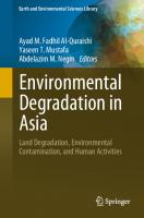
5

to the results of Web of Science, as of December 21, 2022, there have been 4366 publication records using water pollution or water contamination as the search key words in publication titles from 2010 onward (Fig. 1). The number of publications in each year has gradually increased. In the research community, groundwater nitrate pollution, microplastic pollution, fluoride and arsenic pollution, trace metal pollution, and other organic and inorganic pollution are the most frequently reported topics (Aiga et al. 2022; Liu et al. 2022; Mu et al. 2022; Su et al. 2022; Wang et al. 2022; Wei et al. 2022; Zhao et al. 2022). Most recently, Fida et al. (2022) summarized the water pollution status and its impacts on human health in Pakistan, which provides the latest information for Pakistani water quality management. This review updated the old information provided by the earlier review paper of Azizullah et al. (2011). Yang et al. (2022) proposed updated water quality classification criteria for the assessment of groundwater quality using the entropy weight water quality Index (EWQI), which advanced research on the optimization of methods for water quality assessment. Nsabimana and Li (2023) recently proposed an novel industrial water quality index (IndWQI) for integrated industrial water quality assessment, and this new index can give a comprehensive understanding of the industrial water quality. As the second largest economy in the world, China’s water pollution issues are severe. As early as the 1990s, Wu et al. (1999) reviewed the water pollution issue in China and linked it to human health. Later, Wang et al. (2008) and Han et al. (2016) revealed serious water pollution in rural areas of China and deep groundwater pollution in China. However, Hu and Cheng (2013) believed that further industrial transition in China may reduce pollution of surface water, and the improvement of water quality may be accelerated by economic, technological, and policy drivers. This certainly is our good vision, and we do propose that all countries in the earth put their great efforts to increasing water quality and reducing water pollution. In recent years, researchers have performed much work on this topic, but one main research field under this topic is health risk assessment due to waterborne contaminants. Health risk assessment is not a new technique, and it has been proposed by the USEPA for over 30 years (USEPA 1989). However, it began to attract worldwide attention only in the last 10 years. In particular, in the past three years, thousands Fig. 1 Gradual increase in the number of publications on water pollution (the numbers of publications are based on the search results in the Web of Science Core Collection using water pollution or water contamination in publication titles)

6

P. Li and V. Elumalai

of papers in health risk assessment have been published each year, which has been indicative of the increasing awareness of the public toward water quality security (Guo et al. 2022). As has been stated by some researchers, traditional water quality assessment is necessary, but only when health risk is assessed simultaneously can the assessment results be more useful for practical water quality management (Shukla et al. 2021; Wu et al. 2019, 2020). Consequently, health risk assessments have been incorporated into water quality assessments in an increasing number of water quality studies. This has been a driving force for the rapid development in medical geology and achievement of one health goal (Li and Wu 2022a, b; Li et al. 2022b). However, as water pollution issues are still serious worldwide, continuous efforts are expected from governments, organizations, industries and each person.

3 Recent Research Advances in Soil Pollution Soil pollution is usually defined as the state of soil in which the amount of toxic or hazardous substances accumulated in the soil exceeds the self-purification capacity of soil, inducing changes in soil physicochemical and biological properties, declining the agricultural productivity of land and threatening human health (Eugenio et al. 2020). It is another growing universal environmental problem that affects human and ecological health, attracting tremendous attention from researchers (Ceballos et al. 2021; Ciarkowska et al. 2022; Lima et al. 2022; Fei et al. 2022). According to the results of Web of Science, as of December 24, 2022, there have been 5983 publication records using soil pollution or soil quality as the search key words in publication titles from 2010 onward. The number of publications increased from 222 in 2020 to 754 in 2022, which suggests the increasing interest of researchers in this important topic. We generated a word cloud using the words appearing in the titles of the articles published between 2020 and 2022 to show the research trend in soil pollution and soil quality (Fig. 2). As can be inferred from Fig. 2, China might have serious soil pollution problems, as China appeared very frequently in the publication titles. This is logical because China in recent years has experienced very fast development in industry and agriculture as well as in urbanization, and fast development has caused noticeable soil pollution problems. Many researchers (such as Delang 2017; Liu et al. 2019) have reported soil pollution problems in China and have proposed measures and policies for soil pollution remediation (Chen and Ye 2014; Li et al. 2015b). This will help China cope with soil pollution problems. However, soil pollution is also serious in other countries, such as Pakistan, India and Poland (Ali et al. 2019; Pandey et al. 2021; Wierzbicka et al. 2015). Therefore, soil pollution remediation is a universal campaign and requires the efforts of all nations. We can also discover from Fig. 2 that organic pollutants, heavy metals, carbon, microbes and nitrogen are also frequently used terms in publication titles, indicating that these pollutants or elements are usually the research focus of researchers worldwide. Many toxic and hazardous substances have been reported in soil, such as heavy metals, pesticides, antibiotics, phthalic esters,

Recent Advances in Water Quality, Soil Pollution …

7

Fig. 2 Word cloud generated using the article titles published in 2020–2022 based on the search results in the Web of Science Core Collection

environmental hormones, antibiotics resistance genes, and pathogens (He and Cai 2021), among which heavy metals pollution in soil is a common problem and has caused serious damage to ecological security and human health (Fei et al. 2022; Li et al. 2022b). However, remediation of heavy metals pollution in soil is difficult due to the bioaccumulation of metals. In addition, assessment, management, application of agricultural fertilizer, and health risk are also widely investigated topics in soil pollution research.

4 Recent Research Advances in Disaster Risk Reduction The sustainability of society is largely determined by the environments in which people live. However, disasters caused by environmental changes and human activities can definitely constrain sustainability worldwide (Al-Kindi and Hird 2020; Gissing and Langbein 2020). Disasters are diverse and have different types, among which earthquakes, tsunamis, volcanic eruptions, droughts and floods are some natural disasters that directly and indirectly affect tens of thousands of people’s lives every year (Kamel and Arfa 2020; Zuzak et al. 2022). These disasters are usually

8

P. Li and V. Elumalai

regulated by the inner force of the earth or triggered by environmental changes. Other hazards, such as landslides, ground subsidence, ground fissures and mine water inrush, are usually induced by anthropogenic disturbances (Ma et al. 2021b; Xu et al. 2020). Both natural hazards and anthropogenic activity-induced hazards threaten human survival and the sustainable development of society. Therefore, disaster risk reduction has long been the research focus of disaster scientists and engineers. The search results in the Web of Science Core Collection database from 2010 to 2022 using terms such as natural hazard, hazard risk and geological hazard searching in publication titles yielded 3049 publication records, and the word cloud generated using the titles (Fig. 3) shows that research in this field focuses mainly on risk assessment and management, vulnerability assessment and health risk analysis. Many researchers have also paid great attention to radioactivity and models suitable for hazard assessment and prediction. Worldwide climate change has induced many flash flood events, which is a global threat (Gabr et al. 2021; Vo and Tran 2022). In the paper entitled “A novel hybrid of meta-optimization approach for flash-flood susceptibility assessment in a monsoondominated watershed, Eastern India”, Ruidas et al. (2022) focused on flash floodsusceptibility mapping in the Gandheswari basin using support vector regression (SVR) coupled with particle swarm optimization (PSO) and the grasshopper optimization algorithm (GOA). The proposed model provides an alternative for accurate flash flood prediction and thus can help different policymakers set up an early system.

Fig. 3 Word cloud generated using the article titles published in 2010–2022 based on the search results in the Web of Science Core Collection

Recent Advances in Water Quality, Soil Pollution …

9

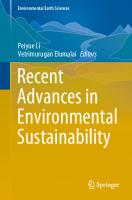
5 Recent Research Advances in Carbon Neutrality Climate warming is caused mainly by greenhouse gases. To mitigate climate warming, it is necessary to achieve carbon neutrality (Zou et al. 2021). carbon neutrality is defined as the creation of a net zero of carbon emissions through waste reduction and the use of carbon offsets or alternatives to sources of energy that generate carbon dioxide (McMahon 2022). It was first proposed in 1997, and since then, it has been a hot term in environmental sciences. There are a number of ways to approach carbon neutrality, energy transition, energy utilization efficiency improvement and ecological carbon sink increase (Wen et al. 2023). In September 2020, China set the goal of achieving a carbon emissions peak by 2030 and carbon neutrality by 2060. Since then, an increasing number of researchers and policy makers have participated in achieving this goal. From the science perspective, a sharp increase in publications was witnessed in 2021 and a further increase in 2022 (Fig. 4). This reflects the increasing interest of researchers in carbon neutrality worldwide. Many researchers believe that carbon neutrality can help achieve the sustainable development of society (Chen 2021), and many nations have also agreed to achieve the carbon neutrality goal by around the middle of this century (Brainard 2020; Dong et al. 2022). In the context of scientific research, Williams et al. (2021) created multiple blueprints for the United States to reach zero CO2 emissions from the energy system by 2050 by considering four basic strategies, including energy efficiency, decarbonized electricity, electrification, and carbon capture. Ge et al. (2023) calculated the carbon sequestration cost at the city level in China to estimate the forest carbon sink cost, and they proposed that different low-carbon policies should be implemented in different regions of China, and afforestation to create carbon sinks can be encouraged in Southwest China, where forest resources are rich. Wu et al. (2022) reviewed the theoretical research and practical progress of carbon neutrality and proposed future directions of carbon neutrality research. However, as many Fig. 4 Increasing trend for the number of publications on carbon neutrality (the numbers of publications are based on the search results in the Web of Science Core Collection)

10

P. Li and V. Elumalai

researchers have mentioned, achieving true carbon neutrality is challenging, and carbon neutrality research, therefore, should be further encouraged by adopting multidisciplinary approaches. The geosciences should be particularly considered when preparing various scenarios for achieving carbon neutrality because the geosciences is the basic discipline involving energy exploitation, carbon capture and cycling, afforestation, and environmental pollution.

6 Final Words Achieving harmony between humans and the environment is difficult, but we should work actively to explore the optimal regulatory methods of harmonious coexistence between humans and nature so that we can find a relatively stable balance. To achieve this goal, the following actions may need particular attention. The key constraints of the harmonious coexistence of humans and nature should be determined based on the current situation of environmental sustainability and the gap between the current situation and the sustainable development goal of a region or a country, and then targeted solutions to weaken the key constraints can be proposed. At the same time, ecological protection and restoration should be continuously enhanced on the basis of studying and judging the relationship between ecosystems. Water resources, land, energy and food are the basic resources to maintain the stable development of the whole society, while the ecological environment is an important factor affecting the high-quality development of human beings (Li 2020; Li and Wu 2019). The water–soil-energy-food-ecosystem nexus is a complex system driven by multiple factors. It is necessary to clarify its complex internal links and mechanisms of the nexus, formulate scientific research plans from the national, watershedwatershed and regional levels, and analyze their coordinated development mode from a systematic and comprehensive perspective to address water security, land security, energy security, and food security. Therefore, under the background of intensified climate change, rapid economic development, rapid population growth, and increasingly worsening environmental pollution, it is particularly important to study the internal relationship and synergy model of the water–soil-energy-food-ecology nexus. Acknowledgements We are grateful for the financial support by the National Natural Science Foundation of China (42072286 and 41761144059), the Qinchuangyuan “Scientist + Engineer” Team Development Program of the Shaanxi Provincial Department of Science and Technology (2022KXJ-005), the Fok Ying Tong Education Foundation (161098), the Special Funds for Basic Scientific Research of Central Colleges (300102299301), and the National Ten Thousand Talent Program (W03070125). Conflict of Interest No conflict of interest has been reported associated with this chapter. Data Availability This chapter has no associated data.

Recent Advances in Water Quality, Soil Pollution …

11

References Aiga H, Nomura M, Mahomed M, Langa JPM (2022) Microbiological contamination of improved water sources, Mozambique. Bull World Health Organ 100:534–543. https://doi.org/10.2471/ BLT.22.288646 Alayish O, Çelik T (2021) Extending disposal route of dewatered sewage sludge produced from the new wastewater treatment plant in Nicosia toward sustainable building materials. Environ Earth Sci 80:146. https://doi.org/10.1007/s12665-021-09439-3 Ali W, Junaid M, Aslam MW, Ali K, Rasool A, Zhang H (2019) A review on the status of mercury pollution in Pakistan: Sources and impacts. Arch Environ Contam Toxicol 76:519–527. https:// doi.org/10.1007/s00244-019-00613-0 Al Kindi MH, Hird R (2020) A review of natural geological hazards in Oman. Environ Earth Sci 79(16):381. https://doi.org/10.1007/s12665-020-09124-x Arya S, Subramani T, Karunanidhi D (2020) Delineation of groundwater potential zones and recommendation of artificial recharge structures for augmentation of groundwater resources in Vattamalaikarai Basin South India. Environ Earth Sci 79:102. https://doi.org/10.1007/s12665-0208832-9 Azizullah A, Khattak MNK, Richter P, Häder D-P (2011) Water pollution in Pakistan and its impact on public health—A review. Environ Int 37479–497.https://doi.org/10.1016/j.envint. 2010.10.007 Brainard J (2020) Japan aims for carbon neutrality. Science 370(6516):509–509 Ceballos E, Dubny S, Othax N, Zabala ME, Peluso F (2021) Assessment of human health risk of chromium and nitrate pollution in groundwater and soil of the Matanza-Riachuelo river basin, Argentina. Expo Health 13:323–336. https://doi.org/10.1007/s12403-021-00386-9 Chakraborty S, Majumdar D, Sahoo S, Saha S (2021) Assessment of future coastal risk zones along the Andaman coast to strengthen sustainable development. Environ Earth Sci 80:637. https:// doi.org/10.1007/s12665-021-09940-9 Chen JM (2021) Carbon neutrality: Toward a sustainable future. The Innovation 2(3):100127. https:/ /doi.org/10.1016/j.xinn.2021.100127 Chen R, Ye C (2014) Resolving soil pollution in China. Nature 505(7484):483. https://doi.org/10. 1038/505483c Ciarkowska K, Konduracka E, Gambus F (2022) Primary soil contaminants and their risks, and their relationship to myocardial infarction susceptibility in Urban Krakow (Poland). Expo Health 14:515–529. https://doi.org/10.1007/s12403-021-00431-7 Delang CO (2017) Causes and distribution of soil pollution in China. Environ Socio-Econ Stud 5(4):1–17. https://doi.org/10.1515/environ-2017-0016 Di Ciaula A (2021) Bioaccumulation of toxic metals in children exposed to urban pollution and to cement plant emissions. Expo Health 13:681–695. https://doi.org/10.1007/s12403-021-004 12-w Dong H, Liu Y, Zhao Z, Tan X, Managi S (2022) Carbon neutrality commitment for China: from vision to action. Sustain Sci 17:1741–1755. https://doi.org/10.1007/s11625-022-01094-2 Drumond A, Liberato MLR, Reboita MS, Taschetto AS (2020) Weather and climate extremes: Current developments. Atmosphere 11(1):24. https://doi.org/10.3390/atmos11010024 Eugenio NR, Naidu R, Colombo CM (2020) Global approaches to assessing, monitoring, mapping, and remedying soil pollution. Environ Monit Assess 192:601. https://doi.org/10.1007/s10661020-08537-2 Fei X, Lou Z, Xiao R, Lv X, Christakos G (2022) Contamination and health risk assessment of heavy metal pollution in soils developed from different soil parent materials. Expo Health. https://doi. org/10.1007/s12403-022-00498-w Fida M, Li P, Wang Y, Alam SMK, Nsabimana A (2022) Water contamination and human health risks in Pakistan: A review. Expo Health. https://doi.org/10.1007/s12403-022-00512-1

12

P. Li and V. Elumalai

Gabr SS, Alkhaldy IA, El Saoud WA, Habeebullah TM (2021) Flash flood modeling and mitigation of Al-Hussainiyah area, Makkah Saudi Arabia. Arab J Geosci 14:2044. https://doi.org/10.1007/ s12517-021-08400-9 Ge J, Zhang Z, Lin B (2023) Towards carbon neutrality: How much do forest carbon sinks cost in China? Environ Impact Assess Rev 98:106949. https://doi.org/10.1016/j.eiar.2022.106949 Gissing A, Langbein F (2020) Australia’s natural hazards risk profile. Aust J Emerg Manag 35(2):17– 18 Gomaa MA, Shabana AR, Zaghlool E (2020) New approach in sustainable development based on groundwater resources, Wadi Dara, Eastern Desert Egypt. Environ Earth Sci 79:320. https://doi. org/10.1007/s12665-020-09073-5 Guo Y, Li P, He X, Wang L (2022) Groundwater quality in and around a landfill in northwest China: characteristic pollutant identification, health risk assessment, and controlling factor analysis. Expo Health 14(4):885–901. https://doi.org/10.1007/s12403-022-00464-6 Han D, Currell MJ, Cao G (2016) Deep challenges for China’s war on water pollution. Environ Pollut 218:1222–1233. https://doi.org/10.1016/j.envpol.2016.08.078 He Y, Cai P (2021) Special issue on soil pollution, control, and remediation. Soil Ecol Lett 3:167– 168. https://doi.org/10.1007/s42832-021-0110-6 He S, Li P, Su F, Wang D, Ren X (2022a) Identification and apportionment of shallow groundwater nitrate pollution in Weining Plain, northwest China, using hydrochemical indices, nitrate stable isotopes, and the new Bayesian stable isotope mixing model (MixSIAR). Environ Pollut 298:118852. https://doi.org/10.1016/j.envpol.2022.118852 He S, Wu J, Wang D, He X (2022b) Predictive modeling of groundwater nitrate pollution and evaluating its main impact factors using random forest. Chemosphere 290:133388. https://doi. org/10.1016/j.chemosphere.2021.133388 Hu Y, Cheng H (2013) Water pollution during China’s industrial transition. Environ Dev 8:57–73. https://doi.org/10.1016/j.envdev.2013.06.001 Kamel M, Arfa M (2020) Integration of remotely sensed and seismicity data for geo-natural hazard assessment along the Red Sea Coast Egypt. Arab J Geosci 13:1195. https://doi.org/10.1007/s12 517-020-06173-1 Li P (2020) Meeting the environmental challenges. Hum Ecol Risk Assess 26(9):2303–2315. https:/ /doi.org/10.1080/10807039.2020.1797472 Li P, Qian H (2018) Water resources research to support a sustainable China. Int J Water Resour Dev 34(3):327–336. https://doi.org/10.1080/07900627.2018.1452723 Li P, Wu J (2019) Sustainable living with risks: meeting the challenges. Hum Ecol Risk Assess 25(1–2):1–10. https://doi.org/10.1080/10807039.2019.1584030 Li P, Wu J (2022a) Medical geology and medical geochemistry: An editorial introduction. Expod Health 14(2):217–218. https://doi.org/10.1007/s12403-022-00479-z Li P, Wu J (2022b) Shukla S (2022b) Achieving the one health goal: Highlighting groundwater quality and public health. Water 14(21):3540. https://doi.org/10.3390/w14213540 Li P, Qian H, Howard KWF, Wu J (2015a) Building a new and sustainable silk road economic belt. Environl Earth Sci 74(10):7267–7270. https://doi.org/10.1007/s12665-015-4739-2 Li XN, Jiao WT, Xiao RB, Chen WP, Chang AC (2015b) Soil pollution and site remediation policies in China: A review. Environ Rev 23(3):263–274. https://doi.org/10.1139/er-2014-0073 Li P, Wu J, Qian H (2016) Regulation of secondary soil salinization in semi-arid regions: A simulation research in the Nanshantaizi area along the Silk Road, northwest China. Environ Earth Sci 75(8):698. https://doi.org/10.1007/s12665-016-5381-3 Li P, Qian H, Zhou W (2017) Finding harmony between the environment and humanity: an introduction to the thematic issue of the silk road. Environ Earth Sci 76(3):105. https://doi.org/10. 1007/s12665-017-6428-9 Li P, Wang D, Li W, Liu L (2022a) Sustainable water resources development and management in large river basins: An introduction. Environ Earth Sci 81(6):179. https://doi.org/10.1007/s12 665-022-10298-9

Recent Advances in Water Quality, Soil Pollution …

13

Li Y, Li P, Liu L (2022b) Source identification and potential ecological risk assessment of heavy metals in the topsoil of the Weining plain (Northwest China). Expo Health 14(2):281–294. https://doi.org/10.1007/s12403-021-00438-0 de Lima Brum R, Penteado JO, Ramires PF, Girónes MCR, Paz-Montelongo S, del Carmén Rubio Armendáriz M, dos Santos M, da Silva Júnior FMR (2022) Recommended Guidance and Checklist for Human Health Risk Assessment of Metal(loid)s in Soil. Expo Health 14:295–304.https:/ /doi.org/10.1007/s12403-021-00440-6 Liu X, Bai Z, Shi H, Zhou W, Liu X (2019) Heavy metal pollution of soils from coal mines in China. Nat Hazards 99:1163–1177. https://doi.org/10.1007/s11069-019-03771-5 Liu L, Wu J, He S, Wang L (2022) Occurrence and distribution of groundwater fluoride and manganese in the Weining Plain (China) and their probabilistic health risk quantification. Expo Health 14(2):263–279. https://doi.org/10.1007/s12403-021-00434-4 Ma C, Yan Z, Huang P, Gao L (2021a) Evaluation of landslide susceptibility based on the occurrence mechanism of landslide: a case study in Yuan’an County, China. Environ Earth Sci 80:94. https:/ /doi.org/10.1007/s12665-021-09381-4 Ma Y, Xu X, Xiao P, Yan Q, Zhao C (2021b) Geomorphic natural hazard on loess terrain: expansion on the gully sidewall. Nat Hazards 109:2535–2555. https://doi.org/10.1007/s11069-021-049 31-2 McMahon M (2022) What Is Carbon Neutrality? Available at https://www.wisegeek.net/what-iscarbon-neutrality.htm, accessed November 29, 2022 Mu D, Wu J, Li X, Xu F, Yang Y (2022) Identification of the spatiotemporal variability and pollution sources for potential pollutants of the malian river water in Northwest China using the PCAAPCS-MLR receptor model. Expo Health. https://doi.org/10.1007/s12403-023-00537-0 Nosrati K, Collins AL (2019) A soil quality index for evaluation of degradation under land use and soil erosion categories in a small mountainous catchment, Iran. J Mt Sci 16(11):2577–2590. https://doi.org/10.1007/s11629-019-5567-8 Nsabimana A, Li P (2023) Hydrogeochemical characterization and appraisal of groundwater quality for industrial purpose using a novel industrial water quality index (IndWQI) in the Guanzhong Basin, China. Geochemistry 83(1):125922. https://doi.org/10.1016/j.chemer.2022.125922 Pandey S, Kumari N, Prasad SP (2021) Soil quality and pollution assessment around Jumar watershed of Jharkhand India. Arab J Geosci 14:2784. https://doi.org/10.1007/s12517-021-090 91-y Ruidas D, Chakrabortty R, Islam ARMT, Saha A, Pal SC (2022) A novel hybrid of meta-optimization approach for fash food-susceptibility assessment in a monsoon-dominated watershed Eastern India. Environ Earth Sci 81:145. https://doi.org/10.1007/s12665-022-10269-0 Santarosa LV, Gastmans D, Sitolini TP, Kirchheim RE, Betancur SB, de Oliveira MED, Campos JCV, Manzione RL (2021) Assessment of groundwater recharge along the Guarani aquifer system outcrop zone in São Paulo State (Brazil): An important tool towards integrated management. Environ Earth Sci 80:95. https://doi.org/10.1007/s12665-021-09382-3 Shukla S, Saxena A, Khan R, Li P (2021) Spatial analysis of groundwater quality and human health risk assessment in parts of Raebareli district India. Environ Earth Sci 80(24):800. https://doi. org/10.1007/s12665-021-10109-7 Skoczynska A, Skoczynska M, Turczyn B, Wojakowska A, Gruszczynski L, Scieszka M (2021) Exposure to arsenic in the air and 15-F2t-isoprostane in urine in a sub-population of inhabitants of a copper smelter region. Expo Health 13:403–418. https://doi.org/10.1007/s12403-021-003 92-x Su F, Wu J, Wang D, Zhao H, Wang Y, He X (2022) Moisture movement, soil salt migration, and nitrogen transformation under different irrigation conditions: Field experimental research. Chemosphere 300:134569. https://doi.org/10.1016/j.chemosphere.2022.134569 USEPA (1989) Risk assessment guidance for superfund, volume 1: human health evaluation manual (part A) ((EPA/540/1–89/002: interim final). Office of Emergency and Remedial Response, Washington

14

P. Li and V. Elumalai

Vo TAN, Tran TK (2022) Climate change and rural vulnerability in Vietnam: An analysis of livelihood vulnerability index. Hum Ecol Risk Assess 28(3–4):326–353. https://doi.org/10.1080/108 07039.2022.2052262 Wang M, Webber M, Finlayson B, Barnett J (2008) Rural industries and water pollution in China. J Environ Manage 86:648–659. https://doi.org/10.1016/j.jenvman.2006.12.019 Wang D, Wu J, Wang Y, Ji Y (2020) Finding high-quality groundwater resources to reduce the hydatidosis incidence in the Shiqu county of Sichuan Province, China: Analysis, assessment, and management. Expo Health 12(2):307–322. https://doi.org/10.1007/s12403-019-00314-y Wang L, Li P, Duan R, He X (2022) Occurrence, controlling factors and health risks of Cr6+ in groundwater in the Guanzhong Basin of China. Expo Health 14(2):239–251. https://doi.org/10. 1007/s12403-021-00410-y Wei M, Wu J, Li W, Zhang Q, Su F, Wang Y (2022) Groundwater geochemistry and its impacts on groundwater arsenic enrichment, variation, and health risks in Yongning County, Yinchuan Plain of northwest China. Expo Health 14(2):219–238. https://doi.org/10.1007/s12403-021-003 91-y Wen H, Liang W, Lee C-C (2023) China’s progress toward sustainable development in pursuit of carbon neutrality: Regional differences and dynamic evolution. Environ Impact Assess Rev 98:106959. https://doi.org/10.1016/j.eiar.2022.106959 Wierzbicka M, Bemowska-Kałabun O, Gworek B (2015) Multidimensional evaluation of soil pollution from railway tracks. Ecotoxicology 24:805–822. https://doi.org/10.1007/s10646-0151426-8 Williams JH, Jones RA, Haley B, Kwok G, Hargreaves J, Farbes J, Torn MS (2021) Carbon-neutral pathways for the United States. AGU Adv 2:e2020AV000284. https://doi.org/10.1029/2020AV 000284 Wu C, Maurer C, Wang Y, Xue S, Davis DL (1999) Water pollution and human health in China. Environ Health Perspect 107(4):251–256. https://doi.org/10.1289/ehp.99107251 Wu J, Wang L, Wang S, Tian R, Xue C, Feng W, Li Y (2017) Spatiotemporal variation of groundwater quality in an arid area experiencing long-term paper wastewater irrigation, northwest China. Environ Earth Sci 76(13):460. https://doi.org/10.1007/s12665-017-6787-2 Wu J, Zhou H, He S, Zhang Y (2019) Comprehensive understanding of groundwater quality for domestic and agricultural purposes in terms of health risks in a coal mine area of the Ordos basin, north of the Chinese Loess Plateau. Environ Earth Sci 78(15):446. https://doi.org/10.1007/s12 665-019-8471-1 Wu J, Zhang Y, Zhou H (2020) Groundwater chemistry and groundwater quality index incorporating health risk weighting in Dingbian County, Ordos Basin of Northwest China. Geochemistry 80(4):125607. https://doi.org/10.1016/j.chemer.2020.125607 Wu X, Tian Z, Guo J (2022) A review of the theoretical research and practical progress of carbon neutrality. Sustain Oper Comput 3:54–66. https://doi.org/10.1016/j.susoc.2021.10.001 Xiao Y, Liu K, Yan H, Zhou B, Huang X, Hao Q, Zhang Y, Zhang Y, Liao X, Yin S (2021) Hydrogeochemical constraints on groundwater resource sustainable development in the arid Golmud alluvial fan plain on Tibetan plateau. Environ Earth Sci 80:750. https://doi.org/10. 1007/s12665-021-10076-z Xu Y, Chang Q, Yan X, Han W, Chang B, Bai J (2020) Analysis and lessons of a mine water inrush accident resulted from the closed mines. Arab J Geosci 13:665. https://doi.org/10.1007/s12517020-05613-2 Yang Y, Li P, Elumalai V, Ning J, Xu F, Mu D (2022) Groundwater Quality Assessment Using EWQI With Updated Water Quality Classification Criteria: A Case Study in and Around Zhouzhi County, Guanzhong Basin (China). Expo Health. https://doi.org/10.1007/s12403-022-00526-9 Zhang Q, Li P, Lyu Q, Ren X, He S (2022) Groundwater contamination risk assessment using a modified DRATICL model and pollution loading: A case study in the Guanzhong Basin of China. Chemosphere 291:132695. https://doi.org/10.1016/j.chemosphere.2021.132695 Zhao H, Li P, He X, Ning J (2022) Microplastics pollution and risk assessment in selected surface waters of the Wei River Plain, China. Expo Health. https://doi.org/10.1007/s12403-022-00522-z

Recent Advances in Water Quality, Soil Pollution …

15

Zou C, Xue H, Xiong B, Zhang G, Pan S, Jia C, Wang Y, Ma F, Sun Q, Guan C, Lin M (2021) Connotation, innovation and vision of “carbon neutrality.” Nat Gas Ind B 8(5):523–537. https:/ /doi.org/10.1016/j.ngib.2021.08.009 Zuzak C, Mowrer M, Goodenough E, Burns J, Ranalli N, Rozelle J (2022) The national risk index: Establishing a nationwide baseline for natural hazard risk in the US. Nat Hazards 114:2331– 2355. https://doi.org/10.1007/s11069-022-05474-w

Investigation of Helium Isotopes in Groundwater of Kuwait Group and Dammam Formation Aquifers of Kuwait T. Rashid, C. Sabarathinam, U. Saravana Kumar, M. Al-Jomaa, B. Al-Salman, and H. Naseeb

Abstract The presence of helium in groundwater has widespread applications, including groundwater dating, groundwater provenance and subsequent flow history, paleoclimatology, recharge mechanism, and crustal, mantle and seismic studies. A total of 36 groundwater samples collected from different locations representing two major aquifers in Kuwait, the Kuwait Group and underlying Dammam Formation aquifers of Kuwait, were analyzed for helium and 3 He/4 He ratios. The concentration of He and 3 He/4 He ratios were assessed using the endmember composition of air, crust and mantle to identify their influence on groundwater. The dissolved helium concentrations in the groundwater of the Kuwait Group aquifer ranged from 3.82 × 10–08 cm3 STP/g to 1.33 × 10–06 cm3 STP/g with an average of 2.23 × 10–07 cm3 STP/ g, whereas they ranged from 9.97 × 10–08 cm3 STP/g to 1.62 × 10–06 cm3 STP/g with an average of 4.57 × 10–07 in the groundwater of the Dammam Formation aquifer. The helium ratios (3 He/4 He) of samples (Rs) were found to be close to atmospheric ratio (Rair = 1.4 × 10–6 cm3 STP g−1 ) in modern groundwater samples collected from shallow wells located in northern parts. The 3 He/4 He ratios were found to be close to ~0.02Rair crustal-derived helium in most groundwater samples collected from deep production wells of the Kuwait Group and Dammam Formation aquifers located in the middle and extreme southern regions. 3 He/4 He ratios equivalent to mantle production (~8Rair ) were not observed in the collected groundwater samples. Geological structural controls were determined in the southern parts of Kuwait, associated with the Kuwait Arch. The study inferred that the structure extends from north to south, acting as an additional conduit of crustal-derived helium in the ground samples located in the southern region of Kuwait. It is also inferred that extensive groundwater production in the central parts of the country at the water fields extracting groundwater could be another reason for the additional source of T. Rashid · C. Sabarathinam (B) · M. Al-Jomaa · B. Al-Salman · H. Naseeb Water Research Center, Kuwait Institute for Scientific Research, P. O. Box: 24885, 13109 Safat, Kuwait e-mail: [email protected] U. Saravana Kumar Isotope Hydrology Section, Division of Physical and Chemical Sciences, International Atomic Energy Agency (IAEA), Vienna, Austria © The Author(s), under exclusive license to Springer Nature Switzerland AG 2023 P. Li and V. Elumalai (eds.), Recent Advances in Environmental Sustainability, Environmental Earth Sciences, https://doi.org/10.1007/978-3-031-34783-2_2

17

18

T. Rashid et al.

crustal-derived and/or deeper horizon-derived helium. Thus, the observation of the study helps to determine the influence of the surface water recharge, paleo recharge and the structural controls of the basin. Moreover, the outcome of the study assists in deriving sustainable management for the use of brackish groundwater resources in the country. Keywords Helium · Groundwater · Geological structural controls · Crustal-derived · Water recharge

1 Introduction The inert nature of the noble gases helium (He), neon (Ne), xeon (Xe), argon (Ar) and krypton (Kr) and their distinctive isotopic characteristics make them ideal tracers in groundwater-related studies, including groundwater dating, groundwater provenance and subsequent flow history, paleoclimatology, mechanism of recharge, crustal, mantle and seismic studies (Ballentine and Burnard, 2002a, b; Kipfer et al. 2002). Among noble gases, He plays a key role in medical cryogenics and other industrial purposes. Petroleum-producing countries such as Australia, Russia, Central Europe, Algeria, Qatar, Iran, Canada and US mid-countries are recent producers of He (Danabalan 2017). Qatar and Algeria have recently been exporting the He obtained from hydrocarbon gas. The failure to recognize the significance of He or undetected He results in the venting of He along with other waste gases (Clarke et al. 2012). helium with large subsurface production rates and large and diagnostic variations in isotopic composition (3 He/4 He) has proven useful to distinguish helium of atmospheric, crustal and mantle origin (Kulongoski et al. 2003, 2005; Oxburgh et al. 1986; Sano et al. 1986). Although there are variations in the He ratio, it is observed that during the mixing between these three sources of He, the signatures could be determined based on the proportion of mixing between these end members (Sheng et al. 2012). Helium in groundwater apart from atmospheric origin is denoted as terrigenic or excess helium (Heex ) and could result from different sources, including β-decay of natural and bomb tritium (tritiogenic 3 Het ), the 6 Li (n, α)3 H(3 He) reaction (nucleogenic 3 He), α-decay of the natural Uranium and Thorium decay series elements in the crustal rocks (radiogenic 4 He), and mantle and magmatic contributions to both 3 He and 4 He. Helium isotope ratios in groundwater are useful indicators of geological processes and groundwater dynamics because atmospheric, crustal, and mantle helium components display distinct 3 He/4 He ratios (Saar et al. 2005). Several authors have studied the He reservoirs globally with respect to local conditions and have also discussed the generation exsolution, migration, and accumulation mechanism in crustal environments (Table 1). Two major sources of He have been discussed in the literature: Radiogenic (crustal) or mantle sources located predominantly along tectonic margins. Studies on He in groundwater from different regions of the world indicate that the sources, geological structures and hydrological conditions play a key role in the He concentration in groundwater. Furthermore, they are mainly derived from lithogenic sources, and tectonically active regions predominate the mantle source. The recent

Investigation of Helium Isotopes in Groundwater …

19

recharge regions have atmospheric signatures; in many regions, they are not ideally of a single source, but a mixture of these processes is observed (Table 1). The overview of the literature indicates that the presence of helium in groundwaters with different concentrations, depending on the source. The ratios of crustal-derived helium, results in 0.02Rair (Castro 2004), and mantle-derived helium results in 8Rair (Graham 2002), whereas Rair = 1.384 × 10–6 (Clarke et al. 1976). Here, we present the results of the helium and isotopic ratio 3 He/4 He of groundwater samples from two major aquifers, the Kuwait Group (KG) and Dammam (DM) Formation aquifer of Kuwait, thereby determining their sources in groundwater.

2 Hydrogeology Sedimentarybasins of the Arabian Peninsula contain groundwater of different ages at various depths with a wide range of salinity, hydraulic properties, and discharge mechanisms. These sedimentary basins represent Paleozoic, Triassic-Jurassic, Cretaceous, and Tertiary-Quaternary systems. The Tertiary-Quaternary system is subdivided into the Eocene aquifer system and the Neogene-Quaternary aquifer system dipping gently toward the northeast (Al-Sharhan et al. 2001a, b; Burdoun 1973). The Eocene system consists of two limestone formations, the Radhuma and DM Formations, which are separated by the anhydrite Rus Formation. This aquifer system is regionally confined except in its recharge outcrop area in Saudi Arabia and in the discharge areas of the Arabian Gulf coast. The recharge of the DM Formation aquifer occurs in the southern Iraqi desert, west of Kuwait, and in Saudi Arabia (400 km south of Kuwait), where exposure of the DM Formation aquifer covers 1200 km2 (Tleel 1973). This aquifer system was recharged mostly during ancient periods, whereas the current recharge is weak. It was estimated that 80% of lateral flow into the part of the DM Formation of Kuwait and the KG aquifers comes from Saudi Arabia and 20% from Iraq (Mukhopadhyay et al. 1994). The discharge from these aquifers is indicated by terrestrial spring, upward discharge into the overlying aquifer, and evaporation through coastal sabkhas. Various gradations of gravel, sand, silt, and clay material can be observed in a discontinuous fashion in the KG aquifer of the study area. Clay represents the base of the KG aquifer and is discontinuous. It covers the N–NE and N–NW parts completely and partially covers the E–NE and E–SE parts. The clay base is absent in the southern part of the study area (Fig. 1). Massive and porous limestone represents the DM aquifer. The thickness of the DM aquifer can be observed to increase from south to north in the study area. The porous limestone appears intercalated with massive limestones of the DM. The DM Formation aquifer has a higher piezometric surface than that of the overlying KG aquifer, and therefore, water moves upward from the DM Formation aquifer into the overlying KG aquifer (Qabazard 2001). Although major recharge to the KG and DM Formation aquifers occurs in recharge areas located in Saudi Arabia and Iraq, local pprecipitation is a minor recharge source for limited freshwater lenses that occur in the upper part (Dibdiba Formation) of the KG, especially in the Raudhatain, Umm Al-Aish, and Abdally areas of northern Kuwait.

20

T. Rashid et al.

Table 1 Studies on He in groundwater from different regions enabling the identification of the sources and geological structures Country/focus

Inferences from the studies

References

1

Alpine region

He release due to tectonic activity around the Alpine region

Marty et al. (1992)

2

Australia

He excess in groundwater and radiogenic He entering groundwater in Great Australian basin

Torgersen and Clarke (1985)

Sinistral strike slip fault and mantle degassing records in carbonic springs deposits

Ring et al. (2016)

3 4

Australia and Switzerland

Model relating to radiogenic He excess in Mazor (1995), stagnant groundwater and heterogeneous aquifer Tolstikhin et al. (1996), Lehman et al. (2003)

5

Canada

Heex in Becancour watershed is higher due to the crustal flux and it is 1000 times expected to be greater than the local lithological source nearby

6

7

Vautour et al. (2015)

Older groundwater in the Becancour watershed Mejean et al. had higher He due to the diffusion to (2016) groundwater through fractures facilitating 234U migration by Alpha recoil China

Release of He due to tectonic activity around Sichuan -Yunnan Block

Meng et al. (2021)

8

Mantle derived He from Tengchong region

Zhang et al. (2016)

9

Deeper sources of He in Changbai Mountains

Wei et al. (2016)

10

He release around the Hinian region

Sheng et al. (2012)

11

Characteristic of mantle derived He from Wudalaianchi volcanic field

Zhang et al. (2017)

12

Noble gas studies in deep confined aquifers proved evidence of degassing in north China plain

Wang et al. (2015)

13 China/India

He and its relation to mantle fluids at the Karakoram fault

Klemperer et al. (2013)

14 East Pacific

Excess He observed in the East Pacific waters

Craig et al. (1975)

15 Ethiopia

Lower Mantle He degassing in the plume lava region

Boucher et al. (2018)

16 Experimental

He concentration depends on the physical properties of the aquifer matrix

Tolstikhin et al. (2020)

17 Germany

migration of gas in multiphase crustal environment including He, in Rotliegend gas field

Barry et al. (2017) (continued)

Investigation of Helium Isotopes in Groundwater …

21

Table 1 (continued) Inferences from the studies

References

18 India

Country/focus

Temperature variations and He sources in groundwater of Cambay region

Gupta and Deshpande (2003)

19

Integrated approach using He, radiocarbon and radon in groundwater of Cambay region

Agarwal et al. (2006)

20

Tectonically active areas around a Narmada River basin was identified using He in groundwater

Deshpande and Gupta (2013)

21 Italy

Evolution of He in groundwater of a structurally Quattrocchi controlled basin (1999)

22

High He values around the Candelaro fault

Hooker et al. (1985)

23 Japan

He anomaly and the changes in strain of the structures during the 2016 Kumamoto earthquake

Sano et al. (2016)

24

He isotopes in groundwater of structurally controlled basin, Osaka

Morikawa et al. (2008)

25

Higher He isotopes are noted in the hot springs of Kii Peninsula

Sano and Wakita (1985), Umeda et al. (2006)

26

Release of He from Median tectonic line, Shikoku Island

Dogan et al. (2006)

27

The structurally controlled upwelling high chlorine and high temperature thermal water of Arima-Type from Kobe basin had higher He isotope ratio

Morikawa (2005)

28

Lesser value of He isotopes was observed in the Wakita et al. eastern region of Uemachi fault (1987)

29

Transport of the gasses through the geological structure like fault in Kii Peninsula

30 Korea

He degassing observed along the strike slip fault Lee et al. (2019)

31 New Zealand

Gas discharge and water chemistry in geothermal fields

Giggenbach and Glover (1992)

32

Release of He through gas rich spring in the intraplate boundaries

Hoke et al. (2000)

33 Norway

Noble gases (including He) and hydrocarbon relationship in Sleipner Vest gas field were reported

Barry et al. (2016)

34 Switzerland

He Excess due to the mixing of freshwater and the porewater in a low permeable aquifer

Tolstikhin et al. (2005)

Matsumoto et al. (2003)

(continued)

22

T. Rashid et al.

Table 1 (continued) Inferences from the studies

References

35 Tanzania

Country/focus

Geothermal spring near the Tanganyika rift shows the crustal dominant source

Kraml et al. (2016)

36

He isotopes observed in the north Tanzania divergence zone and Rukwa basin varied from 0.039 to 6.1Ra

Day et al. (2015)

37

He in the groundwater of Rukwa rift system, Mtili et al. Lupa hydrothermal system and Rungwe (2021) volcanic province were studied to determine their sources of gas. The gas fields were located in southern Tanzania

38 Tunisia

He in geothermal water with mantle He signatures

39 Turkey

migration of crustal fluids and its relation to Burnard et al. velocity along the fault planes in Sea of Marama (2012)

40 USA

He release to the crust and its relation to upper mantle deformation, supported by seismic observations, southern California

Inbal et al. (2016)

41

fault facilitation of He release from the mantle along the San Andreas fault system, California

Kulongoski et al. (2013)

42

Release of He during the last glaciation due to the development of fractures in regions around the Appalachian mountains

Mejean et al. (2017)

43

High He isotope ratio along the strike slip fault in the high intensity earthquake regions at Newport- Inglewood fault zone

Inbal et al. (2016)

44

He concentrations around the mantle subduction Boles et al. zone at New port—Inglewood fault zone (2015)

45

He distribution around, San Andreas Fault

Kennedy et al. (1997)

46

Distribution of He in East Morongo basin, California

Kulongoski et al. (2005)

47

migration of He from the subsurface, Yellowstone national park

Lowenstern et al. (2015)

48 Release mechanism in earthquake regions

He gas release along the fault plane in the earthquake prominent region

Byerlee (1993)

49 Noble gas production, He degassing due to magmatism in the release and transport in continental crust the crust

Fourre et al. (2011)

Ballentine and Burnard (2002a, b)

Investigation of Helium Isotopes in Groundwater …

23

Fig. 1 Lithological cross section of the Shigaya well field developed using litho-log data depicting the Kuwait group of aquifers and the Dammam Formation

The groundwater salinity of the KG aquifer ranges from 4,000 mg/l in the southwest of the country to 50,000 mg/l in the northeast. The groundwater is of the sodium chloride (Na-Cl) and magnesium chloride (Mg-Cl) types and supersaturated with calcite (CaCO3 ) and dolomite [CaMg(CO3 )2 ] (Al-Ruwaih 1993). The groundwater salinity of the DM Formation aquifer increases from 2,500 mg/l in the southwest to 10,000 mg/l in the central part of the country. There is an abrupt increase in salinity toward the north and east up to 150,000 mg/l and higher. The water is of the calcium sulfate (Ca-SO4 ), sodium sulfate (Na2 -SO4 ), and sodium chloride (Na-Cl) types, supersaturated with calcite (CaCO3 ), and saturated with respect to anhydrite (CaSO4 ). The salinity of freshwater lenses of the Raudhatain and Umm Al-Aish areas ranges from 300 to 1,400 mg/l, whereas water is of the sodium sulfate (Na-SO4 ), calcium sulfate (Ca-SO4 ), and sodium bicarbonate (Na-HCO3 ) types (Al-Ruwaih 1985). The distribution of the samples with respect to the cations and anions in the KG and DM formation aquifers reflects the higher concentration of sodium (Na). Chloride (Cl) was identified as the dominant anion in the KG aquifer and SO4 in the DM aquifer (Fig. 2a & b).

3 Analytical Methods Eighteen groundwater samples were collected from the KG aquifer and 18 from the DM formation aquifer in copper tubes mounted on aluminum racks and appropriate plastic containers for noble gases and stable isotopes. The analyses of 2 H and 18 O were carried out in the laboratory of Radio-Analyses et Environments of Tunizia

24

T. Rashid et al.

Fig. 2 Frequency of hydrochemical (major anions) parameters in groundwater samples of a DM and b KG (all values in mg/l)

and the Biofocus laboratory of Germany using a liquid water isotope analyzer, and VSMOW (1σ = ± 0.15‰) was used as a standard. The results were expressed as δ2 H and δ18 O values relative to Vienna Standard Mean Ocean Water (VSMOW) following the equation δ = (Rsample /Rstandard − 1; expressed in permil), where R is the 2 H/1 H, 18 O/16 O ratio in the sample or VSMOW. Carbon-13 (13 C) and carbon (14 C) of groundwater samples were analyzed using the ion ratio mass spectrometry (IRMS) and accelrator mass spectrometry (AMS) facilities, respectively, at the Biofocus Laboratory of Germany. The results were expressed as δ13 C values, following the equation δ = (Rsample /Rstandard − 1; expressed in permil, ‰), where R is the 13 C/12 C ratio in the sample or standard (VPDM-Standard) and 1σ = ± 0.3‰. The 14 C results were reported as percent modern carbon (pmC). He and Ne were analyzed in the IAEA laboratory of Vienna, Austria. At the laboratory, gas extraction of the water samples is performed by connecting the copper tube directly to a high vacuum extraction line. By opening a clamp of the sampler, water flowed into an expansion vessel. Gases are extracted by gentle agitation of the vessel for at least one hour and then transferred to a purification line by means of a capillary tube. The latter allows recovery of almost all the extracted gases while limiting vapor transfer (Osenbrück et al. 1998; Beyerle et al. 2000). Helium and Ne are cryogenically separated from the other noble gases by means of activated charcoal at the temperature of liquid nitrogen that traps the condensable gaseous phases (mainly water vapor and heavy noble gases: Ar, Kr and Xe). After cryogenic separation from the heavy noble gases, He and Ne are introduced into a mass spectrometer for isotopic analysis (Lavielle et al. 2012).

4 Results and Discussion Analytical results of δ2 H, δ18 O, He and Ne and 3 He/4 He ratios (reported as Rs /Rair , where Rs = sample 3 He/4 He, Rair is the air 3 He/4 He ratio = 1.38 × 10–6 ), including well details and 14 C ages of groundwater samples, are presented in Table 2. The helium concentration in the groundwater samples collected from the KG aquifer

Investigation of Helium Isotopes in Groundwater …

25

ranged from 3.82 × 10–8 (P2) to 1.33 × 10–6 (T01) with an average value of 2.23 × 10–7 cm3 STP/g (Fig. 3a), whereas it ranged from 9.97 × 10–8 (Leyah) to 1.62 × 10–6 (WW-2) with an average value of 4.57 × 10–7 cm3 STP/g in the groundwater samples collected from the DM Formation aquifer (Fig. 3b). In both cases, the concentration of He in groundwater was in excess of that of helium (4.457 × 10–8 cm3 STP/g) in air-equilibrated water (Bradley et al. 2009), indicating that there was an additional source of helium. Groundwater from production wells WW-2 and WW-10, located close to the Wafra oil field, yielded the highest concentration of He (1.62x−6 cm3 STP/ g and 1.58x−6 cm3 STP/g). Figure 4 shows the spatial distribution of helium in groundwater samples superimposed on a map of onshore subsurface structural elements in Kuwait. Two hot spots of helium can be noticed: 1. along the south very close to the Wafra oil field (structural part of the southern Kuwait Arch) and 2. situated in the north at Abdally. The Wafra oil field represents one of the most prolific oil-producing zones at depths of 300–400 m in the Paleocene-Eocene Umm Er Radhuma formation. The Wafra reservoir is a structural accumulation formed by a low-amplitude anticline with 4way dip closure, consisting of normal faults with small displacements (Masarik et al. 2012). The plot of helium, neon and isotope ratio (3 He/4 He) data on endmember compositions (Rair = 1.38 × 10–06 , Rdc = 0.02Rair , and Rm = 8Rair ) diagram is presented in Fig. 5. The 3 He/4 He ratio of all groundwater samples plot between the endmember compositions of Rair and Rdc . The 3 He/4 He ratio of groundwater samples from wells (WW2 and WW10) located in the south plot extremely close to Rdc, indicating the influence of crustal-derived helium, i.e., mixing between groundwater of the DM aquifer and crustal origin. Placement of lithostratigraphy of KG and DM Formation aquifers at the locations of wells WW-2 and WW-10 on geological cross-section Table 2 Descriptive statistics of well depths, helium, Neon, Ratios, δ2H, δ18O, and 14C age of groundwater samples

Well ID

Minimum

Maximum

Average

253.89

122.17

KG wells Well depth (m)

29.00

He (cm3 STP/g)

3.82 × 10–8 1.33 × 10–6 2.23 × 10–7

Ne (cm3 STP/g)

7.69 × 10–8 4.31 × 10–7 2.25 × 10–7

Rs /Rair

1.07 × 10–7 1.41 × 10–6 8.02 × 10–7

δ2 H

(‰)

δ18 O (‰) 14 C

−28.79

−7.22

−19.49

−4.45

−0.89

−2.80

23,130

10,222

Age (years BP) 348

DM formation wells Well depth He

(cm3 STP/g)

Ne

(cm3 STP/g)

Rs /Rair δ2 H

485.83

9.97 ×

10–8

1.29 ×

10–7

295.12

1.62 ×

10–6

4.57 × 10–7

3.83 ×

10–7

2.41 × 10–7

1.04 × 10–7 6.79 × 10–7 2.80 × 10–7 −38.71

−16.60

−30.53

−4.68

−2.01

−4.02

Age (years BP) 16,017

32,755

22,763

(‰)

δ18 O (‰) 14 C

165.00

26

T. Rashid et al.

Fig. 3 He and Ne concentrations and their ratios in the groundwater samples of the a Kuwait Group and b Dammam Formation

Fig. 4 Locations of sampled wells of the Kuwait Group and Dammam Formation aquifers, along with the major geological strucutres of Kuwait and spatial varition of helium

Investigation of Helium Isotopes in Groundwater …

27

adopted from Khalaf et al. (1989) showed an abrupt depth change of lithostratigraphic units (Fig. 6). Such an abrupt change in the depth of lithostratigraphic units between wells WW-7 and WW-2 could be an indication of the presence of another fault providing hydraulic communication between the DM Formation and deeper parts of the lithosphere. Studies (Eremeev et al. 1972; Golubev et al. 1975; Levina et al. 1975; and Gumm et al. 2015) have found a direct correlation between high concentrations of helium in groundwater and faults. It has been suggested that the fault zones in the basement could act as conduits for helium found in deeper layers. Therefore, the fault identified between wells WW-7 and WW-2 could act as a conduit for crustal-derived helium. Furthermore, the ages of groundwater from well WW-2 (23,308 years BP) and well WW-10 (17,692 years BP) with depleted and δ18 O-depleted values of − 2.01‰ and −2.28‰, respectively, imply paleo-recharge. The wells WW-2 and WW10 are located adjacent to the Wafra Oil field, whereas; the wells T01 and M1-L are located near to the Raudhatain and Abdally oil fields. Furthermore, the UG wells located along the central part of Kuwait along the Kuwait-KSA border in the Umm Gudair well fields indicate the flow of recharged water along NE from SW across the transboundary aquifer. Furthermore, variations in the He concentration were also observed in the saline wells of the Edward aquifer (USA), and this variation helped to determine the direction of groundwater flow. Although the exact stratigraphic contribution to the groundwater cannot be identified, the predominant terrigenic origin could be traced (Hunt et al. 2010). The spatial variation in He would help in tracing the saline sources of Kuwait aquifers. 1.20E-05 KG Aquifer Wells DM Aquifer Wells

Mantle

1.00E-05 8.00E-06 SU-90

3He/ 4He

6.00E-06

SU-97 SB-01 WM-5

AD-9 WM-3

4.00E-06

SU-72 KISR-1

2.00E-06

M13S

SH-D11 M1-L T01

Crustal

0.00E+00

SU-26

WW-2 WW-10

-2.00E-06

AT-33

SU-101

SH-D10 SU-123

Leyah

P7 UG-59

AT-85

AT-30 SH-C4

UG-65

P2

P1

Air

P3

UG-62

SU-91

P4

SW-PW02

AT-51 SU-89

-4.00E-06 -1

0

1

2

3

4

5

Ne/He Fig. 5 Plot of the 3 He/4 He ratios of samples on the endmember compositions diagram, realting it to Ne/He ratios

28

T. Rashid et al.

Fig. 6 Geological cross-section X–X’ showing lithological correlation

The 3 He/4 He ratios of groundwater samples from wells P1, P2, P3 and P4 located in the fresh groundwater fields of Raudhatain and Umm Al-Aish plot close to Rair, indicating the influence of the atmosphere, i.e., recent precipitation. Age of groundwater samples from P wells that ranged from 280 year BP to 1,675 year BP, inferred as modern recharge. The 3 He/4 He ratios of groundwater samples collected from wells UG-59, UG-62, and UG-65 located in the central part of the study area also appeared to be close to Rair . Although these wells are deep wells of the KG aquifer and are not located in the north, being close to the recharge area (located in Saudi Arabia), the plot of 3 He/4 He data of groundwater from these wells close to Rair indicated the contribution of horizontal subsurface flow of fresh groundwater. This is evidenced by the decrease in the total dissolved solids (TDS) concentrations of groundwater at the UG-62 and UG-65 locations and the stable temporal trend in the TDS concentration of groundwater at the UG-59 location (Fig. 7). The 3 He/4 He ratios of the rest of the groundwater samples from the wells located in the central part of the study area at the locations of brackish groundwater fields tend to be close to Rdc . As mentioned above, DM Formation aquifer has a higher piezometric surface than that of the overlying KG aquifer, and hence, water tends to move upward from the DM Formation aquifer into the KG aquifer (Qabazard 2001). Extensive extraction of groundwater from well fields can further enhance the upward movement of groundwater in deeper parts of the lithosphere laden with He of crustal origin.

Investigation of Helium Isotopes in Groundwater …

29 Well No. UG-62

Data Sen's estimate 2000 Year

2020

TDS (mg/l)

TDS (mg/l)

Well No. UG-59 5000 4000 3000 2000 1000 0 1980

5000 4000 3000 2000 1000 0 1980

Data Sen's estimate 2000 Year

2020

TDS (mg/l)

Well No. UG-65 5000 4000 3000 2000 1000 0 1980

Data Sen's estimate 2000 Year

2020

Fig. 7 Temporal trends of total dissolved solids in groundwater at the locations of wells UG-59, UG-62, and UG-65

5 Conclusion groundwater samples collected from two major aquifers of the Kuwait aquifers indicate that the helium concentration in the groundwater samples collected from the KG aquifer ranged from 3.82 × 10–8 (P2) to 1.33 × 10–6 (T01) with an average value of 2.23 × 10–7 cm3 STP/g, whereas it ranged from 9.97 × 10–8 (Leyah) to 1.62 × 10–6 (WW-2) with an average value of 4.57 × 10–7 cm3 STP/g in the groundwater samples collected from the DM Formation aquifer. The spatial distribution of the concentration shows higher values in three different hotspots, the southern, northern and central parts of Kuwait (Shegaya well field region). Notably, atmospheric and crustal sources are predominant in the region. Samples from the northern region of Kuwait were predominantly from the atmospheric sources, and those from the central and southern regions were predominantly crustal in origin. Furthermore, investigation of the helium isotopes of groundwater in two major aquifers, the Kuwait Group and Dammam Formation, infers paleo- and modern recharge in the southern, central and northern parts of the country, respectively. In addition to vertical recharge the to horizontal subsurface flow of fresh groundwater from the catchment area was also identified. The outcome suggests long-term groundwater quality monitoring to understand the influence of paleo-recharge on groundwater quality essential for the management of groundwater resources. Acknowledgements The authors acknowledge the financial support granted by the International Atomic Energy Agency (IAEA), Vienna, Austria under the Coordinated Research Project (CRP) on the Use of Long-Lived Radionuclides for Dating Very Old groundwater (F33023). The technical

30

T. Rashid et al.

and scientific support received from Dr. Takuya Matsumoto, the Scientific Secretary of the CRP, is gratefully acknowledged.

References Agarwal M, Gupta SK, Deshpande RD, Yadava MG (2006) Helium, radon and radiocarbon studies on a regional aquifer system of the North Gujarat—cambay region, India. Chem Geol 228:209– 232. https://doi.org/10.1016/j.chemgeo.2005.10.007 Al-Ruwaih F (1985) Hydroehemical classification of the groundwater of Umm Al-Aish, Kuwait. Kuwait J Univ Kuwait (Sci) 12(2):288–296 Al-Ruwaih F (1993) Studies of groundwater chemistry of the Al-Shagaya field-D Kuwait. Kuwait J Sci 20:127–142 Al-Sharhan AS, Rizk ZA, Nairn AM, Bakhit DW, Al-Hajari SA (2001a) Hydrogeology of an Arid region: The Arabian Gulf and adjoining areas. Elsevier Science, Amsterdam Al-Sharhan AS, Rizk ZA, Nairn AM, Bakhit DW, Al-Hajari SA (2001b) Hydrogeology of an arid region: The Arabian gulf and adjoining areas. https://doi.org/10.1016/b978-0-444-50225-4.x50 00-3 Ballentine CJ, Burnard PG(2002a) 12. Production, release and transport of noble gases in the continental crust. Noble Gases 481–538. https://doi.org/10.1515/9781501509056-014 Ballentine CJ, Burnard PG (2002b) Production, release and transport of noble gases in the continental crust. Rev Mineral Geochem 47:481–538. https://doi.org/10.2138/rmg.2002.47.12 Barry PH, Lawson M, Meurer WP, Warr O, Mabry JC, Byrne DJ, Ballentine CJ (2016) Noble gases solubility models of hydrocarbon charge mechanism in the sleipner vest gas field. Geochim Cosmochim Acta 194:291–309. https://doi.org/10.1016/j.gca.2016.08.021 Barry PH, Lawson M, Meurer WP, Danabalan D, Byrne DJ, Mabry JC, Ballentine CJ (2017) Determining fluid migration and isolation times in multiphase crustal domains using noble gases. Geology 45:775–778. https://doi.org/10.1130/g38900.1 Beyerle U, Aeschbach-Hertig W, Imboden DM, Baur H, Graf T, Kipfer R (2000) A mass spectrometric system for the analysis of noble gases and tritium from water samples. Environ Sci Technol 34(10):2042–2050. https://doi.org/10.1021/es990840h Boles JR, Garven G, Camacho H, Lupton JE (2015) Mantle helium along the Newport-Inglewood Fault Zone, Los Angeles Basin, California: A leaking Paleo-subduction zone. Geochem Geophys Geosyst 16:2364–2381. https://doi.org/10.1002/2015gc005951 Boucher C, Lan T, Marty B, Burnard PG, Fischer TP, Ayalew D, Mabry J, Maarten de, Moor J, Zelenski ME, Zimmermann L, (2018) Atmospheric helium isotope composition as a tracer of volcanic emissions: A case study of Erta Ale volcano, Ethiopia. Chem Geol 480:3–11. https:// doi.org/10.1016/j.chemgeo.2017.05.011 Bradley DC, Bryant HB, Mora JE, Scanlon BR (2009) Evaluation of noble gas recharge temperature in a shallow unconfined aquifer. Ground Water 47(5):464–659 Burdoun DJ (1973) Groundwater resources of Saudi Arabia. Tunisia, ALECSO Burnard P, Bourlange S, Henry P, Geli L, Tryon MD, Natal’in B, Sengör AMC, Özeren MS, Çagatay MN (2012) Constraints on fluid origins and migration velocities along the Marmara Main Fault (Sea of Marmara, Turkey) using helium isotopes. Earth Planet Sci Lett 341–344:68–78. https:/ /doi.org/10.1016/j.epsl.2012.05.042 Byerlee J (1993) Model for episodic flow of high-pressure water in fault zones before earthquakes. Geology 21:303. https://doi.org/10.1130/0091-7613(1993)021%3c0303:mfefoh%3e2.3.co;2 Castro MC (2004) Helium sources in passive margin aquifers—new evidence for a significant mantle 3 He source in aquifers with unexpectedly low in situ 3 He/4 He production. Earth Planet Sci Lett 222(3–4):897–913. https://doi.org/10.1016/j.epsl.2004.03.031

Investigation of Helium Isotopes in Groundwater …

31

Clarke WB, Jenkins WJ, Top Z (1976) Determination of tritium by mass spectrometric measurement of 3 He. Int J Appl Radiat Isot 27(9):515–522. https://doi.org/10.1016/0020-708x(76)90082-x Clarke RH, Nuttall WJ, Glowacki BA (2012) Introduction. In: Nuttall WJ, Clarke RH, Glowacki BA (eds) The future of Helium as a natural resource. Routledge, Abingdon, UK, pp 1–4 Craig H, Clarke WB, Beg MA (1975) Excess 3 He in deep water on the east pacific rise. Earth Planet Sci Lett 26(2):125–132. https://doi.org/10.1016/0012-821x(75)90079-5 Danabalan D (2017) Helium: Exploration methodology for a strategic resource. PhD thesis, Durham University, Durham, UK Day JM, Barry PH, Hilton DR, Burgess R, Pearson DG, Taylor LA (2015) The helium flux from the continents and ubiquity of low-3 He/4 He recycled crust and lithosphere. Geochim Cosmochim Acta 153:116–133. https://doi.org/10.1016/j.gca.2015.01.008 Deshpande RD, Gupta SK (2013) Groundwater helium: An indicator of active tectonic regions along Narmada river, Central India. Chem Geol 344:42–49. https://doi.org/10.1016/j.chemgeo. 2013.02.020 Do˘gan T, Sumino H, Nagao K, Notsu K (2006) Release of mantle helium from forearc region of the Southwest Japan arc. Chem Geol 233:235–248. https://doi.org/10.1016/j.chemgeo.2006.03.008 Eremeev AN, Sokolov VA, Solovov AP, Yanitskii IN (1972) Application of helium surveying to structural mapping and ore deposit forecasting. In: Jones MJ (ed), Geochemical Exploration 1972. Institution of Mining and Metallurgy. London Fourré E, Di Napoli R, Aiuppa A, Parello F, Gaubi E, Jean-Baptiste P, Allard P, Calabrese S, Mamou AB (2011) Regional variations in the chemical and helium–carbon isotope composition of geothermal fluids across Tunisia. Chem Geol 288:67–85. https://doi.org/10.1016/j.chemgeo. 2011.07.003 Giggenbach WF, Glover RB (1992) Tectonic regime and major processes governing the chemistry of water and gas discharges from the Rotorua geothermal field, New Zealand. Geothermics 21:121–140. https://doi.org/10.1016/0375-6505(92)90073-i Golubev VS, Yeremeyev AN, Yanitskiy IN (1975) Analysis of some models of helium migration in the lithosphere. Geochem Int 11(4):734–742 Graham D (2002) Noble gas isotope geochemistry of mid-ocean ridge and ocean island basalts: Characterization of mantle source reservoirs, in Noble Gases in Cosmochemistry and Geochemistry. In: Porcelli D, Ballentine CJ, Wieler R (eds), vol. 47, Mineral. Soc. of Am, Washington, DC, pp 247–317 Gumm LP, Bense VF, Dennis PF, Hiscock KM, Cremer N, Simon S (2015) Dissolved noble gases and stable isotopes as tracers of preferential fluid flow along faults in the Lower Rhine embayment. Germany. Hydrogeology Journal 24(1):99–108. https://doi.org/10.1007/s10040-015-1321-7 Gupta SK, Deshpande RD (2003) Dissolved helium and TDS in groundwater from Bhavnagar in Gujarat: Unrelated to seismic events between August 2000 and January 2001. J Earth Syst Sci 112:51–60. https://doi.org/10.1007/bf02710043 Hoke L, Lamb S, Hilton DR, Poreda RJ (2000) Southern limit of mantle-derived geothermal helium emissions in Tibet: Implications for lithospheric structure. Earth Planet Sci Lett 180:297–308. https://doi.org/10.1016/s0012-821x(00)00174-6 Hooker PJ, Bertrami R, Lombardi S, O’Nions RK, Oxburgh ER (1985) Helium-3 anomalies and crust-mantle interaction in Italy. Geochim Cosmochim Acta 49:2505–2513. https://doi.org/10. 1016/0016-7037(85)90118-8 Hunt AG, Lambert RB, Fahlquist L (2010) Sources of groundwater based on helium analyses in and near the freshwater/saline-water transition zone of the San Antonio segment of the Edwards aquifer, south-central Texas. Sci Investig Rep 2002–03. https://doi.org/10.3133/sir20105030 Inbal A, Ampuero JP, Clayton RW (2016) Localized seismic deformation in the upper mantle revealed by dense seismic arrays. Science 354:88–92. https://doi.org/10.1126/science.aaf1370 Kennedy BM, Kharaka YK, Evans WC, Ellwood A, DePaolo DJ, Thordsen J, Ambats G, Mariner RH (1997) Mantle fluids in the San Andreas fault system, California. Science 278:1278–1281. https://doi.org/10.1126/science.278.5341.1278

32

T. Rashid et al.

Khalaf F, Mukhopadhyay A, Naji M, Syed M, Shublaq W, Al-Otaibi M, Hadi K, Siwek Z, Saleh N (1989) Geological assessment of the Eocene and post-Eocene aquifers of Umm Gudair, Kuwait. Kuwait Institute for Scientific Research Rep KISR3176, Kuwait, p 322 Kipfer R, Aeschbach-Hertig W, Peeters F, Stute M (2002) 14. Noble gases in lakes and ground waters. Noble Gases 615–700. https://doi.org/10.1515/9781501509056-016 Klemperer SL, Kennedy BM, Sastry SR, Makovsky Y, Harinarayana T, Leech ML (2013) Mantle fluids in the Karakoram fault: Helium isotope evidence. Earth Planet Sci Lett 366:59–70. https:/ /doi.org/10.1016/j.epsl.2013.01.013 Kraml M, Marco J, John R, Dominique L, Florian F, Sami AN (2016) TRACE: Detection of permeable deep-reaching fault zone sections in the upper Rhine Graben, Germany, during lowbudget isotope-geochemical surface exploration. European Geothermal Congress, Strasbourg, France 19–24 Sept Kulongoski JT, Hilton DR, Izbicki JA (2003) Helium isotope studies in the Mojave Desert, California: Implications for groundwater chronology and regional seismicity. Chem Geol 202(1–2):95–113. https://doi.org/10.1016/j.chemgeo.2003.07.002 Kulongoski JT, Hilton DR, Izbicki JA (2005) Source and movement of helium in the eastern morongo groundwater basin: The influence of regional tectonics on crustal and mantle helium fluxes. Geochim Cosmochim Acta 69(15):3857–3872. https://doi.org/10.1016/j.gca.2005.03.001 Kulongoski JT, Hilton DR, Barry PH, Esser BK, Hillegonds D, Belitz K (2013) Volatile fluxes through the big bend section of the San Andreas Fault, California: Helium and carbon-dioxide systematics. Chem Geol 339:92–102. https://doi.org/10.1016/j.chemgeo.2012.09.007 Lavielle B, Matray J-M, Thomas B, Dauzères A, Bensenouci F, Gilabert E (2012) Stages of evolution of a Toarcian compacted claystone around galleries excavated between 1 and 124 years ago by the study of noble gases dissolved in pore water at the Tournemire Underground Research Laboratory (France). Appl Geochem 27(7):1403–1416. https://doi.org/10.1016/j.apgeochem. 2012.01.006 Lee H, Kim H, Kagoshima T, Park J-O, Takahata N, Sano Y (2019) Mantle degassing along strikeslip faults in the southeastern Korean Peninsula. Sci Rep 9. https://doi.org/10.1038/s41598-01951719-3 Lehmann BE, Love A, Purtscher, tR, Collon P, Loosli HH, Kutschera W, Beyerle U, AeschbachHertig W, Kipfer R, Frape SK, Herczeg A, Moran J, Tolstikhin IN, Groning M, (2003) A comparison of groundwater dating with Kr-81, Cl-36 and He-4 in four wells of the Great Artesian Basin, Australia. Earth Planet Sci Lett 211:237–250 Levina LE, Demanov VV, Stadnik VE, Galaskokov VV, Ermakov NN, Gartayenov Yu, A, Yahitskii IN (1975) A measuring device for helium analysis in geological investigations (in Rassian). In: Iskra IF (ed), EI. VEAMS, Series 10, 1 edn, Ministry of Geology. USSR, pp 1–22 Lowenstern JB, Bergfeld D, Evans WC, Hunt AG (2015) Origins of geothermal gases at Yellowstone. J Volcanol Geoth Res 302:87–101. https://doi.org/10.1016/j.jvolgeores.2015.06.010 Marty B, O’Nions RK, Oxburgh ER, Martel D, Lombardi S (1992) Helium isotopes in alpine regions. Tectonophysics 206:71–78. https://doi.org/10.1016/0040-1951(92)90368-g Masarik C, Gonzalez-Mieres R, Jamil F, Buza J (2012) Identifying new opportunities in a mature reservoir: Wara Formation, Wafra Field, Saudi Arabia/Kuwait partitioned zone. All Days. https:/ /doi.org/10.2118/160873-ms Matsumoto T, Kawabata T, Matsuda J.-ichi, Yamamoto K, Mimura K, (2003) 3 He/4 He ratios in well gases in the Kinki District, SW Japan: Surface appearance of slab-derived fluids in a non-volcanic area in Kii Peninsula. Earth Planet Sci Lett 216:221–230. https://doi.org/10.1016/ s0012-821x(03)00479-5 Mazor E (1995) Stagnant aquifer concept Part 1. Large-scale artesian systems—great Artesian basin Australia. J Hydrol 173:219–240. https://doi.org/10.1016/0022-1694(95)02706-u Méjean P, Pinti DL, Larocque M, Ghaleb B, Meyzonnat G, Gagné S (2016) Processes controlling 234 U and 238 u isotope fractionation and helium in the groundwater of the St. Lawrence Lowlands, Quebec: The potential role of natural rock fracturing. Appl Geochem 66:198–209. https://doi.org/10.1016/j.apgeochem.2015.12.015

Investigation of Helium Isotopes in Groundwater …

33

Méjean P, Pinti DL, Ghaleb B, Larocque M (2017) Fracturing-induced release of radiogenic 4he and 234U into groundwater during the last deglaciation: An alternative source to crustal helium fluxes in periglacial aquifers. Water Resour Res 53:5677–5689. https://doi.org/10.1002/2016wr 020014 Meng B, Zhou S, Li J, Sun Z (2021) Mantle-derived helium distribution and tectonic implications in the sichuan–yunnan block, China. ACS Omega 6:30674–30685. https://doi.org/10.1021/acs omega.1c04533 Morikawa N (2005) Estimation of groundwater residence time in a geologically active region by coupling4he concentration with helium isotopic ratios. Geophys Res Lett 32. https://doi.org/10. 1029/2004gl021501 Morikawa N, Kazahaya K, Fourre E, Takahashi HA, Jean-Baptiste P, Ohwada M, LeGuern FJ, Nakama A (2008) Magmatic he distribution around unzen volcano inferred from Intensive Investigation of helium isotopes in groundwater. J Volcanol Geoth Res 175:218–230. https:// doi.org/10.1016/j.jvolgeores.2008.03.038 Mtili KM, Byrne DJ, Tyne RL, Kazimoto EO, Kimani CN, Kasanzu CH, Hillegonds DJ, Ballentine CJ, Barry PH (2021) The origin of high helium concentrations in the gas fields of Southwestern Tanzania. Chem Geol 585:120542. https://doi.org/10.1016/j.chemgeo.2021.120542 Mukhopadhyay A, Al-Sulaimi J, Barrat JM (1994) Numerical modeling of ground-water resource management options in Kuwait. Ground Water 32(6):917–928. https://doi.org/10.1111/j.17456584.1994.tb00931.x Osenbrück K, Lippmann J, Sonntag C (1998) Dating very old pore waters in impermeable rocks by Noble Gas Isotopes. Geochim Cosmochim Acta 62(18):3041–3045. https://doi.org/10.1016/ s0016-7037(98)00198-7 Oxburgh ER, O’Nions RK, Hill RI (1986) Helium isotopes in sedimentary basins. Nature 324(6098):632–635. https://doi.org/10.1038/324632a0 Qabazard HA (2001) Hydrogeological and hydrochemical study of Al-Atraf field, Southwest Kuwait. Thesis, Kuwait University, M.Sc Quattrocchi (1999) Radon and helium as pathfinders of fault system and groundwater [WWW Document], n.d. [WWW Document]. URL https://www.researchgate.net/publication/233860 805Radon and Helium as pathfinders of fault system and groundwater_evolution in different Italian areas accessed 5.24.22 Ring U, Tonguç Uysal I, Yüce G, Ünal-˙Imer E, Italiano F, ˙Imer A, J-xin Z (2016) Recent mantle degassing recorded by carbonic spring deposits along sinistral strike-slip faults, south-Central Australia. Earth Planet Sci Lett 454:304–318. https://doi.org/10.1016/j.epsl.2016.09.017 Saar MO, Castro MC, Hall CM, Manga M, Rose TP (2005) Quantifying magmatic, crustal, and atmospheric helium contributions to volcanic aquifers using all stable noble gases: Implications for magmatism and groundwater flow. Geochem, Geophys, Geosystems 6(3). https://doi.org/ 10.1029/2004gc000828 Sano Y, Wakita H, (1985) Geophysical distribution of 3 He/4 He ratios in Japan: Implications for arc tectonics and incipient magmatism. J Geophys Res 90:8729–8741 Sano Y, Wakita H, Huang CW (1986) Helium flux in a continental land area estimated from 3HE/ 4he ratio in northern Taiwan. Nature 323(6083):55–57. https://doi.org/10.1038/323055a0 Sano Y, Takahata N, Kagoshima T, Shibata T, Onoue T, Zhao D (2016) Groundwater helium anomaly reflects strain change during the 2016 kumamoto earthquake in Southwest Japan. Sci Rep 6. https://doi.org/10.1038/srep37939 Sheng X, Zheng G, Xu Y (2012) Helium, argon and carbon isotopic compositions of spring gases in the Hainan Island China. Acta Geol Sin 86:1515–1523 Tleel J (1973) Surface geology of Dammam Dome Eastern Province, Saudi Arabia. Am Assoc Pet Geol Bull 57:558–576 Tolstikhin I, annibal M, Tarakanov S, Pevzner B, Lehmann B, Ihlyh B, Waber H, (2005) Helium transfer from water into quartz crystals: A new approach for Porewater dating. Earth Planet Sci Lett 238:31–41. https://doi.org/10.1016/j.epsl.2005.07.017

34

T. Rashid et al.

Tolstikhin I, Lehmann BE, Loosli HH, Gautschi A (1996) Helium and argon isotopes in rocks, minerals, and related ground waters: A case study in northern switzerland. Geochim Cosmochim Acta 60:1497–1514. https://doi.org/10.1016/0016-7037(96)00036-1 Tolstikhin I, Tarakanov S, Kolobov V, Gannibal M (2020) Mobility of radiogenic helium in amphibole. Minerals 11:27. https://doi.org/10.3390/min11010027 Torgersen T, Clarke WB (1985) Helium accumulation in groundwater, I: An evaluation of sources and the continental flux of crustal 4 He in the Great Artesian Basin, Australia. Geochim Cosmochim Acta 49:1211–1218. https://doi.org/10.1016/0016-7037(85)90011-0 Umeda K, Ogawa Y, Asamori K, Oikawa T (2006) Aqueous fluids derived from a subducting slab: Observed high 3 He emanation and conductive anomaly in a nonvolcanic region, Kii Peninsula southwest Japan. J Volcanol Geotherm Res 149:47–61 Vautour G, Pinti DL, Méjean P, Saby M, Meyzonnat G, Larocque M, Castro MC, Hall CM, Boucher C, Roulleau E, Barbecot F, Takahata N, Sano Y (2015) 3H/3he, 14c and (U–th)/he groundwater ages in the St.Lawrence lowlands, Quebec Eastern Canada. Chem Geol 413:94–106. https://doi. org/10.1016/j.chemgeo.2015.08.003 Wakita H, Sano Y, Mizoue M (1987) High3he emanation and seismic swarms observed in a nonvolcanic, forearc region. J Geophys Res 92:12539. https://doi.org/10.1029/jb092ib12p12539 Wang K, Brodholt J, Lu X (2015) Helium diffusion in olivine based on first principles calculations. Geochim Cosmochim Acta 156:145–153. https://doi.org/10.1016/j.gca.2015.01.023 Wei F, Xu J, Shangguan Z, Pan B, Yu H, Wei W, Bai X, Chen Z (2016) Helium and carbon isotopes in the hot springs of Changbaishan Volcano, northeastern China: A material connection between Changbaishan Volcano and the West Pacific Plate? J Volcanol Geoth Res 327:398–406. https:// doi.org/10.1016/j.jvolgeores.2016.09.005 Zhang G, Xiang X, Yang F, Liu L, Tang T, Shi Y, Wang X (2016) First Principles Investigation of helium physisorption on an α-al2O3(0001) surface. Phys Chem Chem Phys 18:15711–15718. https://doi.org/10.1039/c6cp01517d Zhang L, Guo Z, Sano Y, Zhang M, Sun Y, Cheng Z, Yang TF (2017) Flux and genesis of CO2 degassing from volcanic-geothermal fields of Gulu-Yadong Rift in the Lhasa Terrane, South Tibet: Constraints on characteristics of deep carbon cycle in the India-Asia continent subduction zone. J Asian Earth Sci 149:110–123. https://doi.org/10.1016/j.jseaes.2017.05.036

Hydrochemistry and Water Quality Assessment in Labuan Island, Malaysia Shameera Natasha Majeed and Prasanna Mohan Viswanathan

Abstract In this research, groundwater and surface water samples were collected from three main water resources in Labuan Island to assess the hydrochemistry and water quality suitability to the community. A total of three groundwater samples (TW1, TW2, and TW3) and three surface water samples (RW1, SW2, and SW3) were analyzed for physicochemical parameters, major ions and heavy metals using standard procedures. Drinking water quality is evaluated using the water quality index (WQI) to assess the water suitability as a source for drinking. The abundance of major cations and anions in the groundwater and surface water samples is in the following order: (Na+ > Ca2+ > Mg2+ > K+ and HCO3 − > SO4 2− > Cl− ) and (Na+ > Mg2+ > Ca2+ > K+ and Cl− > SO4 2− > HCO3 − ), respectively. Further evaluations of the hydrochemistry results show that the dominant hydrochemical facies for groundwater and surface water samples are Ca2+ –Na+ –HCO3 − and Na− –Cl− , respectively. Rock–water interaction and precipitation are dominant processes controlling water chemistry. The heavy metal evaluation indicates that most of the samples are at low risk of pollution. Ionic ratios indicate the predominance of the ion-exchange process. Overall, the results show that most of the samples are of suitable quality for drinking, irrigation and industrial purposes. Keywords Groundwater · Water quality index · Ion exchange · Heavy metal evaluation index · Factor analysis

1 Introduction A good understanding of the hydrogeological and hydrogeochemical characteristics of the aquifer and lithological environment is required for groundwater and surface water quality evaluation (Umar et al. 2001; Li et al. 2014a, b; Ninu Krishnan et al. 2021). Compared to surface water, groundwater has the potential to be potable and has S. N. Majeed · P. Mohan Viswanathan (B) Department of Applied Sciences, Faculty of Engineering and Science, Curtin University Malaysia, CDT 250, 98009 Miri, Sarawak, Malaysia e-mail: [email protected] © The Author(s), under exclusive license to Springer Nature Switzerland AG 2023 P. Li and V. Elumalai (eds.), Recent Advances in Environmental Sustainability, Environmental Earth Sciences, https://doi.org/10.1007/978-3-031-34783-2_3

35

36

S. N. Majeed and P. Mohan Viswanathan

been deemed safe as a supply of water for household, agricultural, and industrial uses (Tadesse et al. 2009; Chidambaram et al. 2022). Groundwater has an extensive range of chemical variation compared to surface water due to its interaction with geological materials and the surrounding environment for a long period of time (Dinka et al. 2015; Adithya et al. 2020). The behavior of the physico-chemical parameters, which are characterized by the geological formations, inland surface water, atmospheric precipitation, and geochemical processes as they are in contact with the rocks, as well as the various anthropogenic activities, can be used to determine the quality of groundwater (Saravanan et al. 2016). Similarly, for surface water, understanding the natural evolution of water chemistry under the process of natural water circulation combined with sufficient knowledge of the lithological environment surrounding the area is necessary to preserve its natural freshwater quality and condition (Mokhtar et al. 2009; Ninu Krishnan et al. 2020). Through baseflow, groundwater is a major source of freshwater for rivers and lakes, especially during the dry season (Howard and Merrifield 2010). This calls for increased attention to groundwater monitoring to prevent contamination of the hydrogeological system as a result of the intense pressure being applied to it (Jones 2011). The decline in the groundwater table and the reduction in groundwater storage are already symptoms of the effects of this extreme pressure on groundwater (Stephan et al. 2022). The depletion of ecosystems and the percolation of seawater in many coastal areas both contribute to the degradation of ground water quality (Selvam et al. 2021; Ming et al. 2022). To assess groundwater’s appropriateness for diverse uses, its chemical and physical qualities must be assessed (Nsabimana and Li 2023; Nsabimana et al. 2023). The interaction between water and soil, the composition of recharge water, the rock contact in the unsaturated zone, the connection between soil and gas, the residence time, and the reaction that occurs in the subsurface aquifer are all factors that affect groundwater quality (Freeze and Cherry 1979; Hem 1989; Fetter 1990; Selvakumar et al. 2014). In the study area (Labuan Island), groundwater is used as the main water resource for various purposes, such as drinking, agriculture and industrial use. However, due to the undersupply of groundwater exploration and unsustainable remediation, current groundwater resources for the island are very limited. The island’s community relies heavily on surface water from rivers and stored rainwater. As surface water resources are gradually becoming scarce and polluted, the groundwater supply in the study area is crucial to act as a substitute for drinking and agricultural purposes for the community of the island. Hence, the assessment of groundwater and surface water chemical characteristics of Labuan Island is crucial to better predict its quality for various purposes. However, only limited studies have focused on water quality in this region. Moayedi et al. (2011) investigated the groundwater quality assessment in Labuan Island by considering few water quality parameters. GIS mapping was used to produce various water quality parameter maps. However, this study was not focused on the various hydrochemical processes controlling groundwater quality. Hence, this research study focused on the detailed assessment of the groundwater, river water and rainwater quality status and its hydrochemical characteristics at Labuan

Hydrochemistry and Water Quality Assessment …

37

Island. The objective of this research is to conduct a hydrogeochemical study of the groundwater and surface water used as drinking water in the study area by assessing the physico-chemical parameters, hydrogeochemical facies and classification as well as the suitability for drinking and irrigation purposes.

2 Study Area 2.1 Geology of the Area Labuan is a triangular-shaped island located in the southeastern part of Malaysia, which is 8 km to the west of mainland Sabah, to the northern edge of Brunei Bay and facing the South China Sea (Nazaruddin et al. 2016; Risha and Douraghi 2021). It has an area of 97 km2, and the topography of the island is mostly flat and undulating, with the highest point being 85 m. The geology of Labuan mainly consists of sandstone and mudstone, with some areas having thin alluvial deposits (Fig. 1) (Wan Hasiah et al. 2013). Labuan is underlain by sedimentary and sedimentary volcanic rocks of the Pleistocene age, consisting of terrace sand and gravel (Risha and Douraghi 2021). The sedimentary rocks of Labuan Island have been assorted to the West Crocker, Temburong, Setap Shale and Belait Formations (Wilson 1964). The Belait Formation consists of fining-upward fluvial deposits, aged from the middle to late Miocene (Tate 1994). The texture starts off at the bottom from conglomerate to pebbly sandstone to shale and coal at the top (Hutchinson 2005). The limbs of the Labuan anticline were formed by the Belait Formation as the youngest unit of the stratigraphic succession (Madon 1997). This formation is well exposed along the northeastern and western coasts of Labuan in a vertical and lateral sense, which makes it geologically ideal.

2.2 Land Use Pattern The land use pattern of Labuan Island is classified into residential, commercial, industrial, agricultural and water catchment areas and open space (Fig. 2) (Selvadurai et al. 2013). However, the island is dominantly covered by residential, agricultural and open space areas. In addition, commercial and industrial activities are mostly carried out in the town center, which is located at the southern tip of the island. The two main water catchments are located along the western coastline of the South China Sea.

38

S. N. Majeed and P. Mohan Viswanathan

Fig. 1 Geology and the sample location map of Labuan Island (adopted from (Risha and Douraghi 2021))

2.3 Hydrogeology Secondary data such as well log data, pumping test data and water level were obtained from the Jabatan Bekalan Air Labuan (JBAL)/Labuan Water Department. The boreholes drilled from the northern area (TW1) and southeastern part (TW2 and TW3) of Labuan belong to the Belait Formation aquifer and are significant aquifers. Based on the well log data, sandstone, mudstone and coal seams are the main lithologies in the Belait Formation. The groundwater level in the northern area was 4.25 m below the ground surface and 15.65 m below the ground surface in the southeastern part of the study area. Pumping test data for the wells located in the northern part indicate transmissivity ranging from 50 to 57 m2 /d. The wells gave a cumulative yield of 3 × 106 m3 /d each. The maximum drawdown permitted for wells was 30 m; hence, the water level should not be permitted to decrease below 40 m depth for each well. For wells located in the southeastern part, the transmissivity ranges between 18 and 73 m2 /d. These wells provided lower cumulative yields, with a maximum of only 7 × 10−7 m3 /d. Labuan has tropical climate conditions, with an annual rainfall of 1716 mm, an average temperature of 27.4 °C and an average humidity of 81%.

Hydrochemistry and Water Quality Assessment …

39

Fig. 2 Land use and land cover map of the study area (adopted from (Selvadurai et al. 2013))

3 Materials and Methods 3.1 Sampling and Data Acquisition In this study, three groundwater samples and three surface water samples (2 stored rainwater tanks and one river water) were collected from different monitoring wells and open water source areas (Fig. 1). The selections of these 6 sampling sites were based on the availability of operating tube wells and main water sources with high utilization for domestic purposes in this region and the practicability of collecting samples. The tube wells were electrically pumped for at least 10 minutes to collect representative groundwater samples. Polyethylene (HDPE) bottles with a capacity

40

S. N. Majeed and P. Mohan Viswanathan

of 1 liter (L) were used to collect samples for detailed physico-chemical analyses. The HDPE bottles were thoroughly rinsed and washed with distilled water and then double-rinsed with groundwater/surface water samples at the sampling site. All the water samples collected were sent to the analytical laboratory for further analysis of physical, chemical, biological and heavy metal parameters.

3.2 Measurement Techniques The water samples were sent to the analytical laboratory of ALS Technichem (M) in Kota Kinabalu, Sabah, and the parameters involved in the analytical results included pH, total dissolved solids (TDS), aggregate organics such as biological oxygen demand (BOD) and chemical oxygen demand (COD), anions such as chlorides (Cl− ), bicarbonates (HCO3 − ) and sulfates (SO4 2− ), major cations such as calcium (Ca2+ ), magnesium (Mg2+ ), potassium (K+ ), sodium (Na+) and heavy metals (Fe, As, Cd, Pb, Mn, Zn) using standard procedures. The analytical results were used to compute several hydrochemical diagrams and indices to characterize the water samples and assess the water suitability for drinking and irrigation purposes by comparing the values with the standard guidelines provided by the World Health Organization (WHO 2017) and National Water Quality Standards for Malaysia for Recommended Drinking Water Quality (MoH 2004). The Water Quality index (WQI) is the most commonly used technique for determining the water type and its suitability for potable water purposes. This current study also adopts the same method in conjunction with other hydrochemical graphical methods, such as Piper trilinear plots, Gibbs plots and Stiff diagrams, using DIAGRAMMES software. In addition, ionic ratio graphs were constructed using Microsoft Excel to understand the processes controlling the hydrochemistry process. In addition, various indices used to determine the suitability of water samples for irrigation and industrial purposes were computed using CHIDAM software (Chidambaram et al. 2021).

3.3 Water Quality Index (WQI) Brown et al. (1970) developed the water quality index (WQI) for the evaluation of water quality using the weighted arithmetic index approach. To assess the water quality for drinking purposes, a total of four steps are needed to compute the WQI values. The first stage involves assigning an individual weight (wi ) between 1 and 5 for each of the parameters considered in this study, depending on their relevancy in the water quality assessment. The next step is the calculation of the relative weight (Wi ) of each parameter using the equation below: wi Wi = En i=1

wi

(1)

Hydrochemistry and Water Quality Assessment …

41

where Wi is the relative weight, wi is the individual weight of the parameters, and n is the number of parameters. Step 3 is the calculation of the quality assessment scale (qi ) by using Eq. (2), as follows: qi =

Ci × 100 Si

(2)

where qi is the quality rating, Ci is the concentration of each parameter in mg/L, and Si is the concentration of the standards provided by (WHO 2017; MoH 2004). The last step involves the figuration of the subindex (SI) for each parameter, determined by Eq. (3) below: S I = Wi × qi

(3)

The final calculation to determine the WQI value is then determined using the following equation (Eq. 4): WQI =

n E

SI

(4)

i=1

Based on the classification model made by (Sahu and Sikdar 2008), WQI values are categorized into five different categories: excellent, good, poor, very poor and unsuitable for drinking.

3.4 Heavy Metal Evaluation Index (HEI) The overall quality of the water in terms of heavy metals is assessed using the HEI (Edet and Offiong 2002), and is expressed as: HEI =

) n ( E Hc Hmac i=1

(5)

where H c and H mac stand for the ith parameter’s monitored value and maximum admissible concentration (MAC), respectively.

42

S. N. Majeed and P. Mohan Viswanathan

4 Results and Discussion 4.1 Hydrochemical Characteristics The physical and chemical compositions of the groundwater and surface water samples analyzed are given in Table 1. The descriptions of the results are explained in the following sections.

4.1.1

Groundwater

A summary of the statistical analysis of the physical and chemical parameters, such as the minimum, maximum, median, average and standard deviation for groundwater and surface water samples, is presented in Table 2. This table also includes the World Health Organization (WHO 2017) and National Water Quality Standards for Malaysia (NWQSM) (MoH 2004) guideline values for drinking water to analyze the suitability of the water samples collected in the study area for various purposes, Table 1 Hydrochemical results of groundwater and surface water on Labuan Island (all values are in mg/L except pH, temp in °C and EC in µS/cm) Parameters

RW-1

SW-2

SW-3

TW-1

TW-2

TW-3

pH

6.4

6.5

6.4

3.7

6.2

6.3

TDS

2920

36

20

94

24

92

EC

5840

72

40

188

48

184

Temp

24

29

29

27

27

27

HCO3 −

34

20

8

PO4 2− > NH4 + > F− . In case of water quality, nutrients analysed are found well within the limits given by WHO and SANS. However, the concentrations observed in the study area are expected to be the part of agricultural return flow(NO3 − and K+ from synthetic fertilizers, NH4 + from urea and ammoniumbased fertilizers etc.), sewage disposals and septic tanks mainly resulting from human settlements.

4.1.3

Trace Metals

Trace metals are considered to be the most common type of contaminants in groundwater water and are mainly part of geogenic sources such as leaching from minerals due to high weathering and anthropogenic sources such as industrial or agricultural affluents. In the current study occurrence and distribution of Li, Pb, Zn, Cr and B

120

R. R. Gantayat et al.

Table 2 Descriptive statistical summary of hydrochemical parameters analysed in 2015 and 2016 Parameter

Min

pH

3.46

Max 7.39

Mean 6.55

SD 0.77

WHO (2011)

SANS 241 (2006)

6.5–8.5

5–9.5

EC (µS/cm)

109.50

947.00

345.70

182.18

–

–

TDS (mg/L)

70.08

606.08

221.24

116.60

1500

1000

TH (mg/L)

50.06

474.67

169.52

10.67

500

–

Ca2+

(mg/L)

9.00

50.50

20.96

9.47

200

150

Mg2+ (mg/L)

4.34

37.03

14.63

7.87

150

70

Na+ (mg/L)

9.50

45.00

17.04

8.27

200

200

K+

4.00

13.50

9.31

2.31

12

50

Cl− (mg/L)

(mg/L)

22.50

89.00

48.44

15.69

250

200

SO4 − (mg/L)

500

400

2.07

15.75

5.80

3.26

−

HCO3 (mg/L)

42.70

279.40

105.54

57.45

–

–

NO3 − (mg/L)

BDL

16.44

4.48

3.86

45

45

NH4 + (mg/L)

BDL

3.88

0.83

1.08

–

–

PO4

2−

(mg/L)

0.20

7.30

0.95

1.10

–

–

F− (mg/L)

0.01

1.53

0.43

0.35

1.5

1.0

Si (mg/L)

0.00

8.97

5.52

2.17

–

–

Li (µg/L)

0.19

0.32

0.22

0.02

–

–

Pb (µg/L)

0.07

0.42

0.20

0.07

10

10

Zn (µg/L)

BDL

0.81

0.10

0.22

5000

3000

B (µg/L)

BDL

0.09

0.01

0.02

2400

–

Cr (µg/L)

0.02

0.04

0.03

0.00

50

50

was studies, and their descriptive statistics is presented in Table 2. The concentration of these metal in ascending order can be seen as Si > Li > Pb > Zn > Cr > B. the metals were found well within the limits of WHO and SANS stands concluding that groundwater is safe for drinking purposes. Metals such as Pb, B and Zn were found higher in centration in western part of the study area, whereas Li concentration is higher in the eastern region and Cr concentration was found to be devoid of any trend.

4.1.4

Irrigation Water Quality Assessment

The major ions in ground water and water salinity share a higher correlation with each other and are the main reason behind adverse osmotic pressure in soil solution hampering its quality for irrigational purposes (Thorne and Peterson 1954). Such process directly affects the permeability, texture, structure and hardness that impacts plant growth (Trivedy and Geol 1984; Li 2016a). Na+ reacts with CO3 2− and forms alkaline soils, while Na+ reacts with Cl− and forms saline soils. Na+ affected soil

Hydrogeochemical Evaluation and Suitability of Groundwater Quality …

121

(alkaline/saline) retards crop growth (Todd 1980). %Na is the study area suggests that all the sampling stations during both years fall in excellent to good category except the 2 river samples collected during 2015 fall in permissible category (Table 1; Fig. 3). The SAR values have an average of 13 and 14 during 2015 and 2016 respectively with maximum value of 27 recorded during 2016. The majority of the samples (38 samples: 2015 and 32 samples: 2016) are within permissible limits whereas rest of samples have values above 18 and are in doubtful to unsuitable category. Similarly, RSC categorised all the samples during both years as suitable except one river sample during 2015 falling in unsuitable category. In case of SSP, all the samples during both years fall in safe for irrigation category (Fig. 3; Table 1). Similarly, Kelly’s ratio also placed all the samples under suitable category during both years. Water with EC can reduce the productivity of crops as it reduces capability of compete with the ion solution present in the soil solution (Mohamed et al. 2017). Recorded CE during 2015 and 2016 suggest that all sample are in safe category in accordance with the salinity hazard and suitable for irrigational activities in the reason (Table 2; Fig. 3). SAR values were used to plot USSL diagram that suggests groundwater samples fall in C1S1 and C2S1 category and are considered excellent for irrigation purposes (Fig. 2). On the other hand, Doneen’s plot of PI classified majority of the samples in Class I and II (>75% permeability), which is suitable for irrigational utilization (Fig. 2). In natural aquatic systems, Ca2+ and Mg2+ maintain a state of equilibrium and disturbance in such leads to change in pH conditions and change in infiltration capacity of soil impacting the yield of crop (Nagaraju et al., 2016; Singh et al.,

Fig. 2 USSL classification (left) and Doneen’s classification of groundwater

122

R. R. Gantayat et al.

Fig. 3 Radial plot showing irrigational indices utilised to classify groundwater

Hydrogeochemical Evaluation and Suitability of Groundwater Quality …

123

2022). In current study area, samples contain high amount of Mg2+ , which requires the study of magnesium hazard to assess its suitability for irrigation. The calculated MH values suggests probable MH in study area as 37 out of 41 and 20 out of 39 sample collected during 2015 and 2016 show unsuitability for irrigation purposes (Fig. 3; Table 1).

4.1.5

Hydrochemical Facies

To assess the chemical status of groundwater in the study area, chemical facies was determined using Piper plot (Fig. 4) (Piper 1944). The results show that majority of the samples fall in Ca-HCO3 facies category during both years followed by mixed Ca-Mg-Cl facies. Such observation indicate towards the recharge of groundwater along with ion exchange. Dominance of Ca-HCO3 can attribute towards temporary water hardness in this region (Ravikumar et al. 2017). The alkaline earth seems to be dominating the alkali earth (Ca2+ + Mg2+ > Na+ + K+ ) and week acid exceeds strong acids (HCO3 > Cl− + SO4 2− ) during both seasons indicating the dissolution of carbonates and evaporites on its pathways.

4.1.6

Controlling Mechanisms of Water Chemistry

The concentration of ions in groundwater is major part of the underlying lithology and mainly controls the chemistry of the groundwater with dissolution of minerals present in it (Guo et al. 2023; Ren et al. 2021; Amiri et al. 2021). Gibbs plot (Gibbs 1970) is one of the efficient ways to study the solution ions sources in groundwater. It mainly utilises ratio of TDS with Na+ /(Na+ + Ca2+ ) and Cl− /(Cl− + HCO3 − ) to identify the underlying controlling mechanisms and source. Gibbs plot in current study suggests rock weathering dominance in groundwater samples (Fig. 5) and the samples leaning towards mostly rainwater precipitation. However, a more accurate interpretation done by Marandi and Shand (2018) helps identifying the nature of soluble mineral group depending upon the low or high values of Na+ /(Na+ + Ca2+ ) on x-axis. Carbonate mineral dominating aquifers or pathways usually leads to low Na+ /(Na+ + Ca2+ ) (< 0.5), whereas silicate mineral dissolution leads to values >0.5 (Banks and Frengstad 2006). Considering such observations, it is safe to consider that ground water chemistry is mainly controlled by carbonate and silicate mineral dissolution on its pathways after precipitation (Marandi and Shand 2018). Apart from Gibbs concept Van Wirdum diagram was also utilised where The EC can be seen as a measure of the salinity, the ionic ratios are a measure of the prevalence of calcium among the cations and chloride among the anions (Van Wirdum 1980). This diagram helps to identify the nature of origin of groundwater such as Atmospheric or rainwater (At), Lithospheric or Ca rich freshwater (Lt) and thalassotrophic or seawater (Th) or in-between (Tanaskovi´c et al. 2012; Van Wirdum 1980). The considered area samples are concentrated near At and are mainly derived from

124

Fig. 4 Piper plot showing hydrochemical facies of groundwater

Fig. 5 Dominant mechanisms controlling groundwater based on Gibbs plot

R. R. Gantayat et al.

Hydrogeochemical Evaluation and Suitability of Groundwater Quality …

125

Fig. 6 Role of direct ion exchange mechanisms controlling chemical composition of groundwater samples (a–c) and dominant mechanisms controlling the groundwater based on van Wirdum’s diagram (d)

rainwater recharge. However, the extension towards Li attribute towards their lithospheric alteration in the aquifer (Fig. 6d). Distribution of samples based on Fig. 6b suggests higher EC compared to Na+ /Cl− in the study area, indicating towards control direct ion exchange process. In addition, study of Ca2+ + Mg2+ concentration against SO4 2− + HCO3 − suggesting similar behaviour (Fig. 6c). Such higher concentration of calcium and magnesium is direct result of their exchange with sodium present in the underlying formations or soil. The Na + K–Cl versus Ca + Mg–SO4–HCO3 ratio was utilised assuming source of Na and Cl is halite and Ca and Mg is from gypsum and carbonates dissolution. Excess of Na in the stud area suggests rules out the dissolution of halite, however significance of Ca + Mg–SO4 –HCO3 and scatter along the negative slope and high correlation coefficient (Fig. 6a) mainly suggests dissolution of carbonate and gypsum in the study area during both seasons.

4.1.7

Multivariate Analysis

Numerous studies around the world use multivariate analysis to simplify and organise large amount of datasets to understand the relation between the parameters (Wu et al. 2020; Li et al. 2019; Amiri et al. 2021). In such scenario, statistical multivariate techniques are found efficient way to standardize the data set with wise range of formulas

126

R. R. Gantayat et al.

and key methods such as Factor analysis. In order to apply the same in the study area and avoid interference the varying unit of parameters, factor analysis was carried out using varimax rotation by considering the average of major ions, nutrients and trace metals. IBM SPSS 25 package was utilised for the purpose and extracted rotated component matrix, related communalities and percentage of variance is presented in Table. In addition, QGIS v3.14.15 software was employed to prepare the spatial variation maps for factor scores acquired from the factor model using IDW interpolation method. From the acquired results, Factor-1 is mainly loaded with EC, TDS, Na, K, Mg, Ca, Cl, HCO3 and Li with highest variance of 33.9%. The association of EC, TDS and all major ions in this component indicate dissolution of minerals of underlying rocks and mainly from geogenic origin. The association of Li however is associated with low extraction in communalities compared to other parameters, indicating little relation with the behaviour of rest of the parameters. This might be due to the leaching of Li from mixed sources such as part of leaching of minerals along with affluents from settlement and agriculture. The dominance of this factor in middle and eastern part of the study area (Fig. 7) which is mainly consists of settlements confirms above assumptions. Factor-2’s association with Mg, NO3 , NH4 , F and Si along with TDS and EC suggests that the component is mainly controlled by leaching from anthropogenic sources such as fertilizers in agricultural lands. This component found higher in lower stream region of the stud area (Fig. 7). The higher loading of Zn, B and Cr of Factor-3 indicate leaching from rock bearing minerals in upstream region or western part as suggested by the factor scores. This region also has highest deforestation zones (Fig. 7), which might be the main reason behind such leaching process. The significant negative loading of Pb along with moderate positive loading form K indicate leaching from varying sources related to mineral dissolution and agricultural input mainly controlled by the change in pH conditions, which can be confirmed by moderate loading of pH in this component. Association of independent PO4 in Factor-5 and higher factor score in middle part of the stud area (Fig. 7) is a result of phosphate base fertilizers and less absorption in vadose zones unlike eastern and western parts.

5 Conclusion . Domination Ca-HCO3 facies in Piper plot and At (atmospheric) in Van Wirdum classification confirmed the catchment as recharge oriented and mainly atmospheric with little mineralogical influence. This is confirmed by the low TDS and EC values. . Rock weathering is dominant mechanisms working the study area and confirmed by Gibbs plot where dissolution of carbonate and silicate plays major role in ion exchange taking place in the study area.

Hydrogeochemical Evaluation and Suitability of Groundwater Quality …

127

Fig. 7 Spatial distribution of factor scores in groundwater samples

. Nutrients such as NO3 − , NH4 + , F− and PO4 3− are of anthropogenic origin specifically part of agricultural return flows whereas Major ions and metals considered are from geogenic origin specifically part of mineral dissolution. However, metal distribution in the eastern part and multivariate statistical analysis suggested leaching of higher metal concentration is mainly from deforestation zones. . The groundwater was found suitable for drinking water purposes by WHO (2011) and SANS (2006). Similarly, the irrigational indices (EC, RSC, %Na, SAR, SSP, KR, PI and USSL classifications) classified the water safe for agricultural purposes with the exception of probable magnesium hazard as suggested my MH. . The study suggest that major arising issue might be from agricultural and urbanisation in Luvuchu catchment region preventive measures must be taken accordingly. Keeping this in observation in consideration, use of insecticides and pesticides for agriculture should be kept bare minimum by replacing it with waste from livestock. It is important to educate small and large ventures in the area regarding their chemical waste production.

128

R. R. Gantayat et al.

Table 3 Rotated component matrix of groundwater samples Parameters

Communalities

pH

0.484

F1 0.333

F2 0.112

F3 0.312

F4 0.480

F5 −0.181

EC

0.955

0.818

0.522

−0.036

0.105

−0.014

TDS

0.955

0.818

0.522

−0.036

0.105

−0.014

Na

0.774

0.864

−0.014

−0.045

0.026

−0.156

K

0.751

0.509

0.260

0.205

0.600

−0.153

Ca

0.922

0.913

0.296

0.013

0.018

−0.002

Mg

0.912

0.772

0.540

−0.062

0.126

0.064

Cl

0.805

0.814

0.318

0.204

0.015

−0.012

HCO3

0.879

0.841

0.364

−0.136

0.145

−0.017

SO4

0.852

0.826

0.395

−0.035

0.096

−0.058

NO3

0.811

0.343

0.805

0.200

0.053

−0.049

NH4

0.849

0.370

0.811

−0.199

0.006

−0.124

F

0.806

0.143

0.852

−0.112

−0.090

−0.195

Si

0.610

0.242

0.674

0.129

0.178

0.222

Li

0.588

0.702

−0.078

−0.111

0.092

0.260

Pb

0.777

0.068

0.065

0.178

−0.812

−0.277

Zn

0.659

−0.114

0.049

0.784

−0.113

0.124

PO4

0.752

0.014

−0.078

0.093

0.079

0.855

B

0.726

−0.010

−0.031

0.820

0.055

0.224

Cr

0.497

−0.011

−0.055

0.641

0.086

−0.274

Percentage of Variance

33.906

19.516

10.346

6.997

6.050

Total Variance

76.815

Acknowledgements Authors from the University of Zululand express their gratitude to National Research Foundation (NRF), South Africa (NRF/NSFC Reference: NSFC170331225349 Grant No: 110773) for providing grants and Department of Research and Innovation and Management of the University of Zululand for their support by providing grants to organize EESIWC 2021 conference.

References A˘gca N, Karanlık S, Ödemi¸s B (2014) Assessment of ammonium, nitrate, phosphate, and heavy metal pollution in groundwater from Amik Plain, southern Turkey. Environ Monit Assess 186:5921–5934 Amiri V, Bhattacharya P, Nakhaei M (2021) The hydrogeochemical evaluation of groundwater resources and their suitability for agricultural and industrial uses in an arid area of Iran. Groundw Sustain Dev 12:100527 APHA (2005) Standard methods for the examination of water and wastewater, 20th edn. American Public Health Association, Washington, DC

Hydrogeochemical Evaluation and Suitability of Groundwater Quality …

129

Ascott MJ, Gooddy DC, Wang L, Stuart ME, Lewis MA, Ward RS, Binley AM (2017) Global patterns of nitrate storage in the vadose zone. Nat Commun 8(1):1416 Banks D, Frengstad B (2006) Evolution of groundwater chemical composition by plagioclase hydrolysis in Norwegian anorthosites. Geochim Cosmochim Acta 70(6):1337–1355 Basahi JM, Masoud MH, Rajmohan N (2018) Effect of flash flood on trace metal pollution in the groundwater-Wadi Baysh Basin, western Saudi Arabia. J Afr Earth Sc 147:338–351 Busari O (2008) Groundwater in the Limpopo Basin: occurrence, use and impact. Environ Dev Sustain 10:943–957 Busico G, Kazakis N, Colombani N, Mastrocicco M, Voudouris K, Tedesco D (2017) A modified SINTACS method for groundwater vulnerability and pollution risk assessment in highly anthropized regions based on NO3− and SO4 2− concentrations. Sci Total Environ 609:1512–1523 Doneen LD (1964) Notes on water quality in agriculture published as a water science and engineering. University of California, paper, Department of Water Sciences and Engineering, p 4001 Durowoju OS, Odiyo JO, Ekosse GIE (2016) Variations of heavy metals from geothermal spring to surrounding soil and Mangifera indica–Siloam village. Limpopo Province. Sustainability 8(1):60 Eaton FM (1950) Significance of carbonate in irrigation water, soil sciences, vol 69 Edet A, Ukpong A, Nganje T (2014) Baseline concentration and sources of trace elements in groundwater of Cross River State, Nigeria. Int J Environ Monit Anal 2(1):1–13 Faure G (1997) Principles and applications of geochemistry, vol 625. Prentice Hall, Upper Saddle River, NJ Feng W, Wang C, Lei X, Wang H, Zhang X (2020) Distribution of nitrate content in groundwater and evaluation of potential health risks: a case study of rural areas in northern China. Int J Environ Res Public Health 17(24):9390 Foster PN (1995) Industrial arts/technology education as a social study: the original intent? J Technol Educ 6(2):4–18 Gibbs RJ (1970) Mechanisms controlling world water chemistry. Science 170(3962):1088–1090 Guo W, Li P, Du Q, Zhou Y, Xu D, Zhang Z (2023) Hydrogeochemical processes regulating the groundwater geochemistry and human health risk of groundwater in the rural areas of the Wei River Basin, China. Expo Health. https://doi.org/10.1007/s12403-023-00555-y Hantzsche NN, Finnemore EJ (1992) Predicting ground-water nitrate-nitrogen impacts. Groundwater 30(4):490–499 Helena B, Pardo R, Vega M, Barrado E, Fernandez JM, Fernandez L (2000) Temporal evolution of groundwater composition in an alluvial aquifer (Pisuerga River, Spain) by principal component analysis. Water Res 34(3):807–816 Kawo NS, Karuppannan S (2018) Groundwater quality assessment using water quality index and GIS technique in Modjo River Basin, central Ethiopia. J Afr Earth Sc 147:300–311 Kazakis N, Mattas C, Pavlou A, Patrikaki O, Voudouris K (2017) Multivariate statistical analysis for the assessment of groundwater quality under different hydrogeological regimes. Environ Earth Sci 76:1–13 Kelly WP (1940) Permissible composition and concentration of irrigated waters. Proc ASCF 66:607 Kelly WP (1963) Use of saline irrigation water. Soil Sci 95(6):385–391 Khan MN, Mobin M, Abbas ZK, Alamri SA (2018) Fertilizers and their contaminants in soils, surface and groundwater. Encycl Anthrop 5:225–240 Lapworth DJ, Nkhuwa DCW, Okotto-Okotto J, Pedley S, Stuart ME, Tijani MN, Wright JJHJ (2017) Urban groundwater quality in sub-Saharan Africa: current status and implications for water security and public health. Hydrogeol J 25(4):1093 Lawniczak AE, Zbierska J, Nowak B, Achtenberg K, Grze´skowiak A, Kanas K (2016) Impact of agriculture and land use on nitrate contamination in groundwater and running waters in central-west Poland. Environ Monit Assess 188:1–17

130

R. R. Gantayat et al.

Lerner DN, Harris B (2009) The relationship between land use and groundwater resources and quality. Land Use Policy 26:S265–S273 Li P (2016a) Groundwater quality in western China: challenges and paths forward for groundwater quality research in western China. Expos Health 8(3):305–310 Li P (2016b) Groundwater environment under human interference and the methodological system for research in this field. South-to-North Water Transf Water Sci Technol 14(1):18–24 Li P, Wu J, Qian H (2013) Assessment of groundwater quality for irrigation purposes and identification of hydrogeochemical evolution mechanisms in Pengyang county, China. Environ Earth Sci 69(7):2211–2225. https://doi.org/10.1007/s12665-012-2049-5 Li P, Tian R, Liu R (2019) Solute geochemistry and multivariate analysis of water quality in the Guohua Phosphorite Mine, Guizhou Province, China. Expo Health 11(2):81–94. https://doi.org/ 10.1007/s12403-018-0277-y Lwimbo ZD, Komakech HC, Muzuka AN (2019) Impacts of emerging agricultural practices on groundwater quality in Kahe catchment, Tanzania. Water 11(11):2263 MacDonald AM, Bonsor HC, Calow RC, Taylor RG, Lapworth DJ, Maurice, Tucker JO Dochartaigh BE (2011) Groundwater resilience to climate change in Africa Marandi A, Shand P (2018) Groundwater chemistry and the Gibbs Diagram. Appl Geochem 97:209– 212 Martin H (2011) Hydrogeological characterisation of crystalline basement aquifers within the Limpopo Province, South Africa. PhD thesis. University of Pretoria. Pretoria, South Africa Mmarete CK (2003) Climate and water resources in the Limpopo Province. Agriculture as the Cornerstone of the Economy in the Limpopo Province. A study commissioned by the Economic Cluster of the Limpopo Provincial Government under the leadership of the Department of Agriculture Molekoa, MD, Avtar R, Kumar P, Minh HVT, Kurniawan TA (2019) Hydrogeochemical assessment of groundwater quality of Mokopane area, Limpopo, South Africa using statistical approach. Water (Switzerland) 11(9). https://doi.org/10.3390/w11091891 Mpenyana ML, Momba MNB (2012) Assessment of groundwater quality in the rural areas of the North West Province, South Africa. Sci Res Essays 7(8):903–914 Munyangane P, Mouri H, Kramers J (2017) Assessment of some potential harmful trace elements (PHTEs) in the borehole water of Greater Giyani, Limpopo Province, South Africa: possible implications for human health. Environ Geochem Health 39:1201–1219 Nagaraju A, Thejaswi A, Sreedhar Y (2016) Assessment of groundwater quality of Udayagiri area, Nellore District, Andhra Pradesh, South India using multivariate statistical techniques. Earth Sci Res J 20(4):E1–E7 Nethononda VG, Elumalai V, Rajmohan N (2019) Irrigation return flow induced mineral weathering and ion exchange reactions in the aquifer, Luvuvhu catchment, South Africa. J Afr Earth Sc 149:517–528 Niu B, Wang H, Loáiciga HA, Shao HS, W, (2017) Temporal variations of groundwater quality in the Western Jianghan Plain, China. Sci Total Environ 578:542–550 Nsabimana A, Li P, Alam SMK, Fida M (2023) Surface water quality for irrigation and industrial purposes: a comparison between the south and north sides of the Wei River Plain (northwest China). Environ Monit Assess 195(6):696. https://doi.org/10.1007/s10661-023-11263-0 Penn CJ, Camberato JJ (2019) A critical review on soil chemical processes that control how soil pH affects phosphorus availability to plants. Agriculture 9(6):120 Piper AM (1944) A graphical interpretation of water analysis. Trans Am Geophys Union 25:914–928 Poeter E, Fan Y, Cherry J, Wood W, Mackay D (2020) Groundwater for agriculture and drinking water. Groundwater in our water cycle. https://books.gw-project.org/groundwater-in-our-watercycle/chapter/groundwater-for-agriculture-and-drinking-water/. Accessed 19 Mar 2023 Qian J, Wang L, Liu Y, Wu B, Wang X (2015) Distribution of nitrate and its implication for the contaminant source in groundwater of Huaibei Plain, Anhui Province. Geosci J 19:537–545

Hydrogeochemical Evaluation and Suitability of Groundwater Quality …

131

Qian J, Wang L, Ma L, Lu Y, Zhao W, Zhang Y (2016) Multivariate statistical analysis of water chemistry in evaluating groundwater geochemical evolution and aquifer connectivity near a large coal mine, Anhui, China. Environ Earth Sci 75(9):747 Raghunath IIM (1987) Groundwater, 2nd edn. Wiley Eastern Ltd., New Delhi, India, pp 344–369 Rajmohan N, Patel N, Amarasinghe SG, UA, (2017) Hydrochemical evaluation and identification of geochemical processes in the shallow and deep wells in the Ramganga Sub-Basin, India. Environ Sci Pollut Res 24(26):21459–21475 Ramalingam S, Panneerselvam B, Kaliappan SP (2022) Effect of high nitrate contamination of groundwater on human health and water quality index in semi-arid region, South India. Arab J Geosci 15(3):242 Ravikumar P, Somashekar RK (2017) Principal component analysis and hydrochemical facies characterization to evaluate groundwater quality in Varahi river basin, Karnataka state, India. Appl Water Sci 7:745–755 Rawat M, Sen R, Onyekwelu I, Wiederstein T, Sharda V (2022) Modeling of groundwater nitrate contamination due to agricultural activities—a systematic review. Water 14(24):4008 Ren X, Li P, He X, Su F, Elumalai V (2021) Hydrogeochemical processes affecting groundwater chemistry in the central part of the Guanzhong Basin, China. Arch Environ Contam Toxicol 80(1):74–91. https://doi.org/10.1007/s00244-020-00772-5 Richards LA (1954) Diagnosis and improvement of saline soils. US Department of Agriculture. Hand Book 60:160 Rowe DR, AbdelMagid IM (1995) Handbook of wastewater reclamation and reuse. CRC Press Inc SANS, 241 (2006) South African national standard—drinking water, 6th edn. Standards South Africa. ISBN 0-626-17752-9 Shamrukh M, Corapcioglu MY, Hassona FA (2001) Modeling the effect of chemical fertilizers on ground water quality in the Nile Valley Aquifer, Egypt. Groundwater 39(1):59–67 Singh P, Rishi MS, Kaur L (2022) Multi-parametric analysis of groundwater quality to assess human health risk and hydrogeochemical processes in an agriculturally intensive alluvial aquifer of Northwest India. Int J Environ Analyt Chem 1–19 Stigter TY, Van Ooijen SPJ, Post VEA, Appelo CAJ, Dill AC (1998) A hydrogeological and hydrochemical explanation of the groundwater composition under irrigated land in a Mediterranean environment, Algarve, Portugal. J Hydrol 208(3–4):262–279 Szabolcs I, Darab C (1964) The influence of irrigation water of high sodium carbonate content of soils. In: Proceedings of 8th international congress of ISSS, Transaction II, pp 803–881 odd, D. K., 1995 Ground Water Hydrology. J 3rd edn. Wiley and Sons Inc, New York, US Tanaskovi´c I, Golobocanin D, Miljevi´c N (2012) Multivariate statistical analysis of hydrochemical and radiological data of Serbian spa waters. J Geochem Explor 112:226–234 Thorne DW, Peterson HB (1954) Irrigated soils. Constable and Company, London Todd DK (1980) Groundwater hydrology, 2nd edn. Wiley, New York Trivedy RK, Geol PK (1984) Chemical and biological methods for water pollution studies. Environ Publications, Karad Van Wirdum G (1980) Description of water-quality changes in a hydrological cycle, for the purpose of nature conservation. Waterqual Groundwater-Flow Syst 5:118–143 Vetrimurugan E, Elango L (2007) Seasonal and spatial variation in magnesium and chloride concentration in groundwater of deltaic regions of Kumbakonam, Nannilam and Karaikal, Tamil Nadu. Indian J Environ Protect 27(11):987–995 Vetrimurugan E, Elango L, Rajmohan N (2013) Sources of contaminants and groundwater quality in the coastal part of a river delta. Int J Environ Sci Technol 10:473–486 Vetrimurugan E, Dlamini NP, Rajmohan N (2019) Evaluation of high fluoride contaminated fractured rock aquifer in South Africa-Geochemical and chemometric approaches. Chemosphere. https://doi.org/10.1016/j.chemosphere.2019.06.065 Vetrimurugan E, Brindha K, Sithole B, Elango L (2017a) Spatial interpolation methods and geostatistics to map groundwater contamination in a coastal area, Kwazulu-Natal, South Africa. https://doi.org/10.1007/s11356-017-8681-6. Environmental Science and Pollution Research

132

R. R. Gantayat et al.

Vetrimurugan E, Brindha K, Elango L (2017b) Human exposure risk assessment due to heavy metals in groundwater by pollution index and multivariate statistical methods: an application from South Africa. Water 9:234. https://doi.org/10.3390/w9040234 Vhonani GN, Vetrimurugan E, Rajmohan N (2019) Irrigation return flow induced mineral weathering and ion exchange reactions in the aquifer, Luvuvhu catchment, South Africa. J Afr Earth Sc 149(2019):517–528 World Health Organisation, (WHO) (2011) Guidelines for drinking water quality, 4th edn. ISBN 978 92 4 154815 1 Wilcox LV (1955) Classification and use of irrigation waters, USDA, circular 969, Washington DC Wright EP (1992) The hydrogeology of crystalline basement aquifers in Africa. In: Wright EP, Burgess WG (eds) Hydrogeology of crystalline basement aquifers in Africa. Geological Society Special Publication No 66. Geological Society, London Wu J, Zhou H, He S, Zhang Y (2019) Comprehensive understanding of groundwater quality for domestic and agricultural purposes in terms of health risks in a coal mine area of the Ordos basin, north of the Chinese Loess Plateau. Environ Earth Sci 78(15):446. https://doi.org/10.1007/s12 665-019-8471-1 Wu J, Li P, Wang D, Ren X, Wei M (2020) Statistical and multivariate statistical techniques to trace the sources and affecting factors of groundwater pollution in a rapidly growing city on the Chinese Loess Plateau. Hum Ecoll Risk Assess 26(6):1603–1621. https://doi.org/10.1080/108 07039.2019.1594156

Climate Change and Extreme Weather

Flood Risk, Food Security and Vulnerability in Two Disparate Communities of the Klein Brak Estuary Floodplain, Western Cape, South Africa Dhiveshni Moodley, Srinivasan Pillay , Kamleshan Pillay, Bhim Adikhari, Bhavna Ramdhani, Shanice Mohanlal, and Hari Ballabh

Abstract The literature indicates that flood hazards are exacerbated by rapid human expansion and climate change, and have substantial social and ecological impacts. Research in this domain has traditionally focused on regional-level impacts on humans and ecosystems. We focus this study on the local scale of households, investigating the impact of flood hazards on urban food insecurity in two communities in South Africa, Riverside and Power Town, both located in close proximity to each other on a broad estuarine floodplain, and each on opposite ends of the socioeconomic spectrum. This study further aims to add to the emerging body of knowledge on urban food security while incorporating the temporal effect of climate change hazards on urban food security. A case study mixed methods approach using a questionnaire and key informant survey was adopted to examine current levels of food security, underlying vulnerabilities, flood impacts and flood exposure of households. The Household Food Insecurity Access scale was used to measure food insecurity among households D. Moodley Environmental Management Services, Council of Scientific and Industrial Research, Durban, South Africa e-mail: [email protected] S. Pillay (B) · B. Ramdhani School of Agricultural Earth and Environmental Science, University of Kwa-Zulu Natal, Westville, South Africa e-mail: [email protected] K. Pillay Global Change Institute, University of Witwatersrand, Johannesburg, South Africa B. Adikhari International Development Research Centre (IDRC), Ottawa, Canada e-mail: [email protected] S. Mohanlal Department of Environmental and Water Science, University of Western Cape, Western Cape, South Africa H. Ballabh District Disaster Management Authority Haridwar, Haridwar, Uttarakhand, India © The Author(s), under exclusive license to Springer Nature Switzerland AG 2023 P. Li and V. Elumalai (eds.), Recent Advances in Environmental Sustainability, Environmental Earth Sciences, https://doi.org/10.1007/978-3-031-34783-2_8

135

136

D. Moodley et al.

within each community. To investigate the relationship of several socioeconomic and demographic variables on household food security status, Fisher’s exact tests of independence and a binary logistic regression analysis were applied. The results revealed that both communities were vulnerable to floods; however, varying vulnerability loads due to socioeconomic differences were observed. Vulnerability loads and linkages between underlying vulnerabilities are key components in designing safety nets and investigating scenarios of future flood event impacts on communities. The identification of underlying vulnerabilities was demonstrated in each community, and potential linkages were discussed. Key linkages of vulnerabilities within the socioeconomically disadvantaged community included severe food insecurity due to low livelihood security, a lack of diversity in food sources and a lack of appropriate social safety nets. Households on the opposite end of the socioeconomic scale did not present any challenges with regard to food security. However, flood perceptions revealed that these houses have experienced greater exposure to physical flood damage. The experience and response of both communities to floods highlights the need to include all households within a flood inundation zone in capacity building and the design of flood mitigation initiatives. The findings further reiterate the need to incorporate all underlying vulnerabilities in flood impact scenario analysis. Keywords Food security · Floods · Vulnerability · Livelihood security

1 Introduction Food security exists when “all people, at all times, have physical, social and economic access to sufficient, safe and nutritious food that meets their dietary needs and food preferences for an active and healthy life” (World Food Summit 1996). This definition gives an indication of the multiple drivers that influence the food equation (Wheeler and von Braun 2013). Food insecurity is therefore identified globally as one of the most complex challenges facing humanity (Ban 2012). Food security consists of four main dimensions: food access, food availability, food utilization and food system stability (Leroy et al. 2015). Food insecurity occurs as a result of the complex interactions between multiple stressors, from both long-term and unanticipated shocks (Wheeler and von Braun 2013). Global population data indicate that 811 million people in the world experienced hunger in 2020 (FAO, IFAD, WFP 2013). The Global Hunger Index also showed that 47 out of 119 countries had ‘extremely alarming’, ‘alarming’, or ‘serious’ levels of hunger in 2021. More countries are becoming cognizant of the need to focus resources on understanding and mitigating food insecurity (Statistics SA 2019); however, the FAO has warned that a considerable amount of effort and planning is still required if we are to eradicate hunger by 2030, as envisioned in the Sustainable Development Goals (SDGs) (FAO, IFAD, WFP 2013). Food insecurity has traditionally been viewed as a result of the unavailability of food from agriculture rather than the inability of households to access food due to

Flood Risk, Food Security and Vulnerability in Two Disparate …

137

failure of livelihoods (Battersby 2012). In 2009, at least three million households in South Africa were recorded to be experiencing some degree of food insecurity; most of these households were located in rural areas (Statistics SA 2009). However, this does not negate the challenge of urban food security. In 2012, approximately 46.3% of urban households in South Africa experienced some degree of food insecurity, and increases in this percentage at varying rates are projected and are attributed mainly to urban expansion (Department of Agriculture Fisheries and Forestry-DAFF 2012). In addition, a report by Statistics South Africa revealed that more than a quarter (25,2%) of the population was living below a food poverty line (R441 per person per month in 2015 food prices) in 2015 (Statistics SA 2019). The rising trend in food insecurity has been strongly linked to economic instability within South Africa; as such, it is predicted that households in lower income cohorts are more likely to be significantly impacted by external shocks (i.e., economic crisis) than households in higher income cohorts (Statistics SA 2019). It is expected that over 80% of South Africa will be urbanized by 2050; therefore, food insecurity is largely viewed as a growing urban challenge (Todes et al. 2010; Battersby 2012). The FAO identified three main drivers of food insecurity globally, one of which is climate variability and extremes (FAO, IFAD, UNICEF, WFP, and WHO 2021). Climate change directly impacts the agricultural sector (Wang et al. 2023; Wheeler and Von Braun 2013) and indirectly constrains human access to suitable and stable food resources. While substantial efforts are dedicated toward problem resolution, progress toward global food security is increasingly threatened by climatic changes (Wheeler and Von Braun 2013). Developing countries, such as South Africa, are expected to experience the adverse impacts of climate change at greater intensity than developed countries due to the increased exposure, lower resiliency and higher vulnerability of the population (Thornton et al. 2014). Climate change projections indicate changes in the intensity, frequency, timing and spatial extent over which climate and weather extremes occur (IPCC SREX 2012). One extreme that has been particularly consequential in recent years is flood hazards (Kundzewicz et al. 2014; Schaer 2015). The adverse effect of climate hazards on the primary and secondary dimensions of food security (e.g., livelihood assets, purchasing power, distribution channels and human health) has been observed in several studies (e.g.Battersby 2012; Simatele et al. 2012; Leroy et al. 2015; Sonnino 2016). Studies project that changes in the frequency and intensity of flood hazards will place added stress on households to meet adequate food requirements and, as such, may decrease the ability of impoverished households to rise out of poverty as well as push households into poverty (Hallegatte et al. 2015; Connolly-Boutin and Smit 2016). The changes in intensity, frequency, timing, and spatial extent over which flood hazards occur may also play a large role in unearthing underlying vulnerabilities, which are not immediately noticeable in communities. A proactive approach to understanding the linkages between vulnerabilities and flood risk and identifying underlying vulnerabilities is required to holistically understand flood risk and progress in terms of household food security (Modirwa and Oladele 2012; Sherman et al. 2016).

138

D. Moodley et al.

The relationship between poverty and food security in rural settings has been thoroughly researched; however, research in the urban setting, particularly in the context of communities residing within the flood inundation zone, is still an emerging area of study (Battersby 2012). In addition, food security research has mostly focused on chronic food insecurity rather than the temporal nature of food security (Berry et al. 2015; Modirwa and Oladele 2012). Food security can be analyzed at varying scales, and this component of food security becomes increasingly important when analyzing the impacts of climate hazards due to the varying spatial scales at which hazards occur (Simatele et al. 2012). While floods generally impact large areas, a downscaled approach to flood risk assessment from the regional to the local level presents opportunities for better understanding the vulnerability and responses of individual communities of varying socioeconomic levels to such climate hazards (McKune et al. 2015). This study therefore aims to assess the vulnerability of high flood risk communities to food insecurity as a consequence of floods and baseline socioeconomic statuses using two communities as case studies. These communities are located on the broad estuarine floodplain of the Klein Brak River of the Mossel Bay Local Municipality (MBLM) of the Western Cape Province (WCP) of South Africa. This study will therefore add to the growing body of research on urban food security by incorporating the temporal effect of climate change hazards on urban food security.

2 Study Area This study is located within the MBLM, which forms part of the larger Garden Route District Municipality (GRDM) (formally Eden District Municipality) of the WCP (Fig. 1). The areal extent of the MBLM is 2007 km2 . The MBLM falls within a narrow year-round rainfall zone, with high rainfall occurring in late spring (Braun et al. 2017; Climate-Data.org n.d CNdV Africa 2016). The Klein Brak River (KBR) is one of the major river systems in the municipality, with a catchment area of approximately 562 km2 (River Health Programme 2003). The KBR is fed by two major tributaries, the Brandwag and Moordkuil Rivers, which join the KBR approximately 3 km from the coast (DWS 2014). The easternmost tributary (i.e., the Moordkuil River) of the KBR accommodates the Klipheuwel dam. Water is abstracted from the lower reaches of the Moordkuils River, transferred to the Klipheuwel Dam and supplied to Mossel Bay for domestic use. The KBR main channel flows in an arc around the south side of the broad estuarine floodplain, while a secondary smaller channel known as the Creek follows an arc along the north side of the floodplain (Fig. 2). This study is focused on the coastal floodplain and the town of ‘Klein Brak Rivier’, one of several towns in the MBLM, specifically on two communities, Riverside and Power Town (Fig. 2), situated on the KBR floodplain. The estuary is identified as a predominantly open tidal estuary that is approximately 750 m at

Flood Risk, Food Security and Vulnerability in Two Disparate …

139

Fig. 1 Regional location of the Klein Brak River Estuary

Fig. 2 Site location of the Riverside and Power Town communities on the Klein Brak floodplain

140

D. Moodley et al.

its broadest and 1 400 m long with the lower reaches containing a combination of unstable sand and mud (Council of Geoscience 2003; Eco Impact Legal Consulting 2015). Within the central section of Creek, dense, black sludge has accumulated over the past few decades. This sludge, together with a dense overgrowth of reeds, has significantly impacted the hydrological functioning of the Creek, blocking flow, particularly during high rainfall periods. Roads constructed on solid berms and other infrastructure further restrict water flow across the floodplain and exacerbate the severity of flooding (Ramdhani 2019). The MBLM was recorded as being the second most populated municipal area within the GRDM. The total population is expected to reach 97 831 by 2024, equating to an average annual growth rate of 0.7 percent (Department of Social Development 2020). The local municipality was recorded as having a Gini coefficient of 0.62 in 2018. This indicates a high level of income inequality and is aligned with the Gini coefficient for South Africa of 0.63. In the context of natural hazards, low-income households are characterized by having restricted coping and adaptive capacities (i.e., droughts and floods) and low food security (Modirwa and Oladele 2012; Bhat et al. 2013). The study area is polarized in a formal, economically wealthier community (Riverside, approximately 76 households) and an informal, poorer community (Power Town, approximately 87 households). These communities are situated in close proximity to each other, separated only by a main road and a national roadway with a corridor width of approximately 100 m (Fig. 2). Formal construction of the Riverside houses on the KBR flood plain occurred in 1905 and was historically undertaken due to the high scenic value offered by the flood plain. Historically, flood impacts on the lower reaches of the KBR were modulated by a hydrologically efficient river system draining a natural landscape with little human interference. Therefore, occasional high rainfall events and floods did not deter settlers from constructing their homes on the KBR flood plain. The community of Power Town grew rapidly in the 1950s as a result of the Group Areas Act (i.e., a combination of three acts enacted under the apartheid government of South Africa that assigned racial groups to different residential sections in urban areas). Under the Act, retired and evicted farm workers who previously resided on nearby farmland were forced to relocate and came to settle on the lower banks of the KBR, forming the community of Power Town (Beyers 2010). Both communities are situated on the floodplain within the 1:50-year flood line (Anchor Environmental Consultants 2015). Consequently, both communities have experienced the devastating impacts of past flood events (Beyers 2010), the most recent floods being recorded in 2011. These two communities were therefore chosen as case studies to better understand the impacts of flood hazards on households with high flood exposure, which represent two different socioeconomic groups.

Flood Risk, Food Security and Vulnerability in Two Disparate …

141

3 Materials and Methods A case study mixed methods approach was adopted. A spatial overlay analysis was performed using ArcGIS to identify communities vulnerable to flooding through delineation of flood inundation zones within the GRDM. Data used in this analysis were provided by the Western Cape Disaster Risk Management (DRM) Centre. Flood lines, flood severity and drainage lines were overlaid with topographic, district municipal boundary and settlement layers. Areas that fell within the demarcated inundation zone were identified as flood-prone areas. A presampling, reconnaissance survey conducted from 17 to 18 April 2019 with the Garden Route District Municipality’s Disaster Management Coordinator was undertaken to identify target communities to be sampled based on expert historical knowledge. Based on the outcomes of the survey, two communities located within the lower reaches of the KBR estuary were identified as being particularly vulnerable. Presampling consultations further indicated that there had been movement of residents out of the area and movement of new residents into both communities since the last major (2011) flood. Data collection took place from 25 June to 29 June 2019. The main data collection instrument employed was a household questionnaire. A total of 116 interviews were conducted in both communities. The household questionnaire comprised both open- and closed-ended questions that were based on six themes: demographics, flood experiences, financial resilience to flood losses, livelihood security, food security and the impact of floods on food security. The vulnerability conceptual framework was chosen to guide the study as a whole and the selection of questions included in the questionnaire. This framework incorporates feedback loops and linkages between food security vulnerability factors (e.g., income stability, age, food prices) and climate hazards, therefore forming a comprehensive guide for this study (McKune et al. 2015). A sampling framework was therefore applied to the communities to assist the researchers in choosing households most applicable to the study (i.e., defining the target population) (Kothari 2004; Puszczak et al. 2013). The target population once defined included all households within the Power Town and Riverside communities that had experienced at least one flood event prior to the study being conducted. The application of these inclusion criteria ensured that flood experiences were accurately captured and the impact of floods on the levels of household food security was investigated. The Riverside community comprises approximately 76 households. All of the households were intended to be sampled; however, only 40% of the households met the study inclusion criteria. The 60% of households that did not meet the criteria comprised (i) holiday homes, which were not occupied during the sampling period, (ii) new residents who did not have any flooding experience and (iii) residents who declined to participate in the study. Therefore, 100% of residents who met the study inclusion criteria and were available and willing to participate in the study were sampled.

142

D. Moodley et al.

3.1 Food Security Indicators: Household Food Insecurity Access Scale (HFIAS) The HFIAS was used to provide baseline information on food insecurity among households in each of the communities and to describe the role of food security in flood vulnerability. This tool assists researchers in measuring the food access dimension of food security of households (Gebreyesus et al. 2015) using nine standardized ‘frequency of occurrence’ questions to investigate domains of food insecurity (Coates et al. 2007; Knueppel et al. 2010; Gebreyesus et al. 2015). Several studies have found the HFIAS to be effective in gauging the severity of household food insecurity in multiple contexts (e.g., Gebreyesus et al. 2015; Mohammadi et al. 2012; Knueppel et al. 2010; Leroy et al. 2015). In this study, the HFIAS formed a subsection of the questionnaire. To gauge household food insecurity, the weighted sum of responses to the baseline questions was calculated. Higher scores indicate greater food insecurity, whereas lower scores indicate better food access (i.e., greater food security) (Coates et al. 2007; FAO 2008). The weighted scores for each household were then used to finalize the scale.

3.2 Key Informant (KI) Interviews KI interviews formed a major proportion of the qualitative data collected in this study. Key informants were selected based on their experience and knowledge of flooding in the study area. Key informants included residents and community leaders of Riverside and Power Town, the owners of the Eden Inn Hotel (located in close in close proximity to the Riverside and Power Town communities), Mossel Bay local municipal officials and Garden Route District Municipality officials (including the Disaster Management Coordinator). Interview questions posed to the key informants covered aspects such as historical flood experiences, recovery time of communities, long-term impacts of floods, comments on the success of current interventions and strategies in improving household resilience.

3.3 Data Analysis Quantitative data (i.e., answers to closed-ended questions) was coded into the Statistical Package for Social Sciences (SPSS, V22) and analyzed using descriptive and inferential statistics. Qualitative data obtained from KI interviews and the household questionnaire were analyzed using thematic narrative analysis due to its associated flexibility and ability to deduce patterns from qualitative datasets (Braun and Clarke 2006; Riessman 2008).

Flood Risk, Food Security and Vulnerability in Two Disparate …

143

Fisher’s exact test of independence and cross tabulations (Baer et al. 2015; Quave and Pieroni 2015) were used to deduce patterns regarding past flood impacts and key areas of vulnerability experienced by households and to answer key research questions posed in the study. Additionally, a binary logistic regression analysis was applied to investigate the effects of several socioeconomic and demographic variables on household food security status. The binary logistic regression model is suited to dichotomous variables, and food security is generally viewed as a dichotomous variable (Maharjan and Joshi 2011; Arene and Anyaeji 2010). In the case of this study, the variables are households that may be ‘food secure’ or ‘food insecure’. The functional form of this model is specified as follows: Y = b0 + b1 X 1 + b2 X 2 + b3 X 3 + b4 X 4 + b5 X 5 + b6 X 6 + b7 X 7

(1)

where Y = Household food security status (1: Household is food secure; 0: Household is food insecure) (Arene and Anyaeji 2010). X1 X2 X3 X4 X5 X6 X7

Gender of household representative (Male = 0; Female = 1) Age of household representative (Years) Household size (Number persons) Dependency ratio (Dependents: Working aged individuals) Employment status (1: Employed; 0: Unemployed) Social safety nets (1: Grant receiving; 0: Non grant receiving) Average household income per month (Rands)

Outputs of the logit model provide the probabilities of a household becoming ‘food secure’ or ‘food insecure’ based on the selected explanatory variables (Arene and Anyaeji 2010). Relationships between the explanatory variables (food security determinants) and food security status were considered nonsignificant at p > 0.05 and significant at p < 0.05. Finally, the results from the Hosmer–Lemeshow’s goodness of fit test were incorporated to assess how well the model fit the data. Insignificant results from this test indicated that the model was a good fit for the data, i.e., There was no difference between the model-predicted values and observed results (Maharjan and Joshi 2011; Arene and Anyaeji 2010).

4 Results 4.1 Sociodemographic Attributes Sociodemographic characteristics are identified as critical determinants of social vulnerability and are therefore indicative of flood vulnerability (Cutter et al. 2013; Koks et al. 2015). These variables (Table 1) contextualize the flood impacts experienced and form key determinants in understanding future flood risk.

144

D. Moodley et al.

Table 1 Sociodemographic characteristics (in percent) of residents in Power Town and Riverside communities Variable

Riverside

Power Town

Average age

59

35

Male

43

62

Female

57

38

Average Household size (persons)

3

4

Average no. of dependents per household (persons)

1

2

Pension

40

1

Child

0

34

Disability

7

9

Below R531

0

12

R531 to R3 500

13

32

R3 501 to R5 000

13

16

R5 001 to R10 000

23

23

Above R10 0000

50

0

None of the above

0

3

Pit latrine

0

94

Sewered system

0

2.3

Septic tank

100

2.3

Electricity (yes)-%

100

76

Borehole

0

15

Community water pump

0

32

Piped water in home

100

53

Gender (%)

Grants (%)

Average household income per month (%)

Access to amenities Toilet facilities (%)

Water source (%)

4.2 Livelihood Security—Employment and Occupation A higher proportion of Power Town representatives were employed in comparison to Riverside representatives (84% and 70%, respectively) (Table 2). Many of the ‘unemployed’ household representatives in the Riverside community receive pension or disability grants (47%) (Table 1). The occupational breakdown (Table 3) shows that the majority of Power Towns (68%) are dependent on general contract and domestic work, whereas greater diversity in occupation types was noted among the residents of Riverside.

Flood Risk, Food Security and Vulnerability in Two Disparate … Table 2 Employment rates of household representatives in the Riverside and Power Town community

Employment status

Power Town (%)

Riverside (%)

Employed

84

70

Unemployed

16

10

0

20

Unemployed (colleting social grant)

Table 3 Occupational breakdown in the Power Town and Riverside Community

145

Location Power Town

Riverside

Occupation Construction

Count

Percentage

3

4

General contract work

25

35

Domestic worker

24

33

Driver

1

1

Painter

14

19

Plumber

1

1

Business owner

2

3

Teacher

2

3

Artist

1

5

Mechanic

2

10

Retail work

4

19

Admin

5

24

Construction

2

10

Business owner

4

19

Plumber

2

10

4.3 Food Security 4.3.1

Determinants of Food Security

Power town community: Eighty percent of the households were found to be severely food insecure, 6% moderately food insecure and 13% food secure (Table 4). Households within the Power Town community were clustered on either end of the Food Security scale; therefore, Food security was transformed into a dichotomous variable to aid in statistical analysis. The ‘Food secure’ variable comprised households classified as ‘food secure’ and ‘mildly food insecure’, whereas the ‘Food insecure’ variable included households classified as ‘Severely food insecure’ and ‘Moderately food insecure’. A binary logistic regression model was applied to investigate the influence of the effect of several household sociodemographic characteristics on their respective food security status (food secure or food insecure). Insignificant results from the Hosmer–Lemeshow’s goodness of fit test indicated that there was no difference between the model-predicted values and observed results.

146

D. Moodley et al.

Table 4 Household food insecurity access prevalence among households in the Riverside and Power Town community

Levels of food security

Power Town N = 86 (%)

Riverside N = 30 (%)

Food secure

13

100

Mildly food insecure

0

0

Moderately food insecure

6

0

Severely food insecure

80

0

Average HFIAS score

6 ± 3.8ª

0

a

Mean and standard deviation

Table 5 Logistic regression results for determinants of food security status of Power Town households (N = 86), parameter estimates from logistic regression model Explanatory variable

B

Standard error (S.E)

Significance

Exp (B) 213.612

Gender (male)

−5.364

2.798

0.055

Age

0.034

0.69

0.626

1.034

Household size

−1.060

0.770

0.169

0.347

Dependency ratio

−0.034

0.044

0.432

0.966

Employed

18.567

8680.684

0.998

0.000

Grant receiving

4.236

1.822

0.020*

69.162

Average monthly household income

0.001

0.000

0.023*

1.001

*

Significant at p < 0.05 level

acceptance of the null hypothesis (H0) of no difference (p = 1.000, p > 0.005). This indicates that the binary logistic regression model was found to be a good fit for the data. The results from the logistic regression are presented below (Table 5). Of the seven predictor variables considered in the binary logistic regression model, two have a significant association with the odds of household food security (‘Grant receiving’ and ‘Average monthly household income’) (Table 5). Both of these variables are positively associated with the probability of households being food secure. Riverside community: All households (100%) sampled within the Riverside community were found to be food secure. Hence, the binary logistic regression model could not be applied to the Riverside community sub population.

4.3.2

Food Item Sources

Food access is largely determined by resources available to the household (Zager 2011). Therefore, the sources from which food items are obtained are important in a disaster risk context and highlight interesting links between food security and livelihood security (Battersby 2012; Sonnino 2016). In the event of a flood, resources that

Flood Risk, Food Security and Vulnerability in Two Disparate …

147

are needed to obtain food may become scarce, specifically among households within a low-income community in which residents are involved in temporary employment (Maharjan and Joshi 2011; Battersby 2012; Wheeler and von Braun 2013; Connolly Boutin and Smit 2016). Home gardens were the least popular food source among both the Riverside and Power Town communities (3% and 17% of households, respectively). Most of the households in the Power Town and Riverside communities purchase the majority of their food items (71% and 97% of households, respectively). For the Power Town community, 80% of the households that purchased the majority of their food items were classified as ‘severely food insecure’ (Fig. 3). Fisher’s exact test of independence was found to be most suitable in describing the relationship between food sources and the food security status of households within the Power Town community. The results from the test indicate that the method in which food is acquired is significantly associated with the level of household food security (p = 0.001; p < 0.05; rejection of H0 ). Therefore, the method in which food is acquired is significantly associated with the level of household food security for lower income households.

Fig. 3 Main sources of food of households with varying food security statuses in the Power Town community

148

D. Moodley et al.

4.4 Trends in Temporary Food Insecurity 4.4.1

Months of Adequate Household Food Provisioning (MAHFP)

Trends in food insecurity can be aperiodic, regular or seasonal (Barrett 2010). The MAHFP tool captures the ability of a household to successfully obtain adequate food resources throughout the year (Bilinsky and Swindale 2010). As such, this tool was adopted to provide a more in-depth understanding of the seasonality of food security over a period of one year. In the context of this study, which investigates seasonal flooding impacts on both communities, the tool provides a rich dataset of annual fluctuations in food shortages. These results will aid in preempting flood impacts and thus build resiliency and proactiveness among communities (Pharoah et al. 2016). None of the households within the Riverside community experienced food shortages during the year; however, a distinct declining trend in the proportion of households experiencing food shortages throughout the year was noted for households within the Power Town community (Fig. 4).

Fig. 4 Months in which households within the Power Town community experienced food shortages (N = 86)

Flood Risk, Food Security and Vulnerability in Two Disparate …

149

The majority of these households experience food shortages in January (60%), and this proportion decreases significantly over the next few months, with none of the households experiencing food shortages from August to November and a small proportion experiencing shortages in December (Fig. 4).

4.4.2

Climate Trends and Projections

To investigate any potential correlations between the MAHFP and months in which floods are experienced, historical and projected rainfall trends were sourced (refer to Fig. 5). Rainfall experienced by both communities throughout the year presents a general bimodal pattern. The amount of rainfall received increases gradually from January to April, with April being one of two months with the highest rainfall. Thereafter, rainfall decreases from May to September and increases significantly in October, after which it decreases gradually throughout November and December. According to the historical records presented above, the highest rainfall is received during October.

4.5 Historical Flood Experience Data describing historical flood impacts experienced by households within either community as well as the severity of impacts experienced and structural characteristics of dwellings were also captured (refer to Figs. 6 and 7). These impacts were analyzed in conjunction with biophysical and socioeconomic attributes of households to gain insight into the current and potential future states of vulnerability of the two communities.

Fig. 5 Long-term mean monthly climate data recorded at Mossel Bay (Cape St. Blai) station (Station ID: 68,928; Altitude: 61 m). Source Climate Information Portal, nd

150

D. Moodley et al.

Fig. 6 The main flood impacts experienced by households from floods within Power Town and Riverside

5 Discussion 5.1 Sociodemographic/Economic Attributes Gender, access to amenities, age and household income are among several principal variables investigated in social vulnerability assessments (e.g., Cutter et al. 2013; Fekete 2009; Battersby 2012; Koks et al. 2015). Age and gender define categories of individuals with different needs, vulnerabilities, and capacities (Ariyabandu and Wickramasighe 2005). Household representatives hold a high decision-making capacity (Patt and Schröter 2008). The age and gender of household representatives therefore provide an indication of the nature in which household members respond to flood hazards (Rakib et al. 2016). Households within the lower income community (i.e., Power Town) were predominantly represented by males (57% of respondents from both communities), whereas households within the Riverside community were represented by a relatively equal

Flood Risk, Food Security and Vulnerability in Two Disparate …

151

Fig. 7 Flood impacts contributing to the absenteeism of residents within each community from school and work

distribution of males and females (Table 1). Men and women draw on assets differently when faced with a flood event (Rakib et al. 2016). Therefore, the gender of a household representative may influence the way households are expected to respond to floods. Progressive gender roles were noted in both communities, with both males and females mentioning equal decision-making responsibilities of household representatives and their partners. The age structure in each community is distinctly different (Table 1). The Riverside community comprises a predominantly aging population, with the average age of household representatives being 60 years old. This differs significantly in the Power Town community, where the average age of household representatives is 35 years old. The age structure is further reiterated by the most common types of grants received in either community. Child grants were the most common type of grant received among households within the Power Town community, whereas pension grants were most common among households in the Riverside community.

152

D. Moodley et al.

5.2 Access to Amenities The spread of gastrointestinal and other flood-related diseases in low-income communities is significantly influenced by sanitation types and limited access to safe water sources (Wade et al. 2004; Hashizume et al. 2008). All of the households sampled in the higher income community (i.e., Riverside) source water via ‘piped water in their homes’ and utilize a subsurface septic tank sanitation system (Table 1), while most (94%) of the Power Town community uses the pit latrine system. Both of these systems have been classified by the World Health Organization-WHO/UNICEF (2010) as ‘improved sanitation systems’ (WHO/UNICEF 2010; Graham and Polizzotto 2013). However, in the context of flood hazards, pit latrine systems have a high potential to result in contamination of surface waters and the spread of diseases (Uddin et al. 2013).

5.3 Livelihood Security Recent studies (e.g., Flatø et al. 2017; Koks et al. 2015) have shown that wealth is indirectly proportional to the level of severe, adverse impacts experienced from climate hazards (Koks et al. 2015). In this study, the ‘total average household income per month’, including grants and money from family, was used as a proxy for household wealth. Income cohorts were delineated based on data gathered from Statistics SA and key stakeholders from the WCG. At Riverside, 73% of the households have an average monthly income of R5001 or more, with 50% of households earning an average monthly income of R 10 000 or more. At Power Town, 60% of households have an average monthly income of R5000 or less (Table 1). The results indicate that the majority of Riverside households are classified as middle-income households, whereas the majority of Power Town households are classified within the low-income cohort (Mossel Bay Municipality 2018). At the time of sampling, a significant proportion of household representatives in the Power Town and Riverside communities were employed (Table 2) with some compositional variation. All KIs mentioned the challenge of unemployment within the low income community (i.e., Power Town); however, the results indicated that a slightly higher proportion of household representatives of Power Town were employed in comparison to Riverside household representatives. Further investigation of the data revealed that the difference in the proportion of employed individuals in the higher income community (i.e., Riverside) and lower income community (i.e., Power Town) was attributed to Riverside, comprising an aging population who were retired and were accessing old age grants (Table 1). The common type of employment among Power Town residents was ‘general contract work’ and ‘domestic work’ (Table 3). Similar findings were noted by Battersby (2012), who found domestic work to be one of the most popular types of employment among three low-income communities in the City of Cape Town.

Flood Risk, Food Security and Vulnerability in Two Disparate …

153

These types of employment arrangements (i.e., general contract work and domestic work) are generally temporary in nature, require a low-skill level and generate low remuneration. Despite the high employment rate recorded at the time of sampling, the temporary nature of employment activities in which the majority of the household within the lower income community (i.e., Power Town) are engaged in poses threats to their overall level of livelihood security. Interviews conducted with KIs further corroborated this finding. The most common type of occupation recorded among household representatives in the higher income community (i.e., Riverside) was generally described as being more formal, requiring a higher level of skill and employees receiving a more stable income. Therefore, residents employed in the Riverside community were found to have higher livelihood security than the employed residents of the Power Town community.

5.4 Food Security The HFIAS, used to gauge food security within the communities, worked well within the Power Town community in capturing disaggregated data on food security dimensions. The scale yielded a disaggregated dataset in which affirmative responses were highest for items indicating ‘severe food insecurity’ and lowest for items indicating ‘mild food insecurity’ (Table 4). Several studies have shown high levels of food insecurity among households in low-income communities (e.g.Battersby 2012; Barrett 2010; Gebreyesus et al. 2015; Leroy et al. 2015; Sherman et al. 2016). These studies also noted variations in the severity of food insecurity experienced within a low-income community, despite households having similar socioeconomic and demographic attributes. Similar findings were noted in this study; the results for the Power Town community indicated variation in the severity of food insecurity within the community, despite households having similar sociodemographic and economic attributes.

5.4.1

Determinants of Food Security

The multidimensional nature of food security requires the use of sociodemographic and economic variables as predictor variables. Such predictor variables highlight areas of food vulnerability (Coates et al. 2007; Maharjan and Joshi 2011; Gebreyesus et al. 2015). These predictor variables draw strong links between livelihood security and food security and thus speak to the overall flood vulnerability of the household. Out of the seven predictor variables considered in the logit model, two have a significant association with the odds of household food security ‘Food secure’ status: ‘Grant receiving’ and ‘Average monthly household income’ (Table 5).

154

D. Moodley et al.

Grant receiving households: Grants are designed to target the most vulnerable in societies, and through predictable cash transfers, these transfers function as social safety nets (Devereux 2016). The results from the logit model indicate that households in which at least one member collects a grant are more likely to be food secure than households in which no members are grant holders (β = 4.236; p < 0.05). Our findings differ from the findings presented by Battersby (2012) and Devereux (2002) pertaining to grant-receiving households and food security. Both studies (i.e., Battersby 2012 and Devereux 2002) observed minimal differences between the food security status of grant-receiving households and nongrant-receiving households. At the time of this study, the values of the child support grant, disability grant and pension grants were R 400, R 1 780, and R 1 780 (R = South African rand), respectively. This finding may indicate that grants are working well in uplifting those most vulnerable in society. The role of grants in improving the level of food security has also been noted by Barrientos and Hulme (2009) and Devereux (2016), who conclude that grants are increasingly being seen as an effective social protection method that works well in mitigating household food insecurity. Income: In this study, the ‘Total average household income per month’, including grants and money from family, is used as a proxy for household wealth. Household income influences the food access dimension of food security. The level of household income directly affects the ability of household members to procure food items (Arene and Anyaeji 2010; Maharjan and Joshi 2011). The results from the logit model indicate that households with higher average monthly incomes are one times more likely to be food secure than households receiving a lower monthly income (β = 0.001; p < 0.05). Employment: The logit model returned insignificant results for the influence of employment status on the level of household food security (Table 5). This was due to the model being run using ‘employment status’ as a predictor variable. A low unemployment rate and high prevalence of food insecurity were recorded within the low-income community (i.e., Power Town) (Table 2). Hence, an insignificant result was obtained between employment status and food security. However, most of the ‘employed’ individuals are involved in temporary employment activities. The stability of income varies based on types of employment activities (Flatø et al. 2017). Therefore, the lack of livelihood stability recorded contributes to the overall lack of food security among Power Town households, despite the high employment rate recorded within the community.

5.4.2

Food Security Among the Riverside Households

All households sampled in the Riverside community were found to be ‘food secure’. Households within this community present different sociodemographic attributes in comparison to households within the Power Town community, hence the high levels of food security. During the sampling process, residents of Riverside further mentioned that they often “buy in bulk” and therefore did not worry about running out

Flood Risk, Food Security and Vulnerability in Two Disparate …

155

of food during flood hazards. The ability to stockpile food may be largely influenced by having the financial means to purchase food in bulk as well as appliances that enable adequate food storage.

5.5 Historical Flood Experiences The most common flood impact experienced among households in both the Power Town and Riverside communities was “Belongings and home damaged” (at 60.5% and 100% of households, respectively; Fig. 6). However, a greater proportion of households in the Riverside community noted tangible damages as a result of past floods than households within the Power Town community. Similar results were found in a study conducted by Huang et al. (2008), whereby households of a higher socioeconomic status who had more assets and assets of higher monetary value experienced greater tangible loss. The most common type of ‘Belongings and home damage’ noted among Riverside households was ‘Damages to housing structure’. This differed among the lower income households (i.e., Power Town community) who mainly experienced ‘Loss of food stocks’. Riverside dwellings are constructed materials that are much more resistant to water damage (e.g., solid brick, concrete, and wood) than the materials with which households in the Power Town community are constructed. The location of the households within the Riverside community (i.e., located closer to the KBR water’s edge than Power Town) and the anthropogenic influence on the floodplains aquatic habits (i.e., sedimentation within streams and inadequately built roadways) (Ramdhani 2019), may explain the higher tangible loss recorded within the community.

5.5.1

Flood Impacts

Floods often result in monetary losses by decreasing household income received due to disruptions in livelihood activities. Therefore, the impact of floods on livelihoods is described as indirect tangible damage (Huang et al. 2008). The proportion of households from which members were not able to attend work or school after a flood event was similar in both the Riverside and Power Town communities (47% and 50%, respectively; Fig. 7); however, the reasons for absence differed. The common reason for absence among households within the Riverside community involved residents having to deal with damage to property and belongings (Fig. 6). The main reason for absence among Power Town households was inaccessible transportation networks and inadequate access to transport systems (Fig. 7). The inherent instability associated with temporary unskilled employment coupled with the disruption in transport facilities adds an additional layer of vulnerability to low-income households, i.e., Power Town residents.

156

5.5.2

D. Moodley et al.

Flood Impacts on Food Security

This study has noted the adverse impact of flood hazards on food access and stability among low-income households. The projected trends in natural hazards are expected to unearth broader underlying vulnerabilities and intensify current vulnerabilities (Moser and Satterthwaite 2010; Sherman et al. 2016). In the context of flood hazards, the determinants of food access shift as the restricted purchasing power and inaccessibility of food sources present challenges in acquiring food items. This finding indicates an additional layer of complexity that must be considered in the sustainable reduction of vulnerability of households at risk to flood hazards. Most of the household representatives in both communities perceived ‘after flood events’ as a few days after a flood. Therefore, the results obtained on the ability to purchase food after floods may speak to short-term food insecurity. It is possible that household representatives in both communities did not attribute food insecurity challenges experienced long after the flood to flood impacts. For example, flood impacts may result in disruptions in income-generating opportunities due to the temporary nature of employment arrangements. Such disruptions may result in a lower household income received or increased expenses (money and time) incurred due to illnesses and/or damage to assets and housing structure. Reduced incomes and increased expenses will ultimately reduce the amount of income available to purchase food and limit the sources from which residents can obtain food (Arene and Anyaeji 2010; Battersby 2012; Maharjan and Joshi 2011). The temporal nature of food insecurity was highlighted by the MAHFP tool. Rainfall patterns experienced by both communities present a bimodal pattern (Fig. 5). Therefore, theoretically, households within the Power Town community should experience the greatest food shortage during April and May and in October and November. However, during March, April October and November (months of high rainfall), few to no households experienced food shortages (households experiencing food shortages: 7%, 3%, 0%, and 0%, respectively; Fig. 4). According to Barrett (2010), communities that experience reoccurring flood events are likely to perceive risks due to past experiences and thus alter behavior to mitigate the risks expected. This reasoning can be applied to households within the Power Town community, as the proportion of households experiencing food shortages is lowest for specific months in which high rainfall is received. The decreased frequency of flood events may also explain the trend observed. According to residents, historical flood records and key informants, neither community has experienced any significant flooding in the past eight years. Therefore, the MAHFP trends observed may be attributed to changes in behavior during these months coupled with the decrease in flood frequency. However, in depth, qualitative studies are needed to confirm behavioral changes among the residents. Households within the Riverside community are less likely to experience challenges regarding food insecurity and food system vulnerability despite experiencing floods at a higher severity because these households are of a higher socioeconomic

Flood Risk, Food Security and Vulnerability in Two Disparate …

157

status and therefore have access to more food resources. The main impact of floods in the Riverside community is experienced through property and asset damage and costs incurred through insurance schemes or the lack thereof.

6 Conclusion Flood hazards are becoming increasingly frequent in the WCP of South Africa, and this increase is partially driven by climate change (Thornton et al. 2014; Western Cape Government 2014). These hazards are normally assessed on a regional level, often leading to lengthy delays in the dissemination of aid. This study was focused on a local municipal-level study of flood hazard-driven food insecurity in two socioeconomically disparate communities. The majority of households within the Power Town community were found to be severely food insecure. Several underlying vulnerabilities, such as livelihood insecurity, inadequate drainage, and housing structures, were noted within the Power Town community. Many of the identified underlying vulnerabilities may be unearthed in the future as a result of severe floods. The riverside community, while not food insecure, has experienced substantial damage as a result of flood hazards. In addition, underlying vulnerabilities caused by anthropogenic influences on the KBR flood plain may also be unearthed in the future as a result of severe floods. The experience and response of the Riverside community to floods highlights the need to include households of this nature (middle income) in capacity building and flood mitigation initiatives. Floods have had and are projected to have detrimental impacts on household food security within the Power Town community. The degree to which food security is compromised is dependent on the drivers of food security, which in the case of the Power Town community is the lack of adequate financial resources. Households within both communities are vulnerable to floods; however, the vulnerability load differs. This difference is attributed to socioeconomic drivers characterizing each community. Varying vulnerability loads as well as linkages between underlying vulnerabilities are key components in designing safety nets and investigating scenarios of future flood event impacts on communities with similar socioeconomic characteristics. Acknowledgements Funding for this work was derived from the International Development Research Centre (IDRC) funded project: Investigating the feasibility of municipal risk pooling as an adaptation finance measure. Grant No. 108620. Compliance with Ethical Standards Ethical clearance/approval obtained from the University of Kwa-Zulu Natal Ethics Committee. Conflict of Interest/Competing Interests The authors declare that they have no conflicts of interest.

158

D. Moodley et al.

References Anchor Environmental Consultants (AEC) (2015) Determination of the ecological reserve for the Klein estuary. Report prepared for the Breede-Gouritz catchment management agency, p 197 Arene CJ, Anyaeji RC (2010) Determinants of food security among households in Nsukka Metropolis of Enugu State, Nigeria. Pak J Soc Sci 30(1):9–16 Ariyanbandu MM, Wackramasinghe WM (2005) Gender dimension in disaster management: a guide for South Asia: Sri Lanka. ITDG Practical Action South Asia Publication, Sri lanka Baer TE, Scherer EA, Fleegler EW, Hassan A (2015) Food insecurity and the burden of health-related social problems in an urban youth population. J Adolesc Health 57(6):601–607 Ban K (2012) A message from the UN Secretary General for the opening session of the 39th Session of the Committee on World Food Security, Rome, 15 to 20 October. www.un-foodsecurity.org/ node/1356 Barrett CB (2010) Measuring food insecurity. Science 327(5967):825–828 Barrientos A, Hulme D (2009) Social protection for the poor and poorest in developing countries: reflections on a quiet revolution: commentary. Oxf Dev Stud 37(4):439–456 Battersby J (2012) Beyond the food desert: finding ways to speak about urban food security in South Africa. Geografiska Ann Ser B Hum Geogr 94(2):141–159 Braun F, Clarke V (2006) Using thematic analysis in psychology. Qual Res Psychol 3(2):77–101 Belda M, Holtanová E, Kalvová HT, J, (2014) Climate classification revisited: from Köppen to Trewartha. Climate Res 59(1):1–13 Beyers N (2010) Empowering Power Town: a contextual study that ascertains social and architectural sustainability [Unpublished master’s thesis]. University of Cape Town, South Africa Bhat GK, Karanth A, Dashora L, Rajasekar U (2013) Addressing flooding in the city of Surat beyond its boundaries. Environ Urban 25(2):429–441 Bilinsky P, Swindale A (2010) Months of adequate household food provisioning (MAHFP) for measurement of household food access: indicator guide (V4). FHI 360/FANTA, Washington, DC, USA Braun K, Bar-Matthews M, Ayalon A, Zilberman T, Matthews A (2017) Rainfall isotopic variability at the intersection between winter and summer rainfall regimes in coastal South Africa (Mossel Bay, Western Cape Province). SA J Geol 120(3):323–340 Climate-Data.org (n.d.). Climate: Western Cape. https://en.climate-data.org/africa/south-africa/wes tern-cape-469/ Coates J, Swindale A, Bilinsky P (2007) Household food insecurity access scale (hfias) for measurement of food access: indicator guide. Food and nutrition technical assistance project, academy for educational Development, Washington, DC 34 Connolly-Boutin L, Smit B (2016) Climate change, food security, and livelihoods in sub-Saharan Africa. Reg Environ Change 16(2):385–399 Council for Geoscience (2003) Simplified Geology: South Africa, Lesotho and Swaziland. http:// www.geoscience.org.za/images/Maps/rsageology.gif Cutter SL, Emrich CT, Morath DP, Dunning CM (2013) Integrating social vulnerability into federal flood risk management planning. J Flood Risk Manage 6:332–344 Department of Agriculture, Forestry and Fisheries-Daff (2012) Food security policy for South Africa, February 2012 Devereux S (2002) Can social safety nets reduce chronic poverty? Dev Policy Rev 20(5):672–673 Devereux S (2016) Social protection for enhanced food security in sub-Saharan Africa. Food Policy 60:52–62 Eco Impact Legal Consulting (2015) Rehabilitation Plan for areas affected by proposed work in the Klein Brak Estuary, Mossel Bay Eden District Municipality (2014) Integrated Waste management plan (2nd generation), Final report. http://wastemanagement.edendm.co.za/wp-content/uploads/2015/10/Eden-Dis trict-Waste-Management-Plan-Final-30-Jan-2015.pdf

Flood Risk, Food Security and Vulnerability in Two Disparate …

159

Fekete A (2009) Validation of a social vulnerability index in context to river-floods in Germany. Nat Hazards Earth Syst Sci 9:393–403 Flatø M, Muttarak R, Pelser A (2017) Women, weather, and woes: the triangular dynamics of femaleheaded households, economic vulnerability, and climate variability in South Africa. World Dev 90:41–62 Food and Agriculture Organization of the United Nations (2008) Report on the use of the Household Food Insecurity Access Scale and household Dietary Diversity a score in two survey rounds in Manica and Sofala Provinces, Mozambique. Rome, Italy. http://www.fao.org/fileadmin/user_u pload/eufao-fsi4dm/doc-training/moz_diet.pdf Gebreyesus SH, Lunde T, Mariam DH, Woldehanna T, Lindtjørn B (2015) Is the adapted Household Food Insecurity Access Scale (HFIAS) developed internationally to measure food insecurity valid in urban and rural households of Ethiopia? BMC Nutrition 1(1):2 Graham JP, Polizzotto ML (2013) Pit latrines and their impacts on groundwater quality: a systematic review. Environ Health Perspect 121(5):521–530 FAO, IFAD, WFP (2013) The state of food insecurity in the world. The multiple dimensions of foor insecurity. Rome: FAO Hallegatte S, Bangalore M, Fay L, Narloch U, Rozenberg J, Treguer D, Vogt-Schilb A (2015) Shock waves: Managing the impacts of climate change on poverty. T1 Hashizume M, Wagatsuma Y, Faruque AS, Hayashi T, Hunter PR, Armstrong B, Sack DA (2008) Factors determining vulnerability to diarrhoea during and after severe floods in Bangladesh. J Water Health 6(3):323–332 Huang X, Tan H, Zhou J, Yang T, Benjamin A, Wen SW, Li S, Liu A, Li X, Fen S, Li X (2008) Flood hazard in Hunan province of China: an economic loss analysis. Nat Hazards 47(1):65–73 IPCC-SREX (2012) Managing the risks of extreme events and disasters to advance climate change adaptation, IPCC special report. http://ipcc-wg2.gov/SREX Knueppel D, Demment M, Kaiser L (2010) Validation of the household food insecurity access scale in rural Tanzania. Publ Health Nutr 13(3):360–367 Koks EE, Jongman B, Husby TG, Botzen WJ (2015) Combining hazard, exposure and social vulnerability to provide lessons for flood risk management. Environ Sci Policy 47:42–52 Kothari CR (2004) Research methodology: methods and techniques. New Age International Kundzewicz ZW, Kanae S, Seneviratne SI, Handmer J, Nicholls N, Peduzzi P, Mechler R, Bouwer LM, Arnell N, Mach K, Muir-Wood R (2014) Flood risk and climate change: global and regional perspectives. Hydrol Sci J 59(1):1–28 Leroy JL, Ruel M, Frongillo EA, Harris J, Ballard TJ (2015) Measuring the food access dimension of food security: a critical review and mapping of indicators. Food Nutr Bull 36(2):167–195 Maharjan KL, Joshi NP (2011) Determinants of household food security in Nepal: a binary logistic regression analysis. J Mt Sci 8(3):403–413 Mahmood Z, Iftikhar S, Saboor A, Khan AU, Khan M (2016) Agriculture land resources and food security nexus in Punjab, Pakistan: an empirical ascertainment. Food Hydrocoll 27(1):52–71 McKune SL, Borresen EC, Young AG, Ryley TDA, Russo SL, Camara AD, Coleman M, Ryan EP (2015) Climate change through a gendered lens: examining livestock holder food security. Glob Food Sec 6:1–8 Modirwa S, Oladele OI (2012) Food security among male and female-headed households in Eden District Municipality of the Western Cape, South Africa. J Hum Ecol 37(1):29–35 Mohammadi F, Omidvar N, Houshiar-Rad A, Khoshfetrat MR, Abdollahi M, Mehrabi Y (2012) Validity of an adapted household food insecurity access scale in urban households in Iran. Public Health Nutr 15(1):149–157 Moser C, Satterthwaite D (2010) Towards pro-poor adaptation to climate change in the urban centres of Low- and Middle-income countries. In: Mearns R, Norton A (eds) Social dimensions of climate change, equity and vulnerability in a warming world. The World Bank, p 231 Mossel Bay Municipality (2018) Socio-economic profile. https://www.westerncape.gov.za/generalpublication/socio-economic-profile-municipalities-2017

160

D. Moodley et al.

Patt A, bSchröter D, (2008) Perceptions of climate risk in Mozambique: implications for the success of adaptation strategies. Glob Environ Chang 18(3):458–467 Pharoah R, Halloway A, Fortune G, Chapman A, Zweig P (2016) Off the radar: summary report. Department of Geography and Environmental Science, University of Stellenbosch, South Africa Puszczak K, Fronczyk A, Urba´nski M, Pashova S (2013) Analysis of sampling frames. http://www. oecd.org/std/leading-indicators Quave CL, Pieroni A (2015) A reservoir of ethnobotanical knowledge informs resilient food security and health strategies in the Balkans. Nat Plants 1(2):14021 Rakib M, Matz JA (2016) The impact of shocks on gender-differentiated asset dynamics in Bangladesh. J Dev Stud 52(3):377–395 Ramdhani B (2019) Investigating the flood hazards for the lower reaches of the Klein Brak River, Garden Route District Municipality, Western Cape Province, South Africa [Unpublished Honours thesis]. University of KwaZulu-Natal, South Africa Riessman CK (2008) Narrative methods for the human sciences. Sage Publications, Thousand Oaks, CA Schaer C (2015) Condemned to live with one’s feet in water? A case study of community based strategies and urban maladaptation in flood prone Pikine/Dakar, Senegal. Int J Clim Change Strat Manage 7(4):534–551 Sherman M, Ford J, Llanos-Cuentas A, Valdivia MJ, IHACC Research Group (2016) Food system vulnerability amidst the extreme 2010–2011 flooding in the Peruvian Amazon: a case study from the Ucayali region. Food Secur 8(3):551–570 Simatele D, Binns T, Simatele M (2012) Urban livelihoods under a changing climate*: perspectives on urban agriculture and planning in Lusaka, Zambia. J Hum Dev Capab 13(2):269–293 Sonnino R (2016) The new geography of food security: exploring the potential of urban food strategies. Geogr J 182(2):190–200 Thornton PK, Ericksen PJ, Herrero M, Challinor AJ (2014) Climate variability and vulnerability to climate change: a review. Glob Change Biol 20:3313–3328 Todes A, Kok P, Wentzel M, Van Zyl J, Cross C (2010) Contemporary South African urbanization dynamics. Urban Forum 21(3):331–348 Uddin SM, Ronteltap M, Van Lier JB (2013) Assessment of urine diverting dehydrating toilets as a flood-resilient and affordable sanitation technology in the context of Bangladesh. J Water Sanit Hygiene Dev 3(2):87–95 Wade TJ, Sandhu SK, Levy D, Lee S, LeChevallier MW, Katz L, Colford JM Jr (2004) Did a severe flood in the Midwest cause an increase in the incidence of gastrointestinal symptoms? Am J Epidemiol 159(4):398–405 Wang D, Li P, He X, He S (2023) Exploring the response of shallow groundwater to precipitation in the northern piedmont of the Qinling Mountains, China. Urban Clim 47:101379. https://doi. org/10.1016/j.uclim.2022.101379 Western Cape Government (WCG) (2014) Western Cape climate change response strategy, (2008, reviewed 2014), Western Cape: Department of Environmental Affairs and Development Planning (DEA & DP) Wheeler T, Von Braun J (2013) Climate change impacts on global food security. Science 341(6145):508–513 WHO (World Health Organization)/UNICEF (2010) Progress on Sanitation and Drinking-water– 2010Update. http://whqlibdoc.who.int/publications/2010/9789241563956_eng_full_text.pdf Zager K (2011) Geography of choice. Unpub. Thesis. Department of Environmental and Geographical Science. University of Cape Town, South Africa

Heavy Rainfall Resulting from Extreme Weather Disturbances in Eastern Coastal Parts of South Africa: 11 April 2022 Venkataraman Sivakumar and Farahnaz Fazel-Rastgar

Abstract This work investigates the synoptic dynamic assessment to understand the specific weather structure initiating serious recent coastal area floods over the eastern coastal area in South Africa (study area) on April 11, 2022. This research compares the climate normal and anomaly structures and shows that abnormally strengthened weather caused severe heavy precipitation over the study area during flood events. The weather chart analysis reveals the existence of an active frontal system with continuous rainfall in the eastern South Africa coastal areas for a few days before severe flood. By reaching the westerly upper trough to the eastern coastal parts, an area of low-pressure system disconnected from the main flow and formed a slowmoving cutoff low westerly slope system. With the drifting down of the warm Agulhas current to the east coast of Africa along with deep surface convergence, strong upward motion occurs at the mid-tropospheric level, triggering severe instability during the flooding day. The composite mean maps along with their anomalies for 700 hPa relative humidity and 500 hPa omega show substantial humidity ranging from 65 to 75% along with a strong vertical pressure velocity with a maximum at ~−0.3 Pa/s corresponding to the deepest convection over the eastern coast. The favorite source of moisture has been provided by the injection of high humidity resulting from more extended warmer isotherms from ~22 °C to ~26 °C for April 2022 rather than the long-term averaged values for the last two decades for the same month. This was observed from sea surface temperature (SST) observations by MODIS-Aqua for southwest currents of the Indian ocean (Agulhas current) to the eastern and southeastern coastal areas in South Africa. Additionally, the averaged upper-level potential vorticity in the upper troposphere from April 11, 2022, at 00Z to April 12, 2002, at 02Z displays high values of the potential vorticity correlated to the vertical extent and the depth of the formed cutoff low system over the study area with the maximum value of potential vorticity (PV) at 200 hPa at ~−7.398 × 10–6 km2 kgs−1 V. Sivakumar (B) · F. Fazel-Rastgar Discipline of Physics, School of Chemistry and Physics, University of KwaZulu-Natal, Private Bag X54001, Durban 4000, South Africa e-mail: [email protected] V. Sivakumar National Institute of Theoretical and Computational Sciences (NiTheCS), University of KwaZuluNatal, Private Bag X54001, Durban 4000, South Africa © The Author(s), under exclusive license to Springer Nature Switzerland AG 2023 P. Li and V. Elumalai (eds.), Recent Advances in Environmental Sustainability, Environmental Earth Sciences, https://doi.org/10.1007/978-3-031-34783-2_9

161

162

V. Sivakumar and F. Fazel-Rastgar

in the south-central east areas. The long-term climatological analysis shows that by the interruption of the south polar vortex, the polar jet stream was turned into a wavier and rather stationary, and along with other specific dynamic impacts, a good situation for severe weather occurred over the study region. Keywords Abnormal weather · Climate change · Severe flood · South Africa · South Polar vortex

1 Introduction Climate change seems to already affect our natural environment, air and water quality, agriculture, food sources, infrastructure, and health around the world, and it may increase in the future (Li and Qian 2018; Su et al. 2022; Wang et al. 2023). Climate change is usually defined based on variations in temperature or precipitation. Any shifts in the rate and severity of extreme experiences are associated with more social and economic costs and can result from climate change (Koç et al. 2021; Seddighi and Seddighi 2020; Carleton and Hsiang 2016; Burke et al. 2014; Revesz et al. 2014; Dietz 2011). It appears that the magnitude of these severe extreme weather consequences is also rising every year across the world (Zhao 2020; Neudegg et al. 2018; Dunlop 2017). The increasing and changing extreme weather events observed during recent decades indicate that climate change can affect natural hazards. Some of these can be related to anthropogenic climate change, such as many more temperature extremes, including warm and cold events, warmer oceans, an increase in severe rainfall amounts, severe unprecedented coastal area floods, and wildfires, which are happenings and arising in many areas around the world (IPCC 2022; Fazel-Rastgar 2022; Summers et al. 2022; Fazel-Rastgar 2020a, b; Palm, and Bolsen 2020; NOAA 2019; Martínez-Austria Polioptro, Bandala Erick, (2018); Muthers et al. 2017; Kundzewicz 2016; Zacharias 2014; Brooks 2013; IPCC 2008). The Intergovernmental Panel for Climate Change (IPCC) defines extreme weather or extreme climate as an occurrence of a weather or climate element below (above) a threshold value near the lower (upper) boundaries of the range of observed amounts of that element (IPCC 2012). Active weather is normally an initiative factor that leads to severe and continuous precipitation (Fazel-Rastgar 2020a, b; Diakakis 2017; Barbería et al. 2014). Floods are the most frequent environmental disasters in the world, and they have caused many devastations in many areas of the globe and seem to be worsening. Global warming and climate change continue to intensify extreme weather and sea level rise and may lead to an expectation of floods to grow across the world. Climate change plays an important role in flooding cases around different places across the world. Therefore, serious floods can be one of the important consequences of climate change as an aggravating factor (Milionis et al. 2021; Hettiarachchi et al. 2018; Wobus et al. 2017; Mallakpour and Villarini 2015). It is important to mention that floods, as weather-related hydrological risks, are associated with important economic human losses and economic costs (Dottori et al. 2018; Muhamad et al. 2017; Doocy et al.

Heavy Rainfall Resulting from Extreme Weather Disturbances …

163

2013; Amaro et al. 2010). Additionally, studies reveal future shifts together in dry and wet extremes in several vulnerable regions to climate change with inequality in precipitation in some areas, such as Africa (Kendon et al. 2019; Prien 2015; Birch et al. 2014; Marsham et al. 2013; Saeed et al. 2013). Africa, as the second largest continent, contains areas with some of the driest climates in the world, such as the Namib and Sahara deserts, and some of the wettest climates in parts of the Congo Basin. Therefore, with relatively warmer oceans along with more sources of moisture provided by the oceans, the strongest weather with more intense precipitation is expected. However, the effect of global warming on the size, intensity, speed, life, and frequency of severe weather systems needs to be addressed with more scientific research across the world. Nevertheless, for somewhat wet weather extremes, it might be stated that stronger precipitation may not necessarily produce flooding, but it may possibly raise the flood flow rate. Occasionally with moderate precipitation, there are chances of severe destruction may occur. Therefore, it is essential to understand that severe incidents result from climate change. Additionally, inspection is needed to determine the influences of severe weather systems due to warmer climates. Therefore, it could provide a broad assessment that integrates both socio-economic and climatic changes. This study explores the synoptic dynamic assessment to realize the weather structure associated with a slow-moving cutoff low westerly slope system linking the fatal recent floods on the east coast of South Africa. One of the most significant weather structures faced in South Africa is the cutoff low, with nearly 20% of these structures related to heavy precipitation and significant causes of flood (Muofhe et al. 2020; Molekwa et al. 2013; Favre et al. 2012; Holloway et al. 2010; Muller et al. 2008; Singleton et al. 2007). This system is more frequent and dominant during austral spring and autumn than in other seasons (Favre et al. 2012; Ndarana et al. 2010). This system can be connected to stratospheric-tropospheric transport of high-level ozone into the mid-troposphere above the cutoff low system (Fazel-Rastgar and Sivakumar 2022; Song et al. 2015; Liu et al. 2013). A cutoff low system is linked with unstable conditions that can cause intense rainfall, severe thunderstorms, snowfall, and very high and intense wind speeds. This system is typified by an unstable and baroclinic structure associated with severe convergence and upward motion, primarily during the intensifying process. This weather system is one of the most considerable synoptic-scale weather structures that frequently develops in South Africa (with a horizontal dimension of ~1000 km). This system slows down from the main westerly trough forms of cold air. Once the cutoff low system forms, it can strengthen and create a specified closed system that reaches the surface level (Barnes et al. 2021; Pinheiro et al. 2019). This typically closed circulation is caused by a high potential vorticity anomaly. It can also move equatorward of the central westerly motion. This weather system normally stays for a few days and may last up to 6 days overall, resulting in heavy rainfall over a confined area. After days of heavy rainfall across the KwaZulu Natal in the eastern coastal province of South Africa, particularly in the city of Durban, on 11 April 2022, deadly floods occurred. By our knowledge, ~435 people died across the province, and an

164

V. Sivakumar and F. Fazel-Rastgar

unknown number of people were missing. Flooding was recorded as one of the deadliest natural disasters in South Africa in the twenty-first century. These floods caused damage to several thousand homes, transportation, some major roads, and construction, and electrical systems. The floods have also affected over R17 billion (US$1.57 billion) in infrastructure destruction (https://www.reuters.com/world/africa/deathtoll-south-african-floods-revised-down435-2022-04-21/). It was the deadliest storm system since the 1987 floods, which occurred between 28 and 30 September in the central and southern parts of KwaZulu Natal and caused nearly 400 fatalities, 50,000 homelessand R400 million infrastructure damaged (De Villiers and Maharaj 1994). In addition, this research examines the anomalies of the different meteorological factors in parallel with the normal climate values and intends to understand the prospect of climate change concern in the indicated terrible recent South African coastal region floods during April 11, 2022.

2 Methodology and Data Collection This work utilizes National Centers for Environmental Prediction/National Center for Atmospheric Research (NCEP/NCAR) both daily and monthly composite means and anomaly datasets. The NCEP/NCAR reanalysis project is a worldwide assimilation reanalysis model using past data from 1948 onward. The model applies a large variety of atmospheric data, including land surface, satellite, buoy, and other data sources, which were developed in the atmospheric data fields (Kalnay et al. 1996). The spatial analysis of the NCEP model is 2.5° × 2.5° with global (Lat/Lon) grid points of 144° × 73° covering from 0°E to 357.5°E and 90 °N to 90 °S. Here, the anomaly maps present the patterns for April 11, 2022, against 1991–2020 as the baseline reference in an average period. WMO’s new services commission meeting proposed a new 30-year baseline, 1991–2020. The anomaly maps exhibit the spatial changes in this difference from the mean values. Here, daily weather maps were analyzed and interpreted to understand the specific weather structure during severe flooding events over the study area. Additionally, the mean and anomaly patterns for a variety of meteorological parameters have been synoptically and dynamically analyzed to understand the abnormal weather structure’s departure from the climate normal baselines. Here, the time-averaged potential vorticity streamers from NASA’s Modern-Era Retrospective Analysis for Research and Applications (MERRA) Model (Rienecker et al. 2011) have been applied to confirm the important role of the dynamic impact of the upper atmospheric contribution to an active weather system during the studied period. Total rainfall was obtained from the Global Land Data Assimilation System (GLDAS; http://ldas.gsfc.nasa.gov) high-resolution model (1°). GLDAS is an ingest satellite- and ground-based observational data product that uses developed land surface modeling and data assimilation methods to produce optimal fields of land surface states and fluxes (Rodell et al. 2004). In addition, the monthly average of the

Heavy Rainfall Resulting from Extreme Weather Disturbances …

165

daytime spatially gridded (L3) global NASA sea surface temperature (SST) results from the Moderate-resolution Imaging Spectroradiometer (MODIS) onboard the Aqua satellite for the months of April 2022 and 2002–2021 was used. Additionally, observations of the total precipitation data during 8–11 April 2022 in the study area (including the first 8 h of 12 April) were used from the South African Weather Service observations.

3 Results and Discussion 3.1 Rainfall/Precipitation Observation The total rainfall observed by the South Africa Weather Service (SAWS) during the most severe floods that affected KwaZulu-Natal (South Africa) in the province during the second week of April is presented in Fig. 1. The rainfall started around the second week of April 2022 and was intended and persisted for days. On 11 April 2022, the night rainfall reported in KwaZulu-Natal highlighted the particularly heavy and extreme nature of the precipitation, with some 24-h precipitation exceeding 200 mm. More notably, based on SAWS, a few other stations even reported 300 mm or more for 24 h. A high amounts of overnight rainfall were observed by the SAWS at different stations, for example, in KwaZulu-Natal province, including Virginia airport (Durban north) with 304 mm, Margate with 311 mm, Mount Edgecombe with 307.4 mm, the King Shaka International Airport with 225 mm and Port Edward at 188 mm. More than 307 mm of precipitation (nearly 12 inches) recorded within 24 h in the city of Durban, which has exceeded more than four times the normal expected value of the rainfall for the complete month of April. Additionally, the rainfall amount for the Pennington South station was recorded at 309.2 mm on 11 April 2022. Overall, this single event has recorded around one-third value of the annual rainfall expected in the KwaZulu-Natal province. To assess this more precisely, we obtained South Africa Weather Service (SAWS) rainfall recorded data over different stations around Durban. The total accumulated daily rainfall data were used and displayed (Fig. 1). Figure 2 shows a time series for every annual April rainfall (mm) from 1980 to 2022 (a), which indicates a significant peak during 2022, and total daily rainfall in the month of April 2022 displayed a sharp peak (307.4 mm) on 11 April at Mount Edgecombe station (weather station with maximum case report). The Mount Edgecumbe station may represent almost the center of the Durban landscape. A time series for the total daily rainfall in the month of April 2022 at Mount Edgecombe station is shown in Fig. 2b We also have a time series of the average total rain precipitation rate from 2000 to 2022 for the month of April resulting from the Global Land Data Assimilation System (GLDAS; http://ldas.gsfc.nasa.gov) highresolution model (1°), which clearly shows a positive slope with an extreme peak (6.34 × 10–5 km−2 s−1 ) over the year 2022 (figures are not shown here). For the total

166

V. Sivakumar and F. Fazel-Rastgar

Fig. 1 Total rainfall (mm) between 8 and 11 April 2022 in the study area (including the first 8 h of 12 April) (Obtained from https://www.weathersa.co.za/Documents/Corporate/Medrel12Apri l2022_12042022142120.pdf, last date accessed on 30 March 2023)

rain precipitation rate time series, a land-area average covering the coast near Durban was considered. To further support the observed event, we obtained the EUMETSAT passage over South Africa and produced precipitation rates close to the time of the major storm. Figure 3 shows the active convective cells over some parts in the east and southeast coastal areas given by the EUMETSAT views of IR 3.9 µm (a) and precipitation rate (with the maximum value at ~15 mm/hr) at ground (b) at 2130 UTC on April 11, 2022.

3.2 Weather Chart Analysis During the Flood Event The mean sea level pressure for the day of April 8, 2022, shows the extension of the surface high-pressure system (centered over the south Atlantic Ocean) tongue (1025 hPa) into the south and east coast of South Africa (see Fig. 4a). During this time in the middle troposphere (500 hPa), as shown in Fig. 4a, b deep trough (blue dashed line) was stretched and accompanied by surface cold air (Fig. 4c) into the

Heavy Rainfall Resulting from Extreme Weather Disturbances …

167

Fig. 2 Time series for April rainfall (mm) from 1980 to 2022 (a) and total daily rainfall in April 2022 at Mount Edgecombe station

southern coastal areas of South Africa. Additionally, at the same time, a shallow westerly trough, depicted in the blue dashed line in Fig. 4b at the northwest boundary of South Africa along with a low-pressure trough (ref. Fig. 4a), was formed over western Botswana, causing atmospheric instability. The baroclinicity structure associated with a strong temperature gradient (warmer waters of the South Indian Ocean with colder land) in the east coast areas over South Africa has clearly been formed and is shown in Fig. 4c. This is along with a deep westerly 500 hPa trough stretching from high southern latitudes to the eastern South Africa coastal areas. Therefore, the atmospheric instability associated with rainfall can be expected over the study area. On the next day (April 9, 2022), the northwesterly low-pressure system intensified

168

V. Sivakumar and F. Fazel-Rastgar

Fig. 3 EUMETSAT views of IR 3.9 µm (a) and precipitation rate at ground level (b) at 2130 UTC on April 11, 2022

(~5 mb) over the northwest (Fig. 4d), and the westerly trough (Fig. 4e) was slightly tilted and moved to the east. However, the gradient of the 500 hPa contours slightly decreased in comparison with the previous day. However, as Fig. 4f shows, a strong temperature gradient is associated with an increase in the pressure gradient (Fig. 4d), and instability has been formed over eastern and southeastern South Africa. Therefore, an upper-level area of a low-pressure system has been struck into the warm water of the South Indian Ocean. This caused baroclinicity instability, which can bring heavy precipitation over the study areas, on April 9, 2022. Therefore, during this time, a mid-tropospheric trough entrenched within the midlatitude westerlies crossed the southern coastal areas of Africa from west to east. Figure 4g–i display the surface and mid-tropospheric patterns for the day of 10 April 2022. By reaching the westerly upper trough to the eastern coastal parts of South Africa, an area of low-pressure system has become disconnected from the main flow. Therefore, by the movement of the cold front forward, in the atmospheric mid-level, the low had

Heavy Rainfall Resulting from Extreme Weather Disturbances …

169

already started to be cut off from the westerly flow. This has caused the formation of a cutoff low system over the study area and formed a rather slow-moving weather system there. A cutoff low system is unstable and baroclinic, which has a slope to the west with height and can be linked to deep convergence and upward motion, especially through deepening. When the cutoff low deepens the atmospheric upper-level trough, which is positioned to the west of the surface low-pressure trough, it can cause convergence and enhanced vertical motion. The surface convergence needs to generate a deep upward motion, which normally can be seen at the mid-tropospheric (~500 hPa) level. Therefore, the warm waters of the Agulhas current (see Sect. 8) have drifted down along the east coast of Africa. Figure 4l shows the existence of horizontal temperature differences in the eastern coastal areas. The cutoff low matured on April 11, 2022, with a rather straight vertical axis (see Fig. 4k). The system was slightly weakened on April 12, 2022, with a rather flat and more zonal flow pattern (Fig. 4m, n) and initiation of the opening of the close cells in the upper level. Therefore, a westerly shallow trough associated with a baroclinicity pattern was formed again on the following day. As the last horizontal panel (April 13, 2022) in Fig. 4q shows, the cutoff low has disappeared and changed to another frontal system associated with the surface low pressure (Fig. 4p) linked with a westerly mid-tropospheric trough (see the blue dashed line in Fig. 4q) named (by Meteo France) the Subtropical Depression ISSA along the coast, causing extra precipitation over the eastern coastal areas in South Africa. Figure 5 shows the composite mean maps for the relative humidity at a level of 700 hPa (a) and vertical pressure velocity (omega) at a level of 500 hPa during the flooding case on 11 April 2022. This figure denotes considerable humidity ranging from 65 to 75% (Fig. 5a) over the eastern coast along with a strong vertical velocity with a maximum of ~−0.3 Pa/s (Fig. 5b). It is noticeable that the negative values of omega reveal where uplift motion (see blue upward arrow in Fig. 5b) is happening, which is an essential factor when locating areas of convective progress and possibly heavy rainfall precipitation. Additionally, the highest relative humidity values correspond to where the deepest convection occurs. In addition, the favorite source of moisture has been provided by the injection of intense humidity from the western and southwest currents of the Indian Ocean (Agulhas current) to the south to the eastern coastal areas in South Africa (see Sect. 8).

4 Observation of Potential Vorticity Figure 6 shows the averaged upper-level potential vorticity at 150 hPa (a), 200 hPa (b), 250 hPa (c), and 300 hPa (d) from April 11, 2022, at 00Z to April 12, 2002, at 02Z over the study area. The negative potential vorticity (southern hemisphere) in the atmospheric upper-level air is a sign of the formation and possible strengthening of a low-pressure system. The negative values of the potential vorticity (PV) in the upper level of the atmosphere and then down toward the atmospheric low level show the vertical extent and the depth of the cutoff low system. The highest values of

170

V. Sivakumar and F. Fazel-Rastgar

Fig. 4 Mean sea level pressure (left vertical panel), 500 hPa (mid vertical panel), and surface temperatures (right vertical panel) during 8–13 April 2022 in the study area. The horizontal and vertical axes represent the latitudes and longitudes in degrees, respectively

PV at 150 hPa (−7.183 × 10–6 km2 kgs−1 ) are seen in the southeastern areas of South Africa. However, the maximum value is also noted at 200 hPa (−7.398 × 10–6 km2 kgs−1 ) in the south-central east areas, which is a typical pattern for cutoff low systems, as the low pressure originates in the upper atmosphere and extends toward the surface over time. However, at 250 hPa and 300 hPa, the highest values are −3.946 × 10–6 km2 kgs−1 and −2.139 × 10–6 km2 kgs−1 , respectively.

Heavy Rainfall Resulting from Extreme Weather Disturbances …

171

Fig. 5 Composite mean of the relative humidity at 700 hPa (a) and vertical velocity (omega) at 500 hPa (b) on 11 April 2022. The horizontal and vertical axes represent the latitudes and longitudes in degrees, respectively

Fig. 6 Averaged upper-level potential vorticity at 150 hPa (a), 200 hPa (b), 250 hPa (c) and 300 hPa (d) from April 11, 2022, at 00Z to April 12, 2002, at 02Z over the study area. The horizontal and vertical axes represent the latitudes and longitudes in degrees, respectively

172

V. Sivakumar and F. Fazel-Rastgar

5 An Abnormal Weather Pattern Analysis During the Flood Event Figure 7 shows the anomaly (departure from climate normal) maps for low-level air temperatures (a) at a level of 925 hPa and sea surface temperatures (b) on April 11, 2022, over the study region. The anomaly map for low-level air temperatures shows the decreased values almost over South Africa with a maximum of ~ 6 K degrees in the northwest area (north of Northern Cape and North Cape provinces). The eastern coastal region has become colder, ranging from ~1 K to ~2 K degrees. During this time, the ocean water areas close to the east coast were warmer than the normal climate, ranging from ~0.2 K to 0.6 K. This is associated with warmer water underlying colder air with respect to normal values, causing more unstable atmospheric conditions for possible deep convergence (see Fig. 7b) over the east coast of South Africa with the occurrence of severe flooding on April 11, 2022. Figure 8 shows the anomaly maps for relative humidity at 700 hPa (a) and vertical pressure velocity (omega) at a level of 500 hPa (b) on April 11, 2022, in the study area. This figure shows an abnormal increase in the relative humidity in most parts of South Africa, with a maximum value of ~45% in the southern part. The east coast shows increase values ranging from 20 to 40%, which indicates the existence of an abnormal abundant moisture situation during the extreme flooding case event over the study area. Figure 8b displays a significant increase with respect to the normal values of omega during the flooding case from ~0.1 to ~0.3 Pa/s over the eastern coastal region. It is noticeable that the negative values of omega reveal that uplift motion is happening somewhere, which is an essential factor when locating areas of convective progress and possibly heavy drops of rainfall. Additionally, the highest relative humidity values correspond to where the deepest convection has occurred.

Fig. 7 Anomaly maps for low-level air temperatures at 925 hPa (a) and sea surface temperatures (b) on April 11, 2022, during the study period. The horizontal and vertical axes represent the latitudes and longitudes in degrees, respectively

Heavy Rainfall Resulting from Extreme Weather Disturbances …

173

Fig. 8 Anomaly maps for 700 hPa relative humidity (a) and 500 hPa omega (b) on April 11, 2022, during the study period

6 Upper Tropospheric Zonal, Meridional and Wind Vector Means and Anomalies The composite mean (a), its anomaly departure from the climate normal (b), and the long-term climatology mean for 200 hPa zonal winds during the severe flooding case are presented in Fig. 9. The climate normal map shows the zonal wind speed changing from ~19 to 20 m/s over the east and south coasts (9c). However, during the flood case, the upper-tropospheric zonal flows (upper westerlies) diminished to between 10 and 20 m/s (Fig. 9b) and reached ~9 and closer to 0 m/s over the eastern and southern areas, respectively. The meridional composite mean map as depicted in Fig. 10 (a and b), during the flooding case shows northerly currents (negative meridional standards specify wind blowing from north to south) with a maximum value at ~−20 m/s in the eastern coastal areas. However, the map for the long-term values shows the south flows for the long-term climate normal meridional currents at ~ 3 to 3.5 m/s over the east coast (Fig. 10c). Therefore, both Figs. 9 and 10 show that during the flooding case, the upper-tropospheric winds changed into a wavy pattern (weaker westerlies and warmer northward) in comparison with the long-term climate mean. The composite mean, anomalies, and climate normal for the horizontal wind vectors at this level are shown in Fig. 11a–c, respectively. This figure clearly shows the weakening of the upper zonal flows (Fig. 10a) and the strengthening of the horizontal wind in the form of northwesterly flows with a maximum of ~27.5 m/ s (Fig. 11a) over the study areas during the severe flood case. Figure 12a–c shows the similar pattern as Fig. 11a–c but in the south polar stereographic projection. This figure shows a jet core wavy pattern (Fig. 12a) rather than a zonal pattern (Fig. 12c) for the climate normal value. It is notable that when the upper-level jet stream turns to shape a wavy pattern, extreme weather is likely to be formed on the sides of ridges or troughs that have been magnified with higher amplitudes and rather slower movement (see Fig. 12a). The results from comprehensive climate models mostly forecast poleward (here also from north to south in the Southern Hemisphere) storm track shifts due to climate change and global warming (Shaw et al. 2018; Vallis

174

V. Sivakumar and F. Fazel-Rastgar

Fig. 9 The composite mean (a), its anomalies departure from the climate normal (b), and the long-term climatology mean for 200 hPa zonal winds during April 11, 2022

et al. 2015; Barnes and Polvani 2013; Chang et al. 2012). Additionally, upper-level anomaly wind analysis shows the weakening of the zonal wind accompanied by the positive meridional wind anomaly in the Northern Hemisphere (here, negative in the Southern Hemisphere) connected to the Rossby wave meridionally stretching.

7 Sea Surface Temperature (SST) Variation The monthly average of the daytime spatially gridded (L3) global NASA sea surface temperature (SST) results from the Moderate-resolution Imaging Spectroradiometer (MODIS) onboard the Aqua satellite for the month of April 2022 is presented in Fig. 15a, b (same but for the past 2 decades from 2002 to 2021). A comparison of these two figures shows an extensive warmer temperature identified with isotherms values from 22 to 26 °C (see green circles in Fig. 13a, b) over the southwest part of the Indian Ocean (Agulhas current) in the east and southeast of coastal areas in South Africa. The Agulhas current is the western boundary current in the southwest of the Indian Ocean, which flows to the south to the eastern coastal areas in South Africa from 27 °S to 40 °S, and the current is found to be strong, swift and narrow. The extensive rather warmer SST along with extensive atmospheric moisture and strong vertical velocity (see Fig. 5) have provided a favorable situation for developing deep convection

Heavy Rainfall Resulting from Extreme Weather Disturbances …

175

Fig. 10 The composite mean (a), its anomalies departure from the climate normal (b), and the long-term climatology mean for 200 hPa meridional winds during April 11, 2022

systems over the ocean that move to the coastal areas (see Sect. 4). However, in a narrow area in the boundary of the lands near Durban, colder temperatures encounter warmer waters (green circles in Fig. 13a), resulting in a temperature gradient leading to instability.

8 Stratospheric Polar Vortex Anomalies Figure 14 shows the composite mean (a) climate normal (b) and anomalies of the stratospheric wind vectors at 10 hPa during the severe flooding case on 11 April 2022 in South Africa. This figure shows that during the flooding case, the stratospheric polar vortex has been extended and intensified toward the Indian Ocean in the south and southeast boundaries of South Africa (see the red arrow in Fig. 14a). However, the pattern for the climate normal is nearly westerlies over southern and southeastern South Africa (see the red arrow in Fig. 14b). During this time, the northeasterly flows have been abnormally developed over South Africa, which is along with an increase in the vector’s gradient over the southern high latitudes and the Indian Ocean (maximum at ~60 °S, 47 °E) in the south and southeast boundaries of South Africa (Fig. 14c). Figure 15 shows the Southern Hemisphere polar stereographic maps for the anomaly patterns during the flooding case for surface air

176

V. Sivakumar and F. Fazel-Rastgar

Fig. 11 The composite mean (a), its anomalies departure from the climate normal (b), and the long-term climatology mean for 200 hPa wind vectors during April 11, 2022

temperatures (a), zonal wind at 200 hPa (b), geopotential height at 10 hPa (c), and air temperatures at 10 hPa (d). This figure displays the nearly extensive abnormal warming ranging from 2.5 to 17.5 K over the south pole region (see Fig. 15a). This warming is linked to the lower temperature gradient between the south pole and midlatitudes and causes weakening of the upper-tropospheric jet stream (strong flow of westerly winds). Therefore, during this time, the zonal tropospheric jet diminished and extended farther north, from the south pole to the study areas, changing from 5 to 25 m/s (see Fig. 15b). Figures 15c, d show the stratospheric polar vortex geopotential heights and temperatures, respectively. It is evident from the Fig. 15c, d that the polar vortex from one side (in the Southern Ocean) has been stronger and colder with maxima of 250 gpm and 6.5 K, respectively, in comparison with the climate normal. However, on the other side (on the right hand side of Fig. 12c), it has been weakened with the maximum value at ~230 gpm and is warmer at ~7 K in comparison with the long-term values. This can be associated with a disrupted polar vortex. Notably, polar vortex disruptions often lead to cold air outbreaks in mid-latitude areas. Additionally, these figures show stretching with deepening (from 10 to 75 gpm) of the geopotential height and colder (from 0.5 to 2 K) temperature (see Fig. 13d) at the level of the polar vortex with a comparison of the climate normal values to the study area. It is noticeable that when the polar vortex is mainly strong, the polar jet stream is likely to stay farther south and present a more zonal pattern

Heavy Rainfall Resulting from Extreme Weather Disturbances …

177

Fig. 12 South polar projection of the composite mean (a), its anomalies departure from the climate normal (b), and the long-term climatology mean for 200 hPa wind vectors during April 11, 2022

with less meandering. Therefore, at the surface, this is caused by a stable stratospheric state associated with colder temperatures than usual and milder-than-usual weather in the mid-latitudes. However, once the Antarctic became warmer rather than normal (i.e., Fig. 15a), the upper tropospheric jet streams were weakened (i.e., Fig. 11c). Therefore, by the disruption of the vortex, the polar jet stream becomes wavier and rather stationary, and in combination with other weather patterns, generates good conditions for severe weather. Therefore, when the polar vortex impacts mid-latitude weather, its influences can be extreme. Here, it can be seen that this has caused the south polar vortex to be moved from its location above the south pole to the north (rather lower latitudes), including in the study areas, and caused abnormal storm weather.

178

V. Sivakumar and F. Fazel-Rastgar

Fig. 13 Sea surface temperature (SST) maps for time averaged at 11 microns daytime from MODIS-Aqua for the month of April in 2022 (a) and over the last 2 decades before the study flooding case time (b)

9 Summary and Conclusions This research has identified the specific weather structure initiating the serious recent floods and has shown that the contribution of the abnormal weather pattern on April 11, 2022, instigated the severe devasting flooding case over the east coast of South

Heavy Rainfall Resulting from Extreme Weather Disturbances …

179

Fig. 14 Composite mean (a) climate normal (b) and anomalies of the stratospheric wind vector patterns at 10 hPa during the severe flood case on 11 April 2022 in the study area. The horizontal and vertical axes represent the latitudes and longitudes in degrees, respectively

Africa. This work has examined observational data, the NCEP reanalysis model, and the MERRA database to investigate synoptic dynamics. The following summary is noted from the results obtained and concluded here. The weather chart analysis has displayed the existence of a frontal system associated with a deep 500 hPa trough stretched from high southern latitudes to the eastern South Africa coastal areas a few days before severe flood events. During this time, due to the presence of a strong temperature gradient in the east coast areas over South Africa, the baroclinicity structure was formed. On April 9, 2022, the northwesterly low-pressure system was strengthened at ~5 mb along with an increase in the pressure gradient over the northwest. Then, the westerly trough was tilted and stirred to the east. Next, an upper-level area (with colder temperatures) of a low-pressure system was struck into the warm water of the South Indian Ocean and caused more instability. Therefore, a mid-tropospheric

180

V. Sivakumar and F. Fazel-Rastgar

Fig. 15 Southern hemisphere polar stereographic maps for the anomaly patterns for surface air temperatures (a), zonal wind at 200 hPa (b), geopotential height at 10 hPa (c), and air temperatures at 10 hPa (d) during the flood

trough entrenched within the midlatitude westerlies intersected the southern coastal areas of Africa from west to east. By reaching the westerly upper trough to the eastern coastal parts of South Africa, an area of low-pressure system has become detached from the main flow and produced a slow-moving cutoff low westerly slope system. Therefore, by drifting down the warm Agulhas current to the east coast of Africa along with deep surface convergence, strong upward motion occurred at the midtropospheric level, causing severe instability over the study area during the flooding day. The system slightly declined on April 12, 2022, with a flatter and more zonal flow pattern. Therefore, a westerly shallow trough was formed again on April 13, 2022, the cutoff low disappeared, and the sub-tropical depression caused additional rainfall over the eastern coastal areas in South Africa. The composite mean maps along with their anomalies for 700 hPa relative humidity and 500 hPa omega during the flooding case have signified considerable humidity ranging from 65 to 75% along with a strong vertical velocity with a maximum of ~−0.3 Pa/s corresponding to the deepest convection over the eastern coast. The favorite source of moisture has been provided by the injection of intense

Heavy Rainfall Resulting from Extreme Weather Disturbances …

181

humidity from the western and southwest currents of the Indian Ocean (Agulhas current) to the south to the eastern coastal areas in South Africa. The averaged upper-level potential vorticity in the upper troposphere from April 11, 2022, at 00Z to April 12, 2002, at 02Z has demonstrated absolute high values of the potential vorticity correlated to the vertical extent and the depth of the formed cutoff low system over the study area. The highest value of PV at 150 hPa (−7.183 × 10–6 km2 kgs−1 ) was determined in the southeastern areas of South Africa. Additionally, the maximum value of PV was observed at 200 hPa (−7.398 × 10–6 km2 kgs−1 ) in the south-central east areas. This research also compared the climate normal and anomaly structures and exposed the occurrence of abnormal patterns associated with intensified active weather during the study period. The anomaly maps for low-level air temperatures and sea surface temperatures on the flooding case time have shown rather colder low-level temperatures over most parts of South Africa with a maximum of ~6 K degrees in the northwest area (north of Northern Cape and North Cape provinces). The eastern coastal region has become colder, varied between ~1 and 3°. However, during this time, the ocean water areas close to the east coast were warmer than the normal climate, ranging from ~0.2 to 0.6 K. This has been correlated with warmer water underlying colder air with respect to normal values affecting a more unstable atmosphere, possibly causing deep convergence over the east coast of South Africa with the occurrence of severe flood. The relative humidity at 700 hPa during the study time in the study area displayed more relativhumidity in most parts of South Africa, with a maximum value of 45% in the southern part. The east coast showed increases varying from 20 to 40%, which indicated the existence of an abnormally abundant moisture situation during the extreme flooding event over the study area. During the flood, a significant increase in omega from 0.1 to 0.3 Pa/s over the eastern coastal region was revealed by this research. During the flooding case, the upper-tropospheric zonal flows diminished to ~10 and 20 m/s and reached ~9 to closer of 0 m/s over the eastern and southern areas. The meridional composite mean map during the flooding case was shaped by northerly currents with a maximum value at ~−20 m/s in the eastern coastal areas. However, the map for the long-term values has indicated the south flows at ~3 and 3.5 m/s over the east coast. Therefore, during the flooding case, the uppertropospheric winds (200 hPa) changed into a wavy pattern (weaker westerlies and warmer northward) in comparison with the long-term climate mean. The composite mean, anomalies, and climate normal for the horizontal wind vectors at 200 hPa have revealed the weakening of the upper zonal flows and forming the north-easterly flow with a maximum of ~27.5 m/s over the study areas during the severe flooding case. The upper-level jet stream has turned to a wavey pattern that can be likened to extreme weather with rather high amplitude and slower movement. The upper-level anomaly wind analysis has shown the weakening of the zonal wind accompanied by the negative meridional wind anomaly connected to the Rossby wave meridionally stretching.

182

V. Sivakumar and F. Fazel-Rastgar

During the flooding case, the stratospheric polar vortex expanded and strengthened toward the Indian Ocean in the southern and southeastern boundaries of South Africa. However, the pattern for the climate normal is nearly westerlies over the south and southeast of South Africa. The north-easterly flows have been abnormally developed over South Africa, which is along with an increase of the vector’s gradient over the southern high latitudes and the Indian Ocean (maximum ~60°S, 47°E) in the south and southeast boundaries of South Africa. The Southern Hemisphere polar stereographic maps for the anomaly patterns during the flooding case displayed nearly extensive abnormal warming ranging from 2.5 K to 17.5 K over the south pole region linked to the lower temperature gradient between the south pole and midlatitudes, leading to upper-tropospheric jet stream weakening. Therefore, during this time, the zonal tropospheric jet diminished and extended farther north, from the south pole to the study areas, changing from 5 to 25 m/s. The stratospheric polar vortex geopotential heights are stronger and colder with maxima of 250 gpm and 6.5 K, respectively, in comparison with the normal climate from one side. However, on the other hand, it has been weakened with the maximum value at ~230 gpm and is warmer at ~7 K in comparison with the long-term values. This study has shown stretching with deepening (from gpm 10 to 75 gpm) and colder (0.5 K to 2 K) geopotential height and temperature at the level of the polar vortex with a comparison of the climate normal values to the study area. This study has indicated that the Antarctic has become warmer rather than normally connected with weakened upper tropospheric jet streams. Therefore, by the disruption of the vortex, the polar jet stream becomes wavier and rather stationary, and in combination with other weather patterns, generates good conditions for severe weather. Therefore, following the stratospheric disruption, the south polar jet stream has developed a wavy shape, with a deeper trough associated with the cutoff low system, which has become almost stationary for days over the study area. Thus, under the presence of the cutoff low system, south cold polar air has encountered the cutoff low trough, making colder conditions in the study area than normal. Due to a strong temperature gradient between colder lands and warmer oceans along with rather high humidity injection resulting from more extended warmer isotherms from ~22 to 26 °C for April 2022 rather than the long-term averaged values for the last 2 decades for the same month to the active system over the east and southeast of South Africa, severe weather associated with severe flooding has occurred. Acknowledgements Thanks are given to the NOAA/ESRL PSD, Physical Science Division, Boulder Colorado web page through http://www.esrl.noaa.gov/psd/, Giovanni online data system, developed and maintained by the NASA GES DISC and EUMETSAT for providing the archive images. Thanks to the South African Weather Service for providing the precipitation data.

Heavy Rainfall Resulting from Extreme Weather Disturbances …

183

References Amaro J, Gayà M, Aran M, Llasat MC (2010) Preliminary results of the social impact research group of MEDEX: the request database (2000–2002) of two meteorological services. Nat Hazard 10(12):2643–2652. https://doi.org/10.5194/nhess-10-2643-2010 Barbería L, Amaro J, Aran M, Llasat MC (2014) The role of different factors related to social impact of heavy rain events: considerations about the intensity thresholds in densely populated areas. Nat Hazard 14(7):1843–1852. https://doi.org/10.5194/nhess-14-1843-2014 Barnes MA, Ndarana T, Landman WA (2021) Cutoff lows in the southern hemisphere and their extension to the surface. Clim Dyn 56(11–12):3709–3732. https://doi.org/10.1007/s00382-02105662-7 Barnes EA, Polvani L (2013) Response of the Midlatitude jets, and of their variability, to increased greenhouse gases in the CMIP5 models. J Clim 26(18):7117–7135. https://doi.org/10.1175/ JCLI-D-12-00536.1 Birch CE, Parker DJ, Marsham JH, Copsey D, Garcia-Carreras L (2014) A seamless assessment of the role of convection in the water cycle of the west African monsoon. J Geophys Res Atmos 119(6):2890–2912. https://doi.org/10.1002/2013jd020887 Brooks H (2013) Severe thunderstorms and climate change. Atmos Res 123:129–138. https://doi. org/10.1016/j.atmosres2012.04.002 Carleton TA, Hsiang SM (2016) Social and economic impacts of climate. Science 353(6304). https:/ /doi.org/10.1126/science.aad9837 Chang KME, Guo Y, Xia X (2012) Cmip5 multimodel ensemble projection of storm track change under global warming. J Gerontol Ser A Biol Med Sci 117:D23118. https://doi.org/10.1029/201 2JD018578 Climate change 2007: Mitigation of climate change: contribution of working group III to the fourth assessment report of the intergovernmental panel on climate change (2008) Choice Reviews Online 45(09): 45-5006-45-5006. https://doi.org/10.5860/choice.45-5006 Contributors to the IPCC special report on the oceans and Cryosphere in a changing climate (2022) The ocean and cryosphere in a changing climate 707–716. https://doi.org/10.1017/978100915 7964.019 De Villiers G du T, Maharaj R (1994) Human perceptions and responses to floods with specific reference to the 1987 flood in the Mdloti River near Durban, South Africa. Water Sa 20(1):09–13 Diakakis M (2017) Flood history analysis and its contribution to flood hazard assessment. The case of marathonas, Greece. Bull Geol Soc Greece 43(3):1323. https://doi.org/10.12681/bgsg.11308 Dietz S (2011) The treatment of risk and uncertainty in the us social cost of carbon for regulatory impact analysis. SSRN Electron J. https://doi.org/10.2139/ssrn.1973473 Doocy S, Daniels A, Murray S, Kirsch TD (2013) The human impact of floods: a historical review of events 1980–2009 and systematic literature review. PLoS Curr. https://doi.org/10.1371/cur rents.dis.f4deb457904936b07c09daa98ee8171a Dottori F, Szewczyk W, Ciscar J, Zhao F, Alfieri L, Hirabayashi Y, Feyen L (2018) Increased human and economic losses from river flooding with anthropogenic warming. Nat Clim Chang 8(9):781–786. https://doi.org/10.1038/s41558-018-0257-z Dunlop S (2017) 7. Severe and unusual weather events. Very Short Introduction. https://doi.org/10. 1093/actrade/9780199571314.003.0007 Favre A, Hewitson B, Lennard C, Cerezo-Mota R, Tadross M (2012) Cutoff lows in the South Africa region and their contribution to precipitation. Clim Dyn 41(9–10):2331–2351. https://doi.org/ 10.1007/s00382-012-1579-6 Fazel-Rastgar F (2020b) Contribution of deforestation to severe fooding in southeast parts of the Caspian Sea: a case study with NDVI analysis. J Extreme Events. https://doi.org/10.1142/s23 45737620500086 Fazel-Rastgar F, Sivakumar V (2022) Weather pattern associated with climate change during Canadian Arctic wildfires: a case study in July 2019. Society and Environment, Remote Sensing Applications, p 100698

184

V. Sivakumar and F. Fazel-Rastgar

Fazel-Rastgar F (2020a) Extreme weather events related to climate change: Widespread flooding in Iran, March–April 2019. SN Appl Sci 2(12). https://doi.org/10.1007/s42452-020-03964-9 Hettiarachchi S, Wasko C, Sharma A (2018) Increase in flood risk resulting from climate change in a developed urban watershed—the role of storm temporal patterns. Hydrol Earth Syst Sci 22(3):2041–2056. https://doi.org/10.5194/hess-22-2041-2018 Holloway A, Fortune G, Chasi V (2010) Risk and development annual review (RADAR), Western Cape. Cape Town: PeriPeri Publications Human cost of disasters (2020) doi:10.18356/ 79b92774-enIMF. Monetary and Capital Markets Department (2013) Global financial stability report, April 2013: Old risks, new challenges. Global Financial Stability Report. https://doi.org/ 10.5089/9781475589580.082 Kalnay E (1996) Ncep/ncar 40-year reanalysis project. Bull.amer.meteor Soc, 77(3):437–472 Kendon EJ, Stratton RA, Tucker S, Marsham JH, Berthou S, Rowell DP, Senior CA (2019) Enhanced future changes in wet and dry extremes over Africa at convection-permitting scale. Nat Commun 10(1). https://doi.org/10.1038/s41467-019-09776-9 Koç G, Natho S, Thieken AH (2021) Estimating direct economic impacts of severe flood events in Turkey (2015–2020). Int J Disast Risk Reduct 58:102222. https://doi.org/10.1016/j.ijdrr.2021. 102222 Kundzewicz ZW (2016) Extreme weather events and their consequences. Papers on Global Change IGBP 23(1):59–69. https://doi.org/10.1515/igbp-2016-0005 Li P, Qian H (2018) Water resources research to support a sustainable China. Int J Water Resour Dev 34(3):327–336. https://doi.org/10.1080/07900627.2018.1452723 Liu C, Liu Y, Liu X, Chance K (2013) Dynamical and chemical features of a cutoff low over Northeast China in July 2007: results from satellite measurements and reanalysis. Adv Atmos Sci 30(2):525–540. https://doi.org/10.1007/s00376-012-2086-8 Mallakpour I, Villarini G (2015) The changing nature of flooding across the central United States. Nat Clim Chang 5(3):250–254. https://doi.org/10.1038/nclimate2516 Marsham JH, Dixon NS, Garcia-Carreras L, Lister GM, Parker DJ, Knippertz P, Birch CE (2013) The role of Moist convection in the west African monsoon system: insights from continentalscale convection-permitting simulations. Geophys Res Lett 40(9):1843–1849. https://doi.org/ 10.1002/grl.50347 Martínez-Austria Polioptro F, Bandala Erick R (2018) Heat waves: health effects, observed trends and climate change. Extreme Weather, 107 Milionis N, Kose HO, Tartaggia M (2021) The European union and climate change: an auditor’s perspective. Sayı¸stay Dergisi 32(122):9–35 Molekwa S, Engelbrecht CJ, Rautenbach CJ (2013) Attributes of cutoff low induced rainfallover the Eastern Cape Province of South Africa. Theoret Appl Climatol 118(1–2):307318. https:// doi.org/10.1007/s00704-013-1061-3 Muhamad Z, Possumah BT, Padli J (2017) Property destruction, human losses and economic paralysis: impact flood in Kelantan. Adv Sci Lett 23(11):10803–10805. https://doi.org/10.1166/asl. 2017.10157 Muller A, Reason CJ, Fauchereau N (2008) Extreme rainfall in the Namib desert during latesummer 2006 and influences of regional ocean variability. Int J Climatol 28(8):1061–1070. https://doi. org/10.1002/joc.1603 Muofhe TP, Chikoore H, Bopape MM, Nethengwe NS, Ndarana T, Rambuwani GT (2020) Forecasting intense cutoff lows in South Africa using the 4.4 km unified model. Climate 8(11):129. https://doi.org/10.3390/cli8110129 Muthers S, Laschewski G, Matzarakis A (2017) The summers 2003 and 2015 in south-west Germany: heat waves and heat-related mortality in the context of climate change. Atmosphere 8(11):224. https://doi.org/10.3390/atmos8110224 Ndarana T, Waugh DW (2010) The link between cutoff lows and Rossby wave breaking in the southern hemisphere. Q J R Meteorol Soc 136(649):869–885. https://doi.org/10.1002/qj.627

Heavy Rainfall Resulting from Extreme Weather Disturbances …

185

Neudegg D, Marshall R, Terkildsen M, Steward G (2018) Severe space weather events in the Australian context. Extreme Events Geospace 711–718. https://doi.org/10.1016/b978-0-12-812 700-1.00030-3 NOAA National Oceanic and Atmospheric Administration (2019) Is sea-level rising? National Ocean Service. https://oceanservice.noaa.gov/facts/sealevel.html. Accessed 4 June 2019 Palm R, Bolsen T (2020) The science of climate change and sea-level rise. Coast Res Library 5–13. https://doi.org/10.1007/978-3-030-32602-9_2 Pinheiro HR, Hodges KI, Gan MA (2019) An intercomparison of subtropical cutoff lows in the southern hemisphere using recent reanalyses: era-interim, ncep-cfrs, merra-2, jra-55, and jra-25. Clim Dyn 54(1–2):777–792. https://doi.org/10.1007/s00382-019-05089-1 Prein AF, Langhans W, Fosser G, Ferrone A, Ban N, Goergen K, Leung R (2015) A review on regional convection-permitting climate modeling: demonstrations, prospects, and challenges. Rev Geophys 53(2):323–361. https://doi.org/10.1002/2014rg000475 Revesz RL, Howard PH, Arrow K, Goulder LH, Kopp RE, Livermore MA, Sterner T (2014) Global warming: improve economic models of climate change. Nature 508(7495):173–175. https://doi. org/10.1038/508173a Rienecker MM, Suarez MJ, Gelaro R, Todling R, Bacmeister J, Liu E, Woollen J (2011) MERRA: NASA’s modern-era retrospective analysis for research and applications. J Clim 24(14):3624– 3648. https://doi.org/10.1175/jcli-d-11-00015.1 Rodell M, Famiglietti JS, Chen J, Seneviratne SI, Viterbo P, Holl S, Wilson CR (2004) Basin scale estimates of evapotranspiration using GRACE and other observations. Geophys Rese Lett 31(20) Saeed F, Haensler A, Weber T, Hagemann S, Jacob D (2013) Representation of extreme precipitation events leading to opposite climate change signals over the Congo basin. Atmosphere 4(3):254– 271. https://doi.org/10.3390/atmos4030254 Seddighi H, Seddighi S (2020) How much the Iranian government spent on disasters in the last 100 years? A critical policy analysis. Cost Effectiv Resource Allocation 18(1). https://doi.org/10. 1186/s12962-020-00242-8 Shaw TA, Barpanda P, Donohoe A (2018) A moist static energy framework for zonal-mean stormtrack intensity. J Atmos Sci 75(6):1979–1994 Singleton AT, Reason CJ (2007) Variability in the characteristics of cutoff low pressure systems over subtropical Southern Africa. Int J Climatol 27(3):295–310. https://doi.org/10.1002/joc.1399 Song Y, Lü D, Li Q, Bian J, Wu X, Li D (2015) The impact of cutoff lows on ozone in the upper troposphere and lower stratosphere over Changchun from ozonesonde observations. Adv Atmos Sci 33(2):135–150. https://doi.org/10.1007/s00376Su F, Li P, Fida M (2022) Dominant factors influencing changes in the water quantity and quality in the Dianshi Reservoir, East China. Hum Ecol Risk Assess 28(3–4):387–407. https://doi.org/ 10.1080/10807039.2022.2053355 Summers JK, Lamper A, McMillion C, Harwell LC (2022) Observed changes in the frequency, intensity, and spatial patterns of nine natural hazards in the United States from 2000 to 2019. Sustainability 14(7):4158. https://doi.org/10.3390/su14074158 U.S. Global Change Research Program, Wuebbles DJ, Fahey DW, Hibbard KA, Dokken DJ, Stewart BC, Maycock TK (2017) Climate science special report: fourth national climate assessment, vol I. US Global Change Research Program. https://doi.org/10.7930/J0J964J6 Vallis GK, Zurita-Gotor P, Cairns C, Kidston J (2015) Response of the large-scale structure of the atmosphere to global warming. Q J R Meteorol Soc 141(690):1479–1501 Van der Geest K, Burkett M, Fitzpatrick J, Stege M, Wheeler B (2020) Climate change, ecosystem services and migration in the Marshall Islands: are they related? Clim Change 161(1):109–127. https://doi.org/10.1007/s10584-019-02648-7 Wang D, Li P, He X, He S (2023) Exploring the response of shallow groundwater to precipitation in the northern piedmont of the Qinling Mountains, China. Urban Clim 47:101379. https://doi. org/10.1016/j.uclim.2022.101379

186

V. Sivakumar and F. Fazel-Rastgar

Wheeler R, Lobley M (2021) Managing extreme weather and climate change in UK agriculture: impacts, attitudes and action among farmers and stakeholders. Clim Risk Manage 32:100313. https://doi.org/10.1016/j.crm.2021.100313 Wobus C, Gutmann E, Jones R, Rissing M, Mizukami N, Lorie M, Martinich J (2017) Climate change impacts on flood risk and asset damages within mapped 100-year floodplains of the contiguous United States. Nat Hazard 17(12):2199–2211. https://doi.org/10.5194/nhess-17-2199-2017 Zacharias S, Koppe C, Mücke H (2014) Climate change effects on heat waves and future heat wave-associated IHD mortality in Germany. Climate 3(1):100–117. https://doi.org/10.3390/cli 3010100 Zhao W (2020) Extreme weather and climate events in China under changing climate. Natl Sci Rev 7(5):938–943. https://doi.org/10.1093/nsr/nwaa069

Sustainable Groundwater Management Under Global Climate Change: Mitigation and Adaptation Measures Puthen Veettil Razi Sadath, Mariappan Rinisha Kartheeshwari, and Lakshmanan Elango

Abstract Sustainable groundwater management is vital under changing climate conditions in the world, and it is essential to focus on both mitigation and adaptation measures to overcome this threat. The impacts of climate change on groundwater resources, including changes in precipitation, evapotranspiration, recharge, and quality, are discussed in this chapter. Strategies for sustainable groundwater management, such as integrated water resources management, groundwater management plans, groundwater banking and recharge, and market-based approaches, are presented. Additionally, adaptive groundwater management approaches, including community-based strategies, climate-resilient infrastructure, capacity building, and climate-smart agricultural practices, are discussed. Case studies and best practices for groundwater management in different contexts, such as arid and semiarid regions, coastal aquifers, irrigated agriculture, and urban areas, are provided. The chapter concludes with a summary of key findings, future directions, and recommendations for effective implementation. Keywords Sustainable groundwater management · Climate change · Integrated water resources management · Groundwater management plans

1 Introduction Groundwater is an important and the world’s largest natural resource meeting domestic, irrigation, and industrial needs. Over two billion people rely on groundwater for their daily needs, and it is also a critical resource for maintaining ecosystems and wetlands. Despite its importance, groundwater is overexploited in several regions of the world, resulting in diminishing water levels, deterioration of water quality, and even resource depletion (Su et al. 2020; Wu et al. 2015). In response to these challenges, the United Nations has set a Sustainable Development Goal (SDG) on water, which includes a focus on sustainable groundwater management P. V. R. Sadath · M. R. Kartheeshwari · L. Elango (B) Department of Geology, Anna University, Chennai 600025, India e-mail: [email protected] © The Author(s), under exclusive license to Springer Nature Switzerland AG 2023 P. Li and V. Elumalai (eds.), Recent Advances in Environmental Sustainability, Environmental Earth Sciences, https://doi.org/10.1007/978-3-031-34783-2_10

187

188

P. V. R. Sadath et al.

(Li et al. 2022, 2023). The term “sustainable groundwater management” refers to the responsible and effective use of groundwater resources with the goal of maintaining these resources for future generations (Elshall et al. 2020). Sustainable groundwater management highlights groundwater connectivity with other water resources and the necessity for a comprehensive approach to management. It also examines the effects of human activities on groundwater resources, such as land use change and pollution, and tries to balance the social, economic, and environmental advantages of groundwater usage (Afshar et al. 2020; Collin and Melloul 2001). The rising demand for water, along with the consequences of climate change, such as drought and variability in precipitation patterns (IPCC 2021), has elevated the need for sustainable groundwater management to a critical level. Changes in recharge, discharge, and water quality are projected to have a considerable influence on groundwater resources as a result of climate change (Pandian et al. 2016; Rajaveni et al. 2016; Sathish et al. 2022). Thus, sustainable groundwater management is critical for providing long-term water security, promoting economic growth, and preserving ecosystem health. Sustainable groundwater management is critical for tackling the complex and interconnected issues that climate change poses to groundwater resources. A sustainable approach to groundwater management considers the interdependence of groundwater with other water resources and balances the competing demands for this vital resource.

2 Understanding Climate Change and Groundwater Interactions Climate change has a significant influence on the world’s groundwater resources, affecting their availability, quality, and distribution (Fig. 1). Climate change has far-reaching implications for groundwater, with serious ramifications for both the ecosystem and human well-being. The followings are some of the most important effects of climate change on groundwater resources: . Changes in Recharge: Climate change can alter the rate and pattern of precipitation, affecting groundwater recharge. Changes in precipitation patterns may cause higher recharge in certain areas while decreasing recharge in others (Eckhardt and Ulbrich 2003; Meixner et al. 2016). . Variability in Water Availability: Climate change may cause higher variability in water availability, with some places having more frequent and serious droughts and others seeing more frequent and heavy rainfall events. This variability can have a considerable influence on groundwater supplies, causing water shortages in some areas and flooding in others (Faramarzi et al. 2013; Piao et al. 2010). . Impacts on Water Quality: Temperature, precipitation, and evapotranspiration can all have an influence on the quality of groundwater supplies. Increased water temperature and evapotranspiration, for example, can cause increased salinity

Sustainable Groundwater Management Under Global Climate Change …

189

Fig. 1 Impacts of climate change on groundwater resources

levels in some areas, while severe rainfall events can cause increased levels of contaminants in groundwater (Whitehead et al. 2009; Xia et al. 2014). . Groundwater-Surface Water Interactions: Climate change can also have an effect on the interaction between groundwater and surface water resources, affecting water quality and availability. Changes in precipitation patterns, for example, and increased evapotranspiration might result in decreased surface water levels, which can alter groundwater recharge and availability (Scibek et al., 2007). Moreover, the rise in evapotranspiration due to atmospheric warming is resulting in a decline in surface water availability, contributing to a further increase in groundwater abstraction. In summary, the effects of climate change on groundwater supplies are farreaching and complicated, with serious consequences for both the environment and human well-being. Addressing these implications would require a comprehensive and long-term strategy for groundwater management that recognizes groundwater’s connection with other water resources and balances conflicting demands for this critical resource. The impacts of climate change in various ways are explored in this section.

190

P. V. R. Sadath et al.

2.1 Climate Change Impacts on Precipitation and Evapotranspiration Climate change has a substantial influence on precipitation patterns, resulting in increased or decreased precipitation in various places. For example, certain locations may suffer more severe and frequent rainfall events, while others may endure longer-lasting droughts (IPCC, 2021). This unpredictability in precipitation patterns can have a substantial impact on groundwater recharge and availability, as well as groundwater quality. An increase in precipitation over a long time can contribute to greater groundwater recharge, which can result in higher groundwater levels and better groundwater quality in locations where precipitation has increased. If the increase in precipitation is by way of a short spell, such as extreme rainfall events, the runoff will lead to an increase in recharge. In places with little precipitation or extended droughts, dropping groundwater levels and limited recharge can occur, resulting in a decrease in groundwater availability and quality. Climate change can alter the quantity of water lost by evapotranspiration, which is the process by which water evaporates from the soil or is taken up by plants, in addition to groundwater recharge. Higher temperatures and decreasing precipitation can lead to increased evapotranspiration rates, further reducing available water supplies and putting more strain on groundwater resources (Fig. 2). Understanding the effects of climate change on precipitation and evapotranspiration is critical, because this information may help to build effective and sustainable groundwater management techniques. Groundwater management strategies may be established to maximize recharge and maintain the long-term availability and quality of this vital resource by taking the changing climate and its effects on precipitation and evapotranspiration into account.

2.2 Groundwater-Surface Water Interactions under Climate Change Groundwater and surface water are inextricably linked, and their interactions can have a large influence on water supply and quality (Li et al. 2014, 2016; Zhang et al. 2022). Climate change has the potential to affect these relationships in complicated ways, resulting in a variety of effects on water supplies. Increased precipitation and runoff can lead to increased recharge to groundwater aquifers and improved surface water-groundwater interactions in some locations. In some locations, however, diminishing precipitation and increasing evapotranspiration can lead to decreased runoff and recharge to groundwater aquifers, resulting in a decrease in surface water-groundwater interactions. Changes in the frequency and severity of extreme weather events, such as droughts and floods, can also have a large influence on surface water-groundwater interactions. During droughts, for example, surface water supplies may dry up, forcing people to rely increasingly on groundwater.

Sustainable Groundwater Management Under Global Climate Change …

191

Fig. 2 Climate change impacts on temperature, evapotranspiration and groundwater level

During floods, however, higher runoff can result in enhanced recharge to groundwater aquifers, resulting in better surface water-groundwater interactions. Understanding the effects of climate change on surface water-groundwater interactions is critical for developing successful and long-term groundwater management plans. Groundwater management plans may be devised to maximize recharge and assure the long-term availability and quality of this vital resource by taking into consideration the changing climate and its effects on these interactions. This can include techniques for conserving surface water resources, such as water harvesting and storage, as well as measures for protecting and restoring groundwater recharge regions, such as aquifer recharge projects.

2.3 Climate Change and Groundwater Recharge Groundwater recharge, or the process through which water enters an aquifer, is an important component of the groundwater system that is influenced by climate change. Climate change may affect the amount and pace of groundwater recharge by changing precipitation patterns, temperature, and evapotranspiration, which can have a substantial influence on the overall health and sustainability of the groundwater system.

192

P. V. R. Sadath et al.

When precipitation patterns vary, the amount and timing of recharge might shift, thereby affecting the water supply. Higher precipitation in certain areas, for example, may result in increased recharge, whereas less precipitation in other areas may result in decreased recharge. Furthermore, variations in temperature and evapotranspiration can alter water demand, which can affect the rate of evaporation. High intensity rainfall events can also reduce groundwater recharge by leading to more runoff and less infiltration into the ground. This can result in less water being available to replenish the groundwater aquifer, which can have negative impacts on groundwater availability and sustainability (Fig. 3). Understanding the effects of climate change on groundwater recharge is vital for managing and protecting this critical resource. By incorporating climate change estimates into groundwater management plans, solutions for ensuring the long-term sustainability of the groundwater system and mitigating the effects of decreased recharge may be devised. This can involve conservation efforts such as lowering water usage and increasing water efficiency, as well as recharge methods such as recharge ponds and artificial recharge systems.

Fig. 3 Impacts of high intensity rainfall on groundwater recharge

Sustainable Groundwater Management Under Global Climate Change …

193

2.4 Climate Change and Groundwater Quality Climate change can also influence groundwater quality, which is an issue for both drinking water and irrigation supplies. Changes in precipitation patterns and temperature, as well as rising carbon dioxide levels in the atmosphere, can all affect groundwater quality. Increased precipitation, for example, might cause increased runoff and pollutant leaching into groundwater aquifers in some areas, affecting water quality. A study carried out by Gowrisankar et al. (2017) indicated the microbial contamination of groundwater after severe flooding due to extreme rainfall. Furthermore, variations in temperature and evapotranspiration can cause changes in water chemistry, such as changes in pH levels and pollutant solubility. Furthermore, increased carbon dioxide levels in the atmosphere can cause acidification of groundwater and surface water systems, increasing the solubility of harmful pollutants such as heavy metals while decreasing the availability of critical minerals such as calcium and magnesium. It is critical to monitor and analyze the effects of climate change on groundwater quality, as well as devise mitigation solutions. This can involve things such as decreasing pollution and waste, improving pollution treatment and disposal, and increasing water-quality monitoring systems to identify and manage any changes in groundwater quality caused by climate change. Furthermore, research and development of novel technologies and procedures for assessing and managing groundwater quality under changing conditions should be prioritized to ensure long-term sustainability.

3 Assessment and Monitoring of the Effects of Climate Change Assessment and monitoring of the effects of climate change on groundwater is critical for effective sustainable groundwater management. In this section, we will discuss various techniques and approaches for groundwater monitoring and assessment, including: . Groundwater Monitoring and Assessment Techniques: Groundwater monitoring entails measuring several physical and chemical factors in groundwater, such as water level, temperature, and dissolved solids, to estimate its quality and quantity. Groundwater assessment is the process of analyzing the state of a groundwater system, including its vulnerability to depletion, contamination, and the effects of climate change. . Groundwater Modeling: Groundwater modeling is a useful technique for analyzing and forecasting the effects of climate change on groundwater systems. Changes in precipitation and evapotranspiration, as well as changes in groundwater quality, can all have an impact on groundwater recharge and discharge, and modeling can help decision-makers understand the possible repercussions. Rajaveni et al. (2016) investigated the impact of climate change on groundwater

194

P. V. R. Sadath et al.

Fig. 4 Application of the groundwater model to study the change in chloride concentration under different scenarios of sea level rise (source Rajaveni et al. 2016)

quantity and quality using groundwater flow modeling. Groundwater modeling is a useful technique for analyzing and forecasting the effects of climate change on groundwater systems. Changes in precipitation and evapotranspiration, as well as changes in groundwater quality, can all have an impact on groundwater recharge and discharge, and modeling can help decision-makers understand the possible repercussions. Rajaveni et al. (2016) investigated the impact of climate change on seawater intrusion in a coastal aquifer using finite element modeling. Figure 4 shows the predicted changes in the chloride concentration due to changes in precipitation and sea level resulting from climate change. . Remote Sensing and Geospatial Techniques for Groundwater Assessment: Groundwater resources can be assessed and monitored using remote sensing and geospatial techniques such as satellite images and geographic information systems (GIS). These methods can aid in the mapping and tracking of changes in land use, vegetation, and other factors that affect groundwater recharge and discharge. Chanu et al. (2020) investigated the application of GRACE for estimating groundwater resources. When combined with other data sources, such as in situ groundwater measurements and hydrological models, GRACE data can improve the accuracy and precision of groundwater storage estimations. . Climate Change Scenarios for Groundwater Assessment: Climatic change scenarios can be used to examine the possible consequences of changes in temperature, precipitation, and other climate factors on groundwater resources. These data can be used to build strategies for long-term groundwater management, such as reducing reliance on groundwater for irrigation, increasing water efficiency, and creating alternate water supplies. By using these techniques and approaches, decision-makers can gain an understanding of the state of groundwater systems under changing climate conditions and take steps to ensure their long-term sustainability.

Sustainable Groundwater Management Under Global Climate Change …

195

4 Sustainable Groundwater Management Strategies 4.1 Integrated Water Resources Management Integrated water resources management (IWRM) is a method of managing water resources that takes a holistic and sustainable approach to all water sources, including surface water and groundwater. IWRM entails the coordination of water management policies, strategies, and practices across many sectors and levels of government. IWRM can help to ensure that groundwater resources are managed in a sustainable manner in the context of climate change, taking into account the possible consequences of climate change on both groundwater recharge and water demands.

4.2 Groundwater Management Plans Groundwater management plans play a critical role in ensuring sustainable groundwater use in the context of global climate change. These plans provide a comprehensive framework for managing groundwater resources over time, taking into account various factors such as supply and demand, quality, recharge, and protection. Given the potential impacts of changing precipitation patterns and other climaterelated factors on groundwater recharge and water demands, it is essential that groundwater management plans incorporate these considerations. This may involve assessing the potential impacts of climate change on groundwater availability and quality, as well as considering adaptation measures that can be taken to mitigate these impacts. Groundwater management plans may also include monitoring and reporting requirements, stakeholder engagement strategies, and mechanisms for decisionmaking and resource allocation. By providing a structured and coordinated approach to managing groundwater resources, these plans can help ensure sustainable use of this vital resource in the face of changing climatic conditions.

4.3 Groundwater Banking and Aquifer Recharge Aquifer recharging and groundwater banking are management strategies that try to enhance the amount of water stored in an aquifer for later use. Groundwater banking often entails the purposeful recharge of an aquifer during periods of abundant water, with the water then being stored for use during periods of drought or scarcity of water. Aquifer recharge can help to improve the overall volume of groundwater stored in an aquifer, thereby mitigating the consequences of diminished groundwater recharge caused by climate change.

196

P. V. R. Sadath et al.

4.4 Groundwater Trading and Market-based Approaches Groundwater trading and market-based techniques are systems for buying, selling, and trading groundwater rights. By allowing water to be transferred from places with excess supply to areas with high demand, these measures can assist in guaranteeing that groundwater resources are utilized in the most efficient and sustainable way possible. These measures can also help to promote water conservation and effective water use in the context of climate change since water rights holders may be more willing to preserve water if they can sell their surplus water to others.

5 Adaptive Groundwater Management Under Climate Change Adaptive groundwater management under climate change is a critical component of ensuring sustainable use of groundwater resources in the face of changing climatic conditions. This involves developing and implementing strategies and approaches that aim to address the challenges posed by climate change on groundwater resources. The following sections elaborate on some of these strategies:

5.1 Community-Based Adaptation Strategies Community-based adaptation solutions promote community ownership and accountability by incorporating local people in groundwater management activities. These solutions frequently include community involvement in water resource evaluations, monitoring, and management planning, as well as supporting community-led groundwater recharge and conservation programmes. By involving local communities in groundwater management activities, these solutions can help to build trust and promote more sustainable use of groundwater resources over the long term.

5.2 Climate-resilient Infrastructure for Groundwater Management Developing and constructing climate-resilient infrastructure is another critical component of adaptive groundwater management. This entails building infrastructure that can withstand the effects of climate change while also ensuring the continuous availability and sustainability of groundwater resources. Examples of climateresilient infrastructure include climate-resilient wells and boreholes, developing

Sustainable Groundwater Management Under Global Climate Change …

197

climate-resilient irrigation systems, and improving the capacity of existing groundwater management infrastructure. By investing in climate-resilient infrastructure, groundwater managers can help to ensure the long-term sustainability of groundwater resources under changing climatic conditions.

5.3 Capacity Building and Knowledge Management Climate change presents enormous difficulties to groundwater management, necessitating the development of new skills, knowledge, and capacities. Capacity building and knowledge management are critical components of good adaptive groundwater management and include activities such as training, awareness-raising, and knowledge sharing. By investing in capacity building and knowledge management activities, groundwater managers can help to develop the skills and knowledge necessary to manage groundwater resources in the face of changing climatic conditions.

5.4 Climate-Smart Agricultural Practices and Groundwater Management Climate-smart agricultural techniques attempt to increase agriculture’s resilience to the effects of climate change and encourage the sustainable use of groundwater resources. Precision agriculture, efficient irrigation procedures, droughtresistant crops, and other climate-smart technologies are examples of these practices. The incorporation of these methods into groundwater management can help to improve agricultural systems’ resilience to climate change and promote sustainable groundwater use.

6 Case Studies and Best Practices of Groundwater Management 6.1 Arid and Semiarid Regions Groundwater management is critical in arid and semiarid regions, which are particularly vulnerable to the effects of climate change. Climate change is predicted to cause changes in precipitation patterns, evapotranspiration, and temperature, which might alter groundwater recharge and availability.

198

P. V. R. Sadath et al.

Examples of best practices in groundwater management in arid and semiarid regions include the followings: . Enhancement of recharge by artificial recharge methods: Artificial recharge is a technique used to promote groundwater aquifer recharge in arid and semiarid locations. This can be accomplished by constructing recharge basins, spreading beds, and check dams, among other things (Fig. 5). The study by Renganayaki & Elango (2016) focused on the implementation of a managed aquifer recharge (MAR) system through the construction of a check dam in an arid region of Tamil Nadu, India. The study assessed the effectiveness of the MAR system in increasing the recharge of groundwater and improving the availability and quality of water for the community. The authors concluded that the check dam had resulted in increased groundwater levels and quality, which had led to the improvement of the local economy and increased food security. The paper provides insights into the potential benefits of MAR systems in arid and semiarid regions and highlights the importance of community involvement and participation in the planning and implementation of such systems. . Integrated Water Resources Management (IWRM): IWRM is a comprehensive approach to water management that takes into account all water sources, including

Fig. 5 Conceptual diagram of the impact of MAR on groundwater resource enhancement

Sustainable Groundwater Management Under Global Climate Change …

199

groundwater, as well as their interconnections. In arid and semiarid environments, IWRM can help to optimize the use of restricted water resources and reduce the risk of groundwater aquifer overexploitation. Sathish and Elango (2016) carried out an integrated study on the characterization of a freshwater lens in a coastal aquifer in southern India. The study aimed to understand the hydrogeological and hydrogeochemical characteristics of the freshwater lens and to identify the factors that affect its thickness and quality. The study used various methods, including geophysical surveys, hydro chemical analysis, and numerical modeling, to assess the freshwater lens in the study area. The findings of the study provide insights into the sustainable management of coastal aquifers, which is crucial for the socioeconomic development of the region. . Water harvesting and rainwater management: Water harvesting and rainwater management can assist in recharging groundwater aquifers in arid and semiarid environments. Rooftop rainwater harvesting, surface runoff collecting, and rainwater storage tanks are examples of such techniques. In Tamil Nadu, the Tamil Nadu Combined Development and Building Rules, 2019, mandate the implementation of rainwater harvesting systems for all new construction, including residential, commercial, and industrial buildings (Tamil Nadu Combined Development and Building Rules 2019). The rule was introduced in response to the state’s severe water shortage and was intended to promote the harvesting and conservation of rainwater to help recharge groundwater resources. Additionally, the Tamil Nadu government provides subsidies for households and organizations that install rainwater harvesting systems. The state’s initiative has been widely praised as a model for rainwater harvesting policies in other regions facing water scarcity. Groundwater management plans are a technique for managing groundwater resources in an environmentally responsible manner. These plans can assist in balancing water demands with the requirement to preserve the long-term health of groundwater aquifers.

6.2 Coastal Aquifers Coastal aquifers are particularly vulnerable to the effects of climate change, such as sea-level rise and saltwater intrusion. Groundwater management in coastal areas requires a comprehensive approach that considers the intricate interconnections between groundwater and surface water systems, as well as the effects of climate change. Sathish et al. (2022) indicated that the RCM-projected drop in rainfall recharge and the increase in sea level will lead to groundwater depletion in the coastal aquifer of Chennai. Furthermore, climate change will lead to an increase in seawater intrusion. As a result, it is advised that groundwater extraction from this aquifer be reduced according to Sathish et al. (2022).

200

P. V. R. Sadath et al.

There are several examples of successful groundwater management in coastal aquifers, including: . Floridan Aquifer System, Florida, USA: Millions of people in Florida and Georgia rely on the Floridan Aquifer System for drinking water. In response to concerns about saltwater intrusion, the state of Florida has put in place a number of measures to manage the aquifer in a sustainable manner, such as setting pumping restrictions, monitoring wells, and promoting conservation and reuse (Water Quality Improvement, South Florida Water Management District, 2023). . Guarani Aquifer, South America: The Guarani Aquifer is one of the world’s largest groundwater resources, encompassing four South American countries. Countries have adopted a cooperative management strategy to ensure the aquifer’s long-term use, including monitoring, data sharing, and the preparation of joint management plans (Foster et al., 2009). . Regional Groundwater Management Plan, Perth, Australia: The Perth region is facing increasing pressure on its groundwater resources from population growth, urbanization, and climate change. As a result, a regional groundwater management plan was created, which includes techniques for monitoring and assessing groundwater, promoting sustainable practices, and mitigating the effects of climate change (Elmahdi et al. 2009). These case studies provide valuable insights into the challenges and opportunities associated with groundwater management in coastal aquifers under a changing climate. They highlight the importance of integrated water resources management, monitoring and assessment, and collaboration between stakeholders.

6.3 Irrigated Agriculture Irrigated agriculture is an important process that relies on groundwater resources. Climate change impacts, such as changes in precipitation patterns and increasing evapotranspiration rates, can have a considerable impact on groundwater recharge and irrigation water supply. As a result, it is critical that irrigation practices be long-lasting and adaptive to changing conditions. Examples of Best Practices in Groundwater Management for Irrigated Agriculture: . Precision Irrigation: Precision equipment, including sensors and drip irrigation systems, is used to maximize water use and reduce waste. Precision irrigation systems are more efficient, save water, and can aid in the maintenance of groundwater levels (Sadler et al., 2005). . Crop Rotation and Fallow: Crop rotation and fallow systems serve to slow the pace of water depletion by allowing for recharge periods between cropping seasons. These methods help to keep groundwater resources productive and decrease the risk of overexploitation (Boincean and Dent 2019; Pala et al. 2007).

Sustainable Groundwater Management Under Global Climate Change …

201

. Water Pricing and Trading: Water pricing and trading schemes are being implemented in various cities around the world to encourage water conservation and ensure efficient use of limited water resources. These systems can also give farmers financial incentives to save water and protect groundwater resources. Examples include Perth, Australia, which implemented a water pricing and trading system in response to severe drought conditions, and Beijing, China, which has a water trading system for companies. California, United States, has a cap-and-trade system for water use, while Singapore has a complex pricing system that reflects the true value of water and encourages conservation. The implementation and extent of these schemes can vary depending on local circumstances and priorities (Hussey and Dovers 2007). . Watershed Management: Conservation tillage, contour farming, and agroforestry are examples of watershed management strategies that can help reduce runoff and boost groundwater recharge. These approaches also have numerous advantages, such as increased soil fertility, improved water quality, and less erosion. India has implemented watershed management programs across various states, such as the Watershed Development Program in Maharashtra and the Hariyali Watershed Development Program in Madhya Pradesh. These programs focus on implementing conservation tillage practices, contour farming, and agroforestry to improve soil health, reduce erosion, and promote groundwater recharge (Singh et al. 2010).

6.4 Urban Areas Groundwater management in urban areas is a critical component of longterm groundwater management, particularly considering climate change. Effective groundwater management in urban settings can help to provide water security and mitigate the effects of water scarcity. The following are some of the best practices and case studies for urban groundwater management: . Rainwater Harvesting: In this technique, rainwater is collected and stored for later use. Rainwater harvesting systems have been placed in homes and public buildings in cities such as Bangalore, India, reducing demand for groundwater resources (Manasi and Umamani, 2013). Singapore’s government has put in place a comprehensive rainwater harvesting infrastructure that includes collecting and treating rainwater for non-potable usage. (Lafforgue and Lenouvel 2015). . Artificial Recharge: This involves artificially replenishing groundwater with surface water from sources such as lakes and rivers. For example, the city of Los Angeles, California, has established a MAR programme to replenish the San Fernando groundwater basin (Green, 2007). The government of Chennai, India, has built an artificial recharge system that uses injection wells to replenish groundwater levels (Misra 2018).

202

P. V. R. Sadath et al.

. Groundwater Recharge Zones: Designating specified locations as groundwater recharge zones and sustaining these areas can help to maintain consistent groundwater levels. Durango established a new groundwater management plan in 2020, which involves designating recharge zones for the city’s aquifers. To sustain healthy groundwater levels, the strategy includes actions such as restoring wetlands and reducing stormwater runoff (Municipal Drought Management Plan 2020). . Watershed Management: Watershed management can help reduce groundwater depletion in metropolitan areas. The Green Streets programme in Portland, Oregon, USA, is one example of excellent urban watershed management (Elkin 2009). This initiative attempts to improve water quality and minimize stormwater runoff by managing stormwater at its source with green infrastructure approaches such as rain gardens, bioswales, and tree planting. The programme helps to replenish groundwater supplies and prevent depletion by minimizing stormwater runoff. . Groundwater Monitoring: Groundwater monitoring is critical for efficiently managing urban groundwater supplies. It entails measuring and analyzing groundwater levels, water quality, and aquifer properties on a regular basis. For example, the government of Beijing, China, has created a groundwater monitoring network to measure changes in groundwater levels and water quality (Zhou et al. 2013).

7 Conclusion 7.1 Summary of Key Findings To summarize, sustainable groundwater management in the face of climate change is a significant concern confronting society today. Climate change’s effects on precipitation, evapotranspiration, and groundwater recharge can alter the amount and quality of groundwater resources, making accurate assessment and monitoring of groundwater resources increasingly critical. Integrated water resource management, groundwater management plans, groundwater banking and aquifer recharge, and market-based techniques are all examples of sustainable groundwater management strategies. Climate change adaptation groundwater management necessitates community-based adaptation techniques, climate-resilient infrastructure, capacity building and knowledge management, and climate-smart agricultural practices. Case studies and best practices in groundwater management show that these approaches work in a variety of situations, including urban areas, desert and semiarid regions, coastal aquifers, and irrigated agriculture. In summary, the key findings from this chapter highlight the importance of continued research, monitoring, and implementation of sustainable groundwater management strategies to mitigate the impacts of climate change and ensure the long-term security of groundwater resources.

Sustainable Groundwater Management Under Global Climate Change …

203

7.2 Future Directions for Sustainable Groundwater Management Under Climate Change Groundwater management will remain a significant topic in future years as the effects of climate change become clearer. To secure the long-term utilization of groundwater resources, it will be necessary to address the effects of changing precipitation patterns, evapotranspiration, and groundwater recharge. Future directions for sustainable groundwater management in the face of climate change will almost certainly include the continued development and implementation of integrated water resource management strategies, groundwater management plans, and adaptive groundwater management strategies tailored to local conditions and the specific challenges faced by each community. Furthermore, the utilization of remote sensing and geospatial techniques, as well as the creation of climate-smart infrastructure and agricultural practices, will be critical to maintaining long-term sustainability.

7.3 Recommendations for Effective Implementation In conclusion, sustainable groundwater management is critical for safeguarding the long-term sustainability and availability of groundwater resources, especially in the face of climate change. Climate change affects groundwater resources through changes in precipitation, evapotranspiration, recharge, and quality, according to research, monitoring, and assessments. To effectively address these difficulties, integrated water resource management solutions such as groundwater management plans, groundwater banking and aquifer recharge, market-based approaches, and community-based adaptation strategies must be implemented. Climate-resilient infrastructure, capacity building and knowledge management, and climate-smart agricultural practices are also important components of effective groundwater management. Future directions must include continued monitoring and assessment of groundwater supplies and their interactions with the changing climate. This will assist in informing decisions and guiding the development of new and innovative groundwater management practices. Furthermore, research into the effects of climate change on groundwater resources should be continued, as should the development and implementation of new technology for groundwater evaluation and monitoring. In terms of implementation recommendations, it is critical to prioritize collaboration and partnerships across government agencies, communities, and other stakeholders. This will help to guarantee that groundwater management choices are inclusive and equitable and that the needs and viewpoints of all stakeholders are properly considered. Furthermore, infrastructure, technology, and capacity building must be invested in.

204

P. V. R. Sadath et al.

References Afshar A, Tavakoli MA, Khodagholi A (2020) Multi-objective hydro-economic modeling for sustainable groundwater management. Water Resour Manage 34(6):1855–1869. https://doi.org/ 10.1007/S11269-020-02533-4/TABLES/1 Boincean B, Dent D (2019) Crop rotation. In: Farming the black earth, pp 89–124. https://doi.org/ 10.1007/978-3-030-22533-9_5 Chanu CS, Munagapati H, Tiwari VM, Kumar A, Elango L (2020) Use of GRACE time-series data for estimating groundwater storage at small scale. J Earth Syst Sci 129(1). Springer. https://doi. org/10.1007/s12040-020-01465-2 Collin ML, Melloul AJ (2001) Combined land-use and environmental factors for sustainable groundwater management. Urban Water 3(3):229–237. https://doi.org/10.1016/S1462-0758(01)000 49-8 Eckhardt K, Ulbrich U (2003) Potential impacts of climate change on groundwater recharge and streamflow in a central European low mountain range. J Hydrol 284(1–4):244–252. https://doi. org/10.1016/J.JHYDROL.2003.08.005 Elkin D (2009) Portland’s green streets: lessons learned retrofitting our urban watersheds. In: Low impact development for urban ecosystem and habitat protection, pp 1–9. https://doi.org/10.1061/ 41009(333)16 Elmahdi A, McFarlane D, et al (2009) A decision support system for sustainable groundwater management. Case study: Gnangara sustainability strategy–Western Australia. Water Resour Manag V Elshall AS, Arik AD, El-Kadi AI, Pierce S, Ye M, Burnett KM, Wada CA, Bremer LL, Chun G (2020) Groundwater sustainability: a review of the interactions between science and policy. Environ Res Lett 15(9):093004. https://doi.org/10.1088/1748-9326/AB8E8C Faramarzi M, Abbaspour KC, Ashraf Vaghefi S, Farzaneh MR, Zehnder AJB, Srinivasan R, Yang H (2013) Modeling impacts of climate change on freshwater availability in Africa. J Hydrol 480:85–101. https://doi.org/10.1016/J.JHYDROL.2012.12.016 Foster S, Hirata R, Vidal A, Schmidt G, Garduño H (2009) The Guarani Aquifer initiative—towards realistic groundwater management in a transboundary context. In: World Bank Gowrisankar G, Chelliah R, Ramakrishnan SR, Elumalai V, Dhanamadhavan S, Brindha K, Antony U, Elango L (2017) Chemical, microbial and antibiotic susceptibility analyses of groundwater after a major flood event in Chennai. Sci Data 4. https://doi.org/10.1038/sdata.2017.135 Green D (2007) Managing water: avoiding crisis in California Hussey K, Dovers S (2007) Managing water for Australia: the social and institutional challenges. CSIRO Publishing IPCC (2021) Climate change information for regional impact and for risk assessment. In: MassonDelmotte V, Zhai P, Pirani A, Connors SL, Péan C, Berger S, Caud N, Chen Y, Goldfarb L, Gomis MI, Huang M, Leitzell K, Lonnoy E, Matthews JBR, Maycock TK, Waterfield T, Yelekçi O, Yu R, Zhou B (eds) Climate change 2021: the physical science basis. contribution of working group i to the sixth assessment report of the intergovernmental panel on climate change Lafforgue M, Lenouvel V (2015) Closing the urban water loop: lessons from Singapore and Windhoek. Environ Sci: Water Res Technol 1(5):622–631. https://doi.org/10.1039/C5EW00 056D Li P, Qian H, Wu J, Chen J, Zhang Y, Zhang H (2014) Occurrence and hydrogeochemistry of fluoride in shallow alluvial aquifer of Weihe River, China. Environ Earth Sci 71(7):3133–3145. https:// doi.org/10.1007/s12665-013-2691-6 Li P, Wu J, Qian H (2016) Preliminary assessment of hydraulic connectivity between river water and shallow groundwater and estimation of their transfer rate during dry season in the Shidi River, China. Environ Earth Sci 75(2):99. https://doi.org/10.1007/s12665-015-4949-7 Li P, Wu J, Shukla S (2022) Achieving the one health goal: highlighting groundwater quality and public health. Water 14(21):3540. https://doi.org/10.3390/w14213540

Sustainable Groundwater Management Under Global Climate Change …

205

Li P, Sabarathinam C, Elumalai V (2023) Groundwater pollution and its remediation for sustainable water management. Chemosphere 329:138621. https://doi.org/10.1016/j.chemosphere.2023. 138621 Manasi S, Umamani KS (2013) Water conservation in urban areas: a case study of rain water harvesting initiative in Bangalore city. Environ Sci Eng 303–328. https://doi.org/10.1007/9783-642-36143-2_19/COVER Meixner T, Manning AH, Stonestrom DA, Allen DM, Ajami H, Blasch KW, Brookfield AE, Castro CL, Clark JF, Gochis DJ, Flint AL, Neff KL, Niraula R, Rodell M, Scanlon BR, Singha K, Walvoord MA (2016) Implications of projected climate change for groundwater recharge in the western United States. J Hydrol 534:124–138. https://doi.org/10.1016/J.JHYDROL.2015. 12.027 Misra AK (2018) Rainwater harvesting and artificial recharge of groundwater. In: Groundwater development and management: issues and challenges in South Asia, pp 421–439. https://doi. org/10.1007/978-3-319-75115-3_18/COVER Municipal Drought Management Plan (2020) Pala M, Ryan J, Zhang H, Singh M, Harris HC (2007) Water-use efficiency of wheat-based rotation systems in a Mediterranean environment. Agric Water Manag 93(3):136–144. https://doi.org/ 10.1016/J.AGWAT.2007.07.001 Pandian RS, Nair IS, Lakshmanan E (2016) Finite element modelling of a heavily exploited coastal aquifer for assessing the response of groundwater level to the changes in pumping and rainfall variation due to climate change. Hydrol Res 47(1):42–60. https://doi.org/10.2166/nh.2015.211 Piao S, Ciais P, Huang Y, Shen Z, Peng S, Li J, Zhou L, Liu H, Ma Y, Ding Y, Friedlingstein P, Liu C, Tan K, Yu Y, Zhang T, Fang J (2010) The impacts of climate change on water resources and agriculture in China. Nature 467(7311):43–51. https://doi.org/10.1038/nature09364 Rajaveni SP, Nair IS, Elango L (2016) Evaluation of impact of climate change on seawater intrusion in a coastal aquifer by finite element modelling. J Clim Chang 2(2):111–118. https://doi.org/10. 3233/jcc-160022 Renganayaki P, Elango L (2016) Managed aquifer recharge by check dam benefiting the society? A case study. Water Energy Int 58:47–54 Sadler EJ, Evans RG, Stone KC, Camp CR (2005) Opportunities for conservation with precision irrigation. J Soil Water Conserv 60(6):371–378. https://www.jswconline.org/content/60/6/371 Sathish S, Chanu S, Sadath R, Elango L (2022) Impacts of regional climate model projected rainfall, sea level rise, and urbanization on a coastal aquifer. Environ Sci Pollut Res 29(22):33305–33322. https://doi.org/10.1007/s11356-021-18213-8 Sathish S, Elango L (2016) An integrated study on the characterization of freshwater lens in a coastal aquifer of Southern India. Arab J Geosci 9(14). https://doi.org/10.1007/s12517-016-2656-7 Scibek J, Allen DM, Cannon AJ, Whitfield PH (2007) Groundwater–surface water interaction under scenarios of climate change using a high-resolution transient groundwater model. J Hydrol 333(2–4):165–181. https://doi.org/10.1016/J.JHYDROL.2006.08.005 Singh P, Behera HC, Singh A (2010) Impact and effectiveness of ‘watershed development programmes’ in India. Mussorrie India Centre Rural Stud 29:1–55 Su Z, Wu J, He X, Elumalai V (2020) Temporal changes of groundwater quality within the groundwater depression cone and prediction of confined groundwater salinity using Grey Markov model in Yinchuan area of northwest China. Expo Health 12(3):447–468. https://doi.org/10.1007/s12 403-020-00355-8 Tamil Nadu Combined Development and Building Rules (2019) Wang D, Li P, He X, He S (2023) Exploring the response of shallow groundwater to precipitation in the northern piedmont of the Qinling Mountains, China. Urban Clim 47:101379. https://doi. org/10.1016/j.uclim.2022.101379 Water Quality Improvement | South Florida Water Management District. (n.d.). https://www.sfwmd. gov/our-work/wq-stas. Accessed 17 Feb 2023

206

P. V. R. Sadath et al.

Whitehead PG, Wilby RL, Battarbee RW, Kernan M, Wade AJ (2009) A review of the potential impacts of climate change on surface water quality. 54(1):101–123. https://doi.org/10.1623/ Hysj.54.1.101. https://doi.org/10.1623/HYSJ.54.1.101 Wu J, Li P, Qian H (2015) Hydrochemical characterization of drinking groundwater with special reference to fluoride in an arid area of China and the control of aquifer leakage on its concentrations. Environ Earth Sci 73(12):8575–8588. https://doi.org/10.1007/s12665-0154018-2 Xia XH, Wu Q, Mou XL, Lai YJ (2014) Potential impacts of climate change on the water quality of different water bodies. J Environ Inform ISEIS. https://doi.org/10.3808/jei.201400263 Zhang L, Li P, He X (2022) Interactions between surface water and groundwater in selected tributaries of the Wei River (China) revealed by hydrochemistry and stable isotopes. Hum Ecol Risk Assess 28(1):79–99. https://doi.org/10.1080/10807039.2021.2016054 Zhou Y, Dong D, Liu J, Li W (2013) Upgrading a regional groundwater level monitoring network for Beijing Plain, China. Geosci Front 4(1):127–138. https://doi.org/10.1016/J.GSF.2012.03.008

Air Quality and Air Pollution

Atmospheric Changes and Ozone Increase in Mexico City During 2020: Recommended Remedial Measures J. S. Sakthi, M. P. Jonathan, G. Gnanachandrasamy, S. S. Morales-García, P. F. Rodriguez-Espinosa, D. C. Escobedo-Urias, and G. Muthusankar

Abstract Atmospheric pollutant (NO2 , SO2 , CO, O3 and PM2.5 ) variations during the COVID-19 pandemic (during 2020) have been studied in Mexico City in Central America. Meteorological factors (i.e., rainfall, temperature and relative humidity) played an important role in increasing the photochemical reaction for the formation of O3 and PM2.5 . The concentration patterns of O3 and PM2.5 were higher at all stations despite the reduced primary pollutants. However, the higher levels of O3 and PM2.5 during the lockdown period in 2020 are mainly due to the air-mass exchange that occurred through the broader channel in the north (Tenango del Aire Pass) and in the southeast (Cuautla-Cuernavaca valley). The higher values of particulate matter are compensated by domestic heating (“Quédate en Casa”/Stay at Home), whereas the increase in O3 is supported by the higher solar radiation and household activities (during lockdown period, both indoor/outdoor). Monitoring stations (BJ, GAM, UAM, SFE) in Mexico City indicate that the level of pollutants (except GAM) was within the WHO guidelines. Comparison of pollutants with other countries indicates a spike in NO2 , O3 and PM2.5 levels. The proposed remedial measures often directly focus on the improvement of transport systems and the use of green J. S. Sakthi (B) · M. P. Jonathan · P. F. Rodriguez-Espinosa Centro Interdisciplinario de Investigaciones Y Estudios Sobre Medio Ambiente Y Desarrollo (CIIEMAD), Instituto Politécnico Nacional (IPN), Calle 30 de Junio de 1520, Barrio La Laguna Ticomán, Del. Gustavo A. Madero, C.P. 07340 Ciudad de México, México e-mail: [email protected] G. Gnanachandrasamy School of Geography and Planning, Sun Yat-Sen University, Guangzhou 510275, China S. S. Morales-García Centro Mexicano Para La Producción Más Limpia (CMP+L), Instituto Politécnico Nacional, Av. Acueducto S/N, Col. Barrio La Laguna Ticomán, Gustavo A. Madero, C.P. 07340 Ciudad de México, México D. C. Escobedo-Urias Centro Interdisciplinario de Investigación Para El Desarrollo Integral Regional (CIIDIR), Instituto Politécnico Nacional (IPN), Colonia San Joachin. Guasave, Bulevar Juan de Dios Bátiz Paredes #250, C.P. 81101 Sinaloa, México G. Muthusankar French Institute of Pondicherry, 11 St Louis Street, P.B. 33, Puducherry 605 001, India © The Author(s), under exclusive license to Springer Nature Switzerland AG 2023 P. Li and V. Elumalai (eds.), Recent Advances in Environmental Sustainability, Environmental Earth Sciences, https://doi.org/10.1007/978-3-031-34783-2_11

209

210

J. S. Sakthi et al.

face technological solutions. Overall, the results indicate that anthropogenic activities influenced by meteorological parameters have affected the air quality in Mexico City and persisted during the lockdown period. Keywords Mexico city metropolitan area (MCMA) · Ozone · Air pollutants · Meteorological influences · COVID-19 · Remedies · Mexico

Abbreviations BJ CO GAM MCMA MOBILE 6.2 NO2 O3 PM2.5 SFE SO2 UAM WHO

Benito Juárez Carbon monoxide Gustavo A Madero Mexico City Metropolitan Area; MIAI: Monthly industrial activity indices Mobile Source EmissionFactorModelfor Mexico Nitrogendioxide Ozone Particulate matter Santa Fe Sulfur dioxide Universidad Autónoma de Metropolitana World Health Organization

1 Introduction COVID-19 is a worldwide ongoing pandemic that was initially chronicled in Wuhan, the capital of Hubei Province in China (Raibhandari et al. 2020), in late December 2019. This contagious disease created chaos across the globe, affecting 208 countries, including developed countries such as the USA, UK, Australia, Japan, Germany, Mexico, India, Singapore, Malaysia, Canada and several other Latin American countries, with a total affected (infected) human case of 410 million (as of 13 February 2022). Without any exception, Mexico also reported its first case during mid-January 2020 in the state of Nayarit and Tabasco and gradually all over the country, totaling 5,555,309 cases and deaths up to 326,869 persons (as of 12th February 2022) (https:// datos.covid-19.conacyt.mx/). Among the different states in Mexico, the most affected cases were detected in Mexico City (as of 10 February 2020). The Mexican government initiated the lockdown slowly during mid-March 2020 by ceasing all high activities and closing schools, movie theaters, restaurants, and public malls to avoid large people gatherings for social distancing. Recently, air pollution has become the

Atmospheric Changes and Ozone Increase in Mexico City During 2020 …

211

most important environmental problem in most megacities, posing threats to human health due to the presence of primary and secondary pollutants resulting from anthropogenic activities and in situ atmospheric reactions. Mexico City, renowned as one of the five largest populated cities in the world, is bustled with heavy human activities and residents >22 million habitants (United Nations 2018). In this context, Mexico City has always noted air pollution since 1940, the era of industrial activities and the gradual rise in pollution (Lezama 2000). Numerous studies have reported air problems in the Mexico City Metropolitan Area (MCMA), especially high ozone (O3 ) and PM2.5 concentrations, making this the most polluted city in North America (Molina et al. 2007). Despite the huge population, Mexico City hosts a large vehicular fleet available as taxi cab, passenger car, ride hauling services, light duty vehicles and heavy vehicles for cargo systems. After very serious episodes of severe air pollution for several years, the Mexican government introduced the Bus Rapid Transit (BRT) system as an initiative to minimize air pollution. Since the epoch of industrialization, there has been a regular increase in vehicles for freight systems, which are considered an important source for emitting pollutants in interurban areas and general public transport fleets in urban areas (Bel and Holst 2018). Most megacities face air pollution risks to human health (Holgate 2017). In recent decades, Mexico City has reported a major air pollution calamity due to the high concentrations of air pollutants such as NO2 , SO2 , CO, O3, and PM2.5, which are high compared to the permissible Air Quality Standards guidelines (WHO 2019). The majority of these pollutants are emitted through urban road transport containing massive vehicle fleets (metro, metro bus, microbus) and simultaneous traffic congestion, which is generally used by 12 million people (INEGI 2018). In addition to the immense use of this public transit, a study conducted on vehicle pollutant measurements disclosed commuter exposure to PM2.5 , CO and benzene, especially in microbuses, buses and metros in Mexico City, which causes carcinogenic health problems (Gómez-Perales et al. 2004; Shiohara et al. 2005). Since 1940, the Mexico City Metropolitan Area has experienced major air pollution due to urbanization and industrial activities; hence, the Mexican government has implemented several strategies during the late twentieth century to control and reduce the emissions triggering air pollution by restraining the emissions from industries for the transport sector, such as driving restrictions called “No Driving Day” (Hoy No Circula program in Spanish) in 1989. Implementing the control measures brought down significant changes in improving the air quality, which also occurred due to the change in the composition of gasoline and verification of the vehicle engine (INEGI 1988; Davis 2008). However, particulate matter (PM) is a major pollutant emitted from the industrial areas present in the city due to in-house activities and different chemical additives from various sectors (Soto-Coloballes 2017; Sicard et al. 2020). The immediate lockdown period announced across the globe made a substantial difference in the environment and the atmosphere, which was well documented through many research articles and social media. We made use of this period (up to June 2020) to identify and understand the causes and processes responsible for persistent air pollution in the Mexico City Metropolitan Area. The main objective

212

J. S. Sakthi et al.

of the present study was to document and understand the changes due to the lockdown that occurred through industrial and transport sectors and the direct effect on the changes in the atmospheric conditions in Mexico City. Moreover, some possible remedial measures are suggested in the last part of the study to adopt and change some of the present problems leading to air pollution.

2 Materials and Methods 2.1 Geographical Information of the Study Area Mexico City is an inland basin located at an elevated position of 2240 m above mean sea level (MSL) enclosed by high mountains of Ajusco and Sierra Chicchinautzin in the south, Iztaccíhuatl- Popocatépetl dormant volcanic mountains in the east bordering the State of Mexico and Puebla (Fig. 1). The Mexico City Metropolitan Area consists of 16 localities formerly known as “Mexico City”, comprising 59 metropolises in the State of Mexico and 1 metropolis in the State of Hidalgo. The topography of Mexico City indicates that it is surrounded by high mountains. In addition, a board opening in the north and a narrow passage in the south– southeastsoutheast at the border of the basin formerly called “Tenango del Aire” act as natural ventilators for the city between the Mexico City basin and CuautlaCuernavaca Valley in the State of Morelos. Since 2000, the drastic transformation in Mexico City caused urbanization, and it expanded over some municipalities bordering the basin from the states of Mexico, Puebla, Tlaxcala, Morelos and Hidalgo, which are under increasing population growth, forming a grand urban complex in Mexico “Mexico City Megalopolis” as the most polluted city in the world (Fig. 1).

2.2 Meteorological Settings The Mexico City basin falls under a subtropical highland climate, which is classified into three patterns: 1) dry winter (November to March); 2) dry summer (April to May and 3) rainy season (June to October) mainly to understand the changes. Summer is the driest season in Mexico and is adjoined by the presence of clear skies with low humidity and a high pressure system with an average ambient temperature of 12–24 °C. The driest months have westerly currents experiencing anti-cyclonic flow along with strong thermal inversion at night (Collins and Scott 1993). This (flow) that often lasts after sunrise due to turbulent mixing and strong heating by the sun enhances the photochemical reaction of ozone (O3 ), recording higher values of pollutants in Mexico City. In contrast, the rainy season has easterly winds prevailing over the mountains surrounding the Mexico City basin, which is due to convection and

Atmospheric Changes and Ozone Increase in Mexico City During 2020 …

213

Fig. 1 Map showing the study area and other major cities in Mexico

the thermal inversions of high moisture concentration. However, during the early morning, turbulent eddies are generated from heat from the sun, causing severe vertical mixing of pollutants (Giovanni et al. 2017). The average annual rainfall in Mexico City is approximately 820 mm, which is intense from July to September. The diverse meteorological conditions in Mexico City are responsible for persistent air pollution, triggering photochemical ozone production and other secondary pollutants, such as aerosol loadings and particulate matter (PM2.5 & PM10 ) (Garrido-Perez et al. 2018). Mexico City has suffered several episodes of ozone pollution over the last few decades, especially during the summer season, which is higher than the permissible limits of Mexican Air Quality Standards and WHO guidelines. The summer seasons are suspected to have UV radiation boosting the photochemical reactions. However, in the rainy season after precipitation by mid-day, ozone pollution occurs throughout the year (Molina. 2002). The low wind velocity prevailing in Mexico City with high ozone concentration during summer and low ozone concentration during winter (1994–2014) is very well correlated with the particulate matter contents with similar changes (Barrett and Raga 2016). Hence, meteorological variables were considered the most important factor in understanding air quality and pollution in Mexico City.

214

J. S. Sakthi et al.

2.3 Pollutant Data Collection This study was carried out by analyzing various sets of data that are considered important for determining and understanding the discrepancies in air quality in Mexico City Megalopolis during the lockdown period. We used meteorological data such as (1) temperature (in °C); (2) relative humidity (in %); (3) wind speed (in m/s); and (4) precipitation (in mm) and air pollutant data (i.e., NO2 , SO2 , CO, O3 , PM2.5 (in µg/ m3 except for CO measured in mg/m3) ) from real-time monitoring stations. In this article, we have limited our data by mentioning only the diurnal average concentrations of the pollutants from January–May 2020 compared with the annual average concentration for 2017, 2018 and 2019. The selection of the data and period was selected primarily to identify the periods, which are considered regular movements in the city limits during recent years. The open data were obtained from the government network called “Red Autómatico de Monitoreo Atmosférico” (RAMA 2020). This network comprises 34 stations in Mexico City and the State of Mexico with regular maintenance of the laboratories and the monitoring equipment. Among the 34 stations, we selected only 5 stations for the study based on the importance of massive human activities and vehicular congestions in Mexico City limits. The selected stations are as follows: (a) Benito Juarez (BJ) (Alt. 2250 MSL); (b) Coyoacán (COY) (Alt. 2280 MSL); (c) Gustavo A. Madero (GAM) (Alt. 2227 MSL); (d) Sante Fe (SFE) (Alt. 2599 MSL) and (e) UAM Xochimilco (UAM) (Alt. 2246 MSL), respectively. The studied pollutants NO2 , SO2 , CO and PM2.5 were obtained as hourly average concentrations, and O3 was obtained on average for 8 h to comply with the standard quality.

2.4 Satellite-Borne Data The primary data of pollutant concentrations were cross-referenced with the satellite image through spatial and temporal analysis of the pollutants. The satellite images were procured from the open access platform from NASA, which is officially available as “NASA GIOVANNI V4.34”. The data obtained were manipulated with the aid of a geographical information system (GIS) for the abovementioned pollutants for the period of 2018–2020 (January–May). The spatial distribution of each pollutant was obtained and specified for our area of interest. We collected different atmospheric pollutant (CO, NO2 , O3 , PM2.5 , and SO2 ) satellite data from 2018 to 2020 for Mexico City. The data accessed from the GIOVANNI (Goddard Earth Sciences Data and Information Services Center, or GES DISC) indicate various geoscience data from NASA satellites directly on the web portal (NASA 2021), without any disturbances of traditional data acquisition and analysis methods. The pollutants CO, SO2 , and PM2.5 were obtained from the source MERRA 2 model (GMAO 2015), and NO2 and O3 were obtained from the source OMDOAO3e (Veefkind et al. 2012) with a spatial resolution of 0.25°. The data were available as vector files obtained from Arc

Atmospheric Changes and Ozone Increase in Mexico City During 2020 …

215

GIS software (Arc Map 10.3), and the data were further classified into four groups, which were used to reclassify the pollutants.

2.5 Mexican Legislatures for Air Quality The Mexico City megalopolis has a great history of air pollution because of economic and demographic growth. Hence, the Mexican government has made a remarkable advance in improving air quality since the 1990s by initiating numerous regulations in the transport and industrial sectors. The Secretariat of Environment (SEDEMA) is in authority for organizing Mexico City Environmental Programs toward air quality and other environmental problems in Mexico City megalopolis and other surrounding municipalities in states of Mexico, Puebla, Tlaxcala, Morelos and Hidalgo. Moreover, Mexico City has many other governmental officialdoms for environmental policies and problems. The Mexican Secretariat of the Environment and Natural Resources (SEMERNAT) for the protection and management of natural resources through some environmental standards known as “Official Mexican Standards” (Norma Oficial Mexicana). The abrupt actions taken by the Mexican government through these environmental agencies were executing air quality standards, monitoring stations in the majority of municipalities, regulating vehicle engine verifications for their emission inventories, modifying the composition of gasoline and supporting newer technologies through scientific research. In 1994, the Mexican government imposed its air quality standards for major air pollutants, especially nitrogen dioxide (NO2 ), sulfur dioxide (SO2 ), carbon monoxide (CO), ozone (O3 ) and particulate matter (PM2.5 ). The above parameters were used in this study as quality guidelines for determining air quality pertained to human health and the changes during the lockdown periods.

3 Results and Discussion 3.1 Spatial and Temporal Distribution of Air Pollutants in Mexico City The average concentrations of air pollutants (NO2 , SO2 , CO, O3 , PM2.5 ) from five studied monitoring stations in Mexico City are shown in Table 1. Likewise, satellite images for the months of January to May 2020 (Fig. 2) were used to observe the changes in air pollutants along with the three previous years (2017, 2018 & 2019) (Fig. 3). Based on the available data set compared to the annual average of 2018, 2019 and 2020 (January to May), the pollutants were concentrated in the following order: NO2 : 2020 > 2019 > 2018; SO2 : 2018 > 2020 > 2019; CO: 2020 > 2018 > 2019; O3 : 2020 > 2018 > 2019 and PM2.5 : 2020 > 2019 > 2018. Compared to the WHO

42.25 –

– –

Annual Avg 2018

35.24 ± 6.71

41.03 ± 22.88 59.86

Avg

Benito Juárez

31.37 – – 16.43 21.51

– 83.23 65.27 60.53

Coyoacán

Gustavo A. Madero

Santa Fe

UAM Xochimilco

11.60 ± 6.85

Benito Juárez

76.06

65.62 ± 10.62

Avg

2020*

14.08

55.86

UAM Xochimilco

19.62

0.76

83.44 63.32

–

–

Santa Fe

Gustavo A. Madero

Coyoacán

37.28

68.81

UAM Xochimilco 11.93

26.19

41.65

Annual Avg 2019

–

12.78

Santa Fe

Gustavo A. Madero

Coyoacán

Benito Juárez

SO2 (µg/m3 )

NO2 (µg/m3 )

Year

Locations

8.37

7.11

–

–

13.5

0.66 ± 0.35

0.86

0.16

-

–

0.96

1.31 ± 0.36

1.27

0.89

–

–

1.78

CO (mg/m3 )

171.69

148.60

169.06

–

148.91

140.78 ± 12.13

144.20

123.66

157.39

–

137.87

144.05 ± 11.87

138.24

142.79

131.70

–

163.45

O3 (µg/m3 )

Table 1 Mean concentration of major air pollutants of five municipalities in Mexico City during lockdown and its comparisons

39.23

36.13

16.95

–

30.43

(continued)

28.20 ± 8.59

27.47

30.63

39.34

–

15.36

20.18 ± 3.42

19.90

14.74

23.69

–

22.37

PM2.5 (µg/m3 )

216 J. S. Sakthi et al.

290/24 h –

– – – – 200/hr

NOM-022-SSAI-2010

NOM-021-SSAI-1993

NOM-020-SSAI-2014

NOM-025-SSAI-2014

WHO Guidelines

Mean concentration from January to May

–

400/hr

NOM-023-SSA1-1994

*

23.10 ± 6.20

71.27 ± 8.90

Avg

20/24 h

–

–

SO2 (µg/m3 )

Year

NO2 (µg/m3 )

Locations

Table 1 (continued)

–

–

–

12.5/8 h

–

–

9.66 ± 2.76

CO (mg/m3 )

100/8 h

–

137/8 h

–

–

–

159.57 ± 10.85

O3 (µg/m3 )

25/24 h

45/24 h

–

–

–

–

35.26 ± 8.53

PM2.5 (µg/m3 )

Atmospheric Changes and Ozone Increase in Mexico City During 2020 … 217

218

J. S. Sakthi et al.

Fig. 2 Concentrations of major air pollutants in Mexico from January-May 2020

values for SO2 (20/24 h µg/m3 ), O3 (100/8 h µg/m3 ) and PM2.5 (25/24 h µg/m3 ), the present local values indicate higher values during the lockdown period of March to May 2020. The significant reduction in SO2 , CO, and O3 during the 2019 period indicates that they were mainly seen during the fuel scarcity period (García-Franco 2020). It should also be observed that nearly 70 explosions (January to May 2020) occurred in the volcano Popocatepetl, emitting an approximately 2500 tons/day load of SO2 into the atmosphere (CENAPRED 2020). This is very well supported by the plume and wind direction, which is NW-W-NNE during the months of March, April and May 2020 (Table 2) (de Foy et al. 2009; Martin Del-Pozzo 2009; Schiavo et al. 2020; SEDEMA-CDMX 2018). In addition, the higher NO2 , CO, and SO2 values during the January and February periods of 2020 are also attributed to the smoke plumes released due to external activities, and the slow winter cold wind circulation increases the enrichment in the quantity of sulfate nitrate, ammonium and potassium, which is responsible for 50% of the total particulate matter (García-Franco 2020; Retama et al. 2019). Carbon monoxide values in Mexico City varied from 7 to 14 mg/m3 in the five studied locations. However, the overall calculated values were well below the permissible limits of NOM-021-SSAI-1993 (Mexican Norm.). Comparing the previous two years (2018–19) of data on CO in Mexico City, the values indicate a five- to sevenfold increase during the lockdown period. Higher values of CO during the lockdown period in Mexico City are mainly due to the indoor emission of CO mainly due to

Atmospheric Changes and Ozone Increase in Mexico City During 2020 …

Fig. 3 Satellite images of pollutants NO2 , SO2 , CO, O3 and PM2.5 from 2019 and 2020

219

220

J. S. Sakthi et al.

Table 2 Eruptions in the volcano de Popocatépetl during January–May 2018, 2019 and 2020 Year

Month

Number of explosion

Direction of plumes

SO2 emission (ton/day)

2018

Jan

11

NE–NNE

2100–3400

Feb

11

NW–NE

700–2100

Mar

15

SE-ESE-N

700

April

18

E–SE

700

May

15

SSW-SW-S

4800

Jan

4

NE

2700

Feb

12

SW–SE

2700–10,900

Mar

20

SW-W-E

10,900

April

–

E

10,900

May

6

SSW-SW-E

10,900

Jan

5

ENE-EW

2500

Feb

15

NE

2500

Mar

19

NW-NNE-ESE

2500

April

14

SW-NW-NNW

1400–2500

May

13

W-SW-SE-E

1400

2019

2020

low grade solid fuel, biofuels clogged chimneys, gas burners, home cooking, woodburning fire places, decorative fire places, etc., which could vent CO into indoor spaces and subsequently to the main route (Howard 1991; Murphy et al. 2007; Wolff et al. 2013; Buchholz et al. 2016). In contrast, the lower values during the two previous years (2018–19) indicate that the major population in the city limits are often out in the streets due to the various workload as individuals and are well stretched in industrial sectors (Lévesque et al. 2001; Maroni et al. 2002). The above distribution of personnel in different workplaces also reduces the use of individual emissions of CO mainly in indoor conditions. In addition, the presence of roadside restaurants and food stalls, which are often popular in developing megacities such as Mexico, also increased the presence of CO and its subsequent reduction in CO in April–May 2020 (Velasco et al. 2019). The high value of PM2.5 in the lockdown period is mainly due to the presence of secondary pollutants, which are generated through photochemical reactions through NO2 , SO2 and CO (Garcia-Franco 2020). This is also supported by the temperatures (18–22 °C) during the months of April and May 2020, when the photochemical reaction is triggered. Earlier reports on PM2.5 concentrations in Mexico indicate that high values are found in areas close to metro stations and rapid transit systems, which include metro and metrobuses (Velasco et al. 2019). Moreover, in congested cities and high traffic zones, the high presence of PM2.5 suggests that the majority of PM2.5 is due to the transport sector, which is trapped during morning and evening periods (Hernandez-Paniagua et al. 2018). Recent studies during lockdown periods

Atmospheric Changes and Ozone Increase in Mexico City During 2020 …

221

Table 3 Correlation matrix analysis of major air pollutants and meteorological factors (JanuaryMay) in Mexico City, Mexico NO2 NO2 SO2 CO

1.00

SO2

CO

−0.87

0.58

1.00

– 1.00

O3 PM2.5

O3

PM2.5

Temp

0.57

0.94

1.00

−0.08

−0.98

−0.89

1.00 1.00

–

0.54

RF −0.84 0.46 −0.93

–

0.53

−0.92

1.00

0.96

−0.61

1.00

−0.81

Temp RF

1.00

p > 0.05; Temp: Temperature; RF: Rainfall

in different countries also suggest that the increase in particulate matter was counterbalanced by domestic heating (Sicard et al. 2020). Likewise, the higher values of SO2 and PM2.5 combined during the lockdown period are not associated with the reduction in vehicles rather than the volcanic explosions from Popocatepetl during the latter half of the lockdown period (March to May 2020) (Table 3).

3.2 Role of Wind in Transporting Pollutants Mexico City has three types of seasons, namely, dry summer, dry winter and rainy season. During the dry summer (April and May), the photochemical reactions of VOC, NO2 and SO2 often cause smog and aerosol loadings (values in µg/m3 ) with high O3 (160) and PM2.5 (35) (Cohen et al. 2018; Salcedo et al. 2012). Higher concentrations (values in µg/m3 ) of NOx (71) and O3 (149) during early morning are from the vehicle rush during the peak hours (8–10 am) and are directly linked to the photochemical reaction. Moreover, pollutants have a tendency to circulate through synoptic patterns throughout the year due to their regional settings of high latitudes and altitude (Edgerton et al. 1999). In addition, the topography of the Mexico City basin shows that it is surrounded by high-elevation mountains, causing a circulation pattern that effectively promotes the diurnal movement of airborne particles of O3 and PM2.5 within the basin, causing persistent O3 enrichment (de Foy et al. 2006). Despite the (in central Mexico region) circulation pattern, the pressure system that prevails in the basin creates a great difference in the distribution of pollutants inside the basin. This is supported by the broader opening in the north of the basin, which acts as a natural window of the city providing ventilation, and, in the south, the “Tenango del aire pass (TAP)”. The natural openings/channels transmit the air polluted by northerly and southerly winds from the TAP with high O3 (110 µg/m3 ) toward the MCMA. The enriched values (µg/m3 ) of NOx (71) and O3 (160) mainly occur through the corridors of the Cuautla–Cuernavaca valley under a high-pressure system (S-SSESE wind direction) (Fig. 4). Meanwhile, the Cuautla–Cuernavaca valley in the south

222

J. S. Sakthi et al.

Fig. 4 Diagram representing the distribution of major air pollutants and wind speed at four air monitoring stations in Mexico City, Mexico (January- May 2020)

transmits clean air from Amecameca prevailing with southerly winds under a low pressure system (LPS) with the lowest ozone concentration (80 µg/m3 ) due to the air mass exchange event, which occurred in a circular manner between the mountain openings (Garcia-Reynoso et al. 2009; Salcedo et al. 2012; Garcia-Yee et al. 2018). Moreover, the increase in O3 is also due to the reduction in particulate matter content (compared to before lockdown), which also leads to surface O3 levels through higher solar radiation and possibly through household garden-related activities (Su et al. 2003; Deng et al. 2010; Li et al. 2013). The meteorological influence of wind on the pollutants (NO2 , SO2 , CO, O3 , PM2.5 , wind speed) in the present study is analyzed for four stations (BJ, GAM, SFE, UAM) in the study area (Fig. 4a-x). The results from the northern monitoring station GAM indicate higher concentrations (in µg/m3 ) of NO2 (83), O3 (169), and PM2.5 (16), which also follow a NNE-NE-ENE direction. The wind velocity was 5.5 to 8.8 m/s, causing pollutants to travel a longer distance from north to south by the strong influence of wind (Fig. 4g, j–l) (Fast et al. 2007). No clear distribution pattern is observed in SO2 and CO. The trajectory of the pollutants suggests that the ventilation of polluted air is transferred through the broad channel in the northern part of Mexico City and is also dependent on the velocity and air pressure (Fast et al. 2007). Data from the central monitoring station indicate elevated values (in µg/m3 ) of NO2 (71), CO (10), and O3 (159) and lower values of PM2.5 (35) and SO2 (23). The wind direction follows a S-SSE-SE and N-NNE-NE-ENE-E, where pollutants are carried away with a maximum velocity of 4.4 to 5.4 m/s (Fig. 4a–f).

Atmospheric Changes and Ozone Increase in Mexico City During 2020 …

223

The two southern monitoring stations UAM and SFE indicate that the concentration (values in µg/m3 ) pattern is at the intermediate level: NO2 : 61, 65; SO2 : 22, 16; CO: 8, 7; O3 : 172, 149; PM2.5 : 39, 36 and wind speed (in m/s): 7.7, 8.8, indicating an SSE-SE-ESE direction. The air mass exchange is mainly through the volcanic mountain series of Xaltepec used Teuhtli. Furthermore, it is evident that there is a “Rossby wave” breaking event, which is an anticyclonic process where cold air passes toward the equator and warm air toward the westward direction (Rodrigues and Wollings 2017). This massive instability in the atmospheric conditions in Mexico City clearly affects the air quality conditions in the region (Silva-Quiroz et al. 2019).

3.3 Role of Temperature in the Distribution of Pollutants Temperature is another important factor governing all meteorological factors, such as rainfall and pressure. Similar to wind, temperature is also an important factor for the formation of secondary pollutants (values in µg/m3 ) O3 (UAM: 172) and PM2.5 (UAM: 39). However, primary pollutants such as NO2 (GAM: 82), SO2 (BJ: 31), and CO (BJ: 14) are formed due to photochemical reactions (Garcia-Franco 2020; Sicard et al. 2020). The above results are very well supported by previous studies indicating a variability in the upper-troposphere circulation “Madden–Julian Oscillation”, where low UV radiation and less ozone exist (Barret and Raga 2016). Ozone concentration studies in 2015 indicate that the temperature reaches higher values during the hotdry seasons accompanied by a minimum boundary layer height (Garzón et al. 2015). The major correlation is with the higher values (µg/m3 ) of PM2.5 (UAM: 39) and O3 (UAM: 172) during the March to May period, where temperature inversions occur during the day and vertical mixing of the air column occurs at night (Whiteman et al. 2000; Garcia-Franco et al. 2020).

3.4 Changes in Vehicle and Industrial Emission Inventories This article mainly infers the origin of pollutants from the transport sector, which was later affected by meteorological influences. The record of the inventories of the transport sector (including road and air) and industrial emissions where the reduction in emissions ceased from February to May 2020. General surface/ground transportation movements in Mexico City involve 17 million commuting trips during week days (INEGI 2017). The aviation movements for national/international movements are documented in Table 4. Six different regions of aviation movements were considered from the available data sets: (a) Domestic and International (DL); (b) American international (AI); (c) Canadian International (CI); (d) Central and Latin America (CL); (e) European (E) and (f) Asian (A). The movement of air traffic for February and March 2020 was reduced from different routes as follows: February 2020 (in %): DI (11.22) > E (9.83) > A (7.56) > CL

224

J. S. Sakthi et al.

(7.26) > AI (6.65) > CI (2.78) and March 2020: CL (35.44) > DI (24.50) > CI (23.75) > AI (13.33) > A (11.46) > E (2.96). The data also infer that the movement of air traffic is based on the policies of each country and region. This also implies that CO2 reduction takes place due to the reduction in air traffic (Le Quere et al. 2020). The surface transport movements in Mexico City from January to May 2020 indicate wide variations and nonreduction of movements in some sectors. The usage (in millions) from January to May (2020) is as follows: metro system 130.709 (January) to 35.900 (May); public transport 12.4 (local and long-distance buses) (in January) to 33.22 (May) and short transport system 44.16 (micro bus) (in January) to 11.61 (in May) (INEGI 2020). Although based on the above data, there was a reduction in public transport movement during the lockdown, other services were operating as they were during normal conditions. This clearly contributes more toward emissions of NO2 , SO2 , CO, PM2.5 and VOC, as they are mostly perceived from the transport sector. The above inference is very well supported by earlier studies in Mexico City that apart from the transport sector, industrial sources (for NO2 , SO2 ), soil erosion (for PM2.5 ) and solvent paints (for VOCs) are responsible for the presence of these pollutants (Molina et al. 2019). Likewise, the adaptations from MOBILE 6.2—Mexico and Moves—Mexico found a significant reduction in total emissions (in %) for NOx by −37, CO by −52 and VOCs by 26%. However, there was an increase observed (in %) for O3 by 6.6 due to the operations in urban traffic stations PM10 by +8 and PM2.5 by 6, mainly due to the contributions from gasoline-based taxis and passenger cars (Guevara et al. 2017). The industrial sector in Mexico City, which has 26 different types (paper, manufacture, mining, fabrication, plastics, rubber), plays a major role in emissions and in transporting pollutants. The “Monthly industrial activity index (MIAI)” was calculated based on the data from 2019 (April–May). The calculated MIAI values for the construction industry were 105 and 99.5 (April and May 2019) and 64.7 and 63.8 (April and May 2020), respectively. Likewise, for manufacturing industries, it was 115.4 and 114.9 (April, May 2019) and 74.3 and 74.1 (April, May 2020), respectively. Overall, the reduction in industrial activity was between 35.7 and 40.3% (construction) and between 40.8 and 41.1% in the manufacturing sector. In the mining industry, it is almost maintained in the same way at 70.3 to 73.1% (for April–May 2019) and 68.2 to 72.3% (for April–May 2020) for Mexico City (Fig. 5). Air quality/emission studies from these industries often indicate that toxic metals (As, V, Fe, Cu) dominate due to the increase in PM2.5 (Morales-García et al. 2014). The above MIAI values suggest that the main contributors exist due to emissions, which also have a direct effect on the higher values of VOCs that often have a direct impact on O3 (Koupal and Palacios 2019).

Atmospheric Changes and Ozone Increase in Mexico City During 2020 …

225

Table 4 Air carriers/services and their reduction during the initial lockdown period in Mexico City Air carriers

2020 (No. of flights) Jan

Feb

Reduction in flights (%) Mar

Jan+ 100

Feb

Mar

Domestic and International (DL) Aeromar

2163

1930

1860

Aeromexico

7307

6277

5225

89

86

86

72

Aeromexico connect

10,054

8953

7511

89

75

Aerounion*

291

236

263

81

90

Estafeta*

341

285

325

84

95

Interjet

10,219

9081

6309

89

62

Mas Air*

126

104

110

83

87

Magnicharters

494

306

310

62

63

Vivaaerobus

6534

5809

5492

89

84

Volaris

11,895

10,899

9908

92

83

Total services & CO2

49,424

43,880

37,313

100

88.78

75.50

100

American International (AI) Alaska Airlines

1139

1136

1228

American Airlines

3113

3141

2897

100

108

101

93

Amerijet International*

24

26

24

108

100

Atlas Air*

40

42

42

105

105

Compass Airlines

70

62

62

89

89

Continental Express

595

578

462

97

78

Delta Airlines

3115

2708

2271

87

73

Envoy Air, Inc

1086

1016

863

94

79

FEDEX*

167

161

166

96

99

Frontier

353

352

306

100

87

Jet Blue Air

324

274

263

85

81

Mesa Airlines

1783

1605

1549

90

87

Southwest Airlines

1070

962

904

90

84

United Airlines

2839

2609

2586

92

91

Total services and CO2

15,718

14,672

13,623

93.35

86.67

95

84

Canadian International (CI) Air Canada

886

839

745

West Jet

1179

1182

930

Total services and CO2

2065

2021

1675

*

100 100

100

100

79

97.22

76.25

Cargo services. + For the month of January 2020 for calculation purposes, the values are kept at 100

226

J. S. Sakthi et al.

Fig. 5 Graphical representation and variation of industries shut down during the lockdown period in Mexico City and State of Nuevo Leon (North Mexico), Mexico

Atmospheric Changes and Ozone Increase in Mexico City During 2020 …

227

4 Statistical Information Cluster analysis was performed with the available data as well as the meteorological variables of temperature and rainfall for 2020 (Li et al. 2019; Wu et al. 2014, 2020). Dendrograms were generated that indicated two different clusters with high linkage distances (Fig. 6). The long linkage distance between O3 and rainfall (avg. rainfall of 20.92 mm for March to May 2020) infers the presence of high O3 and production during the dry seasons (Velasco and Retama 2017). The short linkage values of PM2.5 and SO2 indicate that the particulate matter contents are mainly due to geothermal activity mixed with wind direction (NW) along with vehicle emissions. The individual linkage of NO2 with other parameters (O3 , PM2.5 , CO, SO2 ) suggests that NO2 is the controlling factor for the formation of O3 and for the generation of PM2.5, which also depends on the temperature and other pollutants (Murphy et al. 2007). The above inference is also supported by the notion of “stay at home” (Quédete en Casa), where household heating has increased multiple times (Sicard et al. 2020). The short linkage distance between CO and temperature specifies the absorption of particular radiation where the generation of CO and temperature has a direct relationship. The correlation matrix results (p > 0.05) clearly infer a negative value (r 2 = −0.87) with NO2 , indicating that the SO2 in is from an external source mainly due to the explosions in the Popocateptl volcano assisted by the wind direction. However, the strong association between O3 versus NO2 (r 2 = 0.57) and O3 versus

Fig. 6 Dendrograms for major air pollutants and meteorological factors (January-May 2020) from four air monitoring stations in Mexico City, Mexico

228

J. S. Sakthi et al.

CO (r 2 = 1.00) indicates photochemical reactions and O3 increases (Chin et al. 1994). Particulate matter indicates a positive correlation with NO2 (r 2 = 0.94), which is a governing factor, whereas the negative relationship with SO2 (r 2 = −0.98) indicates that the lower conversion process is responsible for the PM2.5 particles. The positive correlation (r 2 ) of temperature with NO2 (1.00), CO (0.54) and PM2.5 (0.96) suggests that temperature is the dependent factor for the conversion of NO2 and SO2 for sulfate and nitrates (Eatough et al. 1994; Khoder 2002; Lin et al. 2019). The negative relationship (r 2 ) of rainfall with NO2 (−0.84), CO (−0.93), PM2.5 (−0.61) and temperature (−0.81) specifies the low reaction rate for the conversion of NO2 and SO2 to nitrate and sulfate during precipitation time. The moderate positive value for SO2 versus rainfall (0.46) indicates a higher rate of the conversion process due to surface inversion during the night period (Lin et al. 2019). Overall, the results indicate that the distribution of pollutants is dependent on meteorological parameters, whereas the insignificant associations show the independency of the factor for their fate and state in the atmosphere.

5 Comparative Studies Based on the available data compared to the air pollutants reported from different countries during the present pandemic from January to the present (before the lockdown and after lockdown), we collected the available data and compared them with reference to WHO guidelines (Table 5). The NO2 values after the lockdown period in Mexico City are high compared to those in other countries, which is mainly due to direct emissions from vehicles. Likewise, SO2 and CO values indicated spikes at some monitoring stations (especially in Benito Juárez), but they were lower than the permissible limits of the WHO. The higher values in BJ alone are mainly due to topographical features of the station and the wind direction S-SSE-SE. Ozone values were well within the permissible limits of the WHO, but they were two- to threefold higher than those in other countries. PM2.5 values were higher in Mexico City than in other countries as well as WHO values, which is mainly attributed to the photochemical reactions and solar radiation of primary pollutants (Garcia-Yee et al. 2018; Sicard et al. 2020).

6 Remedial Measures for Reducing Air Pollution In Mexico City, the main problem is directly related to the increase in particulate matter (especially PM10 and PM2.5 ) and the concentration of nitrogen dioxide (NO2 ) and ozone (O3 ). The main problem is the excess presence of particulates, which often affects the respiratory tract and often inflates due to the excess particulates. Priority should be given to passenger transport buses that specify Euro IV regulations. Likewise, the use of direct catalytic converters and Euro 6 light-duty vehicle standards

25.2

7

Yangtze River Delta 50

30.9

46.4

51.3

27.8

Nice

Rome

Turin

Valencia

China

Europea

Mexico –

17.4 –

73.2

36.8

41.2

–

7.7

36.3

–

6

52

–

46.7

8.3

23.9

21.5

12.5

40

24

–

–

48.9

27.1

18.8

37.6

21.8

10.9

56

27

63

1.4

Benito Juárez

62.3

31.6

39.5

43

30

–

31.1

–

–

6.76

13.19

Gustavo A. Madero

16.9

–

0.9

674

12

–

−16.8

19.2

13.66

20.16

April to May

–

–

–

33.5

12.4

–

80.51

SO2

January to March

2020

33.3

49

37

Almaty

Kazakhstan

–

Tijuca

–

−15.2 –

28.8

40.2

–

Iraja

0.4

–

34.05

–

Rio de Janeiro†

–

1.03

−1.8

Sao Paulo

Brazil

–

16.08

Bangu

44 cities

China*

45.59

–

Delhi

India

PM2.5

–

8.4

–

0.7

343

94.8

85.0

65.8

64.4

61.9

77.6

64

34

−30.3 34

3.7

32.6

10.7

16.6

14.3

12.4

30

38

–

–

–

−2.7

12.4

5.93

37.75

PM2.5

–

44.6

–

34.32

O3

−42.4 −7.8

0.1

4.58

0.72

CO

NO2

O3

After lockdown (after March 2020)

CO

NO2

SO2

Before lockdown (before March 2020)

24.4

Locations

Country

Table 5 Comparison of air pollutants reported before and after lockdown across the globe

(continued)

Present study

Sicard et al. (2020)

Sicard et al. (2020)

Sicard et al. (2020)

Sicard et al. (2020)

Li et al. (2020)

Kerimray et al. (2020)

Dantas et al. (2020)

Dantas et al. (2020)

Dantas et al. (2020)

Nakada and Urban (2020)

Bao and Zhang (2020)

Mahato et al. (2020)

References

Atmospheric Changes and Ozone Increase in Mexico City During 2020 … 229

9.8

39.0

28.4

Santa Fe

UAM Xochimilco

9.4

9.6

CO 33.8

29.3

PM2.5 34.7

31.8

NO2 5.9

3.9

SO2 5.9

3.9

CO 39.6

34.3

PM2.5

100/8 h 25/24 h

96.8

78.2

O3

After lockdown (after March 2020)

100/8 h 25/24 h 200/hr 20/24 h –

73.6

72.1

O3

References

a

Mean concentrations recorded at four station before and during lockdown; All values in µg/m3 (except CO as mg/m3 ); *Air Quality Index; † Variation in the air pollutants (%)

200/hr 20/24 h –

11.6

SO2

Before lockdown (before March 2020)

NO2

Locations

WHO Guidelines –

Country

Table 5 (continued)

230 J. S. Sakthi et al.

Atmospheric Changes and Ozone Increase in Mexico City During 2020 …

231

are recommended for use inside city roads as well as states surrounding this region (Bel and Rosell 2013). In relation to the evaporation of gasoline, especially volatile organic compounds (VOCs), Tier 3 light duty should be used. The fuel quality used in these regions should be especially low in sulphur (ultralow) so that it will be useful for particulate filters, and clamping on illegal scale of gasoline should be a focus. Green infrastructure is another option to reduce air pollution, where vegetation is introduced in streets, green walls, and green roofs, which will surely improve the air quality in the region.

7 Conclusion Mexico City is well known as one of the most polluted cities in North America, and the present article focuses on the changes in the air quality status amid the present pandemic, which has shook the whole world in one way or the other. Primary and secondary data sets were generated to monitor the pollutants (NO2 , SO2 , CO, O3 and PM2.5 ) at four different monitoring stations located in the Mexico City area. The results indicate higher values in the GAM for all pollutants, which are two- to threefold higher than the WHO permissible limits. The increase in pollutants was mainly due to meteorological factors such as rainfall, temperature, relative humidity, wind speed and wind direction, which foster photochemical reactions. This is very well supported by the evaluation of statistical analysis indicating that the enrichment of pollutants (NO2 , SO2 , CO) was from vehicular fleets and industries. Higher temperatures often promote intense photochemical reactions that enhance the formation of O3 and PM2.5, which are observed at all stations despite the lockdown period and are highly controlled by the wind direction and precipitation. Mexico City suffers severe air pollution through both natural and anthropogenic mechanisms, and the persistence of pollutants occurs via a broad channel in the narrow passage (Tenango del Aire) and Cuautla-Cuernavaca Valley in the south. It is clear that the government should form strong strategies toward air quality management tools with updated technology for both transport vehicles and cars with changes in emissions standards, which will help cooperate to restore the air quality standards. Acknowledgements SSJ wishes to thank CONACyT (Mexico) for the research fellowship. SSMG, PFRE and DCEU wish to express their gratitude to Sistema Nacional de Investigadores (SNI), CONACyT, Mexico. This work is 140th partial contribution from the Earth System Science Group (ESSG), Mexico & Chennai India (Participating members: JSS, GMS and MPJ. Declarations Ethics approval and consent to participate Not applicable Consent for publication Not applicable Availability of data and materials All data generated or analyzed during this study are included in this published article (and its supplementary information files).

232

J. S. Sakthi et al.

Competing Interests All authors certify that they have no affiliations with or involvement in any organization or entity with any financial interest or nonfinancial interest in the subject matter or materials discussed in this manuscript.

References Bao R, Zhang A (2020) Does lockdown reduce air pollution? Evidence from 44 cities in Northern China. Sci Total Environ 731:139052. https://doi.org/10.1016/j.scitotenv.2020.139052 Barrett B, Raga G (2016) Variability of winter and summer surface ozone in Mexico City on the intraseasonal time scale. Atmos Chem Phys 16(23):15359–15370. https://doi.org/10.5194/acp16-15359-2016 Bel G, Holst M (2018) Evaluation of the impact of Bus Rapit Transit on air pollution in Mexico City. Transp Policy 63:209–220. https://doi.org/10.1016/j.tranpol.2018.01.001 Bel G, Rosell J (2013) Effects of the 80 km/hr and variable good limits on air pollution in the metropolitan area of Barcelona. Transp Res Pt D: Transp Environ 23:90–97 Buchholz RR, Paton-Walsh C, Griffith DWT, Kubistin D, Fisher JA, Deutscher NM, Kettlewell G, Riggenbach M, Macantangay R, Krummel PB, Langenfelds RL (2016) Source and meteorological influences on air quality (CO, CH4 & CO2 ) at a Southern Hemisphere urban site. Atmos Environ 126:274–289. https://doi.org/10.1016/j.atmosenv.2015.11.041 CENAPRED (2020) Centro Nacional De Prevención De Destres. Reportes del volcán Popocatépetl. http://www.cenapred.unam.mx/reportesVolcanGobMX. Accessed 18 Aug 2020 Chin M, Jacob DJ, Munger JW (1994) Relationship of ozone and carbon monoxide over North America. J Geophys Res 99(D7):14565–14573. https://doi.org/10.1029/94JD00907 Cohen Y, Petetin H, Thouret V, Marécal V, Josse B, Clark H, Boulanger D (2018) Climatology and long-term evolution of ozone and carbon monoxide in the upper troposphere–lower stratosphere (UTLS) at northern mid-latitudes, as seen by IAGOS from 1995 to 2013. Atmos Chem Phys 18(8):5415–5453. https://doi.org/10.5194/acp-18-5415-2018 Collins CO, Scott SL (1993) Air pollution in the valley of Mexico. Geogr Rev 2:119–133. https:// doi.org/10.1016/j.atmosres.2017.04.035 Dantas G, Siciliano B, França BB, da Silva CM, Arbilla G (2020) The impacto of COVID-19 partial lockdown on the air quality of the city of the Rio de Janeiro, Brazil. Sci Total Environ 729:139085. https://doi.org/ https://doi.org/10.1016/j.scitotenv.2020.139085 Davis LW (2008) The effect of driving restrictions on air quality in Mexico City. J Polit Econ 116(1):38–81. https://doi.org/10.1086/529398 De Foy B, Krotkov NA, Bei A, Herndon N, Huey LG, Martínez A-P, Ruíz-Suárez LG, Wood EC, Zavala M, Molina LT (2009) Hit from both sides: tracking industrial and volcanic plumes in Mexico City with surface measurements and OMI SO2 retrievals during the MILAGRO field campaign. Atmos Chem Phys 9:9599–9617. https://doi.org/10.5194/acp-9-9599-2009 De Foy B, Varela JR, Molina LT, Molina MJ (2006) Rapid ventilation of the Mexico City basin and regional fate of the urban plume. Atmos Chem Phys 6:2321–2335. https://doi.org/10.5194/acp6-2321-2006 Deng JJ, Wang TJ, Liu L, Jiang F (2010) Modeling heterogeneous chemical processes on aerosol surface. Particuology 8:308–318. https://doi.org/10.1016/j.partic.2009.12.003 Eatough D, Caka F, Farber R (1994) The conversion of SO2 to sulfate in the atmosphere. Isr J Chem 34:301–314. https://doi.org/10.1002/ijch.199400034 Edgerton SA, Bian X, Doran JC, Hubbe JM, Malone EL, Shaw WJ, Whiteman CD, Zhong S, Arriaga JL, Ortiz E, Ruiz M, Sosa G, Vega E, Limon T, Guzman F, Archuleta J, Bossert JE, Elliot SM, Lee JT, McNair LA, Chow JC, Watson JC, Coulter R, Doskey PV, Gaffney JS, Marley NA, Neff W, Petty R (1999) Particulate air pollution in Mexico City: a collaborative research

Atmospheric Changes and Ozone Increase in Mexico City During 2020 …

233

project. J Air Waste Manag Assoc 49:10–1221–1229. https://doi.org/10.1080/10473289.1999. 10463915 Fast JD, de Foy B, Rosas FA, Caetano E, Carmichael G, Emmons L, McKenna D, Mena M, Skamarock W, Tie X, Coulter RL, Barnard JC, Wiedinmyer C, Madronich S (2007) A meteorological overview of the MILAGRO field campaigns. Atmos Chem Phys 7:2233–2257. https:/ /doi.org/10.5194/acp-7-2233-2007 García-Franco JL (2020) Air quality in Mexico City during the fuel shortage of January 2019. Atmos Environ 222:117131. https://doi.org/10.1016/j.atmosenv.2019.117131 Garcia-Reynoso A, Jazcilevich A, Ruiz-Suarez LG, Torres-Jardon R, Lastra MS, Juarez NAR (2009) Ozone weekend effect analysis in Mexicoo City. Atmosfera 22:281–297 García-Yee JC, Torres-Jardón R, Barrera-Huertas H, Castro T, Peralta O, García M, Gutiérrez W, Robles M, Torres-Jaramillo JA, Ortínez-Álvarez A, Ruiz-Suárez LG (2018) Characterization of NOx - Ox relationships during daytime interchange of air masses over a mountain pass in the Mexico City megalopolis. Atmospheric Environment 22:100–110. https://doi.org/10.1016/ j.atmosenv.2017.11.017 Garrido-Perez JM, Ordóñez C, Garcia-Herrera R, Barriopedro D (2018) Air stagnation in Europe: spatiotemporal variability and impact on air quality. Sci Total Environ 645:1238–1252. https:// doi.org/10.1016/j.scitotenv.2018.07.238 Garzón JP, Huertas JI, Magaño M, Huertas ME, Cárdenas B, Watanabe T, Maeda T, Wakamatsu S, Blanco S (2015) Volatile organic compounds in the atmosphere of Mexico City. Atmos Environ 119:415–429. https://doi.org/10.1016/j.atmosenv.2015.08.014 Giovanni C, Estévez HR, Valdés-Barrón M, Bonifaz-Alfonzo R, Riveros-Rosas D, Velasco-Herrera VM, Vázquez-Gálvez FA (2017) Aerosol climatology over the Mexico City basin: characterization of optical properties. Atmos Res 194:190–201. https://doi.org/10.1016/j.atmosres.2017. 04.035 Gómez-Perales J, Colvile R, Nieuwenhuijsen M, Fernández-Bremauntz A, Gutiérrez- Avedoy V, Páramo-Figueroa V, Blanco-Jiménez S, Bueno-López E, Mandujano F, Bernabé-Cabanillas R, Ortiz-Segovia E (2004) Commuters’ exposure to PM2.5 , CO, and benzene in public transport in the metropolitan area of Mexico City. Atmos Environ 38:1219–1229. https://doi.org/10.1016/j. atmosenv.2003.11.008 GMAO (2015) Goddard space flight center. https://gmao.gsfc.nasa.gov/pubs/ Guevara M, Tena C, Soret A, Serradell K, Guzmán D, Retama A, Camacho P, Jaimes- Palomera M, Mediavilla A (2017) An emission processing system for air quality modeling in the Mexico City metropolitan area: evaluation and comparison of the MOBILE6.2-Mexico and MOVES-Mexico traffic emissions. Sci Total Environ 584–585:882–900. https://doi.org/10.1016/j.scitotenv.2017. 01.135 Hernández-Paniagua IY, Andraca-Ayala GL, Diego-Ayala U, Ruiz-Suarez LG, Zavala-Reyes JC, Cid-Juárez S, Torre-Bouscoulet L, Gochicoa-Rangel L, Rosas-Párez I, Jazcilevich A (2018) Personal exposure to PM2.5 in the mega City of Mexico: a multimode transport study. Atmosphere 9(2):57. https://doi.org/10.3390/atmos9020057 Holgate ST (2017) Every breath we take: the lifelong impact of air pollution–a call for action. Clin Med 17(1):8–12. https://doi.org/10.7861/clinmedicine.17-1-8 Howard PH (1991) Handbook of environmental degradation rates, 1st edn. Boca Raton Publs., 776p Instituto Nacional de Estadística Geografía (INEGI) (2017) Encuesta origen-destino en hogares de la Zona Metropolitana del Valle de México (EOD 2017). http://www.beta.inegi.org.mx/proyec tos/enchogares/especiales/eod/2017/ Instituto Nacional de Estadística Geografía (INEGI) (2018) https://www.inegi.org.mx/temas/transp orteurb/2018-Red-de-Transporte de Pasajeros Instituto Nacional de Estadística Geografía (INEGI) (2020) Transportes/Información general. Encuesta Anual de Transportes 2020. Serie 2013, Información 2019. MEX-INEGI.EEC3.02EAT-2020 Kerimray A, Baimatova N, Ibragimova OP, Bukenov B, Kenessor B, Plotitsyn P, Karaca F (2020) Assessing air quality changes in large cities during COVID-19 lockdown: the impact of traffic

234

J. S. Sakthi et al.

free urban conditions in Almaty, Kazakhstan. Sci Total Environ 730:139179. https://doi.org/10. 1016/j.scitotenv.2020.139179 Khoder M (2002) Atmospheric conversion of sulfur dioxide to particulate sulfate and nitrogen dioxide to particulate nitrate and gaseous nitric acid in an urban area. Chemosphere 49:675–684. https://doi.org/10.1016/s0045-6535(02)00391-0 Koupal J, Palacios C (2019) Impact of new fuel specifications on vehicle emissions in Mexico. Atmos Environ 201:41–49. https://doi.org/10.1016/j.atmosenv.2018.12.028 Li P, Tian R, Liu R (2019) Solute geochemistry and multivariate analysis of water quality in the Guohua Phosphorite Mine, Guizhou Province, China. Expo Health 11(2):81–94. https://doi.org/ 10.1007/s12403-018-0277-y Li L, Li Q, Huang L, Wang Q, Zhu A, Xu J, Liu Z, Li H, Shi L, Li R, Azari M, Wang Y, Zhang X, Liu Z, Zhu Y, Zhang K, Xue S, Ooi MCG, Zhang D, Chan A (2020) Air quality changes during the COVID-19 lockdown over the Yangtze River Delta Region: an insight into the impact of human activity pattern changes on air pollution variation. Sci Total Environ 732:139282. https:/ /doi.org/10.1016/j.scitotenv.2020.139282 Lin CA, Chen YC, Liu CY, Chen WT, Seinfeld JH, Chou CCK (2019) Satellite—Derived correlation of SO2 , NO2 and aerosol optical depth with meteorological conditions over East Asia from 2005 to 2015. Remote Sens 11:01738. https://doi.org/10.3390/rs11151738 Lévesque B, Allaire S, Gauvin D, Koutrakis P, Gingras S, Rhainds M, Prud-Homme H, Duchesne J-F (2001) Wood burning appliances and indoor air quality. Sci Total Environ 281(1–3):47–62. https://doi.org/10.1016/S0048-9697(01)00834-8 Lezama JL (2000) Aire dividido, Crítica a la política del aire en el Valle de México, El Colegio de México, México. Biblioteca Daniel Cosío Villegas (1° Edición), 330p Le Quere C, Jackson RB, Jones MW, Smith AJP, Abernethy S, Andrew RM, De-Gol AJ, Wills DR, Shan Y, Canadell JG, Friedlingstein P, Creutzig F, Peters GP (2020) Temporary reduction in daily global CO2 emissions during the COVID-19 forced confinement. Nat Climate Change 10:647–653. https://doi.org/10.1038/s41558-020-0797-x Mahato S, Pal S, Ghosh KG (2020) Effect of lockdown amid COVID-19 pandemic on air quality of the megacity Delhi, India. Sci Total Environ 730:139086. https://doi.org/10.1016/j.scitotenv. 2020.139086 Martin Del-Pozzo AL (2009) Precursors to eruptions of Popocatépetl Volcano, Mexico. Geofísica Int 51(1):87–107 Maroni M, Carrer P, Cavallo D, Jantunen M, Katsouyanni K, Kuenzli N (2002) Air pollution exposure of adult population in Milan (Expolis study). In: Proceedings of indoor air 2002, the 9th international conferenes on indoor air quality & climate, Monterey, CA, vol 4, pp 455–460 Molina LT, Kolb CE, de Foy B, Lamb BK, Brune WH, Jimenez JL, Ramos-Villegas R, Sarmiento J, Paramo-Figueroa VH, Cardenas B, Gutierrez-Avedoy V, Molina MJ (2007) Air quality in North America’s most populous City – overview of the MCMA- 2003 campaign. Atmos Chem Phys 7:2447–2473. https://doi.org/10.5194/acp-7-2447-2007 Molina LT, Velasco E, Retama A, Zaval M (2019) Experience from integrated air quality management in the Mexico City metropolitan area and Singapore. Atmosphere 10(9):512. https://doi. org/10.3390/atmos10090512 Molina LT, Molina MJ (2002) Air quality in the Mexico MegaCity: an integrated assessment. Kluwer Academic Publishers, 384 p Morales-García SS, Rodríguez-Espinosa PF, Jonathan MP, Navarrete-López M, Herrera- García MA, Muñoz-Sevilla NP (2014) Characterization of as and trace metals embedded in PM10 particles in Puebla City, México. Environ Monit Assess 186:55–67. https://doi.org/10.1007/s10 661-013-3355-4 Murphy JG, Day DA, Cleary PA, Wooldridge PJ, Millet DB, Goldstein AH, Cohen RC (2007) The weekend effect within and downwind of Sacramento – part 1: observations of ozone, nitrogen oxides, and VOC reactivity. Atmos Chem Phys 7:5327–5339. https://doi.org/10.5194/acpd-611427-2006 NASA (2021) National Aeronautics and Space Administration. https://earthdata.nasa.gov/

Atmospheric Changes and Ozone Increase in Mexico City During 2020 …

235

Nakada LYK, Urban RC (2020) COVID-19 Pandemic: impacts on the air quality during the partial lockdown in São Paulo state, Brazil. Sci Total Environ 730:139087. https://doi.org/10.1016/j. scitotenv.2020.139087 RAMA (2020) Red Automática de Monitoreo Atmosférico. http://www.aire.cdmx.gob.mx/default. phpopc=%27aKBh%27 Raibhandari B, Phuyal N, Shrestha B, Thapa M (2020) Air medical evacuation of Nepalese citizen during epidemic of COVID-19 from Wuhan to Nepal. J Nepal Med Assoc 58(222):125–133. https://doi.org/10.31729/jnma.4857 Retama A, Neria-Hernández A, Jaimes-Palomera M, Rivera-Hernández O, Sánchez-Rodríguez M, López-Medina A, Velasco E (2019) Fireworks: a major source of inorganic and organic aerosols during Christmas and New Year in Mexico City. Atmos Environ X 2:100013. https://doi.org/ 10.1016/j.aeaoa.2019.100013 Rodrigues RR, Woollings T (2017) Impact of atmospheric blocking on South America in austral summer. J Climate 30(5):1821–1837. https://doi.org/10.1175/JCLI-D-16-0493.1 Salcedo D, Castro T, Ruiz-Suárez LG, García-Reynoso A, Torres-Jardón R, Torres- Jaramillo A, Mar-Morales BE, Salcido A, Celada AT, Carreón-Sierra S, Martínez AP, Fentanes-Arriaga OA, Deustúa E, Ramos-Villegas R, Retama- Hernández A, Saavedra MI, Suárez-Lastra M (2012) Study of the regional air quality south of Mexico City (Morelos state). Sci Total Environ 414:417– 432. https://doi.org/10.1016/j.scitotenv.2011.09.041 Schiavo B, Morton-Bermea O, Salgado-Martinez E, Hernandez-Alvarez E (2020) Evaluation of possible impact on human health of atmospheric mercury emanations from the Popocatépetl volcano. Environ Geochem Health 1–13. https://doi.org/10.1007/s10653-020-00610-6 SEDEMA-CDMX (2018) Inventario de Emisiones de la Ciudad de México 2016: contaminantes criterio, tóxicos y compuestos de efecto invernadero. Secretaría del Medio Ambiente de la Ciudad de México. Dirección General de Gestión de la Calidad del Aire, Dirección de Programas de Calidad del Aire e Inventario de Emisiones Shiohara N, Fernández-Bremauntz A, Blanco-Jiménez S, Yanagisawa Y (2005) The commuters’ exposure to volatile chemicals and carcinogenic risk in Mexico City. Atmos Environ 39:3481– 3489. https://doi.org/10.1016/j.atmosenv.2005.01.064 Sicard P, De Marco A, Agathokleous E, Feng Z, Xu X, Paoletti E, Rodriguez JJD, Calatayud V (2020) Amplified ozone pollution in cities during the COVID-19 lockdown. Sci Total Environ 735:139542. https://doi.org/10.1016/j.scitotenv.2020.139542 Silva-Quiroz R, Rivera AL, Ordoñez P, Gay-Garcia C, Frank A (2019) Atmospheric blockages as trigger of environmental contingencies in Mexico City. Heliyon 5:e02099. https://doi.org/10. 1016/j.heliyon.2019.e02099 Soto-Coloballes NV (2017) El control de la contaminación atmosférica en México (1970–1980): tensiones y coincidencias entre el sector salud y los industriales. Dynamis 37(1):187–209 Su FC, Mukherjee B, Batterman S (2003) Determinants of personal, indoor and outdoor VOC concentrations: an analysis of the RIOPA data. Environ Res 126:192–203. https://doi.org/10. 1016/j.envres.2013.08.005 United Nations (2018) Revision of world urbanization prospects. https://www.un.org/development/ desa/publications/2018-revision-of-world-urbanization-prospects.html Veefkind JP, Aben I, McMullan K, Förster H, De Vries J, Otter G, Claas J, Eskes HJ, De Haan JF, Kleipool Q, Van Weele M, Hasekamp O, Hoogeveen R, Landgraf J, Snel R, Tol P, Ingmann P, Voors R, Kruizinga B, Vink R, Visser H, Levelt PF (2012) TROPOMI on the ESA Sentinel-5 Precursor: a GMES mission for global observations of the atmospheric composition for climate, air quality and ozone layer applications. Remote Sens Environ 120:70–83. https://doi.org/10. 1016/j.rse.2011.09.027 Velasco E, Retama A (2017) Ozone’s threat hits back Mexico City. Sustain Cities Soc 31:260–263. https://doi.org/10.1016/j.scs.2016.12.015 Velasco E, Retama A, Segovia E, Ramos R (2019) Particle exposure and inhaled dose while commuting by public transport in Mexico City. Atmos Environ 219:117044. https://doi.org/ 10.1016/j.atmosenv.2019.117044

236

J. S. Sakthi et al.

Whiteman C, Zhong S, Bian X, Fast J, Doran J (2000) Boundary layer evolution and regionalscale diurnal circulations over the Mexico Basin and Mexican plateau. J Geophys Res Atmos 105(D8):10081–10102. https://doi.org/10.1029/2000JD900039 Wolff GT, Kahlbaum DF, Heuss JM (2013) The vanishing ozone weekday/weekend effect. J Air Waste Manag Assoc 63:292–299. https://doi.org/10.1080/10962247.2012.749312 World Health Organization (2019) Ambient (outdoor) air quality and health. https://www.who.int/ en/news-room/fact-sheets/detail/ambient-(outdoor)-air-quality-and-health Wu J, Li P, Qian H, Duan Z, Zhang X (2014) Using correlation and multivariate statistical analysis to identify hydrogeochemical processes affecting the major ion chemistry of waters: Case study in Laoheba phosphorite mine in Sichuan, China. Arab J Geosci 7(10):3973–3982. https://doi. org/10.1007/s12517-013-1057-4 Wu J, Li P, Wang D, Ren X, Wei M (2020) Statistical and multivariate statistical techniques to trace the sources and affecting factors of groundwater pollution in a rapidly growing city on the Chinese Loess Plateau. Hum Ecol Risk Assess 26(6):1603–1621. https://doi.org/10.1080/108 07039.2019.1594156

A Review on Particulate Matter Study in Atmospheric Samples of Mexico: Focus on Presence, Sources and Health J. A. Calva-Olvera, D. C. Escobedo-Urias, P. F. Rodriguez-Espinosa, and M. P. Jonathan

Abstract Suspended particulate matter (PM2.5 ) pollution has an association with some health issues across the world due to its wide variety of sources and the ease with which it can be dispersed over a region. This PM pollution not only brings health problems but also problems in the ecosystem and the environment in general. The present review is based on different studies conducted in recent years, and its intention is to understand and provide adequate information about their origins, routes, and effects on the environment and on the health of citizens. This review also provides information regarding the emissions found at rural and urban sites such as Guadalajara (73–90 μg/m3 ), Mexico City (>50 μg/m3 ), Morelos (10–50 μg/ m3 ), Sinaloa (>10 μg/m3 ), and Tijuana (56–78 μg/m3 ), emphasizing the origin and nature of this particulate matter depending on the anthropogenic activities of the area (transport, industry, dust, etc.). It is important to note the health issues related to this particulate matter because of its impact on the lungs. In particular, there is evidence suggesting a relationship between phthalate esters, ozone, nitrogen oxides, and others and lung diseases. There is also some information regarding the COVID19 virus and its relationship with PM pollution, and this topic has been researched from 2019 onward. Keywords Suspended particulate matter · Health issues · Sources · Transport · Mexico

J. A. Calva-Olvera · P. F. Rodriguez-Espinosa · M. P. Jonathan Centro Interdisciplinario de Investigaciones Y Estudios Sobre Medio Ambiente Y Desarrollo (CIIEMAD), Instituto Politécnico Nacional (IPN), Calle 30 de Junio de 1520, Barrio La Laguna Ticomán, Del. Gustavo A. Madero, C.P. 07340 Ciudad de México (CDMX), México D. C. Escobedo-Urias (B) Centro Interdisciplinario de Investigación Para El Desarrollo Integral Regional (CIIDIR), Instituto Politécnico Nacional (IPN), Bulevar Juan de Dios Bátiz Paredes #250, Colonia San Joachin, Guasave C.P. 81101, Sinaloa, México e-mail: [email protected] © The Author(s), under exclusive license to Springer Nature Switzerland AG 2023 P. Li and V. Elumalai (eds.), Recent Advances in Environmental Sustainability, Environmental Earth Sciences, https://doi.org/10.1007/978-3-031-34783-2_12

237

238

J. A. Calva-Olvera et al.

Abbreviations AQI EEA EPA PAH PM WHO

Air Quality Index European Environment Agency Environmental Protection Agency Polycyclic aromatic hydrocarbons Particulate matter World Health Organization

1 Introduction Air pollution is a problem faced by many countries across the world; it is a great cause of death according to the WHO, and in the case of Mexico, which is a developing country with a large variety of industries and vehicles, it is also not exempted (LópezAyala et al. 2019; López-Feldman et al. 2021; Salcedo et al. 2012). Particulate matter concentration in the air plays a major role in air pollution and quality since it is one of the main pollutants in the atmosphere because it comprises particles such as metals and organic compounds. It is of great importance to study these pollutants due to the ease with which they can be found in the atmosphere in many cities, mainly because of the variety of sources from which they originate. Given that anthropogenic activities are the main source of these PM, it is necessary to understand the activities causing an increase in the concentration of PM (López-Ayala et al. 2019; Singh et al. 2020). Particulate matter includes a great variety of solid, liquid, organic and inorganic particles, which are dispersed in the atmosphere. PM is mainly classified into two groups, depending on its size: PM10 and PM2.5 , where PM10 is particles with an aerodynamic diameter equal to or less than 10 μm, while PM2.5 is particles with an aerodynamic diameter less than or equal to 2.5 μm. A fundamental difference between these two particles, in addition to their size, is that PM2.5 is capable of being breathed, where it can penetrate the interior of the body through the respiratory system. In addition, they are also sometimes called respirable particles, while PM10 , although it can penetrate through the nostrils, is not capable of reaching the bronchial regions of the respiratory system (Flores-Rangel et al. 2007; López-Veneroni 2009; Morales-García et al. 2014; Rodriguez-Espinosa et al. 2017). The problem related to an increase in PM is a severe problem for the population, threatening the ecosystem, and it also affects the temperature of a region because PM interferes with the radiative balance, leading to subsequent changes in the climate (Caudillo et al. 2020). In recent years, the study of PM2.5 pollution has gained importance, mainly due to the rapid urbanization and socioeconomic development of the entities leading to an increase in the rates of respiratory diseases with respect to the past due to the increase and diversification of polluting activities (Fan et al. 2020; Valle-Hernández et al. 2010; Zhang et al. 2020). Due to the size of PM2.5 , there are a greater number of

A Review on Particulate Matter Study in Atmospheric Samples …

239

health-related problems since they can penetrate the lungs and enter the bloodstream. Globally, it has been found that the presence of PM2.5 has 8.0%, 12.8% and 9.4% attributions for cardiopulmonary disease, lung cancer and ischemic heart diseases, respectively (Yue et al. 2020). This chapter is focused on giving an overall view of the particulate matter pollution in Mexican cities, their sources, and its associated health issues. The data reviewed were collected from selected cities such as (1) Mexico City, (2) Monterrey and (3) Guadalajara, which are the major largest regions in the country. Generally, air pollution studies are scarce; hence, it is important to obtain complete information on this subject, especially in Mexico.

2 PM Research in Mexico: Overview Mexico, as a developing country, has a growing economy and all the environmental issues that it carries; hence, research centers and schools have made an increase in the number of publications regarding air and PM pollution because of the overpopulated cities and excessively polluted places. Based on the scientific articles published from 2010 to 2022, it is evident that there exists an increase in the number of studies in different years. Specifically, starting in 2014, it has seen and increasing the number of publications mainly because of the findings worldwide regarding the importance of associating PM pollution with health issues and more with the arrival of the COVID-19 pandemic in 2020. With reference to the geographical location of the present research related to PM pollution in Mexico, it is evident that there is a centralization of the knowledge due to the infrastructure in the central part of the country. Moreover, the number of research centers in other states will have some resources, but the lack of monitoring stations and government participation plays a major role in the lack of publications from those entities. The distribution of research articles in Mexico indicates greater production of research in Mexico City and the lack of studies in other cities. However, some of the research in Mexico City also contemplates the surrounding states such as Puebla, Morelos, Mexico.

3 Relevant Findings on PM Pollution in Mexico PM10 is linked with anthropogenic activities such as transport for school and workdays and industrial emissions, as shown for the author using a periodogram for 7-day and yearly cycles. The 7-day cycle showed that the anthropogenic source of PM10 is linked with human activities. Likewise, the yearly cycle was linked with the meteorological and climatic conditions in Mexico City (Cárdenas-Moreno et al. 2021). Infectious respiratory diseases are related to the deregulation of innate immune response mechanisms, such as host defense peptide expression. This was observed

240

J. A. Calva-Olvera et al.

in a study that evaluated the effect of long-standing exposure (60 days) to PM in Mexico City, especially in the lung’s gene expression and production of three host defense peptides (HDPs). This research was carried out using mice as a subject test (Almaraz-De-Santiago et al. 2021). PAHs are part of PM2.5 and pose a threat to human health. During 2016–2017, the presence of PAHs was compared with the PAHs determined in 2006 in Mexico City, and the results showed a decrease of approximately 34% in carcinogenic PAHs. These findings are curious considering that during that time lapse, the population increased, and with it, the number of vehicles in the city also increased in a componential way (Omar et al. 2022).

4 Regulation of PM Pollution in Mexico Because of the importance of regulating air pollution, specifically PM pollution, it is necessary to have some limits established to the maximum amount of PM concentration in the air. Overall, across the world, there are some standards that are intended to regulate industries and the government to have programs oriented toward reducing the concentrations of PM in the air. In Mexico, to have established limits for PM in the atmosphere, a national regulation standard (NOM-025-SSA1-2021) issued by the Ministry of Health in Mexico exists, which also supervises the establishment of maximum permissible limits of exposure in health-related matters. In Table 1, the established limits for national entities and the EPA are established. It is well known that the standards used in the US and EU (standard) will serve as a good example to strengthen legislation locally as well as at the national level. There are some differences in the severity of the limits established between Mexico and the other standards worldwide, which is due to a delay in updating the limits established by the standard, since no modifications have been made since 2014. This new standard is more rigorous than its predecessor, and it is intended that in a lapse of five years, the limits will be the same as for the EPA standard, with the implementation of minute decreases in the limits over the five-year period. This standard and others related to the regulation of air pollution with the limits established by the Ministry of Health in Mexico are monitored for compliance by an environmental monitoring network called Air Quality Monitoring Systems (Sistemas Table 1 Regulation values for PM pollution in Mexico and internationally Pollutant

Mexico standard1

EPA standard

EU standard

24-h limit (μg/m3 )

24-h limit (μg/m3 )

24-h limit (μg/m3 )

Annual limit (μg/m3 )

Annual limit (μg/m3 )

Annual limit (μg/m3 )

PM2.5

10

41

8

25

ND

25

PM10

36

70

25

50

40

50

1

NOM-025-SSA1-2021

A Review on Particulate Matter Study in Atmospheric Samples …

241

Fig. 1 Yearwise distribution of PM studies in Mexico

de Monitoreo de Calidad del Aire-SMCA). This allows the evaluation of criteria through monitor booths and allows environmental authorities to find solutions or provide alternatives to problems derived from air pollution. In addition, there exists the platform of the National Air Quality Information System (Sistema Nacional de Información de la Calidad del Aire-SINAICA), in which the data obtained from the various automatic atmospheric monitoring networks of the country (Mexico) are stored to disseminate and publicize the current and historical air quality in different cities of the country. This platform is free to access and host the servers of the National Institute of Ecology and Climate Change [Instituto Nacional de Ecología y Cambio Climático (INECC)], Mexico. Figure 3 indicates the geographic distribution of the different stations that form part of the SMCA across the country. It is evident that most of the monitoring stations are in the central part of the country due to the importance of the region where many human settlements are there, increasing the number of emissions registered and the importance of monitoring air pollution.

5 Main Sources of PM Pollution in Mexico Due to the economic activities and population distribution in the different estates of the country, the main sources of PM are from transportation services of both public and private sources, mining, and other associated industries.

242

J. A. Calva-Olvera et al.

Fig. 2 Geographic distribution of PM studies in different states of Mexico

Fig. 3 Location of monitoring stations in different states of Mexico

A Review on Particulate Matter Study in Atmospheric Samples …

243

Fig. 4 Main location of study area and sources in different states of Mexico

5.1 Mining Information Mexico has a relatively high amount of mining activity, where states with the highest total gross mining production in the country are classified in the following order (in %) with Sonora at 35.9, Coahuila 9.7, Durango 9.6, Zacatecas 9.6, Chihuahua 6.1, San Luis Potosí 4.4, Guerrero 3.1, Aguascalientes 2.7, Ciudad de México 2.0, and Baja California Sur 1.9 (INEGI 2018) (Fig. 4). This information is important due to the association that exists between mining activity and the presence of PM in the air since the wind direction can disperse PM over large distances and spread the affected zones (Tian et al. 2019).

5.2 Transport Information It is well known that fuel combustion of motor vehicles is an important source of PM and other pollutants in the air. In view of the impact of this factor on PM pollution, it is necessary to identify the distribution of vehicles in the country (Zavala et al. 2013). The distribution of motor vehicles across the country is divided into 3 categories: private transport, public transport, and freight transport. For each of these categories, the entities with the highest number (INEGI 2020) of registered units are as follows: • Private transport (in %): Mexico (20.1), Mexico City (15.8), Jalisco (6.7), Nuevo Leon (5.2), Baja California (3.9)

244

J. A. Calva-Olvera et al.

• Public transport (in %): Coahuila (23.98), Guerrero (12.74), Mexico (12.42), Mexico City (6.94), Guanajuato (6.70) • Freight transport (in %): Michoacan (10.3), Jalisco (9.9), Mexico (6.9), Veracruz (6.0), Guanajuato (5.4)

5.3 Wind Information Mexico has different wind patterns across the country, but because most of the research is conducted in central Mexico, win data for Mexico City and the surrounding area are presented here. The wind blows from the southwest to the northeast during the year, and the wind speed is higher from December to April, with values from 5 to 12 m/s (Díaz-Esteban et al. 2022).

5.4 Industry Information In Mexico, the main industries that contribute to PM pollution are logistics, production and energy production since the majority of electricity is produced using thermal plants (Díaz-Esteban et al. 2022; Diaz-Mendez et al. 2018). The main emitters of PM are the regions on the outer ring of larger cities such as Mexico City, Monterrey, and Guadalajara, in which large-scale industries strongly contaminate the region. Subsequently, with the action of wind, it often disperses over a large area (Vega et al. 2021). Studies identifying sources of PM in Mexico In Mexico City, the vehicle fleet plays a huge role in air pollution because of the great distances that are needed to move people from their residences to their workplaces. In larger cities such as this, there can be unexpected sources of PM, such as crematoriums, which can emit up to 60 μg/m3 om PM2.5 in just two hours due to their number and the quantity of people requiring this service (González-Cardoso et al. 2018). In Monterrey in the northern part of Mexico, even when the pollution levels were very wide, the limits established for the national regulations exceeded some days. This is mainly due to the contributions to the pollution levels mainly due to fuel (gasoline and diesel) used in vehicles, wood, coal (used in kitchens) and industrial activities such as glass, cement, steel and paper production. (López-Ayala et al. 2019; Vicente et al. 2018). In the northern part of Sinaloa, the state with the highest agricultural activity in the country, the contribution of the common urban sources of PM is very significant due to the contribution of PM causing emissions of ammonia, which is a precursor of PM2.5 (Páez-Osuna et al. 2022). In the case of Puebla, a study focused on finding the main sources for PM with values ranging from 38 to 71 μg/m3 . The sources found during the research were (a) vehicle emissions, (b) agriculture, (c) unpaved roads, and (d) emissions derived from

A Review on Particulate Matter Study in Atmospheric Samples …

245

wood and charcoal cooking. In this region, some emissions from the Popocatepetl Volcano affect the PM values, which is something to keep in mind when analyzing the nature of PM pollution in this region (Ward et al. 2021). In Tijuana in the northwestern part of Mexico, five different sources of PM were found: (a) fresh and aged sea salt; (b) fueled and biomass burning; (c) minerals; (d) industry and (e) road traffic. This information comes from research during 2014 at two sampling points, and the values of PM were 32 and 19 μg/m3 for PM10 and PM2.5, respectively (Minguillón et al. 2014). In general, the following states in Mexico (Mexico City, Mexico, Nuevo Leon, Jalisco, Hidalgo) have (a) higher vehicle fleets, (b) higher industry/mining activities and (c) entities with relevant research on PM pollution (Fig. 4).

6 Health-Related Issues in Mexico It is well known and studied that PM exposure is associated with health problems, mainly cardiovascular and respiratory diseases, but new research has found that PM is often linked to other problems, even in pregnant women. Some of the recent case studies from Mexico, such as (a) Merida, (b) Mexico City (emergency-related issues), (c) Mexico City (Alzheimer); (d) Central Mexico (diabetes); (e) Mexico City (pregnancy issues) (f) Tamaulipas and Mexico City (COVID-19) (g) Mexico City (sleep issues), are being presented to understand the link between the distribution of PM and health-related issues in the region.

6.1 Cardiovascular Problems and PM Pollution Merida is a city located in the Yucatán Peninsula and is a growing city because people from the country and foreigners have arrived to invest, which has increased air pollution. Research has focused on the impact that energy production has on cardiovascular diseases. Merida has a mortality rate of 78.71 over 100,000 persons regarding cardiovascular diseases. Not all of these diseases are directly associated with PM pollution, but they have some relationship, and the authors emphasized trying to reduce emissions of PM as a result of the production of energy using thermal plants (Diaz-Mendez et al. 2018). Cardiovascular emergency visits increased because of PM exposure according to research conducted from 2016 to 2019. This study predicted that 10.3% of these emergency visits in Mexico City may be related to PM10 exposure and 9.5% to PM2.5 exposure (Lozano-Sabido et al. 2021; Secretaria de salud 2021). The results were generated using generalized additive models with distributed lags to determine the changes in emergency visits using time series analysis (Ugalde-Resano et al. 2022).

246

J. A. Calva-Olvera et al.

6.2 Alzheimer’s Disease and PM Pollution Research has been carried out with the aim of associating Alzheimer’s disease with exposure to PM concentrations above the standard limits. This aspect has been done based on the study of different groups, mainly people under 30 years old in Mexico City and the Metropolitan Area. It was found by analyzing the brains (autopsies) of the sampling groups that there were particles such as iron-rich, magnetic, highly oxidative, combustion and friction-derived nanoparticles associated with the development of Alzheimer’s disease, which comes from the particles during the combustion of oil and fuel (Calderón-Garcidueñas et al. 2015b; Calderón-Garcidueñas et al. 2016; Calderón-Garcidueñas et al. 2018; Calderón-Garcidueñas et al. 2019; Calderón-Garcidueñas et al. 2020).

6.3 Diabetes Association with PM Type II diabetes and PM have an association mainly because they cause fasting hyperleptinemia, altered appetite-regulating peptides, and vitamin D deficiency. These problems often lead to the development of insulin resistance, obesity and type II diabetes with cardiovascular disease (Calderón-Garcidueñas et al. 2015a, b). Type II diabetes has a nonlinear relationship with PM2.5 according to research conducted in Central Mexico during 2008–2011. This research also showed that an increase of 10 μg/m3 increased the incidence of type II diabetes by 72% (Cervantes-Martínez et al. 2022).

6.4 Pregnancy-Related Affectations Pregnant women can be affected by the presence of PM pollution, as shown in a cohort study from 2007 to 2011 that aimed to evaluate the effects on bone strength due to PM exposure. This research showed a decrease of 0.18 in the ultrasound speed-of-sound (SOS) T score of trabecular bone strength from the second trimester until 6 months postpartum in the selected group, and it was shown that the bone was affected not only during pregnancy but also at least for the next 6 months after giving birth (Wu et al. 2020). During pregnancy in the second and third trimester exposure to PM2.5 and increase in blood pressure during early life of children, especially in younger male. The research showed that a constant 10 μg/m3 increase in PM2.5 sustained throughout this window would predict a cumulative increase of 2.6 mmHg in systolic blood pressure and 0.88 mmHg in diastolic blood pressure at ages 4–6 years (Rosa et al. 2020).

A Review on Particulate Matter Study in Atmospheric Samples …

247

A window from gestational week 14 through postnatal week 18 was identified during which PM2.5 has an association with a higher risk of ever wheezing at ages 6 to 8 years. The results also showed a window of PM2.5 exposure between postnatal weeks 6 and 39 and a higher risk of current wheezing. These results were compared with children born to mothers exposed to environmental tobacco smoke with mothers who were not exposed (Rivera Rivera et al. 2021).

6.5 Other Health-Related Problems COVID-19 is associated with PM pollution, as some research across the world shows. In Victoria, Tamaulipas, a study suggested that particulate PM exposure has a significant correlation with confirmed cases of COVID-19. The research was conducted using data from four weeks before the lockdown and then the next twelve weeks of partial lockdown that was implemented in the city (Tello-Leal & Macías-Hernández 2021). In Mexico City, individual-level data were also used to estimate the effects of long- and short-term exposure to PM2.5 on the probability of dying from COVID19. The results showed an important association between PM exposure and the probability of presenting a complication in COVID-19 (López-Feldman et al. 2021). An interesting systematic review was carried out to evaluate the association of exposure to air pollution with detriment in sleep quality, and the review showed that sleep is mainly affected because of breathing problems during bedtime, such as sleep apnea and sleep disorder breathing. Sleep quality is often affected because of chronic diseases such as hypertension, which is associated with PM pollution (Cao et al. 2021).

7 Conclusions The efforts and number of studies in Mexico with regard to PM pollution are increasing and gaining relevance, but it is evident that there exists a lack of research outside of large cities (Mexico City, Guadalajara & Monterrey). This is mainly due to PM pollution and its effect on large cities, and it has an impact on all kinds of human settlements, either smaller or larger. Hence, it is necessary to continue making efforts in researching PM to provide solutions to a global issue. Solid air pollution monitoring programs must be implemented outside Mexico City and in other state estates in Mexico. This will lead to better control of the human health of the inhabitants of the country, which could improve the quality of life and make the processes for energy production, transport logistics and other activities more efficient. On the other hand, it is important to recognize the scientific work put into the elaboration of the PM standard in Mexico. The main aspect is to have improved

248

J. A. Calva-Olvera et al.

air quality, which could control the reduction in PM through industries and have an overall check on human health in decreasing the association with other diseases. Acknowledgements JACO wishes to thank CONACyT (Mexico) for the research fellowship. The authors wish to extend their gratitude to IPN (EDI, COFAA), México for their support. DCEU, PFRE and MPJ thank the support by Sistema Nacional de Investigadores (SNI), CONACyT, México. This work is a partial contribution from the Earth System Science Group (ESSG), Mexico & Chennai India (Participating member: MPJ).

References Almaraz-De-Santiago J, Solis-Torres N, Quintana-Belmares R, Rodríguez-Carlos A, RivasSantiago B, Huerta-García J, Mercado-Reyes M, Enciso-Moreno JA, Villagomez-Castro J, González-Curiel I, Osornio-Vargas Á, Rivas-Santiago CE (2021) Long-term exposure to particulate matter from air pollution alters airway β-defensin-3 and -4 and cathelicidin host defense peptides production in a murine model. Peptides 142(November 2020). https://doi.org/10.1016/ j.peptides.2021.170581 Calderón-Garcidueñas L, Franco-Lira M, D’Angiulli A, Rodríguez-Díaz J, Blaurock-Busch E, Busch Y, Ckai C, Thompson C, Mukherjee PS, Torres-Jardón R, Perry G (2015a) Mexico City normal weight children exposed to high concentrations of ambient PM2.5 show high blood leptin and endothelin-1, vitamin D deficiency, and food reward hormone dysregulation versus low pollution controls. Relevance for obesity and Alzheimer dise. Environ Res 140:579–592. https://doi.org/10.1016/j.envres.2015.05.012 Calderón-Garcidueñas L, Kulesza RJ, Doty RL, D’Angiulli A, Torres-Jardón R (2015b) Megacities air pollution problems: Mexico City Metropolitan Area critical issues on the central nervous system pediatric impact. Environ Res 137:157–169. https://doi.org/10.1016/j.envres. 2014.12.012 Calderón-Garcidueñas L, González-Maciel A, Mukherjee PS, Reynoso-Robles R, Pérez-Guillé B, Gayosso-Chávez C, Torres-Jardón R, Cross JV, Ahmed IAM, Karloukovski VV, Maher BA (2019) Combustion and friction derived magnetic air pollution nanoparticles in human hearts. Environ Res 176:108567. https://doi.org/10.1016/j.envres.2019.108567 Calderón-Garcidueñas L, Gónzalez-Maciel A, Reynoso-Robles R, Delgado-Chávez R, Mukherjee PS, Kulesza RJ, Torres-Jardón R, Ávila-Ramírez J, Villarreal-Ríos R (2018) Hallmarks of Alzheimer disease are evolving relentlessly in Metropolitan Mexico City infants, children and young adults. APOE4 carriers have higher suicide risk and higher odds of reaching NFT stage V at ≤ 40 years of age. Environ Res 164:475–487. https://doi.org/10.1016/j.envres.2018.03.023 Calderón-Garcidueñas L, Jewells V, Galaz-Montoya C, van Zundert B, Pérez-Calatayud A, Ascencio-Ferrel E, Valencia-Salazar G, Sandoval-Cano M, Carlos E, Solorio E, Acuña-Ayala H, Torres-Jardón R, D’Angiulli A (2016) Interactive and additive influences of Gender, BMI and Apolipoprotein 4 on cognition in children chronically exposed to high concentrations of PM2.5 and ozone. APOE 4 females are at highest risk in Mexico City. Environ Res 150:411–422. https:/ /doi.org/10.1016/j.envres.2016.06.026 Calderón-Garcidueñas L, Torres-Jardón R, Kulesza RJ, Mansour Y, González-González LO, Gónzalez-Maciel A, Reynoso-Robles R, Mukherjee PS (2020) Alzheimer disease starts in childhood in polluted Metropolitan Mexico City. A major health crisis in progress. Environ Res 183:109137. https://doi.org/10.1016/j.envres.2020.109137 Cao B, Chen Y, McIntyre RS (2021) Comprehensive review of the current literature on impact of ambient air pollution and sleep quality. Sleep Med 79:211–219. https://doi.org/10.1016/j.sleep. 2020.04.009

A Review on Particulate Matter Study in Atmospheric Samples …

249

Cárdenas-Moreno PR, Moreno-Torres LR, Lovallo M, Telesca L, Ramírez-Rojas A (2021) Spectral, multifractal and informational analysis of PM10 time series measured in Mexico City Metropolitan Area. Phys A 565:125545. https://doi.org/10.1016/j.physa.2020.125545 Caudillo L, Salcedo D, Peralta O, Castro T, Alvarez-Ospina H (2020) Nanoparticle size distributions in Mexico city. Atmos Pollut Res 11(1):78–84. https://doi.org/10.1016/j.apr.2019.09.017 Cervantes-Martínez K, Stern D, Zamora-Muñoz JS, López-Ridaura R, Texcalac-Sangrador JL, Cortés-Valencia A, Acosta-Montes JO, Lajous M, Riojas-Rodríguez H (2022) Air pollution exposure and incidence of type 2 diabetes in women: A prospective analysis from the Mexican Teachers’ Cohort. Sci Total Environ 818(655). https://doi.org/10.1016/j.scitotenv.2021.151833 Díaz-Esteban Y, Barrett BS, Raga GB (2022) Circulation patterns influencing the concentration of pollutants in central Mexico. Atmos Environ 274:118976. https://doi.org/10.1016/j.atmosenv. 2022.118976 Diaz-Mendez SE, Torres-Rodríguez AA, Abatal M, Soberanis MA. E, Bassam A,Pedraza-Basulto GK (2018) Economic, environmental and health co-benefits of the use of advanced control strategies for lighting in buildings of Mexico. Energy Policy 113:401–409. https://doi.org/10. 1016/j.enpol.2017.11.028 Fan W, Wang H, Liu Y, Liu H (2020) Spatio-temporal variation of the coupling relationship between urbanization and air quality: a case study of Shandong Province. J Clean Prod 272:122812. https:/ /doi.org/10.1016/j.jclepro.2020.122812 Flores-Rangel, RM, Rodrguez-Espinosa PF, De Oca-Valero JA. M, Mugica-Alvarez V, OrtizRomero-Vargas ME, Navarrete-Lopez M, Dorantes-Rosales HJ (2007) Metal content in air samples collected in an Urban zone in Tampico, Mxico: a first survey. Hum Ecol Risk Assess 13(6):1359–1372. https://doi.org/10.1080/10807030701655608 González-Cardoso G, Hernández-Contreras JM, Santiago-DelaRosa N, Gutiérrez M, MugicaAlvaréz V (2018) PM2.5 emissions from urban crematoriums. Energy Procedia 153:359–363. https://doi.org/10.1016/j.egypro.2018.10.047 Instituto Nacional de Estadística y Geografía (INEGI) (2020) Estadística de vehículos de motor registrados en circulación. Síntesis metodológica. https://www.inegi.org.mx/contenidos/produc tos/prod_serv/contenidos/espanol/bvinegi/productos/nueva_estruc/702825100964.pdf Instituto Nacional de Estadística y Geografía (INEGI) (2021) Censos Económicos 2019. La industria minera ampliada. https://www.inegi.org.mx/contenidos/productos/ prod_serv/contenidos/ espanol/bvinegi/productos/nueva_estruc/702825198848.pdf López-Ayala O, González-Hernández LT, Alcantar-Rosales VM, Elizarragaz-de la Rosa D, HerasRamírez ME, Silva-Vidaurri LG, Alfaro-Barbosa JM, Gaspar-Ramírez O (2019) Levels of polycyclic aromatic hydrocarbons associated with particulate matter in a highly urbanized and industrialized region in northeastern Mexico. Atmos Pollut Res 10(5):1655–1662. https://doi.org/10. 1016/j.apr.2019.06.006 López-Feldman A, Heres D, Marquez-Padilla F (2021) Air pollution exposure and COVID-19: a look at mortality in Mexico City using individual-level data. Sci Total Environ 756:143929. https://doi.org/10.1016/j.scitotenv.2020.143929 López-Veneroni D (2009) The stable carbon isotope composition of PM2.5 and PM10 in Mexico City Metropolitan Area air. Atmos Environ 43(29):4491–4502. https://doi.org/10.1016/j.atm osenv.2009.06.036 Lozano-Sabido ED, Berrios-Barcenas EA, Cazares-Diazleal AC, Viveros-Renterìa E, ÀlvarezMosquera JB, Portos-Silva JM, Kiamco-Castillo CR (2021) ST-elevation myocardial infarction associated with air pollution levels in Mexico City. IJC Heart Vasc 35:100846. https://doi.org/ 10.1016/j.ijcha.2021.100846 Minguillón MC, Campos AA, Cárdenas B, Blanco S, Molina LT, Querol X (2014) Mass concentration, composition and sources of fine and coarse particulate matter in Tijuana, Mexico, during Cal-Mex campaign. Atmos Environ 88:320–329. https://doi.org/10.1016/j.atmosenv. 2013.09.032 Morales-García SS, Rodríguez-Espinosa PF, Jonathan MP, Navarrete-López M, Herrera-García MA, Muñoz-Sevilla NP (2014) Characterization of As and trace metals embedded in PM10

250

J. A. Calva-Olvera et al.

particles in Puebla City, México. Environ Monit Assess 186(1):55–67. https://doi.org/10.1007/ s10661-013-3355-4 Omar AM, González-Ramírez AE, Villalobos-Pietrini R (2022) Polycyclic aromatic hydrocarbons in PM2.5 in the metropolitan zone of Mexico Valley: impact of air quality management programmes. Urban Climate 42:1–16. https://doi.org/10.1016/j.uclim.2022.101096 Páez-Osuna F, Valencia-Castañeda G, Rebolledo UA (2022) The link between COVID-19 mortality and PM2.5 emissions in rural and medium-size municipalities considering population density, dust events, and wind speed. Chemosphere 28:131634. https://doi.org/10.1016/j.chemosphere. 2021.131634 Rivera Rivera NY, Tamayo-Ortiz M, Mercado García A, Just AC, Kloog I, Téllez-Rojo MM, Wright RO, Wright, RJ, Rosa, MJ (2021) Prenatal and early life exposure to particulate matter, environmental tobacco smoke and respiratory symptoms in Mexican children. Environ Res 192. https:/ /doi.org/10.1016/j.envres.2020.110365 Rodriguez-Espinosa PF, Flores-Rangel RM, Mugica-Alvarez V, Morales-Garcia SS (2017) Sources of trace metals in PM10 from a petrochemical industrial complex in Northern Mexico. Air Qual Atmos Health 10(1):69–84. https://doi.org/10.1007/s11869-016-0409-0 Rosa MJ, Hair GM, Just AC, Kloog I, Svensson K, Pizano-Zárate ML, Pantic I, Schnaas L, TamayoOrtiz M, Baccarelli AA, Tellez-Rojo MM, Wright RO, Sanders AP (2020) Identifying critical windows of prenatal particulate matter (PM2.5) exposure and early childhood blood pressure. Environ Res 182:109073. https://doi.org/10.1016/j.envres.2019.109073 Salcedo D, Castro T, Ruiz-Suárez LG, García-Reynoso A, Torres-Jardón R, Torres-Jaramillo A, Mar-Morales BE, Salcido A, Celada AT, Carreón-Sierra S, Martínez AP, Fentanes-Arriaga OA, Deustúa E, Ramos-Villegas R, Retama-Hernández A, Saavedra MI, Suárez-Lastra M (2012) Study of the regional air quality south of mexico city (morelos state). Sci Total Environ 414:417– 432. https://doi.org/10.1016/j.scitotenv.2011.09.041 Secretaria de salud (2021) Salud ambiental. Criterio para evaluar la calidad del aire ambiente, con respecto a las partículas suspendidas PM10 y PM2.5. Valores normados para la concentración de partículas suspendidas PM10 y PM2.5 en el aire ambiente, como medida de protección a la salud de la población (NOM-025-SSA1-2021). https://dof.gob.mx/nota_detalle.php?codigo= 5633855&fecha=27/10/2021 Singh N, Singh S, Mall RK (2020) Urban ecology and human health: implications of urban heat island, air pollution and climate change nexus. In: Urban ecology. Elsevier Inc. https://doi.org/ 10.1016/b978-0-12-820730-7.00017-3 Tello-Leal E, Macías-Hernández BA (2021) Association of environmental and meteorological factors on the spread of COVID-19 in Victoria, Mexico, and air quality during the lockdown. Environ Res 196. https://doi.org/10.1016/j.envres.2020.110442 Tian S, Liang T, Li K (2019) Fine road dust contamination in a mining area presents a likely air pollution hotspot and threat to human health. Environ Int 128(May):201–209. https://doi.org/ 10.1016/j.envint.2019.04.050 Ugalde-Resano R, Riojas-Rodríguez H, Texcalac-Sangrador JL, Cruz JC, Hurtado-Díaz M (2022) Short term exposure to ambient air pollutants and cardiovascular emergency department visits in Mexico city. Environ Res 207. https://doi.org/10.1016/j.envres.2021.112600 Valle-Hernández BL, Mugica-Álvarez V, Salinas-Talavera E, Amador-Muñoz O, Murillo-Tovar MA, Villalobos-Pietrini R, De Vizcaya-Ruíz A (2010) Temporal variation of nitro-polycyclic aromatic hydrocarbons in PM10 and PM2.5 collected in Northern Mexico City. Sci Total Environ 408(22):5429–5438. https://doi.org/10.1016/j.scitotenv.2010.07.065 Vega E, Namdeo A, Bramwell L, Miquelajauregui Y, Resendiz-Martinez CG, Jaimes-Palomera M, Luna-Falfan F, Terrazas-Ahumada A, Maji KJ, Entwistle J, Enríquez JCN, Mejia JM, Portas A, Hayes L, McNally R (2021) Changes in air quality in Mexico City, London and Delhi in response to various stages and levels of lockdowns and easing of restrictions during COVID-19 pandemic. Environ Pollut 285. https://doi.org/10.1016/j.envpol.2021.117664

A Review on Particulate Matter Study in Atmospheric Samples …

251

Vicente AB, Juan P, Meseguer S, Díaz-Avalos C, Serra L (2018) Variability of PM10 in industrialized-urban areas. New coefficients to establish significant differences between sampling points. Environ Pollut 234:969–978. https://doi.org/10.1016/j.envpol.2017.12.026 Ward PM, Sandoval A, Rojas A, Ruiz M (2021) The intersection between the dwelling environment and health and wellbeing in impoverished rural Puebla, Mexico. J Rural Stud 84:192–210. https:/ /doi.org/10.1016/j.jrurstud.2021.02.023 Wu H, Kioumourtzoglou MA, Just AC, Kloog I, Sanders A, Svensson K, McRae N, Tamayo-Ortiz M, Solano-González M, Wright RO, Téllez-Rojo MM, Baccarelli AA (2020) Association of ambient PM2·5 exposure with maternal bone strength in pregnant women from Mexico City: a longitudinal cohort study. Lancet Planet Health 4(11):e530–e537. https://doi.org/10.1016/ S2542-5196(20)30220-5 Yue H, Huang Q, He C, Zhang X, Fang Z (2020) Spatiotemporal patterns of global air pollution: a multi-scale landscape analysis based on dust and sea-salt removed PM2.5 data. Journal of Cleaner Production 252: 119887. https://doi.org/10.1016/j.jclepro.2019.119887 Zavala M, Barrera H, Morante J, Molina LT (2013) Analysis of model-based PM2.5 emission factors for on-road mobile sources in Mexico. Atmosfera 26(1):109–124. https://doi.org/10. 1016/S0187-6236(13)71065-8 Zhang X, Gu X, Cheng C, Yang D (2020) Spatiotemporal heterogeneity of PM2.5 and its relationship with urbanization in North China from 2000 to 2017. Sci Total Environ 744:140925. https://doi. org/10.1016/j.scitotenv.2020.140925

TROPOMI Utilized for the Monitoring of Emissions on Major Road Networks: A Case Study in South Africa During the COVID-19 Lockdown Lerato Shikwambana, Mahlatse Kganyago, and Paidamwoyo Mhangara

Abstract Most petrol and diesel vehicle engines emit pollutants such as NO2 , CO and black carbon aerosols, which affect the ambient air quality and human health. However, monitoring efforts have been limited, especially in developing countries where monitoring stations are rare. The TROPOspheric Monitoring Instrument (TROPOMI) onboard the Sentinel-5P provides daily global observations of key atmospheric constituents, including nitrogen dioxide (NO2 ), carbon monoxide (CO) and aerosols, at a high spatial resolution (i.e., 5.5 km × 3.5 km). This spatial resolution provides prospects for the operational monitoring of vehicle emissions on major road networks. This study exploits TROPOMI’s high resolution to investigate the emission regime on the South African (SA) major road network before and during the global lockdown periods while also focusing on two major economic zones in SA, i.e., Gauteng (GP) and Western Cape (WC). Specific trace pollutants from vehicle traffic, considered here, are NO2 column density, CO column density and aerosols. Generally, the results show a decrease in NO2 , CO and aerosols during the lockdown period compared to the period before the lockdown. Specifically, a CO decline of ~11% is observed in some parts of the Eastern Cape, WC, Northern Cape, and Free State provinces. Moreover, a significant reduction of ~11% of CO and ~59% of NO2 is observed in the GP. A time series of NO2 for GP from 01 February to 31 August 2020 shows a decline during the Level-5 lockdown (01–30 April 2020). A gradual increase in NO2 is observed from May 2020 onward, consistent with the lifting of strict lockdown restrictions. Overall, the study demonstrates the potential of the TROPOMI instrument for (1) quantifying and monitoring air pollutant sources. L. Shikwambana (B) Earth Observation Directorate, South African National Space Agency, Pretoria 0001, South Africa e-mail: [email protected] M. Kganyago Department of Geography, Environmental Management and Energy Studies, University of Johannesburg, Johannesburg 2050, South Africa e-mail: [email protected] L. Shikwambana · P. Mhangara School of Geography, Archaeology and Environmental Studies, University of the Witwatersrand, Johannesburg 2050, South Africa e-mail: [email protected] © The Author(s), under exclusive license to Springer Nature Switzerland AG 2023 P. Li and V. Elumalai (eds.), Recent Advances in Environmental Sustainability, Environmental Earth Sciences, https://doi.org/10.1007/978-3-031-34783-2_13

253

254

L. Shikwambana et al.

The results obtained here can be used as input data to develop detailed air quality monitoring systems. Keywords Air quality · TROPOMI · Nitrogen dioxide · COVID-19 · Emissions · Black carbon · Carbon monoxide

1 Introduction Exhaust fumes from vehicles traveling on roads are a major source of greenhouse gas emissions globally (Ribbeiro et al. 2021) There is growing concern over the increase in greenhouse gases due to the impact on global warming (Storeygard 2016). Increasingly extreme weather events such as floods and droughts linked with global warming and climate change are causing catastrophic effects on vulnerable communities worldwide (Wang et al. 2023; Jedwab and Storeygard 2022). In sub–Saharan Africa, roads are the backbone of transportation and are essential in driving economic activity (Gambhir et al. 2022; Rajak 2021). The use of fossil fuels such as diesel and petrol in combustion engines emits carbon dioxide, methane and nitrous oxide fumes into the atmosphere. It is estimated that 91.2% of fuel combustion emissions emerge from road transportation. The combustion of fossil fuels such as diesel and petrol by vehicles traveling road networks emits 43.411 Mt of carbon dioxide (http:/ /awsassets.wwf.org.za/downloads/wwf_pfu_policy_brief__lowres_.pdf). The lockdown regulations imposed by most governments internationally in 2020 due to the emergence of the COVID-19 pandemic significantly reduced road transportation and slowed economic growth. The lockdown, on the brighter side, resulted in a drop in atmospheric emissions, which temporarily improved the air quality (AQ). Sokhi et al. (2021) presented a comprehensive study of the global reduction in anthropogenic emissions. Among other constituents, their study showed a global decrease in nitrogen dioxide (NO2 ) concentration. Moreover, several authors from different parts of the world also reported a significant decline in atmospheric emissions, especially NO2 . For example, Brandao and Foroutan (2021) reported a 42% and 49.6% decrease in NO2 in Sao Paulo and Rio de Janeiro, respectively, in Brazil in 2020. Mishra et al. (2021) reported a maximum reduction of 40–60% of NO2 in 16 cities in India. Zheng et al. (2021) and Xian et al. (2021) are among some researchers that reported on the reduction of NO2 emissions during the lockdown period in China. Other reports of a decrease in NO2 concentrations because of lockdown measures to reduce the spread of COVID-19 can be found in Koukouli et al. (2021), Bauwens et al. (2020), Ropkins and Tate (2021), Fu et al. (2020) and Prunet et al. (2020). In these studies, most of the NO2 measurements were retrieved from the Ozone Monitoring Instrument (OMI) and/or TROPOspheric Monitoring Instrument (TROPOMI). Prunet et al. (2020) used TROPOMI to successfully quantify NO2 pollution at a city scale. Following their work, in this chapter, we demonstrate that TROPOMI can be further utilized to observe NO2 pollution at a road scale level. This information may

TROPOMI Utilized for the Monitoring of Emissions on Major Road …

255

help in quantifying the amount of contribution by vehicles in any area. Furthermore, together with ground-based observation data, new products through the assimilation of pollutant observations may be developed based on various existing assimilation models and machine learning algorithms. The South African main road network is used to demonstrate this idea. This study explores the measurements of emissions of NO2 , carbon monoxide (CO) and aerosols from vehicles in the South African main road network. The study further compares the emissions from vehicles before and during the lockdown period. In this study, we use spatially resolved NO2 , CO and aerosol data observed by TROPOMI to allow assessment of individual roads during COVID-19 lockdowns in 2020 and compare the emissions to those before the lockdown period. To our knowledge, no such study exists.

2 Materials and Methods 2.1 South African Lockdown Levels On 15 March 2020, the South African government declared a national state of disaster and imposed several regulations. These regulations were set up to slow down the spread of the coronavirus in the country. The lockdown levels were set up from Level 5 to Level 1. Table 1 gives a summary of the periods of lockdown levels from March to August 2020. L5 is referred to as the hard lockdown. This is the period of complete shutdown of all businesses except for businesses or entities involved in the manufacturing, supply or provision of essential goods or services. L5 resulted in fewer vehicles on the roads. L3, on the other hand, is the period when most movement was allowed but restricted within the country. At this level, nonessential vehicles were allowed on the roads. Table 1 Lockdown levels in South Africa during the global pandemic Lockdown level (L)

Duration of Number of lockdown days

Determination of levels

5

27 March 2020–30 April 2020

35

High COVID-19 spread with a low health system readiness

4

01 May 2020–31 May 2020

31

Moderate to a high COVID-19 spread with a low to moderate health system readiness

3

01 June 2020–17 August 2020

47

Moderate COVID-19 spread with a moderate health system readiness

256

L. Shikwambana et al.

Fig. 1 South African provincial map showing national routes

2.2 Study Area South Africa (30.56 °S, 22.94 °E) has a road network of approximately 750 000 km, which makes it the tenth longest network in the world (http://www.treasury.gov.za/publications/igfr/2021/prov/Chapter%207% 20-%20Roads%20and%20Transport.pdf). Because of the vast road network, South Africa is chosen as a case study. Figure 1 shows the provinces and national roads of South Africa that run from north to south and east to west. Some of the national routes run to neighboring countries, namely, Mozambique, Zimbabwe, Botswana, Namibia, Swaziland and Lesotho. However, other regional and main routes exist that are not shown in Fig. 1. These routes are used frequently by vehicles such as cars, buses, taxis, trucks and motorcycles. Therefore, large amounts of gases (such as NO2 and CO) and aerosols are emitted by these vehicles daily.

2.3 Instrument The TROPOspheric Monitoring Instrument (TROPOMI) is on board the Sentinel-5 Precursor satellite that was launched on 13 October 2017. TROPOMI has a local equatorial overpass time of 13:30 UTC, a ground pixel size of 3.5 km × 7 km for all major atmospheric gases retrieved from the UV–VIS, a swath of 2600 km, and daily global coverage with approximately 14 orbits per day (Garane et al. 2019). More details on TROPOMI can be found in Theys et al. (2019), Tilstra et al. (2020) and Verhoelst et al. (2021). In this study, CO, aerosol optical depth (AOD) and NO2 are measured. NO2 is unique due to its relatively short photochemical lifetime, which varies from 2 to 5 h during the summer daytime (Beirle et al. 2019). As a result, tropospheric NO2 concentrations are strongly correlated with local NOX

TROPOMI Utilized for the Monitoring of Emissions on Major Road …

257

emissions, which are often anthropogenic in origin (Goldberg et al. 2021). Therefore, the ambient level of NOx (NOx = NO2 + NO) is a good indicator for AQ in urban and industrialized areas (Prunet et al. 2020; Valin et al. 2014). Savenets (2021) reported that the total column derived from TROPOMI cannot be truthfully estimated to near-ground values. However, the near-ground concentration value can be estimated using Eq. 1 [23], C=

Ccol .M.A H

(1)

where C col is the pollutant column content (mol/m2 ), M is the molar mass (g/mol), A is a constant that is equal to 1000, for conversion from (g/m3 ) to (mg/m3 ), and H is expressed in (m). A value of H = 3000 m can be chosen by assuming that most pollutants are distributed in the lower troposphere. Savenets (2021) noted that this equation has a bias and produces lower values compared to in situ values. Nonetheless, the equation gives a general estimate of the near-ground concentration. However, this will not be used in this study. Vertical column densities expressed in mol/cm2 are more common than those expressed in mol/m2 . Equation 2 gives the formula to convert mol/m2 to mol/cm2 , molec/cm2 = 6.02214 × 1019 × mol/m2

(2)

The intersecting pixels of the three parameters of interest in this study, i.e., CO, AOD and NO2 , were extracted using the South African National Road Layer at a native resolution of TROPOMI in Google Earth Engine (GEE). This was considered relevant since we were interested in the emissions along the road networks, which were well captured by TROPOMI’s resolution. The daily emissions parameters were averaged for the various periods, i.e., Pre-Lockdown (02 Feb–25 Mar 2020), Lockdown L5 (01–30 Apr 2020), Lockdown L4 (01–31 May 2020), and Lockdown L3 (01 Jun–17 Aug 2020). From the average emissions per period, we computed emission anomalies as absolute (Lockdown level–Pre-Lockdown) and relative differences, i.e., Lockdown level—Pre-Lockdown/Pre-Lockdown.

3 Results 3.1 Road Emissions During South African Lockdown Levels Figure 2 shows the TROPOMI measurements of CO and NO2 column densities in the main roads of South Africa before the lockdown and during the various lockdown levels. During prelockdown, low to moderate CO (1.20 × 1018 to 1.51 × 1018 molec/ cm2 ) is observed across South Africa. Limpopo Province (LP) is the only province

258

L. Shikwambana et al.

with moderate to high CO levels (1.51 × 1018 to 1.81 × 1018 molec/cm2 ). The emissions on these routes are largely due to the numerous trucks that transport goods in and out of South Africa. Emissions from the transport sector in South Africa account for ~10.8% of the country’s total greenhouse gas (GHG) emissions. Furthermore, coal mining activities in the region are rife, resulting in many trucks carrying coal from the mines to various power stations. Most notably, Gauteng Province (GP) has the largest road network in South Africa and the highest CO column density. During L5, a sudden decline in CO is observed across South Africa. A decline of ~11% is observed in some parts of the Eastern Cape (EC), Western Cape (WC), Northern Cape (NC) and Free State (FS) provinces. The implementation of restrictions on interprovincial movements is the major cause of the CO decline. No vehicles were allowed to travel to other provinces except for vehicles transporting essential goods. GP and LP observed a CO decline of ~10%. This is due to most people working remotely and fewer vehicles on the roads. During L4, a steady increase in CO is observed in some of the parts of GP, WC and EC areas. In L3, a further increase in CO is observed due to more vehicles on the road and the resumption of interprovincial travel, which was not allowed in L5 and L4. Interestingly, the highest NO2 is observed in the GP and some parts of the Mpumalanga province (MP). MP has the most coal-fired power stations in South Africa 24. Shikwambana et al., 2020). As a consequence, the area has numerous coal trucks (5) string to extreme contamination (Li et al. 2015, 2016).

3.6 Degree of Contamination (Cd ) Overall sediment contamination was done using En Cd which was proposed by Hakanson C f , where Cf = Ms/Mb, Ms is the (1980) and can be represented as Cd = i=0 average metal concentrationof the metal, Mb is the background values of the same. Cd < 8 represents low degree of contamination, 8 ≤ Cd < 16 indicates moderate degree of contamination, 16 ≤ Cd < 32 suggests considerable degree of contamination and Cd ≥ 32 indicates very high degree of contamination (Pejman et al. 2015; El-Sayed et al. 2015).

3.7 Risk Index (RI) RI was proposed by Hakanson (1980) and is useful to identify ecological risk degree of metals (Cui et al. 2014; Maanan et al. 2015). It is calculated using the following formula. RI

i E f

E R if ; E R if = T r i × C if = T r i × Csi /Cni

342

R. R. Gantayat et al.

where, E R if represents the ecological risk factor considered element i; T r i represents the biological toxicity factor for element; which are Mn = 1, Cr = 2, Cu = Ni = i Pb = 5, Cd = 30, Zn = 1 and Hg = 40 (Hakanson 1980); C if , C s and Cni represent the contamination factor, observed concentration in the sediments and background values respectively. Four levels of ecological risk are considered in this Index: low ecological risk (RI ≤ 150), moderate ecological risk150 ≤ 300), high ecological risk (RI = 300 to ≤ 600) and significantly high ecological risk I > 600).

3.8 Hazard Quotient (HQ) and Hazard Index (HI) of Hg In case of health impact assessment, the risk induced by Hg is dependent on its chemical forms, exposure pathways, various organ susceptibility and surrounding environmental factors (Goldblum et al. 2006). Exposure pathways of Hg mainly happens through dermal absorption and incidental ingestion for sediments. So Chronic Daily Intake (CDI) is calculated using different formulas for varying exposure routes such as ingestion, dermal and inhalation. C D I ingestion = C × I R × E T × E F × E D × MC F/BW × AT C D I Der mal = C × S A × AF × AB S × E D × MC F/BW × AT C D I I nhalation = C × I Rair × E T × E F × E D × MC F/BW × AT where, C is concentration of the pollutant, IR is intake rate in mg/event (Adult:12.5; Child: 50), EF is exposure frequency in event/tear (Adult; Child: 52), ED is exposure duration in years (Adult: 30; Child: 6), MCF is mass conversion factor in mg/kg (10–6 ), SA is skin surface area in cm2 /event (Adult:5800; Child: 2324), AF is soil to adherence factor in mg/cm2 (Adult:0.07; Child: 0.2, ABS is dermal absorption factor (Adult; Child: 1), IRair is inhalation rate in m3 /day (Adult:20; Child: 10), BW is body weight in kg (Adult:70; Child: 19.7) and AT represents average time in days (Adult:10,950; Child: 2,190). HQ is calculated based on CDI values along with established reference dose (RfD, that is Hgingestion = Hgdermal = 0.0003 mg/kg day and Hginhalation = 0.000086 mg/kg day (USEPA 1995; Kamunda et al. 2016)). H Q = C D I /R f D In addition, to determine the impact of Hg despite is varying exposure routes, all 3 CDI can be combined to calculate Hazard Index (HI) with values >1 signifying high possibility of antagonistic effect on human health. H I = C D I ingestion + C D I Der mal + C D I I nhalation

Quantitative Assessment of Metal and Microplastics Contamination …

343

3.9 Density Separation of MPs The sediment samples were dried at 40 °C, and 30 g of the dried sample was used to separate the MPs. Using 30 ml of 30% H2 O2 , stirred frequently for 24 h, was used to extract organic material from the sediment. In order to separate the MPs, a density separation method using zinc chloride (ZnCl2 ) brine solution with a density of 1.5 g/cm3 was prepared and added to the sediment sample. The solution was subsequently agitated and left apart for 24 h. Nearly all types of plastic encountered in the environment have been covered by the ZnCl2 recovery rate. (Hidalgo-Ruz et al. 2023; Akkan et al. 2023). The MP-containing supernatant was filtered with the help of a vacuum pump utilizing nitrocellulose filter paper (Merck Millipore, 25 mm diameter, 1.2 m pore size). To prevent the brine solution from precipitating, the beaker was rinsed multiple times with deionized water. For further microscopic inspections, the filter paper was carefully placed into petri dishes that were air dried. The ZnCl2 extraction’s benefit is that it is a single extraction technique with a 95.8% efficiency rate which is highly appropriate for estuarine and marine sediments (Coppock et al. 2017). Additionally, this method enables simultaneous floating of MPs with dense polymers and quick settlement of finer particles.

3.10 MPs Surface and Polymer Analysis Using a stereoscope (Carl Zeiss—Model: Stemi 305 Trino), MPs were first observed and separated to discover their morphology, various hues, and physical shapes (fibers, strands, filaments, films or sheets, foams, pellets). To corroborate the MPs, selected samples with the observed MPs underwent SEM and FTIR analyses, with each analysis being carried out on the particles. To comprehend the morphological characteristic and the surficial elemental composition, the extracted MPs were microphotographed using a scanning electron microscope (SEM) coupled with energy dispersive X-ray (Model: Vega 3 TESCAN at CINVESTAV-IPN, Mexico City). By using a double-sided copper adhesive SEM stub and adjusting the imaging distance based on the sample type and size, SEM imaging of chosen materials was performed (Wang et al. 2017). In each of the 10 zones, 60–70% of the samples were subjected to FTIR analysis (IRAffinity-1 Shimadzu, Japan), and the polymers were identified using an attenuated total reflectance in the 600–4000 cm−1 spectral region with a resolution of 4 cm−1 (ATR Plate). The accessible polymer library was used to compare and identify the FTIR spectra of the examined MPs (Jung et al. 2018). In order to prevent any misinterpretation, noises were removed, and the base was adjusted before peak position was used to identify the spectral matches.

344

R. R. Gantayat et al.

4 Pollutants in KZN Coast 4.1 Metals To identify the influence of anthropogenic activities in KZN coast 5 baseline studies were conducted by Vetrimurugan et al. (2016, 2017, 2018, 2019a, b, 2022) in coastal regions namely Sodwana bay (32 samples), St. Lucia bay (33 samples), Richards bay (53 samples), Mtunzini coast (15 samples), Tugela coast (7 samples), Zinkwazi coast (10 samples), Ballito coast (104 samples), Durban north (50 samples) and Durban south (44 samples) coast. The study considered 348 sediments samples from various beaches from these 9 zones and the average values of the metals such as Fe, Mg, Mn, Cr, Cu, Mo, Ni, Co, Pb, Cd, Zn, As (only in Durban North) and Hg represented in Table 1. The order of metal concentration in these region is as follows. Sodwana bay: Fe > Mg > Cr > Mn > Ni > Co > Mo > Cu > Zn > Pb > Hg > Cd; St. Lucia bay: Fe > Mg > Cr > Mn > Ni > Co > Mo > Cu > Pb > Zn > Pb > Hg > Cd; Richards bay: Fe > Zn > Cr > Mn > Zn > Cu > Ni > Co > Pb > Mo > As > Cd > Hg; Mtunzini coast: Fe > Mg > Cr > Mn > Ni > Co > Zn > Pb > Cu > Mo > Cd; Tugela coast: Fe > Mg > Cr > Mn > Ni > Cu > Zn > Ni > Co > Pb > Mo > As > Hg > Cd; Zinkwazi coast: Fe > Mg > Cr > Mn > Zn > Cu > Ni > Pb > Co > Mo > As > Hg > Cd; Ballito coast: Fe > Mg > Cr > Mn > Zn > Cu > Ni > Pb > Co > Mo > Hg > As > Cd; Durban north: Fe > Mg > Cr > Zn > Ni > Mn > Cu > Pb > Co > As > Mo > Hg > Cd and Durban south: Fe > Mg > Cr > Ni > Mn > Co > Zn > Cu > Pb > Mo > Hg > Cd.

4.2 Statistical Evaluation Metals such as Mg, Mn, Pb, Cd, Zn and As found in highest average concentration in Zinkwazi coast than other zones where Durban south recorded highest average concentration of Ni, Co and Hg. St. Lucia bay recorded highest average concentration of Cr and Mo compared to other regions (Table 1). Considering the Factor analysis and Factor scores (Table 2), Mn, Cu, Pb, Cd, and Zn show higher loading in Factor 1 with factor scores spiking at Mtunzini, Tugela and Zinkwazi region indicating an industrial source or similar discharge source into the respective coasts. These metals have higher concentration than the UCC values (Table 1), which stipulates towards an anthropogenic enrichment of these metals other than geogenic sources in this region. Tugela region is influenced by Tugela river that bring drainage from Natal coal fields, agricultural lands and effluents from largest paper plant. On the other hand, Zinkwazi coast gets most of the effluents from sugarcane field with high levels of pesticides that has been observed around the Zinkwazi estuary (e.g. Howarth 2008; Meyer et al. 2011; Matavire 2015). This observation confirms such metals to be part industrial and agricultural discharge in this region. Factor-2 has significant positive loading of Mg, Mn, Cr, Cu, Mo and Hg and associated with factor spike around Sodwana and Richards bay region (Table 2). These metals are also found in higher concentration

10,909

24,000

–

2779

1017

Marmara Sea, Turkey

Youngil bay, Korea

East Zhejiang coast, China

Tupilipalem Coast, India

Coastal Pakistan

Asia

1072– 27,190

30,964

437,900

Acapulco beach, Mexico

Bahia Solano Beaches, Colombia

Baixada Santista, Southeastern Brazil

North America

South America

Fe

10,752

–

–

–

–

–

–

–

Mg

Metal concentrations

Country/ region

Continent

927.38

416.82

6.85– 586

54.84

–

–

344

Mn

40.23

269.17

0.64– 105.50

123.4

93.9

52.93

28.6

47.8

Cr

30.73

53.93

0.76– 26.97

77.41

3.56

32

49.2

20

Cu

–

–

–

–

–

–

–

–

Mo

19.27

–

0.33– 16.35

51.31

6.44

–

–

38.6

Ni

–

109.08

–

18.38

–

–

–

–

Co

48.19

409.67

0.13– 20.46

42.39

5.67

25.78

36.3

25.4

Pb

–

–

0.1–12.51

1.46

0.72

0.14

1.5

0.5

Cd

133.64

125.3

3.54– 96.23

111.3

14.2

98.08

202.1

43

Zn

–

–

–

–

–

0.045

–

–

Hg

–

–

0.09–5.40

–

–

0.36

–

–

As

(continued)

Kim et al. (2016)

GutiérrezMosquera et al. (2018)

Jonathan et al. (2011)

Saher and Siddiqui (2016)

Ganugapenta et al. (2018)

Jiang et al. (2018)

Lee et al. (2008)

Topcuo˘glu et al. (2004)

References

Table 1 Table showing comparison of metal concentration in various costal systems around the world and considered KZN coast along with UCC, SQGS and ecological values (in µg g−1 )

Quantitative Assessment of Metal and Microplastics Contamination … 345

–

Naples City Port, Italy

South Africa

Africa

Australia

–

Spain

Europe

33,000– 51,100

North Morocco

–

–

7784

7321

5693

Sodwana Bay

St. Lucia

Richards Bay

943

1008

Current Study, KZN coast

6006

29,000

Sydney Harbour

Suez Gulf, Egypt

–

–

Kogarah Bay

–

–

South 17,833 Australian coastline

–

–

Mg

Metal concentrations

Fe

Country/ region

Continent

Table 1 (continued)

65.092

75.71

72.16

256.6– 615.7

42.43

120

–

383

479

399

Mn

9.114

521

426

–

12.89

81

6.6–91

26.62

21.6

18.5

Cr

–

–

–

–

0.6

–

Mo

2.696

5.03

4.53

6.87

6.01

2.8–29.1 –

13.73

200

4.8–100

50.22

21

31.8

Cu

6.412

16.56

15.16

34.2– 79.9

53.59

20

1.3–28

6.88

–

13.8

Ni

5.316

7.71

6.9

18.1–31.7

26.44

–

–

66.05

6.4

9.4

Co

8.678

1.49

1.27

36.1– 447.8

49.25

360

5.4–235

662

23

22.2

Pb

0.742

0.3

0.34

0.1–0.3

5.8

2.8

22.12

0.2

0.3

Cd

78.108

3.29

2.81

65.7– 115.3

49.59

1000

10.6– 433

1609

56

70.2

Zn

0.0032

1.31

1.14

–

–

1.4

–

–

–

–

Hg

–

–

–

–

–

21

1.5–27

19.23

15.8

7.1

As

(continued)

Vetrimurugan et al. (2016)

Vetrimurugan et al. (2018)

Vetrimurugan et al. (2018)

Omar et al. (2015)

El Nemr et al. (2006)

McCready et al. (2006)

Alyazichi et al. (2015)

Chakraborty and Owens (2014)

Adamo et al. (2005)

Alkan et al. (2015)

References

346 R. R. Gantayat et al.

SQGs

Continent

5677.67

Average metal concentration

–

4813

Durban South

PEC

4111

Durban North

–

2692

Ballito

TEC

6001

Zinkwazi

31,792

6291

Tugela

UCC values

6393

–

–

13,871

807.21

916.9

805

577

1041

1021

953

Mg

Metal concentrations

Fe

Mtunzini

Country/ region

Table 1 (continued)

–

–

542

79.12

64.15

27

105

113

97

93

Mn

111

43.4

35

307.24

298.07

92

303

359

378

379

Cr

149

31.6

14

33.17

33.63

17.69

35.78

60.43

71.34

67.39

Cu

–

–

1.4

4.07

3.99

1.17

3.53

4.46

5.37

5.25

Mo

48.6

22.7

19

34.08

101.98

52.49

11.73

31.55

35.78

35.03

Ni

–

–

12

15.06

48.52

12.22

6.33

15.74

16.56

16.24

Co

128

35.8

17

10.83

16.06

14.84

10.03

24.03

10.55

10.56

Pb

4.98

0.99

0.102

0.59

0.41

0.66

0.52

0.83

0.75

0.73

Cd

459

121

52

50.17

44.57

52.17

46.17

85.85

70.87

67.72

Zn

1.06

0.18

0.056

1.02

1.61

0.98

1.46

1

0.95

0.7

Hg

–

–

1.3

1.13

0

2.19

1.4

2.5

2.39

1.73

As

(continued)

MacDonald et al. (2000)

MacDonald et al. (2000)

Wedepohl (1995)

Vetrimurugan et al. (2017)

Vetrimurugan et al. (2019a, b)

Vetrimurugan et al. (2019a, b)

Vetrimurugan et al. (2019a, b)

Vetrimurugan et al. (2019a, b)

Vetrimurugan et al. (2019a, b)

References

Quantitative Assessment of Metal and Microplastics Contamination … 347

20,000

40,000

–

–

LEL

SEL

ERL

ERM

Ecological values

–

–

–

–

Mg

Metal concentrations

Fe

Country/ region

Continent

Table 1 (continued)

–

–

1100

460

Mn

370

81

110

26

Cr

270

34

110

16

Cu

–

–

–

–

Mo

51.6

20.9

75

16

Ni

–

–

–

–

Co

218

46.7

250

31

Pb

9.6

1.2

–

–

Cd

410

150

820

120

Zn

0.71

0.15

2

0.2

Hg

–

–

–

–

As

Long et al. (1995)

Long et al. (1995)

USEPA (2001)

USEPA (2001)

References

348 R. R. Gantayat et al.

Quantitative Assessment of Metal and Microplastics Contamination …

349

compared to the UCC values (Table 1). The presence of the Quaternary beach placer deposits of large ilmenite reserves and associated heavy minerals such as rutile and zircon along the coastal stretch (Hugo 1993; Singh et al. 1997; Sudan 1999; Sudan et al. 2004; Ware & Whitmore 2007; Barath and Dunlevey 2010) and the presence of 56 gold mines this region (Hammerbeck and Coetzee 1976; Bullen et al. 1994; Ward and Wilson 1998) might be contributing towards such enrichment and confirm their geogenic origin. Factor 3 has higher loading of Ni and Co with moderate loading of Hg associated with factor score spike in Durban south area. These 2 metals are highly enriched in this region when compared to UCC values and other coastal regions of KZN. The petrochemical discharge from various refineries and various harbor based activities such as shipping might be source of these metals (Doyle et al. 2015; Cechinel et al. 2016; Brady et al. 2014). Facor-4 has higher positive loading of Fe with factor score spiking in north KZN region whereas significant negative loading of Hg has major negative spike of factor scores in Durban north and south region. Comparison of UCC values of both metal indicate variability of the source of both metals as Fe concentration well below the UCC values and confirmed to be from geogenic sources. However, Hg in Durban region clearly reflects anthropogenic nature of the metal which is originating from chemical pollution of industries, illegal dumping, leaching of poorly planned waste sites and industrial spills situated in this region (Kalicharran and Diab 1993; SDCEA 2016). Table 2 Rotated component matrix and Factor scores of metals in considered coastal zones Metals

Components

Fe

−0.22

0.41

Mg

0.12

0.84

Mn

0.52

0.56

−0.13

0.98

−0.06

0.10

Cu

0.86

0.40

0.17

−0.02

Mo

−0.14

0.97

−0.03

0.19

Ni

0.05

0.02

0.99

Co

0.07

0.11

Pb

0.75

−0.17

Cd

0.91

−0.37

F1

Cr

F2

Factor scores F3

Location

F1

0.87

Sodwana Bay

−1.30

0.36

0.08

St. Lucia Bay

−0.37

−0.08

Richards Bay

−0.12

F4

F2

F3

F4

0.67

−0.45

0.71

−1.35

0.95

−0.51

0.32

−0.17

−2.13

−0.77

0.87

Mtunzini

0.83

0.42

−0.03

0.82

Tugela

1.02

0.63

−0.05

0.47

Zinkwazi

1.55

0.48

0.00

0.09

−0.12

Ballito

0.02

0.13

−1.09

−2.28

0.94

−0.06

Durban North

−0.05

−1.15

0.59

−0.60

0.46

−0.24

Durban South

−0.56

−0.01

2.32

−0.40

−0.11

0.17

Zn

0.89

−0.42

0.06

0.06

Hg

−0.28

0.64

0.39

−0.59

As

0.85

0.12

−0.04

−0.20

350

R. R. Gantayat et al.

4.3 Ecotoxicological Evaluation of Metals Comparison with SQGs, ERM,ERM with observed metal concentration (Table 1) KZN coast suggests Cr and Hg pose severe threat towards biological community in the region. Average Cr concentration is higher at all the coastal zones except Richards bay whereas Hg concentration found higher than PEC at Durban South, Ballito, St. Lucia and Sodwana bay areas. In addition, average Ni concentration in Durban north and south might have adverse impact on existing biological communities near this region. Geochemical risk assessment indices such as EF, Cd , Igeo (Fig. 2) suggest extreme enrichment or contamination of Cr and Hg in all the zones except Richards bay (Table 3). Severe enrichment of Mo was noted in most of the considered coastal zones, whereas Richards bay sediments were found to be severely enriched with Cd. KZN coastal sediments were found to have minor to no enrichment of Mg, Mn, Pb, Cd and Zn. Cd and Igeo values suggest an increasing contamination trend from north to south region of KZN (Fig. 2). In case of Cr higher contamination dominated the southern coast and shows a decreasing trend towards the north (Fig. 2). As discussed before the presence of heavy minerals such as ilmenite, rutile, and zircon, chromebearing spinel’s and finer sediments delivered by various estuaries in the northern might giving rise to high contamination of Cr. The industrial affluents in Durban is playing major role in higher Hg contamination in southern coast of KZN. Similarly, calculated RI values placed all the considered costal zones in extreme ecological risk category except Richards bay (Fig. 2), where majority of toxicity is contributed by the enrichment of Hg. Hg concentration in coastal sediments is effective indicator of recreational safety in sediments as inorganic and organic Hg is categorized as “C”, which indicate possible human carcinogens (Goldblum et al. 2006). Chronic exposure of this element can cause neurological, kidney, gastrointestinal, respiratory, and behavioral disorders in humans. Chronic daily intake for adults and children is presented in Table 4 for all the coastal zones in the study area. Dermal chronic intake in Sodwana, St. Lucia, Ballito and Durban south show higher values for adults whereas it has higher values in all the regions except Richards bay for children (Table 4). These higher values can cause skin related diseases on humans as higher amount of Hg is available in liable from and are easily bioavailable (Huang et al. 2020) in this region. On the other hand, calculated HI values are noted less than 1 (Table 4) and pose no adverse threat from total exposure pathways (Rinklebe et al. 2019).

4.4 Microplastics (MPs) The abundance of MPs was reported for the following zones which are expressed as particles /30 g−1 by the sequential order: Durban South (506) > Durban North (476) > Sodwana Bay (427) > Ballito North (386) > Richards Bay and Saint Lucia

Quantitative Assessment of Metal and Microplastics Contamination …

351

Fig. 1 Map showing samples collection zones in KwaZulu-Natal Coast, South Africa

(212) > Ballito South (164) > Mtunzini, Tugela Mouth, Zinkwazi (156) totalling to 2539 particles. Based on the colour observations, the dominating colour indicated in the following orders Black (948) > Blue (599) > White (422) > Pink (321) > Brown (124) > Red (121) > Green (4). Likewise, based on the domination of colour with reference to the different sampling sites they are classified to identify the type of colour dictating in a particular region. MPs with colour (based on MPs numbers): Black: DS > BS > SL > SB > DN

352

R. R. Gantayat et al.

Fig. 2 Column plot and radial plot degree of contamination (Cd ) values, Geoaccumulation Index (Igeo ) values and RI values in KZN coast

> RB > MTZ > BS; Blue: DS > SB > BN > SL > MTZ > DN > RB > BS; Brown: SB > DS > DN > SL > BN > RB > MTZ > BS; White: SB > DS > DN > BN > MTZ > BS > SB > RB; Red: DS > BN > SB > DN > MTZ > SL > RB > BS; Pink: BN > DS > SB > SL > DN > MTZ > RB > BS and Green: SL > SB > RB > DN > MTZ > BN = DN respectively. The presence of colourful fibres makes it obvious that these materials originated from ropes, cosmetics, commercial fishing ropes, and dyed packaging materials (Gurjar et al. 2023). Due to the existence of commercial harbours and their

–

Mn

–

–

Mg, Mn, Cd

Mg, Cd

Mg, Mn, Cd

Mg, Mn, Cd

Zinkwazi

Ballito

Durban North

Durban South

–

–

Mg, Mn, Cd

Mg, Mn, Cd

Mtunzini

Ni, Co, Pb

Cu, Co, Cd

Co

Minor enrichment

1.5–3

Tugela

Mg, Mn, Pb, Zn

Mg, Mn, Cr, Cu, Mo, Hg

Mg, Mn, Cu, Pb, Cd, Zn

Sodwana Bay

St. Lucia Bay

No enrichment

Classification

Richards Bay

< 1.5

EF Values

Table 3 Enrichment factor (EF) of metals in KZN coast

–

–

–

–

Pb

Pb

–

Ni

Ni

Moderate enrichment

3–5

Pb, Zn

Cu, Mo, Co, Pb, Zn, As

Ni, Co, Pb, As

Ni, Co, Pb, Zn

Ni, Co, Zn, As

Ni, Co, Zn, As

Zn

–

Moderately severe enrichment

5–10

Cu, Mo

Cr, Ni

Zn

Cu, Mo, As

Mo

Cu, Mo

Cd

Mo

Mo

Severe enrichment

10–25

Co

–

Mo

–

Cu

–

–

–

Very severe enrichment

25–30

Cr, Ni, Hg

Hg

Cr, Hg, Cu

Cr, Hg

Cr, Hg

Cr, Hg

–

Cr, Hg

Cr, Hg

Extreme enrichment

>50

Quantitative Assessment of Metal and Microplastics Contamination … 353

354

R. R. Gantayat et al.

Table 4 Table shoeing calculated Chronic Daily Intake (CDI), Hazard Quotient (HQ) and Hazard Index (HI) for Hg in KZN coast Adult

Child

Adult

Sodwana Bay

5.80039E-08

1.64884E-06

0.000193346

0.005496141

St. Lucia

6.66536E-08

1.89472E-06

0.000222179

0.006315741

Richards Bay

1.62818E-10

4.62833E-09

5.42727E-07

1.54278E-05

Mtunzini

3.56164E-08

1.01245E-06

0.000118721

0.003374823

Tugela

4.83366E-08

1.37404E-06

0.000161122

0.004580117

Zinkwazi

5.08806E-08

1.44635E-06

0.000169602

0.004821176

Ballito

7.42857E-08

2.11168E-06

0.000247619

0.007038917

Durban North

4.9863E-08

1.41743E-06

0.00016621

0.004724753

Durban South

8.19178E-08

2.32863E-06

0.000273059

0.007762094

Coastal zones CDIingestion

Child

HQ

HQ

CDIdermal Sodwana Bay

9.41984E-07

3.83191E-06

0.003139945

0.012773031

St. Lucia

1.08245E-06

4.40333E-06

0.003608183

0.014677781

Richards Bay

2.64416E-09

1.07562E-08

8.81388E-06

3.58541E-05

Mtunzini

5.78411E-07

2.35293E-06

0.001928037

0.007843089

Tugela

7.84986E-07

3.19326E-06

0.002616621

0.010644193

Zinkwazi

8.26301E-07

3.36132E-06

0.002754338

0.011204413

Ballito

1.2064E-06

4.90753E-06

0.004021333

0.016358443

Durban North

8.09775E-07

3.2941E-06

0.002699251

0.010980325

Durban South

1.33035E-06

5.41173E-06

0.004434484

0.018039105

Sodwana Bay

4.64031E-08

8.24421E-08

0.000539571

0.000958629

St. Lucia

5.33229E-08

9.47361E-08

0.000620034

0.001101583

Richards Bay

1.30254E-10

2.31416E-10

1.51459E-06

2.69089E-06

Mtunzini

2.84932E-08

5.06223E-08

0.000331316

0.000588632

Tugela

3.86693E-08

6.87018E-08

0.000449643

0.000798858

Zinkwazi

4.07045E-08

7.23176E-08

0.000473308

0.000840903

Ballito

5.94286E-08

1.05584E-07

0.00069103

0.001227718

Durban North

3.98904E-08

7.08713E-08

0.000463842

0.000824085

Durban South

6.55342E-08

1.16431E-07

0.000762026

0.001353854

HQ

CDIinhalation

HI Coastal zones

Adult

Child

Sodwana Bay

1.04639E-06

3.97236E-06

St. Lucia

1.20243E-06

4.56472E-06

Richards Bay

2.93724E-09

1.11505E-08 (continued)

Quantitative Assessment of Metal and Microplastics Contamination …

355

Table 4 (continued) Coastal zones

Adult

Mtunzini

6.42521E-07

Child

Adult

Child

2.43917E-06

Tugela

8.71992E-07

3.3103E-06

Zinkwazi

9.17886E-07

3.48452E-06

Ballito

1.34011E-06

5.0874E-06

Durban North

8.99529E-07

3.41483E-06

Durban South

1.4778E-06

5.61008E-06

effluents, Durban and Richards Bay were among the examined zones that experienced the greatest MPs fibre exposure. Additionally, the average size of the observed MPs was measured to be between 292 and 5830 µm, while the average width of the fibres was 5.82–192 µm. the sizes of the sheets and films were ranged from 184 to 2222 µm (with an average of 1240.09 µm). The region is dominated by multiple activities, including commercial fishing and a significant volume of commercial shipping boats, as evidenced by the vast diversity in fibre diameters (Zhang et al. 2017). Additionally, the morphological investigation of the detected MPs revealed that they had multilayer deterioration along with grooves, fractures, or fissures. The MPs under examination showed that extended exposure to UV light and high temperatures caused the beach sand to deteriorate rapidly. Additionally, the qualitative EDS analysis revealed a larger concentration of carbon and oxygen as the primary constituent anchoring the certainty of MPs particle. Additional elements including sodium, zinc, copper, sulfur, and aluminium that were utilized in their fabrication as plasticizers, fillers, and stabilizers were detected (Munier and Bendell 2018). Since the study found MPs presence through surface morphology analysis, FTIR analysis helped to locate their source in this region. Polymers including polyethylene, polypropylene, polyester, rayon, nylon, polycarbonate, polystyrene, polyacrylonitrile, low density and highdensity polyethylene, and polyethylene terephthalate come in a variety of forms. Overall, the presence of polystyrene and polypropylene indicates that they were produced from materials often used in fishing gear, agricultural films, and packaging. Washing blankets, synthetic materials, and household laundry collectively released polyester (Gurjar et al. 2023). The draining of rivers inputs and channels enhances the transportation of MPs from cities despite their dominant presence in coastal environments. In the study, the coastal longshore Agulhas current—where 506 items/30 g−1 are observed in the Durban city region—plays a significant part in the transportation system of MPs. The “Durban Eddy,” a small cyclonic eddy, generates a recirculation that generates a deep loop on the KZN coast, bringing back low-density plastics and denser MPs (Guastella and Roberts 2016). Additionally, it is a significant phenomenon which owes the greater MP presence all along Durban coastline (Amos et al. 2019). The results were compared with MPs found in coastal sediments from across the world and shown in Table 5 as a result. Like earlier research, the results of this study

356

R. R. Gantayat et al.

also indicate the presence of fibres, pieces, and foam. In previous studies from southeastern coast of Africa the presence of fibre alone was reported which are higher in abundance with 30.7–4757 item m−2 (Nel and Froneman 2015); 87 ± 755 items m−2 (Nel et al. 2017); 4–797 items kg−1 (De Villiers 2018); 4 ± 3.3 items 100 m−2 in KZN coastal region (Naidoo and Glassom 2019) compared to 318 items 30 g−1 in the present study. The MPs levels were discovered to be several times greater than those obtained from this study in Laizhou Bay and the Eastern Mediterranean. Additionally, the existence of related morphotypes, such as fibres, films, and fragments, reveals the same effect of anthropogenic activities in several coastal zones. It was also clear that most of the studies that were examined suggest the existence of PP, PE, PP, PET, and PS as their common polymer, which was generated by common plastics items that predominated in coastal habitats by anthropogenic influences.

5 Probable Remedial Measures Sediment contamination is of the most concerning environmental issues worldwide that requires close attention not only towards its evaluation but also towards its remedial measures (Sparrevik et al. 2011; Akcil et al. 2015). Conventional techniques such as situ capping, landfill disposal, and sea dumping could be utilized keeping in consideration towards their effectiveness is not long term (Qian et al. 2015). Advanced biological treatment, thermal treatment, and in situ chemical treatment could be taken into consideration as these method are efficient and reliable for remediation of coastal sediments (Akcil et al. 2015).

6 Conclusion This chapter summarizes the distribution of metals (Fe, Mg, Mn, Cr, Cu, Mo, Ni, Co, Pb, Cd, Zn and Hg) and MPs in sediments of 800 kms coast of KZN province, South Africa by considering 348 samples collected from 9 zones such as Sodwana bay, St. Lucia bay, Richards bay, Mtunzini, Tugela, Zinwazi, Ballito, Durban north and Durban south coast. After a thorough investigation, the study concludes the following observations. • Metals such as Fe, Mg and Cr are abundant in sediments of KNZ coastal region, where Zinkwazi coast recorded average abundancy of Mg, Mn, Pb, Cd, Zn and As, Durban south recorded higher amount of Ni, Co and Hg and St. Lucia bay has higher abundancy of Cr and Mo. • Statistical evaluation of data revealed that Mn, Cu, Pb, Cd, Zn, Ni, Co and Hg are mainly from anthropogenic effluents such as industrial and agricultural effluents in the northern region and discharges resulting from petrochemical industries and

Quantitative Assessment of Metal and Microplastics Contamination …

357

Table 5 Comparison of microplastics abundances in coastal sediments from different regions around the world Continent Location

Extraction Abundance (item Morphotypes Types of References type in kg−1 ) polymers

Asia

South Yellow Sea, China

NaI

560–4205

Fibers

PP, PE, PS, Nylon

Laizhou Bay, China

NaCl

28–4933

Fibers, films

PET, PP, Teng et al. PVC, (2020) PAN, PE, PVC

Coastal regions, Hong Kong

NaCl

49–279

Fragments, Pellets

PP, HDPE, LDPE

Tsang et al. (2017)

Xialiao Beach, NaCl Taiwan

98 items m−2

Fragments, PP, PE, Foam, Fibers PS

Bancin et al. (2019)

Persian Gulf, Iran

61 ± 49

Fibers, Films PE, PET, Naji et al. Nylon (2017)

Pianosa Island, Manual Italy Picking

1.09 g m−2

Filaments

PP, PE, Mistri PS, PVC, et al. PES (2018)

Gulf of Biscay, KI France

67 ± 76

Fragments

PP, PE, Phuong PS, PVC, et al. PES (2018)

Dikili, Turkey

NaCl

248 ± 47

Fibers, Films –

Lots et al. (2017)

Carey Island, Malaysia

NaCl

0.35 ± 0.08

Fibers, film, pellet

Hamid et al. (2020)

Pilion, Greece

NaCl

232 ± 93

Fibers, Films PP, PE, PES

Lots et al. (2017)

Irish Continental Shelf, Ireland

SPTa

1.42–11.24*

Fragments, Fibers

Martin et al. (2017)

Porto, Portugal NaCl

140 ± 26

Fibers, Films PP, PE

Lots et al. (2017)

Floodplain, Switzerland

5 mg kg−1

–

PE

Scheurer and Bigalke (2018)

165

Fragments, Fibers

PE, PVC Tibbetts et al. (2018)

Europe

NaCl

NaCl

The upper river ZnCl2 Tame, UK

–

PA, PET

Wang et al. (2019)

(continued)

358

R. R. Gantayat et al.

Table 5 (continued) Continent Location

Africa

Extraction Abundance (item Morphotypes Types of References type in kg−1 ) polymers

Eastern ZnCl2 Mediterranean, Lebanon

0–4500

Fibers, films, PP, PE, fragments PET, PS

Celine et al. (2023)

South-eastern Coast, South Africa

NaCl

30.7–4757 items m−2

Fibers

–

Nel and Froneman (2015)

South African Coast, South Africa

NaCl

87 ± 755 items m−2

Fibers

–

Nel (2017)

South African Coast, South Africa

NaCl

4–797

Fibers

–

De Villiers (2018)

KZN Coastal Shelf, South Africa

Sieving

4 ± 3.3 items 100 m−2

Fragments, – Films, Fibers

Southeastern Coast, South Africa

ZnCl2

318 items 30 g−1 Fibers, Fragments, Foam

PP, PE, PES, HDPE, LDPE

Naidoo and Glassom (2019) Present study

harbor activities in Durban in south. However, higher enrichment of metals near Richards bay and Sodwana bay are found to be geogenic in nature. • Ecotoxicological assessment revealed extreme enrichment of Cr and Hg along with severe enrichment Mo with a trend of higher contamination level towards the southern region of KZN. Chronic exposure index suggests no adverse effect of Hg in any exposure pathways in the study area. • Similar observation of abundancy of microplastics are recorded in Durban region, where are mainly resulting from anthropogenic activities. Rivers and channels were found to be the major transport system of MPs and recirculation and redistribution in the coast is controlled by Durban cyclonic eddy. Acknowledgements Authors from the University of Zululand express their gratitude to National Research Foundation (NRF), South Africa (NRF/NSFC Reference: NSFC170331225349 Grant No: 110773) for providing grants and Department of Research and Innovation and Management of the University of Zululand for their support by providing grants to organize EESIWC 2021 conference.

Quantitative Assessment of Metal and Microplastics Contamination …

359

References Adamo P, Arienzo M, Imperato M, Naimo D, Nardi G, Stanzione D (2005) Distribution and partition of heavy metals in surface and sub-surface sediments of Naples city port. Chemosphere 61(6):800–809 Akcil A, Erust C, Ozdemiroglu S, Fonti V, Beolchini F (2015) A review of approaches and techniques used in aquatic contaminated sediments: metal removal and stabilization by chemical and biotechnological processes. J Clean Prod 86:24–36 Akkan T, Gedik K, Mutlu T (2023) Protracted dynamicity of microplastics in the coastal sediment of the Southeast Black Sea. Mar Pollut Bull 188:114722. https://doi.org/10.1016/j.marpolbul. 2023.1 Alkan N, Alkan A, Akba¸s U, Fisher A (2015) Metal pollution assessment in sediments of the southeastern Black Sea Coast of Turkey. Soil Sediment Contam: Int J 24(3):290–305 Alyazichi YM, Jones BG, McLean E (2015) Source identification and assessment of sediment contamination of trace metals in Kogarah Bay, NSW, Australia. Environ Monit Assess 187:1–10 Amos CM, Castelao RM, Medeiros PM (2019) Offshore transport of particulate organic carbon in the California Current System by mesoscale eddies. Nat Commun 10(1). https://doi.org/10. 1038/s41467-019-12783-5 Bancin LJ, Walther BA, Lee Y-C, Kunz A (2019) Two-dimensional distribution and abundance of micro- and mesoplastic pollution in the surface sediment of Xialiao Beach, New Taipei City Taiwan. Mar Pollut Bull 140:75–85. https://doi.org/10.1016/j.marpolbul.2019.01.028 Barath S, Dunlevey JN (2010) Gold in Karoo supergroup heavy-mineral deposits, KwaZulu-Natal, South Africa. S Afr J Geol 113(4):437–444 Barbieri M (2016) The importance of enrichment factor (EF) and geoaccumulation index (Igeo) to evaluate the soil contamination. J Geol Geophys 5(1):1–4 Bhuiyan MAH, Rahman MJJ, Dampare SB, Suzuki S (2011) Provenance, tectonics and source weathering of modern fluvial sediments of the Brahmaputra-Jamuna River, Bangladesh: Inference from geochemistry. J Geochem Explor 111(3):113–137 Botha G (2015) The Maputaland corridor: A coastal geomorphological treasure. LandscS LandfS S Afr: 121–128 Brady JP, Ayoko GA, Martens WN, Goonetilleke A (2014) Temporal trends and bioavailability assessment of heavy metals in the sediments of Deception Bay, Queensland Australia. Mar Pollut Bull 89(1–2):464–472 Bridson JH, Patel M, Lewis A, Gaw S, Parker K (2020) Microplastic contamination in Auckland (New Zealand) beach sediments. Mar Pollut Bull 151:110867 Bullen WD, Thomas RJ, McKenzie A (1994) Gold mineralization in Natal, South Africa. J Afr Earth Sc 18(2):99–109 Cechinel MA, Mayer DA, Pozdniakova TA, Mazur LP, Boaventura RA, de Souza AAU, Vilar VJ (2016) Removal of metal ions from a petrochemical wastewater using brown macro-algae as natural cation-exchangers. Chem Eng J 286:1–15 Celine M, Sharif J, Maria K, El Rahman HA, Myriam L, Myriam G, Milad F (2023) First assessment of microplastics in offshore sediments along the Lebanese coast South-Eastern Mediterranean. Mar Pollut Bull 186:114422. https://doi.org/10.1016/j.marpolbul.2022.114422 Chakraborty P (2017) Oyster reef restoration in controlling coastal pollution around India: A viewpoint. Mar Pollut Bull 115(1–2):190–193 Chakraborty S, Owens G (2014) Metal distributions in seawater, sediment and marine benthic macroalgae from the South Australian coastline. Int J Environ Sci Technol 11:1259–1270 Chetty S (2005) Putting an air quality management plan into place–a case study of the south durban basin multi-point plan. In: Powerpoint presentation at the Sandton Convention Centre, pp 15–16 Cooper JAG (1991) Beachrock formation in low latitudes: implications for coastal evolutionary models. Mar Geol 98(1):145–154 Cooper JAG, Jackson DW (2019) Coasts in Peril? A shoreline health perspective. Front Earth Sci 7:260

360

R. R. Gantayat et al.

Coppock RL, Cole M, Lindeque PK, Queirós AM, Galloway TS (2017) A small-scale, portable method for extracting microplastics from marine sediments. Environ Pollut 230:829–837. https:/ /doi.org/10.1016/j.envpol.2017.07.017 Cui J, Zang S, Zhai D, Wu B (2014) Potential ecological risk of heavy metals and metalloid in the sediments of Wuyuer River basin, Heilongjiang Province, China. Ecotoxicology 23:589–600 De Villiers S (2005) The hydrochemistry of rivers in KwaZulu-Natal. Water SA 31(2):193–197 de Villiers S (2018) Quantification of microfibre levels in South Africa’s beach sediments, and evaluation of spatial and temporal variability from 2016 to 2017. Mar Pollut Bull 135:481–489. https://doi.org/10.1016/j.marpolbul.2018.07.058 Delgado J, Nieto JM, Boski T (2010) Analysis of the spatial variation of heavy metals in the Guadiana Estuary sediments (SW Iberian Peninsula) based on GIS-mapping techniques. Estuar Coast Shelf Sci 88(1):71–83 Doyle A, Saavedra A, Tristao MLB, Aucelio RQ (2015) Determination of S, Ca, Fe, Ni and V in crude oil by energy dispersive X-ray fluorescence spectrometry using direct sampling on paper substrate. Fuel 162:39–46 Dynamics and role of the Durban cyclonic eddy in the KwaZulu-Natal Bight ecosystem (2016) Retrieved March 2, 2023, from African Journal of Marine Science website: https://www.tandfo nline.com/doi/abs/https://doi.org/10.2989/1814232X.2016.1159982? EDTEA (Economic Development, Tourism and Environmental Affairs) (2021) KwaZulu natal Economic Profile-KZNESTEA. Available at: https://www.kznedtea.gov.za/documents/KZn% 20Econoimic%20Profile.pdf (Accessed: February 22, 2023) Element CAS (2007) Method 3051A microwave assisted acid digestion of sediments, sludges, soils, and oils. Z Für Anal Chem 111:362–366 El-Sayed SA, Moussa EMM, El-Sabagh MEI (2015) Evaluation of heavy metal content in Qaroun Lake, El-Fayoum, Egypt. Part I: bottom sediments. J Radiat Res Appl Sci 8(3): 276–285 El-Sorogy AS, Youssef M, Al-Kahtany K (2021) Evaluation of coastal sediments for heavy metal contamination, Yanbu area, Red Sea coast Saudi Arabia. Mar Pollut Bull 163:111966 Fair TJ, Jones T (1991) The ports of Sub-Saharan Africa and their hinterlands: an overview Förstner U, Wittmann GT, Förstner U (1981) Metal pollution assessment from sediment analysis. Met Pollut Aquat Environ: 110–196 Ganugapenta S, Nadimikeri J, Chinnapolla SRRB, Ballari L, Madiga R, Nirmala K, Tella LP (2018) Assessment of heavy metal pollution from the sediment of Tupilipalem Coast, southeast coast of India. Int J Sedim Res 33(3):294–302 Gao X, Chen CTA (2012) Heavy metal pollution status in surface sediments of the coastal Bohai Bay. Water Res 46(6):1901–1911 Garland GG (2010) South Africa—Introduction. In: Bird ECF (ed), Encyclopedia of the world’s coastal landforms. Springer, Dordrecht. https://doi.org/10.1007/978-1-4020-8639-7_176 Goldblum DK, Rak A, Ponnapalli MD, Clayton CJ (2006) The Fort Totten mercury pollution risk assessment: a case history. J Hazard Mater 136(3):406–417 Greenfield R, Wepener V, Degger N, Brink K (2011) Richards Bay Harbour: Metal exposure monitoring over the last 34 years. Mar Pollut Bull 62(8):1926–1931 Guastella LA, Roberts MJ (2016) Dynamics and role of the Durban cyclonic eddy in the KwaZuluNatal Bight ecosystem. Afr J Mar Sci 38(sup1):S23–S42 Gurjar UR, Xavier KAM, Shukla SP, Takar S, Jaiswar AK, Deshmukhe G, Nayak BB (2023) Seasonal distribution and abundance of microplastics in the coastal sediments of northeastern Arabian Sea. Mar Pollut Bull 187:114545. https://doi.org/10.1016/j.marpolbul.2022.114545 Gutiérrez-Mosquera H, Shruti VC, Jonathan MP, Roy PD, Rivera-Rivera DM (2018) Metal concentrations in the beach sediments of Bahia Solano and Nuquí along the Pacific coast of Chocó, Colombia: A baseline study. Mar Pollut Bull 135:1–8 Hakanson L (1980) An ecological risk index for aquatic pollution control. A sedimentological approach. Water Res 14(8):975–1001

Quantitative Assessment of Metal and Microplastics Contamination …

361

Hamid F, Jia W, Zakaria RM (2020) Microplastics abundance and uptake by Meretrix lyrata (Hard Clam) in Mangrove forest. J Eng Technol Sci 52(3):436–448. https://doi.org/10.5614/j.eng.tec hnol.sci.2020.52.3.10 Hammerbeck ECI, Coetzee CB (1976) Gold outside the Witwatersrand triad. Mineral resources of the Republic of South Africa. Handb Geol Surv S Afr 7:75–92 Herut B, Sandler A (2006) Normalization methods for pollutants in marine sediments: review and recommendations for the Mediterranean. IOLR Report H 18:23 HidalgoRuz V, Gutow L, Thompson RC, Thiel M (2012) Microplastics in the marine environment: A review of the methods used for identification and quantification. Environ Sci Technol 46(6):3060–3075. https://doi.org/10.1021/es2031505 Howarth RW (2008) Coastal nitrogen pollution: a review of sources and trends globally and regionally. Harmful Algae 8(1):14–20 Huang JH, Shetaya WH, Osterwalder S (2020) Determination of (Bio)-available mercury in soils: A review. Environ Pollut 263:114323 Hugo V E (1993) A study of titanium-bearing oxides in heavy mineral deposits along the East Coast of South Africa (Doctoral dissertation) Jiang Q, He J, Ye G, Christakos G (2018) Heavy metal contamination assessment of surface sediments of the East Zhejiang coastal area during 2012–2015. Ecotoxicol Environ Saf 163:444–455 Johnson MR, Van Vuuren CJ, Visser JN, Cole DI, Wickens HDV, Christie AD, ... Thomas RJ (2006) Sedimentary rocks of the Karoo Supergroup. Geol S Afr: 461–499 Jonathan MP, Roy PD, Thangadurai N, Srinivasalu S, Rodríguez-Espinosa PF, Sarkar SK, MuñozSevilla NP (2011) Metal concentrations in water and sediments from tourist beaches of Acapulco Mexico. Mar Pollut Bull 62(4):845–850 Jung MR, Horgen FD, Orski SV, Rodriguez C, V., Beers, K. L., Balazs, G. H., Lynch, J. M., (2018) Validation of ATR FT-IR to identify polymers of plastic marine debris, including those ingested by marine organisms. Mar Pollut Bull 127:704–716. https://doi.org/10.1016/j.marpolbul.2017. 12.061 Jury MR (1998) Statistical analysis and prediction of KwaZulu-Natal climate. Theoret Appl Climatol 60:1–10 Kalender L, Uçar SÇ (2013) Assessment of metal contamination in sediments in the tributaries of the Euphrates River, using pollution indices and the determination of the pollution source, Turkey. J Geochem Explor 134:73–84 Kalicharran S, Diab R (1993) Proposals for rehabilitation and management of Isipingo lagoon and estuary, South Africa. Environ Manage 17:759–764 Kamunda C, Mathuthu M, Madhuku M (2016) Health risk assessment of heavy metals in soils from Witwatersrand Gold Mining Basin, South Africa. Int J Environ Res Public Health 13(7):663 Kim BSM, Salaroli AB, de Lima Ferreira PA, Sartoretto JR, de Mahiques MM, Figueira RCL (2016) Spatial distribution and enrichment assessment of heavy metals in surface sediments from Baixada Santista Southeastern Brazil. Mar Pollut Bull 103(1–2):333–338 Lee M, Bae W, Chung J, Jung HS, Shim H (2008) Seasonal and spatial characteristics of seawater and sediment at Youngil bay, Southeast Coast of Korea. Mar Pollut Bull 57(6–12):325–334 Li P, Qian H, Howard KWF, Wu J (2015) Heavy metal contamination of Yellow River alluvial sediments, northwest China. Environ Earth Sci 73(7):3403–3415. https://doi.org/10.1007/s12 665-014-3628-4 Li P, Wu J, Qian H, Zhou W (2016) Distribution, enrichment and sources of trace metals in the topsoil in the vicinity of a steel wire plant along the Silk Road economic belt, northwest China. Environ Earth Sci 75(10):909. https://doi.org/10.1007/s12665-016-5719-x Li Y, Li P, Liu L (2022) Source identification and potential ecological risk assessment of heavy metals in the topsoil of the weining plain (Northwest China). Expo Health 14(2):281–294. https:/ /doi.org/10.1007/s12403-021-00438-0

362

R. R. Gantayat et al.

Long ER, MacDonald DD, Smith SL, Calder FD (1995) Incidence of adverse biological effects within ranges of chemical concentrations in marine and estuarine sediments. Environ Manage 19:81–97 Lots FAE, Behrens P, Vijver MG, Horton AA, Bosker T (2017) A large-scale investigation of microplastic contamination: Abundance and characteristics of microplastics in European beach sediment. Mar Pollut Bull 123(1–2): 219–226. https://doi.org/10.1016/j.marpolbul.2017.08.057 Maanan M, Saddik M, Maanan M, Chaibi M, Assobhei O, Zourarah B (2015) Environmental and ecological risk assessment of heavy metals in sediments of Nador lagoon, Morocco. Ecol Ind 48:616–626 MacDonald DD, Ingersoll CG, Berger TA (2000) Development and evaluation of consensus-based sediment quality guidelines for freshwater ecosystems. Arch Environ Contam Toxicol 39:20–31 Mahu E, Nyarko E, Hulme S, Coale KH (2015) Distribution and enrichment of trace metals in marine sediments from the Eastern Equatorial Atlantic, off the Coast of Ghana in the Gulf of Guinea. Mar Pollut Bull 98(1–2):301–307 Martin J, Lusher A, Thompson RC, Morley A (2017) The deposition and accumulation of microplastics in marine sediments and bottom water from the Irish continental shelf. Sci Rep 7(1). https:/ /doi.org/10.1038/s41598-017-11079-2 Matavire MM (2015) Impacts of sugarcane farming on coastal wetlands of the North Coast of Zululand, Kwadukuza, South Africa (Doctoral dissertation, Stellenbosch: Stellenbosch University) McCready S, Birch GF, Long ER (2006) Metallic and organic contaminants in sediments of Sydney Harbour, Australia and vicinity—a chemical dataset for evaluating sediment quality guidelines. Environ Int 32(4):455–465 Meyer J, Rein P, Turner P, Mathias K, McGregor C (2011) Good management practices manual for the cane sugar industry. International Finance Corporation, Johannesburgo, Sudáfrica Microplastics in Swiss Floodplain Soils (2018) Retrieved March 2, 2023, from Environmental Science & Technology website: https://pubs.acs.org/doi/https://doi.org/10.1021/acs.est.7b0 6003 Mistri M, Infantini V, Scoponi M, Granata T, Moruzzi L, Massara F, Munari C (2018) Microplastics in marine sediments in the area of Pianosa Island (Central Adriatic Sea) Rendiconti Lincei. Scienze Fisiche E Naturali 29(4):805–809. https://doi.org/10.1007/s12210-018-0736-1 Müller G (1979) Heavy metals in the sediment of the rhine-changes seity. Umschau in Wissenschaft und Technik 79:778–783 Munier B, Bendell LI (2018) Macro and micro plastics sorb and desorb metals and act as a point source of trace metals to coastal ecosystems. PLoS ONE 13(2):e0191759. https://doi.org/10. 1371/journal.pone.0191759 Naidoo T, Glassom D (2019) Sea-surface microplastic concentrations along the coastal shelf of KwaZulu–Natal South Africa. Mar Pollut Bull 149:110514. https://doi.org/10.1016/j.marpol bul.2019.110514 Naji A, Esmaili Z, Khan FR (2017) Plastic debris and microplastics along the beaches of the Strait of Hormuz Persian Gulf. Mar Pollut Bull 114(2):1057–1062. https://doi.org/10.1016/j.marpol bul.2016.11.032 Navarrete-López M, Jonathan MP, Rodríguez PF, Salgado JA (2012) Analysis of leached trace metals in natural soils and sediments using autoclave method. Environ Monit Assess J Nel HA, Froneman PW (2015) A quantitative analysis of microplastic pollution along the southeastern coastline of South Africa. Mar Pollut Bull 101(1):274–279. https://doi.org/10.1016/j. marpolbul.2015.09.043 Nel HA, Hean JW, Noundou XS, Froneman PW (2017) Do microplastic loads reflect the population demographics along the southern African coastline? Mar Pollut Bull 115(1–2):115–119. https:/ /doi.org/10.1016/j.marpolbul.2016.11.056 Nemr AE, Khaled A, Sikaily AE (2006) Distribution and statistical analysis of leachable and total heavy metals in the sediments of the Suez Gulf. Environ Monit Assess 118:89–112

Quantitative Assessment of Metal and Microplastics Contamination …

363

Nour HE, Alshehri F, Sahour H, El-Sorogy AS, Tawfik M (2022) Assessment of heavy metal contamination and health risk in the coastal sediments of Suez Bay, Gulf of Suez Egypt. J Afr Earth Sci 195:104663 Nunes M, Leston S (2020) Coastal pollution: An overview. Life Below Water: 1–11 Omar MB, Mendiguchía C, Er-Raioui H, Marhraoui M, Lafraoui G, Oulad-Abdellah MK, Moreno C (2015) Distribution of heavy metals in marine sediments of Tetouan coast (North of Morocco): natural and anthropogenic sources. Environ Earth Sci 74:4171–4185 Oura LE, Kouassi KE, Konan ATS, Koné H, Kouakou AR, Boa D, Yao KB (2022) Spatial distribution of heavy metals in sediments of the Ivory Coastal zone (Toukouzou Hozalem-Assinie) in correlation with anthropic activities. Chem Ecol 38(1):72–94 Peek S (2002). Mondi waste management and the struggle of the South Durban Community Environmental Alliance Pejman A, Bidhendi GN, Ardestani M, Saeedi M, Baghvand A (2015) A new index for assessing heavy metals contamination in sediments: A case study. Ecol Ind 58:365–373 Phuong NN, Poirier L, Lagarde F, Kamari A, Zalouk-Vergnoux A (2018) Microplastic abundance and characteristics in French Atlantic coastal sediments using a new extraction method. Environ Pollut 243:228–237. https://doi.org/10.1016/j.envpol.2018.08.032 Poeta G, Fanelli G, Pietrelli L, Acosta AT, Battisti C (2017) Plastisphere in action: evidence for an interaction between expanded polystyrene and dunal plants. Environ Sci Pollut Res 24:11856– 11859 Qian Y, Zhang W, Yu L, Feng H (2015) Metal pollution in coastal sediments. Curr Pollut Rep 1:203–219 Retama I, Jonathan MP, Shruti VC, Velumani S, Sarkar SK, Roy PD, Rodríguez-Espinosa PF (2016) Microplastics in tourist beaches of Huatulco Bay, Pacific coast of southern Mexico. Mar Pollut Bull 113(1–2):530–535 Rinklebe J, Antoniadis V, Shaheen SM, Rosche O, Altermann M (2019) Health risk assessment of potentially toxic elements in soils along the Central Elbe River, Germany. Environ Int 126:76–88 Roos, C. (2010). Characterising the scale and significance of persistent organic pollutants in South African sediments (Doctoral dissertation, North-West University). Saher NU, Siddiqui AS (2019) Occurrence of heavy metals in sediment and their bioaccumulation in sentinel crab (Macrophthalmus depressus) from highly impacted coastal zone. Chemosphere 221:89–98 - c D (2007) Distribution and fractionation of heavy metals in the Tisa Sakan S, Gržeti´c I, Ðordevi´ (Tisza) River sediments. Environ Sci Pollut Res-Int 14:229–236 Scheurer M, Bigalke M (2018) Microplastics in swiss floodplain soils. Environ Sci Technol 52(6):3591–3598 Sharifinia M, Keshavarzifard M, Hosseinkhezri P, Khanjani MH, Yap CK, Smith WO Jr, Haghshenas A (2022) The impact assessment of desalination plant discharges on heavy metal pollution in the coastal sediments of the Persian Gulf. Mar Pollut Bull 178:113599 Sharifuzzaman SM, Rahman H, Ashekuzzaman SM, Islam MM, Chowdhury SR, Hossain MS (2016) Heavy metals accumulation in coastal sediments. Environ Remediat Technol Met-Contam Soils: 21–42 Singh V, Dunlevey JN, Robinson RE (1997) Mineral Stratigraphy of the Kosi Bay formation, northern, KwaZulu-Natal. Heavy Minerals: 251–254 Smith RMH (1990) A review of stratigraphy and sedimentary environments of the Karoo Basin of South Africa. J Afr Earth Sci (Middle East) 10(1–2):117–137 Smith RMH, Eriksson PG, Botha WJ (1993) A review of the stratigraphy and sedimentary environments of the Karoo-aged basins of Southern Africa. J Afr Earth Sci (Middle East) 16(1–2):143–169 South Durban Community Environmental Alliance (SDCEA) (2016). http://www.h-net.org/~esati/ sdcea/environmentalproblems.html Sparrevik M, Saloranta T, Cornelissen G, Eek E, Fet AM, Breedveld GD, Linkov I (2011) Use of life cycle assessments to evaluate the environmental footprint of contaminated sediment remediation

364

R. R. Gantayat et al.

Sudan P, Whitmore G, Uken R, Woodbourn S (2004) Quaternary evolution of the coastal dunes between Lake Hlabane and cape St Lucia KwaZulu-Natal. S Afr J Geol 107(3):355–376 Sudan P (1999). Sedimentology, stratigraphy and geological history of part of the northern KwaZuluNatal coastal dune cordon, South Africa (Doctoral dissertation) Szefer P (1998) Distribution and behaviour of selected heavy metals and other elements in various components of the southern Baltic ecosystem. Appl Geochem 13(3):287–292 Teng J, Wang Q, Ran W, Wu D, Liu Y, Sun S et al (2019) Microplastic in cultured oysters from different coastal areas of China. Sci Total Environ 653:1282–1292. https://doi.org/10.1016/j.sci totenv.2018.11.057 Tibbetts J, Krause S, Lynch I, Sambrook Smith G (2018) Abundance, distribution, and drivers of microplastic contamination in urban river environments. Water 10(11):1597. https://doi.org/10. 3390/w10111597 Topcuo˘glu S, Kirba¸so˘glu Ç, Yilmaz YZ (2004) Heavy metal levels in biota and sediments in the northern coast of the Marmara Sea. Environ Monit Assess 96:183–189 Tsang YY, Mak CW, Liebich C, Lam SW, Sze ET-P, Chan KM (2017) Microplastic pollution in the marine waters and sediments of Hong Kong. Mar Pollut Bull 115(1–2):20–28. https://doi.org/ 10.1016/j.marpolbul.2016.11.003 United States Environmental Protection Agency (USEPA) (2001) The role of screening level risk assessments and refining contaminants of concern in baseline ecological risk assessments publications. (9345-014, EPA 540/F-01/14, June 2001) USEPA (1995) Integrated Risk Information System (IRIS) Mercuric chloride (HgCl2). http://cfpub. epa.gov/ncea/iris/index.cfm?fuseaction=iris.showQuickView&substance_nmbr=0692 Vetrimurugan E, Jonathan MP, Roy PD, Shruti VC, Ndwandwe OM (2016) Bioavailable metals in tourist beaches of Richards Bay, Kwazulu-Natal South Africa. Mar Pollut Bull 105(1):430–436 Vetrimurugan E, Shruti VC, Jonathan MP, Roy PD, Kunene NW, Villegas LEC (2017) Metal concentration in the tourist beaches of South Durban: An industrial hub of South Africa. Mar Pollut Bull 117(1–2):538–546 Vetrimurugan E, Shruti VC, Jonathan MP, Roy PD, Rawlins BK, Rivera-Rivera DM (2018) Metals and their ecological impact on beach sediments near the marine protected sites of Sodwana Bay and St. Lucia South Africa. Mar Pollut Bull 127:568–575 Vetrimurugan E, Shruti VC, Jonathan MP, Roy PD, Sarkar SK, Rawlins BK, Villegas LEC (2019b) Comprehensive study on metal contents and their ecological risks in beach sediments of KwaZulu-Natal province South Africa. Mar Pollut Bull 149:110555 Vetrimurugan E, Sujitha SB, Jonathan MP (2022) Mercury pollution on tourist beaches in Durban, South Africa: A chemometric analysis of exposure and human health. Mar Pollut Bull 180:113742 Vetrimurugan E, Jonathan MP, Shruti VC, Rawlins BK (2019a) A view on south africa’s kwazulunatal coast: stressors and coastal management. In: Coastal Management. Academic Press, pp 121–139 Vikas M, Dwarakish GS (2015) Coastal pollution: A review. Aquat Procedia 4:381–388 Villanova-Solano C, Díaz-Peña FJ, Hernández-Sánchez C, González-Sálamo J, González-Pleiter M, Vega-Moreno D, Hernández-Borges J (2022) Microplastic pollution in sublittoral coastal sediments of a North Atlantic island: The case of La Palma (Canary Islands, Spain). Chemosphere 288:132530 Wang G, Liu Y, Wang H, Wang X (2014) A comprehensive risk analysis of coastal zones in China. Estuar Coast Shelf Sci 140:22–31 Wang Z-M, Wagner J, Ghosal S, Bedi G, Wall S (2017) SEM/EDS and optical microscopy analyses of microplastics in ocean trawl and fish guts. Sci Total Environ 603–604:616–626. https://doi. org/10.1016/j.scitotenv.2017.06.047 Wang J, Wang M, Ru S, Liu X (2019) High levels of microplastic pollution in the sediments and benthic organisms of the South Yellow Sea, China. Sci Total Environ 651:1661–1669. https:// doi.org/10.1016/j.scitotenv.2018.10.00

Quantitative Assessment of Metal and Microplastics Contamination …

365

Ward JHW, Wilson MGC, Anhaeusser CR (1998) Gold outside the Witwatersrand basin. Miner Resour S Afr 16:350–386 Ware CI, Whitmore GP (2007) Weathering of coastal dunes in northern KwaZulu-Natal, South Africa. J Coastal Res 23(3):630–646 Wedepohl KH (1995) The composition of the continental crust. Geochim Cosmochim Acta 59(7):1217–1232 Whitfield AK (2000) Available scientific information on individual South African estuarine systems. Consort Estuar Res Manag Xu X, Li X, Chen M, Li X, Duan X, Zhu G, Ma Z (2016) Land-ocean-human interactions in intensively developing coastal zone: Demonstration of case studies. Ocean Coast Manag 133:28– 36 Yang Y, Chen F, Zhang L, Liu J, Wu S, Kang M (2012) Comprehensive assessment of heavy metal contamination in sediment of the Pearl River Estuary and adjacent shelf. Mar Pollut Bull 64(9):1947–1955 Zettler ER, Mincer TJ, Amaral-Zettler LA (2013) Life in the “plastisphere”: microbial communities on plastic marine debris. Environ Sci Technol 47(13):7137–7146 Zhang W, Zhang S, Wang J, Wang Y, Mu J, Wang P, Ma D (2017) Microplastic pollution in the surface waters of the Bohai Sea, China. Environ Pollut 231:541–548. https://doi.org/10.1016/j. envpol.2017.08.058 Zhang M, He P, Qiao G, Huang J, Yuan X, Li Q (2019) Heavy metal contamination assessment of surface sediments of the Subei Shoal, China: Spatial distribution, source apportionment and ecological risk. Chemosphere 223:211–222 Zhao H, Li P, He X, Ning J (2022) Microplastics pollution and risk assessment in selected surface waters of the Wei River Plain, China. Expo Health. https://doi.org/10.1007/s12403-022-00522-z

Environmental Engineering and Clean Production

Toward Cleaner Production of the Cement Industry in Indonesia: Life Cycle Assessment of Alternative Fuel and Raw Material Application Aulia Ulfah Farahdiba, Euis Nurul Hidayah, Munawar Ali, and Anis Zusrin Qonita

Abstract The development of the concept of clean production can be analyzed using LCA. The cement industry in Indonesia played an important role during the period of infrastructure development in Indonesia. One of the recommendations for mitigating environmental impacts in the cement industry is to use AFR (alternative fuel and raw materials). This study analyzes the effectiveness of using AFR in the cement industry to reduce the significance of environmental impacts. Gate to gate approach adapted in the mining process, raw mill, coal mill, clinker production (kiln and cooler), and finish mill and using SimaPro 8.5.2 with IMPACT 2002+ method. The production process analyzes raw material data along products produced and emissions. The data analyzed in this study use production data for every 1 ton of cement product. The significant impact category obtained from the results of this analysis is the global warming impact category of 0.22 kg PM2.5 eq, nonrenewable energy of 650 kg CO2 eq, and respiratory inorganics of 6790 MJ. The most significant contribution is the clinker production process (preheating, kiln, cooler), cement mill, and coal mill. Program improvements could be carried out to minimize environmental impacts, such as reducing the use of coal fuel with alternative fuels, substituting raw materials, and reducing electricity consumption. Keywords Cement industry · Life cycle assessment · Environmental impact assessment · Alternative fuel and raw material

A. U. Farahdiba (B) · E. N. Hidayah · M. Ali · A. Z. Qonita Department of Environmental Engineering, Faculty of Engineering, Universitas Pembangunan Nasional “Veteran” Jawa Timur, Jalan Raya Gunung Anyar, Surabaya, East Java 60294, Indonesia e-mail: [email protected] E. N. Hidayah e-mail: [email protected] © The Author(s), under exclusive license to Springer Nature Switzerland AG 2023 P. Li and V. Elumalai (eds.), Recent Advances in Environmental Sustainability, Environmental Earth Sciences, https://doi.org/10.1007/978-3-031-34783-2_17

369

370

A. U. Farahdiba et al.

1 Introduction Cleaner production (CP) is an increasingly efficient use of energy and materials and substitutes products that are more harmful (to the environment and health) with products that are less hazardous. CP is the industry’s response to calls for sustainable development as launched by World Commission on Environment and development (1987) and further elaborated in Rio’s Agenda 21 (United Nation, 1992). For the last 25 years, the concept has changed in scope, methods, and application areas (Hens et al. 2018). This concept has been carried out by several industries in Indonesia that are committed to implementing less environmental impact technologies. Cement production has a high impact on the consumption of energy and resources that causes a severe impact on the environment (García-Gusano et al. 2014; Moretti and Caro 2017). The production process from industrial occupation is expected to produce several byproducts that cause adverse effects on the environment (Teh et al. 2017). AFR (alternative fuel and raw materials) has generally become a promising technology to reduce the need for resources and energy in the clinker stage. Moreover, the effectiveness of AFR is still under development related to the environmental impact itself. The implementation of environmental impact assessment develops from upstream to downstream and is related to the production process, products, and services in the industry. Integrated assessment increases the efficiency of the use of natural resources, prevents environmental pollution, and reduces waste generation at the source to minimize risks to human health and safety and environmental damage (Shi et al. 2018; Farahdiba et al. 2021). An alternative strategy is essential to reduce the burden of emissions resulting from the production process. The Indonesian government has forceful regulation of the environment within industrial performance. Nevertheless, few environmental impact analyses of the cement industry in Indonesia have been conducted. Accordingly, integrated assessment is urgently needed to enhance sustainable development goals, especially in Indonesia (SDGs Team/Ministry of National development Planning 2018). In recent years, research related to the substitution or addition of raw material in the industry has been the second-largest contribution in life cycle assessment (Geng et al. 2017). Utilization of alternative fuel and raw material (AFR) in the cement industry is a commitment to achieving sustainable industrial development. Previous research has developed materials that reduce environmental impacts, such as sludge, aggregates, glass, and other substitute materials (Hong and Li 2011; Shi et al. 2018). Life cycle assessment (LCA) analyzes the environmental impacts caused by the process of cement production. A previous study globally implemented LCA to fulfill sustainability assessments (Iswara et al. 2020; Tucker et al. 2018). The advantages of the LCA method can comprehensively analyze the potential impacts that can occur on the environment (Geng et al. 2017; Weinert 2016). Through the LCA method, environmental impacts can be investigated, i.e., any changes that occur to the environment, whether detrimental or beneficial, in whole or in part caused by environmental aspects (Standard 2000). The objective of this study is to carry out an environmental

Toward Cleaner Production of the Cement Industry in Indonesia: Life …

371

impact assessment of the cement sector industry by identifying with life cycle assessment specifically in recycling product utilization. This assessment confidently could be a benchmark with other similar industries in Indonesia.

2 Sustainable Development Goals-Cleaner Production The Sustainable Development Goals are an international commitment supported by all 193 UN Member States. Achievement of 17 goals and 169 targets to be achieved by 2030. This commitment is the initial goal of the overall environmental sustainability principles that will be implemented by industrial activities. Cleaner production is a preventive and integrated environmental management strategy that needs to be applied continuously to the production process and product life cycle with the aim of reducing risks to humans and the environment (Shi et al. 2021). The Ministry of Environment of Indonesia (2018) defines clean production as an environmental management strategy that is preventive, integrated and continuously applied to every activity from upstream to downstream related to production processes, products and services to increase the efficiency of the use of natural resources, preventing environmental pollution. Pollution and reduce waste generation at the source thereby minimizing risks to human health and safety as well as environmental damage. Figure 1 shows the hierarchy of the industrial cleaner production concept. In industrial processess, cleaner production means increasing the efficiency of the use of raw materials and energy, preventing or replacing the use of hazardous and toxic materials, and reducing the amount and level of toxicity of all emissions and waste before leaving the process (Hoffman and Schmidt n.d., Jacquemin et al. 2012). In addition, there is a process of reuse and recycling of production byproducts that can be reused as raw materials for the process. In products, cleaner production

SDG's 2030

Cleaner Production

Fig. 1 Hierarchy of industrial cleaner production concept

ISO 14044:2006

372

A. U. Farahdiba et al.

aims to reduce the environmental impact throughout the product’s life cycle, from the collection of raw materials to the final disposal after the product is not used.

2.1 ISO 14044:2006 (Life Cycle Assessment) Increased awareness of the importance of environmental protection and the possible environmental impacts associated with products. One technique developed for this purpose is life cycle assessment (LCA). LCAs can propose the following: (a) Identify opportunities to improve a product’s environmental performance at various points in its life cycle, (b) Inform decision-makers in industry, government or nongovernmental organizations (e.g., for the purposes of strategic planning, setting priorities, designing or designing products or processes) (c) Selection of relevant environmental performance indicators, including measurement techniques, and (d) Marketing (e.g., implementing eco-labeling schemes, making environmental claims, or producing environmental product declarations). LCA is a cradle to grave-based method (analysis of the entire cycle from the production process to waste treatment) that is used to determine the amount of energy, costs, and environmental impacts caused by product life cycle stages. Starting from the resource materials until the product is finished being used by consumers (The International Standards Organisation 2006).

3 Materials and Methods This study is conducted in one cement plant on Java Island. This plant was one of the Indonesia cement plants committed to enhancing environmental sustainability to develop an AFR (alternative fuel and raw materials). AFR Department that is assigned to find alternative sources of energy and raw materials for the plant’s production process. Currently, the AFR not only receives waste for alternative fuel but also receives waste from other companies to help waste destruction. It is the second business of cement plants, which can be a beneficial industry as well as cooperating companies. This plant produces Portland Composite Cement (PCC). The primary raw materials for making cement consist of limestone, clay, silica sand, and iron sand. Limestone is taken from the mine on Nusakambangan Island. It is brought to the factory via the river using a barge or a transport boat. Barges are brought to the port of the plant called the jetty. Meanwhile, clay is obtained from the mine in Jeruklegi. The environmental impact category comes from the results of an analysis conducted by Simapro 5.8.2 software. This study used the IMPACT 2002+ method.

Toward Cleaner Production of the Cement Industry in Indonesia: Life …

373

This research was conducted with the IMPACT 2002+ method because this plant measured air pollution with the CEMS test. The CEMS test can show the impact of CO2 on global warming. IMPACT 2002+ was developed especially for the comparative assessment of human toxicity and ecotoxicity in the cement industry, which causes a large impact on the environment (Jolliet et al. 2003).

3.1 Goal and Scope Definition The approach used in this research was cradle-to-gate, which assesses the process of extracting raw materials for the production process. The system limits that were analyzed include mining in Nusakambangan and Jeruklegi, raw mills, coal mills, clinker production involving preheaters, kilns, and coolers, and finish mills. There are fifteen categorical indicators classified into four impact categories. The determined research scope is as follows: 1. 2. 3. 4.

The studied impact, which was characterized within fifteen categories Primary data used Data input, including raw material, energy, and fuel Data output, including product, emission, and waste

3.2 Boundary System To achieve the objective, two boundaries were set. The first boundary was developed in analysis production. The second boundary was set for the clinker production process (Fig. 2). The system boundary affects the environmental impact assessment in terms of the depth and scope of analysis (Farahdiba et al. 2021).

3.3 Data Collection Inventory The objective of the life cycle assessment is to discover how much environmental impact results from the use of the material in the cement production process. The scope of this study is the boundary of the system or the process of cement production. The functional unit represents the product to perform a given specific function, and it provides a reference to which all the inputs and outputs are referred. The function unit used in this Life Cycle Inventory is every 1 ton of cement. The Life Cycle Inventory is the data collection stage. The data consist of the materials or raw materials for the production process, transportation of the materials, products, emissions, and waste produced. In this LCA, the data used are the data on the raw materials, AFR utilization, products, and emissions caused by the production process (Table 1).

374

A. U. Farahdiba et al.

Fig. 2 System boundary

4 Results and Discussion 4.1 Environmental Impact Assessment The magnitude of the impact that occurs in the production of 1 ton of cement, comprising mining, raw mill, coal mill, clinker production (kiln and cooler), and finish mill, is shown by the thickness of the red line in the flow chart. The value of the clay mining process was 0.06811% (0.000091 Pt), limestone mining was 3.36% (0.00449 Pt), the raw mill was 10.2% (0.0136 Pt), the coal mill was 29.6% (0, 0395 Pt), the clinker production process was 71.4% (0.0954 Pt), and the finish mill process was 7.66% (0.0102 Pt). The impact assessment analysis is divided into four analyses: Impact assessment characterization, damage impact assessment, normalization, and single score impact assessment.

4.2 Analysis of Characterization and Process Contribution Characterization analysis is an assessment of the impact magnitude in accordance with the units in each impact category. This analysis results from the multiplication of the inventory calculation results and the characterization factors of each category within midpoint analysis, as shown in Table 2. For every 1 ton of cement production, cement plants contributed to the category of respiratory inorganics impact by 0.22 kg PM 2.5 eq. Meanwhile, in the category of global warming, the impact was 650 kg of CO2 eq, and in the category of nonrenewable energy, the impact arising from cement production was 6790 MJ primary. Table 2 Results from characterization of the cement plant.

0,028

– –

Water

–

Mining Clay

Raw Mill

2

3

–

–

0,087 0,027

Silica

Bottom Ash

– –

0,00014 0,00024

Spent Clay

Paper Sludge

Adsorbent 0,00025 Parex

–

–

0,000002 – 0,00175

Sludge

Spent Catalyst

–

– –

0,14 0,018

Clay

Iron Sand

– –

– –

–

–

0,03

Limestone 0,89

–

Water

–

–

Explosives 0,00028 (ANFO)

Mining limestone

(m3 )

1

Quantity (Ton)

Raw material

No Site unit

Table 1 Life cycle inventory of cement production

Diesel Fuel

Diesel Fuel

Diesel Fuel

Fuel

0,0024

0,039

0,8

–

High 68,616 voltage electricity from PLN*

–

High 10,152 voltage electricity from PLN*

_

CO2

CO2

Quantity Electricity Quantity Air pollution (MJ)

(Litre)

Quantity

_

0,0003

0,0022

(Ton)

Quantity (Ton)

0,144

(continued)

Raw Meal 1,04

Clay

Limestone 0,893

Product

Toward Cleaner Production of the Cement Industry in Indonesia: Life … 375

5

Clinker production (Kiln-Cooler)

Coal Mill

No Site unit

Table 1 (continued)

–

0,005

Water

–

Fuel

–

Diesel Fuel

0,0596

CO

Spent 2,31 Bleaching Earth

CO2

NOX

SO2

PM

PM

HCl

High 75,204 voltage electricity from PLN*

High 16,092 voltage electricity from PLN*

0,02

2,88

Expired Product Material Reject

2070,01 61,91

Fine coal Biomass (rice husk)

23,38

0,0036

Quantity Electricity Quantity Air pollution (Litre) (MJ)

Diesel Fuel

Diesel 0,0025 Fuel

–

0,017

–

–

(m3 )

Raw Meal 1,04

–

Water

–

Water 0,147

0,00012

Spent Earth

Coal

0,00003

(Ton)

Quantity

Coal Sludge Pond

Raw material

Quantity

–

0,001046

0,0000003

0,561176

0,000365

0,000031

0,000046

0,000005

(Ton)

Clinker

Fine Coal

Product

Quantity

(continued)

0,6588

2070,01

(Ton)

376 A. U. Farahdiba et al.

Finish Mill

– 0,0007

0,05 0,03

Gypsum

Fly Ash

Limestone 0,27 Filler

Water

–

–

0,02

Pozzolan

–

–

–

–

0,6588 0,00218

(m3 )

Clinker

(Ton)

Quantity

CKD (Raw Meal)

Raw material

Note * Indonesia State Electricity Corporation

6

No Site unit

Table 1 (continued)

Diesel Fuel

Fuel 0,087

High 127,8 voltage electricity from PLN*

Quantity (Ton)

Product

Particulate 0,0000008 Cement matter

Quantity Electricity Quantity Air pollution (Litre) (MJ)

Quantity 1

(Ton)

Toward Cleaner Production of the Cement Industry in Indonesia: Life … 377

0.0000011

1.49E-08

0.212

7.35

3.79

0.672

650

0.00679

2.08

DALY

DALY

DALY

DALY

DALY

DALY

PDF*m2 *yr

PDF*m2 *yr

PDF*m2 *yr

PDF*m2 *yr

kg CO2 eq

MJ primary

MJ primary

Carcinogens

Noncarcinogens

Respiratory inorganics

Ionizing radiation

Ozone layer depletion

Respiratory organics

Aquatic ecotoxicity

Terrestrial ecotoxicity

Terrestrial acid/nutri

Land occupation

Global warming

Nonrenewable energy

Mineral extraction

4.01E-09

0.000000265

0.000154

0.00000343

Total

Unit

Impact category

Table 2 Characterization

0.000000222

0.000312

0.3

4.66E-08

0.00000138

0.00000153

4.01E-08

4.63E-14

3.8E-15

2.84E-14

3.88E-11

2.59E-13

4.69E-13

Mining clay

0.192

38.7

5.19

0.0332

0.0696

0.307

0.00913

7.26E-10

1.53E-10

7.25E-09

0.00000365

0.000000159

7.58E-08

Mining limestone

0.836

231

18.2

0.149

0.34

1.53

0.0437

3.13E-09

7.53E-10

5.15E-08

0.0000224

7.25E-07

2.34E-07

Raw mill

0.00995

2850

2.79

0.0208

0.0585

0.239

0.00726

4.34E-10

1.24E-10

1.02E-08

0.00000478

0.000000117

3.23E-08

Coal mill

0.897

3310

599

0.27

2.82

3.1

0.089

6.51E-09

1.89E-09

0.000000112

0.0000875

0.00000142

0.000000468

Clinker production

0.15

359

24.5

0.2

0.504

2.17

0.0631

4.15E-09

1.09E-09

8.39E-08

0.0000354

0.00000101

0.000000293

Cement mill

378 A. U. Farahdiba et al.

Toward Cleaner Production of the Cement Industry in Indonesia: Life …

379

4.3 Damage Impact Damage impact is the stage of evaluating the categorized impact. The assessment of the four damages is useful for making decisions to improve the resulting environmental impact. Four impact assessments are human health, ecosystem quality, climate change, and resources. The results of the table illustration from the damage assessment can be seen in Table 3. The total human health impact in the cement production process was 0.000159 DALY. DALY unit is a disability-adjusted life year or the number of years lost due to disability or premature health interruption. The DALY measure is received by a person from the overall burden of disease, for one DALY is equal to one lost year of healthy life (Jolliet et al. 2003). The next category of damage is ecosystem quality, which is an impact that can affect the quality of life of the ecosystems around the environment in the cement production process. The total ecosystem quality in the whole cement production process was 12 PDF*m2 *yr. The result of this impact is the disappearance of species/ecosystems in the area. The units of ecosystem quality are PAF*m2 *yr and PDF*m2 *yr, which will later become PDF*m2 *yr, which assesses damage to ecosystem quality. The total impact of ecosystem quality on SimaPo’s output was 12 PDF*m2 *yr. One PDF*m2 *yr equals 1 m2 of species or ecosystem damage on the surface of the Earth in 1 year. The total output of the climate change damage was 650 kg CO2 eq. The Kg CO2 eq unit is used as a unit in the category of global warming impact characterization. The last damage category is resources, which is the damage to resources that will be experienced by future generations or the unavailability of irreplaceable resources (Gao et al. 2015). The total output of the resource damage category was 6.8 × 103 MJ primary. MJ Primary is the amount of basic energy needed to extract the natural resource.

4.4 Normalization Normalization is the stage of uniting the unit for all impact categories. Normalization was conducted after the damage assessment process. All results of the impact category indicator will produce the same units, which will make it compatible to compare them in conducting the analysis. The output results from the normalization stage are presented in Fig. 3. Figure 3 shows that the largest impact of producing 1 ton of cement was global warming. The second-largest impact of producing 1 ton of cement was nonrenewable energy. Similar to previous research, the cement industry contributes to global warming and nonrenewable energy resource depletion (Çankaya and Pekey 2018). The next largest impact was respiratory inorganics, with the highest contribution from the clinker production process.

650

6800

kg CO2 eq

MJ primary

Climate change

Resources

0.000159

12

DALY

PDF*m2*yr

Human health

Total

Unit

Ecosystem quality

Damage category

Table 3 Damage category

0,000312

0,3

0.000003

3.96E-11

Mining clay

38,9

5,19

0.419

0.00000389

Mining limestone

231

18,2

2,07

0.0000234

Raw mill

2,85E3

2.79

0,325

0.00000494

Coal mill

3,32E3

599

6,28

0.0000895

Clinker production

359

24.5

2,94

0.0000368

Cement mill

380 A. U. Farahdiba et al.

Toward Cleaner Production of the Cement Industry in Indonesia: Life …

381

Fig. 3 Normalization

4.5 Single Score The weighting stage is the fourth stage of the life cycle impact assessment (LCIA), which assigns relative weight or value to different impact categories based on the level of related importance. Figure 4 shows the results of weighting each impact category. Based on the output of data calculations using SimaPro software in Fig. 4, it can be seen that the process that primarily caused the greatest impact on the environment is clinker production. The combustion process in clinker production involves a high intensity of energy and nonrenewable natural materials. In addition, various chemical reactions occur in the clinker production process, such as calcination, which gives rise to the emission of air pollution. Air pollution disturbs the environment and can have a significant impact on temperature changes and global warming. The production

Fig. 4 Single score

382

A. U. Farahdiba et al.

emits respiratory inorganics in the form of CO, NOx , SO2 , CO2 , and particulates/ dust. The second-largest impact was caused by the coal mill process, which was the highest contributor to the nonrenewable energy impact. The impact arose because the coal mill process used coal in large quantities, and it is a nonrenewable natural resource. Furthermore, larger impacts were sequentially caused by the cement mill process, raw mill process, and limestone and clay mining process.

4.6 Interpretation Interpretation is the last step in the LCA to analyze the impact by processing the data. It is necessary to identify each process that has the most significant contribution to the results of the environmental impact indicators by conducting a contribution analysis (Graedel 1999). The purpose of this analysis is to determine the process of cement production, which has the most contribution to environmental damage. Therefore, decisions and suggestions to improve the process that has the most significant contribution can be made. The analysis includes the analysis of the environmental impact characterization, normalization, weighting, a single score, and improvement results. In this research, the three most significant impacts from the process were analyzed. Global Warming The process with the highest contribution was clinker production because the combustion process with diesel fuel and fine coal resulted in unexpected gas emissions, such as CO2 , SO2 , NOx , and CO (Berriel et al. 2018). Global warming can cause greenhouse gas effects. Previous research found that modification of cement processing could reduce CO2 -eq by 45% (Feiz et al. 2015). Nonrenewable energy Nonrenewable energy is the energy obtained from natural resources. In the cement production process, the biggest contributors to the impact of nonrenewable energy were the processes of raw mill, clinker production, and cement mill. The main cause of nonrenewable energy depletion in Indonesia is the use of electricity since the electrical energy generation in the country uses dominantly coal fuel, which produces higher emissions resulting from combustion dust. Respiratory Inorganics The respiratory effect is one of the categories of environmental impacts on human health, especially on the respiratory tract. The impact is caused by pollutants in the air, such as particulates or dust. The most significant contributors to respiratory inorganics were the clinker production process, cement mill, and raw mill. The main factor of respiratory inorganics is the utilization of electricity. Electrical energy generation in Indonesia still dominantly uses coal fuel. Furthermore, it has many

Toward Cleaner Production of the Cement Industry in Indonesia: Life …

383

emissions from burning dust. Moreover, the materials used in the cement production process cause air pollution emissions in the form of CO, CO2 , NOx , SO2 , HCl, and particulate gases (Ali et al. 2016).

5 Analysis of Improvements The selection of alternative improvement programs was carried out to reduce the environmental impact of the cement industry, starting from the mining process to cement production. This improvement program was based on the LCA analysis. The LCA results of the mining and cement production processes show that the coal mill and clinker production (kiln) units are the focus of the improvement program. The hotspot of the process is clinker production, which is in the categories of global warming, respiratory inorganics, and nonrenewable energy. Meanwhile, the hotspot of the impact of the coal mill unit is nonrenewable energy. Some alternative improvement program options are as follows. Reducing the use of coal fuel and replacing it with an alternative fuel Coal fuel for electricity increases carbon emissions (Shi et al. 2018). To overcome this issue, the amount of coal should be reduced by 5% and replaced with Refused Derive Fuel (RDF), which has a calorific value that is almost the same as coal. The heat value of coal is 0.000018 TJ/kg, whereas RDF has a heating value of 0.000022 TJ/ kg (Ciuta et al. 2018). The use of alternative fuels is expected to reduce the impact of global warming and respiratory inorganics arising from the cement production process. Increasing the use of alternative raw materials (ARM) Cement plants have used ARM for the cement production process, but it is still relatively small. The types of ARM used are fly ash, bottom ash, spent clay, and spent earth. Increasing the ARM will reduce the use of nonrenewable natural resources. Previous research found that using biomass, coal fly ashes, stainless steel slag, and other recycled materials as partial cement replacement materials significantly reduces the environmental impact of cement production (Colangelo et al. 2018; Di Maria et al. 2018; Georgiopoulou and Lyberatos 2018; Shi et al. 2018; Teixeira et al. 2016). Alternative energy development The most significant improvements can be made to the energy requirements, both in the clinker kiln process and power consumption (García-Gusano et al. 2014). The utilization of an inverter is able to save electricity. An inverter can control the motor by regulating the input voltage and frequency to obtain the speed and torque that suit the process requirements to maintain motor efficiency. The use of inverters is expected to reduce the impact of respiratory inorganics arising from the electricity needed for the cement production process.

384

A. U. Farahdiba et al.

Sustainable product Sustainable products include products and packaging (Moretti and Caro 2017) among workers and local communities. Social awareness can reduce the impact on the environment. Modifications as well as integrating the social and economic aspects show a significant reduction in the climate and social impacts (Berriel et al. 2018).

6 Conclusion The cleaner production concept can be implemented by using LCA. The case of the cement industry using substitute materials could be a promising solution in developing an environmentally friendly industry. Based on the LCA analysis, the most significant contribution to environmental impacts came from the clinker production process (preheating, kiln, cooler), cement mill, and coal mill. The impact categories are global warming, nonrenewable energy, and respiratory inorganics. The alternative to reducing the environmental impact produced by the cement production process is to reduce the use of coal fuel and replace it with alternative fuels, increase the use of alternative raw materials, and reduce electricity consumption. The impact will eagerly decrease by integrating social and economic assessments.

References Ali AAM, Negm AM, Bady MF, Ibrahim MGE, Suzuki M (2016) Environmental impact assessment of the Egyptian cement industry based on a life-cycle assessment approach: A comparative study between Egyptian and Swiss plants. Clean Technol Environ Policy 18(4):1053–1068. https:// doi.org/10.1007/s10098-016-1096-0 Berriel SS, Ruiz Y, Sánchez IR, Martirena JF, Rosa E, Habert G (2018) Introducing low carbon cement in Cuba—A life cycle sustainability assessment study. RILEM Bookseries 16:415–421. https://doi.org/10.1007/978-94-024-1207-9_67 Çankaya S, Pekey B (2018) Comparative life cycle assessment of clinker production with conventional and alternative fuels usage in Turkey. Int J Environ Sci Dev 9(8): 213–217. https://doi. org/10.18178/ijesd.2018.9.8.1103 Ciuta S, Tsiamis D, Castaldi MJ (2018) Chapter four—field scale developments In: Ciuta S, Tsiamis D, MJBT-G, Castaldi WM (eds), Academic Press, pp 65–91. https://doi.org/10.1016/B978-012-812716-2.00004-2 Colangelo F, Petrillo A, Cioffi R, Borrelli C, Forcina A (2018) Life cycle assessment of recycled concretes: A case study in southern Italy. Sci Total Environ 615:1506–1517. https://doi.org/10. 1016/j.scitotenv.2017.09.107 Di Maria A, Salman M, Dubois M, Van Acker K (2018) Life cycle assessment to evaluate the environmental performance of new construction material from stainless steel slag. Int J Life Cycle Assess 23(11):2091–2109. https://doi.org/10.1007/s11367-018-1440-1 Farahdiba AU, Qonita AZ, Ramadhanti ZL, Juliani FEKA, Amalia A, Iswara AP (2021) Environmental impact assessment for promoting cleaner production: Qualitative process analysis in cement plants. Pollut Res 40(1):63–66

Toward Cleaner Production of the Cement Industry in Indonesia: Life …

385

Feiz R, Ammenberg J, Baas L, Eklund M, Helgstrand A, Marshall R (2015) Improving the CO2 performance of cement, part I: Utilizing life-cycle assessment and key performance indicators to assess development within the cement industry. J Clean Prod 98(98):272–281. https://doi. org/10.1016/j.jclepro.2014.01.083 Gao T, Wang XC, Chen R, Ngo HH, Guo W (2015) Disability adjusted life year (DALY): A useful tool for quantitative assessment of environmental pollution. Sci Total Environ 511:268–287. https://doi.org/10.1016/j.scitotenv.2014.11.048 García-Gusano D, Herrera I, Garraín D, Lechón Y, Cabal H (2014) Life cycle assessment of the Spanish cement industry: Implementation of environmental-friendly solutions. Clean Technol Environ Policy 17(1). https://doi.org/10.1007/s10098-014-0757-0 Geng S, Wang Y, Zuo J, Zhou Z, Du H, Mao G (2017) Building life cycle assessment research: A review by bibliometric analysis. Renew Sustain Energy Rev 76: 176–184. https://doi.org/10. 1016/j.rser.2017.03.068 Georgiopoulou M, Lyberatos G (2018) Life cycle assessment of the use of alternative fuels in cement kilns: A case study. J Environ Manage 216:224–234. https://doi.org/10.1016/j.jenvman.2017. 07.017 Graedel TE (1999) A structured approach to LCA improvement analysis. J Ind Ecol 3(2–3): 85–93. https://doi.org/10.1162/108819899569430 Hens L, Block C, Cabello-Eras JJ, Sagastume-Gutierez A, Garcia-Lorenzo D, Chamorro C, Herrera Mendoza K, Haeseldonckx D, Vandecasteele C (2018) On the evolution of “Cleaner Production” as a concept and a practice. J Clean Prod 172:3323–3333. https://doi.org/10.1016/j.jclepro.2017. 11.082 Hoffman L, Schmidt A (n.d.). Environmental issues series. Eur Environ Agencyonment Agency 6. https://doi.org/10.1111/jiec.12157 Hong J, Li X (2011) Environmental assessment of sewage sludge as secondary raw material in cement production—A case study in China. Waste Manag 31(6): 1364–1371. https://doi.org/ 10.1016/j.wasman.2010.12.020 Iswara AP, Farahdiba AU, Nadhifatin EN, Pirade F, Andhikaputra G, Muflihah, Boedisantoso R (2020) A comparative study of life cycle impact assessment using different software programs. IOP Conf Ser: Earth Environ Sci 506: 012002. https://doi.org/10.1088/1755-1315/506/1/012002 Jacquemin L, Pontalier PY, Sablayrolles C (2012) Life cycle assessment (LCA) applied to the process industry: A review. Int J Life Cycle Assess 17(8):1028–1041. https://doi.org/10.1007/ s11367-012-0432-9 Jolliet O, Margni M, Charles R, Humbert S, Payet J, Rebitzer G, Rosenbaum R (2003) IMPACT 2002+: A new life cycle impact assessment methodology. Int J Life Cycle Assess 8(6):324. https://doi.org/10.1007/BF02978505 Ministry of Environment of the Republic of Indonesia (2018) Apa itu Produksi Bersih?. http://per pustakaan.menlhk.go.id/pustaka/images/docs/Produksi _Bersih.pdf Moretti L, Caro S (2017) Critical analysis of the life cycle assessment of the Italian cement industry. J Clean Prod 152:198–210. https://doi.org/10.1016/j.jclepro.2017.03.136 SDGs Team/Ministry of National Development Planning (2018) Roadmap of SDGs Indonesia towards 2030. 162. http://sdgsindonesia.or.id/%0Ahttps://drive.google.com/file/d/1SnQY_t52 KZaEVub8U6JEh1rSL_BhrY3b/view Shi X, Mukhopadhyay A, Zollinger D (2018) Sustainability assessment for portland cement concrete pavement containing reclaimed asphalt pavement aggregates. J Clean Prod 192: 569–581. https:/ /doi.org/10.1016/j.jclepro.2018.05.004 Shi L, Liu J, Wang Y, & Chiu A (2021) Cleaner production progress in developing and transition countries. J Clean Prod 278. https://doi.org/10.1016/j.jclepro.2020.12376 Standard I (2000) Environmental management—Life cycle assessment—Life cycle interpretation Management environnemental—Analyse du cycle de vie—Interprétation du cycle de vie. Ref Number ISO 14043(14043). https://doi.org/10.1109/IEEESTD.2007.4288250

386

A. U. Farahdiba et al.

Teh SH, Wiedmann T, Castel A, de Burgh J (2017) Hybrid life cycle assessment of greenhouse gas emissions from cement, concrete and geopolymer concrete in Australia. J Clean Prod 152: 312–320. https://doi.org/10.1016/j.jclepro.2017.03.122 Teixeira ER, Mateus R, Camões AF, Bragança L, Branco FG (2016) Comparative environmental life-cycle analysis of concretes using biomass and coal fly ashes as partial cement replacement material. J Clean Prod 112:2221–2230. https://doi.org/10.1016/j.jclepro.2015.09.124 The International Standards Organisation (2006) INTERNATIONAL STANDARD assessment— Requirements and guilelines (Vol. 2006). https://doi.org/10.1007/s11367-011-0297-3 Tucker EL, Ferraro CC, Laux SJ, Townsend TG (2018) Economic and life cycle assessment of recycling municipal glass as a pozzolan in portland cement concrete production. Resour, Conserv Recycl 129(October 2017): 240–247. https://doi.org/10.1016/j.resconrec.2017.10.025 United Nations (1992) United nations conference on environment & development. https://sustainab ledevelopment.un.org/content/documents/Agenda21.pdf Weinert DJ (2016) Guide for interpreting life cycle assessment result. J Can Chiropr Assoc 53(3). https://doi.org/10.2788/171315 World Commission on Environment and Development (1987) Report of the world commission on environment and development: Our common future. https://sustainabledevelopment.un.org/con tent/documents/5987our-common-future.pdf

Microbial Conversion of Waste Glycerol of Biodiesel Production into Value-Added Products Kiruthika Thangavelu, Naganandhini Srinivasan, and Sivakumar Uthandi

Abstract The rising use of biobased fuels and fuel additives such as biodiesel, has resulted in a significant abundance of crude glycerol on the market, posing new problems in terms of its long-term use. Transesterification with methanol produces crude glycerol as a byproduct of biodiesel processing, accounting for 10% (w/w) of the overall biodiesel generated globally. Methanol, water, soap, fatty acids, and fatty acid methyl esters are some of the impurities commonly found in them. It also endangers the economy and the environment. As a result, biotechnological processes must be used to turn this crude glycerol into value-added materials, bringing new profits to biodiesel manufacturers. It can be used as a feedstock for the manufacture of biopolymers, ethanol, n-butanol, polyunsaturated fatty acids, hydrogen, and raw material for various value-added industrial goods. Keywords Crude glycerol · Biodiesel · Microbes · Value-added products

1 Introduction The widespread use of fossil fuels has resulted in environmental problems such as global warming and contamination of the atmosphere (Siles et al. 2010). Fossil fuels must be replaced with green biofuels. Biofuels made from biological feedstocks are a viable choice because they can be made from water, sunlight, and carbon dioxide sustainably (Juang et al. 2011). Biodiesel can be made by transesterifying vegetable oils or animal fats, and this is a field of special concern. Biodiesel is organic, biodegradable, and environmentally sustainable, and it can be used directly in diesel engines without any significant modifications (Lam et al. 2010). It is capable K. Thangavelu · S. Uthandi Department of Agricultural Engineering, Mahendra Engineering College, Namakkal, Tamil Nadu 637503, India N. Srinivasan · S. Uthandi (B) Biocatalysts Laboratory, Department of Agricultural Microbiology, Tamil Nadu Agricultural University, Coimbatore, Tamil Nadu 641003, India e-mail: [email protected]; [email protected] © The Author(s), under exclusive license to Springer Nature Switzerland AG 2023 P. Li and V. Elumalai (eds.), Recent Advances in Environmental Sustainability, Environmental Earth Sciences, https://doi.org/10.1007/978-3-031-34783-2_18

387

388

K. Thangavelu et al.

of resolving environmental and biological problems. Around 4 billion gallons of crude glycerol will be generated, based on the most recent estimate of Organization for Economic Co-operation and Development’s (OECD), which states that global biodiesel output was 46,799 million litres in 2020 and is predicted to reach 49,882 million litres in 2030 (OECD-FAO 2021). In the present scenario, hydrolysis produces 10% glycerol, saponification produces 12%, and transesterification produces 50–80% glycerol (Vivek et al. 2017). According to a survey, the biodiesel industry accounts for 66% of global glycerol production. Glycerol demand is expected to reach 41.9 billion liters globally (Monteiro et al. 2018). The production of glycerol will rise in tandem with biodiesel production, creating a new problem: waste glycerol disposal (Coronado et al. 2014; Luo et al. 2016). The disposal of crude glycerol is not only expensive but can also be inefficient and create environmental issues. As a result, it is important to look for better ways to use glycerol. Earlier, propylene chlorine hydrolyzation in caustic conditions was the primary method for industrial glycerol synthesis (Christoph et al. 2006). Because of the rising cost of petrochemical precursors and the falling price of pure glycerol, the chemical synthesis of glycerol now accounts for just approximately 10% of the current demand (Yazdani and Gonzalez 2007). In recent years, the price of processed glycerol and waste glycerol has decreased from $1.15 to $0.66 per kg and $0.44 to $0.11 per kg, respectively (Yang et al. 2012). The transformation of crude glycerol into value-added goods significantly impacts the biodiesel industry’s economy. Purifying crude glycerol is time-consuming, but using crude glycerol as a raw material for any consumer product is a cost-effective solution. Glycerol has a wide range of applications in markets such as foods, pharmaceuticals, paint, soaps, toothpaste, and cosmetics. Since several microbes can aerobically metabolize glycerol and only a few can anaerobically metabolize it, neither of them is used at the industrial size. Glycerol can be effectively converted into value-added products by Escherichia coli, Klebsiella, Enterobacter, Glucanobacter, Clostridium, Candida, and Aspergillus (Garlapati et al. 2016). This chapter outlines the different value-added products produced from crude glycerol.

2 Biodiesel and Its Crude Glycerol Properties Biodiesel also known as fatty acid methyl ester (FAME), is made by transesterifying triglycerides (vegetable oils, waste cooking oils, animal tallow/fats, edible plants, microalgae, and biomass) with an alcohol (methanol/ethanol) using a basic/acidic catalyst. The reaction can be catalyzed in one of two ways: homogeneous or heterogeneous. Two phases are produced during this process: the upper phase, biodiesel, and a lower phase known as crude glycerol, which is quickly isolated after settling the reaction mixture for a few hours at neutral pH (San Kong et al. 2016; Sutter et al. 2015). In general, 1 mol of glycerol is synthesized for every 3 mol of methyl esters,

Microbial Conversion of Waste Glycerol of Biodiesel Production …

389

accounting for approximately 10% of the overall product (Silva et al. 2010). Figure 1 outlines the scheme of biodiesel production and waste glycerol. For every 9 kg of biodiesel made, the products contain approximately 1 kg of waste/crude glycerol (Fountoulakis and Manios 2009). After methanol recovery, the liquid content of waste glycerol has a pH of approximately 10, and the viscosity ranges from 1213 to 1515 mPa s. The waste glycerol content ranges from 27 to 28 wt%, with a methanol concentration ranging from 6.2 to 12.6 wt%. Waste glycerol contains trace quantities of soap, produced through an unwanted saponification reaction (Hu et al. 2012). The structure of crude glycerol varies greatly based on the reaction conditions and the degree to which crude glycerol is processed by biodiesel factories. The glycerol percentage of crude glycerol can range from 45 to 90% (Varrone et al. 2013). It is difficult to summarize the properties of crude glycerol due to its wide range of composition. Table 1 summarizes the chemical and physical properties of glycerol.

Fig. 1 Scheme of biodiesel production and waste glycerol

Table 1 Chemical and physical properties of glycerol (Coronado et al. 2014)

Molecular formula

C3 H5 (OH)3

Viscosity

1.41 Pa s

Molar mass

92.09 g/mol

Relative density

1260 kg/m3

Surface tension

63.4 mN/m

Heat of vaporization

82.12 kJ/kmol

Specific heat

2.43 kJ/kg K

Heat of formation

667.8 kJ/mol

Boiling point

290 °C

Self-ignition

393 °C

Flash point

160 °C

Melting point

18 °C

390

K. Thangavelu et al.

3 Crude Glycerol Utilization in Microbial Fermentation into Value-Added Products Studies have recently focused on generating green chemicals through microbial fermentation using crude glycerol as a carbon source (Murakami et al. 2016). The final products of these bioconversions have been used to make a variety of platform chemicals and derivatives. As seen in Fig. 2, glycerol is a good substrate for microorganisms to grow on, both aerobically and anaerobically, to generate products such as 1,3-propanediol, docosahexaenoic acid (DHA), 1,2-propanediol, lactic acid (LA), dihydroxyacetone (DHA), citric acid, ethanol, fuel additives, gasoline, single cell oil (SCO), and hydrogen (H2 ) (Ayadi et al. 2016). Lactobacillus, Klebsiella, Clostridium, Rhodosporidium, Escherichia, Lipomyces, Candida, and others are the most common glycerol consuming bacteria (Oh and Park 2015; Vivek et al. 2016). Engineering microbial cocultures have recently emerged as a promising method for bulk processing (Zhang et al. 2015).

Fig. 2 Microbial pathways for the conversion of crude glycerol to value-added products

Microbial Conversion of Waste Glycerol of Biodiesel Production …

391

3.1 1,3-Propanediol This colorless viscous liquid of three carbons is used to make polymers such as poly trimethylene terephthalate (PTT). Yazdani and Gonzalez (2007) stated that it is commonly used to make aliphatic polyesters, adhesives, copolyesters, composites, coatings, antifreeze, laminates, moldings, and wood paints. The hydration of acrolein and hydroformylation of ethylene oxide are the two most popular routes for chemical processing. Biobased 1,3-propanediol (1,3-PDO) is gaining popularity because it is environmentally safe, and microorganisms such as Citrobacter, Klebsiella, Lactobacillus, Clostridium, and Enterobacter are known for producing it naturally (Johnson and Rehmann 2016). For the microbial synthesis of 1,3-PDO under anaerobic conditions, numerous cultivation strategies have been used, including immobilized or free, batch or continuous, natural or genetic, and mono- or multiculture (Metsoviti et al. 2013; Pyne et al. 2016). Rodriguez et al. (2016) discovered that Shimwellia blattae ATCC 33430 produced 1,3-PDO with a yield and productivity of 0.45 g g−1 and 1.19 g L−1 h−1 , respectively. Tabah et al. (2016) registered a 42.3% yield using the fungal strain Saccharomyces cerevisiae under optimum aerobic fermentation at 25 °C. Under fed-batch conditions, Klebsiella oxytoca transforms crude glycerol to 1,3-PDO, with a yield and productivity of 0.53 g mol−1 and 0.83 g L−1 h−1 , respectively (Cho et al. 2015).

3.2 Hydrogen Hydrogen (H2 ) generated by microbial fermentation is a viable option since hydrogen combustion produces only water as a byproduct, eliminating CO2 , NOx , particulate, and other pollutants typically associated with fossil fuels (Sarma et al. 2012). Klebsiella pneumoniae TR17 produces 20 g L−1 hydrogen in batch and continuous fermentation under thermotolerant conditions (Lo et al. 2013). Photofermentation of pretreated waste glycerol to hydrogen by Rhodopseudomonas palustris CGA009 yields 6.1 mol/h/mol glycerol (Pott et al. 2013). Chookaew et al. (2014) reported a two-stage process involving dark fermentation with a microbial fuel cell (MFC)/ microbial electrolysis cell (MEC), attaining a maximum yield of 0.55 mol H2 /mol glycerol and H2 rate of 332 mL L−1 .

3.3 Bioethanol Ethanol has gained popularity as a viable and long-term biofuel in recent years. It is used in thermometers, solvents, fuels, etc. Escherichia coli, Ogataea polymorpha, Saccharomyces cerevisiae, and Enterobacter aerogenes are the best microorganisms

392

K. Thangavelu et al.

for glycerol use, both aerobically and anaerobically in a pH-dependent manner (Jitrwung and Yargeau 2015; Kata et al. 2016). The glycerol utilization efficiency of the Pachysolen tannophilus CBS4044 bacterium was estimated to be 50%, v/v in a submerged batch fermentation process (Oh et al. 2011). In batch and fed-batch fermentation, K. pneumoniae GEM167 produces ethanol at a rate of 0.93 g L−1 h−1 (Fakas et al. 2009). Inactivating fumarate reductase and phosphate acetyltransferase resulted in the development of 1 mol of ethanol and 1 mol of H2 /mol glycerol absorbed in strain E. coli SY03 (Yazdani and Gonzalez 2008).

3.4 N-Butanol Biobutanol processing is of special concern because it has stronger physical properties than ethanol as an alternative fuel. Kao et al. (2013) achieved butanol productivity, concentration, and yield of 0.14 g L−1 h−1 , 11.8 g L−1 , and 0.265 g g−1 glycerol, respectively, using a simultaneous dual-substrate cultivation technique (sugarcane bagasse-25 g L−1 and crude glycerol-60 g L−1 ). Clostridium pasteurianum yielded a maximum yield of 0.28 g L−1 h−1 n-butanol with an initial substrate concentration of 25 g L−1 at 37 °C (Khanna et al. 2013). Using glycerol as a substrate, Clostridium acetobutylicum KF158795 was found to be a potential n-butanol producer, producing 13.57 g L−1 butanol in 96 h (Yadav et al. 2014).

3.5 2,3-Butanediol 2,3-Butanediol (2,3-BDO) is a chemical compound used in various chemical reactions, including the development of epoxides and polyurethanes. It can also be transformed into 1,3-butadiene, which is used in synthetic rubber manufacturing (Hejna et al. 2016). B. amyloliquefaciens B10-127 and crude glycerol as the sole substrate, the yield and productivity of 2,3-BDO were 43.1 g L−1 and 0.45 g L−1 h−1 , respectively. Additionally, it has been observed that 2,3-BDO production reached a concentration, yield, and productivity of 83.3 g L−1 , 0.42 g g−1 , and 0.87 g L−1 h−1 , respectively, using crude glycerol of 80%, w/v and beet molasses of 15%, w/v as a cosubstrate (Yang et al. 2013). Under ideal conditions, a forced pH fluctuation technique provided 70 g L−1 2,3-butanediol with a maximum yield of 0.39 g g−1 glycerol and productivity of 0.47 g L−1 h−1 (Petrov and Petrova, 2010). Using crude glycerol as a carbon source, a metabolically engineered strain, K. oxytoca M1, was able to achieve productivity, yield, and concentration of 0.84 g L−1 h−1 , 0.44 g g−1 crude glycerol, and 131.5 g L−1 , respectively, using a fed-batch fermentation technique (Cho et al. 2015).

Microbial Conversion of Waste Glycerol of Biodiesel Production …

393

3.6 Single-Cell Oil Microorganisms such as microalgae, yeast, and fungi have been investigated for their ability to produce lipids from crude glycerol (Yang et al. 2012). Rakicka et al. (2015) used a continuous culture system to produce TAGs from crude glycerol, yielding 24.2 g L−1 lipids with 0.43 g L−1 h−1 productivity, the maximum among the recorded lipid output from yeast. Liang et al. (2010) found that the marine microalgae Schizochytrium limacinum SR21 produced the highest cellular lipid content of 73.3% using crude glycerol (35 g L−1 ) acquired from used cooking oils. Xu et al. (2017) recorded biomass and lipid accumulation of 26.5 g L−1 and 10 g L−1 , respectively, in Rhodosporidium toruloides AS 2.1389 after two stages of fed-batch fermentation. Chatzifragkou et al. (2011) discovered that yeasts could produce up to 22% (w/w) intracellular lipids, while fungi developed higher concentrations of lipids in their mycelia (18.1–42.6%, w/w). The fungus Thamnidium elegans was found to have a high lipid content of over 70% in batch cultures (Chatzifragkou et al. 2011), while the yeast Rhodotorula glutinis accumulated 60.7% lipid in a fed-batch environment (Saenge et al. 2011).

3.7 Citric Acid Citric acid (CA) is used in ice creams as an emulsifier and cleaning agent in many industries, including pharma and cosmetics. Using crude glycerol as a substrate, acetate-negative mutants of Y. lipolytica were able to generate better citric acid concentrations of >100 g L−1 (Rywi´nska et al. 2012). Y. lipolytica yielded a citric acid concentration of 62.5 g L−1 under nitrogen limitation conditions (Papanikolaou et al. 2008). Morgunov et al. (2013) investigated the physiological and biochemical features of a CA synthesis metabolic pathway in a mutant strain Y. lipolytica NG40/ UV7 derived from a Y. lipolytica VKM Y-2373 strain (wild type) using glycerol as the sole substrate. The mutant strain has a 53:1 citrate:isocitrate metabolite profile, while the wild variety has a 1.7:1 ratio. Pure and crude glycerol yielded 115 g L−1 and 112 g L−1 , respectively, under optimal conditions.

3.8 Propionic Acid Propanoic acid is used to make solvents, poisons, chemical flavors, thermoplastics, and medicinal drugs, which has sparked interest in developing a biotechnological manufacturing process (Bertleff et al. 2005). The three main bacterial strains used to manufacture propionate from glycerol are Clostridium propionicum, Propionibacterium acnes, and Propionibacterium acidipropionici (Garlapati et al. 2016). When glycerol was used as a single substrate, (Liu et al. 2011) recorded propionic acid

394

K. Thangavelu et al.

yield, productivity, and concentration of 0.303 g g−1 , 0.068 g L−1 h−1 , and 11.5 g L−1 , respectively, using the P. acidipropionici CGMCC1.2225 strain. Propionic acid titers and conversion were found to be 21.9 g L−1 and 57.2% and 29.2 g L−1 and 54.4% in batch and fed-batch modes, respectively, in processing media bearing a 4:1 ratio of glycerol and glucose. Under glycerol fermentation, exogenous CO2 increased propionic acid output from 1.56 to 2.94 g L−1 day−1 , according to Zhang et al. (2015). As given in Table 2, Wang et al. (2015) found homologous overexpression of propionyl CoA; succinate CoA transferase increased yield and productivity in P. freudenreichii subspecies shermanii by 10% and 46%, respectively.

3.9 Lactic Acid Lactic acid (LA) is an organic compound that is widely used in polymer technology to make polylactic acid or polylactide (PLA), a biodegradable thermoplastic polyester (Calabia and Tokiwa 2007; Marques et al. 2008). Lactobacillus reuteri, Clostridium pasteurianum, E. coli, Bacillus coagulans, Klebsiella pneumoniae, or Rhizopus oryzae can all produce lactic acid from glycerol (Cheng et al. 2006). Under the optimum processing conditions of 42 °C and pH 6.5, Hong et al. (2009) documented that soil isolate E. coli Ac-521 provided an LA of 85.8 g L−1 , with a yield and productivity of 0.9 mol/mol and 0.97 g L−1 h−1 , respectively. Choubisa et al. (2012) found that Lactobacillus delbrueckii 2025 produced LA of 4.37 g L−1 from 10.37 g L−1 of ingested glycerol, yielding 42%. Mazumdar et al. (2013, 2010) found that engineered strains could generate >32 g L−1 or even 50 g L−1 lactic acid from 40 g L−1 and 56 g L−1 of consumed glycerol, respectively, with a process yield surpassing 90%.

3.10 Succinic Acid Succinic acid, a four-carbon dicarboxylic acid, is used as a substrate for different commodities such as resins, adipic acid, food and beverages, 1,4-butanediol, pharmaceuticals, coatings, pigments, personal care products, plasticizers, solvents, and lubricants. It plays a part in the production of other biodegradable polymers (Pinazo et al. 2015). Blankschien et al. (2010) found that heterologous overexpression of pyruvate carboxylase (pyc) in E. coli from Lactococcus lactis resulted in a higher succinic acid (SA) titer of 5.3 g L−1 compared to 2.1 g L−1 in the wild strain. He also developed a wild-type E. coli MG1655 strain for SA production with a molar yield of 54.4%. Lee et al. (2001) reported that the concentration, yield, and productivity of SA were found to be 4.9 g L−1 , 1.3 g g−1 , and 0.155 g L−1 h−1 , respectively, using Anaerobiospirillum succiniciproducens under anaerobic conditions. With periodic addition of yeast extract and glycerol, a fed-batch technique yielded 1.6 g g−1

Ethanol and H2

Hydrogen

Batch, 45–48 °C 30 °C

O. polymorpha

E. aerogenes SUMI014

1.2 L bioreactor, 37 °C, 200 rpm Fermentation, 37 °C, pH 6.3–6.5, 150 rpm

Mixture of Enterobacter spH1 & E. coli CECT432

Escherichia coli MG1655

Klebsiella sp. TR17, 40 °C Dark fermentation + Photofermentation

Dark fermentation, 17.5 g L−1 glycerol

Enterobacter aerogenes and C. butyricum

Ethanol 7.6 g L−1 , H2 0.56 mol/mol glycerol

EtOH:1.53 g L−1 , H2 1.21 mol/mol glycerol

64.24 mmol H2 /L

–

–

–

1.8 mmol H2 /g glycerol –

(continued)

Cofré et al. (2016)

Maru et al. (2016)

Chookaew et al. (2015)

Pachapur et al. (2016)

Dams et al. (2016)

Poleto et al. (2016)

0.44 mol/molgly

Batch, anaerobic

C. acetobutylicum ATCC 824

–

Cofré et al. (2016)

–

0.50 ± 0.20 mol/molgly –

0.56 mol/molgly

Thapa et al.( 2015)

Kata et al. (2016)

–

34.54 g L−1

–

Cofré et al. (2016)

Stepanov and Efremenko (2017)

Pflügl et al. (2014)

3.1 g L−1 h−1

h−1

Wischral et al. (2016)

Rodriguez et al. (2016)

–

0.65 g

L−1

0.36 g L−1 h−1

0.99 g L−1 h−1

1.19 g

Vivek et al. (2016)

7.58 g L−1 h−1

–

0.45 g

h−1

References

Bacillus amyloliquefaciens Batch, anaerobic

Fed-batch, anaerobic

Anaerobic, batch, 37 °C

E. coli MG1655

E. coli MG1655

Batch/continuous, 36 °C

10 g L−1 , fed batch

Lactobacillus diolivorans

P. tannophilus Y-475

–

Anaerobic, batch, 37 °C

C. beijerinckii DSM 791

Bioethanol

0.55 g g−1

Aerobic, batch, 37 °C

S. blattae ATCC 33430

L−1

0.78 g L−1 h−1

g−1

Productivity

0.89 g g−1

Anaerobic, batch, 36 °C

L. brevis N1E9.3.3

1,3-PDO

Yield

Operating conditions

Microorganisms

Product

Table 2 Microbial conversion of glycerol to value-added products

Microbial Conversion of Waste Glycerol of Biodiesel Production … 395

– –

4.2 g L−1 , 46.2% L−1 ,

C. pasteurianum MTCC 116

Butanol and 1,3-PDO

C. pasteurianum DSM 525 Fermentation, 37 °C, pH 6.8

Fermentation, 30 °C

C. pasteurianum DSM 525 Fermentation, 35 °C, 150 rpm

g−1

crude

Butanol: 0.19–0.28 g g−1 ; 1,3-PDO: 0.06–0.21 g g−1

Butanol: 0.23 g g−1 ; 1,3-PDO: 0.61 g g−1

0.29 g glycerol

–

Fed-batch, aerobic, 32 h

G. oxydans NL71

Khanna et al. (2014)

Johnson and Rehmann (2016)

(continued)

Butanol: 0.032–0.119 g Gallardo et al. L−1 h−1 , 1,3-PDO: (2014) 0.019–0.077 g L-1 h-1

–

0.35 g

h−1

(Zhou et al. 2016) L−1

Zheng et al. (2016) 9.41 g L−1 h−1

Durgapal et al. (2014)

Rossi et al. (2013)

Murakami et al. (2016)

Feng et al. (2014)

Tchakouteu et al. (2015)

Wang et al. (2014)

Xu et al. (2012)

References

7.96 g L−1 h−1

1 g L−1 h−1

47.8 g L−1 , 0.39 mol/mol –

1.48 g L−1 h−1

–

0.99 g g−1 , 55.3 g L−1 59.0 g L−1 , 0.48 mol/ mol

2.07 g L−1 h−1

–

35.9%

–

13.4 g L−1 , 74.10%

12.3 g

Productivity

Yield

G. frateurii CGMCC 5397 Fed-batch, aerobic, 16 h

Fed-batch, Microaerobic

K. pneumoniae DSMZ

Butanol

1,3-dihydroxyacetone

Fed-batch, Microaerobic, 40 h

K. pneumoniae BLh-1

Initial gly. conc.: 30.55 wt.%, 28 °C, 220 rpm

Chlorella protothecoides Fed-batch, aerobic, 30 °C

28 ± 1 °C and 180 ± 5 rpm

Lipomyces starkeyi DSM 70296

E. faecalis QU11

200 rpm, 30 °C, 120 h

Lipomyces starkeyi

Lactic acid

Batch, 5 L fermenter, 30 °C, 5–6 days, 2 vvm

Rhodosporidium toruloides

SCO

Operating conditions

Microorganisms

Product

Table 2 (continued)

396 K. Thangavelu et al.

Anaerobic, 32 °C

Escherichia coli

Propionibacterium jensenii

P. freudenreichii subsp. Shermanii

Free fatty acids

Propionic acid

Fed-batch, 28 °C, pH 5.0

Yarrowia lipolytica

–

112 g L−1 , 0.90 g g−1

Sewage sludge, 50% gly, 1.3 m3 methane/L 50 L CSTR, 35 °C, 0.63% crude glycerol v/v glycerol loading Sewage sludge, 3% CG, pH 7, 37 °C, 12.3 days

–

–

–

Biogas

Note CG: Crude glycerol, SBR: Sequencing batch reactor, CSTR: Continuous stirred tank reactor

0.8 L/g VS

CH4 yield: 380 L/kg VS feed

Swine Manure, 34 °C, 25 L reactor, 80 days, 2–8% v/v glycerol

Anaerobiospirillum succinicproducens ATCC 29305

–

–

1.4 L CH4 /L/d

–

–

92.8 g L−1 , 0.63 g g−1

pH 6; CG conc.: 40 g L−1 ; 34.80 g L−1 , 150 rpm; 39 °C conversion yield: 87%

Stirred-tank reactor, pH 5.5, 30 °C

Yarrowia lipolytica Wratislavia 1.31

0.41 g L−1 h−1

0.62 g g−1

– 0.173 ± 0.008 g L−1 h−1

231 mg g−1

10 g L−1 , 500 mL shake flask (30 °C, 180 rpm)

–

0.27 g L−1 d−1

Productivity

39.43 ± 1.90 g L−1

6.0 g L−1

CG conc.:18.4 g L−1 , 30 °C, Fed-batch, pH 7

–

Yield

Succinic acid

Citric acid

Fed-batch, 3 L bioreactor, 32 °C, 120 rpm

Pseudomonas putida S12

p-Hydroxy-benzoate

CG conc.: 30 mg L−1 , SBR, 20 – 23 °C

Mixed microbial cultures

Polyhydroxy-alkanoates

Operating conditions

Microorganisms

Product

Table 2 (continued)

Athanasoulia et al. (2014)

Nghiem et al. (2014)

Fierro et al. (2016)

Kongruang and Kangsadan (2015)

Morgunov et al. (2013)

Rywi´nska et al. (2012)

Wang et al. (2015)

Liu et al. (2015)

Lee et al. (2014)

Verhoef et al. (2014)

Moita et al. (2014)

References

Microbial Conversion of Waste Glycerol of Biodiesel Production … 397

398

K. Thangavelu et al.

SA with a final concentration of 19 g L−1 . Zhang et al. (2010) examined glycerol fermentation by E. coli with a 125% molar yield.

3.11 Biogas A common method of removing waste glycerol is through codigestion to generate biogas (Fierro et al. 2016; Silvestre et al. 2015). Compared to manure digestion alone, Astals et al. (2013) found that thermophilic anaerobic codigestion (>35 °C) of glycerol with 3% (w/w) pig manure produced 180% more biogas. According to Nartker et al. (2014), mesophilic anaerobic codigestion of primary sewage sludge and glycerol with an optimum loading of 25–60% OLR (organic loading rate) resulted in an increase in biogas output of 82–280%. Athanasoulia et al. (2014) reported that biogas generation increased by 3.8–4.7 times when the glycerol content was 900 days in a constantly stirred anaerobic reactor, and the CH4 yield was 549 ± 25 mL CH4 g VS−1 at a combined OLR of 3.2 g VS L−1 Day−1 (Usack and Angenent, 2015).

4 Commercialization of Products and Their Barriers Bioconversion or chemical conversion of crude glycerol can yield 1,3-PDO. A bioprocess makes it use 40% less energy than petroleum-based PDO. It is made commercially from acrolein or ethylene oxide and is used to make polyester poly trimethylene terephthalate (PTT) (Liu et al. 2010). 1,3-PDO’s present market value is approximately 400 kt y−1 . It is projected to increase by 10% every year in the immediate future (D’Angelo et al. 2018). DuPont, along with other companies such as Genencor and Tate & Lyle, commercializes 1,3-PDO from glycerol or glucose through biological conversion (Haveren et al. 2008). From 2021 to 2028, the global lactic acid market is predicted to increase at a compound annual growth rate (CAGR) of 8%, with a market value of USD 2.7 billion in 2020. Currently, the glycerol market is prone to change abruptly, and the price of glycerol is dependent solely on biodiesel availability. Glycerol prices will fall as biodiesel production rises. The availability of glycerol is determined by the success of the biodiesel industry. The abundance of glycerol on the market poses concerns about biodiesel’s long-term viability (Simasatitkul et al. 2012). Because of pathogenicity, rigid anaerobic environments, and contaminants present in the substrate that may

Microbial Conversion of Waste Glycerol of Biodiesel Production …

399

influence the conversion rates, thus the commercial usage of these species may be restricted. Chemical synthesis of 1,3-PDO requires expensive catalysts, processing of toxic intermediates, and high-pressure conditions that are not environmentally sustainable, preventing the process from being commercialized (Pradima and Kulkarni 2017). Similarly, the process is unsatisfactory for industrialization due to sluggish glycerol consumption levels and undesirable productivity, even though glycerol fermentation yields more ethanol. The use of a batch reactor to develop 1,2-PDO via hydrogenolysis has been identified as a barrier to commercialization in several studies (Nanda et al. 2017). Although this method is widely used on a large scale, it has some drawbacks, most notably a low yield (Almena and Martín 2016). Thus, bioconversion is a superior solution, but its commercialization is limited due to lower conversion and a time-consuming extraction method (Zhou et al. 2018).

5 Conclusion and Perspectives A significant portion of glycerol is generated worldwide as a result of biodiesel production, which encourages researchers to produce new economically viable techniques. The biodiesel industry has grown dramatically in modern years as a result of significant improvements in the quest for renewable energy sources; this also generates substantial quantities of the byproduct glycerol. Low glycerol prices have significantly impacted biodiesel producers and have dragged the economy down. As a result, glycerol is being used as a renewable energy source in a variety of applications, such as chemical synthesis, in fuel companies for hydrogen production and as a fuel additive to enhance fuel efficiency, making fuel cells, gasification, pyrolysis of glycerol, methanol processing, and wastewater treatment. One of the major drawbacks of using crude glycerol is that the substrate inhibits many microorganisms. To address this, many research and development efforts are underway worldwide to improve the use of crude glycerol as a sole carbon and energy source via metabolic engineering and use of resistant strains. Future improvements in this sector could help society in both environment and economy. While some uncertainties exist, the glycerol forecast appears promising and favorable. If glycerol is well commercialized into valuable and profitable goods, demand will rise, and then a strong and safe market will emerge in the coming years, assisting biodiesel growers in offsetting their costs.

References Almena A, Martín M (2016) Technoeconomic analysis of the production of epichlorohydrin from glycerol. Ind Eng Chem Res 55:3226–3238

400

K. Thangavelu et al.

Astals S, Nolla-Ardèvol V, Mata-Alvarez J (2013) Thermophilic co-digestion of pig manure and crude glycerol: process performance and digestate stability. J Biotechnol 166:97–104 Athanasoulia E, Melidis P, Aivasidis A (2014) Co-digestion of sewage sludge and crude glycerol from biodiesel production. Renew Energy 62:73–78 Ayadi I, Kamoun O, Trigui-Lahiani H, Hdiji A, Gargouri A, Belghith H, Guerfali M (2016) Single cell oil production from a newly isolated Candida viswanathii Y-E4 and agro-industrial byproducts valorization. J Ind Microbiol Biotechnol 43:901–914 Baba Y, Tada C, Watanabe R, Fukuda Y, Chida N, Nakai Y (2013) Anaerobic digestion of crude glycerol from biodiesel manufacturing using a large-scale pilot plant: Methane production and application of digested sludge as fertilizer. Biores Technol 140:342–348 Bertleff W, Roeper M, Sava X (2005) Carbonylation. Ullmann’s Encyclopedia of Industrial Chemistry Blankschien MD, Clomburg JM, Gonzalez R (2010) Metabolic engineering of Escherichia coli for the production of succinate from glycerol. Metab Eng 12:409–419 Calabia BP, Tokiwa Y (2007) Production of D-lactic acid from sugarcane molasses, sugarcane juice and sugar beet juice by Lactobacillus delbrueckii. Biotech Lett 29:1329–1332 Chatzifragkou A, Makri A, Belka A, Bellou S, Mavrou M, Mastoridou M, Mystrioti P, Onjaro G, Aggelis G, Papanikolaou S (2011) Biotechnological conversions of biodiesel derived waste glycerol by yeast and fungal species. Energy 36:1097–1108 Cheng K-K, Zhang J-A, Liu D-H, Sun Y, Yang M-D, Xu J-M (2006) Production of 1, 3-propanediol by Klebsiella pneumoniae from glycerol broth. Biotech Lett 28:1817–1821 Cho S, Kim T, Woo HM, Kim Y, Lee J, Um Y (2015) High production of 2, 3-butanediol from biodiesel-derived crude glycerol by metabolically engineered Klebsiella oxytoca M1. Biotechnol Biofuels 8:146 Chookaew T, Prasertsan P, Ren ZJ (2014) Two-stage conversion of crude glycerol to energy using dark fermentation linked with microbial fuel cell or microbial electrolysis cell. New Biotechnol 31:179–184 Chookaew T, Sompong O, Prasertsan P (2015) Biohydrogen production from crude glycerol by two stage of dark and photo fermentation. Int J Hydrogen Energy 40:7433–7438 Choubisa B, Patel H, Patel M, Dholakiya B (2012) Microbial production of lactic acid by using crude glycerol from biodiesel. J Microbiol Biotech Res 2:90–93 Christoph R, Schmidt B, Steinberner U, Dilla W, Karinen R (2006) Glycerol. Ullmann’s encyclopedia of industrial chemistry Cofré O, Ramírez M, Gómez JM, Cantero D (2016) Pilot scale fed-batch fermentation in a closed loop mixed reactor for the biotransformation of crude glycerol into ethanol and hydrogen by Escherichia coli MG1655. Biomass Bioenerg 91:37–47 Coronado CR, Carvalho JA Jr, Quispe CA, Sotomonte CR (2014) Ecological efficiency in glycerol combustion. Appl Therm Eng 63:97–104 D’Angelo SC, Dall’Ara A, Mondelli C, Perez-Ramirez J, Papadokonstantakis S (2018) Technoeconomic analysis of a glycerol biorefinery. ACS Sustain Chem Eng 6:16563–16572 Dams RI, Guilherme AA, Vale MS, Nunes VF, Leitão RC, Santaella ST (2016) Fermentation of residual glycerol by Clostridium acetobutylicum ATCC 824 in pure and mixed cultures. Environ Technol 37:2984–2992 Durgapal M, Kumar V, Yang TH, Lee HJ, Seung D, Park S (2014) Production of 1, 3-propanediol from glycerol using the newly isolated Klebsiella pneumoniae J2B. Biores Technol 159:223–231 Fakas S, Papanikolaou S, Batsos A, Galiotou-Panayotou M, Mallouchos A, Aggelis G (2009) Evaluating renewable carbon sources as substrates for single cell oil production by Cunninghamella echinulata and Mortierella isabellina. Biomass Bioenerg 33:573–580 Feng X, Walker TH, Bridges WC, Thornton C, Gopalakrishnan K (2014) Biomass and lipid production of Chlorella protothecoides under heterotrophic cultivation on a mixed waste substrate of brewer fermentation and crude glycerol. Biores Technol 166:17–23

Microbial Conversion of Waste Glycerol of Biodiesel Production …

401

Fierro J, Martinez EJ, Rosas JG, Fernández RA, López R, Gomez X (2016) Co-Digestion of swine manure and crude glycerine: Increasing glycerine ratio results in preferential degradation of labile compounds. Water Air Soil Pollut 227:78 Fountoulakis MS, Manios T (2009) Enhanced methane and hydrogen production from municipal solid waste and agro-industrial by-products co-digested with crude glycerol. Biores Technol 100:3043–3047 Gallardo R, Alves M, Rodrigues LR (2014) Modulation of crude glycerol fermentation by Clostridium pasteurianum DSM 525 towards the production of butanol. Biomass Bioenergy 71:134–143 Garlapati VK, Shankar U, Budhiraja A (2016) Bioconversion technologies of crude glycerol to value added industrial products. Biotechnol Reports 9:9–14 Haveren JV, Scott EL, Sanders J (2008) Bulk chemicals from biomass. Biofuels, Bioprod Biorefining: Innov Sustain Econ 2:41–57 Hejna A, Kosmela P, Formela K, Piszczyk Ł, Haponiuk JT (2016) Potential applications of crude glycerol in polymer technology–Current state and perspectives. Renew Sustain Energy Rev 66:449–475 Hong AA, Cheng KK, Peng F, Zhou S, Sun Y, Liu CM, Liu DH (2009) Strain isolation and optimization of process parameters for bioconversion of glycerol to lactic acid. J Chem Technol Biotechnol 84:1576–1581 Hu S, Luo X, Wan C, Li Y (2012) Characterization of crude glycerol from biodiesel plants. J Agric Food Chem 60:5915–5921 Jitrwung R, Yargeau V (2015) Biohydrogen and bioethanol production from biodiesel-based glycerol by Enterobacter aerogenes in a continuous stir tank reactor. Int J Mol Sci 16:10650–10664 Johnson EE, Rehmann L (2016) The role of 1, 3-propanediol production in fermentation of glycerol by Clostridium pasteurianum. Biores Technol 209:1–7 Juang C-P, Whang L-M, Cheng H-H (2011) Evaluation of bioenergy recovery processes treating organic residues from ethanol fermentation process. Biores Technol 102:5394–5399 Kao W-C, Lin D-S, Cheng C-L, Chen B-Y, Lin C-Y, Chang J-S (2013) Enhancing butanol production with Clostridium pasteurianum CH4 using sequential glucose–glycerol addition and simultaneous dual-substrate cultivation strategies. Biores Technol 135:324–330 Kata I, Semkiv MV, Ruchala J, Dmytruk KV, Sibirny AA (2016) Overexpression of the genes PDC1 and ADH1 activates glycerol conversion to ethanol in the thermotolerant yeast Ogataea (Hansenula) polymorpha. Yeast 33:471–478 Khanna S, Goyal A, Moholkar VS (2013) Production of n-butanol from biodiesel derived crude glycerol using Clostridium pasteurianum immobilized on Amberlite. Fuel 112:557–561 Khanna S, Shukla AK, Goyal A, Moholkar VS (2014) Alcoholic biofuels production from biodiesel derived glycerol by Clostridium pasteurianum whole cells immobilized on silica. Waste Biomass Valorization 5:789–798 Kongruang S, Kangsadan T (2015) Optimization of succinic acid production from crude glycerol by encapsulated Anaerobiospirillum succinicproducens using response surface methodology. Int J Biosci, Biochem Bioinform 5:11 Lam MK, Lee KT, Mohamed AR (2010) Homogeneous, heterogeneous and enzymatic catalysis for transesterification of high free fatty acid oil (waste cooking oil) to biodiesel: a review. Biotechnol Adv 28:500–518 Lee PC, Lee WG, Lee SY, Chang HN (2001) Succinic acid production with reduced by-product formation in the fermentation of Anaerobiospirillum succiniciproducens using glycerol as a carbon source. Biotechnol Bioeng 72:41–48 Lee S, Park S, Park C, Pack SP, Lee J (2014) Enhanced free fatty acid production by codonoptimized Lactococcus lactis acyl-ACP thioesterase gene expression in Escherichia coli using crude glycerol. Enzyme Microb Technol 67:8–16 Liang Y, Cui Y, Trushenski J, Blackburn JW (2010) Converting crude glycerol derived from yellow grease to lipids through yeast fermentation. Biores Technol 101:7581–7586

402

K. Thangavelu et al.

Liu H, Xu Y, Zheng Z, Liu D (2010) 1, 3-Propanediol and its copolymers: research, development and industrialization. Biotechnol J 5:1137–1148 Liu Y, Zhang Y-G, Zhang R-B, Zhang F, Zhu J (2011) Glycerol/glucose co-fermentation: one more proficient process to produce propionic acid by Propionibacterium acidipropionici. Curr Microbiol 62:152–158 Liu L, Zhuge X, Shin H-d, Chen RR, Li J, Du G, Chen J (2015) Improved production of propionic acid in Propionibacterium jensenii via combinational overexpression of glycerol dehydrogenase and malate dehydrogenase from Klebsiella pneumoniae. Appl Environ Microbiol 81:2256–2264 Lo Y-C, Chen X-J, Huang C-Y, Yuan Y-J, Chang J-S (2013) Dark fermentative hydrogen production with crude glycerol from biodiesel industry using indigenous hydrogen-producing bacteria. Int J Hydrogen Energy 38:15815–15822 Luo X, Ge X, Cui S, Li Y (2016) Value-added processing of crude glycerol into chemicals and polymers. Biores Technol 215:144–154 Marques S, Santos JAL, Gírio FM, Roseiro JC (2008) Lactic acid production from recycled paper sludge by simultaneous saccharification and fermentation. Biochem Eng J 41:210–216 Maru BT, López F, Kengen SWM, Constantí M, Medina F (2016) Dark fermentative hydrogen and ethanol production from biodiesel waste glycerol using a co-culture of Escherichia coli and Enterobacter sp. Fuel 186:375–384 Mazumdar S, Clomburg JM, Gonzalez R (2010) Escherichia coli strains engineered for homofermentative production of D-lactic acid from glycerol. Appl Environ Microbiol 76:4327–4336 Mazumdar S, Blankschien MD, Clomburg JM, Gonzalez R (2013) Efficient synthesis of L-lactic acid from glycerol by metabolically engineered Escherichia coli. Microb Cell Fact 12:1–11 Metsoviti M, Zeng A-P, Koutinas AA, Papanikolaou S (2013) Enhanced 1, 3-propanediol production by a newly isolated Citrobacter freundii strain cultivated on biodiesel-derived waste glycerol through sterile and non-sterile bioprocesses. J Biotechnol 163:408–418 Moita R, Freches A, Lemos PC (2014) Crude glycerol as feedstock for polyhydroxyalkanoates production by mixed microbial cultures. Water Res 58:9–20 Monteiro MR, Kugelmeier CL, Pinheiro RS, Batalha MO, da Silva CA (2018) Glycerol from biodiesel production: Technological paths for sustainability. Renew Sustain Energy Rev 88:109– 122 Morgunov IG, Kamzolova SV, Lunina JN (2013) The citric acid production from raw glycerol by Yarrowia lipolytica yeast and its regulation. Appl Microbiol Biotechnol 97:7387–7397 Murakami N, Oba M, Iwamoto M, Tashiro Y, Noguchi T, Bonkohara K, Abdel-Rahman MA, Zendo T, Shimoda M, Sakai K (2016) L-Lactic acid production from glycerol coupled with acetic acid metabolism by Enterococcus faecalis without carbon loss. J Biosci Bioeng 121:89–95 Nanda MR, Yuan Z, Shui H, Xu CC (2017) Selective hydrogenolysis of glycerol and crude glycerol (a by-product or waste stream from the biodiesel industry) to 1, 2-propanediol over B2 O3 promoted Cu/Al2 O3 catalysts. Catalysts 7:196 Nartker S, Ammerman M, Aurandt J, Stogsdil M, Hayden O, Antle C (2014) Increasing biogas production from sewage sludge anaerobic co-digestion process by adding crude glycerol from biodiesel industry. Waste Manage 34:2567–2571 Nghiem LD, Nguyen TT, Manassa P, Fitzgerald SK, Dawson M, Vierboom S (2014) Codigestion of sewage sludge and crude glycerol for on-demand biogas production. Int Biodeterior Biodegradation 95:160–166 OECD-FAO (2021) OECD-FAO Agricultural Outlook 2021–2030, Biodiesel projections: Production and use Oh S, Park C (2015) Enzymatic production of glycerol acetate from glycerol. Enzyme Microb Technol 69:19–23 Oh B-R, Seo J-W, Heo S-Y, Hong W-K, Luo LH, Joe M-h, Park D-H, Kim CH (2011) Efficient production of ethanol from crude glycerol by a Klebsiella pneumoniae mutant strain. Biores Technol 102:3918–3922

Microbial Conversion of Waste Glycerol of Biodiesel Production …

403

Pachapur VL, Sarma SJ, Brar SK, Le Bihan Y, Buelna G, Verma M (2016) Surfactant mediated enhanced glycerol uptake and hydrogen production from biodiesel waste using co-culture of Enterobacter aerogenes and Clostridium butyricum. Renewable Energy 95:542–551 Papanikolaou S, Fakas S, Fick M, Chevalot I, Galiotou-Panayotou M, Komaitis M, Marc I, Aggelis G (2008) Biotechnological valorisation of raw glycerol discharged after bio-diesel (fatty acid methyl esters) manufacturing process: production of 1, 3-propanediol, citric acid and single cell oil. Biomass Bioenerg 32:60–71 Petrov K, Petrova P (2010) Enhanced production of 2, 3-butanediol from glycerol by forced pH fluctuations. Appl Microbiol Biotechnol 87:943–949 Pflügl S, Marx H, Mattanovich D, Sauer M (2014) Heading for an economic industrial upgrading of crude glycerol from biodiesel production to 1, 3-propanediol by Lactobacillus diolivorans. Biores Technol 152:499–504 Pinazo JM, Domine ME, Parvulescu V, Petru F (2015) Sustainability metrics for succinic acid production: a comparison between biomass-based and petrochemical routes. Catal Today 239:17–24 Poleto L, Souza P, Magrini FE, Beal LL, Torres APR, de Sousa MP, Laurino JP, Paesi S (2016) Selection and identification of microorganisms present in the treatment of wastewater and activated sludge to produce biohydrogen from glycerol. Int J Hydrog Energy 41:4374–4381 Pott RWM, Howe CJ, Dennis JS (2013) Photofermentation of crude glycerol from biodiesel using Rhodopseudomonas palustris: comparison with organic acids and the identification of inhibitory compounds. Biores Technol 130:725–730 Pradima J, Kulkarni MR (2017) Review on enzymatic synthesis of value added products of glycerol, a by-product derived from biodiesel production. Resour-Effic Technol 3:394–405 Pyne ME, Sokolenko S, Liu X, Srirangan K, Bruder MR, Aucoin MG, Moo-Young M, Chung DA, Chou CP (2016) Disruption of the reductive 1, 3-propanediol pathway triggers production of 1, 2-propanediol for sustained glycerol fermentation by Clostridium pasteurianum. Appl Environ Microbiol 82:5375–5388 Rakicka M, Lazar Z, Dulermo T, Fickers P, Nicaud JM (2015) Lipid production by the oleaginous yeast Yarrowia lipolytica using industrial by-products under different culture conditions. Biotechnol Biofuels 8:1–10 Rodriguez A, Wojtusik M, Ripoll V, Santos VE, Garcia-Ochoa F (2016) 1, 3-Propanediol production from glycerol with a novel biocatalyst Shimwellia blattae ATCC 33430: Operational conditions and kinetics in batch cultivations. Biores Technol 200:830–837 Rossi DM, de Souza EA, Ayub MAZ (2013) Biodiesel residual glycerol metabolism by Klebsiella pneumoniae: pool of metabolites under anaerobiosis and oxygen limitation as a function of feeding rates. Appl Biochem Biotechnol 169:1952–1964 ˙ Rywi´nska A, Musiał I, Rymowicz W, Zarowska B, Boruczkowski T (2012) Effect of agitation and aeration on the citric acid production by Yarrowia lipolytica grown on glycerol. Prep Biochem Biotechnol 42:279–291 Saenge C, Cheirsilp B, Suksaroge TT, Bourtoom T (2011) Potential use of oleaginous red yeast Rhodotorula glutinis for the bioconversion of crude glycerol from biodiesel plant to lipids and carotenoids. Process Biochem 46:210–218 San Kong P, Aroua MK, Daud WMAW (2016) Conversion of crude and pure glycerol into derivatives: A feasibility evaluation. Renew Sustain Energy Rev 63:533–555 Sarma SJ, Brar SK, Sydney EB, Le Bihan Y, Buelna G, Soccol CR (2012) Microbial hydrogen production by bioconversion of crude glycerol: A review. Int J Hydrogen Energy 37:6473–6490 Siles JA, Martín MA, Chica AF, Martín A (2010) Anaerobic co-digestion of glycerol and wastewater derived from biodiesel manufacturing. Biores Technol 101:6315–6321 Silva PHR, Gonçalves VLC, Mota CJA (2010) Glycerol acetals as anti-freezing additives for biodiesel. Biores Technol 101:6225–6229 Silvestre G, Fernández B, Bonmatí A (2015) Addition of crude glycerine as strategy to balance the C/N ratio on sewage sludge thermophilic and mesophilic anaerobic co-digestion. Biores Technol 193:377–385

404

K. Thangavelu et al.

Simasatitkul L, Gani R, Arpornwichanop A (2012) Optimal design of biodiesel production process from waste cooking palm oil. Procedia Eng 42:1292–1301 Stepanov N, Efremenko E (2017) Immobilised cells of Pachysolen tannophilus yeast for ethanol production from crude glycerol. New Biotechnol 34:54–58 Sutter M, Silva ED, Duguet N, Raoul Y, Métay E, Lemaire M (2015) Glycerol ether synthesis: a bench test for green chemistry concepts and technologies. Chem Rev 115:8609–8651 Tabah B, Varvak A, Pulidindi IN, Foran E, Banin E, Gedanken A (2016) Production of 1, 3propanediol from glycerol via fermentation by Saccharomyces cerevisiae. Green Chem 18:4657– 4666 Tchakouteu SS, Kalantzi O, Gardeli C, Koutinas AA, Aggelis G, Papanikolaou S (2015) Lipid production by yeasts growing on biodiesel-derived crude glycerol: strain selection and impact of substrate concentration on the fermentation efficiency. J Appl Microbiol 118:911–927 Thapa LP, Lee SJ, Yang X, Lee JH, Choi HS, Park C, Kim SW (2015) Improved bioethanol production from metabolic engineering of Enterobacter aerogenes ATCC 29007. Process Biochem 50:2051–2060 Usack JG, Angenent LT (2015) Comparing the inhibitory thresholds of dairy manure co-digesters after prolonged acclimation periods: Part 1–Performance and operating limits. Water Res 87:446–457 Varrone C, Liberatore R, Crescenzi T, Izzo G, Wang A (2013) The valorization of glycerol: Economic assessment of an innovative process for the bioconversion of crude glycerol into ethanol and hydrogen. Appl Energy 105:349–357 Verhoef S, Gao N, Ruijssenaars HJ, de Winde JH (2014) Crude glycerol as feedstock for the sustainable production of p-hydroxybenzoate by Pseudomonas putida S12. New Biotechnol 31:114–119 Vivek N, Pandey A, Binod P (2016) Biological valorization of pure and crude glycerol into 1, 3-propanediol using a novel isolate Lactobacillus brevis N1E9.3.3. Biores Technol 213:222–230 Vivek N, Sindhu R, Madhavan A, Anju AJ, Castro E, Faraco V, Pandey A, Binod P (2017) Recent advances in the production of value added chemicals and lipids utilizing biodiesel industry generated crude glycerol as a substrate–metabolic aspects, challenges and possibilities: an overview. Biores Technol 239:507–517 Wang R, Wang J, Xu R, Fang Z, Liu A (2014) Oil production by the oleaginous yeast Lipomyces starkeyi using diverse carbon sources. BioResources 9:7027–7040 Wang Z, Ammar EM, Zhang A, Wang L, Lin M, Yang S-T (2015) Engineering Propionibacterium freudenreichii subsp. shermanii for enhanced propionic acid fermentation: Effects of overexpressing propionyl-CoA: Succinate CoA transferase. Metab Eng 27:46–56 Wischral D, Zhang J, Cheng C, Lin M, De Souza LMG, Pessoa FLP, Pereira N Jr, Yang S-T (2016) Production of 1, 3-propanediol by Clostridium beijerinckii DSM 791 from crude glycerol and corn steep liquor: Process optimization and metabolic engineering. Biores Technol 212:100–110 Xu J, Zhao X, Wang W, Du W, Liu D (2012) Microbial conversion of biodiesel byproduct glycerol to triacylglycerols by oleaginous yeast Rhodosporidium toruloides and the individual effect of some impurities on lipid production. Biochem Eng J 65:30–36 Xu J, Zhao X, Du W, Liu D (2017) Bioconversion of glycerol into lipids by Rhodosporidium toruloides in a two-stage process and characterization of lipid properties. Eng Life Sci 17:303– 313 Yadav S, Rawat G, Tripathi P, Saxena RK (2014) A novel approach for biobutanol production by Clostridium acetobutylicum using glycerol: a low cost substrate. Renewable Energy 71:37–42 Yang F, Hanna MA, Sun R (2012) Value-added uses for crude glycerol–a byproduct of biodiesel production. Biotechnol Biofuels 5:1–10 Yang T-W, Rao Z-M, Zhang X, Xu M-J, Xu Z-H, Yang S-T (2013) Fermentation of biodiesel-derived glycerol by Bacillus amyloliquefaciens: effects of co-substrates on 2, 3-butanediol production. Appl Microbiol Biotechnol 97:7651–7658 Yazdani SS, Gonzalez R (2007) Anaerobic fermentation of glycerol: a path to economic viability for the biofuels industry. Curr Opin Biotechnol 18:213–219

Microbial Conversion of Waste Glycerol of Biodiesel Production …

405

Yazdani SS, Gonzalez R (2008) Engineering Escherichia coli for the efficient conversion of glycerol to ethanol and co-products. Metab Eng 10:340–351 Zhang X, Shanmugam KT, Ingram LO (2010) Fermentation of glycerol to succinate by metabolically engineered strains of Escherichia coli. Appl Environ Microbiol 76:2397–2401 Zhang A, Sun J, Wang Z, Yang S-T, Zhou H (2015) Effects of carbon dioxide on cell growth and propionic acid production from glycerol and glucose by Propionibacterium acidipropionici. Biores Technol 175:374–381 Zheng X-j, Jin K-q, Zhang L, Wang G, Liu Y-P (2016) Effects of oxygen transfer coefficient on dihydroxyacetone production from crude glycerol. Braz J Microbiols 47:129–135 Zhou X, Zhou X, Xu Y, Yu S (2016) Improving the production yield and productivity of 1, 3-dihydroxyacetone from glycerol fermentation using Gluconobacter oxydans NL71 in a compressed oxygen supply-sealed and stirred tank reactor (COS-SSTR). Bioprocess Biosyst Eng 39:1315–1318 Zhou Y, Shen Y, Piao J (2018) Sustainable Conversion of Glycerol into Value-Added Chemicals by Selective Electro-Oxidation on Pt-Based Catalysts. Chem Electro Chem 5:1636–1643

Water Remediation Using Magnetic Iron Oxide Nanoparticles for Environmental Sustainability Saleem Reihana Parveen, Jeevanandam Gayathri, Ravisankararaj Vishnupriya, Ramalingam Suhasini, Narayanan Madaboosi, and Viruthachalam Thiagarajan

Abstract Water is the most abundant and predominant source of life for all beings on Earth and the most valuable gift of nature. Rapid industrialization and technological developments have placed water under the extreme threat of pollution. Pollutants from various industries and power plants, including dyes, heavy metals, radioactive waste and leakage of oil spills onto the surface of water reservoirs, lead to massive destruction of biodiversity. To remove these pollutants from water, various separation techniques are available, among which adsorption is the most efficient, simple and cost-effective process. To carry out the adsorption process, various metal oxide nanoparticles are used as adsorbents. Among the available metal oxide nanoparticles, magnetic iron oxide nanoparticles (MIONPs) are the most convenient materials. They use an external magnetic field for easy separation, and reusable applications make them more affordable. These magnetic materials can be enriched with different types of surface coatings, which make them more stable, avoid agglomeration and reduce toxicity. This chapter outlines the important synthetic methods and magnetic properties of MIONPs and some of their recent applications in treating wastewater, which help us to achieve environmental sustainability based on adsorption and desorption studies. Keywords Magnetic iron oxide nanoparticles · Superparamagnetic · Adsorption · Desorption · Reusability · Surface modifications · Wastewater treatment S. R. Parveen, J. Gayathri, and R. Vishnupriya contributed equally to this work. S. R. Parveen · J. Gayathri · R. Vishnupriya · R. Suhasini · V. Thiagarajan (B) Photonics and Biophotonics Lab, School of Chemistry, Bharathidasan University, Tiruchirappalli 620 024, India e-mail: [email protected] N. Madaboosi Department of Biotechnology, Bhupat and Jyoti Mehta School of Biosciences, Indian Institute of Technology Madras, Chennai 600 036, India V. Thiagarajan Faculty Recharge Programme, University Grants Commission (UGC-FRP), New Delhi 110 002, India © The Author(s), under exclusive license to Springer Nature Switzerland AG 2023 P. Li and V. Elumalai (eds.), Recent Advances in Environmental Sustainability, Environmental Earth Sciences, https://doi.org/10.1007/978-3-031-34783-2_19

407

408

S. R. Parveen et al.

1 Introduction Water is inevitable not only for human beings but also for tiny organisms that live on this planet. Earth is the only planet that is blessed to have a liberal supply of water. Even from microscopic cells to massive organisms, all forms of life depend on water for every step in their life cycle. Approximately three-fourths of the earth’s surface is covered with water, and 96.5% of its content is held by oceans, whereas fresh water constitutes only 3.5%. Out of 3.5%, only 0.5% of fresh water is available for living beings, and the remaining 2.5% of fresh water is unavailable because it becomes trapped inside ice caps, snow, glaciers, permanent snow, soil moisture and the atmosphere (Li and Qian 2018). Ironically, if the total water present on the earth is considered to be 26 gal, the usable freshwater resource is approximately half a teaspoon. The quality of this very small amount of available freshwater is influenced by various factors, such as water flow conditions, climate, soil precipitation, soil type, geology, groundwater and human activities (Scanlon et al. 2023). This is an alarming situation since the available freshwater resources are highly contaminated by human activities.

1.1 Water Pollution Industrialization is the major cause of water pollution apart from natural calamities. Water contamination accidentally and intentionally causes large-scale destruction of living communities. Water can be contaminated by various alien substances, such as chemicals that are used in all types of pharmaceutical products, washing materials, heavy metals, radioactive waste dumped during the generation of nuclear energy, dyes from textile industries, nonbiodegradable plastics, etc (Li et al. 2021, 2023). These types of contaminants remain on Earth with the flow of water without any elimination. They cause severe damage to all living organisms when the absorbance capacity of the environment is exceeded (Chaudhry and Malik 2017). Figure 1 illustrates the important water pollutants. In general, minerals and ions from soil particles, sediments, and rocks present in the earth dissolve into ground water, which is fit for drinking and enhances health. Due to contamination, when the specified number of ions or minerals exceeds the maximum permissible quantity, groundwater becomes unfit for drinking. There are two important sources that are involved in water pollution: (i) point sources and (ii) nonpoint sources. When the sources are well known and they are directly implicated in polluting the water, they are said to be point sources of pollution. For example, when water is contaminated by drainage pipes, industrial wastes, sewage treatment plants, etc. The contaminants that are released from different sources and cannot be controlled or separated are said to be nonpoint sources. For example, pesticides and fertilizers are used in agricultural land. Identifying particular types of sources is considered to be a difficult task. Contamination of water through any type of source

Water Remediation Using Magnetic Iron Oxide Nanoparticles …

409

Fig. 1 Illustration of sources of important water pollutants

causes toxicity and severe health hazards, which have been forcing as a threat for centuries.

1.1.1

Oil Spills

Oil plays an important role in the development of the living standards of humans. It is a naturally occurring substance from the decay of plants and animals on Earth. Oil is the primary source of petroleum, gasoline, acetic acid, ammonia, polyvinyl chloride, polyethylene, lubricants, adhesives, agrochemicals, perfumes, paint and pharmaceutical products. The recovery of oil from the oceans can also be performed. During these processes, accidental oil spills occur, causing severe damage to marine living organisms. As soon as the oil spills into the ocean, it forms a thick coat over the surface of the water, and volatile substances such as diesel evaporate into the atmospheric air. Oil contains approximately 1% water-soluble substances, and they start dissolving slowly into the water. The majority of water-insoluble constituents of oil remain as a thick sticky substance on the surface of the water (Barron et al. 2020). Oil contains high levels of hydrocarbons that are absorbed by the tissues of marine beings such as sea birds, fishes, corals, etc. It is rapidly transferred to the animal’s tissue and starts leaching out other components present in the tissues. This slows the metabolism of the animal. Spilled oil makes the bird’s wing sticky, so it is unable to fly. The oil absorbed by fishes finally reaches the food plates of humans. Direct or indirect contact with oil causes severe health hazards such as dizziness, nausea and cancer, and often proves lethal to the central nervous system (Brussaard et al. 2016). Oil spills cause damage to the lungs, reproductive system, tissues and DNA of human beings.

410

1.1.2

S. R. Parveen et al.

Heavy Metals

Heavy metals are considered to be highly toxic. They are generated by human activities such as the treatment of ores, mining, discharging industrial waste and using pesticides. Due to this, heavy metals enter groundwater and the environment, and these types of sources are said to be anthropogenic sources (Ahmad et al. 2021). Despite the fact that trace amounts of metals act as essential micronutrients, at higher concentrations, the same metals become toxic. Heavy metal ions such as As3+ , Hg2+ , Pb2+ and Cd2+ react with the body’s biomolecules, which are difficult to eliminate and become sources of major trouble (Mitra et al. 2022). Heavy metals are highly persistent, and their high mobility makes them easily available to other organisms present in water resources (Xu et al. 2022). In general, heavy metals are dissolved from the Earth’s core to groundwater, and the extent of their reaction with groundwater depends on the pH, acidity level and ion exchange capacity (Hashim et al. 2011). Heavy metal toxicity causes damage to the cardiovascular system and gastrointestinal tract, and deactivates the central nervous system, endocrine glands, kidneys, liver, lungs, and bones. Environmentally friendly methods for the effective removal of heavy metals from wastewater are still in the preliminary stage.

1.1.3

Dyes

There is a danger hidden behind the colored materials we use in our day-to-day life. From the ancient period onwards, people have been giving great importance to attractive clothes. The chemicals responsible for the bright colors are important causes of pollution. Dyes are important pollutants that contaminate the whole water system. They are highly complex structures with high stability against oxidation, light and other external factors. Their aromatic rings make them highly carcinogenic (Mittal et al. 2010). The reoxygenation capacity is blocked because of the high concentration of dyes that are released into water systems. They hamper the photosynthesis process in aquatic plants, which results in an upsetting biological balance. The total ecosystem is disturbed by dye contamination in the environment. Eosin yellow dye, which is used in cosmetics, textiles, etc., is highly toxic to the skin and creates irritation to the lungs when inhaled and causes kidney damage. They are also genotoxic to human organs (Mittal et al. 2013).

1.1.4

Radioactive Waste

Nuclear fuel is one of the most important energy sources for electricity production worldwide. It has been fulfilling the growing electricity demand for the past few decades. However, it produces radioactive waste that consists of radioactive materials that are highly hazardous to all living organisms. Radioactive waste has a high potential to destroy the core of the earth. It cannot be destroyed or eradicated from the environment. The permanent solution would be disposing, recycling and

Water Remediation Using Magnetic Iron Oxide Nanoparticles …

411

reusing the radioactive waste properly. Disposal means that the waste is wiped out completely without any intention of retrieving it later (Alwaeli and Mannheim 2022). Radioactive waste has been dumped deep into the ground and sea. This has led to groundwater contamination until now. The disposed waste that contains radioactive materials dissolves into the groundwater and causes radiation for long periods of time. Radiation exposure has affected wildlife habitats and their health. This type of contamination causes hereditary malfunctions and cell and DNA damage, which create an irreversible effect that cannot be eliminated from the environment.

2 Adsorption Method The removal of organic dyes, heavy atoms, radioactive elements and oil from wastewater can be difficult, and several methods are used to remove pollutants from wastewater, such as adsorption, membrane filtration, ion exchange, coagulation, ozonation, photocatalysis and aerobic degradation. Each method has its own advantages and disadvantages. Among the available methods, adsorption using MIONPs is the most effective method to treat wastewater due to the reusability of the adsorbent as well as the adsorbate without producing any secondary waste along with high adsorption capacity (Suhasini and Thiagarajan 2021; Natarajan et al. 2019). In addition, this method is very simple and cost effective and achieves easy separation of adsorbents from wastewater using an external magnetic field. Recently, it has been found that specific functionalization of magnetic materials depending on the pollutants can lead to highly effective removal of pollutants from wastewater.

3 Magnetic Properties of Superparamagnetic Nanomaterials For reusability applications, it is highly desirable to synthesize a material that possesses strong magnetization in the applied magnetic field and zero magnetization in the absence of the magnetic field (Zhao et al. 2021). Bulk ferromagnetic and ferrimagnetic materials possess strong magnetization in the presence of an applied magnetic field, and magnetization continues even if the applied magnetic field is removed. In contrast to bulk ferromagnetic multidomain materials, nanoscale singledomain magnetic materials possess superparamagnetic behavior in the presence of an external magnetic field along with zero remanence and coercivity if the applied magnetic field is removed (Suhasini and Thiagarajan 2021; Natarajan et al. 2019; Sezer et al. 2021). The magnetic behavior of ferromagnetic and superparamagnetic materials is presented in Fig. 2.

412

S. R. Parveen et al.

Fig. 2 Magnetic behavior of ferromagnetic and superparamagnetic materials in the presence of magnetic field

Nanoparticles synthesized from nickel, cobalt, iron, manganese, gadolinium and chromium with specific size and surface functionalization possess superparamagnetic behavior. Among superparamagnetic nanoparticles (SPMNPs), iron oxidebased materials are well known owing to their easy synthetic methods, abundance of starting materials and biocompatibility. SPMNPs show enormous applications in industrial and biomedical fields when their magnetic behavior is turned on using an external magnetic field as well as flexibility for various surface functionalizations (Natarajan et al. 2019).

4 Synthetic Methods Recent developments in technology and synthetic methods have resulted in a variety of nanomaterials based on metals, metal oxides, polymers, carbon, etc. Among these nanomaterials, metal oxide nanoparticles (iron oxide, zinc oxide, titanium oxide and cerium oxide) show versatile application in water remediation. These metal oxidebased nanoparticles have a large surface area, reactivity and selectivity, making them suitable adsorbents for various pollutants and showing high adsorption capacity in wastewater treatment. Among these metal oxide nanoparticles, iron oxide nanoparticles are cheaper, more widespread and environmentally friendly. They are widely used materials for treating water contamination. Iron oxide nanoparticles are easy to

Water Remediation Using Magnetic Iron Oxide Nanoparticles …

413

synthesize and show super paramagnetic behavior. Based on their structural arrangements, these magnetic nanoparticles can be classified as magnetite (Fe3 O4 ), hematite (α-Fe2 O3 ), maghemite (γ-Fe2 O3 ), and zero-valent iron, which undergoes a temperature-induced phase transition. Hematite acts as the most stable iron oxide under ambient conditions and acts as a starting material for the synthesis of magnetite and maghemite. These materials enhance the removal efficiency of various pollutants through an adsorption process, and upon separation using an external magnetic field, these magnetic nanoparticles are regenerated and can be reused for the removal of water contaminants. The synthesis of nanoparticles follows two common approaches: top-down and bottom-up approaches. Physical methods come under a top-down approach that involves the destruction of bulk materials into smaller units, whereas chemical and biological methods follow a bottom-up approach in which nanoparticles are synthesized from atoms. Figure 3 presents the different approaches used for nanoparticle synthesis. MIONPs with proper surface functionalization, size, shape and composition can be obtained through various physical, chemical and biological methods. Different synthetic methods available under physical, chemical and biological conditions are presented in Fig. 4. In physical methods, the name generally comes from the nature of the instrument used for the synthesis of nanoparticles. Laser ablation, ball milling, electric arc discharge, etc., are the most commonly used methods for the synthesis of MIONPs. These procedures are very complex, and they do not produce controlled shape and size of the particles in the nanometer range (Cuenya 2010). Chemical methods are more advantageous than physical methods since they do not require expensive instruments, and the size and shape of the particles are controlled based on our needs (Wu et al. 2008). To reduce the toxicity of metals, plant metabolites are

Fig. 3 Top-down and bottom-up approaches in nanoparticle synthesis

414

S. R. Parveen et al.

Fig. 4 Different synthetic methods available for MIONP synthesis

used in biological methods. Biological extractions from microorganisms or plants are used in the green synthesis of MIONPs, which are biocompatible and nontoxic (Narayanan and Sakthivel 2010). Coprecipitation, hydrothermal and sol–gel methods are very popular among the various methods available for the synthesis of MIONPs due to their easy surface functionalization, cost effectiveness and control over size.

4.1 Important Chemical Methods 4.1.1

Co-precipitation

Coprecipitation is a simple, eco-friendly and frequently used method for the synthesis of magnetite. The size of the particles depends on the concentration of cations, counter ions, pH, ionic strength and reaction temperature. This method involves the mixing of ferrous and ferric salts in basic media such as sodium hydroxide or ammonium hydroxide, and the schematic representation is presented in Fig. 5. The shape of the particle appears to be spherical and has a broad distribution range of 3–100 nm. The magnetization appears to be in the range of 2–50 emu/g. The first preparation using alkaline precipitation of FeCl2 and FeCl3 magnetic nanoparticles was attempted by Massart, in which the particles were spherical and had a diameter of 8 nm (Massart

Water Remediation Using Magnetic Iron Oxide Nanoparticles …

415

Fig. 5 Schematic representation of the coprecipitation method

1981). This method is very simple and affordable and can be scaled up to large scales, but the crystallinity, shape and size of the particles are not controllable, which can reduce the magnetic susceptibility (Martinez-Mera et al. 2007). The synthesized magnetic nanoparticle can be oxidized to form maghemite, which can be represented by (Girardet et al. 2022) 4Fe3 O4 + O2 →6γ -Fe2 O3 Maghemite

4.1.2

Hydrothermal Method

In the hydrothermal method, the reactions are carried out in the autoclave/reactor in which the temperature is >200 °C and pressure is >2000 psi, and the schematic representation is presented in Fig. 6. Iron oxide nanoparticles can be synthesized by hydrothermal methods using two different routes (Reddy et al. 2012). The first route is hydrolysis and oxidation, in which pure ferrous salts are used, and the other route is the neutralization of mixed metal oxides with a mixture of ferrous and ferric salts sealed in a Teflon-lined autoclave kept in a muffle furnace over a period of time at higher temperatures and pressure. The shape of the nanoparticles is spherical, with a narrow distribution from 2 to 40 nm and saturation magnetization in the range of 56–72 emu/g. The resultant nanoparticles have a controlled size and show excellent crystallinity and morphology. This method also has some drawbacks, as it requires high energy consumption, long reaction time and higher temperatures.

416

S. R. Parveen et al.

Fig. 6 Schematic representation of the hydrothermal method

4.1.3

Sol–Gel Method

The sol–gel method is widely used in the synthesis of nanoparticles and involves the hydrolysis and condensation of metal alkoxide precursors. Initially, metal alkoxides are hydrolyzed to form a colloidal solution called sol. Then, the sol is condensed and polymerized to form a gel. The gel was dried and then crushed to form nanoparticles. The most important parameters that influence the kinetics, growth reactions, hydrolysis, condensation reactions and consequently, the structure and properties of the gel are solvent, temperature, nature and concentration of the salt precursors employed, pH, and agitation (Bose et al. 2002). The particles obtained through the sol–gel method are spherical with a narrow size distribution and high crystallinity. The maximum saturation magnetization appeared to be 47–62 emu/g. Initially, a water molecule gives rise to a reactive group (M-OH) by releasing an alcohol molecule. The formation of nanoparticles can take place by polycondensation (oxolation) and/ or polyaddition (olation) reactions. During these reactions, a reactive hydroxo group forms an oxo or hydroxo bridge by eliminating water or alcohol, as shown below: Hydrolysis reaction M-OR + H2 O → M-OH + R-OH Oxalation reaction M-OH + M-OR → M-O-M + R-OH Olation reaction M-OH + M-OH → M-O-M + H2 O

5 Surface Modification of Iron Oxide Nanoparticles Surface modification is the most important step in the synthesis of MIONPs since it will decide the applications of the synthesized materials. Surface modification changes several surface properties of MIONPs, such as surface area, surface

Water Remediation Using Magnetic Iron Oxide Nanoparticles …

417

Fig. 7 Specific surface functionalized materials for MIONPs based on their applications

charge, roughness, hydrophilicity, hydrophobicity, oleophilic nature, surface energy, biocompatibility and reactivity. Surface modifications are carried out using natural polymers, synthetic polymers, and organic and inorganic materials based on their applications and biocompatibility (Sezer et al. 2021). These modified nanoparticles are used for the removal of various pollutants (oil spills, heavy metals, radioactive elements and dyes) from wastewater, drug delivery, purification of biomolecules, MRI agents, biosensing and cancer treatment (Sezer et al. 2021). This chapter focused on the surface modification of iron oxide nanoparticles for wastewater treatment, oil spill recovery and removal of radioactive elements. Specific surface functionalized materials available for the removal of various pollutants from wastewater using MIONPs are presented in Fig. 7. For oil recovery using MIONPs, the surface of the particles is modified to be hydrophobic in nature to easily separate oil from water. Among the materials available, ethyl cellulose is more advisable for surface modification because it is naturally available and nontoxic. In addition to ethyl cellulose, inorganic materials are distributed more evenly throughout the ethyl cellulose to obtain improved efficiency of MIONPs (Lu and Yuan 2017). After surface modifications, the iron oxide nanoparticles are converted into sponges, nanofibrous membranes, microspheres, etc., for efficient oil recovery. For the removal of heavy metals, iron oxide nanoparticles are coated with detoxifying agents (such as ascorbic acid and 2,3-dimercaptosuccinic acid) to reduce the toxicity of heavy metals. Functionalization of MIONPs with amine, natural and synthetic polymers also increases the adsorption percentage of heavy metals from wastewater (Xin et al. 2012). For the removal of dyes and radioactive elements from wastewater, graphene (Arshad et al. 2018), L-arginine (Dalvand et al. 2016), surfactants (Faraji et al. 2010), polymers (Ge et al. 2012), L-cysteine (Ashour et al. 2016), layered double oxide (Zhu et al. 2019; Natarajan et al. 2020), manganese (O’Hara et al. 2016), rosin amidoxime (Atta and Akl 2015), etc., are utilized for surface modification. Silica functionalization of MIONPS is carried out

418

S. R. Parveen et al.

with various functional groups, such as siloxanes, silanes and silicates, and these functionalized particles are commonly used for widespread applications due to their stability and easy dispersion into solution (Sadeghi et al. 2012).

6 Reusability and Desorption Studies One of the most remarkable properties of iron oxide nanoparticles is their reusability in wastewater management, which occurs through the desorption process. The superparamagnetic property of this material helps to reuse it several times, which makes it more economical to minimize the cost of wastewater treatment. Commonly, the adsorbent is regenerated by washing it three times with double distilled water followed by washing with ethanol after each adsorption cycle. If the adsorption percentage does not increase in consecutive cycles, the regeneration of the adsorbent is carried out using a chemical wash. In some cases, chemical washing leads to a decrease in the adsorption percentage when iron oxide nanoparticles are recoated with surface-functionalized material, which helps to increase the adsorption percentage (Natarajan et al. 2020). The complete regeneration process is presented in Fig. 8. The copper adsorbed on the amino-functionalized iron oxide nanoparticles is desorbed in less than a minute using 0.1 M HCl solution. Regenerated iron oxide nanoparticles were used for 15 adsorption-desorption cycles and could retain the copper removal level until the 15th cycle (Hao et al. 2010). A novel amidoximesubstituted silica-coated Fe3 O4 showed a 97.2% desorption percentage for U(VI) under acidic conditions. This material was regenerated for five consecutive cycles with a slight decrease in uranium adsorption capacity from 0.097 to 0.091 mmol/g in the fifth cycle (Zhao et al. 2014). The desorption percentage of thorium was studied with iron oxide nanoparticles by using different chemicals, such as NaOH, NaCl, HCl and HNO3 . Among the chemicals used, 96% desorption of thorium was observed with 0.2 M nitric acid solution, and the adsorption capacity decreased from 98 to 95%

Fig. 8 Schematic representation of the regeneration of MIONPs after adsorption processes

Water Remediation Using Magnetic Iron Oxide Nanoparticles …

419

after the 3rd cycle (Rouhi Broujeni et al. 2019). The desorption of organic dyes is mainly carried out using acid/base washing. Methylene blue and methyl violet dyes adsorbed on the algal activated carbon MIONPs were desorbed with 0.1 M HCl at different time intervals. Upon increasing the contact time of the desorption process, an increase in the desorption dye percentage was obtained. The desorption percentages for methylene blue and methyl violet were found to be 97.3% and 98.6%, respectively. The dye removal efficiency using these materials was better up to seven adsorptiondesorption cycles, after which the adsorption percentage decreased (Foroutan et al. 2019). Similarly, green synthesized iron oxide nanoparticles using spirulina platensis microalgae could retain their adsorption percentage (94%) for different anionic and cationic dyes (methyl orange and crystal violet) even after the 5th cycle, which proves their reusability (Shalaby et al. 2021). In our lab, Mg–Al layered double hydroxide-coated polyethylene glycol (PEG)modified MIONPs were synthesized for the efficient removal of methyl orange from wastewater. The nanocomposite was reusable until the 31st cycle by washing with water followed by ethanol, after which four different regeneration methods were carried out. In the first and second methods, LDH-coated iron oxide nanoparticles were washed with 0.1 N HCl and NaOH, respectively. In the third method, the material was washed with both acid and base together. Finally, the nanocomposite was recoated with Mg–Al LDH and used for further adsorption cycles, which showed an adsorption capacity of 99.37%, implying the reusability of the newly synthesized magnetic nano adsorbent (Natarajan et al. 2020). For oil adsorption, magnetic silanized ethyl cellulose sponges were used, and this material could maintain excellent oil absorption capacity even after fifty cycles of absorption and desorption. The magnetic property of this material enabled the sponge to be removed easily from the solution (Lu et al. 2017). Thus, these magnetic adsorbents are highly stable, can be recycled several times and have long-term use with less replacement cost. A schematic representation of the regeneration of MIONPs after adsorption processes is presented in Fig. 9. The desorption percentage can be calculated by using the following formula: Percentage of Desorption =

Amount o f desor bed pollutant × 100 Amount o f adsor bed pollutant

7 Applications MIONPs have a wide range of applications in various research fields, such as biomedical, industrial and wastewater treatment plants (Natarajan et al. 2019). In this book chapter, we focused only on water remediation. The adsorption and desorption processes with dyes, heavy metals, oil spills and radioactive elements using MIONPs from wastewater are discussed elaborately.

420

S. R. Parveen et al.

Fig. 9 Schematic representation of the reusability of MIONPs for pollutant removal

7.1 Removal of Dyes Using MIONPs In recent years, due to rapid industrialization, there has been a continuous increase in the discharge of dyes from various industries, such as textiles, cosmetics, paper, printing, food, and pharmaceuticals. This has led to water contamination, which makes the water highly colored with large amounts of harmful organic contents. These colored dyes consist of toxic chemicals that are carcinogenic, mutagenic and dangerous to both humans and aquatic species (Li et al. 2011). Dyes are organic compounds that consist of chromophores and auxochromes that impart color (Gupta 2009). Dyes are classified as anionic, cationic and nonionic dyes based on their charge (Taher et al. 2023). Anionic dyes are also called acid dyes depending on the negative ion (methyl orange, acid blue, acid black), whereas cationic dyes are also called basic dyes based on the positive ion (methylene blue, crystal violet, Nile blue, rhodamine B, safranin O) (Bharathi and Ramesh 2013; Benkhaya et al. 2020). MIONPs act as an important adsorbent for dye removal. The adsorption properties of these materials depend on several parameters, such as the effect of temperature, pH, contact time, time of electrolysis, conductivity, current density, adsorbent dosage, and dye concentration(Perwez et al. 2022). Depending on the surface functionalization of the iron oxide materials and the charge of the dyes, the adsorption percentage either increases or decreases depending on the pH (Keshmirizadeh et al. 2020). Studies based on temperature-dependent adsorption kinetics provide information about the spontaneity of adsorption, and adsorption is endothermic or exothermic (Argun et al.

Water Remediation Using Magnetic Iron Oxide Nanoparticles …

421

2008). In the case of endothermic adsorption, the adsorption capacity increases with increasing pore size and number of active sites (Daoud et al. 2017). The increase in adsorbent dosage also enhances the formation of more active sites with higher surface area, which leads to higher adsorption capacity (Kallel et al. 2016). The effect of contact time is also an important parameter in dye adsorption, in which the researcher designs the adsorbate in such a way that the maximum adsorption occurs in a shorter interval of time (Natarajan et al. 2020). Earlier literature shows that the dye removal efficiency does not depend much on the conductivity of the solution (Chen 2004). Comparative studies have been performed using different dyes in which magnetite shows higher adsorption for erichrome black T, bromophenol blue, bromocresol green and fluorescein compared to other dyes, such as methyl red, methyl orange, and methylene blue, since the former dyes contain hydroxyl groups that bind to hydroxyl groups present on the surface of magnetite (Saha et al. 2011). The decolorization of dyes can occur through several mechanisms, such as electrostatic interactions, hydrogen bonding, Lewis acid–base interactions, pi–pi interactions and reduction processes. In the majority of adsorption processes, the hydroxyl group present on the surface of iron oxide nanoparticles increases the interactions with organic dyes (Fadillah et al. 2020; Rawat et al. 2021). Among the various materials available in the literature, MIONPs have played a key role in the removal of various organic dyes from wastewater (Suhasini and Thiagarajan 2021).

7.2 Removal of Heavy Metals Using MIONPs Marine and fresh water naturally contain heavy metals, which are present in extremely small amounts. In recent years, in many natural water systems, the concentration of metal ions has increased due to human activity from mine drainage, offshore oil, gas exploration and many industries (such as the insecticide, paint, fertilizer, leather and textile industries). Even though heavy metals are necessary for humans to regulate their metabolism, if they exceed their limit, they can cause toxic effects. The toxicity of heavy metals can harm vital organs such as the kidney, lungs, brain, and liver and cause anemia and cancer. Among the various heavy metals, lead is very dangerous because it creates problems in the nervous system as well as the reproductive system of our body. The number of fatalities rises as a result of toxic heavy metals accumulating in fish. For the removal of heavy metals from water, different types of iron oxide nanoparticles (such as magnetite, hematite and maghemite) are utilized. Feng et al. reported the utility of ascorbic acid-coated iron oxide nanocomposites for the effective removal of arsenic from wastewater, and the adsorption capacity was found to be 16.56 mg/g and 46.06 mg/g for As(V) and As(III), respectively (Feng et al. 2012). Amine-functionalized magnetic nanoparticles were used to remove 98% of copper from contaminated water with an adsorption capacity of 25.77 mg/g at pH 7 (Hui et al. 2013). Maghemite nanoparticles synthesized through the coprecipitation method were used to remove heavy metals from electroplating wastewater (Cheng et al. 2012). Phyto-inspired iron oxide nanoparticles were used for the adsorption

422

S. R. Parveen et al.

of Pb(II) from industrial discharge and aqueous wastewater, and this method is very affordable (Das and Rebecca 2018). Dangerous heavy metals such as chromium, lead and zinc from industrial discharge were removed through fixed bed column adsorption processes using tobacco leaf-coated iron oxide nanoparticles. The maximum absorption percentage was found to be 92.26%, 75.57% and 89.36% for chromium (VI), lead (II) and zinc (II), respectively, at an ideal flow rate of 5 ml/min, bed height of 10 cm and 100 mg/L heavy metal concentrations (Venkatraman and Priya 2022). Attarad Ali and his coworkers synthesized trioctylphosphine oxide (TOPO)coated Fe3 O4 NPs for the efficient separation of Ni2+ and Cd2+ metal ions from wastewater. Alkyl chains in TOPO can be immobilized on the surface of metals to facilitate effective adsorption (Ali et al. 2022). Fato et al. synthesized ultrafine mesoporous magnetite nanoparticles for the simultaneous removal of toxic metals such as Pb2+ , Cd2+ , Cu2+ and Ni2+ from tainted river water, and they regenerated the adsorbent materials for reusability cycles using dilute nitric acid (Fato et al. 2019). Lie et al. reported Fe3 O4 @DA-DMSA magnetic nanoparticles (FDDMs) in which iron oxide nanoparticles were surface modified with eco-friendly dopamine and a heavy metal detoxifying agent such as 2,3-dimercaptosuccinic acid (DMSA) for effective and quick adsorption of lead, copper and cadmium. The adsorption between heavy metals and FDDMs occurs via the interaction of oxygen- and sulfurcontaining functional groups. Among these heavy metals, FDDMs show maximum adsorption capacity for Pb2+ from wastewater (Lei et al. 2023). Norouzian Baghani et al. discovered that amine-functionalized magnetite nanoparticles could be used for the removal of Cr(VI) and Ni(II) ions from aqueous solution and that amine groups improve the surface area and lead to higher adsorption capacity (Norouzian Baghani et al. 2016). Wang et al. developed novel amino-functionalized Fe3 O4 @SiO2 nanoparticles for the effective removal of copper, lead and cadmium through the complexation of metal ions through amino groups functionalized on the surface of the silica nanomaterial (Wang et al. 2010). Poly(γ-glutamic acid)-coated Fe3 O4 magnetic nanoparticles were used to remove Cr3+ , Cu2+ , Pb2+ and Ni2+ ions from the aqueous solution, and the maximum adsorption was observed at pH 6 (Chang et al. 2013). Morsi et al. synthesized polythiophene-modified chitosan/magnetite nanocomposites that combine multiple functionalities, including hydroxyl, amino, sulfur and phosphate groups, in addition to the magnetite property of magnetite nanoparticles. These nanocomposites show a higher selectivity toward mercury (II) ions over other metal ions in a wider pH range (Morsi et al. 2018).

7.3 Oil Recovery Three major oil spills (>700 tonnes) and four medium oil spills (7–700 tonnes) occurred in 2022. One major spill in Africa and the other two in Asia. Most typically, these are due to mishaps involving tankers, pipelines, refineries and some natural disasters that result in oil spills in rivers, bays and oceans. It pollutes the environment and causes economic impacts that harm marine animals, birds and the

Water Remediation Using Magnetic Iron Oxide Nanoparticles …

423

entire ecosystem in addition to harming human beings. In particular, it causes health hazards such as liver damage, weakened immunity, elevated cancer risk, and reproductive damage and increases the risk of some toxic substances, such as hydrocarbons and heavy metals, in humans. Among marine animals (sea otters), sea birds (especially diving birds), which are present on the sea surface, are affected and suffer from hyperthermia or hypothermia. Heavier oil spills kill a large number of sea birds when compared to other creatures in the ocean. The extreme level of toxic oil fumes at the sea’s surface causes the death of a large number of dolphins and whales. Oil spills can be cleaned up using a variety of techniques, but they are expensive, labor-intensive, harmful to the environment and adsorb oil with low efficiency. Recent decades have seen the development of nanotechnology, which now serves as one of the tools for recovering oil spills by using a variety of nanomaterials quickly and efficiently. Among the nanomaterials, MIONPs play a significant role in oil recovery because they are less toxic and provide effective magnetic separation. Wang and his coworkers discovered superhydrophobic MIONPs coated with kapok fiber, and their use is an eco-friendly technique for oil separation and recyclability (Wang et al. 2016). MIONPs coated with activated carbon from coconut shell are used for the selective adsorption of oil. It is an environmentally friendly method based on nontoxic and biodegradable cellulose-based adsorbents for oil recovery (Raj and Joy 2015). Some researchers have recently introduced magnetic cellulosebased absorbents that effectively separate oil using iron oxide nanoparticles (Ben Hammouda et al. 2021). Magnetic silanized ethyl cellulose acts as an excellent oil absorption material, and the magnetic sponge has high efficiency and selectivity in oil separation (Lu et al. 2017). A magnetic nanocellulose aerogel three-dimensional network is ideal for enhancing the adsorption of organic solvents and vacuum pump oil. It can also be easily separated from the water’s surface because of its low density (Gu et al. 2020). Jiang et al. reported effective oil adsorption using hydrophobic magnetic polyvinyl alcohol (PVA)–cellulose nanofibril (CNF) hybrid aerogels that can be recycled up to 30 times. The porosity and surface wettability of absorbents contribute to the effectiveness of oil separation in water (Xu et al. 2018). Cellulosebased iron oxide nanoparticles exhibit efficient oil separation. Iron oxide-modified nanoparticles in various forms, such as sponges, aerogels, microspheres, nanotubes, nanofibers and mesoporous materials, are used for effective oil separation. As a result of the low density of synthesized magnetic iron oxide-based materials floating on the surface, they can be operated by an external magnetic field to achieve effective separation of oil. They can also be recycled and used for further adsorption.

7.4 Removal of Radionuclides and Rare Earth Elements Using MIONPs Radionuclides such as uranium-238, thorium-233, radium-226, etc., are naturally occurring radioactive elements in the environment. The anthropogenic activities of

424

S. R. Parveen et al.

these radioactive elements increase the concentration of these contaminants in the earth, causing threats to living organisms. Effective mining activities lead to the discharge of these radionuclides in the surface and water bodies. These contaminants enter the human body when ingested through drinking water, causing cancer, and respiratory and cardiovascular diseases. Uranium acts as an essential nuclear fuel in nuclear power plants. It is a highly soluble radioactive element with a long half-life of radiation when discharged into water. Nuclear wastes are not only hazardous but can be very difficult to manage compared to other toxic industrial wastes. To solve this issue, several researchers are working on materials that can remove radioactive elements without much difficulty. Among the available materials, magnetic materials play a key role due to their easy separation through an external magnetic field. The magnetic nanoadsorbent acts as a suitable material for water remediation due to its large surface area and porosity. Sadeghi et al. synthesized silica-coated Fe3 O4 modified with quercetin magnetic nanoparticles by the sol–gel method, which can effectively remove uranyl ions with an adsorption capacity of 12.33 mg/g (Sadeghi et al. 2012). In another study, maghemite was fabricated onto layered double oxides that enhanced the removal efficiency of uranium, and the adsorption capacity was 526.32 mg/g (Zhu et al. 2019). A novel Fe3 O4 /C/Ni-Al LDH nanocomposite was synthesized by Zhang et al. through a two-step layer-by-layer method that shows higher removal efficiency for uranium(VI) ions in the pH range of 2–7, and its removal efficiency decreases with increasing pH due to the formation of hydrolysis products such as (UO2 )3 (OH)5+ (UO2 )2 (OH)2 2+ and UO2 OH+ (Zhang et al. 2013; Sutton and Burastero 2004). Surface-functionalized iron oxide nanoparticles are used not only for the adsorption of uranium but also for the adsorption of other rare earth elements, such as lanthanum, gadolinium, yttrium, and neodymium. MIONPs functionalized with l-cysteine (Cys-Fe3 O4 NPs) were found to be a better adsorbent for the adsorption of a mixture of four rare earth metals, La3+ , Nd3+ , Gd3+ and Y3+ , and the removal efficiency in the order of Nd3+ > La3+ > Gd3+ > Y3+ ions was 96.7, 99.3, 96.5 and 87%, respectively (Ashour et al. 2016). Removal of thorium ions from water was observed using magnetite nanoparticles coated with rosin amidoxime, which showed a maximum adsorption capacity of 666 mg/g at 25 °C and pH 4 (Atta and Akl 2015). Rouhi Broujeni et al. investigated the comparative adsorption behavior of Th4+ from aqueous solution using iron and aluminum oxide nanoparticles and found that iron is better than Al with an adsorption capacity of 595 mg/g, which fits well with the Langmuir isotherm, and thermodynamic values show spontaneity (Rouhi Broujeni et al. 2019). Fungus magnetite was used to remove thorium(IV) with an adsorbent removal capacity of 280.8 mg/g at pH 3 (Ding et al. 2015). Extraction of radium from water samples was reported using crown ether-modified iron oxide nanoparticles that showed a maximum adsorption percentage of 99 ± 1% in the presence of 0.01 M picric acid at pH 4 (Mesnic et al. 2013). The adsorption efficiency of different alpha-emitting radionuclides, such as polonium, radium, uranium and americium, was tested at different pH ranges using manganese-doped iron oxide nanoparticles (O’Hara et al. 2016). After the adsorption cycles, these MIONPs can be separated using an external magnetic field and used for reusable applications in removing different harmful contaminants from water.

Water Remediation Using Magnetic Iron Oxide Nanoparticles …

425

8 Conclusion In this chapter, the most important synthetic methods, magnetic properties and applications of MIONPs for the treatment of wastewater are discussed in detail. Among the adsorbents, MIONPs act as the best adsorbent for pollutants in water remediation due to their easy separation using an external magnetic field, enabling reusable applications. MIONPs show high adsorption capacity when they are functionalized with specific functional groups. To understand the real-time applications of these nanomaterials, adsorption studies are carried out with water pollutants by varying certain parameters, such as pH, temperature, ionic strength, adsorbent dosage, and contact time. After pollutant removal, these particles are separated from the wastewater using an external magnet and taken for successive reusable cycles by washing with solvents or washing with solvents followed by regeneration through acid/base treatment. MIONPs are very efficient in the removal of major water pollutants such as dyes, heavy metals, oil spills and radioactive waste, which results in clean and sustainable water on Earth. In the future, surface modification of a single MIONP with various functional groups specific to different pollutants will help to remove all pollutants from wastewater using a single MIONP. Acknowledgements V.T. gratefully acknowledges research funding from the Department of Science and Technology, Nanomission, Government of India (Grant No. DST/NM/NB/2018/ 10(G)), Science and Engineering Research Board, Department of Science and Technology, India (Grant No. YSS/2014/00026) and University Grants Commission, India (Grant No. F. 4-5(24-FRP)/ 2013(BSR)). V.T. acknowledges MOE-RUSA 2.0 Physical Sciences, Bharathidasan University for their financial support. R.S. was supported as JRF and SRF from the SERB (YSS/2014/00026). S.R.P. is supported as a JRF by the University Grants Commission, India (F. No. 82-7/2022(SAIII)). R.V. and J.G. is the recipient of the RUSA 2.0 project Fellowship through MOE-RUSA 2.0 Physical Sciences, Bharathidasan University.

References Ahmad W, Alharthy RD, Zubair M, Ahmed M, Hameed A, Rafique S (2021) Toxic and heavy metals contamination assessment in soil and water to evaluate human health risk. Sci Rep 11(1):17006 Ali A, Mannan A, Ali Shah U, Zia M (2022) Removal of toxic metal ions (Ni2+ and Cd2+ ) from wastewater by using TOPO decorated iron oxide nanoparticles. Appl Water Sci 12(5):86 Alwaeli M, Mannheim V (2022) Investigation into the current state of nuclear energy and nuclear waste management—a state-of-the-art review. Energies 15(12):4275 Argun ME, Dursun S, Karatas M, Guru M (2008) Activation of pine cone using Fenton oxidation for Cd (II) and Pb (II) removal. Bioresour Technol 99(18):8691–8698 Arshad A, Iqbal J, Ahmad I, Israr M (2018) Graphene/Fe3 O4 nanocomposite: interplay between photo-Fenton type reaction, and carbon purity for the removal of methyl orange. Ceram Int 44(3):2643–2648 Ashour RM, Abdel-Magied AF, Abdel-Khalek AA, Helaly OS, Ali MM (2016) Preparation and characterization of magnetic iron oxide nanoparticles functionalized by l-cysteine: adsorption and desorption behavior for rare earth metal ions. J Environ Chem Eng 4(3):3114–3121

426

S. R. Parveen et al.

Atta AM, Akl ZF (2015) Removal of thorium from water using modified magnetite nanoparticles capped with rosin amidoxime. Mater Chem Phys 163:253–261 Barron MG, Vivian DN, Heintz RA, Yim UH (2020) Long-term ecological impacts from oil spills: comparison of Exxon Valdez, Hebei Spirit, and Deepwater Horizon. Environ Sci Technol 54(11):6456–6467 Ben Hammouda S, Chen Z, An C, Lee K (2021) Recent advances in developing cellulosic sorbent materials for oil spill cleanup: a state-of-the-art review. J Clean Prod 311:127630 Benkhaya S, M’rabet S, El Harfi A (2020) Classifications, properties, recent synthesis and applications of azo dyes. Heliyon 6(1):e03271 Bharathi KS, Ramesh ST (2013) Removal of dyes using agricultural waste as low-cost adsorbents—a review. Appl Water Sci 3:773–790 Bose P, Bid S, Pradhan SK, Pal M, Chakravorty D (2002) X-ray characterization of nanocrystalline Ni3 Fe. J Alloys Compd 343(1–2):192–198 Brussaard CP, Peperzak L, Beggah S, Wick LY, Wuerz B, Weber J, Samuel Arey J, Van Der Burg B, Jonas A, Huisman J, Van Der Meer JR (2016) Immediate eco-toxicological effects of short-lived oil spills on marine biota. Nat Commun 7(1):11206 Chang J, Zhong Z, Xu H, Yao Z, Chen R (2013) Fabrication of poly (γ-glutamic acid)-coated Fe3 O4 magnetic nanoparticles and their application in heavy metal removal. Chin J Chem Eng 21(11):1244–1250 Chaudhry FN, Malik MF (2017) Factors affecting water pollution-A review. J Ecosyst Ecography 7(1):225–231 Chen G (2004) Electrochemical technologies in wastewater treatment. Sep Purif Technol 38(1):11– 41 Cheng Z, Tan ALK, Tao Y, Shan D, Ting KE, Yin XJ (2012) Synthesis and characterization of iron oxide nanoparticles and applications in the removal of heavy metals from industrial wastewater. Int J Photoenergy 608298 Cuenya BR (2010) Synthesis and catalytic properties of metal nanoparticles: size, shape, support, composition, and oxidation state effects. Thin Solid Films 518(12):3127–3150 Dalvand A, Nabizadeh R, Ganjali MR, Khoobi M, Nazmara S, Mahvi AH (2016) Modeling of Reactive Blue 19 azo dye removal from colored textile wastewater using L-arginine-functionalized Fe3 O4 nanoparticles: optimization, reusability, kinetic and equilibrium studies. J Magn Magn Mater 404:179–189 Daoud M, Benturki O, Kecira Z, Girods P, Donnot A (2017) Removal of reactive dye (BEZAKTIV Red S-MAX) from aqueous solution by adsorption onto activated carbons prepared from date palm rachis and jujube stones. J Mol Liq 243:799–809 Das MP, Rebecca LJ (2018) Removal of lead (II) by phyto-inspired iron oxide nanoparticles. Nat Environ Pollut Technol 17(2):569–574 Ding C, Cheng W, Sun Y, Wang X (2015) Novel fungus-Fe3 O4 bio-nanocomposites as high performance adsorbents for the removal of radionuclides. J Hazard Mater 295:127–137 Fadillah G, Yudha SP, Sagadevan S, Fatimah I, Muraza O (2020) Magnetic iron oxide/clay nanocomposites for adsorption and catalytic oxidation in water treatment applications. Open Chem 18(1):1148–1166 Faraji M, Yamini Y, Tahmasebi E, Saleh A, Nourmohammadian F (2010) Cetyltrimethylammonium bromide-coated magnetite nanoparticles as highly efficient adsorbent for rapid removal of reactive dyes from the textile companies wastewater. J Iran Chem Soc 7:S130–S144 Fato FP, Li DW, Zhao LJ, Qiu K, Long YT (2019) Simultaneous removal of multiple heavy metal ions from river water using ultrafine mesoporous magnetite nanoparticles. ACS Omega 4(4):7543– 7549 Feng L, Cao M, Ma X, Zhu Y, Hu C (2012) Superparamagnetic high-surface-area Fe3 O4 nanoparticles as adsorbents for arsenic removal. J Hazard Mater 217:439–446 Foroutan R, Mohammadi R, Razeghi J, Ramavandi B (2019) Performance of algal activated carbon/Fe3 O4 magnetic composite for cationic dyes removal from aqueous solutions. Algal Res 40:101509

Water Remediation Using Magnetic Iron Oxide Nanoparticles …

427

Ge F, Ye H, Li MM, Zhao BX (2012) Efficient removal of cationic dyes from aqueous solution by polymer-modified magnetic nanoparticles. J Chem Eng 198:11–17 Girardet T, Venturini P, Martinez H, Dupin JC, Cleymand F, Fleutot S (2022) Spinel magnetic iron oxide nanoparticles: properties, synthesis and washing methods. Appl Sci 12(16):8127 Gu H, Zhou X, Lyu S, Pan D, Dong M, Wu S, Guo Z (2020) Magnetic nanocellulose-magnetite aerogel for easy oil adsorption. J Colloid Interface Sci 560:849–856 Gupta VK (2009) Application of low-cost adsorbents for dye removal—a review. J Environ Manage 90(8):2313–2342 Hao YM, Man C, Hu ZB (2010) Effective removal of Cu (II) ions from aqueous solution by amino-functionalized magnetic nanoparticles. J Hazard Mater 184(1–3):392–399 Hashim MA, Mukhopadhyay S, Sahu JN, Sengupta B (2011) Remediation technologies for heavy metal contaminated groundwater. J Environ Manage 92(10):2355–2388 Hui LI, Xiao DL, Hua HE, Rui LIN, Zuo PL (2013) Adsorption behavior and adsorption mechanism of Cu (II) ions on amino-functionalized magnetic nanoparticles. Trans Nonferrous Met Soc 23(9):2657–2665 Kallel F, Chaari F, Bouaziz F, Bettaieb F, Ghorbel R, Chaabouni SE (2016) Sorption and desorption characteristics for the removal of a toxic dye, methylene blue from aqueous solution by a low cost agricultural by-product. J Mol Liq 219:279–288 Keshmirizadeh E, Modarress H, Jahedi F (2020) Removal of Acid Blue 62 textile dye from aqueous solutions by cerium reagents. Environ Technol 41(6):785–796 Lei T, Jiang X, Zhou Y, Chen H, Bai H, Wang S, Yang X (2023) A multifunctional adsorbent based on 2, 3-dimercaptosuccinic acid/dopamine-modified magnetic iron oxide nanoparticles for the removal of heavy-metal ions. J Colloid Interface Sci 636:153–166 Li P, Qian H (2018) Water resources research to support a sustainable China. Int J Water Resour Dev 34(3):327–336. https://doi.org/10.1080/07900627.2018.1452723 Li P, Karunanidhi D, Subramani T, Srinivasamoorthy K (2021) Sources and consequences of groundwater contamination. Arch Environ Contam Toxicol 80(1):1–10. https://doi.org/10.1007/s00 244-020-00805-z Li P, Sabarathinam C, Elumalai V (2023) Groundwater pollution and its remediation for sustainable water management. Chemosphere 329:138621. https://doi.org/10.1016/j.chemosphere.2023. 138621 Li X, Xu H, Chen ZS, Chen G (2011) Biosynthesis of nanoparticles by microorganisms and their applications. J Nanomater 8:1–16 Lu Y, Yuan W (2017) Superhydrophobic/superoleophilic and reinforced ethyl cellulose sponges for oil/water separation: synergistic strategies of cross-linking, carbon nanotube composite, and nano silica modification. ACS Appl Mater Interfaces 9(34):29167–29176 Lu Y, Wang Y, Liu L, Yuan W (2017) Environmental-friendly and magnetic/silanized ethyl cellulose sponges as effective and recyclable oil-absorption materials. Carbohydr Polym 173:422–430 Martinez-Mera I, Espinosa-Pesqueira ME, Pérez-Hernández R, Arenas-Alatorre J (2007) Synthesis of magnetite (Fe3 O4 ) nanoparticles without surfactants at room temperature. Mater Lett 61(23– 24):4447–4451 Massart R (1981) Preparation of aqueous magnetic liquids in alkaline and acidic media. IEEE Trans Magn 17(2):1247–1248 Mesnic N, Sadi B, Li C, Lai E (2013) Application of magnetic nanoparticles for the extraction of radium-226 from water samples. J Radioanal Nucl Chem 298:1501–1509 Mitra S, Chakraborty AJ, Tareq AM, Emran TB, Nainu F, Khusro A, Idris AM, Khandaker MU, Osman H, Alhumaydhi FA, Simal-Gandara J (2022) Impact of heavy metals on the environment and human health: novel therapeutic insights to counter the toxicity. J King Saud Univ Sci 29:101865 Mittal A, Mittal J, Malviya A, Kaur D, Gupta VK (2010) Adsorption of hazardous dye crystal violet from wastewater by waste materials. J Colloid Interface Sci 343(2):463–473 Mittal A, Jhare D, Mittal J (2013) Adsorption of hazardous dye Eosin Yellow from aqueous solution onto waste material De-oiled Soya: isotherm, kinetics and bulk removal. J Mol Liq 179:133–140

428

S. R. Parveen et al.

Morsi RE, Al-Sabagh AM, Moustafa YM, ElKholy SG, Sayed MS (2018) Polythiophene modified chitosan/magnetite nanocomposites for heavy metals and selective mercury removal. Egypt J Pet 27(4):1077–1085 Narayanan KB, Sakthivel N (2010) Biological synthesis of metal nanoparticles by microbes. Adv Colloid Interface Sci 156(1–2):1–13 Natarajan S, Harini K, Gajula GP, Sarmento B, Neves-Petersen MT, Thiagarajan V (2019) Multifunctional magnetic iron oxide nanoparticles: diverse synthetic approaches, surface modifications, cytotoxicity towards biomedical and industrial applications. BMC Mater 1(1):1–22 Natarajan S, Anitha V, Gajula GP, Thiagarajan V (2020) Synthesis and characterization of magnetic superadsorbent Fe3 O4 -PEG-Mg-Al-LDH nanocomposites for ultrahigh removal of organic dyes. ACS Omega 5(7):3181–3193 Norouzian Baghani A, Mahvi AH, Gholami M, Rastkari N, Delikhoon M (2016) One-Pot synthesis, characterization and adsorption studies of amine-functionalized magnetite nanoparticles for removal of Cr (VI) and Ni (II) ions from aqueous solution: kinetic, isotherm and thermodynamic studies. J Environ Health Sci Eng 14:1–12 O’Hara MJ, Carter JC, Warner CL, Warner MG, Addleman RS (2016) Magnetic iron oxide and manganese-doped iron oxide nanoparticles for the collection of alpha-emitting radionuclides from aqueous solutions. RSC Adv 6(107):105239–105251 Perwez M, Fatima H, Arshad M, Meena VK, Ahmad B (2022) Magnetic iron oxide nanosorbents effective in dye removal. Int J Environ Sci Technol 1–18 Raj KG, Joy PA (2015) Coconut shell based activated carbon–iron oxide magnetic nanocomposite for fast and efficient removal of oil spills. J Environ Chem Eng 3(3):2068–2075 Rawat S, Samreen K, Nayak AK, Singh J, Koduru JR (2021) Fabrication of iron nanoparticles using Parthenium: a combinatorial eco-innovative approach to eradicate crystal violet dye and phosphate from the aqueous environment. Environ Nanotechnol Monit Manag 15:100426 Reddy LH, Arias JL, Nicolas J, Couvreur P (2012) Magnetic nanoparticles: design and characterization, toxicity and biocompatibility, pharmaceutical and biomedical applications. Chem Rev 112(11):5818–5878 Rouhi Broujeni B, Nilchi A, Hassani AH, Saberi R (2019) Comparative adsorption study of Th4+ from aqueous solution by hydrothermally synthesized iron and aluminum oxide nanoparticles. Int J Environ Sci Technol 16:4069–4082 Sadeghi S, Azhdari H, Arabi H, Moghaddam AZ (2012) Surface modified magnetic Fe3 O4 nanoparticles as a selective sorbent for solid phase extraction of uranyl ions from water samples. J Hazard Mater 215:208–216 Saha B, Das S, Saikia J, Das G (2011) Preferential and enhanced adsorption of different dyes on iron oxide nanoparticles: a comparative study. J Phys Chem C 115(16):8024–8033 Scanlon BR, Fakhreddine S, Rateb A, de Graaf I, Famiglietti J, Gleeson T, Grafton RQ, Jobbagy E, Kebede S, Kolusu SR, Konikow LF (2023) Global water resources and the role of groundwater in a resilient water future. Nat Rev Earth Environ 31:1–5 Sezer N, Arı I, Bicer Y, Koc M (2021) Superparamagnetic nanoarchitectures: multimodal functionalities and applications. J Magn Magn Mater 538:168300 Shalaby SM, Madkour FF, El-Kassas HY, Mohamed AA, Elgarahy AM (2021) Green synthesis of recyclable iron oxide nanoparticles using Spirulina platensis microalgae for adsorptive removal of cationic and anionic dyes. Environ Sci Pollut Res 28:65549–65572 Suhasini R, Thiagarajan V (2021) Chapter 9. Magnetic nanomaterials for wastewater remediation. In: Nanomaterials for water treatment and remediation. CRC Press, Taylor & Francis Group, USA, pp 279–308 Sutton M, Burastero SR (2004) Uranium (VI) solubility and speciation in simulated elemental human biological fluids. Chem Res Toxicol 17(11):1468–1480 Taher T, Munandar A, Mawaddah N, Wisnubroto MS, Siregar PMSBN, Palapa NR, Wibowo YG (2023) Synthesis and characterization of montmorillonite—mixed metal oxide composite and its adsorption performance for anionic and cationic dyes removal. Inorg Chem Commun 147:110231

Water Remediation Using Magnetic Iron Oxide Nanoparticles …

429

Venkatraman Y, Priya AK (2022) Removal of heavy metal ion concentrations from the wastewater using tobacco leaves coated with iron oxide nanoparticles. Int J Environ Sci Technol 19(4):2721– 2736 Wang J, Zheng S, Shao Y, Liu J, Xu Z, Zhu D (2010) Amino-functionalized Fe3 O4 @SiO2 core– shell magnetic nanomaterial as a novel adsorbent for aqueous heavy metals removal. J Colloid Interface Sci 349(1):293–299 Wang J, Geng G, Liu X, Han F, Xu J (2016) Magnetically superhydrophobic kapok fiber for selective sorption and continuous separation of oil from water. Chem Eng Res Des 115:122–130 Wu W, He Q, Jiang C (2008) Magnetic iron oxide nanoparticles: synthesis and surface functionalization strategies. Nanoscale Res Lett 3:397–415 Xin X, Wei Q, Yang J, Yan L, Feng R, Chen G, Li H (2012) Highly efficient removal of heavy metal ions by amine-functionalized mesoporous Fe3 O4 nanoparticles. J Chem Eng 184:132–140 Xu Z, Jiang X, Zhou H, Li J (2018) Preparation of magnetic hydrophobic polyvinyl alcohol (PVA)– cellulose nanofiber (CNF) aerogels as effective oil absorbents. Cellulose 25:1217–1227 Xu D, Shen Z, Dou C, Dou Z, Li Y, Gao Y, Sun Q (2022) Effects of soil properties on heavy metal bioavailability and accumulation in crop grains under different farmland use patterns. Sci Rep 12(1):9211 Zhang X, Wang J, Li R, Dai Q, Gao R, Liu Q, Zhang M (2013) Preparation of Fe3 O4 @C@layered double hydroxide composite for magnetic separation of uranium. Ind Eng Chem Res 52(30):10152–10159 Zhao Y, Li J, Zhao L, Zhang S, Huang Y, Wu X, Wang X (2014) Synthesis of amidoximefunctionalized Fe3 O4 @SiO2 core–shell magnetic microspheres for highly efficient sorption of U (VI). J Chem Eng 235:275–283 Zhao H, Song F, Su F, Shen Y, Li P (2021) Removal of cadmium from contaminated groundwater using a novel silicon/aluminum nanomaterial: an experimental study. Arch Environ Contam Toxicol 80(1):234–247. https://doi.org/10.1007/s00244-020-00784-1 Zhu K, Chen C, Wang H, Xie Y, Wakeel M, Wahid A, Zhang X (2019) Gamma-ferric oxide nanoparticles decoration onto porous layered double oxide belts for efficient removal of uranyl. J Colloid Interface Sci 535:265–275

Dynamics of Climatic and Vegetation Parameters in Urban and Township Areas: A Case Study Over the City of Johannesburg and Alexandra Township in South Africa Yao Telesphore Brou, Lerato Shikwambana, and Venkataraman Sivakumar

Abstract Johannesburg is one of the most modern and dynamic cities in South Africa. Strong urban dynamics are accompanied by the artificialization of land to the detriment of green spaces due to the densification of buildings and asphalt or paved roads on the one hand and the development of heat islands on the other. Currently, the heat island issue has become an important environmental and societal issue, as it impacts human health. However, very few studies have been conducted at the scale of African cities to identify and consider this phenomenon in urban planning strategies. The objective of this study is to analyze the impacts of the urban density of the city of Johannesburg on the evolution of surface temperatures in relation to other climate parameters (black carbon and relative humidity) and a landcover parameter (NDVI) and to identify the neighborhoods most affected by heat islands. This work highlights the spatial relationships between human and building densities and surface temperatures in Johannesburg. At the scale of Johannesburg, the townships are the neighborhoods that record the highest surface temperatures because of their quasimineralized and treeless surface. The analysis at the township scale shows that the hottest surfaces are the most compact areas of the townships, which mostly have houses that use steel or mineralized materials. These hot surfaces increased over the study period between Y. T. Brou (B) University of Réunion, Laboratory OIES (Indian Ocean: Spaces and Society), 97400 La Réunion, France e-mail: [email protected] L. Shikwambana Earth Observation Directorate, South African National Space Agency, Pretoria 0001, South Africa School of Geography, Archaeology and Environmental Studies, University of the Witwatersrand, Johannesburg 2050, South Africa V. Sivakumar The Discipline of Physics, School of Chemistry and Physics, College of Agriculture, Engineering and Science, Westville Campus, University of KwaZulu Natal, Durban 4000, South Africa National Institute for Theoretical and Computational Sciences, University of KwaZulu Natal, Durban 4000, South Africa © The Author(s), under exclusive license to Springer Nature Switzerland AG 2023 P. Li and V. Elumalai (eds.), Recent Advances in Environmental Sustainability, Environmental Earth Sciences, https://doi.org/10.1007/978-3-031-34783-2_20

431

432

Y. T. Brou et al.

2001 and 2021. Relating surface temperatures to climatic parameters such as black carbon and relative humidity as well as to land use variables such as NDVI confirms the role of urban densities in interannual seasonal variations. Indeed, strong correlations between surface temperature and land use (NDVI) are recorded in the city of Johannesburg. On the other hand, weak correlations are recorded if we only take into account the area outside Johannesburg. Keywords Climate change · Urban dynamics · NDVI · Black carbon · Humidity · Alexandra township · Johannesburg

1 Introduction South Africa is the most urbanized country on the African continent. Even if the townships create structural urban discontinuities, their main cities have a level of development almost similar to those of any other Western countries. South African cities are also characterized by significant spatial dynamics. In Gauteng Province, for example, urban areas grew by almost 85 km2 between 1990 and 2021 (Gauteng City-Region Observatory report 2022). This urban development often results in the replacement of natural green areas with built-up areas, such as industrial, commercial and residential areas (Ramdani and Setiani 2013). In Gauteng, earlier studies noted that undeveloped land decreased from 91.3% in 1990 to 86.2% in 2020 (Gauteng City-Region Observatory 2022). One of the consequences of this strong urban dynamic and the artificialization of land to the detriment of green spaces is the densification of the built environment and asphalt or paved roads, which may stimulate a higher heat content in the development of heat islands. In current studies, the issue of heat islands has become an important environmental and societal issue because of its impact on human health (French National Institute for Health Surveillance (InVS) 2019). Several studies have, in fact, shown the repeated effects of urban heat islands on the excess mortality of urban populations due to increasingly frequent heat waves combined with increasing urban densification (Besancenot 2003; InVS 2019). For this reason, urban heat island trends need to be assessed to show areas containing extreme heat. From an operational point of view, such studies are intended to assist urban planners in proposing approaches that can be applied to overcome the problem of hot cities, such as promoting the creation of green spaces in planning or other measures to mitigate urban heat. However, very few studies have been conducted at the scale of African cities to identify and consider this phenomenon in urban planning strategies. Although several studies (Hardy and Niel 2015; Souverijns et al. 2022) have already highlighted urban heat islands in South Africa, particularly in Johannesburg, these studies do not take into account the geohistorical evolution of cities and human densities. Although Johannesburg is still considered a green city, thanks to the presence of numerous green spaces and some forest relics, some neighborhoods, notably Tembisa, Alexandra, Soweto-Kliptown and the southern part of Braamfontein, which

Dynamics of Climatic and Vegetation Parameters in Urban …

433

are highly mineralized, are almost devoid of vegetation and appear as heat islands. The identification and monitoring of hot surfaces can be a tool for planning and public health, particularly through the creation of cool islands and the raising of awareness among exposed populations. The objective of this study is to analyze the impacts of the urban density of the city of Johannesburg on the evolution of surface temperatures in relation to other climate parameters (black carbon and relative humidity) and a landcover parameter (NDVI) and to identify the neighborhoods most affected by heat islands. This study could be integrated into the current Johannesburg City Development Master Plan, which promotes mixed land use where commercial areas, industrial nodes and residential areas are planned and their development incorporates social infrastructure and green spaces. This aspiration is based on the international vision of promoting the development of green cities as stipulated in the National Strategy for Green Growth and Adaptation to Changing Climate Conditions (Quandt et al. 2023). The development of a green city takes into account the environmental and ecological impacts. Several actions are being taken to reduce urban heat islands in South African cities. For example, in August 2021, WILLARD Batteries and FTA (Forest Trees and Agroforestery) planted more than 750 fruit trees in Buhle Park in Gauteng. This development improves the well-being of these residents through integrated urban planning and management, harnessing the benefits of ecological systems while protecting and maintaining them for future generations. This study is set within this vision of promoting urban growth that takes into account the development of green spaces.

2 Study Area 2.1 City of Johannesburg The city of Johannesburg is located in the Gauteng province of the Republic of South Africa (see Fig. 1). It is the country’s chief industrial and financial metropolis. The city was founded in 1886 following the discovery of gold. Johannesburg is situated on the Highveld, and the elevation ranges from 1740 to 1810 m. Johannesburg has a temperate climate. Summertime temperatures average approximately 24 °C, winter temperatures average approximately 13 °C and may occasionally drop below freezing. The city enjoys approximately eight hours of sunlight per day in both winter and summer. Rainfall averages approximately 700 mm per annum, but the total accumulation varies considerably from year to year. Air pollution poses a significant problem, especially in the winter months, when thermal inversions impede the westward flow of air from the Indian Ocean. Pollution is most severe in the densely settled townships on the city’s periphery, where many residents still rely on coal for fuel. The city comprises more than 500 suburbs and townships. Alexandra township

434

Y. T. Brou et al.

Fig. 1 Map showing the city of Johannesburg and Alexandra township in South Africa

is one example with a 20-square-block enclave carved out of Johannesburg’s white northern suburbs and houses a population of nearly half a million.

2.2 Alexandra Township 2.2.1

Urban Typology of Alexandra Township

Alexandra is one of the oldest townships in Johannesburg. Founded in 1912 and home to approximately 180,000 inhabitants, it is an island of poverty next to Sandton, one of the richest areas in South Africa. In 2001, the state launched a vast urban renewal plan by building thousands of houses and developing streets and parks (authors). Alexandra township is not a homogeneous neighborhood. It is structured in several subtypes of built-up areas. Figure 2 shows a large residential area to the west and south, structured by large asphalt roads (see Photo 1); in the center and north–east, a precarious housing area built roughly with salvaged materials (wood and metal sheets, etc.), with no particular structure, grouped together in blocks and delimited by narrow streets; to the north and southeast of the precarious housing area, a medium-sized housing area, structured by streets. To the east, an area of small houses structured by alleys. One of the striking facts is the almost total absence of vegetation in the precarious neighborhoods in the center and those made up of small houses in the east. With the exception of a few very localized green spaces (sports ground and park), most of the space is mineralized. The streets and courtyards are devoid of vegetation. In contrast, the western and southern residential areas with large residences, structured by large arterial roads, have trees along the street and interior gardens. The most vegetated part is the north, in the medium-sized structured housing area, thanks to the existence of several large green spaces and groups of trees. The river, which crosses the district in its eastern part, favors the development of vegetated space on its sides.

Dynamics of Climatic and Vegetation Parameters in Urban …

435

Fig. 2 Urban typology of Alexandra

Photo 1 General view of the different districts of Alexandra. Photo Brou, 1 February 2023

2.3 Impact of the Densification of Residential Areas and Heat Islands The density of the built environment, marked by promiscuity (few spaces between dwellings preventing the circulation of air), the construction materials, which are largely made up of metal sheets, and the virtual absence of vegetation explain the hot

436

Y. T. Brou et al.

Fig. 3 Geospatial map of surface temperature (LST Landsat, 20 December 2022)

surfaces in the central part of Alexandra. Indeed, on these totally mineralized surfaces, solar radiation is mainly absorbed and stored, thus contributing to the overheating of the surfaces. Surface temperatures are relatively high in the west (see Fig. 3). Indeed, although well structured and marked by the presence of some green spaces and trees along the main roads, this residential area is made up of houses with metal roofs characterized by a high absorption of atmospheric heat. The northern part of the district, which is very green, has lower surface temperatures. The east also has lower temperatures due to its small and spaced out houses.

2.4 Spatial and Temporal Evolution of Surface Temperatures Figure 4 shows the spatial distribution of the surface temperature over the urban heat island in the Alexandra district. In 2001, the surface temperature map shows two situations. The less densely built-up eastern third is marked by lower surface temperatures. In contrast, the surface temperatures are higher in the rest of the district. The highest temperatures are recorded in the central precarious housing area. In 2021, surface temperatures increased in the west and especially in the center. What is remarkable is the extension of hot surfaces in the east. This situation is related to the recent densification of the building stock in this sector of Alexandra. The current situation therefore shows a continuous fabric of hot surfaces throughout the district, with a high increase in the hot center.

Dynamics of Climatic and Vegetation Parameters in Urban …

437

Fig. 4 Surface temperature over the Alexandara location, obtained from Landsat in December 2001 and 2022

3 Data and Methods 3.1 Data 3.1.1

MERRA-2

The Modern-Era Retrospective Analysis for Research and Applications, version (MERRA-2) is a NASA reanalysis product using a major new version of the Goddard Earth Observing System Data Assimilation System Version 5 (GEOS-5). The Global Modeling and Assimilation Office (GMAO) has used its GEOS-5 atmospheric data assimilation system (ADAS) to synthesize the various observations collected over the satellite era (from 1980 to the present) into a dataset that is as consistent as possible over time as it uses a fixed assimilation system. MERRA-2 was created with version 5.2.0 of the GEOS-5 ADAS with a 0.5° latitude × 0.625° longitude × 72 layer model configuration (Gelaro et al. 2017). The bottom 32 layers are terrain following, while the remaining model layers from 164 to 0.01 hPa are constant pressure surfaces (Wargan et al. 2017). MERRA-2 assimilates bias-corrected AOD from the Moderate Resolution Imaging Spectroradiometer (MODIS) and the Advanced Very High-Resolution Radiometer instruments (Buchard et al. 2017; Randles et al. 2017). Buchard et al. (2017) showed that assimilated AOD observations do not constrain aerosol specification, absorption properties, or aerosol vertical structure, and the data assimilation system does produce diagnostics of these unconstrained quantities. More details on MERRA-2 can be found in Gelaro et al. (2017). In this work, the black carbon concentration over the study location is retrieved from MERRA-2.

438

3.1.2

Y. T. Brou et al.

MODIS

The Moderate Resolution Imaging Spectro-radiometer (MODIS) is on-board the two EOS Terra and Aqua satellites and has been providing AOD retrievals twice daily (under cloud free conditions) on a near-global basis with high spatial resolution (10 km2 ) and with good accuracy over dark vegetated surfaces (Levy et al. 2010). MODIS has 36 channels spanning the spectral range from 410 to 14,400 nm, representing three spatial resolutions: 250 m (2 channels), 500 m (5 channels), and 1 km (29 channels). Aerosol retrieval makes use of seven of these channels (470–2130 nm) to retrieve aerosol characteristics (Remer et al. 2005). The MODIS aerosol algorithm is actually three independent algorithms; two derive aerosol characteristics over land and the other over ocean. The MODIS operational collection 5 algorithm from Terra and Aqua provides information about the global distribution of aerosols but not over bright surfaces such as deserts. Land surface temperature (LST) was derived from MODIS, specifically, the MODIS 8-day land surface temperature.

3.1.3

Landsat

Landsat 1 was launched in 1972 and was the first civilian Earth observation satellite in the world (Ridwan et al. 2018). Landsat 1 was followed by a series of consecutive, temporally overlapping Landsat observatories [Landsat 2 (1975), 3 (1978), 4 (1982), 5 (1984) and 7 (1999)] that have provided near-global coverage reflective and thermal wavelength observations with increasing spectral and spatial reliability (Lauer et al. 1997; Williams et al. 2006). Landsat data offer a unique record of the land surface and its modification over time. The Landsat moderate spatial resolution is sufficiently resolved to enable chronicling of anthropogenic and natural change at local to global scales. Landsat data have demonstrated capabilities for mapping and monitoring land cover and land surface biophysical and geophysical properties. One of the products of Landsat is surface temperature. Landsat surface temperature measures the Earth’s surface temperature in Kelvin and is an important geophysical parameter in global energy balance studies and hydrologic modeling. Surface temperature data are also useful for monitoring crop and vegetation health and extreme heat events such as natural disasters (e.g., volcanic eruptions, wildfires) and urban heat island effects.

3.2 Method of Analysis 3.2.1

Pearson’s Correlation

Pearson’s correlation coefficient (r ) is a measure of the linear association of two variables. The values of the correlation coefficient vary from −1 to +1. Positive values of the correlation coefficient indicate a tendency of one variable to increase or

Dynamics of Climatic and Vegetation Parameters in Urban …

439

decrease together with another variable (Kirch 2008). Negative values of the correlation coefficient indicate that the increase in values in one variable is associated with the decrease in values in the other variable and vice versa (Kirch 2008). Values of correlation coefficients close to zero indicate a low association between variables, and those close to −1 or +1 indicate a strong linear association between two variables (Kirch 2008). In this study, Pearson correlation analysis was performed to establish the relationship between the meteorological and vegetation conditions. Each parameter statistic (i.e., regional mean) was extracted using the bounding box shown in the insert map of Fig. 1. The specific parameters tested for their relationship are NDVI, relative humidity (RH), black carbon (BC) and surface temperature (Temp). The correlation coefficient (r ) of the random variables x and y is defined by Eq. 1 as: E (xi − x)(yi − y) , (1) r = /E E (xi − x)2 (yi − y)2 where r is the correlation coefficient, variables xi and yi represent values for each respective variable x and y, respectively, and x and y are mean values of the x and y variables, respectively. More information on the Pearson correlation test can be found in Benesty et al. (2009).

4 Results and Discussion 4.1 Urban Density and Surface Temperature in Johannesburg Johannesburg is a city of medium human concentration. Its population density is 3000 hbts/km2 . The city is structured in two parts. A tree-lined northern half with small urban patches and low population densities; a southern half with a quasicontinuous urban fabric with few trees. Beyond this general structuring, the analysis at the neighborhood level highlights very strong urban disparities. Indeed, overpopulated neighborhoods exist alongside neighborhoods with low or medium levels of population. In some neighborhoods, densities can reach extreme values, beyond 80,000 inhabitants per km2 . These neighborhoods with very high concentrations of people are located in the center-west and are scattered in the east. They are in fact the shanty towns known as townships in South Africa. The five main farms are Soweto in the centerwest, Tembisa and Alexandra in the north–east, Diesploot in the north and Orange Farm in the south (see Fig. 5a). These neighborhoods are made up of closely spaced, highly mineralized tin houses separated or not by very narrow lanes. The townships represent a high percentage of the very modern city of Johannesburg, alternating

440

Y. T. Brou et al.

Fig. 5 Density of population, NDVI and surface temperature (LST MODIS, 16 December 2022)

high-standard neighborhoods such as Sandton and medium-standard neighborhoods such as Melville with several parks and water features (see Fig. 5b). Surface temperatures also highlight spatial disparities. It overlaps quite a bit with population densities. The districts with the highest population densities coincide with the warmest. The warmest areas are located in the townships. A difference of at least 4° exists between this and the surrounding areas (see Fig. 5c). In general, these temperature differences between the townships and their surrounding areas are observed throughout the year. However, it is during hot periods that the differences are most pronounced. For example, in January and February, while surface temperatures are approximately 30 °C in Sandton, Atholl Garden and Sandhurt, they exceed 34 °C in Tembisa and Alexandra townships, a difference of at least 4°. During cooler periods, this temperature difference still exists. For example, in June, the surface temperature in Sandton and Sandhurst is approximately 15 °C, while it reaches 16.5 °C, a difference of 1.5 °C (see Fig. 6).

4.2 Seasonal Spatial Distribution, Trends and Correlation Over Johannesburg 4.2.1

Mean Seasonal Spatial Distribution of Black Carbon

Black carbon is created when fossil fuels, wood, or other fuel types are incompletely combusted. Fortunately, black carbon is a short-lived climate pollutant with a lifetime from days to weeks after release into the atmosphere. However, it can significantly affect the climate, agriculture, and human health. Figure 7 shows the seasonal concentration of black carbon over the Johannesburg region. The highest concentration of black carbon is observed in the June-July August (JJA) period (winter season) (see Fig. 7c). During the winter season, the atmosphere is known to be stable and trap most pollutants. In this region, emissions of black carbon can be attributed to (1) cooking over fire in informal settlements and (2) using fire to keep warm during cold days.

Dynamics of Climatic and Vegetation Parameters in Urban …

441

Annual variation of surface temperatures in Alexandra, Tembisa, Sandton, Atholl Garden et Sanhurt 45.00 40.00 35.00 30.00 25.00 20.00 15.00 10.00

Tembisa

Atholl garden

2022-12-11

2022-12-27

2022-11-09

2022-11-25

2022-10-24

2022-09-14

2022-09-30

2022-08-29

2022-08-13

2022-07-28

2022-06-26

Sandton

2022-07-12

2022-05-25

2022-06-10

2022-05-09

2022-04-23

2022-04-07

2022-03-22

2022-02-18

Alexandra

2022-03-06

2022-02-02

2022-01-01

2022-01-17

5.00

Sand hurt

Fig. 6 Annual variation in surface temperature in Alexandra, Tembisa, Sandton, Atholl and Sandhurt

Fig. 7 Seasonal spatial distribution of black carbon over Johannesburg for the period 2005–2021

442

Y. T. Brou et al.

A low concentration of black carbon is observed in December–January–February (DJF) (summer season) (see Fig. 7a). In this season, there are (1) fewer emissions in general (i.e., no fires for keeping warm), (2) an unstable atmosphere resulting in the distribution of pollutants and (3) an increase in rainfall resulting in the reduction of the concentration of particulate pollutants in the atmosphere. The March–April–May (MAM) (autumn) and September–October–November (SON) (spring) seasons show moderate black carbon concentrations (see Fig. 7b, d, respectively). In general, black carbon absorbs heat in the atmosphere, thus warming Earth.

4.2.2

Mean Seasonal Spatial Distribution of Temperature Over Johannesburg

Temperature varies over different seasons. Figure 8 shows the mean spatial distribution of temperature over Johannesburg. High temperatures are observed during the SON season (see Fig. 8d). The increase in temperature during this season results in warmer air masses rising into the atmosphere. Warmer air masses have the ability to trap heat, thus causing the surface temperature to rise. However, the DJF season (see Fig. 8a) has the most rainfall, which has a cooling effect. The amount of water vapor the air can hold depends on the temperature, i.e., The hotter it is, the more water that is carried, resulting in a slight drop in temperature. In contrast, the JJA season (see Fig. 8c) sees little to no rain and has the lowest temperature due to the amount of heat energy received from the sun (because the Earth’s tilt is away from the sun). The MAM season (see Fig. 8b) experiences moderate temperatures. Overall, the temperature pattern is distinct and precise seasonally over Johannesburg.

Fig. 8 Mean seasonal spatial distribution of temperature over Johannesburg for the period 2005– 2021

Dynamics of Climatic and Vegetation Parameters in Urban …

4.2.3

443

Time-Series Analysis and Correlations Over Johannesburg

Figure 9 shows the time series (black line) of black carbon, NDVI, relative humidity and temperature from 2005 to 2022 and the decomposed (deseasonalized trends (red line)). The data for all the parameters show some seasonality; hence, they are periodic. The linear trend is illustrated as a red colored line in the figure. Figure 9a, b show an increasing trend of BC concentration over Johannesburg, even though the

Fig. 9 Time series analysis of black carbon, NDVI, relative humidity and temperature during the 2005–2022 period over Johannesburg

444

Y. T. Brou et al.

increase is not significant (0.77–0.85 µg·m−3 ). The increase is probably due to (1) more biomass burning from informal settlements as the population increases, (2) an increase in the number of motor vehicles on the road and (3) trapping of more black carbon in the atmosphere. A slight decrease in the black carbon concentration in 2021 might be due to COVID-19 restrictions imposed by the government. Figure 9c, d show a decline in NDVI over Johannesburg from 2005 to 2021. As more people migrate into Johannesburg, they clear vegetation to make informal shelters, which in turn decreases the NDVI values. The lowest drop is seen in 2019 at ~0.397. Relative humidity (see Fig. 9e, f) showed a periodic (up and down) trend between 2005 and 2019. Temperature and water vapor pressure flexibilities are the likely causes of the variation in the relative humidity trend. An increasing trend, however, is observed in 2020. An increase in temperature is also seen between 2005 and 2019. A slight decrease is observed in 2021 due to COVID-19 restrictions. The slight increase, yet persistent, could indicate a change in the historical climate regime. The results of the statistical relationships between different parameters over Johannesburg are presented in Fig. 10. For simplicity of interpretation, the r coefficients are grouped into negligible (±0.0 to ±0.3), weak (±0.31 to ±0.5), moderate (±0.51 to ±0.7), high (±0.71 to ±0.9), and very high (±0.91 to ±1.0) negative or positive correlations. The reason for grouping the coefficient in this manner is to improve the understanding of the results. The results show a high negative correlation between (1) NDVI and black carbon (BC) and (2) BC and relative humidity (RH). An increasing NDVI indicates more green vegetation and less burning of the vegetation; hence, the BC would be low. The relationship between BC and RH is rather strange. The results indicate that an increase in BC will result in a decrease in RH. Does this mean that as more BC is emitted into the atmosphere, RH will deplete? Further investigations are needed to draw conclusions. Furthermore, a high positive correlation is observed between NDVI and RH, which implies that as RH increases (atmospheric moisture) Fig. 10 The relationship between black carbon (BC), temperature (Temp), relative humidity (RH) and NDVI during the 2005–2021 period using Pearson’s correlation over Johannesburg

Dynamics of Climatic and Vegetation Parameters in Urban …

445

in relation to the greenness of the vegetation also increases. The results also show negligible and weak correlations between (1) BC and Temp, (2) NDVI and Temp and (3) RH and Temp. These weak correlations imply that there are no certain relationships between these parameters. Overall, the Pearson’s correlation results clearly show that some climatic parameters are highly correlated with vegetation dynamics, while others are not.

4.3 Time-Series Analysis and Correlations Over Alexandra Figure 11 shows the time series (black line) of black carbon, NDVI, relative humidity and temperature and the decomposed (deseasonalized trends (red line)). Similar to the Johannesburg black carbon trend, Alexandra also shows an increasing trend (see

Fig. 11 Time series analysis of black carbon, NDVI, relative humidity and temperature during the 2005–2022 period over Alexandra

446

Y. T. Brou et al.

Fig. 12 The relationship between black carbon (BC), temperature (Temp), relative humidity (RH) and NDVI during the 2005–2021 period using Pearson’s correlation over Alexandra

Fig. 11a, b). However, the increase in Alexandra is slightly higher. This is because the population density is increasing, and more informal settlements are being built. This results in more burning of biomass for cooking and heating. The building of informal settlements directly leads to the removal of vegetation, which results in a decrease in NDVI (see Fig. 11c, d). There is little change in the relative humidity, and it changes very rarely over time (see Fig. 11e, f). This implies that Alexandra generally has a low relative humidity. The largest change over time in Alexandra is the surface temperature. It increased from 31.5 °C in 2005 to 34.5 °C at the beginning of 2020. The increase in surface temperature could be due to the urban heat island effect. Figure 12 shows the relationship between black carbon, NDVI, relative humidity and temperature during the period of 2005–2022 over Alexandra. The results also show negligible and weak correlations between (1) BC and Temp, (2) NDVI and Temp and (3) RH and Temp. The only high negative correlation is between BC and NDVI. Otherwise, moderate correlations are observed between BC and RH (negative) and between NDVI and RH (positive). The results indicate that climatic and vegetation correlations differ between urban and township areas. Higher correlation values are observed in urban areas than in townships.

5 Conclusion This work highlighted the spatial relationships between human and building densities and surface temperatures in Johannesburg. At the scale of Johannesburg, the townships are the neighborhoods that record the highest surface temperatures because

Dynamics of Climatic and Vegetation Parameters in Urban …

447

of their almost mineralized and treeless surfaces. The analysis at the township scale shows that the hottest surfaces are the most compact areas of the townships, which are made up of houses made of sheet metal or mineralized materials. These hot surfaces increased over the study period between 2001 and 2021. Relating surface temperatures to climatic parameters such as black carbon and relative humidity as well as to land use variables such as NDVI confirms the role of urban densities in interannual seasonal variations. Indeed, strong correlations are recorded in the city of Johannesburg. On the other hand, weak correlations are recorded if we only consider the area outside Johannesburg. Even if Johannesburg is still considered a green city, thanks to the presence of numerous green spaces and some forest relics, certain neighborhoods, notably townships, which are highly mineralized, are almost devoid of vegetation and appear as heat islands. Since the evolution of hot surfaces is closely linked to that of air temperature, a positive trend in the latter can be expected to result in a deepening and further extension of heat islands in Johannesburg. Even if the human consequences of heat islands are difficult to measure in Africa due to the lack of data, the identification and monitoring of hot surfaces can be a tool for planning and public health, particularly through the creation of cool islands and the raising of awareness of exposed populations. One of the priority actions to be carried out to this end would be the reinforcement of field temperature measurements and the implementation of warning systems for the benefit of development actors in the city of Kigali. In addition, in the areas that are not yet urbanized, developments should follow a different pattern from the former residential areas. This can be achieved through the adoption of the integrated land-use planning system that allows for the allocation of land to different uses, including the preservation and creation of green spaces. It can help to control building density, total pavement and asphalt.

References Benesty J, Chen J, Huang Y, Cohen I (2009) Pearson correlation coefficient. In: Noise reduction in speech processing, vol 2. Springer, Berlin, Heidelberg, pp 37–40 Besancenot JP (2003) La mortalité selon le contexte thermique. Réalité présente et scénarios pour le XXIème siècle. Le cas de la France. GICC, Paris, 1–54 Buchard V, Randles CA, da Silva AM, Darmenov A, Colarco PR, Govindaraju R, … Yu H (2017) The MERRA-2 aerosol reanalysis, 1980 onward. Part II: evaluation and case studies. J Clim 30:6851–6872 GCRO (Gauteng City-Region Observatory) (2022) Gauteng’s urban land cover growth: 1990–2020. GCRO Gelaro R, McCarty W, Suárez MJ, Todling R, Molod A, Takacs L, … Zhao B (2017) The modern-era retrospective analysis for research and applications, version 2 (MERRA-2). J Clim 30:5419– 5454 Hardy H, Niel L (2015) Data and techniques for studying the urban heat island effect in Johannesburg. ISPRS Int Arch Photogramm, Remote Sens Spat Inf Sci XL-7/W3:203–206

448

Y. T. Brou et al.

Institut national français de Veille Sanitaire (InVS) (2019) Rôle des îlots de chaleur urbains dans la surmortalité observée pendant les vagues de chaleur. Synthèse des études réalisées par l’Institut de veille sanitaire sur la vague de chaleur d’août 2003. InVS, 4 pages Lauer DT, Morain SA, Salomonson VV (1997) The Landsat program: its origins, evolution, and impacts. Photogramm Eng Remote Sens 63:831–838 Levy RC, Remer LA, Kleidman RG, Mattoo S, Ichoku C, Kahn R, Eck TF (2010) Global evaluation of the collection 5 MODIS dark–target aerosol products over land. Atmos Chem Phys 10:10399– 10420. https://doi.org/10.5194/acp-10-10399-2010 (2008) Pearson’s correlation coefficient. In: Kirch W (ed) Encyclopedia of public health. Springer, Dordrecht, Netherlands, pp 1090–1091 Quandt A, Neufeldt H, Gorman K (2023) Climate change adaptation through agroforestry: opportunities and gaps. Curr Opin Environ Sustain 60:101244 Ramdani F, Setiani P (2013) Spatio-temporal analysis of urban temperature in Bandung City, Indonesia. Urban Ecosyst 17:473–487 Randles CA, da Silva AM, Buchard V, Colarco PR, Darmenov A, Govindaraju R, … Flynn CJ (2017) The MERRA-2 aerosol reanalysis, 1980 onward. Part I: system description and data assimilation evaluation. J Clim 30:6823–6850 Remer LA, Kaufman YJ, Tanré D, Mattoo S, Chu DA, Martins JV, Li R-R et al (2005) The MODIS aerosol algorithm, products, and validation. J Atmos Sci 62:947–973. https://doi.org/10.1175/ JAS3385.1 Ridwan MA, Radzi NAM, Ahmad WSHM, Mustafa IS, Din NM, Isa AM, Othman NS, Zaki WMD (2018) Applications of Landsat-8 data: a survey. Int J Eng Technol UAE) 7:436–441. https:// doi.org/10.14419/ijet.v7i4.35.22858 Souverijns N, Ridder DK, Veldeman N, Lefebrea F, Kusambiza-Kiingi F, Wetu Memela W, Jones NKW (2022) Urban heat in Johannesburg and Ekurhuleni, South Africa: a meter-scale assessment and vulnerability analysis. Urban Clim 46:101331 Wargan K, Labow G, Frith S, Pawson S, Livesey N, Partyka G (2017) Evaluation of the ozone fields in NASA’s MERRA-2 reanalysis. J Clim 30:2961–2987 Williams DL, Goward S, Arvidson T (2006) Landsat: yesterday, today, and tomorrow. Photogramm Eng Remote Sens 72(10):1171–1178

Recent Advancements and Future Prospective in Environmental Sustainability Vetrimurugan Elumalai

and Peiyue Li

Abstract Environmental sustainability has become an essential element while configuring the framework of socioeconomic development. This chapter summarized the background and drivers of environmental sustainability development, highlighting the importance of the Earth and Environmental Sciences International Webinar Conference held in South Africa in sharing the latest achievements in environmental earth sciences. This chapter also summarized the latest advancements in environmental sustainability research, focusing at climate change, water pollution, and air quality. Finally, future prospective was discussed to boost future environmental sustainability research. Keywords Environmental sustainability · Water quality · Soil pollution · Climate change · Ecological integrity · Hydrological cycle · Biogeochemical processes

V. Elumalai (B) Department of Hydrology, University of Zululand, Kwa-Dlangezwa 3886, South Africa e-mail: [email protected]; [email protected] P. Li School of Water and Environment, Chang’an University, No. 126 Yanta Road, Xi’an 710054, Shaanxi, China Key Laboratory of Subsurface Hydrology and Ecological Effects in Arid Region of the Ministry of Education, Chang’an University, No. 126 Yanta Road, Xi’an 710054, Shaanxi, China Key Laboratory of Eco-Hydrology and Water Security in Arid and Semi-Arid Regions of the Ministry of Water Resources, Chang’an University, No. 126 Yanta Road, Xi’an 710054, Shaanxi, China P. Li e-mail: [email protected] © The Author(s), under exclusive license to Springer Nature Switzerland AG 2023 P. Li and V. Elumalai (eds.), Recent Advances in Environmental Sustainability, Environmental Earth Sciences, https://doi.org/10.1007/978-3-031-34783-2_21

449

450

V. Elumalai and P. Li

1 Introduction “Environmental sustainability” is an old concept that conceptualizes the efficient management of environmental resources for future viability without jeopardizing the current needs while causing minimal impact on socioeconomic and environmental systems. In recent world scenarios, the achievement of such a concept seems viable by identifying and solving common issues underlying environmental drivers such as urbanization, increasing population, rapid industrial development, rising consumption and globalization. However, a solution to such problems cannot be considered without considering the affected environmental systems and understanding their close intimacy with each other. Some of the most important and impacted ecosystems might include water quantity and quality, air quality and pollution, soil and sediment contamination, climate change and extreme weather conditions and the close intimacy between them. Considering such a scenario in play, the branch of environmental engineering and clean production plays an end role in finding a solution to the mentioned existing problems. Our environmental vulnerability to climate is the single most important factor in this century and accounts for the majority of the problems existing in the current world. The risk of such events might include global temperature rise leading to extreme weather events, soil degradation, and increased air pollution and water scarcity issues. Alarming climate change over the last 5 decades has been mainly caused by human activities that are projected to continue in the foreseeable future (Karl et al. 2009). Since 2004, a direct relationship has been well established between extreme weather events and major climate change instances (IPCC), such as extreme rainfall in China and extreme drought in South Africa (Engelbrecht and Monteiro 2021; NGS 2023). In addition, more coastal flooding is expected to occur in low laying regions, leading to higher coastal erosion along with ocean acidification, and reduced oxygen levels will occur throughout the twenty-first century (IPCC 2019). Similarly, air pollution is the direct contributor to climate change factors reducing the quality of Earth’s environment human interference, such as industrial activities and power-producing stations, and transport-related combustion contributes 80% of air pollution, which continued to be the biggest scourge in this era (Möller et al. 1994; Manisalidis et al. 2020). Increased particulate matter, nitrogen oxide, sulfur oxide, ozone layer depletion, and carbon monoxides are the main reagents leading to such environmental disturbances while causing health morbidity and mortality. The disturbed air quality due to such factors resulted in 4.2 million premature deaths in 2019 alone (WHO 2019). This continuous paradigm of air pollution is expected to hamper the prevalence of residual and imported infections (Bezirtzoglou et al. 2011) and increase risk toward human health along with underlying support ecosystems such as water and soil (Manisalidis et al. 2020). The inadequate availability of water and its degrading quality paradigms make it the focal point or need of the hour in the case of sustainable development in the twenty-first century considering the fact that it is a basic requirement for all living organisms on the planet (Kundzewicz 1997). Water resource management

Recent Advancements and Future Prospective in Environmental …

451

can be done by following its varying dimensions that deal with combined water resources such as blue (freshwater) and green (saltwater) water management, water users (production functions, regulation functions and carrier functions) and spatial scales (policy levels) along with temporal patterns (distribution of water resources) (Savenije and Van der Zaag 2008). Such factors can be achieved by keeping the three ‘E’s defined by Postel (1997), which signifies the need for fulfilled “equity” in distribution toward the users while maintaining “ecological integrity” toward the environmental regeneration while bringing “efficiency” toward its usage. Likewise, soil and sediment are the coherent part of environmental sustainability and are effectively termed “Earth’s storage device” (Lewis and Maslin 2018), and their dynamics and composition help in understanding the health of the plant. They have played an inevitable role in reconstructing past climate conditions along with the identification of human influences on environmental ecosystems (Owens 2020). Furthermore, the close interplay between sediment and aquatic system (freshwater or saltwater) deposition and the accusation of contaminants makes it an adequate indicator for sustainable assessments in regard to climate change and human impact (Zhang et al. 2021). Past reports suggest that 45–75% of estuaries in the US Atlantic and Golf coasts have enriched metal and pesticide concentrations, and 27% of all estuarine sediments pose adverse ecological threats to biological communities. The contamination has clustered around larger urban areas and industrial centers, confirming that it is part of agricultural and urban run-off systems (Summers 2001), and has worsened in recent years. Keeping the above arising aspects and requirements to address such underlying issues in mind, the Earth and Environmental Sciences International Webinar Conference was conducted at the University of Zululand (Unizulu), South Africa, in conjunction with Chang’an University, China, on the 1st and 2nd of February 2021. The conference was chaired by Professor Vetrimurugan Elumalai from the Department of Hydrology and cochaired by Professor Peiyue Li from Chang’an University and involved 760 registered participants from all over the globe and the establishment of collaboration with 17 universities worldwide. Held as part of UNIZULU’s 60th anniversary, Vice-Chancellor Professor Xoliswa Mtose lauded efforts by terming gathering as “a symbol of human spirit at its best that combines our sense of morality and obligation toward the planet we call our home”. Addressing water contamination, climate change, landslides, earthquakes, air pollution and many other geological and environmental problems, the conference concluded that significant environmental changes faced by humanity cannot be solved without international collaborations, while there is a need to establish and accelerate such collaboration in the future.

2 Recent Advancements Global, continental and regional intensification of climate change has been evident since the 1960s and has given rise to the unavoidable interest of scientists in discovering ways to address such issues. There is a need for detection and attribution

452

V. Elumalai and P. Li

studies that address variations in the atmospheric system and interactions between natural internal and external (natural and anthropogenic) drivers (Sonali and Nagesh Kumar 2020). Such attribute studies have resulted in a better understanding of the physical mechanisms involved, climate models and their developed approaches that explore different roles of influences on the occurrence of extreme events. In the case of flood risk management, feasible adaptation techniques have come into play by integrating risk assessment tools and socioeconomic tools to estimate the costs and benefits associated with adaptation alternatives (Zhou et al. 2012). A similar study by Wilby and Keenan (2012) on flood risk adoption concluded that routine monitoring, flood forecasting, data exchange, institutional reform, bridging organizations, contingency planning for disasters, insurance and legal incentives reduce vulnerability. Air pollution related to climate change has progressed with technological developments such as remote sensing, low-cost sensors, and modern methods of data mining, overcoming the limitations of traditional methods of instrumentation and measurements. As a result, a well-established string association has been concluded between high concentrations of ambient particulate matter and acute effects on human health, resulting in respiratory, cardiovascular and lung problems, chronic obstructive pulmonary diseases (COPDs), asthma, oxidative stress, immune response, and even lung cancer (Sokhi et al. 2022). Since the last decade, artificial neural network models and machine learning have been utilized prominently to assess air quality and have shown promising representations of air quality (Alimissis et al. 2018; Just et al. 2020). Water pollution is the major prevailing cause of ecological degradation worldwide (Li et al. 2021, 2023). As a necessity for human consumption and serious consequences to public health, decades of research have been conducted to slow the anthropogenic impact on this resource, mainly due to the introduction of chemicals, pathogens, and nutrients since the preindustrial era (Deletic and Wang 2019). Historically, quality assessments have been part of water quality research for several decades, mainly focusing on water quality indices (WQI’s) and comparison of field or lab-based data to predefined standards such as WHO water quality. Additionally, statistical techniques were employed to understand the chemical process and various quality indices utilized to categorize the use of water depending upon their need. However, these approaches mainly target a specific analyte or analytes and have continued with fundamental and substantial limitations in accounting for the millions of chemicals that could be present in water (Doyle et al. 2015). In the last 2–3 decades, advancements in information technology, remote sensing and automated data monitoring areas and their integration have allowed scientists to progress in this field. The technological advancement in the analytical chemistry introduction of advanced spectroscopy, model-based event detection, water quality sensors, microfluidics and biosensors integrated with wireless sensor networks is allowing efficient on-site monitoring applications (Zulkifli et al. 2018; Park et al. 2020). The development of modeling tools such as RAINMOD, GCMs, ECM, HELP 3.80D, MIKE-11, MONE RIS, SIMCAT, TOMCAT, TOPCAT-NP, WAVES, MODFLOW and QUAL2K in the recent past has produced more scientifically sound analyses with room for cross interactions of the various processes affecting water quality

Recent Advancements and Future Prospective in Environmental …

453

(Tsakiris and Alexakis 2012). In addition, machine learning techniques such as artificial neural networks (ANNs), convolutional neural networks (CNNs), deep neural networks (DNNs), random forests (RFs), and support vector machines (SVMs) integrated with conventional methods have shown significant progress not only in identifying prevailing issues but also in making accurate predictions in the field of water quality studies (Pal 2021). Sediments are the source of contaminants for hydraulic mediums, namely, weathering of terrestrial areas or direct exchange in riverbeds or paralic areas, and their monitoring is an unavoidable part of environmental sustainability. The sources of such contaminants are dominated by the concentration and behavior of various metals, including REEs (Udosen and Benson 2006). Several sediment quality indices have been developed and widely utilized in the assessment of heavy metals in sediments (Benson et al. 2018), which are mainly dependent on the quantification of metals in aquatic systems. Varying approaches, such as sequential extraction techniques such as BCR techniques, Tessier’s protocols, the diffusive gradient technique, diffusive gradient thin film (DGT) techniques, and Kersten and Forstner sequential extraction, have been successfully utilized to classify metals according to their bioavailability. These techniques have time-consuming sample preparation methods that are limited to the chemical reaction of metal reagents in solution, as suggested by Zimmerman and Weindorf (2010). The improvements in technology-based digestion procedures such as microwave digestion and integrated utilization of XRD/XRF in such procedures have produced improved results and better understanding. In addition, modeling approaches toward hydrodynamic processes such as flocculation, as utilized by Chassagne et al. (2021) and Vowinckel et al. (2022), have improved the understanding of fundamental flocculation dynamics and the associated impact on fine-grained sediment transport. Simultaneously, the recent increase in multifaceted applications and e-waste of REEs from electronics, manufacturing, medical sciences, technology, renewable energy industry and agriculture has brought up a necessity for their impact assessment (Balaram 2019). Recent advances have been made to fill the substantial gaps in understanding their bioaccumulation, adverse impact on humans and anthropogenic cycle. The similar physico-chemical nature of REEs has created difficulties in the identification process with numerous interferences and coincidences in conventional methods using gravimetry, titrimetry, spectrophotometry, flame atomic absorption spectrometry (F-AAS) and graphite furnace atomic absorption spectrometry (GF-AAS) and is very time consuming (e.g., Saxena 1970; Andreev et al. 1974). Advances in analytic instruments such as X-ray fluorescence spectrometry (XRF), inductively coupled plasma–optical emission spectrometry (ICP–OES), glow discharge mass spectrometry (GD-MS), laser-induced breakdown spectroscopy (LIBS) and recently introduced microwave plasma atomic emission spectrometry (MP-AES) have made REE analysis easier (Balaram 2019). Advances have led to a better understanding of their sources, controlling factors, bioaccumulation, bioavailability and controlling mechanisms and toxicity (Tan et al. 2015; Chakraborty et al. 2011; Ma et al. 2019; Ng et al. 2007; Khan et al. 2017; Tang and Johannesson 2010).

454

V. Elumalai and P. Li

3 Future Prospective Environmental sustainability is a crucial concern in various fields, including hydrology, air pollution, sediment contamination, flood risk due to extreme weather, and environmental engineering. In the future, there will be a continued focus on developing sustainable solutions to address environmental issues, particularly in these fields. In hydrology, there will be a greater emphasis on managing water resources sustainably. This will involve using advanced technologies and techniques to monitor and manage water quality and quantity, as well as developing new approaches to water conservation and reuse. The integration of hydrological models with climate models will become more critical for predicting future water availability and quality (Banda et al. 2022). Air pollution will remain a significant issue in the future, and the focus will be on reducing emissions from both natural and anthropogenic sources. There will be a push toward developing low-emission technologies, promoting sustainable transportation, and adopting renewable energy sources. Sediment contamination is another area of concern that requires attention in the future. There will be a continued emphasis on developing remediation technologies to remove pollutants from sediment and soil. The use of natural methods, such as phytoremediation (e.g., He and Chi 2016; Al-Solaimani et al. 2022), will become more popular to treat contaminated sites sustainably. Flood risk due to extreme weather events is expected to increase in the future due to climate change. There will be a focus on developing sustainable flood management strategies, such as the use of green infrastructure, sustainable drainage systems, and nature-based solutions (Štrbac et al. 2023). The future use of flood forecasting and warning systems will rely on the integration of various technological advancements, such as AI, ML, IoT, and mobile apps. These tools will improve the accuracy and timeliness of flood warnings, ultimately reducing the impacts of flooding on communities and improving flood risk management (Goyal et al. 2021). In environmental engineering, there will be a continued focus on developing sustainable technologies and practices for waste management, energy production, and clean production. The use of circular economy principles, such as reducing waste and promoting reuse and recycling, will become more widespread. Concepts such as green chemistry and engineering are important components of environmental engineering, as they offer innovative solutions for improving the sustainability of chemical processes and industrial activities. By adopting green chemistry and engineering principles, it is possible to minimize the environmental impact of industrial activities and to promote a more sustainable future (Colberg et al. 2022). Overall, the future of environmental sustainability in hydrology, air pollution, sediment contamination, flood risk due to extreme weather, and environmental engineering will require a concerted effort to develop sustainable solutions that balance economic, social, and environmental considerations. Collaboration between governments, industries, and communities will be critical to achieve sustainable development. Acknowledgements Authors from the University of Zululand express their gratitude to National Research Foundation (NRF), South Africa (NRF/NSFC Reference: NSFC170331225349 Grant No:

Recent Advancements and Future Prospective in Environmental …

455

110773) for providing grants and Department of Research and Innovation and Management of the University of Zululand for their support by providing grants to organize EESIWC 2021 conference.

References Alimissis A, Philippopoulos K, Tzanis CG, Deligiorgi D (2018) Spatial estimation of urban air pollution with the use of artificial neural network models. Atmos Environ 191:205–213 Al-Solaimani SG, Abohassan RA, Alamri DA, Yang X, Rinklebe J, Shaheen SM (2022) Assessing the risk of toxic metals contamination and phytoremediation potential of mangrove in three coastal sites along the Red Sea. Mar Pollut Bull 176:113412 Andreev PA, Abramov VV, Makarova SF (1974) Optimal conditions for complexometric determination of the concentration of rare-earth elements in glasses. Glass Ceram 31(11):824–826 Balaram V (2019) Rare earth elements: a review of applications, occurrence, exploration, analysis, recycling, and environmental impact. Geosci Front 10(4):1285–1303 Banda VD, Dzwairo RB, Singh SK, Kanyerere T (2022) Hydrological modelling and climate adaptation under changing climate: a review with a focus in Sub-Saharan Africa. Water 14(24):4031 Benson NU, Adedapo AE, Fred-Ahmadu OH, Williams AB, Udosen ED, Ayejuyo OO, Olajire AA (2018) A new method for assessment of sediment-associated contamination risks using multivariate statistical approach. MethodsX 5:268–276 Bezirtzoglou C, Dekas K, Charvalos E (2011) Climate changes, environment and infection: facts, scenarios and growing awareness from the public health community within Europe. Anaerobe 17(6):337–340 Chakraborty P, Babu PR, Sarma VV (2011) A multi-method approach for the study of lanthanum speciation in coastal and estuarine sediments. J Geochem Explor 110(2):225–231 Chassagne C, Safar Z, Deng Z, He Q, Manning A (2021) Flocculation in estuaries: modeling, laboratory and in-situ studies. In: Sediment transport-recent advances. IntechOpen Colberg J, Kuok (Mimi) Hii K, Koenig SG (2022) Importance of green and sustainable chemistry in the chemical industry: a joint virtual issue between ACS Sustainable Chemistry & Engineering and Organic Process Research & Development. Org Process Res Dev 26(8):2176–2178 Deletic A, Wang H (2019) Water pollution control for sustainable development. Engineering 5(5):839–840 Doyle E, Biales A, Focazio M, Griffin D, Loftin K, Wilson V (2015) Effect-based screening methods for water quality characterization will augment conventional analyte-by-analyte chemical methods in research as well as regulatory monitoring Engelbrecht F, Monteiro P (2021) Climate change: the IPCC’s latest assessment report. Quest 17(3):34–35 Goyal HR, Ghanshala KK, Sharma S (2021) Post flood management system based on smart IoT devices using AI approach. Mater Today: Proc 46:10411–10417 He Y, Chi J (2016) Phytoremediation of sediments polluted with phenanthrene and pyrene by four submerged aquatic plants. J Soils Sediments 16:309–317 IPCC (2019) Climate change widespread, rapid, and intensifying. Intergovernmental Panel on Climate Change. https://www.ipcc.ch/2021/08/09/ar6-wg1-20210809-pr/. Accessed 26 Mar 2023 Just AC, Arfer KB, Rush J, Dorman M, Shtein A, Lyapustin A, Kloog I (2020) Advancing methodologies for applying machine learning and evaluating spatiotemporal models of fine particulate matter (PM2. 5) using satellite data over large regions. Atmos Environ 239:117649 Karl TR, Melillo JM, Peterson TC, Hassol SJ (eds) (2009) Global climate change impacts in the United States. Cambridge University Press

456

V. Elumalai and P. Li

Khan AM, Behkami S, Yusoff I, Zain SBM, Bakar NKA, Bakar AFA, Alias Y (2017) Geochemical characteristics of rare earth elements in different types of soil: a chemometric approach. Chemosphere 184:673–678 Kundzewicz ZW (1997) Water resources for sustainable development. Hydrol Sci J 42(4):467–480 Lewis SL, Maslin MA (2018) The human planet: how we created the Anthropocene. Yale University Press Li P, Sabarathinam C, Elumalai V (2023) Groundwater pollution and its remediation for sustainable water management. Chemosphere 329:138621. https://doi.org/10.1016/j.chemosphere.2023. 138621 Li P, Karunanidhi D, Subramani T, Srinivasamoorthy K (2021) Sources and consequences of groundwater contamination. Arch Environ Contam Toxicol 80(1):1–10. https://doi.org/10.1007/s00 244-020-00805-z Ma L, Dang DH, Wang W, Evans RD, Wang WX (2019) Rare earth elements in the Pearl River Delta of China: potential impacts of the REE industry on water, suspended particles and oysters. Environ Pollut 244:190–201 Manisalidis I, Stavropoulou E, Stavropoulos A, Bezirtzoglou E (2020) Environmental and health impacts of air pollution: a review. Front Public Health 14 Möller L, Schuetzle D, Autrup H (1994) Future research needs associated with the assessment of potential human health risks from exposure to toxic ambient air pollutants. Environ Health Perspect 102(suppl 4):193–210 Ng JS, Lui KK, Lai CH, Leung KM (2007) Harpiosquilla harpax (Crustacea, Stomatopoda) as a biomonitor of trace metal contamination in benthic sediments in Hong Kong waters. Mar Pollut Bull 54(9):1523–1529 NGS (National Geographic Society) (2023) The influence of climate change on extreme environmental events. Home - National Geographic Society. https://www.nationalgeographic.org/art icle/influence-climate-change-extreme-environmental-events/. Accessed 26 Mar 2023 Owens PN (2020) Soil erosion and sediment dynamics in the Anthropocene: a review of human impacts during a period of rapid global environmental change. J Soils Sediments 20:4115–4143 Pal OK (2021) The quality of drinkable water using machine learning techniques. Int J Adv Eng Res Sci 8:5 Postel S (1997) Last oasis: facing water scarcity. WW Norton & Company Park J, Kim KT, Lee WH (2020) Recent advances in information and communications technology (ICT) and sensor technology for monitoring water quality. Water 12(2):510 Savenije HH, Van der Zaag P (2008) Integrated water resources management: concepts and issues. Phys Chem Earth, Parts A/B/C 33(5):290–297 Saxena OC (1970) Direct titrimetric determination of samarium and neodymium. Microchem J 15(1):38–41 Sokhi RS, Moussiopoulos N, Baklanov A, Bartzis J, Coll I, Finardi S, ... Kukkonen J (2022) Advances in air quality research–current and emerging challenges. Atmos Chem Phys 22(7):4615–4703 Sonali P, Nagesh Kumar D (2020) Review of recent advances in climate change detection and attribution studies: a large-scale hydroclimatological perspective. J Water Clim Chang 11(1):1– 29 ´ ci´c L, Pucarevi´c M (2023) Green Štrbac S, Kašanin-Grubin M, Pezo L, Stoji´c N, Lonˇcar B, Curˇ infrastructure designed through nature-based solutions for sustainable urban development. Int J Environ Res Public Health 20(2):1102 Summers JK (2001) Ecological condition of the estuaries of the Atlantic and Gulf coasts of the United States. Environ Toxicol Chem: Int J 20(1):99–106 Tan Q, Li J, Zeng X (2015) Rare earth elements recovery from waste fluorescent lamps: a review. Crit Rev Environ Sci Technol 45(7):749–776 Tang J, Johannesson KH (2010) Ligand extraction of rare earth elements from aquifer sediments: implications for rare earth element complexation with organic matter in natural waters. Geochim Cosmochim Acta 74(23):6690–6705

Recent Advancements and Future Prospective in Environmental …

457

Tsakiris G, Alexakis D (2012) Water quality models: an overview. Eur Water 37:33–46 Udosen ED, Benson NU (2006) Spatio-temporal distribution of heavy metals in sediments and surface water in Stubbs Creek, Nigeria. Trends Appl Sci Res 1(3):292–300 Vowinckel B, Zhao K, Ye L, Manning AJ, Hsu TJ, Meiburg E, Bai B (2022) Physics of cohesive sediment flocculation and transport: state-of-the-art experimental and numerical techniques. In: Sediment Transport, edited by AJ Manning. IntechOpen. https://doi.org/10.5772/intechopen. 104094 WHO (2019) Air pollution. WHO. http://www.who.int/airpollution/en/. Accessed 26 Mar 2023 Wilby RL, Keenan R (2012) Adapting to flood risk under climate change. Prog Phys Geogr 36(3):348–378 Zhang Y, Labianca C, Chen L, De Gisi S, Notarnicola M, Guo B, ... Wang L (2021) Sustainable ex-situ remediation of contaminated sediment: a review. Environ Pollut 287:117333 Zhou Q, Mikkelsen PS, Halsnæs K, Arnbjerg-Nielsen K (2012) Framework for economic pluvial flood risk assessment considering climate change effects and adaptation benefits. J Hydrol 414:539–549 Zimmerman AJ, Weindorf DC (2010) Heavy metal and trace metal analysis in soil by sequential extraction: a review of procedures. Int J Anal Chem 2010 Zulkifli SN, Rahim HA, Lau WJ (2018) Detection of contaminants in water supply: a review on state-of-the-art monitoring technologies and their applications. Sens Actuators, B Chem 255:2657–2689

Index

A Ability, 4, 40, 43, 65, 69, 72, 137, 142, 148, 154–156, 277, 442 Abrupt, 23, 215, 264 Absorption, 118, 126, 227, 419, 422, 423, 436, 437, 453 Abundance, 35, 45–47, 303, 315, 319, 320, 325, 328, 350, 356–358, 387, 398, 412 Accuracy, 64, 65, 68–70, 74, 117, 194, 307, 340, 438, 454 Adsorption, 52, 53, 99, 277, 282–284, 286, 288–291, 293, 407, 411–413, 417–425 Advantage, 65, 68, 71, 188, 201, 274, 276, 411 Afforestation, 9, 10 Agriculture, 4, 6, 36, 78, 108, 115, 117, 126, 127, 136, 137, 162, 187, 197, 200, 202, 244, 337, 440, 453 Algorithm, 8, 65, 67, 68, 71, 255, 438 Analysis, 8, 23, 24, 40, 42, 67, 71, 86–89, 91, 95, 97, 98, 117, 125–127, 136, 141–143, 145, 161, 162, 164, 166, 172, 174, 179, 181, 199, 214, 221, 227, 231, 245, 266, 288, 292, 303, 307, 339, 340, 343, 344, 355, 369, 372–374, 379, 382–384, 431, 437–439, 443, 445, 447, 452, 453 Anion, 24, 35, 40, 43, 45–47, 51, 54, 57, 87, 95, 100, 109, 119, 123 Anthropogenic, 8, 36, 45, 93, 114, 115, 119, 126, 127, 155, 157, 162, 210, 211, 231, 237–239, 254, 257, 335, 336, 341, 344, 349, 356, 358, 410, 423, 438, 452–454

Antibiotic, 6, 7 Aquifer, 4, 17, 19–21, 23–29, 35, 36, 38, 47–49, 64, 66, 72, 73, 77, 78, 80–82, 85–88, 90–93, 97, 115–117, 123, 125, 187, 190–195, 198–200, 202, 203 Arsenic, 5, 63–67, 69–74, 115, 421 Atmosphere, 169, 170, 181, 193, 211, 218, 228, 238, 240, 254, 265, 387, 408, 440, 442, 444

B Balance, 4, 10, 69, 79, 92, 95, 96, 98, 108, 117, 188, 189, 238, 293, 327, 336, 398, 410, 438, 454 Basin, 8, 18–22, 64, 80, 85, 87, 93, 96, 163, 198, 201, 212, 221, 305, 306, 315, 319 Bicarbonates, 23, 40, 45, 86, 117 Biogeochemical processes, 64, 96 Biomass, 245, 273–277, 280, 281, 293, 295, 297, 383, 388, 393, 444, 446 Boreholes, 38, 86, 91, 144, 196, 303 Bottles, 39, 40, 98 Brackish, 18, 28, 45, 55

C Calcite, 23, 104, 105, 288, 308, 314 Calcium, 23, 40, 43, 45, 57, 86, 87, 104, 123, 125, 193 Capacity, 6, 39, 53, 57, 65, 82, 85, 121, 136, 140, 150, 157, 187, 197, 202, 203, 271, 279, 290, 408, 410–412, 418, 419, 421, 422, 424, 425

© The Editor(s) (if applicable) and The Author(s), under exclusive license to Springer Nature Switzerland AG 2023 P. Li and V. Elumalai (eds.), Recent Advances in Environmental Sustainability, Environmental Earth Sciences, https://doi.org/10.1007/978-3-031-34783-2

459

460 Carbonate, 45, 49–52, 57, 87, 99, 100, 104, 113, 117, 118, 123, 125, 126, 287, 288 Carbon neutrality, 3, 9, 10 Catchment, 37, 78, 113, 115, 116, 126, 127, 138, 338 Category, 41, 47, 52–57, 67, 121, 123, 150, 243, 369, 372, 374, 378–381 Cation, 35, 40, 43, 45–48, 51, 54, 57, 87, 95, 100, 109, 119, 123, 271, 277, 279, 286, 289, 304, 414 Challenges, 4, 136, 137, 152, 156, 187, 196, 200, 203, 272, 273 Characteristics, 18, 35, 36, 63, 65–71, 80, 87, 97, 109, 113, 114, 117, 143–145, 149, 157, 199, 272, 273, 276–278, 285, 289, 293, 304, 305, 313, 314, 319, 328, 336, 343, 438 Chemistry, 35, 36, 43, 46, 48, 57, 115, 123, 193, 289, 452, 454 Chloride, 23, 40, 43, 52, 54, 86, 123, 194, 409 Circulation, 36, 74, 89, 92, 105, 163, 218, 221, 223, 435 Classification, 5, 37, 41, 51–54, 113, 118, 121, 126, 127, 311 Clean production, 369, 371, 450, 454 Climate change, 8, 10, 92, 93, 96, 135, 137, 138, 157, 162–164, 173, 187–197, 199–203, 241, 254, 265, 449–452, 454 Coefficient, 68, 70, 106, 125, 140, 438, 439, 444 Coexistence, 10 Collaboration, 4, 200, 203, 451, 454 Community, 5, 35, 36, 88, 93, 135–142, 144–157, 187, 196, 198, 202, 203, 254, 291, 336, 340, 350, 384, 408, 451, 454 Component, 18, 95, 96, 98, 99, 102, 104, 105, 126, 128, 136, 138, 157, 191, 196, 197, 201, 203, 262, 307, 310, 314, 325, 409, 454 Composition, 17, 18, 25, 27, 36, 42, 44, 47, 57, 86, 90, 91, 100, 114, 125, 211, 215, 271, 274, 280, 285, 287, 293, 303, 304, 307, 310, 314, 316, 317, 322, 389, 413, 451 Concentration, 17–20, 22–29, 41, 43, 45–47, 49, 51, 53, 63–65, 68–73, 83, 86–88, 90, 91, 95, 96, 99–105, 108–110, 114, 115, 118–120, 123, 125, 127, 194, 209, 211, 213–218,

Index 220–223, 228, 230, 238, 240, 246, 254, 256–258, 261, 262, 264, 272, 280–284, 289–292, 294, 295, 314–316, 318, 323, 327, 328, 339–342, 344–350, 355, 389, 392–394, 398, 410, 414, 416, 420–422, 424, 437, 439, 440, 442–444, 451–453 Conditions, 18, 38, 43, 49, 64, 71, 72, 85, 86, 108, 109, 114, 121, 126, 163, 172, 177, 182, 187, 193–197, 200, 201, 203, 212, 213, 220, 223, 224, 239, 288, 289, 294–296, 303, 304, 312, 314, 327, 388, 389, 391–397, 399, 408, 413, 418, 433, 438, 439, 450, 451 Conduit, 17, 27 Consequences, 92, 138, 162, 188, 189, 194, 195, 258, 327, 432, 447, 452 Constituents, 46, 47, 117, 119, 253, 254, 409 Constraints, 10, 292 Consumption, 43, 51, 57, 81, 87, 88, 115, 369, 370, 383, 384, 415, 450, 452 Contaminants, 5, 96, 114, 119, 189, 297, 336, 408, 413, 424, 451, 453 Contamination, 4, 5, 36, 45, 46, 51, 87, 92, 114, 115, 152, 193, 272, 282–284, 291, 335, 340–342, 350, 352, 356, 358, 387, 408, 410–412, 420, 450, 451, 454 Contribution, 18, 27, 28, 86, 104, 164, 178, 224, 231, 244, 248, 255, 369, 370, 379, 382, 384 Control, 17, 18, 74, 78, 85, 109, 123, 125, 211, 247, 248, 285–287, 290, 292, 307, 414, 447 Correlation, 104, 106, 120, 125, 149, 221, 223, 227, 228, 247, 432, 438–440, 443–447 Corrosion, 56, 57 Crust, 17, 64, 304, 324, 327 Cultivation, 281, 391, 392

D Dating, 17, 18, 29, 90 Deforestation, 113–115, 126, 127 Degassing, 20–22 Degradation, 3, 4, 36, 43, 96, 108, 290, 293, 304, 336, 411, 450, 452 Deposits, 37, 43, 97 Depression, 63, 67, 70–72, 74, 80, 169, 180

Index Depth, 19, 25, 27, 38, 67, 68, 97, 116, 148, 156, 161, 169, 181, 256, 315 Deterioration, 92, 96, 187 Development, 3, 4, 6, 8–10, 64, 66, 74, 77, 78, 85, 136, 140, 157, 187, 193, 197, 199, 201, 203, 238, 246, 272, 328, 369–371, 383, 388, 392, 399, 407, 409, 412, 423, 431–434, 447, 449, 450, 452 Diagrams, 25, 27, 40, 48, 98, 100, 102, 104, 121, 123, 125, 198, 222, 310, 316, 318–323, 325, 328 Disaster, 3, 4, 7, 8, 141, 142, 146, 162, 164, 255, 422, 438, 452 Discharge, 19, 21, 86, 91, 92, 96, 97, 108, 188, 193, 194, 335, 336, 338, 344, 349, 356, 413, 420, 422, 424, 453 Dissolution, 45, 49, 52, 113, 123, 125–127, 314, 315 Distribution, 63–67, 69–74, 79, 87, 88, 101, 115, 117, 119, 125, 127, 137, 151, 188, 214, 215, 220–223, 228, 239, 241–243, 245, 258–265, 306, 316, 318, 335, 340, 356, 414–416, 436, 438, 440–442, 451 Dolomite, 23, 104, 105, 116 Drainage, 78, 79, 141, 157, 408, 421, 454 E Earthquake, 7, 21, 22, 451 Ecological risk, 335, 340–342, 350 Ecosystem, 10, 36, 93, 95, 96, 104, 108–110, 114, 135, 187, 188, 237, 238, 336, 379, 410, 423, 450, 451 Effects, 36, 46, 63, 71, 73, 91–93, 96, 100, 104, 105, 109, 135, 137, 138, 143, 145, 163, 188–194, 196, 197, 199–203, 212, 224, 237, 240, 246, 247, 254, 272, 281–284, 286, 287, 290–296, 305, 327, 335, 340, 411, 420, 421, 432, 438, 442, 446, 452 Eigenvalue, 104 Element, 6, 18, 25, 45, 64, 101, 104, 114, 115, 162, 194, 289, 293, 303, 305, 307, 316–320, 322, 325, 411, 417, 419, 423, 424, 449 Emissions, 9, 210, 211, 215, 218, 220, 223, 224, 227, 228, 231, 237, 239, 241, 244, 245, 253–255, 257, 258, 262–266, 276, 340, 369–371, 373, 382, 383, 440, 442, 453, 454 Employment, 143–145, 147, 152–156 Endmember, 17, 25, 27

461 Energy, 9, 10, 29, 88, 244, 245, 247, 273, 274, 276, 277, 369–374, 378, 379, 381–384, 398, 399, 408, 410, 415, 417, 438, 442, 453, 454 Enrichment, 45, 63, 64, 71, 73, 74, 105, 108, 115, 218, 221, 231, 286, 335, 340, 341, 344, 349, 350, 353, 358 Environment, 3, 4, 7, 10, 18, 20, 23, 35, 36, 46, 63–65, 67, 68, 70–74, 82, 86, 95–98, 100, 101, 103, 104, 108, 109, 162, 189, 199, 211, 215, 237, 238, 265, 271–273, 276, 285, 290, 292, 293, 297, 304, 305, 314, 319, 327, 328, 336, 338, 343, 355, 370, 371, 379, 381, 387, 393, 398, 399, 408, 410, 411, 422, 423, 432, 435, 450 Environmental sustainability, 3, 4, 10, 371, 372, 407, 449–451, 453, 454 Equilibrium, 56, 57, 121 Eutrophication, 96, 108, 115 Evaporation, 19, 45–47, 65, 66, 73, 85, 95–97, 100, 104, 105, 109, 110, 192, 231 Evapotranspiration, 66–68, 79, 92, 187–194, 197, 200, 202, 203 Excess, 18, 20, 21, 25, 70, 125, 196, 228, 432 Exchange, 35, 43, 46–49, 53, 57, 91, 95, 105, 113, 115, 123, 125, 126, 209, 222, 223, 271, 279, 283, 287–289, 410, 411, 452, 453 Existence, 43, 77, 85, 161, 169, 172, 179, 181, 274, 280, 286–288, 291, 434

F Factors, 10, 36, 63–65, 67, 71, 93, 95, 97–99, 104, 105, 107–110, 114, 115, 126, 127, 141, 162, 164, 169, 172, 193–195, 199, 209, 210, 213, 221, 223, 227, 228, 231, 243, 277, 289, 304, 335, 337, 342, 408, 410, 450, 451, 453 Fault, 20–22, 25, 27 Feature, 65, 67–69, 228, 314, 440 Fertilizer, 7, 114, 115, 119, 126, 293, 398, 408, 421 Floodplain, 135, 138–140, 155, 292 Flood risk, 137, 138, 143, 452, 454 Fluids, 20, 22, 315 Foreland, 71, 72, 305, 306 Forest, 9, 63, 65–67, 71, 273, 432, 433, 447, 453

462 Formation, 17, 19, 23, 25–29, 36–38, 80–82, 86, 87, 91, 103, 116, 125, 169, 209, 223, 227, 231, 286, 288–290, 303, 305–308, 314, 318, 324, 325, 328, 338, 416, 421, 424 Fractures, 20, 22, 117 Freshwater, 19, 21, 23, 36, 45, 78, 83, 115, 123, 199, 408, 451

G Gasification, 276, 277 Geology, 6, 37, 38, 66, 70, 80, 82, 116, 408 Geomorphology, 71, 74 Gradient, 47, 63, 67, 68, 71, 73, 74, 167, 168, 175, 176, 179, 182, 453 Greenhouse, 9, 254, 258, 281, 290, 293 Groundwater, 4, 5, 17–29, 35–40, 42–49, 51, 52, 57, 63–74, 77, 78, 83, 85, 86, 88–93, 95–98, 100, 101, 104, 108–110, 113–117, 119–125, 127, 128, 187–203, 408, 410, 411 Guideline, 40, 42, 43, 46, 57, 88, 105, 108, 209, 211, 213, 215, 217, 228, 230, 297, 340 Gypsum, 125

H Harmony, 3, 10 Hazard, 8, 52, 105, 108, 113, 118, 121, 123, 127, 135, 137, 138, 140, 141, 150, 152, 155–157, 162, 342, 354, 409, 423 Health risk, 5–8, 115 Heating, 209, 212, 221, 227, 275–277, 289, 446 Heavy metals, 6, 7, 35, 40, 41, 45, 46, 51, 53, 115, 193, 271, 272, 274, 338, 407, 408, 410, 417, 419, 421–423, 425, 453 Helium, 17–19, 24–27, 29 Homogeneity, 99, 109 Hydraulic, 19, 27, 63, 68, 71, 73, 74, 82, 97, 105, 453 Hydrocarbon, 18, 21, 238, 409, 423 Hydrochemical facies, 35, 46, 123, 124 Hydrochemistry, 35, 40, 95–97, 100, 102, 104, 109, 110 Hydrogeology, 38, 63, 65–67, 70, 77, 78, 80, 81, 86 Hydrometeorology, 88

Index I Immobilization, 271–273, 277, 280–282, 286–293, 297 Indices, 4, 5, 40, 50, 52, 57, 68, 87, 92, 99, 104, 105, 108, 113, 117, 118, 122, 127, 136, 210, 224, 230, 238, 279, 280, 304, 323, 325, 327, 340–342, 352, 354, 358, 452, 453 Infiltration, 48, 53, 68, 115, 116, 121, 192 Inflow, 96, 97, 100, 109 Influence, 17, 18, 25, 28, 29, 45, 71, 72, 87, 98, 114, 115, 126, 136, 145, 151, 154, 155, 157, 163, 177, 188, 190, 191, 193, 222, 223, 262, 266, 272, 280, 285, 286, 288, 289, 336, 341, 344, 356, 416, 451, 452 Influx, 46, 47, 314 Inhabitants, 78, 247, 434, 439 Insight, 95, 99, 110, 149, 198–200, 264 Integrity, 4, 451 Interaction, 35, 36, 43, 46, 47, 49, 57, 73, 92, 96, 108–110, 115, 136, 188–191, 203, 285, 286, 288, 291, 293, 336, 421, 422, 452 Intrusion, 45, 47, 48, 77, 85–87, 91, 92, 194, 199, 200 Irrigation, 4, 35, 37, 40, 52, 53, 56, 57, 63, 64, 66, 78, 87, 92, 95, 97, 99, 105, 107, 108, 110, 114, 115, 117, 120, 121, 123, 187, 193, 194, 197, 200 Isotope, 83

L Lake water, 91, 95–110 Landform, 66 Layer, 68, 69, 74, 114, 141, 155, 156, 223, 257, 308, 424, 437, 450 Limestone, 19, 116, 272, 372, 374, 375, 378, 380, 382

M Machine learning, 64, 65, 67, 68, 71, 74, 255, 452, 453 Magnesium, 23, 40, 43, 45, 87, 91, 113, 118, 123, 125, 127, 193, 295, 320 Management, 5–8, 18, 29, 58, 65, 71, 78, 85–87, 91, 92, 95–97, 108, 115, 141, 142, 187–203, 215, 231, 264, 371, 418, 433, 450–452, 454 Mechanism, 17, 18, 22, 91, 102, 282–284, 289, 290, 293

Index Microorganisms, 96, 103, 390, 391, 393, 395–397, 399, 414 Microplastic pollution, 5 Migration, 18, 20, 22, 66, 73, 292 Mixing, 18, 21, 25, 96, 99, 212, 213, 223, 323, 414 Mixture, 19, 77, 90, 337, 388, 395, 415, 424 Model, 8, 10, 41, 49, 51, 63–71, 73, 74, 87, 89, 92, 126, 143, 145, 146, 153, 154, 164, 165, 173, 179, 194, 199, 210, 214, 245, 255, 437, 452, 454 Modification, 240, 291, 292, 382, 384, 387, 416, 417, 425, 438 Mudstone, 37, 38, 303, 308, 327

N Network, 65, 67, 74, 78, 91, 155, 202, 214, 240, 241, 253–261, 263–266, 423, 452, 453 Nitrate, 5, 86, 87, 114, 115, 218, 228 Nitrogen, 6, 95, 96, 101–104, 108, 109, 210, 215, 228, 237, 253, 254, 276, 450 Nutrient, 95, 96, 101, 102, 104, 105, 110, 113–115, 117, 119, 126, 127, 293, 452

O Occupation, 144, 145, 153, 370, 378 Occurrence, 48, 92, 104, 109, 115, 119, 142, 162, 172, 181, 314, 452 Origin, 18, 25, 27–29, 80, 87, 88, 123, 126, 127, 223, 237, 257, 306, 311, 312, 314, 335, 340, 341, 349 Oxygen, 40, 43, 72, 274, 276, 277, 286–289, 327, 422, 450

P Paleoclimatology, 17, 18 Parameter, 24, 35–37, 40–45, 51–54, 65, 67, 82, 99, 101, 103, 104, 106, 107, 109, 115, 120, 125, 126, 128, 146, 164, 210, 215, 227, 228, 257, 266, 276, 286, 307, 310, 325, 328, 416, 420, 421, 425, 431–433, 438, 439, 443–445, 447 Participation, 91, 93, 198, 239 Particles, 8, 53, 72, 73, 221, 228, 238, 246, 262, 291, 336, 343, 350, 351, 408, 413–418, 425

463 Particulate matter, 209–211, 213, 215, 218, 221, 222, 227, 228, 237–239, 262, 450, 452 Pathways, 113, 117, 123, 342, 350, 358, 390, 393 Pattern, 37, 46, 92, 98, 119, 142, 143, 149, 156, 164, 168–170, 172, 173, 175–182, 188–193, 195, 197, 200, 203, 209, 212, 221–223, 244, 264, 303, 318, 328, 442, 447, 451 Percentage, 52, 99, 107, 118, 126, 137, 261, 389, 417–420, 422, 424, 439 Performance, 65, 67, 69, 70, 74, 281, 370, 372 Permeability, 53, 68, 99, 105, 108, 118, 120, 121 Perspective, 9, 10, 293, 399 Phosphorus, 96, 101, 103 Plants, 81, 85, 88, 96, 101–103, 105, 110, 115, 120, 190, 244, 245, 280–284, 291–294, 339, 372–374, 383, 388, 407–410, 413, 414, 419, 424, 451 Potassium, 40, 43, 87, 114, 218, 295, 315 Practices, 4, 114, 115, 187, 195, 197, 198, 200–203, 454 Precipitation, 19, 28, 35, 36, 47–49, 57, 63, 65–68, 71, 72, 74, 77, 79, 85, 86, 88, 90, 91, 96, 97, 100, 104, 116, 117, 123, 161–163, 165, 166, 168, 169, 182, 187–195, 197, 200, 202, 203, 213, 214, 228, 231, 271, 282, 283, 287, 288, 290–292, 408, 414 Prediction, 8, 64, 65, 67–71, 164, 453 Presence, 17, 19, 27, 45, 77, 86, 88, 91, 114, 179, 182, 211, 212, 220, 224, 227, 228, 239, 240, 243, 246, 273, 293, 303, 325, 328, 411, 412, 424, 432, 436, 447 Pressure, 36, 97, 120, 161, 166–170, 172, 179, 180, 200, 212, 221–223, 246, 276, 313–315, 415, 437, 444 Prevention, 74 Probability, 69, 71, 72, 113, 143, 146, 247 Procedures, 35, 40, 86, 98, 193, 197, 274, 413, 453 Processes, 3, 18, 19, 35, 36, 40, 43, 46, 47, 50, 53, 57, 64, 65, 69, 91, 92, 96, 109, 114, 115, 119, 120, 125, 126, 154, 163, 190, 191, 193, 200, 211, 223, 228, 247, 262, 273, 274, 276, 277, 288–290, 293, 304, 305, 314, 316, 323, 325, 328, 336, 337, 369–374, 379, 381–384, 387, 388,

464 391, 392, 399, 407, 409, 410, 413, 418, 419, 421, 422, 452–454 Production, 17, 18, 22, 25, 78, 85, 127, 213, 227, 239, 240, 243–245, 247, 261, 273–276, 369–376, 378–384, 388, 389, 392, 394, 398, 399, 410, 451, 454 Properties, 6, 52, 66, 155, 157, 202, 273, 280, 285, 286, 292, 293, 388, 389, 392, 407, 411, 416, 418–420, 422, 425, 437, 438 Proportion, 18, 53, 67, 69, 142, 144, 148, 149, 152, 155, 156, 304, 316, 323, 325 R Rainfall, 38, 90, 92, 93, 116, 138, 140, 149, 156, 161–167, 169, 172, 180, 188–190, 192, 193, 199, 209, 213, 221, 223, 227, 228, 231, 337, 433, 442, 450 Rainwater, 36, 39, 48, 49, 74, 77, 88–91, 114, 123, 125, 199, 201 Ratio, 17–19, 21, 22, 24–28, 35, 40, 43, 47, 49, 50, 63, 68, 71, 74, 95, 99, 101, 109, 118, 121, 123, 125, 143, 146, 277, 280, 292, 303–305, 319, 321, 324, 327, 328, 393, 394 Reaction, 18, 36, 45, 57, 96, 209, 211–213, 220, 221, 223, 228, 231, 290–292, 297, 388, 389, 392, 410, 414–416, 453 Recharge, 17–19, 27–29, 36, 47, 49, 66, 72, 73, 77, 78, 85–88, 90, 91, 116, 117, 119, 123, 125, 126, 187–203 Reduction, 3, 7–9, 36, 72, 92, 96, 105, 156, 218, 220–225, 248, 253, 254, 258, 260, 261, 265, 266, 273, 287, 292, 314, 327, 421, 442 Regime, 79, 86, 91, 253, 444 Relationship, 10, 48, 102, 136, 138, 143, 147, 190, 227, 228, 237, 245, 246, 314, 431, 439, 444–446, 450 Renewal, 74, 96, 109, 434 Reservoir, 18, 25, 83, 85, 96, 336, 407 Residence, 36, 49, 50, 52, 83, 244, 275, 276, 289, 434 Residents, 77, 78, 141, 142, 144, 147, 151–156, 211, 433 Resources, 4, 9, 10, 18, 29, 35, 36, 58, 65, 78, 83, 85, 92, 93, 95, 96, 99, 108, 110, 114, 115, 136, 137, 146, 148, 157, 187–192, 194–203, 215, 239,

Index 273, 370, 371, 379, 382, 383, 408, 410, 450–452, 454 River water, 39, 47–49, 51, 57, 422 Runoff, 66, 72, 96, 115, 190–193, 199, 201, 202

S Saline, 77, 82, 85–87, 91, 92, 120, 121 Salinity, 19, 23, 52, 77, 82, 85, 86, 88, 91, 92, 95, 97, 104, 110, 114, 117, 118, 120, 121, 123, 188 Sandstone, 37, 38, 47, 116, 303–308, 310, 311, 313–321, 323–328, 338, 339 Sanitation, 78, 85, 86, 152 Saturation, 49, 51, 56, 57, 99, 104, 415, 416 Scarcity, 85, 96, 108, 115, 195, 199, 201, 218, 450 Scenarios, 4, 10, 114, 115, 125, 136, 157, 194, 293, 297, 323, 336, 337, 388, 450, 451 Seawater, 36, 45–48, 123, 194, 199, 314 Security, 6, 7, 10, 135–138, 140–148, 152–154, 156, 157, 188, 198, 201, 202, 272, 297 Sediment, 43, 63, 66, 73, 97, 109, 292, 303, 304, 306–308, 314, 315, 319–325, 327, 328, 335–344, 350, 355–357, 408, 450, 451, 453, 454 Sedimentary, 19, 37, 63–65, 67, 68, 71, 72, 74, 80, 304–306, 308, 312, 314, 316, 319, 322, 327 Segregation, 43, 53 Settlement, 113, 117, 119, 126, 141, 241, 247, 336, 337, 440, 444, 446 Sewage, 78, 87, 113, 115, 119, 273, 290, 398, 408 Shortage, 77, 85, 96, 148, 149, 156, 188, 199 Signature, 18, 19, 22, 83, 88, 89, 91, 304, 319 Silicate, 49, 50, 113, 123, 126, 288, 304, 323, 325, 418 Simulation, 71, 92 Society, 3, 4, 7–10, 83, 92, 154, 202, 399 Sodium, 23, 40, 43, 52, 54, 56, 86, 87, 92, 99, 105, 108, 118, 125, 315, 414 Software, 40, 99, 126, 215, 372, 381 Soil pollution, 3, 6, 7 Soil quality, 6, 273, 281 Solids, 28, 29, 40, 43, 52, 98, 140, 155, 193, 220, 238, 247, 275, 288, 290, 292 Specificity, 64, 69, 70, 74

Index

465

Spring, 19–22, 96, 102, 105, 115, 138, 163, 442 Statistics, 70, 99, 119, 120, 136, 137, 142, 152, 264, 439 Status, 5, 36, 101, 110, 113, 123, 136, 143, 145–147, 153–155, 157, 231 Strength, 49, 50, 246, 315, 414, 425 Structure, 17, 18, 20, 21, 53, 63, 68, 82, 97, 120, 151, 155–157, 161, 163, 164, 167, 178, 179, 181, 273, 285, 291, 308, 327, 389, 410, 416, 434, 437 Substances, 6, 64, 74, 265, 408, 409, 423 Subsurface, 18, 22, 25, 28, 29, 36, 152 Sulfates, 23, 40, 86, 87, 91, 96, 218, 228, 314 Syncline, 80, 82 System, 4, 8–10, 19, 22, 36, 50, 64, 67, 74, 79, 85, 87, 90, 92, 96, 97, 108, 114, 116, 121, 136, 138, 140, 144, 152, 155, 156, 161, 163–170, 175, 179–182, 191–194, 196–201, 209, 211, 212, 214, 220–222, 224, 231, 238, 240, 241, 248, 254, 255, 258, 280, 293, 335, 336, 345, 355, 358, 409, 410, 421, 433, 437, 447, 450–454

Tritium, 18, 88, 90

T Technique, 5, 40, 92, 125, 190, 191, 193, 194, 196–203, 272–276, 291, 372, 392, 394, 399, 407, 423, 452–454 Technology, 10, 64, 67, 74, 92, 110, 193, 197, 203, 215, 231, 370, 394, 412, 425, 452–454 Temperature, 21, 24, 38, 63, 65, 67, 68, 71–74, 79, 92, 98, 105, 116, 117, 161, 162, 165, 167–170, 172, 174–182, 188, 190–194, 197, 209, 212, 214, 220, 221, 223, 227, 228, 231, 238, 262, 263, 274–277, 280–284, 289, 290, 314, 337, 355, 413–416, 420, 425, 431–433, 436–447, 450 Thickness, 19, 72, 80, 82, 117, 199, 305, 306, 374 Topography, 37, 64, 66, 116, 212, 221, 308 Transition, 5, 9, 308, 413 Transmissivity, 38, 82 Treatment, 51, 57, 85–88, 193, 272, 291, 292, 372, 408, 410, 412, 417–419, 425

W Wastewater, 78, 85, 115, 407, 410–412, 417–419, 421, 422, 425 Water, 4, 5, 8, 10, 17–19, 23–25, 27, 35–54, 56–58, 64, 66–68, 72–74, 77–79, 81–93, 95–101, 103, 105, 108–110, 113–121, 123, 127, 138, 140, 144, 152, 155, 167–169, 172, 175, 179, 181, 187–196, 198–203, 274, 283, 284, 289, 307, 315, 327, 328, 339, 343, 387, 391, 407–410, 412, 413, 416–421, 423–425, 440, 442, 444, 450–452, 454 Water pollution, 3–6, 101, 408, 449, 452 Water quality, 3–6, 35, 36, 40, 42, 43, 51–53, 68, 74, 86–88, 95–97, 99, 101, 105–109, 117, 119, 120, 162, 187–189, 193, 200–202, 452–454 Watershed, 8, 10, 78, 201, 202 Weathering, 43, 45–50, 57, 104, 114, 115, 119, 123, 126, 304, 305, 312, 314, 315, 318, 319, 322, 323, 325, 328, 453 Wellfield, 79–81, 85–91

U Utilization, 9, 39, 64, 65, 95, 110, 121, 136, 203, 370, 371, 373, 382, 383, 390, 392, 453

V Variability, 99, 110, 137, 188, 223, 340, 349 Variance, 103, 104, 126, 128 Variation, 18, 21, 27, 36, 67, 68, 70, 90, 95, 100–103, 108, 110, 119, 126, 152, 153, 162, 174, 192, 193, 209, 224, 226, 230, 266, 285, 312, 432, 441, 444, 447, 452 Vegetation, 66, 68, 115, 194, 231, 433–435, 438, 439, 444–447 Vehicular, 211, 214, 231 Ventilation, 221, 222 Viscosity, 63, 68, 71, 74, 389 Vulnerability, 8, 92, 135–138, 141–143, 149, 150, 153, 155–157, 193, 450, 452

References

Index
Recommend Papers
![Advances in Water Resource Planning and Sustainability (Advances in Geographical and Environmental Sciences) [1st ed. 2023]
9819936594, 9789819936595](https://ebin.pub/img/200x200/advances-in-water-resource-planning-and-sustainability-advances-in-geographical-and-environmental-sciences-1st-ed-2023-9819936594-9789819936595.jpg)
- Author / Uploaded
- Peiyue Li (editor)
- Vetrimurugan Elumalai (editor)
File loading please wait...