Professional SQL Server 2008 Internals and Troubleshooting 0470484284, 9780470484289
605 91 11MB
English Pages 621 Year 2010
Recommend Papers


![Professional Microsoft SharePoint 2007 Reporting with SQL Server 2008 Reporting Services [1 ed.]
9780470579442, 9780470481899](https://ebin.pub/img/200x200/professional-microsoft-sharepoint-2007-reporting-with-sql-server-2008-reporting-services-1nbsped-9780470579442-9780470481899.jpg)


File loading please wait...
Citation preview
Join the discussion @ p2p.wrox.com
Wrox Programmer to Programmer™
SQL Server 2008
Professional
SQL Server 2008 ®
Internals and Troubleshooting Christian Bolton, Justin Langford, Brent Ozar, James Rowland-Jones, Steven Wort
Programmer to Programmer™
Get more out of wrox.com Interact
Join the Community
Take an active role online by participating in our P2P forums @ p2p.wrox.com
Sign up for our free monthly newsletter at newsletter.wrox.com
Wrox Online Library
Browse
Hundreds of our books are available online through Books24x7.com
Ready for more Wrox? We have books and e-books available on .NET, SQL Server, Java, XML, Visual Basic, C#/ C++, and much more!
Wrox Blox Download short informational pieces and code to keep you up to date and out of trouble!
Contact Us. We always like to get feedback from our readers. Have a book idea? Need community support? Let us know by e-mailing [email protected]
PROFESSIONAL SQL SERVER® 2008 INTERNALS AND TROUBLESHOOTING INTRODUCTION . . . . . . . . . . . . . . . . . . . . . . . . . . . . . . . . . . . . . . . . . . . . . . . . . . . . . . . . . . . . xxv CHAPTER 1
SQL Server Architecture . . . . . . . . . . . . . . . . . . . . . . . . . . . . . . . . . . . . . . . . . . 1
CHAPTER 2
Understanding Memory . . . . . . . . . . . . . . . . . . . . . . . . . . . . . . . . . . . . . . . . 23
CHAPTER 3
SQL Server Waits and Extended Events . . . . . . . . . . . . . . . . . . . . . . . . . . 59
CHAPTER 4
Working with Storage . . . . . . . . . . . . . . . . . . . . . . . . . . . . . . . . . . . . . . . . . . 95
CHAPTER 5
CPU and Query Processing . . . . . . . . . . . . . . . . . . . . . . . . . . . . . . . . . . . . .137
CHAPTER 6
Locking and Latches . . . . . . . . . . . . . . . . . . . . . . . . . . . . . . . . . . . . . . . . . . 185
CHAPTER 7
Knowing Tempdb . . . . . . . . . . . . . . . . . . . . . . . . . . . . . . . . . . . . . . . . . . . . . 269
CHAPTER 8
Defining Your Approach To Troubleshooting . . . . . . . . . . . . . . . . . . . . . 305
CHAPTER 9
Viewing Server Performance with PerfMon and the PAL Tool . . . . . . 329
CHAPTER 10
Tracing SQL Server with SQL Trace and Profiler . . . . . . . . . . . . . . . . . . 369
CHAPTER 11
Consolidating Data Collection with SQLDiag and the PerfStats Script . . . . . . . . . . . . . . . . . . . . . . . . . . . . . . . . . . . . . . . . . . . . . . . 437
CHAPTER 12
Introducing RML Utilities for Stress Testing and Trace File Analysis . . . . . . . . . . . . . . . . . . . . . . . . . . . . . . . . . . . . . . . . . . . . . . . . . 459
CHAPTER 13
Bringing It All Together with SQL Nexus . . . . . . . . . . . . . . . . . . . . . . . . . 481
CHAPTER 14
Using Management Studio Reports and the Performance Dashboard . . . . . . . . . . . . . . . . . . . . . . . . . . . . . . . . . . . . . . . . . . . . . . . . . . . 505
CHAPTER 15
Using SQL Server Management Data Warehouse . . . . . . . . . . . . . . . . . 539
CHAPTER 16
Shortcuts to Eicient Data Collection and Quick Analysis . . . . Wrox.com
INDEX . . . . . . . . . . . . . . . . . . . . . . . . . . . . . . . . . . . . . . . . . . . . . . . . . . . . . . . . . . . . . . . . . . . . . 555
PROFESSIONAL
SQL Server® 2008 Internals and Troubleshooting
PROFESSIONAL
SQL Server® 2008 Internals and Troubleshooting Christian Bolton Justin Langford Brent Ozar James Rowland-Jones Jonathan Kehayias Cindy Gross Steven Wort
Professional SQL Server® 2008 Internals and Troubleshooting Published by Wiley Publishing, Inc. 10475 Crosspoint Boulevard Indianapolis, IN 46256
www.wiley.com Copyright © 2010 by Wiley Publishing, Inc., Indianapolis, Indiana Published simultaneously in Canada ISBN: 978-0-470-48428-9 Manufactured in the United States of America 10 9 8 7 6 5 4 3 2 1 No part of this publication may be reproduced, stored in a retrieval system or transmitted in any form or by any means, electronic, mechanical, photocopying, recording, scanning or otherwise, except as permitted under Sections 107 or 108 of the 1976 United States Copyright Act, without either the prior written permission of the Publisher, or authorization through payment of the appropriate per-copy fee to the Copyright Clearance Center, 222 Rosewood Drive, Danvers, MA 01923, (978) 750-8400, fax (978) 646-8600. Requests to the Publisher for permission should be addressed to the Permissions Department, John Wiley & Sons, Inc., 111 River Street, Hoboken, NJ 07030, (201) 748-6011, fax (201) 748-6008, or online at http://www.wiley.com/go/permissions. Limit of Liability/Disclaimer of Warranty: The publisher and the author make no representations or warranties with respect to the accuracy or completeness of the contents of this work and specifically disclaim all warranties, including without limitation warranties of fitness for a particular purpose. No warranty may be created or extended by sales or promotional materials. The advice and strategies contained herein may not be suitable for every situation. This work is sold with the understanding that the publisher is not engaged in rendering legal, accounting, or other professional services. If professional assistance is required, the services of a competent professional person should be sought. Neither the publisher nor the author shall be liable for damages arising herefrom. The fact that an organization or Web site is referred to in this work as a citation and/or a potential source of further information does not mean that the author or the publisher endorses the information the organization or Web site may provide or recommendations it may make. Further, readers should be aware that Internet Web sites listed in this work may have changed or disappeared between when this work was written and when it is read. For general information on our other products and services please contact our Customer Care Department within the United States at (877) 762-2974, outside the United States at (317) 572-3993 or fax (317) 572-4002. Wiley also publishes its books in a variety of electronic formats. Some content that appears in print may not be available in electronic books. Library of Congress Control Number: 2009941346 Trademarks: Wiley, the Wiley logo, Wrox, the Wrox logo, Wrox Programmer to Programmer, and related trade dress are trademarks or registered trademarks of John Wiley & Sons, Inc. and/or its affi liates, in the United States and other countries, and may not be used without written permission. SQL Server is a registered trademark of Microsoft Corporation in the United States and/or other countries. All other trademarks are the property of their respective owners. Wiley Publishing, Inc. is not associated with any product or vendor mentioned in this book.
For Gemma, with all my love and thanks —Christian Bolton This is dedicated to Erika, who has been dedicated to me despite my long working hours. I love you dearly, and I love working on next chapters. —Brent Ozar
ABOUT THE AUTHORS
CHRISTIAN BOLTON is the Technical Director for Coeo Ltd., a leading provider of
SQL Server consulting and managed support services in the UK and Europe. Prior to this Christian worked for 5 years at Microsoft, leading the SQL Server Premier Field Engineering team in the UK. He is a Microsoft Certified Architect, Master and MVP for SQL Server, and co-author of Professional SQL Server 2005 Performance Tuning. He works out of London and lives in the south of England with his wife and children. He can be contacted at [email protected]. Christian authored chapters 1, 2, 7, 13 and the online chapter 16 in addition to lending his authoring expertise where needed on other chapters and functioned as the lead author for the entire project. JUSTIN LANGFORD leads the Managed Support team for Coeo Ltd, delivering out-
sourced 24x7 operations for mission-critical SQL Server platforms. Before joining Coeo, Justin worked for Microsoft in the Premier Field Engineering team and has worked with some of Microsoft’s largest fi nance and government customers in Europe. Justin co-authored Wrox Professional SQL Server 2005 Performance Tuning and lives in London with his girlfriend, Claire. Outside work he enjoys sailing and has a keen interest in classic British sports cars. Justin can be contacted at [email protected]. Justin authored chapters 9, 11, 12, and 15. BRENT OZAR is a SQL Server Expert for Quest Software. He has over a decade of broad IT experience, performing SQL Server database administration, systems administration, SAN administration, virtualization administration, and project management. In his current role, Brent trains DBAs on performance tuning, disaster recovery, and virtualization. He has spoken around the globe at events for PASS, SQLBits, SSWUG, and other organizations. Brent founded the Virtualization Virtual Chapter for the Professional Association for SQL Server (PASS), and serves as the Editor-in-Chief at SQLServerPedia.com.
Brent blogs at www.BrentOzar.com and discusses diverse topics at http://twitter.com/BrentO. When he’s not talking SQL Server, he enjoys traveling, working with social media, snorkeling, and sampling new restaurants. He is the author of chapters 4 and 14. JAMES ROWLAND-JONES works for EMC Consulting EMEA as an Advisory Con-
sultant. His principle focus is the delivery of large, scalable, data warehousing, and business intelligence projects. Within this field James specializes in data integration, database architecture, and performance tuning. He is very active in the technical community and is one of the organizers for SQLBits, Europe’s largest SQL Server community conference. James has received the Microsoft MVP award for 2009 and 2010. You can fi nd him online at http://consultingblogs.emc.com/jamesrowlandjones, twitter (@jrowlandjones), linkedin http://www.linkedin.com/in/jrowlandjones, or even using an old fashioned email, [email protected]. James authored chapters 6 and 10.
JONATHAN KEHAYIAS is a SQL Server MVP, MCITP Database Administrator and Developer, who got started in SQL Server in 2004 as a database developer and report writer in the natural gas industry. After spending two and a half years working in T-SQL, in late 2006, he transitioned to the role of Database Administrator. He has experience in upgrading and consolidating SQL environments, and has experience in running SQL Server in Virtual Environments on VMWare ESX 3.5+. He is a member of the Tampa SQL Server User Group and a regular speaker about SQL Server at events. Jonathan authored chapter 3. CINDY GROSS started her SQL Server life as a DBA with a hospital and health plan company in
1993, and moved to Microsoft in 2000 where she has worked ever since. Her roles at Microsoft have included PSS Product Support Engineer, SQL Content Lead, Yukon Readiness Lead, and most recently Dedicated Support Engineer (DSE), all for SQL Server. Cindy enjoys delivering training throughout the United States as well as in Europe and India, including presentations at SQL PASS. In 2008 she started the Boise SQL Server User Group, an affi liate of the SQLCommunity.org site (where she is a worldwide SQL Server Community Leader) to share SQL Server wisdom in the Idaho SQL Server community. Most recently she obtained the Microsoft Certified Master: SQL Server Qualification, which was a hard-fought prize. Over the years Cindy has learned from many wonderful friends and colleagues and they all deserve a word of thanks for contributing to her success. Cindy authored chapter 8. STEVEN WORT has been working with SQL Server since the early days of SQL Server way back in 1992-93. He is currently a developer in the Windows Division at Microsoft, where he works on performance and scalability issues on large database systems for the Windows Telemetry team. Steven has been at Microsoft since 2000. Prior to working in the Windows Division, Steven spent 2 years working in the SQL Server group, working on performance and scalability. Steven’s first 3 years at Microsoft were spent working in support as an escalation engineer on the SIE team. During this time, Steven was able to travel the world working with some of Microsoft’s customers on their performance and scalability issues. Before coming to Microsoft, Steven spent 20 years working in the United Kingdom as a freelance consultant, specializing in database application development. When Steven isn’t busy working, he can be found spending time with his family and enjoying many fitness activities in the outdoors of the Pacific Northwest. Steven authored chapter 5.
CREDITS
EXECUTIVE EDITOR
Robert Elliott
VICE PRESIDENT AND EXECUTIVE GROUP PUBLISHER
Richard Swadley SENIOR PROJECT EDITOR
Ami Frank Sullivan
VICE PRESIDENT AND EXECUTIVE PUBLISHER
TECHNICAL EDITORS
Barry Pruett
James Boother Jimmy May Paul Nielsen Tony Rogerson James Rowland-Jones Simon Sabin Steven Wort
ASSOCIATE PUBLISHER
Jim Minatel PROJECT COORDINATOR, COVER
Lynsey Stanford
SENIOR PRODUCTION EDITOR
COMPOSITOR
Debra Banninger
Chris Gillespie, Happenstance Type-O-Rama
COPY EDITOR
Luann Rouf
PROOFREADER
Nancy Carrasco EDITORIAL DIRECTOR
Robyn B. Siesky
INDEXER
Robert Swanson EDITORIAL MANAGER
Mary Beth Wakefield
COVER DESIGNER
Michael E. Trent MARKETING MANAGER
Ashley Zurcher
COVER IMAGE
Punchstock / Glowimages PRODUCTION MANAGER
Tim Tate
ACKNOWLEDGMENTS
FROM CHRISTIAN BOLTON: This book has been a far greater challenge and rewarding experience than I ever imagined. As with anything worth shedding blood, sweat, and tears over, it has taken a number of people, generous with their time and talents, to bring this project to life.
First of all, I’d like to thank my wife, Gemma, for her support and eternal patience during the many evenings and weekends I spent researching, writing, and reviewing content for “just a little longer.” My children, Ava and Leighton, deserve a special thank you also for frequently pulling me back to what really matters with cheeky grins, demands to ride on my shoulders, spin in my chair, and an offer to draw a picture of a princess for me to put in the book. I’d also like to thank my fellow authors and contributors for their outstanding efforts in bringing new, interesting, and well researched material to make this book unique: ➤
Justin Langford has been a great friend for many years and is always the first to offer support and encouragement to any project.
➤
James Rowland-Jones for setting impossible goals for his chapters on Locking and SQL Trace and then going past them.
➤
Brent Ozar, for transferring his easy-reading blog style into professional book chapters on Storage and Management Studio Reports that are a pleasure to read.
➤
Jonathan Kehayias for his excellent chapter on Waits and Extended Events that would have been a pale shadow of its current form had he not been involved in the book.
➤
Cindy Gross for bringing her years of experience at Microsoft and defining what it takes to be a Professional when troubleshooting SQL Server.
➤
Steven Wort for working to extremely tight timescales on the CPU and Query Processing chapter and working tirelessly to improve and expand on the original specs.
Starting a new chapter from a blank page is one of the hardest things you can do as an author, but it is ultimately rewarding when you see the fi nished product. I often think that Technical Editors don’t get enough praise for the work they do to make the authors look good, so I want to say a big thank you to our team of Technical Editors for their diligent research, tips, advice, and patience through multiple revisions: Simon Sabin, James Rowland-Jones, James Boother, Jimmy May, Paul Nielsen, Steven Wort, and Tony Rogerson. I’d also like to thank Ami Sullivan, our Project Editor at Wiley, for keeping the schedule moving and working very hard to compensate for our writing delays, and Robert Elliott, our Executive Editor, for buying into the original vision and helping me to refi ne the proposal that eventually became this book. Writing about SQL Server Internals with a sufficient abstraction in certain areas to introduce key topics and then drilling down into the heart of the product in others presents a difficult challenge for anyone, but it is much harder writing from outside Microsoft; and I’d like to thank Bob Ward,
Ewan Fairweather, and Thomas Kejser from Microsoft for their enthusiastic support for the project and for clarifying some of the fi ner details of exactly what the code in SQL Server is doing. I’d also like to thank the following SQL Server professionals, MVPs, and Microsoft staff for their inspiration and support whether knowingly or not: Mark Anderson, Sunil Agarwal, Chirag Roy, Aaron Bertrand, Denny Cherry, Grant Fritchey, and Paul Randal. Finally, I’d like to thank you for buying this book. Everyone involved has given their best game to make it stand-out; especially the authors and contributors who have given a little bit of what makes them special in their field to create a book that they’re proud to put their name to. I hope it lives up to your expectations and you fi nd it a worthy investment. FROM JAMES ROWLAND-JONES: Firstly I’d like to thank Christian for the opportunity to be involved with the book, Simon Sabin and Tony Rogerson (my TE’s) for their efforts and constructive feedback, and also to Ami Sullivan, our editor, for her endless support and patience. The management team at EMC Consulting and especially Rob Grigg have been a constant source of support; both on the book and in the community with user groups and SQLBits, so a big thank you to them. I’d also like to thank Bob Ward and Thomas Kejser for their reviews and insight during some tough times on the locking chapter. Finally, I’d like to thank all my family, but especially my wife Jane and our children Lucy, Kate, and Oliver. Without you life is strangely pointless. FROM BRENT OZAR: Thanks to Jimmy May for hooking me up with such a great team of authors.
My involvement with this book wouldn’t have happened without his encouragement and trust. Similarly, I’d like to thank the authors for giving me an opportunity to work with them. I’m humbled to have my names next to such great technical minds. Thanks also to Christian Hasker, Rony Lerner, Don Duncan, and Joe Sullivan; I have consistently hit the lottery when it comes to managers, and I couldn’t have picked a better string of guys to mentor me and grow my career. If anybody doesn’t succeed under any of them, it’s their own fault. To my coworkers Andy Grant, Brett Epps, Heather Eichman, and everybody else at Quest Software, thanks for making my work so much fun. Thanks to everybody on Twitter for laughing with me while I keep punching harder and faster. My day is infi nitely more enjoyable thanks to folks like @SQLRockstar, @SQLChicken, @SQLAgentMan, @KBrianKelley, @Wendy_Dance, @GFritchey, @MrDenny, @StatisticsIO, @MikeHillwig, @Peschkaj, @SQLSarg, @SQLCraftsman, and many others. Finally, I’d like to thank Dad, Mom, and Caryl for my dashing good looks and brilliant wit. I just wish you’d given me some humility so that I could be perfect.
CONTENTS
INTRODUCTION CHAPTER 1: SQL SERVER ARCHITECTURE
Database Transactions ACID Properties SQL Server Transactions
The Life Cycle of a Query
XXV 1
2 2 3
3
The Relational and Storage Engines The Bufer Pool A Basic Select Query A Simple Update Query Recovery
4 4 5 14 16
The SQLOS (SQL Operating System) Summary
20 22
CHAPTER 2: UNDERSTANDING MEMORY
23
Windows and Memory Physical Memory Virtual Address Space Virtual Memory Manager Tuning 32-Bit Systems Tuning 64-Bit Systems
SQL Server Memory Memory Nodes Memory Clerks, Caches, and the Bufer Pool
Summary CHAPTER 3: SQL SERVER WAITS AND EXTENDED EVENTS
Waits SQL Server Execution Model Understanding Wait Statistics Wait Types
24 24 27 29 31 45
47 47 47
58 59
60 60 61 64
CONTENTS
Extended Events
71 81 87
Examining Waits with Extended Events Summary
90 94
CHAPTER 4: WORKING WITH STORAGE
Types of Storage Understanding Individual Drives Protecting Data with RAID Direct Attached Storage Storage Area Networks
Storage Performance Testing
95
95 96 98 105 105
112
Choosing a Storage Testing Tool Interpreting Storage Test Results
113 119
Configuring Software for Storage
123
Configuring Windows Server Configuring SQL Server 2008 Corruption
Summary CHAPTER 5: CPU AND QUERY PROCESSING
The CPU The CPU and SQL Server Processor Speed Hyper-Threading Licensing with Multicore and Hyper-Threading Cache Multicore Processors
System Architecture Symmetric Multiprocessing NonUniform Memory Access
Query Processing Parsing Binding
xvi
70
Architecture Event Sessions Using the Extended Events Manager
123 128 131
135 137
138 139 139 140 141 141 143
144 145 145
148 148 149
Query Optimization
149
Parallel Plans Algebrizer Trees
151 151
CONTENTS
sql_handle or plan_handle Statistics Plan Caching and Recompilation Influencing Optimization
Query Plans
152 152 154 159
165
Query Plan Operators Reading Query Plans
168 171
Executing Your Queries
175
SQLOS
175
Summary
183
CHAPTER 6: LOCKING AND LATCHES
Transactions Atomic Consistent Isolated Durable
Consequence of Concurrent Access Lost Updates Dirty Reads Non-Repeatable Reads Phantom Reads Double Reads Halloween Efect
Locking Viewing Locks — sys.dm_tran_locks Lock Granularity Lock Modes Lock Hierarchy Lock Compatibility Lock Escalation Deadlocking
Pessimistic Concurrency Pessimistic Isolation Levels Concurrency vs. Isolation
Optimistic Concurrency Optimistic Isolation Levels How Row Versioning Works Row Versioning Deep Dive Monitoring Row Versioning
185
187 187 187 188 188
188 189 191 192 193 196 198
198 199 202 205 212 213 214 216
219 220 231
231 232 240 240 249
xvii
CONTENTS
Latches Latch Types BUF Latch Architecture Latch Modes Grant Order Latch Waits and Blocking
Sub-latches and Super-latches Latching in Action Without Latching With Latching
Summary CHAPTER 7: KNOWING TEMPDB
Overview and Usage User Temporary Objects Internal Temporary Objects The Version Store
251 255 258 260 261
262 263 266 267
268 269
270 271 275 276
Troubleshooting Common Issues
279
Latch Contention Monitoring Tempdb Performance Troubleshooting Space Issues Transaction Log Growing Too Big?
279 289 291 295
Configuration Best Practices Tempdb File Placement Tempdb Initial Sizing and Autogrowth Configuring Multiple Tempdb Data Files
Summary CHAPTER 8: DEFINING YOUR APPROACH TO TROUBLESHOOTING
Approaching the Problem Correctly Having the Right Attitude Dealing with Management When to Call for Outside Help
Defining the Problem Tips for Identifying a Problem Bite-Size Chunks Service-Level Agreements Defining Exit Criteria Understanding Your Baselines Events and Alerts
xviii
251
296 296 300 303
303 305
306 306 307 308
309 309 310 311 311 311 315
CONTENTS
Gathering Data Understanding the Data Gathering Process Tools and Utilities
Analyzing Data SQL Nexus Profiler Database Tuning Advisor Visual Studio Database Edition
Testing Solutions Troubleshooting Other Components Failover Clustering Replication Analysis Services
Summary CHAPTER 9: VIEWING SERVER PERFORMANCE WITH PERFMON AND THE PAL TOOL
Performance Monitor Overview Reliability and Performance Monitor in Windows Server 2008 New Counters for SQL Server 2008 in PerfMon Troubleshooting SQL Server Problems
Getting Started with PerfMon Monitoring Real-Time Server Activity Starting Out with Data Collector Sets Working with User-Defined Data Collector Sets What to Be Aware of When Running PerfMon The Impact of Running PerfMon Servers with Very Poor Performance Common PerfMon Problems
Getting More from Performance Monitor Identifying SQL Server Bottlenecks Wait Stats Analysis Getting a Performance Baseline
Getting Started with Performance Analysis for Logs (PAL) Templates and PAL Capturing PerfMon Logs Using PAL for Log Analysis
Other PerfMon Log Analysis Tools Using SQL Server to Analyze PerfMon Logs Combining PerfMon Logs and SQL Profiler Traces
315 315 316
317 317 317 318 318
318 318 318 319 322
327 329
330 330 333 335
338 338 341 342 346 346 348 348
349 350 356 357
357 358 358 359
363 364 364
xix
CONTENTS
Using Relog Using LogMan Using LogParser
Summary CHAPTER 10: TRACING SQL SERVER WITH SQL TRACE AND PROFILER
Tracing 101 Why Trace When to Trace Where to Trace What to Trace How to Trace
The Architecture of SQL Trace Event Classification and Hierarchies SQL Trace Catalog Views sys.traces sys.trace_categories sys.trace_events sys.trace_columns sys.trace_subclass_values sys.trace_event_bindings
SQL Trace Procedures and Functions sp_trace_create sp_trace_setevent sp_trace_setfilter sp_trace_setstatus sp_trace_generateevent fn_trace_gettable fn_trace_geteventinfo fn_trace_getfilterinfo
Securing SQL Trace Tracing Login Creation/Deletion Logins Changing Passwords When Tracing Login Can View Object Definitions and Parameter Values Securing the Output of SQL Trace
xx
365 366 367
368 369
370 370 370 370 371 371
372 374 376 376 386 387 387 389 391
392 392 394 400 403 404 406 408 409
410 411 412 414 418
CONTENTS
Profiler Advanced Features of Profiler Exporting a Trace Definition Exporting an Existing Server-Side Trace Tips & Tricks
Summary CHAPTER 11: CONSOLIDATING DATA COLLECTION WITH SQLDIAG AND THE PERFSTATS SCRIPT
Approaching Data Collection What Is SQLDiag? An Overview of SQLDiag Using SQLDiag Running SQLDiag in Production
Using the PerfStats Script What Is the PerfStats Script? Where to get the PerfStats Script Configuring the PerfStats Script Running the PerfStats Script Analyzing PerfStats Output
Summary CHAPTER 12: INTRODUCING RML UTILITIES FOR STRESS TESTING AND TRACE FILE ANALYSIS
When to Use RML Utilities Testing New Applications before Going Live Validating the Impact of a Change Determining the Purpose of Testing
What Are RML Utilities? History of RML Utilities What’s in the Download Components of RML Utilities
Performance Testing Testing Scenarios Ensuring a Fair Test Capturing a SQL Trace Analyzing Large Datasets
Summary
420 420 424 431 433
435 437
438 439 440 444 447
451 451 452 454 454 455
457 459
460 461 461 462
462 463 463 464
473 473 473 476 477
478
xxi
CONTENTS
CHAPTER 13: BRINGING IT ALL TOGETHER WITH SQL NEXUS
Getting Started Data Collection Is the Default Data Collection Good Enough? Modifying the Data Collection Collecting Data for a Specific Instance Knowing How Much Data to Collect
Importing Data Available Reports Example Scenario Using SQL Nexus Configuring the Data Collection Generating the Workload Importing the Data Looking at the Bottlenecks Testing the Resolution
Adding Your Own Reports Where Are the PerfMon Reports?
Summary CHAPTER 14: USING MANAGEMENT STUDIO REPORTS AND THE PERFORMANCE DASHBOARD
Using the Standard Reports Interpreting the Standard Server Reports Interpreting the Database Reports
Using the Performance Dashboard Troubleshooting Common Errors Interpreting the Performance Dashboard Reports
Building Custom Reports Building a Custom Report with BIDS Picking Custom Reports Candidates
Summary CHAPTER 15: USING SQL SERVER MANAGEMENT DATA WAREHOUSE
Introducing Management Data Warehouse Background to MDW MDW Architecture
Implementing MDW Creating a Management Data Warehouse Set Up Data Collection
xxii
48 1
484 484 485 487 487 488
489 491 491 492 493 494 494 501
502 503
504 505
506 507 519
524 526 527
531 532 536
537 539
540 540 541
543 544 545
CONTENTS
System Collection Sets Uses for MDW Performance Overhead
545 547 548
Reporting from MDW Custom Data Collection and Reporting
549 551
Defining Custom Collections SSAS Monitoring Scripts for the MDW
551 554
Summary CHAPTER 16: SHORTCUTS TO EFFICIENT DATA COLLECTION AND QUICK ANALYSIS INDEX
554 Wrox.com 555
xxiii
INTRODUCTION
WHILE PUTTING TOGETHER THE PROPOSAL that eventually became this book, the aim was to write a
troubleshooting guide that covered the additional tools available from the SQL Server community. It soon became clear, however, that to effectively talk about the tools, so many digressions were necessary to explain the results that the flow and impact were interrupted. The decision was made to alter the approach to include architectural information, not just on SQL Server, but on the whole platform on which SQL Server depends. If you’re troubleshooting an apparent “SQL Server” issue, you need to be able to troubleshoot the underlying operating system and storage as well as SQL Server, so we wanted to bring together and simplify the architectural details of these components too. A fair amount of Windows and storage internals information is available already, but very little of it that condenses and fi lters the right material to be easily consumed by SQL Server professionals. The available material is either too light or too in depth — with nothing to help bridge the gap. Combining this need with the need for practical internals information on SQL Server, a look at building a troubleshooting methodology, and relevant information on all the extra tools, three goals for the book were established: ➤
To provide in-depth architectural information on SQL Server (and the environment on which it depends) that is easy to consume
➤
To introduce a troubleshooting approach using the same techniques and methodologies that Microsoft uses internally
➤
To present some of the additional free SQL Server troubleshooting tools that are available with real-world examples demonstrating how they can be used together to efficiently and accurately determine the root cause of issues on systems running SQL Server
WHO THIS BOOK IS FOR This book is intended for those people who regard themselves as, or who aspire to be, SQL Server professionals in predominantly relational environments. What I mean by a SQL Server professional, is anyone that regards SQL Server as one of their core product skills and continually strives to develop their knowledge of the product and how to use it. It is not a beginner’s book and makes assumptions that the reader knows the basics of how to install, use, and configure SQL Server and is aware of some of the challenges that troubleshooting SQL Server problems using only the native tools presents. Every effort has been made however, to provide a gentle route into each area for those readers who are less confident in some of the topics presented.
INTRODUCTION
The book is presented in two parts. The fi rst covers internal information which is intended to provide an in-depth grounding in core concepts and provides the knowledge to help understand the output and positioning of the tools covered in part two. Those readers who are confident with the subject matter presented in part one will fi nd that they can start reading from part two and dip back into part one as required to clarify any understanding.
WHAT THIS BOOK COVERS Before launching into a description of the structure of the book and each chapter, it’s important for you to understand some key drivers and assumptions that originally led to the topics the book covers.
Understanding Internals You don’t need to understand too much about how SQL Server works to be successful in many SQL Server–based job roles. You can fi nd numerous well-established, prescriptive guidelines and a very active and helpful community to help you. Eventually, however, you will reach a point when that’s just not enough (usually when something serious has gone wrong). During an unexpected service outage, for example, you need to make quick decisions in order to balance the demands of restoring the service as quickly as possible while gathering enough data to help you diagnose the issue so you can prevent it from happening again. In that situation you cannot depend on external help or goodwill; it won’t arrive fast enough to help you. Understanding internals will enable you to make quick decisions for problem resolution independently. When I worked for Microsoft, one of our customers encountered corruption in a large businesscritical database running on SQL Server. The business decided to take the database offl ine until it was fi xed because it held fi nancial trade data, and mistakes would have been disastrous. They ran DBCC CHECKDB, which can be used in SQL Server to help detect and resolve corruption, but killed it after eight hours in favor of a database restore. The backup was corrupt so they had no option but to run CHECKDB again, which fi xed the problem after another 12 hours. It was a timeconsuming disaster and led to a large fi ne having to be paid by the customer for failing to provide a service to the fi nancial markets. The simple lessons to learn from this example are to test your backups and to know how long CHECKDB takes to run (and that it takes longer when corruption is detected, as it takes another pass with deeper checks). These are “best practices” that can be followed with little understanding of actual internals. However, the reason for including this example is the information that resulted from the postmortem. The original error message that detected the problem contained details of a corrupt page. Armed with a data page number, the troubleshooting team could have used DBCC PAGE to look at the header and determine to which database object it belonged.
xxvi
INTRODUCTION
In this case it actually belonged to a non-clustered index that could have just been rebuilt without having to take the entire database down to run CHECKDB or restore the entire database. This is why it’s useful to know the “internals”; so you can work things out for yourself and take the best course of action. This book covers internals information for Windows and SQL Server that helps you understand the environment in which your application(s) works, how to configure your server to optimize for different requirements, and how to avoid making blind decisions in the heat of the moment because you don’t know why you’re seeing a particular behavior.
Additional Troubleshooting Tools The second part of this book, which was actually its original source of inspiration, deals with a range of free troubleshooting tools that can be used together to form a structured, effective, troubleshooting strategy. We wanted to write a practical guide to these useful tools that can make your life so much easier on a daily basis (but which can seem overly complicated and difficult to learn to the uninitiated).
HOW THIS BOOK IS STRUCTURED The fi rst part of the book starts with a high-level overview of SQL Server’s architecture, leading into chapters on the three core resources that are important to SQL Server: memory, storage, and CPU. Nestled in between these chapters at strategic points are additional chapters which cover material that is critical to understand for effective troubleshooting: SQL Server Waits and Extended Events, Locking and Latches, and tempdb. This section provides an overview of each chapter to put it into context within the book and to help you decide where to start reading.
Chapter 1: SQL Server Architecture This chapter takes you lightly through the life cycle of a query, with enough depth to help you understand fundamental concepts and architectures without getting lost in the complexities of individual components (some of which are looked at closely in later chapters). This chapter will appeal to readers at all levels of skill, whether you’re a developer, a DBA, or a seasoned SQL Server veteran.
Chapter 2: Understanding Memory With this chapter we wanted to expand the scope of “memory” to include the physical components and Windows memory management, rather than just cover SQL Server’s internal usage so you’ll be able to read about the different types of memory modules you can buy and learn how Windows manages physical memory using a Virtual Memory Manager. It also compares 32-bit and 64-bit architectures and the options you have for tuning them.
xxvii
INTRODUCTION
For SQL Server itself, you’ll learn about architectural elements such as memory nodes, clerks, caches, and the buffer pool, as well as the often misunderstood concept of memtoleave and how to measure it. You will also read all about AWE usage and how to implement it in this chapter. The objective of this chapter is to provide you with a thorough understanding of how SQL Server uses memory. Once you understand the core architecture of SQL Server’s memory management, you will be well prepared to diagnose memory-related problems as well.
Chapter 3: SQL Server Waits and Extended Events This chapter introduces the benefits of reviewing SQL Server Waits and the architecture that supports this feature. It looks into how they occur and what they mean; the common wait types of concern; which wait types can be safely ignored; and what new wait types there are in SQL Server 2008. It then covers a new feature in SQL Server 2008 called Extended Events and shows how they can be used to get a deeper look into what waits are occuring for individual tasks and why. Finally, it demonstrates how to implement and manage events using a freeware tool called the Extended Events Manager which was written by the author. The objective of this chapter is to introduce and reinforce the benefits of adding waits analysis to your troubleshooting method and how to take it to the next level with Extended Events.
Chapter 4: Working with Storage This chapter equips you with the knowledge to confidently specify and monitor your storage requirements, from understanding the uses for different types of physical disks and knowing the real-world implications for different RAID levels, to being comfortable with the technologies that make up a storage area network (SAN) and various optimization tips that you can employ on different types of storage. We compare SANs and direct-attached storage (DAS) so you can be clear about the environment in which each is appropriate, and you’ll learn about the implementation details and implications of performance-tuning tips like increasing HBA queue depth and implementing disk sector alignment. The objective of this chapter is to ensure that you and your storage administrator can communicate using common terminology and address key storage performance bottlenecks in a cooperative and collaborative way.
Chapter 5: CPU and Query Processing This chapter covers two key, interrelated areas. First you’ll read about CPUs, looking at how they work and where the technology is heading so you can decide what features are more important to you when choosing the processors that will be available in your server. Then, the chapter takes an in-depth look at how SQL Server processes queries because understanding how a query is processed will help you determine how to tune it. However, understanding what drives SQL Server to determine this plan will also aid you in understanding why SQL Server made
xxviii
INTRODUCTION
that choice. Again, understanding not only how, but also why, enables you to make tuning decisions more quickly and effectively. The objective of this chapter is to distill enough information about CPUs to help you choose what to buy (if indeed you have any influence in the process) and to help you understand how to influence the decisions that SQL Server’s Query Processor makes in order to fi ne-tune the performance of your queries.
Chapter 6: Locking and Latches This chapter takes a very in-depth look at how SQL Server manages isolation and concurrency and contains full details on how SQL Server implements locking and row versioning depending on how its configured. The chapter also clarifies another type of lock that SQL Server uses internally called a latch, and explores the use and detailed implementation of latches within SQL Server — including what can go wrong, how to monitor for problems, and how to resolve them or mitigate against risk. The objective of this chapter is to provide you with the knowledge to be able to choose the most appropriate isolation level for any scenario, evaluate the potential benefits of using Snapshot Isolation and row versioning, and to be able to confidently troubleshoot latch issues.
Chapter 7: Knowing Tempdb This chapter describes which features use tempdb and what the performance implications can be for enabling them, as well as how to monitor and tune the database for best performance and availability. You’ll read about tempdb allocation problems in some depth, including how to detect, resolve, and mitigate any allocation issues by creating multiple data fi les, optimizing temporary object reuse, and using trace flag 1118. The objective of this chapter is for you to not only understand how best to configure tempdb, but also to know when it is likely to be used. Once you are armed with this information, you should be able to analyze a given workload for your SQL Server and know whether or not you will need to invest significant time tuning tempdb.
The Troubleshooting Tools Chapters Part II starts with both a human-oriented and process-driven look at how to approach troubleshooting. Then, it jumps into the tools and technologies that work well independently but are brought together into one easy solution for analysis with SQL Nexus. The fi nal chapters look at the built-in and customizable reporting capabilities of Management Studio, and the brand-new Management Data Warehouse feature in SQL Server 2008. Finally, you will learn several shortcuts, tips, and tricks we use on a daily basis to achieve maximum customer satisfaction by ensuring fast problem resolution with minimal impact.
xxix
INTRODUCTION
Chapter 8: Defining Your Approach to Troubleshooting Your troubleshooting will be far more effective if you do more than just rely on a “gut feeling” or your previous experience with a set of symptoms. Think of troubleshooting as a science rather than an art and you won’t go far wrong. This chapter covers the troubleshooting approach that Microsoft uses within its SQL Server support teams. It looks at having the right attitude and how to manage your sponsors, and helps you to defi ne the problem and understand what to do after you’ve fi xed a problem to prevent it from happening again.
Chapter 9: Viewing Server Performance with PerfMon and the PAL Tool Performance Monitor (PerfMon) has a been a staple data gathering and reporting tool since Windows NT4, but it has obviously increased in size and scope since those early days. This chapter demonstrates how to optimize your data collection using Performance Monitor to reduce the impact on the monitored system, and how to load the data straight into SQL Server to run your own T-SQL queries against the results. It also introduces you to the Performance Analysis of Logs (PAL) tool, which makes analysis of large data captures much easier to consume and draw conclusions from.
Chapter 10: Tracing SQL Server with SQL Trace and Profiler This in-depth chapter covers the Profi ler tool that is provided with SQL Server and the underlying technology used called SQL Trace. It will teach you tracing terminology, what you should be tracing to get the right balance of useful data while minimizing server impact, and how to build less intensive “server-side” traces from scratch instead of using Profi ler. You’ll also learn about best practices for data collection, different problem scenarios for which tracing can be used, and what’s new in SQL Server 2008.
Chapter 11: Consolidating Data Collection with SQLDiag and the PerfStats Script SQLDiag is a great tool that was introduced in SQL Server 2005 to help coordinate the collection of Performance Monitor logs and SQL Traces, as well as the gathering of other system data. In this chapter you’ll learn how to configure, customize, and run SQLDiag, as well as be introduced to Microsoft’s Performance Statistics (PerfStats) script, which adds locking, blocking, and wait stats to the list of collectors that SQLDiag coordinates. This tool is one of the secrets of the trade for efficient data collection, and this chapter is a “must read” for anyone not using it extensively already.
Chapter 12: Introducing RML Utilities for Stress Testing and Trace File Analysis This chapter describes how to configure and run OStress and ReadTrace, which are part of the RML Utilities package, and how to interpret the results. ReadTrace in particular is a very special
xxx
INTRODUCTION
tool that you’ll come back to time and time again after you’ve been introduced to it, as it helps you draw conclusions within seconds — conclusions that would have been unbelievably laborious to reach in the past.
Chapter 13: Bringing It All Together with SQL Nexus SQL Nexus is a freeware tool written by SQL Server escalation engineers at Microsoft, and it is the crown jewel of the troubleshooting tools because it consolidates the analysis and reporting from all the other tools mentioned up to this chapter. In this chapter you’ll learn how to configure, run, and draw conclusions from the reports created by this tool, which is by far the most useful piece of software in the troubleshooting kit bag of people who have taken the time to learn it.
Chapter 14: Using Management Studio Reports and the Performance Dashboard This chapter takes you through some of the most useful Management Studio reports available, describing how you can create your own custom reports and introducing a set of custom reports written by the SQL Server support team at Microsoft, collectively known as the Performance Dashboard.
Chapter 15: Using SQL Server Management Data Warehouse The Management Data Warehouse feature provides a centralized repository for SQL Server 2008 performance data across an organization. It is made up of three key components: the Performance Data Collector, the Data Warehouse, and the Reports. It is intended to provide an out-of-the-box solution for performance management to SQL Server professionals who are responsible for performance and capacity management. This chapter describes what this feature can do and how to set up and configure it for yourself.
Chapter 16: Shortcuts to Eicient Data Collection and Quick Analysis This is a web-only chapter and contains tips, tricks, and real-world scenarios for quick and easy data collection, and on-the-fly analysis of data that can be rolled out quickly and efficiently every day if necessary to give you, your customers, and your internal and external sponsors confidence in the health of a business application running on SQL Server. This last part of the book provides complete coverage of numerous free support tools you can choose to employ. This chapter talks about the ones the authors use every day in consulting, development, and operational environments across many customers with both simple and very complex SQL Server architectures.
xxxi
INTRODUCTION
CONVENTIONS To help you get the most from the text and keep track of what’s happening, we’ve used a number of conventions throughout the book.
Boxes like this one hold important, not-to-be forgotten information that is directly relevant to the surrounding text.
Notes, tips, hints, tricks, and asides to the current discussion are offset and placed in italics like this.
As for styles in the text: ➤
New terms and important words are italicized when introduced.
➤
Keyboard strokes are shown like this: Ctrl+A.
➤
Filenames, URLs, and code within the text looks like so: persistence.properties.
➤
Code is presented in two different ways:
We use a monofont type with no highlighting for most code examples. We use bolded monofont to emphasize code that is of particular importance in the present context.
SOURCE CODE As you work through the examples in this book, you may choose either to type in all the code manually or to use the source code fi les that accompany the book. All of the source code used in this book is available for download at www.wrox.com. Once at the site, simply locate the book’s title (either by using the Search box or by using one of the title lists) and click the Download Code link on the book’s detail page to obtain all the source code for the book. Code snippets that are downloadable from wrox.com are easily identified with an icon; the fi lename of the code snippet follows in a code note that appears after the code, much like the one that follows this paragraph. If it is an entire code listing, the fi lename should appear in the listing title. This code [filename] is available for download at wrox.com
xxxii
INTRODUCTION
Because many books have similar titles, you may fi nd it easiest to search by ISBN; this book’s ISBN is 978-0-470-48428-9.
Once you download the code, just decompress it with your favorite compression tool. Alternately, you can go to the main Wrox code download page at www.wrox.com/dynamic/books/download.aspx to see the code available for this book and all other Wrox books.
ERRATA Every effort is made to ensure that there are no errors in the text or in the code. However, no one is perfect, and mistakes do occur. If you fi nd an error in one of our books, such as a spelling mistake or a faulty piece of code, your feedback is welcome. By sending in errata, you might save another reader hours of frustration, and at the same time you will help us provide even higher quality information. To fi nd the errata page for this book, go to www.wrox.com and locate the title using the Search box or one of the title lists. Then, on the book details page, click the Book Errata link. On this page you can view all errata that has been submitted for this book and posted by Wrox editors. A complete book list, including links to each book’s errata, is also available at www.wrox.com/misc-pages/ booklist.shtml. If you don’t spot “your” error on the Book Errata page, go to www.wrox.com/contact/techsupport .shtml and complete the form there to send us the error you have found. Once the information is checked, a message is posted to the book’s errata page and the problem is fi xed in subsequent editions of the book.
P2P.WROX.COM For author and peer discussion, join the P2P forums at p2p.wrox.com. The forums are a Web-based system for you to post messages relating to Wrox books and related technologies and to interact with other readers and technology users. The forums offer a subscription feature to email you topics of interest of your choosing when new posts are made to the forums. Wrox authors, editors, other industry experts, and your fellow readers are present on these forums. At http://p2p.wrox.com you will fi nd a number of different forums that will help you not only as you read this book, but also as you develop your own applications. To join the forums, just follow these steps:
1. 2.
Go to p2p.wrox.com and click the Register link. Read the terms of use and click Agree.
xxxiii
INTRODUCTION
3.
Complete the required information to join as well as any optional information you wish to provide and click Submit.
4.
You will receive an email with information describing how to verify your account and complete the joining process.
You can read messages in the forums without joining P2P but in order to post your own messages, you must join.
Once you join, you can post new messages and respond to messages other users post. You can read messages at any time on the Web. If you would like to have new messages from a particular forum emailed to you, click the Subscribe to this Forum icon by the forum name in the forum listing. For more information about how to use the Wrox P2P, be sure to read the P2P FAQs for answers to questions about how the forum software works as well as many common questions specific to P2P and Wrox books. To read the FAQs, click the FAQ link on any P2P page.
xxxiv
PROFESSIONAL
SQL Server® 2008 Internals and Troubleshooting
1
SQL Server Architecture WHAT’S IN THIS CHAPTER ➤
Understanding database transactions and the ACID properties
➤
Architectural components used to fulfill a read request
➤
Architectural components used to fulfill an update request
➤
Database recovery and the transaction log
➤
Dirty pages, checkpoints, and the lazywriter
➤
Where the SQLOS fits in and why it’s needed
A basic grasp of SQL Server’s architecture is fundamental to intelligently approach troubleshooting a problem, but selecting the important bits to learn about can be challenging, as SQL Server is such a complex piece of software. This chapter distills the core architecture of SQL Server and puts the most important components into the context of executing a simple query to help you understand the fundamentals of the core engine. You will learn how SQL Server deals with your network connection, unravels what you’re asking it to do, decides how it will execute your request, and fi nally how data is retrieved and modified on your behalf. You will also discover when the transaction log is used and how it’s affected by the configured recovery model; what happens when a checkpoint occurs and how you can influence the frequency; and what the lazywriter does.
2
❘
CHAPTER 1 SQL SERVER ARCHITECTURE
The chapter starts by defi ning a “transaction” and what the requirements are for a database system to reliably process them. You’ll then look at the life cycle of a simple query that reads data, taking a walk through the components employed to return a result set, before looking at how the process differs when data needs to be modified. Finally, you’ll read about the components and terminology that support the recovery process in SQL Server, and the SQLOS “framework” introduced in SQL Server 2005 that consolidates a lot of the low-level functions required by many SQL Server components.
Some areas of the life cycle described in this chapter are intentionally shallow in order to keep the flow manageable, and where that’s the case you are directed to the chapter or chapters that cover the topic in more depth.
DATABASE TRANSACTIONS A transaction is a unit of work in a database that typically contains several commands that read from and write to the database. The most well-known feature of a transaction is that it must complete all of the commands in their entirety or none of them. This feature, called atomicity, is just one of four properties defi ned in the early days of database theory as requirements for a database transaction, collectively known as ACID properties.
ACID Properties The four required properties of a database transaction are atomicity, consistency, isolation, and durability.
Atomicity Atomicity means that all the effects of the transaction must complete successfully or the changes are rolled back. A classic example of an atomic transaction is a withdrawal from an ATM machine; the machine must both dispense the cash and debit your bank account. Either of those actions completing independently would cause a problem for either you or the bank.
Consistency The consistency requirement ensures that the transaction cannot break the integrity rules of the database; it must leave the database in a consistent state. For example, your system might require that stock levels cannot be a negative value, a spare part cannot exist without a parent object, or the data in a sex field must be male or female. In order to be consistent, a transaction must not break any of the constraints or rules defi ned for the data.
The Life Cycle of a Query
❘3
Isolation Isolation refers to keeping the changes of incomplete transactions running at the same time separate from one another. Each transaction must be entirely self-contained, and changes it makes must not be readable by any other transaction, although SQL Server does allow you to control the degree of isolation in order to fi nd a balance between business and performance requirements.
Durability Once a transaction is committed, it must persist even if there is a system failure — that is, it must be durable. In SQL Server, the information needed to replay changes made in a transaction is written to the transaction log before the transaction is considered to be committed.
SQL Server Transactions There are two types of transactions in SQL Server that are differentiated only by the way they are created: implicit and explicit. Implicit transactions are used automatically by SQL Server to guarantee the ACID properties of single commands. For example, if you wrote an update statement that modified 10 rows, SQL Server would run it as an implicit transaction so that the ACID properties would apply, and all 10 rows would be updated or none of them would. Explicit transactions are started by using the BEGIN TRANSACTION T-SQL command and are stopped by using the COMMIT TRANSACTION or ROLLBACK TRANSACTION commands. Committing a transaction effectively means making the changes within the transaction permanent, whereas rolling back a transaction means undoing all the changes that were made within the transaction. Explicit transactions are used to group together changes to which you want to apply the ACID properties as a whole, which also enables you to roll back the changes at any point if your business logic determines that you should cancel the change.
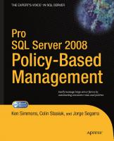
THE LIFE CYCLE OF A QUERY To introduce the high-level components of SQL Server’s architecture, this section uses the example of a query’s life cycle to put each component into context in order to foster your understanding and create a foundation for the rest of the book. It looks at a basic SELECT query fi rst in order to reduce the scope to that of a READ operation, and then introduces the additional processes involved for a query that performs an UPDATE operation. Finally, you’ll read about the terminology and processes that SQL Server uses to implement recovery while optimizing performance. Figure 1-1 shows the high-level components that are used within the chapter to illustrate the life cycle of a query.
4
❘
CHAPTER 1 SQL SERVER ARCHITECTURE
Cmd Parser
Optimizer
Query Executor
SNI
SQL Server Network Interface
Protocol Layer
Relational Engine
Plan Cache Transaction Log
Access Methods
Data file
Transaction Mgr
Storage Engine
Data Cache
Buffer Manager
Buffer Pool
FIGURE 1-1
The Relational and Storage Engines As shown in Figure 1-1, SQL Server is split into two main engines: the Relational Engine and the Storage Engine. The Relational Engine is also sometimes called the query processor because its primary function is query optimization and execution. It contains a Command Parser to check query syntax and prepare query trees, a Query Optimizer that is arguably the crown jewel of any database system, and a Query Executor responsible for execution. The Storage Engine is responsible for managing all I/O to the data, and contains the Access Methods code, which handles I/O requests for rows, indexes, pages, allocations and row versions, and a Buffer Manager, which deals with SQL Server’s main memory consumer, the buffer pool. It also contains a Transaction Manager, which handles the locking of data to maintain Isolation (ACID properties) and manages the transaction log.
The Bufer Pool The other major component you need to know about before getting into the query life cycle is the buffer pool, which is the largest consumer of memory in SQL Server. The buffer pool contains all
The Life Cycle of a Query
❘5
the different caches in SQL Server, including the plan cache and the data cache, which is covered as the sections follow the query through its life cycle. The buffer pool is covered in detail in Chapter 2.
A Basic Select Query The details of the query used in this example aren’t important — it’s a simple SELECT statement with no joins, so you’re just issuing a basic read request. Start at the client, where the fi rst component you touch is the SQL Server Network Interface (SNI).
SQL Server Network Interface The SQL Server Network Interface (SNI) is a protocol layer that establishes the network connection between the client and the server. It consists of a set of APIs that are used by both the database engine and the SQL Server Native Client (SNAC). SNI replaces the net-libraries found in SQL Server 2000 and the Microsoft Data Access Components (MDAC), which are included with Windows.
Late in the SQL Server 2005 development cycle, the SQL Server team decided to eliminate their dependence on MDAC to provide client connectivity. MDAC is owned by the SQL Server team but ships in the box with Windows, which means its shipped ‘out-of-band’ with SQL Server. With so many new features being added in SQL Server 2005, it became cumbersome to coordinate updates to MDAC with Windows releases, and SNI and SNAC were the solutions created. This meant that the SQL Server team could add support for new features and release the new code in-line with SQL Server releases.
SNI isn’t configurable directly; you just need to configure a network protocol on the client and the server. SQL Server has support for the following protocols: ➤
Shared memory: Simple and fast, shared memory is the default protocol used to connect from a client running on the same computer as SQL Server. It can only be used locally, has no configurable properties, and is always tried first when connecting from the local machine.
➤
TCP/IP: TCP/IP is the most commonly used access protocol for SQL Server. It enables you to connect to SQL Server by specifying an IP address and a port number. Typically, this happens automatically when you specify an instance to connect to. Your internal name resolution system resolves the hostname part of the instance name to an IP address, and either you connect to the default TCP port number 1433 for default instances or the SQL Browser service will find the right port for a named instance using UDP port 1434.
➤
Named Pipes: TCP/IP and Named Pipes are comparable protocols in the architectures in which they can be used. Named Pipes was developed for local area networks (LANs) but it can be inefficient across slower networks such as wide area networks (WANs).
6
❘
CHAPTER 1 SQL SERVER ARCHITECTURE
To use Named Pipes you fi rst need to enable it in SQL Server Configuration Manager (if you’ll be connecting remotely) and then create a SQL Server alias, which connects to the server using Named Pipes as the protocol. Named Pipes uses TCP port 445, so ensure that the port is open on any fi rewalls between the two computers, including the Windows Firewall. ➤
VIA: Virtual Interface Adapter is a protocol that enables high-performance communications between two systems. It requires specialized hardware at both ends and a dedicated connection. Like Named Pipes, to use the VIA protocol you first need to enable it in SQL Server Configuration Manager and then create a SQL Server alias that connects to the server using VIA as the protocol. Regardless of the network protocol used, once the connection is established, SNI creates a secure connection to a TDS endpoint (described next) on the server, which is then used to send requests and receive data. For the purpose here of following a query through its life cycle, you’re sending the SELECT statement and waiting to receive the result set.
TDS (Tabular Data Stream) Endpoints TDS is a Microsoft-proprietary protocol originally designed by Sybase that is used to interact with a database server. Once a connection has been made using a network protocol such as TCP/IP, a link is established to the relevant TDS endpoint that then acts as the communication point between the client and the server. There is one TDS endpoint for each network protocol and an additional one reserved for use by the dedicated administrator connection (DAC). Once connectivity is established, TDS messages are used to communicate between the client and the server. The SELECT statement is sent to the SQL Server as a TDS message across a TCP/IP connection (TCP/IP is the default protocol).
Protocol Layer When the protocol layer in SQL Server receives your TDS packet, it has to reverse the work of the SNI at the client and unwrap the packet to fi nd out what request it contains. The protocol layer is also responsible for packaging up results and status messages to send back to the client as TDS messages. Our SELECT statement is marked in the TDS packet as a message of type “SQL Command,” so it’s passed on to the next component, the Query Parser, to begin the path toward execution. Figure 1-2 shows where our query has gone so far. At the client, the statement was wrapped in a TDS packet by the SQL Server Network Interface and sent to the protocol layer on the SQL Server where it was unwrapped, identified as a SQL Command, and the code sent to the Command Parser by the SNI.
The Life Cycle of a Query
❘7
Language Event
Cmd Parser
Optimizer
Query Executor
Relational Engine
TDS
SNI
SQL Server Network Interface
Protocol Layer
FIGURE 1-2
Command Parser The Command Parser’s role is to handle T-SQL language events. It fi rst checks the syntax and returns any errors back to the protocol layer to send to the client. If the syntax is valid, then the next step is to generate a query plan or fi nd an existing plan. A query plan contains the details about how SQL Server is going to execute a piece of code. It is commonly referred to as an execution plan. To check for a query plan, the Command Parser generates a hash of the T-SQL and checks it against the plan cache to determine whether a suitable plan already exists. The plan cache is an area in the buffer pool used to cache query plans. If it fi nds a match, then the plan is read from cache and passed on to the Query Executor for execution. (The following section explains what happens if it doesn’t fi nd a match.)
Plan Cache Creating execution plans can be time consuming and resource intensive, so it makes sense that if SQL Server has already found a good way to execute a piece of code that it should try to reuse it for subsequent requests. The plan cache, part of SQL Server’s buffer pool, is used to store execution plans in case they are needed later. You can read more about execution plans and plan cache in Chapters 2 and 5. If no cached plan is found, then the Command Parser generates a query tree based on the T-SQL. A query tree is an internal structure whereby each node in the tree represents an operation in the query that needs to be performed. This tree is then passed to the Query Optimizer to process. Our basic query didn’t have an existing plan so a query tree was created and passed to the Query Optimizer. Figure 1-3 shows the plan cache added to the diagram, which is checked by the Command Parser for an existing query plan. Also added is the query tree output from the Command Parser being passed to the optimizer because nothing was found in cache for our query.
8
❘
CHAPTER 1 SQL SERVER ARCHITECTURE
Query Tree
Language Event
TDS
Cmd Parser
Query Plan Optimizer Relational Engine
Query Executor
SNI
SQL Server Network Interface
Protocol Layer Plan Cache
Data Cache
Buffer Pool FIGURE 1-3
Optimizer The Optimizer is the most prized possession of the SQL Server team and one of the most complex and secretive parts of the product. Fortunately, it’s only the low-level algorithms and source code that are so well protected (even within Microsoft), and research and observation can reveal how the Optimizer works. It is what’s known as a “cost-based” optimizer, which means that it evaluates multiple ways to execute a query and then picks the method that it deems will have the lowest cost to execute. This “method” of executing is implemented as a query plan and is the output from the optimizer. Based on that description, you would be forgiven for thinking that the optimizer’s job is to fi nd the best query plan because that would seem like an obvious assumption. Its actual job, however, is to fi nd a good plan in a reasonable amount of time, rather than the best plan. The optimizer’s goal is most commonly described as fi nding the most efficient plan. If the optimizer tried to fi nd the “best” plan every time, it might take longer to fi nd the plan than it would to just execute a slower plan (some built-in heuristics actually ensure that it never takes longer to fi nd a good plan than it does to just find a plan and execute it).
The Life Cycle of a Query
❘9
As well as being cost based, the optimizer also performs multi-stage optimization, increasing the number of decisions available to fi nd a good plan at each stage. When a good plan is found, optimization stops at that stage. The fi rst stage is known as pre-optimization, and queries drop out of the process at this stage when the statement is simple enough that the most efficient plan is obvious, obviating the need for additional costing. Basic queries with no joins are regarded as “simple,” and plans produced as such have zero cost (because they haven’t been costed) and are referred to as trivial plans. The next stage is where optimization actually begins, and it consists of three search phases: ➤
Phase 0: During this phase the optimizer looks at nested loop joins and won’t consider parallel operators (parallel means executing across multiple processors and is covered in Chapter 5. The optimizer will stop here if the cost of the plan it has found is < 0.2. A plan generated at this phase is known as a transaction processing, or TP, plan.
➤
Phase 1: Phase 1 uses a subset of the possible optimization rules and looks for common patterns for which it already has a plan. The optimizer will stop here if the cost of the plan it has found is < 1.0. Plans generated in this phase are called quick plans.
➤
Phase 2: This final phase is where the optimizer pulls out all the stops and is able to use all of its optimization rules. It will also look at parallelism and indexed views (if you’re running Enterprise Edition). Completion of Phase 2 is a balance between the cost of the plan found versus the time spent optimizing. Plans created in this phase have an optimization level of “Full.”
HOW MUCH DOES IT COST? The term Cost doesn’t translate into seconds or anything meaningful and is just an arbitrary number used to assign a value representing the resource cost for a plan. However, its origin was a benchmark on a desktop computer at Microsoft early in SQL Server’s life (probably 7.0). The statistics that the optimizer uses to estimate cost aren’t covered here because they aren’t relevant to the concepts illustrated in this chapter but you can read about them in Chapter 5.
Because our SELECT query is very simple, it drops out of the process in the pre-optimization phase because the plan is obvious to the optimizer. Now that there is a query plan, it’s on to the Query Executor for execution.
Query Executor The Query Executor’s job is self-explanatory; it executes the query. To be more specific, it executes the query plan by working through each step it contains and interacting with the Storage Engine to retrieve or modify data.
10
❘
CHAPTER 1 SQL SERVER ARCHITECTURE
The interface to the Storage Engine is actually OLE DB, which is a legacy from a design decision made in SQL Server’s history. The development team’s original idea was to interface through OLE DB to allow different Storage Engines to be plugged in. However, the strategy changed soon after that. The idea of a pluggable Storage Engine was dropped and the developers started writing extensions to OLE DB to improve performance. These customizations are now core to the product, and while there’s now no reason to have OLE DB, the existing investment and performance precludes any justifi cation to change it.
The SELECT query needs to retrieve data, so the request is passed to the Storage Engine through an OLE DB interface to the Access Methods. Figure 1-4 shows the addition of the query plan as the output from the Optimizer being passed to the Query Executor. Also introduced is the Storage Engine, which is interfaced by the Query Executor via OLE DB to the Access Methods (coming up next). Query Tree
Language Event
Cmd Parser
Optimizer
Query Plan Query Executor
TDS
SNI
SQL Server Network Interface
Protocol Layer
Relational Engine OLE DB
Plan Cache
Access Methods
Storage Engine FIGURE 1-4
Buffer Pool
The Life Cycle of a Query
❘ 11
Access Methods Access Methods is a collection of code that provides the storage structures for your data and indexes as well as the interface through which data is retrieved and modified. It contains all the code to retrieve data but it doesn’t actually perform the operation itself; it passes the request to the Buffer Manager. Suppose our SELECT statement needs to read just a few rows that are all on a single page. The Access Methods code will ask the Buffer Manager to retrieve the page so that it can prepare an OLE DB rowset to pass back to the Relational Engine.
Bufer Manager The Buffer Manager, as its name suggests, manages the buffer pool, which represents the majority of SQL Server’s memory usage. If you need to read some rows from a page (you’ll look at writes when we look at an UPDATE query) the Buffer Manager will check the data cache in the buffer pool to see if it already has the page cached in memory. If the page is already cached, then the results are passed back to the Access Methods. If the page isn’t already in cache, then the Buffer Manager will get the page from the database on disk, put it in the data cache, and pass the results to the Access Methods.
The PAGEIOLATCH wait type represents the time it takes to read a data page from disk into memory. You can read about wait types in Chapter 3.
The key point to take away from this is that you only ever work with data in memory. Every new data read that you request is fi rst read from disk and then written to memory (the data cache) before being returned to you as a result set. This is why SQL Server needs to maintain a minimum level of free pages in memory; you wouldn’t be able to read any new data if there were no space in cache to put it fi rst. The Access Methods code determined that the SELECT query needed a single page, so it asked the Buffer Manager to get it. The Buffer Manager checked to see whether it already had it in the data cache, and then loaded it from disk into the cache when it couldn’t fi nd it.
Data Cache The data cache is usually the largest part of the buffer pool; therefore, it’s the largest memory consumer within SQL Server. It is here that every data page that is read from disk is written to before being used. The sys.dm_os_buffer_descriptors DMV contains one row for every data page currently held in cache. You can use this script to see how much space each database is using in the data cache: SELECT count(*)*8/1024 AS ‘Cached Size (MB)’ ,CASE database_id WHEN 32767 THEN ‘ResourceDb’
12
❘
CHAPTER 1 SQL SERVER ARCHITECTURE
ELSE db_name(database_id) END AS ‘Database’ FROM sys.dm_os_buffer_descriptors GROUP BY db_name(database_id) ,database_id ORDER BY ‘Cached Size (MB)’ DESC
The output will look something like this (with your own databases obviously): Cached Size (MB) 3287 34 12 4
Database People tempdb ResourceDb msdb
In this example, the People database has 3,287MB of data pages in the data cache. The amount of time that pages stay in cache is determined by a least recently used (LRU) policy. The header of each page in cache stores details about the last two times it was accessed, and a periodic scan through the cache examines these values. A counter is maintained that is decremented if the page hasn’t been accessed for a while; and when SQL Server needs to free up some cache, the pages with the lowest counter are flushed fi rst. The process of “aging out” pages from cache and maintaining an available amount of free cache pages for subsequent use can be done by any worker thread after scheduling its own I/O or by the lazywriter process, covered later in the section “Lazywriter.” You can view how long SQL Server expects to be able to keep a page in cache by looking at the MSSQL$:Buffer Manager\Page Life Expectancy counter in Performance Monitor. Page life expectancy (PLE) is the amount of time, in seconds, that SQL Server expects to be able to keep a page in cache. Under memory pressure, data pages are flushed from cache far more frequently. Microsoft recommends a minimum of 300 seconds for a good PLE, but for systems with plenty of physical memory this will easily reach thousands of seconds. The database page read to serve the result set for our SELECT query is now in the data cache in the buffer pool and will have an entry in the sys.dm_os_buffer_descriptors DMV. Now that the Buffer Manager has the result set, it’s passed back to the Access Methods to make its way to the client.
A Basic select Statement Life Cycle Summary Figure 1-5 shows the whole life cycle of a SELECT query, described here:
1.
The SQL Server Network Interface (SNI) on the client established a connection to the SNI on the SQL Server using a network protocol such as TCP/IP. It then created a connection to a TDS endpoint over the TCP/IP connection and sent the SELECT statement to SQL Server as a TDS message.
2.
The SNI on the SQL Server unpacked the TDS message, read the SELECT statement, and passed a “SQL Command” to the Command Parser.
The Life Cycle of a Query
3.
The Command Parser checked the plan cache in the buffer pool for an existing, usable query plan. When it didn’t find one, it created a query tree based on the SELECT statement and passed it to the Optimizer to generate a query plan.
4.
The Optimizer generated a “zero cost” or “trivial” plan in the pre-optimization phase because the statement was so simple. The query plan created was then passed to the Query Executor for execution.
5.
At execution time, the Query Executor determined that data needed to be read to complete the query plan so it passed the request to the Access Methods in the Storage Engine via an OLE DB interface.
6.
The Access Methods needed to read a page from the database to complete the request from the Query Executor and asked the Buffer Manager to provision the data page.
7.
The Buffer Manager checked the data cache to see if it already had the page in cache. It wasn’t in cache so it pulled the page from disk, put it in cache, and passed it back to the Access Methods.
8.
Finally, the Access Methods passed the result set back to the Relational Engine to send to the client. Query Tree
Language Event
Cmd Parser
TDS TDS
Optimizer
Query Plan Query Executor
SNI
SQL Server Network Interface
Protocol Layer
Relational Engine
Plan Cache
OLE DB
Access Methods Data Cache
Data file
Storage Engine FIGURE 1-5
Buffer Manager
Buffer Pool
❘ 13
14
❘
CHAPTER 1 SQL SERVER ARCHITECTURE
A Simple Update Query Now that you understand the life cycle for a query that just reads some data, the next step is to determine what happens when you need to write data. To answer that, this section takes a look at a simple UPDATE query that modifies the data that was read in the previous example. The good news is that the process is exactly the same as the process for the SELECT statement you just looked at until you get to the Access Methods. The Access Methods need to make a data modification this time, so before it passes on the I/O request the details of the change need to be persisted to disk. That is the job of the Transaction Manager.
Transaction Manager The Transaction Manager has two components that are of interest here: a Lock Manager and a Log Manager. The Lock Manager is responsible for providing concurrency to the data, and it delivers the configured level of isolation (as defi ned in the ACID properties at the beginning of the chapter) by using locks.
The Lock Manager is also employed during the SELECT query life cycle covered earlier, but it would have been a distraction, and is only mentioned here because it’s part of the Transaction Manager. Locking is covered in depth in Chapter 6.
The real item of interest here is actually the Log Manager. The Access Methods code requests that the changes it wants to make are logged, and the Log Manager writes the changes to the transaction log. This is called Write-Ahead Logging. Writing to the transaction log is the only part of a data modification transaction that always needs a physical write to disk because SQL Server depends on being able to reread that change in the event of system failure (you’ll learn more about this in the “Recovery” section coming up). What’s actually stored in the transaction log isn’t a list of modification statements but only details of the page changes that occurred as the result of a modification statement. This is all that SQL Server needs in order to undo any change, and why it’s so difficult to read the contents of a transaction log in any meaningful way, although you can buy a third-party tool to help. Getting back to the UPDATE query life cycle, the update operation has now been logged. The actual data modification can only be performed when confi rmation is received that the operation has been physically written to the transaction log. This is why transaction log performance is so crucial. Chapter 4 contains information on monitoring transaction log performance and optimizing the underlying storage for it. Once the Access Methods receives confi rmation, it passes the modification request on to the Buffer Manager to complete.
The Life Cycle of a Query
❘ 15
Figure 1-6 shows the Transaction Manager, which is called by the Access Methods and the transaction log, which is the destination for logging our update. The Buffer Manager is also in play now because the modification request is ready to be completed. Query Tree
Language Event
Cmd Parser
Optimizer
Query Plan Query Executor
TDS
SNI
SQL Server Network Interface
Protocol Layer
Relational Engine
Plan Cache
OLE DB Transaction Log
Access Methods Transaction Manager
Storage Engine
Data Cache
Buffer Manager
Buffer Pool
FIGURE 1-6
Bufer Manager The page that needs to be modified is already in cache, so all the Buffer Manager needs to do is modify the page as requested by the Access Methods. The page is modified in the cache, and confi rmation is sent back to Access Methods and ultimately to the client. The key point here (and it’s a big one so pay attention) is that the UPDATE statement has changed the data in the data cache, not in the actual database fi le on disk. This is done for performance reasons, and the page is now what’s called a dirty page because it’s different in memory than it is on disk. It doesn’t compromise the durability of the modification as defi ned in the ACID properties because you can recreate the change using the transaction log if, for example, you suddenly lost power to the server and therefore anything in physical RAM (i.e., the data cache). How and when the dirty page makes its way into the database file is covered in the next section.
16
❘
CHAPTER 1 SQL SERVER ARCHITECTURE
Figure 1-7 shows the completed life cycle for the update. The Buffer Manager has made the modification to the page in cache and has passed confi rmation back up the chain. The database data fi le was not accessed during the operation, as you can see in the diagram. Query Tree
Language Event
Cmd Parser
TDS TDS
Optimizer
Query Plan Query Executor
SNI
SQL Server Network Interface
Protocol Layer
Relational Engine
Plan Cache
OLE DB Transaction Log
D Access Methods
Data file
Transaction Manager
Storage Engine
Data Cache
Buffer Manager
Buffer Pool
FIGURE 1-7
Recovery In the previous section you read about the life cycle of an UPDATE query, which introduced WriteAhead Logging as the method by which SQL Server maintains the durability of any changes. Modifications are written to the transaction log fi rst and are then actioned in memory only. This is done for performance reasons and because you can recover the changes from the transaction log should you need to. This process introduces some new concepts and terminology that are explored further in this section on “recovery.”
The Life Cycle of a Query
❘ 17
Dirty Pages When a page is read from disk into memory it is regarded as a clean page because it’s exactly the same as its counterpart on the disk. However, once the page has been modified in memory it is marked as a dirty page. Clean pages can be flushed from cache using dbcc dropcleanbuffers, which can be handy when you’re troubleshooting development and test environments because it forces subsequent reads to be fulfi lled from disk, rather than cache, but doesn’t touch any dirty pages. A dirty page is simply a page that has changed in memory since it was loaded from disk and is now different from the on-disk page. You can use the following query, which is based on the sys.dm_os_ buffer_descriptors DMV, to see how many dirty pages exist in each database: SELECT db_name(database_id) AS ‘Database’,count(page_id) AS ‘Dirty Pages’ FROM sys.dm_os_buffer_descriptors WHERE is_modified =1 GROUP BY db_name(database_id) ORDER BY count(page_id) DESC
Running this on my test server produced the following results showing that at the time the query was run, there were just under 20MB (2,524*8\1,024) of dirty pages in the People database: Database People Tempdb Master
Dirty Pages 2524 61 1
These dirty pages will be written back to the database fi le periodically whenever the free buffer list is low or a checkpoint occurs. SQL Server always tries to maintain a number of free pages in cache in order to allocate pages quickly, and these free pages are tracked in the free buffer list. Whenever a worker thread issues a read request, it gets a list of 64 pages in cache and checks whether the free buffer list is below a certain threshold. If it is, it will try to age-out some pages in its list, which causes any dirty pages to be written to disk. Another thread called the lazywriter also works based on a low free buffer list.
Lazywriter The lazywriter is a thread that periodically checks the size of the free buffer list. When it’s low, it scans the whole data cache to age-out any pages that haven’t been used for a while. If it fi nds any dirty pages that haven’t been used for a while, they are flushed to disk before being marked as free in memory. The lazywriter also monitors the free physical memory on the server and will release memory from the free buffer list back to Windows in very low memory conditions. When SQL Server is busy, it will also grow the size of the free buffer list to meet demand (and therefore the buffer pool) when there is free physical memory and the configured Max Server Memory threshold hasn’t been reached. For more on Max Server Memory see Chapter 2.
18
❘
CHAPTER 1 SQL SERVER ARCHITECTURE
Checkpoint Process A checkpoint is a point in time created by the checkpoint process at which SQL Server can be sure that any committed transactions have had all their changes written to disk. This checkpoint then becomes the marker from which database recovery can start. The checkpoint process ensures that any dirty pages associated with a committed transaction will be flushed to disk. Unlike the lazywriter, however, a checkpoint does not remove the page from cache; it makes sure the dirty page is written to disk and then marks the cached paged as clean in the page header. By default, on a busy server, SQL Server will issue a checkpoint roughly every minute, which is marked in the transaction log. If the SQL Server instance or the database is restarted, then the recovery process reading the log knows that it doesn’t need to do anything with log records prior to the checkpoint. The time between checkpoints therefore represents the amount of work that needs to be done to roll forward any committed transactions that occurred after the last checkpoint, and to roll back any transactions that hadn’t committed. By checkpointing every minute, SQL Server is trying to keep the recovery time when starting a database to less than one minute, but it won’t automatically checkpoint unless at least 10MB has been written to the log within the period. Checkpoints can also be manually called by using the CHECKPOINT T-SQL command, and can occur because of other events happening in SQL Server. For example, when you issue a backup command, a checkpoint will run fi rst. Trace fl ag 3502 is an undocumented trace fl ag that records in the error log when a checkpoint starts and stops. For example, after adding it as a startup trace fl ag and running a workload with numerous writes, my error log contained the entries shown in Figure 1-8, which indicates checkpoints running between 30 and 40 seconds apart.
FIGURE 1-8
ALL ABOUT TRACE FLAGS Trace fl ags provide a way to change the behavior of SQL Server temporarily and are generally used to help with troubleshooting or for enabling and disabling certain features for testing. Hundreds of trace flags exist but very few are officially documented; for a list of those that are and more information on using trace flags have a look here: http://msdn.microsoft.com/en-us/library/ms188396.aspx
The Life Cycle of a Query
❘ 19
Recovery Interval Recovery Interval is a server configuration option that can be used to influence the time between checkpoints, and therefore the time it takes to recover a database on startup — hence, “recovery interval.” By default the recovery interval is set to 0, which allows SQL Server to choose an appropriate interval, which usually equates to roughly one minute between automatic checkpoints. Changing this value to greater than 0 represents the number of minutes you want to allow between checkpoints. Under most circumstances you won’t need to change this value, but if you were more concerned about the overhead of the checkpoint process than the recovery time, you have the option. However, the recovery interval is usually set only in test and lab environments where it’s set ridiculously high in order to effectively stop automatic checkpointing for the purpose of monitoring something or to gain a performance advantage. Unless you’re chasing world speed records for SQL Server you shouldn’t need to change it in a realworld production environment. SQL Server evens throttles checkpoint I/O to stop it from impacting the disk subsystem too much, so it’s quite good at self-governing. If you ever see the SLEEP_BPOOL_FLUSH wait type on your server, that means checkpoint I/O was throttled to maintain overall system performance. You can read all about waits and wait types in Chapter 3.
Recovery Models SQL Server has three database recovery models: Full, bulk-logged, and simple. Which model you choose affects the way the transaction log is used and how big it grows, your backup strategy, and your restore options.
Full Databases using the full recovery model have all of their operations fully logged in the transaction log and must have a backup strategy that includes full backups and transaction log backups. Starting with SQL Server 2005, Full backups don’t truncate the transaction log. This is so that the sequence of transaction log backups isn’t broken and gives you an extra recovery option if your full backup is damaged. SQL Server databases that require the highest level of recoverability should use the Full Recovery Model.
Bulk-Logged This is a special recovery model because it is intended to be used only temporarily to improve the performance of certain bulk operations by minimally-logging them; all other operations are fullylogged just like the full recovery model. This can improve performance because only the information required to roll back the transaction is logged. Redo information is not logged which means that you also lose point-in-time-recovery.
20
❘
CHAPTER 1 SQL SERVER ARCHITECTURE
These bulk operations include: ➤
BULK INSERT
➤
Using the bcp executable
➤
SELECT INTO
➤
CREATE INDEX
➤
ALTER INDEX REBUILD
➤
DROP INDEX
Simple When the simple recovery model is set on a database, all committed transactions are truncated from the transaction log every time a checkpoint occurs. This ensures that the size of the log is kept to a minimum and that transaction log backups are not necessary (or even possible). Whether or not that is a good or a bad thing depends on what level of recovery you require for the database. If the potential to lose all the changes since the last full or differential backup still meets your business requirements then simple recovery might be the way to go.
THE SQLOS (SQL OPERATING SYSTEM) So far, this chapter has abstracted the concept of the SQLOS to make the flow of components through the architecture easier to understand without going off on too many tangents. However, the SQLOS is core to SQL Server’s architecture so you need to understand why it exists and what it does to complete your view of how SQL Server works. In summary, the SQLOS is a thin user-mode layer (Chapter 2) that sits between SQL Server and Windows. It is used for low-level operations such as scheduling, I/O completion, memory management, and resource management. To explore exactly what this means and why it’s needed, you fi rst need to understand a bit about Windows. Windows is a general purpose OS and is not optimized for server-based applications, SQL Server in particular. Instead, the goal for the Windows development team is to make sure that any application written by a wide-range of developers inside and outside Microsoft will work correctly and have good performance. Windows needs to work well for these broad scenarios so the dev teams are not going to do anything special that would be used in less than 1% of applications. For example, the scheduling in Windows is very basic because things are done for the common cause. Optimizing the way that threads are chosen for execution is always going to be limited because of this broad performance goal but if an application does its own scheduling then there is more intelligence about who to choose next. For example, assigning some threads a higher priority or deciding that choosing one thread for execution will prevent other threads being blocked later on.
The SQLOS (SQL Operating System)
❘ 21
Scheduling is the method by which units of work are given time on a CPU to execute. See Chapter 5 for more information.
In a lot of cases SQL Server had custom code to handle a lot of these areas already. The User Mode Scheduler (UMS) was introduced in SQL Server 7 to handle scheduling and SQL Server was managing its own memory even earlier than that. The idea for SQLOS (which was fi rst implemented in SQL Server 2005) was to take all of these things developed by different internal SQL Server development teams to provide performance improvements on Windows and put them in a single place with a single team that will continue to optimize these low-level functions. This then leaves the other teams to concentrate on challenges more specific to their own domain within SQL Server.
DEFINING DMVS Dynamic Management Views (DMVs) allow much greater visibility into the workings of SQL Server than in any version prior to SQL Server 2005. They are basically just views on top of the system tables, but the concept allows Microsoft to provide a massive amount of useful information through them. The standard syntax starts with sys.dm,_which indicates that it’s a DMV (there are also Dynamic Management Functions but DMV is still the collective term in popular use) followed by the area about which the DMV provides information, for example, sys.dm_os_for SQLOS, sys.dm_db_for database, and sys.dm_exec_for query execution. The last part of the name describes the actual content accessible within the view; sys.dm_db_index_usage_stats and sys.dm_os_waiting_tasks are a couple of examples and you’ll come across many more throughout the book.
Another benefit to having everything in one place is that you can now get better visibility of what’s happening at that level than was possible prior to SQLOS. You can access all this information through dynamic management views (DMVs). Any DMV that starts with sys.dm_os_ provides an insight into the workings of SQLOS. For example: ➤
sys.dm_os_schedulers: Returns one row per scheduler (there is one user scheduler per core) and shows information on scheduler load and health. See Chapters 3 and 5 for more information.
➤
sys.dm_os_waiting_tasks: Returns one row for every executing task that is currently waiting for a resource as well as the wait type. See Chapter 3 for more information.
➤
sys.dm_os_memory_clerks: Memory clerks are used by SQL Server to allocate memory. Significant components within SQL Server have their own memory clerk. This DMV shows all the memory clerks and how much memory each one is using. See Chapter 2 for more information.
22
❘
CHAPTER 1 SQL SERVER ARCHITECTURE
Relating SQLOS back to the architecture diagrams seen earlier, many of the components will make calls to the SQLOS in order to fulfi ll low-level functions required to support their roles. Just to be clear, the SQLOS doesn’t replace Windows. Ultimately, everything ends up using the documented Windows system services; SQL Server just uses them in such a way as to optimize for its own specific scenarios.
SQLOS is not a way to port the SQL Server architecture to other platforms like Linux or MacOS so it’s not an OS abstraction layer. It doesn’t wrap all the OS APIs like other frameworks such as .NET, which is why it’s referred to as a “thin” user-mode layer. Only the things that SQL Server really needs have been put into SQLOS.
SUMMARY In this chapter you learned about SQL Server’s architecture by following the flow of components used when you issue a read request and an update request. You also learned some key terminology and processes used for the recovery of SQL Server databases and where the SQLOS fits into the architecture. The key takeaways from this chapter are: ➤
The Query Optimizer’s job is to find a good plan in a reasonable amount of time; not the best plan.
➤
Anything you want to read or update will need to be read into memory first.
➤
Any updates to data will be written to the transaction log on disk before being updated in memory so transaction log performance is critical; the update isn’t written directly to the data file.
➤
A database page that is changed in memory but not on disk is known as a dirty page.
➤
Dirty pages are flushed to disk by the checkpoint process and the lazywriter.
➤
Checkpoints occur automatically, roughly every minute and provide the starting point for recovery.
➤
The lazywriter keeps space available in cache by flushing dirty pages to disk and keeping only recently used pages in cache.
➤
When a database is using the Full recovery model, full backups will not truncate the transaction log. You must configure transaction log backups.
The SQLOS is a framework used by components in SQL Server for scheduling, I/O, and memory management.
2
Understanding Memory WHAT’S IN THIS CHAPTER ➤
Understanding physical memory and how virtual memory addressing is used
➤
Optimizing 32-bit systems with large amounts of memory
➤
Optimizing the memory configuration on 64-bit systems
➤
AWE and its uses on 32-bit and 64-bit environments
➤
Explaining MemToLeave
➤
SQL Server’s memory clerks, caches, and pools
➤
Looking at SQL Server’s plan cache
➤
Determining a setting for Max Server Memory
➤
An in-depth look at Query/Workspace memory
Memory, disk, and CPU are the holy trinity of resources in a computer system, and memory is fi rst because it’s the area that you’re most likely to have an issue with. Memory issues can cause both disk and CPU saturation, so when troubleshooting a server issue (or at least a performance issue) you need to start by looking at the memory profi le of the system. This chapter explains what to expect from different system architectures, what can be configured, what the Microsoft best practices are, and, most important, how they were originally determined. The fi rst part of this chapter covers memory addressing, which includes physical memory, virtual memory, the Virtual Memory Manager, and the different options you have for tuning 32-bit and 64-bit systems. The second part focuses more on SQL Server’s internal memory structures and consumers. It covers how to manage SQL Server’s memory usage and how to view the details of each consumer.
24
❘
CHAPTER 2 UNDERSTANDING MEMORY
WINDOWS AND MEMORY This section covers topics that are generally considered to be outside the scope of a database professional, but it will give you an understanding of and appreciation for the underlying architectures on which SQL Server depends. The rationale behind this approach is to help you clarify your skill set and enable you to be more creative and inclusive as you troubleshoot.
Physical Memory Physical memory refers to the volatile storage space most commonly referred to as RAM (random access memory). RAM is also referred to as primary storage, main memory, or system memory because it’s directly addressable by the CPU. It is regarded as the fastest type of storage you can use, but it’s volatile, meaning you lose what was stored when you reboot the computer. It’s also expensive and limited in capacity when compared to nonvolatile storage such as a hard disk. For example, Windows Server 2008 Enterprise and Datacenter Editions support up to 2TB of RAM, but buying a server with that much memory will cost you millions of U.S. dollars, whereas a single 1TB hard disk can be picked up for less than $100. Combine a few of those together and you can have tens of TBs of very cost-effective storage space. Consequently, servers use a combination of hard disks to store data, which is then loaded into RAM where it can be worked with more quickly. By way of throughput comparison, the peak transfer rate for a mainstream RAM module would be about 5GB/sec, and the fastest hard disk I could fi nd at the time of writing boasts “Unprecedented performance with a sustained data rate of up to 164MB/sec.” That’s 3.2% of the transfer rate of a reasonable RAM module. This chapter doesn’t delve deeply into different types of RAM, but it can be useful (or at least mildly interesting) to understand some of the acronyms and keywords at a high level, especially if you ever get involved in specifying new hardware for servers running Microsoft SQL Server.
SIMMs and DIMMs Single in-line memory modules (SIMMs) and dual inline memory modules (DIMMs) refer to the physical implementation of a type of RAM. SIMMs were phased out in the mid-1990s, replaced by the more efficient DIMMs, which are the predominant type of memory today. A DIMM is what you get to plug into the motherboard when you buy a memory module.
DRAM Dynamic RAM (DRAM) is a type of RAM that stores data in a capacitor that needs to be periodically “recharged” to prevent the data from being lost. This periodic refresh is where the term dynamic comes from, as opposed to static RAM (SRAM). SRAM does not need to be refreshed, is faster, and consumes less power, but is considerably more expensive. For this reason, DRAM is the basis for mainstream computer memory, although you will fi nd SRAM embedded in small amounts for use in such areas as CPU cache.
Windows and Memory
❘ 25
SDRAM Building upon DRAM technology, synchronous DRAM is synchronized with the computer’s system bus, allowing for more complexity in its usage, including pipelining, which enables instructions to be queued, providing better efficiency.
DDR SDRAM Double-data-rate SDRAM doubles the amount of consecutive data able to be read or written in a single instruction over standard SDRAM. DDR2 doubles that again, and DDR3 is double that of DDR2, providing eight times the amount of consecutive data read or writes per operation compared to the original DDR1. DDR2 is still a common choice for both the server and desktop market. However, processors based on Intel’s microarchitecture (codenamed Nehalem) support only DDR3 so it will quickly become the de facto standard. You can read more about Nehalem in Chapter 5.
Dual-Channel Memory Dual-channel architecture is technology in the memory controller that is used by a supported motherboard to increase the bandwidth to the controller by using standard memory modules in a “paired” fashion. The CPU is the fastest component in a computer, and if the CPU bus speed is greater than the memory bus speed, then you can get a bottleneck at the memory controller. Dual-channel memory was created to relieve that pressure. Intel’s Nehalem architecture has the memory controller on the CPU, so the memory is connected directly to the processor and it uses three-channel memory.
Registered and Unbufered Modules Registered memory modules contain a “register” that reduces electrical load on the memory controller, enabling servers to remain stable with more memory modules. It also requires a supporting motherboard and is an attractive feature for servers that need a lot of memory, so you’ll fi nd that most servers require registered memory. However, because it makes the modules more expensive and adds a performance penalty, they are typically used only in servers and workstations for which scalability and stability is paramount. When buying memory for desktop computers, you might see modules listed as “unbuffered.” This simply means that the module doesn’t have a register.
Error-Correcting Code (ECC) Memory Memory is vulnerable to corruption by background radiation, among others things, which can change a stored bit value. The frequency of these errors is quite low; online research indicates an average of one bit error per gigabyte per month. Although the effect could be as severe as crashing the computer, the chances of it affecting a single bit value that you were using for a critical operation at that moment is very small.
26
❘
CHAPTER 2 UNDERSTANDING MEMORY
On desktop systems that typically don’t run 24/7, the chances of a corruption happening, and happening in a part of memory that you happened to be using at the time, is extremely low. Because of this and the overhead of using ECC, ECC memory and ECC-capable motherboards are not prevalent in the desktop market. For servers that are generally expected to run constantly, however, the risk is greater and the implications more severe. Most servers will support or even require that you use ECC memory modules.
FB-DIMMs Fully Buffered DIMMs are a relatively recent technology standard based on DDR2 that uses an advanced memory buffer (AMB) between the memory controller and the memory module. The memory controller writes to the AMB instead of directly to the module, allowing for more memory bandwidth and error correction (with little overhead) although the addition of the AMB introduces some latency to memory requests. FB-DIMMs need additional power to run the AMB, which means additional heat is generated. This has led to some doubt as to the future of the technology, but it’s still the predominant platform for Intel-based servers a number of years after its expected decline.
Maximum Supported Physical Memory For ease of reference, Table 2-1 shows the maximum supported physical RAM for each edition of SQL Server 2008 running on Windows Server 2008; and Table 2-2 shows the same information for Windows Server 2003 R2. TABLE 2-1: Memory Supported by SQL Server 2008 on Various Windows Server 2008 Editions SQL SERVER EDITION
WINDOWS DATACENTER 32-BIT
WINDOWS DATACENTER 64-BIT
WINDOWS ENTERPRISE 32-BIT
WINDOWS ENTERPRISE 64-BIT
WINDOWS STANDARD 32-BIT
WINDOWS STANDARD 64-BIT
WINDOWS WEB 32-BIT
WINDOWS WEB 64-BIT
Enterprise
64GB1
2TB1
64GB1
2TB1
4GB1
32GB1
4GB1
32GB1
Developer
64GB1
2TB1
64GB1
2TB1
4GB1
32GB1
4GB1
32GB1
Standard
64GB1
2TB1
64GB1
2TB1
4GB1
32GB1
4GB1
32GB1
Web
64GB1
2TB1
64GB1
2TB1
4GB1
32GB1
4GB1
32GB1
Workgroup
64GB1
4GB
64GB1
4GB
4GB1
4GB
4GB1
4GB
Express
1GB
n/a
1GB
n/a
1GB
n/a
1GB
n/a
1 These limitations are the operating system (OS) maximum. Where marked, SQL Server will support the OS maximum, ensuring that SQL Server will be able to take immediate advantage of future revisions of the OS that increase these limits.
Windows and Memory
❘ 27
TABLE 2-2: Memory Supported by SQL Server 2008 on Various Windows Server 2003 R2
Editions with SP2 SQL SERVER EDITION
WINDOWS DATACENTER 32-BIT
WINDOWS DATACENTER 64-BIT
WINDOWS ENTERPRISE 32-BIT
WINDOWS ENTERPRISE 64-BIT
WINDOWS STANDARD 32-BIT
WINDOWS STANDARD 64-BIT
Enterprise
128GB1
2TB1
64GB1
2TB1
4GB1
32GB1
Developer
128GB1
2TB1
64GB1
2TB1
4GB1
32GB1
Standard
128GB1
2TB1
64GB1
2TB1
4GB1
32GB1
Web
128GB1
2TB1
64GB1
2TB1
4GB1
32GB1
Workgroup
128GB1
4GB
64GB1
4GB
4GB1
4GB
Express
1GB
n/a
1GB
n/a
1GB
n/a
1
These limitations are the operating system (OS) maximum. Where marked, SQL Server will support the OS maximum, ensuring that SQL Server will be able to take immediate advantage of future revisions of the OS that increase these limits.
Virtual Address Space If all the processes running on a computer could only use addresses in physical memory, there would be a bottleneck in the system very quickly. They would all have to share the same range of addresses, which would be limited by the amount of RAM installed in the computer. As physical memory is very fast to access and cannot be increased indefi nitely (as just discussed in the previous section) it’s a resource that needs to be used efficiently. Windows (and many other mainstream, modern operating systems) assigns a virtual address space (VAS) to each process. This provides a layer of abstraction between an application and physical memory so that the operating system can choose the most efficient way to use physical memory across all the processes. For example, two different processes can both use the memory address 0xFFF because it’s a virtual address and each process has its own VAS with the same address range. Whether or not that address maps to physical memory or is determined by the operating system or, more specifically (for Windows at least), the Virtual Memory Manager, is covered in the next section. The size of the virtual address space is determined largely by the CPU architecture. A 32-bit CPU running 32-bit software (also known as the x86 platform) is so named because it is based on an architecture that can manipulate values that are up to 32 bits in length. This means that a 32-bit memory pointer can store a value between 0 and 4,294,967,295 to reference a memory address. This equates to a maximum addressable space of 4GB on 32-bit platforms. The 4GB of VAS is logically split into two ranges of 2GB: one for the process and one reserved for system use. These two ranges are commonly referred to as user mode and kernel mode address spaces and are illustrated in Figure 2-1. With a default configuration, each application process (i.e., SQL Server) can access up to 2GB of VAS, and therefore 2GB of physical memory. The options to tune this are covered in depth in the upcoming section “Tuning 32-bit Systems.”
28
❘
CHAPTER 2 UNDERSTANDING MEMORY
OxFFFFFFFF
OxFFFFFFFF
2GB Kernel Mode
4GB Virtual Address Space
Ox80000000 Ox7FFFFFFF
2GB User Mode
Ox00000000
Ox00000000
FIGURE 2-1
The limitation of 4GB exists because it’s effectively the largest number that can fit in a 32-bit pointer. From here, it’s an easy jump to realize that a 64-bit system with 64-bit pointers will increase this limit, but by how much? The easiest way to work it out is to use the power function on a scientific calculator. 232 gives you the 32-bit limit of 4,294,967,295, and calculating 264 gives you the staggering 64-bit limit of 18,446,744,073,709,551,616. This number is so large that in memory/storage terminology it equates to 16 exabytes. You don’t come across that term very often, so to help understand the scale, here is the value converted to more commonly used measurements: 16 exabytes = ➤
16,777,216 petabytes (16 million PB)
➤
17,179,869,184 terabytes (17 billion TB)
➤
17,592,186,044,416 gigabytes (17 trillion GB)
As you can see, it is significantly larger than the 4GB virtual address space usable in 32-bit systems; it’s so large in fact that any hardware capable of using it all is sadly restricted to the realm of science fiction. Because of this, processor manufacturers decided to only implement a 44-bit address bus, which provides a virtual address space on 64-bit systems of 16TB. This was regarded as being more than enough address space for the foreseeable future and logically it’s split into an 8TB range for user mode and 8TB for kernel mode. Each 64-bit process running on an x64 platform will be able to address up to 8TB of VAS. (For more information on processor architectures, see Chapter 5).
Windows and Memory
x64 is the predominant 64-bit architecture in use today and the main focus of this book when discussing 64-bit technologies. Figure 2-2 shows the difference between the virtual address space size per process in Windows x86 (32-bit) and Windows x64. There is an alternative architecture from Intel implemented in their Itanium chips known as IA64, and while there is a version of SQL Server 2008 available for it, there are very few production implementations so the focus in this book is on the x64 platform.
❘ 29
Ox7FFFFFFF000
8TB x64 VAS
2GB x86 VAS Ox00000000000
Virtual Memory Manager FIGURE 2-2
Next, this chapter covers the part of Windows that joins physical memory and virtual address space together; the Virtual Memory Manager (VMM). When a process wants to read from or write something into memory, it references an address in its VAS; and the VMM will map it to an address in physical memory. It isn’t guaranteed, however, to still be mapped to a physical memory address the next time you access it because the VMM may determine that it needs to move your data to the page fi le temporarily to allow another process to use the physical memory address. As part of this process, the VMM will update the VAS address and make it invalid (it doesn’t point to a physical memory address anymore). The next time you access this address, it will have to be loaded from the page fi le on disk so the request will be slower. This is known as a page fault and happens automatically without you knowing. The portion of a process’s VAS that currently maps to physical memory is known as the working set. If a process requests data that isn’t currently in the working set, then it will need to be reloaded back into memory before use. This is called a hard page fault (a soft page fault is when the page is still on the standby list in physical memory); and to fi x it, the VMM will retrieve the data from the page fi le, fi nd a free page of memory, either from its list of free pages or from another process, write the data from the page fi le into memory, and then map the new page back into the process’s virtual address space.
The Memory\Page Faults/sec counter in Performance Monitor includes both hard and soft page faults, so if you want to monitor just the performance sapping hard page faults you need to look at Memory\Page Reads/sec to get the number of times the disk was accessed to resolve hard page faults and compare it to Memory\Pages Input/sec to calculate the average number of pages being read in each disk access.
30
❘
CHAPTER 2 UNDERSTANDING MEMORY
On a system with enough RAM to give every process all the memory it needs, the VMM doesn’t have to do much other than hand out memory and clean up after a process is done with it. On a system without enough RAM to go around, the job is a little more involved. The VMM has to do some work to provide each process with the memory it needs when it needs it. It does this by using the page fi le to temporarily store data that a process hasn’t accessed for a while. This process is called paging, and the data is often referred to as having been paged out to disk. The Virtual Memory Manager keeps track of each mapping for VAS addresses using a page table, and the mapping information itself is stored in a page table entry (PTE). This is illustrated in Figure 2-3 using two 32-bit SQL Server instances as an example. Note that the dotted line indicates an invalid reference that will generate a hard page fault when accessed causing the page to be loaded from the page fi le. Physical RAM Virtual Memory Address 1 SQL Server Inst 1
Virtual Memory Address 2 Virtual Memory Address 3 Virtual Memory Address 4
Virtual Memory Manager: Page Table Page Table Entry (4KB)
0001 0010 DATA 10 0110 0000 1001 00 0101 0000 DATA 00 0110 0111 1100 00 0001 0010 DATA 11 0110 0000 1001 00
PTE
2GB VAS Virtual Memory Address 1 SQL Server Inst 2
PTE
Page file
PTE
0101 0000 DATA 00 0110 0111 1100 00
Virtual Memory Address 2 Virtual Memory Address 3 Virtual Memory Address 4 2GB VAS
FIGURE 2-3
The system PTEs are 4KB in size and share the kernel mode address space with other system data structures and information. If you recall from the previous section, the kernel mode address space is only 2GB on a 32-bit system, which results in an inherent limitation regardless of how much physical memory the computer has. Issues with lack of system PTE space and other kernel mode space consumers are discussed in the next section.
Windows and Memory
❘ 31
Tuning 32-Bit Systems The 2GB process limitation on 32-bit systems became a limiting factor long before 64-bit was ready for widespread adoption, so something needed to be done to take advantage of all the extra physical memory that hardware manufacturers were able to build systems with. This section looks at the different ways you can configure 32-bit Windows to use more than 4GB of RAM and SQL Server to use more than the 2GB process limitation, along with the benefits and inevitable side effects that are very often overlooked. Note that this section is only applicable to 32-bit systems.
/3GB and increaseUserVA The fi rst technique that can be employed to increase the SQL Server process address space is to reduce the amount of kernel mode address space from 2GB to 1GB, which leaves 3GB for the user mode address space. This is implemented by using the /3GB switch, and has been referred to in the past as “4GB Tuning,” or 4GT for short. /3GB needs to be added to the OS entry in boot.ini if you’re running Windows Server 2003 or earlier. To perform the equivalent operation on Windows Server 2008, you need to edit the Boot Configuration Data using BCDEdit from a command prompt using the following switch: BCDEdit /set increaseUserVA 3072
You will fi nd more details about increaseUserVA and / USERVA in the “/PAE and /3GB Together?” section. Once you add /3GB and reboot, each process will have 3GB of address space instead of just 2GB, and the kernel mode address space will be reduced to 1GB. You can see this illustrated in Figure 2-4. To be able to address the extra 1GB, your application has to have been linked with the /LARGEADDRESSAWARE flag. Thankfully, SQL Server has been linked with the appropriate flag, so you don’t need to do anything else and 3GB will be available immediately.
OxFFFFFFFF
OxFFFFFFFF 1GB Kernel Mode
2GB Kernel Mode
OxC0000000 OxBFFFFFFF
Ox80000000 Ox7FFFFFFF
3GB User Mode
2GB User Mode
Ox00000000
Ox00000000
FIGURE 2-4
The downside to this configuration is the implication for consumers of the now reduced kernel mode address space — specifically, nonpaged pool, paged pool, and system PTEs (covered earlier in the section “Virtual Memory Manager”).
32
❘
CHAPTER 2 UNDERSTANDING MEMORY
Paged Pool and Nonpaged Pool Paged pool and nonpaged pool are used to allocate system memory. Nonpaged pool, as its name suggests, can’t be paged out to disk, and so it is used by hardware drivers to prevent the system crashes that would occur if they were paged out. You should monitor these two pools if you’re using /3GB and defi nitely if you’re using it in combination with /PAE (discussed further on). Measuring your paged and nonpaged pool usage is straightforward; you can use Performance Monitor to view the counters for Memory/Pool Paged Bytes and Memory/Pool Nonpaged Bytes. However, these values are only useful if you know the maximum values for these pools on your server, which takes a bit more work to determine. For Windows 2003, the maximum values are calculated on boot and are then fi xed. To view the values, you need to use a kernel debugger; or, alternatively, you can configure the Process Explorer tool from Sysinternals to see them (you’ll also need a connection to the Internet). Execute the following steps to view maximum values:
1.
Download Process Explorer from here: http://technet.microsoft.com/en-us/ sysinternals/bb896653.aspx.
2.
Install the Debugging Tools for Windows to get the dbghelp.dll file: www.microsoft.com/ whdc/devtools/debugging/default.mspx.
3.
Launch Process Explorer (procexp.exe) and go to Options ➪ Configure Symbols. You’ll need to configure the Dbghelp.dll path to use the new DLL you just installed with the Debugging Tools and the “Symbols path” to the following: SRV*C:\SYMBOLS*http://msdl.microsoft.com/downloads/symbols;
If your system drive isn’t C:\, then change the location appropriately. Figure 2-5 shows a screenshot of configured symbols installed where the system drive is D:\.
FIGURE 2-5
4.
Go to View➪System Information, where the values for Paged Limit and Nonpaged Limit are now visible. Figure 2-6 shows the System Information screen after the symbols have been configured correctly.
Windows and Memory
❘ 33
FIGURE 2-6
Enabling /3GB halves the kernel mode address space and the size of the paged and nonpaged pool. Table 2-3 shows typical startup values for Windows Server 2003 SP1. TABLE 2-3: Typical Paged and Nonpaged Values for Windows Server 2003 SP1 SYSTEM RAM
PAGED MA X
NONPAGED MA X
512MB
184MB
125MB
1,024MB
168MB
202MB
1,536MB
352MB
252MB
2,048MB
352MB
252MB
A test server running Windows Server 2003 R2 SP2 with 16GB of RAM (you’ll read about enabling all this memory in the PAE section coming up) has the same Paged Max and Nonpaged Max as the example in the table with only 2GB of RAM. After adding the /3GB switch, these were reduced to 156MB and 128MB, respectively, which might still be OK. Armed with the current usage and maximum values, you can make an informed decision regarding whether /3GB is restricting your paged and nonpaged pools too much.
34
❘
CHAPTER 2 UNDERSTANDING MEMORY
Windows Server 2008 uses dynamic max values for the paged and nonpaged pools, so using /3GB on that OS is less of an issue for paged and nonpaged pool usage. Figure 2-7 shows the same test server as Figure 2-6 running Windows Server 2008.
FIGURE 2-7
System PTEs One of the symptoms of a lack of PTEs is that the server stops responding, so it’s a major issue to avoid. You can monitor the number of free system PTEs using Performance Monitor and viewing the counter for Memory\Free System Page Table Entries. Microsoft recommends that this value should be at least 24,000 on boot-up and should never drop to less than 10,000 or you’re considered “at risk” of running out. The more RAM you have the more PTEs you need to manage the mapping between virtual memory and physical memory. PTEs use space in the kernel mode address space, so any reduction in the size of the kernel mode will affect how much RAM you’ll be able to have in your computer. On a Windows Server 2003 test server with 4GB of RAM, the Free System Page Table Entry count is 180,234 — well above the necessary minimum of 10,000. After adding /3GB this drops to 26,417. It’s a significant drop but still enough to meet the on-boot recommendation, and now the SQL Server instance can use 3GB of physical memory.
Windows and Memory
❘ 35
There is an additional switch you can use with /3GB to slightly reduce the amount of kernel mode space that’s taken to allow for more system PTEs. It’s called /USERVA and is covered in the upcoming section “/PAE and /3GB Together?” In Windows Server 2008, /3GB and / USERVA have been combined into a single setting called increaseUserVA, which is also covered in that section.
/PAE Switch /3GB allows you to gain an extra 1GB for user processes but that’s not a great leap in terms of capacity, so Intel introduced a technology called Physical Address Extension (PAE) that effectively increases the address bus to 36 bits and allows access to up to 128GB of RAM, depending on your OS. The Standard Edition of Windows supports only up to 4GB of RAM, so PAE is available only in the Enterprise and Datacenter Editions. It is enabled in the same way as /3GB: by adding the /PAE switch to boot.ini or the BCD, depending on which OS you’re running.
HOT-ADD MEMORY AND DATA EXECUTION PREVENTION If you’re running Windows Server 2003 Service Pack 1 or later, you may fi nd that PAE is automatically enabled to support additional hardware-based features such as hot-add memory and data execution prevention (DEP). Hot-add memory is self-explanatory: On a running server, it enables you to plug in additional RAM modules, which Windows will automatically detect and start using. For this to work, Windows needs to be ready in PAE mode in anticipation of this additional “hot-added” memory being greater than 4GB. If your server BIOS has support for hot-add memory enabled, Windows Server 2003 SP1 or later will automatically run in PAE mode. DEP is a hardware-enforced security feature of Windows that prevents applications from executing code from non-executable memory, which helps to prevent exploits that might be possible via a buffer overflow. For all the possible memory ranges to be protected, Windows automatically switches on PAE if the technology is enabled in the BIOS. On Intel motherboards, the feature is known as Execute Disable Bit (XD), and on AMD systems it’s known as No-execute (NX) or Advanced Virus Protection. The point is to be aware that you’re very likely to be using PAE automatically on your server without the switch being present in boot.ini or the BCD.
PAE works by modifying the system PTEs (see “Virtual Memory Manager” earlier in the chapter) to be 8KB instead of 4KB, and uses the extra space to map virtual addresses into the physical memory above 4GB. This increase in size is important to note because it effectively doubles the space required for PTEs in the kernel mode address space. When PAE is enabled, Windows will see and manage up to 128GB of RAM on a server. You can tell if it’s working by running winver.exe and checking the amount of memory that Windows has
36
❘
CHAPTER 2 UNDERSTANDING MEMORY
detected. If you have 16GB of RAM in the server and PAE is working, winver will show 16GB. Figure 2-8 shows an example of winver output. You can disable PAE by adding the /EXECUTE / NOPAE switches to boot.ini or the BCD. In order for applications such as SQL Server to use the additional memory provided by PAE, they have to be written to make use of a set of extensions known as Address Windowing Extensions (AWE), which is covered in more detail in the next section.
Address Windowing Extensions (AWE) AWE is a Windows API that enables a 32-bit FIGURE 2-8 process to map memory from outside its virtual address space. That is, it enables a process to reserve a portion of virtual address space (a window), which can then be mapped to any physical address range in a method known as windowing. Figure 2-9 illustrates the concept. To reduce the additional overhead associated with mapping and remapping using AWE, the design ensures that any memory allocated using the APIs cannot be shared with any other process and is made nonpageable, or locked. Up to 128GB
DATA 0110 1001 0001 0110
OxFFFFFFFF
1101 0001 1101 DATA 0001
2GB Kernel Mode
AWE Mapping
Ox80000000 Ox7FFFFFFF 1101 0001 1101 DATA 0001 2GB User Mode AWE Window Ox00000000
0101 DATA 1001 0001 0000 0000 1100 1101 1101 DATA
From 2GB FIGURE 2-9
Windows and Memory
❘ 37
In order for SQL Server to use the AWE APIs, you need to enable AWE using sp_configure or by selecting the check box on the Memory page of a server’s Properties window in Management Studio. Once enabled, the next time SQL Server is started it will attempt to lock memory pages so that it can use AWE. To lock memory pages, the SQL Server process needs to have the “Lock Pages in Memory” Advanced User Right in Windows which is achieved by granting the permission to the SQL Server service account. This permission is not granted automatically, even if the service account is a member of the Local Administrators group. If you enable AWE and haven’t granted the right privilege to the service account, you’ll see the message shown in Figure 2-10 at the beginning of the SQL Server Error Log. If the correct privilege has been granted, you’ll see the message shown in Figure 2-11.
FIGURE 2-10
FIGURE 2-11
To assign the “Lock pages in memory” privilege, you need to modify the Group Policy on the server using gpedit.msc (from the Start menu, select Run and enter gpedit.msc). Navigate down to UserRights Assignment, and add the service account to the Lock pages in memory privilege, as shown in Figure 2-12.
FIGURE 2-12
38
❘
CHAPTER 2 UNDERSTANDING MEMORY
On Windows Server 2003 and Windows Server 2008, AWE memory is dynamically allocated by SQL Server in the same way as normal memory allocations, so you can observe SQL Server starting and taking only the minimum amount of RAM and increasing its usage as necessary. AWE memory still isn’t the perfect solution for working with large amounts of RAM. Complexity and overhead are associated with the windowing process, but the biggest drawback for SQL Server’s usage is that the additional RAM can only be used for data cache. See the “SQL Server Memory” section for details on the data cache. Only data pages can be stored in AWE mapped memory so it cannot directly help if your SQL Server is struggling to support additional users, databases, queries, locks, or other consumers of memory in SQL Server that have to run in non-AWE memory. To scale those components you need to move to a 64-bit platform.
/PAE and /3GB Together? A common debate is whether or not you can, or, more important, should use /PAE and /3GB together to squeeze every last drop of physical memory for use with SQL Server. The benefits should be obvious by now — access to more than 2GB of RAM for SQL Server’s data cache and an additional 1GB stolen from kernel mode for use with any of SQL Server’s memory requirements. According to Microsoft’s official guidelines, using /PAE and /3GB together is not recommended. Official guidance is great and applicable to most scenarios but it’s more useful to you as an IT professional to understand why it’s not recommended so you can make a judgment call yourself. Using both technologies can cause issues because of resulting changes that affect three key areas that depend on kernel mode address space, as mentioned earlier: paged pool, nonpaged pool, and system PTEs. When you implement /3GB on Windows Server 2003, you significantly reduce the maximum memory available for paged pool and nonpaged pool, so you should monitor their usage as described earlier. Similarly, you also reduce the amount of space available for system PTEs as a result of losing 1GB of kernel mode address space, so you should monitor the counter for Memory\Free System Page Table Entries in Performance Monitor to ensure that it stays above 10,000. If you then implement PAE you’re effectively doubling the size of each PTE from 4KB to 8KB in an already reduced space, so a lack of free system PTEs becomes your limiting factor. More RAM requires more PTEs to manage it, so whether you can safely use /PAE and /3GB together depends on how much RAM you have. To determine the best configuration, take a look at some example memory sizes. Table 2-4 shows the values of these components when running with different amounts of RAM on Windows Server 2003 R2 SP2 with /PAE and /3GB enabled. As shown in Table 2-4, even with only 8GB of RAM the server had just 13,653 free system PTEs, which is almost 50% less than the recommended value of 24,000 at boot up. You could still run with this configuration if you monitored the value closely, but you can see why Microsoft doesn’t recommend it.
Windows and Memory
❘ 39
TABLE 2-4: Paged Pool, Nonpaged Pool, and Free System PTEs on Windows Server 2003 R2 SP2 with /PAE and /3GB Enabled SYSTEM RAM
PAGED MA X
NONPAGED MA X
FREE SYSTEM PTE s
8GB
160MB
131MB
13,653
12GB
160MB
131MB
6,500
16GB
160MB
131MB
2,000
With 16GB of RAM there are just about enough free system PTEs to start the server, so it’s clear this configuration won’t sustain a stable server. To alleviate some of the pressure on systems PTEs that this setup creates, a new switch was made available in Windows Server 2003 called / USERVA. Using this switch in combination with /3GB enables you to specify a slightly lower amount of MBs for the user mode address space than 3GB, so you can leave a bit more kernel mode space for system PTEs. Microsoft recommends trying a default value of 3030, but values between 2970 and 3030 are supported (the values are in MB). 3072 is the equivalent of /3GB without /USERVA. Table 2-5 shows the free system PTE results of testing different values for / USERVA with different amounts of RAM on Windows 2003 R2 SP2. The underlined values are optimal but any combination that results in free system PTEs greater than 24,000 at boot up is acceptable. TABLE 2-5: Free System PTE tests with Various Values for /USERVA and
amounts of RAM 16GB RAM
12GB RAM
8GB RAM
USERVA=3030
12200
17200
24500
USERVA=3000
20000
25000
32100
USERVA=2970
27400
32600
39900
From the results you can see that even with 16GB of RAM you can add /3GB / USERVA=2970 to gain an extra 922MB of user mode address space and still have a supported solution.
Windows Server 2008 In Windows Server 2008, /3GB and / USERVA have been combined into a single setting called increaseUserVA, which you modify by using BCDEDIT. Running BCDEDIT /set increaseUserVA 3072 is the equivalent to using /3GB in Windows Server 2003. Table 2-6 shows the values for the key components with different amounts of RAM on a test server running Windows Server 2008.
40
❘
CHAPTER 2 UNDERSTANDING MEMORY
TABLE 2-6: Paged Pool, Nonpaged Pool, and Free System PTEs with /PAE and
/IncreaseUserVA 3072 Enabled SYSTEM RAM
PAGED MA X
NONPAGED MA X
FREE SYSTEM PTE s
8GB
1,024MB
1,024MB
110,500
12GB
1,024MB
1,024MB
105,500
16GB
1,024MB
1,024MB
95,000
You can see from the results that even with 16GB of RAM, giving 3GB to the user mode address space on Windows Server 2008 still leaves plenty of free system PTEs. Moving to the x64 version of Windows removes all these problems with paged pool, nonpaged pool, and free system PTEs because the address space is just so large; 8TB compared to 2GB on x86 or even 1GB if you use the /3GB switch. Figure 2-13 shows the paged maximum at 26.5GB and the nonpaged maximum at 6.5GB. This the same hardware that was used in Figure 2-6, which showed 360MB and 260MB; the only difference is the x64 version of Windows Server 2003. Running Windows Server 2008 x64, the maximum values were 134GB and 12.5GB, but that’s not so important because the maximum is dynamic in Windows Server 2008.
FIGURE 2-13
Windows and Memory
❘ 41
MemToLeave, or ReservedMemory ReservedMemory is a part of SQL Server’s address space that is reserved before SQL Server allocates its buffer pool and then freed afterwards. It’s also referred to as MemToLeave (MTL) because that was the name of an internal variable which referenced the amount of memory to leave. Although formal documentation from Microsoft will be more likely to use the ReservedMemory term, you’ll fi nd that MemToLeave is the most commonly used term in the field, even within Microsoft’s own support organization. There is no such thing as the MemToLeave area but it is an appropriate description of the action that SQL Server takes when the service starts. It will leave, or reserve, a section of virtual memory before it reserves the buffer pool and will then release it afterwards so that there is some free space in the VAS for other components to reserve and commit memory using the VirtualAlloc Windows functions.
VirtualAlloc, VirtualAllocEx, and VirtualAllocExNuma are low-level Windows functions used by applications to reserve and then commit memory in a processes virtual address space.
So who uses VirtualAlloc? ➤
The heap manager (heaps are used to allocate a lower level of granularity that VirtualAlloc normally allows) — so anything using a heap indirectly will as well.
➤
SQL Server uses VirtualAlloc for Multi-Page Allocations (MPAs),which are used when a memory request is larger than a SQL Server page (8KB).
➤
Windows will call VirtualAlloc to create a thread stack (more on this coming up).
➤
Any other components that don’t know anything about the buffer pool and use their normal memory allocation routines that ultimately go to VirtualAlloc such as: ➤
OLE DB providers (including SQL Server Linked Servers)
➤
Extended Stored Procedures
➤
COM objects
There is no MemToLeave in 64-bit SQL Server! MemToLeave is only a part of the startup process in 32-bit SQL Server. Because the virtual address space is so large in 64-bit SQL Server reserving addresses outside the buffer pool isn’t necessary. This is explored in a bit more detail later in the chapter.
How much address space is reserved is determined by SQL Server on startup by the following formula: memory_to_reserve = MemReserved + (NumThreads × Stack Size) Memory_to_reserve is 256MB by default, but can be modified by using the -g startup switch.
42
❘
CHAPTER 2 UNDERSTANDING MEMORY
Changing the memory_to_reserve option can be useful when you have more physical memory than the application virtual address space (2-3GB depending on configuration) and you’re seeing messages in the error log containing “Failed Virtual Allocate Bytes”. This usually indicates that SQL Server doesn’t have enough VAS for the allocations it needs to make outside the buffer pool. If you get these messages and you can’t reduce your linked server, extended stored procedure, and COM object usage try increasing memory_to_reserve from the default of 256 to 384 to provide more space; although be aware that the extra space you’re providing will taken away from the buffer pool. Similarly, you can also set memory_to_reserve to a lower value to provide a bit more space in the buffer pool if you have memory intensive workloads and don’t use many linked servers, extended stored procedures, or COM objects.
NumThreads is the maximum total number of worker threads configured for your SQL Server instance. You can calculate the maximum number of worker threads you can have by using Table 2-7 (64-bit values are included out of interest only, as there is no MemToLeave in 64-bit), or by running the following query: select max_workers_count from sys.dm_os_sys_info
StackSize is the space required to create each thread stack. It varies according to CPU architecture. On x86 (32-bit) its 0.5MB, on x64 (64-bit) its 2MB, and on IA64 its 4MB. TABLE 2-7: Calculating the Number of Worker Threads NUMBER OF CPUs
32-BIT
64-BIT
≤ 4 processors
256
512
8 processors
288
576
16 processors
352
704
32 processors
480
960
SQL Server will only allocate around 35-40 worker threads on startup and then one or two more when you first connect. Additional worker threads will only be created when the worker thread pool isn’t enough to satisfy all the concurrent requests, so you may have hundreds of connections but if they don’t all run concurrently you may only need 5 or 10 threads to service them all.
Windows and Memory
❘ 43
One of the biggest problems around the whole MemToLeave process is not running out, but rather a lack of contiguous memory addresses large enough for a requested allocation. If this happens you will see a message similar to the following in the SQL Server Error Log: WARNING: Failed to reserve contiguous memory of Size=65546
In this example, a request for 64KB couldn’t be allocated. Determining the largest contiguous block size available for a reservation in the virtual address space was difficult in SQL Server 2000; you had to run a tool in kernel mode called vmstat, which wasn’t an attractive prospect on a production SQL Server machine. Thankfully, the introduction of dynamic management views (DMVs) in SQL Server 2005 exposed a lot more internal information without having to resort to risky low-level tools. It’s still a convoluted process to determine the largest contiguous block size but at least it can be done with T-SQL. The script in Listing 2-1 will output how much space is unallocated in SQL Server’s VAS, and, more important, the largest free block size (both in KB). LISTING 2-1: Free virtual address space and largest contiguous block size
With VASummary(Size,Reserved,Free) AS (SELECT Size = VaDump.Size, Reserved = SUM(CASE(CONVERT(INT, VaDump.Base)^0) WHEN 0 THEN 0 ELSE 1 END), Free = SUM(CASE(CONVERT(INT, VaDump.Base)^0) WHEN 0 THEN 1 ELSE 0 END) FROM ( SELECT CONVERT(VARBINARY, SUM(region_size_in_bytes)) AS Size, region_allocation_base_address AS Base FROM sys.dm_os_virtual_address_dump WHERE region_allocation_base_address 0x0 GROUP BY region_allocation_base_address UNION SELECT CONVERT(VARBINARY, region_size_in_bytes), region_allocation_base_address FROM sys.dm_os_virtual_address_dump WHERE region_allocation_base_address = 0x0 ) AS VaDump GROUP BY Size) SELECT SUM(CONVERT(BIGINT,Size)*Free)/1024 AS [Total avail mem, KB] ,CAST(MAX(Size) AS BIGINT)/1024 AS [Max free size, KB] FROM VASummary WHERE Free 0 This code available for download at Wrox.com [Chapter2HowMuchVAS.sql]
44
❘
CHAPTER 2 UNDERSTANDING MEMORY
Using the preceding MemToLeave formula and an example 32-bit system with 2GB of RAM and two CPU cores, the formula, with all the values now known, looks like this: ReservedMemory = 256MB + (256 × 0.5MB)
You can calculate that the ReservedMemory is 384MB, which SQL Server will reserve before reserving what’s left for the buffer pool, which equates to about 1.6GB. This is why you will see SQL Server’s memory usage peak at around a maximum of 1.6GB on a 32-bit server; that is what’s left over after the MemToLeave process. This is illustrated in Figure 2-14.
Buffer Pool 1.6GB 2GB Virtual Address Space
Running the script to determine free virtual address space on this system should yield results like the following: Total avail mem, KB 338,856
Max free size, KB 157,008
This shows that the unallocated virtual address space is 330MB and the largest contiguous block is 153MB. To reinforce what’s happening here and to show that MemToLeave is actually just VAS, you can look at what happens when there is only 1GB of RAM on the server. The buffer pool will never be more than physical RAM, so if you take 1GB of RAM out of the example system, SQL Server will still reserve 384MB during the MemToLeave process and then reserve a buffer pool of only 1,024MB (equal to physical RAM). You can see this illustrated in Figure 2-15. The diagram highlights the fact that the additional space not allocated to the buffer pool is exactly the same as that reserved and released for MemToLeave; it’s just virtual address space not allocated to the buffer pool, which now totals 1,024MB, 640MB larger than previously.
384MB ReservedMemory FIGURE 2-14
640MB VAS
Buffer Pool 1024MB
384MB ReservedMemory FIGURE 2-15
If you run the script again on this system your results will look something like this: Total avail mem, KB Max free size, KB 917,020 364,956
This indicates that there is 895MB of free VAS left and that the largest block is 356MB.
2GB Virtual Address Space
Windows and Memory
❘ 45
Note on 64-Bit Systems As mentioned at the start of this section, in 64-bit SQL Server there is no MemToLeave. As you’ve just seen, MemToLeave is simply unallocated VAS and with the 8TB of VAS available on x64 systems, there is plenty of space and large contiguous blocks shouldn’t be a problem. To show this you can run the code in Listing 2-1 that was used to look at the VAS in previous examples. On an x64 system with four CPU cores and 16GB of RAM the results will look similar to this: Total avail mem, KB 8,572,745,912
Max free size, KB 8,566,727,936
This shows 8,175GB of free VAS left, and the largest block is 8,169GB, which should be more than enough! This is a big justification for moving to 64-bit, especially if you’ve had MemToLeave issues in the past.
Tuning 64-Bit Systems Moving to a 64-bit system solves a lot of the memory related problems discussed so far that are related to the 32-bit platform. However, 64-bit environments bring new potential issues that you should be aware of while also learning how and when to avoid them.
AWE on 64-Bit Systems AWE on a 64-bit system? After reading this far you might be thinking that this is either a trick question or you’ve misunderstood everything up to now. Thankfully, it’s neither; AWE in SQL Server 64-bit systems is used as a workaround for a problem than can occur between the Windows working set manager and SQL Server, particularly on Windows Server 2003 and below. If there isn’t enough free physical memory in Windows to service a request for resources from a driver or another application, the working set manager will trim the working set (the working set reflects the physical memory usage of a process) of all applications running on the server. This is normal behavior and shouldn’t have much noticeable impact. However, if the request is for contiguous memory, the working set manager will force all applications to empty their working sets. This is known as “aggressive working set trimming” and will have a devastating effect on SQL Server’s memory allocation and therefore performance. In SQL Server 2005 SP2, Microsoft added a new error message so you can easily see when this happens. Here is an example: 2009-02-01 21:25:10.14 spid1s A significant part of sql server process memory has been paged out. This may result in a performance degradation. Duration: 0 seconds. Working set (KB): 1086400, committed (KB): 2160928, memory utilization: 50%.
The result can be as severe as SQL Server’s working set dropping from tens of GB to a few hundred MB in just a few seconds, so if you see the error message there’s a good chance you noticed a performance hit before looking at the error log.
46
❘
CHAPTER 2 UNDERSTANDING MEMORY
Resolving this issue (or avoiding it all together) should be tackled using a combination of a few different methods: ➤
First, check for updates to all your device drivers. If the problem was caused by a device driver, it may have been fixed already in a later version.
➤
Next, set Max Server Memory in SQL Server to ensure that Windows and other processes running on the server have enough physical memory to perform their work without asking SQL Server to trim. You can read about calculating a suitable Max Server Memory value in the SQL Server Memory section.
➤
Finally, if you’re still seeing the issue (or if its effects are so severe you don’t want to risk seeing it again), you can configure your SQL Server to use AWE.
In the section on AWE under “Tuning 32-bit Systems” you read that it’s used to access memory above the 32-bit process limitation. It also locks pages in memory to make allocations faster, and it’s this facet of AWE that a 64-bit SQL Server can take advantage of. If SQL Server’s memory pages are “locked,” then its nonpageable and Windows can’t take it when aggressively trimming. The AWE options in sp_configure and SQL Server Management Studio are ignored when you’re running 64-bit, but if you give the SQL Server service account the Lock Pages in Memory privilege and you’re running the Enterprise Edition, then SQL Server will use the AWE APIs to allocate memory.
When SQL Server 2008 was released, being able to lock pages in memory on x64 required you to be running SQL Server Enterprise Edition. As a result of strong community feedback on the working set trimming issue Microsoft eventually enabled support in SQL Server Standard edition with the use of a trace fl ag and SQL Server 2008 SP1 with Cumulative Update 2. You can read more about this and how to enable it here: http://support .microsoft.com/kb/970070
Once the pages are locked they’re not considered part of available memory for working set trimming. However, AWE can only be used to lock SQL Server buffer pool allocations. Windows can still trim the working sets of other processes, affecting resources on which SQL Server depends. AWE on 64-bit systems should be used if you continue to get working set trimming after updating your device drivers and setting a suitable max server memory or if the cost of SQL Server’s working set being trimmed again is too risky. It shouldn’t be used as a default best practice on all your SQL Servers. It’s a workaround and not intended to replace the default behavior on every 64-bit SQL Server implementation. If AWE is working you’ll see the following message in the SQL Server Error Log: Using Locked Pages for Buffer Pool.
SQL Server Memory
❘ 47
Windows Server 2008 has improved the way it handles requests for large or contiguous memory allocations, so in theory you shouldn’t see the working set trimming problem on this platform often, if at all.
SQL SERVER MEMORY The fi rst part of this chapter dealt mainly with the memory environment external to SQL Server — that is, understanding and configuring memory before SQL Server starts. This second part looks at how SQL Server manages memory. The SQL Server memory manager has a three-level structure. At the bottom are memory nodes which are the lowest level allocators for SQL Server memory, the second level consists of memory clerks which are used to access the memory nodes and cache stores which are used for caching. The top layer contains memory objects which provide a smaller level of granularity than the memory clerks allow directly. Only clerks can access memory nodes to allocate memory, so every component that needs to allocate substantial amounts of memory needs to create its own memory clerk when the SQL Server service starts.
Memory Nodes You can view details about the nodes on your server using the sys.dm_os_ memory_nodes DMV. You will always have at least one memory node, which has a memory_node_id of 0. You will have more than one memory node if you have configured Non-Uniform Memory Access (NUMA) or if your system uses AMD processors and you have more than four CPU cores. The AMD processor architecture follows the NUMA specification, and SQL Server will detect NUMA support and create multiple memory nodes if it detects four or more CPU cores.
You can read more about NUMA in Chapter 5.
Each memory node has its own memory clerks and caches, which are distributed evenly across all nodes. SQL Server’s total usage is calculated using the sum of all the nodes.
Memory Clerks, Caches, and the Bufer Pool Memory Clerks are the mechanism by which Memory Caches are used and the Buffer Pool is far the largest consumer of memory in SQL Server. All three are discussed in this section.
Memory Clerks Whenever a memory consumer within SQL Server wants to allocate memory it needs to go through a memory clerk, rather than going straight to a memory node. There are generic memory clerks like
48
❘
CHAPTER 2 UNDERSTANDING MEMORY
MEMORYCLERK_SQLGENERAL, but any component that needs to allocate significant amounts will have been written to create and use its own memory clerk. The buffer pool for instance has its own memory clerk (MEMORYCLERK_SQLBUFFERPOOL) as do query plans (MEMORYCLERK_SQLQUERYPLAN), which makes troubleshooting much easier because you can view the memory allocations made by each Clerk and see who has what. You can view details about all the memory clerks using the sys.dm_os_memory_clerks DMV. For example, running this query against a production SQL Server 2008 Enterprise Edition x64 instance produced the results seen in Figure 2-16: SELECT
[type], memory_node_id, single_pages_kb, multi_pages_kb, virtual_memory_reserved_kb, virtual_memory_committed_kb, awe_allocated_kb FROM sys.dm_os_memory_clerks ORDER BY virtual_memory_reserved_kb DESC ;
The query orders the results by virtual_memory_reserved_kb so what you see in the figure are the top five memory clerks by the amount of VAS that they have reserved.
FIGURE 2-16
You can also see from the results that the buffer pool has 34GB of reserved VAS with over 28GB allocated through AWE. Also note there is a column for MPAs (Multi-Page Allocations). You might recall from earlier in the chapter that the MPAs need to be allocated from VAS outside the buffer pool, which in 32-bit systems is reserved during the MemToLeave process.
Caches SQL Server uses three types of caching mechanism: object store, cache store, and user store. Object stores are used to cache homogeneous types of stateless data but it’s the cache and user stores that you’ll come across most often. They are very similar in that they’re both caches; the main difference between them is that user stores need to be created with their own storage semantics using the development framework, whereas a cache store implements support for the memory objects mentioned previously to provide a smaller granularity of memory allocation. For all intents and purposes, the user stores are mainly used by different development teams within Microsoft to implement their own specific caches for SQL Server features, so you can treat cache stores and user stores the same way.
SQL Server Memory
❘ 49
You can view the different caches implemented on your SQL Server using the sys.dm_os_memory_ cache_counters DMV. For example, running this query will show you all the caches available, ordered by the total amount of space they consume: SELECT
[name], [type], single_pages_kb + multi_pages_kb AS total_kb, entries_count FROM sys.dm_os_memory_cache_counters ORDER BY total_kb DESC ;
Sample output showing the top three caches by size can be seen in Figure 2-17.
FIGURE 2-17
In the figure the caches you can see are all related to query processing (discussed further in Chapter 5). These specific caches are used for the following: ➤
CACHESTORE_OBJCP: Compiled plans for objects such as stored procedures, functions, and triggers.
➤
CACHESTORE_SQLCP: Cached plans for SQL statements or batches that aren’t in stored procedures. If your application doesn’t use stored procedures then the plans will be cached here. However, they are much less likely to be reused than stored procedure plans which can lead to a bloated cache taking lots of memory.
➤
CACHESTORE_PHDR: Algebrizer trees for views, constraints and defaults. An algebrizer tree is the parsed SQL text that resolves table and column names.
Bufer Pool The buffer pool contains and manages SQL Server’s data cache. Information on its contents can be found in the sys.dm_os_buffer_descriptors DMV. For example, the following query will return the amount of data cache usage in MB per database: SELECT count(*)*8/1024 AS ‘Cached Size (MB)’ ,CASE database_id WHEN 32767 THEN ‘ResourceDb’ ELSE db_name(database_id) END AS ‘Database’ FROM sys.dm_os_buffer_descriptors GROUP BY db_name(database_id) ,database_id ORDER BY ‘Cached Size (MB)’ DESC
50
❘
CHAPTER 2 UNDERSTANDING MEMORY
Monitoring SQL Server’s buffer pool is a great way to look out for memory pressure, and Performance Monitor provides numerous counters to help you do this. My favorites for a quick insight are as follows: ➤
MSSQL$:Memory Manager\Total Server Memory (KB): This indicates the current size of the buffer pool.
➤
MSSQL$:Memory Manager\Target Server Memory (KB): This indicates the ideal size for the buffer pool. Total and Target should be almost the same on a server with no memory pressure that has been running for a while. If Total is significantly less than Target, then it’s likely that SQL Server cannot grow the buffer pool due to memory pressure, in which case you can investigate further.
➤
MSSQL$:Buffer Manager\Page Life Expectancy: This is the amount of time, in seconds, that SQL Server expects a page that has been loaded into the buffer pool to remain in cache. Under memory pressure, data pages are flushed from cache far more frequently. Microsoft recommends 300 seconds for a good PLE, but for systems with plenty of physical memory this will easily reach thousands of seconds.
Min and Max Server Memory Min Server Memory (MB) and Max Server Memory (MB) control the allowable size of SQL Server’s buffer pool. The settings do not control all of SQL Server’s memory usage, just the buffer pool. As its name suggests, Min Server Memory controls the minimum physical memory that SQL Server will try to keep committed. I say “try” because it can fall under that if Windows is desperate enough, but to all intents and purposes it sets a “floor” for SQL Server’s buffer pool. When the SQL Server service starts, it does not acquire all the memory configured in Min Server Memory but instead starts with only the minimal required, growing as necessary. Once memory usage has increased beyond the Min Server Memory setting, SQL Server won’t release any memory below that figure. Not surprisingly, Max Server Memory is the opposite of Min Server Memory, setting a “ceiling” for the buffer pool. Both can be set using sp_configure or through Management Studio on the Memory page of the SQL Server Properties window. Configuring a maximum value for the buffer pool is the more important of the two settings and will prevent SQL Server from taking too much memory. This is particularly significant on 64-bit systems where a lack of free physical memory can cause Windows to aggressively trim SQL Server’s working set. See “Tuning 64-bit Systems” for a full description of this issue. There are a quite a few different ways to calculate an appropriate value to configure for Max Server Memory, but two of the most straightforward are as follows: ➤
Look at the buffer pool’s maximum usage.
➤
Determine the maximum potential for non-buffer pool usage.
Each of these options is covered in the following sections.
SQL Server Memory
❘ 51
Looking at the Bufer Pool’s Maximum Usage Set SQL Server to dynamically manage memory and then monitor MSSQL$:Memory Manager\Total Server Memory (KB) counter using Performance Monitor. This counter measures SQL Server’s total buffer pool usage. The Total Server Memory value will decrease if other processes need more physical memory than is currently free, and then increase again to use any free memory. If you monitor this counter for a period of time that is representative for your business (it includes peaks and troughs), you can then set Max Server Memory to the lowest value that was observed for Total Server Memory (KB) and you won’t have to worry about SQL Server having to shrink its usage during normal operations.
Determining the Maximum Potential for Non-Bufer Pool Usage This option is the most popular, as the aim is to calculate the worst-case scenario for memory requirements other than SQL Server’s buffer pool. You should allow the following: ➤
2GB for Windows
➤
xGB for SQL Server worker threads. You can figure out how many threads your instance will configure using Table 2-7, shown earlier. Each thread will use 0.5MB on x86, 2MB on x64, and 4MB on Itanium.
➤
1GB for multi-page allocations, linked servers, and other consumers of memory outside the buffer pool. See the “Reserved Memory, or MemToLeave” section for more details and other consumers.
➤
1–3GB for other applications that might be running on the system, such as backup programs.
For example, on a server with eight CPU cores and 16GB of RAM running SQL Server 2008 x64 and a third-party backup utility, you would allow the following: ➤
2GB for Windows
➤
1GB for worker threads (576 × 2MB rounded down)
➤
1GB for MPAs, etc.
➤
1GB for the backup program
The total is 5GB, and you would configure Max Server Memory to 11GB. That seems like a lot to lose on a 16GB system, but remember that it’s quite a rough calculation of the worst-case scenario. In this example, I’d be tempted to round up Max Server memory to 12GB and keep an eye on memory usage to get the best value. If you added another 16GB to the system to total 32GB, the non-buffer pool maximum requirements would be the same. In that scenario, I’d probably make an allowance for the full 5GB and would set Max Server Memory to 27GB so I didn’t have to worry about it again. Both of these options can be valid in different circumstances. On a single SQL Server from which you need to squeeze every drop of performance, you might use option 1 and monitor Total Server Memory to see how often SQL Server has to give memory back to Windows. However, if you had
52
❘
CHAPTER 2 UNDERSTANDING MEMORY
dozens of SQL Servers to manage or a mission-critical server, you might go with option 2, as it would be easier to calculate across multiple servers and is less likely to cause a failure under exceptional circumstances.
Plan Cache Execution plans can be time consuming and resource intensive to create so it makes sense that if SQL Server has already found a good way to execute a piece of code that it should try to reuse it for subsequent requests. The plan cache is used to cache all the execution plans in case they can be reused. You can view the contents of the plan cache and work out its current size by using the sys.dm_ exec_cached_plans DMV or by running DBCC MEMORYSTATUS and looking for the “Procedure Cache” section, where you’ll fi nd the number of plans in cache and the cache size in 8KB pages.
DBCC MEMORYSTATUS provides a lot of useful information about SQL Server’s memory state but you’ll fi nd that DMVs provide you far more fl exibility with the output so try and get used to fi nding the same information from DMVs whenever you can. These DMVs are a good place to start: ➤
sys.dm_os_memory_nodes
➤
sys.dm_os_memory_clerks
➤
sys.dm_os_memory_objects
➤
sys.dm_os_memory_cache_counters
➤
sys.dm_os_memory_pools
The following example script uses sys.dm_exec_cached_ plans to show the number of cached plans and the total size in MB: SELECT count(*) AS ‘Number of Plans’, sum(cast(size_in_bytes AS BIGINT))/1024/1024 AS ‘Plan Cache Size (MB)’ FROM sys.dm_exec_cached_plans
Running this on a client’s production SQL Server system with 2GB of RAM produced the following results: Number of Plans 8140
Plan Cache Size (MB) 848
This shows 848MB being used just for the plan cache, which is quite significant on a server with only 2GB of RAM. The Page Life Expectancy PerfMon counter was over 28,000 seconds, so the buffer pool wasn’t under any pressure, but it was still worth investigating to see if the large plan cache was justified.
SQL Server Memory
❘ 53
Running this script breaks down the plan cache size by cached object type: SELECT objtype AS ‘Cached Object Type’, count(*) AS ‘Number of Plans’, sum(cast(size_in_bytes AS BIGINT))/1024/1024 AS ‘Plan Cache Size (MB)’, avg(usecounts) AS ‘Avg Use Count’ FROM sys.dm_exec_cached_plans GROUP BY objtype
Results: Cached Object Type
Number of Plans
Plan Cache Size (MB)
Avg Use Count
View Check UsrTab Prepared Adhoc Trigger Proc
108 2 1 24 7796 2 207
7 0 0 2 808 0 31
57 5 2 11 1 20 84
You can see from the results that most of the plan cache is taken up with ad hoc plans, with an average use of 1, indicating that they’re not being reused. Ad hoc plans are created when T-SQL commands are executed outside the context of a stored procedure, function, or trigger, and the plans created are rarely reused. This scenario often occurs because the application has been developed to use dynamically generated SQL instead of stored procedures. If the use of stored procedures (or even parameterized queries) isn’t possible due to the application design then you should monitor the space being used by ad hoc plans and either add more physical memory to the server, clear the ad hoc plans from cache, or enable the new OPTIMIZE FOR ADHOC WORKLOADS sp_configure option if you start to get memory pressure in other areas like the data cache.
A new sp_configure server level option was introduced in SQL Server 2008 called OPTIMIZE FOR ADHOC WORKLOADS that reduces the amount of cache used by single-use plans. Read more about it in Chapter 5.
Running the following statement will flush the ad hoc plans (and prepared plans unfortunately but not stored procedure plans, which are more important to keep) from the cache and will free up the memory: DBCC FREESYSTEMCACHE(‘SQL Plans’)
54
❘
CHAPTER 2 UNDERSTANDING MEMORY
This won’t, of course, prevent the ad hoc plans from repopulating the cache; to do that you’d need to rewrite the code as stored procedures or as parameterized queries. After flushing the ad hoc plans, the cache looked like this: Cached Object Type
Number of Plans
Plan Cache Size (MB)
Avg Use Count
View Check UsrTab Adhoc Trigger Proc
108 2 1 13 2 207
7 0 0 0 0 31
57 5 2 1 20 84
This left a plan cache of just 38MB. You can read more about plan reuse in Chapter 5. The maximum size for the plan cache is calculated by SQL Server as follows: ➤
75% of server memory from 0 – 4GB +
➤
10% of server memory from 4GB – 64GB +
➤
5% of server memory > 64GB
Therefore, a system with 16GB of RAM would have a maximum plan cache of 3GB + 1.2GB = 4.2GB.
Query Memory/Workspace Memory In SQL Server, query memory (also known as workspace memory) is used to temporarily store results during hash and sort operations when executing a query. It’s not very widely known or documented but if you look at an execution plan (also known as an query plan) for a query and you see hash and/or sort operators, that query will need to use query memory to complete execution. Query memory is allocated out of the buffer pool so it’s defi nitely something to be aware of when you’re building up a picture of the memory usage on a server. You can fi nd out how much query memory an individual query uses by looking at the properties of an actual execution plan in Management Studio, as opposed to an estimated execution plan. The estimated plan contains information about how SQL Server will run the query, and will show any hash or sort operators; but the actual plan is what SQL Server used to actually execute the query, and it contains additional run-time data, including how much query memory was used. You can view the details of any queries that already have an allocation of query memory (memory grant) and those that are waiting for a memory grant using the sys.dm_exec_query_memory_grants DMV. Query memory also has its own Memory Clerk which means you can view the sizing information for outstanding memory grants by querying the sys.dm_exec_query_memory_ grants DMV where type = ‘MEMORYCLERK_SQLQERESERVATIONS’.
The AdventureWorks database is a sample database originally released with SQL Server 2005 that is now maintained on the CodePlex Open Source Community website. You will find installation and download instructions here: http://msftdbprodsamples.codeplex.com/
SQL Server Memory
❘ 55
You can use the AdventureWorks2008 database to look at an example memory grant:
1. 2. 3. 4.
Load SQL Server Management Studio and connect to your instance. Press F4 to add the Properties window to your view if you don’t see it already. Press Ctrl+M to Include the Actual Execution Plan. Run the following query: USE AdventureWorks2008 GO SELECT HireDate,LoginID FROM HumanResources.Employee ORDER BY HireDate
5. 6.
Select the Execution Plan tab near the results pane. Left-click either Sort or Clustered Index Scan in the execution plan tab and then click back onto “SELECT” to update the Properties window. You’ll now see an entry called Memory Grant with a value of 1024, which is the number of pages used and equals 8MB. The query used 8MB to process the Sort operation, which was needed because the results were requested out of order based on the Clustered Index by using the ORDER BY clause. Your screen should look similar to Figure 2-18.
FIGURE 2-18
56
❘
CHAPTER 2 UNDERSTANDING MEMORY
The memory requirements for all hash and sort operators in a plan are added together to get the total query memory requirement. The amount of space available as “query memory” is dynamically managed between 25% and 75% of non-AWE buffer pool (remember only data pages can use AWE), but it can grow larger than that if the buffer pool is not under pressure.
If you’re using 32-bit SQL Server with large amounts of RAM, maximum query memory will be reduced because it needs to come out of the 2GB address space, which might already be under pressure to support AWE. With 64GB of RAM, half of the 2GB address space is used just for AWE mapping information.
Five percent of query memory is reserved for small queries that require less than 5MB of memory and have a “cost” of less than 3. SQL Server assigns a cost to queries based on how many resources will be needed to run the query. You can read more about how SQL Server assigns and uses “cost” in Chapter 5. No individual query will get a grant for more than 20% of the total query memory, to ensure that other queries can still be executed. In addition to this safeguard, SQL Server also implements a query memory grant queue. Every query that contains a hash or sort operation has to pass through the global query memory grant queue before executing, which is organized as five queues based on query cost. Each query is put into the appropriate queue based on cost, and each queue implements a fi rst-come fi rst-served policy. This method enables smaller queries with lower memory requirements to be processed even if larger queries are waiting for enough free memory. Figure 2-19 shows a representation of the five queues based on query cost that make up the global memory grant queue on a server with 1GB of query memory. The box at the bottom of the picture contains eight existing memory grants totaling 920MB, leaving 104MB free. The fi rst request to arrive was for 120MB and went into Q3. This request can’t be allocated immediately because only 104MB are free. The next request is only for 20MB and goes into Q2. This request can be fulfi lled immediately because having multiple queues means that it isn’t stuck behind the fi rst request that is still waiting.
The Query Wait Option Queries can timeout if they spend too much time waiting for a memory grant. The timeout duration is controlled by the Query Wait option, which can be modified using sp_configure or on the Advanced page of Server Properties in Management Studio. The default value is -1, which equates to 25 times the cost of the query in seconds. Any positive value for Query Wait will be used as the timeout value in seconds.
SQL Server Memory
❘ 57
1GB Query Memory Q1
Memory Grants Pending
Q2
Q3
20
120
Q5
Q4
memory grant request
140
120
Memory Grants Outstanding
150
104
Free
920
Used
90 120
80
120
100
FIGURE 2-19
It is possible for a transaction that contains a query waiting for a memory grant to hold locks open and cause a blocking problem before it times out. In this situation a lower Query Wait would reduce the impact to other tasks by causing the query to timeout sooner. However, I would fi rst try to reduce the memory requirement for the query or increase the available memory to avoid the timeout before changing a global option like Query Wait because doing so would affect all queries running on the server. The default setting allows for a dynamic timeout value depending on the query cost so it’s generally the best option.
Query Memory Diagnostics There are a number of different ways to get information on query memory use on your SQL Server in addition to the DMVs already discussed at the beginning of the section. Performance Monitor provides the following counters, all of which are found within the instance’s Memory Manager: ➤
Granted Workspace Memory (KB): Total amount of query memory currently in use
➤
Maximum Workspace Memory (KB): Total amount of memory that SQL Server has marked for query memory
➤
Memory Grants Pending: Number of memory grants waiting in the queue
➤
Memory Grants Outstanding: Number of memory grants currently in use
The RESOURCE_SEMAPHORE wait type is a wait on a memory grant, so if you see this near the top in your results from the sys.dm_os_wait_stats DMV then your system is struggling to provide memory grants fast enough. You can read more on waits and wait types in Chapter 3.
58
❘
CHAPTER 2 UNDERSTANDING MEMORY
You can also encounter performance issues other than just a query timing out waiting for a memory grant. Within an execution plan or when analyzing a SQL trace, you may notice Hash Warning or Sort Warning messages if you have selected the relevant events. These occur when the memory grant was insufficient for a query’s requirements. A hash warning occurs when the hash build doesn’t fit in memory and must be spilled to disk. A sort warning occurs when a multi-pass sort is required because the granted memory was insufficient. Both warnings generally occur because the SQL Server Query Optimizer made the wrong choice, usually because of inaccurate statistics or a lack of useful statistics. You can read about statistics in Chapter 5.
SUMMARY In this chapter you have learned about the basics of memory; from physical RAM modules to virtual memory addressing and the differences between 32-bit and 64-bit memory use. You’ve read about how 32-bit systems use technologies such as /PAE and /3GB to overcome memory address limitations and how to get the most out of these environments as well as the options and best practices for configuring 64-bit systems for performance and availability. You’ve also learned how and when to use AWE in both 32-bit and 64-bit environments, all about the infamous MemToLeave process, the architecture behind SQL Server 2008’s memory management system and fi nally, the little known area within SQL Server’s buffer pool known as Query Memory.
3
SQL Server Waits and Extended Events WHAT’S IN THIS CHAPTER ➤
What are wait statistics?
➤
How to look at wait statistics in previous editions of SQL Server
➤
The most common wait types of importance and why they occur
➤
The Extended Events Architecture
➤
How to CREATE and ALTER Extended Event Sessions
➤
How to use Extended Events to capture detailed information on SQL Waits
Being able to troubleshoot problems when they happen in SQL Server is paramount to the success of any database administrator. Performance problems in particular can be a sink or swim type of test of the abilities and value a database administrator brings to the table. In an ideal world, anytime a query or batch is submitted for execution inside of SQL Server it will run immediately without delay. Most people do not, however, live in an ideal world. In fact most often, queries executed against SQL Server have to wait at some point during their execution while the resources required during their execution are gathered, latched/locked, and or other processes execute on the server. When troubleshooting performance problems and tuning SQL Server, understanding common and troublesome waits and how to eliminate them is often one of the ways to get the best bang for your buck. This chapter dives into what wait types are and how to troubleshoot them in SQL Server 2008. In SQL Server 2000 wait statistics were aggregated and maintained at the server level, and were able to be reviewed through the use of DBCC SQLPERF. Additionally, currently waiting sessions could be viewed through the sysprocesses system view by translating the waittype column. In SQL Server 2005, the introduction of Dynamic Management Views simplified
60
❘
CHAPTER 3 SQL SERVER WAITS AND EXTENDED EVENTS
retrieving wait statistics by introducing the sys.dm_os_wait_stats and sys.dm_os_waiting_tasks views, which provided aggregate wait statistics and task-level wait information, respectively. One thing that was missing, however, was the ability to perform fine-grained analysis of wait statistics since the aggregate data was server level data, and active waiting could not easily be tracked historically. SQL Server 2008 provides the answer to this problem. This chapter is split into two sections. The fi rst part covers SQL Server Waits, how they occur and what they mean, the common wait types of concern, which waits can be ignored, and the new waits in SQL Server 2008. The second part will cover a new feature in SQL Server 2008 called Extended Events and how to use Extended Events to get a deep look into what waits are occurring in SQL Server and why. This new feature enables administrators to capture troubleshooting information in a manner that has never before been possible.
WAITS When it comes to understanding performance problems in SQL Server there are a lot of things to look at. One of the most efficient ways to troubleshoot performance problems is to focus on how, when, and why SQL Server spends its time waiting to execute user requests. Understanding this information enables you to determine whether the problem is resource related, and if so, how to pinpoint the exact reason. Inside SQL Server, anytime a process has to wait for something, whether it is for data to be retrieved from disk, written to disk, or even for an external process to run, the time spent waiting is tracked. A waiting process is assigned a wait type that identifies why the process is waiting. Wait time in SQL Server is dead time, so if you can reduce the amount of time spent waiting you’ll be able to achieve better overall performance.
SQL Server Execution Model To understand the wait types inside SQL Server, you need to fi rst understand how SQL Server schedules and executes user requests. When SQL Server starts up, it loads its own operating system, called the SQLOS, which is essentially a resource manager for SQL Server. The SQLOS creates a scheduler for each logical CPU available on the server and then evenly divides the number of workers across the schedulers. At any given point in time, only one worker can be running on a scheduler. To accomplish this, each scheduler has five lists to which workers are assigned: worker, waiter, runnable, I/O, and timer. The worker list is where available workers are kept until assigned to a task. Once assigned to a task, the same worker performs the task to its completion in order to reduce the need for context switching and to improve overall performance. If a worker running on the scheduler requires a resource such as a data page to be read, or a lock or latch to be acquired, it is moved into the waiter list, where it waits until the resource becomes available, enabling other workers waiting in the runnable list to execute on the scheduler. Once the resource has been acquired, the worker moves from the waiter list into the runnable list, where it waits for its turn to execute on the scheduler. When an I/O operation is required, the executing worker creates an asynchronous I/O request and then moves into the I/O list until the I/O operation is completed, yielding the scheduler to the
Waits
❘ 61
next worker in the runnable list. When a worker encounters a timer-based wait — for example, a WAITFOR DELAY in T-SQL code, it yields the scheduler and moves into the timer list. As each worker completes its execution on the scheduler, it checks the I/O and timer lists for completed I/O requests and expired timers, respectively, and moves workers as appropriate from the I/O and timer lists to the runnable list, where the worker(s) wait for their turn to execute on the scheduler. The ability of the SQLOS to manage and perform cooperative scheduling in the manner just described is important to the performance of SQL Server. Because only one worker can execute on a scheduler at a time, and only one scheduler is created per processor, this voluntary yielding by workers prevents context switching on the SQL Server, improving performance. As always, there are exceptions when tasks require preemptive scheduling, such as extended stored procedure calls and linked server queries, which can cause context switching to occur.
Understanding Wait Statistics In SQL Server 2000, the system tables and views provided limited information on waits inside of SQL Server when compared to the amount of information that is available in SQL Server 2005 and SQL Server 2008. The sysprocesses view reflected often used processes sitting in the waiter list, and it could also be used to fi nd processes in the runnable list as well. In SQL Server 2005, dynamic management views (DMVs) were introduced, superseding the sysprocesses view, which was maintained for compatibility purposes only. While sysprocesses still works, the newer DMVs are better. You can use the sys.dm_os_* view to look at the status of the various lists in the execution model. For example, you can fi nd the number of schedulers (sys.dm_os_schedulers), the workers assigned to the schedulers (sys.dm_os_workers), the currently waiting tasks assigned to the wait list (sys.dm_os_waiting_tasks), the tasks in the runnable list waiting on CPU time (sys.dm_exec_ requests), and the cumulative wait statistics for the entire instance (sys.dm_os_wait_stats) in the DMVs available in SQL Server. Because this chapter’s focus is on wait statistics only, it covers only three of these views, and only to the extent that they apply to understanding waiting inside SQL Server: sys.dm_os_waiting_tasks, sys.dm_exec_requests, and sys.dm_os_wait_stats. The sys.dm_os_wait_stats DMV contains aggregated wait statistics for SQL Server. Unfortunately, the wait statistics are aggregated at the server level, with no detail level available. They are also aggregated over time, meaning that the numbers for wait times continue to accumulate as time progresses. The following example enables you to begin looking at the wait statistics that have occurred: SELECT * FROM sys.dm_os_wait_stats WHERE wait_time_ms > 0 ORDER BY wait_time_ms DESC
This will return all waits with an accumulated wait time in milliseconds greater than zero in descending order. Note that not all wait types are bad for performance or avoidable. Numerous wait types are internal waits that can be ignored when reviewing the wait statistics in SQL Server. These are covered in more detail later in this chapter.
62
❘
CHAPTER 3 SQL SERVER WAITS AND EXTENDED EVENTS
Because wait statistics are cleared by the system only when the SQL Service is restarted, when looking at waits occurring on the server it can be helpful to clear them manually using DBCC SQLPERF(“sys.dm_os_wait_stats”,CLEAR). After clearing the values from this DMV, it can be used to analyze the current wait statistics being accumulated. If you are using third-party monitoring tools that track wait statistics, this can cause problems with what the tool reports. In this case, a temporary table and a WAITFOR DELAY can be used to track the changes over a period of time to determine what waits are currently occurring: IF OBJECT_ID(‘tempdb..#wait_stats’) IS NOT NULL DROP TABLE #wait_stats SELECT * INTO #wait_stats FROM sys.dm_os_wait_stats WAITFOR DELAY ‘00:00:05’ SELECT ws1.wait_type, ws2.waiting_tasks_count - ws1.waiting_tasks_count AS waiting_tasks_count, ws2.wait_time_ms - ws1.wait_time_ms AS wait_time_ms, CASE WHEN ws2.max_wait_time_ms > ws1.max_wait_time_ms THEN ws2.max_wait_time_ms ELSE ws1.max_wait_time_ms END AS max_wait_time_ms, ws2.signal_wait_time_ms - ws1.signal_wait_time_ms AS signal_wait_time_ms, (ws2.wait_time_ms - ws1.wait_time_ms) - (ws2.signal_wait_time_ms ws1.signal_wait_time_ms) AS resource_wait_time_ms FROM sys.dm_os_wait_stats AS ws2 JOIN #wait_stats AS ws1 ON ws1.wait_type = ws2.wait_type WHERE ws2.wait_time_ms - ws1.wait_time_ms > 0 ORDER BY ws2.wait_time_ms - ws1.wait_time_ms DESC
When looking at aggregated wait statistics with the sys.dm_os_wait_stats DMV, the wait_time_ ms column includes the resource wait time as well as the signal wait time combined. Signal wait time reflects the time a worker spends in the runnable list before being able to continue execution after leaving the waiter list. To get the resource wait time, subtract the signal_wait_time_ ms from the wait_time_ ms as shown in the previous example. When looking at the difference between resource and signal waits, it can be helpful to look at the percentage of total wait time that each contributes, as shown in the following example. A high percentage of signal waits can be a sign of CPU pressure or the need for faster CPUs on the server. SELECT SUM(signal_wait_time_ms) AS total_signal_wait_time_ms, SUM(wait_time_ms - signal_wait_time_ms) AS resource_wait_time_ms, SUM(signal_wait_time_ms) * 1.0 / SUM (wait_time_ms) * 100 AS signal_wait_percent, SUM(wait_time_ms - signal_wait_time_ms) * 1.0 / SUM (wait_time_ms) * 100 AS resource_wait_percent FROM sys.dm_os_wait_stats
Using the sys.dm_os_wait_stats DMV enables time slice analysis of wait statistics against the entire server, but it doesn’t provide granular wait information for tracking which session, query,
Waits
❘ 63
or database is actually causing the waits to occur. If the server is a shared server that hosts multiple databases, it can be difficult to determine whether high waits are being caused by a resource bottleneck. To assist with this problem, you need to look at what specific tasks are waiting. Understanding what tasks are currently waiting is a very practical starting point to troubleshooting a performance problem, and the sys.dm_os_waiting_tasks DMV is one of the best places to start looking. When a worker moves onto the waiter list, it shows up inside this DMV until it has completed waiting and moves into the runnable list. In addition, if a blocking scenario is occurring, the blocking_session_id DMV is available to assist in troubleshooting any blocking problems that might exist. Since SQL Server 2000, session_ids 1 through 50 are reserved for internal use; and session_ids that are greater than 50 generally represent user sessions. It is very common for internal processes to show up in the results of the sys.dm_os_waiting_tasks DMV. To look only at user sessions, which are typically the most common area of interest when looking at waiting tasks, you can use a fi lter on the session_id column for values greater than 50: SELECT session_id, execution_context_id, wait_duration_ms, wait_type, resource_description, blocking_session_id FROM sys.dm_os_waiting_tasks WHERE session_id > 50 ORDER BY session_id
The preceding example query retrieves only a subset of the columns available in the view. The session_id column is the ID of the session associated with the task. The execution_context_id column is the execution context ID associated with the task. The value will be zero for the main thread and greater than zero for child threads. The wait_duration_ms column is the total amount of time, in milliseconds, that has been spent waiting for this wait type. This value includes any signal wait time as well. The wait_type column is the descriptive name of the wait type. The resource_description column provides description information for the resource that is being waited on. The blocking_session_id column contains the session_id of the session that is blocking the execution of this session. If the task is not blocked, then the value will be NULL. It can also be very useful to perform aggregate queries against this DMV to fi nd information such as the number of tasks for each wait type: SELECT wait_type, COUNT(*) AS num_waiting_tasks, SUM(wait_duration_ms) AS total_wait_time_ms FROM sys.dm_os_waiting_tasks WHERE session_id > 50 GROUP BY wait_type ORDER BY wait_type
This view can quickly indicate whether you are experiencing an abnormal kind of wait type for your server, or at least give you an idea of the most prominent waits currently occurring. An example usage of this would be a high number of waiting tasks for PAGEIOLATCH waits on a server
64
❘
CHAPTER 3 SQL SERVER WAITS AND EXTENDED EVENTS
that has never experienced I/O bottlenecks previously. It could be a sign of increased workload, the introduction of a new poorly performing query, or perhaps a process external to SQL Server that is consuming I/O heavily and affecting SQL Server performance, such as a fi le system defragmentation job or a heavy fi le copy operation. The ability to use the sys.dm_os_waiting_tasks DMV to actively look at current waiters in SQL Server is very helpful, but it does not enable historical tracking of waits in a logged manner very easily. While it is possible to insert the results of querying this DMV into a table, it is highly likely that information would be missed between queries because the view is a snapshot in time. Until SQL Server 2008, no method existed to allow for detailed root cause analysis into wait statistics. However, Extended Events, which are covered later in this chapter, can solve this problem.
Wait Types As previously mentioned, when an executing worker requires a resource that is not available, it is moved to the waiter list. As this happens, the worker is assigned a wait type that identifies why the worker is waiting, and the amount of time spent waiting begins being tracked in milliseconds.
Resource Wait Types Resource waits are without a doubt the best place to focus your efforts when looking at improving performance on your server. This type of wait represents a point where the SQL Server had to wait to acquire a resource, which can be a sign of a bottleneck, although not necessarily. Resource waits can be grouped into potential bottleneck categories, with multiple waits in each category. In general, resource waits are a sign of CPU, memory, I/O, blocking, or network trouble on the SQL Server. As illustrated by the scenarios discussed in the sidebar, the most visible problem isn’t always the actual problem. For this reason, analysis of wait types cannot be done inside of a black box. As each category is discussed, you will notice that it may reference performance counters related to another category of waits, or even another wait category itself. This is done to ensure that the root of the problem is actually discovered, as one category of problems can impact the system to the point that waits begin to form within other categories.
Memory Waits Memory waits occur when a process is waiting for a memory allocation from a memory object in the SQLOS. Two memory related wait types to look for are the CMEMTHREAD and RESOURCE_SEMAPHORE wait types since these occur when a process is unable to obtain the necessary memory to continue. The CMEMTHREAD is most often a sign of plan caching problems in SQL Server. It occurs when a large number of plans are being added to or removed from the plan cache, generally indicative of an adhoc, or non-parameterized workload. In SQL Server 2005 this wait type was associated with problems in the TokenAndPermUserStore. Changes were made post Service Pack 2 in SQL Server 2005 to help address the problem, but it can still show up under certain workloads. The best fi x to this problem is to change the application to utilize parameterization and reduce the number of plans being inserted and removed from the cache. However, if this is not possible, setting Forced Parameterization for the database may provide relief.
Waits
❘ 65
OBVIOUS ISN’T ALWAYS RIGHT When troubleshooting wait issues, it can be very tempting to jump to the most obvious problem immediately in an attempt to quickly fi x the issue. While this is a very logical approach, it can actually be counterproductive in troubleshooting waits in SQL Server. I once worked at a company with a billing system written in Transact-SQL that routinely ran with high CPU utilization during execution of the billing process. It was assumed that the load had outgrown the server and that execution times continued to increase over time. Ultimately, two missing indexes on foreign key columns solved the problem, reducing execution time from four hours to less than fi fteen minutes. In another example, I encountered a SQL Server that had very high disk utilization resulting in high ASYNC_IO_COMPLETION and PAGEIOLATCH wait types in SQL Server. The server’s drive configuration was substantial enough that it should have been more than able to handle the transactional load that the system was under. The actual root cause of the problem was that the SQL Server was memory starved, running 64-bit SQL with CLR enabled and only 4GB of RAM installed. This caused the system to perform repetitive reads from disk because the buffer pool was too small. It also resulted in heavy utilization of tempdb for work tables and sorting and hashing operations. A quick upgrade to 16GB of RAM fi xed the problem immediately.
The RESOURCE_SEMAPHORE wait type occurs when a memory-intensive query is unable to obtain the requested memory it needs to execute (see Workspace Memory section in Chapter 2), though it can also occur when a process has to wait during query optimization. This wait occurs when a memory request cannot be granted immediately to a process due to other concurrent processes. This wait may indicate an excessive number of concurrent processes, or excessive memory request amounts. Large sort or hash operations for example can result in this type of wait occurring. Adding an index with the correct sort order can avoid the sort operation or reduce the data in transit for the hashing operation if one is being performed. When investigating a RESOURCE_SEMAPHORE wait problem, if the wait type is consistently occurring, the sys.dm_exec_query_resource_semaphores DMV can be queried as follows to view how many waits are occurring: SELECT waiter_count, timeout_error_count, forced_grant_count FROM sys.dm_exec_query_resource_semaphores
The waiter_count column shows the number of queries that are waiting on a memory grant to continue executing. The timeout_error_count column shows the number of timeout errors waiting on a memory grant that have occurred since the server last started. The forced_grant_count column shows the number of forced minimum-memory grants since the server last started. Values other than zero for any of these columns should be investigated further.
66
❘
CHAPTER 3 SQL SERVER WAITS AND EXTENDED EVENTS
To further investigate memory waits in SQL you’ll need to gather additional information from the server’s performance counters for correlation. The following counters should be collected from the server: ➤
SQLServer:Memory Manager\Memory Grants Pending
➤
SQLServer:Memory Manager\Memory Grants Outstanding
➤
SQLServer:Buffer Manager\Buffer Hit Cache Ratio
➤
SQLServer:Buffer Manager\Page Life Expectancy
➤
SQLServer:Buffer Manager\Free Pages
➤
SQLServer:Buffer Manager\Free List Stalls/sec
➤
Memory: Available Mbytes
The Memory Grants Pending and Outstanding counters indicate a defi nite memory problem especially a non-zero value for Memory Grants Pending. If the Page Life Expectancy is consistently lower than 300 seconds the SQL Server will perform more hard reads from disk to satisfy requests. The Buffer Cache Hit Ratio is the percent of time that SQL Server was able to fetch a page from the Buffer Pool instead of having to read it from disk. It should be greater than 95% consistently for OLTP workloads. It should be noted that these values will not be accurate immediately following a service or server restart since it takes time for the buffer cache to stabilize under normal transaction load, since all data has to be read from disk initially post restart. The Free Pages counter represents the number of free pages on all lists and should generally be over 300. Values under 300 should be compared with the value for the Free List Stalls/sec, which represents the number of requests per second that had to wait for a free page. Low numbers of Free Pages associated with non-zero values for Free List Stalls can be a sign of memory pressure. The Available Mbytes counter represents the amount of memory available on the server. It should generally remain over 150MB to allow the operating system room to run.
Disk I/O Waits Disk I/O waits occur when a process is waiting for disk I/O to complete before it can continue executing. The most common I/O waits in SQL Server are IO_COMPLETION, ASYNC_IO_COMPLETION, WRITELOG, and the PAGEIOLATCH_* waits. These wait types can be a sign that the disk subsystem is misconfigured, undersized, or overloaded for the current workload, but they can also be a sign of other non-I/O-related problems, such as a missing index, a query performing an expensive table scan being run without a WHERE predicate, or even memory pressure on the server. When the IO_COMPLETION, ASYNC_IO_COMPLETION, or PAGEIOLATCH_* wait types are the top waits on the server, it is also common to fi nd entries in the Error Log similar to the following: SQL Server has encountered occurrence(s) of IO requests taking longer than 15 seconds to complete on file .
This error message is a sign of I/O stalls on the SQL Server, and should be investigated to determine the root cause of the problem. In SQL Server, I/O stalls are tracked by the database engine and can be looked at using the sys.fn_virtualfilestats dynamic management function (DMF). This function accepts two input parameters, @DatabaseID and @FileID, both integer values that are
Waits
❘ 67
nullable. If a default or null value is passed to the function, it will return the virtual fi le stats for all databases and their associated fi les on the server: SELECT mf.name, mf.physical_name, vfs.IoStallMS, vfs.IoStallReadMS, vfs.IoStallWriteMS, * FROM sys.fn_virtualfilestats(null,null) AS vfs JOIN sys.master_files AS mf ON mf.database_id = vfs.DbId AND mf.file_id = vfs.FileId ORDER BY vfs.IoStallMS DESC
Pay close attention to the physical location of fi les that have high I/O stall values, and determine whether the problem is isolated to a single device in the system or is more widespread. Just as with the blocking wait types, troubleshooting an I/O wait problem requires correlating information from a number of different sources. Performance counters are important when troubleshooting I/O problems and can be used to help further guide your troubleshooting efforts. Important counters to collect for the PhysicalDisk are as follows: ➤
Average Disk sec/Read
➤
Average Disk sec/Write
➤
Average Disk Read/Write Queue Length
Disks read or write times greater than 20 ms or high queue length values should be investigated further, as these can be a sign of bottlenecking. When looking at Disk IO bottlenecks, the memory counters listed in the Memory Waits section should also be examined. In addition to the Disk and Memory counters, you should also monitor how SQL Server accesses data. Table and index scans can be expensive compared to seeks. This can be a sign of a missing index or fi lter criteria, requiring the database engine to read more data than would otherwise be necessary to satisfy the request. To monitor for this, collect the following performance counters: ➤
SQL Server: Access Methods\Full Scans/sec
➤
SQL Server: Access Methods \Index Searches/sec
➤
SQL Server: Access Methods \Forwarded Records/sec
High values for any of these counters should be investigated further, as these indicate that the database engine is performing excessive work to satisfy a request. The Forwarded Records counter points to a specific problem with heaps that are frequently updated with variable-length data fields. When a row in a heap is updated and the length of the data is larger than the available space on the page, SQL Server moves the row to the end of the data file and places a forwarded record in the original allocation unit pointing to the new location of the data. If the table has non-clustered indexes, the indexes point to the original row location for lookups. To get the data, an additional page read is required for each forwarded record that exists for the row,
68
❘
CHAPTER 3 SQL SERVER WAITS AND EXTENDED EVENTS
which increases the amount of I/O required to retrieve the data. To correct this problem, consider creating a clustered index on the table, or use ALTER TABLE to rebuild the heap. So far, the WRITELOG wait type has not been covered, and this was intentional. This wait type can occur in combination with the other I/O wait types, but it can also occur on its own. This wait type occurs when SQL Server waits to harden log entries in the database transaction log. It can occur as a result of an overall I/O subsystem problem, or it can occur as a result of improper fi le placement on the disk arrays on the server. The transaction log is written to sequentially, unlike the database data files, which use random reads and writes. For this reason, it is best to separate the database transaction log onto its own disk array in order to separate its sequential workload from the random workload of the data files. Multiple log files on the same disk array can also result in WRITELOG waits as the disk heads move between fi les. When a true bottleneck exists in the disk subsystem, other problems generally occur as well. Long I/O operations and I/O stalls can result in locking issues, as locks are held for the duration of the I/O operation. Locking issues lead to blocked processes on the server.
Blocking Waits Blocking waits (LCK_* wait types) occur when one session is blocked by another session from executing. These are generally related to concurrency locking inside of the database engine. There are 21 wait types in SQL Server 2008 related to locking. Long-term locking can be a sign of a possible transaction management issue inside of user code, but it can also be a sign of memory pressure on the server. When investigating problems involving blocking and LCK_* wait types in SQL Server, it is important to look at additional information available on the server. Performance counters such as the Page Life Expectancy and Buffer Cache Hit Ratio can help determine whether the problem is memory related. Looking at transaction duration with the sys.dm_tran_active_transactions DMV for the blocking session can help determine whether the problem is related to long-running user transactions. In addition, enable the Blocked Process Report with sp_configure and then collect it using SQL Trace to capture detailed information about blocking.
CPU The two most common CPU-related wait types in SQL Server are the CXPACKET and SOS_SCHEDULER_ YIELD waits. The SOS_SCHEDULER_YIELD wait type occurs when a task reaches the end of its quantum and yields the scheduler to the other tasks in the runnable list to allow them to execute. A worker waits with this wait type until its quantum is renewed and then returns to the runnable list to wait for its turn to execute on the scheduler again. When this wait type occurs along with a high signal wait to resource wait ratio, it can be a sign that more powerful processors are needed on the server. The CXPACKET wait type is a parallel processing wait type that occurs when multiple tasks are used to satisfy a request in parallel. When data distribution between tasks is uneven, the task with the smaller set of data will wait with this wait type for the tasks to synchronize. This can have a negative impact on OLTP workloads, but may be acceptable for large-scale data warehouse environments. Reducing the max degree of parallelism to a value that is less than the number of physical
Waits
❘ 69
processors, or disabling parallelism completely using sp_configure, will resolve problems with this wait type. If the SQL Server has hyperthreading-enabled processors, disabling hyperthreading should be tested to determine if the CPU waits are related to context switching caused by running multiple threads concurrently on the same processor. This is contrary to the design and implementation of user mode schedulers by the SQLOS. Because hyperthreading doubles the physical processors as logical processors, SQL Server will have twice the user mode schedulers. This can result in SQL Server attempting to use a degree of parallelism that is greater than the physical hardware can support.
Network Waits Network waits (ASYNC_ NETWORK_IO and DBMIRROR_SEND) occur when a session has to wait to transmit information over the network interface. The ASYNC_ NETWORK_IO wait type can be a sign that the current network adapter bandwidth is reaching a point of saturation. It can also be a sign that the client is not immediately consuming the results being returned by SQL Server — for example, by performing complex operations using a DataReader on the client between row fetches. The DBMIRROR_SEND wait type can indicate that the available bandwidth is insufficient to support the volume of mirrored transactions occurring on the server. It can also indicate database mirroring oversubscription. If multiple databases are mirrored, try reducing the number of mirrored databases, or increasing the network bandwidth by upgrading to a higher-speed adapter. When troubleshooting network waits, it can be beneficial to also investigate the configuration settings of the network adapter as well. Ensure that the server and client adapter settings match as closely as possible. Utilize full duplex and the maximum bandwidth settings available on the adapter. To monitor network adapter performance, the following network performance counters can be collected: ➤
Network\Current bandwidth
➤
Network\bytes total/sec
➤
Network\packets/sec
System Waits As a part of its normal operation, SQL Server and the SQLOS run background tasks that perform internal system tasks. It is common for a number of these tasks to actually exist in a waiting state, which is why they appear in the sys.dm_os_waiting_tasks DMV. Internal tasks such as the deadlock monitor, lazywriter, and Extended Event Engine timer consistently wait until required. A number of these tasks generate high wait times that will show up when querying the sys.dm_os_wait_stats or sys.dm_os_waiting_tasks DMVs under normal operations. Common wait types for internal tasks include the following: ➤
LAZYWRITER_SLEEP
➤
REQUEST_FOR_DEADLOCK_SEARCH
➤
SQLTRACE_BUFFER_FLUSH
➤
XE_TIMER_EVENT
70
❘
CHAPTER 3 SQL SERVER WAITS AND EXTENDED EVENTS
➤
FT_IFTS_SCHEDULER_IDLE_WAIT
➤
LOGMGR_QUEUE
➤
CHECKPOINT_QUEUE
➤
SLEEP_TASK
➤
BROKER_TO_FLUSH
When investigating wait stats in SQL Server, these wait types can often be ignored, and it is not uncommon for them to show up as the top waits for the server.
Preemptive Wait Types As previously covered in the section “SQL Server Execution Model,” SQL Server uses cooperative scheduling inside the SQLOS for most activity. However, when a process makes external code calls like OLE Automation, or uses extended stored procedures in unmanaged code, the task can’t be run cooperatively. Instead, it uses the preemptive scheduling of the Windows operating system. Preemptive tasks in SQL Server have a status of running inside of SQL Server, unlike cooperative tasks, which have a status of suspended while waiting for resources. Prior to SQL Server 2008, preemptive tasks either had no wait type associated with them or they had an obscure wait type like OLEDB associated with them, providing little information as to what the task was actually waiting for. Preemptive wait types, new to SQL Server 2008, provide the capability to track when a worker is executing code using preemptive scheduling: SELECT * FROM sys.dm_os_wait_stats WHERE wait_type LIKE ‘PREEMPTIVE%’
There are 190 preemptive wait types in SQL Server 2008. As you can probably guess, their names provide information about what external process is being executed. Preemptive wait type names take the following format: PREEMPTIVE__
Many of the preemptive waits are OS waits for functionality like authenticating Windows accounts that have access to SQL Server (PREEMPTIVE_OS_ AUTHENTICATIONOPS) and external fi le operations (PREEMPTIVE_OS_FILEOPS). However, there are several COM, OLEDB, and even XE (Extended Event) waits too.
EXTENDED EVENTS Possibly one of the best-kept secrets of SQL Server 2008 during its Community Technology Previews, and even at its release to manufacturing, Extended Events are a refreshing new method for capturing troubleshooting information in SQL Server. Replacing the much older SQL Trace in SQL Server, Extended Events was built entirely from the ground up, with performance a primary concern in its design and implementation. In addition to performance, flexibility and scalability were a chief concern in the implementation of Extended Events in SQL Server 2008.
Extended Events
❘ 71
Architecture While a fundamental understanding of the Extended Events architecture is not required in order to use event sessions in SQL Server 2008, it is helpful when designing sessions that can scale properly and actually capture the information of interest. This section covers the Extended Event Engine, how Extended Event metadata is organized, and the life of an event.
Extended Events Engine The foundation of Extended Events in SQL Server 2008 is the Extended Events Engine (see Figure 3-1), a service running inside the database engine that enables packages to be registered that actually contain the definition metadata of the objects available for defining event sessions. The Engine itself contains no information and has no knowledge of event information until a package is registered by a loading process in the database engine. This separation of the Engine from the package data makes Extended Events one of the most flexible troubleshooting features in SQL Server to date. Because packages contain the defi nition of objects for use by the Extended Events Engine, you can add new events to the system by updating the package metadata loaded by the process into the Engine. The Customer Support Services team at Microsoft can take advantage of this flexibility by providing additional events to customers (during a support case) that may not be appropriate for standard release in the SQL Server product. It also ensures that the Extended Events Engine treats all objects equally during its execution, and ensures the same level of performance and stability for future additions to the product. Extended Events Engine
Events Registered Packages and Metadata
Event Sessions
Bufers
Dispatcher Pool
Targets
Dispatcher
Events
Actions
Types
Maps
Targets
Predicates
FIGURE 3-1
One of the greatest features of Extended Events is that any object from any package registered in the Engine can be used in defi ning event sessions. That is, a target from the package0 package can be used with events from the sqlos package, which includes actions from the sqlserver package. This enables the correlation of data across processes in SQL Server, providing full diagnostic capabilities to resolve problems.
72
❘
CHAPTER 3 SQL SERVER WAITS AND EXTENDED EVENTS
In addition to registering packages and providing metadata, the Extended Events Engine hosts a pool of threads (known as the dispatcher pool) that are used for fi ring events, collecting data, and buffering the information to the targets defined on event sessions. It also manages all of the active sessions defi ned in the SQL Server instance.
Event Firing When a pertinent point in code execution is reached where a registered event exists, the Extended Events Engine is checked to determine whether the event is part of an active session. If so, the session is checked to determine whether the Event has any configurable columns that have been configured for it. If it does, the configured column data is retrieved, and then the base payload column data is retrieved for the event. If no configured columns exist, then only the base payload data is retrieved. With the event data collected, any predicates defi ned on the event are evaluated to a Boolean pass or fail to determine whether the event needs to execute any actions before being written to the synchronous targets immediately. Once the event data has been written to the synchronous targets, it is sent to the Session Buffer memory, where it waits to be dispatched to the asynchronous targets later. This process is shown in Figure 3-2.
Task execution Bufer event data to memory for dispatched write to asynchronous Targets
Event location encountered in code
Check Event subscription in active Session
No
Execute Actions synchronously
Yes
Check for configurable columns
Immediately write event data to the synchronous Targets
No
Yes Collect configurable column data FIGURE 3-2
Collect nonconfigurable column data in the event payload
Fail
Pass
Evaluate Predicates to determine if Event should fire
Extended Events
❘ 73
Once the event data has been buffered, execution continues until the next event is encountered, where the process repeats. One of the keys to the performance of Extended Events in SQL Server 2008 is that the amount of work performed on the executing thread is minimized by design unless additional requirements for synchronous execution are defi ned by the end user in the event session (i.e., actions and synchronous targets).
Dynamic Management Views and Functions Because Extended Events is a new feature in SQL Server 2008, there is no UI support for them in SQL Server Management Studio. To meet this need, you can download from CodePlex a free external community tool called the Extended Events Manager, which is covered later in this chapter. For native support, the only tools available are the built-in dynamic management views and functions. The DMVs are broken down into three subject areas: metadata views, active session views, and session definition views. Each subject area, including its associated views, is covered separately in its own subsection so that you can understand their relationships and appropriately query the views to obtain information from them.
Metadata Views The metadata views contain the queryable metadata that is currently registered in the Extended Events Engine. These views contain information about the packages registered in the Engine, the objects (events, actions, predicates, types, and targets) that can be used to defi ne an event session available in those packages, the columns available for each object, and the map values available inside the Engine. The sys.dm_xe_ packages view (see http://msdn.microsoft.com/en-us/library/bb677239 .aspx) contains a row for each package that has been registered in the Extended Events Engine. While four packages are returned from the view, only three of them can actually be used in userdefi ned event sessions. The capabilities_desc column in this view marks the SecAudit package as a private, internal-only package used by the Server Audit functionality in SQL Server 2008. The sys.dm_xe_objects view (see http://msdn.microsoft.com/en-us/library/bb677276.aspx) contains a row for each object that is available in the server for use in Extended Events. Objects are categorized inside this view by their respective object_type: action, event, map, pred_compare, pred_source, target, and type. This view is joined to the sys.dm_ xe_packages view by the package_guid column to the guid column as shown in the following example: SELECT p.name AS package_name, o.name AS object_name, o.object_type AS object_type, o.description AS object_description FROM sys.dm_xe_packages AS p JOIN sys.dm_xe_objects AS o ON p.guid = o.package_guid WHERE (p.capabilities IS NULL OR p.capabilities & 1 = 0)
The sys.dm_xe_object_columns view (see http://msdn.microsoft.com/en-us/library/ bb630367.aspx) contains the column schema defi nition for Extended Events objects. Two types
74
❘
CHAPTER 3 SQL SERVER WAITS AND EXTENDED EVENTS
of information are contained in this view: read-only internal information that describes the object, such as the channel and keyword for an event, and the column list available for configuring, or returned by the object. When the object type is an event, this view contains the columns carried in the default event payload, and the channel and keyword association for Event Tracing for Windows (ETW). When the object type is a target, it contains the configurable columns for the target such as fi lename for the asynchronous_file_target, or fi ltering event name for the bucketizer target. This view can be joined to the sys.dm_xe_objects view by the object_name column to the name column and object_package_guid column to the package_guid column as shown below: SELECT o.name AS object_name, c.name AS column_name, c.column_id AS column_id, c.column_type AS column_type, c.column_value AS column_value, c.type_name as column_data_type FROM sys.dm_xe_objects AS o JOIN sys.dm_xe_object_columns AS c ON o.package_guid = c.object_package_guid AND o.name = c.object_name WHERE o.name = ‘wait_info’
The sys.dm_xe_ map_values view (see http://msdn.microsoft.com/en-us/library/bb630350 .aspx) contains a row for each mapped internal key to its corresponding text value. This view can be queried and used when defi ning predicates for event fi ltering when building event sessions to identify the correct key values to use during fi ltering. This view can also be joined to when reading target data to translate internal keys into user-readable values.
Session Definition Views When an event session is created on the server, the session information is stored in the master database. The session defi nition views provide access to session information for all sessions created on the SQL Server. The sys.server_event_sessions view (see http://msdn.microsoft.com/en-us/ library/bb677320.aspx) contains a row for each session defi ned in the Extended Events Engine. This view contains the session name, as well as session-level configuration information, including event retention mode, memory partition configuration, dispatch latency, and startup state. Information about the events defi ned in an event session can be found in the sys.server_event_ session_events view (see http://msdn.microsoft.com/en-us/library/bb677310.aspx), which contains a row for each event defi ned in an event session. It includes the event id, event name, event package name, and, if defi ned, the predicate for the event. This view can be joined to the sys.server_event_sessions view with the event_session_id column as shown below. select sese.package AS event_package, sese.name AS event_name, sese.predicate AS event_predicate FROM sys.server_event_sessions AS ses JOIN sys.server_event_session_events AS sese ON ses.event_session_id = sese.event_session_id WHERE ses.name = ‘system_health’
Extended Events
❘ 75
Any actions defi ned on an event in a session can be found in the sys.server_event_session_ actions view (see http://msdn.microsoft.com/en-us/library/bb677218.aspx) view, which contains a row for each action that has been defi ned on an event defi ned in an event session. It is joined to the sys.server_event_session_events view by event_session_id and event_id as shown below: SELECT sese.package AS event_package, sese.name AS event_name, sese.predicate AS event_predicate, sesa.package AS action_package, sesa.name AS action_name FROM sys.server_event_sessions AS ses JOIN sys.server_event_session_events AS sese ON ses.event_session_id = sese.event_session_id JOIN sys.server_event_session_actions AS sesa ON ses.event_session_id = sesa.event_session_id AND sese.event_id = sesa.event_id WHERE ses.name = ‘system_health’
The targets defi ned on an event session can be found in the sys.server_event_session_targets view (see http://msdn.microsoft.com/en-us/library/bb630370.aspx). This view contains a row for each target defi ned in an event session. The configuration options for each target can be found in the sys.server_event_session_fields view (see http://msdn.microsoft.com/en-us/ library/bb677308.aspx), which can be joined to the sys.server_event_session_targets view on event_session_id and the target_id to the object_id as shown below: SELECT ses.name AS session_name, sest.name AS target_name, sesf.name AS option_name, sesf.value AS option_value FROM sys.server_event_sessions AS ses JOIN sys.server_event_session_targets AS sest ON ses.event_session_id = sest.event_session_id JOIN sys.server_event_session_fields AS sesf ON sest.event_session_id = sesf.event_session_id AND sest.target_id = sesf.object_id WHERE ses.name = ‘system_health’
Active Session Views The active session views contain information that is very similar in nature to the information contained in the session defi nition views. However, these views only contain information for event sessions that are active on the SQL Server. If no information is returned by the DMVs, no sessions are currently in a started state. These views can be used to get execution information and target data from an active session. Each running session on the server will have an entry in the sys.dm_xe_sessions view (see http:// msdn.microsoft.com/en-us/library/bb630378.aspx). There may also be a row for the server audits if they are enabled, which are run on top of, but are not a part of, Extended Events. This view can be used to look at and troubleshoot the impact that an Extended Events session has on the
76
❘
CHAPTER 3 SQL SERVER WAITS AND EXTENDED EVENTS
server. It contains information about the various buffer sizes, and, depending on how the session was configured, event drop rates or blocking impact. Events that are subscribed to by an event session can be found in the sys.dm_xe_session_events view (see http://msdn.microsoft.com/en-us/library/bb677260.aspx). This view can be joined to the sys.dm_xe_sessions view by the event_session_address to the address column. Any actions defi ned on an event can be found in the sys.dm_xe_session_event_actions view (see http://msdn.microsoft.com/en-us/library/bb677187.aspx), which can be joined to using the event_session_address, event_name, and event_ package_guid columns as shown below: SELECT s.name AS session_name, e.event_name AS event_name, e.event_predicate AS event_predicate, ea.action_name AS action_name FROM sys.dm_xe_sessions AS s JOIN sys.dm_xe_session_events AS e ON s.address = e.event_session_address JOIN sys.dm_xe_session_event_actions AS ea ON e.event_session_address = ea.event_session_address AND e.event_name = ea.event_name WHERE s.name = ‘system_health’
Information on the targets for an event session can be found using the sys.dm_xe_session_targets view (see http://msdn.microsoft.com/en-us/library/bb677313.aspx), which contains aggregate data for each of the targets defi ned on an event session. This view includes information about the target’s execution count, which is the number of times the target has been executed for the session; total duration spent executing; and XML data for the target if applicable as shown in the following example: SELECT s.name AS session_name, t.target_name AS target_name, t.execution_count AS execution_count, t.execution_duration_ms AS execution_duration, t.target_data AS target_data FROM sys.dm_xe_sessions AS s JOIN sys.dm_xe_session_targets AS t ON s.address = t.event_session_address WHERE s.name = ‘system_health’
You can fi nd configurable options for targets and events that have customizable columns in the sys.dm_ xe_session_object_columns view (see http://msdn.microsoft.com/en-us/library/ bb630380.aspx), which can be joined to using the event_session_address, object_name, and object_ package_guid columns as shown below: SELECT DISTINCT s.name AS session_name, oc.object_name, oc.object_type, oc.column_name, oc.column_value FROM sys.dm_xe_sessions AS s JOIN sys.dm_xe_session_targets AS t ON s.address = t.event_session_address
Extended Events
❘ 77
JOIN sys.dm_xe_session_events AS e ON s.address = e.event_session_address JOIN sys.dm_xe_session_object_columns AS oc ON s.address = oc.event_session_address AND ((oc.object_type = ‘target’ AND t.target_name = oc.object_name) OR (oc.object_type = ‘event’ AND e.event_name = oc.object_name)) WHERE s.name = ‘system_health’
Extended Event Metadata The Extended Events Metadata contains all of the necessary information required to understand and implement Extended Events. This information is loaded into the Extended Events Engine when the respective modules are loaded, and is available through the use of the dynamic management views covered in the previous section of this chapter.
Packages Packages are basically containers of objects that are available to the Extended Events Engine for use in defi ning event sessions. Packages are loaded with their associated module and are registered for use by the Extended Events Engine. They may contain any combination of events, targets, actions, predicates, types, and maps. SELECT * FROM sys.dm_xe_packages WHERE (capabilities IS NULL OR capabilities & 1 = 0)
At the time this chapter was written, three packages were available for user event sessions in SQL Server 2008: package0, a default package containing all of the standard types, maps, compare operators, actions, and targets; sqlos, which contains event information related to the SQL operating system; and sqlserver, which contains event information related to Microsoft SQL Server.
Events Events represent a known point of execution in code inside the SQL Server Database Engine that may be of interest. Whereas SQL Trace has 180 events available for data collection and analysis, Extended Events currently has 525 events available that can be queried using the following example. SELECT p.name AS package_name, o.name AS event_name, o.description FROM sys.dm_xe_packages AS p JOIN sys.dm_xe_objects AS o ON p.guid = o.package_guid WHERE (p.capabilities IS NULL OR p.capabilities & 1 = 0) AND o.object_type = ‘event’
The events in Extended Events overlap SQL Trace events, but they extend beyond the capabilities of SQL Trace, providing much more detailed information into the internal workings of SQL Server. For example, the SQL Trace SQL:StmtStarting event matches the sqlserver.sql_statement_ completed event in SQL Server, but the sqlos.wait_info and sqlos.wait_info_external events in Extended Events don’t have a matching event in SQL Trace.
78
❘
CHAPTER 3 SQL SERVER WAITS AND EXTENDED EVENTS
Each event in Extended Events has a list of columns associated with the event: SELECT oc.name AS column_name, oc.column_type AS column_type, oc.column_value AS column_value, oc.description AS column_description FROM sys.dm_xe_packages AS p JOIN sys.dm_xe_objects AS o ON p.guid = o.package_guid JOIN sys.dm_xe_object_columns AS oc ON o.name = oc.object_name AND o.package_guid = oc.object_package_guid WHERE (p.capabilities IS NULL OR p.capabilities & 1 = 0) AND o.object_type = ‘event’ AND o.name = ‘wait_info’
As shown in the output of this query, there are different types of columns for events, as distinguished by the column_type column. The data columns are the columns included in the default data payload that is collected when the event fi res inside the database engine. The readonly columns are event descriptors for the event. Two readonly columns of importance are CHANNEL and KEYWORD. These are used to group events inside the Event Tracing for Windows framework of categorization. Both of these are implemented as maps inside the metadata and have corresponding lookup values in the sys.dm_ xe_ map_values DMV. Channels are used to defi ne to whom the event may be of interest. Currently, Extended Events includes four channels: Admin, Analytic, Debug, and Operation. Admin events are generally of interest to database administrators, and include common events like deadlocking in SQL. Analytic events are primarily of interest when analyzing performance problems in SQL Server, and include the previously mentioned sqlserver.sql_statement_completed event. Debug events will primarily be of interest to product support or developers when troubleshooting problems inside of SQL Server. Operational events will be of interest to administrators, and include events such as attaching or detaching a database. Keywords are used to subdivide events within a channel, and they provide information about the subsystem that actually raised the event, such as scheduling, memory, or I/O. Keywords are optional, meaning not all events have a keyword associated with them. For example, the user_settable event does not have a keyword because it can be raised by a user session using the sp_usercounter stored procedures inside the executing T-SQL code. Its usage doesn’t apply to any specific subsystem in SQL Server because it can be raised at will by a user. In addition to the readonly and data column types, some events have a third column type of customizable. These optional columns can be enabled to have the event collect additional information for inclusion in its data payload. This data collection adds performance overhead, so you should limit the use of customizable columns only to scenarios in which the data is necessary to troubleshoot a specific problem.
Actions Actions are bound to specific events and provide programmatic response to an event fi ring. As previously covered in this chapter, actions execute synchronously on the calling thread and can therefore
Extended Events
❘ 79
have an impact on performance. There are currently 37 different actions inside Extended Events that can be queried using the following example. SELECT p.name AS package_name, o.name AS action_name, o.description FROM sys.dm_xe_packages AS p JOIN sys.dm_xe_objects AS o ON p.guid = o.package_guid WHERE (p.capabilities IS NULL OR p.capabilities & 1 = 0) AND o.object_type = ‘action’
In most event sessions, the most common use of actions will be to collect further information to add to the base data for a firing event. However, actions have many different purposes, and in addition to being able to collect additional data, actions can be used to gather information about the execution context of the fi ring event, to capture a stack dump, and to aggregate event data. There is also an action that can be used to create a debugging stop in the execution of SQL Server. This action should only be used in conjunction with a support incident and the Customer Support Services team, as it performs a debug break, allowing a debugger to be attached to the SQL Server process for additional investigation of a specific problem.
Targets Targets are the event consumers inside of Extended Events. After an event fi res and any actions defi ned for the event execute, the event and its data payload are buffered for consumption by the targets defi ned on the event session. Currently, six different target types are included in Extended Events that can be queried using the following example. SELECT p.name AS package_name, o.name AS target_name, o.description FROM sys.dm_xe_packages AS p JOIN sys.dm_xe_objects AS o ON p.guid = o.package_guid WHERE (p.capabilities IS NULL OR p.capabilities & 1 = 0) AND o.object_type = ‘target’
There are two persistent targets: Event Tracing for Windows (etw_classic_sync_target) and Event File (asynchronous_file_target); and four short-term memory-resident targets: Event Bucketing (synchronous_bucketizer and asynchronous_bucketizer), Event Pairing (pair_ matching), Synchronous Event Counter (synchronous_event_counter), and Ring Buffer (ring_buffer). When choosing the appropriate target to use, one of your first considerations should be the target’s impact on system performance. The Event Tracing for Windows and Synchronous Event Counter targets are synchronous targets and consume event data on the session executing when an event fi res. Therefore, they can have an impact on performance. The Event Bucketing target can be either synchronous or asynchronous, and its impact depends on which one is selected. The remaining targets consume data asynchronously and will not affect performance when consuming event data.
80
❘
CHAPTER 3 SQL SERVER WAITS AND EXTENDED EVENTS
Like events, targets have columns associated with them, but unlike event columns, which return data, target columns are used to configure the target. These can be found with the following query: SELECT oc.name AS column_name, oc.column_id, oc.type_name, oc.capabilities_desc, oc.description FROM sys.dm_xe_packages AS p JOIN sys.dm_xe_objects AS o ON p.guid = o.package_guid JOIN sys.dm_xe_object_columns AS oc ON o.name = oc.object_name AND o.package_guid = oc.object_package_guid WHERE (p.capabilities IS NULL OR p.capabilities & 1 = 0) AND o.object_type = ‘target’ AND o.name = ‘asynchronous_file_target’
The fi le target has five columns that can be used to configure it: four optional columns and one mandatory one, the fi lename. The optional columns should look familiar to anyone with experience using server-side SQL Trace; they provide the capability to configure the maximum fi le size for each fi le and the maximum number of rollovers to keep on the server. The last column, metadatafile is the name of the metadata descriptor file that defi nes the information stored inside of the target fi le. While this name is optional, creation of a metadata fi le is required; the Extended Events Engine will create a metadata fi le for you if you don’t provide it. The memory-resident targets store event data in the sys.dm_xe_session_targets DMV in the target_data column as XML. The ETW and Event File targets store event data in the fi le system. Currently, there are no SQL Server–based tools for consuming ETW data, as it is intended to be combined with ETW tracing information from the Windows operating system for detailed troubleshooting.
Predicates Predicates allow fi ltering to occur in the Extended Events Engine for an event to determine whether or not the event actually fi res for an event session. Predicates are Boolean expressions that operate on local event data or state data available in the Events Engine. The local event data is defi ned by the columns returned as a part of the events base data payload. The available state data that can be used in the predicate defi nition can be found in the package metadata with the following query: SELECT p.name AS package_name, o.name AS source_name, o.description FROM sys.dm_xe_objects AS o JOIN sys.dm_xe_packages AS p ON o.package_guid = p.guid WHERE (p.capabilities IS NULL OR p.capabilities & 1 = 0) AND o.object_type = ‘pred_source’
There are 29 state data objects available in Extended Events currently. Two of these are counter objects that allow for fi ltering every nth time the event fi res. The remaining objects map to common
Extended Events
❘ 81
data objects in the database engine, such as database_id and client_app_name, and can be used to target events to a specific database or application. Predicate evaluation enables short-circuiting to occur, which minimizes the amount of evaluation performed to determine whether or not the event should fi re. When creating a complex predicate on an event, you can take advantage of this by ordering the criteria in ascending order of likelihood. The fi rst false evaluation in the predicate will halt its evaluation and prevent the event from fi ring. There are 111 different comparison operators, called comparators, available in Extended Events that can be used in defi ning predicates on events. These can be found in the metadata with an object_ type of pred_compare: SELECT p.name AS package_name, o.name AS source_name, o.description FROM sys.dm_xe_objects AS o JOIN sys.dm_xe_packages AS p ON o.package_guid = p.guid WHERE (p.capabilities IS NULL OR p.capabilities & 1 = 0) AND o.object_type = ‘pred_compare’
These operators are used similarly to how a user-defined function is used in Transact-SQL. However, the Extended Events Engine also accepts standard mathematical operators for performing comparisons. Under the covers, the Engine transforms these to their associated comparator for internal use.
Maps Maps are tables of key/value pairs that map internal keys to user-readable values that have meaning. Currently, 59 different maps are available in SQL Server 2008 with Service Pack 1 applied. Four of these are generic maps, 15 are related to SQLOS, and 40 are related to SQL Server. A list of map keys and values for all wait types in SQL Server 2008 can be found with the following query: SELECT name, map_key, map_value FROM sys.dm_xe_map_values WHERE name = ‘wait_types’
Maps have no direct functionality with regard to defi ning an Extended Events session. They are only needed when defi ning session predicates for advanced fi ltering of events so that the correct keys are used in the predicate defi nition, or as lookup values when querying a target.
Event Sessions The event session in Extended Events is essentially the same thing as a trace in SQL Trace. However, unlike SQL Trace, where a trace must be recreated at server restart, event sessions are persisted in the master database until the session is dropped. In simplest terms, an event session is a collection of events, and a target or targets that will consume the output from the events being fi red. The event session is a logical separation point for object defi nitions. The same event may be used in multiple event sessions that are started at the same time, but with different actions attached to it, and using different predicate defi nitions. This can be useful for advanced troubleshooting scenarios for which it may be desirable to collect additional information for a particular problem — for example,
82
❘
CHAPTER 3 SQL SERVER WAITS AND EXTENDED EVENTS
collecting the sqlserver.sql_text action with the sqlos.wait_info event for sessions that encounter a wait type longer than 10 seconds, while collecting the base event data for sqlos.wait_info events for waits with shorter duration. In addition, a single event session can utilize multiple targets for event collection, which allows for different levels of event correlation. The asynchronous_bucketizer target can be used to group event occurrences, while the asynchronous_file_target collects complete event details. As previously stated, Extended Events was designed from the ground up to minimize the impact that event collection has on server performance. However, on a busy server where events are fi red faster than they can be consumed by the session targets, it is possible for a started session to affect performance. To minimize the chance of this occurring, each session has six configurable options that affect the behavior of the event session while it is running on the server. Each event session has its own memory allocation for buffering events before they are dispatched out to the targets. By default, this is configured to 4MB, which is divided evenly across three buffers. This value can be changed using the MAX_ MEMORY option for the session to increase or decrease the amount of memory used for buffering events. If large numbers of events occur in short bursts, then it may be beneficial to configure a larger memory size to allow the buffers to handle the bursts of events. How the memory allocated to the buffers is partitioned can be configured using the MEMORY_PARTITION_ MODE option. By default, one set of buffers is created for the event session. If your server uses NUMA, this option can be set to PER_ NODE, which will create a set of buffers for each NUMA node on the server. For servers with multiple CPUs, the PER_CPU setting can be used to create a set of buffers for each CPU on the server, which partitions the buffers for better performance. For the previously described scenario where events are generated faster than they can be dispatched to the targets, the EVENT_RETENTION_ MODE option can be adjusted to meet the needs of event collection and performance requirements. The default setting, ALLOW_SINGLE_EVENT_LOSS, allows for single events to be dropped when the buffers are full, minimizing both the impact on performance and the amount of event information that is collected and then lost before being served to the session targets. However, this may still have an impact on performance that is unacceptable. In that case, the session option can be changed to ALLOW_ MULTIPLE_EVENT_LOSS, which allows an entire buffer to be dropped, freeing the memory for new events being fired. The number of events lost depends on the size of the events and the MAX_ MEMORY setting for the event session. If it is necessary when troubleshooting a specific problem for all events to be collected, without regard to the impact on server performance, then the NO_EVENT_LOSS option can be configured, though this is not recommended for normal usage. In addition to these options, other options exist that control how the event session functions. The START_STATE option can be used to configure the event session to start automatically when SQL Server starts. The MAX_DISPATCH_LATENCY option can be used to configure how long after an event
fi res it is dispatched to the targets for consumption. By default, an event will be dispatched to the targets when the buffer fi lls up, or 30 seconds after it fi res, whichever occurs fi rst. To assist with event correlation, the TRACK_CAUSALITY option can be enabled, which causes two additional actions to be executed for each event, collecting the package0.attach_activity_id and package0.attach_ activity_id_ xfer with the event payload. These can be used to track the relationship between events that have fi red.
Extended Events
❘ 83
system_health Session SQL Server 2008 ships with an event session that is running by default. Named system_health, it was created by the Customer Service and Support Team for SQL Server to capture events that are important for troubleshooting common problems that result in calls to their team. The system_ health event session is always on unless you prevent it from starting with SQL Server, or you drop the event session from the Extended Events Engine. Without negatively affecting system performance, the system_health session collects events deemed important by the CSS Team. The event session collects the following information: ➤
The sqlsever.error_reported event for errors with severity ≥ 20 or the following error numbers 17803, 791, 802, 8645, 8651, 8657, or 8902
➤
The sqlos.scheduler_monitor_non_yielding_ring_buffer_recorded event
➤
The sqlserver.xml_deadlock_report event
➤
The sqlos.wait_info event for any sessions that have waited on a latch or other resource for >15 seconds or any sessions that have waited on a lock for >30 seconds. This event includes the package0.callstack, sqlserver.sql_text, and sqlserver.session_id actions as additional data in the event payload.
➤
The sqlos.wait_info_external event for any sessions that have waited for >5 seconds for “external” waits or “preemptive waits.” This event includes the package0.callstack, sqlserver.sql_text, and sqlserver.session_id actions as additional data in the event payload.
The system_health session uses a ring_buffer target with 4MB of memory for event retention. As the target fi lls, the oldest events are discarded in a fi rst-in, fi rst out (FIFO) manner. The event data is available once buffered to the target and can be read by querying the event_data column of the sys.dm_ xe_session_targets DMV. While this session was intended to capture events of interest, at the time this chapter was written the XML serialization process limits the amount of information that can be output in the event_data column for the ring_buffer target. To ensure that all event data buffered can be subsequently read from the target, you can adjust the configuration of the ring_buffer target to set the MAX_ MEMORY option to 2MB, which is small enough to ensure that the serialization doesn’t overflow the output limits of the DMV: ALTER EVENT SESSION system_health ON SERVER DROP TARGET package0.ring_buffer ALTER EVENT SESSION system_health ON SERVER ADD TARGET package0.ring_buffer(SET max_memory=2048KB)
Should you decide to alter this event session in any way or accidently drop the session from the server, you can easily recreate the session from the installation script. The script for this
84
❘
CHAPTER 3 SQL SERVER WAITS AND EXTENDED EVENTS
event session can be found in the Install folder in the instance root directory by default, C:\Program Files\Microsoft SQL Server\MSSQL10.SQL2008\MSSQL\Install\ in the u_tables.sql script fi le. It is the last script at the bottom of the fi le.
Managing Extended Events Sessions Like most of the components inside SQL Server, you can manage Extended Events through DDL commands that CREATE, ALTER, and DROP the event session from the server. An event session is created using the CREATE EVENT SESSION command. This command has four sections that are used to defi ne the objects and configuration of the event session: 1. 2.
3. 4.
CREATE EVENT SESSION [long_duration_statements] ON SERVER ADD EVENT sqlserver.sql_statement_completed ( ACTION ( sqlserver.tsql_stack, sqlserver.sql_text ) WHERE ( sqlserver.session_id > 50 AND duration > 5000000 )) ADD TARGET package0.ring_buffer ( SET MAX_MEMORY = 1024KB ) WITH (MAX_DISPATCH_LATENCY = 15 SECONDS)
Using the preceding example session, the fi rst section provides the CREATE EVENT SESSION command and the event session name. The second section defi nes the event(s) that are being added to the event session for collection, any action(s) associated with the event(s), and any predicate(s) that determines whether or not the event fi res. In the previous example, the sql_statement_completed event, has the tsql_stack and sql_text actions, which will execute when the event fi res to collect these additional pieces of data. The sql_statement_completed event will only fi re if the session_id >50, to capture user sessions only, and when the duration of the statement >5,000,000 microseconds, which is five seconds. The third section defi nes the target(s) for the session, in this case the ring_buffer with a MAX_ MEMORY size of 1MB. The fourth section defi nes any session options for the event session’s configuration, in this case to dispatch events to the target within fi fteen seconds of them fi ring. When an event session is created on the server, the session information is stored in the master database, but the event session does not immediately start collecting events. In order to start the event session it must be altered using the ALTER EVENT SESSION command: ALTER EVENT SESSION [long_duration_statements] ON SERVER STATE=START
Once the event session is started, events will begin to be buffered to the targets as the predicate criteria is met and the events fi re. It may happen that while an event session is running, you realize that you selected the wrong type of target for the event session. For the long statements example, the ring_buffer target was used, which is a memory-resident target. If the server is restarted for any reason, the information stored in the ring_buffer will be lost. To maintain a persistent copy of the fi red events, it is possible to add a second target to the event session by altering it: ALTER EVENT SESSION [long_duration_statements]
Extended Events
❘ 85
ON SERVER ADD TARGET package0.asynchronous_file_target ( SET filename = ‘C:\WROX\CH3\long_duration_statements.xel’, metadatafile = ‘C:\WROX\CH3\long_duration_statements.mta’)
This will add to the session an asynchronous_file_target, which exists until removed from the file system. An event session that is in a START state can be altered, to add or remove events and targets, without fi rst stopping the event session. However, to change one of the session-level options — for example, changing the dispatch latency to a lower value — the session must fi rst be stopped before being changed: ALTER EVENT SESSION [long_duration_statements] ON SERVER STATE=STOP ALTER EVENT SESSION [long_duration_statements] ON SERVER WITH (MAX_DISPATCH_LATENCY = 5 SECONDS) ALTER EVENT SESSION [long_duration_statements] ON SERVER STATE=START
Once the option has been changed, the event session can be immediately started again. Changing the state of an event session to the STOP state stops event collection from occurring, but leaves the event session defi nition stored in the master database for reuse at another time. Once an event session has been started and is collecting data, reading the collected event data is accomplished by querying the sys.dm_ xe_session_targets DMV. The target_data column contains the event data collected by the target in nvarchar(max) format. For all of the targets the target_data is actually an untyped XML document that does not conform to any published schemas. To read the data from the ring_buffer target, an XQuery can be used to parse the XML into a tabular format: SELECT event_data.value(‘(@timestamp)[1]’, ‘DATETIME’) AS event_timestamp, event_data.value(‘(data[1]/value)[1]’, ‘VARCHAR(100)’) AS database_id, event_data.value(‘(data[2]/value)[1]’, ‘VARCHAR(100)’) AS object_id, event_data.value(‘(data[3]/value)[1]’, ‘VARCHAR(100)’) AS object_type, event_data.value(‘(data[4]/value)[1]’, ‘VARCHAR(100)’) AS cpu, event_data.value(‘(data[5]/value)[1]’, ‘VARCHAR(100)’) AS duration, event_data.value(‘(data[6]/value)[1]’, ‘VARCHAR(100)’) AS reads, event_data.value(‘(action[1]/value)[1]’, ‘VARCHAR(100)’) AS tsql_stack, event_data.value(‘(action[2]/value)[1]’, ‘VARCHAR(100)’) AS sql_text FROM ( SELECT CAST(target_data as xml) AS target_data FROM sys.dm_xe_sessions AS s JOIN sys.dm_xe_session_targets AS t ON s.address = t.event_session_address WHERE s.name = ‘long_duration_statements’ AND t.target_name = ‘ring_buffer’ ) AS tab CROSS APPLY target_data.nodes(‘//RingBufferTarget/event’) AS tgtNodes(event_data)
86
❘
CHAPTER 3 SQL SERVER WAITS AND EXTENDED EVENTS
The asynchronous fi le target also has an entry in the sys.dm_xe_session_targets DMV, but unlike the ring_buffer target, the event data is not stored in the DMV. Instead, the file target is read using the sys.fn_xe_file_target_read_file DMF. This function accepts four input parameters: path, mdpath, initial_file_ name, and initial_offset. The required path and mdpath parameters represent the path to the fi le and its associated metadata fi le, and are specified when the target is created. These both accept wildcard characters in the name to allow the system to read all files matching the naming convention used. The initial_file_name and initial_offset parameters are a paired parameter set, meaning that if one is provided, the other is required. They allow partial fi le reading beginning at the offset value provided. If left null, then all of the fi les found matching the naming convention will be read by the DMF. For performance reasons, it is best to read the file target data into a temporary table and then perform any XML parsing from the temporary table: DECLARE @filename varchar(128) = ‘C:\WROX\CH3\long_duration_statements*.xel’ DECLARE @metafilename varchar(128) = ‘C:\WROX\CH3\long_duration_statements*.mta’ IF OBJECT_ID(‘tempdb..#File_Data’) IS NOT NULL DROP TABLE #File_Data SELECT CONVERT(xml, event_data) AS event_data INTO #File_Data FROM sys.fn_xe_file_target_read_file(@filename, @metafilename, NULL, NULL) SELECT event_data.value(‘(/event/@timestamp)[1]’, ‘DATETIME’) AS event_timestamp, event_data.value(‘(/event/data[1]/value)[1]’, ‘VARCHAR(100)’) AS database_id, event_data.value(‘(/event/data[2]/value)[1]’, ‘VARCHAR(100)’) AS object_id, event_data.value(‘(/event/data[3]/value)[1]’, ‘VARCHAR(100)’) AS object_type, event_data.value(‘(/event/data[4]/value)[1]’, ‘VARCHAR(100)’) AS cpu, event_data.value(‘(/event/data[5]/value)[1]’, ‘VARCHAR(100)’) AS duration, event_data.value(‘(/event/data[6]/value)[1]’, ‘VARCHAR(100)’) AS reads, event_data.value(‘(/event/action[1]/value)[1]’, ‘VARCHAR(100)’) AS tsql_stack, event_data.value(‘(/event/action[2]/value)[1]’, ‘VARCHAR(100)’) AS sql_text FROM #File_Data
Notice that the XQuery is slightly different for the fi le target than it is for the ring_buffer. While the actual event XML is identical between the two for a single event, the ring_buffer stores multiple event nodes in a single document, and the fi le target returns a single-event XML document for each event fi red. When the event session is no longer needed, or won’t be needed again in the future, it can be removed from the system using DROP EVENT SESSION: DROP EVENT SESSION [long_duration_statements] ON SERVER
It is not necessary to STOP an event session before dropping it from the server. For this reason, care must be taken when using the DROP command with an event session where the target data is volatile, in-memory data. When the session is dropped, any unread events in the buffers will be lost.
Extended Events
❘ 87
Using the Extended Events Manager Managing and using Extended Events without UI support can be a somewhat daunting task. Creating an event session requires an understanding of not only the DDL commands, but also how to query the metadata to fi nd the events to include in the session and determine if the base data payload will contain the information needed. The complexity caused by a lack of UI support for Extended Events led to the creation of a community tool called the Extended Events Manager, which provides an easy-to-use interface for creating and managing event sessions and viewing the target data from active event sessions. The Extended Events Manager is available for download from CodePlex as a compiled application that is ready to run. Full source code for the application can also be downloaded from the CodePlex Team Foundation Server as a part of the project. The address to the tool is http:// extendedeventmanager.codeplex.com. The default view (see Figure 3-3), once connected to a server, uses a multiple document interface with docking panels, much like SQL Server Management Studio, including a Server Explorer and document panel to make using the tool as simple as possible. Just like SQL Server Management Studio, most functionality in the Server Explorer is available through a context menu, which varies according to the TreeView node that is selected when the menu is invoked by right-clicking (see Figure 3-4). At the server level are options to create a new event session, refresh the view, or view XEvent metadata in the metadata viewer, which enables easy clickable access to the metadata available on the server for defining event sessions.
FIGURE 3-3
88
❘
CHAPTER 3 SQL SERVER WAITS AND EXTENDED EVENTS
FIGURE 3-4
Defi ning an event session in the Extended Events Manager is simplified because the tool provides the information for adding events in the Event Editor (see Figure 3-5), sorted by package and then event name, while showing the available columns in the event data payload.
FIGURE 3-5
Extended Events
❘ 89
The available actions that can be bound to an event are also available and can be added to the event defi nition by checking the box for the action in the grid. Finally, the predicate defi nition is simplified with the Predicate Editor (see Figure 3-6), which displays the event data payload columns along with the global state columns available for the predicate defi nition.
FIGURE 3-6
You can configure the target(s) for an event session using the Target Editor (see Figure 3-7), which displays all of the configurable options for the selected target and confi rms that any required fields are specified before the target is added to the session.
FIGURE 3-7
The Extended Events Manager also provides the capability to read and parse target data into a Profilerlike GridView (see Figure 3-8) for all target types in Extended Events except for the Event Tracing for Windows target. This removes the requirement to understand XQuery in T-SQL to consume event data, but it also parses the XML documents faster through the use of LINQ to XML in .NET.
90
❘
CHAPTER 3 SQL SERVER WAITS AND EXTENDED EVENTS
FIGURE 3-8
The foundation of the application is a SMO-like library that can be used by other applications such as PowerShell for managing Extended Events. The library functionality includes a scripting engine that allows changes in the event sessions to be scripted, as well as scripting of the entire event session for use in SQL Management Studio.
EXAMINING WAITS WITH EXTENDED EVENTS With the essential foundations of wait statistics and Extended Events covered, the rest of this chapter focuses on putting Extended Events to work to help identify and troubleshoot waiting tasks in SQL Server 2008. One thing you should have noticed while reading about the system_health session in SQL Server 2008 is that long-duration resource waits are already being logged by default. The problem with this is that the duration required for the event to fi re is 15 seconds for a resource or latch wait and 30 seconds for a lock wait. If you know anything about current application development, you probably know that the default connection timeout in .NET for a SqlConnection object is 30 seconds, at which time the request is
Examining Waits with Extended Events
❘ 91
aborted, raising a SQL timeout back to the application. Should this happen, it is certainly beneficial to have the system_health session capture the event data for analysis; but for a highly transactional system, the duration for a wait of interest should actually be much lower. One of the things that the system_health session provides is a shortcut for defining a custom event session for monitoring waits of interest. For performance and usability reasons, you should minimize the actual number of wait types that should be included. The system_health session captures 56 resource and locking wait types. You can easily use these as a basis for a custom event session to capture wait statistics. As previously mentioned, the script to the system_health session, available in the Install folder under the instance root path, can be edited to create a new session with different duration values. However, the event information is also available in the session definition DMVs as well. The pertinent piece of information that should interest you is the predicate defi nition on the sqlos.wait_ info and sqlos.wait_info_external events: SELECT e.package, e.name, e.predicate FROM sys.server_event_session_events e JOIN sys.server_event_sessions s ON e.event_session_id = s.event_session_id WHERE s.name = ‘system_health’ AND e.name LIKE ‘wait_info%’
You can easily perform a replace operation on the predicate to switch wait_type with map_key to use the values in the predicate to query the sys.dm_xe_ map_values view to look up the actual names of the wait types included: SELECT map_key, map_value FROM sys.dm_xe_map_values WHERE name = ‘wait_types’ AND ( (map_key < 22) OR (map_key > 31 AND map_key < 38) OR (map_key > 47 AND map_key < 54) OR (map_key > 63 AND map_key < 70) OR (map_key > 96 AND map_key < 100) OR (map_key > 174 AND map_key < 177) OR (map_key > 185 AND map_key < 188) OR map_key = 107 OR map_key = 113 OR map_key = 120 OR map_key = 178 OR map_key = 186 OR map_key = 202 OR map_key = 207 OR map_key = 269 OR map_key = 283 OR map_key = 284)
Armed with this information, it is very easy to build an event session to track wait information in detail on the server, a task that was all but impossible in previous versions of SQL Server. However, if you already know what your top wait types are, it is much easier to target the event session in its scope so that it is only fi ring the sqlos.wait_info event for problematic wait types on your server as found in the sys.dm_os_wait_stats aggregated values: SELECT TOP 10 * FROM sys.dm_os_wait_stats ORDER BY wait_time_ms DESC
92
❘
CHAPTER 3 SQL SERVER WAITS AND EXTENDED EVENTS
The output of this query will provide the necessary information to begin planning an event session to perform session and statement-level analysis of the top wait types on the server. For the purpose of providing an example for this chapter, assume that Table 3-1 contains the output of the preceding query, with system wait types removed. TABLE 3-1: Sample Top Wait Statistics WAIT TYPE
WAITING TASKS
WAIT TIME (MS)
COUNT
MA X WAIT
SIGNAL WAIT
TIME (MS)
TIME MS
WRITELOG
234246370
2952746234
54250
54928781
PAGEIOLATCH_SH
247841947
2794660218
39468
11813843
PAGEIOLATCH_EX
25666708
342928281
20500
2464421
CXPACKET
2368839
112430296
199593
638296
SOS_SCHEDULER_YIELD
73317567
103111531
4296
103100031
ASYNC_IO_COMPLETION
213
72021906
3201421
62
The results of this query enable you to determine which wait types should be included in the event session. The aggregated wait statistics information also can be used for estimating the volume of events that may be collected based on the predicate defi nition. The wait_time_ ms column can be divided by the waiting_tasks_count column to determine the average wait time for each wait type, enabling you to determine what an appropriate value should be for filtering on duration. To create a predicate for these wait types, it is fi rst necessary to get the map_key from the sys.dm_ xe_ map_values view for them: SELECT map_key, map_value FROM sys.dm_xe_map_values WHERE name = ‘wait_types’ AND map_value IN (‘WRITELOG’, ‘PAGEIOLATCH_SH’, ‘PAGEIOLATCH_EX’, ‘CXPACKET’, ‘SOS_SCHEDULER_YIELD’, ‘ASYNC_IO_COMPLETION’)
Along with these keys, the previously calculated average duration of wait can be used to defi ne the event for the event session. Based on the value of the waiting_tasks_count column, it can be assumed that the event will fi re a large number of times. Therefore, it’s important to select the appropriate target and configure it properly. Based on the volume of waiting tasks, the target should be configured to ALLOW_ MULTIPLE_EVENT_ LOSS to reduce the possibility of performance problems associated with the event session running,
Examining Waits with Extended Events
❘ 93
and it should be the asynchronous_file_target to allow ongoing analysis without losing events that have been dispatched to the target: CREATE EVENT SESSION [track_wait_stats2] ON SERVER ADD EVENT sqlos.wait_info ( ACTION ( sqlserver.database_id, sqlserver.client_app_name, sqlserver.sql_text ) WHERE ( duration > 1000 AND (wait_type = 66 OR wait_type = 68 OR wait_type = 98 OR wait_type = 120 OR wait_type = 178 OR wait_type = 187) ) ) ADD TARGET package0.asynchronous_file_target ( SET filename = ‘C:\WROX\CH3\track_wait_stats.xel’, metadatafile = ‘C:\WROX\CH3\track_wait_stats.mta’, max_file_size = 10, max_rollover_files = 10)
To assist with the analysis, three actions have been added to the sqlos.wait_info event: database_ id, client_app_name, and sql_text. These can be used after data collection analysis to determine whether a majority of the problems occur from a common database, a common client application, or a common query. The asynchronous_file_target is configured to create fi les that are no more than 10MB in size before rolling over, and to keep the last 10 files on the server. This might seem small, but a 10MB fi le should hold approximately 50,000+ events depending on the size of the sql_text that is collected for each event. The size of the fi le is intentionally small to allow the fi les to be loaded into a temporary table efficiently. The basic wait_info data can be viewed in much the same way as the sql_statement_completed information was previously in this chapter by loading the data into a temporary table and then using XQuery to extract the data and action nodes from the XML document for each fi red event: DECLARE @filename varchar(128) = ‘C:\WROX\CH3\track_wait_stats*.xel’ DECLARE @metafilename varchar(128) = ‘C:\WROX\CH3\track_wait_stats*.mta’ IF OBJECT_ID(‘tempdb..#File_Data’) IS NOT NULL DROP TABLE #File_Data SELECT CONVERT(xml, event_data) as event_data INTO #File_Data FROM sys.fn_xe_file_target_read_file(@filename, @metafilename, NULL, NULL)
94
❘
CHAPTER 3 SQL SERVER WAITS AND EXTENDED EVENTS
The data collected can be used in a number of different ways to troubleshoot the root cause of problems. For example, to look at how each database contributes to each wait_type and the wait time associated with each database, the data can be aggregated as follows: SELECT wait_type, database_id, SUM(duration) AS total_duration, SUM(signal_duration) as signal_duration FROM ( SELECT event_data.value(‘(event/data[1]/text)[1]’, ‘VARCHAR(100)’) AS wait_type, event_data.value(‘(event/action[1]/value)[1]’, ‘VARCHAR(100)’) AS database_id, event_data.value(‘(event/data[3]/value)[1]’, ‘int’) AS duration, event_data.value(‘(event/data[6]/value)[1]’, ‘int’) AS signal_duration FROM #File_Data ) as tab GROUP BY wait_type, database_id ORDER BY database_id, total_duration desc
SUMMARY When investigating performance problems in SQL Server, an understanding of any waits occurring can reduce the time required to get to the root cause of the performance problem. Previous to SQL Server 2008, detailed and thorough analysis of wait types was not possible. Extended Events offer a new, refreshing way to dig into wait types in SQL Server at a level of detail never before possible. As explained in this chapter, when looking at wait information in SQL Server it is important to view information as an entire system to ensure that correct conclusions are drawn from the information being collected. When aggregate wait statistic information isn’t enough to isolate the problem, Extended Events can be used to gather detailed information about specific wait types in a manner not previously possible.
4
Working with Storage WHAT’S IN THIS CHAPTER ➤
The diferences between RAID levels
➤
Configuring Windows and SQL Server to get the best storage performance
➤
Testing storage subsystems to determine if they deliver on their promises
Storage seems to be an impenetrable black box where data comes in and goes back out again, but rarely at the speeds that the database administrator expects. When storage area networking (SAN) is involved (described later in this chapter), the disks might literally be inside a black box. This chapter will demystify what’s inside the black box: the types of storage, how it attaches to the server, and how it works when it’s shared between multiple servers in a SAN. After discussing basics and theories, you’ll dive into testing storage performance in practice to determine whether the I/O subsystems are delivering on expectations, look at where common bottlenecks could be sapping speed, and examine free or low-cost ways to remove those bottlenecks. Finally, these storage concepts are related to how they impact SQL Server, and how they change the decisions database administrators make about database design, configuration, and troubleshooting.
TYPES OF STORAGE Storage is an expensive, long-term investment: It requires careful planning long before the data starts coming in. Other parts of SQL Server can be easy to change on the fly, but even minor changes in storage can require major outages. With that in mind, this section explains
96
❘
CHAPTER 4 WORKING WITH STORAGE
the basic types of drives, shows how they can be combined in groups to achieve faster performance and higher reliability, and explores how the storage can be connected to the server.
Understanding Individual Drives Hard drives are referred to by the method of connectivity to the computer: parallel ATA, serial ATA, serially attached SCSI, or Fibre Channel. Independent of the connection method, the drive itself may be either a conventional magnetic hard drive platter or solid-state storage.
Parallel ATA (PATA, IDE, EIDE) Magnetic Drives PATA drives were historically used in personal computers, not servers, but they’re worth mentioning here because of their weaknesses. The connectivity standard wasn’t particularly fast, the cables were fairly large and bulky, the cable attachment point was susceptible to bent pins, and the cables weren’t designed to support hot swap capabilities. In database storage, where many drives are packed into a tight space and a failed drive must be replaced without taking the server down, this type of drive does not suffice. The next generation of drives was designed to avoid these limitations.
Serial ATA (SATA) Magnetic Drives The successor to PATA, IDE, and EIDE drives, SATA-connected drives support higher connectivity speeds (1.5, 3, or 6 gigabits per second). The SATA connection design means that drives can be hot swapped: A failed drive can be unplugged from a live server without damage or downtime, and a new drive can be plugged-in in its place. Hot swapping is plug and play capabilities for hard drives much like USB is plug and play for external peripherals. External SATA (eSATA) drives are also available. These offer higher throughput than USB-attached hard drives, making them better candidates for backups. Magnetic SATA drives have dominated the home computer market and low-end server market, and they’re available at a very low cost with very high capacities. However, this capacity should not be mistaken for performance: Even though an entire data warehouse can fit on a single SATA drive, that doesn’t mean one drive can handle the load of a data warehouse’s users. The fi rst generations of consumer-level SATA magnetic hard drives were not built for the kind of performance that high-performance databases require. The fi rst clue is in the drive’s rotational speed. Consumer-level SATA drives spin at 5,400 or 7,200 RPM. Enterprise-quality hard drives usually spin at 10,000 RPM or 15,000 RPM. This additional speed means that more data can be pushed through the drive heads, gaining more throughput. However, higher RPMs means more susceptibility to vibration, more heat is produced, and more reliable components are required. These high-performance drives are not usually seen in SATA hard drives, and instead are seen in Serially Attached SCSI (SAS) attached drives, explored later in this chapter. Because of the poor performance of consumer-quality SATA hard drives, SATA drives in general have a bad reputation in the database administrator community. They’re not the fi rst choice for high-performance database implementations, although they do perform well enough for low-cost
Types of Storage
❘ 97
storage or backup in some environments. However, there’s another type of SATA drive with much higher performance capabilities.
Serial ATA (SATA) Solid-State Drives Conventional hard drives are built with spinning magnetic platters and drive heads that dance around to grab the right sectors off the drive. When a request comes in, the drive heads have to position themselves in much the same way that a needle on a record player has to be moved to the correct track. As a result, there’s a delay when the hard drive needs to access data from a different part of the drive platter. This is especially important in random access systems like OLTP databases, where data can be requested from any record in any table at any time. Solid-state drives (SSDs), conversely, use flash memory instead of magnetic platters. Because there’s no head to move around different parts of the hard drive, there’s no penalty for random drive access. In effect, every access of a solid-state drive can be random. Another benefit of not having moving parts is that solid-state drives are not susceptible to vibration. In datacenters with hundreds or thousands of hard drives vibrating in the same rack, vibration can degrade performance. One study found that yelling directly at a rack of hard drives actually caused latency in their operations. Not only are SSDs unaffected by noise and vibration, they don’t produce any either. SSDs have their own weaknesses, chief among them cost: Solid-state drives are typically several times more expensive than conventional magnetic hard drives. This cost increase may be offset by their performance gains in database server storage. Compounding the cost problem is the fact that solid-state drives have a limited life span of writes. A given area of flash memory can only be written to so many times before it fails. Even though this number can be in the tens of thousands, that type of load occurs frequently in databases. SQL Server’s temdb or log files are written to constantly, and may not make a good fit for solid-state drives. Another weakness of solid state drives is write performance. Under heavy write load, such as database backups, SSDs can’t yet match the performance of the fastest magnetic hard drives. Different types of memory chips can worsen the issue: When purchasing solid-state drives for database server use, be careful to avoid those built with MLC memory chips. Their performance is nowhere near that of drives that use enterprise-quality SLC memory chips. Given the pros and cons of solid-state drives, they do have a place: They make for great read performance in OLTP systems. OLTP systems are smaller than large data warehouses, so less SSD drives (and less cost) are needed in order to see a performance improvement. Some storage area network vendors also use SSDs as a second tier of cache between in-memory cache and magnetic hard drives. They’re considered slow memory instead of fast disks.
Serial Attached SCSI (SAS) Magnetic Drives Serial Attached SCSI (SAS) is the successor to the original (parallel) SCSI format. The SCSI format gained wide acceptance in enterprise-quality server drives at the same time ATA became the adopted
98
❘
CHAPTER 4 WORKING WITH STORAGE
standard for desktop-quality drives. At the same time SATA replaced ATA, Serial SCSI also replaced the original SCSI. The SAS connectivity methods don’t necessarily make the drives themselves more robust, but SAS drives are targeted at enterprise use, not home use. As such, SAS drives are equipped with more performance features than SATA drives, such as platters spinning at 10,000 or 15,000 RPM, as opposed to SATA drives spinning at 5,400 or 7,200 RPM. SAS drives are typically rated for much longer runtimes between failure, referred to as MTBF. These drives are designed to run 24/7 at very high rates of speed with very high reliability rates. SAS magnetic drives are used in enterprise-class servers for locally attached storage. They perform quite well, but for the ultimate in performance in large storage implementations, there’s an even more robust (and expensive) type of hard drive.
Fibre Channel (FC) Magnetic Drives Fibre Channel drives are similar to SAS drives: They’re designed to be extremely robust, run at very high speeds, and perform very well. One difference is that Fibre Channel drives are connected with fiber-optic cables, which have historically had higher bandwidth than their SCSI or SAS equivalents — commonly 1Gbps, 2Gbps, or 4Gbps. Fibre Channel drives are used in SANs where large numbers of drives (hundreds or thousands) need to be connected to the same system. The SAS and SATA connectivity standards only allow for a limited number of drives, but Fibre Channel controller architectures tend to scale higher. However, depending on the architecture, all of the drives may share the same bandwidth, presenting a possible hardware bottleneck. This is discussed in the section “Storage Performance Testing” later in this chapter. Regardless of whether a server uses solid-state drives or magnetic hard drives, one hard drive only is rarely fast enough for database storage. In order to handle the high transaction load of databases and to avoid having a single point of failure, database servers need to use multiple hard drives simultaneously.
Protecting Data with RAID Storage faces two challenges: How can the data be moved faster and how can it be kept protected from loss? To address these challenges, storage administrators rely on redundant arrays of inexpensive disks, or RAID. The way that disks are grouped together is called a RAID level, and different RAID levels have different performance and recoverability characteristics. RAID can be implemented in hardware or in software. Hardware RAID takes the form of storage controllers, commonly SAS or SATA controllers that hook up multiple hard drives to a single server. To that server, the storage looks as if it’s a single drive: The hardware RAID controller manages the maintenance work of keeping all of the drives in sync. The RAID controller has a processor and memory to handle this data juggling, and ideally the controller can react faster than the hard drives connected to it. This dedicated hardware means that the added overhead of keeping the hard drives in sync does not slow down the server, the operating system, or the application. Windows is capable of implementing some forms of RAID as well by doing the RAID processing at the operating system level. The DBA can attach two or more hard drives to the server, and Windows
Types of Storage
❘ 99
can keep the contents of those drives in sync. However, this poses two problems: One, it adds a performance penalty, and two, it has a bare minimum of features. Hardware RAID controllers offer ways to group hard drives that Windows can’t, and they do it without a performance overhead. They can also achieve higher levels of performance with onboard memory (cache) that can commit writes even before the disks respond. As a result, for SQL Servers, RAID is rarely implemented in software, and is almost always implemented in hardware. To learn about these more complex and higher-performing RAID options, the following sections discuss the common RAID levels, ways of grouping hard drives together.
RAID 1: Mirroring RAID 1 keeps the same data on two (or more) hard drives at all times. When the operating system writes data, the RAID controller (or Windows, in the case of software RAID) knows to write that data on two identical hard drives at the same time, as shown in Figure 4-1. One drawback of RAID 1 is the cost. It immediately doubles the cost of storing the same amount of data, because the system requires twice as many hard drives.
A1 A2 A3 A4 A5 A6
A1 A2 A3 A4 A5 A6
Disk 1
Disk 2
RAID 1 has a performance advantage for read operations because FIGURE 4-1 the same data exists on two drives. In theory, the two drives can be servicing two read operations for two different users at the same time, or they can retrieve the same large amount of data for one user in half the time, as each drive will retrieve half of the required data. Depending on the RAID controller and the amount of cache, there may be a write penalty: The data has to be written to two separate drives. In most cases, however, the write penalty is minimal. This is a good RAID level to use as an example about why hardware-based RAID controllers can have an edge over software-based RAID: Think about the performance impact of having to perform every write twice. Granted, Windows can issue two simultaneous write commands to two separate drives and in theory both drives can begin and fi nish their writes at the same time, but that still incurs a performance impact on the operating system to manage those writes. The performance impact of software RAID grows in the case of failure on a RAID 1 array. When a drive starts to fail, it may take longer and longer to respond to write commands, or it may return invalid data from reads. In software RAID, Windows is tasked with the process of waiting for the drives to return data, and the operating system can slow dramatically. Even with this simple RAID level, the benefits of a hardware RAID controller start to become apparent. When a drive fails in a RAID 1 array, no data is lost, because the other drive has a perfectly functioning copy of the data. The failed hard drive can be replaced with a new blank one, and the RAID controller will build a new copy of the data onto the new drive. During that rebuild process, performance will be degraded, because the solitary drive is reading out data to write to the new drive. It will be under a higher load than normal, which may penalize read or write speeds for the server depending on the quality and configuration of the RAID controller.
100
❘
CHAPTER 4 WORKING WITH STORAGE
RAID controllers can be configured so that drive rebuilds take a higher or lower priority than queries from the operating system: ➤
Low-priority rebuild: The drive array will take longer to become completely functional, but server activity (queries, backups, data loads) will occur as fast as possible. These operations still won’t be full speed, because the array is missing a drive.
➤
Medium-priority rebuild: The two activities will be roughly balanced.
➤
High-priority rebuild: The drive array will focus mainly on getting the array rebuilt as fast as possible. This penalizes server activity, but it makes sense in environments with a limited number of drives. The faster the array is fully healed, the smaller the time window of risk: Remember that the array is vulnerable to the failure of another drive. In the case of a twodrive RAID 1 array, if the second drive fails, the data is completely lost.
Regardless of performance penalties incurred during a drive rebuild, database administrators can be thankful that they don’t have to restore the drive’s contents from backups. End user activity can continue without an outage notice, as opposed to what happens with the RAID 0: Striping, discussed next.
RAID 0: Striping Whereas RAID 1 keeps duplicate copies of the same data on two hard drives, RAID 0 takes a quite different approach: It splits the data in half, keeping half on each of the two drives. More than two drives can be used, and each drive will have an equal portion of the data. In a five-drive RAID 0 array, each drive will have 20% of the data, as shown in Figure 4-2.
A1 A6 A11 A16 A21 A26
A2 A7 A12 A17 A22 A27
A3 A8 A13 A18 A23 A28
A4 A9 A14 A19 A24 A29
A5 A10 A15 A20 A25 A30
Disk 1
Disk 2
Disk 3
Disk 4
Disk 5
FIGURE 4-2
RAID 0 avoids the cost penalty of RAID 1: Instead of doubling costs, it adds no extra cost. Every added drive can be fully utilized in terms of capacity. If the server needs 1 terabyte of storage, the DBA can buy 1 terabyte of drives arranged in a RAID 0 configuration and use all of the volume. There is no data redundancy with RAID 0, however, which means that when any drive fails, the entire array is unavailable and must be restored from backup. The more drives added to a RAID 0 array, the faster it will perform, but at a higher risk of data loss. If each drive fails once every 10,000 hours, then a ten-drive array will experience a drive failure every 1,000 hours.
Types of Storage
❘ 101
Because of RAID 0’s dangerous approach to recoverability, it’s rarely seen in SQL Server implementations, but it serves as a good introduction to RAID levels 5 and 6.
RAID 5 and 6: Striping with Parity RAID 5 is similar to RAID 0 in that each drive shares an equal part of the data, but it adds a measure of data protection to ensure that a single drive failure won’t take down the entire array. Parity data is stored across the array as shown in Figure 4-3. If any one drive fails, its contents can be rebuilt from the remaining drives.
A1 B1 C1 D1 E Parity F1
A2 B2 C2 D Parity E1 F2
A3 B3 C Parity D2 E2 F3
A4 B Parity C3 D3 E3 F4
A Parity B4 C4 D4 E4 F Parity
Disk 1
Disk 2
Disk 3
Disk 4
Disk 5
FIGURE 4-3
Calculating this parity data is processor-intensive, however: For each write, several blocks of data must be examined to come up with the parity data. These calculations can slow down writes dramatically, but modern RAID controllers have specialized processors designed to calculate this data as fast as possible. This again makes an argument for hardware RAID for database servers, as they do a large number of writes in rapid succession when doing backups, DBCC operations, or index rebuilds. The minimum number of drives needed for a RAID 5 configuration is three: data being stored in two places, and the parity information in a third place. In practice, this does not mean data on two drives and parity on a third drive. RAID controllers balance out the stored data and parity data across all of the drives. In a RAID 5 array, each added drive’s capacity contributes to the array. For example, if the server has four 500GB drives in a RAID 5 array, then the capacity would be 1.5 terabytes: three 500GB units of data, and 500GB of parity data. If another 500GB drive is added to the array, the total capacity available is now 2 terabytes: four 500GB units of data, and 500GB of parity data. Some hardware RAID controllers can add additional drives on the fly, while the array is running, without taking down the server. The administrator can add the additional drive (assuming there’s space in the server’s drive bays), access the RAID controller’s software application, and add the drive to the array. The RAID controller restripes the drives so that the data is evenly spread across all of them, which slows down the array while the restripe takes place, but afterwards the performance is improved by the additional spindle. When troubleshooting performance problems on a RAID 5 array, this means that the administrator can add spindles incrementally to see the performance impact. If one additional drive does not
102
❘
CHAPTER 4 WORKING WITH STORAGE
help in a noticeable way, the DBA can pursue other performance troubleshooting methods instead of pouring a large amount of money into drives without seeing an immediate improvement. One drawback of RAID 5 is that although it can recover from one drive failure, it can’t recover from the failure of more than one drive. If two or more drives fail, the array will lose enough parity data to fail completely, and must be restored from backup. While the thought of a double hard drive failure may seem remote, keep in mind that the two drives don’t have to fail at the same time. If a second drive fails anytime before the RAID array is fi nished rebuilding itself onto a new hot spare drive, then the array will fail. This is more of an issue with high-capacity, low-performance arrays such as SATA drives with 1 terabyte or more of capacity. The higher the drive capacity, the longer the rebuilds take. This reinforces the low/medium/high rebuild priority discussed earlier, and now it becomes more evident why a DBA might choose to have rebuilds take a very high priority. With large SATA drives that might take hours to fully copy, the window of time for failure can be unacceptably long. RAID 6 avoids the double-drive failure that kills RAID 5 by storing more parity data throughout the array, as shown in Figure 4-4. Capacity is reduced by two drives instead of one. RAID 6 makes good sense when using large numbers of SATA drives.
A1 B1 C1 D Parity 1 E Parity 2 F1
A2 B2 C Parity 1 D Parity 2 E1 F2
A3 B Parity 1 C Parity 2 D2 E2 F3
A Parity 1 B Parity 2 C3 D3 E3 F Parity 1
A Parity 2 B4 C4 D4 E Parity 1 F Parity 2
Disk 1
Disk 2
Disk 3
Disk 4
Disk 5
FIGURE 4-4
When relying on either RAID 5 or RAID 6, the database administrator should ensure that the RAID controller’s software drivers and utilities are installed and configured correctly. RAID manufacturers have software utilities that will alert the administrator when a drive fails so that it can be quickly replaced. Remember that drive failures in a RAID array managed by a hardware RAID controller are completely invisible to the operating system: The controller might sound a beeping alarm in the datacenter, and the hard drive might be flashing a red light, but those alerts are useless if the DBA isn’t standing in the datacenter. As long as a RAID 5 array has a dead hard drive, it’s turned into a RAID 0 array — data spread across drives with no redundancy. It’s a ticking time bomb, and the DBA has to get a new drive in as fast as possible. In summary, RAID 5 and 6 are much more cost effective than RAID 1 (which cuts capacity in half), and just slightly more expensive than RAID 0, with a measure of data protection thrown in. Because of this high performance relative to its low cost, levels 5 and 6 are common choices for storage administrators. Where cost isn’t a concern, an even higher level of performance is available.
Types of Storage
❘ 103
RAID 0+1 and RAID 10: Mirroring and Striping For the highest performance possible, RAID levels 0+1 and 10 store two identical copies of the data on two separate sets of drives. The difference between the two methods boils down to whether the data is striped and then mirrored (RAID 0+1) or mirrored and then striped (RAID 10). The differences between these two are shown in Figure 4-5. RAID 0+1 (Mirrored Pair of Stripes) RAID 0 Set #1 (Striped Group)
RAID 0 Set #2 (Striped Group)
A1 A4 A7 A10 A13 A16
A2 A5 A8 A11 A14 A17
A3 A6 A9 A12 A15 A18
A1 A4 A7 A10 A13 A16
A2 A5 A8 A11 A14 A17
A3 A6 A9 A12 A15 A18
Disk 1
Disk 2
Disk 3
Disk 4
Disk 5
Disk 6
RAID 10 (Striped Set of Mirrors)
RAID 1 Set #1 (Mirrored Pair)
RAID 1 Set #2 (Mirrored Pair)
RAID 1 Set #3 (Mirrored Pair)
A1 A4 A7 A10 A13 A16
A1 A4 A7 A10 A13 A16
A2 A5 A8 A11 A14 A17
A2 A5 A8 A11 A14 A17
A3 A6 A9 A12 A15 A18
A3 A6 A9 A12 A15 A18
Disk 1
Disk 2
Disk 3
Disk 4
Disk 5
Disk 6
FIGURE 4-5
RAID 10 handles the failure of multiple drives in the same array, depending on where the failures occur, without data loss. RAID 0+1 handles only the failure of a single drive in each side; further failures result in data loss.
Like RAID 1, these methods incur a high cost penalty: They lose half of their capacity, as two copies of the data are stored at all times. However, they lend themselves well to high-performance database needs, as they allow for more recoverability than RAID 5 or 6.
104
❘
CHAPTER 4 WORKING WITH STORAGE
When comparing performance of these RAID levels with RAID 5, it’s important to frame the discussion in terms of the number of hard drives involved. There are two ways to compare performance: by raw capacity or by usable capacity. RAID 10 cuts the amount of raw capacity in half, as two copies of the data are stored in mirrored sets. RAID 5 uses more capacity in each drive, thereby requiring fewer drives. Figure 4-6 illustrates this capacity difference. 6 Terabytes of Usable Capacity Looks Like: RAID 5 Configuration Means 7 1TB Drives: 1TB
1TB
1TB
1TB
1TB
1TB
data
data
data
data
data
data
+
1TB parity
RAID 10 Configuration Means 12 Drives: 1TB
1TB
1TB
1TB
1TB
1TB
data
data
data
data
data
data
+ Mirrored Copy: 1TB
1TB
1TB
1TB
1TB
1TB
data
data
data
data
data
data
6 Terabytes of Raw Capacity Looks Like: RAID 5 Configuration Means 4TB of Usable Capacity: 1TB
1TB
1TB
1TB
1TB
1TB
data
data
data
data
data
data
+
1TB parity
RAID 10 Configuration Means 3TB of Usable Capacity: 1TB
1TB
1TB
data
data
data
+ Mirrored Copy: 1TB
1TB
1TB
data
data
data
FIGURE 4-6
If you compare by available capacity, a 10-terabyte RAID 10 configuration will outperform a 10-terabyte RAID 5 configuration, but it will cost roughly twice as much. Choosing the right RAID level for a database server’s needs becomes just as much an accounting decision as a technology decision.
Choosing between Performance and Price RAID 5 is the dominant choice for non-database applications because of its cost effectiveness and density. Storage administrators love it because it minimizes the space required in the datacenter (fewer drives need fewer bays). Managers love it because of the cost efficiency. The use of very high
Types of Storage
❘ 105
capacity SATA hard drives gained popularity for these same reasons: high capacity, high density, and low cost. Database administrators, however, need to weigh performance considerations before settling for RAID 5 or SATA hard drives. Either of these may be completely acceptable for an application, and perhaps even both of them together (SATA RAID 5), but each of these factors has a performance impact. In write-intensive applications such as database logs or OLTP environments, RAID 10 can be a better choice. Microsoft has published a list of Storage Top 10 Best Practices for SQL Server: http://technet.microsoft.com/en-us/library/cc966534.aspx. These guidelines recommend that all SQL Server log fi les be placed on RAID 10 (or RAID 1) arrays, rather than RAID 5. SQL Server log fi les tend to undergo large sequential write operations for long periods of time, and RAID 10 excels at that type of load. The faster the logs can be written, the faster transactions can take place. In addition, when choosing the right RAID level for a particular database server, the decision must take into account how many drive bays are available for a given server. Servers with locally attached storage may only have a handful of drive bays and offer a limited amount of RAID configurations, whereas servers attached to a storage area network have a huge number of possibilities with more spindles, more cache, and more RAID flexibility.
Direct Attached Storage When purchasing a server, the server will have a number of internal bays for hard drives. To add storage, simply purchase a drive and slide it into a bay. It’s easy, fast to provision, and easy to support. In some cases, an external chassis with more drive bays can be added to a server as well. The chassis is attached with eSATA or SAS cables connected to the server’s RAID card. This type of storage is called locally attached storage because it’s directly attached to the server and dedicated to that one server alone. Direct attached storage limits a server’s expansion opportunities and lacks flexibility. Servers have only a limited number of drive bays. Adding a dedicated array chassis outside of the server adds capacity, but lacks flexibility: The array chassis is dedicated to that one server alone. If the chassis supports 12 hard drives but the server only needs an additional two drives, the extra bays waste space and money. Blade servers are especially limited when it comes to locally attached storage, as they have two to four hard drive bays available. Adding more drives can be achieved with the use of storage blades, but those consume valuable blade slots — not often available in tightly packed datacenter environments. When servers outgrow the options available with locally attached storage, the next option is to team storage together into a large network of capacity called a storage area network (SAN).
Storage Area Networks Storage area networks, or SANs, are pools of drive arrays linked together with a network. Each server connects into this network and can share drives, cache, and throughput with many more
106
❘
CHAPTER 4 WORKING WITH STORAGE
servers. While initially very expensive, usually in the six to seven figures, SANs can pay off with additional flexibility and cost sharing. The resources in the SAN can be shared, even down to the individual disk level. SAN administrators can set up pools of hard drives and then designate individual spaces on each group for a specific server’s use. For example, the SAN administrator may create a pool of 20 hard drives in a RAID 10 configuration, each with 1 terabyte (TB) of capacity, for a total capacity of 10 terabytes. The administrator can then allocate five 2TB spaces (called LUNs) for five separate servers. Those servers will share the same physical hard drives, but they won’t see each other’s data; the SAN hardware manages that access. The drawback of this type of shared configuration is that performance may not be as predictable as when each server has its own dedicated drives. If one server suddenly creates a huge amount of data, such as when a SQL Server does a reindex job, the other servers may experience slower hard drive access. As this section discusses the components of a SAN, consider how each component might be burdened when shared by multiple servers. Each component can be a bottleneck in the storage environment. Storage area networks are divided into two categories according to the method of networking they use: Fibre Channel or iSCSI.
Fibre Channel Storage Area Networks The fi rst storage area network topology to gain widespread acceptance relied on fiber-optic networking. In the 1980s, fiber-optic networking could be used over longer distances and higher speeds than SCSI cables or Ethernet networks, so it became the standard for enterprise-quality storage connectivity. A Fibre Channel storage area network consists of the following components: ➤
Drives: These can be magnetic hard drives, solid-state drives, or a combination of both.
➤
Drawer or enclosure: A rack-mounted chassis that contains a number of drives
➤
Controller: Somewhat akin to a server, the controller handles communication with the drives and groups them into arrays. A controller may have hundreds or thousands of drives, and may group them together into dozens or hundreds of arrays, each with different RAID levels. Controllers are often paired together in an active/active or active/passive configuration so that if one controller fails, the other controller can continue to manage the storage.
➤
Switches: SAN switches are like conventional network switches in that they pass data between devices (or in SAN terms, servers and controllers). However, SAN switches have additional capabilities: They manage security as well. SAN switches can control which servers see which ports on a given controller, thereby ensuring that one server doesn’t accidentally overwrite another server’s data.
➤
Host bus adapters (HBAs): HBAs are the equivalent of network cards for storage area networks: They plug into servers as expansion cards and connect to the network via fiber-optic patch cables. Each HBA has a unique address called a World Wide Name (WWN), and that identifier is used to designate which arrays and ports it can access on the SAN.
Types of Storage
Figure 4-7 illustrates how these components are connected together to form what’s called a fabric. Advanced SAN users will notice that this diagram contains only a single fabric: Two fabrics and multipathing are discussed later in the chapter. Each of the components in the fabric has its own speed limits, commonly 1, 2, or 4 Gbits/sec. Faster standards have been developed, and are slowly trickling down through enterprises, but it’s more common to see legacy 1/2/4Gbps equipment in production. Speed can be increased beyond those numbers by using multiple connections to each device, just as servers are sometimes connected to TCP/IP networks with multiple network cards in order to get more bandwidth.
Drives
Drives
❘ 107
Drives
Drawer (Enclosure) For Hard Drives, Shown Empty
SAN Controller #1 SAN Controller #2
Switch
Host Bus Adapter
When fiber-optic gear initially came out, it was much faster and more reliable than Ethernet networks, but over time, wired networks caught up in speed and far undercut it in price. Server
iSCSI Storage Area Networks
FIGURE 4-7
With the widespread adoption and cost effectiveness of 1Gbps and 10Gbps Ethernet, storage vendors began to offer storage connected with TCP/IP networks using conventional network cabling instead of fiber optics. iSCSI SANs have several advantages, including lower cost, the ability to use a single connection standard (CAT5/6 Ethernet) throughout the datacenter, and easier deployment via network cards and iSCSI drivers. iSCSI SANs are no different than conventional TCP/IP networks: Connectivity is handled with the same network switches, patch cables, and network cards. In fact, iSCSI traffic can even be handled on the exact same network already being used for conventional traffic. In practice, this is rarely done because iSCSI traffic needs to be extremely fast and extremely reliable: If it shares the same network as end users surfi ng the Internet and streaming videos, then server storage traffic may be penalized. iSCSI SAN traffic is usually handled on a physically separate network from conventional TCP/IP traffic, with its own dedicated switches. The storage controllers have TCP/IP addresses, and each server has a TCP/IP address just for iSCSI SAN traffic. To verify that a server can access a particular storage controller, the database administrator can simply ping the storage controller’s address just like any other server. This is evidence that
108
❘
CHAPTER 4 WORKING WITH STORAGE
iSCSI SANs are easier to set up and troubleshoot than Fibre Channel SANs: Server administrators are already accustomed to implementing and troubleshooting TCP/IP networks.
ALL ABOUT ISCSI In some implementations, specialized network cards (referred to as iSCSI HBAs to mimic the Fibre Channel HBA naming) offload some TCP processing to help the server process data faster. These iSCSI HBAs equipped with TCP Offload Engines (TOEs) can improve storage performance under very heavy loads, like virtualization servers or data warehouses. They also enable servers to boot directly off the iSCSI SAN, something not possible when using conventional network cards to access the SAN. However, if every bit of performance is critical for a server, consider implementing 10GB Ethernet or 4GB Fibre Channel before investing in iSCSI HBAs that are only connected to 1GB Ethernet. iSCSI vendors sometimes tout that their solutions scale linearly — with every added iSCSI SAN controller, bandwidth increases. SANs with ten controllers are touted to have ten times the performance. Unfortunately, this is only true if the connecting servers have enough bandwidth to take advantage of that power. If the server only has one 1GB Ethernet iSCSI network port, then it can’t send and receive more than 1GB throughput, no matter how many servers are on the other end of the network. This is especially problematic in blade server configurations, where a dozen or more servers may be sharing the same network connections out to the rest of the network.
Whether you are using Fibre Channel or iSCSI to access storage arrays, reliability is a prime concern. Servers must always be able to access their drives, or drive corruption and downtime is sure to follow. Ensuring that each server always has a path to its data is called multipathing.
Multipathing: Multiple Routes to the Storage When servers lose access to their storage, bad things happen: Applications stop responding and data may not be able to be written in time to prevent a server crash. As a result, enterprise storage area networks are usually designed with extreme redundancy in mind: ➤
Two or more host bus adapters so that if one network card or patch cable fails, the server can still access its storage
➤
Two or more SAN switches so that if one fails or needs a firmware upgrade, all of the attached servers can still access their storage
➤
Two or more SAN controllers attached to the same set of drive arrays so that if one fails, a power cable becomes dislodged, or a firmware upgrade is necessary, the servers and storage still work
Types of Storage
❘ 109
In a typical enterprise-quality SAN, two completely separate switch networks are used. These two networks are not cabled together in any way; every server will have two HBAs, each accessing a separate network (meaning a separate fabric). Each SAN controller will have two sets of ports, each accessing a separate network. This setup provides the ultimate in redundancy: Even a network-wide issue like an extensive switch problem will not take down the storage. This dual-fabric approach is illustrated in Figure 4-8. Drives
Drives
Drives
Drawer (Enclosure) For Hard Drives, Shown Empty
SAN Controller #1 SAN Controller #2
Switch Fabric A
Switch Fabric B
Host Bus Adapter
Host Bus Adapter
Server FIGURE 4-8
To manage all of this redundancy, the server needs to know which route to take in order to access its hard drives. In conventional networks, this type of issue is handled by solutions such as network card teaming software, load balancers, and routers. In storage area networking, this concept is handled by multipathing software. Because multipathing touches so many components from so many vendors, each multipathing system usually has a strict hardware and software qualification list. Each SAN vendor has its own proprietary multipathing software, and they all have different capabilities.
110
❘
CHAPTER 4 WORKING WITH STORAGE
Basic multipathing is active/passive: Only one route to the storage is used at any given time. If the server has two host bus adapters, then only one of them is used to send and receive traffic to the storage area network. If the HBA in question is a 4GB Fibre Channel adapter, and the server needs more than 4GB of throughput, then an active/passive multipathing system won’t start pushing traffic through a second HBA, even if it’s sitting idle. The second HBA exists only to provide a failover mechanism if something goes wrong. For added performance, active/active multipathing sends traffic over multiple paths at the same time. The more HBAs the server has, the more ports available in the switches, and the more network ports the SAN controllers have, the more performance an active/active system will see. Unfortunately, few true active/active multipathing solutions are available, and they’re not cheap. Even when a vendor touts its solution as active/active, a DBA needs to actually test this claim with the storage performance testing tools discussed later in this chapter. When doing performance testing on a multipathing system that claims to be active/ active, try pulling SAN cables out from the server to test how performance and failover is affected. Users might fi nd that the solution is active/active at the SAN Controller HBA level only, but not at the SAN controller. Of course, don’t try this test on a live production server. Alternatively, the solution may be active/active in the sense that it can utilize multiple HBAs simultaneously but only one per drive array: If the database needs to do a scan of a large data warehouse fact table located on a single drive array, then that storage request will still be confi ned to a single HBA. When working with an active/passive multipathing solution, the DBA needs to think out-of-the-box in order to wring the best possible performance from the system. For example, the SAN may be able to place the data array on one path (one HBA and one controller) and the log array on another path (a different HBA and controller). The opposite path can be configured from failover. The system is still active/ passive by array, but both paths will be utilized simultaneously for different purposes, giving you a higher throughput than you would have been able to obtain without the tweaking. Figure 4-9 shows how this type of pathing can provide additional speed, even though it’s not truly active/active.
SAN Switch Fabric
All Traic for Data Array, Plus Failover for Log Traic
All Traic for Log Array, Plus Failover for Data Traic
Host Bus Adapter
Host Bus Adapter
Server FIGURE 4-9
Choosing Shared or Dedicated Drives In locally attached storage, all of the drives are dedicated solely for the use of the server to which they are attached, thereby ensuring consistent performance. Storage area networks can be configured
Types of Storage
❘ 111
in that same way: The SAN administrator can configure several drives together into a single array, and designate that array solely for the use of a single server. This is called a dedicated configuration, because the drives are dedicated to one server. SANs also have the capability to pool together large numbers of hard drives into very big arrays, and then designate portions of that capacity to different servers. For example, a SAN controller might group 20 500GB drives together into one giant 9.5TB RAID 5 array, and then carve it into several 2TB chunks for four different servers. Each server is using different sections of the same underlying hard drives. This is called a shared configuration. Figure 4-10 shows how a SAN controller’s arrays might be configured for several database servers sharing the same pools of drives.
Server 1 Server 1 Server 1 Server 2 Parity Server 3
Server 1 Server 1 Server 1 Parity Server 2 Server 3
Server 1 Server 1 Parity Server 2 Server 2 Server 3
Server 1 Parity Server 1 Server 2 Server 2 Server 3
Parity Server 1 Server 1 Server 2 Server 2 Parity
Disk 1
Disk 2
Disk 3
Disk 4
Disk 5
FIGURE 4-10
Shared drives are cost effective because resources can be shared between more servers. A server that only needs 50GB of storage for its databases might not be able to justify an entire RAID array by itself, especially because hard drive capacities keep increasing. It wouldn’t make sense to buy a pair of 500GB SATA drives in a RAID 1 configuration and then use less than 10% of that storage capacity. In a shared array configuration, the extra space could be assigned to other servers that need more capacity. On the other hand, this same scenario illustrates the danger of a poorly configured shared storage array. If ten database servers each need 50GB of storage, and the SAN administrator allocates just two SATA drives in a RAID 1 array for the shared use of all ten of those database servers, then performance will be horrible. When configured correctly, shared storage arrays can give each server a large performance boost without cost. For example, if the database administrator has the following servers, it would make sense to consolidate them onto the same shared drive arrays: ➤
A sales database server that customers access frequently between 9:00 a.m. and 5:00 p.m.
➤
A reporting database server that generates and emails reports nightly at 1:00 a.m.
➤
An intranet database server with a large number of archived documents in the database, which are infrequently accessed
When combined, these servers will have different load times that rarely overlap, and thus don’t have confl icting performance needs. When each of the servers needs more performance, it will be able to run faster because it has more drives to share the load. When using a system like this, be careful
112
❘
CHAPTER 4 WORKING WITH STORAGE
to schedule maintenance windows for backups and index rebuilds at staggered times, rather than schedule all servers to begin at midnight. Shared storage empowers administrators to be more flexible with their storage designs, but it also introduces serious performance risks. Unfortunately, SAN vendors tout their shared array configurations as set-it-and-forget-it solutions, and say that their SAN controllers are fast enough to handle all loads via shared storage. This can be true, but only if the SAN administrator buys enough shared storage to overcome performance problems. All too often, SAN storage is purchased by capacity, rather than performance. As illustrated earlier in the example of ten servers sharing a pair of 500GB drives, the pure capacity numbers aren’t enough to gauge whether or not a company has enough storage. As mentioned earlier, whether you use a shared or a dedicated storage configuration, it’s important to test performance to ensure that each server achieves the performance it needs, which is examined in the next section.
STORAGE PERFORMANCE TESTING After establishing exactly what kinds of storage are hooked up to a server, but before putting the server into production, the database administrator needs to test the storage to gauge its limits. Storage performance testing involves pushing as much load as possible through the storage subsystem to probe how it reacts. Just as SQL Server database administrators judge a server’s speed by the number of transactions per second it can sustain, storage administrators have their own metrics to define a system’s capabilities. To help understand these numbers, consider storage a form of shipment. Assume that the database server is a small business that needs to ship its data to a remote warehouse, and that warehouse is the storage system. You want your data to arrive as fast as possible, so you ship it in envelopes and packages via an overnight courier service. Megabytes per second (MB/s, or throughput) indicates how much data you need to send — or in the shipping scenario, it defi nes whether you’re trying to move an envelope or a truckload. This is closely related to IOPs, or input/output operations per second, which is akin to the number of packages being shipped. You might have a large number of small packages (high IOPs, low MB/s) or a small number of large packages (low IOPs, high MB/s). Latency defi nes how long it takes for a package to arrive. This number varies according to how many packages you try to ship at once, so it’s not useful unless it’s considered in combination with everything else. If you call the courier service to deliver a single envelope of data and they send a small station wagon, then there will be a very fast latency time. Conversely, if there are several tons’ worth of data to deliver, then they will not be equipped to handle your needs. The station wagon must make a trip and then return for more of your data. The Perfmon counter Disk Queue Length reflects the number of packages that are currently waiting to be picked up by the courier. A very high disk queue length in and of itself does not necessarily indicate a problem. The fi rst parameters — MB/s, IOPs, latency — help describe the kind of shipping system that is needed, and are commonly used by storage administrators to gauge performance. The Disk Queue Length statistic is not commonly used by storage admins, who typically aren’t
Storage Performance Testing
❘ 113
concerned with the number of waiting requests — that’s viewed as an operating system issue. When doing performance testing, however, you need to configure the number of packages that will be put together. When configuring storage testing software, the number of threads and the queue depth represent that number. These metrics combine to present a picture of how the storage is performing. With this flow in mind, it’s time to choose a storage performance testing tool that measures our storage’s ability to deliver packages of data.
Choosing a Storage Testing Tool When testing storage performance, either before a server goes into production or when it starts to exhibit I/O bottlenecks, it helps to be able to produce benchmark numbers without using SQL Server. Using independent programs that don’t require SQL Server enables storage administrators and vendors to reproduce the speed metrics without understanding how to use SQL Server — and perhaps more important, without blaming SQL Server as the source of the problem. SQLIO and SQLIOSim are two popular storage testing programs that do not require SQL Server to be installed. They take two separate approaches to performance testing: SQLIO is completely parameter driven and knows nothing about SQL Server’s I/O characteristics, while SQLIOSim tries to mimic SQL Server as closely as possible. SQLIO is for pushing the storage boundaries as hard as possible, but the SQL Server itself may not be able to take advantage of the full performance that SQLIO discovers. Your SQL Server database application may not write or read data in the same way that your storage performs best. When deciding between the two, consider using SQLIO if the storage and database teams are separate groups of people. Consider using SQLIOSim if there is no storage team, and the database administrator just needs to find out how fast the database will perform. After deciding which tool makes the most sense for your environment, it’s time to learn how to use it.
Using SQLIO The name SQLIO misleads users into thinking the tool is closely related to SQL Server. In fact, the name couldn’t be further from the truth: SQLIO is just a simple command-line-driven program to measure storage performance. Not only does it not require SQL Server, it doesn’t even approximate SQL Server I/O performance without being explicitly instructed how to do so. SQLIO is a free download from www.microsoft.com/downloads/ details.aspx?familyid=9a8b005b-84e4-4f24-8d65-cb53442d9e19. After installation, SQLIO is run via batch fi les or the command line — there’s no graphical pointand-click interface here. Usability challenges continue when the database administrator reviews the list of possible configurations and parameters, which can at first appear lengthy and obtuse. Edit the param.txt text file in the installation directory (default is c:\program fi les\sqlio), which by default contains the following lines: c:\testfile.dat 2 0x0 100 #d:\testfile.dat 2 0x0 100
114
❘
CHAPTER 4 WORKING WITH STORAGE
The second line is commented out, so focus on the fi rst line instead. The fi rst parameter, c:\testfile.dat, indicates the drive letter and fi le path for the test fi le that will be created. Change this letter to point to the drive that needs to be tested. The last parameter, 100, is the fi le size, in megabytes, of the test fi le that will be created. The test fi le should be much larger than the size of the storage subsystem’s cache. For example, when testing a SAN with 16GB of cache, set the test fi le size to at least 32GB. If the fi le size is smaller than the SAN’s cache, then the results will be artificially fast, but they would only be valid for database servers that have smaller storage needs than the SAN can accommodate in cache. Tests with large test fi les will take longer to set up, but the higher accuracy is worth it. After configuring param.txt, SQLIO is run at the command line. If no parameters are specified, it uses defaults, as shown in Figure 4-11.
FIGURE 4-11
Unfortunately, however, the defaults won’t tax the storage subsystem or replicate SQL Server’s disk patterns. Instead, you need to run it with a long string of parameters like this: Sqlio -kR -t8 -s120 -dM -o16 -fsequential -b64 -BH -LS Testfile.dat
The parameters are as follows: ➤
-kR: R for Read, W for Write testing.
➤
-t8: Eight threads. The more threads used, the heavier the load placed on the storage
subsystem. ➤
-s120: Number of seconds the test will last. Use at least two minutes to reduce possible vari-
ations from other servers running IO activity at the same time. ➤
-dM: Drive letter to be tested — in this case, M.
➤
-o16: Number of outstanding requests that will be sent to the storage at a time. The higher
the number, the more stress for the storage.
Storage Performance Testing
➤
-fsequential: Form of the test, either sequential or random. Magnetic storage performs quite differently based on this parameter.
➤
-b64: Block size.
❘ 115
Rather than test each set of parameters one at a time and document how the storage subsystem reacts, it’s easier to build a batch file with a set of common parameters that mimic how SQL Server stores and reads data. Figure 4-12 shows a set of SQLIO commands in a single batch fi le.
FIGURE 4-12
The DBA can run that batch fi le, go about his or her business, and return 30 minutes later to review the results. Don’t double-click this batch fi le; instead, run it from the command prompt as shown here, making sure to capture the results to a fi le: RunSQLIO.bat > Results.txt
This will produce a text file as shown in Figure 4-13.
116
❘
CHAPTER 4 WORKING WITH STORAGE
FIGURE 4-13
To interpret these metrics, see the section “Interpreting Storage Test Results.”
Rather than analyze these results directly in text file format, import this data into SQL Server and slice and dice it from there. That way, historical data can be kept for all servers in a single database. For instructions on how to perform this, see http://sqlserverpedia.com/wiki/SAN_Performance_Tuning_with_SQLIO.
If you’d like to learn even more about SQLIO and how it can be used to tune performance, pick up Professional SQL Server 2005 Performance Tuning from Wrox. Even though it covers an older version of SQL Server, the material on SQLIO is still current.
Storage Performance Testing
❘ 117
Using SQLIOSim SQLIOSim picks up where SQLIO leaves off: The letters SIM at the end of the tool’s name hint that not only does it test I/O subsystems, it also simulates SQL Server I/O. SQLIOSim has a graphical front end, and it’s favored by database administrators because its I/O load more closely simulates that of SQL Server. One drawback of SQLIOSim is that it may not get the best performance possible from a storage subsystem because it mimics a typical SQL Server behavior. Some storage responds better to different kinds of behavior, and SQL Server’s IO patterns may not get the most IOPs or highest throughput from the drive arrays. Storage administrators may discount these results by saying, “It’s not my fault that SQL Server doesn’t perform well.” In that case, use all of the possible parameters of SQLIO as discussed earlier to determine whether the storage subsystem can sustain a load of any type at all. Another drawback is that it produces some false alarms: It reports errors whenever the storage subsystem takes more than 15 seconds to respond to requests. While that does indeed sound like a problem, it’s to be expected because SQLIOSim is designed to push load until the storage subsystem can’t take any more. It should tax the storage subsystem to the limit, otherwise you wouldn’t know what that limit was. As a result, don’t be concerned when it shows these errors. SQLIOSim can be downloaded at http://support.microsoft.com/kb/231619. You can launch SQLIOSim either as a console application or as a graphical user interface application. It’s easier to start with the GUI. Figure 4-14 shows SQLIOSim’s configuration screen, which immediately seems miles beyond SQLIO’s usability. An administrator can point and click through the configuration, and the configuration options feel much more like SQL Server database setup than SQLIO’s cryptic parameters. The DBA can specify the data fi le, the log fi le, and growth metrics just like a user database is configured in SQL Server Management Studio. For in-depth performance testing, however, the user still needs to edit text files in order to configure advanced settings. Look in the directory where SQLIOSim was installed, and extract the sqliosim .cfg.zip fi le. This compressed fi le includes several INI fi les with default parameter sets that will make testing easier and enable advanced configurations. Figure 4-15 shows some contents of the sqliosim.default.cfg.ini fi le: It’s a text fi le that can be edited with Notepad to tweak parameters. Three of the more useful parameter fi les included with SQLIOSim are as follows: ➤
sqliosim.hwcache.cfg.ini: Behaves as if the hardware cache is large enough to accom-
modate the database’s activity. This configuration is useful with small databases hooked up to large SANs or very fast disk arrays, where the DBA needs to know that the server itself is able to keep up with the I/O. ➤
sqliosim.nothrottle.cfg.ini: Does not use any throttling, meaning it will pour a large volume of I/O at the storage subsystem quickly.
➤
sqliosim.seqwrites.cfg.ini: Simulates a large volume of sequential writes. This mimics a logging database, such as a URL filtering database for a company with a large number of employees or a sensor acquisition database.
118
❘
CHAPTER 4 WORKING WITH STORAGE
FIGURE 4-14
If none of these meet your needs, you can copy one of the INI fi les and tweak the parameters inside the fi le in order to mimic your database application. Unfortunately, it is beyond the scope of this book to discuss modeling a database’s I/O requirements. When testing with SQLIO, the database administrator can use a batch file with a wide range of configuration values to fi nd out what parameters wring the most performance out of the storage. Conversely, with SQLIOSim, testing is geared toward long repeated iterations with the same parameters. In environments with a storage area network (as opposed to locally attached storage), consider running several cycles with durations of an hour or more, rather than the default settings of just five minutes. The longer the tests run, the less likely that usage spikes from other servers in a shared environment will affect the benchmark results.
Storage Performance Testing
❘ 119
FIGURE 4-15
Also be aware that these tests should not be run on a production SQL Server, and should not be run on a shared storage environment that hosts production SQL Servers. Before running any of these tests, communicate the plan to the SAN team so they’re aware of possible outages.
Interpreting Storage Test Results All of the storage performance testing tools described so far produce the same basic results: a report of the IOPs, MB/sec, latency, and drive queue lengths seen with a storage subsystem under different types of load. There are no hard-and-fast rules to gauge when storage is “too slow” or “fast enough,” but Microsoft has produced some general guidelines for storage here: http://technet .microsoft.com/en-us/library/cc966412.aspx.
120
❘
CHAPTER 4 WORKING WITH STORAGE
They explain that the ideal latency numbers are as follows: ➤
1–5 milliseconds for log files
➤
4–20 milliseconds for OLTP data files
➤
30 milliseconds or less on OLAP (decision support) data files
The testing done so far in this chapter, however, hasn’t been on SQL Server fi les, but on the arrays themselves. When reviewing performance tests, think about the fi les that will be placed on each particular array: If an array is delivering 4–5 milliseconds response time for writes, then it will make a good array for log files. If your storage does not meet the minimum metrics for the type of data you’d like to store, it’s time to start looking for bottlenecks and ways to improve performance.
Hitting the 100/200/400MB/sec Wall When reviewing storage performance results for servers connected to a storage area network, it’s common to fi nd MB/sec metrics quickly hit a performance ceiling of around 100, 200, or 400MB/ sec. This matches up with the 1Gbps iSCSI and Fibre Channel bottleneck, or the 2 or 4Gbps Fibre Channel bottlenecks. Work with your storage team to whiteboard the connectivity between the database server and the SAN controller. For each component, document the number of connections upstream to the next component, and the speed of each connection. Somewhere in the chain is a single-path bottleneck that is hampering performance. Examples of this include the following: ➤
A server connected with two 1Gbps HBAs but they’re in an active/passive configuration. To bypass this limit, use more HBAs, or use SAN multipathing software that allows for true active/active multipathing.
➤
A server accessing a SAN controller through several switches that are only interconnected with a single cable. To bypass this bottleneck, use more switch interconnects, or plug the server into the same switch as the SAN controller.
➤
A SAN controller plugged into the SAN only with two fiber-optic cables in an active/passive configuration. To achieve more speed, use more ports on the SAN controller.
Figure 4-16 illustrates how each individual component might seem to have a 4Gbps (400MB/sec) throughput ceiling, but the server would only be able to sustain 200MB/sec due to a switch in the middle of the fabric.
4Gb HBA Server FIGURE 4-16
4Gb Switch
2Gb Switch 4Gb SAN Controller
Storage Performance Testing
❘ 121
These solutions might all sound straightforward, but they’re complicated by the fact that multipathing is not always the active/active solution it’s touted to be, as discussed earlier in this chapter. The proof here is in the test results: If the results seem artificially limited to the 100/200/400MB/sec number, then contact your SAN vendor to find out exactly what’s necessary to take advantage of active/active functionality. In addition, SAN administrators may be reluctant to plug more gear into the SAN fabric due to costs. SAN administration software, monitoring software, and even switch licensing is often determined by the number of network ports in use on the SAN. The more ports plugged in, the more the SAN costs, so additional performance here can have a clear cost. To fi nd out whether the performance gain is worth it, ask the storage team to make a temporary change in configuration in order to redo the test benchmarks, and then see whether storage performance is improved.
Cache Is Not Always King SAN vendors and RAID controller manufacturers have been known to tout that all writes go to the storage controller’s cache: For the operating system, the write is considered complete when it hits the cache. Because the cache consists of memory, the writes should be extremely fast, and in initial testing, they usually are. Problems arise when the number and size of writes overwhelm the system’s cache. With locally attached storage, this can happen during periods of intense writes, such as DBCC operations or index rebuilds. SQL Server’s maintenance plan tasks to rebuild indexes will rebuild all indexes serially, whether they need rebuilding or not, which leads to a higher amount of write load — often more than the storage cache can sustain. With shared storage area networking, the problem becomes more acute because the cache is shared across many servers. Each SAN vendor has different methods of dividing the cache, and it can be difficult to determine exactly how much cache any one server has at a given moment.
Knowing What’s Happening in the Black Box When performance testing a storage area network system that isn’t dedicated to a single server, be aware of what else is going on in the SAN. The SAN controllers don’t pass on information about drive failure events to the upstream servers, for example: If a drive failed and the array is in the process of rebuilding it onto a new drive, the server won’t have any indication that its performance is currently impaired by this operation. This should be a relatively rare operation, but it serves as an example of events that can happen inside the SAN’s “black box” that can affect performance. Shared drive configurations are another common source of drive contention that prevent a server from reaching its full potential performance. If the load testing server is sharing drives with a file server that’s currently undergoing a virus scan or a backup, performance will suffer. If it’s sharing with a database server, that server might be undergoing DBCC operations or index rebuilds, both common storage performance drains. When testing storage performance on a shared array, try to test during the same time windows that the database server will need its peak performance. The closer you can duplicate real-world load conditions, the more you’ll know about how the storage will perform. Even if the drives are dedicated just to that one server, the other components in the SAN are still shared between other servers. SAN controllers have a finite amount of processing power and bandwidth shared between their drives, and that power can be taxed by operations unrelated to the database server. When
122
❘
CHAPTER 4 WORKING WITH STORAGE
a drive fails in any array in the SAN controller, performance can be affected on other arrays during the rebuild. The drives usually share the same backplane, or communication network, and that backplane has a limited amount of network bandwidth that is used up by the rebuild process.
Testing the Worst-Case Scenario When performance testing a server that hasn’t been put into production yet, the database administrator can take the testing to the next level by putting the storage subsystem under unusual strains and watching how it reacts. The right time to test the worst-case scenario is long before users begin accessing the system. This is the way to truly know whether a storage subsystem’s hot swap capabilities, multipathing, and redundancy work correctly. After fi nding the optimal parameters for the storage — the testing configuration that produces the absolute fastest speeds with lowest latency — run the tests again, but during testing, disconnect pieces of the storage and watch how it reacts. If the server is connected to a SAN with multiple HBAs, unplug the cables from one of them during testing. Then note the following: ➤
Does the server freeze?
➤
How long does the server pause before resuming the test?
➤
How much does performance suffer if only one cable is plugged in?
Plug the cable back in, wait a few seconds, and then pull the other cable. Does the storage subsystem recover smoothly, or does the SQL Server service stop or fail? Another stress test example is to begin performance testing and then remove one drive from the array to simulate a failed drive. Watch how the storage subsystem reacts and verify that the administrators are properly notified about the failure. Replace that drive with a brand-new empty drive and verify that the array automatically begins rebuilding data. This is usually visible by watching the drive activity lights — even with no activity on the server, the hard-drive lights should be flashing rapidly, indicating that the rebuild is actively reading from other drives to rebuild the contents of the new drive. Run performance tests again and see what kind of performance is to be expected from the system during drive rebuilds. These kinds of tests are well above and beyond typical storage performance tests, but they enable the database administrator to sleep peacefully at night knowing that a drive failure, cable failure, or HBA failure will be handled gracefully by the system without a production outage. The point of using RAID arrays is to get safe performance: Why not test to ensure that you’re getting the desired result?
Wash, Rinse, and Repeat Storage performance testing should be done before putting a server into production, but more important, it should be repeated periodically during maintenance windows and whenever performance problems are suspected. This process enables the database administrator to start with a known baseline of the server’s performance and then compare that to current performance. Storage performance can change over time due to the following: ➤
SAN controller firmware upgrades
➤
Networking changes (e.g., added or removed uplinks between switches)
Configuring Software for Storage
➤
Cache configuration changes
➤
Driver upgrades
➤
Adding drives to RAID arrays
➤
New servers sharing the same SAN hardware
❘ 123
Storage area networks are designed to mask changes from the connected servers, so it’s not always obvious when these events have taken place. The best way to gauge whether the storage has improved or deteriorated is to continue repeating these storage performance tests quarterly. Once you understand how to repeatedly gauge your storage configuration’s performance, you can begin changing Windows and SQL Server 2008 settings to improve that performance.
CONFIGURING SOFTWARE FOR STORAGE Windows and SQL Server both have ways to tweak storage performance. Initial configurations made when the arrays are fi rst formatted, such as sector alignment and allocation unit size, have a lasting effect on speed. Once set, these settings can only be changed using destructive methods like reformatting the drive, so be sure to pay particular attention to these right away when building a new server. Later in a server’s life cycle, other settings such as HBA queue depth, SQL Server compression, and SQL Server partitioning can help a DBA wring the last bit of performance out of the hardware. Those settings are easier to change without a complete reinstall, but still require planning and implementation time, so they’re not to be taken lightly. Knowing how all of these configurations work together, and how to troubleshoot when things go wrong, empowers a database administrator to achieve improved performance without additional cost.
Configuring Windows Server Starting with Windows 2008, Microsoft’s default operating system settings do a better job of getting storage performance out-of-the-box. Users who aren’t running Windows 2008 yet, however, need to pay particularly close attention to these configuration options as they default to very poor options. This section explores these settings.
Partition Alignment Partition alignment is the single easiest and most effective way to improve storage performance without additional cost. The DBA doesn’t have to change hardware configurations, recable storage area networks, or make any application schema changes. This one simple setting is easy to get right — and even easier to get wrong. Partition alignment is an obscure configuration that used to matter when individual hard drives were attached directly to servers without any form of RAID. In today’s servers where RAID is the default, partition alignment ensures that the operating system’s sectors line up with RAID stripe sizes. When set correctly, each operating system read will line up with as few sectors as possible in the RAID array.
124
❘
CHAPTER 4 WORKING WITH STORAGE
Figure 4-17 illustrates the concept of partition alignment. The top partition is not aligned, and will suffer a performance penalty because read operations will span multiple sectors in cache and on disk. The bottom sector is correctly aligned, and each individual read operation will touch only one sector on the disks.
FIGURE 4-17
Beginning with Windows Server 2008, any new partitions are automatically aligned with an offset of 1024, which should work with the majority of SAN configurations. Unfortunately, this is not the case with Windows 2003 and earlier versions. In addition, if Windows Server 2008 is hooked up to arrays that have already been partitioned by an earlier version of Windows, or if Windows is upgraded in place, the partitions will not be aligned. The only way to correct partition alignment is to do the following:
1. 2. 3. 4. 5.
Back up the data. Erase the drives. Partition the drives again with correct alignment. Format the newly created partitions. Restore the data from backup.
Configuring Software for Storage
❘ 125
This process represents a lengthy outage for servers, so it’s not usually practical to fi x existing servers. Instead, this process makes the most sense when new servers or new arrays are added into the environment. When creating a new partition on an empty disk array on Windows 2003 or earlier, simply follow the instructions in Microsoft Knowledge Base article #929491: http://support.microsoft.com/ kb/929491. The key instruction is the one to create a partition with align=1024, which aligns the partition for best performance with the vast majority of storage equipment regardless of the underlying disk hardware. That same knowledge base article also provides instructions for checking whether a partition is already aligned correctly. For more explicit instructions, however, use the following website: http://blogs.msdn.com/jimmymay/archive/2008/12/04/ disk-partition-alignment-sector-alignment-for-sql-server-part-4-essentials-cheatsheet.aspx.
NTFS Allocation Unit Size After the partition has been set up with the correct alignment, the next step in storage setup is to format the newly created partition. During the formatting process on NTFS volumes, Windows asks the user to configure NTFS allocation unit size, also known as cluster size, as shown in Figure 4-17. This unit size is the smallest amount of space that a fi le will take on the disk. The default size is 4KB, which makes sense when working with fi le servers that have a large number of small text fi les. If the server has thousands of 1KB–3KB text fi les, a lot of space will be wasted. The same concept holds true for files with a 5KB size: They would use two 4KB allocation units. When working with a Microsoft SQL Server, however, the database administrator knows that the fi le sizes are going to be very large. A SQL Server database fi le will always be much larger than 4KB, and there won’t be a great deal of fi les on a data or log array. Therefore, you can use higher allocation unit sizes. The easiest way to get a performance improvement for the majority of SQL Servers is to follow Microsoft’s recommendation of a 64KB allocation unit size for SQL Server. However, in some cases smaller allocation unit sizes make sense depending on the application’s read/write mix and sequential versus random activity. For OLTP servers that see a high volume of small random writes, a smaller unit size of 8KB can achieve a performance benefit during that activity. If the array will be used exclusively for OLTP databases, then the 8KB unit size makes sense.
If you have tested this on multiple arrays but seen no performance difference, check out this article for more information: http://kendalvandyke.blogspot .com/2009/02/disk-performance-hands-on-series.html
Because this setting can’t be changed after the volume is formatted, consider starting with the 64KB recommendation and monitoring performance or doing benchmarking within the application itself.
126
❘
CHAPTER 4 WORKING WITH STORAGE
Over time, as the server is moved to other storage, the allocation unit size can be tweaked with each new volume. Be aware that using the 64KB size removes the administrator’s ability to enable NTFS compression on the volume. However, this setting is not recommended by Microsoft, as it’s not an efficient way to achieve compression for SQL Server data. In environments where data compression is needed, consider using SQL Server’s built-in compression, discussed later in this chapter.
Configuring HBA Queue Depth Host bus adapters in a storage area network have a queue depth setting that determines how many requests the HBA will send out over the SAN at any given time. If the operating system needs a large amount of data, the HBA will send out its requests one-by-one until it receives data back from the SAN controllers. If the HBA’s queue depth setting is 32, then it will send out a maximum of 32 requests before pausing to wait to hear back from the SAN controller. Then, as each request comes back from the SAN with the appropriate data, the HBA will send out another request for more data. In a Fibre Channel SAN environment, the HBA has to closely monitor the outgoing requests because the SAN fabric itself cannot accept more than a certain amount of traffic before encountering collisions or a full queue on the SAN controller. The maximum queue depth depends on the following: ➤
The number of SAN ports on the SAN controller
➤
The number of connected HBAs from each server (also known as initiators, because they initiate conversations with the SAN controller)
➤
The queue depth on each HBA
This is only the tip of the iceberg, however: Remember that each SAN typically has two fabrics to control failover. The environment would have two of these 256-queue ports, and the DBA may want to try to load balance activity between the two ports. To really maximize performance, the servers might want to pull as much load as possible through both SAN ports, but a problem arises when one of the ports fails and traffic is failed over to the other port. Suddenly, too much traffic is going through that individual port, more than its queue depth can handle. Another complexity arises when the server administrators try to plan around load windows. If the environment has a single data warehouse that processes data only between 11:00 p.m. and 3:00 a.m., and then runs a handful of very small reports during the day, it’s tempting to consider setting its HBA queue depth at 256 if you think it will be the only server using the SAN during that time window. If you max out the SAN’s queue depth during that time and another server tries to do a backup or a virus scan against that same SAN, then performance problems will arise. Setting exactly the right queue depth for your environment requires complex, detailed calculations with spreadsheets, fan-out ratios, and time windows, and is outside the scope of this book. Getting a better queue depth than the default, however, can be quite easy. Double-check your HBA queue depth on each server, because different HBA vendors and driver versions will have different HBA queue depth defaults. Use that data to whiteboard a list of connected servers and their queue depths, and get the maximum queue length supported by your SAN controller. By drawing this out as
Configuring Software for Storage
❘ 127
shown in Figure 4-18, the database administrator can get a rough idea of whether the SAN fabric is currently oversubscribed or undersubscribed, and adjust accordingly.
SAN Controller Max Depth: 256 Host Bus Adapter Max Depth: 64
Server A
Host Bus Adapter Max Depth: 64
Switch
Switch Host Bus Adapter Fabric B Max Depth: 64 Server B
Server D
Host Bus Adapter Max Depth: 32
Host Bus Adapter Max Depth: 64 Server E Server C
Host Bus Adapter Max Depth: 32
FIGURE 4-18
Starting queue depth recommendations range from 32 to 128. For a list of recommendations, see the MSDN blog post at http://blogs.msdn.com/joesack/archive/2009/01/28/ sql-server-and-hba-queue-depth-mashup.aspx.
Adapting to Virtual Servers The concepts discussed so far have all focused on physical servers running Windows Server natively, without virtualization. Virtualization adds a layer of complexity between the operating system and its underlying hardware. This layer can ease the pains of administration, speed the process of moving from one brand of hardware to another, and increase uptime by avoiding unnecessary outages. Virtualization is designed to be as invisible as possible to the operating system and applications, and to abstract away the hardware. This hardware abstraction makes management easier, but it can make performance tuning more difficult. The key is to consider the virtualization platform as another layer of settings that must be actively documented, managed, and tweaked in order to gain the best performance possible.
128
❘
CHAPTER 4 WORKING WITH STORAGE
For example, when testing storage performance, the database administrator must be aware of the underlying hardware that’s handling the database server. The make and model is not enough — the testing documentation needs to include the following: ➤
The types and quantity of host bus adapters on the host hardware
➤
How the HBA load balancing is configured
➤
The SAN fabric network topology between the host and the SAN controllers
➤
The number of other guest servers running on the same host hardware
➤
The version level of the virtualization platform
All of these things affect how much performance the server will get, and they need to be tracked as the DBA benchmarks performance over time. Updates to any of these can be completely transparent to a DBA; and if the DBA is not the person managing the virtualization platform, then he or she may not be aware of any changes made. Storage performance changes might be the only indication that something is amiss. In addition, virtualization features such as Microsoft Hyper-V’s Live Migration and VMware’s VMotion enable the virtualization administrator to migrate guest servers around to different hardware in real time. If end users complain of storage performance problems on a Friday night, and the DBA doesn’t check it out until Monday morning, the guest server might be already running on completely different hardware. With VMware’s VMotion, the server’s data might even be on a different SAN array. When servers are running in a fluid environment like this, it’s important to get real-time 24/7 monitoring of storage performance and store it persistently over time. The performance monitoring tutorials in Chapters 9 and 15 are especially helpful for servers in virtual environments. Use this information to maintain a long-term repository of performance data for troubleshooting.
Configuring SQL Server 2008 After understanding the storage subsystem, testing how it performs, and verifying that it protects data under stressful conditions, the database administrator can begin to configure SQL Server for that particular storage. SQL Server configuration can and should change depending on the storage being used. The well-educated DBA can mitigate bad storage designs with good database configuration, and can take advantage of a great storage design with an advanced database configuration. Because storage is so expensive and can be so difficult to change after it is implemented, the database administrator needs to understand how to adapt to storage bottlenecks and work around them. Placing SQL Server data fi les, log fi les, tempdb, and other resources is all about resource allocation: Knowing which fi les will need the most storage performance, getting them the right resources, and monitoring to ensure that the initial decisions are still correct.
Choosing Which Files to Place on Which Disks Best practices dictate that SQL Server data fi les, log fi les, tempdb fi les, and backup fi les are all written to separate arrays. This concept is touched on in Chapter 1 and Chapter 7 but it’s worth mentioning here what types of drives can serve each purpose.
Configuring Software for Storage
❘ 129
Log fi les, whenever possible, should be placed on RAID 10 arrays because their performance characteristics match the way RAID 10 performs best. Log fi les are the focus of heavy write activity, and RAID 10 specializes in high-speed writes. SAN vendors have been known to say that their RAID 5 arrays perform just as well under write conditions, but as Ronald Reagan said, “Trust, but verify.” Use the performance testing tools in this chapter to back up that claim, and only accept RAID 5 for logs if this fast write performance can be conclusively demonstrated under load. Data fi les, on the other hand, can be more flexibly placed on RAID 5/6 arrays in order to save money. When deciding what array to use, consider the read/write mix of the database. The Performance Dashboard Reports shown in Chapter 14 will enable database administrators to explore the current performance characteristics of their existing databases. Reviewing their read/ write mix will help show which databases undergo mostly writes (and need RAID 10) versus which ones experience mostly reads (and can live on RAID 5). Whenever possible, write backups to a different array than the array being used for data and logs. This achieves two things: faster backups and easier recovery from disaster. Backups will be written faster because they’re not contending for the same drives as the data is being read from: Data can be streamed off the data drives and written to the backup drives as quickly as possible. Then, when disaster strikes and the data and/or log arrays go down for any reason, the backups will not be lost because they reside on a separate array. A backup array can be shared between multiple SQL Servers, and this is an excellent use case for shared drive designs described earlier in the discussion about storage area networking. A RAID 10 array of SATA magnetic hard drives can often be fast enough to accommodate backups from a large number of servers simultaneously. The SATA drives will have a high capacity, which is useful in a backup environment where the DBA wants to keep as much history online as possible at one time. Configure each database server to run its backups during a slightly different time window in order to minimize the random writes: If each server is writing by itself, the writes will be mainly sequential. SATA magnetic hard drive performance suffers during random activity, so this type of array will not perform well if multiple servers try to write full backups simultaneously. Keep in mind, though, that reducing the number of drives by using large hard drives has a detrimental impact on IO throughput, which slows down backups.
Using Compression to Gain Performance SQL Server 2008 added the capability to compress data: Tables and indexes can be stored in a compressed state, which takes up less disk capacity. In today’s high-capacity SATA market, lowered storage costs may not always be an attractive benefit, but for low-capacity solid-state drives, this means that databases might be able to fit on SSDs with SQL Server’s compression. Besides having the advantage of taking up less disk capacity, this also increases performance. The less data that has to be read or written off the storage, the faster the requests can be completed. If a 10GB index is compressed down to 3GB, then an index scan will be completed 70% faster simply because the data takes less time to read off the drives. Data compression does incur a slight CPU penalty: The SQL Server engine has to compress the data before writing the page, and decompress the data after reading the page. However, in practice this penalty is far outweighed by the time saved waiting for storage (see: http://msdn.microsoft.com/ en-us/library/dd894051.aspx).
130
❘
CHAPTER 4 WORKING WITH STORAGE
Backup compression has similar payoffs: Backup times are faster because there’s less data to write to disk, and restore times are faster because there’s less data to read from disk. Rather than gaining more performance out of existing drives, this technique can be used to swap out fast Fibre Channel drives for slower but more cost-effective SATA drives in a backup array. With backup compression writing less data to disk, the SATA drives may be able to keep up just as well, plus deliver the added benefit of being able to keep more history on disk, as SATA drives have a much higher capacity. Both backup compression and data compression require Enterprise Edition or Developer Edition. Backup compression is as easy as enabling a switch during backup, as shown in Figure 4-19, but data compression is not nearly as straightforward. The DBA must apply T-SQL code to each individual object that needs to be compressed. To make matters worse, compression is not something that can be scripted by default, and is not inherited from an object. If the DBA sets up a table’s clustered index with compression, and developers later add more indexes, those indexes are not compressed by default. The DBA must constantly patrol for new indexes and objects, and apply compression where it makes sense from a performance perspective.
FIGURE 4-19
Configuring Software for Storage
❘ 131
Storage changes over time, and applications change over time. Staying on top of SQL Server performance means being vigilant about the server’s storage performance. Being an effective troubleshooter means knowing ahead of time when these changes have taken place, and how they affect the demands of the application and the users.
Corruption When SQL Server hands off data to the operating system to write to storage, it doesn’t have a way of knowing that the writes were executed correctly. Corruption often happens as data is written to storage, but SQL Server won’t be aware of the problem until it tries to read that data back. The storage subsystem may have hardware, fi rmware or driver problems that cause it to write the wrong data to disk, or the drives themselves may not store data correctly. Since these things happen in the background, it’s important for DBAs to regularly check their databases for corruption before end users call in with query errors.
Detecting Corruption The DBCC CHECKDB command checks a database’s consistency to make sure that objects are stored correctly and don’t contain invalid values. Unfortunately, the larger the database, the longer this process takes, and the more it impedes end user queries. If there’s not a sufficient daily or weekly maintenance window for a full CHECKDB, consider using the PHYSICAL_ONLY option. The checks will run much faster, and they will still detect most hardware-introduced problems like pages that cannot be read. However, no logical checks of the data will be performed, such as computed columns with the wrong values or datetime fields with an invalid time. When using the PHYSICAL_ONLY option, consider running a full DBCC CHECKDB at least once per month to catch these other errors. DBCC CHECKDB can be scheduled using SQL Server’s Maintenance Plans or by using SQL Server Agent jobs to run the T-SQL directly. The method chosen usually depends on how the DBA runs regular maintenance jobs like backups. Ideally, the consistency checks are performed prior to doing a full backup; otherwise, the server is backing up a corrupt database. Whichever way the operation is scheduled, it’s vital that the output is captured and sent to the database administration teams so that they can react quickly. The DBA’s ability to recover from corruption depends on the ability to react quickly while valid backups are still available.
Unfortunately, SQL Server will often encounter corruption before DBCC CHECKDB catches it. An end user’s query will try to read corrupt data, and their query will fail. SQL Server saves these error messages in the SQL Server log along with a severity level. To be alerted of these events when they happen, use SQL Server Agent to set up operators and alerts for severity levels 20 through 25. For complete instructions on accomplishing this, see the book Professional Microsoft SQL Server 2008 Administration (Wrox).
132
❘
CHAPTER 4 WORKING WITH STORAGE
Recovering from Corruption Just as many hurricane deaths result from people making bad decisions after the storm passes, such as sightseeing in dangerous areas, data corruption problems can be made much worse after the initial diagnosis. Before taking any steps, review this list of actions to avoid: ➤
Don’t detach the database — the corruption will still exist, and to make matters worse, SQL Server will refuse to attach the corrupt database.
➤
Don’t restart SQL Server — the problem won’t go away.
➤
Don’t run DBCC CHECKDB REPAIR_ALLOW_DATA_LOSS — this may end up being the final solution, but it does delete data. By examining the corruption in more detail, the DBA may be able to get all of the data back more quickly.
Rather than jumping into those ill-advised options, here are the steps to take in order. Don’t try jumping ahead, as the situation can get worse when steps are skipped.
Fix the Underlying Cause First Database corruption can be caused by storage problems such as a defective SAN controller, failing hard drives, bad memory, cabling, and more. Before repairing the database, make sure that the underlying problems are fi xed, or else the corruption will just keep recurring. Fixing the database corruption fi rst is like trying to bail water out of a sinking boat: Find the hole in the boat fi rst instead, and you’ll have a fighting chance of saving the vessel. For local storage, check the server’s Windows Event Viewer in the System category. Go into Control Panel, Administrative Tools, Event Viewer, System. Depending on the server’s activity levels, this screen may produce a high amount of informational alerts. These can be filtered out by clicking View, Filter, and unchecking the Information box. Any resulting errors that refer to storage should be investigated, because this is where storage controllers report their problems. Double-click on each event, and if it refers to storage, work with your system administrators and hardware vendor to fi x the problems. When using storage area networking, check the SAN controller’s error logs. SAN controller errors usually don’t show up in the Windows Event Viewer on the database server, and they can pinpoint exactly which storage component is failing. These errors may not repeat continuously; go back through the last several months of the SAN controller’s logs looking for errors. A failing HBA may only cause problems every few weeks, for example. Work with the SAN team to make sure any problematic gear is replaced. If other SQL Servers store data on the same SAN controller, run DBCC CHECKDB against their databases as well. They may have corruption errors that haven’t surfaced yet.
Focus on the Worst Problem First Different kinds of corruption have different repair methods, and some methods are more destructive than others. If a database has corrupt system tables, the only option may be to restore the database from backup. You don’t want to waste time repairing non-clustered indexes, something easy to rebuild from scratch, if you have to end up restoring the whole database anyway.
Configuring Software for Storage
❘ 133
When running DBCC CHECKDB in SQL Server Management Studio, it’s unwieldy to work with dozens, hundreds, or heaven forbid, thousands of errors. Instead, check the database from a command line and capture all of the results to a text fi le with this command: sqlcmd -E -Q”DBCC CHECKDB (master) WITH ALL_ERRORMSGS, NO_INFOMSGS” -oC:\errorlist.txt
When DBCC CHECKDB returns more than one error, look for the worst error. This section covers the errors from worst to least impactful. If the database has an error that requires recovering from backup, that dictates how recovery should proceed.
Dealing with Damaged System Tables Sadly, DBCC CHECKDB can’t fi x everything. Each database contains a set of metadata tables that describe where objects are stored on disk. If the clustered indexes of these system tables are damaged, SQL Server won’t be able to tell where user tables are stored. Repairing something that massive is beyond the abilities of an automated tool. In cases like this, the only options are restoring from database backups that aren’t corrupted or scripting out the objects. To choose between them, fi nd out which option involves losing the least amount of data. If the database has a recent full backup and a complete set of transaction log backups up to the point where the corruption occurred, the DBA may be able to restore those and lose the bare minimum of data. If transaction log backups weren’t being performed, if the database wasn’t in full recovery mode, or if the corruption is present in all of the backups, then the DBA will need to try to export data from the live database via scripting. To script out objects in SQL Server Management Studio, right-click on the database and click Tasks, Generate Scripts. Check the box to Script All Objects in the Database, and in the Script Options step, choose as many options as you need, especially the Script Data option. During script generation, SQL Server will likely encounter errors as it runs across damaged objects, so this procedure may need to be performed one object at a time. After scripting as many objects as possible, create a new database on another server and run the scripts to recreate the data.
Dealing with Corrupt Clustered Indexes When a table’s clustered index is corrupt, the best option is to restore the database under another name, delete the table in the live database, and copy that table out of the restored copy. Depending on the table’s design, this may involve dropping foreign keys, constraints, triggers, and so on. The DBA will need to make sure orphaned records are not introduced. This option may sound like a lot of work, but the other option involves a risk of data loss. DBCC CHECKDB REPAIR_ALLOW_DATA_LOSS can fi x the problem without restoring from backup, but it accomplishes the repair by outright deleting the affected rows or pages. In this case, DBCC’s primary goal is to get a clean, valid copy of the table online as fast as possible without regard to saving data. It ignores constraints and triggers as it removes corrupt data. The end result is a database that is structurally sound, but may have application logic problems like orphaned parent/ child records.
134
❘
CHAPTER 4 WORKING WITH STORAGE
In rare situations where the DBA discovers corruption very quickly, there’s hope for a quick fix. If the database is in full recovery mode and the corruption occurred after the last full backup, individual pages can be restored from backup. This process requires a complete unbroken log chain from the last full backup until now. Use the RESTORE DATABASE command with the PAGE option to grab the exact page(s) required, then apply all subsequent transaction logs. For more information about how to perform this process, see the following Microsoft article: http://msdn.microsoft.com/en-us/library/ms175168.aspx.
Dealing with Data Purity Errors In SQL Server, times are measured with the number of minutes past midnight. This number cannot be greater than 1,440, because there’s only 1,440 minutes in a day. If for some reason the storage subsystem reports back that a particular datetime field has 1,509 minutes past midnight, the database engine flags that as a data purity error because it can’t possibly be correct. Other datatypes with similar possibilities for data purity errors are Unicode, real, float, decimal, and numeric. DBCC CHECKDB can’t fi x data purity errors because it can’t determine what the valid data should be, and it won’t update user data with fake values. When repairing other corruption problems, DBCC will delete data outright, but it won’t put in fake data. The DBA has to run manual UPDATE statements against the affected rows in order to fi x the data. To fi nd out which rows are affected, use the queries in Microsoft Knowledge Base article #923247: http://support.microsoft.com/kb/923247
In a perfect world, the DBA would restore the database from backup to another location (another database server or as another database name) to get the correct values to use in the UPDATE statements. If the only available database backups also have the data purity errors, the DBA will need to use default values (like midnight for a time) or use nulls.
Dealing With Corrupt Non-Clustered Indexes In most cases, the fastest way to fi x this type of corruption is to simply drop the index and recreate it. Don’t try to rebuild the index – just drop it altogether before creating a new one. This method keeps the database online for end user access while the repair is performed, minimizing disruption. Another repair option is to use DBCC CHECKDB REPAIR_REBUILD, but this method requires the database to be in single-user mode. Since that takes the database away from all end user access, it’s not a preferred method.
The Final Steps After Any Repairs After performing any corruption repairs, the DBA needs to follow up with a few more actions.
1.
Run another DBCC CHECKDB. Problems may have been hidden by the first round of corruption.
Summary
❘ 135
2.
Run DBCC CHECKCONSTRAINTS. Some methods of data repairs will get the table back online but ignore any constraints in the process.
3.
Double-check the backups. If the root cause was not completely fixed, this database may become corrupt again. This would be an excellent time to proactively schedule more frequent backups.
4.
Schedule regular DBCC checks. Set up a SQL Agent job to run DBCC CHECKDB on all databases at least once per week and email the results to the DBA.
SUMMARY DBAs can avoid storage corruption and performance problems by designing, testing, and maintaining a solid storage system from the ground up. Doing so doesn’t require an in-depth education in SAN technology, but rather, the DBA just needs to follow a few basic guidelines: ➤
Use the highest performing storage possible. Insist on RAID 10 where available for data, log, and tempdb arrays. Avoid SATA and IDE-based drives unless cost requirements simply can’t justify faster storage.
➤
Stress test the storage before going live. Long before installing SQL Server, the DBA should use SQLIO to find out how fast the storage can really go, and what happens when the storage breaks.
➤
Set up regular DBCC checks to find corruption problems quickly. Learn how to recover from corrupted data ahead of time rather than trying to learn it under the gun.
By checking off these tasks, the DBA can stop wasting time troubleshooting storage problems and start focusing on other issues like end user queries, discussed in the next chapter.
5
CPU and Query Processing WHAT’S IN THIS CHAPTER ➤
How CPU architecture afects SQL Server performance
➤
How SQL Server processes queries
➤
Understanding query optimization
➤
Reading query plans
➤
Using options to afect query plans
➤
Using plan hints to afect query plans
The CPU is at the core of everything that happens on a computer. This is especially true when working with SQL Server. An understanding of how the CPU works, and what it does is very valuable when trying to understand what SQL server is doing. Query processing is one of the most critical activities that SQL Server performs when taking your T-SQL queries and returning data to you. Understanding how SQL Server process queries, how they are optimized, and executed is essential to understanding what SQL Server is doing, and why it is doing what it is doing in the way it has chosen to do it. This chapter brings together essential information on both the CPU, and Query Processing. In the fi rst part of this chapter you will see how a modern CPU works, learn about the key elements of the CPU, learn about hyperthreading, and multiple core processors, and how these and other processor features can affect the performance you get from SQL Server. In the second part of the chapter you will learn how SQL Server query processing works, looking at the details of query optimization, you will examine the various options that you can use to influence the optimization process, how SQL Server schedules activities, and executes them.
138
❘
CHAPTER 5 CPU AND QUERY PROCESSING
THE CPU The modern CPU is an extremely complex combination of millions of individual transistors combined to deliver extremely high-performance computing capabilities to laptops, desktops, workstations, and servers. The basic building blocks of the CPU, however, have not changed since the fi rst electronic computers were built. At the core of the CPU are groups of transistors that combine to provide a set of primitive services such as moving data between memory and registers, performing basic math functions such as adding and subtracting, and comparing the contents of different registers. These basic services comprise all that’s needed to build on and create the most powerful computer programs that operate today. From Main Memory The basic services provided by the CPU are commonly broken down into four stages: fetch, decode, execute, and store, as shown in Figure 5-1 and described here: ➤
Fetch: This stage is responsible for fetching the next set of instructions of data from main memory, and making it available to the rest of the CPU.
➤
Decode: This stage has to decode the instructions from their external form, which is machine code, into the micro operations that the execution unit works on.
➤
Execute: This stage is the execution unit, where the individual micro operations are performed.
➤
Store: This stage is responsible for moving the results of the execution of the micro operations back into main memory.
Fetch
Decode
Execute
Store
To Main Memory FIGURE 5-1
Modern CPUs make use of many enhancements to this basic model in order to keep data and instructions flowing to the execution unit as quickly as possible. Some of these enhancements include the use of multiple parallel “pipelines” at the fetch and decode stages. As well as having multiple parallel pipelines, these pipelines are becoming deeper so that multiple sequences of instructions can be processed in parallel at the same time. The addition of multiple pipelines led to further developments (such as hyperthreading) that will be discussed later in this chapter. Processors also include complex logic in order to predict branches in code that might invalidate the contents of a pipeline. Figure 5-2 illustrates how the addition of pipelines affects the basic model. This diagram shows that there are now four sets of the fetch and decode steps all working in parallel. These feed into a new out-of-order unit that arranges the various streams of micro instructions before they are passed to the execution unit. After the execution unit, another new step is responsible for reordering the results from the execution unit such that the results are consistent with the original stream of instructions. Now that you have had a brief look inside a modern processor, in the next section you will see how SQL Server uses the CPU.
The CPU and SQL Server
Fetch
Fetch
Fetch
Fetch
Decode
Decode
Decode
Decode
❘ 139
Out-of-Order
Execute
Re-Order
Store FIGURE 5-2
THE CPU AND SQL SERVER SQL Server, like any program that runs on a modern computer, needs three resources from the computer in order to do anything: memory, storage, and CPU. You can read more about SQL Server’s use of memory in Chapter 2 and storage in Chapter 4. This section describes how SQL Server interacts with the CPU. As the heart of the modern computer, the CPU is where all the work happens, but the CPU can only remain busy doing work if memory and storage resources are fast enough to supply the CPU with everything it needs when it needs it. Unfortunately this is not usually the case, and the CPU can end up sitting idle for periods of time while it waits for more data to arrive, or for the results it has just fi nished with to be put back in memory. Different operations in SQL Server require different amounts of the three server resources, and operations that require more CPU than anything else are regarded as being processor-intensive. Some operations that fit into this category are compression, bulk load operations, compiling or recompiling queries, and executing CPU-intensive query operations. These operations reflect activities for which speed is an important factor.
Processor Speed When you look at the specifications for a processor, one of the key numbers that is mentioned is the clock speed. For the current generation of processors, this ranges from 1GHz to around 3.6GHz. This value indicates how fast the processor’s internal clock runs, and many people assume that this
140
❘
CHAPTER 5 CPU AND QUERY PROCESSING
is how fast individual instructions are executed. However, that is not the case. In fact, nearly all instructions require multiple clock cycles to complete, which slows down the processor’s throughput. At the same time, because modern processors have multiple-instruction fetch and decode pipelines, and a lot of other complicated logic to keep the processor running as quickly as possible, some instructions may approach one execution per clock cycle. Because of internal differences between the two major processor manufacturers, Intel and AMD, it’s not possible to do a direct performance comparison based on processor clock speed alone. In other words, you should not expect to get the same performance from an Intel processor with a clock speed of 2.6GHz, as you would from an AMD processor with the same 2.6GHz clock speed. However, both manufacturers are well represented in many different benchmarks, so it should be relatively easy to fi nd benchmark results for a workload that has some relevance to what you want to do, and thus get a more realistic comparison of actual processor performance. A good place to look for benchmark results is the website for your processor manufacturer, either www.intel.com or www.amd.com. Another good place is the TPC website at www.tpc.org.
Hyper-Threading Hyper-Threading is an optimization to the processor’s design that enables one processor to appear to execute two software threads at the same time. It is an Intel-specific technology and is possible because there are a lot of steps in the actual pipeline between main memory and the execution unit, and detailed analysis performed by Intel revealed that for many workloads, a lot of the parallel steps in the pipeline were not busy at the same time. Intel found that by adding some additional logic to maintain the concept of architectural state, they could make one processor appear to execute two threads at the same time. This is the basis for hyperthreading and is illustrated in Figure 5-3. Unfortunately, the maximum theoretical benefit that can be gained from Hyper-Threading is just 1.3 times better than nonhyperthreaded execution, and that’s in the best case. This information comes from Intel’s own whitepapers, and printed material on hyperthreading. In the worst case, Hyper-Threading can cause a serious degradation in performance. There are a number of blogs and KB articles that discuss the current best practice recommendations for using hyperthreading with SQL Server.
Architectural State
Architectural State
Execution Engine FIGURE 5-3
In a SQL Server environment, one of the optimizations that SQL Server can choose is to use parallelization in a query plan. This is more fully discussed in the section on parallel plans later in this chapter. Basically, parallelization describes the process whereby the Query Optimizer decides that a specific operation within a query would benefit from being split into multiple operations that can be run on different processors at the same time (in parallel), one piece on each of the available processors. If the available processors are hyperthreaded, then they are not really separate processors; and because each thread in a parallel plan needs to update its status to a single set of data structures, on a system with Hyper-Threading enabled, a parallel plan can see a severe performance degradation.
The CPU and SQL Server
❘ 141
If your system has Hyper-Threading capabilities, you need to determine whether it should be enabled. While doing so might seem an obvious choice, various SQL Server experts are split on this question. The currently accepted best practice recommendation is that you should run SQL Server with Hyper-Threading disabled, unless you have explicitly tested your application with it enabled and have determined that it did not cause a performance degradation. While it’s impossible to generalize about a best practice for all workloads, it is generally thought that OLTP-type workloads that don’t generate parallel plans are more likely to benefit from having Hyper-Threading enabled, whereas DSS-type workloads, which are more likely to generate parallel plans, are more likely to suffer a performance degradation from having Hyper-Threading enabled.
OLTP VERSUS DSS WORKLOADS An Online Transaction Processing (OLTP) workload is one in which a lot of small inserts are occurring, with a lot of small reads from reference data. A Decision Support System (DSS) workload is one in which the database consists of multiple large tables, probably with numerous indexes, running complex queries joining multiple tables, or long-running queries.
Licensing with Multicore and Hyper-Threading Microsoft’s licensing policy is the opposite of its competitors in that it licenses by the socket, not by the core or thread. This means that in some configurations it’s possible for the operating system (and SQL Server) to see up to 12 processors when using a single socket(using the latest Intel Xeon hexacore processors with Hyper-Threading enabled) and still run on a mid-range operating system such as Windows Server 2008 Standard Edition.
Cache Modern processors need cache because they run at 2–3GHz, and main memory simply cannot keep up with the processor’s appetite for this resource. To accommodate this heavy load, processor designers added several layers of cache. The caches work by storing recently used data, pre-fetching additional data, which makes it available in very fast memory. Pre-fetching data is the acquisition of additional data before and after the data that was explicitly requested. The amount of memory loaded on each request is determined by the cache line size and the pre-fetch parameters of the processor’s caching algorithm. This behavior is based on the assumption that once the program is done with the data it just asked for, the next thing it will do is ask for data either just before or just after that data. The cache on modern processors is typically implemented as multiple layers (L1, L2, L3, etc.). Each successive layer is physically farther from the processor core, and larger and slower relative to main memory.
142
❘
CHAPTER 5 CPU AND QUERY PROCESSING
Some caches are general-purpose and hold copies of any memory (L2 and L3). Other caches are very specific and hold only address lookups (TLB), data (L1 data), or instructions (instruction cache). Typically, L1 is smaller and faster than L2, which is smaller and faster than L3. L3 cache is often physically located on a separate chip, and therefore farther from the processor core than L1 or L2, but still closer than main memory. Processor cache is implemented as a transparent look-through cache. This means that controlling functions on the chip manage the process of fi lling the cache and managing cache entries. The process of fi lling and managing the cache is the job of the processor. Application developers have nothing to do with this task, and simply benefit from this feature of the processor. Thus, as far as the application is concerned, the cache is transparent. The latest generation of Intel Xeon hexa-core processors are now available with 12–16MB of L3 cache. This design attempts to keep all six cores busy, with the memory they need located in L3 cache, enabling all six cores to keep running as fast as possible without having to wait for cache misses to be fetched from main memory. Now for some SQL Server specifics. SQL Server 2008 is a considerably more complex product than SQL Server 2000. The cost of building in all this additional complexity is more lines of code, which appear as additional bytes in the size of the fi nal Sqlservr.exe fi le. The exe for SQL Server 2000 was 8.9MB. The exe for SQL Server 2005 is 28MB. Sqlservr.exe for SQL Server 2008 now weighs in at 40MB. In addition, simply starting the service requires more system resources. SQL Server 2000 runs in about 29MB of memory (Task Manager MEM Usage = Working Set). Connecting with OSQL or SQLCMD and issuing a simple query (select name from master.sysdatabases) adds another 0.5MB to that number. SQL Server 2005 uses around 50MB (49,604KB, ~35) of virtual memory just to start. Connecting with OSQL and issuing the same command makes that grow to 53MB (53,456KB). SQL Server 2008 uses around 102MB to start, and that grows to 104MB after making a single connection and executing the same query. All this increased complexity results in a lot more code to do the same thing in SQL Server 2008 than in SQL Server 2000. This manifests itself as an increase in sensitivity to cache size: The smaller the cache, the slower the system might run; the larger the cache, the faster it might run. The net result of this is that if you have a choice between two processors running at the same speed, go for the one with the largest cache. Unfortunately, the increased cache usually comes at a price. Whether that additional cost is worth it is very difficult to quantify. If possible, running a test on both processors is the best way to determine this. Try to devise a test that delivers a specific metric that you can factor against the cost in order to get a clear indication of the cost/benefit of larger cache. Having said all that, some of the preceding information should be qualified. SQL Server 2008’s increased complexity is apparent in how it determines the best plan to execute your query. You will see this in an increase in the time it takes to compile a query — and, in most cases, a decrease in query execution time. This means that the fi rst time a new query is run, there is a chance that it may actually take longer to run than in SQL Server 2000, but future executions of the plan from cache will execute considerably faster. Please note that this difference in time is in the order of milliseconds, or in a bad case, maybe tenths of a second. If your query is only run once or twice, this isn’t a problem, but in the case where your
The CPU and SQL Server
❘ 143
query is being compiled every time it’s run, and has to be run thousands of times a second, all those extra milliseconds can add up to a big performance problem. This is an excellent reason to make use of any feature that enables you to reuse a plan. After SQL Server has taken all that time to determine the best way to get you your data, reuse that plan as much as you can before it’s thrown away. This way, you can offset the time SQL Server took to figure out a great plan for you. One way not to take advantage of this, and to set yourself up for worse performance, is to issue only ad-hoc statements for which the T-SQL changes significantly each time it is executed. In this case, the ad-hoc SQL is compiled into a plan that is cached each time but never reused because the T-SQL changes for the next query, Changing the T-SQL for each execution ensures that there is no plan reuse. You will spend a lot of time compiling statements that are never reused. In summary, when considering different processors, it’s important to consider the amount of cache available, and be aware that more cache is better than less cache when running SQL Server 2008.
Multicore Processors One of the biggest challenges facing multiprocessor system designers is how to reduce the latency caused by the physical limitations of the speed of light and the distance between processors and memory. This becomes critical because the electric signals — the data being sent from memory to the processor — can’t travel faster than the speed of light. As processor speeds get faster, and motherboards get larger, the speed of light starts to become a factor. One way to overcome this limitation is to put multiple processors on a single chip. This is what a multicore processor does, providing the potential for better performance than single-core systems. This is such a good idea that it’s now pretty much become the standard for server systems, and multicore processors are also appearing in high-end and middle-market desktop systems as well. Due to this prevalence, the main question now becomes not whether you should buy a system with multicore processors, but how many cores do you want? The answer depends on how much you are willing to pay, and what your longer-term plans are for the system. Systems with fewer sockets are typically cheaper than systems with more sockets, which require more circuitry and more space on the motherboard. Another consideration is the physical interface for the socket, and is the socket at or approaching the end of its life, or is it a newer socket that will enable you to upgrade to more cores as future generations of processors are released. To get some idea of the relative performance of different systems, you can always check out what the hardware vendors are doing with their Transaction Processing Performance Council (TPC) benchmark numbers. These can be found on the TPC website at http://www.tpc.org. The TPC results are a great way to compare hardware, although some hardware vendors are reluctant to participate, so you may not fi nd results for all of the systems you want to compare. Another factor to consider is scalability. Rather than purchase a quad-socket, dual-core system, consider purchasing a dual-socket system with a quad-core processor. Make sure when doing this that the socket is compatible with the latest processors if possible, and then you’ll have a better chance of being able to upgrade to the latest hexa-core processors. Intel has plans to deliver 12-core versions of some processors in the future.
144
❘
CHAPTER 5 CPU AND QUERY PROCESSING
Multicore Terminology Before going further, it’s worthwhile to clarify some terminology used here to avoid confusion when discussing multicore systems: ➤
Socket: New to many people is the concept of a socket. The socket is the physical component or slot into which you plug the processor die. Before multicore systems were introduced, there was a direct one-to-one relationship between sockets and execution units.
➤
Core: A core is equivalent to an execution unit, or what we would previously have considered to be a processor. A multicore processor has two or more of these per socket.
➤
Thread: A thread is only relevant in the context of hyperthreading. This is not a new execution unit, but rather a new pipeline on the front of an existing execution unit. See the section “HyperThreading” earlier in the chapter for more details about how this is implemented.
Figure 5-4 illustrates a dual-socket, quad-core computer with hyperthreading enabled, which delivers eight threads and appears to the OS as eight processors, but is licensed as two sockets.
1st Thread
5th Thread
2nd Thread
6th Thread
1st Core
3rd Core
3rd Thread
7th Thread
4th Thread
8th Thread
2nd Core
4th Core
1st Socket
2nd Socket
FIGURE 5-4
SYSTEM ARCHITECTURE System architecture refers to how the various components of the computer system are connected. The components in this context are the processor, main memory or RAM, disk drives, memory controllers, Interface controllers, and address and system buses.. Beyond the processor, other important aspects of the system have a large impact on the performance you will experience from SQL Server when running on any given computer. This section introduces some of the more interesting aspects of system architecture that can impact SQL Server’s ability to utilize the available CPU resources. Processors are laid out and connected on the motherboard in one of two possible configurations: symmetric multiprocessing (SMP) or non-uniform memory access (NUMA). The difference between them is mostly reflected in where the memory controller lives. In systems based on AMD processors, which have a memory controller on each processor, then the architecture is NUMA. In systems based on Intel processors, where the processor design doesn’t have an onboard memory controller, then architecture has been SMP. Historically, choosing an Intel processor or an AMD processor led to different system architectures because of choices that each manufacturer made in their system design. However, Intel has recently released a new line of processors that have changed this. See the section on “AMD or Intel?” for details.
System Architecture
❘ 145
The fi nal part of this discussion touches on the differences between processors and computer systems marketed as servers, workstations, or desktops, as the boundaries between these systems are blurring; and it’s becoming increasingly difficult to determine when you should pay more money for a server that appears to have a lower specification, rather than purchase a cheaper workstation or machine with a desktop specification.
Symmetric Multiprocessing In a symmetric multiprocessing (SMP) architecture, all processors are connected to a single pool of memory through a shared system bus. This is the typical architecture you will fi nd on any system with less than 8 or 16 cores using Intel processors. AMD processors have a different internal architecture, one which places the memory controller inside each processor (socket) such that they are not considered to have SMP. The SMP architecture works great on smaller systems: The physical distance between resources is small, the number of resources is small, and the demand for those resources is small. Figure 5-5 shows an eight-processor SMP system. CPU
CPU
CPU
CPU
CPU
CPU
CPU
CPU
FSB
Memory Controller
Main Memory FIGURE 5-5
NonUniform Memory Access A non-uniform memory access (NUMA) architecture refers to a system where there the total available memory is broken down into multiple nodes, with groups of processors connecting directly to each node of memory, which is considered the “local” memory pool. Each node also has access to all other memory on the other nodes, which are considered remote or nonlocal memory. NUMA systems are often referred to as ccNUMA, which means cache-coherent NUMA. The cache coherent (cc) part of this term reflects the fact that additional logic is built into the system to ensure that any piece of data is only ever loaded into cache at one place at any point in time.
146
❘
CHAPTER 5 CPU AND QUERY PROCESSING
A NUMA system architecture has the advantage that each processor in a node doesn’t pay the cost of using a shared bus to access memory, provided the data it wants is in the local memory pool. If the data it wants is in remote memory, then the cost of getting access to it is a little higher than on an SMP system. Therefore, one of the objectives with a NUMA system is to try to maximize the amount of data that is used from the local memory, and avoid accessing data that is in remote memory. NUMA systems can have a variety of configurations regarding sockets per node and cores per socket, and total processors up to the current Windows OS maximum of 256 for Windows Server 2008 R2 Data Center Edition. One of the problems with NUMA systems is growth; as they get larger, maintaining cache coherency becomes more difficult, and introduces additional overhead that the operating system has to manage. In addition, as the number of nodes increases, it’s less likely that the data needed by a newly scheduled thread will be local to the processor that is running the thread. The operating system must also be NUMA-aware in order to schedule threads and allocate memory local to the node, which is more performant than allocating remote memory, or to schedule a thread to run on a different node. Either of these actions incurs a remote memory access — either to fetch new data from main memory or to move the thread’s data from the old node to the new node. Figure 5-6 shows an eight-processor NUMA system, comprised of two four-CPU nodes. Local Memory
Memory Controller
CPU
Local Memory
Local Memory
Memory Memory Controller ext Controller
CPU
CPU
Local Memory
Local Memory
Memory Controller
Memory Controller
CPU
CPU
Node 0
Local Memory
Local Memory
Memory Memory ext Controller Controller
CPU
CPU
Local Memory
Memory Controller
CPU
Node 1
HyperTransport
FIGURE 5-6
AMD or Intel? One question that I hear a lot is “Should I choose Intel or AMD processors for my new server?” The answer is that it depends — both on what the best deal is at the moment, and where each company is in terms of the perpetual leapfrogging that goes on between processor capabilities of the two companies. It may also depend on which server manufacturer has been able to get the latest processor technology to market fi rst.
System Architecture
❘ 147
Both manufacturers produce single, dual, quad, and now six-core processors; both manufacturers are discussing future versions that include options to increase to 12 cores; and both manufacturers produce processors of nearly comparable speeds, although Intel does tend to lead with higher clock speeds, but that’s usually offset in performance benchmarks by AMD’s ability to better utilize the available clock cycles, meaning a slower AMD processor may be able to outperform a faster Intel processor for a given benchmark. To be consistent with both manufacturers’ literature, in the following discussion, “processor” refers to what has previously been referred to as a socket, which may contain 1, 2, 4, 6, 8, or 12 cores. Other than price, there has always been one major difference between the architecture used by these two companies. Intel has used a front-side, bus-based architecture that makes servers based on its products appear as SMP systems, unless the hardware vendor goes to a lot of trouble to build a NUMA system. AMD has a built-in memory controller per processor, and a HyperTransport technology for interprocessor communication, which means that servers based on AMD processors appear as NUMA systems without any effort from the server manufacturer. However, this comparison is about to be made moot, as Intel is now shipping its latest generation of processors, code-named Nehalem. These processors use the new Intel QuickPath Interconnect technology, along with an on-processor memory controller. This means that servers based on this new generation of processors will appear as NUMA systems. It is also an architectural step above AMD’s HyperConnect technology, which is limited to three system interconnects, limiting AMDbased servers to no more than 4–8 sockets without the need for additional system features. The Intel QuickPath Interconnect technology is a switched-system interconnect that can support 2–8 sockets, and it allows larger “super” computer systems to be built by using a hierarchy of 2–8 interconnected nodes.
Server, Workstation, or Desktop In today’s market for computers, the lines between the specifications for a high-end desktop machine, a workstation, and a low-end server are all blurring. Combine this with the latest scalability whitepapers from the likes of Google, Facebook, MySpace, etc where they talk about using “commodity” hardware, and large farms of desktop class machine to do their processing, and it is easy to see why there is a lot of renewed interest in running SQL Server on cheaper machines. While it may seem very attractive fi nancially to use a considerably cheaper desktop or workstation class of machine on which to run SQL Server, there are many performance, and reliability reasons why you should very carefully consider doing this. While at an initial glance the machines’ specifications may appear similar, in the server class machine you’re paying more for a reason, and that reason is typically that you’re getting more robust hardware that’s designed to be operated 24 hours a day, 7 days a week, 365 days a year. The server may include many of the following features: ➤
ECC memory: to reduce the chance of data corruption from bad memory which becomes more of a problem as you add more memory to the machine
➤
Hot swap memory: to allow faulty memory modules to be replaced without taking the machine offline, and to allow additional memory to be added without taking the machine offline
148
❘
CHAPTER 5 CPU AND QUERY PROCESSING
➤
Hot swap disks: to allow faulty disk drives ( in a RAID array) to be replaced without shutting the machine down
➤
SCSI disk interface: which provides higher capacity, to a more robust disk architecture than SATA drives
➤
Dual power supplies: to provide redundancy and keep the server up in the event of a single component failure
➤
Greater IO capacity: through the use of more and faster interface slots
These are just some of the features you might fi nd on a server class machine that would be absent from a workstation, or desktop class of machine, and start to show why the server is more expensive than what may appear to be a comparable desktop or workstation computer.
QUERY PROCESSING This section uses the AdventureWorks 2008 database, so now is a good time to download it from the SQL Server section on CodePlex if you haven’t already. The AdventureWorks 2008 samples can be found at www.codeplex.com/ SqlServerSamples.
Query processing is done by the Relational Engine in SQL Server. It is the process of taking the T-SQL statements you write and converting them into something that can make requests to the Storage Engine and retrieve the results needed. SQL Server takes four steps to process a query. The four steps are: Parse, Bind, Optimize, and Execute. They are shown in Figure 5-7. Parse
Bind
Optimize
Execute
FIGURE 5-7
The fi rst three steps are all done in the Relational Engine. The output of the third step is the optimized plan that is scheduled, and during which calls are made to the Storage Engine to retrieve the data that becomes the results of the query you are executing. Query optimization and execution are covered later in this chapter. The following sections briefly discuss parsing and binding.
Parsing During the parsing stage SQL Server performs basic checks on the source code (your T-SQL batch). This parsing looks for invalid SQL syntax, such as incorrect use of reserved words, column and table names, and so on.
Query Optimization
❘ 149
If parsing completes without errors, it generates a parse tree, which is passed onto the next stage of query processing, binding. The parse tree is an internal representation of the query. If parsing detects any errors, the process stops and the errors are returned.
Binding The binding stage is also referred to as the algebrizer stage after the changes made with SQL Server 2005. In SQL 2000 this stage was referred to as normalization. During binding, SQL Server performs several operations on the parse tree, and generates a query tree that is passed on to the Query Optimizer. Some of the steps performed during binding are as follows: ➤
Step 1: Name resolution — Checks that all objects exist and are visible in the security context of the user. This is where the table and column names are checked to ensure that they exist and that the user has access to them.
➤
Step 2: Type derivation — Determines the final type for each node in the parse tree.
➤
Step 3: Aggregate binding — Determines where to do any aggregations.
➤
Step 4: Grouping binding — This is where any aggregations are bound to the appropriate select list.
Binding will also detect any syntax errors, at which point the optimization process halts and the error is returned to the user.
QUERY OPTIMIZATION The job of the Query Optimizer is to take the query tree that was generated by parsing and binding your T-SQL query, and fi nd a “good” way to retrieve the data (results) needed. Note the emphasis on “good” here, rather than best, as for any nontrivial query, there may be hundreds, or even thousands, of different ways to achieve the same results, and fi nding the absolutely best one could become an extremely time-consuming process. Therefore, in the interests of providing results in a timely manner, the Query Optimizer looks for a “good enough” plan, and uses that. This does mean that you may well be able to do better when you manually inspect the query plan, and different ways you can affect the decisions that SQL Server makes during optimization are covered in the upcoming section on Influencing Optimization. The query optimization process uses the principle of cost, which is an abstract measure of work that is used to evaluate different query plan options. There is some discussion as to what the units for cost are, with some people suggesting that it’s an estimate of the time in seconds the query is expected to take. However, cost should be considered to be a dimensionless value that doesn’t have any units, its only value is for comparing to the cost of other plans in the search for the cheapest plan. So there are no true units for cost values. The exact details of what SQL Server does within the optimization phase are a closely guarded secret, but it’s possible to get a glimpse at some of what goes on. For the purposes of this book, you don’t need to know every intimate detail, and in fact such a deep understanding isn’t useful anyway.
150
❘
CHAPTER 5 CPU AND QUERY PROCESSING
For one thing, there is nothing you can do to alter this process; moreover, with each new service pack or hotfi x, the SQL Server team tunes the internal algorithms, thereby changing the exact behavior. If you were to know too much about what was going on here, you could build in dependencies that would break with every new version of SQL Server. Rather than know all the details, you need only understand the bigger picture. Even this bigger picture is often too much information, as it doesn’t offer any real visibility into what the Query Optimizer is doing. All you can see of this secretive process is what is exposed in the DMV sys.dm_exec_query_optimizer_info. This can be interesting, but it’s not a great deal of help in understanding why a given T-SQL statement is assigned a particular plan, or how you can “fix” what you think may be a non-optimal plan. The current model provided by the SQL Server team works something like this: ➤
Is a valid plan cached? If yes, then use the cached plan. If no plan exists, then continue.
➤
Is this a trivial plan? If yes, then use the trivial plan. If no, then continue.
➤
Apply simplification. Simplification is a process of normalizing the query tree, and applying some basic transformations to additionally “simplify” the tree.
➤
Is the plan cheap enough? If yes, then use this. If no, then start optimization.
➤
Start cost-based optimization.
➤
Phase 0: Explore basic rules, and hash and nested join options.
➤
Does the plan have a cost of less than 0.2? If yes, then use this. If no, then continue.
➤
Phase 1: Explore more rules, and alternate join ordering. If the best (cheapest) plan costs less than 1.0, then use this plan. If not, then if MAXDOP > 0 and this is an SMP system, and the min cost > cost threshold for parallelism, then use a parallel plan. Compare the cost of the parallel plan with the best serial plan, and pass the cheaper of the two to phase 2.
➤
Phase 2: Explore all options, and opt for the cheapest plan after a limited number of explorations.
The output of the preceding steps is an executable plan that can be placed in the cache. This plan is then scheduled for execution, which is explored later in this chapter. You can view the inner workings of the optimization process via the DMV sys.dm_exec_query_ optimizer_info. This DMV contains a set of optimization attributes, each with an occurrence and a value. Refer to SQL Books Online (BOL) for full details. Here are a few that relate to some of the steps just described: select * from sys.dm_exec_query_optimizer_info where counter in ( ‘optimizations’ , ‘trivial plan’ , ‘search 0’ , ‘search 1’ , ‘search 2’ ) order by [counter]
Query Optimization
❘ 151
The preceding will return the same number of rows as shown below, but the counters and values will be different. You will see that the value for optimizations matches the sum of the trivial plan, search 0, search 1, and search 2 counters (2328 + 8559 + 3 + 17484 = 28374): Counter Optimizations search 0 search 1 search 2 trivial plan
28374 2328 8559 3 17484
occurrencevalue 1 1 1 1 1
Parallel Plans A parallel plan is any plan where the optimizer has chosen to split an applicable operator into multiple threads that are run in parallel. Not all Operators are suitable to be used in a parallel plan, and you will only see the optimizer choose a parallel plan if the server has multiple processors, and the maximum degree of parallelism setting allows parallel plans, and the cost threshold for parallelization sql server configuration option is set to a value lower than the lowest cost estimate for the current plan. In the case where all these criteria are met, then the Optimizer will choose to parallelize the operation. An example of this that illustrates how this works could be trying to count all the values in a table that match a particular search criteria. If the set of rows in the table is large enough, and the cost of the query high enough, and the other criteria are met, then this might be parallelized by the optimizer breaking the total set of rows in the table into equal chunks, one for each processor core. The operator is then executed in parallel, with each processor core executing one thread, and dealing with 1/ number of cores of the total set of rows. This lets the operation complete in a lot less time than if a single thread had to scan thru the whole table.
Algebrizer Trees As mentioned above, the output of the parser is a parse tree. This isn’t stored anywhere permanently, so you can’t see what this looks like. The output from the algebrizer is an algebrizer tree, which isn’t stored for any T-SQL queries either, but some algebrizer output is stored — namely, views, defaults, and constraints. This is stored because these objects are frequently reused in other queries, so caching this information can be a big performance optimization. The algebrizer trees for these objects are stored in the cache store, where type = CACHESTORE_PHDR. It’s only when you get to the next stage — i.e., the output from optimization — that things start to get really interesting, and here you can see quite a bit of information. This very useful data provides details about each optimized plan.
152
❘
CHAPTER 5 CPU AND QUERY PROCESSING
sql_handle or plan_handle In the various execution-related DMVs, some contain a sql_handle, while others contain the plan_handle. Both are hashed values: sql_handle is the hash of the original T-SQL source, whereas plan_handle is the hash of the cached plan. Because of the auto-parameterization of SQL queries, the relationship between these means that many sql_handles can map to a single plan_handle. You can see the original T-SQL for either using the dynamic management function (DMF) sys.dm_exec_sql_text (sql_handle | Plan_handle). You can see the XML showplan for the plan using the DMF sys.dm_exec_query_plan (plan_handle).
Statistics Statistics are a critical piece of information needed by SQL Server when performing query optimization. SQL Server statistics contain information about the data, and what the data looks like in each table within the database. The query optimization process uses statistics to determine how many rows a query might need to access for a given query plan. It uses this information to develop its cost estimate for each step in the plan. If statistics are missing or invalid, the Query Optimizer can arrive at an incorrect cost for a step, and thus choose what ends up being a bad plan. You can examine the statistics for any table in the database by using SQL Server Management Studio, expanding the Object Explorer to show the table you are interested in. For example, Figure 5-8 shows the person.Address table in the AdventureWorks2008 database. Expand the table node, under which you will see a Statistics node. Expand this, and you will see a statistic listed for each index that has been created, and in many cases you will see additional statistics listed, often with cryptic names starting with _WA. These are statistics that SQL Server has created automatically for you, based upon queries that have been run against the database.
FIGURE 5-8
Query Optimization
❘ 153
To see the actual statistic values, you can select an individual statistic, right-click it, and select the Properties option from the menu options. This will show you the Properties dialog for the statistic you selected. The fi rst page, General Details, shows you the columns in the statistic, and when it was last updated. The details page contains the real guts of the statistic, and shows the data distribution. For the PK_ Address-AddressID statistic on the person.address table in AdventureWorks2008, you should see something similar to Figure 5-9.
FIGURE 5-9
This figure shows just part of the multi-column output, which is the same output that you get when running the following DBCC command: DBCC SHOW_STATISTICS (“Person.Address”, PK_Address_AddressID);
The following SQL Server configuration options control how statistics are created.
Auto_create_statistics When this is on, SQL Server will automatically create statistics when it deems them necessary. That usually means when it’s optimizing a query that references a table that doesn’t have statistics, or when it determines that statistics are out of date. However, several other statistics-related options influence exactly when this occurs. These other options are auto_update_statistics, and auto_update_statistics_asynchronously, which are discussed in more detail in the following sections.
Auto_update_statistics When this is on, SQL Server will automatically update statistics when it deems necessary. By default, this is done synchronously, which means that a query has to wait for the statistics to be updated before the optimization process can be completed.
154
❘
CHAPTER 5 CPU AND QUERY PROCESSING
Auto_update_statistics_asynchronously When this option is on, SQL Server updates statistics asynchronously. This means that when it’s trying to optimize a query and the statistics are outdated, it will continue optimizing the current query using the old stats, and queue the stats to be updated asynchronously. As a result, the current query doesn’t benefit from the new stats, but it does not have to wait while stats are being updated before getting a plan and running. Any future queries can then benefit from the new stats.
Plan Caching and Recompilation Once the Query Optimizer has come up with a plan, which may have taken a considerable amount of work, SQL Server does its best to ensure that you can leverage all that costly work again. It does this by caching the plan it just created, and taking steps to ensure that the plan is reused as widely as possible. It does this by using parameterization options.
Parameterization Parameterization is a process whereby SQL Server will take the T-SQL you entered and look for ways to replace values that may be variables with a token, so that if a similar query is processed, SQL Server can identify it as being the same underlying query, apart from some string, or integer values, and make use of the already cached plan. For example, the following is a basic T-SQL query to return data from the Adventure Works 2008 database: select * from person.person where lastname = ‘duffy’
The parameterization of this query would result in the string ‘duffy’ being replaced with a parameter such that if another user executes the following query, the same plan would be used, saving on compilation time: select * from person.person where lastname = ‘miller’
Note that this is just an example, and this particular query gets a trivial plan, so it isn’t a candidate for parameterization. The SQL Server Books Online topic on “Forced Parameterization” contains a lot of very specific details about what can and cannot be converted to a parameter. To determine whether a query has been parameterized, you can search for it in the DMV sys .syscacheobjects (after fi rst executing the query to ensure it is cached). If the SQL column of this DMV shows that the query has been parameterized, you will see that any literals from the query have been replaced by variables, and those variables are declared at the beginning of the batch. Parameterization is controlled by the SQL Server configuration options — simple or forced: ➤
Simple Parameterization: The default operation of SQL Server is to use simple parameterization on all queries that are suitable candidates. Books Online provides numerous details about which queries are selected and how SQL Server performs parameterization.
Query Optimization
❘ 155
Using simple parameterization, SQL Server is able to parameterize only a relatively small set of the queries it receives. ➤
Forced Parameterization: For more control over database performance, you can specify that SQL Server use forced parameterization. The Forced parameterization option forces SQL Server to parameterize all literal values in any select, insert, update, or delete statement queries. There are some exceptions to this, and these are well documented in SQL Server Books Online. Forced parameterization is not appropriate in all environments and scenarios. It is recommended that you use it only for a very high volume of concurrent queries, and when you are seeing high CPU from a lot of compilation/recompilation. If you are not experiencing a lot of compilation/recompilation, then forced parameterization is probably not appropriate. If you use forced in the absence of these symptoms, you may end up with a degradation in performance and/or throughput, as SQL Server takes more time to parameterize a lot of queries that are not then reused. Forced parameterization can also be more fi nely controlled through the use of plan guides. You will learn about plan guides in more detail later in this chapter.
Looking into the Plan Cache The plan cache is built on top of the caching infrastructure provided by the SQL OS. This provides objects called cache stores, which can be used to cache all kinds of objects. The plan cache contains several different cache stores used for different types of objects. To see the contents of a few of the cache stores most relevant to this conversation, run the following T-SQL: select name, entries_count, single_pages_kb, multi_pages_kb from sys.dm_os_memory_cache_counters where [name] in ( ‘object plans’ , ‘sql plans’ , ‘extended stored procedures’ )
Example output when I ran this on my laptop is as follows: name Object Plans SQL Plans Extended Stored Procedures
entries_count 54 48 4
single_pages_kb 12312 2904 48
multi_pages_kb 96 232 0
Each cache store contains a hash table that is used to provide efficient storage for the many plans that may reside in the plan cache at any time. The hash used is based on the plan handle. The hash provides buckets to store plans, and many plans can reside in any one bucket. SQL Server limits both the number of plans in any bucket and the total number of hash buckets. This is done to avoid issues with long lookup times when the cache has to store a large number of plans, which can easily happen on a busy server servicing many different queries. To fi nd performance issues caused by long lookup times, you can look into the contents of the DMV sys.dm_os_ memory_cache_hash_tables, as shown in the following example. It is recommended
156
❘
CHAPTER 5 CPU AND QUERY PROCESSING
that no bucket should contain more than 20 objects; and buckets exceeding 100 objects should be addressed. select * from sys.dm_os_memory_cache_hash_tables where type in ( ‘cachestore_objcp’ , ‘cachestore_sqlcp’ , ‘cacchestore_phdr’ , ‘cachestore_xproc’ )
Use the following DMV to look for heavily used buckets: select bucketid, count(*) as entries_in_bucket from sys.dm_exec_cached_plans group by bucketid order by 2 desc
You can look up the specific plans in that bucket using this query: select * from sys.dm_exec_cached_plans where bucketid = 236
If the plans you fi nd fi lling the same bucket are all variations on the same query, then the solution is to try to get better plan reuse through parameterization. If the queries are already quite different, and there is no commonality that would allow parameterization, then the solution is to rewrite the queries to be dramatically different, enabling them to be stored in emptier buckets. Four different kinds of objects are stored in the plan cache. Although not all of them are of equal interest, each is briefly described here: ➤
Algebrizer trees are the output of the algebrizer, although only the algebrizer trees for views, defaults, and constraints are cached.
➤
Compiled plans are the objects you will be most interested in. This is where the query plan is cached.
➤
Cursor execution contexts are used to track the execution state when a cursor is executing, and are similar to the next item.
➤
Execution contexts track the context of an individual compiled plan.
The fi rst DMV to look at in the procedure cache is sys.dm_exec_cached_ plans. The following query gathers some statistics on the type of objects exposed through this DMV (note that this doesn’t include execution contexts, which are covered next): select cacheobjtype, objtype, COUNT (*) from sys.dm_exec_cached_plans group by cacheobjtype, objtype order by cacheobjtype, objtype
Query Optimization
❘ 157
Running the preceding on my laptop resulted in the following output; your results will vary depending on what was loaded into your procedure cache: CACHEOBJTYPE Compiled Plan Compiled Plan Compiled Plan Extended Proc Parse Tree Parse Tree Parse Tree
OBJTYPE Adhoc Prepared Proc Proc Check UsrTab View
(NO COLUMN NAME) 43 20 54 4 2 1 64
To see the execution contexts, you must pass a specific plan handle to sys.dm_exec_cached_ plans_ dependent_objects. However, before doing that, you need to fi nd a plan_handle to pass to this dynamic management function (DMF). To do that, run the following T-SQL: -- Run this to empty the cache -- WARNING !!! DO NOT TRY THIS ON A PRODUCTION SYSTEM !!! dbcc freeproccache -- Now see how many objects there are in the cache -- There will always be a bunch of stuff here -- from background activities SQL is always running. select cacheobjtype, objtype, COUNT (*) from sys.dm_exec_cached_plans group by cacheobjtype, objtype order by cacheobjtype, objtype
The output of this query can be seen here: CACHEOBJTYPE OBJTYPE (NO COLUMN NAME) Compiled Plan Adhoc 5 Compiled Plan Prepared 1 Compiled Plan Proc 11 Extended Proc Proc 1 Parse Tree View 10 -- run this in the aw2008 DB, from another connection? select lastname, COUNT (*) from Person.Person_test group by lastname order by 2 desc
The output of the prior query is not of interest, so it’s not shown here.The following query goes back and re examines the cache. -- Check that we got additional objects into the cache select cacheobjtype, objtype, COUNT (*) from sys.dm_exec_cached_plans group by cacheobjtype, objtype order by cacheobjtype, objtype
158
❘
CHAPTER 5 CPU AND QUERY PROCESSING
The output from the above query is shown here: CACHEOBJTYPE Compiled Plan Compiled Plan Compiled Plan Extended Proc Parse Tree
OBJTYPE Adhoc Prepared Proc Proc View
(NO COLUMN NAME) 9 2 14 2 13
At this point you can see that there are four more AdHoc compiled plans, and a number of other new cached objects. The objects you are interested in here are the AdHoc plans. Run the following T-SQL to get the SQL text and the plan handle for the T-SQL query you ran against the AdventureWorks2008 database: select p.refcounts, p.usecounts, p.plan_handle, s.text from sys.dm_exec_cached_plans as p cross apply sys.dm_exec_sql_text (p.plan_handle) as s where p.cacheobjtype = ‘compiled plan’ and p.objtype = ‘adhoc’ order by p.usecounts desc
This should give you something similar to the results shown in Figure 5-10.
FIGURE 5-10
To see the execution context, take the plan_handle that you got from the preceding results and plug it into the DMF sys.dm_exec_cached_ plan_dependent_objects, as shown in the following example: select * from sys.dm_exec_cached_plan_dependent_objects (0x06000F005163130CB880EE0D000000000000000000000000)
The preceding code returned the following results: USECOUNTS MEMORY_OBJECT_ADDRESS CACHEOBJTYPE 1 0x0DF8A038 Executable Plan
Query Optimization
❘ 159
Another interesting thing you can examine are the attributes of the plan. These are found in the DMF sys.dm_exec_ plan_attributes (plan_handle) Note that you need to pass the DMF a plan handle, and then you will get the attributes for that plan: select * from sys.dm_exec_plan_attributes (0x06000F00C080471DB8E06914000000000000000000000000)
This gave me a list of 28 attributes, a select few of which are shown here: ATTRIBUTE set_options objectid dbid language_id date_format date_first compat_level sql_handle
VALUE 135419 491225280 15 0 1 7 100 0x02000000C080471DB475BDA81DA97B1C6F2EEA51417711E8
IS_CACHE_KEY 1 1 1 1 1 1 1 0
The sql_handle in these results can then be used in a call to the DMF sys.dm_exec_sql_text(sql_ handle) to see the SQL that was being run.
Compilation/Recompilation Compilation and recompilation are pretty much the same thing, just triggered at slightly different times. When SQL Server decides that an existing plan is no longer valid, which is usually due to a schema change, statistics changes, or some other event, it will re-optimize the plan. This only happens when someone tries to run the query. If they try and run the query when no one else is using the plan, it is a compile event. If this happens when someone else is using a copy of the plan, it is a recompile event. You can monitor the amount of compilation/recompilation that’s occurring by observing the PerfMon Object SQL Server: SQL Statistics and then looking at the following two counters: SQL compilations/sec and SQL recompilations/sec.
Influencing Optimization There are two main ways you can influence the Query Optimizer — by using query hints or plan guides.
Query Hints Query hints are an easy way to influence the actions of query optimization. However, you need to very carefully consider their use, as in most cases SQL Server will already be choosing the right plan. As a general rule, you should avoid using query hints, as they provide many opportunities to cause more issues than the one you are attempting to solve. In some cases, however, such as with complex queries or when dealing with complex datasets that defeat SQL’s cardinality estimates on specific queries, using query hints may be necessary.
160
❘
CHAPTER 5 CPU AND QUERY PROCESSING
Before using any query hints, run a web search for the latest information on issues with query hints. Try searching on the keywords “SQL Server Query Hints” and look specifically for anything by Craig Freedman, who has written several great blog entries on some of the issues you can encounter when using query hints. Problems with using hints can happen at any time — from when you start using the hint, which can cause unexpected side effects that cause the query to fail to compile, to more complex and difficult to fi nd performance issues that occur later. As data in the relevant tables changes, without query hints the Query Optimizer automatically updates statistics and adjusts query plans as needed; but if you have locked the Query Optimizer into a specific set of optimizations using query hints, then the plan cannot be changed, and you may end up with a considerably worse plan, requiring further action (from you) to identify and resolve the root cause of the new performance issue. One fi nal word of caution about using query hints: Unlike locking hints (also referred to in BOL as table hints), which SQL Server attempts to satisfy, query hints are stronger, so if SQL Server is unable to satisfy a query hint it will raise error 8622, and not create any plan. Query hints are specified using the OPTION clause, which is always added at the end of the T-SQL statement — unlike locking or join hints, which are added within the T-SQL statement after the tables they are to affect.
Refer to SQL Server 2008 Books Online for a complete list of query hints.
The following sections describe a few of the more interesting query hints.
FAST number_rows Use this query hint when you want to retrieve only the fi rst n rows out of a relatively large result set. A typical example of this is a website that uses paging to display large sets of rows, where the first page shows only the fi rst web page worth of rows, and where a page might contain only 20, 30, or maybe 40 rows. If the query returns thousands of rows, then SQL Server would possibly optimize this query using hash joins, which work well with large datasets but have a higher setup time than perhaps a nested loop join, which has a very low setup cost and can return the fi rst set of rows more quickly but takes considerably longer to return all the rows. Using the FAST query hint causes the Query Optimizer to use nested loop joins and other techniques, rather than hashed joins, to get the fi rst n rows faster. Typically, once the fi rst n rows are returned, if the remaining rows are retrieved, then the query performs slower than if this hint were not used.
{Loop | Merge | Hash } JOIN The JOIN query hint applies to all joins within the query. While this is similar to the join hint that can be specified for an individual join between a pair of tables within a large more complex query,
Query Optimization
❘ 161
the query hint applies to all joins within the query, whereas the join hint applies only to the pair of tables in the join it is associated with. To see how this works, here is an example query using the AdventureWorks2008 database that joins three tables. The fi rst example shows the basic query with no join hints.
These examples include plan details that are discussed in more detail later in this chapter.
use adventureworks2008 go set statistics profile on go select p.title, p.firstname, p.middlename, p.lastname , a.addressline1, a.addressline2, a.city, a.postalcode from person.person as p inner join person.businessentityaddress as b on p.businessentityid = b.businessentityid inner join person.address as a on b.addressid = a.addressid go set statistics profile off go
This returns two result sets. The fi rst is the output from the query, and returns 18,798 rows; the second result set is the additional output after turning on the statistics profile option. One interesting piece of information in the statistics profile output is the totalsubtreecost column. To see the cost for the entire query, look at the top row. On my test machine, this query is costed at 4.647023. The following shows just the PhysicalOp column from the statistics profile output, and this shows which operator was used for each step of the plan: PHYSICALOP NULL Merge Join Clustered Index Scan Sort Merge Join Clustered Index Scan Index Scan
This next example shows the same query but illustrates the use of a table hint. In this example the join hint applies only to the join between person.person and person.businessentity: use adventureworks2008 go set statistics profile on go select p.title, p.firstname, p.middlename, p.lastname
162
❘
CHAPTER 5 CPU AND QUERY PROCESSING
, a.addressline1, a.addressline2, a.city, a.postalcode from person.person as p inner loop join person.businessentityaddress as b on p.businessentityid = b.businessentityid inner join person.address as a on b.addressid = a.addressid go set statistics profile off go
The totalsubtree cost for this option is 8.430738. This is quite a bit higher than the plan that SQL chose, and indicates that our meddling with the optimization process has actually had a negative impact on performance. The PhysicalOp column of the statistics profile output is shown next. This shows that the whole order of the query has been dramatically changed, and that the merge joins have been replaced with a loop join as requested, but this has then forced the Query Optimizer to use a hash match join for the other join. PhysicalOp NULL Hash Match Nested Loops Clustered Index Scan Clustered Index Seek Index Scan
The fi nal example shows the use of a join query hint. Using this forces both joins within the query to use the join type specified: use adventureworks2008 go set statistics profile on go select p.title, p.firstname, p.middlename, p.lastname , a.addressline1, a.addressline2, a.city, a.postalcode from person.person as p inner join person.businessentityaddress as b on p.businessentityid = b.businessentityid inner join person.address as a on b.addressid = a.addressid option (hash join ) go set statistics profile off go
The total subtreecost for this plan is 5.249676. This is considerably better than the previous option, but still worse than the plan chosen by SQL Server. The PhysicalOp column of the following statistics profile output indicates that both joins are now hash joins: PhysicalOp NULL
Query Optimization
❘ 163
Hash Match Hash Match Index Scan Clustered Index Scan Index Scan
Using a query hint can cause both compile and run-time issues. The compile-time issues are likely to happen when SQL Server is unable to create a plan due to the query hint. Run-time issues are likely to occur when the data has changed enough such that the Query Optimizer needs to create a new plan using a different join strategy, yet is locked into using the joins defi ned in the query hint.
MAXDOP n The MAXDOP query hint is only applicable on systems and SQL Server editions for which parallel plans are possible. On single-processor systems, multiprocessor systems where CPU affi nity has been set to a single processor, or systems that don’t support parallel plans, this query hint has no effect. On systems where parallel plans are possible, and in the case of a query where a parallel plan is being generated, using MAXDOP (n) will allow the Query Optimizer to spawn only n workers. On very large SMPs or NUMA systems, where the SQL Server configuration setting for Max Degree of Parallelism is set to some number less than the total available CPUs, this option can be useful if you want to override the system wide Max Degree of Parallelism setting for a specific query. A good example of this might be a 16-way SMP server with an application database that needs to service a large number of concurrent users, all running potentially parallel plans. To minimize the impact of any one query, the SQL Server configuration setting Max Degree of Parallelism is set to 4, yet some activities have a higher “priority” and you want to allow them to use all CPUs. An example of this may be some operational activity such as an index rebuild, when you don’t want to use an online operation, and want the index to be created as quickly as possible. In this case, the specific queries for index creation/rebuilding can use the MAXDOP 16 query hint, which allows SQL Server to create a plan that will use all 16 processors.
OPTIMIZE FOR Because of the extensive use of plan parameterization, and the way that the Query Optimizer sniffs for parameters on each execution of a parameterized plan, SQL Server doesn’t always do the best job of choosing the right plan for a specific set of parameters. The OPTIMIZE FOR hint enables you to tell the Query Optimizer what values you expect to see most commonly at runtime. Provided the values you specify are the most common case, this can result in better performance for the majority of the queries, or at least those that match the case you optimized for.
RECOMPILE The RECOMPILE query hint is a more granular way to force recompilation in a stored procedure than using the WITH RECOMPILE option, which forces the whole stored procedure to be recompiled.
164
❘
CHAPTER 5 CPU AND QUERY PROCESSING
When the Query Optimizer sees the RECOMPILE query hint, it forces a new query plan to be created regardless of what plans may already be cached. The new plan is created with the parameters within the current execution context. This is a very useful option if you know that a particular part of a stored procedure has very different input parameters that can affect the resulting query plan dramatically. Using this option may incur a small cost for the compilation needed on every execution, but if that’s a small percentage of the resulting query’s execution time, it’s a worthwhile cost to pay to ensure that every execution of the query gets the most optimal plan. For cases in which the additional compilation cost is high relative to the cost of the worst execution, using this query hint would be detrimental to performance.
USE PLAN N ‘xml plan’ The USE PLAN query hint tells the Query Optimizer that you want a new plan, and that the new plan should match the shape of the plan in the supplied XML plan. This is very similar to the use of plan guides (covered in the next section), but whereas plan guides don’t require a change to the query, the USE PLAN query hint does require a change to the T-SQL being submitted to the server. Sometimes this query hint is used to solve deadlock issues or other data-related problems. However, in nearly all cases the correct course of action is to address the underlying issue, but that often involves architectural changes, or code changes that require extensive development and test work to get into production. In these cases the USE PLAN query hint can provide a quick workaround for the DBA to keep the system running while the root cause of a problem is found and fi xed. However, the preceding course of action assumes that you have a “good” XML plan from the problem query that doesn’t show the problem behavior. If you just happened to capture a bunch of XML plans from all the queries running on your system when it was working well, then you are good to go. That’s not likely something that anyone ever does, as you typically leave systems alone when they are working OK, and capturing XML plans for every query running today just in case you may want to use the USE PLAN query hint at some point in the future is not a very useful practice. What you may be able to do, however, is configure a test system with data such that the plan your target query generates is of the desired shape, capture the XML for the plan, and use that XML plan to “fi x” the plan shape on your production server.
Plan Guides Plan guides, which were added in SQL Server 2005, are a way for the DBA to affect the optimization of a query without altering the query itself. Typically, plan guides are used by DBAs seeking to tune query execution on third-party application databases, where the T-SQL code being executed is proprietary and cannot be changed. Typical examples of applications for which plan guides are most likely to be needed would be large ERP applications such as SAP, PeopleSoft, and so on. Although plan guides were fi rst added in SQL Server 2005, significant enhancements, primarily regarding ease of use, have been made to them in SQL Server 2008.
Query Plans
There are three different types of plan guide: ➤
Object plan guide: Can be applied to a stored procedure, trigger, or user-defined function
➤
SQL plan guide: Applied to a specific SQL statement
➤
Template plan guide: Provides a way to override database settings for parameterization of specific SQL queries
To make use of plan guides, the fi rst step is to create or capture a “good” plan; the second step is to apply that plan to the object or T-SQL statement for which you want to change the Query Optimizer’s behavior.
QUERY PLANS Now that you have seen how your T-SQL is optimized, the next step is to look at the query plan that the Query Optimizer generated for it. There are several ways to view query plans, but perhaps the easiest is to view the graphical plan using SQL Server Management Studio (SSMS). SSMS makes this extra easy by providing a contextsensitive menu option that enables you to highlight any piece of T-SQL in a query window and display the estimated execution plan, as shown in Figure 5-11. This provided the output shown in Figure 5-12.
FIGURE 5-12
FIGURE 5-11
❘ 165
166
❘
CHAPTER 5 CPU AND QUERY PROCESSING
You can also include SET statements with your query to enable several options that provide additional output that displays the query plan for you. These options are SHOWPLAN_TEXT and SHOWPLAN_ ALL. The following code example demonstrates how to use these options: Use Adventureworks2008 go set showplan_text on go select * from person.person go set showplan_text off go
Following are the two result sets returned by this query. Note that this is the output after setting the query result options to results to text, rather than results to grid: StmtText select * from person.person (1 row(s) affected) StmtText |--Clustered Index Scan(OBJECT:([AdventureWorks2008].[Person].[Person] .[PK_Person_BusinessEntityID])) (1 row(s) affected) Use Adventureworks2008 go set showplan_all on go select * from person.person go set showplan_all off go
Some of the output columns from this query are shown in Figure 5-13.
FIGURE 5-13
Query Plans
❘ 167
You can also use SHOWPLAN_ XML to get the plan in an XML format: Use Adventureworks2008 go set showplan_xml on go select * from person.person go set showplan_xml off go
The results from this query are shown in Figure 5-14.
FIGURE 5-14
Clicking on the XML will display the graphical execution plan shown in Figure 5-15.
FIGURE 5-15
Another option is STATISTICS_PROFILE. Enabling this option adds statistical information to the showplan. This consists of the actual row count and number of times each operator was run when the query was actually executed: Use Adventureworks2008 go set statistics profile on go select * from person.person go set statistics profile off go
168
❘
CHAPTER 5 CPU AND QUERY PROCESSING
Some of the columns’ output from this query is shown in Figure 5-16.
FIGURE 5-16
Another place to look for query plans is in the plan cache itself. When dealing with a lot of queries on a busy production system, it’s often necessary to fi nd the query plan for a particular query that’s currently being used. To do this, use the following T-SQL to return either the XML for the plan or the text of the plan. Select * From sys.dm_exec_query_plan(plan_handle) Select * From sys.dm_exec_text_query_plan(plan_handle)
Note that you can use two DMFs here: One refers to returning the XML plan, whereas the other implies it will return the text of the plan, suggesting it would be similar to the showplan_text output, but in fact both return the XML format of the plan. The difference is that the data type of the query_plan column in one is XML, whereas the data type in the other result set is text.
Query Plan Operators The Query Optimizer can use many different operators to create your plan. Covering them all is beyond the scope of this book, so this section instead focuses on some examples demonstrating the most common operators you will come across. For a full list of operators, refer to SQL Server Books Online (SQL BOL). Search for topics such as “graphical execution plan icons” or “logical and physical operators reference.”
Join Operators Join operators enable SQL Server to fi nd matching rows between two tables. Prior to SQL Server 2005, there was only a single join type, the nested loop join, but since then additional join types have been added, and SQL Server now provides the three join types described in Table 5-1. These join types deal with rows from two tables; for a self-join, the inputs may be different sets of rows from the same table.
Query Plans
❘ 169
TABLE 5-1: SQL Server Join Types JOIN TYPE
BENEFIT
Nested loop
Good for small tables where there is an index on the inner table on the join key
Merge join
Good for medium-size tables where there are ordered indexes, or where the output needs to be ordered
Hash join
Good for medium to large tables. Works well with parallel plans, and scales well.
Nested Loop The nested loop join is the original SQL Server join type. The behavior of a nested loop is to scan all the rows in one table (the outer table) and for each row in that table, it then scans every row in the other table (the inner table). If the rows in the outer and inner tables match, then the row is included in the results. The performance of this join is directly proportional to the number of rows in each table. It performs well when there are relatively few rows in one of the tables, which would be chosen as the inner table, and more rows in the other table, which would then be chosen as the outer table. If both tables have a relatively large number of rows, then this join starts to take a very long time.
Merge The merge join needs its inputs to be sorted, so ideally the tables should be indexed on the join column. Then the operator iterates through rows from both tables at the same time, working down the rows, looking for matches. Because the inputs are ordered, this enables the join to proceed quickly, and to end as soon as any range is satisfied.
Hash The hash join operates in two phases. During the fi rst phase, known as the build phase, the smaller of the two tables is scanned and the rows are placed into a hash table that is ideally stored in memory, but for very large tables, it can be written to disk. When every row in the build input table is hashed, the second phase starts. During the second phase, known as the probe phase, rows from the larger of the two tables are compared to the contents of the hash table, using the same hashing algorithm that was used to create the build table hash. Any matching rows are passed to the output. The hash join has variations on this processing that can deal with very large tables, and therefore the hash join is the join of choice for very large input tables, especially when running on multiprocessor systems where parallel plans are allowed.
170
❘
CHAPTER 5 CPU AND QUERY PROCESSING
HASH WARNINGS Hash warnings are SQL Profi ler events that are generated when hash recursion, or hash bailout, occurs. Hash recursion happens when the output from the has operation doesn’t fit entirely in memory. Hash bailout occurs when hash recursion reaches its max level of recursion, and a new plan has to be chosen. Anytime you see hash warnings, it a potential indicator of performance problems, and should be investigated. Possible solutions to hash warnings are to: ➤
Increase memory on the server.
➤
Make sure statistics exist on the join columns.
➤
Make sure statistics are current.
➤
Force a different type of join.
Spool Operators The various spool operators are used to create a temporary copy of rows from the input stream and deliver them to the output stream. Spools typically sit between two other operators: The one on the right is the child, and provides the input stream. The operator on the left is the parent, and consumes the output stream. The following list provides a brief description of each of the physical spool operators. These are the operators that actually execute. You may also see references to logical operators, which represent an earlier stage in the optimization process, and are subsequently converted to physical operators before executing the plan. ➤
Non-clustered index spool: This operator reads rows from the child table, places them in tempdb, and creates a non-clustered index on them before continuing. This enables the parent to take advantage of seeking against the non-clustered index on the data in tempdb when the underlying table has no applicable indexes.
➤
Row count spool: This operator reads rows from the child table and counts the rows. The rows are also returned to the parent, but without any data. This enables the parent to determine whether rows exist in order to satisfy an EXISTS or NOT EXISTS requirement.
➤
Table spool: This operator reads the rows from the child table and writes them into tempdb. All rows from the child are read and placed in tempdb before the parent can start processing rows.
Query Plans
❘ 171
Scan and Seek Operators These operators enable SQL Server to retrieve rows from tables and indexes when a larger number of rows is required. This behavior contrasts with the individual row access operators key lookup and RID lookup, which are discussed in the next section. ➤
Scan operator: The scan operator scans all the rows in the table looking for matching rows. When the number of matching rows is > 20 percent of the table, scan can start to outperform seek due to the additional cost of traversing the index to reach each row for the seek. There are scan operator variants for clustered index scan, non-clustered index scan, and table scan.
➤
Seek operator: The seek operator uses the index to find matching rows — either a single value, a small set of values, or a range of values. When the query needs only a relatively small set of rows, seek is significantly faster than scan to find matching rows. However, when the number of rows returned exceeds 20 percent of the table, the cost of seek will approach that of scan; and where nearly the whole table is required, scan will perform better than seek. There are seek operator variants for clustered index seek and non-clustered index seek.
Lookup Operators Lookup operators perform the task of fi nding a single row of data. The following is a list of common operators: ➤
Bookmark lookup: Bookmark lookup is only seen in SQL Server 2000 and earlier. It’s the way that SQL Server looks up a row using a clustered index. In SQL Server 2005 and later, this is done using either key lookup or RID lookup.
➤
Key lookup: Key lookup is how a single row is returned when the table has a clustered index. In contrast with dealing with a heap, the lookup is done using the clustering key. The key lookup operator was added in SQL Server 2005 SP2. Prior to this, and currently when viewing the plan in text or XML format, the operator is shown as a clustered index seek with the keyword lookup.
➤
RID lookup: RID lookup is how a single row is looked up in a heap. RID refers to the internal unique row identifier (hence RID), which is used to look up the row.
Reading Query Plans Unlike reading a typical book such as this one, whereby reading is done from top left to bottom right (unless you’re reading a translation where the language is read in reverse), query plans in all forms are read bottom right to top left. Once you have downloaded and installed the sample database, to make the examples more interesting you will need to remove some of the indexes that the authors of AdventureWorks added for you. To do this, you can use either your favorite T-SQL scripting tool or the SSMS scripting features, or run the AV2008_ person_drop_indexes.sql sample script (available on the book’s website in the
172
❘
CHAPTER 5 CPU AND QUERY PROCESSING
Chapter 5 Samples folder) This script drops all the indexes on the person.person table except for the primary key constraint. After you have done this, you can follow along with the examples, and you should see the same results.
Because you are looking at the inner workings of the Query Optimizer, and because this is a feature of SQL Server that is constantly evolving, installing any service pack or patch can alter the behavior of the Query Optimizer, and therefore display different results.
You will begin by looking at some trivial query plans, beginning with a view of the graphical plans but quickly switching to using the text plan features, as these are easier to compare against one another, especially when you start looking at larger plans from more complex queries. Here is the fi rst trivial query you will examine: select firstname, COUNT (*) from Person.Person group by firstname order by COUNT (*) desc
After running this in SSMS after enabling the “Show Execution Plan” option, three tabs are displayed. The fi rst is the results, but the one you are interested in now is the third tab, which shows the graphical execution plan for this query. You should see something like the image shown in Figure 5-17.
FIGURE 5-17
Starting at the bottom right, you can see that the fi rst operator is the clustered index scan operator. While the query doesn’t need, or get any benefit from, a clustered index, because the table has a
Query Plans
❘ 173
clustered index and is not a heap, this is the option that SQL Server chooses to read through all the rows in the table. If you had removed the clustered index, so that this table was a heap, then this operator would be replaced by a table scan operator. The action performed by both operators in this case is identical, which is to read every row from the table and deliver them to the next operator. The next operator is the hash match. In this case, SQL Server is using this to sort the rows into buckets by fi rst name. After the hash match is the compute scalar, where SQL Server counts the number of rows in each hash bucket, which gives you the count (*) value in the results. This is followed by the sort operator, which is there to provide the ordered output needed from the T-SQL. You can fi nd additional information on each operation by hovering over the operator. Figure 5-18 shows the additional information available on the clustered index scan operator. While this query seems pretty trivial, and you may have thought it would generate a trivial plan because of the grouping and ordering, this is not a trivial plan. You can tell this by monitoring the results of the following query before and after running it:
FIGURE 5-18
select * from sys.dm_exec_query_optimizer_info where counter in ( ‘optimizations’ , ‘trivial plan’ , ‘search 0’ , ‘search 1’ , ‘search 2’ ) order by [counter]
Once the query has been optimized and cached, subsequent runs will not generate any updates to the Query Optimizer stats unless you flush the procedure cache using dbcc freeproccache. On the machine I am using, the following results were returned from this query against the Query Optimizer information before I ran the sample query: COUNTER optimizations search 0 search 1 search 2 trivial plan
OCCURRENCE 10059 1017 3385 1 5656
VALUE 1 1 1 1 1
174
❘
CHAPTER 5 CPU AND QUERY PROCESSING
And then again after I ran the sample query: COUNTER optimizations search 0 search 1 search 2 trivial plan
OCCURRENCE 10061 1017 3387 1 5656
VALUE 1 1 1 1 1
From this you can see that the trivial plan count didn’t increment, but the search 1 count did increment, indicating that this query needed to move onto phase 1 of the optimization process before an acceptable plan was found. If you want to play around with this query to see what a truly trivial plan would be, try running the following: select lastname from person.person
The following T-SQL demonstrates what the same plan looks like in text mode: set statistics profile on go select firstname, COUNT (*) from Person.Person group by firstname order by 2 desc go set statistics profile off go
When you run this batch, rather than see a third tab displayed in SSMS, you will see that there are now two result sets in the query’s Results tab. The fi rst is the output from running the query, and the second is the text output for this plan, which looks something like what is shown in Figure 5-19.
FIGURE 5-19
Executing Your Queries
❘ 175
Figure 5-19 shows only some of the columns in the result set, as there are too many columns returned to fit onto a single screen.
The following example shows some of the content of the StmtText column, which illustrates what the query plan looks like, just as in the graphical plan but this time in a textual format: |--Sort(ORDER BY:()) |--Compute Scalar(DEFINE:()) |--Hash Match(Aggregate, HASH:( [FirstName]), RESIDUAL:([FirstName] = [FirstName]) DEFINE:( COUNT(*))) |--Clustered Index Scan(OBJECT:( [PK_Person_BusinessEntityID]))
The preceding output has been selectively edited to fit into the available space.
As mentioned before, this is read from the bottom up. You can see that the fi rst operator is the clustered index scan, which is the same operator shown in Figure 5-12. From there (working up), the next operator is the hash match, followed by the compute scalar operator, and then the sort operator. While the query you examined may seem pretty simple, you have seen how even for this query, the Query Optimizer has quite a bit of work to do. As a follow-up exercise, try adding one index at a time back into the Person table, and examine the plan you get each time a new index is added. One hint as to what you will see is to add the index IX_Person_Lastname_firstname_ middlename fi rst. From there you can start to explore with simple table joins, and look into when SQL Server chooses each of the three join operators it offers: nested loop, merge, and hash joins.
EXECUTING YOUR QUERIES So far in this chapter, you have learned how SQL Server parses, algebrizes, and optimizes the T-SQL you want to run. Now you will learn how SQL Server executes the query plan. First, however, you have to step back a little and look at the larger picture — namely, how SQL Server architecture changes with SQL Server 2005 and the introduction of SQLOS.
SQLOS SQL Server 2005 underwent a major change in the underlying architecture with the introduction of SQLOS. This component provides basic services to the other SQL Server components, such as the Relational Engine, the Storage Engine, and so on. This architecture is illustrated in the diagram shown in Figure 5-20.
176
❘
CHAPTER 5 CPU AND QUERY PROCESSING
Other Services
Relational Engine
Tools/ Utilities
Storage Engine
SQL OS Services
Windows Operating System Services
Hardware FIGURE 5-20
The main services provided by SQLOS are scheduling, which is where our main interest lies, and memory management, which we also have an interest in because the memory management services are where the procedure cache lives, and that’s where our query plans live. SQLOS also provides many more services that are not relevant to the current SQLOS discussion. For more details on the other services provided by SQLOS, refer to Chapter 1 or SQL Server Books Online. Memory Node
SQLOS implements a hierarchy of system objects that provide the framework for scheduling. Figure 5-21 shows the basic hierarchy of these objects — from the parent node SQLOS down to the workers, tasks, and OS threads where the work is actually performed. The starting point for scheduling and memory allocation is the memory node.
Memory Nodes The SQLOS memory node is a logical container for memory associated with a node, which is a collection of CPUs with shared memory. This can be either a “real” memory node, if the server has a NUMA architecture, or an artificial grouping that you created as a “soft” NUMA configuration. Refer back to the section on System Architecture for more details on NUMA vs. SMP systems.
CPU Node
Scheduler
Worker
Tasks FIGURE 5-21
Along with the memory nodes created to model the physical hardware of the server, there is always one additional memory node used by the dedicated administrator connection (DAC). This ensures that some resources are always available to service the DAC, even when all other system resources are being used. On an eight-processor SMP system without soft NUMA, there would be one memory node for general server use, and one for the DAC. This is illustrated in Figure 5-22.
Executing Your Queries
CPU
CPU
CPU
CPU
CPU
CPU
CPU
❘ 177
CPU
FSB
Memory Controller
Main Memory FIGURE 5-22
On an eight-processor NUMA system with two nodes of four cores, there would be two memory nodes. This is illustrated in Figure 5-23. Local Memory
Memory Controller
Local Memory
Local Memory
Memory Memory Controller ext Controller
CPU
CPU
CPU
Local Memory
Local Memory
Memory Controller
Memory Controller
CPU
CPU
Node 0
Local Memory
Local Memory
Memory Memory ext Controller Controller
CPU
CPU
Local Memory
Memory Controller
CPU
Node 1
HyperTransport
FIGURE 5-23
By querying the DMV sys.dm_os_ memory_nodes, you can view the layout of memory nodes on your server. However, it makes more sense to include the node state description column from sys.dm_os_ nodes using this query. Note the join between node_id in sys.dm_os_nodes and memory_node_id in sys.dm_os_ memory_nodes: select c.node_id, c.memory_node_id, m.memory_node_id, c.node_state_desc , c.cpu_affinity_mask, m.virtual_address_space_reserved_kb from sys.dm_os_nodes as c inner join sys.dm_os_memory_nodes as m on c.node_id = m.memory_node_id
178
❘
CHAPTER 5 CPU AND QUERY PROCESSING
Here is the output from this query when run on a 16-way SMP server:
NODE_ID MEMORY_NODE_ID MEMORY_NODE_ID NODE_STATE_DESC CPU_AFFINITY_MASK 0 0 0 ONLINE 65535 64 0 64 ONLINE DAC 0
VIRTUAL_ ADDRESS_ SPACE_ RESERVED_KB 67544440 2560
In this case, Node 0 has nearly all the 64GB of memory on this server reserved, and Node 64 is reserved for the DAC, which has just 2.5MB of memory reserved. Following is the output from this query on a 192-processor NUMA system. The server is structured as eight NUMA nodes. Each NUMA node has four sockets, and each socket has six cores (using Intel Xeon hexa-core processors), resulting in 24 cores per NUMA node:
NODE_ID 0 1 2 3 4 5 6 7 64
MEMORY_NODE_ID 0 1 2 3 4 5 6 7 0
MEMORY_NODE_ID 0 1 2 3 4 5 6 7 64
NODE_STATE_DESC ONLINE ONLINE ONLINE ONLINE ONLINE ONLINE ONLINE ONLINE ONLINE DAC
CPU_AFFINITY_MASK 16777215 16777215 16777215 16777215 281474959933440 281474959933440 281474959933440 281474959933440 0
VIRTUAL_ ADDRESS_ SPACE_ RESERVED_KB 268416 248827056 22464 8256 11136 4672 4672 5120 2864
Soft NUMA In some scenarios, you may be able to work with an SMP server and still get the benefit of having a NUMA-type structure with SQL Server. You can achieve this by using soft NUMA. This enables you to use Registry settings to tell SQL Server that it should configure itself as a NUMA system, using the CPU-to-memory-node mapping that you specify. As with anything that requires Registry changes, you need to take exceptional care, and be sure you have backup and rollback options at every step of the process. One common use for soft NUMA is when a SQL Server is hosting an application that has several different groups of users with very different query requirements. After configuring your theoretical 16-processor server for soft NUMA, assigning 2 × 4 CPU nodes and one 8-CPU node to a third NUMA node, you would next configure connection affi nity for the three nodes to different ports, and then change the connection settings for each class of workload, so that workload A is “affi nitized” to port x, which connects to the fi rst NUMA node; workload B is affi nitized to port y, which connects to the second NUMA node, and all other workloads are affi nitized to port z, which is set to connect to the third NUMA node.
Executing Your Queries
❘ 179
CPU Nodes A CPU node is a logical collection of CPUs that share some common resource, such as a cache or memory. CPU nodes live below memory nodes in the SQLOS object hierarchy. Whereas a memory node may have one or more CPU nodes associated with it, a CPU node can be associated with only a single memory node. However, in practice, nearly all configurations have a 1:1 relationship between memory nodes and CPU nodes. CPU nodes can be seen in the DMV sys.dm_os_nodes. Use the following query to return select columns from this DMV: select node_id, node_state_desc, memory_node_id, cpu_affinity_mask from sys.dm_os_nodes
The results from this query, when run on a single-CPU system are as follows: NODE_ID NODE_STATE_DESC MEMORY_NODE_ID CPU_AFFINITY_MASK 0 ONLINE 0 1 32 ONLINE DAC 0 0
The results from the previous query, when run on a 96-processor NUMA system, comprising four nodes of four sockets, each socket with six cores, totaling 24 cores per NUMA node, and 96 cores across the whole server are as follows: NODE_ID 0 1 2 3 64
NODE_STATE_DESC ONLINE ONLINE ONLINE ONLINE ONLINE DAC
MEMORY_NODE_ID 1 0 2 3 0
CPU_AFFINITY_MASK 16777215 281474959933440 16777215 281474959933440 16777215
The hex values for the cpu_affinity_ mask values in this table are as follows: 16777215 = 0x00FFFFFF 281474959933440 = 0x0F000001000000FFFFFF0000
This indicates which processor cores each CPU node can use.
Processor Ainity CPU affi nity is a way to force a workload to use specific CPUs. It’s another way that you can affect scheduling and SQL Server SQLOS configuration. CPU affi nity can be managed at several levels. Outside SQL Server, you can use the operating system’s CPU affi nity settings to restrict the CPUs that SQL Server as a process can use. Within SQL Server’s configuration settings, you can specify that SQL Server should use only certain CPUs. This is done using the affinity mask and affinity64 mask configuration options. Changes to these two options are applied dynamically, which means that schedulers on CPUs that are either enabled or disabled while SQL is running will be affected immediately. Schedulers associated with CPUs that
180
❘
CHAPTER 5 CPU AND QUERY PROCESSING
are disabled will be drained and set to offline. Schedulers associated with CPUs that are enabled will be set to online, and will be available for scheduling workers and executing new tasks. You can also set SQL Server I/O affi nity using the affi nity I/O mask option. This option enables you to force any I/O-related activities to run only on a specified set of CPUs. Using connection affi nity as described earlier in the section “Soft NUMA,” you can affi nitize network connections to a specific memory node.
Schedulers The scheduler node is where the work of scheduling activity occurs. Scheduling occurs against tasks, which are the requests to do some work handled by the scheduler. One task may be the optimized query plan that represents the T-SQL you want to execute; or, in the case of a batch with multiple T-SQL statements, the task would represent a single optimized query from within the larger batch. When SQL Server starts up, it creates one scheduler for each CPU that it fi nds on the server, and some additional schedulers to run other system tasks. If processor affinity is set such that some CPUs are not enabled for this instance, then the schedulers associated with those CPUs will be set to a disabled state. This enables SQL Server to support dynamic affi nity settings. While there is one scheduler per CPU, schedulers are not bound to a specific CPU, except in the case where CPU affi nity has been set. Each scheduler is identified by its own unique scheduler_id. Values from 0–254 are reserved for schedulers running user requests. Scheduler_id 255 is reserved for the scheduler for the dedicated administrator connection (DAC). Schedulers with a scheduler_id > 255 are reserved for system use and are typically assigned the same task. The following code sample shows select columns from the DMV sys.dm_os_schedulers: select parent_node_id, scheduler_id, cpu_id, status, scheduler_address from sys.dm_os_schedulers order by scheduler_id
The following results from the preceding query indicate that scheduler_id 0 is the only scheduler with an id < 255, which implies that these results came from a single-core machine. You can also see a scheduler with an id of 255, which has a status of VISIBLE ONLINE (DAC), indicating that this is the scheduler for the DAC. Also shown are three additional schedulers with IDs > 255. These are the schedulers reserved for system use. PARENT_NODE_ID 0 32 0 0 0
SCHEDULER_ID 0 255 257 258 259
CPU_ID 0 0 0 0 0
STATUS SCHEDULER_ADDRESS VISIBLE ONLINE 0x00480040 VISIBLE ONLINE (DAC) 0x03792040 HIDDEN ONLINE 0x006A4040 HIDDEN ONLINE 0x64260040 HIDDEN ONLINE 0x642F0040
Tasks A task is a request to do some unit of work. The task itself doesn’t do anything, as it’s just a container for the unit of work to be done. To actually do something, the task has to be scheduled by one of the schedulers, and associated with a particular worker. It’s the worker that actually does something, and you will learn about workers in the next section.
Executing Your Queries
❘ 181
Tasks can be seen in the DMV sys.dm_os_tasks. The following example shows a query of this DMV: Select * from sys.dm_os_tasks
The task is the container for the work that’s being done, but if you look into sys.dm_os_tasks, there is no sign of what work is being done. Figuring out what each task is doing takes a little more digging. First, dig out the request_id. This is the key into the DMV sys.dm_exec_requests. Within sys.dm_exec_requests you will fi nd some familiar fields — namely, sql_handle, along with statement_start_offset, statement_end_offset, and plan_handle. You can take either sql_handle or plan_handle and feed them into sys.dm_exec_sql_text( plan_handle | sql_handle ) and get back the original T-SQL that is being executed: Select t.task_address, s.text From sys.dm_os_tasks as t inner join sys.dm_exec_requests as r on t.task_address = r.task_address Cross apply sys.dm_exec_sql_text (r.plan_handle) as s where r.plan_handle is not null
Workers A worker is where the work actually gets done, and the work it does is contained within the task. Workers can be seen in the DMV sys.dm_os_workers: Select * From sys.dm_os_workers
Some of the more interesting columns in this DMV are the following: ➤
Task_address: Allows you to join back to the task, and from there back to the actual request, and get the text that is being executed
➤
State: Shows the current state of the worker
➤
Last_wait_type: Shows the last wait type that this worker was waiting on
➤
Scheduler_address: Joins back to sys.dm_os_schedulers
Threads To complete the picture, SQLOS also contains objects for the operating system threads it is using. OS threads can be seen in the DMV sys.dm_os_threads: Select * From sys.dm_os_threads
Interesting columns in this DMV are the following: ➤
Scheduler_address: Address of the scheduler that this thread is associated with
➤
Worker_address: Address of the worker currently associated with this thread.
➤
Kernel_time: Amount of kernel time that this thread has used since it was started
➤
Usermode_time: Amount of user time that the thread has used since it was started
182
❘
CHAPTER 5 CPU AND QUERY PROCESSING
Scheduling Now that you have seen all the objects that SQLOS uses to manage scheduling, and know how to look at what’s going on within these structures, it’s time to look at how SQL OS actually schedules work. One of the main things to understand about scheduling within SQL Server is that it uses a nonpreemptive scheduling model, unless the task being run is not SQL Server code. In that case, SQL Server marks the task to indicate that it needs to be scheduled preemptively. An example of code that might be marked to be scheduled preemptively would be any code that wasn’t written by SQL Server that gets to run inside the SQL Server process, so this would apply to any CLR code.
PREEMPTIVE VS. NON-PREEMPTIVE SCHEDULING With preemptive scheduling, the scheduling code manages how long the code can run before interrupting it, giving some other task a chance to run. The advantage of preemptive scheduling is that the developer doesn’t need to think about yielding; the scheduler takes care of it. The disadvantage is that the code can be interrupted and prevented from running at any arbitrary point, which may result in the task running more slowly than possible. In addition, providing an environment that offers preemptive scheduling features also requires a lot of work. With non-preemptive scheduling, the code that’s being run is written to yield control at key points. At these yield points, the scheduler can determine whether a different task should be run. The advantage of non-preemptive scheduling is that the code running knows best when it should be interrupted. The disadvantage is that if the developer doesn’t yield at the appropriate points, then the task may run for an excessive amount of time, retaining control of a CPU when it’s waiting. In this case, the task blocks other tasks from running, wasting CPU resources.
SQL Server begins to schedule a task when a new request is received, after the Query Optimizer has completed its work arriving at the best plan. A task object is created for this user request, and the scheduling starts from there. The newly created task object has to be associated with a free worker in order to actually do anything. When the worker is associated with the new task, the worker’s status is set to init. When the initial setup has been done, the status changes to runnable. At this point, the worker is ready to go but there isn’t a free scheduler to allow this worker to run. The worker state remains as runnable until a scheduler is available. When the scheduler is available, the worker is associated with that scheduler, and the status changes to running. It remains running until either it is done or it releases control while it waits for something to be done. When it releases control of the scheduler, its state moves to suspended (the reason it released control is logged as a wait_type. See Chapter 3 for more information). When the item it was waiting on is available again, the status of the worker is changed
Summary
to runnable. Now it’s back to waiting for a free scheduler again, and the cycle repeats until the task is complete. At that point, the task is released, the worker is released, and the scheduler is available to be associated with the next worker that needs to run. The state diagram for scheduling workers is shown in Figure 5-24.
❘ 183
Init
Runnable Suspended Running
SUMMARY Done This chapter discussed the hardware details of different processors, and looked at some of the details that differentiFIGURE 5-24 ate different processors. You learned about the differences between SMP and NUMA architectures, how SQL Server uses CPU resources, and some of the things that SQL can do that use more CPU resources. You also learned about query execution, including the optimization process and some of the operators used by the Query Optimizer, and then you took a look at query plans, including the different ways that you can examine them, and how to read them. Finally, you learned about the objects that SQLOS uses to manage scheduling, and how scheduling works.
Some key points you should take away from this chapter include the following: ➤
The CPU is core to everything that happens on a modern computer system.
➤
Hyperthreading can provide additional CPU resources, but you have to consider its use carefully.
➤
AMD processors and the associated system architecture is typically NUMA.
➤
Intel processors before the latest Nehalem family had a SMP system architecture. Now with the Nehalem family they will have a NUMA architecture.
➤
SQL Server uses cost based optimization to find what it thinks is a good enough plan. This won’t always be the best plan.
➤
Statistics are a vital part of the optimization process
➤
There are many factors that influence how SQL Server chooses a query plan.
➤
You can alter the plan chosen using a variety of plan hints, and other configuration settings.
6
Locking and Latches WHAT’S IN THIS CHAPTER ➤
SQL Server’s transactional model, with particular focus on isolation
➤
Locking internals and architecture
➤
Extensive coverage of both pessimistic and optimistic concurrency
➤
An analysis of the internals of SQL Server’s version store
➤
An in-depth look at latches
Ask yourself this question: What is a lock trying to achieve? Any process that your application has to go through prior to getting to the data represents added overhead, so what is a lock’s purpose? In Chapter 1 the ACID properties of a transaction were described as the stepping-stone for understanding the life span of a query. The chapter then walked you step-by-step through an example of the sequence of events that a solitary select would need to negotiate prior to a user receiving data. This was followed by a similar pattern for the next example, that of an update. These examples were run through sequentially, as you’d expect in a book, and so the data from one query to the next was always isolated from the other as each query took its turn to execute. In this scenario there is no need for locking; a single view of the data is maintained by synchronously executing the examples. However, suppose there were 10 different queries in the chapter, or 100 or even 1,000, but this time they are all running at once. Imagine if everyone reading the book at this very moment (here’s hoping that’s a lot of people) were sending their example queries to a central database. Everyone would be reading and writing data, accessing and updating the same data, all at the same time. How do you keep a single view of the data now? Do queries form an orderly line before acting on data if they have noticed that someone else is in front? Queries aren’t British! An unruly bunch, they don’t like to queue, and won’t if you let
186
❘
CHAPTER 6 LOCKING AND LATCHES
them. Queries are like the infamous car drivers in the city of Rome. They will go as fast as they can to achieve their goal, cutting any permitted corner possible in order to do so. What’s needed, and what SQL Server provides, is a traffic officer, aka the lock manager. The streets of Rome are given order by the Italian traffic police, the vigili urbani, who keep the traffic flowing. However, they also need to keep everyone safe. Maximum safety can be ensured by only allowing one person to use a junction at a time. Unfortunately, the safer and therefore the more isolated the cars are, the slower the process becomes. As the number of drivers increases, the situation becomes less acceptable to those left waiting, and soon becomes untenable. Everyone wants to navigate the junction at the same time — they want concurrent access to the junction. Ultimately, there needs to be a trade-off between safety and practicality. The vigili therefore reduce the safety level for increased throughput and greater concurrency by allowing more than one driver to use the junction at the same time. Though drivers want to achieve different goals when using the junction, if their intent doesn’t confl ict with one another, all is well. Otherwise, the drivers’ actions must be sequenced to avoid a collision or crash. SQL Server is somewhat analogous to this. Rather than cars, SQL Server uses transactions to marshal activity in the database. Transactions must exhibit the four ACID properties. This chapter revisits them shortly to see how they apply to locking. One of these properties in particular is all about SQL Server “road safety” — the isolation property. In order to isolate one’s data (and keep it safe), SQL Server implements a number of isolation levels from which you can choose. These are discussed in detail later in the chapter. For now, understand that in general terms, the higher the isolation level used by the transaction, the greater the risk of impact on the level of concurrency that can be achieved. SQL Server needs to provide highly concurrent access to data. Its “attitude” to concurrency is critical to understanding how locking works and what options you have when developing your applications. When transactional volume isn’t high, locking might never be a problem; but on a busy system, the decisions you made when designing your system with regard to concurrency may well be the difference between a highly concurrent system and a single-user application! Concurrency, in a SQL Server context, is defi ned early on in the chapter, as it is a fundamental precursor to understanding SQL Server’s locking architecture. The chapter concludes with a good look at SQL Server’s other locking mechanism: latches. Not much is understood or written about latches with regard to locking. However, at scale these can be the blighters that stand between you and a highly concurrent scalable system. In breaking the Extract, Transform, and Load (ETL) world record with SQL Server Integration Services (SSIS), the SQL Server Customer Advisory Team (SQLCAT) encountered a number of latch issues. The reason for including latches in this chapter is to improve your general understanding of latches, recognize their value and purpose, and aid you in troubleshooting scenarios. However, before looking at latches or how SQL Server delivers highly concurrent data access, you should fi rst baseline your knowledge in relation to transactions, which underpin pretty much everything in SQL Server. Without transactions there wouldn’t be any need for locks or latches because there wouldn’t be any feature driving a requirement to have them. Everyone would happily overwrite each other’s data though, so I am glad they exist.
Transactions
❘ 187
TRANSACTIONS According to Wikipedia, a transaction is “a unit of work performed within a database management system (or similar system) against a database, and treated in a coherent and reliable way independent of other transactions.” That’s a bit of a mouthful but basically hits the spot. Simply put, transactions exist to group individual operations into a single logical unit of work. However, in order for a transaction to be deemed valid, it must exhibit the four ACID properties. Transactions are also essentially dumb. They do what they are told and ask no questions; they provide a wrapper to a set of instructions that logically must either all succeed or fail. It is therefore your responsibility as a programmer to ensure that they are coded correctly and perform optimally. No warnings are issued that the design of a transaction could result in a long-running, resourceintensive beast that will severely impact the server. You must do all this work yourself. So what does SQL Server provide? If you are doing all the work, what are you getting from the relational database management system (RDBMS)? Well, the role of the RDBMS is to persist whatever we encapsulate in the transaction so that we may retrieve it later — guaranteed. You also want the RDBMS to ensure that the data in the integer columns represent numbers in a valid range, and it would be very nice if it could ensure that the colleague sitting next to you doesn’t destroy your work before it was fi nished. SQL Server does all these things because it delivers the ACID properties against any accepted type of transaction. Let’s briefly revisit the acid properties now, paying special attention to how they relate to the physical integrity of the data and, of course, locking. Feel free to skip this section if you are already well versed in the world of ACIDity. I won’t hold it against you.
Atomic The fi rst transactional property is atomicity, which means that the set of operations contained within the transaction must be treated as a whole. The set is either atomic or it isn’t. A partially complete transaction cannot be committed. SQL Server provides this level of transaction management by guaranteeing that only complete transactions are committed. How does this affect locking? In order to allow for the transaction to be rolled back, and therefore be atomic in nature, modification locks must be held for the duration of the transaction.
Consistent The second property that a transaction must support is consistency. The database must be in a consistent state both before the transaction begins and after the transaction has completed, irrespective of whether the transaction was a success (and therefore committed) or a failure (and therefore rolled back). What affects consistency of data? Only valid data should make it into the database. If an insert violates a check constraint or the referential integrity of the table in question, then the transaction must be rolled back or a compensating action in the transaction must take place. The Data Defi nition Language (DDL) of the database determines its consistency, and SQL Server ensures that any rules imposed in the DDL are adhered to. The data must move from one consistent state to another consistent state.
188
❘
CHAPTER 6 LOCKING AND LATCHES
Isolated The third ACID property is isolation. SQL Server can address a great number of concurrent requests, but all users should feel like they are the only person on the system. This issue isn’t one of performance, but rather one relating to the state of the data. For example, if, as a user, you read a value in a table and that value equals 2, you expect the answer of a subsequent read in the same transaction to also be 2. If this behavior is desired (known as a repeatable read), then all other queries that want to look at this value would need to wait for your transaction to complete before gaining access to the value. The requirement to be able to repeatedly read the same value can place a significant overhead on the concurrency of the database. In order to support this type of behavior, any lock taken would need to be held for the full duration of the transaction. This in turn affects the time that other users of the system have to wait before SQL Server can process their queries. It does, however, give you the feeling that you are the only person on the system. Interestingly, the isolation property is also the most flexible of the four properties. In other words, you can augment its behavior. The preceding example uses a single transaction that repeatedly reads a single value. The isolation level set when executing the transaction determines whether or not the value read back is guaranteed to be the same with each read. By altering the isolation level, you can change this behavior. For example, it could be set such that other queries could execute and change a value between your reads. This improves concurrency (as two queries are now running at the same time), but at the cost of the transaction’s isolation. Instead of reading a 2, as you might expect, the value might now be 5.
Durable The fourth and fi nal property that a transaction must be able to support is that of durability. That is, when the transaction is committed, it stays committed. Even if the SQL Server fails one picosecond after the commit has gone through, that transaction must be imprinted on the database for all time. Similarly, if the SQL Server fails one picosecond before the commit is issued, then it must roll back the transaction on restart. SQL Server ensures durability with the Write-Ahead Logging protocol, which represents the code used to write changes to the database’s transaction log file during the commit phase. Note that this is used to update only the log file, not the data fi le. Just enough information is logged in the transaction log to ensure that if there were a database failure, then the transactions could be replayed in sequence to update the database and return it to the state it was in. This is known as “rolling forward.” The data fi le or fi les are updated using different mechanisms — either by the tasks themselves, a checkpoint, the eager writer, or the lazywriter, so it has no bearing on the durability property of a transaction.
CONSEQUENCE OF CONCURRENT ACCESS As mentioned earlier, you can control the isolation of a transaction by changing its isolation level. The more onerous the isolation level the greater the overall integrity of each individual transaction, but the concurrency of the application is likely to also be affected.
Consequence of Concurrent Access
❘ 189
Concurrency can be defi ned in database terms as the ability of multiple processes to act on data resident in the same database at the same time. As soon as you have more than one process attempting to access data in a database at the same time, the application is operating concurrently. However, if one process is looking at orders and another is looking at products, then this is unlikely to be an issue. Concurrency is of interest when multiple processes are attempting to access the same table at the same time. Imagine a work queue application in which all the call center staff members are picking jobs off a queue before acting on them. The call center staff may be told to process the queue of customers on a fi rst in, fi rst out (FIFO) basis. In this scenario, there is going to a large amount of activity and interest in a relatively small number of rows, as each staff member is focusing on the top few rows. At this point you might be wondering which scenarios necessitate all this locking. Locking represents additional overhead in the database management system. Is it really necessary? What does it achieve? The following sections describe the six generally accepted scenarios in which the chosen isolation level will affect the behavior of a given query. As you go through them, consider whether each scenario would be unwanted on the systems you manage. Sometimes they are; sometimes they are not.
Lost Updates A lost update occurs when two processes read the same data and then try to update the data with a different value. Consider a scenario in which you and your partner had the romantic notion of a joint bank account. On pay day, your respective employers both deposit your salaries into the joint account. To perform the update, each process reads the data. At the time of the payments, all is well in the world and you have an outstanding balance of $10,000. Each process therefore reads $10,000 as its starting point. Your employer attempts to update the $10,000 figure with your monthly salary of $2,000, but at the same time your partner’s employer updates the sum with his or her salary of $4,000. Your partner’s salary is added just before yours, updating the $10,000 balance to $14,000. Your payment then runs and updates the $10,000 balance to $12,000. A look at the ATM shows $12,000. The fi rst update has been lost, and even worse, it represented the bigger update! Developers of transactions can introduce this behavior themselves. Consider this example: /* SESSION 1*/ USE AdventureWorks2008; DECLARE @SafetyStockLevel ,@Uplift
int = 0 int = 5;
BEGIN TRAN; SELECT @SafetyStockLevel = SafetyStockLevel FROM Production.Product WHERE ProductID = 1; SET
@SafetyStockLevel = @SafetyStockLevel + @Uplift;
WAITFOR DELAY ‘00:00:05.000’; UPDATE SET WHERE
Production.Product SafetyStockLevel = @SafetyStockLevel ProductID = 1;
SELECT
SafetyStockLevel
190
❘
CHAPTER 6 LOCKING AND LATCHES
FROM WHERE
Production.Product ProductID = 1;
COMMIT TRAN;
Does it look OK? The developer has wrapped the read and the write in an explicit transaction, but all this scenario needs is for some concurrent activity and a lost update will occur. The WAITFOR is only present to make it easier to detonate the code. In a separate session, have the following code ready: /* SESSION 2*/ USE AdventureWorks2008; DECLARE @SafetyStockLevel ,@Uplift
int = 0 int = 100;
BEGIN TRAN; SELECT @SafetyStockLevel = SafetyStockLevel FROM Production.Product WHERE ProductID = 1; SET
@SafetyStockLevel = @SafetyStockLevel + @Uplift;
UPDATE SET WHERE
Production.Product SafetyStockLevel = @SafetyStockLevel ProductID = 1;
SELECT FROM WHERE
SafetyStockLevel Production.Product ProductID = 1;
COMMIT TRAN; This code is available for download at Wrox.com [CH06 Lost Update Tran.sql]
Now run Session 1, and then as soon as you have executed it, fl ick over to Session 2 and execute that code. Session 2 should come back almost immediately showing that the transaction has raised the safety stock level from 1000 to 1100. See Figure 6-1 for details. If you return to Session 1, you should now be able to see that this transaction has also completed except that the Safety Stock Level has gone from 1000 to 1005 as captured in Figure 6-2. The design of the transaction is flawed, causing an FIGURE 6-1 update to be lost. What caused this loss? The developer wrote the transaction in such a way that both sessions are able to read the data and store the stock level in a variable. Consequently, when the update is made, both transactions start with the same value. As you will see later in this chapter, the lost update can be avoided by explicitly raising the isolation level.
FIGURE 6-2
I know you are all too smart to code your transactions in this way, but it does show what can happen when insufficient consideration is given to the transaction design.
Consequence of Concurrent Access
❘ 191
Dirty Reads A dirty read takes no notice of any lock taken by another process. The read is officially “dirty” when it reads data that is uncommitted. This can become problematic if the uncommitted transaction fails or for some other reason is rolled back. Imagine a scenario in which you are shopping on a website and place an item into your basket and proceed to payment. The site’s checkout process decrements the stock by one and starts to charge your card all in the one transaction. At that time, a second unrelated process starts. The website’s back office stock interface runs and makes a dirty read of all the product inventory levels, reading the reduced value. Unfortunately, there is a problem with your transaction (insufficient funds) and your purchase transaction is rolled back. The website stock level has now reverted to the original level, but the stock interface has just reported a different value. You can run the following example against the AdventureWorks2008 database. Session 1 starts an explicit transaction to update all persons with a last name of “Jones” to have the same fi rst name of “James.” This transaction will be rolled back after five seconds, and a SELECT is run to show the original values: /* SESSION 1 */ USE AdventureWorks2008; BEGIN TRANSACTION; UPDATE SET WHERE
Person.Person FirstName = ‘James’ LastName = ‘Jones’;
WAITFOR DELAY ‘00:00:05.000’; ROLLBACK TRANSACTION; SELECT FROM WHERE
FirstName ,LastName Person.Person LastName = ‘Jones’;
FIGURE 6-3
Once Session 1 is running, quickly fl ip over to a second session and execute the following SQL statement. The SQL in this second session will perform a dirty read. If you time it right and execute this query while the transaction in Session 1 is open (it has not yet been rolled back), then your output will match Figure 6-3 and every person with a surname of “Jones” now has a fi rst name of “James”: /* SESSION 2 */ USE AdventureWorks2008; SET TRANSACTION ISOLATION LEVEL READ UNCOMMITTED; SELECT FROM WHERE
FirstName ,LastName Person.Person LastName = ‘Jones’; This code is available for download at Wrox.com [CH06 Dirty Read.sql]
192
❘
CHAPTER 6 LOCKING AND LATCHES
Non-Repeatable Reads A non-repeatable read is one in which data read twice inside the same transaction cannot be guaranteed to contain the same value. This very behavior was discussed when looking at transactions earlier in the chapter. Depending on the isolation level, another transaction could have nipped in and updated the value between the two reads. Non-repeatable reads occur because at lower isolation levels reading data only locks the data for the duration of the read, rather than for the duration of the transaction. This behavior might well be completely desirable. Some applications may want to know the absolute, real-time value, even mid transaction, whereas other types of transactions might need to read the same value multiple times. Consider the following example. In Session 1 the transaction reads the data for the top five people from Person.Person and then waits for five seconds before repeating the step. Execute the code in Session 1 before fl ipping to a second session and executing the code in Session 2: /*SESSION 1*/ USE AdventureWorks2008; SET TRANSACTION ISOLATION LEVEL READ COMMITTED; --REPEATABLE READ; BEGIN TRANSACTION; SELECT TOP
FROM ORDER BY
5 FirstName ,MiddleName ,LastName ,Suffix Person.Person LastName;
WAITFOR DELAY ‘00:00:05.000’; SELECT TOP
FROM ORDER BY
5 FirstName ,MiddleName ,LastName ,Suffix Person.Person LastName;
COMMIT TRANSACTION; /*SESSION 2*/ USE AdventureWorks2008; BEGIN TRANSACTION; UPDATE SET
Person.Person Suffix = ‘Junior’
Consequence of Concurrent Access
WHERE AND
LastName FirstName
❘ 193
= ‘Abbas’ = ‘Syed’;
COMMIT TRANSACTION; /* UPDATE SET WHERE AND */
Person.Person Suffix = NULL LastName = ‘Abbas’ FirstName = ‘Syed’;
This code is available for download at Wrox.com [CH06 Non-Repeat Read.sql]
Providing you execute the update in Session 2 in time, your results will match Figure 6-4, and the fi rst read from Session 1, Syed Abbas, had no suffi x; but in the second read he’s now Syed Abbas Junior. The fi rst read therefore hasn’t been repeatable. You can use the commented-out code in Session 2 to reset the data. Execute this code now. To get a repeatable read, change the transaction isolation level in Session 1 as indicated here: SET TRANSACTION ISOLATION LEVEL --READ COMMITTED; REPEATABLE READ;
FIGURE 6-4
Now rerun Session 1 and Session 2 as before. You should notice that Session 2 has been blocked from performing its update until after the transaction has been completed. The fi rst read in Session 1 is now repeatable. Your results from Session 1 should now match those in Figure 6-5.
Please see the section “Pessimistic Isolation Levels” later in this chapter for a more in-depth treatment of the repeatable read isolation level. FIGURE 6-5
Phantom Reads Phantom reads occur when a row is inserted into or deleted from a range of data by one transaction that is being read by another set of data. Think back to the earlier work queue scenario. Suppose a user reads the work queue searching for new work items and gets back 10 records. Another user inserts a new work order. Shortly afterward, the fi rst user refreshes the list of new work orders. There are now 11. This additional row is a phantom row.
194
❘
CHAPTER 6 LOCKING AND LATCHES
Often this outcome is desirable. In cases when you need to be able to rely on the range of data previously read, however, it is not. The following example uses the Person.Person table to demonstrate a phantom: /*SESSION 1*/ USE AdventureWorks2008; SET TRANSACTION ISOLATION LEVEL READ COMMITTED; --SERIALIZABLE; BEGIN TRANSACTION; SELECT TOP
FROM ORDER BY
5 FirstName ,MiddleName ,LastName ,Suffix Person.Person LastName;
WAITFOR DELAY ‘00:00:05.000’; SELECT TOP
FROM ORDER BY
5 FirstName ,MiddleName ,LastName ,Suffix Person.Person LastName;
COMMIT TRANSACTION;
In Session 1 the transaction is again going to read the top five people from the Person.Person table twice in relatively quick succession. Session 2, however, inserts a new person who meets the criteria in the results of the query. /*SESSION 2*/ USE AdventureWorks2008; BEGIN TRANSACTION; INSERT INTO [Person].[BusinessEntity] ([rowguid] ,[ModifiedDate]) VALUES (NEWID() ,CURRENT_TIMESTAMP); DECLARE @Scope_Identity int; SELECT @Scope_Identity = SCOPE_IDENTITY(); INSERT INTO [Person].[Person] ([BusinessEntityID] ,[PersonType] ,[NameStyle] ,[Title]
Consequence of Concurrent Access
❘ 195
,[FirstName] ,[MiddleName] ,[LastName] ,[Suffix] ,[EmailPromotion] ,[AdditionalContactInfo] ,[Demographics] ,[rowguid] ,[ModifiedDate]) VALUES (@Scope_Identity ,’EM’ ,’0’ ,’Mr.’ ,’James’ ,’Anthony’ ,’A’ ,Null ,0 ,Null ,Null ,NEWID() ,CURRENT_TIMESTAMP ); EXEC SP_EXECUTESQL N’PRINT ‘’DELETE FROM Person.Person WHERE BusinessEntityID = ‘’ +CAST(@Scope_ Identity as varchar(8)); PRINT ‘’DELETE FROM Person.BusinessEntity WHERE BusinessEntityID = ‘’ +CAST(@Scope_Identity as varchar(8));’ ,N’@Scope_Identity int’,@Scope_Identity = @Scope_Identity SELECT @Scope_Identity as BusinessEntityID COMMIT TRANSACTION; This code is available for download at Wrox.com [CH06 Phantom.sql]
Run Session 1 now before fl ipping over and executing Session 2. You should see in the results of the fi rst query from Session 1 (see Figure 6-6) that Syed Abbas is the fi rst person of five returned. However, in the result of the second query from Session 1 (see Figure 6-7) James Anthony A is now fi rst. James Anthony A is a phantom.
FIGURE 6-6
To demonstrate how phantoms can be prevented, fi rst remove James Anthony A from the table. If you revert to Session 2 and look in your message tab, you should see two delete statements. Look at Figure 6-8 for details. FIGURE 6-7
196
❘
CHAPTER 6 LOCKING AND LATCHES
FIGURE 6-8
Copy those two rows into a new window and execute them. In Session 1, change the transaction isolation level from Read Committed to Serializable, and repeat the example by running the code in Session 1 fi rst, followed by that in Session 2: SET TRANSACTION ISOLATION LEVEL --READ COMMITTED; SERIALIZABLE;
This time the results for selects one and two from Session 1 are the same, as shown in Figure 6-9. Note that the insert from Session 2 still happened, but only after the transaction in Session 1 had been committed. Don’t forget to remove James Anthony A from your AdventureWorks2008 database before continuing by repeating the steps mentioned above.
FIGURE 6-9
Please see the section “Pessimistic Isolation Levels” later in this chapter for more in-depth treatment of phantoms and the serializable isolation level.
Double Reads Double reads can occur when scanning data while using the default “read committed” isolation level, covered later in this chapter. During a period of concurrent activity it is possible for one query to perform a range scan on a table and, as it is scanning, a second transaction can come in and move a row thus causing it to be read twice. This can happen when the initial read during the range scan is not repeatable. The locks taken when reading data are by default released as soon as the data has been successfully read. Specific action is required to prevent this; you must increase the isolation level. An example follows below. The code below moves Bethany Raheem and so reads her record twice. There are only five Raheems in the Adventureworks2008 database. However, in this example you will see six.
Consequence of Concurrent Access
❘ 197
First, Session 1 creates a blocking update midway through the range scan of the Raheem data: /* SESSION 1 PART 1 */ Use AdventureWorks2008; BEGIN TRAN UPDATE Person.Person SET LastName = ‘Raheem_DOUBLE_READ_BLOCK’ WHERE LastName = ‘Raheem’ AND FirstName = ‘Kurt’;
Now Session 2 starts a scan to return all persons whose surname begins with Raheem. This query will scan the index and be blocked by our uncommitted update in Session 1: /* SESSION 2 */ USE AdventureWorks2008; SELECT FROM WHERE
FirstName ,LastName Person.Person LastName Like ‘Raheem%’;
Return to Session 1 and move Bethany Raheem ,who has already been read, to a position in the index after the row being updated in Session 1: /* SESSION 1 PART 2 */ UPDATE Person.Person SET LastName = ‘Raheem_DOUBLE_READ_REAL’ WHERE LastName = ‘Raheem’ AND FirstName = ‘Bethany’; COMMIT TRAN; This code is available for download at Wrox.com [CH06 Double Read.sql]
The range scan query in Session 2 can now complete, and the results look like those in Figure 6-10.
FIGURE 6-10
For further details on the double read, please look at the following blog post from Craig Freedman: http://blogs.msdn.com/craigfr/archive/2007/ 04/25/read-committed-isolation-level.aspx
198
❘
CHAPTER 6 LOCKING AND LATCHES
Halloween Efect The Halloween effect refers to a scenario in which data moves position within the result set and consequently could be changed multiple times. This effect is different from the double read because it is driven by data modification, rather than read queries. In order to perform an update, the data must be read fi rst. This is performed using two cursors: one for the read and the other for the write. If the data is updated by the write cursor before all the data was read in, then it is possible that a row will move position (courtesy of the update), potentially be read a second time, and consequently be updated again. In theory, this could go on forever. Reading the data using an index whose key is going to be updated by the query is an example of the Halloween effect. This scenario is highly undesirable and thankfully the Storage Engine in SQL Server protects against it. As mentioned, SQL Server uses two cursors during an update: one to perform the read and another to perform the write. To ensure that the data available to the write has been read fully, SQL Server needs to inject a blocking operator such as a spool into the plan. It doesn’t have to be the spool, but this operator is commonly selected because it invariably has the lowest cost attached to it. That said, it still isn’t very efficient, as it means all the data has to be inserted into tempdb before it can be used by the write cursor. It does ensure that all the data is read before any modifications take place. To achieve a greater level of efficiency, SQL Server actually looks out for the Halloween effect problem when creating the plan. It introduces the blocking operator only when there is a chance of the Halloween effect occurring. Even then it adds an extra one only if there is no blocking operator already present in the plan that is performing this function. In most update scenarios the index is used to locate data, and other non-key columns are updated in the table. You wouldn’t normally expect the key to be frequently updated as well, so being able to remove the blocking operator is an important optimization. It is worth remembering the performance penalty of the Halloween effect when deciding on your indexing strategy. Perhaps that index you were thinking of adding isn’t such a great idea after all. When index or performance tuning, it is always worthwhile to keep an eye on the impact that your changes have on tempdb.
To learn more details of how SQL Server protects you from the Halloween Effect, please see another excellent blog post from Craig Freedman http://blogs.msdn.com/craigfr/archive/2008/02/27/ halloween-protection.aspx
LOCKING So far you have looked at transactions and why isolating them might be desirable, and what impact that might have on the overall concurrency of our systems. Now you are going to step into locking. Before moving on to look at SQL Server’s “attitude” toward concurrency, you need to understand
Locking
❘ 199
the core functionality of locking. Once you understand how locks have been implemented in SQL Server, you’ll be better able to understand how they are used to facilitate both pessimistic and optimistic concurrency.
SQL Server can be either pessimistic or optimistic in its attitude to concurrency. Both attitudes are covered in depth later in this chapter.
First, however, look at how you can query locks in SQL Server.
Viewing Locks — sys.dm_tran_locks When it comes to locks, there is one dynamic management view (DMV) that rules them all, and it is the starting point for any locking analysis. Sys.dm_tran_locks is that view. Although sp_lock and sys.syslockinfo are still available, their use has been deprecated in favor of the DMVs, so you are strongly advised to take the time to learn them and break those old familiar habits. In most cases the DMVs are also more powerful and offer greater flexibility than the legacy methods. I’d like to encourage you to make the transition to DMVs, so I won’t be covering the “old” ways of doing things in this chapter. The columns available in sys.dm_tran_locks can basically be broken down into two groups. Those prefi xed with request_, and those prefi xed with resource_*. The resource_* columns, listed in Table 6-1, describe the resource on which the lock is requested. The request_* columns, shown in Table 6-2, are used to describe the process making the request for the lock. It may seem counterintuitive to look at the DMV before the concepts, but it is a bit of a chickenand-egg situation. Without the DMV it would be difficult to show you the locks, but without the explanation of the fields, the output might not be meaningful. However, most are reasonably self-explanatory, and I hope that my descriptions of the fields will help you get through any early difficulty. TABLE 6-1: Resource Columns COLUMN NAME
DESCRIPTION
resource_type
Describes the kind of resource that a transaction is trying to take a lock on, for example, OBJECT, PAGE, KEY, etc.
Resource_subtype
Provides a sub classification of the resource requested. Not mandatory, but good for qualifying the resource, for example, if you create a table in a transaction you will get a sub-type of DDL on the DATABASE resource_type lock.
Resource_database_id
The database in which the resource was requested continues
200
❘
CHAPTER 6 LOCKING AND LATCHES
TABLE 6-1 (continued) COLUMN NAME
DESCRIPTION
Resource_description
Contains information describing the resource that isn’t available in any other column
Resource_associated_ entity_id
Describes the entity upon which the lock is being requested. It can be one of three things depending on the resource type: Object ID HoBT ID Allocation Unit ID
Resource_lock_partition
Normally 0. Lock partitioning must be available to you in order to see anything in this column, and that is only available on machines with 16 cores presented. It applies only to object locks, and even then only to those without a resource_subtype.
Of these columns, the ones that you’ll pay specific attention to are the resource type, the subtype, and the associated entity. The database ID is mainly present to help you when fi ltering the data returned in your queries, and the lock partition has a very specialized niche usage. TABLE 6-2: Request Columns COLUMN NAME
DESCRIPTION
Request_mode
The mode in which the lock is requested. If the lock has a status of granted, then this is the lock mode under which the resource is currently operating, for example, IX (Intent Exclusive), X (Exclusive), etc.
Request_type
This value is always LOCK in SQL 2005 and 2008 because this view only supports locks at the moment.
Request_status
One of three values: GRANT: The requested lock is in efect. WAIT: The lock is prevented from being acquired (blocked) because the resource is already locked with an incompatible locking mode. For instance one connection has a “GRANT” X (Exclusive) lock on the object, and you are trying to also acquire an exclusive lock on the same object. CONVERT: The lock was previously granted with another status and is trying to upgrade to a more restrictive mode but is currently being blocked from doing so.
Request_reference_count
An approximate count for the number of times that a requestor has requested a lock on the given resource
Locking
COLUMN NAME
DESCRIPTION
Request_session_id
In most cases this is the session that requested the resource.
❘ 201
Two special values: -2: An orphaned distributed transaction -3: A deferred recovery transaction Request_exec_context_id
Execution context of the process that owns the request
Request_request_id
Batch ID of the request that owns the resource
Request_owner_type
The entity type of the owner of the request. Possible types are as follows: TRANSACTION CURSOR SESSION SHARED_TRANSACTION_WORKSPACE EXCLUSIVE_TRANSACTION_WORKSPACE
Request_owner_id
Used when the owner type is Transaction and represents the transaction ID
Request_owner_guid
Used when the owner type is Transaction and the request has been made by a distributed transaction. In that circumstance, the value equates to the MSDTC GUID for that transaction.
Not covered here are a couple of unsupported/internal-use only columns on sys.dm_tran_locks that begin with a request_ prefix. They are unlikely to be of interest and you aren’t meant to be using them.
The lock owner address, shown in Table 6-3, is the one column that isn’t prefi xed in the view with either resource_ or request_. However, it is very important. If you are embracing the new DMV world and are shying away from sp_who2, you’ll need to join sys.dm_tran_locks to sys.dm_os_ waiting_tasks to get a view that shows you which requests are blocking others. TABLE 6-3: The Lock Owner Address COLUMN NAME
DESCRIPTION
Lock Owner Address
Represents the in-memory address of the request. Use this column to join to the resource_address column in sys.dm_os_waiting_tasks to see blocking lock information.
202
❘
CHAPTER 6 LOCKING AND LATCHES
Below is an example of how the join between sys.dm_tran_locks and sys.dm_os_waiting_tasks can be made which demonstrates how you can fi nd out which session is causing blocking in your system using these DMVs. SELECT
FROM JOIN ON
lok.resource_type ,lok.resource_subtype ,DB_NAME(lok.resource_database_id) ,lok.resource_description ,lok.resource_associated_entity_id ,lok.resource_lock_partition ,lok.request_mode ,lok.request_type ,lok.request_status ,lok.request_owner_type ,lok.request_owner_id ,lok.lock_owner_address ,wat.waiting_task_address ,wat.session_id ,wat.exec_context_id ,wat.wait_duration_ms ,wat.wait_type ,wat.resource_address ,wat.blocking_task_address ,wat.blocking_session_id ,wat.blocking_exec_context_id ,wat.resource_description sys.dm_tran_locks lok sys.dm_os_waiting_tasks wat lok.lock_owner_address = wat.resource_address This code is available for download at Wrox.com [CH06 Blocking Lock.sql]
Lock Granularity SQL Server has a highly granular locking method that caters to a lot of different scenarios when needed. When a transaction interacts with data, it will typically take several locks on different resources. In general terms, the more specific, and therefore selective, the query you write, the more granular the lock that will be sought by SQL Server. This is good. High granularity means greater concurrency, but it does also mean higher resource usage. Table 6-4 provides a list of the resources that you might see while viewing locks. TABLE 6-4: Lock Resources RESOURCE TYPE
EX AMPLE OF RESOURCE
DESCRIPTION
RID
1:8185:4
A Row IDentifier used to lock a single row when the table in question is a heap The RID Format can be understood as:
The lock resource RID can be retrieved with the undocumented %%lockres%% function.
Locking
❘ 203
RESOURCE TYPE
EX AMPLE OF RESOURCE
DESCRIPTION
KEY
(3a01180ac47a)
A lock on a single row on an index. This includes row locks taken on tables that have a clustered index on them. The resource is a hash value that can be retrieved against your table with %%lockres%%.
PAGE
1:19216
A lock on an index or data page Breaks down as :
These map to the file_id and page_id fields in the sys.dm_os_bufer_descriptors DMV. EXTENT
1:19216
A contiguous set of eight pages. Pages are allocated to tables in extents. :
HoBT
72057594058637312
OBJECT
2105058535
HoBT is a Heap or Balanced Tree (BTree). When a table is a heap (no clustered index), it protects the heap. Otherwise, it protects the BTree of the index. Normally a table lock but could be anything with an OBJECT_ID. If it’s a table lock, then it will cover both
data pages and all indexes on the table. APPLICATION
0:[MyAppLock]: (6731eaf3)
An application lock. Set by sp_getapplock.
METADATA
xml_collection_ id = 65536
Used to lock SQL Server system metadata — e.g., when taking a schema stability lock on metadata of an XML column when querying a row.
ALLOCATION_ UNIT
72057594039828480
Allocation Unit ID seen during deferred drop operations, such as on a large table. Also visible during minimally logged operations such as SELECT INTO.
FILE
0
Seen when adding or removing files from a database No resource description information is published.
DATABASE
7
A lock against the entire database. This can be a shared transaction workspace lock to identify a connection in the DB or a transaction lock when altering the database. Changing from read_write to read_ only would need an exclusive transaction against the database.
As mentioned in the introduction to this section, there is a cost to increased granularity. Simply put, the greater the degree of granularity the more locks that need to be taken. This consumes SQL Server resources — notably CPU and memory. Each lock equates to 96 bytes of memory, so many
204
❘
CHAPTER 6 LOCKING AND LATCHES
fi ne-grained locks can consume a large amount of memory in a short period of time, especially if the transaction in question is writing data and lasts a long time. Consider this trivial example: USE AdventureWorks2008; SET TRANSACTION ISOLATION LEVEL REPEATABLE READ; BEGIN TRAN; SELECT LastName ,FirstName ,BusinessEntityID FROM Person.Person WHERE LastName LIKE ‘SM%’; SELECT
resource_type ,resource_subtype ,request_mode ,COUNT(*) FROM sys.dm_tran_locks WHERE request_session_id = @@SPID GROUP BY resource_type ,resource_subtype ,request_mode; COMMIT TRAN; This code is available for download at Wrox.com [CH06 Session Lock Count.sql]
As shown in Figure 6-11, the select returned 105 rows. That explains the 105 KEY locks — one key lock per row returned. In theory, then, if you selected all rows from the Person .Person table, you would see 19,974 KEY locks. Well, no. If this happened, it would translate to around 1.8MB of memory consumed just in lock resources for this one query. SQL Server uses a heuristic locking model. Based on a number of factors, SQL Server can decide ahead of time to either use a more FIGURE 6-11 coarse-grained lock and lock at the page level, or as in this case, realize that it is taking too many fi ne-grained row locks for the query. In these situations SQL Server will attempt to escalate to a table level lock. So rather than take out nearly 20,000 row locks, SQL Server attempts, and in our case succeeds, in escalating the locking strategy to take out a single object lock (i.e. a table lock). Lock escalation is a big topic covered later, but just so you can see this for yourselves why not comment out the where clause from the select statement on Person.Person above and run the query again. Your query on sys.dm_tran_locks should now return an object (table lock) as seen in Figure 6-12.
Locking
❘ 205
FIGURE 6-12
Think back to the original example. What were all these other locks? What were they doing there? The row locks were in place, so why did you need a lock on the page and the object? To answer these questions, you need to understand the lock mode and the lock hierarchy, covered next.
ROW LOCKS OR PAGE LOCKS? During query runtime SQL Server will initially be taking row locks or page locks as the lowest level of lock granularity prior to any decision about lock escalation. How SQL Server decides which one is a closely guarded secret, but one factor is the number of rows that fit onto each page. Narrow tables with many rows are much more likely to see page locks when range scans are being used to query the data than wide fact or denormalized tables. Why? One factor is the sheer number of rows on the page. It has to be worthwhile for SQL Server to use page locks. If each row is wide, then the ratio of rows to pages won’t be sufficient to trigger page lock usage. The code to see SQL Server use page locks over row locks is available for download at Wrox.com [CH06 Row vs Page locks.sql]
Lock Modes When SQL Server requests a lock, it chooses a mode in which to affect that lock. The mode determines what level of compatibility the lock will have with other locks being requested by other tasks. This applies to all locks at all levels of the hierarchy. If the lock requested is compatible with other locks, then all is well and the lock will be granted. However, if the lock mode is not compatible with an already granted lock, then that lock request will be blocked and forced to wait. The requested lock mode will then be evident as the name of the wait type in the sys.dm_os_wait_ stats DMV. It stays on the wait list until one of two things happens (assuming no one turns off your SQL Server in the meantime). Either the other blocking lock will be released, in which case the requesting lock will now be granted, or the lock request will time out. By default, SQL Server’s lock
206
❘
CHAPTER 6 LOCKING AND LATCHES
timeout option is set to never expire, so unless the default has been changed, SQL Server will force the requesting task to literally wait indefi nitely. (Users may also get fed up waiting and cancel their task, so one could say that’s a third way of coming off the wait list!)
You can change the lock timeout setting at the connection level with SET Lock_ Timeout. See Books Online for details http://msdn.microsoft.com/en-us/ library/ms189470.aspx
Let’s now go through the requesting modes and how they relate to lock requests in the locking hierarchy.
Shared Lock Mode (S) When a read request for a row of data is made by a task, by default SQL Server will request a lock in shared mode. Shared mode is compatible with most other locks, as it is only permitted to read the row on the data page.
Update Lock Mode (U) Update mode is a special kind of lock. It is used when searching data during a data modification request. The process is straightforward. SQL Server uses the update lock to find the data and when located prevents others from updating it. It prevents other requests from modifying the data by virtue of the update lock’s compatibility with other locks. Any other requests wishing to lock the resource with an update or exclusive lock would be forced to wait. However, in order to effect the change, the update lock must be converted to an exclusive lock. As the update lock has blocked all other data modification locks, all it needs to do is wait until it can get an exclusive lock when the last, if any, shared locks have been released. This allows for greater concurrency in the system as opposed to all writers just taking exclusive locks. If the latter were the case then blocking would be a much greater problem. Concurrent queries would be blocked for the entire duration of the update (the read part and the write) as opposed to just the write.
Exclusive Lock Mode (X) Exclusive locks are all about data modification via insert, update, and delete. In terms of compatibility, exclusive locks are not compatible with any other kind of lock including other exclusive locks. All locks must wait for the exclusive lock to be released before they can proceed; provided your solution isn’t using dirty reads and therefore bypassing the lock entirely. As mentioned earlier, exclusive locks are held until the end of the transaction, whether that is by commit or rollback.
Schema Lock Modes (Sch-S), (Sch-M) There are actually two types of schema lock mode: schema modifi cation (Sch-M) and schema stability (Sch-S). These locks are taken by different processes but basically boil down to the same thing. A query takes a schema-modification lock when it wants to change the schema in some way. Schema stability is designed to block schema-modification if needed. For example, when a stored
Locking
❘ 207
procedure is compiled, a schema-stability lock is taken to ensure that no one changes the table during the compilation process. Alternatively, a schema-modification is taken when altering a table, as you have seen, but also when performing partition switching. In this case, a Sch-M is taken on both the source and the target.
Intent Lock Modes (IS), (IU), (IX) As you saw previously in the lock granularity section, SQL Server can grant locks at various levels or degrees of granularity. These levels are used to form a hierarchy within SQL Server. A row is at the bottom of this hierarchy and belongs to a page; the page itself belongs to a table and so on. The lock hierarchy will be dealt with in detail in the next section. The purpose of the intent lock is to indicate at the higher levels of the lock hierarchy that a part of the resource actually has a lock held against it. This allows for checks to be performed at the level in which a lock is requested, which is a great performance optimization. If an exclusive row lock is acquired on a table, the page and the table will have intent exclusive locks held against them. Consequently, if another process wishes to take out a table lock, it can check at the table level, see that there is an intent exclusive lock present, and know it’s blocked without having to scan the entire table looking for conflicting locks. Therefore, intent locks shouldn’t be considered as locks in the same vein as a shared, update, or exclusive lock. They act as indicators to SQL Server and point out that an actual lock has been acquired at a lower level in that hierarchy for that resource. Consider an ALTER TABLE statement, which needs to be executed when no other users are trying to run queries against the table. If the table changed during the query, this would be very bad news indeed. However, it would also be a massive pain to check the locks for every row of the table to see if any are being read or modified. Instead, a table-level check takes place, which would indicate immediately in a single request whether there was any other activity in the table. Try this for yourself. In Session 1, run the following code: USE AdventureWorks2008; /* SESSION 1 */ BEGIN TRANSACTION; UPDATE Production.Product SET SafetyStockLevel = SafetyStockLevel WHERE ProductID =1; --ROLLBACK TRAN; SELECT
FROM WHERE
resource_type ,resource_subtype ,resource_description ,resource_associated_entity_id ,request_mode ,request_status sys.dm_tran_locks request_session_id = @@spid;
208
❘
CHAPTER 6 LOCKING AND LATCHES
FIGURE 6-13
Can you see the intent locks (request_mode is “IX”) on page and object in Figure 6-13? Now try to run this ALTER TABLE statement in another query window: USE AdventureWorks2008; /* SESSION 2 */ BEGIN TRANSACTION; ALTER TABLE Production.Product ADD TESTCOLUMN INT NULL; --ROLLBACK TRANSACTION; This code is available for download at Wrox.com [CH06 Intent Locks.sql]
The ALTER TABLE statement should be blocked. How do you know this? First, it will take forever to make that change, as the explicit transaction in Session 1 hasn’t been closed. However, more important, look at row 5 in the output shown in Figure 6-14 (I have rerun the query for sys.dm_tran_locks in the Session 1 window but also included the spid used for Session 2). Note the request_mode contains a schema modify lock, and that the request_status is set to WAIT. This means it is on the wait list, which ties back to the fact that it is blocked. Finally, look at the resource_type. It’s an object resource request. SQL Server will have checked for the existence of an object resource_type for the same resource_associated_entity_id as the one requested. Because one exists, the ALTER TABLE cannot proceed.
FIGURE 6-14
You might want to roll back those transactions now.
You will read about intent locks again in the lock hierarchy section later in this chapter.
Locking
❘ 209
Conversion Lock Modes (SIX), (SIU), (UIX) SQL Server also provides the facility to convert shared, update, or exclusive locks to shared with intent exclusive (SIX), shared with intent update (SIU), or update with intent exclusive (UIX). This happens when a statement inside transaction already holds a lock at a course granularity (a table) but now needs to modify a component of the resource held at a much fi ner granularity (a row). The lock held against the course granularity needs to reflect this. Consider this example of a SIX lock. USE AdventureWorks2008; SET TRANSACTION ISOLATION LEVEL SERIALIZABLE; BEGIN TRANSACTION; SELECT
FROM SELECT
BusinessEntityID ,FirstName ,MiddleName ,LastName ,Suffix Person.Person;
FROM WHERE
resource_type ,resource_subtype ,resource_description ,resource_associated_entity_id ,request_mode ,request_status sys.dm_tran_locks request_session_id = @@SPID;
UPDATE SET WHERE AND
Person.Person Suffix = ‘Junior’ FirstName = ‘Syed’ LastName = ‘Abbas’;
SELECT
resource_type ,resource_subtype ,resource_description ,resource_associated_entity_id ,request_mode ,request_status sys.dm_tran_locks request_session_id = @@SPID;
FROM WHERE
ROLLBACK TRANSACTION; This code is available for download at Wrox.com [CH06 SIX Lock.sql]
A transaction has selected all rows from the Person.Person table. This generates a table level shared lock as can be seen in Figure 06-15.
210
❘
CHAPTER 6 LOCKING AND LATCHES
FIGURE 6-15
The transaction continues though to update a single row. This triggers the need to convert the tablelevel shared lock to a SIX lock as the row must be exclusively locked. Figure 6-16 clearly shows that the row is locked with an exclusive KEY lock, but also that the table/object has converted its lock from shared (S) to shared with intent exclusive (SIX).
FIGURE 6-16
Bulk Update Lock Mode (BU) Bulk Update fi rst appeared in SQL Server 2005. It is designed to allow multiple table level locks on a single heap while using the Bulk load API. This is important for parallel loading in data warehousing. However, in order to see it, you need to be loading into a heap and must have specified a Tablock on the target table. The Tablock is a hint to say you’ll take a table lock, but this is optimized. SQL Server sees that it is the bulk API that is making the assertion, so a BU lock is issued instead. Since multiple BU locks are permitted on the same table, you are therefore empowered to perform parallel loading into the heap as each loader will take its own compatible BU lock. Note that dirty reads are also permitted against the target table.
If you do not specify a Tablock hint when bulk loading data into a heap, then you will see exclusive page locks instead. If the target table has a clustered index, then use trace fl ag 610 and you will also see page locks on the bulk insert. See the Data Loading Performance Guide from the SQLCAT team for further details.
Look at the SQL code example below. It is using the bulk insert statement to load into a replica heap of the dbo.factinternetsales table. Notice that a Tablock hint has also been used. You can see the BU lock that is issued as a result in Figure 6-17 by querying sys.dm_tran_locks in a separate session as before. You’ll have to be quick though! The sample data fi les only contain 60,398 rows.
Locking
❘ 211
USE AdventureWorksDW2008; CREATE TABLE [dbo].[TestFactInternetSales]( [ProductKey] [int] NOT NULL, [OrderDateKey] [int] NOT NULL, [DueDateKey] [int] NOT NULL, [ShipDateKey] [int] NOT NULL, [CustomerKey] [int] NOT NULL, [PromotionKey] [int] NOT NULL, [CurrencyKey] [int] NOT NULL, [SalesTerritoryKey] [int] NOT NULL, [SalesOrderNumber] [nvarchar](20) NOT NULL, [SalesOrderLineNumber] [tinyint] NOT NULL, [RevisionNumber] [tinyint] NOT NULL, [OrderQuantity] [smallint] NOT NULL, [UnitPrice] [money] NOT NULL, [ExtendedAmount] [money] NOT NULL, [UnitPriceDiscountPct] [float] NOT NULL, [DiscountAmount] [float] NOT NULL, [ProductStandardCost] [money] NOT NULL, [TotalProductCost] [money] NOT NULL, [SalesAmount] [money] NOT NULL, [TaxAmt] [money] NOT NULL, [Freight] [money] NOT NULL, [CarrierTrackingNumber] [nvarchar](25) NULL, [CustomerPONumber] [nvarchar](25) NULL) ON [PRIMARY]; BULK INSERT dbo.TestFactInternetSales FROM ‘C:\users\James.Rowland-Jones\factinternetsales.txt’ WITH (TABLOCK ,FORMATFILE = ‘C:\users\James.Rowland-Jones\formatFIS.txt’ ); /* SESSION 2 */ SELECT resource_type ,resource_subtype ,resource_description ,resource_associated_entity_id ,request_mode ,request_status FROM sys.dm_tran_locks where request_session_id = This code is available for download at Wrox.com [CH06 BU Lock.sql, CH06 factinternetsales.txt, CH06 formatFIS.txt]
FIGURE 6-17
212
❘
CHAPTER 6 LOCKING AND LATCHES
Table 6-5 provides the full list of lock modes. TABLE 6-5: SQL Server Lock Modes LOCK MODE
WAIT TYPE
DESCRIPTION
S
LCK_M_S
Shared — Other processes can read but not modify the locked resource when granted.
X
LCK_M_X
Exclusive — No processes can read or write to the locked resource when granted.
U
LCK_M_U
Update — Blocks other updates or exclusives. An update lock is granted when data is read as part of an update statement. The lock can then be converted to an Exclusive or X lock without risking a deadlock when the update is made.
IS
LCK_M_IS
Intent Shared — A child row or page is locked with a shared lock.
IU
LCK_M_IU
Intent Update — A child row or page is locked with an update lock.
IX
LCK_M_IX
Intent Exclusive — A child row or page is locked with an exclusive lock.
SIX
LCK_M_SIX
Shared with Intent Exclusive — A conversion lock. From shared to shared with exclusive.
SIU
LCK_M_SIU
Shared with Intent Update — A conversion lock. From shared to shared with intent update.
UIX
LCK_M_UIX
Update with Intent Exclusive — A conversion lock. From update to update with intent exclusive.
Sch-S
LCK_M_SCHS
Schema Stability — A stored procedure may be being compiled or a METADATA read may be taking place.
Sch-M
LCK_M_SCHM
Schema Modify — A partition could be being switched or a table altered.
BU
LCK_M_BU
Bulk Update — A bulk insert of data is occurring.
Lock Hierarchy As you have just seen, SQL Server can lock at varying degrees of granularity. For data this can be at the row, page, or table (object) level. The multi-grained approach allows flexibility in determining the trade-off between many small granular locks and, for example, a single table lock. However, in truth, to fully protect the locked resource, several locks need to be taken in order to ensure that the resource is protected at all levels of the hierarchy. This is the purpose of the intent locks, which enable the lock manager to know that something at a lower level in the hierarchy is acting on the data. Figure 6-18 shows the basic hierarchy.
Locking
At the top level of the hierarchy is the table, which contains pages belonging to one of three allocation units. Each page can have many rows. When an update occurs, an exclusive lock is ultimately sought on the row in question. As part of the process of granting the lock, SQL Server also grants intent locks on the page and the table. These facilitate other lookups by ensuring that there is a lock made at every level of the hierarchy. Consequently, if a request is submitted to alter the structure of the table, the lock manager only needs to look for a lock at that level. An ALTER TABLE request would need to be granted a schema modification lock. However, because a process is already updating a row, this request must wait and is blocked. How do we know whether one lock is compatible with another? This leads us nicely into the next topic: lock compatibility.
Hierarchy
❘ 213
Lock Mode
OBJECT/TABLE
PAGE
ROW FIGURE 6-18
Lock Compatibility Locking is a form of resource scheduling. Some resources and activities can run in parallel, whereas others must run in sequence. The mode of the lock determines its intent and its willingness to operate concurrently with other tasks. All the different modes have been mapped by Microsoft into the matrix shown in Figure 6-19, which clearly indicates which ones can co-exist with one another. I have included it here for reference, but it is available in Books Online and at http://msdn.microsoft .com/en-us/library/ms186396.aspx.
FIGURE 6-19
214
❘
CHAPTER 6 LOCKING AND LATCHES
Just because you specify a hint and have therefore explicitly told SQL Server what you want to happen, do not make the mistake of thinking that this is the only lock taken by SQL Server. Even if you exclude the intent locks, you might fi nd a few surprises in store that lead to unexpected compatibility issues. If this piques your interest, take a look at the “Read Uncommitted” section coming up under “Pessimistic Isolation Levels” for a surprising example.
Lock Escalation Lock escalation has been touched on briefly in this chapter, but it’s worth knowing more about the details of it. That way, you can identify both when it is happening and when it is likely to happen. Lock escalation occurs when SQL Server realizes it is locking either too many pages or too many rows. This can be identified in one of two ways. Either the number of locks required to satisfy the query has exceeded the lock threshold or the lock manager has consumed too much memory for a single query, and the memory threshold has been exceeded. When either threshold has been exceeded SQL Server will attempt an escalation. By this I mean SQL Server will try to grab a table lock. The only exception to this is in SQL Server 2008, where the escalation for a partitioned table would be to the HoBT, rather than to the table. Books Online states that the threshold for a lock escalation is reached when the statement has acquired in excess of 5,000 row or page level locks on a single instance of an object (see the following note). At this point, an attempt is made to convert a higher-level lock on the object (either an IS or an IX lock) to an S lock or an X lock on the table. If this fails, perhaps because the table is being used by someone else, then SQL Server will back off and try again if it acquires another 1,250 locks on the same instance of the object. Remember that all locks attained must originate from the same object within the statement to qualify for exceeding the lock threshold, so 4,000 locks from tableA that is self-joined (i.e., another set of 4,000 locks) would not qualify. Unlike the lock threshold, the memory threshold for lock escalation isn’t managed completely internally. You can influence it both with trace flags and serverwide permissions in sp_configure, which is covered next as you learn how to control lock escalation.
The threshold for lock escalation is not a fi xed limit. In basic lock threshold testing I have regularly seen a lock escalation attempt once there have been more than 6,250 individual locks attained (either row or page). The subsequent section on detecting lock escalation details how you can determine when a lock has been escalated.
Locking
❘ 215
Controlling Lock Escalation In SQL Server 2008, lock escalation can be controlled at the table level with the following syntax: ALTER TABLE dbo.FactInternetSales SET (LOCK_ESCALATION = AUTO|TABLE|DISABLE)
This allows lock escalation at either the HoBT level or the table level, or disables it. The latter isn’t completely disabled, but it is to all intents and purposes. If a serializable transaction were issued against a heap that had to be scanned in full, then SQL Server would be forced to take a table lock to protect the transaction. This is a great step forward, as it provides much fi ner-grained control over this feature. An alternative method would be to try to control it in code by using hints. By manually setting the PAGLOCK or TABLOCK hints, SQL Server is forced to take less granular locks. Be warned, however, this will be at the cost of reduced concurrency. Trace flags 1211 and 1224 can also be used to disable lock escalation. Trace flag 1211 completely disables lock escalation. Setting this trace flag can generate a large number of lock resources and ultimately lead to a 1204 error message (unable to lock resource) due to memory starvation. Trace flag 1224 disables lock escalation based on the number of locks but allows it to operate if memory consumption becomes an issue. Exceeding either one of the following conditions will cause lock escalation to be triggered: ➤
Forty percent of the memory used by the database engine is used by lock objects when the locks property of sp_configure is set to 0.
➤
Forty percent of the value set for the locks property in sp_configure. The locks property in Sp_configure contains the total number of locks SQL Server is permitted to issue. This therefore affects the amount of memory used by SQL Server for locking. For example, if the locks option had been set to 100 and a single object in a query had exceeded 40 locks then SQL Server would attempt to escalate the lock.
Detecting Lock Escalation Lock escalation can be seen in Profi ler but only for successful attempts. Unsuccessful attempts do not appear. Unsurprisingly, this event belongs to the Locks event class. Interestingly, The Lock:Escalation class provides additional information on the point at which the escalation occurred. Through the event subclass you can see if the escalation was triggered by the number of locks attained or was due to the amount of memory used. The IntegerData and IntegerData2 fields detail the number of locks held by the HoBT at the time of escalation and the escalated lock count (number of locks converted), respectively.
For full details on the Lock:Escalation class, please refer to the “lock escalation [SQL Server], event class” section of Books Online. Alternatively, the web version of this article can be found on msdn at http://msdn.microsoft.com/ en-us/library/ms190723.aspx.
216
❘
CHAPTER 6 LOCKING AND LATCHES
Deadlocking Deadlocking occurs when two processes each hold a lock or set of locks that is incompatible with a lock that the other process is trying to acquire. As neither process can complete, the two processes are said to be deadlocked. Rather than look on in morbid fascination, SQL Server chooses a victim based on which of the two processes is easiest to roll back, which is based on the amount of resources it has consumed. The victim is then rolled back. If you have trace flags 1204 or 1222 running on the server or are using Profi ler/SQL Trace to capture deadlock events, you can gather information on what processes were involved in the deadlock and which one or ones were chosen as the victim. This normally makes the identification of deadlocks a relatively straightforward process. Resolving them can be another matter entirely! Consider this straightforward example:
1.
Create the table and data: CREATE TABLE dbo.conn1 (col1 INT) INSERT dbo.conn1 (col1) VALUES(1) CREATE TABLE dbo.conn2 (col1 INT) INSERT dbo.Conn2 (col1) VALUES(1)
2.
In Session 1, run the following code snippet: /*SESSION 1*/ BEGIN TRAN UPDATE dbo.conn1 SET col1 = 1
3.
Run this code in Session 2: /*SESSION 2 */ BEGIN TRAN UPDATE dbo.conn2 SET col1 = 1 UPDATE dbo.conn1 SET col1 = 1
4. 5.
Fire up Profiler, select the deadlock events, as shown in Figure 6-20, and click OK. Return to Session 1 and run this last code snippet: UPDATE dbo.conn2 SET col1 = 1
You should now have an error message in the Messages tab of Session 1 that looks this: Msg 1205, Level 13, State 45, Line 2 Transaction (Process ID 52) was deadlocked on lock resources with another process and has been chosen as the deadlock victim. Rerun the transaction.
If your Profi ler trace successfully captured the deadlock graph, then you should also have a picture that looks like the one shown in Figure 6-21.
Locking
❘ 217
FIGURE 6-20
RID Lock
Server Process ID: 52 Server Batch ID: 0 Execution Context ID: 0 Deadlock Priority: 0 Log Used: 132 Owner ID: 631651 Transaction Descriptor: 0x68bcc19
e: U
t Mod
s Reque
Owne
DB ID: 27 File ID: 1 Page ID: 118 associated objid: 72057594039238656
RID Lock
r Mod
e: X
DB ID: 27 File ID: 1 Page ID: 114 associated objid: 72057594039173120
Owne
r Mod
e: X
e: U
t Mod
s Reque
Server Process ID: 57 Server Batch ID: 0 Execution Context ID: 0 Deadlock Priority: 0 Log Used: 132 Owner ID: 631698 Transaction Descriptor: 0x14176280
FIGURE 6-21
Hovering over the circles shows you the syntax of the statements made in the batch. Personally, I don’t fi nd this to be very informative. You can derive the tables involved via the associated objid’s that are held in the RID Lock boxes. However, often you need to be able to see the rows involved.
218
❘
CHAPTER 6 LOCKING AND LATCHES
If the SQL statements were actually stored procedure executions, then you might also fi nd that the hover-over text is a lot less useful. However, help is at hand. You can extract the event data from Profi ler down to XML. First click on the deadlock graph event and then right-click to bring up some options. Look for something entitled Extract Event Data (see Figure 6-22), and then save the fi les. Locate the .xdl fi le saved at the location you specified after extracting the event data in Figure 6-22. If you just double-click the fi le, it will open in Management Studio and you are no further along. However, right-click this fi le and open it with an XML editor of your choice. I like XML Spy.
FIGURE 6-22
I have compressed the output shown in Figure 6-23, but it is hoped that you’ll do this yourself so you won’t be relying on the window shown here.
FIGURE 6-23
Immediately, you can see that there is a lot more information. Key items include the following: ➤
deadlock victim: Always handy
➤
logused: One factor in determining which one to roll back is the amount of the transaction log used by either process.
➤
waitresource: A very important piece of info. With this, you can identify the row. For a heap this is the row id (RID). On a clustered index this is a hashed value that represents the row. A RID follows the following format :::. An example of a hashed value used for a clustered index would be (0400b4b7d951).
➤
lastbatchstarted: You know when it occurred.
➤
isolationlevel: It’s read committed, so you know that SH locks weren’t being held unnecessarily.
Pessimistic Concurrency
❘ 219
Now it’s time to go find the rows. You know the tables involved so this shouldn’t take long: SELECT FROM WHERE SELECT FROM WHERE
%%lockres%% ,* dbo.Conn2 %%LockRes%% = ‘1:118:0’ %%lockres%% ,* dbo.Conn1 %%LockRes%% = ‘1:114:0’ The code for the deadlocking scenario is available for download at Wrox.com [CH06 Deadlock.sql, CH06 Deadlock_XML.xdl (for reference)]
Although this little function was mentioned before, what it does was not explained. Basically, it returns the hash value or the RID for the locked resource. By taking a portion of the wait resource from the XML seen in Figure 6-23, you are able to uniquely identify the rows in question in Figure 6-24 using the SQL above. FIGURE 6-24
OK, so the rows aren’t that interesting — but you have found the rows that experienced contention. A word to the wise, however: %%lockres%% isn’t a documented function. It is also resource intensive. Therefore, use it only if necessary. You can get the fi le and page information through documented methods via the sys.dm_os_buffer_ descriptors DMV but you won’t get the slot or row data. However, using it in favor of %%lockres%% will be less resource-intensive and will reduce the cost of fi nding the rows in question. For a much more advanced scenario involving %%lockres%%, feel free to head over to http:// blogs.conchango.com/jamesrowlandjones/archive/2009/05/28/ the-curious-case-of-the-dubious-deadlock-and-the-not-so-logical-lock.aspx.
PESSIMISTIC CONCURRENCY SQL Server’s default position is to be pessimistic. In fact, up until 2005 it was the only way it knew. Before row-level locking was introduced in SQL Server 7, this was a real issue. Entire pages were pessimistically locked, which could have quite a dramatic impact on concurrency. What does it mean to be pessimistic about concurrency? To put it simply, it means that SQL Server is betting that concurrent access to the data is likely to cause blocking, so it sets its stall out for this kind of workload. The locking implementation by default will be such that readers will block writers and writers will block readers. Writers will always block concurrent writers, even in an optimist’s world. However, it still means that multiple readers can access the same data at the same time. Optimistic concurrency will be covered in depth after we have explored the pessimistic model. The extent to which this impacts SQL Server is largely defi ned by the isolation level. So without further ado, let’s fi rst look at the pessimistic isolation levels.
220
❘
CHAPTER 6 LOCKING AND LATCHES
Pessimistic Isolation Levels Earlier, the chapter looked at the reasons why transactions need to support isolation. To re-cap; when writing data, a transaction might exhibit certain behaviors that may be considered undesirable. Those behaviors were: ➤
Lost Updates
➤
Dirty Reads
➤
Non-Repeatable Reads
➤
Phantom Reads
To deal with these behaviors SQL Server provides five isolation levels to ensure the safety of your transactions.
Read Uncommitted This is the lowest level of isolation offered in SQL Server. Setting this isolation level in your procedure would be the equivalent of putting a (NOLOCK) hint on every table referenced in the FROM clause of your query. This level allows data reads from uncommitted transactions (dirty reads), non-repeatable reads, and phantoms. However, please note that read uncommitted is not the same as not having any locks — it only applies to the data locks that would otherwise be generated when reading data. Furthermore, you can still be blocked when reading data even when you use this isolation level. Consider the following example. In Session 1, type the following and execute it: /* SESSION 1 */ USE ADVENTUREWORKS2008; BEGIN TRANSACTION; ALTER TABLE Person.Person ADD LastName2 nvarchar(50); --ROLLBACK TRANSACTION;
In Session 2, type the following and execute it: /* SESSION 2 */ USE ADVENTUREWORKS2008; SET TRANSACTION ISOLATION LEVEL READ UNCOMMITTED; SELECT * FROM Person.Person WHERE BusinessEntityID = 1;
Pessimistic Concurrency
❘ 221
In Session 3, type the following and execute it: /* SESSION 3 */ USE [AdventureWorksDW2008]; SELECT
request_session_id ,resource_type ,resource_subtype ,resource_description ,resource_associated_entity_id ,request_mode ,request_status FROM sys.dm_tran_locks WHERE request_session_id IN (54,57) --Substitute your own SPID’s here for sessions 1&2 ORDER BY request_session_id; This code is available for download at Wrox.com [CH06 Read Uncommitted.sql]
Session 2 is blocked by Session 1! How can that be? Well, as you will see, locks aren’t only held against the data in the database. Even for read uncommitted transactions, SQL Server needs to take locks to ensure the integrity of the read. In the preceding example Session 1 tried to alter the structure of the table; therefore, SQL Server took out a schema modification lock (Sch-M), described earlier, on the table. The output from Session 3 can be seen below in Figure 6-25 and confi rms the Schema modify lock.
FIGURE 6-25
How does the Schema modification lock impact the dirty read, you ask? The observant among you will see why from Figure 6-25. However, to understand this fully we’ll look at this problem in a
222
❘
CHAPTER 6 LOCKING AND LATCHES
slightly different way. First of all you should release the schema modification lock in Session 1. If you copied the example completely, then you should see at the bottom a commented-out line of code to rollback the transaction. If you just highlight the words “Rollback Transaction” and execute that, the transaction should disappear from the system. Now run that query again but this time with some additional trace flags on to help us see what is happening — remember these can be turned off later by using the corresponding DBCC TRACEOFF. This time, run the following code in Session 2 (you may need to run the SELECT part twice to get just the locks, as the fi rst time will include all the plan info as well): USE ADVENTUREWORKS2008 DBCC TRACEON (-1,3604)-- OUTPUT TO THE CLIENT DBCC TRACEON(-1,1200) -- SHOWS ALL LOCK INFO SET TRANSACTION ISOLATION LEVEL READ UNCOMMITTED SELECT * FROM Person.Person WHERE BusinessEntityID = 1
You should see output similar to the following in the Messages window of Session 2: Process 71 acquiring Sch-S lock on OBJECT: 10:1499152386:0 (class bit0 ref1) result: OK Process 71 acquiring Sch-S lock on METADATA: database_id = 10 XML_COLLECTION (xml_collection_id = 65536) (class bit2000000 ref1) result: OK Process 71 acquiring Sch-S lock on METADATA: database_id = 10 XML_COLLECTION(xml_collection_id = 65537) (class bit2000000 ref1) result: OK (1 row(s) affected) Process 71 releasing lock on OBJECT: 10:1509580416:0
Ignoring the METADATA locks for a moment, you can clearly see that a lock has in fact been taken on an OBJECT. The number sequence next to the OBJECT identifies it as being in Database 10, with an Object_ID of 1509580416. The fi nal zero would normally relate to the page, but in this case that isn’t relevant so it is represented by a zero. A quick check with the following query confi rms our suspicions; a read uncommitted read actually does take a lock, namely a schema stability (Sch-S) lock, for the duration of the read. As we saw earlier when looking at lock compatibility, Schema Stability locks are not compatible with any other type of lock. As Session 1 was altering the table and held a schema modify lock, the read would have been incompatible with the write. Hence, the read uncommitted read was legitimately blocked. USE ADVENTUREWORKS2008 SELECT DB_ID(10) ,OBJECT_NAME(1509580416)
Refer back to Figure 6-25 down at the bottom and you will see that the object schema stability lock is present in the output. The answer was there all along! The key point here is that the request_ status is set to WAIT and not GRANT.
Pessimistic Concurrency
❘ 223
Read Committed Read committed is SQL Server’s default isolation level. It strikes a balance between isolation and concurrency. With read committed, it is not possible to take a dirty read without explicitly using a locking hint, covered later. However, you can, and in all likelihood will, get non-repeatable reads and phantom reads with this isolation level. Read locks, however, are only taken for the duration of the read at this level, not for the duration of the transaction. That is why if you run a select statement in one session and try to look at the locks held in a second session you won’t see them. This is the case even when you create an explicit transaction, as shown in the following example: /* Run in Session 1 */ USE ADVENTUREWORKS2008; SET TRANSACTION ISOLATION LEVEL READ COMMITTED; BEGIN TRANSACTION; SELECT FirstName ,MiddleName ,LastName ,Suffix FROM Person.Person WHERE BusinessEntityID = 1; --ROLLBACK TRANSACTION; /* Run in Session 2 */ USE ADVENTUREWORKS2008; SELECT
FROM WHERE AND AND
request_session_id as [Session] ,DB_NAME(resource_database_id) as [Database] ,Resource_Type as [Type] ,resource_subtype as SubType ,resource_description as [Description] ,request_mode as Mode ,request_owner_type as OwnerType sys.dm_tran_locks request_session_id > 50 resource_database_id = DB_ID(‘AdventureWorks2008’) request_session_id @@SPID; This code is available for download at Wrox.com [CH06 Read Committed.sql]
Assuming you have no other active connections you should see three rows of data in the results of Session 2 as can be seen in Figure 6-26 below.
FIGURE 6-26
224
❘
CHAPTER 6 LOCKING AND LATCHES
Look at the column named resource_type, which is in this sys.dm_tran_locks query, and is aliased as [Type]. You can see one DATABASE row and two more of those METADATA rows. What you shouldn’t see are any rows that look like they are holding locks on data — because they have already been released. As an aside, the DATABASE lock is present because in Session 1 you were asked to execute a USE statement to place the subsequent queries in the context of AdventureWorks2008. This represents our connection to this database.
Repeatable Read With repeatable read, SQL Server needs to ensure that should the same data be read more than once in a transaction, the user can expect the same result. In the description of read committed, you saw how the locks on a read were released as soon as the data had been read. With repeatable read, those locks have to be held for the duration of the transaction. This prevents other users from modifying the data read during the lifetime of the transaction. It does not protect you from users inserting or deleting rows in between the range of rows that your query has read, however. For that level of protection see the Serializable sub-section next. Repeatable read also enables us to see those locks in the DMV. We can modify the previous example only very slightly to get a much clearer picture of what is going on: /* Run in Session 1 */ USE ADVENTUREWORKS2008; SET TRANSACTION ISOLATION LEVEL REPEATABLE READ; BEGIN TRANSACTION; SELECT FirstName ,MiddleName ,LastName ,Suffix FROM Person.Person WHERE BusinessEntityID = 1; --ROLLBACK TRANSACTION; /* Run in Session 2 */ USE ADVENTUREWORKS2008; SELECT
FROM WHERE AND AND
request_session_id as [Session] ,DB_NAME(resource_database_id) as [Database] ,Resource_Type as [Type] ,resource_subtype as SubType ,resource_description as [Description] ,request_mode as Mode ,request_owner_type as OwnerType sys.dm_tran_locks request_session_id > 50 resource_database_id = DB_ID(‘AdventureWorks2008’) request_session_id @@SPID;
Pessimistic Concurrency
❘ 225
You should now see something akin to that shown in Figure 6-27 in the Results tab for Session 2.
FIGURE 6-27
Note the sixth row. The Type is a key lock, which equates to a row in a table (in our case a Mr. Ken J Sanchez Snr), and the Mode is a shared lock (S). The Description actually pinpoints the row being locked. We can clearly see that the lock has been taken and held until we decide to release the lock in Session 1. Try that now yourself. Roll back the lock in Session 1 and then rerun the query in Session 2. The result of rerunning the query in Session 2 should now look like that shown in Figure 6-28.
FIGURE 6-28
Now prove the repeatable read. Rerun Session 1 to generate a lock on the row and then run the following code in a third session to try to update that row: /*SESSION 3 */ USE AdventureWorks2008; BEGIN TRANSACTION; DECLARE @LastName table ( OldLastName nvarchar(50) , NewLastName nvarchar(50) ); UPDATE SET OUTPUT INTO WHERE SELECT FROM
Person.Person LastName = ‘Rowland-Jones’ DELETED.LastName ,INSERTED.LastName @LastName BusinessEntityID = 1; * @LastName;
--ROLLBACK TRANSACTION This code is available for download at Wrox.com [CH06 Repeatable Read.sql]
226
❘
CHAPTER 6 LOCKING AND LATCHES
The query in Session 3 is blocked, your query in Session 3 hasn’t completed, and the update hasn’t taken place. Now try running just the SELECT statement in Session 1 by highlighting that part of the code only and pressing F5. Our original row from Session 1 (Mr. Sanchez) has not had his name changed to Rowland-Jones by Session 3. You can do this any number of times, and you will always be able to repeat the read. Now fl ip to Session 2 and see what is going on with the locking. You should have results that look like those shown in Figure 6-29.
FIGURE 6-29
The new session, which in this case is 67, has taken an update lock signifi ed by the U in the Mode column on row 10 and is trying to get an exclusive lock (mode X) to perform the update on row 7. However, note the Status change on the far right. Whereas the update lock has a status of GRANT (and you’ll see why that is later), the exclusive lock has a status of CONVERT. This means that SQL Server is trying to upgrade the existing update lock to a fully exclusive lock but can’t because the read in Session 54 is blocking it. You can also prove this by making a join to another DMV, sys.dm_os_waiting_tasks: USE AdventureWorks2008; SELECT
lo.request_session_id as [Session] ,DB_NAME(lo.resource_database_id) as [Database] ,lo.resource_type as [Type] ,lo.resource_subtype as SubType ,lo.resource_description as [Description] ,lo.request_mode as Mode ,lo.request_owner_type as OwnerType ,lo.request_status as [Status] ,CASE WHEN lo.resource_type = ‘OBJECT’ THEN OBJECT_NAME(lo.resource_associated_entity_id) WHEN lo.resource_associated_entity_id IS NULL OR lo.resource_associated_entity_id = 0 THEN NULL ELSE OBJECT_NAME(p.[object_id]) END As Associated_Entity
Pessimistic Concurrency
❘ 227
,wt.blocking_session_id ,wt.resource_description FROM sys.dm_tran_locks as lo LEFT JOIN sys.partitions as p ON lo.resource_associated_entity_id = p.partition_id LEFT JOIN sys.dm_os_waiting_tasks as wt ON lo.lock_owner_address = wt.resource_address WHERE lo.request_session_id > 50 AND lo.resource_database_id = DB_ID(‘AdventureWorks2008’) AND lo.request_session_id @@SPID ORDER BY [SESSION] ,[TYPE]; This code is available for download at Wrox.com [CH06 Blocking Script2.sql]
Looking at the output, shown in Figure 6-30, now you can categorically see that the attempted update in Session 67 is being blocked by Session 54. You can read the same data any number of times and nothing can alter the state of that data.
FIGURE 6-30
This can start to become problematic from a concurrency perspective. If these transactions have any significant duration, then these shared locks are going to be hanging around, affecting the ability of other users to write data. Don’t forget that you can, if needed, store data temporarily in a temp table or variable if you need to read it multiple times and reliably get the same value. Therefore, your solution only needs to use Repeatable Read isolation if you want to prevent rows read from being updated or deleted by a competing process.
Serializable The fi nal, and highest, level of pessimistic isolation is known as serializable. A transaction using serializable for its isolation level will not experience dirty reads, non-repeatable reads, or phantoms. Its name is derived from the fact that data access is serialized to prevent those side effects. It does, however, have the greatest impact by far on concurrency. Interestingly, the default isolation level for an application transaction via, say, ADO.NET is serializable. It is always valuable to check with your application developers to ensure that when they are
228
❘
CHAPTER 6 LOCKING AND LATCHES
initiating transactions in their code, they take into account the isolation level and make the appropriate decision. It’s actually quite rare for an application to need a serializable transaction; a telltale sign is when you start seeing waits appear for key range locks in the wait stats. To see serialization in action you have to actually query for a range of data, rather than a single row. You therefore need to change the query in Session 1 slightly. Look for all persons whose BusinessIdentityID value is less than 10. Session 1 now reads as follows: /*Session 1 */ USE ADVENTUREWORKS2008; SET TRANSACTION ISOLATION LEVEL SERIALIZABLE; BEGIN TRANSACTION; SELECT * FROM Person.Person WHERE BusinessEntityID < 10; --ROLLBACK TRANSACTION;
As shown in Figure 6-31, nine rows have been returned.
FIGURE 6-31
Reuse the lock monitoring script from the repeatable read scenario above. The results contain some additional locks, as shown in Figure 6-32.
FIGURE 6-32
Pessimistic Concurrency
❘ 229
Note that you now have rows being returned from the sys.dm_tran_locks view with a mode of RangeS-S. But wait. On closer inspection, there are 10 RangeS-S locks but only nine rows have been returned. What is the purpose of the additional lock? Fire up a new session (Session 3) and insert a row: /* Session 3 */ USE AdventureWorks2008; BEGIN TRANSACTION; SET IDENTITY_INSERT Person.BusinessEntity ON; INSERT INTO [Person].[BusinessEntity] ([BusinessEntityID] ,[rowguid] ,[ModifiedDate] ) VALUES (0 ,NEWID() ,getdate() ); SET IDENTITY_INSERT Person.BusinessEntity OFF; Select FROM WHERE
* Person.BusinessEntity BusinessEntityID = 0;
INSERT INTO [Person].[Person] ([BusinessEntityID] ,[PersonType] ,[NameStyle] ,[Title] ,[FirstName] ,[MiddleName] ,[LastName] ,[Suffix] ,[EmailPromotion] ,[AdditionalContactInfo] ,[Demographics] ,[rowguid] ,[ModifiedDate]) VALUES (0 ,’EM’ ,0 ,’Mr’ ,’James’ ,’Anthony’ ,’Rowland-Jones’ ,’III’ ,1 ,NULL ,NULL
230
❘
CHAPTER 6 LOCKING AND LATCHES
,newid() ,getdate()); --ROLLBACK TRANSACTION; This code is available for download at Wrox.com [CH06 Serializable.sql]
To insert a row into Person.Person, fi rst insert a row into Person.BusinessEntity. In order to show the blocking for a phantom based on our query running in Session 1, it is necessary to manually pick an identity value for BusinessEntityID. I have chosen 0. If you now try to run this query in Session 3, you are blocked. Figure 6-33 shows the partial output of the locking query in Session 2.
FIGURE 6-33
Sure enough, our query is again blocked. Check the details of the blocking information provided, as shown in Figure 6-34.
FIGURE 6-34
You are once again blocked, but this time by a lock using mode RangeS-S. This is a range key lock. Recall that there were 10 locks but only nine rows returned. This is the tenth lock. It is preventing us from inserting a phantom row that would otherwise occur by an insert of a BusinessEntityID with a value of 0. In fact, that last lock will stop us from inserting any value from -2,147,483,648 to 0. Did you also notice the lock mode we were blocked from using? The Range I-N mode, which stands for Insert Range Null Resource, is specific to serialized transactions. It is used to test a range before inserting a new key into the index. However, you were trying to insert a value of zero into the key, and the original query in Session 1 had the following WHERE clause: WHERE
BusinessEntityID < 10
Optimistic Concurrency
❘ 231
Therefore, there was no chance of us getting that row in until Session 1 released the lock. For reference, Table 6-6 shows all the Key Range lock modes. TABLE 6-6: Key Range Lock Modes RANGE
ROW
MODE
DESCRIPTION
RangeS
S
RangeS-S
Shared lock on the key range and a shared lock on the ending resource key value
RangeS
U
RangeS-U
Shared lock on the key range and an update lock on the ending resource key value
RangeIn
Null
RangeIn-N
Used to test ranges before adding a new key into the index
RangeX
X
RangeX-X
Exclusive lock on the key range and an exclusive lock on the ending resource key value
Concurrency vs. Isolation To conclude our look at pessimistic concurrency, I’ve included an extra table (Table 6-7) to help you remember which isolation levels you should use to protect yourself from the concurrency issues we saw earlier on. TABLE 6-7: Concurrency vs. Isolation CONCURRENCY ISSUE HALLOWEEN
PHANTOMS
DIRTY
LOST
DOUBLE
NON
READ
UPDATE
READ
REPEATABLE
ISOLATION LEVEL
READ
Read Uncommitted
✔
Read Committed
✔
✔
Repeatable Read
✔
✔
✔
✔
✔
Serializable
✔
✔
✔
✔
✔
✔
OPTIMISTIC CONCURRENCY Optimism came late to SQL Server. Prior to SQL Server 2005 there only existed pessimistic methods of concurrency control. As a reminder, that meant readers of data blocked writers, and writers blocked readers.
232
❘
CHAPTER 6 LOCKING AND LATCHES
All that changed in SQL Server 2005 with the advent of new functionality called row versioning. This was in part a response to competing vendors that offered optimistic concurrency solutions, but it also enabled the development of other new features that can also leverage this technology. Now, not only can writers write at the same time that readers are reading, but SQL Server is able to provide online index operations and Multiple Active Result Sets (MARS). In addition, row versioning is used to build the inserted and deleted tables seen in Triggers. This means you don’t need to issue I/O read requests against the transaction log anymore. There are plenty of reasons to be cheerful! However, before anyone gets too carried away and starts looking for the options to set their databases into an optimistic model immediately, it is worth considering a couple of points. First, there is no free lunch! In order to provide optimistic concurrency, SQL Server has a different workload to perform. This may make your system better or faster, but it may not. It depends on how the applications interact with their data, i.e., the mixture of reads and writes, whether multiple users are accessing the same data, if blocking is currently a problem, that sort of thing. Second, optimistic isn’t always best — personally, I prefer a pessimistic DBA than an optimistic one! With regard to concurrent access by multiple writers, this will still cause blocking. From this perspective, nothing has really changed — you still need to know about lock modes, lock compatibility, and blocking, except now you might make your situation worse by enabling optimistic concurrency and introducing even greater strain or side effects to your system. In short, your concurrency may improve, but the performance of the individual queries may also be affected. You will look at the causes for performance degradation under optimistic concurrency as you make your way through this chapter. This section looks at row versioning in depth, as it is the core functionality that underpins the optimistic transaction isolation levels. However, fi rst you need to understand the new isolation levels and what they offer us as system builders.
Optimistic Isolation Levels Two new isolation levels have been enabled by row versioning. The fi rst is known as read committed snapshot isolation and is a natural extension of the pessimistic read committed isolation level. The second is entirely new and is called snapshot isolation. The minimum objective of both these isolation levels is to prevent the readers blocking writers scenario. However, snapshot isolation is also designed to provide a greater degree of isolation, as you will soon see. Note that there are some incompatibilities in SQL Server with regard to optimistic concurrency. For example, you can’t use either option if there are fi lestream fi le groups in the database. If you try, you’ll get an error message like this one: Msg 5099, Level 16, State 3, Line 1 ALTER DATABASE failed because the READ_COMMITTED_SNAPSHOT and the ALLOW_SNAPSHOT_ISOLATION options cannot be set to ON when a database has FILESTREAM filegroups. To set READ_COMMITTED_SNAPSHOT or ALLOW_SNAPSHOT_ ISOLATION to ON, you must remove the FILESTREAM filegroups from the database. Msg 5069, Level 16, State 1, Line 1 ALTER DATABASE statement failed.
Optimistic Concurrency
❘ 233
It is not unusual for the SQL Server Product Team to restrict the applicability of a new feature. In my opinion, it’s much better to release the functionality and fi nd a market for it than hold onto it until every possible area supports the new feature. This way, everyone gets to see many more features in each release than they would otherwise. However, it is always a good idea to be aware of restrictions like these early on in your design process.
Read Committed Snapshot Isolation Read committed snapshot isolation (RCSI) is essentially delivering the same isolation to a transaction that read committed provides in the pessimistic concurrency model. However, it achieves this without taking any shared locks when reading data. When RCSI is enabled in a database, SQL Server will use it as the default transactional isolation level for all transactions that don’t explicitly specify their isolation level. To put your database into RCSI mode (and note that this is a database-level setting, not a serverlevel setting), simply execute the following statement (note there cannot be any connections — sleeping or active — that have their database context set to the database you are trying to change): ALTER DATABASE AdventureWorks; SET READ_COMMITTED_SNAPSHOT ON;
Once set, SQL Server starts versioning the data immediately, and all subsequent requests with no explicit isolation level requests will be satisfied using RCSI. However, while single-user mode isn’t required to enable this setting, you need to be the only user connected to the database at the time. Your ALTER DATABASE request will be blocked until this is the case. In order to make the change SQL Server needs to take two locks. First it takes out a schema modify (Sch-M) lock on the metadata of the database held in master; then it acquires a full database Exclusive (X) lock to effect the change in the user database. Naturally, this is also the case if you wish to reverse your optimistic decision. You can force the database into single user mode with the following script. However, be warned that this version throws everyone out forcibly. USE AdventureWorks2008; ALTER DATABASE AdventureWorks2008 SET SINGLE_USER WITH ROLLBACK IMMEDIATE; --SET MULTI_USER WITH ROLLBACK IMMEDIATE;
In RCSI the data that the user can read is the data provided at the time the statement inside the transaction starts. In that sense it is every bit the same as a pessimistic read committed transaction. This does distinguish it from its more heavyweight partner in optimistic crime, covered in detail next.
234
❘
CHAPTER 6 LOCKING AND LATCHES
Snapshot Isolation Whereas RCSI might be considered a revision of an existing isolation level, snapshot isolation is completely new. It is designed to give users the option of optimistic concurrency but with protection from phantoms and implementing repeatable read. With snapshot isolation, data that is read during a snapshot transaction will be transactionally consistent. The view is of the data that existed in the system at the point the transaction started. In other words, changes to data that occurred before the transaction begins are visible, but those made during it are not. Once the transaction starts, time effectively stands still for that data until it is committed. In essence it is a picture of the data. From the user’s perspective, their changes are the only ones that they should see. Snapshot transactions do not take share locks when reading data unless the database is in recovery. Snapshot transaction reads also do not block other transaction writes. Transactions writing data are still possible in other transactions (otherwise it wouldn’t be very optimistic), and data can be updated inside the snapshot transaction. Updates made inside the snapshot transaction can be seen by the transaction (as you’d expect), and they will take locks to isolate those changes; but updates made outside the transaction are not visible. In this situation, the snapshot transaction is given a versioned row. Enabling snapshot isolation is a two-step process. First, the database must be enabled to permit snapshot transactions: ALTER DATABASE AdventureWorks2008 SET ALLOW_SNAPSHOT_ISOLATION ON;
Once enabled, SQL Server waits for all open transactions to be completed before allowing you to create a snapshot transaction. For as long as open transactions exist in the database, SQL Server will have this setting in a state of in_transition_to_on as you can see in Figure 6-35. Once all previously open transactions have been closed out, the status will be set to on. You can see the current state by querying sys.databases as follows: SELECT
name ,snapshot_isolation_state ,snapshot_isolation_state_desc FROM sys.Databases;
FIGURE 6-35
Optimistic Concurrency
❘ 235
Second, because this is a new isolation level (and not modifying the default as per RCSI), anytime you want a snapshot isolated transaction you must explicitly ask for one: SET TRANSACTION ISOLATION LEVEL SNAPSHOT; BEGIN TRAN SELECT FirstName ,LastName ,ContactID FROM AdventureWorks.Person.Contact WHERE ContactID IN (991,992); COMMIT TRAN;
If you have not enabled snapshot isolation at the database level fi rst, you will receive this error: Msg 3952, Level 16, State 1, Line 4 Snapshot isolation transaction failed accessing database ‘AdventureWorks2008’ because snapshot isolation is not allowed in this database. Use ALTER DATABASE to allow snapshot isolation.
One very important thing to note with snapshot transactions is that the transaction does not begin with the BEGIN TRAN statement. It actually starts the moment data is fi rst accessed: SET TRANSACTION ISOLATION LEVEL SNAPSHOT; BEGIN TRAN SELECT FirstName -- 50 ;
Now you can check to see how much space a temporary table takes up by running this script to create a temporary table with one column and populate it with one row: CREATE TABLE #TempTable ( ID INT ) ; INSERT INTO #TempTable ( ID ) VALUES ( 1 ) ; GO
Overview and Usage
SELECT FROM WHERE
❘ 275
session_id, database_id, user_objects_alloc_page_count sys.dm_db_session_space_usage session_id > 50 ;
This code available for download at Wrox.com [Chapter7TempTableVsTableVariableSpace.sql]
The results on my server (shown in Figure 7-3) indicate that the table was allocated one page in tempdb.
FIGURE 7-3
Now run the same script but use a table variable this time: DECLARE INSERT VALUES GO SELECT FROM WHERE
@TempTable TABLE ( ID INT ) ; INTO @TempTable ( ID ) ( 1 ) ; session_id, database_id, user_objects_alloc_page_count sys.dm_db_session_space_usage session_id > 50 ;
This code available for download at Wrox.com [Chapter7TempTableVsTableVariableSpace.sql]
You can see in Figure 7-4 that using the table variable caused another page to be allocated in tempdb, so table variables are not created in memory.
FIGURE 7-4
Table variables and temporary tables are both likely to be cached, however, so in reality, unless your server is memory constrained and you’re using particularly large tables, you’ll be working with them in memory anyway.
Internal Temporary Objects Internal temporary objects are objects used by SQL Server to store data temporarily during query processing. Operations such as sorts, spools, hash joins, and cursors all require space in tempdb to run. You can read more about query processing in Chapter 5. You can see how many pages have been allocated to internal objects for each session by looking at the internal_object_alloc_ page_count column in the sys.dm_db_session_space_usage DMV. You’ll fi nd more details on looking at tempdb usage in the “Troubleshooting Common Issues” section later in the chapter.
276
❘
CHAPTER 7 KNOWING TEMPDB
The Version Store Many features in SQL Server 2008 require multiple versions of rows to be maintained, and the version store is used to store these different versions of index and data rows. The following features make use of the version store: ➤
Triggers: These have used row versions since SQL Server 2005, rather than scan the transaction log as they did in SQL Server 2000.
➤
Snapshot Isolation and Read-Committed Snapshot Isolation: Two new isolation levels based on versioning of rows, rather than locking. You can read more about them in Chapter 6.
➤
Online Index Operations: Row versioning to support index updates during an index rebuild.
➤
MARS (Multiple Active Result Sets): Row versioning to support interleaving multiple batch requests across a single connection. You can search SQL Server Books Online for more information on this.
Version Store Overhead The overhead of row versioning is 14 bytes per row, which consists of a transaction sequence number referred to as an XSN and a row identifier referred to as a RID. You can see this illustrated in Figure 7-5.
Data Row
XSN
RID
6 bytes
8 bytes
FIGURE 7-5
The XSN is used to chain together multiple versions of the same row; the RID is used to locate the row version in tempdb. The 14-byte overhead doesn’t reduce the maximum possible row size of 8,060 bytes and is added the fi rst time a row is modified or inserted when: ➤
you’re using snapshot isolation;
➤
or the underlying table has a trigger;
➤
or you’re using MARS;
➤
or an online index rebuild is running on the table;
and will be removed when: ➤
snapshot isolation is switched off;
➤
or the trigger is removed;
➤
or you stop using MARS;
➤
or an online index rebuild is completed.
You should also be aware that creating the additional 14 bytes could cause page splits if the data pages are full and will affect your disk space requirement.
Overview and Usage
❘ 277
Append-Only Stores The row versions are written to an append-only store of which there are two; index rebuilds have their own version store and everything else uses the common version store. To increase scalability, each CPU scheduler has its own page in the version store to store rows, as illustrated in Figure 7-6 with a computer with four CPU cores. You can read about CPU cores and schedulers in Chapter 5. You can view the entire contents of the version store using the sys.dm_tran_version_store DMV but use it with care as it can be resource intensive to run.
Append-Only Version Store
0
1
2
3
Schedulers FIGURE 7-6
For an example demonstrating how row versioning is used, Figure 7-7 illustrates an example of multiple read and write transactions operating under snapshot isolation. Read3 (xsn-110) Read2 (xsn-100) Write1 (xsn-110)
Write2 (xsn-120)
Read1 (xsn-100)
0
10
20
30
40
45
50
55
60
FIGURE 7-7
Along the bottom of the diagram a timeline is represented from 0 to 60; the horizontal arrows represent the duration of a specific transaction. The sequence of events occurs like this: ➤
At timeline 10 a transaction called Read1 starts and reads the row associated with XSN-100.
➤
At 20 another transaction starts called Write1 that wants to modify the row. Snapshot isolation guarantees a repeatable read for Read1 and ensures that any new readers can read committed data at the point a write starts. Therefore, it copies the rows associated with XSN-100 to the version store and allows Write1 to modify the row under XSN-110.
➤
Read2 starts before Write1 has committed, so the version chain is traversed from XSN-110 to XSN-100 in the version store to get the last committed value.
➤
Read3 starts after Write1 has committed and reads the value from XSN-110.
➤
Write2 now starts and wants to modify the row. Read1 and Read2 still need the version under XSN-100 and Read3 needs the version under XSN-110, so a new version is created for XSN-120, and XSN-110 is moved to the version store in tempdb.
➤
Write2 commits XSN-120.
➤
Read1 completes, but XSN-100 is still being used by Read2.
278
❘
CHAPTER 7 KNOWING TEMPDB
➤
Read2 completes and XSN-100 is now stale.
➤
Read3 completes and XSN-110 is now stale.
A background thread removes stale versions of rows from tempdb every minute, so at that point only the result of the write operation carried out by transaction Write2 will be stored and no previous versions will be available or stored in tempdb. Figure 7-8 represents the state of the row on the data page and the versions stored in tempdb at timeline 0. You can see that the only available result is the currently committed value as of XSN-100. User Database
Tempdb Append-Only Version Store
XSN-100
FIGURE 7-8
Figure 7-9 shows the state at timeline 45. Two versions are being maintained in tempdb to provide a repeatable read for the Read1, Read2, and Read3 transactions. User Database
Tempdb Append-Only Version Store XSN-110 XSN-100
XSN-120
FIGURE 7-9
Figure 7-10 shows timeline 60. All transactions that required previous versions to maintain the snapshot isolation level have now completed, so the stale versions stored in tempdb have been cleaned up by a background thread. You’ll fi nd more in-depth information on snapshot isolation, including its uses and its drawbacks, in Chapter 6.
Troubleshooting Common Issues
User Database
❘ 279
Tempdb Append-Only Version Store
XSN-120
FIGURE 7-10
TROUBLESHOOTING COMMON ISSUES The unique nature of tempdb as a shared resource for temporary objects makes it more prone to specific performance problems than other databases. In this section you’ll read about the most common issues that tempdb is vulnerable to and how to troubleshoot and avoid them.
Latch Contention Compared to a normal database, tempdb’s use as a temporary storage area makes the workload pattern likely to contain a disproportionate amount of the creation and destruction of many small objects. This type of workload can lead to latch contention on the pages required to allocate objects in a database. If you’ve read the previous chapter on locking and latches, you should have a good grasp of what a latch is, so it’s covered only briefly here for the sake of context.
What Is a Latch? A latch is a short-term synchronization lock used by SQL Server to protect physical pages. You can’t influence latching behavior by changing the isolation level or by using “hints,” as you can with normal locks; latches are used automatically behind the scenes to protect pages in memory from being modified by another task while the content or structure is being changed or read from disk.
Allocation Pages When you create an object such as a temporary table in tempdb, it needs to be allocated space in exactly the same way as creating a table in a normal database. There are three pages in the allocation process that you need to be aware of: Page Free Space, Global Allocation Map, and Shared Global Allocation Map, all of which are covered in the following sections.
280
❘
CHAPTER 7 KNOWING TEMPDB
PFS (Page Free Space) The PFS page stores 1 byte of information for each page, containing how much free space is on it and what it’s used for, which means that a single PFS page can store information about roughly 64MB of pages. Therefore, you’ll fi nd a new PFS page at close to 64MB intervals throughout a database data fi le. The fi rst page on any database data fi le is always a PFS page so it’s easy to spot the page in an error message. If you see “2:1:1” anywhere it’s referring to the fi rst page on the fi rst data fi le in database_ id 2, which is tempdb. “5:3:1” would be the fi rst PFS page in file_id 3 in database_id 5.
GAM (Global Allocation Map) The GAM page tracks 1 bit per extent (an extent is 8 pages) showing which extents are in use and which are empty. SQL Server reads the page to fi nd free space to allocate a full extent to an object. Storing only 1 bit for each extent (instead of 1 byte per page like the PFS page) means that a single GAM page can track a lot more space and you’ll fi nd a new GAM page at roughly 4GB intervals in a data fi le. However, the fi rst GAM page in a data fi le is always page number 2, so “2:1:2” would refer to the fi rst GAM page in tempdb.
SGAM (Shared Global Allocation Map) The SGAM page (pronounced ess-gam) also stores 1 bit per extent but the values represent whether the extent is a mixed extent with free space or a full extent. SQL Server reads this page to fi nd a mixed extent with free space to allocate space to a small object. A single SGAM can track 4GB of pages, so you’ll fi nd them at 4GB intervals just like GAM pages. The fi rst SGAM page in a data fi le is page 3, so “2:1:3” is tempdb’s fi rst SGAM page.
Allocation Page Contention Imagine that you take an action within an application that needs to create a temporary table. To determine where in tempdb to create your table, SQL Server will read the SGAM page (2:1:3) to fi nd a mixed extent with free space to allocate to the table. SQL Server will take out an exclusive latch on the SGAM page while it’s updating the page and will then move on to read the PFS page to fi nd a free page within the extent to allocate to the object. An exclusive latch will also be taken out on the PFS page to ensure that no one else tries to allocate the same data page, which is then released when the update is complete. This is quite a simple process (but maybe not to explain) and works very well until tempdb becomes overloaded with allocation requests. The threshold can be hard to predict, but in SQL Server 2005 a few changes were made to the allocation process for tempdb that makes this issue far less likely. Even with the improvements brought forward from SQL Server 2005, however, there is still the potential for the issue to arise. The next section describes several things you can do to proactively avoid it.
Troubleshooting Common Issues
❘ 281
The issue itself manifests as a PAGELATCH wait with 2:1:1 or 2:1:3 as the resource description. See Chapter 3 for more details on waits. Figure 7-11 shows contention on the allocation pages because multiple users are trying to allocate many objects at the same time. TEMPDB PFS
PFS 64MB SGAM
SGAM 4GB
FIGURE 7-11
Allocation Page Contention Example In order to demonstrate page contention I‘ve created a couple of stored procedures and a table in an empty database called demo. If you want to step through the example yourself, I have provided all the necessary steps and scripts, starting with the creation script in Listing 7-3. LISTING 7-3: Allocation contention demo stored procedure that uses tempdb
(Chapter7AllocationContentionSetup.sql) -- Create stored procedure that creates a temp table, a clustered index and populates with 10 rows -- The script expects a database called Demo to exist USE [demo] ; GO CREATE PROCEDURE [dbo].[usp_temp_table] AS CREATE TABLE #tmpTable ( c1 INT, c2 INT, c3 CHAR(5000) ) ; CREATE UNIQUE CLUSTERED INDEX cix_c1 ON #tmptable ( c1 ) ; DECLARE @i INT = 0 ; WHILE ( @i < 10 ) BEGIN
continues
282
❘
CHAPTER 7 KNOWING TEMPDB
LISTING 7-3 (continued)
INSERT INTO #tmpTable ( c1, c2, c3 ) VALUES ( @i, @i + 100, ‘coeo’ ) ; SET @i += 1 ; END ; GO -- Create stored procedure that runs usp_temp_table 50 times CREATE PROCEDURE [dbo].[usp_loop_temp_table] AS SET nocount ON ; DECLARE @i INT = 0 ; WHILE ( @i < 100 ) BEGIN EXEC demo.dbo.usp_temp_table ; SET @i += 1 ; END ;
The usp_temp_table stored procedure creates a table in tempdb with three columns and a unique clustered index on column 1. The table is then populated with 10 rows. The usp_loop_temp_table stored procedure runs the usp_temp_table procedure 100 times. To simulate multiple users trying to run the same procedure at the same time, I’m going to use a tool called OStress, which is part of a download called RML Utilities, covered in detail in Chapter 12, for stress testing and trace fi le analysis. For the purpose of the demo I’m just going to use OStress very simply to run the usp_loop_temp_ table procedure using 300 connections. The aim is to simulate 300 people running a stored procedure that recursively calls another stored procedure 100 times. OStress needs to be run from the command prompt: C:\”Program Files\Microsoft Corporation”\RMLUtils\ostress -Scosimo\reading -E -Q”EXEC demo.dbo.usp_loop_temp_table;” -ooutput.txt -n300
Of course, cosimo\reading is my SQL Server instance name, so change it to your own if you’re following along. While OStress is running, take a look at the sys.dm_os_waiting_tasks DMV (see Chapter 3 for more details) using the following script: SELECT * FROM sys.dm_os_waiting_tasks WHERE resource_description = ‘2:1:1’ OR resource_description = ‘2:1:2’ OR resource_description = ‘2:1:3’ ;
You should see results similar to those shown in Figure 7-12.
Troubleshooting Common Issues
❘ 283
FIGURE 7-12
At the time I took this snapshot of sys.dm_os_waiting_tasks, more than 200 tasks were waiting for a PAGELATCH on page 2:1:1 (which is the PFS page), so there is evidence of allocation page contention. Before moving on to reducing the contention, I’m going to use the sys.dm_os_wait_stats DMV to provide another benchmark, as well as the timings from OStress in order to measure any improvements. If you haven’t already done so, you can read all about wait stats and the sys.dm_os_wait_ stats DMV in Chapter 3. To quickly recap, the sys.dm_os_wait_stats DMV is an aggregation of all the waits that have occurred within the SQL Server instance since the last service restart. It contains one row for every wait type and has columns showing the following: ➤
Total number of tasks that have waited for that wait type
➤
Total time they’ve spent waiting
➤
Maximum time that a single task has spent waiting
➤
Total signal wait time for that wait (indicates CPU pressure)
Although sys.dm_os_wait_stats aggregates information since the last service restart, you can clear the information using the following command: DBCC sqlperf(‘sys.dm_os_wait_stats’,clear) ;
This can be very useful in a dev or test environment (if you’re the only user) before running a batch that you want to test because you’ll then have the aggregated wait stats for just your batch of code. This is exactly what we want to do for the OStress load. Clear the wait stats and run SELECT * FROM sys.dm_os_wait_stats just to ensure that all the values are zero. Now, if you start the OStress tool you’ll be gathering all the wait information for this DMV. As soon as OStress completes, run this script: SELECT * FROM sys.dm_os_wait_stats ORDER BY wait_time_ms DESC ;
284
❘
CHAPTER 7 KNOWING TEMPDB
On my server, OStress completed in 4 minutes and 5 seconds. The top three wait types are shown in Figure 7-13.
FIGURE 7-13
These page latch waits are consistent with my expectations based on the sys.dm_waiting_tasks results in Figure 7-12, although they may not all relate to waits against the allocation pages. Based on these statistics you can conclude the following baseline for this workload: ➤
Duration: 4 minutes 5 seconds
➤
Total tasks waiting on PAGELATCH: 3,553,591
➤
Total time waiting on PAGELATCH: 70,553 seconds
➤
Maximum single wait for a PAGELATCH: 721 milliseconds
Now that a baseline has been established, you can look into what can be done to alleviate the problem.
Resolving and/or Avoiding Allocation Page Contention Problems Once you’ve determined that you’re suffering from allocation page contention in tempdb (or even if you’re not sure), there are a few different ways to reduce the likelihood of it happening.
Multiple Tempdb Data Files If you’re a DBA rather than a developer, you might be tempted to opt for this solution fi rst. Recall that there is a set of allocation pages at the start of each data fi le, so if you have more than one fi le and can balance the load between them you’ll be less likely to get a hot spot on the allocation pages compared to a single fi le.
8GB
4GB
4GB
4GB
Tempdb data files
It’s a good best practice to have multiple tempdb files for your instance anyway because doing so is a simple, risk-free way of reducing the likelihood of contention occurring. Tempdb works with multiple data fi les by using a proportional fill algorithm to try to balance the amount of free space across all the fi les. The effect of this is to favor the fi le with the most free space until it equals all the other fi les. This is a bad scenario if you’re trying to balance the allocation requests evenly across the fi les, so you need to ensure that all the tempdb data fi les are the same size. This is illustrated in Figure 7-14.
5GB
5GB
5GB
Tempdb data files FIGURE 7-14
5GB
Troubleshooting Common Issues
❘ 285
You can learn more about how to configure multiple tempdb data fi les in the last major section of this chapter, “Configuration Best Practices.” To determine whether simply adding more fi les can make a measurable difference to the contention example from the previous section, we can configure the server to have four equally sized tempdb data fi les. It’s not important for them to be on separate drives because you’re not doing it to improve I/O performance but simply to have more allocation pages. Listing 7-4 contains the script used to configure the data fi les, which are all on the same disk. LISTING 7-4: Modifying tempdb to have four data files of equal size
(Chapter7AddingNewTempdbFiles.sql) ALTER DATABASE tempdb MODIFY FILE (name=tempdev,size=512MB) ; GO ALTER DATABASE tempdb ADD FILE (name=tempdev2,size=512MB,filename=’D:\data\tempdev2.ndf’) ; GO ALTER DATABASE tempdb ADD FILE (name=tempdev3,size=512MB,filename=’D:\data\tempdev3.ndf’) ; GO ALTER DATABASE tempdb ADD FILE (name=tempdev4,size=512MB,filename=’D:\data\tempdev4.ndf’) ;
Clearing sys.dm_os_wait_stats, running OStress, and viewing the wait stats again returns the results shown in Figure 7-15.
FIGURE 7-15
Totaled up along with the OStress timings, this provides a performance measurement as follows: ➤
Duration: 3 minutes 10 seconds
➤
Total tasks waiting on PAGELATCH: 727,979
➤
Total time waiting on PAGELATCH: 53,017 seconds
➤
Maximum single wait for a PAGELATCH: 1799 milliseconds
This represents a significant improvement in all results except the maximum single wait, but the net impact has been enough to reduce the overall run time by 55 seconds, which isn’t bad for a configuration change.
286
❘
CHAPTER 7 KNOWING TEMPDB
Temporary Object Reuse This optimization is a little-known feature called temporary object reuse. If you’re a developer and you manage the code rather than the server, the fi rst thing you’ll likely look at is optimizing the code, rather than reviewing server best practices. In most scenarios changing the code will yield the best performance improvements anyway, so it’s not a bad starting approach. Beginning with SQL Server 2005, it’s possible for SQL Server to cache temporary object defi nitions so that they can be reused if the same object needs to be created again. To be more specific, one IAM page (Index Allocation Map) and one extent are cached. Objects that are reused don’t have to be allocated new space and therefore won’t contribute to any allocation problems. Optimizing your code to ensure that your temporary tables are being cached will help to reduce any potential problems. SQL Server tries to cache temporary tables by default, so the fi rst thing you need to check is whether or not SQL Server is caching yours. To check this you can run your code in a loop and monitor the difference between the “temp table creation rate” performance monitor counter at the start and end of the loop. Fortunately, Sunil Agarwal from Microsoft has written a nice wrapper script that does it for us, which you’ll fi nd in Listing 7-5. LISTING 7-5: Script to show how many temporary tables are created by your code
(Chapter7HowManyTempTablesCreated.sql) SET NOCOUNT ON ; GO DECLARE @table_counter_before_test BIGINT ; SELECT @table_counter_before_test = cntr_value FROM sys.dm_os_performance_counters WHERE counter_name = ‘Temp Tables Creation Rate’ ; DECLARE @i INT = 0 ; WHILE ( @i < 10 ) BEGIN EXEC demo.dbo.usp_loop_temp_table ; SELECT @i += 1 ; END ; DECLARE @table_counter_after_test BIGINT ; SELECT @table_counter_after_test = cntr_value FROM sys.dm_os_performance_counters WHERE counter_name = ‘Temp Tables Creation Rate’ ; PRINT ‘Temp tables created during the test: ‘ + CONVERT(VARCHAR(100), @table_counter_after_test - @table_counter_before_test) ;
To use the script yourself simply change the stored procedure name you want to test from usp_loop_ test_table to whatever code you want.
If the code you want to test is complicated, you might want to set the loop iterations to 1 the fi rst time you run this script just to be sure how many different temporary tables are created. Once you know that, you can set it back to 10 loop iterations as in the example.
Troubleshooting Common Issues
❘ 287
In my example code I know that I only have one temporary table creation statement that’s called many times, so if the value returned from Listing 7-5 is more than 1, then I can be confident that I’m not getting temporary object reuse. Running the script as shown in Listing 7-5 gives me the following result: Temp tables created during the test: 1000
During 10 executions, 1,000 temporary tables were created, so I can conclude that the table isn’t being cached (remember that the looping procedure executes the procedure creating the temp table 100 times, 10 * 100 = 1,000). There’s obviously a problem in the example code somewhere, so what I need to understand now is under what circumstances SQL Server will cache temporary tables so I can determine whether any changes can be made to the code. Temporary objects will be cached as long as: ➤ ➤
Named constraints are not created. DDL (Data Definition Language) statements that affect the table, such as CREATE INDEX or CREATE STATISTICS, are not run after the table has been created.
➤
The object is not created using dynamic SQL; using sp_executesql, for example.
➤
The object is created inside another object such as the following: ➤
Stored procedure
➤
Trigger
➤
User-defined function
➤
The return table of a user-defined table-valued function
If you look back at Listing 7-3 you’ll notice that a unique clustered index is created after the table defi nition, which breaks the rules for cached temporary objects: CREATE UNIQUE CLUSTERED INDEX cix_c1 ON #tmptable ( c1 ) ;
All is not lost, however, because you can utilize a constraint within the temp table definition to achieve the same results without breaking the rules for temporary object caching. Listing 7-6 shows the new defi nition with the old CREATE INDEX statement commented out. LISTING 7-6: Allocation contention demo stored procedure with unique constraint
(Chapter7TempObjectReuse.sql) USE [demo] ; GO CREATE PROCEDURE [dbo].[usp_temp_table] AS CREATE TABLE #tmpTable (
continues
288
❘
CHAPTER 7 KNOWING TEMPDB
LISTING 7-6 (continued)
c1 INT UNIQUE CLUSTERED, c2 INT, c3 CHAR(5000) ) ; --CREATE UNIQUE CLUSTERED INDEX cix_c1 ON #tmptable ( c1 ) ; DECLARE @i INT = 0 ; WHILE ( @i < 10 ) BEGIN INSERT INTO #tmpTable ( c1, c2, c3 ) VALUES ( @i, @i + 100, ‘coeo’ ) ; SET @i += 1 ; END ; GO
You can see that I’ve added a unique clustered constraint to the c1 column, which SQL Server will enforce internally by using a clustered index, so I’ve been able to keep exactly the same functionality. Testing the new stored procedure using the temp table creation test now returns the following result: Temp tables created during the test: 1
The stored procedure has been successfully optimized for temporary object reuse, but what effect will it have on the allocation page contention example earlier in this chapter? Clearing dm_os_wait_stats, running OStress, and viewing the wait stats again returns the results shown in Figure 7-16.
FIGURE 7-16
Those results, totaled up along with the OStress timings, provide the following performance measurement: ➤
Duration: 1 minutes 13 seconds
➤
Total tasks waiting on PAGELATCH: 552,227
➤
Total time waiting on PAGELATCH: 18,355 seconds
➤
Maximum single wait for a PAGELATCH: 676 milliseconds
These figures are a result of the combined optimizations for temporary object caching and multiple tempdb data fi les, and are a vast improvement over the original baseline. Combined, they shaved off 2 minutes and 52 seconds from the original workload duration — a performance improvement of over 70%.
Troubleshooting Common Issues
❘ 289
Trace Flag 1118 This trace flag was introduced in SQL Server 2000 to help alleviate contention on the SGAM page (2:1:3) by disabling nearly all mixed extent allocations in tempdb. You might remember from earlier in the chapter that SGAM pages track mixed extents that have free space available. Every time you create a new table that’s not big enough to fill an extent (which happens a lot in tempdb), the SGAM page is read to fi nd a mixed extent with enough free space to allocate to your table. The effect of enabling this trace flag is that every object you create in tempdb will be allocated its very own extent (a uniform extent). The only downside to this is the extra disk space that’s needed because every table needs at least 64KB; although that’s unlikely to be an issue on most systems. SQL Server 2008 contains an improved algorithm for allocating space in mixed extents so you’ll be unlikely to encounter this issue often if at all with SQL Server 2008. This is why the allocation page contention example used previously only shows contention on 2:1:1, the PFS page. Comparing the results from the same contention example run against SQL Server 2005, you can see in Figure 7-17 that all the PAGELATCH waits were on 2:1:3, the SGAM page. The PFS page is the next page to be accessed when allocating objects so you can conclude that SQL Server 2008 doesn’t suffer from the same problem. Even though you’re unlikely to fi nd SGAM contention in SQL Server 2008, trace flag 1118 still works exactly the same as it does in SQL Server 2000 and 2005; it disables mixed extent allocations in tempdb.
FIGURE 7-17
Monitoring Tempdb Performance Troubleshooting SQL Server implies a very reactive activity; an issue has occurred that now needs to be fi xed. That may be true but one of the differences that separates an average SQL Server professional from a good one is knowing about a problem before it has an impact on a live system. You should be aware by now of tempdb’s importance to the overall health of an entire instance, so it shouldn’t be a hard sell to realize the benefits of being proactive and monitoring tempdb to get early warning of potential problems before they affect a production system. This section covers the specifics of monitoring tempdb: What you should be looking at and what thresholds should prompt you to do something.
I/O Performance The speed at which requests to store and retrieve data are processed against tempdb is important to the overall performance of any SQL Server instance and can even be critical where tempdb is either heavily used or part of an important business process.
290
❘
CHAPTER 7 KNOWING TEMPDB
Whether you have tempdb on local storage or a SAN (storage area network), on a RAID10 volume or RAID1, the simplest method of checking I/O system performance is to look at the latency of I/O requests. You’ll fi nd a lot more detailed information about storage, including SANs, RAID levels, and benchmarking performance, in Chapter 4. There are two methods for measuring disk latency: using Performance Monitor (see Chapter 9) and using SQL Server DMVs. Which one you should choose depends on how you want to monitor performance and how accurate you need it to be.
Performance Monitor The PerfMon counters that you should be interested in are as follows: ➤
Avg. Disk sec/Transfer
➤
Avg. Disk sec/Read
➤
Avg. Disk sec/Write
You’ll fi nd them grouped under “Logical Disk,” which shows the logical drives and drive letters presented in Windows as you would see them in Explorer; and “Physical Disk,” which shows the drives as Windows sees them internally. Which group you get the counters from won’t matter in the majority of cases so I tend to use the Logical Disk counters because it’s easier to work with drive letters. The counters themselves all provide the average latency in milliseconds for I/O requests. “Avg. Disk sec/Transfer” is the combined average for both reads and writes to a drive. This counter provides the simplest measurement for regular long-term monitoring. “Avg. Disk sec/Read” and “Avg. Disk sec/Write” separate the requests into read and write measurements that can be useful for determining how to configure disk controller cache (see Chapter 4). For example, if you’re seeing poor read performance and excellent write performance, you might want to optimize the cache more for reads.
SQL Server DMVs Monitoring the performance of a disk volume using Performance Monitor is a useful indicator of a potential storage performance issue, but you can get a further level of granularity from SQL Server itself. The script in Listing 7-7 uses the sys.dm_io_virtual_file_stats DMV to calculate the read and write latency for all database files that have been used since the SQL Server service was last started. LISTING 7-7: Script to show I/O latency for all database files (Chapter7IOLatency.sql)
SELECT
FROM WHERE
DB_NAME(database_id) AS ‘Database Name’, file_id, io_stall_read_ms / num_of_reads AS ‘Avg Read Transfer/ms’, io_stall_write_ms / num_of_writes AS ‘Avg Write Transfer/ms’ sys.dm_io_virtual_file_stats(-1, -1) num_of_reads > 0 AND num_of_writes > 0 ;
Troubleshooting Common Issues
You can see part of the output from running the script on a busy production SQL Server in Figure 7-18. Tempdb has four data files with file_id’s 1, 3, 4, and 5, and a transaction log with file_id 2. All the data fi les have the same read and write latency, which is a positive indicator that the I/O is balanced across all the fi les, and all the results indicate good performance from tempdb.
❘ 291
FIGURE 7-18
Thresholds Microsoft suggests the following performance thresholds for disk latency on drives containing SQL Server database fi les: Database data fi les ➤
Target: 20ms
Database log fi les ➤
Target: 15ms
You should use these thresholds for guidance only because some systems will never be able to achieve the target latency. If you don’t have any performance issues with your application and you’re seeing latency of 20ms, then it’s not so important; but you can still look at Chapter 4 to see if there’s anything you can do to optimize your existing storage investment. I tend to use 20ms as a rule of thumb target on most systems unless SQL Server is spending a lot of time waiting for I/O requests. Chapter 3 explains how to measure SQL Server I/O waits.
Troubleshooting Space Issues The beginning of this chapter mentioned that there is only one tempdb that all the databases on an instance have to share. During the development of SQL Server 2005, pressure was put on Microsoft by some of its largest SQL Server customers to provide a means for multiple tempdbs to be used to help isolate workloads. This proved to be too big of an architectural change to make it into the product, however, so Microsoft focused instead on improving the visibility of what was being used in tempdb and by whom. The result was three new DMVs, which are the focus of this section.
sys.dm_db_file_space_usage This DMV provides a view of the number and types of pages that are allocated in tempdb by fi le. Looking at a simple SELECT * FROM sys.dm_db_file_space_usage on my server gave me the results shown in Figure 7-19
292
❘
CHAPTER 7 KNOWING TEMPDB
FIGURE 7-19
You can tell based on the number of rows that there are four data fi les configured. The columns are as follows: ➤
database_id: the integer used by SQL Server to reference each database. The only database_id here is 2 so the DMV works only for tempdb.
➤
file_id: the integer used to reference each file that makes up a database. You can see that the numbers are incremental and that number 2 is missing. That’s because it’s the transaction log file and the DMV is reporting only on data files.
➤
unallocated_extent_page_count: shows the number of free 8KB pages in each file. This could be used in a tempdb free space calculation.
➤
version_store_reserved_page_count: the number of pages in use for row versioning.
➤
user_object_reserved_page_count: shows the number of pages in use by user objects such as temporary tables or table variables.
➤
internal_object_reserved_page_count: the number of objects in use for internal use to support operators such as sorts, spools, hash joins, and cursors.
➤
mixed_extent_page_count: shows the number of allocated and unallocated pages in allocated mixed extents.
This DMV is most useful when totaling the values across all the fi les to get a single view of the breakdown of tempdb usage, which can help you to narrow down the scope of the problem in the event of unexpected usage. An example script for this can be found in Listing 7-8. LISTING 7-8: Script to total tempdb usage by type across all files
(Chapter7TempdbSpaceUsage.sql) SELECT
FROM
SUM(user_object_reserved_page_count) AS user_object_pages, SUM(internal_object_reserved_page_count) AS internal_object_pages, SUM(version_store_reserved_page_count) AS version_store_pages, total_in_use_pages = SUM(user_object_reserved_page_count) + SUM(internal_object_reserved_page_count) + SUM(version_store_reserved_page_count), SUM(unallocated_extent_page_count) AS total_free_pages sys.dm_db_file_space_usage ;
On my server the script produced the results shown in Figure 7-20.
FIGURE 7-20
Troubleshooting Common Issues
❘ 293
sys.dm_db_task_space_usage This DMV provides details of tempdb usage for currently running tasks. The values are set to 0 at the start of the task and deleted when the task completes, so it’s useful for troubleshooting live issues with currently executing tasks. For example, running the query in Listing 7-9 will give you the topfive sessions currently using space in tempdb, ordered by the total amount of space in use. LISTING 7-9: Script to find the top five sessions running tasks that use tempdb
(Chapter7TempdbSpaceUsage.sql) SELECT TOP 5 * FROM sys.dm_db_task_space_usage WHERE session_id > 50 ORDER BY user_objects_alloc_page_count + internal_objects_alloc_page_count DESC ;
Running this on my server returned the results shown in Figure 7-21.
FIGURE 7-21
From these results you can see that my top consumer of space in tempdb is a task running under session_id 57, which has so far allocated 717,008 pages in tempdb. You can also see that it has subsequently deallocated the same amount of pages so at the time of the snapshot the task wasn’t consuming any space. To help investigate this further I can use a feature that was added in SQL Server 2005 that enables users to view the execution plan (see Chapters 1 and 5) for a currently running task. For many previous versions of SQL Server, it has been possible to get at least some of the query text for an executing task, but until SQL Server 2005 it just wasn’t possible to get the execution plan for a query that was already running. This meant that troubleshooting a “live” issue was very difficult because you couldn’t see what decisions the optimizer (see Chapter 1) had made for the execution of that query; instead, you had to rely on a “post-mortem” approach (see Chapter 8) or set up some data collection and wait for the problem to reoccur. To help in this situation, a column called plan_handle was added to the sys.dm_exec_requests DMV and a system table-valued function (TVF) called sys.dm_exec_query_ plan was provided to get the actual execution plan in use based on the plan_handle. The script in Listing 7-10 returns the session_id, the text of the query that is running, and the execution plan in XML format for all sessions that are running application code. It uses the
294
❘
CHAPTER 7 KNOWING TEMPDB
CROSS APPLY operator to evaluate the two TVFs for every row returned from sys.dm_exec_ requests and returns only rows that produce a result.
LISTING 7-10: Script to return currently running T-SQL with Execution Plans
(Chapter7TempdbSpaceUsage.sql) SELECT FROM
session_id, text, query_plan sys.dm_exec_requests CROSS APPLY sys.dm_exec_sql_text(sql_handle) CROSS APPLY sys.dm_exec_query_plan(plan_handle) ;
I’m only interested in session_id 57 so I added a WHERE clause to return only the details for that session, and got the result shown in Figure 7-22.
FIGURE 7-22
When you return the sql_text for a running stored procedure it contains the stored procedure defi nition, so you can determine from my results that session 57 was running dbo.usp_temp_table, rather than creating it as you might fi rst assume. SQL Server Management Studio has also recognized that the query_ plan is an XML document and has provided a link to display it. When you click the link, Management Studio detects that it contains an execution plan and renders it properly, as you can see in Figure 7-23. This is a new feature for the tools in SQL Server 2008, and it will also work against a SQL Server 2005 instance. If you’re still using the SQL Server 2005 toolset, the XML version of the plan is displayed, but if you save it with a “.sqlplan” extension and load it into Management Studio again it renders the graphical plan for you. FIGURE 7-23
Troubleshooting Common Issues
❘ 295
You can read about how to interpret SQL Server execution plans in Chapter 5.
As a quick summary, you’ve just seen how to view the most active tempdb sessions using sys.dm_ db_task_space_usage, how to get the code that a session is running, and the execution plan that’s being used.
sys.dm_db_session_space_usage When a task completes, the values from sys.dm_db_task_usage are aggregated by session, and these aggregated values are viewable using sys.dm_db_session_space_usage. The example code in Listing 7-11 demonstrates how to use this DMV, showing you all the sessions in order of total tempdb usage. LISTING 7-11: Script to find historic tempdb usage by session(Chapter7TempdbSpaceUsage.sql)
SELECT * FROM sys.dm_db_session_space_usage WHERE session_id > 50 ORDER BY user_objects_alloc_page_count + internal_objects_alloc_page_count DESC ;
You can see the results from running this script on my server in Figure 7-24.
FIGURE 7-24
The results show that session_id 54 has been the top consumer of tempdb during its connection period. This won’t include any currently executing tasks so it’s not very useful for a live issue, but you can look up the session_id in sys.dm_exec_requests to gather information on who’s using that session_id, such as their login details, the server they’re connecting from, and the application that they’re using.
Transaction Log Growing Too Big? I’ve experienced this issue twice with two different customers and since then have read a few forum posts from other people having the same issue. Chapter 1 covered how and why the transaction log is used, and the beginning of this chapter established that tempdb is always in Simple recovery mode. Every time a checkpoint occurs, log records from all committed transactions are marked for reuse, so you shouldn’t have to worry about the transaction log for tempdb unless you have a very long running transaction that prevents part of the log from being reused.
296
❘
CHAPTER 7 KNOWING TEMPDB
One scenario to keep an eye out for is when there are no active transactions in tempdb but the transaction log keeps fi lling up and autogrowing until it runs out of disk space. It’s a puzzling scenario to work with until you realize that issuing a manual checkpoint using the T-SQL CHECKPOINT command with tempdb as the database context clears the transaction log completely (and safely). It’s easy to conclude from an observation like this that automatic checkpointing for tempdb is broken, but in both the scenarios that I came across the problem was actually due to poor I/O performance. Checkpoints happen automatically roughly every minute, starting with the user databases followed by the system databases. Automatic checkpoints are all handled by a single process; there is nothing specific just for tempdb. In both cases that I worked on, I/O performance wasn’t good enough for the checkpoints on the user databases to complete fast enough to move on and checkpoint the system databases, including tempdb. Issuing a manual checkpoint forced a checkpoint to occur outside of the automatic checkpointing process and clears the transaction log, inevitably preventing downtime. The correct solution, of course, is to fi x the cause of the issue, which is poor I/O performance, but that can be difficult and sometimes expensive to achieve. Another sensible solution is to create an alert that triggers a manual checkpoint in tempdb if the transaction log becomes 70% full. It may not fi x every tempdb transaction log problem but you’ve got nothing to lose by running it, and automating it might just save you some downtime. Sample code [Chapter7CheckpointAlert.sql] to set this up is available for download at Wrox.com.
CONFIGURATION BEST PRACTICES Because several of the issues addressed in this chapter have required configuration changes, this section consolidates all the best practices for configuring tempdb. You won’t just fi nd prescriptive rules here, but also the background to the recommendations and guidance on how to choose the best configuration for any particular environment. In this section you read about: ➤
Where to place tempdb
➤
Initial sizing and autogrowth
➤
Configuring multiple files
Tempdb File Placement It’s quite a well-known best practice to “separate data, transaction logs, and tempdb” for performance reasons. What this means is that as a rule of thumb, performance will be better if you store these components on separate physical disk arrays (separate spindles) because they can have different patterns of I/O. However, one thing they do have in common is the recommendation to store them on a RAID 10 disk array, which provides the best overall combination of disk protection and performance levels.
Configuration Best Practices
❘ 297
In determining the best disk configuration for data, log, and tempdb, I’m going to assume RAID10 as a fi xed requirement. You can read more details about storage terminology and RAID levels in Chapter 4. Many questions come up time and time again with regard to this best practice, but the two most common are these: ➤
“I don’t have many disks; what should I prioritize?”
➤
“I can’t guarantee separate spindles so should I bother separating the components?”
The following two scenarios address these questions.
Scenario 1: Single Instance Failover Cluster with 12 Disks in a Shared Disk Array This is the most common scenario that I come across among clients with mid-size systems for which they’re unlikely to have a large corporate-wide SAN for storage, but instead have an entry-level disk array with space for 12 disks. Best practice for a single SQL Server instance in this scenario requires you to separate data, log, and tempdb but also provision a quorum disk for the cluster (in the most common cluster configuration scenario). This translates to a minimum requirement of the following: ➤
Database files: 4 disks in RAID 10
➤
Transaction log files: 4 disks in RAID 10
➤
Tempdb: 4 disks in RAID 10
➤
Quorum disk: 2 disks in RAID 1 (mirrored)
The total number of disks required is 14, so already you’re going to have to make some compromises — and this is where the heated debates start about what to prioritize. You’re going to have to make some decisions that some people would applaud and others would passionately disagree with; there’s no perfect answer, so the most important thing for you to do is to be aware of all the arguments before making your choice.
The Quorum Disk The fi rst decision point is about the quorum disk, which, among other things, is used to arbitrate who should have control of the disks in the event that the cluster nodes lose communication. It’s a very important resource in the cluster but the disk space requirement for the quorum will be 30%
Process
% Processor Time (sqlservr)
Percent of total time SQL Server spent running on CPU (user mode + privilege mode)
> 80%
Process
% Privilege Time (sqlservr)
Percent of time SQL Server was executing in Privilege mode
> 30% of % Processor Time (sqlservr)
Common Causes of CPU Problems The three common causes of high CPU conditions are: ➤
Missing or Outdated Statistics: The Query Optimizer is dependent on relevant statistics to determine a good execution plan — missing or outdated statistics could cause it to select a sub-optimal plan, causing excessive CPU consumption.
➤
Missing Indexes: A lack of useful indexes can result in a high-CPU condition. SQL Server is dependent on meaningful indexes to retrieve data efficiently, and missing indexes can often
Getting More from Performance Monitor
❘ 353
cause excessive CPU utilization. A lack of useful indexes can result in expensive operations such as hash joins and sorts that could otherwise be avoided with improved indexes. ➤
Excessive Recompilations: Poor plan reuse can cause a high-CPU condition whereby SQL Server consumes excessive CPU cycles while generating query plans. Recompilations can be caused by ad hoc or dynamic queries or by a lack of memory (procedure cache), causing plans to be dropped from cache.
Investigating Memory-Related Problems SQL Server performance is closely related to the availability and performance of suffi cient memory. SQL Server configuration-related memory settings include the following: ➤
➤
SP_CONFIGURE: ➤
Min/max server memory
➤
AWE Enabled
➤
Min memory per query
Windows: ➤
/3GB, /USERVA, /PAE
➤
Lock Pages in Memory privilege
Typically, using Windows Task Manager doesn’t provide a representative measure of the memory consumed by SQL Server because Task Manager only reflects the buffer pool, and SQL Server makes memory allocations outside this space for objects such as extended stored procedures, linked servers, and the CLR. Additionally, when SQL Server is using AWE on 32-bit servers, Task Manager will not reflect the correct memory allocation.
Types of Memory Pressure SQL Server can suffer from internal or external memory pressure, and understanding how to identify and troubleshoot each will enable more targeted troubleshooting. External memory pressure occurs most often when SQL Server is running on a shared computer and several processes are competing for memory. In this situation, the Resource Monitor within the SQL Server Operating System (SQLOS) will receive a signal from Windows requesting SQL Server to reduce its committed memory. This will cause SQL Server to recalculate its target commit level, reducing it if required. Internal memory pressure occurs when internal SQL Server resources compete with each other for memory. This is typically caused by SQL Server shrinking the buffer pool. Use the DBCC MEMORYSTATUS command to gain visibility of SQL Server memory consumption.
Virtual Address Space Every Windows process has its own virtual address space (VAS), the size of which varies according to processor architecture (32-bit or 64-bit) and the operating system edition. The VAS is a fi xed-size resource that can be exhausted, even on 64-bit computers, and even when there might be physical memory available.
354
❘
CHAPTER 9 VIEWING SERVER PERFORMANCE WITH PERFMON AND THE PAL TOOL
Memory Performance Counters Table 9-5 describes the PerfMon counters that are key to gaining visibility of memory availability and consumption. TABLE 9-5: Key Memory PerfMon Counters COUNTER
WHAT TO LOOK FOR
PROBLEM CONDITION
Memory
Available MB
Amount of free physical memory in MB; values below 100MB could indicate external memory pressure.
< 100MB
Memory
Pages/sec
A high value doesn’t necessarily mean a problem. Review this counter if you suspect external memory pressure, and always consider it within the context of other memory counters.
< 500
Memory
Free System Page Table Entries
Page table entries are most likely to become depleted (i.e., a bottleneck) on x86 servers, particularly where /3GB or /USERVA switches are used in boot.ini.
< 5,000
Paging File
% Usage, % Usage Peak
Generally, workload increases demand for virtual address space (VAS), which increases demand for page filing. Heavy reliance on page file use is usually an indication of memory problems.
> 70%
MSSQL Bufer Manager
Page Life Expectancy
Duration, in seconds, that a data page resides in the bufer pool. A server with suicient memory has high page life expectancy.
< 300 seconds
MSSQL Bufer Manager
Bufer Cache Hit Ratio
Percent of page requests satisfied by data pages from the buffer pool
< 98%
MSSQL Bufer Manager
Lazy Writes/sec
Number of times per second SQL Server relocates dirty pages from bufer pool (memory) to disk
> 20
Getting More from Performance Monitor
❘ 355
Disk or Storage Problems SQL Server read/write performance is closely related to the ability of Windows to retrieve and write data pages to disk efficiently. Chapter 4 is dedicated to correct storage configuration and tuning best practices. Efficient and timely data access is dependent on both configuration- and schema-based factors, such as data and log fi le sizing and placement, useful indexes, and index fragmentation. Optimizing disk and storage performance can be a hugely complex and protracted exercise, often confused by terminology and logical abstractions that can make it hard to identify the root cause. However, regardless of storage hardware, disk layout, or path configuration, the only aspect of real interest is the time required to read from or write to disk because this is a great indicator of whether disk access performance is likely to cause SQL Server problems. Typically, once disk access has been identified as a bottleneck, tools more specialized than PerfMon must be employed to detect bottlenecks (most SAN vendors provide performance monitoring tools). Disk performance problems have wide and varied potential resolutions, including extensive disk reconfiguration, such as changing RAID level, disk group membership, and stripe size. You can also make many enhancements within SQL Server, including right-sizing data and log fi les; pre-allocating space; and, for very large databases, table partitioning. Table 9-6 describes the main disk-related PerfMon counters. TABLE 9-6: Key Disk PerfMon Counters COUNTER
WHAT TO LOOK FOR
PROBLEM CONDITION
Physical Disk
Avg. disk sec/Read
Average time in seconds to complete a read from disk
> 0.010 Sub-optimal > 0.020 Poor
Physical Disk
Avg. disk sec/Write
Average time in seconds to complete a write to disk
> 0.010 Sub-optimal > 0.020 Poor
SQL Server Performance Problems Sometimes server hardware resources do not cause bottlenecks but application performance is still bad. In this situation, internal SQL Server resources can become exhausted or depleted. Table 9-7 represents the principal counters for monitoring internal SQL Server resources. TABLE 9-7: Key SQL Server PerfMon Counters COUNTER
MSSQL SQL Statistics
Batch Requests/sec
WHAT TO LOOK FOR
PROBLEM CONDITION
Number of T-SQL batches processed by SQL server. Higher is better. Useful for baseline and should be considered when making any comparisons.
> 1,000 Indicates a server with high activity
continues
356
❘
CHAPTER 9 VIEWING SERVER PERFORMANCE WITH PERFMON AND THE PAL TOOL
TABLE 9-7 (continued) COUNTER
WHAT TO LOOK FOR
PROBLEM CONDITION
MSSQL SQL Statistics
SQL Compilations/ sec
Number of batches requiring plan compilations per second. High compilations indicates either poor plan reuse or many ad hoc queries.
> 20% Batch Requests/sec
MSSQL SQL Statistics
SQL Recompilations/sec
Number of statement recompiles per second
> 20% Batch Requests/sec
MSSQL General Statistics
Processes Blocked
The number of currently blocked processes
Investigate when > 0
MSSQL Locks
Lock Waits/sec
Number of user requests waiting for locks, per second. Can be indicative of blocking.
>0
MSSQL Locks
Lock Timeouts/sec
Number of lock timeouts per second. Anything greater than 1 should be investigated.
>0
MSQQL Transactions
Free Space in Tempdb (KB)
Reports free space in Tempdb in KB
< 100MB
Wait Stats Analysis SQL Server Wait Stats record the resource and time SQL Server spends waiting for each resource. A number of these wait types are exposed as PerfMon counters: ➤
Lock waits
➤
Log write waits
➤
Network I/O waits
➤
Non-page latch waits
➤
Page I/O latch waits
➤
Page latch waits
It may be easier to access these wait stats from the DMVs within SQL Server; however, collecting them as part of a system-wide data gathering exercise with PerfMon minimizes the logistics effort involved in collecting the data.
Getting Started with Performance Analysis for Logs (PAL)
❘ 357
Getting a Performance Baseline A performance baseline is simply a PerfMon log from a time frame representing “normal” performance, retained for future review. The PerfMon log should contain counters that provide a complete picture of hardware and SQL Server resources during a representative workload period. The performance baseline can provide answers to questions that no person will be able to answer otherwise. When performance problems occur, the baseline will be available for comparison; and by mapping the SQL Server batch requests per second against other values, it will be possible to compare problem server activity/workload with the workload of a known good data capture. The baseline should be kept current; otherwise, configuration changes or tuning optimizations could alter the output and invalidate any comparison. It’s useful to get into the habit of taking a fresh baseline periodically. The frequency to create a baseline depends on the system purpose (i.e. is the business/ application cyclic) and the rate of change; generally speaking, the rule is the more changes (hardware, application, business logic stored in the database) the more frequently a baseline should be created. As a rule of thumb, it’s useful to run a basic baseline for each server quarterly, unless there is a specific reason to do so more or less frequently (such as many changes or no changes within the environment).
GETTING STARTED WITH PERFORMANCE ANALYSIS FOR LOGS (PAL) When faced with reviewing many gigabytes of PerfMon logs, it can be very time consuming and difficult to discern problems from noise generated by daily activity. Often the log analysis task involves knitting logs together to attempt to form a picture for forensic analysis. In the absence of a system baseline it can be difficult to highlight problem areas to focus on, as it can be easy to perceive either no problems or dozens of problems, any of which could be the root cause. Performance Analysis for Logs is a tool created by engineers from the product support organization within Microsoft to automate log fi le analysis to provide rapid identification of problems within log fi les. PAL works using templates to analyze performance data and will flag values outside the acceptable range as determined in the templates. PAL was designed to reduce the labor-intensive log analysis tasks and help engineers provide faster turnaround in log analysis. Since its original release PAL has been enhanced to include templates to analyze performance logs for many popular Microsoft server products, such as IIS, BizTalk, Exchange, Active Directory, and SQL Server. Templates are based on thresholds used by product support teams at Microsoft when troubleshooting customer problems. Using PAL simplifies the task of log analysis, providing a report that highlights key problem areas. PAL uses templates and widely-tested thresholds that correlate performance data from multiple counters, which means reports provide a robust and reliable solution for log fi le analysis. However, there is always potential for unusual or outlying problems that have not been included or are out of scope of the templates. As such you should view PAL as a tool to assist troublehooting, not a complete solution to identify performance problems. PAL is not a replacement for good methodology and usual troubleshooting steps!
358
❘
CHAPTER 9 VIEWING SERVER PERFORMANCE WITH PERFMON AND THE PAL TOOL
Templates and PAL The PAL tool uses templates that consist of performance rules, each called an Analysis within the tool. System-wide Analyses include Processor, Memory, and Disk. These are present in the System Overview template as well as each of the product-specific templates. An example Analysis from the Processor group is “Excessive Processor Use by Processes.” This Analysis consists of a single PerfMon counter \Process(*)\% Processor Time. Two thresholds are specified to determine alert criteria and warning condition (which can be either Information, Warning, or Critical states) where the color and priority is also specified, as follows: ➤
Significant Processor Use Suspected: More than 60% CPU Utilization (warning — yellow, priority 50)
➤
Execessive Processor Use Suspected: More than 80% CPU Utilisation (critical — red, priority 100)
Within the SQL Server 2005 template there are also Analysis configured using more than one PerfMon counter to handle more complex conditions/ warnings. One such example can be found in the SQL Server: SQL Statistics group, where an Analysis is configured for SQL Compilations/ sec. This Analysis operates using the following two source counters: ➤
SQLServer:SQL Statistics\Batch Requests/sec
➤
SQLServer:SQL Statistics\SQL Compilations/sec
Using these two counters allows a ratio comparison of the number of compilations per second to the number of batches each second. The template threshold provides an alert if the ratio exceeds 1 compilation for every 100 batch requests per second. The PAL release at time of writing includes the following templates for log analysis from SQL Server machines: ➤
SQL Server 2000
➤
SQL Server 2005
➤
SQL Server Replication
These templates provide a starting point for log analysis and thresholds, and Analysis can be edited and tuned to values meaningful within your environment.
Capturing PerfMon Logs Using the PAL tool to successfully analyze performance logs is dependent on the source logs containing the right counters. Each analysis in the threshold fi le can consist of one or more performance counters. If any of the counters are missing PAL will skip analysis for the threshold and the report becomes less useful. To resolve this, ensure all counters required by the Analysis within PAL are gathered during data capture and the PAL tool can help with this.
Getting Started with Performance Analysis for Logs (PAL)
❘ 359
The PAL tool can be used to export a PerfMon template fi le. The PerfMon template can then be used to capture the data required by PAL for log analysis. To use this feature, choose the Export to Perfmon Template File button. When saving the fi le, an information box is displayed notifying that the PerfMon counter does not support named instances. The PAL tool supports log analysis from named instances, but the template creation process does not because of the path setup for named instance counters. This means if you are using named instances or failover clusters you will need to configure the PerfMon log to capture data the counters required (the HTM fi le containing the counters can be viewed in Internet Explorer for a complete list). This PerfMon fi le export creates a fi le with an HTM extenstion that can be drag/ dropped to PerfMon to start data capture immediately.
Using PAL for Log Analysis PAL is available from Microsoft’s Open Source community project, CodePlex. PAL works on computers running Windows XP SP2, Windows Vista, and Windows Server 2003 or newer. PAL requires LogParser 2.2 as a pre-requisite, and if setup detects LogParser isn’t installed the installer opens a web browser window to the download page on www.microsoft.com. LogParser requires Microsoft Office Web Components (OWC) 11. This is because LogParser uses the OWC to generate charts and graphs for reporting. Since the OWC were only released in 32-bit versions, the PAL tool is currently only supported on 32-bit machines.
There is no need to install the PAL on a production server. Performance analysis is resource intensive; therefore, to avoid impacting performance of a production server, capture the logs on the server suffering the problem and copy these to a desktop or test server for analysis with PAL.
The PAL User Interface (UI) requires .NET Framework v2.0; however, all functionality of the PAL tool is available from the command line. Therefore, the UI is optional and there is no need to install .NET 2.0 if the UI isn’t required. The PAL tool itself is a Visual Basic Script (VBS) and the UI provides a convenient way to construct the command line with parameters to start the tool with the desired settings.
1.
Download and install the latest release of PAL and LogParser (linked from the PAL homepage on codeplex) www.codeplex.com/PAL.
2.
Once installed, launch PAL from the Start menu, and the Welcome page will appear as seen in Figure 9-8.
3.
Select the Counter Log tab and browse to select the PerfMon log illustrated in Figure 9-9.
360
❘
CHAPTER 9 VIEWING SERVER PERFORMANCE WITH PERFMON AND THE PAL TOOL
FIGURE 9-8
FIGURE 9-9
4.
Click Next or select the Threshold File option from the top menu bar. Select the required Threshold File from the drop-down selection box. At time of writing the current release of PAL doesn’t have a SQL Server 2008 template, so the SQL Server 2005 template provides the closest match (these templates can be configured and adapted as required). This is shown in Figure 9-10.
Getting Started with Performance Analysis for Logs (PAL)
❘ 361
FIGURE 9-10
5.
There are five further questions to answer from the Variables dialog at the bottom left of the Thresholds screen. Respond to these questions to provide output with thresholds tailored to the server on which the PerfMon log was captured. Ensure that you populate logical cores, not physical sockets, when choosing the number of CPUs.
6.
Click Next, or choose the Analysis Interval menu item. Use this tab to control the time interval used by PAL to sample log files for analysis.
The default (Auto) uses 30 time slices. For a log file captured in 30 minutes, the log file will be sampled every 1 minute and a 60 minute log file will be sampled every 2 minutes. Be careful when choosing All from the drop-down box, because doing so causes PAL to analyze every single data point in the log file (this could be very many) and analysis will be lengthy. Generally, leave this set to Auto unless you have a specific reason to change it.
7.
Click Next or choose the Output Options item from the menu bar. Here it’s possible to control the output types and location. The default settings are usually fine unless something specific is required.
8.
Move to the Execute tab, where usually the default settings are adequate. Click Finish to begin log analysis, which launches the script shown in Figure 9-11.
Once the PAL tool has finished, an MHT fi le will be displayed in Internet Explorer containing the results. A recent 254MB log fi le analyzed by PAL on a quad-core computer took around 45 minutes to analyze. Figure 9-12 shows the report.
362
❘
CHAPTER 9 VIEWING SERVER PERFORMANCE WITH PERFMON AND THE PAL TOOL
FIGURE 9-11
FIGURE 9-12
Other PerfMon Log Analysis Tools
❘ 363
The report produced by PAL analyzes performance metrics for the key hardware resources: Processor, Network, Disk, Memory, and SQL Server. The report is color-coded to help identify problem areas more quickly. Figure 9-13 shows the output for a particular server suffering a performance problem, although the figure is printed in black and white. Three alert levels are displayed: Disk C is green (OK); Disk E is yellow (warning — spike of more than 25ms for disk access); Disk G is red (critical — disk responsiveness is very slow, more than 24ms).
FIGURE 9-13
OTHER PERFMON LOG ANALYSIS TOOLS This section of the chapter evaluates common tools for managing, manipulating, and interpreting PerfMon logs. Since PerfMon logs can be saved or converted to comma-separated value (CSV) fi les, you have many options for data analysis, including loading the file into SQL Server, analysis with Microsoft Excel, and almost any other data manipulation tool.
364
❘
CHAPTER 9 VIEWING SERVER PERFORMANCE WITH PERFMON AND THE PAL TOOL
Using SQL Server to Analyze PerfMon Logs Analyzing large quantities of performance logs with SQL Server can be a useful solution when data analysis through other methods could be cumbersome and labor intensive. The data load process from CSV fi les could simply make use of the ad hoc Import/Export Wizard launched from SQL Server Management Studio; alternately, this process could be automated and scheduled. SQL Server can’t read the native Binary Log File (BLG) fi le type, so PerfMon logs should either be written to a log file as a CSV fi le type, or use the Relog utility to convert the fi le post-capture (more detail to follow) from BLG to CSV. It is also possible for PerfMon to log directly to a SQL Server database through a DSN, although additional overhead is associated with this process, which can be avoided by logging to a file. Analyzing PerfMon logs from within a database has the benefit of data access through the familiar language of T-SQL, meaning problems should be easier to identify and you can write queries looking for specific problem conditions. In the following example, three counters could be combined to identify a low-memory condition: ➤
Available memory less than 100MB
➤
Page life expectancy less than 60 seconds
➤
Buffer cache hit ratio less than 98%
If the PerfMon logs have already been imported into SQL Server, the following query could be used to identify any instance during the data capture window when the low memory condition existed: SELECT * FROM subset WHERE Mem_Avail_Bytes < 1000000 AND Buff_Mgr_PLE < 60 AND Buff_Cache_Hit_Ratio < 98
This example should be modified to reflect the table and column names specified during the data import, of course, and you can see how the concept could be adapted for any number of scenarios. Additionally, this method could be used to manage performance data across a number of servers, and Reporting Services could be used to present the data.
Combining PerfMon Logs and SQL Profiler Traces A feature fi rst available in SQL Server 2005 was the capability to combine PerfMon logs with SQL Profi ler traces. Using Profi ler to combine logs in this way enables you to view T-SQL code that’s running on the server, combined with the hardware impact of running the code, such as high CPU or low memory. The combined view presents a time axis, which can then be navigated by selecting a moment when a CPU spike occurred; the Profi ler trace automatically relocates to the T-SQL that was executing at the time of the spike.
Other PerfMon Log Analysis Tools
❘ 365
Using Relog Relog is a command line tool that can be used to create new log fi les with a different sampling rate or a different fi le format from existing PerfMon logs. Relog was fi rst included in Windows XP and can be useful when handling large logs or in situations where many surplus counters are included. Additionally, in some cases a log may contain data for many hours but the time frame of interest is much shorter. Relog can assist in extracting the interesting time window for easier analysis. Table 9-8 summarizes the parameters you can use with Relog. TABLE 9-8: Relog Parameters OPTION
DESCRIPTION
-?
Display context-sensitive help
-a
Append output to the existing binary file
-c
Counters to filter from the input log
-cf
File listing performance counters to filter from the input log. The default is all counters in the original log file.
-f
Output file format
-t
Only write every nth record into the output file. The default is to write every record.
-o
Output file path or SQL database
-b
Begin time for the first record to write into the output file
-e
End time for the last record to write into the output file
-config
Settings file containing command options
-q
List performance counters in the input file
-y
Answer yes to all questions without prompting
The following section provides three examples of the scenarios and syntax for Relog.
Extracting Performance Data for a Specific Timeframe This technique can be useful when using PerfMon to log over many hours or days. Were a problem to occur at 10:30 a.m. on March 15, it would be useful to extract the time frame from 10:00 a.m. to 11:00 a.m. to provide a manageable log size, without losing any data points, as shown in the following example: Relog Server001_LOG.blg -b 15/03/2009 10:00:00 -e 15/03/2009 11:00:00 -o Server001_LogExtract.blg
366
❘
CHAPTER 9 VIEWING SERVER PERFORMANCE WITH PERFMON AND THE PAL TOOL
Extracting Specific Performance Counters When monitoring tools (or sometimes other engineers) gather logs containing extraneous counters; you can extract specific counters for analysis using Relog. The Relog parameter -c enables a subset of counters to be specified. In the following example, just the memory counters would be extracted to a new log fi le: Relog Server001_Log.blg -c “\Memory\*” -o Server001Memory_Log.blg
Further, it is possible to perform more complex fi ltering by passing Relog a text fi le containing a subset of counters from the original performance log. The following command creates a new log fi le containing only counters included in the fi lter fi le (CounterList.txt in the example) from the original log: Relog Server001_Log.blg -cf CounterList.txt -o Server001Overview_Log.blg
The preceding example requires CounterList.txt to contain a single counter per line with those counters to be extracted.
Converting Log Files to New Formats PerfMon creates log fi les in a binary log format (BLG) by default. In some situations it can be desirable to convert a performance log to a new format to enable applications other than PerfMon to read the log. For example, this can be useful when importing the data to SQL Server or analyzing performance in Excel. The following example shows how to convert the BLG file to a CSV fi le: Relog Server001_Log.blg -f CSV -o Server001_Log.csv
Using LogMan LogMan is a command line tool used to create and manage PerfMon logs. The LogMan tool can be used to schedule the starting and stopping of logs. This can be a useful alternative to using the Windows AT scheduler or the scheduler functions available within PerfMon. The great benefit of using LogMan is that you can centrally start and stop performance monitoring. Using LogMan it’s possible to defi ne a data collector and copy that collector to multiple servers from a single, central location. To use LogMan, here’s the syntax: logman [create|query|start|stop|delete|update|import|export] [options]
Table 9.9 describes the parameters used to control LogMan. The following example creates a collector named DBOverviewLog, which contains all Processor, Memory, and LogicalDisk counters with a sample interval of 30 seconds, and a max log fi le size of 254MB: Logman create counter “DBOverviewLog” -si 30 -v nnnn -max 254 -o “D:\logs\DBOverview” -c “\Processor(*)\*” “\Memory(*)\*” “\LogicalDisk(*)\*”
Other PerfMon Log Analysis Tools
❘ 367
TABLE 9-9: LogMan Usage VERB
DESCRIPTION
Create
Create a new data collector.
Query
Query data collector properties. If no name is given, all data collectors are listed.
Start
Start an existing data collector and set the start time to manual.
Stop
Stop an existing data collector and set the stop time to manual.
Delete
Delete an existing data collector.
Update
Update properties of an existing data collector.
Import
Import a data collector from an XML file.
Export
Export a data collector to an XML file.
Table 9-10 shows the four options available with LogMan, including the useful -s parameter, which enables the collector to be created, started, and stopped on remote computers. TABLE 9-10: LogMan Options OPTION
DESCRIPTION
-?
Display context-sensitive help.
-s
Perform the command on the specified remote system.
-config
Settings file containing command options
-ets
Send commands to event trace sessions directly without saving or scheduling.
Using LogMan it’s possible to script a collection for a baseline dataset from an entire application environment. This could be incredibly useful when performing performance testing, baselining application performance, or troubleshooting live problems.
Using LogParser LogParser is a simple to use yet powerful tool for log file analysis, popularized for analyzing logs from IIS web servers. LogParser can be used to examine a range of log types, and can provide output in various forms. Once installed, LogParser also allows pseudo-SQL querying of log fi les! This can be great when searching Windows event logs, IIS logs, or PerfMon logs. LogParser is part of the Windows Resource Kit and is available as a standalone download from www.microsoft.com. PerfMon logs must be converted to CSV (using ReLog) prior to analysis with LogParser.
368
❘
CHAPTER 9 VIEWING SERVER PERFORMANCE WITH PERFMON AND THE PAL TOOL
SUMMARY PerfMon is often the fi rst choice tool when troubleshooting performance problems since it can be used to capture system-wide performance data and gain visibility of server behavior with little overhead. PerfMon can be useful in narrowing the problem scope and determining whether hardware performance is a major bottleneck. This chapter includes details on when and how to capture a system baseline and sample values that can be used to identify specific resources as problem areas. Performance Analysis for Logs (PAL) is a tool to reduce time and effort required to analyze PerfMon log fi les. The tool uses customizable templates with predefi ned values to build a report containing color-coded alerts to help quick assessment of problems. Problem areas are highlighted based on green (ok), yellow (warning), and red (critical) status.
10
Tracing SQL Server with SQL Trace and Profiler WHAT’S IN THIS CHAPTER ➤
An overview of why tracing is important
➤
Deep look into the Architecture of SQL Trace
➤
Comprehensive coverage of the Tracing views, functions, and stored procedures
➤
An extended analysis of Security and SQL Trace
➤
Profiler, Profiler, and more Profiler
Profi ler is a GUI; SQL Trace is the juice. That’s the message for this chapter. SQL Trace is the architecture upon which server-side tracing and Profi ler are built. Those who know and understand how SQL Trace works use server-side tracing to minimize the impact on their production servers. Profiler is a very useful tool and is a great option for ad-hoc performance analysis. However, it does tend to get used in situations where it should not be used. In this chapter you will learn all about SQL Trace. Once you understand its architecture you’ll come to appreciate the subtleties between server-side tracing and Profi ler. Both methods have their advantages and disadvantages as you will soon see. This chapter is going to take a deep dive into the guts of SQL Trace. You will learn all about its strengths and weaknesses. You will also learn much about security issues that arise from Profi ler traces. The objective is for you to really understand the best ways to use both Profi ler and server-side tracing so that ultimately you also understand your SQL Server.
370
❘
CHAPTER 10 TRACING SQL SERVER WITH SQL TRACE AND PROFILER
TRACING 101 Before diving headfi rst into the guts of SQL Trace it’s probably worth stepping back and asking some fundamental questions about why SQL Server provides us with the ability to trace in the fi rst place. Anything you add to a system is an overhead and will consume resources — resources that could be spent servicing requests for data. This section then covers the basic why, when, where, what, and how questions of tracing and remind ourselves of its importance in our role as DBAs.
Why Trace As a DBA, SQL Trace is one of the most important tools in your arsenal. Without it you wouldn’t have a clue about what was happening to your SQL Server. Your insight would be restricted to the performance counters found in Performance Monitor (PerfMon) and any information you might be able to glean from the dynamic management views (DMV). Therefore, you would be able to see how much memory or CPU was being consumed but not which queries were being run, their durations, or frequencies. At least you wouldn’t be able to see that very easily. SQL Trace gives you a real-time, run-time insight into SQL Server without having to use Trace Flags or any black magic. I fi nd not having to resort to a SQL Server Shaman to tell me what is going on with my SQL Server to be a great bonus! The fact that this information is very easy to gain access to is also a great plus. Therefore, a trace should be one of the fi rst diagnostic options you should turn to when faced with a problem.
When to Trace Now you understand the why; then the next question to ask yourself is when. When should you be tracing my SQL Server? In production I would say: All the time! Imagine your business sells children’s shoes. Your business is very popular, and you have measured that, on average, your website sales volume is $100,000 an hour. However, one day the SQL Server encounters a problem and the site is effectively down. Without having a trace running you have minimal information to go on to diagnose your issue. How long does the site have to be down before that trace would have paid for itself? On modern hardware it could be as little as 5 minutes. A slightly more powerful server (if it is required at all) costs a fraction of the business of a website outage. To compound the situation without the trace you might not be able to diagnose the problem. Consequently you then have to set up your trace and wait for it to happen again. In other words you actually need your problem to re-occur to find out what the fi rst fault was. Rather than one outage of an hour ($100,000 cost to the business) you now have two outages ($200,000). Now that the trace is up you can monitor your SQL Server and pro-actively look out for anomalies. Clearly then, tracing the activity of your SQL Server and analyzing the results is a key part of the DBA role.
Where to Trace The beauty of tracing is that it can help you in different ways depending on where you are in the product life-cycle. In development for example a .NET developer can use Profiler to make sure his calls to the stored procedures are getting through to the database. Whereas a development DBA
Tracing 101
❘ 371
might also be running a trace to see what calls the same developer is making. By running a trace the DBA can answer the following questions: ➤
How many calls are being made to the database?
➤
How long are the calls taking?
➤
Are the calls synchronous or asynchronous in nature?
➤
Has the developer used stored procedures or are the calls all ad-hoc SQL statements?
The information collected might indicate facets of the design choices made during development, if there are no stored procedure calls, for example, that might indicate that the data access layer is using a persistence framework such as Entity Framework or nHibernate. It might therefore be a good idea, given the dynamic generation of T-SQL from such frameworks, to keep an even closer eye on performance as the DBA has no real control on what queries will be issued to the database. In my experience you will reap huge dividends from keeping a close eye on what is happening in the development cycle and discover early on any performance issues. Likewise if you have integration or system test and UAT environments you should also be running traces there as well. However, in these environments, rather than looking at a single page or user you might be looking at an applications performance. Why might you do this? Well what if the SQL Server in production was host to many applications. You might need to benchmark the resources consumed and for that you’d more than likely use PerfMon, but what if you needed to see why the CPU suddenly spiked during a test? Having a trace running will help you understand what caused that spike.
What to Trace The SQL Trace architecture is present to answer three types of questions. The fi rst, as you have seen, relates principally to performance. SQL Server can tell you via SQL Trace what was being executed when and by whom. The “by whom” part of the last sentence leads me nicely into the second type of question: The “what has changed” question. SQL Trace captures lots of information relating to change. It can answer the “who accessed the system and changed a table” question but also the “who changed the permissions for a given user” question as well. Using SQL Trace you can build your own auditing solution. The third type of question is the “what went wrong” question. SQL Trace enables you to track errors and warnings and can guide you to answer some problems in your solutions. You can get some of this information from the SQL log or the windows event log. However, the nice bit about capturing this data in SQL Trace is that it makes it easy to see those errors in context. Knowing that a certain stored procedure had just started prior to an exception being raised may be critical to diagnosing a fault or issue.
How to Trace There are only two ways to trace information out of SQL Server and both of these methods use the SQL Trace architecture. The fi rst method is to use Profi ler and the second method is to build and execute a server-side trace.
372
❘
CHAPTER 10 TRACING SQL SERVER WITH SQL TRACE AND PROFILER
Profi ler is a graphical user interface (GUI) which you can use to interactively build and execute a tracing session. You can select any combination of events and SQL Trace will return them to the GUI so you can see what is happening in real time. Whilst the basics of setting up a trace in Profi ler won’t be covered in this book, it does also offer lots of extended functionality, and these more advanced aspects of Profi ler are indeed covered in this book. The server-side trace however is the main event, in my opinion, when it comes to tracing SQL Server, especially in production environments. You create server-side trace by executing a number of system stored procedures against SQL Server. The server-side trace then writes the events that you have asked it to capture to a file on the fi le system. For auditing style traces you should always use a server-side trace. You will discover why when you look at the architecture of SQL Trace.
THE ARCHITECTURE OF SQL TRACE The best way to understand SQL Trace is to think of SQL Server in terms of any mature application. All well written applications instrument the application source code by writing out tracing messages. This helps developers understand what code is executing at a given point. This information is invaluable for understanding what was going on when something unexpected happened. As important as knowing what these events are, developers also need to know and understand the sequence of those events. This makes the process of debugging much easier. It certainly helps if you know the path the code took by examining the sequence of the events. Ideally, a developer will normally also want to reduce the events being raised to only those they are interested in. Otherwise the number of events being raised on the server might result in them having to find a needle in a haystack. This can be done by supplying additional information to the trace or by putting conditional logic into the tracing code. This helps reduce the volume of trace information — possibly down to the actions of a single user, for example. In SQL Server, this tracing information is implemented as a series of events. The various components of the database engine are collectively known as event producers. Producing events can be expensive. You only want events to be raised if someone has said that they are interested in receiving them. If no one is interested, then what is the point of raising them? In a regular custom application, this might be a setting in a configuration fi le. This setting might even have a verbosity flag so you can tune the level at which the tracing information is created. SQL Server provides the trace controller, shown in Figure 10-1. The trace controller component tells the rest of the database engine, via a bitmap, which events are being requested by a tracer. Don’t worry about who that tracer might be right now — suffice it to say it could be you, using Profiler; it could be me, using a server-side trace; or it could be SQL Server itself. If someone, anyone, has an open trace running and wants a given event, then the database engine will generate that event when it occurs. An open trace equates to a trace session. Once the event has been generated by the event producer, the trace controller decides what to do with it. The event is held in a queue and synchronized while the trace controller determines what it needs to do with it. Because the trace controller knows what events each trace has requested, it passes the complete event down the line to each trace session that has asked for it.
The Architecture of SQL Trace
Trace Controller
SQL : StmtStarting Global State
Database Engine Event Producers
❘ 373
Bitmap 0101101 Event Synchronization Queue
SQL : StmtCompleted SQL : BatchCompleted
Trace 1 Filter
Queue
I/O Provider
File
I/O Provider
Rowset
I/O Provider
Rowset
Trace 2 Filter
Queue
Trace 2 Filter
Queue
FIGURE 10-1
The trace session can now act on the trace data it has received from the controller. Each event received contains a complete set of columns which can be used to further fi lter the data that is captured in the trace. For example, you might be interested in only those events generated by the actions of a single user, consequently you may have created a fi lter to only keep events from a specific SPID. In addition to fi ltering the rows, this step also removes any columns that have not been requested to be kept. You might be asking yourself why SQL Server fi lters the columns in the trace session rather than earlier in the process. Simply put, by deferring this process to session fi ltering, SQL Server ensures that it only needs to track which events the sessions are interested in and raise the event once and nothing more. The tracing session knows which columns have been requested and can safely remove the others. Remember the session has its own copy of the event. A tracing session cannot adversely affect other tracing sessions. After the events have been fi ltered, the event can be sent to the I/O provider for the trace. The I/O provider is the determining factor for the endpoint of the trace event. The event is either written to a fi le or sent to a rowset provider, where it is consumed by an application such as Profi ler.
374
❘
CHAPTER 10 TRACING SQL SERVER WITH SQL TRACE AND PROFILER
It’s worth pointing out that the consumer of trace data doesn’t have to be Profi ler. You can, of course, build your own, using the built-in object model, which enables you to build your own tracing applications. Details about this object model are out of the scope of this chapter, but you can fi nd all the information you need to get started at http://msdn.microsoft.com/en-us/library/ ms162565.aspx. An example of a custom tracing application is the free Trace File Source Adapter that Darren Green and Allan Mitchell created for SQL Server Integration Services (SSIS). Using their free adapter for reading trace fi les, you can process them any way you like in a data flow task. You can download a copy of this source adapter at http://sqlis.com/post/Trace-File-Source-Adapter.aspx.
EVENT CLASSIFICATION AND HIERARCHIES Event data is classified by a mini-hierarchy that consists of two levels. The top level is the event category, which logically groups the events together. An example might be locks or stored procedures. Note that there is no root level that contains all event categories. There are 21 different categories in SQL Server 2008. The second level of the hierarchy reflects the events themselves and is known as the event class. The event class represents the type of event that can be traced and contains all the columns that can be reported by an event. Each event class belongs to a single category in a parent-child relationship. There are 180 event classes in the database engine. As I have just mentioned events are bound to event columns to form the event class. There is a distinct list of 66 event columns. Event columns are bound to events according to whether they are applicable to the event or not. In total, there are 4,304 permissible bindings between events and event columns. An event class can also be sub-classified. An event subclass consists of a subclass name and a subclass value. An event subclass is grouped together by the event column and the event class to create a unique list of permissible names and values for an event column. The event subclass is then bound to the event class as part of the column binding process. Some event subclasses have the same names and sometimes even have the same values, so it looks as though they have been repeated. You must look at the context for the sub-classification. Each event and column combination that wishes to use a sub-classification must create its own list of subclass names and values. In other words it is a different sub-classification even though the names are the same. To determine the correct list of sub-classifications you must know both the event class to be raised and the column that is subject to the sub-classification. Take a look at Figure 10-2 for a graphical example of how event categories, event classes, the binding, and the subclass all fit together.
Although there may be many event subclasses with the same name they may not have the same value associated with them. Look at the Authenticate subclass name as an example. For the “Audit Server Operation Event” event class it uses the value 4 for the subclass in the EventSubClass column. However, for the “Audit Database Operation Event” it uses the subclass value 3 in the EventSubClass column.
Event Classification and Hierarchies
Locks
Event Category
Lock: Acquired
Binding
S-3 X-5
Lock: Cancel
Event and Column
S-3 Event and Column
LOCK-0
DatabaseID
X-5 LOCK-0
Mode
TextData
Subclass Event/Value
Subclass Event/Value
Event Class
❘ 375
IntegerData2
Column
FIGURE 10-2
Happily, you can use catalog views to access this information. There is one view for each of the six grey boxes seen in Figure 10-2 above. Notice how the binding box wires everything together. The sys.trace_event_bindings view holds the many-to-many relationships between events and event columns to form the event class. Let’s look at how the views can be brought together: SELECT
cat.name AS category_name ,ev.name AS event_name ,col.name AS column_name ,col.is_filterable AS column_is_filterable ,col.max_size AS column_max_size ,col.[type_name] AS column_type_name ,sub.subclass_name AS subclass_name ,sub.subclass_value AS subclass_value FROM sys.trace_categories cat JOIN sys.trace_events ev ON cat.category_id = ev.category_id JOIN sys.trace_event_bindings bi ON bi.trace_event_id = ev.trace_event_id JOIN sys.trace_columns col ON bi.trace_column_id = col.trace_column_id LEFT JOIN sys.trace_subclass_values sub ON sub.trace_column_id = bi.trace_column_id AND sub.trace_event_id = bi.trace_event_id ORDER BY cat.name ,ev.name ,col.name ,sub.subclass_value This code is available for download at Wrox.com: CH10 Trace View.sql
376
❘
CHAPTER 10 TRACING SQL SERVER WITH SQL TRACE AND PROFILER
This is the full list of categories, events, applicable columns, and sub-classifications for all events. If you run this query on your SQL Server 2008 instance it should return 9,477 rows! Figure 10-3 shows a sample of this output from the T-SQL category and StmtRecompile event, in particular to illustrate the information available.
FIGURE 10-3
Clearly, the event subclass for a statement recompile can have one of 14 permissible values, which can be used for diagnosing the cause of the recompile.
SQL TRACE CATALOG VIEWS In the previous section you saw and queried the majority of the tracing catalog views. However, in some respects, that section missed the most important view: sys.traces. This is the view that actually shows you the list of trace defi nitions on the server. All the other tracing views are present to provide the metadata, but sys.traces shows the actual object defi nitions of user-defi ned and system-defi ned traces. This section takes a more in-depth look at the information provided by sys.traces before reviewing the purpose and applicability of the other views.
sys.traces This is the catalog view to see all traces that have been configured against the SQL Server. A trace will appear in this view when a SQL trace defi nition has been created using sp_trace_create. A server-side trace is fi rst created with a status of “stopped.” The reason for creating the status in a “stopped” state is simple. sp_trace_create only creates the trace defi nition, which in itself is much like a container — at this point the trace hasn’t been configured to request events to be sent to it, so there is no point in starting this trace yet. SQL Trace stored procedures are covered later in the chapter. The stopped state is mentioned here because the status of the trace determines its visibility in sys .traces. A trace is visible when in two states: stopped or started. However, using sp_trace_setstatus you can also close the trace. As soon as the trace is “closed” the definition is removed from the system.
SQL Trace Catalog Views
❘ 377
Therefore, it is no longer visible — and to all intents and purposes that trace definition never existed. Table 10-1 shows the columns of the sys.traces view.
If you want to audit the creation and deletion of traces on a SQL Server, you can always create a trace to do this yourself. You can’t use triggers on system catalogs, and so creating a trace is your best option here. You can see the mechanics of creating a trace defi nition with Profiler in the “Exporting a Trace Definition” section toward the end of this chapter.
TABLE 10-1: Columns of sys.traces COLUMN NAME
DATA TYPE
DESCRIPTION
ID
Int
This is the trace ID. You need to know this value when modifying the trace — for example, adding events to a trace definition using sp_trace_addevent.
Status
Int
The current state of the trace. 0 = Stopped (value on creation) 1 = Running Change this value with sp_trace_setstatus.
Path
Nvarchar (260)
Nullable value that shows the path to the trace file when tracing to a file. Null when trace is using a rowset provider. 260 values are possible, as this is the maximum character length for a file path in Windows.
Max_Size
Bigint
Nullable value that highlights the maximum size of a trace file. If the trace has been configured to roll over, it will grow to this size first and then create another file.
Stop_Time
Datetime
Date and time to stop running a trace
Max_Files
Int
Maximum number of files that a trace can generate. This is only used in conjunction with rollover.
Is_rowset
Bit
Identifies a trace definition as one using the rowset provider. Profiler creates trace definitions using the rowset provider when tracing interactively. 0 = File Provider Trace 1 = Rowset Provider Trace
Is_rollover
Bit
States whether the trace is allowed to roll over events into a new file once the current file has reached Max_Size. The trace will continue to do this until it hits Max_Files. 1 = RollOver Enabled
continues
378
❘
CHAPTER 10 TRACING SQL SERVER WITH SQL TRACE AND PROFILER
TABLE 10-1 (continued) COLUMN NAME
DATA TYPE
DESCRIPTION
Is_shutdown
Bit
States whether SQL Server should shut down if it is unable to write events. 1 = Shutdown Enabled
Is_default
Bit
States whether the trace in question is the “default trace.” Should only be Trace ID 1. This is a special trace that SQL Server always runs by default.
Bufer_count
Int
A count of the number of in-memory bufers the trace is consuming
Bufer_size
Int
The size of each bufer in KB
File_position
Bigint
Populated for file provider only. Denotes the last trace file position.
Reader_spid
Int
Populated when the rowset provider is used as the output provider for a trace. Contains the SQL Server SPID of the reading session (i.e., Profiler’s SPID).
Start_time
Datetime
Date-time of trace start
Last_event_time
Datetime
Time that the last event was raised
Event_count
Bigint
Total number of events that have occurred
Dropped_ event_count
Int
Total number of dropped events. This should be zero when the output provider is a file, but a positive value may be present when used with a rowset provider. If the output is a file and events are dropped, keep an eye on the is_shutdown bit flag, as SQL Server should shut down.
Of the columns presented in the preceding table, some are naturally of more interest than others. Those worth another look in particular are the bit flags and their associated columns.
Is_rowset Of the bit flags, this one is the least interesting. It is used to identify traces that are being consumed by a consumer such as Profi ler or the SMO trace provider. Using the READER_SPID column, it is easy to see which SPID is responsible for the trace and then track down that user courtesy of his or her login information: SELECT
trc.id ,trc.[status] ,trc.start_time ,trc.last_event_time ,trc.event_count
AS AS AS AS AS
Trace_ID Trace_Status Trace_StartTime Trace_LastEventTime Trace_EventCount
SQL Trace Catalog Views
FROM JOIN WHERE
,trc.dropped_event_count ,ses.login_time ,ses.[host_name] ,ses.[program_name] ,ses.login_name ,ses.nt_domain ,ses.nt_user_name ,ses.cpu_time ,ses.memory_usage ,ses.reads ,ses.writes ,ses.logical_reads ,ses.last_request_start_time ,ses.last_request_end_time sys.traces trc sys.dm_exec_sessions ses is_rowset = 1
AS AS AS AS AS AS AS AS AS AS AS AS AS AS
❘ 379
Trace_DroppedEventCount Session_LoginTime Session_HostName Session_ProgramName Session_LoginName Session_NTDomain Session_NTUserName Session_CPUTime Session_MemoryUsage Session_Reads Session_Writes Session_LogicalReads Session_LastRequestStartTime Session_LastRequestEndTime
ON trc.reader_spid = ses.session_id
This code is available for download at Wrox.com: CH10 Trace Rowset.sql
The results of this query (transposed to fit on the page) are shown in Table 10-2. TABLE 10-2: Rowset Query Results COLUMN NAME
VALUES
Trace_ID
2
Trace_Status
1
Trace_StartTime
19/07/2009 02:18:21.3
Trace_LastEventTime
19/07/2009 02:29:17.8
Trace_EventCount
2264
Trace_DroppedEventCount
0
Session_LoginTime
19/07/2009 02:18:16.1
Session_HostName
HostName
Session_ProgramName
SQL Server Profiler - 3092c2ca-08f2-4fea-9e2a-198029dd057b
Session_LoginName
DOMAIN\UserName
Session_NTDomain
DOMAIN
Session_NTUserName
UserName
Session_CPUTime
63
continues
380
❘
CHAPTER 10 TRACING SQL SERVER WITH SQL TRACE AND PROFILER
TABLE 10-2 (continued) COLUMN NAME
VALUES
Session_MemoryUsage
2
Session_Reads
0
Session_Writes
0
Session_LogicalReads
0
Session_LastRequestStartTime
19/07/2009 02:18:21.3
Session_LastRequestEndTime
19/07/2009 02:18:21.3
Is_rollover Tracing can generate a large amount of data. When writing to a fi le, this can quickly translate to something large and unwieldy. When fi les get beyond a certain size, then they become more difficult to move and administer making house-keeping more difficult — especially if you need to move these fi les over unreliable network links.
By keeping files under 2GB you can also use the windows compression functions to conserve space.
SQL Trace provides a feature in the file provider known as rollover. When enabled, SQL Trace will generate a new linked fi le when the current fi le reaches the size set in the MAX_SIZE parameter. Both the IS_ROLLOVER and the MAX_SIZE values need to be set for this to work. Without MAX_SIZE, SQL Trace wouldn’t know when to roll over the fi le so it uses its default value of 5MB instead. If rollover isn’t enabled and the fi le has reached the MAX_SIZE, then SQL Server will simply stop tracing — the trace will be stopped and closed, resulting in the defi nition being deleted from the system. However, if rollover is enabled, then SQL Trace will create a new fi le and write events to it instead. The new fi le will have the same name as the original file, but with an incremented suffi x. For example, when rolled over, C:\Tmp\MyTrace.trc would become C:\Tmp\MyTrace_2.trc. This continues until the maximum number of fi les has been reached (if this value has been specified) or until the trace is stopped. Once the MAX_FILES value has been reached, SQL Server eliminates the oldest file before creating a new fi le. SQL Server attempts to maintain the number of fi les at the MAX_ FILES number, but if for some reason it is prevented from deleting the fi le, then it will just ignore it. This fi le would need to be cleaned up manually. To continue our example, if MAX_FILES had been set to 2 and C:\Tmp\MyTrace_2.trc was fi lled, then SQL Server would delete C:\Tmp\MyTrace.trc before creating C:\Tmp\MyTrace_3.trc.
SQL Trace Catalog Views
❘ 381
It is worth remembering how rollover works when performing security or audit tracing, as invariably you don’t want to ever lose the trace data that you are collecting. Ensure that you haven’t set the MAX_ FILES option when performing security or audit tracing to avoid having your audit data overwritten by the rollover functionality.
Is_shutdown If this flag is set in the trace defi nition, then SQL Server will shut itself down if for any reason it isn’t able to write out the trace information successfully. This setting is normally used during security or audit tracing, where the trace is the defi nitive log of access to the SQL Server. This option should only be set by a trace using the fi le provider, as the rowset provider isn’t designed to guarantee that all events are persisted. Using this option with the rowset provider therefore makes it much more likely that a SQL Server might be shut down. Interestingly, the sys.traces catalog view also provides the number of dropped events by a trace. From this value you can infer just how dangerous it would be to use this feature with a given trace configuration.
Is_default The default trace is a SQL Trace that is always running and is designed to be a lightweight trace that ticks along in the background. It was added at the request of the Microsoft Customer Support Team to help troubleshoot issues, and is a step up from the optional black box trace that a DBA could enable in SQL Server 2000. Unfortunately, the black box trace needed to be started manually, so in order to have this running in an automated fashion, DBAs needed to create system startup stored procedures to make all this work. Not so with the default trace. The default trace is started at system startup and is managed as a server-wide session. Its objective is similar to the black box trace in as much as it stores only the most recent activity on the system. You might by now be asking yourself a few questions about the default trace. ➤
Where is it located?
➤
Can I change the location?
➤
Can I read it?
➤
What events does it capture?
➤
What impact does it have on my server?
Some of these questions are easier to answer than others. However, starting from the top, the files are located in the MSSQL\Log location of your SQL Server. You cannot change this location. You
382
❘
CHAPTER 10 TRACING SQL SERVER WITH SQL TRACE AND PROFILER
can, however, read the data — by using either Profi ler or a user-defi ned function that hasn’t been discussed yet called fn_trace_gettable. Using the latter, it is very straightforward to query the fi les and load the data into a table where the data can be manipulated further: SELECT data.* INTO TraceTable FROM sys.traces t CROSS APPLY fn_trace_gettable(t.path,default) data WHERE is_default = 1 This code is available for download at Wrox.com: CH10 Trace Insert Simple.sql
The next questions are slightly trickier to answer. In order to get at the trace defi nition and convert it into something human readable, you actually need to do quite a bit of work. This is because there are no catalog views for the events, columns, or filters defi ned in SQL Server 2008. Instead, you must use some of the user-defi ned functions and translate the integers they provide to the textual descriptions: DECLARE @vTraceID INT; SET @vTraceID = 1; WITH filter AS ( SELECT columnid ,CASE logical_operator WHEN 0 THEN ‘AND’ WHEN 1 THEN ‘OR’ ELSE ‘err’ END AS logical_operator ,CASE comparison_operator WHEN 0 THEN ‘ = ‘ WHEN 1 THEN ‘ ‘ WHEN 2 THEN ‘ > ‘ WHEN 3 THEN ‘ < ‘ WHEN 4 THEN ‘ >= ‘ WHEN 5 THEN ‘ ) 3 - Less Than (=) 5 - Less Than or Equal To ( in SQLDiag.XML. Remember that the virtual machine name is different from the instance name, and the virtual server name is configured in the failover cluster resource group.
In addition to developing and editing Transact-SQL and DMX scripts, SQL Server Management Studio (SSMS) also supports editing XML fi les. Using SSMS is a quick and convenient way to customize XML-based SQLDiag configuration files.
The next important customization controls which SQL Server instances are targets for the data capture. The default setting means SQLDiag will capture data for all instances running on a target computer. This is expressed using an asterisk: . If the target is a standalone machine with a single SQL Server instance, this does not need to be changed. If the target has multiple instances, such as a default instance and several named instances, and the problem instance is known, then restrict the data collection to just the problem instance. This will reduce the overhead of monitoring and make data analysis simpler because the dataset to analyze will be smaller. When working with XML configuration fi les, it is useful to be aware of the nested structure of elements within the fi le, as this can save some configuration effort. The XML document consists of many named elements, which may contain any number of child or sub-elements. If the parent element is disabled (i.e., enabled=”false”), then the child elements will be ignored. For example, consider the element, which contains three child elements (Application, Security, and System) controlling collection of the Windows event logs. Each child log is enabled, but the event logs will not be collected because the parent element — — is disabled. In this situation, if the event logs are required for collection, then this can be specified at the element. Otherwise, the event logs will not be collected and it is not necessary to set each of the child elements to .
Using SQLDIAG Out-of-the-box, SQLDiag provides a configurable tool to administer data collection for the purposes of troubleshooting. SQLDiag can be run from the command line or as a service. Because it can run as a service, this also means data collection can be scheduled, avoiding the need to manually start and stop collection during non-business hours, such as at night or during weekends. SQLDiag is administered through configuration fi les, which can be either XML or INI type fi les. Three templates are provided with SQLDiag and these can be run as is or, in some situations, customized prior to running SQLDiag. SQLDiag must be run directly on the server; there’s no method to execute remotely. Here’s a straightforward execution of SQLDiag from the command prompt, using an XML configuration fi le called sqldiag_blocking.xml and writing all output to the folder D:\TEMP: sqldiag /I sqldiag_blocking.xml /O D:\TEMP
What Is SQLDiag?
❘ 445
SQLDiag can also be configured to save space by using NTFS compression for the output folder. To enable compression, use the /C parameter. You can fi nd complete syntax details and parameters by checking Books Online or by querying as follows: sqldiag /?
When SQLDiag begins, it goes through some initialization steps to gather the data configured for collection in the XML fi le. How long initialization takes depends in part on the options enabled for collection and the size of event logs or error logs to be collected. Frequently, servers suffering problems may have large error logs containing spurious errors and warnings — writing out large event logs or error logs can be time consuming. As such, initialization may take several minutes. It isn’t complete until the following message, shown in Figure 11-2 is displayed: SQLDIAG Collection started. Press Ctrl+C to stop it.
The initialization process on an otherwise idle machine, with the default collector options enabled, took around 14 seconds.
FIGURE 11-2
If you’re attempting to recreate a problem for the purpose of troubleshooting, wait until the preceding message (which appears in green onscreen) has displayed before starting the steps to recreate the problem.
Using SQLDiag on Failover Clusters When running SQLDiag in the default configuration on a multi-instance failover cluster, the command window will show numerous red errors. In this situation, because SQLDiag.XML has not been changed to reflect a specific virtual server of instance names, SQLDiag automatically detects the cluster and gathers logs and configuration information for every virtual server and instance. Errors are displayed in the command window because SQLDiag attempts to connect to each instance at
446
❘
CHAPTER 11 CONSOLIDATING DATA COLLECTION WITH SQLDIAG AND THE PERFSTATS SCRIPT
every virtual server, resulting in several failures, e.g., a two-instance cluster will generate two failures because SQLDiag will attempt to connect to each instance at both virtual servers. In this case, either configure the SQLDiag.XML fi le with the required target’s virtual server name or ignore these errors. If any errors are displayed, they can be safely ignored. Likewise, the log file (##SQLDIAG.LOG) is usually easier to read and interpret to identify errors that can be safely ignored.
Configuring the PerfMon Collector There are three SQLDiag templates: SQLDiag. XML, SD_General. XML, and SD_ Detailed. XML. The SD_General. XML and SD_ Detailed. XML templates are both configured to collect PerfMon data. These two templates set up PerfMon collections to fi les using a five-second polling interval and .BLG log fi les, which roll over to a new file at 256MB. The SD_General.XML and SD_Detail.XML templates both capture exactly the same PerfMon counters. Within the XML configuration fi les, the SQL Server counters are conveniently located at the top of the fi le. All SQL Server counters and instances are enabled by default, capturing everything, including Analysis Services, SQL Agent, SSIS, and Full-Text Search. Additionally, all key hardware performance counters are included, such as Processor, Memory, LogicalDisk, PhysicalDisk, and NetworkInterface. The only routine addition to the template could be the PagingFile counter, unless troubleshooting a specific problem elsewhere within Windows, when other counters such as Process, PagingFile, and System may be necessary.
Configuring the Profiler Collector The same two templates that capture PerfMon logs also run a SQL Trace but collect slightly different SQL trace events. The SD_Detailed.XML template includes more events than SD_General.XML. Review the XML content of either template for details of events that are the same across templates; Table 11-2 shows only the extra events captured by SD_Detailed.XML. TABLE 11-2: Profiler Collector Templates EVENTS
SD_GENERAL.XML
SD_DETAILED.XML
Broker
Broker:Message Classify
No
Yes
Broker
Broker:Conversation
No
Yes
Cursors
CursorOpen
No
Yes
Performance
Showplan XML Statistics Profile
No
Yes
Stored Procedures
SP:StmtCompleted
No
Yes
T-SQL
SQL:StmtCompleted
No
Yes
Exercise caution when working on systems with high transaction throughput or limited free system resources, as capturing the events with the SD_Detailed.XML template could be prohibitively
What Is SQLDiag?
❘ 447
expensive. The templates are set up to create 350MB trace fi les, and once this is reached the trace rolls over to a new file. Increase the fi le size for busy servers to avoid an unmanageable number of 350MB trace fi les.
Adding Custom Collectors The configuration information and performance data collection by SQLDiag is comprehensive, and one of the most powerful aspects is that it can be adapted to meet almost any requirement for data collection. You can add new custom collectors to the SQLDiag XML configuration fi le and they will be run as part of the normal collection. In situations where a problem is transitive, it may be necessary to run the same query successively to gain insight into SQL Server activity or behavior over time. The following query will run a loop and output size, in kilobytes, of the TokenAndPermUserStore, an area of memory that can become quite large with certain workloads on some builds of SQL Server: WHILE 1=1 BEGIN SELECT SUM(single_pages_kb + multi_pages_kb) AS ‘CurrentSizeOfTokenCache(KB)’ FROM sys.dm_os_memory_clerks WHERE name = ‘TokenAndPermUserStore’ WAITFOR DELAY ‘00:05:00’ END GO
The preceding query runs in a loop, executing every five minutes, and should be saved as a .sql fi le located on the server. In order to add this script as a custom collector in SQLDiag, insert the following code above , which is toward the bottom of the template XML configuration fi le:
The contents of the script can be adapted to run any required query, and the frequency — controlled by the WAITFOR DELAY statement — should be adapted as necessary.
Running SQLDiag in Production In almost all cases, if there’s a problem, gathering data is a necessary evil in order to resolve it. There are a couple of things to consider when running SQLDiag in a production environment, primarily performance overhead and disk space. Always log to nonsystem drives, as the impact of a disk fi lling to capacity is less and recovery is simpler. The performance impact of increased disk I/O activity to SQL Server while writing SQL Trace fi les can be minimized by writing to a dedicated disk, if a suitable volume is available for this purpose. Avoid writing trace fi les to a disk group hosting the data files or transaction logs.
448
❘
CHAPTER 11 CONSOLIDATING DATA COLLECTION WITH SQLDIAG AND THE PERFSTATS SCRIPT
PerfMon logs have linear growth based on the number of counters and the polling frequency. Sampling 100 counters every 15 seconds may produce a 100MB log fi le each hour, so it’s reasonable to predict 800MB PerfMon logs after eight hours. Required disk space can be harder to predict if SQL tracing is enabled because the size of the trace (.trc) fi les is directly related to workload: The busier the server, the larger the trace fi les will be, so it can be difficult to predict the size of trace fi les based on current sizes. Trace file forecasts should be made based on knowledge of usage patterns and volumes — for example, a 1GB fi le generated every 15 minutes during the day may be small compared to what’s generated in an evening if the platform supports website users whose usage pattern is predominately in the evening. Minimizing the number of events included in the trace will reduce the size of the trace fi les. Some guidelines to follow include the following: ➤
There is a direct relationship between overhead and the number of trace events and Performance Monitor (PerfMon) counters captured.
➤
Capture only data that can be analyzed.
➤
Take an iterative approach whereby a high-level set of counters and events are captured initially, and then focus on the problem.
➤
Be methodical about adding more counters in a targeted and logical approach, remembering to remove any nonrequired counters.
➤
If the cause of a problem is unknown, avoid the temptation to capture data on everything “just in case” — use an iterative approach, ruling elements in or out of a list of potential causes.
When carrying out performance planning and capacity analysis, consider ensuring sufficient free capacity to run SQLDiag. Since many serious SQL Server problems will require some kind of data gathering, there should be enough capacity to enable these tools to run. There may, of course, be situations in which a resource becomes completely depleted — for example, high CPU or low memory conditions. Such a situation could be caused by a missing index, a poor query plan, or another problem that causes the CPUs to be pegged (utilization is consistently at 100%), and in this case it may still be necessary to run SQLDiag. Test and monitor the overhead of SQLDiag. If possible, run SQLDiag with an appropriate configuration in a representative test environment, generate a workload, and note whether system response times are affected. If you are nervous about the impact of using SQL Trace, start small with data capture and add additional events slowly, as required.
Alert-Driven Data Collection with SQLDiag Intermittent problems are often the hardest to solve, whether it’s a problem with a car, a hot water supply, or the performance of a database server. The ability to reproduce a fault on demand goes a long way toward solving a problem, as it reflects a basic understanding of the conditions under which the problem occurs. Equipped with the knowledge of a sequence of events or simultaneous operations that cause a specific problem, it’s much easier to recreate the problem in a controlled environment, such as a test platform, and interrogate the problem until the root cause is identified. Unfortunately, this isn’t always possible because sometimes the elapsed time between problem conditions is so long that no correlation is made, or pressure from the business to clear the fault
What Is SQLDiag?
❘ 449
(restarting SQL Server, freeing caches, etc.) is so high that little or no relevant data is captured about the problem. In such situations, it is often undesirable to leave detailed monitoring running indefi nitely because the ongoing performance cost can be high and disk space requirements can be large. In addition, the data to analyze could be unmanageable. However, it is possible to launch SQLDiag based on a SQL Server Agent alert configured to fi re when a performance condition is encountered. Once an alert has fi red, a SQL Server Agent job can be nominated to take an action in response to the alert. For this purpose, a SQL Server Agent job can be prepared, which starts SQLDiag using a custom template and runs for a designated period. An example illustrates the concept of alert-driven data capture with SQLDiag. A good example of an intermittent performance problem that can be hard to pinpoint is excessive blocking. Because intermittent blocking problems can appear when multiple instances of a problem batch or stored procedure execute simultaneously, or when two different stored procedures execute simultaneously, there could be a long period between occurrences of the blocking problem, which makes the problem harder to resolve. The fi rst step is to create a job that will start SQLDiag. This requires a single CmdExec command to call SQLDiag, as shown here and in Figure 11-3: start /min cmd.exe /C”sqldiag.exe /E +00:15:00 /Q /O E:\TEMP”
Depending on the nature of the problem, SQLDiag can be configured to capture any range of data. In this case, the default template is used, and the /E switch means SQLDiag will collect data for 15 minutes before stopping.
FIGURE 11-3
450
❘
CHAPTER 11 CONSOLIDATING DATA COLLECTION WITH SQLDIAG AND THE PERFSTATS SCRIPT
Next, create the alert that will watch for the performance condition, and when the blocked processes threshold is met, the SQL Agent job will be fi red. Create a new SQL Server performance condition alert, specifying the General Statistics object and the Processes blocked counter. The number of blocked processes before performance is affected depends on the system; setting the threshold to alert if it exceeds 4 means an alert will be fi red for five blocked processes, as shown in Figure 11-4. The alert-driven solution could also be implemented by registering SQLDiag as a service, and the SQL Server Agent job step could then consist of a single command: NET START SQLDiag.
FIGURE 11-4
Finally, configure an alert response. This step associates the job to start SQLDiag with the performance alert. As shown in Figure 11-5, simply select the SQL Agent SQLDiag job from the dropdown list. Using the Options tab, an alert can be configured to send an email or use a message sent via net send to notify an administrator when the alert has fired and the data has been captured to avoid the need to check the output folder or job history repeatedly. Finally, confi rm the Agent job works as expected, this can be done by running the job manually, verifying the output folder to ensure the alert fi res, and then creating a blocking chain of five sessions to ensure SQLDiag starts automatically.
Using the PerfStats Script
❘ 451
FIGURE 11-5
USING THE PERFSTATS SCRIPT The PerfStats script was created by the SQL Server support group at Microsoft in addition to the already great SQLDiag templates. Make use of these ready-made data gathering tools to reduce the time and effort needed to gather meaningful data from problem servers. You can further reduce the time it takes to resolve performance problems and gain valuable insight by combining data gathering with PerfStats and data analysis with SQLNexus.
What Is the PerfStats Script? The PerfStats script helps reduce the time and complexity required to gather performance data by controlling the start and stop of data collection. The PerfStats script extends the capability of SQLDiag by capturing additional blocking data and gathering more dynamic management view (DMV) data. Out-of-the-box, three templates are provided to collect the necessary data for three common scenarios: ➤
General performance statistics
➤
Blocking details
➤
Latch contention
452
❘
CHAPTER 11 CONSOLIDATING DATA COLLECTION WITH SQLDIAG AND THE PERFSTATS SCRIPT
The PerfStats script can be used as a general-purpose troubleshooting utility in place of SQLDiag, as the data gathered is more detailed and provides information for more problem scenarios.
Where to get the PerfStats Script The PerfStats script is available for download from CodePlex; however, it is not a standalone solution, but rather is integrated with SQL Nexus, and locating the scripts isn’t intuitive! Use the following steps to navigate to the download page:
1. 2.
3. 4. 5.
Browse to www.codeplex.com/sqlnexus. Locate point 4 in the Highlights section and select “SQL 2005 Perf Stats Script or SQL 2008 Perf Stats.” If the Highlights section is not available, use the following URL to navigate directly to the SQL Nexus Wiki page: http://sqlnexus.codeplex.com/Wiki/ View.aspx?title=Sql2005PerfStatsScript. Click Page Info from the navigation bar. Scroll down to locate the File Attachments section. Click to download PerfStatsScript2008.zip.
After downloading the PerfStats zip fi le, extract it to a working folder. Table 11-3 lists the eight files included in the download. TABLE 11-3: What’s Included in the PerfStats Download FILENAME
PURPOSE
SQLDiagPerfStats_Detailed_Trace2008.XML
SQLDiag XML configuration files control data to be captured.
SQLDiagPerfStats_Trace2008.XML SQLDiagReplay2008.xml
Three templates are provided and can be configured as necessary.
SQL_2008_Perf_Stats.sql
Captures DMV output and detailed blocking information
SQL_2008_Perf_Stats_Snapshot.sql StartSQLDiagDetailed_Trace2008.cmd StartSQLDiagForReplay2008.cmd
Batch files are used to start and stop data capture by passing the filename for the XML template.
StartSQLDiagTrace2008.cmd StartSQLDiagNoTrace.cmd (only included in the SQL Server 2005 download)
Three templates are provided, each with a corresponding command script that is preconfigured with the XML template name for convenience. In situations where no customization is required, choose a template and double-click the command script to begin collection immediately.
Using the PerfStats Script
❘ 453
All three templates capture the same following information: ➤
Event logs
➤
PerfMon
➤
SQLDiag
➤
Blocking information
➤
SQL Trace
The SQLDiag templates provided with PerfStats are somewhat different than the native templates provided with SQLDiag and an additional custom collector to gather more data from the server. The additional custom collector, called SQL 2008 Perf Stats, executes two T-SQL scripts and executes a test with the RDTSC utility. The collector consists of three TSQL_Script tasks; one script is executed twice (on startup and again on shutdown) and the second script is executed once. The RDTSC utility is used to check drift between CPU clocks, which can lead to SQL Server recording inaccurate query duration. The difference between the templates is the events captured in the Profi ler configuration. The following table summarizes each SQLDiag template and the Profi ler template used. TABLE 11-4: SQLDiag PerfStats Template Summary SQLDIAG TEMPLATE
PROFILER TEMPLATE
PURPOSE
SQLDiagPerfStats_Trace2008.XML
_GeneralPerformance10.xml
General performance data capture
SQLDiagPerfStats_Detailed_ Trace2008.XML
DetailedPerformance10.xml
Detailed Profiler Trace events
SQLDiagReplay2008.xml
PSSReplay10.xml
Use to capture workload for replay in test environment
Select the most appropriate template based on the objectives of the data gathering activity. There will always be a compromise between data to be captured and performance overhead. Each additional event included in the SQL trace will add an element of overhead. However, there are times when knowing the poorly performing stored procedure is not enough and statement-level information is required to understand the long-running batch or problem statement within the stored procedure; and this level of detail can only be obtained with statement-level tracing. The Replay template can be used to capture activity on a production server to be replayed in a test environment. The OStress utility, part of the Replay Markup Language (RML) Utilities, can be used to replay a trace generated using this template. OStress can also be used to generate a specific workload or activity, which can be useful when load and performance testing.
454
❘
CHAPTER 11 CONSOLIDATING DATA COLLECTION WITH SQLDIAG AND THE PERFSTATS SCRIPT
The General Purpose template should be used when a SQL Trace is required to capture high level, lightweight, performance and activity. This template will capture batch activity using the SQL:BatchStarting and SQL:BatchCompleted events and RPC:Starting and RPC:Completed. The Detailed Performance template provides an extra level of detail by adding statement-level activity and stored procedure actions with the following additional events: ➤
SQL:StmtStarting and SQL:StmtCompleted
➤
SP:Starting and SP:Completed
➤
SP:StmtStarting and SP:StmtCompleted
Additional overhead is required to trace these events compared with the general-purpose data capture, but this may be necessary and justified in some performance troubleshooting scenarios.
Configuring the PerfStats Script The XML configuration fi les used for PerfStats are an extended version of those used for SQLDiag; some additional custom collectors are added to gather the extra information by PerfStats. As with SQLDiag, the default configuration collects data from all SQL Server instances on the local machine. The machine name needs to be configured with the virtual server name if PerfStats is running on a failover cluster. Always specify the instance name to reduce the performance overhead and the volume of data collected. ➤
Machine name:
➤
Instance name:
Finally, consider changing the output location, because by default a new folder named SQLDiagOutput will be created in the same location as the configuration fi les. The PerfMon and Profi ler logs can grow very large and affect read/write performance on the volume, so it is usually beneficial to relocate the output folder to a temporary or scratch volume. To do this, edit the relevant command fi le and use /O to specify the required output folder.
When customizing the SQLDiag XML configuration files provided with the PerfStats download, note that these files have the Read-only property set. Open the working folder where the files are extracted, right-click, and remove the Read-only check box. Now the files can be edited and saved with the original filename.
Running the PerfStats Script The PerfStats script must already be running at the time a problem occurs for you to be able to capture data on it. However, if there is no problem condition exhibited during your data collection the data gathered could still be useful to form a baseline. The SQL Trace and PerfMon logs are necessary to gain visibility of the problem; and if the problem doesn’t happen, these should be archived
Using the PerfStats Script
❘ 455
and kept as a baseline. The narrower the window of monitoring, the better the chance of resolution, although this is largely dependent on the nature of the problem, e.g., some problems occur reliably at 3:00 p.m. daily, in other situations performance degrades during the working day. Narrowing the focus of data gathering means less data to analyze, less monitoring overhead, and a shorter collection period. Choose the right template. Ensure the objectives of data collection are understood and there is a clear goal for the activity. This will help identify one of the existing templates to meet the requirements; otherwise, a template should be customized to capture the data needed to satisfy the objectives. Monitor the output folder. PerfMon logs (.blg) will grow with a predictable linear size, whereas the size of Profi ler (.trc) fi les is workload dependent and therefore less easy to predict. When running PerfStats on a failover cluster; the XML template fi le should be customized to include the virtual server name and SQL Server instance name. Additionally, the command script (which is used to call SQLDiag and pass required parameters) may also need to be modified if the output folder is to be moved to a volume on the shared storage for better performance.
PERFSTATS OVERHEAD The most frequently asked question by engineers or managers when logging or tracing on a production server is, “What’s the overhead?” Typically, they want to know the performance cost of the data capture, and the answer is largely dependent on the configuration of the tool. There have been users who perceived PSSDiag as a tool that hinders performance, although they would routinely run PerfMon captures and SQL Traces without issue. This perception could be accurate, as any misconfigured monitoring tool can significantly affect performance, but this doesn’t mean that SQLDiag or PSSDiag are bad tools! The component tools (Profi ler, PerfMon, etc.) could be run individually and manually, with much more human effort and administration required, and the burden on the server would be the same. In most cases, in order to resolve a problem you need to understand the server activity, resource utilization, and SQL Server behavior; and in many situations the only method available is additional monitoring on the server.
Analyzing PerfStats Output The PerfStats collector generates three output fi les (.OUT) with quite similar fi lenames. All fi les are prefi xed by server name and instance name: ServerName_InstanceName_SQL_2008_Perf_Stats_Snapshot_Startup.OUT ServerName_InstanceName_SQL_2008_Perf_Stats_Startup.OUT ServerName_InstanceName_SQL_2008_Perf_Stats_Snapshot_Shutdown.OUT
456
❘
CHAPTER 11 CONSOLIDATING DATA COLLECTION WITH SQLDIAG AND THE PERFSTATS SCRIPT
The fi rst and third output fi les are snapshots taken as the collector starts and completes. This snapshot script contains details of missing indexes, and conveniently includes the CREATE INDEX statement for each missing index. Both snapshot output fi les also contain the top 50 worst-performing queries (by disk, CPU, and duration) from sys.dm_exec_query_stats. This is a non-intrusive method to retrieve the worst-performing query data without requiring a SQL Trace. Be aware that frequently querying this DMV can tax a system and have other limitations because it is based on the plan cache. Not every query plan will be inserted into the plan cache (there are more details in the header of the output fi le); therefore, poorly performing queries without a cached plan could be overlooked. The second output fi le in the preceding list (without snapshot in the fi lename) has the main content and will be much larger than the other two fi les. This output fi le contains data collected on two polling cycles: Information on active queries is collected every 10 seconds and instance-wide data is collected once per minute.
Active Queries The active queries polling cycle gathers the following data every 10 seconds, grouped in three sections: ➤
Requests
➤
Head Blocker Summary
➤
Notable Active Queries
The Requests section contains extensive and detailed information for every session with an active query. This information includes CPU time, memory usage, reads, writes, program name, login name, wait type, duration and blocking details, plus many more columns.
When reviewing the output file in Notepad or WordPad, use the Find feature (Ctrl+F) to quickly locate these sections. Search for string text — requests, head, or notable — to navigate directly to these sections.
The Head Blocker Summary section will be displayed if blocking is detected. When blocking is detected, session information such as the head of the blocking chain, number of sessions blocked, and statement text is recorded in the output fi le. The Notable Active Queries output section contains procedure name, statement text, and execution statistics.
Instance-Wide Data The same output fi le also captures some basic instance-wide performance data once per minute. This performance data includes a subset of the SQL Server PerfMon counters, virtual fi le stats, and waitstats data.
Summary
❘ 457
SUMMARY Investing a little time to become familiar with SQLDiag and the PerfStats script will save time when troubleshooting difficult or complex problems. Knowledge of the common command-line arguments and awareness of the template contents will enable you to resolve production problems effectively. Combining SQLDiag and the PerfStats script for data gathering with SQLNexus and Performance Analysis for Logs (PAL) provides a powerful combination for analyzing the toughest problems. These are the same tools used by Microsoft to support its customers, and using these tools effectively reduces the occasions when external assistance is required to resolve a SQL Server problem.
12
Introducing RML Utilities for Stress Testing and Trace File Analysis WHAT’S IN THIS CHAPTER ➤
How and when to use RML Utilities
➤
Using RML Utilities to replay workload
➤
Ensuring fair and representative replay testing
Like many of the utilities presented in this book, the RML Utilities are a set of tools originally developed by the SQL Server support organization within Microsoft to help engineers effectively resolve customer support incidents. The RML Utilities consist of four key components: ReadTrace, OStress, ORCA, and Reporter. When combined, these utilities enable developers and administrators to replay workload, identify problems, and compare performance. The high-level process to generate real production workload on a test server is as follows:
1. 2. 3.
Capture a trace on a production server. Convert the trace with ReadTrace. Replay the trace on the test server using OStress.
The Replay Markup Language (RML) is an XML-like language that can be used to replay workload against a SQL Server. A trace containing the statements executed against a server are captured using SQL Server Profi ler, then ReadTrace is used to convert the .TRC (profi ler trace output) to .RML fi les, which can then be replayed using OStress. It can be difficult to simulate production workload in a test environment, and RML Utilities addresses this challenge. In addition to providing a testing platform, the tools within RML Utilities can provide powerful insight into performance data. Moreover, the tools are easy to learn, flexible, and available for free.
460
❘
CHAPTER 12 INTRODUCING RML UTILITIES FOR STRESS TESTING AND TRACE FILE ANALYSIS
WHEN TO USE RML UTILITIES The RML Utilities are useful in situations where testing will be undertaken to identify database system performance or capacity problems. The motivation for such performance testing activities can usually be grouped into the following categories: ➤
Testing new applications before going live
➤
Validating the impact of a change
➤
Identifying problems in a current environment
➤
Baselining
Commercial load generation tools typically simulate user activity and provide workload generation for an end-to-end application environment, including web servers, application servers, middleware, and load balancers. RML Utilities can be used to replay trace data against SQL Server only, therefore they are useful (but limited to) generating traffic and testing the database server only. RML Utilities is designed to support effective troubleshooting of SQL Server, so it is not a competitor of these tools. RML Utilities can be used very effectively in conjuction with such tools.
Database administrators, engineers, and developers may each want to replay a trace or generate a test workload on a server for many different reasons. In many troubleshooting situations it is important to undertake a structured approach and attempt to prove or disprove a given hypothesis about the cause of a problem. When tackling problems with complex systems, often multiple hypotheses must be ruled out before the root problem is identified. It’s often necessary to iterate through this process systematically, and use the early stages of troubleshooting to eliminate common and easyto-resolve problems. Once any relevant but obvious or easy to resolve problems are excluded as potential problem sources — only then is it necessary to move onto more detailed problems. As troubleshooting continues, steps to prove or disprove a hypothesis become more time consuming, invasive, risky, and less easy to reverse, while the degree of certainty as to the actual cause may be reduced. In situations with long-running problems, it can prove invaluable to reproduce the problem in a test environment. Assuming a trace representative of the live environment and containing the problem can be captured — RML Utilities can be used to replay the workload and simulate the problem in the test environment. This can be a useful test in itself to determine whether the problem is resident within the database code (T-SQL) or is environment specific, such as data access components, drivers, hardware, resource usage. When using RML Utilities to replay traces, consider the hardware specification used for replay. When the hardware used for replay is identical to the production hardware where the trace was captured — direct performance comparison can be made between the servers. If their servers utilize different hardware, for example they could be virtualized, replay results are less easy to compare. In situations when the replay hadware is different
When to Use RML Utilities
❘ 461
from the source hardware, the best comparison can be made by creating a baseline and observing the difference, then applying a factor for the difference to all subsequent results. If the problem does manifest itself while replaying in the test environment, then you can narrow the replay window in order to zoom in on the problem. An iterative approach to identifying the source of the problem will almost always yield results, after which you can determine the best remediation actions. Finally, the remediation steps can be carried out in the test environment and the trace replayed to confi rm the desired outcome with no undesirable impact on the production system. Note: This is especially useful if the systems are identical. If not, RML Utilities can be used to replay on the production system to identify and quantify any environment differences. The trace replay capability and processes with RML Utilities described above are intended to provide DBAs with the ability to reproduce production workload and provide repeatable testing. It is important that confidence is gained in test results and the testing process is rigourous and valid — this confidence can be built by executing several iterations of trace replay using a trace fi le.
Testing New Applications before Going Live Most applications have some form of performance or application response time target in the form of a service-level agreement (SLA). Developers, DBAs, and architects need to be confident that once a platform is commissioned and servicing live users, the database platform will be capable of handling the volume of requests generated by the application. Although there are tools available to simulate user workload for website visitors, few of these focus on the database or provide the level of workload replay that RML Utilities provides. Testing the database should be considered in the wider context of the application environment, and an approach to testing that includes other middle and application or presentation tiers of the application solution should also be considered.
Validating the Impact of a Change Once an application is in service (i.e., users are actively working with the application and the business has a database that is required for daily operations, revenue generation, and payment settlements), one of the most high-risk activities is changes to the environment. Application functionality and performance might be acceptable, but the organization may require the following: ➤
Application Release
➤
New functionality
➤
Bug fixes to existing functionality
➤
Performance improvements (database indexes, statistics)
➤
System Software Upgrade ➤
Operating system upgrade or service pack
➤
SQL Server upgrade or service pack
➤
BIOS, firmware, or driver updates
462
❘
CHAPTER 12 INTRODUCING RML UTILITIES FOR STRESS TESTING AND TRACE FILE ANALYSIS
➤
Hardware Upgrade
➤
Memory, CPU, or disk performance improvements
➤
Upgraded storage capacity
The approach to managing the risk of changes through testing remains the same regardless of software or hardware changes. RML Utilities provide an effective tool to help rigorously test changes, limiting the risks that changes might cause in the live environment, and thereby ensuring predictable post-change performance. When capturing the trace baseline that is used for repeatable testing — ensure the trace is representative including any seasonal variations or re-capture the trace regularly to ensure complete coverage of application usage scenarios. RML Utilities can be helpful in establishing a baseline for known good performance. Using this approach pre-change and post-change means performance can be compared, enabling you to more readily identify discrepancies. Once the trace captured from production is known to provide as near complete code coverage as possible — plus the shape of the trace data matches production (i.e. the number of requests in relation to each other are representative), this trace can be used in replay scenarios for validating impact and effective in reducing risk.
Determining the Purpose of Testing This may seem obvious but it’s important to clearly defi ne and understand the intention of testing. In many situations, multiple tests are required to satisfy all requirements for testing. Testing labels such as performance testing, load testing, capacity testing, and functional testing are often used interchangeably and may have different meanings for project managers, developers, database administrators, and hardware engineers. If a problem occurs subsequent to the change or going live, it can be useful to review test plans to determine whether the same test passed successfully earlier in the project or whether the testing could be improved. Closing the loop to reduce repeat occurrences of problems improves the test cycles and ensures completeness.
WHAT ARE RML UTILITIES? As mentioned earlier, the RML Utilities are tools built around the Replay Markup Language (RML) to enable engineers to create production-like workload in test environments. The ReadTrace component of RML Utilities is used to convert SQL Server trace fi les to an XML-like structure that can be used by OStress to generate the same workload against another server. RML Utilities allow you to replay traces at the same rate they were captured. That means you get a better representation of true user activity and server workload than you do with other tools that condense the statements and execute them in sequence. The Reporter component of RML Utilities provide a useful reporting capability, similar to SQL Nexus. Reporter will identify like queries executing with different parameters and these will be aggregated and grouped in the report based on unqiue query structure. Although it’s not as
What Are RML Utilities?
❘ 463
comprehensive, because SQL Nexus can also import the PerfStats script output, the Reporter utility still provides useful Top N reports for worst-performing queries by duration, CPU, reads, or writes.
History of RML Utilities RML Utilities were developed by Keith Elmore and Bob Dorr from the SQL Server Escalation team in Texas. The Replay Markup Language itself has been around since 1998 and was the product of an evolving troubleshooting toolset used by the SQL Server Escalation team to enable support engineers to resolve customer problems by reproducing them on demand. These tools have subsequently been released for wider use by the SQL Server user community, and the Customer Support Services (CSS) team continues to support and provide assistance for these tools as best as it can outside the product (i.e., it isn’t possible to raise a case or bug against these tools). RML Utilities are used by SQL Nexus, discussed in detail in Chapter 13.
What’s in the Download The RML Utilities can be downloaded from http://support.microsoft.com/?kbid=944837. After the download completes, run setup, which requires elevated privileges if User Account Control (UAC) is enabled. Common setup issues and known workarounds are included in the document titled “Errors and Info” located in the Help folder. The toolkit provides support for SQL Server 2000, 2005, and 2008, and is available in x86 and x64 versions. It consists of the executables shown in Table 12-1. TABLE 12-1: Executables from the Toolkit FILE
PURPOSE
CABPipe.exe
Streams .TRC(s) files from a .CAB over a secure named pipe so ReadTrace can process it directly from memory
ORCA.exe
The OStress Replay Control Agent is used to coordinate sequencing between one or more OStress instances. It provides replay sequencing in addition to DTC import and export functionality.
OStress.exe
An ODBC application used to read .RML and .SQL files for replay against SQL Server
ReadTrace.exe
Converts SQL Server Profiler trace files (.TRC) into Replay Markup Language (.RML) format. Provides filtering, mirroring, and performance analysis.
Reporter.exe
Report Viewer-based application providing interactive performance analysis
ZIPPipe.exe
Streams .TRC(s) files from a .ZIP over a secure named pipe so ReadTrace can process it directly from memory
464
❘
CHAPTER 12 INTRODUCING RML UTILITIES FOR STRESS TESTING AND TRACE FILE ANALYSIS
The latest version of RML Utilities contains a very detailed PDF user guide called “RML Help.” The user guide explains the command-line syntax, the architecture, and detailed design information about each of the RML Utilities. RML Utilities also includes a compressed fi le (SAMPLES.CAB) containing sample fi les. These assist with getting started because they contain examples to set up and generate trace workload. Once the samples compressed fi le is extracted, you can access several SQL scripts, batch files, and ReadMe fi les to create an environment and a working example demonstrating use of the tools. Select a non-production SQL Server for trace fi le analysis (a test machine or desktop will suffice providing the trace fi les are of a manageable size ( 0 then (sum(s.logical_reads) - isnull(sum(s. reads), 0)) / convert(float, sum(s.logical_reads)) else NULL end as cache_hit_ratio from sys.dm_exec_sessions s where s.is_user_process = 0x1
Line 276 causes a bug because it compares two dates using milliseconds. Change it to the following: sum(convert(bigint, CAST ( DATEDIFF ( minute, login_time, getdate()) AS BIGINT) *60000 + DATEDIFF ( millisecond, DATEADD ( minute, DATEDIFF ( minute, login_time, getdate() ), login_time ),getdate() ))) - sum(convert(bigint, s.total_elapsed_time)) as idle_connection_time,
Then rerun this setup.sql script on the SQL Server instance being monitored.
“Index (zero based) must be greater than or equal to zero and less than the size of the argument list.” This error appears when attempting to run a Performance Dashboard report on a database with the compatibility level of 80 (SQL Server 2000) instead of 90 (SQL 2005) or 100 (SQL 2008). The Performance Dashboard works only for databases with a compatibility level of 90 or higher.
“The ‘version_string’ parameter is missing a value.” This error appears when trying to run one of the Performance Dashboard drilldown reports directly. Instead, run performance_dashboard_ main.rdl and then drill down to the relevant report.
Interpreting the Performance Dashboard Reports After setup.sql has been successfully executed on the server and performance_dashboard_main.rdl runs, the results are shown (see Figure 14-18). The first difference between this report and the Standard Reports should be immediately obvious: drilldowns. By clicking on graph elements and hyperlinked words, the user can jump to other reports that have more information about an underlying problem. This screenshot shows two waiting requests, which the user can click on to fi nd the performance bottlenecks. The System CPU Utilization, Current Waiting Requests, and Current Activity sections of the report give the DBA a heads-up view of the SQL Server’s current health. Clicking on each of their hyperlinks leads to more detailed information about that section. For example, clicking on User Requests yields a list of current queries, what they’re waiting on, how long they’ve been waiting, and even the execution plan of the query. This information is useful for looking at what’s currently happening, but the Performance Dashboard provides even more value in the Historical Information section.
528
❘
CHAPTER 14 USING MANAGEMENT STUDIO REPORTS AND THE PERFORMANCE DASHBOARD
FIGURE 14-18
Historical Waits Report The Waits link in the Historical Information section leads to the report shown in Figure 14-19. It can also be run independently by right-clicking on a SQL Server instance name, clicking Reports ➪ Custom Reports, and choosing historical_waits.rdl from the Performance Dashboard installation folder. This report shows how long SQL Server has spent waiting on different resources, but it’s not a complete picture. This report was originally designed for SQL Server 2005, and SQL Server 2008 introduced new waits. As a result, this report lumps a large number of events into the Other category. To understand why, review the code in the scalar function msdb. MS_PerfDashboard.fn_ WaitTypeCategory, shown here: create function [MS_PerfDashboard].[fn_WaitTypeCategory](@wait_type nvarchar(60)) returns varchar(60) as begin declare @category nvarchar(60) select @category = case when @wait_type like N’LCK_M_%’ then N’Lock’ when @wait_type like N’LATCH_%’ then N’Latch’ when @wait_type like N’PAGELATCH_%’ then N’Buffer Latch’ when @wait_type like N’PAGEIOLATCH_%’ then N’Buffer IO’ when @wait_type like N’RESOURCE_SEMAPHORE_%’ then N’Compilation’
Using the Performance Dashboard
when @wait_type = N’SOS_SCHEDULER_YIELD’ then N’Scheduler Yield’ when @wait_type in (N’LOGMGR’, N’LOGBUFFER’, N’LOGMGR_RESERVE_APPEND’, N’LOGMGR_FLUSH’, N’WRITELOG’) then N’Logging’ when @wait_type in (N’ASYNC_NETWORK_IO’, N’NET_WAITFOR_PACKET’) then N’Network IO’ when @wait_type in (N’CXPACKET’, N’EXCHANGE’) then N’Parallelism’ when @wait_type in (N’RESOURCE_SEMAPHORE’, N’CMEMTHREAD’, N’SOS_RESERVEDMEMBLOCKLIST’) then N’Memory’ when @wait_type like N’CLR_%’ or @wait_type like N’SQLCLR%’ then N’CLR’ when @wait_type like N’DBMIRROR%’ or @wait_type = N’MIRROR_SEND_MESSAGE’ then N’Mirroring’ when @wait_type like N’XACT%’ or @wait_type like N’DTC_%’ or @wait_type like N’TRAN_MARKLATCH_%’ or @wait_type like N’MSQL_XACT_%’ or @wait_type = N’TRANSACTION_MUTEX’ then N’Transaction’ when @wait_type like N’SLEEP_%’ or @wait_type in(N’LAZYWRITER_SLEEP’, N’SQLTRACE_BUFFER_FLUSH’, N’WAITFOR’, N’WAIT_FOR_RESULTS’) then N’Sleep’ else N’Other’ end return @category end
FIGURE 14-19
❘ 529
530
❘
CHAPTER 14 USING MANAGEMENT STUDIO REPORTS AND THE PERFORMANCE DASHBOARD
Any wait_types that weren’t explicitly included in this function show up in the Other category. The good news is that the database administrator can modify this function to include new wait types, and any wait types that appear in subsequent versions of SQL Server. Keep in mind that just because a wait statistic shows up, that doesn’t mean it’s a performance bottleneck. In this screenshot, database mirroring waits are the top statistic, but this server is running database mirroring in asynchronous mode. No queries were actually waiting for database mirroring to complete, so focusing on improving database mirroring performance wouldn’t be the best use of the database administrator’s time. Understanding the results of this report are the key to successful actions, so spend time in Chapter 3 before taking action on this report.
Missing Index Report For a decade or more, database administrators have been eagerly awaiting the arrival of the mythical “self-tuning database server:” a database platform that automatically adds indexes where appropriate, removes indexes where they’re no longer needed, and answers phone calls from irate users. While SQL Server 2008 is still not that version, the Missing Index Report, shown in Figure 14-20, gets one step closer.
FIGURE 14-20
This broadly inclusive report exposes the contents of the sys.dm_db_ missing_index_* DMVs. The Overall Impact column shows how much faster the missing index would make related queries by taking into account the number of queries and how much faster they would be. A minor improvement in speed for a very frequently executed query would be more important than a major
Building Custom Reports
❘ 531
improvement in speed for a rarely executed query. On the other hand, in environments like data warehouses that run time-intensive overnight queries, improving the performance of a single query might be exactly what the DBA needs. Don’t blindly add every single recommended query, however; the database administrator needs to carefully examine these recommendations in relationship to each other and to the database’s indexing strategy. Adding every index can sometimes result in a speed penalty instead of a speed gain. For example, note the output of the Missing Index Detail report shown in Figure 14-21. The bottom three recommended indexes are very similar; and in fact the index on CustomerID alone is completely redundant. Implementing the indexes on CustomerID and Status will fulfi ll the need for the index on CustomerID alone.
FIGURE 14-21
These are also accumulative stats, but can be cleared for a db by setting the DB in single user mode. Like the Wait Stats report, this report demonstrates that it’s not enough to simply run these Performance Dashboard reports and take action on them without understanding their contents. The database administrator must understand the concepts of performance tuning and troubleshooting, and apply them to the report results. After accumulating a wealth of knowledge about how SQL Server works, DBAs may want to extend the Performance Dashboard reports with their own personal expertise, or build new custom reports from scratch.
BUILDING CUSTOM REPORTS Throughout their careers, effective database administrators accumulate knowledge about how to do a better job of monitoring and troubleshooting their servers. They collect scripts, tips, and software to automate tasks, and they reuse these tools as they move from company to company. Just as many DBAs build a folder of their favorite T-SQL scripts, they can also amass a group of Management Studio custom reports. These reports are simple text fi les, not much more complicated than T-SQL script fi les, that can be used anywhere and passed from DBA to DBA.
532
❘
CHAPTER 14 USING MANAGEMENT STUDIO REPORTS AND THE PERFORMANCE DASHBOARD
SSMS delivers these reports using SQL Server Reporting Services technology, but don’t be scared off: Building custom reports doesn’t require in-depth reporting expertise or business intelligence experience. In this section, you’ll learn how to get started with Microsoft’s report development tool, BIDS, build a sample report, and examine some good candidates for custom reporting.
Building a Custom Report with BIDS Microsoft’s Business Intelligence Development Studio (BIDS), shown in Figure 14-22, is a version of Visual Studio with a set of project types for the building of an entire BI solution. This tool is included on the SQL Server installation DVD, and can be selected during the installation process. If you already have visual studio installed, setup will add the BI project types to your existing install, if not it will install a version of Visual Studio. If it’s not already on a workstation, simply rerun the SQL Server installation process and add the Business Intelligence Development Studio feature.
FIGURE 14-22
Building Custom Reports
❘ 533
Sharp-eyed readers will notice that the window shows Visual Studio 2005, not 2008; this is not a publishing error. SQL Server Management Studio 2008’s embedded reporting technology is not actually compatible with reports produced in BIDS 2008. So ironically, DBAs can’t use SQL Server 2008 tools in order to build reports for SQL Server Management Studio 2008. Opening a BIDS 2008 custom report in SSMS 2008 results in the error message “The report definition is not valid.”
The following section demonstrates the process for developing a custom report that will display database information. Start by building a simple report that queries sys.databases, by executing the following steps:
1.
After installing and launching BIDS 2005, click File ➪ New Project, and select the Report Server Project.
2.
Enter a solution name, report name and location, and click OK. For this example, use DatabaseList as the solution and report name. Take note of where the solution’s files are stored because you’ll need to open the files later in SQL Server Management Studio.
3.
In the Solution Explorer window, right-click on Reports and choose Add New Report as shown in Figure 14-23. This will start the Report Wizard. If you wish to start with a blank report click on Add and then on Report.
4.
Use the Report Wizard to build the first report. Connections to databases used by the report are called Data Sources, because this solution has no shared data sources yet, the first data source will be a new one.
5.
For the data source name, enter the name of the instance to be queried, and use the Edit button to build a connection string. For now, don’t check the button to make it a shared data source, because this won’t be reused — you do not want the real reports to automatically pull their connection string information from the SQL Server Management Studio context.
6. 7.
After testing the connection string, click Next. In the Report Query step, enter the following for the query: select * from master.sys.databases
8. 9.
Click Next. The Report Wizard will ask what type of report to generate; choose Tabular. The Design the Table step, shown in Figure 14-24, enables the DBA to configure which fields from the recordset will be shown on the report. Enter the following fields in the Details area: ➤
name
➤
compatibility_level
➤
state
➤
recovery_model
➤
log_reuse_wait
534
❘
CHAPTER 14 USING MANAGEMENT STUDIO REPORTS AND THE PERFORMANCE DASHBOARD
FIGURE 14-23
FIGURE 14-24
Building Custom Reports
10.
❘ 535
Click Finish, enter DatabaseList as the name of the report, and check the Preview Report box before clicking Finish again. If all goes well, the result will be a list of databases, as shown in Figure 14-25.
FIGURE 14-25
This report’s configuration data was stored by BIDS in an RDL fi le, the name of which is shown in the Solution Explorer at the top right. In this screenshot, it was Report1.rdl. Congratulations — you have created a SQL Server Management Studio Custom Report. Open SSMS, connect to a SQL Server instance, right-click on the instance, and click Reports ➪ Custom Reports. Navigate to the RDL fi le that was just created by BIDS and open it. The results are shown in SQL Server Management Studio (see Figure 14-26). Next, connect to a different SQL Server instance with different databases and use this custom report. Right-click on the instance name and click Reports ➪ Custom Reports, and then navigate to the RDL fi le. The report shows the database list for the currently connected server — not the database connection that was specified when the report was originally designed!
536
❘
CHAPTER 14 USING MANAGEMENT STUDIO REPORTS AND THE PERFORMANCE DASHBOARD
FIGURE 14-26
This sample report is obviously a set of training wheels; it gives the database administrator just a taste of how easy it is to create an SSMS Custom Report. From here, the next steps are designing better-looking reports and building more powerful datasets. The matter of report design is best left to SQL Server Reporting Services books, so instead the next section dives into building queries to drive reports.
Picking Custom Reports Candidates Throughout this book, T-SQL query examples have been used to illustrate troubleshooting techniques, and many of these queries can be built into Custom Reports. The best candidates for custom reports are queries that involve numeric information that would be easier to understand in a graph. The worst candidates are queries whose results are frequently copied and pasted into other windows for subsequent querying.
Summary
❘ 537
SSMS custom reports can include more than just DMVs and default trace data. Systems management software such as Dell OpenManage, HP System Insight Manager, IBM Director, Microsoft SystemCenter, and VMware VirtualCenter can all use Microsoft SQL Server as a back end. Companies using these inventory systems can query that data in SSMS custom reports. Imagine running an SSMS report that included hardware information, virtual server host information, or patch levels. Keep in mind, however, that these repositories may live on other database servers, and the report would need to use linked server queries.
When writing custom reports, especially those that use business logic in stored procedures and functions, be cognizant of the differences between SQL Server versions. If there’s a way to avoid using a T-SQL feature found only in newer versions of SQL Server, such as MERGE, then avoid it to improve compatibility. The more servers the report runs on, the more it will be used by peers, and the more it can be used on both SQL Server 2005 and 2008 servers. Consider using a case-sensitive SQL Server for report development. Even though the other servers in the company may not be using a case-sensitive collation, this helps build a better result. Sooner or later, every DBA will be faced with a case-sensitive server, and it’s better to plan for this eventuality in advance. By ensuring that all of the scripts and reports work on as many servers as possible, the DBA will be able to take quicker troubleshooting action regardless of how a broken server is configured.
SUMMARY In SQL Server 2008 and 2005, Microsoft’s new dynamic management views gave DBAs insight into what’s happening inside the Storage Engine, and the SSMS reports helped surface that information. When troubleshooting SQL Server, DBAs can make their jobs easier by: ➤
Using the bundled Standard Reports to get a quick view of basic health metrics
➤
Installing the Performance Dashboard Reports to deliver more insightful information on problems
➤
Building their own reports modeled on the Performance Dashboard Reports for truly powerful analysis
However, when managing dozens or hundreds of servers in an enterprise, it might be easier to use more Microsoft technology rather than reinvent the wheel. If building these custom reports sounds like too much work and testing, don’t despair. In SQL Server 2008, Microsoft added another solution for monitoring performance of servers, databases, queries, and users: the Management Data Warehouse. The next chapter explores this new tool.
15
Using SQL Server Management Data Warehouse WHAT’S IN THIS CHAPTER ➤
Purpose of the Management Data Warehouse (MDW)
➤
Configuring the MDW
➤
Creating custom collectors
➤
Reporting on the MDW
The Management Data Warehouse provides a solution to medium and long-term database performance data collection and reporting. When SQL Server 2005 was released, the user community became very excited about the visibility of systems internals provided by dynamic management views (DMVs) and dynamic management functions (DMFs). However, the DMVs have a limitation because data is not persisted between service restarts. This is a limitation because data that is useful for performance analysis, trending, and capacity analysis is lost each time the SQL Server service is restarted. Performance Data Collection is the method of collecting SQL Server performance data organized as sets, from targets for consolidation and reporting in the MDW. Three System Data Collection Sets are created during the MDW setup and these provide server performance overview. Additionally MDW provides a framework for custom data collection that is useful for independent software vendors or applications that were developed in-house. The Management Data Warehouse is a relational data warehouse configured and managed within SQL Server Management Studio.
540
❘
CHAPTER 15 USING SQL SERVER MANAGEMENT DATA WAREHOUSE
INTRODUCING MANAGEMENT DATA WAREHOUSE The Management Data Warehouse is intended as a centralized repository for performance data from servers across an enterprise, providing an out-of-the-box solution to performance management for SQL Server administrators who are responsible for performance and capacity management. The MDW is populated using data collectors. Three data collectors are set up as default by MDW setup wizard and further collectors can be configured as required. The MDW offers a scalable, customizable reporting solution that requires a minimal investment of configuration effort before providing value. The data collection solution utilizes SQL Server components such as SQL Server Agent jobs, SQL Server Integration Services to load performance data, and a relational data warehouse; and data is presented using SQL Server Reporting Services. The MDW is not a monitoring solution, as it has no capability to configure acceptable performance or operational thresholds and alerts; and it doesn’t provide real-time performance information (Activity Monitor provides this information). Nor does the MDW provide a centralized overview of all servers within an organization. In most medium-size and enterprise environments, it is still necessary for capacity and performance planning across the server estate, rather than on a per-server basis. However, used for the right purpose, MDW provides better insight than what was available before, as much of the valuable data available within DMVs can be harvested and stored for mid and longterm performance trending and analysis.
Background to MDW In 2007, Tom Davidson and Sanjay Mishra of the SQL Server Customer Advisory Team (CAT) within Microsoft released a data warehouse and set of SQL Server Agent jobs for SQL Server 2005 called DMVStats. The purpose of DMVStats was to collect performance data from dynamic management views (DMVs) and store it within a data warehouse for reporting. While DMVStats was an early incarnation of the MDW, the primary limitation of DMVStats was that it collected data only from a local instance. Writing data to a local data warehouse was a better solution than losing the data entirely, but the overhead of setup and ongoing management of many localized performance data warehouses made the solution cumbersome and unattractive to many organizations that require the data. The Performance Dashboard for SQL Server 2005, released around the same time as Service Pack 2, used an updated version of the default trace to present a server performance report with drillthrough capability, including detailed wait statistics and worst performing queries by reads, writes, duration, and CPU time. While the Performance Dashboard was extremely successful at making useful data more readily available to the DBA, it was still built on the default trace, which has a nonvolatile repository; therefore, performance data was lost with each service restart. The MDW has been included in the core SQL Server product to provide customers with a built-in solution for central performance data capture and reporting — something that was previously available only in third-party products or with significant self-development effort.
Introducing Management Data Warehouse
❘ 541
MDW Architecture The MDW consists of the following three key components: ➤
Data collection sets
➤
Data warehouse
➤
Reports
The Data Collection Sets are defi ned as SQL Server Agent jobs used to collect and upload data from target servers to the data warehouse. The data warehouse is a centralized repository for performance data storage. Reports are executed against the data warehouse to present data stored in the data warehouse.
Data Collection Sets Data collection is necessary to retrieve performance data from the targets and store this in the data warehouse. Performance data collection is carried out by a user-mode process called DCEXEC.EXE that runs on each target server. This application is called by a SQL Server Agent job and is responsible for collecting performance data based on collection items defined in the collection set. Data collection is mainly performed using a SQL Server Integration Services (SSIS) package that controls data collection and upload. Data collection sets can be configured in either cached mode or non-cached mode. Table 15-1 summarizes the differences between caching modes. TABLE 15-1: Data Collection Caching Modes MODE
DESCRIPTION
Cached
Data collection and upload jobs are two separate jobs configured on individual schedules. Supports continuous data collection and scheduled data uploads, e.g., collection could run every 60 seconds and upload every 20 minutes.
Non-cached
Collection and upload are a single job running on one schedule. The collector runs and uploads data at a configured frequency. Non-cached mode enables the collection and uploading of data on demand, as well as at intervals specified in the job.
There are two categories of data collections: System Data Collections and Custom Data Collections. System Data Collections are those configured out-of-the-box by the MDW (of which there are three), and Custom Data Collections are any user-defined Data Collection Sets.
542
❘
CHAPTER 15 USING SQL SERVER MANAGEMENT DATA WAREHOUSE
The terminology for creating and managing data collections can be confusing because of the minor subtleties between component names. Figure 15-1 illustrates the hierarchy between collection sets, items, types, and providers. The three System Data Collections are Disk Usage, Query Statistics, and Server Activity, and these are set up when the MDW is configured. Each Data Collection Set consists of one or more collection items. The Disk Usage collection has two collection items, one item Collection for data fi les and a second for log fi les. Set These collection items use the T-SQL collector type to gather details about Collection the data and log fi le sizes from system Item tables such as sys.database_fi les and sys.partitions for data file use and DBCC Collection SQLPERF(LOGSPACE) to determine free Type space in the transaction log. When defi ning custom collections, four collector types are available to gather data, as summarized in Table 15-2.
Provider FIGURE 15-1
TABLE 15-2: Custom Collector Types COLLECTOR TYPE
DESCRIPTION
T-SQL query
Executes a T-SQL query, storing the output in the data warehouse
SQL Trace
Loads output from SQL Trace into the data warehouse
Performance Counters
Collects Windows Performance Monitor (PerfMon) counters
Query Activity
Gathers query text and query plan for queries matching defined criteria
The MDW implementation is designed to reuse as much SQL Server infrastructure as possible, and as such leverages the functionality of SQL Server Agent to control data collection and perform uploads to the data warehouse. Each target will have two SQL Server Agent jobs for each collection set, with a suffi x indicating the job function — for example, collection_set_2_collection and collection_set_2_upload. One limitation of the MDW is that target instances for monitoring must be SQL Server 2008. Currently, there is no option to monitor earlier versions of SQL Server.
Data Warehouse The data warehouse is the database used for storing data gathered by the data collectors. This is a regular SQL Server database that can be created and modified like any other database. The MDW is populated using SQL Server Agent to gather data, and SSIS to perform data upload to the MDW based on a schedule controlled through a SQL Server Agent job.
Implementing MDW
❘ 543
When the MDW is configured, a job is created named mdw_ purge_data[MDW], which is responsible for removing expired data from the MDW database based on the retention policy set in each collection set.
If the MDW becomes bloated, running this job manually may not help, as only expired data is purged. In order to reduce the size of a bloated MDW, first edit each collection set to reduce the retention period, then rerun the purge data job. By default, the purge data job runs daily at 02:00, although this can be altered if any conflicts occur.
When the MDW is installed, two schemas are created: core schema and snapshot schema. The core schema is used to store metadata about data snapshots, such as source and time details. The snapshot schema is used to store data from the system collection sets and custom trace and Performance Monitor collection sets. A third collection set, custom_snapshots, is used when custom collection sets are created using the Generic T-SQL collector type. Books Online contains a detailed description of the schema and tables within MDW.
Reports Reports are the interface to the data warehouse — these are SQL Server Reporting Services (SSRS) reports that present the data collected and stored in the MDW. Three reports are provided with the MDW: ➤
Server Activity History
➤
Disk Usage Summary
➤
Query Statistics History
These reports provide details on poorly performing queries, missing indexes, resource contention, and disk consumption. The reports provide drilldown functionality within each chart and offer a rounded overview of SQL Server performance. While the data repository provides centralized data storage, the reports must still be launched by registering each server and expanding the Management and Data Collection folders before the rightclick Reports option is available.
IMPLEMENTING MDW The MDW is set up and configured from a wizard launched from SQL Server Management Studio. The wizard steps you through the process of setting up the MDW and starting data collection. There are two phases to implementing the MDW:
1. 2.
Configure the Management Data Warehouse. Set up data collection.
544
❘
CHAPTER 15 USING SQL SERVER MANAGEMENT DATA WAREHOUSE
The fi rst step, configuring the MDW, is required once only and creates the database that will be used to store the performance data for an organization. The second step, setting up data collection, is required for every server participating in the MDW, potentially every production SQL Server within an organization. Ensure SQL Server Agent is running and set to auto-start, then expand the Management folder within SQL Server Management Studio; right-click Data Collection to launch the Configure MDW Wizard. Figure 15-2 shows the first dialog following the flash screen, enabling you to choose a task to perform. Table 15-3 summarizes the terms relating to collection sets, types, and collection items.
FIGURE 15-2
TABLE 15-3: Collector Terms COLLECTOR TERMS
DESCRIPTION
Collection Set
Group of related collection items, such as the system collection sets: disk usage, server activity, and query statistics
Collector Type
Logical wrapper for an SSIS package to collect then upload data to the MDW. Collector types include: T-SQL Query, SQL Trace, Performance Counter, and query activity.
Collection Item
Data gathered from a single data provider, e.g., value of a specific PerfMon monitor counter
Creating a Management Data Warehouse The fi rst step in implementing the MDW is to identify and configure the server that will be used to host the data warehouse. In large organizations it may be possible to dedicate a SQL Server instance or server to the MDW, but in all but the largest deployments a utility database server will suffice. The process required to create the MDW consists of two steps:
1. 2.
Configure MDW storage. Map logins and users.
The MDW should use a dedicated database, which you can create before the wizard is started (and then select the required database from the drop-down) or create a new database. Ensure that the
Implementing MDW
❘ 545
data warehouse is sized appropriately; allow 250-500 MB data per instance per day. Additionally, apply best practices such as separating data and log fi les and configuring a fi xed autogrow size for the MDW database. The MDW operates using a series of SQL Server Agent jobs that contain the database name. Therefore, changing the database name also requires changing these SQL Server Agent jobs to reference the new name. The fi nal step to complete setup of the MDW is to map users and logins. The MDW uses three database roles, mdw_admin, mdw_reader, and mdw_writer, and these should each be mapped to appropriate logins.
Set Up Data Collection The Configure MDW Wizard should be run on each target (SQL Server instance) to configure the MDW destination. During this wizard, you’ll be asked to provide security credentials and configure the cache location. Because the MDW utilizes SQL Server Agent to control data collection and perform uploads, this should be running, preferably using a domain service account. The service account for SQL Server Agent requires access to the MDW database, as the SSIS upload task will run to this destination. When troubleshooting, the SQL Server Agent logs can be useful, and you can launch a data collection log viewer by rightclicking on Data Collection and choosing View Logs. Figure 15-3 shows the dialog used to capture MDW connection details and control cache settings. If the cache directory is not specified during the configuration wizard, the temp directory for the SQL Server Agent service account will be used. Because the cache folder can grow quite large, potentially affecting the read/ write performance of the disk hosting the cache folder, it’s a good practice to specify a location with sufficient capacity and where cache read/write activity will not impact I/O throughput of SQL Server.
FIGURE 15-3
System Collection Sets The MDW is provided with three system collection sets out-of-the-box, and these provide server performance overview and baseline information. The Disk Usage collection set uses two collectors of the Generic T-SQL collector type (two different T-SQL scripts are used; the data fi le disk usage collector is shown in the following code example) to retrieve data and log fi le size for each
546
❘
CHAPTER 15 USING SQL SERVER MANAGEMENT DATA WAREHOUSE
database. Using the default settings, this data is collected every 60 seconds, uploaded to the MDW every six hours, and retained for 730 days: DECLARE DECLARE DECLARE DECLARE DECLARE DECLARE
@dbsize bigint @logsize bigint @ftsize bigint @reservedpages bigint @pages bigint @usedpages bigint
SELECT @dbsize = SUM(convert(bigint,case when type = 0 then size else 0 end)) ,@logsize = SUM(convert(bigint,case when type = 1 then size else 0 end)) ,@ftsize = SUM(convert(bigint,case when type = 4 then size else 0 end)) FROM sys.database_files SELECT @reservedpages = SUM(a.total_pages) ,@usedpages = SUM(a.used_pages) ,@pages = SUM(CASE WHEN it.internal_type IN (202,204) THEN 0 WHEN a.type != 1 THEN a.used_pages WHEN p.index_id < 2 THEN a.data_pages ELSE 0 END) FROM sys.partitions p JOIN sys.allocation_units a ON p.partition_id = a.container_id LEFT JOIN sys.internal_tables it ON p.object_id = it.object_id SELECT @dbsize as ‘dbsize’, @logsize as ‘logsize’, @ftsize as ‘ftsize’, @reservedpages as ‘reservedpages’, @usedpages as ‘usedpages’, @pages as ‘pages’
The Query Statistics system collection set consists of a single collection item for query statistics. Under the default configuration, this collection runs every 10 seconds, is uploaded to the MDW every 15 minutes, and data is retained for 14 days. The Server Activity collection set consists of one Generic T-SQL collector type used to snapshot the following dynamic management views (DMVs): ➤
dm_os_waiting_tasks
➤
dm_os_latch_stats
➤
dm_os_process_memory
➤
dm_os_memory_nodes
➤
dm_os_schedulers
➤
dm_io_virtual_file_stats
Implementing MDW
❘ 547
The Server Activity Collection set uses a second collection item to gather Performance Monitor data. The two collection set properties are shown in Figure 15-4.
FIGURE 15-4
The Performance Counter collection item includes a subset of serverwide performance counters such as Memory, Logical Disk, and Processor, as well as SQL Server–specific counters such as Buffer Manager\Page Life Expectancy and SQL Statistics\Batch Requests/sec. Each collector runs every 60 seconds, uploading data every 15 minutes, and retaining data for 14 days by default.
Uses for MDW In addition to the server performance information that is available from the MDW, the data collection infrastructure provides a framework for software vendors to construct their own data collection mechanisms. The MDW provides reusable components that can be leveraged to provide insight into custom applications, potentially providing application vendors with detailed application performance and usage information to improve their product and enable them to better support their customers.
548
❘
CHAPTER 15 USING SQL SERVER MANAGEMENT DATA WAREHOUSE
Performance Overhead Assuming the MDW is deployed as intended, a central data warehouse server is designated for the purpose of data storage and reporting functions. The aspect most DBAs are concerned with is overhead on the production SQL Servers. Deploying the MDW consists of two key steps for every target server,he overhead is derived from the load of each of these steps: ➤
Effect of the data collection
➤
Impact of the data upload
It is reasonable to surmise that increased data collection and frequency will result in increased overhead. The three default System Data Collection Sets are estimated to add 4% CPU overhead to each target SQL Server instance. Additionally, the cache mode of each data collection set will affect the overhead on the target server. In non-cache mode there is a single step for data collection and upload, whereas the cache mode data upload can happen much less frequently than data collection, thereby reducing overhead. Using a local cache and decreasing the frequency of data upload will reduce the overhead of the MDW.
DISABLING THE DEFAULT TRACE When using the MDW, the default trace will still be running, which may no longer be required because the data collected by the default trace (and more) is captured by the System Data Collectors. Disabling the default trace will reduce overhead on each target. Use the following T-SQL to disable the default trace: sp_configure ‘default trace enabled’, 0 reconfigure with override go
The performance overhead of any custom collection set can be quantified by the impact of running the collection type outside the MDW framework. For example, configuring a SQL Trace to capture lock acquired and lock released events will generate many events on busy servers, as this is a very common occurrence in SQL Server. The effect of using SQL Trace to capture such events will be the same whether the start/stop of data capture is controlled by a server-side trace or through a Data Collection Set. There’s no free lunch when monitoring performance. Every attempt to observe server activity and resource performance has an affect on performance, and it’s important to be sensitive to the server environment and resource usage when creating custom data collections. Test data collections carefully with a known workload (see Chapter 12 for details on replaying a SQL Trace), and validate that the impact is minimal. If there’s any question whether data collection is the cause of a performance problem, stop collection for a short period and try to identify whether the problem disappears.
Reporting from MDW
❘ 549
REPORTING FROM MDW Reporting is the purpose of data collection and the whole purpose of the MDW. Previous incarnations of MDW, such as DMVStats and the Performance Dashboard (both for SQL Server 2005), were adopted widely because of the feature-rich drill-through reports. These reports enable DBAs to gain a systemwide view and drill down to specific problem query plans and wait statistics within a few mouse clicks. The MDW provides three reports that present data captured in each of the three System Data Collection sets. Reports are launched from the right-click menu available on the Data Collection object within the Management folder. Each report contains a time control component that enables selection of the date range for the report. Use a wide date range for a long-term view of server activity and performance, or a narrow range when investigating a specific problem. The Server Activity History, shown in Figure 15-5, provides a server performance overview, including resources such as CPU, memory, disk, and network, where total resource usage and SQL Server resource use alone are represented (such as % CPU Utilization and SQL Server % Processor time). Also included are SQL Server waits and general SQL Server activity, including Batches/sec, Logins/ sec, and Compilations/sec. Clicking any of the chart lines enables drilling down for more detailed information — for example, clicking through the Memory Usage chart displays an additional report plotting Total Working Set and Page Reads/second.
FIGURE 15-5
550
❘
CHAPTER 15 USING SQL SERVER MANAGEMENT DATA WAREHOUSE
The second report provided is the Disk Usage report. As shown in Figure 15-6 this report displays the data and log fi le size and growth statistics for each database on the instance. This report’s most useful aspect is displaying the average growth per day, and a trend line indicates rapid-growth databases.
FIGURE 15-6
The third out-of-the-box report provided with the MDW is the Query Statistics report. This report presents the top 10 worst-performing queries, grouped by CPU time, duration, total I/O, physical reads, or logical reads. Figure 15-7 shows an example of the top 10 worst-performing queries by duration, including a clearly identifiable overall worst-performing query. The power of the MDW can be demonstrated by clicking either the vertical bar or the fi rst query in the table (both behave the same), which provides a summary of the query execution statistics. The really interesting feature here is that the query plan is captured and stored, which means the graphic showplan can be subsequently retrieved. In addition to the three reports provided with the MDW, additional custom reports can be designed and run fairly readily. By customizing the Report Defi nition Language (RDL) fi les that construct the reports provided with MDW, a pre-built report can be adapted as required.
Custom Data Collection and Reporting
❘ 551
FIGURE 15-7
CUSTOM DATA COLLECTION AND REPORTING The MDW provides a broad and powerful out-of-the-box performance data capture and reporting solution. It also offers more than a one-size-fits-all approach, as the MDW provides a framework for defi ning and managing custom data collections. Unlike the setup of the MDW, there’s no wizard or interface within SQL Server Management Studio to support creation of custom data collection sets — this must be done through T-SQL scripts. The scripts required to defi ne a data collection can be written from scratch, or you could use SQL Server Management Studio to adapt an existing collection set to the purpose. MDW provides four collector types to gather data: T-SQL query, PerfMon, SQL-Trace, and Query Activity (the query activity collector is only useful within the System Collection).
Defining Custom Collections Custom collections provide extensibility, enabling DBAs to leverage the MDW infrastructure and adapt to specific organizational or technical requirements. To illustrate the flexibility of the MDW, the following example uses the People database (introduced in Chapter 13), where index
552
❘
CHAPTER 15 USING SQL SERVER MANAGEMENT DATA WAREHOUSE
fragmentation is captured nightly. Capturing index fragmentation each night enables volatile tables to be identified, which in turn potentially enables optimizations to be made, such as lowering the index fi ll factor to reduce page splits. The following query can be used to identify fragmentation levels for every index within the People database: SELECT object_name(IdxPhysStats.object_id) AS [Table], SysInd.name AS [Index], IdxPhysStats.Index_type_desc, IdxPhysStats.avg_fragmentation_in_percent, IdxPhysStats.avg_fragment_size_in_pages, IdxPhysStats.avg_page_space_used_in_percent, IdxPhysStats.record_count, IdxPhysStats.ghost_record_count, IdxPhysStats.fragment_count, IdxPhysStats.avg_fragment_size_in_pages FROM sys.dm_db_index_physical_stats (db_id(N’People’), NULL, NULL, NULL , ‘DETAILED’) IdxPhysStats JOIN sys.tables SysTab WITH (NOLOCK) ON IdxPhysStats.object_id = SysTab.object_id JOIN sys.indexes SysInd WITH (NOLOCK) ON IdxPhysStats.object_id = SysInd.object_id AND IdxPhysStats.index_id = SysInd.index_id
The preceding T-SQL query can be built and tested within SQL Server Management Studio; and once the query is complete and robust enough for inclusion within a data collection set, the next step is to wrap the query in the T-SQL necessary to create a collection set. The Disk Usage collection set (one of the System Collections) uses the Generic T-SQL collector type, and therefore provides a good base for adaptation for this purpose. The next code snippet was initially scripted from the Disk Usage collection set, and uses the index fragmentation query provided above. To briefly narrate the code sample, the fi rst part creates the collection set, including the name, expiration date, and schedule (which must be predefi ned). The second part defi nes the collector types that will be used — in this case, the Generic T-SQL query. In logical progression, the third part creates the collection item where the T-SQL query body is wrapped in XML; be careful to escape any single quotes with an additional quotation mark. The fi nal part contains error handling and provides meaningful error messages. Begin Transaction Begin Try -- Part 1 Declare @collection_set_id_1 int Declare @collection_set_uid_2 uniqueidentifier EXEC [msdb].[dbo].[sp_syscollector_create_collection_set] @name=N’Index Fragementation’, @collection_mode=1, @description=N’Record daily index fragmentation’, @logging_level=0, @days_until_expiration=90,
Custom Data Collection and Reporting
@schedule_name=N’Every Night at 3AM’, @collection_set_id=@collection_set_id_1 OUTPUT, @collection_set_uid=@collection_set_uid_2 OUTPUT -- Part 2 Declare @collector_type_uid_3 uniqueidentifier Select @collector_type_uid_3 = collector_type_uid From [msdb].[dbo].[syscollector_collector_types] Where name = N’Generic T-SQL Query Collector Type’; -- Part 3 Declare @collection_item_id_4 int EXEC [msdb].[dbo].[sp_syscollector_create_collection_item] @name=N’Collect index fragementation’, @parameters=N’
SELECT object_name(IdxPhysStats.object_id) AS [Table], SysInd.name AS [Index], IdxPhysStats.Index_type_desc, IdxPhysStats.avg_fragmentation_in_percent, IdxPhysStats.avg_fragment_size_in_pages, IdxPhysStats.avg_page_space_used_in_percent, IdxPhysStats.record_count, IdxPhysStats.ghost_record_count, IdxPhysStats.fragment_count, FROM sys.dm_db_index_physical_stats (db_id(‘’People’’), NULL, NULL, NULL , ‘’DETAILED’’) IdxPhysStats JOIN sys.tables SysTab WITH (NOLOCK) ON IdxPhysStats.object_id = SysTab.object_id JOIN sys.indexes SysInd WITH (NOLOCK) ON IdxPhysStats.object_id = SysInd.object_id AND IdxPhysStats.index_id = SysInd.index_id ORDER BY 1,5 Index Fragmentation ’, @collection_item_id=@collection_item_id_4 OUTPUT, @collection_set_id=@collection_set_id_1, @collector_type_uid=@collector_type_uid_3 -- Error handling Commit Transaction; End Try Begin Catch Rollback Transaction; DECLARE @ErrorMessage NVARCHAR(4000); DECLARE @ErrorSeverity INT; DECLARE @ErrorState INT; DECLARE @ErrorNumber INT; DECLARE @ErrorLine INT; DECLARE @ErrorProcedure NVARCHAR(200); SELECT @ErrorLine = ERROR_LINE(), @ErrorSeverity = ERROR_SEVERITY(), @ErrorState = ERROR_STATE(),
❘ 553
554
❘
CHAPTER 15 USING SQL SERVER MANAGEMENT DATA WAREHOUSE
@ErrorNumber = ERROR_NUMBER(), @ErrorMessage = ERROR_MESSAGE(), @ErrorProcedure = ISNULL(ERROR_PROCEDURE(), ‘-’); RAISERROR (14684, @ErrorSeverity, 1 , @ErrorNumber, @ErrorSeverity, @ErrorState, @ErrorProcedure, @ErrorLine, @ErrorMessage); End Catch; GO
Once the data collection set has been created, it will be visible within SQL Server Management Studio but not yet started. Collection sets can be started by right-clicking Start Collection Set or using the sp_syscollector_start_collection_set stored procedure in MSDB. The following query can be used to view the data collected by the T-SQL collector and display historic index fragmentation details: SELECT [Table], [Index], Index_type_desc, avg_fragmentation_in_percent, avg_page_space_used_in_percent, record_count, fragment_count, avg_fragment_size_in_pages FROM [MDW].[custom_snapshots].[Index Fragmentation]
This could be further enhanced by using a Reporting Services report to present the data retrieved from the MDW. A report designed in SQL Server Reporting Services can provide drill-through presentation for each table, showing the indexes and fragmentation levels plotted on a chart over time.
SSAS Monitoring Scripts for the MDW The SQL Server Customer Advisory Team (SQLCAT) at Microsoft has produced a monitoring solution based on the MDW for SQL Server Analysis Services (SSAS). The solution is freely available via CodePlex (http://www.codeplex.com/SQLSrvAnalysisSrvcs) and extends the MDW functionality to SSAS. The Codeplex download includes a paper with configuration and deployment guidelines for the SSAS monitoring solution.
SUMMARY The MDW provides a rapid-deployment solution for long-term SQL Server performance data collection and reporting. It offers a framework for custom data capture and reporting that can be leveraged by end users and software vendors to provide custom performance trending and diagnostic data. Because the MDW does carry a small CPU overhead, testing should be carried out prior to production deployment to measure the impact of data collection sets and determine the optimal configuration of caching and upload scheduling. The MDW does not provide support for SQL Server 2000 or SQL Server 2005 targets, so its adoption is likely to be lower until all servers are upgraded.
INDEX
Symbols -?, 365, 367
A -a, 365
Access Methods, 10, 11 Relational Engine, 13 Transaction Manager, 15 ACID, 2–3, 187–188 actions, Extended Events, 78–79 Active Directory, 349 active session views, 75–77 active/active multipathing, 110 active/passive multipathing, 110 Activity – All Blocking Transactions, 514 Activity – All Cursors, 514 Activity – Top Sessions, 514 Activity Monitor, SSMS, 434, 514–515 Activity Reports, SMSS, 514–515 ad hoc plans, 53–54, 158 T-SQL, 143 Address Windowing Extensions (AWE), 36–38 data pages, 38 Server Error Log, 46 64-bit systems, 45–47 advanced memory buffer (AMB), 26 Advanced Virus Protection, 35 AdventureWorks CodePlex, 54, 148 query processing, 148–183 affi nity mask, 179 affi nity64 mask, 179 aggressive working set trimming, 45
alerts SQLDiag, 448–451 troubleshooting, 315 algebrizer trees plan cache, 156 Query Optimizer, 151 allocation contention, 502 latches, 254 multiple data fi les, 303 allocation pages tempdb, 279–289 waits, 281 allocation unit lock, 203 ALLOW_MULTIPLE_EVENT_LOSS, 82 ALLOW_SINGLE_EVENT_LOSS, 82 ALTER, event sessions, 84 ALTER LOGIN, 412–413 WITH PASSWORD, 414 ALTER SETTINGS, 417 ALTER TRACE, 410, 416, 419
AMB. See advanced memory buffer AMD, Intel, 146–147 Analysis Services, 322–326 connectivity, 325 counters, 446 HTTP, 326 IIS, 326 instances, 446 Kerberos, 326 processing, 322–323 security, 325 append-only stores, 276–279 application lock, 203 application logs, 316 parent/child, 133
555
application mode – Bufer Manager
application mode, 27 kernel mode, 352 asynchronous_file_target, 93 ASYNC_IO_COMPLETION, 66 ASYNC_NETWORK_IO, 69
atomicity, 2, 187 Audit Database Operation Event, 374 Audit Login, 325 Auto Scroll, 421 turning off, 433 Auto Stats, 497 auto_create_statistics, 153 AutoGrow, 521 autogrowth baseline, 314 SQL Nexus, 497 tempdb, 300–303, 497 transaction logs, 302–303, 497 AutoShrink, 521 auto_update_statistics, 153 auto_update_statistics_ asynchronously, 154
Average Disk Queue Length, 503 AWE. See Address Windowing Extensions
B -b , 365
Backup and Restore Events Report, SMSS, 521–522 backups compression, 130 RAID 10, 129 SQL Trace, 418 transaction logs, 512 baselines PerfMon, 312, 357 performance, 357 troubleshooting, 311–314 BatchCompleted, 415 BatchStarting, 415 BCDEDIT, 39 BEGIN TRANSACTION, 3 BIDS. See Business Intelligence Development Studio
556
Bigint, sp_trace_create, 393 Binary log (BLG), 344 CSV, 366 PerfMon, 366 SQL Server 2008, 364 binding events, 374 security, 149 blade servers, 105 BLG. See Binary log .blg. See PerfMon logs BLOB, 240 Blocked Process Report, 68 Blocking and Wait Statistics, Bottleneck Analysis, 490, 494–497 Blocking Chains, SQL Nexus, 482–483 blocking waits, 68 blocking_session_id, 63 bookmark lookup, 171 Boother, James, 503 boot.ini, 35 /EXECUTE/NOPAE, 36 Bottleneck Analysis Blocking and Wait Statistics, 494–497 CPU, 494 locks, 494 SQL Nexus, 481–482, 490, 494–500 waits, 494 bottlenecks, SQL Server 2008, 350–356 BU. See bulk update lock mode BUF. See buffer latches buffer(s), 256 baseline, 312 Buffer Cache Hit Ratio, 66, 68 buffer latches (BUF), 252–258 arrays, 256–257 data pages, 252, 257–258 I/O, 254–255 structure, 256–257 Buffer Manager, 11, 15–16 buffer pool, 255 data cache, 13 Performance Counter, 547
bufer pool – compareplan.sql
buffer pool, 4–5, 49–50 Buffer Manager, 11, 255 Max Server Memory, 50–52 memory clerks, 48 Min Server Memory, 50–52 PerfMon, 50 plan cache, 13 RAM, 44 build phase, 169 bulk update lock mode (BU), 210–212 bulk-logged recovery model, 19 Business Intelligence Development Studio (BIDS), 501 custom reports, 532–536
C C2-level auditing, 417 CABPipe.exe, 463 cache, 48–49. See also specific cache types CPU, 141–143 Data Collection Sets, 541 RML, 476 SAN, 121 SQL Server 2008, 142 table variables, 275 temporary objects, 286 temporary tables, 275, 287 TLB, 142 cache stores, 48 plan cache, 155 T-SQL, 155 cache-coherent NUMA (ccNUMA), 145 CACHESTORE_OBJCP, 49 CACHESTORE_SQLCP, 49 CACHSTORE_PHDR, 49 CancelDelay, 472 CancelDelayMin, 472 CancelPct, 472 capacity planning, PerfMon, 345 CAT. See Customer Advisory Team catalog views, SQL Trace, 376–392 ccNUMA. See cache-coherent NUMA
CDC. See Change Data Capture -cf , 365 Change Data Capture (CDC), 242 CHECKDB, 131 CHECKPOINT, 18 tempdb, 296 checkpoints, 17, 18–19 I/O, 296 clean pages, 17 Cleanup Agents, 321 client_app_name, 93 clock speed, 139 clones, Query Optimizer, 476 CmdExec, SQLDiag, 449 CMEMTHREAD, 64 CodePlex AdventureWorks, 54, 148 Extended Events, 73 PerfStats, 452 SQL Nexus, 317, 484 SSAS, 554 collection items, 544 collection sets, 544 Disk Usage, 545–546 MDW, 545–547 Query Statistics, 546 Server Activity, 546–547 collectors custom, 447 SQLDiag, 441, 443 types, 544 XML, 443 ColumnID, sp_trace_setevent, 395 Columnid fn_trace_getfilterinfo, 409 sp_trace_setfilter, 401
Comma Separated log format (CSV), 344, 364 BLG, 366 Command Parser, 4, 7 plan cache, 13 COMMIT TRANSACTION, 3 committed transactions, 18 Common Criteria, 417–418 compareplan.sql, 477
557
Comparison_operator – Current Activity
Comparison_operator fn_trace_getfilterinfo, 409 sp_trace_setfilter, 401
compilation, 159 compiled plans, plan cache, 156 compression backups, 130 NTFS, 445 SQL Server 2008, 129–131 SQL Trace, 380 SQLDiag, 445 COMPUTE BY, 333 concurrency, 186 consequences, 188–198 isolation, 231 optimistic, 231–251 pessimistic, 219–231 -config , 365 -config , 367 Configuration Changes History security, 511–512 SSMS, 510–512 troubleshooting, 510 confl ict resolution, 321 Connection Options, OStress, 471 connectivity Analysis Services, 325 problems, 309 consistency, 2, 187 parent/child, 2 consolidation, 520 controllers, 106 multipathing, 108 conversion lock modes (SIX, SIU, UIX), 209–210 cores, 144 corruption, storage, 131–135 cost, 9 MDW, 548 PerfStats, 455 RAID 1, 99 working set, 46 counters adding, 340 Analysis Services, 446
558
auto-scaling, 332–333 CPU, 352 Data Collection Sets, 542 Data Collector Sets, 342 Full-Text Search, 446 memory, 67, 354 mirroring, 333 missing, 349 number of, 347 PerfMon, 32, 332–335, 346, 347 PerfMon logs, 448 Physical Disk, 67 Relog, 366 SQL Agent, 446 SSIS, 446 CPU, 137–148 baseline, 314 Bottleneck Analysis, 494 cache, 141–143 counters, 352 indexes, 352–353, 448 nodes, 179–180 query plans, 448 Query Statistics, 550 ReadTrace, 465 recompilation, 353 Resource Overview, 331–332 Server Activity History, 549 SQL Server 2008, 139–144, 351–353 statistics, 352 troubleshooting, 309 version store, 277 waits, 68–69, 501 cpu_ticks_in_ms, setup.sql, 526 CREATE
Distribution Agent, 321 event sessions, 84 CREATE INDEX, 456 CROSS APPLY, 294 CSS. See Customer Support Services CSV. See Comma Separated log format Current Activity, Performance Dashboard, 527–528
Current Waiting Requests – dedicated administrator connection
Current Waiting Requests, Performance Dashboard, 527–528 CURSOR, 201 cursor execution contexts, plan cache, 156 Custom Data Collections, 541 , 447 Customer Advisory Team (CAT), 186, 540, 554 Customer Support Services (CSS), 440, 463 ORCA, 472 Performance Dashboard, 506 CXPACKET, 68–69
D DAC. See dedicated administrator connection data cache, 11–12 Buffer Manager, 13 UPDATE, 15 data collection, 315–317 MDW, 540 PerfStats, 451–456 SQL Nexus, 484–489 SQL Trace, 77 SQLDiag, 437–456 Data Collection Sets cache, 541 counters, 542 MDW, 541–542 PerfMon, 542 Query Activity, 542 SQL Trace, 542 T-SQL, 542 Data Collector Sets, 330, 341–345 counters, 342 log fi les, 347 Profi ler, 420 Properties, 344 Data Defi nition Language (DDL), 287 Extended Events, 84 Schema Changes History, 510 security, 511 service restarts, 511–512 triggers, 512
data execution prevention (DEP), 35 Data File AutoGrow, 497 data fi les multiple, 303 RAID 5/6, 129 SQL Trace, 447 tempdb, 291, 303 transaction log, 298 Data Lineage, Reporter, 467 data modification language (DML), 384 data pages AWE, 38 BUF, 252, 257–258 memory pressure, 12, 50 data purity errors, 134 data source name (DSN), 344 data warehouse, 345 MDW, 542–543 database clones, Query Optimizer, 476 database lock, 203 Database Tuning Advisor (DTA), 318 database_id, 93, 292 data-driven troubleshooting, 337 Datetime, sp_trace_create, 393 Davidson, Tom, 540 DBCC CHECKCONSTRAINTS, 135 DBCC CHECKDB REPAIR_ALLOW_DATA_LOSS, 133 DBCC CHECKDB REPAIR_REBUILD, 134 DBCC DROPCLEANBUFFERS, 476 dbcc dropcleanbuffers, 17 DBCC MEMORYSTATUS, 353 DBCC TRACESTATUS, 441 DBMIRROR_SEND, 69 db_owner, 419 DBREINDEX, 333
DDL. See Data Defi nition Language DDR SDRAM. See double-data-rate SDRAM Deadlock victim, 218 deadlocking, 216–219 Debugging Tools, 32 Decision Support System (DSS), 141 decode, 138 dedicated administrator connection (DAC), 176, 309
559
dedicated configuration – event logs
dedicated configuration, 110–112, 121 DELETE, 499 Dell OpenManage, 537 DEP. See data execution prevention destroy latch (DT), 260 DetailedPerformance10.xml, 453, 454 “Difference of two datetime columns caused overflow at runtime.”, Performance Dashboard, 526–527 DIMMs. See dual inline memory modules dirty pages, 15, 17 dirty reads, 191 Disk I/O waits, 66–68 disk latency, 290 thresholds, 291 Disk Queue Length, 112–113 PerfMon, 112 Disk Usage, 550 collection sets, 545–546 System Data Collections, 542 Disk Usage Report IFI, 520 SMSS, 520–521 Disk Usage Summary, 543 dispatcher pool, 72 Distribution Agent, 321 DMFs. See Dynamic Management Functions dm_io_virtual_file_stats, 546 DML. See data modification language dm_os_latch_stats, 546 dm_os_memory_nodes, 546 dm_os_process_memory, 546 dm_os_schedulers, 546 dm_os_waiting_tasks, 546 DMVs. See Dynamic Management Views DMVStats, 540 MDW, 549 Door, Bob, 463, 472 double reads, 196–197 double-data-rate SDRAM (DDR SDRAM), 25 DRAM. See dynamic RAM drawers, 106 drives, 106 DROP, event sessions, 84 -dServer01PerfAnalysis, 466 560
DSN. See data source name DSS. See Decision Support System DT. See destroy latch DTA. See Database Tuning Advisor dual inline memory modules (DIMMs), 24 dual power supplies, 148 dual-channel memory, 25 dump fi les, 309 durability, 3, 188 Buffer Manager, 15 Write-Ahead Logging, 16 Dynamic Management Functions (DMFs), 539 plan_handle, 157 query plans, 168 Dynamic Management Views (DMVs), 21, 539 Extended Events, 73–77 PerfStats, 451 plan cache, 52 Server Activity, 546 SSMS, 505 Standard Reports, 506 tempdb, 270, 290–291 waits, 61 dynamic RAM (DRAM), 24
E ECC. See error-correcting code memory EIDE, 96–97 Elmore, Keith, 463, 472 error-correcting code memory (ECC), 25–26, 147 eSATA. See external SATA ETL. See Extract, Transform and Load -ets, 367 ETW. See Event Tracing for Windows , 444 Event Bucketing, 79 event category, 374 Event Editor, 88 Event File, 79 event fi ring, 72–73 event logs, 316 I/O, 315 PerfStats, 453 troubleshooting, 315
Event Pairing – first in
Event Pairing, 79 event sessions, 81–86 memory, 82 targets, 82 event subclass, 374 Event Tracing for Windows (ETW), 74, 79, 343 Event Viewer log, troubleshooting, 309 EventID sp_trace_generateevent, 404 sp_trace_setevent, 395 , 444 EVENT_RETENTION_MODE, 82
events binding, 374 classification, 374–376 Extended Events, 77–78 hierarchy, 374–376 SGAM, 289 SQL Trace, 372 Events Selection, 427 EventSubclass, 391 EX. See exclusive latch Excel, 324 Exception, 497 exclusive latch (EX), 260 PFS, 280 SGAM, 280 exclusive lock mode (X), 206 EXCLUSIVE_TRANSACTION_WORKSPACE, 201
execute, 138 Execute Disable Bit (XD), 35 /EXECUTE/NOPAE, boot.ini, 36 execution contexts plan cache, 156 plan_handle, 158 execution plan, 7 execution_context_id, 63 EXISTS, 170 exit criteria, troubleshooting, 311 explicit transactions, 3 export server-side trace, 431–433 trace defi nitions, 424–431
Extended Events, 70–94 actions, 78–79 CodePlex, 73 DDL, 84 DMVs, 73–77 events, 77–78 maps, 81 targets, 79–80 waits, 90–94 Extended Events Engine, 71–72 packages, 77 predicates, 80–81 Extended Events Manager, 87–90 Extended Events Metadata, 77–81 extent lock, 203 external SATA (eSATA), 96 Extract, Transform and Load (ETL), 186 Extract Event Data, Profi ler, 422–423
F -f , 365
fabric, 107 failover cluster PerfStats, 454, 455 SQLDiag, 443–444, 445–446 tempdb, 297–299 troubleshooting, 318–319 FAST, 160 FB-DIMMs. See fully buffered DIMMs FC. See Fibre Channel magnetic drives fetch, 138 Fibre Channel magnetic drives (FC), 98 fibre channel storage networks, 106–107 HBAs, 126 FIFO. See fi rst in, fi rst out fi le lock, 203 FileCount, sp_trace_create, 393 file_id, 292 fi lters Profi ler, 401 SQL Trace, 400–402 trace session, 373 fi rst in, fi rst out (FIFO), 189 latches, 260 561
flat-file provider – INDEXDEFRAG
flat-fi le provider, 418
hash warnings, 170
fn_trace_geteventinfo, 408 fn_trace_getfilterinfo, 409–410 fn_trace_gettable, 382, 406–408, 465
hashID
Forced Parameterization, 65, 155 forced_grant_column, 65
Forwarded Records, 67 free buffer list, 17 threshold, 17 Free Pages, 66 Freedman, Craig, 160 full recovery model, 19 Full-Text Search, 446 fully buffered DIMMs (FB-DIMMs), 26
G GAM. See Global Allocation Map garbage collection, 248–249 _GeneralPerformance10.xml, 453, 454 Generic T-SQL, 546 GETDATE, 471 Global Allocation Map (GAM), 280 global temporary tables, 271 gpedit.msc, 37 grant queue, 56 Granted Workspace Memory, 57 graphical user interface (GUI) Profi ler, 372, 420 PSSDiag, 316 SQL Nexus, 437 SQLIOSim, 117 Group, Profi ler, 421–422 Group Query Execute, 522 GUI. See graphical user interface GUID, ID, 351
H Halloween effect, 198 hard drives, 96–98 hot swapping, 148 hash joins, 169, 292 hash table, 256
562
ReadTrace, 464 Reporter, 477–478 HBAs. See host bus adapters Head Blocker Summary, PerfStats, 456 heap manager, 41 Heap or Balanced Tree (HoBT), 203 heaps, 499 Historical Waits Information, Performance Dashboard, 528–530 historical_waits.rdl, 528 HoBT. See Heap or Balanced Tree host bus adapters (HBAs), 106 fibre channel storage networks, 126 iSCSI, 108 multipathing, 108 queue depth, 126–127 hot swapping, 96, 147–148 HTTP, Analysis Services, 326 Hyper-Threading, 140–141 bottlenecks, 351 OLTP, 141 Hyper-V, 128
I -i, 471
IAM. See Index Allocation Map IBM Director, 537 ID, GUID, 351 IDE, 96–97 IFI. See Instant File Initialization IIS. See Internet Information Server implicit transactions, 3 import, SQL Nexus, 489–490 increaseUserVA, 35, 39 Index Allocation Map (IAM), 286 “Index (zero based) must be greater than or equal to zero and less than the size of the argument list.”, Performance Dashboard, 527 Index Physical Statistics Report, SMSS, 523–524 Index Usage Statistics Report, SMSS, 522–523 INDEXDEFRAG, 333
indexes – join operators
indexes CPU, 352–353, 448 Performance Dashboard, 530–531 PerfStats, 456 SQLDiag, 440, 448 INI OStress, 471 SQLDiag, 442, 444 input/output operations per second (IOPs), 112 INSERT INTO...EXEC, 274 Insight Manager, 537 , 444 , 454
instances Analysis Services, 446 Full-Text Search, 446 PerfStats, 487–488 ReadTrace, 465 SQL Agent, 446 SSIS, 446 tempdb, 270 Instant File Initialization (IFI), 302–303 Disk Usage Report, 520 log fi les, 521 security, 302 Instructions, Bottleneck Analysis, 490 Int fn_trace_gettable, 406–408 sp_trace_create, 393
Integration Services, 408 Intel, AMD, 146–147 intent lock modes (IS, IU, IX), 207–210 Interesting Events, 497–498 Reporter, 467 internal temporary objects, query processing, 275 internal_object_reserved_page, 292 Internet Information Server (IIS), 336 Analysis Services, 326 I/O BUF, 254–255 checkpoints, 296 event logs, 315
latency, 298 provider, 373 Query Statistics, 550 SQL Trace, 447 tempdb, 289–290 transaction log, 298 troubleshooting, 309 waits, 356 IO_COMPLETION, 66 IOPs. See input/output operations per second IS. See intent lock modes iSCSI, 107–108 Is_default, 381–385 is_filterable, sys.trace_columns, 400–402 isolation, 3, 188 concurrency, 231 latches, 279 Lock Manager, 14 pessimistic concurrency, 220–232 RCSI, 233 read committed, 223–224 read uncommitted, 220–222 repeatable read, 224–227 serializable, 227–231 snapshot, 234–239 version store, 276 Isolationlevel, 218 is_repeatable, 388 is_repeated_base, 388 Is_rollover, 380–381 MAX_SIZE, 380–381 security, 381 Is_rowset, 378–380 Is_shutdown, 381 IU. See intent lock modes IX. See intent lock modes
J job monitoring, SQL Agent, 512 JOIN, 160–163 join hints, 160, 161 join operators, 168–170
563
keep latch – lost updates
K keep latch (KP), 259 Kerberos, Analysis Services, 326 kernel debugger, 32 kernel mode, 27 application mode, 352 Kernel_time, 181 key lock, 203 key lookup, 171 keywords, 78 KP. See keep latch
L LANs. See local area networks Last User Lookup Time, 522 Last User Scan, 522 Last User Seeks, 522 Lastbatchstarted, 218 Last_wait_type, 181 latch blocking, 261–262 latch waits, 261–262, 356 statistics, 284 latches, 251–262. See also specific latch types with, 267–268 without, 266–267 allocation contention, 254 baseline, 313 FIFO, 260 isolation, 279 modes, 258–261 parent/child, 262 Relational Engine, 263 tempdb, 279–289 latency, 112 I/O, 298 lazywriter, 17 LCK_*, 68 least recently used (LRU), 12 licensing, 141 LINQ to XML, 89 Little Endian, 245 Live Migration, 128
564
local area networks (LANs), 5 locally attached storage, 105 lock(s), 198–219 baseline, 313 Bottleneck Analysis, 494 compatibility, 213–214 database, 203 escalation, 214–215 granularity, 202–205 hierarchy, 212–213 modes, 205–212, 231 RID, 202 threshold, 214 viewing, 199–202 Lock Manager, 14 lock waits, 356 Lock:Acquired, 389 locking hints, 160 Log File Autogrow, 497 log fi les Data Collector Sets, 347 IFI, 521 RAID 10, 129 troubleshooting, 309 Log Reader Agent, 320 log write waits, 356 Logical Disk, 290 baseline, 312 Performance Counter, 547 logical operators, 170 logical unit numbers (LUNs), SAN, 299–300 Logical_operator fn_trace_getfilterinfo, 409 sp_trace_setfilter, 401
logins passwords, 412–414 Performance Dashboard, 525 SQL Trace, 411–414 LogMan, 366–367 LogParser, 359, 367 Logused, 218 look-through cache, 142 lookup operators, 171 {Loop|Merge|Hash}JOIN, 160–163 lost updates, 189–190
LRU – Microsoft Management Console
LRU. See least recently used LUNs. See logical unit numbers
M , 454 main memory. See random access memory Management Data Warehouse (MDW), 317, 539–554 collection sets, 545–547 cost, 548 custom data collection and reports, 551–554 data collection, 540 Data Collection Sets, 541–542 data warehouse, 542–543 DMVStats, 549 Memory Consumption Report, 512 Performance Dashboard, 506, 549 Profi ler, 420 Reporting Services, 554 Server Agent, 542, 545 SSAS, 554 SSRS, 543 Standard Reports, 506 maps, Extended Events, 81 MARS. See Multiple Active Result Sets MAX, 399–400 Max Degree of Parallelism (maxdop), 510 Max Server Memory, 46, 50–52 threshold, 17 MAX_DISPATCH_LATENCY, 82 maxdop. See Max Degree of Parallelism MAXDOP, 163 MaxFileSize, sp_trace_create, 393 Maximum Workspace Memory, 57 MAX_MEMORY, event sessions, 82 MAX_SIZE, Is_rollover, 380–381 MB/s. See megabytes per second MDAC. See Microsoft Data Access Components .mdmp, 316 MDW. See Management Data Warehouse mdw_purge_data[MDW], 543 MDX queries, 322, 324–325 megabytes per second (MB/s), 112
memory, 23–58 baseline, 312 counters, 67, 354 event sessions, 82 hot swapping, 147 page fault, 332 Performance Counter, 547 Resource Monitor, 353 Server Activity History, 549 64-bit systems, 45–47 SQL Server 2008, 353–355 SQLOS, 353 table variables, 274–275 32-bit systems, 31–45 troubleshooting, 23, 309 Windows Server 2008, 26–27 Memory Clerks, 47–48 query memory, 54 Memory Consumption Report MDW, 512 SMSS, 512–513 memory dumps, 316 memory grant, 54 RESOURCE_SEMAPHORE, 65 Memory Grants Outstanding, 57, 66 Memory Grants Pending, 57, 66 Memory Manager, 57 memory nodes, 176–178 memory pressure, 353, 503 data pages, 12, 50 memory waits, 64–66 Memory\Free System Page Table Entries, 34 MEMORY_PARTITION_MODE, 82 memory_to_reserve, 42 MemToLeave (MTL), 41–45 VAS, 44 Merge Agent, 321 merge join, 169 metadata lock, 203 metadata views, 73–74 microseconds, Profi ler, 427 Microsoft Data Access Components (MDAC), 5 Microsoft Management Console (MMC), 330 PerfMon, 348
565
Min Server Memory – Online Index Operations
Min Server Memory, 50–52 mini-dumps, 441 mirroring, 99–100 counters, 333 striping, 103–104 Mishra, Sanjay, 540 Missing Index Report, Performance Dashboard, 530–531 mixed extents, 292 SGAM, 280 mixed_extent_page_count, 292 MLC memory chips, 97 MMC. See Microsoft Management Console Mode, 389, 391 Monitoring Tools, 330 MPAs. See Multi-Page Allocations .msi, 524 msinfo32, 440, 441, 442 MSSQL\Log, 381 MTL. See MemToLeave multicore processors, 143–144 Multi-Page Allocations (MPAs), 41 memory clerks, 48 multipathing, 108–110 Multiple Active Result Sets (MARS), 232, 276 ReadTrace, 467 multiple data fi les, allocation contention, 303
N -n, 470
Named Pipes, 5–6 troubleshooting, 309 nested loop join, 169 .NET Framework, PAL, 359 NET SEND, 344 NET START SQLDiag, 442, 450 NetMon. See Network Monitor Network Monitor (NetMon), 316 network waits, 69 NHibernate, 396 NO_EVENT_LOSS, 82 No-execute (NX), 35 Non-BUF. See non-buffer latches
566
non-buffer latches (Non-BUF), 252 non-clustered index spool, 170 nonpaged pool, 32–34 /PAE and /3GB, 39 non-preemptive scheduling, 182 non-repeatable reads, 192–193 non-uniform memory access (NUMA), 144, 145–146 event sessions, 82 SMP, 178 soft, 178 normalization, 351 NOT EXISTS, 170 Notable Active Queries, PerfStats, 456 No-Uniform Memory Access (NUMA), 47 NTFS, 125–126 compression, 445 SQLDiag, 445 NULL subclass_name, 390 WHERE, 390
NUMA. See non-uniform memory access NumThreads, 42 Nvarchar(256), fn_trace_gettable, 406–408 NX. See No-execute
O -o, 365
Object Explore, SSMS, 508 object lock, 203 object plan guides, 165 object stores, 48 OBJECT_ID, 203 ObjectType, 391 scalar functions, 398 ODBC, OStress, 463, 469 Office Web Components (OWC), 359 OLE DB Access Methods, 11 Storage Engine, 10 OLTP. See Online Transaction Processing On, sp_trace_setevent, 395 Online Index Operations, 276
Online Transaction Processing – PerfMon logs
Online Transaction Processing (OLTP), 465 Hyper-Threading, 141 SQL Trace, 397 OpenManage, 537 optimistic concurrency, 231–251 OPTIMIZE FOR, 163 Optimizer, 8–9 trivial plans, 13 OPTIMIZE FOR ADHOC WORKLOADS, 53 Options, sp_trace_create, 393 ORCA. See OStress Replay Control Agent ORCA.exe, 463 OStress, 282–284, 459 Connection Options, 471 INI, 471 ODBC, 463, 469 Query Options, 471 ReadTrace, 461 Replay Options, 471 RML, 453, 469–472 stress testing, 469–470 OStress Replay Control Agent (ORCA), 459, 463 CSS, 472 RML, 472 OStress.exe, 463 .OUT, 455 overhead. See cost OWC. See Office Web Components
P -P, 465–466, 470
packages, Extended Events Engine, 77 PAE. See Physical Address Extension /PAE, 35–36 /3GB, 38–40 page fault, 29 memory, 332 Page Free Space (PFS), 280 EX, 280 tempdb, 501 Page Life Expectancy (PLE), 12, 68 PerfMon, 52 Performance Counter, 547 SQL Nexus, 503
Page Life Expectancy PerfMon, 52 page lock, 203 row lock, 205 page table, 30 page table entry (PTE), 30 /PAE and /3GB, 39 PerfMon, 34 /USERVA, 39 paged pool, 32–34 /PAE and /3GB, 39 PAGEIOLATCH, 63 PAGEIOLATCH_*, 66 PAGELATCH, 281 waits, 501 PAGIOLATCH, Buffer Manager, 11 PAL. See Performance Analysis for Logs parallel ATA (PATA), 96 parallelism, 510 bottlenecks, 351 Query Optimizer, 140, 151 threshold, 150 parameterization, T-SQL, 154–155 parent/child, 133 application logs, 133 consistency, 2 latches, 262 spool operators, 170 XML, 444 parity, striping, 101–106 parsing, 148–149 partition alignment, 123–125 passwords, logins, 412–414 PATA. See parallel ATA PBM. See Policy-Based Management PER_CPU, 82 PerfAnalysis, 465–466 PerfMon. See Performance Monitor PerfMon logs counters, 448 growth of, 448, 455 PAL, 358–359 SQL Nexus, 485 SQL Server 2008, 364 SQLDiag, 441
567
performance – pessimistic concurrency
performance baselines, 357 RML, 473–478 SQL Trace, 396–400 Performance – Object Execution Statistics Profi ler, 516 SMSS, 515–517 Performance Analysis for Logs (PAL), 357–367 .NET Framework, 359 PerfMon logs, 358–359 templates, 358 Performance Counter, 343, 547 Properties, 344 Performance Dashboard CSS, 506 Current Activity, 527–528 “Difference of two datetime columns caused overflow at runtime.”, 526–527 Historical Waits Information, 528–530 “Index (zero based) must be greater than or equal to zero and less than the size of the argument list.”, 527 indexes, 530–531 logins, 525 MDW, 506, 549 Missing Index Report, 530–531 PSS, 524 SMSS, 524–531 System CPU Utilization, 527–528 troubleshooting, 526–527 “The ‘version_string’ parameter is missing a value.”, 527 waits, 528–530 Performance Monitor (PerfMon), 249, 316, 329– 357. See also PerfMon logs baselines, 312, 357 BLG, 366 buffer pool, 50 capacity planning, 345 counters, 32, 332–335, 346, 347 Data Collection Sets, 542 Disk Queue Length, 112 log formats, 344 MMC, 348
568
PerfStats, 453 Physical Disk, 355 PLE, 52 Profi ler, 364, 423–424 PTE, 34 query memory, 57 real-time server activity, 338–340 remote monitoring, 345, 348–349 sample interval, 347 SD_Detailed.XML, 446 SD_General.XML, 446 Server Activity, 547 64-bit systems, 348 SQL Nexus, 503–504 SQLDiag, 440, 446 storage, 355 tempdb, 290 T-SQL, 364 performance thresholds. See thresholds performance_dashboard_main.rdl, 527 PerfStats CodePlex, 452 cost, 455 data collection, 451–456 DMVs, 451 event logs, 453 failover cluster, 454, 455 Head Blocker Summary, 456 indexes, 456 instances, 487–488 Notable Active Queries, 456 PerfMon, 453 Requests, 456 SQL Nexus, 437, 467, 484–485 SQL Trace, 453 SQLDiag, 451–456, 453 sys.dm_exec_query_stats, 456 templates, 452–453 T-SQL, 453 XML, 452–453, 454 permissions, 417–419 Standard Reports, 506 PER_NODE, 82 pessimistic concurrency, 219–231
PFS – query plans
PFS. See Page Free Space phantom reads, 193–196 Physical Address Extension (PAE), 35–36 Physical Disk, 290 baseline, 312 counters, 67 PerfMon, 355 physical memory, 24 PHYSICAL_ONLY, 131 plan cache, 7–8, 49, 52–54 buffer pool, 13 cache stores, 155 Command Parser, 13 Query Optimizer, 154–159 SQL Server 2008, 143 plan guides, 164–165 plan_handle, 152 DMFs, 157 execution context, 158 sys.dm_exec_requests, 293 PLE. See Page Life Expectancy pointer bytes, 245–247 Policy-Based Management (PBM), 315, 317 power supplies, dual, 148 PowerShell, 90 SQL Trace, 418 PrecisionPerformance, 464 predicates, Extended Events Engine, 80–81 preemptive scheduling, 182 preemptive waits, 70 pre-fetching, 141 primary storage. See random access memory probe phase, 169 Process Explorer, 32 Processor, Performance Counter, 547 processor affi nity, 179–180 ProClarity, 324 Product Support Services (PSS), 440 Performance Dashboard, 524 Profi ler, 317, 420–436 Data Collector Sets, 420 Extract Event Data, 422–423 fi lters, 401 Group, 421–422
GUI, 372, 420 MDW, 420 microseconds, 427 PerfMon, 364, 423–424 Performance – Object Execution Statistics, 516 RML, 459 SQLDiag, 446–447 templates, 433–434 T-SQL, 420 Profi ler Security Audit, 325 Properties Data Collector Sets, 344 Performance Counter, 344 proportional fi ll, 284 protocl layer, 6–7 PSS. See Product Support Services PSSDiag, 316 SQLDiag, 440 PSSReplay10.xml, 453 PTE. See page table entry
Q -q, 365
Query Activity, Data Collection Sets, 542 Query Executor, 7, 9–10 query hints, 159–160 query life cycle, 3–4 UPDATE, 14 query memory, 54–58 Query Optimizer, 4, 149–165 algebrizer trees, 151 database clones, 476 parallelism, 140, 151 plan cache, 154–159 statistics, 152–154, 352 table variables, 272 Query Options, OStress, 471 query plans, 165–175 CPU, 448 DMFs, 168 operators, 168–171 reading, 171–175 SQLDiag, 448
569
query processing – remote monitoring
query processing, 148–183 internal temporary objects, 275 Relational Engine, 148 SQLOS, 175–183 Query Statistics, 550 collection sets, 546 System Data Collections, 542 Query Statistics History, 543 Query Wait, 56–57 query_plan, 294 queue depth, HBAs, 126–127 quick plans, 9 quorum disk, 297–299
R -r, 465–466, 470
RAID. See redundant arrays of inexpensive disks RAID 0, 100–101 RAID 0+1, 103–104 RAID 1, 99–100 RAID 5/6, 101–106 data fi les, 129 troubleshooting, 101–102 RAID 10, 103–104 backups, 129 log fi les, 129 tempdb, 296–297 RAM. See random access memory random access memory (RAM), 24 AWE, 38 buffer pool, 44 VMM, 30 Windows Server 2008, 24 Rangeln, 231 RangeS, 231 RangeX, 231 RCSI. See read committed snapshot isolation RDL. See Report Defi nition Language RDTSC, 453 READ, 3 read committed, isolation, 223–224
570
read committed snapshot isolation (RCSI), 233, 276 read uncommitted, isolation, 220–222 ReadTrace, 459 CPU, 465 hashID, 464 instances, 465 MARS, 467 OStress, 461 RML, 464–467 SPID, 464, 467 templates, 464 Top Unique Batches, 482–483 trace fi les, 461 XML, 461 ReadTrace.exe, 463 ReadTrace_Main, Bottleneck Analysis, 490 Real-time – Server Status, Bottleneck Analysis, 490 real-time server activity, PerfMon, 338–340 recompilation, 159 CPU, 353 SQL Nexus, 497 RECOMPILE, 163–164 recovery, 15–20 models, 19–20 Recovery Interval, 19 redundant arrays of inexpensive disks (RAID), 98–105 registered memory, 25 Registry, 343 remote monitoring, 345, 349 Relational Engine, 4 Access Methods, 11, 13 latches, 263 query processing, 148 Reliability Monitor, 332 Reliablity and Performance Monitor, Windows Server 2008, 330–333 Relog, 365 counters, 366 ReLog.exe, 345 remote monitoring failures, 348–349
repeatable data – Sabin
PerfMon, 345, 348–349 Registry, 345, 349 security, 349 repeatable data, 388 repeatable read, isolation, 224–227 Replay Markup Language (RML), 459–479 cache, 476 ORCA, 472 OStress, 453, 469–472 performance, 473–478 Profi ler, 459 ReadTrace, 464–467 Reporter, 467–469 SLAs, 461 SPID, 467 troubleshooting, 460–461 T-SQL, 460 UAC, 463 Replay Options, OStress, 471 replication, troubleshooting, 319–322 Replication Monitor, SSMS, 322 Report Defi nition Language (RDL), 550 Report Server Messages, 433 Reporter, 459, 462–463 Data Lineage, 467 hashID, 477–478 Interesting Events, 467 RML, 467–469 SQL Nexus, 462, 467 Reporter.exe, 463 Reporting Services, 324 MDW, 554 SQL Nexus, 501 SSMS, 505 Request_exec_context_id, 201 Request_mode, 200 Request_owner_guid, 201 Request_owner_id, 201 Request_owner_type, 201 Request_reference_count, 200 Request_request_id, 201 Requests, PerfStats, 456 Request_session_id, 201
Request_status, 200 Request_type, 200
ReservedMemory, 41–45 Resource Governor, 323, 333 Resource Monitor, memory, 353 Resource Overview, 331–332 Resource Pool Stats, 333 Resource_associated_entity_id, 200 Resource_database_id, 199 Resource_description, 200 Resource_lock_partition, 200 RESOURCE_SEMAPHORE, 57, 65 Resource_subtype, 199 resource_type, 199 RESTORE DATABASE, 134
RID. See row identifier Ring Buffer, 79 ring_buffer, 85–86 RML. See Replay Markup Language .RML, .TRC, 459, 463 RML Utilities, 282 rogue transactions, 247–248 ROLAP, 325 ROLLBACK TRANSACTION, 3 row count spool, 170 row identifier (RID), 218 locks, 202 lookup operators, 171 version store, 276 row lock, page lock, 205 row versioning, 240–251, 292 rowset provider, 418, 419–420 RPC:Completed, 422 _GeneralPerformance10.xml, 454 RPC:Starting, 385, 422 _GeneralPerformance10.xml, 454
S S. See shared lock mode -S, 470 -s , 367 Sabin, Simon, 397–398
571
sample interval – server-side trace
sample interval, PerfMon, 347 SAMPLES.CAB, 464 SAN. See storage area networking SAS. See Serial Attached SCSI SATA. See serial ATA scalar functions, ObjectType, 398 scan operator, 171 Scheduler Health Report, SMSS, 512–513 scheduler nodes, 180 Scheduler_address, 181 scheduling, SQLOS, 182–183 Schema Changes History DDL, 510 SMSS, 510–512 schema lock modes, 206–207 schema modification (Sch-M), 206–207 temporary tables, 274 schema stability (Sch-S), 206–207 schema-based bottlenecks, 351 Sch-M. See schema modification Sch-S. See schema stability screenshots, troubleshooting, 309 Script Wizard, 476 SCSI, 148 SD_Detailed.XML, 443 PerfMon, 446 SQL Trace, 446 SD_General.XML, 443 PerfMon, 446 SQL Trace, 446 SDRAM. See synchronous DRAM security Analysis Services, 325 binding, 149 Configuration Changes History, 511–512 DDL, 511 DEP, 35 IFI, 302 Is_rollover, 381 Is_shutdown, 381 remote monitoring, 349 SAN, 106 SAN switches, 106 SQL Trace, 410–420
572
switches, 106 .trc, 489
seek operator, 171 SELECT, 3
Buffer Manager, 11 data cache, 12 fn_trace_getfilterinfo, 409–410
Lock Manager, 14 Storage Engine, 10 TDS, 6, 12 temporary tables, 273 SELECT INTO, 203 SELECT...INTO, 406–408 serial ATA (SATA), 96–97 Serial Attached SCSI (SAS), 97–98 serializable, isolation, 227–231 Server Activity collection sets, 546–547 DMVs, 546 Performance Monitor, 547 System Data Collections, 542 Server Activity History, 543, 549 Server Agent, 433 MDW, 542, 545 SQLDiag, 449 Server Configuration Manager, 6 Server Dashboard Report, 509 Server Error Log, 37 AWE, 46 MemToLeave, 43 SQLDiag, 440, 441 troubleshooting, 309, 315 Server Memory Change, 497 Server Native Client (SNAC), 5 Server Network Interface (SNI), 5–6 TCP/IP, 12 Server Process IDs (SPID), 378, 434–435 ReadTrace, 464, 467 RML, 467 Server Processes Trace Data, 424 server-side trace, 439 export, 431–433 SQL Trace, 371–372 SQLDiag, 441
Service Pack 1 – spool operators
Service Pack 1 (SP1), 35, 46 Reporting Services, 501 SQL Nexus, 484 Service Principle Name (SPN), 326 service restarts, DDL, 511–512 service-level agreements (SLAs), 311 RML, 461 SESSION, 201 session defi nition views, 74–75 session_id, 63, 293, 295 SET, 166 Setup.SQL, 464 setup.sql, cpu_ticks_in_ms, 526 SGAM. See Shared Global Allocation Map SH. See shared latch shared configuration, 110–112, 121 Shared Global Allocation Map (SGAM), 280 events, 289 EX, 280 mixed extents, 280 trace flag 1118, 289 shared latch (SH), 259 shared lock mode (S), 206 shared memory, 5 SQLOS, 176 SHARED_TRANSACTION_WORKSPACE, 201 Shea, Linchi, 400 SHOWPLAN_ALL, 166 SHOWPLAN_TEXT, 166 SHOWPLAN_XML, 167 SIMMs. See single in-line memory modules Simple Parameterization, 154–155 simple recovery model, 20 single in-line memory modules (SIMMs), 24 SIU. See conversion lock modes SIX. See conversion lock modes 64-bit systems AWE, 45–47 memory, 45–47 PerfMon, 348 SLAs. See service-level agreements SLC memory chips, 97 SLEEP_BPOOL_FLUSH, 19 SMP. See symmetric multiprocessing
SMSS Activity Reports, 514–515 Backup and Restore Events Report, 521–522 custom reports, 531–537 Disk Usage Report, 520–521 Index Physical Statistics Report, 523–524 Index Usage Statistics Report, 522–523 Memory Consumption Report, 512–513 Performance – Object Execution Statistics, 515–517 Performance Dashboard, 524–531 Scheduler Health Report, 512–513 Schema Changes History, 510–512 Standard Reports, 506–524 Top Queries Reports, 517–518 Top Transactions Reports, 518–519 SNAC. See Server Native Client Snapshot Agent, 320 Snapshot Isolation, 276 snapshot isolation, 234–239 updates, 235–237 SNI. See Server Network Interface sockets, 144 soft NUMA, 178 software, storage, 123–135 solid state drives (SSDs), 97 Sort Warnings, 497 SOS_SCHEDULER_YIELD, 68 SP1. See Service Pack 1 sp_blocker_pss08, 439 SP:Completed, DetailedPerformance10.xml, 454 sp_config, 50, 53 sp_configure, 37, 441 sp_executesql, 274, 287 sp_getapplock, 203 sp_helpdb, 441 sp_helpextendedproc, 441 SPID. See Server Process IDs sp_lock, 441 sp_msforeachdb, 522 SPN. See Service Principle Name spool operators, 170–171 parent/child, 170 tempdb, 170
573
sp_password – SQL Server Reporting Services
sp_password, 412
SP:Recompile, 497 SP:Starting, DetailedPerformance10 .xml, 454 SP:StmtCompleted, 398–399 DetailedPerformance10.xml, 454 SP:StmtStarting, DetailedPerformance10.xml, 454 sp_syscollector_start_collection_ set, 554 sp_trace_create, 376, 392–394, 424
parameters, 393 sp_trace_generateevent, 404–405 sp_trace_setevent, 394–396, 395, 427
parameters, 395 sp_trace_setfilter, 400–402, 409, 427
parameters, 401 sp_trace_setstatus, 376, 403–404, 464 *sp_trace.trc, 488 sp_who, 441
SQL Agent counters, 446 instances, 446 job monitoring, 512 SQL CAT, 477 SQL Nexus, 317, 481–504 autogrowth, 497 Blocking Chains, 482–483 Bottleneck Analysis, 481–482, 490, 494–500 CodePlex, 317, 484 data collection, 484–489 GUI, 437 import, 489–490 PerfMon, 503–504 PerfMon logs, 485 PerfStats, 437, 467, 484–485 PLE, 503 recompilation, 497 Reporter, 467 Reporting Services, 501 reports, 490 SP1, 484 SQL Trace, 485–487 SQLDiag, 437 574
statistics, 497 SQL Operating System (SQLOS), 20–22 memory, 353 query processing, 175–183 scheduling, 182–183 shared memory, 176 SQL plan guide, 165 SQL Server 2000 Perf Stats, Bottleneck Analysis, 490 SQL Server 2005 Perf Stats, Bottleneck Analysis, 490 SQL Server 2008 BLG, 364 bottlenecks, 350–356 cache, 142 compression, 129–131 CPU, 139–144, 351–353 memory, 353–355 PerfMon logs, 364 plan cache, 143 SQLDiag, 441 storage, 128–131 troubleshooting, 335–338 SQL Server 2008 Perf Stats, Bottleneck Analysis, 490 SQL Server Analysis Services (SSAS) CodePlex, 554 MDW, 554 SQL Server Customer Advisory Team (SQLCAT). See Customer Advisory Team SQL Server Integration Services (SSIS), 271 counters, 446 instances, 446 Trace File Adapter, 374 SQL Server Management Studio (SSMS), 165, 294, 505–537 Activity Monitor, 434, 514–515 Configuration Changes History, 510–512 DMVs, 505 Object Explore, 508 Replication Monitor, 322 Reporting Services, 505 XML, 444 SQL Server Reporting Services (SSRS), MDW, 543
SQL Statistics/Batch Requests/sec. – Standard Reports
SQL Statistics/Batch Requests/sec., Performance Counter, 547 SQL Trace, 77, 314, 369–436 backups, 418 catalog views, 376–392 compression, 380 data collection, 77 Data Collection Sets, 542 data fi les, 447 events, 372 fi lters, 400–402 I/O, 447 logins, 411–414 OLTP, 397 performance, 396–400 PerfStats, 453 PowerShell, 418 SD_Detailed.XML, 446 SD_General.XML, 446 security, 410–420 server-side trace, 371–372 SQL Nexus, 485–487 SQLDiag, 440 transaction logs, 447 troubleshooting, 439 SQL_2008_Perf_Stats_Snapshot.sql, 452 SQL_2008_Perf_Stats.sql, 452 SQL:BatchCompleted, 392, 422 _GeneralPerformance10.xml, 454 SQL:BatchStarting, 385, 392, 422 _GeneralPerformance10.xml, 454
SQLDiag, 316 alerts, 448–451 CmdExec, 449 collectors, 441, 443 compression, 445 custom collectors, 447 data collection, 437–456 failover cluster, 443–444, 445–446 indexes, 440, 448 INI, 442, 444 NTFS, 445 PerfMon, 440, 446 PerfMon logs, 441
PerfStats, 451–456, 453 Profi ler, 446–447 PSSDiag, 440 query plans, 448 Server Agent, 449 Server Error Log, 440, 441 SQL Nexus, 437 SQL Server 2008, 441 SQL Trace, 440 statistics, 440 templates, 442, 444 virtual servers, 446 XML, 442, 444 SQLDIAG.BLG, 488 ##SQLDIAG.LOG, 445–446 SQLDiagOutput, 454 SQLDiagPerfStats_Detailed_Trace2008 .XML, 452, 453 SQLDiagPerfStats_Trace2008.XML,
452, 453, 485 SQLDiagReplay2008.xml, 452, 453 SQLDiag_Schema.XSD, 443 SQLDiag.XML, 445–446 sql_handle, 152
SQLIO, 113–116 SQLIOSim, 117–119 SQLnnnnn.RML, 467 SQLOS. See SQL Operating System sqlos.wait_info, 93 .sqlplan, 294 SQL:StmtCompleted, DetailedPerformance10.xml, 454 SQL:StmtStarting, DetailedPerformance10.xml, 454 sql_text, 294
SRAM. See static RAM SSAS. See SQL Server Analysis Services SSDs. See solid state drives SSIS. See SQL Server Integration Services SSMS. See SQL Server Management Studio SSRS. See SQL Server Reporting Services StackSize, 42 Standard Reports Activity Reports, 514–515
575
StartSQLDiagDetailed_Trace2008.cmd – sys.dm_exec_requests
Backup and Restore Events Report, 521–522 Disk Usage Report, 520–521 DMVs, 506 Index Physical Statistics Report, 523–524 Index Usage Statistics Report, 522–523 MDW, 506 Memory Consumption Report, 512–513 Performance – Object Execution Statistics, 515–517 Performance Dashboard, 524–531 permissions, 506 Scheduler Health Report, 512–513 Schema Changes History, 510–512 SMSS, 506–524 Standard Reports, 506–524 Top Queries Reports, 517–518 Top Transactions Reports, 518–519 troubleshooting, 507–508 StartSQLDiagDetailed_Trace2008.cmd, 452 StartSQLDiagForReplay2008.cmd, 452 StartSQLDiagTrace2008.cmd, 452, 485 StartSQLNoTrace.cmd, 452 START_STATE, 82 state, 181 static RAM (SRAM), 24 statistics baseline, 313 CPU, 352 latch waits, 284 Query Optimizer, 152–154, 352 SQL Nexus, 497 SQLDiag, 440 table variables, 272 STATISTICS_PROFILE, 167 Status, sp_trace_setstatus, 403 StmtRecompile, 375 StmtText, 175 STOP, event sessions, 85 Stop Condition, 344 StopTime, sp_trace_create, 393 storage, 95–135 corruption, 131–135 PerfMon, 355 software, 123–135 576
SQL Server 2008, 128–131 Windows Server, 123–128 Windows Server 2008, 123–128 storage area networking (SAN), 95, 105–112 cache, 121 LUNs, 299–300 security, 106 switches, 106 Storage Engine, 4 OLE DB, 10 SELECT, 10 storage performance testing, 112–123 stress testing, 282 OStress, 469–470 striping, 100–101 mirroring, 103–104 parity, 101–106 sub-class value, 374 subclass_name, NULL, 390 subclass_name_length, 390 subclass_value, 390 sub-latches, 262–263 super-latches, 262–263 switches, 106 multipathing, 108 SAN, 106 security, 106 symmetric multiprocessing (SMP), 144, 145 NUMA, 178 synchronous DRAM (SDRAM), 25 Synchronous Event Counter, 79 sys.configurations, 417 sysdatabases, 441 sys.dm_db_file_space_usage, 291–292 sys.dm_db_index_usage_stats, 21 sys.dm_db_missing_index_*, 530 sys.dm_db_session_space_usage, 295 sys.dm_db_task_space_usage, 293–295 sys.dm_exec_connections, Activity Reports, 515 sys.dm_exec_query_plan, 293 sys.dm_exec_query_stats, 516 PerfStats, 456 sys.dm_exec_requests
Activity Reports, 515 plan_handle, 293
sys.dm_exec_sessions – template plan guides
sys.dm_exec_sessions, 441
Activity Reports, 515 sys.dm_exec_sql_text, 516 sys.dm_io_virtual_file_stats, 441 sys.dm_memory_clerks, 52 sys.dm_memory_pools, 52 sys.dm_os_buffer_descriptors, 10, 12 sys.dm_os_memory_cache_counters,
49, 52 sys.dm_os_memory_nodes, 52 sys.dm_os_memory_objects, 52 sys.dm_os_schedulers, 441 sys.dm_os_waiting_tasks, 21, 60 sys.dm_os_wait_stats, 60 sys.dm_tran_locks, 199–202 sys.dm_tran_top_version_generators,
250–251 sysprocesses, 61
system architecture, 144–148 System CPU Utilization, Performance Dashboard, 527–528 System Data Collections, 541–542 Disk Usage, 542 Query Statistics, 542 Server Activity, 542 system memory. See random access memory System Performance collector, 341–342 System Stability Index, 332 system waits, 69–70 SystemCenter, 537 system_health, 83–84, 90–91 sys.trace_categories, 386 sys.trace_columns, 387–389, 420 is_filterable, 400–402 sys.trace_event_bindings, 375, 387, 391–392 sys.trace_events, 387, 420 sys.traces, 376 sys.trace_subclass_values, 389–391
T -t , 365 Tab Separated log format, 344 table hints. See locking hints
table spool, 170 table variables cache, 275 memory, 274–275 Query Optimizer, 272 statistics, 272 temporary tables, 272–275 Tablock, 210 tabular data stream (TDS), 6 SELECT, 6, 12 Target Editor, 89 targets event sessions, 82 Extended Events, 79–80 Task Manager, 352 task_address, 181 tasks, 180–181 TCP/IP, 5 iSCSI, 107–108 SNI, 12 troubleshooting, 108, 309 TDS. See tabular data stream tempdb, 65, 269–304 allocation pages, 279–289 autogrowth, 300–303, 497 CHECKPOINT, 296 data fi les, 291, 303 DMVs, 270, 290–291 failover cluster, 297–299 fi le placement, 296–300 Halloween effect, 198 initial sizing, 300–303 instances, 270 I/O, 289–290 latches, 279–289 monitoring performance, 289–291 multiple data fi les, 303 PerfMon, 290 PFS, 501 RAID 10, 296–297 spool operators, 170 transaction log, 270, 291, 295–296 troubleshooting, 279–296 template plan guides, 165
577
templates – .trc
templates PAL, 358 PerfStats, 452–453 Profi ler, 433–434 ReadTrace, 464 SQLDiag, 442, 444 XML, 452–453 temporary object reuse, 286–289 temporary objects, cache, 286 temporary tables, 271 cache, 275, 287 Sch-M, 274 SELECT, 273 table variables, 272–275 TextData, 389 “The ‘version_string’ parameter is missing a value.”, Performance Dashboard, 527 32-bit systems, memory, 31–45 threads, 144 SQLOS, 181 /3GB, 32–35 /PAE, 38–40 thresholds, 291 free buffer list, 17 locks, 214 Max Server Memory, 17 parallelism, 150 timeout_error_count, 65 TLB, cache, 142 TokenAndPermUserStore, 64, 447 Top Queries Reports, SMSS, 517–518 Top Transactions Reports, SMSS, 518–519 Top Unique Batches, ReadTrace, 482–483 _TOTAL, 347 Total Server Memory, 51 TP. See transaction processing TPC. See Transaction Processing Performance Council trace categories, default, 383–384 trace controller, 372, 389 trace defi nitions export, 424–431 XML, 427
578
trace events, default, 383–384 Trace File Adapter, SSIS, 374 trace fi le analysis, 282 baseline, 314 trace fi les, ReadTrace, 461 trace flag(s), 18 troubleshooting, 18 working set, 46 trace flag 1118, 289 Trace Properties, 391 trace session, 372–373 fi lters, 373 Trace Template Properties, 433 TraceDB, 419 TraceFile, sp_trace_create, 393 TraceID sp_trace_create, 393 sp_trace_setevent, 395 sp_trace_setfilter, 401 sp_trace_setstatus, 403 TRACK_CASUALTY, 82
tracker tokens, 320 TRANSACTION, 201
transaction logs, 15 autogrowth, 302–303, 497 backups, 512 data fi les, 298 I/O, 298 SQL Trace, 447 tempdb, 270, 291, 295–296 WRITELOG, 68 Transaction Manager, 4, 14–15 transaction processing (TP), 9 Transaction Processing Performance Council (TPC), 143 transaction sequence number (XSN), 243 bytes, 245–247 version store, 276 transactions, 2, 187–188 baseline, 313 Transparent Data Encryption, 509 .TRC, .RML, 459, 463 .trc. See Profi ler security, 489
triggers – /USERVA
triggers, 276 DDL, 512 trivial plans, 9, 174 Optimizer, 13 troubleshooting, 305–327 alerts, 315 analyzing data, 317–318 baselines, 311–314 Configuration Changes History, 510 connectivity, 310 CPU, 309 data-driven, 337 event logs, 315 Event Viewer log, 309 exit criteria, 311 failover cluster, 318–319 gathering data, 315 I/O, 309 log fi les, 309 memory, 23, 309 Named Pipes, 309 performance, 310 Performance Dashboard, 526–527 RAID 5, 101–102 replication, 319–322 RML, 460–461 screenshots, 309 Server Error Log, 309, 315 SQL Server 2008, 335–338 SQL Trace, 439 Standard Reports, 507–508 TCP/IP, 108, 309 tempdb, 279–296 testing solutions, 318 tools for, 337–338 trace flags, 18 waits, 65 T-SQL, 7, 89 ad hoc plans, 143 cache store, 155 Data Collection Sets, 542 Distribution Agent, 321
Generic, 546 parameterization, 154–155 PerfMon, 364 PerfStats, 453 Profi ler, 420 RML, 460 TSQL_Script, 453 TVFs, 294 Type, 391
U U. See update lock mode -U, 465–466, 470 UAC. See User Access Control UIX. See conversion lock modes UMS. See User Mode Scheduler unallocated_extent_page_count, 292
unbuffered modules, 25 uniform extent, 289 UP. See update latch UPDATE, 3, 499 Buffer Manager, 11 data cache, 15 query life cycle, 14 update latch (UP), 259–260 update lock mode (U), 206 updates, snapshot isolation, 235–237 USE PLAN, XML, 164 User Access Control (UAC), 442 RML, 463 user dumps, 316 user mode. See application mode User Mode Scheduler (UMS), 21 User Scans, 522 User Seeks, 522 user store, 48 UserData, sp_trace_generateevent, 404 UserInfo, sp_trace_generateevent, 404 Usermode_time, 181 /USERVA, 35 PTE, 39
579
Value – XML
V Value, sp_trace_setfilter, 402
VAS. See virtual address space VBS. See Visual Basic Script version store, 240, 276–279 append-only stores, 276–279 CPU, 277 isolation, 276 RID, 276 XSN, 276 version_store_reserved_page_count, 292
VIA. See Virtual Interface Adapter VIEW DEFINITION, 414 virtual address space (VAS), 27–29, 353 memory clerks, 48 MTL, 44 Virtual Center, 537 Virtual Interface Adapter (VIA), 6 Virtual Memory Manager (VMM), 29–30 virtual servers, 127–128 SQLDiag, 446 VirtualAlloc, 41 Visual Basic Script (VBS), 359 Visual Studio, 318. See also Business Intelligence Development Studio VMM. See Virtual Memory Manager VMotion, 128 VMware, 537
W Wait Stats, 356 Waitresource, 218 waits, 60–70 allocation pages, 281 baseline, 313 Bottleneck Analysis, 494 CPU, 68–69, 501 Extended Events, 90–94 I/O, 356 PAGELATCH, 501 Performance Dashboard, 528–530 troubleshooting, 65 types, 64–70
580
WANs. See wide area networks WHERE, NULL, 390 wide area networks (WANs), 5 windowing, 36–38 Windows Resource Kit, 367 Windows Server 2008 memory, 26–27 RAM, 24 Reliability and Performance Monitor, 330–333 storage, 123–128 Windows-on-Windows (WOW), 348 Wintel, 245 winver.exe, 35–36 WITH ENCRYPTION, 415 WITH PASSWORD, 411 ALTER LOGIN, 414 WITH RECOMPILE, 163–164 worker threads, 42 Worker_address, 181 workers, 181 working set, 29 agressive trimming, 45 cost, 46 trace flags, 46 Workload Group Stats, 333 Workload.SQL, 464 workspace memory. See query memory World Wide Name (WWN), 106 WOW. See Windows-on-Windows Write-Ahead Logging, 14, 188 durability, 16 WRITELOG, transaction log, 68 WWN. See World Wide Name
X X. See exclusive lock mode XD. See Execute Disable Bit XML collectors, 443 parent/child, 444 PerfStats, 452–453, 454 PSSDiag, 316
XML Schema Definition – ZIPPipe.exe
query_plan, 294 ReadTrace, 461 rowset provider, 419 SHOWPLAN_XML, 167 SQLDiag, 442, 444 SSMS, 444 templates, 452–453 trace defi nitions, 427 USE PLAN, 164 XML Schema Defi nition (XSD), 443 XMLA queries, 322
XQuery, 85–86, 89 XSD. See XML Schema Defi nition XSN. See transaction sequence number
Y -y, 365
Z ZIPPipe.exe, 463
581
Programmer to Programmer
TM
Take your library wherever you go. Now you can access complete Wrox books online, wherever you happen to be! Every diagram, description, screen capture, and code sample is available with your subscription to the Wrox Reference Library. For answers when and where you need them, go to wrox.books24x7.com and subscribe today!
Find books on • ASP.NET • C#/C++ • Database • Java • Mac • Microsoft Ofice • .NET
• Open Source • PHP/MySQL • SQL Server • Visual Basic • Web • XML
www.wrox.com
An in-depth look at SQL Server and best practices for troubleshooting When faced with a variety of SQL Server issues, you need to be able to troubleshoot SQL Server as well as its underlying operating system. To that end, this author group of SQL Server experts presents you with invaluable advice that brings together—and simplifies—practical internal information concerning SQL Server along with troubleshooting techniques and methodologies. Packed with real-world examples of ways to effectively use troubleshooting tools, this book shows you how to efficiently and accurately determine the root of your SQL Server problem so you can successfully resolve it.
wrox.com
• Escorts you through the lifecycle of a query to establish an understanding of the fundamental concepts and architectures
Programmer Forums
• Examines the use of memory including the physical components, Windows memory management, and SQL Server’s own memory architecture
Join our Programmer to Programmer forums to ask and answer programming questions about this book, join discussions on the hottest topics in the industry, and connect with fellow programmers from around the world.
• Reviews SQL Server wait types and how to monitor them with Extended Events • Equips you with the knowledge to confidently specify and monitor your storage performance requirements • Details SQL Server’s locking model, the internal use of latches, and row versioning • Shows you how to use SQLDiag, RML Utilities, SQL Nexus, the Management Data Warehouse, and how to build your own SQL Server Management Studio reports Christian Bolton is coauthor of Professional SQL Server 2005 Performance Tuning and Technical Director for Coeo Ltd. Justin Langford is coauthor of Professional SQL Server 2005 Performance Tuning and leads the Managed Support team for Coeo Ltd. Brent Ozar is a SQL Server expert for Quest Software. James Rowland-Jones is an advisory consultant for EMC Consulting. Steven Wort is a developer in the Windows Division at Microsoft. Wrox guides are crafted to make learning programming languages and technologies easier than you think. Written by programmers for programmers, they provide a structured, tutorial format that will guide you through all the techniques involved.
Database Management / General
$59.99 USA $71.99 CAN
Code Downloads Take advantage of free code samples from this book, as well as code samples from hundreds of other books, all ready to use.
Read More Find articles, ebooks, sample chapters and tables of contents for hundreds of books, and more reference resources on programming topics that matter to you.